ICBEN 2008
853
__________________________________________________________________________ __________________________________________________________________________ ICBEN 2008 Mashantucket, Connecticut, USA, July 21-25, 2008 The 9th Congress of the International Commission on the Biological Effects of Noise Noise as a Public Health Problem Proceedings Edited by Barbara Griefahn
-
Upload
khangminh22 -
Category
Documents
-
view
5 -
download
0
Transcript of ICBEN 2008

__________________________________________________________________________
__________________________________________________________________________
ICBEN 2008
Mashantucket, Connecticut, USA, July 21-25, 2008
The 9th Congress of the International Commission on the Biological Effects of Noise
Noise as a Public Health Problem
Proceedings Edited by Barbara Griefahn
__________________________________________________________________________
__________________________________________________________________________
ORGANISING COMMITTEE
Jerry Tobias (Congress President)
Larry Finegold
(Congress Vice-President)
Mardi Hastings Pennsylvania State University
Barbara Griefahn (Proceedings editor)
INTERNATIONAL COMMISSION ON BIOLOGICAL EFFECTS OF NOISE
President: Dr. R. F. Soames Job (Australia) Vice-President: Prof. Dr. Peter Lercher (Austria) Secretary: Prof. Dr. Stephen Stansfeld (UK) Past President: Prof. Dr. Barbara Griefahn (Germany)
2

__________________________________________________________________________
__________________________________________________________________________
Scientific Advisory Committee
Charlotte Clark, Queen Mary University of London/UK Hugh W. Davies, University of British Columbia/Canada
Adrian C. Davis, University of Nottingham/UK Judy Edworthy, University of Plymouth/UK
Ingela Enmarker, Royal Centre of Technology/Sweden Larry Finegold, Centerville Ohio/U.S.A. and Tokyo/Japan
Christian Giguère, University of Ottawa/Canada Truls Gjestland, SINTEF, Trondheim/Norway
Barbara Griefahn, Dortmund Technical University/Germany Mardi Hastings, Penn State University/U.S.A.
Ken Hume, Manchester Metropolitan University/UK Soames R.F. Job, University of Sydney, Australia
Peter Lercher, Innsbruck University, Austria Jacques Lambert, INRETS, Bron/France
Carl Oliva, Zurich/Switzerland Brigitte Schulte-Fortkamp, Technical University Berlin/Germany
Mariola Sliwinska-Kowalska, Nofer Institute Lodz/Poland Stephen Stansfeld, Queen Mary University of London/UK
Jerry Tobias, Tobias Consulting, Connecticut U.S.A. Irene van Kamp, RIVM/The Netherlands
3

__________________________________________________________________________
__________________________________________________________________________
© IfADo, Dortmund 2008 Institut für Arbeitsphysiologie an der Universität Dortmund Leibniz Research Centre for Working Environment and Human Factors Ardeystr. 67 D-44139 Dortmund/GERMANY
ISBN 978-3-9808342-5-4
4

__________________________________________________________________________
__________________________________________________________________________
Tobias Consulting 6 Huntington Way
Ledyard Connecticut CT 06339-1921
[email protected] Principal Sponsor
Finegold & So, Consultants 1167 Bournemouth Court
Centerville, Ohio 45459 USA and Tokyo, Japan
[email protected] Major Sponsors
Sure Fire, LLC 18300 Mount Baldy Circle Fountain Valley, CA 92708
http://www.surefire.com/
American Speech-Language-Hearing Association (ASHA)
2200 Research Boulevard Rockville, MD 20850-3289 USA
http://www.asha.org/
Sponsors
U.S. Institute of Noise Control Engineering (INCE/USA)
210 Marston Hall Ames, IA 50011-2153 USA
Sponsorship Level: Contributing Sponsor http://www.inceusa.org/
Partnership for AiR Transportation Noise and Emissions Reduction
(PARTNER) Program U.S. FAA/NASA/Transport Canada
Massachusetts Institute of Technology 77 Massachusetts Avenue, Room 33-408
Cambridge, MA 02139 USA http://www.partner.aero/
Harris Miller Miller & Hanson Headquarters –
77 South Bedford Street Burlington, MA 01803 USA
http://www.hmmh.com/
5

Contents
Preamble 17Foreword . . . . . . . . . . . . . . . . . . . . . . . . . . . . . . . . . . . . . . . 17Acknowledgements . . . . . . . . . . . . . . . . . . . . . . . . . . . . . . . . . 19Conference Program . . . . . . . . . . . . . . . . . . . . . . . . . . . . . . . . . 20
Opening Session 34Official statement by Her Excellency M. Jodi Rell, Governor of the State of
Connecticut . . . . . . . . . . . . . . . . . . . . . . . . . . . . . . . . . . . 35Dedication to Henning Edgar von Gierke
Eldred KM . . . . . . . . . . . . . . . . . . . . . . . . . . . . . . . . . . . . 36Dedication to Alexander Samel
Griefahn B . . . . . . . . . . . . . . . . . . . . . . . . . . . . . . . . . . . 38Outlines of ICBEN
Jansen G . . . . . . . . . . . . . . . . . . . . . . . . . . . . . . . . . . . . 40Noise: Public health challenges and solutions
Davis A . . . . . . . . . . . . . . . . . . . . . . . . . . . . . . . . . . . . . 46Review of underwater noise and its effects on marine animals
Gentry RL . . . . . . . . . . . . . . . . . . . . . . . . . . . . . . . . . . . . 47Effects of environmental sounds on bat sonar
Simmons JA . . . . . . . . . . . . . . . . . . . . . . . . . . . . . . . . . . 48
Noise-Induced Hearing Loss 49Noise-induced hearing loss in humans – 5 year update
Sliwinska-Kowalska M . . . . . . . . . . . . . . . . . . . . . . . . . . . . . 50Acute, chronic and delayed consequences of noise exposure in animal models
- 5 year updateKujawa SG . . . . . . . . . . . . . . . . . . . . . . . . . . . . . . . . . . . 51
Relative contributions of aging and noise to the overall societal burden of adulthearing lossDobie RA . . . . . . . . . . . . . . . . . . . . . . . . . . . . . . . . . . . . 52
The relationships between work-based noise over the adult life course andhearing in middle ageDavis A, Ecob R, Smith P . . . . . . . . . . . . . . . . . . . . . . . . . . . 53
6

Dangerous Decibels R© I: Noise induced hearing loss and tinnitus preventionin children. Noise exposures, epidemiology, detection, interventions andresourcesMeinke DK, Martin WH, Griest SE, Howarth LC, Sobel JL, Scarlotta T . . 62
Methods of fit testing hearing protectors, with representative field test dataBerger EH, Voix J, Hager LD . . . . . . . . . . . . . . . . . . . . . . . . . 71
Risk for NIHL from personal listening devicesFligor B . . . . . . . . . . . . . . . . . . . . . . . . . . . . . . . . . . . . . 79
Threshold shifts and restitution of the hearing after energy-equivalent noiseexposures with an equal NRC-value and non-equal frequency composi-tionStrasser H, Chiu M-C, Müller O . . . . . . . . . . . . . . . . . . . . . . . . 80
Dose-response relationship for noise induced hearing loss in impulse noiseand continuous noise exposure workers by kurtosis adjusting exchangerateZhao Y-M, Hamernik RP, Zeng L, Cheng X-r, Chen S-s, Qiu W, Davis B . 89
Opportunities and challenges in longitudinal assessment of hearing parame-ters among construction workersSeixas N, Feeney P, Mills D, Folsom R, Sheppard L, Neitzel R, Kujawa SG 90
Dangerous Decibels R© II: Critical components for an effective educational pro-gram and special considerations for hearing loss prevention devices forchildrenMartin WH, Meinke DK, Sobel JL, Griest SE, Howarth LC . . . . . . . . . 91
Effects of aromatic solvents on acoustic reflexesCampo P, Maguin K . . . . . . . . . . . . . . . . . . . . . . . . . . . . . . 98
A European multicenter study on the audiometric findings of styrene-exposedworkersMorata TC, Sliwinska-Kowalska M, Johnson A-C, Starck J, Pawlas K,Zamyslowska-Szmytke E, Nylen P, Toppila E, Krieg E, Prasher D . . . . . 106
Personal noise exposure assessment of overhead-traveling crane drivers insteel-rolling millsZeng L, Chai D-L, Li H-J, Lei Z, Zhao Y-M . . . . . . . . . . . . . . . . . . 108
Acoustics versus insight: Strategies against noise-induced auditory damagesFleischer G, Müller R . . . . . . . . . . . . . . . . . . . . . . . . . . . . . . 117
Ratio of total cholesterol over HDL is a better hyperlipidemia indicator for sen-sorineural hearing loss?Mokhtar RH, Ahmad R, Ayob A, Ishlah W . . . . . . . . . . . . . . . . . . 124
Auditory effects of chronic exposure to carbon monoxide and noise amongworkersLeroux T, Lacerda A, Gagné J-P . . . . . . . . . . . . . . . . . . . . . . . 125
Detailed DPOAE level/phase maps provide insight into normal and noise-damaged human earsMeinke DK, Stagner BB, Lonsbury-Martin BL, Martin GK . . . . . . . . . . 133
7

Use of narrow band noise to screen for cochlear dead regionsShanker AS, Dhamani I, Rajashekar B . . . . . . . . . . . . . . . . . . . . 134
Central auditory dysfunction associated with solvent exposureFuente A . . . . . . . . . . . . . . . . . . . . . . . . . . . . . . . . . . . . 135
Temporal processing disorders associated with styrene exposureZamyslowska-Szmytke E, Fuente A, Sliwinska-Kowalska M . . . . . . . . 136
The contribution of genetic variations to the individual susceptibility to noisePawelczyk M, van Laer L, Konings A, Rajkowska E, Dudarewicz A, FransenE, van Camp G, Sliwinska-Kowalska M . . . . . . . . . . . . . . . . . . . . 137
User-friendly parameterizations of an unscreened population dataset for theprediction of noise- and age-related hearing threshold shiftsTufts J, Weathersby PK, Ferry G . . . . . . . . . . . . . . . . . . . . . . . 138
Audiological characteristics, attitudes and habits of Brazilian young adults andnoiseMorata TC, Fontana Zocoli AM, Mendes Marques J . . . . . . . . . . . . 139
AHEAD III – Assessment of hearing in the elderly: Aging and degeneration -integration through immediate interventionSliwinska-Kowalska M, Grandori F, Baumgartner W-D, Ernst A, JanssenT, Kramer S, Stenfelt S, Probst R, Davis A . . . . . . . . . . . . . . . . . . 140
Comparison of school-based hearing screening protocols and the identifica-tion of noise induced hearing loss in adolescentsMeinke DK, Dice N . . . . . . . . . . . . . . . . . . . . . . . . . . . . . . . 141
Changing knowledge, attitudes and intended behaviors regarding sound ex-posure in high school students: A challenging target groupMartin WH, Griest SE, Sobel JL . . . . . . . . . . . . . . . . . . . . . . . . 148
The CDC/National Institute for Occupational Safety and Health (NIOSH) Hear-ing Loss Prevention Research Strategic PlanSchulz TY, Gürtunca G, Stephenson M, Randolph R, Calvert GM, MateticRJ, Kovalchik P, Murphy WJ, Davis R . . . . . . . . . . . . . . . . . . . . . 149
Different approaches towards knowledge about noise induced hearing loss inworking lifeJohnson A-C, Backenroth-Ohsako G, Canlon B, Hagerman B, PedersenNL, Rosenhall U, Theorell T, Ulfendahl M . . . . . . . . . . . . . . . . . . 150
Educating the public about the safe usage of personal audio technologyGladstone VS, Purvis GO, Burrows D . . . . . . . . . . . . . . . . . . . . 151
A university-based hearing conservation program for high school studentsKanekama Y, Downs D . . . . . . . . . . . . . . . . . . . . . . . . . . . . . 152
Theory-based health communication interventions to prevent NIHLKerr MJ, Hong O, Lusk SL . . . . . . . . . . . . . . . . . . . . . . . . . . . 159
Communicating hearing protection behaviors in adolescentsSobel JL . . . . . . . . . . . . . . . . . . . . . . . . . . . . . . . . . . . . . 160
A university course on preventing hearing lossBlood IM, Blood GW . . . . . . . . . . . . . . . . . . . . . . . . . . . . . . 169
8

How loud is your music? Beliefs and practices regarding use of personalstereo systemsMartin WH, Martin GY, Griest SE, Lambert WE . . . . . . . . . . . . . . . 176
Meet Jolene: An inexpensive device for doing public health research and ed-ucation on personal stereo systemsMartin WH, Martin GY . . . . . . . . . . . . . . . . . . . . . . . . . . . . . 177
Hearing loss in rats from combined exposure to carbon monoxide, toluene andimpulsive noiseLund SP, Kristiansen GB, Campo P . . . . . . . . . . . . . . . . . . . . . . 182
Noise and Communication 187Noise as an explanatory factor in work-related fatality reports: a descriptive
studyDeshaies P, Martin R, Belzile D, Fortier P, Laroche C, Girard S-A, LerouxT, Nélisse H, Arcand R, Poulin M, Picard M . . . . . . . . . . . . . . . . . 188
Optimal installation of audible warning systems in the noisy workplaceGiguère C, Laroche C, Al Osman R, Zheng Y . . . . . . . . . . . . . . . . 197
Test of hearing loss and hearing impairment in employees complaining ofnoise annoyanceLund SP, Grevstad P, Kristiansen J . . . . . . . . . . . . . . . . . . . . . . 205
Establishment of fitness standards for hearing-critical jobsLaroche C, Giguère C, Soli SD, Vaillancourt V . . . . . . . . . . . . . . . . 210
Effect of priming and amplitude fluctuations on age-related differences in re-lease from informational maskingEzzatian P, Li L, Pichora-Fuller K, Schneider BA . . . . . . . . . . . . . . 219
Understanding the listening problems in noise experimented by children withAuditory Processing DisordersLagacé J, Jutras B, Gagné J-P . . . . . . . . . . . . . . . . . . . . . . . . 220
Hearing protection and communication in an age of digital signal processing:Progress and prospectsBrammer AJ, Yu G, Petersen DE, Bernstein ER, Cherniack MG . . . . . . 228
High output ear canal transducer for active noise reductionLyon RH . . . . . . . . . . . . . . . . . . . . . . . . . . . . . . . . . . . . . 236
Evaluation of short-time speech-based intelligibility metricsPayton KL, Shrestha M . . . . . . . . . . . . . . . . . . . . . . . . . . . . 243
Speech recognition in fluctuating background noise in presence of envelopeand fine structure cues: Implications in cochlear implantsAyas M, Dhamani I, Rajashekhar B . . . . . . . . . . . . . . . . . . . . . . 252
The unexamined rewards for excessive loudnessBlesser B, Salter L-R . . . . . . . . . . . . . . . . . . . . . . . . . . . . . . 254
9

Non-Auditory Effects of Noise 262Environmental noise and cardiovascular disease: Five year review and future
directionsDavies HW, van Kamp I . . . . . . . . . . . . . . . . . . . . . . . . . . . . 263
Hypertension and exposure to noise near airports - results of the HYENAstudyBabisch W, Houthuijs D, Pershagen G, Katsouyanni K, Velonakis M, CadumE, Jarup L . . . . . . . . . . . . . . . . . . . . . . . . . . . . . . . . . . . . 272
Conceptual differences between experimental and epidemiological approachesto assessing the causal role of noise in health effectsJob RFS, Sakashita C . . . . . . . . . . . . . . . . . . . . . . . . . . . . . 280
Urban road-traffic noise and blood pressure in school childrenBelojevic G, Jakovljevic B, Paunovic K, Stojanov V, Ilic J . . . . . . . . . . 287
Road traffic noise and air pollution exposure and incidence of cardiovasculareventsde Kluizenaar Y, van Lenthe FJ, Miedema HME, Mackenbach JP . . . . . 293
The association of noise and air pollution from road traffic with cardiovascularmortalityHouthuijs D, Beelen R, Hoek G, Brunekreef B, van den Brandt PA, SchoutenLJ, Goldbohm RA, Fischer P, Armstrong B . . . . . . . . . . . . . . . . . . 294
Environmental noise and mental health: Five year review and future directionsvan Kamp I, Davies HW . . . . . . . . . . . . . . . . . . . . . . . . . . . . 295
Self-reported noise exposure as a risk factor for long-term sickness absenceKristiansen J, Clausen T, Christensen KB, Lund T . . . . . . . . . . . . . . 302
Health effects and noise exposure among flight-line maintenersJensen A, Lund SP, Lücke T . . . . . . . . . . . . . . . . . . . . . . . . . . 307
Relationship between subjective health and disturbances of daily life due toaircraft noise exposure – Questionnaire study conducted around NaritaInternational Airport –Miyakawa M, Matsui T, Uchiyama I, Hiramatsu K, Hayashi N, Morita I,Morio K, Yamashita K, Ohashi S . . . . . . . . . . . . . . . . . . . . . . . 314
Health effects and major co-determinants associated with rail and road noiseexposure along transalpine traffic corridorsLercher P, de Greve B, Botteldooren D, Dekoninck L, Oettl D, Uhrner U,Rüdisser J . . . . . . . . . . . . . . . . . . . . . . . . . . . . . . . . . . . . 322
Joint effects of noise and air pollution: A progress report on the Vancouverretrospective cohort studyDavies HW, Demers PA, Buzzelli M, Brauer M . . . . . . . . . . . . . . . . 334
Relation between aircraft noise reduction in schools and standardized testscoresEagan ME, Anderson G, Nicholas B, Horonjeff R, Tivnan T . . . . . . . . 335
Stress-related personality tests and noise effects: New evidence but old inter-pretationsJob RFS . . . . . . . . . . . . . . . . . . . . . . . . . . . . . . . . . . . . . 347
10

Dose-response relationship between hypertension and aircraft noise exposurearound Kadena airfield in OkinawaMatsui T, Uehara T, Miyakita T, Hiramatsu K, Yamamoto T . . . . . . . . . 348
Noise and Performance 354The influence of noise on performance and behavior – 5 year update
Clark C . . . . . . . . . . . . . . . . . . . . . . . . . . . . . . . . . . . . . 355Varieties of auditory distraction
Jones D, Hughes R, Marsh J, Macken W . . . . . . . . . . . . . . . . . . . 362The effects of classroom and environmental noise on children’s academic per-
formanceShield B, Dockrell J . . . . . . . . . . . . . . . . . . . . . . . . . . . . . . . 369
Positive effects of noise on cognitve performance: Explaining the ModerateBrain Arousal modelSöderlund G, Sikström S . . . . . . . . . . . . . . . . . . . . . . . . . . . 378
A comparison of structural equation models of memory performance acrossnoise conditions and age groupsHygge S, Enmarker I, Boman E . . . . . . . . . . . . . . . . . . . . . . . . 387
Effect of speech intelligibility on task performance - an experimental laboratorystudyHaapakangas A, Haka M, Keskinen E, Hongisto V . . . . . . . . . . . . . 395
Effects of building mechanical system noise with fluctuations on human per-formance and perceptionWang LM, Novak CC . . . . . . . . . . . . . . . . . . . . . . . . . . . . . . 402
Recall of spoken words presented with a prolonged reverberation timeLjung R, Kjellberg A . . . . . . . . . . . . . . . . . . . . . . . . . . . . . . 403
Disruption of reading comprehension by irrelevant speech: The role of updat-ing in working memorySörqvist P, Halin N, Hygge S . . . . . . . . . . . . . . . . . . . . . . . . . 410
Task performance and speech intelligibility - a model to promote noise controlactions in open officesHongisto V, Haapakangas A, Haka M . . . . . . . . . . . . . . . . . . . . 418
Student performance when taught in a noisy environmentAylward R, Esterhuizen H . . . . . . . . . . . . . . . . . . . . . . . . . . . 427
Emoacoustics: Sound character versus source meaning in emotional responsesto soundsBergman P, Västfjäll D, Asutay E, Tajadura A, Sköld A, Genell A, Frans-son N . . . . . . . . . . . . . . . . . . . . . . . . . . . . . . . . . . . . . . 428
The effect of school location on retention of knowledge learned from an edu-cational hearing conservation programChen H . . . . . . . . . . . . . . . . . . . . . . . . . . . . . . . . . . . . . 429
Effects of hearing protection on auditory annoyance from ultrasonic scalersused by dental hygiene studentsDowns D, Gonzalez B, Kanekama Y, Belt L . . . . . . . . . . . . . . . . . 433
11

Perceived acoustic environment, work performance and well-being - surveyresults from Finnish officesHaapakangas A, Helenius R, Keskinen E, Hongisto V . . . . . . . . . . . 434
Effects of sound masking on workers - a case study in a landscaped officeHongisto V . . . . . . . . . . . . . . . . . . . . . . . . . . . . . . . . . . . 442
Memory of a text heard in noiseLjung R, Kjellberg A, Green A-M . . . . . . . . . . . . . . . . . . . . . . . 450
Causes and effects of noise pollution: An overviewShrivatava SK, Kailash . . . . . . . . . . . . . . . . . . . . . . . . . . . . . 454
Effects of Noise on Sleep 455Sleep disturbance due to noise: Research over the last and next five years
Hume KI . . . . . . . . . . . . . . . . . . . . . . . . . . . . . . . . . . . . . 456Single and combined effects of air, road and rail traffic noise on sleep
Basner M, Elmenhorst E-M, Maass H, Müller U, Quehl J, Vejvoda M . . . 463Experimental studies on sleep disturbances due to railway and road traffic
noiseÖhrström E, Ögren M, Jerson T, Gidlöf-Gunnarsson A . . . . . . . . . . . 471
Temporally limited nocturnal traffic curfews to prevent noise induced sleep dis-turbancesGriefahn B, Marks A, Robens S . . . . . . . . . . . . . . . . . . . . . . . . 479
Habitual traffic noise at home reduces overall cardiac parasympathetic toneduring sleepGraham MA, Janssen SA, Passchier-Vermeer W, Vos H, Miedema HME . 487
Nocturnal aircraft noise exposure increases objectively assessed daytime sleepi-nessBasner M . . . . . . . . . . . . . . . . . . . . . . . . . . . . . . . . . . . . 488
Mental distress and modeled traffic noise exposure as determinants of self-reported sleep problemsKristiansen J, Persson R, Björk J, Albin M, Jakobsson K, Östergren P-O,Ardö J, Stroh E . . . . . . . . . . . . . . . . . . . . . . . . . . . . . . . . . 489
Sleep disturbance caused by impulse soundsVos J . . . . . . . . . . . . . . . . . . . . . . . . . . . . . . . . . . . . . . . 496
Markov State Transition Models for the prediction of changes in sleep structureinduced by aircraft noiseBasner M, Siebert U . . . . . . . . . . . . . . . . . . . . . . . . . . . . . . 499
Aircraft noise effects on sleep: A systematic comparison of EEG awakeningsand automatically detected cardiac arousalsBasner M, Müller U, Elmenhorst E-M, Griefahn B . . . . . . . . . . . . . . 503
The sleep disturbance index – a measure for structural alterations of sleep dueto environmental influencesGriefahn B, Robens S, Bröde P, Basner M . . . . . . . . . . . . . . . . . . 510
12

Investigation of road traffic noise and annoyance in Beijing: A cross-sectionalstudy of 4th Ring RoadLi H-J, Yu W-B, Lu J-Q, Zeng L, Li N, Zhao Y-M . . . . . . . . . . . . . . . 518
How many people will be awakened by nighttime aircraft noise?Miller NP, Gardner RC . . . . . . . . . . . . . . . . . . . . . . . . . . . . . 526
Field research on the assessment of community impacts from large weaponsnoiseNykaza ET, Luz GA, Pater LL . . . . . . . . . . . . . . . . . . . . . . . . . 534
Noise and vibration generation for laboratory studies on sleep disturbanceÖgren M, Öhrström E, Jerson T . . . . . . . . . . . . . . . . . . . . . . . . 542
Nocturnal road traffic noise and sleep: Day-by-day variability assessed byactigraphy and sleep logs during a one week sampling. Preliminary find-ingsPirrera S, De Valck E, Cluydts R . . . . . . . . . . . . . . . . . . . . . . . 550
Community Response to Noise 555Research on community response to noise - in the last five years
Gjestland T . . . . . . . . . . . . . . . . . . . . . . . . . . . . . . . . . . . 556A comparison of regional noise-annoyance-curves in alpine areas with the
European standard curvesLercher P, de Greve B, Botteldooren D, Rüdisser J . . . . . . . . . . . . . 562
Dose-response relationship between aircraft noise and annoyance around anairport in JapanKaneko T, Goto K . . . . . . . . . . . . . . . . . . . . . . . . . . . . . . . . 571
Perception and attitudes to transportation noise in France: A national surveyLambert J, Philipps-Bertin C . . . . . . . . . . . . . . . . . . . . . . . . . . 576
Community annoyance from road traffic noise and construction noise in urbanspacesJeon JY, Lee PJ, You J . . . . . . . . . . . . . . . . . . . . . . . . . . . . . 583
Exposure-response relationships on community annoyance to transportationnoiseLee S, Hong J, Kim J, Lim C, Kim K . . . . . . . . . . . . . . . . . . . . . 587
Trends in annoyance by aircraft noiseJanssen SA, Vos H, van Kempen EEMM, Breugelmans ORP, MiedemaHME . . . . . . . . . . . . . . . . . . . . . . . . . . . . . . . . . . . . . . . 594
Soundwalk for evaluating community noise annoyance in urban spacesLee PJ, Jeon JY . . . . . . . . . . . . . . . . . . . . . . . . . . . . . . . . 595
Estimating the magnitude of the change effectBrown L, van Kamp I . . . . . . . . . . . . . . . . . . . . . . . . . . . . . . 600
The metrics of mixed traffic noise: Results of simulated environment experi-mentsOta A, Yokoshima S, Tamura A . . . . . . . . . . . . . . . . . . . . . . . . 608
13
Modeling the role of attention in the assessment of environmental noise an-noyanceBotteldooren D, De Coensel B, Berglund B, Nilsson ME, Lercher P . . . . 617
The results of hum studies in the United StatesCowan JP . . . . . . . . . . . . . . . . . . . . . . . . . . . . . . . . . . . . 626
The effectiveness of quiet asphalt and earth berm in reducing annoyances dueto road traffic noise in a residential areaGidlöf-Gunnarsson A, Öhrström E . . . . . . . . . . . . . . . . . . . . . . 631
Acoustical factors influencing noise annoyance of urban populationJakovljevic B, Belojevic G, Paunovic K . . . . . . . . . . . . . . . . . . . . 639
A measurement model for general negative reaction to noiseKroesen M, Molin EJE, Miedema HME, Vos H, Janssen SA, van Wee B . 644
Assessing the role of mediators in the noise-health relationship via StructuralEquation analysisKroesen M, Stallen PJM, Molin EJE, Miedema HME, Vos H, Janssen SA,van Wee B . . . . . . . . . . . . . . . . . . . . . . . . . . . . . . . . . . . 653
Human annoyance response to a step change in noise exposure followingopening of a new railway extension in Hong KongLam K-c, Au W-h . . . . . . . . . . . . . . . . . . . . . . . . . . . . . . . . 662
The effect on annoyance estimation of noise modeling proceduresLercher P, de Greve B, Botteldooren D, Baulac M, Defrance J, Rüdisser J 670
Study on sound environment and community response to noise in Tianjin, aChinese cityMa H, Yano T . . . . . . . . . . . . . . . . . . . . . . . . . . . . . . . . . . 678
Influence of attitudes to noise sources on annoyanceMorihara T, Sato T, Yano T . . . . . . . . . . . . . . . . . . . . . . . . . . . 679
The importance of non-acoustical factors on noise annoyance of urban resi-dentsPaunovic K, Jakovljevic B, Belojevic G . . . . . . . . . . . . . . . . . . . . 684
Annoyance from road traffic noise with horn sounds: A cross-cultural experi-ment between Vietnamese and JapanesePhan HAT, Nishimura T, Phan HYT, Yano T, Sato T, Hashimoto Y . . . . . 688
Social surveys on community response to road traffic noise in Hanoi and HoChi Minh CityPhan HYT, Yano T, Phan HAT, Nishimura T, Sato T, Hashimoto Y, NguyenTL . . . . . . . . . . . . . . . . . . . . . . . . . . . . . . . . . . . . . . . . 699
The improvement of helicopter noise management in the UKWaddington D, Kendrick P, Kerry G, Muirhead M, Browne R . . . . . . . . 707
A new method of social survey on transportation noise using the Internet andGISYamada I, Kaku J, Yokota T, Namba S, Ogata S . . . . . . . . . . . . . . . 715
Reanalysis of dose-response curves of Shinkansen railway noiseYokoshima S, Morihara T, Ota A, Tamura A . . . . . . . . . . . . . . . . . 724
14

Sound-masking technique for combined noise exposure in open public spacesYou J, Jeon JY . . . . . . . . . . . . . . . . . . . . . . . . . . . . . . . . . 731
Noise and Animals 737The costs of lost auditory awareness for wildlife and park visitors
Fristrup K, Barber J . . . . . . . . . . . . . . . . . . . . . . . . . . . . . . 738Evolution of noise exposure criteria for fishes
Hastings MC, Popper AN . . . . . . . . . . . . . . . . . . . . . . . . . . . 739Introduction of the new ASA Subcommittee on Animal Bioacoustics
Delaney DK, Blaeser SB . . . . . . . . . . . . . . . . . . . . . . . . . . . . 740Protecting horses from excessive music noise – a case study
Huybregts C . . . . . . . . . . . . . . . . . . . . . . . . . . . . . . . . . . 741
Noise Policies: Regulations and Standards 750Progress on development of noise policies from 2003-2008
Finegold LS, Oliva C, Lambert J . . . . . . . . . . . . . . . . . . . . . . . 751Overview of the World Health Organization Workshop on Aircraft Noise and
HealthBerglund B, Stansfeld S, Kim R . . . . . . . . . . . . . . . . . . . . . . . . 757
Airport noise policies in Europe: The contribution of human sciences researchVallet M . . . . . . . . . . . . . . . . . . . . . . . . . . . . . . . . . . . . . 765
Aircraft noise effects on sleep: Substantiation of the DLR protection conceptfor airport Leipzig/HalleBasner M . . . . . . . . . . . . . . . . . . . . . . . . . . . . . . . . . . . . 772
A strategic approach on environmental noise management in developing coun-triesSchwela D, Finegold LS, Stewart J . . . . . . . . . . . . . . . . . . . . . . 780
Road noise charges based on the marginal cost principleÖgren M, Andersson H . . . . . . . . . . . . . . . . . . . . . . . . . . . . 788
Maslow’s hierarchy of needs as a model for the process of the development ofnational noise regulationsLuz GA . . . . . . . . . . . . . . . . . . . . . . . . . . . . . . . . . . . . . 793
Acoustical design of hospitals: Standards and priority indexesLuzzi S, Bellomini R, Romero C . . . . . . . . . . . . . . . . . . . . . . . . 801
Requirements for criteria and emission limits in view of social adequacy –codified law aspectsJansen P . . . . . . . . . . . . . . . . . . . . . . . . . . . . . . . . . . . . 809
Community response to military shooting noise immissions - preliminary re-sultsBrink M, Wunderli J-M, Boegli H . . . . . . . . . . . . . . . . . . . . . . . 817
Effects of science-based noise control laws, standards and policiesLundberg WR . . . . . . . . . . . . . . . . . . . . . . . . . . . . . . . . . . 825
15

Consideration elements for a legislation on the airport noise: The Italian expe-rienceCurcuruto S, Silvaggio R, Sacchetti F, Marsico G . . . . . . . . . . . . . . 834
Using acoustic data to manage air tour noise in national parksTurina F . . . . . . . . . . . . . . . . . . . . . . . . . . . . . . . . . . . . . 841
Airborne ultrasonic standards for hearing protection, 2008Lenhardt ML . . . . . . . . . . . . . . . . . . . . . . . . . . . . . . . . . . 842
Index of Authors 849
16

9th International Congress on Noise as a Public Health Problem (ICBEN) 2008, Foxwoods, CT
Foreword The 9th International Congress on Noise as a Public Health Problem took place in Mashantucket, Connecticut, U.S.A. from July 21 to July 25, 2008. The congress was organized under the auspices of the International Commission on Biological Effects of Noise (ICBEN), that was founded 1973 in Dubrovnik, Yugoslavia. It was organized by one of its founders, Jerry V. Tobias. ICBEN aims at the promotion of a high level of scientific research that includes all the aspects of noise-induced effects on humans and on animals as well as preventive regulatory measures and the promotion of a vivid communication among scientists working in this area. To achieve this ambitious goal the founders of ICBEN created a unique structure where the responsibility was not concentrated on the officers (President, Vice Presi-dent, Secretary, Past President). Instead they primarily delegated the responsibility to the International Noise Teams (INT), in particular to the very experts who are ap-pointed at the beginning of each 5-years term (and at the utmost for a second term). As these experts are familiar with the state of the art in their respective research area they are expected to build and to chair a team of highly qualified scientists actively working in that field. Apart from themselves they shall appoint not more than 10 addi-tional members, where not more than 2 shall come from the same country. 'Perma-nent' membership (i.e. reappointment every new 5-years term) is possible only as long as the person in question is actively working in the respective field on a high sci-entific level. So, the International Noise Teams are renewed every 5-years. The Chair-/Co-Chairpersons take care for a vivid communication among the members of the Team and they are expected to design the program of the next congress. Most important for ICBEN is its truly international representation. The four officers usually come from four different countries, the two Chairpersons of each International Noise Team come from two different countries. The members of the Executive Com-mittee (Officers, all Past Presidents and 6 highly respected scientists) currently rep-resent more than 10 countries. Contrary to other societies ICBEN does not require membership fees. Concerning finances, the constitution simply states, that 'the officers and the Executive Commit-tee are authorized to solicit funds in support of the activities of the Commission.' Thus, ICBEN officers, Chairpersons and Members must meet costs from their institu-tions and from their own resources. Consequently conferences must be run without any financial support from ICBEN. Despite this, since its birth successful conferences were performed every five years. The willingness of a person or institution to spend time and energy to organize a conference and to bear the (financial) risk depends largely on the contribution of ICBEN-members. Instead of membership fees they are expected work on a highly ranked scientific level.
17

9th International Congress on Noise as a Public Health Problem (ICBEN) 2008, Foxwoods, CT
The program of the congresses is designed by the structure of ICBEN that currently consists of 8 Teams. Team 1: Noise-induced Hearing loss Team 2: Noise and Communication Team 3: Non-auditory Physiological Effects of noise Team 5: Effects of Noise on Sleep Team 6: Community Response to Noise Team 7: Noise and Animals Team 9 Regulations and Standards. Two members of the Executive Committee passed away since the last congress held 2003 in Rotterdam. These are - Henning von Gierke, who was the third President of ICBEN and who decisively
promoted the research on noise and vibrations. - Alexander Samel, who co-chaired Team 5 (Noise-induced sleep disturbances)
since 2003. According to the merits of both the congress was dedicated to Henning von Gierke and the Session on noise-induced sleep disturbances to Alexander Samel. July 2008 Barbara Griefahn (editor of the proceedings)
18

Acknowledments: 9th International Congress on Noise as a Public Health Problem (ICBEN) 2008, Foxwoods, CT
Acknowledgments The editing of congress proceedings is a rather hectic, occasionally even chaotic and in any case time-consuming task. A few authors send their papers soon after their paper is accepted, most near the deadline, some after the deadline or never; some withdraw their paper thus causing a permanent change of the program according to which the proceedings are structured. Moreover, despite the provision of a template many authors use their preferred formats, fonts, letter sizes, and modes of literature citations, arrangement of figures and tables etc. Coping with these problems requires a competent team that keeps an overview at any time and in any situation. I am grateful for having worked with such a team.
Susanne Lindemann was not only the technical editor, she also evaluated all papers concerning correct citations of the literature, the arrangement of the tables and figures. In case of (rather frequent) inconsistencies she corresponded with the authors until the problem was solved. She did a really great job.
Daniela Frohberg was responsible for the design of the cover page and of the CD of the proceedings.
Peter Bröde wrote the software that linked the individual papers to the proceedings volume.
Harry Schmidt provided the essential computer skills for the technical realisation of the CD-ROM content.
Christiane Grevelhörster was responsible for the correspondence with the authors and the collection of the incoming papers.
Dortmund, July 2008 Barbara Griefahn The organizers of the congress thank the publishers who repeatedly announced the 9th International Congress on Noise as a Public Health Problem in their journals. These are in the first case S. Karger AG, Medical and Scientific Publishers Audiology & Neurotology Folia Phoniatrica et Logopaedica ASHA Leader.
19

9th International Congress on Noise as a Public Health Problem
21-25 July 2008, Foxwoods, Connecticut, USA
Program
Monday 21st July Morning Sessions
Opening session 08.30-10.30 Chair: Stephen Stansfeld
Co-chair: Peter Lercher
08.30-08.45 Soames Job Welcome by the President of ICBEN
08.45-09.00 Jerry Tobias President of the 9th International Congress on Noise as a Public Health Problem Governor's Proclamation
09.00-09.30 Outlines of ICBEN Gerd Jansen
09.30-10.00 Noise: Public health challenges and solutions Adrian Davis
10.00-10.30 Review of underwater noise and its effects on marine animals Roger L Gentry
Coffee break 10.30-11.00
Team 7: Noise and Animals Session 1 11.00-12.20
Chair: Mardi C. Hastings
11.00-11.20 The costs of lost auditory awareness for wildlife and park visitors Kurt Fristrup, J Barber
11.20-11.40 Evolution of noise exposure criteria for fishes Mardi C Hastings, AN Popper
11.40-12.00 Introduction of the new ASA Subcommittee on Animal Bioacoustics David K Delaney, SB Blaeser
12.00-12.20 Protecting horses from excessive music noise – a case study Cornelius (Neil) Huybregts
Brief oral presentations of posters (Teams 6 & 7) during lunch hour
20

Monday 21st July Afternoon Sessions
Team 6: Community Response to Noise Session 1 01.45-05.30
Chair: Truls Gjestland Co-chair: Soogab Lee
01.45-02.05 Research on community response to noise – in the last five years Truls Gjestland
02.05-02.25 A comparison of regional noise-annoyance-curves in alpine areas with the European standard curve Peter Lercher, B de Greve, D Botteldooren, J Rüdisser
02.25-02.45 Dose-response relationship between aircraft noise and annoyance around an airport in Japan Tetsuya Kaneko, K Goto
02.45-03.05 Perception and attitudes to transportation noise in France: a national survey Jacques Lambert, C Philipps-Bertin
Coffee break 3.05-3.30
Session 2 03.30-05.30
Chair: Truls Gjestland Co-chair: Soogab Lee
03.30-03.50 Community annoyance from road traffic noise and construction noise in urban spaces Jin Yong Jeon, PJ Lee, J You
03.50-04.10 Exposure-response relationships on community annoyance to transportation noise Soogab Lee, J Hong, J Kim, C Lim, K Kim
04.10-04.30 Trends in annoyance by aircraft noise Sabine Anne Janssen, H Vos, EEMM van Kempen, ORP Breugelmans, HME Miedema
04.30-04.50 Soundwalk for evaluating community noise annoyance in urban spacesPyoung Jik Lee, JY Jeon
04.50-05.10 Estimating the magnitude of the change effect Lex Brown, I van Kamp
05.10-05.30 The metrics of mixed traffic noise: Results of simulated environment experiments Atsushi Ota, S Yokoshima, A Tamura
21

Tuesday 22nd July Morning Sessions
Team 1: Noise-Induced Hearing Loss Session 1 08.30-10.30
Chair: Mariola Sliwinska-Kowalska Co-chair: Adrian Davis
08.30-08.55 Noise-induced hearing loss in humans – 5 year update Mariola Sliwinska-Kowalska
08.55-09.20 Acute, chronic and delayed consequences of noise exposure in animal models – 5 year update Sharon G Kujawa
09.20-09.45 Relative contributions of aging and noise to the overall societal burden of adult hearing loss Robert A Dobie
09.45-10.10 Dangerous Decibels® I: Noise induced hearing loss and tinnitus prevention in children. Noise exposures, epidemiology, detection, interventions and resources. Deanna K Meinke, WH Martin, SE Griest, L Howarth, JL Sober, T Scarlotta
10.10-10.30 Methods of fit testing hearing protectors, with representative field test data Elliott H Berger, J Voix, LD Hager
Coffee break 10.30-11.00
Session 2 11.00-12.30
Chair: Thais Morata Co-chair: Robert Dobie
11.00-11.18 Risk for NIHL from personal listening devices Brian Fligor
11.18-11.30 Threshold shifts and restitution of the hearing after energy-equivalent noise exposures with an equal NRC-value and non-equal frequency composition Helmut Strasser, MC Chiu, O Mueller
11.30-11.42 Dose-response relationship for noise induced hearing loss in impulse noise and continuous noise exposure workers by kurtosis adjusting exchange rate Yi-ming Zhao, RP Hamernik, L Zeng, X Cheng, S Chen, W Qiu, B Davis
11.42-11.54 Opportunities and challenges in longitudinal assessment of hearing parameters among construction workers Noah Seixas, P Feeney, D Mills, R Folsom, L Sheppard, R Neitzel, S Kujawa
11.54-12.06 Dangerous Decibels® II: Critical components for an effective educational program and special considerations for hearing loss prevention devices for children William Hal Martin, DK Meinke, JL Sobel, SE Griest, LC Howarth
12.06-12.18 Effects of aromatic solvents on acoustic reflexes Pierre Campo, K Maguin
12.18-12.30 A European multicenter study on the audiometric findings of styrene-exposed workers Thais C Morata, M Sliwinska-Kowalska, AC Johnson, J Starck, K Pawlas, E Zamyslowska-Szmytke, P Nylen, E Toppila, E Krieg, D Prasher
Brief oral presentations of posters (Teams 1 & 5) during lunch hour
22

Tuesday 22nd July Afternoon Sessions
Team 5: Effects of Noise on Sleep Session 1 01.45-03.00
Chair: Barbara Griefahn Co-chair: Ken Hume
01.45-02.00 Laudatio Alexander Samel Barbara Griefahn
02.00-02.20 Sleep disturbance due to noise: Research over the last and next five years Kenneth I Hume
02.20-02.40 Single and combined effects of air, road and rail traffic noise on sleep Mathias Basner, E-M Elmenhorst, H Maass, U Müller, J Quehl, M Vejvoda
02.40-03.00 Experimental studies on sleep disturbances due to railway and road traffic noise Evy Öhrström, M Ögren, T Jerson, A Gidlöf-Gunnarsson
Coffee break 03.00-03.30
Session 2 03.30-05.10
Chair: Ken Hume Co-chair: Barbara Griefahn
03.30-03.50 Temporally limited nocturnal traffic curfews to prevent noise induced sleep disturbances Barbara Griefahn, A Marks, S Robens
03.50-04.10 Habitual traffic noise at home reduces overall cardiac parasympathetic tone during sleep MA Graham, SA Janssen, W Passchier-Vermeer, H Vos, HME Miedema
04.10-04.30 Nocturnal aircraft noise exposure increases objectively assessed daytime sleepiness Mathias Basner
04.30-04.50 Mental distress and modeled traffic noise exposure as determinants of self-reported sleep problems Jesper Kristiansen, R Persson, J Björk, M Albin, K Jakobsson, PO Östergren, J Ardö, E Stroh
04.50-05.10 Sleep disturbance caused by impulse sounds Joos Vos
23
Wednesday 23rd July Morning Sessions
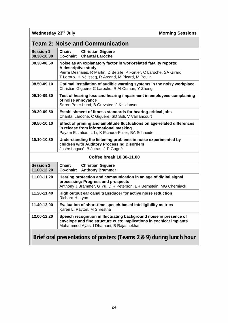
Team 2: Noise and Communication Session 1 08.30-10.30
Chair: Christian Giguère Co-chair: Chantal Laroche
08.30-08.50 Noise as an explanatory factor in work-related fatality reports: A descriptive study Pierre Deshaies, R Martin, D Belzile, P Fortier, C Laroche, SA Girard, T Leroux, H Nélisseq, R Arcand, M Picard, M Poulin
08.50-09.10 Optimal installation of audible warning systems in the noisy workplace Christian Giguère, C Laroche, R Al Osman, Y Zheng
09.10-09.30 Test of hearing loss and hearing impairment in employees complaining of noise annoyance Søren Peter Lund, B Grevsted, J Kristiansen
09.30-09.50 Establishment of fitness standards for hearing-critical jobs Chantal Laroche, C Giguère, SD Soli, V Vaillancourt
09.50-10.10 Effect of priming and amplitude fluctuations on age-related differences in release from informational masking Payam Ezzatian, L Li, K Pichora-Fuller, BA Schneider
10.10-10.30 Understanding the listening problems in noise experimented by children with Auditory Processing Disorders Josée Lagacé, B Jutras, J-P Gagné
Coffee break 10.30-11.00
Session 2 11.00-12.20
Chair: Christian Giguère Co-chair: Anthony Brammer
11.00-11.20 Hearing protection and communication in an age of digital signal processing: Progress and prospects Anthony J Brammer, G Yu, D R Peterson, ER Bernstein, MG Cherniack
11.20-11.40 High output ear canal transducer for active noise reduction Richard H. Lyon
11.40-12.00 Evaluation of short-time speech-based intelligibility metrics Karen L. Payton, M Shrestha
12.00-12.20 Speech recognition in fluctuating background noise in presence of envelope and fine structure cues: Implications in cochlear implants Muhammed Ayas, I Dhamani, B Rajashekhar
Brief oral presentations of posters (Teams 2 & 9) during lunch hour
24

Wednesday 23rd July Afternoon Sessions
Team 9: Noise Policies: Regulations and Standards Session 1 01.45-03.05
Chair: Larry S. Finegold Co-chair: Jacques Lambert
01.45-02.05 Progress on development of noise policies from 2003-2008 Lawrence S. Finegold, C Oliva, J Lambert
02.05-02.45 Overview of the World Health Organization Workshop on Aircraft Noise and Health Birgitta Berglund, S Stansfeld, R Kim
02.45-03.05 Airport noise policies in Europe: The contribution of human sciences research Michel Vallet
Coffee break 03.05-03.30
Session 2 03.30-05.40
Chair: Jacques Lambert Co-chair: Larry S. Finegold
03.30-03.50 Aircraft noise effects on sleep: Substantiation of the DLR protection concept for airport Leipzig/Halle Mathias Basner
03.50-04.10 A strategic approach on environmental noise management in developing countries Dieter Schwela, LS Finegold, J Stewart
04.10-04.30 Road noise charges based on the marginal cost principle Mikael Ögren, H Andersson
04.30-05.00 Maslow’s hierarchy of needs as a model for the process of the development of national noise regulations George A. Luz
05.00-05.20 Acoustical design of hospitals: Standards and priority indexes Sergio Luzzi, R Bellomini, C Romero
05.20-05.40 Requirements for criteria and emission limits in view of social adequacy – codified law aspects Peer Jansen
25
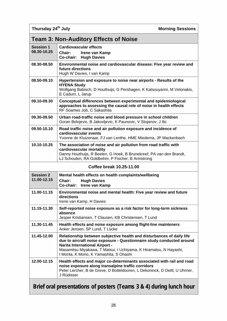
Thursday 24th July Morning Sessions
Team 3: Non-Auditory Effects of Noise Session 1 08.30-10.25
Cardiovascular effects Chair: Irene van Kamp Co-chair: Hugh Davies
08.30-08.50 Environmental noise and cardiovascular disease: Five year review and future directions Hugh W Davies, I van Kamp
08.50-09.10 Hypertension and exposure to noise near airports - Results of the HYENA Study Wolfgang Babisch, D Houthuijs, G Pershagen, K Katsouyanni, M Velonakis, E Cadum, L Jarup
09.10-09.30 Conceptual differences between experimental and epidemiological approaches to assessing the causal role of noise in health effects RF Soames Job, C Sakashita
09.30-09.50 Urban road-traffic noise and blood pressure in school children Goran Belojevic, B Jakovljevic, K Paunovic, V Stojanov, J Ilic
09.50-10.10 Road traffic noise and air pollution exposure and incidence of cardiovascular events Yvonne de Kluizenaar, FJ van Lenthe, HME Miedema, JP Mackenbach
10.10-10.25 The association of noise and air pollution from road traffic with cardiovascular mortality Danny Houthuijs, R Beelen, G Hoek, B Brunekreef, PA van den Brandt, LJ Schouten, RA Goldbohm, P Fischer, B Armstrong
Coffee break 10.25-11.00
Session 2 11.00-12.15
Mental health effects on health complaints/wellbeing Chair: Hugh Davies Co-chair: Irene van Kamp
11.00-11.15 Environmental noise and mental health: Five year review and future directions Irene van Kamp, H Davies
11.15-11.30 Self-reported noise exposure as a risk factor for long-term sickness absence Jesper Kristiansen, T Clausen, KB Christensen, T Lund
11.30-11.45 Health effects and noise exposure among flight-line mainteners Anker Jensen, SP Lund, T Lücke
11.45-12.00 Relationship between subjective health and disturbances of daily life due to aircraft noise exposure - Questionnaire study conducted around Narita International Airport - Masamitsu Miyakawa, T Matsui, I Uchiyama, K Hiramatsu, N Hayashi, I Morita, K Morio, K Yamashita, S Ohashi
12.00-12.15 Health effects and major co-determinants associated with rail and road noise exposure along transalpine traffic corridors Peter Lercher, B de Greve, D Botteldooren, L Dekoninck, D Oettl, U Uhrner, J Rüdisser
Brief oral presentations of posters (Teams 3 & 4) during lunch hour
26

Thursday 24th July Afternoon Sessions
Team 4: Noise and Performance Session 1 01.45-03.00
Chair: Charlotte Clark Co-chair: Patrik Sörqvist
01.45-02.00 The influence of noise on performance and behavior – 5 year update Charlotte Clark
02.00-02.30 Varieties of auditory distraction Dylan M Jones, RW Hughes, JE Marsh, WJ Macken
02.30-03.00 The effects of classroom and environmental noise on children's academic performance Bridget Shield, J Dockrell
Coffee break 03.00-03.30
Session 2 03.30-05.30
Chair: Charlotte Clark Co-chair: Patrik Sörqvist
03.30-04.00 Positive effects of noise on cognitve performance: Explaining the Moderate Brain Arousal model Göran Söderlund, S Sikström
04.00-04.15 A comparison of structural equation models of memory performance across noise conditions and age groups Staffan Hygge, I Enmarker, E Boman
04.15-04.30 Effect of speech intelligibility on task performance - an experimental laboratory study Annu Haapakangas, M Haka, E Keskinen, V Hongisto
04.30-04.45 Effects of building mechanical system noise with fluctuations on human performance and perception Lily M Wang, CC Novak
04.45-05.00 Recall of spoken words presented with a prolonged reverberation time Robert Ljung, A Kjellberg
05.00-05.15 Disruption of reading comprehension by irrelevant speech: The role of updating in working memory Patrik Sörqvist, N Halin, S Hygge
05.15-05.30 Task performance and speech intelligibility - a model to promote noise control actions in open offices Valtteri Hongisto, A Haapakangas, M Haka
Banquet 06:30-09:00
Banquet Talk James A. Simmons
Effects of environmental sounds on bat sonar
27

Friday 25th July Morning Sessions
Summary and Closing Session Session 08.30-10.30
Chair: Barbara Griefahn Co-chair: Peter Lercher
08.30-10.30 Team summaries: Teams 1,2,3,4,5,6,9 (15 mins each+ questions)
Coffee break 10.30-11.00
11.00-11.30 Conference Summary Stephen Stansfeld
11.30-12.15 Presidential Address Soames Job
12.15-12.30 Final summary Jerry Tobias
28

Poster Presentations Posters can be presented throughout the congress, they can be put up at the beginning of the congress and remain until the end. Brief oral presentations by the authors in front of their posters are foreseen during the lunch hour according to the following schedule
Monday: Team 6 Tuesday: Teams 1 (posters 1-12) and 5 Wednesday: Teams 1 (posters 13-24), 2 and 9 Thursday: Teams 3 and 4
Team 1: Noise-Induced Hearing Loss Brief oral presentations during lunch hour on
- Tuesday, 22nd July (Posters 1-12) Chairpersons: Ann-Christine Johnson, Noah Seixas
- Wednesday, 23rd July (Posters 13-24) Chairpersons: Sharon Kujawa, Tony Leroux
1. Personal noise exposure assessment of overhead-traveling crane drivers in steel-rolling mills Lin Zeng, D Chai, H Li, Z Lei, Y Zhao
2. Acoustics versus insight: Strategies against noise-induced auditory damages Gerald Fleischer, R Müller
3. Ratio of total cholesterol over HDL is a better hyperlipidemia indicator for sensorineural hearing loss? Rafidah Hanim Mokhtar, R Ahmad, A Ayob, W Ishlah
4. Auditory effects of chronic exposure to carbon monoxide and noise among workers Tony Leroux, A Lacerda, J-P Gagné
5. Detailed DPOAE level/phase maps provide Insight into normal and noise-damaged human ears Deanna K Meinke, BB Stagner, BL Lonsbury-Martin, GK Martin
6. Use of narrow band noise to screen for cochlear dead regions A Shubhra Shanker, I Dhamani, B Rajashekar
7. Central auditory dysfunction associated with solvent exposure Adrian Fuente
8. Temporal processing disorders associated with styrene exposure Ewa Zamyslowska-Szmytke, A Fuente, M Sliwinska-Kowalska
9. The contribution of genetic variations to the individual susceptibility to noise Malgorzata Pawelczyk, L van Laer, A Konings, E Rajkowska, A Dudarewicz, E Fransen, G van Camp, M Sliwinska-Kowalska
10. User-friendly parameterizations of an unscreened population dataset for the prediction of noise- and age-related hearing threshold shifts Jennifer Tufts, PK Weathersby, G Ferry
29

11. Audiological characteristics, attitudes and habits of Brazilian young adults and noise Thais C. Morata, AM Fontana Zocoli, J Mendes Marques
12. AHEAD III - Assessment of hearing in the elderly: Aging and degeneration - integration through immediate intervention Mariola Sliwinska-Kowalska, F Grandori, W-D Baumgartner, A Ernst, T Janssen, S Kramer, S Stenfelt, R Probst, A Davis
13. Comparison of school-based hearing screening protocols and the identification of noise-induced hearing loss in adolescents Deanna K Meinke, N Dice
14. Changing knowledge, attitudes and intended behaviors regarding sound exposure in high school students: A challenging target group William Hal Martin, SE Griest, JL Sobel
15. The CDC/National Institute for Occupational Safety and Health (NIOSH) Hearing Loss Prevention Research Strategic Plan Theresa Y. Schulz, G Gürtunca, M Stephenson, R Randolph, GM Calvert, RJ Matetic, P Kovalchik, WJ Murphy, R Davis
16. Different approaches towards knowledge about noise induced hearing loss in working life Ann-Christin Johnson, G Backenroth-Ohsako, B Canlon, B Hagerman, NL Pedersen, U Rosenhall, T Theorell, M Ulfendahl
17. Educating the public about the safe usage of personal audio technology Vic S Gladstone, GO Purvis, D Burrows
18. A university-based hearing conservation program for high school students Yori Kanekama, D Downs
19. Theory-based health communication interventions to prevent NIHL Madeleine J Kerr, O Hong, SL Lusk
20. Communicating hearing protection behaviors in adolescents Judith L Sobel
21. A university course on preventing hearing loss Ingrid M Blood, GW Blood
22. How loud is your music? Beliefs and practices regarding use of personal stereo systems William Hal Martin, GY Martin, SE Griest, WE Lambert
23. Meet Jolene: An inexpensive device for doing public health research and education on personal stereo systems William Hal Martin, GY Martin
24. Hearing loss in rats from combined exposure to carbon monoxide, toluene and impulsive noise Søren Peter Lund, GB Kristiansen, P Campo
Team 2: Noise and Communication Brief oral presentations during lunch hour on Wednesday, 23rd July
1. The unexamined rewards for excessive loudness Barry Blesser, L-R Salter
30

Team 3: Non-Auditory Effects of Noise Brief oral presentations during lunch hour on Thursday, 24th July
1. Joint effects of noise and air pollution: A progress report on the Vancouver retrospective cohort study Hugh W Davies, PA Demers, M Buzzelli, M Brauer
2. Relation between aircraft noise reduction in schools and standardized test scores Mary Ellen Eagan, G Anderson, B Nicholas, R Horonjeff, T Tivnan
3. Stress-related personality tests and noise effects: New evidence but old interpretations R.F. Soames Job
4. Dose-response relationship between hypertension and aircraft noise exposure around Kadena airfield in Okinawa Toshihito Matsui, T Uehara, T Miyakita, K Hiramatsu, T Yamamoto
Team 4: Noise and Performance Brief oral presentations during lunch hour on Thursday, 24th July
1. Student performance when taught in a noisy environment Ron Aylward, H Esterhuizen
2. Emoacoustics: Sound character versus source meaning in emotional responses to sounds Penny Bergman, D Västfjäll, E Asutay, A Tajadura, A Sköld, A Genell, N Fransson
3. The effect of school location on retention of knowledge learned from an educational hearing conservation program Hsiaochuan Chen
4. Effects of hearing protection on auditory annoyance from ultrasonic scalers used by dental hygiene students David Downs, B Gonzalez, Y Kanekama, L Belt
5. Perceived acoustic environment, work performance and well-being - survey results from Finnish offices Annu Haapakangas, R Helenius, E Keskinen, V Hongisto
6. Effects of sound masking on workers - a case study in a landscaped office Valtteri Hongisto
7. Memory of a text heard in noise Robert Ljung, A Kjellberg, A-M Green
8. Causes and effects of noise pollution: An overview Sanjeev Kumar Shrivatava, Kailash
Team 5: Noise and Sleep Brief oral presentations during lunch hour on Tuesday, 22nd July
1. Markov State Transition Models for the prediction of changes in sleep structure induced by aircraft noise Mathias Basner, U Siebert
2. Aircraft noise effects on sleep: A systematic comparison of EEG awakenings and automatically detected cardiac arousals Mathias Basner, U Müller, E-M Elmenhorst, B Griefahn
31

3. The sleep disturbance index – a measure for structural alterations of sleep due to environmental influences Barbara Griefahn, S Robens, P Broede, M Basner
4. Investigation of road traffic noise and annoyance in Beijing: A cross-sectional study of 4th Ring Road Hui-Juan Li, W Yu, J Lu, L Zeng, N Li, Y Zhao
5. How many people will be awakened by nighttime aircraft noise? Nicholas P. Miller, RC Gardner
6. Field research on the assessment of community impacts from weapons noise Edward T. Nykaza, GA Luz, LL Pater
7. Noise and vibration generation for laboratory studies on sleep disturbance Mikael Ögren, E Öhrström, T Jerson
8. Nocturnal road traffic noise and sleep: Day-by-day variability assessed by actigraphy and sleep logs during a one week sampling. Preliminary findings Sandra Pirrera, E de Valck, C Raymond
Team 6: Community Responses to Noise Brief oral presentations during lunch hour on Monday, 21st July
1. Modeling the role of attention in the assessment of environmental noise annoyance Dick Botteldooren, B de Coensel, B Berglund, ME Nilsson, P Lercher
2. The results of hum studies in the United States James P. Cowan
3. The effectiveness of quiet asphalt and earth berm in reducing annoyances due to road traffic noise in a residential area Anita Gidlöf-Gunnarsson, E Öhrström
4. Acoustical factors influencing noise annoyance of urban population Branko Jakovljevic, G Belojevic, K Paunovic
5. A measurement model for general negative reaction to noise Maarten Kroesen, EJE Molin, HME Miedema, H Vos, SA Janssen, B van Wee
6. Assessing the role of mediators in the noise-health relationship via Structural Equation analysis Maarten Kroesen, PJM Stallen, EJE Molin, HME Miedema, H Vos, SA Janssen, B van Wee
7. Human response to a step change in noise exposure following the opening of a new railway extension in Hong Kong Kin-che Lam, W Hong
8. The effect on annoyance estimation of noise modeling procedures Peter Lercher, B de Greve, D Botteldooren, M Baulac, J Defrance, J Rüdisser
9. Study on sound environment and community response to noise in Tianjin, a Chinese city Hui Ma, T Yano
10. Influence of attitudes to noise sources on annoyance Takashi Morihara, T Sato, T Yano
11. The importance of non-acoustical factors on noise annoyance of urban residents Katarina Paunovic, B Jakovljevic, G Belojevic
12. Annoyance from road traffic noise with horn sounds: A cross-cultural experiment between Vietnamese and Japanese Hai Anh Thi Phan, T Nishimura, HYT Phan, T Yano, T Sato, Y Hashimoto
32
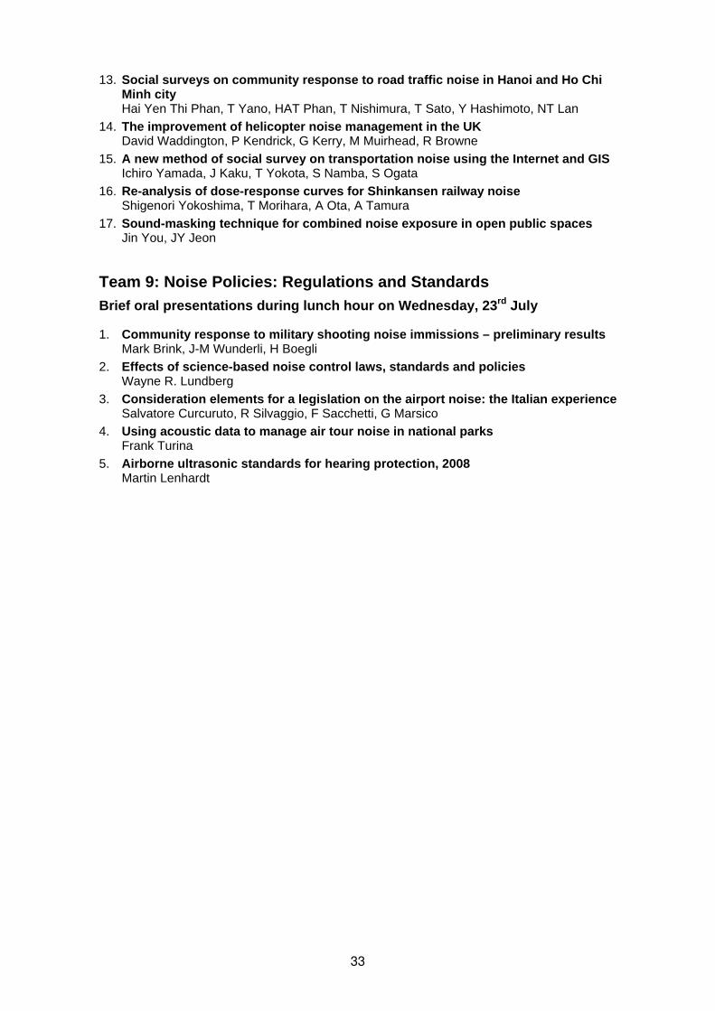
13. Social surveys on community response to road traffic noise in Hanoi and Ho Chi Minh city Hai Yen Thi Phan, T Yano, HAT Phan, T Nishimura, T Sato, Y Hashimoto, NT Lan
14. The improvement of helicopter noise management in the UK David Waddington, P Kendrick, G Kerry, M Muirhead, R Browne
15. A new method of social survey on transportation noise using the Internet and GIS Ichiro Yamada, J Kaku, T Yokota, S Namba, S Ogata
16. Re-analysis of dose-response curves for Shinkansen railway noise Shigenori Yokoshima, T Morihara, A Ota, A Tamura
17. Sound-masking technique for combined noise exposure in open public spaces Jin You, JY Jeon
Team 9: Noise Policies: Regulations and Standards Brief oral presentations during lunch hour on Wednesday, 23rd July
1. Community response to military shooting noise immissions – preliminary results Mark Brink, J-M Wunderli, H Boegli
2. Effects of science-based noise control laws, standards and policies Wayne R. Lundberg
3. Consideration elements for a legislation on the airport noise: the Italian experience Salvatore Curcuruto, R Silvaggio, F Sacchetti, G Marsico
4. Using acoustic data to manage air tour noise in national parks Frank Turina
5. Airborne ultrasonic standards for hearing protection, 2008 Martin Lenhardt
33

__________________________________________________________________________
__________________________________________________________________________
ICBEN 2008
Opening Session
34

35
Dedication to Henning Edgar von Gierke 9th International Congress on Noise as a Public Health Problem (ICBEN) 2008, Foxwoods, CT
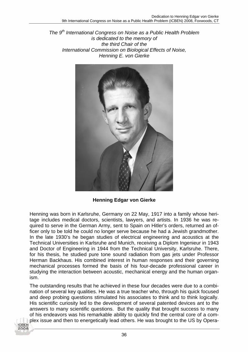
The 9th International Congress on Noise as a Public Health Problem is dedicated to the memory of
the third Chair of the International Commission on Biological Effects of Noise,
Henning E. von Gierke
Henning Edgar von Gierke Henning was born in Karlsruhe, Germany on 22 May, 1917 into a family whose heri-tage includes medical doctors, scientists, lawyers, and artists. In 1936 he was re-quired to serve in the German Army, sent to Spain on Hitler’s orders, returned an of-ficer only to be told he could no longer serve because he had a Jewish grandmother. In the late 1930’s he began studies of electrical engineering and acoustics at the Technical Universities in Karlsruhe and Munich, receiving a Diplom Ingenieur in 1943 and Doctor of Engineering in 1944 from the Technical University, Karlsruhe. There, for his thesis, he studied pure tone sound radiation from gas jets under Professor Herman Backhaus. His combined interest in human responses and their governing mechanical processes formed the basis of his four-decade professional career in studying the interaction between acoustic, mechanical energy and the human organ-ism. The outstanding results that he achieved in these four decades were due to a combi-nation of several key qualities. He was a true teacher who, through his quick focused and deep probing questions stimulated his associates to think and to think logically. His scientific curiosity led to the development of several patented devices ant to the answers to many scientific questions. But the quality that brought success to many of his endeavors was his remarkable ability to quickly find the central core of a com-plex issue and then to energetically lead others. He was brought to the US by Opera-
36

Dedication to Henning Edgar von Gierke 9th International Congress on Noise as a Public Health Problem (ICBEN) 2008, Foxwoods, CT
tion Paperclip after the war where he was launched on a research career in biophys-ics at Wright Field in Dayton Ohio and then from 1956-88 he was the Director of the Biodynamics and Bioengineering Division at AMRL. There, he had many accom-plishments, including developing the equal energy rule as the time intensity trade-off for Air Force hearing conservation regulation. Many years later he chaired the ISO working group which prepared and obtained consensus for the adoption of ISO 1999 which used the equal energy rule as the basis for determining occupational noise exposure and estimating its hearing impairment. Henning has been a member of the Acoustical Society of America for over 50 years, a Fellow since 1956, and its President in 1979-80. He has been a leader in the de-velopment of the Society’s Standards Program, chairing the S2 Committee on Bio-acoustics, and serving as the first Standards Director. For many years he organized and led the US delegation to the ISO TC/43 Technical Committee on Noise, and for 30 years he chaired the ISO TC/108 Subcommittee on Human Exposure to Mechani-cal Shock and Vibration. He was past Chair of the NRC Committee on Hearing, Bio-acoustics and Biomechanics, past Chair of the International Commission on Biologi-cal Effects of Noise, past Chair of the ANSI Acoustical Standards Management Board, and a member of INCE and the Aerospace Medical Association.. He was a fellow and past vice president of the Aerospace and Environmental Medicine Asso-ciation, an elected member if the National Academy of Engineering, the International Academy of Aviation Medicine, and the International Academy of Astronautics. He received many awards, including the Meritorious Executive Rank Award (twice), the Department of Defense Distinguished Civilian Service Award, the Commander’s Cross of the Order of Merit of Germany, the Rayleigh Medal from the United Kingdom Institute of Physics, the Lesser Award from the American Society of Mechanical En-gineers, and both the Silver and Gold Medals from the Acoustical Society. He is survived by his wife Honlo and his daughter Karin. His second daughter, Susi, died of multiple sclerosis in 2002.
Kenneth M. Eldred
37
Dedication to Alexander Samel 9th International Congress on Noise as a Public Health Problem (ICBEN) 2008, Foxwoods, CT
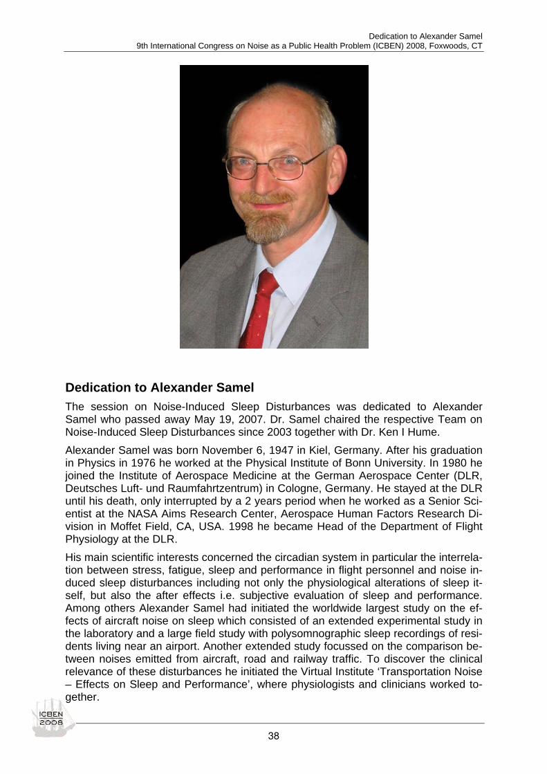
Dedication to Alexander Samel The session on Noise-Induced Sleep Disturbances was dedicated to Alexander Samel who passed away May 19, 2007. Dr. Samel chaired the respective Team on Noise-Induced Sleep Disturbances since 2003 together with Dr. Ken I Hume. Alexander Samel was born November 6, 1947 in Kiel, Germany. After his graduation in Physics in 1976 he worked at the Physical Institute of Bonn University. In 1980 he joined the Institute of Aerospace Medicine at the German Aerospace Center (DLR, Deutsches Luft- und Raumfahrtzentrum) in Cologne, Germany. He stayed at the DLR until his death, only interrupted by a 2 years period when he worked as a Senior Sci-entist at the NASA Aims Research Center, Aerospace Human Factors Research Di-vision in Moffet Field, CA, USA. 1998 he became Head of the Department of Flight Physiology at the DLR. His main scientific interests concerned the circadian system in particular the interrela-tion between stress, fatigue, sleep and performance in flight personnel and noise in-duced sleep disturbances including not only the physiological alterations of sleep it-self, but also the after effects i.e. subjective evaluation of sleep and performance. Among others Alexander Samel had initiated the worldwide largest study on the ef-fects of aircraft noise on sleep which consisted of an extended experimental study in the laboratory and a large field study with polysomnographic sleep recordings of resi-dents living near an airport. Another extended study focussed on the comparison be-tween noises emitted from aircraft, road and railway traffic. To discover the clinical relevance of these disturbances he initiated the Virtual Institute ‘Transportation Noise – Effects on Sleep and Performance’, where physiologists and clinicians worked to-gether.
38

Dedication to Alexander Samel 9th International Congress on Noise as a Public Health Problem (ICBEN) 2008, Foxwoods, CT
Dr. Samel was a member of numerous research associations, i.e. the Society of Re-search of Biological Rhythms, the German Sleep Society, the European Sleep Re-search Society, the International Commission on Biological Effects of Noise, the German Society of Aviation and Space Medicine, the Aerospace Medical Association (Airtransport Medicine Committee), and the International Civil Aviation Organisation (ICAO). He was a corresponding Member of the International Academy of Astronaut-ics and was appointed to the Joint Aviation Authorities’ Project Advisory Group for Human Factors and to the European Transport Safety Council, ‘Airsafety Working Party’. He received the Howard K. Edwards Aerospace Medical Association Memorial Award of the US Aerospace Medical Association in 1998; he became member of the Inter-national Academy of Astronautics in 2001, fellow of the Aerospace Medical Associa-tion in 2002 and fellow of the Aerospace Human Factors Association (USA) in 2006. Despite his very tight time schedule he always had the time to discuss scientific prob-lems and to offer a solution even in areas where he himself did not work. These char-acteristics/traits made him a respected and reliable partner in research cooperation. Alexander’s views and statements were always well researched and honest and he never propagated information he wasn’t absolutely sure of. Alexander was an excel-lent teacher who had the ability to detect and to promote young scientists. We lost not only an excellent honest scientist, but also a friend. His death caused a gap that is difficult to fill. We are grateful to have known him.
Barbara Griefahn
39

Opening: 9th International Congress on Noise as a Public Health Problem (ICBEN) 2008, Foxwoods, CT
Outlines of ICBEN
THE COMMISSION, THE CONGRESSES AND THE INFLUENCE OF HENNING VON GIERKE ON NOISE EFFECTS RESEARCH AND PUBLIC NOISE POLICY Gerd Jansen Institut für Arbeits- und Sozialmedizin, Universität Düsseldorf, Universitätsstr. 1, D-40217 Düsseldorf, Germany
*corresponding author: e-mail: [email protected]
1 THE COMMISSION Prof. Dix Ward organized the 1st National Conference on Noise as a Public Health Hazard in Washington/DC, USA and the 2nd Congress on “Noise as a Public Health Problem” in Dubrovnik/Yugoslavia, May 1973. On occasion of the 2nd congress Prof. Gerd Jansen conceived the idea of ICBEN. In a special meeting during the congress I proposed the audience the foundation of an institution uniting worldwide all experts in research and all important decision - makers in the broad fields of noise impacts on human beings. This proposal was vig-orously supported by two outstanding experts: by the organizer of the Dubrovnik congress and of the First National Conference on Noise as a Public Health Hazard (Washington 1968) Prof. Dix Ward and by Dr. Jerry Tobias. A fair discussion on the advantages and possible disadvantages resulted finally in the founding of ICBEN. Gerd Jansen was elected as Chairman of ICBEN, Dix Ward Co-chairman and as Secretary Jerry Tobias, who later established the Constitution of ICBEN which since then is working well. Sceptical arguments and sceptics against the founding of ICBEN based on the wrong idea that the new body should be an additional scientific society among others with annual meetings but special main focuses and emphasis. But, while preparing the inaugurating assembly the triumvirate – Gerd Jansen, Dix Ward and Jerry Tobias – developed the conception of five years periods to convene experts presenting only valid, reliable and proven results of noise research that are suitable for national and supranational bodies for their administrative and/or their legislative work. You remember the time around 1968–1973 when the measurements, evaluations und calculations of scientific tests were not computer–aided and therefore time–consuming. ICBEN was never interested in quick spectacular gains of results but only in proven results. Therefore the five-years-period seemed adequate. But already during the Freiburg Congress 1978 the discussion of shorter periods came up and was repeated during the following years up to now. In the last few months the discussion was intensified by the fact that within 2008 several conven-tions and congresses with relation to noise problems took place. Financial restrictions and the different emphases of institutions might have prevented highly interested ex-perts to join all conventions I think the length of the period between two congresses is worth while being dis-cussed during the coming Business Meeting and being decided and executed by the Executive Board of ICBEN. Deduced from the conception of ICBEN the “triumvirate” proposed the name “Interna-tional Commission”. The sceptics again opposed asking: “By whom are you commis-sioned?” The answer was that we offer our results and our active cooperation to in-
40

Opening: 9th International Congress on Noise as a Public Health Problem (ICBEN) 2008, Foxwoods, CT
terested institutions like WHO, ICA, Governments etc. In the past 35 years as an or-ganisation we notice that numerous and outstanding representatives of these institu-tions mentioned took part in our congresses not only as participants but mainly as keynote speakers or representatives of their institutions.
2 THE CONGRESSES As mentioned above the inaugurating assembly of ICBEN took place at the Dubrov-nik Congress 1973 which was the “2nd International Congress on Noise as a Public Health Problem”. The preceding (first) congress was the “First National Conference on Noise as a Public Health Hazard with International Experts” in Washington, DC, 1968. The organizer was Dix Ward, among the experts Gerd Jansen reported on the effects of noise on physiological extraaural functions. This research field developed to an increasing importance for physical health as well as for noise – induced annoy-ance. The Dubrovnik congress was summarized at its end by Ira Hirsh. After the Dubrovnik congress the elected (first) chairman Gerd Jansen organized the “3rd Congress on Noise as a Public Health Problem” 1978 in Freiburg/Germany. Fig-ure 1 shows the logo of ICBEN on the cover side of the Preliminary Program. The logo of ICBEN was designed by Jerry Tobias.
Figure 1: International Commission on Biological Effects of Noise (ICBEN) - International Noise Teams
Simultaneously with designing the logo Jerry Tobias established the Constitution which is putting in order the structure and the procedures of ICBEN. The leading idea within ICBEN and the intention of the congresses refers to a complete knowledge of all results of noise effects on human beings as a unity. This means that parallel ses-sions during the congress should be avoided. By this, every participant of the con-gress could have an overview of the present state of knowledge concerning all noise effects on human health. Each of the single teams of ICBEN is responsible for the invited experts and the se-quence of papers. But, each team session is to run according to a schedule as it is shown in Figure 2:
Team 1 Noise Induced Hearing Team 2 Noise and Communication Team 3 Non-Auditory Physiological Effects Induced by Noise Team 4 Influence of Noise on Performance and Behaviour Team 5 Noise disturbed Sleep Team 6 Community Response to Noise Team 7 Noise and Animals Team 8 Effects of Interactions between Noise and Physical or Chemical Agents Team 9 Regulations and Standards
Figure 2: Schedule for Team Sessions
41

Opening: 9th International Congress on Noise as a Public Health Problem (ICBEN) 2008, Foxwoods, CT
Figure 3: List of the teams
The above mentioned Teams are still existing. They are working more or less strictly according to the given directives (see Figure 2). Many difficulties have risen with Team 8. Interactions with other Teams have been occurred very often. During the Planning Meeting this problem was discussed intensively. The participants decided to
42

Opening: 9th International Congress on Noise as a Public Health Problem (ICBEN) 2008, Foxwoods, CT
propose to the business meeting of this congress to cancel team 8. Simultaneously it was decided to propose to name team 9 into “Noise Research and Noise Policy” Each congress is containing Opening and Closing Sessions. Especially in the Open-ing Session contributions from National and International Institutions are occurring. The next Figure 4 from the Freiburg Congress (1978) shows the order of the agenda for the closing session. The contributions in the closing sessions are the reports of the Chairpersons of the single noise teams, a short discussion on the chairpersons reports and the conclusion for future work.
Figure 4: Agenda of the Closing Session at the Freiburg Congress 1978
At the very end of each congress the Congress Summary is a constant factor of all congresses. In 1983 (Congress in Turin) congress summarizer Gerd Jansen went the following week to the ICA congress in Paris in order to open this Congress with the Summary of the Turin congress representing the recent state of knowledge of noise effects on human health. Five years later the summary of the Stockholm congress was done again by Gerd Jansen who went three days later to Avignon / France where the Internoise Congress took place. The Stockholm Summary was the Intro-ductary Speech at Avignon.
3 THE INFLUENCE OF HENNING VON GIERKE ON ICBEN On occasion of the 5th congress at Stockholm / Sweden 1988 which was opened by his Majesty The King Gustav XVI Karl the chairman Henning von Gierke and the Ex-ecutive Committee took part in a reception of the King. In the discussion with the King Henning underlined the political importance of the protection of human beings from health endangering noise. He pointed out that ICBEN is offering its scientific knowl-edge to all political and administrative institutions and bodies on national and interna-tional levels. The need for taking more attention to political and administrative questions of noise influences on human beings is caused by a change of the contents of research. For instance, research of sonic boom effects as it was done in the past had no longer any priority whereas experimentally-based epidemiological investigations show an in-creasing importance. In the course of the meeting at the Stockholm congress and by the initiative of Hen-ning von Gierke a new team 9 was founded for “Regulations and Standards”. Gerd
43

Opening: 9th International Congress on Noise as a Public Health Problem (ICBEN) 2008, Foxwoods, CT
Jansen was elected Team Chair 9 and Dr. Bernd Rohrmann Co-Chair. During the Sydney Congress 1998 Larry Finegold was elected chairman, Carl Oliva (Switzer-land) and Jacques Lambert (France) were the co-chairs. At the Rotterdam Congress 2003 Martin van den Berg (The Netherlands) succeeded Larry, but resigned in 2007 from his chairmanship, so Larry with Oliva and Lambert as co-chairs continued up to the coming elections of team chairpersons here in Mashantucket. In the following congresses at Nice / France 1993, Sydney / Australia 1998 and Rot-terdam 2003 the contributions of the members of this team 9 showed an increasing importance. Especially WHO practised a fruitful cooperation by establishing noise related documents by working together with members of ICBEN. Henning, too, con-tributed to the themes of team 9 by publishing suitable transactions. Among his publi-cations you can find a title like ”How much is too much?”. This article is expressing exactly the intentions of ICBEN’s team 9: Transfer of scientific results into regulations for the community. During the Planning Meeting for this Congress on July 29 -31, 2007 it was decided to recommend in the business meetings of ICBEN a change of the name of team 9 from “Standards and Regulations” into “Noise Research and Noise Policy” as the results of noise research are getting more and more important for the communities. Also, in the Planning Meeting it was decided to recommend to the coming business meetings here in Mashantucket to cancel team 8. The combined effects of noise and other agents are interfering with many other research projects of the different teams of ICBEN. We regret that we cannot ask Henning to know his opinion.
Figure 5: Henning von Gierke
4 DEDICATION OF THE 9TH ICBEN CONGRESS TO HENNING VON GIERKE The preceding chapters have been established containing among others also a spe-cial view on Henning’s activity within ICBEN. He promoted vigorously our activities. Henning Edgar von Gierke ,born on May 22, 1917 in Karlsruhe / Germany studied Electrical Engineering and Acoustics at Karlsruhe and Munich and became a Doctor of Engineering. Very early he was fascinated by the interactions between mechani-cal/acoustic energy and responses of the human organism. Soon after World War II he was brought to USA and was launched on a research ca-reer in biophysics at Wright Patterson Air Field in Dayton / Ohio. From 1956–1988 he was Director of the Biodynamic and Bioengineering Division at AMRL. Besides this
44

Opening: 9th International Congress on Noise as a Public Health Problem (ICBEN) 2008, Foxwoods, CT
he served as chairman of the ISO Working Group which prepared and obtained con-sensus for the adoption of ISO 1999. As member of the Acoustical Society of Amer-ica for over 50 years he served as its President in 1979-1980. There is a long list of functions and activities of Henning in various societies, national and international boards which have already celebrated Henning’s merits. An intense obituary for Hen-ning is published by Kenneth M. Eldred who knew him best. ICBEN and its members are very happy to remember him as a dynamic and out-standing expert and a friend with many key qualities. He quickly found the central core of complex issues. He convinced and stimulated in scientific discussions search-ing for the truth. He gave us answers to many scientific questions. It is worth while dedicating our congress 2008 to Henning von Gierke.
45

Keynote: 9th International Congress on Noise as a Public Health Problem (ICBEN) 2008, Foxwoods, CT
Noise: Public health challenges and solutions Adrian Davis MRC Hearing and Communication Group, Manchester University, M13 9PL
Correspondence: [email protected]
Noise is a major public health challenge. It is major because noise is all pervasive in our societies at a level that it can seriously affect population health and quality of life throughout the lifecourse. It is a challenge because the noise sources are constantly changing as the pace of technology and change gathers globally. As some areas of the world legislate or change their strategies the issue is displaced or changed rather than lessons being learnt and applied globally. There is much that we know in terms of solutions in good practice that is reduced in effectiveness because it is not known widely or is not applied / seen as a priority. There are also huge gaps in our knowl-edge of current population exposure and effectiveness of new ways to combat noise e.g. in particularly challenged groups such as in military or in airline / airport industry. There is a huge gap in our knowledge of the impact of noise from music or from combined exposures with chemicals on the natural history of impact on hearing, at-tention, performance, communication and social life. I will present evidence on the impact of noise exposure that seems from the small amount of evidence we have to affect the rate of change of degradation in hearing function beyond the time for which the individual is exposed. Does this apply to all other areas of function affected by noise? We need the research to address these issues! We know that in working age people (up to say 65 years of life) that hearing loss associated with noise is in the top 8 global public health challenges, yet it appears that very little effort is expended globally to tackle this problem by proposing acceptable, cost-effective solutions. However, this statistic really understates the problem, because with greater life ex-pectancy globally the impact of hearing loss and other health issues caused by noise exposure will have a major impact on quality of life and of communication. The need for new policies and research to underpin the development of these is now an urgent public health priority that should be addressed!
46

Opening: 9th International Congress on Noise as a Public Health Problem (ICBEN) 2008, Foxwoods, CT
Review of underwater noise and its effects on marine animals Roger L. Gentry Sound and Marine Life Joint Industry Programme
Correspondence: [email protected]
This talk reviews the issues and research concerning marine anthropogenic noise and its effects on animals. A 1994 low frequency tomography experiment (ATOC) aroused public concern about the possible effects of acoustic exposure on whales. Alarmist environmental predictions, based on gaps in scientific knowledge, triggered the formation of expert panels which listed the needed research, some of which has recently been completed. Over time public concern shifted to low frequency naval sonar, pile driving, and mid-frequency sonar, and from marine mammals to fish. New research shows that auditory injury in mammals may occur within about 500 m of the most intense acoustic sources. TTS onset in dolphins occurs at about 195 dB re 1 µPa2•sec (SEL), the dynamic ranges of their ears are 20 dB greater than in humans, and PTS onset (scant evidence) occurs between 40 and 60 dB of TTS. It is still uncertain whether fish experience PTS because damaged hair cells may regenerate. Fish somatic tissue injury has been well quantified for barotrauma but not for acoustic exposure per se. The behavioral effects of acoustic exposure on any marine animals are poorly known. Noise exposure criteria for marine mammals are now available, and similar criteria for fish and turtles are being written. Scientifically the key question is whether animal reproduction and survival rates will decrease from masking effects as ambient noise levels increase? More data on long-term trends in marine ambient noise are needed.
47

Banquet talk: 9th International Congress on Noise as a Public Health Problem (ICBEN) 2008, Foxwoods, CT
BANQUET TALK Effects of environmental sounds on bat sonar James A. Simmons
Department of Neuroscience, Brown University, Providence RI 02912
Correspondence: [email protected]
Echolocating bats respond to different kinds of environmental sounds in ways that illustrate general principles of noise effects on hearing and behavior. Big brown bats broadcast wideband ultrasonic (~20-100 kHz) frequency-modulated (FM) sounds and perceive objects from echoes that return to their ears. They emerge in the dark, which limits the usefulness of vision and makes echolocation critical for all aspects of their orientation. Bats use 'active' sonar to detect and track flying insects, to avoid obsta-cles, especially while flying through vegetation, to follow landmarks on flight paths through familiar surroundings, and to guide bat-to-bat 'dogfights', which also involve hearing other bats’ sounds. For a single echolocating bat, environmental sound consists largely of noise that masks weak echoes from targets at long range or actual echoes reflected by extraneous objects (clutter), such as vegetation or the ground. However, bats also use 'passive' hearing, listening for the sounds of prey and homing in on insect calls or the buzzing sounds of the insect’s wingbeats. These sounds often are largely ultra-sonic, so bats cannot simply filter out background noises to avoid interference. In many situations, ultrasonic insect calls are a significant source of intense ultrasound that can interfere with echo recep-tion. Hearing also is used for acoustic communication and for listening to the echolocation sounds of other bats. Several bats of the same species commonly will forage for insects together in the same area, within hearing range of each other. Moreover, large numbers of bats sometimes swarm over water to drink or hunt for insects. Because the sonar sounds of different bats in the same species are very similar, mutual interference is a real problem. Although their sounds all are wideband, covering the same frequencies, individual bats introduce a small frequency shift of a few kilohertz at the low-frequency end of the sweeps. Although this shift is only a few percent of the total band and thus seems insufficient for each bat to segregate the broadcasts and echoes of other bats, psychophysical tests reveal that bats can suppress spurious 'echoes' in their images when these shifts are present. In the most extreme situations of bats involved in dogfight pursuits through vegetation, several strategies of coping with environmental sounds are combined to render this seemingly impossible scenario quite easy.
48

__________________________________________________________________________
__________________________________________________________________________
ICBEN 2008
Noise-Induced Hearing Loss
49

Hearing loss: 9th International Congress on Noise as a Public Health Problem (ICBEN) 2008, Foxwoods, CT
Noise-induced hearing loss in humans – 5 year update Mariola Sliwinska-Kowalska Department of Audiology and Phoniatrics, Nofer Institute of Occupational Medicine, Lodz, Poland and Department of Environmental Otorhinolaryngology, Medical University of Lodz, Lodz, Poland
Corresponding author: e-mail: [email protected]
During 2003-2008, over 500 investigations on noise-induced hearing loss (NIHL) in humans have been published. Several papers address the hazardous effects of noi-se on hearing and the risk assessment of NIHL for several occupations (e.g. con-struction workers, farmers, firefighters, railway workers, pilots, policemen, space sta-tion workers, dentists and orthopedics, theater employees). An increasing number of data is pointing out to the additive adverse effect of exposure to industrial chemicals on NIHL. New policy for the protection of workers who are co-exposed to noise and organic solvents has been proposed. Much attention has been given to environ-mental noise exposure and to the prevalence of NIHL in general populations, particu-larly in children and adolescents. Few alarming studies have indicated the increasing number of noise-induced-like type of audiogram in teenagers. Few studies have also indicated that environmental noise may add to the risk for occupational NIHL. Vulnerability factors for NIHL such as age, smoking, and hypertension have been further explored. Large national and international studies on candidate genes for in-creased susceptibility to NIHL have been conducted, indicating that some K+ ions recycling genes and oxidative stress genes may play a role. Clinical issues involved: further exploration of the utility of otoacoustic emissions for monitoring of NIHL, tinnitus assessment, and vestibular myogenic evoked potentials changes due to noise exposure. The value of several hearing protector techniques and approaches has been evalu-ated and the medico-legal aspects of NIHL have been discussed. New hearing pre-servation and training programs have been developed in several centers.
50
Hearing loss: 9th International Congress on Noise as a Public Health Problem (ICBEN) 2008, Foxwoods, CT
Acute, chronic and delayed consequences of noise exposure in animal models – 5 year update Sharon G. Kujawa Department of Otology and Laryngology, Harvard Medical School, Boston, MA 02115, USA
Eaton-Peabody Laboratory and Department of Audiology, Massachusetts Eye and Ear Infirmary, Bos-ton, MA 02114, USA; Program in Speech and Hearing Bioscience and Technology, Division of Health Science and Technology, Harvard & MIT, Cambridge, MA 02139, USA
Corresponding author: e-mail: [email protected]
Noise-induced hearing loss (NIHL) is a serious problem, affecting many millions, worldwide. After acoustic overexposure, hearing thresholds are immediately ele-vated, but improve with a roughly exponential time course for several weeks, depend-ing on initial severity of the insult and characteristics of the individual. Thresholds may recover fully ('temporary' threshold shift) or may stabilize at an elevated value ('permanent' threshold shift). The acoustic trauma literature suggests that: 1) func-tionally important structural changes in permanent NIHL involve damage to hair cells and their stereocilia, whereas neural loss after noise is only seen secondarily to loss of inner hair cells; 2) complete threshold recovery indicates reversal of damage to mechanosensory and neural structures and, thus, a benign level of exposure; and 3) delayed changes seen at remote post-exposure times can be attributed to other causes; for example, aging. New insights into the mechanisms and time course of noise-induced cellular injury and functional loss provided by low-variance mouse models suggest that these basic tenets need re-evaluation. This talk will summarize current understanding of acute and chronic noise-induced hearing loss and cochlear injury, and will discuss how the-se outcomes are shaped by genetic background, age, and post-exposure time. It will describe recent work documenting delayed neurodegenerative outcomes; progres-sion of inner ear damage long after noise exposure stops, even in ears in which post-exposure threshold sensitivity recovery is complete. Such observations raise impor-tant concerns about the long-term effects of apparently benign acoustic overexpo-sures.
51

Hearing loss: 9th International Congress on Noise as a Public Health Problem (ICBEN) 2008, Foxwoods, CT
Relative contributions of aging and noise to the overall societal burden of adult hearing loss Robert A. Dobie Otolaryngology, University of California at Davis
Correspondence: [email protected]
Noise is certainly the most important preventable cause of hearing loss in developed countries, and perhaps in the world as a whole, but population models suggest that its contribution to the total burden of hearing loss in adults is much smaller than that of aging (Nelson et al. 2005; Dobie 2008). The burden attributable to occupational noise is felt most in middle-aged men, as age-related threshold shifts are added to noise-induced shifts from earlier exposures. Because of increasing lifespans and industrial job migration, this relative burden is probably declining in developed countries. It may be growing in developing countries. At least in the USA, non-occupational noise, especially shooting, may be as important as occupational noise. Reduction or elimination of very high-level unprotected exposures would reduce societal hearing loss burden far more than reductions of current exposure limits (typically 85 dBA for an 8-hour day).
Dobie RA (2008). The burdens of age-related and occupational noise-induced hearing loss in the United States. Ear Hear (in press).
Nelson DI, Nelson RY, Concha-Barrientos M, Fingerhut M (2005). The global burden of occupational noise-induced hearing loss. Am J Ind Med 48: 446-458.
52
Hearing loss: 9th International Congress on Noise as a Public Health Problem (ICBEN) 2008, Foxwoods, CT
The relationships between work-based noise over the adult life course and hearing in middle age Adrian Davis1*, Russell Ecob2, Pauline Smith3
1 MRC Hearing and Communication Group, The University of Manchester, UK
2 MRC Hearing and Communication Group, The University of Manchester, UK
3 Hearing Services Department, University Hospitals of Leicester NHS Trust, UK
* corresponding author: e-mail: [email protected]
INTRODUCTION Between 1971 and 1991 in the US there has been an increase in prevalence of age-adjusted hearing loss (National Center for Health Statistics [NCHS] data in Lustig & Niparko 2002), attributed in part to increases in environmental noise. Over this period there has been substantial evidence of increase in non-work based noise. Indus-trial/occupational exposure to noise is still the major route through which noise im-pacts on the individual, but this may change in the near future. Noise exposure is thought to explain around 25 % of variation in sensorineural hear-ing loss (SNHL) (Starck 1998; Pykko et al. 2000; Robinson 1970; ISO 1999 (1990)). However, individual susceptibility to noise has been reported to vary according to dif-ferences in ear musculature and size, pre-exposure to noise at lower levels, differ-ences in vascular pathology, use of analgesics, serum cholesterol levels, blood pres-sure, smoking, genetic pre-disposition, pigmentation and age (Prasher 1998; Pykko et al. 2000) (though see Ward 1995 for an alternative view). Clearly effects of noise levels on adult hearing are larger at 4 kHz than at 1 kHz (Taylor et al. 1965; Robin-son 1970) and this area is typically affected before other regions and so is often the major interest in any analysis – especially of younger populations. To date, there is little evidence about the particular life stages at which the sensitivity of the individual to noise exposure is highest. This study aims to explore the age sensitivity in adults to noise, using ways of enhancing existing data from a British birth cohort; estimated exposure to noise based on membership of Occupational Unit Groups (OUGs) derived using the Registrar General's categories of Occupation groups; and self-reported exposure to work-based noise at different ages.
Data sources In addition to a retrospective question of work- based noise exposure, the study uses data from a British birth cohort (Power & Elliott 2006) with pure tone audiometry measurements, both in childhood (ages 7,11,16 years) and adult pure tone audiome-try was repeated at age 45 years. We used detailed information on social and demo-graphic characteristics from which information on Occupational Unit Groups can be derived. Expert raters (four experienced audiologists and noise researchers) as-sessed each of the OUGs in respect of their noise level at each of four levels. We ad-justed analysis for differences in childhood hearing loss, including any early social or genetic influences which work through this. This allowed us to:
a. quantify the effect of exposure to work-based noise at a number of adult ages (23, 33, 42 years) on hearing loss (1 kHz and 4 kHz ) at age 45 years.
b. examine the adjusted effect of each exposure given exposures at other ages
53

Hearing loss: 9th International Congress on Noise as a Public Health Problem (ICBEN) 2008, Foxwoods, CT
c. provide estimates which adjust for social class at each age (note that the so-cial class based noise ratings may also reflect other aspects of social class, including cultural correlates, which influence hearing loss, Ecob et al. 2008)
d. examine the effects of change in exposure to noise levels between adult ages e. examine possible interactions between effects of noise exposure at different
ages f. examine the impact of these workplace-derived noise levels in relation to a ret-
rospective question (at age 45 years) on exposure (duration) to work-based noise.
METHODS Occupational Unit Groups (OUG) estimates of work based noise exposure OUGs were rated corresponding to first job at age 23 years (in 1981) and to last or current job at ages 23, 32, 42 years (in 1981, 1991, 2000). Each OUG was given by a one line description and jobs within this were rated according to the percentage of people in these jobs with exposure, without hearing protection, at each of four ordinal categories, with descriptions in terms of a range of noise levels and the voice level needed to communicate at a distance of four feet. Figures 1 and 2 show the aver-aged values from the three best raters over major groups for 1980 and then for 1991/2000. The majority of major groups have low noise levels. Average noise levels in each of the major occupational groups in 1980 and 1990 are given in Figure 1 and Figure 2. High noise ratings are seen to be confined to few major groups.
Figure 1: Average noise levels in major groups, 1981
Key: Major groups – 1981 1. Professional and related supporting management; senior national and local government man-
agers 2. professional and related in education, welfare and health 3. literacy, artistic and sports 4. professional and related in science, engineering, technology and similar fields 5. managerial 6. clerical and related 7. selling 8. security and protective service 9. catering, cleaning, hairdressing and other personal services 10. farming, fishing and related
16.0015.0014.0013.0012.0011.0010.009.008.007.006.005.004.003.002.001.00
ord
2.25
2.00
1.75
1.50
1.25
1.00
Estim
ated M
argina
l Mea
ns
Estimated Marginal Means of average noise rating, 1980
54

Hearing loss: 9th International Congress on Noise as a Public Health Problem (ICBEN) 2008, Foxwoods, CT
11. materials processing; making and repairing (excluding metal and electrical) 12. processing, making, repairing and related (metal and electrical) 13. painting, repetitive assembling, product inspecting, packaging and related 14. construction, mining and related not identified elsewhere 15. transport operating, materials moving and storing and related 16. miscellaneous
Figure 2: Average noise levels in major groups, 1991/2000
Key: Major groups 1991 1 Managers & administrators 2 Professional occupations 3 Associate professional & technical occupations 4 Clerical & secretarial occupations 5 Craft & related occupations 6 Personal & protective service occupations 7 Sales occupations 8 Plant & machine operatives 9 Other occupations
Duration of occupational noise was assessed at age 45 years by a self-completed, retrospective question: “Have you ever worked in a place that was so noisy that you had to shout to be heard?”. Questions were asked about age and duration.
Study sample Participants were originally enrolled in the Perinatal Mortality Survey (PMS) of all those born in England, Scotland and Wales during one week in March 1958 (Power & Elliott 2006) and followed up throughout childhood and adulthood, most recently at 44-45 years. The Total Cohort Sample for this study was 18,558, out of which 12,069 participants at 44-45 years were still in contact with the study.
Pure tone audiometry at ages 7, 11 and 16 years and at 44-45 years Pure tone audiometry was performed by air conduction in each ear, at frequencies 0.25 0.5, 1, 2, 4, 8 kHz, at three ages (7, 11, 16 years). The conditions in which these tests were carried were not closely standardized, so may not reflect true audiometric thresholds. Despite these reservations, the consistent relationships between adult and childhood hearing threshold level (HTL) at corresponding frequencies at each age (adjusted) is encouraging (Ecob, 2007). Pure tone audiometry by air conduction at
9.008.007.006.005.004.003.002.001.00
mgrps
1.70
1.60
1.50
1.40
1.30
1.20
1.10
1.00
Estim
ated M
argina
l Mea
ns
Estimated Marginal Means of average noise rating, 1990
55

Hearing loss: 9th International Congress on Noise as a Public Health Problem (ICBEN) 2008, Foxwoods, CT
frequencies 1 and 4 kHz at age 44-45 years was performed according to the British So-ciety of Audiology recommended procedure (BSA 1981). The median HTL at both fre-quencies in this study at age 45 years is lower (better) than other recent studies in comparable unscreened populations in the UK (see National Study of Hearing; Davis 1995) and, indeed, the predictions for screened populations (‘pure’ prebyacusis) from ISO 7029 (1984).
Social class Adult socio-economic position (referred to as current social class) is shown based on age at 23, 33, 42 years based on the participant’s current or most recent occupation in the Registrar General’s occupational groups: professional (I), managerial/technical (II), other non-manual (IIInm), skilled manual (IIIm), partly skilled (IV) and unskilled manual (V). For social class of origin those with no male head of household in child-hood were grouped with class V.
Family history of hearing loss This is measured by a question in biomedical wave (age 45 years). “Did any of your parents, children, brothers or sisters have great difficulty in hearing before age 55?”
Adjustment for possible conductive hearing loss in childhood Two variables, at ages 7 & 11 years, provided proxy measures of possible present or past conductive hearing loss. No such variables were available at 16 years, though the prevalence above 11 years is known to be much lower (Haggard & Hughes 1991).
Adjustment for childhood hearing threshold level (HTL) Childhood HTL was included in all statistical models as a combination of polynomial terms (up to cubic) in the ‘base’ frequency (that frequency in childhood most predic-tive of HTL in adulthood) and polynomial contrasts (up to quadratic) between the lin-ear terms in this and other frequencies. At all childhood ages the ‘base’ frequency most predictive of HTL at 4 kHz in adulthood was found to be 4 kHz; for HTL at 1 kHz it was 2 kHz. Terms were selected for inclusion in the model on the basis of prelimi-nary regressions of HTL at age 45 years on these childhood frequencies, selecting those with coefficients which were statistically significant at the 0.05 level. The final model includes seven terms over the three years in childhood HTL for 4 kHz outcome and five terms for 1 kHz outcome (Ecob 2007).
Models Regression models were constructed to estimate effects of noise (as estimated both through the OUG measure at different ages and the retrospective measure), current social class, and childhood HTL on HTLs at age 45 years. Interactions between the effects of OUG based noise were examined at different ages. Multiple Imputation methods (Royston 2005) were used in all analyses using childhood HTL to impute missing values on all explanatory variables (details given in Ecob et al. 2008). Where there was valid data at 4 kHz at age 45 years, data was missing in childhood for 30 %, 26 %, and 29 % at 7, 11 16 years respectively. Only 44 % had complete HTL data at all childhood ages. All models were adjusted for each of the following vari-ables: family history of hearing impairment, whether there was background noise at time of adult test, gender, whether migration within UK between birth and adulthood
56

Hearing loss: 9th International Congress on Noise as a Public Health Problem (ICBEN) 2008, Foxwoods, CT
(standard region), region at birth and currently (age 45 years), proxies for conductive hearing loss in childhood (at 7, 11 years of age).
RESULTS Table 1 shows OUG noise levels at the different ages. At all ages the proportions at each level are similar. The retrospective noise rating (Table 2) has a similar propor-tion at the lower end (no noise) but a higher proportion in the top category (>5 years noise exposure).
Table 1: OUG noise levels
Age 23 (first) (1981)
Age 23 (current/last)(1981)
Age 33 (1991)
Age 42 (2000)
1 low 9323 (76.3 %) 7897 (78.5 %) 7606 (71.3 %) 7254 (75.3 %) 2 medium 2389 (20.0 %) 1855 (18.5 %) 2600 (24.4 %) 2011 (20.9 %) 3 high 503 (4.2 %) 303 (3.0 %) 468 (4.4 %) 369 (3.8 %) total 12216 (100 %) 10055 (100 %) 10674 (100 %) 9634 (100 %)
Table 2: Retrospective noise levels (given valid 4 kHz threshold at age 45 years)
1 No noise 5749 (70.1 %) 2 Yes but less than 1 year 832 (10.1 %) 3 Yes and 1-5 years 643 (7.8 %) 4 Yes and >5 years 980 (12.0 %) total 8204 (100 %)
Table 3 shows the stability of OUG noise levels over time. The substantial instability (69 %) in noise levels between first and current/last job in 1981 does not appear to be carried over to the instability between years, the stability over the last ten year pe-riod being higher (83 %) than the previous (74 %). Current/last job in 1981 shows stronger relations to 1991 and 2000 job than does the first job in 1981.
Table 3: % agreement between allocated noise levels to each individual over time
% 1981 first v 1981 current/last 69 1981 first v 1991 72 1991 first v 2000 72 1981 current/last v 1991 74 1981 current/last v 2000 75 1991 current/last v 2000 83
Table 4 shows the marginal relation of hearing loss (1, 4 kHz) to the noise ratings, both OUG based and retrospective. Relationships are substantially higher at 4 kHz than at 1 kHz and show, for the high OUG noise ratings, some evidence of an in-creasing relationship with age. The relationship with high OUG is comparable with the retrospective high relationship for both frequencies, though the prevalence (see Table 2) is higher for the retrospective noise exposure for both frequencies.
57

Hearing loss: 9th International Congress on Noise as a Public Health Problem (ICBEN) 2008, Foxwoods, CT
Table 4: Marginal relation on raw scale of hearing loss (1,4 kHz) to noise ratings (in relation to low noise) 1
a) 1 kHz
1981 first (age 23)
1981 current/last (age 23)
1991 (age 33)
2000 (age 42)
Low - - - - Medium 0.65 (0.28, 1.02) 0.57 (0.19, 0.94) 0.59 (0.21, 0.97) 0.49 (0.13, 0.86) high 0.63 (-0.15,1.41) 0.76 (0.04, 1.47) 1.53 (0.83, 2.23) 1.09 (0.34, 1.82)
b) 4 kHz 1981 first
(age 23) 1981 current/last (age 23)
1991 (age 33)
2000 (age 42)
low - - - - Medium 2.83 (2.06, 3.60) 2.53 (1.71, 3.35) 2.46 (1.73, 3.18) 2.19 (1.45, 2.94)
high 4.18 (2.13, 6.24) 3.64 (2.17, 5.12) 4.60 (3.03, 6.18) 5.05 (3.30, 6.79)
c) Retrospective noise rating in relation to hearing loss (4 kHz, 1 kHz) Code Description 1 kHz 4 kHz 1 No noise - - 2 Yes but less than 1 year -0.47 (-0.90, -0.05) 0.86 (-0.06,1.78) 3 Yes and 1-5 years 0.76 (0.27, 1.25) 2.80 (1.73, 3.87) 4 Yes and >5 years 0.78 (0.37, 1.20) 4.10 (3.16, 5.03)
We applied the models to look at the relation of OUG noise to hearing loss (4 kHz and 1 kHz) at age 23, 33 and 42 years and found that:
• When we look at the marginal relationship and mutually/non-retrospective re-lationship, the relation of OUG noise appears to be stronger at earlier ages for 4 kHz and 1 kHz
• If we additionally adjust for social class at each age we find the same pattern
• If we further mutually adjust to include retrospective self-ratings of noise ex-posure we find the same pattern
• The 1981 OUG effect at 4 kHz for age 23 years is stronger than the OUG ef-fect for 1991 and 2000.
This is confirmed by re-analyzing the data to show directly the effects of changes in noise ratings between the years (Table 5). The 4 kHz hearing loss is strongly related to the noise level in 1981, with a 4.1 dB (CI 2.8, 5.4) difference in hearing loss occur-ring between the low and medium/high ratings. An increase in noise rating from 1981 to 1991 (ages 23, 33 years) from low to medium/high is associated with an increase in hearing loss (1.5 dB, CI 0.6, 2.5) and, correspondingly a decrease from low to me-dium/high is associated with an decrease in hearing loss (-2.7 dB, CI -3.8, -1.5).
1 from log model, transformed back
58

Hearing loss: 9th International Congress on Noise as a Public Health Problem (ICBEN) 2008, Foxwoods, CT
Table 5: Adjusted relationship of hearing loss to noise exposure ratings in 1981 and to and changes between 1981 and 1991 and between 1991 and 2000 (estimates (with CI))234
Noise rating 1 kHz 4 kHz N 1981 (yes) 0.36 (-0.26,0.98) 4.10 (2.78, 5.42) 1991 yes given 1981 no 0.12 (-0.37,0.61) 1.52 (0.58,2.45) 1141 1991 no given 1981 yes -0.14(-0.74, 0.45) -2.68(-3.84, -1.52) 471
2000 yes given 1991 no 0.32 (-0.31, 0.94) 0.76 (-0.38, 1.90) 460
2000 no given 1991 yes -0.08 (-0.44, 0.61) -0.83 (-1.78,0.12) 730
Table 6 shows, for 4 kHz only, the effect of this overall measure, in relation to no noise. In models without control for childhood hearing loss the effects of the overall OUG measure are larger than the retrospective measure but with control for child-hood hearing loss, and especially social class, the effects are comparable.
Table 6: OUG ratings amalgamated over time
model 4 kHz A (overall oug only) Oug-medium 3.01 (2.48, 3.54) Oug-high 6.52 (5.69, 7.36) B (adjusted for retrospective, with retrospective)
Oug-medium 2.41 (1.86,2.95)
Oug-high 5.20 (4.34, 6.06) retrospective-low 1.05 (0.32, 1.78) retrospective-medium 1.89 (1.03, 2.74) retrospective-high 2.95 (2.17, 3.72) C ( B + social class only) Oug-medium 2.11 (1.57, 2.65) Oug-high 4.65 (3.82, 5.49) retrospective-low 0.98 (0.29, 1.68)
retrospective-medium 1.68 (0.88, 2.48)
retrospective-high 2.70 (1.97, 3.42) D ( B + childhood hearing loss only)
Oug-medium 1.48 (0.75, 2.21)
Oug-high 3.45 (2.31, 4.59) retrospective-low 0.63 (-0.23, 1.49) retrospective-medium 1.89 (0.85, 2.92) retrospective-high 3.00 (2.01, 3.99) E ( B + childhood hearing loss + social class)
Oug-medium 0.93 (0.25, 1.61)
Oug-high 2.42 (1.39, 3.47) retrospective-low 0.50 (-0.29, 1.29) retrospective-medium 1.47 (0.53, 2.41) retrospective-high 2.52 (1.62, 3.41)
2 social class at ages 23, 33, 42 years are adjusted for 3 from log model, transformed back 4 italic =statistically significant at 0.05 level
59

Hearing loss: 9th International Congress on Noise as a Public Health Problem (ICBEN) 2008, Foxwoods, CT
DISCUSSION We have shown how longitudinal data sets can be enhanced to give age related es-timates of noise exposure through OUGs rated by experts for average noise levels on a probabilistic basis. We have noted also the tendency (at 4 kHz) for the ratings at earlier adult ages to more strongly related to subsequent hearing loss. This is despite the likelihood of a greater variability in noise exposure over time at younger ages. Could this apparent increase in the effect of noise at earlier occasions be due to artifacts? The likely ef-fect of the difference in OUG coding schemes between 1981 and 1991 is difficult to assess but is likely, if anything, to bias the results towards greater effects at the later periods. It is possible that a greater exposure to noise in 1980 was due to differential hearing protection over time (note that the ratings of noise for the OUGs were made on the assumption of no hearing protection throughout). Legal requirements meant that hearing protection increased over this period in the UK, so there may have been greater actual exposure in the early adult years in this cohort; in the later adult years protection may have improved.
We now raise a number of further issues 1. How comparable are the different estimates of noise exposure? In this study we have used a number of ways of estimating noise exposure and found reasonable comparability. Of course there are caveats. The OUG estimates are contemporary (though at one point in time only) and form averages over all those in a particular OUG (through probabilistic coding). They also pick up effects of social classification of individuals which may proxy for further aspects of noise exposure apart from work based noise, perhaps especially at younger adult ages. These are of intensity only, though duration can be estimated crudely though averaging of the ratings, possibly recoded, at different occasions (1981, 1991, 2000). In contrast the retrospective noise exposure is of duration not intensity, is prone to the biases (e.g. telescoping) associated with retrospective reports over a long period of time (up to 30 years). In the final model (E) (Table 5), in which social class is adjusted for, the effects of the retrospective noise dominates all the OUG estimates, although less strongly for those for 1981. However it is likely that this model underestimates the effects of noise from OUGs and that the results adjusting for social class are more appropriate because they eliminate some of the real differences (those between social groups) in noise levels (see Ecob et al. 2008). 2. The absence of any evidence of interaction between effects of OUG based noise at different ages provides some evidence against theories about the protective effect of noise at early adult ages. 3. This enhancement to this data set increases the potential of using it in the study of the relation to the effects of noise on other health outcomes (malaise etc) and of the combined effects of noise with a range of other characteristics (anthropological, so-cial) on hearing loss. Such enhancements can be applied to any data set with hear-ing measures, longitudinal or otherwise, and information on type and nature of work undertaken. Large studies are very costly and time-consuming; enhancing data from existing studies is an important way of expanding our knowledge on noise exposure and hearing loss. With thanks for their contribution to: Gordon Brown, Kezia Hills, Mark Lutman, Graham Sutton, Chris Power, David Strachan
60
Hearing loss: 9th International Congress on Noise as a Public Health Problem (ICBEN) 2008, Foxwoods, CT
REFERENCES BSA, British Society of Audiology (1981). Recommended procedures for pure tone audiometry using a manually operated instrument. Br J Audiol 15: 213-216.
Cohen J (1960). A coefficient of agreement fro nominal scales. Educ Psychol Meas 20: 37-46.
Davis A (1995). Hearing in adults. London: Whurr Publ.
Ecob R (2007). Optimal modelling of hearing impairment in middle age in relation to hearing in childhood as measured by audiograms. CLS Working Paper (as yet unpublished). London: Institute of Education.
Ecob R, Sutton G, Rudnicka A,Smith P, Power C, Strachan D, Davis A (2008). Is the relation of social class to change in hearing threshold levels from childhood to middle age explained by noise, smoking and drinking behaviour? Int J Audiol 47: 100-108. Haggard,MP, Hughes E (1991). Screening children’s hearing. London: HMSO.
ISO, International Organisation for Standardisation (1984). ISO 7029: Acoustics - Threshold of hearing by air conduction as a function of age and sex for otologically normal persons. Geneva: ISO.
ISO, International Organisation for Standardisation (1990). ISO 1999: Acoustics; determination of occupational noise exposure and estimation of noise-induced hearing impairment. Genava: ISO.
Lustig LR, Niparko JK (2002). Sensorineural hearing loss. In: Lustig LR, Niparko J, Minor LB, Zee DS (Eds.): Clinical neu-rotology: Diagnosing and managing disorders of hearing, balance and the facial nerve (chapt. 10). Informa Healthcare.
Power C, Elliott J (2006). Cohort profile: 1958 British birth cohort (National Child Development Study). Int J Epidemiol 35: 34-41.
Prasher D (1998). Factors influencing susceptibility to noise induced hearing loss. In: Prasher D, Luxon LM (eds.): Advances in noise research, Vol 1: Biological effects (chapt. 11). London: Whurr.
Pykko I, Toppila E, Starck J, Kaksonen R, Isgizaki H (2000). Individual risk factors in the development of noise-induced hear-ing loss. Noise & Health 2(8): 26-70.
Robinson DW (1970). Relations between hearing loss and noise exposure. In: Burns W, Robinson DW (eds.): Hearing and noise in industry (appendix 10). London: HMSO.
Royston P (2005). Multiple imputation of missing values: update of ice. The Stata Journal 5(4):1-16.
Starck J (1998). How should different susceptibility factors be evaluated? In: Prasher D, Luxon LM (eds.): Advances in noise research, Vol 1: Biological effects (chapt. 10). London: Whurr.
Taylor W, Pearson J, Mair A, Burns W (1965). Study of noise and hearing in jute weaving. J Acoust Soc Am 38: 113-120.
Ward WD (1995). Endogenous factors related to susceptibility to damage from noise. Occup Med 10: 561-575.
61

Hearing loss: 9th International Congress on Noise as a Public Health Problem (ICBEN) 2008, Foxwoods, CT
Dangerous Decibels® I: Noise induced hearing loss and tinnitus prevention in children. Noise exposures, epidemiology, detection, interventions and resources Deanna K. Meinke1*, William Hal Martin2, Susan E. Griest2, Linda Howarth2, Judith L. Sobel3, Theresa Scarlotta1 1 University of Northern Colorado, Audiology & Speech Language Sciences, Gunter 1500, Campus
Box 140, Greeley, CO 80639
2 Oregon Health & Science University, Oregon Hearing Research Center, 3181 SW Sam Jackson Park Road, NRC04, Portland, Oregon, USA 97239
3 Portland State University, School of Community Health, PO Box 751 – SCH Portland, OR 97207
* corresponding author: e-mail: [email protected]
INTRODUCTION Youth of today participate in a variety of “noisy activities” and many accompany their parents or caregivers to loud events. Blair et al. (1996) noted that 97 % of 273 third graders surveyed had been exposed to hazardous sound levels. The World Health Organization (WHO) indicated that North American children “may receive more noise at school than workers from an 8-hour work day at a factory” (WHO 1997). Developmentally, the risk of sound over-exposure for children begins at birth and continues through adolescence. The risk of noise induced hearing loss may increase with age as youth engage in both noisy activities and enter the workforce. Even in a neonatal intensive care unit (NICU) the sound levels may exceed acceptable levels (Busch-Vishniac et al. 2005). The risk of noise induced hearing loss has been de-monstrated for youth engaged in farming (Broste et al. 1989), utilizing firearms (Clark 1991), playing with toys or fireworks (Axelsson & Jenson 1985; Gupta & Vishwa-karma 1989; Hellstrom et al. 1992; Weber et al. 1967), or listening to amplified music (Clark 1991; Meyer-Bisch 1996, West & Evans 1990). In a study of 405 adolescents aged 12-17 years, meadian weekly Leq was 85.1 dBA and 51 % of the subjects ex-ceeded 85 dBA (Jokitulppo et al. 1997). High sound levels can be encountered in the home, community, school and work en-vironments. It is estimated that 1.5 million youth aged 16-19 years are engaged in work with noise-hazardous exposures (Hager 2006). Many of these jobs are sea-sonal or informal in nature and may not receive the full benefit of annual health and safety programs designed to protect the full-time workers from workplace injury. Niskar et al. (2001) provided evidence of audiometric configurations suggestive of noise induced hearing loss in children aged 6 to 19 years. Extrapolating their 12.5 % of children with a “noise induced threshold shift or NITS” to 5.2 million children in the United States, the need for prevention and intervention becomes readily evident. Nis-kar et al. also noted that the older (12-19 years) children were more likely (15.5 %) to have NITS than the younger (6-11 years) group (8.5 %). Although the literature is lacking in terms of longitudinal studies, some cross-sectional studies suggest that the prevalence of NIHL among children is increasing (Chermak & Peters-McCarthy 1991; Montgomery & Fujikawa 1992). Rural youth engaged in farm work may be at twice the risk of NIHL as compared to their peers not involved in farm work (Broste et al. 1989). Additional insight into the prevalence of NIHL may be gained by reviewing the
62

Hearing loss: 9th International Congress on Noise as a Public Health Problem (ICBEN) 2008, Foxwoods, CT
ongoing results of the Dangerous Decibels® science museum exhibit which does public health research by measuring the hearing thresholds at 4 kHz of visitors aged 6 to 85 years. Results for 6 to 19 year old visitors revealed thresholds > 20 dBHL in 16 % of 23,183 children as of May 2008 (www.dangerousdecibels.org/resultshearing-loss.cfm). It is encouraging to realize that the noise-related auditory damage and tinnitus is pre-ventable. We have the opportunity in youth to instill the knowledge and mold the atti-tudes and behaviors that will enable them to minimize their risk and prevent noise induced hearing loss. This requires partnerships and the dissemination of effective educational resources such as those developed for the Dangerous Decibels® pro-gram.
METHODS Hearing loss prevention materials, resources and programs are available from sev-eral sources (Folmer et al. 2002). The Dangerous Decibels program is a public health partnership involving hearing scientists, audiologists, physicians, teachers, museum exhibit designers and builders, education outreach specialists, health communication and public health experts and many others with the goal of reducing the incidence of noise induced hearing loss and related tinnitus (Martin 2008; Martin et al. 2006). The program uses various forms of educational outreach, museum exhibitry and research to promote and study hearing health. All Dangerous Decibels activities are intended to communicate the three educational messages:
• What are sources of dangerous sounds?
• What are the consequences of being exposed to dangerous sounds?
• How do I protect myself from dangerous sounds? Developing health promotion resources represents a special challenge because the goal is to not only increase knowledge on a topic, but to also change attitudes and behaviors towards a specific health risk. Health communication theory was applied to the development of the Dangerous Decibels resources (Sobel & Meikle 2008) and included these principles: Gear the program to the target audience. Schools are composed of a wide variety of students with varied backgrounds, cultures and knowledge bases. It is essential to know the characteristics of the population for a successful campaign. Urban and rural adolescents may respond differently to an educational program, even though they have similar knowledge bases prior to the intervention (MacDonald 1999). In some settings, it is advantageous to apply prevention interventions to an entire school rather than to just individual classes (Main et al. 1994). Gender assumptions may be false (Foshee et al. 1998). Researchers focusing on tobacco prevention in adoles-cents living in a tobacco-producing region recognized the need to provide a culturally relevant program, and were rewarded by lower smoking rates for those involved in raising tobacco than those who were not (Noland et al. 1998). Use interactive, not passive instruction. Interactive peer-led interventions are sta-tistically superior to non-interactive lecture programs led by teachers or researchers when working with middle school children (Black et al. 1998). Interactive programs were defined as those utilizing face-to-face peer interactions, role-plays, age-appropriate information, and feedback from peers to stimulate active participation. This is in contrast to non-interactive, teacher-led programs that involve passive ex-changes between teachers and students. Chermak et al. (1996) reported that stu-
63

Hearing loss: 9th International Congress on Noise as a Public Health Problem (ICBEN) 2008, Foxwoods, CT
dents who received the hearing conservation message through an interactive style of instruction exhibited greater improvement on post-instruction tests than students who heard it in a more traditional lecture format. Results from a study by Bennett and English (1999) agree with this conclusion. Incorporate skills-based learning. Self-efficacy at a healthy behavior is important. It is necessary to teach skills needed to accomplish a task requiring a student to refuse or avoid something, and allow time to practice the new skills in class (Black et al. 1998; Devries et al. 1992; Lukes & Johnson 1998; Main et al. 1994; Noland et al. 1998; Price et al. 1998; Reding et al. 1996). When a student has learned about the normal function of the body and the negative impact of a health behavior, they need to learn about how to prevent damage to themselves (Chermak & Peters-McCarthy 1991; Devries et al. 1992; Knobloch & Broste 1998; Lukes & Johnson 1998; Mac-Donald 1999; Reding et al. 1996). Use multi-component programs and program repetitions. Successful programs include acquisition of skills and development of self-efficacy, but this requires ade-quate class time, activities beyond the classroom, and adequate teacher training (Main et al. 1994). Frequency and duration of the educational program can be impor-tant to the success of the outreach, but many programs have demonstrated signifi-cant knowledge gains in just a few sessions. Some programs have devoted large amounts of time to health topics (Main et al. 1994), and others have had relatively brief exposures (Reding et al. 1996), depending on need or availability of resources. Select appropriate scientific content. Recommendations for hearing health promo-tion content has included recommended instruction about normal auditory mecha-nisms, types of hearing loss and their causes, noise and its effect on hearing, warn-ing signs of noise-induced hearing loss, specific recommendations for preventing noise-induced hearing loss and the consequences of hearing loss and how it can af-fect life quality, and the types of noises or noisy activities are most dangerous to hearing (Anderson 1991; Folmer 2008; Lass et al. 1987; Martin 2008; Martin et al. 2006).
RESULTS Museum Exhibition A permanent Dangerous Decibels museum exhibition is at the Oregon Museum of Science and Industry (OMSI) and consists of 12 interactive, educational exhibit com-ponents (Figure 1). It is the only museum exhibition in the world dedicated to the pre-vention of noise-induced hearing loss and tinnitus. Exhibit components include pres-entations of the core science used throughout all Dangerous Decibels activities: the physics of sound, normal anatomy and physiology of hearing, simulations of noise-induced hearing loss and tinnitus, indicators of dangerous sound levels, interactive instruction on the selection of appropriate hearing protection, a “game show” style group interactive about hearing health facts and a computer game that educates, en-tertains, and performs data acquisition about the visitor’s noise exposure history while simultaneously performing hearing screening. The exhibit has been on display to approximately 670,000 visitors per year, including 72,000 K-8 students per year on school group field trips.
64
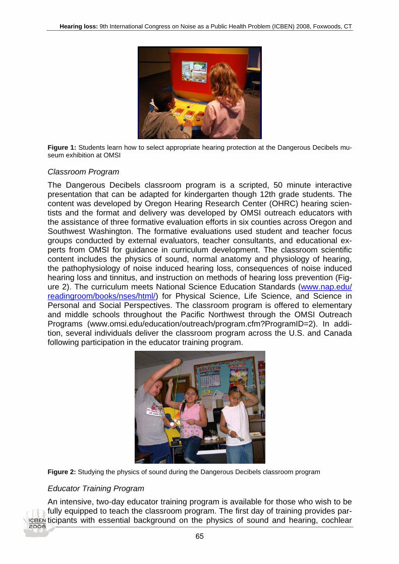
Hearing loss: 9th International Congress on Noise as a Public Health Problem (ICBEN) 2008, Foxwoods, CT
Figure 1: Students learn how to select appropriate hearing protection at the Dangerous Decibels mu-seum exhibition at OMSI
Classroom Program The Dangerous Decibels classroom program is a scripted, 50 minute interactive presentation that can be adapted for kindergarten though 12th grade students. The content was developed by Oregon Hearing Research Center (OHRC) hearing scien-tists and the format and delivery was developed by OMSI outreach educators with the assistance of three formative evaluation efforts in six counties across Oregon and Southwest Washington. The formative evaluations used student and teacher focus groups conducted by external evaluators, teacher consultants, and educational ex-perts from OMSI for guidance in curriculum development. The classroom scientific content includes the physics of sound, normal anatomy and physiology of hearing, the pathophysiology of noise induced hearing loss, consequences of noise induced hearing loss and tinnitus, and instruction on methods of hearing loss prevention (Fig-ure 2). The curriculum meets National Science Education Standards (www.nap.edu/ readingroom/books/nses/html/) for Physical Science, Life Science, and Science in Personal and Social Perspectives. The classroom program is offered to elementary and middle schools throughout the Pacific Northwest through the OMSI Outreach Programs (www.omsi.edu/education/outreach/program.cfm?ProgramID=2). In addi-tion, several individuals deliver the classroom program across the U.S. and Canada following participation in the educator training program.
Figure 2: Studying the physics of sound during the Dangerous Decibels classroom program
Educator Training Program An intensive, two-day educator training program is available for those who wish to be fully equipped to teach the classroom program. The first day of training provides par-ticipants with essential background on the physics of sound and hearing, cochlear
65

Hearing loss: 9th International Congress on Noise as a Public Health Problem (ICBEN) 2008, Foxwoods, CT
physiology, hearing loss, standards for recommended limits for sound exposure, background on noise induced hearing loss in children and instruction on hearing loss protection devices and other means of hearing protection for children, health com-munication theory applied to hearing health, classroom management strategies and a walk through the classroom program. The second day, participants present the class-room program to small groups in order to refine presentation skills and clarify misun-derstandings about the material. Each participant receives a course syllabus with a summary of the essential information, a detailed, step-by-step script of the entire classroom program and an educator kit with all of the essential materials, graphics and instrumentation needed to present the classroom program. Participants who complete the full training are certified as Dangerous Decibels Educators. The educa-tor training program is intended for teachers, school nurses, high school students, audiologists, physicians, scientists, speech pathologists and other interested in pre-senting of the Dangerous Decibels curriculum.
Figure 3: High school students are trained to be Dangerous Decibels educators
Teacher’s Resource Guide and DVD The Dangerous Decibels Teacher’s Resource Guide contains age-appropriate, hands-on science activities about the anatomy and physiology of hearing, the physics of sound, and health-related behaviors for prevention of noise-induced hearing loss that meet National Science Education Standards. It also includes a glossary of terms and diagrams and images that can be used in the classroom program. The activities were designed to either be included in the classroom program or to serve as pre- or post-classroom activities to facilitate learning of the educational messages. The Teacher’s Resource Guide can be purchased as hard copy or downloaded for free from the Dangerous Decibels website (www.dangerousdecibels.org/teachers_guide.cfm). The Dangerous Decibels DVD is complementary tool to the Teacher’s Resource Guide. It contains visual demonstrations of many of the activities presented in the written guide and also has instructional presentations, demonstrations and interviews about hearing, hearing loss, tinnitus and hearing protection that are appropriate for teacher training or to be shown in classrooms. The DVD is available for order (www.dangerousdecibels.org/teachers_guide/DVD_TRG_Order_Form.pdf) with or without the Teacher’s Resource Guide.
Science Festivals Another mode of science outreach for OMSI is through Science Festivals at major events such as County or State Fairs. At these events, the museum presents several science-based, hands-on exhibits. Three of the Dangerous Decibels museum exhib-its have been adapted into traveling versions that appear at Science Festivals. These
66

Hearing loss: 9th International Congress on Noise as a Public Health Problem (ICBEN) 2008, Foxwoods, CT
exhibits communicate the Dangerous Decibels educational messages to approxi-mately 250,000 participants each year.
Televideo-conference Classroom Program OHSU scientists and OMSI educators work together to conduct long-distance Dan-gerous Decibels classroom presentations using internet televideo-conferencing. Sev-eral schools can be connected via internet to a Portland-based studio for live interac-tion with the educators and with each other. Classroom materials and supplies for hands-on activities are forwarded to the schools in advance. The educators lead the students through activities just as if all were in the same classroom. This venue en-ables classrooms in rural and frontier areas to access hearing scientists and educa-tors directly, engage in exchanges of questions and answers, and enable them to receive a complete version of the Dangerous Decibels classroom program.
Web-based Virtual Museum Exhibition Eight of the OMSI museum exhibits have been translated into computer activities, demonstrations and games forming a virtual museum exhibition that communicate the fundamental educational messages of the project (www.dangerousdecibels.org/ virtualexhibit.cfm). The Virtual Exhibit was developed as an experimental intervention for a research project and was found to promote improvements in knowledge, atti-tudes and behaviors regarding hearing health as a stand-alone activity and as a booster activity for students having received a presentation of the Dangerous Deci-bels classroom program. It is a resource that is used in National Institute of Occupa-tional Safety and Health (NIOSH) young worker safety training and U.S. military edu-cational programs for new recruits.
Jolene Jolene is the product of a Dangerous Decibels student researcher’s desire to design and construct an innovative, visually intriguing sound level measuring system, to be used in public places as part of an education program to alert young people about risks of noise-induced hearing loss and tinnitus resulting from listening to music at high levels through headphones. Constructed using a used mannequin, sound level meter and a wardrobe from a second-hand store, Jolene has made friends wherever she goes. The sound level meter microphone was coupled to a silicone ear. Partici-pants are invited to set their personal stereo systems to their typical listening level and then allow Jolene to listen to it and measure the sound in dB (A-weighted, slow response). The transfer function of the outer ear (TFOE) was determined allowing decibel measures to be equated to national and international standards for recom-mended exposure levels. Jolene became so popular that many schools, organiza-tions and individuals wanted information on how to make their own versions. In re-sponse, the National Hearing Conservation Association (www.hearingconservation.org) funded the production of the Jolene Cookbook (Mar-tin & Martin 2007), a detailed instruction manual on how to make a Jolene for your-self. The cookbook has been downloaded across the United States and by groups in Canada, Japan, Mexico, New Zealand, Portugal, and Saipan. Jolene now has many siblings around the world and many have begun to send photos to the Jolene Family Album at the Dangerous Decibels website. A recent research study, using Jolene as a sound pressure measuring device, found that 16 % of 14-18 year olds sampled lis-tened to their personal stereo systems at levels and durations that exceed NIOSH recommended exposure levels on a daily basis (Martin et al. 2008).
67

Hearing loss: 9th International Congress on Noise as a Public Health Problem (ICBEN) 2008, Foxwoods, CT
Figure 4: Jolene visiting Niagara Falls on a trip to Canada
The combined Dangerous Decibels activities, including the museum exhibition at OMSI, classroom presentations, OMSI Science Festivals at County Fairs and educa-tional training sessions, reach nearly one million people annually.
CONCLUSIONS Partnerships are the key to the success of any public health initiative. The challenges include conflicts in cultures, work patterns, terminology, priorities, institutional agen-das, personalities, and time tables. The rewards of partnering include the ability to produce innovative, expansive and effective health promotion programs in ways that far exceed the ability of any individual contributor. Dangerous Decibels resources are still in development. Research is currently underway on applying these tools in spe-cific communities at-risk for noise exposure. One such partnership is between the Dangerous Decibels group and the Northwest Portland Area Indian Health Board, representing the 43 Native American tribes and nations in the Pacific Northwest. Other initiatives with the Hispanic/Latino population in the Northwest are being devel-oped.
REFERENCES Anderson KL (1991). Hearing conservation in the public schools revisited. Semin Hearing 12: 340–364.
Axelsson A, Jerson T (1985). Noisy toys: A possible source of sensorineural hearing loss. Pediatrics 76: 574-478.
Bennett JA, English K (1999). Teaching hearing conservation to school children: comparing the outcomes and efficacy of two pedagogical approaches. J Educ Audiol 7: 29-33.
Black DR, Gobler NS, Sciacca JP (1998). Peer helping/involvement: an efficacious way to meet the challenge of reducing alcohol, tobacco, and other drug use among youth. J School Health 68: 87-93.
Blair JC, Hardegree D, Benson PV (1996). Necessity and effectiveness of a hearing conservation program for elementary students. J Educ Audiol 4: 12-16.
Broste SK, Hansen DA, Strand RL, Stueland DT (1989). Hearing loss among high school farm students. Am J Public Health 79: 619-622.
Busch-Vishniac IJ, West JE, Barnhill C, Hunter T, Orellana D, Chivukula R (2005). Noise levels in Johns Hopkins Hospital. J Acoust Soc Am 118: 3629-3645.
Chermak GD, Peters-McCarthy E (1991). The effectiveness of an educational hearing conservation program for elementary school children. Lang Speech Hear Serv Schools 22: 308-312.
Chermak GD, Curtis L, Seikel JA (1996). The effectiveness of an interactive hearing conservation program for elementary school children. Lang Speech Hear Serv Schools 27: 29-39.
Clark WW (1991). Noise exposure from leisure activities: A review. J Acoust Soc Am 90: 175-181.
Devries H, Weijts W, Dijkstra M, Kok G (1992). The utilization of qualitative and quantitative data for health-education pro-gram-planning, implementation, and evaluation - a spiral approach. Health Educ Quart 19: 101-115.
68

Hearing loss: 9th International Congress on Noise as a Public Health Problem (ICBEN) 2008, Foxwoods, CT
Folmer RL (2008). Hearing-loss prevention practices should be taught in schools. Semin Hearing 29: 67-80.
Folmer RL, Griest SE, Martin WH (2002). Hearing conservation education programs for children: a review. J School Health 72: 51-57.
Foshee VA, Bauman KE, Arriaga XB, Helms RW, Koch GG, Linder GF (1998). An evaluation of safe dates, an adolescent dating violence prevention program. Am J Public Health 88: 45-50.
Gupta D, Vishwakarma SK (1989). Toy weapons and firecrackers: A source of hearing loss. Laryngoscope 99: 330-334.
Hager L (2006). Working youth, noise exposure and hearing loss. Paper presented at the Noise-Induced Hearing Loss in Children at Work and Play conference. Cincinnati, OH.
Hellstrom PA, Dengerink HA, Axelsson A (1992). Noise levels from toys and recreational articles for children and teenagers. Brit J Audiol 26: 267-270.
Jokitulppo JS, Björk EA, Akaan-Pentitilä E (1997). Estimated leisure noise exposure and hearing symptoms in Finnish teen-agers. Scand Audiol 26: 257-262.
Knobloch MJ, Broste SK (1998). A hearing conservation program for Wisconsin youth working in agriculture. J School Health 68: 313-318.
Lass JE, Woodford CM, Lundeen C, Lundeen DJ, Everly-Myers DS, McGuire K, Mason DS, Parknik L, Phillips RP (1987). A hearing-conservation program for a junior high school. Hear J 40: 32-40.
Lukes E, Johnson M (1998). Hearing conservation: community outreach programs for high school students. AAOHN J 46: 340-343.
MacDonald SA (1999). The cardiovascular health education program: Assessing the impact on rural and urban adolescents' health knowledge. Appl Nurs Res 12: 86-90.
Main DS, Iverson DC, McGloin J, Banspach SW, Collins JL, Rugg DL, Kolbe LJ (1994). Preventing HIV-Infection among adolescents - evaluation of a school-based education-program. Prev Med 23: 409-417.
Martin GY, Martin WH (2007). The Jolene Cookbook. Portland: Oregon Health & Science University. http://www.dangerousdecibels.org/jolene.cfm
Martin GY, Martin WH (2008). NIHL prevention in children and adolescents: The Jolene Cookbook. Presented at the 33rd Annual Hearing Conservation Conference of the National Hearing Conservation Association. Portland, Oregon.
Martin GY, Martin WH, Griest SE, Lambert W (2008). How loud is your music? Beliefs and practices regarding use of per-sonal stereo systems. Presented at the 33rd Annual Hearing Conservation Conference of the National Hearing Conservation Association. Portland, Oregon.
Martin WH (2008). Dangerous Decibels®. Partnership for preventing noise induced hearing loss and tinnitus in children. Semin Hearing 29: 102-110.
Martin WH, Sobel JL, Griest SE, Howarth L, Shi Y-B (2006). Noise induced hearing loss in children: Preventing the silent epidemic. J Otol 1: 11-21.
Meyer-Bisch C (1996). Epidemiological evaluation of hearing damage related to strongly amplified music (personal cassette players, discotheques, rock concerts) – high definition audiometric survey on 1364 subjects. Audiology 35: 121-142.
Montgomery JK, Fujikawa S (1992). Hearing thresholds of students in the second, eighth, and twelfth grades. Lang Speech Hear Serv Schools 23: 61-63.
Niskar AS, Kieszak SM, Holmes AE, Esteban E, Rubin C, Brody DJ (2001). Estimated prevalence of noise-induced hearing threshold shifts among children 6 to 19 years of age: The third national health and nutrition examination survey, 1988-1994, United States. Pediatrics 108: 40-43.
Noland MP, Kryscio RJ, Riggs RS, Linville LH, Ford VY, Tucker TC (1998). The effectiveness of a tobacco prevention pro-gram with adolescents living in a tobacco-producing region. Am J Public Health 88: 1862-1865.
Price JH, Beach P, Everett S, Telljohann SK, Lewis L (1998). Evaluation of a three-year urban elementary school tobacco prevention program. J School Health 68: 26-31.
Reding DJ, Fischer V, Gunderson P, Lappe K, Anderson H, Calvert G (1996). Teens teach skin cancer prevention. J Rural Health 12: 265-272.
Sobel J, Meikle M (2008). Applying health behavior theory to hearing-conservation interventions. Semin Hearing 29: 81-89.
Weber HJ, McGovern FJ, Zink P (1967). An evaluation of 1000 children with hearing loss. J Speech Hear Disord 32: 343-354.
69

Hearing loss: 9th International Congress on Noise as a Public Health Problem (ICBEN) 2008, Foxwoods, CT
West PD, Evans EF (1990). Early detection of hearing damage in young listeners resulting from exposure to amplified music. Brit J Audiol 24: 89-103.
WHO (1997). Strategies for prevention of deafness and hearing impairment. Prevention of noise-induced hearing loss. Ge-neva: World Health Organization.
70

Hearing loss: 9th International Congress on Noise as a Public Health Problem (ICBEN) 2008, Foxwoods, CT
Methods of fit testing hearing protectors, with representative field test data Elliott H. Berger1*, Jeremie Voix2, Lee D. Hager2 1 Aearo Technologies, 7911 Zionsville Rd., Indianapolis, IN, USA, 46268-1657
2 Sonomax Hearing Healthcare, 8375 Mayrand St. Montreal, Quebec, Canada, H4P 2E2
* corresponding author: e-mail: [email protected]
INTRODUCTION Numerous published studies in the past 20 years clearly demonstrate that use of laboratory measurements to predict real-world attenuation for groups of workers, or even more problematically for individual workers, is fraught with inaccuracies. Thus, the ability to properly assign hearing protectors in critical high-noise environments or even for lower noise levels when one wishes to closely match attenuation to actual exposure, is questionable. Even if the laboratory data were representative of the ac-tual group using the device, the individual variability is large enough that attempts at predicting one person’s performance from group data can easily err by up to 20 dB (Gauger & Berger 2004). One approach to solving these problems is the development of systems to allow indi-vidual fit testing in the field, and indeed such systems have been garnering increas-ing visibility in recent years. In fact, fit-test technology has been available in the labo-ratory in many forms for nearly 30 years (Berger 1984, 1986, 1988, 1989), but only in the past decade has the hearing conservation community started to look more closely at this issue. Recently, Berger (2006) discussed seven important applications for field-test methods, as listed below.
1) Train and motivate employees to properly and consistently wear their HPDs 2) Train the trainer on how to train employees 3) Assign HPDs based upon noise exposures and expected protection levels 4) Provide useful standard-threshold-shift (STS) follow up to see if the problem
may be HPD related 5) Present data that may be accepted by OSHA improved alternative to deter-
mine HPD adequacy 6) Audit departments to assess overall HPD effectiveness and suitability 7) Provide potentially useful documentation to defend against workers’ compen-
sation claims regarding HPD adequacy and provision of sufficient training Today there are a number of systems that provide field-test capabilities. Herein we explore various options, especially with respect to their advantages and disadvan-tages. We will then focus on one of those methods, microphone-in-real-ear (MIRE) and its implementation as a quick and portable field method, termed field-MIRE, ab-breviated F-MIRE (Hager & Voix 2006). Representative outputs from the system will be examined to understand how variability may be accounted for in practice, and ac-tual data from industrial plants will be summarized to indicate the types of perform-ance that are currently being achieved.
71

Hearing loss: 9th International Congress on Noise as a Public Health Problem (ICBEN) 2008, Foxwoods, CT
METHODS OF FIELD TESTING HEARING PROTECTOR ATTENUATION Field test methods exist in three basic “flavors,” consisting of subjective (psycho-acoustic), objective, and non-acoustic methods, as outlined below:
• Subjective (psychoacoustic) o REAT (real-ear attenuation at threshold)
Sound field (in a small booth or chamber) Circumaural (with earphones in large noise-excluding cups) Supra-aural (using supra-aural audiometric earphones)
o Loudness balance • Objective [microphone-in-real-ear (MIRE)]
o Probe microphone passed through or around an earplug o Microphones mounted inside and outside of earmuff cups
• Non-acoustic: static pressure / pneumatic seal measurements With the exception of the loudness-balance method, all of the subjective procedures are variants of the “gold standard,” real-ear attenuation at threshold (REAT) proce-dure that is well documented in current and prior ANSI standards (ANSI S12.6). In the field, the intention is to replicate laboratory-based REAT. REAT requires listeners to track their hearing threshold levels to measure their hearing sensitivity. The sounds are normally presented from loudspeakers in a test chamber and the proce-dure is repeated, both with and without HPDs. The difference in the two thresholds is the attenuation of the device. This procedure is called real-ear attenuation at thresh-old since the attenuation of the HPD is measured on real ears of human subjects, and since it is computed from differences in the threshold of hearing, with and without the hearing protector in place (Berger 2000). When taking REAT into the field the loudspeakers are normally replaced with head-phones, i.e. speakers in large circumaural cups (or as noted above, sometimes mounted in standard audiometer earphone cushions). This enables only the testing of earplugs. However, earplugs are the type of HPD that is most problematic and variable in fit and therefore most in need of fit testing. When the field procedure is accomplished using a small noise enclosure or sound booth, both earmuffs and ear-plugs can be evaluated, but with the additional cost and difficulty associated with po-tentially transporting and then positioning a booth near the workplace. The advantage of field REAT is that it can yield valid data with only one known measurement artifact - it produces values of attenuation that are spuriously high by typically up to a few decibels in the frequencies at and below 250 Hz. This is due to physiological noise masking in the occluded ear (Berger & Kerivan 1983). The three field-REAT variants that are listed above have all been successfully implemented according to the literature, but the use of supra-aural earphones can be problematic due to potential artifacts (Berger 1984, 1986). A principal disadvantage of field REAT is its time-consuming nature. Each frequency tested takes at least 30 seconds, requiring a minimum of at least one minute to test the fit in each ear since both an open and an occluded threshold is required, much longer if multiple frequencies are to be tested. Furthermore there is an inherent vari-ability since the data rely on the listener’s ability to track his or her own threshold. The process itself has a substantial imprecision of approximately + 5 dB for typical subjects. Finally accurate REAT measurements require low background noise so that the open-ear thresholds are not masked and contaminated. Even when field REAT is conducted under large noise-excluding earmuff cups, or in a sound booth near the
72

Hearing loss: 9th International Congress on Noise as a Public Health Problem (ICBEN) 2008, Foxwoods, CT
workplace, care must be exercised to be sure that the environment is adequately quiet. The remaining subjective field procedure is loudness balance, recently updated with a new paradigm (Soli et al. 2005). In this method, applicable to only earplugs, instead of comparing open and occluded thresholds, the subject is asked to establish a bal-ance in the loudness between signals presented to occluded and unoccluded ears. Like a threshold procedure this requires a listener’s subjective response and the at-tendant time and potential variability, especially for the untrained workers in industry. Also, though the balance is probably not inherently any more difficult to track than a threshold, employees generally have familiarity with threshold tracking because of the annual audiograms they receive as enrollees in a hearing conservation program. Another potential problem is that it may not be possible to generate sufficiently in-tense test signals for a worker with high-frequency hearing loss to detect the stimuli and effect a loudness balance while wearing a hearing protector. An advantage of loudness balance is that it is less susceptible to contamination than REAT from background noise since the testing is conducted at sound levels that are normally at least 30 to 40 dB greater than in the REAT protocol. An alternative to the subjective procedures is to make objective measurements with microphones, termed a microphone-in-real-ear (MIRE) technique (Berger 1986). When applied in occupational settings this becomes a field-MIRE (F-MIRE) method-ology (Hager & Voix 2006; Voix 2006). With F-MIRE the sound pressure levels in the earcanal under the hearing protector and those outside the HPD, are simultaneously measured. Using suitable correction factors to account for known and quantifiable acoustic differences between the F-MIRE and REAT, the values can be used to ac-curately estimate the hearing protector’s attenuation. MIRE can be conducted with probe measurement devices that consist of thin flexible tubes connected to microphones, with the tubes either placed in the earcanal or through the earplugs or between the earplugs and the canal walls. Working with the tubing can be problematic and can substantially affect the performance of the ear-plugs unless the tubing is sealed through the body of the plugs. The tubing itself can also leak sound through its wall (i.e., a flanking pathway) if the material of the tube does not possess a sufficiently high insertion loss. The F-MIRE system in this report incorporates a single small dual-element micro-phone and associated proprietary technology (Voix & Laville 2002, 2004; Voix 2006). One section of the dual-element microphone couples through the earplug to pickup the sound pressure levels in the earcanal, and the other section measures the exter-nal sound field. Broadband steady-state sound is presented via a small speaker in front of the subject. The actual measurement takes about 10 seconds for one fit in one ear for the standard 7 test frequencies from 125 Hz to 8 kHz, from which is cal-culated an overall noise reduction rating called the Personal Attenuation Rating (PAR1). The PAR, though it appears to be an exact number, also contains its own variability, albeit much less than in the classical approach of using mean laboratory data to make individual field predictions. The extent of variability in PAR is defined and explicitly provided with the measurement (Berger 2007). In addition to the brevity of the test, another advantage is that it can be conducted in substantially higher noise levels than can a field-REAT measurement, and it reduces
1 The PAR is computed like the Noise Level Reduction Statistic (NRSA as defined in ANSI S12.68) except it is calculated individually for each subject and reported as a median PAR instead of at the 80th and 20th percentiles.
73

Hearing loss: 9th International Congress on Noise as a Public Health Problem (ICBEN) 2008, Foxwoods, CT
Figure 1: Key components of the F-MIRE system
the inherent variability by replacing the variance of the subject’s open and occluded thresholds, or loudness balances, with the smaller variance of the measurement sys-tem. The system is useful for training, monitoring, and other applications (Berger 2006), but it does rely on surrogate HPDs that consist of earplugs modified by pass-ing probe tubes through them. Thus the plug that the subject fits is not identical to the plug that will be worn on a day-to-day basis. This is discussed further in the following section. Another implementation of MIRE approach is to instrument earmuff cups with internal and external microphones as has been done for research purposes, as well as in a commercially available product intended for regular use in industry to monitor hearing protector effectiveness (Berger 1986; Burks & Michael 2003). The last type of field test method listed above is one based on static pressure meas-urements to determine the presence of a pneumatic seal. This method has been pri-marily used to validate that a custom earmold is well made and fits the ear properly, and indeed it is suitable for such a purpose. However, translation of that seal to as-surance of a particular degree of sound attenuation has sufficient uncertainty that this is not a viable method for field protection, except for possibly a pass/fail determina-tion for selected types of products. This would not be a suitable way to test most foam earplugs since although they provide a strong acoustic barrier to sound, one of their positive attributes is that they leak at very low frequencies and hence do not create a pneumatic seal.
COMPONENTS OF A FIELD MICROPHONE-IN-REAL-EAR (F-MIRE) SYSTEM Of the preceding methods, in our estimation, F-MIRE provides the best balance be-tween speed, accuracy, repeatability, and correspondence with actual practice. The F-MIRE method investigated in this study was adapted from one developed by So-nomax Hearing Healthcare Inc. (Voix & Laville 2002; Voix 2006) for use with their custom earmold technology. Certain features of the system required modification for use with a wide range of earplugs such as non-custom foam and premolded earplugs that provide higher-levels of attenuation than the earplugs for which the system was initially designed. The particular F-MIRE implementation evaluated in this study is the E•A•RFit™ system from Aearo Technologies. Figure 1 illustrates the compo-nents of the system and Figure 2 provides an expanded view of the microphone and probed earplug tips. The F-MIRE system consists of a sound source that generates high-levels of broadband random (pink) noise at the listener’s ear, a dual-element microphone that simultaneously measures in a repeatable location the sound present at the outside of the ear-plug and in the earcanal after having passed through the ear-plug, a probed earplug to act as a surrogate for the actual earplug that subjects will wear, and an analysis system in-stalled on a desktop or laptop PC that can rapidly record accurate and repeatable measurements. The sound levels used, depending upon the amount of attenuation
74

Hearing loss: 9th International Congress on Noise as a Public Health Problem (ICBEN) 2008, Foxwoods, CT
provided by the earplug, are up to 90 dBA with a duration of approximately 10 sec-onds. The listener’s nose is positioned 30 cm from the front of the loudspeaker at a preset elevation. A key feature of the development of this F-MIRE system was the design of the probed test tips. The tubing through the plug needed to allow measurement via the dual-element mic of the sound pressure levels in the earcanal, but at the same time provide high levels of self-insertion loss (i.e., sound transmission through the walls of the tubing) so as not to affect the attenuation properties of the earplug. The tubing was selected to minimize its effect on use of the HPD, being of sufficiently small di-ameter and suitable softness so as not to materially affect the listener’s ability to in-sert the earplugs. In the case of the foam tips the tubing also could not affect the abil-ity to roll the plug into a tiny crease-free cylinder for insertion into the earcanal. F-MIRE can provide a close approximation of REAT, but F-MIRE measurements yield a noise reduction (NR) value which is the difference between the levels outside and inside the earcanal. REAT, however, is an insertion loss (IL) measurement that is the difference in the sound pressure levels at one point in space (such as the ear-drum) with and without the HPD in place. NR and IL are directly related, but they are not the same; thus a mathematical adjustment is required that uses the transfer func-tion of the open ear (TFOE). TFOE is the difference between the sound pressure lev-els in the sound field and at the eardrum (Berger 1986). In addition to a TFOE correc-tion, the variation of sound conduction with frequency through the probe tips and other correction factors are also needed utilize F-MIRE to predict REAT (Voix 2006). The most direct way to account for all of the above factors is to make a simultaneous measurement of REAT and NR, for a given fitting of probed earplugs on a group of subjects. One can then directly compare the two measured values of attenuation and determine the correction factors (also called compensation) to bring them into the closest possible agreement (Voix & Laville 2002). This approach is commonly ac-cepted and has previously been used for other types of field-test systems (Michael et al. 1976). The compensation factors noted above only describe the differences due to system bias, factors that are stable from measure to measure. There is also an inherent vari-ability of the REAT and F-MIRE procedures. Accounting for this multiplicity of factors required the development of a complex test paradigm that has been described by Berger et al. (2006). An example of the correspondence between REAT and F-MIRE values is shown in Figure 3.
VARIABILITY Berger et al. (2006) found that on the average, their F-MIRE predictions were reliable indicators of REAT values. However, review of the data indicated that REAT vs. F-MIRE differences for a single measurement on a given subject could exceed 10 dB for individual 1/3-octave bands.
Figure 2: The dual-microphone element and representative probed tips for foam and premolded earplugs
75
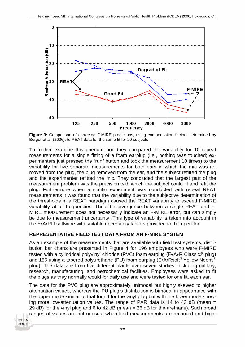
Hearing loss: 9th International Congress on Noise as a Public Health Problem (ICBEN) 2008, Foxwoods, CT
Figure 3: Comparison of corrected F-MIRE predictions, using compensation factors determined by Berger et al. (2006), to REAT data for the same fit for 20 subjects
To further examine this phenomenon they compared the variability for 10 repeat measurements for a single fitting of a foam earplug (i.e., nothing was touched; ex-perimenters just pressed the “run” button and took the measurement 10 times) to the variability for five separate measurements for both ears in which the mic was re-moved from the plug, the plug removed from the ear, and the subject refitted the plug and the experimenter refitted the mic. They concluded that the largest part of the measurement problem was the precision with which the subject could fit and refit the plug. Furthermore when a similar experiment was conducted with repeat REAT measurements it was found that the variability due to the subjective determination of the thresholds in a REAT paradigm caused the REAT variability to exceed F-MIRE variability at all frequencies. Thus the divergence between a single REAT and F-MIRE measurement does not necessarily indicate an F-MIRE error, but can simply be due to measurement uncertainty. This type of variability is taken into account in the E•A•Rfit software with suitable uncertainty factors provided to the operator.
REPRESENTATIVE FIELD TEST DATA FROM AN F-MIRE SYSTEM As an example of the measurements that are available with field test systems, distri-bution bar charts are presented in Figure 4 for 196 employees who were F-MIRE tested with a cylindrical polyvinyl chloride (PVC) foam earplug (E•A•R Classic® plug) and 155 using a tapered polyurethane (PU) foam earplug (E•A•Rsoft® Yellow Neons® plug). The data are from five different plants over seven studies, including military, research, manufacturing, and petrochemical facilities. Employees were asked to fit the plugs as they normally would for daily use and were tested for one fit, each ear. The data for the PVC plug are approximately unimodal but highly skewed to higher attenuation values, whereas the PU plug’s distribution is bimodal in appearance with the upper mode similar to that found for the vinyl plug but with the lower mode show-ing more low-attenuation values. The range of PAR data is 14 to 43 dB (mean = 29 dB) for the vinyl plug and 6 to 42 dB (mean = 26 dB for the urethane). Such broad ranges of values are not unusual when field measurements are recorded and high-
76

Hearing loss: 9th International Congress on Noise as a Public Health Problem (ICBEN) 2008, Foxwoods, CT
light the difficulty of predicting individual performance from group data measured in the laboratory.
Figure 4: Distribution of PARs for Classic (N=196) and Neon (N=155) users in 7 different industrial plants
Keeping in mind that PAR is intended to be subtracted from A-weighted sound levels while Noise Reduction Ratings (NRRs) per the current labeling requirements (EPA 1979) are to be subtracted from C-weighted sound levels, one must make an adjust-ment to properly compare NRR to PAR. Based on Gauger and Berger (2004) the mean and median C – A value for industrial noises are 2.5 and 1.9 dB respectively. Thus, a 2-dB C – A correction was subtracted from the NRR to compare to PAR. For a PVC plug with an NRR of 29 dB, 98 % of users fitting the device under the exact conditions of the laboratory REAT test should have obtained approximately 27 dB of protection, but in these plants only about 73 % of users did so; their effective real-world NRR achieved by 98 % of the employees (computed from PARs) was 18 dB. This is better than anticipated for a PVC plug based on prior real-world studies (Ber-ger, 2000). For the PU plug, 98 % of users should have achieved a PAR of 31 dB (based on a labeled NRR of 33) but only 38 % did so, for an effective real-world NRR of 10 dB. The differences between the PVC and PU earplugs are unexplained at this time, but it is interesting to note that in a prior real-world study that examined the performance of various products including foam earplugs, the PVC plug exceeded a PU plug by approximately 9 dB in terms of a mean less one standard deviation (Scott 1995), and in this study the difference is 8 dB.
CONCLUSIONS The concept and importance of field fit testing is reviewed and various subjective, objective, and non-acoustic methods are described. Seven important applications for field test methods are highlighted, with the most obvious being for training and moti-vation. An objective method, F-MIRE is selected as one of the more useful ap-proaches and a system incorporating that technology is presented along with a brief discussion of its development. Uncertainty in laboratory and field test methods is dis-cussed so that users understand that all methods include an inherent degree of vari-ability. Test data from recent implementations using the F-MIRE system are presented to illustrate the wide variability of earplug performance in practice, the large divergence
77

Hearing loss: 9th International Congress on Noise as a Public Health Problem (ICBEN) 2008, Foxwoods, CT
between laboratory and field-measured performance, and the need for individual fit testing to characterize the performance that will be obtained for workers in practice.
REFERENCES ANSI (1997). Methods for measuring the real-ear attenuation of hearing protectors. S12.6-1997 (Rev. 2002). New York: American National Standards Institute.
ANSI (2007). Methods of estimating effective A-weighted sound pressure levels when hearing protectors are worn. S12.68-2007. New York: American National Standards Institute.
Berger EH (1984). Assessment of the performance of hearing protectors for hearing conservation purposes. Noise Vibr Control Worldwide 15(3): 75-81.
Berger EH (1986). Review and tutorial - methods of measuring the attenuation of hearing protection devices. J Acoust Soc Am 79: 1655-1687.
Berger EH (1988). Use of circumaural and supra-aural earphones to measure the real-ear attenuation of earplugs. In: Ameri-can Industrial Hygiene Conference, San Francisco, CA, paper 39.
Berger EH (1989). Exploring procedures for field testing the fit of earplugs. In: Proceedings, 1989 Industrial Hearing Conser-vation Conference, Off. Eng. Serv., Univ. Kentucky, Lexington, KY, 7-10.
Berger EH (2000). Hearing protection devices. In: Berger EH, Royster LH, Royster JD, Driscoll DP, Layne M (eds.): The Noise manual, 5th ed. (pp 379-454). Fairfax, VA: American Industrial Hygiene Association.
Berger EH (2006). Introducing F-MIRE testing - background and concepts. E•A•R Technical Report 06-29/HP. Indianapolis, IN: Aearo Technologies.
Berger EH (2007). What is a personal attenuation rating (PAR)? E•A•R Technical Report 07-21/HP. Indianapolis, IN: Aearo Technologies.
Berger EH, Kerivan JE (1983). Influence of physiological noise and the occlusion effect on the measurement of real-ear attenuation at threshold. J Acoust Soc Am 74: 81-94.
Berger EH, Voix J, Kieper RW (2006). Methods of developing and validating a field-MIRE approach for measuring hearing protector attenuation. Spectrum 24(1): 22. Burks JA, Michael KL (2003). A new best practice for hearing conservation: the Exposure Smart Protector (ESP). In: Holger DK, Maling GC (eds.): Proceedings of the Noise-Conference 2003 (paper 009). Washington, DC: Institute of Noise Control Engineering.
EPA (1979). Noise labeling requirements for hearing protectors. Environmental Protection Agency. Fed Regist 44(190): 40CFR Part 211, 56130 56147.
Gauger D, Berger EH (2004). A new hearing protector rating: the noise reduction statistic for use with A weighting (NRSA). Report for US Environmental Protection Agency. Approved by ANSI S12/WG11, E-A-R 04-01/HP, Indianapolis, IN.
Hager LD, Voix J (2006). Individual field fit testing of hearing protectors – a Field-MIRE approach. In: Conference of the American Society of Safety Engineers (ASSE), Seattle, WA.
Michael PL, Kerlin RL, Bienvenue GR, Prout JH, Shampan JI (1976). A real-ear field method for the measurement of the noise attenuation of insert-type hearing protectors. Cincinnati, OH: National Institute for Occupational Safety and Health. US Dept. of HEW, Report No. 76-181.
Scott RF (1995). Study of factors affecting at-work protection afforded by hearing protection devices on steelworks. Doc. FR S373-5 942. London: British Steel plc.
Soli SD, Vermiglio A, Larson VD (2005). A system for assessing the fit of hearing protectors in the field. Spectrum 22 (Suppl. 1): 25.
Voix J (2006). Mise au point d'un bouchon d'oreille ‘intelligent’ (Development of a ‘smart’ earplug). Ph. D. Thesis, École de technologie supérieure, Montréal, Canada.
Voix J, Laville F (2002). Expandable earplug with smart custom fitting capabilities. In: Proceedings of InterNoise 02, Noise Control Foundation, Poughkeepsie, NY.
Voix J, Laville F (2004). New method and device for customizing in situ a hearing protector. Canad Acoust 32: 86-87.
78

Hearing loss: 9th International Congress on Noise as a Public Health Problem (ICBEN) 2008, Foxwoods, CT
Risk for NIHL from personal listening devices Brian Fligor Children’s Hospital Boston and Harvard Medical School
Correspondence: e-mail: [email protected]
The risk for noise-induced hearing loss (NIHL) from using personal listening devices (PLD) such as the Apple iPod® has received considerable popular media attention in recent years. The true risk for NIHL from using a PLD, however, may be much less than purported by the popular media, potentially detracting from other, more signifi-cant sources of leisure noise exposure. It is the profession’s responsibility to deline-ate true risk from media hyperbole. This presentation will provide a summary the lit-erature to date documenting risk for NIHL from PLD, and explain results from three studies on PLD use. The first study will report the A-weighted free-field equivalent output levels from several commercially-available .mp3 players and suggested rec-ommendations for limiting risk for NIHL. The second study will explain the influence of background noise on chosen listening level, and why some in-ear earphones actu-ally mitigate risk for NIHL. The third study will provide diagnostic test criteria meas-ures (including positive predictive value) for the question, “if I can hear another per-son’s music from their headphones, does that mean it’s too loud?”
79
Hearing loss: 9th International Congress on Noise as a Public Health Problem (ICBEN) 2008, Foxwoods, CT
Threshold shifts and restitution of the hearing after energy-equivalent noise exposures with an equal NRC-value and non-equal frequency composition Helmut Strasser*, Min-Chi Chiu, Oliver Müller Ergonomics Division, University of Siegen, Paul-Bonatz-Str. 9-11, D-57068 Siegen/Germany
*correspondence author: e-mail: [email protected]
ABSTRACT Based on industrial noise, test noise exposures were configured that were completely comparable in the sense that they all had a mean level of 94 dB(A) for 1 h and a Noise Rating Curve-value of 92, but for two of them, the band levels were increased in the lower frequency range and in the higher frequency range of the industrial noise, respectively, with compensating attenuation in the other frequency ranges. Ten otologically normal test subjects were exposed to the 3 noises which followed a change-over test design on 3 days. The maximum threshold shift TTS2 and the time needed for a complete recovery of the hearing, associated with the accented high-frequency noise were substantially higher and lasted longer than with the unaltered original industrial noise. The accented low-frequency noise also resulted in substantially higher threshold shifts that persisted for a longer time than those of the unaltered noise exposure. As a result, the Integrated Restitution Temporary Threshold Shifts (IRTTS), known as measure for the “Physiological Costs” in their entirety that the hearing must “pay” for the preceding noise exposures, differend very distinctly. Finally, when the IRTTS-values of the two test series with the altered spectra are expressed relative to the value for the original industrial noise, the quotients of 5.26 and 1.99 indicate substantially higher physiological responses associated with accented high-frequency and low-frequency components in energetically identical noise exposures.
1 INTRODUCTION AND MOTIVATION OF THE STUDY In the rating of noise exposures, very simple and easily manageable methods that are based on so-called single number values are typically used (referring to their problematic use see, e.g., Strasser 2005; Strasser & Irle 2006) instead of measures that attempt to do the hearing’s complexity justice such as binaural loudness measurements or psycho-acoustic methods (cp. Zwicker & Fastl 1990; Genuit 2005). Particularly common is the daily noise exposure level LEx/8 h (the former rating level LArd), an energy-equivalent mean value that is related to an 8-hour day (NN 2007a) that is calculated from noise of different level and duration via a formula (cp. Fig. 1). For instance, a daily noise exposure level of 85 dB for 8 h, due to the 3-dB exchange rate, can be built by 88 dB for 4 h, 91 dB for 2 h, or also energy-equivalent 94 dB for 1 h (cp. left part of Fig. 1). The use of the A-filter pretends to represent at least an attempt to relate the frequency weighting of the noise to the characteristics of the hearing. The daily mean noise dose, however, that is expressed in such a fashion fails to consider whether quiet spells occur in between the individual noise exposures – which would be advantageous to the hearing – or whether those important resting phases are filled up with additional noise. While such noise may be energetically insignificant, is still hinders the hearing’s restitution after threshold shifts that were caused by preceding high noise exposures (see Irle et al. 1998). Indeed, according to the right part of Fig. 1, it is energetically irrelevant, whether a daily noise exposure of
80

Hearing loss: 9th International Congress on Noise as a Public Health Problem (ICBEN) 2008, Foxwoods, CT
85 dB(A) stems from a noise level of 94 dB(A) for 1 h and a silent period for 7 h, or whether these 7 h are filled up with noise of 75 dB(A). In addition to the offsetting to noise exposures of varying duration and loudness, the inadequate dose maxim – with respect to the effects of noise on the hearing – is also applied in the rating of noise exposures with different frequencies. That is, the 3-dB exchange rate is not only applied to the time dimension, but also to the frequency. In the latter case, the filling up of frequency bands up to a certain degree is once again possible without a resulting change in the rating level even in the decimal places. Similarly, the use of Noise Criterion and Noise Rating Curves (NC, NRC) for the frequency weighting and, ultimately, for the rating of stationary noise, i.e., noise that is constant over time, does not appear to be appropriate to address the problem sufficiently.
Figure 1: Sound pressure levels of different duration leading to an equal daily noise exposure level (in this case LEx, 8 h = 85 dB(A), using the “3-dB exchange rate”)
Since Noise Rating Curves look like the equal-loudness contours (NN 1987), it can be assumed that they would have been established based on profound psycho-physiological responses. Engineers, very often, appreciate Noise Rating Curves because they believe in these criteria giving direction to a highly qualified assessment of annoyance and speech intelligibility as well as to a general rating of noise (cp., e.g., Schmidt 1988). In a serious evaluation, however, they are both problematic and curious. No matter, an octave-band level analysis of the sound exposure is carried out but thereafter, the valuable information about the spectral distribution of the exposure is overruled completely in order to create a single number rating value which is determined solely by one frequency band level. Despite the fact, that ISO R 1996 (NN 1971), dealing with NRC, has been withdrawn already, Noise Rating Curves, however, still exist in guidelines (NN 2000), in textbooks (NN 1991a; Schmidt 1988), as well as in the scientific literature (e.g., Broner 2005). As can be seen in Fig. 2, similar to the curves of perceived (subjective) loudness, with the 1 kHz octave band as reference point, the Noise Rating Curves permit higher levels at lower frequencies and dictate lower levels at higher frequencies. Rather than only forming a single number parameter with the A-filter, this method at least includes an octave-level analysis of the noise, which is followed by a comparison of the results with the Noise Rating Curves. Details on Noise Criterion Curves, published first by Beranek (1957), the replaced NCB (Balanced Noise Criterion Curves) and Noise Rating Curves see amongst others Beranek (1988), Kosten & Van Os (1962), NN (1989) and Schaefer (1984). For example, the noise spectrum shown in the left part of Fig. 2 is characterized with a NRC value of 80. However, since ultimately only the octave level that is tangent to the highest NR curve is used as the relevant single number parameter (and the noise
81
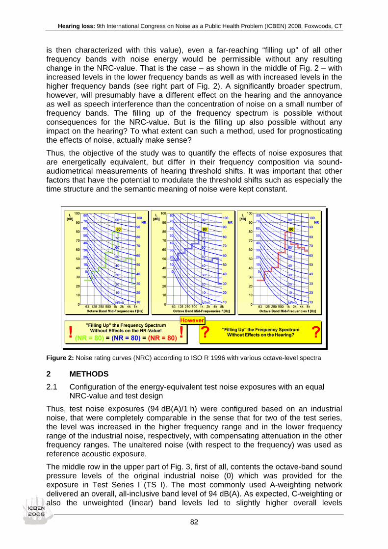
Hearing loss: 9th International Congress on Noise as a Public Health Problem (ICBEN) 2008, Foxwoods, CT
is then characterized with this value), even a far-reaching “filling up” of all other frequency bands with noise energy would be permissible without any resulting change in the NRC-value. That is the case – as shown in the middle of Fig. 2 – with increased levels in the lower frequency bands as well as with increased levels in the higher frequency bands (see right part of Fig. 2). A significantly broader spectrum, however, will presumably have a different effect on the hearing and the annoyance as well as speech interference than the concentration of noise on a small number of frequency bands. The filling up of the frequency spectrum is possible without consequences for the NRC-value. But is the filling up also possible without any impact on the hearing? To what extent can such a method, used for prognosticating the effects of noise, actually make sense? Thus, the objective of the study was to quantify the effects of noise exposures that are energetically equivalent, but differ in their frequency composition via sound-audiometrical measurements of hearing threshold shifts. It was important that other factors that have the potential to modulate the threshold shifts such as especially the time structure and the semantic meaning of noise were kept constant.
Figure 2: Noise rating curves (NRC) according to ISO R 1996 with various octave-level spectra
2 METHODS 2.1 Configuration of the energy-equivalent test noise exposures with an equal NRC-value and test design Thus, test noise exposures (94 dB(A)/1 h) were configured based on an industrial noise, that were completely comparable in the sense that for two of the test series, the level was increased in the higher frequency range and in the lower frequency range of the industrial noise, respectively, with compensating attenuation in the other frequency ranges. The unaltered noise (with respect to the frequency) was used as reference acoustic exposure. The middle row in the upper part of Fig. 3, first of all, contents the octave-band sound pressure levels of the original industrial noise (0) which was provided for the exposure in Test Series I (TS I). The most commonly used A-weighting network delivered an overall, all-inclusive band level of 94 dB(A). As expected, C-weighting or also the unweighted (linear) band levels led to slightly higher overall levels
82

Hearing loss: 9th International Congress on Noise as a Public Health Problem (ICBEN) 2008, Foxwoods, CT
(96.6 dB(C) and 96.8 dBlin, respectively). For an other Test Series (TS II) a deliberately low-frequency accentuated exposure was used (indicated by L in Fig. 3). For this reason, i.e., the octave bands around 63 and 125 Hz of the original noise were amplified by 11 and 14 dB. Due to the strong negative relative response (attenuation) of the A-weighting network, the dB(A)-value of the exposure remained unchanged despite only small level reductions in the higher frequency bands occurred. For the accented high-frequency noise in TS III (cp. H in Fig. 3) the band levels in the higher frequency range, e.g., the octave-band level around 8 kHz had been increased by 10.8 dB while very limited compensating level reductions in the lower frequency range took place. As can be seen by rating the three spectra by the NR curves, all three exposures with an energy-equivalent mean level of 94 dB(A) and a dominant level of 94 dB, each, in the octave around 500 Hz, are identical also with respect to the NRC-value of 92.
Figure 3: Octave-band pressure levels of the test exposures and level differences of the low- and high-frequency accentuated noises as well as A-weighted, C-weighted, and linear levels with NR-curves
The physiological responses to the exposures (94 dB(A)/1 h, each) were expected to depend on the preceding type of exposure. This should be true for the maximum temporary threshold shifts which can be measured in the form of TTS2-values immediately after the exposure. Similarly, the restitution, especially the restitution time t(0 dB), i.e., the time duration until the threshold shifts have completely subsided, was expected to be also a function of the preceding exposure in TS I through TS III. The exposures were played on a CD player and were transmitted via an amplifier to (two) loudspeakers in a soundproof cabin. Simultaneously, a nominal value adjustment was provided. The test subject was sitting in the cabin in a standardized position, whereby the resting hearing threshold (prior to the exposure) was measured, and the restitution time course (after the exposure) until the resting threshold was reached again were audiometrically determined.
83

Hearing loss: 9th International Congress on Noise as a Public Health Problem (ICBEN) 2008, Foxwoods, CT
2.2 Subjects and audiometric procedures In a cross-over test design, 10 test subjects (Ss) were exposed to the three noises in randomized order on different days, thus acting as their own control. All (5 male and 5 female young) subjects (in the age of 21 to 24 years) were individuals with no previous damage to the haring. They had been selected as otologically normal Ss according to DIN ISO 4869-1 (NN 1991b). The individual resting hearing threshold, which was determined before every test, served as a basis for subsequent measurements and analyses. After the sound exposure, the individual hearing threshold shift was quantified via multiple measurements, whereby the frequency of a test subject’s maximum threshold shift TTS2 had to be determined within the first 2 min. With this frequency of the maximum threshold shift (normally 4 kHz), also the hearing threshold shift’s restitution was measured. The individual restitution time course TTS(t) was determined, starting with the measurement of TTS2. The last audiometric measurement occurred at t(0 dB), i.e. the time needed for a complete recovery of the hearing. The shape of the restitution time course resembles a decreasing exponential function, when a linear time scale is used. If, however, it is plotted against a logarithmic time scale the regression function TTS(t) is a straight line. Details on quantifying hearing threshold shifts associated with sound exposures and depicting audiometric parameters such as TTS2 reg., t(0dB)reg. and IRTTS (Integrated Restitution Temporary Threshold Shifts) by regression-analytical analyses see Irle & Strasser (2005).
3 RESULTS Fig. 4 summarizes the audiometric responses to the various energy-equivalent noise exposures. For TS I, i.e., the original noise exposure, regression-analytically determined characteristic values TTS2 reg. of 8.7 dB (at the beginning) and t(0 dB)reg of 43 min (at the end of the “smoothed” restitution course) lead to overall physiological costs IRTTS of 99 dBmin. For the low-frequency accentuated exposure in TS II, the characteristic values were 11.6 dB, 70 min, and 197 dBmin. The high-frequency accentuated industrial noise in TS III was associated with 16.3 dB, 148 min, and finally, an IRTTS-value of 521 dBmin, which represents a multiple of the total physiological costs of the other exposures. According to the two-tailed WILCOXON-test, the differences in the maximum temporary threshold shifts are significant. Similar is true for the restitution times, and for the IRTTS-values. When the IRTTS-values of the two test series with the altered spectrum are expressed relative to the value for the original industrial noise in TS I, the quotient 197 dBmin/99 dBmin = 1.99 indicates already a doubling of the physiological costs, which the hearing has to pay for intensive low-frequency components in the noise exposure. The exposure to accented high-frequency components even resulted in a value of 5.26 (521 dBmin/99 dBmin) and thus “physiological costs” that were more than 5 times as high as after the exposure to the original noise.
84
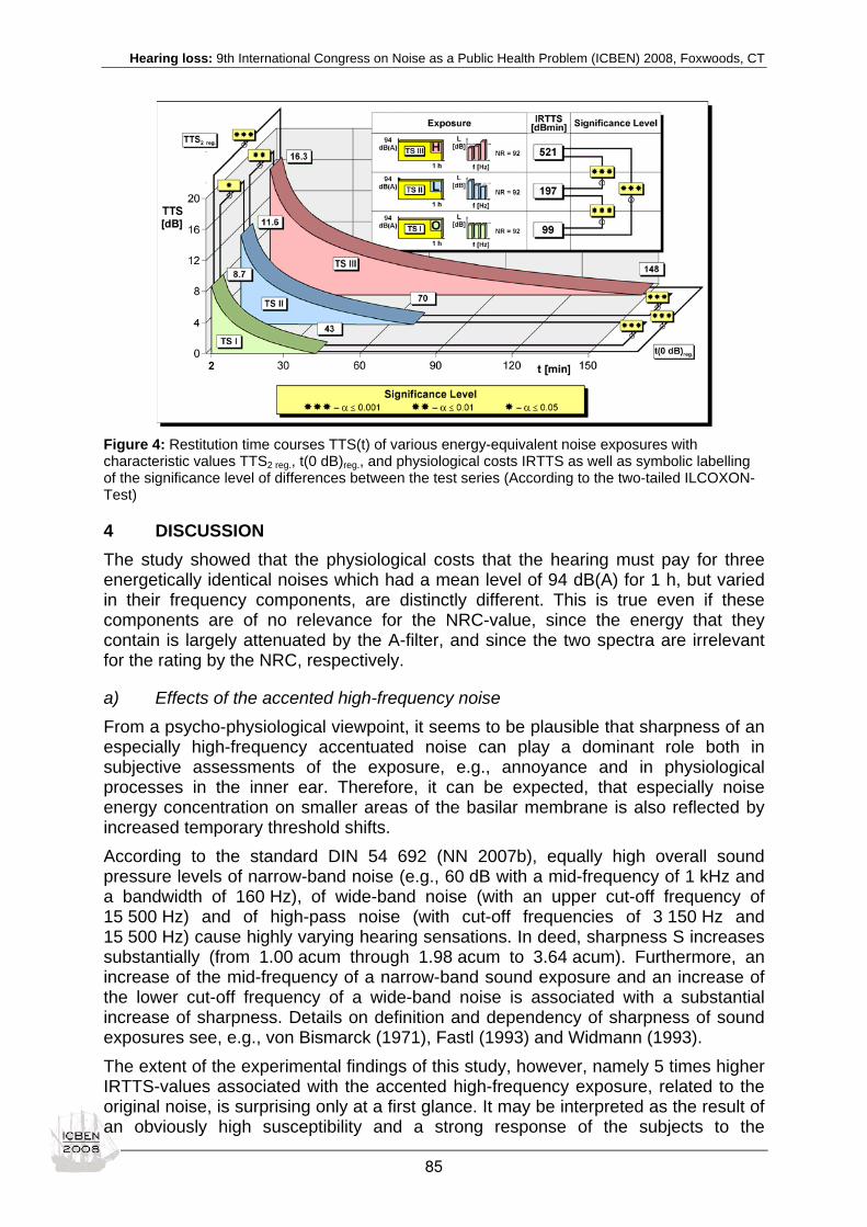
Hearing loss: 9th International Congress on Noise as a Public Health Problem (ICBEN) 2008, Foxwoods, CT
Figure 4: Restitution time courses TTS(t) of various energy-equivalent noise exposures with characteristic values TTS2 reg., t(0 dB)reg., and physiological costs IRTTS as well as symbolic labelling of the significance level of differences between the test series (According to the two-tailed ILCOXON-Test)
4 DISCUSSION The study showed that the physiological costs that the hearing must pay for three energetically identical noises which had a mean level of 94 dB(A) for 1 h, but varied in their frequency components, are distinctly different. This is true even if these components are of no relevance for the NRC-value, since the energy that they contain is largely attenuated by the A-filter, and since the two spectra are irrelevant for the rating by the NRC, respectively.
a) Effects of the accented high-frequency noise From a psycho-physiological viewpoint, it seems to be plausible that sharpness of an especially high-frequency accentuated noise can play a dominant role both in subjective assessments of the exposure, e.g., annoyance and in physiological processes in the inner ear. Therefore, it can be expected, that especially noise energy concentration on smaller areas of the basilar membrane is also reflected by increased temporary threshold shifts. According to the standard DIN 54 692 (NN 2007b), equally high overall sound pressure levels of narrow-band noise (e.g., 60 dB with a mid-frequency of 1 kHz and a bandwidth of 160 Hz), of wide-band noise (with an upper cut-off frequency of 15 500 Hz) and of high-pass noise (with cut-off frequencies of 3 150 Hz and 15 500 Hz) cause highly varying hearing sensations. In deed, sharpness S increases substantially (from 1.00 acum through 1.98 acum to 3.64 acum). Furthermore, an increase of the mid-frequency of a narrow-band sound exposure and an increase of the lower cut-off frequency of a wide-band noise is associated with a substantial increase of sharpness. Details on definition and dependency of sharpness of sound exposures see, e.g., von Bismarck (1971), Fastl (1993) and Widmann (1993). The extent of the experimental findings of this study, however, namely 5 times higher IRTTS-values associated with the accented high-frequency exposure, related to the original noise, is surprising only at a first glance. It may be interpreted as the result of an obviously high susceptibility and a strong response of the subjects to the
85

Hearing loss: 9th International Congress on Noise as a Public Health Problem (ICBEN) 2008, Foxwoods, CT
unnatural “sharp” acoustic load. Apparently this experience was not limited to the psychological domain but also had an impact on physiological correlates. Furthermore, the distinct characteristics of the exposure with respect to the frequency distribution and energy content – which will be explained in the following – may play a role for the effects on the hearing. The increase of the octave-band levels around 4 and 8 kHz (from 74.7 and 64.8 dB in the original noise) by 5.3 and even 10.8 dB (to 80.0 and 75.6 dB) (cp. upper part of Fig. 3), remarkably did alter neither the A- or C-weighted nor the unweighted (linear) all-inclusive level. Using the A-weighting network intentionally led to identical 94 dB(A) for all exposures. When using the C-weighting or the linear network, (with 96.0 dB(C) and 96.3 dBlin) the accented high-frequency exposure appeared to be even slightly lower than the original noise which exhibits levels of 96.6 dB(C) and 96.8 dBlin. This strange result is due to the fact that for the original and the accented high-frequency noise, the band levels of the two upper octaves related to the band levels for the octaves between 125 Hz and 1 kHz, especially the dominant level of 94 dB for the octave around 500 Hz, are absolutely negligible in terms of energy (of the exposure). With 87.8, 85.2, 94.0, and 88.8 dB compared to 74.7 and 64.8 dB the band level differences in the original noise amount to much more than 10 dB. Thus, the lower levels, not at all, can contribute to the overall-inclusive level. Almost similar is true for the altered noise despite its high-frequency accentuation. Even the rather high levels of 80.0 and 75.6 dB in addition to 86.4, 83.8, 94.0 and 87.6 dB are energetically absolutely irrelevant. But this, not at all, does mean that energy inherent in the band levels does not exist for the hearing. As shown already in prior studies [6], energetically negligible noise of 70 dB(A) for 3 h in addition to preceding 94 dB(A)/1 h increased IRTTS substantially by the factor of 2.44. What happens for the hearing when, e.g., resting phases in between high noise exposures are filled up by noise with levels which remain more than 10 dB below the peak levels (cp. Strasser 2005), can also be expected at least hypothetically for the filling up of frequency bands in noise exposures. As shown by Strasser et al. (2007), a narrow-band sound exposure in the higher frequency range (an octave-band level of 94 dB(A)/1 h around the mid-frequency of 2 kHz) also caused significantly higher IRTTS values than an energy-equivalent wide-band sound exposure (overall level of 94 dB(A)/1 h of 4 band levels with the mid-frequencies 250 Hz, 500 Hz, 1 kHz and 2 kHz). Compared to an extremely low-frequency narrow-band noise (octave-band level of 94 dB(A)/1 h around 250 Hz) the physiological costs to the hearing were even 5 times higher.
b) Effects of the accented low-frequency noise Also irritating, at a first glance, are the effects of increased band levels in the lower frequency range. The IRTTS-values that were almost two times as high as after the exposure to the unaltered original noise, however, can be explained by a substantially higher load of the hearing due to the filling up of band levels in the low-frequency range. An increase, e.g., of 11 or even 14 dB in the two lowest octave bands was almost completely levelled off by the relative response of the A-weighting network. This, oftentimes, leads to an underestimation of the effects of low-frequency noise (cp., e.g., Berglund & Hassmen 1996; Genuit 2007; Leventhall 2003). When using the C-weighting network which normally should be applied for frequency weighting of sound levels between 90 and 120 dB, the accented low-frequency noise exhibits a substantially higher acoustic load than the unaltered noise. Its overall level of 100.0 dB(C) exceeds the 96.6 dB(C) of the original noise level by more than 3 dB.
86

Hearing loss: 9th International Congress on Noise as a Public Health Problem (ICBEN) 2008, Foxwoods, CT
It should not come as a surprise if an increase of this extent is also associated with a doubling of the physiological costs (IRTTSTS II/IRTTSTS I = 1.99) for the hearing.
5 CONCLUDING REMARKS The experimental results discussed above raise serious questions about the use of conventional measures that give exactly identical ratings to the examined real-life acoustic exposures using the concept of energy-equivalence, the A-weighting network, and Noise Rating Curves. From the quite different short-term reversible responses of the hearing to the exposures with a limited mean level of 94 dB(A)/1 h which was due to ethical reasons, an also quite different long-term hearing risk can be prognosticated when unnatural exposures are repeatedly higher in the “rough” industrial working world.
6 REFERENCES Beranek LL (1957). Revised criteria for noise in buildings. Noise Control 19-27.
Beranek LL (1988). Criteria for noise and vibration in communities, buildings, and vehicles (chapter 18). In: Beranek LL (ed.): Noise and Vibration control. Rev. ed. Washington, DC: Institute of Noise Control Engineering.
Berglund B, Hassmen P (1996). Sources and effects of low-frequency noise. J Acoust Soc Am 99: 2985-3002.
Broner N (2005). Rating and assessment of noise. AIRAH’s Acoustics Conference, Melbourne/ Australia 2004; (www.airah.org.au/downloads) EcoLibrium: 21-25.
Fastl H (1993). Calibration signals for meters of loudness, sharpness, fluctuation strength, and roughness. Proceedings Internoise ’93, Vol. III, 1257-1260.
Genuit K (2005). Gesamtgeräuschbeurteilung aus der Sicht der Psychoakustik. In: Fastl H, Fruhmann M (Hrsg.): Fortschritte der Akustik. CD der wiss. Beiträge zur 31. Jahrestagung der Deutschen Gesellschaft für Akustik (DAGA’05) (S 497). München.
Genuit K (2007). Tiefe Frequenzen sind nicht gleich tiefe Frequenzen – Tieffrequente Geräuschanteile und deren (Lärm-) Wirkungen. In: DAGA 2007, 33. Jahrestagung für Akustik (S 348). Stuttgart.
Irle H, Hesse JM, Strasser H (1998). Physiological cost of energy-equivalent noise exposures with a rating level of 85 dB(A) – Hearing threshold shifts associated with energetically negligible continuous and impulse noise. Int J Ind Ergon 21: 451-463.
Irle H, Strasser H (2005). Methods for quantifying hearing threshold shifts of sound exposures and for depicting the parameters TTS2, t(0 dB), and IRTTS indicating the physiological costs to the hearing. In: Strasser H (ed.): Traditional rating of noise versus physiological costs of sound exposures to the hearing (pp 53-66). Amsterdam: IOS-Press.
Kosten CW, Van Os GJ (1962). Community reaction criteria for external noise. National Physical Laboratory Symposium No. 12, London: HMSO, pp 373-387.
Leventhall G (2003). A review of published research on low frequency noise and its effects. London: Report for Department for Environment, Food and Rural Affairs.
NN (1971). ISO R 1996. Assessment of noise with respect to community response, withdrawn.
NN (1987). ISO 226. Normal equal-loudness level contours.
NN (1989). Noise control reference handbook. Industrial Acoustics Company. Rev. ed.
NN (1991a). Noise control in industry. 3rd ed. – fully rev. and upd. Sound Research Laboratories Ltd., Sudbury Suffolk, Great Britain. London: Chapman and Hall.
NN (1991b). DIN EN ISO 4869-1. Acoustics; hearing protectors; Part 1: Subjective method for the measurement of sound attenuation. Berlin: Beuth-Verlag.
NN (2000). VDI 2081. (Guide Line of the German Association of Engineers) Geräuscherzeugung und Lärmminderung in Raumlufttechnischen Anlagen. Entwurf. Berlin: Beuth-Verlag.
NN (2007a). Verordnung zum Schutz der Beschäftigten vor Gefährdungen durch Lärm und Vibrationen (Lärm- und Vibrations-Arbeitsschutzverordnung – LärmVibrationsArb.SchV).
NN (2007b). DIN 45 692-E. Messtechnische Simulation der Hörempfindung Schärfe. Entwurf. Berlin: Beuth-Verlag.
87

Hearing loss: 9th International Congress on Noise as a Public Health Problem (ICBEN) 2008, Foxwoods, CT
Schaefer P (1984). Entwurf eines umfassenden Lärmbewertungsverfahrens. Düsseldorf: VDI-Verlag. (Fortschritt-Berichte VDI Reihe 17, Nr. 20).
Schmidt H (1988). Schalltechnisches Taschenbuch. 4. Aufl. Düsseldorf: VDI-Verlag.
Strasser H (2005). Problems of measurement, evaluation, and rating of environmental exposures in occupational health and safety associated with the dose maxim and energy equivalence. In: Strasser H (ed.): Traditional rating of noise versus physiological costs of sound exposures to the hearing (pp 1-24). Amsterdam: IOS-Press.
Strasser H, Irle H (2006). Noise: Measuring, evaluation, and rating in ergonomics. In: Karwowski W (ed.): International encyclopedia of ergonomics and human factors, 2nd ed. (pp 844-851). London: Taylor & Francis.
Strasser H, Chiu MC, Irle H, Grünig T (2007). Threshold shifts and restitution of the hearing after energy-equivalent narrow-band and wide-band noise exposures. Proceedings-CD Internoise 2007 (pp 1-10). Istanbul/Turkey.
von Bismarck G (1971). Timbre of steady sounds: Scaling of sharpness. Proceedings of 7th International Conference on Acoustics, Budapest, Vol. 3, pp. 637-640.
Widmann U (1993). Untersuchungen zur Schärfe und zur Lästigkeit von Rauschen unterschiedlicher Spektralverteilung. Fortschritte der Akustik, DPG-GmbH, Bad Honnef. DAGA’93, pp. 644-647.
Zwicker E, Fastl H (1990). Psychoacoustics: facts and models. Berlin: Springer-Verlag.
88
Hearing loss: 9th International Congress on Noise as a Public Health Problem (ICBEN) 2008, Foxwoods, CT
Dose-response relationship for noise induced hearing loss in impulse noise and continuous noise exposure workers by kurtosis adjusting exchange rate Yi-ming Zhao1*, Roger P. Hamernik2, Lin Zeng1, Xiao-ru Cheng1, Shan-song Chen3, Wei Qiu2, Bob Davis2 1 Research Center of Clinical Epidemiology, Peking University Third Hospital, Beijing 100083, China
2 Auditory Research Laboratory, State University of New York, Plattsburgh, NY 12901 USA
3 Center for Disease Control and Prevention Zhengzhou Province, Zhengzhou 450053, China
* corresponding author: e-mail: [email protected]
PURPOSE. To adjust dose-response relationship for high-frequency noise induced hearing loss (HFNIHL) in industrial impulse noise with different exchange rate calcu-lated by kurtosis (ERk), and to compare the dose-response curve with that in continu-ous noise. SUBJECT AND METHOD. Select 32 mechanical workers as impulse noise group and 163 textile workers as continuous noise group. Use SH-126 dosimeter to meas-ure A-weighted sound pressure level of 8 hours (LAeq.8h) during full working duration. The cumulative noise exposure (CNE) was calculated by LAeq.8h and noise working years. Hearing thresholds were measured by audiometer and adjusted with ISO 1999:1990. Temporal kurtosis were calculated by using METLAB, with a 40 s time window. ERk was calculated with a semi-experiential formula. Statistical analyses were done using SPSS13.0. RESULTS. CNE of impulse noise group (103.2(dBA•year)) was significant lower than that of continuous noise group (110.6(dBA•year)) (P < 0.05). But prevalence of HFNIHL in both groups was similar (65.6 % vs 64.4 %). Both groups showed a good fitting dose-response curve. But the curve of impulse noise was left shift and sharper slope than the other one. The mean kurtosis was about 3.28 for continuous noise, and 39.96 for impulse noise. After adjust noise dose assessment by ERk, the dose-response relationship (data and curve) of the tow group were similar. CONCLUSION. The damage of impulse noise on HFNIHL was more severe than that of continuous noise according to equal energy rule. When adjust ER by temporal kur-tosis in impulse noise, the dose-response curve could be similar to that of continuous noise.
89

Hearing loss: 9th International Congress on Noise as a Public Health Problem (ICBEN) 2008, Foxwoods, CT
Opportunities and challenges in longitudinal assessment of hearing parameters among construction workers Noah Seixas1*, Patrick Feeney2, David Mills2, Richard Folsom2, Lianne Sheppard1, Richard Neitzel1, Sharon Kujawa3 1 University of Washington, Department of Environmental and Occupational Health Sciences,
Seattle, WA
2 University of Washington, Bloedel Hearing Research Center, Seattle, WA
3 Massachusetts Eye and Ear Infirmary, Department of Otology and Laryngology, Harvard University, Boston, MA
* corresponding author: e-mail: [email protected]
Longitudinal assessment of hearing damage in relation to well-characterized noise exposure holds significant potential for documenting the natural history, describing the exposure-response relationship, and identifying means of early detection and prevention for noise-induced damage. To accomplish these goals, a study was initi-ated in 1999 among a group of new construction apprentices. Annual assessments have been conducted since then including pure-tone audiometric thresholds (PTT) and distortion product otoacoustic emissions (DPOAEs), in addition to questionnaires and noise exposure measurements. After the first five years, the protocol was amended to use updated PTT and DPOAE testing equipment and to add wideband measures of middle-ear energy reflectance and the acoustic stapedius reflex (ASR) threshold. Numerous challenges have been addressed in the context of these studies including the test-retest variability of the measurements, analysis and interpretation of low-level DPOAEs, calibration of the updated DPOAE test system in comparison with the older one, and challenges in calculation of the AR. One hundred and fifty-five subjects have completed the first round of tests with the updated protocols. Despite these challenges, we are able to begin to model the effect of occupational noise on both PTT and DPOAEs, and to consider the potential modifying effect of the ASR.
90

Hearing loss: 9th International Congress on Noise as a Public Health Problem (ICBEN) 2008, Foxwoods, CT
Dangerous Decibels® II: Critical components for an effective educational program and special considerations for hearing loss prevention devices for children William Hal Martin1*, Deanna K. Meinke2, Judith L. Sobel3, Susan E. Griest1, Linda C. Howarth1 1 Oregon Health & Science University, Oregon Hearing Research Center, 3181 SW Sam Jackson
Park Road, NRC04, Portland, Oregon, USA 97239
2 University of Northern Colorado, Audiology & Speech Language Sciences, Gunter 1500, Campus Box 140, Greeley, CO 80639
3 Portland State University, School of Community Health, PO Box 751 – SCH Portland, OR 97207
* corresponding author: e-mail: [email protected]
INTRODUCTION The World Health Organization - Prevention of Deafness and Hearing Impairment met in October, 1997 in Geneva, Switzerland to address the prevention of noise induced hearing loss (World Health Organization 1997). A subset of key points from that meeting included:
• Exposure to excessive noise is the major avoidable cause of permanent hearing impairment worldwide.
• Noise-induced hearing loss is an important public health priority because, as populations live longer and industrialization spreads, NIHL will add substantially to the global burden of disability.
• In a developed country, excessive noise is at least partially the cause in more than one-third of those with hearing impairment.
• In developed countries, the risk from social noise is increasing for young people.
• National Programs for prevention of noise-induced hearing loss should be established or strengthened in all countries and integrated with Primary Health Care (PHC).
• Because there is widespread ignorance of the hazard, awareness must be increased about the harmful effects of noise on hearing and about the prevention and control of noise-induced hearing loss.
• A positive image of hearing should be promoted, including its contribution to the daily quality of life.
• Communication and collaboration should be strengthened between developed and developing countries to facilitate research and development in this field.
In addition, the summary noted that “In North America recent studies of environmental noise have shown that children may receive more noise at school than workers from an 8-hour work day at a factory” and that globally “Key messages on these topics should be widely disseminated by multiple methods in a coordinated program, to the general public, to schools, for health education, and to PHC workers, for advocacy in the local community”. Significant noise exposures and their
91

Hearing loss: 9th International Congress on Noise as a Public Health Problem (ICBEN) 2008, Foxwoods, CT
consequences in children and adolescents are well documented (Folmer 2003; Kujawa & Liberman 2006; Martin et al. 2006; Niskar et al. 2001). Health communication research indicates that early and effective intervention is essential to the prevention of noise-induced hearing loss (NIHL) and tinnitus (Folmer 2003, 2008; Folmer et al. 2002; Griest et al. 2007; Martin et al. 2006; Schunk & Carbonari 1984; Sobel & Meikle 2008). Educational interventions can be effective at changing knowledge, attitudes and behaviors about exposure to loud and dangerous sounds (Griest et al. 2007; Knobloch & Broste 1998; Lukes & Johnson 1999; Randolph et al. 2003; Roeser et al. 1983). Hearing loss prevention educational content recommended by Lass et al. (1987a, b) included the following topics; instruction about normal auditory mechanisms, types of hearing loss and their causes, noise and its effect on hearing, warning signs of noise-induced hearing loss, and specific recommendations for preventing noise-induced hearing loss. Anderson (1991) added to this list instruction about consequences of hearing loss and how it can affect life quality and what type of noises or noisy activities are most dangerous to hearing. The classroom represents a special venue for communicating hearing health promotion information and practices. Hearing health can be integrated into other topics including science, health, music, physics and mathematics. The development of hearing health program should be based upon health communication theory (Sobel & Meikle 2008), focus on specific educational messages (Martin et al. 2006), and include formative and summative evaluations (Griest et al. 2006, 2007). Dangerous Decibels® is a public health partnership with the goal of reducing the incidence of noise induced hearing loss and related tinnitus (Martin 2008, Martin et al. 2006). The program uses educational outreach, museum exhibitry and research to promote and study hearing health. All Dangerous Decibels activities are intended to communicate the three educational messages:
• What are sources of dangerous sounds? – It is the intention that participants will acquire the technical and experiential knowledge necessary to know when they are in situations that provides risk of hearing loss and tinnitus due to sound exposure levels and durations.
• What are the consequences of being exposed to dangerous sounds? – It is the intention that participants will understand the value of having normal hearing and the personal loss of having hearing impairment in terms of communication, enjoyment of music and other sounds, and loss of peace and quiet through continual tinnitus.
• How do I protect myself from dangerous sounds? – It is the intention that participants will have knowledge and self-efficacy in simple methods of hearing protection, specifically turning the volume down, moving away from the source of the sound and proper use of hearing protective device. In addition, it is intended that they will know how to select and use appropriate protective measures for specific sound exposure situations and conditions.
Content recommendations have been recommended by Lass et al. (1987a, b) who recommended that hearing loss prevention education include instruction about normal auditory mechanisms, types of hearing loss and their causes, noise and its effect on hearing, warning signs of noise-induced hearing loss, and specific recommendations for preventing noise-induced hearing loss. Anderson (1991) added
92

Hearing loss: 9th International Congress on Noise as a Public Health Problem (ICBEN) 2008, Foxwoods, CT
to this list instruction about consequences of hearing loss and how it can affect life quality and what type of noises or noisy activities are most dangerous to hearing.
METHODS The Dangerous Decibels program has developed numerous resources that are being used to prevent NIHL and tinnitus (Martin 2008, Martin et al. 2006). One component is a classroom program targeting and adaptable to kindergarten though 12th grade students. The scientific content was developed by hearing scientists at the Oregon Hearing Research Center (OHRC) and the format and delivery was developed through three formative evaluations in six counties across Oregon and Southwest Washington. The formative evaluations included student and teacher surveys and focus groups conducted by external evaluators, review and direction from teacher consultants, and creative input on communicating complex messages in fun, interactive ways from educational experts from the Oregon Museum of Science and Industry (OMSI). Graphical displays, 3-D models and interactive “hands-on” activities provide a multimodality learning experience that can be modified in complexity according to the target grade level. Formative evaluation allowed the developers to determine if the format was acceptable to students and teachers, and whether or not the educational messages were being communicated effectively. Summative evaluations were performed with 478 fourth grade students and 506 seventh grade students to access the effectiveness of the classroom program at changing knowledge, attitudes and behaviors regarding exposure to dangerous sound levels and the use of hearing protective strategies (Griest et al. 2007). Summative evaluation of an additional 1,119 fourth grade students, comparing four different forms of educational intervention, is now underway. The program was designed to comply with Science Standards and Benchmarks from the National Science Education Standards (http://www.nap.edu/readingroom/books/nses/html/) for Physical Science, Life Science, and Science in Personal and Social Perspectives.
RESULTS The Dangerous Decibels classroom program incorporates a series of interactive activities designed to convey basic knowledge and simplified prevention strategies for hearing loss prevention. The program has been delivered by a wide range of individuals including audiologists, classroom teachers, school-nurses, high-school students, graduate students, hearing scientists, deaf educator specialists, speech-language pathologists, museum outreach educators and lay persons. A script of the classroom program was developed to insure a consistent and orderly flow of concepts and to see that each critical component is covered by the instructor. The educational topics included in the classroom program are as follows: 1. What do we hear? This section uses activities to teach the physics of sound
emphasizing that it is the vibrational energy of sound carried through the air that has the power and ability to permanently damage the ear. Tuning forks and ping-pong balls are distributed to students who are directed in playful experimentation of physical concepts (Figure 1). Sound measurement in dBA is taught using household devices (e.g. blenders, radios) as sound sources. The concept of the relationship between sound intensity and duration in causing damage is developed through table-top exhibit pieces and web-based interactives.
93

Hearing loss: 9th International Congress on Noise as a Public Health Problem (ICBEN) 2008, Foxwoods, CT
Figure 1: Students learning how sound requires vibration to exist and that it can have power to permanently damage the ear
2. How do we hear? Students are given age-appropriate instruction and demonstration of the normal anatomy and physiology of hearing including an understanding of hair-cell physiology and transduction. Electron microscope and confocal microscope images of cellular and sub-cellular structures that are damaged by extensive sound exposure are presented.
3. How do our ears break? The pathophysiology of high-level or prolonged sound exposure is presented through images, experiments and modeling of hair cells being damaged through an interactive story-telling activity (Figure 2). Simulations of the challenges of listening with hearing loss are presented as well as a simulation of high-frequency tinnitus, commonly reported by individuals with NIHL. Another interactive demonstrates common sound sources that have the capacity to cause hearing loss base upon standards set by the National Institute for Occupational Safety and Health.
Figure 2: Students finding out how loud sound can damage hair bundles on hair cells causing permanent hearing loss and possibly tinnitus
4. How do I protect myself from loud sounds? Three primary methods of hearing protection are presented.
a. Turn it down. Whenever possible, the volume of a sound should be reduced to safe listening levels. An emphasis is placed on personal stereo systems in light of their extreme popularity and utilization among young people. “Jolene” is a sound measuring device that gives students the opportunity to measure the sound pressure levels at which they commonly listen in order to develop a subjective reference for potentially dangerous levels (Figure 3).
94

Hearing loss: 9th International Congress on Noise as a Public Health Problem (ICBEN) 2008, Foxwoods, CT
Figure 3: Student using “Jolene” to measure the sound level output of a personal stereo system
b. Walk away. During the demonstrations about the physics of sound,
students learn that sound pressure decreases dramatically as one moves away from the sound source. They are taught that if they can not turn the volume of a sound down, they can often move away from the source to a distance at which their ears are no longer in danger.
c. Protect your ears. Hearing protective devices are demonstrated to the students. Protective devices present a great challenge in children. Nearly all hearing protection devices in the United States are designed for use by adults. Ear muffs may be too large or heavy for a child. Ear plugs may also be too large or may be awkward to fit. Our experience in classrooms trials with fourth grade student indicated that the vast majority of students were not able to correctly roll and insert foam type ear plugs without assistance. In contrast, pre-formed, flanged ear plugs were properly inserted the vast majority of the time with instruction (Figure 4). Public health theory indicates that self-efficacy is essential for someone to take the step of implementing a safety intervention. It is important that children not only know how to put in ear plugs from an intellectual stand point, as accomplished through watching a demonstration, but they must also have the confidence attained by a successful hands-on trial of the fitting.
Figure 4: Flanged ear plugs (left) are often more easily inserted by children than the foam type (right)
The effectiveness of the Dangerous Decibels classroom program to promote hearing health in students has been evaluated after presentations by museum outreach educators, school nurses and high school students (Griest et al. 2006). In all cases significant improvements were identified in areas of knowledge about the above topics, attitudes about the value of hearing and necessity for hearing protective behavior, and in intended behaviors in situations where potentially dangerous sound levels exist.
95

Hearing loss: 9th International Congress on Noise as a Public Health Problem (ICBEN) 2008, Foxwoods, CT
Pre- and post-classroom program activities are encouraged in order to increase the likelihood of success of the intervention. These activities can include a visit to the Oregon Museum of Science and Industry permanent Dangerous Decibels exhibit or a visit to the Dangerous Decibels virtual exhibit, a web-based collection of educational interactives, at the Dangerous Decibels website (www.dangeroudecibels.org).
CONCLUSIONS One very important means of communicating hearing health information to young people is through classroom education. However, it is important that the classroom program is developed based upon health communication theory and practices. It is also essential that the development of any hearing health intervention include formative and summative evaluation to determine whether or not the program is effective and if not, to provide insights into how to improve it. The Dangerous Decibels staff has developed an in-depth educator training program that has been used to train and equip a wide range of individuals as presenters of the Dangerous Decibels curriculum. Educators receive the extensive background information on the topics mentioned above as well as in common noise risks, health communication theory, classroom management and other essential items. Each participant is required to do a practice presentation of the classroom program while other participants observe. This provides participants with an opportunity to hone their skills as presenters and provides the instructors an opportunity to identify and correct misunderstandings and insure that the essential concepts are correctly presented. Educator workshops are offered periodically through the Dangerous Decibels program (contact [email protected]).
REFERENCES Anderson KL (1991). Hearing conservation in the public schools revisited. Semin Hearing 12: 340–364.
Folmer RL (2003). The importance of hearing conservation instruction. J School Nursing 19: 140-148.
Folmer RL (2008). Hearing-loss prevention practices should be taught in schools. Semin Hearing 29: 67-80.
Folmer RL, Griest SE, Martin WH (2002). Hearing conservation education programs for children: a review. J School Health 72: 51-57.
Griest SE, Martin WH, Sobel J, Howarth L (2006). Program evaluation: results for noise induced hearing loss and tinnitus prevention. Presented at the Conference on Noise-induced Hearing Loss in Children at Work & Play, Cincinnati, Ohio.
Griest SE, Folmer RL, Martin WH (2007). Effectiveness of "Dangerous Decibels," a school-based hearing loss prevention program. Am J Audiol 16: S165-S181.
Knobloch MJ, Broste SK (1998). A hearing conservation program for Wisconsin youth working in agriculture. J School Health 68: 313-318.
Kujawa SG, Liberman MC (2006). Acceleration of age-related hearing loss by early noise exposure: Evidence of a misspent youth. J Neurosci 26: 2115–2123.
Lass NJ, Woodford CM, Lundeen C, Lundeen DJ, Everly-Myer D (1987a). A survey of high school students’ knowledge and awareness of hearing, hearing loss, and hearing health. Hear J 40: 15–19.
Lass NJ, Woodford CM, Lundeen C, Lundeen DJ, Everly-Myers DS, McGuire K, Mason DS, Paknik L, Phillips RP (1987b). A hearing-conservation program for a junior high school. Hear J 40: 32–40.
Lukes E, Johnson M (1999). Hearing conservation: an industry-school partnership. J School Nursing 15: 22-25.
Martin WH (2008). Dangerous Decibels®: Partnership for preventing noise induced hearing loss and tinnitus in children. Semin Hearing 29: 102-110.
Martin WH, Sobel JL, Griest SE, Howarth L, Shi Y-B (2006). Noise induced hearing loss in children: Preventing the silent epidemic. J Otol 1: 11-21.
96

Hearing loss: 9th International Congress on Noise as a Public Health Problem (ICBEN) 2008, Foxwoods, CT
Niskar AS, Kieszak SM, Holmes AE, Esteban E, Rubin C, Brody DJ (2001). Estimated prevalence of noise-induced hearing threshold shifts among children 6 to 19 years of age: the Third National Health and Nutrition Examination Survey, 1988-1994, United States. Pediatrics 108: 40-43.
Randolph RF, Hudak RL, Vaught C (2003). Communicating hearing loss information to young children effectiveness of lecture and printed materials. AAOHN J 51: 433-438.
Roeser RJ, Coleman T, Adams RM (1983). Implementing an industrial hearing conservation program in the schools. J School Health 53: 408-411.
Schunk DH, Carbonari JP (1984). Self-efficacy models. In: Matarazzo JD, Weiss SM, Herd JA et al. (eds.): Behavioural health: A handbook of health enhancement and disease prevention (pp 230-247). New York: Wiley.
Sobel J, Meikle M (2008). Applying health behavior theory to hearing-conservation interventions. Semin Hearing 29: 81-89.
World Health Organization (1997). Prevention of noise-induced hearing loss. Report of an informal consultation, Geneva, Switzerland. WHO. Available at: http://www.who.int/pbd/deafness/en/noise.pdf
97

Hearing loss: 9th International Congress on Noise as a Public Health Problem (ICBEN) 2008, Foxwoods, CT
Effects of aromatic solvents on acoustic reflexes Pierre Campo, Katy Maguin Institut National de Recherche et de Sécurité, Rue du Morvan, CS 60027, 54519 Vandœuvre Cédex, France; Tel: 33 3 83 50 21 55; Fax : 33 3 83 50 20 96 ; [email protected]
INTRODUCTION Chronic exposure to toluene (Tol) can impair the central nervous system (Yama-nouchi et al. 1995; Greenberg 1997). Tol shares many effects with nervous system depressant compounds such as anesthetics (Evans & Balster 1991). In the past, the neuroactivity of anesthetics and related compounds was thought to be attributed to their ability to perturb the plasma membrane (Engelke et al. 1992). Today, clear evi-dence is emerging from the literature regarding actions of solvents on ion channels expressed in neurons. For instance, NMDA (Cruz et al. 1998), GABA (Krasowski & Harrison 2000) and Ach (Bale et al. 2002) receptors are important to nervous system and sensitive to Tol. Besides, Tol alters the function of several voltage-dependent ion channels including voltage-dependent Ca2+ channels (VDCCs) (Tillar et al. 2002; Shafer et al. 2005). Chronic exposure to Tol can impair the inner ear as well (Odkvist et al. 1982; Rybak 1986). The notion of ototoxicity stemming from organic com-pounds is important for people exposed at workplace (Morata & Campo 2001). Cer-tain aromatic solvents are ototoxic and can even worsen the effects of noise (Lataye & Campo 1997; Lataye et al. 2000; Brandt-Lassen et al. 2000; Cappaert et al. 2001; Sliwinska-Kowalska et al. 2003; Chang et al. 2006). The studies carried out in the rat showed that a co-exposure to noise and aromatic solvent can have synergistic adverse effects on hearing. The fair assumption pro-posed to explain these effects was that the solvents could weaken the outer hair cell (OHC) membranes and thereby increase their vulnerability to noise. But, in recent investigations performed with rats, it has been shown that Tol can inhibit Ach recep-tors (Lataye et al. 2007) and cancel the protective effect of the middle-ear reflex (MER) (Campo et al. 2007). In the rat, motoneurons involved in the MER are mediated by Ach (Liu et al. 1998; Zaninetti et al. 1999), which is also the major neurotransmitter involved (1) in the synaptic network within the facial and trigeminal nuclei or integrator centers (Lee et al. 2006) and (2) in neuromuscular junctions connected to the MER muscles. In the nervous system, Ach exocytosis is mainly activated by P/Q-type Ca2+ channels (Wright & Angus 1996; Day et al. 1997) and to a lesser extent by N-type Ca2+ chan-nels (Hamilton & Smith 1992; Rossoni et al. 1994). In contrast, the L-type Ca2+ chan-nels are mainly dedicated to muscular contraction (Catterall et al. 1988; Patterson et al. 1995). There is therefore a dominating role of P/Q- and N-type Ca2+ channels at the level of motoneurons and a dominating role of L-type Ca2+ channels in muscles. If Tol can inhibit the MER, the cellular sites of its action were still not completely elu-cidated. Could Tol interact with VDCCs in motoneurons, integrator centers or mus-cles? To better understand the Tol action at the level of the MER arc, two specific VDCCs blockers were used in the present study:
• the ω-conotoxin MVIIC (ω-Ctx), which is the only pharmacological tool inhibit-ing both P/Q- and N-type Ca2+ channels (Hillyard et al. 1992; McDonough et al. 1996) expressed in neurons,
• the verapamil, which inhibits the L-type Ca2+ channels, which are mainly ex-pressed in muscular fibers (Almers et al. 1985).
98

Hearing loss: 9th International Congress on Noise as a Public Health Problem (ICBEN) 2008, Foxwoods, CT
These blockers have been administered in the rat by intra-carotidal injections to study their effects on the CMP, which is a good electrophysiological tool to record (1) the electro-activity of the OHCs (Withnell 2001) and (2) the trigger of the MER (Dancer and Franke 1980; Campo et al. 2007). The aim of this investigation was to study the prevailing action of Tol on the different elements of the MER arc. In this purpose, the effects of VDCC antagonists were compared to those of Tol adminis-trated in the same experimental conditions.
METHODS Adult rats were used throughout this investigation. Anesthesia was induced by i.p. injection of ketamine (50 mg/kg). Then, a platinum electrode was inserted in the bulla and placed on the round window, whereas the ground electrode was placed over the olfactory bulb. This technique allows auditory-evoked potentials to be recorded from the cochlea. A circular custom-made catheter was fitted into the carotid connected to the operated ear for administrating the tested substances. The acoustic stimulus was a 2.6-s burst emitted every 12 s, its spectrum was a nar-row BN centered at 4 kHz emitted at 85 dB SPL. The CMP (RMS) was amplified 5000X and filtered from 2 to 8 kHz. Three concentrations of Tol (58.4, 116.2 and 229.5 mM) were tested with different groups of rats (n = 5). A dose-response study was carried out for the two VDCC blockers:
• ω-Conotoxin MVIIC (ω-Ctx) (CAS 147794238), a snail neurotoxin which blocks both P/Q- and N-type VDCCs. Three concentrations of ω-Ctx: 83.5, 145.2 and 211.4 µM, were tested with different groups of rats (n = 2).
• Verapamil (CAS 152114), a drug which blocks L-type VDCCs. The effects of three increasing concentrations of blocker: 312.5, 625 and 1250 µM, were evaluated in different groups of rats (n = 3).
RESULTS In each figure, curve represents the data obtained with one animal representative of the group. Toluene effects on CMP Figure 1 displays the CMP obtained with 85-dB SPL noise-stimulated rats before, during and after a 100-µL injection of Tol at 58.4, 116.2 and 229.5 mM. The Tol injec-tions of 116.2 and 229.5 mM caused rapid and transient rises in CMP amplitude called P component. The mean amplitudes obtained with 0, 58.4, 116.2 and 229.5 mM were 0.0 ± 0.4 dB, 0.4 ± 0.9 dB, 4.3 ± 1.5 dB and 4.1 ± 1.7 dB respectively. The lowest concentration, 116.2 mM, causing a significant (K = 13.59; p = 0.004) increase in CMP was chosen as reference concentration in this experimental context.
99

Hearing loss: 9th International Congress on Noise as a Public Health Problem (ICBEN) 2008, Foxwoods, CT
Figure 1: CMP (RMS) vs. Tol concentrations. 100-µl bolus of Tol were injected into the carotid. The acoustic stimulation was a 4 kHz-BN emitted at 85 dB SPL.
ω-Ctx effects on CMP Figure 2 depicts the CMP obtained with 85-dB SPL noise-stimulated rats before, dur-ing and after a 100-µL injection of ω-Ctx at 83.5, 145.2 and 211.4 µM. Due to the ex-pensive price along with a heavy administrative procedure to get the toxin from the supplier, we could afford only 2 experiments per concentration. Hopefully, the results were clear enough to draw conclusions. The injections of 145.2 and 211.4-µM of ω-Ctx provoked rapid and transient rises in CMP. The mean amplitudes obtained with 0, 83.5, 145.2 and 211.4 µM were 0.0 ± 0.4 dB, 0.3 ± 0.3 dB, 3.8 ± 0.8 dB and 7.3 ± 0.3 dB respectively. ω-Ctx-induced CMP rises were clearly concentration–dependent.
Verapamil effects on the CMP Figure 3 illustrates the CMP obtained with 85-dB SPL noise-stimulated rats before, during and after a 100-µL injection of verapamil at 312.5, 625 and 1250 µM. The blocker induced rapid and transient CMP rises which the amplitude increases as a function of concentration. The mean amplitudes obtained with 0, 312.5, 625 and 1250 µM were 0.0 ± 0.4 dB, 1.4 ± 0.5 dB, 3.4 ± 0.7 dB and 4.1 ± 1.2 dB respectively. The verapamil effects on CMP were concentration-dependent (K=11.60; p=0.009).
2
0
2
4
6
-400 -200 0 200 400 600
58.4 mM116.2 mM229.5 mM
Normalized CMP amplitude (dBV)
Time (s) Injection
P component
100

Hearing loss: 9th International Congress on Noise as a Public Health Problem (ICBEN) 2008, Foxwoods, CT
-2
0
2
4
6
8
-400 -200 0 200 400 600
83.5 µM145.2 µM211.4 µM
Figure 2: CMP (RMS) vs. ω-conotoxin concentration. 100-µl bolus of ω-Ctx were injected into the carotid. The acoustic stimulation was a 4 kHz-BN emitted at 85 dB SPL.
-2
0
2
4
6
-400 -200 0 200 400 600
312.5 µM625 µM1250 µM
Figure 3: CMP (RMS) vs verapamil concentrations. 100-µL bolus of verapamil were injected into the carotid. The acoustic stimulation was a 4 kHz-BN emitted at 85 dB SPL.
Tol vs. VDCC blockers Figure 4 allows the CMP obtained with blockers to be compared with that obtained with Tol. 145.2 µM of ω-Ctx and 1250 µM of verapamil were the required concentra-tions to induce a CMP change similar to that obtained with 116.2-mM of Tol (~4 dB). There were large differences of concentrations between the chemicals to induce the same amplitude of the P component: (Tol/ω-Ctx=800), (Tol/verapamil=93), (verapa-mil/ ω-Ctx=9). In the same way, there were also large differences of the area under curve (AUC) between the CMP obtained with Tol and blockers (Figures 1-3). These differences between AUC are well illustrated in Figure 4. For instance, the AUC ratios are (Tol/ω-Ctx=1.4), (Tol/verapamil=3.6), (verapamil/ω-Ctx=5.2). Therefore, verapa-mil had a long-lasting effect with respect to those of Tol and ω-Ctx.
Time (s) Injection
Normalized CMP amplitude (dBV)
Injection Time (s)
Normalized CMP amplitude (dBV)
101

Hearing loss: 9th International Congress on Noise as a Public Health Problem (ICBEN) 2008, Foxwoods, CT
-2
0
2
4
6
-400 -200 0 200 400 600
Toluene 116.2 mMCtx MVIIC 145.2µMVerapamil 1250µM
Figure 4: CMP (RMS) obtained with VDCC blockers and Tol. 100-µL bolus were injected into the ca-rotid. The acoustic stimulation was a 4 kHz-BN emitted at 85 dB SPL.
CONCLUSIONS Lataye et al. (2007) demonstrated in rats that Tol could induce a CMP rise by its anti-cholinergic-like effects and thereby confirmed Bale’s results (Bale et al. 2002, 2005) obtained with in vitro preparations. Later on, Campo et al. (2007) demonstrated that this Tol-induced CMP rise corresponded to an inhibition to the MER. Unfortunately, the authors did not go further in their investigations and did not test others potential molecular targets for Tol. In the present in vivo study, ω-Ctx- and verapamil- induced CMPs were compared to that induced by Tol in order to (1) confirm the VDCCs as potential molecular targets, (2) localize the cellular sites perturbed by the solvent in the MER arc. As expected, the Tol dose-response study (Figure 1) showed a re-versible MER inhibition from 116.2mM of Tol. Figures 2 and 3 show the reversible inhibition of the MER induced by neuronal and muscular VDCC blockers. By comparing the curve patterns having the same amplitude (~4 dB), the ω-Ctx sen-sitivity was 9-fold higher with respect to that of verapamil (145.2, 1250 µM). The re-versibility and the concentration-dependent responses were comparable with those previously obtained with Ach receptor antagonists. Figure 4 emphasizes the differ-ence of concentration needed for Tol (116.2 mM) and for VDCC blockers (145.2-µM ω-Ctx; 1250-µm verapamil) to induce a 4-dB response. In our opinion, the concentra-tion cannot be considered as a pertinent parameter because of the vehicle nature. Indeed, Tol needed a lipophilic vehicle (Intralipid) to be dissolved, but the efficiency of verapamil was deeply depressed by it (Tebbutt et al. 2006). Therefore, a saline solution was chosen as vehicle for both blockers. Because of this experimental bias, it seemed unrealistic to compare the concentrations to evaluate the relative affinity of Tol with regard to that of blockers. Indeed, the most striking drawback of Intralipid is that it can confine a part of the solvent, keeping the free-available part of the solvent low. Consequently, the Tol dose at the target structure is likely overestimated with respect to that inside the syringe. Actually, the most reliable approach was to com-pare the patterns of the responses having the same amplitude regardless of the dif-ference of concentrations between solvent and blockers. By comparing the patterns of the Tol-induced inhibition with those induced by 145.2-µM ω-Ctx and 1250-µM verapamil (Figure 4), it clearly appeared that the verapamil-
Time (s) Injection
Normalized CMP amplitude (dBV)
102

Hearing loss: 9th International Congress on Noise as a Public Health Problem (ICBEN) 2008, Foxwoods, CT
induced CMP lasted longer than those induced by Tol and ω-Ctx. Such a difference could be explained by the nature (muscular vs. neuronal) of the targets inhibited by the VDCC blockers. Since the verapamil inhibits mainly the muscular L-type VDCCs, it is likely that the duration required for reestablishing a normal muscular contraction was larger than that required for restoring a normal nervous conduction. In case of a neuronal inhibition (Figure 2), the middle-ear muscles were forced in rest although functional. In fact, the nervous control of the middle-ear muscles was tem-porary interrupted but they kept the ability of contracting. In case of verapamil injection (Figure 3), the L-type VDCCs were inhibited in the muscular T-tubules (invaginations) of the plasma membrane. T-tubules are the major sites for the coupling of excitation/contraction, which is the process whereby the spreading depolarization is converted into force production by muscle fibers. The L-type VDCCs are activated in response to nervous stimulation and this activation causes a mechanical interaction between L-type VDCCs and Ca2+-release channels located on the adjacent sarcoplasmic reticulum membrane. This mechanical interac-tion is critical to trigger a proper skeletal muscle contraction (Tanabe et al. 1988; Na-kai et al. 1998; Endo 2006). This all process lasted probably longer than the simple reestablishment of the nervous conduction. Whatever the reasons on the origin of the different patterns recorded with both blockers, it appeared that Tol and ω-Ctx curves had a similar pattern (Figure 4). Therefore, Tol would act rather like a neuronal VDCC blocker, as suggested by Tillar et al. (2002) and Shafer et al. (2005) with in vitro experiments. In the present study, the in vivo findings confirmed the in vitro data and proved that VDCCs represent po-tential sensitive targets for Tol. In addition, since N-, P/Q-type channels constitute the major component of the Ca2+ channels expressed in the neuronal compartment of the MER arc (Plant et al. 1998; Hsiao et al. 2005), it seems therefore reasonable to claim that Tol can block the reflex by inhibiting the neuronal VDCCs at the level of its mo-toneurons and integrator centers. Inhibition of the transmitter receptors and associ-ated Ca2+ channels would constitute the central mechanism responsible for the syn-ergistic adverse effects on hearing of a co-exposure to noise and Tol: a higher acoustic energy penetrating into the cochlea would make the noise exposure more damaging.
REFERENCES Almers W, McCleskey E, Palade P (1985). Ca2+ channels in vertebrate skeletal muscle. In: Rubin RP, Weiss GB, Putney JW (eds.): Calcium in biological systems (pp 321-330). New York, London: Plenium Publ. Corp.
Bale A, Smothers CT, Woodward JJ (2002). Inhibition of neuronal nicotinic acetylcholine receptors by the abused solvent, toluene. Br J Pharmacol 137: 375-383.
Bale AS, Meacham CA, Benignus VA, Bushnell PJ, Shafer TJ (2005). Volatile organic compounds inhibit human and rat neuronal nicotinic acetylcholine receptors expressed in Xenopus oocytes. Toxicol Appl Pharmacol 205: 77-88.
Brandt-Lassen R, Lund SP, Jepsen GB (2000). Rats exposed to toluene and noise may develop loss of auditory sensitivity due to synergistic interaction. Noise & Health 3: 33-44.
Campo P, Maguin K, Lataye R (2007). Effects of aromatic solvents on acoustic reflexes mediated by central auditory path-ways. Toxicol Sci 99: 582-590.
Cappaert NLM, Klis SFL, Muijser H, Kulig BM, Smoorenburg GF (2001). Simultaneous exposure to ethyl benzene and noise: synergistic effects on outer hair cells. Hear Res 162: 67-79.
Catterall WA, Seagar MJ, Takahashi M (1988). Molecular properties of dihydropyridine-sensitive Ca2+ channels in skeletal muscle. J Biol Chem 263: 3535-3538.
103

Hearing loss: 9th International Congress on Noise as a Public Health Problem (ICBEN) 2008, Foxwoods, CT
Chang SJ, Chen CJ, Lien CH, Sung FC (2006). Hearing loss in workers exposed to toluene and noise. Environ Health Per-spect 114: 1283-1286.
Cruz SL, Mirshahi T, Thomas B, Balster RL, Woodward JJ (1998). Effects of the abused solvent toluene on recombinant N-methyl-D-aspartate and non-N-methyl-D-aspartate receptors expressed in Xenopus oocytes. J Pharmacol Exp Ther 286: 334-340.
Dancer A, Franke R (1980). Intracochlear sound pressure measurements in guinea pigs. Hear Res 2: 191-205.
Day NC, Wood SJ, Ince PG, Volsen SG, Smith W, Slater CR, Shaw PJ (1997). Differential localization of voltage-dependent Ca2+ channel α1 subunits at the human and rat neuromuscular junction. J Neurosci 17: 6226-6235.
Endo M (2006). Ca2+ ion as a second messenger with special reference to excitation-contraction coupling. J Pharmacol Sci 100 : 519-524.
Engelke M, Diehl H, Tahti H (1992). Effects of toluene and n-hexane on rat synaptosomal membrane fluidity and integral enzyme activities. Pharmacol Toxicol 71: 343-347.
Evans E, Balster T (1991). CNS depressant effects of volatile organic solvents. Neurosci Biobehav Rev 15: 233-241.
Greenberg MM (1997). The central nervous system and exposure to toluene a risk characterization. Environ Res 72: 1-7.
Hamilton BR, Smith DO (1992). Ca2+ currents in rat motor nerve terminals. Brain Res 584: 123-131.
Hillyard DR, Monje VD, Mintz IM, Bean BP, Nadasdi L, Ramachandran J, Miljanich G, Cruz LJ (1992). A new Conus peptide ligand for mammalian presynaptic Ca2+ channels. Neuron 9: 69-77.
Hsiao C, Wu N, Chandler S (2005). Voltage-dependent Ca2+ currents in trigeminal motoneurons of early postnatal rats: modulation by 5-HAT receptors. J Neurophysiol 94: 2063-2072.
Krasowski MD, Harrison NL (2000). The actions of ether, alcohol and alkane general anaesthetics on GABAA and glycine receptors and the effects of TM2 and TM3 mutations. Br J Pharmacol 129: 731-743.
Lataye R, Campo P (1997). Combined effects of a simultaneous exposure to noise and toluene on hearing function. Neuro-toxicol Teratol 19: 373-382.
Lataye R, Campo P, Loquet G (2000). Combined effects of noise and styrene exposure on hearing function. Hear Res 139: 86-96.
Lataye R, Maguin K, Campo P (2007). Increase in cochlear microphonic potential after toluene administration. Hear Res 230: 34-42.
Lee DJ, De Venecia RK, Guinan JJ, Brown MC (2006). Central auditory pathways mediating the rat middle ear muscle re-flexes. Anat Rec A288: 358-369.
Liu L, Chang GQ, Jiao YQ, Simon SA (1998). Neuronal nicotinic acetylcholine receptors in rat trigeminal ganglia. Brain Res 809: 238-245.
McDonough SI, Swartz KJ, Mintz IM, Boland LM, Bean BP (1996). Inhibition of Ca2+ channels in rat central and peripheral neurons by ω-conotoxin MVIIC. J Neurosci 16: 2612-2623.
Morata T, Campo P (2001). Auditory function after single or combined exposure to styrene: a review. In: Noise-induced hearing loss: basic mechanisms, prevention and control (pp 293-304). Noise Research Network.
Nakai J, Sekiguchi N, Rando TA, Allen PD, Beam KG (1998). Two regions of the ryanodine receptor involved in coupling with L-type Ca2+ channels. J Biol Chem 273: 13403-13406.
Odkvist L, Bergholtz L, Ahlfeldt H, Anderson B (1982). Otoneurological and audiological findings in workers exposed to in-dustrial solvents. Acta Otolaryngol 386: 249-251.
Patterson M, Constantin B, Cognard C, Raymond G (1995). Properties of Ca2+ currents and contraction in cultured rat dia-phragm muscle. Pfluegers Arch 430: 837-845.
Plant TD, Schirra C, Katz E, Uchitel OD, Konnerth A (1998). Single-cell RT-PCR and functional characterization of Ca2+ channels in motoneurons of the rat facial nucleus. J Neurosci 18: 9573-9584.
Rossoni G, Berti F, La Maestra L, Clementi F (1994). Omega-conotoxin GVIA binds to and blocks rat neuromuscular junc-tion. Neurosci Lett 176: 185-188.
Rybak L (1986). Ototoxic mechanisms. In: Altschuler R (ed.): Neurobiology of hearing (pp 441-454). New York: Raven Press.
Shafer TJ, Bushnell PJ, Benignus VA, Woodward JJ (2005). Perturbation of voltage-sensitive Ca2+ channel function by vola-tile organic solvents. J Pharmacol Exp Ther 315: 1109-1118.
104

Hearing loss: 9th International Congress on Noise as a Public Health Problem (ICBEN) 2008, Foxwoods, CT
Sliwinska-Kowalska M, Zamyslowska E, Szymczak W, Kotylo P, Fiszer M (2003). Ototoxic effects of occupational exposure to styrene and co-exposure to styrene and noise. J Occup Environ Med 45: 15-24.
Tanabe T, Beam KG, Powell JF, Numa S (1988). Restoration of excitation-contraction coupling and slow Ca2+ current in dysgenic muscle by dihydropyridine receptor complementary DNA. Nature 336: 134-139.
Tebbutt S, Harvey M, Nicholson T, Cave G (2006). Intralipid prolongs survival in a rat model of verapamil toxicity. Acad Emerg Med 13: 134-139.
Tillar R, Shafer T, Woodward J (2002). Toluene inhibits voltage-sensitive Ca2+ channels expressed in pheochromocytoma cells. Neurochem Int 41: 391-397.
Withnell RH (2001). Brief report: the cochlear microphonic as an indication of outer hair cell function. Ear Hear 22: 75-77.
Wright CE, Angus JA (1996). Effects of N-, P- and Q-type neuronal Ca2+ channel antagonists on mammalian peripheral neurotransmission. Br J Pharmacol 119: 49-56.
Yamanouchi N, Okada SI, Kodama K, Hirai S, Sekine H, Murakami A, Komatsu N, Sato T (1995). White matter changes caused by chronic solvent abuse. AJNR Am J Neuroradiol 16: 1643-1649.
Zaninetti M, Tribollet E, Bertrand D, Raggenbass M (1999). Presence of functional neuronal acetylcholine receptors in brain-stem motoneurons of the rat. Eur J Neurosci 11: 2737-3748.
105

Hearing loss: 9th International Congress on Noise as a Public Health Problem (ICBEN) 2008, Foxwoods, CT
A European multicenter study on the audiometric findings of styrene-exposed workers Thais C. Morata1*, Mariola Sliwinska-Kowalska2, Ann-Christin Johnson3, Jukka Starck4, Krystyna Pawlas5, Ewa Zamyslowska-Szmytke2, Per Nylen3, EskoToppila4, Edward Krieg6, Deepak Prasher7 1 Division of Applied Research and Technology, National Institute for Occupational Safety and
Health, USA
2 Nofer Institute of Occupational Medicine, Łódź, Poland
3 National Institute for Working Life, Karolinska Institute, Sweden
4 Finnish Institute for Occupational Health, Finland
5 Institute of Occupational and Environmental Health, Poland
6 National Institute for Occupational Safety and Health, USA
7 University College London, UK
* corresponding author: e-mail: [email protected]
The objective of this multicenter, cross-sectional study was to evaluate the auditory effect of occupational exposure to styrene. It was conducted by occupational health institutes in Finland, Sweden and Poland, as part of NoiseChem, a research project funded by the European Commission 5th Framework Programme. Participants' ages ranged between 18-63 years (N=1,620 workers, 1,276 male and 312 female respon-dents). Participants exposed to styrene, alone or in combination with noise, were from manufacturing plants of reinforced fiberglass products (n= 862). Comparison groups were comprised of workers either exposed to noise alone (n= 400) or controls (n= 358) from various industries. The medical history, audiometric and exposure data collected by each laboratory was combined for analysis. Styrene exposure was evaluated in air collected by passive samplers from the breathing zone of participants and through the biological monitoring of mandelic acid and creatinine in the urine. Styrene exposure, measured in air or urine, was associated with poorer hearing thresholds at several of the test frequencies. Age and styrene exposure measured in air were the variables that met the significance level criterion in the multiple logistic regression for the binary outcome 'hearing loss' (p < 0.0001). Noise exposure was not significant as a variable by itself, but interacted significantly with styrene exposure (p < 0.0001). In a second model, age, gender and urinary mandelic acid were the variables that met the significance level criterion in the multiple logistic regression (p < 0.0001, p < 0.03 and p < 0.001, respectively). Our findings indicate that expo-sure to styrene has a toxic effect on the auditory system. Disclaimer: The findings and conclusions in this abstract have not been formally dis-seminated by the National Institute for Occupational Safety and Health and should not be construed to represent any agency determination or policy.
106

__________________________________________________________________________
__________________________________________________________________________
ICBEN 2008
Noise-Induced Hearing Loss
107

Hearing loss: 9th International Congress on Noise as a Public Health Problem (ICBEN) 2008, Foxwoods, CT
Personal noise exposure assessment of overhead-traveling crane drivers in steel-rolling mills Lin Zeng1, Dong-liang Chai2, Hui-juan Li1, Zhuo Lei2, Yi-ming Zhao1* 1 Research Center of Clinical Epidemiology, Peking University Third Hospital, 49 Huayuan road,
Haidian District, Beijing 100083, China
2 Department of Occupational Health, Center for Disease Control and Prevention, Taiyuan Iron & Steel (Group) Company LTD., 332 Datong road, Taiyuan, Shanxi province 030003, China
*corresponding author: Zhao Yi-ming e-mail: [email protected]
INTRODUCTION Noise is one of the most widespread occupational hazardous agents. It’s attributable for 16 % mortality and morbidity due to occupational exposures for global burden of occupational disease and injury (Nelson et al. 2005). According to the World Health Organization (WHO), noise-induced hearing impairment is the most common irre-versible (and preventable) occupational hazards world-wide. And in most developing countries, industrial noise levels are higher than those in developed countries (Nel-son & Schwela 2001). Many countries around the world had developed Hearing Con-servation Programs to protect the workers. Noise exposure assessment is the first step in a Hearing Conservation Program. Noise exposure in steel plants is well known for being one of the highest among all industries both in developed and de-veloping countries. According to International Labour Organization (ILO), the iron and steel industry is the most important industry in China. Overhead-traveling cranes are widely used in this industry, but few studies characterizing overhead-traveling crane drivers’ noise exposure levels have been published so far. According to Legrisa and Poulinb, personal noise exposure levels among crane drivers they had measured using noise dosimeters ranged from 74 to 97 dB(A), depending on the carrying ca-pacity and whether the crane had an insulated cab or not (Legrisa & Poulinb 1998). Noise dosimeters are usually small and easily carried on workers’ waist or put into their dungarees pocket, so that they can collect full-shift noise exposure data by mov-ing together with the workers. Thus, they have been used extensively in the past two decades to measure noise exposure of workers who work in non-steady noise envi-ronments where sound pressure levels shift significantly during the period of obser-vation. Increasingly, investigators have used noise dosimeters to evaluate occupa-tional and environmental exposure to noise (Ahmed et al. 2001; Sadhra et al. 2002; Neitzel et al. 2004; Reeb-Whitaker et al. 2004; Landon et al. 2005; Cesar Diaz & An-tonio 2006). Moreover, personal noise dosimeters have been used internationally for large-scale noise surveys (Kock et al. 2004; Daniell et al. 2006). As there are few data on noise exposure of overhead-traveling crane drivers, in this study, we used personal noise dosimeters to assess full-shift noise exposure of over-head-traveling crane drivers in a hot steel-rolling mill and a cold steel-rolling mill of the same steel plant. We would like to describe the characteristics of noise expo-sures and examine if the noise exposures of these crane drivers exceeds the limit value of 85 dB(A) for 8 hour work shift or daily personal noise exposure recom-mended by US National Institute of Occupational Safety and Health (NIOSH) (NIOSH 1998) and Chinese criterion of Occupational Exposure Limit for Noise in Workplace (MOH P.R. China 2002).
108

Hearing loss: 9th International Congress on Noise as a Public Health Problem (ICBEN) 2008, Foxwoods, CT
SUBJECTS AND METHODS Subjects This study was conducted in two steel-rolling mills of the same steel plant. This plant is over 80 years’ old and is the largest stainless steel manufactory in China, which produces over five million tons of steel each year. One of the two mills is hot rolling and the other is cold rolling. This study was conducted in fall 2005. There were 17 overhead-traveling cranes in the hot steel-rolling mill and 24 cranes in the cold one, all of which were 17 meters high. According to locations and tracks, overhead-traveling cranes in the hot and cold steel-rolling mill gathered and formed six lines and nine lines respectively. Loads of the cranes were between 15 tons and 100 tons. The crane operating cabins were built of steel plates, with a dimension of 1.5×1.8×2m (W×L×H). There were three windows in the operating cabin. One was opposite to the door; the other two were in front of and at the back of the operating panel. There were no noise insulating measures in operating cabins. All overhead-traveling crane drivers of the two mills were enrolled in this survey, 92 overhead-traveling crane drivers in the cold steel-rolling mill and 56 in the hot one. After exclusion of workers who were absent (on vacation, taking sick leave, or out for job training), the exact number of the participants was 76 in the cold steel-rolling mill and 48 in the hot one. Most of the overhead-traveling crane drivers are male. Gender proportions of male to female crane drivers in both of the rolling mills were approxi-mately the same (p=0.977), about 8 to 2 (Table 1). Table1: Gender of the participants in the tow steel rolling mills
Participants n (%)
Male Female Total
Absent n (%)
Total number of crane drivers
Hot rolling mill 38 (79.2) 10 (20.8) 48 8 (14.3) 56 Cold rolling mill 60 (78.9) 16 (21.1) 76 16 (17.4) 92
Total 98 (79.0) 26 (21.0) 124 24 (16.2) 148
Gender proportionsχ2=0.001 P=0.977
Overhead-traveling crane drivers in these mills worked 8 hours a shift with an aver-age of 5.25 shifts a week. Each crane was operated by one driver at a time, but some drivers might operate more than one crane during a shift. That is, crane drivers might change lines in their work shifts.
Noise exposure measurement Personal noise dosimeters (AIHUA Instruments Model AWA5610e, Hangzhou, China) were used to collect full-shift noise exposure data for the participants. The dosimeters meet the International Electrotechnical Commission (IEC) standard IEC61672-2002 class 2, Chinese national standards (GB) of sound level meter GB3785-1983, and personal noise dose meter standards GB/T15952-1995. Dosime-ters collected noise exposure data according to Chinese national standard (85 dB(A) criterion, 3 dB exchange rate). Dosimeters were fitted and removed by the research-ers at subjects’ workstations. Microphones were covered with windscreens and placed near subjects’ collars. Dosimeters were calibrated before each measurement. The logging period was two seconds, allowing for the collection of 14400 2-second A-weighted equivalent continuous sound levels (LAeq.2s) data for an 8-h work shift. Crane drivers were asked to fulfill work logs about their activities during work shifts. Contents included date, crane code, working activities and time and location of activi-
109

Hearing loss: 9th International Congress on Noise as a Public Health Problem (ICBEN) 2008, Foxwoods, CT
ties (Hung et al. 2003; Chen et al. 2003). 124 work logs were collected in total. Re-searchers checked whether the noise data of each crane drivers was consistent to his work log after noise exposure measurement. If they didn’t match, the driver would be measured again.
Data analysis and statistical methods 8-hour A-weighted equivalent continuous sound levels (LAeq.8h) were computed by commercial software AWA5610e (AIHUA Instrument, Hangzhou, China). In order to estimate noise exposure in different lines, A-weighted equivalent continuous sound levels (LAeq) based on lines were obtained through analyzing personal noise expo-sure data according to work logs. So if a driver changed lines during his work shift, personal noise exposure data would be divided into segments based on the lines in which they worked14. Each LAeq based on lines was considered to be a measurement of noise exposure for a line. A-weighted equivalent continuous sound levels, LAeq.8h and LAeq based on lines, were calculated according to the equal energy principle, us-ing the following formula (Kryter 1985; Malchaire & Piette 1997)
⎥⎥⎦
⎤
⎢⎢⎣
⎡⎟⎟⎠
⎞⎜⎜⎝
⎛+…++×= 101010 1010101log10
21 eqneqeq LLL
Aeq nL
where n=number of 2 second measurements, and Leq1, Leq2 … Leqn are the average noise levels during each measurement 2 second interval. Personal noise exposure levels (LAeq.8h) were presented by arithmetic mean and standard deviation, geometric mean and median etc. Noise levels based on lines were presented by arithmetic mean and standard deviation, minimum, maximum and range. Furthermore, we assess exposure to high noise levels by computing the per-centage of workers and lines above 85 dB(A). Student t-test was used to determine differences in LAeq.8h of crane drivers between the two steel-rolling mills. Nested de-sign analysis of variance (nested design ANOVA) was used to compare the noise exposure levels based on different lines in the two mills. A two-tailed P-value less than 0.05 was considered statistically significant. All statistical analyses were done using SPSS13.0. Typical personal noise exposure level figures of overhead-traveling crane drivers were drawn by using R2.3.0.
RESULTS Personal noise exposure level The average personal noise exposure (LAeq.8h) of overhead-traveling crane drivers in the hot and the cold steel-rolling mills was 85.03 ± 2.25 dB(A) and 83.05 ± 2.93 dB(A) respectively. Personal noise exposure level in the hot steel-rolling mill was higher than that in the cold one, and the difference was statistically significant (p<0.001). The arithmetic mean, geometric mean and median of LAeq.8h in hot steel-rolling mill were approximate the same, but the LAeq.8h median in cold steel-rolling mill was a little smaller than the arithmetic mean and geometric mean. The range of noise level in the cold steel-rolling mill was almost twice as large as the hot one. 54.2 % personal noise exposure measurements in the hot steel-rolling mill and 23.7 % in the cold one were over the 85 dB(A) criteria (Table 2). Most measurements of LAeq.8h of crane drivers in the hot steel-rolling mill were between 83 and 87 dB(A). The distribution of measurements in the hot steel-rolling mill was approximately normally distributed. The shape of personal noise exposure in the cold steel-rolling mill was right skewed
110

Hearing loss: 9th International Congress on Noise as a Public Health Problem (ICBEN) 2008, Foxwoods, CT
and spread much wider than that in the hot one (Figure 1). Hence, the LAeq.8h median in the cold steel-rolling mill was smaller than arithmetic mean and geometric mean.
Table 2: LAeq.8h (dB(A)) of overhead-traveling crane drivers in two steel-rolling mills)
Mill Measure-ments
Arithmetic Mean (SD)
Geometric mean Median Min Max Range
Measurements over 85 dB(A) n (%)
Cold steel-rolling mill
76 83.05 (2.93) 83.00 82.05 77.0 94.1 17.1 26 (54.2)
Hot steel-rolling mill
48 85.03 (2.25) 85.00 85.20 79.1 89.9 10.8 18 (23.7)
t=4.25, df=117.2, p<0.001
Figure 1: Distribution of personal noise exposure (LAeq.8h) among crane drivers in the two steel-rolling mills; left section of Figure 1 is distribution of LAeq.8h in the cold steel-rolling mill. Right section is that in the hot steel-rolling mill. Class interval of the frequency distribution is 2 dB.
Overhead traveling cranes in the two mills There are 17 overhead traveling cranes in hot steel-rolling mill and 24 cranes in the cold one. Carrying capacities of these cranes vary from 15 tons to 100 tons. Accord-ing to the locations and tracks, cranes form six lines in hot steel-rolling mill and nine lines in cold one (Figure 2). There are no partition walls among lines. Hence, in addi-tion to the noise generated from the cranes themselves (e.g. crane engines), noise exposure of overhead-traveling crane drivers was also influenced by all other noise sources in the entire work place.
111

Hearing loss: 9th International Congress on Noise as a Public Health Problem (ICBEN) 2008, Foxwoods, CT
Figure 2: Location of overhead-traveling cranes in the two steel-rolling mills; the left section of this figure is sketch map of the hot steel-rolling mill. Right section is that of the cold steel-rolling mill. The broken lines in the map are the tracks of overhead traveling cranes. Panes in the broken lines are overhead-traveling cranes. Numbers in the panes are the loads of cranes (T=tons).
Figure 3 presents the changing noise exposure levels of overhead-traveling drivers during their work-shifts. The upper part of the figure illustrates personal noise expo-sure data of a crane driver in the hot steel-rolling mill. According to the work log re-corded by the driver, he had worked in three lines during his work-shift. The lower part of the figure illustrates data of a driver in the cold steel-rolling mill who had worked in two lines during his work shift. From this figure, it can be seen that noise exposures were unstable in both mills. Noise exposure at lunch time and the time when drivers stayed in their work stations was much lower than when they worked in the lines. In the hot steel-rolling mill, the rolling line was noisier than the pickle and edge-finish lines, and noise exposure in edge-finish line was more unstable than the other two lines. In the cold steel-rolling mill, noise exposure in the hot surface-finish line was higher than the cold surface-finish line.
Figure 3: Typical personal noise exposure of overhead-traveling crane drivers in the two steel-rolling mills; the upper section in the figure illustrates personal noise exposure data of a crane driver in the hot steel-rolling mill. The lower section illustrates that in the cold steel-rolling mill. Different colors re-present different activities of drivers during a work shift.
112

Hearing loss: 9th International Congress on Noise as a Public Health Problem (ICBEN) 2008, Foxwoods, CT
Noise exposure level based on lines Overhead-traveling crane drivers might operate more than one crane during a work shift. And the cranes they steer may be in different lines (e. g. Figure 3). In order to estimate noise exposure for lines, personal noise exposure data were divided into different segments based on lines in which drivers worked during the work shift. Each segment was regarded as one noise exposure measurement of a particular line. Ta-ble 3 shows the noise exposures for the various lines in the hot and cold steel-rolling mills.
Table3: Noise exposure levels of overhead-traveling cranes in the two steel-rolling mills based on lines (dB(A))
mill* Lines** Measure-ments
(n) LAeq
Mean(SD) Min Max Range Measurements
over 85 dB(A)n (%)
Pickle line 9 83.9 (3.50) 79.1 89.0 9.9 4 (44.4) Roller preparing lie 4 84.7 (2.39) 82.8 88.1 5.3 1 (25.0) Rolling line 12 85.0 (3.00) 79.5 89.9 10.4 6 (50.0) Edge-finish line 11 85.3 (1.79) 81.0 87.9 6.9 8 (72.7) Raw material line 13 85.8 (2.10) 81.4 89.9 8.5 10 (76.9) Product line 3 87.8 (1.40) 86.7 89.4 2.7 3 (100.0)
Hot steel-rolling mill
Total 52 85.2 (2.61) 79.1 89.9 10.8 32 (61.5)
No.2 cold surface –finish line 6 81.6 (1.99) 78.8 84.6 5.8 0 (0) No.1 rolling line 6 81.7 (1.56) 79.7 83.7 4.0 0 (0) No.1 cold surface –finish line 10 82.1 (1.95) 79.8 86.2 6.4 1 (10) Main line 22 82.3 (2.49) 77 88.1 11.1 4 (18.2) Edge-finish line 12 83.3 (2.58) 80.5 89.8 9.3 3 (25) No.3 cold surface –finish line 8 84.2 (2.13) 81.0 86.6 5.6 4 (50) No.2 rolling line 9 85.0 (3.13) 80.9 90.4 9.5 3 (33.3) Mixed surface-finish line 12 85.2 (3.93) 80.4 94.1 13.7 5 (41.7) Hot surface-finish line 4 85.5 (6.57) 79.7 94.0 14.3 2 (50)
Cold steel-rolling mill
Total 89 83.3 (3.10) 77.0 94.1 17.1 22 (24.7)
Nested design ANOVA, *Fmill=12.673, Pmill=0.001 ** Flines=2.061, Pline=0.021
The average noise exposure level based on lines in hot steel-rolling mill and the cold one were 85.2 ± 2.61 dB(A) and 83.3 ± 3.10 dB(A), respectively. Noise exposure lev-els based on lines were similar to personal noise exposures (85.03 ± 2.25 dB(A) and 83.05 ± 2.93 dB(A)) in both mills. Total mean noise level of lines in the hot steel-rolling mill was obtained by enrolling all 52 measurements of noise exposure based on lines in this mill. And that in the cold steel-rolling mill was obtained by enrolling all 89 measurements in this mill. The average noise exposure level based on lines in hot steel-rolling varied from 83.9 to 87.8 dB(A). The “noisiest” line in hot steel-rolling mill was the product line (87.8 ± 1.40 dB(A)), which hoisted finished products to the packaging area. And the “quietest” line was the pickle line (83.9 ± 3.50 dB(A)), which hoisted steel plates to the pickling pool. Noise levels in four out of the six lines were above 85 dB(A) stated in the Chinese national standard. Over 60 percent of the measurements exceeded this criterion. The mean noise exposure level based on lines in the cold steel-rolling varied from 81.6 to 85.5 dB(A). Most noise exposures of lines in this mill were below 85 dB(A). Only 24.7 percents of the measurements were above the Chinese national criterion. Differences among the noise exposure of lines were statistically significant between mills and lines (nested design ANOVA: pmill=0.001 and pline=0.021). The means of noise exposure levels for these lines were varied from each other.
113

Hearing loss: 9th International Congress on Noise as a Public Health Problem (ICBEN) 2008, Foxwoods, CT
DISCUSSION Overhead-traveling crane drivers are exposed to many safety and health risks. Since operating cabins are high above the ground and crane drivers have to keep looking down during their work shift, they may suffer from neck and shoulder pain, work in-jury and fatality. Furthermore, crane drivers may be exposed to risk agents which exist in their workplace, such as noise, dust, and heat. It is difficult to assess expo-sure levels for these risks without portable measurement devices. As a result, there are not many published data about occupational risk factors exposure for overhead-traveling crane drivers. This survey is a study to estimate the noise exposure levels of overhead-traveling crane drivers by using personal noise dosimeters. There are two ways to evaluate noise exposure (Cheng et al. 2001). One way is based on measuring the workplace environment, while the other is based on measuring workers individually. Noise as-sessment based on environmental measurement may be sufficient if noise is stable. However, since noise in most workplaces is inconsistent and workers are mobile in the workplace, noise assessment based on measuring the environment is not always sufficient to reflect their true exposure. Personal assessment by portable devices is one of the most suitable methods for this situation. The overhead-traveling crane driver is a typical example. They work in an operating cabin 17 m high and move dur-ing the work shift in these two mills. Noise in these two mills is inconsistent (Fig-ure 3). Using noise dosimeters, we measured the noise exposure levels of the drivers and lines in two steel-rolling mills. Noise exposure of more than half of the drivers in the hot steel-rolling mill and less than 30 percents in the cold steel-rolling mill had exceeded the 85 dB(A) criterion. These workers should have been included in the Hearing Conservation Program. In our previous study in the cold steel-rolling mill, personal noise exposures of work-ers who worked on the ground varied from 81.2 to 100.0 dB(A) (Chai et al. 2006). Personal noise exposures of overhead-traveling crane drivers in this mill varied form 77.0 to 94.1 dB(A). The range of personal noise exposure levels was approximately the same for workers who work on the ground and overhead-traveling crane drivers in this mill. Noise in this mill which mostly came from rolling machines and edge-finishing machines was unstable. Because of the distance to the sound resources, personal noise exposure of overhead-traveling crane drivers was about 5 6 dB(A) lower than that of workers on the ground. It suggests that noise exposure of over-head-traveling crane drivers are dependent upon background noise levels of the mill and noise levels on the ground in the workshop. Average personal noise exposure levels of overhead-traveling crane drivers in the hot steel-rolling mill was significantly higher than that in the cold one. But before drawing a conclusion, background noise should be taken into account. Actually, the background noise levels in the hot steel-rolling mill were higher than that in the cold one due to the following reasons. Firstly, there was airflow dynamic noise from the large-scale heater which heated the steel plates before rolling in the hot mill, while the steel coils rolled in cold steel-rolling mill were not heated before rolling. Noise ex-posure of the heating and rolling procedure on the ground in the hot steel-rolling mill was above 95 dB(A) on average (from our unpublished research) and that of the roll-ing procedure in the cold steel-rolling mill was 89 dB(A) (Chai et al. 2006). Secondly, the raw material of steel plates is much thicker than the steel coils. The thicker the raw material is the higher the noise level will be, especially in the edge-finish proc-ess, which means that noise levels in edge-finish area of the hot steel-rolling mill are higher than that in the cold one. Noise exposures of the edge-finishing procedure on
114

Hearing loss: 9th International Congress on Noise as a Public Health Problem (ICBEN) 2008, Foxwoods, CT
the ground in the hot steel-rolling mill was above 96 dB(A) on average (from our un-published research) and that in the cold steel-rolling mill was 89-92 dB(A) (Chai et al. 2006). In this survey we included as many overhead-traveling drivers in these two mills as possible, and each one of them had completed personal noise exposure measure-ment in one of their work shifts. Noise exposure data in the hot steel-rolling mill indi-cate that the noise exposure levels of the drivers in the mill were quite similar. As-suming that noise exposure levels of the overhead-traveling drivers in this mill are the same, it might not be necessary to measure personal noise exposures of all the driv-ers in this mill for exposure assessment. Overhead-traveling crane drivers in this mill could be regarded as one job-exposure group (Roach 1991), and we should be able to evaluate their noise exposure levels by sampling some drivers (e. g. three or four drivers), which can save time and resources. But in the case of the cold steel-rolling mill, the variation in noise exposure among overhead-traveling drivers was much lar-ger than that in the hot one. Drivers in this mill can not be regarded as one job group. Since noise exposure of overhead-traveling crane divers is mostly from the environ-ment they work, drivers in the cold steel-rolling mill might be divided into several job groups by lines in which they work. In order to characterize noise exposure levels in a complex workplace, proper grouping and sampling are of prime importance. Since there are no well-established principles of grouping and sampling, more work should be done to solve these problems.
CONCLUSION Noise dosimeters as potable instruments are suitable for assessing noise exposure level of overhead-traveling crane drivers. Noise exposure of these drivers in the two steel-rolling mills was inconstant. And it was dependent upon background noise lev-els and noise levels on the ground in the mill. As the noise exposure levels of some of these workers and some of the lines were above the 85 dB(A) criteria, these driv-ers should be involved in a Hearing Conservation Program to protect their hearing.
Acknowledgements—The authors would like to thank the participating company, employers and employees who helped us in our field work. We also thank Jin-qiao Lu for helping us in our statistical analyses. We also appreciate Ignatius Tak-sun YU and Edmund Seto for their valuable review comments. The study was financed by National Natural Science Fund of China, grant nos. 30271112 and 30640085. REFERENCES Ahmed HO, Dennis JH, Badran O, Ismail M, Ballal SG, Ashoor A, Jerwood D (2001). Occupational noise exposure and hearing loss of workers in two plants in eastern Saudi Arabia. Ann Occup Hyg 45: 371-380.
Chai DL, Lu JQ, Zeng L, Su YG, Lei Z, Zhao YM (2006). Measurement of personal noise exposure in a cold rolling mill. Chin J Prev Med (chin) 40: 93-96.
Cesar Diaz, Antonio P (2006). Sound exposure during daily activities. Appl Acoust 67: 271-283.
Chen SS, Cheng XR, Li YQ,Yang JW, Zhao YM (2003). Measurement and assessment on personal noise exposure in pun-ching and cutting workers in the same workshop. Chin Occup Med (chin) 30: 6-8.
Cheng XR, Chen SS, Li YQ, Zhao YM (2001). Dose-response relationship for continuous noise induced high frequency hearing loss with two different noise measurements and assessments in textile workers. Chin J Ind Med (chin) 14: 263-265.
Daniell WE, Swan SS, McDaniel MM, Camp JE, Cohen MA, Stebbins JG (2006). Noise exposure and hearing loss preven-tion programmes after 20 years of regulations in the United States. Occup Environ Med 63: 343-351.
115
Hearing loss: 9th International Congress on Noise as a Public Health Problem (ICBEN) 2008, Foxwoods, CT
Hung YL, Zhu WJ, Shao LH, Wang JX, Ai LP, Yang Y et al. (2003). Measurement of personal noise exposure for group crew at an airport.. Ind Health Occup Dis (chin) 29: 326-328.
Kock S, Anderson T, Kolstad HA, Kofoed-Nielsen B, Wiesler F, Bonde JP (2004). Surveillance of noise exposure in the Danish workplace: a baseline survey. Occup Environ Med 61: 838-843.
Kryter KD (1985). The effects of noise on man. Orlando, FL: Academic Press.
Landon P, Breysse P, Chen Y (2005). Noise exposures of rail workers at a North American chemical facility. Am J Ind Med 47: 364-369.
Legrisa M, Poulinb P (1998). Noise exposure profile among heavy equipment operators, associated laborers, and crane operators. Am Ind Hyg Assoc J 59: 774-778.
Malchaire J, Piette A (1997). A comprehensive strategy for the assessment of noise exposure and risk of hearing impair-ment. Ann Occup Hyg 41: 467-484.
Neitzel R, Seixas N, Goldman B, Daniell W (2004). Contributions of non-occupational activities to total noise exposure of construction workers. Ann Occup Hyg 48: 463-473.
Nelson DI, Schwela D (2001). Foreword. In: Goelzer B, Hanson CH, Sehrndt GA (eds.): Occupational exposure to noise evaluation, prevention and control (pp 19-20). Federal Institute for Occupational Safety and Health.
Nelson DI, Nelson RY, Concha-Barrientos M, Fingerhut M (2005). The global burden of occupational noise-induced hearing loss. Am J Ind Med 48: 446-458.
Reeb-Whitaker CK, Seixas NS, Sheppard L, Neitzel R (2004). Accuracy of task recall for epidemiological exposure assess-ment to construction noise. Occup Environ Med 61: 135-142.
Roach SA(1991). Alternative ways of monitoring occupational exposure. In: Rappaport SM, Smith TJ (eds): Exposure as-sessment for epidemiology and hazard control (pp 3-20). Chelsea, MI.
Sadhra SJC, Ryder T, Brown MJ (2002). Noise exposure and hearing loss among student employees working in university entertainment venues. Ann Occup Hyg 46: 455-463.
116

Hearing loss: 9th International Congress on Noise as a Public Health Problem (ICBEN) 2008, Foxwoods, CT
Acoustics versus insight: Strategies against noise-induced auditory damages Gerald Fleischer, Reinhard Müller Auditory Research, Justus-Liebig-University School of Medicine, Aulweg 123, Gießen, Germany
corresponding author: e-mail: [email protected]
INTRODUCTION For two decades our team is working intensively on the relation between auditory performance and acoustic environment. This is being done using two different ap-proaches. One is the basis for our archive of acoustic impulses. All sorts of acous-tic events are being collected, that caused noise-induced auditory damage. The vic-tims come to us, or they are referred to us by ENT specialists. These persons get a thorough inspection of the ear, plus tympanometry and pure-tone audiometry from 125 Hz to 16 kHz. Pulsed tones are being used for easy recognition. Everyone gets a detailed questionnaire, related to everything around ear and hearing, including tinni-tus. The damaging event itself is handled next. It is important to know exactly what caused the harmful acoustic emission, how far it was from the ear(s), along with de-tails about the environment at the time. In most cases it is possible to re-create these conditions and measure the resulting acoustic emission. For this purpose we use a special impulse-dummy that can handle pressure peaks up to 188 dB. Simultane-ously a free-field microphone attached to the outside of the dummy is also used. In both cases – dummy and external microphone – the pressure-time-history of the event is recorded with a sampling rate of 100 kHz. The collection contains data on persons from the age of 6 years to 70 years. All our audiometric data on injury of hearing refer to permanent threshold shift (PTS). In other words, we are not involved in experiments on temporary threshold shift (TTS). Harmful objects examined include toys for children, machinery at workplaces, airbags, and weapons, all the way up to tanks and howitzers. Everyone knows that occupational noise varies enormously among the many differ-ent types of jobs. In order to find out how this affects the sense of hearing we were (and are) studying entire groups of persons, as completely as possible. There is – and was – no selection of persons. Such an approach has the advantage that a number of persons are being examined that have never been patients of ENT ex-perts. Studying entire groups of persons is the other major procedure. Among those groups examined are construction workers, office personnel, fire fighters, po-lice officers, orchestra musicians, sound designers, airline pilots, school children of various age, congenitally blind persons, fans as well as avoiders of discotheques, Tibetan monks, nomadic people and mountain-dwellers in remote parts of China that are not exposed to technical noise. All these persons participated voluntarily, they got a thorough inspection of the ears, a detailed questionnaire, and a training session in audiometry, before undergoing the audiometric measurement that is being used for comparative analysis of the results. To compare various groups directly, a new analytical technique had to be developed that enables comparison of audiograms of entire groups of persons, independent from the age of its individuals. The result of our technique is called “auditory group curves”, and an overview is presented in Fleischer and Müller (2007a). Its basic con-cept is to compare the audiogram of an individual not with the auditory threshold of young adults, as usual. Instead, the individual´s audiogram is compared to those of
117

Hearing loss: 9th International Congress on Noise as a Public Health Problem (ICBEN) 2008, Foxwoods, CT
persons of the same age, with normal aging of the ear. With such a procedure it is possible to compare different groups of persons directly, independent from the size of the groups, and the age of the persons in both groups. Ranking of different groups can be worked out, regarding the quality of the auditory threshold, as well as the oc-currence and severity of auditory damage.
CONTINUOUS NOISE Apparent and widespread damage to the sense of hearing during the second world war boosted research in the field of noise-induced auditory damage, and it started in earnest with the extensive study by Rüedi and Furrer (1946). A large number of ex-perimental studies followed, applying a bewildering array of different types of acoustic exposures of various experimental animals. More than half a century ago Eldred et al. (1955) created the equal-energy-concept, stating that it is the long-term amount of acoustic energy reaching the ear that is causing permanent injury to hearing. Fur-thermore, the same amount of acoustic energy is said to cause the same amount of damage. More details in Henderson et al. (1976). At the time this was a great pro-gress, making studies and preventive activities comparable and understandable. This principle later became the basis for the world-wide noise-standard ISO 1999, as well as a large number of concepts and activities. In fact, some modifications not with-standing, it still is the basis for protecting the ear against harmful noise at the work-place, Figure 1.
Figure 1: Evaluation of continuous noise
After exposure to high noise-levels – at the workplace or in a discotheque – the ear is less sensitive, because of temporary threshold shift (TTS). According to the energy principle the TTS is an injury that can heal relatively fast, but over time this healing process is said to become slower and slower, and finally remaining permanently (PTS). Hence, TTS is declared a negative phenomenon. However, the auditory sys-tem is an enormously complex and highly regulated functional component. If it recog-nizes that the sound level it is exposed to is too high, it reduces its sensitivity. As a
118

Hearing loss: 9th International Congress on Noise as a Public Health Problem (ICBEN) 2008, Foxwoods, CT
result, TTS is a sign of protective activities of the auditory system, and it can be re-garded as a positive phenomenon.
IMPULSES
Figure 2: Influence of the distance between ear and impulse
Analysing damages to the ear, caused by powerful impulses, reveals that there is one parameter that is much more prominent than the others. It is the distance be-tween the source of the impulse and the ear(s), Figure 2. If only a microphone is present – as in free-field measurements – peak sound pressure increases systemati-cally and predictable as the distance between impulse and ear decreases. If a human being is present, the pinna, the outer acoustic meatus, as well as the middle ear modify and increase the signal. There is a further increase due to reflections, espe-cially in narrow spaces. Such relations are not new, of course, but they are widely ignored, at the workplace and elsewhere. It is apparent that impulses that are harm-less at arm´s length, can be extremely harmful very close to the ear. Free-field measurements cannot be directly compared to measurements by an impulse dummy, but dummies are very helpful to realistically determine the danger caused by im-pulses close to the ear. – The brown horizontal line in Figure 2 indicates the maximal peak allowed for the unprotected ear, according to the EU-Directive 2003/10. Sound sources very close to the ear are especially harmful, but the European standard for the safety of toys – CEN(1998) – does not seem to care about this at all. A survey of the harmful impulses in our database reveals four basic damage-patterns in the audiogram, Figure 3. According to our analysis the types (A), (B), (C) are the result of resonances within the middle ear. Damage of type (A) is caused by impulses with powerful low-frequency impulses, such as shots of heavy weapons near by (in connection with type (D)), or a collision of big objects, such as an excava-tor hitting the cargo unit of a heavy truck. Type (B) is the well-known c5 notch, repre-sented primarily by resonance of the entire stapes. Type (C) is caused by “ringing” or “tilting” by the stapes, stimulated by extremely short impulses – lasting only a fraction of a milli-second. In such cases the distance between impulse and ear is always less than one meter. The last of these forms of damage is type (D). It is the result of a massive impulse, the pressure of which is rising extremely rapid. As far as we can
119

Hearing loss: 9th International Congress on Noise as a Public Health Problem (ICBEN) 2008, Foxwoods, CT
see, there is a non-linear destructive wave running into the cochlea causing massive damage, and loosing its power at lower frequencies, higher up in the cochlea.
Figure 3: Typical damage patterns of powerful impulses
These basic types of damage are the footprints of powerful impulses. If such a pat-tern shows up, one single impulse can have caused such harm, or a few of them. But such patterns do not appear as a result of long-lasting high sound levels. Strong im-pulses produce a damaging mechanism of their own. If such forms of damage are apparent, it is not relevant to determine the long-term level of acoustic energy. Of course, such patterns can only be detected if many frequencies are being tested dur-ing audiometry. The frequencies declared relevant by the ISO 1999 noise standard are definitely not sufficient to use the modern tool of pattern recognition. Functional details of the ear have long been known as highly non-linear (Khanna & Tonndorf 1972; Eiber & Breuninger 2005) and many others. They are an indicator that the mode of stimulating the ear is more important than the simple energy content or the peak pressure. After a long time for development the Human Auditory Hazard Assessment Algorithm (Human AHAAH) was explained to the public (Price 2007). It shall evaluate the risk to the ear, presented by impulses. Characteristic damage patterns are not shown, and it appears to have serious systematic deficiencies, as shown by a thorough test (Fleischer & Müller 2007b). According to the AHAAH procedure, probably the most dangerous device for the ear appears to be the widely used referee whistle, despite the fact that referees are hearing well.
120

Hearing loss: 9th International Congress on Noise as a Public Health Problem (ICBEN) 2008, Foxwoods, CT
Figure 4: Continuous noise compared to strong impulses
Combining all our experience – based on two decades of detailed work, covering data on roughly 11,000 persons – it can be summarised in one illustration, Figure 4. There are different mechanisms for noise-induced damage: continuous noise is wear-ing down the cochlea after years or even decades. Strong impulses can massively damage the ear after exposure time of a fraction of a second. Quite often it takes only less than one thousands of a second for an impulse to ruin the ear. As far as shots or impulses are concerned the equal-energy-concept is simply invalid. The pressure-time-history is the relevant signal, and that is why this sort of signal should be re-corded and analysed thoroughly. Peak-pressure is less relevant for evaluation of the danger caused by impulses. It is important to notice that a single impulse can seriously damage the ear, even in total absence of loud continuous noise (Fleischer 2002). At the workplace it is impor-tant to recognize that damage caused by an impulse can easily occur even under conditions with an LEX well below 80 dB(A). The common practice to deny that noise-induced auditory damage at the workplace can occur at such low sound levels ig-nores the harmful effects of impulses. A strong impulse, lasting just one millisecond, can permanently ruin the ear. Such rare, harmful events, shall not be declared as atypical, and otherwise ignored.
DIDACTIC PRINCIPLES The equal-energy-concept means that the ear is basically functioning like an ancient grindstone. While steel is being ground, the grindstone itself is slowly but unavoidably being worn down. Hence, the best you can do for the grindstone is not to grind steel. According to traditional thinking, along the lines of the equal-energy-concept, sound – especially if it is loud – is slowly wearing down the ear. So the best you can do for the ear is to generally protect it from sound. Therefore, it is assumed that people liv-ing in remote areas under conditions without technical noise are hearing excellent, up
121
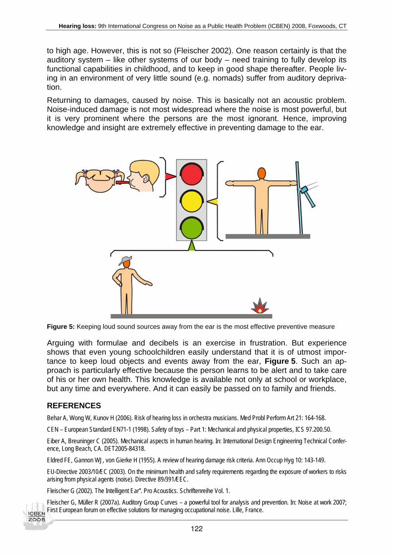
Hearing loss: 9th International Congress on Noise as a Public Health Problem (ICBEN) 2008, Foxwoods, CT
to high age. However, this is not so (Fleischer 2002). One reason certainly is that the auditory system – like other systems of our body – need training to fully develop its functional capabilities in childhood, and to keep in good shape thereafter. People liv-ing in an environment of very little sound (e.g. nomads) suffer from auditory depriva-tion. Returning to damages, caused by noise. This is basically not an acoustic problem. Noise-induced damage is not most widespread where the noise is most powerful, but it is very prominent where the persons are the most ignorant. Hence, improving knowledge and insight are extremely effective in preventing damage to the ear.
Figure 5: Keeping loud sound sources away from the ear is the most effective preventive measure
Arguing with formulae and decibels is an exercise in frustration. But experience shows that even young schoolchildren easily understand that it is of utmost impor-tance to keep loud objects and events away from the ear, Figure 5. Such an ap-proach is particularly effective because the person learns to be alert and to take care of his or her own health. This knowledge is available not only at school or workplace, but any time and everywhere. And it can easily be passed on to family and friends.
REFERENCES Behar A, Wong W, Kunov H (2006). Risk of hearing loss in orchestra musicians. Med Probl Perform Art 21: 164-168.
CEN – European Standard EN71-1 (1998). Safety of toys – Part 1: Mechanical and physical properties, ICS 97.200.50.
Eiber A, Breuninger C (2005). Mechanical aspects in human hearing. In: International Design Engineering Technical Confer-ence, Long Beach, CA. DET2005-84318.
Eldred FE, Gannon WJ, von Gierke H (1955). A review of hearing damage risk criteria. Ann Occup Hyg 10: 143-149.
EU-Directive 2003/10/EC (2003). On the minimum health and safety requirements regarding the exposure of workers to risks arising from physical agents (noise). Directive 89/391/EEC.
Fleischer G (2002). The Intelligent Ear”. Pro Acoustics. Schriftenreihe Vol. 1.
Fleischer G, Müller R (2007a). Auditory Group Curves – a powerful tool for analysis and prevention. In: Noise at work 2007; First European forum on effective solutions for managing occupational noise. Lille, France.
122
Hearing loss: 9th International Congress on Noise as a Public Health Problem (ICBEN) 2008, Foxwoods, CT
Fleischer G, Müller R (2007b). Evaluation of powerful acoustic impulses and their effect on the human ear. In: Symposium Acoustics in Defense, Meppen, Germany.
Fleischer G, Hoffmann E, Lang R, Müller R (1998). Dokumentation der Auswirkungen von Kinderknallpistolen (Effects of toy pistols). HNO 47: 535-540.
Fleischer G, Müller R, Bache T, Heppelmann G (2003). Auditory effects of some Millennium celebrations in Germany. Z Audiol 42: 106-116.
Henderson D, Hamernik RP, Dosanjh DS, Mills JH (eds.) (1976). Effects of noise on hearing. New York: Raven Press.
ISO1999 (1990). International Standard: Acoustics – Determination of occupational noise exposure and estimation of noise-induced hearing impairment. 2nd ed. Geneva: ISO.
Khanna SM, Tonndorf J (1972). Tympanic membrane vibrations in cats, studied by time-averaged holography. J Acoust Soc Am 51: 1904-1920.
Niu X, Tahera Y, Canlon B (2007). Environmental enrichment to sound activities dopaminergic pathways in the auditory system. Physiol Behav 92: 34-39.
Price RG (2007). Validation of the auditory hazard assessment algorithm for the human with impulse noise data. J Acoust Soc Am 122: 2786-2802.
Puria S (2003). Measurements of human middle-ear forward and reverse acoustics; Implications for acoustic emissions. J Acoust Soc Am 113: 2773-2789.
Rüedi L, Furrer W (1946). Das akustische Trauma. Pract Otorhinolaryngol 8: 177-372.
123

Hearing loss: 9th International Congress on Noise as a Public Health Problem (ICBEN) 2008, Foxwoods, CT
Ratio of total cholesterol over HDL is a better hyperlipidemia indica-tor for sensorineural hearing loss? Rafidah Hanim Mokhtar1*, Raja Ahmad2, Azizi Ayob1, Wan Ishlah2 1 Department Basic Medical Sciences, Faculty of Medicine, International Islamic University Malaysia
2 Department Otolaryngology-Head & Neck Surgery, Faculty of Medicine, International Islamic Uni-versity Malaysia
* corresponding author: e-mail: [email protected], [email protected]
Introduction. Sensorineural hearing loss (SNHL) have been attributed to hyperlipidaemia by postulated mechanisms such as atherosclerosis, metabolic, ageing and even hypertension. However, current researches showed that the assessment of low density lipoprotein (LDL) or total cholesterol alone may not be sufficient to identify an individual at risk for the various mechanisms mentioned above. In fact, in the 26-year follow-up of the Framingham study, 20 % of patients with myocardial infarctions had their cholesterol level below 5.17 mmol/L, a level considered safe according to most guidelines. The present study was undertaken to see the relationship of SNHL and the various lipid profiles. Methods. This is a cross sectional study where patients were recruited from those attending the Otorhinolaryngology clinic at Tengku Ampuan Afzan Hospital, Malaysia with SNHL, which was confirmed via the pure tone audiometry. Patients who suffered hearing loss secondary to trauma, suppurative otitis media and tumor within the cerebellopontine angle region are excluded from this study. All the subjects were required to fast for at least 12 hours before antecubital venous blood was taken for lipid profile determination. Results. Subjects with SNHL have significantly lower level of HDL (1.23 ± 0.47 vs 1.82 ± 0.60 mmol/L, P < 0.01) and higher level of triglyceride (1.32 ± 0.83 vs 0.91 ± 0.93 mmol/L, P < 0.01) and TC:HDL (4.21 ± 1.51 vs 3.01 ± 1.07) as compared to control. Surprisingly, there were no significant difference in total cholesterol level and LDL level between groups. Conclusion. The study suggested that the TC:HDL ratio may be a more useful marker in detecting subject with high risk of developing SNHL.
124

Hearing loss: 9th International Congress on Noise as a Public Health Problem (ICBEN) 2008, Foxwoods, CT
Auditory effects of chronic exposure to carbon monoxide and noise among workers Tony Leroux1*, Adriana Lacerda2, Jean-Pierre Gagné1
1 School of Speech-Language Pathology and Audiology, University of Montreal, Montreal, Quebec, Canada
2 School of Speech-Language Pathology and Audiology, University of Tuiuti do Paraná, Curitiba, Paraná, Brazil
*corresponding author: e-mail adress: [email protected]
INTRODUCTION For more than a century, scientific publications have discussed the numerous harm-ful consequences of noise exposurte on hearing (Berglund & Lindvall 1995). How-ever, in addition to the presence of noise in working environments, other environ-mental factors represent a potential risk of acquiring a noise-induced hearing loss (NIHL) (Fechter 2004). The risk of acquiring a hearing loss in the presence of moderate exposure to noise associated to the presence of asphyxiant chemical substances has been evaluated mostly in rats (Fechter et al. 1987, 1988, 1997, 2000a, b, 2002; Fechter 1989, 1995; Young et al. 1987; Chen et al. 1999, 2000, 2001; Chen & Fechter 1999; Rao & Fechter 2000; Rao et al. 2001). These studies investigated the effects of acute simul-taneous exposure to high concentrations of carbon monoxide (CO) and to moderate levels of noise. As a whole, the results show the emergence of a NIHL from the ex-posure of CO in rats exposed to noise levels which, alone, do not produce any sig-nificant changes to hearing detection thresholds. Effects of chronic combined expo-sure to CO and noise on human hearing in a working environment were investigated in only two studies (Sulkowski & Bojarski 1988; Ahn et al. 2005). While the results of the previously mentioned studies suggest a significant interaction between CO and noise, the specific effects of chronic combined exposure to these contaminants on hearing remain largely unknown. Considering the large distribution of CO and noise in the working environment and the large number of exposed work-ers, it is of utmost importance to confirm a potential effect of chronic exposure to both CO and noise on human hearing. The aim of this study was to determine if workers chronically exposed to CO and noise, in the workplace or during non-occupational activities face a greater risk of acquiring NIHL.
METHODOLOGY The data used in this study were extracted from the database developed and main-tained by the Centre d’expertise en dépistage of the Institut national de santé pub-lique du Québec (CED-INSPQ) between 1983 and 1996. This database contained information from 49,495 workers who have completed a questionnaire about their hearing history, including personal information (gender, age, extraprofessional noise exposure, etc.), medical (surgery, middle ear problems, vertigos, etc.) and occupa-tional history (occupation, noise dose at the current work position, number of years at current position, total number of years of employment, etc.), and who had undergone an audiometric examination in a mobile laboratory used by the CED-INSPQ across various industrial settings in Quebec. The audiometric examination procedure used by the CED-INSPQ is a conventional air-conducted pure tone test, using a Békésy-
125

Hearing loss: 9th International Congress on Noise as a Public Health Problem (ICBEN) 2008, Foxwoods, CT
automated method. The evaluation is carried out under supraaural or inserts ear-phones in a standard audiometric room, which complied with the ANSI S.31-1999 standard recommendations (ANSI 1999), using a clinical instrument. The CED-INSPQ’s database did not contain direct information regarding occupa-tional exposure to CO. Indirect information about occupational exposure to CO was obtained through a panel of five experts used to assess potential CO exposure for each professions included in the Canadian Classification and Dictionary of Occupa-tions (CCDO) also available in the CED-INSPQ’s database. The members of the panel individually reviewed each occupation listed in the CCDO and ascertain a value to a dichotomized CO occupational exposure variable (present/absent). A Kappa test was then used to measure intra-judge agreement on the dichotomized CO variable (Landis & Koch 1977). The results showed good to excellent intra-judge agreement (0.4 ≤ K ≤ 0.75 and K > 0.75) for 82% of the occupations listed in the CCDO. Two additional experts were recruited for a second analysis to conciliate the differences obtained for the remaining 18% of the occupations. The dichotomized variable was then incorporated to the original CED-INSPQ’s database. Two studies were conducted. First, a case-control study was design to estimate the risk of acquiring NIHL for workers exposed either to noise alone or in combination with CO. The only cases retained were those where the individual only work in one single noisy workplace and where the number of years worked in that environment and the corresponding noise exposure levels were documented. Workers that pre-sented with a contributing medical or personal history (vertigo, Menière’s disease, middle ear problem or abnormal tympanogram, sudden or congenital hearing loss, extraprofessional noise exposure, military career) were excluded from this study. Due to the very small number of cases, women were also excluded from the study. After exclusions, data from 6,812 audiometric assessments were retained for analy-sis and were divided among four groups: (1) CO plus noise ≥ 90 dB(A)-8h (exposed cases); (2) noise alone ≥ 90 dB(A)-8h (non-exposed cases); (3) CO plus noise < 90 dB(A)-8h (exposed controls); and (4) noise alone < 90 dB(A)-8h (non-exposed con-trols). Table 1 presents the summary of the composition of the four groups according to the sample size, the means and standard deviations for: age, number of years of noise exposure at the current occupation and total number of years of occupational noise exposure. Table 1: Groups composition of first study according to sample size, age, number of years at current occupation and total number of years of employment
CO & NOISE ≥ 90 dB(A)-8h
Exposed Cases
NOISE ≥ 90 dB(A)-8h Non-Exposed
Cases
CO & NOISE < 90 dB(A)-8h Exposed Con-
trols
NOISE < 90 dB(A)-8h Non-exposed
Controls Sample size 1872 2383 1031 1526
Age (mean ± SD) 29.2 ± 9.6 30.4 ± 9.8 30.2 ± 9.7 31.0 ± 9.8 Years at current occupa-
tion (mean ± SD) 6.1 ± 7.2 6.6 ± 7.6 6.7 ± 7.4 6.8 ± 7.2
Years of employment (mean ± SD) 6.3 ± 7.1 6.8 ± 7.5 7.0 ± 7.3 7.1 ± 7.2
The independent variables used for the analyses were: frequency (0.5, 1, 2, 3, 4 and 6 kHz), dose of noise at current workplace (< 90 dB(A) and ≥ 90 dB(A) LAeq-8h), and exposure to CO. The dependent variable used for the analyses was the auditory threshold averaged across ears. To control for age, the 90th percentile for pres-byacousia provided by ISO-7029 standard (ISO 2000) was used to decide whether a
126

Hearing loss: 9th International Congress on Noise as a Public Health Problem (ICBEN) 2008, Foxwoods, CT
significant hearing deficit existed. Odds ratios [OR= (exposed cases / non-exposed cases) / (exposed controls / non-exposed controls)] were determined for three groups of workers: (1) exposed to CO and noise ≥ 90 dB(A)-8h; (2) noise alone ≥ 90 dB(A)-8h; and, (3) CO and noise < 90 dB(A)-8h. A second study examined the effects of non-occupational combined exposure to CO and noise. The aim of this study was to verify if a combined, non-occupational expo-sure to noise and CO could affect the hearing thresholds of workers with occupa-tional noise exposure. The samples were constructed with 6,395 workers that re-ported non-occupational noise exposure including or not concomitant CO exposure. Workers who reported snowmobile, motorbike, farm vehicles, snow blower, and/or chainsaw use as a non-occupational activity were described as having been exposed to non-occupational noise and CO exposure. Workers who reported electrical power tools and/or loud music used is non-occupational context were described as having been exposed to non-occupational noise only. Inclusion in one or the other category is mutually exclusive, e.g. a worker that reported electrical power tools and snowmo-bile use were excluded from the study. Table 2 shows the distribution of mean age per study group according to the mean number of years of occupational noise expo-sure. Table 2: Mean age distribution according to groups (non-occupational CO & Noise; non-occupational Noise) and years of occupational noise exposure (from 0 to 30 years)
For the second study, a multivariate analysis of variance (MANOVA) using repeated measures was used and the appropriate Greenhouse-Geisser adjustment was ap-plied. The independent variables for this test were: the frequency (0.5, 1, 2, 3, 4, and 6 kHz), the non-occupational CO exposure (non-occupational Noise+CO exposure and non-occupational Noise exposure), years of occupational noise exposure (7 categories, based on 5-year clusters and ranging from no occupational noise expo-sure to 30 years of occupational noise exposure), and current occupational noise ex-posure level (8 categories, ranging from exposure < 80 dB(A) LAeq-8hr to exposure > 100 dB(A) LAeq-8hr). The dependent variable for this test was the average hearing threshold. Age, a potential confounding variable, was used as a covariate in the analysis.
RESULTS In the first study, odds ratios were determined for three groups of workers: (1) ex-posed to CO and noise ≥ 90 dB(A)-8h; (2) noise alone ≥ 90 dB(A)-8h; and, (3) CO and noise < 90 dB(A)-8h. The results of those calculations are shown in Table 3.
Mean age (± SD) of the subjects as a function of years of occupational noise exposure in 5-year clusters Groups
non-occupational exposure ≥ 0 - < 5 ≥ 5 - < 10 ≥ 10 - < 15 ≥ 15 - < 20 ≥ 20 - < 25 ≥ 25 - < 30
CO & Noise (n=3306)
27.4 ± 7.4 31.7 ± 6.7 35.3 ± 6.5 40.3 ± 6.1 44.0 ± 5.7 49.1 ± 5.3
Noise (n=3089)
24.4 ± 5.0 29.2 ± 5.6 33.3 ± 4.6 38.1 ± 5.0 42.1 ± 4.1 47.9 ± 5.3
127

Hearing loss: 9th International Congress on Noise as a Public Health Problem (ICBEN) 2008, Foxwoods, CT
Table 3: Results of clinical thresholds analysis according to age – Risk factors for the groups
1) Clinical thresholds analysis according to age – Risk factors: CO and noise ≥ to 90 dB(A)
Frequency Hz Normal Hearing loss Odd Ratio 95% CI p
500 2797 601 1.158 0.969-1.385 0.11
1000 3014 384 1.311* 1.055-1.628 0.01
2000 3068 330 1.232 0.978-1.552 0.08
3000 2834 564 1.348* 1.121-1.622 0.002
4000 2557 841 1.388* 1.184-1.627 < 0.001
6000 2227 1171 1.419* 1.229-1.639 < 0.001
At least one 1508 1890 1.347* 1.175-1.543 < 0.001
2) Clinical thresholds analysis according to age – Risk factor: noise ≥ to 90 dB(A)
Frequency Hz Normal Hearing loss Odd Ratio 95% CI p
500 3228 681 1.110 0.936-1.317 0.24
1000 3473 436 1.251* 1.015-1.542 0.04
2000 3541 368 1.146 0.917-1.432 0.24
3000 3256 653 1.329* 1.113-1.586 0.002
4000 3011 898 1.155 0.990-1.348 0.07
6000 2646 1263 1.178* 1.025-1.353 0.02
At least one 1795 2114 1.180* 1.037-1.342 0.01
3) Clinical thresholds analysis according to age – Risk factors: CO and noise < 90 dB(A)
Frequency Hz Normal Hearing loss Odd Ratio 95% CI p
500 2113 444 1.157 0.941-1.423 0.18
1000 2283 274 1.254 0.975-1.614 0.08
2000 2333 224 1.014 0.767-1.340 0.94
3000 2178 379 1.014 0.879-1.368 0.43
4000 1987 570 1.131 0.936-1.366 0.21
6000 1763 794 1.110 0.937-1.317 0.24
At least one 1203 1357 1.147 0.979-1.345 0.09
Elevated ORs were observed at 4 frequencies for the combined exposure to CO and noise (≥ 90 dB(A)-8h). Significant ORs were obtained at 1, 3, 4 and 6 kHz (95% CI ranged from 1.055-1.628 (1 kHz) to 1.229-1.639 (6 kHz). The OR remained signifi-cant when its computation was restricted to a deficit at a single frequency (95% CI = 1.175-1.543). Noise exposure alone (≥ 90 dB(A)-8h) was associated to the hearing deficit at 1, 3 and 6 kHz (95% CI ranged from 1.015-1.542 (1 kHz) to 1.113-1.586 (3 kHz). The OR remained significant when its computation was restricted to a deficit at a single frequency (95% CI = 1.037-1.342). The effect of CO exposure with moderate noise exposure (< 90 dB(A)-8h) was not significant at all frequencies. No significant effect on hearing threshold could be demonstrated even when considering a deficit at a single frequency (95% CI = 0.979-1.345). The MANOVA applied to the second dataset showed a significant interaction (F[122,19183] = 1.36; p = 0.005; Greenhouse-Geisser adjustment = 0.61) for frequency *
128

Hearing loss: 9th International Congress on Noise as a Public Health Problem (ICBEN) 2008, Foxwoods, CT
non-occupational CO exposure * years of occupational noise exposure * occupa-tional noise exposure levels. Figure 1 depicts the hearing thresholds at 0.5, 1, 2, 3, 4, and 6 kHz according to years of occupational noise exposure (a: ≥ 0 and < 5 years; b: ≥ 5 and < 10 years; c: ≥ 10 and < 15 years; d: ≥ 15 and < 20 years; e: ≥ 20 and < 25 years; and f: ≥ 25 and < 30 years) and for the two study groups (non-occupational exposure to noise; combined non-occupational exposure to CO and noise). Based on the analysis of the confidence intervals around group means (95% CI), significant differences between groups were observed for 3, 4 and 6 kHz for the workers with ≥ 15 and < 20 years of occupational exposure (Figure 1, panel d). For the workers having ≥ 20 and < 25 years of occupational exposure, significant differ-ences were noted only for 3 and 6 kHz (Figure 1, panel e). For the group of workers having ≥ 25 and < 30 years of occupational exposure, significant differences were also observed at 3 and 6 kHz but also extend at the frequency of 2 kHz (Figure 1, panel f). These results suggest that the hearing thresholds for the high frequencies are affected first by the non-occupational combined CO and noise exposure. As the number of years of exposure increases, the hearing loss progressively extends to-wards low frequencies. The impact of non-occupational CO and noise exposure on hearing thresholds across the frequencies tested is especially striking for workers having ≥ 25 and < 30 years of occupational noise exposure. There was no significant difference between groups at 4 kHz for workers having the longer occupation noise exposure (≥ 20 and < 25 years, ≥ 25 and < 30 years). Figure 2 depicts hearing thresholds at 0.5, 1, 2, 3, 4, and 6 kHz according to the cur-rent occupational noise exposure level (a: no significant occupational noise expo-sure; b: LAeq-8hr ≥ 80 and < 85 dB(A); c: LAeq-8hr: ≥ 85 and < 90 dB(A); d: LAeq-8hr: ≥ 90 and < 100 dB(A); and e: LAeq-8hr: ≥ 100 dB(A)) and for the two study groups. A significant difference between groups was observed only at 2 kHz when the sub-jects had no occupational noise exposure. The differences noted between groups at 3 and 4 kHz were close to the significant level in the same condition (Figure 2, panel a). Intersubject variation is larger among subjects in the CO+Noise group, (range from 151 to 228 %) when compare to the variation observed in the Noise group thus reducing the statistical power. As the level of occupational noise exposure increases, the difference between groups disappears (Figure 2, panels b-e). These results high-light the effect of non-occupational combined noise and CO exposure on workers’ hearing thresholds even when the workers have no occupational noise exposure.
CONCLUSION Two main conclusions may be drawn for the first study. First, CO interacts with noise to increase the risk of hearing loss in workers exposed to dose levels that are supe-rior to 90 dB(A)-8h. Second, a chronic exposure to CO and noise should be consid-ered when the risk for acquiring a NIHL is being assessed. For the second study, the results indicate that non-occupational noise and CO expo-sure interacts with occupational noise exposure to worsen hearing thresholds. A long history of non-occupational noise and CO exposure as well as occupational noise exposure is a risk factor for NIHL. Combined non-occupational noise and CO expo-sure and low level occupational noise exposure is a risk factor for NIHL which should be clinically assessed.
129
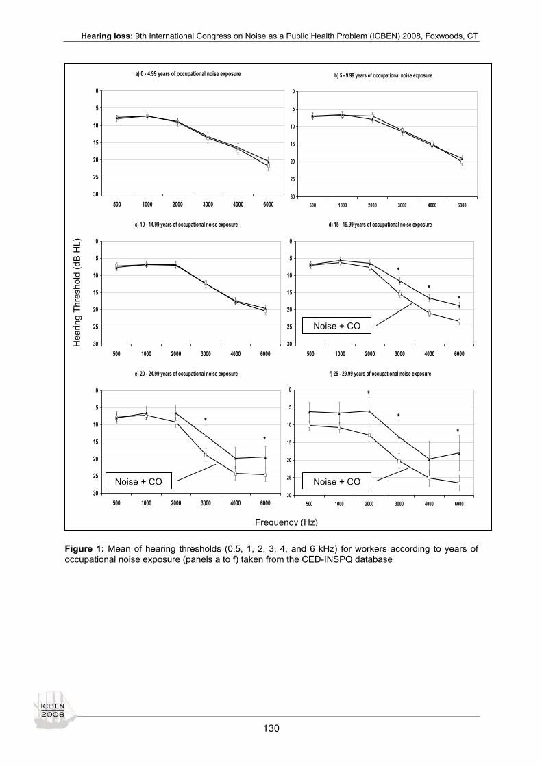
Hearing loss: 9th International Congress on Noise as a Public Health Problem (ICBEN) 2008, Foxwoods, CT
a) 0 - 4.99 years of occupational noise exposure
0
5
10
15
20
25
30500 1000 2000 3000 4000 6000
b) 5 - 9.99 years of occupational noise exposure
0
5
10
15
20
25
30500 1000 2000 3000 4000 6000
c) 10 - 14.99 years of occupational noise exposure
0
5
10
15
20
25
30500 1000 2000 3000 4000 6000
d) 15 - 19.99 years of occupational noise exposure
0
5
10
15
20
25
30500 1000 2000 3000 4000 6000
*
**
e) 20 - 24.99 years of occupational noise exposure
0
5
10
15
20
25
30500 1000 2000 3000 4000 6000
*
*
f) 25 - 29.99 years of occupational noise exposure
0
5
10
15
20
25
30500 1000 2000 3000 4000 6000
*
*
*
Frequency (Hz)
Hea
ring
Thre
shol
d (d
B H
L)
Noise + CO
Noise + CO Noise + CO
Figure 1: Mean of hearing thresholds (0.5, 1, 2, 3, 4, and 6 kHz) for workers according to years of occupational noise exposure (panels a to f) taken from the CED-INSPQ database
130

Hearing loss: 9th International Congress on Noise as a Public Health Problem (ICBEN) 2008, Foxwoods, CT
** *
**
*
a) No occupational noise exposure
-5
0
5
10
15
20
25
30500 1000 2000 3000 4000 6000
*
b) Level of occupational noise exposure 80-84.9 dB(A)
0
5
10
15
20
25
30500 1000 2000 3000 4000 6000
c) Level of occupational noise exposure 85-89.9 dB(A)
0
5
10
15
20
25
30500 1000 2000 3000 4000 6000
d) Level of occupational noise exposure 90-99.9 dB(A)
0
5
10
15
20
25
30500 1000 2000 3000 4000 6000
e) Level of occupational noise exposure 100 dB(A)
0
5
10
15
20
25
30500 1000 2000 3000 4000 6000
≥
Frequency (Hz)
Hea
ring
Thre
shol
d (d
B H
L)
Noise + CO
Figure 2: Mean of hearing thresholds (0.5, 1, 2, 3, 4, and 6 kHz) for workers according to level of oc-cupational noise exposure (panels a to e) taken from the INSPQ database
Based on our findings we recommend: (1) that field studies be undertaken to con-tinue to evaluate the combined effect of noise and CO on hearing sensitivity among exposed workers; (2) the identification of the minimal dose of CO (over a worker’s career) that can safely co-exist with noise without any deleterious effects on hearing; 3) that studies be undertaken to elucidate the effects of simultaneous exposure of CO and noise in combination with other ototoxic agents; and, 4) in addition to pure-tone audiometry, hearing assessments administered in the workplace should incor-porate test procedures (i.e. otoacoustic emissions) that could be more sensitive to the physiopathologic process occurring within the cochlea when noise and chemical asphyxiants are present in the working environment.
131

Hearing loss: 9th International Congress on Noise as a Public Health Problem (ICBEN) 2008, Foxwoods, CT
REFERENCES Ahn YS, Morata TC, Stayner LT, Smith R (2005). Hearing loss among iron and steel workers exposed to low levels of carbon monoxide and noise. Presentation at the International Symposium on Neurobehavioral Methods and Effects in Occupational and Environmental Health, September 26 - 29, Gyeongju, Korea.
ANSI (American National Standards Institute) 1999. Maximum permissible environment noise levels for audiometric test rooms. ANSI S 3.1-1999, New York.
Berglund B, Lindvall T (eds.) (1995). Community noise. Document prepared for the World Health Organization. Arch Center Sensory Res 2: 1-195.
Chen GD, Fechter LD (1999). Potentiation of octave-band noise induced auditory impairment by carbon monoxide. Hear Res 132: 149-159.
Chen GD, Mc Williams ML, Fechter LD (1999). Intermittent noise-induced hearing loss and the influence of carbon monox-ide. Hear Res 138: 181-191.
Chen GD, Mc Williams ML, Fechter LD (2000). Succinate dehydrogenase (SDH) activity in hair cells: a correlate for perma-nent threshold elevations. Hear Res 145: 91-100.
Chen GD, Kong J, Reinhard K, Fechter LD (2001). NMDA receptor blockage protects against permanent noise-induced hearing loss but not its potentiation by carbon monoxide. Hear Res 154: 108-115.
Fechter LD (1989). A mechanistic basis for interactions between noise and chemical exposure. Arch Commun Environ Stud 1: 23-28.
Fechter LD (1995). Combined effects of noise and chemicals. Occup Med: State of the Art Rev 10: 609-621.
Fechter LD (2004). Promotion of noise-induced hearing loss by chemical contaminants. J Toxicol Environ Health 67A: 727-740.
Fechter LD, Thorne PR, Nuttall AL (1987). Effects of carbon monoxide on cochlear electrophysiology and blood flow. Hear Res 27: 37-45.
Fechter LD, Young JS, Carlisle L (1988). Potentiation of noise induced threshold shifts and hair cell loss by carbon monox-ide. Hear Res 34: 39-48.
Fechter LD, Liu Y, Pearce TA (1997). Cochlear protection from monoxide exposure by free radical blockers in the guinea pig. Toxicol Appl Pharmacol 142: 42-55. Fechter LD, Liu Y, Herr DW, Crofton KM (1998). Trichloroethylene ototoxicity: evidence for a cochlear origin. Toxicol Sci 42: 28-35.
Fechter LD, Chen GD, Rao D (2000a). Characterising conditions that favour potentialization of noise induced hearing loss by chemical asphyxiants. Noise & Health 3(9): 11-21.
Fechter LD, Chen GD, Rao D, Larabee J (2000b). Predicting exposure conditions that facilitate the potentiation of noise-induced hearing loss by carbon monoxide. Toxicol Sci 58: 315-323.
Fechter LD, Chen GD, Rao D (2002). Chemical asphyxiants and noise. Noise & Health 4(14): 49-61.
ISO (International Standard Organization) (2000). ISO-7029. Acoustics. Statistical distribution of hearing thresholds as a function of age. Geneva, Switzerland.
Landis JR, Koch GG (1977). An application of hierarchical kappa-type statistics in the assessment of majority agreement among multiple observers. Biometrics 33:363-374.
Rao DB, Fechter LD (2000). Increased noise severity limits potentiation of noise induced hearing loss by carbon monoxide. Hear Res 150: 206-214.
Rao DB, Moore DR, Reinke LA, Fechter LD (2001). Free radical generation in the cochlea during combined exposure to noise and carbon monoxide: an electrophysiological and an EPR study. Exposure Res 161: 113-122.
Sulkowski WJ, Bojarski K (1988). Hearing loss due to combined exposure to noise and carbon monoxide – A field study. In: Noise as a public health problem: Proceedings of 5th International Congress on Noise as a Public Health Problem (p 179).
Young JS, Upchurch MB, Kaufman MJ, Fechter LD (1987). Carbon monoxide exposure potentiates high-frequency auditory threshold shifts induced by noise. Hear Res 26: 37-43.
132

Hearing loss: 9th International Congress on Noise as a Public Health Problem (ICBEN) 2008, Foxwoods, CT
Detailed DPOAE level/phase maps provide insight into normal and noise-damaged human ears Deanna K. Meinke1*, Barden B. Stagner2, Brenda L. Lonsbury-Martin3, Glen K. Martin2 1 University of Northern Colorado, Audiology & Speech-Language Sciences, Campus Box 140,
GrCO 0639
2 Jerry Pettis Memorial Veterans Medical Center, Research Service (151), 11201 Benton Street, Loma Lda, A 92357
3 Division of Otolaryngology-Head & Neck Surgery, Department of Surgery, Loma Linda University, Loma Lnda, CA 92350
* corresponding author: e-mail: [email protected]
Distortion product otoacoustic emission (DPOAE) level/phase maps were generated from detailed 2f1-f2 and 2f2-f1 DPOAE measurements obtained from 20 normal-hearing subjects and 10 patients with noise-induced hearing loss (NIHL). The experimental paradigm used an f2/f1 fixed-ratio approach incremented in 0.025-interval steps between 1.025 and 1.5 in response to two equi-level and one, offset-level primary-tone sweeps (L1=L2=75 and 80, and L1,L2=65,55 dB SPL). The extended DPOAE frequency span ranged from 0.5-6 kHz in DPOAE frequency steps of 44 Hz. While both wave- and place-fixed emissions were evident for the 2f1-f2 emission, only place-fixed emissions were apparent for the 2f2-f1 emission in both normal and NIHL subjects with measurable emissions. In addition, DPOAE level/phase maps were used to compute comprehensive measures of DPOAE group delay. The group-delay measures in normal-hearing subjects were consistent with data in the literature and were sufficiently sensitive to reveal expected differences due to primary-tone levels and frequency-sweep methods. In general, while NIHL appeared to eliminate or reduce both 2f1-f2 and 2f2-f1 DPOAEs, the effects of NIHL on group delays were level- and/or frequency-dependent. For example, for primary-tone levels of 65,55 dB SPL, group delays were substantially (16-30 %) longer in the low frequency region. Consequently, DPOAE level/phase mapping may be a useful technique for the early detection and monitoring of cochlear structural irregularities caused by hazardous noise exposure.
133

Hearing loss: 9th International Congress on Noise as a Public Health Problem (ICBEN) 2008, Foxwoods, CT
1
Use of narrow band noise to screen for cochlear dead regions A. Shubhra Shanker*, Imran Dhamani, B. Rajashekar
Manipal University
* corresponding author: e-mail: [email protected]
According to Moore and Glasberg (1997), cochlear dead zones are regions where the inner hair cells and/or adjacent neurons are not functional. Thus, in these regions, the information generated by the basilar membrane vibration is not transmitted to the central nervous system. Nonetheless, a sound in a dead zone frequency, if intense enough, may be detected in places with functional neurons and inner hair cells, through apical or basal spread of the vibration pattern. This causes a difficulty in de-coding the acoustic information and even information overload in one same region. Moore (2001) re-ported that hearing thresholds above 75-80 dB in low frequencies and above 90 dB in the high fre-quencies indicate a probable presence of dead zones in the cochlea. Cochlear dead zones can not be diagnosed based on the audiogram (Moore et al. 2000). Thus, Moore (Moore et al. 2000) created a test called TEN (Threshold Equalizing Noise), which is an efficient clinical test for the diagnosis of cochlear dead zones. But it requires some amount of clinical skill and time and cannot be administered for patients with greater degree of hearing loss. Moreover it can only be used to diagnose dead re-gions only till 4-6 kHz. Another diagnostic means is the psychophysical measure of tuning curves, described by Moore and Alcántara (2001) which may be useful and reliable to identify cochlear dead zones and to outline the region involved. However, it bears the disadvantage of being a long and complex test, making it unfeasible for routine clinical use. Eguti (2002) assessed cochlear dead zones using the technique proposed by Moore et al. (2000), however using the audiometers white noise and found reliable and conclusive results. Thus this current study was aimed at using narrow band noise at various center frequencies to screen for cochlear dead regions. Narrow Band Noise (NBN) thresholds at centre frequencies from 250-8000 Hz were established for a group of normal hearing and sen-sorineural hearing impaired individuals confirmed to have dead regions using the TEN test. These NBN thresholds were then compared with the pure tone thresholds at the respective frequencies in both these groups. The results indicated good correlation between both the procedures in screening dead regions. Although, not diagnostic NBN-pure tone threshold comparison may be used as a screening tool for identifying cochlear dead regions.
Eguti EY (2002). Identificação das zonas mortas na cóclea utilizando a técnica de mascaramento com ruído branco [tese]. São Paulo: Universidade Federal de São Paulo.
Moore BCJ (2001). Dead regions in the cochlea: diagnosis, perceptual consequences, and implications for the fitting of hearing aids. Trends Amplificat 5: 1-34.
Moore BCJ, Alcantara JI (2001). The use of psychophysical tuning curves to explore dead regions in the cochlea. Ear Hear 22: 268-278.
Moore BCJ, Glasberg BR (1997). A model of loudness perception applied to cochlear hearing loss. Audit Neurosci 3: 289-311.
Moore BCJ, Huss M, Vickers DA, Glasberg BR, Alcantara JI (2000). A test for the diagnosis of dead regions in the cochlea. Brit J Audiol 34: 205-224.
134

Hearing loss: 9th International Congress on Noise as a Public Health Problem (ICBEN) 2008, Foxwoods, CT
Central auditory dysfunction associated with solvent exposure Adrian Fuente School of Speech and Hearing Sciences, Medical Faculty, the University of Chile, Santiago-Chile
Correspondence: [email protected]
The primary aim of this project was to study possible central auditory dysfunction as-sociated with organic solvent exposure. 100 solvent-exposed workers and 100 non-exposed workers were selected to participate in the research. The test battery com-prised pure-tone audiometry (PTA), acoustic reflexes, acoustic reflex decay test, transient evoked otoacoustic emissions (TEOAE), and the following auditory process-ing (AP) procedures: Hearing-in-Noise (HINT), Dichotic Digits (DD), and Random Gap Detection (RGD) tests. Also a self report inventory on subjects’ level of hearing functioning, the Amsterdam Inventory for Auditory Disability and Handicap (AIADH), was conducted. Significant differences between solvent-exposed and non-exposed subjects were found for most of the auditory processing tests. Solvent-exposed sub-jects presented with poorer mean test results than non-exposed subjects. A high prevalence of auditory processing disorder was found among solvent-exposed sub-jects. Also, significant differences between groups were found for TEOAE reproduci-bility and AIADH scores. A higher percentage of solvent-exposed subjects presented with absent acoustic reflexes in comparison to non-exposed subjects. A bivariate and multivariate linear regression model analysis was performed. One model for each auditory outcome (PTA, TEOAE, HINT, DD, RGD, and AIADH) was independently constructed. For most of the models solvent exposure was significantly associated with the auditory outcome. Age, hearing level, and gender also appeared significantly associated with some auditory outcomes. This study provides further evidence of the possible adverse effect of solvents on the central auditory functioning.
135

Hearing loss: 9th International Congress on Noise as a Public Health Problem (ICBEN) 2008, Foxwoods, CT
Temporal processing disorders associated with styrene exposure Ewa Zamyslowska-Szmytke1*, Adrian Fuente2, Mariola Sliwinska-Kowalska1 1 Department of Audiology and Phoniatrics, Nofer Institute of Occupational Medicine, Lodz, Poland
2 Centre for Communication Disorders, The University of Hong Kong
* corresponding author: e-mail: [email protected]
Due to known neurotoxic styrene properties it is likely that auditory processes/abilities such as auditory temporal processing may be affected. The aim of the study was to assess temporal processing abilities in styrene-exposed workers (67 subjects, mean age 40.3 ± 8.7) versus non exposed control individuals (50 subjects, mean age 36.5 ± 11.2). All participants presented either normal hearing or mild sensorineural hearing loss. The mean styrene exposure in the study group was 37.8 mg/m3 (S.D. 23.8). The following temporal processing tests were implemented: Gaps-in-noise (GIN), Frequency pattern test (FPT), Duration Pattern Test (DPT) using adequate sensation levels of stimuli. Audiometric hearing thresholds were significantly worse in styrene-exposed subjects for most of the frequencies tested. Abnormal results for GIN test presented 14 (20.89 %) styrene-exposed individuals vs. 6 (12 %) controls; for FPT - 35 (52.23 %) styrene-exposed workers and 10 (20 %) unexposed controls; for DPT 50 (74.62 %) exposed subjects vs. 13 (26 %) control subjects. Exploring Chi-square test a signifi-cant association was found between styrene exposure and test results for FPT and DPT. Analysis of covariance (ANCOVA) was performed to compare the dependent variables between styrene-exposed and non-exposed subjects including age and average hearing thresholds in the analysis. Significant differences between styrene-exposed and non-exposed subjects were found for FPT (p=0.010), and DPT (p=0.000). Age showed to be significantly associated with FPT results only, hearing level with GIN scores only. We conclude that styrene can be related to central auditory dysfunction characterised by a temporal processing disorders. Disclaimer: The study was supported by the 6th European Framework Project under the Marie Curie Host Fellowship for the Transfer of Knowledge ‘NoiseHear’ (Contract No. MTKD-CT-2004-003137).
136
Hearing loss: 9th International Congress on Noise as a Public Health Problem (ICBEN) 2008, Foxwoods, CT
The contribution of genetic variations to the individual susceptibility to noise Malgorzata Pawelczyk1*, Lut van Laer2, Annelies Konings2, Elzbieta Rajkowska1, Adam Dudarewicz3, Erik Fransen2, Guy van Camp2, Mariola Sliwinska-Kowalska1,3
1 Department of Audiology and Phoniatrics, Nofer Institute of Occupational Medicine, Lodz, Poland
2 Department of Medical Genetics, University of Antwerp, Antwerp, Belgium
3 Department of Physical Hazards, Nofer Institute of Occupational Medicine, Lodz, Poland
* corresponding author: e-mail: [email protected]
Hearing impairment associated with exposure to noise (noise-induced hearing loss – NIHL) is an im-portant occupational hazard that results from an interaction between environmental and genetic fac-tors. Although the former has been extensively studied, little is currently known about the genetic basis of NIHL.
Genes that may influence the development of NIHL have been grouped in several categories: oxida-tive stress genes, potassium recycling pathway genes, mitochondrial genes and human monogenic hearing impairment genes. So far, only a limited number of association studies has been performed and only three have led to a possible identification of NIHL susceptibility genes: KCNE1, GSTM1 and CAT.
However, promising results have been obtained for genes associated with potassium recycling path-way in the inner ear. Single Nucleotide Polymorphisms (SNPs) in 10 genes (GJB1, GJB2, GJB3, GJB4, GJB6, KCNE1, KCNQ1, KCNQ4, KCNJ10 and SLC12A2) were investigated whether they influ-ence noise susceptibility. Audiometric data from over 2000 noise-exposed Polish workers was ana-lyzed. Based on ISO 1999:1990 up to 20 % most susceptible and 20 % most resistant individuals were chosen for analysis. In total 99 SNPs were selected and genotyped. The results of this study indicate statistically significant differences of genotype and haplotype frequencies between susceptible and resistant to noise individuals, particularly for GJB2 and GJB6 genes.
To discover the complete picture of NIHL it is necessary to combine the power of molecular genetics with the development of a complex statistical model that includes additional potential risk factors, e.g. smoking, elevated blood pressure or cholesterol levels.
The study was performed in cooperation with the Department of Medical Genetics directed by prof. Guy Van Camp (University of Antwerp, Belgium) and was supported by the State Scientific Committee for Research (Grant No. PB 0911/P05/2004/26), bilateral cooperation project FLANDRIA/2004 and the 6th European Framework Project under the Marie Curie Host Fellowship for the Transfer of Knowl-edge ‘NoiseHear’ (Contract No. MTKD-CT-2004-003137).
137

Hearing loss: 9th International Congress on Noise as a Public Health Problem (ICBEN) 2008, Foxwoods, CT
User-friendly parameterizations of an unscreened population data-set for the prediction of noise- and age-related hearing threshold shifts Jennifer Tufts*, Paul K. Weathersby, Gales Ferry University of Connecticut, Storrs, CT
* corresponding author: e-mail: [email protected]
ABSTRACT In a noise-exposed adult with hearing loss, a portion of the deviation from audiomet-ric “normal” may be due to noise exposure, and another portion may be due to age. Since age-related hearing loss occurs concurrently with noise-induced hearing loss, measurement or prediction of the noise effect is confounded. This confound may be managed at the population level with the use of a reference, non-noise-exposed population. However, one of the most commonly used reference populations (ISO 1999-1990, Annex A) is considered too highly screened or “pristine” for comparison with many noise-exposed populations. A less highly screened reference population is available (ISO 1999-1990, Annex B, also reproduced in ANSI 3.44-1996). Published data from this population are presented as a table of hearing thresholds for the me-dian, 10th, and 90th percentiles at decade age intervals (age 30, age 40, etc.). Unfor-tunately, in this form, the data cannot be used for predicting age-related hearing loss for other ages and percentiles (e.g., age 37, 84th percentile). To improve the flexibility and usefulness of the Annex B dataset, we conducted several complete parameteri-zations of the entire dataset using constrained least-squares fitting methods. In this presentation, we will describe the theoretical and practical considerations behind our choice of models. Additionally, we will present preliminary equation sets for calculat-ing predicted age-related hearing thresholds for adults of any age. Among the bene-fits resulting from this project is flexible access to an appropriate reference population in investigations of noise-induced hearing loss.
138

Hearing loss: 9th International Congress on Noise as a Public Health Problem (ICBEN) 2008, Foxwoods, CT
Audiological characteristics, attitudes and habits of Brazilian young adults and noise Thais C. Morata1*, Angela Maria Fontana Zocoli2, Jair Mendes Marques2 1 Division of Applied Research and Technology, National Institute for Occupational Safety and
Health, USA
2 Universidade Tuiuti do Paraná, Brazil
* corresponding author: e-mail: [email protected]
The objective of this study was to examine behaviors and attitudes of Brazilian teen-agers towards noise and determine their audiological characteristics. Participants were 245 young men and women between 14 and 18 years old who attended private school in Brazil. Behaviors and attitudes were measured using the validated Brazilian Portuguese version of the 'Youth Attitude to Noise Scale (YANS)' The hearing of a sub-sample of 24 participants was evaluated by pure-tone audiometry and distortion-product otoacoustic emissions. The most common source of exposure reported by participants was music played through personal media players. Forty-two percent of the participants indicated listening to personal media players daily, 29 % reported listening several days a week, and 21 % used them periodically. Temporary tinnitus was reported by 69 % of the participants after attending disco clubs, music concerts, and listening to music through headphones. Female participants had a statistically significant more positive attitude towards noise than males. Only four teenagers (1.6 %) reported hearing protector use. Among the 24 participants who underwent hearing tests, 3 young women had abnormal results: one (4 %) had a middle ear problem while two (8 %) had bilateral audiometric notches at 6 kHz. Only three par-ticipants (12 %) had DPOAE responses bilaterally at all frequencies; the remaining participants had absent responses at one or more frequencies. Comparative studies between countries can elucidate differences in cultural background, socio-economic status, and educational efforts which can impact attitudes and behaviors towards risk and aid in the development of effective hearing conservation initiatives. Disclaimer: The findings and conclusions in this abstract have not been formally dis-seminated by the National Institute for Occupational Safety and Health and should not be construed to represent any agency determination or policy.
139
Hearing loss: 9th International Congress on Noise as a Public Health Problem (ICBEN) 2008, Foxwoods, CT
AHEAD III – Assessment of hearing in the elderly: Aging and degeneration - integration through immediate intervention Mariola Sliwinska-Kowalska1*, Ferdinando Grandori2, Wolf-Dieter Baumgartner3, Arne Ernst4, Thomas Janssen5, Sophia Kramer6, Stefan Stenfelt7, Rudolf Probst8, Adrian Davis9 1 Department of Environmental Otolaryngology, Clinic of Otolaryngology and Laryngological Oncolo-
gy, Medical University of Lodz, Lodz, Poland
2 Istituto di Ingegneria Biomedica, Italy
3 Medical University Vienna, ENT-Otology Department, Austria; Chryssoula Thodi, CH & M Cyprus Audiology Center Interacoustics Ltd, Cyprus
4 Hospital of the University of Berlin, Department of Otolaryngology, Germany
5 Technische Universitaet Muenchen, Falkultät für Medizin, Lehrstuhl für Hals-Nasen-Ohrenheilkunde, Germany
6 VU University Medical Center, Department of ENT/Audiology, The Netherlands
7 Linköpings Universitet, Faculty of Health Sciences, Division of Technical Audiology, Sweden
8 Universität Zürich, Klinik für Ohren-, Nasen-, Hals- und Gesichtschirurgie, Switzerland
9 University of Manchester, MRC Hearing and Communication Group, United Kingdom
* corresponding author: e-mail: [email protected]
Hearing loss is one of the most common chronic health conditions in the elderly po-pulation with important implications for patient quality of life. The diminished ability to hear and to communicate is frustrating in and of itself, but the strong association of hearing loss with depression and functional decline adds further to the burden on in-dividuals who are hearing impaired. Hearing loss can limit communication skills: not to hear means not to understand what is being said. Despite the prevalence and bur-den of hearing loss, hearing impairment is largely underdiagnosed in older persons and undertreated. The reason for this is that one of the most conspicuous signs of a hearing loss is that it cannot be seen! Actually, this is the reason why deafness does not receive the necessary attention. Too often, the public and still too many health care professionals underestimate the dramatic effects of deafness. Novel strategies should be explored to make screening and early intervention a feasible part of routine care. Project AHEAD III has been specifically designed to: Provide evidence of the effects of hearing impairment in adults and particularly in the elderly. Analyse costs associated with the implementation of integrated large scale programs of hearing screening and intervention in the elderly. Provide quality standards and minimum re-quirements for screening methods and related diagnostic techniques. Develop guide-lines and recommendations on how to implement successful screening programs to be tuned to the local, social, and economical conditions of a country. Acknowledgment: Supported by the 7th EC Framework Programme – Project acro-nym: AHEAD III, Grant agreement no. 200835; grant Co-ordinator – prof. Ferdinando Grandori
140

Hearing loss: 9th International Congress on Noise as a Public Health Problem (ICBEN) 2008, Foxwoods, CT
Comparison of school-based hearing screening protocols and the identification of noise induced hearing loss in adolescents Deanna K. Meinke1*, Noel Dice2
1 University of Northern Colorado, Audiology & Speech-Language Sciences, Gunter 1500, Campus Box 140, Greeley, CO 80634.
2 Peakview Medical Center, 5881 W. 16th St, Greeley, CO 80634.
*corresponding author: e-mail: [email protected]
INTRODUCTION School-based hearing screening programs have been commonplace in the United States since the 1960’s. Historically, the enrollment of children in the public school system afforded the first opportunity to have access to a large population of children in order to screen for hearing disorders. Such programs were primarily designed to identify hearing losses that necessitated medical referral and treatment and/or the students with educationally significant hearing loss. Typically, the screening ap-proach focused on capturing children with congenital hearing loss and those with conductive hearing losses due to medical conditions such as otitis media. In the con-temporary era, infants receive their initial hearing screening before hospital dis-charge, and the educational setting serves as a subsequent opportunity to identify hearing loss that has a later onset due to various genetic and environmental influ-ences. Certainly, noise is one environmental hazard that may contribute to the later onset of hearing loss and tinnitus in children and adolescents. The risk of NIHL has been demonstrated for youth engaged in farming (Broste et al. 1989), utilizing firearms (Clark 1991), playing with toys or fireworks (Axelsson & Jer-son 1985; Gupta & Vishwakarma 1989; Weber et al. 1967) or listening to amplified music (Clark 1991; Meyer-Bisch 1996; West & Evans 1990). Even within the school environment itself, hazardous sound levels may be encountered during woodworking or band (Grayston & Alvord 1993; Lankford & West 1993; Plakke 1985; Roeser 1980; Woodford 1973). Occupational noise exposure may also begin during adolescence. Lankford et al. (1991) found that 12.4 % of high school students reported workplace noise exposure. The National Institute of Occupational Safety and Health (NIOSH) reports that 5.1 % of the U.S. workforce is comprised of teens aged 16-19 years (NIOSH 2004). It is estimated that 1.5 million youth aged 16-19 years are engaged in work with noise-hazardous exposures (Hager 2006). Evidence of noise induced hearing loss (NIHL) in school-aged youth is offered by Niskar et al. (2001). These researchers evaluated audiometric threshold data from the U.S. National Health and Nutitrition Examination Survey III (NHANES III) and were interested in determining the prevalence of noise induced threshold shift (NITS) for children age 6 to 19 years (n=5,249). The criteria for a NITS or noise notch in-cluded all of the following (P1);
• Audiometric thresholds < 15 dB HL at 500 and 1000 Hz.
• A notching configuration in the audiogram at 3000, 4000, or 6000 Hz at least 15 dB poorer than the poorest threshold at 500 or 1000 Hz.
• Recovery of at least 10 dB at 8000 Hz.
141

Hearing loss: 9th International Congress on Noise as a Public Health Problem (ICBEN) 2008, Foxwoods, CT
In their analysis, 12.5 % (n=597) or approximately 5.2 million children in the United States had a noise notch in one or both ears. Bilateral NITS was evident in 14.6 % of those exhibiting a noise notch. This implies that there are at least three children with a hearing loss suggestive of noise damage in every classroom (assuming an average class size of 24). These same authors also noted that as children advanced in age [or school grade], there was a corresponding increase in the prevalence of NITS. The older youth, aged 12-19 years had a NITS prevalence of 15.5 % versus the 8.5 % prevalence for the younger 6-11 year olds. Interestingly, the noise notches in these children were primarily limited to a single test frequency (3000, 4000 or 6000 Hz). The 6000 Hz NITS was most common (77.1 %) among those audiograms meeting the Niskar et al. (2001) notch criteria. These findings offer significant implications for school-based hearing screening program design if the intent is to identify noise-induced hearing loss. The need for school-based hearing screening programs to identify high-frequency (> 3000 Hz) NIHL was first expressed by Cozad et al. (1974). These researchers studied 18,600 rural Kansas youth and found that high-frequency sensorineural hear-ing loss occurred at three times the rate as compared to conductive hearing losses. The audiometric configurations for these subjects with high-frequency hearing loss were suggestive of NIHL. These investigators also demonstrated that the occurrence of the high-frequency sensorineural hearing loss was more common in males and increased with age (between 6 to 18 years). Over thirty years ago, Cozad et al. (1974) advocated that schools implement medical referral, noise control, hearing pro-tection, periodic audiological monitoring and formal educational interventions as pre-ventive measures for children. Currently, there are no federally mandated or nationally standardized school-based hearing screening programs in place in the United States. This is in contrast to the universal newborn hearing screening programs which look toward the Joint Commit-tee on Infant Hearing (JCIH) position statements (JCIH 2007) to afford guidance, evi-dence-based outcomes and benchmarking. In the absence of federally or multi-disciplinary school-based hearing screening guidelines, state or local agencies are free to voluntarily implement and define the hearing screening program purpose and protocol. School-based hearing screening protocols have typically been designed with one of two fundamental purposes; 1) an educational orientation to identify children with a hearing loss that might have negative academic consequences or 2) medically ori-ented programs designed for the early identification of existing health conditions that necessitate medical referral. The state level Department of Education (purpose #1) or Department of Health (purpose #2) is typically the authoritative agency for the major-ity of school-based hearing screening programs (Penn & Wilkerson 1999). A preven-tive approach for the purposes of identifying early signs of NIHL has not been a focus for school-based hearing screening programs. Although pure-tone air-conduction screening is the most commonly used hearing screening method (Johnson 2002), there is considerable variability between different hearing screening guidelines. Penn and Wilkerson (1999) summarized 40 state pro-tocols and found seven different frequency combinations and two different stimulus presentation levels (20 or 25 dB HL) were utilized. Additionally, they noted that states tended to focus hearing screening on the elementary school-level students, and 12 states did not include hearing screening at the high school level in their guidelines.
142

Hearing loss: 9th International Congress on Noise as a Public Health Problem (ICBEN) 2008, Foxwoods, CT
The present study was undertaken to compare hearing screening outcomes for cur-rently implemented school-based screening protocols in terms of the ability to poten-tially detect NIHL in high school students by identifying students with a high-frequency notch (HFN) using the Niskar et al. (2001) noise notch criteria. The analy-sis was applied to an existing database of pure-tone threshold data from 9th and 12th-grade students in Colorado. For reporting this study, the terminology of HFN will be used rather than the Niskar et al. (2001) NITS terminology, since the underlying eti-ology of the hearing impairment is unknown, although the audiometric configuration is suggestive of noise damage.
METHODS School hearing screening guidelines were gathered from each U.S. state using a va-riety of approaches, including Internet searches, e-mail correspondence, library ref-erence search and phone inquiries to state agencies during the 2005 calendar year. The protocols were then summarized with respect to frequencies screened and deci-bel level(s) utilized. Each protocol was assigned a P# (protocol number) beginning with P2 (P1 referred to the Niskar et al.,2001 notch criteria). If a protocol afforded the opportunity for the screener to use more than one decibel level, then each protocol was further identified alphabetically for increasing decibel level. For instance, if pro-tocol #2 had a screening level of either 20 or 25 dB HL, then the protocols were separately identified as P2a and P2b respectively. An anonymous Colorado Department of Education high school audiometric database (HSAD) from 2004 was accessed with permission. The database included 641 stu-dents in the 9th (n=376) and 12th (n=265) grades from a suburban Colorado high school. Ethnicity was primarily Caucasian (n=399) and Hispanic (n=217). The data-base included valid air-conduction thresholds for 500, 1000, 2000, 3000, 4000, 6000 and 8000 Hz. Audiometric threshold data was exported to Microsoft Excel 2003 for three separate groups, 9th grade only, 12th grade only and 9th and 12th grade combined. Audiograms were first reviewed and identified (counted) as having a HFN by applying the Niskar et al. (2001) NITS criteria described previously. For all other screening protocols, the number of student audiograms that would potentially be identified with a HFN were identified by meeting all of the following criteria;
• Thresholds < 15 dB HL at 500 and/or 1000 Hz.
• Thresholds greater than the minimum screening level (dB HL) in either ear at 3000, 4000, or 6000 Hz (provided that the test frequency was included in the state protocol).
• Demonstrated recovery of 10 dB or more at 8000 Hz as compared to the poor-est threshold at 3000, 4000, or 6000 Hz. (note: this criteria was applied regard-less of the absence of 8000 Hz in the screening protocol to avoid identification of high-frequency hearing losses that were not suggestive of NIHL).
Significant differences were evaluated by comparing the number of student’s identi-fied with a HFN using the Niskar et al. (2001) notch criteria (P1) and the number of students identified with each state protocol. A non-parametric chi-square analysis was utilized. A significant difference was defined as a p-value < .05. Yates’s correc-tion was applied for cell values < 5.
143
Hearing loss: 9th International Congress on Noise as a Public Health Problem (ICBEN) 2008, Foxwoods, CT
RESULTS Screening protocols were obtained for 46 states and the District of Columbia as well as for the American Academy of Audiology (AAA 1997), the American Speech-Language Hearing Association (ASHA 1997) and the American Academy of Pediat-rics (AAP; Cunningham & Cox 2003). Twenty-two unique combinations of test fre-quencies and presentation levels were identified. Six protocols have more than one screening level permitted. A complete review of the screening protocols and statisti-cal analysis can be referenced in Meinke & Dice (2007). Upon application of the Niskar et al. (2001) notch criteria to the combined 9th and 12th grade database, 45 students would be identified with NITS. This number serves as the expected outcome values for the chi-square analysis. Colorado, Kansas and Iowa protocols have the greatest potential to identify students with an HFN (n=20). In contrast, the Alabama and Delaware protocols did not identify any students with a HFN. The remaining protocols identify between 6 % and 33 % (n=3-15) of the stu-dents with a HFN. The HFN involved the frequencies of 4000 Hz (48.8 %) and 6000 Hz (46.1 %) rather than 3000 Hz (5.1 %). A unilateral HFN was more common for the left ear (61.8 %) than the right ear (38.2 %). Chi-square statistical comparisons were not possible for those protocols that did not identify any HFN’s. When combining grade levels, significantly fewer students were identified with a HFN when using any of the school screening protocols as compared to the Niskar et al. (2001) notch criteria regardless of decibel level utilized. During separate grade analysis, the Colorado (P13) protocol at the 9th grade level and the Iowa protocol (P14a) at the 12th-grade level were the only insignificant findings. Hearing screening conducted at 1000, 2000 and 4000 Hz at either 20 or 25 dB HL is the most commonly used hearing screening protocol in the U.S. This screening ap-proach will only identify 10 out of the 45 students (22 %) with a HFN. The second most commonly used hearing screening protocol (500, 1000, 2000 and 4000 Hz at 20 or 25 dB HL) also only identified 22 % of the students with a HFN. Therefore, only 22 % of the students with a HFN will be identified in by hearing screening programs conducted in 33 states. The two protocols that included 4000 and 6000 Hz (Kansas & Colorado) were most likely to identify a student with NIHL. Iowa’s protocol includes screening at 15 dB HL and it also proved more likely to identify HFN’s. The Kansas, Colorado and Iowa protocols each identified 20 students with a potential NIHL, or 44 % of the total number of students with a HFN.
DISCUSSION Prevalence of HFNs The present study suggests a HFN occurrence of 7 % for the combined 9th and 12th grades. This is a lower prevalence when compared to the 15.5 % reported by Niskar et al. (2001) for the same general age group (12-18 years). Perhaps this is attributed to study population differences including gender, race-ethnicity, socioeconomic status, urban status, or geographical region. It might also be attributable to methodo-logical differences between the NHANES III testing protocol and the audiometric pro-cedures used for the Colorado student testing. Lastly, such difference may relate to the actual noise exposures encountered by the students or alternative etiologies not investigated in the present study.
144

Hearing loss: 9th International Congress on Noise as a Public Health Problem (ICBEN) 2008, Foxwoods, CT
Unilateral HFN The unilateral nature of HFN’s is confirmed in this study. Niskar et al. (2001) reported 85.4 % unilateral NITS while 85.4 % were unilateral HFNs in the present data set. Acoustic trauma, progression of NIHL or asymmetrical vulnerability to NIHL may be considered in terms of possible explanations for unilateral noise notches. Gupta & Vishwakarma (1989) noted that toy weapons and fireworks were the primary expla-nations for NIHL in a pediatric study.
Importance of Audiometric Test Frequency The importance of screening at 4000 and 6000 Hz is apparent in the present study as was also advocated by previous researchers (Axelsson et al. 1981; Katt & Spra-gue 1981; Holmes et al. 1997; Niskar et al. 2001). Historically, issues surrounding the inclusion of 6000 Hz have been debated on the basis of calibration issues, earphone coupling and potential normative reference errors (Luxon 1998). In the current study, if the HFN was attributable to calibration or standardization errors, especially at 6000 Hz, one would expect the HFNs to be found bilaterally and not predominately unilat-eral. Ultimately, the optimal test frequencies to include a school-based hearing screening protocol designed for the early detection of NIHL needs further study and investigation.
Pure-Tone Presentation Level The higher the decibel screening level, the more likely NIHL remains undetected. It is necessary to screen at low 15 or 20 dB HL decibel levels in order to detect minimal or slight high-frequency hearing loss suggestive of NIHL. Twenty-one states recom-mend screening at 20 dB HL at all test frequencies. Seven states recommend screening at 25 dB HL. Other protocols have variable presentation levels between 15 and 30 dB HL. Nine states permit the screener to choose more than one screening level. Ambient noise levels in the test environment may drive the higher decibel lev-els used for screening and diminish the opportunity to provide early identification of NIHL in youth.
Failure to Detect HFNs It appears that less than half of the students with potential NIHL would be detected during hearing screenings in the U.S. In this study, the 9th and 12th graders were given hearing tests and provided the opportunity to identify developing hearing losses. In most instances, school-based hearing screening is discontinued by the 9th grade. Consequently, if screening is not conducted, there exists no possibility of iden-tifying NIHL. If noise induced hearing loss goes undetected in the adolescent population, then op-portunities to intervene and prevent further deterioration are missed. It is important for school administrators and professionals to recognize the limitations of existing hearing screening protocols with regard to NIHL. If noise notches are not identified, students and teachers may not recognize the risks from their daily activities and school systems may encounter medicolegal challenges in the future if a false sense of security was perceived due to “passing” the hearing screening. Medical referral, education and follow-up would not be provided to the affected individual(s). Certainly, the burden of expanding the screening program to a larger student contingent is more costly. There may not be adequate resources or personnel available to design and implement a screening program for the early detection of NIHL.
145

Hearing loss: 9th International Congress on Noise as a Public Health Problem (ICBEN) 2008, Foxwoods, CT
Future Directions Innovative approaches are necessary to identify students at risk of NIHL. Perhaps noise risk surveys or student/parent/teacher interviews would determine the potential risk of NIHL for an individual and targeted audiometric monitoring would then be pro-vided. Periodic monitoring may be more beneficial in terms of early identification of NIHL or monitoring existing NIHL. Pure-tone threshold monitoring also affords an op-portunity for ongoing evaluation regarding the effectiveness of interventions applied, such as the use of hearing protection in sound hazardous classrooms. Audiometric monitoring in the schools may be enhanced by applying the industrial model of hear-ing testing to at risk students and teachers (Meinke et al. 2008). The use of insert earphones may help address the high ambient noise levels encountered during school-based hearing testing and promote screening at more sensitive decibel levels. It might also be worthwhile to consider the use of otoacoustic emissions as a screen-ing tool for NIHL. Lastly, educational outreach and prevention can be integrated into existing hearing screening programs to create realistic expectations regarding the existing programs and the need for individuals at risk of NIHL to monitor their hearing thresholds closely. Currently, teachers, parents and students should not rely on the school hearing screening outcomes with regard to the detection of NIHL. Future research is necessary, especially with regard to sensitivity and specificity for NIHL obtained by school-based hearing screening programs. There is a longstanding need for longitudinal research regarding the detection and progression of NIHL in children. Schools may afford an optimal public health environment for such a study. In the short-term, cross-sectional studies may be beneficial. Certainly, this study highlights the need for a public health-focused research initiative to address the lack of standardization and consensus regarding school-based hearing screening, espe-cially in the era of widespread universal newborn hearing screening.
CONCLUSION School-based hearing screening protocols vary greatly from state to state within the U.S. The currently implemented protocols are non-standardized and inadequate for the detection of NIHL in adolescents. Early detection and intervention for NIHL is de-nied and incipient NIHL will go undetected. Ultimately, such losses may progress to-ward a more debilitating hearing loss in the future. There is a critical need to stan-dardize and implement effective and efficient hearing screening and monitoring pro-grams in U.S. schools, especially with regard to the prevention of NIHL.
REFERENCES AAA (American Academy of Audiology) (1997). Identification of hearing loss and middle-ear dysfunction in preschool and school age children. Retrieved on May 29, 2008 from www.audiology.org/publications/documents/positions/ Ped+Diagnostics/ihlpre.htm.
ASHA (American Speech-Language-Hearing Association) (1997). Guidelines for audiologic screening. Retrieved on May 29, 2008 from www.asha.org/docs/html/GL1997-00199.html.
Axelsson A, Jerson T (1985). Noisy toys: A possible source of sensorineural hearing loss. Pediatrics 76: 574-478.
Axelsson A, Jerson T, Lindberg U, Lindgren F (1981). Early noise-induced hearing loss in teenage boys. Scand Audiol 10: 91-96.
Broste SK, Hansen DA, Strand RL, Stueland DT (1989). Hearing loss among high school farm students. Am J Public Health 79: 619-622.
Clark WW (1991). Noise exposure from leisure activities: A review. J Acoust Soc Am 90: 175-181.
146

Hearing loss: 9th International Congress on Noise as a Public Health Problem (ICBEN) 2008, Foxwoods, CT
Cozad RL, Marston L, Joseph D (1974). Some implications regarding high frequency hearing loss in school-age children. J School Health 44: 92-96.
Cunningham M, Cox EO, Committee on Practice and Ambulatory Medicine, & the Section on Otolaryngology and Bronchoe-sophagology (2003). Hearing assessment in infants and children: Recommendations beyond neonatal screening. Pediatrics 111: 436-440.
Grayston PD, Alvord LS (1993). Noise levels in secondary school band rooms. Rocky Mountain J Commun Disord (Fall), 5-6.
Gupta D, Vishwakarma SK (1989). Toy weapons and firecrackers: A source of hearing loss. Laryngoscope 99: 330-334.
Hager L (2006). Working youth, noise exposure and hearing loss. Paper presented at the Noise-Induced Hearing Loss in Children at Work and Play conference. Cincinnati, OH.
Holmes AE, Kaplan HS, Phillips RM, Kemker FJ, Weber FT, Isart FA (1997). Screening for hearing loss in adolescents. Lang Speech Hear Serv Schools 28: 70-76.
JCIH (Joint Committee on Infant Hearing) (2007). Year 2007 position statement: Principles and guidelines for early hearing detection and intervention programs. Pediatrics 120: 898-921.
Johnson CD (2002). Hearing and immittance screening. In: Katz J (ed.): Handbook of clinical audiology (5th ed., pp 481-494). Philadelphia: Lippincott, Williams & Wilkins.
Katt D, Sprague H (1981). Determining the pure tone frequencies to be used in identification audiometry. J Speech Hear Disord 46: 433-436.
Lankford JE, West DM (1993). A study of noise exposure and hearing sensitivity in a high school woodworking class. Lang Speech Hear Serv Schools 24: 167-173.
Lankford JE, Mikrut TA, Jackson PL (1991). A noise-exposure profile of high school students. Hearing Instrum 42: 19-24.
Luxon LM (1998). The clinical diagnosis of noise-induced hearing loss. In: Prasher D, Luxon L (eds.): Biological effects of noise (pp 83-113). London: Whurr.
Meinke DK, Dice N (2007). Comparison of audiometric screening criteria for the identification of noise-induced hearing loss in adolescents. Am J Audiol 16: S190-S202.
Meinke DK, Meade S, Johnson CD, Jensema J (2008). Occupational model of mobile audiometric testing for high school students. Semin Hearing 29: 49-58.
Meyer-Bisch C (1996). Epidemiological evaluation of hearing damage related to strongly amplified music (personal cassette players, discotheques, rock concerts) – high definition audiometric survey on 1364 subjects. Audiology 35: 121-142.
NIOSH (National Institute of Occupational Safety and Health) (2004). Worker health chartbook. (NIOSH Publication No. 2004-146). Retrieved May 29, 2008, from www.cdc.gov/niosh/docs/chartbook/.
Niskar AS, Kieszak SM, Holmes A, Esteban E, Rubin C, Brody DJ (2001). Estimated prevalence of noise induced hearing threshold shifts among children 6 to 19 years of age; The third national health and nutrition examination survey, 1988-1994, United States. Pediatrics 108: 40-43.
Penn TO, Wilkerson B (1999). A summary: School-based hearing screening in the United States. Audiol Today 11: 20-22.
Plakke BL (1985). Hearing conservation in secondary industrial arts classes: A challenge for school audiologists. Lang Speech Hear Serv Schools 16: 75-79.
Roeser RJ (1980). Industrial hearing conservation programs in the high schools (protect the ear before the 12th year). Ear Hear 1: 119-120.
Weber HJ, McGovern FJ, Zink P (1967). An evaluation of 1000 children with hearing loss. J Speech Hear Disord 32: 343-354.
West PD, Evans EF (1990). Early detection of hearing damage in young listeners resulting from exposure to amplified music. Brit J Audiol 24: 89-103.
Woodford C (1973). A perspective on hearing loss and hearing assessment in school children. J School Health 43: 572-576.
147

Hearing loss: 9th International Congress on Noise as a Public Health Problem (ICBEN) 2008, Foxwoods, CT
Changing knowledge, attitudes and intended behaviors regarding sound exposure in high school students: A challenging target group William Hal Martin1*, Susan E. Griest1, Judith L. Sobel2 1 Oregon Health & Science University, Oregon Hearing Research Center
2 Portland State University School of Community Health
* corresponding author: e-mail: [email protected]
Weichbold & Zorowka (2007) indicated that hearing education was ineffective at im-proving hearing protective behaviors in high school students. This raises concerns about exactly how to reach this demographic. This study investigated the changes in knowledge and attitudes about hearing health and noise exposure, and the intended behaviors regarding the use of hearing protection in high school students who were trained and active as educators of elementary school students. Methods: 19 high school students were recruited to serve as educators in a study of health communication theory-based interventions for NIHL and tinnitus prevention. Students completed baseline questionnaires prior to them obtaining any information about the topic or the project. Participants received training and presented the Dan-gerous Decibels classroom program then presented it to elementary students as part of the health communications study. At the end of the school year, they were de-briefed about their experiences with the project and completed a follow-up program. Results: All students who participated provided positive reports of their experiences in training and in doing their classroom presentations. As a group, there were signifi-cant improvements in every knowledge topic, attitudes, and in intended use of hear-ing protection at a loud concert in the presence of their peers. Discussion: These results indicate that high school students can be effectively reached with hearing loss and tinnitus prevention messages, but that it may take more than conventional educational methods. Health communication theory indicates that health promotion efforts should begin early in life and be repeated with different modalities. Weichbold V, Zorowka P (2007). Can a hearing education campaign for adolescents change their music listening behavior? Int J Audiol 46: 128-133.
148
Hearing loss: 9th International Congress on Noise as a Public Health Problem (ICBEN) 2008, Foxwoods, CT
The CDC/National Institute for Occupational Safety and Health (NIOSH) Hearing Loss Prevention Research Strategic Plan Theresa Y. Schulz1*, Güner Gürtunca1, Mark Stephenson2, Robert Randolph1, Geof-frey M. Calvert3, RJ Matetic1, Pete Kovalchik1, William J. Murphy2, Rick Davis2 1 National Institute for Occupational Safety and Health, Pittsburgh Research Laboratory, Pittsburgh,
PA
2 National Institute for Occupational Safety and Health, Division of Applied Research and Technolo-gy, Cincinnati, OH
3 Division of Surveillance, Hazard Evaluations and Field Studies, Cincinnati, OH
* corresponding author: e-mail: [email protected]
This paper presents a formal statement of goals for the National Institute for Occupational Safety and Health (NIOSH) Hearing Loss Research (HLR) program, and the strategic plan for attaining those goals during the next decade (2007-2016). The plan capitalizes on a 2006 review of relevance and impact of NIOSH hearing loss research conducted during the previous decade (1995-2006) which was recently completed by the National Academies of Science, Institute of Medicine (IOM). It is vital to share the NIOSH HLR strategic plan and specific goals for the next decade with fellow researchers and key stakeholders. These strategic goals and the planned intramural and recommended extramural research associated with each goal are presented in the paper. The vision that drives the Plan is: “In 10 years every occupational noise exposed worker in the US will be touched by NIOSH knowledge and technology”.
149
Hearing loss: 9th International Congress on Noise as a Public Health Problem (ICBEN) 2008, Foxwoods, CT
Different approaches towards knowledge about noise induced hearing loss in working life Ann-Christin Johnson1*, Gunnel Backenroth-Ohsako2, Barbara Canlon3, Björn Hagerman4, Nancy L. Pedersen5, Ulf Rosenhall6, Thöres Theorell7, Mats Ulfendahl8 1 Dept. of Clinical Science, Intervention and Technique, Unit of Audiology and Centre of Hearing and
Communication Research (CfH) at Karolinska Institutet (KI), Stockholm, SWEDEN
2 Dept. of Clinical Neuroscience, Unit of Psychiatry and Cfh, KI
3 Dept. of Physiology and Pharmacology, Unit of Experimental Audiology and Cfh, KI
4 Dept. of Clinical Neuroscience, Unit of Technical and Experimental Audiology and Cfh, KI
5 Dept. of Medical Epidemiology and Biostatistics, KI
6 Dept. of Clinical Neuroscience, Unit of Technical and Experimental Audiology and Cfh, KI
7 Dept. of Public Health Sciences, KI
8 Cfh and Dept. of Clinical Neuroscience, KI
*corresponding author: e-mail: [email protected]
ABSTRACT Late in 2007, a consortium started at the Karolinska Institutet in Stockholm, Sweden, with the aim of taking a novel approach to the problem of hearing disability in working life and society. The consortium consists of members of the Centre of Hearing and Communication Research at the Karolinska Institutet as well as members from other areas such as epidemiology and stress research, all with an interest in hearing research from several different view points. The consortium provides a potential for synergism between research groups that are focusing on hearing research in working life. Research projects will develop over time with a focus on work environment, risk factors, prevention of hearing loss and rehabilitation, within the following areas: Epidemiology of hearing loss where prevalence, risk factors (noise exposures, other exposures such as solvents, stress) and genetics will be investigated, both in smaller and larger groups of noise exposed workers and in the general population in Sweden. Both screening audiograms and in depth measurements with special tests will be used.
150
Hearing loss: 9th International Congress on Noise as a Public Health Problem (ICBEN) 2008, Foxwoods, CT
Educating the public about the safe usage of personal audio technology Vic S. Gladstone1, George O. Purvis2, Dennis Burrows1 1 American Speech-Language-Hearing Association
2 Audiology & Speech Pathology Service, VA Medical Center, Louisville, KY 40206
* corresponding author: e-mail: [email protected]
ABSTRACT ASHA’s award winning campaign, America: Tuned In Today . . . But Tuned Out To-morrow? focuses on educating the public about the safe usage of personal audio technology. It encourages consumers to turn down the volume, limit listening time, and upgrade their headphones, strategies that would reduce the likelihood of turning up volume levels to block out unwanted sound. ASHA’s campaign has been referenced in news reports and it is responsible for se-veral “firsts” including convening national legislators and experts to address the po-tential risk of hearing loss from the misuse of the technology; and, having collabora-tors from industry (the Consumer Electronics Association, Unwired Technology, Cali-fone International) and from the world of music (the rock group O.A.R.), among others. The presentation will present survey data on personal audio technology usage ha-bits; highlight some of the resources developed and utilized in the campaign; and describe outcomes achieved to date.
151

Hearing loss: 9th International Congress on Noise as a Public Health Problem (ICBEN) 2008, Foxwoods, CT
A university-based hearing conservation program for high school students Yori Kanekama*, David Downs
Department of Communication Sciences and Disorders, Wichita State University, 1845 Fairmount Street, Wichita, KS, USA 67260-0075
* corresponding author: e-mail: [email protected]
ABSTRACT
Several researchers have suggested the prevalence of noise-induced hearing loss (NIHL) is increasing among secondary school students. Causes include exposure to loud music and toys, firearms, power tools, fireworks, snowmobiles, Jet Skis, motorcycles and, especially, personal stereo systems (e.g., iPods, MP3 players, CD players) played at loud volumes. Although teachers and audiologists in some school districts have addressed this problem, many secondary schools do not have personnel with adequate time and expertise to educate students about protecting their hearing. The purpose of this study was to develop, implement, and evaluate a hearing conservation program offered during recruitment of local, high school students to a USA university. Specifically, faculty in the university’s College of Health Professions offered 20-minute presentations about their discipline during open houses to recruit high school students. This included two audiologists from the Department of Communication Sciences and Disorders (CSD) who presented 32, interactive, hearing conservation sessions to about 800 students divided into groups of 10 to 30 students. The presentation was entitled,“You Only Have Two Ears: Protecting Hearing of Teenagers.” Each group learned about basic anatomy of the ear, listened to a recorded simulation of NIHL; tried different hearing protection devices; and measured sound intensities of their personal stereo systems. Verbal and written comments by students indicated improvements in their knowledge and attitudes toward protecting their hearing. We are continuing and refining this hearing conservation program to educate local secondary school students about protecting their hearing while simultaneously recruiting some of them into their programs.
INTRODUCTION
Several researchers (Cooley Hidecker 2008; Deconde Johnson & Meinke 2008; Folmer 2008; Holmes et al. 1997; Meinke & Dice 2007; Niskar et al. 1998, 2001) have reported that the prevalence of NIHL is inceasing among teenagers attending secondary schools (i.e., middle and high schools) in the USA. Athough these NIHLs may be classified as “minimal” hearing losses, they can hinder language, behavioral, academic, and social development of some teenagers (Bess et al. 1998; Ross et al. 2008; Yoshinaga-Itano et al. 2008). Potential causes of NIHL in teenagers include exposure to loud music and toys, firearms, power tools, fireworks, snowmobiles, Jet Skis, motorcycles and, especially, personal stereo systems (e.g., iPods, MP3 players, CD players) played at loud volumes (Cooley Hedecker 2008; Fligor & Cox 2004; Meyer-Bisch 1996; Mostafapour et al. 1998; Wong et al. 1990). Chung et al. (2005), nevertheless, reported that most teenagers consider NIHL as a much smaller risk than other health risks they are warned about: sexually transmitted diseases, alcohol and substance abuse, depression, smoking, weight issues, and even acne.
152

Hearing loss: 9th International Congress on Noise as a Public Health Problem (ICBEN) 2008, Foxwoods, CT
As information about the prevalence and impact of NIHL in teenagers has increased over the past decade, calls for hearing conservation programs have grown. Prevention of NIHL through public education was one of the national health objectives included in Healthy People 2010 (US Department of Health and Human Services (2000). Folmer (2008) reports that several organizations now provide materials and curricula for educating students about hearing conservation. In 1999, for example, the Oregon Hearing Research Center (OHRC), the Oregon Museum of Science and Industry (OMSI), the Veterans Affairs National Center for Rehabilitative Auditory Research (NCRAR), and the American Tinnitus Association (ATA) began partnering to promote hearing health. This culminated in Dangerous Decibels an educational program de-signed to improve students’ long-term knowledge and attitudes toward protecting their hearing (Martin 2008). Griest (2008) reported that Dangerous Decibels hearing loss provided a relatively efficient and effective hearing conservation curriculum. Howarth (2008), however, provided a real life “case study” detailing how developing, imple-menting, and evaluating Dangerous Decibels required personnel at several schools considerable time and effort in preparation, collaboration, scheduling, coordination, and outcomes measurements.
To our knowledge, no one has previously reported on a university-based hearing conservation program for secondary school students. The purpose of this study was to develop, implement, and evaluate a hearing conservation program offered during recruitment of local, high school students to a USA university. That is, rather than having the program delivered to students at their schools, the program was delivered while high school students were visiting the university.
METHOD
Participants: Approximately 800 juniors and seniors drawn from 11 Wichita, Kansas high schools participated in this study. All of the participants had expressed an interest to their high school teachers and guidance counselors about attending college and majoring in medicine or an allied health profession. In cooperation with these schools, administrative coordinators from the College of Health Professions at Wichita State University (WSU) invited these students to attend “open houses” at WSU. They were conducted on four consecutive Friday mornings during the fall semester of 2007. When up to 250 students arrived at the College of Health Professions each Friday morning, the open house coordinators divided them into groups of 10 to 30 students. Each group was chaperoned by a staff member from their school - often a science or health teacher.
Presenters: WSU does not have a medical school. Its College of Health Professions, however, houses departments in Dental Hygiene, Health Services Management and Communication Development, Medical Technology, Physician Assistants, Physical Therapy, Nursing, and Communication Sciences and Disorders (CSD). At least one faculty member from six of these departments developed a program that they pre-sented several times at the open houses. The two presenters from CSD were audi-ologists who were certified by the American Speech-Language-
Hearing Association and licensed to practice in Kansas. One instructor, Downs, was an assistant professor of audiology with extensive teaching and clinical experience in hearing conservation with adults, children, and adolescents. This included developing and presenting previous university-based hearing conservation programs for secon-dary school students. The other instructor, Kanekama, was a student in the CSD PhD program and was Downs’ teaching and research assistant.
153
Hearing loss: 9th International Congress on Noise as a Public Health Problem (ICBEN) 2008, Foxwoods, CT
Facilities and Equipment: All of the open house programs were conducted in classrooms of the College of Health Professions. All sessions of the CSD hearing conservation program were conducted in a single classroom seating up to 40 students. The presenters prearranged equipment on a table in front of the classroom, including a large model of the ear; a CD player presenting a commercially-recorded hearing loss simulation of different degrees of high-frequency hearing loss; a radio playing music at 85 dB SPL; a Type III sound level meter; passive and active hearing protection devices (i.e., earmuffs, earplugs, and semi-aural devices); and personal stereo systems fur-nished by students (i.e., iPods, MP3 player, cell phones).
Procedures: The open house on each Friday morning was divided into eight, 20-minute sessions with a five-minute break between sessions. Students rotated in their groups to each of their sessions. The two main purposes of the open house were (1) for local high school students to learn about different health professions, and (2) for the College of Health Profession to eventually recruit some of these students into one of their undergraduate and graduate programs. Accordingly, the college coordinators of the open house requested presenters to spend a couple of minutes during their program talking about their profession, in general; and then to devote the bulk of pro-gram to an interesting topic in their discipline.
The CSD presenters designed a 20-minute presentation with the title, “You Only Have Two Ears: Protecting Hearing of Teenagers.” The emphasis was not only to recruit students into CSD, but also for students to learn interactively about the need and ways to protect their hearing. Moreover, they chose this topic (in lieu of other topics in speech-language pathology or audiology) because (1) it was not complicated, but could be addressed in a brief period of time; (2) it lent itself to an educational and entertaining approach; (3) NIHL was a leading, preventative, cause of communication disorders in teenagers; and (4) all teenagers are exposed to noise in their everyday activities, and therefore could identify with the topic.
The presenters first practiced their program together without students. On the first Friday with students, Downs presented the first four sessions and Kanekama pre-sented the second four sessions. Kanekama also attended Downs’ third and fourth sessions on the first Friday to insure consistency between their presentations. Be-tween them, Downs and Kanekama then individually presented eight more sessions during each of the next three Fridays. Accordingly, they presented 32 sessions to about 800 participants over the month.
Table 1 outlines the three general areas of their presentation, the specific topics they covered, and equipment they employed with each topic. The presenters began each session with a brief description of speech-language pathology and audiology, moved to how noise can damage hearing, and concluded with how students can protect their hearing. To make the discussion more interactive and meaningful, the presenters used several large pieces of equipment that participants could see, or hear, or both. Moreover, the presenters had participants volunteer to manipulate the equipment. As illustration, some participants read off sound level meter readings of music from the radio. Others individually played their personal stereo systems at their typical listening volumes, and then they read their output levels (from as low as 75 dBA to as high as 130 dBA) on the sound level meter. All students got to listen to sounds in the room with passive earmuffs. Some students, moreover, wore active earmuffs and reported how sound suddenly decreased in intensity when the presenter hit a hammer on a desk. Finally, from beginning to end of each session, the presenters encouraged students to ask questions, or prompted their comments by asking questions like, “What is ear wax
154

Hearing loss: 9th International Congress on Noise as a Public Health Problem (ICBEN) 2008, Foxwoods, CT
for?” “Who works around noise?” “How do you clean your ear?” “What can you do to protect your hearing?”
Table 1: General areas and specific topics discussed in the program and equipment used (in paren-theses) to illustrate different topics
Description of Profession
Self introduction of presenters.
What audiologists and speech-language pathologists do.
Variety of settings where they work.
The college education needed to work in these professions.
How much we they get paid.
Effects of Noise on Hearing
Basic anatomy and physiology of the ear (Model of ear).
How hair cells are damaged.
Listening to hearing loss simulation (CD recording).
What are unacceptable noise levels (Sound level meter, radio).
Measuring levels of personal stereo devices (Sound level meter, students own
devices).
Protecting Hearing of Teenagers
Reduce noise levels.
Wear hearing protection devices (Muffs, plugs, semi-aural devices).
Not sticking things in ears.
RESULTS
Several students offered positive verbal feedback to the presenters immediately after each session. Moreover, after all four open houses were completed, the coordinators gave each student a form to write down comments about presentations they attended. The open house coordinators compiled and typed out the comments and gave them to the presenters in each department. The CSD presenters then sorted participants’ comments into three general themes (see Table 2). Specifically, the themes suggested the participants considered the hearing conservation presentation entertaining, in-formative, and relevant. The open house coordinators also asked students to write down which presentations they attended in the College of Health Professions im-pressed them the most. Most of the students rated CSD as the first or second most impressive. Some of the students, moreover, also stated they were more interested in pursuing CSD as a profession after they had attended the presentation.
155

Hearing loss: 9th International Congress on Noise as a Public Health Problem (ICBEN) 2008, Foxwoods, CT
Table 2: General themes about the presentations and specific, verbatim, written, comments illustrating these themes
The presentation was entertaining.
“The guy was pretty funny.”
“CSD lady was cool.”
“Made it fund (sic) and put it in a way we could understand.”
“Funny!!!”
“She was very insightful and she also made my day!”
“She was really energetic.”
“Had a few laughs.”
The presentation was Informative.
“I learned fun facts I didn't know because it explains how loud sounds
even one time can give you ear damage.”
“The simulation of NIHL was interesting.”
“Interesting things about sound levels I didn't know.”
“It really interest (sic) me and he gave us lots of information.”
“Hearing loss, because it was the most informational.”
“Had nice explanations and examples.”
“I like the concept of specialized in one particular part of the body.
“I got to learn how we lose our hearing at an early age.”
“I learned some vital information that I never knew.”
“I learned a lot of things I didn't know.”
“I got to learn about how the ear works.”
“A lot of facts that haven't know before.”
“I learned lots of things that I did not know about noise and ear relationships.”
The presentation was relevant to participants’ lives.
“It was interesting to see how loud my iPod really was.”
“She went through everything and showed us what we do to ourselves everyday.”
“I listen to a lot of loud music.”
“I probably listen to my MP3 too loud.”
“It was hands on.”
“It dealt with things that pertain more to my life.”
“It was very interactive.”
“Relatable, good examples.”
“She did hands on stuff.”
156
Hearing loss: 9th International Congress on Noise as a Public Health Problem (ICBEN) 2008, Foxwoods, CT
DISCUSSION
The purpose of this study was to develop, implement, and evaluate a university-based hearing conservation program offered during recruitment of local, high school students to WSU. The program was relatively easy to develop and efficient to implement: During 32, 20-minute sessions on four mornings during the Fall of 2007, the two CSD presenters completed 32, 20-minute presentations to approximately 800 juniors and seniors. At least among the students who offered written and verbal comments, the presentation was entertaining to attend, informative about effects of noise on hearing, and relevant to their everyday lives. Moreover, after completing the open house, some of the students were more disposed to consider disciplines within the WSU College of Health Professions, including audiology or speech-language pathology, as possible university majors.
Our hearing conservation program did have some limitations that we or others may wish to address in future university-based hearing conservation programs. First, measuring the intensity levels of students’ personal stereo devices was probably the most enlightening portion of the presentation. The high schools, however, prohibited their students to bring them to school. Accordingly, students were reluctant to volunteer when we asked which ones had brought their personal stereo players with them. Their teachers were in an equally awkward position when they let the students expose their stereo systems for sound measurements. This predicament may be forestalled by in-forming school administrators in advance that we wished students be permitted to bring their stereo systems to school on the day of the open house. Second, we are unaware how many of the students attending our hearing conservation program will, in the long run, carry over our recommendations for protecting their hearing. Follow-up surveys of students attending future university-based hearing conservations would be useful.
Finally, the students who attended our university-based hearing conservation program were only those university-bound students who expressed an interest in matriculating into health sciences professions. Our presentations missed university –bound students who hoped to major in disciplines outside of our College of Health Professions. More important, we missed high school students who were not intending to attend a uni-versity. More of these students, speculatively, may enter jobs or have lifestyles in which they are even more exposed to high-intensity noise than college bound students in the health sciences. We have begun to address this problem as we continue to refine our university-based hearing conservation program. During the past year, for example, we have offered slightly modified hearing conservation presentations at WSU for col-lege-bound high school students interested in the natural sciences and engineering, and, more important for all students from a local junior high school who came to WSU on a field trip.
In closing, 237 universities in the USA currently have masters degree programs in speech-Language pathology and the 73 have doctor of audiology programs (American Speech-Language-Hearing Association 2008). These programs have many profes-sors, clinical educators, and graduate students with adequate training, facilities, and materials to deliver hearing conservation programs. Moreover, these programs often have mandates to recruit high school students to their universities as well as to provide services to the community. Implementing a university-based program like the one detailed in this study may allow these programs to “kill two or three birds with one stone.” They educate a high-risk population of teenagers from their community about NIHL while recruiting some of these students to their programs.
157
Hearing loss: 9th International Congress on Noise as a Public Health Problem (ICBEN) 2008, Foxwoods, CT
REFERENCES American Speech-Language-Hearing Association. (2008). Retrieved May 1, 2008 from http://www.asha.org/students/academic/EdFind/default.htm.
Bess FH, Dodd-Murphy J, Parker RA (1998). Children with minimal sensorineural hearing loss: Prevalence, educational per-formance, and functional status. Ear Hear 19: 339-354.
Chung JH, Des Roches CM, Meunier J, Eavey RD (2005). Evaluation of noise-induced hearing loss in young people using a web-based survey technique. Pediatrics 115: 861-867.
Cooley Hidecker MJ (2008). Noise-induced hearing loss in school-age children: What do we know? Semin Hear 29: 19-28.
Deconde Johnson C, Meinke DK (2008). Noise-induced hearing loss:Implications for schools. Semin Hear 29: 59-66.
Fligor BJ, Cox LC (2004). Output levels of commercially available portable compact disc players and the potential risk to hearing. Ear Hear 25: 513-527.
Folmer RL (2006). Noise-induced hearing loss in young people. Pediatrics 117: 248-249.
Folmer RL (2008). Hearing-loss prevention practices should be taught in schools. Semin Hear 29: 67-80.
Griest S (2008). Evaluation of a hearing-loss prevention program. Semin Hear 29: 122-130.
Holmes AE, Kaplan HS, Phillips RM, Kemker FJ, Weber FT, Isart FA (1997). Screening for hearing loss in adolescents. Lang Speech Hear Serv Schools 28: 71-76.
Howarth LC (2008). Coordinating a hearing health education program: Challenges and strategies. Semin Hear 29: 111-119.
Martin WH (2008). Dangerous decibels: Partnerships for preventing noise-induced hearing loss and tinnitus in children. Semin Hear 29: 102-110.
Meinke DK, Dice N (2007). Comparison of audiometric screening criteria for the identification of noise-induced hearing loss in adolescents. Am J Audiol 16: S190-S202.
Meyer-Bisch C (1996). Epidemiological evaluation of hearing damage related to strongly amplified music (personal cassette players, discotheques, rock concerts) - high-definition audiometric survey of 1364 subjects. Audiology 35: 121-142.
Mostafapour SP, Lahargoue K, Gates GA (1998). Noise-induced hearing loss in young adults: The role of personal listening devices and other sources of leisure noise. Laryngoscope 108: 1832-1839.
Niskar AS, Kieszak SM, Holmes A, Esteban E, Rubin C, Brody DJ (1998). Prevalence of hearing loss among children 6 to 19 years of age: The third national health and nutrition examination survey. J Am Med Assoc 279: 1071-1075.
Niskar AS, Kieszak SM, Holmes AE, Esteban E, Rubin C, Brody DJ (2001). Estimated prevalence of noise-induced hearing threshold shifts among children 6 to 19 years of age: The third national health and nutrition examination survey, 1988-1994, United States. Pediatrics 108: 40-43.
Ross DS, Gaffney M, Green D, Holstrum WJ (2008). Prevalence and effects. Semin Hear 29: 141-148.
US Department of Health and Human Services (2000). Healthy people 2010. Retrieved May 13, 2008 from www.healthypeople.gov.
Wong TW, van Hasselt CA, Tang LS, Yiu PC (1990). The use of personal cassette players among youths and its effects on hearing. Public Health 104: 327-330.
Yoshinaga-Itano C, DeConde Johnson C, Carpenter K, Stredler Brown A (2008). Outcomesof children with mild bilateral hearing loss and unilateral hearing loss. Semin Hear 29: 196-211.
158

Hearing loss: 9th International Congress on Noise as a Public Health Problem (ICBEN) 2008, Foxwoods, CT
1
Theory-based health communication interventions to prevent NIHL Madeleine J. Kerr1, OiSaeng Hong2, Sally L. Lusk3 1 University of Minnesota, School of Nursing, Minneapolis, MN
2 University of California, San Francisco, CA
3 University of Michigan, Ann Arbor, MI
* corresponding author: e-mail: [email protected]
Worldwide, the prevention of noise-induced hearing loss (NIHL) is a priority for occu-pational health research, policy and practice. Good quality studies of interventions promoting the use of hearing protection are needed according to Cochrane reviews. The purpose of this presentation is to describe the implementation and evaluation of theory-based health communication interventions to prevent NIHL through promoting the use of hearing protection among construction workers (operating engineers, car-penters, roofers, and laborers) and factory workers. The theoretical model most often applied to workers’ hearing protection behavior is Pender’s Health Promotion Model. Through testing of Pender’s model, occupational health researchers derived the Pre-dictors of Use of Hearing Protection Model (PUHPM) that has been used to deter-mine significant predictors of use of hearing protection and to design effective inter-ventions to promote use of hearing protection, thus reducing NIHL in workers. For example, health messages have been designed to increase self-efficacy and percep-tions of benefits of using hearing protection while decreasing perceived barriers to use of hearing protection. Three completed intervention studies with workers in con-struction and manufacturing demonstrated that changes in theoretically-specified variables were associated with changes in use of hearing protection; therefore those were important variables to consider in a hearing loss prevention program. Specific health communication strategies such as tailoring to the individual’s perceptions, atti-tudes, and behaviors and targeting to groups will be illustrated through case exam-ples. Based on the findings from the completed studies, recommendations and impli-cations for future research to reduce NIHL in the global workforce will be addressed.
159

Hearing loss: 9th International Congress on Noise as a Public Health Problem (ICBEN) 2008, Foxwoods, CT
Communicating hearing protection behaviors in adolescents Judith L. Sobel*
Portland State University, 506 SW Mill St., Portland, OR 97207
*corresponding author: e-mail: [email protected]
ABSTRACT The relationship between social influence and adolescent health behaviors, like hearing protection, has come into sharp focus in the last few years, after nearly a half century of research. There have been intensive school-based interventions in the areas of smoking, drug abuse, skin cancer, and more recently, exercise and obesity. These studies clearly demonstrate that, in addition to awareness and knowledge, attitudes, social normative expectations, and self-efficacy are critical to understanding adolescent motivations concerning risky behaviors. Psychosocial theories, such as the Theory of Reasoned Action and Planned Behavior, have been found to be highly predictive of adolescent intentions to behave in a certain way, and these in turn are predictive of actual behavior. Hearing protection is a health behavior that requires a targeted effort to create new normative expectations in the adolescent population. This can only be done by adopting tested behavioral theories and using them to guide each intervention. It is incumbent upon hearing conservation researchers and advocates to examine the health behavior and communication literature where a large reservoir of research is waiting to be exploited.
INTRODUCTION A number of efforts have been made in the United States to develop educational programs aimed at teaching children how to protect themselves from damaging levels of noise (for a recent survey, see Folmer et al. (2002)). The existing programs are varied and innovative, and have made valuable contributions to our knowledge of how to address the need for hearing conservation programs geared to young people. However, as with many other public health problems, there are substantial barriers to acceptance of the hearing conservation message. Surveys have demonstrated that even when teens are knowledgeable about the hazards of noise exposure, they do not use hearing protection (Koski & Sobel 2006). Thus, there is a continuing need to find better and more effective methods for prevention of noise-induced hearing loss (NIHL) among U.S. children and adolescents. In this regard, the knowledge and experience gained by effective health communication interventions can be applied to adolescent hearing loss prevention programs. Informative conceptual models can be found in the health behavior literature. These models have been tested in a variety of settings over many decades. Continuing health interventions that examine changes in awareness levels, attitudes, and risky behaviors have supported their key constructs. The theoretical models below have been applied to many disparate behaviors affecting our health, and they have been tested on diverse populations. Interventions attempting to prevent smoking, drug abuse, pregnancy, skin cancer, HIV/AIDS, violence as well as other risky behaviors are replete in the health behavior literature. While individual health behaviors can be substantively different from one another (for example, using sun screen to protect the skin, as opposed to reducing dietary fat to lower cholesterol), the information gleaned from relevant risk reduction research can provide a guide for hearing loss interventions in the future.
160

Hearing loss: 9th International Congress on Noise as a Public Health Problem (ICBEN) 2008, Foxwoods, CT
The National Cancer Institute report “Theory at a Glance” (2005) classifies theories by whether they apply to the individual, the relationships between individuals, or the interrelationships between people and structures in their community. Intrapersonal level theories predict how knowledge, attitudes, beliefs, and other traits within the individual will affect health behaviors. Interpersonal level theories predict how our relationships with significant others affect our social identity and normative expectations, and how these in turn will affect our health behaviors. And finally, community level theories predict how regulations and policies can affect health behaviors. For the purposes of this paper, our main focus will be on intrapersonal and interpersonal levels of theories that have particular relevance to hearing conservation programs at present. Four theories are featured below (see Table 1).
Table 1: Constructs of four health behavior theories
Intrapersonal Theories: The Transtheoretical Model The Transtheoretical Model (also called Stages of Change), advanced by Prochaska and colleagues (1994, 1996) focuses on an individual’s readiness to make a change in behavior. The underlying principle of this model is that behavior change is achieved through various stages. The first stage, precontemplation, is a stage in
Theory Constructs Change Strategies Intrapersonal: Transtheoretical Model (Stages of Change)
Self-efficacy: confidence in ability to perform task Self Awareness: self reevaluation and self liberation are needed to move from stage to stage Decisional Balance: weighs pros and cons of changing behavior
Match strategy to individual's stage of change
Intrapersonal: Theory of Planned Behavior and Theory of Reasoned Action
Attitude: personal evaluation of the behavior Intention: likelihood of performing the behavior Subjective norm: whether significant others believe the behavior is important Perceived behavioral control: whether individuals believe they can control the behavior
Social pressure, public contract-making, influencing social norms; modeling of behavior by significant others
Intrapersonal: The Health Belief Model
Susceptibility: perceived susceptibility to health threat Severity: perceived severity of health threatPerceived Benefits: benefit of acting to avoid threat Perceived Barriers: costs of taking action Self-efficacy: confidence in ability to perform task
Provide concrete "how to" information; promote awareness; use reminder systems
Interpersonal: Social Cognitive Theory
Reciprocal determinism: mutual influence of person's behavior on environment and environment on person Behavioral capacity: skill at performing a behavior Expectations: anticipated outcome of behavior Self-efficacy: confidence in ability to perform task Observational learning: learning via modeling behavior of others Reinforcements: responses to behavior that influence the likelihood of reoccurence
Peer modeling, role play, mentoring programs
161

Hearing loss: 9th International Congress on Noise as a Public Health Problem (ICBEN) 2008, Foxwoods, CT
which individuals are content with “unhealthy” behaviors and are not thinking about making any changes. At the next stage, contemplation, individuals are aware that behaviors they engage in are risky, and are planning on taking action fairly soon, such as within the next six months. The third or preparation stage involves preparatory actions for making the behavior change, such as acquiring an exercise machine or signing up for a weight loss program. The action stage is when behavior changes are initiated. During the maintenance stage, individuals strive to maintain the new behavior. Finally, at the termination phase, the new behavior is performed consistently and without apparent tendencies to revert to the prior, unhealthy behavior. In Prochaska’s presentation of this model, it was explicitly recognized that individuals do not all go through the various stages at the same pace, and the different stages are not necessarily reached in sequential order. Messages will vary according to the apparent stage of change through which individuals or groups are moving. Specific transtheoretical model constructs include: self-efficacy, or confidence in the individual’s ability to perform the task, self-awareness for re-evaluation of attitudes, and the ability to weigh the pros and cons of the behavior. The Stages of Change model has been applied to a number of health behavior studies, some of which have been reviewed by Prochaska (1996). One successful application was a smoking cessation program, where it was found that adapting the program to a given smoker’s current phase made the program more effective. The model has also been applied in attempts to promote healthy behaviors associated with HIV prevention, alcohol abuse, diet and weight control, and sun exposure (Prochaska et al. 1994). Recent research continues to demonstrate the usefulness of this model. A study by Hacker and colleagues (2005) found that the Transtheoretical Model was a useful tool for promoting pregnancy prevention and disease prevention in teens. Hollis et al. (2005) tailored tobacco reduction messages for teens based on their smoking status and stage of change, with significant results. Aveyard et al. (2003) used the model to measure the effects among teens who dropped out of a smoking cessation program. Kristjánsson et al. (2003) found that the model was most effective for moving students from precontemplation to contemplation with regard to sunbathing avoidance. Finally, a school-based injury prevention program found this model particularly effective for increasing safety behavior changes in students (Kidd et al. 2003).
With respect to hearing protection and NIHL, the majority of the U.S. public might be characterized as being in the precontemplation stage, with many people still not aware of the dangers of exposure to damaging levels of noise. Tailored messages can increase awareness of the prevalence and seriousness of the problem. Some people are probably aware of the risk of exposure to loud sounds, but unaware of what they can do to reduce this risk. Such individuals can benefit from education designed to develop their skills in preventive behaviors. And even though a small number of young people may have reached the action stage, they will continue to need encouragement and support to help them maintain both their skills and motivation to protect their hearing.
162

Hearing loss: 9th International Congress on Noise as a Public Health Problem (ICBEN) 2008, Foxwoods, CT
Intrapersonal Theories: The Theory of Reasoned Action and the Theory of Planned Behavior There is substantial evidence that behavioral intentions are highly predictive of future behavior, and therefore it is important to determine what factors influence behavioral intentions. According to the Theory of Reasoned Action advanced by Fishbein & Ajzen (1975), there are three constructs that are fundamental to planned changes to risky behavior (intentions to change): these are (1) the individual’s attitude about the behavior, (2) the individual’s perceived control over the behavior in question—how easy or difficult it is to change the undesirable behavior (Albarracin et al. 2001), and (3) the subjective norms related to the behavior – perceptions of how others (peers) view the behavior. This theory suggests that social norms often determine individual attitudes, and strategies for behavioral change must consider the range of relevant social influences. A typical example involves research in which elementary school children were instructed in a sun-safety program (Donovan & Singh 1999). The investigators found that children were opposed to wearing long-sleeved shirts in the sun if they believed that their peers would tease them for that behavior. Other research programs has confirmed the dramatic effects of peer attitudes on the use of hearing protection and on avoidance of noise exposure (Chemak et al. 1996). Several studies have looked at the effectiveness of older age peers teaching younger peers under the assumption that students closer in age but a few years older are role models and a trusted source of information regarding what is acceptable and even normative (Caron et al. 2004; Stock et al. 2007). One such program, Dangerous Decibels, has demonstrated the influence of older peers in the classroom. In this research study trained older peers were effective at increasing knowledge, changing attitudes and changing behavioral intentions about using hearing protection, in 4th graders (Griest 2008). Fishbein & Ajzen (1975) also identified the importance of adult attitudes and behaviors in shaping young peoples’ actions with respect to risk-avoidance. In the context of hearing conservation, their findings suggest that students receiving training in prevention of hearing loss will be more likely to accept such programs if they believe that their parents, teachers and/or other important adults identify hearing health as a significant issue. The Theory of Planned Behavior is an extension of the Theory of Reasoned Action. Here the construct of perceived behavioral control is added (National Cancer Institute 2005). Bandura (1977, 1986a) emphasized the importance of beliefs in one’s own ability to perform (self-efficacy) and control (perceived behavioral control) desired behaviors. Bandura (1986b) stated, “People tend to avoid tasks and situations they believe exceed their capabilities, but they undertake and perform assuredly activities they judge themselves capable of.” Recent studies have demonstrated the usefulness of these theories in reducing verbal and physical aggression in teens (Meyer et al. 2004), increasing healthy eating among high school students (Tsorbatzoudis 2005; Backman et al. 2002), and increasing consumption of fruits and vegetables in seventh graders (Lien et al. 2002). In addition, Baranowski and colleagues (2003) reviewed seven different models in an effort to identify the best fit to understand the nature of obesity and identified a modified Theory of Planned Behavior as most explanatory.
163

Hearing loss: 9th International Congress on Noise as a Public Health Problem (ICBEN) 2008, Foxwoods, CT
Research suggests that students who know how to determine when a particular risk-avoidance behavior is appropriate, and who believe they have command of the relevant behavioral skills, are more likely to engage in these behaviors (Bandura 1986a). As an example of this type of approach, a program to increase hearing-protective behavior in rural high school students included substantial practice in correct methods for inserting earplugs In addition to a formal instructional program about hearing, the students were also trained in the use of sound level meters and encouraged to use them to measure sound levels of noisy equipment on their own farms. An important adjunct in strengthening young peoples’ feelings of self-efficacy involves their communication skills, particularly where interaction with their peers is concerned. Such interactions can be important for establishing links between social norms and desirable risk-avoidance behaviors. Learning how to explain to one’s peers the reasons for avoiding risk and for practicing risk-avoidance behaviors can be very important because these behaviors have been found to increase the likelihood that an individual will actually engage in the avoidance behavior. Furthermore, if the individual succeeds in convincing one or more peers about the importance and feasibility of risk avoidance, these communication skills also increase the likelihood that the social norm will be altered. There are various skills needed for effective communication with peers, including behavior modeling and role playing, developing refusal skills and techniques for resisting social pressures, public contract-making and assertiveness training (Devries et al. 1992; Main et al. 1994; Noland et al. 1998; Price et al. 1998).
Intrapersonal Theories: The Health Belief Model Young people are known to harbor a wide variety of beliefs concerning risks to health, and these beliefs may influence their reactions to programs such as hearing conservation. In the Health Belief Model, Janz & Becker (1984) identified five important factors that may influence an individual’s decision to practice a health behavior. First, there are perceived “roadblocks” or barriers to performing the recommended behavior (whether these barriers are physical, mental, or social). Second, there is the individual’s perception of potential benefits to be gained from practicing the recommended behavior. Third is the extent to which the individual perceives his or her susceptibility to the risk; and fourth, the extent of potential damage or harm to be incurred if the risk is not avoided. In addition, self-efficacy, or the ability to perform the task involved in the behavior is critical. Finally, individuals will experience a variety of cues to action (such as media messages or school-based health interventions), which can potentially shape their beliefs regarding the need for a behavior change. A review of 46 different health-behavior studies incorporating the Health Belief Model summarized the results in the light of the five factors listed above, and concluded that there is substantial empirical support for the model (Janz & Becker 1984). The Health Belief Model underscores a number of significant challenges that exist for hearing conservation programs. Experience has shown that concern about their own susceptibility to hearing damage appears to be low in many young people. Equally pervasive are misperceptions about the potential damage to our hearing caused by loud sounds. Further, potential benefit to be gained from the use of hearing-protective devices, or from avoidance of overly loud music or damaging recreational noise, are evident only in the long term and not immediately. There are also extensive barriers in the form of social pressures to accept dangerously loud
164
Hearing loss: 9th International Congress on Noise as a Public Health Problem (ICBEN) 2008, Foxwoods, CT
recreational noise such as motorcycles, “boom” cars, or amplified music. These factors make it difficult to convince young people that hearing protection is important for their long-term health. In the face of these discouraging observations, the Health Belief Model provides useful guidance by emphasizing those topics that should receive special emphasis in hearing conservation programs aimed at youth. The model supports the specific value of cues to action such as well-crafted media messages alerting adolescents and children to risks of loud sound exposure and to the long-term benefits to be gained from adopting preventive strategies. The Health Belief Model is rarely studied as an entire model. More often individual constructs are examined separately, such as barriers to change and cues to action (Basen-Engquist 1992). Perhaps most important for hearing conservation programs is the notion that perceived susceptibility is critical for behavior change to occur (Catania et al. 1990). Unlike smoking-related diseases, most young people do not perceive themselves as susceptible to NIHL. For this reason, the Health Belief Model may be applicable to examining hearing protection behavior
Interpersonal Theories: The Social Cognitive Theory Bandura (1986b) and the Social Cognitive Theory made one of the most influential contributions to the study of health behavior. This theory attempts to predict behavior by measuring the interactions that take place within an individual’s social environment. Bandura argued that behaviors are learned and adapted through social interactions with others and the environment in a reciprocal model in which individuals can understand and anticipate the outcomes of a prescribed behavior. According to this theory, individuals learn by observing, anticipating behavioral outcomes, practicing skills and developing confidence in them. Experiences with behaviors, whether they are positive or negative, will predict whether a behavior will be reinforced or not. In the case of hearing-protective behaviors, Social Cognitive Theory emphasizes the need to identify and deal effectively with existing social pressures that contradict the importance of hearing or denigrate efforts to avoid potentially damaging situations. The immediate physiological rewards associated with tanning, or use of alcohol or other drugs of abuse is clear, but in addition, there are potent social rewards for young people engaging in behaviors that make them appear “cool” or more adult or more in command of their own choices. As hearing professionals know, wearing hearing protective devices such as ear plugs or ear muffs is seldom viewed as “cool”—except, perhaps, in the context of space exploration or other high-technology activities. However, behavior that is modeled by desirable role models (such as by adolescents who are perceived as leaders) can lead to imitative efforts by those who are somewhat younger or in positions of lower social influence. That fact has led to the use of “peer presenters” to educate school children about various health behavior issues. For example, Black et al. (1998) reviewed over 100 drug-prevention programs designed for middle school children. They found that children were more receptive to sessions led by peer “facilitators” because of the following factors: peer presenters were seen as having more realistic understanding of situations in which drugs might be used; children were more receptive to communications from peer presenters than from teachers or other adults; peer-led educational interactions were in general more comfortable and also more fun for the subjects involved. Similarly, peer facilitators were found to be effective presenters in a program to teach third graders about the dangers of sun exposure and how to achieve skin cancer prevention (Reding et al. 1996).
165

Hearing loss: 9th International Congress on Noise as a Public Health Problem (ICBEN) 2008, Foxwoods, CT
Recent studies have found success using the Social Cognitive Theory. Health behavior interventions driven by this theory have focused on increasing physical activity in adolescent girls (Garcia et al. 1995; Levers-Landis et al. 2003; Fulkerson et al. 2004; Dishman et al. 2004, 2005) and adolescents in general (Hortz & Petosa 2006). Dietary issues, including those involved with diabetic adolescents have also used the social cognitive theory to develop interventions (Trevino et al. 1998; Baranowski et al. 2000) identify perceptions (Burgess-Champoux et al. 2006) and increase self-efficacy (Rinderknecht & Smith 2004). The usefulness of the Social Cognitive Theory for teaching hearing conservation to adolescents is clear. Using peers or older-age peers to change attitudes and behavior is well documented. This “role model” strategy has the potential to reduce risk taking in both the target audience and those chosen to be older peer leaders.
CONCLUSION Many other models of behavior change have been described and examined in the literature. These new additions build on the constructs identified in the theories noted above. Noted examples include 1) the Health Promotion Model (Shin et al. 2005) which identifies constructs that describe the benefits and barriers to behavior change called behavior-specific cognitions and affect, 2) social ecology models that incorporate constructs accounting for social and environmental factors in the change setting (Booth 2001), and 3) other models like the Precede-Proceed Model (Green & Kreuter 1999) and RE-AIM (Klesges et al. 2005), which serve important functions for structured planning and evaluation. New additions to the theoretical landscape are illustrative. They demonstrate that theory building continues to be dynamic and far-reaching. This is in no small measure because the challenge of reducing risks by changing behaviors is vital. This is particularly true in adolescent hearing protection. Earplugs are not cool (at least not yet), and most adolescents do not perceive hearing loss as important. In order to overcome these obstacles, it is incumbent upon hearing conservation programmers to incorporate the knowledge gleaned over many decades by health behavior research.
REFERENCES Albarracin D, Fishbein M, Johnson BT, Muellerleile PA (2001). Theories of reasoned action and planned behaviors as models of condom use: A meta-analysis. Psychol Bull 127: 142-161.
Aveyard P, Markham WA, Almond J, Lancashire E, Cheng KK (2003). The risk of smoking in relation to engagement with a school-based smoking intervention. Soc Sci Med 56: 869-882.
Backman DR, Haddad EH, Lee JW, Johnston PK, Hodgkin GE (2002). Psychosocial predictors of healthful dietary behavior in adolescents. J Nutr Educ Behav 34: 184-193.
Bandura A (1977). Self-efficacy: Toward a unifying theory of behavior change. Psychol Rev 84: 191-215.
Bandura A (1986a). Self-efficacy: The exercise of control. Englewood Cliffs, NJ: Prentice Hall.
Bandura A (1986b). Social foundations of thought and action: A social cognitive theory. Englewood Cliffs, NJ: Prentice Hall.
Baranowski T, Davis M, Resnicow K, Baranowski J, Doyle C, Lin LS, Smith M, Wang DQT (2000). Gimme 5 Fruit, Juice, and vegetable for fun and health: Outcome evaluation. Health Educ Behav 27: 96-111.
Baranowski T, Cullen KW, Nicklas T, Thompson D, Baranowski J (2003). Are current health behavioral change models helpful in guiding prevention of weight gain efforts? Obesity Res 11 (Suppl): 23S-43S.
Basen-Engquist K (1992). Psychosocial predictors of ‘safer sex’ behaviors in young adults. AIDS Educ Prev 4: 120-134. Black DR, Gobler NS, Sciacca JP (1998). Peer helping/involvement: An efficacious way to meet the challenge of reducing alcohol, tobacco, and other drug use among youth. J School Health 68: 87-93.
166

Hearing loss: 9th International Congress on Noise as a Public Health Problem (ICBEN) 2008, Foxwoods, CT
Booth S (2001). Environmental and social factors affect food choices and physical activity: Rationale, influences, and leverage points. Nutr Rev 59: 21-29.
Burgess-Champoux T, Marquart L, Vickers Z, Reicks M (2006). Perceptions of children, parents, and teachers regarding whole-grain foods, and implications for a school- based intervention. J Nutr Educ Behav 38: 230-237.
Caron F, Godin G, Otis J, Lambert LD (2004). Evaluation of a theoretically based AIDS/STD peer education program on postponing sexual intercourse and on condom use among adolescents attending high school. Health Educ Res 19: 185-197.
Catania J, Kegeles SM, Coate TJ (1990). Towards an understanding of risk behavior: An AIDS risk reduction model (ARRM). Health Educ Q 17: 53-77.
Chemak GD, Curtis L, Seikel JA (1996). The effectiveness of an interactive hearing conservation program for elementary school children. Language Speech Hear Serv Schools 27: 29-39.
Devries H, Dijkstra W, Kok G (1992). The utilization of qualitative data for health-education program-planning, implementation, and evaluation - a spiral approach. Health Educ Q 19: 101-115.
Dishman RK, Motl RW, Saunders R, Felton G, Ward DS, Pate RR (2004). Self-efficacy partially mediates the effect of a school-based physical activity intervention among girls. Prev Med 38: 628-638.
Dishman RK, Sallis JF, Dunn AL, Birnbaum AS, Welk GJ, Bedimo-Rung AL, Voorhees CC, Jobe JB (2005). Self-management strategies mediate self-efficacy and physical activity. Am J Prev Med 29: 10-11.
Donovan TD, Singh SN (1999). Sun-safety behavior among elementary school children: The role of knowledge, social norms, and parental involvement. Psychol Rep 24: 831-836.
Fishbein M, Ajzen I (1975). Belief, attitude, intention and behavior: An introduction to theory and research. Reading, MA: Addison-Wesley.
Folmer RL, Griest SE, Martin WH (2002). Hearing conservation education programs for children: A review. J School Health 72: 51-57.
Fulkerson JA, French SA, Story M, Hannan PJ, Sztainer-Neumark D, Himes JH (2004). Weight-bearing physical activity among girls and mothers: Relationships to girls' weight status." Obesity Res 12: 258-266.
Garcia AW, Broda MAN, Frenn M, Coviak C, Pender NJ, Ronis DL (1995). Gender and developmental differences in exercise beliefs among youth and prediction of their exercise behavior. J School Health 65: 213-219.
Green LW, Kreuter MW (1999). Health promotion planning: An educational and ecological approach. Mountain View, CA: Mayfield.
Griest S (2008). Evaluation of a hearing-loss prevention program. Sem Hear 29, 1. Hacker K, Brown E, Cabral H, Dodds, D (2005). Applying a Transtheoretical Behavioral Model (TTM) of behavioral change to adolescent reproductive health counseling. Journal of Adolescent Health 37,3: S80-93.
Hollis JF, Polen MR, Whitlock EP, Lichtenstein E, Mullooly JP, Velicer WF, Redding CA (2005). Teen reach: Outcomes from a randomized controlled trial of a tobacco reduction program for teens seen in primary medical care. Pediatrics 115: 981-989.
Hortz B, Petosa R (2006). Impact of the 'Planning to be Active' leisure time physical program on rural high school students. J Adolesc Health 39: 530-535.
Janz NK, Becker MH (1984). The Health Belief Model: A decade later. Health Educ Q 11: 1-47.
Kidd P, Reed D, Weaver L, Westneat S, Rayens MK (2003). The Transtheoretical Model of Change in adolescents: Implications for injury prevention. J Saf Res 34: 281-288.
Klesges LM, Estabrooks PA, Dzewaltowski DA, Bull SS, Glasgow RE (2005). Beginning with the application in mind: Designing and planning health behavior change interventions to enhance dissemination. Ann Behav Med 29: 66-75. Koski A, Sobel J (2006). Beliefs about hearing loss and hearing protection in a small public high school in Oregon. Poster presentation at National Hearing Conservation Association Conference. Cincinnati, OH.
Kristjánsson S, Helgason AR, Mansson-Brahme E, Widlund-Ivarson B, Ullén H (2003). ‘You and your skin': A short duration presentation of skin cancer prevention for teenagers. Health Educ Res 18: 88-97.
Levers-Landis CE, Burant C, Drotar D, Morgan L, Trapl ES, Kwoh CK (2003). Social support, knowledge, and self-efficacy as correlates of osteoporosis preventive behaviors among preadolescent females. J Pediatr Psychol 28: 335-345.
Lien N, Lytle LA, Komro KA (2002). Applying theory of planned behavior to fruit and vegetable consumption of young adolescents." Am J Health Prom 16: 189-197.
167

Hearing loss: 9th International Congress on Noise as a Public Health Problem (ICBEN) 2008, Foxwoods, CT
Main DS, Iverson DC, McGloin J, Banspach SW, Collins JL, Rugg DL, Kolbe LJ (1994). Preventing HIV-infection among adolescents: Evaluation of a school-based education program. Am J Prev Med 23: 409-417.
Meyer G, Roberto AJ, Boster FJ, Roberto HL (2004). Assessing the get real about violence (R) curriculum: Process and outcome evaluation results and implications. Health Commun 16: 451-474.
National Cancer Institute, U.S. Dept. of Health and Human Services (2005). Theory at a glance: A guide for health promotion practice. NIH Publication No. 05-3896: 1-49.
Noland MP, Kryscio RJ, Riggs RS, Linville LH, Ford VY, Tucker TC (1998). The effectiveness of a tobacco prevention program with adolescents living in a tobacco-producing region. Am J Public Health 88: 1862-1865.
Price JH, Beach P, Everett S, Telljohann SK, Lewis L (1998). Evaluation of a three-year urban elementary school tobacco prevention program. J School Health 68: 26-31.
Prochaska JO (1996). A stage paradigm for integrating clinical and public health approaches to smoking cessation. Addict Behav 21: 721-732.
Prochaska JO, Redding CA, Harlow LL, Rossi JS, Velicer WF (1994). The Transtheoretical Model of Change and HIV prevention: A review. Health Educ Q 21: 471-486.
Reding DJ, Fisher V, Gunderson P, Lappe K, Anderson H, Calvert G (1996). Teens teach skin cancer prevention. J Rural Health 12: 265-272.
Rinderknecht K, Smith C (2004). Social cognitive theory in an after-school nutrition intervention for urban Native American youth. J Nutr Educ Behav 36: 298-304.
Shin YH, Yun SK, Pender NJ, Jang HJ (2005). Test of the health promotion model as a causal model of commitment to a plan for exercise among Korean adults with chronic disease. Res Nurs Health 28: 117-125.
Stock S, Miranda C, Evans S, Plessis S, Ridley J, Yeh S, Chanoine JP (2007). Healthy Buddies: A novel, peer-led health promotion program for the prevention of obesity and eating disorders in children in elementary school. Pediatrics 120: e1059-e1068.
Trevino RP, Pugh JA, Hernandez AE, Menchaca VD, Ramirez RR, Mendoza M (1998). Bienestar: A diabetes risk-factor prevention program. J School Health 68: 62-67.
Tsorbatzoudis H (2005). Evaluation of a planned behavior theory-based intervention programme to promote healthy eating. Percept Mot Skills 101: 587-604.
168
Hearing loss: 9th International Congress on Noise as a Public Health Problem (ICBEN) 2008, Foxwoods, CT
A university course on preventing hearing loss Ingrid M. Blood*, Gordon W. Blood The Pennsylvania State University, Department of Communication Sciences and Disorders, 308 Ford Building, University Park, Pennsylvania, USA
*corresponding author: e-mail: [email protected]
INTRODUCTION Noise is a well documented health hazard and has negative effects on student learn-ing, work productivity, family/social relationships, participation in recreational activi-ties, and the general health and well being of children, youth, and adults. Recently Griest et al. (2007) reported on the positive increases in knowledge about hearing loss and noise for students in grades 4 through 7 using "Dangerous Decibels," a school-based hearing loss prevention program. Unfortunately, the authors concluded that “while fourth-grade students retained their improved attitudes at least 3 months after the presentation, seventh-grade students did not. The greatest challenge in health education for adolescents is changing their high-risk behaviors.” (p. 173). Edu-cating individuals about healthy lifestyles, choices and maintaining their general well being across the lifespan, especially with regard to hearing and noise, should be part of general education for all life-long learners. This becomes more critical as adoles-cents and young adults are reportedly increasing their exposure to dangerously high levels of noise through music (e.g. iPods, MP3 players, personal listening devices, etc.), work (e.g. construction, highways, transportation, etc.), recreation (e.g. snow-mobiles, hunting, etc.), and social situations (e.g. concerts, clubs, sporting events, etc.). Although programs are desperately needed at the elementary and high school levels, recent studies suggest that lasting attitude changes and resulting behavior changes may not occur during the middle school years. More than 5.2 million (12.5 %) indi-viduals in the United States ages 6 to 19 years old are predicted to have noise-induced threshold shift in one or both ears (Niskar et al. 2001). Music-induced hear-ing loss is predicted to develop into a significant social and public health problem with the increases in the daily use of iPods, MP3 players, and personal listening devices for hours at a time (Crandell et al. 2004; Chung et al. 2005; Vogel et al. 2007). Holmes et al. (2007) concluded that hearing protection use was reported as limited for all college student participants in their study, with the majority reporting never hav-ing used hearing protection. In fact, 20 % of the respondents reported temporary threshold shifts after noise exposure “at least sometimes”, ear pain, and/or tinnitus.
The Problem Increased exposure to high levels of noise in adolescents and young adults may re-sult in severe adverse long-term effects on quality of life. University students need to be made aware of the dangers of noise. They need to learn about environmental noise as a cause of hearing loss, safe levels and the Occupational Safety and Health Administration (OSHA) guidelines, the effects of medications on hearing, effects of loud music, excessive noise from recreational activities, work related noise issues, how to protect themselves from noise induced hearing loss (NIHL), hearing loss symptoms, and how noise damages the hearing mechanism. We decided to develop a university course on the prevention of hearing loss, especially hearing loss caused by the adverse effects of noise.
169

Hearing loss: 9th International Congress on Noise as a Public Health Problem (ICBEN) 2008, Foxwoods, CT
METHOD The Penn State University is a large, research university with an enrollment of more than 80,000 students in central Pennsylvania. It has a long-standing tradition of Gen-eral Education requirements which supports one of the missions of the University that students’ programs of study include a wide range of skills and knowledge bases for life-long learning. One of the General Education requirements is a Health Science and/or Physical Activity requirement. Courses in this requirement area focus on a diversity of topics ranging from theories and practices of wellness and fitness activi-ties to knowledge, perceptions and skills needed to live satisfying, high quality, and healthy lives. Courses include such topics as use of leisure time, sports activities, alcohol and drug abuse, obesity and eating disorders, safety education, etc. In order to reach the broadest group of students at the University, we decided to submit CSD 101: Preventing Hearing Loss for approval as one of 80+ University courses fulfilling the General Education requirement. The supporting materials desc-ribed the critical nature of hearing across the lifespan, the influence of noise on the quality of life, problems with noise in communities, schools and social environments, the relationship between hearing loss and noise, and the potential for changing the adverse effects of noise through knowledge and skills acquisition. The request for course approval was routed through departmental, college and university Commit-tees. Approval was based on the rationale that noise was a major health threat. As outlined, the best way to influence behavior was to increase students’ knowledge about the susceptibility and vulnerability to noise induced hearing loss and actions they could take to protect their hearing across the lifespan.
Course Development We developed the course using a theoretical foundation based on Bloom’s (1984) taxonomy for learning and Becker’s Health Belief Model (Becker 1974). Bloom (1984) developed a classification of 6 major levels of intellectual behavior critical to effective learning. Using these 6 levels we created modules that included: 1) knowledge (e.g. recognizing, locating and recalling facts about hearing and noise; defining noise terms, listing parts of the auditory pathways); 2) comprehension (e.g. identifying haz-ardous noise levels, summarizing information from journal articles, describing infor-mation from streaming videos); 3) application (e.g. how does this information trans-late or apply to the learners’ life and health choices, demonstrate how to use on-line audiometer); 4) analysis (e.g. differentiating types of noise, hearing losses, calculat-ing noise levels); 5) synthesis (e.g. designing plans for companies to assist workers with NIHL, composing advocacy papers, predicting the possibility of hearing loss); and 6) evaluation (e.g. making decisions about the use of earplugs and assistive de-vices, the value of hearing across the lifespan, estimating the likelihood of noise in-duced hearing damage). We combined these categories with the underlying principles of the Health Belief Mo-del (Becker 1974; Glantz et al. 1990) of changing lifestyle behaviors. This model pro-poses that changes in individuals’ health-related behaviors are dependent on their beliefs in their ability to change, knowledge about themselves, and their confidence in changing the behavior. The model stresses an individual’s perception of four con-cepts for effective change to take place: a) the perceived severity of the problem (e.g. noise pollution), b) the perceived susceptibility to the negative effects or risk of the problem (e.g. adverse physical and psychological effects of noise), c) perceived be-nefits to reducing the problem using self-protective actions (e.g. the benefits of hear-ing protections, noise control, etc.), and d) the perceived barriers and negative con-
170

Hearing loss: 9th International Congress on Noise as a Public Health Problem (ICBEN) 2008, Foxwoods, CT
sequences in taking self-protective activities (e.g. peer pressure, wearing earplugs to a concert, etc). Using the underlying principles of Bloom (1984) and Becker (1974) we designed a semester-long, online, web-based course offered through the De-partment of Communication Sciences and Disorders for undergraduates entitled, CSD 101: Preventing Hearing Loss.
Online Course Development Grabowski & Small (1997) suggest that basic to effective online instruction and the development of successful learning environments are the principles of information, instruction, and learning. Koszalka & Ganesan (2004) in discussing taxonomies for online course development defined information as “the basic unit of facts or data that can be used to present a flow of messages,” instruction as “specifically selected, or-ganized, and sequenced data with the deliberate intent of directing procedures or learning activities”, and learning as “specifically engage participants in active cogni-tive processing to support the development of knowledge.” (p. 245). Developing and teaching effective online courses is not just simply translating tradi-tional courses/lectures into web materials (Bude 2005; Chou & Tsai 2002; Mupinga et al. 2006). Online instruction utilizes listserves, web pages, streaming videos, making personal short videos, functional Power Point presentations, articles, pod casts and responding to hundreds of individual e-mails. These courses make use of other ex-perts in the field who allow free access to websites, videos and lessons, sites and information in the public domain, and teaching learners how to search and surf the internet. These skills are necessary for informed consumers and life-long learners in the 21st century. Student learning is also evaluated differently through quizzes and assignments which assess abilities to retrieve, comprehend, synthesize information, and share results through both formative and summative assessments. The advantages of online learning are numerous. Asynchronous learning, greater flexibility, greater likelihood for students from multiple continents and cultures in one course, self-paced tutorials and immediate feedback when assignments are submit-ted are a few of the strengths and additional benefits of online learning. In addition, faculty can access immediate tracking of student progress and online activity, interac-tive simulations, and diverse websites to develop the optimal educational experience for responsible and independent undergraduate learners (Chou & Tsai 2002; Po-males-Garcia & Liu 2006; Sinn 2004). However, there are also a number of chal-lenges to online learning. Faculty need to deal with the lack of face-to-face contact, difficulties in building rapport and learning communities, absence of social interaction and discussions, and even simple questions answered in a few words in a traditional class often require multiple e-mails and explanations. Other problems include break-downs in technology, servers and websites inaccessible due to repairs or mainte-nance. Students also need to have appropriate software available to access the ma-terials to successfully complete the course (Chou & Tsai 2002; Mupinga & Maughan 2008; Sinn 2004).
Procedures The online course was offered in multiple sections of 40 learners. An introductory 2-minute video welcoming students to the course and explaining the format, the need for responsibility, accountability, self-pacing, and independence was provided for re-view. We monitored online activity and time spent by the authors/professors and stu-dents for this 1.5 credit course.
171

Hearing loss: 9th International Congress on Noise as a Public Health Problem (ICBEN) 2008, Foxwoods, CT
The course requires students to have state-of-the-art computer systems, software programs and either personal internet use or University internet access. There were no required course books and all materials were online. Students needed to com-plete all 11 assignments and could complete a maximum of three assignments per week. All contact with the authors/professors was through the university course man-agement system (ANGEL), and e-mail correspondence. Frequent e-mail contact was encouraged and contact with students was made through messages sent a minimum of four times per week. The purpose was to encourage community building, discuss course requirements, answer questions addressed by some students to all learners and keep the lines of communication open and positive. We also encouraged tele-phone and mail contact if necessary. The course objectives included: 1) Demonstrate knowledge of hearing and hearing disorders, including etiologies, characteristics, assessment, and prevention. 2) Dem-onstrate knowledge of noise, noise levels, types, measurements and adverse biologi-cal and psychological effects. 3) Demonstrate prevention methods and rehabilitation strategies for hearing loss. 4) Demonstrate knowledge about the susceptibility, vul-nerability to NIHL, the benefits of changing current behaviors and the barriers to mak-ing those changes. Table 1 presents an outline and brief overview of the course as-signments and testing.
Table 1: Course outline and content for CSD 101: Preventing hearing loss
Lessons Assignments Online welcome and review of syllabus, course policies, requirements, and independence/responsibility needed to successfully complete online courses.
Plagiarism quiz as a useful reminder and review of independent work requirements and academic honesty
Plagiarism on-line
Test quiz: How to access and use ANGEL Course Management System Test Quiz Lesson #1: Noise, hearing, basics, some facts. Videos from NIH, Power Point presentations on loud noise, misconceptions about noise and hea-ring, pamphlets, noise measurement devices, online hearing quiz and information about potential sports/recreational noise problems
Quiz # 1: Introduction, Noise, Facts 40 questions for this assignment.
Lesson #2: Definitions: Terms to increase your basic knowledge and understanding about hearing and noise
Quiz # 2: Definitions 40 questions for this assignment.
Lesson #3: Basic acoustics principles and a little dose of human ear anatomy and physiology
Quiz # 3: Acoustics 40 questions for this assignment.
Lesson #4: Introductory information about hearing anatomy and physio-logy of the hearing mechanism and terminology; basics for understan-ding hearing and hearing loss; PowerPoint’s and streaming videos
Quiz # 4: Anatomy and Physiology 40 questions for this assignment.
Lesson #5: Noise pollution, facts and types of pollution. Information on noise levels, noise control, permanent and temporary hearing loss, pa-pers from Pediatrics, brochures from National Hearing Conservation Association, information on MP3 players, iPODs, personal hearing devi-ces, etc.
Quiz # 5: Noise Pollu-tion 40 questions for this assignment.
Lesson #6: Hearing loss and hearing assessment. Information about hearing testing, types of losses and configurations of audiograms, otitis media, JAMA pamphlets, hearing loss simulations, effects of ototoxic medications
Quiz # 6: Hearing Loss and Testing 40 questions for this assignment.
Lesson #7: Causes of hearing loss in adults. Hearing in young adults through the lifespan, aging and hearing process, complications of NIHL and the aging process, social stigma, screening in medical fields, schools, industry, tinnitus videos, websites on infectious diseases
Quiz # 7: Etiology of Hearing Loss: Adults. 40 questions for this assignment.
172

Hearing loss: 9th International Congress on Noise as a Public Health Problem (ICBEN) 2008, Foxwoods, CT
Lesson #8: Hearing loss and prevention in children. Videos, readings from journals, Power Point presentations, classroom acoustics, univer-sal infant screening
Quiz # 8: Etiology of Hearing Loss: Children. 40 questions for this assignment.
Lesson #9: Hearing conservation. Hearing conservation programs, ear protectors, noise abatement methods, hearing aids, assistive listening devices, gene therapy, stem cell research, classroom acoustics
Quiz # 9: Hearing Con-servation 40 questions for this assignment.
Lesson #10: Hearing loss rehabilitation. Videos on hearing aid fittings and other assistive listening devices, articles from the popular press, child and adult hearing rehabilitation programs, readings from journals, NIH, NIOSH, Boys Town, OSHA, ASHA, ASA, ADA, and other websites
Quiz # 10: Hearing Loss Rehabilitation 40 questions for this assignment.
Lesson #11: The final assignment is a synthesis paper. Students are provided with a case study of an individual with a noise-induced hearing loss. Background information and work related issues on job performan-ce are provided. Students are required to present the most logical cause of the hearing loss, explain the path of sound, explain 3 possible envi-ronmental factors that could have contributed to the hearing loss/problem, why the individual responds better to his male coworkers, and 3 things the company can do for the individual.
A Drop-Box is provided for online submission of the advocacy paper.
Student Rating of Teaching Effectiveness completed after final grade assigned.
Online survey
RESULTS Time spent online by students Time spent online by students was measured by the ANGEL course management system. This metric is only an approximation of time spent on the course as learners were able to download articles, readings, and Power Point presentations for later study and review. Of the 1,937 students who completed the course since 2003, the average amount of time spent in online activities ranged from 12.4 hours a semester to 85.2 hours a semester (mean time 29.3 hours a semester). In a traditional class-room, this 1.5 credit course met for 17.5 hours in class with additional time for quiz-zes, exams, outside readings and independent studying.
Student Feedback Students rated the overall quality of the course instruction very high in all 49 sections of CSD 101 taught between 2003 and 2008. Using a 7-point rating scale where 1 = the lowest rating and 7 = the highest rating, 88 % of all students rated the overall quality of the course as a 6 or 7. Using the same 7-point scale, 91 % rated the or-ganization of the course materials, 83 % rated the extent to which interest in the sub-ject matter was generated by this course, and 74 % rated the fairness of exams in terms of difficulty with either a 6 or 7. Qualitative, constructive student comments were incorporated into each revision of the course. Of the thousands of comments, 91 % were positive and grouped into seven catego-ries. This first category was labeled Format Using Multiple Learning Strategies and included items such as: “Course materials were well prepared and carefully explai-ned.” “Online courses are so much better for visual learners like me.” “I liked that eve-rything was written out or I could go back and re-read or listen to the videos a second time.” I liked I could listen to the videos, read the Power Points over two and three times and still e-mail you with tons of questions.” The second category was labeled Flexibility and 24/7 Access and comments in-cluded: “I thought the convenience was really good.” “I was able to schedule a class
173

Hearing loss: 9th International Congress on Noise as a Public Health Problem (ICBEN) 2008, Foxwoods, CT
when it suited my work schedule.” “This was great. I met all the course requirements just about anywhere I found a computer.” “Doing all the work online, at 2:00 am was great.” The third category was labeled Encouragement of Active, Independent Learning and included statements such as: “I learn better when I manage the time.” “I learned so-mething in this class every time I went online that changed my ideas about noise and hearing.” “I changed my lifestyle and actually went to my children’s school and asked about classroom acoustics and learning.” The fourth category was labeled Immediate and Prompt Feedback including: “I really liked all the immediate feedback on the quizzes when we submitted them.” “Thanks for the daily reminders and updates.” “Online feedback was great and all the detailed explanations helped me understand my mistakes.” The fifth overall category was labeled Communication of High Expectations. Com-ments included: “This class was intellectually challenging and stimulating, thanks.” “The expectations were high but appropriate even for a 100 level course.” “Material, expectations and explanations were clear.” The sixth category, Satisfaction with Learning Activities included comments such as: “I was in Pakistan taking this course on an internship and really got a great deal out of it. I am already telling other people to protect their hearing.” “The readings and web sites were valuable and added to my understanding of the noise and hearing.” “My paper was really well thought out because I wasn’t rushed to hurry and finish some-thing in a few hours.” “I plan on using the information learned in this class on a daily basis.” The final category of responses was labeled Overall Evaluation of the Course and included: “This was a really great class!” “This is one of the best courses I took.” “I found this type of class reduced my testing anxiety. It wasn’t just memorizing facts to spit it back.” Of the 9 % of comments that were deemed negative, comments were grouped into three categories. The first category was labeled Workload Issues. Comments in-cluded: “This was a ridiculous amount of material for a 1.5 credit course. Cut it down by at least 50 %.” “I couldn’t keep up with all the work and lessons and you should send more reminders when assignments were due.” “The final assignment was too difficult and required too much time to complete.” The second category was labeled Technology Problems. This category included comments such as: “Way too many (technical) problems with ANGEL (course man-agement system).” “I really hated the computer meltdowns.” Computer glitches were terrible.” The third category of negative responses was labeled Lack of Faculty/Student Con-tact. Qualitative comments included: “I did not feel as I was part of the class.” “I didn’t like the lack of one-on-one and personal attention I would like to get.” “It takes too much time to e-mail and wait for a response.”
CONCLUSIONS CSD 101: Preventing Hearing Loss is an online course designed for undergraduate students at a major university to meet their General Education requirements. It pro-vides University students with exposure to important information about their hearing and the dangerous effects of noise. The course has generated positive student
174

Hearing loss: 9th International Congress on Noise as a Public Health Problem (ICBEN) 2008, Foxwoods, CT
comments and feedback suggesting learners acquire knowledge about their suscep-tibility, vulnerability, possible changes to prevent hearing damage and NIHL, and bar-riers to making those lifestyle changes. This course can serve as a model for other universities in providing students with information about hearing, hearing disorders in children and adults, the adverse effects of noise, and conservation programs.
REFERENCES Becker MH (1974). The health belief model and personal health behavior. Health Educ Monogr 2: 387-408.
Bloom BS (1984). Taxonomy of educational objectives. Boston: Allyn & Bacon.
Bude S (2005). Examining instructional design and development of a web-based course: A case study. Int J Distance Educ Tech 3: 62-76.
Chou C, Tsai C (2002). Developing web-based curricula: Issues and challenges. J Curriculum Stud 34: 623-636.
Chung JH, Des Roches CM, Meunier J, Eavey RD (2005). Evaluation of noise induced hearing loss in young people using a web-based survey technique. Pediatrics 115: 861-867.
Crandell C, Mills TL, Gauthier R (2004). Knowledge, behaviors and attitudes of hearing loss and hearing protection among racially/ethically diverse young adults. J Natl Med Assoc 96: 176-186.
Glantz K, Lewis FM, Rimer BK (1990). Health behavior and health education: Theory research and practice. New York: Jossey-Bass Publ.
Grabowski B, Small R (1997). Information, instruction and learning: A hypermedia perspective. Perf Improv Quart 10: 156-166.
Griest SE, Folmer RL, Martin WH (2007). Effectiveness of "Dangerous Decibels," a school-based hearing loss prevention program. Am J Audiol 16: S165-S181.
Holmes AE, Widen SE, Erlandsson S, Carver CL, White LL (2007). Perceived hearing status and attitudes toward noise in young adults. Am J Audiol 16: S182-S189.
Koszalka TA, Ganesan R (2004). Designing online courses: A taxonomy to guide strategic use of features available in course management systems (CMS) in distance education. Distance Educ 25: 243-256.
Mupinga DM, Maughan GR (2008). Web-based instruction and community college faculty workload. Coll Teach 56: 17-21.
Mupinga DM, Nora RT, Yaw DC (2006). The learning styles, expectations, and needs of online students. Coll Teach 54: 58-76.
Niskar AS, Kieszak SM, Holmes AE, Esteban E, Rubin C, Brody DJ (2001). Estimated prevalence of noise-induced hearing threshold shifts among children 6 to 19 years of age: the third national health and nutrition examination survey, 1988-1994, United States. Pediatrics 108: 40-43.
Pomales-Garcia C, Liu Y (2006). Web-based distance learning technology: The impacts of web module length and format. Am J Distance Educ 20: 163-179.
Sinn J (2004). Electronic course delivery in higher education: Promise and challenge. J Tech Studies 30: 39-45.
Vogel I, Brug J, vanderPloeg C, Raat H (2007). Young people’s exposure to loud music. Am J Prev Med 33: 124-133.
175

Hearing loss: 9th International Congress on Noise as a Public Health Problem (ICBEN) 2008, Foxwoods, CT
How loud is your music? Beliefs and practices regarding use of personal stereo systems William Hal Martin1*, Genevieve Y. Martin2, Susan E. Griest1, William E. Lambert3 1 Oregon Health & Science University, Oregon Hearing Research Center
2 Oregon Health & Science University, Oregon Hearing Research Center, and Boston University School of Communications
3 Oregon Health & Science University, Public Health & Preventive Medicine
* corresponding author: e-mail: [email protected]
A modified mannequin (dubbed 'Jolene') was equipped with a calibrated sound level meter to measure the listening levels of people who use personal stereo systems. Curious visitors at a science museum (n= 221, average 17 years.) completed ques-tionnaires about their beliefs and listening practices regarding personal stereo sys-tems. Participants set the listening level of an MP3 player to their 'typical' level and sound pressure levels were measured by coupling the headphone in Jolene’s ear. Participants received a brief explanation on their risk for noise-induced hearing loss. A TFOE (transfer function for the outer ear) was computed to determine a diffuse-field equivalent sound pressure correction. Using these measurements, and the par-ticipant’s self-reported duration of device usage per day, typical listening levels were classified as safe or dangerous listening levels relative to NIOSH recommended daily exposure levels.
RESULTS 1. At least some participants in every age group exceed NIOSH recommended
exposures on a daily basis. 2. Over 86 % of participants believe that loud sounds can permanently damage
hearing, while 3.2 % did not and 10.5 % were unsure. 3. 28 % of those whose listen at dangerous levels did not think that they listened at
dangerous levels. 4. 44 % of those who listen at dangerous levels said that they would change their
listening practices in the future after this single interactive intervention.
CONCLUSION Even though most understood that loud sound can be dangerous, a significant num-ber of those listening to unsafe levels were unaware of it. Even one, simple educa-tional intervention can impact intended behaviors.
176

Hearing loss: 9th International Congress on Noise as a Public Health Problem (ICBEN) 2008, Foxwoods, CT
Meet Jolene: An inexpensive device for doing public health re-search and education on personal stereo systems William Hal Martin1*, Genevieve Y. Martin1,2 Oregon Health & Science University, Oregon Hearing Research Center, 3181 SW Sam Jackson Park Road, NRC04, Portland, Oregon, USA 97239
Boston University College of Communication, 640 Commonwealth Avenuem Boston, Massachusetts, USA 02215
* corresponding author: [email protected]
INTRODUCTION Hearing loss is prevalent among young people to a degree well beyond what one would expect from the normal aging and disease processes (14.9 % of 6 to 19 year olds. Niskar et al. 1998). A substantial portion of youth hearing loss has been attrib-uted to exposure to loud sound (12.5 % of 6 – 19 year olds. Niskar et al. 2001). Chil-dren and adolescents are exposed to a wide range of potentially harmful sound sources but lack access to information and strategies that can help them protect themselves from acquiring hearing loss (Folmer 2003, 2008). Extensive noise expo-sure during development may have far-reaching consequences on hearing abilities later in life (Kujawa & Liberman 2006). Personal stereo systems are capable of generating sound levels that can readily cause noise-induced hearing loss and tinnitus (Portnuff & Fligor 2006). Surveys of actual listening practices indicate that 12-25 % of personal stereo system users are listening at levels that exceed international safety recommendations on a daily basis (Williams 2005; Martin et al. 2008). The unprecedented availability of up to 40 con-tinuous listening hours and 40,000 songs to choose from (the iPod Classic, 2008) at levels exceeding 100 dBA (Portnuff & Fligor 2006) has also resulted in an unprece-dented opportunity for new extremes in personal sound exposure. Apple alone has sold over 120 million iPods as of October 2007 (Associated Press). Volume limiting software is available and vague warnings are posted in packaging materials, but there is little information available to the public on what are safe listening parameters. Williams (2005) reported that approximately 25 % of personal stereo system users studied listened at sound pressure levels and reported durations that exceed NIOSH recommended exposure levels. Young people appear to especially be at risk for ex-cessive sound exposure through devices. Vogel et al. (2008) reported that most ado-lescents, especially male students from vocational schools, often listened to personal stereo systems at maximum volume, despite awareness that loud sound could cause hearing loss. There are no longitudinal studies of the effects of personal stereo sys-tem use and acquired hearing loss, but it is reasonable to expect that continual expo-sure to music at high levels through these systems will eventually cause permanent NIHL. In light of the probable risk, it is prudent to find creative ways of reaching young people with information that could positively influence their listening behaviors. Dangerous Decibels® is a program intended to decrease the incidence of NIHL and related tinnitus (Griest et al. 2007; Martin et al. 2006b; Martin 2008). Jolene is one of the research and educational components of Dangerous Decibels. “Jolene” was the brainchild of an undergraduate student during her summer fellow-ship in the Center for Research on Environmental and Occupational Toxicology at the Oregon Health & Science University (Figure 1). The intention was to create an in-
177

Hearing loss: 9th International Congress on Noise as a Public Health Problem (ICBEN) 2008, Foxwoods, CT
triguing and inviting device that would attract young people and engage them in dis-cussions and evaluations of their beliefs and practices regarding use of personal ste-reo systems. A used (and partially broken) mannequin served as the host for a sound level meter that was modified and wired to a silicon, life-like ear on the mannequin’s head. Jolene was fashionably attired with clothes and accessories. The sound level meter was calibrated and transfer functions for the outer ear for a music signal were established so results could be compared to established recommended exposure levels (e.g. NIOSH, World Health Organization, Environmental Protection Agency, OSHA). Jolene has made guest appearances at schools, conferences and in public venues and used to educate the public about risks related to personal stereo sys-tems and for research on such exposures. Jolene was developed as an instrument for hearing loss prevention and education. She has appeared in numerous classrooms, at health fairs and public events, and at several educational conferences. Her popularity has fostered such interest that schools, clinics, Universities and other organizations have requested instruction on how to build a Jolene. In response to those requests, the National Hearing Conserva-tion Association (www.hearingconservation.org) funded the production of the Jolene Cookbook (Martin & Martin 2007, 2008) (Figure 2). The Cookbook includes a list of tools and supplies necessary to construct a Jolene and a list of relevant scientific ref-erences. The Cookbook can be downloaded for free from the Dangerous Decibels website (www.dangerousdecibels.org).
Figures 1 and 2: Jolene (left) and the cover of the Jolene Cookbook (right)
METHODS The production of the first Jolene was exploratory, experimental and full of pitfalls. Most of the steps were documented in photographs. The Cookbook combined those initial images with a second set, shot with the specific intention of being used in a manual. An outline of each step was prepared, based on the construction of the original Jolene and on the construction of a second version that was made exclusively for the purpose of documenting the process in great detail. Several shots were taken at each step in order to insure the clarity and quality required for someone trying to make one for the first time. The 130 images included were painstakingly cropped, edited resized and in many case retaken. Nearly 1,000 photos were taken in the process (Figures 3-5).
178
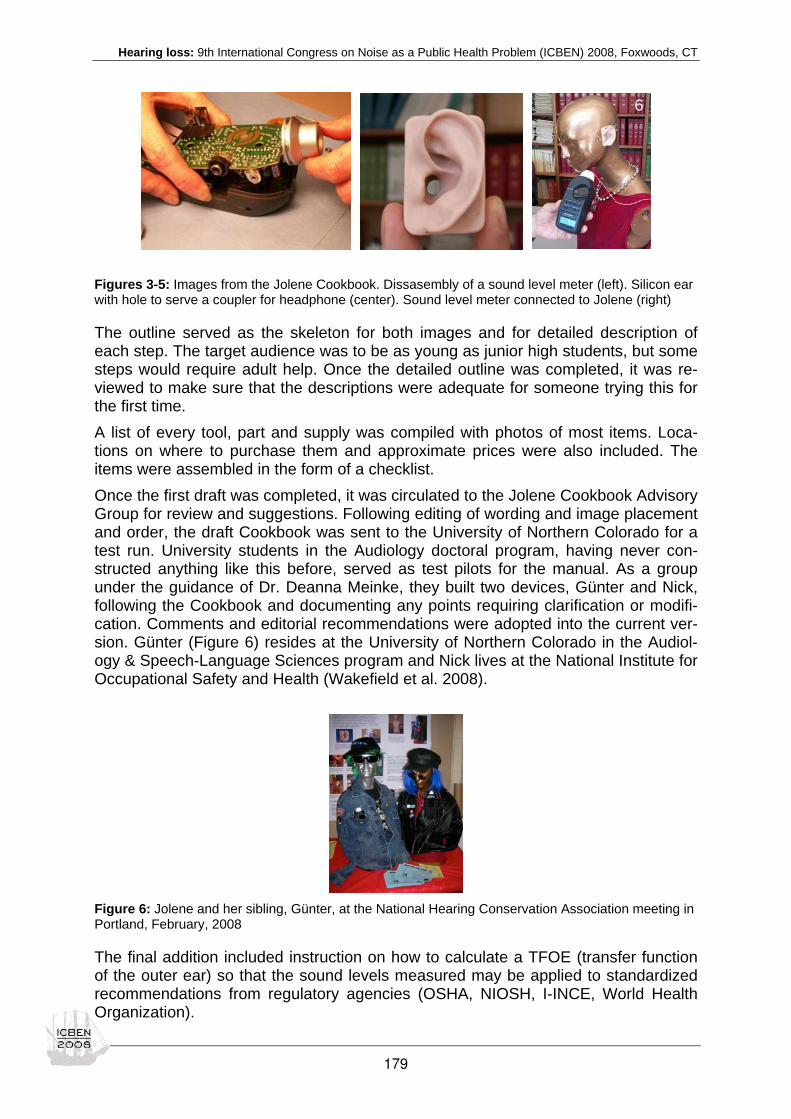
Hearing loss: 9th International Congress on Noise as a Public Health Problem (ICBEN) 2008, Foxwoods, CT
66
Figures 3-5: Images from the Jolene Cookbook. Dissasembly of a sound level meter (left). Silicon ear with hole to serve a coupler for headphone (center). Sound level meter connected to Jolene (right)
The outline served as the skeleton for both images and for detailed description of each step. The target audience was to be as young as junior high students, but some steps would require adult help. Once the detailed outline was completed, it was re-viewed to make sure that the descriptions were adequate for someone trying this for the first time. A list of every tool, part and supply was compiled with photos of most items. Loca-tions on where to purchase them and approximate prices were also included. The items were assembled in the form of a checklist. Once the first draft was completed, it was circulated to the Jolene Cookbook Advisory Group for review and suggestions. Following editing of wording and image placement and order, the draft Cookbook was sent to the University of Northern Colorado for a test run. University students in the Audiology doctoral program, having never con-structed anything like this before, served as test pilots for the manual. As a group under the guidance of Dr. Deanna Meinke, they built two devices, Günter and Nick, following the Cookbook and documenting any points requiring clarification or modifi-cation. Comments and editorial recommendations were adopted into the current ver-sion. Günter (Figure 6) resides at the University of Northern Colorado in the Audiol-ogy & Speech-Language Sciences program and Nick lives at the National Institute for Occupational Safety and Health (Wakefield et al. 2008).
Figure 6: Jolene and her sibling, Günter, at the National Hearing Conservation Association meeting in Portland, February, 2008
The final addition included instruction on how to calculate a TFOE (transfer function of the outer ear) so that the sound levels measured may be applied to standardized recommendations from regulatory agencies (OSHA, NIOSH, I-INCE, World Health Organization).
179

Hearing loss: 9th International Congress on Noise as a Public Health Problem (ICBEN) 2008, Foxwoods, CT
RESULTS Version 1.0 of the Jolene Cookbook went online on January 4, 2008. The current Version 1.1a is available online for free. The Cookbook has 39 pages including 130 color images, 10 detailed steps to production, a calibration section and a description of how to calculate a TFOE (transfer function for the outer ear). A table of National Institute for Occupational Safety and Health (NIOSH) recommended exposure limits and list of 35 relevant references on noise-induced hearing loss are included. The base cost to produce a Jolene is roughly $100. The greatest variable in price relates to the access to a used mannequin and your choice of wardrobe and accessories. Jolene has been useful as an educational outreach and research tool (Martin et al. 2006a, 2008; Martin & Martin 2008). A study using Jolene indicated that 16 % of 14-18 year-olds were using their personal stereo systems at levels and durations that exceed NIOSH recommended exposure levels on a daily basis. However, using Jolene as an educational tool for those identified at-risk for NIHL in that study proved helpful. After only a brief encounter with Jolene and her student educator companion, 44 % of those who regularly exceed NIOSH safety levels said that they intended to lower listening volumes on their devices in the future. The Cookbook has been downloaded across the US and in Canada, Japan, Mexico, New Zealand, Portugal, and Saipan. As a result the number of Jolene’s siblings is rapidly growing and her family album is on the Dangerous Decibels website.
CONCLUSION The Jolene Cookbook is available for research and outreach education to a wide va-riety of groups, schools, professional organizations and individuals. This makes an excellent science project for health & science students. Once complete, Jolene can be used as part of a hearing health education program, promoting awareness of risks related to prolonged listening to personal stereo systems at high volumes. She can also be used to help individuals develop a “feel” for what appropriate listening levels should be (Figure 7). Jolene and her siblings each have a unique style created by their fabricators. This personality moves away from production line products and draws curious people wherever she goes. Health communication research indicates that peer or older-peer education is effective at hearing health promotion (Sobel & Meikle 2008). Developed by a young person for young people, she meets an impor-tant need in the health communication strategy to promote hearing health in a high-risk age group.
Figure 7: Jolene educating young personal stereo system users about safe listening levels
180
Hearing loss: 9th International Congress on Noise as a Public Health Problem (ICBEN) 2008, Foxwoods, CT
Jolene also serves as a useful research too for those studying NIHL related to per-sonal stereo systems. Once calibrated and modified to accommodate a TFOE, val-ues recorded by Jolene are quite comparable to those acquired using much more expensive instrumentation.
REFERENCES Associated Press (2007) Apple 4Q Earnings Beat Analyst Views. CBS Broadcasting Inc. http://cbs5.com/technology/apple.4Q.earnings.2.461081.html.
Folmer RL (2003). The importance of hearing conservation instruction. J School Nursing 19: 140-148.
Folmer RL (2008). Hearing-loss prevention practices should be taught in schools. Semin Hearing 29: 67-80.
Griest SE, Folmer RL, Martin WH (2007). Effectiveness of "Dangerous Decibels," a school-based hearing loss prevention program. Am J Audiol 16: S165-S181.
Kujawa SG, Liberman MC (2006). Acceleration of age-related hearing loss by early noise exposure: Evidence of a misspent youth. J Neurosci 26: 2115–2123.
Martin GY, Martin WH (2007). The Jolene Cookbook Instruction Guide. Copyright ©, Oregon Health & Science University.
Martin GY, Martin WH (2008). NIHL prevention in children and adolescents: The Jolene Cookbook. Presented at the 33rd Annual Hearing Conservation Conference of the National Hearing Conservation Association, Portland.
Martin GY, Martin WH, Lambert W (2006a). Jolene: How loud is your music? Presented at the Conference on Noise-induced Hearing Loss in Children at Work & Play, Cincinnati.
Martin GY, Martin WH, Griest SE, Lambert W (2008). How loud is your music? Beliefs and practices regarding use of per-sonal stereo systems. Presented at the 33rd Annual Hearing Conservation Conference of the National Hearing Conservation Association, Portland.
Martin WH (2008). Dangerous Decibels®: Partnership for preventing noise induced hearing loss and tinnitus in children. Semin Hearing 29: 102-110.
Martin WH, Sobel JL, Griest SE, Howarth L, Shi Y-B (2006b). Noise induced hearing loss in children: Preventing the silent epidemic. J Otol 1: 11-21.
Niskar AS, Kieszak SM, Holmes A, Esteban E, Rubin C, Brody DJ (1998). Prevalence of hearing loss among children 6 to 19 years of age: The Third National Health and Nutrition Examination Survey. J Am Med Assoc 279: 1071–1075.
Niskar AS, Kieszak SM, Holmes AE, Esteban E, Rubin C, Brody DJ (2001). Estimated prevalence of noise-induced hearing threshold shifts among children 6 to 19 years of age: the Third National Health and Nutrition Examination Survey, 1988-1994, United States. Pediatrics 108: 40-43.
Portnuff CDF & Fligor BJ (2006) Output levels of portable digital music players. Presented at the Conference on Noise-induced Hearing Loss in Children at Work & Play, Cincinnati.
Sobel J, Meikle M (2008). Applying health behavior theory to hearing-conservation interventions. Semin Hearing 29: 81-89.
Vogel I, Brug J, Hosli EJ, van der Ploeg CPB, Raat H (2008). MP3 players and hearing loss: Adolscents’ perceptions of loud music and hearing conservation. J Pediatr 152: 400-405.
Wakefield E, Adkisson K, Flint R, McIntosh L, Tobin J, Tuell C, Vogel B, Wakefield N, Walstrom E, Bright K, Martin GY, Martin WH, Meinke DK (2008). Building Jolene’s children, a recipe for success. Presented at the 33rd Annual Hearing Con-servation Conference of the National Hearing Conservation Association, Portland.
Williams W (2005). Noise exposure levels from personal stereo use. Int J Audiol 44: 231-236.
181
Hearing loss: 9th International Congress on Noise as a Public Health Problem (ICBEN) 2008, Foxwoods, CT
Hearing loss in rats from combined exposure to carbon monoxide, toluene and impulsive noise Søren Peter Lund1*, Gitte B. Kristiansen1, Pierre Campo2 1 National Research Centre for the Working Environment, Lerso Parkallé 105,
DK-2100 Copenhagen, Denmark
2 Institut National de Recherche et de Sécurité, Avenue de Bourgogne, BP 27, 54501 Vandoeuvre-les-Nancy, France cédex
* corresponding author: e-mail: [email protected]
INTRODUCTION In combined exposure with ototoxic chemicals, potentiation of noise induced hearing loss (NIHL) may certainly be a hazard (Sliwinska-Kowalska et al. 2007). However, as impulsive noise has the potential to induce hearing loss even at low levels of daily noise exposure (LEX,8h), the greatest risk for hearing loss from combined exposures seems to be from simultaneous exposure to ototoxic chemicals and impulsive noise. Toluene exposure may cause hearing loss in rats at high levels of exposure without exposure to noise, but in combination with exposure to noise synergistic interaction may potentiate the hearing loss, especially in combined exposure to impulsive noise (Lund & Kristiansen 2008). The mechanisms involved in the ototoxicity of toluene and other aromatic organic solvents have not been fully elucidated, but toluene may act to impair the auditory medial efferent system, thereby augmenting the acoustic en-ergy absorbed by the cochlea in response to the noise exposure (Lataye et al. 2007). However, in another experiment toluene treatment did not modify the responses in the cochlea in rats with non-functional middle ear muscles, although toluene did in-stead inhibit the action of the middle ear reflex, possibly by their anticholinergic effect on the efferent motor neurons (Campo et al. 2007). Altogether, exposure to organic solvents appears in general to have additive rather than synergistic effects in com-bined exposure with noise, while asphyxiants like carbon monoxide (CO) appear ca-pable of true synergistic effects on NIHL (Fechter 2004). CO exposure by itself does not seem to have persisting effects on the hearing of rats, but it does potentiate the effects of NIHL at exposure levels of 500 ppm and higher. The potentiation of noise by CO may not be related to a specific effect of CO on the auditory cells, but may instead reduce the cell's ability to repair the noise induced damage (Chen & Fechter 1999). The combined effect of impulsive noise and both toluene and CO may reveal the full potential for NIHL from impulse noise exposure, because the functional pro-tective mechanisms as well as the repair processes may be hampered. Nevertheless, this combination of exposures does appear to be a rather realistic scenario in the working environment. In order to test this hypothesis, groups of rats were exposed to impulsive noise, CO and toluene. The hearing was tested before and after exposure by assessment oto-acoustic emissions over 30 frequencies between 1 and 70 kHz, and cochleograms was made on 3-4 animals in each group.
METHODS The animal welfare committee, appointed by the Danish Ministry of Justice, has granted ethical permission for the studies. All the procedures were carried out in compliance with the EC Directive 86/609/EEC and with the Danish law regulating experiments on animals. The exposures of the rats were performed in dedicated 1200 l inhalation chambers with walls made of stainless steel and glass. The airflow
182

Hearing loss: 9th International Congress on Noise as a Public Health Problem (ICBEN) 2008, Foxwoods, CT
is driven by a radial fan at the outlet, giving a slight negative pressure within the chambers, eliminating possible leakage of toluene or CO to the surroundings. The air exchange rate was 12 per hour, air temperature 20 ± 2 ºC and humidity 55 ± 10 %RH. To be exposed, the rats were transferred daily from their home cages to the inhalation chambers and kept in pairs in wire mesh cages without access to food and drinking water. All groups were exposed to CO and/or toluene 8 hours a day for 10 days, but only to noise 6 hours a day, starting 2 hours after the onset of the chemical exposure. CO was fed to the air inlet of the chamber, under the control of simple flow meters (Porter). The CO concentration was measured with an infrared gas cell spectrophotometer (Foxboro MIRAN-1A) in one chamber every 5 minutes, automatically changing from chamber to chamber. The toluene and the noise expo-sure have been described recently (Lund & Kristiansen 2008), and only a brief de-scription will be given in the following. Toluene (purity >99.5 % GC; CAS-No. [108-88-3]) was evaporated in the air inlet of each exposure chamber by individual HPLC-pumps feeding the toluene to the top of glass spirals, which were slightly heated by circulating water. The toluene concentration in the chambers was measured with an infrared gas cell spectrophotometer. Noise was generated by a PC with a 16-bit D/A-converter board, amplified by audio amplifiers, and delivered by dome tweeters lo-cated above each cage. The noise exposure used was a mixture of impulse and Wide band noise (WBN), with the main energy (75 %) as impulsive noise, composed of sound impulses with a peak level just above 130 dB, and the different levels of noise were generated by varying the interval between the impulses. The sound field was measured at various points at the floor level of the cages with a ½” condenser microphone (B&K4133) and a spectrum analyzer (HP35670A) by averaging a large number of samples (4096 or more). Further analyses of the noise exposures (Leq) were made on time samples of several minutes at 100 kHz sampling frequency. The impulse frequency distribution of the impulse noise was somewhat unequal due to a slightly higher energy level toward the lower frequencies, and the level varied up to ±1.5 dB between measuring points within the sound field. In order to find the lowest-observed-adverse effect level (LOAEL) between exposure to noise and CO, two groups of rats (n=12) were exposed to CO (0 ppm and 500 ppm) and either Leq8h = 81 dB or Leq8h = 84 dB SPL impulsive noise. Further, groups of rats (n=12) were ex-posed to impulsive noise (Leq8h = 84 dB SPL), CO (0 ppm, 300 ppm and 500 ppm) and toluene (0 ppm, 500 ppm and 1000 ppm). The hearing was tested before and after exposure by assessment of DP-grams, i.e. the cubic distortion product (CDP) from distortion product oto-acoustic emissions (DPOAE) over 30 frequencies of f2 between 1 and 70 kHz (Lund and Kristiansen 2008). The DP-grams was made at a fixed ratio of the primaries (f2=f1x13/16=1.23) and fixed levels of stimulation (L1=L2+10 dB=60 dB SPL). Further, cochleograms (not shown) were made on 3-4 animals in each group.
RESULTS Exposure to the impulsive noise alone at Leq8h = 81 dB had little effect on hearing, while the effects were barely notably at exposure to Leq8h = 84 dB SPL. However, when combined with exposure to CO, the hearing impairment at the latter noise level was statistically significant from the group without CO exposure at the 500 ppm level (see Figure 1).
183

Hearing loss: 9th International Congress on Noise as a Public Health Problem (ICBEN) 2008, Foxwoods, CT
Figure 1: DP-grams (f2/f1= 1.23; L1= 60 dB and L2= 50dB SPL) from group of rats two weeks after the end of 10 days combined exposure to either 0, or 500 ppm carbon monoxide (CO) and impulsive noise exposure at Leq8hours = 81 dB SPL (Top Panel), and 0 ppm, 300 ppm or 500 ppm CO and impul-sive noise exposure at Leq8hours = 84 dB SPL (Bottom Panel). Each point marks the mean with indica-tion of 95 % CI, and NF denotes the noise floor, determined by the mean value in the frequency bins next to the CDP. No effects from combined exposure are observed at the 81 dB noise level, but clear dose-dependant effects can be seen at the 84 dB level.
The main effect of the noise exposure occurs within the 8-10 kHz frequency range, but the frequencies above 30 kHz seem also to be slightly affected. Further, addition of toluene exposure without CO did not increase the hearing impairment from the impulsive noise, but the addition of CO to the toluene exposure, did increase the hearing loss considerably. The dose-effect relationship seems to be rather complex (see Figure 2): Both CO and toluene exposure potentiated the effects of the 84 dB impulsive noise exposure, although not in fully dose-dependant manner. The toluene exposure without CO did not potentiate the effects of the impulsive noise exposure, but with addition of 300 ppm CO, there was clear potentiation at both levels of tolu-ene exposure. Increasing the CO level to 500 ppm only exacerbated the effects of the 1000 ppm toluene exposure, but not the effects of the 500 ppm toluene exposure.
DISCUSSION The exposure to impulsive noise at Leq8h = 81 dB SPL for 10 days did not induce no-tably hearing impairment even in combined exposure with 500 ppm CO. This CO lev-el has previously been shown to be the LOAEL for elevations of NIHL in combined exposure with steady state noise (Fechter 2004). In the exposure to impulsive noise at Leq8h = 84 dB SPL there was an effect of the impulsive noise exposure.
184
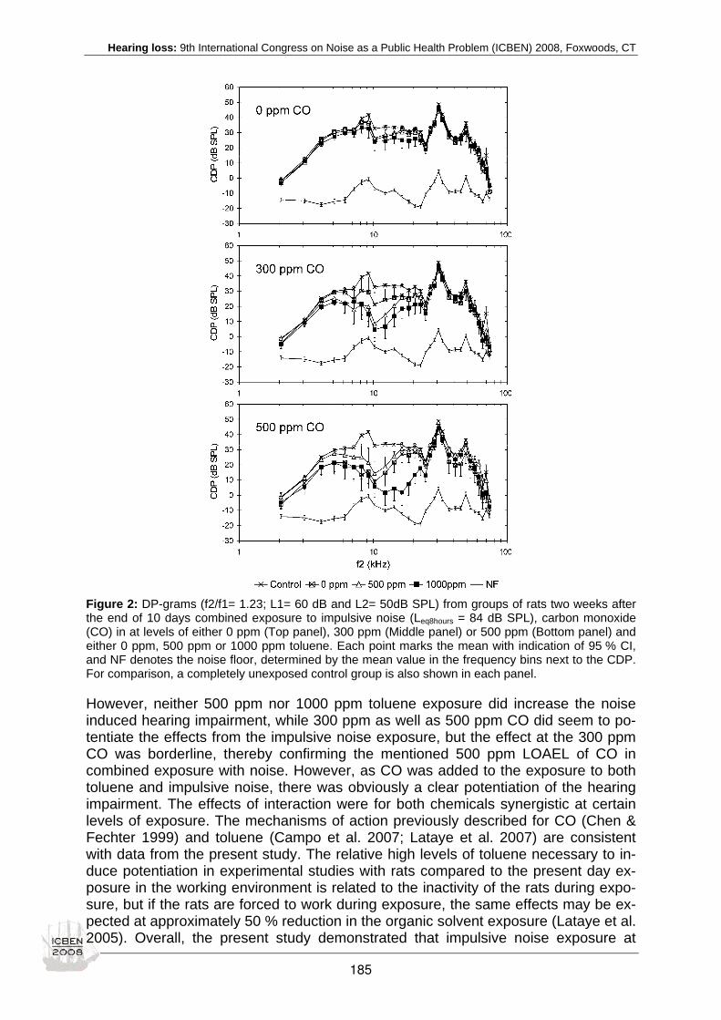
Hearing loss: 9th International Congress on Noise as a Public Health Problem (ICBEN) 2008, Foxwoods, CT
Figure 2: DP-grams (f2/f1= 1.23; L1= 60 dB and L2= 50dB SPL) from groups of rats two weeks after the end of 10 days combined exposure to impulsive noise (Leq8hours = 84 dB SPL), carbon monoxide (CO) in at levels of either 0 ppm (Top panel), 300 ppm (Middle panel) or 500 ppm (Bottom panel) and either 0 ppm, 500 ppm or 1000 ppm toluene. Each point marks the mean with indication of 95 % CI, and NF denotes the noise floor, determined by the mean value in the frequency bins next to the CDP. For comparison, a completely unexposed control group is also shown in each panel.
However, neither 500 ppm nor 1000 ppm toluene exposure did increase the noise induced hearing impairment, while 300 ppm as well as 500 ppm CO did seem to po-tentiate the effects from the impulsive noise exposure, but the effect at the 300 ppm CO was borderline, thereby confirming the mentioned 500 ppm LOAEL of CO in combined exposure with noise. However, as CO was added to the exposure to both toluene and impulsive noise, there was obviously a clear potentiation of the hearing impairment. The effects of interaction were for both chemicals synergistic at certain levels of exposure. The mechanisms of action previously described for CO (Chen & Fechter 1999) and toluene (Campo et al. 2007; Lataye et al. 2007) are consistent with data from the present study. The relative high levels of toluene necessary to in-duce potentiation in experimental studies with rats compared to the present day ex-posure in the working environment is related to the inactivity of the rats during expo-sure, but if the rats are forced to work during exposure, the same effects may be ex-pected at approximately 50 % reduction in the organic solvent exposure (Lataye et al. 2005). Overall, the present study demonstrated that impulsive noise exposure at
185

Hearing loss: 9th International Congress on Noise as a Public Health Problem (ICBEN) 2008, Foxwoods, CT
Leq8h = 84 dB SPL has little or no margin of safety, and even if the occupational ex-posure limits are not exceeded, concomitant exposure to ototoxic chemicals may in-crease the hazards of impulsive noise exposure considerably.
REFERENCES Campo P, Maguin K, Lataye R (2007). Effects of aromatic solvents on acoustic reflexes mediated by central auditory path-ways. Toxicol Sci 99: 582-590.
Chen GD, Fechter LD (1999). Potentiation of octave-band noise induced auditory impairment by carbon monoxide. Hear Res 132: 149-159.
Fechter LD (2004). Promotion of noise-induced hearing loss by chemical contaminants. J Toxicol Environ Health A67: 727-740.
Lataye R, Campo P, Loquet G, Morel G (2005). Combined effects of noise and styrene on hearing: comparison between active and sedentary rats. Noise & Health 7: 49-64.
Lataye R, Maguin K, Campo P (2007). Increase in cochlear microphonic potential after toluene administration. Hear Res 230: 34-42.
Lund SP, Kristiansen GB (2008). Hazards to hearing from combined exposure to toluene and noise in rats. Int J Occup Med Environ Health 21: 47-57.
Sliwinska-Kowalska M, Prasher D, Rodrigues CA, Zamysłowska-Szmytke E, Campo P, Henderson D, Lund SP, Johnson AC, Schäper M, Odkvist L, Starck J, Toppila E, Schneider E, Möller C, Fuente A, Gopal KV (2007). Ototoxicity of organic solvents - from scientific evidence to health policy. Int J Occup Med Environ Health 20: 215-222.
186

__________________________________________________________________________
__________________________________________________________________________
ICBEN 2008
Noise and Communication
187

Communication: 9th International Congress on Noise as a Public Health Problem (ICBEN) 2008, Foxwoods, CT
Noise as an explanatory factor in work-related fatality reports: A descriptive study Pierre Deshaies1,2,3,4*, Richard Martin1, Danny Belzile1, Pauline Fortier2, Chantal Laroche5, Serge-André Girard2, Tony Leroux6, Hughes Nélisse7, Robert Arcand2, Maurice Poulin2, Michel Picard6 1 Direction de santé publique de Chaudière-Appalaches
2 Institut national de santé publique du Québec
3 Centre hospitalier affilié universitaire Hôtel-Dieu de Lévis
4 Université Laval
5 Université d’Ottawa
6 Université de Montréal
7 Institut de recherche Robert-Sauvé en santé et en sécurité du travail
* corresponding author: e-mail: [email protected]
INTRODUCTION “The recognition of noise as a serious health hazard as opposed to a nuisance is a recent development and the health effects of hazardous noise exposure are now considered to be an increasingly important public health problem” (WHO 2001). Workplace noise exposure is a common reality in Quebec and worldwide. In 1990, approximately 30 million people in the USA were exposed to daily occupational noise levels greater than 85 dBA, compared to over nine million in 1981 (WHO 2001). In 1998, the Institut de la statistique du Québec (Quebec Statistical Institute) estimated that 12.8 % of Quebec workers were exposed, often or always, to occupational noises hindering conversations occurring a few feet away, even when shouted (ISQ 2001). Projected to the 2005 worker population, this would represent an estimated 476,000 workers. Occupational noise exposure has been linked to numerous adverse health effects (Berglund 1999). The assumption of a causal or contributive impact of occupational noise on the occurrence of occupational accidents was addressed in some studies (Barreto et al. 1997; Dias & Cordeiro 2007; Melamed et al. 1992; Zwerling et al. 1997; Moll van Charante & Mulder 1990; Cordeiro 2005). Recent work by Girard et al. suggests a dose-response relationship between noise exposure, hearing impair-ment and accident risk (Girard et al. 2003a-c). Based primarily on two explanatory models (Figures 1 and 2) (Hétu 1994; Wilkins 1981) and empirical data, there is a biological plausibility for a causal relationship between noise exposure and accident risk (Hétu 1993; Wilkins 1981; Laroche et al. 1991). Ambient noise interference with communication appears as a chief plausible pathway (Robinson et al. 2000; Suter 1992; Hétu 1994; Ayres & Beyer 1994). Other plausible explanatory factors include habituation and reduced vigilance (Passchier-Vermeer & Passchier 2000; Smith 1992; Wilkins & Acton 1982). Nevertheless, the extent to which noise does act as a causal or contributive factor in fatal workplace accidents remains unclear and subject to debate.
188

Communication: 9th International Congress on Noise as a Public Health Problem (ICBEN) 2008, Foxwoods, CT
Figure 1: Outline of the various effects of occupational noise exposure (Hétu 1994)
Figure 2 : Conceptual model of warning sound perception (Wilkins 1981)
Originating from a review of work-related fatality reports, this study aims at: 1- de-scribing the characteristics and circumstances of fatal accidents occurring in noisy workplaces; 2- determining the number of instances where noise was identified as one of the potential causes and retained as such; 3- determining the number of in-stances where noise could have been identified as one of the potential causes; and, 4- examining the methods used in reports for analyzing the noise factor during acci-dent investigations. Albeit not presented in this paper, a final objective was to deter-mine the worth of fatality reports as a potential surveillance data source.
METHODS Alike a multiple case studies design, this population-based descriptive study is based on a thorough analysis of the content found in the 788 fatal accident reports com-
189

Communication: 9th International Congress on Noise as a Public Health Problem (ICBEN) 2008, Foxwoods, CT
pleted by various inspectors from the Commission de la santé et de la sécurité du travail du Québec (Quebec Workers Compensation Board (WCB)) during the 1990-2005 period. During their investigation into the causes of a fatal injury, two inspectors are assigned to each case. As a more standardized inquiry process was adopted in 2000, the reports were divided into two blocks: a main block covering accident re-ports issued between 2000 and 2005 (n=284), and a complementary block assessing those in the 1990-1999 period (n=504). Briefly stated, assigned inspectors are responsible for gathering all interesting and relevant facts from various sources (witnesses, simulations, etc.), as well as classify-ing the information into essential and secondary items upon which they must identify potential causes to be further analyzed in reaching a plausible conclusion as to the causes of the fatal event. Within this study, appreciation of the noise factor was lim-ited to the written information found in the publicly available reports regarding the es-sential contextual and technical elements used to assess the noise-accident relation-ship. The underlying framework for analyzing each accident report is presented in Figure 3. Accidents were deemed to have occurred in a noisy environment whenever it was clearly indicated that at least one source of noise was operating within the victim’s work area at the time of the accident, irrespective of the noise level. To be classified “Noise mentioned explicitly”, a report had to contain at least one key word relating to the following categories: masking noise, warning signal or hearing loss. When men-tioned explicitly, noise was classified as treated either “Directly” when analyzed as a potential cause per se, “Indirectly” when analyzed within another potential cause, or “In a general manner” when merely mentioned in the description of the fatal event. Lastly, reports, in which noise was identified as a cause of the fatal event by the in-spectors, were classified “Noise retained as a cause”. When noise was mentioned explicitly, an in-depth content analysis was first carried out separately by at least two expert authors (audiologists or acoustic engineer) to examine the methods used by the inspectors in analyzing the noise factor. Thereaf-ter, during a meeting to discuss individual reports, consensus was reached by all au-thors regarding the inspectors’ choice of noise measurements and whether their analyses and conclusions were appropriate. The number of reports to be analyzed in-depth was determined by reaching saturation in the information of interest relative to the study’s objectives. All reports not thoroughly analyzed were revised summarily by one of the authors to verify any new relevant information. A comprehensive analysis of accident reports of the main block in which noise was not mentioned explicitly was also carried out to determine if noise could have been considered as a potential cause. To reach such a conclusion, the accident must have occurred in a noisy environment and involved a victim being “struck by a vehicle”, since noise is more likely to interfere with communication in this context. Whereas reports from the main block were scrutinized for information relative to all 4 objectives, those from the complementary block were analyzed only when noise was mentioned explicitly (objectives 2 and 4).
190

Communication: 9th International Congress on Noise as a Public Health Problem (ICBEN) 2008, Foxwoods, CT
Noise mentioned explicitly?
Noisy environment?
No
Reports excluded
Main block of reports (2000-2005)284/788
Complementary block of reports (1990-1999)504/788
Characteristics and circumstances of thefatal accidents
Yes
At which level ofconsideration?
Directly(analyzed as apossible cause
per se)
Indirectly(within another
analyzedcause)
In a generalmanner
(ex. descriptionof accident site)
Yes
Noiseretained
as acause
Noise notretained/
rejected asa cause
No
Yes No
Could noise havebeen considered?
Noise mentioned explicitly?
Yes No
Reports excluded
Figure 3: Framework for the analysis of noise in the Quebec WCB fatal accidents reports 1990-2005 (N=788)
RESULTS From the 788 work-related accident reports covering the 1990-2005 period, noise was mentioned explicitly in 67 (8.5 %) reports (Figure 4). Among those, noise was treated “Directly” in 21 (2.7 %), “Indirectly” in 15 (1.9 %) and “In a general manner” in 31 (3.9 %). Moreover, inspectors concluded that noise was one of the causes in the fatal event in 18 (2.3 %) of 21 reports in which noise was analyzed directly. From the 67 reports in which noise was mentioned explicitly, 50 were analyzed com-prehensively, including 28 out of 32 from the main block and 22 out of 35 from the complementary block. The analysis revealed four noise assessment methods used by the inspectors: a) qualitative assessment (21 (42 %)), 19 of which also included quantitative measures; b) event simulations (13 (26 %)), 2 of which with expert con-sultants; c) quantitative measures only (6 (12 %)); and d) general description only (10 (20 %)). From the available information and despite poor data in some cases (i.e.
191
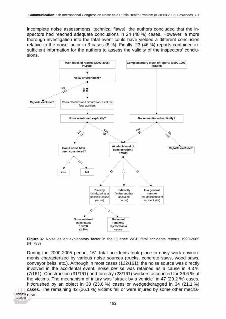
Communication: 9th International Congress on Noise as a Public Health Problem (ICBEN) 2008, Foxwoods, CT
incomplete noise assessments, technical flaws), the authors concluded that the in-spectors had reached adequate conclusions in 24 (48 %) cases. However, a more thorough investigation into the fatal event could have yielded a different conclusion relative to the noise factor in 3 cases (6 %). Finally, 23 (46 %) reports contained in-sufficient information for the authors to assess the validity of the inspectors’ conclu-sions.
Noise mentioned explicitly?
Noisy environment?
No123
Reports excluded
Main block of reports (2000-2005)284/788
Complementary block of reports (1990-1999)504/788
Characteristics and circumstances of thefatal accident
Yes32
At which level ofconsideration?
67/788
Directly(analyzed as apossible cause
per se)
Indirectly(within another
analyzedcause)
In a generalmanner
(ex. description ofaccident site)
31
18
Noise retainedas as cause
18/788(2.3%)
Noise notretained/
rejected as acause
3
Yes No
124
Could noise havebeen considered?
Noise mentioned explicitly?
Yes35 No469
Reports excluded
Figure 4: Noise as an explanatory factor in the Quebec WCB fatal accidents reports 1990-2005 (N=788)
During the 2000-2005 period, 161 fatal accidents took place in noisy work environ-ments characterized by various noise sources (trucks, concrete saws, wood saws, conveyor belts, etc.). Although in most cases (122/161), the noise source was directly involved in the accidental event, noise per se was retained as a cause in 4.3 % (7/161). Construction (31/161) and forestry (28/161) workers accounted for 36.6 % of the victims. The mechanism of injury was “struck by a vehicle” in 47 (29.2 %) cases, hit/crushed by an object in 38 (23.6 %) cases or wedged/dragged in 34 (21.1 %) cases. The remaining 42 (26.1 %) victims fell or were injured by some other mecha-nism.
192
Communication: 9th International Congress on Noise as a Public Health Problem (ICBEN) 2008, Foxwoods, CT
Over the same period (2000-2005), noise was not explicitly mentioned in 129 reports investigating fatal accidents in noisy work environments, including 29 (22.5 %) acci-dents involving a worker being “struck by a vehicle”. Following a comprehensive con-tent analysis of these 29 reports, the authors concluded that noise could have been considered in 5 (3.9 %) reports because of sufficient circumstantial evidence of pos-sible interference of ambient noise with communication or warning signals percep-tion. However, the available written information did not make it possible to conclude if noise was actually a cause or not. In all other reports involving a worker being struck by a vehicle (24/29), the authors agreed with the inspectors’ findings that noise did not need to be considered as other identified causes were sufficiently obvious to explain the event, irrespective of the noise levels.
DISCUSSION Noise was explicitly stated as one of the cause in 2.3 % (18/788) of the fatal acci-dents reports. Although qualitative methods are more typically designed to explain phenomena than explore causal relationships, the goal of the inspectors’ inquiry is to gather all relevant information in order to reach conclusions with regards to the causes of a fatal event. The content analysis of 788 reports spanning a 16-year pe-riod strongly argues in favor of, although it cannot prove it, a causal relationship be-tween noise and fatal accidents in the 18 cases identified by the inspectors. Given methodological limitations (i.e. access to written reports but not to inspectors’ notes, limited data in some reports, review of fatal accident reports only) and inspectors’ constraints during investigations, this Figure (2.3 %) most likely underestimates the proportion of workplace accidents explained at least partly by noise. Interference with communication likely explains the causal relationship between noise and accidents. In all 18 cases in which inspectors identified noise as a cause (15 in-volving a worker being struck by a moving vehicle), communication was impaired. Indeed, the content analysis revealed that the warning device either failed or could not be heard over the ambient noise. Interestingly, noise was identified as a cause in 11 cases during the 1990-1999 pe-riod, a time when inspectors were not, to the authors’ knowledge, specifically trained to carry out noise assessments and during which the causal relationship between noise and accidents was not yet well known or established. As inspectors gathered information from witnesses and other sources to understand the circumstances sur-rounding a fatal accident, the hypothesis of noise acting as one essential factor in cases where communication was at stakes likely emerged intuitively. So did interfer-ence with communication as a noise-related cause of accidents. This observation reinforces the authors’ interpretation of these results. Noise is typically not identified as the sole cause in explaining fatal events. Indeed, multiple causes were identified in most accident reports. For the 21 cases in which noise was analyzed directly as a potential cause, shortcomings in work methods and work organization were also identified in all but 4 reports (data not shown). Lack of adequate training, poor visibility and faulty or absent safety measures were among the other identified modifiable causes, providing useful insight into the occurrence of fatal accidents within noisy work settings. Such factors could be considered potential confounders, along with other known factors such as age, in epidemiological studies investigating the relationship between noise and workplace accidents.
193

Communication: 9th International Congress on Noise as a Public Health Problem (ICBEN) 2008, Foxwoods, CT
Other known adverse effects of noise may also contribute to fatal accidents, including reduced vigilance, precision and visual span (Hétu 1994). Since inspectors only in-clude essential elements in their analysis to conclude on potential causes, noise would not be identified as a cause in situations where these adverse effects come into play. This may partly explain why the impact of noise, measured in terms of rela-tive risk or attributable fraction reported in some epidemiological studies (Moll van Charante & Mulder 1990; Girard et al. 2003a; Dias & Cordeiro 2007), is greater than the findings of the current study may suggest. In the current study, only fatal accident reports were revised. However, some epide-miological studies report an association between noise and non fatal accidents (Moll van Charante & Mulder 1990; Girard et al. 2003a; Dias & Cordero 2007). Given a causal relationship between noise and accidents, noise would likely contribute to a significantly greater number of accidents than what these findings suggest if non fatal injuries were also included. Author consensus was achieved relative to the inspectors’ choice of noise measure-ments, analyses and conclusions. Such judgment was based solely on the informa-tion available in the written reports. Access to the full range of information gathered by the inspectors (including notes, simulations and interviews) might have yielded a different judgment. Inferences were often necessary to determine if the fatal accident had occurred in a noisy environment since most reports did not contain noise measurement data. Noise may affect communication at various levels, as its effect consists of a complex inter-action between different factors according to Hétu’s (1994) and Wilkins’ (1981) mod-els. Nevertheless, a conservative approach was used in this study to define a noisy environment in order to minimize overestimation. A rather conservative approach was also used by the authors in deciding that noise could have been mentioned in cases when it was not explicitly stated by inspectors. This may partly explain the rather low percentage of such reports (3.9 %) in the 2000-2005 subset. However, the authors judged that noise was considered as a potential cause by the inspectors in the vast majority of events in which it should have been. The findings of this study suggest that noise should be systematically considered as a potential cause in all investigations of work-related accidents where vehicular movement or communication between workers is at stake. As noise may also inter-fere with vigilance and other risk factors for accidents, it may be a much more impor-tant contributing factor to accidents than what was previously thought and what the findings of the current study seem to suggest. Given the omnipresence of noise and its plausible effects on worker safety, it should be a key component in the prevention of occupational accidents. In addition to reducing the risk for hearing loss, published results suggest that reducing workplace noise can yield beneficial effects on commu-nication, worker comfort and, potentially, vigilance (Damongeot 1995; Cordeiro 2005; Smith 2003; Chabot & Gignac 2001; Suter 1987; Hoyos & Zimolong 1988; Moll van Charante & Mulder 1990; Wilkins 1982; Cohen 1976). Further studies, particularly those exploring contexts of impaired communication, such as warning sound percep-tion, and interaction between noise and other risk factors for accidents, are needed to better understand the ways in which noise may cause or contribute to accidents, as well as to increase the effectiveness of accident prevention efforts.
194

Communication: 9th International Congress on Noise as a Public Health Problem (ICBEN) 2008, Foxwoods, CT
REFERENCES Ayres TJ, Beyer RR (1994). Effectiveness of truck backup alarms. American Trucking Association Safety Management Council, National Meeting and Exhibition.
Baretto SM, Swerdlow AJ, Smith PG, Higgins CD (1997). A nested case-control study of fatal work related injuries among Brazilian steel workers. Occup Environ Med 54: 599-604.
Berglund B, Lindvall T, Schwela DH (eds) (1999). Guidelines for community noise. Geneva: WHO.
Chabot A, Gignac S (2001). Évaluation d’une intervention visant l’amélioration de l’audibilité des avertisseurs sonores dans un établissement. In: Quimper C, Parent M, Gignac S (2002). Programme d’intervention visant la diminution des conséquen-ces de la surdité professionnelle. Rapport du comité du projet pilote. Annexe C. Beauport: Direction de santé publique de Québec.
Cohen A (1976). The influence of company hearing conservation program on extra-auditory problems in workers. J Safety Res 8: 146-162.
Cordeiro R, Clemente APG, Diniz CS, Dias A (2005). Occupational noise as a risk factor for work-related injuries. Rev Saude Publica 39: 461-466.
Damongeot A (1995). Prévention des accidents dus à la non-perception des signaux sonores de danger. Cas du personnel à pied travaillant sur les chantiers de travaux publics ou sur les voies ferrées. Cah Notes Document INRS 160: 388-398.
Dias A, Cordeiro R (2007). Attributable fraction of work accidents related to occupational noise exposure in a Southeastern city of Brazil. Cad Saude Publica 23: 1649-1655.
Girard SA, Jean S, Larocque R, Simard M, Simpson A, Picard M, Turcotte F (2003a). Problèmes de sécurité du travail attri-buables à une perte d’audition en milieu de travail bruyant - Milieux de travail à risque. Québec: Institut national de santé publique du Québec.
Girard SA, Jean S, Larocque R, Simard M, Simpson A, Picard M, Turcotte F (2003b). Problèmes de sécurité du travail attri-buables à une perte d’audition en milieu de travail bruyant - Le cas des événements multiples. Québec: Institut national de santé publique du Québec.
Girard SA, Jean S, Larocque R, Simard M, Simpson A, Picard M, Turcotte F (2003c). Problèmes de sécurité du travail attri-buables à une perte d’audition en milieu de travail bruyant - Description de milieux de travail à risque – Document complé-mentaire. Québec: Institut national de santé publique du Québec.
Hétu R (1993). Capacités auditives, critères d’embauche et droits de la personne. Groupe d’acoustique de l’université de Montréal. Can Acoust/Acoust Canad 21: 3-14.
Hétu R (1994). The hearing conservation paradigm and the experienced effects of occupational noise exposure. Can Acoust/Acoust Canad 22: 3-19.
Hétu R, Quoc HT (1994). Évaluation des capacités de détection auditive en milieu bruyant et intégration des personnes déficientes auditives. Montréal: Profil-Recherche PR-151, IRSST.
Hoyos CG, Zimolong B (1998). Hazard recognition and risk-taking behavior. In: Hoyos CG, Zimolong B (ed.): Advances in human factors/ergonomics II. Amsterdam: Elsevier.
ISQ, Institut de la statistique du Québec (2001). Enquête sociale et de santé 1998 – 2e éd.. Les Publications du Québec, Niveau 1 – Caractéristiques de l’individu - État de santé et de bien-être. http://www.stat.gouv.qc.ca/publications/sante/pdf/e_soc98v2-6.pdf
Laroche C, Hétu R, L’Espérance A (1991). Des alarmes de recul qui tuent! Trav Santé 7: 9-13.
Melamed S, Luz JY, Green MS (1992). Noise exposure, noise annoyance and their relation to psychological distress, acci-dent and sickness absence among blue-collar workers - The Cordis study. Isr J Med Sci 28: 629-635.
Moll van Charante AW, Mulder PGH (1990). Perceptual acuity and the risk of industrial accidents. Am J Epidemiol 131: 652-663.
Passchier-Vermeer, Passchier WF (2000). Noise exposure and public health. Environ Health Perspect 108 (Suppl 1): 123-131.
Robinson GS, Casali JG (2000). Speech communications and signal detection in noise. In: Berger EH (ed.): The Noise man-ual. Rev. 5th ed. (pp 567-600). Fairfax, VA: American Industrial Hygiene Association.
Smith A (1992). The non-auditory effects of noise. Occup Health Rev Aug/Sept: 21-23.
195

Communication: 9th International Congress on Noise as a Public Health Problem (ICBEN) 2008, Foxwoods, CT
Smith AP (2003). Noise, accidents, minor injuries and cognitive failures. In: de Jong RG, Houtgast T, Franssen EAM, Hof-man WF (eds.): Proceedings of 8th International Congress on Noise as a Public Health Problem Conference, Rotterdam (pp 140-144). Schiedam: Foundation ICBEN.
Suter AH (1987). Noise reduction can benefit speech communication and warning signal detection. In: Peizi L (ed.): Proceed-ings of Inter-Noise 87 (pp 1049-1052). Beijing: Acoustical Society of China.
Suter AH (1992). Communication and job performance in noise : a review. ASHA Monogr 28: 1-84.
Taupin JP, Barbier JP, Smolick HJ, Lefaure JM, Jusselin F (1994). L’audibilité d’un signal sonore lors du recul d’un engine est-elle le gage d’une sécurité efficace pour les salariés travaillant dans l’environnement proche? Cah Méd Interprof 34 : 473-480.
Wilkins PA (1981). The specification and use of industrial warning sounds. In: Proceedings of Inter-Noise 1981 (pp 765-768).
Wilkins PA, Acton WI (1982). Noise and accidents – a review. Ann Occup Hyg 25: 249-260.
WHO, World Health Organization (2001). Occupational and community noise. Fact sheet No. 258, revised February 2001 http://www.who.int/mediacentre/factsheets/fs258/en/index.html
Zwerling C, Whitten PS, Davis CS, Sprince NL (1997). Occupational injuries among workers with disabilities: The National Health Interview Survey, 1985-1994. J Am Med Assoc 278: 2163-2166.
196

Communication: 9th International Congress on Noise as a Public Health Problem (ICBEN) 2008, Foxwoods, CT
Optimal installation of audible warning systems in the noisy workplace Christian Giguère*, Chantal Laroche, Rida Al Osman, Yun Zheng Audiology and SLP Program, University of Ottawa, Ottawa, Ontario, K1H 8M5, Canada
*corresponding author: e-mail: [email protected]
INTRODUCTION Warning sounds are necessary to promptly alert workers of events that can compromise safety. A wide range of strategies, including verbal and non-verbal signals have been used in different environments (Edworthy & Adams 1996; Haas & Edworthy 2006; Edworthy & Hellier 2006). Unfortunately, the use of warning signals in industry is often submitted to intuitive installation practices with little regard to the many factors contributing to an efficient and safe use (Tran Quoc & Hétu 1996). There may also be a mismatch between auditory demands and capabilities in the workplace (Hétu 1994). Failure to react to alarms can increase the risk of accidents. The installation of warning devices in a noisy workplace poses particular challenges for optimal detection and recognition of acoustic signals, such as the use of adequate sound levels (ISO 7731). Factors affecting the audibility of warning sounds include the noise field in the work area (level, spectrum, and type), the hearing status of the population of workers, the use of hearing protectors, and the acoustical properties of the work area (size, reverberation, distance between warning devices and workstations). All workers must be able to hear audible signals, in the presence of background noise, warning them of an emergency, the presence of hazardous events or other circumstances requiring their immediate attention. A too soft warning sound can be easily masked by the background noise and draw little attention, while excessively loud warning sounds may be uncomfortable and impede verbal communication in the critical moments following the onset of the alarm or cause hearing damage in extreme cases. Proper analysis of all interacting factors is difficult without detailed models and computerized tools. Methods to optimize the level of warning sounds are typically based on the concept of masked threshold (ISO 7731; Robinson & Casali 2000; Zheng et al. 2007). The latter is the signal level which is just detectable in the presence of an interfering masker (e.g. the workplace noise). Warning sounds need to be adjusted at a certain level above the masked threshold to ensure they attract attention and are recognizable. In practice, a level of 10 to 15 dB above the masked threshold has been proposed (Patterson & Milroy 1980; Wilkins & Martin 1978; Laroche et al. 1991; ISO 7731). An upper limit is also warranted to prevent overly loud warning signals, typically 25 dB above the masked threshold for each frequency component of the warning signal (Coleman et al. 1984; Laroche et al. 1991). Acoustic warning devices are normally installed on walls or on the ceiling in the work area at a certain distance from the targeted workstations. Therefore, in addition to a detailed psychoacoustic analysis of warning sound requirements at each workstation, the sound transmission path from the warning devices to the workstations must also be considered (Nanthavanij & Yenrades 1999). This paper presents a general framework to deal both with the psychoacoustical and the acoustical constraints in the work area. An implementation using two integrated modeling tools, Detectsound and AlarmLocator, is described. The final solution is
197

Communication: 9th International Congress on Noise as a Public Health Problem (ICBEN) 2008, Foxwoods, CT
provided in a format that can be easily used in the field; i.e. the number of warning devices needed in the work area, their optimal location on walls, and their sound power level specifications by frequency. The method allows investigating the effects of noise-induced hearing loss and use of hearing protectors on warning sound perception in a systematic way.
MODELING FRAMEWORK The general framework proposed for the installation of warning devices is illustrated in Figure 1 and consists of two main modeling blocks: AlarmLocator and Detectsound. Detectsound (Giguère et al. 2003; Zheng et al. 2007) analyzes the noise field in the industrial room and specifies the target acoustical characteristics of warning signals (optimal sound level range by frequency) at each workstation in the room. The analysis can be adapted to the needs of specific workers or populations of workers. Detectsound requires four input parameters:
(1) Noise field at each workstation (Lp); (2) Hearing protector attenuation (if used by worker(s)); (3) Absolute hearing thresholds of the worker(s); (4) Frequency selectivity characteristics of the worker(s).
The last 2 inputs can be obtained through clinical measurements or predicted through ISO 1999 based on age, gender and lifetime occupational noise exposure. The output of Detectsound is the predicted optimal range (or design window) of warning signal levels at each workstation. Lower (TLlow) and upper (TLup) target levels are specified, consisting of levels 12 and 25 dB above masked detection thresholds (THR) for warning sound perception in the given noise field, over a range of signal frequencies (125-3150 Hz). A 105-dB SPL maximum limit is also imposed. During the installation of warning devices, warning levels between TLlow and TLup are targeted and, ideally, at least 4 frequency components should fall within the design window (Tran Quoc & Hétu 1996). Figure 2 shows an example design window at a workstation and a warning signal for which 4 of the 5 frequency components meet the requirements set by Detectsound.
Figure 1: Modeling framework for guiding the installation of audible warning devices
WORKERS
WARNING DEVICES WORKSTATIONS
Warning signal target levels
AlarmLocator Detectsound
Room layout, Reverberation time, Workstation coordinates
Hearingthresholds
WORK ENVIRONMENTFrequency selectivity(Xk, Yk, Zk)
[TLlow ,TLup ]
WORKERS
WARNING DEVICES WORKSTATIONS
Warning signal target levels
AlarmLocator Detectsound
Room layout, Reverberation time, Workstation coordinates
Hearingthresholds
NumberND
Coordinates(Xi, Yi, Zi)
Power levelLw
NoiseLp
HPDattenuation
NumberND
Coordinates(Xi, Yi, Zi)
Power levelLw
NoiseLp
HPDattenuation
WORK ENVIRONMENTFrequency selectivity(Xk, Yk, Zk)
[TLlow ,TLup ]
WORKERS
WARNING DEVICES WORKSTATIONS
Warning signal target levels
AlarmLocator Detectsound
Room layout, Reverberation time, Workstation coordinates
Hearingthresholds
WORK ENVIRONMENTFrequency selectivity(Xk, Yk, Zk)
[TLlow ,TLup ]
WORKERS
WARNING DEVICES WORKSTATIONS
Warning signal target levels
AlarmLocatorAlarmLocator DetectsoundDetectsound
Room layout, Reverberation time, Workstation coordinates
Hearingthresholds
NumberND
Coordinates(Xi, Yi, Zi)
Power levelLw
NoiseLp
HPDattenuation
NumberND
Coordinates(Xi, Yi, Zi)
Power levelLw
NoiseLp
HPDattenuation
NumberND
Coordinates(Xi, Yi, Zi)
Power levelLw
NoiseLp
HPDattenuation
NumberND
Coordinates(Xi, Yi, Zi)
Power levelLw
NoiseLp
HPDattenuation
WORK ENVIRONMENTFrequency selectivity(Xk, Yk, Zk)
[TLlow ,TLup ]
198

Communication: 9th International Congress on Noise as a Public Health Problem (ICBEN) 2008, Foxwoods, CT
Figure 2: Example of a Detectsound warning signal design window (shaded area) generated by Detectsound. The lower horizontal curve is the background noise at the workstation under study. The received level of the warning signal components (vertical bars) must fall within the design range. Four of the five components meet the specifications in this example.
The AlarmLocator model deals with the sound propagation of warning signals from the physical device location (on walls or ceiling) to the position of individual workers or workstations (Al Osman et al. 2006). The model takes into account the direct field from the warning devices and the reverberant field due to wall, ceiling, floor and other reflections. A hybrid computational method is used combining the mirror-image technique for the direct wave and early reflections (up to three orders of room reflections) and the statistical room acoustics theory for the residual reverberation (Al Osman 2007). AlarmLocator requires the following inputs:
(1) The target warning sound levels [TLlow,TLup] at each workstation, as determined by Detectsound;
(2) The physical and acoustical characteristics of the work area (room layout, reverberation time or average sound absorption, and location of workstations in the room).
AlarmLocator actively searches for warning device configurations that satisfy the Detectsound warning sound level specifications jointly at all workstations in the work area, and specifically identifies:
(1) The minimum number of warning devices required ND; (2) The optimal spatial coordinates of the warning devices in the room; (3) The required sound power level Lw of each warning device.
Together, these three outputs form a complete solution to the problem of installing acoustic warning devices that can be easily understood and used in the workplace. The minimum number of devices and optimal power level specifications are required for procurement purposes, whereas the optimal location of devices on walls and ceilings is required during installation. Figure 3 shows an example for an industrial room with three workstations (W1-W3). In this case, three warning devices (D1-D3) are required to ensure optimal audibility of warning sounds at all workstations by all workers. The actual solution depends on the noise field in the room, the location of the workstations and the hearing status of workers, among other factors.
60
70
80
90
100
110
125 200 315 500 800 1250 2000 3150Frequency (Hz)
dB S
PLDesign window
Background noise
TLup = THR+25 dB
TLlow = THR+12 dB
TLmax = 105 dB SPL
Window:
60
70
80
90
100
110
125 200 315 500 800 1250 2000 3150Frequency (Hz)
dB S
PLDesign window
Background noiseBackground noise
TLup = THR+25 dB
TLlow = THR+12 dB
TLmax = 105 dB SPL
Window:
TLup = THR+25 dB
TLlow = THR+12 dB
TLmax = 105 dB SPL
Window:
199
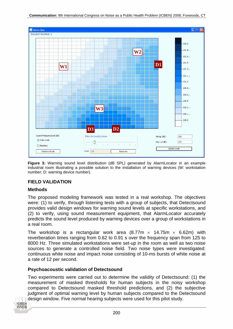
Communication: 9th International Congress on Noise as a Public Health Problem (ICBEN) 2008, Foxwoods, CT
Figure 3: Warning sound level distribution (dB SPL) generated by AlarmLocator in an example industrial room illustrating a possible solution to the installation of warning devices (W: workstation number; D: warning device number).
FIELD VALIDATION Methods The proposed modeling framework was tested in a real workshop. The objectives were: (1) to verify, through listening tests with a group of subjects, that Detectsound provides valid design windows for warning sound levels at specific workstations, and (2) to verify, using sound measurement equipment, that AlarmLocator accurately predicts the sound level produced by warning devices over a group of workstations in a real room.
The workshop is a rectangular work area (8.77m × 14.75m × 6.62m) with reverberation times ranging from 0.62 to 0.91 s over the frequency span from 125 to 8000 Hz. Three simulated workstations were set-up in the room as well as two noise sources to generate a controlled noise field. Two noise types were investigated: continuous white noise and impact noise consisting of 10-ms bursts of white noise at a rate of 12 per second.
Psychoacoustic validation of Detectsound Two experiments were carried out to determine the validity of Detectsound: (1) the measurement of masked thresholds for human subjects in the noisy workshop compared to Detectsound masked threshold predictions, and (2) the subjective judgment of optimal warning level by human subjects compared to the Detectsound design window. Five normal hearing subjects were used for this pilot study.
W1
W2
W3
D1
D2D3
W1
W2
W3
D1
D2D3
200

Communication: 9th International Congress on Noise as a Public Health Problem (ICBEN) 2008, Foxwoods, CT
In the first experiment, subjects were seated at one of the three workstations in the noisy workshop and listened to a warning sound. Using an ascending/descending adaptive threshold search method, individual masked thresholds were determined in continuous and impact noise for pulsed pure tone warning sounds at 500, 1000 and 2000 Hz. The continuous noise condition was also carried out with Peltor H9 hearing protectors. The subjective masked threshold measurements are reported in Table 1 and compared with Detectsound masked threshold predictions (which are the lower bound of the design window minus 12 dB). These predictions were based on the measured noise field at the workstation where subjects were seated. Over all 9 test conditions (frequency, noise, hearing protection), the mean prediction error is 0.0 dB and the standard deviation is 1.4 dB, thereby indicating very good predictive validity for Detectsound. The greatest difference between the subjective data and Detectsound predictions is a 2.5 dB overestimate at 2000 Hz using the Impact noise without protection. By noise type, there is a tendency for Detectsound to slightly underestimate subjective data for the continuous noise by 0.6 dB on average over the three frequencies, and to slightly overestimate the subjective data for the Impact noise by 0.6 dB. Detectsound predictions for the condition with hearing protection indicate no evidence of overestimation or underestimation and are all within 1.0 dB of the subjective data.
Table 1: Mean subjective masked thresholds with and without hearing protectors and comparison to Detectsound predictions at one workstation
Measured masked thresholds Condition Noise Freq.
(Hz) mean (dB SPL)
s.d. (dB)
Detectsound predictions
TLlow (dB SPL)
Error
(dB)
500 67.2 1.4 66.1 -1.1 1000 63.1 2.4 61.1 -2.0 Continuous
noise 2000 60.5 2.4 61.7 1.2 500 61.4 1.8 61.9 0.5 1000 58.0 1.2 56.8 -1.2
No hearing protection
Impact noise
2000 55.0 0.9 57.5 2.5 500 66.4 1.7 66.1 -0.3 1000 61.6 2.6 61.1 -0.5 Hearing
protection Continuous
noise 2000 60.9 1.4 61.7 0.8
In the second experiment, subjects were asked to optimally adjust the level of a three-component warning sound (500, 1000, 2000 Hz) to a preferred listening level ensuring clear audibility while maintaining comfort. The warning sound complex signal was so designed that each frequency component reached threshold synchronously. The results in Table 2 show that preferred listening levels are very close to the middle (18.5 dB) of the Detectsound design window (12 to 25 dB above masked thresholds). The mean preferred listening levels ranged from 15.5 dB to 21.7 dB above the masked thresholds. Over all conditions, the mean adjustment is 18.3 dB above masked thresholds. From these data, it appears that with hearing protection, individuals prefer levels slightly higher than what would be predicted from their masked thresholds. It is important to note that the background noise levels used in this experiment (73-77 dBA) were less than what would typically be found in many occupational settings and that loudness judgments are dependent on background noise levels. Caution must therefore be exerted in the interpretation of these results and measures should be repeated in more realistic background noise levels, using a greater number of subjects.
201

Communication: 9th International Congress on Noise as a Public Health Problem (ICBEN) 2008, Foxwoods, CT
Table 2: Mean preferred listening level of a 3-frequency component warning signal to ensure clear audibility and comfort at one workstation
Preferred listening level relative to masked
thresholds Condition Noise
Mean s.d. Continuous noise 17.6 0.9 No hearing
protection Impact noise 15.5 1.8 Hearing protection Continuous noise 21.7 2.2
Acoustic validation of AlarmLocator The acoustic validation of AlarmLocator was carried out using sound measurement equipment to verify that it could provide realistic predictions of the sound pressure level Lp in the workshop produced by omnidirectional warning sound devices located along the room walls, given the sound power Lw of the devices. This was evaluated independently for three source positions S1-S3 (fixed along two lateral walls and at one wall intersection), three simulated workstations W1-W3 and three octave bands of noise. Table 3 shows the difference between the sound level measurements for the 27 conditions (3 sources by 3 receiving workstations by 3 octave bands) and the predictions by AlarmLocator. Over all measurements, the prediction error varies between -2.1 dB (S1-W1 at 500 Hz) and +1.7 dB (S2-W3 at 500 Hz). Averaged over workstations, the prediction error varies between -0.1 dB (W1) and 0.3 dB (W3). Averaged over source locations, the prediction error varies between -0.1 dB (S1) and 0.2 dB (S2). Averaged over octave bands, the prediction error varies between -0.2 dB (500 Hz) and 0.4 dB (2000 Hz). Altogether, there is no indication of any systematic error over workstation, source location or frequency. Moreover, these errors are very small for all practical purposes when compared to the size of the Detectsound design window (13 dB). Thus, the estimation error is unlikely to affect the decision outcome for Detectsound.
Table 3: Sound pressure level prediction error (dB) for 3 source positions, 3 workstations and 3 octave bands. Positive numbers indicate an overestimation
1/1Oct W1 W2 W3 500 Hz -2.1 0.3 -1.4
1000 Hz -0.9 1.5 0.2 S1 2000 Hz 0.8 0.1 0.8
500 Hz 1.4 0.1 1.7 1000 Hz -0.7 -0.6 0.6 S2 2000 Hz -0.2 -0.8 0.6
500 Hz -0.3 -0.6 -0.9 1000 Hz 0.1 0.5 0.4 S3 2000 Hz 1.2 0.3 0.9
202
Communication: 9th International Congress on Noise as a Public Health Problem (ICBEN) 2008, Foxwoods, CT
DISCUSSION AND CONCLUSIONS This research contributes to the advancement of scientifically-based practical tools to guide the design and generation of warning sounds in industrial work areas. This is achieved through the use of two modeling tools: Detectsound and AlarmLocator. The first tool is a psychoacoustic model that takes into account the noise field, the use of hearing protectors and the hearing status of worker(s) to determine the optimal characteristics of warning sounds (level, frequency components) at each workstation in the work area. The second tool is a model for the acoustic propagation of warning sounds from the physical device source location to the receiving stations in the work area. The final solution is provided in a format that can be easily used in the field; i.e. the number of warning devices needed in the work area, their optimal location on walls, and their sound power level specifications by frequency. The method allows investigating the effects of noise-induced hearing loss and use of hearing protectors on warning sound perception in the workplace in a very systematic way (Giguère et al. 2007). In practice, use of the tools developed in this research would follow the general procedure detailed below (Figure 1):
(1) Specify the floor layout and location of the workstations; (2) Measure the noise level Lp at each workstation under realistic work
conditions and the reverberation time in the room; (4) Identify the specific workers or the general characteristics of the
population of workers at each workstation (age, gender, and years of occupational noise exposure);
(5) Measure the hearing status of the identified workers or estimate hearing thresholds and frequency selectivity based on age, gender and years of exposure (e.g. ISO 1999);
(6) Determine if hearing protectors are required in the work area and specify the attenuation of the devices;
(7) Using Detectsound, determine the optimum target warning sound levels TLlow and TLup at each workstation;
(8) Using AlarmLocator, determine the number of warning devices required ND, their location on walls and their sound power Lw;
(9) Install the warning devices in the work area as per AlarmLocator specifications;
(10) Verify that the devices produce warning sound levels within the Detectsound window specifications at each workstation using a sound level meter. A minimum of four frequency components within the Detectsound window are recommended.
The method is aimed at stakeholders in occupational health and safety to help them make informed decisions regarding the procurement and installation of warning devices in the workplace. It is hoped that this work could also contribute to new knowledge and insight into the optimal design and operation of warning devices in the workplace, which would be directly relevant to industrial hygienists and engineers, device manufacturers and standardization organizations. Finally, the method strictly deals with the audibility of warning sounds in the workplace. It does not specifically address other important factors such as the distinctiveness and sense of urgency conveyed by the warning sounds, and the cognitive load or demands associated with the workers’ tasks (Edworthy & Adams, 1996; Smith, 2003).
203

Communication: 9th International Congress on Noise as a Public Health Problem (ICBEN) 2008, Foxwoods, CT
REFERENCES Al Osman R (2007). Development of “AlarmLocator”: A computerized model for predicting the optimum number, location, and power level of acoustic warning devices in noisy work plants. Systems Science Master’s Thesis, University of Ottawa.
Al Osman R, Giguère, C, Laroche C (2006). ALARMLOCATOR: A software tool to facilitate the installation of acoustic warning devices in noisy workplants. Can Acoust 34(3): 20-21.
Coleman CJ, Graves RJ, Collier SG, Golding D, Nicholl AG, Simpson GC, Sweetland KF, Talbot CF (1984). Communications in noisy environments. Final Report on CEC Contract 7206/00/8/09. Edinburgh: Institute of Occupational Medicine.
Edworthy J, Adams A (eds.) (1996). Warning design: a research perspective. London: Taylor & Francis.
Edworthy J, Hellier E (2006). Complex nonverbal and auditory signals and speech warnings. In: Wogaltier MS (ed.): Handbook of warnings (pp 199-220). Mahwah NJ: Lawrence Erlbaum Associates.
Giguère C, Laroche C, Zheng Y, Sabourin C (2003). A warning sound perception model software. International Congress on Noise as a Public Health Problem (pp 80-81). Rotterdam, June 29-July 3.
Giguère C, Laroche C, Al Osman R, Zheng Y (2007). Influence de la perte auditive et du port de protecteurs auditifs sur l’installation d’avertisseurs sonores en milieux bruyants. Congrès international sur l’ingénierie des risques industriels (pp 29-43). Montréal, 17-19 Décembre.
Haas E, Edworthy J (2006). An introduction to auditory warnings and alarms. In: Wogalter MS (ed.): Handbook of warnings (pp 189-198). Mahwah NJ: Lawrence Erlbaum Associates.
Hétu R (1994). Mismatches between auditory demands and capabilities in the industrial work environment. Audiology 33: 1-14.
ISO 1999 (1990). Acoustics – Determination of occupational noise exposure and estimation of noise-induced hearing impairment. Geneva: International Organization for Standardization.
ISO 7731 (2003). Danger signals for work places – Auditory danger signals. Geneva: International Organization for Standardization.
Laroche C, Tran Quoc H, Hétu R, McDuff S (1991). Detectsound: A computerized model for predicting the detectability of warning signals in noisy workplaces. Appl Acoust 32: 193-214.
Nanthavanij S, Yenrades P (1999). Predicting the optimum number, location, and signal sound level of auditory warning devices for manufacturing facilities. Int J Ind Ergon 24: 569-578.
Patterson RD, Milroy R (1980). The appropriate sound level for auditory warnings on civil aircraft. J Acoust Soc Am 67: S58.
Robinson GS, Casali JG (2000). Speech communications and signal detection in noise. In: Berger EH, Royster LH, Royster JD, Driscoll DP, Layne M (eds.): The Noise manual (pp 567-600). Fairfax VA: American Industrial Hygiene Association.
Smith AP (2003). “Noise, accidents, minor injuries and cognitive failures.” Proceedings of the 8th International Congress on Noise as a Public Health Problem, pp 140-144.
Tran Quoc H, Hétu R (1996). La planification de la signalisation acoustique en milieu industriel: critères de conception des avertisseurs sonores de danger. Can Acoust 24(2): 3-17.
Wilkins P, Martin AM (1978). Hearing protection and warning sounds in industry - a review. Appl Acoust 21: 267-293.
Zheng Y, Giguère C, Laroche C, Sabourin C, Gagné A, Elyea M (2007). A psychoacoustic model for specifying the level and spectrum of acoustic warning signals in the workplace. J Occup Environ Hyg 4: 87-98.
204

Communication: 9th International Congress on Noise as a Public Health Problem (ICBEN) 2008, Foxwoods, CT
Test of hearing loss and hearing impairment in employees com-plaining of noise annoyance Søren Peter Lund1*, Berit Grevstad1, Jesper Kristiansen1 1 National Research Centre for the Working Environment, Lerso Parkallé 105, DK-2100
Copenhagen, Denmark
* corresponding author: e-mail: [email protected]
INTRODUCTION Complaints of noise annoyance are increasing in several areas of the working envi-ronment, particularly in open offices, schools and kindergartens. The noise levels seldom reach noise levels with risk of noise induced hearing loss, but the cause emerges from a complex interplay between the level and the character of the noise, the acoustics of the workplace, psychosocial stress-factors, and individual factors including hearing ability. Among the main problems are the acoustic quality of the rooms, and the hearing ability of the employees. With longer life expectancy and a change towards service jobs with high communicative and high cognitive demands, it is important that the working environment does not exclude employees with reduced hearing abilities, who have great difficulties in hearing in noisy surroundings of low acoustic quality. Another trend in hearing ability is reduced hearing among adoles-cence, which seems to be serious with the expectancy of a longer working life. Regu-lar tests of hearing thresholds in noise exposed employees are required all over the world, but the audiogram may not determine minor deficits in hearing or initial signs of noise induced hearing loss (Attias et al. 2001; Torre et al. 2007). Oto-acoustic emissions (Job et al. 2007) and suppression of oto-acoustic emissions (Zhang et al. 2007) may be a valuable tool in measuring the plasticity of hearing, but further valida-tion is needed. If a greater number of subjects have to be tested, it is also necessary to introduce time optimized protocols (Sisto et al. 2007). We have tested these meth-ods in a binaural setup, and will present a series of decisions, which has to be made in order to do assessments in the field.
METHODS Hearing thresholds and oto-acoustic emissions were tested on military officers (n=51, aged 21-63 years from a Danish telegraph regiment. Otoscopic examination and 226-Hz probe tone tympanometry (Madsen Zodiak 901) were used to screen participants before the tests of hearing. Distortion product oto-acoustic emissions (DPOAE) were performed bi-aurally with two identical DSP-systems from Tucker-Davis Technologies (TDT, Alchua, FL) and two Ethymotic Research (ER, Elk Grove Village, IL) micro-phone probe systems (ER10B+ connected by tubes to ER2 sound transducers). Two 24-bit RX6 Piranha DSP-processors were generating simultaneous in- and output (8192 samples) at 24,414 Hz. The output level was controlled by four programmable attenuators (TDT PA5) driving each of the sound transducers according to drive specifications of the transducers (100 dB SPL at 1 Vrms). The balance of four trans-ducers was equalized in a 2 cc coupler (B&K DB0138) towards a ½” pressure-field microphone (B&K 4192) and a HP35670A analyzer. The input from the ER10B mi-crophone drivers were amplified 30 dB (TDT MA3 microphone amplifiers) before fil-tering (sigma-delta) and A/D-conversion by the DSP-processors, using the supplied calibration curves of the microphones. The data were collected from the DSP-processors by a fiber optic interface (TDT Gigabit Interface), analyzed and controlled by computer using TDT ActiveX modules, Agilent VEE 7.0, and MATLAB. The
205
Communication: 9th International Congress on Noise as a Public Health Problem (ICBEN) 2008, Foxwoods, CT
DPOAE assessments on each ear consisted of six DP-grams with measurements of the cubic distortion product (CDP= 2f1-f2) from 32 sets of primary input tones (f2/f2=1.23; f2 ranging from 707 Hz to 10,374 Hz) and 8 repeated time series aver-aged for each set of primaries. The six DP-grams were obtained at five different lev-els of the primaries (L2= 45 dB, 50 dB, 55 dB, 60 dB, 65 dB, and 55dB SPL; L1= L2+10 dB). The background noise level across frequencies at each level of stimula-tion was determined by calculation of the average response of all the measurements, where the primaries were not generating a specific response at the frequency of the CDP measurement. Single frequencies with high level of both CDP and background noise due to swallowing or movements were redone at the end of each DP-gram as-sessment. The same setup and probe systems was used for assessments of audio-grams with automatic threshold determination (125.2 Hz, 250.3 Hz, 500.7 Hz, 1001 Hz, 1541 Hz, 2000 Hz, 3085 Hz, 3999 Hz, 6169 Hz, and 7999 Hz; 1 kHz upwards, 1 kHz downwards) in 5 dB steps. The input from each microphone was tested regularly in a B&K 4230 sound level calibrator. All tests of hearing were performed in a trans-portable sound booth (IAC 250 Sound Shelter, complying with ISO 6189). Before measurements of either hearing thresholds or oto-acoustic emissions, proper fitting of the earplugs was tested by measurement of the output from each transducer in situ at 500 Hz.
RESULTS The tests of each individual including otoscopic examination and tympanometry was planned to be performed within an hour and up to 8 persons per day. However, this proved to be a problem because the output from the ER 10B microphones dropped during continued use. This turned out to be caused by substantial sensitivity to high relative humidity, which increased the variation of the results and seriously disturbed the intentions of the study. However, of the 51 officers participating in the study, only three individuals were left out because of technical difficulties. The rest (48) was di-vided in quartiles on the basis of the average 1-8 kHz hearing thresholds on the right ear, and the audiograms and DP-grams of left ear and right ears from the four quar-tiles are shown in Figure 1 and Figure 2. Both the audiograms and the DP-grams show initial impairment at 1.5 to 4 kHz, and again above 4 kHz, which may be related to impulse noise exposure from small firearms. With increased hearing thresholds the amplitude of the CDP and the steepness of the IO-functions changes on both ears. Where the DP-grams with increasing stimulation (L2 from 45 to 65 dB SPL) lie close together, the growth of input-output function (IO-function) shows the normal com-pressive function of the Basilar Membrane (Moore 1998), but even with small changes in hearing thresholds, the shape of the IO-function changes to a more steep increase with the increase in stimulation.
DISCUSSION Measuring small changes in hearing thresholds is a laborious task, being in nature a testing of a signal to noise ratio. Proper testing demands low background noise level and may be time consuming. If one wishes to introduce a new test of hearing ability, the total time cannot be extended of testing very much, because the salaries of the
206

Communication: 9th International Congress on Noise as a Public Health Problem (ICBEN) 2008, Foxwoods, CT
Figure 1: Right ear audiograms (Left: Hearing thresholds, HT) and DP-grams (Right: Cubic Distortions Products, CDP) of 48 male officers, divided in 4 quartiles on the basis of right ear average hearing thresholds from 1-8 kHz. The DP-grams are made with L2 primary levels from 45 to 65 dB SPL, the thick line being the average between two measurements at L2= 55 dB SPL. The dotted line is the av-erage background noise level without primaries.
participants has to be paid, either by their employer, the participants themselves, or financed by the study. Using longer time of testing may often decrease the number of participants, which does make it difficult to study more subtle risk factors of hearing impairment. Oto-acoustic emissions has potential to study both subtle hearing loss as well as the some of the dynamic parameters of hearing, which may be very valuable in assessing noise sensitivity and future demands to acoustic quality, as well as test-ing for early signs of noise induced hearing loss. At present time, no such system seems be commercially available, but the current price of DSP-processors and com-puter power no longer inhibits the acquisition of systems with sufficient capacity to
207

Communication: 9th International Congress on Noise as a Public Health Problem (ICBEN) 2008, Foxwoods, CT
Figure 2: Left ear audiograms (Left: Hearing thresholds, HT) and DP-grams (Right: Cubic Distortions Products, CDP) of 48 male officers, divided in 4 quartiles on the basis of right ear average hearing thresholds from 1-8 kHz. The DP-grams are made with L2 primary levels from 45 to 65 dB SPL, the thick line being the average between two measurements at L2= 55 dB SPL. The dotted line is the av-erage background noise level without primaries.
make the assessments in real time. The main problem is to design and validate a system for extended use, which is fast, robust and easy to use. The assessments of one DP-gram with the present system takes approximately 90 seconds, and often one or several frequencies has to be redone because of swallowing or head move-ments, increasing the time of one DP-gram to about 2 min. In order to test the effer-ent system (the medial olivocochlear reflex) by contra-lateral suppression oto-acoustic emissions, a bi-aural system is preferable, but that also necessitates calibra-tion and balancing between left and right probe system. Further, using low primary stimulus levels requires low background noise levels or averaging number of re-cordings as time series, and the latter certainly increases the total time of testing across many frequencies and several stimulus levels (IO-curves). The better signal to
208

Communication: 9th International Congress on Noise as a Public Health Problem (ICBEN) 2008, Foxwoods, CT
noise ratio is in favor of measurements at higher levels of the primaries, but as seen on the DP-grams in Figure 1 and Figure 2, the high stimulus levels reveal less infor-mation of the actual status of the cochlear amplifier along the basilar membrane. Therefore it should be performed at reasonable levels of primaries to yield a CDP response before the top of the IO-curve and well above the noise floor, and the opti-mum seems to lie at L2 ~50-55 dB SPL.
REFERENCES Attias J, Horovitz G, El-Hatib N, Nageris B (2001). Detection and clinical diagnosis of noise-induced hearing loss by oto-acoustic emissions. Noise & Health 3(12): 19-31.
Job A, Raynal M, Kossowski M (2007). Susceptibility to tinnitus revealed at 2 kHz range by bilateral lower DPOAEs in normal hearing subjects with noise exposure. Audiol Neurootol 12: 137-144.
Moore BCJ (1998). Cochlear hearing loss. London: Whurr Publishers Ltd.
Sisto R, Chelotti S, Moriconi L, Pellegrini S, Citroni A, Monechi V, Gaeta R, Pinto I, Stacchini N, Moleti A (2007). Otoacoustic emission sensitivity to low levels of noise-induced hearing loss. J Acoust Soc Am 122 :387-401.
Torre P 3rd, Dreisbach LE, Kopke R, Jackson R, Balough B (2007). T Risk factors for distortion product otoacoustic emis-sions in young men with normal hearing. J Am Acad Audiol 18: 749-759.
Zhang F, Boettcher FA, Sun XM (2007) Contralateral suppression of distortion product otoacoustic emissions: effect of the primary frequency in Dpgrams. Int J Audiol 46: 187-195.
209

Communication: 9th International Congress on Noise as a Public Health Problem (ICBEN) 2008, Foxwoods, CT
Establishment of fitness standards for hearing-critical jobs Chantal Laroche1*, Christian Giguère1, Sigfrid D. Soli2, Véronique Vaillancourt1 1 Audiology and SLP Program, University of Ottawa, Ottawa, Ontario, K1H 8M5, Canada
2 Department of Human Communication Sciences and Devices, House Ear Institute, Los Angeles, California, 90057, United-States of America
*corresponding author: e-mail: [email protected]
INTRODUCTION In many occupational settings, medical standards are necessary to ensure that work-ers are fit to conduct safe and effective operations, given the specific task demands for each job. In occupations such as the military, the firefighting service, the coast guard, the police force and other law enforcement jobs, medical standards extend to the hearing modality (Hétu 1993; Laroche 1994; MacLean 1995; Forshaw & Hamilton 1997; Soli & Vermiglio 1999; Laroche et al. 2003). These occupations all require a number of functional hearing abilities or skills such as speech communication, sound detection and localization, which must often be used in noisy environments. A suffi-cient level of functional hearing ability is needed from each worker to prevent safety risks to themselves, to fellow workers, and to the general public. Some noise envi-ronments and task situations can at times be very challenging, and allowing workers with hearing loss in these workplaces is an important issue that must be addressed. Fitness for work, however, must not be based on the degree or configuration of the hearing loss as such, but on the ability (or inability) to perform the various auditory skills needed by the job at the required performance level, taking into account the relevant parameters of the listening environment for every task. Unfortunately, occupational hearing standards are primarily based on simple diag-nostic measures of hearing, such as the absolute hearing threshold at specific fre-quencies or the pure-tone average (Coles & Sinclair 1988; Hétu 1993; Bhérer et al. 2002). Such measures were originally designed to compensate workers for noise-induced hearing loss, and not to assess the minimum hearing abilities necessary to function effectively in the workplace. Moreover, these measures implicitly assume a strong relationship between auditory tasks and, more specifically, between hearing sensitivity measures and functional hearing abilities at particular supra-threshold le-vels. It is well known that individuals with essentially identical hearing sensitivity may have a wide range of speech recognition abilities in noise (e.g. Smoorenburg 1992; Soli & Vermiglio 1999; Killion & Niquette 2000; Laroche et al. 2005). Models of real-world auditory performance based solely on the audiogram would therefore predict identical speech communication abilities in the workplace for individuals with identical audiograms, and likewise for other auditory skills. Such a framework clearly lacks sufficient accuracy and specificity to serve as a basis for making employment deci-sions regarding individual workers (Coles & Sinclair 1988; Begines 1995; MacLean 1995; Bhérer et al. 2002), and it has been successfully challenged in courts as job discrimination in some cases (Laroche 1994; Laroche et al. 2003). Recent applications have contributed significantly to moving away from simple diag-nostic measures of hearing to assess fitness for work. Two such applications are de-scribed in this paper, including the establishment of hearing standards for the De-partment of Fisheries and Oceans Canada (DFO) and the evaluation of Royal Cana-dian Mounted Police (RCMP) members wearing hearing aids.
210

Communication: 9th International Congress on Noise as a Public Health Problem (ICBEN) 2008, Foxwoods, CT
FUNCTIONALLY-BASED SCREENING CRITERIA FOR HEARING-CRITICAL JOBS BASED ON THE HEARING IN NOISE TEST Rationale In many occupational settings, the work environment is characterized by a wide range of noises. It is well established that speech recognition depends on the ener-getic (global level, spectrum, temporal fluctuations, etc.) and informational masking properties of the noise (Festen & Plomp 1990; Studebaker et al. 1994; ANSI 1997; Brungart et al. 2001; Rhebergen & Versfeld 2005), and thus functional hearing as-sessment procedures must ultimately take into account the specific noise environ-ments in which HC tasks are performed in the workplace. One approach would be to screen each individual worker in each noise environment where s/he is expected to perform HC tasks. Such a strategy would be highly impractical and time-consuming as a screening measure, and could raise validity and reliability issues unless a pro-hibitive amount of testing could be conducted. Instead, the approach adopted in this research is to use a well-established speech perception test with well-defined psychometric properties (i.e., sensitivity, reliability, etc.) and normative data as the basic single measure to screen individual workers. Through statistical modeling, scores on this screening test are then empirically re-lated to speech recognition performance in the real-world noise environments where HC tasks are performed. Listening experiments in the different noise environments characterizing the workplace are still required with this approach, but only during the development and validation phases of the predictive model. The assessment phase for a worker only requires administration of the screening speech perception test it-self, which is quick, reliable, and can be conducted in a wide range of audiological settings. Using this statistical approach, screening test results can be used to predict the individual worker’s speech recognition ability in the different real-world workplace noises with a known amount of prediction error, which can be taken into account when establishing minimum standards and screening criteria. Moreover, models attempting to relate clinical scores to real-world performance must not solely rely on an individual’s measured abilities but also take into consideration the constant interaction of those abilities with various aspects of the environment (noise, talker, communication tasks) and rehabilitation process (technologies, envi-ronmental modifications, communication strategies, realistic expectations). Indeed, the complete communication situation from talker to listener needs to be taken into account, as illustrated in Figure 1. Factors affecting speech production (voice level and spectrum) include the gender (M, F), the speech material, the vocal effort (nor-mal, raised, shouted voice) of the talker, the Lombard effect of naturally raising one’s voice in noise, and the use of HPDs. The latter can affect speech production by re-ducing the amount of Lombard effect due to the reduction in the noise perceived by the talker as a result of the attenuation of the protector and the increase in the per-ception of one’s voice caused by the occlusion effect of the device (Tufts & Frank 2003). Distance and reverberation modify the speech transmission process, whereas factors affecting speech perception include the hearing status of the listener, whether or not the message can be repeated, the spatial distribution of the speech signal and noise (or binaural unmasking), the intrinsic characteristics of the competitive noise and the use of hearing devices or HPDs.
211
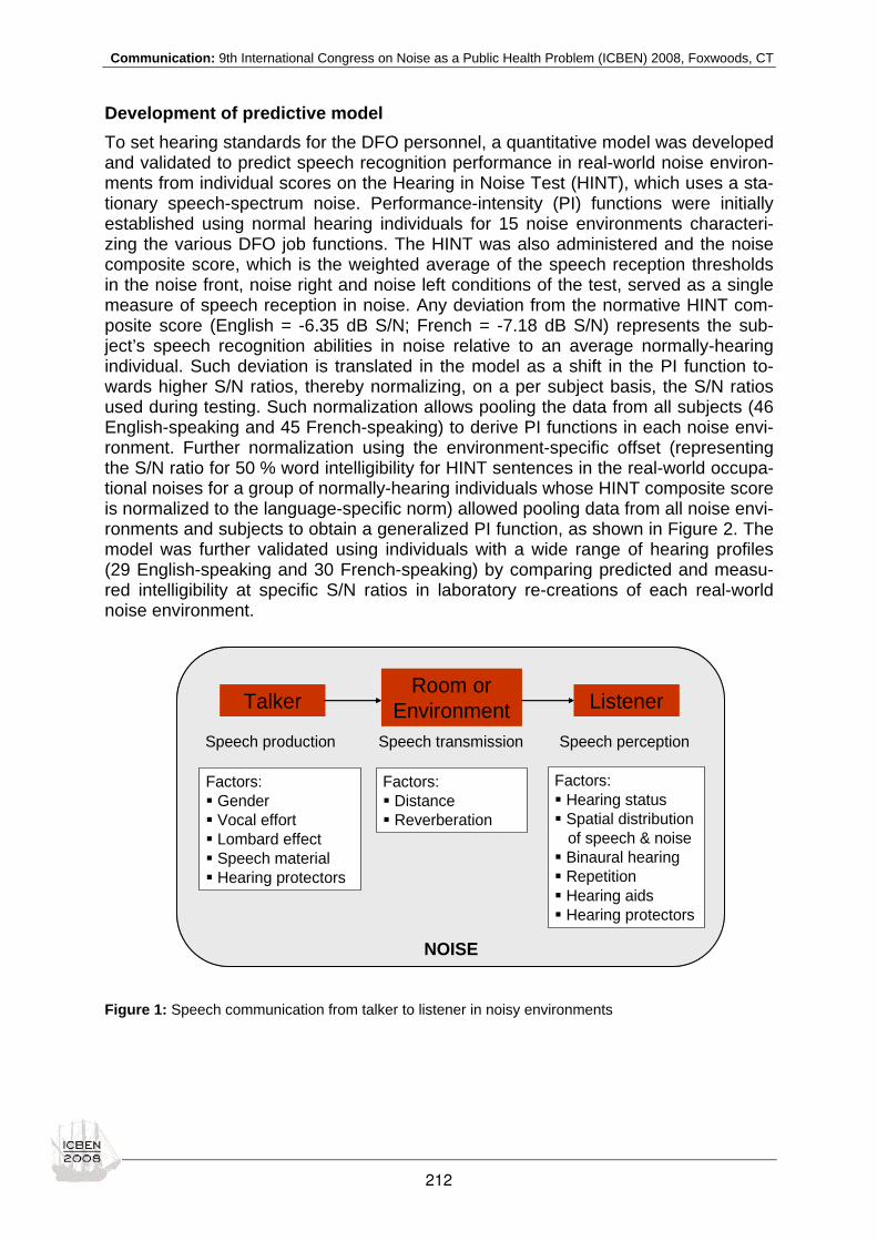
Communication: 9th International Congress on Noise as a Public Health Problem (ICBEN) 2008, Foxwoods, CT
Development of predictive model To set hearing standards for the DFO personnel, a quantitative model was developed and validated to predict speech recognition performance in real-world noise environ-ments from individual scores on the Hearing in Noise Test (HINT), which uses a sta-tionary speech-spectrum noise. Performance-intensity (PI) functions were initially established using normal hearing individuals for 15 noise environments characteri-zing the various DFO job functions. The HINT was also administered and the noise composite score, which is the weighted average of the speech reception thresholds in the noise front, noise right and noise left conditions of the test, served as a single measure of speech reception in noise. Any deviation from the normative HINT com-posite score (English = -6.35 dB S/N; French = -7.18 dB S/N) represents the sub-ject’s speech recognition abilities in noise relative to an average normally-hearing individual. Such deviation is translated in the model as a shift in the PI function to-wards higher S/N ratios, thereby normalizing, on a per subject basis, the S/N ratios used during testing. Such normalization allows pooling the data from all subjects (46 English-speaking and 45 French-speaking) to derive PI functions in each noise envi-ronment. Further normalization using the environment-specific offset (representing the S/N ratio for 50 % word intelligibility for HINT sentences in the real-world occupa-tional noises for a group of normally-hearing individuals whose HINT composite score is normalized to the language-specific norm) allowed pooling data from all noise envi-ronments and subjects to obtain a generalized PI function, as shown in Figure 2. The model was further validated using individuals with a wide range of hearing profiles (29 English-speaking and 30 French-speaking) by comparing predicted and measu-red intelligibility at specific S/N ratios in laboratory re-creations of each real-world noise environment.
Figure 1: Speech communication from talker to listener in noisy environments
Factors:GenderVocal effortLombard effectSpeech materialHearing protectors
TalkerRoom or
Environment Listener
Speech production Speech perceptionSpeech transmission
Factors:Hearing statusSpatial distributionof speech & noiseBinaural hearingRepetitionHearing aidsHearing protectors
NOISE
Factors:Distance Reverberation
Factors:GenderVocal effortLombard effectSpeech materialHearing protectors
TalkerRoom or
Environment ListenerTalkerRoom or
Environment Listener
Speech production Speech perceptionSpeech transmission
Factors:Hearing statusSpatial distributionof speech & noiseBinaural hearingRepetitionHearing aidsHearing protectors
NOISE
Factors:Distance Reverberation
212

Communication: 9th International Congress on Noise as a Public Health Problem (ICBEN) 2008, Foxwoods, CT
Figure 2: Generalized PI function, across all subjects and noise environments
Prediction of occupational performance The generalized PI function allows predictions of the expected speech intelligibility score for given individuals as a function of the S/N ratio in each workplace noise envi-ronment. An example is provided in Figure 3. The curve representing the intelligibility performance in DFO Noise Location 1 for an individual scoring -2.0 dB S/N on the English HINT is obtained by shifting the generalized PI function by -9.9 dB (= location 1 offset) to the left and then by 4.35 dB (= HINT deviation relative to norm) to the right. This curve represents the word intelligibility score that can be expected from this individual as a function of S/N ratio in the specified noise environment.
Figure 3: Use of the generalized PI function to predict speech intelligibility in DFO Noise Location 1 (fishing boats – fixer gear) for a listener scoring -2.0 dB S/N on the English HINT (composite)
In order to predict a more specific occupational performance, the actual S/N ratio available to the listener during each hearing-critical (HC) task must be specified. This requires knowledge of the expected speech level of the talker at the listener’s posi-tion in various communication situations. It is well known that the vocal effort and acoustic output from a talker in face-to-face communications depends on the noise level in the environment, a phenomenon known as the Lombard effect (Lane & Tra-
Generalized PI function
0
10
20
30
40
50
60
70
80
90
100
-15 -10 -5 0 5 10 15
Normalized S/N Ratio (dB)
Perc
ent I
ntel
ligib
ility
English data
French data
5th
50th
95th
N=691
Generalized PI function
0
10
20
30
40
50
60
70
80
90
100
-15 -10 -5 0 5 10 15
Normalized S/N Ratio (dB)
Perc
ent I
ntel
ligib
ility
English data
French data
5th
50th
95th
N=691
0
10
20
30
40
50
60
70
80
90
100
-20 -15 -10 -5 0 5 10S/N Ratio (dB)
Perc
ent I
ntel
ligib
ility
Generalized PILocationLocation + HINT
HINT deviation (4.35 dB)
Location offset (-9.9 dB)
0
10
20
30
40
50
60
70
80
90
100
-20 -15 -10 -5 0 5 10S/N Ratio (dB)
Perc
ent I
ntel
ligib
ility
Generalized PILocationLocation + HINT
HINT deviation (4.35 dB)
Location offset (-9.9 dB)
213
Communication: 9th International Congress on Noise as a Public Health Problem (ICBEN) 2008, Foxwoods, CT
nel 1971; Summers et al. 1988; Junqua 1996). The voice level reaching the listener also depends on the distance between the talker and the listener. The model was therefore based on published data on the Lombard effect (Pearsons & Bennett 1977) predicting conversational speech levels as a function of noise level for communications occurring at 1-meter distances. Typically, the model assumes that in background noises of 45 dB(A) or less, talker speech levels are constant at 55 dB(A) and thereafter increase at a rate of 0.6 dB per 1 dB increase in noise level until reaching 86 dB(A) – the level of sustained shouted speech. As speech levels increase at a slower rate than noise levels, the S/N ratio decreases gradually as the noise level increases. From the distribution of levels in each noise environment, the distribution of S/N ratios at the listener position can be established. The model can be adapted to allow the user to specify: 1) the vocal effort of the talker, by expanding it to include speech levels produced by shouted vocal effort (typically 86 dB (A) at 1 meter), regardless of the background noise level, 2) the effects of communication distance using basic acoustical principles (reduction in speech levels by 6 dB for every doubling of distance) and 3) the effect of repeating the communication. By multiplying the distribution of S/N ratios for a given noise environment by the measured PI function, one can determine the expected speech intelligibility associ-ated with each HINT score, as a function of the communication distance of the com-munication, the vocal effort used by the talker and whether or not the message was repeated. An individual’s ability to understand speech in a wide range of noisy envi-ronments can therefore be predicted from HINT scores, for various scenarios. In oc-cupational settings, Subject Matter Experts are critical in the process of attempting to predict performance or set hearing criteria as they have extended knowledge of the communication tasks required by the specific job and can specify the parameters sur-rounding these tasks (distance, voice level, expected level of performance). Using the SME specifications and the modeling tools described above, a HINT screening score is derived in each workplace noise environment where the tasks can be performed. An example is provided in Table 1, for a few HC tasks. These thresh-olds indicate the maximum (worst) HINT composite scores required to ensure that workers would meet the minimum intelligibility level specified for the task. As shown, the HINT screening scores for a given HC task depend strongly on the acoustical characteristics of the noises. In cases where a worker must perform a specific HC task in all noise environments, the lowest (most stringent) HINT composite score from all environments is used for screening (last column of Table 1).
214

Communication: 9th International Congress on Noise as a Public Health Problem (ICBEN) 2008, Foxwoods, CT
Table 1: Sample of different HC task communication parameters (vocal effort, distance, and repetition) in the DFO project, the minimum speech intelligibility performance specified by the SMEs, and English HINT composite screening threshold in each environment. Empty cells indicate that the given task is not performed in the specific environment. An “X” is inserted in cells where the performance level that cannot be met by normally-hearing individuals. These situations should not be used for screening the hearing of employees based on the definition of a HC task. The last column is the most stringent HINT screening score from each task.
PROTOCOL FOR THE EVALUATION OF AUDITORY FUNCTIONS FOR RCMP MEMBERS To set scientifically-based hearing standards knowledge of the HC tasks, the noise environments where these tasks are performed and the parameters surrounding these tasks (distance, voice level and expected level of performance) is paramount. To ensure public safety, employers may however need to make quick judgments on the operational status of their employees prior to or during efforts to set new hearing standards, as was the case for the RCMP. To assist the RCMP in making more informed decisions regarding fitness to work in officers wearing hearing aids without detailed information regarding HC tasks, com-munication parameters and noise characteristics, a testing protocol has been pro-posed which includes unaided and aided soundfield measures of sound detection, speech perception and sound localization, in addition to standard audiologic evalua-tions. The Hearing in Noise Test (Nilsson et al. 1994; Vaillancourt et al. 2005) and a measure of sound localization (S.E.L.A – System for Evaluating Localization Acuity) are used in their clinical format to test members with the hearing aids set at the pro-gram and settings used on a regular basis in occupational settings. The protocol is used to: 1) evaluate the auditory functions for individual RCMP mem-bers currently facing operational restrictions because they do not meet the hearing criteria set forth in the RCMP Hearing Policy and could therefore compromise the safety of others as well as their own, and 2) verify if hearing aids allow these mem-bers to carry out the necessary auditory functions required to safely perform their job. While individual results help the medical team at RCMP in making more informed decisions about the operational suitability of each member, a secondary objective is to use the overall results across all tested members, together with the complete de-scription of hearing aid parameters used, to form a database that will hopefully help
215

Communication: 9th International Congress on Noise as a Public Health Problem (ICBEN) 2008, Foxwoods, CT
identify best practices in hearing aid fitting for optimal functional hearing abilities in the RCMP work environment. Given that research-based hearing standards have not yet been established for the various jobs performed by RCMP members, unaided and aided member perform-ances on tasks of speech perception in noise and sound localization are compared to the 5th percentile performance amongst individuals with normal hearing on these same tasks to determine operational suitability. Representing the poorest perform-ances amongst a group of individuals with normal hearing, the 5th percentile was deemed an appropriate interim screening criterion. Typically, the criterion could not be more stringent than the 5th percentile as some people with normal hearing would not be able to meet the required performance level. On the other hand, a more lax criterion cannot be proposed until supported by further research to establish func-tionally-based hearing standards, using an approach similar to that previously used for the Department of Fisheries and Oceans Canada (DFO). Individuals who meet the interim criteria are deemed fit to carry out effectively the auditory functions re-quired by their job. For others, operational restrictions can be maintained until the proper hearing standards are established, at which point their results can be com-pared to the set standards.
CONCLUSIONS In recent applications of fitness for work, diagnostic measures of hearing have been replaced with simple computerized screening measures of functional hearing in reference noises. The proposed approach in setting hearing standards utilizes the individual’s score in relation to the norm, as measured in reference noises in the screening test, to predict functional hearing ability in real-world noise environments. The current research marks the first time that such a detailed modeling approach combining both speech production and perception parameters has been used to solve practical noisy workplace communication problems. Although the proposed ap-proach addressed some components of the general model describing speech com-munication from talker to listener in noise (Figure 1), much work remains. The tools developed, while applicable to other occupational environments, require a substantial amount of human subject testing in the development and validation stages of the predictive model to establish the generalized PI function and location offsets relevant to the specific workplace noises under study. Work is currently undergoing to esti-mate these model parameters directly from the noise recordings using objective tools such as the Speech Intelligibility Index (ANSI 1997). The current research also uncovered several areas where there is relatively little data in the literature upon which to base modeling. One such aspect is the effect of re-peating a verbal command on speech perception (Thwing 1956; Haggard 1973; Clark et al. 1985). Recent research (Mercille et al. 2006) seems to indicate that the benefits of repeating a spoken message depends on the temporal structure of the noise, with more benefits being accrued for fluctuating than continuous noises. The Lombard effect appears equally dependent on the temporal characteristics of background noises, being greater for fluctuating than continuous noises (Giguère et al. 2006). In essence, model contributions from the Lombard and repetition effects would hence vary from one noisy environment to the next rather than be consistently applied across various work environments in the establishment of hearing standards. Another aspect to consider is the effects of cognitive loading of the listener (Schnei-der 2004) during HC tasks. The wearing of hearing protectors may also affect speech
216

Communication: 9th International Congress on Noise as a Public Health Problem (ICBEN) 2008, Foxwoods, CT
perception (Berger 2000), and this would need to be accounted for in workplaces where noise levels exceed regulatory limits. Talkers wearing hearing protectors were also found to produce lower speech levels in noise than talkers not wearing them (Tufts & Frank 2003), and this could lead to particular speech communication prob-lems in the workplace. Finally, the model was previously applied to situations in which visual information (visual cues) was not available to the listener. Further developments of the model will include modeling the effect on speech intelligibility of, among others: visual informa-tion, attenuation provided by hearing protection, communication devices and informa-tional maskers.
REFERENCES ANSI, American National Standards Institute (1997). Methods for calculation of the speech intelligibility index. ANSI S3.5-1997. New York: ANSI.
Begines T (1995). Fitness and risk evaluation. Spectrum 12: 8-11.
Berger EH (2000). Hearing protection devices. In: Berger EH, Royster LH, Royster JD, Driscoll DP, Layne M (eds.): The Noise manual (pp 379-454). 5th ed. Fairfax: American Industrial Hygiene Association.
Bhérer L, Deshaies P, Fortier P, Laroche C, Tremblay V et al. (2002). La surveillance médicale de l’audition exigée par qua-tre règlements québécois: Analyse de la pertinence. Avis formulé à l’intention du Directeur national de la santé publique. Comité médical provincial en santé au travail du Québec, 26 pp.
Brungart DS, Simpson BD, Ericson MA, Scott KR (2001). Informational and energetic masking effects in the perception of multiple simultaneous talkers. J Acoust Soc Am 110: 2527-2538.
Clark JE, Dermody P, Palethorpe S (1985). Cue enhancement by stimulus repetition: Natural and synthetic speech compari-sons. J Acoust Soc Am 78: 458-462.
Coles RRA, Sinclair A (1988). Hearing. In: Edwards FC, McCallum RI, Taylor PJ (eds.): Fitness for work. The medical as-pects (pp 67-89). Oxford: Oxford University Press.
Festen JM, Plomp R (1990). Effects of fluctuating noise and interfering speech on the speech-reception threshold in impaired and hearing. J Acoust Soc Am 88: 1725-1736.
Forshaw S, Hamilton K (1997). Assessment of occupational hearing requirements. Can Acoust 25: 3-9.
Giguère C, Laroche C, Brault É, Ste-Marie J-C, Brosseau-Villeneuve M, Philippon B, Vaillancourt V (2006). Quantifying the Lombard effect in different background noises, 4th Joint Meeting of the Acoustical Society of America and the Acoustical Society of Japan, Honolulu, 28 November – 2 December. J Acoust Soc Am 120: 3378.
Haggard M (1973). Selectivity versus summation in multiple observation tasks: evidence with spectrum parameter noise in speech. Acta Psychol 37: 285-299.
Hétu R (1993). Capacités auditives, critères d’embauche et droits de la personne. Can Acoust 21: 3-14.
Killion M, Niquette PA (2000). What can be pure-tone audiogram tell us about a patient’s SNR loss? Hearing Journal 53:46-48, 50, 52-53.
Junqua J-C (1996). The influence of acoustics on speech production: A noise-induced stress phenomenon known as the Lombard reflex. Speech Communication 20:13-22.
Lane H, Tranel B (1971). The Lombard sign and the role of hearing in speech. J Speech Hear Res 14: 677-709.
Laroche C (1994). Cases of possible job discrimination based on hearing loss. Can Acoust 22: 89-90.
Laroche C, Giguère C, Soli S, Lagacé J, Vaillancourt V (2003). An approach to the development of hearing standards for hearing-critical jobs. Noise & Health 6: 17-37.
Laroche C, Giguère C, Vaillancourt V, Soli S (2005). Development and validation of hearing standards for Canadian Coast Guard Seagoing Personnel and C&P and land-based personnel. Phase II, Final report to Department of Fisheries and Oceans under Contract No. F7053-000009.
MacLean S (1995). Employment criteria in hearing critical jobs. Spectrum 12: 20-23.
217

Communication: 9th International Congress on Noise as a Public Health Problem (ICBEN) 2008, Foxwoods, CT
Mercille C, Larose R, Giguère C, Laroche, C (2006). Quantifying the benefits of sentence repetition on the intelligibility of speech in continuous and fluctuating noises, 4th Joint Meeting of the Acoustical Society of America and the Acoustical Soci-ety of Japan, Honolulu, 28 November - 2 December. J Acoust Soc Am 120: 3252.
Nilsson M, Soli SD, Sullivan JA (1994). Development of the hearing in noise test for the measurement of speech reception thresholds in quiet and in noise. J Acoust Soc Am 95: 1085-1099.
Pearsons KS, Bennett RL (1977). Speech levels in various noise environments. Washington: EPA, Office of Health and Ecological Effects.
Rhebergen KS, Versfeld NJ (2005). A speech intelligibility Index-based approach to predict the speech reception threshold for sentences in fluctuating noise for normal-hearing listeners. J Acoust Soc Am 117: 2181-2192.
Schneider BA (2004). From acoustics to cognition: some surprising results. Can Acoust 32: 14-15.
Smoorenburg GF (1992). Speech reception in quiet and in noisy conditions by individuals with noise-induced hearing loss in relation to their tone audiogram. J Acoust Soc Am 91: 421-437.
Soli SD, Vermiglio A (1999). Assessment of functional hearing abilities for hearing critical jobs in law enforcement. Report for the California Peace Officers Standards and Training Commission, 29 pp.
Studebaker GA, Taylor R, Sherbecoe RL (1994). The Effect of noise spectrum on speech recognition performance-intensity functions. J Speech Hear Res 37: 439-448.
Summers WV, Pisoni DB, Bernacki RH, Pedlow RI, Stokes MA (1988). Effects of noise on speech production: Acoustic and perceptual analyses. J Acoust Soc Am 84: 917-928.
Thwing EJ (1956). Effect of repetition on articulation scores for PB words. J Acoust Soc Am 28: 302-303.
Tufts JB, Frank T (2003). Speech production in noise with and without hearing protection. J Acoust Soc Am 114: 1069-1080.
Vaillancourt V, Laroche C, Mayer C, Basque C, Nali M, Eriks-Brophy A, Soli SD, Giguère C (2005). Adaptation of the HINT (Hearing In Noise Test) for adult Canadian Francophone populations. Int J Audiology 44: 358-369.
218

Communication: 9th International Congress on Noise as a Public Health Problem (ICBEN) 2008, Foxwoods, CT
Effect of priming and amplitude fluctuations on age-related differences in release from informational masking Payam Ezzatian*, Liang Li, Kathy Pichora-Fuller, Bruce A. Schneider
University of Toronto
* corresponding author: e-mail: [email protected]
Presenting listeners with all but the last word of a target nonsense sentence immediately prior to pre-senting the full sentence produces a greater release from two-talker speech masking than from speech-spectrum-noise masking, suggesting that an auditory prime can release speech from informa-tional masking (Freyman et al. 2004; Yang et al. 2007). In Experiment 1 of the present study we showed that auditory priming produced an equivalent amount of release from informational masking in younger and older adults with clinically normal hearing. However, we also found that older adults suf-fered more from the presence of a two-talker speech masker in the background than did younger adults. In experiment 2, we noise-vocoded the speech masker, and presented target nonsense sen-tences to a new group of younger and older participants. Here, we found that release from masking was greater for younger than for older adults. These results indicate that both age groups benefit equally from auditory priming, and that younger adults can make better use of amplitude fluctuations in a speech masker than can older adults.
Freyman RL, Balakrishnan U, Helfer KS (2004). Effect of number of masking talkers and auditory priming on informational masking in speech recognition. J Acoust Soc Am 115: 2246-2256.
Yang ZG, Chen J, Huang Q, Wu XH, Wu YH, Schneider BA, Li L (2007). The effect of voice cuing on releasing Chinese speech from informational masking. Speech Commun 49: 892-904.
219
Communication: 9th International Congress on Noise as a Public Health Problem (ICBEN) 2008, Foxwoods, CT
Understanding the listening problems in noise experimented by children with Auditory Processing Disorders Josée Lagacé1*, Benoît Jutras1, Jean-Pierre Gagné1 1 École d’orthophonie et d’audiologie, Faculté de Médecine, Université de Montréal, 2375, Côte Ste-
Catherine, Montréal (Québec) H3T 1A8 Canada
* corresponding author: e-mail: [email protected]
INTRODUCTION Earlier studies have shown that children with normal hearing function perform more poorly than adults on different tasks that involve the perception of speech in noise (Fallon et al. 2000; Hall et al. 2002; Johnson 2000; Picard & Bradley 2001). Some authors have suggested that children’s immature cognitive capacity and less devel-oped coping strategies explain this difference between children and adults (Stansfeld & Matheson 2003). Others have proposed that children’s poorer speech perception performances while they are in presence of background noise can be attributed to their immature central auditory processing system abilities (Blandy & Lutman 2005; Fallon et al. 2000). And, some have suggested that children’s speech perception in noise difficulties can be accounted for by the fact that they have immature linguistic competencies (Elliott 1979). At the present time, there is no agreement about the causes that may explain why children perform more poorly on speech perception in noise tasks compared to adults. However, there is a consensus that, with children, the ability to perceive speech in noise improves as a function of age until they reach adolescence. As the hearing abilities and the brain are developing, it is conceivable that there is an increased specialization and fine tuning of the different perceptual and cognitive processes such as the ones involved for speech recognition in pres-ence of background noise. Children with auditory processing disorders (APD) have more difficulty perceiving speech in background noise compared to children presenting normal auditory func-tions. In general, APD are described as difficulties to interpret acoustic message without any peripheral evidence of hearing loss or lesions and this, particularly while in presence of background noise (Bellis 2003; Musiek & Geurkink 1980; Vanniase-garam et al. 2004). The American Speech-Language-Hearing Association (ASHA 2005) Working Group on Auditory Processing Disorders describes APD as a deficit in the neural processing of auditory stimuli that is not due to higher order language, cognitive, or related factors. Listeners with APD exhibit little or no difficulty under-standing speech in ideal listening environments, but they do have difficulties in noisy backgrounds (Bellis 2003; Musiek & Geurkink 1980). However, some have proposed that these difficulties may be more related to attention problems (Cacace & MacFarland 2005; Keller & Tillery 2002) or to language comprehension problems (Rees 1981) than to central auditory dysfunction. Children with APD are often referred for audiological evaluation because of academic problems (Smoski et al. 1992). But, the underlying cause of the problems to under-stand speech while in noisy conditions in the case of APD is still not clearly identified. Children with different types of learning difficulties have problems on some language measures and tests of central auditory functions (Sloan 1998). No one test is a per-fect indicator of a specific disorder. Hence, we need different kinds of information in order to determine the nature of the difficulties, the possible methods for intervention, and the most effective coping strategies (Sloan 1998). Most of the time, the assess-
220

Communication: 9th International Congress on Noise as a Public Health Problem (ICBEN) 2008, Foxwoods, CT
ment team approach is favored, thus making it possible to proceed by elimination. Defining the problem can take months and in many cases, it is not possible. Interven-tion strategies could be more specific and effective if the audiologist could predict the underlying cause of the speech in noise difficulties. For instance, if the difficulties are language-based, the intervention should probably be more geared to the develop-ment of linguistic skills or strategies. On the other hand, if the difficulties have audi-tory causes, then the intervention should be more helpful if focused around the de-velopment of auditory skills or strategies. The Speech In Noise (SPIN) test has been used in many studies to explore the un-derlying cause of the speech perception in noise problems, but never in cases of APD. The objective of the present article is to describe the various steps undertaken to develop of a French Canadian adaptation of the SPIN test as it seems to provide interesting information about the linguistic and auditory competencies of the listener. The SPIN test was originally developed to assess how well individuals with acquired peripheral hearing loss utilize contextual information to facilitate speech-recognition (Kalikow et al. 1977; Elliott 1995). The Revised SPIN test material consists of eight tape-recorded lists of 50 sentences aligned with a multitalker speech babble (Bilger et al. 1984). Half of the sentences are highly predictable (HP) as they contain contex-tual information that facilitates the identification of the last word (ex.: She made the bed with clean sheets), while the other half of the list is composed of low predictable (LP) sentences (ex.: I should have considered the map). The listener has to report the sentence-final word after each sentence is presented. This test was developed on the premise that essentially two processing operations are involved in speech perception 1) auditory processing of the signal and, 2) lan-guage-based processing of that information (Kalikow et al. 1977). Hence the recogni-tion of the last word of HP sentences can be accomplished through one or both of these operations, while the recognition of the last word of the LP sentence depends essentially on the auditory processing of the signal (Kalikow et al. 1977). By compar-ing the performance that an individual obtained for the two types of sentences pre-sented in background noise, the SPIN test sentences can be used to determine the extent to which listeners benefit from context (language-based function). The level of the speech babble can be varied while presenting the different lists of the SPIN sen-tences, which is relevant for determining the extent to which the listeners are affected by the signal-to-noise ratio (auditory function).
METHODS The approach used is similar to the one reported by Kalikow et al. (1977) and in-cludes: a) the development of a large set of sentences; b) the recording of the speech material; c) the determination of the key-word familiarity; d) the test of intelli-gibility in noise; e) the test of key-word predictability; and f) the establishment of equivalent test lists.
Participants A total of 75 French Canadian participants took part at the various steps of the study but participated in only one individual step. Participants met the following inclusion criteria, they: 1) were native French-Canadian speakers who used primarily French for most of their daily activities; 2) were completing or had completed their education in French; 3) had hearing responses at 15 dBHL (20 dBHL for the children) from 0,25 to 4 kHz and 4) had a negative otological history.
221

Communication: 9th International Congress on Noise as a Public Health Problem (ICBEN) 2008, Foxwoods, CT
Development of the speech material As suggested by Kalikow et al. (1977), one of the first questions that must be ad-dressed in formulating a sentence test concerns the type of response to be elicited from the participant. In order to simplify the task for the listener and to reduce the de-pendence on linguistic and memory skills, single-word responses are used in the SPIN test. The response word is the last word of the sentence, the key word. This allows a reasonable degree of flexibility in the design of the sentences. It is also con-venient for the examiner as the task is simply to check for only one word response. In order to further control the types of sentences, an additional restriction is that the key word must be a monosyllabic word. By this limit, it is easy to formulate test sentences in which the key word receives main stress and in this way, a certain degree of acoustic control over the prosodic aspects of the sentences can be achieved (Kali-kow et al. 1977). Another aspect of the original version of the SPIN test is the homo-geneity of the sentence length. All sentences are constrained to contain five to eight words, and six to eight syllables. No equivalent French corpus was available. As a result, French sentences had to be developed, taking into account the previously dis-cussed requirements as well as the familiarity of the key words. The word’s familiarity influences their intelligibility when they are presented in noise (Kalikow et al. 1977). Hence, all the key words in the test materials were selected from the Manulex data-base (Lété et al. 2004). This database indicates the frequency at which each word is used in school manuals and books for children. Two hundred monosyllabic words with word frequency use within the range of 0,02 to 1106,32 per million words were taken as the initial pool of key words. It is assumed that words that are frequently used in children books are also the ones that are well known by children. From this pool of frequently used monosyllabic words, and given the constraints pre-viously noted with regard to sentence length, position of final stress, and familiarity, a set of 200 high-predictability (HP) sentences was developed. In addition, a set of 200 low-predictability (LP) sentences was produced by using the same key words with various combinations of constructions like ‘Marie a un très gros ___’, ‘J'aime jouer avec mon ___’,. etc. The corpus of 400 sentences resulting from this procedure underwent a paper-and-pencil test, to determine the predictability of the key words. Nine female participants, aged from 9 to 11 years old, took part to this test. The sentences were listed on an-swer sheets with the final word deleted. Participants were instructed to fill in the word that they thought would more likely occur at the end. No further instruction was given. HP sentences that obtained a score lower than 10 % were deleted from the corpus as well as LP sentences that obtained a score of more than 10 %. The remaining corpus consisted of 160 HP sentences and 160 sentences
Recording of the speech material The remaining corpus was recorded using a female voice as this is known to be more recognizable by children than male voices (Fallon et al. 2000). A Quebec native French speaker who already participated in various recordings was chosen. The sen-tences were recorded by using the IMOVIE software (.mov file). The Cool Edit Pro software was used to modify the intensity of some sentences (59 sentences) that had a mean average intensity value of ± 2 dB compared to the total average of the cor-pus. This modification was to ensure that all the sentences of the corpus presented an average intensity value within the same range. The key words were then edited into individual files in order to obtain four lists of 40 key words.
222

Communication: 9th International Congress on Noise as a Public Health Problem (ICBEN) 2008, Foxwoods, CT
Determination of key word familiarity Forty (40) children from 5,42 and 7,33 years old (average = 6,5 years old) partici-pated in that part of the study. Only the children who had signed the assent form, following the consent of their parents, were allowed to take part in this study. Each child was seen individually in a quiet room of the school. First, a hearing screening at 20 dBHL was performed in both ears. The children were asked to put a little stone in a basket every time they heard a sound, no matter how loud it was. Screening audiometers (Beltone A2 and Maico MA41) were used, with TDH 39 headphones. If a child presented responses at higher level than 20 dBHL, he or she was given a letter that was addressed to the parents, suggesting that a complete audiological evaluation be performed. Ten participants could not participate for that reason, or because they refused to continue or, presented obvious language prob-lems. When the hearing responses were obtained at 20 dBHL for all the frequencies tested bilaterally, the child was invited to take part to the experimentation. The four lists of 40 words were presented monaurally at 60 dBHL. The order of the lists was counterbalanced between the participants who were instructed to report each word that they heard, and to guess if necessary. After each list, the child was rewarded with a sticker. This was also the moment to take a short break. At the end of the test-ing session, a letter was given to the child to inform the parents about the hearing screening and to thank them also for their consent to let their child participate. The majority (80 %) of the words were identified by 81 % or more of the participants. Results are presented on Figure 1. The key words that obtained a percentage of identification of 65 % or less were removed from the corpus, to ensure the familiarity of the key words. Hence, 20 keywords were removed from the corpus, which corre-sponds to 40 sentences as each key word appears in a HP and a LP sentence.
1 1 2 3 4 5 8 15
38
123
0
20
40
60
80
100
120
0-10 011-20 21-30 31-40 41-50 51-60 61-70 71-80 81-90 91-100
Correct responses (%)
Nu
mb
er o
f mon
osyl
labi
c w
ords
(N
=200
)
Figure 1: Distribution of the 200 monosyllabic words presented according to the percentage of times they were correctly identified by the 40 participants
Based on the results obtained from the key word familiarity testing, the remaining corpus of 280 sentences was divided into 7 lists of 40 sentences, ensuring that the familiarity value of the key words was evenly distributed across the lists. Each list contained 20 HP and 20 LP sentences. Each key word appeared only once in a given list.
223

Communication: 9th International Congress on Noise as a Public Health Problem (ICBEN) 2008, Foxwoods, CT
Intelligibility in noise testing Ten adults (4 female and 6 male participants) between 18 and 40 years of age (aver-age= 22,70 years old) participated in the intelligibility in noise testing. Each partici-pant was tested in the audiology laboratory at the University of Montreal during the summer of 2007. Once the consent form was signed, each participant had a general interview to rule out any conditions that would indicate any exclusion criteria (history of middle ear problems, language or academic problems, general development prob-lems, etc.). If no exclusion criteria were identified, the participants were ask to under-take a bilateral 15 dBHL hearing screening at 500, 1000, 2000 and 4000 Hz. The seven lists of 40 sentences were presented at 65 dBHL monaurally along with a speech babble at a signal to noise (S/N) of 0 dB, in ipsilateral condition. The sen-tences were presented with a compact disc player (Panasonic RXD 27) connected to the audiometer (Midimate 622). A French talkers speech babble (4 female and 4 male, by Perrin & Grimault (2005) was used as it is more representative of the noisy conditions of the target population (ie.: Canadian French children). The speech bab-ble was on a separate CD and presented with a CD player (TASCAM) also con-nected to the audiometer. The order in which the lists were presented was counter-balanced across the participants, who were instructed to report the last word of each sentence they heard, and to guess if necessary. The overall average percentage of correct answers was calculated for each list, as well as the average of the HP sentences and the LP sentences separately, as pre-sented on Figure 2. Figure 2: Percentage of correct answers obtained at the intelligibility in noise testing for each list
Based on the results obtained from the intelligibility in noise testing, the sentences were re-distributed in 7 lists of 40 sentences, ensuring an even distribution of the keywords across the lists according to their familiarity and intelligibility in noise value. The seven lists respected the previously discussed constraints, i.e.: 20 HP and 20 P sentences per list, each key word appearing only once in a given list, etc.).
0
10
20
30
40
50
60
70
80
90
100
List 1 List 2 List 3 List 4 List 5 List 6 List 7
Perc
enta
ge o
f cor
rect
ans
wer
s
Percentage correct - HP sentences Percentag correct - LP sentencesPercentage correct - HP & LP
224

Communication: 9th International Congress on Noise as a Public Health Problem (ICBEN) 2008, Foxwoods, CT
Key word predictability testing Although the corpus of sentences was developed by taking into account the results obtained at the paper-and-pencil testing to determine the predictability of the sen-tences, it was considered desirable to conduct further testing to ensure that the de-gree of predictability of the sentences was equivalent across the lists. This part of the study was carried out with 14 participants (11 female, 3 male) between 21 to 27 years age (average =23,43 years old). The participants were tested in the audiology laboratory of the University of Montreal during the fall of 2007. Prior to the testing, participants were also screened for normal hearing (responses at 15 dBHL, from 500 to 4000 Hz). The inclusion and exclusion criteria were the same as for the intelligibil-ity in noise testing. The seven lists of 40 sentences were presented at S/N ratio of -2 dB (sentences at 65 dBHL and speech babble at 67 dBHL) with monaural earphone presentation. The S/N ratio of -2 dB was selected following pilot data obtained with 3 participants that indicated that the maximum difference between HP and LP sentences was within that S/N ratio range. The equipment was the same as the one used for the intelligibility in noise testing. Figure 3: Percentage of correct answers obtained at the predictability testing for each list
The results obtained are illustrated on Figure 3 which shows the percentage of cor-rect answers for the HP and LP sentences across the lists. The average percentage obtained for the LP sentences is 39,48 % (SD=5,3) and the average percentage ob-tained for the HP sentences is 59,67 % (SD=2,69). A difference of 20,25 % between HP and LP sentences is concordant with the literature about contextual benefit for speech recognition in noise. The percentage of correct answers across the lists did not differ significantly, as con-firmed by the results of the ANOVA for repeated measures (F(1,6)= 0,508, p= 0,802). The percentage of correct answers obtained for the HP sentences was also analyzed separately from the one obtained for the LP sentences. The difference of the per-formance obtained for the HP sentences across the lists was not significantly differ-
0
10
20
30
40
50
60
70
List 1 List 2 List 3 List 4 List 5 List 6 List 7
Per
cent
age
of c
orre
ct a
nsw
ers
Percentage correct - HP sentences Percentag correct - LP sentencesPercentage correct - HP & LP
225

Communication: 9th International Congress on Noise as a Public Health Problem (ICBEN) 2008, Foxwoods, CT
ent according to the results of the ANOVA (F(1,4)= 0,689, p= 0,595), but was signifi-cant across the lists for the LP sentences (F(1,4)= 3,62, p= 0,009)). The difference of percentage obtained for each key word from the two types of sen-tences was also analyzed (difference of percentage between HP and FP). The key-words that obtained a higher percentage with the LP sentence compared to the per-centage obtained with the corresponding HP sentence had to be removed from the corpus, as the contextual difference was the contrary to the one obtained from the pencil-and-paper predictability testing. From that analysis, 40 key words had to be removed the corpus (80 sentences).
Next steps The remaining corpus consists of 100 HP sentences and 100 LP sentences, that was merged into five equivalent lists of 40 sentences, presenting the same previously mentioned constraints (i.e.: equal number of HP and LP sentences per list, a key word is appearing only once in each list, etc.). The five lists are presently being tested at various signal to noise ratios, with three groups of participants presenting a normal hearing: 1) one group between 9 and 11 years of age, 2) one group between 11 and 13 years of age, and 3) one group of adults between 18 to 45 years of age), to investigate the effect of age on perform-ance for normal hearing participants.
DISCUSSION According to the results of earlier studies with different hearing impaired populations (Elliott 1979, 1995; Pichora-Fuller et al. 1995; Dubno et al. 2000), the SPIN test pro-vides interesting information about the auditory and language-bases underlying com-petencies of the listener for speech perception in noise. As this test is not available in French, the adaptation of the SPIN test has been attempted and this article described the different issues that have to be taken into account when developing a speech perception in noise test for the children population. This French Canadian adaptation of the SPIN test has not yet received adequate calibration and validation for its clinical use with the population of children diagnosed as having an auditory processing disorder. However, the performance of normally hearing children is currently being evaluated. Eventually, we expect to use the test with children who have APD diagnoses. It is believed that a better understanding of the cause of the hearing difficulties underlying speech perception in noise problems in the case of APD would lead to the development and use of more specific and ef-fective intervention programs.
REFERENCES ASHA, American Speech-Language-Hearing Association (2005). (Central) Auditory Processing Disorders. Available at http://www.asha.org/members/deskref-journals/deskref/default.
Bellis TJ (2003). Assessment and management of central auditory processing disorders in the educational setting: from science to practice. 2nd ed. Clifton Park: Thomson Delmar Publ.
Bilger RC, Nuetzel JM, Rabinowitz WM, Rzeczkowski C (1984). Standardization of a test of speech perception in noise. J Speech Hear Res 27: 32-48.
Blandy S, Lutman M (2005). Hearing threshold levels and speech recognition in noise in 7-year-olds. Int J Audiol 44: 435-443.
Cacace AT, McFarland DJ (2005). The importance of modality specificity in diagnosing central auditory processing disorders. Am J Audiol 14: 112-123.
226

Communication: 9th International Congress on Noise as a Public Health Problem (ICBEN) 2008, Foxwoods, CT
Dubno JR, Ahlstrom JB, Horwitz AR (2000). Use of context by young and aged adults with normal hearing. J Acoust Soc Am 107: 538-546.
Elliott LL (1979). Performance of children aged 9 to 17 years on a test of speech intelligibility in noise using sentence mate-rial with controlled word predictability. J Acoust Soc Am 66: 651-653.
Elliott LL (1995). Verbal auditory closure and the speech perception in noise (SPIN) Test. J Speech Hear Res 38: 1363-1376.
Fallon M, Trehub SE, Schneider BA (2000). Children’s perception of speech in multitalker babble. J Acoust Soc Am 10: 3023-3029.
Hall III JW, Grose JW, Bus E, Dev MB (2002). Spondee recognition in a two-talker masker and a speech-shaped noise masker in adults and children. Ear Hear 23: 159-165.
Johnson C (2000). Children’s phoneme identification in reverberation and in noise. J Speech Lang Hear Res 43: 144-156.
Kalikow DN, Stevens KN, Elliott LL (1977). Development of a test of speech intelligibility in noise using materials with con-trolled word predictability. J Acoust Soc Am 61: 1337-1351.
Keller W, Tillery KL (2002). Reliable differential diagnosis and effective management for auditory processing and attention deficit hyperactivity disorders. Semin Hear 23: 337-347.
Lété B, Sprenger-Charolles L, Colé P (2004). MANULEX: a grade-level lexical database from French elementary-school readers. Behav Res Methods Instrum Comput 36: 156-166.
Musiek FE, Geurkink NA (1980). Auditory perceptual problems in children: considerations for the otolaryngologist and audi-ologist. Laryngoscope 90: 962-971.
Perrin F, Grimault N (2005). Fonds sonores. Laboratoire UMR CNRS 5020. Lyon, France.
Picard MS, Bradley JS (2001). Revisiting speech interference in classrooms. Audiology 40: 221-244.
Pichora-Fuller KM, Schneider B, Daneman M (1995). How young and old adults listen to and remember speech in noise. J Acoust Soc Am 97: 593-608.
Rees NS (1981). Saying more than we know: is auditory processing disorder a meaningful concept? In: Keith R (ed.): Central auditory and language disorders in children (pp 92-120). San-Diego: College-Hill Press.
Sloan C (1998). Management of auditory processing difficulties. Semin Hear 19: 367-378.
Smoski WJ, Brunt MA, Tannahill JC (1992). Listening characteristics of children with central auditory processing disorders. Lang Speech Hear Serv Schools 23: 145-152.
Sperry JL, Wiley TL, Chial MR (1997). Word recognition performance in various background competitors. J Am Acad Audiol 8: 71-80.
Stansfeld SS, Matheson MP (2003). Noise pollution: non-auditory effects on health. Brit Med Bull 88: 243-257.
Vanniasegaram I, Cohen M, Rosen S (2004). Evaluation of selected auditory tests in school-age children suspected of audi-tory processing disorders. Ear Hear 25: 567-597.
227
Communication: 9th International Congress on Noise as a Public Health Problem (ICBEN) 2008, Foxwoods, CT
Hearing protection and communication in an age of digital signal processing: Progress and prospects Anthony J. Brammer1,2*, Gongqiang Yu1, Donald R. Peterson1, Eric R. Bernstein1, Martin G. Cherniack1 1 University of Connecticut Health Center, 263 Farmington Ave., Farmington CT, 06030-2017 USA
2 Institute for Microstructural Sciences, National Research Council, Montreal Rd., Ottawa, K1A 0R6 Canada
*corresponding author: e-mail: [email protected]
INTRODUCTION The analog active noise control (ANC) technology of the 1980s-90s enabled the de-velopment of commercial, circumaural, hearing protection devices (HPDs) that are effective in reducing low-frequency environmental noise and, in many cases, in im-proving speech intelligibility within a built-in communication channel. The technology did little, however, to restore the user's loss of contact with the environment external to the HPD, most often evidenced by a reduction in the audibility of speech and warn-ing sounds, as well as a reduction in the ability to localize sounds (Abel et al. 1997). Some current commercial HPDs address these issues with various forms of feed-through electro-acoustic devices incorporated into the HPD, most of which reproduce the environmental noise at the ear under some conditions. Initial evaluations of the effectiveness of such devices in quiet are encouraging (Abel et al. 2007). The advent of inexpensive, high-performance, micro-miniature, digital signal proces-sors has rekindled interest in the development of advanced signal processing schemes for application to HPDs. The combination of signal processing and sound field sensing are believed to hold promise for improving noise reduction and speech intelligibility in environmental noise (Davis 2002; Hornsby et al. 2001). The technol-ogy is most advanced for hearing aids (Chung 2004): its applicability to HPDs re-mains to be established (Chung 2007). In this paper, the consequences of simultaneously applying ANC and digital signal processing to an HPD are considered. The performance of an HPD equipped with ANC is first described, and a basis provided for the attenuation observed. The influ-ence of the structure of the control system on performance is stressed, and employed to introduce the expected and observed results for devices equipped with digital ANC systems. The approach provides an introduction to the more complex processing schemes that may be expected to evolve in the future. The discussion does not dis-tinguish between an earmuff and earplug unless the effects are different. Accordingly, the source producing cancelling sound will be referred to throughout as a "loud-speaker", although for earplugs it should be considered to be an earphone.
METHODS AND RESULTS The attenuation of an HPD equipped with ANC contains both passive and active components, the former derived from the mechanical components and construction of the device, and the latter from the electronics and electro-acoustic components. Of importance to the present discussion are the magnitudes and frequencies at which passive and active attenuation are commonly obtained. In general, the passive at-tenuation increases with frequency, often from as low as ~10 dB at 100 Hz, irrespec-tive of whether the device is a circumaural HPD or an earplug. In contrast, the active
228

Communication: 9th International Congress on Noise as a Public Health Problem (ICBEN) 2008, Foxwoods, CT
attenuation reaches 10-20 dB at frequencies below 500 Hz for an ANC system mounted in an earmuff, but there will be little attenuation at higher frequencies (Zera et al. 1997). The active attenuation of earplugs may extend to ~2 kHz (McKinley et al. 2005). The overall, or total, attenuation changes little, or more commonly increases slowly, with frequency. The ability to affect the performance electronically depends on the signals selected for processing. The effects will also be influenced by the control structure of the active noise reducing system.
Figure 1: Passive, active and total attenuation at one-third octave-band frequencies of a circumaural HPD equipped with active noise control, when worn by human subjects. Measurements performed at the entrance to the ear canal
Active noise control for hearing protectors The noise reduction of an HPD equipped with ANC consists of the traditional passive attenuation supplemented by that produced by the active system (Figure 1). Simpli-fied block diagrams containing the essential elements of basic feedback, and feed-forward, active control systems for an HPD are shown in Figure 2A and 2B, respecti-vely. The HPD contains a miniature loudspeaker, S, and one, or more, microphones (E and R). In the feedback configuration, shown by the thick lines in Figure 2A, the control filter adjusts the signal so as to reduce the sound pressure at E. An integral part of the process of sound cancellation is the transformation of the electrical signal to sound by the loudspeaker, S, the propagation of sound from S to E, and the trans-formation of sound into an electrical signal by the microphone, E. These elements together define the transfer function from S to E, which is termed the error path. In essence, the microphone detects the "error" in the cancellation of the environmental noise at E. Feeding back the output of the error microphone to the input of the control filter, shown by the thick lines, ensures that there is a continually updated correction to the performance of the control system. The signal flow for the simplest feed-forward configuration is shown by the thick lines in Figure 2B. The control system employs a microphone, R, to sense the sound field external to the HPD: there is no error microphone. In consequence, the control filter must accurately reproduce the transfer function from R to S. A limitation of the “open-loop” feed-forward control structure is the lack of sensing the success of noise can-cellation. This limitation is important as the transfer function, and the characteristics
229

Communication: 9th International Congress on Noise as a Public Health Problem (ICBEN) 2008, Foxwoods, CT
of the sound field enclosed by the HPD, change every time the HPD is fitted to, or repositioned on, the head (e.g., air leaks around seal between cushion and ear, or around earplug). The variability is commonly overcome by adding an error micro-phone, E, and the remaining elements shown by the continuous lines in Figure 2B. It should be noted that the error path is also subject to variability from the fitting of the HPD on the head, or in the ear canal (e.g., change in acoustic load impedance of loudspeaker). In practice, the transfer function of the control filter is continually ad-justed to optimize performance, and is usually implemented digitally for this purpose by an adaptive filter. The algorithm to optimize the control filter requires a comparison between the signals at R and E. In the most common implementation, the signal from the reference microphone is pre-filtered by a representation of the transfer function from S to E (the error path model in Figure 2) before being compared with the signal from the error microphone. The difference between the signals is repeatedly used to compute the control filter coefficients by calculating the least mean squares error (LMS adapter in Figure 2B) (Kuo & Morgan 1996).
Figure 2: Basic elements of an HPD with A - feedback, and B - feed-forward, ANC and a built-in communication channel. R and E are the reference and error microphones, respectively, and S is a loudspeaker. The transfer function from S to E is represented by the error path model. An adaptive feed-forward controller involves the elements shown by the continuous lines (see text).
Active HPDs with a built-in communication channel Communication signals have been introduced into circumaural HPDs or headsets with feedback active control systems in several ways. The most effective is shown by the dashed lines in Figure 2A, where the signal paths include signal summation (Σ+) and subtraction (Σ-). Note that the signal from the error microphone now contains the residual environmental noise and speech. In consequence, the speech sensed by the error microphone needs to be removed prior to entering the control filter. This is done by subtracting the communication signal from the error signal after first filtering it by an estimate of the error path transfer function (see Figure 2A). In this way, the filtered communication signal will approximate the magnitude of the residual speech in the error signal. A prototype communication headset equipped with such an ANC system has been demonstrated to improve speech intelligibility in noise (Steeneken 1998),
230

Communication: 9th International Congress on Noise as a Public Health Problem (ICBEN) 2008, Foxwoods, CT
as assessed by the Speech Transmission Index (STI) (IEC 60628, 1998). There are commercial variants of this system. With a feed-forward active control system, the communication signal is also directly summed with the output of the control filter and fed to the loudspeaker, as shown in Figure 2B. Note that this method for introducing the communication signal is inde-pendent of whether the active control system is adaptive or non-adaptive. Note also that the output of the error microphone does not enter the control filter, and so cannot influence the speech signal. No compensation for the presence of speech in the error signal is thus required. In normal use, the air seal formed between the cushion of the ear muff and the head, or between the earplug and the wall of the ear canal, will atte-nuate the speech sounds reproduced by S reaching the reference microphone, so that there will be effectively no contamination of the control signal by speech. The intelligibility of the speech may then be expected to depend solely on the fidelity of sound reproduced by the communication channel and the speech signal-to-noise (S/N) ratio.
Implications of control structure on performance In a feedback controller, the signal from the error microphone becomes the control signal (see Figure 2A), and so the system will attempt to cancel all sounds sensed by the microphone. This will include desired sounds such as speech external to the HPD or from a communication channel, or warning sounds, as well as the environmental noise. Furthermore, maintaining the stability of the feedback loop dictates all aspects of the performance. Thus, the transducers and electronics are selected to satisfy the need for maintaining stability of the feedback loop, rather than for the fidelity of sound reproduced by a built-in communication channel. The fidelity of speech reproduction is also compromised by the difficulty removing all of the residual speech from the er-ror signal. An improvement in fidelity can usually be obtained by introducing a second loudspeaker solely to reproduce communication signals (not shown in Figure 2), which will not be restricted by feedback loop stability considerations. The need to subtract the residual communication signal from the error signal in the feedback loop, however, remains. The inherent time delay for sound to propagate from S to E intro-duces phase shifts in the feedback loop that restrict the maximum frequency at which active noise reduction can be obtained to ~1 kHz for earmuffs, and ~2 kHz for ear-plugs (McKinley et al. 2005). In a feed-forward controller, the error signal does not enter the control filter (see Fi-gure 2B), and only sounds that are correlated with the sound sensed by the reference microphone (i.e., external to the ear) will be reduced. In practice, this will limit the up-per frequency of active control to ~500 Hz for earmuffs and ~2 kHz for earplugs. In contrast to a feedback controller, the noise reduction is spectrum dependent (Pan et al. 1995), with tonal sounds attenuated more than broadband sounds, and intensity dependent, the LMS algorithm giving more weight, and hence more reduction, to in-tense signals (Brammer et al. 1997). In addition, the desired sounds in a communica-tion channel will not be cancelled, and the transducers and electronics may be se-lected for fidelity of sound reproduction (Brammer et al. 2005).
Speech intelligibility, warning sounds and spatial perception There have been several studies of the intelligibility of speech reproduced by the communication system built into headsets with ANC. In most cases the results com-pare the performance of different commercial devices, without reference to the basis for the differences in intelligibility observed. Recently, the speech intelligibility of a
231

Communication: 9th International Congress on Noise as a Public Health Problem (ICBEN) 2008, Foxwoods, CT
communication headset with a feedback control structure (Figure 2A) has been com-pared to one with an adaptive, digital, feed-forward control structure (Figure 2B), in circumstances in which the control systems produced similar magnitudes of active noise reduction (Brammer et al. 2005). Under these conditions the two devices may be expected to provide equal improvement in intelligibility from any reduction in masking of a speech signal within the communication channel, for a given environ-mental noise. Even though the active noise reduction occurred mostly at frequencies below 300 Hz, the STI was generally greater for the headset with the feed-forward control structure than that with the feedback control structure. The difference was attributed to the difference in fidelity of sound reproduction by the communication channel of the headset, in particular to the flatter frequency response of the loudspeaker and its associated drive electronics. There does not appear to have been a comparison between a headset with feed-forward ANC and one with feed-back ANC and a second loudspeaker for speech reproduction. Size constraints would appear to eliminate the use of a second loudspeaker for a communication earplug equipped with ANC if the device is to fit within the ear canal. The perception of speech or warning sounds when both are external to the HPD can be expected to be similar to that of passive HPD of comparable geometry at low and moderate environmental sound pressure levels. For environmental noise with high sound pressure levels at low frequencies, an improvement in speech intelligibility from a reduction in the upward spread of masking may be expected when the ANC system is operating. This is a consequence of the frequency characteristics of the active and passive attenuation of the HPD. Reference to Figure 1 shows that there is commonly little passive attenuation at low frequencies in the absence of active noise reduction. Thus, an improvement in speech intelligibility may be obtained for noise sources with dominant frequency components at 300 Hz, and below (Buck et al. 2003). No improvement in intelligibility can be expected for environmental noise with other spectral shapes without further signal processing, and none has been observed (Nakamura et al. 2007). Similar conclusions would be expected to apply to the perception of warning sounds. The audibility of a tonal warning sound (e.g., back up alarm) has been found to be improved when assessed by the masked threshold (Casali et al. 2004). However, the localization of the warning sound is degraded compared to an unoccluded ear when wearing any form of circumaural HPD (Abel et al. 2007). The degradation of localiza-tion when wearing earplugs is less that when wearing earmuffs, most probably due to retention of directional cues from the pinna.
DISCUSSION More complex ANC systems have been developed for HPDs, including combinations of the basic feed-forward and feedback control structures shown in Figure 2 (Rafaely & Jones 2002; Ray et al. 2006). While these systems may be expected to combine the performance of the separate control structures, it is not apparent that they will lead to a further improvement in speech communication and in the audibility of warn-ing sounds, or address the deficiencies in spatial perception when wearing earmuffs. HPDs in which the signal processing amplifies low-level environmental sounds and attenuates high-level sounds, with or without ANC, address the isolation of the user from the environment. If the external sounds are reproduced binaurally by the loud-speakers, an improvement in spatial perception in the horizontal plane compared with other forms of circumaural HPDs is obtained at low noise levels (Abel et al. 2007; Carmichel et al. 2007). However, this form of automatic gain control (AGC) would not
232

Communication: 9th International Congress on Noise as a Public Health Problem (ICBEN) 2008, Foxwoods, CT
be expected to influence communication, audibility and spatial perception at high sound pressure levels beyond that of an equivalent HPD equipped only with ANC. Under these conditions the AGC is attenuating all sounds external to the HPD, and any "electronic" improvement in performance will be obtained from the ANC. Feed-through AGC schemes that permit sounds external to the HPD to reach the ears binaurally at higher noise levels under selected conditions (e.g., for short dura-tions) can be expected to maintain the improvement in spatial perception observed in quiet, provided the desired sounds remain audible. The accompanying increase in noise exposure, however, will need to be carefully controlled. Nevertheless, a signal processing strategy in which a predetermined sound is identified electronically caus-ing it to be briefly transmitted to the user, together with ongoing monitoring of the overall noise exposure to ensure it remains within acceptable limits, is feasible. More radical signal processing may, however, improve performance in intense noise. The development of earplugs equipped with ANC introduces the possibility of restor-ing localization associated with sound diffracted by the pinna (McKinley et al. 2005). For circumaural HPDs, some form of binaural feed-through processing, such as de-scribed, would appear necessary to restore spatial perception in the horizontal plane. Initial attempts have employed multiple microphones and signal processing to intro-duce head-related transfer functions (HRTFs) in an attempt to restore directional hearing, by simulating the acoustical effects of the head, ears and body (Bronkhorst et al. 2005; Johnson et al. 2004). The detection of tonal warning alarm sounds may be aided by the presence of the harmonic components of the signal (Darwin 2006).
Sub-band processing The improvement of signal intelligibility in noise may be addressed by dividing the speech spectrum into separate frequency bands that are processed simultaneously (Moore 1995). Techniques for implementing so-called delayless sub-band processing have been described for ANC (Qiu et al. 2006), but have not yet been applied to HPDs where the overall time delay introduced by the signal processing is of critical importance. The processing time cannot exceed the time for sound to propagate from R to S for a feed-forward ANC system (Figure 2B), and this becomes extremely short for an earplug (~100us). For a feedback ANC HPD, the processing time must always be as short as possible. Introducing separate frequency bands permits the intensity within each to be calculated, and the speech S/N estimated either directly, in the case of separate environmental noise and speech within the communication channel, or from the modulation content of the frequency bands, in the case when all sounds are external to the HPD (Bentler et al. 2006). The former situation should benefit from sub-band signal processing, as it is an extension of the improvement in intelligibility already demonstrated with ANC. The benefit to the user to be gained when the speech and warning sounds are both in the environment external to the HPD remains to be demonstrated. Nevertheless, dividing the frequency spectrum in sub-bands offers the prospect for implementing signal processing strategies for HPDs with ANC that have been devel-oped to assist users of hearing aids listen to speech in noisy environments (Chung 2007). While the sub-band intensity modulation detection based S/N approaches have proved to be of limited benefit to hearing aid users for detecting speech in a background of many talkers or noise (Bentler 2005), they may be expected to prove beneficial for circumstances in which there is intense low-frequency environmental noise (van Dijkhuizen et al. 1997). This situation is common in HPDs, where the pas-sive attenuation tends to emphasize low frequencies in the absence of ANC (e.g.,
233

Communication: 9th International Congress on Noise as a Public Health Problem (ICBEN) 2008, Foxwoods, CT
see Figure 1). In this case the benefit in performance is again obtained from a reduc-tion in the upward spread of masking. It should be noted that the improvement in speech intelligibility in noise observed for a hearing aid equipped with modulation de-tection based sub-band processing was attributed primarily to the high fidelity of sound reproduction (Alcántara et al. 2003), which suggests, again, that maintaining a flat frequency response and low distortion will remain an important consideration in ANC electro-acoustic system design.
Microphone arrays As already noted, two, or more, microphones may be mounted on the exterior of a circumaural HPD, or helmet, and employed with signal processing to reproduce, in principle, the HRTFs lost by covering the external ear. The attempts to restore direc-tional hearing in this way have so far not produced any advantage over a single mi-crophone used to feed-through the environmental sound binaurally to the ears (Bronkhorst et al. 2005; Johnson et al. 2004). While the reasons for the lack of im-provement in spatial perception are unclear, it should be noted that the error path will change every time the HPD is doffed and donned, or repositioned on the head, a fac-tor that was not taken into account in either study. This mechanism would introduce errors in the reconstruction of appropriate HRTFs that may have been sufficient to offset any benefit in localization. When attempting to listen to a talker against a background of the speech noises from other talkers, such as at a party, hearing aid users appear to derive slightly more benefit from the use of aids with directional microphones than from those with noise reduction schemes (Bentler 2005). The improvement of spatial perception of sounds external to the HPD in noise may hence be addressed by employing a microphone array to produce directional sensing of sound.
ACKNOWLEDGEMENT This work was supported by NIOSH grant R01 OH008669.
REFERENCES Abel SM, Giguère C (1997). A review of the effect of hearing protective devices on auditory perception: the interaction of active noise reduction and binaural technologies. Final Report for contract W7711-6-7316/001 SRV. National Defence, Ca-nada.
Abel SM, Shelly Paik JE (2005). Sound source identification with ANR earmuffs. Noise & Health 7(27): 1-10.
Abel SM, Tsang S, Boyne S (2007). Sound localization with communication headsets: comparison of passive and active systems. Noise & Health 9(37): 101-107.
Alcántara JI, Moore BCJ, Kühnel V, Launer S (2003). Evaluation of the noise reduction system in a commercial digital hear-ing aid. Int J Audiol 42: 34-42.
Bentler RA (2005). Effectiveness of directional microphones and noise reduction schemes in hearing aids: a systematic review of the evidence. J Am Acad Audiol 16: 473-484.
Bentler R, Chiou LK (2006). Digital noise reduction: An overview. Trends in Amplification 10: 67-82.
Brammer AJ, Pan GJ, Crabtree RB (1997). Adaptive feedforward active noise reduction headset for low-frequency noise. In: Proc. Active 97 (pp 365-372). Budapest, Hungary.
Brammer AJ, Peterson DR, Cherniack MG, Gullapalli S (2005). Improving the effectiveness of communication headsets with active noise reduction: influence of control structure. In: RTO-MP-HFM-123 “New Directions for Improving Audio Effective-ness” (paper NBR 6-1). Neuilly-Sur-Seine, France: North Atlantic Treaty Organization.
Bronkhorst AW, Verhave JA (2005). A microphone array-based system for restoring sound localization with occluded ears. In: RTO-MP-HFM-123 “New Directions for Improving Audio Effectiveness” (paper 20-1). Neuilly-Sur-Seine, France: North Atlantic Treaty Organization.
234

Communication: 9th International Congress on Noise as a Public Health Problem (ICBEN) 2008, Foxwoods, CT
Buck K, Zimpfer-Jost V (2005). Active hearing protection systems and their performance. Lecture NATO Series.
Carmichel EL, Harris FP, Story BH (2007). Effects of binaural electronic hearing protectors on localization and response time to sounds in the horizontal plane. Noise & Health 9(37): 83-95.
Casali JG, Robinson GS, Dabney EC, Gauger D (2004). Effect of electronic ANR and conventional hearing protectors on vehicle backup alarm detection in noise. Hum Factors 46: 1-10.
Chung K (2004). Challenges and recent developments in hearing aids: Part I, Speech understanding in noise, microphone technologies and noise reduction algorithms. Trends in Amplification 8: 83-124.
Chung K (2007). Effective compression and noise reduction configurations for hearing protectors. J Acoust Soc Am 121: 1090-1101.
Darwin CJ (2006). Contributions of binaural information to the separation of different sound sources. Int J Audiol 45: S20-S24.
Davis GM (2002). Noise reduction in speech applications. Boca Raton, FL: CRC Press.
Hornsby BWY, Ricketts TA (2001). The effects of compression ratio, signal-to-noise ratio, and level on speech recognition in normal-hearing listeners. J Acoust Soc Am 109: 2964-2973.
IEC 60268-16 (1998). Sound system equipment – Part 16: Objective rating of speech intelligibility by the speech transmission index. Geneva: International Electrotechnical Commission.
Johnson M, Carneal JP, Goldstein A (2004). Natural hearing restoration. Part II: Experimental results. In: Proc Active 2004, Williamsburg, USA.
Kuo SM, Morgan DR (1996). Active noise control systems. New York: Wiley & Sons.
McKinley RL, Bjorn VS, Hall JA (2005). Improved hearing protection for aviation personnel. In: RTO-MP-HFM-123 “New Directions for Improving Audio Effectiveness” (paper 13-1). Neuilly-Sur-Seine, France: North Atlantic Treaty Organization.
Moore BCJ (1995). Frequency analysis and masking. In: Moore BCJ (ed.): Hearing (pp 161-205). San Diego: Academic Press.
Nakamura A, Abel SM, Duncan M, Smith D (2007). Hearing, communication and cognition in low-frequency noise from ar-moured vehicles. Noise & Health 9(35): 35-41.
Pan GJ, Brammer AJ, Zera J, Goubran R (1995). Application of adaptive feed-forward active noise control to a circumaural hearing protector. In: Proc. Active 95 (pp 1319-1326). Newport Beach, USA.
Qiu X, Ningrong LI, Hansen CH (2006). The implementation of delayless subband active noise control algorithms. In: Proc Active 2006. Adelaide, Australia.
Rafaely B, Jones M (2002). Combined feedback-feedforward active noise reducing headset - the effect of acoustics on broadband performance. J Acoust Soc Am 112: 981-989.
Ray LR, Solbeck JA, Streeter AD, Collier RD (2006). Hybrid feedforward-feedback active noise reduction for hearing protec-tion and communication. J Acoust Soc Am 120: 2026-2036.
Steeneken HJM (1998). Personal active noise reduction with integrated speech communication devices: development and assessment. Noise & Health 1(1): 67-75.
van Dijkhuizen JN, Festen JM, Plomp R (1991). The effect of frequency-selective attenuation on the speech-reception threshold of sentences in conditions of low-frequency noise. J Acoust Soc Am 90: 885-894.
Zera J, Brammer AJ, Pan GJ (1997). Comparison between subjective and objective measures of active hearing protector and communication headset attenuation. J Acoust Soc Am 101: 3486-3497.
235

Communication: 9th International Congress on Noise as a Public Health Problem (ICBEN) 2008, Foxwoods, CT
High output ear canal transducer for active noise reduction Richard H. Lyon RH Lyon Corp, 60 Prentiss Lane, Belmont MA 02478 and Acentech, Inc,, 33 Moulton St., Cambridge, MA 02138
*corresponding author: e-mail: [email protected]
ABSTRACT Military personnel operating on the deck of an aircraft carrier can be exposed to noise levels of 140-150 dB. Passive methods of noise reduction such as external muffs and ear canal plugs are able to reduce this noise at the eardrum to 110-120 dB, a level that severely restricts the use of and communication with servicing personnel. An active noise reduction system that employs a small transducer is to be placed in the earplug is added to the system in order to reduce the noise to 80-90 dB. This requires a transducer small enough to fit in the ear canal and robust enough to produce sound levels in the range of 120-125 dB with sufficient phase stability to operate within an ANR system. Ordinary hearing aid transducers are unable to meet these requirements. Acentech Inc. of Cambridge. MA is cooperating with Intricon Tibbetts of Camden ME to develop transducers based on design concepts by RH Lyon Corp of Belmont, MA to meet these requirements. A description of these transducers and their expected performance is presented (Work supported by the US Air Force).
1 INTRODUCTION According to Air Force estimates (2004) there are about 22,000 claims for hearing loss to the Air Force, Navy, and Marines per annum at a cost of $630 M. These numbers have more than doubled since 2004. The cost of hearing loss is in addition of course to the loss in duty time for those serving and the potential hazards of lost communication and situational awareness in high noise environments, as well as the personal cost to service people who must live with tinnitus and hearing loss. With noise levels approaching 150 dB on the deck of an aircraft carrier, conventional protection such as muffs and deep insert earplugs are not sufficient to protect hearing, even when worn properly. For that reason, the Air Force and Navy have joined in a joint program to develop active noise reduction (ANR) earplugs to provide added noise reduction and improved communication. A part of that effort is the design of transducers (drivers or loudspeakers) to be embedded in the plugs capable of sufficient output to cancel the intruding noise. The work described here was initiated as a US Air Force SBIR Phase I contract with RH Lyon Corp in cooperation with Tibbetts Industries, and continued in Phase II (2005) in the RH Lyon Division of Acentech Inc. The basic design concepts were established in Phase I and included three electro-dynamic designs (balanced armature, magnetostrictive, and voice coil) and two electrostatic designs (piezoelectric and electret). Evaluations of the designs were based primarily on paper results (modeling and computation) and discussions with fabricators and materials suppliers. In Phase II these were reduced to two designs, balanced armature and piezoelectric bimorph. The work continues on those two designs and is described here.
236
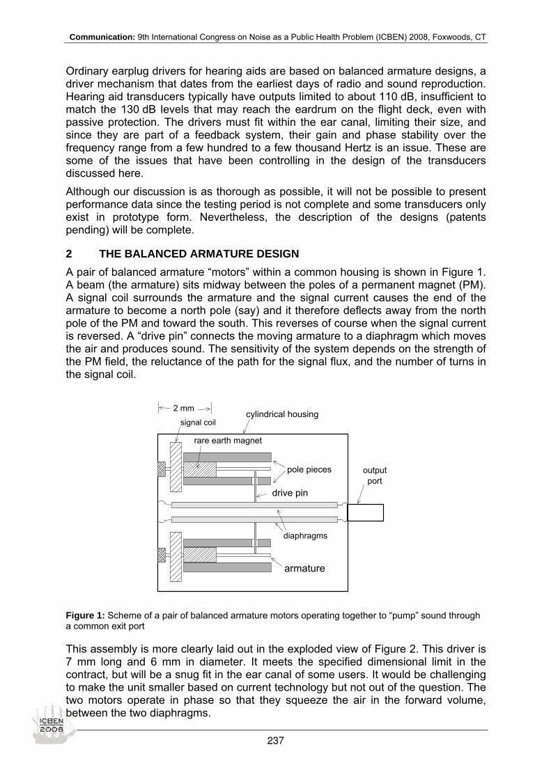
Communication: 9th International Congress on Noise as a Public Health Problem (ICBEN) 2008, Foxwoods, CT
Ordinary earplug drivers for hearing aids are based on balanced armature designs, a driver mechanism that dates from the earliest days of radio and sound reproduction. Hearing aid transducers typically have outputs limited to about 110 dB, insufficient to match the 130 dB levels that may reach the eardrum on the flight deck, even with passive protection. The drivers must fit within the ear canal, limiting their size, and since they are part of a feedback system, their gain and phase stability over the frequency range from a few hundred to a few thousand Hertz is an issue. These are some of the issues that have been controlling in the design of the transducers discussed here. Although our discussion is as thorough as possible, it will not be possible to present performance data since the testing period is not complete and some transducers only exist in prototype form. Nevertheless, the description of the designs (patents pending) will be complete.
2 THE BALANCED ARMATURE DESIGN A pair of balanced armature “motors” within a common housing is shown in Figure 1. A beam (the armature) sits midway between the poles of a permanent magnet (PM). A signal coil surrounds the armature and the signal current causes the end of the armature to become a north pole (say) and it therefore deflects away from the north pole of the PM and toward the south. This reverses of course when the signal current is reversed. A “drive pin” connects the moving armature to a diaphragm which moves the air and produces sound. The sensitivity of the system depends on the strength of the PM field, the reluctance of the path for the signal flux, and the number of turns in the signal coil.
Figure 1: Scheme of a pair of balanced armature motors operating together to “pump” sound through a common exit port
This assembly is more clearly laid out in the exploded view of Figure 2. This driver is 7 mm long and 6 mm in diameter. It meets the specified dimensional limit in the contract, but will be a snug fit in the ear canal of some users. It would be challenging to make the unit smaller based on current technology but not out of the question. The two motors operate in phase so that they squeeze the air in the forward volume, between the two diaphragms.
rare earth magnet
cylindrical housing
pole pieces outputport
diaphragms
drive pin
armature
2 mm
signal coil
237
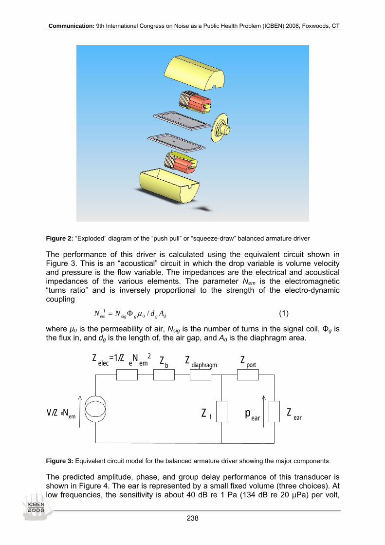
Communication: 9th International Congress on Noise as a Public Health Problem (ICBEN) 2008, Foxwoods, CT
Figure 2: “Exploded” diagram of the “push pull” or “squeeze-draw” balanced armature driver
The performance of this driver is calculated using the equivalent circuit shown in Figure 3. This is an “acoustical” circuit in which the drop variable is volume velocity and pressure is the flow variable. The impedances are the electrical and acoustical impedances of the various elements. The parameter Nem is the electromagnetic “turns ratio” and is inversely proportional to the strength of the electro-dynamic coupling
dggsigem AdNN /01 µΦ=− (1)
where µ0 is the permeability of air, Nsig is the number of turns in the signal coil, Φg is the flux in, and dg is the length of, the air gap, and Ad is the diaphragm area.
Figure 3: Equivalent circuit model for the balanced armature driver showing the major components
The predicted amplitude, phase, and group delay performance of this transducer is shown in Figure 4. The ear is represented by a small fixed volume (three choices). At low frequencies, the sensitivity is about 40 dB re 1 Pa (134 dB re 20 µPa) per volt,
V/Z e N em
Z elec =1/Z e N em 2 Zb Z diaphragm
Z f
Zport
Z ear pear
238

Communication: 9th International Congress on Noise as a Public Health Problem (ICBEN) 2008, Foxwoods, CT
dropping off 30 dB at 5 kHz. The phase shift is about 1 radian at low frequencies due to the electrical impedance of the signal coil, a matter of concern since the transducer is part of a feedback system. The group delay shows peaks at the internal acoustic resonances of the transducer.
Figure 4: Performance of the push-pull balanced armature driver calculated using the model in Figure 3. Low frequency sensitivity is about 130 dB/volt
3 THE PIEZOELECTRIC BIMORPH DESIGN In the ‘70’s a new class of electrostrictive ceramics was discovered based on single crystal solutions of lead titanate in lead-magnesium-niobate ((1-x)PMN-xPT). When polarized, these materials have electromechanical strain coefficients dij several times greater than polycrystalline lead-zirconate-titanate (PZT) and fracture strains greater than 1 %. Example properties of this material are presented in Table 1 for 0.30. Because of our desire for greater output of the driver, it was decided to use this material in the design.
102
103
104
-10
0
10
20
30
40
50
Magnitude of push-pull balanced armature driver TFs, working into trapped volume only
dB, r
e 1
Pa/
Vol
t
trapped vol. = 0.1cctrapped vol. = 0.5cctrapped vol. = 1cc
102 103 104-10
-8
-6
-4
-2
0
2(unwrapped) Phase of push-pull balanced armature driver TFs, working into trapped volume only
radi
ans
trapped vol. = 0.1cctrapped vol. = 0.5cctrapped vol. = 1cc
102 103 104-0.5
0
0.5
frequency in Hz
mse
cs.
Group delays for the push-pull balanced armature driver TFs above, working into trapped volume only
trapped vol. = 0.1cctrapped vol. = 0.5cctrapped vol. = 1cc
239

Communication: 9th International Congress on Noise as a Public Health Problem (ICBEN) 2008, Foxwoods, CT
Table 1: Comparison of electrical and mechanical properties of PZT and PMN-PT
Property PZT PMN-0.35PT
Dielectric constant 1300-3000 5500-7500
Loss factor (electrical) 0.004-0.02 <0.01
d13 (pC/N) 60-200 ~800-1000
Max reverse field 5 – 15 kV/cm 2 kV/cm
Fracture stress (MPa) 60-75 (~0.1 % strain) ~300 (~2.5%strain; polished)
Curie temp 190-375° C 140 – 160° C
Density (kg/m3) 8000 8000
Modulus (GPa) 48-77 ~ 12
Mech. loss factor 0.001-0.07 0.025
The bimorph push-pull design is shown in Figure 5 in both exploded and cutaway drawings. Each bimorph element consists of a pair of PMN-PT plates with a common center signal electrode and upper and lower (outer) electrodes at ground potential. The plates are polarized so that the applied voltage causes the upper plate to stretch and the lower to shrink (and vice versa) through the d13 coupling. These elements are mounted on a frame that forms the common forward volume as in the balanced armature design. The displaced air travels out through the port into the ear cavity. The equivalent circuit model shown in Figure 6 contains many of the same elements as in Figure 3, although the layout for the electrical elements is different because this is a form of an electrostatic transducer with a conversion “turn ratio” Nes. This parameter, as in the case of the electro-dynamic transducer, is inversely proportional to the strength of the coupling:
2213
1 /8 pes hDkdN =− (2)
where d13 is the electro-static strain parameter, D is the bending rigidity of the element, k is a shape parameter for the bending mode, and hp is the piezoelectric plate thickness. The product d13D is called a piezoelectric stress coefficient.
240

Communication: 9th International Congress on Noise as a Public Health Problem (ICBEN) 2008, Foxwoods, CT
Figure 5: Earplug driver using a pair of piezoelectric bimorph elements in the push-pull configuration
Figure 6: Equivalent circuit model for the bimorph piezoelectric driver
The calculated performance for a transducer having the same external dimensions as the balanced armature design is shown in Figure 7. At low frequencies, the sensitivity is about 1 Pa/volt or 94 dB/volt, about 40 dB less sensitive than the balanced armature design. This means it will take about 63 volts of signal to produce the desired 130 dB of output. However, the response is quite flat, so that at 5 kHz it is only 10 dB less sensitive than the balanced armature design. The electrical impedance of the transducer (that of a small capacitor) means there is no phase shift when the load is a simple cavity until the mechanical resonance of the bimorph element at 8 kHz is reached.
V/Nes Ze/Nes2
ZbZdiaphragm
Zf
Zport
Zearpear
241

Communication: 9th International Congress on Noise as a Public Health Problem (ICBEN) 2008, Foxwoods, CT
Figure 7: Performance of the push-pull piezoelectric bimorph driver calculated using the model in Figure 6. Low frequency sensitivity is about 95 dB/volt
4 SUMMARY AND CONCLUSIONS Both the balanced armature and the piezoelectric bimorph designs appear promising as drivers for the ANR earplugs. Each has its limitations and advantages, but the bimorph design has a unique advantage. It is simpler in construction, and can be made smaller if desired, a property not shared with the balanced armature design.
102
103
104
-30
-20
-10
0
10
20
30
40Magnitude of push-pull PZT bimorph plate driver TFs, work ing into trapped volume only
dB, r
e 1
Pa/
Vol
t
t rapped vol. = 0.1cctrapped vol. = 0.5cctrapped vol. = 1cc
102
103
104
-12
-10
-8
-6
-4
-2
0
2(unwrapped) Phase of push-pull PZT bimorph plate driver TFs, work ing into trapped volume only
radi
ans
t rapped vol. = 0.1cctrapped vol. = 0.5cctrapped vol. = 1cc
102 103 1040
0.2
0.4
0.6
0.8
1
frequency in Hz
mse
cs.
Group delays for the push-pull PZT bimorph plate driver TFs above, work ing into trapped volume only
trapped vol. = 0.1cctrapped vol. = 0.5cctrapped vol. = 1cc
242

Communication: 9th International Congress on Noise as a Public Health Problem (ICBEN) 2008, Foxwoods, CT
Evaluation of short-time speech-based intelligibility metrics
Karen L. Payton*, Mona Shrestha
University of Massachusetts Dartmouth, 285 Old Westport Rd., N. Dartmouth, MA 02747
*corresponding author: e-mail: [email protected]
INTRODUCTION
The Speech Transmission Index (STI) is based on acoustic measurements in envi-ronments and has been shown to be correlated with speech intelligibility under a wide range of acoustic conditions (Houtgast & Steeneken 1984). It is a weighted average of metrics derived from envelope signals in multiple frequency bands spanning the speech spectrum. A variety of methods have been proposed to compute the STI (Houtgast & Steeneken 1971; Steeneken & Houtgast 1980; Ludvigsen 1987; Drull-man et al. 1994a, b; Payton et al. 1994; Drullman 1995; IEC 1998; Payton & Braida 1999; Payton et al. 2002; Goldsworthy & Greenberg 2004). Some of these methods use speech as the test stimulus rather than artificially modulated noise as originally proposed by Houtgast and Steeneken (1985). Many of the speech-based techniques have been shown to provide the same result as the traditional STI (Ludvigsen et al. 1990; Payton et al. 2002), which is based on modulation reductions in intensity-modulated noise and as a theoretically derived STI which is obtained from weighted signal-to-noise ratios (SNRs) in seven octave bands and room reverberation time (RT) (Houtgast & Steeneken 1985). To date, all speech-based approaches have used speech materials lasting at least a minute or two to generate metrics correlated with long-term speech intelligibility. Consequently, they have not been used to predict short-time changes in intelligibility due to time-varying environments such as fluctuat-ing background noise. The current work investigates the ability of two speech-based methods to track short-term STI results by using speech segments of various lengths to compute results for environments with stationary speech-shaped noise, speech-shaped noise plus reverberation or multi-talker babble. The methods that will be evaluated are the Envelope Regression (ER) and the Normalized Correlation (NC) methods. The ER method is based on the speech-based STI method proposed by Ludvigsen et al. (1990). The NC method was proposed by Goldsworthy and Green-berg (2004) who also analyzed the long-term characteristics of both metrics.
METHODS
Figure 1 depicts a block diagram of the signal processing steps used to obtain the results for the speech-based algorithms. Specifically, for both the ER and NC tech-niques, the clean and the degraded signals, originally digitized at 20 kHz with a 9.5 kHz antialiasing filter, were digitally filtered using a bank of 6th order octave-wide Butterworth band-pass filters with center frequencies from 125 Hz – 4 kHz and a 6th-order Butterworth high-pass filter with a cutoff frequency of 6 kHz. For each band, i, the clean and the degraded signals were then squared and low-pass filtered with a cut off frequency of 50 Hz. The lowpass filter impulse response was a 10 ms Ham-ming window. The intensity envelopes, xi (t) and yi (t), were down-sampled to 134 Hz (a factor of 49) to reduce computation time without risking aliasing. Next, for each octave band, a modulation metric, Mi, was calculated from the intensity envelopes. Each approach used a different algorithm to compute this modulation metric.
243

Communication: 9th International Congress on Noise as a Public Health Problem (ICBEN) 2008, Foxwoods, CT
Figure 1: Block diagram of signal processing steps necessary to compute speech-based intelligibility metrics
For the Envelope Regression (ER) method, the modulation metric for each band was computed from the envelope signals using Eqn (1):
( )( ){ }
( ){ }2)(
)()(
xii
yiixii
yixi
ikxE
kykxEM
µ
µµµµ
−
−−= (1)
where µxi and µyi are the means of xi(t) and yi(t) respectively. For the Normalized Correlation (NC) method, Mi was computed using Eqn (2):
{ }{ } { })()(
)()(22
2
kyEkxEkykxEMii
iii
⋅
⋅= (2)
(Goldsworthy & Greenberg 2004).
Once the modulation metrics were computed, the apparent signal-to-noise ratio in each band, aSNRi, was computed as
⎟⎟⎠
⎞⎜⎜⎝
⎛−
=i
ii M
MaSNR1
log10 10 (3)
and then clipped to the range of -15 to +15 dB. The apparent SNR in each band was converted to a transmission index, TIi, according to Eqn (4):
30
15+= i
iaSNRTI (4)
Finally, the overall STI value (ranging from 0 to 1) was calculated as a weighted sum of the TIi values:
∑ ∑= =
+×−=7
1
6
11
i iiiiii TITITISTI βα (5)
HP FilterCutoff=6 kHz
Envelope Extraction
Clean Degraded
Octave BP Filters CF=125 Hz
.......
.......
.......
.......
.......
.......
SquareLP Filter
Cutoff=50 Hz Modulation
Metric
M1 aSNR1
aSNR7
TI1
TI7
STI
Clean Degraded
X1
Y7
Y1
X7
M7
244

Communication: 9th International Congress on Noise as a Public Health Problem (ICBEN) 2008, Foxwoods, CT
where the αi’s represent the octave weighting factors and the βi’s represent the re-dundancy correction factors given in the IEC standard (IEC 1998).
Short-Time Implementation Issues
For both the ER and NC methods, sample means of the windowed envelope signals were calculated. Correlations were calculated as biased estimates:
( ) ( ){ } ( ) ( )[ ]∑=
=N
kiiii kykx
NkykxE
1
1 and ( ){ } ( )∑
==
N
kii kx
NkxE
1
22 1 (6)
where N was the window length (in samples). These correlation values were used directly in Eqn (2) for the NC method. The cross- and auto-covariances needed for the ER method were calculated from the correlation estimates of Eqns. (6) as
( )( ) ( )( ){ } ( ) ( ){ } yixiiiyiixii kykxEkykxE µµµµ .−=−− and
( )( ){ } ( ){ } 222xiixii kxEkxE µµ −=− (7)
and used in Eqn. (1). Window lengths were adjusted from 107 sec (length of 50 con-catenated sentences) down to 78 ms for the analyses presented below. Windows were overlapped by 75 %.
Theoretical STI
In order to compare the short-time metrics with the “true” STI, the theoretical STI was also calculated over the same time windows as the short-time metrics. The speech and the noise (as opposed to the degraded speech) were separately passed through the octave-band filter bank shown in Figure 1 and within-band powers used to get signal to noise ratio (Si/Ni in Eqn (8)) in each band. The modulation index in each band, Mi(F), was then calculated as specified by Steeneken and Houtgast (1980):
⎟⎟⎟
⎠
⎞
⎜⎜⎜
⎝
⎛
+⎟⎟⎟⎟⎟
⎠
⎞
⎜⎜⎜⎜⎜
⎝
⎛
⎟⎠⎞
⎜⎝⎛+
= −10
/2101
1
8.1321
1)(ii NSi
FTFM
π (8)
The first term in Eqn (8) estimates the modulation reduction due to reverberation. The variable F corresponds to modulation frequency (between 0.63 and 25 Hz) and T cor-responds to the reverberation time of the environment (T60). The second term esti-mates the reduction due to additive noise. The theoretical STI was computed by sub-stituting Mi(F) for Mi in Eqn (3), the variable aSNRi(F) was averaged across F after clipping to obtain aSNRi.
245

Communication: 9th International Congress on Noise as a Public Health Problem (ICBEN) 2008, Foxwoods, CT
Stimuli
The stimuli used in this study were 50 concatenated nonsense sentences, spoken conversationally by a male talker totaling 107 s of speech (Payton et al. 1994). These nonsense sentences are grammatically correct but do not provide any semantic con-text to help word identification, e.g., “His guests could teach his turnpike”. Each sen-tence consists of four to eight key words (underlined in example) where the key words consist of the nouns, adjectives, verbs and adverbs in the sentence.
Degradation Conditions
Three environmental degradations were evaluated: stationary speech-shaped noise, stationary noise plus simulated reverberation and multi-talker babble. The speech-shaped noise was generated by filtering white Gaussian noise to approximate the average long-term spectra of speech (Payton et al. 1994). The noise was added to the speech at an average SNR of 0dB. For the noise plus reverberation condition, speech plus noise at 0 dB SNR was convolved with a simulated conference room impulse response (Peterson 1986; Payton et al. 1994). The multi-talker babble was taken from a recording of restaurant noise. The babble also was added to the speech at 0 dB SNR.
RESULTS
Results from both the ER and NC methods were compared with the theoretical STI for each degradation condition as functions of window length. Linear regression analyses also were carried out for the metrics and theoretical STI results. For the re-gression analyses, results for two window lengths are presented. The 0.3 s window results are typical of all the longer windows. The 78 ms window is presented to show a window for which the metrics deviate from the theoretical STI during silent intervals.
Zero dB SNR with Stationary Speech-Shaped Noise
The results for each method over the length of one sentence are plotted as functions of time in Figure 2.
0
0.5
1Theoretical STI
0
0.5
0
STI
ER Method
0 0.5 1 1.50
0.5
0
Time (s)
NC Method
107s 1.2s 0.6s 0.3s 0.16s 78ms LT STI
Figure 2: Metric results vs. window length (top) theoretical STI (center) ER method and (bottom) NC method for 0 dB SNR stationary speech-shaped noise condition. Different curve types represent re-sults with different window lengths as given in the legend. The black dotted line in each plot represents the long-term STI.
246

Communication: 9th International Congress on Noise as a Public Health Problem (ICBEN) 2008, Foxwoods, CT
For visual reference, an SNR of 0 dB corresponds to an STI value of about 0.5 (the exact value depends on the spectral characteristics of the speech and noise). Both the ER and NC metrics (center and bottom plots respectively) generally matched lo-cal fluctuations in the theoretical STI (top plot) for each window length and the ER result for entire corpus (blue line in center plot) matched the long-term STI (black dot-ted line) exactly. The ER method tracked the theoretical STI more closely than the NC method for all window lengths analyzed. For all window lengths, the NC method predicted slightly higher values than either the ER method or the theoretical STI in agreement with long-term results of Goldsworthy and Greenberg (2004).
Once window length was decreased to 78 ms (tan dashed lines), both the ER and NC methods deviated greatly from the theoretical STI at the beginnings and ends of sentences. Where the theoretical STI was zero because only noise was present (SNR = -∞ dB) both metrics often generated non-zero results.
Figure 3 plots linear regression analyses of metric results versus theoretical STI for two window lengths: 0.3 s (top row) and 78 ms (bottom row). Each data point repre-sents the results for a single window. Regression lines and the goodness of fit (R2) statistics are also shown for each window length. As can be seen from the figure, the ER method results (left column) closely match the theoretical STI for the 0.3 s win-dow, indicated by the R2 statistic of 0.99. The results are also close for the 78 ms window (R2=0.91). However, for the 78 ms window, some of the ER results were above zero on the y-axis which means that, during the silent intervals, when the theo-retical STI was zero the ER method sometimes generated values greater than zero (up to 0.4).
0
0.5
1
Spe
ech-
Bas
ed M
etric
ER0.3 s
0 0.5 00
0.5
0
Theoretical STI
78 ms
0.3 sNC
0 0.5 1
78 ms
Figure 3: Metrics computed from ER (left column) and NC (right column) methods vs. theoretical STI for 0 dB SNR using 0.3 s windows (top row) and 78 ms windows (bottom row). The solid lines repre-sent best linear fits to the data.
The NC method regression analysis results are shown in the right column of Figure 3. This method predicted higher values than the theoretical STI for all window lengths as can be seen by the upward shift of the linear regression lines from the main di-agonal. The R2 statistic of 0.96 for 0.3 s window shows that, despite this shift, the NC method followed the theoretical STI quite closely. For the 78 ms window, the metric did not perform as well. The R2 statistic is also reduced (0.62) in part because, when the theoretical STI was zero, the NC method generated values ranging from 0.1 to 0.8.
R2=0.99
R2=0.91
R2=0.96
R2=0.62
247

Communication: 9th International Congress on Noise as a Public Health Problem (ICBEN) 2008, Foxwoods, CT
In order to study how well, on average, the short-time metrics match the long-term theoretical STI over the range of window lengths, the metrics and theoretical STI were averaged over the entire speech corpus (107 s) for each window length. The averages are plotted in Figure 4 as functions of window length. In the figure, the solid red line represents ER method averages, the blue dash-dot line represents the NC method averages and the black dotted line represents the theoretical STI.
It can be seen that ER method produced the same average value as the theoretical STI over virtually the entire window range studied. The averages for all metrics de-creased as the window was decreased. This is because voiced speech segments dominated the metric results and when the windows were shortened to the point that some windows contained primarily unvoiced and/or silent intervals then the results for those windows were significantly reduced. The leftmost data points are for the 78 ms window. For that window length, the ER did not decrease quite as much as the theo-retical STI and the NC method actually increased slightly.
0 2 4 6 8 100
0.2
0.4
0.6
0.8
1
Length of Window (s)
Met
ric A
vera
ge
ER MethodNC MethodTheoretical STI
Figure 4: Metric averages computed over entire speech corpus for speech in 0 dB stationary speech-shaped noise, as functions of window lengths.
Zero dB SNR Plus Reverberation
When reverberation was added to the noisy speech, the metrics generated values that varied more widely when compared to the theoretical STI. In Figure 5, metrics are plotted (ER on the left and NC on the right) versus the theoretical STI for the two window lengths. The 0.3 s window results are plotted in the top row and the 78 ms results in the bottom row. As before, each symbol corresponds to a single window result, linear regression lines are overlaid on the data and the goodness of fit statis-tics are shown.
248

Communication: 9th International Congress on Noise as a Public Health Problem (ICBEN) 2008, Foxwoods, CT
0
0.5
1
Spe
ech-
Bas
ed M
etric
0.3 s
ER
0 0.5 00
0.5
0
Theoretical STI
78 ms
0.3 s
NC
0 0.5 178 ms
Figure 5: Metrics computed from ER (left column) and NC (right column) methods vs. theoretical STI for 0 dB SNR plus reverberation using 0.3 s windows (top row) and 78 ms windows (bottom row). The solid lines represent best linear fits to the data.
It can be seen from Figure 5 that, for the 0.3 s window, the results from both methods tracked the theoretical STI fairly closely although the ER method predicted values that were, on average, slightly lower than the theoretical STI across the range. The NC method predicted higher values than the theoretical at the low STI end and lower values at the high STI end. The corresponding R2 statistics are 0.79 and 0.69 for the ER and NC methods respectively. For the 78 ms window, the results are much more divergent (R2=0.35 and 0.18 respectively indicating very poor correlations). In particu-lar, when the theoretical STI was zero, both metrics generated results that varied over a wide range (0 to 0.4 for the ER method and 0.1 to 0.8 for the NC method). Furthermore, there appears to be a nonlinear relation such that the metric values de-viated from the linear regression line more at the higher STI values.
Averages for both methods and the theoretical STI as functions of window length are given in Figure 6. The solid red line plots the ER method averages, the blue dash-dot line shows the NC method and the black dotted line represents the theoretical STI.
0 2 4 6 8 100
0.5
1
Length of Window (s)
Met
ric A
vera
ge
ER MethodNC MethodTheoretical STI
Figure 6: Metric averages computed over entire speech corpus for speech in 0 dB stationary speech-shaped noise plus reverberation, as functions of window length.
R2=0.79
R2=0.35
R2=0.69
R2=0.18
249

Communication: 9th International Congress on Noise as a Public Health Problem (ICBEN) 2008, Foxwoods, CT
It can be seen from Figure 6 that, for the noise plus reverberation condition, the ER method generated values that paralleled but were consistently less than the theoreti-cal STI for all window lengths. It should also be noted that, as for the speech plus noise condition, the NC method actually increased for the shortest windows while the ER and theoretical STI continued to decrease.
Zero dB SNR with Multi-Talker Babble
As for the prior two conditions, metric results are plotted against the theoretical STI in Figure 7 and a linear regression analysis is performed for each plot. It can be seen from the left column in the figure that the STI from ER method is highly correlated with the theoretical STI for the 0.3 s window where R2=0.93 while data is much more scattered for the 78 ms window for which R2=0.84. As was observed for the other conditions, when the theoretical STI produced values near zero, the ER values cov-ered a wide range, in this case from 0 to 0.8.
0
0.5
1
Spe
ech-
Bas
ed M
etric
0.3 s
ER
0 0.5 00
0.5
0
Theoretical STI
78 ms
0.3 s
NC
0 0.5 178 ms
Figure 7: Metrics computed from ER (left column) and NC (right column) methods vs. theoretical STI for 0 dB SNR multi-talker babble using 0.3 s windows (top row) and 78 ms windows (bottom row). The solid lines represent best linear fits to the data.
Regression analysis results for the NC method are shown in right column of Figure 7. The R2 statistic of 0.93 for the 0.3 s window indicates that the NC method followed the theoretical STI fairly closely although the values it generated were consistently greater than the theoretical STI. For the 78 ms window, when the theoretical STI generated values below 0.1, the NC method results ranged from 0.1 up to 0.8 and R2=0.74. When the asymptotic behavior of the metrics was analyzed for speech plus multi-talker babble, the plots were identical in shape to Figure 4, just shifted up slightly to asymptote at 0.6 for the theoretical STI and ER method and 0.8 for the NC method (plot not shown due to space constraints).
CONCLUSIONS
The data presented have demonstrated the ability of two short-time, speech-based, metrics to accurately track short-term fluctuations in STI down to window lengths of 0.3 s for two different noise environments and a noise plus reverberation environ-ment. Because these metrics are speech based, they have the potential to be used in a wide variety of settings to estimate speech intelligibility under conditions not ame-
250

Communication: 9th International Congress on Noise as a Public Health Problem (ICBEN) 2008, Foxwoods, CT
nable to standard intelligibility measurement techniques such as during live perform-ances. Further investigation is underway to analyze the 78 ms window results more thoroughly.
ACKNOWLEDGEMENTS
This work was supported by NIDCD grant RO1-DC007152.
REFERENCES Drullman R (1995). Temporal envelope and fine structure cues for speech intelligibility. J Acoust Soc Am 97: 585-592.
Drullman R, Festen JM, Plomp R (1994a). Effect of reducing slow temporal modulations on speech reception. J Acoust Soc Am 95: 2670-2680.
Drullman R, Festen JM, Plomp R (1994b). Effect of temporal envelope smearing on speech reception. J Acoust Soc Am 95: 1053-1064.
Goldsworthy RL, Greenberg JE (2004). Analysis of speech-based speech transmission index methods with implications for nonlinear operations. J Acoust Soc Am 116: 3679-3689.
Houtgast T, Steeneken HJM (1971). Evaluation of speech transmission channels by using artificial signals. Acustica 25: 355-367.
Houtgast T, Steeneken HJM (1984). A multi-language evaluation of the RASTI-method for estimating speech intelligibility in auditoria. Acustica 54: 185-199.
Houtgast T, Steeneken HJM (1985). A review of the MTF concept in room acoustics and its use for estimating speech intelli-gibility in auditoria. J Acoust Soc Am 77: 1069-1077.
Houtgast T, Steeneken HJM, Plomp R (1980). Predicting speech intelligibility in rooms from the Modulation Transfer Function I. General room acoustics. Acustica 46: 60-72.
IEC (1998). Sound system equipment - Part 16: Objective rating of speech intelligibility by speech transmission index. 2nd Ed, Internat. Standard No. 60268-16, International Electrotechnical Commission.
Ludvigsen C (1987). Prediction of speech intelligibility for normal-hearing and cochlearly hearing-impaired listeners. J Acoust Soc Am 82: 1162-1171.
Ludvigsen C, Elberling C, Keidser G, Poulsen T (1990). Prediction of intelligibility of non-linearly processed speech. Acta Otolaryngol Suppl 469: 190-195.
Payton KL, Braida LD (1999). A method to determine the speech transmission index from speech waveforms. J Acoust Soc Am 106: 3637-3648.
Payton KL, Uchanski RM, Braida LD (1994). Intelligibility of conversational and clear speech in noise and reverberation for listeners with normal and impaired hearing. J Acoust Soc Am 95: 1581-1592.
Payton KL, Braida LD, Chen S, Rosengard P, Goldsworthy R (2002). Computing the STI using speech as a probe stimulus. In: v. Wijngaarden, SJ (ed.): Past, present and future of the SpeechTtransmission Index (pp 97-119). TNO Human Factors, The Netherlands.
Peterson PM (1986). Simulating the response of multiple microphones to a single acoustic source in a reverberant room. J Acoust Soc Am 80: 1527-1529.
Steeneken HJM, Houtgast T (1980). A physical method for measuring speech-transmission quality. J Acoust Soc Am 67: 318-326.
251
Communication: 9th International Congress on Noise as a Public Health Problem (ICBEN) 2008, Foxwoods, CT
Speech recognition in fluctuating background noise in presence of envelope and fine structure cues: Implications in cochlear implants Muhammed Ayas*, Imran Dhamani, B. Rajashekhar
Manipal University
* corresponding author: e-mail: [email protected]
Speech perception mainly depends on the perception of the envelope and fine structure cues embedded in the speech signal. Cochlear Implant is a prosthetic device used for patients with severe to profound sensorineural hearing impairment. Perception of speech in individuals using a cochlear implant is primarily through envelope based cues. One of the major challenges faced in cochlear implant technology is to improve the perception of pitch and speech in noise. Previous studies revealed that the Cochlear implantees exhibit better speech perception in the presence of steady state noise compared to fluctuating background noise which can be attributed to factors like poor frequency selectivity, frequency resolution, absence of fine structure cues, and poor pitch perception. Speech enhancement techniques like envelope enhancement and providing fine structure cues may improve the perception of speech in the presence of fluctuating background noise. The current study aims to study the speech perception in steady state noise and fluctuating background noise under simulated conditions. In addition, the effect of providing additional fine structure cues to improve speech perception in noise were also studied. The study consisted of four simulated conditions. Speech recognition in each condition was assessed by using Phonetically Balanced (PB) words. Results revealed poor performance in speech recognition in the presence of fluctuating background noise. The clinical implication of this study, especially in relation to the cochlear implantees will be further discussed.
252

__________________________________________________________________________
__________________________________________________________________________
ICBEN 2008
Noise and Communication
253

Communication: 9th International Congress on Noise as a Public Health Problem (ICBEN) 2008, Foxwoods, CT
The unexamined rewards for excessive loudness Barry Blesser*, Linda-Ruth Salter Blesser Associates, P. O. Box 155, Belmont, MA 02478, USA
*corresponding author: e-mail: [email protected]
INTRODUCTION Throughout the centuries and across cultures, the battle to reduce disruptively loud sound has met uneven success, even though the social and biological consequences are well known. As far back as the 14th century, an anonymous European poet complained of excessive street noise (Gimpel 1977). An 18th century print by William Hogarth, The Enraged Musician, depicts indignation when street sounds invade his studio. Thompson (2002) provides a summary of the political failure to manage noise pollution beginning in the late 19th century. Recent studies reveal that personal knowledge about the dangers of loud music is frequently insufficient to change behavior (Miller et al. 2007; Rawool & Colligon-Wayne 2008). Other studies described the physical, social, cognitive, and emotional consequences of hearing disabilities (Arlinger 2003; Zimbardo et al. 1981; Roth 1955), which often result from repeated exposure to loud sound. Although social and medical experts have experimented with different strategies for changing attitudes toward damagingly high sound levels, success has been, at best, uneven. There are numerous examples where individuals willingly choose to immerse themselves in recreational sound fields that destroy hearing. In these venues, sound levels are well above the limits set for occupational settings. Examples include popular music concerts, advertising in cinema theaters, battles in aggressive video games, corrosive acoustics in restaurants, amplified music in dance clubs, motorcycles with disabled mufflers, enhanced automobile sound systems, and portable music devices with a direct connection to the ear canal. In many of these venues, the result is self-inflicted damage to the auditory system. To strengthen the battle against disruptive noise, we suggest reversing the question: rather than focusing exclusively on the dangers of loudness, we ask why individuals consciously choose to immerse themselves in destructively loud sound fields, especially in recreational venues? Discussions about the negative consequences of these environments are incomplete if we do not acknowledge that excessive loudness produces personal rewards. A review of the literature reveals two major classes of rewards, which we call Altered States of Consciousness and Controlling the Experience of Social Space. In both cases, individuals use loudness as a means of influencing their interior and exterior environments. Loud sound carries symbolic meaning, representing such qualities as energy, dominance, spatial ownership, and the psychological freedom to be transported to another place. Because loud music has more emotional impact than soft music, loudness intensifies sensory experience and manipulates listeners’ emotional states. In addition, loudness is an important mechanism for achieving social and spatial control by overriding social interactions and physical boundaries. We argue that there exists a personal reward system for loudness, and that its existence explains the difficulty in changing behavior. Positive rewards suppress recognition of the negative consequences. Moreover, the rewards are immediate, while the costs are subtle and delayed for years. This time imbalance skews the
254

Communication: 9th International Congress on Noise as a Public Health Problem (ICBEN) 2008, Foxwoods, CT
trade-off between damage and pleasure. Based on the behavior of individuals in the 21st century, we appear to be loosing the battle. When a culture accepts loudness as being a legitimate right in recreational sound venues, that acceptance tends to legitimize all forms of noise pollution. As a culture with advancing sonic tools and amplification, there are increasing opportunities to be immersed in destructively loud sound fields. We believe that acceptance of loudness in entertainment then carries over to a tolerance of disruptive noise from airplanes, jackhammers, powered garden equipment, and so on. Loudness becomes the cultural norm. We hope that understanding the rewards of loudness will lead to better strategies for changing our culture.
Loudness connects evolution, biology and culture The roles of the various senses depend on culture rather than being a biological imperative. In earlier cultures, hearing was the dominant sense for experiencing the world (Howes 1991; Ong 1982). Hearing can only be understood when cultural relativism is also included, which is part of sensory anthropology. The Hausa people, for example, recognize only two senses: seeing and experiencing life, which itself encompasses intuition, emotion, smell, touch, taste, and sound (Ritchie 1991). They use vision primarily for avoiding obstacles. Even in the 20th century, rural citizens relied on sound for connecting to events (Schafer 1978). Because sound flows over long distances, and because it is not obscured by objects, hearing was a critically important means of survival for early humans. Sound allows for the detection of objects and dynamic events without depending on light. The auditory system for mammals is active 24/7 because there is neither the equivalent of ear-lids nor controlled focus. Loudness is a measure of distance, power, and relevance. For example, both running elephants and falling boulders have high energy levels and are more likely to pose a threat than low energy events. As a species, we are wired to have a strong response to loud sound because intensity is an indicator of a significant dynamic event that is nearby and/or of high energy level. The linguistic label of “size” for typical environmental sounds includes the dimension of loudness (Kidd and Watson 2003). In addition, by detecting important sonic events, the auditory system can steer the visual system to focus on the location of critical important events. Knowing about such events had survival value. Loudness is so important that there are brain substrates that are particularly sensitive to rising sound intensity, which serves as an early warning that a sonic event will become loud. From an evolutionary perspective, estimating the rate of arrival of approaching sound-sources (such as dangerous animals) in natural environments had survival value. Seifritz et al. (2002) commented: “The prioritization of rising sound intensity…modulates attentional and space recognition processes and, as such, is likely to provide an adaptive advantage.” In combining knowledge of neurobiology, musicology, and psychology, Huron (2006) offers a unifying theory. In his view, human emotions arise from an activation of the brain stem (so called reptilian brain) to produce biological readiness for a flight, fight, or freeze response. But after a sensory trigger prepares the organism for one of these fast responses (arousal), the high level cortex may then assess the situation as being innocuous. Arousal unconsciously originates as fear, even when we consciously know that there is no danger. This is perhaps akin to the fearful pleasure of riding a roller coaster or watching a scary movie. Since the auditory system is connected to numerous other brain substrates, loud sound is a major source of
255

Communication: 9th International Congress on Noise as a Public Health Problem (ICBEN) 2008, Foxwoods, CT
arousal, which is then experienced as a positive emotion. Increasing the intensity of a sound, which elevates arousal, then increases the magnitude of the physiologic response.
Altered states of consciousness While the phrase “altered state of consciousness” acquired a negative meaning during the drug culture of the 1960s, we all engage in manipulating our emotional and psychological state whenever we choose particular stimuli. From this perspective, there is no unaltered state of consciousness because all stimuli, be they exercise, sunshine, sugar, alcohol, or music, change an individual’s internal emotional and psychological state. We depend on a sensory connection to the external world. When fully deprived of sensory input, psychological disintegration takes place within a few minutes (Cohen et al. 1965); sanity requires sensory stimulation. Strong personalities are well aware of their ability to manipulate the emotional state of others through sound. The role of a shaman, especially in the use of music for creating trance states, has a long history that can be traced back to the ancient Greeks (Rouget 1985). Preachers, politicians, disc jockeys, salesmen, and demagogues manipulate people with sound that appeals to their unconscious sensitivities. Independently of the message’s content, loudness communicates an orator’s passion, sincerity, and conviction. Musicians and composers use sound intensity as a musical attribute that complements pitch and timbre. Patel (1996) noticed that a message on the inside cover of the album Disintegration, advises that “this music has been mixed to be played loud so turn up the volume.” Composers of western music use increases in sound intensity to influence the listener’s internal state (Huron 1992). Berlyne (1961, 1971) theorizes that stimulus preference is a function of physiological arousal, which depends on intensity. Sounds that are complex and intense increase arousal and are generally preferred over simplistic and weak sounds. For both music and speech, loud excerpts were judged as being more pleasant, energetic, and tense than soft excerpts (Ile & Thompson 2006). Loud music produces high levels of arousal, especially when the music matches the individual’s preference (Gowensmith & Bloom 1997). Changes in the emotional state are often observed with concomitant changes in physiology. Huron (2006) observed that the phenomenon of music-induced “chills and goose bumps,” called frisson, depends on loudness. Excitative music produces feelings of vigor and tension, accompanied by the physiological responses of increased heart rate, respiration, and blood pressure (Iwanaga & Moroki 1999). Tolerance to pain shifts with music (Mitchell & MacDonald 2006). Increased loudness of music makes time appear to slow down and events to last longer (Kellaris 1996). Loudness changes an individual’s psychology and behavior. Loudness represents power, which may be a form of machismo, like flexing muscles. Fligor & Ives (2007) observed that men prefer louder music than women. Rentfrow & Gosling (2003) suggest that “individuals who listen to heavy metal music at loud volume with their car windows rolled down may be trying to convey a ‘tough’ image to others.” A motorcyclist driving through a suburban town at 3 o’clock in the morning is clearly demonstrating his power to wake a large number of people. By raising the arousal state, loud music increases the quantity of alcohol consumption among adolescents (van de Goor et al. 1990). Males consume more alcohol than females when listening
256

Communication: 9th International Congress on Noise as a Public Health Problem (ICBEN) 2008, Foxwoods, CT
to loud music (Guéguen et al. 2004). Young tennis players consciously selected music to elicit various emotional states to improve their mood, increase arousal, and provoke imagery (Bishop et al. 2007). A study of music levels during aerobic exercise revealed that music intensity was related to enjoyment and provided an increased motivation to engage in energetic exercise (Wilsont & Herbstein 2003). For those exercising in a quieter class, they reported that the music was too soft, which made them enjoy the class less and not work as hard. Similar results were found in studies of portable walkmans, live concerts and nightclubs: intensity relates to enjoyment and motivation. Disc jockeys, who have control over both the music selection and sound levels in nightclubs venues, willing subject themselves to average sound levels of 96 dB(A) with peaks of 108 dB(A) (Bray et al. 2004). When questioned, more than 50 % of adolescents approved of the sound levels at discotheques that they visited (Weichbold and Zorowaka, 2005). More than 50 % of a sample of listeners at a music festival considered a sound level of 100 dB(A) to be acceptable or too low (Mercier et al. 2003). Curiously, toddlers aged 2 to 3.5 years also show an innate preference for fast and loud music, compared to slow and quiet music (Lamont 2003), perhaps as a form of a self-medicating stimulus. Todd and Cody (2000) provide evidence that activation of the vestibular system may be evoked with sound stimuli above 90 dB and with frequencies between 100 and 300 Hz. Such sound is typical of dance clubs and rock concerts. Moreover, the threshold for vibrotactile sensations is lowest for frequencies of 200 Hz. This is consistent with elevated bass so that listeners can “feel” the music, especially in the context of dancing and synchronized motion. Various researchers have postulated that brain activity and hedonistic stimuli are linked; individuals regulate their level of sensation to achieve optimal hedonic tone (Tucker et al. 1990). Adolescents explain their preference for listening to music at high intensities because it produces bodily pleasure (Vogel et al. 2008). Bill Thompson (2008), a professor of psychology at Macquarie University, explained that people tend to want more of anything that has a positive valence, and loudness is simply a way to amplify the intake of a desired emotion. From their study of the neurological response to emotional music, Blood & Zatorre (2001) commented that “music recruits neural systems of reward and emotion similar to those known to respond specifically to biologically relevant stimuli, such as food and sex, and those that are artificially activated by drugs of abuse.” Increased intensity usually increases the response to positive stimuli. Some young adults who listen excessively to loud music have been observed to have maladaptive patterns similar to that exhibited by substance abusers, such as alcohol addiction (Florentine et al.1998). Some subjects in the study described withdrawal symptoms when trying to stop listening to loud music. Any class of stimuli that creates a pleasurable internal state has the potential to become addictive. Loudness, acting as an intensifier of pleasure can then becomes addictive. Tolstoy (1890), writing in the 19th century, summarizes our view of music at high intensities: “Music makes me forget myself, my true condition, it carries me off into another state of being, one that isn’t my own; under the influence of music I have the illusion of feeling things that I do not feel, of understanding things that I do not understand, being able to do things I’m not able to do.” This quotation is not unlike that of those who describe a psychedelic high on drugs. Loudness amplifies the
257

Communication: 9th International Congress on Noise as a Public Health Problem (ICBEN) 2008, Foxwoods, CT
experience for those who seek this kind of response. It applies not only to music, but also to a passionate sermon, political speech, and gunshot in a video game.
Controlling the experience of social space While sound changes an individual’s emotional and psychological state, such changes are also an adaptation to the environment. Sound connects human beings directly to sonic events, and they both exist in the external environment. On the one hand, spatial acoustics influences our experience of sound sources, and on the other hand, sound is a means of experiencing space itself. As discussed in our recent book (Blesser & Salter 2007) on aural architecture, space and sound cannot be separated. Each sensory modality creates its own sensory space, which need not be consistent with other sensory spaces. A person can exist in a visual space, aural space, tactile space, olfactory space, and so on. To appreciate the difference between an aural and visual space, consider two examples of a box over your head. In the first case, the box is made of glass, while in the second case it is made of black cloth. With a glass box, you have a small aural space but a large visual space, and conversely, with the cloth box, you have a large aural space but a small visual space. Examining aural space is challenging. Sound is ethereal; it does not leave physical evidence of its previous existence; it’s hard to accurately recall; and there are few words to describe it. An aural space is empirical because its boundaries are based on our ability to hear sonic events occurring within it. Aural space exists from the perspective of the listener. If you can hear a sonic event, then it exists within your aural space, but if you cannot hear the event, it is outside your aural space. The boundary delineating the space is thus experiential, rather than physical, and is called the acoustic horizon. There are numerous examples of how the acoustic horizon is determined by the loud sounds. In his study of 19th century French villages, Corbin (1998) described how hearing the town bells were the basis for citizenship. Those that could hear the bells were rooted in the social fabric of the town with enhanced self-esteem and civic pride. Because louder bells created a larger and more powerful community, metallurgy technology was the equivalent of military power in being able to expand the area of the town. You were a citizen of the town if the bells existed within your aural space. In a quiet home, you can hear your footsteps on a hardwood floor and thus your feet are part of your aural space, but in a noisy city you cannot hear your footsteps. Your aural space has shrunk, and your feet are outside your space. Before a concert begins, you can hear the breathing of your friend sitting next to you, but after it begins you hear nothing other than the music. Loud sounds mask all other sounds, thus making a listener functionally deaf to everything else. Before the music, your friend was part of your aural space. Once the music begins, the sound of your friend’s breathing falls outside your acoustic horizon. Loud sounds can capture our perceptual system, often overcoming other sensory information about the physical space. For example, loud music transports listeners from the physical and social space of their surroundings to the musical space of the performers. When the motorist in a car raises the volume of music, he is transported out of the road space and into the virtual space created by musicians and sound engineers. Listening to music with earphones blocks extraneous environmental sounds, transporting the listener to an entertaining music space. In NYC, three people wearing headphones were killed when they unheedingly stepped into the
258

Communication: 9th International Congress on Noise as a Public Health Problem (ICBEN) 2008, Foxwoods, CT
physical space of the street while existing in an experiential musical space. Loudness is a space transporter because people become functionally deaf to their immediate environment if the virtual environment has louder sounds. Advertisers presenting messages on television and before movies raise the volume relative to the regular entertainment. They know that loudness helps to sell because the listener cannot focus on other events. While eyelids provide the individual with voluntary control to select what is being seen, there are no corresponding earlids to control what is being heard. Humans are coupled to their aural space without being able to be in control of its size or its content. Sound often manifests itself in a Darwinian combat: loud sound is like the stronger “animal,” winning the battle over space and resources. Advertisers know that whoever produces the loudest sound controls the space. Musicians performing in a live venue frequently find that they are simultaneously living in two or more spaces. On the one hand, the sound from headphones embeds musicians in their electronic music; on the other hand, environmental sounds connect musicians to real people in a real space. How can a musician transport himself, at will, from one space to the other? To a large extent, the only control mechanism is loudness. The louder space dominates. There is no biological means for controlling sound intensity, but electronic amplification allows headphone space to dominate an environment space. Because loud sound suppresses awareness of the internal space of daydreams, images, and self-generated sounds, people often use sound to help them focus on mental tasks. Petersen (2007) argues that in-ear headphones can be used to make the musical space dominate the environmental space by creating sound levels above 140 dB, which is very dangerous. Such levels are not accidents. Consider the case of a fully packed nightclub with intoxicated listeners, and consider that the musician’s headphones do not block out the audience noise. To be exclusively in the musical space, the musician may choose high amplification to mask unwanted ambient sound. In some cases, musicians will blast one ear with their amplified music while leaving the other ear for the sounds of the environment. Just as we switch our attention at a dinner party among various dialogs, these musicians switch between their music and their audience of screaming fans. There is one last example of loudness as a means of controlling attention among competing sonic elements. Amplification of music makes subtle aural nuances, which are relatively quiet, more apparent. Musicians may listen to the music at high intensity in order to focus on such otherwise inaudible nuances as the bowing noise of a violin; and similarly, audio engineers use loudness to focus on technical artifacts of the mixing process and the balance among high frequency overtones.
SUMMARY AND CONCLUDING COMMENTS An aural space with loud music is often experienced as “exciting” because loudness creates emotions and arousal. Because sound is always associated with a dynamic event that requires energy, loud music is equivalent to intense energy. In our pre-electronic world, creating a loud sound always required intense physical exertion, as for example, loud drums require violent pounding. We respond to the implied physicality of loudness, even though electronic amplification only mimics physical exertion. From an evolutionary perspective, we still respond to loudness as if it represented a big event that was relevant to our survival. Loudness gets our attention.
259

Communication: 9th International Congress on Noise as a Public Health Problem (ICBEN) 2008, Foxwoods, CT
We believe that changing attitudes towards the physiological destructiveness of loud sound requires an acknowledgment that there are rewards for doing so. Like everything else in life, there are trade-offs between the advantages and disadvantages of a particular behavior. But by focusing only on the negative, an advocate is unlikely to get attention. A successful dialog requires an open discussion, and this is best done with understanding and empathy. Focusing on the negative is a form of criticism and castigation, which is seldom heard. Acknowledging the rewards of loudness is the basis for negotiating between the rewards and the costs. We end with the critical question. If loudness produces immediate social and emotional rewards, are there less damaging alternatives that produce the equivalent rewards?
REFERENCES Arlinger S (2003). Negative consequences of uncorrected hearing loss — a review. Int J Audiol 42 (Suppl 2): S17-S20.
Berlyne D (1961). Conflict and the orientation response. J Exp Psychol 62: 476-483.
Berlyne D (1971). Aesthetics and psychobiology. New York: Appleton-Century-Crofts.
Bishop D, Karageorghis C, Loizou G (2007). A grounded theory of young tennis players’s uise of music to manipulate emotional state. J Sport Exerc Psychol 29: 584-607.
Blesser B, Salter L (2007). Spaces speak, are you listening? Experiencing aural architecture. Cambridge, Ma.: MIT Press. Also see www.SpacesSpeak.com for other literature on aural architecture.
Blood A, Zatorre R (2001). Intensely pleasurable responses to music correlate with activity in brain regions implicated in reward and emotion. Proc Natl Acad Sci U S A 98: 11818-11823.
Bray A, Szymanski M, Mills R (2004). Noise induced hearing loss in dance music disc jockeys and an examination of sound levels in nightclubs. J Laryngol Otol 118: 123-128.
Cohen S, Silverman A, Bressler B, Shmavonian B (1965). Problems in isolation studies. In: Solomon P, Kubzanski PE, Leiderman PH, Mendelson JH, Trumbull R, Wexler D (eds.): Sensory deprivation. A symposium held at Harvard Medical School, Cambridge: Harvard Univ Press.
Corbin A (1998). Villiage bells: sounds and meaning in the 19th-Century French Countryside. Translated by M. Thom. New York: Columbia University Press.
Fligor B, Ives T (2007). Does earphone type affect risk for recreational noise-induced hearing loss? Unpublished manuscript available on the Internet at http://www.hearingconservation.org/docs/virtualPressRoom/FligorIves.pdf
Florentine M, Hunter W, Robinson M, Ballou M, Buus S (1998). On behavioral characteristics of loud-music listening. Ear Hear 19: 420-428.
Gimpel J (1977). The medieval machine: the industrial revolution of the middle ages. New York: Penguin.
Gowensmith W, Bloom L (1997). The effect of heavy metal music on arousal and anger. J Music Ther 34: 33-45.
Guéguen N, Le Guellec H, Jacob C (2004). Sound level of background music and alcohol consumption: an empirical evaluation. Percept Mot Skills 99: 34-38.
Howes D (1991) (ed.). The varieties of sensory experience. Toronto: University of Toronto Press.
Huron D (1992). The ramp archetype and the maintenance of passive auditory attention. Music Percept 10: 83-92.
Huron D (2006). Sweet anticipation. Cambridge, MA: MIT Press.
Ile G, Thompson W (2006). A comparison of acoustic cues in music and speech for three dimensions of affect. Music Percept 23: 319-329.
Iwanaga M, Moroki Y (1999). Subjective and physiological responses to music stimuli controlled over activity and preference. J Music Ther 36: 26-38.
Kellaris J, Mantel S, Altsech M (1996). Decibels, disposition, and duration: the impact of musical loudness and internal states on time perception. Adv Consum Res 23: 498-503.
Kidd G, Watson C (2003). The perceptual dimensionality of environmental sounds. J Noise Contr Eng 51: 216-231.
Lamont A (2003). Toddlers’ musical preferences: musical preferences and musical memory in the early years. Ann N Y Acad Sci 999: 518-519.
260

Communication: 9th International Congress on Noise as a Public Health Problem (ICBEN) 2008, Foxwoods, CT
Mercier V, Luy D, Hohmann B (2003). The sound exposure of the audience at a music festival. Noise & Health 5: 51-59.
Miller V, Stewart M, Lehman M. (2007). Noise exposure level for student musicians. Med Probl Perform Art 22: 160-165.
Mitchell L, MacDonald R (2006). An experimental investigation of the effects of preferred and relaxing music listening on pain perception. J Music Ther 43: 295-316.
Ong W (1982). Orality and literacy: The technologizing of the Word. London: Methuen.
Patel T (1996). Falling on deaf ears — a new French law will curb the volume of personal stereos to protect young people’s hearing. New Scientist 150 (No. 2036): 12-13.
Petersen G, (2007). The quiet stage. Mix Magazine, 1 May.
Rawool V, Colligon-Wayne L (2008). Auditory lifestyles and beliefs related to hearing loss among college students in the USA. Noise & Health 10: 1-10.
Rentfrow P, Gosling S (2003). The do re mi’s of everyday life: the structure and personality correlates of music preferences. J Pers Soc Psychol 84: 1236-1256.
Ritchie I (1991). Fusion of the faculties: a study of the language of the senses in Hausaland. In: Howes D (ed.): The varieties of sensor experience. Toronto: University of Toronto Press.
Roth M (1955). The natural history of mental disorder in old age. J Ment Sci 101: 281-301.
Rouget G (1985). Music and trance: a theory of the relations between music and possession. Translated from the French by B. Biebuyck. Chicago: Univeristy of Chicago Press.
Schafer RM (1978). The Vancouver Soundscape. Vancouver: ARC Publications.
Seifritz E, Neuhoff J, Bilecen D, Scheffler K, Mustovics H, Schächlinger H, Elefante R, Di Salle F (2002). Neural processing of auditory looming in the human brain. Curr Biol 12: 2147-2151.
Thompson B (2008). Personal communications.
Thompson E (2002). The Soundscape of modernity. Cambridge, MA: MIT Press.
Todd N, Cody F (2000). Vestibular response to loud dance music: a physiological basis for the “rock and roll threshold”? J Acoust Soc Am 107: 496-500.
Tolstoy L (1890). The Kreutzer Sonata and other stories. Repr. 1998. New York: Oxford University Press.
Tucker D, Vannatta K, Rothlind J (1990). Arousal and activation systems and primitive adaptive controls on cognitive priming. In: Stein N, Leventhal B, Trabasso T (eds.): Psychological and biological approaches to emotions. Hillsdale, NJ: Lawrence Erlbaum Associates.
van de Goor L, Knibbe R, Drop M (1990). Adolescent drinking behavior: an observational study of the influence of situation factors on adolescent drinking rates. J Stud Alcohol 51: 548-555.
Vogel I, Brug J, Hosu E, van der Ploeg P, Raat H (2008). MP3 players and hearing loss: adolescent perceptions of loud music and hearing conservation. J Paediatr 152: 400-404.
Weichbold V, Zorowka R (2005) Führt eine Schallpegalabsenkung in Diskotheken zu einem Rückgang der Besucher? HMO 10: 845-851.
Wilsont W, Herbstein N (2003). The role of music intensity in aerobics: the implications for hearing conservation. J Am Acad Audiol 14: 29-38.
Zimbardo P, Anderson S, Kabat L (1981). Induced hearing deficit generates experimental paranoia. Science 212: 1529-1531.
261

__________________________________________________________________________
__________________________________________________________________________
ICBEN 2008
Non-Auditory Effects of Noise
262

Non-auditory: 9th International Congress on Noise as a Public Health Problem (ICBEN) 2008, Foxwoods, CT
Environmental noise and cardiovascular disease: Five year review and future directions Hugh Davies1, Irene van Kamp2 1 School of Environmental Health, University of British Columbia, Vancouver, BC, Canada, V6T 1Z3
2 National Institute of Public Health and the Environment, PO Box 1 Mailbox 10, 372 BA BILTHOVEN, NL
* corresponding author: e-mail: [email protected]
INTRODUCTION There continues to be steady research interest in the cardiovascular effects of noise. This summary of peer-reviewed English-language publications for the period of 2003 to 2007 shows a continuing trend of increasing sophistication in study design and analytical methods, and increased emphasis on research issues such as improved characterization of noise exposure, refinement of health outcomes, multiple outcome measures, dose-response relations and the joint effects of air pollution and noise, issues deemed important in the last review presented at an ICBEN meeting (Stansfeld & Lercher 2003). Several other reviews have been published in the inter-vening years, and we refer the readers to those reviews here (Babisch 2003, 2004, 2006; Babisch et al. 2005; Ising & Kruppa 2004; Rabinowitz 2005). The review is structured along dimensions of outcome and exposure, with a distinction made be-tween short-term physiological response and long-term effects. Objective and subjec-tive blood pressure changes are discussed alongside hypertension for efficiency rea-sons. Adult and child studies are discussed under the same headings, and mediating factors are discussed under the different headings, when measured.
Physiological Effects Cortisol In models of noise, stress and disease cortisol plays a key role in hypothalamic-pituitary-adrenal (HPA) axis activity and was examined in three recent studies of nighttime noise exposure. In the sole observational study, Ising obtained salivary cor-tisol samples from 68 children who had had recent physician contact for bronchitis (Ising et al. 2004). They found that nighttime noise levels above 53 dB(A) were asso-ciated with increased morning cortisol levels and perhaps led in the long term to ag-gravation of bronchitis in children. There were two laboratory sleep studies using salivary cortisol. In the first, low frequency noise (40 dB(A), ≤125 Hz) was associated with an attenuated cortisol response after wakening, such that cortisol levels had not peaked at 30 minutes post wakening as they did in controls (NTOT=12) (Persson-Waye et al. 2003). In the second, exposure to simulated vehicle backup alarms (60-80 dB(A), 1000 Hz) failed to elicit change in cortisol concentration profiles the follow-ing day, but could not be directly compared with the first study because of the differ-ences in timing of samples (Michaud et al. 2006). Interpretation of cortisol measure-ment data remains complex, as discussed in reviews of the use of stress hormone in noise research (Babisch 2003; Bigert et al. 2005). However there may be several factors that influence the variability seen in cortisol response to noise stimulation, including timing or measurement, type of stressor, controllability, individual response characteristic and individual psychiatric sequalae (Miller et al. 2007); future studies should consider these factors in analyses and interpretation. Finally, in an endeavor to use cortisol increase as a norm for aircraft noise exposure Spreng (2004) used a
263

Non-auditory: 9th International Congress on Noise as a Public Health Problem (ICBEN) 2008, Foxwoods, CT
simple physiological model to enumerate a table of “tolerable numbers of overflights per night” based on limiting cortisol accumulation.
Catecholamines Sympathic-adrenal-medullary (SAM) pathway activation in response to stress is characterized by elevations in catecholamine responses. Serum noradrenaline levels (and HR, but not adrenaline nor cortisol) were shown to be elevated in conditions of high noise/high crowding compared to low noise/low crowding conditions in a small experimental study (Martimportugues-Goyenechea & Gomez-Jacinto 2005). While the use of salivary cortisol has largely replaced urinary measurement, salivary cate-cholamine measurement has proven difficult because of low levels and rapid degra-dation (Miyakawa et al. 2006). This has led to the investigation of novel markers such as alpha-amylase and chomogranin A that can be measured in saliva and whose cor-relation with catecholamine levels make them good potential substitutes for cate-cholamine measurement. Miyakawa looked at short-term salivary chomogranin A (CgA) changes in response to 15 minutes of 90 dB white noise. Among the 20 sub-jects, 3 distinct response type groups were observed: (a) cGA increased, and did not decrease after exposure; (b) cGA increased, and decreased after exposure; and (c) cGA did not increase during or after exposure. The differences were tentatively re-lated to individual’s noise sensitivity (Miyakawa et al. 2006). In the Michaud study, however, salivary alpha amylase level concentrations climbed steadily throughout the day from awakening to before sleep, but there was no apparent difference between noise exposed and non-exposed groups (Michaud et al. 2006).
Blood pressure/Hypertension Occupational Studies In what is probably the first major retrospective cohort study examining hypertension (HT), Sbihi followed 10,872 sawmill workers for 8 years, identifying 828 cases from physician-billing and hospital-discharge records. Noise exposure was estimated from predictive models based on 1,900 personal dosimetry measurements. The study re-ported a statistically significant exposure response for noise and HT reaching a RRADJ of 1.5 after 30 years exposure over 85 dB(A) (Sbihi et al. 2008). Lusk et al. (2004) examined ambulatory blood pressure (BP) and HR in 46 automobile engine assembly plant workers. Ambulatory BP is considered to provide better estimates of acute effects as it provides continuous monitoring of BP during normal work tasks, and perhaps reducing bias associated with traditional clinic measurement techniques. The study used mixed-effect modeling because of the repeated BP measures (taken at 10-minute intervals). Logged noise dosimetry allowed the calculation of short-term exposure metrics over the same intervals. After controlling for a large number of per-sonal cardiovascular disease (CVD) risk factors, they found noise associated with 3 physiological measures (systolic and diastolic blood pressure [SBP, DBP], and heart rate [HR]), and showed a possible difference in mechanisms between BP (that they showed was correlated to average acute noise) and HR (which was correlated to peaks). As the authors had previously found chronic effects in same population, they suggested that acute effect may be “harbingers of future cardiac disease”. Chang et al. (2003) used mixed-effect modeling in a small (N=20) cross-sectional study of 24-hour ambulatory BP data, with logging personal dosimetry collecting 5-minute read-ings (day) though only a single off-work nighttime measurement. Ambulatory BP was measured every 30 minutes during the day and every 60 minutes at night. SBP was increased in the exposed group (mean 85 dB(A)) compared to the unexposed (mean
264
Non-auditory: 9th International Congress on Noise as a Public Health Problem (ICBEN) 2008, Foxwoods, CT
59 dB(A)) during work and during sleep, demonstrating a sustained impact; diastolic differences were not as large, but examining effects “lagged” by 30 and 60 minutes strengthened the effect. The same group also examined arterial compliance or “stiff-ness” in this population (Chang et al. 2007). Arterial stiffness of large elastic arteries has been shown to be a major determinant of vascular function perhaps playing a role in left ventricular hypertrophy and arteriosclerosis. Several measures, including brachial artery compliance, brachial artery distensibility, systemic vascular compli-ance, and systemic vascular resistance showed sustained differences between ex-posed and unexposed groups, but the authors cautioned careful interpretation due to small study size and lack of complete control of potential confounders. Two further cross-sectional studies examined the noise-HT relation in different industrial settings. In the first, 77 turboprop pilots (Leq = 93 dB(A)) were compared with 224 jet pilots (Leq=79 dB(A)) with noise measured at ear inside helmet (Tomei et al. 2005). There were differences between groups in several hemodynamic parameters, including in-creased DBP and HR in the noisier group. However while the two groups were well matched for many risk factors it was not clear that adequate control could be made for the differences in environment and tasks for pilots flying turboprop transport air-craft versus jet fighter aircraft. Inoue et al. examined male pulp and paper workers who had held the same job since start of employment (Inoue et al. 2005). They com-pared 242 workers from paper manufacturing (mean 92 dB(A), and using hearing protection) versus 173 from chemical products (mean 75 dB(A)). They found a sig-nificant negative association for HT and noise in both crude and adjusted analyses. The authors suggested several possibilities for this unexpected result including expo-sure misclassification, that seems probable when plant mean levels are used, but a lack of control over potential confounders such as health promotion program partici-pation.
Environmental studies - road traffic Earlier reviews have noted a lack of adequate data to adequately assess the effect of road traffic on HT (van Kempen et al. 2002) but we have seen several recent studies addressing this issue and emphasizing nighttime noise exposures in the home. Belo-jevic et al. studied 328 children aged 3-7 years from 10 downtown Belgrade kinder-gartens, obtaining daytime noise levels at the kindergartens and nighttime noise measurements at the home (Belojevic et al. 2008). SBP was 5 mmHg higher in sub-jects from quiet-home/quiet-kindergarten versus noisy-home/noisy-kindergarten, and HT and HR were also significantly increased. In adjusted multivariable linear regres-sion, only a significant difference for SBP remained. These findings differ from van Kempen et al; in this study (part of the multi-center RANCH study of cognitive and health outcomes (van Kempen et al. 2006)), BP was measured in 853 Children aged 9 – 10 years living around Heathrow (UK) and Schipol (NL) airports. Road noise was modeled at school in both countries, and for the home for Schipol only. Associations between road traffic noise at home and at school and BP measures were mostly negative, and in the combined UK/NL and NL sample negative estimates for SBP were statistically significant. This study had a large combined sample size, good con-trast in exposure, and good control of confounders. There was a strong correlation between day (school) and night (home) noise levels, too high to disentangle school/home effects. The authors suggested that negative associations might have resulted in exposure misclassification (e.g. from measurements taken at building fa-cades that might not reflect interior exposures). Bluhm et al. studied self-reported HT for 667 adults of a municipality near Stockholm (Bluhm et al. 2007). Road noise was modeled for major roads (55-65 db) and the rest (n=513) estimated by expert judg-
265

Non-auditory: 9th International Congress on Noise as a Public Health Problem (ICBEN) 2008, Foxwoods, CT
ment. Thirteen percent of subjects were diagnosed with HT. There was a linear ex-posure response relation between traffic noise and prevalence of HT with an ORADJ of 1.38 per 5 dB(A). The authors also showed interactions for time in residence, bed-room orientation, glazing, and older homes. In another study of self-reported HT, de Kluizenaar el al examined self-reported use of HT medications in 40,856 adults aged 28-75 years in Groningen, NL (de Kluizenaar et al. 2007). A subcohort of 8592 had follow-up screening (BP measurement, cholesterol, and pharmacy reports). Exposure measures (LDEN) were from standard noise maps. There were significant associations in the unadjusted full group (OR=1.31) and subcohort (OR=1.35) per 10 dB(A). In adjusted models effects remained only for 45-55 year age group and for those ex-posed over 55 dB(A) (the latter in full cohort only). This study was perhaps the first to consider the joint-effects of air pollution. In the fully-adjusted noise models, further adjustment for PM10 did not affect noise-effect estimates; this was taken to mean that PM10 was not confounding the noise-HT relation, but the authors point out there was very limited contrast in PM10 exposure.
Environmental studies - aircraft traffic Ericksson et al. examined HT in a cohort of 2,037 males who were participants in a 10-year follow up of a diabetes surveillance project. Subjects were from 4 Stockholm municipalities surrounding Arlanda airport (Eriksson et al. 2007). They utilized stan-dard noise models to generate weighted LA,eq,24 measures and LMAX (highest level occurring > 3 times in 24 hours); these two metrics were highly correlated. Cases were defined as self-reported HT diagnosis in previous 10 years, or having SBP/DBP >140/90 mmHg at follow up. Adjusted relative risks were all statistically significant: 1.1 per 5 dB (LA,eq,24) or per 3 dB (LMAX), and 1.2 for > 50 dB (LA,eq,24) or LMAX > 70 dB(A). Effects were stronger in older subjects, and among non-smokers. The RANCH study also examined effects of aircraft noise (van Kempen et al. 2006). When UK and NL results were pooled for analysis, both aircraft noise at home and at school showed similar increases in SBP of 0.1 mmHg per dB(A) but after adjustment for co-factors the effect remained significant only for home exposure. No significant effects were evident in UK sample, while for the NL results were positive (between 0.13 and 0.20 mmHg/dB(A)) for SBP and DBP for both day and night noise exposure at home, and for both SBP and DBP during daytime exposure at school. The authors sug-gested that the country differences might be due to systematic biases due to differ-ences in modeled exposures, difference in the insulation of homes and schools, dif-ferences in schooling system and/or teacher’s attitude toward noise affecting chil-dren's attitude. Finally, Greiser et al. published a study that linked individual prescrip-tion data for 809,379 subjects around the Cologne-Bonn airport to individual resi-dence through geo-coded addresses (Greiser et al. 2007). Following adjustment for a number of psychosocial factors, gender and other noise sources, they found evi-dence of increasing use of prescription drugs with increasing nighttime aircraft noise (LEQ,A,0305) in all drug combinations reviewed, i.e. for HT-medications only, for CVD-medications, for combined HT/CVD medications, and for HT/CVD plus anxiolytic medications, but the exposure-response curves were not consistent.
Ischemic Heart Disease Occupational Studies Several large longitudinal studies of ischemic heart disease (IHD) in occupational settings were reported during the review period. Davies et al. examined acute myo-cardial infarction (AMI) mortality in a large (n=27,464) retrospective cohort study of
266
Non-auditory: 9th International Congress on Noise as a Public Health Problem (ICBEN) 2008, Foxwoods, CT
blue-collar workers (Davies et al. 2005). The study featured a quantitative exposure assessment using predictive models based on personal dosimetry and case ascer-tainment using linkage to national death registry. Increasing relative risks (to RRADJ=1.5) were associated with both increasing cumulative exposure and increas-ing duration of exposure. Risks were greatest during working years, and exposure-response trends strongest when analyses restricted to subjects who did not use HPD, suggesting that HPD use contributed to a misclassification of exposure meas-urement and results in attenuation of the dose-response relation. McNamee et al. conducted a nested case-control study in 2 UK nuclear power stations (McNamee et al. 2006a, b). Subjects comprised 1,101 male case-control pairs. Using comprehen-sive work histories, noise exposure was assessed using available noise surveys and expert judgment. The authors undertook comprehensive validation of their exposure assessment (McNamee et al. 2006a, b) by using their assessed exposures to predict changes in hearing thresholds obtained from subjects’ audiometry data. Cases (1,220) had died from IHD aged 75 or under, and controls were matched on age, start date and site. Overall, and at one site (“A”), there was no effect; but at site “B”, odds ratios were 1.15, 1.32 and 1.31 for low/medium/high exposure groups respec-tively. The authors concluded that the difference in findings between the two plants might have been related to exposure misclassification as validation was successful in plant “B” but not plant “A”. In two, related, studies Virkunnen (Virkkunen et al. 2005, 2006) utilized extracts of industrially-employed participants from the Helsinki heart study; in both, health end-points were taken from national hospital discharge and death registries. In the first study (n=6,005), subjects were followed from 1982 to 1999; continuous and impulsive noise exposure was assigned from a national job-exposure matrix (FINJEM) linked on occupation, and combined into three exposure classes for analysis: (a) none, (b) continuous over 80 dB, and (c) both continuous and impulse noise. Relative risks for category (b) and (c) were increased, reaching 1.5 and remained significant when adjusted for potential confounders. One potential problem with this study was that 23 % of subjects were taking the lipid-lowering drug gemfibrozil. The authors suggested that a finding of reduced risk due to noise among those taking gemfibrozil may however have indicated specific HPA involvement in the pathophysiology of the disease, as gemfibrozil is known to lower risk of coronary heart disease (CHD), especially in those with metabolic syndrome. In the second study, the authors examined concomitant exposure to noise, shift work and physical activity in a population of 1,804 followed from 1987 until 1999. Shift work data was obtained by questionnaire, while noise and physical workload were ascertained using FINJEM. Only the joint effect for noise and physical workload (RRADJ 1.4) remained (borderline) significant after adjustment for potential confounders. Relative risk esti-mates were highly consistent among all four of these occupational studies. One ma-jor difference being that the effect persisted after retirement in Virkunnen’s study, counter to the findings of Davies 2005 who found a decreased effect following retire-ment. Heinonen-Guzejev et al. examined the role of noise sensitivity and noise exposure in CHD and CVD mortality in Finnish adults from the Finnish twin study (Heinonen-Guzejev et al. 2007). Among one thousand and five twin pairs noise sensitivity was assessed in 1988 and again in 2002 and found to be a highly stable trait. Lifetime exposure to noise was assessed as self-reported exposure duration of noise at resi-dence, work and during recreation. Health outcome were CHD and CVD deaths from 1989 to 2003 obtained from the national death registry. No statistically significant in-creased risks were found in males for either noise or noise sensitivity. However in females elevated risks were found for noise sensitivity and CVD after adjusting for
267
Non-auditory: 9th International Congress on Noise as a Public Health Problem (ICBEN) 2008, Foxwoods, CT
potential confounders. Interaction effects were found in women only, both CHD and CVD (RR = 3.1, 2.9 respectively) in those with noise sensitivity who were also ex-posed, and 5.1 and 3.6 respectively for those with noise sensitivity and HT.
Environmental Studies Babisch et al. examined incident myocardial infarction (MI) between 1998 and 2001, recruiting patients with confirmed MI’s at 32 Berlin hospitals (Babisch et al. 2005). A sophisticated noise assessment was conducted utilizing noise maps for roads with volumes over 6,000 vehicles per day, with lower volume roads characterized as “quiet”. This assumption was validated and subjects’ addresses further checked and their exposures reassigned if they lived near but not on a main road that was noisier than their own road. In adjusted multivariate analyses there was a slight increase in risk for males only. This was strengthened when analysis was restricted to those who had lived in residence for > 10 years (RRADJ=1.3 > 65 dB(A), 1.8 > 70 dB(A)). There was no effect in females. Noise annoyance was linked to MI in males (for traffic noise at night, RR = 1.1) and females (for aircraft noise at night, RR = 1.3), and noise sen-sitivity was increased risk in males (RR = 1.14). The authors suggested that these gender differences might be due to difference in sex hormones, contraceptive use, different time/activity patterns or small sample size. Babisch et al’s unexposed group was found (a posteriori) to have different relative risks for those with measured expo-sure versus those assumed to be “quiet” based on traffic volume. The reason for this was unknown, but as there were no grounds to distinguish the two subgroups on any acoustical basis, they were considered a valid reference group. A reanalysis was conducted however using only “measured” roads in the reference group (Willich et al. 2006a, b). In this analysis similar effects were seen in males, but strongly elevated levels found in females (RR=3.4); these authors also suggested different time/activity pattern might be influencing the results. A discussion of the two analyses followed Willich’s paper (Babisch et al. 2006; Willich et al. 2006a, b). Babisch et al. had earlier examined the role of noise sensitivity and its interaction with pre-existing disease in IHD incidence (Babisch et al. 2003). Of a sample of 3,950, 1,519 were considered to have a pre-existing disease. Noise sensitivity was measured through several ques-tions regarding general annoyance and specific questions regarding activ-ity/relaxation disturbance or sleep problems. Health outcome was IHD death or non-fatal MI. Traffic noise levels were associated with IHD incidence (RR = 1.3 in those exposed 66-70 dB(A)) increasing to 1.8 in those with pre-existing disease, but neither estimate reached statistical significance. General annoyance, disturbance of relaxa-tion or conversation, and feeling nervous or tense were all associated with increased risk for IHD, but in each case the risk was higher among those without pre-existing disease than for those with pre-existing disease, a fact the authors attributed to recall bias. Finally, Grazuleviciene examined males presenting with first-time MI’s at 4 car-diology departments in Kaunas (Grazuleviciene et al. 2004). Subjects (N=518) were attributed an average noise exposure for their electoral district; analyses were strati-fied on age, but no personal risk factor information was available. The authors found elevated risk for older males, with greatest RR of 1.9 in males 55-64 exposed >70 dB (compared to “unexposed” group <60).
Conclusion, and future directions The past five years has seen a number of high quality studies that addressed many of the past concerns of study design, power, analytical approach, exposure assess-ment and outcome classification. While these studies have largely supported the hy-pothesis that noise and mediating factors such as noise sensitivity are causally asso-
268

Non-auditory: 9th International Congress on Noise as a Public Health Problem (ICBEN) 2008, Foxwoods, CT
ciated with cardiovascular diseases including hypertension, there remain several ar-eas that require future attention. First is the issue of the joint effects of air pollution and noise on CVD (Schwela et al. 2005). A number of studies have begun to exam-ine this; one is reviewed in this paper (de Kluizenaar et al. 2007), and others (Jarup et al. 2005; Babisch et al. 2008) reported on the study design of HYENA and its early results, which will be the first large multi-center study to investigate modifying effects of air pollution on road and air traffic effects around 6 major EU airports. Other stud-ies are in progress (Davies et al. 2008) and will be reported in the next few years. Other key issues that have surfaced or remain are the effects of noise on susceptible populations, the inconsistencies found in studies of noise and blood pres-sure/hypertension among children, and gender effects. This effort will require contin-ued improvements in exposure assessment techniques, improvements in case defini-tions (eg objective measures of HT), analytic designs that better cope with the limita-tions of existing exposure assessment and systematic adjustment for confounding factors.
REFERENCES Babisch W (2003). Stress hormones in the research on cardiovascular effects of noise. Noise & Health 5: 1-11.
Babisch W (2004). Health aspects of extra-aural noise research. Noise & Health 6: 69-81.
Babisch W (2006). Transportation noise and cardiovascular risk: updated review and synthesis of epidemiological studies indicate that the evidence has increased. Noise & Health 8: 1-29.
Babisch W, Ising H, Gallacher JE (2003). Health status as a potential effect modifier of the relation between noise annoy-ance and incidence of ischaemic heart disease. Occup Environ Med 60: 739-745.
Babisch W, Beule B, Schust M, Kersten N, Ising H (2005). Traffic noise and risk of myocardial infarction. Epidemiology 16: 33-40.
Babisch W, Beule B, Ising H, Kersten N, Schust M, Wende H (2006). Noise burden and the risk of myocardial infarction: False interpretation of results due to inadequate treatment of data. Eur Heart J 27: 263.
Babisch W, Houthuijs D, Pershagen G, Katsouyanni K, Velonakis M, Cadum E, Jarup L (2008). Hypertension and exposure to noise near airports - results of the HYENA study. In: 9th International Congress on Noise as a Public Health Problem (ICBEN) 2008, Foxwoods, CT.
Belojevic G, Jakovljevic B, Stojanov V, Paunovic K, Ilic J (2008). Urban road traffic noise and blood pressure and heart rate in preschool children. Environ Int 34: 226-231.
Bigert C, Bluhm G, Theorell T (2005). Saliva cortisol--a new approach in noise research to study stress effects. Int J Hyg Environ Health 208: 227-230.
Bluhm G, Berglind N, Nordling E, Rosenlund M (2007). Road traffic noise and hypertension. Occup Environ Med 64: 122-126.
Chang TY, Jain RM, Wang CS, Chan CC (2003). Effects of occupational noise exposure on blood pressure. J Occup Environ Med 45: 1289-1296.
Chang T, Su T, Lin S, Jain R, Chan C (2007). Effects of occupational noise exposure on 24-hour ambulatory vascular pro-perties in male workers. Environ Health Perspect 115: 1660-1664.
Davies HW, Teschke K, Kennedy SM, Hodgson MR, Hertzman C, Demers PA (2005). Occupational exposure to noise and mortality from acute myocardial infarction. Epidemiology 16: 25-32.
Davies HW, Demers PA, Buzzelli M, Brauer M (2008). Joint effects of noise and air pollution: A progress report on the Van-couver retrospective cohort study. In: 9th International Congress on Noise as a Public Health Problem (ICBEN) 2008, Fox-woods, CT.
de Kluizenaar Y, Gansevoort RT, Miedema HM, de Jong PE (2007). Hypertension and road traffic noise exposure. J Occup Environ Med 49: 484-492.
Eriksson C, Rosenlund M, Pershagen G, Hilding A, Ostenson CG, Bluhm G (2007). Aircraft noise and incidence of hypertension. Epidemiology 18: 716-721.
269

Non-auditory: 9th International Congress on Noise as a Public Health Problem (ICBEN) 2008, Foxwoods, CT
Grazuleviciene R, Lekaviciute J, Mozgeris G, Merkevicius S, Deikus J (2004). Traffic noise emissions and myocardial infarc-tion risk. Pol J Environ Stud 13: 737-741.
Greiser E, Greiser C, Janhsen K (2007). Night-time aircraft noise increases prevalence of prescriptions of antihypertensive and cardiovascular drugs irrespective of social class - The Cologne-Bonn Airport study. J Public Health 15: 327-337.
Heinonen-Guzejev M, Vuorinen HS, Mussalo-Rauhamaa H, Heikkila K, Koskenvuo M, Kaprio J (2007). The association of noise sensitivity with coronary heart and cardiovascular mortality among Finnish adults. Sci Total Environ 372: 406-412.
Inoue M, Laskar MS, Harada N (2005). Cross-sectional study on occupational noise and hypertension in the workplace. Arch Environ Occup Health 60: 106-110.
Ising H, Kruppa B (2004). Health effects caused by noise: evidence in the literature from the past 25 years. Noise & Health 6: 5-13.
Ising H, Lange-Asschenfeldt H, Moriske HJ, Born J, Eilts M (2004). Low frequency noise and stress: bronchitis and cortisol in children exposed chronically to traffic noise and exhaust fumes. Noise & Health 6: 21-28.
Jarup L, Dudley ML, Babisch W, Houthuijs D, Swart W, Pershagen G, Bluhm G, Katsouyanni K, Velonakis M, Cadum E, Vigna-Taglianti F (2005). Hypertension and Exposure to Noise near Airports (HYENA): study design and noise exposure assessment. Environ Health Perspect 113: 1473-1478.
Lusk SL, Gillespie B, Hagerty BM, Ziemba RA (2004). Acute effects of noise on blood pressure and heart rate. Arch Environ Health 59: 392-399.
Martimportugues-Goyenechea C, Gomez-Jacinto L (2005). Simultaneous multiple stressors in the environment: physiological stress reactions, performance, and stress evaluation. Psychol Rep 97: 867-874.
McNamee R, Burgess G, Dippnall WM, Cherry N (2006a). Occupational noise exposure and ischaemic heart disease mortal-ity. Occup Environ Med 63: 813-819.
McNamee R, Burgess G, Dippnall WM, Cherry N (2006b). Predictive validity of a retrospective measure of noise exposure. Occup Environ Med 63: 808-812.
Michaud DS, Miller SM, Ferrarotto C, Konkle AT, Keith SE, Campbell KB (2006). Waking levels of salivary biomarkers are altered following sleep in a lab with no further increase associated with simulated night-time noise exposure. Noise & Health 8: 30-39.
Miller G, Chen E, Zhou E (2007). If it goes up, Must it come down? Chronic stress and the hypothalamic-pituitary-adreno-cortical axis in humans. Psychol Bull 133: 25-45.
Miyakawa M, Matsui T, Kishikawa H, Murayama R, Uchiyama I, Itoh T, Yoshida T (2006). Salivary chromogranin A as a measure of stress response to noise. Noise & Health 8: 108-113.
Persson-Waye K, Clow A, Edwards S, Hucklebridge F, Rylander R (2003). Effects of nighttime low frequency noise on the cortisol response to awakening and subjective sleep quality. Life Sci 72: 863-875.
Rabinowitz PM (2005). Is noise bad for your health? Lancet 365: 1908-1909.
Sbihi H, Davies HW, Demers PA (2008). Hypertension in noise-exposed sawmill workers: a cohort study. Occup Environ Med [doi:10.1136/oem.2007.035709]
Schwela D, Kephalopoulos S, Prasher D (2005). Confounding or aggravating factors in noise-induced health effects: air pollutants and other stressors. Noise & Health 7: 41-50.
Spreng M (2004). Noise induced nocturnal cortisol secretion and tolerable overhead flights. Noise & Health 6: 35-47.
Stansfeld S, Lercher P (2003). Non-auditory physiological effects of noise: five year review and future directions. In: Interna-tional Congress on the Biological Effects of Noise, Rotterdam, Netherlands (pp 84-89).
Tomei F, De Sio S, Tomao E, Anzelmo V, Baccolo TP, Ciarrocca M, Cherubini E, Valentini V, Capozzella A, Rosati MV (2005). Occupational exposure to noise and hypertension in pilots. Int J Environ Health Res 15: 99-106.
van Kempen E, Kruize H, Boshuizen H, Ameling C, Staatsen B, de Hollander A (2002). The association between noise ex-posure and blood pressure and ischemic heart disease: a meta analysis. Environ Health Perspect 110: 307-317.
van Kempen E, van Kamp I, Fischer P, Davies H, Houthuijs D, Stellato R, Clark C, Stansfeld S (2006). Noise exposure and children's blood pressure and heart rate: the RANCH project. Occup Environ Med 63: 632-639.
Virkkunen H, Kauppinen T, Tenkanen L (2005). Long-term effect of occupational noise on the risk of coronary heart disease. Scand J Work Environ Health 31: 291-299.
270

Non-auditory: 9th International Congress on Noise as a Public Health Problem (ICBEN) 2008, Foxwoods, CT
Virkkunen H, Harma M, Kauppinen T, Tenkanen L (2006). The triad of shift work, occupational noise, and physical workload and risk of coronary heart disease. Occup Environ Med 63: 378-386.
Willich SN, Wegscheider K, Stallmann M, Keil T (2006a). Noise burden and the risk of myocardial infarction. Eur Heart J 27: 276-282.
Willich SN, Wegscheider K, Stallmann M, Keil T (2006b). Noise burden and the risk of myocardial infarction: False interpreta-tion of results due to inadequate treatment of data: reply. Eur Heart J 27: 264.
World Health Organization (2007). Quantifying burden of disease from environmental noise: Second technical meeting re-port. Geneva: World Health Organization.
271

Non-auditory: 9th International Congress on Noise as a Public Health Problem (ICBEN) 2008, Foxwoods, CT
Hypertension and exposure to noise near airports - results of the HYENA study Wolfgang Babisch1*, Danny Houthuijs2, Göran Pershagen3, Klea Katsouyanni4, Manolis Velonakis5, Ennio Cadum6 and Lars Jarup7 – for the HYENA consortium 1 Federal Environment Agency, Corrensplatz 1, Berlin, 14195, Germany
2 The National Institute for Public Health and the Environment, PO Box 1, Bilthoven, 3720 B A, The Netherlands
3 Karolinska Institute, Box 210, Stockholm, 17177, Sweden
4 National and Kapodistrian University of Athens, 75 Mikras Asias St, Athens, 11527, Greece
5 National and Kapodistrian University of Athens, 123 Papadiamadopoulou St, Athens, 115277, Greece
6 Piedmont Regional Environmental Protection Agency, Via Sabaudia 164, Grugliasco (TO), 10095, Italy
7 Imperial College London, Norfolk Place, London, W2 1PG. United Kingdom
*corresponding author: e-mail: [email protected]
ABSTRACT Hypertension is an important risk factor for cardiovascular disease. Even a small contribution in risk from environmental factors may have a major impact on public health. The HYENA study aimed to assess the relations between noise from aircraft or road traffic near airports and the risk of hypertension. Blood pressure was measured, and data on health (history of hypertension, medication), socio-economic, life-style factors and potential effect and exposure modifiers (personality factors, remedies to reduce the noise) were collected via questionnaire at home visits for 4,861 persons aged 45 to 70, who had lived at least five years near any of six major European airports. Aircraft noise contours and road traffic noise levels were modeled using the Integrated Noise Model (INM) and national calculation methods. The noise levels were linked to each participant's home address using graphical information systems. Significant exposure-response relationships between night-time aircraft as well as average daily road traffic noise and risk of hypertension were found after adjustment for major confounders. For night-time aircraft noise (Lnight), a 10 dB(A) increase in exposure was associated with an odds ratio of 1.14 (95 % confidence interval: 1.01-1.29). For 24h road traffic noise (Leq,24h), a 10 dB(A) increase in exposure was associated with an odds ratio of 1.10 (95% confidence interval: 1.00-1.20). The exposure-response relationships for road traffic noise was stronger for men with an odds ratio of 1.54 (95% CI: 0.99-2.40) in the highest exposure category (>65dB); (ptrend = 0.008). The results indicate excess risks of hypertension related to long term noise exposure, primarily for night-time aircraft noise and daily average road traffic noise.
272
Non-auditory: 9th International Congress on Noise as a Public Health Problem (ICBEN) 2008, Foxwoods, CT
INTRODUCTION The number of aircraft movements in Europe is increasing at a rapid rate, recent forecasts by IATA predicting an average annual growth of 4.3 % until the year 2015. Community noise, including aircraft and road traffic noise, is the major source of nui-sance in our communities. It causes annoyance, sleep disturbance and stress reac-tions. In the long run, aircraft noise is a risk factor for cardiovascular diseases in chronically exposed subjects, including high blood pressure and ischemic heart dis-ease (Babisch 2006, 2008; van Kempen et al. 2002; Passchier-Vermeer & Passchier 2000). Both, the objective exposure (noise level) and the subjective perception of the noise (annoyance) are inter-related and appear on the pathway from noise exposure to clinical disorders (disease). The overall objective of the HYENA project has been to assess the impacts on cardiovascular health (primarily reflected by high blood pressure) of noise generated by aircraft and road traffic near airports. It was funded by a grant from the European Commission within the 5th Framework Programme (grant QLRT-2001-02501).
METHODS The HYENA study (HYENA = HYpertension and Exposure to Noise near Airports) is a large-scale multi-centred study carried out simultaneously in 6 European countries. The study population included 4861 people (2404 men and 2467 women) aged be-tween 45 and 70 years at the time of interview, and who had been living for at least 5 years, near one of the six major European airports (London Heathrow (GB), Berlin Tegel (D), Amsterdam Schiphol (NL), Stockholm Arlanda (S), Milan Malpensa (I) and Athens Elephterios Venizelos (GR)). In Stockholm, also the population living near the City Airport (Bromma) was included to increase the number of exposed subjects. Subjects were selected at random from available registers (e.g. registration office, electoral roll, health service). Field work was carried out during the years 2003-2005. Response rates differed between 30 %-78 % between the countries. However, par-ticipation rates did not differ much between the different noise exposure categories in each country and non-responder analyses did not raise any concerns regarding se-lection bias. More details were given elsewhere (Babisch et al. 2007a, b; Haralabidis et al. 2008; Jarup et al. 2005, 2008).
Noise level To facilitate comparability between the HYENA countries, the 'Integrated Noise Model' (INM) served as the standard model for the assessment of the aircraft noise exposure based upon radar flight tracks (Gulding et al. 2002). In the UK the model 'Ancon' was applied. For aircraft noise LAeq,16hr (Lday,16hr) and Lnight were calculated (day defined as the hours from 7:00 to 23:00 or 6:00 to 22:00 according to the 'Euro-pean Environmental Noise Directive' (Directive 2002/49/EC 2002)). To minimize the impact of inaccuracies on the noise levels at the lower end, cut-off values of 35 dB(A) for LAeq,16hr and of 30 dB(A) for Lnight were introduced. Road traffic noise assessment was based on available noise data according to the national assessment methods (GB: Calculation of Road Traffic Noise; D, I: Richtlinien für den Lärmschutz an Straßen; GR, NL: Standaard Rekenen Meetvoorschrift (SRM); S: Nordic Prediction Method) and the 'Good Practice Guide for Strategic Noise Map-ping' (Bendtsen 1999; Bundesministerium für Verkehr 1990; Department for Trans-port and Welsh Office 1988; European Commission Working Group 2003; Ministry of Housing Spatial Planning and the Environment 2002). Noise levels were modeled for
273

Non-auditory: 9th International Congress on Noise as a Public Health Problem (ICBEN) 2008, Foxwoods, CT
2002; this year was assumed to be representative for the five-year period preceding the health assessment. In most countries only aggregated 24-hour data on the inten-sity of road traffic were available. LAeq,24hr and Lnight were derived from these data, and thus highly correlated (overall rp = 0.97). The calculation was made with reference to the nearest facades of the houses. To minimize the impact of inaccuracies on the noise levels at the lower end, cut-off values of 45 dB(A) for LAeq,24hr and of 35 dB(A) for Lnight were introduced. Modeled noise exposure levels were linked to each participant’s home address using geographic information systems (GIS) technique. The spatial resolution (grid size) was 250 x 250 m for aircraft and 10 x10 m for road traffic noise. For both aircraft and road traffic noise the levels had a 1 dB resolution, except for the UK where only 5 dB classes for road traffic noise could be procured. The midpoints of these classes were chosen for the analyses using continuous exposure data.
Noise annoyance During the home visits personal interviews were carried out. The standardized ques-tionnaire consisted of questions regarding health status, socio-demographic, lifestyle and behavioral factors, annoyance and personality factors. Noise annoyance was assessed using the non-verbal 11-point ICBEN scale, because verbal translations were only available in English, German and Dutch (Fields et al. 2001). The Greek, Swedish and Italian partners of HYENA had to make their own translations. This was done carefully by the partners using back- and forward translation. Native English speakers were involved, and existing material in the partner countries was consid-ered for the translation process. The battery of annoyance items referred to air traffic, road traffic and other community noise or indoor noise sources (e.g. railway, motor-cycles, industry, construction, neighbors and indoor installations). A distinction was made between source-specific noise annoyances during the day and the night, and between the global noise annoyance with open and closed windows.
Confounding factors and effect modifiers A number of potential confounders were assessed in the HYENA study. The following were used for adjustment in the statistical analyses country (categorical), age (con-tinuous), gender (categorical), years of education (categorical: quartiles standardized by country means in order to account for differences in education systems between countries), alcohol intake (continuous: units per week), body mass index (continu-ous), physical activity (categorical: exercise <1 time/week, 1-3 times/week, >3 times/week). Smoking (categorical: non-smoker, ex-smoker, 1-10/day, 11-20/day, >20/day) and salt intake (categorical: always add to meals yes/no) were also as-sessed but did not show a significant association with blood pressure or had a con-siderable impact on the associations between noise and high blood pressure. As part of the interview potential effect modifiers were assessed. These included per-sonality and behavioral factors were assessed, including noise sensitivity (10 items, 6 point Weinstein scale, dichotomous variable (cut = median) (Stansfeld & Shine 1993)) and coping style (4 items, 2 point scale, sum score, dichotomous variable (cut = mean) (van Kamp 1990)), belief in authorities (5 items, 6 point scale, sum score, dichotomous variable (cut = median, standardized by country) (van Kamp 1990)) and attitude towards the airport (1 item 11 point scale, dichotomous variable (cut = me-dian)). Furthermore, the frequency of usage of noise reducing remedies (during the day or during the night) was assessed (e.g. ear plugs, closing windows, closing win-dow shutters, other, dichotomous variable (if any of them 'often' or 'always' used:
274

Non-auditory: 9th International Congress on Noise as a Public Health Problem (ICBEN) 2008, Foxwoods, CT
coding =1, otherwise coding =0)). These variables were treated as covariates in the present data analyses and were used for stratification of the statistical models. Sub-group analyses were carried out with respect to years of residence in the present home (>15years), annoyance ('highly' annoyed = categories 8,9,10 on the 11 point scale) and other factors.
High blood pressure Blood pressure (BP) measurements were carried during the home visits under stan-dardized conditions using validated automated blood pressure instruments (e. g. OMRON M5-1). Subjects were classified as hypertensive according to the WHO cri-terion (systolic BP >= 140 mmHg or diastolic BP >= 90 mmHg), or the prevalence of doctor-diagnosed hypertension ("Have you ever been diagnosed as having high blood pressure?"), or antihypertensive medication in conjunction with a diagnosis of hypertension (ATC-codes C02, C03, C07, C08, C09).
RESULTS Main findings: Multiple logistic regression analyses were carried out to assess the associations be-tween aircraft noise, road traffic noise and high blood pressure (variable 'HT-Main'). Aircraft noise during the day (Lday,16hr, range: ≤ 35 to 75 dB(A)), aircraft noise during the night (Lnight, range: ≤ 30 to 70 dB(A)) and road traffic noise (LAeq,24hr, range: ≤ 45 to 77 dB(A)) were considered simultaneously in the model, controlling for confound-ers. The results are shown in Table 1 (model 1). An increase of aircraft noise during the day of 10 dB(A) was associated with a relative risk (odds ratio) of OR = 0.93 (95% confidence interval CI = 0.83-1.04, p = 0.190), an increase of aircraft noise dur-ing the night with a relative risk of OR = 1.14 (CI = 1.01-1.29, p = 0.031), and an in-crease of road traffic noise over 24 hours with a relative risk of OR = 1.10 (CI = 1.00-1.20, p = 0.044) (Jarup et al. 2008). Since both aircraft noise indicators were highly correlated (rp = 0.8) also models were calculated where only one aircraft and one road traffic noise indicator were considered (models 2,3). While the road noise effect remained the same, the aircraft noise effects diminished slightly, but was still border-line significant (OR = 1.07, p = 0.068). Aircraft noise during the day was not signifi-cantly associated with hypertension. When the potential effect modifiers were addi-tionally considered as covariates in the model, the odds ratios of Lday,16hr (air), Lnight (air) and LAeq,24hr(road) did not change (model 4). Although not being significant, cop-ing style, noise sensitivity, attitude towards the airport, belief in authorities, and use of remedies during the night were negatively associated with high blood pressure (use of remedies during the day positively).
Stratified analyses The effect estimates were larger in males than in females, particularly with respect to road traffic noise (models 5,6). Lengths of residence (living for more than 15 years in the present home (n = 2827)) had no impact on the effects of aircraft noise on hyper-tension (model 7). The odds ratio for road traffic noise, however, was slightly larger in subjects with longer lengths of residence (OR = 1.16, p = 0.013). The association between aircraft noise during the night and hypertension was stronger for subjects that were 'highly' annoyed by aircraft noise during the day (OR = 1.24, p = 0.015, n = 1383, models 9,11) compared to less annoyed subjects (OR = 1.04, p = 0.421, n = 3473, models 8,10). When the same kind of stratification was made with respect to the annoyance due to aircraft noise during the night, no such difference between the
275

Non-auditory: 9th International Congress on Noise as a Public Health Problem (ICBEN) 2008, Foxwoods, CT
two subgroups was found (models 13,15 vs. models 12,14). The orientation of rooms was a-priory not considered to have an impact as an effect modifier on the associa-tions regarding aircraft noise, because the noise coming from the top is not shielded by the houses themselves (no quiet side). However, stratification according to the type of housing revealed different odds ratios in the subgroups. Although not being significant, a slightly larger effect estimate for the association between aircraft noise during the night and hypertension was found for subjects that lived in flats and apartments (OR = 1.22, p = 0.186, n = 1389, model 17) than for subjects that lived in whole houses or bungalows (OR = 1.13, p = 0.065, n = 3459, model 16). With re-spect to road traffic noise, however, a difference of the odds ratios between the sub-groups was much larger (OR = 1.26, p = 0.004 vs. OR = 1.03, p = 0.095). Noise sensitivity had no effect modifying impact on the associations (models 18,19). The association between road traffic noise and high blood pressure was stronger in subjects that used noise reducing remedies during the day or the night regularly (OR = 1.18, p = 0.017, n = 2113, model 21 vs. OR = 1.08, p = 0.248, n = 2724, model 20), indicating that the use of noise reducing remedies was not effective. However, when the subjects were asked whether they kept the living room windows closed when they were in the room (during winter and summer), a slightly smaller odds ratio for the as-sociation between road traffic noise and hypertension was found in the subgroup that always kept the windows closed (closed windows: OR = 1.06, p = 0.503, n = 1171, model 23 vs. opened windows: OR = 1.13, p = 0.029, n = 3653, model 22). Similar results for road traffic noise were found with respect to the window opening habits of the bedroom (closed windows: OR = 1.02, p = 0.732, n = 2232, model 25 vs. opened windows: OR = 1.19, p = 0.008, n = 2576, model 24). No such tendencies were found for aircraft noise. 'Attitude towards the airport' seemed to have an effect modifying impact on the results. The association between aircraft noise during the night and hypertension was stronger in subjects with no positive attitude (OR = 1.22, p = 0.027, n = 2475, model 26 vs. OR = 1.07, p = 0.414, n = 2342, model 27). However, the ef-fect disappeared when aircraft noise during the day was excluded from the model, which was associated with lower blood pressure (collinearity of multiple variables). When the analysis was stratified according to 'belief in authorities' the association between road traffic noise and hypertension was stronger in subjects without belief that the authorities would do something about the noise (OR = 1.16, p = 0.021, n = 2640, model 30 vs. OR = 1.03, p = 0.708, n = 2199, model 31). There was no notice-able indication of an effect modifying impact of 'coping style' on the results (models 28, 29).
CONCLUSION The Hyena study supports previous studies that have suggested an effect of long-term road traffic noise on high blood pressure (Babisch 2006, 2008). In particular, the prevalence of hypertension increased with increasing noise exposure. The findings also indicate an effect of night-time aircraft noise on hypertension. Stratified analyses (subgroups) suggested that annoyance due to aircraft noise during the day could be an effect modifier of the association between aircraft noise during the night and hy-pertension (larger odds ratio in annoyed subjects), and that closing the windows was an effect modifier of the association between road traffic noise and hypertension (smaller odds ratio in subjects who kept the windows closed). Type of housing and belief in the authorities were also found to have a potentially effect modifying impact on the association between road traffic noise and high blood pressure.
276

Non-auditory: 9th International Congress on Noise as a Public Health Problem (ICBEN) 2008, Foxwoods, CT
Table 1: Associations between aircraft noise, road traffic noise and high blood pressure
Model Noise Indi-cator
A = Air R = Road
Covariates Odds Ratio OR
per 10 dB(A)
95% Confidence
Interval CI
Significancep-value
1
A: Lday,16hr A: Lnight
R: LAeq,24hr
Confounders 0.928 1.141 1.097
0.829-1.038 1.012-1.286 1.003-1.201
0.190 0.031 0.044
2
A: Lday,16hr R: LAeq,24hr
Confounders 1.021 1.101
0.953-1.095 1.006-1.205
0.550 0.037
3
A: Lnight R: LAeq,24hr
Confounders 1.071 1.099
0.995-1.154 1.004-1.202
0.068 0.041
4
A: Lday,16hr A: Lnight
R: LAeq,24hr
Confounders Effect modifiers
0.919 1.143 1.092
0.819-1.031 1.013-1.289 1.008-1.182
0.170 0.030 0.030
5
A: Lday,16hr A: Lnight
R: LAeq,24hr
Confounders Subgroup: males
0.891 1.166 1.181
0.760-1.045 0.986-1.379 1.039-1.341
0.149 0.073 0.011
6
A: Lday,16hr A: Lnight
R: LAeq,24hr
Confounders Subgroup: females
0.955 1.112 1.023
0.814-1.012 0.937-1.032 0.899-1.163
0.571 0.225 0.732
7
A: Lday,16hr A: Lnight
R: LAeq,24hr
Confounders Subgroup: length of residence
0.878 1.133 1.158
0.759-1.016 0.975-1.318 1.031-1.301
0.080 0.103 0.013
8
A: Lday,16hr A: Lnight
R: LAeq,24hr
Confounders Subgroup: not highly annoyed
by aircraft noise during day
0.995 1.041 1.092
0.871-1.137 0.902-1.202 0.985-1.212
0.938 0.580 0.095
9
A: Lday,16hr A: Lnight
R: LAeq,24hr
Confounders Subgroup: highly annoyed by
aircraft noise during day
0.733 1.467 1.099
0.759-1.016 0.975-1.318 1.031-1.301
0.033 0.001 0.317
10
A: Lnight R: LAeq,24hr
Confounders Subgroup: not highly annoyed
by aircraft noise during day
1.037 1.093
0.902-1.202 0.985-1.212
0.421 0.094
11
A: Lnight R: LAeq,24hr
Confounders Subgroup: highly annoyed by
aircraft noise during day
1.244 1.110
1.043-1.483 0.922-1.336
0.015 0.269
12
A: Lday,16hr A: Lnight
R: LAeq,24hr
Confounders Subgroup: not highly annoyed by aircraft noise during night
0.942 1.128 1.090
0.819-1.043 0.990-1.285 0.988-1.202
0.200 0.071 0.085
13
A: Lday,16hr A: Lnight
R: LAeq,24hr
Confounders Subgroup: highly annoyed by
aircraft noise during night
1.052 1.082 1.122
0.739-1.498 0.781-1.499 0.883-1.426
0.777 0.635 0.345
14
A: Lnight R: LAeq,24hr
Confounders Subgroup: not highly annoyed by aircraft noise during night
1.055 1.092
0.972-1.146 0.990-1.204
0.200 0.079
15
A: Lnight R: LAeq,24hr
Confounders Subgroup: highly annoyed by
aircraft noise during night
1.122 1.122
0.908-1.385 0.883-1.425
0.286 0.347
16
A: Lday,16hr A: Lnight
R: LAeq,24hr
Confounders Subgroup: whole house, bun-
galow or mobile home
0.995 1.134 1.028
0.805-1.045 0.992-1.296 0.917-1.152
0.938 0.580 0.095
17
A: Lday,16hr A: Lnight
R: LAeq,24hr
Confounders Subgroup: flat, maisonette or
apartment
0.917 1.221 1.258
0.711-1.181 0.909-1.640 1.078-1.468
0.501 0.186 0.004
18
A: Lday,16hr A: Lnight
R: LAeq,24hr
Confounders Subgroup: noise sensitivity <
median
0.930 1.121 1.100
0.795-1.089 0.951-1.322 0.966-1.254
0.366 0.172 0.151
277

Non-auditory: 9th International Congress on Noise as a Public Health Problem (ICBEN) 2008, Foxwoods, CT
19
A: Lday,16hr A: Lnight
R: LAeq,24hr
Confounders Subgroup: noise sensitivity ≥
median
0.953 1.139 1.108
0.809-1.122 0.955-1.359 0.977-1.256
0.563 0.147 0.110
20
A: Lday,16hr A: Lnight
R: LAeq,24hr
Confounders Subgroup: no noise reducing remedies during day or night
0.947 1.142 1.077
0.918-1.094 0.972-1.343 0.950-1.222
0.458 0.107 0.248
21
A: Lday,16hr A: Lnight
R: LAeq,24hr
Confounders Subgroup: noise reducing
remedies during day or night
0.944 1.127 1.180
0.784-1.137 0.937-1.356 1.030-1.352
0.544 0.204 0.017
22
A: Lday,16hr A: Lnight
R: LAeq,24hr
Confounders Subgroup: living room win-
dows not always closed
0.914 1.140 1.126
0.700-1.045 0.984-1.321 1.012-1.253
0.189 0.082 0.029
23
A: Lday,16hr A: Lnight
R: LAeq,24hr
Confounders Subgroup: living room win-
dows always closed
1.009 1.169 1.062
0.809-1.260 0.946-1.444 0.891-1.266
0.935 0.149 0.503
24
A: Lday,16hr A: Lnight
R: LAeq,24hr
Confounders Subgroup: bedroom windows
not always closed
0.978 1.090 1.188
0.843-1.135 0.938-1.266 1.045-1.353
0.770 0.262 0.008
25
A: Lday,16hr A: Lnight
R: LAeq,24hr
Confounders Subgroup: bedroom windows
always closed
0.910 1.167 1.024
0.760-1.090 0.948-1.437 0.899-1.167
0.307 0.146 0.723
26
A: Lday,16hr A: Lnight
R: LAeq,24hr
Confounders Subgroup: no positive attitude
towards the airport
0.853 1.217 1.093
0.724-1.006 1.023-1.449 0.961-1.244
0.059 0.027 0.177
27
A: Lday,16hr A: Lnight
R: LAeq,24hr
Confounders Subgroup: positive attitude
towards the airport
0.999 1.072 1.092
0.851-1.174 0.907-1.269 0.960-1.241
0.995 0.414 0.179
28
A: Lday,16hr A: Lnight
R: LAeq,24hr
Confounders Subgroup: no coping
0.906 1.104 1.069
0.782-1.050 0.943-1.305 0.924-1.238
0.190 0.248 0.370
29
A: Lday,16hr A: Lnight
R: LAeq,24hr
Confounders Subgroup: coping
0.969 1.135 1.120
0.851-1.174 0.907-1.269 0.960-1.241
0.729 0.171 0.054
30
A: Lday,16hr A: Lnight
R: LAeq,24hr
Confounders Subgroup: no belief in authori-
ties
0.917 1.157 1.155
0.784-1.071 0.984-1.359 1.022-1.307
0.273 0.077 0.021
31
A: Lday,16hr A: Lnight
R: LAeq,24hr
Confounders Subgroup: belief in authorities
0.929 1.120 1.026
0.786-1.098 0.934-1.343 0.897-1.174
0.386 0.221 0.708
REFERENCES Babisch W (2006). Transportation noise and cardiovascular risk: Updated review and synthesis of epidemiological studies indicate that the evidence has increased. Noise & Health 8: 1-29.
Babisch W (2008). Road traffic noise and cardiovascular risk. Noise & Health 10: 27-33.
Babisch W, Houthuijs D, Pershagen G, Cadum E, Velonakis M, Katsouyanni K, Jarup L (2007a). Associations between road traffic noise, aircraft noise and noise annoyance. Preliminary results of the HYENA study. In: Proceedings of the 19th Inter-national Congress on Acoustics, ICA 2007, Madrid, paper No. ENV-04-001. Madrid: Sociedad Espanola de Acoustica.
Babisch W, Houthuijs D, Pershagen G, Katsouyanni K, Velonakis M, Cadum E, Dudley ML, Bluhm G, Breugelmans O, Charalampidis A, Dimakopoulou K, Savigny P, Seiffert I, Selander J, Sourtzi P, Swart W, Vigna-Taglianti F, Järup L (2007b). Association between noise annoyance and high blood pressure. Preliminary results from the HYENA study. In: Proceedings of the 36th International Congress and Exhibition on Noise Control Engineering. Inter-noise 2007, Istanbul, paper No. in07-133. Istanbul: Turkish Acoustical Society, Istanbul Technical University, Faculty of Mechanical Engineering.
Bendtsen H (1999). The Nordic prediction method for road traffic noise. Sci Total Environ 235: 331–338.
Bundesministerium für Verkehr (1990). Richtlinien für den Lärmschutz an Straßen (RLS90). Bonn: Bundesministerium für Verkehr.
278

Non-auditory: 9th International Congress on Noise as a Public Health Problem (ICBEN) 2008, Foxwoods, CT
Department for Transport and Welsh Office (1988). Calculation of road traffic noise. London: HMSO.
Directive 2002/49/EC (2002). Directive of the European Parliament and of the Council of 25 June 2002 relating to the as-sessment and management of environmental noise. Off J Europ Comm L 189: 12-25.
European Commission Working Group (2003). Good practice guide for strategic noise mapping and the production of asso-ciated data on noise exposure, Version 1, 5 December 2003. Position paper. WG-AEN 016.2003.doc.
Fields JM, de Jong RG, Gjestland T, Flindell IH, Job RFS, Kurra S, Lercher P, Vallet M, Yano T, Guski R, Felscher-Suhr U, Schumer R (2001). Standardized general-purpose noise reaction questions for community noise surveys: research and recommendation. J Sound Vibr 242: 641-679.
Gulding JM, Olmstead JR, Fleming GG (2002). Integrated noise model (INM) version 6.0 user's guide. Report No. FAA-AEE-99-03. Washington, DC.: Department of Transportation, Federal Aviation Administration.
Haralabidis AS, Dimakopoulou K, Vigna-Taglianti F, Giampaolo M, Borgini A, Dudley M-L, Pershagen G, Bluhm G, Houthuijs D, Babisch W, Velonakis M, Katsouyanni K, Jarup L (2008). Acute effects of night-time noise exposure on blood pressure in populations living near airports. Eur Heart J 29: 658-664.
Jarup L, Dudley M-L, Babisch W, Houthuijs D, Swart W, Pershagen G, Bluhm G, Katsouyanni K, Velonakis M, Cadum E, Vigna-Taglianti F (2005). Hypertension and exposure to noise near airports (HYENA): study design and noise exposure assessment. Environ Health Perspect 113: 1473-1478.
Jarup L, Babisch W, Houthuijs D, Pershagen G, Katsouyanni K, Cadum E, Dudley M, Savigny P, Seiffert I, Swart W, Breugelmans O, Bluhm G, Selander J, Charalampidis AS, Dimakopoulou K, Sourtzi P, Velonakis M, Vigna-Taglianti F (2008). Hypertension and exposure to noise near airports - the HYENA study. Environ Health Perspect 116: 329-333.
Ministry of Housing Spatial Planning and the Environment (2002). Reken- en Meetvoorschrift Wegverkeerslawaai (SRM). Den Haag: Ministry of Housing, The Netherlands.
Passchier-Vermeer W, Passchier WF (2000). Noise exposure and public health. Environ Health Perspect 108(Suppl 1): 123-131.
Stansfeld S, Shine P (1993). Noise sensitivity and psychophysiological responses to noise in the laboratory. In: Vallet M (ed.): Noise and man '93. Proceedings of the 6th International Congress on Noise as a Public Health Problem, Nice 1993, pp 481-484. Arcueil Cedex: Institut National de Recherche sur les Transports et leur Sécurité.
van Kamp I (1990). Coping with noise and its health consequences. Thesis, University of Groningen. Groningen: STYX.
van Kempen EEMM, Kruize H, Boshuizen HC, Ameling CB, Staatsen BAM, de Hollander AEM (2002). The association be-tween noise exposure and blood pressure and ischaemic heart disease: A meta-analysis. Environ Health Perspect 110: 307-317.
279

Non-auditory: 9th International Congress on Noise as a Public Health Problem (ICBEN) 2008, Foxwoods, CT
Conceptual differences between experimental and epidemiological approaches to assessing the causal role of noise in health effects R.F. Soames Job1, Chika Sakashita2 1 School of Psychology, University of Sydney, Sydney 2006, Australia
2 Fleming Job and Associates, 34/98 Dee Why Parade, Dee Why, NSW 2099. Australia
* corresponding author: e-mail: [email protected]
ABSTRACT Prima facie evidence for detrimental physical and mental health effects of noise has been extensively established in cross-sectional research. However, people living in high versus low noise areas may differ in many (confounding) ways: air pollution, age, socio-economic status, education, and lifesyle. A key scientific issue in this field is the causal link (if any) between noise exposure and the health effects. Broadly, there are three approaches to this issue: (1) the direct assertion that the cross-sectional research is sufficient to establish a causal link; (2) the experimental approach; and (3) the epidemiological approach. The experimental approach suggests, at the simplest level, the comparison between otherwise comparable (through matching or random assignment) groups given forced exposure to noise or control conditions. The epidemiological approach suggests measurement and then statistical control of the confounding factors to assess the extent to which noise remains a predictor of health after all confounders are controlled in the statistical model. These approaches differ radically in terms not only of statistical versus methodological control of confounding factors, but also in terms of preparedness to make claims regarding the nature of the exposure variable (e.g., specific noise versus all sounds), and the confounding versus causally linked nature of variables (e.g., is reaction a confounder or a causal link between noise and health?). The success of these approaches depends on the varacity of the assumptions and the strength of their use. Inconsistent results and the failure to resolve the issue of the extent to which noise produces health effects, arise in part from the failure to appreciate the different strengths and weaknesses of these distinct research traditions. This paper recommends that within the limitations of field research, which dictate the epidemiological approach, a key change to this approach is to allow assumptions in relation to underlying causal variables.
INTRODUCTION For the purposes of this paper, which addresses different methodological ap-proaches to the issue of the effects of noise on people, it is necessary to initially identify the possible, likely, and established effects of noise. These are hearing loss (see Ward 1993), stress (e.g. Evans et al. 1995; Ising et al. 2004), cognitive impair-ments (Haines et al. 2001), sleep disturbance (Griefahn et al. 2006; Griefahn & Spreng 2004), community reaction or negative emotional reactions (often restricted to annoyance, but including more: Job 1988; Schulte-Fortkamp & Fiebig 2006; van Kamp et al. 2004), and a variety of physical and mental health effects. A number of reviews of methodology have been published, considering the evidence for the proposed causal link from noise exposure to health effects. These have drawn divergent conclusions from supporting evidence for the health effects of noise (e.g. Ising & Kruppa 2004; Job 1996) to going further and identifying the noise levels
280

Non-auditory: 9th International Congress on Noise as a Public Health Problem (ICBEN) 2008, Foxwoods, CT
at which the various health effects occur (e.g. Berglund & Lindvall 1995; Schwela 1999) to challenging the evidence for the effects (e.g. Flindell & Cartwright 1999). The present review does not consider each study in detail, but rather considers the principle differences between the methodologies. Consideration of the core research methodologies (experimental and epidemiological) is of value for two reasons. First, they differ substantially in their strengths and weaknesses. Second, the divergence of opinion on the issue of noise effects often corresponds with the methodological background; with more support generally proposed from the experimental camp, than from the epidemiological camp. It should be acknowledged that other methodologies have been applied to the re-search question of the effects of noise (such as case studies: e.g. Feldmann & Pitten 2004). While adding to the weight of evidence, and sometimes providing worthwhile hypotheses for further research, these studies do not compellingly address the issue of causality.
EXPERIMENT AND EPIDEMIOLOGICAL METHODOLOGIES The problem Many studies attest to the association (observed correlation) between noise expo-sure and each of the effects listed in the introduction above. The problem may be seen clearly with a broad example. A number of studies have shown positive correla-tions between noise exposure and blood pressure. Alternatively, in two group com-parison studies people living in noisy areas near busy roads have been shown to be more likely to have high blood pressure than those living in quiet areas. The point of the latter example is only to highlight that the limitations below do not only apply to studies based on statistical correlation (as in the misleadingly simple warning: corre-lation is not causation). Rather, these limitations apply to all observational studies. An observational study is one in which two or more variables (in this case noise and health) are measured (observed) and the relationship between them is assessed. (In contrast, a manipulation is the hallmark of an experiment. In this case one of the two variables is deliberately manipulated and the other is measured.) The problem for the simple observational study is that it cannot directly establish a causal connection. A real correlation/association between A and B, could occur for one of five reasons: A causes B (directly or indirectly), or B causes A (directly or indi-rectly), or some third factor, C, causes both A and B, or some third factor C, causes A and co-occurs with B, or C causes B and co-occurs with A. For example, the observed association of noise and blood pressure may occur be-cause:
1. Noise (A) causes higher blood pressure (B). 2. Lower socio-economic status or education (C) causes higher blood pressure
(B) and in virtue of allowing less choice of living location – a quiet, expensive area is unaffordable– co-occurs with noise.
3. Lower education is associated with more alcohol consumption, more smoking and less medical attention, causing high blood pressure, and lower education is associated with living in higher noise areas.
Numerous other interrelationships may also be hypothesised. The above are just a few examples. Broadly, there are two ways to attempt to resolve these alternative interpretations: experiment and epidemiological study.
281

Non-auditory: 9th International Congress on Noise as a Public Health Problem (ICBEN) 2008, Foxwoods, CT
EXPERIMENTAL SOLUTION The experimental approach addresses this issue most directly by avoiding the prob-lem of measurement of two variables in the first place. Rather, one variable is delib-erately manipulated. The advantage of this approach arises from the removal of the possible role of other variables (C in the above discussion) producing an artifactual relationship between noise and outcome. In order to ensure no potential confounding variable is re-introduced it is necessary to avoid the groups exposed to the manipu-lated (e.g. high versus low) levels of noise being allowed to differ in other ways. Thus, subjects should be randomly assigned or matched, and other variables con-trolled. To achieve this level of control typically requires a well controlled environ-ment in a laboratory. The weaknesses of this approach lie in ecological validity. The key question is – Are the conditions of the laboratory, the level and chronicity of noise, and the measures of outcomes valid representations of real life?
EPIDEMIOLOGICAL SOLUTION Among the various features of the epidemiological approach, three stand out as most relevant to the present discussion. First, the appropriate temporal sequence is the sine qua non of causality. Thus, the approach also typically requires, at a minimum, that a temporal relationship be identified such that noise exposure precedes the health effects. In practice, this temporal requirement is often ignored. Second, poten-tial confounding features are addressed by being measured and statistically con-trolled in the analysis of the key relationship under investigation. Third, the simplicity of the approach arises in part from the absence of assumptions about the nature of the underlying causal connection. The second feature represents the strength of this approach. Careful epidemiological analyses reveal critically informative relationships (e.g. between noise exposure, sensitivity, and depression: Stansfeld 1992; see also Babisch 1998, for a methodological commentary). As an example of how the critical variables can be missed, Meecham and Shaw (1979) compared mortality rates in high and low aircraft noise exposure zones around Los Angeles Airport. Among their findings were increased mortality rates for cirrhosis of the liver and stroke. However, the study failed to control for many possi-ble confounding differences between the populations compared, and Frerichs et al. (1980) found that when the mortality rates were adjusted for age, gender and race the previously reported differences disappeared. It seems, in this study, the sup-posed effect is clearly explicable in terms of factors other than noise exposure. Even this strength is vulnerable: critical related/confounding variables may be poorly measured, not feasible to measure, and/or go unrecognised. In this paper it is ar-gued that the third feature introduces key strengths and key weaknesses to the epi-demiological method. The study of the effects of noise draws out the weaknesses. A key strength of the resistance to making assumptions regarding causal sequences is that the study remains unbiased by the variability of assumptions the researchers may be prepared to make. At the extreme end, this means that in a pure epidemiol-ogical study, we would assess the effects of all sound (not noise) on health. Thus, we would measure all sound received by our subjects (regardless of it being noise – unwanted sound or desired sound – music or conversation). We would seek associa-tions between sound exposure and health effects, resisting any assumptions regard-ing the negative effects of unwanted sound versus wanted sound. Clearly, given the extensive evidence for negative emotional effects of noise (not sounds), such an as-
282

Non-auditory: 9th International Congress on Noise as a Public Health Problem (ICBEN) 2008, Foxwoods, CT
sumption free approach may miss real noise-health relationships by combining noise and desired sound in the exposure side of the equation. It is acknowledged that this is an extreme end point of epidemiology, and of various statistical methods (path analysis, etc.) if applied purely- without assumptions.
THE PSYCHOLOGICAL APPROACH A potential solution to the assumption related limitation of the epidemiological ap-proach is to allow for assumed relationships between variables, based on previous research. For example, the exposure variable must be noise not sound. Numerous other relationships may exist at a psychological level. These possibilities cannot be ignored in interpretation of statistical results. However, in considering the interrela-tionships of possible effects, myriad possibilities exist, each with at least strong sug-gestive evidence or logic (see Figure 1, in which each line represents one- or often two with bi-directional causality- of the possibilities).
Sound/Noise
Sleep Loss
Subjective ReactionDissatisfactionAnnoyance DisturbanceFrustration
Reaction ModifiersAttitude to the noise source Noise sensitivity Perceived control over noise
Health EffectsMental health Heart rate Blood pressure Fatigue Minor accidents Digestive system effects
Health ModifiersOther stresses Genetics Social support Exercise Other risk factors (smoking, alcohol abuse, etc.)
Figure 1: A model of the causal connections between noise, community reaction, modifiers and health effects
Psychological Approach: Some assumptions appear well founded. The primary assumption suggested here as the psychological method, is that the causal connection from noise to health effects lies through psychological reaction to the noise via the stress effects caused by or entailed in this reaction. Thus, the as-sumption asserts that noise causes community reaction which causes or itself entails stress. The stress causes the health effects, consistent with established effects of other stressors (Sarafino 1994) and with the stress-personality relationship influenc-ing the health outcome (Job 2008). The connection between stress and health ef-fects may itself occur directly or through other indirect mechanisms such as stress related sleep loss, or stress induced changes in other health related behaviors such
283

Non-auditory: 9th International Congress on Noise as a Public Health Problem (ICBEN) 2008, Foxwoods, CT
as drug, tobacco or alcohol use, diet and exercise. These mechanisms are them-selves important research issues for determination. The value of this psychological approach will depend on the validity of the underlying assumptions. The following assumptions are offered, based on the literature as briefly reviewed above and elsewhere (e.g., Job 1996). Apart from assumption 1, these may be the subject of ongoing debate, although in the present authors’ views the evidence is quite strong. 1. Noise causes negative psychological/emotional reactions. 2. Psychological reactions cause and/or entail stress (see Hatfield et al. 2001). 3. The stress arising from noise has direct and/or indirect adverse effects on health
(e.g., by compromised immunity: Ader & Cohen 1993; Job 2008; or by stress in-duced changes in cholesterol: Brennan et al. 1992; Lercher & Kofler 1993).
4. Noise causes sleep loss and disruption to sleep architecture. 5. The sleep disruption and loss arising from noise has direct and/or indirect ad-
verse effects on health (e.g., via stress- see Carter et al. 1993 or via compro-mised immunity: Palmblad et al. 1979).
SUMMARY AND CONCLUSIONS Experimental manipulation is the compelling method for establishing causal relation-ships, but many suffer from limited ecological validity, making field research a key element of resolution of applied research questions such as the extent of health ef-fects of noise. Field research approaches to establishing the existence or (non-existence) of a causal connection between noise and relevant health effects may be divided into those which make no assumptions regarding the underlying causal mechanism(s) by which noise may produce health effects (the epidemiological approach) and those which make, often unstated, assumptions regarding the casual mechanism (e.g., the underlying psychological reaction to the noise causes stress and health effects). While the epidemiological approach demands rigorous measurement of the two criti-cal variables, and if possible, other related variables, and the assumption free ap-proach has obvious appeal, this limits the research to assessment of noise or even sound exposure as the only pertinent independent variable. If, on the other hand, a correct assumption is made regarding the underlying causal mechanism, then the measurement of this variable (e.g., as suggested here negative emotional reaction to the noise, or sleep loss) allows closer examination of the relationship between this critical variable and putative health effects. The present analysis suggests that: (1) The causal mechanism assuming approach is only as good as the assumptions it
makes; (2) There is good evidence for the assumption of certain underlying causal mecha-
nisms; (3) Most importantly, the epidemiological approach is not simply aided by the as-
sumption free approach, but rather may fail to identify real relationships. (4) The strongest evidence comes from the combined application of rigorous experi-
mental and epidemiological research, with the later able to make effective use of well founded assumptions regarding the causal sequence already established by experimental data (the psychological approach).
284

Non-auditory: 9th International Congress on Noise as a Public Health Problem (ICBEN) 2008, Foxwoods, CT
REFERENCES Ader R, Cohen N (1993). Psychoneuroimmunology: conditioning and stress. Annu Rev Psychol 44: 53-85.
Babisch W (1998). Epidemiological studies of the cardiovascular effects of occupational noise - a critical appraisal. Noise & Health 1(1): 24-39.
Berglund B, Lindvall T (eds.) (1995). Community noise. Arch Centre Sensory Res 2: 1-195.
Brennan FX, Job RFS, Watkins LR, Maier SF (1992). Total plasma cholesterol levels of rats are increased following three sessions of tailshock. Life Sci 50: 645-650.
Carter NC, Crawford G, Kelly D, Hunyor S (1993). Environmental noise during sleep and sympathetic arousal assessed by urinary catecholamines. In: Vallet M (ed.): Noise as a public health problem, Vol. 2 (pp 388-392). Arcueil Cedex, France: INRETS.
Evans GW, Hygger S, Bullinger M (1995). Chronic noise and psychological stress. Psychol Sci 6: 333-338.
Feldmann J, Pitten PA (2004). Effects of low frequency noise on man – a case study. Noise & Health 7(25): 23-28.
Flindell IH, Cartwright J (1999). Military training noise and health – methodological in issues research. In: Proceedings of Internoise (pp 1147-1152). Fort Lauderdale, FL.
Frerichs RR, Beeman BL, Coulson AH (1980). Los Angeles airport noise and mortality - faulty analysis and public policy. Am J Public Health 70: 357-362.
Griefahn B, Spreng M (2004). Disturbed sleep patterns and limitation of noise. Noise & Health 6(22): 27-33.
Griefahn B, Marks A, Basner M (2006). Awakening related to noises from various traffic modes. In: Inter-noise 2006 “Engi-neering a quieter world”, Honolulu, Hawaii, USA, 3-6 Dec 2006. Congress program and abstracts (p 137). Honolulu.
Haines MM, Stansfeld SA, Job RFS, Berglund B, Head J (2001). Chronic aircraft noise exposure, stress responses, mental health and cognitive performance in school children. Psychol Med 31: 265-277.
Hatfield J, Job RFS, Peploe P, Carter NL, Taylor R, Morrell S (2001). The influence of psychological factors on the physio-logical and health effects of noise. Noise & Health 3(10) 1-14.
Ising H, Kruppa B (2004). Health effects caused by noise: Evidence in the literature from the past 25 years. Noise & Health 6(22): 5-13.
Ising H, Lange-Asschenfeldt H, Moriske H-J, Born J, Eilts M (2004). Low frequency noise and stress: bronchitis and cortisol in children exposed chronically to traffic noise and exhaust fumes. Noise & Health 6 (23): 21-28.
Job RFS (1988). Community response to noise: a review of factors influencing the relationship between noise exposure and reaction. J Acoust Soc Am 83: 991-1001.
Job RFS (1996). The influence of subjective reactions to noise on health effects of the noise. Environ Int 22: 93-104.
Job RFS (2008). Stress-related personality tests and noise effects: new evidence but old interpretations. In: 9th International Congress on Noise as a Public Health Problem (ICBEN) 2008, Foxwoods, CT.
Lercher P, Kofler W (1993). Adaptive behavior to road traffic noise blood pressure and cholesterol. In: Vallet M (ed.): Noise as a public health problem, Vol. 2 (pp 465-468). Arcueil Cedex, France: INRETS.
Meecham WC, Shaw N (1979). Effects of jet noise on mortality rates. Br J Audiol 13: 77-80.
Palmblad J, Petrini B, Wasserman J, Akerstedt T (1979). Lymphocyte and granulocyte reactions during sleep deprivation. Psychosom Med 41: 273-278.
Sarafino EP (1994). Health psychology: biopsychosocial interactions. (2nd ed.). New York: Wiley.
Schulte-Fortkamp B, Fiebig A (2006). Soundscape analysis in a residential area: an evaluation of noise and people’s mind. Acta Acust Acust 92: 875-880.
Schwela DH (1999). Announcement of new world health organisation guidelines on community noise. In: Proceedings of Internoise (pp 1159-1164). Fort Lauderdale, FL.
Stansfeld SA (1992). Noise, noise sensitivity and psychiatric disorder: epidemiological and psychophysical studies. Psychol Med. Monogr Suppl 22.
van Kamp I, Job RFS, Hatfield J, Haines M, Stellato R, Stansfeld S (2004). The role of noise sensitivity in the noise-response relationship: a comparison of three international airport studies. J Acoust Soc Am 116: 3471-3479.
285

Non-auditory: 9th International Congress on Noise as a Public Health Problem (ICBEN) 2008, Foxwoods, CT
Ward D (1993). Developments in noise induced hearing loss during the last 25 years. In: Vallet M (ed.): Noise as a public health problem, Vol. 3 (pp 37-41). Arcueil Cedex, France: INRETS.
286

Non-auditory: 9th International Congress on Noise as a Public Health Problem (ICBEN) 2008, Foxwoods, CT
Urban road-traffic noise and blood pressure in school children Goran Belojevic1*, Branko Jakovljevic1, Katarina Paunovic1, Vesna Stojanov2, Jelena Ilic1 1 School of Medicine, Institute of Hygiene and Medical Ecology, Dr Subotica 8, 11000 Belgrade,
Serbia
2 Center for Arterial Pressure Disorders, Clinical Center of Serbia, Pasterova 2, 11000 Belgrade, Serbia
*corresponding author: [email protected]
INTRODUCTION Blood pressure regulation might be disturbed during a long term exposure to noise through the raise of circulatory stress hormones: adrenaline, nor-adrenaline and cor-tisol (Maschke et al. 2000). Several epidemiological studies have shown that road- traffic noise might increase the risk of arterial hypertension (RR between 1.5 and 3.0) in adults who live in areas with daytime average sound pressure levels exceeding 65 dB(A) (Babisch 2006). However, the results of the studies on noise exposure and children’s blood pressure are less consistent. This association was found to be nega-tive and non-significant (Lercher 1992), negative and significant (van Kempen et al. 2006), positive and borderline significant (Evans et al. 2001), or positive and signifi-cant (Regecova & Kellerova 1995; Belojevic et al. 2008). There are several possible reasons for inconsistency in the results of studies on road traffic noise and blood pressure in children: noise exposure was assessed in different settings – either at home or at school or at kindergartens, the children were of differ-ent age (ranging from preschool to school age), road traffic noise was sometimes combined with other sources of noise (aircraft, railway) and daytime noise level was predominantly used as a noise exposure indicator at home instead of nighttime noise level. We used the nighttime noise as an exposure indicator at home in our previous study on preschool children (Belojevic et al. 2008), as children spend a larger part of their evening and nighttime sleeping at home than the adults (Xue et al. 2004). The same noise exposure design was applied in this study. The aim of this study was to investigate the effects of urban road-traffic daytime noise around schools and nighttime noise around residences on blood pressure levels of school children.
METHODS Study sample A cross-sectional study was performed on school children aged 7–11 years, who attended 6 primary schools in Belgrade. Children came to school at 8 a.m. and stayed there for 4-5 hours. Parents were informed and gave written consent for participation in the study. Out of 856 interwieved parents, 557 (65 %) returned the questionnaires with approval for examination. The inclusion criteria for the study sample were: living on the present address for three or more years, and the orienta-tion of child’s room towards the streets. The exclusion criterion was the presence of chronic diseases affecting arterial blood pressure (diabetes mellitus and/or renal dis-eases). After applying the inclusion and exclusion criteria there were 163 and 3 subjects respectively, who were not included in the sample. Thus, the final sample consisted of 391 school children (186 boys and 205 girls).
287

Non-auditory: 9th International Congress on Noise as a Public Health Problem (ICBEN) 2008, Foxwoods, CT
Noise measurements Equivalent noise levels (Leq) were measured during night in front of children's residences and during day in front of schools. Noise Level Analyser type 4426 “Brüel & Kjær” was used, according to recommendations of the International Standard Or-ganization for the measurement of community noise (ISO 1982). Equivalent noise levels (Leq) were measured in two night intervals in front of children’s residences: be-tween 22:00 and 23:30. and between 24:00 and 1.30 a.m. In front of each school noise measurements were performed in two daily periods (9.00h-10.30h and 11:30h-13:00h). Time interval of each measurement was 15 minutes; the speed of sampling was 10 per second, with 9000 samples collected per measurement. From the ob-tained Leq a composite nighttime Leq was calculated for each street and a daytime Leq for each school. A residence was regarded noisy if Leq exceeded 45 dB(A) during night and quiet if the Leq was ≤ 45 dB(A). School was regarded noisy if Leq exceeded 60 dB(A) during day and quiet if the Leq was ≤ 60 dB(A). The children were divided into four groups according to noise exposure: 1. Quiet residence and quiet school; 2. Quiet residence and noisy school; 3. Noisy residence and quiet school, and 4. Noisy residence and noisy school. Questionnaire The questionnaire consisted of two segments. The first part comprised general socio-demographic data: child's age, sex, birth by order, parents' education (1-elementary school; 2-secondary school; 3- college; 4 - faculty), parental employment, marital status, monthly income (1-insufficient; 2- sufficient; 3- more than sufficient), apart-ment size, number of dwellers, floor, period of residence and orientation of a bed-room towards the street. The second part of the questionnaire consisted of questions on family history of arte-rial hypertension and diseases related to AH (diabetes mellitus, renal diseases). Anthropometric measuring Body height and weight were measured in the morning, in light clothes, without shoes. Body mass index (BMI) was calculated from body weight and height. Software available on the website of the Centers for Disease Control and Prevention was used to calculate body mass index-for-age percentile (Kuczmarski et al. 2000). Blood pressure measuring Children's blood pressure was measured with mercury sphygmomanometer. Cuff size of 11×27 cm was used according to arm measurement criteria (Kirkendall et al. 1981). The measurements were performed after a 15 minute rest, in a sitting posi-tion, with a child's right arm at heart level. Two measurements were performed on the right arm with five-minute interval. If the difference between measurements exceeded 5 mmHg, the third measurement was performed and mean values of systolic and diastolic arterial blood pressure were calculated.
288

Non-auditory: 9th International Congress on Noise as a Public Health Problem (ICBEN) 2008, Foxwoods, CT
Statistical analysis Descriptive statistic is presented as mean values ± standard deviation (SD). Differ-ences between groups in parametric data were tested using Student's t-test and one-way ANOVA [followed by Least Significant Difference Test (LSD) post hoc analysis]. Mann Whitney U-test and Χ2 test were used for nonparametric data. Pearson correla-tion analysis was performed to test the association between variables from the ques-tionnaire and children's blood pressure. Based on the results of univariate analyses, variables significantly related to blood pressure were included in a multiple linear re-gression model.
RESULTS Concerning the basic characteristics of the study population, boys had significantly higher body weight, BMI-for-age-percentile and systolic pressure compared to girls Table1).
Table 1: Basic characteristics of boys and girls from the study population (mean±standard deviation)
Parameter Boys Girls Total p value Number 186 205 391 Age (months) 109.53±13.23 109.70±14.49 109.62±13.89 0.904* Body weight (kg) 35.56±9.28 33.18±7.63 34.29±8.51 0.006* Body height (cm) 138.80±8.96 137.48±9.77 138.10±9.41 0.176* BMI-for-age-percentile 60.73±29.10 50.22±29.00 55.13±29.48 <0.0001** Systolic pressure (mmHg) 103.53±8.74 98.54±8.59 100.86±9.00 <0.0001* Diastolic pressure (mmHg) 58.37±7.79 57.47±7.37 57.89±7.57 0.253*
* Student’s t-test ** Mann-Whitney U test
Correlation analysis between relevant variables from the questionnaire and children's blood pressure levels showed that body weight, body height, BMI-for-age percentile, family income and family history of hypertension were significantly and positively re-lated to children's systolic pressure. Concerning diastolic pressure we found a signifi-cant negative correlation with age and a positive correlation with BMI-for-age percen-tile (Table 2).
Table 2: Results of the Pearson correlation analysis between variables from the questionnaire and children's cardiovascular parameters (N=391)
Parameter Mean systolic pressure
Mean diastolic pressure
Age (months) 0.033 -0.128* Birth by order -0.057 -0.015 Body weight (kg) 0.366** 0.098 Body height (cm) 0.192** 0.016 BMI-for-age-percentile 0.345** 0.176** Mother’s education 0.028 -0.054 Family income 0.126* 0.048 Years of residence 0.072 0.025 Apartment size per dweller 0.007 -0.037 Floor 0.050 0.057 Family history of hypertension 0.161** 0.051
* p<0.05 (2-tailed) ** p<0.01 (2-tailed)
289

Non-auditory: 9th International Congress on Noise as a Public Health Problem (ICBEN) 2008, Foxwoods, CT
Systolic blood pressure was significantly higher (4-9 mm Hg, on average) among children from noisy schools and quiet residences and from both noisy environments, compared to children from both quiet environments. There were no significant differences in diastolic pressure between children from noisy schools and/or noisy residents and from both quiet environments. Gender distribution, average body weight, height and body mass index-for-age-percentile were similar in four investigated groups. Children from noisy residences and quiet schools were older than children from both quiet environments (Table 3).
Table 3: Comparison of the studied subgroups of children in relation to age, anthropometric parame-ters and blood pressure (mean±standard deviation); Q=quiet; N=noisy; R=residence; S=school
Parameter QR*-QS† QR*-NS§ NR‡-QS† NR‡-NS§ p value Number 42 65 45 239 Boys (%) 38.1 55,4 48.9 46.9 0.364** Age (months) 108.95±16.66 106.37±12.01 118.93±15.34†† 108.87±12.88 <0.0001‡‡ Body weight (kg) 34.17±7.69 34.831±8.65 36.63±10.31 33.73±8.20 0.210‡‡ Body height (cm) 136.92±9.19 137.292±8.27 141.87±11.56 137.82±9.20 0.061‡‡ BMI-for-age-percentile
59.74±29.56 61.72±28.18 51.53±33.11 53.17±28.93 0.118‡‡
Systolic pressure (mmHg)
96.59±8.61 105.11±9.16†† 99.52±10.32 100.64±8.32†† <0.0001‡‡
Diastolic pres-sure (mmHg)
57.62±6.56 60.18±7.36 58.49±6.72 57.18±7.84§§
0.039‡‡
* Leq,night ≤ 45 dB(A) † Leq,day ≤ 60 dB(A) ‡ Leq,night ≥ 45 dB(A) § Leq,day ≥ 60 dB(A) ** Χ2 test †† p<0.001 vs. QR-QS; LSD post hoc analysis ‡‡ One-way ANOVA §§ p<0.005 vs. QR-NS; LSD post hoc analysis
Multiple regression, after allowing for gender, age, BMI-for-age percentile, family history of hypertension and family income, showed significant positive correlation between noise exposure at school and children's systolic pressure (Table 4).
Table 4: Multiple regression analysis between systolic pressure (dependent variable) and relevant variables in the study population of children (n=391)
Parameter B 95 % Confidence Inter-val for B
Standard error t p value
Noise exposure at school* 3.413 1.903 4.923 0.769 4.438 <0.0001
Gender -2.114 -3.317 -0.911 0.613 -3.449 0.001 Age (months) 0.064 0.021 0.107 0.022 2.943 0.003 BMI-for-age-percentile 0.111 0.091 0.131 0.010 10.900 <0.0001
Family history of hy-pertension -1.325 -3.735 1.086 1.228 -1.079 0.281
Family income -0.657 -1.885 0.572 0.626 -1.049 0.294 Constant 88.266 80.393 96.139 4.011 22.007 <0.0001
*Coded as: 1 – quiet school; 2 – noisy school
290

Non-auditory: 9th International Congress on Noise as a Public Health Problem (ICBEN) 2008, Foxwoods, CT
Diastolic blood pressure was significantly and positively correlated only with BMI-for-age-percentile (Table 5).
Table 5: Multiple regression analysis between diastolic pressure (dependent variable) and relevant variables in the study population of children (n=391)
Parameter B 95 % Confidence Inter-val for B
Standard error t p value
Noise exposure at school* -0.413 -1.764 0.938 0.688 -0.600 0.549
Gender 0.122 -0.954 1.197 0.548 0.222 0.824 Age (months) -0.037 -0.075 0.002 0.020 -1.884 0.060 BMI-for-age-percentile 0.050 0.032 0.068 0.009 5.469 <0.0001
Family history of hy-pertension -1.113 -2.625 0.398 0.770 -1.446 0.149
Family income -0.471 -1.575 0.632 0.562 -0.838 0.402 Constant 62.595 56.059 69.132 3.329 18.800 <0.0001
*Coded as: 1 – quiet school; 2 – noisy school Constant – the value of y in the multiple regression equation when all the independent values are zero
Regression coefficient (B) – for the respective variable is calculated in the multiple regression equation by minimizing the sum of the squares of the differences from the observed and predicted outcome variables.
SE – standard error
t-value is the regression coefficient estimate divided by its SE
DISCUSSION In this study on school children we found that systolic blood pressure was higher in children exposed to nighttime noise at home of Leq > 45 dB(A) and to day time noise around schools of Leq > 60 dB(A) compared to those exposed to noise at home of Leq ≤ 45 dB(A) and to noise schools of Leq ≤ 60 dB(A). Noise around schools was a sig-nificant independent factor for children's systolic pressure in a multiple regression analysis, after allowing for confounders. These effects may be of a temporary nature and it is unknown whether the effects of noise on blood pressure are reversible if exposure to noise ceases. It is difficult to indicate whether and to what extent slight increases in children’s blood pressure can cause possible health risks in later life, although there are evidences that elevations of blood pressure in childhood may predict hypertension in young adults (Bao et al. 1995). Our results are in accordance with our previous study (Belojevic et al. 2008) in which mean systolic pressure was significantly higher (5 mm Hg on average) in pre-school children from noisy kindergartens and homes (Leq,day > 60 dB(A) and LAeq,night > 45 dB(A), respectively) than in children from the quiet environments (Leq, day ≤ 60 dB(A) and Leq, night ≤ 45 dB(A), respectively). The results of our study are partially in accordance with the results from Bratislava study on pre-school children (Regecova & Kellerova 1995) and with the Inn Valley study (Evans et al. 2001). In the Bratislava study significantly higher systolic and diastolic blood pressure readings were found in children from homes and/or kindergartens exposed to traffic noise of Leq24h > 60 dB compared to those from less exposed areas (Leq,24h ≤ 60 dB). The noise exposure indicator was 24 h Leq at homes and kindergartens. The Inn Valley study found mar-ginal and borderline significant effect of noise on elevated resting systolic blood pres-
291

Non-auditory: 9th International Congress on Noise as a Public Health Problem (ICBEN) 2008, Foxwoods, CT
sure in children of 4th grade, who were exposed to high noise levels (Ldn >60 dB) from road and railway noise, compared to less exposed children (Ldn < 50 dB). Opposite to our results are the findings of the London and Amsterdam study (Van Kempen et al. 2006) and the Tyrol study (Lercher 1992). The London and Amsterdam study showed negative and significant association between day time road traffic noise at schools and systolic blood pressure. However, nighttime aircraft noise was signifi-cantly and positively associated with blood pressure. The Tyrol study showed lower, non-significant, blood pressure readings in children aged 8-12 years and exposed to highway noise of Leq,24h ≥ 64 dB(A) compared to control group living in quiet areas (Leq,24h < 50 dB(A). Limitations of the study include a relatively low response rate of 65 %, although par-ents and the school boards were fully informed about the study. Secondly, we did not check for hearing acuity of the children. Third, with a two factorial design we could not investigate a dose response relationship. Fourth, we did not control the insulation of children's homes and schools.
CONCLUSIONS The results of our study have showed that systolic blood pressure was significantly higher in children exposed to nighttime noise at home of Leq > 45 dB(A) and to day time noise around schools of Leq > 60 dB(A), compared to those exposed to noise at home of Leq ≤ 45 dB(A) and to noise at schools of Leq ≤ 60 dB(A). In a multiple re-gression analysis, noise around schools was a significant independent factor for children's systolic pressure, after allowing for confounders.
REFERENCES Babisch W (2006). Transportation noise and cardiovascular risk: updated review and synthesis of epidemiological studies indicate that the evidence has increased. Noise & Health 8: 1-29.
Bao W, Threefoot SA, Srinivasan SR, Berenson GS (1995). Essential hypertension predicted by tracking of elevated blood pressure from childhood to adulthood: the Bogalusa Heart Study. Am J Hypertens 8: 657-665.
Belojevic G, Jakovljevic B, Stojanov V, Paunovic K, Ilic J (2008). Urban road traffic noise and blood pressure and heart rate in preschool children. Environ Int 34: 226-231. Evans GW, Lercher P, Meis M, Ising H, Kofler W (2001). Community noise exposure and stress in children. J Acoust Soc Am 109: 1023-1027.
ISO, International Organization for Standardization (1982). Acoustics—description and measurement of environmental noise—Part l, Basic quantities and procedures. International Standard Organization. ISO 1996-1. Geneva.
Kirkendall WM, Feinleib M, Freis ED, Mark AL (1981). Recommendations for human blood pressure determination by sphygmomanometers. Subcommittee of the AHA Postgraduate Education Committee. Hypertension 3: 510A–519A.
Kuczmarski RJ, Ogden CL, Grummer-Strawn LM, Flegal KM, Guo SS, Wei R, Mei Z, Curtin LR, Roche AF, Johnson CL (2000). CDC growth charts: United States. Advance data from vital and health statistics; no. 314. Hyattsville, MD: National Center for Health Statistics.
Lercher P (1992). Auswirkungen des Straßenverkehrs auf Lebensqualität und Gesundheit. Transitverkehrs-Studie, Teil II. Innsbruck: Amt der Tiroler Landesregierung, Landesbaudirektion, Landessanitätsabteilung.
Maschke C, Rupp T, Hecht K (2000). The influence of stressors on biochemical reactions – a review of present scientific findings with noise. Int J Hyg Environ Health 203: 45-53.
Regecova V, Kellerova E (1995). Effects of urban noise pollution on blood pressure and heart rate in preschool children. J Hypertension 13: 405-412.
van Kempen E, van Kamp I, Fischer P, Davies H, Houthuijs D, Stellato R, Clark C, Stansfeld S (2006). Noise exposure and children’s blood pressure and heart rate: the RANCH project. Occup Environ Med 63: 632-639.
Xue J, McCurdy T, Spengler J, Ozkaynak H (2004). Understanding variability in time spent in selected locations for 7-12 year old children. J Exp Anal Environ Epidemiol 14: 222-233.
292

Non-auditory: 9th International Congress on Noise as a Public Health Problem (ICBEN) 2008, Foxwoods, CT
Road traffic noise and air pollution exposure and incidence of cardiovascular events Yvonne de Kluizenaar1,2*, F.J. van Lenthe2, H.M.E. Miedema1, J.P. Mackenbach2 1 TNO, Department of Environment and Health, Postbus 49, 2600 AA Delft, Netherlands
2 Department of Public Health, Erasmus-MC, University Medical Center Rotterdam, Rotterdam, Netherlands
* corresponding author: e-mail: [email protected]
Living near a major road has been associated with cardiovascular health effects. Health effects of major road traffic have been attributed to both air pollution and noise. However few studies have considered both stressors. We present a large study investigating the relationship of cardiovascular morbidity with both road traffic noise and air pollution exposure. Exposure to road traffic noise and air pollution (particulate matter; PM10) was as-sessed with a high level of detail for subjects in a large ongoing cohort study. The cohort consisted of a large random sample (N = 18,220) of inhabitants of the Eindho-ven region, a large urban area in the Netherlands. For individual exposure assess-ment detailed spatial data (e.g. traffic characteristics, buildings, screening objects) were used together with geographical information systems (GIS) and state-of-the-art modeling techniques in combination with air pollution monitoring data. Prospective analyses were carried out to investigate the association between resi-dential road traffic noise and air pollution exposures and hospital based incidence of cardiovascular diseases. The assessment of exposure to road traffic noise and air pollution, and results and insights with respect to associations with morbidity will be presented and discussed.
293

Non-auditory: 9th International Congress on Noise as a Public Health Problem (ICBEN) 2008, Foxwoods, CT
The association of noise and air pollution from road traffic with cardiovascular mortality Danny Houthuijs1, Rob Beelen2, Gerard Hoek2, Bert Brunekreef2, Piet A. van den Brandt3, Leo J. Schouten3, R. Alexandra Goldbohm4, Paul Fischer5, Ben Armstrong6 1 National Institute for Public Health and the Environment, The Netherlands
2 Institute for Risk Assessment Sciences (IRAS), University Utrecht, The Netherlands
3 Department of Epidemiology, Maastricht University, The Netherlands
4 TNO Quality of Life, Department of Prevention and Health, Leiden, The Netherlands
5 National Institute for Public Health and the Environment, The Netherlands
6 Public and Environmental Research Unit, London School of Hygiene and Tropical Medicine, United Kingdom
* Corresponding author: e-mail: [email protected]
Cardiovascular mortality has been associated with exposure to traffic-related noise and air pollution, but both exposures have previously been studied separately. We investigated associations between cardiovascular mortality and noise and air pollution together. We used data from an ongoing cohort study on diet and cancer (NLCS, 120,852 subjects) with follow-up from 1987 to 1996. We evaluated cardiovascular causes of death. Exposure to road traffic noise was modeled with a 25 x 25 m resolution. Exposure to black smoke (BS) and traffic intensity on the nearest road were assessed at the home address. We conducted Cox proportional hazard analyses for the association between exposure and cardiovascular mortality. Traffic intensity on the nearest road was associated with cardiovascular mortality, with highest relative risk for ischemic heart disease mortality. There was an excess of cardiovascular mortality in the highest noise category (> 65 dB Letmaal), which was concentrated in ischemic hearth disease and especially hearth failure mortality. Relative risk for background BS concentrations were elevated for cerebrovascular and heart failure mortality. After adjustment for BS concentrations and traffic intensity, effects of road traffic noise were reduced. The associations for background BS concentrations and traffic intensity were insentitive for the adjustment of traffic noise.
294
Non-auditory: 9th International Congress on Noise as a Public Health Problem (ICBEN) 2008, Foxwoods, CT
Environmental noise and mental health: Five year review and future directions Irene van Kamp1*, Hugh Davies2 1 National Institute of Public Health and the Environment, Po Box 1 Mailbox 10,
372 BA BILTHOVEN, Netherlands
2 UBC School of Environmental Health, 2206 East Mall, Vancouver, BC, V6T 1Z3, Canada, [email protected]
* corresponding author: e-mail: [email protected]
INTRODUCTION Since the previous review of Stansfeld and Lercher (2003) there has been modest but continuing interest in the mental health effects of noise over the last five years (2003-2008). In particular the aspect of noise sensitivity has been studied more ex-tensively in this period. Also recent results of longitudinal studies around major air-ports and the so called LARES (Large Analysis and Review of European housing and health Status) study shed more light on the relationship between noise and mental health, and the role of mediating factors. In children the effect of noise on hyperactive symptoms was confirmed and an effect of noise on subjective health symptoms found in several studies. A few studies placed - both theoretically and empirically - the relationship between noise and mental health in a broader context of sound-scapes and environmental quality. Especially of interest is the increasing attention for the restorative function of quiet and green areas in particular, where mental health effects are concerned.
NOISE AND MENTAL HEALTH: EVIDENCE Mental health effects in adults Mental health is a general term referring to a state of emotional and psychological well being allowing someone to function in society and cope with the demands of daily living. The effect of environmental noise on mental health has not been mapped extensively. Results from recent international surveys suggest that long term noise exposure is associated with mental health problems such as anxiety and depression without seriously affecting psychological functioning in the sense of clinically-defined psychiatric disorders. But chronic noise exposure does influence the stress response and psychological well being (Stansfeld et al. 2000; Stansfeld & Matheson 2003). Smith et al. (2001) report a statistical significant relationship between noise exposure and depression and cognitive failures, but several other studies in the field show in-consistent results (Stansfeld & Lercher 2003). A recent Sardinian study (Hardoy et al. 2005) compared subjects living close to an airport with control subjects living in other areas matched by sex, age and employment status. Subjects living in the proximity of an airport reported higher levels of ‘generalized anxiety disorder’ and ‘anxiety disor-der not otherwise specified’ on the Composite International Diagnostic Interview than did their counterparts living further away from the airport. This is one of the first stud-ies finding an association between aircraft noise exposure and psychiatric diagnoses rather than psychological symptoms but there is a problem with this study as it only measured noise exposure in terms of distance from the airport. In an earlier study Devroey et al. (2002) reported that among a group of general practitioner patients who attributed their complaints to noise exposure around a Belgium airport, tinnitus (p=0,02), depression (p<0,001), tiredness (p=0,02), sleeplessness (p=0,001), inexpli-
295

Non-auditory: 9th International Congress on Noise as a Public Health Problem (ICBEN) 2008, Foxwoods, CT
cable muscular pain (p<0,001), anxiety, nervousness and irritability (p<0,001) were more prevalent in patients living in the vicinity of an airport than in patients living fur-ther away from the airport. A longitudinal study around Schiphol airport in Amsterdam found no association be-tween noise exposure levels and mental health either prior to or after the opening of a fifth runway (van Kamp et al. 2007). With the exception of the GHQ-12 the preva-lence of mental health indicators remained stable in the area after the opening of a new runway in 2003. The number of people with two or more mental health com-plaints increased from 22 % to 26 % but these percentages are comparable with those found elsewhere in the Netherlands. No data were available to draw further conclusions about this trend. A panel study likewise did not show an association be-tween (changes in) noise and mental health. However, people who were severely annoyed by aircraft noise reported more mental health complaints than others. This result has also been reported elsewhere based on a cross sectional study (Meister & Donatelle 2002). No conclusions can be drawn about the direction of the association; on the one hand people who are severely annoyed might be more at risk for the on-set of mental health effects due to aircraft noise, but it is also possible that mental health problems enhance annoyance or annoyed persons might be more prone to attribute their problems to noise (Babisch et al. 2003) a phenomenon referred to as ‘recall bias’. It is also possible that people with mental health problems stay more at home and thus have fewer possibilities to avoid exposure to aircraft noise. These findings were confirmed in the Frankfurt study (Meis & Schreckenberg 2007) that found no relationship between noise levels and mental health indicators as measured by the Vitality and Mental health subscales of the SF36. For the results on health-related quality of life, all scales and subscales reached standardized values. This is in contrast to a recent study performed around Sydney Airport (Issarayangyun et al. 2005) which did report effects of noise exposure on the score of the SF-36 Mental Health Scale, but only when extreme exposure groups were compared. Results of Wallenius (2004) reveal an interactive effect of noise-related stress and personal stress on self-rated general health and somatic symptoms as adaptive costs of cop-ing with multiple stressors. Annoyance especially interacts with personal stress. The annoyance might be due to noise inside the house as well as disturbed daily activi-ties providing restoration or demanding concentration (e.g. sleeping, relaxing, read-ing or studying). An important finding is that these relations are independent of neu-roticism. Within the context of the LARES-survey, noise annoyance in the housing environment was evaluated in connection with several medically diagnosed illnesses (Niemann et al. 2006). Adults who indicated chronic severe annoyance by neighbor-hood noise were found to have an increased risk of depression and migraine.
Mental health effects in children The previous finding of inconsistent mental health results were confirmed in three studies examining the impact of aircraft noise on child health around Heathrow air-port. In the West London Schools Study aircraft noise was weakly associated with hyperactivity and psychological morbidity as measured by the Strengths and Difficul-ties Questionnaire (SDQ5) completed by parents (Haines & Stansfeld 2003). The RANCH study (Stansfeld et al. 2005) confirmed no effects of aircraft noise or road traffic noise on children’s overall mental health measured by the Strengths and Diffi-culties Questionnaire (Goodman 2001). The rates of psychological distress reported by the RANCH sample were comparable with UK national data drawn from a health population sample (Meltzer et al. 2000). However, higher levels of aircraft noise were associated with higher scores on the hyperactivity subscale and there was an inverse
296

Non-auditory: 9th International Congress on Noise as a Public Health Problem (ICBEN) 2008, Foxwoods, CT
association between road traffic noise exposure and the conduct problems subscale (Stansfeld et al. 2005). In the RANCH data set no direct association was found be-tween noise exposure and a quality of life index including a set of symptoms such as fatigue, sleep complaints, belly aches, dizziness and headache (van Kempen et al. 2008). As in adults noise annoyance appears to be an important predictor of subjec-tive health complaints such as fatigue, headaches etc. in children. Likewise Wålinder et al. (2007) reported that in a study among schoolchildren (3 classes), equivalent sound-levels were significantly related to an increased prevalence of symptoms of fatigue and headache and a reduced diurnal cortisol variability, but no direct relation of blood pressure and emotional indicators were found with respect to sound levels.
NOISE AND MENTAL HEALTH IN CONTEXT Environmental quality Housing type and quality, neighborhood quality, noise, crowding, indoor air quality, and light have all been linked to personal mental health (Evans 2003). Loud exterior noise sources (e.g., airports) elevate psychological distress but do not produce seri-ous mental illness. A recent study of Guite et al. (2006) confirmed an association be-tween the physical environment and mental well-being across a range of domains. The most important factors that operated independently were neighbor noise, sense of over-crowding in the home and escape facilities such as green spaces and com-munity facilities, and fear of crime. This study highlighted the need to intervene on both design and social features of residential areas to promote mental well-being.
The role of noise sensitivity The current discussion regarding policy-making around major noise sources is aimed at a two-pronged approach, combining acoustical and non-acoustical factors (RIVM en RIGO 2005). Noise sensitivity is generally accepted as one of the most important non-acoustical modifier of the noise-reaction relationship (van Kamp et al. 2004; Miedema & Vos 2003). People differ strongly in their sensitivity to noise; some people are just more responsive to noise than others, depending on personal as well as con-textual factors. Noise sensitivity (NS) refers to internal states – biological, psychologi-cal, or lifestyle determined – of an individual, that increase their degree of reactivity to noise in general (Job 1999). In the general population the percentage of people esti-mated to be extremely sensitive to noise varies between 12-15 %. Meta-analysis of three international datasets (van Kamp et al. 2004) revealed that the prevalence and influence of NS is generic across a range of cultures and climates. Noise sensitivity has been shown in the past to be associated with higher levels of noise annoyance (sleep) disturbance, as well as psychological distress, and psychiatric disorders (see van Kamp et al. 2004). Results of the Caerphilly study (Stansfeld et al. 2000) showed an association between NS and psychiatric disorder, but this influence was con-founded by anxiety. Anxious people might be more aware of threatening aspects of the environment (including noise) and more prone to psychiatric disorders. A parallel can be drawn with syndromes referred to as environmental sensitivity, environmental or modern worries, electromagnetic sensitivity (EMS), multi chemical sensitivity (MCS). Perhaps people reporting environmental sensitivity have a distinctive physio-logical predisposition for sensitivity to physical and psychosocial environmental stressors as was suggested by Lyskov et al. (2001). The association between noise sensitivity and general environmental sensitivity has not been studied in the past. A recent experiment (White 2008) which was carried out in the framework of a doctoral study at the University of Amsterdam showed a strong association between noise
297

Non-auditory: 9th International Congress on Noise as a Public Health Problem (ICBEN) 2008, Foxwoods, CT
sensitivity and depression, anger, fatigue, stress, neuroticisme extraversion (negative association), annoyance, mental health (subscale SF36) and general environmental sensitivity. The findings regarding the association with extraversion support previous findings (Dornic & Ekehammar 1990; Campbell 1992).
The importance of quiet in mental restoration Research carried out in Sweden (Nilsson & Berglund 2006) has examined how ad-verse health effects of noise are related to individual exposure and perceived sound-scapes in residential areas with and without access to quiet areas. Their results show that access to a quiet façade of a dwelling reduces annoyance to noise by 10-20 %, depending on the sound level from road traffic at the most exposed side. Results suggest that a good urban outdoor soundscape should (a) be dominated by positive sounds from nature, and (b) have an overall equivalent sound level below 50 dB(A) during the daytime. Klæboe (2005) examined the differential effect of noisy and quiet areas within a neighborhood on noise annoyance in Oslo. Results indicate that noisy neighborhoods have the potential to increase residential noise annoyance primarily for apartments exposed to low residential noise levels whereas quiet neighborhood areas have the potential to reduce residential noise annoyance primarily at interme-diate and high residential noise levels. In the Netherlands, a review of current research (Health Council of the Netherlands 2006) has concluded that the percentage of time during which a disturbance is pre-sent (or the duration of a quiet period at acceptable levels) is generally more impor-tant than the actual noise level (van den Berg & van den Berg 2006). Alongside these acoustic criteria, additional criteria are also important pertaining to the appropriate-ness of noise for a given context (Brown & Muhar 2004). A similar approach was used in Italy by Licitra and Memoli (2006) to identify indicators which describe per-ceived soundscapes although the method was more complex. Temporal variations in noise showed to be more important than distinct noise levels in predicting percep-tions. In general, nature could have an important restorative function in recovering from work related pressures, urban noise and other (daily) stressors, but so far only one field study in the USA was performed (Hartig et al. 2003), indicating greater stress reduction in a natural environment than in an urban environment. The role in this re-storative process of other environmental aspects such as noise/quiet, clean air, is still unclear. Furthermore, most studies address the restorative effects of natural recrea-tional areas outside the urban environment. The question is whether natural and quiet areas within and in the vicinity of the urban environment contribute to psycho-physiological and mental restoration after stress as well. Does restoration require the absence of urban noise? Beside the immediate restorative effects, there may be long-term effects of access to environmental amenities in the immediate living envi-ronment. One Dutch cross-sectional study (Groenewegen et al. 2006; Maas et al. 2006) found that residents in green neighborhoods report a better general health. Do natural and quiet environments (micro/macro) positively influence long-term general health and well being, and which environmental aspects are important? On the basis of the scarce evidence the Health Council of the Netherlands (2006) suggests that people who are sensitive to sound will probably benefit most from quiet areas inside and outside cities. People who describe themselves as sensitive to sound are not only more annoyed by noise, but are often also more sensitive to other stress factors. People with mental disorders (such as autism, schizophrenia and
298
Non-auditory: 9th International Congress on Noise as a Public Health Problem (ICBEN) 2008, Foxwoods, CT
ADHD) are sometimes also extremely sensitive to sound, often without themselves being aware (Miedema & Vos 2003).
CONCLUSION New evidence leans towards the conclusion that there is no direct association be-tween environmental noise and mental health. However, anxiety and depressive symptoms seem to be more prevalent in people living in the vicinity of large airports than people who live further away. However, there are some methodological pro-blems related to the operationalization of noise and subject selection for analysis. Noise annoyance is consistently found to be an important mediator. A conclusion of no overall mental health effect of noise in children was confirmed in new data. Sub-jective health symptoms such as fatigue and headaches are consistently more fre-quently reported by children living near an airport or going to school in a noisy area. There is an increasing notion that noise sensitivity is highly correlated with a more general sensitivity for environmental stressors, but also with a vulnerability to mental health problems. Although evidence is still anecdotal it could may be hypothesized that noise sensitive individuals could profit most from a balanced variation of noisy and quiet areas in urban environments, but not exclusively one or the other.
Future directions The trend of a more integral and contextual approach of the issue of noise and (men-tal) health is considered promising (see also Vlek 2005). Studies into the positive and restorative effects of quiet areas are recommended, including both sensitive and non sensitive subjects. In view of the given fact that environmental stressors tend to clus-ter in certain areas, the relationship between general environmental sensitivity and noise sensitivity is worthwhile studying more in depth in children as well as adults. Conceptual issues should get more explicit attention and be aimed at reaching a more clear distinction between diagnosed mental health, medically unexplained symptoms and indicators of well being and quality of life as well as the development of standardized instruments to measure these.
REFERENCES Babisch W, Ising H, Gallacher JEJ (2003). Health status as a potential effect modifier of the relation between noise annoy-ance and incidence of ischaemic heart disease. Occup Environ Med 60: 739-745.
Brown AL, Muhar A (2004). An approach to the acoustic design of outdoor space. J Environ Plan Managem 47: 827-842.
Campbell JB (1992). Extraversion and noise sensitivity: a replication of Dornic and Ekehammar’s study. Person Individ Diff 13: 953-955.
Carpiniello B (2005). Exposure to aircraft noise and risk of psychiatric disorders: the Elmas survey--aircraft noise and psychi-atric disorders. Soc Psychiatry Psychiatric Epidemiol 40: 24-26.
Defra (2006). Research into quiet areas. Recommendations for identification. September 2006.
Devroey D, Betz W, Coigniez P (2002). Onderzzoek naar de invloed van geluidsoverlast op de gezondheidswaarneming van stadsbewoners: epidemiologisch 0onderoek. [Influence of noise on the patients' health perception: An epidemiological regis-tration]. Tijdschr Geneesk 58: 1392-1397.
Dornic S, Ekehammar B (1990). Extraversion, neuroticism, and noise sensitivity. Person Individ Diff 11: 989-992.
Evans GW (2003). The built environment and mental health. J Urban Health 80: 536–555. Goodman R (2001). Psychometric properties of the strengths and difficulties questionnaire. J Am Acad Child Adolesc Psy-chiatry 40: 1337-1345.
Groenewegen PP, van den Berg AE, de Vries S, Verheij RA (2006). Vitamin G: effects of green space on health, well-being, and social safety. BMC Public Health 6 (149), doi:10.1186/1471-2458-6-149.
299

Non-auditory: 9th International Congress on Noise as a Public Health Problem (ICBEN) 2008, Foxwoods, CT
Guite HF, Clark C, Ackrill G (2006). The impact of the physical and urban environment on mental well-being. Public Health 120: 1117-1126.
Haines M, Stansfeld S (2003). Ambient neighbourhood noise and children’s mental health. Occup Environ Med 60: 146.
Hardoy MC, Carta MG, Marci AR, Carbone F, Cadeddu M, Kovess V, Dell'Osso L, Carpiniello B (2005). Exposure to aircraft noise and risk of psychiatric disorders: the Elmas survey-aircraft noise and psychiatric disorders. Soc Psychiatry Psychiatr Epidemiol 40: 24-26.
Hartig T, Evans GW, Jamner LJ, Davis DS, Gärling T (2003). Tracking restoration in natural and urban field settings. J Envi-ron Psychol 23: 109-123.
Health Council of the Netherlands (2006). Quiet areas and health. The Hague: Health Council of the Netherlands. Publication no. 2006/12. [in Dutch; summary and keynote by Professor AL Brown in English]
Issarayangyun T, Black D, Black J, Samuels S (2005). Aircraft noise and methods for the study of community health and well-being. J East Asia Soc Transport Stud 6: 3293-3308.
Job RFS (1999). Noise sensitivity as a factor influencing human reactions to noise. Noise & Health 3: 57-68.
Klæboe R (2005). Are adverse impacts of neighbourhood noise areas the flip side of quiet areas? Appl Acoust 68: 557-575.
Licitra G, Memoli G (2006). Testing new solutions for action plans in quiet areas. In: Proceedings of Euronoise 2006, Tam-pere, Finland.
Lyskov E, Sandstrom M, Mild KH (2001). Provocation study of persons with perceived electrical hypersensitivity and controls using magnetic field exposure and recording of electrophysiological characteristics. Bioelectromagnetics 22: 457-462.
Maas J, Verheij RA, Groenewegen PP, de Vries S, Spreeuwenberg P (2006). Green space, urbanity, and health: how strong is the relation? J Epidemiol Commun Health 60: 587-592.
Meis M, Schreckenberg D (2007). Effects of aircraft noise on noise annoyance and quality of life around Frankfurt Airport (2007) on behalf of IFOK GmbH – Institut für Organisationskommunikation, Bensheim Agency of Regional Dialogue Forum Frankfurt Airport, Bensheim.
Meister EA, Donatelle RJ (2002). The impact of commercial aircraft noise on human health: A neighborhood study in Metro-politan Minnesota. J Environ Health 63: 9-15.
Meltzer H et al. (2000). The mental health of children and adolescents in Great Britain: summary report. London: HMSO.
Miedema HME, Vos H (2003). Noise sensitivity and reactions to noise and other environmental conditions. J Acoust Soc Am 113: 1492-1504.
Niemann H, Bonnefoy X, Braubach M, Hecht K, Maschke C, Rodrigues C, Röbbel N (2006). Noise-induced annoyance and morbidity results from the pan-European LARES study. Noise & Health 8(31): 63-79.
Nilsson ME, Berglund B (2006). Soundscapes in city parks and suburban green parks. In: Proceedings of Euronoise 2006, Tampere, Finland.
RIVM en RIGO (2005). Evaluatie Schipholbeleid. Schiphol beleefd door omwonenden. Ministerie van Verkeer en Waterstaat. (Leidelmeijer K, van Kamp I, Houthuijs D).
Smith A, Hayward S, Heatherley S, Diamond I (2001). Aircraft noise, noise sensitivity, sleep and health. In: Proceedings of the 17th International Congress of Acoustics, Rome.
Stansfeld SA, Lercher P (2003). Non-auditory physiological effects on noise: five year review and future directions. In: Pro-ceedings of the 8th International Congress on Noise as a Public Health Problem, Rotterdam.
Stansfeld SA, Matheson MP (2003). Noise pollution: non-auditory effects on health. Brit Med Bull 68: 243-257.
Stansfeld S, Haines M, Brown B (2000). Noise and health in the urban environment. Rev Environ Health 15: 43-82.
Stansfeld S, Berglund B, Clark C, Lopez-Barrio I, Fischer P, Öhrström E, Haines M, Head J, Hygge S, van Kamp I, Berry B, on behalf of the RANCH study team (2005). Aircraft and road traffic noise and children's cognition and health: a cross-national study. Lancet 365(9475): 1942-1949.
van den Berg MMHE, van den Berg GP (2006). Quiet areas: health issues and criteria. In: Proceedings of Euronoise 2006, Tampere, Finland.
van Kamp I, Job SRF, Hatfield J, Haines M, Stellato RK, Stansfeld SA (2004). The role of noise sensitivity in the noise-response relation: A comparison of three International Airport Studies 2004. J Acoust Soc Am 116: 3471-3479.
van Kamp I, Houthuijs D, van Wiechen C, Breugelmans O (2007). Environmental noise and mental health: evidence from the Schiphol monitoring program. In: Internoise proceedings, Istanbul, 2007.
300

Non-auditory: 9th International Congress on Noise as a Public Health Problem (ICBEN) 2008, Foxwoods, CT
van Kempen EEMM, van Kamp I, Nilsson ME, Lammers J, Clark C, Haines MM, Stansfeld SA (2008). Annoyance in relation to noise and children’s health (submitted).
Vlek C (2005). “Could we all be a little more quiet, please?" A behavioural-science commentary on research for a quieter Europe in 2020. Noise & Health 7(26): 59-70.
Wålinder R, Gunnarsson K, Runeson R, Smedje G (2007): Physiological and psychological stress reactions in relation to classroom noise. Scand J Work Environ Health 33:260-266.
Wallenius MA (2004). The interaction of noise stress and personal project stress on subjective health. J Environ Psychol 24: 167-177.
White K (2008). Arousal, physiological and psychological variables in subjective noise sensitivity people. Master Thesis, University of Amsterdam.
301

Non-auditory: 9th International Congress on Noise as a Public Health Problem (ICBEN) 2008, Foxwoods, CT
Self-reported noise exposure as a risk factor for long-term sickness absence Jesper Kristiansen1*, Thomas Clausen1, Karl Bang Christensen1, Thomas Lund1,2 1 National Research Centre for the Working Environment, Lersø Parkallé 105, DK-2100 Copenha-
gen, Denmark
2 Danish National Institute for Social Research, Dept. of Employment and Integration, Herluf Trolles Gade 11, Copenhagen, Denmark
*corresponding author: e-mail: [email protected]
INTRODUCTION Little is known about the social consequences of occupational noise exposure, such as sickness absence. A number of studies show that noise exposure appears to have an impact on the well-being of the individual, which again can be construed as a pre-cursor for long-term sickness absence i.e. ill physical or mental health. For example, evidence suggests that noise exposure is associated with physiological stress reac-tions (Evans & Johnson 2000; Waye et al. 2002) and self-reported stress (Morrison et al. 2003). In a study of noise effects in blue-collar workers Melamed and coworkers (Melamed et al. 1992) observed significant associations between noise levels and sickness absence in both men and women. In a study of the association of noise and sickness absence amongst white-collar employees exposed to relatively low noise levels (average 63 dBA) Fried and his colleagues (Fried et al. 2002) found a joint moderating effect of job complexity and gender on the relation between noise and sickness absence. These studies point to an association between occupational noise exposure and increased sickness absence. The purpose of the present article is therefore to investigate the relation between self-reported noise exposure and long-term sickness absence in the Danish working population aged 18 to 69.
METHODS Population This study is part of the project DWECS/DREAM, which is based on a merge be-tween the Danish Work Environment Cohort Study (DWECS) and a national register, DREAM, on social transfer payments (Lund et al. 2005; Hjollund et al. 2007). DWECS features a random sample of 11,437 people living in Denmark, of which 8,583 (75 %) participated in interviews. Of these 5,357 were aged 18-69 and had worked as employees for at least two months prior to the baseline interview. This in-terview was conducted in 2000, and assessed exposure to noise and other work en-vironment exposures, age, gender, education, family status, chronic disease, and health behavior. The cohort was followed up in the DREAM register from January 1st 2001 to June 30th 2002. DREAM contains weekly information on granted sickness absence compensation for all citizens in Denmark. Sickness absence compensation is given to the employer, who can apply for a refund from the State for employees after two weeks of sickness absence. However, the DREAM register contains no in-formation on the health reasons on which sickness absence compensation is granted. A total of 5,186 persons (96.8 %) without missing values on baseline risk factor vari-ables were included in the study: 2,529 (48.8 %) women and 2,657 men (51.2 %). They were followed in DREAM for 78 weeks. People who died, emigrated or retired
302

Non-auditory: 9th International Congress on Noise as a Public Health Problem (ICBEN) 2008, Foxwoods, CT
were censored at the time of death, immigration or retirement, but were considered to be at risk until that time. Information about death, immigration and retirement was obtained from the DREAM register. Furthermore, as we analyze risk factors for the onset of long-term sickness absence, people were censored at first sickness absence spell.
Sickness absence The outcome variable, sickness absence, was defined as two or more consecutive weeks of sickness absence in the follow-up period from January 1st 2001 to June 30th 2002.
Noise Noise was assessed with the question “Are you exposed to noise so loud, that you have to raise your voice in order to talk with other people?” (response options: “Al-most all the time”, “¾ of the time”, “½ of the time”, ¼ of the time”, “rarely/very little” or “never”). The population is divided into four groups: “¾ to almost all the time”, “¼ to ½ of the time”, “rarely/very little” and “never”.
Demographics, occupation, physical workload and health behavior Employees provided information on age, gender, education (no high school degree and less than 3 years of vocational education; high school or 3–4 years of vocational education; university degree or > 4 years of vocational education), cohabitation (living alone/living with a partner), and children living at home (none, one child, two children, three or more children). The Body Mass Index (BMI) was calculated from self-reported information on weight and height (BMI = kg/m2) and then categorized into underweight (BMI < 18.5), normal (18.5–24.9), overweight (25–29.9) and obesity (BMI ≥ 30). Alcohol consumption was measured with a question regarding the num-ber of units of alcohol per week and then categorized into (1) no consumption of al-cohol, (2) moderate consumption (> 14 and 21 units of alcohol per week for women and men, respectively), and (3) heavy consumption (> 14/21 units of alcohol per week) in line with the guidelines of the Danish National Board of Health. Smoking status was assessed with a single item. The response options were current smoker, ex-smoker, and non-smoker. Leisure time physical activity was measured with a sin-gle item. The response options were: 0–2 h per week, 2–4 h per week, > 4 h per week or strenuous, > 4 h per week and strenuous. The occupational physical work-load was measured with 5 indices covering lifting, pushing and pulling, and working with awkward body, arm or hand positions (Lund et al. 2006).
Analyses In order to examine the relationship between self-reported noise at baseline and the onset of sickness absence during follow-up, the data were analyzed using the Cox proportional hazards model. Hazard ratios (HR) and 95 % confidence intervals (95 % CI) were calculated. Analyses were stratified by gender, and adjusted for age, educa-tion, cohabitation, children living at home, BMI, alcohol consumption and smoking status, and self-reported physical workload. Data were analyzed using SAS 9.
RESULTS Table 1 shows hazard ratios and 95 % confidence intervals for onset of long-term sickness absence for women, and Table 2 shows the same results for men. The ha-zard ratios are adjusted for age, education, cohabitation, children living at home, BMI,
303

Non-auditory: 9th International Congress on Noise as a Public Health Problem (ICBEN) 2008, Foxwoods, CT
alcohol consumption, and smoking status (Model 1) and additionally adjusted for self-reported physical work environment (Model 2).
Table 1: Hazard ratios (HR) and 95 % confidence intervals (95 % CI) for the onset of long-term sick-ness absence in women during the 18 months of follow-up
Model 1 Model 2
Self-reported noise exposure
Total risk time Events HR* |95 % CI| HR* |95 % CI|
More than 75 % of the time
358.81 67 1.38 |1.04-1.82| 1.04 |0.77-1.40|
Between 25 % and 75 % of the time
566.27 83 1.15 |0.89-1.49| 1.01 |0.78-1.32|
Rarely 742.15 94 1.03 |0.80-1.32| 0.99 |0.77-1.27|
Never 1643.73 196 1.00 - 1.00 -
* Hazard ratios in Model 1 are adjusted for age, education, cohabitation, children living at home, BMI, alcohol consumption, smoking status, and in Model 2 also for self-reported physical work environment exposure.
Women exposed to noise for more than three quarters of their working time had a 38 % (95 % CI: 4-82 %) increased risk of long-term sickness absence when adjusting for demographics and health behavior (Model 1). However, this association disap-peared when further adjusting with self-reported physical workload (Model 2). In men those exposed to noise for more than three quarters of the working time had a 53 % (95 % CI: 11-110 %) increased risk of long-term sickness absence, when compared to the group who reported no noise exposure at their workplace. Increased risk was also seen for men who responded that they were rarely exposed to noise at work (61 %, 95 % CI: 26-105 %) or were exposed to noise between one quarter and three quarters of their time at work (107 %, 95 % CI: 62-163 %). As was the case for the results for women, further adjusting for physical workload reduced the risk estimates, but in contrast to women a significant association between noise exposure and sick-ness absence remained in the group that was rarely exposed (increased risk: 37 %, CI: 7-76 %) and the group exposed to noise between one quarter and three quarters of their time at work (increased risk: 43 %, CI: 10-85 %).
Table 2: Hazard ratios (HR) and 95 % confidence intervals (95 % CI) for the onset of long-term sick-ness absence in men during the 18 months of follow-up
Model 1 Model 2
Self-reported noise exposure
Total risk time Events HR* |95 % CI| HR* |95 % CI|
More than 75 % of the time
344.65 55 1.53 |1.11-2.10| 0.87 |0.61-1.23|
Between 25 % and 75 % of the time
690.23 141 2.07 |1.41-2.32| 1.43 |1.10-1.85|
Rarely 917.21 136 1.61 |1.16-1.89| 1.37 |1.07-1.76|
Never 1508.15 128 1.00 - 1.00 -
* Hazard ratios in Model 1 are adjusted for age, education, cohabitation, children living at home, BMI, alcohol consumption, smoking status, and in Model 2 also for self-reported physical work environment exposure.
304

Non-auditory: 9th International Congress on Noise as a Public Health Problem (ICBEN) 2008, Foxwoods, CT
One explanation for the lack of increased risk in the group reporting the highest noise exposure may be a healthy worker effect. A second explanation may be that the use of hearing protection had confounded the association at the highest self-reported noise exposures, but not at lower levels. The findings in the present study should be compared to those of Melamed et al. (1992) who identified a significant main effect of noise on sickness absence for both men and women. There are several possible explanations why our results differ in that we only find a significant effect for men: Firstly, the study of Melamed et al. (1992) focused on blue-collar workers while our study population contains both blue-and white-collar workers. Compared to men, women are more frequently employed in white-collar jobs, and less frequently in blue-collar jobs. In addition, our noise expo-sure metric is based on self-reporting of ”loud noise” which may be perceived differ-ently depending on the type of job you hold. These factors in combination may result in different observed associations between (self-reported) noise exposure and sick-ness absence. A second possible explanation pertains to differences in controlling confounders. We adjusted for various factors associated with lifestyle and health as well as physical workload. The results by Melamed et al. were not controlled for these potential confounders. Thirdly, the outcome measure in the study by Melamed et al. included both short-term and long-term sickness absence, while our analysis is based on sickness absence for at least 2 weeks. Short-term and long-term sickness absences probably have different etiologies, and short-term sickness absence could reflect coping behavior to a higher degree than long-term sickness absence.
CONCLUSIONS This study demonstrated an association between self-reported noise exposure and long-term sickness absence for men but not for women, after controlling for individual demographic and occupational characteristics and characteristics related to individual health behavior. Given the fact that the analysis is prospective and that the outcome stems from another data source the study provides some evidence in support of a causal relationship, but confounding stemming from personality traits and psychoso-cial work environment factors cannot be completely ruled out. The results support the hypothesis of an association between noise exposure and sickness absence.
REFERENCES Evans GW, Johnson D (2000). Stress and open-office noise. J Appl Psychol 85: 779-783.
Fried Y, Melamed S, Ben-David HA (2002). The joint effects of noise, job complexity, and gender on employee sickness absence: An exploratory study across 21 organizations- the CORDIS study. J Occup Psychol 75: 131-144.
Hjollund NH, Larsen FB, Andersen JH (2007). Register-based follow-up of social benefits and other transfer payments: Accu-racy and degree of completeness in a Danish interdepartmental administrative database compared with a population-based survey. Scand J Public Health 35: 497-502.
Lund T, Labriola M, Christensen KB, Bültmann U, Villadsen E, Burr H (2005). Psychosocial work environment exposures as risk factors for long-term sickness absence among Danish employees: Results from DWECS/DREAM. J Occup Environ Med 47: 1141-1147.
Lund T, Labriola M, Christensen KB, Bültmann U, Villadsen E (2006). Physical work environment risk factors for long term sickness absence: prospective findings among a cohort of 5357 employees in Denmark. Br Med J 332: 449-452.
Melamed S, Luz J, Green MS (1992). Noise exposure, noise annoyance and their relation to psychological distress, accident and sickness absence among blue-collar workers - the Cordis Study. Isr J Med Sci 28: 629-635.
Morrison WE, Haas EC, Shaffner DH, Garrett ES, Fackler JC (2003). Noise, stress, and annoyance in a pediatric intensive care unit. Crit Care Med 31: 113-119.
305

Non-auditory: 9th International Congress on Noise as a Public Health Problem (ICBEN) 2008, Foxwoods, CT
Waye KP, Bengtsson J, Rylander R, Hucklebridge F, Evans P, Clow A (2002). Low frequency noise enhances cortisol among noise sensitive subjects during work performance. Life Sci 70: 745-758.
306

Non-auditory: 9th International Congress on Noise as a Public Health Problem (ICBEN) 2008, Foxwoods, CT
Health effects and noise exposure among flight-line mainteners Anker Jensen1*, Søren Peter Lund2, Thorsten Lücke3 1 Danish Defence, Occupational Health Centre South, Fredericia, Denmark
2 National Research Centre for the Working Environment, Copenhagen, Denmark
3 Danish Armed Forces Health Services, Fighter Wing Skrydstrup, Skrydstrup, Denmark
*corresponding author: e-mail: [email protected]
INTRODUCTION It is a common experience that exposure to high level noise in the low frequency band cause discomfort in the abdominal region. It has been discussed if low frequency noise (LFN) at a very high level can cause immediate damage to the internal organs. The possibility of using LFN as a weapon has even been discussed (Jauchem & Cook 2007). A Portuguese researcher group has reported long term effects on the internal organs through prolonged exposure to LFN, defined as noise < 500 Hz and > 90 dB (Castelo Branco & Alves-Pereira 2004), and have grouped the changes and symptoms in a syndrome called Vibro-Acoustic-Disease (VAD). Their main finding is proliferation of connective tissue, i.e. thickening of the pericardium, but changes of the respiratory and gastric epithelium are also reported. Late onset epilepsia and endocrine or autoimmune disorders have also been described as possible expressions of VAD. However, their research results have been questioned (von Gierke & Mohler, 2002). Research results from other researchers than the Portuguese on extra aural health effects through high level noise is scarce. It is known, that pressure waves can cause damage to internal organs (Yang et al. 1996), mainly the air-filled organs, but it is not clear, if this effect only is related to single and extreme pressure waves or also can be caused by high level noise, which simplified is repeated pressure waves. In animal studies changes to the myocardium have been reported (Gesi et al. 2002), but this might equally well be caused by a stress reaction to the noise exposure. One important study group of the Portuguese researchers were airfield ground personnel (Marciniak et al. 1999). A high prevalence of different health effects were reported and related to the noise exposure. The actual noise exposure of this study group is assessed (Bento Coelho et al., 1999), but the cumulative exposure of the airfield personnel is not quite clear. The Danish Air Force also employs ground personnel exposed to aircraft noise. This is especially the case for the crew chiefs (flight line mainteners), who are standing directly beside the jet fighters during running up and shutting down the jet engine. They are carrying double hearing protection to prevent noise induced hearing loss, but they are not protected against noise exposure of other parts of the body like i.e. German crew chiefs are (Flugmedizinisches Institut der Luftwaffe 2002). It was decided to investigate the health among Danish jet fighter crew chiefs compared to an adequate control group, and we wanted to provide documentation of the noise exposure of crew chiefs during launch and recovery procedures.
307

Non-auditory: 9th International Congress on Noise as a Public Health Problem (ICBEN) 2008, Foxwoods, CT
METHODS In a Danish air base about 50 crew chiefs have been working with launch and recovery procedures on F16 jet fighters since 1980, many of these with a considerable seniority. About 300 aircraft mechanics are taking care of the maintenance of the jet fighters, and all crew chiefs have a background as aircraft mechanics. Health requirements of aircraft mechanics and crew chiefs are identical and both groups have participated in identical health checks every second year since 1992. Thus, these 2 groups are widely comparable, apart from their specific job tasks, and comparable health data are present for both groups. This study has a controlled cross sectional design using the crew chiefs as research group and the aircraft mechanics as control group. Crew chiefs have a specific exposure to high level noise during launch and recovery procedures, but otherwise the noise exposure of both groups is supposed to be at the same level. Measuring of noise level, frequency and duration of the noise exposure during launch and recovery was carried out in the 2 different sorts of aircraft shelters present on the air base and in the open air. Knowing the total number of launches a total specific noise exposure for the crew chiefs could be estimated. The noise exposure during launch and recovery was recorded using a man borne microphone and a multi-channel front end from Brüel & Kjær. A stationary microphone was used as a control. The recorded frequency spectrum was 0.1 Hz to 20 kHz, and the noise tracks were later analyzed in 1/3 octaves. The total noise exposure and the exposure in the bands 0.1–500 Hz and 0.1–200 Hz was calculated. These 2 low frequency bands are used as a definition of LFN by other researchers. The duration of the noise exposure through the running jet engine during launch and recovery was recorded. A list of present crew chiefs and aircraft mechanics was obtained in December 2006. For each crew chief an aircraft mechanic of comparable age and seniority was randomly selected. Aircraft mechanics, which had been crew chiefs, were excluded. In order to reveal a possible healthy worker effect, as many health data as possible was obtained from former crew chiefs, which left the job before planned retirement. Health data of the 2 matched groups and of the retired crew chiefs were extracted from the existing health records. The health records mainly consisted of a questionnaire with self-reported health data, simple blood tests, a urine test and a lung function test. The self reported health data were “yes” or “no” answers to present or earlier diseases in one of the major disease groups. Remarks from the examining physician were recorded when present. Data from the present crew chiefs were compared to data from aircraft mechanics and from former crew chiefs. Statistical analysis was carried out comparing and results were regarded as significant, when p<0.05.
RESULTS Our investigation group consisted of 42 crew chiefs with a mean age of 47.8 years, a mean seniority in the Danish Defense of 26.7 years and a mean seniority as crew chief of 19.6 years. The control group consisted of 42 aircraft mechanics with a mean age of 45.8 years and a mean seniority of 24.1 years. Health data were obtained from 38 earlier crew chiefs with a mean age of 41.5 years. It was not possible to get data from all former crew chiefs and data on seniority and lung function tests from the earlier crew chiefs were not obtainable.
308

Non-auditory: 9th International Congress on Noise as a Public Health Problem (ICBEN) 2008, Foxwoods, CT
The frequency of diseases of the ear, including hearing loss, was higher among crew chiefs than among aircraft mechanics, although not significant (Table 1). Crew chiefs had more often traces of blood in urine, but the traces were weaker among crew chiefs than among aircraft mechanics. For most other organ systems the frequency of reported diseases was slightly higher for aircraft mechanics than among crew chiefs. The numerical results did not show remarkable differences.
Table 1: Health data on crew chiefs compared to aircraft mechanics
Crew chiefs
Aircraft mechanics p
n= 42 42 Personal data Min-max Min-max Age 47.8 (27-58) 45.8 (27-57) Seniority as crew chief 19.6 (4-27) Seniority 26.7 (6-41) 24.1 (6-40) Questionnaire % % Frequent airways infections 1 2.4 % 2 4.8 % 0.5589Cough 1 2.4 % 2 4.8 % 0.5589Hoarseness 1 2.4 % 0 0.0 % 0.3173Vertigo 1 2.4 % 3 7.1 % 0.3084Frequent headache 1 2.4 % 4 9.5 % 0.1691Diseases of the eye 2 4.8 % 4 9.5 % 0.3996Diseases of the ear, hearing loss 9 21.4 % 3 7.1 % 0.0629Gastrointestinal diseases 4 9.5 % 5 11.9 % 0.7258Diseases of kidney/urinary system 0 0.0 % 1 2.4 % 0.3173Serious infections 1 2.4 % 0 0.0 % 0.3173Skin diseases 4 9.5 % 5 11.9 % 0.7258Cardiovascular diseases 0 0.0 % 0 0.0 % Serious accidents 2 4.8 % 2 4.8 % Hospital treatment 8 19.0 % 10 23.8 % 0.5971Daily medicine intake 8 19.0 % 11 26.2 % 0.4367Smokers 13 31.0 % 15 35.7 % Urine sample % % Blood (trace) in urine 6 14.3 % 3 6.7 % 0.2928Test results Min-max Min-max Height (cm) 179.3 (166-196) 178.0 (164-193) Weight (kg) 84.0 (69-124) 86.1 (66-124) 0.46Pulse 64.6 (38-125) 64.8 (48-90) 0.95Systolic blood pressure (mm Hg) 131.8 (107-185) 128.9 (105-169) 0.42Diastolic blood pressure (mm Hg) 77.4 (54-100) 74.2 (59-91) 0.15Hemoglobin (mmol/l) 9.5 (8.3-11.8) 9.3 (7.4-11.3) 0.18Cholesterol (mmol/l) 5.26 (2.72-9.38) 5.08 (2.59-7.39) 0.47ALAT/GPT (U/l) 27.5 (16-65.6) 29.0 (10.7-70.8) 0.62Spirometry Min-max Min-max FVC (l) 5.27 5.14 FVC in % of normal 110 (70-167) 107 (79-153) 0.41FEV1 (l) 4.11 3.98 FEV1 in % of normal 104 (61-155) 101 (72-137) 0.42
Former crew chiefs reported significantly more frequent airways infections than present crew chiefs, but they had a significantly lower frequency of diseases of the ear, including hearing loss (Table 2). Otherwise, the differences were small, taking the relatively small number of former crew chiefs into account.
309

Non-auditory: 9th International Congress on Noise as a Public Health Problem (ICBEN) 2008, Foxwoods, CT
Table 2: Health data on present crew chiefs compared to former crew chiefs
Crew chiefs
Earlier crew chiefs p
n= 42 17 Personal data Min-max Min-max Age 47.8 (27-58) 41.5 (31-50) Seniority as crew chief 19.6 (4-27) Seniority 26.7 (6-41) Questionnaire % % Frequent airways infections 1 2.4 % 3 17.6 % 0.0362 Cough 1 2.4 % 2 11.8 % 0.1407 Hoarseness 1 2.4 % 1 5.9 % 0.5045 Vertigo 1 2.4 % 1 5.9 % 0.5045 Frequent headache 1 2.4 % 0 0.0 % 0.5246 Diseases of the eye 2 4.8 % 1 5.9 % 0.8604 Diseases of the ear, hearing loss 9 21.4 % 0 0.0 % 0.0398 Gastrointestinal diseases 4 9.5 % 0 0.0 % 0.1913 Diseases of kidney/urinary system 0 0.0 % 0 0.0 % Serious infections 1 2.4 % 0 0.0 % 0.5246 Skin diseases 4 9.5 % 1 5.9 % 0.6520 Cardiovascular diseases 0 0.0 % 0 0.0 % Serious accidents 2 4.8 % 0 0.0 % Hospital treatment 8 19.0 % 3 17.6 % 0.9013 Daily medicine intake 8 19.0 % 0 .0 % 0.0550 Smokers 13 31.0 % 6 35.3 % Urine sample Blood (trace) in urine 6 14.3 % 2 12 % 0.7995 Test results Min-max Min-max Height (cm) 179.3 (166-196) 180.5 (164-191) Weight (kg) 84.0 (69-124) 81.6 (60-99) 0.46 Pulse 64.6 (38-125) 63.2 (37-81) 0.72 Systolic blood pressure (mm Hg) 131.8 (107-185) 131.3 (119-145) 0.92 Diastolic blood pressure (mm Hg) 77.4 (54-100) 75.7 (62-97) 0.59 Hemoglobin (mmol/l) 9.5 (8.3-11.8) 9.6 (7.9-11) 0.83 Cholesterol (mmol/l) 5.26 (2.72-9.38) 4.71 (3.2-6.24) 0.13 ALAT/GPT (U/l) 27.5 (16-65.6) 26.5 (9.8-53) 0.77
On the background of the recorded duration of noise exposure, the total number of launches each year and the number of crew chiefs, the mean duration of exposure during launch and recovery procedures for each crew chief could be calculated to be between 19 and 29 hours yearly, depending on the time period. The average cumulated duration of this noise exposure during their entire duty could be calculated to be 470 hours during the 19.6 years of mean seniority. The noise level during three launches and 2 recoveries were recorded in one type of shelter and 2 launches and 2 recoveries in the other type of shelter. Only 1 launch and no recovery could be recorded in open air due to the actual procedures at the air base (Table 3). There was a failure of the stationary microphone in some of the tests in one of the shelters.
310

Non-auditory: 9th International Congress on Noise as a Public Health Problem (ICBEN) 2008, Foxwoods, CT
80,0
85,0
90,0
95,0
100,0
105,0
110,0
115,0
120,0
0,1 0,2 0,4 0,8 1,6 3,156,3 12,5
25 50 100200
400800
16003150
630012500Freq. (Hz)
dB(li
n))
Launch shelter 1 Launch shelter 2 Launch open air
Recovery shelter 1 Recovery shelter 2
Table 3: Duration and noise levels during launch and recovery procedures. All values in dB(lin)
0.1–20 k Hz (dB) 0.1–500 Hz (dB) 0.1–200 Hz (dB) Man-Borne Stationary Man-
borne Stationary Man-
borne Stationary
Time (min)
Leq Peak Leq Peak Leq Leq Leq Leq Launch
Shelter 1
13 10 10
124 122 122
144 143 144
123 - -
146 - -
121 120 119
121 - -
120 119 118
121 - -
Shelter 2
11 9
117 119
141 140
115 115
143 142
112 112
110 111
108 109
108 110
Open air 11 117 137 114 146 110 110 106 110 Recovery Shelter 1
6 5
118 117
140 139
- -
- -
114 115
- -
114 114
- -
Shelter 2
6 6
115 118
140 142
114 -
140 142
111 108
113 -
109 107
112 -
The distribution according to frequency bands of aircraft noise during launch and recovery procedures shows an overweight of high frequencies (Figure 1), apart from a peak around 1.6 Hz representing the resonance frequency of the shelters and thus, not present in open air.
Figure 1: Frequency distribution of aircraft noise during launch and recovery
DISCUSSION The noise exposure of crew chiefs is considerable, even though the duration is limited. The specific noise exposure in connection with launch and recovery of jet fighters has duration of roughly calculated 1.5 % of the total time on duty. Still, this exposure is specific for crew chiefs, and the exposure level exceeds by far the noise level usual in private and professional settings. Aircraft mechanics are exposed to aircraft noise like all other employees at air bases, but not to noise levels like those measured at run-up and shut-down of jet engines, and there is a clear exposure
311
Non-auditory: 9th International Congress on Noise as a Public Health Problem (ICBEN) 2008, Foxwoods, CT
contrast between crew chiefs and aircraft mechanics. This assumption is supported by the higher frequency of ear diseases among crew chiefs compared to aircraft mechanics. Furthermore, the crew chiefs had a relatively high seniority. Only 4 crew chiefs had a seniority of less than 10 years. If LFN is a major risk factor for diseases other than hearing loss, an elevated relative disease frequency would be expected among crew chiefs. Using existing health data from regular health checks has advantages and disadvantages. Neither the health examination nor the questionnaire is very specific for the health effects of special interest. There might have been slight differences in the way, the health checks are carried out. Still, the health checks used in this study were following a fixed protocol and enclose all major disease groups. The data from the health checks will not tend to be biased, because neither the examining physician nor the employee knew, that the test results later would be used for this study. It was not possible to obtain health data for all crew chiefs, who left the job before planned retirement; at the obtained health data were not complete. The significantly elevated rate of frequent airways infections is an interesting difference to the present crew chiefs. Diseases of the airways is among the reported health effects of LFN according to the Portuguese group (De Sousa Pereira et al. 1999). It cannot be ruled out completely that airway disease in connection with LFN exposure has contributed to the decision to leave the job for some crew chiefs. Still, no elevated rate of frequent airways infections were found among present crew chiefs. One former crew chief reported allergy-like symptoms when exposed to fuel vapor. Anecdotal reports among crew chiefs, why some crew chiefs had chosen to leave the job, gave no indications of health factors as a relevant factor.
CONCLUSIONS This study does not support the findings of the Portuguese researcher group. The present data does not indicate that there is a specific disease risk apart from hearing loss among crew chiefs, although they have a considerable specific exposure to high level noise. Although the data on former crew chiefs could not completely rule out a healthy worker effect, it still does not seem likely, that a healthy worker effect is of importance.
REFERENCES Bento Coelho J, Ferreira A, Serrano J, Castelo Branco N (1999). Noise assessment during aircraft run-up procedures. Aviat Space Environ Med 70: A22-A26.
Castelo Branco N, Alves-Pereira M (2004). Vibroacoustic disease. Noise & Health 6: 3-20.
De Sousa Pereira A, Aguas AP, Grande NR, Mirones J, Monteiro E, Castelo Branco N (1999). The effect of chronic exposure to low frequency noise on rat tracheal epithelia. Aviat Space Environ Med 70: A86-A90.
Flugmedizinisches Institut der Luftwaffe, Germany (2002). Kompendium der Flugmedizin.
Gesi M, Fornai F, Lenzi P, Ferrucci M, Soldani P, Ruffoli R, Paparelli A (2002). Morphological alterations induced by loud noise in the myocardium: the role of benzodiazepine receptors. Microsc Res Tech 59: 136-146.
Jauchem JR, Cook MC (2007). High-intensity acoustics for military nonlethal applications: a lack of useful systems. Mil Med 172: 182-189.
Marciniak W, Rodriguez E, Olszowska K, Atkov O, Botvin, I, Araujo A, Pais F, Soares Ribeiro C, Bordalo A, Loureiro J, Prazeres De Sa E, Ferreira A, Castelo Branco MSN, Castelo Branco N (1999). Echocardiographic evaluation in 485 aeronautical workers exposed to different noise environments. Aviat Space Environ Med 70: A46-A53.
von Gierke H, Mohler S (2002). Vibroacoustic disease. Aviat Space Environ Med 73: 829-830.
312

Non-auditory: 9th International Congress on Noise as a Public Health Problem (ICBEN) 2008, Foxwoods, CT
Yang Z, Wang Z, Tang C, Ying Y (1996). Biological effects of weak blast waves and safety limits for internal organ injury in the human body. J Trauma 40: S81-S84.
313

Non-auditory: 9th International Congress on Noise as a Public Health Problem (ICBEN) 2008, Foxwoods, CT
Relationship between subjective health and disturbances of daily life due to aircraft noise exposure ― Questionnaire study conducted around Narita International Airport ― Masamitsu Miyakawa1*, Toshihito Matsui2, Iwao Uchiyama2, Kozo Hiramatsu3, Naoki Hayashi4, Iwao Morita 4, Kenichi Morio 5, Koichi Yamashita 5, Shinji Ohashi 5 1 Kibi International University, 8 Iga-machi, Takahashi, Okayama 716-8508, Japan
2 Graduate School of Engineering, Kyoto University, Kyotodaigaku Katsura, Kyoto 615-8540, Japan
3 Graduate School of Asian and African Area Studies, Kyoto University, Kyoto 606-8501, Japan
4 Airport Division, Narita City Office, Hanazaki-cho, Narita, Chiba 286-8585, Japan
5 Nittobo Acoustic Engineering Co., Ltd., 1-21-10 Midori, Sumida-ku, Tokyo 130-0021, Japan
* corresponding author: e-mail: [email protected]
INTRODUCTION Many studies have reported that environmental noise has adverse effects such as annoyance, dissatisfaction, and disturbances of daily life (e.g. sleep disturbance and hearing interference). It also causes adverse health effects (e.g. physiological health problems such as cardiovascular disease and hypertension) (WHO 1999). Annoy-ance is one of the most widely investigated effects since it is considered to be a com-prehensive indicator of the adverse effects of environmental noise. However, the causation between annoyance and adverse health effects has not been fully con-firmed. We carried out a questionnaire-based study in a residential area around Narita Inter-national Airport in 2005 and 2006. The questionnaire included the 28-item General Health Questionnaire (GHQ-28) (Goldberg 1978; Goldberg & Hillier 1979), Weinstein’s noise sensitivity scale (WNS) (Weinstein 1978, 1980), questions on dis-turbances of daily life due to aircraft noise exposure, and questions on annoyance at aircraft noise exposure. The present paper investigates the effects of aircraft noise exposure on subjective health identified by the GHQ-28 taking noise sensitivity into account. Furthermore, the relationships among subjective health, disturbances of daily life, and annoyance were analyzed in order to find the primary cause of the adverse effects on subjective health.
METHODS Study area and population Narita International Airport, located in the eastern part of the greater Tokyo area, opened in 1978. Subsequently, an interium parallel runway (Runway B) opened in 2002. In 2005 and 2006, the questionnaire study was carried out in the residential area around the airport using a leave-and-pick up method. Urbanized areas and newly developed areas were excluded from this study. Figure 1 indicates the studied area and the runways of the airport. In the figure, the noise-exposed area is divided into three parts (Areas A, B, and C).
314
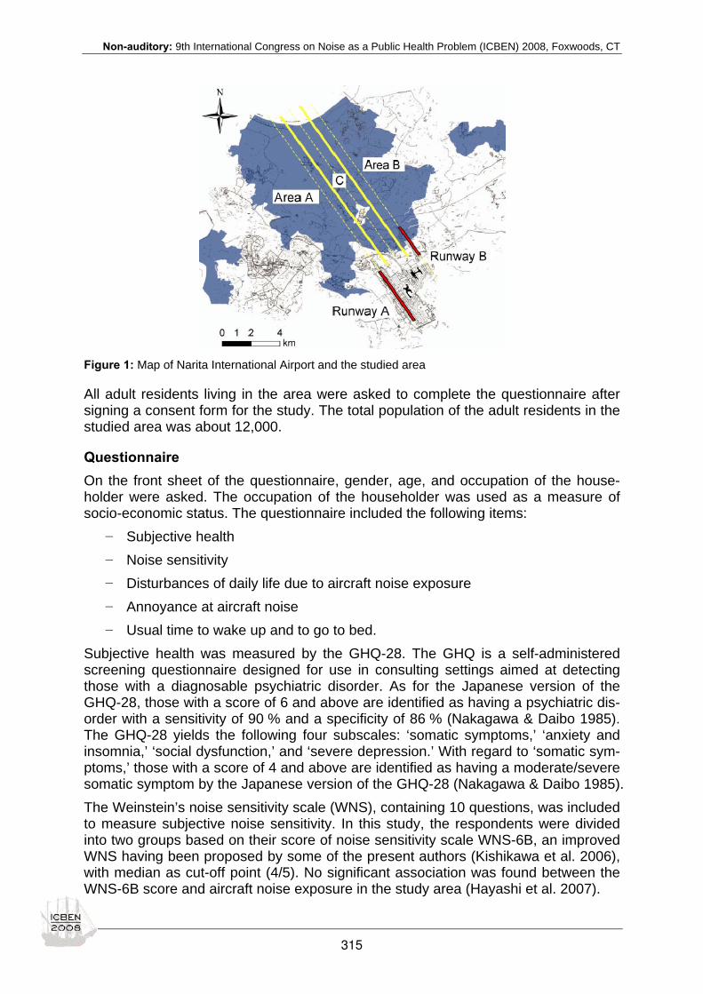
Non-auditory: 9th International Congress on Noise as a Public Health Problem (ICBEN) 2008, Foxwoods, CT
Figure 1: Map of Narita International Airport and the studied area
All adult residents living in the area were asked to complete the questionnaire after signing a consent form for the study. The total population of the adult residents in the studied area was about 12,000.
Questionnaire On the front sheet of the questionnaire, gender, age, and occupation of the house-holder were asked. The occupation of the householder was used as a measure of socio-economic status. The questionnaire included the following items:
− Subjective health − Noise sensitivity − Disturbances of daily life due to aircraft noise exposure − Annoyance at aircraft noise − Usual time to wake up and to go to bed.
Subjective health was measured by the GHQ-28. The GHQ is a self-administered screening questionnaire designed for use in consulting settings aimed at detecting those with a diagnosable psychiatric disorder. As for the Japanese version of the GHQ-28, those with a score of 6 and above are identified as having a psychiatric dis-order with a sensitivity of 90 % and a specificity of 86 % (Nakagawa & Daibo 1985). The GHQ-28 yields the following four subscales: ‘somatic symptoms,’ ‘anxiety and insomnia,’ ‘social dysfunction,’ and ‘severe depression.’ With regard to ‘somatic sym-ptoms,’ those with a score of 4 and above are identified as having a moderate/severe somatic symptom by the Japanese version of the GHQ-28 (Nakagawa & Daibo 1985). The Weinstein’s noise sensitivity scale (WNS), containing 10 questions, was included to measure subjective noise sensitivity. In this study, the respondents were divided into two groups based on their score of noise sensitivity scale WNS-6B, an improved WNS having been proposed by some of the present authors (Kishikawa et al. 2006), with median as cut-off point (4/5). No significant association was found between the WNS-6B score and aircraft noise exposure in the study area (Hayashi et al. 2007).
315

Non-auditory: 9th International Congress on Noise as a Public Health Problem (ICBEN) 2008, Foxwoods, CT
Three questions on sleep disturbance (i.e. difficulty in falling asleep, awakening dur-ing sleep, and awakening early in the morning) were included in the questionnaire. In each question, frequency of sleep disturbance was asked with 5 choices (not at all, 1–2 days a month, 1–2 days a week, 3–4 days a week, and almost every day). A-mong the three questions, the most frequent sleep disturbance was used to evaluate the sleep disturbance. Hearing interference was also asked with 5 choices (not at all, 1–2 times a week, 1–2 times a day, 5–6 times a day, and more than 10 times a day). Annoyance was asked with 5 choices (not annoyed, a little annoyed, annoyed, very annoyed, and intolerably annoyed).
Statistical analysis Dose-response relationships between subjective health identified by the GHQ-28 and Lden were obtained for both the sensitive and insensitive groups by multiple logistic regression analysis with adjustment for gender, age, occupation of the householder, and the interaction between gender and age. Trend test of the dose-response rela-tionships was also carried out for the sensitive and insensitive groups, respectively. Relationships between moderate/severe somatic symptoms identified by the GHQ-28 and disturbances of daily life were analysed by multiple logistic regression analysis with adjustment for gender, age, occupation of the householder, and the interaction between gender and age in order to find the primary cause of the adverse effects on subjective health. Furthermore, an analysis with adjustment for annoyance was also conducted in order to evaluate the effects of annoyance on subjective health. All statistical analyses were performed using SPSS, version 15.0.
RESULTS AND DISCUSSION Sample About 12,000 questionnaires were distributed to all the adult residents and approxi-mately 70 % of them were collected. The collected questionnaires without a signature on the consent form were regarded as invalid. About 85 % of the collected question-naires were valid. Furthermore, respondents aged over 80 years or less than 20 years were excluded because the number of such respondents was small. Thus, the number of the valid sample was 6,527, which was more than half of the distributed questionnaires. In the present paper, the 2,861 questionnaires obtained from Area A (see Figure 1) were entered into the analysis. Areas B and C were excluded from the analysis be-cause of the high reaction with the opening of the new runway (Hayashi et al. 2007). Table 1 lists the number of analysed sample stratified by Lden, gender, and age. The noise exposure level in Area A ranged from 51 to 67 dB in Lden. There was no particu-lar difference in the demographic attributes (i.e. gender, age, and occupation of the householder) of the respondents among the noise exposure levels.
Effects of aircraft noise exposure on subjective health Figure 2 presents the dose-response relationships between subjective health identi-fied by the GHQ-28 and Lden. Figure 2(a) presents the dose-response relationships of psychiatric disorders. No significant relationship was observed between psychiatric disorders and Lden.
316

Non-auditory: 9th International Congress on Noise as a Public Health Problem (ICBEN) 2008, Foxwoods, CT
Table 1: The number of analysed samples stratified by Lden, gender, and age
Gender Age Lden (dB) Male Female 20-29 30-39 40-49 50-59 60-69 70-79
Total
51–53 20 23 3 4 12 7 12 5 43 53–56 412 418 90 86 118 227 164 145 830 56–59 331 339 68 86 96 187 136 97 670 59–62 270 270 55 48 108 132 99 98 540 62–65 176 167 44 39 63 80 58 59 343 65–67 226 209 40 65 68 109 82 71 435 Total 1,435 1,426 300 328 465 742 551 475 2,861
Figure 2(b) presents the dose-response relationships obtained by an analysis in which two questions related to sleep quality were excluded from the GHQ-28. The dose-response relationship showed an increasing trend in the sensitive group; how-ever, it was not statistically significant (p = 0.052). Figure 2(c) shows the dose-response relationships of moderate/severe somatic symptoms. A significant dose-response relationship was found between somatic symptoms and Lden in the sensitive group (p = 0.007), but was not in the insensitive group. No significant dose-response relationships were observed between the other sub-scales and Lden.
(a) Total score (b) Total score (without sleep)
(c) Somatic symptoms
Figure 2: Dose-response relationships of subjective health identified by the GHQ-28 for the sensitive and insensitive groups. The symbols and whiskers indicate the odds ratios and their 95 % confidence intervals with adjustment for gender, age, and occupation of the householder. All respondents in the 53–56 dB group were set to the reference group. The 51–53 dB group was included in the 53-56 dB group since the number of respondents in this group was small. The p-values in the figures are the significance probabilities of the trend tests.
317

Non-auditory: 9th International Congress on Noise as a Public Health Problem (ICBEN) 2008, Foxwoods, CT
The results mentioned above suggest that the adverse effects on subjective health due to aircraft noise exposure may exist especially in sensitive subgroups and that aircraft noise exposure has adverse effects on somatic symptoms of the residents in the study area.
Disturbances of daily life and annoyance due to aircraft noise exposure Figure 3 presents the dose-response relationships of disturbances of daily life and annoyance due to aircraft noise exposure. In the highest noise-exposed area, about 27 % of the respondents were disturbed in their sleep 3–4 days a week or almost every day, and about 52 % of the respondents were highly annoyed (very/intolerably annoyed).
(a) Sleep disturbance (b) Hearing interference
(c) Annoyance
Figure 3: Disturbances of daily life and annoyance vs. Lden
Relationship among somatic symptoms, disturbances of daily life, and annoy-ance Relationships among moderate/severe somatic symptoms identified by the GHQ-28, disturbances of daily life, and annoyance were analysed in order to find the primary cause of the adverse effects on subjective health. In the analyses, the sample was limited to the sensitive residents in the 59–67 dB group, since the higher odds ratios for somatic symptoms were obtained only in the group (see Figure 2(c)). Figure 4 shows the relationships among moderate/severe somatic symptoms, distur-bances of daily life, and annoyance. Sleep disturbance correlated significantly with somatic symptoms. On the other hand, hearing interference did not show any significant associations with somatic symptoms.
318
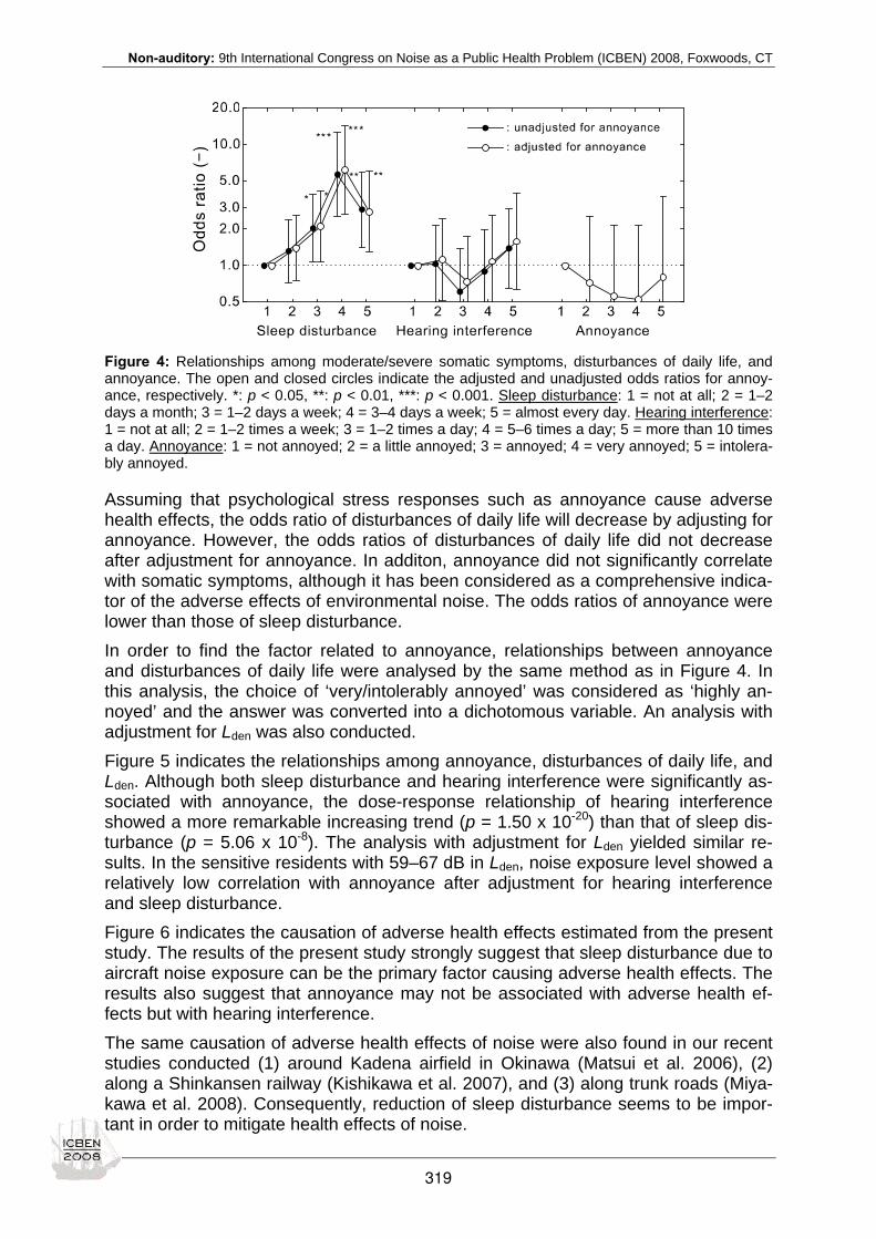
Non-auditory: 9th International Congress on Noise as a Public Health Problem (ICBEN) 2008, Foxwoods, CT
Figure 4: Relationships among moderate/severe somatic symptoms, disturbances of daily life, and annoyance. The open and closed circles indicate the adjusted and unadjusted odds ratios for annoy-ance, respectively. *: p < 0.05, **: p < 0.01, ***: p < 0.001. Sleep disturbance: 1 = not at all; 2 = 1–2 days a month; 3 = 1–2 days a week; 4 = 3–4 days a week; 5 = almost every day. Hearing interference: 1 = not at all; 2 = 1–2 times a week; 3 = 1–2 times a day; 4 = 5–6 times a day; 5 = more than 10 times a day. Annoyance: 1 = not annoyed; 2 = a little annoyed; 3 = annoyed; 4 = very annoyed; 5 = intolera-bly annoyed.
Assuming that psychological stress responses such as annoyance cause adverse health effects, the odds ratio of disturbances of daily life will decrease by adjusting for annoyance. However, the odds ratios of disturbances of daily life did not decrease after adjustment for annoyance. In additon, annoyance did not significantly correlate with somatic symptoms, although it has been considered as a comprehensive indica-tor of the adverse effects of environmental noise. The odds ratios of annoyance were lower than those of sleep disturbance. In order to find the factor related to annoyance, relationships between annoyance and disturbances of daily life were analysed by the same method as in Figure 4. In this analysis, the choice of ‘very/intolerably annoyed’ was considered as ‘highly an-noyed’ and the answer was converted into a dichotomous variable. An analysis with adjustment for Lden was also conducted. Figure 5 indicates the relationships among annoyance, disturbances of daily life, and Lden. Although both sleep disturbance and hearing interference were significantly as-sociated with annoyance, the dose-response relationship of hearing interference showed a more remarkable increasing trend (p = 1.50 x 10⁻²⁰) than that of sleep dis-turbance (p = 5.06 x 10⁻⁸). The analysis with adjustment for Lden yielded similar re-sults. In the sensitive residents with 59–67 dB in Lden, noise exposure level showed a relatively low correlation with annoyance after adjustment for hearing interference and sleep disturbance. Figure 6 indicates the causation of adverse health effects estimated from the present study. The results of the present study strongly suggest that sleep disturbance due to aircraft noise exposure can be the primary factor causing adverse health effects. The results also suggest that annoyance may not be associated with adverse health ef-fects but with hearing interference. The same causation of adverse health effects of noise were also found in our recent studies conducted (1) around Kadena airfield in Okinawa (Matsui et al. 2006), (2) along a Shinkansen railway (Kishikawa et al. 2007), and (3) along trunk roads (Miya-kawa et al. 2008). Consequently, reduction of sleep disturbance seems to be impor-tant in order to mitigate health effects of noise.
319
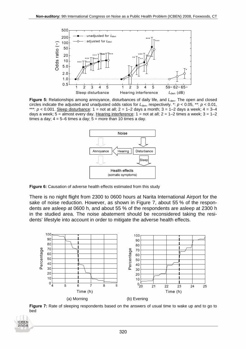
Non-auditory: 9th International Congress on Noise as a Public Health Problem (ICBEN) 2008, Foxwoods, CT
Figure 5: Relationships among annoyance, disturbances of daily life, and Lden. The open and closed circles indicate the adjusted and unadjusted odds ratios for Lden, respectively. *: p < 0.05, **: p < 0.01, ***: p < 0.001. Sleep disturbance: 1 = not at all; 2 = 1–2 days a month; 3 = 1–2 days a week; 4 = 3–4 days a week; 5 = almost every day. Hearing interference: 1 = not at all; 2 = 1–2 times a week; 3 = 1–2 times a day; 4 = 5–6 times a day; 5 = more than 10 times a day.
Figure 6: Causation of adverse health effects estimated from this study
There is no night flight from 2300 to 0600 hours at Narita International Airport for the sake of noise reduction. However, as shown in Figure 7, about 55 % of the respon-dents are asleep at 0600 h, and about 55 % of the respondents are asleep at 2300 h in the studied area. The noise abatement should be reconsidered taking the resi-dents’ lifestyle into account in order to mitigate the adverse health effects.
(a) Morning (b) Evening
Figure 7: Rate of sleeping respondents based on the answers of usual time to wake up and to go to bed
320
Non-auditory: 9th International Congress on Noise as a Public Health Problem (ICBEN) 2008, Foxwoods, CT
CONCLUSIONS The cross-sectional field study conducted around Narita International Airport revealed a significant correlation between moderate/severe somatic symptoms identified by the GHQ-28 and aircraft noise exposure in the sensitive group. This result suggests that the adverse effects on subjective health due to aircraft noise exposure may exist especially in sensitive subgroups and that aircraft noise exposure has adverse effects on somatic symptoms of the residents in the study area. The investigation on the relationships among somatic symptoms, disturbances of daily life, and annoyance revealed a significantly high correlation with sleep distur-bance and no correlation with hearing interference and annoyance. The investigation also revealed that annoyance was strongly correlated with hearing interference. These results suggest that sleep disturbance due to aircraft noise exposure can be the primary factor causing adverse health effects and that annoyance may not be associated with adverse health effects.
REFERENCES Goldberg DP (1978). Manual of the General Health Questionnaire. Nfer-Nelson Pub. Co., Ltd.
Goldberg DP, Hillier VF (1979). A scaled version of the General Health Questionnaire. Psychol Med 9: 135-145.
Hayashi N, Morita I, Morio K, Takaki K, Yamashita K, Ohashi S, Iijima T, Matsui T, Hiramatsu K (2007). Questionnaire study conducted around Narita International Airport — Effects of aircraft noise and validity of noise indices. In: Internoise 2007.
Kishikawa H, Matsui T, Uchiyama I, Miyakawa M, Hiramatsu K, Stansfeld SA (2006). The development of Weinstein's noise sensitivity scale. Noise & Health 8(33): 154–160.
Kishikawa H, Matsui T, Uchiyama I, Daimon S (2007). Noise sensitivity and adverse effects on subjective health due to noise and vibration from Shinkansen railway. J INCE Jpn 31: 158–165 (in Japanese).
Matsui T, Hiramatsu K, Yamamoto T, Miyakita T (2006). Relationship between psychiatric disorder and disturbances of daily life due to aircraft noise — Epidemiological study around Kadena airfield. In: Proceedings of the 2006 Autumn Meeting of the INCE of Japan (pp 85–88). (in Japanese).
Miyakawa M, Kawakubo H, Kishikawa H, Matsui T, Uchiyama I (2008). Relationship between psychiatric disorder and distur-bances of daily life due to noise and vibration from road traffic. J INCE Jpn 32: 71–79 (in Japanese).
Nakagawa Y, Daibo I (1985). Japanese version of the General Health Questionnaire. Tokyo: Nihon Bunka Kagakusya. (in Japanese).
Weinstein ND (1978). Individual differences in reactions to noise: A longitudinal study in a college dormitory. J Appl Psychol 63: 458-466.
Weinstein ND (1980). Individual differences in critical tendencies and noise annoyance. J. Sound Vibr 68: 241-248.
WHO (1999). Guidelines for community noise. Geneva: WHO.
321

Non-auditory: 9th International Congress on Noise as a Public Health Problem (ICBEN) 2008, Foxwoods, CT
Health effects and major co-determinants associated with rail and road noise exposure along transalpine traffic corridors Peter Lercher1*, Bram de Greve2, Dick Botteldooren2, Luc Dekoninck2, Dietmar Oettl3, Ullrich Uhrner3, Johannes Rüdisser1 1 Department of Hygiene, Microbiology and Social Medicine, Medical University Innsbruck, Austria
2 Acoustics group, Department of Information Technology, Ghent University, Gent, Belgium
3 Technical University of Graz, Austria
* corresponding author: e-mail: [email protected]
INTRODUCTION Traffic noise exposure in the community is generally considered as a weak risk factor for more severe health effects. Reported relative risks associated with noise expo-sure vary typically in the range of 1.0 to 1.5 (Babisch 2006, 2008) for cardio-vascular effects. As it is known from annoyance research that up to three quarters of the vari-ance can be explained by non-acoustic factors (Job 1988) - it is a major public health interest to gain equally insight into co-determinants/moderators for other health ef-fects of noise which render people with certain personal or environmental character-istics at higher risk than others. Hitherto, only few studies reported the modifying ef-fect on the noise-health relationship of personal and environmental factors. Among the personal factors e.g. studies have observed an inconsistent sex-noise relationship with hypertension and myocardial infarction (von Eiff & Neus 1980; Her-bold et al. 1989; Babisch et al. 2005; Belojevic & Saric-Tanaskovic 2002; Jarup et al. 2007). Recently, the HYENA study did show a noise-hypertension relationship for men with road traffic but no sex difference with air traffic. In another large study a significant noise-hypertension relation was evident only in middle-aged people (45-55 yrs) but not in older ones and no sex difference were observed (de Kluizenaar et al. 2007). Further, persons without pre-existing disease did show stronger associations of noise with myocardial infarction (Babisch et al. 2005). Among the environmental factors studied – e.g. duration of residence, single versus apartment homes, double versus triple-glass windows, bedroom orientation did show modifications of the noise-hypertension relationship (Bluhm et al. 2007). Recently, the HYENA-study did show associations with hypertension of night-time aircraft noise but daytime road traffic noise (Jarup et al. 2007). It has been hypothesized that stronger associations observed with the reported factors may only indicate less ex-posure misclassification rather than real factors. Bluhm et al. (2007) demonstrated a much stronger relationship with noise when three of these factors (triple glazed, old house, bedroom facing road) were combined (RR 2.47). Another general concern is about possible confounding from air pollution. Especially for myocardial infarction there is good reason to be concerned, while for blood pres-sure there is less good evidence (Ibald-Mulli et al. 2001; de Kluizenaar et al. 2007). However, it could also be a reasonable assumption to expect combined effects of air and noise pollution on cardiovascular health outcomes. Hitherto, only one study has investigated by design this possibility of a combined ef-fect and found a relationship with doctor’s visits for bronchitis (Ising et al. 2005).
322

Non-auditory: 9th International Congress on Noise as a Public Health Problem (ICBEN) 2008, Foxwoods, CT
In the framework of an environmental health impact assessment (BBT) and in a re-search study (ALPNAP) we had the opportunity to study the relationship between noise exposure from road and rail traffic with a broad range of health outcomes.
METHODS Area characteristics Both areas of investigation, the Unterinntal and the Wipptal are part of the most im-portant access route for heavy goods traffic over the Brenner Pass which provides the most direct link for central and northern Europe’s traffic to southern Europe. The goods traffic over the Brenner has tripled within the last 25 years and the fraction of goods moved on the road has substantially increased (up to 2/3). The area consists of small towns and villages with a mix of industrial, small business and agricultural activities. The primary noise sources are motorway and rail traffic. Also important are main roads, which link the villages and provide access to the motorway. The areas differed in topography (U versus V valley), meteorology (much wind versus lot of temperature inversions), geographic orientation (north-south versus east-west) and reason for study (EHIA versus research study).
Study characteristic, sample selection and recruitment All 3 studies were cross-sectional. In the Wipptal (BBT surveys) a phone (N=2,002) and a interview study (N=2,070) were carried out. A pooled sample was created (N=3,630) from both studies (omitting those who participated in both studies: N=442) to get more statistical power and better representation. In the Unterinntal (ALPNAP study) a nearly identical phone survey (N=1,643) was conducted. The participation at the individual level varied between studies (62, 80, 35 % respectively). The research phone study had the lowest participation. Participation at the household level was significantly higher (61 to over 80 %).The age range included was slightly broader in the Wipptal (17-85 yrs) than in the Unterinntal (25-75 yrs). People were contacted by phone based on a stratified, random sampling strategy. The address base was stratified by the use of a Geographic information system (GIS) into areas defined by distance categories to the major traffic sources (rail, motorway, main road), leaving a common „background area“ lying outside major traffic activities and an area with exposure to more than one traffic source “mixed traffic area”. Households were randomly selected from these areas and replaced in case of non-participation. Apart from age selection criteria were sufficient hearing and language proficiency. Excluded were persons living less than one year at this address. Some addresses were not valid, did not have telephone or could not be reached by 3 at-tempts at different times of the day. While the BBT-interview survey resulted in a bal-anced sex ratio (983 men and 1,082 women), both phone surveys showed a clear excess of participating women (65 % and 61 %). This reflects the much higher flexi-bility of the interviewers in terms of appointments compared with the limited random dialing approach on the phone (3 attempts), which favored women’s participation who on average spend more time at home and easier to reach.
Noise exposure assessment Three traffic noise sources were considered in the noise exposure assessment: Mo-torway traffic, traffic on main roads and railway traffic. For motorway traffic the yearly average load (light and heavy vehicles) is combined with an average diurnal traffic pattern. Available traffic frequency data on main roads were supplemented with addi-
323
Non-auditory: 9th International Congress on Noise as a Public Health Problem (ICBEN) 2008, Foxwoods, CT
tional traffic counting. Noise emission by road traffic was calculated on an early ver-sion (BBT-study) and the later version (ALPNAP-study) of the Harmonoise source model (Jonasson 2007). In addition, micro-simulations of the traffic flow were con-ducted with Paramics (Quadstone®, www.paramics-online.com) to obtain optimal in-dividual vehicle characteristics (speed and acceleration). Railway noise emission is extracted from a typical day out of several long-term noise immission measurements (up to two weeks at different seasons) at close distance to the source. Noise model-ing was carried out with Bass3, which is an extended version of ISO 9613. The model includes up to four reflections and two sideway diffractions (de Greve et al. 2005, 2007). Extensive noise monitoring campaigns during summer and winter were con-ducted in both areas to check the validity of these simulations against the measure-ment results. In addition, the predicted sound pressure levels resulting from PE-modeling have been evaluated against the long-term measurements in the Inntal (van Renterghem et al. 2007). Indicators of day, evening, night exposure and Lden were calculated for each source. Eventually, total exposure from all or from specific source combinations at several points of the building facade of the participant’s home was calculated. In the present analyses Lden of the individual sources at the most exposed façade was utilized.
Air pollution exposure assessment Annual means for NOx, NO2 and PM10 were calculated for an area 27 km (W-E) × 23 km (N-S) east of Innsbruck and seven overlapping model domains along the Wipptal (>300 km²). For these air quality assessment about 300 flow fields were cal-culated with the meteorological model GRAMM (Graz Mesoscale Model, Almbauer et al. 2000; Öttl et al. 2005) for each domain and sub-domain (up to 100 x 100 m2 reso-lution). Traffic emissions were modeled using the network emission model NEMO (Rexeis & Hausberger 2005). For each flow field a dispersion simulation with the La-grangian particle model GRAL (Öttl et al. 2003a, b, 2007) was calculated on horizon-tal resolutions of 10 x 10m2 and in the vertical on 2 m resolution. The model system uses special algorithms to account for low wind or calm conditions (Öttl et al. 2001, 2005). Each run was weighted due to its meteorological classification and frequency. Thereafter, annual, summer and winter means were calculated by post processing and weighting the numerous dispersion calculations. The NOx to NO2 conversion is calculated according to the scheme of Romberg et al. (1996). The entire model chain was developed at the Institute for Internal Combustion Engines and Thermodynam-ics, Technical University Graz, Austria. The model type resolves the dispersion proc-esses close to strong sources such as busy roads. Model results can be compared with measurements from air quality monitoring stations located very close to strong sources (so called hot spots). Hence, in contrast to many other air quality models the model results are meaningful in areas with high exposure levels and where people live. Because the model calculates the exposure resulting from specified emissions such as traffic, domestic heating etc. a residuum results when comparing simulations ver-sus observations. This residuum or so-called background value which is the abscissa of the regression analysis is attributable to not accounted emissions or secondary aerosol formation or regional transport not accounted in these micro-scale dispersion calculations. Within ALPNAP the simulation results were compared with 7 air quality stations located in the Inn Valley. The background values within this study were height corrected according to Seinfeld & Pandis (1997). Calculated NO2 and PM10 values for each of the participant's home were assigned by GIS.
324
Non-auditory: 9th International Congress on Noise as a Public Health Problem (ICBEN) 2008, Foxwoods, CT
Questionnaire information The questionnaire covered socio-demographic data, housing, satisfaction with the environment, general noise annoyance, attitudes toward transportation, interference of activities, coping with noise, occupational exposures, lifestyles, dispositions such as noise and weather sensitivity, health status, selected illnesses and medications. The phone interview took about 15-20 minutes. The longer questionnaire of the face to face interview required about 45-60 minutes. Health information was based on doctor reported diagnoses and prescriptions. Re-porting time was related to the last 12 months. Health status was assessed by a five grade Likert type question. In the analyses only three categories were used: very good, good and less than good (3+4+5 of the 5-point scale). Education was meas-ured in 5 grades (basic, skilled labor, vocational school, A-level, University degree). The top two grades (University and A-level) were combined in the analyses.
Statistical analysis Exposure-effect curves were calculated with extended logistic regression methods using restricted cubic spine functions to accommodate for non-linear components in the fit if appropriate (Harrell 2001). The non-parametric regression estimate and its 95 % confidence intervals are based on smoothing the binary responses and taking the logit transformation of the smoothed estimates. Adjustments for confounding dif-fer with respect to the health outcome. However, basic adjustments were always made for age, sex, education and the most important co-factors known in literature. The analysis was carried out with R version 2.4.1 and 2.5.1 (R Development Core Team 2006) using the contributed packages “Design” and “Hmisc” from Harrell (2001).
RESULTS Wipptal (BBT-studies) Figures 1 and 2 show the noise-health status relationships for motorway and overall sound level. There is a clear gradient for education but also a significant trend with sound level visible. The ranking in the educational gradient differs slightly from the Inntal results: the group with higher education is not better than all other groups with some additional schooling. Figure 2 reveals an interaction with chronic illness: there is no increase in poor health status with increasing noise in people without chronic illness – but with chronic disease status in spite of less power (N=2,070). Without testing for interaction you get a zero relationship (larger group with chronic illness).
325

Non-auditory: 9th International Congress on Noise as a Public Health Problem (ICBEN) 2008, Foxwoods, CT
Figure 1: Exposure effect relationship for poor health status by motorway and different levels of education (left N=3,630)
Figure 2: Exposure effect relationship for poor health status by overall sound exposure (right N=2,070) by reported chronic illness status (95 % confidence intervals omitted)
The relation between depression and combined noise exposure (road & rail) shows a stronger departure of the slope particularly for people with poor health status (Fi-gure 3) and with persisting trauma experience (Figure 4) in the phone study. Figure 3: Exposure effect relationship: proportion Figure 4: Exposure effect relationship: proportion with depression diagnosis related to sound level with depression diagnosis related to sound level from combination of all sources by health status from combination of all sources by trauma status
The relation between overall sound exposure (all sources) and hypertension (Fi-gure 5) exhibits a mixed picture: The face to face study shows a linear trend (OR=1.28 (1.03-1.58 (for 50 to 60 dBA) and reaches a plateau around 60 dBA. The phone study levels off strongly around 60 dBA (OR=1.43 (1.05-1.95 (65 to 75 dBA) and the analysis for the main valley nearly reaches significance (OR=1.14(0.98-1.31) (for 60 to 70 dBA). The non-linear relation of hypertension medication (Figure 6) with rail noise is quite strong (OR=1.63 (1.12-2.36) (for 60 to 70 dBA) while the face to face study shows no relation and the analysis for the inhabitants of the main valley is also not significant.
30 40 50 60 70 80Sound level motorway,Lden,dBA
0.0
0.2
0.4
0.6
0.8
Hea
lth s
tatu
s=
poor
Basic educationSkilled labour
Vocational schoolHigher education
30 40 50 60 70 80Sound level motorway,Lden,dBA
0.0
0.2
0.4
0.6
0.8
Hea
lth s
tatu
s=
poor
Basic educationSkilled labour
Vocational schoolHigher education
Basic educationSkilled labour
Vocational schoolHigher education
Basic educationSkilled labour
Vocational schoolHigher education
30 40 50 60 70 80
0.0
0.1
0.2
0.3
0.4
0.5
0.6
Hea
lth s
tatu
s=
poor
30 40 50 60 70 80
with reported chronic illness
without reported chronic illness
Overall sound level,Lden,dBA30 40 50 60 70 80
0.0
0.1
0.2
0.3
0.4
0.5
0.6
0.0
0.1
0.2
0.3
0.4
0.5
0.6
Hea
lth s
tatu
s=
poor
30 40 50 60 70 80
with reported chronic illness
without reported chronic illness
Overall sound level,Lden,dBA
40 50 60 70 80
0.00
0.05
0.10
0.15
0.20
0.25
0.30
Not traumatized
For some time
Still traumatized
Prop
ortio
n w
ith d
epre
ssio
n di
agno
sis
Combined sound level, Lden,dBA
Phone study: N=2002
40 50 60 70 80
0.00
0.05
0.10
0.15
0.20
0.25
0.30
0.00
0.05
0.10
0.15
0.20
0.25
0.30
Not traumatized
For some time
Still traumatized
Prop
ortio
n w
ith d
epre
ssio
n di
agno
sis
Combined sound level, Lden,dBA
Phone study: N=2002
50 60 70 80Combined sound level, Lden,dBA
0.00
0.05
0.10
0.15
0.20
0.25
0.30
Prop
ortio
n w
ith d
iagn
osis
dep
ress
ion
Very good
Good
Health status: poor
Phone study: N=2002
50 60 70 80Combined sound level, Lden,dBA
0.00
0.05
0.10
0.15
0.20
0.25
0.30
Prop
ortio
n w
ith d
iagn
osis
dep
ress
ion
Very good
Good
Health status: poor
50 60 70 8050 60 70 80Combined sound level, Lden,dBA
0.00
0.05
0.10
0.15
0.20
0.25
0.30
0.00
0.05
0.10
0.15
0.20
0.25
0.30
Prop
ortio
n w
ith d
iagn
osis
dep
ress
ion
Very good
Good
Health status: poor
Phone study: N=2002
326

Non-auditory: 9th International Congress on Noise as a Public Health Problem (ICBEN) 2008, Foxwoods, CT
Figure 5: Exposure effect relationship: proportion Figure 6: Exposure effect relationship: proportion with hypertension diagnosis related to overall with hypertension diagnosis related to overall sound level by study type and area sound level by study type and area
The same analysis conducted in the phone study by source (Figure 7) reveals a sig-nificant relation only with railway and main road but not with motorway noise. Against a reference level of 55 dBA the relative risk (OR) increases to 1.84 (1.15-2.95) for rail and 1.83 (1.17-2.86) for main road at 70 dBA. In contrast to the previous results the combined endpoint angina pectoris/myocardial infarction is significantly associated in the phone study (OR 1.70 (1.16-2.47)(for 60 to 70 dBA) and the main valley analysis (OR=1.34(1.05-1.71) with motorway noise (Figure 8) – but not in the face to face study. Figure 7: Exposure effect relationship: proportion Figure 8: Exposure effect relationship: proportion with hypertension medication related to sound with diagnosed angina/myocardial infarction re-level by study type and area lated to motorway sound by study type and area
Inntal (ALPNAP-study) The observations for overall noise (Figure 9) show a significant increase in the preva-lence of persons with poorer health which is paralleled by a decrease in population prevalence with very good health when the sound level increases.
30 40 50 60 70Sound level motorway,Lden,dBA
0.00
0.02
0.04
0.06
0.08
0.10
0.12
0.14
Prop
ortio
n w
ithdi
agno
sise
Angi
na/M
I
30 40 50 60 7030 40 50 60 70
Face to face study
Phone-study
Main valley*
* From both studies
30 40 50 60 70Sound level motorway,Lden,dBA
0.00
0.02
0.04
0.06
0.08
0.10
0.12
0.14
0.00
0.02
0.04
0.06
0.08
0.10
0.12
0.14
Prop
ortio
n w
ithdi
agno
sise
Angi
na/M
I
30 40 50 60 7030 40 50 60 70
Face to face study
Phone-study
Main valley*
* From both studies
Sound level of the respective source,Lden,dBA
Prop
ortio
n w
ithhy
perte
nsio
nm
edic
atio
n
30 40 50 60 70 8030 40 50 60 70 80
0.00
0.05
0.10
0.15
0.20
0.00
0.05
0.10
0.15
0.20
0.25
0.30
0.00
0.05
0.10
0.15
0.20
0.25
Motorway
Main road
Railway
Phone study: N=2002
Sound level of the respective source,Lden,dBA
Prop
ortio
n w
ithhy
perte
nsio
nm
edic
atio
n
30 40 50 60 70 8030 40 50 60 70 8030 40 50 60 70 8030 40 50 60 70 80
0.00
0.05
0.10
0.15
0.20
0.00
0.05
0.10
0.15
0.20
0.25
0.30
0.00
0.05
0.10
0.15
0.20
0.25
0.00
0.05
0.10
0.15
0.20
0.00
0.05
0.10
0.15
0.20
0.25
0.30
0.00
0.05
0.10
0.15
0.20
0.25
Motorway
Main road
Railway
Phone study: N=2002
30 40 50 60 70 80Overall-sound level,Lden,dBA
0.00
0.02
0.04
0.06
0.08
0.10
0.12
0.14
Prop
ortio
n w
ith h
yper
tens
ion
diag
nosi
s
30 40 50 60 70 80
0.04
0.06
0.08
0.10
0.12
0.14
30 40 50 60 70 80
Face to face study: N=1546Main valley*: N=2640
Phone-study: N=1886
* From both studies
30 40 50 60 70 80Overall-sound level,Lden,dBA
0.00
0.02
0.04
0.06
0.08
0.10
0.12
0.14
Prop
ortio
n w
ith h
yper
tens
ion
diag
nosi
s
30 40 50 60 70 80
0.04
0.06
0.08
0.10
0.12
0.14
30 40 50 60 70 80
Face to face study: N=1546Main valley*: N=2640
Phone-study: N=1886
* From both studies
30 40 50 60 70 80
0.00
0.02
0.04
0.06
0.08
0.10
0.12
30 40 50 60 70 8030 40 50 60 70 80Sound level railway,Lden,dBA
Prop
ortio
n w
ith h
yper
tens
ion
med
icat
ion
Face to face study: N=1130
Main valley*N=1872
Phone-study: N=1037
* From both studies
30 40 50 60 70 80
0.00
0.02
0.04
0.06
0.08
0.10
0.12
0.00
0.02
0.04
0.06
0.08
0.10
0.12
30 40 50 60 70 8030 40 50 60 70 80Sound level railway,Lden,dBA
Prop
ortio
n w
ith h
yper
tens
ion
med
icat
ion
Face to face study: N=1130
Main valley*N=1872
Phone-study: N=1037
* From both studies
327

Non-auditory: 9th International Congress on Noise as a Public Health Problem (ICBEN) 2008, Foxwoods, CT
Figure 9: Proportion with very good (left) and poor (right) health status and overall sound level by educational status (MITHRA-SIG modeling)
In order to evaluate the possible effect of air pollution, a model without and with ad-justment for a specific noise indicator was evaluated. The curves show a small non-significant trend for an increase in poor health with higher level of particulate pollution when noise is not adjusted for (Figure 10 left). However, when an adjustment for overall noise exposure is made, the air pollution effect disappears completely (Fi-gure 10 right). Hence, at higher noise levels, 65 versus 45 dBA, the proportion of per-sons with poor health is higher, completely independent of the level of air pollution. The analyses for depression did not reveal a direct relationship with noise indicators. Overall, significant associations with noise exposure were seen only in people with poor health status (not shown), psychological trauma experience (Figure 11 left) or higher noise sensitivity (Figure 11 right). Noise exposure from main roads did exhibit the strongest associations (similar to the annoyance results).
Hea
lth s
tatu
s =
poor
10 15 20 25 30 35 40
0.0
0.1
0.2
0.3
0.4
0.5
0.6
Mean annual PM10-concentration,µg/m³
Model unadjusted for noise levelSkilled labourBasic education
Vocational schoolHigher education
Hea
lth s
tatu
s =
poor
10 15 20 25 30 35 4010 15 20 25 30 35 40
0.0
0.1
0.2
0.3
0.4
0.5
0.6
0.0
0.1
0.2
0.3
0.4
0.5
0.6
Mean annual PM10-concentration,µg/m³
Model unadjusted for noise levelSkilled labourBasic education
Vocational schoolHigher education
Skilled labourBasic education
Vocational schoolHigher education
Mean yearly PM10-levels,µg/m³
Hea
lth s
tatu
s =
poor
10 15 20 25 30 35 40
0.0
0.1
0.2
0.3
0.4
0.5
0.6
45 dBA65 dBA
Mean annual PM10-concentration,µg/m³Mean yearly PM10-levels,µg/m³
Hea
lth s
tatu
s =
poor
10 15 20 25 30 35 40
0.0
0.1
0.2
0.3
0.4
0.5
0.6
0.0
0.1
0.2
0.3
0.4
0.5
0.6
45 dBA65 dBA
Mean annual PM10-concentration,µg/m³ Figure 10: Proportion with poor health status by education and mean annual PM10 concentration (left) and stratified by high versus low overall noise exposure (right). PM10 modeling by TU-Graz
all.sources.dB.max.Lden
30 40 50 60 70 80
0.0
0.2
0.4
0.6
0.8
Overall sound level, Lden,dBA
Hea
lth s
tatu
s=
very
good
Skilled labourBasic education
Vocational school*Higher education
* Regression line masked by skilled labour
30 40 50 60 70 80
MITHRA-S IG
0.2
0.4
0.6
0.8
0.0
all.sources.dB.max.Lden
30 40 50 60 70 80
0.0
0.2
0.4
0.6
0.8
Overall sound level, Lden,dBA
Hea
lth s
tatu
s=
very
good
Skilled labourBasic education
Vocational school*Higher education
Skilled labourBasic education
Vocational school*Higher education
* Regression line masked by skilled labour
30 40 50 60 70 8030 40 50 60 70 80
MITHRA-S IG
0.2
0.4
0.6
0.8
0.0
0.2
0.4
0.6
0.8
0.0
Overall sound level, Lden,dBA
Hea
lth s
tatu
s =
poor
30 40 50 60 70 80
0.0
0.1
0.2
0.3
0.4
0.5
0.6
30 40 50 60 70 80
Overall sound level, Lden,dBA
Hea
lth s
tatu
s=
poor
Skilled labourBasic education
Vocational schoolHigher education
0.1
0.3
0.4
0.6
0.0
0.2
0.5
MITHRA-SIG
Overall sound level, Lden,dBA
Hea
lth s
tatu
s =
poor
30 40 50 60 70 80
0.0
0.1
0.2
0.3
0.4
0.5
0.6
30 40 50 60 70 8030 40 50 60 70 80
Overall sound level, Lden,dBA
Hea
lth s
tatu
s=
poor
Skilled labourBasic education
Vocational schoolHigher education
Skilled labourBasic education
Vocational schoolHigher education
0.1
0.3
0.4
0.6
0.0
0.2
0.5
0.1
0.3
0.4
0.6
0.0
0.2
0.5
MITHRA-SIG
328

Non-auditory: 9th International Congress on Noise as a Public Health Problem (ICBEN) 2008, Foxwoods, CT
Figure 11: Proportion with depression by trauma status (left) and noise sensitivity (right) and main road sound level
Figure 12: Proportion with hypertension diagnosis (left) and medication (right) by family history and motorway sound level
The relationship of hypertension with motorway noise exhibits significance only when potential moderators are considered (Figure 12).
DISCUSSION For a broad range of possible health outcomes significant (mostly non-linear) rela-tionships were observed in three larger studies in alpine valleys with continuously increasing exposure to mixed traffic sources (rail, main road, motorway) over the last 25 years. The sources often run in parallel and therefore the noise exposure can be characterized as combined exposure – mostly a combination of two or even three sources. The sources can be perceived quite well by the receptors, since the sources have distinct noise characteristics and time pattern and the existing background lev-els are low, particularly during night (Heimann et al. 2007). Furthermore, many noise abatement measures have been implemented over the last years – but the imple-mentation was not coordinated across areas. Hence in the BBT study areas were significant differences between the northern and southern area regarding the imple-mentation of counter-measures. In an earlier communication (Lercher & Botteldooren 2006) we have reported different relationships for the noise-health relationships in the northern and southern part. It is, therefore, not surprising that the relations of the
Main road sound level, Lden,dBA
Pro
porti
on w
ith d
epre
ssio
n
30 35 40 45 50 55 60 65
0.00
0.05
0.10
0.15
0.20
0.25
Adjusted to: alter=47 sex=1 bildung4=Matura/Hochschule laerm.day.sum=6 gesund.
Main road sound level - depression - by level of noise sensitivity
main.den.max
30 35 40 45 50 55 60 65
0.00
0.05
0.10
0.15
0.20
0.25
Adjusted to: alter=47 sex=1 bildung4=Matura/Hochschule laerm.day.sum=6 gesund.Main road sound level,Lden,dBA
Prop
ortio
n w
ithde
pres
sion
30 4035 45 50 55 60 55
Less
High
Main road sound level, Lden,dBA
Pro
porti
on w
ith d
epre
ssio
n
30 35 40 45 50 55 60 65
0.00
0.05
0.10
0.15
0.20
0.25
Adjusted to: alter=47 sex=1 bildung4=Matura/Hochschule laerm.day.sum=6 gesund.
Main road sound level - depression - by level of noise sensitivity
main.den.max
30 35 40 45 50 55 60 65
0.00
0.05
0.10
0.15
0.20
0.25
Adjusted to: alter=47 sex=1 bildung4=Matura/Hochschule laerm.day.sum=6 gesund.Main road sound level,Lden,dBA
Prop
ortio
n w
ithde
pres
sion
30 4035 45 50 55 60 5530 4035 45 50 55 60 55
Less
High
Main road sound level,Lden,dBA
Pro
porti
on w
ith d
epre
ssio
n
30 35 40 45 50 55 60 65
0.00
0.05
0.10
0.15
0.20
0.25
Adjusted to: alter=47 sex=1 bildung4=Matura/Hochschule laerm.day.sum=6 gesun
Main road sound level - depression - by trauma status
NR.dB.max.Lden
30 35 40 45 50 55 60 65
0.00
0.05
0.10
0.15
0.20
0.25
Adjusted to: alter=47 sex=1 bildung4=Matura/Hochschule laerm.day.sum=6 gesun
With trauma history
No trauma history
Main road sound level, Lden,dBA
MIT
HR
A-S
IG
Prop
ortio
n w
ithde
pres
sion
0.00
0.05
0.10
0.15
0.20
0.25
35 45 55 6530 40 50 60
Main road sound level,Lden,dBA
Pro
porti
on w
ith d
epre
ssio
n
30 35 40 45 50 55 60 65
0.00
0.05
0.10
0.15
0.20
0.25
Adjusted to: alter=47 sex=1 bildung4=Matura/Hochschule laerm.day.sum=6 gesun
Main road sound level - depression - by trauma status
NR.dB.max.Lden
30 35 40 45 50 55 60 65
0.00
0.05
0.10
0.15
0.20
0.25
Adjusted to: alter=47 sex=1 bildung4=Matura/Hochschule laerm.day.sum=6 gesun
With trauma history
No trauma history
Main road sound level, Lden,dBA
MIT
HR
A-S
IG
Prop
ortio
n w
ithde
pres
sion
0.00
0.05
0.10
0.15
0.20
0.25
0.00
0.05
0.10
0.15
0.20
0.25
35 45 55 6530 40 50 6035 45 55 6530 40 50 60
Highway sound level,Lden,dBA
Pro
porti
on w
ith m
edic
atio
n
30 40 50 60 70
0.0
0.1
0.2
0.3
0.4
0.5
0.6
Motorway sound level,Lden,dBA
MIT
HR
A-SI
G
With family history
No family history
Pro
porti
on w
ithm
edic
atio
n
0.0
0.1
0.2
0.3
0.4
0.5
0.6
30 40 50 60 70
Highway sound level,Lden,dBA
Pro
porti
on w
ith m
edic
atio
n
30 40 50 60 70
0.0
0.1
0.2
0.3
0.4
0.5
0.6
Motorway sound level,Lden,dBA
MIT
HR
A-SI
G
With family history
No family history
Pro
porti
on w
ithm
edic
atio
n
0.0
0.1
0.2
0.3
0.4
0.5
0.6
30 40 50 60 70
Highway sound level, Lden,dBA
Pro
porti
on w
ith h
yper
tens
ion
30 40 50 60 70
0.0
0.1
0.2
0.3
0.4
0.5
0.6
Highway sound level - Hypertension - among people with and without disposition
HW.dB.max.Lden
30 40 50 60 70
0.0
0.1
0.2
0.3
0.4
0.5
0.6
Motorway sound level,Lden,dBA
Prop
ortio
n w
ith d
iagn
osis
of h
yper
tens
ion
0.0
0.1
0.2
0.3
0.4
0.5
0.6
30 40 50 60 70
MIT
HR
A-S
IG
With family history
No family history
329

Non-auditory: 9th International Congress on Noise as a Public Health Problem (ICBEN) 2008, Foxwoods, CT
various health outcomes with the calculated noise exposure do not always agree in the summary analyses which reflect only the average result over the full area or the two studies. However, some results are consistent across analyses: The relation of health status with noise exposure is valid across educational levels adjusted for age, sex, BMI, noise & weather sensitivity, trauma and emotional coping. Within the range of the observed levels air pollution in the studied areas did not make a significant contribution when noise exposure indicators were introduced in the ad-justed models. All tests for interaction with noise failed also to reach significance. This is in line with the hitherto only peer reviewed study which has evaluated air pol-lution in addition to noise with respect to hypertension (de Kluizenaar et al. 2007). This observation is further strengthened by similar experience with other health end-points (health status, depression, heart disease) in this study. Furthermore, the strong importance of modifying factors receives further support. The analyses have repeatedly shown moderation on the noise-health relation across studies and areas of health status, noise sensitivity, trauma experience. Further ef-fects on the observed noise-health relationship were seen by study type (phone vs face to face) and area layout with respect to the traffic sources in terms of exposure combinations. This observation was more visible in the BBT-studies, where more variation in exposure-mix occurred across the studied area than in the ALPNAP-study, where exposure was more homogeneous along the valley due to a more uni-form topographic layout and implementation of noise abatement measures. Eventu-ally, these findings support the adoption of a contextual approach in risk assessment and prevention (Staples 1996; Lercher 1996, 1998, 2002, 2007) and follow up on re-sults reported from earlier surveys in these valleys (Lercher & Kofler 1993, 1996; Ler-cher et al. 2000).
CONCLUSION In spite of the implementation of noise control measures in the study areas significant relations with exposure to single and combined noise sources could be observed. Strong moderation components often lead to the typical large spread and prevent the detection of significant noise-health relationships when not considered in design and analysis. The additional consideration of air pollution did not weaken the noise-health relations. Health status is a very accurate predictor of future mortality and morbidity and should be further utilized in noise studies, since very stable relations with noise exposure could be established in these investigations.
ACKNOWLEDGEMENTS The authors acknowledge the support by a research grant provided to the Medical University Innsbruck from the BBT-SE (funds received from the European Union for an EHIA) and the EU support for the ALPNAP project within the INTERREG IIIb pro-gram “Alpine space”. Further support was received by the Division of Social Medi-cine, Medical University Innsbruck (for a measurement campaign) and the BEG (Brenner Eisenbahn Gesellschaft) for air pollution and meteorological data from addi-tional monitoring stations. Phone surveys were carried out by IMAD-Innsbruck. Eventually, we thank the people of the Inn- and Wipptal for their participation. Further contributions were made in the planning and conductance of these studies by Dr Edda Amann, M.P.H., Dr Alex Eisenmann, Mag Tom Kugener, Dr David Schnaiter.
330

Non-auditory: 9th International Congress on Noise as a Public Health Problem (ICBEN) 2008, Foxwoods, CT
REFERENCES Almbauer RA, Öttl D, Bacher M, Sturm PJ (2000). Simulation of the air quality during a field study for the city of Graz. Atmos Environ 34: 4581-4594.
Babisch W (2006). Transportation noise and cardiovascular risk: Updated review and synthesis of epidemiological studies indicate that the evidence has increased. Noise & Health 8: 1-29.
Babisch W (2008). Road traffic noise and cardiovascular risk. Noise & Health 10: 27-33.
Babisch W, Beule B, Schust M, Kersten N, Ising H (2005). Traffic noise and risk of myocardial infarction. Epidemiology 16: 33-40.
Belojevic G, Saric-Tanaskovic M (2002). Prevalence of arterial hypertension and myocardial infarction in relation to subjec-tive ratings of traffic noise exposure. Noise & Health 4(16): 33-37.
Bluhm GL, Berglind N, Nordling E, Rosenlund M (2007). Road traffic noise and hypertension. Occup Environ Med 64: 122-126.
Botteldooren D, Lercher P (2004). Soft-computing base analyses of the relationship between annoyance and coping with noise and odor. J Acoust Soc Am 115: 2974-2985.
de Greve B, de Muer T, Botteldooren D (2005). Outdoor beam tracing over undulating terrain. In:Proceedings of Forum Acusticum 2005, Budapest, Hungary.
de Greve B, van Renterghem T, Botteldooren D (2007). Outdoor sound propagation in mountainous areas: comparison of reference and engineering models. In: Proceedings of ICA on CD-ROM. Madrid, Spain.
de Kluizenaar Y, Gansevoort RT, Miedema HME, de Jong PE (2007). Hypertension and road traffic noise exposure. J Occup Environ Med 49: 484-492.
Harrell FE Jr (2001). Regression modeling strategies. New York: Springer.
Herbold M, Hense H-W, Keil U (1989). Effects of road traffic noise on prevalence of hypertension in men: results of the Lübeck blood pressure study. Soz Praeventivmed 34: 19-23.
Ibald-Mulli A, Stieber J, Wichmann HE, Koenig W, Peters A (2001). Effects of air pollution on blood pressure: a population-based approach. Am J Public Health 91: 571-577.
Ising H, Lange-Asschenfeldt H, Eilts M (2005). Bronchitis in children exposed to road traffic noise and exhaust fumes. Som-nologie 9: 105-110.
Jarup L, Babisch W, Houthuijs D, Pershagen G, Katsouyanni K, Cadum E, Dudley M, Savigny P, Seiffert I, Swart W, Breugelmans O, Bluhm G, Selander J, Charalampidis AS, Dimakopoulou K, Sourtzi P, Velonakis M, Vigna-Taglianti F (2007). Hypertension and exposure to noise near airports - the HYENA study. Environ Health Perspect 116: 329-333.
Job RSF (1988). Community response to noise: A review of factors influencing the relationship between noise exposure and reaction. J Acoust Soc Am 83: 991-1001.
Jonasson HG (2007). Acoustical source modeling of road vehicles. Acta Acust Acust 93: 174-183.
Lercher P (1996). Environmental noise and health: An integrated research perspective. Environ Int 22: 117-129.
Lercher P (1998). Context and coping as moderators of potential health effects in noise-exposed persons. In: Prasher D, Luxon L (eds.): Advances in noise series, Vol. 1: Biological effects (pp 328-335). London: Whurr.
Lercher P (2002). The association between transportation noise and hypertension in an alpine area: A comparison of two approaches. Epidemiology 13: S89.
Lercher P (2007). Environmental noise: A contextual public health perspective. In: Luxon L, Prasher D (eds.): Noise and its effects (pp 345-377). London: Wiley.
Lercher P, Botteldooren D (2006). General and/or local assessment of the impact of transportation noise in environmental health impact studies ? In: Proceedings of Euronoise 2006, CD-ROM edition. Tampere: European Acoustics Association.
Lercher P, Kofler W (1993). Adaptive behavior to road traffic noise: Blood pressure and cholesterol. In: Vallet M (ed.). Noise as a public health problem, Vol. 2 (pp 465-468). Nice: Institut National de Recherche sur les Transports et leur Sécurité.
Lercher P, Kofler WW (1996). Behavioral and health responses associated with road traffic noise exposure along alpine through-traffic routes. Sci Total Environ 189/190: 85-89.
Lercher P, Widmann U, Kofler WW (2000). Transportation noise and blood pressure: the importance of modifying factors. In: Casserau D (ed.): Proceedings of InterNoise 2000, Vol. 4 (pp 2302-2307). Nice: Sociéte Francaise d'Acoustique.
331

Non-auditory: 9th International Congress on Noise as a Public Health Problem (ICBEN) 2008, Foxwoods, CT
Öttl D, Almbauer R, Sturm PJ (2001). A new method to estimate diffusion in low wind, stable conditions. J Appl Meteorol 40: 259-268.
Öttl D, Sturm P, Pretterhofer G, Bacher M, Rodler J, Almbauer R (2003a). Lagrangian dispersion modeling of vehicular emis-sions from a highway in complex terrain. J Air Waste Managem Assoc 53: 1233-1240.
Öttl D, Almbauer RA, Sturm PJ, Pretterhofer G (2003b). Dispersion modelling of air pollution caused by road traffic using a Markov Chain - Monte Carlo model. Stochastic Environ Res Risk Assess 17: 58-75.
Öttl D, Goulart A, Degrazia G, Anfossi (2005). A new hypothesis on meandering atmospheric flows in low wind speed condi-tions. Atmos Environ 39: 1739-1748.
Öttl D, Sturm P, Anfossi D, Trini Castelli S, Lercher P, Tinarelli G, Pittini T (2007). Lagrangian particle model simulation to assess air quality along the Brenner transit corridor through the Alps; Air Pollution Modelling and its Applications XVIII (pp 689-697). New York: Elsevier. (Developments in environmental science, Vol. 6).
R Development Core Team (2006). R: A language and environment for statistical computing. Vienna, Austria: R Foundation for Statistical Computing. http://www.R-project.org.
Rexeis M, Hausberger S (2005). Calculation of vehicle emissions in road networks with the model "NEMO". In: Conference Proceedings of the 14th Symposium on Transport and Air Pollution 1-3 June 2005, Graz (pp 118-127).
Romberg E, Bösinger R, Lohmeyer A, Ruhnke R, Röth E (1996): NO-NO2-Umwandlung für die Anwendung bei Immissions-prognosen für Kfz-Abgase. Gefahrstoffe - Reinhaltung der Luft 56: 215-218.
Seinfeld JH, Pandis SN (1997). Atmospheric chemistry and physics: From air pollution to climate change. New York: Wiley-Interscience.
Staples SL (1996). Human response to environmental noise. Psychological research and public policy. Am Psychologist 51: 143-150.
van Renterghem T, Botteldooren D, Lercher P (2007). Comparison of measurements and predictions of sound propagation in a valley-slope configuration in an inhomogeneous atmosphere. J Acoust Soc Am 121: 2522-2533.
von Eiff AW, Neus H (1980). Verkehrslärm und Hypertonierisiko. 1. Mitt. Münch Med Wschr 122: 894-896.
332

__________________________________________________________________________
__________________________________________________________________________
ICBEN 2008
Non-Auditory Effects of Noise
333

Non-auditory: 9th International Congress on Noise as a Public Health Problem (ICBEN) 2008, Foxwoods, CT
Joint effects of noise and air pollution: A progress report on the Vancouver retrospective cohort study Hugh W. Davies1*, P.A. Demers1, M. Buzzelli2, M. Brauer1 1 University of British Columbia, Vancouver BC, Canada
2 Queens University
* corresponding author: e-mail: [email protected]
To investigate the joint effects of noise and air pollution on CVD, we are following an adult population of all those 45-85 years old in 1999 who have lived in the Greater Vancouver Regional District (GVRD) for 5 years (approximate N=800,000), including a sub-cohort who had a significant co-morbidity in the preceeding 5 years (the 'susceptible cohort'). Residential histories and health outcomes (deaths, hospital admissions, and potentially all physician visits, pharmacy records) were linked through administrative health records. Exposure assessment for noise and air pollution were obtained by computer modeling using Cadna/A mapping software for the former, and land-use regression modeling for the latter. Disease rates in various exposure groups will be examined by tradition epidemiologic strategies. To date, the cohort has been created and air pollution level surfaces prepared. We are currently producing a noise 'map' for the metropolitan Vancouver area, the first of its scale in North America. We will present the project methodology in detail, project findings to date, as well as discuss the challenges faced and the expected outcomes of the study, as well as future opportunities for research with this new tool.
334

Non-auditory: 9th International Congress on Noise as a Public Health Problem (ICBEN) 2008, Foxwoods, CT
Relation between aircraft noise reduction in schools and standard-ized test scores Mary Ellen Eagan1, Grant Anderson,1 Bradley Nicholas1, Richard Horonjeff2, Terry Tivnan2
1 Harris Miller Miller & Hanson Inc., 77 South Bedford St., Burlington, MA
2 Harvard University Graduate School of Education, Appian Way, Cambridge, MA 02138
* corresponding author: e-mail: [email protected]
INTRODUCTION Research on the effects of aircraft noise on children’s learning suggests that aircraft noise can interfere with learning in the following school areas: reading, motivation, language and speech acquisition, and memory (Evans et al. 1998). The strongest findings to date are for the school subject of reading, for which the majority of studies have shown that children in noise-impact zones are negatively affected by aircraft. Recent research, which confirms conclusions from the 1970s, shows learning de-creases in reading when outdoor-noise LAeq is 65 dB or higher (Stansfeld et al. 2000). It is also possible that, for the same outdoor LAeq, the effects of aircraft noise on classroom learning may be greater than the effects of road and railroad noise (Hygge et al. 2003). In February 2000, the Federal Interagency Committee on Aviation Noise (FICAN) held a public forum to address the issue of the effects of aircraft noise on children. As a result of that forum, FICAN decided to sponsor this current study, which is based upon existing publicly available data. In brief, this study is designed to investigate the relation between (1) reduction in indoor classroom noise levels through airport clo-sure or school sound insulation and (2) student academic performance, as measured by scores on state-standardized tests.
METHODS Research questions This study concerns the relation between aircraft sound in classrooms and concur-rent student test scores. More specifically, this study attempts to answer the follow-ing: Is aircraft noise reduction within classrooms related to test-score improvement, after controlling for demographics? Moreover, does this relationship vary by age group; student group; or test type?
Airports and schools Aircraft sound within classrooms can change for many reasons. For adequate analy-sis in this study, aircraft-sound changes needed to be relatively large in magnitude and not highly disruptive of the socio-economic environment. Three types of changes met these constraints: (1) the opening or closing of individual airport runways, (2) the opening or closing of entire commercial airports, and (3) school sound insulation. The following three airports/states met these constraints and were therefore chosen for this study: Airport 1: One airport in Texas (airport closing); Airport 2: Another air-port in Texas (school sound insulation); and Airport 3: One airport in Illinois (school sound insulation). Only public schools were chosen for this study, because state-wide testing in the U.S. is mandatory only for students in public schools. Near these three
335

Non-auditory: 9th International Congress on Noise as a Public Health Problem (ICBEN) 2008, Foxwoods, CT
airports, a total of 35 public schools have experienced reduction in aircraft noise dur-ing the last ten years, due either to commercial-airport closure or to school sound insulation. In particular: ■ 20 public schools near Airport 1—all those within the DNL 65 dB contour, plus
a 2,000-foot buffer outside this contour ■ 4 public schools near Airport 2—all those that were sound-insulated the sum-
mer of 1994 or later ■ 11 public schools near Airport 3—all those that were insulated the summer of
1995 or later. Of these 35 schools, three are high schools (grade 9 and higher), 13 are middle schools (grades 7 and 8), and 19 are elementary schools (grade 6 and lower). These airports and schools are not guaranteed to be representative. For that reason, results of this study should not be used nationally without subsequent studies of additional airports and schools.
Standardized tests This study used mandatory state-standardized tests, exclusively, as the measure of student performance. This was decided because standardized test results have be-come increasingly important in the U.S. in recent years. Among other things, such tests help determine student class credit, student grade advancement, student graduation, school funding, and official school accreditation. Figure 1 and Figure 2 show the available standardized tests for this study. Separately for high, middle and elementary schools, these two figures show the tested subjects, grade levels and school years of testing. The abbreviations denote different test re-gimes within each state, as shown below each figure. All these tests are mandatory in their state—all public schools, all students. In addition, their detailed test results are all available publicly, either on the internet or from research divisions of the two state departments of education.
TAAS: Texas Assessment of Academic Skills
Figure 1: Texas Standardized Tests
336

Non-auditory: 9th International Congress on Noise as a Public Health Problem (ICBEN) 2008, Foxwoods, CT
IGAP: Illinois Goal Assessment Program ISAT: Illinois Standards Achievement Tests PSAE: Prairie State Achievement Examination
Figure 2: Illinois Standardized Tests
For the horizontal bars in these two figures, each school year extends between its “start year” and its “end year.” In this study, school years are numbered by the “year test given,” the same way graduating classes are named; for example, the class of 2,000 graduates in June 2000 (after taking the year-2000 tests. The study’s database included 1-year and 2-year “lags” after noise reduction occurred. However, only the lag-1 values were evaluated—that is, noise reduction was only assessed after one year of noise-reduced schooling. For the tests in these two figures, three types of test scores were available and used in this study: percentage of students with the “worst” test grade; average numerical score; and percentage of students with the “best” test grade. For most tests in most years, these scores were available separately for the two student groups of interest: IEP (learning disabled) and non-IEP. Average numerical score was available for fewer than half the tests.
Aircraft noise exposures This study departs from most prior studies in the details of its major predictor vari-ables—that is, its noise exposures. First, this study used computed noise exposures, rather than measured ones. Computation resulted in noise exposures that: included each entire school year, rather than just sampled measurement periods during that year; included just the school months of each year, rather than the full year; included just school hours, rather than 24 hours; and converted all computed noise exposures to indoor values, to account for school/window structure. As a result, this study’s noise exposures are potentially more closely linked with actual student noise expo-sure than in most prior studies. The major predictors of interest in this study concern before-after changes in cumula-tive noise exposure. Although contours of day-night sound levels (DNL) were avail-able for each airport, such contours are too influenced by early morning, evening and nighttime aircraft activity to be of use in this study. Instead, a series of noise expo-
337

Non-auditory: 9th International Congress on Noise as a Public Health Problem (ICBEN) 2008, Foxwoods, CT
sures were desired—all for the 9-hour school day (7am to 4pm), and all inside the school classrooms. This section describes the noise exposures of this study. At each school location, the FAA’s Integrated Noise Model (INM) was used to com-pute the following noise metrics that are relevant to this study: SEL (Sound Exposure Level) for each aircraft flyover; and LAmax (maximum A-weighted sound level) for aircraft flyover. Since the INM computes only outdoor aircraft noise, computation pro-ceeded in two steps: (1) INM computation of outdoor metrics; and (2) conversion from these outdoor metrics to the desired indoor cumulative noise exposures. First, outdoor school-hour metrics were computed, separately for each of the three airports in the study, and for each study year, using the INM (version 6.1) and stan-dard airport noise modeling techniques. Annual traffic levels were adjusted based on airline schedules and other sources. Next, these outdoor sound levels were converted to indoor values and different noise exposures, using school-specific construction details and proprietary software. In brief, this process involved: ■ Computation of outdoor-to-indoor level reduction (OILR), in octave bands, using
construction details of individual schools ■ Conversion of outdoor aircraft spectra (from INM) to indoor spectra, based upon
the computed values of OILR ■ Computation of the specific indoor cumulative noise exposure for the study. ■ Resulting indoor cumulative noise exposures For the relevant years and time periods, the following indoor cumulative noise expo-sures were computed: ■ A-weighted noise exposures:
■ Equivalent sound level (ALeq): the indoor equivalent sound level, averaged over the 9-hour school day (7 am to 4 pm)
■ Number of aircraft events with indoor LAmax greater than three candidate thresholds: ANEv>35 dBA; ANEv>40 dBA; and ANEv>45 dBA
■ Fraction of time with indoor LA greater than three candidate thresholds: AFnTm>35 dBA; AFnTm>40 dBA; and AFnTm>45 dBA.
■ Speech Intelligibility Index (SII): ■ Number of events disrupting indoor speech—for students in the back of the
classroom, when the teacher uses “raised voice”—per three candidate thresh-olds:
■ ANEv<0.80SII (disrupts five percent of words) ■ ANEv<0.90SII (disrupts three percent of words) ■ ANEv<0.98SII (disrupts one percent of words).
■ Speech Interference Level (SIL): ■ Number of events disrupting indoor speech—Articulation Index (AI) equals
0.50 for students in the back of the classroom, when the teacher (either gen-der) uses “raised voice”—per three candidate thresholds: ANEv>35SIL; ANEv>40SIL; and ANEv>45SIL
■ Fraction of indoor time speech is disrupted, per three candidate thresh-olds:AFnTm>35SIL; AFnTm>40SIL; and AFnTm>45SIL.
338

Non-auditory: 9th International Congress on Noise as a Public Health Problem (ICBEN) 2008, Foxwoods, CT
Among these noise exposures, only the following were advanced into analysis: LAeq; AFnTm>40 dBA; ANEv>40 dBA; and ANEv<0.98SII.
Multi-variate multilevel regression Multilevel regression was used for all analyses. The basic analysis equation for this study is:
1 2 3 4change in change in prior prior
noise exposuretest score noise exposure test score
four terms defining the various subgroups
change in four demographic principal components
C C C C⎛ ⎞ ⎛ ⎞ ⎛ ⎞= + + +⎜ ⎟ ⎜ ⎟ ⎜ ⎟
⎝ ⎠ ⎝ ⎠ ⎝ ⎠+
⎛ ⎞+ ⎜⎝ ⎠
prior values offour principal demographic components
three terms defining "cause," "state" and "test-regime change"
change in"interaction" terms of variable with .noise exposureevery
⎟
⎛ ⎞+ ⎜ ⎟⎝ ⎠
+
⎛ ⎞+ ⎜ ⎟
⎝ ⎠
(1)
In this equation, “change in noise exposure” was measured separately with each of the study’s four cumulative noise exposures. In addition, it was measured by a vari-able (QQuiet) not dependent upon the noise computations—simply whether the school had noise reduction that year, or not. In the regression, if the net effect of all coefficients involving “change in noise” is sta-tistically significant, then a relationship exists between change in test scores and change in noise exposure. In addition, this relationship exists while simultaneously controlling for (1) demographics, (2) the cause of noise reduction, (3) the specific sta-te, and (4) test-regime change (in Illinois). Wherever the regression associated with these control variables is stronger than with “change in noise exposure,” then the re-gression ascribes more association to them than to noise. In that way, the regression subtracts out their effect, when it predominates, rather than ascribing that effect to the change in noise exposure. In all, regressions were performed for three score types: (1) Failure rate: Percent of students with worst test score, (2) Average test score (scaled from 0 to 100), and (3) Top-score rate: Percent of students with best test score; for all combinations of: age group (high, middle and elementary school), student group (IEP and non-IEP), and test type (verbal and math/science). For these conditions, an initial regression in-volved all possible predictor terms, while the final regression involved only those pre-dictor terms that proved statistically significant in the initial regression. Numerically, terms were deemed statistically significant (retained) if their initial-regression stan-dard uncertainties were smaller than their values. However, if an interaction term was retained per this test, then its “parent” term was also retained, no matter how large its own standard uncertainty.
Primary demographic “control” Between one year and the next, a change in classroom noise exposure may influ-ence standardized test scores. But demographic changes over the same time period may also influence these test scores. It is necessary to “control” for these demo-
339

Non-auditory: 9th International Congress on Noise as a Public Health Problem (ICBEN) 2008, Foxwoods, CT
graphic changes during the analysis. In that manner, only the proper portion of test-score change will be associated with noise-exposure change, and the remaining por-tion with these demographic variables. The relative portions will be determined mathematically in the analysis and will depend upon how strongly each variable re-lates to test-score change in the data. As the primary method of demographic control, comparisons were made while hold-ing “school” constant, as follows: (1) first, the resulting regression equation was evaluated for all tests given in that school on the year after noise reduction; (2) then, the same regression equation was evaluated for all tests given in prior school years (prior to noise reduction); (3) finally, these two results were subtracted, to obtain the “effect” of noise reduction, controlled for results on non-noise-reduced (prior) years. This method of demographic control works well because school demographics are not likely to change much from year to year. Their relative constancy is a great bene-fit to before-after studies of this type. This constancy means, to a first approximation, that these variables are automatically controlled in the analysis—by holding “school” constant from “before” to “after.” With this demographic control, the study asks, “How much different is test-score change, before-to-after noise reduction, from test-score change at these same schools but when they were not concurrently experiencing noise reduction?”
Supplemental demographic “control” As a result of the study’s primary demographic control, “noise-reduction” and “control” groups automatically have the same demographics, at least over a ten-year average. Even so, possible year-to-year changes in demographics remain. To explicitly control for year-to-year demographic changes (and also for each school’s long-term average demographics), publicly available demographic data were collected from individual school records, state boards of education, and from the year-2000 census. Table 1 contains the 24 demographic variables that were available in both Texas and Illinois. The table contains each variable’s abbreviation in this study, its more complete defi-nition, and whether it describes an entire school district or a specific school. The last variable in this table (percentage drop out) had many missing values in the database and was therefore dropped from the study, thereby leaving 23 demographic variables in the analysis. None of the other variables had any missing values, whatsoever.
Table 1: Available demographic variables common to Texas and Illinois
Type
Abbreviation in
the study Definition
Sch
ool
dist
rict
Spe
cific
scho
ol
DStTchExp Teacher experience (years), average x DStStntTchRat Student-teacher ratio x DStTchSal Teacher salary ($), average x DSt$PrStnt School expenditure per student ($), average x DSt%OwnOcc % owner-occupied housing x DSt%Pvty % poverty (households) x DSt%ChldPvty % child poverty (under 18 years of age) x DSt%NoSch % adults with no schooling x DSt%8orLess % adults who finished 8th grade or less x DSt%9to12 % adults with some high school education (9th through 12th grade) x
340

Non-auditory: 9th International Congress on Noise as a Public Health Problem (ICBEN) 2008, Foxwoods, CT
Type
Abbreviation in
the study Definition
Sch
ool
dist
rict
Spe
cific
scho
ol
DSt%SmCollg % adults with some college education x DSt%GradDeg % adults with graduate degrees x DStHsVal House value ($), representative x DStHsInc Household income ($), representative x DStEnrl Enrollment in the school x DSt%Attnd % student attendance x DSt%LwInc % low-income students x DSt%RcWht % race, white x DSt%RcBlk % race, black x DSt%RcHsp % race, Hispanic x DSt%RcAsn % race, Asian x DSt%RcNAm % race, native American x DSt%LmtEng % with limited English proficiency x DSt%Drpout % drop out x
This many demographic variables cause two problems in the analysis: first, their sheer number greatly increases the complexity of the analysis regressions; and sec-ond, their unavoidable correlation causes ambiguous regression results, due to “con-founding” among the regression variables. To eliminate both difficulties, Principal Components Analysis was used to simultaneously (1) condense the number of vari-ables in the analysis from 23 to four principal components, and (2) guarantee that these four components are mutually independent. Each principal component is a lin-ear combination of all 23 original variables, each with its own “factor coordinate” be-tween plus 1 and minus 1. Where a demographic variable’s factor coordinate is small (nearly zero), that variable is unimportant to that principal component. In all, the following principal components were identified and named: ■ D1: Overall wealth and level of parental education ■ D2: Spanish language ■ D3: Socio-economic status ■ D4: School-district size. These principal components enter Eq. (1) above, in two ways—as prior year’s values and as the before/after change in value—with a separate coefficient for each.
Additional regression terms Several other predictor variables were included in Eq. (1) above, to control for various nuisance factors: ■ Prior test score. When a school class scores worse than average in a given year,
it will most likely improve the following year, or “regress towards its mean (aver-age).” To control for this effect, each regression for a “change in test score” in-cluded as a predictor variable the prior year’s actual test score, also. As a result, a portion of the change in test scores was ascribed to the prior year’s test-score value.
■ Prior noise exposure. Each regression attempts to associate test-score change with noise-exposure change from “before” to “after” noise reduction. That associa-tion might be influenced by prior noise exposure, however. For example, when-
341

Non-auditory: 9th International Congress on Noise as a Public Health Problem (ICBEN) 2008, Foxwoods, CT
ever prior noise exposure is very low, then no test-score improvement can possi-bly be obtained from noise reduction. To control for this potential effect, the prior year’s noise exposure was added as a predictor in the regression.
■ Cause of an airport’s noise reduction, combined with testing state (Illinois or Texas). The three airports in this study involved two distinct causes of noise re-duction (airport closing and school sound insulation) and tests within two different states (Texas and Illinois)—in all, three combinations of these two variables. To control for potential effects of these distinctions, two additional dummy variables were added to each regression. The first of these applied to Texas schools that were sound insulated. The second applied to Texas schools that were near an airport closure. Then neither applied to schools near the Illinois airport. In all, the two dummy variables accounted for the three combinations of “cause” and “state.”
■ Test-regime change within Illinois. As shown in Figure 2 above Illinois test re-gimes changed between 1998 and 2000. Some of the before/after test-score changes occurred simultaneously with these changes in test regime. For this rea-son, part of the test-score change might be more tightly associated with a change in the type of question or the method of scoring—and perhaps more tightly than with the change in noise exposure. To control for this possibility, a dummy vari-able tagged those particular before/after years in Illinois that involved test-regime change.
RESULTS Regression coefficients were combined, as appropriate, for various student sub-groups—for example, IEP elementary-school students taking verbal tests. After these are summed, their respective uncertainties combine in the standard manner, which takes into account their individual standard uncertainties and the covariances among these standard uncertainties. Combining terms and their uncertainties in this manner yields Table 2. In the table, verbal tests are reported separately from math/science tests. Within each of these two categories, the three score types appear in the first column of each table. In generating this table, average values were used for each variable in the regression, where these averages were computed specifically for the relevant subgroup being computed. The various student subgroups (combinations of IEP and high/mid/elementary schools) are shown in the right set of six columns. For each subgroup, the table con-tains five numerical results—one result for each of the cumulative noise exposures in the second column. Rather than simple regression coefficients, the tabulated results consist of the expected test-score change for a particular noise-exposure change. For example, the third table entry for IEP high-school students is equal to –20. This is the change in failure rate (20 percentage points fewer failures) for a 5-point reduction in the percent time that indoor aircraft noise (LA) is greater than 40 dB. In other words, a 5-percentage-point reduction in loud aircraft sound (those greater than 40 dB) is associated with a 20-percentage-point reduction in failure rate (an improve-ment in performance).
342

Non-auditory: 9th International Congress on Noise as a Public Health Problem (ICBEN) 2008, Foxwoods, CT
Table 2: Study results
Verbal TestsThe study associates this amount of change in
test score (percentage points)IEP Non-IEP
HighN = 24
MidN = 49
ElemN = 65
HighN = 36
MidN = 165
ElemN = 589
Any amount of change -12 *** -1 0 -12 *** -1 0School-day Leq down by 10 decibels -1 -1 -1 -1 -1 -1Percent time LA > 40 dB down by 5 points -20 ** 0 0 -20 ** 0 0Number events LAmax > 40 dB down by 20 -2 ** -2 ** -2 ** -2 ** -2 ** -2 **Number events disrupting speech down by 20 -7 4 3 -14 * -3 -3Any amount of change Note 3School-day Leq down by 10 decibels -6 13 ~ 12 -6 13 ~ 12Percent time LA > 40 dB down by 5 points 7 * 9 ** 7 * 7 * 9 ** 7 *Number events LAmax > 40 dB down by 20 -18 *** 4 *** 4 *** -18 *** 4 *** 4 ***Number events disrupting speech down by 20 -4 -2 * -3 *** -4 -2 * -3 ***Any amount of change -3 *** -3 *** -3 *** -2 *** -2 *** -2 ***School-day Leq down by 10 decibels -4 *** -1 -1 -3 *** 0 0Percent time LA > 40 dB down by 5 points -5 * -5 * -5 * -2 -2 -2Number events LAmax > 40 dB down by 20 -2 -2 * -2 * -2 -1 -1Number events disrupting speech down by 20 -5 ~ 0 -2 -5 ~ 0 -2
Math/Science TestsThe study associates this amount of change in
test score (percentage points)IEP Non-IEP
HighN = 12
MidN = 32
ElemN = 78
HighN = 20
MidN = 110
ElemN = 421
Any amount of change -10 ** 1 2 -10 ** 1 2School-day Leq down by 10 decibels 0 0 0 0 0 0Percent time LA > 40 dB down by 5 points -20 ** 0 0 -20 ** 0 0Number events LAmax > 40 dB down by 20 -2 ** -2 ** -2 ** -2 ** -2 ** -2 **Number events disrupting speech down by 20 -7 4 3 -14 * -3 -3Any amount of change Note 3School-day Leq down by 10 decibels -7 12 ~ 11 -7 12 ~ 11Percent time LA > 40 dB down by 5 points 7 * 9 ** 7 * 7 * 9 ** 7 *Number events LAmax > 40 dB down by 20 -17 *** 5 *** 4 *** -17 *** 5 *** 4 ***Number events disrupting speech down by 20 -4 -2 * -3 *** -4 -2 * -3 ***Any amount of change -3 *** -3 *** -3 *** -2 *** -2 *** -2 ***School-day Leq down by 10 decibels -4 *** -1 -1 -3 *** 0 0Percent time LA > 40 dB down by 5 points -2 -2 -2 1 1 1Number events LAmax > 40 dB down by 20 -2 -2 * -2 * -2 -1 -1Number events disrupting speech down by 20 -5 2 0 -5 2 0
For this amount of change in classroom noise (due to sound insulation or airport closure)
Score type
Failure rate
Average score
Top-score rate
Score type For this amount of change in classroom noise (due to sound insulation or airport closure)
Failure rate
*** means more than 99.9% certain.** means more than 99% certain.* means more than 95% certain.~ means more than 90% certain. means less than 90% certain.
Note 1. Cells are shaded when both (1) the test-score change is 4 or more, and (2) that change is more than 95% certain.Note 2. Darker shading means test-score change is for the better. Lighter shading means test-score change is for the worse.Note 3. These two regressions did not converge.
Average score
Top-score rate
The asterisks in the table show the statistical confidence of individual results (see the table’s footer). All entries with asterisks are statistically significant (95 % confidence or better). Shaded in the table are all values (1) greater than four and (2) statistically significant. The darker shadings mean that test-score change is for the better. In con-trast, lighter shading means test-score change is for the worse—for example, a de-crease in average test score after noise is reduced. The values of N in the column headings are the number of tested classes that contribute to each category.
Combined uncertainties Note in Table 2 that several pairs of entries are identical (e.g., the two shaded entries of –12 in the table’s first row). The numerical equality of these two entries means that these changes in high-school scores do not depend upon the IEP variable—that is, whether or not the student had an IEP. Notice also that several pairs of entries are
343
Non-auditory: 9th International Congress on Noise as a Public Health Problem (ICBEN) 2008, Foxwoods, CT
identical between the upper and the lower table (e.g., the shaded entry of –20 in the third row of both the upper and lower table). Their numerical equality means that the-se changes in high-school scores do not depend upon the type of test: verbal or math/science. In this study, many measures of test-score change were separately analyzed: differ-ent academic subjects, different student grade levels, and different percentiles for a given test. If each of these were to be analyzed with only 95 % certainty, it is quite likely that one or another of these analyses might appear statistically significant, just by chance alone. In brief, 95 % certainty allows a 5 % chance (1 out of 20) of appar-ent certainty, just by chance alone. So with 20 separate analyses, we would actually expect one to appear statistically certain. To guard against such mistaken certainty, this study analyzed to a tighter certainty than 95 %. The analysis was determined from the number of independent analyses. Whenever a regression examined multiple subgroups of data, the criteria for confidence was therefore tightened. With sub-groups, instead of desiring 95 % confidence for the data as a whole, desired was 95 % confidence for each and every one of the separate subgroups—a much stricter standard. With twelve subgroups, for example, that stricter standard requires 99.6 % confidence for each subgroup. So when the regression mathematics reports 99.6 % confidence, that value must be mathematically diluted to 95 % confidence. Such con-fidence-level dilution has been done throughout this analysis. As a result, the confi-dence values in Table 2 incorporate this mathematical dilution, thereby becoming more stringent than without such dilution for multiple tests.
Summary of all results The results of Table 2 above suggest: ■ Failure rate (all high-school students, both test types). This study found substan-
tial association between noise reduction and decrease in failure rate of high-school students. This improvement in test scores is essentially the same for all student/test subgroups. The association was detected most “efficiently” when noise exposure was quantified as the percent time that the classroom LA ex-ceeded 40 dB. When that noise exposure decreased by 5 percentage points, the associated improvement was a substantial 20-percentage-point decrease in fail-ure rate (with 99 % certainty). This result was confirmed, though not as strongly, with the exposure called “any amount of change.” In addition, it was confirmed for non-IEP students with the exposure called “number of events disrupting speech” reduced by 20. In fact for this subgroup, all table entries show improvement in failure rate, and none show increased failure—further confirmation that improve-ment for failing high-school students is real.
■ Failure rate (all elementary and middle-school students, both test types). This study found no substantial association between noise reduction and decrease in failure rate for elementary and middle-school students. All statistically significant table entries do show improvement (reduction in failure rate), but are very small in magnitude. Those “contrary” entries that show increased failure have extremely small confidences (44 %, 39 %, 4 % and 0.1 %) that the test-score change truly differs from zero.
■ Average test score (all subgroups). This study also found significant association between noise reduction and average test scores, for all student/test subgroups. Measured by the percent time LA was greater than 40 dB, all subgroups showed modest average-score improvement—between 7 and 9 percentage points, when this noise exposure decreased by 5 percentage points. In addition, when meas-
344

Non-auditory: 9th International Congress on Noise as a Public Health Problem (ICBEN) 2008, Foxwoods, CT
ured by the number of events with LAmax greater than 40 dB, middle and ele-mentary students showed modest average-score improvement—between 4 and 5 percentage points, when the number of such events decreased by 20. However, for high-school students, reduction in the number of such events was associated with poorer average scores—between 17 and 19 percentage points.
■ Top-score rate (all subgroups). This study found moderate association between noise reduction and change in top-score rates, mainly for IEP students on verbal tests. For those, a 5-point decrease in “percent time LA was greater than 40 dB” was associated with reduction in the top-score rate by 5 percentage points.
CONCLUSIONS This study found substantial association between noise reduction and decrease in failure rates on standardized tests for low-performing students. Several mechanisms are possible for this association. Student failure may be due to impaired learning in the classroom, perhaps caused in part by noise stress. To the extent that noise stress contributes to student failure, then failing students are the ones most likely to benefit from noise reduction. In contrast, top-score students are less likely to benefit. Such a rationale is consistent with the results of this study. In addition, this study found little distinction between test-score change and type of test: verbal or math/science. That finding is not consistent with past studies. How-ever, to the extent that teacher-student communication is important to learning then noise interruption of that communication would be detrimental to classroom learning, independent of the classroom subject (verbal or math/science).
Potential limitations of the methodology The standardized tests used in this study are given to students in their classrooms, and as a result potentially measure both acute and chronic noise exposure. Thus, a student’s score might improve after noise reduction because either (1) the student learned more during the year (reduced chronic stress), or (2) the student was stressed less during the actual testing time (reduced acute stress). Although this study cannot distinguish between these two situations, both are potentially serious impacts on students. Students who do not learn because classrooms are noisy will certainly suffer for lack of knowledge. In addition, students who do learn, but who cannot prove their knowledge during noisy tests, may suffer through lower grades, or not advancing to the next grade level, or not graduating from school. Recommendations for future studies The authors make the following recommendations for follow-up studies: ■ Airports and schools. Include a larger number of airports and schools. ■ Students. Follow individual students from year to year, rather than using only
class-average results. Almost all of the statistical uncertainty in this study derived from test-to-test differences, where each test was a class average.
■ Testing location. Determine which tests were actually given in “teaching” class-rooms and which were given elsewhere—perhaps in a quieter environment. Such knowledge would help distinguish between chronic and acute noise stress.
■ Precision of noise computations. Obtain airport data directly from airports. Also incorporate actual outdoor-to-indoor measurements at each school.
In general, wherever these recommendations increase the amount of data, compared to this current study, they will increase the levels of confidence for all results.
345

Non-auditory: 9th International Congress on Noise as a Public Health Problem (ICBEN) 2008, Foxwoods, CT
In addition, imprecise input always tends to partially reduce the numerical magnitude of (wash out) the associations found in regression analysis. It is likely this has oc-curred in the current study. Therefore, wherever these recommendations increase the precision of input data, they will tend to increase the numerical magnitude of all associations between noise reduction and test-score change.
REFERENCES ANSI, American National Standards Institute (1977/86). Rating noise with respect to speech interference. ANSI S3.14-1977 (Rev. 1986). New York: Acoustical Society of America.
ANSI, American National Standards Institute (1997). Methods of calculation of the Speech Intelligibility Index. ANSI S3.5-1997. New York: Acoustical Society of America.
Evans GW, Bullinger M, Hygge S (1998). Chronic noise exposure and physiological response: a prospective study of chil-dren living under environmental stress. Psychol Sci 9: 75–77.
Goldstein H (2003). Multilevel statistical models. 3rd ed. London: Kendall’s Library of Statistics, Arnold.
Hygge S, Boman E, Enmarker I (2003). The effects of road traffic noise and meaningful irrelevant speech on different mem-ory systems. Scand J Psychol 44: 13–21.
MLwiN (software package for fitting multilevel models). Bristol: Centre for Multilevel Modelling, University of Bristol. www.cmm.bristol.ac.uk/MLwiN/index.shtml.
Stansfeld SA, Haines MM, Head J, Berry B, Jiggins M, Brentnall S, Roberts R (2000). Aircraft noise at school and child per-formance and health initial results from the West London Schools Study. In: Proceedings of Inter-Noise.
STATISTICA (data analysis software system). Statsoft Inc. www.statsoft.com.
346

Non-auditory: 9th International Congress on Noise as a Public Health Problem (ICBEN) 2008, Foxwoods, CT
Stress-related personality tests and noise effects: New evidence but old interpretations R.F. Soames Job University of Sydney, Australia
Corresponding author: e-Mail: [email protected]
The Grossarth-Maticek personality stress inventory (GMPSI) predicts future death and by what cause. It allows identification of cancer-prone, cardiovascular desease-prone, and future healthy individuals. The old interpretations of critics that the results were 'too good to be true' are at odds with results from our independent research at the University of Sydney supporting Grossarth-Maticek's initial findings, refining an English version of his questionnaire, and examining the relationships between the personality types and responses to noise. In summary, our research shows that the the GMPSI predicts reaction to specific laboratory stressors, to real life stressors, and to noise among those living under the flight path of Sydney International Airport. There is a risk that these findings are misinterpreted in the following terms. First, that not all people are affected by noise and so the effects are 'not real'; second, that reactions to noise are really 'psychological not real'; and third, that reactors need psychological treatment rather than less noise. On the contrary, individual differences in susceptibility are not evidence that the effects are 'not real'. Asbestos exposure or smoking does not kill everyone, but the effects are real. Physical health effects of noise continue to be supported by a broad range fo evidence. Personality effects on those physical health effects of, and community reaction to, noise offer the opportunity to better understand the harmful mechanisms of noise in terms of individual differences in reactions to stress.
347

Non-auditory: 9th International Congress on Noise as a Public Health Problem (ICBEN) 2008, Foxwoods, CT
Dose-response relationship between hypertension and aircraft noise exposure around Kadena airfield in Okinawa Toshihito Matsui1*, Takashi Uehara2, Takashi Miyakita3, Kozo Hiramatsu4, Takeo Yamamoto1 1 Graduate School of Engineering, Kyoto University, Kyoto 615-8540, Japan
2 Okinawa Prefectural Institute of Health and Environment, Okinawa 901-1202, Japan
3 Kumamoto Gakuen University, Kumamoto 860-0811, Japan
4 Graduate School of Asian and African Area Studies, Kyoto University, Kyoto 606-8501, Japan
*corresponding author: e-mail: [email protected]
INTRODUCTION Effects of traffic noise on blood pressure have been shown by many epidemiological studies (Babisch 2006, 2008; WHO 1999). Some of the studies obtained dose-response relationships between risk for hypertension and noise exposure level. How-ever, higher prevalence rate of hypertension in the elderly may affect the relative risk for hypertension, and consequently the dose-response relationship could be influ-enced by age. In this paper, the dose-response relationships of hypertension due to aircraft noise exposure were investigated for different age subgroups based on the health exami-nation data of the Okinawa study (Okinawa prefectural government 1999; Matsui et al. 2001, 2004).
METHODS Material Systolic and diastolic blood pressures were obtained from the records of the health examination conducted by the local governments around the Kadena airfield in Oki-nawa, Japan (see Figure 1) in the fiscal years of 1994 and 1995. The examination covered the residents who were self-employed persons, part-time workers, house wives and unemployed persons. The data contained information about age, gender, weight, height and address of the residents. Noise exposure level of the residents was determined from the noise contour in WECPNL designated by DFAA (Defense Facilities Administration Agency) in 1978, and converted into Lden by subtracting 13 dB.
Statistical Procedures The sample was classified into 6 subgroups according to gender and age. Multiple logistic regression analysis was applied to obtain the relationship between aircraft noise level and hypertension defined by WHO with adjustment for age, BMI and their interactions. Trend analysis was also applied to investigate the significance of linear dose-response relationship with Lden. Dose-response relationships were obtained for the different subgroups to investigate the effects of age on the relationship. Relative risk and attributable risk were also cal-culated for each of the subgroups. All the statistical analyses were done with SPSS 15.0J.
348

Non-auditory: 9th International Congress on Noise as a Public Health Problem (ICBEN) 2008, Foxwoods, CT
1 2 3 4 5 km0N
YomitanVillage
KadenaTown
Ishikawa City
Gushikawa City
Okinawa City
ChatanTown
KitanakagusukuVillage
Ginowan City
U.S. military use
KadenaAirfield
FutenmaAirfield
Lden
82 -77 - 8272 - 77
62 - 6767 - 72
Figure 1: Aircraft noise contour around the Kadena airfield
Table 1: Sample size in the municipalities stratified by Lden
Lden (dB) Year Municipality
–62 62–67 67–72 72–77 82–87 87– Total
Okinawa City 2,938 4,337 1,006 189 0 0 8,470Kadena Town 0 0 0 1,556 155 0 1,711Chatan Town 0 441 923 437 15 93 1,909
1994
Kitanakagusuku Village 1,190 2 0 0 0 0 1,192Ishikawa City 338 905 642 101 1,986Gushikawa City 2,066 1,627 247 213 4,153Okinawa City 80 85 1 0 166
1995
Yomitan Village 0 4,021 222 0 4,243Total 6,612 11,418 3,041 2,496 170 93 23,830
RESULTS Sample Table 1 shows the valid sample size in each municipality stratified by Lden. In the analysis, the noise exposure was classified into 4 levels combining the highest three categories (Lden>72 dB) into one category because of the small sample size. The category with the lowest noise exposure (Lden<62 dB) was considered as the control group. Table 2 indicates the sample size classified by Lden, gender and age. About 70 % of the sample was female and the sample size of the youngest age subgroup (20–39 years) was comparatively small. Dose-response relationships were obtained for male and female respectively, and were also obtained for the six subgroups classified by gender and age in the table.
349

Non-auditory: 9th International Congress on Noise as a Public Health Problem (ICBEN) 2008, Foxwoods, CT
Table 2: Sample size classified by Lden, gender and age
Lden (dB) Gender Age
–62 62–67 67–72 72–77 Total
20–39y 331 570 150 153 1,204 40–59y 683 1,194 348 286 2,511 60–79y 1,077 2,151 552 489 4,269
Male
Subtotal 2,091 3,915 1,050 928 7,984 20–39y 833 1,156 300 311 2,600 40–59y 1,772 2,866 831 702 6,171 60–79y 1,916 3,481 860 818 7,075
Female
Subtotal 4,521 7,503 1,991 1,831 15,846 Total 6,612 11,418 3,041 2,759 23,830
−62 62−67 67−72 72−
Lden (dB)
0.8
1.0
1.2
1.5
2.0
Odd
s ra
tio
*
*
MalepG2 = 0.032pG1 = 0.062pHN = 0.719
−62 62−67 67−72 72−
Lden (dB)
0.8
1.0
1.2
1.5
2.0O
dds
ratio *
***
*
**
***
FemalepG2 = 0.001pG1 = 0.099pHN = 0.003
Classification of Blood Pressure Level
Grade 2 Grade 1 High Normal Figure 2: Dose-response relationships between hypertension and Lden for male and female. Odds ratios and their 95 % confidence intervals are illustrated as a function of Lden. The p-values in the fig-ure show the significance probabilities of linear trend of the relationships for three classifications of blood pressure level. Asterisks indicate the significance of odds ratio [*: p<0.05, **: p<0.01, ***: p<0.001].
Dose-response relationship Based on the classification of blood pressure level defined by WHO, dose-response relationships of ‘Moderate hypertension (Grade 2),’ ‘Mild hypertension (Grade 1)’ and ‘High normal blood pressure’ were obtained with adjustment for age, BMI and their interactions. Figure 2 indicates the results of the analysis for male and female. The female sample showed more significant p-values of the trend test than the male sample, and the li-near trend of the dose-response relationship for Grade 2 hypertension was highly significant in female.
350

Non-auditory: 9th International Congress on Noise as a Public Health Problem (ICBEN) 2008, Foxwoods, CT
−62 62−67 67−72 72−
Lden (dB)
0.7
1.0
1.5
2.0
3.0
4.0
6.0
Odd
s ra
tio
*
**
*
Grade 2; Femalep20−39 = 0.110p40−59 = 0.004p60−79 = 0.053
−62 62−67 67−72 72−
Lden (dB)
0.7
1.0
1.5
2.0
3.0
4.0
Odd
s ra
tio
*
Grade 1; Femalep20−39 = 0.209p40−59 = 0.025p60−79 = 0.964
−62 62−67 67−72 72−
Lden (dB)
0.7
1.0
1.5
2.0
3.0
Odd
s ra
tio
*
*
Age
20−39
40−59
60−79
High Normal; Femalep20−39 = 0.206p40−59 = 0.026p60−79 = 0.114
Figure 3: Dose-response relationships between hypertension and Lden for different age subgroups in female. Odds ratios and their 95 % confidence intervals are illustrated as a function of Lden. The p-values in the figure show the significance probabilities of linear trend of the relationships for three generations. Asterisks indicate the significance of odds ratio [*: p<0.05, **: p<0.01, ***: p<0.001].
The dose-response relationships of Grade 2 hypertension, Grade 1 hypertension and High normal blood pressure in female are shown in Figure 3. The relationships were obtained for three generations respectively. The youngest age subgroup (20–39 years) showed relatively higher odds ratios than the elder age subgroups, though the differences were not statistically significant. The confidence intervals of the odds ra-tios in the youngest age subgroup were wider than those of other age subgroups, because the sample size was small and the prevalence rate of hypertension was also small in the youngest age subgroup. These results suggest that the dose-response relationship between hypertension and noise exposure may be influenced by age, and that an epidemiological study cover-ing the elderly over 40 years may be efficient to raise the power of statistical analysis.
351

Non-auditory: 9th International Congress on Noise as a Public Health Problem (ICBEN) 2008, Foxwoods, CT
Table 3: Relative risk and attributable risk in the highly noise-exposed area (Lden>72 dB)
Relative risk Attributable risk (/1,000) Gender Hypertension
20–39 y 40–59 y 60–79 y 20–39 y 40–59 y 60–79 y Grade 1 1.01 1.07 1.06 1.2 21.7 29.6
Male Grade 2 1.08 1.19 1.30 3.0 17.0 40.1 Grade 1 1.57 1.24 1.03 19.8 57.0 12.3
Female Grade 2 3.57 1.72 1.24 9.3 34.7 26.8
−62 62−67 67−72 72−
Lden (dB)
0
10
20
30
40
50
Attr
ibut
able
ris
k (
/100
0) Grade 2 hypertension
MaleFemale
Age: 60−79 years
Figure 4: Dose-response relationships between Lden and attributable risk for hypertension in the eldest age subgroup
Many evidences have been reported on cardiovascular effects of traffic noise. Most of the studies showed relative risk or odds ratio for the health effects. From the view-point of public health, attributable risk is considered to be useful for evaluation of life-time risk and for comparison with other risks. The values of relative risk and attribut-able risk in the highly noise-exposed area (Lden>72 dB) are tabulated in Table 3 for the six subgroups classified by gender and age. In female, the relative risks decreased with age, though the increasing trend was found in male. This difference, however, was not statistically significant. Further in-vestigation may be necessary to detect the difference between genders. The attributable risk showed higher values in the elder age subgroups than the youngest age subgroup, which was considered to be reasonable because the health effects of noise should be chronic and cumulative. Figure 4 shows the dose-response relationships between Lden and the attributable risk for Grade 2 hypertension in the eldest age subgroup (60–79 years). The attributable risk in the highly noise-exposed area was 30–40 per mil. To evaluate lifetime risk due to noise exposure, the attributable risk in the eldest age subgroup seemed to be a better risk measure than the relative risk, because the rela-tive risk did not show the number of affected residents by noise exposure. If the rela-tive risk in younger age subgroup was applied with a high prevalence rate in the eld-erly for the evaluation of lifetime risk, the calculated result could be an overestimate.
352

Non-auditory: 9th International Congress on Noise as a Public Health Problem (ICBEN) 2008, Foxwoods, CT
CONCLUSIONS The dose-response relationships of hypertension were obtained for different age subgroups. In female, the gradients of the dose-response relationships decreased with age, which might be caused by the high prevalence rate in the elderly. However, the same result was not found in the male sample. Further study with an enough sample size may be necessary to obtain more precise dose-response relationships for different age subgroups. Attributable risks for hypertension were also calculated for the subgroups classified by gender and age. The attributable risk increased with age, and the risk of 30–40 per mil was detected in the highly noise-exposed area for the eldest age subgroup. From the viewpoint of public health, it was suggested that the attributable risk in the elderly was a better risk measure than the relative risk because it indicated the num-ber of affected residents by noise exposure.
ACKNOWLEDGEMENTS The authors wish to express their gratitude to Okinawa prefectural government for its support to carry out the study.
REFERENCES Babisch W (2006). Transportation noise and cardiovascular risk: Updated review and synthesis of epidemiological studies indicate that the evidence has increased. Noise & Health 8(30): 1-29.
Babisch W (2008). Road traffic noise and cardiovascular risk. Noise & Health 10(38): 27-33.
Matsui T, Uehara T, Miyakita T, Hiramatsu K, Osada Y, Yamamoto T (2001). Association between blood pressure and air-craft noise exposure around Kadena airfield in Okinawa. In: Proceedings Internoise 2001.
Matsui T, Uehara T, Miyakita T, Hiramatsu K, Osada Y, Yamamoto T (2004). The Okinawa study: effects of chronic aircraft noise on blood pressure and some other physiological indices. J Sound Vibr 277: 469-470.
Okinawa prefectural government (1999). A report on the aircraft noise as a public health problem in Okinawa. http://www.asahikawa-med.ac.jp/dept/mc/hygiene/okinawa/report-e.html.
WHO (1999). Guidelines for community noise (eds.: by Berglund B, Lindvall T, Schwela DH). Geneva: WHO.
353
__________________________________________________________________________
__________________________________________________________________________
ICBEN 2008
Noise and Performance
354

Performance: 9th International Congress on Noise as a Public Health Problem (ICBEN) 2008, Foxwoods, CT
The influence of noise on performance and behavior – 5 year update Charlotte Clark Centre for Psychiatry, Barts & the London School of Medicine, London, EC1M 6BQ, United Kingdom
Corresponding author: e-mail: [email protected]
INTRODUCTION This paper attempts to highlight some of the recent developments in the field of noise effects on performance and behavior. It by no means represents a systematic review of the field due to the difficulties of conducting accurate literature searches caused by the broad scope of the field. The most recent ICBEN review of this field (Hygge et al. 1998) concluded that there was a need for further field studies of children’s cognition and irrelevant sound and speech; greater consideration should be given to the possible mechanisms underly-ing effects of noise on performance; and further studies on individual differences of the effects of noise on performance should be conducted. Over the past five years, studies detailing new developments in the fields of irrelevant sound and noise effects on children’s cognition have been published. Studies exam-ining mechanisms for effects are emerging, alongside studies of individual differ-ences in noise effects on performance (Hygge et al. 2003; Enmarker et al. 2006; Söderlund et al. 2007), indicating that individual differences may be helpful in eluci-dating the mechanisms for effects. Recent developments in the field of irrelevant sound and speech are summarised in a separate paper for Team 4 at this conference by Dylan Jones and colleagues. The current paper describes recent findings relating to noise effects on performance and behavior.
Effects on cognitive performance The effect of noise exposure on children’s cognitive performance and learning con-tinues to be a focus of research. Chronic noise exposure has been examined by me-thodologically robust epidemiological studies; acute noise exposure has been exam-ined in experimental, laboratory studies. Overall, evidence for the effects of noise on children’s cognition is strengthening and there is increasing synthesis between epi-demiological studies, with over twenty studies having shown detrimental effects of noise on children’s memory and reading (Evans & Hygge 2007).
Epidemiological studies: The past five years has seen the publication of the findings of the large scale RANCH study (Road traffic and aircraft noise exposure and children’s cognition and health) (Stansfeld et al. 2005; Clark et al. 2006). The RANCH study compared the effect of road traffic and aircraft noise on the cognitive performance of over 2000 9-10 year old children attending 89 schools around three major airports in the Netherlands, Spain and the United Kingdom. The study represents the largest cross-sectional study of its type to date and is the first to derive exposure-effect associations and to compare effects across countries. Cognition was measured using the same paper and pencil tests of cognition across the countries, administered in the classroom. Reading com-prehension, recognition memory, conceptual recall, information recall, working mem-
355

Performance: 9th International Congress on Noise as a Public Health Problem (ICBEN) 2008, Foxwoods, CT
ory and sustained attention were examined. Parents and children also completed questionnaires to obtain information about socioeconomic and demographic factors, and noise annoyance. The data were pooled and analysed using multi-level model-ing. There was a linear exposure-effect relationship between chronic aircraft noise expo-sure and impaired reading comprehension and recognition memory, after taking a range of confounding and socioeconomic factors into account including mother’s education, long-standing illness, extent of classroom insulation against noise, and acute noise during testing (Stansfeld et al. 2005). No associations were observed between chronic road traffic noise exposure and cognition, with the exception of con-ceptual recall and information recall, which surprisingly showed better performance in high road traffic noise areas. Neither aircraft noise nor road traffic noise affected at-tention or working memory. In terms of the magnitude of the effect of aircraft noise on reading comprehension, a 5 dBA LAeq16 increase in aircraft noise exposure was asso-ciated with a 2 month delay in reading age in the UK and a 1 month delay in the Netherlands (Clark et al., 2006): this association remained after adjustment for air-craft noise annoyance and cognitive abilities including recognition memory, working memory and attention. The findings of the RANCH study, along with previous findings (Haines et al. 2001; Hygge et al. 2002) suggest that noise may directly affect reading comprehension or could be accounted for by other mechanisms including teacher and pupil frustration (Evans & Lepore, 1993), learned helplessness (Evans & Stecker 2004) and impaired attention (Cohen et al. 1973; Evans & Lepore 1993). It has been suggested that chil-dren may adapt to chronic noise exposure by filtering or tuning out the unwanted noise stimuli: this filter may then be applied indiscriminately to situations where noise is not present, leading to learning deficits through lack of attention. Future research needs to focus on the mechanisms for the effects. Whilst aircraft noise appears to only have a small effect on reading comprehension, it is possible that children may be exposed to aircraft noise for many of their childhood years and the consequences of long-term noise exposure on reading comprehension and further cognitive development remain unknown. A follow-up of the UK RANCH sample is currently being conducted by Clark & Stansfeld, to examine the long-term effects of aircraft noise exposure at primary school on children’s reading comprehen-sion. The findings of the study, funded by the Economic and Social Research Council (UK), will be available in 2009. One further contribution of the RANCH study is that the exposure-effect associations identified between aircraft noise and reading comprehension and recognition mem-ory, make it possible to start to quantify the magnitudes of noise induced impairments on children’s cognition. Figure 1 shows the exposure-effect association between air-craft noise exposure and reading comprehension in the RANCH study (Stansfeld et al. 2005), which can be used to guide decision making by stakeholders and policy makers, as well as to estimate the benefits of noise reduction.
356

Performance: 9th International Congress on Noise as a Public Health Problem (ICBEN) 2008, Foxwoods, CT
Figure 1: Adjusted mean reading Z score (95 % Confidence Intervals) for 5 dB bands of aircraft noise (adjusted for age, sex and country)
Given the increasing evidence for noise effects on children’s cognition, several pa-pers examining the role of classroom acoustics in noise effects have been published in the past five years (Shield & Dockrell 2004, 2008; Dockrell & Shield 2004, 2006; Sato & Bradley 2008; Bradley & Sato 2008; Astolfi & Pellerey 2008; de Oliveira Nu-nez & Sattler 2006). These studies typically focus upon noise interference with verbal communication as the mechanism for the effect: some studies simply describe the acoustic characteristics of classrooms, some specifically assess speech intelligibility, and a few relate acoustic conditions to performance. Interestingly, studies of speech intelligibility which traditionally fall within the remit of Team 2 ‘Noise and Communica-tion’ at ICBEN are becoming increasingly pertinent for Team 4 as they have rele-vance for the mechanisms for performance effects, as well as for building design and policy. For example, one important issue to take into account when considering noise effects on children’s learning is that speech intelligibility may vary with age. Bradley & Sato (2007) found that 6 year old children needed a 7 dBA higher signal-to-noise ra-tio to achieve the same speech intelligibility scores as 11 year old children. A series of studies by Shield and Dockrell (Shield & Dockrell 2004, 2008; Dockrell & Shield 2004, 2006) have focused on characterising the classroom acoustics of typical schools in the United Kingdom. Knowledge about typical exposures and acoustics has great relevance for policy as most previous studies focus on high noise exposure situations near airports and major roads, rather than typical exposures. For external noise exposure they found that the average external noise outside of school was 57 dB LAeq, with 86% of schools being exposed to road traffic noise (Shield & Dockrell 2004). For internal noise, the average LAeq of occupied classrooms was 72 dBA, with levels fluctuating by approximately 20 dB according to classroom activity (Shield & Dockrell 2004). External noise levels affected children’s reports of how easy it was to hear their teacher (Dockrell & Shield 2004). These findings were then applied to examine associations between classroom acous-tics on the performance of primary school children on a series of verbal literacy and non-verbal speed tasks. Children completed the tasks under one of three experimen-tal conditions; quiet, babble (noise of children at 65 dBA LAeq), or babble and envi-ronmental noise (65 dBA LAeq). Noise affected verbal and non-verbal performance in
-.20
.2.4
Rea
ding
Z-s
core
30 35 40 45 50 55 60 65 70aircraft noise dB(A)
357

Performance: 9th International Congress on Noise as a Public Health Problem (ICBEN) 2008, Foxwoods, CT
different ways: non-verbal processing tasks were performed significantly more poorly by those exposed to babble and environmental noise, whilst the verbal literacy tasks were performed most poorly by those exposed to the babble noise. Children with special education needs performed differently in noise compared with the rest of the sample: they had poorer performance on the verbal tasks in the babble condition, but better performance on the non-verbal tasks in babble. A recent further study has confirmed associations between external and internal noi-se exposure at school and the results of national tests for children aged 7-11 years attending London Primary schools (Shield & Dockrell 2008). External noise showed a greater effect on the performance of older children and LAmax showed the strongest association with test scores, suggesting that individual noise events may play an im-portant role on performance effects. The latter finding is supported by Astolfi & Pel-lerey (2008) who found that pupil’s subjective assessments of noise disturbance and noise intensity showed a stronger relationship with LAmax than with LAeq or LA90 noise measurements. Astolfi & Pellerey concluded that pupils seem to be disturbed more by intermittent loud noises than by constant noise.
Experimental studies: In the past five years, as well as further demonstrating effects of noise exposure on performance, experimental studies have focused on trying to develop a greater un-derstanding of how memory processes are affected by noise. A series of experiments have tried to account for the findings of epidemiological and experimental studies in relation to noise effects on cognition (Hygge et al. 2003; Boman et al. 2005; En-marker et al. 2006). These papers all exploit the same experimental data from a study where participants from four age groups (13-14y, 18-20y, 35-45y, and 55-65y) completed 18 memory tests, covering episodic and semantic systems in declarative memory, whilst exposed to one of three noise conditions: meaningful irrelevant speech, road traffic noise or quiet. In terms of noise effects on performance, both road traffic noise and meaningful ir-relevant speech had a similar effect on task performance and noise effects were strongest for memory of texts, followed by episodic and semantic memory tasks. (Hygge et al. 2003; Boman et al. 2005). Interestingly, there was no evidence that the youngest group (13-14y) were more vulnerable to the effects of noise on task per-formance than the older age groups. These analyses suggest that noise may affect memory by impairing the quality with which information is rehearsed or stored in memory (Hygge et al. 2003). A later paper by the group, attempts to structure the findings of experimental and epidemiological studies into theoretical models (Enmarker et al. 2006) to examine whether noise effects on memory are caused by a reorganisation of the memory sys-tem. The paper tests the theory that noise may impair memory through causing the redistribution of memory systems by examining the latent structure of memory. Ana-lyses confirmed Nyberg et al.’s (2003) model of declarative memory (see Figure 2). Semantic and episodic memory were second order factors across the noise condi-tions, suggesting that noise exposure does not alter the structure of the different as-pects of declarative memory, despite the fact that noise exposure was related to the magnitude of memory impairment in the previous analyses of the dataset. The find-ings suggest that noise does not influence performance via a change in resource al-location or strategy. Further analyses of this dataset will be presented as a separate paper for Team 4 at this conference by Staffan Hygge and colleagues.
358

Performance: 9th International Congress on Noise as a Public Health Problem (ICBEN) 2008, Foxwoods, CT
Figure 2: Nyberg’s Conceptual model of declarative memory supported by Enmarker et al. (2006)
A further mechanism which has been applied to explain noise effects on performance is the Moderate Brain Arousal model (MBA; Sikström & Söderlund 2007), which is also the subject of a further paper at the conference. In an experimental study, Sö-derlund et al. (2007) found that noise improved the cognitive performance for a group of children with Attention Deficit Hyperactivity disorder (ADHD) but impaired perform-ance for a control group, suggesting that ADHD children require greater noise expo-sure for optimum cognitive performance. These results were explained in terms of the MBA model which suggests that the low dopamine levels in ADHD children shifts per-formance on the stochastic resonance curve (the inverted U-curve between noise exposure and performance, where performance peaks at a moderate noise level) to the right, so that the ADHD children are operating on the part of the curve where noi-se is beneficial, whilst for control group this represents the part of the curve where performance declines.
CONCLUSIONS The studies reviewed in this paper are indicative of the breadth of the research which has been published in the field of noise effects on performance and behavior within the past five years. Research has been very much focused on noise effects on chil-dren’s performance. Future directions within this field include establishing further evi-dence of exposure-effect associations between noise exposure and performance, as well as further assessment of the associations between classroom acoustics, speech intelligibility and noise effects on performance. Further knowledge, in both of these areas would be informative for policy and decision making in relation to school envi-ronments. Furthermore, whilst the past five years has seen the publication of excel-lent experimental studies that aim to develop a greater understanding of the mecha-nisms underlying noise effects on cognition, there remains much still to be learnt about mechanisms and individual differences in the effects. Two notable areas of research have been overlooked in the past few years. Firstly, studies of noise effects on adult performance are few and restricted to experimental studies (Hygge et al. 2003; Hongisto 2005). Noise could potentially influence many aspects of adult working performance especially given the predominance of open plan offices, as well as mobile working practices. Whilst studies of noise effects within adult working environments may prove methodologically challenging, they would make an important contribution to knowledge, policy and design. Secondly, without doubt, research has focused on noise effects on performance to the cost of noise
Episodic Semantic
Recognition Recall Knowledge Fluency
359
Performance: 9th International Congress on Noise as a Public Health Problem (ICBEN) 2008, Foxwoods, CT
effects on behavior. Well designed studies of noise effects on human behavior and relations should therefore become a focus of future research in this field.
ACKNOWLEDGEMENTS The author would like to thank Bridget Shield for her assistance with suggesting and providing papers for this review.
REFERENCES Astolfi A, Pellerey F (2008). Subjective and objective assessment of acoustical and overall environmental quality in secon-dary school classrooms. J Acoust Soc Am 123: 163-173.
Boman E, Enmarker I, Hygge S (2005). Strength of noise effects on memory as a function of noise source and age. Noise & Health 7(27): 11-26.
Bradley JS, Sato H (2008). The intelligibility of speech in elementary school classrooms. J Acoust Soc Am 123: 2078-2086.
Clark C, Martin R, van Kempen E, Alfred T, Head J, Davies H, Haines MM, Lopez Barrio I, Matheson M & Stansfeld SA (2006). Exposure-effect relations between aircraft noise and road traffic noise exposure at school and reading comprehen-sion: The RANCH project. Am J Epidemiol 163: 27-37.
Cohen S, Glass DC, Singer JE (1973). Apartment noise, auditory discrimination, and reading ability in children. J Exp Soc Psychol 9: 407-422.
de Oliveira Nunes MF, Sattler MA (2006). Aircraft noise perception and annoyance at schools near Salgado Filho Interna-tional Airport, Brazil. J Build Acoust 13: 159-172.
Dockrell JE, Shield BM (2004). Children’s perceptions of their acoustic environment at school and at home. J Acoust Soc Am 115: 2964-2973.
Dockrell JE, Shield BM (2006). Acoustical barriers in classrooms: the impact of noise on performance in the classroom. Brit Educ Res J 32: 509-525.
Enmarker I, Boman E, Hygge S (2006). Structural equation models of memory performance across noise conditions and age groups. Scand J Psychol 47: 449-460.
Evans GW, Hygge S (2007). Noise and performance in children and adults. In: Luxon L, Prasher D (eds.): Noise and its effects. London: Whurr Publ.
Evans GW, Lepore SJ (1993) Non-auditory effects of noise on children. Children's Environ 10: 51.
Evans GW, Stecker R (2004). The motivational consequences of environmental stress. J Environ Psychol 24: 143-165.
Haines MM, Stansfeld SA, Brentnall S, Head J, Berry B, Jiggins M, Hygge S (2001). The West London Schools Study: the effects of chronic aircraft noise exposure on child health. Psychol Med 31: 1385-1396.
Hongisto V (2005). A model predicting the effect of speech of varying intelligibility on work performance. Indoor Air 15: 458-468.
Hygge S, Jones DM, Smith AP (1998). Recent developments in noise and performance. In: Noise effects ’98. Congress proceedings, Vol. 1. 7th International Congress on Noise as a Public Health Problem, Australia (pp 321-328).
Hygge S, Evans GW, Bullinger M (2002). A prospective study of some effects of aircraft noise on cognitive performance in school children. Psychol Sci 13: 469-474.
Hygge S, Boman E, Enmarker I (2003). The effects of road traffic noise and meaningful irrelevant speech on different mem-ory systems. Scand J Psychol 44: 13-21.
Nyberg L, Maitland SB, Rönnlund M, Bäckman L, Dixon RA, Wahlin Å. Nilsson L-G (2003). Selective adult age differences in an age-invariant multifactor model of declarative memory. Psychol Aging 18: 149–160.
Sato H, Bradley JS (2008). Evaluation of acoustical conditions for speech communication in working elementary school classrooms. J Acoust Soc Am 123: 2064-2077.
Shield BM, Dockrell JE (2004). External and internal noise surveys of London primary schools. J Acoust Soc Am 115: 730-738.
Shield BM, Dockrell JE (2008). The effects of environmental and classroom noise on the academic attainments of primary school children. J Acoust Soc Am 123: 133-144.
360

Performance: 9th International Congress on Noise as a Public Health Problem (ICBEN) 2008, Foxwoods, CT
Sikström S, Söderlund G (2007). Stimulus-dependent dopamine release in attention-deficit/hyperactivity disorder. Psychol Rev 114: 1047-1075.
Söderlund G, Sikström S, Smart A (2007). Listen to the noise: noise is beneficial for cognitive performance in ADHD. J Child Psychol Psychiatry Allied Discipl 48: 840-847.
Stansfeld SA, Berglund B, Clark C, Lopez Barrio I, Fischer P, Ohrstrom E, Haines MM, Head J, Hygge S, van Kamp I, Berry B (2005). Aircraft and road traffic noise and children’s cognition & health: exposure-effect relationships. The Lancet 365: 1942-1949.
361

Performance: 9th International Congress on Noise as a Public Health Problem (ICBEN) 2008, Foxwoods, CT
1
Varieties of auditory distraction Dylan Jones*, Robert Hughes, John Marsh, William Macken School of Psychology, Cardiff University, Cardiff CF10 3AT, United Kingdom
* corresponding author: email: [email protected]
INTRODUCTION Historically, laboratory research on the effects of noise on performance is split into two eras; one, up to the 1970s was concerned with how loud white noise interfered with cognitive and motor tasks (see Jones & Broadbent 1991, for an overview), the other, from the 1980s recognized that sound need not be loud to be distracting, in-deed, speech sounds as quiet as a whisper could disrupt cognitive performance ap-preciably. This was something that we all knew from personal experience, but it had been difficult to demonstrate it in the laboratory. In the thirty years or so since this second era of research was begun, the scope of mental activities found to be sus-ceptible to distraction from not-very-loud sounds has broadened appreciably and at the same time our understanding of these effects has increased steadily. This paper attempts to chart this progress and set out the areas of residual ignorance in an at-tempt to guide further work.
REVIEW Studies of the threshold at which noise has behavioral effects have all but disap-peared – those studies that we shall be describing use sounds roughly in the range 50 to 75 dB(A) – rather, the preoccupation is now with how the content of the sound together with the nature of the mental activity, or focal task, results in distraction. At the same time, this implies that when considering contexts outside the laboratory, a preoccupation with sound intensity will be misleading; instead, understanding the na-ture of mental work and its relationship to the nature of the sound will help us under-stand the likely level of distraction. The resulting ‘big picture’ is rather complex and involved, to the extent that research is converging on the conclusion that there are several distinct varieties of distraction and that even within a variety there are subtle distinctions, ones that are perhaps a little arcane but which are nevertheless impor-tant to our understanding of distraction. For some readers it will be enough to know what types of mental activity and what types of sound should be avoided if one wants to preserve efficiency in noisy settings, but we hope that there will be others who might be interested in the detail of just how low-intensity sound disrupts cognitive performance. Much of the action of irrelevant sound on cognition seems to stem from the sentinel character of the auditory modality. We argue that sound is subject to obligatory pro-cessing, so that organisational processes such as streaming, occur without consci-ous attention or effort. In essence, we think these organisational processes impair the performance of concurrent cognitive tasks. Hearing’s capacity to inform about remote, novel, possibly important, events bestows upon it a unique position among the senses, contributing to the balancing act required of the brain’s attentional sys-tem: the need to focus on and engage steadfastly with the task at hand while at the same time remaining open to changes in the environment that might have important consequences for adaptation.
362
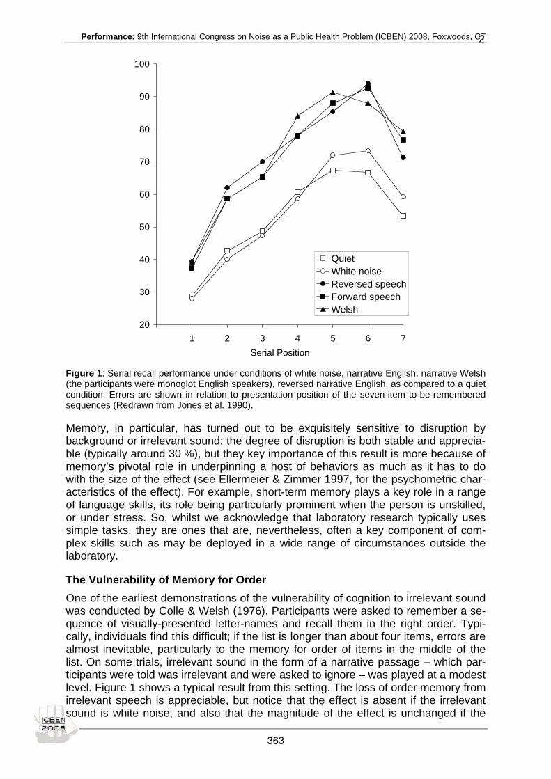
Performance: 9th International Congress on Noise as a Public Health Problem (ICBEN) 2008, Foxwoods, CT
2
Figure 1: Serial recall performance under conditions of white noise, narrative English, narrative Welsh (the participants were monoglot English speakers), reversed narrative English, as compared to a quiet condition. Errors are shown in relation to presentation position of the seven-item to-be-remembered sequences (Redrawn from Jones et al. 1990).
Memory, in particular, has turned out to be exquisitely sensitive to disruption by background or irrelevant sound: the degree of disruption is both stable and apprecia-ble (typically around 30 %), but they key importance of this result is more because of memory’s pivotal role in underpinning a host of behaviors as much as it has to do with the size of the effect (see Ellermeier & Zimmer 1997, for the psychometric char-acteristics of the effect). For example, short-term memory plays a key role in a range of language skills, its role being particularly prominent when the person is unskilled, or under stress. So, whilst we acknowledge that laboratory research typically uses simple tasks, they are ones that are, nevertheless, often a key component of com-plex skills such as may be deployed in a wide range of circumstances outside the laboratory.
The Vulnerability of Memory for Order One of the earliest demonstrations of the vulnerability of cognition to irrelevant sound was conducted by Colle & Welsh (1976). Participants were asked to remember a se-quence of visually-presented letter-names and recall them in the right order. Typi-cally, individuals find this difficult; if the list is longer than about four items, errors are almost inevitable, particularly to the memory for order of items in the middle of the list. On some trials, irrelevant sound in the form of a narrative passage – which par-ticipants were told was irrelevant and were asked to ignore – was played at a modest level. Figure 1 shows a typical result from this setting. The loss of order memory from irrelevant speech is appreciable, but notice that the effect is absent if the irrelevant sound is white noise, and also that the magnitude of the effect is unchanged if the
20
30
40
50
60
70
80
90
100
1 2 3 4 5 6 7Serial Position
QuietWhite noiseReversed speechForward speechWelsh
363

Performance: 9th International Congress on Noise as a Public Health Problem (ICBEN) 2008, Foxwoods, CT
3
irrelevant sound is either played backwards or is in a language that the participant does not understand. Clearly, the meaning of the sound seems unimportant, but speech seems to be an important pre-requisite, possibly because the focal memory task used verbal stimuli. But both these conclusions, to different degrees, turned out to be wrong. First, speech turns out not to be a necessary condition. Later work was able to show that pure tones produced disruption – to a diminished degree, granted, as did band-pass noise (providing it conveyed center-frequency changes) – but appreciable dis-ruption nevertheless. Instead another qualification became apparent, both for se-quences of speech sounds and for tones, the condition necessary for disruption was that there was acoustic variability, that is, the sound had to change: repeated se-quences of tones or speech produced no effects, but when they varied in composi-tion the sound was disruptive. This result was important for a variety of reasons, not least that it ruled out certain classes of explanation. Among these was the idea that the irrelevant speech sound was arriving at some point in the brain at which the pho-nological or speech-like character of materials was being processed and that the dis-ruption was based on the degree of similarity between the to-be-remembered visual items and the to-be-ignored sound. Later results ruled out such an explanation, but left the question of just how the disruption occurred unanswered.
25
30
35
40
45
0 2 5 10
Separation - semitones
Perc
ent e
rror
Figure 2: Effect of frequency separation of tones in an irrelevant sequence on serial recall
Two types of evidence, one relating to the nature of the focal task, the other relating to the organisation of the irrelevant sound, were instrumental in furnishing a plausible hypothesis. A number of studies suggested that the organisation of the irrelevant sound played a pivotal role. Figure 2 shows the effect of the auditory organisation of sound as ABA triplets are played in which the pitch difference between the A and the B components is increased (see Jones et al. 1999). Performance is hardly affected when the difference is small and increases appreciably as the pitch difference in-creases, but this diminishes again when the pitch is very large. Another way of see-ing this manipulation of pitch is in terms of degree of change in the sequence; disrup-tion is minimized when the degree of change is small (either when there is one un-changing stream or when the pitch difference results in fission of the sequence into two unchanging streams). This ‘changing state’ condition seems to be an important and general effect: It is true for all types of auditory stimuli – speech and non-speech – in this setting. We shall return to the significance of this finding shortly. Second, that the focal memory task is verbal is neither a sufficient nor necessary condition for disruption. If we alter the focal task so that it does not require memory for order, but nevertheless involves verbal material, then the distracting effect is
364

Performance: 9th International Congress on Noise as a Public Health Problem (ICBEN) 2008, Foxwoods, CT
4
markedly reduced if present at all. So, a sequence of six days of the week, drawn without replacement from the full set of seven to make a randomly ordered list, can be interrogated in at least two distinct ways. One way is to present one of the week-days and ask for a report of what followed it in the list, the other is to ask which day of the week was missing. These two methods call for distinctly different types of in-formation; the former (or probe) method requires a knowledge of the order of items, the latter (missing item) method requires a judgement of familiarity of items. It turns out that irrelevant sound disrupts the probe version but not the missing item version: the disruption is, therefore, highly context-sensitive in the sense of happening only with some tasks. From two perspectives, then, a factor related to the ordering of events seems to be at the heart of the distraction: the disruption only occurs if the brain needs to keep track of changing sounds, and it also only occurs if the order of events needs to be re-membered in the focal task. So, it is not so much to do with how similar the to-be-ignored events are to the to-be-remembered ones, rather it is the similarity of proc-essing of the two streams of mental activity. One way to characterise these effects is to think of the setting as one where the problem is of selecting the right response from a range of those currently prevailing; this difficulty becomes more acute when the ignored events are plausible candidates – by virtue of the processing to which they are subject – for the focal skill of remem-bering in serial order. We refer to this as a ‘conflict of process’. Notice that the degree of distraction cannot be predicted by considering either the character of the task or the character of the sound in isolation; it can only be understood by joint considera-tion of the obligatory processing of sound into ordered streams and the ordering process involved in the focal task.
Attentional Capture That the sound needs to be changing in state for disruption to occur has been asso-ciated with a rather different interpretation of the effect of irrelevant sound, namely, that the effect of change is the result of successive episodes of ‘attentional capture’. According to this view, attention is drawn involuntarily to an event if a mental model of the world of sound is violated: as we experience successive auditory events we build a ‘mental model’ of its characteristics, but any event that marks a sharp depar-ture from that model commandeers attention away from the task at hand (thereby impairing efficiency). This suggests too that in the long run the impact of any irrele-vant sound (as long as it has repeated elements) will be diminished by repeated presentation. Whilst recent experimental work has shown convincingly that an unexpected devia-tion from an established pattern of sound does capture attention, and that this has a material impact on cognitive performance, there is also evidence that this mechanism does not underpin the ‘changing state’ effect we described earlier. Just as before, the verbal serial recall task was used, this time with sound sequences in which the estab-lished sequence was violated, for example, by presenting one irrelevant spoken item in a different voice from the remainder. Again, a drop in memory performance is ob-served, but this effect is not context sensitive: it happens just as much with the probe as the missing-item versions of the memory task (Hughes et al. 2007). This strand of work has also been fruitful in further elucidating the nature of the men-tal model. One view is that the brain is quicker to build up a mental model if the sound is repeated than if it is not repeated; again, recent evidence has shown that
365

Performance: 9th International Congress on Noise as a Public Health Problem (ICBEN) 2008, Foxwoods, CT
5
this is not the case: the effect of a deviant stimulus – such as a slight change in tim-ing in a single member of the sequence – is just as great if it occurs in a sequence of changing letter-words or a repeated letter (Hughes et al. 2005). At the same time, these results show that the construct of ‘habituation’ has limited use in explaining these distraction effects, else the effect of the deviant would be more marked when it appears in a repeated than in a changing sequence. Other evidence also converges on the suggestion that habituation plays little role: typically, the impact of irrelevant sound does not diminish over the duration of an experiment (in which the exposure to irrelevant sounds and hence the opportunity for habituation would have been appre-ciable) nor does it diminish over successive days of testing (Hellbrück et al. 1996). This last set of findings is reassuring, insofar as it suggests that the distraction is not a fleeting phenomenon, but an enduring one, which suggests that it will have an im-pact in any setting outside the laboratory. Although attentional capture does not underpin the changing state effect, it is none-theless important to our understanding of the impact of single auditory events. Re-search on deviants is germane to the design of auditory alarms, for example (see Ljungberg et al. 2008).
The Vulnerability of Semantic Memory For some time it seemed the effect on serial order was highly specific and that similar effects did not occur in other settings. Clearly, such an outcome would mean that the phenomena would be of limited generality and difficult perhaps to apply to everyday life. However, in just the last few years, evidence has emerged of low-intensity dis-traction in an apparently quite distinct domain: retrieval of semantic information. Here the emphasis is not on remembering the order of events, rather the dominant prevail-ing mental activity is remembering or retrieving words according to their meaning. Figure 1 illustrated the point that for serial recall, the meaning of the speech has no effect. However, it is now apparent that meaning is important and can act as a dis-tractor, but only if the focal task contains, and involves, the organisation of material by virtue of its meaning. This is in line with the idea that if the sound processing and the focal task processing are similar then distraction will occur. For example, if we present visually a list of (say, twenty) words whose membership is drawn from a few (say, four) semantic categories, such as ‘fruits’, ‘animals’ and so forth, we find that the number of words that can be recalled, as well as their coherence (typically meas-ured by the degree to which the words are recalled not in the order in which they were presented but in clusters according to their meaning) is diminished in the pres-ence of meaningful sound (Marsh et al. 2008a). For this semantic distraction to occur, the similarity of the meaning of the to-be-ignored and to-be-remembered words is important, but this is not a direct product of the similarity of the words one to another; rather, it depends on the processing to which the to-be-remembered words are subject. Only if the focal task requires se-mantic processing will the semantic character of the to-be-ignored words be disrup-tive. If the self-same words in the focal task are processed and recalled in a non-semantic way, say just in the order in which they were presented, there will be no dis-ruption from the semantic features of the irrelevant sound. Such effects occur as a result of 'conflict of process'. In the selection of the correct word, several competing words are in contention for production: words 'come to mind' that, while being plausi-ble candidates, are not correct and some means must be found to inhibit their pro-duction. Our view is that in order to ensure that to-be-ignored sounds are not pro-duced, they are inhibited but that this inhibition spills over so that it also impairs the
366

Performance: 9th International Congress on Noise as a Public Health Problem (ICBEN) 2008, Foxwoods, CT
6
production of appropriate items. This would explain why the nature of the focal task processing is important and why the similarity in semantic content is important. Another factor is also important in these settings, the extent to which the person can discriminate whether a word was heard or seen, or indeed generated 'internally' by the search through memory, namely their capacity to use source monitoring accu-rately. Indeed, this type of auditory distraction is one that has its roots in episodic memory, that is, memory for the time and place in which an event occurred. It is be-coming clear that part of the difficulty of retrieving from memory is that individuals have difficulty in distinguishing whether they saw or heard the event. So, we have re-cently observed that the number of intrusion errors from the heard sequence of words also increases alongside the effect of the similarity of meaning of the heard to the to-be-remembered words (Marsh et al. 2008b). Such auditory distraction is par-ticularly relevant to ear- and eye-witness testimony – the witness will have difficulty knowing the source of information if the irrelevant stream and the relevant one occur at the same time. Finally, recent work has shown that these effects of semantic memory can occur in cases where no list is presented, in settings where participants are retrieving particu-lar instances from their long-term memory. A typical task is one in which the partici-pant is given a category (say, ‘fruits’’) and asked to retrieve as many words belonging to that category (the ‘semantic fluency’ task). Here again we witness a depression in performance if this is done in the presence of meaningful irrelevant sounds. How-ever, asking for a different sort of retrieval, one not based on meaning (such as ask-ing for words beginning with a particular letter – so-called ‘phonemic fluency’) is not susceptible to disruption (Marsh et al. 2008c).
CONCLUSIONS: HOW MANY VARIETIES? Although on the face of it the effects in serial recall and in semantic memory appear distinct, we think this is illusory and instead believe they stem from a mechanism that acts to govern the selection of action. That is, the obligatory and ‘sub-conscious’ analysis of sound yields various sorts of information that can be used as the basis of action. When the results of this analysis are compatible with, but inappropriate to, a currently-prevailing skill, such as serial recall or retrieval involving semantic memory, they need to be inhibited in some way. What we witness in this type of auditory dis-traction is the price we pay for exercising control over this conflict of processing. This inhibition incurs a cost in maintaining the focal task and performance is damaged as a result. All this flows from the sentinel functional character of the auditory system; the obligatory access of sound to perceptual organisation and, indeed, higher cogni-tive analysis such as semantic processing (but not everybody agrees with this par-ticular view: Carlyon 2004). At the same time, it should be acknowledged that this penalty for attentional flexibility must be weighed against the undoubted benefits of the organism having the general capacity to change the focus of attention adroitly in response to its adaptive needs. Although we can see a conceptual similarity between the results within semantic memory and serial recall, it is important to recollect that another, rather specific, mechanism is also involved in semantic memory retrieval: source monitoring. Attentional capture, the effect of brief, infrequent, unexpected, sounds on cognitive performance seems to be a separate variety of distraction from that resulting from the conflict of process that we have just described. It is not the basis of changing state effects, but something that reflects an intrusion of attention – an ‘interrupt-and-reorientate’ mechanism if you will – that signals the need to abandon the current task
367

Performance: 9th International Congress on Noise as a Public Health Problem (ICBEN) 2008, Foxwoods, CT
7
and seek information elsewhere. Again, for the most part, this is a highly adaptive function of the sentinel of the senses. We began by noting the historical development of this area of study: it has moved away from the preoccupation with intensity and the associated constructs of behav-ioral arousal. Instead, most of the effects of low intensity sound are couched in terms of the obligatory organisation of sound and the relation of that processing to that in the focal mental activity. This requires a more thoroughgoing analysis of both the task and the auditory events but we are finding effects on performance at sound in-tensities and in tasks that were thought to be immune just a couple of decades ago. Attentional capture is the exception to this rule, however. The task of the future is to extend still further our catalogue of varieties and the settings in which they operate, as well as understand how these effects on performance influence such factors as annoyance and distress occasioned by sound. The picture is complex, but then again, nobody expected it to be easy.
ACKNOWLEDGEMENT Most of the work undertaken in our laboratory has been sponsored by series of re-search grants by the UK’s Economic and Social Research Council.
REFERENCES Carlyon RP (2004). How the brain separates sounds. T Cog Sci 8: 465-471.
Colle HA, Welsh A (1976). Acoustic making in primary memory. J Verb Learn Verb Behav 15: 17-32.
Ellermeier W, Zimmer K (1997). Individual differences in susceptibility to the "irrelevant speech effect". J Acoust Soc Am 102: 2191-2199.
Hellbrück J, Kuwano S, Namba S (1996). Irrelevant background speech and human performance: Is there long-term habitua-tion? J Acoust Soc Jpn 17: 239-247.
Hughes RW, Vachon F, Jones DM (2005). Auditory attentional capture during serial recall: Violations at encoding of an algo-rithm-based neural model? J Exp Psychol: LMC 31: 736-749.
Hughes RW, Vachon F, Jones DM (2007). Disruption of short-term memory by changing and deviant sounds: Support for a duplex-mechanism account of auditory distraction. J Exp Psychol: LMC 33: 1050-1061.
Jones DM, Broadbent DE (1991). Human performance and noise. In: Harris C (ed.): Handbook of acoustical measurements and noise control (3rd ed.). NewYork: McGraw Hill.
Jones DM, Miles C, Page J (1990). Disruption of proofreading by irrelevant speech: Effects of attention, arousal or memory? Appl Cog Psychol 4: 89-108.
Jones DM, Alford D, Bridges A, Tremblay S, Macken W (1999). Organisational factors in selective attention: the interplay of acoustic distinctiveness and auditory streaming in the irrelevant sound effect. J Exp Psychol: LMC 25: 464-473.
Ljungberg JK, Hughes RW, Macken WJ, Jones DM (2008). Auditory attentional capture: Dissociations between objective and subjective indices. Manuscript in preparation.
Marsh JE, Hughes RW, Jones DM (2008a). Interference by process, not content, determines semantic auditory distraction. Cognition (in press).
Marsh JE, Hughes RW, Jones DM (2008b). Auditory distraction in semantic memory: A process-based approach. J Mem Lang 58: 682-700.
Marsh JE, Hughes RW, Jones DM (2008c). Disruption of verbal fluency by to-be-ignored spoken words: Support for a proc-ess-based account of auditory distraction. Manuscript submitted.
368

Performance: 9th International Congress on Noise as a Public Health Problem (ICBEN) 2008, Foxwoods, CT
The effects of classroom and environmental noise on children’s academic performance Bridget Shield1* and Julie Dockrell2 1 Department of Engineering Systems, Faculty of Engineering, Science and Built Environment, Lon-
don South Bank University, London SE1 0AA, UK
2 School of Psychology and Human Development, Institute of Education, London, WC1A 0HH, UK
* corresponding author: e-mail: [email protected]
INTRODUCTION There has been a considerable amount of research in the past 40 years into the ef-fects of noise on the performance of school children (Hetu et al. 1990; Evans & Lepore 1993; Shield & Dockrell 2003). It is generally accepted that noise has a detri-mental effect upon the learning and performance of primary school children, and that the older children in this age group are more affected than the younger children (Berglund & Lindvall 1995; Institute for Environment and Health 1997). Activities af-fected by noise include memory, reading, motivation, and attention (Bronzaft 1981; Cohen et al. 1981; Hygge et al. 1996; Berg et al. 1996; Maxwell & Evans 2000; Lundquist et al. 2000; Haines et al. 2002; Clark et al. 2006). There is increasing evi-dence that poor classroom acoustics can have a particularly negative effect upon children with special needs such as hearing impairment (Nelson & Soli 2000) or learning difficulties (Bradlow et al. 2003) This paper presents the results of a project carried out to assess the noise exposure of children at primary schools in London (UK) and to examine the impact of both envi-ronmental and classroom noise upon their academic performance. The impact of noise upon performance was examined in two ways: by investigating relationships between internal and external noise levels and children’s performance in nationally standardized tests of numeracy, literacy and science; and by experimental testing of children in different classroom noise conditions. It will be shown that the results of the two investigations of the impact of noise were consistent, showing that both environ-mental and classroom noise have detrimental effects upon children’s academic per-formance; and also that noise has more of an impact upon children with special edu-cational needs than upon other children.
METHOD – COMPARISON OF NOISE AND TEST RESULTS The initial part of the study consisted in carrying out internal and external noise sur-veys of London schools (Shield & Dockrell 2004). A questionnaire survey of over 2,000 primary school children was also undertaken, in which children’s perceptions of noise sources heard and annoyance from noise were assessed (Dockrell & Shield 2004). Noise levels were correlated with school results in nationally standardized tests (Shield & Dockrell 2008). Demographic data on each of the surveyed schools were obtained from the govern-ment Department of Children, Schools and Families (DCSF), in order to control for socio-economic factors in the analysis. This data consisted of the percentage of chil-dren receiving free school meals (FSM); the percentage of children for whom English was an additional language (EAL); and the percentage of children with special edu-cational needs (SEN). The FSM score has been shown to be a reliable indicator of social disadvantage in an area (Williamson & Byrne 1977).
369

Performance: 9th International Congress on Noise as a Public Health Problem (ICBEN) 2008, Foxwoods, CT
Noise surveys Noise levels were measured outside 142 schools within eight miles of central London (Shield & Dockrell 2004). Areas of London where aircraft are the predominant noise source were avoided as there was already a considerable body of research into the effects of aircraft noise (Evans & Lepore 1993; Cohen et al. 1981; Hygge et al. 1996; Haines et al. 2002). The main noise source to which the surveyed schools were ex-posed was therefore road traffic. The schools surveyed were all state primary schools in three London boroughs: bor-ough A was an ‘outer’ borough situated around six to eight miles of central London; the other two boroughs, B and C, were close to central London. Different characteris-tics of the boroughs can be illustrated by their respective population densities. The average noise levels measured in each borough are shown in Table 1, together with population densities and average school socio-economic factors.
Table 1: External noise levels and demographic data for primary schools in three London boroughs
Borough Noise levels Socio economic factors LAeq LA90 LAmax %FSM %EAL %SEN
Population/km2
A 57.4 49.2 70.5 38.8 43.9 10.3 7,600 B 56.2 46.5 68.3 41.5 35.3 28.3 12,200 C 58.9 50.2 72.0 33.6 39.6 26.2 10,100
Internal noise surveys were carried out in occupied and unoccupied spaces in 16 schools in boroughs A and B, chosen to reflect the full range of external noise levels. Spaces measured included 110 occupied classrooms and 30 empty classrooms. In-ternal levels measured are summarized in Table 2.
Table 2: Noise levels inside London schools
Noise level Occupied classrooms
Empty class-rooms
Corridor/ foyer
Occupied halls Empty halls
LAeq 72.1 47.0 58.1 73.4 53.2 LA90 54.1 36.9 44.6 55.1 44.3
Standardized assessment tests (SATs) Primary school children in England and Wales take standardized tests in English, Mathematics and Science at the ages of seven (‘Key Stage 1’) and eleven (‘Key Stage 2’) years. Average results for each school, consisting of the percentages of children achieving a specified criterion level at each stage, are published by DCSF. At the time of the study the tests taken at each stage were as follows: Key Stage 1 – Reading, Writing, Spelling, Mathematics Key Stage 2 – English, Mathematics, Science
METHOD - COGNITIVE TESTING IN NOISE Children performed a series of cognitive tests in three different noise conditions, which were based upon the results of the classroom noise and questionnaire sur-veys.
Tests A battery of verbal and non-verbal tests appropriate for eight year old children was developed (Dockrell & Shield 2006). The verbal tests consisted of two measures of
370

Performance: 9th International Congress on Noise as a Public Health Problem (ICBEN) 2008, Foxwoods, CT
literacy: a reading test and a spelling test. Two non-verbal tests were used: a speed of performance test designed to assess how quickly a child can perform simple men-tal operations, and a written arithmetic test.
Subjects The tests were performed by 158 eight year old children from six classes in four schools. The schools were matched for external noise levels, social disadvantage as measured by FSM scores, and SATs results. Of the children 38 (24 %) were identi-fied as having recognized special educational needs.
Noise conditions The children performed the tests in one of three noise conditions, derived from the results of the internal and external noise surveys of schools and children’s question-naire responses concerning noise sources heard in the classroom (Shield & Dockrell 2004; Dockrell & Shield 2004). The three noise conditions were as follows:
• base, that is their normal classroom condition when the children are working qui-etly with no talking and no additional noise
• babble, that is children’s babble, played at a steady level of 65 dB(A) LAeq, this being the average level measured in classrooms when children were working in-dividually (Shield & Dockrell 2004)
• babble and environmental noise, that is children’s babble as in the ‘babble’ condi-tion, with intermittent noise events from various sources (eg sirens, lorries) at ran-dom intervals, at a level of 58 dB(A) LAmax (that is the average internal level esti-mated from the external LAmax levels measured outside schools)
Classes were randomly assigned to one of the three noise conditions. All children carried out all tests in their allocated noise condition.
RESULTS This section presents the results of the two different investigations of the effects of noise, and also of the effects of noise upon children with SEN.
Effects of noise on standardized test results All internal and external noise parameters were correlated with Key Stage 1 (KS1) and Key Stage 2 (KS2) SATs scores for each subject, plus school average scores for each stage. The outer and central boroughs were treated separately in the analysis. Results were very similar for all KS1 literacy tests (Reading, Writing, Spelling) as would be expected. Therefore in the following discussion results are presented only for KS1 Reading to illustrate the impact of noise on the younger children’s attain-ments in literacy. For the outer borough, borough A, significant negative relationships existed between all SATs scores and all external noise parameters, except for KS1 Mathematics and LAmax, as shown in Table 3. However, this pattern was not repeated for central bor-oughs B and C when all schools were considered. If only those schools in boroughs B and C with external levels greater than 60 dB LAeq (the level specified as the upper limit at the site boundary in UK guidance on selection of a site for a new school) were considered, then there were significant negative correlations between test and noise parameters as also shown in Table 3.
371

Performance: 9th International Congress on Noise as a Public Health Problem (ICBEN) 2008, Foxwoods, CT
Obviously many factors apart from noise affect children’s academic performance. To control for the schools’ socio economic status as represented by FSM, EAL and SEN data, partial correlation was carried out. Many of the negative relationships between noise and tests scores were still significant, as shown in Table 4, which presents the significant correlation coefficients between LAeq and LAmax and Key Stage 2 test scores when controlling for socio-economic factors.
Table 3: Significant (at 1 % or 5 %) correlation coefficients between external noise and SATs results
Key Stage 1 Key Stage 2 Borough Noise level Reading Maths Average English Maths Science Average LAeq -0.34 -0.31 -0.36 -0.37 -0.40 -0.40 -0.41 LAmax -0.31 -0.32 -0.39 -0.46 -0.45 -0.45 A LA90 -0.37 -0.43 -0.40 -0.40 -0.40 -0.42 -0.43 LAeq -0.40 -0.39 LAmax -0.40 -0.43 -0.36 -0.39 B & C
(LAeq>60) LA90 -0.37
Table 4: Significant (at 1 % or 5 %) correlation coefficients between external noise and KS2 SATs results when correcting for socio-economic factors
LAeq LAmax Borough Factor English Maths Science Ave English Maths Science Ave
FSM -0.36 -0.34 -0.36 EAL -0.27 -0.32 -0.32 -0.33 -0.38 -0.44 -0.42 -0.45 A SEN -0.34 -0.38 -0.39 -0.39 -0.37 -0.44 -0.44 -0.44 FSM -0.34 -0.46 -0.35 -0.41 EAL -0.37 -0.46 -0.32 -0.37 -0.41 B & C
(LAeq>60) SEN -0.48 -0.34 -0.37 -0.43
Tables 3 and 4 show that all test scores were negatively correlated with noise levels. In borough A all except one relationship was significant at the .01 or .05 level, the strongest correlations being for KS2 Maths and Science. In boroughs B and C the subject score most closely associated with noise was KS2 English. In all boroughs the noise parameter most closely associated with noise was LAmax, and KS2 scores were more strongly related to noise than KS1 scores. This pattern is maintained when data are controlled for school socio-economic factors. A scatter plot illustrating the relationship between external LAmax levels and average KS2 scores in borough A is shown in Figure 1.
y = -0.70x + 120
30
40
50
60
70
80
90
100
40 50 60 70 80 90 100Noise level, LAmax (dB)
KS
2 A
vera
ge s
core
Figure 1: Scatter diagram relating external LAmax levels and average KS2 test scores in borough A
372

Performance: 9th International Congress on Noise as a Public Health Problem (ICBEN) 2008, Foxwoods, CT
For the analysis of the effects of internal noise on test scores all 16 schools were considered together. Internal noise levels measured in different school locations were compared with test scores. Negative correlation coefficients were found between all subject test scores and noise levels measured in occupied and unoccupied class-rooms and in corridors and foyers. The strongest correlations were with noise levels measured in occupied classrooms, particularly LA90 levels. Table 5 shows the signifi-cant correlation coefficients between test scores and LAeq and LA90 levels in occupied classrooms. When correcting for socio-economic factors there were still significant negative correlations between LA90 levels in occupied classrooms and noise; these are also shown in Table 5.
Table 5: Significant (at 1 % or 5 %) correlation coefficients between noise in occupied classrooms and SATs results
Correcting for socio economic factors LA90
SATs stage Subject LAeq LA90
FSM EAL SEN Reading -0.60 -0.60 Maths -0.57 -0.60
Key Stage
1 Average -0.58 English -0.55 -0.77 -0.66 -0.69 -0.76 Maths
Science -0.50 -0.59
Key Stage
2 Average -0.64 -0.51 -0.54 -0.63
A scatter plot illustrating the relationship between LA90 levels in occupied classrooms and average KS2 scores is shown in Figure 2.
y = -2.45x + 207
40
50
60
70
80
90
100
45 50 55 60 65Noise level, LA90 (dB)
Ave
rage
KS
2 sc
ore
Figure 2: Scatter diagram relating occupied classrooms LA90 levels and average KS2 test scores
Effects of noise on verbal and non-verbal reasoning Table 6 shows the means and standard deviations of the children’s performance scores in the cognitive tests in the three different noise conditions.
373
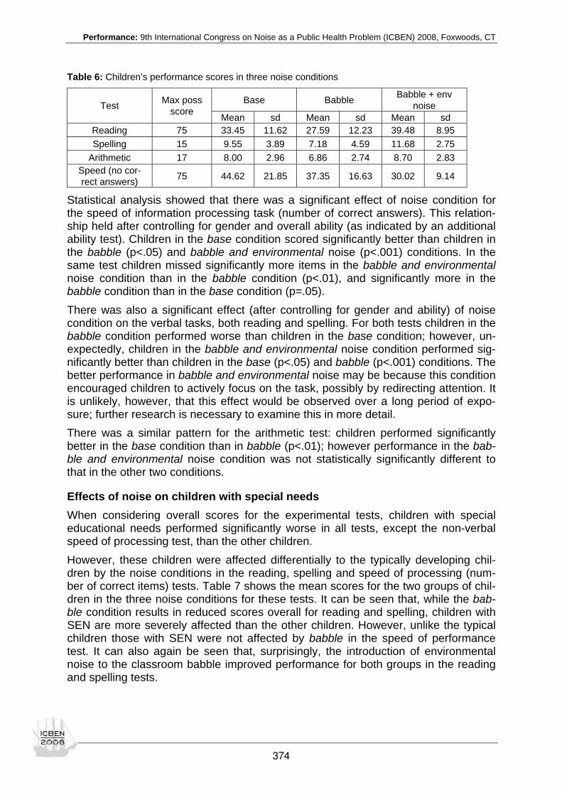
Performance: 9th International Congress on Noise as a Public Health Problem (ICBEN) 2008, Foxwoods, CT
Table 6: Children’s performance scores in three noise conditions
Base Babble Babble + env noise Test Max poss
score Mean sd Mean sd Mean sd Reading 75 33.45 11.62 27.59 12.23 39.48 8.95 Spelling 15 9.55 3.89 7.18 4.59 11.68 2.75
Arithmetic 17 8.00 2.96 6.86 2.74 8.70 2.83 Speed (no cor-rect answers) 75 44.62 21.85 37.35 16.63 30.02 9.14
Statistical analysis showed that there was a significant effect of noise condition for the speed of information processing task (number of correct answers). This relation-ship held after controlling for gender and overall ability (as indicated by an additional ability test). Children in the base condition scored significantly better than children in the babble (p<.05) and babble and environmental noise (p<.001) conditions. In the same test children missed significantly more items in the babble and environmental noise condition than in the babble condition (p<.01), and significantly more in the babble condition than in the base condition (p=.05). There was also a significant effect (after controlling for gender and ability) of noise condition on the verbal tasks, both reading and spelling. For both tests children in the babble condition performed worse than children in the base condition; however, un-expectedly, children in the babble and environmental noise condition performed sig-nificantly better than children in the base (p<.05) and babble (p<.001) conditions. The better performance in babble and environmental noise may be because this condition encouraged children to actively focus on the task, possibly by redirecting attention. It is unlikely, however, that this effect would be observed over a long period of expo-sure; further research is necessary to examine this in more detail. There was a similar pattern for the arithmetic test: children performed significantly better in the base condition than in babble (p<.01); however performance in the bab-ble and environmental noise condition was not statistically significantly different to that in the other two conditions.
Effects of noise on children with special needs When considering overall scores for the experimental tests, children with special educational needs performed significantly worse in all tests, except the non-verbal speed of processing test, than the other children. However, these children were affected differentially to the typically developing chil-dren by the noise conditions in the reading, spelling and speed of processing (num-ber of correct items) tests. Table 7 shows the mean scores for the two groups of chil-dren in the three noise conditions for these tests. It can be seen that, while the bab-ble condition results in reduced scores overall for reading and spelling, children with SEN are more severely affected than the other children. However, unlike the typical children those with SEN were not affected by babble in the speed of performance test. It can also again be seen that, surprisingly, the introduction of environmental noise to the classroom babble improved performance for both groups in the reading and spelling tests.
374

Performance: 9th International Congress on Noise as a Public Health Problem (ICBEN) 2008, Foxwoods, CT
Table 7: Mean performance scores of typical children and children with SEN in three noise conditions
Base Babble Babble + env noise Test Max poss
score Typical SEN Typical SEN Typical SEN Reading 75 35.50 28.00 30.76 13.44 40.36 36.93 Spelling 15 10.20 7.80 8.28 2.33 11.78 11.43
Speed (no correct answers) 75 49.20 32.40 36.96 39.00 20.90 30.36
DISCUSSION The comparison of noise levels and SATs results showed that both external and in-ternal classroom noise have a detrimental impact upon children’s academic perform-ance, with older children in the primary school age range being more affected than the younger children. The younger children were more affected by ambient and background levels of external noise, while the test scores of the older children were more closely related to maximum noise levels. This suggests that the performance of the older children is affected by the noise of individual events such as sirens, lorries or motorbikes passing the schools. This is consistent with the results of a question-naire survey into children’s perceptions of noise and its effects (Dockrell & Shield 2004) carried out during the same period, which showed that older children were more aware of external noise and that annoyance was related to external LAmax lev-els. The impact of noise of indivdual events is also consistent with the findings of re-search into the effects of aircraft and railway noise on children’s performance (Cohen et al. 1981; Bronzaft 1981; Hygge et al. 1996; Haines et al. 2002; Clark et al. 2006). Differences were found in the relationships between noise and test scores in the three areas of London which participated in the survey. In the central boroughs ef-fects of noise on test scores were only found for those schools where the external noise levels exceeded 60 dB(A) LAeq. A possible explanation is that schools in these two areas have a considerably higher percentage of children with special needs than in the other borough, which may result in ‘floor’ effects in these areas; that is, no mat-ter how quiet the area around the school test results would not improve above a cer-tain level. However, for the ‘noisier’ schools the general pattern of noise effects was similar to that in the outer borough. It was found that internal noise levels were more closely related to test results than external levels, again particularly for the older children. Background (LA90) levels in occupied classrooms were found to be the most closely associated with test scores; this is likely to be the level of general background classroom noise, such as back-ground ‘chatter’. This finding was consistent with the results of the controlled experimental testing which found that classroom babble had a detrimental effect upon children’s perform-ance in verbal and non-verbal tasks. Surprisingly performance in some tasks im-proved in babble and environmental noise. However, the age of the children in these tests was close to that of the younger children in the SATs/noise study which found that environmental noise had more of an impact upon the older children than the younger ones, and in particular that the younger children were more affected by am-bient and background noise and the older children by maximum noise levels, that is the noise of individual events. The only experimental task in which the children per-formed worst in babble and environmental noise was the speed of information proc-essing task. These results may explain why test scores for KS2 English were particu-
375

Performance: 9th International Congress on Noise as a Public Health Problem (ICBEN) 2008, Foxwoods, CT
larly strongly related to internal classroom background noise levels, while (in Borough A) KS2 Mathematics scores were the ones most strongly related to external LAmax levels. The experimental testing also found that children with special educational needs are particularly susceptible to detrimental effects of classroom babble upon their per-formance in verbal tasks (reading and spelling). However, interestingly the children with SEN did not appear to experience the same detrimental effect of babble as the other children in the speed of information processing task. It thus appears that chil-dren with SEN are less able to process language in classroom babble, but are less distracted by babble than other children when performing non-verbal tasks.
CONCLUSIONS The results show that both chronic and acute exposure to environmental and class-room noise have a detrimental effect upon children’s learning and performance. For external noise it appears to be the noise of individual events which have the most impact, while background noise in the classroom also has a significant negative ef-fect. Children with special educational needs were found to be more susceptible to the effects of classroom babble upon verbal tasks than other children. These results raise specific challenges for national and international policies which aim to educate all children in ‘inclusive’ environments. These studies have shown that it is essential to give careful consideration to the acoustic design of a school in order to optimize conditions for teaching and learning. The siting and internal layput of a school should be such that classrooms are not ex-posed to high levels of external noise. Also individual classrooms should be sited and designed so that background noise levels are miminised.
ACKNOWLEDGEMENTS The authors wish to thank researchers Ioannis Tachmatzidis and Rebecca Asker who collected some of the data and the UK Department of Health and DEFRA for funding this research.
REFERENCES Berg F, Blair J, Benson P (1996). Classroom acoustics: the problem, impact and solution. Lang Speech Hear Serv Schools 27: 16-20.
Berglund B, Lindvall T (1995). Community noise. Arch Center Sensory Res 2(1): 1-195.
Bradlow A, Krauss N, Hayes E (2003). Speaking clearly for children with learning disabilities: sentence perception in noise. J Speech Lang Hear Res 46: 80-97.
Bronzaft A (1981). The effect of a noise abatement program on reading ability. J Environ Psychol 1: 215-222.
Clark C, Martin R, van Kempen E, Alfred T, Head J, Davies H, Haines M, Lopez B, Matheson M, Stansfeld S (2006). Expo-sure-effect relations between aircraft and road traffic noise exposure at school and reading comprehension: the RANCH project. Am J Epidemiol 163: 27-37.
Cohen S, Evans G, Krantz D, Stokols D, Kelly S (1981). Aircraft noise and children: longitudinal and cross-sectional evidence on adaptation to noise and the effectiveness of noise abatement. J Person Soc Psychol 40: 331-345.
Dockrell J, Shield B (2004). Children’s perceptions of their acoustic environment at school and at home. J Acoust Soc Am 115: 2964-2973.
Dockrell J, Shield B (2006). Acoustical barriers in classrooms: the impact of noise on performance in the classroom. Brit Educ Res J 32: 509-525.
Evans G, Lepore S (1993). Nonauditory effects of noise on children: a critical review. Children's Environ 10: 31-51.
376

Performance: 9th International Congress on Noise as a Public Health Problem (ICBEN) 2008, Foxwoods, CT
Haines M, Stansfeld S, Head J, Job R (2002). Multi-level modelling of aircraft noise on performance tests in schools around Heathrow Airport London. J Epidemiol Commun Health 56: 139-144.
Hetu R, Truchon-Gagnon C, Bilodeau S (1990). Problems of noise in school settings: a review of literature and the results of an exploratory study. J Speech Lang Pathol Audiol 14: 31-38.
Hygge S, Evans G, Bullinger M (1996). The Munich Airport noise study: Cognitive effects on children from before to after the change over of airports. In: Proceedings Inter-Noise ’96 (pp 2189– 2192).
Institute for Environment and Health (1997). The non-auditory effects of noise. Report R10.
Lundquist P, Holmberg K, Landstrom U (2000). Annoyance and effects on work from environmental noise at school. Noise & Health 2(8): 39-46.
Maxwell L, Evans G (2000). The effects of noise on pre-school children’s pre-reading skills. J Environ Psychol 20: 91-97.
Nelson P, Soli S (2000). Acoustical barriers to learning: children at risk in every classroom. Lang Speech Hear Schools 31: 356-361.
Shield B, Dockrell J (2003). The effects of noise on children at school: a review. J Build Acoust 10: 97-106.
Shield B, Dockrell J (2004). External and internal noise surveys of London primary schools. J Acoust Soc Am 115: 730-738.
Shield B, Dockrell J (2008). The effects of environmental and classroom noise on the academic attainments of primary school children. J Acoust Soc Am 123: 133-144.
Williamson W, Byrne D (1977). Educational disadvantage in an urban setting. In: Herbert D, Smith D (Eds.): Social problems and the city. Oxford: Oxford Univ. Press.
377

Performance: 9th International Congress on Noise as a Public Health Problem (ICBEN) 2008, Foxwoods, CT
Positive effects of noise on cognitve performance: Explaining the Moderate Brain Arousal model Göran Söderlund1*, Sverker Sikström2 1 Department of Linguistics, Stockholm University, Sweden and School of Psychology, University of
Southampton, UK
2 Lund University Cognitive Science (LUCS), Sweden
* corresponding author: e-mail: [email protected]
ABSTRACT Distractors and environmental noise has long been regarded as detrimental for cognitive processing. In particular children with Attention Deficit Hyperactivity Disorder (ADHD) are extremely sensitive to distraction from task irrelevant stimuli. However, recently it has been shown that exposure to auditory white noise facilitated cognitive performance in ADHD children whereas control children performed worse. The Moderate Brain Arousal (MBA) model (Sikström & Söderlund 2007) suggest that this selective effect of noise adheres from stochastic resonance (SR). This phenomenon occurs in any system where a signal plus noise requires passing of a threshold, for example the all or none nature of action potentials in neural systems. The basic assumption is that noise in the environment, through the perceptual system introduces noise in the neural system. According to the SR phenomenon moderate noise is beneficial for cognitive performance whereas both excessive and insufficient noise is detrimental. The MBA model suggests that the amount of noise required for optimal cognitive performance is modulated by levels of dopamine. The model predictes that low dopamine children, as in ADHD, require more noise compared to high dopamine children for optimal cognitive performance; in short, when dopamine is low noise is good. Keywords: ADHD, noise, episodic memory, dopamine, model
INTRODUCTION It has long been known that, under most circumstances, cognitive processing is eas-ily disturbed by environmental noise and non-task compatible distractors (Broadbent 1958). This effect is believed to be due to competition for attentional resources be-tween the distractor and the target stimuli. The distractor effects hold across a wide variety of tasks, distractors and participant populations (Belleville et al. 2003; Boman et al. 2005; Hygge et al. 2003; Rouleau & Belleville 1996; Shidara & Richmond 2005). Children with attentional problems such as ADHD are more vulnerable to dis-traction compared to normal control children (Corbett & Stanczak 1999; Geffner et al. 1996). In contrast to the main body of evidence regarding distractors and noise, there have been a few reports of contradictory findings, although these findings have not been satisfactory explained. Specifically that under certain circumstances children with attentional problems (such as ADHD), rather than being distracted, actually benefit from environmental noise presented concurrently with the target task. Until recently the facilitative effect of non-task related environmental stimulation has been limited to the effects of background music on simple arithmetic task performance (Abikoff et al. 1996; Gerjets et al. 2002). More recently, Stansfeld et al. (2005) found that under certain conditions even road traffic noise can improve performance on epi-sodic memory tasks, especially in children with low socio-economic status and from
378

Performance: 9th International Congress on Noise as a Public Health Problem (ICBEN) 2008, Foxwoods, CT
crowded households, groups that are likely to be distinguished by attentional prob-lems and academic under-achievement. However, these earlier studies did not use or introduce SR as theoretical account for the beneficial effect of noise. The aim of this manuscript is to show that auditory white noise can, under certain prescribed circumstances, improve attention and cognitive performance in inattentive children. Our research group has found compelling data supporting the counterintui-tive notion that noise exposure under certain conditions can be beneficial for per-formance in cognitive tasks, in particular for individuals with attentional problems such as Attention Deficit/Hyperactivity Disorder (ADHD). The purpose of this presen-tation is to overview a model and findings showing a link between noise stimulation and cognitive performance. This is accomplished in the Moderate Brain Arousal model (Sikström & Söderlund 2007), which suggests a link between attention, dopa-mine transmission, and external auditory noise (white noise) stimulation.
The Moderate Brain Arousal model Signaling in the brain is characterized by myriads of noisy inputs and outputs with a poor fidelity. The capacity of the central nervous system to distinguish between the information-carrying component of the neuronal signaling and the noisy racket of neuronal inputs is a remarkable feature, which includes an ability to deal with noisy signals and to use them to its advantage to increase the signal-to-noise ratio (SNR). A fundamental mechanism that contributes to this process is the phenomenon of sto-chastic resonance (SR), which is a core concept of the MBA model. SR is the coun-terintuitive statistical phenomena where signals that are too weak to be detected be-come detectable when a random (stochastic) noise is added, see Figure 1. Although SR is a paradoxical phenomenon, it is well established across a range of settings; it exists in any threshold-based system where noise and signal are required to pass a threshold for the registering of a signal. The concept of SR was originally introduced to explain climate changes (Benzi et al., 1982), it has been identified in a number of naturally occurring phenomena, like bistable optical systems (Gammaitoni et al. 1998); mechanoreceptors of the crayfish (Douglass et al. 1993); and the feeding be-havior in the paddlefish (Russell et al. 1999). In particular SR has been found in neu-ral systems and in behavior.
Figure 1: Stochastic resonance where a weak sinusoidal signal goes undetected as it does not bring the neuron over its activation threshold. With added noise, the same signal results in action potentials
Threshold phenomena in neural systems are found in the all-or-none nature of action potentials. They can be modeled by a non-linear activation function, for example the sigmoid function, that simulates the probability that a neural cell will fire (Servan-Schreiber et al. 1990). The firing probability is influenced by the gain parameter that modifies how responsive a neural cell is to stimulation.
ThresholdSignalNoise + signal
= Threshold passing event
379

Performance: 9th International Congress on Noise as a Public Health Problem (ICBEN) 2008, Foxwoods, CT
In humans SR has been found in: touch (Wells et al. 2005), auditive (Zeng et al. 2000), and visual (Simonotto et al. 1999) sensory modalities, where moderate noise improves sensory discrimination. In fMRI scans a moderate noise level increased neural cortical activity in visual cortex (Simonotto et al. 1999). Most SR studies are done in perception tasks, requiring a detection of weak peripheral sensory inputs. However less known, empirical evidence suggests that SR also improve central processing and cognitive performance, For example, SR has been found in cognitive tasks where auditory noise improved the speed of arithmetic computations in a nor-mal group (Usher & Feingold 2000). Our research group has focused on cognitive effects of SR in particular groups with attentional problems like in ADHD. The attentional problems in ADHD are associated with impairment in multiple behavioral paradigms and also depends on the subtype of ADHD diagnosis (Nigg 2005). The implicated domains include; delay aversion, deficit in arousal/activation regulation, and executive function/inhibitory deficits (Castellanos & Tannock 2002). Delay aversion refers to an intolerance for waiting and has been used to explain difficulty in sustaining attention on long and boring tasks (Sonuga-Barke 2002). Poor regulation of activation or arousal are also associated with inatten-tion (Castellanos & Tannock 2002) where hyperactivity may be seen as a form of self-stimulation to achieve a higher arousal level. Executive deficits are predomi-nantly linked to impairments in working memory and effortful attentional control shown in the difficulty to stop an ongoing response and response shift (Casey et al. 1997). In the framework of MBA, the attentional problem comes from overactive response from environmental stimuli caused by too low levels of extracellular dopamine. Do-pamine signaling consists of two components; a stimulus independent tonic firing that determines concentration of dopamine in the extra-cellular fluid and a spike (stimu-lus) dependent phasic dopamine release. Tonic levels are continuous and modulate phasic reactivity. Autoreceptors in the pre-synaptic cell are activated when the tonic level is too high and suppresses spike-dependent phasic dopamine release, whereas low tonic levels increase phasic release (Grace 1995). Excessive tonic firing is sug-gested to cause inhibited phasic release and is associated with cognitive rigidity. Low tonic levels, in contrast, cause neuronal instability and boosted phasic responses (Grace et al. 2007). Excessive phasic transmission is suggested to cause instability in neuronal activation and is associated with cognitive symptoms such as failure to sustain attention, distractibility and excessive flexibility, symptoms that are hallmarks of ADHD. ADHD suffers from low tonic dopamine levels (Volkow et al. 2002) and consequently excessive phasic dopamine release causing the behavioral problems seen in ADHD. Furthermore, we suggest that ADHD symptoms should not be seen as a discrete category, but rather as a continuous dimension. This view implies that ADHD like symptoms are distributed in populations and can explain inattention and hyperactivity seen in normal populations as well. A major insight gained from the MBA model is that individual differences in the level of background noise within the neural system (linked to differences in dopamine signaling) will be reflected in differ-ent effects of environmental noise on performance. Neurocomputational modeling of the MBA model shows that a neural system with low dopamine levels (low gain parameter), requires more noise for an optimal perform-ance. Therefore inattentive and ADHD children, with low levels of dopamine, require more environmental noise than attentive children for optimal performance in cognitive tasks. Attentive children are suggested to possess sufficient internal noise levels for a high performance. Thus, neural systems with low levels of noise require more exter-
380

Performance: 9th International Congress on Noise as a Public Health Problem (ICBEN) 2008, Foxwoods, CT
nal noise for the facilitating effect of SR to be observed. Systems with high internal noise levels require less external noise. In this sense the individual levels of neural noise, and the individual SR curve, influence the external noise and performance dif-ferently. The size of the effect of noise on performance follows an inverted U-shaped curve. That is, a moderate noise is beneficial for performance whereas too little and too much noise attenuates performance. Levels of noise that enhance performance of children with low internal noise attenuate performance for children with higher lev-els of internal noise. Input parameters to the MBA model are external noise and sig-nal that activates internal neural noise and signal. Through the SR phenomenon these provide an output measured by cognitive performance. Thus, this provides a straightforward prediction of noise-induced improvement in cognitive performance in ADHD and inattentive children. In summary, the MBA model predicts that cognitive performance in ADHD and inat-tentive children benefits from noisy environments because the dopamine system modulates the SR phenomenon. It suggests that the stochastic resonance curve is right shifted in ADHD due to lower gain or lower dopamine. The MBA model predicts that for a given cognitive task ADHD children and inattentive children require more external noise or stimulation, compared to control children, in order to reach optimal (i.e. moderate) brain arousal level. This prediction was experimentally tested in three studies presented below.
Experimental support of the MBA model The affirmed predictions of the MBA model have been experimentally tested in an episodic memory task consisting of learning of word pairs. The main manipulations have been auditory noise and grouping of children based on ADHD and other behav-ioral testing. Participants are presented with verbal commands, simple verb – noun sentences such as “roll the ball” or “break the match” (Nilsson 2000). At the subse-quent memory test, participants are instructed to remember as many of the verbal commands presented as possible.
METHODS Participants Study 1. Forty-two, 9.4 – 13.7 years (M=11.2), children participated in the study. The ADHD group consisted of 21 boys, and no girls. This group was diagnosed by pedia-tricians (in Hospitals or local neuro-teams) according to the guidelines of DSM IV (APA 1994) Fifteen of the children were diagnosed ADHD-combined type (ADHD-C) and six as predominantly inattentive (ADHD-I). Seven children where medicated dur-ing the experiment (methylphenidate), and their results were analysed seperatly. The ADHD group was recruited from special schools or classes in Stockholm and the control group from ordinary schools in the same district matched after gender, age, and school performance level. Study 2. Thirty-two secondary school pupils (Sogndal, Norway) between 10-12 years (M=11.5) participated in the study. The group consisted of 22 boys and 10 girls. Par-ticipants where divided into groups after achievements or scholastic skills by judg-ment of their teachers for abilities concerning general school performance in three levels: below average, average, and above average relatively to what are expected from this age group. School performance were merged into two groups (be-low/average and above average achievers) while the below average group only con-sisted of four participants.
381

Performance: 9th International Congress on Noise as a Public Health Problem (ICBEN) 2008, Foxwoods, CT
Study 3. Fifty-one secondary school pupils (Sogndal, Norway, different school from study one) between 11-12 years (M=11.7) participated in the study. The group con-sisted of 25 boys and 26 girls. Participants where divided into groups in three levels after three different criteria: 1) school performance (teachers judgments); 2) Raven scores (Raven 1995); and 3) attention and/or hyperactivity (teachers judgments, scoring high in either of these behaviors or in both). Design and materials The design of the study was a 2 x 2, where no noise vs. noise was the within sub-ject’s manipulation. The between group variable where in study 1: ADHD vs. control. In study 2 and 3 the between group variable was based on cognitive performance as described above. The to-be-remembered (TBR) items consisted of 96 sentences divided into 8 sepa-rate lists with 12 verb-noun sentences in each list. Each sentence consisted of a uni-que verb and a unique noun (e.g., “roll the ball”). The sentences were placed in ran-dom order. All to-be-remembered sentences were recorded on a CD. In the no noise conditions the sentences were read in absence of noise and in the noise conditions they were read in presence of white noise. The equivalent continuous sound level of the white noise and the speech signal was 81 and 80 dB respectively, thus signal-to noise-ratio was -1 dB in study 1. In study 2 and 3 noise and speech levels where 78 and 86 dB, respectively and the signal-to-noise ratio was 8 dB. However, in all condi-tions the signal was sufficiently strong so that all participants could errorless perceive the content of the words (i.e., the tests were a cognitive memory test and not a per-ceptual test). The affirmed noise levels were chosen to correspond to levels where earlier studies have found effect of SR on cognition in an arithmetic’s test for a nor-mal population (Usher & Feingold 2000) and on working memory for Alzheimer pa-tients (Belleville et al. 2003). Recordings were made in a sound studio. Procedure In all studies the participants were tested individually in a room. The test lasted for about 45 minutes including instructions. Before starting the experiment proper, two practicing sentences were presented. All TBR items were recorded on a CD, a new item was read every 9th second. Time taken to present each list was approximately 1 min. 40 s. The noise exposure was continuous during the encoding phase and was present every second list. Directly after presentation of the last item subjects per-formed a free recall test in which they spoke out loud as many sentences as possible, in any order.
RESULTS Results from the studies are summarized in Figures 2 to 4 below. For a more exten-sive description of study 1 see Söderlund et al. (2007), study 2 and 3 see Söderlund et al. (in preparation).
382

Performance: 9th International Congress on Noise as a Public Health Problem (ICBEN) 2008, Foxwoods, CT
Figure 2: Study 1; Percentage correct recall as a function of noise and group (ADHD vs. Control)
The interaction between noise and group is significant when the medicated children where excluded while medication could be a possible confound. (F(1,33)= 5.73, p= .023, eta2= .15) (see Figure 2). When medicated group was included, to see if noise effect was present in this group too, in the assessment the interaction between noise and group became stronger (F(1,40) = 8.41, p = 0.006, eta2= .17). Study 2 comprised a normal population of school children. In this study cognitive per-formance was measured by teacher’s judgment of general scholastic skills in three levels: average, above and below average. While the below group only consisted of four participants the below and average groups were merged together Figure 3A shows that the interaction between noise and group is significant (F(1,30) = 5.92, p = 0.021, eta2= .14). The significant difference between groups in the no noise condition (t(30)= 3.67, p= .001) disappears in the noise condition (Figure 3A) Study 3 consisted of a normal population of school children. The children were grouped according to (1) teachers’ judgments of general school performance, (2) teacher judgments of inattention/hyperactivity, and (3) the score on a Raven test. The results are presented in figures 3B, 4A, and 4B (below), note that group sizes differ between the figures.
Figure 3A: Study 2: Recall performance as a function of noise and school performance in two groups (teachers judgments: above N= 12, below/average N= 20)
Figure 3B: Study 3: Recall performance as a function of noise and school performance (tea-chers judgments in three groups: above N= 22; average N= 22; below N= 7)
A
No Noise Noise0.2
0.3
0.4
0.5
0.6
ADHDControlP
erce
nt c
orre
ct in
free
reca
ll
Interaction: p = .023
No Noise Noise0.2
0.3
0.4
0.5
0.6
aboveaveragebelow
Interaction: p = .069
Per
cent
cor
rect
in fr
ee re
call
Below, above: p = .039
B
No Noise Noise0.2
0.3
0.4
0.5
0.6
abovebelow/average
Interaction: p = 021
Per
cent
cor
rect
in fr
ee re
call
383
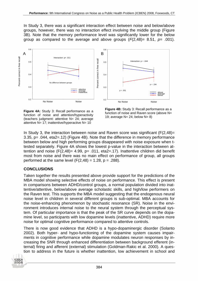
Performance: 9th International Congress on Noise as a Public Health Problem (ICBEN) 2008, Foxwoods, CT
In Study 3, there was a significant interaction effect between noise and below/above groups, however, there was no interaction effect involving the middle group (Figure 3B). Note that the memory performance level was significantly lower for the below group as compared to the average and above groups (F(2,48)= 8.51, p= .001).
Figure 4A: Study 3: Recall performance as a function of noise and attention/hyperactivity (teachers judgment: attentive N= 24; average attentive N= 17; inattentive/hyperactive N= 10
Figure 4B: Study 3: Recall performance as a function of noise and Raven score (above N= 19; average N= 24; below N= 8)
In Study 3, the interaction between noise and Raven score was significant (F(2,48)= 3.35, p= .044, eta2=.12) (Figure 4B). Note that the difference in memory performance between below and high performing groups disappeared with noise exposure when t-tested separately. Figure 4A shows the lowest p-value in the interaction between at-tention and noise (F(2,48)= 4.99, p= .011, eta2=.17). Inattentive children did benefit most from noise and there was no main effect on performance of group, all groups performed at the same level (F(2,48) = 1.28, p = .288).
CONCLUSIONS Taken together the results presented above provide support for the predictions of the MBA model showing selective effects of noise on performance. This effect is present in comparisons between ADHD/control groups, a normal population divided into inat-tentive/attentive, below/above average scholastic skills, and high/low performers on the Raven test. This supports the MBA model suggesting that the endogenous neural noise level in children in several different groups is sub-optimal. MBA accounts for the noise-enhancing phenomenon by stochastic resonance (SR). Noise in the envi-ronment introduces internal noise to the neural system through the perceptual sys-tem. Of particular importance is that the peak of the SR curve depends on the dopa-mine level, so participants with low dopamine levels (inattentive, ADHD) require more noise for optimal cognitive performance compared to attentive controls. There is now good evidence that ADHD is a hypo-dopaminergic disorder (Solanto 2002). Both hyper- and hypo-functioning of the dopamine system causes impair-ments in cognitive performance while dopamine modulates neuron responses by in-creasing the SNR through enhanced differentiation between background efferent (in-ternal) firing and afferent (external) stimulation (Goldman-Rakic et al. 2000). A ques-tion to address in the future is whether inattention, low achievement in school and
A B
No Noise Noise0.2
0.3
0.4
0.5
0.6
aboveaveragebelow
Interaction: p = .044
Per
cent
cor
rect
in fr
ee re
call
p = .001
p = .194
No Noise Noise0.2
0.3
0.4
0.5
0.6
attentiveaverage inattentive
Interaction: p= .011
Perc
ent c
orre
ct in
free
reca
ll
No differnce between groups
384

Performance: 9th International Congress on Noise as a Public Health Problem (ICBEN) 2008, Foxwoods, CT
demanding cognitive tasks such as Raven is to some extent caused by insufficient dopamine signaling. Although a number of studies demonstrates improved CNS function in clinical groups with stochastic stimulation e.g., in diabetes and stroke (Priplata et al. 2006), in elderly (Priplata et al. 2003), or in Parkinson’s disease (Yamamoto et al. 2005) the action mechanisms at the system level are poorly understood. Little is known about which parts of the brain (other than primary and secondary afferent neurons) that are acti-vated by stochastic noise stimulation. Furthermore, little is known about how SR in-terferes with normal CNS processing and if SR stimulation restores low dopamine levels (gain) or if it works by other means. There are limitations in present studies and many important queries remain to be sol-ved, e.g.: 1) to map out the inverted u-curve for the stochastic resonance by studying several noise levels for participants with different cognitive capacities; 2) to explore the generalization of the SR effect over different cognitive tasks; 3) to examine whether the SR effect has an effect on higher cognition supplied in different modali-ties and if SR works cross modal. The finding reviewed here strongly suggests that noise is not always bad for cognitive performance. However, the positive effect of noise depends on individual factors. This suggests that factors such as noise, and cognitive abilities interact in a complex way that should be acknowledged in any future work measuring cognitive tasks. The inverted U-shape of the SR phenomenon suggests that interesting effects could be hidden in mean values, which may emerge as interesting findings when the data is divided into groups.
REFERENCES
Abikoff H, Courtney ME, Szeibel PJ, Koplewicz HS (1996). The effects of auditory stimulation on the arithmetic performance of children with ADHD and nondisabled children. J Learn Disabil 29: 238-246.
APA (1994). DSM-IV. Diagnostic and statistical manual of mental disorders. American Psychiatric Publ. Inc.
Belleville S, Rouleau N, van der Linden M, Collette F (2003). Effect of manipulation and irrelevant noise on working memory capacity of patients with Alzheimer's dementia. Neuropsychology 17: 69-81.
Benzi R, Parisi G, Sutera S, Vulpiani A (1982). Stochastic resonance in climatic change. Tellus 34: 10-16.
Boman E, Enmarker I, Hygge S (2005). Strength of noise effects on memory as a function of noise source and age. Noise & Health 7(27): 11-26.
Broadbent DE (1958). The effects of noise on behaviour. Elmsford, NY: Pergamon Press.
Casey BJ, Castellanos FX, Giedd JN, Marsh WL (1997). Implication of right frontostriatal circuitry in response inhibition and attention-deficit/hyperactivity disorder. J Am Aacd Child Adolesc Psychiatry 36: 374-383.
Castellanos FX, Tannock R (2002). Neuroscience of attention-deficit/hyperactivity disorder: the search for endophenotypes. Nature Rev Neurosci 3: 617-628.
Corbett B, Stanczak DE (1999). Neuropsychological performance of adults evidencing Attention-Deficit Hyperactivity Disor-der. Arch Clin Neuropsychol 14: 373-387.
Douglass JK, Wilkens L, Pantazelou E, Moss F (1993). Noise enhancement of information transfer in crayfish mechanore-ceptors by stochastic resonance. Nature 365(6444): 337-340.
Gammaitoni L, Hänggi P, Jung P, Marchesoni F (1998). Stochastic resonance. Rev Modern Physics 70: 223-287.
Geffner D, Lucker JR, Koch W (1996). Evaluation of auditory discrimination in children with ADD and without ADD. Child Psychiatry Hum Develop 26: 169-180.
Gerjets P, Graw T, Heise E, Westermann R, Rothenberger A (2002). Deficits of action control and specific goal intentions in hyperkinetic disorder. II: Empirical results/Handlungskontrolldefizite und störungsspezifische Zielintentionen bei der Hyperki-netischen Störung: II: Empirische Befunde. Z Klin Psychol Psychother 31: 99-109.
385

Performance: 9th International Congress on Noise as a Public Health Problem (ICBEN) 2008, Foxwoods, CT
Goldman-Rakic PS, Muly EC 3rd, Williams GV (2000). D(1) receptors in prefrontal cells and circuits. Brain Res Rev 31: 295-301.
Grace AA (1995). The tonic/phasic model of dopamine system regulation: its relevance for understanding how stimulant abuse can alter basal ganglia function. Drug Alcohol Depend 37: 111-129.
Grace AA, Floresco SB, Goto Y, Lodge DJ (2007). Regulation of firing of dopaminergic neurons and control of goal-directed behaviors. Trends Neurosci 30: 220-227.
Hygge S, Boman E, Enmarker I (2003). The effects of road traffic noise and meaningful irrelevant speech on different mem-ory systems. Scand J Psychol 44: 13-21.
Nigg JT (2005). Neuropsychologic theory and findings in attention-deficit/hyperactivity disorder: the state of the field and salient challenges for the coming decade. Biol Psychiatry 57: 1424-1435.
Nilsson LG (2000). Remembering actions and words. In: Tulving E, Craik FIM (eds.): The Oxford handbook of memory (pp 137-148). Oxford: Oxford Univ. Pr.
Priplata AA, Niemi JB, Harry JD, Lipsitz LA, Collins JJ (2003). Vibrating insoles and balance control in elderly people. Lancet 362(9390): 1123-1124.
Priplata AA, Patritti BL, Niemi JB, Hughes R, Gravelle DC, Lipsitz LA, Veves A, Stein J, Bonato P, Collins JJ (2006). Noise-enhanced balance control in patients with diabetes and patients with stroke. Ann Neurol 59: 4-12.
Raven JC (1995). Coloured progressive matrices. Oxford: Oxford Psychological Press.
Rouleau N, Belleville S (1996). Irrelevant speech effect in aging: an assessment of inhibitory processes in working memory. J Gerontol B: Psychol Sci Soc Sci 51: P356-P363.
Russell DF, Wilkens LA, Moss F (1999). Use of behavioural stochastic resonance by paddle fish for feeding. Nature 402(6759): 291-294.
Servan-Schreiber D, Printz H, Cohen JD (1990). A network model of catecholamine effects: gain, signal-to-noise ratio, and behavior. Science 249(4971): 892-895.
Shidara M, Richmond BJ (2005). Effect of visual noise on pattern recognition. Exp Brain Res 163: 239-241.
Sikström S, Söderlund GBW (2007). Stimulus-dependent dopamine release in attention-deficit/hyperactivity disorder. Psy-chol Rev 114: 1047-1075.
Simonotto E, Spano F, Riani M, Ferrari A, Levero F, Pilot A, Renzetti P, Parodi RC, Sardanelli F, Vitali P, Twitty J, Chiou-Tan F, Moss F (1999). fMRI studies of visual cortical activity during noise stimulation. Neurocomputing 26-27: 511-516.
Söderlund GBW, Sikström S, Smart A (2007). Listen to the noise: Noise is beneficial for cognitive performance in ADHD. J Child Psychol Psychiatry 48: 840-847.
Söderlund GBW, Sikström S, Loftesnes JM (in preparation). Noise is not a nuisance: Noise improves cognitive performance in low achieving school children.
Solanto MV (2002). Dopamine dysfunction in AD/HD: integrating clinical and basic neuroscience research. Behav Brain Res 130: 65-71.
Sonuga-Barke EJ (2002). Interval length and time-use by children with AD/HD: a comparison of four models. J Abnorm Child Psychol 30: 257-264.
Stansfeld SA, Berglund B, Clark C, Lopez-Barrio I, Fischer P, Ohrstrom E, Haines MM, Head J, Hygge S, van Kamp I, Berry BF, RANCH study team (2005). Aircraft and road traffic noise and children's cognition and health: a cross-national study. Lancet 365(9475): 1942-1949.
Usher M, Feingold M (2000). Stochastic resonance in the speed of memory retrieval. Biol Cybern 83: L11-L16.
Volkow ND, Fowler JS, Wang G, Ding Y, Gatley SJ (2002). Mechanism of action of methylphenidate: insights from PET imaging studies. J Attent Disord 6(Suppl 1): S31-S43.
Wells C, Ward LM, Chua R, Timothy Inglis J (2005). Touch noise increases vibrotactile sensitivity in old and young. Psychol Sci 16: 313-320.
Yamamoto Y, Struzik ZR, Soma R, Ohashi K, Kwak S (2005). Noisy vestibular stimulation improves autonomic and motor responsiveness in central neurodegenerative disorders. Ann Neurol 58: 175-181.
Zeng FG, Fu QJ, Morse R (2000). Human hearing enhanced by noise. Brain Res 869: 251-255.
386

Performance: 9th International Congress on Noise as a Public Health Problem (ICBEN) 2008, Foxwoods, CT
A comparison of structural equation models of memory performance across noise conditions and age groups
Staffan Hygge1*, Ingela Enmarker1,2,3, Eva Boman2
1 Centre for Built Environment, University of Gävle, SE-801 76 Gävle, Sweden
2 Department of Education and Psychology, University of Gävle, SE-801 76 Gävle, Sweden
3 Department of Health, Campus Namsos, Nord-Trøndelag University College, Serviceboks 2501, NO-7729 Steinkjer, Norway
* corresponding author: e-mail: [email protected]
INTRODUCTION In a recent study (Enmarker et al. 2006) structural equation models (SEM) of memory performance across noise conditions and age groups were compared and tested. The latent variable structures were basically invariant across the three noise condi-tions (quiet, road traffic, and irrelevant speech). For the four age groups (13-14, 18–20, 35–45, and 55–65 years) the latent variable structures wtere invariant across the three older groups, but the youngest group stood out from the others. The pupils in the youngest group who performed best on the memory tasks showed a SEM mem-ory structure that was similar to the group aged 18-20 years, but those who per-formed worse did not. This may signify something of a developmental shift in cogni-tive development. In the present study more detailed contrasting models of the memory performance of the three noise conditions and four age groups are formulated and tested. In particu-lar, an attempt is made to identify memory structures for the group aged 13-14 years that can account for differences in memory structure in that group and give a hint about the nature of their memory development and susceptibility to noise.
METHODS Participants and Basic Design
Participants (total N = 288) were randomly assigned to each of three independent groups: (a) road traffic noise, (b), meaningful irrelevant speech and (c) silence. This was crossed with four age groups, with an equal number of male and female partici-pants in each of the noise conditions in the age groups 13-14 and 18-20 years. (N=96 for 13-14 and 18-20 years). For age groups 35-45 and 55-65 years, N=48 in each group, but there were slightly more females in these age groups.
Procedure The experiments were run in a climate chamber and two to four participants stayed in the experimental room at the same time. The only difference between the three noise groups was the different noise conditions during the first part of the experiment. In the second part of the experiment retrieval measures on all the episodic memory tasks were taken in quiet to unconfound noise effects at encoding and retrieval.
387

Performance: 9th International Congress on Noise as a Public Health Problem (ICBEN) 2008, Foxwoods, CT
Noise
In the noise conditions digital recordings of meaningful irrelevant speech and road traffic noise were played back through loudspeakers in front of the room. The equiva-lent sound level (Leq) in the noise conditions was set to 66 dBA 2 m in front of the loudspeakers. The sound level in the quiet control group was 38 dBA Leq.
The road traffic noise recording was made up of a background of continuous traffic noise (~62 dBA) with superimposed segments of trucks passing by. The meaningful irrelevant speech recording consisted of background babble (~62 dBA) without any discernible meaning, with superimposed segments of a dialogue between two teen-agers. In the segments only one person was talking at a time. This dialogue was dis-tinct and interpretable, but did not convey much of information. The dBA-against-time history of the traffic noise and the speech noise were matched against other. The peaks (fast) in the superimposed segments were at 78 dBA for both noise sources and occurred on the average once per minute and with different duration. The domi-nant frequency range for the road traffic noise (100-300 Hz) was lower than that for the meaningful irrelevant speech (500-1500 Hz).
Dependent Measures
See Table 1 for a list of the memory items, their abbreviations, and their assignment to latent variables.
Table 1: Memory items in the latent variables and the abbreviations employed in Figure 1
Abbreviation Item name Items in Episodic memory RCLtxt FRwE FRwoE CRCwE CRCwoE CRNwE CRNwoE
Recall Recall of text Free recall with enactment Free recall without enactment Cued recall categories with enactment Cued recall categories without enactment Cued recall nouns with enactment Cued recall nouns without enactment
RCGtxt Face rcg GN IncL FN IntL
Recognition Recognition of text Face recognition Given name incidental learning Family name intentional learning
Items in Semantic memory W comp
Knowledge Word comprehension
WF A WF M WF prof
Fluency Word fluency letter A Word fluency letter M Word fluency professions
388
Performance: 9th International Congress on Noise as a Public Health Problem (ICBEN) 2008, Foxwoods, CT
Episodic memory. The participants read a text about a fictitious ancient culture for 15 min at the beginning of the experiment (in silence, road traffic noise or irrelevant speech according to experimental group). They were tested in writing in silence for cued recall and recognition of the text at the end of the experiment.
Several other of our memory tests were adapted from the Betula study of health, memory and ageing. This study is a large (N > 3,000) prospective Swedish study on memory, health and ageing (see Nilsson et al. 1997 for a description).
In testing sentences with and without enactment (Nilsson et al. 1997) the participants were presented with two successive lists in imperative form (e.g., knock on the pan, roll the pineapple) with 16 sentences each. For one of the lists the encoding was done with enactment (Engelkamp 1995). In the Betula project, Nilsson et al. (1997) also developed a face and name recognition task for testing intentional and incidental learning and recognition for non-verbal material in episodic memory. This test was computerized and adapted to group presentation in our experiments. A total of 24 faces and names were presented during testing. Twelve were target faces and names of the 16 presented initially, and 12 were distractor faces and names. Target and distractor faces appeared one by one for 15 s on the computer screen in a ran-dom order.
Semantic memory. In the word fluency test, a semantic memory task, three sets of words were generated, each set starting with a letter of its own. The sets were: words, five-letter words and professions (Nilsson et al. 1997). Each set was given one minute to complete.
In the word comprehension task participants were presented with a list of 30 target words. Next to each target five other words were presented, one of which being syn-onymous to the target word. This task was a test of the noise impact on the general knowledge in semantic memory.
All the items assigned to episodic memory were encoded according to experimental condition (silence, road traffic noise, meaningful irrelevant speech) but always tested for in silence at the end of the session. All the semantic memory tasks were per-formed according to experimental condition. The memory test items were assigned in advance to the latent variables episodic and semantic memory.
First- and second-order factors.
Nyberg et al. (2003) formulated and tested SEM for parts of the memory test battery in the Betula study. As several of our tests have a close similarity to the tests in the Betula study, we followed some of the SEM ideas in Nyberg et al. (2003). First- and second-order factors were identified for model testing. As seen in Figure 1, recall and recognition were identified as first-order factors for episodic memory, and knowledge and fluency for semantic memory. In the Betula study or in the test battery analyzed by Nyberg et al. (2003), there was no test for a text. Thus, in addition to Nyberg et al. (2003) Text was introduced a latent variable of its own in out SEM.
The statistical testing strategy followed was basically the same as in Nyberg et al. (2003). Initially one matrix across all age groups and noise conditions was tested against competing structural models, with and without 2nd-order factors.
389

Performance: 9th International Congress on Noise as a Public Health Problem (ICBEN) 2008, Foxwoods, CT
In Enmarker et al. (2006) model fit was evaluated by examining the χ2 and mean-square error of approximation (RMSEA; Browne & Cudeck 1993), comparative fit in-dex (CFI; Bentler 1990), and non-normed fit index (NNFI; Bentler & Bonnet 1980). Priority was given to the RMSEA criterion, following the suggestion by Browne and Cudeck (1993) that a RMSEA about .08 or less is a reasonable fit, and about .05 or less is a good fit.
See Figure 1 for the SEM, standardized loadings, and free error covariances be-tween items.
Figure 1: Conceptual diagram of a model for a single sample with the addition of a separate first-order factor (Text) for the text memory items (RCLtxt, RCGtxt) loaded on the second-order factor Episodic, with the corresponding indicators, standardized loadings, and free error covariances (χ2 = 90.17, df = 74, p = 0.097, RMSEA = 0.028). In all cases the standardized latent variable–item coefficients were significant (all ts > 4.03, all ps < 0.001), and none of the items had a higher standardized latent vari-able–item coefficient when loaded on another latent variable than the one hypothesized.
Episodic
Semantic
Recall
Recogn
Knowl
Fluency
TextRCLtxt
RCGtxt
WF A
WF M
WF prof
W comp
FRwE
FRwoE
CRCwE
CRCwoE
CRNwE
CRNwoE
Face rcg
GN IncL
FN IntL
.71 .61 .67 .44 .76 .61 .48 .51 .69 .50 .59 .83 .79 .58 .55
.86
.90
.86
.56
.97
.88
390

Performance: 9th International Congress on Noise as a Public Health Problem (ICBEN) 2008, Foxwoods, CT
Mediation models. Figure 1 depicts a good model fit for the single sample where age groups and noise conditions are collapsed. However, follow up tests of that model indicated that quite the youngest age group (13-14 years) did not abide to the gen-eral model. Also, the model presented in Figure 1 did not include Noise as a latent variable, nor was there any attempt to model mediation between the latent variables. As the youngest group stands out it would be interesting to find out whether there is any mediation model that applies to the youngest age group and another model that applies to the older groups. One way to approach this is to formulate and test alterna-tive models to see whether some of the models show a good fit with data for the young ones and another model for the older groups. Comparing the models could then give some insight into which kind of developmental change that with growing cognitive maturity and whether noise exposure has any impact. Five models were chosen for further testing. They are depicted in Figure 2. With the exception of model 4, they all have the latent variable Text as a last chain in the me-diation link, and with the other variables as mediating or moderating links. Model 4 differs from the other models in the respect that it does not include any element of mediation, and thus may serve as an independence base line. The strategy was to compare the five models under three restrictions: (1) with all four age groups included, (2) with the youngest group (13-14 years) excluded, and (3) only with the youngest age group. Models that show a good fit with data under re-strictions 2 or 3 may be viable candidates for theorizing about what is equal and what is different between the youngest group and the older groups. In the model testing the error covariances were set free between the same pairs of item as in Figure 1.
RESULTS
In evaluating the outcome of the model fit only the RMSEA criterion was employed. A RMSEA about .08 or less is taken a reasonable fit, and about .05 or less as a good fit (Browne & Cudeck 1993).
The results of the comparison between the models are shown in Table 2. As can be seen the mediation chains with only complete mediation from Noise by Semantic by Episodic to Text (Model 1) may be satisfactory for the age groups 18-20 years and older, but not for the youngest groups. For the youngest group there is a somewhat better fit with Model 2 where Episodic precedes Semantic in the mediation chain.
Model 3, in which Noise only influences Text has some merit to it, both in the young-est group by itself and also in all age groups from 18-20 years and older.
Model 4, the independence model does not rate well, neither with the youngest group, nor with the age groups from 18-20 years and older.
The fit for Model 5 is about as good as for Model 3. That is, which is in contrast to Model 3, that Noise may have a direct influence on both Semantic and Episodic, but no direct path to Text. This model has about the same goodness of fit both for the youngest group and for the age groups from 18-20 years and older.
391
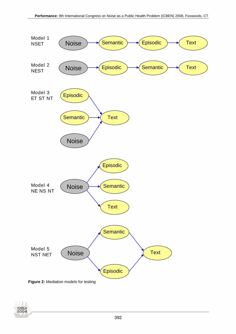
Performance: 9th International Congress on Noise as a Public Health Problem (ICBEN) 2008, Foxwoods, CT
Figure 2: Mediation models for testing
Noise Semantic Episodic Text
Noise Episodic Semantic Text
Noise
Episodic
Semantic Text
Noise
Episodic
Semantic
Text
Noise
Semantic
Episodic
Text
Model 1 NSET
Model 2 NEST
Model 3 ET ST NT Model 4 NE NS NT Model 5 NST NET
392

Performance: 9th International Congress on Noise as a Public Health Problem (ICBEN) 2008, Foxwoods, CT
Table 2: RMSEA-values and dfs for the five conceptual models with the youngest age group included, excluded, and as a separate group
Model All age groups (df)
Not age group 13-14 years (df)
Only age group 13-14 years (df)
1 NSET
.081 (499) .053 (363) .084 (91)
2 NEST
.079 (499) .062 (363) .055 (91)
3 ET ST NT
.073 (497) .046 (361) .051 (89)
4 NE NS NT
.081 (499) .061 (363) .074 (91)
5 NST NET
.078 (498) .053 (362) .051 (90)
CONCLUSIONS The models that came out relatively best on best models in our tests were number 3 and 5. What this implies is maybe better stated in terms of which theoretical models that were not given support, numbers 1, 2, and 4.
Model number 1 and 2 is in terms of one single chain of mediation, with Noise as a start and Text as the end product. The short-coming of these models indicate that there is no simple full mediation from Noise to Text by Semantic and Episodic, or the last two in reversed order. Further, Model 3, assuming no interdependency or media-tion between Semantic, Episodic, and Text, also is not the best of our models. Thus, what remains is a kind of partial mediation model. Models number 3 and 5 are such models.
Although there are only 96 persons in age group 13-14 years (32 in each noise con-dition), and a summed total of 192 in the other age groups, the RMSEA-value, which will be lower with a lower N, for the youngest groups is not substantially lower for the other age groups combined.
In Enmarker et al. (2006) it was noted that noise from meaningful irrelevant speech does not produce any appreciable shift in the covariance matrix as compared to the matrix when exposed to road traffic noise, or for that matter, in the quiet condition. A direct two sample test involving only the Road traffic noise group and the Speech group, with the same restraints as in Figure 1, showed good agreement between the two (χ2 = 209.40, df=193, p=0.199, RMSEA=0.030). Thus, in this respect speech is not special (Lieberman, 1982). However, this was not tested separately for the youngest age group.
Thus, the SEM memory problem with the young group may lie somewhere else than in how our conceptualization of how the latent variables Episodic, Semantic and Text interact. It may be the case that the two different noise conditions, road traffic noise and irrelevant speech have their own differential effects on semantic and episodic memory for children, which may be in a developmental transition state, and which were not properly modeled in the latent memory structure models we have tested here.
393

Performance: 9th International Congress on Noise as a Public Health Problem (ICBEN) 2008, Foxwoods, CT
As a strengthening argument for the validity of our findings on the noise invariant memory structure, it should be borne in mind the quite satisfactory goodness-of-fit measures were obtained without excluding the youngest age group, which according to the age invariant analyses stands out from the other age groups on latent memory structure.
In summary, we have shown that some of the possible meditational models of how noise influences episodic and semantic memory and text reading for children can be ruled out. What remains to be analyzed is whether speech noise and road traffic noise tap different or similar memory capacities for children as for adults.
However, how that should be put to scrutiny is a future story.
REFERENCES Bentler PM (1990). Comparative fit indexes in structural models. Psychol Bull 107: 238-246.
Bentler PM, Bonnet DG (1980). Significance tests and goodness-of-fit in the analysis of covariance structures. Psychol Bull 88: 588-600.
Browne MW, Cudeck R (1993). Alternative ways of assessing model fit. In: Bollen KA, Long JS (eds.): Testing structural equation models. London: Sage.
Engelkamp J (1995). Visual imagery and enactment of actions in memory. Brit J Psychol 86: 227-240.
Enmarker I, Boman E, Hygge S (2006). Structural equation models of memory performance across noise conditions and age groups. Scand J Psychol 47: 449-460.
Hygge S, Boman E, Enmarker I (2003). The effects of road traffic noise and meaningful irrelevant speech on different mem-ory systems. Scand J Psychol 44: 13-21.
Liberman AM (1982). On finding that speech is special. Am Psychologist 37: 148-167.
Nilsson L-G, Bäckman L, Erngrund K, Nyberg L, Adolfsson R, Bucht G, Karlsson S, Widing M, Winblad B. (1997). The Betula prospective cohort study: Memory, health, and aging. Aging Neuropsychol Cogn 4: 1–32.
Nyberg L, Maitland SB, Rönnlund M, Bäckman L, Dixon RA, Wahlin Å, Nilsson L-G (2003). Selective adult age differences in an age-invariant multifactor model of declarative memory. Psychol Aging 18: 149–160.
394
Performance: 9th International Congress on Noise as a Public Health Problem (ICBEN) 2008, Foxwoods, CT
Effect of speech intelligibility on task performance - an experimental laboratory study Annu Haapakangas1*, Miia Haka2, Esko Keskinen2, Valtteri Hongisto1 1 Finnish Institute of Occupational Health, Indoor Environment Laboratory, 20520 Turku, Finland
2 University of Turku, Department of Psychology, 20014 Turku, Finland
*corresponding author: e-mail: [email protected]
ABSTRACT The aim of this study was to examine the effects of speech varying in intelligibility on cognitive performance and subjective perceptions of sound environment disturbance. 37 subjects performed a series of tasks in three conditions in which speech transmission indexes were 0.10, 0.35 and 0.65. These correspond to cellular office, well-designed open office and unsatisfactory open office, respectively. The experiment was conducted in an office laboratory in which the direction of the speech source varied. The sound environments were presented at 48 dBA. Performance deteriorated in condition 0.65 compared to the other two conditions in a serial recall task (p < .05) and in a complex working memory task (p < .001). Proofreading performance did not differ in different conditions but the task was experienced as easier in the condition with lowest STI value than in the other two (p < .05). Questionnaire measures showed consistent, statistically significant differences between all three situations: the higher the STI value was, the more it was experienced to disturb performance and draw attention away from the task (p < .001). Similarly, the ease of habituation and the pleasantness of sound were rated higher as the STI value declined (p < .001). Self-rated work efficiency declined with ascending STI values (p < .05). Continuous background noise was not experienced to disturb performance in any condition. This supports the use of continuous masking sound in minimizing speech intelligibility, i.e. increasing speech privacy in open offices.
INTRODUCTION Office surveys have shown that speech is experienced as the most distracting noise source in offices (e.g., Haapakangas et al. 2008). The problem is particularly great in open offices. Earlier laboratory experiments have shown that the disruptive effects of speech are not produced by the level of speech but speech intelligibility (Colle 1980; Ellermeier & Hellbrück 1998; Venetjoki et al. 2006; Schlittmeier et al. 2008). According to Hongisto et al. (2007), speech intelligibility in open offices varies greatly but it can be lowered by proper acoustical design. Research is needed on the effect of speech intelligibility on task performance in order to encourage investments in acoustic improvements. However, there are only a few published studies that have studied the effect of speech on cognitive performance with varying levels of speech intelligibility. Speech intelligibility can be evaluated with Speech Transmission Index (STI). For example, STI value 0.50 expresses roughly that 50 percent of syllables are correctly heard. STI can be easily determined between office workstations using acoustical measurements. The first experiment that used STI as a descriptor of irrelevant speech was published by Venetjoki et al. (2006). It was found that proofreading per-formance deteriorated significantly in STI 0.80 compared to STI 0.00. Later, similar experiments have been conducted by Schlittmeier et al. (2008).
395
Performance: 9th International Congress on Noise as a Public Health Problem (ICBEN) 2008, Foxwoods, CT
The aim of this experiment was to show how the level of speech intelligibility affects cognitive performance. Speech was expected to deteriorate performance more in higher levels of speech intelligibility. The study focused on the STI range from 0.10-0.65 because the acoustic conditions of offices are typically in this area. The study also aimed to validate the model of Hongisto et al. (2008) that predicts the deteriora-tion of performance as a function of STI.
METHODS Subjects and test setup A repeated measures design with three speech conditions was used. Altogether 37 students took part in the experiment in December 2007. The three speech conditions were STI 0.10, STI 0.35 and STI 0.65. A group of four participants was tested at a time. Experiments were conducted be-tween 8.15 a.m. and 12.30 p.m. The experiment included a practice session and three test sessions lasting for about 55 minutes each. Each situation was followed by a 5-minute break. The order of speech conditions was counterbalanced across sub-jects, as was the presentation of different speech samples and test versions in differ-ent speech conditions. Subjects performed five tasks: a serial recall task, a complex working memory task, a proofreading task, a visual short-term memory task and a reading comprehension tasks. The latter two were mainly included as filler tasks to increase the length of test sessions and were being piloted for future experiments. The serial recall task was conducted following classic procedures in which digits from 1 to 9 are presented on a computer screen in random order. Subjects' task is to recall the digits in the same order. The number of digits recalled in correct serial positions is measured. The complex working memory task was modified from the operation span task devel-oped by Turner and Engle (1989). In the task, subjects had to state whether simple arithmetic calculations, presented on a computer screen, were true or false. Each calculation was followed by a presentation of a word that the subject had to memo-rize. At the end of each equation-word pair list, subjects were asked to recall the pre-sented words in the same order. The number of words to be remembered increased from 3 to 8. The total number of correctly recalled words was measured. The proofreading task was the same as in our earlier study (Venetjoki et al. 2006). It was a pen-and-paper task in which subjects looked for mistakes in the text. Half of the errors were spelling errors whereas half required semantic processing. Each speech condition was followed by a questionnaire that assessed subjective perceptions of the sound environment. A 5-point Likert scale was used in most ques-tions. Disturbance of other environmental factors was included in the questionnaire that was presented after the last sound condition. Background information was gath-ered with a separate questionnaire before practice session.
Speech conditions The investigations were carried out in an office laboratory (Figure 1). Three speech conditions were used:
• STI=0.10 - corresponds to a private office room with the door closed. Speech intelligibility is extremely low.
396
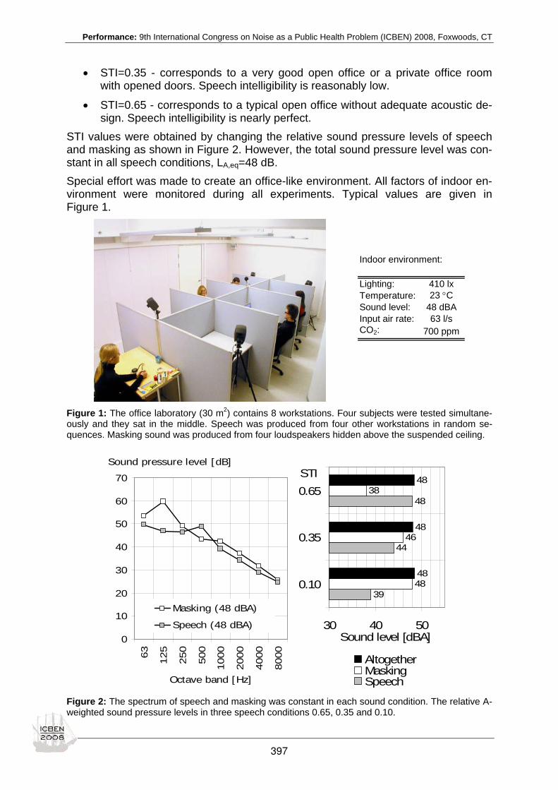
Performance: 9th International Congress on Noise as a Public Health Problem (ICBEN) 2008, Foxwoods, CT
• STI=0.35 - corresponds to a very good open office or a private office room with opened doors. Speech intelligibility is reasonably low.
• STI=0.65 - corresponds to a typical open office without adequate acoustic de-sign. Speech intelligibility is nearly perfect.
STI values were obtained by changing the relative sound pressure levels of speech and masking as shown in Figure 2. However, the total sound pressure level was con-stant in all speech conditions, LA,eq=48 dB. Special effort was made to create an office-like environment. All factors of indoor en-vironment were monitored during all experiments. Typical values are given in Figure 1.
Indoor environment:
Lighting: 410 lxTemperature: 23 °CSound level: 48 dBAInput air rate: 63 l/sCO2: 700 ppm
Figure 1: The office laboratory (30 m2) contains 8 workstations. Four subjects were tested simultane-ously and they sat in the middle. Speech was produced from four other workstations in random se-quences. Masking sound was produced from four loudspeakers hidden above the suspended ceiling.
Sound pressure level [dB]
0
10
20
30
40
50
60
70
63
125
250
500
1000
2000
4000
8000
Octave band [Hz]
Masking (48 dBA)
Speech (48 dBA)
STI
39
44
48
48
46
38
48
48
48
30 40 50
0.10
0.35
0.65
Sound level [dBA]
AltogetherMaskingSpeech
Figure 2: The spectrum of speech and masking was constant in each sound condition. The relative A-weighted sound pressure levels in three speech conditions 0.65, 0.35 and 0.10.
397

Performance: 9th International Congress on Noise as a Public Health Problem (ICBEN) 2008, Foxwoods, CT
RESULTS Data was analyzed with SPSS 16.0 program using variance analysis of repeated measures.
Performance measures Task performance was affected by speech intelligibility in the serial recall task (p < .05) and in the complex working memory task (p < .001). In the serial recall task, the contrast comparisons showed a significant decline in the percentage of correctly recalled digits in STI 0.65 compared to other two speech conditions (Table 1). The performance did not differ between STI 0.35 and STI 0.10.
Table 1: Serial recall task. The table shows the percentages of digits recalled in correct serial position in different speech conditions.
Speech condition Mean SD STI 0.10 56,4 13,7 STI 0.35 55,9 14,0 STI 0.65 51,5 14,6
A similar pattern emerged for the complex working memory task (Table 2). The num-ber of correctly recalled words did not differ between STI values 0.10 and 0.35 but performance deteriorated significantly between STI 0.35 and STI 0.65 (p < .01). Proofreading task was not affected by different levels of speech intelligibility but the task was experienced as easier in STI 0.10 than in the other speech conditions (p < .01).
Table 2: Complex working memory task. Percentages of correctly recalled words in different speech conditions are shown.
Speech condition Mean SD STI 0.10 83,2 9,7 STI 0.35 82,6 8,8 STI 0.65 76,7 12,2
Subjective ratings Analyses of questionnaire measures showed consistent, statistically significant differences between all three speech conditions. The results for perceptions of speech conditions are shown in Figure 3. The higher the STI value was, the more the sound condition was experienced to disturb performance and draw attention away from the task (p < .001). Similarly, speech condition was perceived more pleasant and easier to habituate to as the STI value declined (p < .001). Self-rated efficiency also declined with ascending STI values with a significant deterioration in STI 0.65 in comparison to the other two speech conditions (p < .01).
398

Performance: 9th International Congress on Noise as a Public Health Problem (ICBEN) 2008, Foxwoods, CT
1
2
3
4
5
0,00 0,20 0,40 0,60 0,80 1,00
Speech Transmission Index STI
Habituation to SC
Pleasantness of SC
Disturbance of SC
Capture of attentionfrom SC
Figure 3: Subjective ratings of the qualities of speech conditions (SC). The figure shows average val-ues on a scale from 1 (not at all) to 5 (very much).
The subjective disturbance of different sound sources is shown in Figure 4. Speech was the most distracting sound in all speech conditions. The disturbance of speech increased with growing STI-values (p < .001). The perceived disturbance of the sound level followed the pattern of disturbance from speech, increasing with ascend-ing speech intelligibility (p < .001) although the actual sound pressure level was the same in all speech conditions. It must be noted that, in speech condition STI 0.10, the sound pressure level of speech was 9 dB below the sound pressure level of masking (Figure 2). Yet, speech was experienced as the most disturbing sound source even in this condition and the difference between the disturbance of speech and masking noise was statistically significant (p < .01). The disturbance of masking noise did not differ in different speech conditions.
1
2
3
4
5
0,00 0,20 0,40 0,60 0,80 1,00Speech Transmission Index STI
Speech
Overall sound level
Computer tapping
Background hum(masking noise)
Figure 4: Distraction caused by different noise sources on a scale from 1 (not at all) to 5 (very much). Mean values for each condition are shown.
399

Performance: 9th International Congress on Noise as a Public Health Problem (ICBEN) 2008, Foxwoods, CT
DISCUSSION The present study demonstrated the deteriorating effects of intelligible speech on cognitive performance. As in other similar studies (e.g., Schlittmeier et al. 2008), se-rial recall deteriorated in the speech condition in which speech was most intelligible. The performance in a complex working memory task followed a similar pattern but the degree of deterioration due to intelligible speech was slightly bigger than in the serial recall task. The working memory task taps into both the storage and the proc-essing functions of working memory whereas serial recall only requires short-time storage of information. Such tasks are generally better predictors of complex cogni-tive abilities than simple digit recall tests (Daneman & Merikle 1996) and complex working memory tasks may therefore have more relevance when the purpose is to find measures that capture cognitive processes essential in real office work. Speech transmission index proved to be a good predictor of both performance loss and subjective disturbance. It is important to note that performance in the situation corresponding to private room conditions (STI 0.10) did not differ from the speech condition corresponding to well-designed open office conditions (STI 0.35). The drop in performance occurred between 'good open office' condition (STI 0.35) and 'poor open office' condition (STI 0.65). This is in line with Hongisto's (2005) model that pre-dicts that performance starts to deteriorate when STI exceeds 0.30. Unlike performance tests, the subjective disturbance ratings showed consistent dif-ferences between all three speech conditions. Schlittmeier et al. (2008) who ob-served similar differences between objective and subjective measures, have sug-gested that the experienced disturbance might cause participants to invest more ef-fort in performing tasks. This could amplify differences in subjective perceptions while reducing differences in performance between different conditions. It is likely that noise affects performance via several routes. Disturbance of cognitive mechanisms, such as working memory, represents a direct link between environmental conditions and performance effects. It is possible that subjective perceptions of disturbance pre-dict long-term effects of noise that may indirectly influence performance, e.g. motiva-tional effects and stress. However, this question cannot be answered in laboratory settings alone. Speech intelligibility did not affect all tasks in the same way. Contrary to expectations, proofreading performance was not affected by different levels of speech intelligibility. A few possible explanations exist for this. In our earlier experiment (Venetjoki et al. 2006), proofreading performance differed between STI values 0.00 and 0.80 but a narrower range of STI values was used in the present experiment. Proofreading may be less sensitive to changes in speech intelligibility than short-term and working memory tasks because it allows more flexible use of different strategies. For exam-ple, in proofreading, one can compensate temporary disruptions of attention by stop-ping and going back in the text. In serial recall and working memory tasks, the pace of information processing is to a large degree set by the test program. Thus, the dis-turbing effect of intelligible background speech may be compensated in proofreading by changes in strategies and enhanced effort. The finding that the task was experi-enced as more difficult with higher STI-values supports this possibility. Another explanation concerns the method of presenting speech samples. In our pre-vious experiment (Venetjoki et al. 2006), speech was produced from loudspeakers that were in front of the subject and visible. In the present experiment, open office conditions were better simulated by producing speech from adjacent workstations and varying the direction of speech source randomly. Even with equal STI values, the
400

Performance: 9th International Congress on Noise as a Public Health Problem (ICBEN) 2008, Foxwoods, CT
listening experience differs depending on the speech production method. This may complicate the comparison of different experiments. Other studies have typically pro-duced speech monaurally or binaurally using headphones. In real open offices, rooms are reverberant, the speaker's direction is changing, listening is binaural and the speech enters, not directly, but via room reflections to the listener. These issues should be taken into account when speech production is planned for experiments on speech intelligibility. It would also be important to investigate whether the way of pre-senting speech confounds the relation between STI and performance. Finally, the results have practical relevance for acoustic design of offices. It is sug-gested that more appropriate conditions for individual work performance can be cre-ated in open offices by lowering speech intelligibility, e.g. by using masking noise. The subjective disturbance ratings showed that masking noise was not experienced to disturb participants at all.
ACKNOWLEDGEMENTS This study was carried out as a part of a national research programme MAKSI (Per-ceived and Modelled Indoor Environment) funded by Tekes, National Technology Agency, Finnish Institute of Occupational Health and several participating companies. The authors thank Jukka Hyönä, Johanna Kaakinen, Virpi Kalakoski, Andreas Liebl and Sabine Schlittmeier for co-operation in designing tests for the experiment.
REFERENCES Colle HA (1980). Auditory encoding in visual short-term recall: effects of noise intensity and spatial location. J Verbal Learn Verbal Behav 19: 722-735.
Daneman M, Merikle PM (1996). Working memory and language comprehension: A meta-analysis. Psychon Bull Rev 3: 422-433.
Ellermeier W, Hellbrück J (1998). Is level irrelevant in irrelevant speech? Effects of loudness, signal-to-noise ratio, and binau-ral unmasking. J Exp Psychol: HPP 24: 1406-1414.
Haapakangas A, Helenius R, Keskinen E, Hongisto V (2008). Perceived acoustic environment, work performance and well-being - survey results from Finnish offices. In: 9th International Congress on Noise as a Public Health Problem (ICBEN) 2008, July 21-25, Mashantucket, Connecticut, USA.
Hongisto V (2005). A model predicting the effect of speech of varying intelligibility on work performance. Indoor Air 15: 458-468.
Hongisto V, Virjonen P, Keränen J (2007). Determination of acoustic conditions in open offices and suggestions for acoustic classification. In: 19th International Congress on Acoustics, Madrid, Spain, Sept 2-7, 2007.
Hongisto V, Haapakangas A, Haka M (2008). Task performance and speech intelligibility - a model to promote noise control actions in open offices. In: 9th International Congress on Noise as a Public Health Problem (ICBEN) 2008 July 21-25, Mashantucket, Connecticut, USA.
Pejtersen J, Allermann L, Kristensen TS, Poulsen OM (2006). Indoor climate, psychosocial work environment and symptoms in open-plan offices. Indoor Air 16: 392-401.
Schlittmeier SJ, Hellbrück J, Thaden R, Vorländer M (2008). The impact of background speech varying in intelligibility: Ef-fects on cognitive performance and perceived disturbance. Ergonomics 51: 719-736.
Turner ML, Engle RW (1989). Is working memory task dependent? J Memory Lang 28: 127-154.
Venetjoki N, Kaarlela-Tuomaala A, Keskinen E, Hongisto V (2006). The effect of speech and speech intelligibility on task performance. Ergonomics 49: 1068–1091.
401

Performance: 9th International Congress on Noise as a Public Health Problem (ICBEN) 2008, Foxwoods, CT
Effects of building mechanical system noise with fluctuations on human performance and perception Lily M. Wang1*, Cathleen C. Novak2 1 University of Nebraska - Lincoln, 101A Peter Kiewit Institute, Omaha, NE
2 PMK Consultants, Las Vegas, NV
* corresponding author: e-mail: [email protected]
Modern mechanical systems in buildings can generate noise that fluctuates in level and/or time, and these fluctuations may annoy or distract human occupants. This study investigates the effects of noise with fluctuations, typical of building mechanical system noise, on human performance and perception. Thirty test subjects were ex-posed in a controlled test chamber to six different noise signals, each with a varying degree of level- or time-fluctuation, for one hour at a time. The subjects were asked to complete sequences of typing, math and verbal reasoning tasks, as well as a sub-jective questionnaire. Results show that the noise characteristics that are most likely to affect subjective ratings of annoyance and distraction are loudness, followed by the degree of fluctuations, roar or rumble. Statistical analysis did not find that per-formance scores were significantly affected by any noise attribute, though; trends in the data do indicate that (a) louder signals with significant low frequency fluctuations and (b) signals that vary on a larger time scale are still of concern. Correlations of the results with commonly used indoor-noise criteria, such as Noise Criteria (NC), Room Criteria (RC) and others, are also presented. [Work supported by the American Soci-ety of Heating, Refrigerating and Air-Conditioning Engineers (ASHRAE)]
402

Performance: 9th International Congress on Noise as a Public Health Problem (ICBEN) 2008, Foxwoods, CT
Recall of spoken words presented with a prolonged reverberation time Robert Ljung*, Anders Kjellberg Centre for Built Environment, University of Gävle, Sweden
*corresponding author: e-mail: [email protected]
ABSTRACT The aim of the study was to explore if a long reverberation has the same effect on recall of spoken words as background noise was shown to have in a previous study. A further aim was to study the role of working memory capacity for performance in these conditions. Thirty-two subjects performed a word recall and a sentence recog-nition test. They repeated each word to ensure correct identification. A reading span test measured their working memory capacity. Performance of the word recall task was impaired by the long reverberation time. The effect was most evident in the pri-macy part of the word list. The reading span score was unrelated to recall perform-ance.
INTRODUCTION One common indicator of speech intelligibility is the signal-to-noise ratio. When the difference between signal and noise decreases, the listeners lose information and have to rely more on redundancy and contextual cues to understand the message. Reverberation time (RT) is another parameter that may have the same effect. RT is a measure of the decay time of a sound and depends on how much of the sound that is reflected and how much is absorbed by the surfaces in the room. The sound that ar-rives at the listeners’ ear is a mixture of direct sound from the source and reflected sound, which arrives later and is superimposed on the direct sound and may mask it. A shorter RT therefore gives a clearer signal and better speech intelligibility given a constant signal-to-noise ratio (Hodgson & Nosal 2002). Like noise, a too long RT thus means that phonological coding becomes more resource demanding, which should leave less resources for the further processing of the speech. A previous study of Kjellberg et al. (2008) showed that a background noise impairs recall of a list of spoken words although they had been correctly heard. Subjects lis-tened to lists of 50 words with and without a background noise, and they loudly re-peated each word to ensure correct identification. Free recall followed directly after the listening session. Fewer words were recalled in the noise condition and a further analysis revealed that the noise effect was found both in the primacy and recency parts of the list. Their interpretation of the noise effect was that that the noise made word identification more difficult, which left less working memory resources for the further processing of the words. Their conclusion therefore was that effective learning requires that a message can be heard without excessive effort. However, the noise was continuous and an alternative interpretation therefore would be that the back-ground noise disturbed rehearsal and encoding processing between the presented words. In the present experiment identification of the spoken words was made more difficult by presenting the words in a virtual room with a long RT. Since RT distorts the signals without affecting the pauses between them, an effect of RT on recall of words is not open to this alternative interpretation. Researchers in the field of acoustic environments with a focus on RT have mainly been interested in music perception and speech intelligibility and have very seldom
403

Performance: 9th International Congress on Noise as a Public Health Problem (ICBEN) 2008, Foxwoods, CT
studied memory effects. However, there are a few exceptions. Beaman & Holt (2007) presented distracting irrelevant sounds with different RT during memory tasks with visual stimuli. They used an extremely long RT (5 s), which smoothened the distract-ing sound and therefore should decrease the “irrelevant sound effect” on serial recall as predicted by the changing-state hypothesis (Jones & Macken 1993). Their results confirmed this hypothesis, this is interesting as a test of the changing state theory, but have small practical importance since five seconds RT is unrealistic. Perham et al. (2007) performed a similar study but with more realistic RT values (0,7 and 0,9 seconds) for the distracting sound, and found no effect on serial recall for the visual presented stimuli. From a practical point of view beneficial effects of an extremely long RT on distract-ing irrelevant sounds are of less importance than the possible negative effects on the understanding and memory of relevant spoken information. This is a realistic risk since we know that many of today’s classrooms have a very poor acoustic quality (Seidel et al. 2005). Many classrooms do not even meet the basic requirement that it should be possible for everyone in the room to hear what is said, and especially so for children, old persons and people with hearing impairment (Helfer & Wilber 1990). The situation is even worse if it turns out that understanding and memory of what is said may be impaired also with RT’s that only make it more effortful to listen. If the critical effect of bad listening conditions is that word identification requires a larger part of the available working memory resources, persons with a low working memory capacity should be especially vulnerable to this effect. Kjellberg et al. (2008) found such a relationship for the noise effect but only on the recency part of the serial position curve. The present study is a near replication of Kjellberg et al. (2008) with the background noise substituted for a long RT. Words and sentences were presented with a long or a short RT, and working memory capacity was tested with a test of reading span. The objective was to test the following three hypotheses: - Recall of words is better when they are presented with a short RT. - Recognition of sentences is less sensitive to the RT than the recall of words, but
prolongs response times. Kjellberg et al. (2008) found no effects on recognition, but they used an easier task than in the present study.
- The better the working memory capacity, the less effect does the long RT have on recall and recognition.
A further aim was to analyze how the RT affected the recall of different parts of the list of items-to-be-remembered by comparing the serial position curves for the long and short RT conditions.
METHOD Participants and design The study included 32 participants (27 women and 5 men with an age range of 18-35 years). All participants were native speakers of Swedish and all reported their hearing to be normal. A within-subject design was used with two conditions long RT or short RT. The order between conditions was counterbalanced.
404

Performance: 9th International Congress on Noise as a Public Health Problem (ICBEN) 2008, Foxwoods, CT
Apparatus The experiment was conducted in an anechoic chamber with the subject seated in a chair in the middle of the room. The speech was presented by 12 loudspeakers placed in a circle around the subject. The stimulus material was mixed with a sur-round system to obtain a diffuse sound field in the anechoic chamber. For visual presentation of the reading span and recognition tests a laptop was used.
The speech and acoustic conditions The speech stimuli were a part of a package of standardized tests for speech audi-ometry (Hagerman 1982). The speech had an equivalent sound level of 64 dB(A), and was mixed with broadband noise to get a S/N-ratio of 15 dB(A). Two virtual classrooms were designed in CATT-Acoustics 8.0 software. All geometri-cal values were common for the two classrooms; both had the same size (length 10 m, width 6 m, height 3 m) and were furnished with 30 desks. The sound source was placed one meter ahead the blackboard in the center of the classroom at a height of 1.7 meters, and the receiver was placed 6.6 meters in front of the source at a height of 1 meter. The classroom with short RT had various absorbing panel on the walls and the ceiling, and 30 pupils where seated in the desks. In the classroom with long RT only 15 pupils where seated and some absorbing panels where substituted with concrete walls. In the short RT condition mean RT 0.25-4 kHz was 0.53 s (with max RT 0.58 at 0.25 kHz) and in the long RT condition it was 1.17 s (with max RT 1.41 at 0.125 kHz). The STI values indicate that the two conditions stood for very good (73.5) and fair (56.1) intelligibility, respectively.
Performance tests Reading Span test. Working memory capacity was assessed with the reading span test, which was taken from the cognitive test battery TIPS (Hällgren et al. 2001). The subject’s task was to comprehend sentences and to recall either the first or the final words of the presented sentences. The sentences were presented in a word-by-word fashion. Each word was shown on the screen for 0.8 s. The inter-word interval was 0.075 s. Half of the sentences were absurd (e.g., “the house read a newspaper”), and half normal (e.g., “the pupil came too late”). The subjects’ task was to indicate, during a 1.75 s interval, whether the sentence was normal or absurd by pressing a key on the keyboard. After a sequence of sentences (three, four, five or six sentences), the experimenter indicated that the subject should start to report orally as many as pos-sible of either the first or the final words of the presented sentences. The number of correctly recalled words was registered. Hagerman’s sentences (recognition test). The Hagerman test is a list of spoken Swedish sentences with the same grammatical structure and is a part of a package of standardized tests for speech audiometry (Hagerman 1982). The subjects’ task was to memorize the orally presented sentences for later recognition. There were approximately seven seconds of silence between sentences; the subjects repeated each sentence aloud to check that they had identified it. Two lists with ten sentences each were used. Each sentence contained five words and their structure was identi-cal (name, verb, number, adjective, noun) but within this structure the words were not predictable (e.g. Kim bought six white pillows). Both lists contained exactly the same words but combined in new ways. One list was presented in the long RT condition and one in the short RT condition in a counterbalanced way. Directly after presenta-tion the subjects were shown a series of 20 sentences, ten of which had been pre-
405

Performance: 9th International Congress on Noise as a Public Health Problem (ICBEN) 2008, Foxwoods, CT
sented previously. The task was to determine whether the sentence was one of the old ones or a new one. The number of correct answers and reaction times were measured. Phonetically balanced word list (recall test). Two phonetically balanced word lists each with 50 one-syllable words were presented orally to the subjects. The lists are a part of a package of standardized tests for speech audiometry (Hagerman 1982). The task was to memorize the words for later recall. There were approximately three sec-onds of silence between each presented word when the subject was asked to repeat the word aloud in order to check whether they had identified it correctly. One list was presented with a long and one with a short RT in a counterbalanced way. Directly after presentation the subjects were asked to write down on a paper all the words they could recall. Recall performance was measured in two ways. The first was the number of words correctly recalled of the words that they had stated when the list was presented irrespective of whether the word had been correctly identified or not (stated words). The second recall measure was the percentage words recalled of those that had been correctly identified (correct words). The lists of words and sen-tences have previously been shown to be equally intelligible (Hagerman 1982; Mag-nusson 1995).
Rated effort To validate the assumption that word identification became more effortful by the long RT subjects rated the effort required to follow the speech using Borg’s CR10 scale (Borg 1998). This was done directly after the presentations of the word and sentence lists. The scale has range of 0-10 with verbal label on eight steps. The scale values of the verbal labels have been chosen with the aim to approximate ratings at a ratio scale level.
Procedure All subjects performed the Reading Span Test in silence followed by the auditory re-call (word list) and recognition (sentences) tests, with short RT and long RT (the or-der between the two conditions was counterbalanced). Altogether, the experimental sessions lasted for approximately 40 minutes and were conducted between 9 AM and 4 PM. At the outset subjects were informed that the study was about memory.
RESULTS As a check of the RT effect on the difficulty of the task, the mean of self-reported ef-fort and number of incorrectly repeated words and sentences were calculated. A two-way ANOVA (RT conditions X order of conditions) showed that effort and the number of incorrectly repeated words and sentences were significantly higher in the Long RT condition (Table 1). Table1: Mean values (standard deviation) of effort and number of incorrectly repeated words in Long RT and Short RT conditions and results from two-way analyses of variance of the effect of conditions and order of presentation.
Long RT M (s)
Short RT M (s)
F
p
Effort -word 4,64 (2,23) 2,53 (1,40) 50,25 <0,001 Effort -sentences 3,94 (2,69) 2,30 (2,26) 24,90 <0,001 Incorrectly repeated words 9,44 (3,05) 3,00 (2,02) 171,95 <0,001 Incorrectly repeated sentences 1,03 (1,12) 0,25 (0,51) 16,19 <0,001
406

Performance: 9th International Congress on Noise as a Public Health Problem (ICBEN) 2008, Foxwoods, CT
Recall of words. The number recalled of correct and stated words were almost per-fectly correlated (.981 and .996 in the Long RT and Short RT condition, respectively). Therefore, only the analyses of correctly recalled stated words are reported. Two two-way ANOVAs (condition x presentation order) were performed of recall perform-ance. Recall of stated words was significant lower in the Long RT than in the Short RT condition (mean=12.97 and 10.78 respectively (F (1,30) = 7.67, p=0.01, eta2=.20). The effect of presentation order was not significant but recall in the Short RT condition was significantly better when it was performed as the second condition whereas no such difference was seen in the long RT condition. This was shown as an interaction between condition and presentation order (F(1,30) = 4.32, p<0.046, eta2=.25). The interaction between order and RT was primarily the result of four subjects that performed extremely much better in the second condition. Three of them had long RT as their first condition, and the order effect therefore strengthened the hypothesized difference between conditions. An interview directly after the experiment revealed that these subjects had changed to a more effective mnemonic strategy in the sec-ond condition. A two-way analysis of variance with these four subjects excluded showed that the main effect of RT conditions remained significant (F(1,25) = 6.31, p =<0.019, eta2=.20) despite the loss in mean value difference (2.19 in the whole group and 1.58 in the reduced group). Furthermore, in this group there was no significant interaction between order and condition. In order to explore the serial position effect the word lists were split up into five parts with ten words in each part. As shown by Figure 1, the RT effect had only an influ-ence on the recall of the first two parts of the list. This was reflected in an interaction between condition and parts in the linear trend (F (1, 30) = 10.16; p = 0.003, eta2=.25). A test of the difference between RT conditions in the first two parts of the list showed that this effect was significant also after exclusion of the four subjects with an extreme order effect (F(1,26) = 16.31, p<0.001, eta2=.39) although the mean difference between conditions was smaller than in the whole group (0.99 in the whole group and 0.74 in the reduced group).
Part54321
3
2
1
0
Short RT
Long RT
Figure 1: Correct recalled words in the five parts of recall test in the Long RT and Short RT conditions.
407

Performance: 9th International Congress on Noise as a Public Health Problem (ICBEN) 2008, Foxwoods, CT
Recognition of sentences. A two-way ANOVA (condition x presentation order) showed no significant difference between the conditions regarding the number of cor-rect responses of Hagerman’s sentences. Neither was there any effect of presenta-tion order or interaction between order and condition for any of the accuracy meas-ures. However, an analysis of response times revealed that when sentences were heard in the short RT condition subjects were faster to identify that a sentence had not been presented previously (Short RT M = 3.03 s, Long RT M = 3.42 s, F(1,31) = 4.62, p =<0.04, eta2=.13). Relation between working memory and RT effect. Correlations were calculated for the relation between reading span score and recall score overall and for the five parts of the word lists. No significant correlations were found. Neither was there any corre-lation between reading span score and the effect of RT on recall. A corresponding analysis was made for the sentence recognition test, with the same result.
DISCUSSION In line with the hypothesis subjects recalled fewer words when the word list had been presented with a long RT. The RT effect was most pronounced at the beginning of the word list. Recognition of sentences was expected to be less sensitive to long RT, which was true, but measurements of response time revealed faster responses then sorting out irrelevant sentences. Contrary to the hypothesis, reading span perform-ance was unrelated to both recall and recognition as well as to the effect of RT in these tests. The effect of the long RT was apparent on the recall of the primacy part of the word list; which indicates that the long RT impaired the encoding and transfer to long-term storage, alternatively early consolidation in the long-term memory. In line with the noise effect found in the previous study (Kjellberg et al. 2008) recall of words was impaired in the deteriorated listening condition. They assumed that the critical effect of the noise was to make word identification more cumbersome. The alternative interpretation was that the noise between the words disturbed the short- or long-term storing of the word. In the present study this interpretation was excluded since only the speech signal was affected by the RT, making the two conditions iden-tical in the pauses between the words. In the previous noise experiment there were both recency and primacy effects, but in the present study there was only a primacy effect. This indicates that the effect of the noise on the recency part in the former study was a result of interference with the rehearsal process in working memory by the noise in the pauses between the words. The primacy effect obtained in both stud-ies thus probably is an effect of the degraded signal, which is more resource de-manding to listen to and to understand. This leaves fewer resources and less time for the transfer to long-term storage, alternatively early consolidation in the long-term memory. In the previous study (Kjellberg et al. 2008) the results from the working memory test lent some support to this interpretation. They found a significant correla-tion between the subject’s working memory capacity and the noise effect on recall, but this was just true for the mid and last part of the list (recency part), not for the first part (primacy). In the absence of a recency effect in the present study we obtained no significant correlation between working memory capacity and the effect of RT on re-call. A strong order effect might conceal such a correlation, but this seems unlikely in this case since the exclusion of the four subjects with the strongest order effect did not change the result.
408

Performance: 9th International Congress on Noise as a Public Health Problem (ICBEN) 2008, Foxwoods, CT
As predicted the RT effect on recognition performance was restricted to the reaction time measures. This effect was shown as a shorter processing time to sort out the sentences that had not been presented during the listening session. To decide if you have not heard a sentence requires that you search the entire to-be-remember list of sentences before you are able to determine that it was not presented. That task therefore is more demanding than the recognition of previously presented sentences and should be more vulnerable to bad listening conditions. The result supports the hypothesis that a degraded signal impairs recall. A further prediction was that the noise effect could be less severe for persons with a better working memory capacity (Pichora-Fuller et al. 1995; Pichora-Fuller 2003). The pre-sent study gave no support for that hypothesis. Maybe, the reading span test used in the present study was not sensitive enough because only number of correct re-sponses could be used as dependent variable. It would be interesting to expand the reading span test and measure reaction time, or add tests taping other executive functions in a future study. The present study demonstrated that a long RT may disrupt memory of spoken in-formation, also for words that have been correct identified. This is important to keep in mind when discussing acoustical norms for classrooms and other premises where understanding and memory of spoken information is vital.
REFERENCES Beaman CP, Holt NJ (2007). Reverberant auditory environments: the effects of multiple echoes on distraction by irrelevant speech. Appl Cogn Psychol 21: 1077-1090.
Borg G (1998). Borg's perceived exertion and pain scales. Champaign, IL: Human Kinetics.
Hällgren M, Larsby B, Lyxell B, Arlinger S (2001). Evaluation of a cognitive test battery in young and elderly normal-hearing and hearing-impaired persons. J Am Acad Audiol 12: 357-370.
Hagerman B (1982). Sentences for testing speech intelligibility in noise. Scand Audiol 11: 79-87.
Helfer SK, Wilber AL (1990). Hearing loss, ageing, and speech perception in reverberation and noise. J Speech Hear Res 33: 149-155.
Hodgson M, Nosal E (2002). Effect of noise and occupancy on optimal reverberation times for speech intelligibility in class-rooms. J Acoust Soc Am 111: 931-939.
Jones DM, Macken WJ (1993). Irrelevant tones produce an ”irrelevant speech effect”: Implications for phonological coding in working memory. J Exp Psychol: LMC 19: 1-13.
Kjellberg A, Ljung R, Hallman D (2008). Recall of words heard in noise (p n/a). Appl Cogn Psychol (in press). DOI: 10.1002/acp.1422.
Magnusson L (1995). Reliable clinical determination of speech recognition scores using Swedish PB words in speech-weighted noise. Scand Audiol 24: 217-223.
Perham N, Banbury S, Jones DM (2007). Do realistic reverberation levels reduce auditory distraction? Appl Cogn Psychol 21: 839-847.
Pichora-Fuller MK (2003). Cognitive aging and auditory information processing. Int J Audiol 42 (Suppl 2): S26-S32.
Pichora-Fuller MK, Schneider BA, Daneman M (1995). How young and old adults listen to and remember speech in noise. J Acoust Soc Am 97: 593–608.
Seidel J, Weber L, Leistner P, Laschczok S (2005). Acoustic properties in German class rooms and their effect on the cogni-tive performance of primary school pupils. Paper presented at the Forum Acusticum, Budapest.
409

Performance: 9th International Congress on Noise as a Public Health Problem (ICBEN) 2008, Foxwoods, CT
Disruption of reading comprehension by irrelevant speech: The role of updating in working memory Patrik Sörqvist1*, Niklas Halin2, Staffan Hygge1 1 Laboratory of Applied Psychology, Centre for Built Environment, University of Gävle, SE-801 76
Gävle, Sweden, Phone: +46 26 64 85 42 (direct)
2 Department of Education and Psychology, University of Gävle, Sweden
*corresponding author: e-mail: [email protected]
ABSTRACT This investigation examined the relationship between updating in working memory and the effect of irrelevant speech on reading comprehension. In updating tasks, par-ticipants can make two types of errors labelled delayed intrusions and immediate intrusions. Delayed intrusions measures people’s ability to suppress active informati-on in working memory, while immediate intrusions measure people’s ability to inhibit information from becoming too active. In our study, a negative relationship between reading comprehension and delayed intrusions was found, and reading comprehen-sion was disrupted by irrelevant speech. This disruption was larger for participants with poor updating ability, specifically for those who made a lot of immediate intrusion errors. The results suggest that people with poor updating ability are not only less able to comprehend what they read, but also more susceptible to the disruptive ef-fects from background speech while reading. Keywords: irrelevant speech, reading comprehension, updating, working memory
INTRODUCTION A few investigations have proven reading comprehension to be disrupted by irrele-vant speech (Martin et al. 1988; Oswald et al. 2000). For example, Oswald et al. (2000) had participants read prose in silence, and with a meaningful and a mea-ningless task-irrelevant background speech. Performance was most hampered by meaningful irrelevant speech. The authors concluded that the presence of meaning in the irrelevant sound increases disruption on tasks that call upon semantic proces-ses. However, what semantic processes that are related to the effect of irrelevant speech on reading comprehension remained undetermined. One such semantic pro-cess is people’s ability to select relevant information for further processing. This type of process is performed by the executive function labelled updating (e.g., Miyake et al. 2000). The purpose of the present study was to investigate the relationship bet-ween updating and the effect of irrelevant speech on reading comprehension. There is a well-known relationship between reading comprehension and working memory performance (see Daneman & Merikle 1996, for a review), especially that between reading comprehension and updating (Carretti et al. 2005; De Beni et al. 1998; Palladino et al. 2001). Palladino et al. (2001) developed an updating task which emphasizes language processes. This task is labelled the Word updating task. In this task, sequences of words are presented to the participants. The participant’s task is to recall the three words that correspond to the three smallest objects. Hence, the participants have to update the contents of working memory when the objects held in memory are larger than an upcoming object. Palladino et al. found performan-ce on the Word updating task to be related to reading comprehension performance. The participants can make two types of errors when performing tasks such as Word
410

Performance: 9th International Congress on Noise as a Public Health Problem (ICBEN) 2008, Foxwoods, CT
updating. First, they can make delayed intrusions. Delayed intrusions are made when participants recall items from the sequence that once were appropriate for recall, but should have been replaced as more appropriate items were presented later in the sequence. Second, they can make immediate intrusions. An immediate intrusion er-ror is made when participants recall an item that should never have been considered appropriate for recall because more appropriate items were presented before it in the sequence. The significance of holding these two types of errors separate is that de-layed intrusions measures the ability to suppress information in working memory that is no longer relevant, while immediate intrusions measures the ability to inhibit irrele-vant information from gaining access to working memory. Several investigations have found that poor comprehenders make more delayed intrusion errors than do good comprehenders (e.g., Carretti et al. 2005; Palladino et al. 2001). It seems as if poor comprehenders have difficulty with suppressing information held in working memory that no longer is relevant. This inability is held by many to be a mediating factor, responsible for the relationship between performance on updating and reading comprehension (Carretti et al. 2005; Chiappe et al. 2000; Gernsbacher 1993). Several investigations have found that people with good working memory capacity are less impaired by noise than those with poor working memory capacity (e.g., Beaman 2004; Elliott et al. 2006; Kjellberg et al. 2008). This finding suggests that the effect of irrelevant speech on reading comprehension is smaller for those with good updating ability. One possible reason for this is that people with good updating ability are able to inhibit information from gaining access to working memory. In this context, immediate intrusion errors are of special interest. As immediate intrusions are related to people’s ability to inhibit irrelevant information from entering working memory, the tendency to make immediate intrusions could be related to the tendency to become distracted by irrelevant speech while reading. This suggestion is in line with the fin-ding that people with poor working memory capacity (as measured with operational span) are more likely to report hearing their own name spoken in a task-irrelevant speech (Conway et al. 2001), which indicates that people with poor working memory capacity have problems with inhibiting irrelevant sounds from entering working me-mory. The present investigation administered an updating task and a reading comprehension task and asked participants to perform these tasks with and without an irrelevant background speech in order to determine the relationship between up-dating and the effect of irrelevant speech on reading comprehension.
METHOD A total of 40 people (25 women) with a mean age of 23.70 (SD = 4.39) years partici-pated in the experiment in exchange for a cinema ticket. All reported having normal or corrected-to-normal vision, normal hearing ability and normal reading skills. The irrelevant speech was recorded in an anechoic room. The speech consisted of a sto-ry about a fictive culture, read by a male actor. The recording was downloaded into a computer and divided into 14 parts. Silent pauses between words and sentences we-re removed with computer software in order to maintain a constant flow of words. This manipulation did not reduce intelligibility. The sound was played back through headphones at approximately 70-75 dBA. A within-subject design was used. The par-ticipants were seated alone in a silent room in front of a computer. They were asked to wear the headphones throughout the experiment, even if no sound was played. Afterwards, they were asked if they had complied with this requirement and everyone acknowledged that they had. They were also instructed to ignore any sound they would hear in the headphones. The participants performed the tasks in two phases. First, they began with performing one updating task in silence and another with irre-
411

Performance: 9th International Congress on Noise as a Public Health Problem (ICBEN) 2008, Foxwoods, CT
levant background speech; and second, they performed one reading comprehension task in silence and another with irrelevant background speech. The order of the background conditions and the tasks was counterbalanced within the phases. Two number updating tasks were constructed (Carretti et al. 2007). Each task con-sisted of 14 unique lists. Each list consisted of 10 two-digit numbers. The lists were presented in the centre of the computer screen with a 72 point font-size. Each list was preceded by the symbol ## which indicated to the participants where the num-bers would be presented. Thereafter, the ten numbers in the list were presented se-quentially. The numbers were displayed for 2 seconds and the inter stimulus interval was 1 second. The numbers in each list varied pseudo randomly between 15 and 99. The arithmetic distance between the lowest and the highest number within each list varied between 30 and 36. The difference between two arithmetic adjacent numbers within the list varied between 2 and 6. These restrictions were made because the arithmetic distance between within-list numbers has been found to affect performan-ce (Carretti et al. 2007). The numbers to be recalled occurred only once within each task. Of the 14 lists, half required 5 updates and half required 2 updates. The order of the lists within each test was the same for each participant and pseudo random. That is, the same list type was never presented more than twice in a row. The participants began with reading an instruction for the task. They were told that they should recall the three smallest numbers in the list in their order of presentation. They were in-structed to guess if they had forgotten a number and make sure to place the numbers they remembered on the correct serial position. They were also given an example of a list and shown the correct recall for that list. The participants began with performing 2 practice trials, one of each list type, and then proceeded throughout the remaining 12 lists. A recall box appeared on the screen two seconds after the final number had been presented in each list. The participants typed their answer in the box and pres-sed a button allowing for the next list to be presented. When the updating task was performed in the irrelevant speech condition, the irrelevant speech began playing one second before the symbol ## was presented and stopped one second before the re-call box appeared on the screen. Each list was accompanied with one of the 14 parts of irrelevant speech. Each part was only played once within the test and the parts were presented in the same random order for each participant. The updating task was scored according to the following criteria. A correct answer was made when one of the three smallest list numbers was recalled in the correct serial position. A delay-ed intrusion was made when the participants recalled a number that once was ap-propriate for recall, but should have been replaced by a lower number presented later in the list. An immediate intrusion was made when the participants recalled a number that should have been immediately discarded because more appropriate numbers preceded it. An order error was made when the correct number was recalled, but at wrong serial position. Innovations were made when participants typed a number that had not been presented in the list. The two reading comprehension tasks were constructed in a similar manner. Each task consisted of 20 short texts. The texts were presented sequentially on the compu-ter screen. Each text was accompanied with a question and four alternative answers (out of which only one was correct). The participants were given 90 seconds to ans-wer each question respectively. In the first 5 of the texts, the question was written below the text and in order to answer the question, the participants had to draw con-clusions from the meaning of the text and select one of the four alternative answers. In the remaining 15 texts, a word was missing in the text. The participant’s task was to select one of four words that should be placed at the position of the missing word
412

Performance: 9th International Congress on Noise as a Public Health Problem (ICBEN) 2008, Foxwoods, CT
in order to make the text coherent. Each of the four alternatives would make the phrase grammatically correct, but only one of them was accurate given the meaning of the text. Before the participants begun the task, they were shown two text examples with questions and alternative answers. The participants gave an answer by a button click on the computer keyboard. When an answer was given or if the par-ticipants failed to give an answer within the time limit, the next text was presented. The computer calculated the number of correct answers and the time taken to complete each question. When the test was performed with irrelevant speech, the 14 parts of the speech were played sequentially in the same random order for each par-ticipant throughout the test.
RESULTS The updating task was scored in terms of correct answers, delayed intrusions, imme-diate intrusions, order errors, and innovations. These results are summarized in Tables 1 and 2. A 2 (list type: lists with 5 vs. 2 updates) × 2 (background conditions: irrelevant speech vs. silence) × 2 (condition order: irrelevant speech first vs. silence first) analysis of variance revealed that the participants made less correct answers with lists that demanded 5 updates in comparison with lists that demanded 2 upda-tes, F(1, 39) = 70.89, MSE = 5.82, p < .000001, η2 = .65. This finding is consistent with previous research (Carretti et al. 2007). Further, irrelevant speech reduced the overall number of correct answers, F(1, 39) = 10.52, MSE = 5.82, p < .01, η2 = .22. However, no interaction between list type and background conditions was noted, F < 1. There was no main effect of condition order, F < 1, but condition order interacted with background conditions, F(1, 39) = 10.52, MSE = 5.82, p < .01, η2 = .22. Follow-up analysis of this interaction revealed that participants who first did the updating task in silence and then with irrelevant speech had a close to equal performance with a mean score of 20.95 (SD = 5.06) in silence and 20.95 (SD = 7.54) with irrelevant speech. The participants who first did the updating task with irrelevant speech and later in silence, on the other hand, had a mean score of 16.95 (SD = 4.82) with irrele-vant speech and 21.90 (SD = 5.91) in silence, t(19) = 4.93, p < .0001. Compared on the updating task made first on a between-participants basis, the difference between those who made the updating task in silence and those who had background speech was significant, t(38) = 2.56, p < .05. The analysis of variance revealed no interaction between all three variables.
Table 1: Total score on the updating task performed in silence and with irrelevant speech
Silence Irrelevant speech M (SD) M (SD) F η2 Total number of correct answers 21.43 (5.45) 18.95 (6.56) 8.46** .18
Lists with two updates 12.40 (3.84) 11.00 (3.37) 5.44* .12
Lists with five updates 9.03 (2.42) 7.95 (3.79) 5.59* .13
* p < .05, ** p < .01
413

Performance: 9th International Congress on Noise as a Public Health Problem (ICBEN) 2008, Foxwoods, CT
Table 2: Errors on the updating task performed in silence and with irrelevant speech
Silence Irrelevant Speech M (SD) M (SD) F η2 Total number of errors 14.55 (5.42) 17.10 (6.59) 6.28* .42 Delayed intrusions 2.40 (1.82) 2.63 (2.29) < 1 .01 Immediate intrusions 1.40 (1.57) 1.28 (1.19) < 1 < .01 Order errors 3.95 (3.53) 4.03 (3.07) < 1 < .01 Innovations 6.80 (2.70) 9.18 (4.41) 14.77* .28
* p < .01
A 2 (background conditions: irrelevant speech vs. silence) × 2 (condition order: irrele-vant speech first vs. silence first) on type of error (delayed intrusions, immediate intrusions, order errors, and innovations) multivariate analysis of variance was per-formed in order to outline the effect of irrelevant speech on different types of errors in the updating task. The analysis revealed a main effect of background conditions, F(4, 35) = 6.28, Wilks’ lambda = .58, p < .001, η2 = .42. There was no main effect of con-dition order, F(4, 35) = 1.26, Wilks’ lambda = .87, p = .30, η2 = .13, but a marginally significant interaction between background conditions and condition order, F(4, 35) = 2.49, Wilks’ lambda = .78, p = .06, η2 = .22. As can be seen in Table 2, irrelevant speech increased the number of innovations, F(1, 19) = 14.77, MSE = 7.64, p < .001, η2 = .28. However, no difference between the background conditions was noted on the other type of errors, all F < 1, and no significant difference was found between the two condition orders on any type of error. An interaction between background conditions and condition order was noted on innovations, F(1, 38) = 4.26, MSE = 7.64, p < .05, η2 = .10, but not on the other type of errors. This interaction indicates that the difference between the background conditions was larger when the partici-pants performed the first updating task with background speech and the second in silence. The mean score on reading comprehension was 11.55 (SD = 2.24) in silence and 10.58 (2.93) with speech. Time taken was 14.22 minutes (SD = 3.00) in silence and 14.41 (SD = 2.56) in speech. A 2(background conditions: irrelevant speech vs. silen-ce) × 2 (condition order: irrelevant speech first vs. silence first) multivariate analysis of variance on reading comprehension score and the time taken to complete the test revealed a main effect of background conditions, F(2, 37) = 3.38, Wilks’ lambda = .85, p < .05, η2 = .15, but no main effect of condition order, F(2, 37) = 1.17, Wilks’ lambda = .94, p = .30, η2 = .06, and no interaction between background conditions and condition order, F(2, 37) = 1.98, Wilks’ lambda = .90, p = .15, η2 = .09. The uni-variate tests revealed that irrelevant speech disrupted reading comprehension, F(1, 38) = 6.34, MSE = 2.99, p < .05, η2 = .14, but it did not affect the time taken to complete the task, F < 1. There was neither a main effect of condition order on rea-ding comprehension score, F < 1, nor on time taken to complete the test, F(1, 38) = 2.33, MSE = 10.68, p = .14, η2 = .06, and there was no interaction between the vari-ables on reading comprehension score, F(1, 38) = 1.84, MSE = 2.99, p = .18, η2 = .05, nor on time take to complete the task, F(1, 38) = 2.49, MSE = 1.96, p = .12, η2 = .06. Hence, irrelevant speech was found to disrupt reading comprehension perfor-mance. This result did neither depend on the time take to complete the task nor on the presentation order of conditions.
414

Performance: 9th International Congress on Noise as a Public Health Problem (ICBEN) 2008, Foxwoods, CT
In order to investigate the relationship between updating and the effect of irrelevant speech on reading comprehension, residual analyses were calculated rather than analyses of simple difference scores following the statistical advice in Cronbach and Furby (1970) and Zumbo (1999). However, consistent results were found with analy-ses based on difference scores. In order to test if the effect from irrelevant speech on reading comprehension is larger for participants with poor updating ability, a hierar-chical regression analysis was calculated. Reading comprehension with irrelevant speech was selected as dependent variable, reading comprehension in silence and condition order were selected as independent variables in the first step, and correct answers on updating in silence and with background speech was selected as inde-pendent variables in the second step. Both models were significant, R = .59, F(2, 37) = 9.65, MSE = 5.93, p < .001, and, R = .67, F(4, 35) = 6.97, MSE = 5.31, p < .001, respectively. Reading comprehension in silence, β = .53, t(39) = 3.74, p < .001 (in the second step), and updating in silence, β = .36, t(39) = 2.08, p < .05, added signifi-cantly to the prediction while condition order, β = .08, t(39) = 0.56, p = .58, and upda-ting with background speech, β = -.05, t(39) = -0.27, p = .79, did not. These results indicate that the effect of irrelevant speech on reading comprehension was larger for participants with poor updating ability. However, there is no evidence of relationship between the effect of irrelevant speech on updating and the effect of irrelevant speech on reading comprehension. In order to investigate if the effect from irrelevant speech on reading comprehension is larger for participants who tend to allow irrele-vant information to become too active in working memory, an additional hierarchical regression analysis was calculated. Reading comprehension with irrelevant speech was selected as dependent variable, reading comprehension in silence was selected as independent variable in the first step and immediate intrusions in silence and with background speech was selected as independent variables in the second step. Both models were significant, R = .57, F(1, 38) = 18.14, MSE = 5.95, p < .001; and, R = .67, F(3, 36) = 9.63, MSE = 5.14, p < .0001, respectively. Reading comprehension in silence, β = .53, t(39) = 4.21, p < .001 (in the second step), and immediate intrusions in silence, β = -.36, t(39) = 2.81, p < .01, added significantly to the prediction, while immediate intrusions with background speech did not, β = .03, t(39) = 0.24, p = .81. Hence, immediate intrusions made in silence were found to moderate the effect of irrelevant speech on reading comprehension. The more immediate intrusions the par-ticipants made in the updating task in silence, the more were they disturbed by irrele-vant speech while reading. As the number of immediate intrusion errors made with irrelevant speech did not contribute to the prediction, the moderating role of immedia-te intrusions must be interpreted with caution.
DISCUSSION This study aimed to investigate the relationship between updating and the effect of irrelevant speech on reading comprehension. The experiment revealed four major findings. First, irrelevant speech disrupted updating performance; second, irrelevant speech disrupted reading comprehension; third, participants who performed poor on updating also performed poor on reading comprehension, specifically those who ma-de a lot of delayed intrusion errors; and forth, the effect of irrelevant speech on rea-ding comprehension was larger for participants with poor updating abilities, specifical-ly for those who made a lot of immediate intrusion errors. The relationship between updating and reading comprehension found in the present experiment is consistent with previous research (Carretti et al. 2005; De Beni et al. 1998; Palladino et al. 2001) and provide further support for the assumption that poor comprehenders lack efficient updating abilities. Specifically, poor comprehenders
415

Performance: 9th International Congress on Noise as a Public Health Problem (ICBEN) 2008, Foxwoods, CT
made more delayed intrusion errors than good comprehenders did, which supports the assumption that poor comprehenders exhibit a general problem with suppressing activated information in working memory (e.g., Gernsbacher 1993). The effect of irre-levant speech on reading comprehension was larger for participants with poor upda-ting abilities. This finding is in line with investigations that have proven people with poor working memory capacity to be more hampered by noise (e.g., Elliott et al. 2006; Kjellberg et al. 2008) and have a stronger tendency to report words heard in task-irrelevant speech (Beaman 2004; Conway et al. 2001) than people with good working memory capacity. Specifically, the effect of irrelevant speech on reading comprehension was larger for participants who made a lot of immediate intrusions errors in the updating task in silence. This finding suggests that the degree of disrup-tion from irrelevant speech on reading comprehension is determined by people’s abi-lity to inhibit irrelevant information from becoming too active in working memory. A similar result was not found, however, with immediate intrusions made in the upda-ting task with background speech. One possible interpretation is that the number of immediate intrusion errors made in silence is a more valid measure of participant’s failure to inhibit information from gaining access to working memory, than the number of immediate intrusions made when participants are engaged in trying to inhibit both potential immediate intrusions and the irrelevant speech from gaining access. A close analysis of the type of errors made in the updating task revealed that more innovations were made in the irrelevant speech condition, while no difference was found on order errors, delayed intrusions and immediate intrusions. These findings indicate that irrelevant speech does not have an immediate effect on inhibition me-chanisms. If, for example, the participants had made more delayed intrusions with background speech, this would have reflected a disrupted ability to suppress irrele-vant information in working memory and would probably have contributed to the explanation of the effect of irrelevant speech on reading comprehension given the relationship between delayed intrusions and reading comprehension. As it is, the present investigation found no evidence of a relationship between the effect of irrele-vant speech on reading comprehension and the effect of irrelevant speech on inhibi-tion mechanisms. In conclusion, people with poor updating ability are not only less able to comprehend what they read, but also more susceptible to the disruptive effect from irrelevant speech while reading.
REFERENCES Beaman CP, Holt NJ (2007). Reverberant auditory environments: the effects of multiple echoes on distraction by irrelevant speech. Appl Cogn Psychol 21: 1077-1090.
Carretti B, Cornoldi C, De Beni R, Romanò M (2005). Updating in working memory: A comparison of good and poor compre-henders. J Exp Child Psychol 91: 45-66.
Carretti B, Cornoldi C, Pelegrina SL (2007). Which factors influence number updating in working memory? The effects of size distance and suppression. Brit J Psychol 98: 45-60.
Chiappe P, Hasher L, Siegel LS (2000). Working memory, inhibitory control, and reading disability. Memory Cogn 28: 8-17.
Conway ARA, Cowan N, Bunting MF (2001). The cocktail party phenomenon revisited: The importance of working memory capacity. Psychon Bull Rev 8: 331-335.
Cronbach LJ, Furby L 1970). How should we measure "change" - or should we? Psychol Bull 74:, 68-80.
Daneman M, Merikle PM (1996). Working memory and language comprehension: A meta-analysis. Psychon Bull Rev 3: 422-433.
De Beni R, Palladino P, Pazzaglia F, Cornoldi C (1998). Increases in intrusion errors and working memory deficit of poor comprehenders. Quart J Exp Psychol 51A: 305-320.
416

Performance: 9th International Congress on Noise as a Public Health Problem (ICBEN) 2008, Foxwoods, CT
Elliott EM, Barrilleaux KM, Cowan N (2006). Individual differences in the ability to avoid distracting sounds. Eur J Cogn Psy-chol 18: 90-108.
Gernsbacher MA (1993). Less skilled readers have less efficient suppression mechanisms. Psychol Sci 4: 294-298.
Kjellberg A, Ljung R, Hallman D (2008). Recall of words heard in noise (p n/a). Appl Cogn Psychol (in press). DOI: 10.1002/acp.1422.
Martin RC, Wogalter MS, Forlano JG (1988). Reading comprehension in the presence of unattended speech and music. J Mem Language 27: 382-398.
Miyake A, Friedman NP, Emerson MJ, Witzki AH, Howerter A, Wager TD (2000). The unity and diversity of executive func-tions and their contributions to complex “frontal lobe” tasks: A latent variable analysis. Cogn Psychol 41: 49-100.
Oswald CJP, Tremblay S, Jones DM (2000). Disruption of comprehension by the meaning of irrelevant sound. Memory 8: 345-350.
Palladino P, Cornoldi C, De Beni R, Pazzaglia F (2001). Working memory and updating processes in reading comprehen-sion. Memory Cogn 29: 344-354.
Zumbo BD (1999). The simple difference score as an inherently poor measure of change: Some reality, much mythology. In: Thompson B (ed.): Advances in social science methodology, Vol. 5 (pp. 269-304). Greenwich, CT: JAI Press.
417

Performance: 9th International Congress on Noise as a Public Health Problem (ICBEN) 2008, Foxwoods, CT
Task performance and speech intelligibility - a model to promote noise control actions in open offices Valtteri Hongisto1*, Annu Haapakangas1, Miia Haka2 1 Finnish Institute of Occupational Health, Indoor Environment Laboratory, 20520 Turku, Finland,
Europe.
2 University of Turku, Department of Psychology, 20014 Turku, Finland, Europe
* corresponding author: e-mail: [email protected]
ABSTRACT According to several independent field surveys, noise is the most adverse factor of indoor environment in open offices. Speech has been rated as the most distracting sound source. Laboratory experiments have shown that speech impairs the perform-ance of cognitively demanding tasks, e.g. verbal and memory recall tasks. Speech intelligibility determines the distracting power of speech primarily, not the sound pres-sure level of speech. These results should be translated into common language to promote the importance of noise control in open offices. The aim of this study is to suggest a new model that predicts the decrease in work performance as a function of Speech Transmission Index, STI. Subjective speech intelligibility can be evaluated by measuring the STI between office workstations. Work performance is best when speech is absent (STI=0.00), and worst when speech is perfectly understood (STI=1.00). The shape of the performance loss versus STI between 0.00 and 1.00 was based on previously known relation of subjective speech intelligibility and STI. The performance loss starts to increase strongly when STI exceeds 0.20. The in-crease ceases when STI exceeds 0.60. The model was validated using recent ex-perimental data. Although the model ignores, e.g., task demands, habituation, aural effects and loudness of speech, it seems to work as a link between environmental psychology and acoustic design. It can be used directly to promote noise control since the payback time of investments can be estimated by means of improved work performance.
INTRODUCTION According to several independent field surveys, noise is often the most detrimental factor of the indoor environment in open offices (Becker et al. 1983; Danielsson 2005; Jensen et al. 2005; Pejtersen et al. 2006; Haapakangas et al. 2008). Speech is the most distracting sound source since it occurs unpredictably, its loudness is vary-ing and it has the highest possible information content. After speech, distraction is caused also by phone ringing tones, footsteps and other activities. But ventilation, computer and traffic noises are seldom complained about since they are constant, predictable, free of information and easy to habituate to. Although the detrimental effects of speech are well-known in basic research of mem-ory, building sector is not aware of it because the results should be translated into general language. It must be understood by building owners (decisions during con-struction), company managers (decisions about premises to be rented) and architects (room level proposals). Most of the brainwork is done in offices and the distraction of unwanted speech is a serious problem worldwide. Thus, the need to reduce the ad-verse effects of speech and noise from activity is obvious. But in the current situation, investments on room acoustical conditions are difficult to justify economically be-cause estimation of the "payback time" cannot be made.
418

Performance: 9th International Congress on Noise as a Public Health Problem (ICBEN) 2008, Foxwoods, CT
One way to emphasize the benefit of acoustic design might be to show that noise reduction, i.e. improvement of speech privacy, improves work performance. Such a model was introduced by Hongisto (2005). The model suggests that the work per-formance depends on speech intelligibility. At the time of publication, there was very little experimental evidence to support the model. The aim of this study is to present an updated version of this model using recent experimental data.
MATERIALS AND METHODS Literature review The model was based on the analysis of published laboratory experiments. In the following, a short review of literature is presented. The effects of continuous steady noise, such as ventilation noise or pink noise, on work performance have been studied several decades. Continuous and steady noise does not affect work performance directly at moderate noise levels. In practice, aver-age noise levels do not differ very much from office to office, while speech privacy and spatial attenuation of speech can vary significantly. Thus, the sound level of noise is not the main explanation to acoustic distraction. Colle and Welsh (1976) were among the first researchers who found the dramatic effect of speech on the performance of working memory. Their study has been re-peated by many researchers using similar or modified tasks and sound environ-ments. Thereafter, Colle (1980) studied the serial recall performance using different speech-to-noise ratios. Speech-to-noise ratio, LSN, expresses the difference between the sound pressure levels of speech and background noise. The decrease in per-formance was almost independent of speech level within 40 to 80 dBA. It was con-cluded that speech intelligibility explains the distraction, not sound pressure level. However, the speech intelligibility conditions cannot be used to create a general model because only one low speech intelligibility condition was used. However, this study was the starting point to the creation of the current model based on speech intelligibility. More than 30 laboratory studies were reviewed to evaluate the performance decre-ments caused by speech or office noise (Hongisto 2005). The effect of speech on performance is indisputable, see Table 1. Performance decrements due to speech have been between 4 and 41 % compared to performance in silence. Large variation of performance loss is caused from, e.g. different task demands, task lengths and sound environments. Speech seems to interfere only with the performance of cogni-tively demanding work tasks and not on routine tasks. The exact mechanism how speech interferes with memory during different tasks is still under research. Most of the experiment reviewed had been carried out by brain researchers being primarily interested in the operation of working memory. Speech stimulus was used to test suggested memory hypotheses. Therefore, most experiments had been car-ried out only in two situations, with speech and in silence. All of these studies are valuable since they prove that unwanted speech undoubtedly impairs task perform-ance. However, they cannot be applied to promote noise control in open offices where speech intelligibility values between 0 and 1 are all equally probable. To utilize this research area in the promotion of noise control of open offices, such studies are necessary where speech intelligibility is varied, preferably in such a way that the speech intelligibility scores can be directly transformed into numbers used in room acoustics measurements, i.e. Speech Transmission Index.
419

Performance: 9th International Congress on Noise as a Public Health Problem (ICBEN) 2008, Foxwoods, CT
Table 1: Summary of literature review showing the decrease in performance depending on task type and sound environment. N is the number of published studies. The change in performance, ∆P, is defined in Equation (1).
Task type, sound environment N AVERAGE Minimum MaximumMemory for letters presented visually, speech 4 -19 -5 -29Memory for 9 digits presented visually, speech 7 -10 -5 -13Reading comprehension, speech 1 -10Proof-reading, speech 3 -7 -4 -10Other tasks, speech 9 -15 -7 -29Varying tasks, office noise with or w/o speech 5 -26 -13 -41Short-term memory of digits, music with or without voice 1 -10 -4 -14
∆P [%]
Colle (1980) started the discussion about the importance of speech intelligibility. Thereafter, speech intelligibility has been the descriptor of speech stimulus, in a way or another, in at least four published studies which are referred in the following. They are used in the validation of the current model. Ellermeier and Hellbrück (1998) studied the serial recall in four different speech-to-noise ratios in two separate experiments. They found a clear improvement of task performance with reducing speech-to-noise ratio. The problem of using speech-to-noise ratio is that it does not alone explain speech intelligibility, see next chapter. However, the speech-to-noise ratios could be translated into STI values, with certain reservations, and utilized in the validation of the model. The experiment of Venetjoki et al. (2006) determined the exact Speech Transmission Index, STI. The three sound conditions corresponded with real situations in offices: private room and doors closed (STI=0.00), private room and doors open (STI=0.30) and open office with poor acoustic design (STI=0.80). Total sound level was quite low, 48 dB(A), in all cases. Different values of STI were obtained by modifying the relative sound levels of speech and masking. Proof-reading performance was lowest in the highest STI value while performance was not affected between 0.00 and 0.30. Performance of cognitively non-demanding tasks were not affected by speech. Schlittmeier et al. (2008) continued the work of Ellermeier and Hellbrück using serial recall and arithmetic reasoning. Four different conditions were tested: bad, good and perfect intelligibility and silence having sound pressure levels 35, 35, 55 and 20 dB(A), respectively. The speech spectra in two first situations were based on realistic listening situations between office rooms. Performance of both tasks reduced mo-notonously with increasing speech-to-noise ratio. The speech-to-noise ratios could be translated into STI values, with certain reservations, and utilized in the validation of the model. Haapakangas et al. (2008) continued the work of Venetjoki et al. (2006). The test ar-rangements were similar but narrower STI range was used (0.10, 0.35 and 0.65) and five different tests were used. Task performance in serial recall and complex working memory reduced with increasing STI. Three other tasks were independent of speech. These studies included also subjective feedback which indicated clearly the negative effects of speech on acoustic comfort, concentration and other factors.
420

Performance: 9th International Congress on Noise as a Public Health Problem (ICBEN) 2008, Foxwoods, CT
Speech intelligibility theory Speech intelligibility is a subjective measure that describes the percent of correctly heard items, like syllables, words or sentences. Speech intelligibility must be deter-mined by using listening tests including many listeners, which is laborious. A good estimation of speech intelligibility can be made by measuring the Speech Transmis-sion Index, STI, between the speaker and listener. The subjective meaning of STI is presented in Table 2. It should be noted that the aim of acoustical design of offices is good speech privacy, that is, poor speech intelli-gibility. STI is determined in the frequency range 100 to 10000 Hz. STI depends mostly on the speech-to-noise ratio, LSN, but also on early decay time, which is very much the same as reverberation time in open offices, Figure 1. Exact frequency-dependent method to determine STI is described in, e.g. Hongisto et al. (2004). The direction of speaker and listener affect STI as well but they can be ignored in open offices be-cause speaker and listener seldom see each other. Recently, STI has been applied in open offices to evaluate speech privacy between workstations, e.g. Hongisto et al. (2007), Virjonen et al. (2007) and Hongisto et al. (2004). The STI between workstations is easy to determine and most acoustic con-sultants are able to make it as well. Therefore, the use of STI as the explaining room acoustical parameter of performance decrement was justified. The correlation between STI and subjective speech intelligibility is shown in Figure 2.
Table 2: The subjective meaning of Speech Transmission Index, STI. Good speech intelligibility is desired in auditoria. In open offices, the opposite situation is appropriate.
STI Speech intelligibility Speech privacy Examples in offices0.00 … 0.05 very bad confidential Between two single-person office rooms, high sound insulation0.05 … 0.20 bad good Between two single-person office rooms, normal sound insulation0.20 … 0.40 poor reasonable Between workstations in a high-level open-plan office
Between two single-person office rooms, doors open0.40 … 0.60 fair poor Between desks in a well designed open-plan office0.60 … 0.75 good very poor Between desks in an open-plan office, reasonable acoustical design0.75 … 0.99 excellent no Face-to-face discussion, good meeting rooms Between desks in an open-plan office, no acoustical design
Model and validation The model should predict the change of performance as a function of STI. The model was based on three assumptions: 1. Highest performance is obtained when speech is absent, STI=0.00. 2. The largest decrease in performance is A % and this is reached when speech is
perfectly heard, i.e. STI=1,00. 3. The dependence of performance in the range STI=0.00-1.00 is based on the sen-
tence intelligibility vs. STI curve of Figure 2. The mathematical model was created by normalizing the curve of Figure 2 to the maximum estimated change of work performance. The model was validated against four studies, including seven experiments. In each experiment, either the performance during condition "silence" or "lowest speech intel-ligibility" represented the best work performance (lowest error rate), P0 [%]. The per-
421

Performance: 9th International Congress on Noise as a Public Health Problem (ICBEN) 2008, Foxwoods, CT
centage of errors, Pi, in each sound condition, i, was determined and the change of performance, ∆P [%], was determined as
(1) iPPP −=∆ 0
0.0 0.5 1.0 1.50.00.10.20.30.40.50.60.70.80.91.0
g
f
e
d
c
b
a
a) LSN = 15 dBb) LSN = 10 dBc) LSN = 5 dBd) LSN = 0 dBe) LSN = -5 dBf) LSN = -10 dBg) LSN = -15 dB
Spe
ech
Tran
smis
sion
Inde
x S
TI
Early decay time T [s]
Figure 1: Dependence of STI on speech-to-noise ratio LSN and early decay time. This graph is valid when the shapes of speech and background spectra are equal and reverberation time is independent on frequency. Typically, the graph predicts STI with an accuracy of 0.05.
Subjective speech intelligibility [% correctly heard]
0
10
2030
40
50
60
7080
90
100
0.0 0.2 0.4 0.6 0.8 1.0Speech Transmission Index, STI
Phonetically balanced(PB) words
Consonant-vocal-consonant (CVC)syllables
Sentences
Figure 2: Experimental relations between subjective speech intelligibility and STI according to IEC 60268-16:2003
RESULTS The prediction model gets the following mathematical form (2)
( )[ ] ASTI
AP −−+
=∆06.0/4.0exp1
The model is outlined in Figure 3.
422

Performance: 9th International Congress on Noise as a Public Health Problem (ICBEN) 2008, Foxwoods, CT
The constant A is the highest estimated decrease of performance which occurs dur-ing highly intelligible speech. In this study, a value A=7 % was used as a compro-mise. It represents a general situation that can be used for many task types requiring cognitive efforts. The model was validated using experiments where speech intelligibility was varied. They are indicated as individual points in Figure 3. The tasks are given in Table 3.
Change in performance, ∆P [%]
-14
-12
-10
-8
-6
-4
-2
0
2
0.0 0.2 0.4 0.6 0.8 1.0
Speech Transmission Index, STI
Model of Equation 1
Ellermeier and Hellbrück(1998) Exp. 2A
Ellermeier and Hellbrück(1998) Exp. 2B
Venetjoki et al. (2006)
Haapakangas et al. (2008)Task 1
Haapakangas et al. (2008)Task 2
Schlittmeier et al. (2008)Exp. 1
Schlittmeier et al. (2008)Exp. 2
private room open office
Figure 3: The change of task performance as a function of STI. The model was located to the safe side of the experimental points.
Table 3: The tasks used in the experiments of Figure 2. N is the number of subjects in the experiment.
Experiment Task NEllermeier and Hellbrück (1998) Exp. 2A Serial recall 24Ellermeier and Hellbrück (1998) Exp. 2B Serial recall 29Venetjoki et al. (2006) Proof-reading 36Haapakangas et al. (2008) Task 1 Complex working memory 36Haapakangas et al. (2008) Task 2 Serial recall 36Schlittmeier et al. (2008) Exp. 1 Serial recall 20Schlittmeier et al. (2008) Exp. 2 Mental arithmetic 24
DISCUSSION The experimental data supports well the previously developed model. The original form of Hongisto (2005) did not need to be changed. It seems that performance is very little affected at small values of STI. But above STI=0.20, decrease of perform-ance is strong. The model predicts that the decrease ceases above STI=0.70 but there is not much experimental evidence on that. However, it is very probable that
423

Performance: 9th International Congress on Noise as a Public Health Problem (ICBEN) 2008, Foxwoods, CT
performance will no longer reduce above 0.70 because syllable intelligibility is perfect and subjective differences do not appear (Figure 2). The model includes an assumption that the maximum change of performance is -7 %, i.e. A=7 % It must be emphasized that the choice is not universal. The choice represents merely a safe estimate of the maximum change of performance. Most studies have resulted in larger absolute values of ∆P than Eq. (2), see e.g. Figure 3 and Table 1. Therefore, the present choice is practically credible. Scientifically, the model is too simplified. Changes in performance depend on many other things in addition to speech intelligibility, like cognitive demands of the task, speech content, task length, learning, motivation and individual factors. In laboratory conditions, subjective speech intelligibility may also depend on speech production and listening condition. The applicability of the model to real working conditions can be difficult. Firstly, the laboratory environment does not correspond to real office. But the experimental re-search aiming at reliable quantitative results is extremely difficult to carry out in office environments: work output is nearly impossible to measure accurately in real offices. STI varies significantly with speakers distance, direction and vocal effort. Other fac-tors affect work performance more severely than noise. Secondly, the tasks used in laboratory experiments do not correspond to real office work. But there is no universal definition for office work either. All psychological tasks used in laboratory experiments have used the same cognitive processes as typical office work. In the future, the development of tasks is still important to obtain better practical relevance. The model should be validated in the future mainly using laboratory experiments. It is still important to find more data to the STI range 0.20 - 0.60 where the performance should change most dramatically. This range is also of main interest for the motiva-tion of acoustic improvements in offices because field measurements have shown that the variation of STI between workstations is typically between 0.30 and 0.70, depending on distance (Hongisto et al. 2004, 2007). As shown in Table 3, also more versatile tasks should be used to represent better different cognitive demands of of-fice work. Although there is large scatter in the STI range 0.60 - 1.00, dependence of perform-ance on STI is not expected because of the findings of Colle (1980). Instead, range 0.00 - 0.30 should be investigated to find confirmation to the model. An important question is, could we find some supporting evidence from real office conditions, despite the difficulties of performance measurement? The cross-sectional survey of Haapakangas et al. (2008) showed that self-estimated daily waste of work-ing time due to noise was almost twofold in open offices (STI=0.60...0.80) compared to private office rooms (STI=0.20...0.40). The results agree with the model but more similar studies would facilitate the distribution of the model in building sector. Hongisto et al. (2007) have shown that there are enormous differences of STI be-tween the open offices. Speech privacy improves (STI reduces) with increasing room absorption, increasing screen height and increasing masking sound level. The pre-sent study promotes strongly the profitability of acoustic design. However, it must not be forgotten that room acoustic design is not the only way to improve acoustic conditions. Open offices can be equipped with special rooms for intensive work periods, long conversations or phone calls. The employment of office
424

Performance: 9th International Congress on Noise as a Public Health Problem (ICBEN) 2008, Foxwoods, CT
etiquette reduces unnecessary noises from the room. The effective use of mobile technology facilitates the use of these means. The current model can be combined with a new room acoustical design tool of Keränen et al. (2007). It can be used to predict STI in an open office. Thereafter, the performance decrement can be estimated by Figure 3.
ACKNOWLEDGEMENTS This study was a part of the national research programmes Productive Office 2005 and MAKSI (Perceived and modelled indoor environment) funded by Tekes, FIOH, and several participating companies during 2001-2004 and 2005-2008, respectively.
REFERENCES Becker FD, Gield B, Gaylin K, Sayer S (1983). Office design in a community college. Environ Behav 15: 699-726.
Colle HA (1980). Auditory encoding in visual short-term recall: effects of noise intensity and spatial location. J Verbal Learn Verbal Behav 19: 722-735.
Colle HA, Welsh A (1976). Acoustic masking in primary memory. J Verbal Learn Verbal Behav 15: 17-31.
Danielsson C (2005). Office environment, health and job satisfaction. Stockholm, Sweden: KTH Technology and Health, Licentiate Thesis.
Ellermeier W, Hellbrück J (1998). Is level irrelevant in irrelevant speech? Effects of loudness, signal-to-noise ratio, and binau-ral unmasking, J Exp Psychol: HPP 24: 1406-1414.
Haapakangas A, Haka M, Keskinen E, Hongisto V (2008). Effect of speech intelligibility on task performance - an experimen-tal laboratory study. In: 9th International Congress on Noise as a Public Health Problem (ICBEN) 2008, July 21-25, Mashan-tucket, Connecticut, USA.
Haapakangas A, Helenius R, Keskinen E, Hongisto V (2008). Perceived acoustic environment, work performance and well-being - survey results from Finnish offices. In: 9th International Congress on Noise as a Public Health Problem (ICBEN) 2008, July 21-25, Mashantucket, Connecticut, USA.
Hongisto V (2005). A model predicting the effect of speech of varying intelligibility on work performance. Indoor Air 15: 458-468.
Hongisto V, Keränen J, Larm P (2004). Simple model for the acoustical design of open-plan offices. Acta Acust 90: 481-495.
Hongisto V, Virjonen P, Keränen J (2007). Determination of acoustic conditions in open offices and suggestions for acoustic classification. In: 19th International Congress on Acoustics, Madrid, Spain, Sept 2-7, 2007.
IEC 60268-16:2003 (E) Sound system equipment - Part 16: Objective rating of speech intelligibility by speech transmission index, Annex E. International Electrotechnical Commission, Geneva, Switzerland.
Jensen KL, Arens E, Zagreus L (2005). Acoustical quality in office workstations as assessed by occupant surveys. In: Pro-ceedings of Indoor Air 2005, pp 2401-2405.
Keränen J, Virjonen P, Hongisto V (2007). A new model for acoustic design of open offices. In: 19th International Congress on Acoustics, Madrid, Spain, Sept 2-7, 2007.
Pejtersen J, Allermann L, Kristensen TS, Poulsen OM (2006). Indoor climate, psychosocial work environment and symptoms in open-plan offices. Indoor Air 16: 392-401.
Schlittmeier SJ, Hellbrück J, Thaden R, Vorländer M (2008). The impact of background speech varying in intelligibility: Ef-fects on cognitive performance and perceived disturbance. Ergonomics 51: 719-736.
Venetjoki N, Kaarlela-Tuomaala A, Keskinen E, Hongisto V (2006). The effect of speech and speech intelligibility on task performance. Ergonomics 49: 1068-1091.
Virjonen P, Keränen J, Helenius R, Hakala J, Hongisto V (2007). Speech privacy between neighboring workstations in an open office - a laboratory study. Acta Acust 93: 771-782.
425

__________________________________________________________________________
__________________________________________________________________________
ICBEN 2008
Noise and Performance
426
Performance: 9th International Congress on Noise as a Public Health Problem (ICBEN) 2008, Foxwoods, CT
Student performance when taught in a noisy environment Ron Aylward*, Hennie Esterhuizen Tshwane University of Technology, Pretoria, South Africa
* corresponding author: e-mail: [email protected]
After complaints by students stating that they find it difficult to follow lessons in class a study was performed to identify and analyze the problem. The first problem investi-gated was to identify the relation between the home language of the lecturer and stu-dent and the lecturing language. The second problem investigated was the relation between speech intelligibility and noise levels in class. As speech intelligibility is of utmost importance in learning activities this was used as the measure for the experi-ments. Two experiments were set up and a representative group of students and lec-turers used. The results obtained found that firstly there was a good relation between speech intelligibility and home language. More fundamental was cultural background bias and accent of the speaker vs. that of the class. The most profound influence was found to be the environmental noise on speech intelligibility. The results were pre-sented to management and some steps implemented to address issues such as re-verberance and air conditioner related noise.
427

Performance: 9th International Congress on Noise as a Public Health Problem (ICBEN) 2008, Foxwoods, CT
Emoacoustics: Sound character versus source meaning in emotio-nal responses to sounds Penny Bergman*, Daniel Västfjäll, Erkin Asutay, Ana Tajadura, Anders Sköld, Anders Genell, Niklas Fransson Chalmers University of Technology
* corresponding author: email: [email protected]
ABSTRACT People react emotionally to auditory stimuli. Despite this fact relatively little is known how sounds can create emotional reactions in listeners. We have developed a framework, the Emotion Reaction Model (ERM), that predicts that both form features (i.e. classical psychophysical attributes such as loudness, sharpness etc.) and content features (i.e. psychological associations to the sound producing source). Using ERM we tested the relative contribution of form vs. content in producing emotional reactions to sounds. In a first experiment, participants rated their emotional reactions to sounds from qualitatively different categories (animals, humans, machine noise) and to same sounds with time or frequency scrambling applied (thus rendering them difficult to identify, but with retained psychoacoustical properties). Experiment 2 used the same sounds but with a priming procedure and experiment 3 assessed emotional reactions using physiological measures. Overall, content, rather than form, appeared to have the biggest impact on emotional reactions. This research may complement traditional psychoacoustical theories that focus solely on form features.
428

Performance: 9th International Congress on Noise as a Public Health Problem (ICBEN) 2008, Foxwoods, CT
The effect of school location on retention of knowledge learned from an educational hearing conservation program Hsiaochuan Chen* Graduate Institute of Audiology and Speech Therapy, National Kaohsiung Normal University, Kaohsiung, Taiwan
* corresponding author: e-mail: [email protected]
INTRODUCTION Lipscomb listed several formats of educational hearing conservation program (HCP) in his book and had compared their advantages and disadvantages (Lipscomb 1994). These formats included lecture series, movies, videos, and slide presentations, programmed learning booklets, computer assisted instruction (CAI), distribution of printed materials, individual conferences. Research indicates that all these formats of educational HCP not only achieve certain degree of success in terms of its effectiveness but also in various educational levels (Blair et al. 1996; Brookhouser et al. 1992; Chermak et al. 1996, 1998; Chermak & Peters-McCarthy 1991; Griest et al. 2007; Lass et al. 1987a, b; Lewis 1989). Schools do not provide enough information in educational HCP (Frager & Kahn 1998). Teachers’ knowledge in educational HCP needs to be improved as well (Lass et al. 1985). It is imperative to provide educational HCP in different levels of schools. However, it is unknown how would children retain the knowledge learned from the educational HCP and how would school location affect it. Do we need different approaches in administering the program according to different school location? The purposes of the study were to investigate (1) the effectiveness of an comprehensive educational HCP on elementary school children, and (2) the effect of school location on children’s retention of knowledge learned from an educational HCP.
METHODS A 45-minute educational HCP was designed for elementary School students. It consisted of a lecture, poster-exhibition, questions and answers, games, demonstration and trying-on of hearing protection devices, and a distribution of earplugs.
SUBJECTS Participants were 3rd-graders of elementary schools. Among them, 27 (48.2%) were from a school in the rural area and 29 (51.8%) were students of a school located in the city. The gender distribution of the subjects was depicted in Figure 1. There were more girls in the school located in rural area than in the city.
010203040506070
%
rural area city
School location
boygirl
Figure 1: Subjects’ gender distribution
429

Performance: 9th International Congress on Noise as a Public Health Problem (ICBEN) 2008, Foxwoods, CT
Tool A hearing conservation questionnaire (HCQ) was developed to assess subjects’ knowledge in general health of hearing, noise hazard, and strategies in hearing protection. It included 21-items of questions and could be scored in three different subtests, which were general health of ears (6 items), noise hazard (6 items), and hearing protection (9 items). Children answered them with yes, no, or “do not know”. “Do not know” was considered as an incorrect answer. The total numbers of correct items were summed as the raw scores. Percentage scores were calculated with raw scores divided by the number of items in the whole test and they were used for further analyses.
Procedures HCQ was administered at three different intervals, prior to the educational HCP (pre-test), one day after (post-test), and two-months later (delayed-test).
RESULTS A mixed design was adopted in the study. Subjects’ scores in HCQ were used as the scores for dependent variable (Fig. 2). The test-interval was the independent variable for testing the within subject effect and the school location was the independent variable for testing the between subject effect. A two-way ANOVA was applied on the data. The results indicated a significant interaction between the above two variables (p<.01) (Table 1). A simple main effect was then examined and the results were shown in Table 2. In terms of the effect of school location, no significant differences were observed either in the pre- or in the post-scores between different schools. However, school location does make a difference in delayed-test scores (p<.01). City-school subjects scored higher than rural-school subjects. As for the test-interval effect, rural-school subjects scored the highest in the post-test, followed by the delayed-test and then the pre-test. City-school subjects performed equally well in the post- and the delayed-tests and both scores were significantly higher than those in the pre-test. The comparison between the pre- and the post-measurement indicates the effectiveness of the educational HCP, regardless of the school location. However, the interaction between the intervals of measurement and the school-location upon children’s performance in HCQ showed that school location would affect children’s performance in educational HCP. Two months after they participated in the educational program, city-school children kept on increasing in their HCQ scores, whereas rural-school children scored significantly lower than what they did in the post-test, even though still higher than the pre-test scores. The difference in scores of delayed-test between two groups of students was statistically significant (p<.01). Obviously, the retention of knowledge in educational HCP was affected by school-locations. It seems that once city-school children learned in the classrooms, they kept on absorbing information from different resources and this helps them to achieve better performance in the delayed-test. Rural-school children did not show the same type of learning mechanism. Instead, their scores dropped a little bit after the administration of the educational HCP two months later, although not to a significant degree. It might be necessary to have a second session of educational HCP for children of rural school, to refresh them with the concepts they learned in the program.
430
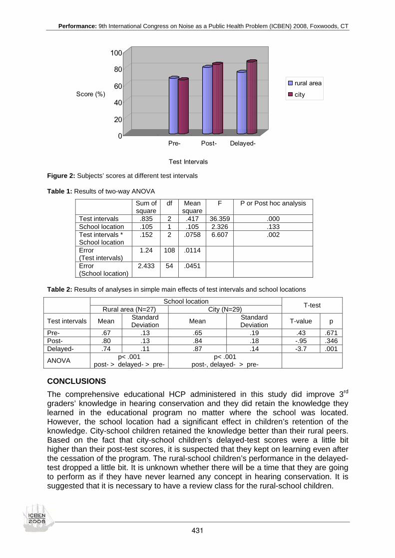
Performance: 9th International Congress on Noise as a Public Health Problem (ICBEN) 2008, Foxwoods, CT
0
20
40
60
80
100
Score (%)
Pre- Post- Delayed-
Test Intervals
rural area
city
Figure 2: Subjects’ scores at different test intervals
Table 1: Results of two-way ANOVA
Sum of square
df Mean square
F P or Post hoc analysis
Test intervals .835 2 .417 36.359 .000 School location .105 1 .105 2.326 .133 Test intervals * School location
.152 2 .0758 6.607 .002
Error (Test intervals)
1.24 108 .0114
Error (School location)
2.433 54 .0451
Table 2: Results of analyses in simple main effects of test intervals and school locations
CONCLUSIONS The comprehensive educational HCP administered in this study did improve 3rd
graders’ knowledge in hearing conservation and they did retain the knowledge they learned in the educational program no matter where the school was located. However, the school location had a significant effect in children’s retention of the knowledge. City-school children retained the knowledge better than their rural peers. Based on the fact that city-school children’s delayed-test scores were a little bit higher than their post-test scores, it is suspected that they kept on learning even after the cessation of the program. The rural-school children’s performance in the delayed-test dropped a little bit. It is unknown whether there will be a time that they are going to perform as if they have never learned any concept in hearing conservation. It is suggested that it is necessary to have a review class for the rural-school children.
School location Rural area (N=27) City (N=29) T-test
Test intervals Mean Standard Deviation Mean Standard
Deviation T-value p
Pre- .67 .13 .65 .19 .43 .671 Post- .80 .13 .84 .18 -.95 .346 Delayed- .74 .11 .87 .14 -3.7 .001
ANOVA p< .001 post- > delayed- > pre-
p< .001 post-, delayed- > pre-
431

Performance: 9th International Congress on Noise as a Public Health Problem (ICBEN) 2008, Foxwoods, CT
REFERENCES Blair JC, Hardegree D, Benson PV (1996). Necessity and effectiveness of a hearing conservation program for elementary students. J Educ Audiol 4: 12-16.
Brookhouser PE, Worthington DW, Kelly WJ (1992). The effectiveness of an educational hearing conservation program for elementary school children. Laryngoscope 102: 645-655.
Chermak GD, Peters-McCarthy E (1991). The effectiveness of an educational hearing conservation program for elementary school children. Lang Speech Hear Serv Schools 22: 308-312.
Chermak G.D, Curtis L, Seikel JA (1996). The effectiveness of an interactive hearing conservation program for elementary school children. Lang Speech Hear Serv Schools 27: 29-39.
Folmer RL (2004). Why aren’t hearing conservation practices taught in schools. http://www.healthyhearing.com/hearing_library/article_content.asp?article_id=151
Frager AM, Kahn A (1998). How useful are elementary school health textbooks for teaching about hearing health and protection? Lang Speech Hear Serv Schools 19: 175-181.
Griest SE, Folmer RL, Martin WH (2007). Effectiveness of “dangerous decibels,” a school-based hearing loss prevention program. Am J Audiol 16: S165-S181.
Lass NJ, Carlin MF, Woodford CM, Campanelli-Humphreys AL, Judy JM, Hushion-Stemple, EA (1985). A survey of classroom teachers’ and special educators’ knowledge of and exposure to hearing loss. Lang Speech Hear Serv Schools 16: 211-222.
Lass NJ, Woodford CM, Lundeen C, Lundeen DJ, Everly-Myers D (1987a). A survey of high school students’ knowledge and awareness of hearing, hearing loss, and hearing health. Hear J 40: 15-19.
Lass NJ, Woodford CM, Lundeen C, Lundeen DJ, Everly-Myers D (1987b). A hearing conservation program for a junior high school. Hear J 40: 32-42.
Lerman Y, Feldman Y, Shnaps R, Kushnir T, Ribak, J (1998). Evaluation of an occupational Health education program among 11th grade students. Am J Industr Med 34: 607-613.
Lewis D (1989). A hearing conservation program for high-school-level students. Hear J 42: 19-24.
Lipscomb D (1994). The employee education program. In: Lipscomb D (ed.): Hearing conservation: in industry, school, and the military (pp 193-202). San Diego, CA: Singular Publ. Group. Inc.
432

Performance: 9th International Congress on Noise as a Public Health Problem (ICBEN) 2008, Foxwoods, CT
Effects of hearing protection on auditory annoyance from ultrasonic scalers used by dental hygiene students David Downs1, Barbara Gonzalez2, Yori Kanekama1, Lisa Belt2 1 Department of Communication Sciences & Disorders, Wichita State University
2 Department of Dental Hygiene; Wichita State University
* corresponding author: e-mail: [email protected]
ABSTRACT Researcher have reported that ultrasonic frequencies associated with high-frequency tools and ultrasonic cleaners can cause auditory annoyance in humans. Dental hy-gienists, for example, routinely use ultrasonic scalers to remove deposits from pa-tients' teeth. Although the ultrasonic intensity of the scaler ranges from 68 to 75 dBA, motion from the scaler's parts, and from the air and fluid it propels when contacting teeth, produce more intense sounds that are audible and, reportedly, annoying. The purpose of this study (now being completed during Spring, 2008) is to measure ef-fects of hearing protection on auditory annoyance from ultrasonic scalers used during training of dental hygiene students. Participants alternate between wearing or not wearing ER20 high-fidelity earplugs during several sessions of cleaning their patients' teeth using an ultrasonic scaler. After cleaning, all participants, whether wearing or not wearing earplugs, rate auditory annoyance of the scaler on a 7-point Likert-type scale. After cleanings, participants wearing earplugs also rate physical discomfort of their earplugs on a different 7-point Likert-type scale. Investigators also measure each subject's hearing thresholds with and without earplugs and sound intensities of ultrasonic scalers during cleanings. Specifically, investigators employ an untreated control group design (with dependent, pretest and post-test samples and switching replications) to answer these questions: (1) do earplugs reduce participants' auditory annoyance from the scalers; (2) do participants' auditory annoyance from the scalers differ over time when wearing or not wearing earplugs; and (3) do participants' physi-cal discomfort from wearing earplugs decrease over time?
433

Performance: 9th International Congress on Noise as a Public Health Problem (ICBEN) 2008, Foxwoods, CT
Perceived acoustic environment, work performance and well-being - survey results from Finnish offices Annu Haapakangas*1, Riikka Helenius1, Esko Keskinen2, Valtteri Hongisto1 1 Finnish Institute of Occupational Health, Indoor environment laboratory, Lemminkäisenkatu 14-18
B, 20520 Turku, Finland, Europe.
2 University of Turku, Department of psychology, 20014 Turku, Finland
*corresponding author: e-mail: [email protected]
ABSTRACT The aim of the study was to investigate workers' perceptions of the acoustic environment of offices and study its relations to work performance and well-being. Questionnaire results from 11 companies and 689 respondents were analyzed. Occupants in private rooms and open offices were compared. Noise was the main indoor environmental problem in open offices. Speech was the most distracting source of noise in both office types but the degree of disturbance was lower in private rooms. About half of open office occupants and 20 % of occupants in private rooms were dissatisfied with acoustics. Office noise disturbed particularly conversations and tasks relying on working memory and verbal processes, such as text comprehension and creative thinking. Routine tasks were little disturbed by noise. In open offices, attempts to cope with noise reflected risk factors to individual productivity and well-being, such as taking extra breaks, compromising the quality of work, working overtime and exerting oneself harder. Self-estimated waste of daily working time due to noise was twofold in open offices. Open office workers experienced more stress symptoms, particularly overstrain and difficulties in concentration, and attributed these symptoms to office noise to a greater extent than workers in private rooms. Possibilities to influence issues related to one's work and work-space privacy were lower among open office occupants. The results suggests that private rooms are superior to open offices in all respects.
INTRODUCTION There is an increasing worldwide trend to build open offices instead of private room offices. Open offices are preferred because of better space economy, spaciousness and flexibility. Open offices are also assumed to facilitate teamwork and information sharing. However, there is continuous debate on the positive and negative effects of open offices on work performance and well-being. According to a meta-analysis car-ried out by DeCroon et al. (2005), there is strong evidence that working in open of-fices reduces worker’s psychological privacy and job satisfaction. Some evidence exists that cognitive workload increases in open offices. Cross-sectional office surveys that have compared different office lay-outs, e.g. Becker et al. (1983), Danielsson (2005), Pejtersen et al. (2006) and Jensen et al. (2005), have shown that the most severe factor causing office dissatisfaction is noise. Danielsson (2005) compared several office lay-outs and concluded that dissatisfac-tion with noise and privacy was highest in large open offices and lowest in cellular offices. Pejtersen et al. (2006) found that the percentage of occupants complaining about noise was ten-fold in large open offices compared to cellular offices. The same study demonstrated an association between office size and several symptoms, in-cluding fatigue, headache and difficulties in concentration. Open office occupants
434

Performance: 9th International Congress on Noise as a Public Health Problem (ICBEN) 2008, Foxwoods, CT
have also reported more subjective performance loss due to noise than cellular office workers, e.g. in the amount of accomplished work (Becker et al. 1983). The present study aims to improve the general understanding of open office condi-tions and its effects on work performance and worker well-being. This is done by us-ing a questionnaire method that addresses a wide range of issues related to noise disturbance, its effects on work and workers and the functional performance of office lay-out. Open office conditions are compared to conditions in private offices. This pa-per continues the work of Helenius et al. (2007) using to large extent the same mate-rial.
METHODS Subjects A total of 689 subjects from 11 office buildings took part in the study. In addition, there were 60 respondents occupying shared offices of 2 to 4 people but their results are not reported in this paper. Data was gathered between 2002 and 2008. Back-ground information of the data is presented in Table 1. The acoustical conditions of the office buildings represented typical Finnish offices built after 1990. Seven of the studied companies had a combination of private rooms and open offices while three companies had mainly open offices and one had only private rooms. The number of respondents varied between 13 and 196 in different companies. Different lines of business were included in the sample. The survey always targeted all workers of a department participating in the study so the workers represented a wide range of pro-fessions not enumerated here.
Table 1: Background information
Number of respondents
Private room Open office Age in years
Range (mean) Female
% Male
%
Sample A 93 260 19-65 (44,4) 36,8 63,2
Sample B 88 248 20-65 (40,9) 63,4 36,6
Full sample 181 508 19-65 (42,7) 49,7 50,3
Questionnaire An office acoustics questionnaire was developed on the basis of a literature review and a pilot study. The questionnaire had several sections. Indoor environment and Noise sources covered the disturbance of indoor environmental factors in general, the disturbance of specific noise sources, satisfaction with work environment and acoustic satisfaction. Noise effects covered the disturbance of different work tasks, behavioral efforts to cope with noise and self-estimated waste of daily working time due to noise. Well-being covered general stress symptoms and symptoms attributed to office noise. Psychosocial environment covered psychosocial stress factors, e.g. job satisfaction and hurry at work. Office lay-out performance assessed quality of teamwork and communication, privacy, comfort and availability of practical resources in the office area. Work space preference was also inquired with one question. Most questions were answered on a 5-point Likert scale. Individual factors, e.g. noise sen-sitivity, were also assessed but are not reported in this paper. Some modifications were made to the questionnaire during the research period and some companies did not allow all sections to be included, e.g. questions about the
435

Performance: 9th International Congress on Noise as a Public Health Problem (ICBEN) 2008, Foxwoods, CT
psychosocial issues. Therefore, the number of respondents varies in different ques-tions and is reported separately for each analysis. In the sections Indoor Environment and Noise Sources the data from all companies could not be combined because of a change in the phrasing of the question: in half of the offices (Sample A), respondents were asked to rate how often they were disturbed whereas the other half (Sample B) rated how much they were disturbed. Asking about frequency instead of degree of disturbance resulted in higher estimates of distraction and some of the differences were statistically significant. Data was therefore analyzed separately for the two sub-samples in these specific sections.
RESULTS The data was analyzed with SPSS 16.0 statistical program. The comparisons be-tween open offices and private rooms were performed using Mann-Whitney U-test. Indoor environment. Noise was the main indoor environmental problem in open of-fices in both samples. Open office occupants were significantly more disturbed by noise than workers in private rooms. Open office occupants also complained more about other indoor environment factors than did workers in private rooms. The distur-bance of indoor environment factors was similar in both subsamples and only the subsample focusing on the frequency of disturbance is reported in Table 2. Distur-bance caused by noise is reported for both samples.
Table 2: The average disturbance of indoor environment factors. Scale 1-5, with 1 indicating no dis-turbance and 5 indicating highest level of disturbance. Subsample A rated the frequency of distur-bance while subsample B rated the degree of disturbance.
Mean (SD)
Sub-sample
N ItemsCronbach's
alpha Private room Open office P-value
Thermal conditions A 344 2 0,683 2,11 (0,89) 2,40 (0,98) 0,016
Air quality A 346 4 0,800 1,93 (0,79) 2,19 (0,80) 0,007
A 346 1 - 2,45 (0,97) 3,55 (1,16) 0,000
Noise B 335 1 - 2,50 (0,97) 3,29 (1,05) 0,000 Lighting (amount of light and glare)
A 352 1 - 2,12 (0,98) 2,51 (1,12) 0,004
Noise sources. Results for the Sample A focusing on the frequency of disturbance of sounds are shown in Table 3. The most distracting sound sources in open offices were speech near one's work station and sounds of phones ringing. Speech also dis-turbed private room occupants the most but not to the same extent. The pattern of disturbance from different sounds was similar in Samples A and B, except that in Sample B open office occupants were less disturbed by ventilation noise (p < .01) than private room occupants. Satisfaction with the indoor environment as a whole and acoustic satisfaction were lower among open office occupants (Table 4). Fifty percent of open office occupants were dissatisfied with acoustics at their work station while only 21 percent of private rooms occupants were dissatisfied.
436
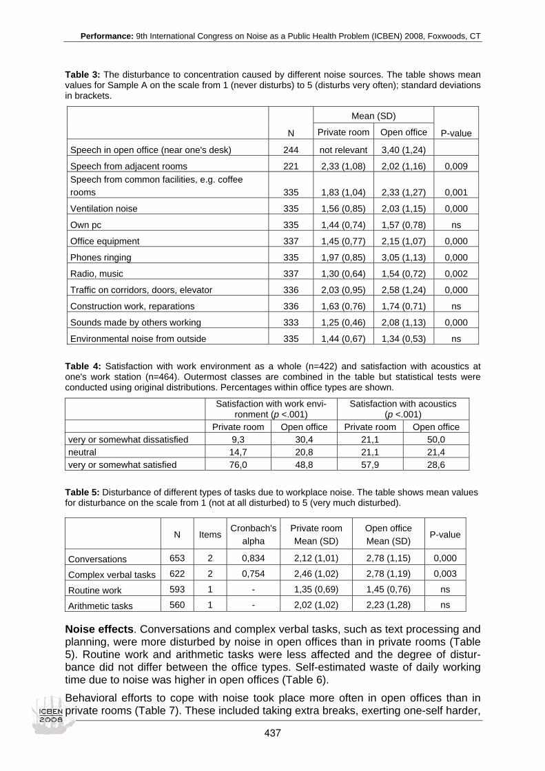
Performance: 9th International Congress on Noise as a Public Health Problem (ICBEN) 2008, Foxwoods, CT
Table 3: The disturbance to concentration caused by different noise sources. The table shows mean values for Sample A on the scale from 1 (never disturbs) to 5 (disturbs very often); standard deviations in brackets.
Mean (SD)
N Private room Open office P-value
Speech in open office (near one's desk) 244 not relevant 3,40 (1,24)
Speech from adjacent rooms 221 2,33 (1,08) 2,02 (1,16) 0,009 Speech from common facilities, e.g. coffee rooms 335 1,83 (1,04) 2,33 (1,27) 0,001
Ventilation noise 335 1,56 (0,85) 2,03 (1,15) 0,000
Own pc 335 1,44 (0,74) 1,57 (0,78) ns
Office equipment 337 1,45 (0,77) 2,15 (1,07) 0,000
Phones ringing 335 1,97 (0,85) 3,05 (1,13) 0,000
Radio, music 337 1,30 (0,64) 1,54 (0,72) 0,002
Traffic on corridors, doors, elevator 336 2,03 (0,95) 2,58 (1,24) 0,000
Construction work, reparations 336 1,63 (0,76) 1,74 (0,71) ns
Sounds made by others working 333 1,25 (0,46) 2,08 (1,13) 0,000
Environmental noise from outside 335 1,44 (0,67) 1,34 (0,53) ns
Table 4: Satisfaction with work environment as a whole (n=422) and satisfaction with acoustics at one's work station (n=464). Outermost classes are combined in the table but statistical tests were conducted using original distributions. Percentages within office types are shown.
Satisfaction with work envi-
ronment (p <.001) Satisfaction with acoustics
(p <.001) Private room Open office Private room Open office very or somewhat dissatisfied 9,3 30,4 21,1 50,0 neutral 14,7 20,8 21,1 21,4 very or somewhat satisfied 76,0 48,8 57,9 28,6
Table 5: Disturbance of different types of tasks due to workplace noise. The table shows mean values for disturbance on the scale from 1 (not at all disturbed) to 5 (very much disturbed).
Noise effects. Conversations and complex verbal tasks, such as text processing and planning, were more disturbed by noise in open offices than in private rooms (Table 5). Routine work and arithmetic tasks were less affected and the degree of distur-bance did not differ between the office types. Self-estimated waste of daily working time due to noise was higher in open offices (Table 6). Behavioral efforts to cope with noise took place more often in open offices than in private rooms (Table 7). These included taking extra breaks, exerting one-self harder,
N Items
Cronbach's alpha
Private room Mean (SD)
Open office Mean (SD)
P-value
Conversations 653 2 0,834 2,12 (1,01) 2,78 (1,15) 0,000
Complex verbal tasks 622 2 0,754 2,46 (1,02) 2,78 (1,19) 0,003
Routine work 593 1 - 1,35 (0,69) 1,45 (0,76) ns
Arithmetic tasks 560 1 - 2,02 (1,02) 2,23 (1,28) ns
437

Performance: 9th International Congress on Noise as a Public Health Problem (ICBEN) 2008, Foxwoods, CT
working overtime and doing remote work. Quality of work was also more often com-promised in open offices in order to cope with noise. Compromising quality of work correlated with overall coping (r = .702, p < .01) but it was left out of the sum variable because of a lower number of respondents.
Table 6: Self-estimated waste of daily working time due to noise in minutes
N
Private room Mean (SD)
Open office Mean (SD)
P-value
Wasted working time 615 12,00 (15,00) 21,48 (20,11) 0,000
Table 7: Behavioral coping efforts and stress symptoms on a scale from 1 to 5 (1 indicating no symp-toms/coping and 5 indicating very much symptoms/coping)
N Items
Cronbach's alpha
Private roomMean (SD)
Open office Mean (SD)
P-value
Coping efforts 581 4 0,840 1,76 (0,64) 2,14 (0,81) 0,000
Compromising quality of work 444 1 - 1,43 (0,69) 1,85 (1,02) 0,000
Stress symptoms 380 4 0,890 2,27 (0,75) 2,64 (0,95) 0,000
Well-being. Overall stress was higher among open office workers (Table 7). Sepa-rate analyses of each symptom showed that particularly difficulties in concentration were more prevalent among open office occupants (Table 8). Workers in open offices also experienced more tiredness and exhaustion. Irritation and motivational difficul-ties seemed to be more prevalent among open office occupants but the difference failed to reach statistical significance.
Table 8: Prevalence of stress symptoms and the percentage of occupants attributing symptoms to noise. Prevalence of symptoms was evaluated on a scale from 1 (not at all) to 5 (very much). Percent-age of noise-related symptoms is calculated for the population expressing little or more symptoms (values 2-5 in the symptom prevalence question).
Prevalence of symptom, mean (SD)
Occupants attributing symptom to noise, %
N Private Open P-value Private Open P-value
Irritation 476 2,36 (0,88) 2,58 (1,10) 0,058 16,3 48,6 0,000 Tiredness or exhaustion 450 2,60 (0,93) 2,91 (1,05) 0,008 9,3 42,1 0,000 Difficulties in concentration 475 2,24 (0,94) 2,69 (1,16) 0,000 23,0 56,3 0,000 Motivational difficulties 407 2,19 (1,01) 2,41 (1,12) 0,064 10,7 28,2 0,000
Percentage of occupants attributing symptoms to office noise was calculated for the population that indicated having symptoms (values 2 'little' to 5 'very much'). About 87 percent of private room occupants and 82 percent of open office occupants belonged to this group. Those who indicated that their symptoms might be due to office noise 'to some degree' or more (values 3 to 5) were considered to attribute the symptom to noise. Those respondents whose symptoms were 'little' or 'not at all' due to noise (values 1 to 2) were considered not to have noise-related symptoms. The results show that open office occupants attributed symptoms to office noise to a greater ex-tent than private office occupants.
438

Performance: 9th International Congress on Noise as a Public Health Problem (ICBEN) 2008, Foxwoods, CT
Psychosocial environment. Most psychosocial stress factors did not differ between the office types (Table 9). Open office occupants received more support from co-workers or managers than did workers in private offices. This may also reflect the content of work as it is likely that workers with private offices have more independent job descriptions, and therefore, less need for support. Possibilities to influence issues related to one's work were perceived lower among open office occupants.
Table 9: Psychosocial stress factors. Scale 1= not at all, 5= very much
N Private room Mean (SD)
Open office Mean (SD) P-value
Hurry at work 392 3,48 (0,85) 3,43 (0,90) ns Work feels interesting and inspiring 336 3,66 (0,90) 3,61 (0,93) ns Mental strain experienced at work 444 3,33 (0,80) 3,25 (0,90) ns Support received from co-workers or manager 248 3,25 (0,94) 3,54 (0,81) 0,015 Possibilities to influence one's work 303 3,26 (0,95) 2,88 (0,96) 0,003 Job satisfaction 380 3,82 (0,68) 3,71 (0,82) ns
Functional performance of the office lay-out. Open office occupants experienced lower privacy in their work area than private room occupants (Table 10). Less practi-cal resources, such as work space and meeting facilities, were perceived to be avail-able in open offices. Comfort was assessed more negatively in open offices than in private offices. Contrary to expectations, the quality of teamwork and communication did not differ between open offices and private offices. In fact, the mean values for the quality of communication are nearly identical. The sum variable for teamwork in-cluded statements such as, 'colleagues are within easy reach', 'information is shared well between colleagues' and 'collaboration is effective'.
Table 10: Functional performance of the office lay-out. Factors have been assessed on a scale from 1 to 5, with '1' indicating most negative assessment and '5' most positive
N Items
Cronbach's alpha
Private room Mean (SD)
Open office Mean (SD)
P-value
Privacy 492 2 0,888 3,83 (0,78) 2,34 (1,04) 0,000
Teamwork and communication 490 4 0,845 3,75 (0,62) 3,74 (0,73) ns
Availability of practical resources 489 3 0,714 3,77 (0,74) 3,37 (0,84) 0,000
Comfort 489 2 0,776 3,33 (0,74) 2,66 (0,95) 0,000
Work space preference. Results for work space preference are shown in Table 11. The results show that 21 percent of open office occupants prefer working in open offices and 33 percent would choose a shared office.
Table 11: Workspace preference in percentages for open office and private room occupants (N=569)
Prefered work space Work space at present
Private room Shared office of 2 to
4 persons Open office Private room 97,6 0,6 1,8 Open office 46,9 32,6 20,5
439

Performance: 9th International Congress on Noise as a Public Health Problem (ICBEN) 2008, Foxwoods, CT
DISCUSSION The results suggest that open offices have versatile acoustic problems in terms of subjective disturbance, performance effects and worker well-being. The expected benefits of open offices regarding functional efficiency were not supported by the re-sults. Modern office work is increasingly characterized by cognitively demanding tasks in which background noise is perceived as particularly disturbing. The study gives no support to an extensive preference of open offices when workers' well-being and efficiency are of main concern. Objective measurement of performance effects of noise is very difficult in real offices. In this study, subjective evaluations of wasted working time due to noise were higher in open offices than in private rooms, providing one measure for the performance effects of noise. The estimates of lost minutes cannot be regarded as exact in objec-tive terms but the finding that workers change their behavior to cope with noise sup-ports the conclusion that working time is indeed wasted because of noise. For exam-ple, open office occupants reported taking extra breaks and rescheduling work due to workplace noise. Open office occupants suffered more from difficulties in concentration and tiredness. In open offices, a greater percentage of those suffering from symptoms attributed symptoms to office noise. It seems unlikely that the higher stress levels among open office occupants were due to differences in psychosocial work environments as these factors were mostly assessed similarly in open and private offices. Our results are in line with the view that open office conditions and the accompanying lack of privacy form an extra stress factor to an individual worker. Further analyses will be conducted with the data to address the relations between office type, stress, indoor environment and psychosocial environment in more depth. The results contradict the most common assumption of the benefits of open office layouts, that is, facilitation of communication and co-operation. The quality of team-work and communication did not differ between open offices and private rooms at all. However, it is likely that in most of the studied open offices the respondents' work was characterized mainly by individual performance in which constant availability of colleagues and information exchange is not necessary. Open offices may be suitable for specific jobs that are mainly comprised of teamwork. The study does not suggest that open offices should not be used. Twenty-one per-cent of open office workers preferred open offices to other office types. Although evi-dence could not be presented in this study, it is probable that many of these persons have a continuous need for communication with colleagues. The main problem seems to be that the selection of occupant's workstation is not based on the analysis of job demands. As periods of individual work and telephone conversations are still predominant in most office professions, open offices do not provide sufficient acous-tic, visual and psychological privacy for typical office work. Future studies should include a more detailed analysis of the job type of open office workers and a more detailed analysis of the open office type. There are very large differences in the size of open offices, in the facilities available to workers and also in the flexibility of workstations which were not considered in this study. It is very impor-tant to be able to develop instructions for designing most appropriate work environ-ments. Acoustic conditions in the open offices can vary significantly. Hongisto et al. (2007) have shown that in good offices, the distraction of speech restricts to 5 meters from
440

Performance: 9th International Congress on Noise as a Public Health Problem (ICBEN) 2008, Foxwoods, CT
the speaker while in worst offices, the speech distracts up to 20 meters from the speaker. The acoustic quality of open offices should also be measured in future sur-veys to show how acoustic problems depend on acoustic design.
ACKNOWLEDGEMENTS This study was carried out as a part of a national research programme MAKSI (Per-ceived and Modelled Indoor Environment) funded by Tekes, National Technology Agency, Finnish Institute of Occupational Health and several participating companies. Thanks are due to the companies and office workers who participated the study. The authors thank Henri Riuttala for valuable advice on the statistical analyses and Anu Kaarlela-Tuomaala and Jaana Jokitulppo for co-operation during early years.
REFERENCES Becker FD, Gield B, Gaylin K, Sayer S (1983). Office design in a community college. Environ Behav 15: 699-726.
Danielsson C (2005). Office environment, health and job satisfaction. Stockholm, Sweden: KTH Technology and Health, Licentiate Thesis.
DeCroon EM, Sluiter JK, Kuijer PPFM, Frings-Dresen MHW (2005). The effect of office concepts on worker health and per-formance: as systematic review of the literature. Ergonomics 48: 119-134.
Helenius R, Keskinen E, Haapakangas A, Hongisto V (2007). Acoustic environment in Finnish offices - the summary of ques-tionnaire studies. In: International Congress on Acoustics, paper RBA-10-001, 2-7 September 2007, Madrid, Spain.
Hongisto V, Virjonen P, Keränen J (2007). Determination of acoustic conditions in open offices and suggestions for acoustic classification. In: 19th International Congress on Acoustics, Madrid, Spain, Sept 2-7, 2007.
Jensen KL, Arens E, Zagreus L (2005). Acoustical quality in office workstations as assessed by occupant surveys. In: Pro-ceedings of Indoor Air 2005, pp 2401-2405.
Pejtersen J, Allermann L, Kristensen TS, Poulsen OM (2006). Indoor climate, psychosocial work environment and symptoms in open-plan offices. Indoor Air 16: 392-401.
441

Performance: 9th International Congress on Noise as a Public Health Problem (ICBEN) 2008, Foxwoods, CT
Effects of sound masking on workers - a case study in a land-scaped office Valtteri Hongisto* Finnish Institute of Occupational Health, Indoor Environment Laboratory, Turku, Finland
* corresponding author: e-mail: [email protected]
INTRODUCTION Noise is the most disturbing factor of indoor environment in open offices (Haapakan-gas et al. 2008a). Several independent laboratory experiments have shown that noise, especially speech, reduces task performance of cognitively demanding tasks. According to the model of Hongisto et al. (2008), task performance reduces with in-creasing speech intelligibility. The room acoustic design of open offices should, there-fore, aim at the reduction of speech intelligibility between workstations. This can be achieved by mainly by three factors: increasing room absorption, increasing screen height and increasing masking sound level. Appropriate masking is necessary to reach acceptable speech privacy between two neighboring workstations. Masking means that the stable background noise of the office is raised controllably to minimize the intelligibility of nearby speech without cre-ating a new source of distraction. In Finland, the recommended level of masking is 40 to 45 dBA (SFS 2004). Optimum masking sound is smooth and unnoticeable, e.g. ventilation noise. Sound pressure level and spectrum need to be considered to obtain a balance between acoustic comfort and efficient masking performance. In many cases, ventilation creates an appropriate masking. In large and high open offices, constant occupant activities and babble can create an appropriate masking. But in many cases, the creation of optimum masking requires an electronic audio system. Masking was mentioned already in the early open office design guidelines (Hardy 1957). Masking was the presupposition of speech privacy also in the original con-cepts of landscaped and open-plan offices in 1960's (Boje 1971). However, the use of electronic masking has not become a common practice although the importance of masking is emphasized in the acoustic design guidelines worldwide. One reason may be that very few scientific experiments have been published in this area and the re-sults have been contradictory. Some studies are reviewed below. Warnock (1973) conducted experiments with electronic masking sound levels 45 to 51 dBA. Occupants responded to simple feedback forms. The sample size was not reported. They rejected each masking condition and preferred the situation without electronic masking. Interviews revealed that their work was not distracted by intruding speech sounds indicating no need to improve speech privacy. In addition, the original sound level of ventilation was already at a recommended masking level, 40 to 45 dBA, producing nearly sufficient speech privacy and additional need for masking was questionable on the whole. Although the setup of the study was interesting, the methodological weaknesses of the experiment are obvious. Keighley and Parkin (1979) tested different masking sounds, sound levels and spec-tra. The experiment was carried out in a landscaped office of 40 workers. Altogether 15 different masking conditions, with sound levels from 37 to 46 dBA, were tested, 3 weeks each. Questions about conversation difficulties, overall acoustic satisfaction and acceptability were presented. None of the conditions were found successful. Un-fortunately, no masking sound was produced at and above 4 kHz and very little also
442

Performance: 9th International Congress on Noise as a Public Health Problem (ICBEN) 2008, Foxwoods, CT
at 2 kHz. Therefore, the efficiency of masking in the consonants area did not occur. Acoustic attenuation performance of the room was not described so that the objective speech privacy remained unknown. The measurement of perceived concentration difficulties, acoustic distraction and speech privacy could have been very informative as well. The study has antiquated because typewriters, which produced natural masking itself, are no longer used. Lewis et al. (2003) investigated the effect of masking system on 136 office workers. Masking system reduced significantly subject's self-reported level of distraction and their awareness of sounds. Suggestive evidence was found that performance was improved after the change. Unfortunately, technical information of the masking sys-tem, room acoustics and sound levels was not reported. Helenius and Hongisto (2004) studied the effect of noise control on workers in an open office. Noise control included the installation of masking system, added ceiling absorption and some phone conversation rooms. Noise control improved the per-ceived acoustic conditions. However, the influence of masking cannot be separated. Laboratory experiments have shown the benefits of masking for both acoustic com-fort and task performance, e.g. Venetjoki et al. (2006) and Haapakangas et al. (2008b). None of previous field studies have been able to combine room acoustic and envi-ronmental psychological expertise to a robust longitudinal workplace experiment. The aim of this pilot study was to investigate the effects of artificial masking sound at 44 dBA on workers in a small department of 15 workers. Room acoustic measure-ments and occupant questionnaires were conducted before and after launching the system.
MATERIALS AND METHODS The experiment was carried out in the telephone exchange of an international Finnish bank in Helsinki. More than 60 % of working time consisted of connecting the calls of clients to the correct person in the company. The workers had complained about acoustic distractions from nearby speech and lack of confidential privacy during phone conversations. The company was aware of the expected benefits of masking and wanted to test the technology in this small department. A total of 15 workers took part in the survey before and 13 after the installation of masking. All subjects were female. 13 workers responded both before and after the masking and the statistical analysis was made with these respondents. The response rate was above 80 % both before and after the survey. Subjects were informed that the masking system will be installed to reduce acoustic distractions. No organiza-tional changes took place during the test period. The acoustic measurements were made to evaluate the objective speech privacy. The measurements included the spatial attenuation of sound pressure level, SPL, of normal effort speech and spatial decay of Speech Transmission Index, STI, which decribes well the speech intelligibility, or inversely, speech privacy. Measurement method is described by Hongisto et al. (2007). The questionnaire method is described by Haapakangas et al. (2008a). Here, only the most important findings were reported. The analysis was made using SPSS soft-ware and Wilcoxon signed rank test.
443

Performance: 9th International Congress on Noise as a Public Health Problem (ICBEN) 2008, Foxwoods, CT
The floor area of the office was approximately 250 m2 (Figure 1a) including 20 per-manent workstations. The room height was 3.3 m. The height of the screens was 1.4 m. Workstations were enclosed from 2 to 4 sides. Screens were weakly sound absorbing (EN 11654 class E). The whole ceiling was covered with sound absorbing material (class A). Three walls out of six were covered with the same material by 40 % of area. The floor was not sound-absorbing. Because room absorption was ini-tially exceptionally high and higher screens were not permitted, the remaining room acoustic means was the installation of a masking system. It was recommended by the research group because of low background noise level of ventilation, LA,eq=35 dB. The sound masking system consisted of a central unit (sound generator, filter, ampli-fier) and 21 loudspeakers, Figure 2. The spectrum of noises is presented in Figure 1b. The spectrum was a compromise between the suggestions of Veitch et al. (2002) and the original spectrum of ventilation noise. The masking level was raised from 35 dB to 44 dB slowly to avoid complaints about sudden change, Figure 3.
Sound pressure level [dB]
10
15
20
25
30
35
40
45
50
125 250 500 1000 2000 4000 8000Octave band [Hz]
Average, before (35 dB)Average, after (44 dB)
(a) (b)
Figure 1: (a) The layout of the office. The average distance between loudspeakers (balls) was 3 me-ters; (b) Spectrum of the background noise of ventilation (before) and masking system (after). The average A-weighted sound pressure levels were 35 and 44 dB, respectively.
(a) (b)
Figure 2: (a) Central unit of masking system consisting of rack mounted signal generator and ampli-fier. The filters of the signal generator were configured with PC; (b) One of the masking loudspeakers installed above electric ceiling shelf. The cone is directed towards the ceiling to have smoother spatial distribution of sound and to make aural localization of the loudspeaker more difficult.
444

Performance: 9th International Congress on Noise as a Public Health Problem (ICBEN) 2008, Foxwoods, CT
A-weighted sound pressure level [dB]
0
10
20
30
40
50
60
16 20 24 28 32 36 40 44 48 52 4 8 12Week
2005
questionnairephase I
questionnairephase IIplanning (16-22)
cable installation (23)loudspeaker installation (23)central unit finishing (26)launching (26)
gradual increase of masking
2006
36 dBA
43 dBA
Figure 3: Time schedule of the experiment
RESULTS The results of room acoustic measurements are summarized in Table 1. The spatial attenuation of the SPL of speech and spatial attenuation of STI are presented in Fi-gure 4. DL2 expresses the reduction of SPL of speech per distance doubling. It did not change because attenuation was not changed. Radius of distraction, rd, is the distance where STI falls below 0.50. A significant improvement in objective speech privacy occurred after the installation of masking system. The radius of distraction reduced from 13 to 6 meters. Noise and thermal conditions were the most disturbing indoor environment factors in the office, Figure 5. After the installation of the masking system, noise disturbance declined but the change was not statistically significant. Other indoor environmental factors were also rated better. The change in thermal conditions and draught could be explained by seasonal changes. Disturbance caused by lighting was reduced sig-nificantly (p < .05). The reason for the unexpected change is unknown but it may re-flect general satisfaction to the improvement. However, satisfaction with work envi-ronment as a whole and satisfaction with acoustic environment did not change sig-nificantly. Speech and human-borne sounds were the most disturbing sound sources, Figure 6. The distraction of most sound sources reduced but only the distraction of speech and laughter was reduced significantly (p < .05). Disturbance caused by ventilation and background hum, including masking, increased slightly but not significantly. It seems that masking sound was noticed by some people but the loudness was not too high to create a new source of distraction for most workers. Before the masking, noises disturbed phone conversations, the primary task, the most, Figure 7. After the change, all types of work were less distracted by noise. The change in the task "email, internet" was statistically significant (p < .05). The use of coping methods altogether reduced significantly (p < .05, Table 2). After the masking, these negative behavioural effects of noise were on a very low level. The self-rated waste of working time due to noise halved after the installation of masking. The change was not statistically significant, Table 3. Noise-related symptoms were also inquired. Concentration difficulties did not change.
445

Performance: 9th International Congress on Noise as a Public Health Problem (ICBEN) 2008, Foxwoods, CT
Table 1: Summary of the room acoustic measurements. A-weighted SPL of speech at 4 m from the speaker, Lp,S,4m, spatial attenuation rate of A-weighted SPL of speech per distance doubling, DL2, ra-dius of distraction, rD, A-weighted background noise level, Lp,B, and average reverberation time, T20, in the range 125-8000 Hz.
Lp,S,4m DL2 rD Lp,B T20
[dBA] [dB] [m) [dBA] [s]Before 51 6.0 13.2 35 0.3After 51 6.0 6.2 44 0.3
A-weighted SPL [dB]
15
20
25
30
35
40
45
50
55
1 10 100
Distance from speaker [m]
speech, before & afterbackground, beforebackground, afterspeech, desirable
DL2=6 dB
DL2=11 dB
Speech Transmission Index, STI
0.000.100.200.300.400.500.600.700.800.901.00
1 10 100
Distance from speaker [m]
beforeafter
rD=13 m
rD=6 m
Figure 4: (a) Spatial attenuation of the A-weighted SPL of speech; (b) Spatial reduction of STI
1
2
3
4
5draught
thermal conditions
dry or humid air
smellsnoise
lighting, glare
dust or dirt
BeforeAfter1 not at all
5 very much
(p<.05)
Figure 5: "How much have the following indoor environmental factors disturbed you at your work sta-tion during the last month?" Mean values
446

Performance: 9th International Congress on Noise as a Public Health Problem (ICBEN) 2008, Foxwoods, CT
1 2 3 4 5
Speech and laughted from neighboringworkstations
Ventilation, background hum
Telephone ringing tones
Movement in corridors, footsteps, doors, lift, clatter
Construction sounds
Computer noise
Road traffic noise
Sounds caused by work, e.g. keyboard strikes,paper rustle
Common office equipment
BeforeAfter
1 not at all5 very much
p<.05
Figure 6: "How much do the following sounds disturb your concentration on your work at your work station?" Mean values
1 2 3 4 5
reading, studying
phone conversations
work-related conversations
email, internet
planning, creative work
counting
text processing, writing
practical organization, e.g. copying
BeforeAfter
1 not at all5 very much
p<.05
Figure 7. "How much do the sounds disturb the following types of work?" Mean values
Table 2: "How often do you act in the following way to cope with your work because of the sounds in your work environment?" Mean values. Scale: 1=never 5: very often
Before After
discussed the noise problem with colleagues 3.4 2.5
made an even greater effort 3.1 2.5tried to be quieter in the hope that others would do the same 2.9 2.2used a sign so that your colleagues avoid disturbing you temporarily 2.4 2.2made a proposal to the management to improve the acoustic conditions 3.3 2.1slowed down the pace to maintain concentration and quality of work 2.5 2.1
interrupted your work or left your desk 1.7 1.8
447

Performance: 9th International Congress on Noise as a Public Health Problem (ICBEN) 2008, Foxwoods, CT
Table 3: "When you think about the effects of the sounds in your work environment, how many min-utes are wasted per day? Mean values and the corresponding percentage of daily working time
[min] [%]Before 14 3.2After 6 1.4
GENERAL DISCUSSION The need for further acoustic improvements became negligible because major acous-tic problems no longer existed after the installation of masking. However, it is expected that even higher acoustic satisfaction would have been ob-tained if the spatial attenuation had been increased together with masking so much that DL2=11 dB would be reached (see dotted line in Figure 4). Now, DL2 was very low because of low screen height. Therefore, the acoustic conditions after the instal-lation of masking did not represent the best possible room acoustic situation. No adverse effects of masking were reported by the workers. This contradicts with previous studies, e.g. Warnock (1973) and Keighley and Parkin (1979) but agrees with Helenius and Hongisto (2004) and Lewis et al. (2003). The results showed several positive trends. Some of them were statistically almost significant (p < .05). With a larger sample, many of positive trends found in this study would have reached the statistical significance. The study was carried out in a small department doing a specific job. Different results might have observed in different kind of work. Regarding the noise sensitivity of job types, this study agrees with the cross-sectional survey of Haapakangas et al. (2008a), according to which verbal tasks and conversations are most distracted by speech while routine work is not. The background noise level was initially quite low. Therefore, the change in acoustic privacy was reasonably large. If the change in background noise level would have been smaller, the subjective responses would have been weaker as well. In general, masking can be suggested only when the initial level is low, much below 40 dBA. This study gives suggestive evidence that masking could be recommended in open offices when acoustic complaints exist and initial background noise levels are low. It is still expected that masking technology can be easily rejected because of emotional grounds: everybody knows that noise is detrimental to health and comfort. The in-crease of noise level is against this basic assumption and investment on additional noise is not reasonable. However, it must be emphasized that the SPL of recommended office masking is very low, 42 to 45 dBA. This does not increase the average noise level during the working day because the average noise levels in open offices are above 50 to 55 dBA because of speech and activities. Negative health effects are not expected to take place because noise energy does not increase. On the contrary, this study gives evidence that distractions reduce which imply that noise-related stress would reduce, indicating positive rather than negative changes in well-being. The need of future research is evident both in field and laboratory conditions. Ex-periments in offices should include both team and individual office work, larger num-ber of respondents, different office sizes and different masking technologies. Large-
448

Performance: 9th International Congress on Noise as a Public Health Problem (ICBEN) 2008, Foxwoods, CT
scale experiments are very difficult to carry out because of several practical reasons. However, they are necessary to achieve scientific evidence about the benefits and restrictions of masking. The methodology presented in this study seems to work well in such interventions.
CONCLUSIONS The effect of masking was experimented in a small open office of 13 respondents. This pilot study gives suggestive evidence that masking can be recommended in open offices when workers are dissatisfied with acoustic environment and the initial background noise level is low. The current study is restricted because of specific of-fice work and small sample size. Future experiments should include different types of offices, job types, masking technologies and larger number of respondents.
ACKNOWLEDGEMENTS This study was a part of national research programme MAKSI (Perceived and mod-elled indoor environment) funded by Tekes, National Technology Agency, Finnish Institute of Occupational Health and several participating companies. Thanks are due to the company who let their premise at our disposal. Thanks belong to my colleague Annu Haapakangas for giving comments to this manuscript.
REFERENCES Boje A (1971). Open-plan offices. Ed. Walley BH, London: Business Books.
Haapakangas A, Helenius R, Keskinen E, Hongisto V (2008a). Perceived acoustic environment, work performance and well-being - survey results from Finnish offices. In: 9th International Congress on Noise as a Public Health Problem (ICBEN) 2008, July 21-25, Mashantucket, Connecticut, USA.
Haapakangas A, Haka M, Keskinen E, Hongisto V (2008b). Effect of speech intelligibility on task performance - an experi-mental laboratory study. In: 9th International Congress on Noise as a Public Health Problem (ICBEN) 2008, July 21-25, Mashantucket, Connecticut, USA.
Hardy HC (1957). A guide to office acoustics. Architect Rec 121: 235-240.
Helenius R, Hongisto V (2004). The effect of acoustical improvement of an open-plan office on workers. In: Proceedings of Inter-Noise 2004, paper 674, Aug 21-25, Prague, Czech Republik.
Hongisto V, Virjonen P, Keränen J (2007). Determination of acoustic conditions in open offices and suggestions for acoustic classification. In: 19th International Congress on Acoustics, Madrid, Spain, Sept 2-7, 2007.
Hongisto V, Haapakangas A, Haka M (2008). Task performance and speech intelligibility - a model to promote noise control actions in open offices. In: 9th International Congress on Noise as a Public Health Problem (ICBEN) 2008, July 21-25, Mashantucket, Connecticut, USA.
Keighley EC, Parkin PH (1979). Subjective response to sound conditioning in a landscaped office. J Sound Vibr 64: 313-323.
Lewis E, Sykes D, Lemieux P (2003). Using a web-based test to measure the impact of noise on knowledge workers' produc-tivity. In: Proceedings of the Human Factors and Ergonomics Society, HFES 47th Annual Meeting, Denver, CO. 10/2003.
SFS (2004). SFS 5907; en. Acoustic classification of spaces in buildings. Helsinki, Finland: Finnish Standards Association.
Veitch JA, Bradley JS, Legault LM, Norcross S, Svec JM (2002). Masking speech in open-plan offices with simulated ventila-tion noise: noise level and spectral composition effects on acoustic satisfaction. Institute for Research in Construction, Inter-nal Report IRC-IR-846, April, Canada.
Venetjoki N, Kaarlela-Tuomaala A, Keskinen E, Hongisto V (2006). The effect of speech and speech intelligibility on task performance. Ergonomics 49: 1068–1091.
Warnock ACC (1973). Acoustical privacy in the landscaped office. J Acoust Soc Am 53: 535-1543.
449

Performance: 9th International Congress on Noise as a Public Health Problem (ICBEN) 2008, Foxwoods, CT
Memory of a text heard in noise Robert Ljung, Anders Kjellberg*, Anne-Marie Green Centre for the Built Environment, Laboratory for Applied Psychology, University of Gävle, SE-80176 Gävle, Sweden
*corresponding author: e-mail: [email protected]
INTRODUCTION Cognitive effects of noise have been demonstrated in a large number of experimental studies (Beaman 1998; Jones 1990; Jones et al. 1990; Macken et al. 1999). There are also several studies that indicate that long-term exposure to noise may impair cognitive performance of school children (Haines et al. 2001; Shield & Dockrell 2003). Both the studies of acute effects and the effects of long-term exposure have almost exclusively used text based test material, although many tasks in schools and workplaces require processing and storing of orally presented information. The reason for the choice of written material is of course that the effects obtained should not be an effect of the noise making it impossible to hear what is said. Rabbitt (1966) as well as Kjellberg et al. (2008) argued that a background noise may impair memory of spoken material also when it is possible to hear what is said. If the noise makes it more effortful to identify the words spoken, less of the limited working memory capacity should be available for the further processing and storing of the material. The results from these two studies confirmed this hypothesis. The memory of a word list was impaired by a background noise although subjects had repeated the words during their presentation to ensure that they were correctly identified. When the content of the message is in correspondence with the context, and when the speech signal is clearly audible, speech understanding does not require any effort for normal hearing individuals. When listening conditions are degraded, speech understanding can still be good, if the semantic context and the linguistic structure offer redundancy, but then the speech signal gets less audible and one has to rely more on redundancy and top-down processes, speech understanding changes from being effortless to become straining. The more resources that are used for word recognition, the fewer are left for parallel processing and storage of information. Speech understanding in bad signal/noise conditions therefore requires more of the limited resources of the working memory, than speech understanding in good acoustical conditions does (Kjellberg 2004). An analogue effect was demonstrated by Pichora-Fuller et al. (1995) who found that older subjects recalled fewer of the items in a working memory task than young subjects in noisy conditions, although there was no difference in the recall ability of the two age groups when they had read the items. Given that this interpretation of the effect of background noise is correct, the effect should be related to working memory capacity. The less capacity the fewer resources should be left for the further processing of the speech after the identification of the words spoken. Recall of word lists is a task rarely met outside the laboratory. From an ecological point of view it would be of more interest to study the effect of background noise on the recall of a longer spoken text. This was done by Rabbitt (1968) who showed that degraded listening conditions (+5 dB S/N) impaired memory of a spoken prose
450

Performance: 9th International Congress on Noise as a Public Health Problem (ICBEN) 2008, Foxwoods, CT
passage. However, it cannot be excluded that subjects actually did not heard the parts of the text. In the present study recall and recognition of the content of shorter lectures were studied with and without a background noise. A hearing test was included to ensure that it was possible to hear what was said. To get a measure of the subjects’ working memory capacity such tests were included.
EXPERIMENT 1 Participants and design 28 university students 19-35 years old were paid to participate in the experiment. All participants were native speakers of Swedish and reported normal hearing. The study had a within subject design, with two conditions. A noise condition where subjects listened to a text with a broadband background noise, and a control condition without the noise.
Speech and Noise In the noise condition, the broadband noise was presented simultaneously with the spoken text giving a signal-to-noise ratio of + 29 dBA. In the control condition The S/N ratio was +5 dB, which made listening demanding, but made it possible to hear all the text. The texts were presented by two loudspeakers, which were placed one on each side about 1.5 meters in front of the table where the subject was seated.
Memory and hearing tests Hearing test. The hearing tests consisted of two lists of ten sentences presented with and without recorded broadband noise. All sentences had the same structure (e.g. Sean took eighteen old balls, Anna held three beautiful rings), and were constructed to be non-redundant; i.e. the context gave few cues to what exact word would follow only to what word category the word belonged. The subjects immediately repeated each sentence aloud. The five first sentences in each list were considered as training, thus only the results from the five last sentences were used to measure the hearing ability. The sentences were taken from a standardized hearing test (Hagerman 1982). Reading Span test. Working memory capacity was assessed with the reading span test, which was taken from the cognitive test battery TIPS (Hällgren et al. 2001). Series of sentences were presented in a word-by-word fashion. The subject’s immediate task during a 1.75 s interval between sentences was to decide by pressing a key whether the sentence was absurd or normal. After a sequence of sentences (three, four, five or six sentences), the experimenter indicated that the subject should start to report orally as many as possible of either the first or the final words of the sentences. The subjects did not know beforehand if they should report the first or the last words. The number of correctly recalled words was used as the performance measure. Memory test of spoken narrative information. The spoken texts (eight minutes long) were taken from two reading comprehension tests previously used in the Swedish University Test (SAT). The subjects listened to one text with recorded broadband background noise and another text without the background noise. One text dealt with inductivism and scientific methods, and the other text was about acting. After listening to a text, the subject was given eight multiple choice questions about comprehensive aspects of the text and eight open-ended questions about details of
451

Performance: 9th International Congress on Noise as a Public Health Problem (ICBEN) 2008, Foxwoods, CT
the text. The number of correctly answered questions was calculated for both categories of questions separately. Ratings of effort, attention and audibility After each condition the subject was asked to rate effort and audibility with Borg’s CRT-scale (Borg 1998) where 0 means No effort at all and 10 means Extremely strong effort. Audibility and attention were rated with a five-step scales (20 % of the words or more were impossible to hear-it was possible to hear almost every word; very difficult-very easy to keep attention on the task).
PROCEDURE The experiment was conducted in a sound attenuated climate chamber, with the subjects seated at a desk in the middle of the room. The experiment took approximately 60 minutes. The order between conditions and between texts was counterbalanced.
RESULTS The mean number of hearing errors was small but differed significantly between the two conditions (0.5 and 0.07 for the noise and control condition, respectively). Two types of analyses were therefore performed: Analyses that included all subjects (n=28) and analyses only including subjects without any error in the hearing test with the background noise (n=16). The order between conditions was balanced also among the16 selected subjects and the two texts appeared eight times in both conditions. Subjective measurements of effort, attention and audibility The listening was rated as considerably more effortful and requiring more concentration in the noise condition in both the whole and the reduced group. Memory test of the texts The multiple choice questions regarding general understanding of the texts did not show any significant effect of the noise neither in the whole or the selected group. Scores of the open-ended recall questions of detailed information were significantly lower in the noise than in the control condition, F(1,26)=7.26, p=.012), and the effect did not differ between the two texts. Subjects without hearing faults showed the same pattern of results as the whole group (Figure 1).
0
0,5
1
1,5
2
2,5
3
3,5
4
Whole group (n=28) Selected group (n=16)
NoiseControl
Figure 1: Mean number of correct answers to open questions about details of the two texts in the noise and control conditions in the whole group and the selected without any errors in the hearing test in the noise condition.
452

Performance: 9th International Congress on Noise as a Public Health Problem (ICBEN) 2008, Foxwoods, CT
There were no significant correlations between the effects of noise on the memory tests and the reading span performance. Neither did the noise effect correlate with differences in rated effort in the two conditions.
DISCUSSION The experiment showed that recall of an orally presented text is impaired by a background noise. The overall comprehension of the texts was not affected by noise, but recall of detailed information was significantly worse when the text was heard in the noise condition. The fact that this effect was seen also in the group that had no error in the hearing test with a background noise makes it improbable that missed words could explain the noise effect. The experiment gave no support to the hypothesis that larger working memory capacity (as measured by reading span) reduced the noise effect. One possible interpretation of this result is that the reading span test does not assess a capacity that is critical for the understanding, storing and recall of a spoken text. However, it is also possible that the number of correct words in the reading span test isn’t sensitive enough to catch such an effect. It would probably be better to use a test that also allows the measurement of processing times. The issue of how the noise effect is related to working memory capacity is an important one. Tests of working memory capacity, like reading span and updating tests have repeatedly been shown to be closely related to scholastic performance. Thus, if the hypothesis is correct, it means that bad acoustic conditions would be especially detrimental for students that also for other reasons have problem of understanding and remembering what the teacher says.
REFERENCES Beaman CP (1998). Auditory distraction from low-intensity noise: a review of the consequences for learning and workplace environments. Appl Cogn Psychol 19: 1041-1064.
Borg G (1998). Borg's perceived exertion and pain scales. Champaign, IL: Human Kinetics.
Hällgren M, Larsby B, Lyxell B, Arlinger S (2001). Evaluation of a cognitive test battery in young and elderly normal-hearing and hearing-impaired persons. J Am Acad Audiol 12: 357-370.
Hagerman B (1982). Sentences for testing speech intelligibility in noise. Scand Audiol 11: 79-87.
Haines MM, Stansfeld SA, Job RFS, Berglund B, Head J (2001). Chronic aircraft noise exposure, stress responses, mental health and cognitive performance in school children. Psychol Med 31: 265-277.
Jones D (1990). Recent advances in the study of human performance in noise. Environ Int 16: 447–458.
Jones DM, Miles C, Page J (1990). Disruption of proofreading by irrelevant speech: effects of attention, arousal or memory? Appl Cogn Psychol 4: 89–108.
Kjellberg A (2004). Effects of reverberation time on the cognitive load in speech communication: theoretical considerations. Noise & Health 7: 11-22.
Kjellberg A, Ljung R, Hallman D (2008). Recall of words heard in noise (p n/a). Appl Cogn Psychol (in press). DOI: 10.1002/acp.1422.
Macken WJ, Mosdell N, Jones DM (1999). Explaining the irrelevant-sound effect: Temporal distinctiveness or changing-state? J Exp Psychol: LMC 25: 810-814.
Pichora-Fuller MK, Schneider BA, Daneman M (1995). How young and old adults listen to and remember speech in noise. J Acoust Soc Am 97: 593–608.
Rabbitt P (1966). Recognition memory for words correctly heard in noise. Psychonom Sci 6: 383-384.
Rabbitt PMA (1968). Channel-capacity, intelligibility and immediate memory. Quart J Exp Psychol 20: 241-248.
Shield BM, Dockrell JE (2003). The effects of noise on children at school: a review. J Build Acoust 10: 97-106.
453

Performance: 9th International Congress on Noise as a Public Health Problem (ICBEN) 2008, Foxwoods, CT
Causes and effects of noise pollution: An overview Sanjeev Kumar Shrivatava1, Kailash2 1 Department of Physics, Bundelkhand University, Jhansi-284 128, Uttar Pradesh, India
2 Department of Physics, BNV College, Rath-210 431, Uttar Pradesh, India
Correspondence: [email protected], [email protected]
Noise is technically one of the most complex and least understood forms of pollution. The present generation and the coming generations have to solve three grave prob-lems namely, population, poverty and pollution if they have to survive. Pollution being the most dangerous problem like cancer in which death is sure but slow. Noise is be-coming an increasingly omnipresent, yet unnoticed form of pollution even in devel-oped countries. Whether knowingly or unknowingly, every one of us contributes to noise pollution, because most of our day-to-day activities generate some noise. Noise is an important environmental pollutant like noxious gases that befoul our air, water and soil. It destroys bridges and produces cracks in buildings. The noise can cause physiological and psychological deterioration that accompanies it as an inevi-table part of our lives. This paper deals with causes, effects and control of noise pol-lution. In this connection, adolescent education, neural-effects, occupational envi-ronment, transportation, psychological and physiological effects will also be dis-cussed in detail.
454
__________________________________________________________________________
__________________________________________________________________________
ICBEN 2008
Effects of Noise on Sleep
455

Sleep: 9th International Congress on Noise as a Public Health Problem (ICBEN) 2008, Foxwoods, CT
Sleep disturbance due to noise: Research over the last and next five years Kenneth I. Hume Division of Health Science, BCHS, Manchester Metropolitan University, Manchester M1 5GD, UK
corresponding author: e-mail: [email protected]
INTRODUCTION Sleep is a fundamental human behavior which is essential for development, health and well-being. Sleep displays both homeostatic and rhythmical features and its al-ternating pattern with wake presents one of the most obvious and essential human circadian rhythms. Sleep is a reversible process which can be readily disturbed by noise to cause a full range of perturbations from full awakening to minor unconscious autonomic effects. It is generally accepted that the developed and developing world are becoming nois-ier places with eg. mobile ring tones having the ability to disturb the most tranquil place at any time of day or night. Noise pollution has been described as the ‘modern unseen plague’. Humans are responsible for most of the noise that disturbs sleep in the home – a loud snoring partner is an unwelcome bed-fellow. Noise is generally considered ‘bad’ but is frequently a by-product of well-accepted operations which are valued by the community at large (ie. ‘good’) such as most forms of modern transportation. This is similar to many controversial issues in the world today where there is need for a balance to be achieved between the potential damage that noise can cause and the benefits that accrue to many from modern transport systems. Scientist’s role in such dilemmas is to assess the potential dam-age to health and well-being and determine the point at which unacceptable damage is likely to occur. Part of the increase in global noise is due to continued growth of a 24h culture in most developed countries which results in more activity and noise intrusion into the night-time and sleep period. Not only is the environment becoming noisier but it seems from some annoyance data that our ‘ears are becoming bigger’ as we are be-coming more sensitive and annoyed by noise, particularly aircraft noise. Noise can have a number of unwanted effects ie. reduces the fidelity of communication, inter-feres with cognitive processes, causes annoyance and complaint and disturbs sleep. Many workers in the field consider sleep disturbance to be the most detrimental to health. This brief review will consider some fundamental issues concerning noise and sleep disturbance, outline some of the developments over the last five years and consider the continuing and emerging issues with some suggestions how research will de-velop in the future.
Noise and sleep disturbance Sleep is the paramount restorative process necessary to maintain normal levels of brain and behavioral functioning, mood and well-being while awake. Sleep distur-bance is important because if it is sufficiently severe it reduces our nightly recupera-tion which affects our waking performance as well as our health and mood. There are limited techniques available to measure the effect of sleep loss or disruption on wak-ing activities and they are cumbersome and time consuming eg. multiple sleep la-
456

Sleep: 9th International Congress on Noise as a Public Health Problem (ICBEN) 2008, Foxwoods, CT
tency test (MSLT) and vigilance tasks. More recently there has been interest in day-time studies that highlight previous night’s sleep problems eg. driving error in simula-tors. Besides the acute waking effects of sleep disturbance there are potential chro-nic additive effects of nighly noise which have been suggested to have the potential to contribute to cardiovascular disease. The HYENA study has established that air-craft noise increases the risk of hypertension. There are both internal and external causes of sleep disturbance. Internally there are sleep pathologies eg. sleep apnea but also somatic illness eg. infections and cough as well as factors of a more psychological origin eg. anxiety and stress frequently work related. The most important external cause of sleep disturbance is due to noise pollution - we have control over many things in our home environment except for noi-se as we cannot switch off our hearing. There are varying reports from different coun-tries as to what form of noise pollution in the home environment at night is the most disturbing eg. mopeds in the Netherlands but transportation noise at night is a major factor in most reports. A recent reviewer (Muzet 2007) has echoed a well known fact in ‘complaint analysis’ that the “psychological dimension of the expressed annoyance is highly related to the specific relationship that exists between the noise producer and receiver” in essence, your neighbor’s dog barks louder than your dog! Sleep disturbance is not a unitary concept, there is a full range of effect from full blown awakening to subtle changes in autonomic physiology and these changes are not necessarily consistent within an individual for a given level of noise stimulus as there are complex patterns of neurophysiology associated with the different EEG-defined sleep stages and the time of night. Given this complex process it is easy to see that there are various end-points that can be chosen to assess the degree of sleep disturbance. These range from measures extracted from the EEG based poly-somnography, which is considered the ‘gold-standard’ of sleep recording and pro-vides a direct measure of cerebral activity from which a number of macro and micro-structural features can be extracted (Basner et al. 2008). In addition, actigraphy which measures limb movement, which is frequently associated with relatively major arousals in the EEG, to autonomic nervous system arousals eg. heart rate accelera-tions which can occur in response to noise without major EEG arousals. Other stud-ies have employed direct behavioral action as an end-point eg. pressing a button when awoken by a noise. A number of reviewers have pointed out that this diversity of end-points has detracted from the clarity of results that can be communicated to wider audiences. In this short paper it is impossible to fully review all the relevant work on sleep distur-bance due to noise and not necessary when adequate longer reviews exist. How-ever, it is possible to consider the main important consensus findings and understand the pressures eg. political, social and economic that are operating and what, based on current evidence, useful suggestion and pointers can be made for the future. The World Health Organisation (WHO - European Office) have been instrumental in bringing experts together in recent years and preparing documents that have focused on establishing Night Noise Guidelines for Europe (NNG), Aircraft Noise and Health and Practical Guidance for Health Risk Assessment of Environmental Noise in Euro-pe, which contain up to date reviews of noise and sleep disturbance and the potential risk to health, further details of full publication will be reported at ICBEN 2008. The WHO NNG summarize the relationship between night noise and health effects in the population into four ranges of continuous outside sound level at night Ln:
457

Sleep: 9th International Congress on Noise as a Public Health Problem (ICBEN) 2008, Foxwoods, CT
<30 dB - no substantial biological effects could normally be expected; 30-40dB - pri-mary effects on sleep start to emerge and adverse effects in vulnerable groups; 40 – 55dB – sharp increase in adverse health effects while vulnerable groups become se-verely affected; >55dB – adverse health effects occur frequently with high percentage of the population highly annoyed.
Main developments The fuller understanding of the effect of noise on sleep depends to a large extent on more fully understanding the fundamental questions of the nature and function of sleep. For example, the work on memory consolidation during sleep indicating the roles of SWS for explicit contents and REM for implicit contents has shown consider-able advance in recent years (eg. Yoo et al. 2007). Therefore, the more we under-stand what undisturbed sleep does the more we will understand what deficits will be incurred when sleep is disturbed. One direct advance in sleep research which benefits our fuller understanding of the effects of noise on sleep is work into establishing the level and nature of normal val-ues of spontaneous arousals and perturbations that occur in sleep (Halasz et al. 2004) which allows clearer assessment and identification of what may be a significant increase due to some potential sleep disturbing factor such as noise. Also, studies directed at understanding the essential link between EEG arousals, sleep fragmenta-tion and reduced daytime functioning (Bonnet & Arand 2007). The most generalized disturbing noise in the urban and suburban environment, whe-re most of the population in the developed world live, is due to transportation noise, particularly due to road, rail and specifically air traffic. This is reflected in papers submitted to ICBEN, in 2003 there were 17 papers published in the proceedings, 12 were on transportation noise of which 9 were concerned with aircraft noise. There is a similar focus in the abstracts for ICBEN 2008 with 11 papers on transportation of which 6 involve aircraft noise. Therefore similar to previous years transportation noise dominates concern and research affecting sleep. Before the ICBEN 2003 there had been 3 major field studies (Ollerhead et al. 1992; Fidell et al. 1995; Passchier-Vermeer et al. 2002) into aircraft noise induced sleep disturbance which had used a mix of methods to determine sleep disturbance. Michaud et al. (2007) reviewed this early work, but did not include the DLR studies, and concluded that, sleep disturbance due to aircraft noise was potentially one of the most serious effects on humans. However, there was difficulty in generalizing these early findings because of differences in: individual subjects, methodological and ana-lytical approaches and limited predictive relationships that only accounted for a small part of the variance. However, they concluded that disturbance was more likely later in the night than earlier, indoor noise recordings should be preferred to outdoor be-cause the relationship is not always clear, a need to be aware of frequent indoor generated noises and spontaneous subject arousals. Finally these authors warned against over simplification of these studies and to treat with caution development of regulatory policy for aircraft noise. Muzet (2007) echoed some of these findings stating that research has focused on different situations and environments and therefore suffered with variable results. The major development over the last 5 years in this field has been the full publication of the largest and most comprehensive study carried out by Alex Samel and Mathias Basner and co-workers at the DLR-Institute of Aerospace Medicine in Germany which have provided a wealth of information on the effect of aircraft noise on sleep.
458

Sleep: 9th International Congress on Noise as a Public Health Problem (ICBEN) 2008, Foxwoods, CT
They recorded a total of 2,240 subject nights in both the laboratory and field. This database provided clear results in terms of changes in the macrostructure of sleep stages, immediate event related analysis, dose – response relationships between aircraft maximum sound pressure levels and the probability of awakening (Basner & Samel 2005). The DLR group also applied their findings directly to the difficult practi-cal problems of noise disturbance around busy airports and developed the concept of ‘noise protection zones’ on the basis of sleep disturbance rather than the traditional noise contours which are based solely on acoustic criteria (Basner et al. 2006).
Continuing and emerging issues There are many indications that the number of people exposed to transportation noi-se and particularly aircraft noise disturbance will increase over the next 20-30 years. There have been substantial increases in aircraft noise over the last five years. Euro-pe has witnessed a marked increase of low cost ‘budget’ air operations over recent years, which has had the effect of increasing air travel and, due to limited capacity at the major airports, this market has moved to smaller regional airports. This has in-creased the number of flights at these traditionally ‘quiet’ airports and importantly they tend to have a much lower ambient noise level compared to the major airports which are usually found in larger conglomerations. Therefore the potential for noise disturbance has increased and spread considerably. Despite the majority of major European airports being subjected to noise related ca-pacity constraints many airports are developing wherever possible to maximize their customer throughput and maximize profit. Additionally, with the ‘awakening of sleep-ing giants’ in Asia (eg. China and India), global travel is set to rise at a considerable rate as economic prosperity and affluence is linked with industry, trade and travel. In parallel to the recent and projected increase in aircraft noise disturbance there are increases in the expectations of the quality-of-life which is seen in the heightened sensitivity and reduced tolerance in noise affected communities. The problem of air-craft noise involves a complex interaction of a number of non-acoustic factors includ-ing psychological and sociological issues. As a result there is a number of research groups investigating the non-auditory effects of noise eg. annoyance. As a conse-quence of this complexity that contributes to people’s perceptions and response to disturbance there has been an inability of acoustic variables (eg. Leq noise contours) on their own, to satisfactorily predict annoyance and complaint due to environmental noise (Thomas et al. 2004). A number of authors have commented on the disparity in the physiological response to noise, which is produced by an individual noise event and the sound pressure en-tering the ear at that moment in time, while the environmental noise is measured in Leq which averages sound energy over a given period eg. 8 hours. Residents in noi-se affected areas comment that the degree of disturbance is more determined by the number of loud events, not a computed average level of sound energy outside the house. Obviously the two are related but not exactly. Another fundamental problem with such technical noise metrics as descriptors is that they do not describe noise exposure patterns in ways that the general public can understand and this presents a major problem when trying to engage and conduct a meaningful dialogue with eg. airport residents (DOTARS 2003). However, it is more politically expedient to use outside noise levels and an average sound pressure level over the 8h, particularly as the European Noise Directive has theoretically furnished us with maps which indicate average sound pressure levels for different periods of the 24 hours. Never-the-less, there is a strong case for supplementary descriptors to aid communication. A recent
459

Sleep: 9th International Congress on Noise as a Public Health Problem (ICBEN) 2008, Foxwoods, CT
five year UK Government funded project OMEGA (Opportunities for meeting the envi-ronmental challenge of growth in aviation) addresses some of the above issues and operates as a knowledge transfer network that addresses the future sustainability of civil aviation. There is a growing realisation that raw noise level in terms of decibels (dB) is a crude measure and does not adequately define the full nature of the noise stimulus. It may be possible to more thoroughly categorize transportation sounds through insights gained from the study of soundscapes and be able to more meaningfully appreciate the impact on the human listener. There has been an EU funded study (SEFA – sound engineering for aircraft – AST-CT-2003-502865) looking at aircraft’s noise-producing components and how they could be modified to produce a more pleasing sound or more acceptable aircraft noise. In terms of methodological issues concerning noise and sleep disturbance: EEG-based studies have remained the gold-standard as sleep is a phenomenon uniquely associated with the brain whose gross activity is directly measured by EEG and REM sleep needs EOG and EMG additionally for correct classification; ECG and other au-tonomic measures are useful for determining cardiovascular responses to noise sti-muli and can provide insights into disease aetiology; Actimetry is a convenient ad-junct, cost effective, easy to use and analyse but its interpretation is not always pre-cisely clear; signalled awakening again provide a simple and convenient technique but can be prone to problems of poor compliance; sleep logs and questionnaires pro-vide useful subjective data and complaints have motivation issues but are key drivers in the political arena. A new technique is being developed that would be an asset to the field of noise a sleep disturbance which is an ECG-based algorithm for the auto-matic identification of autonomic activations associated with cortical arousals, which saves considerable human analysis time and aids consistency and objectivity (Bas-ner et al. 2007). Field research into the effect of noise on sleep is essential for realism while labora-tory studies can deliver appropriate high levels of control of confounding variables that are usually present in the field. Therefore both these types of study are impor-tant. Early field studies showed much less sleep disturbance than what was predicted from laboratory results. This has been explained by a lack of habituation in the labo-ratory setting (Hume & Whitehead 2003). Despite all the work in this area there is still uncertainty as to the long term health consequences of night-time noise disturbance on exposed populations. Some au-thors have commented on the lack of an epidemiological study that shows a causal link between noise, sleep disturbance (aircraft) and long-term illness. So, there is still a need for large scale field studies with representative samples of the population to investigate the association between night-time aircraft noise exposure and cardio-vascular disease. Looking to the future, there is an exciting development to greatly increase our poten-tial for accessing considerable field data due to the greatly increasing number of households that are linked by broadband internet services and WiFi in developed countries eg. Western Europe. This could allow residents from wide areas eg. around airports, to pass digital information, when they would nomally be off-line eg. in bed at night, to a central receiver and analysis point which could also collect co-terminus noise and flight data. There would have to be some development and suitable inter-facing to transmit eg. electrophysiological data, actimetry and simple subject signal-
460

Sleep: 9th International Congress on Noise as a Public Health Problem (ICBEN) 2008, Foxwoods, CT
ling. The ECG signal presents itself as a robust and easily recorded signal that would be ideal for this system and in combination with the algorithm work indicated above. Premature awakening can be an extremely annoying experience and frequently complained about. Community complaints and annoyance have been key drivers in the political noise arena. There has been some work (Hume et al. 2003) to system-atically analyse complaints and annoyance in high noise areas to better understand these issues. The basic rationale is that the data is provided free, provides a rapid feedback and reflects regional/area annoyance. Thus providing a better understand-ing of how noise affects individuals and provides evidence for noise producers (air-craft, airlines and airports) to modify operating systems and aircraft movement pat-terns to reduce noise exposure in affected areas. The problems of road, rail and air traffic have become a major issue at the local level with noise and air quality and at the global level with carbon emission and global warming (Thomas et al. 2004). There has been significant work completed on com-bined transportation modes and how additive the disturbance which is addressed in papers at ICBEN 2008. In the future the combined effects of noise exposure with other agents eg. poor local air quality on health needs to be addressed. One issue which has considerable potential to add to the noise burden and disturb sleep has developed at a much more rapid pace than was foreseen five years ago are wind turbines as alternative power sources to carbon fuels. Fortunately up until now these wind-farms have been sited in very exposed locations on the tops of mountains and at sea ie. well away from the main areas of human habitation, but in the UK there is a very recent political move to encourage individual households to make use of this technology and install roof top turbines which will be close to bed-rooms. This could be a very contentious issue, and one in which sleep researchers may well become involved. The study of the increased risk in vulnerable groups including young, old, sleep dis-order patients, shift workers is frequently mentioned but rarely studied. It is surprising that given major airports operate 24h for 7 days a week and employ considerable numbers of local staff who have to work night shifts that this clearly highly vulnerable group, who one would surmise have disturbed sleep, have not been studied in depth, to my knowledge. Looking to the future and the increased longevity of westernized cultures due to im-proved medication and health care, there are predictions that the proportion of the elderly in society will grow significantly over the next 30 years. This suggests another vulnerable group will grow ie. Hospital patients, Nursing and Care Home residents. There is a literature based around noise and sleep problems associated with hospi-talization, acute/intensive care units and institutionalization particularly in old age homes. Koch et al. (2006) found that adopting a multidisciplinary approach combining noise reduction, promotion of daytime activity and reduction of night time nursing ca-re were the most effective means of promoting sleep, while the long term use of se-datives is questionable practice and overuse reduces the quality of life of older peo-ple. As we all get older it is in our interest to help provide the knowledge to aid sleep and improve the quality of wakefulness in the elderly. A number of authors have indicated another vulnerable group who are also affected by sleeping at vulnerable times near to airports and that is children who are in bed during the ‘shoulder hours’ of airport operations which is the hour or so before and after the night curfew restrictions are in force. This is a time of increased aircraft mo-
461

Sleep: 9th International Congress on Noise as a Public Health Problem (ICBEN) 2008, Foxwoods, CT
vements and it is typically a time when children are in bed in the evening and morn-ing. These and many other sleep and noise disturbance issues would benefit from prop-erly funded, planned and executed research studies over the next five years.
REFERENCES Basner M, Samel A (2005). Effects of nocturnal aircraft noise on sleep structure. Somnologie 9: 84-95.
Basner M, Isermann U, Samel A (2006). Aircraft noise effects on sleep: Application of the results of a large polysomno-graphic field study. J Acoust Soc Am 119: 2772-2784.
Basner M, Griefahn B, Müller U, Plath G, Samel A (2007). An ECG-based algorithm for the automatic identification of auto-nomic activations associated with cortical arousal. Sleep 30: 1349-1360.
Basner M, Glatz C, Griefahn B, Penzel T, Samel A (2008). Aircraft noise: effects on macro and micro-structure of sleep. Sleep Med 9: 382-387.
Bonnet M, Arand DL (2007). EEG arousal norms by age. J Clin Sleep Med 3: 271-274.
DOTARS (2003). Guidance manual for selecting and providing aircraft noise information. Government of Australia.
Fidell S, Pearsons K, Tabachnick B, Howe R, Silvati L, Barber D (1995). Field study of noise-induced sleep disturbance. J Acoust Soc Am 98: 1025-1033.
Guilleminault C, Ahbad VC, Philip P, Stoohs R (2006). The effect of CNS activation versus EEG arousal during sleep on heart rate response and daytime tests. Clin Neurophysiol 117: 731-739.
Halasz P, Terzano M, Parrino L, Bodizs R (2004). The nature of arousal in sleep. J Sleep Res 13: 1-23.
Hume KI, Whitehead C (2003). Sleep disturbance due to introduced aircraft noise. In: Proceedings of the 8th International Congress on Noise as a Public Health Problem (pp 199-201).
Hume KI, Gregg M, Thomas CS, Terranova D (2003). Complaints caused by aircraft operations: an assessment of annoy-ance by noise level and time of the day. J Air Transp Managem 9: 153-160.
Koch S, Haesler E, Tiziani A, Wilson J (2006). Effectiveness of sleep management strategies for residents of aged care facilities: findings of a systematic review. J Clin Nurs 15: 1267-1275.
Michaud DS, Fidell S, Pearson K, Campbell KC, Keith SE (2007). Review of field studies of aircraft noise induced sleep disturbance. J Acoust Soc Am 121: 32-41.
Muzet A (2007). Environmental noise, sleep and health. Sleep Med Rev 11: 135-142.
Ollerhead JB, Jones CJ, Cadoux RE, Woodley A, Atkinson BJ, Horne JA, Pankhurst FL, Reyner LA, Hume K, Van F, Watson A, Diamond ID, Egger P, Holmes D, McKean J (1992). Report of a field study of aircraft noise and sleep disturbance. Lon-don: Department of Transport.
Passchier-Vermeer W, Vos H, Steenbekkers JHM, van der Ploeg FD, Groothuis-Oudshoorn K (2002). Sleep disturbance and aircraft noise exposure - exposure effect relationships. Report 2002.027. TNO, Netherlands.
Thomas CS, Hume KI, Hooper (2004). Aircraft noise, airport growth and regional development. In: 10th AIAA/CEAS Aeroacoustics Conference, Collection of Technical Papers, Vol. 1, pp 93-98. Unedited version of the WHO – NNG. http://ec.europa.eu/health/ph_projects/2003/action3/docs/2003_08_frep_en.pdf
Yoo S, Hu PT, Gujar N, Jolesz FA, Walker MP (2007). A deficit in the ability to form new memories without sleep. Nature Neurosci 10: 385-392.
462

Sleep: 9th International Congress on Noise as a Public Health Problem (ICBEN) 2008, Foxwoods, CT
Single and combined effects of air, road and rail traffic noise on sleep Mathias Basner*, Eva-Maria Elmenhorst, Hartmut Maass, Uwe Müller, Julia Quehl, Martin Vejvoda German Aerospace Center (DLR), Institute of Aerospace Medicine, 51170 Köln, Germany
* corresponding author: e-mail: [email protected]
ABSTRACT INTRODUCTION: It is a well known fact that noise annoyance depends on the traffic mode. Much less is known about differences in physiological effects, especially on combined effects. Therefore, we investigated the effects of air (AI), road (RO) and rail (RA) traffic noise on sleep in the AIRORA study. METHODS: 72 subjects (40 ± 13 years, 32 male) were polysomnographically investigated during 11 consecutive nights in the laboratory. Electrophysiological signals included EEG, EOG, EMG, EKG, respiratory movements and finger pulse amplitude. Cortisol and noradrenalin were measured in nocturnal urine samples. Each traffic mode consisted of five noise categories (maximum SPL 45, 50, 55, 60 and 65 dBA) with 8 different noise events, i.e. 40 noise events in total. Therefore, between 40 and 120 noise events were realistically played back during single (AI, RO, RA, RORO), double (AIRO, AIRA, RORA) and triple (AIRORA) exposure nights. The design was complemented with a noise-free control night and carefully balanced. RESULTS: Annoyance due to aircraft noise was stronger compared to both rail and road traffic noise. However, according to multvariable random subject effect logistic regression models, awakening probability increased in the order AI, RO, RA (AI<RO, AI<RA, both p<0.0001; RO<RA, p=0.513). Cumulative effects in double and triple exposure nights were both lower (S1, SWS) and higher (Wake, REM) compared to expectations based on single exposure nights. Nocturnal traffic noise exposure had no influence on stress hormone excretion rates. CONCLUSIONS: Traffic modes differ in their noise effects on sleep. Field studies are needed to validate our results.
INTRODUCTION It is a well known fact that noise annoyance depends on the traffic mode. Much less is known about differences in physiological effects, especially on combined effects. Therefore, the German Aerospace Center (DLR) investigated the effects of air (AI), road (RO) and rail (RA) traffic noise on sleep in the AIRORA study.
STUDY DESIGN AND PROTOCOL Subjects were investigated for eleven consecutive nights. Night one served as adap-tation. Nine different noise scenarios were played back during exposure nights two to ten. Night eleven served as a backup night, i.e. if signals of relevant electrodes were lost and sleep stage classification was impossible for one subject in nights two to ten, the respective noise scenario was presented in night eleven again.
463

Sleep: 9th International Congress on Noise as a Public Health Problem (ICBEN) 2008, Foxwoods, CT
Table 1: Composition of exposure nights
Number of Noise Events
Scenario Air Road Rail Total LAS,eq
AI 40 0 0 40 39.7 RO 0 40 0 40 36.9 RA 0 0 40 40 39.7 RORO 0 80 0 80 39.7 AIRO 40 40 0 80 41.2 AIRA 40 0 40 80 42.5 RORA 0 40 40 80 41.2 AIRORA 40 40 40 120 43.3 NO 0 0 0 0 30.0
There were nine different noise scenarios (see Table 1) with single, double and triple exposure nights. The three single exposure nights each consisted of 40 noise events from one traffic mode only, i.e. aircraft (AI), road (RO) or rail (RA). Noise events be-longed to one of five maximum sound pressure level categories: 45, 50, 55, 60 or 65 dB. Sound pressure levels were A-weighted with the time constant set to slow. Therefore, single exposure nights consisted of eight noise events from each of the SPL categories. For rail noise, each SPL category was divided into four noise events from freight trains and four noise events from passenger trains. For road noise, each category was divided into five noise events from passenger cars with dry roads, one noise event from passenger cars with wet roads, one noise event from motorcycles and one noise event from trucks. Aircraft noise was not divided further. There were three double exposure nights: Aircraft plus road noise (AIRO), aircraft plus rail noise (AIRA) and road plus rail noise (RORA). Each of the double exposure nights consisted of both 40 noise events from the respective single exposure nights, i.e. 80 noise events in total. There was one triple exposure night (AIRORA) consisting of all 120 noise events from the single exposure nights. With this study design, exposures with different traffic modes were comparable ac-cording to number and maximum SPL of noise events. Additionally, the equivalent continuous sound levels LAS,eq of the single exposure nights of aircraft and rail traffic noise were identical. This was accomplished by cutting out middle pieces of two 65 dB freight trains. Because of the shorter duration of road traffic noise events, the LAS,eq of the road traffic single exposure night was lower than 39.7 dB. In order to get an LAS,eq of 39.6 dB, the number of road noise events was doubled in exposure night RORO. In that way, it was possible to compare single exposure nights according to the LAS,eq as well. Additionally, there was one night free of any traffic noise. Here, the LAS,eq of 30 dB(A) was caused by the constant sound of the air-condition system.
Design of study periods In order to be able to balance the study design, i.e. that each exposure was applied in each study night position once, there were nine study periods with eight subjects each. Therefore, 72 subjects (40 ± 13 years, 32 male) were investigated polysomno-graphically in total. Electrophysiological signals included EEG, EOG, EMG, EKG, respiratory movements and finger pulse amplitude. Cortisol and noradrenalin were measured in nocturnal urine samples. Because sound insulation of sleep cabins was
464

Sleep: 9th International Congress on Noise as a Public Health Problem (ICBEN) 2008, Foxwoods, CT
not absolute, in each study period, all eight subjects received the same noise pattern in the same night. There were no noise-free nights interposed between two exposure nights, i.e. there were no wash-out periods. On the one hand, the noise strain of study participants should be high enough to be able to observe noise effects during the night and in the next morning, but, on the other hand, it should not be too high in order to prevent subjects from discontinuing the study early. Therefore, nights were divided into high exposure nights (AIRO, AIRA, RORA, RORO, AIRORA) and low exposure nights (AI, RO, RA, NO), and the study was designed in a way that (1) each exposure pattern was applied in every position (N2 to N10) once, and (2) there were no more than two high exposure nights in a row. Archdeacon et al. (1980) described a sequentially counterbalanced square for nine exposures, where each exposure is applied in every position once and is preceded by every other exposure once as well. There are 9!=362,880 possibilities of attribut-ing the nine different noise scenarios to this square. All possible combinations were tested, but in every combination there was at least one study period with three high exposure nights in a row. Therefore, all designs meeting both criteria (1) and (2) were calculated with a com-puter program, and one design was chosen. Of the possible study designs the one was chosen with the best balance according to prior exposure (see final design in Table 2). Low exposure nights were preceded by high exposure nights in six and by low exposure nights in two cases, allowing a direct comparability between single ex-posure nights and with the noise-free night according to prior exposure.
Table 2: Composition of study periods (abbreviations explained in the text)
Study Night
Period 2 3 4 5 6 7 8 9 10
1 AI AIRA AIRORA RO RORO RA AIRO RORA NO
2 AIRA NO RORA AIRO RO AIRORA RA RORO AI 3 AIRO RORO AI NO AIRA RO RORA RA AIRORA
4 AIRORA AIRO NO AI RA RORA AIRA RO RORO 5 RORA AI RO AIRA AIRORA NO RORO AIRO RA
6 RA RO AIRO RORO AI AIRA AIRORA NO RORA 7 RORO RARO RA AIRORA AIRO AI NO AIRA RO
8 RO RA RORO RORA NO AIRO AI AIRORA AIRA 9 NO AIRORA AIRA RA RORA RORO RO AI AIRO
Composition of single noise nights The length of the time interval between the start of two noise events differed depend-ing on the number of noise events per night and was otherwise randomly chosen us-ing block randomization techniques. The length of the interval differed in nights with - 40 noise events between 3 and 21 min, - 80 noise events between 3 and 9 min and - 120 noise events between 3 and 5 min.
465

Sleep: 9th International Congress on Noise as a Public Health Problem (ICBEN) 2008, Foxwoods, CT
In single, double and triple exposure nights playback of noise events started after twelve, six and four minutes, respectively. Playback always started at the beginning of a full minute, which coincided with the beginning of a 30-second sleep epoch.
RESULTS Sleep quality Questionnaires were filled out by study participants about 10 minutes after wake up time. Subjects were asked about their sleep quality on a five-point scale. The per-centage of subjects choosing the upper two categories depending on traffic pattern are shown in Figure 1.
12.9%
60.6%
51.4%
44.4%
34.7%38.6%
32.4%30.1%
26.3%22.2%
0%
10%
20%
30%
40%
50%
60%
70%
ADAPT NO RO AI RA AIRO RORO AIRA RORA AIRORA
Perc
enta
ge w
ith g
ood
or v
ery
good
sle
ep q
ualit
y
Figure 1: Sleep quality depending on traffic noise pattern (ADAPT = adaptation night #1, NO = noise free night, AI = air traffic, RO = road traffic, RA = rail traffic)
Only 12.9 % of the subjects rated the sleep quality of the adaptation night as good or very good, whereas 60.6 % of the subjects evaluated the noise-free night as good or very good. Sleep quality decreased in single exposure nights in the order road (51.4 %), air (44.4 %) and rail (34.7 %) traffic noise. Sleep quality in double exposure nights was generally perceived worse than in single exposure nights, except for nights with rail traffic noise only, which was perceived worse than nights with road and air traffic noise. Sleep quality in the triple exposure night AIRORA was perceived worst and only a little better compared to the adaptation night.
Annoyance Subjects were asked whether they perceived air, road or rail traffic noise during the night. If they perceived noise of two sources, they were asked by which they felt more annoyed. If they perceived all three traffic modes, they were first asked which an-noyed them most, and then which of the remaining two annoyed them more. Results are shown in Figure 2.
466

Sleep: 9th International Congress on Noise as a Public Health Problem (ICBEN) 2008, Foxwoods, CT
57.6%
72.9% 68.8%
21.6%
27.1%
56.3%
20.9%31.3%
43.7%
AIRORA(N=139)
AIRA(N=59)
AIRO(N=64)
RORA(N=71)
ROADRAILAIR
Figure 2: Noise annoyance comparison between the three modes air (AI), road (RO) and rail (RA) traffic. Number of nights given in parentheses
If subjects had exactly perceived what had been played back, N=72 would be ex-pected in each category. N=139 in the AIRORA category indicates that in many nights with two or even one traffic mode all three categories have been perceived. Here, subjects felt most strongly annoyed by aircraft noise (57.6 %), followed by equal percentages of road (20.9 %) and rail (21.6 %) traffic noise. If two traffic modes were perceived including aircraft noise, subjects felt stronger annoyed by aircraft noise then by road or rail traffic noise in 68.8 % and 72.9 %, respectively. At the same time, annoyance ratings between road and rail traffic noise did not differ if both traffic modes were perceived. In conclusion, subjects felt most strongly annoyed by aircraft noise, followed by equal annoyance ratings of road and rail traffic noise.
Stress hormones There was no statistically significant influence of traffic noise exposure on excretion rates of cortisol and noradrenalin. All values were within normal limits.
Polysomnography Figure 3 A summarizes the effects of traffic noise on sleep structure irrespective of traffic mode and number of noise events per night (i.e., pooled data of all exposure nights are compared to noise-free baseline nights). Typical for studies on the effects of noise on sleep (Basner & Samel 2005; Griefahn et al. 2006, 2008), amounts of wake and S1 were increased while amounts of SWS and REM were decreased. Also, both latencies to SWS and REM were significantly increased.
467

Sleep: 9th International Congress on Noise as a Public Health Problem (ICBEN) 2008, Foxwoods, CT
Figure 3: A Effects of traffic noise (pooled data of all nights with noise exposure vs. noise-free nights) on sleep structure ± 95 % confidence intervals (SOL=sleep onset latency, SWSLat=latency to slow wave sleep, REMLat=latency to REM sleep). B Cumulative effects of traffic noise in single (1x), dou-ble (2x) and triple (3x) exposure nights. The y-axis shows the difference in the amount of the respec-tive sleep stage relative to the noise-free control night. The horizontal red bars represent the value one would expect if the values observed in single exposure nights were doubled or tripled.
In Figure 3 B, amounts of wake, S1, REM and SWS are compared for single, double, and triple exposure nights. The effects were more than additive for REM and wake, while they were less than additive for S1 and SWS. Event correlated analysis of changes to sleep stage S1 or Wake under the influence of traffic noise was performed as described in Basner et al. (2004). Random subject effects logistic regression (SAS Systems Inc., Version 9.1) were adjusted for LAS,max, age, gender, current sleep stage, elapsed sleep time and study night. Reaction prob-ability increased with LAS,max (p<0.0001), age (p=0.263), male gender (p=0.0488) and elapsed sleep time (p<0.0001). It decreased towards the end of the study (p=0.0739). Reaction probability was lower in SWS and REM sleep compared to sleep stage S2 (both p<0.0001). In a combined model for all three traffic modes, re-action probabilities were significantly higher for road and rail traffic noise compared to aircraft noise (both p<0.0001), while road and rail traffic noise did not differ signifi-cantly (p=0.5130). Exposure-response relationships are shown in Figure 4.
468

Sleep: 9th International Congress on Noise as a Public Health Problem (ICBEN) 2008, Foxwoods, CT
Figure 4: A-C Exposure-response relationships for aircraft (A, red), road (B, blue), and rail (C, black) traffic noise depending on maximum sound pressure level LAS,max. Point estimates and 95 % confi-dence limits are given. Three separate multivariable models were calculated for each of the traffic modes. Exposure-response relationships were calculated for the reference categories female, 40 years, sleep stage S2, middle of the 6th study night. The dashed gray line in D represents spontane-ous reaction probability in noise-free nights.
DISCUSSION AND CONCLUSIONS Differences in the effects of air, road and rail traffic noise on sleep were investigated in a polysomnographical study with a carefully balanced cross-over design. Addition-ally, the effect of combined exposures to two or three traffic modes was examined. Sleep quality (questionnaire data) decreased in the order road, air and rail traffic noise, with lower sleep quality in double and the lowest sleep quality in triple expo-sure nights. In a comparative analysis, subjects felt most annoyed by air traffic noise, and equally annoyed by road and rail traffic noise. Stress hormone excretion rates were not significantly altered by noise exposure, cor-roborating earlier findings (Maaß & Basner 2006). The method does not seem sensi-tive enough. Exposure to traffic noise led to typical changes in sleep structure. Obviously, expo-sure to more than one traffic mode led to more severe changes in objective and sub-jective sleep structure variables than exposure to a single traffic mode. Depending on the outcome variable, these effects were found to be both more and less than addi-tive. Regardless, all traffic modes should be simultaneously taken into account by legislative and political bodies. More data from field studies are needed to corrobo-rate these findings.
469

Sleep: 9th International Congress on Noise as a Public Health Problem (ICBEN) 2008, Foxwoods, CT
Event-related analyses based on multivariable regression models indicate decreasing awakening probabilities in the order rail, road and air traffic noise. This finding is cor-roborated by a recent study of Marks et al. (2008), where the same ranking was found. Therefore, the order observed for annoyance reactions during the day is re-versed for sleep fragmentation effects during the night, most probably caused by the special acoustical properties of the three traffic modes (e.g. high rise times, see Marks et al. 2008).
REFERENCES Archdeacon DS, Dinitz JH, Stinson DR, Tillson TW (1980). Some new row-complete Latin squares. J Combin Theory 29: 395-398.
Basner M, Samel A (2005). Effects of nocturnal aircraft noise on sleep structure. Somnologie 9: 84-95.
Basner M, Buess H, Elmenhorst D, Gerlich A, Luks N, Maaß H, Mawet L, Müller EW, Müller U, Plath G, Quehl J, Samel A, Schulze M, Vejvoda M, Wenzel J (2004). Effects of nocturnal aircraft noise (Vol. 1): Executive summary. FB2004-07/E. Co-logne: Deutsches Zentrum für Luft- und Raumfahrt (DLR).
Griefahn B, Marks A, Robens S (2006). Noise emitted from road, rail and air traffic and their effects on sleep. J Sound Vibr 295: 129-140.
Griefahn B, Basner M, Bröde P, Robens S (2008). Development of a sleep disturbance index (SDI) for the assessment of noise-induced sleep disturbances. Somnologie 12: 150-157.
Maaß H, Basner M (2006). Effects of nocturnal aircraft noise (Vol. 3): Stress hormones. FB 2004-09/E. Cologne: Deutsches Zentrum für Luft- und Raumfahrt.
Marks A, Griefahn B, Basner M (2008). Event-related awakenings caused by nocturnal transportation noise. Noise Contr Eng J 56: 52-62.
470

Sleep: 9th International Congress on Noise as a Public Health Problem (ICBEN) 2008, Foxwoods, CT
Experimental studies on sleep disturbances due to railway and road traffic noise Evy Öhrström1*, Mikael Ögren2, Tomas Jerson3, Anita Gidlöf-Gunnarsson1 1 The Sahlgrenska Academy at the University of Gothenburg , Department of Occupational and
Environmental Medicine, SE 405 30 Gothenburg
2 The Swedish National Road and Transport Research Institute, SE-402 78, Gothenburg, Sweden
3 WSP Environmental Acoustics, Box 13033, SE 415 26 Gothenburg, Sweden
*corresponding author: e-mail: [email protected]
INTRODUCTION A “bonus” of 5 dB has been applied to railway noise in most European Union (EU) countries, e.g. Austria, Germany, France and Sweden. The reason for this is that the majority of international and Swedish studies show that railway noise is less annoying than road traffic noise and aircraft noise (Miedema & Oudshoorn 2001; EU position paper 2002). According to the meta-analysis (Miedema & Oudshoorn 2001) based on data from a large number of studies the proportion annoyed varies between the different noise sources, e.g. aircraft noise is most annoying (38 %) followed by road traffic (26 %) and railway noise (15 % annoyed) at Lden 60 dB.
The effect of railway noise on sleep has been studied to a much smaller extent than general annoyance. The EU position paper on sleep disturbances (2004), which is based on meta-analyses from a relatively large number of field studies, shows less sleep disturbances for railway noise than for road traffic and aircraft noise at the same (outdoor) sound levels. A large study by Moehler et al. (2000) among 1600 individuals exposed to railway noise or road traffic noise showed that reported sleep quality was less affected by railway noise than by road traffic noise. In a sub population of 400 individuals within the same study sleep was also measured by actimetry and these results showed, as opposed to reported sleep quality, no relation with sound levels and no difference in effects between the two noise sources. During more recent years a number of studies, both in field and in experimental settings, show somewhat contradictory results and the railway bonus does not always seem to be justified (Griefahn et al. 2006; Öhrström et al. 2007). According to the recent review (Öhrström & Skånberg 2006) it seems likely that a railway bonus is justified for general annoyance and possibly for sleep disturbances but not for speech interference. However, with an extensive increase in railway traffic with faster trains and heavier freight trains as well as new railway lines, new studies are needed to obtain a better basis of knowledge on adverse health effects, especially effects on sleep. The objectives of the present study were, firstly, to study the effects on sleep quality from railway noise in comparison with road traffic noise with the same equivalent sound level (Lnight) (a) and in comparison with road traffic noise with the same maximum sound level (LAFmax) (b) and, secondly, to compare perceived disturbance during night from the three type of sound exposures.
471

Sleep: 9th International Congress on Noise as a Public Health Problem (ICBEN) 2008, Foxwoods, CT
METHOD AND MATERIALS Laboratory settings and test subjects
The experimental studies on sleep were conducted in the new Sound Environment Laboratory at the Department of Occupational and Environmental Medicine, The Sahlgrenska Academy at the University of Gothenburg. The study was carried out during spring 2007. The sound laboratory rooms were furnished as a homelike apartment with three bedrooms, a combined kitchen and living room (see photos Figure 1). The background sound levels (ventilation etc.) in the laboratory are very low, 13 dBA. The sound exposures used in the sleep study were played from the control room via two loudspeakers mounted on the wall in the bedrooms at the same side as the bed. The temperature in the bedrooms could be adjusted according to the subjects’ requests. The subjects had their own keys to the dwelling and could come and go as they pleased during the day. During the experimental period, sleep during daytime hours or consumption of alcohol was not permitted.
Figure 1: The laboratory environment, bedroom (upper left) and combined kitchen and living room
Eighteen healthy subjects, 10 women and 8 men aged 23 – 35 years (average age 26.8 years, SD ± 4.3) took part in the sleep experiment. All subjects had normal hearing and passed the audiometric test without any remarks. A majority of the subjects (67 %) estimated their home environment as quiet or rather quiet. Most of them noticed noise from road traffic at home but few (4 subjects) noticed railway noise at home. Sixty-one percent considered themselves as “not at all” or “not very sensitive” to noise/sound and 39 % characterized themselves as “rather” or “very sensitive” to noise/sound on the 4-point verbal category scale. All subjects usually slept rather or very well at home and only 2 subjects estimated that it took more than 30 minutes to fall asleep. Half of them used to sleep with their bedroom window open at night during summer time.
472

Sleep: 9th International Congress on Noise as a Public Health Problem (ICBEN) 2008, Foxwoods, CT
Experimental design Three subjects at a time participated in the experiment and slept 5 consecutive nights in the laboratory. The experiment started with two nights for habituation, one with road traffic noise exposure and one quiet night followed by three nights with either railway noise or two types of road traffic noise (Table 1). The three exposure nights (night 3 – 5) were presented in a randomized order during the six experimental sessions.
Sound exposures from road traffic and railway A detailed description of sound exposures used in the experiment is given in the paper by Ögren et al. (2008) in this conference. The sound exposures were chosen to allow for comparisons with previous experimental sleep studies on road traffic noise with different numbers of events and LAFmax-levels (Öhrström et al. 1990; Öhrström 1995), and the recent field studies in Lerum municipality on road traffic and railway noise (Öhrström et al. 2007). The railway noise was synthesized using recordings of freight-, local and long distance trains with the same composition during night as on the railway line Västra Stambanan between Gothenburg and Alingsås through Lerum municipality, i.e. 44 trains between 11 pm and 7 am. Two kinds of road traffic noise exposures were used, one exposure with the same equivalent sound level as the railway noise (LAeq,23-07 31 dB) and one exposure with the same maximal sound level as railway noise (LAFmax 54 dB). The frequency spectra of the three sound exposures were filtered to correspond to a realistic situation in the home with the bedroom window slightly open. Table 1 gives the information on sound levels in LAeq and LAFmax together with number of noise events for exposure and habituation nights.
Table 1: Sound levels and number of events during different nights
LAeq
LAFmax 1)
Number of events 8h (11 pm-7 am)
(time in bed)
Number of events 10h (10 pm-8 am)
Railway noise (Rail) 31 54 44 63 Road traffic (RoadLAeq) 31 50 369 714 Road traffic (Roadmax) 29 54 28 35 Habituation night 1, road traffic 26 45 369 714 Habituation night 2, quiet 25 26 - - 1) Highest sound level for one or more noise events during 8 hours.
The railway noise (Rail) consisted of 25 freight trains with LAFmax-levels of 48.6-53.9 dB, 9 fast passenger trains (LAFmax: 42.8-48.6 dB) and 10 local passenger trains (LAFmax: 40.3-42.7 dB). The 28 road traffic noise events (Roadmax) consisted of 12 vehicles with a LAFmax-level of 54 dB, 6 vehicles at 50 dB and 10 vehicles at LAFmax 46 dB.
Table 2 shows sound level distribution for LAeq and LAFmax for 2-hour periods during the three different sound exposure nights. LAeq- and LAFmax-levels are evenly distributed during night Roadmax and relatively even distributed during night Rail. The equivalent sound level is 4-6 dB lower between 01 – 05 hrs as compared with the first and last 2-hour period of night RoadLAeq.
473
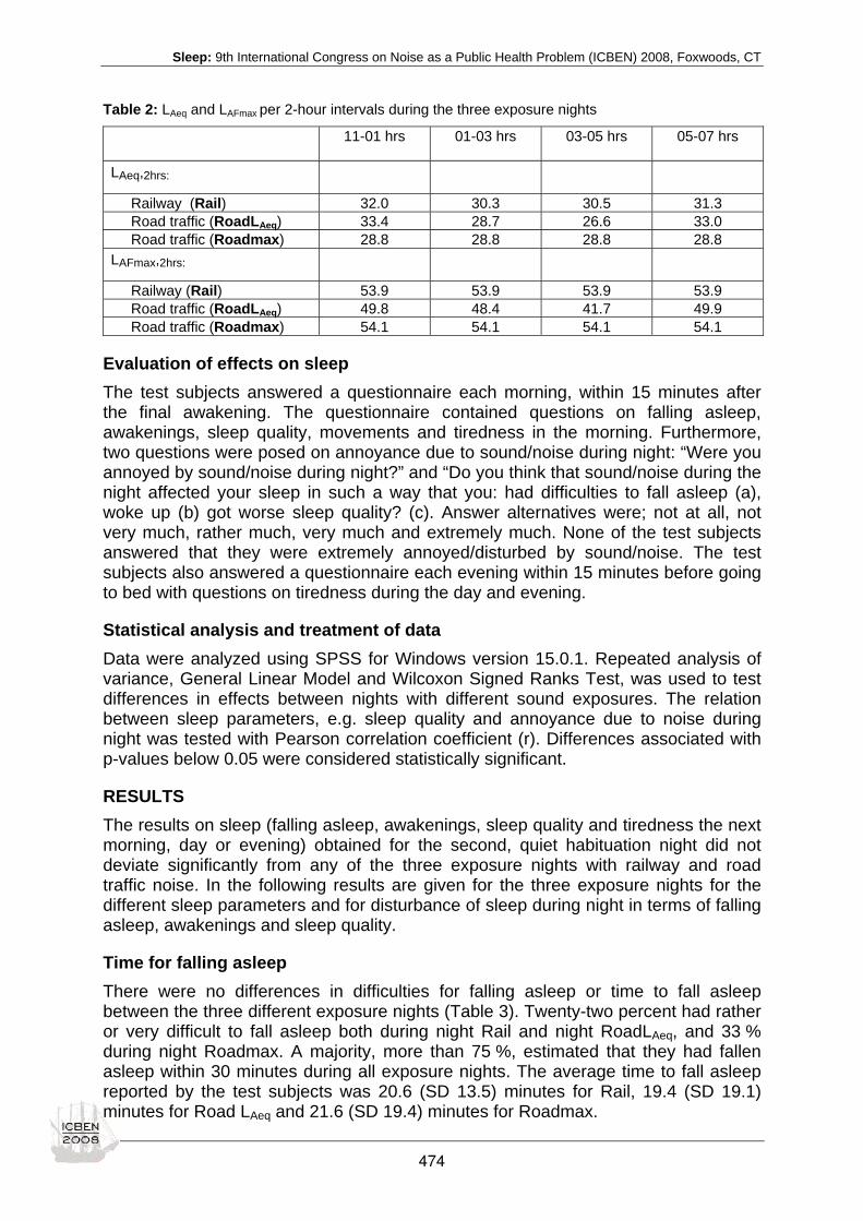
Sleep: 9th International Congress on Noise as a Public Health Problem (ICBEN) 2008, Foxwoods, CT
Table 2: LAeq and LAFmax per 2-hour intervals during the three exposure nights
11-01 hrs 01-03 hrs 03-05 hrs 05-07 hrs
LAeq,2hrs:
Railway (Rail) 32.0 30.3 30.5 31.3 Road traffic (RoadLAeq) 33.4 28.7 26.6 33.0 Road traffic (Roadmax) 28.8 28.8 28.8 28.8 LAFmax,2hrs:
Railway (Rail) 53.9 53.9 53.9 53.9 Road traffic (RoadLAeq) 49.8 48.4 41.7 49.9 Road traffic (Roadmax) 54.1 54.1 54.1 54.1
Evaluation of effects on sleep The test subjects answered a questionnaire each morning, within 15 minutes after the final awakening. The questionnaire contained questions on falling asleep, awakenings, sleep quality, movements and tiredness in the morning. Furthermore, two questions were posed on annoyance due to sound/noise during night: “Were you annoyed by sound/noise during night?” and “Do you think that sound/noise during the night affected your sleep in such a way that you: had difficulties to fall asleep (a), woke up (b) got worse sleep quality? (c). Answer alternatives were; not at all, not very much, rather much, very much and extremely much. None of the test subjects answered that they were extremely annoyed/disturbed by sound/noise. The test subjects also answered a questionnaire each evening within 15 minutes before going to bed with questions on tiredness during the day and evening.
Statistical analysis and treatment of data Data were analyzed using SPSS for Windows version 15.0.1. Repeated analysis of variance, General Linear Model and Wilcoxon Signed Ranks Test, was used to test differences in effects between nights with different sound exposures. The relation between sleep parameters, e.g. sleep quality and annoyance due to noise during night was tested with Pearson correlation coefficient (r). Differences associated with p-values below 0.05 were considered statistically significant.
RESULTS The results on sleep (falling asleep, awakenings, sleep quality and tiredness the next morning, day or evening) obtained for the second, quiet habituation night did not deviate significantly from any of the three exposure nights with railway and road traffic noise. In the following results are given for the three exposure nights for the different sleep parameters and for disturbance of sleep during night in terms of falling asleep, awakenings and sleep quality.
Time for falling asleep There were no differences in difficulties for falling asleep or time to fall asleep between the three different exposure nights (Table 3). Twenty-two percent had rather or very difficult to fall asleep both during night Rail and night RoadLAeq, and 33 % during night Roadmax. A majority, more than 75 %, estimated that they had fallen asleep within 30 minutes during all exposure nights. The average time to fall asleep reported by the test subjects was 20.6 (SD 13.5) minutes for Rail, 19.4 (SD 19.1) minutes for Road LAeq and 21.6 (SD 19.4) minutes for Roadmax.
474
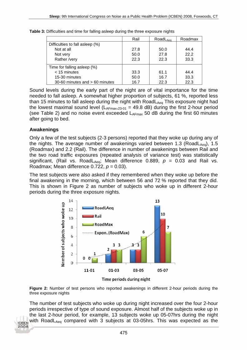
Sleep: 9th International Congress on Noise as a Public Health Problem (ICBEN) 2008, Foxwoods, CT
Table 3: Difficulties and time for falling asleep during the three exposure nights
Rail RoadLAeq Roadmax Difficulties to fall asleep (%) Not at all Not very Rather /very
27.8 50.0 22.3
50.0 27.8 22.3
44.4 22.2 33.3
Time for falling asleep (%) < 15 minutes 15-30 minutes 30-60 minutes and > 60 minutes
33.3 50.0 16.7
61.1 16.7 22.3
44.4 33.3 22.3
Sound levels during the early part of the night are of vital importance for the time needed to fall asleep. A somewhat higher proportion of subjects, 61 %, reported less than 15 minutes to fall asleep during the night with RoadLAeq This exposure night had the lowest maximal sound level (LAFmax,23-01 = 49.8 dB) during the first 2-hour period (see Table 2) and no noise event exceeded LAFmax 50 dB during the first 60 minutes after going to bed.
Awakenings Only a few of the test subjects (2-3 persons) reported that they woke up during any of the nights. The average number of awakenings varied between 1.3 (RoadLAeq), 1.5 (Roadmax) and 2.2 (Rail). The difference in number of awakenings between Rail and the two road traffic exposures (repeated analysis of variance test) was statistically significant, (Rail vs. RoadLAeq; Mean difference 0.889, p = 0.03 and Rail vs. Roadmax; Mean difference 0.722, p = 0.03). The test subjects were also asked if they remembered when they woke up before the final awakening in the morning, which between 56 and 72 % reported that they did. This is shown in Figure 2 as number of subjects who woke up in different 2-hour periods during the three exposure nights.
Figure 2: Number of test persons who reported awakenings in different 2-hour periods during the three exposure nights
The number of test subjects who woke up during night increased over the four 2-hour periods irrespective of type of sound exposure. Almost half of the subjects woke up in the last 2-hour period, for example, 13 subjects woke up 05-07hrs during the night with RoadLAeq compared with 3 subjects at 03-05hrs. This was expected as the
475

Sleep: 9th International Congress on Noise as a Public Health Problem (ICBEN) 2008, Foxwoods, CT
proportion of deep sleep is much higher during the first period of the night. Both Rail and RoadLAeq nights have higher equivalent sound levels during the last 2-hour period which may explain why some more subjects woke up during these nights as compared with the RoadMax night.
Sleep quality and tiredness in the morning Reported sleep quality is closely related to difficulties falling asleep and awakenings during night and also with how rested one feels in the morning after the final awakening. Sleep quality, movements and tiredness the following morning, day and evening after the different exposure nights was measured with several different questions (5-point verbal category scale and a numeric 0-10 scale). The results are shown in Table 4.
Table 4: Sleep quality and tiredness after different exposure nights
Rail RoadLAeq Roadmax
Sleep quality (%) Very bad/bad/not very good Rather good Very good
22.2
50 27.8
5.9 58.8 35.3
16.7 61.1 22.2
Sleep quality, Scale 0-10 (Mean, SD) (0 very bad - 10 very good)
6.9 (2.14)
7.4 (1.62)
7.2 (1.83)
Movements, Scale 0-10 (Mean, SD) (0 lay still - 10 moving all night)
3.6 (2.28)
3.1(1.71)
3.6 (1.69)
Tired- alert morning (%) Very tired/tired/rather tired Rather alert and rested Very alert and rested
55.5 38.9 5.6
50
44.4 5.6
50
33.3 16.7
Tired-alert, Scale 0-10 (Mean, SD) (0 very tired – 10 alert and rested)
Morning after 5.4 (2.48) 5.9 (2.19) 5.9 (2.24) Day after 6.1 (2.53) 5.4 (2.48) 5.8 (2.67) Evening after 3.6 (1.72) 4.0 (2.33) 3.9 (1.94)
There were no significant differences for any of the sleep parameters between the three exposure nights. The proportion of test subjects who reported very good sleep quality was slightly higher after RoadLAeq (35 %) and this was also the case for the numeric scale (Mean value 7.4) and movements during sleep (Mean value 3.1).
Reported annoyance and disturbance of sleep by sound/noise The test subjects answered questions on how sound/noise annoyed them during night and how sound/noise disturbed falling asleep, awakenings and sleep quality. The proportion of test subjects being disturbed in falling asleep by sound/noise was the same for the three sound exposures (28 %). A slightly higher proportion of the test subjects reported that they were annoyed and disturbed by Rail as compared with RoadLAeq and RoadMax, but there were no significant differences between the three exposure nights (Figure 3).
476

Sleep: 9th International Congress on Noise as a Public Health Problem (ICBEN) 2008, Foxwoods, CT
Figure 3: Proportion annoyed or disturbed (% rather and very) by sound/noise during the three exposure nights; annoyed during night (upper), woken up due to sound/noise (lower, left) and worse sleep quality due to sound/noise (lower, right).
Relationship between sleep quality and annoyance/disturbance due to noise There was a statistically significant correlation (p < 0.001, Pearson correlation test, r) between sleep quality (Table 4) and reported annoyance/disturbance due to sound/noise during night, for exposure nights RoadLAeq and for exposure nights Roadmax; r = 0.68 and for exposure nights Rail; r = 0.71. This means that annoyance/disturbance due to road traffic noise explained 46 % of the variance (r2) in sleep quality during nights with road traffic noises. Annoyance/disturbance due to railway noise explained 50 % of the variance in sleep quality during nights with railway noise.
COMMENTS AND CONCLUSIONS The overall results revealed no differences between nights with railway noise and nights with road traffic noise with the same sound levels in Lnight or LAFmax. The average number of awakenings per night was however somewhat higher for railway noise (2.2) as compared with road traffic noise (1.5 and 1.3 respectively). The reduction in sleep quality compared with the second, quiet night was small, -11 % for Rail, -5 % for Roadmax and -3 % for RoadLAeq. In the previous series of sleep experiments (Öhrström et al. 1990; Öhrström 1995) we studied effects of road traffic noise with different LAFmax-levels (45–60 dB) and number of noise events (4–128) and found on average a similar decrease (-12 %) in sleep quality and about the same number of awakenings per night (1.9, variation 1.1– 3.1). The test subjects in the present study were all young and healthy with normal hearing. Thus, the results cannot be generalized to a general population without caution. The sound exposures used in the study correspond to normally occurring indoor sound levels and frequency spectra for road traffic and railway noise when the bedroom window is kept slightly open which is common, provided that the outdoor sound levels are not too high, above Lnight 55 dB (e.g. Öhrström et al. 2006). If windows are kept closed, the same outdoor sound level from road traffic and railway
477
Sleep: 9th International Congress on Noise as a Public Health Problem (ICBEN) 2008, Foxwoods, CT
noise would result in a 5 dB lower indoor sound level for railway noise than for road traffic noise. With windows slightly open, however, the difference in sound level would only be about 0.5 dB. The exposure situation in this experiment, where we used a frequency filter to simulate an open window situation, is therefore reasonably similar to a homelike sound environment with windows slightly open. Considering this, comparisons between the present experiment and sleep studies in the field are probably more appropriate than experiments with no adjustment of the frequency spectra for the two types of noise sources. The results from the present experiment disclosed somewhat more awakenings due to railway noise as compared with road traffic noise with the same sound levels corresponding to a situation with the window slightly open but no other significant differences in reported sleep disturbances were found. The results contradict to some extent, the EU position paper (2004) on sleep disturbances and the results obtained in the updated meta-analysis by Miedema & Vos (2007) of dose-response relationships between sleep disturbances and different types of traffic noise, which suggest that railway noise causes less sleep disturbances than road traffic noise.
ACKNOWLEDGEMENTS The study forms part of the Swedish research program TVANE (Train Vibration and Noise Effects) (year 2006-2010) funded by the Swedish Railroad Administration.
REFERENCES EU (2002). Position paper on dose response relationships between transportation noise and annoyance. EU´s Future Noise Policy, WG2 – Dose/Effect. European Communities.
EU (2004). Position paper on dose-effect relationships for night time noise, 11 Nov 2004. European Commission Working Group on Health and Socio-Economic Aspects.
Griefahn B, Marks A, Robens S (2006). Noise emitted from road, rail and air traffic and their effects on sleep. J Sound Vibr 295: 129-140.
Miedema HME, Oudshoorn CGM (2001). Annoyance from transportation noise: relationships with exposure metrics DNL and DENL and their confidence intervals. Environ Health Perspect 109: 409-416.
Miedema HME, Vos H (2007). Associations between self-reported sleep disturbance and environmental noise based on reanalyses of pooled data from 24 studies. Behav Sleep Med 5: 1-20.
Moehler U, Liepert M, Schuemer R, Griefahn B (2000). Differences between railway and road traffic noise. J Sound Vibr 231: 853-864.
Ögren M, Öhrström E, Jerson T (2008). Noise and vibration generation for laboratory studies on sleep disturbances. Proceedings of the 9th International Congress on Noise as a Public Health Problem (ICBEN) 2008, Foxwoods CT, USA (in this volume)
Öhrström E (1995). Effects of low levels from road traffic noise during night - a laboratory study on number of noise events, maximum noise levels and noise sensitivity. J Sound Vibr 179: 603-615.
Öhrström E, Skånberg A (2006). Litteraturstudie – Effekter avseende buller och vibrationer från tåg- och vägtrafik. (Litterature review – Effects of noise and vibrations from railway and road traffic) Arbets- och miljömedicin, Sahlgrenska Akademin vid Göteborgs universitet. Rapport 112, 2006.
Öhrström E, Björkman M, Rylander R (1990). Effects of noise during sleep with reference to noise sensitivity and habituation: studies in laboratory and field. Environ Int 16: 477-482.
Öhrström E, Skånberg A, Svensson H, Gidlöf-Gunnarsson A (2006). Effects of road traffic noise and the benefit of access to quietness. J Sound Vibr 295: 40-59.
Öhrström E, Barregård B, Andersson E, Skånberg A, Svensson H, Ängerheim P (2007). Annoyance due to single and combined exposure from railway and road traffic noise. J Acoust Soc Am 122: 2642-2652.
478

Sleep: 9th International Congress on Noise as a Public Health Problem (ICBEN) 2008, Foxwoods, CT
Temporally limited nocturnal traffic curfews to prevent noise induced sleep disturbances Barbara Griefahn*, Anke Marks, Sibylle Robens Institute for Occupational Physiology at Dortmund Technical University (Institut für Arbeitsphysiologie an der Technischen Universität Dortmund), Ardeystr. 67, D-44139 Dortmund, Germany
*corresponding author: e-mail: [email protected]
ABSTRACT This study aimed at the identification of a time frame suitable for the prevention of noise induced sleep disturbances. Curfews at the end of nights were expected to provide the best protection; further persons with corresponding bed times were expected to profit most. Subjects and methods. 24 students (12 women, 12 men, 21-27 yrs) slept two consecutive weeks four nights each in the laboratory being exposed one week each to rail or road traffic noise. The 4 nights each week consisted of a quiet night and three noisy nights with different curfews (23–3 h, 23–5 h, 3–7 h). Eight persons each went to bed at 22, 23, and 24 h and got up 8 h later. The resulting 9 exposure patterns were condensed to 3 patterns with curfews at the beginning, in the middle or at the end of the night. Polysomnograms were recorded each night and the participants evaluated their sleep every morning. Results and conclusions. Traffic curfews are beneficial only at the end of the night and disturbances experienced in the beginning of the night are then compensated. Even short periods of subsequent noise cause sleep disturbances. Thus late sleepers whose nights always end with a noisy period profit scarcely from these regulations.
INTRODUCTION Sleep disturbances are considered as the most deleterious effects of noise. Acute event related effects are cortical and autonomic arousals, sleep stage changes, awakenings and body movements that are determined by the temporal acoustical microstructure of the single vehicles (temporal variation of levels and frequencies, rise time, duration, type of noise etc.), the macrostructure of the whole noise scenario (sequences of vehicles, noise-free intervals etc.) as well as by the actual situation (sleep depth etc.) (Basner et al. 2006; Brink et al. 2008; Griefahn 1989; Marks et al. 2008). These primary reactions cause eventually alterations of whole nights' sleep (Basner et al. 2004; Griefahn et al. 2006), followed by worse ratings of sleep quality and impaired performance the next day (Basner 2008; Marks & Griefahn 2005; Öhrström & Björkman 1988; Öhrström et al. 2006). In the long run nocturnal noise is even suspected to contribute to the genesis of cardiovascular diseases (Babisch 2006). Thus sleep disturbances are undoubtedly relevant for health and noise abatement becomes an essential element of public health care. Though the actual noise load is already critical for numerous residents living along busy roads, railway tracks and in the vicinity of airports traffic volume is expected to increase further. But as neither the road nor the railway networks will be enlarged accordingly traffic density and thereby transportation noise will increase more during the shoulder hours and during the night than during the day. This will consequently increase and aggravate noise induced sleep disturbances.
479

Sleep: 9th International Congress on Noise as a Public Health Problem (ICBEN) 2008, Foxwoods, CT
Concerning noise abatement suitable measures are traffic curfews for all or at least for the noisiest vehicles (motorcycles, trucks, high speed trains, freight trains), for the whole night or for defined sections of the night. Concerning the latter it is not yet clear whether these curfews should be established at the beginning, in the middle or at the end of the night. But as the noises in these studies were more or less evenly distributed over the night and as the reaction to a distinct stimulus depends on the reactions to previous stimuli it is not justified to set the time frames for traffic curfews without adequate tests. This study aimed at the identification of a time frame for traffic curfews that provide a sufficient protection. It was hypothesized that noise induced sleep disturbances are best prevented by traffic curfews in the late night. Noise in the beginning of the subjective night (that indicates the individual noise load of a person due to his/her individual bed time) affects the process of falling asleep but subsequent curfews provide the opportunity to compensate these disturbances. Curfews at the beginning of the night will, however, not affect sleep onset but subsequent noise exposure causes sleep disturbances that cannot be compensated thereafter. Further, as the time frames of curfews are fixed (e.g. to the sleep behavior of the majority of the adult population) persons with corresponding bed times are probably sufficiently protected. But persons with earlier or later bed times profit less from such regulations as for them the quiet periods are either reduced or embedded into an initial and a terminal noise exposure. This study evaluated three temporally limited curfews where the respective time frames are oriented to the sleep behavior of the majority of the German population. Most people go to bed around 23 h and get up at around 7 h. Two evening curfews started at 23 h and lasted 4 or 6 hours until 3 or 5 h, respectively, a morning curfew started at 3 h and lasted until 7 h. Persons with normal, early, late bed times were observed during two consecutive weeks in the laboratory while exposed to road and rail traffic noise.
MATERIALS AND METHODS Participants 24 healthy and normal hearing students (12 women, 12 men, 21-27 yrs) gave their written informed consent to the study that was approved by the Local Ethics Committee. 8 persons each had normal, early or late bed times (23, 22, 24 h).
Experimental Design After a habituation night the participants slept two consecutive weeks, each week four consecutive nights from Monday night to Thursday night in the laboratory. Bedtimes were 23, 22 and 24 h for normal, early and late sleepers respectively. Time in bed (TIB) was terminated eight hours later at 7, 6 and 8 h, respectively. The participants were exposed in a balanced order to rail and to road traffic noise during the first or the second week, respectively. The four nights of each week consisted of a random sequence of a quiet and three noisy nights with different traffic curfews.
480

Sleep: 9th International Congress on Noise as a Public Health Problem (ICBEN) 2008, Foxwoods, CT
Noise load A 10 hours noise scenario from 22 to 8 h was created with lower traffic density in the middle of the night. It consisted of recordings of real traffic pass-bys. The road traffic scenario consisted of a mixture of private cars and trucks and the rail traffic scenario of a mixture of passenger and freight trains. The maximum levels varied between 56 to 68 dBA at the sleepers' ears. The hourly equivalent noise levels were LAeq = 45 dB with 48 road and 30 rail pass-bys per hour. The levels decreased to LAeq = 38 dB from 1 to 2 h and from 4 to 5 h with 33 and 24 pass-bys per hour. The LAeq from 2 to 4 h was 34 dB with 16 road and 10 rail pass-bys per hour. Three traffic curfews were applied to this scenario. Two evening curfews started at 23 h, one lasting 6 hours until 5 h, the other 4 hours until 3 h. A morning curfew started at 3 h and lasted until 7 h. The three bed times and three curfews resulted in nine different exposure patterns (Fig. 1) which were then grouped to three patterns with the curfew in the beginning (Q N), in the middle (N Q N) and at the end (N Q) of the subjective night. To achieve for the 6 hours traffic curfew the same equivalent noise level the number of pass-bys was elevated to 62 and 40 for road traffic and rail traffic, respectively. A 28 dBA red noise was continuously applied throughout all nights, even during quiet nights.
Individual noise loads (dark grey areas) determined by individual bed times
41.4 dB
39.8 dB
39.7 dB
41.3 dB
39.8 dB 39.8 dB
Trafficcurfews
6-hours23 – 5 h
4-hours23 – 3 h
4-hours3 – 7 h
11 pm 1 am 3 am 5 am 7 am
39.8 dB
25
40
30
45
35
41.3 dB
25
40
30
45
35
25
40
30
45
3539.7 dB
Early bedtimes(22 – 6 h)LAeq, 8h
Normal bedtimes(23 – 7 h)LAeq, 8h
Late bedtimes(24 – 8 h)LAeq, 8h
hour
lyeq
uiva
lent
leve
lho
urly
equi
vale
ntle
vel
hour
lyeq
uiva
lent
leve
l
23 h 1 h 3 h 5 h 7 h 23 h 1 h 3 h 5 h 7 h 23 h 1 h 3 h 5 h 7 h
23 h 1 h 3 h 5 h 7 h 23 h 1 h 3 h 5 h 7 h 23 h 1 h 3 h 5 h 7 h
23 h 1 h 3 h 5 h 7 h 23 h 1 h 3 h 5 h 7 h 23 h 1 h 3 h 5 h 7 h
Figure 1: Exposure patterns and equivalent noise levels of the three traffic curfews for early, normal, and late sleepers
Equivalent noise levels over the 8 hours in bed varied in most nights between 39.7 and 39.8 dBA but increased to 41.3 to 41.4 dBA for early and late sleepers whose individual morning and evening curfew, respectively lasted 3 instead of 4 hours. Equipment. The participants slept in separate sound shielded rooms with room temperature adjusted to 20 °C. All rooms were equipped with two loudspeakers. An intercom system provided the possibility to contact the experimenter at any time.
481
Sleep: 9th International Congress on Noise as a Public Health Problem (ICBEN) 2008, Foxwoods, CT
Recording of physiological parameters and subjective evaluation Polysomnogram. The polysomnograms (2 EEG, 2 EOG, 1 EMG) were continuously recorded throughout each night and rated according to Rechtschaffen and Kales (1968). The parameters derived from each polysomnogram were sleep onset latency (SOL, sleep onset: the first occurrence of 3 successive epochs of stage S1), sleep period time (SPT = sleep onset until final awakening), wakefulness after sleep onset (WASO), total sleep time (TST = SPT–WASO), Sleep-Efficiency-Index (here, as bed times were fixed to 8 h, defined as SEI = TST/SPT), and the time spent in each sleep stage (separately for SPT and for the first sleep cycle). Sleep stages S3 and S4 were combined to slow-wave-sleep (SWS) and the times awake and in stage S1 were for the first sleep cycle combined to S0&1. Seven parameters that are typically though moderately affected during nocturnal noise exposure were condensed to a 'Sleep-Disturbance-Index' (SDI, Griefahn et al. 2008a). These were: SOL (sleep onset latency), SWSL (latency from sleep onset to the first epoch of slow-wave-sleep), WASO (wakefulness after sleep onset until final awakening), W>3min (number of awakenings >3 min), sleep stages S1, SWS (time in sleep stages S3 + S4) and REM (time in rapid-eye-movement sleep). Subjective evaluations. Using 6 ten-point scales (ranging from 0 to 10) the participants evaluated their sleep every morning, the difficulty to fall asleep (very easy – very difficult), calmness of sleep (very calm – very restless), sleep depth (very deep – very shallow), sleep duration (very long – very short), restoration (very high – very low), body movements (very little – very much). According to a factor analysis all these scales loaded on a single factor and were summed up and subtracted from the maximum achievable number (60) and the result was labeled as 'Sleep quality' (SQ).
RESULTS Comparison between groups and traffic modes There were no significant differences between the three groups defined by normal, early and late bed times during quiet nights. Concerning road and railway noise there was a tendency (p ≤ 0.1) for shorter TST, less REM-sleep, prolonged WASO, reduced SEI and increased SDI during nights with railway noise than during nights with road traffic noise. But as none of the various sleep parameters revealed a significant (p ≤ 0.05) difference the corresponding situations defined by the temporal location of the curfews were averaged across nights with rail and road traffic noise for further statistics.
Effects of traffic curfews Table 1 shows the differences between quiet nights and noisy conditions with different curfews, where positive numbers indicate higher values in noisy than in quiet nights. Concerning SOL and the first sleep cycle curfews in the beginning of the subjective night (Q N) did not, as compared to entirely quiet nights, cause significant alterations. In contrast noise in the beginning of the subjective night (N Q, N Q N) was associated with a significant reduction of SWS during the first sleep cycle and non-significant prolongations of SOL, SWSL and S0&1.
482

Sleep: 9th International Congress on Noise as a Public Health Problem (ICBEN) 2008, Foxwoods, CT
Table 1: Means and standard deviations (SD) of the differences between quiet and noisy conditions for three curfews (positive values indicate longer times in noisy nights). **: p ≤ 0.01, * p ≤ 0.05 in columns 2-4 indicate significant within-subject differences between noisy and quiet nights. Kruskal-Wallis and Wilcoxon tests concern the differences between conditions (temporal position of curfews).
Exposure pattern Temporal position of curfews during nights
Kruskal-Wallis
Wilcoxon test
Q N (1) N Q N (2) N Q (3) 1:2 1:3 2:3 mean ± SD mean ± SD mean ± SD p p p p
SOL and first sleep cycle SOL 1.7 ± 7.6 12.7 ± 19.4 ** 2.0 ± 8.7 0.06 0.02 0.46 0.06 SWSL 0.3 ± 3.7 2.0 ± 7.1 * 4.6 ± 13.7 0.27 0.05 0.29 0.41 S0&1 0.8 ± 3.1 1.8 ± 3.0 * 1.8 ± 7.1 0.41 0.12 0.46 0.27 SWS -0.4 ± 9.2 -7.2 ± 10.7 ** -12.1 ± 14.3 ** 0.02 0.03 <0.01 0.52
Whole nights sleep TST -12.2 ± 17.8 ** -23.3 ± 23.0 ** 0.7 ± 22.6 0.27 0.28 0.06 <0.01WASO 10.2 ± 12.2 ** 6.8 ± 11.3 * -3.9 ± 18.9 0.06 0.44 0.01 0.06 SEI -0.02 ± 0.03 ** -0.02 ± 0.03 * 0.01 ± 0.05 0.08 0.72 0.02 0.05 SDI 0.58 ± 0.79 ** 0.66 ± 0.68 ** 0.12 ± 0.90 0.20 0.84 0.09 0.05 SQ -6.0 ± 5.7 ** -7.9 ± 6.3 ** -3.8 ± 7.9 0.32 0.26 0.36 0.09
Concerning the whole night none of the physiological parameters or subjective evaluation differed significantly from the entirely quiet nights when the subjective nights were terminated with a curfew (N Q). But noise periods at the end of the nights were irrespective of the temporal position of the (Q N, N Q N) associated with worse sleep. WASO was then prolonged at the expense of TST, the SEI was lower and the SDI was higher; sleep quality was rated worse (see Fig. 2). The between-conditions tests confirm this, i.e. no significant differences between both the situations with noise at the end of the subjective night but these conditions differed from nights with a traffic curfew at the end.
****0.0
0.2
0.4
0.6
0.8Sleep Disturbance Index
***
-0.03
-0.02
-0.01
0.00
0.01
0.02 Sleep EfficiencyIndex ****
-10-8-6-4-20
Subj. sleep quality (0-60)
Alte
ratio
n
*** p <= 0.01
p <= 0.05Noise-Quiet-Noise Quiet-Noise Noise-Quiet
Figure 2: Alterations of the SDI, the SEI and subjective sleep quality during noisy nights with differently terminated curfews as compared to entirely quiet nights.
Comparison between persons with different bed times The time frames of the curfews applied to 'normal' bed times (23–7 h). The assumption that persons with earlier or later bed times profit less from these regulations was tested for both the 4 hour curfews at the beginning and at the end of
483

Sleep: 9th International Congress on Noise as a Public Health Problem (ICBEN) 2008, Foxwoods, CT
the night (Q N, N Q). The respective means and standard deviations of normal, early and late sleepers are listed in Table 2. The parameters of early and late sleepers were, using the Wilcoxon test, compared to those of normal sleepers. Figure 3 shows the alterations of the SDI. Table 2: Means and standard deviations (SD) of selected sleep parameters of early, normal and late sleepers, separately for nights with evening or morning curfews. Wilcoxon-test for the comparison between early or late sleepers vs. normal sleepers: **: p ≤ 0.01, * p ≤ 0.05.
Early sleepers Normal sleepers Late sleepers mean ± SD mean ± SD mean ± SD Curfew 23 – 3 h TST 410.5 ± 37.0 433.6 ± 8.3 414.3 ± 26.8 WASO 36.7 ± 19.7 27.8 ± 9.1 42.7 ± 20.4 SEI 0.92 ± 0.04 0.94 ± 0.02 0.91 ± 0.05 SDI 0.27 ± 1.17 0.10 ± 0.60 0.55 ± 0.79 SQ 30.3 ± 5.9 32.6 ± 6.7 30.2 ± 4.8 Curfew 3 –7 h TST 430.1 ± 16.6 437.9 ± 7.7 406.0 ± 31.2 ** WASO 21.4 ± 8.4 23.3 ± 3.6 35.5 ± 14.6 * SEI 0.95 ± 0.02 0.95 ± 0.01 0.92 ± 0.04 ** SDI -0.19 ± 0.91 -0.17 ± 0.52 0.49 ± 0.70 * SQ 35.8 ± 5.0 36.2 ± 8.2 29.7 ± 7.5
The evening curfew (23–3 h) was preceded by one hour in noise in early sleepers and reduced by 1 hour for late sleepers. But this did not cause a further worsening of sleep than in normal sleepers. The morning curfew (3–7 h) was reduced to 3 hours for early sleepers. But none of the sleep parameters (Table 2) deviated significantly from those of the normal sleepers. But late sleepers for whom this curfew was followed by a single noisy hour had a significantly longer WASO, a lower SEI, a greater SDI and lower sleep quality.
*
-0.3
-0.2
-0.1
0.0
0.1
0.2
0.3
0.4
0.5
0.6Curfew 3 – 7 hCurfew 23 – 3/5 h
-0.3
-0.2
-0.1
0.0
0.1
0.2
0.3
0.4
0.5
0.6Sleep DisturbanceIndex
Sleep DisturbanceIndex
earlysleepers
latesleepers
normalsleepers
earlysleepers
latesleepers
normalsleepers
Noise-Quiet-Noise Quiet-Noise Noise-Quiet
Individual distribution of noise during the nights
Figure 3: Alteration of the SDI in nights with different curfews as compared to entirely quiet nights in persons with different bed times.
484

Sleep: 9th International Congress on Noise as a Public Health Problem (ICBEN) 2008, Foxwoods, CT
DISCUSSION Concerning noise abatement significant short-term alleviations are expected by the establishment of traffic curfews. This study focused therefore on the identification of time frames that provide the best relief. A few studies where noise was applied only in the early or in the late night dealt with noise from aircraft (Maschke 1992) and from military training camps (Griefahn 1989). The present study is the first that focused on the most frequent noise source, i.e. on noise from surface transportation (rail and road traffic). Further, as these time frames are oriented to the sleep behavior of the majority of the adult population this study considered in contrast to previous studies also persons who have habitually or due to their profession earlier or later bed times. Noise in the beginning of the subjective night caused as expected a delay of sleep onset and deep sleep, a prolongation of the time awake and of sleep stage S1 on the costs of the time in deep sleep of the first sleep cycle. But these disturbances were obviously compensated when sleep was terminated in quiet. Then neither the physiological indicators of sleep nor the subjective evaluation of whole nights’ sleep differed significantly from that of entirely quiet nights. Similar observations were already reported for the effects of sonic booms, noises from military training camps or aircraft (Griefahn 1989; Maschke 1992). As indicated by the data of the early sleepers a three hours quiet at the end of the subjective night is probably sufficient for complete compensation. But as soon as this period was followed by an even short noise exposure none of the curfews was beneficial. Evening curfews that are irrespective of the individual bed times followed by a noise period were associated with considerable disturbances. Concerning the morning curfew, however, persons with normal and with early bed times did not sleep worse than during entirely quiet nights. But persons with late bed times, for whom this curfew was followed by one hour in noise slept then significantly worse. Thus temporally limited curfews are only useful when the subjective night is terminated in quiet. The greater vulnerability during the late night is certainly related to the lower sleep depth and the then elevated sympathetic tone. There are of course some limitations. The participants were young and healthy. It is conceivable to assume that the differences in the beneficial effect of morning and evening curfews are smaller in older persons whose sleep becomes flatter (Bliwise 2005; Griefahn 1985). The differences might also be less when these curfews are established in the field because reactions in the field are usually less than in the laboratory (e.g. Basner et al. 2004).
CONCLUSIONS This study concerns the value of different time frames of traffic curfews to avoid sleep disturbances due to noises emitted from rail and road vehicles. It has shown that traffic curfews are beneficial only at the end of the subjective night, where a 3 hours period would be sufficient. Only then whole nights' sleep deviates scarcely from that of entirely quiet nights. Any, even short noise periods at the end of the subjective night cause prolongations of intermittent wakefulness, reduced sleep efficiency, increases of the SDI and a reduction of subjective sleep quality. This implies that late sleepers benefit scarcely from these regulations as their subjective night always ends with a noisy period.
485

Sleep: 9th International Congress on Noise as a Public Health Problem (ICBEN) 2008, Foxwoods, CT
Acknowledgement This paper is dedicated to the late Alexander Samel, a great scientist and friend. I shared with him a long and trusting working relationship. This work was supported by the German Ministry of Education and Research.
REFERENCES Babisch W (2006). Transportation noise and cardiovascular risk. Review and synthesis of epidemiological studies. Dose-effect curve and risk estimation. WaBoLu-Hefte 01/06.
Basner M (2008). Nocturnal aircraft noise exposure increases objectively assessed daytime sleepiness. Somnologie 12: 110-117.
Basner M, Buess H, Elmenhorst D, Gerlich A, Luks N, Maaß H, Mawet L, Müller E.W, Müller U, Plath G, Quehl J, Samel A, Schulze M, Vejvoda M, Wenzel J (2004). Nachtflugwirkungen. Volume 1, Summary. www.dlr.de/me/institut/abteilungen/ flugphysiologie/fluglärm/fb2004-07-d.pdf.
Basner M, Samel A, Isermann U (2006). Aircraft noise effects on sleep: Application of the results of a large polysomnographic field study. J Acoust Soc Am 119: 2772-2784.
Bliwise DL (2005). Normal aging. In: Kryger MH, Roth T, Dement WC (eds.): Principles and practice of sleep medicine (pp 24-28). Philadelphia: Elsevier Saunders.
Brink M, Lercher P, Eisenmann A, Schierz C (2008). Influence of slope of rise and event order of aircraft noise events on high resolution actimetry parameters. Somnologie 12: 118-128.
Griefahn B (1985). Schlafverhalten und Geräusche. Feld- und Laboruntersuchungen über Straßenverkehr, EEG-Analyse, Literaturauswertung. Stuttgart: Enke.
Griefahn B (1989). Cardiac responses caused by shots of tanks during sleep. J Sound Vibr 128: 109-119.
Griefahn B, Robens S, Bröde P, Basner M (2008a). The sleep disturbance index – a measure for structural alterations of sleep due to environmental influences. In: 9th International Congress on Noise as a Public Health Problem (ICBEN) 2008, Foxwoods, CT.
Griefahn B, Basner M, Bröde P, Robens S (2008b). Development of a sleep disturbance index (SDI) for the assessment of noise-induced sleep disturbances. Somnologie 12: 150-157.
Marks A, Griefahn B (2005). Railway noise – its effects on sleep, mood, subjective sleep quality, and performance. Somnologie 9: 68-75.
Marks A, Griefahn B, Basner M (2008). Event-related awakenings caused by nocturnal transportation noise. J Noise Contr Eng 56: 52-62.
Maschke C (1992). Der Einfluß von Nachtfluglärm auf den Schlafverlauf und die Katecholaminausscheidung. Berlin, Techn. Univ., Diss.
Öhrström E, Björkman M (1988). Effects of noise-disturbed sleep – a laboratory study on habituation and subjective noise sensitivity. J Sound Vibr 122: 277-290.
Öhrström E, Skånberg A, Svensson H, Gidlöf-Gunnarsson A (2006). Effects of road traffic noise and the benefit of access to quietness. J Sound Vibr 295: 40-59.
Rechtschaffen A, Kales A (1968). A manual of standardized terminology, techniques and scoring system for sleep stages in human subjects. Bethesda, MA: U.S. Dept of Health, Education, and Welfare. Public Health Service – National Institutes of Health, National Institute of Neurological Diseases and Blindness, Neurological Information Network.
486

Sleep: 9th International Congress on Noise as a Public Health Problem (ICBEN) 2008, Foxwoods, CT
Habitual traffic noise at home reduces overall cardiac para-sympathetic tone during sleep M.A. Graham*, S.A. Janssen, W. Passchier-Vermeer, H. Vos, H.M.E. Miedema Department of Environment and Health, TNO Netherlands Organisation for Applied Scientific Research, Delft, the Netherlands
* corresponding author: e-mail: [email protected]
Environmental noise from aircraft, road, or rail traffic during the night has been identi-fied as a major cause of sleep disturbance. Also, long running cohort studies indicate that long-term 24-hour road traffic noise exposure can influence long-term health. The mechanisms through which environmental noise may act upon human physiol-ogy during sleep in real-life conditions are at present not entirely understood. Be-cause of the possible role in the mechanisms of noise-induced health effects, the in-fluence of road and rail traffic noise exposure on cardiac sympathetic and parasym-pathetic tone during sleep (assessed by pre-ejection period (PEP) and respiratory sinus arrhythmia (RSA), respectively) was investigated in a field study. Thirty-six sub-jects from the general population of 7 residential areas within the Netherlands partici-pated for 6 consecutive nights (approximately 190 valid subject-nights). The relation-ships between the mean levels of PEP and RSA and road or rail traffic noise expo-sure levels within the bedroom during the sleep period were investigated. Multilevel linear regression models for PEP and for RSA, with subjects as random factor, were employed. The possible influence of covariates (e.g. gender, age, body-mass index, noise source) was investigated. The results suggest that increased indoor traffic noise exposure levels may lead to a reduction in overall cardiac parasympathetic tone during sleep. No statistically significant effect of indoor traffic noise on cardiac sympathetic tone was established. The apparent alteration in autonomic nervous sys-tem activity during sleep found here could constitute part of an environmental noise-induced sleep disturbance mechanism.
487

Sleep: 9th International Congress on Noise as a Public Health Problem (ICBEN) 2008, Foxwoods, CT
Nocturnal aircraft noise exposure increases objectively assessed daytime sleepiness Mathias Basner* German Aerospace Center (DLR), Institute of Aerospace Medicine, 51170 Cologne, Germany
*corresponding author: e-mail: [email protected]
ABSTRACT OBJECTIVES: There is no doubt that noise in general and aircraft noise specifically disturb sleep. However, so far no study assessed the effects of traffic noise on daytime sleepiness objectively. METHODS: In a polysomnographic laboratory study, 24 subjects (mean ± SD age 33.9 ± 10.8 years, 12 male) were investigated between 7:30 am and 8:30 am with infrared pupillography after a noise-free baseline night and after 9 nights with varying degrees of aircraft noise exposure. RESULTS: The natural logarithm of the pupillary unrest index (lnPUI) differed significantly (p=0.006) between noise (lnPUI=1.61) and baseline (lnPUI=1.48) nights, indicating higher levels of sleepiness after nights with noise exposure. Objective sleepiness levels increased significantly with the number of noise events (p=0.021), with the maximum sound pressure level of noise events (p=0.028), and with the equivalent continuous noise level (p=0.013) in exposure nights. However, these levels did not reach pathological levels observed in another study on untreated obstructive sleep apnea patients. CONCLUSIONS: This is the first study to show that nocturnal aircraft noise exposure increases objectively assessed sleepiness in the next morning. These findings stress the relevance and the potential public health impact of sleep disturbances induced by environmental noise. Further studies are needed to investigate the association of nocturnal traffic noise exposure and objectively assessed sleepiness in the field. A manuscript based on the study described in the abstract was recently published. In order not to infringe copyright agreements, only the abstract is printed here. The manuscript is available online as: Basner M: Nocturnal aircraft noise exposure increases objectively assessed daytime sleepinness, Somnologie 12(2), 110-117, published online 13 May 2008, DOI 10.1007/s11818-008-0344-x Reprints can be obtained from the author: [email protected]
488

Sleep: 9th International Congress on Noise as a Public Health Problem (ICBEN) 2008, Foxwoods, CT
Mental distress and modeled traffic noise exposure as determinants of self-reported sleep problems Jesper Kristiansen1*, Roger Persson1, Jonas Björk2, Maria Albin3, Kristina Jakobsson3, Per-Olof Östergren4, Jonas Ardö5, Emilie Stroh3 1 National Research Centre for the Working Environment, Lersø Parkallé 105,
DK-2100 Copenhagen, Denmark
2 Competence Center for Clinical Research, Lund University Hospital, Lund, Sweden
3 Department of Occupational and Environmental Medicine, Lund University Hospital, Lund, Sweden
4 Department of Health Sciences, Division of Social Medicine and Global Health, Malmö University Hospital, Sweden
5 Department of Physical Geography and Ecosystem Analysis, Lund University, Lund
*corresponding author: e-mail: [email protected]
INTRODUCTION Sleep is necessary for mental and physical reconstitution (for a review, see Åkerstedt & Nilsson (2003)). Poor sleep is prospectively associated with an increased risk for a number of adverse outcomes, such as myocardial infarction (Nilsson et al. 2001; Leineweber et al. 2003), type 2 diabetes (Nilsson et al. 2004; Nilsson 2008), depres-sion (Breslau et al. 1996; Roberts et al. 2000) and work accidents (Åkerstedt et al. 2002). Mental distress plays a role in causing disturbed sleep. For example, occupational stress has been found to be associated with sleep disorders (Kalimo et al. 2000; Fahlén et al. 2006). Other sources of mental distress should probably have the same effect as job stress on sleep quality, but have been less thoroughly studied in occu-pationally active populations. Traffic noise is another factor that might influence the sleep quality negatively, although studies on the association between traffic noise and sleep troubles show conflicting results, probably due to partial habituation (Öhrström 2000; Stansfeld & Matheson 2003; Griefahn et al. 2006). The fact that both job stress and traffic noise exposure have disturbed sleep as common effect suggests that environmental traffic noise exposure may add to, or even amplify, the adverse consequences of psychosocial exposures at work. To our knowledge the possible interaction between occupational stress and traffic noise has not been ad-dressed previously. Accordingly, the aims of the present study were: (i) to investigate the independent influence of traffic noise and occupational stress, and other sources of mental distress on sleep, and (ii) to investigate the possible interaction between occupational stress and traffic noise on sleep disturbance. With regard to the latter our hypothesis is that the mental distress caused by occupational stress increases the physiological arousal, which leads to an increased propensity to disturbance and awakening by traffic noise.
METHODS Population The identification of participants was based on a population based public health sur-vey from 2004, encompassing 47,621 persons 18 to 80 years old in Scania, Sweden (Rosvall et al. 2005). The total response rate was 59 % (n=27,879). From this initial
489

Sleep: 9th International Congress on Noise as a Public Health Problem (ICBEN) 2008, Foxwoods, CT
survey, all 11,629 persons that were occupationally active, employed at least half-time and not having used sleep medication within the last 3 months were selected for analysis. Among these persons 6,096 (52 %) were women and 5,533 (48 %) men. Mean age ± standard deviation (range) was 44 ± 11 (18-71) years for women, and 44 ± 12 (18-80) years for men. Among the women, 4,712 (78 %) were married or coha-biting, and for the men this number was 4,187 (76 %). Regarding the type of resi-dence 3,893 (64 %) of the women lived in a private house or a town house. The re-maining 2,187 (36 %) lived in a rental home or another type of residence. The corre-sponding numbers for men were 3,399 (62 %) and 2 114 (38 %), respectively.
Outcome measures General sleep problems was measured with two questions that assessed disturbed sleep without asking about attribution to external sources of disturbance: The first question read “Do you feel that you get sufficient sleep to feel rested?”. The response categories were: 1=”Yes, usually”; 2=”Yes, but not sufficiently often” and 3=”No, never or almost never”. In the analysis the responses were dichotomized 1+2 (“Yes”) and 3 (“No”). The second question regarding general sleep problems read: “Have you within the last 14 days been troubled by sleeping difficulties or sleep problems and if this is the case how troubled have you felt?”. The response categories were: 1=”Yes, very troubled”, 2=”Yes, a little troubled”, and 3=”No”. In our analysis the responses were dichotomized 1+2 (“Yes”) and 3 (“No”). Disturbed sleep attributed to traffic was measured with two items that followed the question: “Does traffic noise (road, train or airplane) lead to some of the following disturbances in your home? a) Difficult to sleep; b) Awakening”. The response cate-gories to both questions were: 1=”Yes, at least once per day”, 2=”Yes, at least once per week”, 3=”Yes, more rarely”, and 4=”No". The responses were dichotomized into 1+2 (“Yes”) if at least one response was 1 or 2, and 3 (“No or rarely”) for all other re-sponses.
Distress measures The Swedish version of the Job Content Questionnaire (JCQ) was used to assess how the participants perceived the work environment in terms of psychological job demands, job control and job support (Karasek et al. 1998). Psychological job de-mands and job control was measured with 9 items each. Following JCQ theory, job control has two subdimensions: decision authority and skill discretion. In this study we focused on decision authority measured by 3 items. Both job control and job de-mand items are formulated as statements and responded to on a 4-point scale: 1=“I agree completely”, 2=“I agree”, 3=“I disagree” and 4=“I completely disagree”. The mean score of the relevant items were used as the score in the decision authority and demand dimensions, respectively (after reversal of scores where appropriate). The persons were thereafter assigned to decision authority and job demand groups according to a robust classification of the mean scores (1-1.99: Low; 2-2.99: Medium; 3-4: High). Next, job strain groups were formed based on the balance between de-mands and decision authority: High strain was defined as belonging to the High de-mand group and Low or Medium decision authority group, or belonging to the Me-dium demand group and Low decision authority group. Medium strain was defined as belonging to the High demand group and the High decision authority group, or be-longing to Medium demand group and the Medium decision authority group, or be-longing to the Low demand and the Low decision authority group. Lastly, low strain was defined as belonging to the Low demand group and the High or Medium deci-
490

Sleep: 9th International Congress on Noise as a Public Health Problem (ICBEN) 2008, Foxwoods, CT
sion authority group, or belonging to the Medium demand group and the High deci-sion authority group. The formation of job strain categories from job demand and de-cision authority categories is illustrated in Figure 1.
Figure 1: Formation of job strain categories into Low, Medium and High. The formation is based on the balance between job demands and decision authority categories.
The participant’s perception of current health was measured by a single item from the General Health Questionnaire-12 (GHQ-12) (Goldberg & Williams 1988) that read: “How would you estimate your current health in general?”. The five response catego-ries were reduced to four: 1=”Very good”, 2=”Good”, 3=”Fair”, 4=”Bad or very bad”. The distressing experience of pain was measured by a single item that followed a question that read: ”Indicate the statement that best describes your present state of health”. The item was “Pain/afflictions”. The item was responded to on a three point scale: 1=”I have no pain or afflictions”, 2=”I have some pain or afflictions” and 3=”I have strong pain or afflictions”. The responses were dichotomized 1 (“No pain”) and 2+3 (“Pain”). Financial distress was measured by a single item that read: “How often within the last 12 months do you have had problems to pay your bills?". The item was responded to on a four point scale: 1=”Every month”, 2=”About half of the months”, 3=“Sometimes”, and 4=”Never”. The responses were dichotomized 1+2+3 (“Yes”) and 4 (“No”). Lastly, the distress from taking care of a sick, old or disabled relative was measured by a single item: “Do you have an old, sick or disabled relative that you have to help in their everyday routines, look after or take care of?” The response categories were 1=”No” and 2 =“Yes”.
Modeled traffic noise exposure We assessed individual exposure with high resolution, using Geographical Informa-tion Systems (GIS) as a tool to link the individual geocoded residential addresses at the end of year 2003 with available exposure data attributed this address (geocoded,
LOW (control ex-ceed de-mands)
LOW MEDIUM
HIGH LOW
HIGH MEDIUM
+
+
+
LOW LOW
MEDIUMMEDIUM
HIGHHIGH
+
+
+
HIGH LOW
MEDIUMHIGH
LOW MEDIUM
+
+
+
Demands Decision authority Demands
Decision authority Demands Decision
authority
MEDIUM (balanced)
HIGH (demands
exceed control)
491

Sleep: 9th International Congress on Noise as a Public Health Problem (ICBEN) 2008, Foxwoods, CT
or grid data) as previously described (Ardö 2005; Björk et al. 2006; Persson et al. 2007). Because we had no information on when people went to bed or awoke, night time noise exposure was estimated by using modelled A-weighted energy equivalent continuous sound pressure levels during a full day (24 hr; LAeq,24) at the residential address.
Statistical analysis Statistical computations were made with the SPSS computer software, version 15.0. P-values below 0.05 were considered statistically significant. The relationship be-tween outcome measures and distress measures (including modelled noise levels) was analyzed in a multiple logistic regression in which relevant co-variates also were entered. Accordingly, we used the noise level (LAeq,24, continuous), job strain, self-rated health, financial distress, distress from pain, distress from taking care of rela-tive, age, gender, marital status and type of residence as forced entry predictors, and the dichotomized disturbed sleep scores as outcomes. The interaction between job strain and noise levels was included to test whether job strain increased the effect of noise level.
RESULTS There was no interaction between exposure to noise at the home address and job strain on any sleep outcome. Consequently, only main effects model results are re-ported below.
General sleep problems (non-attributed) Results from the main effect multiple logistic regression analyses of non-attributed general sleep problems are presented in Table 1. Traffic noise was not associated with increased risk of not getting enough sleep or having had sleep problems within the last two weeks. However, all other mental distress sources, including job strain, were significant predictors of sleep problems in the logistic regression model. Particu-larly, self-rated health was strongly associated with both sleep outcomes. Persons rating their health as bad or very bad had 10-20-fold greater risk of reporting sleep problems in comparison to persons rating their health as very good. Taking care of sick, old or disabled relative lead to moderately increased risk of reporting sleep problem, but did not significantly influence the persons’ perception of getting suffi-cient sleep (Table 1).
Sleep problems attributed to traffic noise In contrast to generally disturbed sleep, sleep problems that were attributed to traffic noise was significantly associated with traffic noise levels (Table 2). Job strain and other mental distress factors were also strongly associated with this type of sleep problems. However, it is noteworthy that self-rated health is not as strong as predictor as it is for non-attributed sleep problems, and a dose-response relation between sleep problems attributed to traffic noise and self-rated health is absent (Table 2).
492

Sleep: 9th International Congress on Noise as a Public Health Problem (ICBEN) 2008, Foxwoods, CT
Table 1: Multiple logistic regression: Odds ratios (OR) and 95 % confidence intervals (95 % CI) for generally disturbed sleep. Adjusted for gender, age, marital status, and type of residence Not getting enough sleep Having sleep problems within the last 2
weeks Variable Level OR [95 % CI] p-value OR [95 % CI] p-value 24 hr traffic noise level (LAeq,24)
(continuous; effect per unit increase)
1.00 [0.99-1.00] NS 1.00 [0.99-1.01] NS
Low 1.00 - 1.00 - Medium 1.68 [1.46-1.94] P<0.001 1.30 [1.06-1.60] P=0.012 Job strain High 2.14 [1.74-2.62] P<0.001 1.53 [1.15-2.02] P<0.001
Very good 1.00 - 1.00 - Good 2.46 [1.94-3.12] P<0.001 2.87 [1.88-4.36] P<0.001 Fair 6.12 [4.72-7.94] P<0.001 7.32 [4.72-11.4] P<0.001
Self-rated health
Bad/very bad 12.0 [8.23-17.6] P<0.001 19.6 [11.5-33.1] P<0.001
No 1.00 - 1.00 - Pain Yes 1.65 [1.42-1.92] P<0.001 2.05 [1.62-2.60] P<0.001
No 1.00 - 1.00 - Financial problems Yes 1.37 [1.19-1.59] P<0.001 1.40 [1.14-1.72] P=0.002
No 1.00 - 1.00 - Taking care of old/sick relative
Yes 1.18 [0.97-1.45] NS 1.34 [1.02-1.73] P=0.027
Table 2: Multiple logistic regression: Odds ratios (OR) and 95 % confidence intervals (95 % CI) for sleep disturbance attributed to traffic noise. Adjusted for gender, age, marital status, and type of resi-dence
Sleep problems caused by traffic noise at least one time per week
Variable Level OR [95 % CI] p-value 24 hr traffic noise level (LAeq,24)
(continuous; effect per unit increase)
1.04 [1.03-1.05] P<0.001
Low 1.00 - Medium 1.24 [1.02-1.50] P=0.029 Job strain High 1.56 [1.18-2.05] P=0.002
Very good 1.00 - Good 1.02 [0.80-1.30] NS Fair 1.62 [1.21-2.17] P=0.001
Self-rated health
Bad/very bad 1.24 [0.70-2.21] NS
No 1.00 - Pain Yes 1.32 [1.08-1.62] P=0.007
No 1.00 - Financial problems Yes 1.71 [1.41-2.07] P<0.001
No 1.00 - Taking care of old/sick relative
Yes 1.54 [1.20-1.98] P=0.001
Influence of covariates There was no association between gender or marital status on any of the sleep out-comes. Age was significantly associated with the risk of reporting that sleep was in-sufficient. Persons in the higher age groups had a significantly lower risk of not get-ting enough sleep compared to persons in younger age groups. The type of resi-dence was not significantly associated with any of the general (not attributed) sleep outcomes, but those persons living in a rental home compared to those living in a
493

Sleep: 9th International Congress on Noise as a Public Health Problem (ICBEN) 2008, Foxwoods, CT
private house or town house had a significantly increased odds ratio for reporting dis-turbed sleep attributed to traffic noise.
CONCLUSIONS Several measures of mental distress showed to be significant predictors of disturbed sleep attributed to traffic noise as well as of general sleep disturbances that was not attributed to any cause what so ever. Traffic noise exposure as measured with 24 hr LAeq,24 was also significantly associated with sleep disturbances attributed to traffic noise, but not to sleep disturbances in general. The results confirm previous findings that the perceived psychosocial working environment contribute to disturbed sleep (Kalimo et al. 2000; Fahlén et al. 2006). However, since our data are cross-sectional in nature, we can not determine the order of factors in the cause-effect chain. It seems plausible that disturbed sleep is caused by work stress, but is also plausible that poor sleep and lacking restitution negatively affects the person’s ability to cope with work and therefore perceives work as more demanding and stressful. Our last conclusion concerns the interaction between job strain and traffic noise exposure. Our analysis do not suggest a significant interaction, thus, the results did not confirm our hypothesis that distress due to work stress will increase the propensity to wake up or to feel disturbed by traffic noise when trying to sleep.
REFERENCES Åkerstedt T, Nilsson PM (2003). Sleep as restitution: an introduction. J Intern Med 254: 6-12.
Åkerstedt T, Fredlund P, Gillberg M, Jansson B (2002). A prospective study of fatal occupational accidents - relationship to sleeping difficulties and occupational factors. J Sleep Res 11: 69-71.
Ardö J (2005). Trafik, människor och miljö i Skåne. Lund, Sweden: GIS Centre at Lund University.
Björk J, Ardö J, Stroh E, Lövkvist H, Östergren P-O, Albin M (2006). Road traffic noise in southern Sweden and its relation to annoyance, disturbance of daily activities and health. Scand J Work Environ Health 32: 392-401.
Breslau N, Roth T, Rosenthal L, Andreski P (1996). Sleep disturbance and psychiatric disorders: a longitudinal epidemiologi-cal study of young adults. Biol Psychiatry 39: 411-418.
Fahlén G, Knutsson A, Peter R, Åkerstedt T, Nordin M, Alfredsson L, Westerholm P (2006). Effort-reward imbalance, sleep disturbance and fatigue. Int Arch Occup Environ Health 79: 371-378.
Goldberg DP, Williams P (1988). User’s guide to the General Health Questionnaire. Windsor: NFER-Nelson Publ. Co.
Griefahn B, Marks A, Robens S (2006). Noise emitted from road, rail and air traffic and their effects on sleep. J Sound Vibr 295: 129-140.
Kalimo R, Tenkanen L, Härma M, Poppius E, Heinsalmi P (2000). Job stress and sleep disorders: findings from the Helsinki Heart Study. Stress Med 16: 65-75.
Karasek R, Brisson C, Kawakami N, Houtman I, Bongers P, Amick B (1998). The Job Content Questionnaire (JCQ): an instrument for internationally comparative assessments of psychosocial job characteristics. J Occup Health Psychol 3: 322-355.
Leineweber C, Kecklund G, Janszky I, Akerstedt T, Orth-Gomer K (2003). Poor sleep increases the prospective risk for recurrent events in middle-aged women with coronary disease. The Stockholm Female Coronary Risk Study. J Psychosom Res 54: 121-127.
Nilsson PM (2008). Why does sleep disturbance increase the risk of diabetes mellitus, and is there really a gender differ-ence? Sleep Med 9: 219-220.
Nilsson PM, Nilsson JA, Hedblad B, Berglund G (2001). Sleep disturbance in association with elevated pulse rate for predic-tion of mortality-consequences of mental strain? J Intern Med 250: 521-529.
Nilsson PM, Roost M, Engstrom G, Hedblad B, Berglund G (2004). Incidence of diabetes in middle-aged men is related to sleep disturbances. Diabetes Care 27: 2464-2469.
494

Sleep: 9th International Congress on Noise as a Public Health Problem (ICBEN) 2008, Foxwoods, CT
Öhrström E (2000). Sleep disturbances caused by road traffic noise - studies in laboratory and field. Noise & Health 2(8): 71-78.
Persson R, Björk J, Ardö J, Albin M, Jakobsson K (2007). Trait anxiety and modeled exposure as determinants of self-reported annoyance to sound, air pollution and other environmental factors in the home. Int Arch Occup Environ Health 81: 179-191.
Roberts RE, Shema SJ, Kaplan GA, Strawbridge WJ (2000). Sleep complaints and depression in an aging cohort: a prospec-tive perspective. Am J Psychiatry 157: 81-88.
Rosvall M, Khan AF, Nilsson M, Östergren P-O (2005). Hälsoförhållanden i Skåne. Folkhälsoenkät Skåne 2004. Malmö: Socialmedicinska enheten, Region Skåne, Universitetssjukhuset MAS.
Stansfeld SA, Matheson MP (2003). Noise pollution: non-auditory effects on health. Br Med Bull 68: 243-257.
495

Sleep: 9th International Congress on Noise as a Public Health Problem (ICBEN) 2008, Foxwoods, CT
Sleep disturbance caused by impulse sounds
Joos Vos
TNO Human Factors, Kampweg 5, 3769 DE Soesterberg, The Netherlands
e-mail: [email protected]
ABSTRACT Objective Detailed information about sleeping disturbance caused by nocturnal impulse sounds such as those produced at military training fields by firearms, and those produced in docks by container transshipment, is lacking. Both the Dutch Ministry of Defense and the Dutch Ministry of Housing, Spatial Planning, and the Environment contracted TNO Human Factors to determine, amongst other things, relations between the sound level of impulse sounds and the probability of behaviorally-confirmed noise-induced awakening reactions.
METHOD
Due to the limited frequency of the training activities, it was not feasible to conduct a study in residential areas around military firing ranges or training fields. Due to the poor predictability of the occurrence of the sounds of interest, and the uncertainty about the availability of a sufficient number of participants, the feasibility was low for designing a conventional field survey also for the other more civil sounds. As an al-ternative, the sounds were presented by means of loudspeakers in the bedrooms of 50 volunteers. The shooting sounds had been produced by a small and a medium-large firearm, and the sound fragments consisted of individual bangs or volleys of ten isolated or partly overlapping impulses. The civil impulse sounds had been produced by slamming one of the doors of a van, and by transshipment of a container. Again, the sound fragments consisted of single or multiple events. Aircraft sound was in-cluded as a reference source. The sounds were presented during a six-hour period that started 75 min after the beginning of the sleeping period. The time period be-tween the various stimuli varied between 12 and 18 min. Each subject participated in 18 nights to be completed within four weeks.
RESULTS
Forty-four subjects completed all or nearly all 18 nights. Half of this group was pre-sented with the shooting sounds, and the other half was presented with the civil im-pulse sounds. For these subjects, the probability of awakening clearly increased with increasing A-weighted sound exposure level (ASEL) of the impulse and aircraft sounds. The dose-response relations for the single impulse sounds, thus both for those produced by the rifle and the machine gun, and those produced by the door slam and the container transshipment, were much the same as that for the aircraft sounds. At equal indoor ASELs, the probability of awakening induced by the sound fragments with multiple events, i.e., the volleys of the shooting noise and the repeti-tive door slam and container sounds, was significantly higher than that induced by the single impulse and aircraft sounds. In the course of the three or four weeks with
496

Sleep: 9th International Congress on Noise as a Public Health Problem (ICBEN) 2008, Foxwoods, CT
experimental sounds, the probability of awakening induced by the multiple impulse sounds and the aircraft sounds decreased by nearly a factor of two.
CONCLUSIONS
At equal indoor ASELs, the probability of awakening for single impulse sounds was equal to that for aircraft sounds. The probability of awakening induced by the multiple impulse sounds, however, was significantly higher than that induced by the single impulse sounds and the aircraft sounds. In spite of the significant relation between awakening and ASEL within the set of multiple events, we must therefore conclude that ASEL is not a universal measure for predicting awakening. For obtaining equal probabilities of awakening, the ASELs of the multiple shooting sounds (volleys) must be about 15 dB lower, and the ASELs of the multiple civil impulse sounds (door slam and container transshipment) must be about 12 dB lower than those of the single bangs and the aircraft sounds. The 12-15 dB level difference did not depend on the degree of habituation. Repetitive sounds led to more awakenings than single isolated sounds did. Future research should focus in more detail on the effect of the multiple sounds.
497
__________________________________________________________________________
__________________________________________________________________________
ICBEN 2008
Effects of Noise on Sleep
498

Sleep: 9th International Congress on Noise as a Public Health Problem (ICBEN) 2008, Foxwoods, CT
Markov State Transition Models for the prediction of changes in sleep structure induced by aircraft noise Mathias Basner1,3*, Uwe Siebert2,3 1 German Aerospace Center (DLR), Institute of Aerospace Medicine, 51170 Köln, Germany
2 Department of Public Health, Medical Decision Making and Health Technology Assessment, UMIT, Eduard Wallnöfer-Zentrum I, 6060 Hall i.T., Austria
3 Institute for Technology Assessment and Department of Radiology, Massachusetts General Hospi-tal, Harvard Medical School, Boston, MA, USA
* corresponding author: e-mail: [email protected]
ABSTRACT OBJECTIVES: To quantitatively assess the effects of the introduction of a nocturnal air traffic curfew at Frankfurt Airport on sleep structure. METHODS: A six state (Wake, S1, S2, S3, S4 and REM) Markov state transition sleep model was built. Transition probabilities between states were calculated with autoregressive multinomial logistic regression based on polysomnographic laboratory study data. Monte Carlo simulation trials were performed for modelling a noise-free night and three noise scenarios: (1) traffic at Frankfurt Airport on 16 August 2005, (2) as (1), but flights between 11 pm and 5 am cancelled and (3) as (2), with flights between 11 pm and 5 am from (1) rescheduled to periods before 11 pm and after 5 am. RESULTS: The results indicate that there will be a small benefit for airport residents compared to the current situation even if all traffic is rescheduled (average time spent awake -3.2 %, S1 -4.6 %, S2 -0.9 %, S3 +3 %, S4 +9.2 %, REM +0.6 %, number of sleep stage changes -2.5 %). This benefit is likely to be outweighed by the increase in air traffic during shoulder hours, especially for those who choose to or have to go to bed before 10:30 pm or after 1 am. CONCLUSIONS: Alternative strategies might be necessary to both guarantee undisturbed sleep of airport residents and to minimize economic and legal disadvantages accompanied by a traffic curfew. The models developed in this investigation may serve as a valuable tool for optimizing air traffic patterns at airports, and therefore guide political decision making.
INTRODUCTION Aircraft noise may cause changes in sleep structure and impair recuperation. People living in the vicinity of airports are very concerned about possible short- and long-term effects of a chronically disturbed sleep on health. Frankfurt Airport plans to build a new runway in order to meet increasing traffic demands. The airport applied for a ban of air traffic between 11 pm and 5 am in order to compensate people living in the highly populated vicinity of Frankfurt Airport for increased traffic volumes during the day. Some of the flights starting or landing between 23:00 and 05:00 today are likely to be rescheduled to periods before 23:00 or after 05:00. Therefore, it is unclear whether and to what extend sleep of airport residents will benefit from an air traffic ban in the night.
499

Sleep: 9th International Congress on Noise as a Public Health Problem (ICBEN) 2008, Foxwoods, CT
OBJECTIVES To quantitatively assess the impact of the introduction of a ban of air traffic at Frank-furt Airport between 23:00 and 05:00 on sleep structure using epidemiological and decision-analytic methods. The main question was whether a ban of air traffic will still be beneficial for residents in terms of sleep structure if all nighttime air traffic is re-scheduled to periods before 23:00 and after 05:00.
METHODS Analyses were based on a polysomnographical laboratory study on the effects of air-craft noise on sleep performed at the German Aerospace Center (DLR) in Cologne between 1999 and 2003 (Basner et al. 2004; Basner & Samel 2005). A six state (sleep stages Wake, 1, 2, 3, 4 and REM) Markov state transition model was used to simulate nights with and without aircraft noise. Transition probabilities for the Markov models were calculated with autoregressive multinomial logistic regression (de Vries et al. 1998). Both regression and simulation results were validated with empirical data. Different times of falling asleep were considered in the analyses. The outcome variables "time spent in the different sleep stages", and "number of sleep stage changes". Three noise scenarios were compared with a noise-free night and with each other: (1) Scenario 1 (Noise): the current situation in Frankfurt with nocturnal air traffic, (2) Scenario 2 (Ban): a ban of air traffic between 23:00 and 05:00, and (3) Scenario 3 (Rescheduled): as (2), but with flights that took place between 23:00
and 05:00 in (1) rescheduled to periods before 23:00 and after 05:00.
RESULTS A first-order autoregressive multinomial logistic regression model with elapsed sleep time as the only additional explanatory variable was used for the calculation of transi-tion probabilities. Monte Carlo simulation trials showed that a ban of air traffic without rescheduling of flights lead to sleep structural improvements. These were diminished if 2005 traffic that took place between 23:00 and 05:00 was rescheduled to periods before 23:00 and after 05:00, but still, a small benefit remained: Compared to the 2005 situation without a ban of air traffic, average time spent awake decreased from 43.1 to 41.7 min (-3.2 %), S1 decreased from 9.2 to 8.7 min (-4.6 %), S2 decreased from 212.8 to 210.8 min (-0.9 %), S3 increased from 37.2 to 38.3 min (+3.0 %), S4 increased from 23.5 to 25.7 min (+9.2 %), REM increased from 84.7 to 85.3 min (+0.6 %), the number of sleep stage changes decreased from 121.3 to 118.3 (-2.5 %, see Table 1).
500
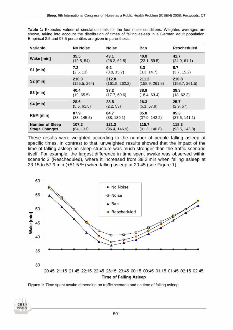
Sleep: 9th International Congress on Noise as a Public Health Problem (ICBEN) 2008, Foxwoods, CT
Table 1: Expected values of simulation trials for the four noise conditions. Weighted averages are shown, taking into account the distribution of times of falling asleep in a German adult population. Empirical 2.5 and 97.5 percentiles are given in parenthesis.
Variable No Noise Noise Ban Rescheduled
Wake [min] 35.5 (19.5, 54)
43.1 (26.2, 62.8)
40.0 (23.1, 59.5)
41.7 (24.9, 61.1)
S1 [min] 7.2 (2.5, 13)
9.2 (3.8, 15.7)
8.3 (3.3, 14.7)
8.7 (3.7, 15.2)
S2 [min] 210.9 (155.5, 264)
212.8 (161.8, 262.2)
211.2 (158.9, 261.8)
210.8 (158.7, 261.5)
S3 [min] 40.4 (19, 65.5)
37.2 (17.7, 60.6)
38.9 (18.4, 63.4)
38.3 (18, 62.3)
S4 [min] 28.6 (5.5, 61.5)
23.5 (2.2, 53)
26.3 (5.1, 57.9)
25.7 (2.9, 57)
REM [min] 87.9 (38, 145.5)
84.7 (38, 139.1)
85.8 (37.9, 142.2)
85.3 (37.6, 141.1)
Number of Sleep Stage Changes
107.2 (84, 131)
121.3 (96.4, 146.9)
115.7 (91.3, 140.8)
118.3 (93.5, 143.8)
These results were weighted according to the number of people falling asleep at specific times. In contrast to that, unweighted results showed that the impact of the time of falling asleep on sleep structure was much stronger than the traffic scenario itself. For example, the largest difference in time spent awake was observed within scenario 3 (Rescheduled), where it increased from 38.2 min when falling asleep at 23:15 to 57.9 min (+51.5 %) when falling asleep at 20:45 (see Figure 1).
Figure 1: Time spent awake depending on traffic scenario and on time of falling asleep
501

Sleep: 9th International Congress on Noise as a Public Health Problem (ICBEN) 2008, Foxwoods, CT
DISCUSSION If a ban of air traffic between 23:00 and 05:00 is introduced at Frankfurt Airport, our models indicate that it will be beneficial for sleep structure of affected people even if all traffic is rescheduled to periods before 23:00 and 05:00 (a worst case scenario). However, the expected benefits are rather small. At the same time, the results of the analyses stress the importance of air traffic during shoulder hours, which will increase in case of an expansion of Frankfurt Airport, both because of a general increase of traffic and because of flights rescheduled from the period between 23:00 and 05:00. Several limitations have to be borne in mind for the interpretation of the results, which are discussed in detail elsewhere (Basner 2006).
CONCLUSIONS The results indicate that the small sleep structural benefits of the introduction of a noise-free period between 23:00 and 05:00 are likely to be outweighed by far by the impact of air traffic during shoulder hours. Simultaneously, a ban of air traffic between 23:00 and 05:00 will be accompanied by severe economic and legal disadvantages. Therefore, alternative strategies might be necessary to both guarantee undisturbed sleep of airport residents and to minimize economic and legal disadvantages. The models developed here may serve as a valuable tool for optimizing air traffic patterns at airports, and therefore guide political decision making. A detailed report of the study can be found here (Basner 2006): http://www.dlr.de/me/Portaldata/25/Resources/dokumente/flugphysiologie/FB_2006-07_markov.pdf
REFERENCES Basner M (2006). Markov state transition models for the prediction of changes in sleep structure induced by aircraft noise. FB 2006-07. Köln: Deutsches Zentrum für Luft- und Raumfahrt (DLR).
Basner M, Samel A (2005). Effects of nocturnal aircraft noise on sleep structure. Somnologie 9: 84-95.
Basner M, Buess H, Elmenhorst D, Gerlich A, Luks N, Maaß H, Mawet L, Müller EW, Müller U, Plath G, Quehl J, Samel A, Schulze M, Vejvoda M, Wenzel J (2004). Effects of nocturnal aircraft noise (Vol. 1): Executive summary. FB2004-07/E. Köln: Deutsches Zentrum für Luft- und Raumfahrt (DLR).
de Vries SO, Fidler V, Kuipers WD, Hunink MG (1998). Fitting multistate transition models with autoregressive logistic re-gression: supervised exercise in intermittent claudication. Med Decis Making 18: 52-60.
502

Sleep: 9th International Congress on Noise as a Public Health Problem (ICBEN) 2008, Foxwoods, CT
Aircraft noise effects on sleep: A systematic comparison of EEG awakenings and automatically detected cardiac arousals Mathias Basner1*, Uwe Müller1, Eva-Maria Elmenhorst1, Barbara Griefahn2 1 German Aerospace Center (DLR), Institute of Aerospace Medicine, 51170 Köln, Germany
2 Institute for Occupational Physiology at Dortmund University, Ardeystr. 67, 44139 Dortmund, Ger-many
*corresponding author: e-mail: [email protected]
ABSTRACT OBJECTIVES: Polysomnography is the gold standard for investigating noise effects on sleep, but data collection and analysis are sumptuous and expensive. We recently developed an automatic algorithm for the identification of cardiac activations associated with cortical arousals, which uses heart rate information derived from a single electrocardiogram (ECG) channel (Basner et al. 2007a). We hypothesized that cardiac arousals can be used as estimates for EEG awakenings. METHODS: Polysomnographic EEG awakenings and automatically detected cardiac activations were systematically compared using laboratory data of 112 subjects (47 male, mean ± SD age 37.9 ± 13 years), 985 nights and 23,855 aircraft noise events (ANEs). RESULTS: The overall agreement was higher in control (81.9 %) compared to noise nights (76.4 %). However, if corrected for chance expected agreement according to Landis and Koch (1977), agreement was higher in noise (к=0.60) compared to control nights (к=0.33), representing “moderate to substantial” and “fair” agreement respectively. The probability of automatically detected cardiac arousals increased monotonously with increasing maximum sound pressure levels of ANEs, exceeding the probability of EEG awakenings by up to 18.1 %. If spontaneous reactions were taken into account, exposure-response curves were practically identical for EEG awakenings and cardiac arousals. CONCLUSIONS: Automatically detected cardiac arousals can be used as estimates for EEG awakenings. This inexpensive, objective, and non-invasive method facilitates large scale field studies on the effects of traffic noise on sleep. More investigations are needed to further validate the ECG algorithm in the field and to investigate inter-individual differences in its ability to predict EEG awakenings.
INTRODUCTION There is no doubt that noise in general and aircraft noise specifically disturb sleep (Muzet 2007). These disturbances can be characterized by changes in the composi-tion of sleep stages and by a fragmentation of sleep. Although there is still debate, awakenings are usually considered an adequate indicator of noise induced sleep dis-turbances (Basner et al. 2006; Griefahn et al. 2008; Ollerhead et al. 1992). Polysomnography, i.e. the simultaneous recording of the electroencephalogram (EEG), the electrooculogram (EOG), and the electromyogram (EMG) remains the gold standard for measuring and evaluating sleep. According to specific conventions (Iber et al. 2007; Rechtschaffen et al. 1968), the night is divided into 30-s epochs. Depending on EEG frequency and amplitude, specific patterns in the EEG, muscle tone in the EMG, and the occurrence of slow or rapid eye movements in the EOG, different stages of sleep are assigned to each epoch. Shorter activations in the EEG
503

Sleep: 9th International Congress on Noise as a Public Health Problem (ICBEN) 2008, Foxwoods, CT
and EMG, so-called arousals, can be detected with the polysomnogram (Bonnet et al. 2007; Iber et al. 2007). These arousals are usually accompanied by activations of the autonomic nervous system (Basner et al. 2007a; Sforza et al. 2004). However, polysomnography also has some disadvantages. EEG, EOG, and EMG electrodes and wires are somewhat invasive and may therefore influence sleep. The instrumentation of subjects is cumbersome and cannot be done by the subjects themselves. Finally, sleep stage classification requires trained personnel, and is known to be associated with high inter- and intra-observer variability (Drinnan et al. 1998; Loredo et al. 1999). Hence, only a few polysomnographical noise effects stud-ies with relatively small sample sizes have been conducted in the past (see Basner & Samel (2005) for a short review). It is absolutely legitimate to use methods other than polysomnography (e.g. ques-tionnaires, actigraphy, or signalled awakenings) in order to gather information on the effects of noise on sleep. However, one has to be aware that these alternative meth-ods never cover all aspects of sleep. Relevant changes in sleep structure may be overlooked, while changes may be indicated without a relevant correlate in the CNS. Nevertheless, it would be highly desirable to have a method with low methodological expense (self administered by the subjects, automatic objective analysis) and high validity compared to the gold standard polysomnography. We recently developed an ECG-based algorithm for the automatic identification of cardiac activations associated with cortical arousal (Basner et al. 2007a). This algo-rithm uses beat-to-beat information derived from a single ECG channel to automati-cally calculate the beginning and the end of increases in heart rate (so-called cardiac activations) that are likely to be associated with cortical arousals including EEG awakenings. Repeated noise induced autonomic activations may play a key role in the genesis of hypertension and associated cardiovascular diseases. However, as of today there is no generally accepted convention on what exactly constitutes a cardiac arousal, e.g., how strong a heart rate increase must be in order to be classified as a relevant cardiac activation that may be associated with short-term or long-term clini-cal consequences. Recent findings of a carefully designed experiment by Guil-leminault et al. (2006) support the thesis that EEG arousals are a prerequisite for the detrimental effects of sleep fragmentation on daytime functioning. Therefore, it seemed reasonable to determine the relevance of cardiac activations depending on whether they are accompanied by cortical arousals or not. In this study, polysomno-graphical EEG awakenings and automatically detected cardiac activations were sys-tematically compared based on 985 laboratory nights of 112 subjects.
METHODS Subjects and Protocol We investigated 128 subjects in a laboratory study on the effects of aircraft noise on sleep that was conducted between 1999 and 2004 at the Institute of Aerospace Medicine at the German Aerospace Center (DLR) and is described in detail else-where (Basner & Samel 2005). In each of 16 study phases, 8 subjects were investi-gated simultaneously with polysomnography. They slept in separate bedrooms in the underground sleep facility of the DLR-Institute of Aerospace Medicine for 13 con-secutive nights. Here, ANEs with maximum SPLs of 45, 50, 55, 60, 65, 70, 75, or 80 dB(A) were played back via loudspeakers during nights 3-11. In one of the 11 nights, always the same ANE was repeatedly played back 4, 8, 16, 32, 64, or 128 times per night. Night 1 served as adaptation, night 2 as baseline, and nights 12 and
504

Sleep: 9th International Congress on Noise as a Public Health Problem (ICBEN) 2008, Foxwoods, CT
13 as recovery. Lights were turned off at 11 pm and on again at 7 am. 16 subjects served as a control group. They were not exposed to aircraft noise and excluded from this analysis. The experimental group consisted of 112 subjects (47 male, mean ± SD age 37.9 ± 13 years).
ECG-analysis The ECG was derived from the chest wall (derivation Einthoven II) and sampled at 1000 Hz. R-waves were automatically detected with a software developed in a Lab-VIEWTM environment (Samel et al. 1997). The time of each heartbeat was stored in a separate line of an ASCII file together with the heart rate (beats per minute, bpm) derived from the interval to the preceding beat. An ECG-based algorithm was used to automatically detect cardiac activations associated with cortical arousal as defined by the American Sleep Disorders Association in 1992 (Bonnet et al. 1992). The algo-rithm itself is extensively described elsewhere (Basner et al. 2007a). Briefly, a me-dian heart rate is calculated for a ± 90 s interval relative to the momentary heart beat. In a Bayesian approach and comparable to five sequential diagnostic tests, differ-ences of five consecutive heartbeats to the median heart rate are used to determine cardiac activations, i.e. whether the sequence of heart rate differences is associated with a cortical arousal. The ECG-algorithm software stored start and end times of cardiac activations in separate files for each night.
Event-related analysis An event-related analysis establishes a direct temporal association between the oc-currence of an ANE and the reaction of the investigated subject (Basner et al. 2006; Ollerhead et al. 1992; Passchier-Vermeer et al. 2002). This analysis was only possi-ble because during the study electrophysiological signals were synchronously sam-pled with a trigger signal indicating noise on- and offset. Probability of reactions addi-tionally caused by aircraft noise (PADDITIONAL) and of aircraft noise induced reactions (PINDUCED) were calculated according to Brink et al. (2006). We set the screening in-terval for both EEG awakenings and cardiac activations to 60 s (or 2 polysomno-graphical epochs), as this maximized both PADDITIONAL and PINDUCED for EEG awaken-ings. EEG awakenings were defined as sleep stage changes from any other sleep stage to stage Wake. An epoch was defined as the first epoch under the influence of noise if the ANE started within ± 15 s relative to the start of the epoch. By design, the ANEs started exactly at the beginning of the epoch in 85 % of all noise events. The first noise epoch and the epoch following it were screened for an EEG awakening. The same 60 s interval, but now relative to the onset of the ANE, was screened for the onset of a cardiac activation as defined by Basner et al. (2007a). An ANE was ex-cluded from the analysis if the subject was already awake in the epoch preceding the first noise epoch. Therefore, noise events outside of SPT, i.e. before sleep onset or after final awakening, were also excluded from the analysis. Finally, the ANE was only included if the 10-s interval preceding noise onset was free of cardiac activa-tions. Spontaneous reaction probability was determined in noise-free baseline nights. Here, elapsed time after sleep onset was determined for each noise event onset, and the respective interval in the baseline night of the same subject was screened for spontaneous reactions with the above mentioned methodology. It was one objective of the study to demonstrate that a valid cardiac activation analy-sis is possible without or with minimal human supervision. Therefore, ECG raw data were deliberately not visually inspected prior to data analysis. Rather, an automatic
505

Sleep: 9th International Congress on Noise as a Public Health Problem (ICBEN) 2008, Foxwoods, CT
algorithm was used to investigate heart beats within a -100 s to +150 s interval rela-tive to noise onset. Heart beats with heart rates below 28 or above 105 were consid-ered invalid. A prior analysis of the data had shown that less than 0.2 % of heart-beats were below 28 bpm or above 105 bpm. The ANE was excluded form the analy-sis if more than 10 % of heartbeats in the interval were considered invalid. The ANE was also excluded if a single heart beat was lower than 10 bpm, indicating an ECG signal loss of 6 s or longer, or if there was no ECG signal at all.
RESULTS From 30,580 ANEs originally planned for playback, 23,855 ANEs (78.0 %) were used for the final analysis. 5,054 ANEs (16.5 %) were excluded because the ANEs oc-curred outside of SPT, because the subject was awake prior to noise onset, or be-cause the 10 s interval prior to noise onset overlapped with a cardiac activation. Only 1,671 ANEs (5.5 %) were excluded due to subject withdrawal or equipment failure. Spontaneous reaction probability estimations were based on 23,937 virtual-ANEs. A B C
Figure 1: Exposure-response relationships (ERLs). A ERLs for EEG awakenings and cardiac activa-tions depending on maximum sound pressure level LAS,max inside the bedroom. The spontaneous reac-tion probability (labelled “Control”) was determined in noise-free baseline nights. Point estimates and 95 % confidence intervals are shown. B ERLs for reactions additional to spontaneous reactions are shown. They were calculated according to equation (1). C ERLs for noise induced reactions are shown. They were calculated according to equation (2).
The probability of EEG awakenings and cardiac activations depending on maximum SPL (measured at the sleeper’s ear) as well as spontaneous reaction probabilities are shown in Figure 1 A. Both EEG awakenings and cardiac activations increased monotonously with increasing SPLs, but absolute cardiac activation probability was higher for all maximum SPLs compared to EEG awakenings. The difference in prob-abilities (cardiac activations minus EEG awakenings) decreased with increasing SPLs. Based on the 60 s screening interval spontaneous reaction probabilities were about fourfold higher for cardiac activations (22.2 %) compared to EEG awakenings (5.2 %). The results of an agreement analysis between EEG awakenings and cardiac activa-tions across all subjects and nights and based on single ANEs showed that the over-all agreement was higher in control (81.9 %) compared to noise nights (76.4 %). However, if corrected for chance expected agreement according to Landis and Koch (1977), agreement was higher in noise (к=0.60) compared to control nights (к=0.33), representing “moderate to substantial” and “fair” agreement, respectively. Reaction probabilities PADDITIONAL and PINDUCED depending on maximum SPL are shown for EEG awakenings and cardiac activations in Figure 1 B and C. For both PADDITIONAL and PINDUCED, the observed exposure-response curves for EEG awaken-
506

Sleep: 9th International Congress on Noise as a Public Health Problem (ICBEN) 2008, Foxwoods, CT
ings and cardiac activations almost ran on top of each other. PADDITIONAL tended to be lower for cardiac activations compared to EEG awakenings for maximum SPLs ≥ 70 dB(A) (Figure 1 B), whereas PINDUCED for cardiac activations marginally sur-passed PINDUCED for EEG awakenings for all SPLs except for 45 dB(A) and 80 dB(A) ANEs (Figure 1 C).
DISCUSSION In this study, polysomnographically determined EEG awakenings and automatically detected cardiac activations were systematically compared in noise-free control nights and nights with exposure to aircraft noise using event-related analysis. It was shown that both EEG awakenings and cardiac activations increased monoto-nously with increasing maximum SPLs, but probability of cardiac activations was higher compared to EEG awakenings in all exposure conditions and the control nights. The higher prevalence of cardiac activations was expected, as the ECG algo-rithm was designed to detect cardiac activations associated with cortical arousals (Basner et al. 2007a). The latter are defined as activations of the central nervous sys-tem lasting 3 s or longer (Bonnet et al. 1992; Iber et al. 2007), and they are therefore more frequent and less specific than EEG awakenings. Bonnet and Arand (2007) observed 10.6-21.9 spontaneous EEG arousals per h total sleep time (TST) in healthy subjects, compared to 2.9-7.3 awakenings per h TST (both frequencies in-creased with age). The difference in reaction probabilities (cardiac activations minus EEG awakenings) decreased with increasing SPLs, i.e. - compared to EEG awakenings – the ECG al-gorithm was more sensitive to detect noise induced alterations at low noise levels, corroborating recent findings of Basner et al. (2007b). Low SPLs seem to be loud enough to increase the number of EEG arousals (and associated cardiac activa-tions), but most of these arousals also seem to be too brief to be scored as an EEG awakening as well. The higher sensitivity of the ECG algorithm may therefore be ad-vantageous in situations with low exposure levels or chronic noise exposure with ha-bituation. At noise levels above 65 dB(A), and especially at 80 dB(A), ECG and EEG exposure-response curves converged. Here, most of the CNS activations seemed to be long enough to be scored both as cardiac activations and EEG awakenings. The small increase in the probability of cardiac activations at 80 dB(A) compared to 75 dB(A) suggests a ceiling effect, but exposure nights with noise levels greater than 80 dB(A) would be needed to confirm this impression. If spontaneous reaction probability is taken into account according to Brink et al. (2006), exposure-response curves were practically identical for EEG awakenings and cardiac activations (Figure 1 B and C). If (additionally) induced EEG awakenings are considered the primary outcome of a noise effects study, it may therefore be possible to replace polysomnography with a single channel ECG in order to achieve reliable estimates of the frequency of noise induced EEG awakenings by automatically de-tected cardiac activations.
CONCLUSION In conclusion, using data of 112 subjects and 23,855 ANEs with maximum SPLs be-tween 45 and 80 dB(A), this investigation showed that the probability of automatically detected cardiac activations increased monotonously with increasing SPLs of ANEs. Furthermore, exposure-response curves for reactions (additionally) induced by air-craft noise were practically identical for EEG awakenings and cardiac activations.
507

Sleep: 9th International Congress on Noise as a Public Health Problem (ICBEN) 2008, Foxwoods, CT
The latter could therefore be used as estimates for EEG awakenings. Replacing polysomnography with a single channel ECG would be advantageous in several ways. In contrast to the EEG, ECG electrodes could be attached unsupervised and without problems by the investigated subjects themselves. This would facilitate large scale field studies with low methodological expense but high validity of results, as long as (additionally) induced EEG awakenings are the primary endpoint of the inves-tigation. The method could be combined with other low maintenance methods like actigraphy in order to further increase the validity and scope of the results. Further-more, the ECG is analyzed automatically and objectively by the ECG algorithm and therefore more reliable, less time consuming and cheaper than polysomnography. However, using a single channel ECG necessarily leads to data reduction and poly-somnography therefore remains the gold standard for investigating noise effects on sleep. More analyses and studies are needed to further validate the ECG algorithm in the field and to investigate inter-individual differences in its ability to predict EEG awakenings.
ACKNOWLEDGEMENTS This manuscript is dedicated to Alexander Samel, who passed away May 19th, 2007. We miss Alexander as an excellent and honest scientist and as a dear friend. This work was partially supported by the HGF-Virtual Institute “Transportation Noise Ef-fects on Sleep and Performance” (grant #VH-VI-111). We would like to thank all sub-jects who agreed to participate in our studies as well as the investigators from the DLR Flight Physiology Division for their extraordinary effort in sampling the data. The authors declare no conflicts of interest regarding the work presented in this manu-script.
REFERENCES
Basner M, Samel A (2005). Effects of nocturnal aircraft noise on sleep structure. Somnologie 9: 84-95.
Basner M, Isermann U, Samel A (2006). Aircraft noise effects on sleep: Application of the results of a large polysomno-graphic field study. J Acoust Soc Am 119: 2772-2784.
Basner M, Griefahn B, Müller U, Plath G, Samel A (2007a). An ECG-based algorithm for the automatic identification of auto-nomic activations associated with cortical arousal. Sleep 30: 1349-1361.
Basner M, Glatz C, Griefahn B, Penzel T, Samel A (2007b). Aircraft noise: effects on macro- and micro-structure of sleep. Sleep Med 9: 382-387.
Bonnet M, Arand DL (2007). EEG arousal norms by age. J Clin Sleep Med 3: 271-274.
Bonnet M, Carley DW, Carskadon MA, Easton P, Guilleminault C, Harper R, Hayes B, Hirshkowitz M, Ktonas PY, Keenan S, Pressman M, Roehrs T, Smith J, Walsh JK, Weber S, Westbrook PR (1992). EEG arousals: Scoring rules and examples. A preliminary report from the Sleep Disorders Atlas Task Force of the American Sleep Disorders Association. Sleep 15: 173-184.
Bonnet MH, Doghramji K, Roehrs T, Stepanski EJ, Sheldon SH, Walters AS, Wise M, Chesson AL Jr (2007). The scoring of arousal in sleep: reliability, validity, and alternatives. J Clin Sleep Med 3: 133-145.
Brink M, Schierz C, Basner M, Samel A, Spreng M, Scheuch K, Stahel W, Bögli H (2006). Bericht zum Workshop "Auf-wachwahrscheinlichkeit". Bestimmung lärminduzierter Aufwachwahrscheinlichkeiten in der Nachtlärmwirkungsforschung und Anwendung entsprechender Wirkungsmodelle für Prognosezwecke. Zürich: Zentrum für Organisations- und Arbeitswissen-schaften. [http://e-collection.ethbib.ethz.ch/show?type=bericht&nr=485].
Drinnan MJ, Murray A, Griffiths CJ, Gibson GJ (1998). Interobserver variability in recognizing arousal in respiratory sleep disorders. Am J Respir Crit Care Med 158: 358-362.
Griefahn B, Bröde P, Marks A, Basner M (2008). Autonomic arousals related to traffic noise during sleep. Sleep 31: 569-577.
Guilleminault C, Abad VC, Philip P, Stoohs R (2006). The effect of CNS activation versus EEG arousal during sleep on heart rate response and daytime tests. Clin Neurophysiol 117: 731-739.
508

Sleep: 9th International Congress on Noise as a Public Health Problem (ICBEN) 2008, Foxwoods, CT
Iber C, Ancoli-Israel S, Chesson A, Quan SF (2007). The AASM manual for the scoring of sleep and associated events: rules, terminology and technical specifications. 1st ed. Westchester, IL: American Academy of Sleep Medicine.
Landis JR, Koch GG (1977). The measurement of observer agreement for categorical data. Biometrics 33: 159-174.
Loredo JS, Clausen JL, Ancoli-Israel S, Dimsdale JE (1999). Night-to-night arousal variability and interscorer reliability of arousal measurements. Sleep 22: 916-920.
Muzet A (2007). Environmental noise, sleep and health. Sleep Med Rev 11: 135-142.
Ollerhead JB, Jones CJ, Cadoux RE, Woodley A, Atkinson BJ, Horne JA, Pankhurst FL, Reyner LA, Hume K, Van F, Watson A, Diamond ID, Egger P, Holmes D, McKean J (1992). Report of a field study of aircraft noise and sleep disturbance. Lon-don: Department of Transport.
Passchier-Vermeer W, Vos H, Steenbekkers JHM, van der Ploeg FD, Groothuis-Oudshoorn K (2002). Sleep disturbance and aircraft noise exposure - exposure effect relationships. Report 2002.027. TNO, Netherlands.
Rechtschaffen A, Kales A, Berger RJ, Dement WC, Jacobsen A, Johnson LC, Jouvet M, Monroe LJ, Oswald I, Roffwarg HP, Roth B, Walter RD (1968). A manual of standardized terminology, techniques and scoring system for sleep stages of human subjects. Washington, DC: Public Health Service, U.S. Government Printing Office.
Samel A, Diedrich A, Drescher J, Lorenz B, Plath G, Vejvoda M, Wenzel J (1997). [Long-term monitoring of psychophysi-ologic values in flight physiology]. Internist 38: 755-769.
Sforza E, Chapotot F, Lavoie S, Roche F, Pigeau R, Buguet A (2004). Heart rate activation during spontaneous arousals from sleep: effect of sleep deprivation. Clin Neurophysiol 115: 2442-2451.
509

Sleep: 9th International Congress on Noise as a Public Health Problem (ICBEN) 2008, Foxwoods, CT
The sleep disturbance index – a measure for structural alterations of sleep due to environmental influences Barbara Griefahn1*, Sibylle Robens1, Peter Bröde1, Mathias Basner2 1 Institute for Occupational Physiology at Dortmund Technical University (Institut für Arbeitsphysiologie an der Technischen Universität Dortmund), Ardeystr. 67, D-44139 Dortmund, Germany 2 German Aerospace Center (DLR), Institute of Aerospace Medicine, 51170 Cologne, Germany, Linder Höhe, 51147 Köln
*corresponding author: e-mail: [email protected]
SUMMARY Sleep disturbances caused by noise and other environmental influences are usually rather moderate but have a rather typical pattern with reduced times in slow-wave-sleep (SWS) and in REM-sleep, with delays of sleep onset and of the first occurrence of SWS, with prolonged wakefulness after sleep onset and sleep stage S1 as well as an increase of the number of wake periods longer than 3 minutes. This paper presents a newly developed sleep disturbance index (SDI) that constitutes a reliable and valid indicator of physiological sleep quality. It was developed on the basis of the 7 aforementioned sleep parameters derived from polysomnograms recorded during an undisturbed night of 38 men and 28 women (19-34 yrs, reference sample). Reliability was ascertained by application of the SDI to a quiet night of 82 persons of the same age from two other laboratory studies. Validity was verified by significantly higher index-values indicating more disturbed sleep, that were determined for noisy nights of 50 persons (25 men, 25 women, 19-28 yrs) and for the first night in the laboratory of 62 persons (37 men, 25 women, 19-34 yrs) as compared with quiet reference nights of the respective sample. Further the index-values increased with age as determined with polysomnograms from 193 participants observed in the laboratory and 56 persons observed in a field study whose age varied between 18 and 68.
INTRODUCTION Nocturnal noise provokes sleep disturbances which in turn cause after effects, i.e. subjectively degraded sleep quality and impairments of mood and performance. The physiological alterations that are derived from the polysomnogram are usually described by an ensemble of various parameters where only a few are significant. Based on a literature review and the analysis of our own studies 7 variables were identified which were frequently observed to alter during noisy nights, however, not necessarily simultaneously. Instead, some studies revealed mainly reductions of SWS or of REM-sleep or an increase of the time awake either by prolonged sleep onset latency or by intermittent wakefulness (e.g. Eberhardt 1987; Griefahn 1986). This paper describes the development of a sleep disturbance index (SDI) which allows a reliable estimate of physiological sleep quality. It bases on data recorded during quiet nights of young persons. Validity was tested by within-subject comparisons between the index-values calculated for quiet nights on one hand with the index-values determined for noisy nights and for the first night in the laboratory on the other hand and further by relating the index-values recorded in quiet nights to age.
510

Sleep: 9th International Congress on Noise as a Public Health Problem (ICBEN) 2008, Foxwoods, CT
DEVELOPMENT OF THE SLEEP DISTURBANCE INDEX, SDI Data base The polysomnograms (PSG, 2 EEG, 2 EOG, 1 EMG) used for the development and for the validation of the sleep disturbance index were taken from six experimental studies (Studies I-VI) and a field study (Study VII) performed at the Institute for Occupational Physiology at Dortmund Technical University (IfADo) and at the Institute of Aerospace Medicine of the German Aerospace Center (DLR). The same methods were applied in all these studies and the PSG were evaluated according to Rechtschaffen and Kales (1968). – Studies I-III: 58 persons (19 male, 29 female, 19-28 yrs) observed in the laboratory
(Griefahn et al. 2006a, b), where a first night for habituation was followed by a sequence of four consecutive nights (bedtime 2300 to 0700 h) in each of two or three consecutive weeks. Apart from 8 persons who slept in quiet throughout, one quiet (reference) night was randomly arranged with three noisy nights each week where either aircraft-, rail- or road traffic noise was applied with equivalent noise levels of 39, 44 or 50 dBA. (From those persons who participated in more than one study, only the observation in the first study in which he/she participated was considered for this analysis.)
– Study IV with 9 men (19 – 34 yrs) concerned night sleep after experimental work shifts in the afternoon.
– Study V: 128 persons (53 men, 75 women, 19-65 yrs) observed in the laboratory during 13 consecutive nights from 2300 to 0700 h (Basner & Samel 2005). While 16 persons slept in quiet throughout, 112 persons were exposed to aircraft noise during the 3rd to 11th night. The individual average of the 2nd and the 12th night were used for the analysis.
– Study VI: 65 persons (31 men, 34 women, 18-8 yrs) whose sleep was recorded in the laboratory during 11 consecutive nights from 2300 to 0700 h (Basner et al. 2006a). After a habituation night aircraft, rail and/or road traffic noise was presented during 8 nights within which a reference night without noise exposure was systematically interspersed.
– Study VII: 58 residents (25 men, 33 women, 19-61 yrs) living in the vicinity of an airport with heavy nocturnal traffic load (Basner et al. 2006b). Their sleep was recorded during 9 consecutive nights in their own bedrooms. Bedtimes varied according to the participants’ habitual sleep times. The 6th night (Saturday night) with the lowest number of flyovers was used for the calculation of the SDI.
Frequently ascertained alterations of sleep in noisy nights Due to a literature review and the studies performed at IfADo and DLR (> 300 participants, ≈ 4 000 nights) the following alterations were frequently though not necessarily simultaneously ascertained during nights with noise exposure:
(1) prolongation of sleep onset latency (SOL), i.e. minutes from the start of the observation period and the first epoch of sleep stage S1,
(2) increase of latency to slow-wave-sleep (SWSL) i.e. minutes from sleep onset to the first occurrence of SWS,
(3) increase of wakefulness after sleep onset (WASO), i.e. minutes awake from sleep onset to final awakening,
511

Sleep: 9th International Congress on Noise as a Public Health Problem (ICBEN) 2008, Foxwoods, CT
(4) increase of the number of periods awake of more than three minutes (W3min),
(5) increase of the time spent in sleep stage S1 (in minutes), (6) decrease of the time spent in SWS (in minutes), (7) decrease of the time spent in REM-sleep (in minutes).
Remark: Sleep stage S2 was not regarded as alterations might be related to alterations of the time spent in stage S1 and/or in SWS and/or in REM-sleep.
Principal component analysis Sixty-six quiet reference nights of 38 male and 28 female participants (Studies I-IV) were chosen for the development of the SDI. The seven parameters listed above were derived from each PSG and submitted to a principal component analysis, after some of them had been transformed to their natural logarithms (log) or square roots (SQRT) for a better approximation to normality. The first principle component (PC1, Table 1) with the highest eigenvalue of > 2 explained about 35 % of the variance and was the only component where the times spent in SWS and in REM-sleep loaded negatively and all the others positively thus meeting the criteria derived from the literature analysis and allowing to interprete the PC1 as an indicator of 'disturbed sleep' where higher values indicate worse and lower values better sleep.
Table 1: Results of the principal component analysis with means and standard deviations (SD) of the (transformed) 7 variables. PC: principal component
Variable mean SD Scores of the principal components PC1 PC2 PC3 PC4 PC5 PC6 PC7 (1) log (WASO) 3.27 0.46 0.326 -0.311 -0.196 0.005 0.274 -0.049 1.539(2) SQRT (minutes in S1) 4.28 1.29 0.110 -0.109 0.599 0.653 0.530 0.081 -0.204(3) Minutes in SWS 68.69 26.15 -0.279 -0.262 0.289 -0.329 0.017 1.005 0.611(4) Minutes in REM 113.99 22.16 -0.167 0.370 -0.453 0.457 0.569 0.561 0.296(5) log (SOL + 0.5) 2.59 0.88 0.177 0.424 0.207 -0.638 0.736 0.046 -0.088(6) log (SWS-latency + 0.5) 2.74 0.29 0.224 0.472 0.205 0.166 -0.795 0.503 0.538(7) SQRT (W3min-events) 0.88 0.72 0.315 -0.251 -0.251 -0.040 -0.000 0.827 -1.154 Eigenvalue 2.469 1.282 1.200 0.847 0.540 0.440 0.222 explained variance 0.353 0.183 0.171 0.121 0.077 0.063 0.032
The SDI was then calculated while using the (transformed) values xi of the seven input variables, the sample means (AMi) and standard deviations (SDi) with the scores of the first principle component (PC1i) as follows
∑=
−×=
7
1
1i i
iii SD
AMxPCSDI
The index was thus standardized to the mean value 0 and the standard deviation 1 for the base sample with undisturbed sleep in the laboratory.
RELIABILITY OF THE SLEEP DISTURBANCE INDEX
To test its reliability the SDI was applied to the quiet nights of 82 persons of the same age whose sleep was recorded in Studies V and VI. Mean and standard deviation (-0.07 ± 1.06) did not significantly differ from the respective data of the reference sample (p = 0.66).
512
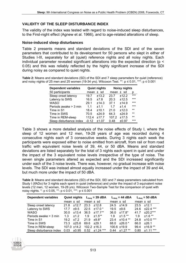
Sleep: 9th International Congress on Noise as a Public Health Problem (ICBEN) 2008, Foxwoods, CT
VALIDITY OF THE SLEEP DISTURBANCE INDEX The validity of the index was tested with regard to noise-induced sleep disturbances, to the First-night effect (Agnew et al. 1966), and to age-related alterations of sleep.
Noise-induced sleep disturbances Table 2 presents means and standard deviations of the SDI and of the seven parameters that contributed to its development for 50 persons who slept in either of Studies I-III, separately for all (quiet) reference nights and all noisy nights. Each individual parameter revealed significant alterations into the expected direction (p < 0.05) and this was reliably reflected by the highly significant increase of the SDI during noisy as compared to quiet nights.
Table 2: Means and standard deviations (SD) of the SDI and 7 sleep parameters for quiet (reference) and noisy nights of 25 men and 25 women (19-34 yrs). Wilcoxon Test. **: p ≤ 0.01, ***: p ≤ 0.001
Dependent variables 50 participants
Quiet nights mean ± sd
Noisy nights mean ± sd p
Sleep onset latency 19.7 ±13.2 23.7 ±12.2 *** Latency to SWS 16.5 ± 7.8 20.3 ±12.5 *** WASO 29.1 ±14.3 37.1 ±14.9 *** Periods awake > 3 min 1.1 ± 1.1 1.7 ± 1.4 *** Time in S1 18.4 ±10.1 21.0 ±12.0 ** Time in SWS 70.5 ±24.9 64.3 ±24.9 ** Time in REM-sleep 112.4 ±17.7 107.2 ±17.5 ** Sleep disturbance index -0.12 ±1.07 0.48 ±0.97 ***
Table 3 shows a more detailed analysis of the noise effects of Study I, where the sleep of 12 women and 12 men, 19-28 years of age was recorded during 4 consecutive nights each of 3 consecutive weeks. During 3 nights each week the participants were exposed either to noise emitted from aircraft, from rail or from road traffic with equivalent noise levels of 39, 44, or 50 dBA. Means and standard deviations are listed separately for the total of 3 nights each spent in quiet and under the impact of the 3 equivalent noise levels irrespective of the type of noise. The seven single parameters altered as expected and the SDI increased significantly under each of the 3 noise levels. There was, however, no gradual increase with noise levels. The SDI was instead almost equally increased under the impact of 39 and 44, but much more under the impact of 50 dBA.
Table 3: Means and standard deviations (SD) of the SDI, SEI and 7 sleep parameters calculated from Study I (IfADo) for 3 nights each spent in quiet (reference) and under the impact of 3 equivalent noise levels (12 men, 12 women, 19-28 yrs). Wilcoxon Two-Sample Test for the comparison of quiet with noisy nights. *: p ≤ 0.05, **: p ≤ 0.01, ***: p ≤ 0.001
Dependent variables Quiet nights mean ± sd
LAeq = 39 dBA mean ± sd
LAeq = 44 dBA mean ± sd
LAeq = 50 dBA mean ± sd
Sleep onset latency 21.8 ±12.7 23.3 ±12.8 24.5 ±14.9 23.5 ±12.1 Latency to SWS 17.7 ±9.5 22.5 ±17.0 * 19.5 ±9.6 24.6 ±22.4 *** WASO 30.0 ±13.4 36.5 ±17.1** 36.0 ±17.8 * 41.7 ±20.2 *** Periods awake > 3 min 1.3 ±1.2 1.9 ±1.5** 1.9 ±1.5 ** 1.9 ±1.6 ** Time in S1 19.2 ±7.2 21.9 ±9.8* 23.4 ±10.4 ** 24.8 ±10.0 *** Time in SWS 73.3 ±25.6 69.6 ±29.1 68.0 ±26.0 * 66.0 ±26.1 Time in REM-sleep 107.0 ±14.2 102.2 ±16.3 100.6 ±19.9 99.4 ±16.9 ** Sleep disturbance index 0.03 ±0.95 0.52 ±1.24 *** 0.44 ±1.27 ** 0.80 ±1.11 ***
513

Sleep: 9th International Congress on Noise as a Public Health Problem (ICBEN) 2008, Foxwoods, CT
First night effect Table 4 presents means and standard deviations calculated for the first nights in the laboratory of 62 persons (37 men, 25 women, 54 participants from studies I-III, 8 from study IV)) and for the first (quiet) reference night. Despite the same acoustic conditions each single parameter indicated, though not always significantly, a worse sleep quality in the first as compared to the first quiet nights. The SDI was slightly negative during quiet and significantly (p < 0.001) higher during the first night.
Table 4: Means and standard deviations (sd) of the SDI, SEI and 7 sleep parameters calculated from Studies I-IV (IfADo) for first (habituation) nights and quiet nights of 37 men and 25 women, 19 to 34 years of age. Wilcoxon Two-Sample Test for the comparison of first nights with the first following night quiet nights. *: p ≤ 0.05, **: p ≤ 0.01, ***: p ≤ 0.001
Dependent variables 62 participants
Quiet nights mean ± sd
1st night mean ± sd p
Sleep onset latency 22.5 ±20.3 33.3 ±24.7 *** Latency to SWS 16.2 ± 6.5 21.0 ±22.5 WASO 30.4 ±21.5 40.1 ±25.4 ** Periods awake > 3 min 1.0 ± 1.2 2.2 ± 2.1 *** Time in S1 19.4 ±11.9 20.3 ±12.1 Time in SWS 68.3 ±27.3 63.7 ±25.8 Time in REM-sleep 108.1 ±23.5 89.5 ±28.8 *** Sleep disturbance index -0.01 ±1.22 0.75 ±1.35 ***
Alteration with age Noise-induced alterations of sleep are non-specific. As similar alterations occur with increasing age (e.g. Griefahn 1985), the SDI was supposed to correlate significantly with age. To test this, the SDI was applied to Studies V-VII where the age of the participants varied in a wider range (18-68 yrs).
Table 5 shows the statistical parameters calculated for age and for the SDI together with the respective correlation coefficients that are highly significant for each of the 3 samples, though much lower for the field study. According to Figure 1 the SDI increased gradually with age.
Table 5: Means, standard deviations (sd), minima and maxima of the age and the sleep disturbance index values calculated for a quiet night ascertained in Studies V, VI, VII performed at DLR, ***: p ≤ 0.001
N Age SDI Corr. Study mean ± sd min - max mean ± sd min - max SDI:age
V 128 38 ± 13 19 - 65 0.47 ±1.22-2.1 -4.3 0.50 *** VI 65 39 ± 13 18 - 68 0.46 ±1.15-1.9 -3.6 0.56 ***
V+VI 193 38 ± 13 18 - 68 0.46 ±1.20-2.1 -4.3 0.52 *** VII 58 37 ± 12 19 - 61 0.53 ±1.04-1.5 -4.4 0.33 ***
514
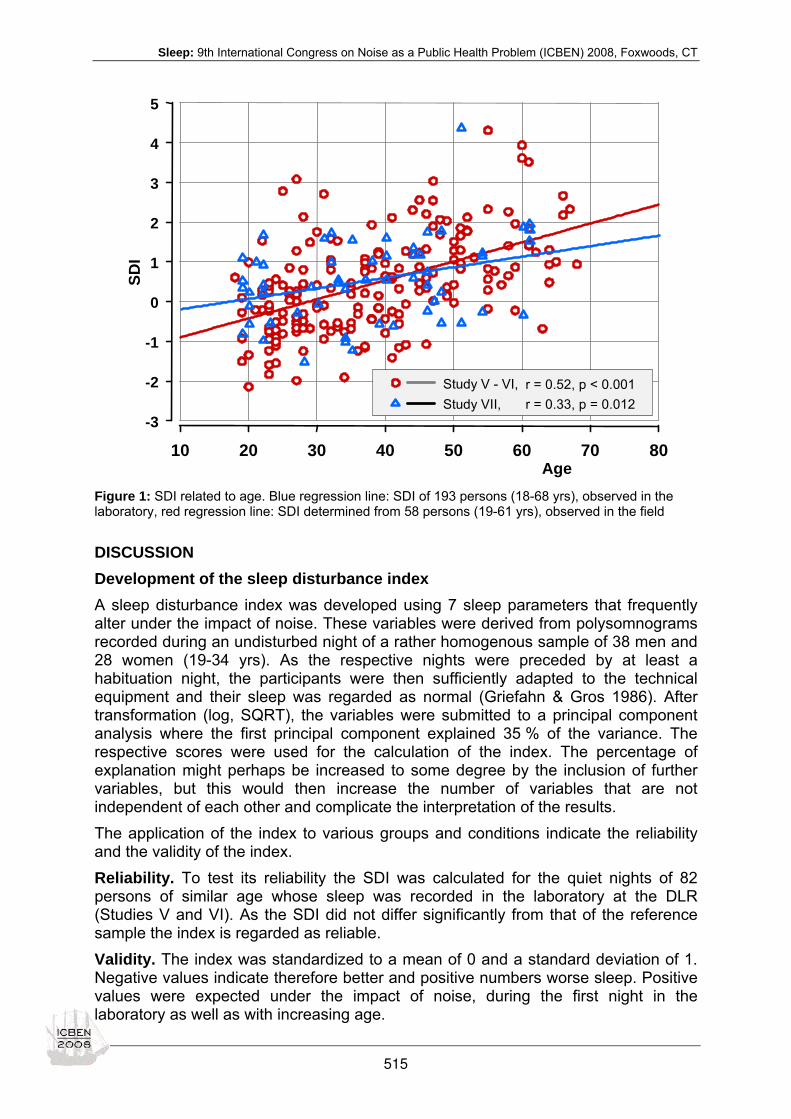
Sleep: 9th International Congress on Noise as a Public Health Problem (ICBEN) 2008, Foxwoods, CT
Age10 20 30 40 50 60 70 80
SDI
-3
-2
-1
0
1
2
3
4
5
Study V - VI,Study VII,
r = 0.52, p < 0.001r = 0.33, p = 0.012
Figure 1: SDI related to age. Blue regression line: SDI of 193 persons (18-68 yrs), observed in the laboratory, red regression line: SDI determined from 58 persons (19-61 yrs), observed in the field
DISCUSSION Development of the sleep disturbance index A sleep disturbance index was developed using 7 sleep parameters that frequently alter under the impact of noise. These variables were derived from polysomnograms recorded during an undisturbed night of a rather homogenous sample of 38 men and 28 women (19-34 yrs). As the respective nights were preceded by at least a habituation night, the participants were then sufficiently adapted to the technical equipment and their sleep was regarded as normal (Griefahn & Gros 1986). After transformation (log, SQRT), the variables were submitted to a principal component analysis where the first principal component explained 35 % of the variance. The respective scores were used for the calculation of the index. The percentage of explanation might perhaps be increased to some degree by the inclusion of further variables, but this would then increase the number of variables that are not independent of each other and complicate the interpretation of the results. The application of the index to various groups and conditions indicate the reliability and the validity of the index. Reliability. To test its reliability the SDI was calculated for the quiet nights of 82 persons of similar age whose sleep was recorded in the laboratory at the DLR (Studies V and VI). As the SDI did not differ significantly from that of the reference sample the index is regarded as reliable. Validity. The index was standardized to a mean of 0 and a standard deviation of 1. Negative values indicate therefore better and positive numbers worse sleep. Positive values were expected under the impact of noise, during the first night in the laboratory as well as with increasing age.
515

Sleep: 9th International Congress on Noise as a Public Health Problem (ICBEN) 2008, Foxwoods, CT
Effects of noise on sleep. Using the nights recorded in Studies I-III the SDI clearly revealed higher values during noisy as compared to quiet nights. One would have expected that sleep disturbances and thereby the SDI increase gradually with the equivalent noise level, a metric that indicates the total acoustic energy over a defined time period (here the bedtime, 23-7 h). But though the highest noise level evoked the strongest increase of the SDI (Table 3) the response did not differentiate between both the lower noise levels. This is supported by other studies that clearly disqualify the equivalent noise level as a reliable predictor of sleep disturbances (Basner et al. 2006b; Eberhardt 1987; Griefahn et al. 2006b; Öhrström & Rylander 1982). First-night-effect. The 'first-night-effect', initially described by Agnew et al. (1966) indicates a less restorative sleep during the first night in experimental studies not only in the laboratory but also in field studies (e.g. Griefahn & Gros 1986). Sleep in the first night is usually characterized by a prolonged time to fall asleep and to reach SWS, by a shorter time in SWS and in REM-sleep as well as by an increase of the time awake and of the number of sleep stage changes. This night was evaluated here to test the validity of the SDI which was significantly greater than during the quiet nights, thus not only confirming the 'first-night-effect' but also the validity of the SDI. Alterations with age. As the alterations of sleep evoked by noise are non-specific and rather diffuse, similar alterations were expected with increasing age (e.g. Griefahn 1985). Accordingly, the SDI correlated significantly (p < 0.01) with the age of the 193 participants observed in Studies V and VI. The correlation coefficient dropped, however, from r = 0.52 (p < 0.001) in the laboratory studies to a still significant coefficient of 0.33 (p = 0.012) in the field study with 58 residents near an airport (Study VII). Several facts might have contributed to the lower coefficient. First, the participants adhered to their usual bedtimes that varied not only between but also within one and the same person. Second, the acoustic load varied between the residents who lived at different distances to the runway and thereby under the impact of a different number of flyovers with different noise levels. Limitations. The sleep disturbance index developed here was designed to evaluate rather moderate sleep disturbances as caused by noise and other environmental influences. It reliably indicates worsening and improvement of sleep but cannot substitute the subtly differentiated evaluation required for clinical purposes. As it is true for many other indices, the condensation of different (weighted) variables to a single number, might mask possible causal relations, e.g. between physiological alterations and after-effects. Additional calculations performed with the data from Study I revealed for instance a better correlation of subjectively evaluated sleep quality (r = 0.29, p < 0.001) with the SDI than with most of the 7 included variables. The SDI was developed on the basis of nights with an exactly 8 h time in bed. The significant correlation between the SDI and age in the field study indicates its possible suitability for different bed times. The coefficient between SDI and age was, however, lower than calculated for the laboratory studies (0.33 vs 0.52). The SDI calculated for the 26 persons of the same age category as of the reference sample (19-34 yrs) was for the night from Saturday to Sunday 0.21 ± 0.87, which differed not significantly (p = 0.34) from the SDI of the reference sample (0 ± 1). The respective bed times varied, however, between 5.7 and 10.5 hours (8.56 ± 0.88 h). Application. However, specific alterations of only 2 or 3 sleep parameters are not likely for sleep disturbances evoked by noise, by other environmental influences or for the alterations that accompany increasing age. These disturbances are rather
516
Sleep: 9th International Congress on Noise as a Public Health Problem (ICBEN) 2008, Foxwoods, CT
moderate and diffuse, i.e. determined by complex alterations of several parameters that are well reflected by the SDI. Studies on the effects of environmental influences on sleep performed in different laboratories are often difficult to compare as most authors tend to focus their reports mainly on significant alterations, where it is often not clear, whether variables that are not mentioned are not affected or not even considered for evaluation. The application of the SDI would therefore facilitate the comparability of studies. Acknowledgement: Studies I-III were supported by the German Federal Ministry of Education and Research, Study IV by the Deutsche Forschungsgemeinschaft, Studies V-VII were financed within the DLR/HGF-project “Quiet Air Traffic” and the DLR-project “Quiet Air Traffic II”. The analysis was performed with financial support of the Virtual Institute 'Transportation Noise – Effects on Sleep and Performance' of the Helmholtz Gemeinschaft (HGF) under the grant-n° VH-VI-111.
References Agnew H W Jr, Webb W B, Williams R L (1966). The first night effect: An EEG study of sleep. Psychophysiology 2: 263-266.
Basner M, Samel A (2005). Effects of nocturnal aircraft noise on sleep structure. Somnologie 9: 84-95.
Basner M, Elmenhorst EM, Maaß H, Müller U, Quehl J, Vejvoda M, Samel A (2006a). Single and combined effects of air, road and rail traffic noise on sleep. In: Institute of Noise Control Engineering of the USA (ed): Proceedings of Internoise 2006, Dec 3-6, Honolulu, Hawaii, USA (10 pp.). CD-ROM.
Basner M, Isermann U, Samel A (2006b). Aircraft noise effects on sleep: Application of the results of a large polysomnographic field study. J Acoust Soc Am 119: 2772-2784.
Eberhardt JL (1987). The influence on sleep of noise and vibrations caused by road traffic. Akademisk avhandling. Lund: Bloms Boktrycheri AB.
Griefahn B (1985). Schlafverhalten und Geräusche. Feld- und Laboruntersuchungen über Straßenverkehr, EEG-Analyse, Literaturauswertung. Stuttgart: Enke.
Griefahn B (1986). Grenzwerte nächtlicher Belastbarkeit durch Straßengeräusche. Appl Acoust 19: 265-284.
Griefahn B, Gros E (1986). Noise and sleep at home, a field study on primary and after-effects. J Sound Vibr 105: 373-383.
Griefahn B, Marks A, Robens S (2006a). Noise emitted from road, rail and air traffic and their effects on sleep. J Sound Vibr 295: 129-140.
Griefahn B, Marks A, Basner A (2006b). Awakenings related to noises from various traffic modes. In: Institute of Noise Control Engineering of the USA (ed): Proceedings of Internoise 2006, Dec 3-6, Honolulu, Hawaii, USA (10 pp.). CD-ROM.
Öhrström E, Rylander R (1982). Sleep disturbance effects of traffic noise – a laboratory study on after effects. J Sound Vibr 84: 87-103.
Rechtschaffen A, Kales A (eds.) (1968). A manual of standardized terminology, techniques and scoring system for sleep stages of human subjects. Los Angeles, CA: BIS/BRI, UCLA.
517
Sleep: 9th International Congress on Noise as a Public Health Problem (ICBEN) 2008, Foxwoods, CT
Investigation of road traffic noise and annoyance in Beijing: A cross-sectional study of 4th Ring Road Hui-Juan Li, Wen-Bo Yu, Jing-Qiao Lu, Lin Zeng, Nan Li, Yi-Ming Zhao Research Center of Occupational Medicine and Research Center of Clinical Epidemiology, Peking University Third Hospital, Beijing, P. R. China
Address correspondence to: Hui-Juan Li, Research Center of Clinical Epidemiology Peking University Third Hospital, 49 North Huayuan Road, Haidian District, Beijing, 100083, P.R. China. Tel (Fax):+86-010-62017691 ext 2732, E-mail:[email protected]
ABSTRACT The aim of this study was to evaluate traffic noise level and noise annoyance in Bei-jing and the impact of the noise on quality of life of the residents. A cross-sectional study had been carried out in a 12-floor college dormitory near 4th Ring Road in Bei-jing. The north-side rooms of the building were noisy with windows facing the road. Both indoor and outdoor noise was measured. A sample of 1293 college students li-ving in the dormitory were questioned about their response of road traffic noise an-noyance using both a five-item verbal scale and a 0-11 numerical scale. The results showed that average outdoor day-night noise level (Ldn) in the noisy rooms was 79.2 dB(A), and 64.0 dB(A) in the quiet rooms. Nearly 39 % respondents living in the noisy rooms indicated that they were highly annoyed by traffic noise according to the response on the verbal scale, and 50 % respondents living in the noisy rooms were highly annoyed according to the numerical scale. Keywords: noise, road traffic, annoyance, Beijing
INTRODUCTION Traffic noise tends to be a dominant noise source in urban area. Most of today's re-search on noise control is focused on noise from transportation of urban traffic. An amount of literature was written on the subject of the various effects of traffic noise on people. Traffic noise interferes with basic activities such as sleeping, resting, studying and communicating, it can also cause heart disease, mental health problems and hearing damage (Stansfeld et al. 2000; Ohrström 2004; Lundqvist et al. 2000; Babisch et al. 2005). Noise annoyance is seen as the major effect of noise, which can include feelings of nuisance or disturbance (Passchier-Vermeer & Passchier 2000; Guski & Felscher-Suhr 1999). Existing evidence indicates that traffic noise is the most important source of environmental annoyance, such studies have found a positive correlation between annoyance and sound level (Ali 2003; Fidell 2003; Ising & Kruppa 2004; Michaud et al. 2005; Miedema 2004; Ouis 2002; Yano & Ma 2004). The simplest and most wide-spread scheme in use is the presentation of a self-reported scale of annoyance (Fields 1984; Fields et al. 2001). With the exception of Japan, all of these regions were Euro-American. In 2004 Yano and Ma have translated the standardized 5-point verbal noise scale into Chinese (Yano & Ma 2004). There is growing recognition of the importance of environmental noise pollution in Beijing, capital of China. Heavy traffic flows have lead to high noise pollution levels in these areas. The maximum Leq reaches 79.5 dB(A) with an average Leq of 75.6 dBA at the monitoring locations surrounding main roads (Li et al. 2002; Li & Tao 2004). Some studies reported that about 16 % of the people (1 million) live in the areas sur-
518

Sleep: 9th International Congress on Noise as a Public Health Problem (ICBEN) 2008, Foxwoods, CT
rounding main roads in Beijing (Wang et al. 2000; Wang & Liu 2004). So far, very few studies have been carried out to investigate and assess noise annoyance in Beijing. A cross-sectional study was carried out in a 12-floor college dormitory nearby north 4th Ring Road in Beijing to assess traffic noise level and noise annoyance degree. Both indoor and outdoor noise of this building was measured, and two standardized questions were used for noise annoyance survey in accordance with the recommen-dations provided by ICBEN and Yano’s study.
METHODS The 12-floor dormitory was 20 meters away from the north 4th Ring Road. There were 50 rooms on each floor. The north-side rooms of the building were noisy with windows facing the road, and the south-side rooms were relatively quiet (Figure 1). We selected two rooms from each floor (one room on the noisy side, the other on the quiet side), with a total of 24 rooms. The selected noisy room number was N42 and the quiet room was N43 in each floor (N=floor number), made sure all of the rooms were in the same vertical section (Figure 1). If the pre-selected room was absent, the room next it on the same side was measured. For example, if room 842 was absent when we conducted the measurement, then room 844 or 846 next to it would be measured randomly.
Figure 1: Sketch map of noise assessment on one floor of the dormitory
Indoor and outdoor noise was measured in the 24 rooms from 22:30 to next day 21:00 using 24 noise dosimeters (AWA5610E, Hang Zhou Ai Hua Instruments Co. Ltd., Hangzhou, China) in two days. In the first day, both indoor and outdoor noise of 12 rooms on the 1, 3, 5, 7, 9, 11 floors were measured, and in the second day those of the 2, 4, 6, 8, 10, 12 floors were measured. The dosimeters meet the requirements of IEC61672-2002 standard for class 2 integrating sound level meter, Chinese Na-tional Standards (GB) of sound level meter GB3785-1983 and personal noise dose meter standards GB/T15952-1995.
519

Sleep: 9th International Congress on Noise as a Public Health Problem (ICBEN) 2008, Foxwoods, CT
Equivalent A-weighted sound pressure level (LAeq) was computed with a sample in-terval of 4 seconds. Day-night noise levels (Ldn) have been calculated from the for-mula:
Ldn= where Ld and Ln represent the daytime and night-time equivalent noise level, respec-tively. The daytime period was from 06:30 to 21:00 and the nighttime period was from 22:30 to 06:30. Dosimeters measuring outdoor noise were located in the windowsills of these rooms. Make sure the microphones pointed to the outside and windows were open all the day. Dosimeters for indoor noise were located on the top of wardrobes (2 meters height) inside these rooms with microphones exceeding the wardrobes 3 to 5 cm and pointing to the center of the room (Figure 1). The survey was performed all by volunteer distributors who were members of the en-vironmental protection association in this university. Questionnaires were distributed to each room of the dormitory. The questionnaires were completed by the respon-dents in their dorms and were collected one hour later. Out of 1560 questionnaires distributed, 1463 were filled, giving the response rate 93.8 %. 170 questionnaires were excluded in which both of the noise annoyance questions were not filled. The final sample consisted of 1293 respondents, 720 in the quiet rooms, 573 in the noisy rooms. The questionnaire comprised demographic characters (age, sex, period of resi-dence), noise annoyance degree and noise sensitivity score. In accordance with the recommendations provided by ISO/TS-15666 the following two questions were asked about road traffic noise annoyance. One question is: Thinking about the last 12 months or so, when you are at home, how much dose noise from road traffic bother, disturb, or annoy you? The subjects were asked to re-sponse with a 5-point verbal scale. We used the standardized noise annoyance scales in Chinese14 in which not at all was translated to yi dian ye bu, slightly to hao xiang you dian, moderately to bi jiao, very to xiang dang, extremely to te bie. The second question is: Thinking about the last 12 months or so, what number from zero to ten best shows how much you are bothered, disturbed or annoyed by road traffic noise ? The answer is a 0-10 numerical scale that zero is equivalent to “not at all bothered” (yi dian ye bu fan in Chinese) and ten is equivalent to “extremely both-ered”(te bie fan in Chinese). Noise sensitivity is an intervening variable between noise exposure and annoyance (Belojevic et al. 2003; van Kamp et al. 2004; Job 1999). In our study, we used a Swedish version of the Weinstein Noise Sensitivity Scale to assess noise sensitivity, which consists of 16 items with a 7-point scale to response (Vastfjall 2002). Higher scores indicate higher sensitivity to noise. ANOVA was used to compare noise from different positions, followed by Fisher’s pro-tected least significant difference (LSD) if significant. Student’s t-test was used to compare age, years of residence between noisy and quiet rooms. χ2 test was used to compare gender. Correlation between 5-point verbal scale and 0-10 numerical scale was computed using Pearson correlation coefficients. Multiple logistic regres-sion analysis was used to investigate the association of possible factors for noise an-noyance. All analyses were performed using SPSS version 13.0 for Windows.
]10*810*5.145.22
1lg[10 10/)10(10/ ++ nd LL
520

Sleep: 9th International Congress on Noise as a Public Health Problem (ICBEN) 2008, Foxwoods, CT
RESULTS Both indoor and outdoor noises were measured on every floor. The results of the average noise levels are shown in Table 1. The average Ldn of outdoor noise is 79.2 dB(A) in the noisy rooms, which is 15 dB(A) higher than in the quiet rooms. No significant differences of indoor noise Ldn were observed between the noisy and quiet rooms. Noise in the night was about 2-6 dB(A) lower than in the day of each position. The outdoor noise in the night was very high in the noisy rooms, which was 72.6 dB(A). We also computed equivalent noise levels from 2:00 to 5:00 in the mor-ning when every resident was sleeping. The result showed that the average indoor noise of the noisy rooms was 4.8 dB(A) higher than of the quiet rooms in the wee hours. In short, the results supported that road traffic noise highly affected outdoor noise environments in the noisy rooms. Indoor noise during sleep time in the noisy rooms was also influenced.
Table 1: Noise from different positions in the 12-floor dormitory (unit: dB)
Positions N
(floors)
Daytime
LAeq,14.5h
Nighttime
LAeq,8h
Day-night level
Ldn
wee hours
LAeq,3h(2:00-5:00)
outdoor 12 74.4 ± 3.5a 72.6 ± 3.0a 79.2 ± 3.1a 71.1 ± 3.0a Noisy
indoor 10 59.1 ± 3.2b 53.4 ± 4.0b 61.5 ± 3.1b 45.8 ± 4.6b
outdoor 12 61.0 ± 2.4b 56.3 ± 3.1b 64.0 ± 2.4b 52.4 ± 1.6c Quiet
indoor 10 59.8 ± 2.5b 54.7 ± 5.3b 63.4 ± 2.4b 41.0 ± 0.5d
P-value < 0.01 < 0.01 < 0.01 < 0.01
Results marked with different letters are significantly different for each index, LSD test, P<0.05. Indoor noise of two noisy rooms and two quiet rooms were not measured because of residents’ disagree-ment.
All of the 1293 respondents were college school students living in the 12-floor dormi-tory. The time of residence varied from 1 month to 6 years. The average age was 20.9 years old, ranging from 16 to 30. About 75.9 % of the respondents were female and 24.1% were male. The comparison of general characteristics between noisy and quiet rooms are shown in Table 2. There were no significant differences in gender and years of residence between the two sides. Respondents from the noisy rooms showed more sensitive to noise (P=0.002) and they were a little younger (P=0.045).
521

Sleep: 9th International Congress on Noise as a Public Health Problem (ICBEN) 2008, Foxwoods, CT
Table 2: General characteristics
Position General characteristics
quiet Noisy P-value
No. of residents 720 573
Age (mean ± SD, y) 21.0 ± 1.7 20.8 ± 1.6 0.045
Men (%) 24.7 22.0 0.238
Years of residence (mean ± SD) 1.9 ± 1.4 1.8 ± 1.4 0.228
Noise sensitivity score (mean ± SD) 69.7 ± 13.9 72.1 ± 13.4 0.002
The correlation between the verbal scale and 0-10 numerical scale was high (Pearson correlation co-efficient=0.923, P<0.01). In this survey, significant differences were found on both noise annoyance scales between respondents in the noise and quiet rooms (Mann-Whitney’s U-test, P<0.001). Re-spondents in the noisy rooms were clearly more disturbed by traffic noise than those in the quiet rooms.
Those who answered “very” or “extremely” on the verbal scale or score >6 on the 0-10 numerical scale were considered “highly annoyed”. (On the 0-10 numerical scale: 0+1=not at all; 2+3=slightly; 4+5+6=moderately; 7+8=very and 9+10=extremely). Nearly 39 % of the respondents in the noisy rooms indicated that they were highly annoyed by traffic noise according to the response on the verbal scale, but only 6 % in the quiet rooms (Figure 2). Percent of highly annoyed responses was even higher on the 0-10 numerical scale, which was 50% in the noisy rooms and 9% in the quiet rooms (Figure 2).
Figure 2: The distribution of road traffic noise annoyance on the verbal and numerical scale among respondents in the noisy and quiet rooms of the dormitory
Two models were used to evaluate the factors which might affect the annoyance le-vels of the subjects with both of the annoyance scales. After adjusting for years of residence, living floor and gender, the multivariate logistic regression analysis dem-onstrated that residence in noisy rooms was identified as an important predictor for the occurrence of highly annoyed response (OR=12.42, P<0.05, in model 1;
522

Sleep: 9th International Congress on Noise as a Public Health Problem (ICBEN) 2008, Foxwoods, CT
OR=12.95, P<0.05, in model 2; Table 3). Residents with higher noise sensitivity showed more highly annoyed response (OR=1.07,P<0.05, in model 1&2). There were no differences between the two models except the years of residence was sig-nificant in model 2 (0-10 numerical scale) (OR=0.88,P<0.05).
Table 3: Multivariate logistic regression analyses showing ORs (95 % CIs) of highly annoyed response
Model 1 (verbal scale) Model 2 (0-10 numerical scale) Variables
OR (95 % CI) P-value OR (95 % CI) P-value
Position (noisy vs quiet)* 12.42 (8.40-18.37) < 0.001 12.95 (9.17-18.28) < 0.001
Noise sensitivity score 1.07 (1.06-1.09) < 0.001 1.07 (1.06-1.08) < 0.001
Years of residence 0.94 (0.83-1.06) 0.325 0.88 (0.78-0.99) 0.028
Floor 0.95 (0.89-1.02) 0.137 0.96 (0.90-1.03) 0.234
Gender (female vs male) 1.34 (0.78-2.31) 0.291 1.08 (0.65-1.79) 0.769
* Noisy: Outdoor Ldn=79.2 dB, Quiet: Outdoor Ldn=64.0 dB
DISCUSSION In this study, high level of road traffic noise was observed near the 4th Ring Road in Beijing, which was in accordance with previous study (Li et al. 2002; Li & Tao 2004). The average noise level during night time (22:30-nextday 06:30) was 72.6 dB(A), which exceeded the national standard of 45 dB(A) (GB3096-93) by 27.6 dB(A) (EPA China 1993). Big trucks were allowed to come into the urban area only from 23:00-06:00 in Beijing, which was the main reason of noise pollution during nighttime. Indoor noise exposure assessment was conducted in this study, which could reflect the real noise environment where people live. But there were no significant differ-ences of indoor noise between the noisy and quiet rooms except for the sleeping time (Figure 2, Table 1). Indoor noise was also influenced by people’s conversation and other activities. So we computed indoor noise levels from 2:00 to 5:00 a.m., the result showed that the average indoor noise of the noisy rooms was 4.8 dB(A) higher than of quiet rooms in the wee hours. Indoor noise measurement during the sleeping time might be ideal to evaluate how much traffic noise affected people’s life. The out-door noise was 10 dB(A) larger than indoor noise for the quiet rooms from 2:00-5:00 a.m. The outdoor noise might be affected by traffic noise diffraction from 4th Ring Road, for the quiet rooms only faced a small footpath in the college and there was no noise source during this 3-hour period. In our study we used both a five-item verbal scale and a 0-10 numerical scale. The correlation between the two scales was high (Pearson correlation coefficient=0.923, P<0.01), and the percents of highly annoyance were different which were 39 % on the verbal scale and 50 % on the numerical scale in the noisy rooms. ISO 1996-1:2003 gives guidance on predicting the potential annoyance response of a commu-nity to long-term exposure from various types of environmental noises. To compare which scale was more believable, we used the ISO standard for assessment proce-
523
Sleep: 9th International Congress on Noise as a Public Health Problem (ICBEN) 2008, Foxwoods, CT
dures for environmental noise the percent highly annoyed is obtained from the rating level (RL) using equation:
% highly annoyed=100/[1+exp(10.4-0.132*RL)]
The relationship for road traffic noise is obtained when RL equals Ldn .The number of daylight hours is 15, defined as hours from 07:00-22:00 (ISO 2003; Michaud et al. 2005). Outdoor noise Ldn in the noisy rooms in the present study was 79.4 dB(A), the calculated percent of highly annoyed was 51.36 % according to the equation. It indi-cates that the result of the numerical scale is closer to 51.36 % and maybe more comfortable for the evaluation of road traffic noise annoyance. The logistic regression analysis demonstrated that residents in noisy rooms and those with higher noise sensitivity showed more highly annoyed response in model 1 & 2. Years of residence was only significant in model 2 (0-10 numerical scale) (OR=0.88, P<0.05) which means that subjects living longer time in this residence showed less annoyance. It might because the 0-10 numerical scale was more accu-rate than the 5-point verbal scale. In our study the average year of residence was less than 2 years, so we need to evaluate more groups of people with different ages to testify. To our knowledge, the present study is the first to evaluate level of annoyance to traf-fic noise in Beijing. We found that 50 % respondents living in the noisy rooms were highly annoyed by road traffic noise (using numerical annoyance scale). Authorities in Beijing have increased aware of the effects of road traffic noise in urban areas, soundproof windows have been built in several districts along 4th Ring Road. Reduc-ing traffic volume is another method to solve noise pollution problem (Ohrström 2004). In recent years, the government in Beijing keeps on developing urban public traffic and begins to restrict the increase of private cars. In order to greet the Beijing 2008 Olympic Game, Beijing will still shoulder heavy responsibilities to improve acoustical environment.
Our study has one limitation that we only focused on a certain group of college stu-dents in Beijing, and the noise observation targets the north 4th Ring road. To form a whole picture of people's noise annoyance in Beijing, we need to select different groups of people in different spots of the city, and according to the noise map in Bei-jing we can establish the relationship between road traffic noise level and percentage of respondents that feel “highly annoyed”.
REFERENCES Ali S (2004). Investigation of the dose–response relationship for road traffic noise in Assiut, Egypt. Appl Acoust 65: 1113-1120.
Babisch W, Beule B, Schust M, Kersten N, Ising H (2005). Traffic noise and risk of myocardial infarction. Epidemiology 16: 33-40.
Belojevic G, Jakovljevic B, Slepcevic V (2003). Noise and mental performance: personality attributes and noise sensitivity. Noise & Health 6 (21): 77-89.
EPA, China (1993). GB3096-93: noise standard in urban environment. Beijing: Publishing House of China Environmental Sciences.
Fidell S (2003). The Schultz curve 25 years later: a research perspective. J Acoust Soc Am 114: 3007-3015.
Fields JM (1984). The effect of numbers of noise events on people's reactions to noise: An analysis of existing survey data. J Acoust Soc Am 75: 447-467.
524

Sleep: 9th International Congress on Noise as a Public Health Problem (ICBEN) 2008, Foxwoods, CT
Fields JM, De Jong RG, Gjestland T, Flindell IH, Job RFS, Kurra S, Lercher P, Vallet M, Yano T, Guski R, Felscher-Suhr U, Schümer R (2001). Standardized general-purpose noise reaction questions for community noise surveys: research and a recommendation. J Sound Vibr 242: 641-679.
Guski R, Felscher-Suhr U (1999). The concept of noise annoyance:how international experts see it. J Sound Vibr 223: 513-527.
Ising H, Kruppa B (2004). Health effects caused by noise: evidence in the literature from the past 25 years. Noise & Health 6 (22): 5-13.
ISO, International Organization for Standardization (2003). Acoustics-Description, measurement and assessment of envi-ronmental noise, Part 1: Basic quantities and assessment procedures. ISO 1996-1: 2003 (E).
Job RF (1999). Noise sensitivity as a factor influencing human reaction to noise. Noise & Health 1 (3): 57-68.
Li BG, Tao S (2004). Influence of expanding ring roads on traffic noise in Beijing City. Appl Acoust 65: 244-249.
Li BG, Tao S, Dawson RW (2002). Evaluation and analysis of traffic noise from the main urban roads in Beijing. Appl Acoust 63: 1137-1142.
Lundqvist P, Holmberg K, Landstrom U (2000). Annoyance and effects on work from environmental noise at school. Noise & Health 2 (8): 39-46.
Michaud DS, Keith SE, McMurchy D (2005). Noise annoyance in Canada. Noise & Health 7 (27): 39-47.
Miedema HM (2004). Relationship between exposure to multiple noise sources and noise annoyance. J Acoust Soc Am 116: 949-957.
Ohrström E (2004). Longitudinal surveys on effects of changes in road traffic noise-annoyance, activity disturbances, and psycho-social well-being. J Acoust Soc Am 115: 719-729.
Ouis D (2002). Annoyance caused by exposure to road traffic noise: an update. Noise & Health 4 (15): 69-79.
Passchier-Vermeer W, Passchier WF (2000). Noise exposure and public health. Environ Health Perspect 108 (Suppl 1): 123-131.
Stansfeld S, Haines M, Brown B (2000). Noise and health in the urban environment. Rev Environ Health 15: 43-82.
van Kamp I, Job RF, Hatfield J, Haines M, Stellato RK, Stansfeld SA (2004). The role of noise sensitivity in the noise-response relation: a comparison of three international airport studies. J Acoust Soc Am 116: 3471-3479.
Vastfjall D (2002). Influences of current mood and noise sensitivity on judgments of noise annoyance. J Psychol 136: 357-370.
Wang Y, Liu JL (2004). Urban area acoustic environment reviews and prospects of Beijing. Noise Vibr Contr 5: 23-25.
Wang Y, Song FX, Xu H. (2000). Investigations and countermeasures for pollution on the traffic noise Ii Beijing area. Noise Vibr Contr 3: 31-35.
Yano T, Ma H (2004). Standardized noise annoyance scales in Chinese, Korean and Vietnamese. J Sound Vibr 277: 583-588.
Yoshida T, Osada Y, Kawaguchi T, Hoshiyama Y, Yoshida K, Yamamoto K (1997). Effects of road traffic noise on inhabitants of Tokyo. J Sound Vibr 205: 517-522.
525

Sleep: 9th International Congress on Noise as a Public Health Problem (ICBEN) 2008, Foxwoods, CT
How many people will be awakened by nighttime aircraft noise? Nicholas P. Miller1*, Robin C. Gardner2 1 Harris Miller Miller & Hanson Inc., 77 S. Bedford Street, Burlington, MA 01720
2 Harris Miller Miller & Hanson Inc., 8880 Cal Center Drive, Suite 430, Sacramento, CA 95826
*corresponding author: e-mail: [email protected]
INTRODUCTION Increasing demand for air travel has prompted plans by several airports around the U.S. to increase their capacity, primarily by adding new runways or by extending existing ones. These capacity-increase plans usually raise public concerns about in-creased noise. One common concern is increased sleep disturbance. In response to this public concern, some of the associated environmental documents attempt to ad-dress sleep disturbance. The relevant environmental regulations do not prescribe specific criteria, metrics, or computation methods for determining sleep disturbance. Now, however, a recently published method, Anderson & Miller (2007), based on analysis of sleep awakening data has been incorporated in part in a working group final draft ANSI standard, ANSI (R2005). The application uses a dose-response rela-tionship and computes the number of people or percent of a population likely to be awakened at least once during a night of aircraft noise events (ANE).
METHOD BASED ON PROBABILITY OF AWAKENING The method determines the number of people or percent of the population likely to be awakened at least once from a full night of ANE. Most sleep disturbance data are reduced to a relationship of the form of a dose-response curve similar to that shown in Figure 1, from Marks et al. (2008).
Such relationships cannot be applied directly to determine awakenings that may re-sult from a full night of ANE. However, such a dose-response relationship can be used to determine first the probability that a single event will produce an awakening. This probability may then be converted into a probability of NOT being awakened (1 minus the probability of being awakened). Next, the probability of NOT being awa-kened all night by multiple events is computed as the joint probability of not being awakened by any of the night time events. Finally, the probability of being awakened
Figure 1: Representative dose-response curve derived from polysomnogram re-cords
526

Sleep: 9th International Congress on Noise as a Public Health Problem (ICBEN) 2008, Foxwoods, CT
at least once by any of the night time events is one minus the probability of not being awakened at all. Eq. (1) expresses this approach,
( )
( )
, ,
1
1
1
1
1 1 ,
awake once multiple sleep thru multipleN
sleep thru,single aaN
awake,single aa
p p
p
p
=
=
= −
= −
= − −
∏
∏
Eq. (1)
where: a = index across all N noise events during the night, and
awake,singlep is the probability of being awakened by the nth single event.
Hence, if Figure 2 gives the probability of awakening an average person by a single aircraft, then application of this method for multiple aircraft (all with the same Sound Exposure Level) gives Figure 3 which shows how the probability of awakening for this average person is affected by multiple aircraft during the night.
Single Aircraft: Dose-response Curve for Average Person
Cha
nce
of a
wak
enin
g, %
1 aircraft 40 50 60 70 80 90 100 110Indoor Sound Exposure Level, dBA
0
10
20
30
40
50
60
70
80
90
100
100
90
80
70
60
50
40
30
20
10
0
Cha
nce
of n
ot a
wak
enin
g (s
leep
ing
thro
ugh)
, %
Multiple Aircraft: Dose-response Curves for Average Person
Cha
nce
of a
wak
enin
g du
ring
the
nigh
t, %
50 aircraft 20 aircraft 10 aircraft 5 aircraft 2 aircraft 1 aircraft40 50 60 70 80 90 100 110
Indoor Sound Exposure Level, dBA
0
10
20
30
40
50
60
70
80
90
100
100
90
80
70
60
50
40
30
20
10
0
Cha
nce
of s
leep
ing
thro
ugh
the
nigh
t, %
Figure 2: Dose-response curve for probability of awakening from one aircraft, average person
Figure 3: Dose-response curves for multiple aircraft, average per-son
527

Sleep: 9th International Congress on Noise as a Public Health Problem (ICBEN) 2008, Foxwoods, CT
REFINEMENT OF DOSE-RESPONSE CURVE By applying logistic regression to raw awakening data, more variables may be in-cluded in the dose-response curves. Data for these regressions were obtained in people’s homes by Dr. Sanford Fidell and his co-workers, have been previously re-ported in the acoustical literature, Fidell et al. (1994, 1995a, b, 2000), and were pro-vided to HMMH courtesy Larry Finegold and Robert Lee. Data were from studies in communities around Denver International, Los Angeles International and Castle Air Force Base. Data were of the form pictured in Figure 4. In this figure, each vertical column repre-sents the results for one subject; subject numbers are given on the horizontal axis. For each subject, the indoor SEL of each event, its time of occurrence, and whether or not it resulted in a behavioral awakening were contained in the data set. Hence regressions could include not only SEL, but also time of night and subject.
Figure 4: Aircraft noise events experienced by subjects at Denver International
The analyses of these three data sets provided results of the form:
11 e
awake,single Zp −=+
Eq. (2)
where
0 L AE T retire S sensitivityZ L T Sβ β β β= + + + Eq. (3)
and
0, , , Constants Indoor SEL
Time since retiring, minutes Sensitivity for population segment
L T S
AE
retire
sensitivity
LTS
β β β β =
==
=
528
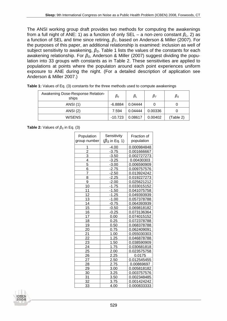
Sleep: 9th International Congress on Noise as a Public Health Problem (ICBEN) 2008, Foxwoods, CT
The ANSI working group draft provides two methods for computing the awakenings from a full night of ANE: 1) as a function of only SEL – a non-zero constant βL, 2) as a function of SEL and time since retiring, βT, based on Anderson & Miller (2007). For the purposes of this paper, an additional relationship is examined: inclusion as well of subject sensitivity to awakening, βS. Table 1 lists the values of the constants for each awakening relationship. For βS, Anderson & Miller (2007) suggest dividing the popu-lation into 33 groups with constants as in Table 2. These sensitivities are applied to populations at points where the populaton around each point experiences uniform exposure to ANE during the night. (For a detailed description of application see Anderson & Miller 2007.)
Table 1: Values of Eq. (3) constants for the three methods used to compute awakenings
Awakening Dose-Response Relation-ships β0 βL βT βS
ANSI (1) -6.8884 0.04444 0 0
ANSI (2) 7.594 0.04444 0.00336 0
W/SENS -10.723 0.08617 0.00402 (Table 2)
Table 2: Values of βS in Eq. (3)
Population group number
Sensitivity (βS in Eq. 1)
Fraction of population
1 -4.00 0.0009848482 -3.75 0.0016666673 -3.50 0.0027272734 -3.25 0.004303035 -3.00 0.0065909096 -2.75 0.0097575767 -2.50 0.0139242428 -2.25 0.0192272739 -2.00 0.025621212
10 -1.75 0.03301515211 -1.50 0.04107575812 -1.25 0.04939393913 -1.00 0.05737878814 -0.75 0.06439393915 -0.50 0.06981818216 -0.25 0.07313636417 0.00 0.07401515218 0.25 0.07237878819 0.50 0.06837878820 0.75 0.06240909121 1.00 0.05503030322 1.25 0.04687878823 1.50 0.03859090924 1.75 0.03068181825 2.00 0.02357575826 2.25 0.017527 2.50 0.01254545528 2.75 0.0086969729 3.00 0.00581818230 3.25 0.00375757631 3.50 0.00234848532 3.75 0.00142424233 4.00 0.000833333
529

Sleep: 9th International Congress on Noise as a Public Health Problem (ICBEN) 2008, Foxwoods, CT
APPLICATION TO REALISTIC SCENARIOS By using the probability of awakening method and the three different dose-response relationships defined by Eq. (2) and Eq. (3), the percent of people awakened can be computed for different realistic scenarios. For this paper, the awakenings are com-puted at a single point with assumed distributions of ANE. The assumptions include a realistic distribution of SEL values, three different numbers of nighttime aircraft noise events (ANE), and three different outdoor-to-indoor noise reductions. Figure 5 gives the assumed distribution of aircraft produced outdoor SEL. This distri-bution was measured by a permanent noise monitor located about 3½ statute miles from the airport (at the approximate location of the 65 dB Ldn level for that airport).
Distribution of Aircraft Produced SEL(~ 3 ½ miles from airport)
0%
5%
10%
15%
20%
25%
30%
35%
74 76 78 80 82 84 86 88 90 92 94 96
Outdoor SEL
Perc
ent o
f Ope
ratio
ns
Figure 5: Assumed distribution of outdoor SEL values
Two different distributions of nighttime ANE are assumed, Table 3. For purposes of this comparison, these events are grouped into thirds of the night. These distributions are intended to represent what might occur when increases in operations are not matched by increases in airport capacity. If distribution 1 represents an existing con-dition, then distribution 2 and distribution 3 might both be the result of a significant increase in operations at the airport, with no increase in capacity – operations arrive later at night (distribution #2) or leave earlier in the morning (distribution 3).
Table 3: Assumed distributions of nighttime ANE
ANE by Hour Starting: Dist #1 Dist #2 Dist #3
10pm 11pm
Midnight 20 35 20
1am 2am 3am
5 5 5
4am 5am 6am
20 20 35
Total 45 60 60
530

Sleep: 9th International Congress on Noise as a Public Health Problem (ICBEN) 2008, Foxwoods, CT
Awakenings are computed assuming the three different outdoor-to-indoor noise re-ductions listed in Table 4.
Table 4: Assumed Distributions of Nighttime ANE
Outdoor to Indoor Noise Reduction 15 dB 23 dB 30 dB
(Window Open) (Window Closed) (Sound Insulated)
RESULTS Figures 6, 7 and 8 give the percent of the population awakened at least once for all scenarios. The percents across the three different relationships demonstrate some expected trends. All relationships show decreasing awakenings with increasing out-door-to-indoor sound reductions, and all show increased awakenings with increased operations, except that, as expected, ANSI (1) shows no difference between distribu-tion 2 and 3, because they both have the same number of operations, but at different times of night.
Percent Awakened at Least OnceDistribution 1
54%
42%
32%
66%
54%
42%
62%
47%
34%
0%10%20%30%40%50%60%70%80%90%
100%
15 dB 23 dB 30 dBOutdoor-to-Indoor Reduction
Perc
ent A
wak
ened
ANSI (1)ANSI (2)W/SENS
Percent Awakened at Least OnceDistribution 2
64%
51%
40%
72%
59%
47%
65%
50%
36%
0%10%20%30%40%50%60%70%80%90%
100%
15 dB 23 dB 30 dBOutdoor-to-Indoor Reduction
Perc
ent A
wak
ened ANSI (1)
ANSI (2)W/SENS
Figure 6: Results for different relationships, distribution 1
Figure 7: Results for different relationships, distribution 2
531

Sleep: 9th International Congress on Noise as a Public Health Problem (ICBEN) 2008, Foxwoods, CT
Percent Awakened at Least OnceDistribution 3
64%
51%
40%
81%
69%
57%
71%
57%
43%
0%10%20%30%40%50%60%70%80%90%
100%
15 dB 23 dB 30 dBOutdoor-to-Indoor Reduction
Perc
ent A
wak
ened
ANSI (1)ANSI (2)W/SENS
Interestingly, when sensitivity is included, the benefits in reduced awakenings pro-duced by sound insulation are greater than those shown by either of the other two methods, Figure 9. Heuristically this result makes sense because sound insulation lowers the distribution of ANE and for ANSI (1) and ANSI (2) this is equivalent to moving down a single dose-response curve, whereas for W/SENS, this lowering means some people (those less sensitive) will drop out of the computations – their probability of awakening becomes relatively smaller or approaches zero.
Reduction in AwakeningsIncreased Sound Insulation 23 dB to 30 dB
23% 21% 21%21% 20% 18%
28% 27% 24%
0%10%20%30%40%50%60%70%80%90%
100%
Distribution 1 Distribution 2 Distribution 3Nighttime Operations Distribution
Perc
ent R
educ
tion
ANSI (1)ANSI (2)W/SENS
CONCLUSIONS The working group draft final ANSI standard provides a pragmatic general method for estimating the awakening effects of night time noise events. By applying this method to the two dose-response relationships described in the standard and the one of Anderson & Miller (2007), this paper demonstrates the relative differences that can be expected when using these relationships. All three relationships produce roughly similar results. However, the relationship - ANSI (1) - that uses only the indoor SEL as a variable will show no time-of-night ef-
Figure 8: Results for different relationships, distribution 3
Figure 9: Reductions in awakenings pro-duced by sound insu-lation as computed by the three methods
532
Sleep: 9th International Congress on Noise as a Public Health Problem (ICBEN) 2008, Foxwoods, CT
fect – an effect that was strongly indicated (p < 0.01) in the regression analysis of Anderson & Miller (2007), and has been observed by others, Brink et al. (2006). The author judges this phenomenon important in assessing the effects likely to occur as air travel increases and night time operations become more likely. Without the inclusion of population sensitivity, though not widely researched, it ap-pears over estimation of awakening may occur. Awakening responses are very com-plex, see for example Passchier-Vermeer et al. (2002), and if this additional factor of sensitivity can be confirmed and included in predictive methods, better informed de-cisions might be possible regarding effects of night time noise on communities, sound insulation benefits, night time operations scheduling, night time runway use, etc. In any event, any of these methods will provide more information about the likely effects of night time ANE than do cumulative measures such as Day-Night Average Sound Level, which have shown no useful predictive association with sleep distur-bance, Fidell et al. (1995a).
REFERENCES Anderson GS, Miller NP (2007). Alternative analysis of sleep-awakening data. Noise Contr Eng J 55 (2), March-April.
ANSI S12.9-2000 (R2005). Revised, BSR/ASA S12.9-200X/Part 6.
Brink M, Wirth K, Schierz C (2006). Effects of early morning aircraft overflights on sleep and implications for policy making. EuroNoise 2006, Tampere, Finland.
Fidell S, Pearsons K, Howe R, Tabachnick B, Silvati L, Barber D (1994). Noise-induced sleep disturbance in residential settings. Report AL/OE-TR- 1994-0131, Occupational & Environmental Health Division, Armstrong Laboratory, Wright Pat-terson Air Force Base, Ohio.
Fidell S, Pearsons K, Tabachnick B, Howe R, Silvati L, Barber D (1995a). Field study of noise-induced sleep disturbance. J Acoust Soc Am 98: 1025-1033.
Fidell S, Pearsons K, Howe R, Tabachnick B, Sneddon M (1995b). “Noise-induced sleep disturbance in residences near two civil airports,” NASA Contractor Report 198252, Contract NAS1-200101.
Fidell S, Pearsons K, Howe R, Tabachnick B (2000). Effects on sleep disturbance of changes in aircraft noise near three airports. J Acoust Soc Am 107: 2535-2547.
Marks A, Griefahn B, Basner M (2008). Event-related awakenings caused by nocturnal transportation noise. Noise Contr Eng J 56: 52-62.
Passchier-Vermeer W, Vos H, Steenbekkers JHM, van der Ploeg FD, Groothuis-Oudshoorn K (2002). Sleep disturbance and aircraft noise exposure: Exposure-effect relationships. Report TNO 2002.027, Division Public Health, The Netherlands.
533

Sleep: 9th International Congress on Noise as a Public Health Problem (ICBEN) 2008, Foxwoods, CT
Field research on the assessment of community impacts from large weapons noise Edward T. Nykaza1*, George A. Luz2, Larry L. Pater1
1 Engineer Research and Development Center, Construction Engineering Research Laboratory, 2902 Newmark Drive, Champaign, IL 61822
2 Luz Social and Environmental Associates, 4910 Crowson Ave, Baltimore, MD 21212
* corresponding author: e-mail: [email protected]
INTRODUCTION Large weapons noise, which is often referred to as blast noise, is the noise produced by detonation of explosives and projectiles and by artillery and armor muzzle blast. These noise events are of short duration, typically a fraction of a second to a few seconds. The spectrum is rather broad, with acoustical energy typically concentrated at frequencies between 1 and 100 Hz. High-energy impulsive noise from military weapons can be very loud at distances of many tens of kilometers. Ground-to-ground propagation of blast noise is strongly influenced by atmospheric temperature and wind structure. Experiments have shown variation of more than 50 dB (Schomer et al. 1978) in received noise levels, all factors held constant except for weather. A data range of 50 dB implies a standard deviation in received noise level on the rough or-der of 8 dB (assuming the data lie predominantly within 3 standard deviations about the mean) due to changes in atmospheric meteorological parameters that influence sound propagation. Conventional noise impact assessment procedures are based on the “equal energy hypothesis”, i.e. that annoyance response depends on the total sound exposure dose averaged over 1 year, without regard to details of how that sound energy is distrib-uted in time or on the magnitude of individual noise events. There is no difference between 100,000 noise events spread over a year or a small number of high-energy events all occurring in 1 day. An example of this problem is given in Figure 1, which shows peak and average annual contours for 100,000 small events occurring in one year and 20 large events occurring sporadically throughout the year. The equal en-ergy principle is an efficient annoyance predictor for traffic noise, where each day’s exposure consists of hundreds of sound events that are of similar magnitude from day to day. With so many events, the brain fails to retain a memory of individual events (Björkman 1991) and only remembers the impression of the general din. For blast noise, the sounds are intermittent, with a few noisy days typically interspersed within a larger number of quiet days. The noise level is highly variable because of the large range of sound energy emission from various weapons and as previously stated, can vary over a range of 50 dB due to variation in meteorological conditions. Experience strongly indicates (Pater 1976) that noise complaints correlate quite strongly with blast noise level; though it is not known to what extent complaints lodged by individuals represent general community annoyance. It is hypothesized that dynamic annoyance response to noise events may depend strongly on the in-stantaneous noise level, and may have bearing on long-term community annoyance response. Luz and others (Luz et al. 1994) found that 5-point-scale annoyance rat-ings to individual blasts by known complainants correlated quite strongly with blast level.
534
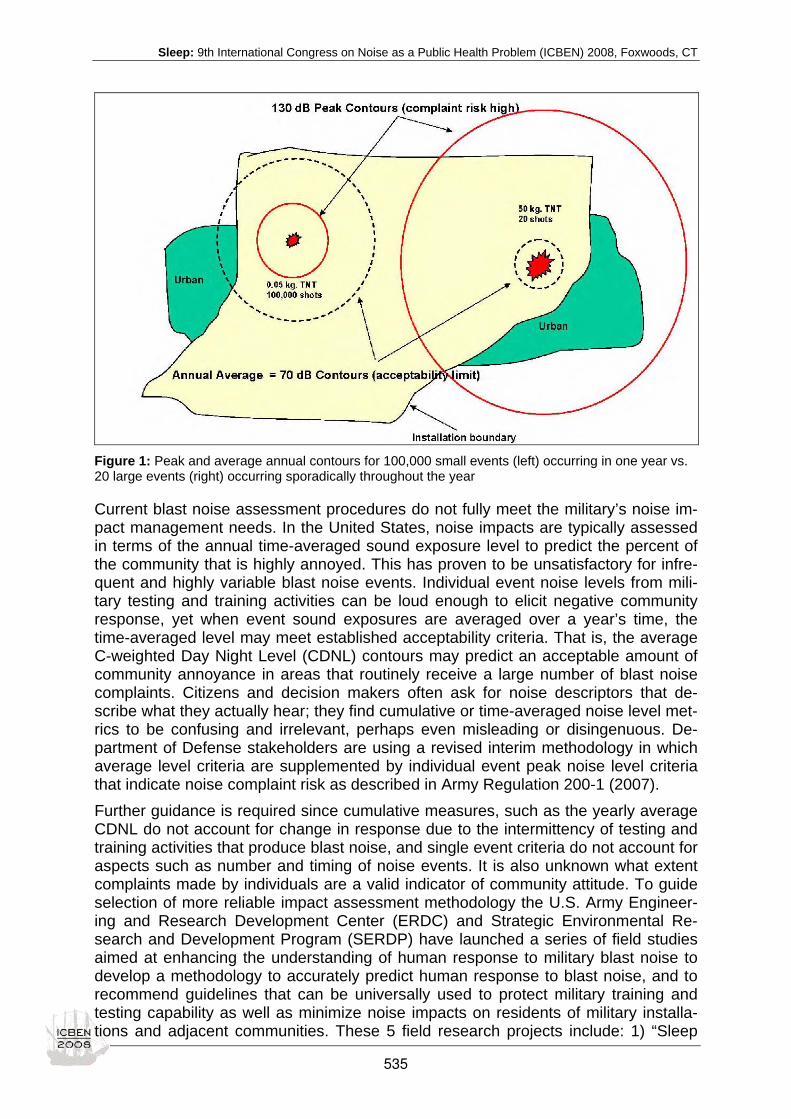
Sleep: 9th International Congress on Noise as a Public Health Problem (ICBEN) 2008, Foxwoods, CT
Figure 1: Peak and average annual contours for 100,000 small events (left) occurring in one year vs. 20 large events (right) occurring sporadically throughout the year
Current blast noise assessment procedures do not fully meet the military’s noise im-pact management needs. In the United States, noise impacts are typically assessed in terms of the annual time-averaged sound exposure level to predict the percent of the community that is highly annoyed. This has proven to be unsatisfactory for infre-quent and highly variable blast noise events. Individual event noise levels from mili-tary testing and training activities can be loud enough to elicit negative community response, yet when event sound exposures are averaged over a year’s time, the time-averaged level may meet established acceptability criteria. That is, the average C-weighted Day Night Level (CDNL) contours may predict an acceptable amount of community annoyance in areas that routinely receive a large number of blast noise complaints. Citizens and decision makers often ask for noise descriptors that de-scribe what they actually hear; they find cumulative or time-averaged noise level met-rics to be confusing and irrelevant, perhaps even misleading or disingenuous. De-partment of Defense stakeholders are using a revised interim methodology in which average level criteria are supplemented by individual event peak noise level criteria that indicate noise complaint risk as described in Army Regulation 200-1 (2007). Further guidance is required since cumulative measures, such as the yearly average CDNL do not account for change in response due to the intermittency of testing and training activities that produce blast noise, and single event criteria do not account for aspects such as number and timing of noise events. It is also unknown what extent complaints made by individuals are a valid indicator of community attitude. To guide selection of more reliable impact assessment methodology the U.S. Army Engineer-ing and Research Development Center (ERDC) and Strategic Environmental Re-search and Development Program (SERDP) have launched a series of field studies aimed at enhancing the understanding of human response to military blast noise to develop a methodology to accurately predict human response to blast noise, and to recommend guidelines that can be universally used to protect military training and testing capability as well as minimize noise impacts on residents of military installa-tions and adjacent communities. These 5 field research projects include: 1) “Sleep
535

Sleep: 9th International Congress on Noise as a Public Health Problem (ICBEN) 2008, Foxwoods, CT
Disturbance” from blast noise to determine preferred times to conduct nighttime train-ing, 2) “Complaint Risk” from blast noise to recommend improved guidelines to better manage testing and training firing schedules, 3) “In-Situ” diary studies with individual residents who experience blast noise to measure near-real-time in-home annoyance responses, 4) “General Survey” studies with community members who experience blast noise to measure community response and how it changes with time and noise environment, and 5) “Correlation of Complaints and Annoyance” to determine the interrelationship between blast noise level, complaints, and annoyance.
METHODS Study 1. Sleep Disturbance Training during the hours of darkness is a necessity for the military and often a com-mon cause for complaints as seen in Europe and North America. For example, Ry-lander and Lundquist (1996) found that of the 399 Swedish citizens surveyed living in the vicinity of eight ranges, half chose the evening and about a third chose the night as the time of day when heavy weapons noise was most annoying. About 10 % stated that shooting made it difficult to fall asleep at night and about the same per-centage stated that shooting awakened them. In the United States evidence of the problem of nighttime training noise is in the numerous restrictions imposed at most testing and training installations. Although some information about sleep disturbance from heavy weapons blasts has been available from a laboratory study with tape-recorded 120 mm tank gun blasts by Griefahn (1989), there had never been a field study of sleep disturbance among people routinely exposed to the sounds of tank gunnery training. This is likely due to the difficulty in finding an installation willing to sponsor such a field study and because periods of intense night firing at any one range are sporadic. In order to better understand the impact of blast noise on residents living near U.S. military installations a field study was conducted by Engineering Research and De-velopment Center in 2004. To ensure the highest possibility of success in the field study, it was preceded by a laboratory study of actimeter reliability using reproduced tank gun blasts which approached (but did not meet) the full spectrum of a real tank gun blast (Luz et al. 2008). It was important to have the highest possible reliability in the measurement instrumentation, which was limited to a wrist-worn actimeter with a button to signal awakening. Following this successful equipment “shakedown” and “dry run,” the field test was conducted among 33 subjects living between 1.8 and 8.9 km from 120 mm tank gun firing points and exposed to blasts during their sleeping hours in the range of 102 to 124 dB linear peak sound pressure level (SPL). This pa-per has been submitted for publication (Nykaza et al.) and further details can be found in an ERDC technical report (Nykaza et al. 2006). There were two important findings to come out of this research. It was found that residents were less likely to awaken from blast noise disturbances during the middle of the night (between midnight and 0200) and that the threshold of awakening during the shoulder hours, which was between 2100 and 2300 and between 0200 and 0400 hours, was approximately 115 dB linear peak SPL. The first finding was significant because it contradicted the current guidelines that all nighttime firing be conducted up until midnight and ceased thereafter. The second finding showed agreement with Pater’s complaint risk criteria (Pater 1976) which states that there is a moderate risk of complaints when received blast noise events fall in the range of 115 to 130 dB lin-ear peak SPL.
536

Sleep: 9th International Congress on Noise as a Public Health Problem (ICBEN) 2008, Foxwoods, CT
Study 2. Complaint Risk The complaint risk study, which is ongoing, has two purposes. The first is to improve the performance of a real time blast noise monitoring system which has been operat-ing for over 15 years at a testing installation. The second is to improve the ability to predict complaints from the noise measurement data generated by this system. Improving the blast noise monitoring system had to be completed before the second purpose could begin. Three technical improvements were made. 1) A time drift in the noise monitors and server was corrected. Each noise monitor was found to have a unique time drift, which was a consequence of the clock time drift on the server that updated the clocks on the noise monitors each night. The original program on the server often malfunctioned and did not download or update each clock on every monitor each night. This problem was solved by installing a new server, writing a new downloading software program, and synchronizing to the server to the National Insti-tute of Standards and Technology (NIST) time server. 2) Algorithms were developed to determine the likely source location and shot time of the improperly time-stamped data (Nykaza & Donaldson 2007) and simpler algorithms were implemented to de-termine the likely source and location of data gathered after the implementation of the new server and download program. These algorithms facilitated identification of the noise sources that most likely elicited a given complaint among many firings and false triggers that might occur on a given day. 3) An additional 33 noise monitors were added to original 18 monitors used in the 2001 study in order to cover the 64 by 64 km study area. For each complaint received by the installation, the sound level at the complainant’s home was estimated by interpolating or extrapolating on the basis of geometrical spreading from the received levels of noise monitors located within a 10 km radius of the complainant. The importance of the technical improvements was underscored by success in linking complaints with measured levels. In comparison to an earlier study conducted at the same installation in which only 35 % of complaints could be linked to measured levels (Luz 2001), 90 % were linked in the current effort. Further details on the preliminary results of this study can be found in a paper accepted for publica-tion (Nykaza et al. 2008a). Thus far, there are three statistically-significant findings: 1) first time complainants were linked to a higher level than repeat complainants as seen in Table 1, 2) com-plainants who were complaining about a single loud noise event were linked to a higher level than complainants who complained about multiple events as seen in Ta-ble 2, and 3) complainants who complained about noise events that occurred during the day were linked to a higher level than complainants during the evening as seen in Table 3. As previously mentioned, this study is on going and the results presented here are based upon a mere 40 complaints. At the time of the writing of this paper there are an additional 114 complainants yet to be analyzed which should provide the statistical strength of subsequent analyses. This study also finds agreement with the Pater (1976) complaint risk criteria and it is expected that future analyses will be able to define the importance and interaction of the number of events, level of events, and timing of events.
537

Sleep: 9th International Congress on Noise as a Public Health Problem (ICBEN) 2008, Foxwoods, CT
Table 1: Comparison of first complainants verses repeat complainants with Mann-Whitney nonpara-metric test
Sample Size Median Un-
weighted Peak Level (dB)
First Time Com-plainants 26 120
Repeat Com-plainants 10 107
Table 2: Comparison of single-shot complaints verses multi-shot complaints with Mann-Whitney non-parametric test
Sample Size Median Un-
weighted Peak Level (dB)
Single Shot Complaints 8 125
Multiple Shot Complaints 18 117.5
Table 3: Comparisons of the time of day complaints were filed with Mann-Whitney nonparametric test
Sample Size Median Un-
weighted Peak Level (dB)
Complaints During Working
Hours (7 AM to 5 PM)
20 121
Complaints During Evening
Hours (5 PM to 10PM)
6 111.5
Study 3. In-Situ An upcoming In-Situ study, with an estimated start date of 2009, will examine how people respond to individual blast events in near real-time. A cross-sectional sample of residents who live near military installations will be selected to participate. Micro-phones and accelerometers will be set up outside and inside residents’ homes to document the stimulus (i.e. blast noise, vibration, rattle) and personal digital assis-tants (PDAs) will be used to record the residents’ response. Based on experience from a pilot study involving four persons routinely exposed to blast noise in their homes (Luz et al.1994) and International Commission on Biological Effects of Noise recommendations (Fields et al. 2001), subjects will be asked to rate the annoyance of each noticed event on a five-point scale (not annoying to extremely annoying). The study will be conducted over a 9-month period at two installations, involving approxi-mately 25 subjects at each site to capture a statistically significant data set and to sample the range of variation in received noise level due to seasonal weather changes. The strength of the In-Situ study is detailed data regarding the variation of subject response to variable stimulus levels (dose response functionality). This study will in-corporate research procedures commonly used in diary studies to mitigate the extent
538

Sleep: 9th International Congress on Noise as a Public Health Problem (ICBEN) 2008, Foxwoods, CT
to which the increased awareness and attention to blast events may skew their re-sponses. Digitized measurements of the time history of the blasts taken outdoors in the vicinity of the subject’s home will allow for comparisons between various predictors of blast noise annoyance suggested by different national regulations and/or researchers, such as C-weighted sound exposure level (SEL), A-weighted SEL, A-weighted SEL adjusted for the difference between C and A (Vos 2001), C-weighted SEL adjusted for the difference between C and A (Buchta 1996), peak level, or various combina-tions of weighted 1/3 octave bands. Measurement outdoors will ensure that all signifi-cant blasts will be registered, including the ones which the subjects do not notice. To further understand each subject’s detectability threshold, outdoor-to-indoor house transfer functions will be obtained for each residence. In addition to the transfer func-tion, vibration measurements of each blast will be taken from a wall, window and cor-ner of the side of the house facing the range. Based on the 1994 pilot study, it is an-ticipated that peak vibration levels from these three measurements will be highly cor-related. Statistical analyses (e.g. multiple correlation) will be used to determine whether a combination of sound and vibration measurements improves the prediction of annoyance beyond the prediction based on sound alone.
Study 4. General Survey An upcoming General Survey study (estimated start date of 2009) will be unique in that the variation with time of the noise environment will be accurately known throughout the community by co-locating this protocol with the In-Situ study. Com-munity response will be measured at 3 intervals during the study via social survey. By contrast, previous blast noise surveys conducted in the U.S. correlated a single value of the annual time-averaged noise level with a one-time annoyance survey. These studies took place in the 1980’s at Fort Lewis, Washington (Schomer 1985) and at Fort Bragg, North Carolina (Schomer 1982). Lessons learned from other surveys conducted in the vicinity of heavy weapons ranges, such as the Grafenwoehr Train-ing Area in Germany (Buchta et al. 1986) and Holsworthy Artillery Range in Austrlia (Bullen et al. 1991) have been incorporated into the survey questions along with the ICBEN recommendations. The General Survey utilizes a questionnaire that will be administered several times in coordination with the In-Situ Protocol, but will sample a different set of subjects in the population each time. Professional interviewers will conduct in-person interviews at randomly selected households in the study areas. A cross-sectional representative sample (different households each time) will gauge the level of response among community residents at each point in time, and a panel sample of households (the same households surveyed each time) will illuminate changes in household response over time. The survey will be conducted at approximately 3-month intervals with the representative cross-sectional samples of households, and at approximately 6-month intervals with the panel sample of households. Unlike similar past studies in this category, exposure will be extrapolated and interpolated from measurements made along a grid and not projected by computer models. With the opportunity afforded by direct measurement, it should be possible to track the effect of short term changes in average exposure in relation to changes in annoyance.
539

Sleep: 9th International Congress on Noise as a Public Health Problem (ICBEN) 2008, Foxwoods, CT
Study 5. Correlation of Complaints and Annoyance A study of the correlation between the annoyance of individual complainants and general community annoyance is scheduled to begin in the summer of 2008 at the same installation as the complaint risk study above. One of the primary goals of this research is to determine if individual complainants are representative of the general community annoyance. It is possible that unnecessary testing and training restrictions have been implemented because of the complaints of a few noise-sensitive com-plainants. On the other hand, complaints may be a useful indicator of the general community response. The relationship between complaints and community response will be tested by surveying residents in the vicinity of recent noise complaints within a week of a complaint. The survey questions designed in the General Survey study will be used for uniformity between tests, and the surveying area will include a random sample of 10 residents living within the vicinity of complainants. Of the five studies, this is the riskiest, since the research team has no control over the pattern of firing, the density of houses around the complainant, the number of people who will be home at the same time as the complainant or the willingness of potential interviewees to be interviewed.
CONCLUSIONS The objective of the research outline above is to collectively enhance the understand-ing of human response to blast noise, and to recommend guidelines that can be uni-versally applied and used to protect military training and testing capability as well as minimize noise impacts on residents of military installations and adjacent communi-ties. The multi-study approach is already yielding practical results for the management of noise from heavy weapons training. These include: Low likelihood of awakening when the outdoor level of blasts is below 115 dB peak SPL, less likelihood of awak-ening to blasts at any level between the hours of midnight and 0200, and importance of predicting complaints on the basis of sound level, number of events, and timing of events rather than on sound level alone. As these studies continue, information on whether some other measure besides the C-weighted SEL and the CDNL can yield better predictions of impact on the commu-nity is anticipated. Further information on the In-Situ, General Survey, and Complaint Annoyance Correlation studies can be found in two Pater et al. papers (2007).
ACKNOWLEDGEMENTS We acknowledge the Strategic Environmental Research and Development Program (SERDP) and U.S. Army ERDC-CERL for funding support for this research.
REFERENCES Army Regulation 200-1 (2007). Environmental protection and enhancement. Washington, DC: Department of the Army.
Björkman M (1991). Community noise annoyance: importance of noise levels and the number of noise events. J Sound Vibr 151: 497-503.
Buchta E (1996). Annoyance caused by shooting noise – determination of the penalty for various weapon calibers. In: Pro-ceedings of Internoise 96, Liverpool, England (pp 2495-2500).
Buchta E, Loosen W, Buchta C, Rohland P (1986). Lärmbelästung in der Umgebung von Truppenübungsplätzen [Noise annoyance in the vicinity of troop training areas]. Report 105 01 314/02 Berlin: German Federal Environmental Protection Agency.
Bullen R, Hede A, Job R (1991) Community reaction to noise from an artillery range. Noise Contr Engineering J 37: 115-128.
540

Sleep: 9th International Congress on Noise as a Public Health Problem (ICBEN) 2008, Foxwoods, CT
Fields J, De Jong R, Gjestland T, Flindell I, Job R, Kurra S, Lercher P, Vallet M, Yano T, Guski R, Felscher-Suhr U, Schumer R (2001). Standardized general-purpose noise reaction questions for community noise survey: research and a recommenda-tion. J Sound Vibr 242: 641-679.
Griefahn B (1989). Cardiac responses caused by shots of tanks during sleep. J Sound Vibr 128: 109-119.
Luz G (2001). Using 115 dB peak as a predictor of complaints about heavy weapons noise. Paper given at International Military Noise Conference, US Army Center for Health Promotion and Preventive Medicine, Aberdeen Proving Ground, MD, April 24-25, 2001 (presentation available at http://chppm-www.apgea.army.mil/imnc/environmental/Env_Presentations.html).
Luz G, Lewis N, Russell W (1994). Homeowner judgments of the annoyance of individual heavy weapons blasts. Paper given at 128th Meeting of the Acoustical Society of America, Austin, TX.
Luz G, Nykaza E, Stewart C, Pater L (2008). Use of actimeters to define the threshold of awakening from the sound of large guns. Noise Contr Engineering J 56: 1-7.
Nykaza E, Donaldson N (2007). Use of correlation between received impulsive noise event times. Paper NC 07-205, Pro-ceedings of Noise-Con 2007, Reno, Nevada. CD published by Institute of Noise Control Engineering.
Nykaza E, Pater L, Melton R (2006). Sleep impacts of nighttime training noise from large weapons on residents living near a military installation. Technical report ERDC/CERL TR-06-21. Champaign, IL: Army Construction Engineering Research Laboratory (available at www.cecer.army.mil).
Nykaza E, Pater L, Luz G (2008a). Improved procedure for correlating blast noise events with complaint logs at U.S. Army Installations. Noise Contr Engineering J (in press).
Nykaza E, Pater L, Melton R, Luz G (2008b). Awakening to blast noise among residents living near a tank gunnery range. J Acoust Soc Am (submitted).
Pater L (1976). Noise abatement program for explosive operations at NSWC/DL. Paper presented at the 17th Explosives Safety Seminar of the DoD Explosives Safety Board, Denver, CO.
Pater L, Nykaza E, Hodgdon K, Atchley A, Baumgartner R, Rathbun P, Luz G (2007a) Assessing human response to infre-quent blast events. Paper NC 07-305, Proceedings of Noise-Con 2007, Reno, Nevada. CD published by Institute of Noise Control Engineering.
Pater L, Nykaza E, Hodgdon K, Atchley A, Baumgartner R, Rathbun P, Luz G (2007b). An investigation of community atti-tudes toward blast noise. Technical report ERDC/CERL SR-07-24. Champaign, IL: Army Construction Engineering Research Laboratory (available at www.cecer.army.mil).
Rylander P, Lundquist B (1996). Annoyance caused by noise from heavy weapon shooting ranges. J Sound Vibr 192: 199-202.
Schomer P (1982) A model to describe community response to impulse noise. Noise Contr Engineering J 18: 5-15.
Schomer P (1985). Assessment of community response to impulsive noise. J Acoust Soc Am 77: 520-535.
Schomer P, Goff R, Little L (1978). Statistics of amplitude and spectrum of blasts propagated in the atmosphere. J Acoust Soc Am 63: 1431-1443.
US EPA (1974). Levels of environmental noise requisite to protect public health and welfare with an adequate margin of safety. Washington, DC: U.S. Government Printing Office.
Vos J (2001). On the annoyance caused by impulse sounds produced by small, medium-large, and large firearms. J Acoust Soc Am 109: 244-253.
541

Sleep: 9th International Congress on Noise as a Public Health Problem (ICBEN) 2008, Foxwoods, CT
Noise and vibration generation for laboratory studies on sleep disturbance Mikael Ögren1*, Evy Öhrström2, Tomas Jerson3 1 The Swedish National Road and Transport Research Institute, Box 8077, SE-40278, Gothenburg,
Sweden, [email protected]
2 The Sahlgrenska Academy at the University of Gothenburg , Department of Occupational and Envi-ronmental Medicine, SE 405 30 Gothenburg, Sweden, [email protected]
3 WSP Environmental Acoustics, Box 13033, SE 415 26 Gothenburg, Sweden, [email protected]
* corresponding author: e-mail: [email protected]
INTRODUCTION The research project TVANE is aimed at studying the effects of noise and building vibrations from railway traffic, and is sponsored by the Swedish railway infrastructure manager Banverket. The project includes many studies performed both in the field with questionnaires and noise and vibration measurements, and in the laboratory. This paper describes the design of a low cost vibrating bed used in laboratory sleep-ing experiments, and also the sound and vibration signals that the subjects were ex-posed to. The results of the experiments are under evaluation, but details on the out-come of a previous similar study without vibrations are presented in a parallel paper in these proceedings, Öhrström et al. (2008). There are several technical possibilities for vibrating beds in sleep experiment set-ups. In Arnberg et al. (1990) hydraulic actuators were used (often called vibrating tables), but these are typically rather large and noisy systems, so the bed must be suspended a certain height above the floor and some form of sound insulation intro-duced. Preferably the whole laboratory room should be built on top of the vibrating table itself. Another approach is to use electrodynamical actuators, where the main concern is that it is difficult and expensive to build actuators with high power output and low distortion levels at low frequencies. The vibrations being studied here correspond to building vibrations caused by a heavy train passage, where the vibrations are transmitted through relatively soft soil such as clay. For Swedish conditions this tends to cause vibrations in the 5 – 10 Hz range, and the predominant vibration direction is typically vertical for low buildings and horizontal perpendicular to the tracks for buildings with more than one floor, see for example (Hannelius 1978; Bahrekazemi 2004; Hassan 2006). For stiffer ground types the transmitted vibrations are at higher frequencies (> 25 Hz), and may cause complex interactions between vibrations and low frequency sound, but this is not the focus of the TVANE project. A typical example of this situation is a railroad tunnel in an urban area that generates vibrations that are then radiated as low frequency sound inside the nearby buildings.
METHOD In the experiment setup discussed here three identical rooms are equipped with loudspeakers and vibrators for noise and bed vibration generation. The subjects sleep in the rooms, and a computer located in an adjacent control room generates audio and vibration signals during the night. The sleep quality of the subjects is evaluated using questionnaires. As can be seen in the photo in Figure 1, the bed-
542

Sleep: 9th International Congress on Noise as a Public Health Problem (ICBEN) 2008, Foxwoods, CT
rooms have been decorated to resemble a normal room, and the speakers, cables and vibration actuators have been hidden as much as possible. Before the start of the study presented here the rooms were already equipped with a sound system and had been used for other sleep experiments, but the vibration system was added dur-ing this study.
Figure 1: Photo of the bedrom interior with the bed and some furniture
Generating the noise Each bedroom is equipped with 22 roof mounted panels, each with four ten inch speakers, for generating the low frequency part of the sound field in the room. The high frequencies are handled by two small speaker cabinets in the corners, with a crossover frequency between the two systems of 125 Hz. The reverberation time of the room is around 0.3 s for high frequencies, which corre-sponds to a fairly damped room, but below 200 Hz standing wave patterns are pre-sent in the sound field. Therefore a 1/3 octave band equalizer is used to adjust the sound levels and spectrum in the receiver positions close to the bed, for more details see Ögren et al. (2007). During the night the sound system plays train passages that are based on recorded real passages of different train types. The recording position was around 30 m from the nearest track and the maximum train speeds at the location were about 130 km/h for passenger trains and 90 km/h for freight trains. All recordings were filtered to cor-respond to indoor levels with a window towards the railway slightly open (about 30 mm open). Apart from control nights when no audio was played, two sets of sounds were used, one with the maximum (FAST) A-weighted sound pressure level (LAFmax) of 54 dB and one with the same traffic but with the overall audio volume lowered to 48 dB. The traffic pattern was modeled to fit Västra Stambanan, the main railroad between Stockholm and Göteborg in Sweden, and the total number of passages during the sleep period between 23:00 and 07:00 were 44 (25 freight, 9 high speed and 10 commuter trains). The equivalent A-weighted level (LAEq) and maximum levels are given in 5 minute intervals during the night in Figure 2. The 1/3 octave band spectrum of the total exposures is given in Figure 3. Since the background sound level is as
543

Sleep: 9th International Congress on Noise as a Public Health Problem (ICBEN) 2008, Foxwoods, CT
low as 13 dB(A) in the rooms at night an artificial background was added that raised the background to 25 dB(A).
Figure 2: Equivalent and maximum A-weighted sound pressure level in 5 min intervals
Figure 3: Equivalent level in 1/3 octave bands of the total exposure from 23:00 to 07:00
Generating bed vibrations For the experiments presented here electrodynamical actuators were selected, since the vibrating beds where to be introduced into the already existing laboratory built for sound exposure, with limited space available for hydraulics or sound insulation under the beds. Another important aspect was that electrodynamical actuators can be con-trolled from the already present sound system, simply treated like audio signals to speakers, whereas a hydraulic system would have needed a new control system al-together.
544

Sleep: 9th International Congress on Noise as a Public Health Problem (ICBEN) 2008, Foxwoods, CT
Professional electrodynamical actuators are expensive, but recently several variants have become available for the home theater/stereo market. The difference in price can be as much as a factor of 20. They are typically also a lot smaller than the corre-sponding professional variants. Therefore it was decided early on to try out those cheaper vibrators in this project. One of the major drawbacks with using cheaper actuators turned out to be distortion; they do not give a perfect sine wave output when the driving signal is a sine wave. If they are mounted stiffly into the bed frame they generate lots of audible frequencies even if the driving signal contains no energy above 10 Hz. This interferes with the well controlled sound exposure situation of the experiment and is unacceptable. Therefore we designed a mechanical resonant filter, which makes the mechanical system receive more power at frequencies close to the resonance and filters out higher frequencies. The principle is illustrated in Figure 4.
Figure 4: Sketch of the mechanical system with the actuator directly coupled to the bed (left) and indi-rectly via the resonant mechanical filter (right)
The mechanical filter together with the introduction of sound insulation around the actuator itself reduced the sound level at a position 5 cm above the pillow to 29 dB(A) when the shaker was driven at the maximum amplitude. This was deemed accept-able since the noise from the train masks the vibrations, but it is still possible to hear the low frequency part, especially if lying on the side with the ear pressed against the pillow. As mentioned earlier the typical frequency of building vibrations due to railway traffic is in the region of 5 – 10 Hz, but the vibrators had trouble reproducing frequencies lower than 10 Hz without reaching the excursion limit (maximum movement of the coil). Therefore the frequency 10 Hz was chosen for the driving signal. Real vibra-tions are of course more complex than a simple steady state sine wave, therefore a modulation was introduced. By looking at the many time signals for freight trains at speeds around 80 – 90 km/h published in Hannelius (1978), a modulation at 0.2 Hz was introduced together with an extra deep minimum once each 15 s, see Figure 5. This signal was then ramped up when a freight train audio signal was played and re-peated periodically until the audio signal was turned off, see Figure 6.
545
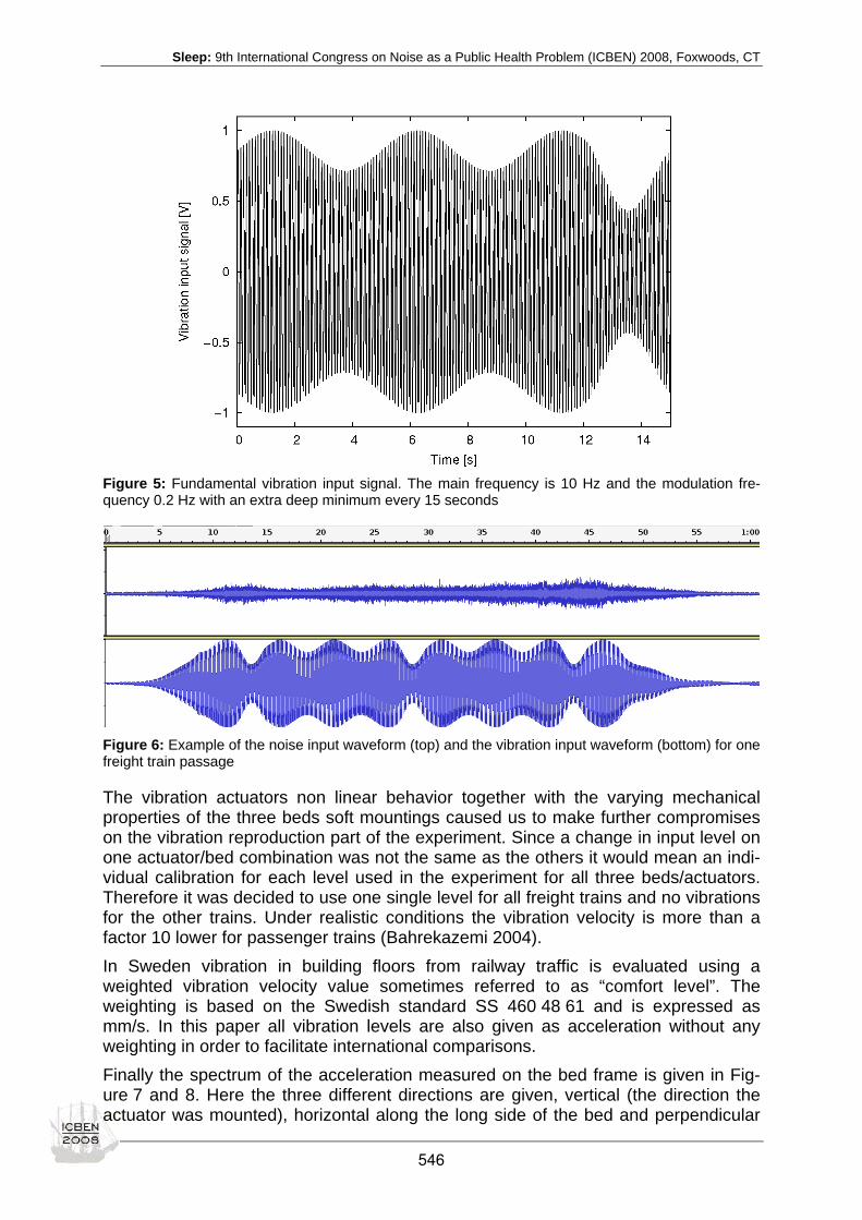
Sleep: 9th International Congress on Noise as a Public Health Problem (ICBEN) 2008, Foxwoods, CT
Figure 5: Fundamental vibration input signal. The main frequency is 10 Hz and the modulation fre-quency 0.2 Hz with an extra deep minimum every 15 seconds
Figure 6: Example of the noise input waveform (top) and the vibration input waveform (bottom) for one freight train passage
The vibration actuators non linear behavior together with the varying mechanical properties of the three beds soft mountings caused us to make further compromises on the vibration reproduction part of the experiment. Since a change in input level on one actuator/bed combination was not the same as the others it would mean an indi-vidual calibration for each level used in the experiment for all three beds/actuators. Therefore it was decided to use one single level for all freight trains and no vibrations for the other trains. Under realistic conditions the vibration velocity is more than a factor 10 lower for passenger trains (Bahrekazemi 2004). In Sweden vibration in building floors from railway traffic is evaluated using a weighted vibration velocity value sometimes referred to as “comfort level”. The weighting is based on the Swedish standard SS 460 48 61 and is expressed as mm/s. In this paper all vibration levels are also given as acceleration without any weighting in order to facilitate international comparisons. Finally the spectrum of the acceleration measured on the bed frame is given in Fig-ure 7 and 8. Here the three different directions are given, vertical (the direction the actuator was mounted), horizontal along the long side of the bed and perpendicular
546

Sleep: 9th International Congress on Noise as a Public Health Problem (ICBEN) 2008, Foxwoods, CT
to that direction. The difference between the fundamental frequency and the first harmonic is approximately 7 dB measured in the acceleration power spectral density (PSD) diagram, which makes it around 13 dB if measured in velocity instead. The difference between the vertical direction and the horizontal is about 10 dB.
Figure 7: PSD and 1/3 octave spectrum of the acceleration in three directions on the frame of the bed expressed in dB relative to 1e-6 m/s3/2
Figure 8: 1/3 octave spectrum of the acceleration in three directions on the frame of the bed ex-pressed in dB relative to 1e-6 m/s2
The exposure situation during the experiment night is summarized in Table 1, where all vibration levels are given as maximum values with an exponential time weighting of 1 s (known as the SLOW weighting) is applied. The design of the exposure strat-egy during the week each subject slept in the lab is not described in detail here, but the basics are two nights as habituation followed by the active nights in Table 1 in a randomized order.
547

Sleep: 9th International Congress on Noise as a Public Health Problem (ICBEN) 2008, Foxwoods, CT
Table 1: Noise and vibration exposure levels for the three different exposure conditions
54 dB strong vibrations
54 dB soft vibrations
48 dB strong vibrations
Maximum SPL LAFmax [dB]
54 54 48
Equivalent SPL LAEq,8h [dB]
31 31 27
Max (S) velocity SS 460 48 61 [mm/s] 1.1 – 1.5 0.2 – 0.4 1.1 – 1.5 Max (S) acceleration [m/s2] 0.09 – 0.12 0.018 – 0.025 0.09 – 0.12
Number of sound events 23 – 07 44 44 44 Number of vibration events 23 – 07 25 25 25
DISCUSSION The simple electrodynamical shakers used in this project forced us to make two compromises in the design of the study; all freight trains during one night cause the same vibration signal and 10 Hz is at the higher end of frequencies in real situations. We were also forced to build a soft mounting and introduce sound insulation in order to reduce the sound emissions during operation. On the other hand the low cost shakers were easily available, have proven to be reli-able during the experiments, did produce sufficient power output at 10 Hz and were small enough to fit under the beds without increasing the height of the bed construc-tion above the floor by more than approximately 10 cm.
ACKNOWLEDGEMENTS The advice received from Göran Wallmark is gratefully acknowledged. This study has been funded by the Swedish Rail Administration (Banverket).
REFERENCES Arnberg P, Bennerhult O, Eberhardt J (1990). Sleep disturbance caused by vibrations from heavy road traffic. J Acoust Soc Am 88: 1486-1493.
Bahrekazemi M (2004). Train-induced ground vibration and its prediction. PhD thesis from the Division of Soil and Rock Mechanics, Royal Institute of Technology, Stockholm, Sweden.
Hannelius L (1978). Vibrations from heavy rail traffic (only available in Swedish). SJ report 36, Stockholm, Sweden.
Hassan O (2006). Train-induced groundbourne vibration and noise in buildings. Essex: Multi Science Publishing.
Ögren M, Öhrström E, Jerson T (2007). A system for railway noise sleep disturbance trials. In: Proceedings of the 9th Interna-tional Workshop on Railway Noise and Vibration (IWRN), Munich, September 4 – 8, 2007.
Öhrström E, Ögren M, Jerson T, Gidlöf-Gunnarsson A (2008). Experimental studies on sleep disturbances due to railway and road traffic noise. In: Proceedings of the 9th International Congress on Noise as a Public Health Problem (ICBEN 2008) Foxwoods, CT.
APPENDIX This appendix is a brief description of the sounds used in a previous set of experi-ments, where the results on sleep are discussed in Öhrström et al. (2008). The experiment used three different sound exposures for three different nights. One was the same as the sound described in the section “Generating the noise” above. The other two were based on road traffic, and were recorded and filtered in a similar manner as for the railway sound. In Figure 9 the sound levels are given in five minute intervals in the same way as in Figure 2. The first of the road sounds used a normal
548

Sleep: 9th International Congress on Noise as a Public Health Problem (ICBEN) 2008, Foxwoods, CT
traffic pattern with 369 vehicle passages giving the same equivalent level as the rail-way noise, the other a pattern that tried to emulate the noise pattern of a railway line, i.e. fewer and louder events. In the second case the maximum level was the same as for the railway.
Figure 9: Two nights of road noise exposure similar to the railway noise in Figure 2
549
Sleep: 9th International Congress on Noise as a Public Health Problem (ICBEN) 2008, Foxwoods, CT
Nocturnal road traffic noise and sleep: Day-by-day variability assessed by actigraphy and sleep logs during a one week sampling. Preliminary findings Sandra Pirrera¹*, Elke De Valck¹, Raymond Cluydts¹ ¹ Unit of Biological Psychology, Faculty of Psychology and Educational Sciences, Vrije Universiteit
Brussel, Pleinlaan 2, B-1050 Brussels, Belgium
* corresponding author: e-mail: [email protected]
INTRODUCTION The impact of nocturnal road traffic noise on sleep has been well documented over the past 30 years (Job 1988; Muzet 2007; Griefahn & Spreng 2004). Given the com-plexity of the different domains involved – sleep, noise and the individual perception – the need for further evaluation and consolidation of results still persists. To protect people against sleep disturbances and to enhance general quality of life, the World Health Organization (Berglund et al. 2000) recommend a maximum sound level of 30 dB (LAeq, 22-06) indoor for continuous background noise with individual noise events not exceeding 45 dB(A). Those recommendations have been adopted and implemented in the Brussels Capital area with a noise management plan which was created and elaborated by the Brussels Institute for Management of the Environment (BIME). Brussels, the capital of Belgium, faces the typical issues of large cities with cultural, social and recreational programs embedded in a growing economy. A survey con-ducted by BIME revealed that 73 % of the Brussels inhabitants consider noise as one of the most annoying factors of environmental pollution in their city, with road traffic noise being the strongest annoying source (www.ibgebim.be). The BIME worked out an acoustic map of the city including the specific black spots of diurnal and nocturnal road traffic noise. The need for complementary, longitudinal field studies, which as-sess the real life impact of road traffic noise on sleep and general well being, is needed for a better understanding of the complexity of these issues and to provide local support for the current noise management plan. Field studies have the advantage of assessing subjects in their real life situation, which is important in the study of road traffic noise effects as individual evaluation of noise is strongly influenced by context (Muzet 2007). The lack of experimental control is one of the main disadvantages of field studies. The use of actigraphy – a low cost, easy in use and low inconvenience monitoring method, appears to be a good choice for home environment studies (Sadeh & Acebo 2002). It allows registration for sev-eral consecutive nights and can be performed by the subject without help. It also permits to maintain the natural sleep and wake rhythm of the subject, so the loss of crucial information on sleep and wake habits can be reduced to a minimum. Although several empirical studies reported contradictory results in the use of actigraphy in sleep research (Sadeh & Acebo 2002; Cole et al. 1992; Paquet et al. 2007; Pollak et al. 2001), those studies mainly compared the use of actigraphy with polysomnogra-phy. Results of a longitudinal field study by Öhrström & Skånberg (2004) demon-strated that the use of a sleep log along with actigraphy can account for more reliable data. Therefore, it is strongly recommended to use a sleep log as a complementary source of information when assessing sleep with actigraphy (Sadeh & Acebo 2002; Tamura et al. 2002).
550

Sleep: 9th International Congress on Noise as a Public Health Problem (ICBEN) 2008, Foxwoods, CT
The Brussels field project This longitudinal study investigates the relationship between road traffic noise, sleep quality and general well-being of inhabitants of the Brussels Capital Region. We will focus on specific high density road traffic noise regions, or ‘black spot’ regions, de-fined by BIME as ‘Residential or building areas with either a concentration of various types of noise pollution, or a high number of complaints concerning noise pollu-tion.’(www.ibgebim.be). The first part of this field study will focus on sleep quality, general well-being and stress levels of inhabitants in those black spots. This will allow us to see to what degree we can relate subjective complaints concerning sleep and general well-being with objective noise and sleep measurments. A retest situation will be carried out, approximately one year after the initial test period. We hereby are interested in finding possible habituation effects to the noise. In the second part, a control group of inhabitants of quiet regions in the Brussels Capital will be included in this study. In the last part of this project, the results of the same test protocol of two groups of commuters (by car and by public transportation) travelling between their homes and work place (Brussels) will be compared with the two Brussels groups. The main goal hereby will be to investigate if any impact caused by road traffic noise in the Brussels black spots could equal the stress and discomfort of daily commuters. We will evaluate its value as an alternative for living in the city nearby the working the place. In this paper we focus on the first part of the study, the inhabitants of the Brussels black spots. The effect of nocturnal road traffic noise on sleep was assessed by daily sleep logs and actigraphy during 7 consecutive days. The first step in this project is to compare the subjective (sleep log) and objective (actigraphy) assessment of sleep and to investigate their relationship with nocturnal road traffic noise.
METHOD The Brussels area and study population Subjects were recruited in the identified black spots in Brussels. These regions were already defined and mapped by BIME. An additional screening of these areas was performed in order to avoid a maximum of confounding variables such as noise from pubs, restaurants and others. 68 % of the studied locations were apartments (apartments above the 5th floor were excluded), 27 % were enclosed houses and 5 % detached houses. In 36 % of the places, the bedroom faced the roadside. The living room was in 77 % situated at the roadside. 86 % of the bedrooms and 81 % of the living rooms had double glazed windows. Subjects were recruited mainly by mailing. 20 subjects (16 females, 4 males) with an average age of 44 years (ages between 24 and 62) participated. A good general health, a regular sleep-wake schedule (between 6 to 9 hours sleep per night) and having a professional activity in the Brussels Capital were the major inclusion criteria. Exclusion criteria included pregnancy, having young children, shift work, the use of hypnotics and other medication influencing alertness level. The mean average time of living in the black spots was 7,5 years. This study was approved by the Ethics Committee of the Free University of Brussels. Data recording took place from 9/2006 till 5/2007. Holiday periods were excluded due to the diminished road traffic volume.
551

Sleep: 9th International Congress on Noise as a Public Health Problem (ICBEN) 2008, Foxwoods, CT
Nocturnal road traffic noise Nocturnal road traffic noise LAeq(22-08) was measured inside and outside the bedroom place during 7 consecutive nights using Integrator Class 1 (inside) & 2 (outside) Sound Level Meter (Metravib). Class 1 Sound Level meter has a measurement range of 20-137 dB(A), and 30-137 dB(A) for Class 2 Sound Level Meter. Recorded noise levels were matched with the acoustic maps of the BIME. The outside sound level meters were set up according to the appropriate guidelines, taking into account the façade reflection but also safety measures for vandalism or robbery. Noise data were analysed with a corresponding program dBTrait (version 4.805).
Assessment of sleep quality: actigraphy recordings and daily sleep log Subjective sleep quality was assessed with daily sleep logs during 7 days, completed each morning. Questions included time to go to bed, time of lights-out, estimated sleep onset latency, wake after sleep onset time, number and reason for possible awakenings during the night and subjective morning sleep quality. The Sensewear Armband Pro2 from Bodymedia Inc. Sensewear® was used to re-cord body movements. A press button on the actigraph allows to put time stamps at specific events (in this study time for lights-on and lights-off). Analyses were per-formed with Innerview Professional 5.0. software and derived sleep parameters were: total sleep time (TST), sleep latency (SL) and wake episodes (AW).
Statistics In this within subject design, 3 main analysis were performed: First, a repeated measures ANOVA with additional post hoc analysis was used for assessing the day-by-day variability of nocturnal road traffic noise. As 60 % of the subjects were still asleep at 7:00 am, the timeframe 22:00 pm - 08:00 am was selected. Second, the strength of the relationship between sleep log variables and actigraph parameters is given by a Pearson product-moment correlation coefficient. Finally, the same correlation coefficient was used to assess the relationship between road traffic noise, objective and subjective sleep measurements.
RESULTS Nocturnal road traffic noise: assessment of day-by-day variability
Figure 1: Evolution of nocturnal road traffic noise in black spots in the Brussels Capital (LAeq 22-08)
35,00
40,00
45,00
50,00
55,00
60,00
65,00
70,00
Mon Tue Wed Thu Fri Sat Sun
dB Inside bedroom
Outside bedroom
552

Sleep: 9th International Congress on Noise as a Public Health Problem (ICBEN) 2008, Foxwoods, CT
The evolution of nocturnal road traffic noise in the Brussels black spots is presented in Figure 1. Significant variability is found for noise outside the bedroom [F(1,6)=0.05;p<.05]. Post hoc analysis indicate that dB levels outside the bedroom are lower on Sunday nights in comparison with the first 3 weekdays (all p<.05). How-ever, analysis of variance shows no significant day-by-day variability in road traffic noise inside the bedroom [F(1,6)=0.65;ns)].
Relationship between sleep log variables and actigraphy parameters A statistically significant positive correlation between actigraphy and sleep logs for TST and SL (r=0.64 and r=0.52;p<.05) was found (see Table 1).
Table 1: Pearson Correlations between sleep log and actigraphy variables (TST: total sleep time; SL: sleep latency; AW: awakenings; act: actigraphy; log: sleep log) (*p<.05)
TST act SL act AW act TST log 0.64* SL log 0.52* AW log 0.11
Relationship between sleep log, actigraph and road traffic noise The inside bedroom noise was only found to be negatively correlated with the TST of the sleep logs (r=-0.27;p.<.05) (see Table 2).
Table 2: Pearson Correlations between traffic noise in the bedroom with sleep variables (TST: total sleep time; SL: sleep latency; AW: awakenings; act: actigraphy; log: sleep log) (*p<.05)
TST (log) TST (act) SL (log) SL (act) AW (log) AW (log) L Aeq (22-08) -0.27* -0.05 0.11 0.03 -0.05 -0.07
DISCUSSION The noise levels were matched and found to be in the same ranges with the acoustic maps of the BIME. The levels were above those recommended by the WHO and show only a significant variation for Sunday compared with the first 3 weekdays. Only partial correlation was found for a direct relationship between nocturnal road traffic noise and sleep measurements, with an indication that TST decreases as the noise level inside the bedroom increases. A comparison of the sleep log variables and actigraphy measurements clearly shows the need of using both types of meas-urements in a complementary way. It has been shown that a fully conscious awakening during the night is seen as the strongest reaction to noise (WHO 2005). Between that one extreme on the sleep-wake continuum, a broad range of physiological reactions exists. The appearance of K-complexes in any sleep phase as registered by polysomnography can account for the most primary effect of noise disturbance on sleep (Griefahn 2002), followed by increased cortical activity, changes of sleep architecture, continuously increasing autonomic functions and body movements. It becomes clear that one doesn’t have to be awakened during the night to experience the deleterious effects of noise on sleep and general well being (Passchier-Vermeer et al. 2002; Griefahn et al. 2008). Body movements assessed by actigraphy can thus provide valuable information on sleep fragmentation and noise exposure.
553

Sleep: 9th International Congress on Noise as a Public Health Problem (ICBEN) 2008, Foxwoods, CT
Another discussion point concerns the sleep wake schedule of subjects studied. Only 14 % of the subjects woke up before or at 6:00 am, 60 % were still asleep at 7:00 am. Selection criteria for participation in this study included having a professional ac-tivity in the Brussels City, which leads directly to a shorter home-work distance and possibly indirectly to a longer sleep period time. A possible extension of the morning hours proposed by the WHO (LAeq,22-06), could help enhance to protect against sleep disturbances caused by nocturnal road traffic noise (Öhrström 2004; Griefahn 2002). Different timeframes have been applied before in research (Passchier-Vermeer et al. 2002). It might be of interest to compare the effects of noise on sleep during the WHO proposed time frame with an extended time frame.
Further directions The next step in the elaboration of our study is the analysis of the test-retest situa-tion, with special emphasis on body movements and possible habituation effects. Also, there is a need for further validation of the results. Laboratory experiments will be carried out where pre-recorded road traffic noise will be exposed to the sleeping subjects. Simultaneous PSG and actigraphic recordings will be conducted and de-tailed information on motility on one hand and the appearances of K-complexes on the other hand will offer a more complete picture of the impact of nocturnal road traf-fic noise on human sleep.
REFERENCES Brussels Institute for Management of the Environment - BIME. www.ibgebim.be.
Berglund B, Lindvall T, Schwela DH, Goth K-T (eds.) (2000). Guidelines for community noise. Geneva: World Health Organi-zation.
Cole RJ, Kripke DF, Gruen W, Mullaney DJ, Gillin JC (1992). Automatic sleep/wake identification from wrist actigraphy. Sleep 15: 461-469.
Griefahn B (2002). Sleep disturbances related to environmental noise. Noise & Health 4(15): 57-60.
Griefahn B, Bröde P, Marks A, Basner M (2008). Autonomic arousals related to traffic noise during sleep. Sleep 31: 569-577.
Griefahn B, Spreng M (2004). Disturbed sleep patterns and limitations of noise. Noise & Health 6(22): 27-33.
Job FRS (1988). Community response to noise: A review of factors influencing the relationship between noise exposure and reaction. J Acoust Soc Am 83: 991-1001.
Muzet A (2007). Environmental noise, sleep and health. Sleep Med Rev 11: 135-142.
Öhrström E, Skånberg A (2004). Longitudinal surveys on effects of road traffic noise: substudy assessed by wrist actigraphs and sleep logs. J Sound Vibr 272: 1097-1109.
Öhrström E (2004). Longitudinal surveys on effects of road traffic noise: effects of sleep assessed by general questionnaires and 3-day sleep logs. J Sound Vibr 276: 713-727.
Paquet J, Kawinska A, Carrier J (2007). Wake detection capacity of actigraphy during sleep. Sleep 30: 1362-1369.
Passier-Vermeer W, Vos T, Steenbekkers JHM, van der Ploeg FD, Groothuis-Oudshoorn K (2002). Sleep disturbances and aircraft noise exposure: exposure-effect relationships. Report 2002.027. Leiden: TNO Institute of Preventive Health Care.
Pollak CP, Tryon WW, Nagaraja H, Dzwoncyk R (2001). How accurately does wrist actigraphy identify the states of sleep and wakefulness? Sleep 24: 957-965.
Sadeh A, Acebo C (2002). The role of actigraphy in sleep medicine. Sleep Med Rev 6: 113-124.
Tamura Y, Horiyasu T, Sano Y (2002). Habituation of sleep to a ship’s noise as determined by actigraphy and a sleep ques-tionnaire. J Sound Vibr 250: 107-113.
World Health Organisation (2005). Report on the third meeting on night noise guidelines. Lisbon, Portugal.
554

__________________________________________________________________________
__________________________________________________________________________
ICBEN 2008
Community Response to Noise
555

Community: 9th International Congress on Noise as a Public Health Problem (ICBEN) 2008, Foxwoods, CT
Research on community response to noise – in the last five years Truls Gjestland* SINTEF ICT, Trondheim, Norway
* corresponding author: e-mail: [email protected]
GENERAL There have been few significant research projects on community response to noise during the last five years. Funding has been limited. However, there has been some activity, especially in the following areas:
o some new social surveys, notably in Asia o re-analysis and meta-analysis of existing survey data o laboratory studies on the micro-structure of annoyance issues o attempts to establish a firm link between annoyance and health o development of the soundscape concept
New social surveys Several new surveys on annoyance reactions to transportation noise have been con-ducted in Japan. These surveys seem to confirm that the annoyance response is source dependent, as stated by Miedema and Vos (1998). However, the responses are different from those adopted by the EU. Yano et al. (2007) have studied the response to road traffic, rail and aircraft noise in Japan (see Figure 1). Their results seem to confirm the Miedema and Vos (1998) relationship for road traffic noise, but they report a much higher annoyance due to aircraft noise. Their results also show that noises from railroads are more annoying than noise from road traffic. Figure 1: Dose-response functions reported by Yano et al. (2007)
Similar results have been reported by Ota et al. (2007) (see Figure 2). They have found that the response to conventional railroad noise and road traffic noise is quite similar, whereas noise from high speed trains, the Shinkansen, cause reactions simi-lar to aircraft noise. There is no indication of a so-called “railroad bonus” in Japan.
556

Community: 9th International Congress on Noise as a Public Health Problem (ICBEN) 2008, Foxwoods, CT
Figure 2: Dose-response functions reported by Ota et al. (2007). Residents living in detached houses (left) and apartment buildings (right)
Phan et al. (2007) have studied the response to road traffic noise in Vietnam (see Figure 3). The results are similar to those reported by Miedema and Vos (1998).
Figure 3: Dose-response functions reported by Phan et al. (2007, straight line) compared with function reported by Miedema and Vos (curved line)
The results from new surveys indicate that existing, commonly used, dose-response functions need to be updated. The issue of railroad bonus is quite controversial. ISO 1996 specifies that the bonus should not be applied to trains at higher speed than 250 km/h. The Miedema and Vos curves have a railroad bonus of about 6 dB, and no restrictions on train speed. Similarly new surveys on aircraft noise yield in general higher annoyance scores than older studies. One possible explanation is that “the equivalent level does not tell the full story”. For aircraft noise, in particular, the exposure situation has changed signifi-cantly over the past ten years. The aircraft have become more quiet, and more air-craft movements are required today to produce the same equivalent level as with the older ones. Some authorities therefore recommend supplementary metrics, for in-stance N75, to describe a certain aircraft noise situation.
An alternative noise metric It is an often forgotten fact that one “does not hear an equivalent level”. In a commu-nity noise setting, the noise is perceived as a series of more or less distinct events. In most cases the annoyance refer to an indoor situation. An assessment based on in-door maximum levels may be a possible supplement.
557

Community: 9th International Congress on Noise as a Public Health Problem (ICBEN) 2008, Foxwoods, CT
Consider the most recent set of data from surveys on aircraft and road traffic noise. For simplicity we may use the following equations: Aircraft: Lmax ≈ Leq + 15 dB Road traffic Lmax ≈ Leq + 10 dB If we assume 25 dB facade attenuation, the original data set in Figure 4: annoyance versus outdoor LEQ, can be transformed to the data set in Figure 5: annoyance ver-sus indoor maximum levels. The two linear trend functions will nearly coincide, and the annoyance functions appear virtually source independent. The onset of annoy-ance is between 40 dBA and 45 dBA, which is when a noise event is clearly audible in a typical indoor setting. A more detailed analysis of existing survey data along these lines may be well worth trying.
0
20
40
60
80
100
40 50 60 70 80
Leq outdoor
aircraftroad trafficLinear (road traffic)Linear (aircraft)
Figure 4: Annoyance versus outdoor LEQ
0
20
40
60
80
100
30 40 50 60 70
Lmax indoor
aircraftroad trafficLinear (aircraft)Linear (road traffic)
Figure 5: Annoyance versus indoor maximum levels
Dose-response functions Miedema and Oudshoorn (2001) performed a re-analysis of 47 different surveys on transportation noise. Their results, which were later “adopted” by the EU for noise assessment according to the Directive 2002/49/EC (2002), are shown in Figure 6.
558

Community: 9th International Congress on Noise as a Public Health Problem (ICBEN) 2008, Foxwoods, CT
0
20
40
60
80
100
45 50 55 60 65 70 75
DNL
% H
A AircraftRoadRail
Figure 6: Dose-response functions for transportation noise according to Miedema & Oudshoorn (2001): percentage highly annoyed versus LDN
The dose-response functions for aircraft, road, and rail are distinctly different, and separated by approximately 6 dB. This corresponds to a 6 dB “rail bonus” and a 6 dB “aircraft malus” compared to road traffic noise. These differences are not constant, as the three dose-response functions are different (and not only shifted sideways). The revised international standard ISO 1996 – Part 1 (2003) suggests another dose-response function. This is the “original” Schultz’ curve. The standard has a table for source dependent corrections. Aircraft noise levels are corrected “3 to 6 dB” relative to road traffic noise and the railroad bonus is also defined as “3 to 6 dB”. Figure 7 shows a comparison of the Miedema and Oudshoorn (2001) function for road traffic noise (adopted by EU) and the corresponding function suggested by ISO. The difference between the two is greatest around Ldn 60 dB, about 3 dB. The differ-ence for railroad and aircraft can be much greater depending on the choice of correc-tion factor.
0
10
20
30
40
50
60
45 50 55 60 65 70 75
DNL
% H
A MiedemaSchultz
Figure 7: Dose-response functions for road traffic noise used by EU (Miedema & Oudshoorn 2001) and ISO 1996 (Schultz 1978)
The American standard ANSI 12.9 – Part 4 (2003) specifies yet another dose-response function. This standard uses the same function as ISO 1996, but the cor-
559

Community: 9th International Congress on Noise as a Public Health Problem (ICBEN) 2008, Foxwoods, CT
rection factors are different. There is no railroad bonus, and the aircraft noise penalty varies between “0 dB” and “5 dB”. In other words, three recognized parties use three different dose-response functions for assessing the annoyance from transportation (and other types of) noise. And these dose-response functions are based on more or less the same set of data. It would be desirable if the relevant parties joined forces and developed a single set of assessment functions.
Annoyance and the micro structure of noise exposure There have been several studies, in particular in connection with the EU-funded SI-LENCE project (www.silence-ip.org), on the importance of the micro structure of the noise exposure situation. It is recognized that the equivalent level is not “telling the full story”. Different traffic noise situations with the same LEQ, may be assessed dif-ferently with respect to annoyance. This is important information for people who try to reduce the negative impact of road traffic noise through various traffic management measures. Laboratory experiments have shown for instance that:
o an even flow of traffic causes the same annoyance as if the vehicles are clus-tered, but an even flow is more damaging to mental performance than clus-tered traffic,
o a large difference between LEQ and Lmax is more annoying than a small dif-ference,
o trams should receive a 3 dB “bonus” compared with busses, o different noises from a rail yard at equal LEQ may have a subjective difference
of as much as 5 dB. This is another indication that the “equal energy principle” should be challenged in future studies.
Annoyance and health Community noise is often ignored by politicians and decision makers because it can-not “compete” with other pollutants. The fact that people “are annoyed” is often re-garded not so serious that one needs to take any action. Good health, as defined by the World Health Organization (WHO), implies a “state of complete physical, mental, and social well being”. Annoying noises are therefore per definition unhealthy. WHO is now including noise annoyance in their document “Burden of disease”. An-noyance will be rated along with other negative health factors, and will be given a specific “weight” that can be assessed in the same way as other “ordinary” diseases.
Soundscapes The soundscape issue has been growing in momentum. This is yet another indication that “LEQ is not sufficient” for describing a noise situation. Important results have been presented, for instance as part of the Swedish project “Soundscape Support to Health”. One important finding, for instance, is that the annoyance experienced by a person is not only dependent on the noise level at the most exposed facade of the residence. The annoyance can be reduced if the residence also has a quiet side, and the person
560

Community: 9th International Congress on Noise as a Public Health Problem (ICBEN) 2008, Foxwoods, CT
has access to this side. By careful city planning it is therefore possible to reduce the overall annoyance experienced by the residents, without actually reducing the total noise emission. The soundscape issue looks promising, but so far it has been difficult to express the ideas in quantitative terms. It is therefore not yet possible to apply the soundscape idea for regulatory purposes.
REFERENCES Directive 49/EC(2002) of the European Parliament and the Council, 25 June 2002, relating to the assessment and manage-ment of environmental noise.
ISO Standard 1996 (2003). 1. Acoustics – Description, measurement and assessment of environmental noise – Part 1: Basic quantities and assessment procedures. Geneva: ISO.
Miedema HME, Oudshoorn CG (2001). Annoyance from transportation noise: relationships with exposure metrics DNL and DENL and their confidence intervals. Environ Health Perspect 109: 409-416.
Miedema HME, Vos H (1998). Exposure-response relationships for transportation noise. J Acoust Soc Am 104: 3432-3445.
Ota A, Yokoshima S, Tamura A (2007). Comparison of dose-response relationships among different traffic noises. In: Inter-Noise 2007, Istanbul, Turkey.
Phan HYT, Yano T, Phan HAT, Nishimura T, Sato T, Hashimoto Y (2007). Row house and apartment residents’ reactions to road traffic noise in Hanoi. In: InterNoise 2007, Istanbul, Turkey.
Schultz TJ (1978). Synthesis of social surveys on noise annoyance. J Acoust Soc Am 64: 377-405.
US ANSI Standard S12.9 (2003). Quantities and procedures for description and measurement of environmental sound – Part 4: Noise assessment and prediction of long term community response.
Yano T, Sato T, Morihara T (2007). Dose-response relationships for road traffic, railway and aircraft noises in Kyushu and Hokkaido, Japan. In: InterNoise 2007, Istanbul, Turkey.
561

Community: 9th International Congress on Noise as a Public Health Problem (ICBEN) 2008, Foxwoods, CT
A comparison of regional noise-annoyance-curves in alpine areas with the European standard curves Peter Lercher1*, Bram de Greve2, Dick Botteldooren2, Johannes Rüdisser1 1 Department of Hygiene, Microbiology and Social Medicine, Medical University Innsbruck, Austria
2 Acoustics group, Department of Information Technology, Ghent University, Gent, Belgium
* corresponding author: e-mail: [email protected]
INTRODUCTION The assessment of the burden of exposure to community noise is primarily based on the effects of noise on annoyance. Although other more specific health effects exist (e.g. cognitive impairment, insomnia, hypertension) the less-specific general expres-sion of community annoyance is assumed to provide the best estimate of the overall effect environmental noise exerts on society (CALM network 2007). Therefore, the European environmental noise directive (END) builts its actual strategy to combat noise upon the assessment of noise effects derived from standard noise annoyance curves (European Noise Directive 2002/49/EC). The claim made is that reliable esti-mates of community effects can be provided by linking the information of large-scale noise mapping efforts to the standard curves (Miedema & Vos 1998; Miedema & Oudshoorn 2001). This is clearly a step ahead for the implementation of a evidence-based policy at the national and supra-national level. It may, however, be not an ap-propriate mean to do impact assessments at smaller scales (“it yields a view of the forest, not the trees”, Fidell 1984), such as regional and community levels or at the level of projects subjected to an Environmental Health Impact assessment (EHIA). The generalized approach to apply the same assessment strategy at all scales is op-posed by old and more recent empirical data and discussions which demand a more cautious and context specific approach at smaller scales of impact assessment (Sta-ples 1997; Lercher & Botteldooren 2006). Meta-analyses have demonstrated large variations in the exposure-annoyance curves at study level and identified a long list of factors which may account for these differences (Job 1988; Fields 1993; Lercher 1996; Miedema & Vos 1999, 2003, Miedema & Fields 2005). Fields et al. (2000) have calculated that the community re-sponse differs on average by the equivalent of about 7 decibel in noise exposure and stated later “There is almost no research” into these differences (Fields 2003). It would, however, be important to investigate the determinants of these differences, “because it identifies communities that might be treated differently in noise regula-tions”. Klæboe et al. (2005, 2006) have observed large variations of the so-called “neighourhood soundscape effect” (values varied between 0 and 17 dBA) by includ-ing a neighbourhood maximum difference indicator in the analyses. From another perspective Guski (2004) has started a discussion about time-trends in exposure-response relationships related to aircraft noise. By re-arranging the underlying data of the standard curve he showed that people’s annoyance reactions towards aircraft noise may have changed over time: people today become more annoyed due to air-craft noise than in earlier surveys. This finding was later supported by a systematic review of an extended data base (van Kempen & van Kamp 2005). Also in Korea a recent aircraft survey revealed higher annoyance responses than predicted from the standard curve (Lim et al. 2007). Thus, the basic critique here is that the data on which the standard annoyance assessment is based are outdated (most surveys
562
Community: 9th International Congress on Noise as a Public Health Problem (ICBEN) 2008, Foxwoods, CT
conducted before 1990) and should be replaced by a more recent data base. A hot debate was triggered by the results of the ANASE-study in the UK, which could also be interpreted as supporting the hypothesis of a change in annoyance due to aircraft noise exposure over time (http://www.dft.gov.uk/pgr/aviation/environmentalissues/ Anase/). Other older and more recent field data from Asian countries increasingly provide con-sistent evidence that the standard-annoyance curves used in the END may not be equally valid across countries. The specific concern is with the application of the so-called rail bonus. The bonus is supported by the standard curves but has not been found in several carefully conducted noise surveys in Japan and Korea (Yano et al. 1998; Morihara et al. 2004; Lim et al. 2006). We have reported deviations from standard curves in an alpine region previously (Lercher 1998; Lercher et al. 1999) and have got the opportunity to re-evaluate these results through repeated surveys in the same areas.
METHODS Area characteristics Both areas of investigation, the Unterinntal and the Wipptal are part of the most im-portant access route for heavy goods traffic over the Brenner pass which provides the most direct link for central and northern Europe’s traffic to southern Europe. The goods traffic over the Brenner has tripled within the last 25 years and the fraction of goods moved on the road has substantially increased (up to 2/3). The area consist of small towns and villages with a mix of industrial, small business and agricultural ac-tivities. The primary noise sources are motorway and rail traffic. Also important are main roads, that link the villages and provide access to the motorway. The areas dif-fered in topography (U versus V valley), meteorology (much wind versus lot of tem-perature inversions), geographic orientation (north-south versus east-west) and rea-son for study (EHIA versus research study).
Study characteristic, sample selection and recruitment All 3 studies were cross-sectional. In the Wipptal (BBT surveys) a phone (N=2,002) and an interview study (N=2,070) were carried out. A pooled sample was created (N=3,630) from both studies (omitting those who participated in both studies: N=442) to get more statistical power and better representation. In the Unterinntal (ALPNAP study) a nearly identical phone survey (N=1,643) was conducted. The participation at the individual level varied between studies (62, 80, 35 % respectively). The research phone study had the lowest participation. Participation at the houshold level was sig-nificantly higher (61 to over 80 %).The age range included was slightly broader in the Wipptal (17-85 yrs) than in the Unterinntal (25-75 yrs). People were contacted by phone based on a stratified, random sampling strategy. The address base was stratified by the use of a Geographic information system (GIS) into areas defined by distance categories to the major traffic sources (rail, motorway, main road), leaving a common „background area“ lying outside major traffic activities and an area with exposure to more than one traffic source “mixed traffic area”. Households were randomly selected from these areas and replaced in case of non-participation. Apart from age selection criteria were sufficient hearing and language proficiency. Excluded were persons living less than one year at this address. Some addresses were not valid, did not have telephone or could not be reached by 3 at-tempts at different times of the day. While the BBT-interview survey resulted in a bal-
563

Community: 9th International Congress on Noise as a Public Health Problem (ICBEN) 2008, Foxwoods, CT
anced sex ratio (983 men and 1,082 women), both phone surveys showed a clear excess of participating women (65 % and 61 %). This reflects the much higher flexi-bility of the interviewers in terms of appointments compared with the limited random dialing approach on the phone (3 attempts), which favoured women’s participation who on average spend more time at home and easier to reach.
Noise exposure assessment Three groups of traffic noise sources are considered in the noise exposure assess-ment: Motorway road traffic, road traffic on main roads, and railway traffic. For mo-torway traffic the yearly average load (light and heavy vehicles) is combined with an average diurnal traffic pattern. Existing traffic frequency data on main roads were supplemented with additional traffic counting. Noise emission by road traffic was cal-culated on an early version of the Harmonoise source model (Jonasson 2007). In addition, microsimulations of the traffic flow were conducted with Paramics (Quad-stone®, www.paramics-online.com) to obtain optimal individual vehicle characteristics (speed and acceleration). Railway noise emission is extracted from a typical day out of several long-term noise immission measurements (one to two weeks at different seasons) at close distance to the source. Noise modeling was carried out with Bass3, which is an extended in-house development of ISO-9613. The model includes up to four reflections and two sideway diffractions (de Greve et al. 2005). Extensive noise monitoring campaigns were conducted in both areas to check the validity of these simulations against the measurement results. Measurements re-vealed slightly higher levels – probably due to additional sources resulting from daily human activities not covered in the transportation noise simulations. In the Wipptal 692 binaural short-term (15 minutes) day-night recordings were con-ducted in summer (May-July) and winter (October-November) and 10 long-term mono-aural measurements (7-10 days) at selected points and used for validation against modeling. In the Unterinntal, at 38 locations sound levels were recorded for over one week during winter (October to January) and summer (June to August). In addition, the predicted sound pressure levels resulting from PE-modelling have been evaluated against these long-term measurements (van Renterghem et al. 2007). Indicators of day, evening, night exposure and Lden were calculated for each source. Eventually, total exposure from all or from specific source combinations at several points of the building facade of the participants home was calculated. In the present analyses Lden of the individual sources at the most exposed façade was utilized.
Questionnaire information The questionnaire covered socio-demographic data, housing, satisfaction with the environment, general noise annoyance due to rail, motorway and main road noise, attitudes toward transportation, interference of activities, coping with noise, work ex-posures, lifestyles, dispositions such as noise and weather sensitivity, health status, selected types of illnesses and medications. The phone interview took about 15-20 minutes to complete. Due to the longer questionnaire the face to face interview took about 45-60 minutes to complete. Noise annoyance was measured with a 5-point verbal scale according to ICBEN and ISO standards (Fields et al. 2001; ISO TC 43/SC 1 2002) in the phone study. In the present analyses, highly annoyed was defined by responses to the two upper points (4+5) on the 5-point verbal scale. In the face to face study noise annoyance was measured on a 11-point scale (compliant with ICBEN and ISO standards). The four
564

Community: 9th International Congress on Noise as a Public Health Problem (ICBEN) 2008, Foxwoods, CT
upper points (8+9+10+11) of the 11-point scale were labeled as highly annoyed. For the pooled sample (N=3,630) scales were standardized to 100 and the cutoff-point for highly annoyed chosen at 72 according to Miedema & Oudshoorn (2001).
Statistical analysis Exposure-effect curves, with the exception of the results shown in Figures 1, 2 and 3, were calculated with extended logistic regression methods using restricted cubic spine functions to accommodate for non-linear components in the fit if appropriate (Harrell 2001). The non-parametric regression estimate and its 95% confidence inter-vals are based on smoothing the binary responses and taking the logit transformation of the smoothed estimates. The analysis was carried out with R version 2.4.1 (R De-velopment Core Team 2006) using the contributed packages “Design” and “Hmisc” from Harrell. The results presented in Figures 1, 2 and 3 are obtained by fitting a Gaussian distri-bution on all levels of annoyance. This technique resembles much more the method used by Miedema & Oudshoorn (2001) and Groothuis-Oudshoorn & Miedema (2006) to obtain what are called the standard curves in this paper. In contrast to them we did not assume the relationship between annoyance level and noise level would be linear but considered several 5 dBA classes.
RESULTS Figures 1, 2 and 3 show a side-by-side comparison of the noise-annoyance relation-ships for motorway, main road and railway sound levels noise modeling of the BBT-studies. For comparsion, the standard exposure-annoyance curve (from END) is in-serted. The strongest deviation from the standard curve is observed in the railway graph at levels above 70 dBA while below 50 dBA a reasonable agreement is visible. Con-versely, in both road traffic curves a stronger deviation is observed already at low levels and again between 60 and 70 dBA - but much less when compared with mo-torway sound modeling. The interview sample displays slightly higher annoyance. Figures 1 and 2: Exposure effect relationships: highly annoyed by motorway (left) and main road sound exposure (right) by different noise modeling procedures compared with the standard curve (En-vironmental Noise Directive). Vertical lines indicate 95 % confidence intervals.
Standard curve
0%
10%
20%
30%
40%
50%
60%
30 40 50 60 70 80Motorway sound level, Lden,dBA
% h
ighl
y an
noye
d(H
A) Interview-studyBoth studiesStandard curveStandard curve
0%
10%
20%
30%
40%
50%
60%
30 40 50 60 70 80Motorway sound level, Lden,dBA
% h
ighl
y an
noye
d(H
A) Interview-studyBoth studies
Standard curve
60%
0%
10%
20%
30%
40%
50%
30 40 50 60 70 80Main road sound level, Lden,dBA
% h
ighl
y an
noye
d(H
A) Interview-studyBoth studiesStandard curveStandard curve
60%
0%
10%
20%
30%
40%
50%
30 40 50 60 70 80Main road sound level, Lden,dBA
% h
ighl
y an
noye
d(H
A) Interview-studyBoth studies
565

Community: 9th International Congress on Noise as a Public Health Problem (ICBEN) 2008, Foxwoods, CT
In Figure 4 area differences between the northern and southern Wipptal are re-vealed. While rail exposure is more dominant in the South, in the North road noise triggers stronger annoyance. It is also visible that the rail-bonus is lost above 60 dBA, where the slope for rail noise is leveling off quite strongly. Figure 3: Exposure effect relationship: highly Figure 4: Exposure effect relationship: highly annoyed by railway sound exposure modeling annoyed due to railway and road exposure by compared with the Standard curve subarea: North versus South (phone study)
Figures 5 and 6 display the effect relationships in the Inntal (ALPNAP). The main road effect relationship is quite striking. All curves depart significantly from the stan-dard. We see a clear rail bonus with the Lden indicator – but not when Lnight (Fig-ure 6) is used. During night, the motorway remains the most annoying source below 50 dBA.
Figure 5: Exposure effect relationships: highly Figure 6: Exposure effect relationships: highly annoyed by motorway, main road and rail. annoyed during night by motorway, main Lden (ALPNAP: Unterinntal) Lnight (ALPNAP: Unterinntal)
Standard curve
0%
10%
20%
30%
40%
50%
60%
30 40 50 60 70 80Railway sound level, Lden,dBA
% h
ighl
y an
noye
d(H
A) Interview-studyBoth studiesStandard curve
0%
10%
20%
30%
40%
50%
60%
30 40 50 60 70 80Railway sound level, Lden,dBA
% h
ighl
y an
noye
d(H
A) Interview-studyBoth studies
30 40 50 60 70 800
20
40
60
80
Road northRail north
Rail south
Road south
% h
ighl
y an
noye
d(H
A)Sound level road/rail, Lden,dBA
30 40 50 60 70 800
20
40
60
80
Road northRail north
Rail south
Road south
% h
ighl
y an
noye
d(H
A)Sound level road/rail, Lden,dBA
Traffic sound level, Lden,dB,A
Pro
porti
on h
ighl
y an
noye
d
30 40 50 60 70 80
0.0
0.2
0.4
0.6
0.8
Traffic sound levels - proportion highly annoyeda comparison between the sources
hw.den.max
30 40 50 60 70 80
0.0
0.2
0.4
0.6
0.8
main.den.max
30 40 50 60 70 80
0.0
0.2
0.4
0.6
0.8
Traffic sound levels, Lden, dBA
BA
SS
3 (IS
O)
Railway
Main roadMotorway
%hi
ghly
anno
yed
(HA)
30 40 50 60 70
20
40
60
80
0
80Traffic sound level, Lden,dB,A
Pro
porti
on h
ighl
y an
noye
d
30 40 50 60 70 80
0.0
0.2
0.4
0.6
0.8
Traffic sound levels - proportion highly annoyeda comparison between the sources
hw.den.max
30 40 50 60 70 80
0.0
0.2
0.4
0.6
0.8
main.den.max
30 40 50 60 70 80
0.0
0.2
0.4
0.6
0.8
Traffic sound levels, Lden, dBA
BA
SS
3 (IS
O)
Railway
Main roadMotorwayRailway
Main roadMotorway
%hi
ghly
anno
yed
(HA)
30 40 50 60 70
20
40
60
80
0
20
40
60
80
0
80rail.n.max
30 40 50 60 70 80
0.00
0.05
0.10
0.15
0.20
hw.n.max
Hig
hly
anno
yed
durin
g ni
ght
30 40 50 60 70 80
0.00
0.05
0.10
0.15
0.20
main.n.max
30 40 50 60 70 80
0.00
0.05
0.10
0.15
0.20
Sound level, Lnight,dBA
BASS
3 (IS
O)
% h
ighl
y an
noye
d (n
ight
) RailwayHighwayMain road
30 40 50 60 70
0
10
15
20
5
rail.n.max
30 40 50 60 70 80
0.00
0.05
0.10
0.15
0.20
hw.n.max
Hig
hly
anno
yed
durin
g ni
ght
30 40 50 60 70 80
0.00
0.05
0.10
0.15
0.20
main.n.max
30 40 50 60 70 80
0.00
0.05
0.10
0.15
0.20
Sound level, Lnight,dBA
BASS
3 (IS
O)
% h
ighl
y an
noye
d (n
ight
) RailwayHighwayMain road
30 40 50 60 70
0
10
15
20
5
0
10
15
20
5
566
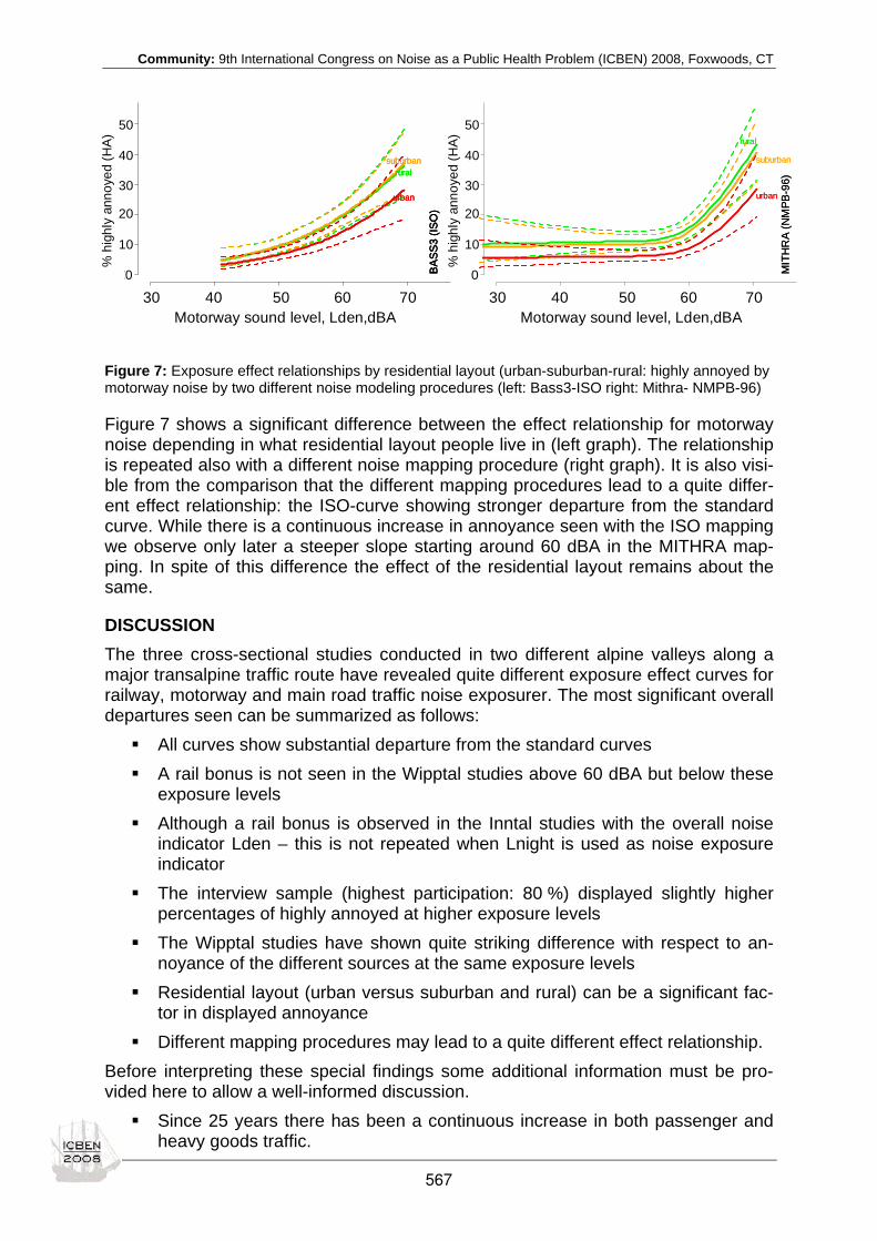
Community: 9th International Congress on Noise as a Public Health Problem (ICBEN) 2008, Foxwoods, CT
Figure 7: Exposure effect relationships by residential layout (urban-suburban-rural: highly annoyed by motorway noise by two different noise modeling procedures (left: Bass3-ISO right: Mithra- NMPB-96)
Figure 7 shows a significant difference between the effect relationship for motorway noise depending in what residential layout people live in (left graph). The relationship is repeated also with a different noise mapping procedure (right graph). It is also visi-ble from the comparison that the different mapping procedures lead to a quite differ-ent effect relationship: the ISO-curve showing stronger departure from the standard curve. While there is a continuous increase in annoyance seen with the ISO mapping we observe only later a steeper slope starting around 60 dBA in the MITHRA map-ping. In spite of this difference the effect of the residential layout remains about the same.
DISCUSSION The three cross-sectional studies conducted in two different alpine valleys along a major transalpine traffic route have revealed quite different exposure effect curves for railway, motorway and main road traffic noise exposurer. The most significant overall departures seen can be summarized as follows:
All curves show substantial departure from the standard curves A rail bonus is not seen in the Wipptal studies above 60 dBA but below these
exposure levels Although a rail bonus is observed in the Inntal studies with the overall noise
indicator Lden – this is not repeated when Lnight is used as noise exposure indicator
The interview sample (highest participation: 80 %) displayed slightly higher percentages of highly annoyed at higher exposure levels
The Wipptal studies have shown quite striking difference with respect to an-noyance of the different sources at the same exposure levels
Residential layout (urban versus suburban and rural) can be a significant fac-tor in displayed annoyance
Different mapping procedures may lead to a quite different effect relationship. Before interpreting these special findings some additional information must be pro-vided here to allow a well-informed discussion.
Since 25 years there has been a continuous increase in both passenger and heavy goods traffic.
Motorway sound level,Lden,dBA
% h
ighl
y an
noye
d (H
A)
30 40 50 60 70
0.0
0.1
0.2
0.3
0.4
0.5
rural
suburban
urban
Adjusted to: f6strers.2=Not annoyed f6staub.2=Less annoyed
30 40 50 60 700
10
20
30
40
50
% h
ighl
y an
noye
d(H
A)
Motorway sound level, Lden,dBA
MIT
HR
A(N
MPB
-96)
Motorway sound level,Lden,dBA
% h
ighl
y an
noye
d (H
A)
30 40 50 60 70
0.0
0.1
0.2
0.3
0.4
0.5
rural
suburban
urban
Adjusted to: f6strers.2=Not annoyed f6staub.2=Less annoyed
30 40 50 60 7030 40 50 60 700
10
20
30
40
50
% h
ighl
y an
noye
d(H
A)
Motorway sound level, Lden,dBA
MIT
HR
A(N
MPB
-96)
Motorway sound level,Lden,dBA
% h
ighl
y an
noye
d (H
A)
30 40 50 60 70
0.0
0.1
0.2
0.3
0.4
0.5
ruralsuburban
urban
Adjusted to: f6strers.2=Not annoyed f6staub.2=Less annoyed
BA
SS3
(ISO
)
30 40 50 60 700
10
20
30
40
50%
hig
hly
anno
yed
(HA)
Motorway sound level, Lden,dBAMotorway sound level,Lden,dBA
% h
ighl
y an
noye
d (H
A)
30 40 50 60 70
0.0
0.1
0.2
0.3
0.4
0.5
ruralsuburban
urban
Adjusted to: f6strers.2=Not annoyed f6staub.2=Less annoyed
BA
SS3
(ISO
)
Motorway sound level,Lden,dBA
% h
ighl
y an
noye
d (H
A)
30 40 50 60 70
0.0
0.1
0.2
0.3
0.4
0.5
ruralsuburban
urban
Adjusted to: f6strers.2=Not annoyed f6staub.2=Less annoyed
BA
SS3
(ISO
)
30 40 50 60 7030 40 50 60 700
10
20
30
40
50%
hig
hly
anno
yed
(HA)
Motorway sound level, Lden,dBA
567

Community: 9th International Congress on Noise as a Public Health Problem (ICBEN) 2008, Foxwoods, CT
Within this timeframe a slight shift of heavy goods traffic from road to rail has occurred. The shift has resulted in higher night exposure since the additional heavy goods trains had to be rescheduled from day to night.
Since December 1989 a night ban was implemented for trucks not fulfilling the label “low noise”. This has decreased significantly noise exposure during night from trucks on the highway (about 3 dBA reduction in level).
In both valleys several noise abatement strategies have been implemented (noise barriers nearly along the whole route on both, the motor- and railway).
Although there has been signs of a normalization of the railway annoyance curve in the Inntal – the curve in the Wipptal did not show the same development. The smaller distance to the slopes in this V-valley compared with the Inntal (U-valley) is a possi-ble explanation. The direct propagation of noise to the slopes (no ground effect) may still be underestimated in the noise mapping (van Renterghem et al. 2007). Consequently, the efficiency of noise barriers is largely compromised. Since the rail bonus is still lost in the Inntal during night this may be related to the larger signal to background ratio which displays during night in the alpine valleys and increases the detectability and therefore the perception of sound in a human state of enhanced susceptibility (see notice event concept in Botteldooren et al. (2008) at this conference). A further explanation was put forward in two other papers where the effect of noise exposure from mixed sources is explored (Lercher et al. 2007; Botteldooren et al. 2007). In these analyses we have found that the rail noise annoyance curve in the Inntal is not displaying a more shallow slope beyond 300 m of the rail track as has been observed in a large survey in a flat area (Flandern, Belgium). Eventually, not every applied noise mapping procedure may be appropriate for use in both alpine valleys and flat areas. This is evidenced by the comparsion in Figure 7 and in an accompaying paper (Lercher et al. 2008 at this conference).
CONCLUSION Although enormeous efforts have been made to cope with the increasing rail and road traffic over the Brenner pass in the Tyrol by implementing noise abatement measures along both tracks noise annoyance curves still display strong departures from the standard curve of the END. The lower background level experienced in al-pine valleys, the direct propagation of the noise to the slopes and possible effects from the combined exposure of rail and road traffic are likely to contribute to the con-sistent deviation from standard curves. Finally, not all noise propagation routines may be able to provide adequate noise mapping in alpine areas.
ACKNOWLEDGEMENTS The authors acknowledge the support by a research grant provided to the Medical University Innsbruck from the BBT-SE (funds received from the European Union for an EHIA) and the EU support for the ALPNAP project within the INTERREG IIIb pro-gram “Alpine space”. Further support was received by the Division of Social Medi-cine, Medical University Innsbruck for a more extensive noise measurement cam-paign with accompanying meteorological measurements. Both phone surveys were carried out by IMAD-Innsbruck.
568

Community: 9th International Congress on Noise as a Public Health Problem (ICBEN) 2008, Foxwoods, CT
Eventually, we thank the people of the Inn- and Wipptal for their participation. Further contributions were made in the planning and conductance of these studies by Dr Edda Amann, M.P.H., Dr Alex Eisenmann, Mag Tom Kugener, Dr David Schnaiter.
REFERENCES Botteldooren D, de Greve B, Dekoninck L, De Coensel B, Lercher P, van Renterghem T (2007). Annoyance by combined exposure to noise from road traffic and rail traffic discussed in the framework of the noticing model. In: Proceedings of ICA 2007 (on CD). Madrid, Spain.
Botteldooren D, De Coensel B, Berglund B, Nilsson ME, Lercher P (2008). Modeling the role of attention in the assessment of environmental noise annoyance. In: Proceedings of the 9th International Congress on Noise as a Public Health Problem (ICBEN) 2008, Foxwoods, CT.
de Greve B, de Muer T, Botteldooren D (2005). Outdoor beam tracing over undulating terrain. In: Proceedings of Forum Acusticum 2005, Budapest, Hungary.
de Greve B, van Renterghem T, Botteldooren D (2007). Outdoor sound propagation in moutainous areas: comparison of reference and engineering models. In: Proceedings of ICA 2007 (on CD). Madrid, Spain.
Fidell S (1984). Community response to noise. In: Jones DL, Chapman AJ (eds.). Noise and society. Chichester: Wiley.
Fields JM (1993). Effect of personal and situational variables on noise annoyance in residential areas. J Acoust Soc Am 93: 2753-2763.
Fields JM (2003). Community response research. Powerpoint presentation of the invited lecture at the 8th International Con-gress on Noise as a Public Health Problem. Rotterdam 2003.
Fields JM, Ehrlich GE, Zador P (2000). Theory and design tools for studies of reactions to abrupt changes in noise exposure. Langley Research Center. Report No: NAS 1.26210280.
Fields JM, de Jong RG, Gjestland T, Flindell IH, Job RFS, Kurra S, Lercher P, Vallet M, Yano T, Guski R, Felscher-Suhr U, Schumer R (2001). Standardized general-purpose noise reaction questions for community noise surveys: research and a recommendation. J Sound Vibr 242: 641-679.
Groothuis-Oudshoorn CG, Miedema HME (2006). Multilevel grouped regression for analyzing self-reported health in relation to environmental factors: the model and its application. Biometr J 48: 67–82.
Guski R (2004). How to forecast community annoyance in planning noisy facilities. Noise & Health 6(22): 59-64.
Harrell FE Jr (2001). Regression modeling strategies. New York: Springer.
ISO TC 43/SC 1 (2002-02), N/A. Acoustics - Assessment of noise annoyance by means of social and socioacoustic surveys. Geneve: ISO Central Secretariat.
Job RSF (1988). Community response to noise: A review of factors influencing the relationship between noise exposure and reaction. J Acoust Soc Am 83: 991-1001.
Jonasson HG (2007). Acoustical source modelling of road vehicles. Acta Acust Acust 93: 174-183.
Lercher P (1996). Environmental noise and health: An integrated research perspective. Environ Int 22: 117-129.
Lercher P (1998). Deviant dose-response curves for traffic noise in "sensitive areas"? In: The New Zealand Acoustical Soci-ety Inc. (Ed.): Inter Noise 98 (Paper # 0242). Conference Proceedings on CD-ROM. Christchurch: Causal Productions.
Lercher P, Botteldooren D (2006). General and/or local assessment of the impact of transportation noise in environmental health impact studies? In: Proceedings of Euronoise 2006, CD-ROM edition. Tampere: European Acoustics Association.
Lercher P, Brauchle G, Widmann U (1999). The interaction of landscape and soundscape in the Alpine area of the Tyrol: an annoyance perspective. In: Cuschieri J, Glegg S, Yong Y (eds.): Proceedings of Internoise (pp 1347-1350). Fort Lauderdale: INCE.
Lercher P, Botteldooren D, de Greve B, Dekoninck L, Rüdisser J (2007). The effects of noise from combined traffic sources on annoyance: the case of interactions between rail and road noise. In: Proceedings Internoise 2007 on CD. Istanbul: Turk-ish Acoustical Society.
Lercher P, de Greve B, Botteldooren D, Baulac M, Defrance J, Rüdisser J (2008). The effect on annoyance estimation of noise modeling procedures. In: Proceedings of the 9th International Congress on Noise as a Public Health Problem (ICBEN) 2008, Foxwoods, CT.
569
Community: 9th International Congress on Noise as a Public Health Problem (ICBEN) 2008, Foxwoods, CT
Lim C, Kim J, Hong J, Lee S (2006). The relationship between railway noise and community annoyance in Korea. J Acoust Soc Am 120: 2037-2042.
Lim Ch, Kim J, Hong J, Lee S, Lee S (2007). The relationship between civil aircraft noise and community annoyance in Ko-rea. J Sound Vibr 299: 575-586.
Klæboe R, Kolbenstvedt M, Fyhri A, Solberg S (2005). The impact of an adverse neighbourhood soundscape on road traffic noise annoyance. Acta Acust Acust 91: 1039-1050.
Klæboe R, Engelien E, Steinnes M (2006). Context sensitive noise impact mapping. Appl Acoust 67: 620-642.
Miedema HME, Fields JM (2005). Effect of season and meteorological conditions on community noise annoyance. J Acoust Soc Am 117: 2853-2865.
Miedema HME, Oudshoorn CG (2001). Annoyance from transportation noise: relationships with exposure metrics DNL and DENL and their confidence intervals. Environ Health Perspect 109: 409-416.
Miedema HME, Vos H (1998). Exposure-response relationships for transportation noise. J Acoust Soc Am 104: 3432-3445.
Miedema HME, Vos H (1999). Demographic and attitudinal factors that modify annoyance from transportation noise. J Acoust Soc Am 105: 3336-3344.
Miedema HME, Vos H (2003). Noise sensitivity and reactions to noise and other environmental conditions. J Acoust Soc Am 113: 1492-1504.
Morihara T, Sato T, Yano T (2004). Comparison of dose-response relationships between railway and road traffic noises: the moderating effect of distance. J Sound Vibr 277: 559–565.
R Development Core Team (2006). R: A language and environment for statistical computing. Vienna, Austria: R Foundation for Statistical Computing. http://www.R-project.org.
Staples SL (1997). Public policy and environmental noise: modeling exposure or understanding effects. American Journal of Public Health 87(12):2063-2067.
van Kempen EEMM, van Kamp I (2005). Annoyance from air traffic noise: Possible trends in exposure-response relation-ships. RIVM Report 01/2005 MGO. Bilthoven: The Netherlands: EvK.
van Renterghem T, Botteldooren D, Lercher P (2007). Comparison of measurements and predictions of sound propagation in a valley-slope configuration in an inhomogeneous atmosphere. J Acoust Soc Am 121: 2522-2533.
Yano T, Sato T, Kawai K, Kurosawa K (1998). Comparison of community response to road traffic and railway noises. J Acoust Soc Jpn 54: 489-496.
570
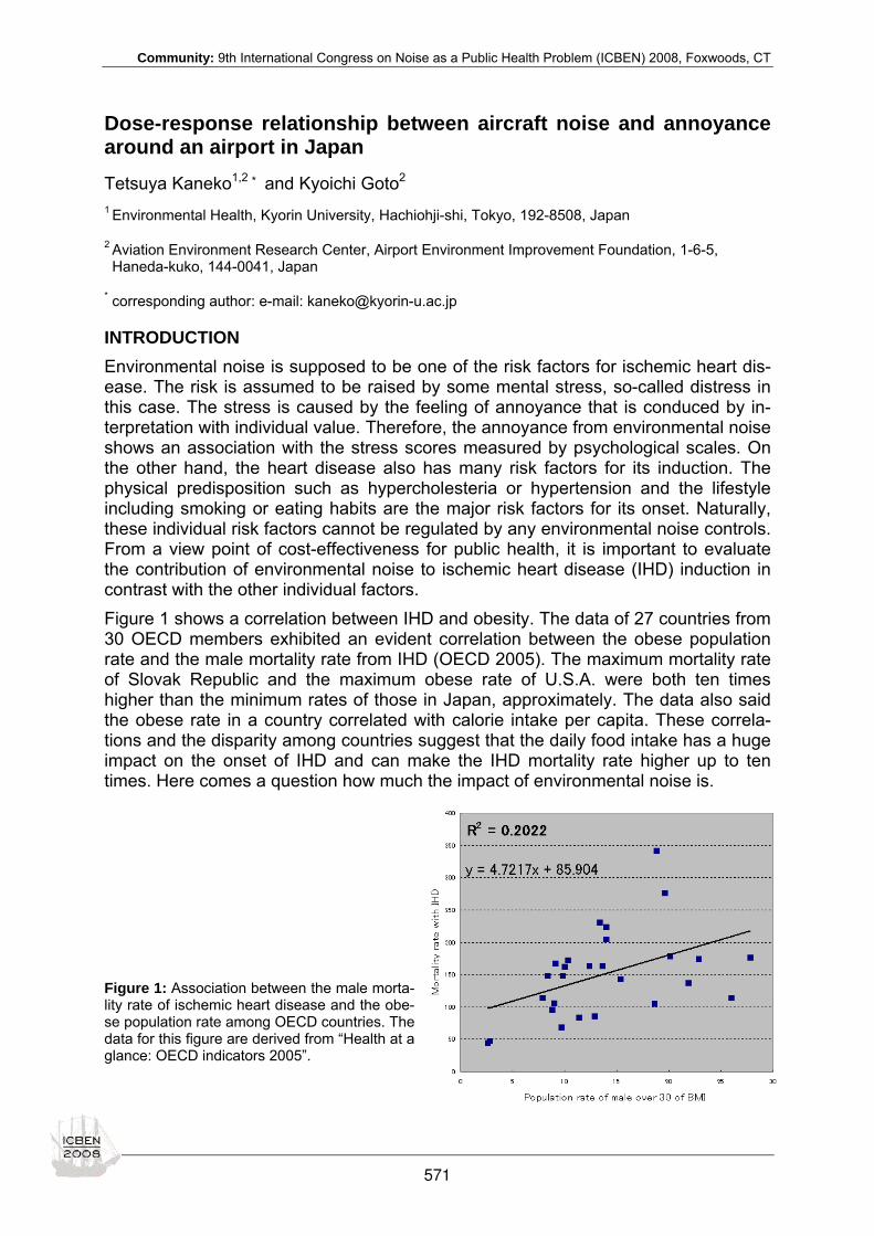
Community: 9th International Congress on Noise as a Public Health Problem (ICBEN) 2008, Foxwoods, CT
Dose-response relationship between aircraft noise and annoyance around an airport in Japan
Tetsuya Kaneko1,2* and Kyoichi Goto2 1 Environmental Health, Kyorin University, Hachiohji-shi, Tokyo, 192-8508, Japan
2 Aviation Environment Research Center, Airport Environment Improvement Foundation, 1-6-5, Haneda-kuko, 144-0041, Japan
* corresponding author: e-mail: [email protected]
INTRODUCTION Environmental noise is supposed to be one of the risk factors for ischemic heart dis-ease. The risk is assumed to be raised by some mental stress, so-called distress in this case. The stress is caused by the feeling of annoyance that is conduced by in-terpretation with individual value. Therefore, the annoyance from environmental noise shows an association with the stress scores measured by psychological scales. On the other hand, the heart disease also has many risk factors for its induction. The physical predisposition such as hypercholesteria or hypertension and the lifestyle including smoking or eating habits are the major risk factors for its onset. Naturally, these individual risk factors cannot be regulated by any environmental noise controls. From a view point of cost-effectiveness for public health, it is important to evaluate the contribution of environmental noise to ischemic heart disease (IHD) induction in contrast with the other individual factors. Figure 1 shows a correlation between IHD and obesity. The data of 27 countries from 30 OECD members exhibited an evident correlation between the obese population rate and the male mortality rate from IHD (OECD 2005). The maximum mortality rate of Slovak Republic and the maximum obese rate of U.S.A. were both ten times higher than the minimum rates of those in Japan, approximately. The data also said the obese rate in a country correlated with calorie intake per capita. These correla-tions and the disparity among countries suggest that the daily food intake has a huge impact on the onset of IHD and can make the IHD mortality rate higher up to ten times. Here comes a question how much the impact of environmental noise is.
Figure 1: Association between the male morta-lity rate of ischemic heart disease and the obe-se population rate among OECD countries. The data for this figure are derived from “Health at a glance: OECD indicators 2005”.
571

Community: 9th International Congress on Noise as a Public Health Problem (ICBEN) 2008, Foxwoods, CT
We have conducted a health care support program with free medical examination around three major airports. As a part of the program, some approaches with psycho-logical scales have been also performed from a mental health aspect. From an analysis on the database, we previously reported that the systolic blood pressure showed a significant association not with the aircraft noise level estimated for each residential area, but with annoyance from road traffic noise, though the anxiety corre-lated with the aircraft noise level (Kaneko & Goto 2006). This suggested that some latent factors were the key to understand these relationships. Here we show a noise response model with personal factors extracted and combined by analysis of covariance, and suggest that the environmental noise just reveals dormant vulnerability of a highly sensitive group in a population in the noise of a mid-dle range level.
METHODS Subjects are 894 examinees from 86 communities, around ten persons per commu-nity, who received free medical check service, gave us the agreement to join this study and filled - up questionnaire sheet. They were classified into four groups based on the flight noise level estimated for their residential area. Weighted Equivalent Con-tinuous Perceived Noise Level (WECPNL) of Japanese style was used for the esti-mation. The highest level estimated among the four was 85 dB WECPNL, nearly 72 dB(A) of Ldn. The lowest was under 75 dB of WECPNL (Figure 2).
Figure 2: The area for health care service around an airport. The light gray zone indicates Noise Zone 1 where the noise level of WECPNL is over 75 dB and the dark gray zone indicates Noise Zone 2 where the level is over 80 dB. In surrounding area outside the Noise Zone-1 the noise level is estima-ted under 75 dB. Rectangles and open circles are train stations and dark lines are railroads. White lines mean highways.
highwayhighway
major line
local lines
572

Community: 9th International Congress on Noise as a Public Health Problem (ICBEN) 2008, Foxwoods, CT
Questionnaire was composed of State Trait Anxiety Inventory (STAI, Spielberger et al. 1970), General Health Questionnaire (GHQ) (Goldberg et al. 1988), a verbal an-noyance scale against environmental noise (Yano et al. 2004), subjective value scale for circumstances in residential area and some checks on personal lifestyle. STAI can extract the state anxiety as a mental stress apart from the trait anxiety derived from personality. GHQ is widely used to observe a depressive mood as mental stress. The annoyance scale used here consists of five words to evaluate the annoy-ance of soundscape and of specific noises from several sources including air, road and railway traffic. The obtained data ware analyzed with a package software of sta-tistics, AMOS (version 16) combined with SPSS (version16).
RESULTS The area holding 86 communities has mainly three traffic noise sources: railway, road traffic and aircraft, however the dominant noise source is the aircraft. This character of the area was confirmed with the fact that the most annoying noise source were reported as the aircraft, and that the proportion of people who chose the top category in five grade annoyance scale, so-called the percent highly annoyed, showed signifi-cant association with the aircraft noise level estimated with WECPNL, when they were asked about overall annoyance at home against environmental noise, in other words, a negative value of soundscape. Figures 3 and 4 show the dose-response relation curves of the percent highly an-noyed against aircraft noise, where the subjects were classified into five groups by 5 dB increase of estimated flight noise levels. Figure 3 is for the overall annoyance to environmental noise, and Figure 4 is for the annoyance against aircraft noise. Both responses of annoyance revealed significant association with the noise level (Kendall τ test: p<0.01), though the response rates against flight noise levels were signifficantlly different between the two. The former resembles the dose-response curve proposed by Schultz (1978) or Finegold (2004), and the latter is comparable to the curve reported by Miedema and Vos (1998). These figures suggest that the response of annoyance from overall environmental noise is different from that from aircraft noise even under the same noise. This gap can be elucidated by assuming that the latter was affected by the psychological image of the noise source, aircrafts.
Figures 3 and 4: Proportion of highly annoyed people and estimated WECPNL in each zone. Figure 3 (left) shows the percent highly annoyed in response to soundscape, and Figure 4 (right) shows the one in response to aircraft noise.
573

Community: 9th International Congress on Noise as a Public Health Problem (ICBEN) 2008, Foxwoods, CT
Figure 5 is a path diagram of the result of structural equation modeling based on analysis of covariance. This is the core structure of noise - annoyance - stress rela-tionship in this field. Main indicators signified the fitness of this model. A latent factor that was named vulnerability here showed significantly high correlation with the an-noyance from road traffic noise, and low correlation with the annoyance from aircraft noise, but none with an aircraft noise level. The annoyance from railway noise was meaningless in these relations. The score of trait- and state- anxiety were located in this diagram for comparison. Only trait one showed significant correlation with vul-nerability directly, however, the state one was suggested to be correlate with that in-directly. The variable of age did negatively correlate with trait-anxiety. The GHQ score was excluded because the data made the fitness of this model worse. GHQ has a medical feature in nature and is so much different from psychological charac-teristics in STAI. All the medical check data did not exhibit meaningful correlation sta-tistically and were excluded from this path diagram. All the distributions of variables can be considered simultaneously in this analysis, so that the extracted variables and relations are considered to be properly reliable. In other words, the annoyance from traffic noise and the anxiety related with environmental noise were all dominated by a personal inner factor, which was named vulnerability here. And the health indicators such as blood pressure or other medical check data did not exhibit significant correla-tion with factors illustrated here. These results suggest that an inner personal factor has the dominant role on the noise annoyance and stress relating matters in the mid-dle range of environmental noise.
Noise Level(WECPNL)
Annoyancefrom Aircraft Noise
STAI_S e2
Annoyancefrom Raod- traffic
AGE
STAI_T e3
- .23
- .08
.70vulnerability.13
.11
.01
d3.94
.30
.00
e5
e6
e7
.13
Figure 5: Structural equation modeling for annoyance from transportation noise and anxiety. The mo-del was built with covariance analysis. All the annoyance was evaluated with a Japanese verbal scale of ICBEN model. STAI_T and STAI_S mean the trait- and state- anxiety score. The vulnerability on the center of figure above is an assumed latent variable. Figures attached on arrows are partial correlation or regression coefficients. Indicators for the fitness of this model are as follows:
chi square= 18.306, df = 5, p = 0.003, GFI=0.993, AGIF=0.972.
CONCLUSIONS In the environment with noise of a middle range level, the noise annoyance and the stress measured with an anxiety scale are dominated by some inner personal factor, such as vulnerability, noise sensitivity or something. Environmental noise seems to explicit the latency just like as opening the boxes.
574

Community: 9th International Congress on Noise as a Public Health Problem (ICBEN) 2008, Foxwoods, CT
REFERENCES Finegold L(2004). Development of exposure-response relationship between transportation noise and community annoyance. In: Proceedings of the Internet symposium 2002, Noise annoyance, stress and health effects. (AERC).
Goldberg D, Bridges K, Duncan-Jones F, Grayson D (1988). Detecting anxiety and depression in general medical settings. Brit Med J 297: 897-899.
Kaneko T, Goto K (2006). Noise annoyance, stress and health around an airport in Japan. In: Proceedings of the 35th Inter-national Congress and Exhibition on Noise Control Engineering.
Miedema HME, Vos H (1998). Exposure-response relationships for transportation noise. J Acoust Soc Am 104: 3432-3445.
OECD (2005). Health at a glance: OECD indicators.
Schultz TJ (1978). Synthesis of social surveys on noise annoyance. J Acoust Soc Am 64: 377-405.
Spielberger CD, Gorsuch RL, Lushene RE (1970). Manual for State-Trait Anxiety Inventory. (Self-Evaluating Questionnaire). Palo Alto, CA: Consulting Psychologists Press.
Yano T, Sato T, Morihara T, Hashimoto Y (2004). On the percent highly annoyed in community responses to noise as meas-ured by the ICBEN 5-point scale in Japanese. In: Proceedings of the 33rd International Congress and Exhibition on Noise Control Engineering.
575
Community: 9th International Congress on Noise as a Public Health Problem (ICBEN) 2008, Foxwoods, CT
Perception and attitudes to transportation noise in France: A national survey Jacques Lambert*, Chrystèle Philipps-Bertin INRETS-LTE, 25 avenue François Mitterrand, F-69675 Bron, France
* corresponding author: [email protected]
INTRODUCTION For a long time transportation has been a significant source of many adverse envi-ronmental impacts, in particular noise, air pollution, landscape and visual impact, and greenhouse gas emissions. The need for a better knowledge of the public views re-lated to these impacts led INRETS to conduct a national environmental nuisances survey already carried out twice in the past (Maurin & Lambert 1990). The aim of this survey was to identify or to assess:
- the current environmental concerns of the French population, particularly those related to transportation,
- the environmental nuisances (exposure – self-reported adverse effects) per-ceived at home (noise, vibrations, air pollution …) and also in other locations (during commuting, at workplace, in leisure areas ...),
- the behaviors adopted by individuals to minimise or to avoid these effects, - the expectations of the population related to these environmental nuisances
(information – public mitigation policies), - the influence of socio-demographic and socio-economic variables on the opin-
ions, attitudes and behaviors related to environmental issues. This survey was conducted in France during fall 2005 amongst adults aged 18 or over. Over 2,000 people, representative of the French population, were interviewed. The results reported in this paper focus only on noise issues.
SURVEY DESIGN The selected 3-stage sampling was close to a random sampling. It can be briefly de-scribed as follows.
- step 1: collection of 220 starting addresses within a national phone list (9 re-gion categories x 7 agglomeration categories),
- step 2: collection of addresses from the 220 starting addresses using a ran-dom route method (the route chosen gives every household in the survey an equal chance of being selected). 6242 addresses were then selected for an objective of achieving 2000 interviews,
- step 3: selection of the individual to be interviewed within the household using the “anniversary method”.
To validate the structure of the survey sample, a comparison was made with the last available national population census data (1999). A weighting adjustment was then applied for the following socio-demographic variables: region – size of agglomeration – type of housing – age – gender – family size – profession.
576

Community: 9th International Congress on Noise as a Public Health Problem (ICBEN) 2008, Foxwoods, CT
The questionnaire was administrated at home by face to face interviewing using CAPI (computer assisted personal interview). It was divided into 7 parts (69 ques-tions):
- 1: description of housing and immediate surroundings, including exposure/ transportation infrastructures,
- 2: environmental concerns and attitudes, - 3: attitudes towards nuisances abatement policies in the transportation sector, - 4: perception of environmental nuisances (home, other places) and adverse
effects, - 5: behaviors and attitudes to transportation, - 6: information sources and expectations related to the environment, - 7: respondent and household characteristics (including self-reported health).
The average length of the questionnaire was 47 minutes.
MAIN RESULTS General noise concerns Transportation is considered by the French population as the main sector at the ori-gin of environmental problems (74.5 %), and secondly the industrial sector (65.5 %). Transportation noise (and vibrations) is considered by 56 % (Table 1) of the French population as an environmental problem (27.7 % as the main one), just after local air pollution.
Table 1: Environmental problems due to transportation
Environmental problems First answer (%) Cumulated answers (%) Local air pollution 35.1 77.8 Noise and vibrations 27.7 56.0 Greenhouse effect 22.9 56.0 Fauna, flora, landscape 5.0 33.8 Land consumption 2.3 16.6 No problem 6.2 - No response 0.8 - * Basis: total survey sample
Factors such as type of area (urban/rural) and age (young/old) have an influence on the perception of noise as an environmental problem. Why is noise considered by the French population as an environmental problem? Firstly because of the effects of noise on the quality of life (49.7 %), and secondly because of the health effects (23.7 %), particularly in vulnerable people (16.7 %).
Public expectations towards information on noise 13.1 % of the French population expect more (and better) information about noise exposure levels (through noise maps for example). This social demand is higher in large cities (14.6 %) than in small cities and rural areas (10.7 %). People who are very sensitive to noise are those who are the most interested by this information (18.2 %) in comparison to non-sensitive people (6.1 %). Information about health effects of noise is also a public demand (17.1 %), particu-larly in very sensitive people (21.3 % against 12.8 % in non-sensitive people).
577

Community: 9th International Congress on Noise as a Public Health Problem (ICBEN) 2008, Foxwoods, CT
Public attitudes and expectations towards noise abatement policies The French population considers local authorities (46.9 %) as well as the government (44.3 %) as the main bodies that should take decisions aiming to fight transportation noise; and to a lesser extent (31.4 %) the transport industry (car manufacturers par-ticularly). Is noise policy related to transportation considered as efficient in France? More than 75 % of the population say “No”. Therefore, what kind of measures should be decided and implemented to fight transportation noise? Table 2 provides clear elements of the answer.
Table 2: Priority actions for fighting transportation noise
Priority actions % population* Strengthening vehicle noise emission standards 20.1Strengthening vehicle noise emission inspections 9.5Promoting public transport in cities 14.4Banning new infrastructure construction in the vicinity of existing residential areas 11.8Limiting road traffic in city centres by creation of pedestrian areas 9.5
* Basis: population considering noise as an important environmental problem
To sum up, reducing transportation noise at the source (emission standards and in-spection program) is considered by the French population as the priority action. Measures aiming to promote public transport in cities or to limit construction of large infrastructures (highway – airport - train line) are the second and third priorities. On the contrary, measures aiming to limit car circulation (regulation – charges etc) are strongly rejected by the population.
Noise perceived in the daily life Almost 4 French people out of 5 (78.3 %) perceive noise coming from outside; more-over 41.6 % perceive noise often or all the time. The main noise sources perceived at home are as follows (Table 3): road traffic, neighborhood, neighbors and air traffic.
Table 3: Noise sources perceived at home
Noise sources % population*Road traffic 67.9Neighborhood 35.9Neighbors 19.3Air traffic (including helicopters) 17.1Construction work 9.7Industry 7.9Rail traffic 7.9Recreational activities (restaurant – bars etc) 6.5Maritime and waterways transport 0.4Others 1.0* Basis: population perceiving outside noise
Transportation noise (road-rail-air traffic) is perceived by 59.4 % of the French popu-lation: around 80 % amongst this population perceived only one noise source (mainly road traffic), 17 % perceived two sources (mainly road and air traffic) and 2.5 % three noise sources (road-air and rail traffic) (Table 4).
578

Community: 9th International Congress on Noise as a Public Health Problem (ICBEN) 2008, Foxwoods, CT
Table 4: Transportation noise sources perceived at home
Transportation noise sources % population*1. Only one source 80.3 - Road 70.2 - Aircraft 7.5 - Rail 2.62. Two sources 17.2 - Road + Aircraft 11.9 - Road + Rail 4.7 - Rail + Aircraft 0.63. Three sources 2.5 - Road + Rail + Aircraft 2.5* Basis: population perceiving transportation noise
Therefore, 11.7 % of the French population are living in combined transportation noise exposure situations.
Noise annoyance What about noise annoyance? 33.7 % of the French population are annoyed (% A) by transportation noise: 30 % by road traffic noise (12.5 % HA), 6.6 % by air traffic noise (2.8 % HA) and 2.2 % by rail traffic noise (0.8 % HA). What means of transpor-tation annoy the French population (Table 5): passenger cars first, then motorbikes and trucks. Far behind come delivery trucks, buses, commercial aircraft and military aircraft.
Table 5: People annoyed transportation in France
Transportation % population annoyed by noise* Car 51.8 Motorbike 42.7 Truck 37.8 Delivery truck 18.3 Bus - Coach 16.5 Commercial aircraft 9.6 Military aircraft 7.3 Helicopter 7.1 Leisure aircraft 2.9 Freight train 3.7 Passenger train 3.9 High speed train 1.3 Tramway 1.3 * Basis: population annoyed (A) by transportation noise
Who are the people highly annoyed by transportation noise? Rather young people (< 34 years), living in urban areas, with quite a low income. When are people an-noyed? First during daytime and at a lesser extent during the night (Table 6).
Table 6: Annoyance vs. periods of the day
Period of the day First answer (%) Cumulated answers (%)Morning 26.2 47.4 Daytime 24.6 48.8 Evening 23.4 57.0 Night-time 11.3 26.3 All the time 14.5 14.5 * Basis: population annoyed (A) by transportation noise
579

Community: 9th International Congress on Noise as a Public Health Problem (ICBEN) 2008, Foxwoods, CT
Exposure to noise also leads to disturbed activities at home, particularly relaxation, rest and sleep (Table 7).
Table 7: Activities disturbed by noise at home
Activities at home % frequently disturbedRelaxation, rest 12.5 Sleep 8.7 Conversations 5.5 School work 2.2 Use of garden, balcony 8.4 *Basis: total survey sample
In particular, people who are frequently sleep disturbed by noise are significantly much more annoyed than the others (Table 8): 6 times more highly annoyed people within frequently sleep disturbed than within not frequently sleep disturbed.
Table 8: Sleep disturbance vs. annoyance
Frequently sleep disturbed % annoyed (A) - % highly annoyed (HA) Yes 87 % - 61.1 % No 29 % - 10.4 % * Basis: total survey sample
However no significant relationship was found between (self-reported) sleep distur-bance and (self-reported) health status (Table 9).
Table 9: Sleep disturbance vs. health status (11-point scale)
Frequently sleep disturbed Mean health value SD 50 % percentile % < 5 Yes 7.3 2.0 8.0 7.0 No 7.5 1.8 8.0 5.0 * Basis: total survey sample
People are also annoyed by noise in other places than at home, particularly when moving and at the workplace (Table 10).
Table 10: Noise annoyance in specific situations
Places and activities % annoyed*In the vicinity of the workplace (outside) 35.3 When traveling by car 7.0 When traveling by bike 5.3 When traveling by public transport 22.3 When traveling by foot 21.8 When walking in public parks 16.7 * Basis: total survey sample
Behavioral actions To avoid or to limit the effects of transportation noise, many people react by adopting protection behaviors, particularly insulating their home, closing their windows and to a lesser extent changing the use of the rooms of their dwelling (Table 11).
Table 11: Behavioral actions against noise
Protection actions % population*Insulation 58.4 Closing windows 34.6 Changing the use of rooms 7.4 * Basis: total survey sample
580

Community: 9th International Congress on Noise as a Public Health Problem (ICBEN) 2008, Foxwoods, CT
Insulation is not strongly linked to noise exposure (or annoyance), but principally with the necessity to save energy. As observed in the past (Lambert et al. 1984; Lercher & Kofler 1996), the two other behavioral actions are highly linked to noise exposure and annoyance (Table 12).
Table 12: Behavioral actions and annoyance
Protection action
Annoyance Insulation Closing
windowsChanging use
of rooms
Extremely/Very 54.0 % 74.7 % 20.7 % Moderately 63.9 % 46.8 % 9.8 % Slightly 61.0 % 30.4 % 5.1 % Not at all 49.8 % 9.8 % 5.2 % * Basis: total survey sample
Comparison with the 1986 survey As in the 1986 survey, noise remains the main environmental nuisance due to trans-portation. In particular road traffic remains the main origin of this pollution. However, compared to the 1986 survey, a high increase of the French population annoyed by transportation noise was observed in the 2005 survey (Table 13).
Table 13: French population annoyed (% LA) by transportation noise
INRETS survey Road traffic noise Rail traffic noise Aircraft noise 2005* 45.3 % 4.7 % 11.3 % 1986** 18.9 % 2.1 % 1.9 % * at least slightly annoyed; ** at least a little annoyed
This huge difference is partially explained by: - the type of survey: multi-topic survey in 1986 – environment survey in 2005, - the wording and the scale of the annoyance question (4-point scale in 1986 –
5-point scale (ICBEN scale) in 2005 survey). But also explained by the strong increase in traffic volumes (road, rail and air) be-tween 1986 and 2005, leading to more exposed people:
- increase of 50 % in the national vehicle fleet (number of vehicles), of 25 % in the road network length (km), and consequently an increase of 68 % in the road traffic (veh.km),
- increase of 105 % in the air traffic (number of movements), - but only an increase of 3.9 % in the rail traffic (train-km).
And probably by the higher sensitivity of the French (and European) population to the environment as observed in recent surveys carried out in Europe (EC 2008).
CONCLUSIONS In France, transportation noise still remains one of the major environmental concerns for citizens and the major daily environmental nuisance for residents despite noise policies implemented over the last 20 years, which are perceived as inefficient by the majority of the population. One main reason of this deterioration is the continuous increase of the traffic, particularly road and air. Transportation noise is perceived by the French population as an adverse effect to quality of life and to health. Road traffic is the main source of noise annoyance, be-
581

Community: 9th International Congress on Noise as a Public Health Problem (ICBEN) 2008, Foxwoods, CT
fore aircraft noise. However, a significant part of the population is annoyed by com-bined noise sources (particularly road + aircraft). Behavioral actions (linked to the degree of annoyance), such as closing of windows and changing the use of rooms, are often adopted to limit annoyance and other adverse effects (sleep disturbance). To fight transportation noise, the social demand highlights the strengthening of vehi-cle noise standards as well as of noise emission inspections and to a lesser extent the promotion of public transport in cities and the banning of new infrastructure con-struction close to existing residential areas.
ACKNOWLEDGMENTS The INRETS 2005 survey was commissioned and funded by ADEME (French Envi-ronment and Energy Management Agency).
REFERENCES EC, European Commission (2008). Attitudes of European citizens towards the environment. Special Eurobarometer 295, final report, March 2008.
Lambert J, Simmonet F, Vallet M (1984). Patterns of behaviour in dwellings exposed to road traffic noise. J Sound Vibr 92: 159-172.
Lercher P, Kofler WW (1996). Behavioral and health responses associated with road traffic noise exposure along alpine through-traffic routes. Sci Total Environ 189/190: 85-89.
Maurin M, Lambert J (1990). Exposure of the French population to transport noise. Noise Contr Eng J 35: 5-18.
582

Community: 9th International Congress on Noise as a Public Health Problem (ICBEN) 2008, Foxwoods, CT
Community annoyance from road traffic noise and construction noise in urban spaces Jin Yong Jeon*, Pyoung Jik Lee, Jin You Department of Architectural Engineering, Hanyang University, Seoul, 133-791, Korea
* corresponding author: e-mail: [email protected]
ABSTRACT This paper provides an overview of the exposure-response relationship between environmental noise and community annoyance and sound masking technique for noise abatement in urban spaces. Most previous studies focused on the community response in residential areas not urban spaces and evaluated the indoor environmental quality. However, many residents spent their daytime in outdoor such as open public space. Outdoor environmental quality is also important, and it is necessary to investigate the reaction to environmental noise in urban spaces. Social survey for evaluating the outdoor envinromental quality was introduced, and application of sound masking technique was suggested to improve the outdoor soundscape.
INTRODUCTION Many researchers have investigated sound level or sound quality of noises in urban public area. This is because acoustical characteristics are one of the important as-pects indicating the amenity of the place. However, most of the open public areas are necessarily accompanied with heavy flux of transportation and complicated activities so that excessive noise evokes annoyance to community. Among the various noises, road traffic noises are reported as one of the most dominant factors affecting com-munity annoyance (Miedema & Vos 1998) so that many studies were concentrated on finding the method of transportation noise reduction. Several methods such as tree-planting or advanced pavements can be applied to the urban spaces. However, effects of the methods are limited in actual environments with various noises espe-cially intermittent or impulsive noises such as construction noise are present. There-fore, sound masking technologies should be introduced to the urban public spaces in order to improve the soundscape more effectively. Also, more advanced measure-ment methods of soundwalking system should be applied for the realistic analyses and evaluations. In the present study, community annoyance in urban spaces was obtained by social survey and construction noise as well as road traffic noise was dealt with as noise source. Standardized questions to obtain the noise annoyance were applied and syn-thesis curves for the relationship between noise exposure and annoyance were de-rived. Also, noise level and sound quality characteristics of the road traffic and con-struction site noises were defined by using physical analyses and subjective evalua-tions.
NOISE MEASUREMENTS Methods A total of sixteen urban areas around Seoul were chosen considering road traffic and construction sites. The dominant noise source of the four sites was the road traffic noise, and twelve sites were exposed to the construction noise as well as the road
583

Community: 9th International Congress on Noise as a Public Health Problem (ICBEN) 2008, Foxwoods, CT
traffic noise. The sites can be categorized into two groups, residential area and open public space according to the usage. The sites selected in this study are listed in Ta-ble 1.
Table 1: Categorization of sites
Number of site Noise source Residential area Open public space
Road traffic noise 2 2 Road traffic noise with construction noise 6 6
Total 8 8
The sound pressure levels were measured using a binaural ear microphone (B&K Type 4101) while one subject walked around each site. In addition, visual data was captured using a camcorder (Sony DCR-HC90) to investigate the effect of visual in-formation in the auditory test. Also, Head and Torso Simulator (HATS, B&K Type 4100) was positioned considering the walking path of pedestrians in public spaces. Height of microphone was determined as 1.5 m from the ground.
SUBJECTIVE EVALUATIONS Field survey ICBEN team 6 (Fields et al. 2001) recommends that each survey use two questions to measure annoyance reactions for the purpose of making comparisons between social surveys. Therefore, the questions with 5-point verbal scale question and 11-point numerical answer scale were used in the present study. Annoyance responses from two questions were translated into a scale from 0 to 100 to assess the %HA (percentage of highly annoyed). The %HA is the percentage of annoyance responses exceeding a certain cutoff point. Schultz (1978) used a cutoff at 72 in his influential synthesis to define %HA, and same cutoff point was chosen in this study. Construction type and progress of the selected sites were various. Some sites with construction noise were in the progress of excavation and rock removal work, and others were exposed to noise from hammering, drilling and grinding. Field survey was conducted in the afternoon (13:00-18:00) on the basis of the assumption that the outdoor activities are most frequent at that period. A total of 15 subjects (7 females, 8 males) between 20 and 30 years age participated in the survey. The soundwalk was conducted in silence and participants were asked to concentrate on what they could hear as they walked and to look at the urban environments in order to make connec-tions between what they could see and what they could hear. After soundwalking for 30 minute at each site, participants were asked to evaluate the annoyance from the noise sources.
Laboratory experiments Laboratory experiments were composed of three experiments in order to determine characteristics of masker. First, masker sound among various natural sounds was selected by preference tests. Second, signal to noise ratio between masker and maskee sounds was determined and finally, sound quality characteristics of the masker sound was manipulated in order to enhance the effectiveness of masking. For all of the three experiments, paired comparison method was used. All of the sub-jects were asked to choose the preferred one between two sound stimuli in each pair. Duration of each pair was 17.5 second because an interval sound of 3.5 second du-
584

Community: 9th International Congress on Noise as a Public Health Problem (ICBEN) 2008, Foxwoods, CT
ration was set between the 7.0 second stimulus and another 7.0 second stimulus. All of the stimuli pairs were randomly presented to the subjects. Visual image of the ac-tual sites was presented to subjects before the auditory tests began. Twelve subjects between 20 and 30 years age evaluated the sounds via headphone system in a semi-anechoic chamber. Presentation level of the sound stimuli was set to 58 and 60 dBA for road traffic and construction noise, respectively, by considering the actual sound level of the noise at the real sound fields.
RESULTS Exposure-response relationship Exposure-response relationships were obtained as a function of LAeq from 5-point verbal scale and 11-point numerical scale respectively. And the curves for %A and %HA are given in Figure 1. %HA from 5-point verbal scale question was slightly higher than that from 11-point verbal scale at same noise exposure level. The differ-ence between %HA curves from two different annoyance scales was statistically sig-nificant (p<0.01). However, %A curves from 5-point verbal scale and 11-point nu-merical scale were almost same in contrast to the results of %HA.
Figure 1: The percentages highly annoyed (%HA) and annoyed (%A) as a function of LAeq
Figure 2: Scale value of preference according to relative presentation level: Left, Construction noise; Right, Road traffic noise
Preferred sound characteristics of noise masker Sound characteristics of noise masker were determined. Among 9 natural sounds of ‘Waterfall’, ‘Rainfall’, ‘Stream’, ‘Lake’, ‘Birds in forest, ‘Seagulls in port’, ‘Insects’, ‘Church bell’, and ‘Wind sound’, the sounds of ‘Stream’ and ‘Lake’ were preferred the most as the noise masker. Therefore, sounds of ‘Stream’ and ‘Lake’ were applied to investigate the appropriate signal to noise ratio between the masker and maskee. As shown in Figure 2, in the case of construction noise, the scale value of preference
585

Community: 9th International Congress on Noise as a Public Health Problem (ICBEN) 2008, Foxwoods, CT
showed high value when the sound masker was presented with 3 dBA lower sound pressure level than that of the noise. In the case of road traffic noise, the scale value of preference showed high level when the sounds of ‘Stream’ and ‘Lake’ were pre-sented 0 dBA and 3 dBA lower than the noise, respectively. The scale value was de-creased when the level of sound masker was increased over the level of site noise.
SUMMARY AND FURTHER STUDIES Community annoyance was investigated in urban spaces on the basis of sound measurements and field survey. Soundwalking methodology was introduced to calcu-late the sound levels of urban public spaces more accurately. Standardized annoy-ance question and procedure to obtain the annoyance measure such as %HA (highly annoyed) and %A (annoyed) were applied. In case of %HA, questions with 11-point numerical scale caused less annoyance than 5-point verbal scale, as the subjects rarely chose ‘8’, ‘9’ and ‘10’ in the 11-point scale even though they were exposed to higher noise levels. However, it was found that the %A curves from 5-point scale and 11-point scale were almost same. It ap-pears that most subjects chose ‘3’ in the 5-point scale when they were exposed to a wide range of noise levels. Also, sound characteristics for noise masker were investigated as a preceding re-search for the application of sound masking system to reduce the annoyance from road traffic or construction site noises. Results which were taken both in laboratory and actual conditions, show that sound maskers such as ‘Stream’ and ‘Lake’ are ef-fective for both road traffic and construction noises. When the presentation level of the sound masker is up to 3 dB lower than that of the combined noise sources, the scale values of preferences actually increase.
REFERENCES Ahn DS (2002). Analyses on the cognitive effects of masking traffic noise by sounds of water. J Korean Inst Forest Recreat 6(4): 9-19.
Anderson LM, Mulligan BE, Goodman LS, Regen HZ (1983). Effects of sounds on preferences for outdoor settings. Environ Behav 15: 539–566.
Berglund B, Nilsson ME (2006). On a tool for measuring soundscape quality in urban residential areas. Acta Acust Acust 92: 938-944.
Fields JM, De Jong JM, Gjestland T, Flindell IH, Job RFS, Kurra S, Lercher P, Vallet M, Yano T, Guski R, Felscher-Suhr U, Schumer R (2001). Standardized general-purpose noise reaction questions for community noise surveys: research and a recommendation. J Sound Vibr 242: 641-679.
Guastavino C, Katz BFG, Polack JD, Levitin DJ, Dubois D (2005). Ecological validity of soundscape reproduction. Acta Acust 91: 333–341.
ISO 15666 (2003). Acoustics - Assessment of noise annoyance by means of social and socio-acoustic surveys.
Jeon JY, Kim KH, Yano T (2003). Standardized noise annoyance modifiers in Korean according to the ICBEN method. J Acoust Soc Kr 22: 56-61.
Miedema HME, Vos H (1998). Exposure-response relationships for transportation noise. J Acoust Soc Am 104: 3432-3445.
Schafer RM (1977). The tuning of the world. New York: Alfred Knopf, Inc.
Schultz THJ (1978). Synthesis of social surveys on noise annoyance. J Acoust Soc Am 64: 377–405.
Semidor C (2006). Listening to a city with the soundwalk method. Acta Acust Acust 92: 959-964.
Skanberg A, Ohrstrom E (2002). Adverse health effects in relation to urban residential soundscapes. J Sound Vibr 250: 151–155.
586
Community: 9th International Congress on Noise as a Public Health Problem (ICBEN) 2008, Foxwoods, CT
Exposure-response relationships on community annoyance to transportation noise Soogab Lee1*, Jiyoung Hong1, Jaehwan Kim1, Changwoo Lim2, Kyutae Kim1
1 Department of Mechanical and Aerospace Engineering and Center for Environmental Noise and Vibration Research, Seoul National University, San 56-1, Shilim-Dong, Kwanak-Gu, Seoul, 151-744, Republic of Korea
2 Department of Environmental policy, Republic of Korea Air Force, P.O. Box, 501-306, Bunam-ri, Namseon-myeon, Gyeryong-si, Chungcheongnam-do, Republic of Korea
* corresponding author: e-mail: [email protected]
INTRODUCTION The first synthesis study for the community response to noise was reported by Shultz in 1978 (Schultz 1978). It covers the response to all the traffic noise including aircraft as well as ground vehicles. Kryter found that the response to ground traffic noise dif-fered from that to air traffic noise at the same exposure level (Kryter 1982). Finegold et al. reanalyzed the datasets and recommended three different curves to describe the community annoyance to aircraft, road traffic and railway noise (Finegold et al. 1994). Recently, Miedema et al. made a synthesis study from datasets of 45 different social surveys and established annoyance curves for each transportation noise (Miedema & Vos 1998; Miedema & Oudshoorn 2001). Datasets used in those analyses were mainly obtained from either north American countries or from western European countries. The annoyance response could vary with different areas, different cultures, and different languages. The researches in various cultural areas are necessary for more comprehensive exposure-response relationships for transportation noise. This article presents synthesis results from an in-depth study made in Korea during several years. Exposure-response relationships based on all 87 datasets were established. Noise metrics and annoyance measures which were used here for analysis and the information of the field surveys are intro-duced. More details on this research are in preparation for publishing as a follow-up paper.
METHODS To establish the relationships between noise exposure and community annoyance, Ldn was used as the descriptor of noise exposure from four different traffic modes. It is defined as a day-night average sound level, and applies a 10 dB penalty to noise at night. The definition is as follows:
Here Lday and Lnight are the long-term LAeq as defined by ISO (ISO 1996-2 1987), each represents the average sound levels during the day from 07:00 to 22:00 and the night-time from 22:00 to 07:00, respectively. ICAO (International Civil Aviation Organization) recommended WECPNL (Weighted Equivalent Continuous Perceived Noise Level) as a metric of the aircraft noise (ICAO 1971) and, in Korea, the modified WECPNL has been applied to evaluate the aircraft noise and to establish the noise criteria. This modified WECPNL was used, in this
587

Community: 9th International Congress on Noise as a Public Health Problem (ICBEN) 2008, Foxwoods, CT
article, as the noise metric when the responses to aircraft noise are separately ana-lyzed from those to other transportation noise. The definition is as follows:
where, denotes the energy mean of all maximum aircraft noise levels during a day. N2 and N3 are the number of events during the day from 07:00 to 19:00 and the night-time from 19:00 to 22:00. N1 and N4 are the number of events from 00:00 to 07:00 and from 22:00 to 24:00, respectively. Field survey for military aircraft noise was performed in 25 sites near the Suwon and Daegu airbase and the average number of daily flights is about 33. For commercial aircraft noise, the field survey was performed in 20 sites around two major airports. These airports have different volumes of flight operations, where the average number of flights in Gimpo and Gimhae airports is 160 and 80 a day, respectively. Aircrafts rarely operate at night, so the number of flight operations hardly includes the opera-tions during the night-time. Eighteen sites along Gyungbu and Honam railway lines were selected to investigate the effects of railway noise. Railway traffic was com-posed of passenger trains and freight trains, where the mean number of daily opera-tions was about 253 and the component ratio of two train types were 61 % and 39 %, respectively. For road traffic noise, 17 sites around the principle roads and the high-ways in Seoul city were selected. The operation was composed of two types of road vehicles: light vehicles and heavy vehicles including heavy trucks. The traffic volume at the principle roads is about over 50,000 a day and the component percentages of the daily traffic are 69 % for light vehicles and 31 % for heavy vehicles. To assess the effects of noise, the percentage of respondents who felt highly an-noyed (%HA) is selected as the indicator of noise annoyance in many researches. WHO also has recommended %HA as one of the environmental health indicators to explain the effects of noise on health (WHO 2000). In this study, respondents were asked to answer the question, ‘How much have you been bothered or annoyed from military aircraft (or commercial aircraft/railway/road traffic) noise when you are in and around the house for the last 12 months or so?’, by selecting one of 11 degrees of annoyance. A numerical scale from 0 (not annoyed at all) to 10 (extremely annoyed) was used in the survey. For the responses of exceeding 7, the percentage of the re-spondents is called the percentage of highly-annoyed population (%HA). In total 87 datasets derived from the questionnaire surveys have been used in the present syn-thesis. Table 1 gives the information on the demographic characteristics of 2,944 re-spondents for 87 datasets.
Table 1: Information on the demographic characteristics of the respondents
Noise source categories Demographic characteristics Military aircraft Commercial aircraft Railway Road traffic
Total number respondents 1,031 753 653 779 Male (%) Female (%)
12 88
33 67
24 76
25 75
Distribution of age ~ 20th (%)
20th ~ 40th (%)
40th ~ 60th (%) 60th ~ (%)
1 66 28 5
6 37 38 19
4 52 32 13
8 51 30 11
Marital status Single (%) Married (%)
9 91
19 81
13 87
24 76
588

Community: 9th International Congress on Noise as a Public Health Problem (ICBEN) 2008, Foxwoods, CT
RESULTS To establish the exposure-response relationships for each traffic mode, datasets ob-tained from the field survey have been accumulated. For a data-point contains at least 30 cases, corresponding %HA and %A are determined and plotted. A metho-dology used to determine the relationships follows the recently reported article by the authors (Lim et al. 2006). In Figure 1, data points and %HA (%A) prediction curves for four traffic modes were shown. For military and commercial aircraft, WECPNL was used as the noise metric and the relationships for railway and road traffic were established as a funtion of Ldn.
40 50 60 70 80 90 1000
102030405060708090
100
% (H
ighl
y) A
nnoy
ed
WECPNL
40 50 60 70 80 90 1000
102030405060708090
100
% (H
ighl
y) A
nnoy
ed
WECPNL
30 40 50 60 70 80 900
102030405060708090
100
% (H
ighl
y) A
nnoy
ed
Ldn30 40 50 60 70 80 90
0102030405060708090
100
% (H
ighl
y) A
nnoy
ed
Ldn
Figure 1: %HA (solid line; —) and %A (dashed line; – – ) prediction curves with %HA data points (▲) for military aircraft, commercial aircraft, railway, and road traffics (in turns of (a), (b), (c) and (d))
Figure 2 shows the annoyance curves for four traffic modes together with respect to Ldn. At a given exposure level, both military and commercial aircraft cause the high-est %HA, followed by railway and road traffic. Overall the railway curve lies below the aircraft curves and above the road traffic curve, indicating a substantial difference between these sources. The differences between the curves for four traffic modes were considered to be caused by non-acoustical factors as well as acoustical factors. For example, fear of a plane crash may cause people to be more annoyed to aircraft noise than others. In comparison of the annoyance response induced by commercial and military air-craft noise, it is found that the trend of curves of commercial and military aircraft
(a) Military aircraft
(b) Commercial aircraft
(c) Railway
(d) Road traffic
589

Community: 9th International Congress on Noise as a Public Health Problem (ICBEN) 2008, Foxwoods, CT
30 40 50 60 70 80 900
10
20
30
40
50
60
70
80
90
100 Military aircraft Commercial aircraft Railway Road traffic
% H
A
Ldn
noise turned to be reversed at 58 dBA. Over 58 dBA, military aircraft noise causes more annoyance than commercial aircraft noise at the same exposure level and vice versa below 58 dBA. Such a result as the comparison of community response be-tween military and commercial aircraft noise has hardly been reported before the au-thors‘ recently conducted study (Kim et al. 2007).
Figure 2: Comparison of %HA prediction curves for four traffic modes together as a function of Ldn
Exposure-response relationships for commercial aircraft were compared according to different background noise levels. Each dataset was divided into two groups by the difference between aircraft noise levels and background noise levels. The descriptor for background noise is LAeq,1h. The differences between aircraft noise levels in WECPNL and background noise levels in LAeq,1h for group 1 are over 20 dB and those for group 2 are about 10 dB, where background noise levels of group 1 and group 2 are 42 and 55.5 dBA. Figure 3 shows %HA with respect to WECPNL in both groups and it is found that the annoyance response to aircraft noise was significantly affected by background levels.
Figure 3: Comparison between %HA prediction curves of commercial aircraft noise according to background noise levels (▲and ●, field survey data in group 1 and group 2, respectively; —, %HA prediction curve of group 1, N=487; – – , %HA prediction curve of group 2, N=212)
A comparison of exposure-response relationships with those reported by other re-searchers has been undertaken. Figure 4 shows the comparison between the an-noyance curves in this research and others in European, American and Japanese surveys for different traffic modes. There are significant differences between curves
40 50 60 70 80 90 1000
10
20
30
40
50
60
70
80
90
100
110
%H
A
WECPNL
590

Community: 9th International Congress on Noise as a Public Health Problem (ICBEN) 2008, Foxwoods, CT
from various researches for aircraft and railway noise. Especially with respect to rail-way noise, a number of studies in foreign countries showed that railway noise causes less annoyance than other transportation noise. This is called a “railway bonus” in European countries. Some researchers explain that railways are socially considered as more acceptable than other traffic modes because of safety, economic efficiency, and convenience (Fields & Walker 1982).
Figure 4: Comparison between %HA prediction curve of commercial aircraft noise in Korea and those in other countries (in Figure 4 (c), Conv; Conventional railway, Shin; Shinkansen express railway)
Recent Japanese studies have reported different results (Igarashi 1992; Kaku & Ya-mada 1996; Yano et al. 1997; Morihara et al. 2004), where railway noise annoyance in Japan is much higher than in European countries. Figure 4 (c) shows that the re-sult of this research is similar to that of the survey in Japan. %HA response to the conventional railway noise of Korea shows the same result with Japan’s at over 60 dB. The distance between the railway and the house may be an important cause of the difference in the annoyance responses. A number of houses in Korea are situ-ated closer to railway lines than those in Western countries due to high population density (Lim et al. 2006; Hong et al. 2007). Therefore, vibration levels caused by train passages are usually higher than those of Western countries. Unlike the results of aircraft and railway noise, there is no significant difference between the road traffic annoyance curve in this survey and that in European‘s as well as Japan‘s. The situa-tion of surroundings near the roads is mostly similar in many countries, so the results supposed to be similar.
(b) Commercial aircraft
(c) Railway
30 40 50 60 70 80 900
10
20
30
40
50
60
70
80
90
100 K orea F inego ld M iedem a Japan
Ldn
% H
A
30 40 50 60 70 80 900
10
20
30
40
50
60
70
80
90
100
% H
A
K o rea M ie d e m a J ap an
Ldn
30 40 50 60 70 80 900
10
20
30
40
50
60
70
80
90
100 K o rea M ied em a
% H
A
Ldn30 40 50 60 70 80 90
0
10
20
30
40
50
60
70
80
90
100
%H
A
L Aeq , 24h
K o rea (C o n v .) Jap an (C o n v .) Jap an (S h in .)
(a) Road traffic
591
Community: 9th International Congress on Noise as a Public Health Problem (ICBEN) 2008, Foxwoods, CT
CONCLUSIONS An in-depth study on the community response to transportation noise has been made in Korea during several years and this article presents synthesis results. Exposure-response relationships to long-term noise exposure has been established from large-scaled investigations. The annoyance response to military aircraft noise has been examined in distinction from that to commercial aircraft noise which has been usually focused in the most of previous researches. We have obtained an interesting conclu-sion reached by comparing two annoyance curves for commercial and military aircraft noise, which has not been reported yet. As an important factor on community annoy-ance, background noise has been assessed concerning commercial aircraft noise areas. The response shows much more annoying when background noise levels are considerably lower than aircraft noise levels. In most of European and American researches for the community response to trans-portation noise, it has been shown that railway noise is less annoying than road traffic noise as well as aircraft noise. The result is reflected in noise regulation of some European countries as a so-called “railway bonus”. On the contrary, the annoyance response to transportation noise in Korea has shown the opposite trend, where rail-way noise is more annoying than road traffic noise. From this investigation on com-munity annoyance to transportation noise, the authors attempt to establish the rela-tionships and provide background information for policy-making activities. The results presented in this article might be representative responses of Korean to transporta-tion noise.
REFERENCES Fields JM, Walker JG (1982). Comparing the relationships between noise level and annoyance in different surveys: A railway noise vs. aircraft and road traffic comparison. J Sound Vibr 81: 51-80.
Finegold LS, Harris CS, von Gierke HE (1994). Community annoyance and sleep disturbance: Updated criteria for assessing the impacts of general transportation noise on people. Noise Contr Eng J 42: 25-30.
Hong J, Kim J, Lim C, Kim K, Lee S (2007). Comparative study on sleep disturbance from railway and road traffic noise. In: Proceedings of the Inter-noise 2007, Istanbul, Turkey, pp 181-181.
ICAO (1971). International Standards and Recommended Practices Environmental Protection Annex 16. International Civil Aviation Organization.
Igarashi J (1992). Comparison of community response to transportation noise: Japanese results and annoyance scale. J Acoust Soc Jpn 13: 301–309.
ISO 1996-2 (1987). Acoustics-description and measurement of environmental noise. Geneva: International Standards Or-ganization.
Kaku J, Yamada I (1996). The possibility of a bonus for evaluating railway noise in Japan. J Sound Vibr 193: 445-450.
Kim K, Kim J, Hong J, Lim C, Lee S (2007). Comparison of community annoyance from commercial and military aircraft noise. In: Proceedings of the Inter-noise 2007, Istanbul, Turkey.
Kryter KD (1982). Community annoyance from aircraft and ground vehicle noise. J Acoust Soc Am 72: 1222-1242.
Lim C, Kim J, Hong J, Lee S (2006). The relationship between railway noise and community annoyance in Korea. J Acoust Soc Am 120: 2037-2042.
Miedema HME, Oudshoorn CGM (2001). Annoyance from transportation noise: relationships with exposure metrics DNL and DENL and their confidence intervals. Environ Health Perspect 109: 409-416.
Miedema HME, Vos H (1998). Exposure-response relationships for transportation noise. J Acoust Soc Am 104: 3432-3445.
Morihara T, Sato T, Yano T (2004). Comparison of dose-response relationships between railway and road traffic noises: The moderating effect of distance. J Sound Vibr 277: 559–565.
Schultz TJ (1978). Synthesis of social surveys on noise annoyance. J Acoust Soc Am 64: 377.
592

Community: 9th International Congress on Noise as a Public Health Problem (ICBEN) 2008, Foxwoods, CT
WHO (2000). Environmental health indicators: development of a methodology for WHO European Region. Copenhagen: World Health Organization.
Yano T, Yamashita T, Izumi K (1997). Comparison of community annoyance from railway noise evaluated by different cate-gory scales. J Sound Vibr 205: 505-511.
593

Community: 9th International Congress on Noise as a Public Health Problem (ICBEN) 2008, Foxwoods, CT
Trends in annoyance by aircraft noise Sabine Anne Janssen1*, H. Vos1, E.E.M.M. van Kempen2, O.R.P. Breugelmans2, H.M.E. Miedema1 1 TNO Department of Environment and Health, P.O. Box 49, 2600 AA Delft, Netherlands
2 National Institute for Public Health and the Environment, P.O. Box 1, 3720 BA Bilthoven, Netherlands
* corresponding author: e-mail: [email protected]
Annoyance due to transportation noise has been recognized by policy makers as a harmful effect that should be prevented or reduced. On the basis of combined data from field studies, exposure-response relationships were established earlier to enable the prediction by policy makers of the annoyance response given a certain level of noise exposure. Recently, the validity of exposure-response curves based on data from several decades ago was questioned, especially for aircraft noise, for which an-noyance appeared to have increased over the years. One explanation put forward concerns the changing noise exposure situations around airports. The objective of the present study was to verify the hypothesized trend and to identify its possible causes. To this end, the large database used to establish earlier expo-sure-response relationships was updated with original data from several recent cross-sectional surveys. Multilevel grouped regression was used to determine the effect estimates of the relationship between exposure and annoyance, after which meta-regression was used to investigate whether characteristics of the study can ex-plain the heterogeneity in effect estimates between airports. While the main factor of interest is year of the study, the possible mediating role of differences in study meth-ods (type of contact, type of annoyance scale), individual characteristics (age, noise sensitivity, fear) and acoustical characteristics (insulation, number of overflights) was also investigated. The results are important with regard to the applicability of general-ized exposure-response relations in the prediction of the annoyance response.
594

Community: 9th International Congress on Noise as a Public Health Problem (ICBEN) 2008, Foxwoods, CT
Soundwalk for evaluating community noise annoyance in urban spaces Pyoung Jik Lee, Jin Yong Jeon* Department of Architectural engineering, Hanyang university, Seoul, 133-791, Korea
* corresponding author: e-mail: [email protected]
ABSTRACT Community noise annoyance has been investigated in open public spaces exposed to construction and road traffic noises. Sixteen field surveys were conducted as soundwalking using 5-point verbal and 11-point numerical scales according to ISO 15666 (2003). The questionnaire contains demographic factors, dwelling types, health-related symptoms and noise sensitivity. The noise levels in the chosen areas were also measured in terms of A-weighted equivalent level (LAeq) using binaural microphones. Synthesis curves for the relationship between noise levels and per-centage of highly-annoyed (%HA) for the combined noise sources were derived.
INTRODUCTION Many studies have been carried out to investigate noise exposure-annoyance rela-tionships for various noise sources such as transportation noise, industry noise and impulsive noise. Based on the previous study of Schultz (1978), Miedema and Vos (1998) reported synthesis curves for transportation noise, applying 95 % confidence intervals around the exposure-annoyance curves. Total annoyance caused by com-bined noise sources was investigated and prediction models such as energy summa-tion model and energy equivalent model were proposed (Miedema 2004). However, most of the studies have investigated noise annoyance of indoor environment and dealt with stationary noise. Studies of outdoor environment such as urban spaces were initiated by Schafer (1977) as a concept of soundscape. Recently, soundwalking methodology has been adopted for identifying perception of the urban acoustic environment (Semidor 2006; Berglund & Nilsson 2006). However, the procedure for assessing urban environment has not been standardized yet and more discussions are needed. The methodology for evaluating the noise annoyance and dose-response function in urban soundscape has not been a major issue in the environmental studies. In this study, noise annoyance in urban spaces was investigated by soundwalking; construction noise as well as road traffic noise was dealt as a combined noise source. Questions to investigate the noise annoyance were used and the synthesis curves for the relationship between noise exposure and annoyance were derived.
QUESTIONNAIRE As the ICBEN team 6 recommends the use of two questions to measure annoyance reactions for comparison between social surveys (Fields et al. 2001), both 5-point verbal and 11-point numerical scales were used in this study. The questions ad-dressed in the ISO 15666 were translated into Korean and, as shown in Table 1, the standardized noise annoyance modifiers (Jeon et al. 2003) used in the 5-point verbal scale questions.
595
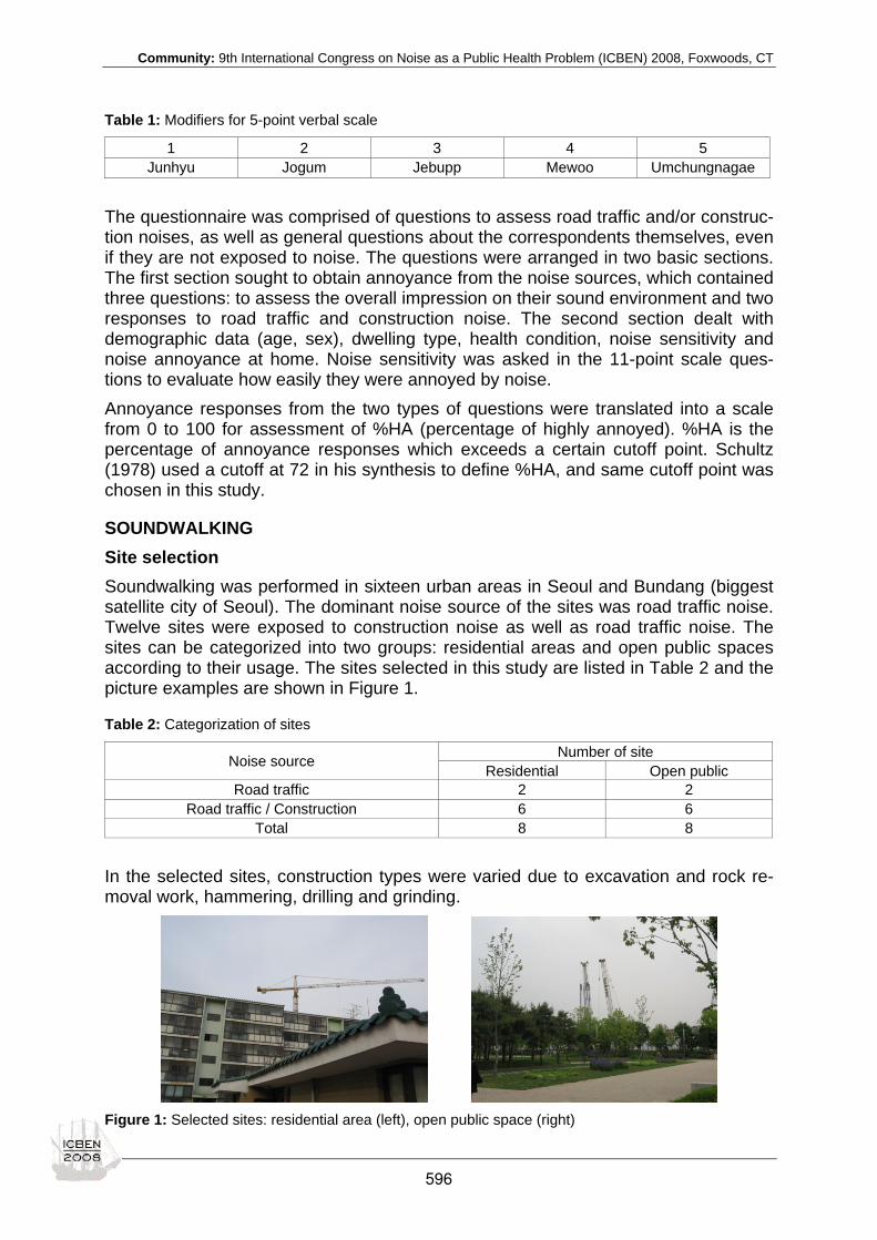
Community: 9th International Congress on Noise as a Public Health Problem (ICBEN) 2008, Foxwoods, CT
Table 1: Modifiers for 5-point verbal scale
1 2 3 4 5 Junhyu Jogum Jebupp Mewoo Umchungnagae
The questionnaire was comprised of questions to assess road traffic and/or construc-tion noises, as well as general questions about the correspondents themselves, even if they are not exposed to noise. The questions were arranged in two basic sections. The first section sought to obtain annoyance from the noise sources, which contained three questions: to assess the overall impression on their sound environment and two responses to road traffic and construction noise. The second section dealt with demographic data (age, sex), dwelling type, health condition, noise sensitivity and noise annoyance at home. Noise sensitivity was asked in the 11-point scale ques-tions to evaluate how easily they were annoyed by noise. Annoyance responses from the two types of questions were translated into a scale from 0 to 100 for assessment of %HA (percentage of highly annoyed). %HA is the percentage of annoyance responses which exceeds a certain cutoff point. Schultz (1978) used a cutoff at 72 in his synthesis to define %HA, and same cutoff point was chosen in this study.
SOUNDWALKING Site selection Soundwalking was performed in sixteen urban areas in Seoul and Bundang (biggest satellite city of Seoul). The dominant noise source of the sites was road traffic noise. Twelve sites were exposed to construction noise as well as road traffic noise. The sites can be categorized into two groups: residential areas and open public spaces according to their usage. The sites selected in this study are listed in Table 2 and the picture examples are shown in Figure 1.
Table 2: Categorization of sites
Number of site Noise source Residential Open public
Road traffic 2 2 Road traffic / Construction 6 6
Total 8 8
In the selected sites, construction types were varied due to excavation and rock re-moval work, hammering, drilling and grinding.
Figure 1: Selected sites: residential area (left), open public space (right)
596

Community: 9th International Congress on Noise as a Public Health Problem (ICBEN) 2008, Foxwoods, CT
Procedure Sixteen field surveys were conducted all in the afternoon (13:00-18:00) on the basis of the assumption that the outdoor activities are most frequent at that period. The field survey continued for 4 days (four sites per each day), and 15 subjects (7 female and 8 male) between 20 and 30 years of age participated. The subjects were chosen when consistent responses for 4 days were obtained. Soundwalk was conducted in silence and participants were asked to concentrate on what they could hear as they walked and observed the urban environments. After soundwalking for 30 minutes in each site, participants were asked to evaluate the annoyance from the noise sources.
Noise metrics The LAeq for ten minute was used as a descriptor of the noise exposure. The sound pressure levels were measured using a binaural microphone (B&K Type 4101) while one subject walked around each site. In addition, the visual image was captured us-ing a camcorder (Sony DCR-HC90) to investigate the effect of visual information on the judgement of the soundscape in the auditory test. Frequency characteristics and sound levels of measured sounds in each site are shown in Figure 2.
Figure 2: Measured sound pressure levels: residential area (left), open public space (right)
RESULTS Exposure-response relationship Exposure-response relationships were obtained as a function of LAeq from 5-point verbal and 11-point numerical scales. As shown in Figure 3. The %HA from 5-point verbal scale question was slightly higher than that from 11-point verbal scale at the same noise exposure level.
Figure 3: The percentages highly annoyed (%HA) and annoyed (%A) as a function of LAeq
597

Community: 9th International Congress on Noise as a Public Health Problem (ICBEN) 2008, Foxwoods, CT
The differences of %HA curves for the two scales were statistically significant as shown in Table 3. However, the %A curves from 5-point verbal and 11-point numeri-cal scales were almost same in contrast to the results of %HA.
Table 3: The difference between %HA curves from 5-point verbal scale and 11-point numerical scale
Difference 95 % Confidence Interval of the
Difference Mean Std. Std. error mean Lower Upper
t df Sig.
-1.59 1.13 0.28 -2.19 -0.99 -5.63 15 0.00
Polynomial approximations for road traffic noise with construction noise are given in Eq. (1) and (2), here quadratic functions are sufficient to get very close approxima-tions. These polynomials were forced through zero at 60 and 62 dBA (%HA) and 57 and 55 dBA (%A), respectively, are based on model curves fitted to data in the LAeq range 55-80 dBA. 5-point verbal scale : %HA = 1191 - 40.77 LAeq + 0.349 LAeq
2
%A = 538 – 22.06 LAeq + 0.222 LAeq2 (1)
11-point numerical scale : %HA = 696 – 24.25 LAeq + 0.21 LAeq2
%A = 993 – 35.81 LAeq + 0.324 LAeq2 (2)
The influence of LAeq and other factors on annoyance A simple model with LAeq as the only predictor can be extended with addition of extra independent variables as a same manner in the previous study (Miedema, 2004), the prediction model is as follows: Annoyance = β0 + β1 LAeq + β2 X1 + ··· βn Xn + C (3) Comparisons of model from 5-point verbal and 11-point numerical scales are listed in Table 4. Using other parameters as well as LAeq, the total coefficients of the models from 5-point verbal and 11-point numerical scale were 0.52 and 0.72 (p<0.01), re-spectively. In the prediction model from 5-point scale, LAeq, dwelling type, and vibra-tion annoyance are statistically significant. LAeq, vibration annoyance and noise an-noyance are also statistically significant in the prediction model with 11-point numeri-cal scale. The reason why age and noise sensitivity do not affect annoyance is be-cause the number of subjects is much less than previous studies.
SUMMARY AND FURTHER STUDIES The noise annoyance was evaluated in urban spaces on the basis of a simple field survey known as ‘soundwalk’. The standardized questions and procedures to obtain the annoyance measure, such as %HA (highly annoyed) and %A (annoyed), were applied. A model of the distribution of noise annoyance as a function of the noise ex-posure was presented for road traffic noise with construction noise.
598

Community: 9th International Congress on Noise as a Public Health Problem (ICBEN) 2008, Foxwoods, CT
Table 4: Prediction models from 5-point and 11-point scales (*p<0.05, **p<0.01)
5-point verbal scale 11-point numerical scale Constant -182.41** -192.04** LAeq 2.73** 3.38** Age/100 135.51 -1.92 Dwelling -5.6* -3.71 Sensitivity 0.07 0.09 Dust -0.15 0.16 Vibration 0.33* 0.29* Annoyance-home 0.04 0.13** Dependent variables Annoyance 0-100 11-point scale for annoyance
Predictor variables LAeq 55-78 Noise exposure Age 24-30 Age of respondent in years Dwelling 0-1 0=other, 1=apartment Sensitivity 0-100 11-point scale for noise sensitivity Dust 0-100 11-point scale for annoyance from dust Vibration 0-100 11-point scale for annoyance from vibration Annoyance-home 0-100 11-point scale for annoyance at home
In case of %HA, questions with 11-point numerical scale caused less annoyance than 5-point verbal scale, as the subjects rarely chose ‘8’, ‘9’ and ‘10’ in the 11-point scale even though they were exposed to higher noise levels. However, it was found that the %A curves from 5-point scale and 11-point scale were almost same. It ap-pears that most subjects chose ‘3’ in the 5-point scale when they exposed to wide range of noise levels. In the prediction model from different annoyance scales, some factors except sound pressure levels were not able to relate to annoyance since the number of subjects was not enough. Thus auditory experiments with more subjects should be further conducted to investigate the annoyance from road traffic noise and construction noise.
REFERENCES Berglund B, Nilsson ME (2006). On a tool for measuring soundscape quality in urban residential areas. Acta Acust Acust 92: 938-944.
Fields JM, de Jong RG, Gjestland T, Flindell IH, Job RFS, Kurra S, Lercher P, Vallet M, Yano T, Guski R, Felscher-Suhr U, Schumer R (2001). Standardized general-purpose noise reaction questions for community noise surveys: research and a recommendation. J Sound Vibr 242: 641-679.
ISO 15666 (2003). Acoustics - Assessment of noise annoyance by means of social and socio-acoustic surveys.
Jeon JY, Kim KH, Yano T (2003). Standardized noise annoyance modifiers in Korean according to the ICBEN method. J Acoust Soc Kr 22: 56-61.
Miedema HME (2004). Relationship between exposure to multiple noise sources and noise annoyance. J Acoust Soc Am 116: 949-957.
Miedema HME, Vos H (1998). Exposure-response relationships for transportation noise. J Acoust Soc Am 104: 3432-3445.
Schafer RM (1977). The tuning of the world. New York: Alfred Knopf, Inc.
Schultz THJ (1978). Synthesis of social surveys on noise annoyance. J Acoust Soc Am 64: 377–405.
Semidor C (2006). Listening to a city with the soundwalk method. Acta Acust Acust 92: 959-964.
599

Community: 9th International Congress on Noise as a Public Health Problem (ICBEN) 2008, Foxwoods, CT
Estimating the magnitude of the change effect Lex Brown1*, Irene van Kamp2 1 Urban Research Program, Griffith School of Environment, Griffith University, Nathan, 4111,
Australia
2 National Institute for Public Health and the Environment, Centre of Environmental Health Research, PO Box 1, 32700 BA, Bilthoven, The Netherlands
* corresponding author: e-mail: [email protected]
INTRODUCTION Conventional wisdom is that human response to a step change in transport noise should be able to be predicted from existing synthesized exposure-response curves. However most, if not all, of the human response measurements used in these syn-theses would have been conducted at sites at which the prevailing noise environment had changed little over preceding years. Exposure-response curves derived from these studies thus reflect human response to noise in situations of steady-state, con-stant or unchanging noise exposure. These same curves are now used extensively, in noise impact assessments, to estimate likely response of a population experien-cing a change in noise exposure. There are now a significant number of studies which have examined human re-sponse where there has been a step change, or abrupt change, in noise exposure). The results suggest, though not invariably, that response may be different where there has been an increase or decrease in level, to that predicted from steady-state curves (van Kamp & Brown 2003; Brown & van Kamp 2005). In other words, human response to change in exposure may include a change effect as well as an exposure effect and the change effect manifests itself as an excess response that persists over time. The focus of this paper is the magnitude of the effect in those situations in which a change-effect has been observed. Previously, excess response has been described by various terms such as exagger-ated response (Huybregts 2003), overreaction (Fields 1993; Job 1988; Schrecken-berg & Meis 2007; Breugelmans et al. 2007) or overshoot (Guski 2004). Lambert et al. (1998) use the term new infrastructure effect. However, in the psychological litera-ture overreaction is defined as an exaggerated response or a reaction with unneces-sary or inappropriate force, emotional display, or violence. We suggest that terminol-ogy which carries such connotations be abandoned in favor of the more neutral term excess response. Kastka et al. (1995a) and Baughan and Huddart (1993) have pre-viously used a related term, excess effects. There is continuing interest in response to change (Anotec Consulting 2003; Huy-bregts 2003; Guski 2004; van Kempen & van Kamp 2005; Klæboe et al. 2006). Driv-ing much of this interest is the predicted growth in land and surface traffic, the new infrastructure to accommodate this growth, and community response and health ef-fects associated with these changes (for example, Egan et al. 2003). Examples where step changes in exposure will occur are the new runways being planned at major EU airports such as Frankfurt, Schiphol and Heathrow.
600

Community: 9th International Congress on Noise as a Public Health Problem (ICBEN) 2008, Foxwoods, CT
SOME CHARACTERISTICS OF CHANGE IN NOISE EXPOSURE A step change in noise exposure may occur through different mechanisms. Type 1 changes result from a new or eliminated source, or change in intensity of the source (changes in traffic flow rates, road bypass construction or change in runway configu-rations, for example). Type 2 changes result from some (usually noise path) mitiga-tion intervention. In Type 2 changes, there are no changes in the transport source flow rates or source noise emissions, just in exposure of the respondents (for exam-ple, the erection of barriers along roadways or railways). Dimensions of the change in exposure include the direction of the change - increase or decrease; the magnitude of the change; and whether the change is a step change or whether it is gradual; and if gradual the rate of change. Some noise exposure changes may be temporary (such as shutting a runway for maintenance) whereas others are permanent.
ESTIMATES OF THE MAGNITUDE OF THE CHANGE EFFECT Seven reviews of change studies have been conducted: Fields (1994); Vallet (1996); Horonjeff & Robert (1997); Schuemer & Schreckenberg (2000); Stansfeld et al. (2001); Fields et al. (2000); and Huybregts (2003). We focus in this paper on the quantitative estimates of the magnitude of the excess-response change effect made by Horonjeff and Robert (1997) and build on their results (using their methodology) by incorporating change-effect results from more recent studies. The review by Horonjeff and Robert (1997) - itself built largely on the work of Fields (1994) - identified 23 change studies in 51 citations, covering road (12 studies), rail (2) and air (9) transport sources. Of interest in this paper was their synthesis of the magnitude of change-effects measured in the studies they reviewed. Such a synthe-sis required them to make approximations (described in the original paper) to over-come the difficulties presented by different acoustic measures, response scales, and available baseline responses from which to estimate the change-effect. The latter ranged from locally-derived baseline exposure-response curves, control site expo-sure-response curves, to synthesized exposure-response curves (mostly Schultz 1978). The Horonjeff and Robert (1997) synthesis was in terms of a decibel-equivalent esti-mate (see Fields 1990) of the magnitude of what they called the abrupt-change ef-fect. This is the change, in decibels, on an appropriate exposure-response curve, additional to the change in exposure between the before and after conditions neces-sary to achieve the observed change in response. Their synthesis included air, road and rail sources, Type 1 and Type 2 changes, and changes in exposure ranging from 18 dB decreases to 15 dB increases. While there was wide variation in the results, the majority of the data points included in their review supported the existence of an excess-response change effect. Horonjeff and Robert (1997) also found that nine studies designed to measure the decay of the excess response generally failed to find evidence of decay - that is, there was no evidence of adaptation or habituation of the change effect. Most first post-change interviews were conducted three to seven months after the change (one at 0.5 months, one at 12 months), with last post-change interviews conducted 16 to 96 months after the change.
601

Community: 9th International Congress on Noise as a Public Health Problem (ICBEN) 2008, Foxwoods, CT
MORE RECENT ESTIMATES OF THE CHANGE EFFECT In a wide review conducted by the present authors of all studies that included a change in noise exposure, several were identified whose results could be included in this synthesis of estimates of the magnitude of the change-effect. Two of the seven sites in a Fidell et al. (2002) study of change in aircraft noise levels experienced sufficient increase in exposure to allow decibel equivalent change-effects to be estimated (we used the FICON (1992) exposure-response curve to es-timate the change-effect from the reported data). Nilsson and Berglund (2006) and Öhrström (2004) reported studies of decrease in road traffic noise exposure, the first from the placement of a barrier, the second from a reduction in traffic flow. These authors suggested that there was no excess response to the change indoors, but our reanalysis (using the Miedema & Oudshoorn (2001) and Miedema & Vos (1998) ex-posure-response curves respectively) suggests that there was a large change-effect at three of the “sites” (actually three “distance from roadway categories” - change in noise exposure of more distant categories could not be estimated from the paper) in the barrier study, and at the one site in the traffic reduction study. Kastka et al. (1995a) revisited the barrier sites reported previously (Kastka & Paulsen 1979), re-porting new data and readjusting their steady-state exposure-response baseline. Kastka et al. (1995a) examined residents’ responses in 1988 and 1976 to barriers that had been constructed after the first survey. We have calculated decibel-equivalent changes at their seven barrier sites (using their noise disturbance score and their before exposure-response relationship - Table 10 in Kastka et al. (1995a). At five of the sites there is a small excess response, but an under-reaction, one large, at two sites. A recent longitudinal study of response to noise around Schiphol Airport incorporates the most comprehensive and purpose-designed study of change to date, though de-tailed results are not yet widely reported (Ministry of Transport, Public Works and Water Management 2005). Surveys of effects of aircraft noise exposure were con-ducted around Schiphol in 1996, 2002 and 2005 (Houthuijs et al. 2007). A new run-way at the airport was opened in February 2003, and a panel of 640 persons, whose exposure was likely to change as a result of the new runway, was selected from the 2002 survey group. This panel was resurveyed annually over the 2 1/2 years follow-ing the change, with half of the panel surveyed in northern hemisphere springs and half in autumns, giving six data points subsequent to the change (Breugelmans et al. 2007). In total, 478 respondents completed four panel interviews, one before the change and three after the change. The panel was made up of three subgroups: one experiencing an increase in exposure, one a decrease, and one as control experienc-ing negligible change. Results from the first (before change) panel round were used to derive a baseline exposure-response relationship based on noise exposure (Lden) over the previous 12 months. Breugelmans et al. (2007) reported significant excess response for the subgroup ex-periencing the increase in exposure. Excess response was observed from the sec-ond round of surveys and continued throughout the study. There was a drop in the penultimate round but a return to large excess-response in the latest round. The subgroup experiencing the decrease in exposure, and the control group experiencing negligible change, did not exhibit excess response in any of the survey rounds.
602

Community: 9th International Congress on Noise as a Public Health Problem (ICBEN) 2008, Foxwoods, CT
Overall, these more recent studies show magnitudes of change-effect excess re-sponse in line with those reported in the original synthesis by Horonjeff and Robert (1997).
DISCUSSION The results for the airport studies were, in general, quite different to those for the roadway studies. With the exception of our estimate of large excess response in the studies by Fidell et al. (2002) and by Breugelmans et al. (2007), the change-effect in the airport studies was very small - in some cases, an under-reaction - compared to the predominance of excess response in the roadway studies. While this may de-monstrate a difference in response to change between aircraft noise and roadway noise, another and perhaps more obvious, explanation is that the difference may be an artifact of the nature of the particular noise changes that occurred at most of the airports studied. Horonjeff and Robert (1997) had also noted that most of the airport studies they re-viewed either involved temporary changes in noise exposures (Fidell et al. 1985; Raw & Griffiths 1985; Gjestland et al. 1995) or small changes of 3 dB or less in noise exposure; Fidell & Jones 1975; Fidell et al. 1985). Some airport change studies (Fi-dell et al. 1996; Kastka et al. 1995b) and some road change studies (Stansfeld et al. 2001) also had the acoustic characteristic of a gradual change in noise exposure. As Fields et al. (2000) has previously noted, these are very different situations to where there is an abrupt or step change in exposure. Because of the potentially confounding effect of the limited magnitude and different nature of the changes that occurred in the various airport studies for which data is available, it would be inappropriate to draw conclusions from these studies about res-ponse to change around airports. Further studies involving change at airports that do not have these constraints (as, for example, the Schiphol study reported by Breugel-mans et al. (2007) and Houthuijs et al. (2007)), will be necessary to examine whether there might be any difference between response to change for different transport modes. The same applies for situations, for any mode, where there has been a grad-ual change in exposure as against a step-change. Studies of both Type 1 and Type 2 changes were included in the reviews, and there is some evidence that people may respond differently in Type 2 changes, reporting less response and little or no change-effect (Griffiths & Raw 1986). Langdon and Griffiths (1982) re-examined the results of Kastka and Paulsen’s (1979) longitudinal study of barriers and found under-reaction, explaining this as due to the differential effect of noise reductions by barriers rather reductions of the noise source. However, as noted above, using the new data for these sites from Kastka et al. (1995a) there was a small excess response at the majority of the sites, but an under-reaction at two sites. Vincent and Champelovier (1993) reported that noise annoyance shows only a small reduction for a 9 dB drop of noise levels resulting from barrier construction at their one site. No excess response to change was also suggested in the longitudinal study by Lambert (1978) of the effect of a single barrier. While Nilsson and Berglund (2006) reported no excess response in a barrier study, reanalysis by the current au-thors suggests that there was. Baughan and Huddart (1993) also note that the change-effect may not be present in Type 2 changes While Fields et al. (2000) concluded that studies aimed at evaluating the effect of noise-shielding interventions (barriers, double glazing), rarely lead to findings of an
603

Community: 9th International Congress on Noise as a Public Health Problem (ICBEN) 2008, Foxwoods, CT
excess response, evidence of the presence and direction of change-effects in Type 2 studies to date is ambiguous. A reasonable conclusion at this stage is that the results of Type 1 and Type 2 studies should be separated in any future analysis of change studies given the mixed evidence above regarding excess response in Type 2 stud-ies. Type 1 step changes in roadway noise Given the conclusions above regarding airport change studies and Type 2 change studies, it is reasonable to separately examine change-effects in a subset of change studies - those where (a) the source was road traffic and (b) where the nature of the change in exposure was a Type 1 change. Figure 1 shows the magnitude of the change effect for Type 1 change studies of roadway sources only. These are situations where the change in noise exposure has resulted from changes in the roadway source itself - the construction of new road-ways, either as new sources or providing traffic relief on existing roadways, or some other change in traffic flow. All available studies demonstrate, with remarkable con-sistency, an excess response in situations of both increments and decrements of noise exposure: respondents whose noise exposure has increased report more an-noyance than expected from steady-state studies; respondents whose noise expo-sure has decreased report less annoyance than expected from steady-state studies. The effect is present even for quite small changes in noise exposure.
Figure 1: Decibel-equivalent excess response change-effect for Type 1 changes for roadway traffic sources only. The broken line indicates a change-effect of the same magnitude (dB-equivalent) as the change in noise exposure. Data points are from the original review by Horonjeff and Robert (1997) or (those plotted using square symbols) from more recent studies.
The broken line shown in the figure is not a line of best-fit as we have chosen not to suggest a predictive relationship between noise change and its associated change-effect from the studies reviewed - given the differences between the studies in terms of metrics and designs, and the approximations necessary to estimate the change- effect from the data reported in them. However, the broken line (a plot of equal mag-nitude of change in noise exposure and of change-effect) does show that, in roadway
604

Community: 9th International Congress on Noise as a Public Health Problem (ICBEN) 2008, Foxwoods, CT
studies with Type 1 changes, the decibel-equivalent magnitude of the excess re-sponse tends to be greater (often much greater) than the change in noise levels it-self.
CONCLUSIONS A change-effect is unequivocally present in the results of the road traffic noise stud-ies where the intensity of the road traffic source changes through changes in traffic volume on the source roadways (Type 1 changes). For these types of change situa-tions, the decibel-equivalent magnitude of the excess responses (both the excess benefit arising from reductions in exposure, and the excess disbenefits arising from increases in exposure) can be greater, often much greater, than the change in noise levels itself. For changes resulting from the insertion of barriers or other path mitiga-tion interventions (Type 2 changes), the evidence for a change effect is not clear. The excess-response change-effect does not appear to attenuate over time - even years - after the change. Consistent evidence of a similar change effect for aircraft noise and railway noise changes is lacking but, rather than this indicating that human response to change is different between different transportation noise sources, we suggest that this may be a result of the nature of the noise changes available in most aircraft and railway noise change studies to date: generally small, gradual or temporary. As environmental appraisals of transport infrastructure plans are generally conducted in situations where there will be a step change, or an abrupt change, in noise expo-sure, the presence and magnitude of the excess response warrants consideration of a change-effect in assessing the impact of infrastructure changes, and in policy mak-ing with respect to such changes.
REFERENCES Anotec Consulting (2003). Studies on current and future aircraft noise exposure at and around community airports. Summary for policy makers. Doc. N o. PAN012-6-0.
Baughan C, Huddart L (1993). Effects of traffic noise changes on residents‘ nuisance ratings. In: Proceedings of the 6th International Congress on Noise as a Public Health Problem, Noise & Man ’93, Nice, July, Vol. 2, pp 585-588.
Breugelmans O, Houthuijs D, van Kamp I, Stellato R, van Wiechen C, Doornbos G (2007). Longitudinal effects of a sudden change in aircraft noise exposure on annoyance and sleep disturbance around Amsterdam Airport. In: Proceedings ICA, Madrid, ENV-04-002-IP.
Brown AL, van Kamp I (2005). Towards a design for studies of response to a change in noise. In: Proceedings of IN-TER-NOISE 05, Rio de Janeiro, Brazil.
Egan M, Petticrew M, Ogilvie D, Hamilton V (2003). New roads and human health: a systematic review. Am J Public Health 93: 1463-1471.
FICON, Federal Interagency Committee on Noise (1992). Federal Agency review of selected airport noise analysis issues.
Fidell S, Jones G (1975). Effects of cessation of late-night flights on an airport community. J Sound Vibr 42: 411-427.
Fidell S, Horonjeff R, Mills J, Baldwin E, Teffeteller S, Pearsons K (1985). Aircraft annoyance at three joint air carrier and general aviation airports. J Acoust Soc Am 77: 1054-1068.
Fidell S, Silvati L, Pearsons K (1996). On the noticeability of small and gradual declines in aircraft noise exposure levels. In: Proceedings Internoise 96, Liverpool, Vol. 5, pp 2247-2252.
Fidell S, Pearsons K, Tabachnik BG, Howe R (2000). Effects on sleep disturbance of changes in aircraft noise near three airports. J Acoust Soc Am 107: 2535-2547.
Fidell S, Silvati L, Haboly E (2002). Social survey of community response to a step change in aircraft noise exposure. J Acoust Soc Am 111: 200-209.
605
Community: 9th International Congress on Noise as a Public Health Problem (ICBEN) 2008, Foxwoods, CT
Fields JM (1990). A review of an updated synthesis of noise / annoyance relationships. NASA Report 194950, Georgia Insti-tute of Technology, Atlanta, GA.
Fields JM (1993). Effect of personal and situational variables on noise annoyance in residential areas. J Acoust Soc Am 93: 2753-2763.
Fields JM (1994). A review of an updated synthesis of noise/annoyance relationships. NASA-CR-194950. Hampton, VA: NASA Langley Research Center.
Fields JM, Ehrlich GE, Zador P (2000). Theory and design tools for studies of reactions to abrupt changes in noise exposure. NASA-CR-2000-210280. Hampton, VA: NASA Langley Research Center.
Gjestland T, Liasjø K, Granøien I (1995). Community response to noise from short-term military aircraft exercises. J Sound Vibr 182: 221-228.
Griffiths ID, Raw GJ (1986). Community and individual response to changes in traffic noise exposure. J Sound Vibr 111: 209-217.
Guski R (2004). How to forecast community annoyance in planning noisy facilities. Noise & Health 6(22): 59-64.
Horonjeff RD, Robert WE (1997). Attitudinal response to changes in noise exposure in residential communities. Harris. Miller, Miller and Hanson Inc., Burlington, MA. NASA CR-97-205813. Washington, DC: National Aeronautics and Space Administra-tion.
Houthuijs D, Breugelmans O, van Kamp I, van Wiechen C (2007). Burden of annoyance dues to aircraft noise and non-acoustical factors. In: Proceedings of Internoise 2007, Istanbul, Turkey, paper no. 838472.
Huybregts C (2003). Community response to changes in railway noise exposure - a review. In: Proceedings of Wespac VIII, April, Melbourne, Australia.
Job RFS (1988). Over-reaction to changes in noise exposure: The possible effect of attitude. J Sound Vibr 126: 550-552.
Kastka J, Paulsen R (1979). Untersuchung über die subjektive und objektive Wirksamkeit von Schallschutzeinrichtungen und ihre Nebenwirkungen auf die Anlieger. (A study into the subjective and objective effectiveness of noise barriers and their side effects on residents). Düsseldorf: Institut für Hygiene, Universität.
Kastka J, Buchta U, Ritterstaedt R, Paulsen R, Mau U (1995a). The long term effect of noise protection barriers on the an-noyance response of residents. J Sound Vibr 184: 823-852.
Kastka J, Borsch-Galetke E, Guski R, Krauth J, Paulsen R, Schuemer R, Oliva C (1995b). Longitudinal study on aircraft noise effects at Düsseldorf airport 1981-1993. In: Proceedings of 15th ICA, Trondheim, Vol. IV, pp 447-451.
Klæboe R, Kolbenstvedt M, Lercher P, Solberg S (1998). Changes in noise reactions – evidence for an area effect? In: Proceedings Internoise 98, Christchurch, New Zealand, CD-ROM.
Klæboe R, Engelien E, Steinnes M (2006). Context sensitive noise impact mapping. Appl Acoust 67: 620-642.
Lambert RF (1978). Experimental evaluation of a freeway noise barrier. Noise Contr Eng J 11: 86-94.
Lambert J, Champelovier P, Vernet I (1998). Assessing the railway bonus: the need to examine the “new infrastructure” effect. In: Proceedings Internoise 1998, Christchurch, New Zealand.
Langdon FJ, Griffiths ID (1982). Subjective effects of traffic noise exposure, II: Comparisons of noise indices, response scales, and the effects of changes in noise levels. J Sound Vibr 83: 171-180.
Miedema HME, Oudshoorn CGM (2001). Annoyance from transportation noise: relationships with exposure metrics DNL and DENL and their confidence intervals. Environ Health Perspect 109: 409-416.
Miedema HME, Vos H (1998). Exposure response relationships for transportation noise. J Acoust Soc Am 104: 3432-3445.
Ministry of Transport, Public Works and Water Management (2005). Evaluatie Schipholbeleid: Schiphol beleefd door om-wonenden (Evaluation Schiphol: Schiphol perceived by its residents). Directorate-General Transport and Aviation.
Moehler U, Hegner A, Schuemer R, Schuemer-Kohrs A (1997). Efects of railway-noise reduction on annoyance after rail-grinding. In: Proceedings Internoise 97, Budapest, Vol. 2, pp 1021-1026.
Nilsson ME, Berglund B (2006). Noise annoyance and activity disturbance before and after the erection of a roadside noise barrier. J Acoust Soc Am 119: 2178-2188.
Öhrström E (2004). Longitudinal surveys on effects of changes in road traffic noise - annoyance, activity disturbances, and psycho-social well-being. J Acoust Soc Am 115: 719-729.
606

Community: 9th International Congress on Noise as a Public Health Problem (ICBEN) 2008, Foxwoods, CT
Raw GJ, Griffiths ID (1985). The effect of changes in aircraft noise exposure. (Letter to the editor). J Sound Vibr 101: 273-275.
Schreckenberg D, Meis M (2007). Noise annoyance around an international airport planned to be extended. In: Proceedings of Internoise 2007, Istanbul, Turkey.
Schuemer R, Schreckenberg D (2000). Änderung der Lärmbelastung bei Massnahme bedingter stufenweise veränderter Geräuschbelastung – Hinweise auf einige Befunde und Interpretationsansätze. (The effect of stepwise change of noise exposure on annoyance). Z Lärmbekämpf 47: 134-143.
Schultz TJ (1978). Synthesis of social surveys on noise annoyance. J Acoust Soc Am 64: 377–405.
Stansfeld SA, Haines MM, Curtis SE, Brentnall SL, Brown B (2001). Rapid review on noise and health for London. London: St Bartholmew’s and the Royal London School of Medicine and Dentistry, Queen Mary, University of London.
Vallet M (1996). Annoyance after changes in airport noise environment. In: Proceedings Internoise 96, Liverpool, UK, Vol. 5, pp 2329-2335.
van Kamp I, Brown AL (2003). Response to changed dose of environmental noise: diverse results and explanations in the literature. In: Proceedings of the International Conference on the Biological Effects of Noise, Rotterdam.
van Kempen EEMM, van Kamp I (2005). Annoyance from air traffic noise. Possible trends in exposure-response relationships. Report Nr. 01/2005 MGO Evk, RIVM, Bilthoven.
Vincent B, Champelovier P (1993). Changes in the acoustic environment: need for an extensive evaluation of annoyance. In: Proceedings Noise and Man ’93. Sixth International Congress on Noise as a Public Health Problem, Vol. 2, pp 425-428.
607

Community: 9th International Congress on Noise as a Public Health Problem (ICBEN) 2008, Foxwoods, CT
The metrics of mixed traffic noise: Results of simulated environment experiments Atsushi Ota1*, Shigenori Yokoshima2, Akihiro Tamura1 1 Yokohama National University, 79-5 Tokiwadai Hodogaya Yokohama, Japan
2 Kanagawa Prefectural Government Shonan Region Prefectural Administration Center, 1-3-1 Nishi-Yawata Hiratsuka, Japan
* corresponding author : e-mail: [email protected]
INTRODUCTION Some types of noise, including traffic noise, railway noise, and aircraft noise have previously been evaluated individually. However, it is also necessary to consider the combined noise resulting from these sources because residents in urban areas are often exposed to these types of noises simultaneously. In spite of the studies that have considered combined noise, in which different evaluation models have been proposed (Ollerhead 1978; Powell 1979; Flindell 1983; Vos 1992; Kaku 1999), there is little agreement about which model is the most effective (Gjestland 1997). In addi-tion, there have only been a few studies carried out specifically in Japan that have considered combined noise. It is therefore important to consider whether the results obtained from studies carried out elsewhere (including in western countries) are ap-plicable to Japan, given its different culture and the differences in the structure of its cities and houses. This is done by reinvestigating the effects of combined noise, this time in Japan, and collecting additional information related to the study. The aim of this study is to identify the most effective evaluation model for combined noise. For this purpose, we conducted experiments in the laboratory and social sur-veys relating to the combined noise of conventional railway and road traffic noise car-ried out from 2004 to 2006. In this paper, we focus on the results of experiments car-ried out during this three-year period.
OUTLINE OF THE EXPERIMENTS Four experiments (one in 2004, two in 2005 and one in 2006) were carried out. These are referred to as Experiment I to Experiment IV in this paper.
Experimental Procedures The experiments were carried out in a simulated living room located at Yokohama National University (Figure 1). The subjects were asked to evaluate combined noises simulating noises coming from outside a window. Figure 2 shows the flow of the ex-periment. The subjects were exposed to 5 minutes of stimuli, and were instructed to evaluate the noise after the five minute period had elapsed. In the middle of the ex-periment, the subjects rested for 10-15 minutes.
The Simulated Living Room and the Anteroom Figure 1 shows the layout of the simulated living room and the anteroom. The stimuli (combined noises) were produced by speakers in the anteroom. The two rooms were connected by a French window and the curtain on the window was closed. One of the experimenters stayed in the living room and gave instructions to the subjects about the experiment.
608
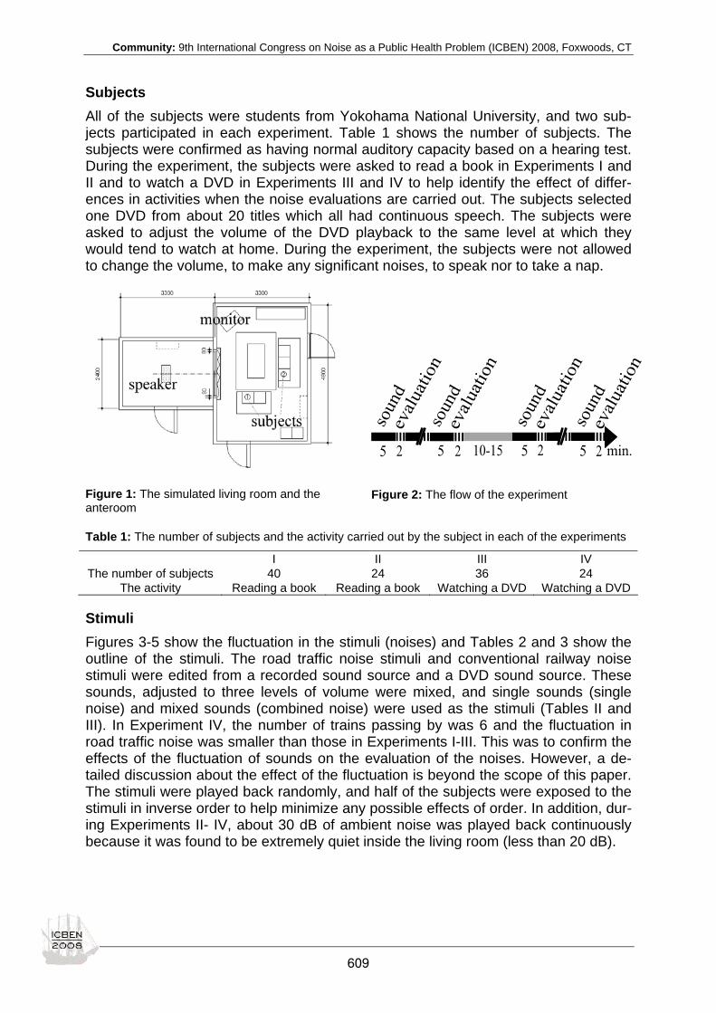
Community: 9th International Congress on Noise as a Public Health Problem (ICBEN) 2008, Foxwoods, CT
Subjects All of the subjects were students from Yokohama National University, and two sub-jects participated in each experiment. Table 1 shows the number of subjects. The subjects were confirmed as having normal auditory capacity based on a hearing test. During the experiment, the subjects were asked to read a book in Experiments I and II and to watch a DVD in Experiments III and IV to help identify the effect of differ-ences in activities when the noise evaluations are carried out. The subjects selected one DVD from about 20 titles which all had continuous speech. The subjects were asked to adjust the volume of the DVD playback to the same level at which they would tend to watch at home. During the experiment, the subjects were not allowed to change the volume, to make any significant noises, to speak nor to take a nap.
Figure 1: The simulated living room and the anteroom
Figure 2: The flow of the experiment
Table 1: The number of subjects and the activity carried out by the subject in each of the experiments
I II III IV The number of subjects 40 24 36 24
The activity Reading a book Reading a book Watching a DVD Watching a DVD
Stimuli Figures 3-5 show the fluctuation in the stimuli (noises) and Tables 2 and 3 show the outline of the stimuli. The road traffic noise stimuli and conventional railway noise stimuli were edited from a recorded sound source and a DVD sound source. These sounds, adjusted to three levels of volume were mixed, and single sounds (single noise) and mixed sounds (combined noise) were used as the stimuli (Tables II and III). In Experiment IV, the number of trains passing by was 6 and the fluctuation in road traffic noise was smaller than those in Experiments I-III. This was to confirm the effects of the fluctuation of sounds on the evaluation of the noises. However, a de-tailed discussion about the effect of the fluctuation is beyond the scope of this paper. The stimuli were played back randomly, and half of the subjects were exposed to the stimuli in inverse order to help minimize any possible effects of order. In addition, dur-ing Experiments II- IV, about 30 dB of ambient noise was played back continuously because it was found to be extremely quiet inside the living room (less than 20 dB).
609

Community: 9th International Congress on Noise as a Public Health Problem (ICBEN) 2008, Foxwoods, CT
10203040506070
0 50 100 150 200 250 300
(dB)
(s)
Figure 3: The fluctuation of the stimuli during Experiment I (LAeq,5min.=50dB)
10203040506070
0 50 100 150 200 250 300
(dB)
(s)
Figure 4: The fluctuation of the stimuli during Experiments II and III (LAeq,5min.=50dB)
10203040506070
0 50 100 150 200 250 300
(dB)
(s) Figure 5: The fluctuation of the stimuli during Experiment IV (LAeq,5min.=50dB)
Table 2: Outline and names of the stimuli druing Experiments I- III
LAeq/CR =0dB LAeq/CR =40dB LAeq/CR =50dB LAeq/CR =60dB LAeq/RT = 0dB - CR40 CR50 CR60 LAeq/RT =40dB RT40 RT40/CR40 RT40/CR50 RT40/CR60 LAeq/RT =50dB RT50 RT50/CR40 RT50/CR50 RT50/CR60 LAeq/RT =60dB RT60 RT60/CR40 * RT60/CR50 RT60/CR60
LAeq/RT: equivalent noise level of road traffic, LAeq/CR: equivalent noise level of conventional railway * RT60/CR40 was omitted from Experiment I because the conventional noise was not heard.
Table 3: Outline and names of the stimuli during Experiment IV
LAeq/CR =45dB LAeq/CR =50dB LAeq/CR =55dB LAeq/RT =45dB RT45/CR45 RT45/CR50 RT45/CR55 LAeq/RT =50dB RT50/CR45 RT50/CR50 RT50/CR55 LAeq/RT =55dB RT55/CR45 RT55/CR50 RT55/CR55
Evaluation Method The evaluation sheets (Figure 6) were delivered to the subjects after exposure to each stimulus. The subjects evaluated the noise environment for three categories: the total sound environment, road traffic noise alone and conventional railway noise alone. The terms “automobile sounds” and “train sounds” were used to express “road traffic noise” and “conventional railway noise” to avoid excessive specific concerns of noise from the subjects. During Experiment I, the above three categories were evalu-ated based on “loudness”, “noisiness” and “annoyance”. However, some of the sub-jects reported that they could not make any distinction between “noisiness” and “an-noyance”. As a result, the three evaluation categories were assessed based on “loudness” and “noisiness or annoyance”, and “interference with reading a book” dur-ing Experiment II. For Experiments III and IV, “interference with watching a DVD” was used instead of “interference with reading a book”. The range of possible evaluation scores was 0 -10.
Road trafficConventional railway
610
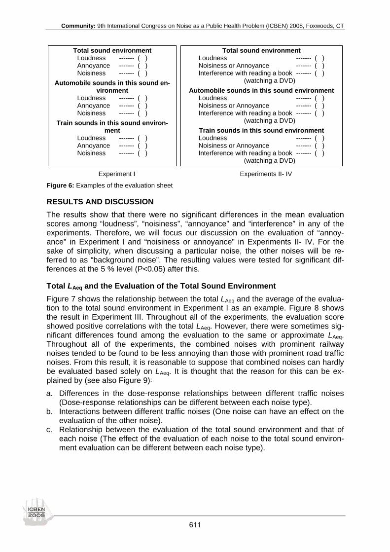
Community: 9th International Congress on Noise as a Public Health Problem (ICBEN) 2008, Foxwoods, CT
Experiment I Experiments II- IV
Figure 6: Examples of the evaluation sheet
RESULTS AND DISCUSSION The results show that there were no significant differences in the mean evaluation scores among “loudness”, “noisiness”, “annoyance” and “interference” in any of the experiments. Therefore, we will focus our discussion on the evaluation of “annoy-ance” in Experiment I and “noisiness or annoyance” in Experiments II- IV. For the sake of simplicity, when discussing a particular noise, the other noises will be re-ferred to as “background noise”. The resulting values were tested for significant dif-ferences at the 5 % level (P<0.05) after this.
Total LAeq and the Evaluation of the Total Sound Environment Figure 7 shows the relationship between the total LAeq and the average of the evalua-tion to the total sound environment in Experiment I as an example. Figure 8 shows the result in Experiment III. Throughout all of the experiments, the evaluation score showed positive correlations with the total LAeq. However, there were sometimes sig-nificant differences found among the evaluation to the same or approximate LAeq. Throughout all of the experiments, the combined noises with prominent railway noises tended to be found to be less annoying than those with prominent road traffic noises. From this result, it is reasonable to suppose that combined noises can hardly be evaluated based solely on LAeq. It is thought that the reason for this can be ex-plained by (see also Figure 9): a. Differences in the dose-response relationships between different traffic noises
(Dose-response relationships can be different between each noise type). b. Interactions between different traffic noises (One noise can have an effect on the
evaluation of the other noise). c. Relationship between the evaluation of the total sound environment and that of
each noise (The effect of the evaluation of each noise to the total sound environ-ment evaluation can be different between each noise type).
Total sound environment Loudness ------- ( ) Noisiness or Annoyance ------- ( ) Interference with reading a book ------- ( )
(watching a DVD)
Automobile sounds in this sound environment Loudness ------- ( ) Noisiness or Annoyance ------- ( ) Interference with reading a book ------- ( )
(watching a DVD)
Train sounds in this sound environment Loudness ------- ( ) Noisiness or Annoyance ------- ( ) Interference with reading a book ------- ( )
(watching a DVD)
Total sound environment Loudness ------- ( ) Annoyance ------- ( ) Noisiness ------- ( )
Automobile sounds in this sound en-vironment
Loudness ------- ( ) Annoyance ------- ( ) Noisiness ------- ( )
Train sounds in this sound environ-ment
Loudness ------- ( ) Annoyance ------- ( ) Noisiness ------- ( )
611

Community: 9th International Congress on Noise as a Public Health Problem (ICBEN) 2008, Foxwoods, CT
0
2
4
6
8
10
35 45 55 65annoyance evaluation of the
total sound environment
LAeq/total (dB) Figure 7: The relationship between the total LAeq and the evaluation of the total sound environ-ment (Experiment I)
0
2
4
6
8
10
35 45 55 65annoyance evaluation of the
total sound environment
LAeq/total (dB) Figure 8: The relationship between the total LAeq and the evaluation of total sound environment (Experiment III)
Figure 9: Schematic diagram of the evaluation
Differences in the Dose-Response Relationships between Different Traffic Noises Figures 10-12 show the relationships between the average annoyance evaluation score of each noise and the LAeq of each noise in Experiments II-IV when the back-ground noise level was 50 dB. For Experiment II, for subjects reading books, there were no significant differences found between the road traffic noise and the railway noise, except in the 40 dB range, though conventional railway noise was found to be slightly annoying. For Ex-periment III, when the stimuli were the same as those of Experiment II but where the subjects were watching DVDs, it was found that the differences between the road traffic noise and the railway noise were significant in the 40 and 50 dB range, and the annoyance response for railway noise was higher than that for road traffic noise. It was thought that the listening disturbance tended to be more severe in the case of railway noise, which has a long duration and high peak value. For Experiment IV, the fluctuations in the noises were different from those in Experiment III, conventional railway noise was found to be much more annoying than road traffic noise. It is sup-posed that this is due to the road traffic noise which was steadier than that in Experi-ment III. From this we can conclude that the relationship between the evaluation and the noise level will be different depending on the task being carried out by the listener. This is because the degree to which a noise is perceived as being a nuisance differs accord-ing to the characteristics of the fluctuations in the noise levels.
Evaluation of Total Sound Environment
Road Traffic Noise
Evaluation of Road Traffic Noise Evaluation of Conventional Railway Noise
Conventional Railway Noise
a a
c c
b
612

Community: 9th International Congress on Noise as a Public Health Problem (ICBEN) 2008, Foxwoods, CT
It is clear that it is not apporpirate to apply the results of laboratory-based studies di-rectly to the evaluation of noise in the real world. This is because the exposure in real-world cases tends to extend over significantly longer periods of time and cause many different interference effects. Therefore, it is also necessary to discuss the re-sults of social surveys to establish an effective combined noise index.
0
2
4
6
8
10
40 50 60annoyanceevaluation
LAeq(dB)
RTCR
Figure 10: The relationship between the LAeq of each noise and the evaluation of each noise (Experiment II, background noise: 50 dB)
0
2
4
6
8
10
40 50 60annoyanceevaluation
LAeq(dB)
RTCR
Figure 11: The relationship between the LAeq of each noise and the evaluation of each noise (Experiment III, background noise: 50 dB)
0
2
4
6
8
10
45 50 55annoyanceevaluation
LAeq(dB)
RTCR
Figure 12: The relationship between the LAeq of each noise and the evaluation of each noise (Experiment IV, background noise: 50 dB)
Interaction Effects between Different Traffic Noises We now consider the interaction effects between each type of traffic noise, in other words, the effect of road traffic noise on the evaluation of conventional railway noise and the effect of conventional railway noise on the evaluation of road traffic noise. Figure 13 compares the dose-response relationship of road traffic noise between the levels of conventional railway noise in Experiment I, and Figure 14 compares the dose-response relationship of conventional railway noise between levels of road traf-fic noise in Experiment III. At a glance, one noise seems to have little effect on the evaluation of the other noise. None of the experiments showed any obvious evidence of interactions between dif-ferent traffic noises, though the dose-response relationships were not always exactly the same for the level of background noise, as shown in Figure 14. From these results, it can be concluded that there are no significant interactions ef-fects. However, it is still possible that interactions occur under some specific condi-tions.
**
*
* *
*
613

Community: 9th International Congress on Noise as a Public Health Problem (ICBEN) 2008, Foxwoods, CT
0
2
4
6
8
10
RT40 RT50 RT60
annoyance evaluation of road
traffic noise
CR60CR50CR40
Figure 13: Relationship between LAeq/RT and the annoyance evaluation of road traffic noise by level groups of conventional railway noise (Ex-periment I)
0
2
4
6
8
10
CR40 CR50 CR60
annoyance evaluation of
conventional railway noise RT60
RT50RT40
Figure 14: Relationship between LAeq/CR and the annoyance evaluation of conventional railway noise by level groups of road traffic noise (Expe-riment III)
Relationship between the Evaluation of the Total Sound Environment and that of Each Noise Figures 15 and 16 show the evaluation scores for the total sound environment and those of each noise. These figures suggest that the evaluation of the total sound en-vironment approximates that of the more annoying noise. However, the evaluation scores of the total sound environment and those of the more annoying noise were not always the same.
0
2
4
6
8
10
RT40
RT50
RT60
CR40
CR50
CR60
RT40\CR40
RT40\CR50
RT40\CR60
RT50\CR40
RT50\CR50
RT50\CR60
RT60\CR40
RT60\CR50
RT60\CR60
annoyance evaluation Total
RTCR
Figure 15: Evaluations of the total sound envi-ronment and each noise (Experiment II)
0
2
4
6
8
10
RT40
RT50
RT60
CR40
CR50
CR60
RT40\CR40
RT40\CR50
RT40\CR60
RT50\CR40
RT50\CR50
RT50\CR60
RT60\CR40
RT60\CR50
RT60\CR60
annoyance evaluation Total
RTCR
Figure 16: The evaluations of the total sound environment and each noise (Experiment III)
Next, we will discuss the relationship between the evaluation scores of the total noise environment and those of each noise on every experiment. The x-axis in Figure 17 shows the difference in the evaluation scores between each noise, (road traffic noise evaluation scores) - (conventional railway noise evaluation scores). Road traffic noises are more annoying in the right field of the figure and conventional railway noises are more annoying in the left field. The y-axis on this figure shows the differ-ence in the evaluation between the total noise environment and each noise, (each noise evaluation scores) - (total sound environment evaluation scores). In other words, the evaluation scores of each noise are more than those of the total sound environment in the upper field of the figure and the evaluation scores of the total sound environment are more than those of each noise in the lower field. Note that this figure also contains the results of the single noises in Experiments I-III.
614

Community: 9th International Congress on Noise as a Public Health Problem (ICBEN) 2008, Foxwoods, CT
From this figure, we can say that the evaluation of road traffic noise approximates that of the total sound environment when road traffic noise is much more annoying than conventional railway noise. On the other hand, when conventional railway noise is much more annoying than road traffic noise, the evaluation score of conventional railway noise is more than that of the total sound environment, though the evaluation of conventional railway noise more closely approximates the total sound environment than that of road traffic noise. When the evaluations of road traffic noise and conven-tional railway noise are approximate, both evaluations of each noise contribute to that of the total sound environment, and the evaluation score of the total sound environ-ment is slightly more than that of each noise.
-6
-4
-2
0
2
4
-8 -6 -4 -2 0 2 4 6 8
(each noise evaluation scores) -
(total sound environment
evaluation scores)
(road traffic noise evaluation scores) -(conventional railway noise evaluation scores)
RT-totalCR-total
Figure 17: Relationship between the evaluation of the total sound environment and that of each noise
CONCLUSIONS Combined noises cannot be evaluated based solely on LAeq. The perceived degree of annoyance of each noise depends on the degree of the nuisance which is affected by the characteristics of the noise fluctuation. Intermittent noise such as railway noise easily causes healing interference. However, when the conventional railway noise is much more annoying than the road traffic noise, the total sound environment is not regarded as being as annoying as conventional railway noise. In this study, we were unable to find any obvious evidence of interactions between road traffic noise and conventional railway noise.
REFERENCES Flindell IH (1983). Pressure Leq and multiple noise sources: A comparison of exposure-response relationships for railway noise and road traffic noise. J Sound Vibr 87: 327-330.
Gjestland T (1997). Assessment of noise impact in a multisource environment. In: Inter-noise 97: 1033-1036.
Kaku J (1999). Study on the evaluation method of combined noises in environmental impact assessment by use of two tech-niques of laboratory experiment and social survey: Doctoral thesis, Osaka University.
Ollerhead JB (1978). Predicting public reaction to noise from mixed sources. In: Inter-noise 78: 579-584.
Powell CA (1979). A summation and inhibition model of annoyance response to multiple community noise sources. NASA Technical Paper 14479.
Vos J (1992). Annoyance caused by simultaneous impulse, road-traffic, and aircraft sounds: A quantitative model. J Acoust Soc Am 91: 3330-3345.
615

__________________________________________________________________________
__________________________________________________________________________
ICBEN 2008
Community Response to Noise
616
Community: 9th International Congress on Noise as a Public Health Problem (ICBEN) 2008, Foxwoods, CT
Modeling the role of attention in the assessment of environmental noise annoyance Dick Botteldooren1*, Bert De Coensel1, Birgitta Berglund2, Mats E. Nilsson2, Peter Lercher3 1 Acoustics Group, Department of Information Technology, Ghent University
St.-Pietersnieuwstraat 41, B-9000 Ghent, Belgium
2 Gösta Ekman Laboratory, Karolinska Institutet and Stockholm University, Sweden
3 Division of Social Medicine, Medical University Innsbruck, Austria
* corresponding author (e-mail: [email protected])
ABSTRACT Community noise effects in general and noise annoyance in particular are mostly studied by relating them to exposure through blind statistical analyses of large data-sets. This paper reports on a specific part of a quite different approach. Using mathematical simulation of basic perception and psychophysical mechanisms for a large synthetic population, insight is sought into the mechanisms underlying the emergence of noise effects. This is achieved by comparing – in a phenomenological way – the statistics of the data gathered from the simulated synthetic population to that of the real population. This paper focuses on modeling the role of attention. At-tention could play a role in two distinct aspects of the process: firstly, attention can be drawn away from other tasks by the environmental sound or tasks requiring sus-tained attention can suppress the noticing of the environmental sound; secondly, at-tention can jump between sounds in multisource sonic environments. In modeling this dual role of attention, care must be taken to simplify existing knowledge on these as-pects of perception in such a way that the model can be used to study long exposure times and large populations. Such modeling may support the assessment of real life situations where multiple environmental sounds interfere and cause noise annoy-ance. Example simulations involving exposure to railway noise, road traffic noise, natural sound and sound produced by the individual’s own activity show the influence of attention on the model outcome.
INTRODUCTION Noise plays an important role in the perception of the quality of the living environ-ment, and there is a growing public concern about the disruptive effect of an adverse living environment on health. Noise annoyance is commonly considered as the most widespread effect of environmental noise, and community noise annoyance is found to be a reasonable indicator to assess the impact of environmental noise pollution on man. Community noise effects in general, and noise annoyance in particular, are usually studied in relation to exposure through blind statistical analyses of large data-sets. In earlier work (De Muer et al. 2005; De Coensel & Botteldooren 2007, 2008; Bottel-dooren & De Coensel 2008), the authors have followed a quite different approach. The proposed methodology consists of simulating a large synthetic population of modeled individuals, each with its own personal characteristics and within its own context. The model for a single individual tries to achieve a balance between compu-tational efficiency and psychoacoustic and psychological plausibility. Results are ana-lyzed statistically on a population basis, exactly as one would analyze results of field
617

Community: 9th International Congress on Noise as a Public Health Problem (ICBEN) 2008, Foxwoods, CT
studies with human participants. This paper reports on a specific process within the model for a single individual: the role of attention. Attention could play a dual role in the perception of environmental noise, and conse-quently in the emergence of noise annoyance. Firstly, attention can be drawn away from other tasks by the environmental sound, or tasks requiring sustained attention can suppress the noticing of environmental sound. Secondly, attention can jump be-tween sounds in multisource sonic environments. Knowledge on the neurological ba-sis of auditory attention has recently expanded enormously (Fritz et al. 2007). This evolution stimulated the development of very detailed computational models, such as that of Wrigley & Brown (2004). However, they mainly focus on speech processing. In modeling the dual role of attention in environmental noise perception, care must be taken to simplify existing knowledge on auditory perception in such a way that the model can be used to study long exposure times and large populations. In the next section, the layout of such a model for a single individual is explained in detail. Subsequently, results of simulations involving a large number of individuals are given. The influence of attention on the model outcome is illustrated with simula-tions in environments with road traffic noise, railway noise, natural sound and sound produced by the individual’s own activity.
METHODOLOGY The proposed framework for including attention mechanism in modeling perception of and annoyance caused by environmental sound is shown in Figure 1. Simulated time series of the sound levels caused by various environmental sound sources form the input of the model. In a pre-attentive phase, salient parts of the sonic environment are detected. Inspired by available neurobiological knowledge on attention (Fritz et al. 2007; Knudsen 2007), the model implements a balance between top-down and bottom-up focusing; similar mechanisms have been identified in visual attention fo-cusing (Itti & Koch 2001; Shi & Yang 2007). In the following subsections, we will briefly describe how each sub-mechanism is implemented in the model.
Simulating the sonic environment Typical simulations consider the sound produced by vehicular traffic, railway traffic and natural ambient sources (wind in trees, birds, etc.) in the vicinity of the modeled individual. Vehicular and railway traffic is accounted for by simulating the emission of each vehicle/train individually. However, the model treats natural ambient sounds (including the sound produced by the modeled individual itself) as a whole, rather than to consider the sounds produced by each bird, each tree, etc. separately. Natu-ral ambient sound is assumed to fluctuate according to a 1/f characteristic, because this characteristic was found in many recordings of environmental sounds (De Coensel et al. 2003). Using a simple sound propagation model which considers only attenuation caused by geometrical divergence, the time-varying sonic environment (LAeq,1s time series for each source) at the location of the modeled individual is simu-lated.
Pre-attentive processes: masking, stream regrouping and saliency detection A sound presented at the ear will be observed only when it is not completely ener-getically masked by other parts of the sonic environment. Therefore, the first step in the processing of the environmental sound reaching the ear of the modeled individual will account for masking. Temporal effects involved have time constants of a few
618

Community: 9th International Congress on Noise as a Public Health Problem (ICBEN) 2008, Foxwoods, CT
100 ms at most. Therefore, within the scope of a long-term analysis and given the time step of 1 s that was chosen, temporal effects of masking are safely ignored.
Figure 1: Layout of the proposed model
In the proposed model, masking thresholds for each sound in the sonic environment are based on the overall sound of all other sources. A comprehensive model for (par-tial) masking should be based on the specific loudness of each sound. However, be-cause the proposed model is aimed at simulating large populations of listeners for long durations, the use of a detailed model such as that of Moore et al. (1997) is computationally infeasible. Therefore, the total A-weighted sound level of all other sounds is used as a proxy for the masking threshold. In other words, sounds (signals) are not energetically masked by all other sound (noise) if their signal-to-noise ratio (S/N) is positive. The model could also allow for regrouping of auditory streams. When a listener is exposed to an environment with multiple sound sources, the acoustic pattern at the ear will consist of the sum of all concurrent sounds. Nevertheless, the human audi-tory system is able to separate this mixture of sounds, and to form separate descrip-
619

Community: 9th International Congress on Noise as a Public Health Problem (ICBEN) 2008, Foxwoods, CT
tions of each sound source. This mechanism is commonly referred to as auditory scene analysis (ASA) (Bregman 1994). Stream separation is performed on the basis of a variety of acoustic cues (bottom-up) and on the basis of acquired expectations from prior experience or knowledge (Fritz et al. 2007). By simulating auditory streams for each separate environmental sound source, the non-trivial problems of modeling ASA and sound source identification are effectively by-passed. However, this ap-proach imposes an a priori stream segregation, which may not coincide with actual perception. Examples are the sound of a fountain making road traffic noise being perceived as part of the fountain sound, whether individual cars are heard or the sound of a street, whether individual bird songs are heard or the morning chorus of birds etc. Therefore, at least conceptually, a stream regrouping process is allowed in the model. Saliency detection is probably the most important feature of the biological auditory system. Novelty may trigger bottom-up attention, but this is not a necessary conse-quence. Saliency may be detected based on various temporal and spectral cues. Sa-liency detection is implemented in the model, for each auditory stream separately, by comparing the S/N of the stream to a predicted value. For simplicity, a linear predictor based on the exponential average of earlier S/N is used. A future improvement could be to include a neural network, dynamically trained for optimal prediction, possibly based on remembered sounds retrieved from memory. Because the peak detection is implemented for each individual type of sound, deviant behavior on the frequency axis, which is usually included in the calculation of a saliency map (Kayser et al. 2005), can be neglected in a first approximation. Figure 2 shows two examples of calculated saliency. Close to the road where only few vehicles an hour come by, saliency roughly follows the individual car passage events. Since remembered sounds of car passages are not used in this first approxi-mation and the time between passages is unpredictable, the prediction is poor and saliency keeps popping up at each individual passage. Close to the road carrying more traffic, the predictor gradually improves and saliency decreases.
Bottom-up attention mechanism High levels of saliency attract attention (bottom-up). However, the perceptual system does not stay focused on this salient feature continuously. The mechanism playing a crucial role here is inhibition of return (IOR) (Itti & Koch 2001), which prohibits atten-tion to come back to the same salient streams over and over again. This mechanism is implemented in a simplified way as a competition between an ac-tivator, AA, and inhibitor, AI. Activation is triggered by saliency. It has a very short rise time τAr and a somewhat longer decay time τAd. Because the rise time probably is shorter than the 1 s resolution of the simulation, AA jumps up almost instantaneously in the model. Decay starts immediately after this jump. The strength of activation is assumed to be a saturation process. If activation is higher than inhibition for a par-ticular auditory stream, this stream spikes for attention. As soon as attention gets fo-cused on the particular stream by the mechanism explained in the next section, inhi-bition comes into play. It is modeled as a slow process with a short rise time τIr (>τAr) and a very long decay time τId (>τAd). AI continues increasing until eventually it ex-ceeds AA at which time the stream stops spiking for attention. Attraction of bottom-up attention is thus implemented as a spiking mechanism: the process will fire a couple of times, until either saliency decreases or attention is obtained, at which time the IOR mechanism will stop the spiking.
620

Community: 9th International Congress on Noise as a Public Health Problem (ICBEN) 2008, Foxwoods, CT
In Figure 2 activation and inhibition levels are shown together with the spikes (green line) resulting from it. For the low intensity traffic stream, (bottom-up) attention is asked for at almost every car passage although occasionally a noise event is over-looked. The higher traffic intensity situation shown in the lower graphs results in slightly more attention requests, but after the initial adaptation period of a few hun-dred seconds, a quite different regime sets in: the time since the last granted request is as least as important as the instantaneous saliency.
a)
b) Figure 2: Road traffic noise level and background level in dBA together with intervals of attention for road traffic noise (upper graphs); saliency, activation, inhibition and bottom-up attention triggers (lower graphs): a) close to a road with few vehicles/h, b) close to a road with about 500 vehicles/h
621

Community: 9th International Congress on Noise as a Public Health Problem (ICBEN) 2008, Foxwoods, CT
Top-down attention mechanism and attention switching Top-down attention focusing is guided by higher cognitive processes. It results in a change in sensitivity for a particular auditory stream, which implies that it has no ef-fect as long as no stimulus is present. Top-down attention for environmental sounds may depend on
• the task that the person is performing, which in turn is related to the current activ-ity;
• emotional state such as anxiety, arousal etc.
• personal treats such as noise sensitivity etc.
• the information content of the stream to which attention is currently directed. The bottom-up mechanism makes attention switch between auditory streams, whereas the top-down mechanism tries to focus attention on a single stream. Spo-radically attention stays caught by the bottom-up mechanism, resulting in remem-bered noticing of the environmental sound. It could be assumed that limited availabil-ity of resources mainly plays a role in sustained attention. The attention switching mechanism can be seen as a gating mechanism that switches off all but a couple of auditory streams at a single instance in time. The sen-sitivity for non-attended sources is decreased. Parallel processing is changed to se-rial processing: the individual listens to a single stream at a time. The implementation of the top-down mechanism consists of an activity related part DAa, a personal related part DAp, and a part related to the information content of the attended sound DAi. The first two parts are independent from the sound. They could be modeled using time-activity patterns of the studied population, but currently are fixed for every modeled individual in the population. The last part could depend on the meaning that people give to the sound, but currently is modeled solely on the ba-sis of the overall saliency of the attended signal, which could be seen as a measure of interesting variation in the sound. If this variation is lost, attention drops. The attention switch that is mathematically implemented is a winner-take-all mecha-nism. The selection is based on the sum of the overall DA and an activation of the bottom-up attention. The activation of the bottom-up attention is an integrator that receives an additional activation δUA every time the bottom-up mechanism described in the previous section spikes for attention, and decays rather fast with a time con-stant τUA afterwards. The gate is opened for the winning stream, resulting in a pass-ing of the auditory stream to the cognitive process of attaching meaning (currently only the calculation of DAi based on saliency). This situation is kept until another stream gets attention. In order for this numerical model to work properly, non-auditory processes should be allowed to draw attention away from the auditory streams. Indeed, particular tasks could prevent noticing of sounds even though they do not involve listening at all. To account for this, an additional non-auditory stream is added that periodically fires for attention. Figure 2 also shows the actual attention paid to the road traffic (red line in upper curves). It can be seen that it responds roughly to the triggers received from the bot-tom-up mechanism but not always since the modeled individual may be involved in other activities requiring attention. The duration of actual attention is also longer than
622
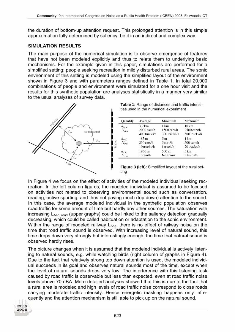
Community: 9th International Congress on Noise as a Public Health Problem (ICBEN) 2008, Foxwoods, CT
the duration of bottom-up attention request. This prolonged attention is in this simple approximation fully determined by saliency, be it in an indirect and complex way.
SIMULATION RESULTS The main purpose of the numerical simulation is to observe emergence of features that have not been modeled explicitly and thus to relate them to underlying basic mechanisms. For the example given in this paper, simulations are performed for a simplified setting: people seeking recreation in mildly disturbed rural areas. The sonic environment of this setting is modeled using the simplified layout of the environment shown in Figure 3 and with parameters ranges defined in Table 1. In total 20,000 combinations of people and environment were simulated for a one hour visit and the results for this synthetic population are analyses statistically in a manner very similar to the usual analyses of survey data.
Table 1: Range of distances and traffic intensi-ties used in the numerical experiment
Figure 3 (left): Simplified layout of the rural set-ting
In Figure 4 we focus on the effect of activities of the modeled individual seeking rec-reation. In the left column figures, the modeled individual is assumed to be focused on activities not related to observing environmental sound such as conversation, reading, active sporting, and thus not paying much (top down) attention to the sound. In this case, the average modeled individual in the synthetic population observes road traffic for some amount of time but hardly any other sources. The saturation with increasing LAeq, road (upper graphs) could be linked to the saliency detection gradually decreasing, which could be called habituation or adaptation to the sonic environment. Within the range of modeled railway LAeq, there is no effect of railway noise on the time that road traffic sound is observed. With increasing level of natural sound, this time drops down very strongly but interestingly enough, the time that natural sound is observed hardly rises. The picture changes when it is assumed that the modeled individual is actively listen-ing to natural sounds, e.g. while watching birds (right column of graphs in Figure 4). Due to the fact that relatively strong top down attention is used, the modeled individ-ual succeeds in its goal and observes natural sounds most of the time, except when the level of natural sounds drops very low. The interference with this listening task caused by road traffic is observable but less than expected, even at road traffic noise levels above 70 dBA. More detailed analyses showed that this is due to the fact that a rural area is modeled and high levels of road traffic noise correspond to close roads carrying moderate traffic intensity. Hence energetic masking happens only infre-quently and the attention mechanism is still able to pick up on the natural sound.
623
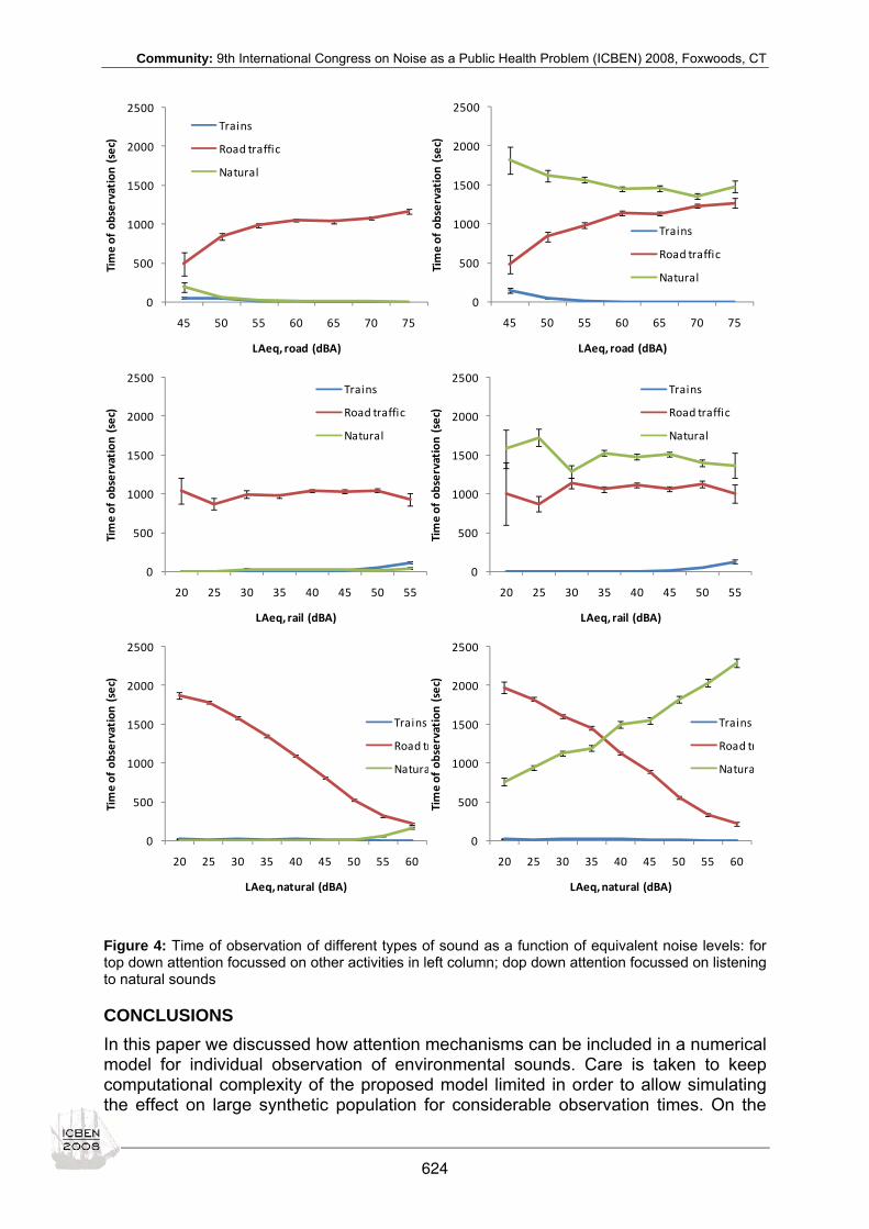
Community: 9th International Congress on Noise as a Public Health Problem (ICBEN) 2008, Foxwoods, CT
0
500
1000
1500
2000
2500
45 50 55 60 65 70 75
Time of observation
(sec)
LAeq, road (dBA)
Trains
Road traffic
Natural
0
500
1000
1500
2000
2500
45 50 55 60 65 70 75
Time of observation
(sec)
LAeq, road (dBA)
Trains
Road traffic
Natural
0
500
1000
1500
2000
2500
20 25 30 35 40 45 50 55
Time of observation
(sec)
LAeq, rail (dBA)
Trains
Road traffic
Natural
0
500
1000
1500
2000
2500
20 25 30 35 40 45 50 55
Time of observation
(sec)
LAeq, rail (dBA)
Trains
Road traffic
Natural
0
500
1000
1500
2000
2500
20 25 30 35 40 45 50 55 60
Time of observation
(sec)
LAeq, natural (dBA)
Trains
Road tr
Natura
0
500
1000
1500
2000
2500
20 25 30 35 40 45 50 55 60
Time of observation
(sec)
LAeq, natural (dBA)
Trains
Road tr
Natura
Figure 4: Time of observation of different types of sound as a function of equivalent noise levels: for top down attention focussed on other activities in left column; dop down attention focussed on listening to natural sounds
CONCLUSIONS In this paper we discussed how attention mechanisms can be included in a numerical model for individual observation of environmental sounds. Care is taken to keep computational complexity of the proposed model limited in order to allow simulating the effect on large synthetic population for considerable observation times. On the
624

Community: 9th International Congress on Noise as a Public Health Problem (ICBEN) 2008, Foxwoods, CT
one hand saliency detection and bottom up attention triggering were modeled in de-tail, on the other hand top down attention was included in a more general way. Simulation of a synthetic population recreating in a mildly disturbed rural area allowed investigating how such a model can generate emergent features for the population as a whole. At least some of these results can be related in a qualitative way to earlier field studies such as (De Coensel & Botteldooren 2006) where we noted that the equivalent noise level of road traffic noise did not accurately predict the disturbance of silence. This could be explained by the saturating time of observation of road traffic sound with LAeq and the limited effect on the observation of natural sound (when fo-cusing attention on it) with increasing LAeq. The better correlation with LA50 observed in this field work could not be checked in the modeling at the time that this paper was written. This paper presents another step forward in an ongoing effort to model the effect of environmental sound on everyday life numerically based on basic knowledge on hu-man perception. An effort that aims at bridging the gap between environmental noise specialists, medical researchers, and psychologists.
REFERENCES Botteldooren D, De Coensel B (2008). A model for long-term environmental sound detection. In: Proceedings of the IEEE World Congress on Computational Intelligence, Hong Kong.
Bregman AS (1994). Auditory scene analysis: the perceptual organization of sound. Cambridge, MA: MIT Press.
De Coensel B, Botteldooren D (2006). The quiet rural soundscape and how to characterize it. Acta Acust Acust 92: 887–897.
De Coensel B, Botteldooren D (2007). Models for soundscape perception and their use in planning. In: Proceedings of Inter-noise, Istanbul, Turkey.
De Coensel B, Botteldooren D (2008). Modeling auditory attention focusing in multisource environments. In: Proceedings of Acoustics’08, Paris, France.
De Coensel B, Botteldooren D, De Muer T (2003). 1/f noise in rural and urban soundscapes. Act Acust Acust 89: 287-295.
De Muer T, Botteldooren D, De Coensel B, Berglund B, Nilsson ME, Lercher P (2005). A model for noise annoyance based on notice-events. In: Proceedings of Internoise, Rio de Janeiro, Brazil.
Fritz JB, Elhilali M, David SV, Shamma SA (2007). Auditory attention – focusing the searchlight on sound. Curr Opin Neuro-biol 17: 437-455.
Gygi B, Shafiro V (2007). General functions and specific applications of environmental sound research. Front Biosci 12: 3152-3166.
Itti L, Koch C (2001). Computational modelling of visual attention. Nat Rev Neurosci 2: 194-203.
Kayser C, Petkov C, Lippert M, Logothetis NK (2005). Mechanisms for allocating auditory attention: an auditory saliency map. Curr Biol 15: 1943-1947.
Knudsen EI (2007). Fundamental components of attention. Annu Rev Neurosci 30: 57-78.
Moore BCJ, Glasberg BR, Baer T (1997). A model for the prediction of thresholds, loudness, and partial loudness. J Audio Eng Soc 45: 224-240.
Sagi B, Nemat-Nasser SC, Kerr R, Hayek R, Downing C, Hecht-Nielsen R (2001). A biologically motivated solution to the cocktail party problem. Neural Comput 13: 1575-1602.
Shi H, Yang Y (2007). A computational model of visual attention based on saliency maps. Appl Math Comput 188: 1671-1677.
Wrigley SN, Brown GJ (2004). A computational model of auditory selective attention. IEEE Trans Neural Netw 15: 1151-1163.
625
Community: 9th International Congress on Noise as a Public Health Problem (ICBEN) 2008, Foxwoods, CT
The results of hum studies in the United States James P. Cowan
URS Corporation, 5 Industrial Way, Salem, New Hampshire, USA
ABSTRACT Stories of mysterious hums, low frequency sounds that only select individuals can hear without being able to identify the source, have become prevalent throughout the world over the past 20 years. In the United States, the first formal study to determine the source of a hum was performed in the Toas, New Mexico area in the early 1990's. The results of that study were inconclusive. In 2003, another U.S. hum study was commissioned in Kokomo, Indiana, where hundreds of residents reported hearing a hum and blamed other, non-acoustical effects on the same phenomenon. In this paper, the lead investigator of the Kokomo Hum study discusses the study and its results, as well as consistencies with the results of the Toas Hum study and the reports of others around the world, in an effort to identify the still-elusive source of this mysterious phenomenon.
INTRODUCTION Over the past 20 years, reports of untraceable sounds that can be heard by select individuals (which have adopted the label of hums by the press) have surfaced around the world. Since the reports began, several studies have been performed to attempt to identify the source of hums, most notably in Europe and the United States. The two largest funded hum studies in the United States were in Taos, New Mexico in 1993 and in Kokomo, Indiana in 2003. The author of this paper was the lead inves-tigator for the Kokomo Hum study, and this paper discusses the nature of hums in general, the specifics of the Taos and Kokomo studies, and lessons learned from those studies that may point us in the direction of identifying these noise sources. As there are many people suffering from the effects of hums, the ultimate goal is to de-termine how to provide relief for affected individuals.
Characteristics of hums A “hum,” as labeled by the press, is a sound that can be heard by some people but cannot be localized using standard acoustic instrumentation. In many cases, hums have been traceable to low frequency acoustic signals generated by industrial sources near communities, but in other cases, no acoustical signals can be detected where affected residents are located. Some people have reported feeling hums through vibrations sensed in different parts of their bodies. Because a small fraction of the populace can sense hums, people who have reported these sensations have often been ridiculed by peers and the press, making people less inclined to report such feelings. One of many common threads among people who sense hums is that they do not appear to be mentally infirm, as vocal critics who do not sense hums have tended to think. What they are sensing is real and is caused by something that they are sensitive to and most others are not. Our task is to determine the source of this phenomenon. Most people who sense hums state that the sensations have begun suddenly and most who hear hums say that what they hear sounds like an idling diesel engine with a pulsating sound pattern. Covering the ears or using hearing protection devises usually does not reduce the sound level heard. Although many have learned to live with the sound, some have reported physiological effects which may or may not be
626

Community: 9th International Congress on Noise as a Public Health Problem (ICBEN) 2008, Foxwoods, CT
related. The most common reported effects include headache, nausea, diarrhea, fa-tigue, and memory loss. Psychological effects of annoyance, feelings of helpless-ness, sleep deprivation, and suicidal thoughts have been reported by affected indi-viduals, all related to the nature of the source being undefined and uncontrolled. It is also interesting to note that many of those affected who have dogs as pets have re-ported that their dogs react to the hums at the same times as they do. Erratic behav-ior of birds and dying vegetation near their homes have also been described by af-fected individuals. Unlike tinnitus, a physical condition for which internal sound is heard all the time at any location, hums appear to be site-specific. Most people who sense hums report that they do not sense the hums when they leave a general area (as large as a city or state), and they sense the hums both inside and outside of their homes. When driv-ing out of an area the hum often is reported to go away and when driving back into the original area the hum returns. This implies an external stimulus. Most people who sense hums also report that the signals are most noticeable late at night but they still hear them most of the time in specific geographic areas. There do not appear to be trends related to gender and age among people who sense hums. Since the cause of these hums is elusive, many theories have arisen as the cause for the hums, which vary from the plausible to the extreme, adding fuel to the media fire of interest in the phenomenon. A plethora of theories fill the internet with statements of proof for the cause of hums, yet none of these statements provides clearly sup-portable data.
Hum studies The two most comprehensive hum studies performed in the United States were in Taos, New Mexico and Kokomo, Indiana. These are discussed below.
The Taos Hum Study The most publicized of the American hum studies took place in Taos, New Mexico in the spring of 1993. The Taos Hum study resulted from U.S. congressional action re-acting to local concern. The official study took place over a week-long period through a cooperative effort between Los Alamos National Laboratory, Sandia National Labo-ratories, Phillips Air Force Laboratory, and the University of New Mexico. The study was set up as an open public investigation coordinated by the University of New Mexico to allay concerns that a government agency may have been responsible for the hum and government-funded laboratories, working alone, may bias the results of the study. According to unpublished study documentation in internal memoranda, 161 people reported sensing the hum out of a survey of 8,000 residents. Some of these residents took part in the study to identify when they sensed the hum concurrent with the moni-toring. Equipment was used to monitor not only sound, but seismic activity and elec-tromagnetic fields in the area. After a week of continuous monitoring (during which time affected residents were hearing the hum), the only unusual activity that could be reported by the measuring instruments was an elevated electromagnetic field level that was reportedly related to the local power lines. There had also been reports from affected people related to malfunctioning of electrical appliances in and around their homes.
627

Community: 9th International Congress on Noise as a Public Health Problem (ICBEN) 2008, Foxwoods, CT
Although many affected residents could replicate the sounds that they heard on sig-nal generating equipment, no such acoustic signals were detected by any instru-ments during the study. No hum source was identified from the Taos Hum study.
The Kokomo Hum Study The Kokomo Hum study resulted from a fund commissioned by the City of Kokomo, Indiana. The team performing the study was chosen through a national search and interview process. The study began with a public meeting and private interviews of affected residents. One hundred twenty six residents were formally documented as being affected by the hum. Their homes were spread throughout the City. Several of those who were inter-viewed stated that they knew other affected residents who did not wish to be identi-fied for personal reasons. During the last weeks of March and April 2003, the project team recorded sound and ground vibration levels at the homes of affected residents throughout the City. Due to the reported electrical issues in Taos and Kokomo, elec-tromagnetic fields were also recorded using a portable gauss-meter. According to American National Standards Institute (ANSI) Standard ANSI 3.29-1983, (“Guide to the Evaluation of Human Exposure to Vibration in Buildings”), the mean human perception limit for ground-borne vibrations in the 8 to 80 Hz frequency range is 8,000 microinches per second. The same standard states that the most sen-sitive human perceptibility limit is 4,000 microinches per second. These limits in-crease for frequencies lower than 8 Hz. With these limits in mind, ground-borne vibra-tion levels were monitored at 12 locations throughout the City where hums had been reported. No ground vibration levels in excess of 200 microinches per second were measured at any location, including locations where residents claimed that they felt vibrational symptoms while the data were being recorded. Since the measured vibra-tions were more than 10 times below the level of minimum perception, it was con-cluded that ground-borne vibration was not an issue for this investigation. From acoustic measurements, significant sound pressure level tones at 10 Hz (along with associated harmonics up to 60 Hz) and 36 Hz were detected at some of the residential locations while residents were present and feeling symptoms. These tones were each 20 to 40 decibels above the background levels. A 360-degree rotat-ing dual-microphone boom was used at three locations to localize the 10 Hz tone to air compressors in an industrial facility near the center of the City. The 36 Hz tone was localized to a cooling tower on the roof of another industrial plant in a different section of town. In each case, the tones were clearly detectable at more than a 1 km radius from the sources. In addition to these two facilities, several residents mentioned two other facilities that they were concerned about in the northern end of the City. Tunneling operations were being conducted at one of these facilities so underground access needed to be granted to investigate whether the noise from these operations or their associated ventilation fans could be generating the low-frequency tones measured in the com-munities. Since the fans did not generate any tones consistent with what was moni-tored in the communities and the facility did not operate at night (when most of the affected people sensed the hum), this facility was eliminated from consideration. No noise was audible or measurable from the other facility. Management from the two industrial facilities that were identified as generating 10 and 36 Hz tones each volunteered to replace equipment and install silencing equip-ment to lower the emission levels of the tones. After these noise control measures
628

Community: 9th International Congress on Noise as a Public Health Problem (ICBEN) 2008, Foxwoods, CT
had been implemented in the spring of 2004, the project team visited the City and monitored the acoustic signals at the same locations as before. At that time, the 10 and 36 Hz tones were not detectable above the background levels at the same loca-tions where they were previously more than 20 dB above the background. At this point, some affected residents expressed relief from their symptoms but most did not. In fact, one affected resident had become so disturbed that she moved more than 700 miles away to relieve her symptoms. Since many affected residents mentioned unusual occurrences related to home elec-trical systems, including appliances suddenly burning out and cars having remote starters unexpectedly starting in garages, electromagnetic fields were monitored in areas where residents appeared to be most affected. In most cases, elevated elec-tromagnetic field strengths of 3 to 50 milliGauss were experienced in and around the homes.
DISCUSSION There has been a fair amount of discussion among affected individuals relating hums to low frequency sound, mainly because most people who hear hums report hearing just that. However, most hums that remain untraceable cannot be detected with acoustic instrumentation. If low frequency sound is the foundation of hums, it would be detectable by microphones that are sensitive to those frequency ranges. In fact, a special microphone was developed by the Taos Hum team to monitor low frequency acoustic signals and that microphone picked up nothing unusual in that study. Al-though no special microphones were used for the Kokomo Hum study, the micro-phones were rated to perform well down to below 5 Hz. Although low frequency tones were found in Kokomo, their reduction in intensity made little difference for most of the people affected by the hum. All indications were that the hum is not a tra-ditional acoustical phenomenon and therefore not associated with low frequency acoustic energy. The only apparent common thread is that of elevated electromagnetic fields and the potential for some people to have the sensation of hearing stimulated by these fields. Research by Frey (1962) more than 40 years ago introduced the potential for micro-wave hearing, a phenomenon by which people (including the clinically deaf) can hear sounds related to electromagnetic field exposures that are not accompanied by measureable acoustic pressure fluctuations. This has been attributed to ther-moacoustic effects in the brain (bypassing the traditional hearing mechanism) caused by electromagnetic energy but little research on the phenomenon has been per-formed since Frey’s early work. Symptoms other than hearing sounds referenced in Frey’s work, such as a “pins-and-needles sensation,” have been reported by indi-viduals experiencing hums. When asked what changed in their environment at the time they began sensing the hum, most referred to utility work associated with telephone, cable television, or power line maintenance, or a new cell phone tower in the neighborhood. Since being involved with the Kokomo Hum study, the author has been contacted by people from many areas of the United States, as well as Europe, with similar stories to those in the Kokomo area, both in terms of symptoms and environmental changes. Hums are clearly not localized to Taos and Kokomo. Earlier in this discussion, there was mention of the observance of erratic bird and dog behavior related to this phenomenon. It has long been recognized by authors such as Ritz et al. (2000) that the natural geomagnetic fields surrounding the earth are related
629

Community: 9th International Congress on Noise as a Public Health Problem (ICBEN) 2008, Foxwoods, CT
to migratory patterns of birds and other animals, so these animals may be more sen-sitive to variations in electromagnetic fields than most people. There has been a significant amount of debate related to the health effects of elec-tromagnetic fields and this discussion is not meant to support either side of that ar-gument. The results of the Taos and Kokomo studies shed light on the need for fur-ther investigation to determine the potential for electromagnetic fields to become au-dible by a means other than the auditory apparatus. By uncovering this transduction mechanism, indications are that we will solve the mystery of hums around the globe and find practical solutions for those who are affected by them.
REFERENCES Frey AH (1962). Human auditory system response to modulated electromagnetic energy. J Appl Physiol 17: 689-692.
Ritz T, Adem S, Schultenet K (2000). A model for photoreceptor-based magnetoreception in birds. Biophys J 78: 707-718.
630

Community: 9th International Congress on Noise as a Public Health Problem (ICBEN) 2008, Foxwoods, CT
The effectiveness of quiet asphalt and earth berm in reducing annoyances due to road traffic noise in a residential area Anita Gidlöf-Gunnarsson1*, Evy Öhrström1 1 The Sahlgrenska Academy at the University of Gothenburg, Department of Occupational and
Environmental Medicine, Box 414, SE 405 30 Gothenburg, Sweden
* corresponding author: e-mail: [email protected]
INTRODUCTION Current noise abatement measures largely focuses on caring the indoor sound envi-ronment with closed windows (today, façade reduction > 40 dB is possible). The out-door sound environment has been much more difficult to protect. For example, road-side noise barriers may reduce traffic sound levels from 7 up to 10 dB. An alternative technique is “quiet” asphalt or “silent roads”, which commonly reduces the level slightly less than a barrier does, but has less impact on the visual landscape. There is, however, very little research on how effective these types of abatement measures are in improving the perceived sound environment and reducing adverse noise health effects. Studies on noise barriers (e.g., Lambert 1978; Kastka et al. 1995; Öhrström 1995; Nilsson & Berglund 2006) indicate both greater and smaller effects on annoy-ance than would be expected from the amount of reduction of the noise level. Sug-gested factors of importance for explaining these findings are, for example, the physical and visual effects of barriers and expectations about the effectiveness of barriers to reduce traffic noise (Öhrström 1995), the use of a different response pat-tern to noise or coping patterns in the before and after situations (e.g., Kastka et al. 1995), if noise sources are visually hidden or not (e.g., Watts et al. 1999), not sepa-rated measures of indoor and outdoor annoyances (Nilsson & Berglund 2006), a psychological treatment effect (Adair 1984), and attitudes towards the noise source (Job 1988). The application of quiet asphalt has during recent years steadily increased and been suggested as an effective abatement measure to reduce noise levels from road traf-fic. However, it is hard to find studies that evaluates how the quiet asphalt affect sub-jective experiences e.g., perceptions of the sound environment and effects on health and well-being. Bendtsen and colleagues (Bendtsen et al. 2002) conducted an inter-vention study with the application of various types of two-layer pavements on an ur-ban road (speed limit 50 km/h). The reduction of noise levels were ~7.6 dB and an-noyance indoors with closed window decreased from ~38 to ~12 % in the after study. The residents also experienced less annoyance from air pollution, dust/dirt and vibra-tions due to the traffic. The objectives first stated in the present before-after study was to investigate the ef-fects on resident’s noise responses of two types of roadside noise barriers; a conven-tional noise barrier of wood and an earth berm. However, after the before study was conducted in 2005, responsible authorities decided to replace the wooden barrier with quiet asphalt. This consequently changed the circumstances for the after study. The objectives then shifted to study how an intervention with quiet asphalt only and an intervention with quiet asphalt and an earth berm as a combined noise abatement measure affected the resident’s responses to noise.
631

Community: 9th International Congress on Noise as a Public Health Problem (ICBEN) 2008, Foxwoods, CT
A B
C
METHOD Design, study area and population, and response rate A longitudinal questionnaire field study including two waves was conducted in the same residential areas: Wave 1 in September 2005 and Wave 2 in September 2007 after implementation of noise abatement measures during 2006. The investigated area, which consists of 3-4 storey apartment buildings built during 1950 and 1960, is located close to a traffic-intensive road (“Högsboleden”) in Gothenburg, Sweden (see the aerial photograph in Figure 1). In Quarter A, three buildings and a small play-ground are exposed to high levels of traffic noise, up to LAeq,24h 71 dB (free field val-ue) at the most exposed dwellings. In Quarter B, one building is located diagonally towards the main road. A green area with trees separates the building and “Högs-boleden”. An open parking deck is also situated there, but it has a minor screening effect on the traffic noise. Sound levels at most exposed dwellings are about LAeq,24h 66 dB. The buildings in Quarter C are mainly located along a local road (”Guldmynts-gatan”) with sound levels between LAeq,24h 58-61 dB. The study population were all 262 adult residents (18-75 years of age) living in the apartment buildings. In the before study, the participation rate was 68 % (n=177). In the after study, 93 out of 152 residents (61 %) responded (some had moved, were sick or had died). Out of the original study population, 53 % participated both before and after the intervention of noise abatement measures. Figure 1: Aerial photograph shows residential areas before noise abatement measures were implemented: Quarter A = quiet asphalt; Quarter B = quiet asphalt+earth berm; and Quarter C = no direct abatement measure were applied here.
Noise abatement measures The first suggestion of noise abatement measures to implement referred to a 376 m long and between 2.4 to 2.7 m high conventional noise barrier of wood in Quarter A and a 115 m long and 3.4 m high earth berm in Quarter B (Figure 2). However, due to insufficient financial resources it was decided that 2-Layered Porous Asphalt (max chipping size of first and second layers are 11 and 16 mm, respectively) should re-place the noise barrier of wood in Quarter A, but also be laid further down the main road passing Quarter B (approximately length after implementation = 700 m of quiet asphalt). The length and height of the earth berm decreased somewhat to 105 m and 2.4 m, respectively, when implemented.
632

Community: 9th International Congress on Noise as a Public Health Problem (ICBEN) 2008, Foxwoods, CT
Figure 2: Schematic picture of planned noise abatement measures (the study area is shown in an opposite angle compared to Figures 1 and 3).
Assessment of traffic sound levels In 2001, the number of counted vehicles on the main road “Högsboleden” was be-tween 19,700 to 24,100 vehicles/24h (7 % were heavy vehicles). The speed limit is set to 70 km/h. Calculations of equivalent sound levels (LAeq,24h) in the before study were made based on the Nordic Calculation Model (Swedish EPA, 1996) at noise-exposed and quieter facades, 5 m above ground, which corresponds to the second floor of the houses (see the circles in Figure 3). A set of short-term measurements (~30 min) were made in October 2005 and 2006 by the Environmental and Health Authority in Gothenburg (Brandberg 2006), before and after the implementation of noise abatement measures. Figure 3: Calculated LAeq,24h in the studied residential area (circles) before implementation of noise abatement measures and locations of short-term measurements (red stars) in 2005 and 2006.
Short-term measurements of A-weighted sound pressure level with time weighting FAST (LAFmax) and LAeq,30min before and after implementation of noise abatement measures (see location in Figure 3, red stars) show that the application of quiet aphalt in Quarter A decreases both LAFmax and LAeq with ~5.5 dBA (median sound levels of 2 X LAeq,30min).
Quarter B Quarter A
Earth berm
Wodden barrier with a section of glass
Wodden barrier with vegetation
65
616466
61
65 63 62
61 62
59
5857
5050
Wooden barrier with a section of glass
Wooden barrier with vegetation
633

Community: 9th International Congress on Noise as a Public Health Problem (ICBEN) 2008, Foxwoods, CT
Figure 4: Spectra for two 30 min measurements conducted in Quarter A before (red line) and after (green line) application of quiet asphalt.
Figure 4 shows average 1/3-octave band spectra of two 30 min measurements, be-fore (red line) and after (green line) the application of quiet asphalt in Quarter A. The result indicates that the quiet asphalt did not reduce the sound levels in the low-frequency bands, i.e., below ~200 Hz band. Correspondingly, the implementation of quiet asphalt+earth berm in Quarter B reduced the sound levels somewhat more, ~6.5 dB, but up to 10 dB in the low-frequency band between 100-250 Hz (Figure 5), which mainly depends on the shielding effect of the earth berm. The reduction of sound levels in Quarter C was estimated to be ~4 dB. (Brandberg 2006). Figure 5: Spectra for two 30 min measurements conducted in Quarter B before (red line) and after (green line) application of quiet asphalt+earth berm.
Questionnaire The self-administered questionnaire was based on previously developed question-naires evaluating adverse health effects and well-being due to road traffic noise (Öhrström et al. 2006), but adapted to the present intervention study. Overall, the same questionnaire was used in both study waves. The questionnaire contained sec-tions about subject’s living environment and various sources of nuisance, noise an-noyance and interferences with various activities, percieved sleep quality, socio-demographic and person factors etc. The current paper is mainly focused on present-ing the effect of noise abatement measures on road traffic noise annoyances, per-ceptions of the outdoor sound environment, appraisal of sound quality outdoors, as
1/3-octave-band center frequency (Hz)
1/3-
octa
ve-b
and
soun
d le
vel (
dB)
1/3-octave-band center frequency (Hz)
1/3-
octa
ve-b
and
soun
d le
vel (
dB)
634

Community: 9th International Congress on Noise as a Public Health Problem (ICBEN) 2008, Foxwoods, CT
well as resident’s expectations of how noise abatement measures will change the sound environment.
RESULTS Traffic noise annoyances as a function of type of noise abatement measures Noise annoyance at home was assessed with an ISO standardized 5-point category scale ranging from “not at all annoyed” to “extremely annoyed” (ISO 2003). Left panel in Figure 6 shows percentage of annoyed residents (moderately and very and ex-tremely) as a function of intervention of noise abatement measure. Only the imple-mentation of quiet asphalt+earth berm in Quarter B significantly decreased the pro-portion of annoyed residents from 41 to 19 % (p<0.05, McNemar-test). For noise an-noyance indoors with open window (10-point numeric scale with verbal end points; 0=not at all annoyed and 10=extremely annoyed), the average annoyance signifi-cantly decreased with quiet asphalt+earth berm (p<0.01, paired samples T-test). There were no significant effects of quiet asphalt on annoyances in Quarter A. Figure 6: Percentage annoyed residents (left panel) and mean annoyance with open window (right panel) before and after noise abatement measures in Quarter A = quiet asphalt, n=39; Quarter B = quiet asphalt+earth berm, n=27; and Quarter C = no direct abatement measure implemented, n=27. *p<0.05; **p<0.01
Perceptions of the outdoor sound environment appraisal of sound quality Perceptions of the outdoor sound environment were assessed with two statements referring to experiencing the sound environment as relaxing and as dominated by road traffic noise. Four-point scales were used ranging from “totally disagree” to “to-tally agree”. Figure 7 shows percentage of the residents “totally agree” in the state-ments in relation to type of noise abatement measures. The results indicate that the perceived outdoor sound environment differ a lot between the quarters. Before the intervention, a greater proportion of resident’s in Quarter A experienced the outdoor sound environment in a positive way than resident’s in Quarter B and C did. How-ever, the implementation of quiet asphalt and earth berm did not significantly change the perceptions of the outdoor sound environment in any of the three Quarters.
**
*
635

Community: 9th International Congress on Noise as a Public Health Problem (ICBEN) 2008, Foxwoods, CT
Figure 7: Percentage of residents who totally agree in statements about the outdoor sound environ-ment before and after noise abatement measures in Quarter A = quiet asphalt, n=39; Quarter B = quiet asphalt+earth berm, n=27; and Quarter C = no direct abatement measure implemented, n=27.
Appraisal of sounds when being outdoors close to the dwelling were assessed with 14 sound quality descriptors on 5-point category scales ranging from “not present” to “dominates”. A principal component analysis with varimax rotation of the before-study data extracted three factors with an eigen value above 1. In total 63 % of the vari-ance was explained by these three factors. Factor 1 represent distinct sounds (e.g., sharp, rattles), Factor 2 represent high frequency sounds like swishing and buzzing, and Factor 3 represent low frequency sounds such as muffled and dull. Figure 8 shows the sound quality descriptor with the highest loading in each of the three fac-tors extracted as percentage of the resident’s hearing the sounds very clearly or do-minating when being outdoors close to the dwelling. In the before-study, sounds of sharpness appeared most clearly in Quarters A and C, and correspondingly for Quar-ter B, it was the swishing sounds. After application of the quiet asphalt and the earth berm, the sharp and muffled sounds were found to have decreased significantly for residents in Quarter B and the sharp sounds in Quarter C (p<0.05, McNemar-test). Figure 8: Percentage of residents reporting sounds appearing very clearly/dominating in the outdoor environment close to the dwelling before and after noise abatement measures in Quarter A = quiet asphalt, n=39; Quarter B = quiet asphalt+earth berm, n=27; and Quarter C = no direct abatement measure implemented, n=27. *p<0.05
Sharp Swishing Muffled Sharp Swishing Muffled Sharp Swishing Muffled
BeforeAfter
*
*
*
636

Community: 9th International Congress on Noise as a Public Health Problem (ICBEN) 2008, Foxwoods, CT
Expectations of a better sound environment and association with annoyance Since a noise barrier of wood and an earth berm were the planned noise interven-tions in 2005, statements about the effectiveness of a noise barrier (not quiet asphalt) in improving the outdoor sound environment were asked in the before study (four re-sponse categories ranging from “no or low expectations” to “very high expectations”). As can be seen in Table 1, about the same amount of residents in Quarters A and B had high expectations about the noise barrier’s effectiveness of improving the out-door sound environment (fewer residents in Quarter C). However, high expectations about possibilities to be outdoors without being disturbed by traffic and be able to have a relaxed communication in the before study were only significantly correlated (r) with high noise annoyance outdoors in the after study for Quarter A. Table 1: Expectations in the before study about effects of the erection of noise barriers (%) for Quar-ter A = quiet asphalt; Quarter B = quiet asphalt+earth berm; and Quarter C = no direct abatement measure implemented and associations with noise annoyance outdoors (r).
Quarter A Quarter B Quarter C Expectations about effects of noise abatement measures on various residential situations
%a rb %a rb %a rb
To be able to be outdoors closed to the dwell-ing without being disturbed by traffic
36 0.41* 35 0.26 23 0.14
To be able to communicate outdoors in a relaxed way without being disturbed by traffic
36 0.45** 38 0.17 19 -0.12
To be able to hear sounds from nature (e.g., birdsong, whistling wind) when being outdoors
51 0.28 50 0.10 31 0.03
a Percentage with high and very high expectations b Pearsons’ product moment correlation coefficient between expectations and noise annoyance outdoors (0-10 response scale) *p < 0.05; **p <0.01
COMMENTS AND CONCLUSIONS The overall results indicate that only the implementation of both quiet asphalt and an earth berm in Quarter B significantly reduced resident’s general noise annoyance and annoyance indoors with open window. Unexpectedly, the application of quiet asphalt in Quarter A had a negligible effect on annoyance. In Quarter C with no direct noise abatement measure implemented, the annoyance result was mixed. According to short-term measurements, sound levels in quarter A, B, and C decreased in year 2007 by ≈5.5, 6.5, and 4 dB, respectively, which are in agreement with estimated reduction of the sound levels for the three situations before the intervention. However, the differences in annoyance reduction indicate that there is not a simple causal relation with noise level reductions. Although the general noise annoyance in the before study was somewhat higher in Quarter B than in Quarter A and C, the mean noise levels estimated for each resident did not differ much between Quarter A and B (mean=64.3, SD=1.60 and mean=63.6, SD=1.37, respectively). In Quarter C, sound levels were lower (mean=59.1, SD=1.31). For perceptions of the outdoor sound environment nearby the dwelling, we found a small or no effect of the implementation of the quiet asphalt and the earth berm. However, there were differences between the three Quarters in responses. Before the implementation of the noise abatement measures, only very few in Quarter A and C perceived the outdoor sound environment as relaxing, whereas one fourth perceived this in Quarter B. In both Quarter A and C many residents instead experienced the outdoor sound environment as dominated by road traffic sounds. A probable reason for this is that more residents in Quarter A had access to a quiet
637

Community: 9th International Congress on Noise as a Public Health Problem (ICBEN) 2008, Foxwoods, CT
outdoor place (59 %), as self-reported in the questionnaire, in comparison with Quar-ter A (13 %) and C (30 %). Previous studies show that access to a quiet side of one’s dwelling is important for reducing adverse health effects due to road traffic noise (Öhrström et al. 2006). Thus, a quieter shielded outdoor place, such as a common courtyard, will give opportunities to escape from the noisy outdoor side of the building and to perceive a more positive sound environment. The appraisal of sounds heard when being outdoors close to the dwelling and the decrease of some sounds in the after study indicates an association with locations of the buildings and type of noise abatement measure implemented. In both Quarter A and C, the sharpness sound appeared very clearly among a somewhat higher proportion of the residents than in Quarter B. This may be due to the fact that the apartment buildings in both Quarter A and C are located closer to the trafficked roads than the apartment building in Quarter B, which is diagonally situated towards the main road. The significant reduction of the muffled sounds in Quarter B indicate an effect of the earth berm. This is supported by the reduction of the low-frequency noise mearsured in the before and after studies and shown in Figure 5. A potential important factor in explaining the insignificant effect of the quiet asphalt in the present study is the unexpectedly change of planned noise abatement measure from a noise barrier to the application of quiet asphalt for the residents in Quarter A. This change together with high expectations of a significant improvement of the sound environment after the intervention may have created feelings of disappoinment that could have influenced the results.
ACKNOWLEDGEMENTS This study is based on research performed as part of the program Soundscape Sup-port to Health, sponsored by the Swedish Foundation for Strategic Environmental Research (MISTRA).
REFERENCES Adair G (1984). The Hawthorne effect: A reconsideration of the methodological artifact. J Appl Psychol 69: 334-345.
Bendtsen H, Larsen LE, Greibe P (2002). Udvikling af støjreducerande vejbelægninger til bygader. Statusrapport efter 3 års målinger. Rapport 4, Danmarks Transport Forskning. [www.dtf.dk].
Brandberg J (2006). Bullermätningar före och efter asfaltering med bullerdämpande asfalt på Högsboleden 2006. PM 2006-11-18, Miljöförvaltningen Göteborgs Stad.
ISO (2003). Technical Specifikation ISO/TS15666.
Job RFS (1988). Over-reaction to changes in noise exposure: The possible effect of attitude. J Sound Vibr 126: 550-552.
Kastka J, Buchta E, Ritterstaedt U, Paulsen R, Mau U (1995). The long-term effect of noise protection barriers on the annoy-ance response of residents. J Sound Vibr 184: 823-852.
Lambert R (1978). Experimental evaluation of a freeway noise barrier. Noise Contr Engineering Sep-Oct: 86-94.
Nilsson ME, Berglund B (2006). Noise annoyance and activity disturbance before and after erection of a roadside barrier. J Acoust Soc Am 119: 2178-2188.
Öhrström E (1995). Upplevelsemässiga aspekter på bullerskydd. En litteraturstudie [Perceptual aspects of noise abatement measures: A literature review]. Borlänge: Vägverket, Rapport 1/98. Department of Occupational and Environmental Medicine at the University of Gothenburg.
Öhrström E, Skånberg A, Svensson H, Gidlöf-Gunnarsson A (2006). Effects of road traffic noise and the benefit of access to quietness. J Sound Vibr 295: 40-59.
Watts G, Chinn L, Godfrey N (1999). The effects of vegetation on the perception of traffic noise. Appl Acoust 56: 39-56.
638

Community: 9th International Congress on Noise as a Public Health Problem (ICBEN) 2008, Foxwoods, CT
Acoustical factors influencing noise annoyance of urban population Branko Jakovljevic1*, Goran Belojevic1, Katarina Paunovic1 1 Institute of Hygiene and Medical Ecology, School of Medicine, University of Belgrade, Dr Subotica
8, 11000 Belgrade, Serbia
*corresponding author: e-mail: [email protected]
INTRODUCTION Noise annoyance is a feeling of displeasure (“nuisance”, “disturbance” or “irritation”) caused by noise, which affects people’s quality of life. Several characteristics of noise – its level, source, and number of noise events, are associated with noise annoyance. Noise annoyance is a major public health problem, since 24 million peo-ple (out of 380 million) in the European Union are highly annoyed by road traffic noise higher than 55 dB for 24 hours (Ldn) (EEA 2000). Noise measurements per-formed in Belgrade in the last 30 years indicate that noise limits are exceeded by 11-16 dB in daytime and by 10-14 dB at night (Institute of Public Health of Belgrade 2002). However, the extent of noise annoyance in Serbian population is not known. In the near future Serbia will implement several environmental regulations, including the Directive 2002/49/EC of the European Parliament and of the Council, relating to the assessment and management of environmental noise (Directive 2002/49/EC, 2002). Therefore, this is the first study on noise annoyance in Serbian population. The aim of this study was to assess the effect of acoustical factors influencing noise annoyance of residents of city centre of Belgrade, Serbia.
METHODS The study was performed in city centre of Belgrade, on a sample of 1,836 adults (mean age 46±23 years): 776 men and 1,060 women. Investigators distributed a questionnaire on noise annoyance to flat owners, and collected them the other day. Noise annoyance was assessed using a self-reported numerical scale (range 0-10), and high-level noise annoyance was described as score ≥ 6. Subjects were asked to rate the most important sources of noise in their environment. All questionnaires were anonymous. Noise was measured in all 70 streets of the municipality, using Noise Level Analyzer type 4426 “Brüel & Kjær” (ISO 1982). Equivalent noise levels [Leq (dBA)] were measured in two day intervals, an evening interval, and two night intervals. Time in-terval of each measurement was 15 minutes; the speed of sampling was 10 per sec-ond, with 9,000 samples collected per measurement at one site. From the obtained Leq levels, we calculated composite daytime Leq, evening Leq, nighttime Leq, and 24-hour Leq for each street and maximal noise levels (Lmax) at daytime and night-time. Traffic density at each site was measured by counting light and heavy vehicles per hour. Descriptive statistic is presented as mean values ± standard deviation (SD) for nu-meric variables, or as percents (relative numbers) for categorical variables. The dif-ferences between groups were tested using Chi-square test and Mann-Whitney U test. The association between mean score on annoyance scale and noise character-istics was measured by Pearson's correlation coefficient. Univariate logistic regres-sion was performed to calculate odds ratios for high-level annoyance in relation to relevant independent variables. The influence of noise characteristics on high-level annoyance was estimated using multivariate logistic regression.
639

Community: 9th International Congress on Noise as a Public Health Problem (ICBEN) 2008, Foxwoods, CT
RESULTS The population was highly annoyed by noise: mean score on noise annoyance scale was 7.14±2.07 for men, and 7.23±3.05 for women. In total, nearly 36 % of the popu-lation was highly annoyed by noise (Table 1). Highly annoyed and less annoyed groups were comparable by age, gender, education, and residential characteristics (flat size and years of residence).
Table 1: Basic characteristics of investigated population
The most important noise sources Less annoyed Highly annoyed Total p value
Number of subjects 1,169 (63.7 %) 667 (36.3 %) 1,836 (100.0 %) Gender (male) 468 (40.0 %) 256 (38.4 %) 724 (39.4 %) 0.421*
Age (years) 45.7±20.3 47.6±17.8 46.2±23.1 0.741† Education 724 (61.9 %) 373 (55.9 %) 1,097 (59.7 %) 0.058* Flat size 65.7±24.0 63.8±25.7 64.3±25.6 0.066†
Years of residence 18.4±16.1 17.3±14.8 17.8±15.3 0.483†
* Chi-square test
† Mann-Whitney U test
The most important noise sources are represented in Table 2. More than a half of all residents identified road traffic as the most important source of noise, but significantly more highly annoyed residents (63.3 %), than less annoyed persons (51.6 %). Second most important source of noise were construction works in the street, and they were more important for less annoyed residents. Neighborhood noise, industrial facilities and electrical appliances in buildings were least important sources of noise in the investigated population.
Table 2: Subjective rating of noise sources of investigated population
The most important noise sources Less annoyed Highly annoyed Total p value Road traffic 603 (51.6 %) 422 (63.3 %) 1025 (55.8 %) <0.0001*
Construction works in the street 275 (23.5 %) 104 (15.6 %) 379 (20.6 %) 0.004* Neighborhood noise 192 (16.4 %) 100 (15.0 %) 292 (15.9 %) 0.216* Industrial facilities 49 (4.2 %) 36 (5.4 %) 85 (4.6 %) 0.737*
Electrical appliances & elevators 96 (8.2 %) 38 (5.7 %) 134 (7.3 %) 0.202*
* Chi-square test
In the whole population, noise annoyance was strongly correlated with nighttime noise level (Leq) and number of heavy vehicles during night. Besides, 24-hour noise, daytime and evening noise, as well as number of vehicles at day and night, were alos significantly correlated to mean annoynace score (Table 3).
640

Community: 9th International Congress on Noise as a Public Health Problem (ICBEN) 2008, Foxwoods, CT
Table 3: Correlation coefficients between noise characteristics and mean score on noise annoyance scale of investigated population
Noise characteristics Correlation coefficients* p value Nighttime noise level (dBA) 0.135 <0.0001
Number of heavy vehicles during night 0.129 <0.0001 Maximum noise at night (dBA) 0.099 <0.0001
24-hour noise level (dBA) 0.090 <0.0001 Evening noise level (dBA) 0.085 <0.0001 Daytime noise level (dBA) 0.084 <0.0001
Number of heavy vehicles during day 0.081 <0.0001 Number of light vehicles during day 0.074 0.001 Number of light vehicles during night 0.073 0.001
Maximum noise at night (dBA) 0.013 0.542
* Pearson’s correlation coefficient
Logistic regression identified nighttime noise level and number of heavy vehicles as the strongest predictors of high-level noise annoyance of urban population (Table 4).
Table 4: Odds Ratios (95% Confidence Interval) for high-level noise annoyance* in relation to noise characteristics of investigated population, adjusted for age and gender
Noise characteristics† OR 95 % CI p value Nighttime noise level (dBA) 1.026 1.011-1.042 0.001
Number of heavy vehicles during night 1.015 1.000-1.010 <0.0001
* High-level noise annoyance defined as mean score on annoyance scale ≥ 6
† Variables in model: Age, Gender, Nighttime noise level, Evening noise level, Daytime noise level, 24-hour noise level, Number of light vehicles during night, Number of heavy vehicles during night, Number of light vehicles during day, Number of heavy vehicles during day
DISCUSSION There are numerous evidences for dose-effect relationship between noise level and annoyance level (Fidell et al. 1991; Bjorkman 1991; Sato et al. 1999; Klæboe et al. 2004). Miedema & Oudshoorn (2001) developed a mathematical model that can pre-dict the percentage of persons annoyed by noise level. Noise exposure in these stud-ies was described as either composite day-night Leq level (Ldn) or composite day-evening-night noise level (Lden). Most of these authors studied road traffic, aircraft and railway noise separately. In our study, when all noise characteristics are consid-ered, nighttime noise was the strongest independent predictor for noise annoyance. This finding may be explained by the fact that residents of urban areas usually spend their daytime at work, whereas they spend most of their evenings and nights at home. Another important noise characteristic is the number of noise events. Our study shows that number of vehicles during nighttime and daytime correlate with annoy-ance, but the most important is the number of heavy vehicles at nighttime. This is similar to the findings of Björkman (1991), who reported increase of the extent of an-noyance with the increase of noise events, and suggested that the number of heavy vehicles can be a good indicator of the number of noise events for road traffic noise. The relationship between noise annoyance and nighttime number of noisy events was also confirmed for aircraft noise (Quehl & Basner 2006). On the other hand, Sato
641

Community: 9th International Congress on Noise as a Public Health Problem (ICBEN) 2008, Foxwoods, CT
et al. (1999) found strong relationship between noise annoyance caused by road traf-fic noise and noise levels, but not with the number of noise events. In comparing the different means of transportation, noise from road traffic is more annoying than that from the railroad (Ouis 2001). On the other hand, Kurra et al. (1999) found that railway noise was the most prominent noise source in the overall annoyance, but also concluded that the source type was not a highly deterministic factor while the respondents were concentrating on daily work at home. However, we find that various sources of noise should not be observed separately. Miedema (2004) suggested a model concerning noise annoyance from combined sources (aircraft, road-traffic and railway noise). In our study, we considered road traffic noise to be the most important, and we measured equivalent noise levels for road traffic noise. Nevertheless, based on the responses from our subjects, sources of noise other than traffic, such as neighborhood noise, are probably equally impor-tant. Therefore, one limitation of this study is that we did not include noise emitted from other sources that our residents consider important.
CONCLUSIONS In conclusion, this cross-sectional study on an adult population of a Belgrade munici-pality showed significant association between nighttime road-traffic noise and high noise annoyance of urban residents. We suggest the use of nighttime noise level as exposure indicator for noise annoy-ance assessment. Nighttime noise countermeasures might also have a greater public health impact compared to daytime, including a possible influence on the incidence of noise annoyance in urban population.
ACKNOWLEDGEMENT This study was financially supported by the Ministry of Science of Serbia, Project No. 145013, 2006-2010.
REFERENCES Björkman M (1991). Community noise annoyance. Importance of noise levels and the number of noise events. J Sound Vibr 151: 497–503.
Directive 2002/49/EC (2002). European Parliament and of the Council of 25 June 2002 relating to the assessment and man-agement of environmental noise. Off J Europ Comm L 189/12.
EEA, European Environment Agency (2000). Are we moving in the right direction? Indicators on transport and environmental integration in the EU: TERM 2000. Environmental issue report No 12. Indicator 4: Traffic noise: exposure and annoyance. Copenhagen, Denmark: European Environment Agency.
Fidell S, Barber DS, Schultz TJ (1991). Updating a dosage-effect relationship for the prevalence of annoyance due to gen-eral transportation noise. J Acoust Soc Am 89: 221–233.
Institute of Public Health of Belgrade (2002). Ecological atlas of Belgrade. Final document of II stage of the project "Ecologi-cal assessment of the map of Belgrade." Vol. B. Cartographic reports on the sectors analyses [CDROM]. Belgrade, Serbia: GZZZ. (in Serbian).
ISO, International Organization for Standardization (1982). Acoustics – Description and measurement of environmental noise – Part l, Basic quantities and procedures. International Standard. ISO 1996-1. Geneva: International Organization for Stan-dardization.
Klæboe R, Amundsen AH, Fyhri A, Solberg S (2004). Road traffic noise – the relationship between noise exposure and noise annoyance in Norway. Appl Acoust 65: 893–912.
Kurra S, Morimoto M, Maekawa ZI (1999). Transportation noise annoyance – a simulated-environment study for road, rail-way and aircraft noises, Part 1: Overall annoyance. J Sound Vibr 220: 251–278.
642
Community: 9th International Congress on Noise as a Public Health Problem (ICBEN) 2008, Foxwoods, CT
Miedema HM (2004). Relationship between exposure to multiple noise sources and noise annoyance. J Acoust Soc Am 116: 949–957.
Miedema HM, Oudshoorn CG (2001). Annoyance from transportation noise: relationships with exposure metrics DNL and DENL and their confidence intervals. Environ Health Perspect 109: 409–416.
Ouis D (2001). Annoyance from road traffic noise: a review. J Environ Psychol 21: 101–120.
Quehl J, Basner M (2006). Annoyance from nocturnal aircraft noise exposure: laboratory and field-specific dose–response curves. J Environ Psychol 26: 127–140.
Sato T, Yano T, Björkman M, Rylander R (1999). Road traffic noise annoyance in relation to average noise level, number of events and maximum noise level. J Sound Vibr 223: 775–784.
643

Community: 9th International Congress on Noise as a Public Health Problem (ICBEN) 2008, Foxwoods, CT
A measurement model for general negative reaction to noise Maarten Kroesen1, Eric J.E. Molin1, Henk M.E. Miedema2, Henk Vos2, Sabine A. Janssen2, Bert van Wee1 1 Delft University of Technology, Faculty of Technology, Policy and Management, P.O. Box 5015,
2600 GA Delft, The Netherlands
2 TNO Department of Environment and Health, P.O. Box 49, 2600 AA Delft, The Netherlands
*corresponding author: Maarten Kroesen, e-mail: [email protected]
INTRODUCTION In order to compare results of community surveys from different countries noise reac-tion questions have been standardized (Fields et al. 2001). The two selected ques-tions, a 5-point verbal and an 11-point numeric scale, ‘seek to obtain general, persis-tent reactions that allow respondents to integrate their experiences over different times and locations in their home’ (Fields et al. 2001, p. 665). The questions are for-mulated as follows: “Thinking about the last (12 months or so), when you are here at home, how much does noise from (noise source) bother, disturb, or annoy you?” However, Job & Sakashita (2007) note that negative reactions to noise encompass more aspects than the mere concept of annoyance. In this respect they refer to a study of Hede et al. (1979) which found that respondents use many different words, other than and unrelated with annoyance, to describe their negative reactions in re-sponse to the noise. Hence, the standardized scale captures only a part of subjects’ overall (negative) assessment with respect to the impact of a certain noise source on their living conditions. This argument is also substantiated with reference to the work of Job et al. (2001), in which general measures of reaction (dissatisfaction and per-ceived affectedness) have been shown to have superior psychometric properties in comparison to specific reactions such as annoyance. Job & Sakashita (2007) there-fore claim that the inclusion of these general measures is imperative for the valid measurement of community reaction. With this background the aim of the present study is to assess to which extent noise annoyance captures all negative reactions in response to aircraft noise. For this pur-pose aircraft noise annoyance is hypothesized to be a manifestation of a more gen-eral concept, labeled ‘general negative reaction in response to aircraft noise’. Using the analytical framework of Edwards (2001), this concept is measured indirectly via a measurement model by specifying it as a reflective second-order construct. To em-pirically test the specified structure, data from two available datasets are re-analyzed (Fields' codes NET-371 and GER-531). The use of two datasets provides an effective way to cross-validate the results. Lastly, to assess the validity of the specified model structure, the second-order factor is used to predict two criterion variables, namely residential satisfaction and perceived health. The remaining part of this paper is structured as follows. The method section de-scribes the methodological approach adopted to answer the question whether noise annoyance indeed captures all relevant negative responses to aircraft noise. Next, the results of two measurement models, which can be used to answer this question, are presented. The last section presents the conclusions and ends with several direc-tions for future research.
644
Community: 9th International Congress on Noise as a Public Health Problem (ICBEN) 2008, Foxwoods, CT
DEVELOPMENT OF A MEASUREMENT MODEL In this section the approach to measure general negative reaction via a measure-ment model will be described. The idea is that if this concept can be adequately measured, it can also be inferred how well noise annoyance performs as indicator of this construct. The conceptualization of the measurement model is based on two im-portant premises. In the first place it is assumed that such a general negative reac-tion concept exists in the real world. Evidence for the tenability of this premise is pro-vided by Job et al. (2001) who have shown that general reaction measures have su-perior psychometric properties in comparison to specific reaction measures. The second premise is that the variance in specific reaction measures is composed of variation specific to the measure plus variation related to the general negative reac-tion concept. Hence, to a certain extent, specific reaction measures are assumed to reflect (or manifest) the more abstract negative reaction concept. Through specifica-tion of an underlying factor the variance common to these specific measures can then be extracted and this abstract concept can be measured. Via a literature review four distinct and specific measures of negative reaction, which have been found to correlate with physical noise levels in previous research, are identified:
• Noise annoyance: Schultz (1978), Job (1988) and Fidell (2003).
• Perceived disturbance, alternative labels: sleep disturbance, speech interfer-ences (Taylor 1984), activity interference (Lercher 1996).
• Non-noise annoyances, alternative labels: awareness of non-noise problems (Fields 1993), non-noise impacts like odor and vibrations (Lercher 1996).
• Anxiety and fear, alternative labels: perceived health effects of noise (McKen-nell 1963), fear of aircraft accidents (Leonard & Borsky 1973), fear or harm connected with the noise source (Guski 1999).
In Figure 1 the measurement model is fully specified. To exclude measurement er-rors at the level of the dimensions, they are not measured directly, but via multiple observed indicators. The general negative reaction concept is modeled as a second-order reflective factor (Edwards 2001), which extracts the common variance of the specific dimensions. The validity of this conceptualization is tested in four ways:
• Firstly, the overall fit of the model will be reviewed to assess whether the data supports the second-order factor structure;
• secondly, the strength and significance of the parameter estimates will be ex-amined to assess whether the dimensions converge on the same underlying construct;
• thirdly, the common variance extracted by the second-order construct will be used to predict two outcome variables, namely residential satisfaction and perceived health. It can then be tested whether the specific dimensions can explain variance over and above the general negative reaction construct, or whether the latter concept indeed ‘captures’ all variance relevant for this pre-diction. If the latter is the case, this would support the construct validity of the general negative reaction factor, for it would indeed measure what it is in-tended to measure.
645

Community: 9th International Congress on Noise as a Public Health Problem (ICBEN) 2008, Foxwoods, CT
• And lastly, it will be assessed whether the results are consistently replicated across two samples.
If the results are supportive for the specified factor structure, the question to which extent noise annoyance captures all relevant negative feelings and emotions can be easily answered through examination of the (standardized) factor loading of this di-mension.
Noise Annoyance
(NA)
NA1
NA2
NAx
εζ1
Perceived disturbance
(PD)
PD1
PD2
Non-noise Annoyances
(NN)
PDx
NN1
NN2
NNx
Anxiety and fear related to noise source
(AF)
AF1
AF2
General negative reaction
Second-order factor
Dimensions of generalnegative reaction(first-order factors)
Manifestitems (observed variables)
ζ2
ζ3
ζ5
ε
AFx
Residentialsatisfaction
(RS)
Perceivedhealth(PH)
ε
ε
ε
ε
ε
ε
ε
ε
ε
ε
RS1
RS2
ε
ε
Manifestitems (observed variables)
ζ6
ζ7
Consequences of negative reaction
RSx
PH1
PH2
PHx
ε
ε
ε
ε
Figure 1: Measurement model and consequences of general negative reaction Note: because residential satisfaction and perceived health may be causally related or a third variable may influ-ence both, the error terms of these factors are assumed to correlate.
METHOD
Data Data from two community surveys, one at Schiphol Airport in the Netherlands (model I) and the other at Frankfurt Airport in Germany (model II), are used to estimate the hypothesized model in Figure 1. For the first model a dataset from an aircraft noise study in the Netherlands (Fields’ code NET-371), described by TNO/RIVM (1998), Miedema et al. (2000) and Franssen et al. (2004), is used (N=11,812). In this study a stratified random sample was drawn from the population living within a 25 kilometer radius around Schiphol airport, which is the largest airport in the Netherlands. The response rate was 39 %. Cases with more than 10 % missing values are deleted (N=954). The second model uses a dataset from an aircraft noise study conducted in Germany at Frankfurt Airport (N=2,312; Fields’ code GER-531), described in Schreckenberg & Meis (2006). Within this study a random sample was drawn from residents living in 66 residential areas located within a 40 kilometer radius around the Frankfurt Airport.
646

Community: 9th International Congress on Noise as a Public Health Problem (ICBEN) 2008, Foxwoods, CT
The response rate was 61 %. Again, cases with more than 10 % of the values miss-ing are deleted (N=106). The remaining cases in both datasets, N=10,858 and N=2,206, are unequal in size. A random sample of N=2,206 from the NET-371 dataset is therefore selected to ensure that both studies have equal power (i.e. the probability of rejecting a false H0) of the chi-square test to detect discrepancies between the model implied and observed co-variance matrix.
Measures To ensure that the structural estimates of the paths between the constructs are cor-rected for random measurement errors, each construct in Figure 1 is measured with multiple observed indicators. With respect to the used observed items of the constructs it needs to be noted that the used questions for noise annoyance in the GER-531 sample exactly match the standardized noise reaction questions developed by Fields et al. (2001). For noise annoyance in the NET-371 sample only the first question is the same as the first standardized question. The rest of the used indicators are not the same in the two datasets (i.e. different wording, scales, etc.). Due to restrictions in the available space they are not reported.
Table 1: Intercorrelations (all p< .001) and reliability estimates (on the diagonals in italic)
NET-371 sample (N=2,206) Dimensions Label # items NA PD NN AF RS PH Noise annoyance NA 2 0.89 Perceived disturbance PD 4 0.92 0.86 Non-noise annoyances NN 2 0.81 0.82 0.75 Anxiety and fear AF 3 0.85 0.81 0.80 0.77 Criterion variables Residential satisfaction RS 2 -0.46 -0.48 -0.46 -0.46 0.60 Perceived Health PH 2 -0.23 -0.31 -0.24 -0.27 0.34 0.68 GER-531 sample (N=2,206) Dimensions Label # items NA PD NN AF RS PH Noise annoyance NA 2 0.93 Perceived disturbance PD 5 0.91 0.93 Non-noise annoyances NN 1* 0.77 0.74 0.91 Anxiety and fear AF 3 0.82 0.84 0.76 0.88 Criterion variables Residential satisfaction RS 2 -0.43 -0.45 -0.34 -0.37 0.60 Perceived Health PH 2 -0.19 -0.18 -0.20 -0.25 0.12 0.79
* For non-noise annoyances in the GER-531 sample only one indicator was present in the dataset. The reliability of this construct was therefore fixed by constraining the error variance of the observed indicator underlying this construct. For this purpose the assumption is made that the reliability of the dimensions is equal to the average reliability of the other dimensions (α=0.91).
Table 1 presents the number of items, the correlation matrices and the reliability es-timates (Cronbach alpha’s) of the constructs.
Analysis The chi-square statistic, generally used to test the fit of the model, is due to its sensi-tivity to large sample sizes (N>2,000), expected to be significant (indicating a lack of
647

Community: 9th International Congress on Noise as a Public Health Problem (ICBEN) 2008, Foxwoods, CT
fit). The following fit indices, which are not dependent on sample size, are therefore used to evaluate the fit of the estimated models: the Root Mean Square Error of Ap-proximation (RMSEA) (Browne & Cudeck 1993), the Standardized Root Mean Re-sidual (SRMR) and the Comparative Fit Index (CFI) (Bentler 1990). A well-fitting model is defined as having values below .06 and .08 for RSMEA and SRMR respec-tively and a CFI value greater than .95 (Hu & Bentler 1999). To avoid biased estimates due to problems with non-normality, the Asymptotic Distri-bution Free (ADF) estimator of AMOS 7.0, which is developed by Browne (1984), is used to estimate the models.
RESULTS
Test 1: Overall model fit In Table 2 the fit statistics of both models are presented. Based on these figures it can be concluded that both datasets fit the second-order factor structure well. In ad-dition, a review of the modification indices indicates that adding additional paths or correlations does not lead to substantial decreases in the chi-square statistic. Hence, the model structure, as it is depicted in Figure 1, is supported by the data. This means that, as hypothesized, the specified dimensions and criterion variables are the sole causes for the structural (common) variance in their respective observed indica-tors and that the general negative reaction construct is the sole cause for the struc-tural (common) variance in the four dimensions.
Table 2: Fit statistics of two models
N=2,206 χ2 Df RMSEA SRMR CFI Model 1 (NET-371) 421.0 83 0.043 0.035 0.986 Model 2 (GER-531) 453.1 84 0.045 0.045 0.995
Test 2: Factor loadings Table 3 presents the standardized factor loadings and regression weights of the di-mensions and criterion variables respectively. All estimates fall below the .001 sig-nificance level. The factor loadings are all greater than the conventional minimum value of .7. This means that the dimensions converge on the same underlying con-struct and can be treated as indicators of the same concept.
Table 3: Standardized parameter estimates and proportions of explained variance
NET-371 GER-531
Dimensions Factor Loading
Explained variance (%)
Factor Loading
Explained variance (%)
Noise annoyance 0.96 92.5 0.95 90.1Perceived disturbance 0.95 89.8 0.96 92.4Non-noise annoyances 0.87 75.1 0.88 78.0Anxiety and fear 0.89 78.9 0.90 80.2
Test 3: Predictive accuracy In the prediction of the two criterion variables the general negative reaction con-structs performs well. In residential satisfaction it can explain 25.4 % and 21.7 % of the total variance in the Dutch and German sample respectively. For perceived health these figures are 8.7 % and 5.8 % respectively (see Table 3).
648

Community: 9th International Congress on Noise as a Public Health Problem (ICBEN) 2008, Foxwoods, CT
Table 4: Standardized parameter estimates and proportions of explained variance in criterion vari-ables
NET-371 GER-531
Criterion variables Regression weight
Explained variance (%)
Regression weight
Explained variance (%)
Residential satisfaction -0.50 25.4 -0.47 21.7 Perceived health -0.30 8.7 -0.24 5.8
The real question is whether the variance extracted by the general negative reaction construct is the only relevant variance in the prediction of residential satisfaction and perceived health and thus whether variance specific to the dimensions is irrelevant. This is done through a review of the modification indices related to the paths which can be drawn between the dimensions and the criterion variables (Edwards 2001). These indices indicate the decrease in the chi-square statistic which would be ob-tained if the extra parameters related to these paths were really estimated. Hence, if such decreases are not statistically significant it can be concluded that the dimen-sions do not contain additional variance, which could be used to explain variance in the criterion variables over and above the general negative reaction construct. This would mean that this latter construct captures all relevant negative feelings and reac-tions in response to aircraft noise.
Table 5: Modification indices for the paths from the dimensions to the criterion variables
NET-371 Criterion variable Dimension Residential satisfaction Perceived health Noise annoyance 0.03 0.45 Perceived disturbance 0.00 0.60 Non-noise annoyances 0.17 0.14 Anxiety and fear 0.03 0.41 GER-531 Criterion variable Dimension Residential satisfaction Perceived health Noise annoyance 0.01 0.03 Perceived disturbance 0.15 0.13 Non-noise annoyances 0.02 0.00 Anxiety and fear 0.52 2.02
In Table 4 the modification indices for the relationships between the dimensions and the criterion variables are given. Since none of the modification indices in Table 5 exceed the conventional value of 4, it can be concluded that dimension specificities (i.e. variance specific to the dimensions) are irrelevant in the prediction of the two criterion variables. These results provide additional support for the validity of the measurement model and indicate that the general negative reaction construct is ef-fective in capturing all relevant information residing in the dimensions.
Test 4: Cross-validation A remarkable (and desirable) result is that both models, which are estimated based on data from different populations and used different observed indicators (i.e. alterna-tive question wording, number of items and overall questionnaire design), are very much alike in terms of overall model fit as well as the parameter estimates. The two patterns of factor loadings and regression estimates match each other very well (the estimates from both models are almost the same). The fact that the results can be replicated so well and under such different circumstances provides strong evidence for the validity of the model.
649

Community: 9th International Congress on Noise as a Public Health Problem (ICBEN) 2008, Foxwoods, CT
Noise annoyance: a good measure of general negative reaction? Lastly, the question, whether noise annoyance is a good indicator for general nega-tive reaction, can be answered. From Table 3 it can be inferred that noise annoyance and perceived disturbance perform equally well as indicators of general negative re-action. Non-noise annoyances and anxiety and fear related to the noise source also perform well in an absolute sense but are relatively worse indicators in comparison to noise annoyance and perceived disturbance. Overall, it can be concluded that noise annoyance is a strong reflection of general negative reaction, but does not capture all relevant variance. Table 5 provides sev-eral figures to further illustrate this point. The given values indicate the loss in predic-tive accuracy if noise annoyance, instead of general negative reaction, would be used in the prediction of the two criterion variables. It can be concluded that, using noise annoyance, a smaller proportion of the total variance in the criterion variables can be explained.
Table 5: Explained variance in criterion variables
CONCLUSION In this study a measurement model is developed to measure general negative reac-tion in response to aircraft noise. Estimation of the model using two different datasets yielded a good fit to the data and supported the second-order factor structure. Addi-tional support for the specified structure is found in the superior predictive accuracy of the general negative construct and the fact that the results are consistently repli-cated in two different samples. Using the general negative construct it is inferred that noise annoyance is a strong reflection of this construct, but does not capture all rele-vant information. Based on a reflection on the present study two directions for future research are identified. The first is related to identifying old as well as developing new theories which can explain the particular strong factor structure found in the data. Such theo-ries should be able to answer the question why these very different responses (e.g. annoyance, fear and disturbance) are so strongly interrelated. It might be that several theoretical notions, which relate to the individual associations between variables, un-derlie the present data structure, or that there is one overarching theory which can provide a holistic explanation. A theory of the latter kind might be the social-psychological consistency theory of Festinger (1957), which is previously applied to the appraisal of aircraft noise by Bröer (2006). According to Bröer subjects appraise noise within a holistic frame which consists of a set of consonant feelings and beliefs. This would provide an explanation for the consistent responses found in this study. The second research direction is related to the assumption that the factor structure as hypothesized in Figure 1 holds for all people, which is, of course, an assumption underlying the models presented in this study. Additionally, if this structure is indeed the same for different people, which would indicate so-called configural invariance, it might be that the factor loadings connecting the factors with their indicators are not of
NET-371 GER-531 Criterion variables
Predictor: general negative reaction
Predictor: noise annoyance
Predictor: general negative reaction
Predictor: noise annoyance
Residential satisfaction 25.4 % 20.6 % 21.7 % 17.3 %
Perceived health 8.7 % 5.0 % 5.8 % 3.9 %
650

Community: 9th International Congress on Noise as a Public Health Problem (ICBEN) 2008, Foxwoods, CT
equal size for different groups, which would indicate the presence of measurement variance. An interesting question, for example, would be whether the pattern of factor loadings is different for people living close to the airport in comparison to people liv-ing distant from it. More specifically, it can hypothesized that within the former group reactions like fear or non-noise annoyances (i.e. vibrations) play a greater role within the general reaction construct and hence would receive a greater factor loading. This would mean that the meaning of the concept of general reaction would differ for this group and also that it might be stronger related to criterion variables like residential satisfaction and perceived health.
REFERENCES Bentler PM (1990). Comparative fit indices in structural models. Psychol Bull 107: 238-246.
Bröer C (2006). Beleid vormt overlast. Amsterdam: Aksant.
Browne MW (1984). Asymptotic distribution free methods in the analysis of covariance structures. Br J Math Stat Psychol 37: 62-83.
Browne MW, Cudeck R (1993). Alternative ways of assessing model fit. In: Bollen KA, Long JS (eds.): Testing structural equation models (pp 136-162). Thousand Oaks, CA: Sage.
Edwards JR (2001). Multidimensional constructs in organizational behaviour research: an integrative analytical framework. Organ Res Methods 4: 144-192.
Festinger L (1957). A theory of cognitive dissonance. Evanston, IL: Row, Perterson & Company.
Fidell S (2003). The Schultz curve 25 years later: a research perspective. J Acoust Soc Am 114: 3007-3015.
Fields JM (1993). Effect of personal and situational variables on noise annoyance in residential areas. J Acoust Soc Am 46: 2753-2763.
Fields JM, de Jong RG, Gjestland T, Flindell IH, Job RFS, Kurra S, Lercher P, Vallet M, Yano T, Guski R, Schumer R (2001). Standardised general-purpose noise reaction questions for community noise surveys: research and a recommendation community response to noise team of ICBEN (the International Commission on the Biological Effects of Noise). J Sound Vibr 242: 641-679.
Franssen EAM, van Wiechen CMAG, Nagelkerke NJD, Lebret E (2004). Aircraft noise around a large international airport and its impact on general health and medication use. Occup Environ Med 61: 405-413.
Hede AJ, Bullen RB, Rose JA (1979). A social study of the nature of subjective reaction to aircraft noise. National Acoustic Laboratories Report no. 79. Canberra: Australian Government Publishing Services.
Hu L, Bentler PM (1999). Cutoff criteria for fit indices in covariance structure analysis: conventional criteria versus new alter-natives. Struct Equat Model 6: 1-55.
Job RFS (1988). Community response to noise: a review of factors influencing the relationship between noise exposure and reaction. J Acoust Soc Am 83: 991-1001.
Job RFS, Sakashita C (2007). Assessment of community reaction to noise: methodology in question wording and delivery. Proceedings of the Internoise 2007 congress. Istanbul, Turkey.
Job RFS, Hatfield J, Carter NL, Peploe P, Taylor R, Morrell S (2001). General scales of community reaction to noise (dissat-isfaction and perceived affectedness) are more reliable than scales of annoyance. J Acoust Soc Am 110: 939-946.
Leonard S, Borsky PN (1973). A causal model for relating noise exposure, psychological variables and aircraft noise annoy-ance. Proceedings of the International Congress on Noise as a Public Health Problem (pp 627-644). Dubrovnik.
Lercher P (1996). Environmental noise and health: an integrated research perspective. Environ Int 22: 117-129.
McKennell AC (1963). Aircraft noise annoyance around London (Heathrow) Airport. U.K. Government Social Survey Report SS337. London: HMSO.
Miedema HME, Vos H, de Jong RG (2000). Community reaction to aircraft noise: time-of-day penalty and tradeoff between levels of overflights. J Acoust Soc Am 107: 3245–3253.
Schreckenberg D, Meis M (2006). Belästigung durch Fluglärm im Umfeld des Frankfurter Flughafens: Gutachten im Auftrag des Regionalen Dialogforums Flughafen Frankfurt; Endbericht. Bochum, Oldenburg: AG Fluglärmwirkung.
Schultz TJ (1978). Synthesis of social surveys on noise annoyance. J Acoust Soc Am 64: 377-405.
651

Community: 9th International Congress on Noise as a Public Health Problem (ICBEN) 2008, Foxwoods, CT
Taylor SM (1984). A path model of aircraft noise annoyance? J Sound Vibr 96: 243-260.
TNO/RIVM (1998). Hinder, slaapverstoring, gezondheids en belevingsaspecten in de regio Schiphol, resultaten van een vragenlijstonderzoek. TNO-PG, Leiden, The Netherlands, Report 98.039/RIVM, Bilthoven, The Netherlands, Report 441520010.
652

Community: 9th International Congress on Noise as a Public Health Problem (ICBEN) 2008, Foxwoods, CT
Assessing the role of mediators in the noise-health relationship via Structural Equation analysis Maarten Kroesen1, Pieter Jan M. Stallen2, Eric J.E. Molin1, Henk M.E. Miedema3, Henk Vos3, Sabine A. Janssen3, Bert van Wee1 1 Delft University of Technology, Faculty of Technology, Policy and Management, P.O. Box 5015,
2600 GA Delft, The Netherlands
2 Leiden University, Faculty of Social Sciences, Wassenaarseweg 52, 2333 AK Leiden, The Nether-lands
3 TNO Department of Environment and Health, P.O. Box 49, 2600 AA Delft, The Netherlands
*corresponding author: Maarten Kroesen, e-mail: [email protected]
INTRODUCTION Over the past four decades the global aviation sector has developed rapidly and is, with an average annual growth rate of 5 % (De Haan 2007), expected to continue to do so over the coming years. With respect to aircraft noise, one of the negative con-sequences of this transportation mode, it is estimated that in 2007 roughly 2.7 million European inhabitants will be exposed to noise levels of 55 dB(A) or more (ANOTEC Consulting 2004), the upper limit in residential areas as set by the World Health Or-ganization (WHO 1999). In addition, this number is expected to increase to 3.4 mil-lion in 2015 (ANOTEC Consulting 2004). In previous research it has been established that noise can have several negative effects on human health. These range from “soft” effects, like annoyance (Schultz 1978), mental health (Stansfeld et al. 2000) and psychological well-being (Ohrstrom 1993), to “hard” effects, like hypertension and ischemic heart disease (Babisch 2000; 2006). However, the interrelationships between noise, subjective reaction (e.g. an-noyance), reaction modifiers (e.g. attitude to the noise source), health effects (e.g. blood pressure) and health modifiers (e.g. smoking) are, as indicated by Job (1996), poorly understood. One way to provide a deeper understanding in these interrelationships is to study them within an individual or situational difference model (Lercher 1996), in which re-lationships between variables are modeled at an individual level. Next to physical stimuli and human responses, this perspective acknowledges the role of cognitive mediators. In line with the individual difference model, the first aim of the present study is to em-pirically estimate, via a (tentative) theoretical model, the total effect (i.e. direct and indirect) of noise exposure on (self-reported) perceived health. The main hypothesis is that inclusion of mediator variables will significantly decrease the direct effect be-tween noise exposure and perceived health. Hence, next to an estimation of the di-rect effect between noise exposure and perceived health, several possible indirect mediation paths are identified and estimated. The following variables are considered to be important mediator variables and are therefore included in the model: noise annoyance from aircrafts, noise annoyance from neighbors and residential satisfac-tion. The second aim of this study is to provide an estimate of the relative importance of the model variables on perceived health. Since Structural Equation Modeling (SEM) is especially suitable to model complex paths (in this case the indirect mediation effects) this method will be used to estimate
653

Community: 9th International Congress on Noise as a Public Health Problem (ICBEN) 2008, Foxwoods, CT
the developed model. An additional benefit of this method is that it can take meas-urement errors into account. This leads to less bias in the parameter estimates and generally larger proportions of explained variance in the endogenous variables. Data to estimate the constructed model is obtained via a previously conducted survey among residents living within in a 25 kilometer radius around Schiphol Airport in the Netherlands.1 This paper is structured as follows. In the next section a theoretical model will be de-veloped based on previously found associations between variables. The two sections that follow will discuss the research method and results respectively. The last section will present the conclusion and end with some reflective remarks.
Development of a theoretical model In the following evidence related to the associations between aircraft noise exposure, noise annoyance from aircrafts, noise annoyance from neighbors, residential satis-faction and perceived health will be discussed and used to develop a theoretical model. In previous research noise exposure has been shown to correlate with “soft” health outcomes, like mental health, psychological well-being, psychiatric hospital admis-sion rate, use of prescriptive drugs and sedatives and self-reported health symptoms (e.g. headaches, tiredness) (for reviews see Job (1996) and Stansfeld et al. (2000)). As mentioned in the introduction, the main hypothesis (H1 in Figure 1) is that this di-rect effect (i.e. the effect between aircraft noise exposure and perceived health) will become smaller or even insignificant after effects via indirect paths from noise expo-sure to perceived health are accounted for. The first considered mediator variable is noise annoyance (i.e. negative reaction to noise). This variable has, next to noise exposure, also been shown to be associated with psychosocial well-being, nervous stomach and health ratings (Job 1996), as well as with self-reported general health and health symptoms like headaches (Franssen et al. 2004). Based on such results Job (1996) has suggested that negative reaction to noise might predict health outcomes over and above the direct effect of noise ex-posure. This constitutes the second hypothesis of the developed model: noise an-noyance from aircrafts influences perceived health (H2 in Figure 1). The well-established relationship between noise exposure and negative subjective reaction (see e.g. Schultz 1978; and Miedema & Vos 1998) leads to the specification of the third relationship: aircraft noise exposure influences noise annoyance from aircrafts (H3 in Figure 1). For the following two hypotheses, a second indirect mediation path between noise exposure and perceived health is considered. The existence of this path is prompted by research of Yokoshima et al. (2007) who, via Structural Equation Modeling, showed there is a significant negative relation between road traffic noise exposure and railway noise annoyance. We believe an explanation for this effect is that the existence of the road traffic noise source captures the attention of the affected resi-dent and therefore has a diminishing effect on the railway noise annoyance. This principle is applied to our model in the formulation of the following hypothesis (H4 in Figure 1): aircraft noise exposure has a negative effect on noise annoyance from
1 Fields’ code NET-371
654

Community: 9th International Congress on Noise as a Public Health Problem (ICBEN) 2008, Foxwoods, CT
neighbors.2 In addition, since there is empirical evidence for an effect between noise annoyance from aircrafts and perceived health, this relation is also assumed to be present between noise annoyance from neighbors and perceived health (H5 in Fig-ure 1). Note, however, that no empirical evidence pertaining to this relationship could be found in the literature. Three additional mediation paths arise from the inclusion of residential satisfaction. Theories related to residential satisfaction generally conceptualize this construct as a measure for the difference between residents’ actual and desired residential condi-tions (Galster & Hesser 1981). According to Rossi (1955) incongruence between the current and desired conditions creates dissatisfaction and more importantly stress. As such, residential satisfaction can be classified in the group of ambient stressors which is defined by Campbell (1983) as ‘chronic, global conditions of the environment – pollution, noise residential crowding, traffic congestion – which, in a general sense, represent noxious stimulation, and which, as stressors, place demands upon us to adapt or cope.’ Additional support for this classification is provided by a study of Phil-lips et al. (2005) who showed that residential satisfaction plays a mediating role be-tween residential living conditions and psychological well-being. In line with this con-clusion residential satisfaction is, in the theoretical framework developed here, pos-ited in between the different components of the residential environment, being noise annoyance from aircrafts, noise annoyance from neighbors and aircraft noise expo-sure, and, on the other side, perceived health (H6 through H9 in Figure 1).
Aircraft noise
exposure(ANE)
Perceived Health(PH)
Noise annoyance
from neighbors(NAN)
Noise annoyance
from aircrafts(NAA)
Residential Satisfaction
(RS)
H3
H8
H1→ 0
H4H7
H5
H2
H9
H6
ζ
ζ
ζ
ζH10
Figure 1: Theoretical model for studying the direct and indirect effects of aircraft noise exposure
Lastly, since noise annoyance from neighbors and noise annoyance from aircrafts are expected to have additional co-determinants next to aircraft noise exposure, like noise sensitivity (Miedema & Vos 2003), the errors terms of these variables are hy-pothesized to correlate (H10 in Figure 1). Reverse relationships between perceived health and its determinants have also been suggested. Job (1996), for example, notes that ‘if a respondent believes he/she is suffering ill-health because of the noise, it would seem likely that this would increase dissatisfaction and annoyance with the noise.’ However, inclusion of these reciprocal effects in the present framework would render the model unidentified. The choice is therefore made to include only those 2 It needs to be noted that this principle can also be used the other way around, in that the physical noise caused by the neighbors has a diminishing effect on noise annoyance experienced from aircrafts. However, since this physical index is not measured this effect is excluded from the present model.
655

Community: 9th International Congress on Noise as a Public Health Problem (ICBEN) 2008, Foxwoods, CT
paths towards perceived health, since the theory underlying these paths is more compelling than the notions related the existence of the reverse effects. In Figure 1 the full theoretical model is presented.
METHOD To estimate the model in Figure 1 data is used from a survey among residents around Schiphol Airport conducted in 1996 (N=11,812; response rate 39 %). For a description of this dataset and the data gathering procedure we refer to TNO/RIVM (1998), Miedema et al. (2000) and Franssen et al. (2004). Cases with more than 10 % missing values are deleted (N=954). In Table 1 the used constructs and their indicators are presented. Via the use of mul-tiple indicators for the constructs the structural estimates of the paths between the constructs are corrected for random measurement errors. Table 2 presents the inter-correlations and the reliability estimates (Cronbach alpha’s) of the constructs. The signs of the correlations are all consistent with the a priori expectations. In addition, the correlation between aircraft noise annoyance and perceived health (r=-0.10) clearly shows that an estimated direct effect between the two, without controlling for additional variables, would become significant.
Table 1: Constructs and indicators
Construct Label Observed indicator Yearly mean aircraft noise exposure during day-time (7:00h-22:00h) (L0722 in dB(A)) Aircraft noise exposure ANE Yearly mean aircraft noise exposure during night-time (22:00h-7:00h ) (L2207 in dB(A)) Noise annoyance from aircrafts Noise annoyance from aircrafts during weekdays Noise annoyance from aircrafts NAA Dissatisfaction with aircraft noise
Noise annoyance from neighbours NAN Noise annoyance from neighbours Satisfaction with residential environment
Residential satisfaction RS Unpleasant aspects of residential environment (sum-mated scale) Perceived health status Perceived health PH Recent health complaints (summated scale)
Table 2: Intercorrelations (all p<.001) and reliability estimates (on the diagonal in italic)
Construct # indicators ANE NAA NAN RS PH ANE 2 0.81 NAA 3 0.38 0.92 NAN 1* -0.09 0.14 0.92 RS 2 -0.21 -0.45 -0.36 0.71 PH 2 -0.10 -0.24 -0.10 0.32 0.64
* For noise annoyance from neighbors (NAN) only one indicator was present in the dataset. The reliability of this construct was therefore fixed by constraining the error variance of the observed indicator underlying this construct. For this purpose the assumption is made that NAN is measured with the same reliability as NAA (α=0.92).
The Asymptotic Distribution Free estimation procedure, as employed by software program AMOS 7.0, is used to estimate the structural equation model. As a result of the large sample size (N=10,858), the chi-square statistic is expected to be signifi-cant (which would unjustly suggest a lack of model fit). The following fit indices are therefore used to evaluate the fit of the estimated models: the Root Mean Square Error of Approximation (RMSEA) (Browne & Cudeck 1993), the Standardized Root
656
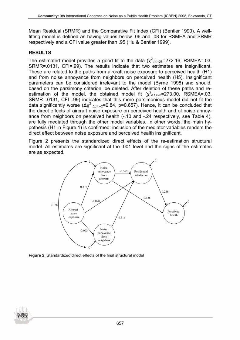
Community: 9th International Congress on Noise as a Public Health Problem (ICBEN) 2008, Foxwoods, CT
Mean Residual (SRMR) and the Comparative Fit Index (CFI) (Bentler 1990). A well-fitting model is defined as having values below .06 and .08 for RSMEA and SRMR respectively and a CFI value greater than .95 (Hu & Bentler 1999).
RESULTS The estimated model provides a good fit to the data (χ2
d.f.=26=272.16, RSMEA=.03, SRMR=.0131, CFI=.99). The results indicate that two estimates are insignificant. These are related to the paths from aircraft noise exposure to perceived health (H1) and from noise annoyance from neighbors on perceived health (H5). Insignificant parameters can be considered irrelevant to the model (Byrne 1998) and should, based on the parsimony criterion, be deleted. After deletion of these paths and re-estimation of the model, the obtained model fit (χ2
d.f.=28=273.00, RSMEA=.03, SRMR=.0131, CFI=.99) indicates that this more parsimonious model did not fit the data significantly worse (∆χ2
∆d.f.=2=0.84, p=0.657). Hence, it can be concluded that the direct effects of aircraft noise exposure on perceived health and of noise annoy-ance from neighbors on perceived health (-.10 and -.24 respectively, see Table 4), are fully mediated through the other model variables. In other words, the main hy-pothesis (H1 in Figure 1) is confirmed: inclusion of the mediator variables renders the direct effect between noise exposure and perceived health insignificant. Figure 2 presents the standardized direct effects of the re-estimation structural model. All estimates are significant at the .001 level and the signs of the estimates are as expected.
Aircraft noise
exposure
Perceived health
Noise annoyance
from neighbors
Noise annoyance
from aircrafts
Residential satisfaction
0.377
-0.098
-0.093
-0.316
-0.126
0.258
-0.367
ζ
ζ
ζ
ζ0.188
Figure 2: Standardized direct effects of the final structural model
657

Community: 9th International Congress on Noise as a Public Health Problem (ICBEN) 2008, Foxwoods, CT
Table 2: Standardized total effects and proportions of explained variance
NAN NAA RS PH ANE -0.093 0.377 -0.206 -0.101 NAA 0 0 -0.367 -0.220 NAN 0 0 -0.316 -0.082 RS 0 0 0 0.258 Explained variance (%) 0.9 14.2 29.7 11.1
Summation of the indirect and direct effects yields the total effects of the model vari-ables on the endogenous variables in the model. These effects (in their standardized form) as well as the proportions of explained variance are presented in Table 2.
DISCUSSION AND CONCLUSION With respect to the present study the following conclusions can be summarized. Firstly, the main hypothesis is confirmed: inclusion of the mediation paths between aircraft noise exposure and perceived health renders the direct effect between these two variables insignificant. Secondly, aircraft noise exposure is not the largest envi-ronmental determinant of perceived health. The standardized effects of noise annoy-ance from aircrafts and residential satisfaction (-.220 and .258 respectively) are more than twice as large as the effect of aircraft noise exposure (-.101). Since the effect of aircraft noise exposure is fully mediated, it holds that only if people become annoyed by the noise will it have negative health consequences. However, it should be noted that if there is no noise present there will be no annoyance. The significance of noise exposure, that is, of noise reduction measures, should therefore not be underesti-mated. In relation to this study several reflective remarks can be made and related research directions be formulated. Firstly, the used health indicators, i.e. a general health rat-ing and a summated scale of recent health complaints, can be qualified as “soft”. It therefore remains unknown whether for “hard” medical outcomes, like hypertension and cardiovascular diseases, the effects of aircraft noise exposure are also mediated via cognitive variables, like noise annoyance. However, the three basic requirements for a mediator relationship (see Baron & Kenny 1986) are also present for these ef-fects: 1) there is an effect between the independent variable (i.e. noise) and the out-come variable (i.e. hypertension), as recently evidenced by Jarup et al. (2008), there is an effect between the mediator (i.e. annoyance) and the outcome variable, as evi-denced by Babisch et al. (2007), and there is an effect between the independent variable and the mediator, as evidenced by Schultz (1978) and Miedema & Vos (1998). In addition, a study of Black et al. (2007) has provided evidence that the ef-fect of noise on (self-reported) hypertension becomes insignificant if chronic noise stress is included as a mediator. To study the extent of the mediation effect we rec-ommend inclusion of these objective “hard” outcomes in future models. In addition, models can be developed that include both the “soft” and the “hard” health indicators to investigate their underlying relational pattern. Secondly, the estimated model in this study is based on cross-sectional data. This means that the assumption of time-precedence required to make causal inferences is solely based on theoretical grounds and cannot be empirically investigated. Due to theoretical uncertainty it remains unknown whether the specified model structure is indeed correct. For example, as mentioned earlier, there is reason to believe that re-ciprocal effects between health and its determinants are present. These might be
658

Community: 9th International Congress on Noise as a Public Health Problem (ICBEN) 2008, Foxwoods, CT
direct, as indicated by Job (1996), in that an awareness of ill-health can lead to more dissatisfaction with the noise, as well as indirect, as indicated by Babisch et al. (2007), in that ill-health can lead to an increased sensitivity to the noise which, in turn, causes more dissatisfaction with the noise. Useful ways to assess the tenability of the time-precedence criterion as well as to study reciprocal effects are to develop models based on panel data or to conduct experiments in the controlled environment of the laboratory. Lastly, with respect to the present model it could be objected that the estimated rela-tionships are confounded by several personal characteristics such as sex, age, etc. Therefore, a second model was estimated which included the variables: sex, age, education level, country of origin, smoking behavior and degree of urbanization (cf. Franssen et al. 2004). Because the estimates of this extended model did not differ substantially from those of the model of interest in this study (see Figure 1), the choice was made to present the results of this latter more parsimonious model. The conclusion that the direct effect of noise exposure is mediated has important im-plications for researchers as well as policy makers. For researchers it means that the effect of noise exposure on health can be better estimated when also taking into ac-count factors influencing noise annoyance and residential satisfaction. For policy makers it means that noise policies should not solely be concerned with controlling the physical level of exposure, but also with subjective factors that function as cogni-tive mediators and the causes behind these factors. For example, next to the role of noise exposure, which in this study can only explain 14.2 % of the variation in noise annoyance, research has consistently shown the important role of so-called non-acoustical factors in the appraisal of aircraft noise (Fields 1993; Miedema & Vos 1999; Maris et al. 2007). These factors constitute variables like fear of the source, trust in the noise source authorities or the capacity of people to control or cope with noise. Hence, effective noise management should take such factors into account (Stallen 1999; Guski 1999). The second conclusion, that noise exposure is not the most important determinant of perceived health, further supports the use of a broad range of regulatory actions aimed at these subjective evaluations instead of a narrow focus on noise exposure. The Thomas theorem, a fundamental law in sociology, ap-plies to this situation: ‘if men define situations as real, they are real in their conse-quences’ (Thomas 1966). To conclude, we refer to Passchier-Vermeer & Passchier (2000), who mention that most effects of noise on health were already identified in the 1960s. In addition, they emphasize that ‘a subject for further research is the elucidation of the mechanisms underlying noise-induced cardiovascular disorders and the relationship of noise with annoyance and non-acoustical factors modifying health outcomes’ (Passchier-Vermeer & Passchier 2000). We concur with this assessment and believe that the present study constitutes a step in this direction.
REFERENCES ANOTEC Consulting (2004). Study on current and future aircraft noise exposure at and around Community Airports (revision of baseline study). http://ec.europa.eu/transport/air_portal/environment/studies/doc/aircraft_noise_revision.pdf (assessed April 2008).
Babisch W (2000).Traffic noise and cardiovascular disease: Epidemiological review and synthesis. Noise & Health 2(8):9-32.
Babisch W (2006).Transportation noise and cardiovascular risk: updated review and synthesis of epidemiological studies indicate that the evidence has increased. Noise & Health 8(30):1-29.
659

Community: 9th International Congress on Noise as a Public Health Problem (ICBEN) 2008, Foxwoods, CT
Babisch W, Houthuijs D, Pershagen G, Katsouyanni K, Velonakis M, Cadum E, Dudley M-L, Bluhm G, Breugelmans O, Charalampidis A, Dimakopoulou K, Savigny P, Seifferta I, Selanderc J, Sourtzi P, Swart W, Vigna-Taglianti F, Järup L (2007). Association between noise annoyance and high blood pressure. Proceedings of the Internoise 2007 Congress, 27-31 August. Istanbul, Turkey.
Baron RM, Kenny DA (1986). The moderator-mediator variable distinction in social psychological research: conceptual, strategic and statistical considerations. J Pers Soc Psychol 51: 1173-1182.
Black DA, Black JA, Issarayangyun T, Samuels SE (2007). Aircraft noise exposure and resident’s stress and hypertension: a public health perspective for airport environmental management. J Air Transp Manag 13: 264-276.
Bentler PM (1990). Comparative fit indices in structural models. Psychol Bull 107: 238-246.
Browne MW, Cudeck R (1993). Alternative ways of assessing model fit. In: Bollen KA, Long JS (eds.): Testing structural equation models (pp 136-162). Thousand Oaks, CA: Sage.
Byrne BM (1998). Structural equations modelling with Lisrel, Prelis and Simplis: basic concepts, applications and program-ming. London: LEA.
Campbell JM (1983). Ambient stressors. Environ Behav 15: 355-380.
De Haan ARC (2007). Aircraft technology’s contribution to sustainable development. PhD Dissertation, Delft University of Technology, Delft.
Fields JM (1993). Effect of personal and situational variables on noise annoyance in residential areas. J Acoust Soc Am 93: 2753-2763.
Franssen EAM, van Wiechen CMAG, Nagelkerke NJD, Lebret E (2004). Aircraft noise around a large international airport and its impact on general health and medication use. Occup Environ Med 61: 405-413. Galster GC, Hesser GW (1981). Residential satisfaction: compositional and contextual correlates. Environ Behav 13: 735-758.
Guski R (1999). Personal and social variables as co-determinants of noise annoyance. Noise & Health 1(3): 45-56.
Hu L, Bentler PM (1999). Cutoff criteria for fit indices in covariance structure analysis: conventional criteria versus new alter-natives. Struct Equat Model 6: 1-55.
Jarup L, Babisch W, Houthuijs D, Pershagen G, Katsouyanni K, Cadum E, Dudley M-L, Savigny P, Seiffert I, Swart W, Breugelmans O, Bluhm G, Selander J, Haralabidis A, Dimakopoulou K, Sourtzi P, Velonakis M, Vigna-Taglianti F (2008). Hypertension and exposure to noise near airports: the HYENA Study. Environ Health Perspect 116: 329-333.
Job RFS (1996). The influence of subjective reactions to noise on health effects of the noise. Environ Int 22: 93-104.
Lercher P (1996). Environmental noise and health: an integrated research perspective. Environ Int 22: 117-129.
Maris E, Stallen PJ, Vermunt R, Steensma H (2007). Noise within the social context: annoyance reduction through fair pro-cedures. J Acoust Soc Am 121: 2000-2010.
Miedema HME, Vos H (1998). Exposure-response relationships for transportation noise. J Acoust Soc Am 104: 3432-3445.
Miedema HME, Vos H (1999). Demographic and attitudinal factors that modify annoyance from transportation noise. J Acoust Soc Am 105: 3336-3344.
Miedema HME, Vos H. (2003). Noise sensitivity and reactions to noise and other environmental conditions. J Acoust Soc Am 113: 1492-1504.
Miedema HME, Vos H, De Jong RG (2000). Community reaction to aircraft noise: time-of-day penalty and tradeoff between levels of overflights. J Acoust Soc Am 107: 3245–3253.
Ohrstrom E (1993). Long-term effects in terms of psychosocial wellbeing, annoyance and sleep disturbance in areas ex-posed to high levels of road traffic noise. In: Vallet M (ed.): Noise as a public health problem. Arcueil Cedex, INRETS, France.
Passchier-Vermeer W, Passchier WF (2000). Noise exposure and public health. Environ Health Perspect 108: 123-131.
Phillips DR, Siu O-L, Yeh AGO, Cheng KHC (2005). The impacts of dwelling conditions on older persons’ psychological well-being in Hong Kong: the mediating role of residential satisfaction. Soc Sci Med 60: 2785-2797.
Rossi PH (1955). Why families move. Glenco,IL: The Free Press.
Schultz TJ (1978). Synthesis of social surveys on noise annoyance. J Acoust Soc Am 64: 337-405.
Stallen PJ (1999). A theoretical framework for environmental noise annoyance. Noise & Health 1(3): 69-80.
660

Community: 9th International Congress on Noise as a Public Health Problem (ICBEN) 2008, Foxwoods, CT
Stansfeld SA, Haines MM, Burr M, Berry B, Lercher P (2000). A review of environmental noise and mental health. Noise & Health 2(8): 1-8.
Thomas WI (1966). On social organization and social personality. Chicago, IL: Phoenix Books/The University of Chicago Press.
TNO, RIVM (1998). Hinder, slaapverstoring, gezondheids en belevingsaspecten in de regio Schiphol, resultaten van een vragenlijstonderzoek. TNO-PG, Leiden, The Netherlands, Report 98.039/RIVM, Bilthoven, The Netherlands, Report 441520010.
WHO, World Health Organization (1999). Guidelines for community noise. (Eds.: Berglund B, Lindvall T, Schwela DH). http://www.who.int/docstore/peh/noise/guidelines2.html (assessed April 2008).
Yokoshima S, Ota A, Tamura A (2007). Application of covariance structure analysis to the evaluation structure of mixed noises. Proceedings of the Internoise 2007 Congress, 27-31 August. Istanbul, Turkey.
661

Community: 9th International Congress on Noise as a Public Health Problem (ICBEN) 2008, Foxwoods, CT
Human annoyance response to a step change in noise exposure following opening of a new railway extension in Hong Kong Kin-che Lam*, Wai-hong Au Department of Geography and Resource Management, Chinese University of Hong Kong, Shatin, NT., Hong Kong SAR
* corresponding author: e-mail: [email protected]
ABSTRACT A study was undertaken to determine the change in exposure of households to road traffic and railway noise and the residents’ annoyance reactions in a new town in Hong Kong following the opening of an 11.4-km railway extension line. The acoustic changes were determined by noise mapping and validated by field measurements. Social surveys were performed six months before, three months following, and one year after operation of the railway. The results show that despite introduction of rail-way noise had resulted in a small increase in total noise exposure, the annoyance of the residents decreased over time during the study period, indicating that annoyance was not significantly related to noise exposure levels or the magnitude of change in noise exposure. A separate but parallel questionnaire survey for a different cohort of residents was undertaken to determine if annoyance reaction could be modified by bias in the available information and use of the new railway service. The results from these two surveys provide circumstantial evidence to indicate that the attenuation of annoyance over time could be partly attributable to media sensitization around the time of railway opening and the gradual adoption of the rail as a mode of transport by local residents. Findings of these surveys should have implications in environmental management.
INTRODUCTION This study investigated the change in acoustic environment of a new town in Hong Kong following the opening of a new railway extension. The literature abounds with examples showing that changes in the acoustic environment may cause changes in human annoyance reactions and performance in undertaking daily activities. How-ever, these studies also show that there is no simple relationship between human annoyance reactions and the magnitude of acoustic change (Miedema & Vos 1998), particularly when the change is sudden. Based on a comprehensive review of the literature, Brown and van Kamp (2005) suggested that there is as yet no conclusive evidence to show that people overreact to such step changes and the purported re-sponse may attenuate over time. They called for further investigations on human noise-annoyance responses in dynamic acoustic situations using a multi-stage framework to collect the data needed to determine if overreaction indeed exists and persists. Many studies have shown that annoyance reactions are shaped not only by the ab-solute noise level but also by the magnitude of acoustic change, the shift in the dominant noise source, as well as many other non-acoustic factors (Lambert 1998; Joncour et al. 2000; Lam et al. 2008) that may provoke noise responses even more intense than those induced by acoustic ones (Job & Hatfield 1998). The interactions among acoustic and non-acoustic factors and their effects on noise annoyance can be very complicated and merit in-depth investigations. Among the various non-acoustic factors, the literature shows that people are generally more annoyed if they
662

Community: 9th International Congress on Noise as a Public Health Problem (ICBEN) 2008, Foxwoods, CT
believe that noise could have been avoided or reduced by the authorities (Schreck-enberg et al. 1998). Availability and accessibility of information about noise abate-ment procedures have also been shown to have a significant influence on people’s noise annoyance (Solberg 2005). Increased media coverage of a new project can also sensitize the affected local community and provoke greater negative reactions (Hume et al. 2004). Whether or not the respondents make use of the noise-emitting infrastructure can also possibly affect annoyance reactions. However, not many stud-ies have focused on the interactions among these non-acoustic factors and their ef-fectiveness in shaping human noise response. Nor has any study tried to relate these non-acoustic factors to an exaggerated noise annoyance response under a step-change in noise exposure. An opportunity arose in Hong Kong when an extension was added to an existing railway network in 2004. Recognizing that the railway extension may bring about acoustic changes and consequential human annoyance responses, the present study attempted to determine the mode and magnitude of acoustic change and to gauge the change in human annoyance reactions. Known as the Ma On Shan Railway (MOSR), the new railway extension was constructed and opened in December 2004 (Figure 1) to provide train services to the Ma On Shan (MOS) New Town with a popu-lation of around 250,000 who had previously relied on road transport to commute to the city.
Figure 1: Map of the Ma On Shan Railway (MOSR) extension line in Hong Kong
This new railway extension, 11.4 km in length, run for most of its part along existing roadways with small sections (16 % of total length) encroaching on housing devel-opments in relatively quiet areas. The extension has changed the traffic mode of the residents in MOS by providing them with an alternative transport mode and at the same time bringing a new noise source to the new town. Railway noise in Hong Kong is controlled by the Noise Control Ordinance which stipulates a maximum of 65 dB (LAeq, 30 min) for most parts of the new town and 60 dB (LAeq, 30 min) for the qui-eter areas. The potential railway noise impact attracted a lot of attention in the news media lasting for several months before and shortly after opening of the railway. The
663

Community: 9th International Congress on Noise as a Public Health Problem (ICBEN) 2008, Foxwoods, CT
debate focused on the adequacy of noise mitigation measures provided by the rail-way operator.
METHODS This research adopted a three-pronged approach to the research questions. Firstly, the change in acoustic environment, in terms of both noise level and sound sources, due to the operation of the MOSR was ascertained by noise mapping validated by field noise measurements. Secondly, noise annoyance response of local residents of MOS and its change over time was monitored by questionnaire surveys conducted before and after the operation of the MOSR. Finally, a “control experiment” was con-ducted to unravel possible non-acoustical factors affecting annoyance reaction by manipulating the information provided to the residents. It is hoped that results of this study can provide valuable information on the understanding of human noise annoy-ance response and insightful implications on how to minimize noise annoyance reac-tions towards new noise emitting infrastructure. To ascertain the acoustic changes in the study area, a traffic impact study of the MOSR was undertaken (Lam & Au 2008), using road traffic and railway operation data obtained from official sources, traffic counts in the field and information from the bus and minibus operators on the rescheduling, rerouting and cancellation of bus services. These data were also used for noise exposure mapping using the software LIMA version 5.0 estimating the façade LAeq during peak hour of the day following the Calculation of Road Traffic Noise (CRTN) and Calculation of Railway Noise (CRN) methods respectively. Field measurements showed that the predictions were accurate to ± 2 dB(A) in about two thirds of sites (Lam & Au 2006). Changes in the exposure to road traffic and railway noises were determined, both separately and combined, before and after operation of the railway extension. A total of 74,860 dwelling units were covered in the noise mapping exercise. To gauge the human annoyance reactions to the railway noise, over 6,000 invitation letters were dropped off at the mailboxes of all dwelling units in high-rise buildings of 18 housing estates which are in direct line of sight with the MOSR. Appointments were then made with those who accepted the invitation and whose age was 16 or above for a questionnaire interview at their dwellings. This was a follow-through study lasting for 18 months comprising of three separate phases. The first was a face-to-face interview before opening of the MOSR. Following the first interview, the respon-dents were contacted for a follow-up face-to-face interview immediately after opening of the MOSR and also a telephone interview one year later. In addition to ascertain-ing the respondents’ level of annoyance towards the overall transportation noise us-ing a 7-point numeric scale, the survey also obtained information on (a) residents’ satisfaction with their living environment; (b) impact of noise on their daily activities; (c) their attitude towards road traffic and railway as a mode of transport; and (d) whether or not they rode on the new MOSR. A separate “control experiment” involving the manipulation of information and target-ing a different cohort of respondents was conducted in parallel with the social survey just mentioned. At about three months after opening of the new rail line, letters were mailed to thousands of residents of housing estates in line-of-sight with the railway, inviting them to participate in this study and to return a consent form in which they also reported their annoyance rating of the noise from the MOSR on a 7-point scale and their frequency of riding the train. About 2,500 completed consent forms were received. After eliminating those with missing data, those completed by individuals under the age of 16, those who spent less than 2 waking hours at home each day
664

Community: 9th International Congress on Noise as a Public Health Problem (ICBEN) 2008, Foxwoods, CT
and those who reported extreme annoyance ratings, only 500 participants were left in the pool for subsequent surveys. They were randomly assigned to two groups of 250 matched in annoyance rating: Group N (the negative group) and Group P (the posi-tive group). Respondents in these two groups were provided with fact sheets contain-ing different information. For Group N, the fact sheet listed all the additional noise mitigation measures that could be, but had not yet been, employed to further reduce the noise from the MOSR; for Group P, the fact sheet listed all the noise mitigation measures that had already been employed to reduce noise from the MOSR. Both sets of information were obtained from publicity materials published by the Govern-ment and Railway Corporation and from extensive newspaper review. To ensure that respondents of both groups had read the information provided, they were asked to pick the most important five items from the information sheets. They were then re-quested to return a questionnaire indicating their level of satisfaction with the mitiga-tion measures already employed. 103 and 128 completed questionnaires were re-turned from Groups N and P respectively. A month later, another questionnaire was sent to the 231 participants who had re-sponded to the fact sheets. This questionnaire contained 11 questions which as-sessed their noise annoyance response in different aspects of life and a question asking about their adaptation to the noise from the MOSR. This questionnaire was the same for both Group N and Group P. A total of 103 and 128 respondents in Group N and Group P respectively returned their completed questionnaires. To as-certain the validity of the returns, an attrition analysis was undertaken and there was no evidence to show that the respondents in later phases were biased samples of earlier ones.
RESULTS Traffic and noise impacts The information collated from various sources and field counts indicates that the traf-fic impacts were different for the main and secondary roads in the township. On the main roads, the total vehicular flow increased because of natural growth in population and increasing demand for transportation link with other towns and the city. On the secondary roads, the opening of the MOSR has resulted in some reduction in traffic flow probably because of a change in transport mode of the residents. It is notewor-thy that the percentage of heavy vehicles decreased both on the main and secondary roads as a result of the cancellation of franchised bus and minibus services after opening of the MOSR. Results of the noise mapping indicate that the noise exposure of dwellings in the study area increased only slightly immediately after opening of the railway and there was a further small increase one year later (Lam & Au 2008). About 30 % of the dwellings in MOS, located mostly along the railway corridor, experienced 2 to 4 dB(A) increase in noise level after opening of the MOSR; and majority of the rest experi-enced an increase of less than 1 dB(A). The greatest increase took place in housing estates located in relatively quiet parts of the new town where the background was less than 55 dB(A).
665
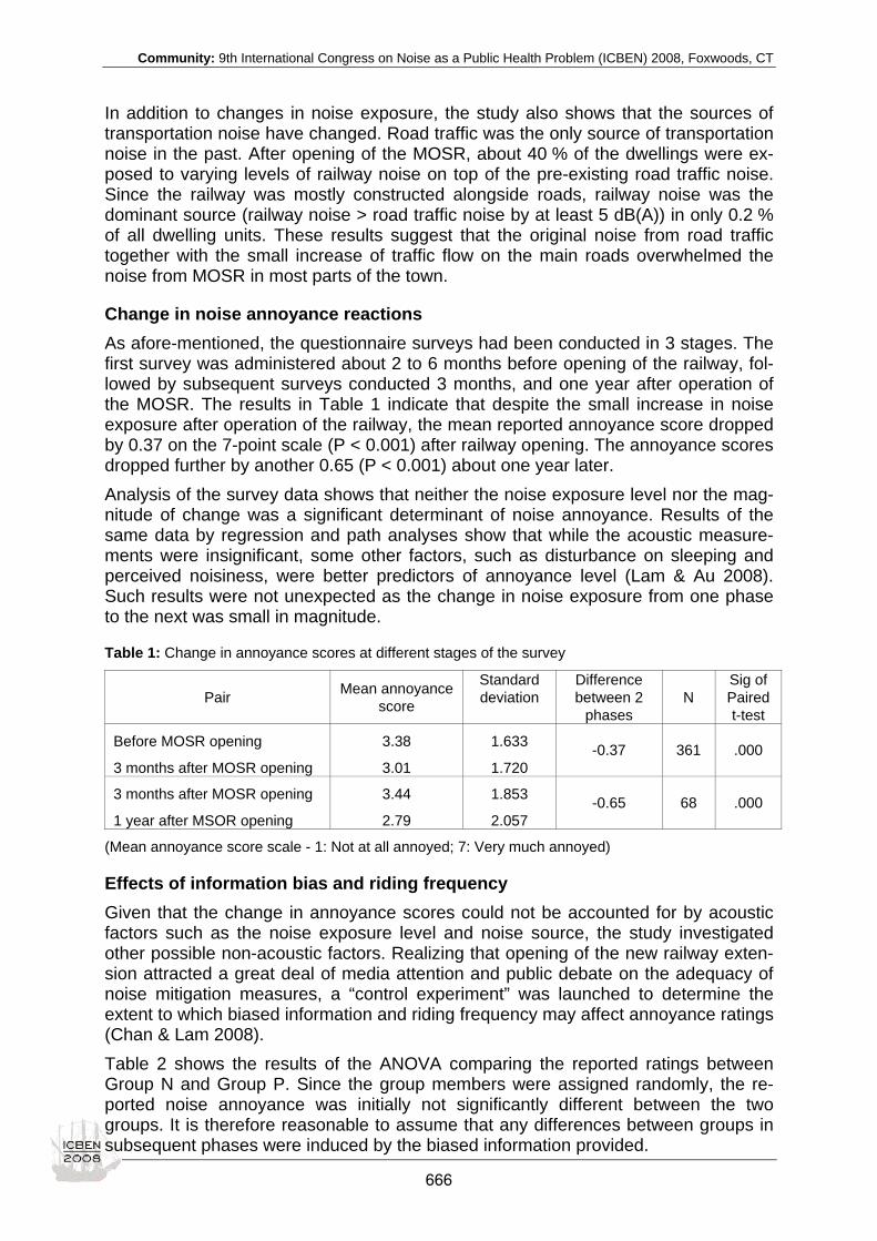
Community: 9th International Congress on Noise as a Public Health Problem (ICBEN) 2008, Foxwoods, CT
In addition to changes in noise exposure, the study also shows that the sources of transportation noise have changed. Road traffic was the only source of transportation noise in the past. After opening of the MOSR, about 40 % of the dwellings were ex-posed to varying levels of railway noise on top of the pre-existing road traffic noise. Since the railway was mostly constructed alongside roads, railway noise was the dominant source (railway noise > road traffic noise by at least 5 dB(A)) in only 0.2 % of all dwelling units. These results suggest that the original noise from road traffic together with the small increase of traffic flow on the main roads overwhelmed the noise from MOSR in most parts of the town.
Change in noise annoyance reactions As afore-mentioned, the questionnaire surveys had been conducted in 3 stages. The first survey was administered about 2 to 6 months before opening of the railway, fol-lowed by subsequent surveys conducted 3 months, and one year after operation of the MOSR. The results in Table 1 indicate that despite the small increase in noise exposure after operation of the railway, the mean reported annoyance score dropped by 0.37 on the 7-point scale (P < 0.001) after railway opening. The annoyance scores dropped further by another 0.65 (P < 0.001) about one year later. Analysis of the survey data shows that neither the noise exposure level nor the mag-nitude of change was a significant determinant of noise annoyance. Results of the same data by regression and path analyses show that while the acoustic measure-ments were insignificant, some other factors, such as disturbance on sleeping and perceived noisiness, were better predictors of annoyance level (Lam & Au 2008). Such results were not unexpected as the change in noise exposure from one phase to the next was small in magnitude.
Table 1: Change in annoyance scores at different stages of the survey
Pair Mean annoyance score
Standard deviation
Difference between 2
phases N
Sig of Paired t-test
Before MOSR opening
3 months after MOSR opening
3.38
3.01
1.633
1.720 -0.37 361 .000
3 months after MOSR opening
1 year after MSOR opening
3.44
2.79
1.853
2.057 -0.65 68 .000
(Mean annoyance score scale - 1: Not at all annoyed; 7: Very much annoyed)
Effects of information bias and riding frequency Given that the change in annoyance scores could not be accounted for by acoustic factors such as the noise exposure level and noise source, the study investigated other possible non-acoustic factors. Realizing that opening of the new railway exten-sion attracted a great deal of media attention and public debate on the adequacy of noise mitigation measures, a “control experiment” was launched to determine the extent to which biased information and riding frequency may affect annoyance ratings (Chan & Lam 2008). Table 2 shows the results of the ANOVA comparing the reported ratings between Group N and Group P. Since the group members were assigned randomly, the re-ported noise annoyance was initially not significantly different between the two groups. It is therefore reasonable to assume that any differences between groups in subsequent phases were induced by the biased information provided.
666
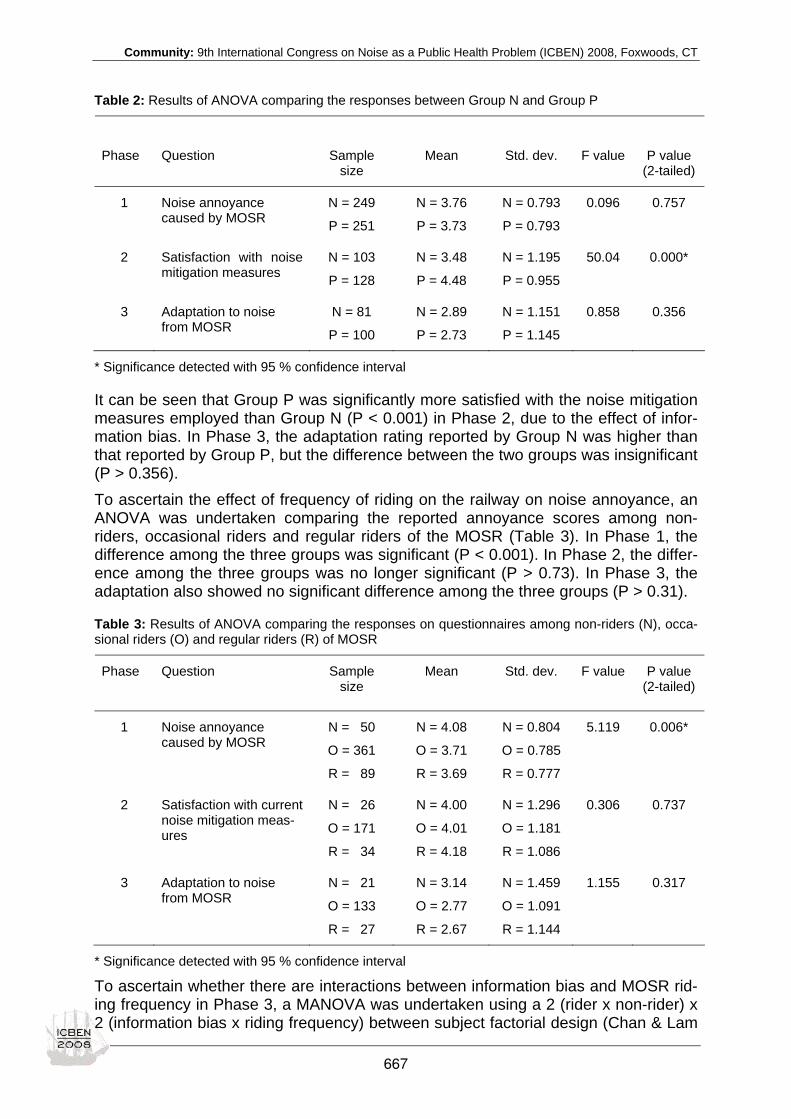
Community: 9th International Congress on Noise as a Public Health Problem (ICBEN) 2008, Foxwoods, CT
Table 2: Results of ANOVA comparing the responses between Group N and Group P
Phase
Question
Sample size
Mean
Std. dev.
F value
P value (2-tailed)
1 Noise annoyance caused by MOSR
N = 249
P = 251
N = 3.76
P = 3.73
N = 0.793
P = 0.793
0.096 0.757
2 Satisfaction with noise mitigation measures
N = 103
P = 128
N = 3.48
P = 4.48
N = 1.195
P = 0.955
50.04 0.000*
3 Adaptation to noise from MOSR
N = 81
P = 100
N = 2.89
P = 2.73
N = 1.151
P = 1.145
0.858 0.356
* Significance detected with 95 % confidence interval
It can be seen that Group P was significantly more satisfied with the noise mitigation measures employed than Group N (P < 0.001) in Phase 2, due to the effect of infor-mation bias. In Phase 3, the adaptation rating reported by Group N was higher than that reported by Group P, but the difference between the two groups was insignificant (P > 0.356). To ascertain the effect of frequency of riding on the railway on noise annoyance, an ANOVA was undertaken comparing the reported annoyance scores among non-riders, occasional riders and regular riders of the MOSR (Table 3). In Phase 1, the difference among the three groups was significant (P < 0.001). In Phase 2, the differ-ence among the three groups was no longer significant (P > 0.73). In Phase 3, the adaptation also showed no significant difference among the three groups (P > 0.31).
Table 3: Results of ANOVA comparing the responses on questionnaires among non-riders (N), occa-sional riders (O) and regular riders (R) of MOSR
Phase Question Sample size
Mean Std. dev. F value P value (2-tailed)
1 Noise annoyance caused by MOSR
N = 50
O = 361
R = 89
N = 4.08
O = 3.71
R = 3.69
N = 0.804
O = 0.785
R = 0.777
5.119 0.006*
2 Satisfaction with current noise mitigation meas-ures
N = 26
O = 171
R = 34
N = 4.00
O = 4.01
R = 4.18
N = 1.296
O = 1.181
R = 1.086
0.306 0.737
3 Adaptation to noise from MOSR
N = 21
O = 133
R = 27
N = 3.14
O = 2.77
R = 2.67
N = 1.459
O = 1.091
R = 1.144
1.155 0.317
* Significance detected with 95 % confidence interval
To ascertain whether there are interactions between information bias and MOSR rid-ing frequency in Phase 3, a MANOVA was undertaken using a 2 (rider x non-rider) x 2 (information bias x riding frequency) between subject factorial design (Chan & Lam
667
Community: 9th International Congress on Noise as a Public Health Problem (ICBEN) 2008, Foxwoods, CT
2008). The results indicate that both information bias (P < 0.01) and riding frequency (P < 0.02) significantly affected respondents’ noise annoyance reactions, but no in-teraction was observed between the two factors (P > 0.40).
DISCUSSION AND CONCLUSIONS The objective of this study was to unravel factors affecting noise annoyance re-sponse when there is a sudden increase in noise exposure following the introduction of a new railway extension. More specifically, the study attempted to determine whether or not non-acoustic factors play a role in shaping noise annoyance re-sponse. The opening of a new railway extension in the MOS new town offered an opportunity to monitor changes in the acoustic environment and human response over a two-year period using noise mapping technique, repeated social surveys and an experiment to gauge human reactions given different information about the rail-way project. For this type of study, it would be ideal to adopt the framework proposed by Brown and van Kamp (2005) which requires the first social survey to be conducted well in advance of the operation of the railway extension. This was unfortunately not feasible in this study due to time and resource constraints. Nevertheless, findings of the re-peated social surveys undertaken in this study six months before, three months fol-lowing, and one year after, operation of the railway do provide some insight into how local residents react to the sudden change in acoustic environment. Findings of the social survey reveal a statistically significant decline in noise annoyance reactions over the study period despite a small increase in noise levels caused by the new railway noise source. The current experimental setup does not allow all non-acoustic factors that might possibly affect annoyance response to be fully explored. However, realizing that opening of the new railway extension also coincides with a phase with heightened media attention, intense public debate and possible change in the habit of transporta-tion, the present study incorporated a “control experiment” attempting to investigate how two non-acoustic factors, namely information bias and riding frequency, can af-fect the annoyance response of local residents exposed to the noise created by the new railway line. Findings of the experimental study show that information bias, de-pending on which side of the coin is revealed to the recipient, can have quite oppo-site effects. Respondents receiving only information on positive measures taken by the authority to reduce noise emission are more tolerant of the noise impact, but those receiving only critical views tend to be more annoyed because they feel that not all measures to reduce noise have been employed. The effect of information bias may start very strong and then decrease in magnitude but stay significant for at least a few weeks. Regular riders were more tolerant of the new railway noise than occa-sional riders and non-riders, but this effect, which is relatively stable over time, could be overwhelmed by that of information bias. The study of noise annoyance reactions towards step-changes of noise exposure has attracted considerable attention in recent years. Findings of this study confirm that significant changes in annoyance response can occur shortly after the introduc-tion of a new noise-emitting infrastructure and such change cannot be ascribed en-tirely to changes in the acoustic environment. Among the many possible factors that may account for the temporal shift in annoyance reactions, the effects of media sen-sitization, information bias and the habit of transportation cannot be overlooked.
668

Community: 9th International Congress on Noise as a Public Health Problem (ICBEN) 2008, Foxwoods, CT
ACKNOWLEDGEMENT
This research was substantially supported by a grant from the Research Grants Council of the Hong Kong SAR Government (Project No. CUHK 4248/03H).
REFERENCES Brown AL, van Kamp I (2005). Towards a design for studies of response to a change in noise exposure. In: Proceedings of InterNoise 2005 (CD-ROM), Rio de Janeiro, Brazil.
Chan TC, Lam KC (2008). The effects of information bias and riding frequency on noise annoyance to a new railway exten-sion in Hong Kong. Transportation Res, Pt. D 13: 334-339.
Hume KI, Morley H, Thomas C (2004). Community response to a new runway: preliminary results. In: Proceedings of Inter-Noise 2004. Prague, Czech Republic.
Job RSF, Hatfield J (1998). Community reaction to noise. Acoust Austral 26: 35-39.
Joncour C, Gautier C, Lambert J (2000). Annoyance due to combined noise source. In : Proceedings of Internoise 2000 (CD-ROM), Nice, France.
Lam KC, Au WH (2006). Quantifying the spatial and temporal variations in the urban soundscape by noise mapping. In: Starrett SK, Hong J, Lyon WG (eds.): Environmental science and technology 2006, Vol. 2. Proceedings from the 2nd Interna-tional Conference on Environmental Science and Technology, held August 19-22, 2006 in Houston, Texas, USA (pp 380-384). Houston, TX: American Science Press.
Lam KC, Au WH (2008). Human response to a step change in noise exposure following the opening of a new railway exten-sion in Hong Kong. Acta Acust Acust (in press).
Lam KC, Chan PK, Chan TC, Au WH, Hui WC (2008). Annoyance response to mixed transportation noise in Hong Kong. Appl Acoust (in press).
Lambert J (1998). Assessing the railway bonus: the need to examine the “new infrastructure” effect. In: Proceedings of Inter-noise 1998 (CD-ROM), Christchurch, New Zealand.
Miedema HME, Vos H (1998). Exposure-response relationships for transportation noise. J Acoust Soc Am 104: 3432-3445.
Schreckenberg D, Schuemer R, Schuemer-Kohrs A, Griefahn B, Moehler U (1998). Attitudes toward noise source as deter-minants of annoyance. In: Fastl H, Scheuren J (eds.): Euronoise 98. Designing for silence. Prediction, measurement and evaluation of noise and vibration. Proceedings, Vol. I (pp 595-600). München.
Solberg S (2005). Giving people control of their noise problem – techniques to prevent annoyance. In: Proceedings of Forum Acusticum 2005. Budapest, Hungary.
669

Community: 9th International Congress on Noise as a Public Health Problem (ICBEN) 2008, Foxwoods, CT
The effect on annoyance estimation of noise modeling procedures Peter Lercher1*, Bram de Greve2, Dick Botteldooren2, Marine Baulac3, Jérome Defrance3, Johannes Rüdisser1 1 Department of Hygiene, Microbiology and Social Medicine, Medical University Innsbruck
2 Acoustics group, Department of Information Technology, Ghent University, Gent, Belgium
3 CSTB, Saint-Martin-d’Hères, France
* corresponding author: e-mail: [email protected]
INTRODUCTION Worldwide the impact of noise exposure on a community is estimated by the per-centage highly annoyed. The proper determination of the percentage highly annoyed depends among other factors related to the quality of the survey (sample size, selec-tion, questionnaire) also on the quality of the noise assignments related to the type and quality of the modeling procedure. Meta-analyses have demonstrated large variations in the exposure-annoyance curves and described personal, environmental and social factors which may be responsible for these differences (Job 1988; Fields 1993; Miedema & Vos 1999, 2003; Miedema & Fields 2005). Even when these indi-vidual differences are accounted for, Fields et al. (2000) have observed that on aver-age the community response still differs the equivalent of about 7 decibel in noise exposure. At the last ICBEN conference Fields (2003) stated “There is almost no re-search” into these differences. It would, however, be important to investigate the de-terminants of these differences, “because it identifies communities that might be treated differently in noise regulations”. In practice, several modeling standards and minor or larger variations of these coexist. Hitherto, a systematic cross-validation of the effect of the various modeling procedures on the estimation of the percentage highly annoyed in community studies is missing. Realizing this fact, the European community has spent a lot of research money (Harmonoise & Imagine projects) to establish a new modeling standard. This new standard should account better for to-pographical and meteorological conditions which vary a lot across (not only) Europe (low and high land, coastal regions). It should guarantee that the costly noise map-ping exercise – enforced by the Environmental Noise directive (END) – actually leads to what is intended: to get reliable cross-national estimates of the percentage of peo-ple exceeding certain thresholds of noise exposure (e.g. 55 dBA or 65 dBA) by 2012. Furthermore, utilizing the exposure-effect curves from the END appendixes (Miedema & Oudshoorn 2001) reliable percentages of highly or moderately annoyed for various noise indicators (Lden, Lnight) should be calculated. The Alps can be considered as a specific case in terms of orography, climate and meteorology and hence a real challenge for noise modeling. The ALPNAP project (“Monitoring and Minimisation of Traffic-Induced Noise and Air Pollution Along Major Alpine Transport Routes”) was funded to describe the Alpine-specific processes that determine the propagation of air and noise in Alpine valleys and their impact on health. One collaboration across disciplines aimed at assessing the effects on the estimation of the percentage highly annoyed in an alpine valley for rail and main road traffic due to the use of different modeling techniques (ISO9613 (Bass3 by INTEC), NMPB-96 (Mithra-Sig by CSTB). Additionally, for motorways the Harmonoise/Imagine method (implemented by INTEC and CSTB) was evaluated. It should be stressed that the same source power for road vehicles and trains is used as well as the same
670

Community: 9th International Congress on Noise as a Public Health Problem (ICBEN) 2008, Foxwoods, CT
traffic densities and thus the differences between these models only originate from differences in approximation of the propagation term.
METHODS Area, sample selection and recruitment The area of investigation, the Unterinntal, is the most important access route for heavy goods traffic over the Brenner. The goods traffic over the Brenner has tripled within the last 25 years and the fraction of goods moved on the road has substantially increased (up to 2/3). The area consist of small towns and villages with a mix of in-dustrial, small business and agricultural activities. The primary noise sources are highway and rail traffic. In addition a main road is of importance. This road links the villages and access roads to the highway. People were contacted by phone based on a stratified, random sampling strategy. The address base was stratified by use of the GIS (Geographic information system), based on fixed distances to the major traffic sources (rail, highway, main road), leav-ing a common „background area“ outside major traffic activities and an area with ex-posure to more than one traffic source “mixed traffic”. From these five areas house-holds were randomly selected and replaced in case of non-participation. Selection criteria for people were age between 25 and 75 years, sufficient hearing and lan-guage proficiency. An exclusion criterion was duration of living less than one year at this address. 45 % did not want to participate. The rest of the addresses were not valid (commercial etc), did not have telephone or could not be reached by 3 attempts at different times of the day. Eventually, 1,643 persons (35 % of the original sample on an individual basis), participated in this study. On household level the participation was much higher. Women were more willing to participate (61 %).
Noise exposure assessment Three groups of traffic noise sources are covered: Motorway traffic, traffic on main roads, and railway traffic. For motorway traffic the yearly average load (light and heavy vehicles) is combined with an average diurnal traffic pattern. Traffic frequency data on main roads were supplemented with additional counting data. Road traffic noise emission is calculated on the basis of the Harmonoise source model (Jonasson 2007). Railway noise emission is extracted from a typical day of noise immission measurements at close distance to the source. Bass3 is an extended version of ISO9613. The model includes up to four reflections and two sideway diffractions (de Greve et al. 2005, 2007). Mithra-Sig is the NMPB-96 implementation by CSTB, the current standard engineer-ing method recommended by the END for road traffic modeling. The Harmonoise/Imagine point-to-point propagation model is a candidate European standard engineering model that builds upon the Nord2000 project (van Maercke & Defrance 2007; Defrance et al. 2007). It promises better performance in complex ter-rain – but is computationally quite intensive and some simplifications had to be made to be applicable in such a large area. Only one reflection and two vertical diffraction edges were accounted for in this implementation. An extensive noise monitoring campaign was conducted to check the validity of these simulations. At 38 locations sound levels were recorded for over one week during winter (October to January) and during summer (June to August). In addition, the
671
Community: 9th International Congress on Noise as a Public Health Problem (ICBEN) 2008, Foxwoods, CT
predicted sound pressure levels resulting from PE-modeling have been evaluated against these long-term measurements (van Renterghem et al. 2007). Indicators of day, evening, night exposure and Lden were calculated for each source and total exposure at several points on the facade of the building of the survey par-ticipants. In the present analyses Lden of the respective sources was utilized.
Questionnaire information The questionnaire covered socio-demographic data, housing, satisfaction with the environment, general noise annoyance, attitudes toward transportation, interference of activities, coping with noise, occupational exposures, lifestyle, reported sensitivi-ties, health status, selected illnesses and medications. The phone interview took about 15-20 minutes to complete Noise annoyance was measured with a 5-point ver-bal scale according to ICBEN and ISO standards (Fields et al. 2001; ISO TC 43/SC 1, 2002). In the present analyses, highly annoyed was defined by responses to the two upper points (4+5) on the 5-point verbal scale.
Statistical analysis Exposure-effect curves were calculated with extended logistic regression methods using restricted cubic spine functions to accommodate for non-linear components in the fit if appropriate (Harrell 2001). The non-parametric regression estimate and its 95 % confidence intervals are based on smoothing the binary responses and taking the logit transformation of the smoothed estimates. The analysis was carried out with R version 2.4.1 (R Development Core Team 2006) using the contributed packages “Design” and “Hmisc” from F Harrell.
RESULTS Figures 1, 2 and 3 show a side-by-side comparison of the noise-annoyance relation-ships for motorway, main road and railway sound levels for BASS3-ISO, MITHRA-SIG and HARMONOISE/IMAGINE (only motorway) noise modeling. For comparison, the standard exposure-annoyance curve (from END) is inserted (black line) in addi-tion. For motorway noise, the sound modelling with MITHRA-SIG shows reasonable agreement with the standard curve, except for an underestimation at higher sound levels. Both, the BASS3-ISO and the HARMONOISE/IMAGINE modeling depart sub-stantially and indicate higher annoyance at any noise level. The strongest deviation from the standard curve is observed in the main road graph while both modeling techniques agree quite well. Railway annoyance (Figure 3) is increasingly underestimated at higher levels by MITHRA-SIG modeling - but much less when compared with motorway sound modeling.
672

Community: 9th International Congress on Noise as a Public Health Problem (ICBEN) 2008, Foxwoods, CT
Figures 1 and 2: Exposure effect relationships: highly annoyed by motorway (left) and main road sound exposure (right) by different noise modelling procedures compared with the standard curve (Environmental Noise Directive). Dashed lines indicate 95 % confidence intervals.
Figure 3: Exposure effect relationship: highly Figure 4: Exposure effect relationship: highly annoyed by railway sound exposure by two annoyed by railway exposure during night by modeling strategies and compared with the two modeling strategies and compared with Standard annoyance relationship the Standard annoyance relationship
Figure 5: Exposure effect relationship: highly Figure 6: Exposure effect relationship: highly annoyed by motorway exposure during night annoyed by main road exposure during night by two modeling strategies and compared by two modeling strategies and compared with with the Standard annoyance relationship the Standard annoyance relationship
rail.den.max
40 50 60 70 80
0.0
0.2
0.4
0.6
0.8
railway.dB.max.Lden
40 50 60 70 80
0.0
0.2
0.4
0.6
0.8
Railway sound level - highly annoyed
Sound level railway, Lden,dBA
Prop
ortio
n hi
ghly
anno
yed
Pro
porti
on h
ighl
yan
noye
d
Railway sound level, Lden,dBA40 50 60 70 80
0.2
0.4
0.6
0.8
0.0
MITHRA-SIG (CSTB)BASS3 (INTEC)
Standard (EnvironmentalNoise Directive (END)
rail.den.max
40 50 60 70 80
0.0
0.2
0.4
0.6
0.8
railway.dB.max.Lden
40 50 60 70 80
0.0
0.2
0.4
0.6
0.8
Railway sound level - highly annoyed
Sound level railway, Lden,dBA
Prop
ortio
n hi
ghly
anno
yed
Pro
porti
on h
ighl
yan
noye
d
Railway sound level, Lden,dBA40 50 60 70 80
0.2
0.4
0.6
0.8
0.0
rail.den.max
40 50 60 70 80
0.0
0.2
0.4
0.6
0.8
railway.dB.max.Lden
40 50 60 70 80
0.0
0.2
0.4
0.6
0.8
Railway sound level - highly annoyed
Sound level railway, Lden,dBA
Prop
ortio
n hi
ghly
anno
yed
Pro
porti
on h
ighl
yan
noye
d
Railway sound level, Lden,dBA40 50 60 70 80
0.2
0.4
0.6
0.8
0.0
0.2
0.4
0.6
0.8
0.0
MITHRA-SIG (CSTB)BASS3 (INTEC)
Standard (EnvironmentalNoise Directive (END)
MITHRA-SIG (CSTB)BASS3 (INTEC)
Standard (EnvironmentalNoise Directive (END)
Railway sound level, Lnight, dBA
Per
cent
age
high
ly a
nnoy
ed: n
ight
40 50 60 70 80
0.00
0.10
0.20
0.30
Railways sound level - highly annoyed at nighta comparison with the standard curve
railway.dB.max.Lnight
40 50 60 70 80
0.00
0.10
0.20
0.30
40 50 60 70 80
05
1015
2025
3035
LN
HS
Dra
ilS
Railway sound levels, Lnight, dBA
Prop
ortio
nhi
ghly
anno
yed:
nig
ht
40 50 60 70 80
BASS3 (ISO)MITHRA-SIGStandard curve
0.0
0.1
0.2
0.3
Railway sound level, Lnight, dBA
Per
cent
age
high
ly a
nnoy
ed: n
ight
40 50 60 70 80
0.00
0.10
0.20
0.30
Railways sound level - highly annoyed at nighta comparison with the standard curve
railway.dB.max.Lnight
40 50 60 70 80
0.00
0.10
0.20
0.30
40 50 60 70 80
05
1015
2025
3035
LN
HS
Dra
ilS
Railway sound levels, Lnight, dBA
Prop
ortio
nhi
ghly
anno
yed:
nig
ht
40 50 60 70 8040 50 60 70 80
BASS3 (ISO)MITHRA-SIGStandard curve
BASS3 (ISO)MITHRA-SIGStandard curve
0.0
0.1
0.2
0.3
0.0
0.1
0.2
0.3
Motorway sound level, Lnight, dBA
Per
cent
age
high
ly a
nnoy
ed: n
ight
40 45 50 55 60 65 70 75
0.00
0.10
0.20
0.30
Motorway sound level highly annoyed at nighta comparison with the standard curve
HW.dB.max.Lnight
40 45 50 55 60 65 70 75
0.00
0.10
0.20
0.30
BASS3 (ISO)MITHRA-SIGStandard curve
Motorway sound levels, Lnight, dBA
Prop
ortio
nhi
ghly
anno
yed:
nig
ht
40 45 50 55 60 65 70 75
0.00
0.10
0.20
0.30
Motorway sound level, Lnight, dBA
Per
cent
age
high
ly a
nnoy
ed: n
ight
40 45 50 55 60 65 70 75
0.00
0.10
0.20
0.30
Motorway sound level highly annoyed at nighta comparison with the standard curve
HW.dB.max.Lnight
40 45 50 55 60 65 70 75
0.00
0.10
0.20
0.30
BASS3 (ISO)MITHRA-SIGStandard curve
BASS3 (ISO)MITHRA-SIGStandard curve
Motorway sound levels, Lnight, dBA
Prop
ortio
nhi
ghly
anno
yed:
nig
ht
40 45 50 55 60 65 70 7540 45 50 55 60 65 70 75
0.00
0.10
0.20
0.30
0.00
0.10
0.20
0.30
Main road sound level, Lnight, dBA
Per
cent
age
high
ly a
nnoy
ed: n
ight
30 35 40 45 50 55 60 65
0.0
0.1
0.2
0.3
0.4
Main roads sound level highly annoyed at nighta comparison with the standard curve
NR.dB.max.Lnight
30 35 40 45 50 55 60 65
0.0
0.1
0.2
0.3
0.4
Main road sound level, Lnight, dBA
Prop
ortio
nhi
ghly
anno
yed:
nig
htPr
opor
tion
high
lyan
noye
d: n
ight
0.0
0.1
0.2
0.3
0.4
30 35 40 45 50 55 60 65
BASS3 (ISO)MITHRA-SIGStandard curve
Main road sound level, Lnight, dBA
Per
cent
age
high
ly a
nnoy
ed: n
ight
30 35 40 45 50 55 60 65
0.0
0.1
0.2
0.3
0.4
Main roads sound level highly annoyed at nighta comparison with the standard curve
NR.dB.max.Lnight
30 35 40 45 50 55 60 65
0.0
0.1
0.2
0.3
0.4
Main road sound level, Lnight, dBA
Prop
ortio
nhi
ghly
anno
yed:
nig
htPr
opor
tion
high
lyan
noye
d: n
ight
0.0
0.1
0.2
0.3
0.4
0.0
0.1
0.2
0.3
0.4
30 35 40 45 50 55 60 6530 35 40 45 50 55 60 65
BASS3 (ISO)MITHRA-SIGStandard curve
BASS3 (ISO)MITHRA-SIGStandard curve
Motorway sound level, Lden,dB,A
Pro
porti
on h
ighl
y an
noye
d
30 40 50 60 70
0.0
0.2
0.4
0.6
0.8
Motorway sound level - highly annoyed
hw.den.max
30 40 50 60 70
0.0
0.2
0.4
0.6
0.8
highways.dB.Max.Lden
30 40 50 60 70
0.0
0.2
0.4
0.6
0.8
Sound level motorway, Lden,dBA
Pro
porti
onhi
ghly
anno
yed
Motorway sound level, Lden,dBA30 40 50 60 70
0.2
0.4
0.6
0.8
0.0
MITHRA-SIG (CSTB)Harmonoise/IMAGINE (INTEC)BASS3-ISO (INTEC)
Standard (EnvironmentalNoise Directive (END)
Motorway sound level, Lden,dB,A
Pro
porti
on h
ighl
y an
noye
d
30 40 50 60 70
0.0
0.2
0.4
0.6
0.8
Motorway sound level - highly annoyed
hw.den.max
30 40 50 60 70
0.0
0.2
0.4
0.6
0.8
highways.dB.Max.Lden
30 40 50 60 70
0.0
0.2
0.4
0.6
0.8
Sound level motorway, Lden,dBA
Pro
porti
onhi
ghly
anno
yed
Motorway sound level, Lden,dBA30 40 50 60 7030 40 50 60 70
0.2
0.4
0.6
0.8
0.0
0.2
0.4
0.6
0.8
0.0
MITHRA-SIG (CSTB)Harmonoise/IMAGINE (INTEC)BASS3-ISO (INTEC)
Standard (EnvironmentalNoise Directive (END)
MITHRA-SIG (CSTB)Harmonoise/IMAGINE (INTEC)BASS3-ISO (INTEC)
Standard (EnvironmentalNoise Directive (END)
main.den.max
30 40 50 60 70
0.0
0.2
0.4
0.6
0.8
NR.dB.max.Lden
30 40 50 60 70
0.0
0.2
0.4
0.6
0.8
Pro
porti
on h
ighl
yan
noye
d
Main road sound level, Lden,dBA30 40 50 60 70
0.2
0.4
0.6
0.8
0.0
MITHRA-SIG (CSTB)BASS3 (INTEC)
Standard (EnvironmentalNoise Directive)
main.den.max
30 40 50 60 70
0.0
0.2
0.4
0.6
0.8
NR.dB.max.Lden
30 40 50 60 70
0.0
0.2
0.4
0.6
0.8
Pro
porti
on h
ighl
yan
noye
d
Main road sound level, Lden,dBA30 40 50 60 70
0.2
0.4
0.6
0.8
0.0
main.den.max
30 40 50 60 70
0.0
0.2
0.4
0.6
0.8
NR.dB.max.Lden
30 40 50 60 70
0.0
0.2
0.4
0.6
0.8
Pro
porti
on h
ighl
yan
noye
d
Main road sound level, Lden,dBA30 40 50 60 7030 40 50 60 70
0.2
0.4
0.6
0.8
0.0
0.2
0.4
0.6
0.8
0.0
MITHRA-SIG (CSTB)BASS3 (INTEC)
Standard (EnvironmentalNoise Directive)
MITHRA-SIG (CSTB)BASS3 (INTEC)
Standard (EnvironmentalNoise Directive)
673

Community: 9th International Congress on Noise as a Public Health Problem (ICBEN) 2008, Foxwoods, CT
Figure 7: Cumulative distribution of sound levels by subregion displaying three percentiles (25th, 50th, 75th) for a comparison with two sound modeling procedures (ISO left, Mithra right)
Viewing the modeling differences between Mithra and Bass3 for the Lnight-indicator (Figures 4, 5, 6) it is evident that they are not completely mimicking the differences seen with the Lden-indicator. Especially, the motorway curve shows a smaller sys-tematic difference and the difference for the railway is shaped in another way. How-ever, the distance of the annoyance curves to the standard curves remains about the same. The cumulative distribution plots by region (Figure 7) reveal different values in urban and rural areas for the models. MITHRA tends to give higher values here. Figure 8 gives an estimate of the mapping effect size in two situations. The preva-lence at higher sound levels (>70 dBA) is over- and at lower levels under-estimated by Mithra mapping. The difference in the estimation is much larger for the fraction below 55 dBA which is not surprising since overall accuracy is lower.
Figure 8: Proportions of sound levels above 70 dBA (left side) and below 55 dBA (right side) by region and type of sound level calculation (BASS3-ISO upper graphs, MITHRA-SIG lower graphs)
DISCUSSION By independent comparison of standard techniques in noise modeling we could demonstrate significant differences in the estimation of the highly annoyed. The best agreement among the modeling procedures was found for main road noise followed by railway noise exposure. The largest discrepancy observed was with mo-
0.0
0.1
0.2
0.3
0.4
0.5
prop
ortio
n >
70dB
A
0.0
0.1
0.2
0.3
0.4
0.5
0.0
0.1
0.2
0.3
0.4
0.5
0.0
0.1
0.2
0.3
0.4
0.5
rural suburban urban rural suburban urban
rural suburban urban rural suburban urban
BASS3 (ISO) BASS3 (ISO)
MITHRA-SIG MITHRA-SIG
Proportions above or below a certain threshold level
prop
ortio
n >
70dB
A
prop
ortio
n <
55 d
BA
prop
ortio
n <
55 d
BA
0.0
0.1
0.2
0.3
0.4
0.5
prop
ortio
n >
70dB
A
0.0
0.1
0.2
0.3
0.4
0.5
0.0
0.1
0.2
0.3
0.4
0.5
0.0
0.1
0.2
0.3
0.4
0.5
rural suburban urban rural suburban urban
rural suburban urban rural suburban urban
BASS3 (ISO) BASS3 (ISO)
MITHRA-SIG MITHRA-SIG
Proportions above or below a certain threshold level
prop
ortio
n >
70dB
A
prop
ortio
n <
55 d
BA
prop
ortio
n <
55 d
BA
0.0
n:1642 m:1
rural
suburbanurban
0.2
0.4
0.6
0.8
1.0
Cum
ulat
ive
prop
ortio
n<=
x0.
0
40 50 60 70 80Overall traffic sound level,Lden,dBA
0.0
n:1642 m:1
rural
suburbanurban
0.2
0.4
0.6
0.8
1.0
Cum
ulat
ive
prop
ortio
n<=
x0.
0
40 50 60 70 80Overall traffic sound level,Lden,dBA
BA
SS
3 (IS
O)
40 50 60 70 80
0.2
0.4
0.6
0.8
1.0
Cum
ulat
ive
prop
ortio
n<=
x
n:1643 m:0
ruralsuburban
urban
Overall traffic sound level,Lden,dBA
0.0
40 50 60 70 80
0.2
0.4
0.6
0.8
1.0
Cum
ulat
ive
prop
ortio
n<=
x
n:1643 m:0
ruralsuburban
urban
Overall traffic sound level,Lden,dBA
0.0 M
ITH
RA
-SIG
0.0
n:1642 m:1
rural
suburbanurban
0.2
0.4
0.6
0.8
1.0
Cum
ulat
ive
prop
ortio
n<=
x0.
0
40 50 60 70 80Overall traffic sound level,Lden,dBA
0.0
n:1642 m:1
rural
suburbanurban
0.2
0.4
0.6
0.8
1.0
Cum
ulat
ive
prop
ortio
n<=
x0.
0
40 50 60 70 80Overall traffic sound level,Lden,dBA
BA
SS
3 (IS
O)
0.0
n:1642 m:1
rural
suburbanurban
0.2
0.4
0.6
0.8
1.0
Cum
ulat
ive
prop
ortio
n<=
x0.
0
40 50 60 70 80Overall traffic sound level,Lden,dBA
0.0
n:1642 m:1
rural
suburbanurban
0.2
0.4
0.6
0.8
1.0
Cum
ulat
ive
prop
ortio
n<=
x0.
0
40 50 60 70 80Overall traffic sound level,Lden,dBA
BA
SS
3 (IS
O)
40 50 60 70 80
0.2
0.4
0.6
0.8
1.0
Cum
ulat
ive
prop
ortio
n<=
x
n:1643 m:0
ruralsuburban
urban
Overall traffic sound level,Lden,dBA
0.0
40 50 60 70 80
0.2
0.4
0.6
0.8
1.0
Cum
ulat
ive
prop
ortio
n<=
x
n:1643 m:0
ruralsuburban
urban
Overall traffic sound level,Lden,dBA
0.0 M
ITH
RA
-SIG
40 50 60 70 80
0.2
0.4
0.6
0.8
1.0
Cum
ulat
ive
prop
ortio
n<=
x
n:1643 m:0
ruralsuburban
urban
Overall traffic sound level,Lden,dBA
0.0
40 50 60 70 80
0.2
0.4
0.6
0.8
1.0
Cum
ulat
ive
prop
ortio
n<=
x
n:1643 m:0
ruralsuburban
urban
Overall traffic sound level,Lden,dBA
0.0 M
ITH
RA
-SIG
674

Community: 9th International Congress on Noise as a Public Health Problem (ICBEN) 2008, Foxwoods, CT
torway noise. The HARMONOISE/IMAGINE mapping implementation was closer to the ISO-variant Bass3 than to Mithra. Because no gold standard is available for comparison it cannot be decided on the ground of this study what is the truth. The comparisons between the regional annoyance curves and the standard curve from the END have revealed that all curves show higher annoyance at the same sound exposure. The strongest departure in annoyance is observed with main road noise exposure which shows a steeper slope than motorway noise. Around 60 dBA, the underestimation of the percentage of highly annoyed by the standard exposure response would be more than 25 %. This substantial departure from the standard curve is likely to reflect a recent increase in the exposure to traffic which bypasses the motorway due to the introduction of restrictions for trucks, a new toll on the mo-torway and increasing traffic jams. On the other hand – although both motorway and railway annoyance are higher than in the standard curve at the same sound level – annoyance due to railway noise is lower than due to motorway noise. A comparison with an identical survey ten years ago (Heimann et al. 2007) has shown a decreasing annoyance prevalence and a “normalization” of the exposure response curve – probably due to an extended noise abatement program over the years and less reported annoyance from rail induced vibrations. However, the separately asked question about annoyance during night still shows larger percentages of highly annoyed by rail than by motorway (Heimann et al. 2007). The annoyance due to noise from the motorway is still at a high level. Mithra noise mapping would underestimate the percentage highly annoyed at 70 dBA against HARMONOISE/IMAGINE mapping by 20 % and even 30 % against the Bass3-ISO mapping implementation. Furthermore, the different estimation of the population exposure above or below a certain threshold or guideline by Mithra and Bass3 is another worrying finding of rele-vance for planning, risk assessment and noise control. The findings about the different performance of Bass3 and Mithra in urban versus rural areas may be an important reason for the different population exposure as-sessment of these two mapping methods. The evaluations carried out in this comprehensive study differ in some relevant as-pects from previous validation work (van Leeuwen 2000; Lui et al. 2006; van Renterghem et al. 2007).
Earlier evaluation studies were conducted predominantly in “easier” open area propagation conditions. This study performed in complex terrain and under the difficult meteorological conditions of alpine valleys.
The sound propagation had to be calculated for much larger distances (> 1000m) from the main sources and for rather different pattern of residential living (urban, suburban, rural settings).
Previous evaluations of sound propagation models focused on the comparison between predicted sound levels and levels from long-term measurements.
This study related the results of the various modeling procedures to the actu-ally reported annoyance and hence was able to evaluate the effect different
675
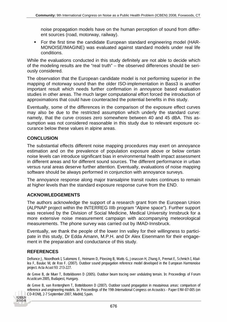
Community: 9th International Congress on Noise as a Public Health Problem (ICBEN) 2008, Foxwoods, CT
noise propagation models have on the human perception of sound from differ-ent sources (road, motorway, railway).
For the first time the candidate European standard engineering model (HAR-MONOISE/IMAGINE) was evaluated against standard models under real life conditions.
While the evaluations conducted in this study definitely are not able to decide which of the modeling results are the “real truth” – the observed differences should be seri-ously considered. The observation that the European candidate model is not performing superior in the mapping of motorway sound than the older ISO-implementation in Bass3 is another important result which needs further confirmation in annoyance based evaluation studies in other areas. The much larger computational effort forced the introduction of approximations that could have counteracted the potential benefits in this study. Eventually, some of the differences in the comparison of the exposure effect curves may also be due to the restricted assumption which underly the standard curve: namely, that the curve crosses zero somewhere between 40 and 45 dBA. This as-sumption was not considered reasonable in this study due to relevant exposure oc-curance below these values in alpine areas.
CONCLUSION The substantial effects different noise mapping procedures may exert on annoyance estimation and on the prevalence of population exposure above or below certain noise levels can introduce significant bias in environmental health impact assessment in different areas and for different sound sources. The different performance in urban versus rural areas deserve further attention. Eventually, evaluations of noise mapping software should be always performed in conjunction with annoyance surveys. The annoyance response along major transalpine transit routes continues to remain at higher levels than the standard exposure response curve from the END.
ACKNOWLEDGEMENTS The authors acknowledge the support of a research grant from the European Union (ALPNAP project within the INTERREG IIIb program “Alpine space”). Further support was received by the Division of Social Medicine, Medical University Innsbruck for a more extensive noise measurement campaign with accompanying meteorological measurements. The phone survey was carried out by IMAD-Innsbruck. Eventually, we thank the people of the lower Inn valley for their willingness to partici-pate in this study, Dr Edda Amann, M.P.H. and Dr Alex Eisenmann for their engage-ment in the preparation and conductance of this study.
REFERENCES Defrance J, Noordhoek I, Salomons E, Heimann D, Plovsing B, Watts G, Jonasson H, Zhang X, Premat E, Schmich I, Abal-lea F, Baulac M, de Roo F. (2007). Outdoor sound propagation reference model developed in the European Harmonoise project. Acta Acust 93: 213-227.
de Greve B, de Muer T, Botteldooren D (2005). Outdoor beam tracing over undulating terrain. In: Proceedings of Forum Acusticum 2005, Budapest, Hungary.
de Greve B, van Renterghem T, Botteldooren D (2007). Outdoor sound propagation in moutainous areas: comparison of reference and engineering models. In: Proceedings of the 19th International Congress on Acoustics - Paper ENV-07-005 (on CD-ROM), 2-7 September 2007, Madrid, Spain.
676

Community: 9th International Congress on Noise as a Public Health Problem (ICBEN) 2008, Foxwoods, CT
Fields, JM (1993). Effect of personal and situational variables on noise annoyance in residential areas. J Acoust Soc Am 93: 2753-2763.
Fields JM (2003). Statement unpublished on the 8th International Congress on Noise as a Public Health Problem, Rotter-dam, The Netherlands, 29 June – 3 July, 2003.
Fields JM, Ehrlich GE, Zador P (2000). Theory and design tools for studies of reactions to abrupt changes in noise exposure. Langley Research Center. Report No: NAS 1.26210280.
Fields JM, de Jong RG, Gjestland T, Flindell IH, Job RFS, Kurra S, Lercher P, Vallet M, Yano T, Guski R, Felscher-Suhr U, Schumer R (2001). Standardized general-purpose noise reaction questions for community noise surveys: research and a recommendation. J Sound Vibr 242: 641-679.
Harrell FE Jr (2001). Regression modeling strategies. New York: Springer.
Heimann D, de Franceschi M, Emeis S, Lercher P, Seibert P (eds) (2007). Air pollution, traffic noise and related health ef-fects in the alpine space - a guide for authorities and consulters. ALPNAP comprehensive report. Trento, Italy: Università degli Studi di Trento, Dipartimento di Ingegneria Civile e Ambientale.
ISO TC 43/SC 1 (2002-02), N/A. Acoustics - Assessment of noise annoyance by means of social and socioacoustic surveys. Geneve: ISO Central Secretariat.
Job RSF (1988). Community response to noise: A review of factors influencing the relationship between noise exposure and reaction. J Acoust Soc Am 83: 991-1001.
Jonasson HG (2007). Acoustical source modelling of road vehicles. Acta Acust united with Acust 93: 174-183.
Lui WK, Li KM, Ng PL, Frommer GH (2006). A comparative study of different numerical models for prediction train noise in high-rise cities. Appl Acoust 67:432-449.
Miedema HME, Oudshoorn CG (2001). Annoyance from transportation noise: relationships with exposure metrics DNL and DENL and their confidence intervals. Environ Health Perspect 109: 409-416.
Miedema HME, Vos H (1999). Demographic and attitudinal factors that modify annoyance from transportation noise. J Acoust Soc Am 105: 3336-3344.
Miedema HME, Vos H (2003). Noise sensitivity and reactions to noise and other environmental conditions. J Acoust Soc Am 113: 1492-1504.
Miedema HME, Fields JM, Vos H (2005). Effect of season and meteorological conditions on community noise annoyance. J Acoust Soc Am 117: 2853-2865.
R Development Core Team (2006). R: A language and environment for statistical computing. R Foundation for Statistical Computing, Vienna, Austria. http://www.R-project.org.
van Leeuwen HJA (2000). Railway Noise Prediction Models: A Comparison. J Sound Vib 231 (3): 975-987.
van Maercke D, Defrance J (2007). Development of an analytical model for outdoor sound propagation within the Har-monoise project. Acta Acust 93: 201-212.
van Renterghem T, Botteldooren D, Lercher P (2007). Comparison of measurements and predictions of sound propagation in a valley-slope configuration in an inhomogeneous atmosphere. J Acoust Soc Am 121: 2522-2533.
677

Community: 9th International Congress on Noise as a Public Health Problem (ICBEN) 2008, Foxwoods, CT
Study on sound environment and community response to noise in Tianjin, a Chinese city Hui Ma1*, Takashi Yano2 1 School of Architecture, Tianjin University, China
2 Kumamoto University, Japan
* corresponding author: e-mail: [email protected]
A social survey on sound environment and community response to noise was carried out in Tianjin, the third biggest city in China. Dose-response relationship curves of road traffic noise were firstly constructed by using ICBEN method. At the same time, acoustical condition in Tianjin and resident’s attitude to noise problem was analyzed in demographic point of view.
678

Community: 9th International Congress on Noise as a Public Health Problem (ICBEN) 2008, Foxwoods, CT
Influence of attitudes to noise sources on annoyance Takashi Morihara1*, Tetsumi Sato2, Takashi Yano3 1 Ishikawa National College of Technology, Kitachujo, Tsubata, Kahoku Gun, Ishikawa, Japan
2 Hokkai Gakuen University, South 26, West 11, Chuo-Ku, Sapporo, Japan
3 Kumamoto University, Kurokami 2-39-1, Kumamoto, Kumamoto, Japan
* corresponding author: e-mail: [email protected]
INTRODUCTION The influence of transportation noise on the quality of life has so far been investi-gated by socio acoustical surveys, some of which have shown that noise annoyance is affected by not only noise exposure but also non-acoustical factors. Fields (1993) conducted meta-analysis on the effects of personal and situational variables on an-noyance, in which he indicated that noise annoyance was strongly affected by three attitudes (fear, preventability, sensitivity) and weakly by situational factors but not by demographic factors (age, social status, etc.), exposure time, ambient noise and in-terview method. Miedema & Vos (1999) also pointed out that fear and sensitivity were important on the prediction of noise annoyance. Hong et al. (2007) also showed by ANOVA that sensitivity had a significant effect on sleep disturbance but sex and age of participants did not. Sandrock et al. (2008) demonstrated that people who are more sensitive to tram and bus noise gave higher annoyance at experimental study. On the other hand, using a magnitude estimation method in laboratory experiment, Ellermeier et al. (2001) showed that the degree of sensitivity did not affect response to noise. Though these studies were mainly related to sensitivity, there were a few other studies which investigated the influence of the attitudes towards noise sources. Since noise annoyance is usually affected by socio-cultural factors, investigating the effect of the attitudes on annoyance in Japan may be the key to find out the difference in dose-response relationships for transportation noises between Japan and Euro-American countries (Fields & Walker 1982; Knall & Schuemer 1983; Moehler 1988; Miedema & Vos 1998; Kaku & Yamada 1996 and Morihara et al. 2002). The purpose of this study is, therefore, to investigate whether the attitudes, in terms of the frequency of noise source usage, cognition to noise source and safety image of noise source, affect noise annoyance.
METHODS
Social surveys Data from three socio-acoustic surveys, respectively on community response to road traffic and railway noises in Ishikawa 2007, on high speed train noise in Fukuoka 2003 and on aircraft noise in Kumamoto 2006 were analyzed, in which noise annoyance was measured by the ICBEN standardized 5-point verbal scale. Table 1 shows the summary of the socio-acoustic surveys. The sample sizes were 950, 724 and 413, respectively. The respondents were randomly selected on a one-person per family basis from detached houses. Questionnaires consisted of questions on an-noyance due to transportation noise source as the key question, activity disturbances caused by each noise source, house structure, residential environment, attitudes to-wards transportation and personal factors. Questions on the three attitude variables and the relative frequency of responses are shown in Table 2.
679

Community: 9th International Congress on Noise as a Public Health Problem (ICBEN) 2008, Foxwoods, CT
Table 1: Summary of socio-acoustic surveys
Survey ID Year Source Area Sample size Response rate (%) HRW03 2003 High speed train Fukuoka 724 66 AC06 2006 Aircraft Kumamoto 413 53
RT&RW07 2007 Road traffic and Railway Ishikawa 950 59
Table 2: Question wordings and relative frequency
HRW03 AC06 RT&RW07 (car)
RT&RW07 (railway)
Q1 (frequency): How frequently do you use the transportation (noise source)? 1. not at all 2. seldom 3. sometimes 4. often 5. very often
3.7 15.5 36.1
8.0 36.8
5.9 13.0 30.9
7.2 43.1
5.0 4.5
14.5 23.3 52.7
28.1 44.5 21.5 4.3 1.6
Q2 (cognition): What do you think about usage of transportation (noise source) in the general pub-lic?
1. positively 2. as … as possible 3. neither 4. as … as possible not 5. not at all
9.7 30.9 52.3
4.5 2.7
6.1 19.0 65.6
6.3 2.9
5.0 10.6 45.8 37.9 0.8
15.5 52.7 30.0 1.6 0.2
Q3 (safety): What do you think about safety of transportation (noise source)? 1. very safe 2. relative safe 3. neither safe nor dangerous 4. relative dangerous 5. very dangerous
20.8 46.2 28.8
3.5 0.7
7.1 31.4 46.1 12.0
3.4
2.0 19.6 40.8 31.9 5.6
22.3 54.6 21.3 1.6 0.1
Noise exposure The outdoor noise exposure levels at the nearest points from the sound source were calculated by measurement and equation of estimating attenuation. Noise exposure levels have not yet measured in Ishikawa survey. Noise exposure levels of LAeq,24h ranged from 32 to 50 dB in high speed train survey and from 43 to 53 dB in aircraft noise survey.
RESULTS In this study, the effects of the three attitudes on noise annoyance were investigated by correlation coefficient and dose response relationships. The correlation coefficient was calculated with the data of HRW03, AC06 and RT&RW07 (abbreviations see Table 1. The dose-response relationships were established by using the data of HRW03 and AC06 and were compared between two groups divided by the attitude degree.
680

Community: 9th International Congress on Noise as a Public Health Problem (ICBEN) 2008, Foxwoods, CT
Correlation Coefficient Correlation coefficient between each attitude and noise/exhaust gas/vibration annoy-ance is shown in Table 3. It was indicated that the correlation coefficients between frequency of transportation usage and three kinds of annoyance were very small in all surveys (maximum value is -0.096). The correlation coefficients between cognition and annoyance were also small. Though the correlation coefficients between safety and annoyance were small for HRW03 and RT&RW07, the correlation coefficient be-tween safety and noise/vibration annoyance for AC06 were slightly larger, 0.165 and 0.238, respectively.
Table 3: Correlation Coefficient between attitudes and annoyance
annoyance attitude survey ID
noise exhaust gas vibration frequency HRW03 -0.052 - -0.001 AC06 0.039 - 0.055 RT&RW07(car) -0.012 -0.096 -0.022 RT&RW07(rail) 0.044 - 0.029 cognition HRW03 0.046 - 0.072 AC06 0.062 - 0.041 RT&RW07(car) 0.043 0.026 0.001 RT&RW07(rail) 0.055 - 0.058 safety HRW03 0.030 - 0.082 AC06 0.165 - 0.238 RT&RW07(car) 0.062 0.044 0.048 RT&RW07(rail) 0.059 - 0.057
Dose-response relationships This section shows whether dose-response curves would differ statistically between the two groups divided based on attitude factors. The curves were drawn by a nomi-nal logistic regression analysis: the objective variable was noise annoyance, and the explanatory variables were noise exposure (LAeq, 24h) and each attitude. Annoy-ance was set to dummy variables as 1 is extremely; 0 is not at all, slightly, moder-ately and very. The attitudes were also set to dummy variables accordingly. The es-timates of the parameters and their standard errors are shown in Table 4 (HRW03) and Table 5 (AC06), except the cases that the sample sizes were under 100. Figure 1 shows that aircraft usage significantly affected the dose-response relationships be-tween noise annoyance and LAeq,24h for AC06 at 5 % level. However, the cognition and the safety did not significantly affect annoyance in AC06. Also the frequency of usage, the cognition and the safety had no significant effects on noise annoyance in HRW03. This may be because the people who frequently use aircraft know the air-plane well, and they recognize that the aircraft should be quieter than the present cir-cumstances.
CONCLUSIONS The frequency of usage and the cognition of the noise sources had almost no corre-lations to noise, exhaust gas and vibration annoyance. The safety image of aircraft had very small correlations to noise and vibration annoyance. Dose-response curves were affected by the frequency of aircraft usage. It was found that the group fre-quently using aircraft was more annoyed than the other group. The cognition and the
681

Community: 9th International Congress on Noise as a Public Health Problem (ICBEN) 2008, Foxwoods, CT
safety image of noise sources not affect dose-response curves in both noise sources. This study does not investigate the indirect effect of the attitudes towards noise sources, and there is scope for further discussion.
Table 4: Estimates, standard errors and p values are based on HRW03
(a) Frequency of transportation usage 1+2 [1] vs. other [0] 5 [1] vs. other [0] 4+5 [1] vs. other [0]
Estimate s.e. P value Estimate s.e. P value Estimate s.e. P value
Constant -13.96 1.80 <.0001 -13.95 1.81 <.0001 -13.96 1.81 <.0001LAeq, 24h 0.28 0.04 <.0001 0.28 0.04 <.0001 0.28 0.04 <.0001Frequency 0.24 0.25 0.346 -0.35 0.22 0.116 -0.29 0.21 0.164(b) Cognition of noise source
1+2 [1] vs. other [0]
Estimate s.e. P value Constant -13.71 1.75 <.0001 LAeq, 24h 0.27 0.04 <.0001 Cognition 0.22 0.21 0.289 (c) Safety images to noise source
1 [1] vs. other [0] 1+2 [1] vs. other [0]
Estimate s.e. P value Estimate s.e. P value Constant -13.37 1.73 <.0001 -13.30 1.74 <.0001 LAeq, 24h 0.27 0.04 <.0001 0.26 0.04 <.0001 Safety -0.04 0.25 0.877 -0.08 0.21 0.706
Table 5: Estimates, standard errors and p values are based on AC06
(a) Frequency of transportation usage 5 [1] vs. other [0] 4+5 [1] vs. other [0]
Estimate s.e. P value Estimate s.e. P value
Constant -11.15 1.66 <.0001 -11.33 1.67 <.0001LAeq, 24h 0.19 0.03 <.0001 0.19 0.03 <.0001Frequency 0.70 0.31 0.025 0.76 0.32 0.018(c) Safety images to noise source
1+2 [1] vs. other [0]
Estimate s.e. P value Constant -10.52 1.6 <.0001 LAeq, 24h 0.18 0.03 <.0001 Safety -0.10 0.31 0.756
ACKNOWLEDGMENTS
This work was partially supported by Grant-in-Aid for Scientific Research (Project No: 19760408).
682
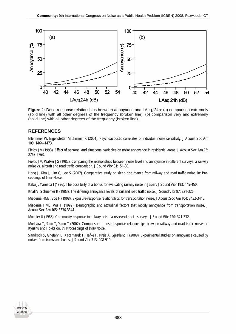
Community: 9th International Congress on Noise as a Public Health Problem (ICBEN) 2008, Foxwoods, CT
Figure 1: Dose-response relationships between annoyance and LAeq, 24h: (a) comparison extremely (solid line) with all other degrees of the frequency (broken line); (b) comparison very and extremely (solid line) with all other degrees of the frequency (broken line).
REFERENCES Ellermeier W, Eigenstetter M, Zimmer K (2001). Psychoacoustic correlates of individual noise sensitivity. J Acoust Soc Am 109: 1464–1473.
Fields JM (1993). Effect of personal and situational variables on noise annoyance in residential areas. J Acoust Soc Am 93: 2753-2763.
Fields JM, Walker JG (1982). Comparing the relationships between noise level and annoyance in different surveys: a railway noise vs. aircraft and road traffic comparison. J Sound Vibr 81: 51-80.
Hong J, Kim J, Lim C, Lee S (2007). Comparative study on sleep disturbance from railway and road traffic noise. In: Pro-ceedings of Inter-Noise.
Kaku J, Yamada I (1996). The possibility of a bonus for evaluating railway noise in Japan. J Sound Vibr 193: 445-450.
Knall V, Schuemer R (1983). The differing annoyance levels of rail and road traffic noise. J Sound Vibr 87: 321-326.
Miedema HME, Vos H (1998). Exposure-response relationships for transportation noise. J Acoust Soc Am 104: 3432-3445.
Miedema HME, Vos H (1999). Demographic and attitudinal factors that modify annoyance from transportation noise. J Acoust Soc Am 105: 3336-3344.
Moehler U (1988). Community response to railway noise: a review of social surveys. J Sound Vibr 120: 321-332.
Morihara T, Sato T, Yano T (2002). Comparison of dose-response relationships between railway and road traffic noises in Kyushu and Hokkaido. In: Proceedings of Inter-Noise.
Sandrock S, Griefahn B, Kaczmarek T, Hafke H, Preis A, Gjestland T (2008). Experimental studies on annoyance caused by noises from trams and buses. J Sound Vibr 313: 908-919.
0
25
50
75
100
40 42 44 46 48 50 52 54LAeq,24h (dB)
Anno
yanc
e (%
)
0
25
50
75
100
40 42 44 46 48 50 52 54LAeq,24h (dB)
Anno
yanc
e (%
)
Anno
yanc
e (%
)
0
25
50
75
100
40 42 44 46 48 50 52 54LAeq,24h (dB)
Anno
yanc
e (%
)
0
25
50
75
100
40 42 44 46 48 50 52 54LAeq,24h (dB)
(a) (b)
683

Community: 9th International Congress on Noise as a Public Health Problem (ICBEN) 2008, Foxwoods, CT
The importance of non-acoustical factors on noise annoyance of urban residents Katarina Paunovic1*, Branko Jakovljevic1, Goran Belojevic1 1 Institute of Hygiene and Medical Ecology, School of Medicine, University of Belgrade, Dr Subotica
8, 11000 Belgrade, Serbia
*corresponding author: e-mail: [email protected]
INTRODUCTION Noise annoyance is a feeling of displeasure or disturbance caused by noise. It is a sensitive indicator of adverse noise effects. Noise annoyance can only be partially explained by acoustical characteristics of noise – its level, frequency, duration, source etc. Non-acoustical factors, such as personal characterisitcs (age, gender, noise sensitivity), and social, residential or environmental factors are also related to noise annoyance (Ouis 2001). Noise annoyance experiments typically do not con-sider all non-acoustical factors, because they are interested in average response of a large population. Several mechanisms explain the onset of noise annoyance in relation to noise. Noise annoys because it masks other sounds, it makes intellectual activities difficult, it dis-turbs one’s attention and concentration, leads to physiological arousal, and triggers “negative” or distressing affective/emotional reactions (Miedema 2007). According to this model, personal characteristics, such as neuroticism (Ohrström et al. 1988), in-troversion (Belojevic et al. 2001), and noise sensitivity (Ohrström et al. 1988; van Kamp et al. 2004) are highly correlated with noise annoyance. Social factors that trigger stressful reactions are also strongly correlated to noise an-noyance. For example, marital status, presence of children, or longer duration of stay at home at day (due to unemployment or retirement) may increase stress level in many persons (Wallenius 2004). Residential factors (type of dwelling, number of dwellers, floor level, years of residence), and environmental characteristics (neighborhood safety, air pollution etc.) may be related to socio-economic status, which in turn means that people with lower socio-economic status are exposed to multiple adverse environmental conditions, including high noise levels (Evans & Kan-trowitz 2002). The aim of this study was to assess the influence of personal and residential factors on noise annoyance of residents of Belgrade.
METHODS The study was performed in a city center of Belgrade, Serbia, from 2004-2006. We interviewed all adult residents in every tenth flat in all streets, thus obtaining a ran-domized sample of 6,000 people (10 % of the population of the municipality, accord-ing to census data). The questionnaires were distributed to post boxes inside the buildings according to the list of dwellers. The response rate was 52.8 %, with 3,169 filled questionnaires. After applying the inclusion criterion for the study (period of residence for at least 3 years), the study sample comprised 2,155 middle-aged residents (1,003 men and 1,152 women). Noise measurements were performed in all 70 streets of the municipality, using Noise Level Analyzer type 4426 “Brüel & Kjær” (ISO 1982). A composite 24-hour equivalent
684

Community: 9th International Congress on Noise as a Public Health Problem (ICBEN) 2008, Foxwoods, CT
noise level [Leq (dBA)] was calculated from noise measurement at daytime, evening and night. Noise annoyance was assessed using a self-reported numeric scale (range 0-10); high-level annoyance was identified as score ≥ 6. A questionnaire on personal characteristics (age, gender, marital status, education, income) and residential factors (flat size, number of dwellers, years of residence, floor level) was anonymous. Descriptive statistic is presented as mean values ± standard deviation (SD) for nu-meric variables, or as percents (relative numbers) for categorical variables. The dif-ferences between groups were tested using Student’s test, Chi-square test and Mann-Whitney U test. The association between parametric data was measured by Pearson's correlation coefficient. Univariate logistic regression was performed to cal-culate odds ratios for high-level annoyance in relation to relevant independent vari-ables. The influence of personal and social characteristics on high-level annoyance was estimated using multivariate logistic regression.
RESULTS The investigated population comprised 1,453 residents with low-level of noise annoyance and 702 highly annoyed residents (Table 1). The prevalence of highly annoyed residents was 32.6 %. The studied groups were similar by age, gender, marital status, having children, education and income. They also had similar dwelling characteristics. However, highly annoyed residents more often reported having windows of their bedroom oriented toward the streets (30.5 % compared to 9.9 % of not annoyed residents).
Table 1: Basic characteristics of investigated population in relation to noise annoyance
Residential and environmental characteristics
Low-level an-noyance
High-level an-noyance Total p value
Number of subjects 1453 (67.4 %) 702 (32.6 %) 2155 (100.0 %)
Age (years) 41.7±16.7 43.6±16.8 42.4±16.8 0.088* Gender (male) 407(40.6 %) 367 (36.6 %) 774 (35.9 %) 0.074†
Married subjects 696 (47.9 %) 362 (51.6 %) 1058 (49.1 %) 0.293† Subjects with children 800 (55.1 %) 425 (60.5 %) 1225 (56.8 %) 0.101†
Education (college/ university) 782 (53.8 %) 392 (55.8 %) 1174 (54.5 %) 0.148† Income (very good/ excellent) 1001 (68.9 %) 491 (69.9 %) 1492 (69.2 %) 0.719†
Type of work (intellectual) 946 (65.1 %) 462 (65.8 %) 1408 (65.3 %) 0.591† Years of employment 20.2±12.6 20.6±11.9 20.4±12.5 0.699‡ Years of residence 17.3±14.1 18.4±14.9 17.7±14.4 0.367‡ Flat size per dweller 23.1±12.6 23.9±11.8 23.4±12.4 0.052‡
Floor 2.6±1.8 2.7±2.2 2.6±1.9 0.623‡ Windows of bedroom oriented
toward the street 144 (9.9 %) 214 (30.5 %) 358 (16.6 %) <0.0001†
* Student’s t-test
† Chi-square test
‡ Mann-Whitney U test
The correlation between mean score on noise annoyance scale and personal and social characteristics is presdented in Table 2. Mean annoyance score showed strong positive correlation with residents’ age, years of employment, length of residence, and number of hours spent at home. Inverse correlation was found only
685
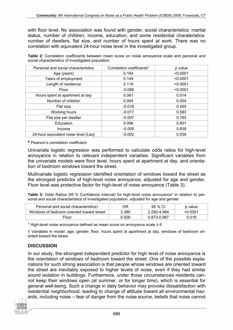
Community: 9th International Congress on Noise as a Public Health Problem (ICBEN) 2008, Foxwoods, CT
with floor level. No association was found with gender, social characteristics: marital status, number of children, income, education; and some residential charateristics: number of dwellers, flat size, and number of hours spent at work. There was no correlation with equivalent 24-hour noise level in the investigated group.
Table 2: Correlation coefficients between mean score on noise annoyance scale and personal and social characteristics of investigated population
Personal and social characteristics Correlation coefficients* p value Age (years) 0.164 <0.0001
Years of employment 0.149 <0.0001 Length of residence 0.119 <0.0001
Floor -0.088 <0.0001 Hours spent at apartment at day 0.061 0.014
Number of children 0.045 0.054 Flat size -0.018 0.450
Working hours -0.017 0.583 Flat size per dweller -0.007 0.785
Education 0.006 0.801 Income -0.005 0.839
24-hour equivalent noise level (Leq) -0.002 0.939
* Pearson’s correlation coefficient Univariate logistic regression was performed to calculate odds ratios for high-level annoyance in relation to relevant independent variables. Significant variables from the univariate models were floor level, hours spent at apartment at day, and orienta-tion of bedroom windows toward the street. Multivariate logistic regression identified orientation of windows toward the street as the strongest predictor of high-level noise annoyance, adjusted for age and gender. Floor level was protective factor for high-level of noise annoyance (Table 3).
Table 3: Odds Ratios (95 % Confidence Interval) for high-level noise annoyance* in relation to per-sonal and social characteristics of investigated population, adjusted for age and gender
Personal and social characteristics† OR 95 % CI p value Windows of bedroom oriented toward street 3.380 2.292-4.984 <0.0001
Floor 0.928 0.873-0.987 0.018
* High-level noise annoyance defined as mean score on annoyance scale ≥ 6
† Variables in model: age, gender, floor, hours spent at apartment at day, windows of bedroom ori-ented toward the street
DISCUSSION In our study, the strongest independent predictor for high level of noise annoyance is the orientation of windows of bedroom toward the street. One of the possible expla-nations for such strong association is that people whose windows are oriented toward the street are inevitably exposed to higher levels of noise, even if they had similar sound isolation in buildings. Furthermore, under those circumstances residents can-not keep their windows open (at summer, or for longer time), which is essential for
general well-being. Such a change in daily behavior may provoke dissatisfaction with residential neighborhood, leading to change of attitude toward all environmental haz-ards, including noise – fear of danger from the noise source, beliefs that noise cannot
686

Community: 9th International Congress on Noise as a Public Health Problem (ICBEN) 2008, Foxwoods, CT
be prevented, feeling of insecurity, increased noise sensitivity, and even distrust to-ward environmental authorities (Fields 1993; Guski 1999). The preventive effect of floor level is explained by lower level of noise in the apart-ment. On the other hand, living on higher floors may prevent people from doing some everyday activities – feeding, clothing – especially for the elderly and disabled. Such circumstances alone can lead to higher stress level and probably lead to higher an-noyance (Wallenius 2004). The limitation of the study is that we did not assess the hearing capacity of the par-ticipants, their general stress level and noise sensitivity.
CONCLUSIONS This cross-sectional study identified orientation of bedroom toward the street as the most significant independent predictor of high annoyance in adult population of a Belgrade municipality. This finding may help exposed residents find other efficient behavioral strategies of coping with noise.
ACKNOWLEDGEMENT This study was financially supported by the Ministry of Science of Serbia, Project No. 145013, 2006-2010.
REFERENCES Belojevic G, Slepcevic V, Jakovljevic B (2001). Mental performance in noise: the role of introversion. J Environ Psychol 21: 209–213.
Evans GW, Kantrowitz E (2002). Socioeconomic status and health: the potential role of environmental risk exposure. Annu Rev Public Health 23: 303–331.
Fields JM (1993). Effect of personal and situational variables on noise annoyance in residential areas. J Acoust Soc Am 93: 2753–2763.
Guski R (1999). Personal and social variables as co-determinants of noise annoyance. Noise & Health 1: 45–56.
ISO (International Organization for Standardization) (1982). Acoustics – Description and measurement of environmental noise – Part l, Basic quantities and procedures. International Standard. ISO 1996-1. Geneva: International Organization for Standardization.
Miedema HM (2007). Annoyance caused by environmental noise: elements for evidence-based noise policies. J Soc Issues 63: 41–57.
Öhrström E, Björkman M, Rylander R (1988). Noise annoyance with regard to neurophysiological sensitivity, subjective noise sensitivity and personality variables. Psychol Med 18: 605–613.
Ouis D (2001). Annoyance from road traffic noise: a review. J Environ Psychol 21: 101–120.
van Kamp I, Soames Job RF, Hatfield J, Haines M, Stellato RK, Stansfeld SA (2004). The role of noise sensitivity in the noise–response relation: A comparison of three international airport studies. J Acoust Soc Am 116: 3471–3479.
Wallenius MA (2004). The interaction of noise stress and personal project stress on subjective health. J Environ Psychol 24: 167–177.
687

Community: 9th International Congress on Noise as a Public Health Problem (ICBEN) 2008, Foxwoods, CT
Annoyance from road traffic noise with horn sounds: A cross-cultural experiment between Vietnamese and Japanese Hai Anh Thi Phan1*, Tsuyoshi Nishimura1, Hai Yen Thi Phan2, Takashi Yano2, Tetsumi Sato3 ,Yoritaka Hashimoto4 1 Sojo University, Ikeda 4-22-1, Kumamoto 860-0082, Japan
2 Kumamoto University, Kurokami 2-39-1, Kumamoto 860-8555, Japan
3 Hokkai Gakuen University, Minami 26, Nishi 11, Chuo-ku, Sapporo 064-0926, Japan
4 Osaka City University, Sugimoto 3-3-138, Sumiyoshi, Osaka 558-8585, Japan
* corresponding author: e-mail: [email protected]
INTRODUCTION Over the past decades a large number of social surveys on community response to noise and psychoacoustic experiments have been conducted in developed and, to a lesser extent, developing countries (Schultz 1978; Namba et al. 1991a, b; Fastl et al. 1996; Miedema & Vos 1998; Lam 1994; Fields 2001; Sato et al. 2000). The current authors have conducted social surveys on community response to noise in Hanoi in Vietnam since 2004 (Phan HYT et al. 2006; Phan HAT et al. 2006, 2007), and road traffic noise in Hanoi was found to be characterized by a great number of motorbikes creating frequent horn sounds. The LAeq,24h was obtained, ranging from 70 to 77 dB. In order to investigate the effects of horn sounds on road traffic noise annoyance sys-tematically, a psychoacoustic experiment was carried out in 2006 with young Viet-namese and Japanese students in Hanoi and Kumamoto, respectively. The main findings obtained were that Japanese were more annoyed by noise with frequent horn sounds than that without horn sound, while there was no significant difference in annoyance between the two types of noise for Vietnamese and that Japanese were more annoyed by noise than Vietnamese. The authors have hypothesized the possi-ble reasons for the above findings. (1) Vietnamese were more used to noise with fre-quent horn sounds; (2) Young Vietnamese were more tolerant to noise with frequent horn sounds than the older Vietnamese; (3) The modifiers of noise annoyance scale in Vietnamese were more intense than those in Japanese. Accordingly, to validate these hypotheses, three additional experiments were carried out in Kumamoto and Hanoi, respectively, on the extended groups of subjects includ-ing a group of Vietnamese living in Japan for a certain period of time and a group of older Vietnamese living in Hanoi (over 30 years of age), and on the intensity of Viet-namese and Japanese modifiers for their annoyance scales.
EXPERIMENT Four experiments were performed. The three experiments (Experiment A, B, C) were to cross-culturally investigate the annoyance caused by road traffic noise with and without horn sounds. The first experiment (Experiment A) was performed to compare annoyance between young Vietnamese and Japanese students. The second experiment (Experiment B) was to compare annoyance evaluated by Vietnamese living in Japan for a period of time with that by young Vietnamese obtained in Experiment A. The third experiment
688

Community: 9th International Congress on Noise as a Public Health Problem (ICBEN) 2008, Foxwoods, CT
(Experiment C) was to compare annoyance evaluated by the older Vietnamese with that by young Vietnamese obtained in Experiment A. The last one (Experiment D) was carried out to compare the intensity of modifiers used for noise annoyance scales between Vietnamese and Japanese.
Experiments on road traffic noise annoyance (Experiment A; B; C) Test sound Twelve kinds of test sound at three noise levels (LAeq,35s): 75, 65, 55 dB and four horn sound frequencies were used: Road traffic noise in Japan without horn sound (RTNJ); Road traffic noise in Hanoi without horn sound (RTN0); Road traffic noise in Hanoi with 12 noticeable horn sounds (RTN12); Road traffic noise in Hanoi with 51 noticeable horn sounds (RTN51). The road traffic noise in Japan at 75 dB and at 65 dB were obtained from the com-mercial CD, which were recorded at 5 m and 25 m distance from the road shoulder. To create RTNJ at 55 dB, noise at 75 dB was decreased by 20 dB through a “house filter” which was created based on indoor and outdoor level differences produced by Japanese typical house window in real-life conditions. The road traffic noise in Hanoi was recorded in Hanoi in September 2005, at 12 m distance from the road shoulder. RTN51, RTN12, RTN0 at 75 dB were taken from the parts of the noise recording with many, few and no horn sounds, respectively. To make test sounds at 65 dB, the road traffic noise was decreased by 10 dB by adjust-ing the volume of amplifier. A house filter was used again to reduce 20 dB from 75 dB noise level of the recorded to create test sounds at 55 dB. The sound level fluctuation of test sound RTN51 with RTNJ and of test sound RTN51 with RTN0 is demonstrated in Figure 1 (a) and (b), respectively. The sharp peaks identified on the solid line in both figures are the horn sounds. The relative cumula-tive frequency curves for test sounds RTNJ, RTN51 and RTN0 can be seen in Figure 2. Test sound RTN51 is distributed more widely, ranging from 42 to 92 dB, mean-while, test sounds RTNJ and RTN0 have smaller range from approximately 45 to 85 dB.
50
60
70
80
90
100
10 20 30
RTN51RTNJ
A-w
eigh
ted
soun
d pr
essu
re le
vel (
dB)
Time (s)Figure 1(a) : Fluctuation pattern of sound levelRoad traffic noise in Japan without horn sound (RTNJ) &road traffic noise in Hanoi with 51 horn sound (RTN51)
50
60
70
80
90
100
10 20 30
RTN51
RTN0
A-w
eigh
ted
soun
d pr
essu
re le
vel (
dB)
Time (s)
Figure 1(b): Fluctuation pattern of sound levelRoad traffic noise in Hanoi without horn sound (RTN0) & road traffic noise in Hanoi with 51 horn sound (RTN51)
689

Community: 9th International Congress on Noise as a Public Health Problem (ICBEN) 2008, Foxwoods, CT
40 50 60 70 80 90 1000
20
40
60
80
100
RTNJRTN51RTN0
A-weighted sound pressure level (dB)
Rel
ativ
e cu
mm
ulat
ive
frequ
ency
(%)
Figure 2: Relative cumulative frequency of noise level
0
30
60
90
Anechoic room in Kumamoto
Recording studio in Hanoi
31.5 500 1k 2k 4k 8k 16k63 250125
1/3
Ota
ve b
and
soun
d pr
essu
re le
vel (
dB)
Center Frequency (Hz)Figure 3: Frequency analysis of test sound RTN51
The result of 1/3 octave band frequency analysis of test sound RTN51 is shown in Figure 3. The thick line with filled symbols denotes the result produced in the anech-oic room at Kumamoto University, and the thin line with open symbols indicates the result from the recording studio in Hanoi. In the 2-4 kHz range, main frequency com-ponents of horn sound can be seen clearly. Even though these results correspond well in the middle and high frequency ranges, the result at low frequency range of reproduced sound in the recording studio in Hanoi is seen higher due to the reso-nance.
Facilities setting Experiment A was performed in an anechoic room at Kumamoto University in Ku-mamoto, Japan (internal dimensions 4.8 m x 5.4 m x 4.5 m); and a recording studio in Hanoi, Vietnam (internal dimensions 3.98 m x 3.86 m x 2.83 m). Experiment B was performed in the same anechoic room at Kumamoto University. Experiment C was performed in the same recording studio in Hanoi. The test sounds were reproduced with a CD player, amplified and then played back from a loudspeaker which was set up in front of an internal wall. Subjects sat on chairs 3 m away from the loudspeaker.
Subjects Experiment A: 30 Japanese students (15 males and 15 females) from 18 to 24 years of age and 30 Vietnamese students (15 males and 15 females) from 20 to 24 years of age. Experiment B: Nine Vietnamese students (6 males and 3 females) who have been living in Kumamoto from one to seven years. Experiment C: 18 Vietnamese (9 males and 9 females) from 30 to 45 years of age. All subjects have self-reported normal hearing threshold. One error, however, was identified on the result of one Japanese and one Vietnamese subject. Therefore, the analysis was made based on only the results of 29 Japanese and 29 Vietnamese.
Procedure The procedures of all experiments were the same in both locations.The experiments were conducted with every three subjects entering the test room at once. Each sub-ject was given a set of instructions outlining the purpose and procedures of the ex-periment. Subjects were seated at the assigned spots, and were told, “Please take your time and imagine that you are relaxing at home after school or work.” Each experiment consisted of three parts: annoyance evaluation using a 5-point ver-bal scale or an 11-point numeric scale (Session 1), annoyance evaluation using the 11-point numeric scale or the 5-point verbal scale (Session 2) and semantic differen-tial evaluation (Session 3). There was a five-minute pause between Session 2 and 3.
690

Community: 9th International Congress on Noise as a Public Health Problem (ICBEN) 2008, Foxwoods, CT
The 5-point verbal scale and the 11-point numeric scale were constructed according to ICBEN method in Japanese and Vietnamese (Yano & Ma 2004). In Session 1 and 2, subjects were to evaluate noise annoyance twice for each of the 12 types of test sound using the 5-point verbal scale (Figure 4) and the 11-point nu-meric scale (Figure 5). Test sounds were presented randomly. The order of the nu-meric and verbal scales was switched every three subjects, that is, if the first three subjects evaluated using the numeric scale first, the next three subjects would evalu-ate using the verbal scale first. With this procedure, the order effect can be cancelled. In Session 3, subjects were to evaluate the impressions of test sounds using seman-tic differential scales. Six test sounds, including RTNJ, RTN5, RTN0 at 75 dB and 55 dB, were chosen from the 12 sound types used in Session 1 and 2. The impressions are evaluated using 7-point dichotomous scales, which were labeled with 13 pairs of antonymous adjectives at the extremes (Fastl et al. 2003). The antonymous adjec-tives are shown in Figure 6. The total time of the experiment was 45 minutes.
Experiment on intensities of modifiers (Experiment D) Modifiers Ten modifiers in Japanese and Vietnamese, from 21 modifers used in the original study of Team 6 of the International Commission on Biological Effects of Noise (IC-BEN) were selected (Table 1).
Table 1: Modifiers
(No/lowest degree of noise annoyance)
(Highest degree of noise annoyance)
Tieng on o muc nho nhat Tieng on o muc lon nhat
うるさくない状態/ 最小のうるささ 最大のうるささ
Hijoni
Japanese Mattaku…nai, kanari, sugoku, sukoshi, sorehodo…nai, daibu, tasho, hijoni, hotondonai, warini
Vietnamese Hoan toan…khong, kha on, cuc on, khong qua on, on phan nao, it on, on nhieu, qua on, rat on
Not at all Slighly Moderately Very Extremely
Mattaku…nai Sorehodo..nai Tasho Daibu Hijoni
Hoan toan khong On phan nao Khong qua On nhieu Cuc on
(a) English (b) Japanese (c) Vietnamese
Figure 4: The 5-point verbal scale
Figure 6: The semantic differential scale
Not at all Extremely 0 1 2 3 4 5 6 7 8 9 10
Figure 5: The 11-point numeric scale
Figure 7: Intensity line-marking
softnot frightening
re laxedweak
pleasant safe
inconspicuousvague
soft
slowdeepdark
tranquil
frighteningloud
tensepowerfulunpleasantdangerousconspicuousdistincthardbusyfastshrillbright
691

Community: 9th International Congress on Noise as a Public Health Problem (ICBEN) 2008, Foxwoods, CT
Subjects Twenty subjects from 23 to 56 years of age, who speak fluently both Japanese and Vietnamese participated in the study. Japanese was the first language of six males (mean age: 45) and four females (mean age: 37), while Vietnamese was the first lan-guage of five males (mean age: 39) and five females (mean age: 30). The Japanese subjects had lived in Vietnam for an average of five years and the Vietnamese sub-jects had lived in Japan for an average of four years.
Procedure Based on the method devised by ICBEN Team 6 (Masden & Yano 2004), all of the subjects assigned the intensity associated with each word of the 20 Japanese and Vietnamese modifiers by placing a mark on a 10 cm line that extends from “No/lowest degree of annoyance” to “Highest degree of noise annoyance” as shown in Figure 7. The modifiers were presented sequentially in a random order. The experiment took the total time of approximately 15 minutes to complete.
RESULTS The trends of the results are almost the same between the verbal and the numeric scales. Thus only the results from the numeric are presented hereafter.
Comparison of annoyance of road traffic noise with and without horn sounds between young Vietnamese students living in Hanoi and Japanese
Mean annoyance score A The mean values of noise annoyance score evaluated by the numeric scale by young Japanese and Vietnamese students are displayed in Figures 8 and 9, respectively. The mean values of noise annoyance from test sounds RTN51 and RTNJ were com-pared between Japanese and Vietnamese subjects. Japanese seemed to be more annoyed by the test sound with horn sound, while for Vietnamese horn sound did not seem to affect noise annoyance (Figure 10).
0
5
10
55 65 75
RTNJRTN51RTN12RTN0
LAeq (dB)
Anno
yanc
e sc
ore
Figure 8: Noise annoyance evaluated by Japanese using an 11- point numeric scale
0
5
10
55 65 75
RTNJ RTN51 RTN12 RTN0
Ann
oyan
ce s
core
LAeq (dB)Figure 9: Noise annoyance evaluated by young Vietnamse using an 11-point numeric scale
692
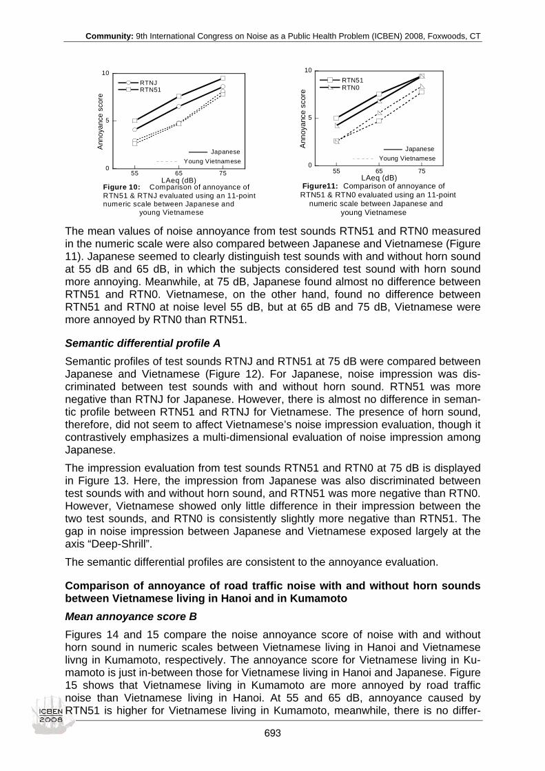
Community: 9th International Congress on Noise as a Public Health Problem (ICBEN) 2008, Foxwoods, CT
0
5
10
55 65 75
RTNJ RTN51
Ann
oyan
ce s
core
LAeq (dB)Figure 10: Comparison of annoyance of RTN51 & RTNJ evaluated using an 11-point numeric scale between Japanese and young Vietnamese
Young VietnameseJapanese
0
5
10
55 65 75
RTN51RTN0
Ann
oyan
ce s
core
LAeq (dB) Figure11: Comparison of annoyance ofRTN51 & RTN0 evaluated using an 11-point numeric scale between Japanese and young Vietnamese
Young VietnameseJapanese
The mean values of noise annoyance from test sounds RTN51 and RTN0 measured in the numeric scale were also compared between Japanese and Vietnamese (Figure 11). Japanese seemed to clearly distinguish test sounds with and without horn sound at 55 dB and 65 dB, in which the subjects considered test sound with horn sound more annoying. Meanwhile, at 75 dB, Japanese found almost no difference between RTN51 and RTN0. Vietnamese, on the other hand, found no difference between RTN51 and RTN0 at noise level 55 dB, but at 65 dB and 75 dB, Vietnamese were more annoyed by RTN0 than RTN51.
Semantic differential profile A Semantic profiles of test sounds RTNJ and RTN51 at 75 dB were compared between Japanese and Vietnamese (Figure 12). For Japanese, noise impression was dis-criminated between test sounds with and without horn sound. RTN51 was more negative than RTNJ for Japanese. However, there is almost no difference in seman-tic profile between RTN51 and RTNJ for Vietnamese. The presence of horn sound, therefore, did not seem to affect Vietnamese’s noise impression evaluation, though it contrastively emphasizes a multi-dimensional evaluation of noise impression among Japanese. The impression evaluation from test sounds RTN51 and RTN0 at 75 dB is displayed in Figure 13. Here, the impression from Japanese was also discriminated between test sounds with and without horn sound, and RTN51 was more negative than RTN0. However, Vietnamese showed only little difference in their impression between the two test sounds, and RTN0 is consistently slightly more negative than RTN51. The gap in noise impression between Japanese and Vietnamese exposed largely at the axis “Deep-Shrill”. The semantic differential profiles are consistent to the annoyance evaluation.
Comparison of annoyance of road traffic noise with and without horn sounds between Vietnamese living in Hanoi and in Kumamoto Mean annoyance score B Figures 14 and 15 compare the noise annoyance score of noise with and without horn sound in numeric scales between Vietnamese living in Hanoi and Vietnamese livng in Kumamoto, respectively. The annoyance score for Vietnamese living in Ku-mamoto is just in-between those for Vietnamese living in Hanoi and Japanese. Figure 15 shows that Vietnamese living in Kumamoto are more annoyed by road traffic noise than Vietnamese living in Hanoi. At 55 and 65 dB, annoyance caused by RTN51 is higher for Vietnamese living in Kumamoto, meanwhile, there is no differ-
693

Community: 9th International Congress on Noise as a Public Health Problem (ICBEN) 2008, Foxwoods, CT
ence between RTN51 and RTNJ for Vietnamese living in Hanoi at almost every level of noise exposure. However, at 75 dB, no difference between two types of noise was found for both groups of Vietnamese.
1 2 3 4 5 6 7
RTNJ RTN51
Soft
Not frighteningRelaxed
WeakPleasant
SafeInconspicuous
Vague
SoftTranquil
SlowDeepDark
FrighteningLoud
TensePowerfulUnpleasant
DangerousConspicuousDistinctHard
BusyFastShrillBright
LAeq 75dB
Figure12: Comparison of semantic profiles of RTN51 & RTNJ between Japanese and young Vietnamese
young Vietnamese Japanese
1 2 3 4 5 6 7
RTN51RTN0
Soft
Not frighteningRelaxed
Weak
PleasantSafe
InconspicuousVague
SoftTraquil
SlowDeepDark
Loud
FrighteningTense
Powerful
UnpleasantDangerous
ConspicuousDistinct
HardBusy
Fast
Shrill
Bright
LAeq = 75 dB
Figure13: Comparison of semantic profiles of RTN51 & RTN0 between Japanese and young Vietnamese
young Vietnamese
Japanese
0
5
10
55 65 75
RTNJ RTN51
Ann
oyan
ce s
core
LAeq (dB)
Vietnamese living in KumamotoVietnamese living in Hanoi
Japanese
Figure 14: Comparison of annoyance of RTN51 & RTNJ evaluated using an 11-point numeric scale among Japanese and Vietnamese living in Hanoi & Kumamoto
0
5
10
55 65 75
RTN51 RTN0
Ann
oyan
ce s
core
LAeq (dB)
Vietnamese living in KumamotoVietnamese living in Hanoi
Figure 15: Comparison of annoyance ofRTN51 & RTN0 evaluated using an11-point numeric scale among Japanese and Vietnamese living in Hanoi & Kumamoto
Japanese
Semantic differential profile B
1 2 3 4 5 6 7
RTNJ RTN51
LAeq = 75 dBSoftNot frightening
RelaxedWeak
PleasantSafe
InconspicuousVague
SoftTraquil
SlowDeepDark
Loud
FrighteningTense
PowerfulUnpleasantDangerous
ConspicuousDistinctHardBusyFastShrillBright
Vietnamese living in KumamotoVietnamese living in Hanoi
Japanese
Figure 16 : Comparison of semantic profiles of RTN51 & RTNJ among Japanese and Vietnamese living in Hanoi & Kumamoto
Semantic profiles of test sounds RTNJ and RTN51 at 75 dB were compared between two groups of Vietnamese (Figure 16). For Vietnamese living in Kumamoto, noise impression was slightly distinguished between test sounds with and without horn sound. The impression of RTN51 was slightly more negative than that of RTNJ. For Vietnamese living in Hanoi, there is al-most no difference in semantic profile between RTN51 and RTNJ. The profiles of Vietnamese living in Ku-mamoto is in-between Vietnamese living in Hanoi and Japanese.
694
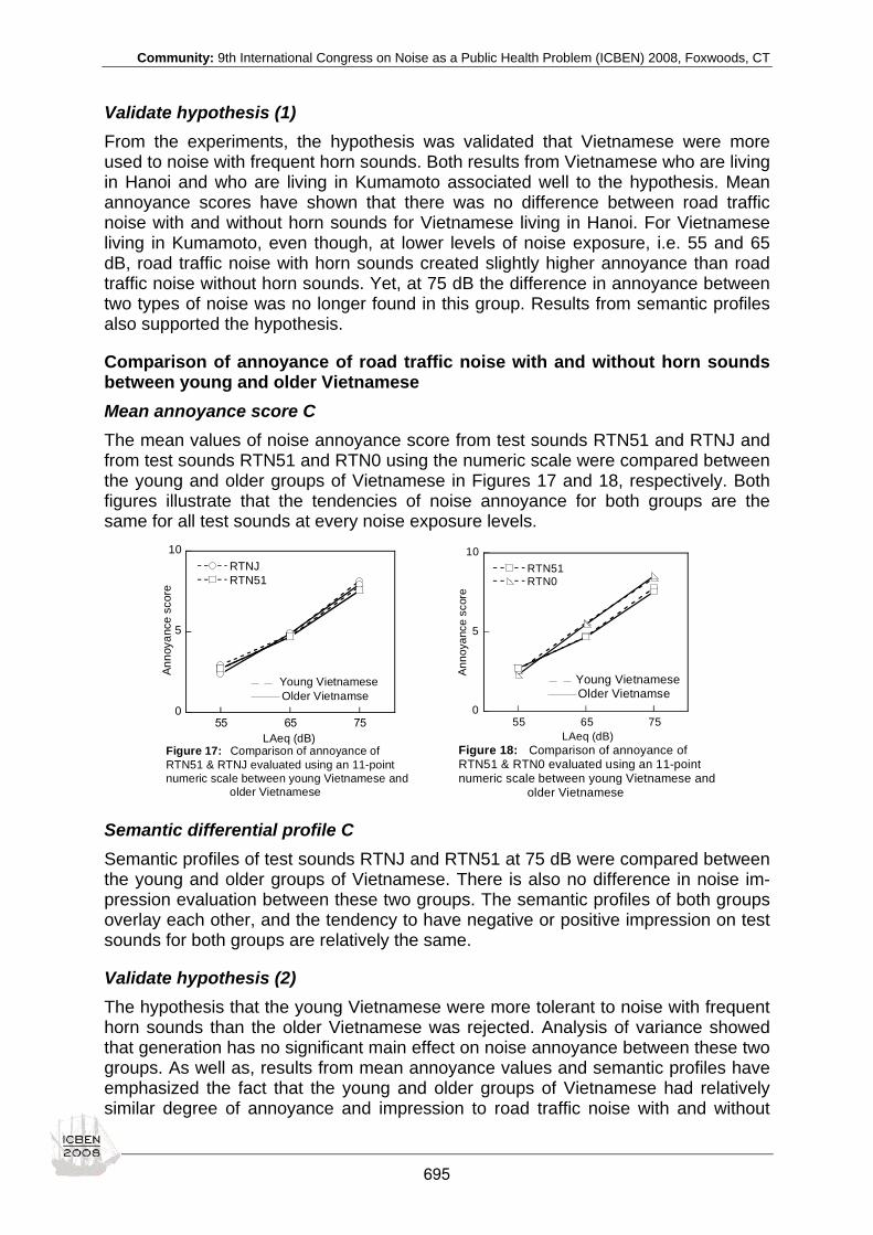
Community: 9th International Congress on Noise as a Public Health Problem (ICBEN) 2008, Foxwoods, CT
Validate hypothesis (1) From the experiments, the hypothesis was validated that Vietnamese were more used to noise with frequent horn sounds. Both results from Vietnamese who are living in Hanoi and who are living in Kumamoto associated well to the hypothesis. Mean annoyance scores have shown that there was no difference between road traffic noise with and without horn sounds for Vietnamese living in Hanoi. For Vietnamese living in Kumamoto, even though, at lower levels of noise exposure, i.e. 55 and 65 dB, road traffic noise with horn sounds created slightly higher annoyance than road traffic noise without horn sounds. Yet, at 75 dB the difference in annoyance between two types of noise was no longer found in this group. Results from semantic profiles also supported the hypothesis.
Comparison of annoyance of road traffic noise with and without horn sounds between young and older Vietnamese Mean annoyance score C The mean values of noise annoyance score from test sounds RTN51 and RTNJ and from test sounds RTN51 and RTN0 using the numeric scale were compared between the young and older groups of Vietnamese in Figures 17 and 18, respectively. Both figures illustrate that the tendencies of noise annoyance for both groups are the same for all test sounds at every noise exposure levels.
0
5
10
55 65 75
RTNJ RTN51
Anno
yanc
e sc
ore
LAeq (dB)
Young VietnameseOlder Vietnamse
Figure 17: Comparison of annoyance ofRTN51 & RTNJ evaluated using an 11-point numeric scale between young Vietnamese and older Vietnamese
0
5
10
55 65 75
RTN51RTN0
Anno
yanc
e sc
ore
LAeq (dB)
Young VietnameseOlder Vietnamse
Figure 18: Comparison of annoyance of RTN51 & RTN0 evaluated using an 11-point numeric scale between young Vietnamese and older Vietnamese
Semantic differential profile C Semantic profiles of test sounds RTNJ and RTN51 at 75 dB were compared between the young and older groups of Vietnamese. There is also no difference in noise im-pression evaluation between these two groups. The semantic profiles of both groups overlay each other, and the tendency to have negative or positive impression on test sounds for both groups are relatively the same.
Validate hypothesis (2) The hypothesis that the young Vietnamese were more tolerant to noise with frequent horn sounds than the older Vietnamese was rejected. Analysis of variance showed that generation has no significant main effect on noise annoyance between these two groups. As well as, results from mean annoyance values and semantic profiles have emphasized the fact that the young and older groups of Vietnamese had relatively similar degree of annoyance and impression to road traffic noise with and without
695
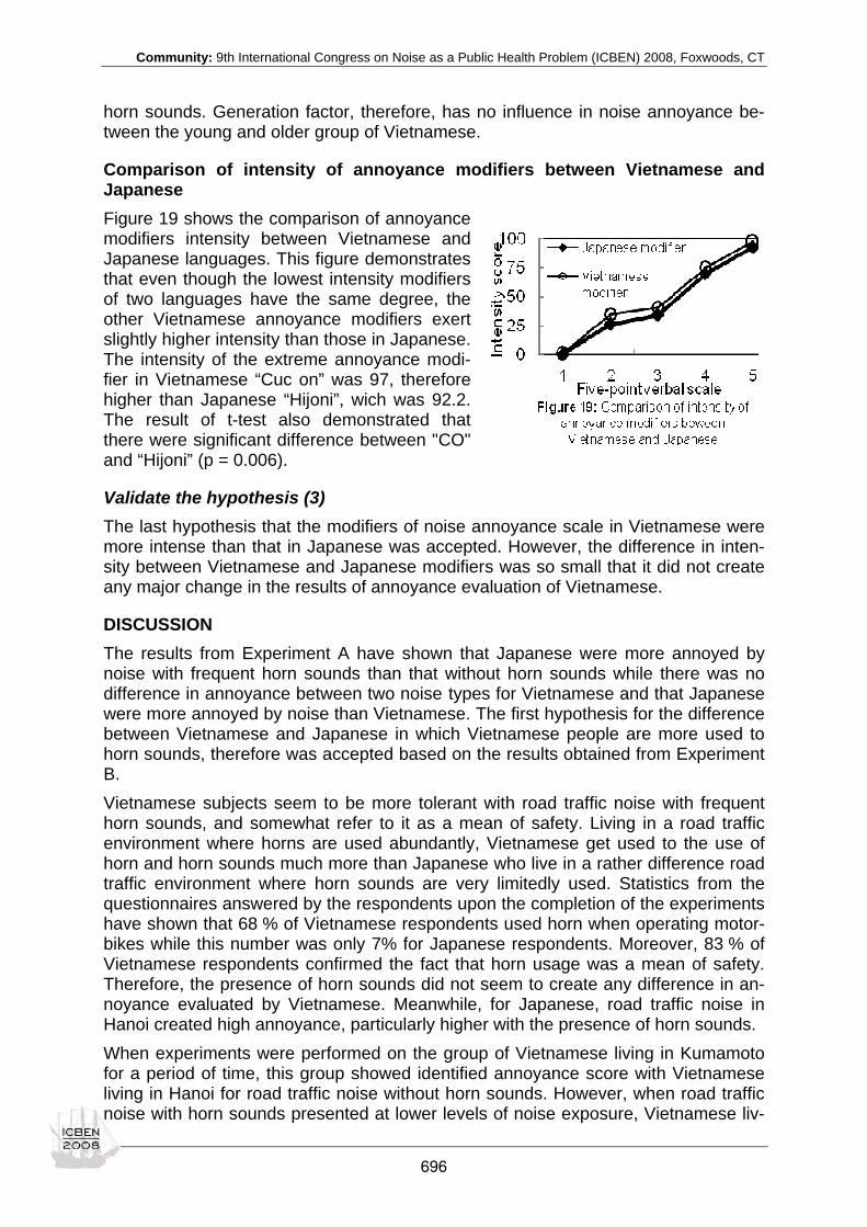
Community: 9th International Congress on Noise as a Public Health Problem (ICBEN) 2008, Foxwoods, CT
horn sounds. Generation factor, therefore, has no influence in noise annoyance be-tween the young and older group of Vietnamese.
Comparison of intensity of annoyance modifiers between Vietnamese and Japanese Figure 19 shows the comparison of annoyance modifiers intensity between Vietnamese and Japanese languages. This figure demonstrates that even though the lowest intensity modifiers of two languages have the same degree, the other Vietnamese annoyance modifiers exert slightly higher intensity than those in Japanese. The intensity of the extreme annoyance modi-fier in Vietnamese “Cuc on” was 97, therefore higher than Japanese “Hijoni”, wich was 92.2. The result of t-test also demonstrated that there were significant difference between "CO" and “Hijoni” (p = 0.006).
Validate the hypothesis (3) The last hypothesis that the modifiers of noise annoyance scale in Vietnamese were more intense than that in Japanese was accepted. However, the difference in inten-sity between Vietnamese and Japanese modifiers was so small that it did not create any major change in the results of annoyance evaluation of Vietnamese.
DISCUSSION
The results from Experiment A have shown that Japanese were more annoyed by noise with frequent horn sounds than that without horn sounds while there was no difference in annoyance between two noise types for Vietnamese and that Japanese were more annoyed by noise than Vietnamese. The first hypothesis for the difference between Vietnamese and Japanese in which Vietnamese people are more used to horn sounds, therefore was accepted based on the results obtained from Experiment B. Vietnamese subjects seem to be more tolerant with road traffic noise with frequent horn sounds, and somewhat refer to it as a mean of safety. Living in a road traffic environment where horns are used abundantly, Vietnamese get used to the use of horn and horn sounds much more than Japanese who live in a rather difference road traffic environment where horn sounds are very limitedly used. Statistics from the questionnaires answered by the respondents upon the completion of the experiments have shown that 68 % of Vietnamese respondents used horn when operating motor-bikes while this number was only 7% for Japanese respondents. Moreover, 83 % of Vietnamese respondents confirmed the fact that horn usage was a mean of safety. Therefore, the presence of horn sounds did not seem to create any difference in an-noyance evaluated by Vietnamese. Meanwhile, for Japanese, road traffic noise in Hanoi created high annoyance, particularly higher with the presence of horn sounds. When experiments were performed on the group of Vietnamese living in Kumamoto for a period of time, this group showed identified annoyance score with Vietnamese living in Hanoi for road traffic noise without horn sounds. However, when road traffic noise with horn sounds presented at lower levels of noise exposure, Vietnamese liv-
696

Community: 9th International Congress on Noise as a Public Health Problem (ICBEN) 2008, Foxwoods, CT
ing in Kumamoto seemed to be more annoyed than Vietnamese living in Hanoi, but less annoyed than Japanese. From this result and the analysis of variance, environ-ment factor seemed to have certain significant impact on annoyance from Vietnam-ese living in Kumamoto. Nevertheless, when road traffic noise with horn sounds was presented at high level of noise exposure, Vietnamese living in Kumamoto then de-veloped the same annoyance score with Vietnamese living in Hanoi. Again, no differ-ence between road traffic noise with and without horn sounds was found between these two groups. The first hypothesis is accepted. Under the second hypothesis that the younger Vietnamese are more tolerant with road traffic noise with horn sounds than the older Vietnamese, a number of analysis were done, however, no evidence was found for generation as an influencing factor on noise annoyance evaluation. This finding confirmed the stableness in annoyance score evaluated by Vietnamese, both young and older groups who are living in Ha-noi. For the third hypothesis, the comparison of intensity of annoyance modifiers between Japanese and Vietnamese and between the present study and the ICBEN Joint study have shown that Vietnamese modifiers used for the verbal scale are consis-tently more intense than Japanese. The intensity score was applied to noise annoy-ance evaluation between Vietnamese and Japanese. This result, even though con-firmed the third hypothesis to be true, did not influence the outcome of noise annoy-ance evaluation by both groups.
SUMMARY Results from a series of cross-cultural psychoacoustic experiments can be summa-rized as follows:
1. There was almost no effect of horn sound on road traffic noise annoyance for Vietnamese subjects.
2. Japanese subjects were more annoyed by noise with frequent horn sounds than noise without horn.
3. Japanese subjects were more annoyed by road traffic noise than Vietnamese 4. The semantic differential evaluation showed that road traffic noise with fre-
quent horn sounds were more negative for Japanese than Vietnamese and that there was small differences in loudness impression between Japanese and Vietnamese subjects.
5. The above difference is caused by the fact that Vietnamese people are used to noisy environment with frequent horn sounds.
6. Generation did not affect the above difference. 7. The difference in intensity between Vietnamese and Japanese noise annoy-
ance modifiers did not affect the above differences
ACKNOWLEDGEMENT This study is financially supported by the Core University Program between Japan Society for the Promotion of Science (JSPS) and National Center for Science and Technology (NCST) and Grant-in-Aid for Scientific Research (Project No.17560533). The authors highly appreciate the kind support in the experiment planning and pro-ceeding in Hanoi to Prof. Pham Ngoc Dang, Prof. Pham Duc Nguyen, Dr. Nguyen Thu Hoa and students from Hanoi University of Civil Engineering.
697

Community: 9th International Congress on Noise as a Public Health Problem (ICBEN) 2008, Foxwoods, CT
REFERENCES Fastl H, Kuwano S, Namba S (1996). Assessing the railway bonus in laboratory studies. J Acoust Soc Jpn (E) 17.
Fastl H, Fruhmann M, Ache S (2003). Railway bonus for sounds without meaning? Acoust Austral 31: 99-101.
Fields JM (2001). An updated catalogue of 521 social surveys of residents’ reactions to environmental noise (1943-2000), NASA/CR: 2001-211257.
Fields JM, de Jong RG, Gjestland T, Flindell IH, Job RFS, Kurra S, Lercher P, Vallet M, Yano T, Guski R, Felscher-Suhr U, Schuemer R (2001). Standardized general-purpose noise reaction questions for community noise surveys: research and a recommendation. J Sound Vibr 242: 641-679.
Lam K-C (1994). Are all noises the same? A laboratory simulation study of human response to road and rail traffic noise. Proceeding of the Inter-noise 2004, Prague, Czech Republic, August 2004.
Masden K, Yano T (2004). Equivalence of noise annoyance scales in Japanese and English: An experiment using bilingual subjects. Acoust Sci Tech 25 (2).
Miedema HME, Vos H (1998). Exposure-response relationships for transportation noise. J Acoust Soc Am 104: 3432-3445.
Namba S, Kuwano S, Hashimoto T, Berglund B, Rui ZD, Schick A, Hoege H, Florentine M (1991a). Verbal expression of emotional impression of sound: A cross-cultural study. J Acoust Soc Jpn (E) 12.
Namba S, Kuwano S, Schick A, Aclar A, Florentine M, Rui ZD (1991b). A cross-cultural study on noise problems: comparison of the results obtained in Japan, The U.S.A, China and Turkey. J Sound Vibr 151: 471-477.
Phan HAT, Phan HYT, Nishimura T, Dang PN, Nguyen PD, Nai LV, Hashimoto Y, Sato S, Cuong TD, Yano T (2006). Com-munity response to road traffic noise in Hanoi -Part 2: Effects of moderators on annoyance caused by road traffic noise in Hanoi. In: Proceedings of Internoise 2006, Honolulu.
Phan HAT, Nishimura T, Phan HYT, Yano T, Sato T, Hashimoto Y (2007). A psychoacoustics experiment on the effects of horn sound on road traffic noise annoyance. In: Proceedings of Internoise 2007, Istanbul.
Phan HYT, Phan HAT, Nishimura T, Dang DN, Nguyen PD, Nai LV, Hashimoto Y, Sato T, Cuong TD, Yano T (2006). Com-munity response to road traffic noise in Hanoi – Part I: Outline of social survey and noise measurement”. In: Proceedings of Internoise 2006, Honolulu.
Sato T, Yano T, Bjorkman M, Rylander R (2000). Comparison of community response to road traffic noise in Sweden, Japan and Thailand, Proceedings of the Seventh Western Pacific Regional Acoustics Conference (Kumamoto), Vol. 2: 907-912.
Sato T, Yano T, Morihara T, Masden K (2005). Relationships between rating scales, question stem wording and community responses to railway noise. J Sound Vibr 277: 609-616.
Schultz TJ (1978). Synthesis of social surveys on noise annoyance. J Acoust Soc Am 64: 377-405.
Yano T, Ma H (2004). Standardized noise annoyance scales in Chinese, Korean and Vietnamese. J Sound Vibr 277: 583-588.
698

Community: 9th International Congress on Noise as a Public Health Problem (ICBEN) 2008, Foxwoods, CT
Social surveys on community response to road traffic noise in Hanoi and Ho Chi Minh City Hai Yen Thi Phan1*, Takashi Yano1, Hai Anh Thi Phan2, Tsuyoshi Nishimura2, Tetsumi Sato3, Yoritaka Hashimoto4, Nguyen Thu Lan1
1 Kumamoto University, Kurokami 2-39-1, Kumamoto 860-8555, Japan
2 Sojo University, Ikeda 4-22-1, Kumamoto 860-0082, Japan
3 Hokkai Gakuen University, Minami 26, Nishi 11, Chuo-ku, Sapporo 064-0926, Japan
4 Osaka City University, Sugimoto 3-3-138, Sumiyoshi, Osaka 558-8585, Japan
* corresponding author: e-mail: [email protected]
INTRODUCTION Though a number of social surveys on community response to noise have been con-ducted in European and in American countries as well as in Japan (Fields 2001; Miedema & Vos 1998; Schultz 1978), only few surveys in other Asian countries es-pecially the developing countries have been published (Sato et al. 2000). Vietnam is one of the developing countries in Asia that suffers excessive noise emission from road traffic. The problem is that there has not been any proper measure to cope with the situation, and that Vietnam does not have a national policy on noise. Data on community response to road traffic noise have, therefore, been collected, which is hoped to be a major source for the establishment of a practical noise policy for Viet-nam. Serving this purpose, social surveys on community response to road traffic noise and noise measurements have been conducted in major cities in Vietnam, i.e. Hanoi and Ho Chi Minh city, in order to investigate the characteristics of road traffic noise here and to establish dose-response relationships for road traffic noise in Viet-nam. Hanoi is the capital city of Vietnam, serving as the political, the cultural and the lar-gest educational center. Hanoi attracts a large number of not only world-wide tour-ists, but also inhabitants from other provinces coming here for work. While Hanoi is reflected as a major metropolitan area of Northern area, Ho Chi Minh city is consid-ered the largest city in Southern area and the biggest urban agglomeration of Viet-nam. While Hanoi’s population is 4.2 million people (2006), Ho Chi Minh’s population now exceeds 6 million people (2006), excluding over 2 million migrants who live here as temporary residents or commuters. Together with many positive sides both cities have to offer, Hanoi and Ho Chi Minh are now facing worsening situations of road traffic noise, increasing volumes and chaotic flows of road traffic. In September 2005 and September 2007, two large-scaled social surveys on com-munity response to road traffic noise and noise measurements were conducted in Hanoi and Ho Chi Minh city, respectively. The sample sizes were 1503 in Hanoi, and 1471 in Ho Chi Minh city, including both row house and apartment residents.
SOCIAL SURVEY AND NOISE MEASUREMENT Social surveys and noise measurements were conducted in Hanoi and Ho Chi Minh city under the same method. Based on preliminary investigation, eight sites (coded as “site” with number accordingly from 1 to 8) were selected based on overall criteria: (1) having high traffic volume; (2) having high density of residential population; and (3) being a combined dwelling area of row houses and apartments. All row houses
699
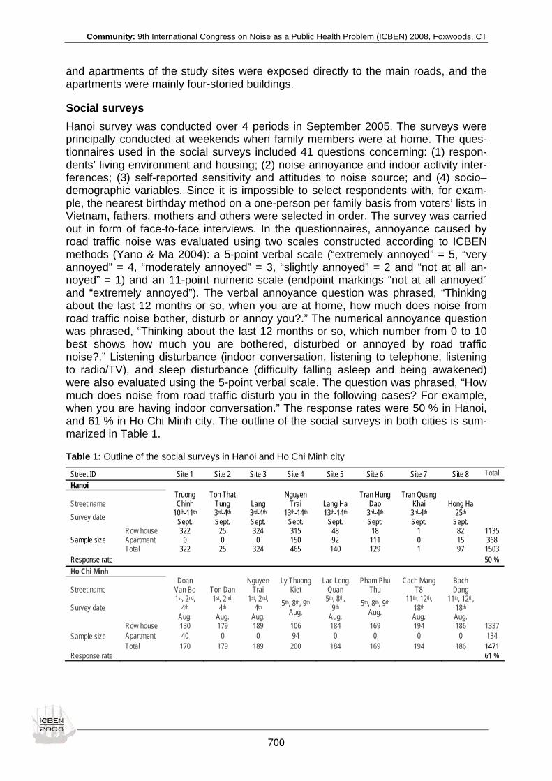
Community: 9th International Congress on Noise as a Public Health Problem (ICBEN) 2008, Foxwoods, CT
and apartments of the study sites were exposed directly to the main roads, and the apartments were mainly four-storied buildings.
Social surveys Hanoi survey was conducted over 4 periods in September 2005. The surveys were principally conducted at weekends when family members were at home. The ques-tionnaires used in the social surveys included 41 questions concerning: (1) respon-dents’ living environment and housing; (2) noise annoyance and indoor activity inter-ferences; (3) self-reported sensitivity and attitudes to noise source; and (4) socio–demographic variables. Since it is impossible to select respondents with, for exam-ple, the nearest birthday method on a one-person per family basis from voters’ lists in Vietnam, fathers, mothers and others were selected in order. The survey was carried out in form of face-to-face interviews. In the questionnaires, annoyance caused by road traffic noise was evaluated using two scales constructed according to ICBEN methods (Yano & Ma 2004): a 5-point verbal scale (“extremely annoyed” = 5, “very annoyed” = 4, “moderately annoyed” = 3, “slightly annoyed” = 2 and “not at all an-noyed” = 1) and an 11-point numeric scale (endpoint markings “not at all annoyed” and “extremely annoyed”). The verbal annoyance question was phrased, “Thinking about the last 12 months or so, when you are at home, how much does noise from road traffic noise bother, disturb or annoy you?.” The numerical annoyance question was phrased, “Thinking about the last 12 months or so, which number from 0 to 10 best shows how much you are bothered, disturbed or annoyed by road traffic noise?.” Listening disturbance (indoor conversation, listening to telephone, listening to radio/TV), and sleep disturbance (difficulty falling asleep and being awakened) were also evaluated using the 5-point verbal scale. The question was phrased, “How much does noise from road traffic disturb you in the following cases? For example, when you are having indoor conversation.” The response rates were 50 % in Hanoi, and 61 % in Ho Chi Minh city. The outline of the social surveys in both cities is sum-marized in Table 1.
Table 1: Outline of the social surveys in Hanoi and Ho Chi Minh city
Street ID Site 1 Site 2 Site 3 Site 4 Site 5 Site 6 Site 7 Site 8 Total Hanoi
Street name Truong Chinh
Ton That Tung Lang
Nguyen Trai Lang Ha
Tran Hung Dao
Tran Quang Khai Hong Ha
Survey date 10th-11th Sept.
3rd-4th Sept.
3rd-4th Sept.
13th-14th Sept.
13th-14th Sept.
3rd-4th Sept.
3rd-4th Sept.
25th Sept.
Row house 322 25 324 315 48 18 1 82 1135 Apartment 0 0 0 150 92 111 0 15 368 Sample size Total 322 25 324 465 140 129 1 97 1503
Response rate 50 % Ho Chi Minh
Street name Doan
Van Bo Ton Dan Nguyen
Trai Ly Thuong
Kiet Lac Long
Quan Pham Phu
Thu Cach Mang
T8 Bach Dang
Survey date 1st, 2nd,
4th Aug.
1st, 2nd, 4th
Aug.
1st, 2nd, 4th
Aug. 5th, 8th, 9th
Aug. 5th, 8th,
9th Aug.
5th, 8th, 9th Aug.
11th, 12th, 18th Aug.
11th, 12th, 18th Aug.
Row house 130 179 189 106 184 169 194 186 1337 Apartment 40 0 0 94 0 0 0 0 134 Sample size Total 170 179 189 200 184 169 194 186 1471
Response rate 61 %
700

Community: 9th International Congress on Noise as a Public Health Problem (ICBEN) 2008, Foxwoods, CT
Noise measurements In Hanoi, noise measurement for row houses was conducted at eight sites in Sep-tember 2005 from the 19th to 22nd, including 24-hour noise measurement and short-term noise measurement. The 24-hour measurement was performed at reference points, 1.2 m high and from 2 m to 12 m away from the road shoulders. Short-term noise measurement was carried out at the reference points and other several points simultaneously. Distance reduction equations were formulated based on the short-term measurement. Noise exposure to each house was estimated by the 24-hour noise measurement values and the distance reduction equations. All noise data was analyzed without any special sound identified in 24 hours such as ambulance and/or trains’ horn sounds, etc. Day-evening-night noise level (Lden) in Hanoi ranged from 69 to 83 dB. An additional vertical noise reduction measurement for apartments was conducted at four sites (sites 4, 5, 6 and 8) in September 2006. Short-term vertical noise reduction measurement was performed at every floor of the apartment block simultaneously. At each floor, a microphone was placed at an assigned spot on the balcony facing to the road, and all was operated at the same time. In Ho Chi Minh city, the same noise measurement method was conducted at the eight sites from the 17th to 18th of September 2007, including the 24-hour noise measurement, short-term horizontal noise reduction measurement and short-term vertical reduction measurement for apartment. The representative noise exposure values were estimated as the exposure at the average distant points. The vertical noise reduction measurement for apartments were performed at two sites (sites 1 and 4). The noise exposure to apartments was calculated as the average noise level by weighting the number of respondents living on each floor. Day-evening-night noise level (Lden) in Ho Chi Minh city ranged highly from 75 to 83 dB. In both cities, traffic volume counting was performed by reproducing a video camera recording. Figures 1 and 2 show the traffic volume at all sites in Hanoi and Ho Chi Minh city, respectively.
Figure 1: Motorbike volume in Hanoi Figure 2: Motorbike volume in HCMC
RESULTS Characteristic of road traffic noise Road traffic noise in both cities is characterized by a large amount of motorbikes emitting frequent horn sounds. As it can be seen in Figures 1 and 2, a large number of motorbikes in use during 24 hours in both cities can be observed. Though Ho Chi Minh city seemed to have slightly more motorbikes than Hanoi, the time pattern of traffic volume is almost the
701
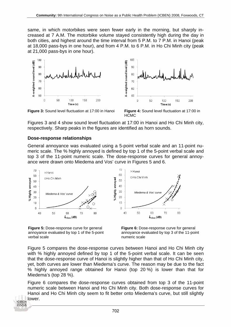
Community: 9th International Congress on Noise as a Public Health Problem (ICBEN) 2008, Foxwoods, CT
same, in which motorbikes were seen fewer early in the morning, but sharply in-creased at 7 A.M. The motorbike volume stayed consistently high during the day in both cities, and highest around the time interval from 5 P.M. to 7 P.M. in Hanoi (peak at 18,000 pass-bys in one hour), and from 4 P.M. to 6 P.M. in Ho Chi Minh city (peak at 21,000 pass-bys in one hour).
Figure 3: Sound level fluctuation at 17:00 in Hanoi Figure 4: Sound level fluctuation at 17:00 in
HCMC
Figures 3 and 4 show sound level fluctuation at 17:00 in Hanoi and Ho Chi Minh city, respectively. Sharp peaks in the figures are identified as horn sounds.
Dose-response relationships General annoyance was evaluated using a 5-point verbal scale and an 11-point nu-meric scale. The % highly annoyed is defined by top 1 of the 5-point verbal scale and top 3 of the 11-point numeric scale. The dose-response curves for general annoy-ance were drawn onto Miedema and Vos’ curve in Figures 5 and 6.
Figure 5 compares the dose-response curves between Hanoi and Ho Chi Minh city with % highly annoyed defined by top 1 of the 5-point verbal scale. It can be seen that the dose-response curve of Hanoi is slightly higher than that of Ho Chi Minh city, yet, both curves are lower than Miedema’s curve. The reason may be due to the fact % highly annoyed range obtained for Hanoi (top 20 %) is lower than that for Miedema’s (top 28 %). Figure 6 compares the dose-response curves obtained from top 3 of the 11-point numeric scale between Hanoi and Ho Chi Minh city. Both dose-response curves for Hanoi and Ho Chi Minh city seem to fit better onto Miedema’s curve, but still slightly lower.
Miedema & Vos‘ curve Miedema & Vos‘ curve
Figure 5: Dose-response curve for general annoyance evaluated by top 1 of the 5-point verbal scale
Figure 6: Dose-response curve for general annoyance evaluated by top 3 of the 11-point numeric scale
702
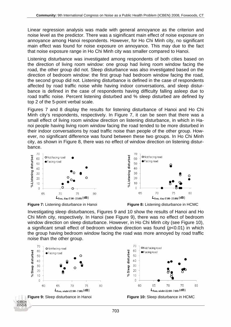
Community: 9th International Congress on Noise as a Public Health Problem (ICBEN) 2008, Foxwoods, CT
Linear regression analysis was made with general annoyance as the criterion and noise level as the predictor. There was a siginificant main effect of noise exposure on annoyance among Hanoi respondents. However, for Ho Chi Minh city, no significant main effect was found for noise exposure on annoyance. This may due to the fact that noise exposure range in Ho Chi Minh city was smaller compared to Hanoi. Listening disturbance was investigated among respondents of both cities based on the direction of living room window: one group had living room window facing the road, the other group did not. Sleep disturbance was also investigated based on the direction of bedroom window: the first group had bedroom window facing the road, the second group did not. Listening disturbance is defined in the case of respondents affected by road traffic noise while having indoor conversations, and sleep distur-bance is defined in the case of respondents having difficulty falling asleep due to road traffic noise. Percent listening disturbed and % sleep disturbed are defined by top 2 of the 5-point verbal scale. Figures 7 and 8 display the results for listening disturbance of Hanoi and Ho Chi Minh city’s respondents, respectively. In Figure 7, it can be seen that there was a small effect of living room window direction on listening disturbance, in which in Ha-noi people having living room window facing the road tended to be more disturbed in their indoor conversations by road traffic noise than people of the other group. How-ever, no significant difference was found between these two groups. In Ho Chi Minh city, as shown in Figure 8, there was no effect of window direction on listening distur-bance.
Figure 7: Listening disturbance in Hanoi Figure 8: Listening disturbance in HCMC
Investigating sleep disturbances, Figures 9 and 10 show the results of Hanoi and Ho Chi Minh city, respectively. In Hanoi (see Figure 9), there was no effect of bedroom window direction on sleep disturbance. However, in Ho Chi Minh city (see Figure 10), a significant small effect of bedroom window direction was found (p<0.01) in which the group having bedroom window facing the road was more annoyed by road traffic noise than the other group.
Figure 9: Sleep disturbance in Hanoi Figure 10: Sleep disturbance in HCMC
703

Community: 9th International Congress on Noise as a Public Health Problem (ICBEN) 2008, Foxwoods, CT
Effects of moderators on road traffic noise annoyance Several non-acoustical factors subjecting to moderate variations in road traffic noise annoyance were assessed in the questionnaires. The factors investigated were noise sensitivity and attitudes to noise source. Noise sensitivity was evaluated using the 5-point verbal scale. The respondents of both cities were divided into two groups, the insensitive group (first 2 categories–slightly and not at all–of the verbal scale) and the sensitive group (last 2 categories–very and extremely). Annoyance taken by top 1 of the 5-point verbal scale was com-pared between these two groups of respondents in both cities. Figure 11 indicates that in Hanoi the noise sensitive group had higher annoyance than the insensitive group. Significant difference (p<0.01) was found in annoyance response between these two groups. As Figure 12 illustrates, Ho Chi Minh city’s re-spondents also developed the same tendency with Hanoi’s, in which the noise sensi-tive group was significantly more annoyed by road traffic noise than the insensitive group (p<0.01).
Investigating the effect on annoyance of the moderator as attitude to noise source, the question was phrased, “How safe do you think the following transportation is? For example, motorbikes.” Attitude to noise source was evaluated by the 5-point verbal scale, from which two groups of respondents were divided: one group considered motorbikes safe (taken by first two categories of the verbal scale) and the other group considered motorbikes not safe (taken by last two categories).
Figures 13 and 14 compare % highly annoyed between these two groups in Hanoi and Ho Chi Minh city, respectively. In Figure 13, it is indicated that in Hanoi noise annoyance of the group considering motorbikes not safe seemed to be greater than that of the other group. A significant difference (p<0.01) in annoyance response be-
Figure 11: Compare % highly annoyed based on noise sensitivity in Hanoi
Figure 12: Compare % highly annoyed based on noise sensitivity in HCMC
Figure 13: Compare % highly annoyed based on attitudes to noise source in Hanoi
Figure 14: Compare % highly annoyed based on attitudes to noise source in HCMC
704

Community: 9th International Congress on Noise as a Public Health Problem (ICBEN) 2008, Foxwoods, CT
tween the two groups was found. In Ho Chi Minh city (see Figure 14), there was a clearer difference in annoyance response between the two groups in which the group considering motorbikes not safe was significantly more annoyed by road traffic noise than the group considering motorbikes safe (p<0.01). Multiple regression analysis was made with annoyance assessed on the 5-point ver-bal scale as the criterion and noise exposure together with noise sensitivity and atti-tudes to noise source in terms of safety evaluation as the predictors. The results are shown in Table 2(a) and (b). The result in Table 2(a) indicates that in Hanoi, the factors noise sensitivity, attitudes to noise source and noise level are associated with noise annoyance. In sum noise sensitivity contributes more to the prediction of noise annoyance in Hanoi. There were significant correlations between noise exposure and noise sensitivity (r=0.21, p<0.01), and between noise sensitivity and attitudes to noise source (r=0.18, p<0.01). However, no significant correlation was found between noise exposure and attitudes to noise source. Table 2(a): Results of multiple regression analysis with noise annoyance (assessed on 5-point verbal) as the criterion and noise level and some moderators as the predictors in Hanoi
Parameters B SE Beta T p Intercept -2.19 0.54 -4.05 0.00 Noise level (Lden) 0.05 0.01 0.17 7.55 0.00 Noise sensitivity 0.47 0.02 0.50 22.04 0.00 Attitudes to noise source (Safety evaluation) 0.06 0.03 0.05 2.19 0.03
R² = .325
Table 2(b): Results of multiple regression analysis with noise annoyance (assessed on 5-point verbal) as the criterion and noise level and some moderators as the predictors in Ho Chi Minh
The result from Table 2(b) demonstrates that in Ho Chi Minh city, only two factors noise sensitivity and attitudes to noise source were associated with noise annoyance, among which in sum noise sensitivity also contributes more to noise annoyance pre-diction. There were significant correlations between noise exposure and noise sensi-tivity (r=0.05, p<0.05), and between noise sensitivity and attitudes to noise source (r=0.14, p<0.01). However, no significant correlation was found between noise expo-sure and attitudes to noise source.
CONCLUSIONS It was obtained that road traffic noise in Hanoi and Ho Chi Minh city was characte-rized by a large number of motorbikes emitting frequent horn sounds. Dose-response relationships between noise exposure and % highly annoyed (evaluated by top 1 of the 5-point verbal scale and top 3 of the 11-point numeric scale) were established, in which dose-response curves were drawn onto Miedema and Vos’ curve. Dose re-sponse curves of Hanoi and Ho Chi Minh city are slightly lower compared to Miedema and Vos’ curve.
Parameters B SE Beta T p Intercept 1.88 0.88 2.15 0.03 Noise level (Lden) 0.00 0.01 -0.01 -0.41 0.68 Sensitivity to noise 0.55 0.02 0.59 27.63 0.00 Attitudes to noise source (Safety evaluation) 0.10 0.03 0.07 3.45 0.00
R² = .363
705

Community: 9th International Congress on Noise as a Public Health Problem (ICBEN) 2008, Foxwoods, CT
Listening disturbance was compared between two groups of respondents based on living room window direction. A small effect of window direction was found in Hanoi; however, this was not statistically significant. Sleep disturbance was also compared between two groups of respondents based on bedroom window direction. A signifi-cant small effect of window direction was found in Ho Chi Minh city, i.e. people with houses having bedroom window facing the road were more disturbed by road traffic noise. The effect of moderators on annoyance was investigated, and the results were con-sistent to the previous studies (Miedema & Vos 1999, 2003). Moreover, multiple re-gression analysis suggested that the moderators were strongly associated with noise annoyance, especially in Ho Chi Minh city, the moderators contributed more to the prediction of noise annoyance.
ACKNOWLEDGEMENT This study is financially supported by the Core University Program between Japan Society for the Promotion of Science (JSPS), National Center for Science and Tech-nology (NCST), Grant-in-Aid for Scientific Research (Project No. 17560533) and the 2006 Kajima Foundation’s Research Grant. The authors also appreciate the support for the social surveys from Prof. Pham Ngoc Dang, Prof. Pham Duc Nguyen and stu-dents at Hanoi University of Civil Engineering, and from Ms. Nguyen Thi Bich Ngoc and students from Ho Chi Minh University of Architecture.
REFERENCES Fields JM (2001). An updated catalogue of 521 social surveys of residents’ reactions to environmental noise (1943-2000). NASA/CR-2001-211257.
Miedema HME, Vos H (1998). Exposure-response relationships for transportation noise. J Acoust Soc Am 104: 3432-3445.
Miedema HME, Vos H (1999). Demographic and attitudinal factors that modify annoyance from transportation noise. J Acoust Soc Am 105: 3336-3344.
Miedema HME, Vos H (2003). Noise sensitivity and reactions to noise and other environmental conditions. J Acoust Soc Am 113: 1492-1504.
Sato T, Yano T, Bjorkman M, Rylander R (2000). Comparison of community response to road traffic noise in Sweden, Japan and Thailand. Proceedings of the 7th Western Pacific Regional Acoustics Conference (Kumamoto), Vol. 2, pp.907-912.
Schultz TJ (1978). Synthesis of social surveys on noise annoyance. J Acoust Soc Am 64: 377-405.
Yano T, Ma H (2004). Standardized noise annoyance scales in Chinese, Korean and Vietnamese. J Sound Vibr 277: 583-588.
706

Community: 9th International Congress on Noise as a Public Health Problem (ICBEN) 2008, Foxwoods, CT
The improvement of helicopter noise management in the UK David Waddington1*, Paul Kendrick1, Geoff Kerry1, Matthew Muirhead2, Ray Browne2 1 Acoustics Research Centre, University of Salford, Salford M5 4WT, UK
2 QinetiQ Ltd, Cody Technology Park, Ively Road, Farnborough GU14 0LX, UK
*Corresponding author: e-mail: [email protected]
ABSTRACT Central to the management of noise from helicopter operations is the awareness that community response to helicopter noise is a sociological phenomenon rather than purely an acoustic problem. For example, one problem identified in the UK is that it is often difficult to complain about helicopter noise, since it is unclear which organiza-tion is responsible for dealing with the complaint. Consequently, the Department for Environment, Food and Rural Affairs (Defra, UK) has commissioned research to summarize the nature and extent of the concern about helicopter noise in the UK, the rules and regulations governing operations, and existing procedures for handling complaints. Stakeholders contributing to this work include local authorities, the mili-tary, helicopter manufacturers, and the British Helicopter Advisory Board. This stage of the project will produce a detailed report together with a short non-technical guide. This paper summarizes the findings of this project with regard to subjective res-ponses to helicopter noise [Work funded by Defra, UK].
INTRODUCTION Helicopter noise can have a negative impact on the quality of life for some people. Affected populations are not just those living close to heliports, but include those ex-posed to noise from helicopters used by emergency services, the military, commer-cial companies and private individuals. One problem identified is that it is often diffi-cult to complain about helicopter noise since it is unclear which organization is re-sponsible for dealing with the complaint. This research project was proposed by Defra with the objective of improving the management of noise from helicopter operations. This was due to a perceived lack of information in connection with helicopter noise, and in particular, with regard to whom complaints should be addressed. Clarification was also required on remediation and mitigation. Current perceptions were supported by the recent London Assembly Environment Committee report (2006). That report states that there is anecdotal evidence of a growing concern amongst members of the public about helicopter noise. This report for Defra, which also looks at procedures abroad, addresses many of the questions raised in the London Assembly report although the scope of this study is UK wide. This paper summarizes the findings of this work with regard to the subjective res-ponses to helicopter noise. This paper first addresses the adverse effects of helicop-ter noise including sleep disturbance, health and annoyance, before moving on to non-acoustic factors including 'virtual noise' and building vibration. Throughout com-parisons are drawn between the effects of helicopter noise with the effects of fixed wing aircraft noise.
707

Community: 9th International Congress on Noise as a Public Health Problem (ICBEN) 2008, Foxwoods, CT
SOCIAL EFFECTS The 2004 FAA report to US Congress entitled, ‘Non-military Helicopter Urban Noise Study’ (FAA 2004) (henceforth referred to as the FAA report), contains a comprehen-sive literature review on the effects of noise on the individual. The FAA report (2004) was itself in part based upon the US military report 'Community response to helicop-ter noise' (US ACHPM 2000). Studies have shown that environmental noise, includ-ing aircraft and traffic noise can adversely affect classroom learning (Cohen et al. 1973; Bronzaft & McCarthy 1975; Green 1980; Hygge et al. 1996; Hygge & Evans 2000; Lercher et al. 2000; Stansfeld et al. 2001). It has been shown that low achie-ving students were the most adversely affected. In addition, students with hearing impairments, students with English as a second language and music students may be particularly adversely affected (WHO 2000). The WHO (World Health Organiza-tion) recommends for schools a maximum equivalent indoor level of background noise not exceeding 35 dBA. This is so that the average voice level (50 dBA) is at least 15 dBA above the background level (WHO 2000). The FAA report states that nearly all of the studies relate to the classroom environment and that “at the present time, little can be said of environmental noise effects on communications and per-formance except as it relates to the classroom setting”. Studies carried out by Mugridge et al. (2000) at RAF Shawbury, which has around 114,000 helicopter movements per year, indicated no clear correlation between tradi-tional acoustic parameters and soundscape perception and acceptance. There did, however, appear to be a correlation between acceptance and the value/meaning at-tributed to the noise/event. Sixsmith (2008) has suggested that the use of the term of 'annoyance' might be replaced with a number of other terms. This suggestion stems from her work with 'work-related stress', a phenomenon that is now described in terms of 6 different factors; demands, control, support, relationships, roles and change. A number of studies over the past 30 years have suggested that a subsection of the population is more sensitive to low frequency noise than the majority. Patterson et al. (1977) performed tests with different frequency weightings on aircraft noise, compar-ing the dB level with annoyance. It was reported that most of the ratings correlated best with A-weighting. However, 11 out of 25 subjects also had good correlation with C-weighting, and of the 11, 3 exhibited better correlation with C-weighting. For this reason, it was concluded that A-weighting might not be the ideal weighting. ANSI S12.9 Part 4 provides a supplemental measure to A-weighting for assessing indus-trial noise sources with strong low-frequency content. Schomer suggested the use of equal loudness contours as more detailed frequency weighting curves for different amplitudes and showed a 2 dB difference between fixed-wing and rotary wing aircraft derived directly from these known functions of human hearing (FAA 2004). In addi-tion, it is found that increasing the loudness of a modulating sound by 2-5 dB pro-duces the same change in perceived loudness as if it were a change in loudness of 10 dB (Schomer & Bradley 2000). This could be significant for helicopters indicating one reason why they are rated differently to fixed wing craft. Likewise, Defra-funded research by Moorhouse et al. (2005) on the assessment of LFN complaints con-cluded that 5 dB was an appropriate penalty for fluctuating low frequency sounds.
HEALTH EFFECTS The Department for Transport in 1992 commissioned a report entitled ‘Report of a Field Study of Aircraft Noise and Sleep Disturbance’ (Civil Aviation Authority 2000). This study measured the sleep disturbance of people in their homes near Heathrow,
708

Community: 9th International Congress on Noise as a Public Health Problem (ICBEN) 2008, Foxwoods, CT
Gatwick, Stansted and Manchester airports. The report concluded that high aircraft noise levels could awaken people but that the likelihood of the average person hav-ing his or her sleep noticeably disturbed due to an individual aircraft noise event was relatively low. However, a small minority of people was more sensitive. Additionally, it was unclear amongst those who suffer disturbance due to noise, whether a single loud noise event or the accumulation of smaller noise events causes more distur-bance. In 1998, a further study was commissioned by the Department for Transport to review existing research in the UK and abroad, and to conduct a trial to assess methodology and analytical techniques and to determine whether to proceed to a full-scale study of either sleep prevention or total sleep loss (DORA R&D 2000). A social survey was also carried out to help explore the marked difference between objec-tively measured and publicly perceived disturbance due to nighttime aircraft noise. However again it is worth noting that fixed wing aircraft would have been predomi-nate. The UK Government announced on 8 May 2001 that a new full-scale objective sleep disturbance study would be unlikely to add significantly to existing knowledge; it is to concentrate instead on further research into subjective responses to aircraft dur-ing both day and night. Laboratory experiments (ANSI 2000) have shown sleep disturbance at relatively low noise levels but field tests results have shown people are much less susceptible to being disturbed. For example, field tests show 1 % of participants were awakened at 60 dB (A-weighted sound exposure level) while in laboratory tests at 60 dB about 20 % of people were disturbed. The US Federal Interagency Committee on Aviation Noise (FICAN) recommends using a dose-response curve for predicted awakening based upon the field data. In essence, the dose-response curve would follow the “maximum percentage of the exposed population expected to be behaviorally awak-ened” related to SEL. The FAA agrees with this recommendation. The WHO (2000) states that long-term exposure to noise levels exceeding 65-70 dB (24 h Leq) is known to be associated with causing cardiovascular problems. Passchier-Vermeer and Passchier (2000), commenting on results from studies car-ried out in the Netherlands, state that the observation threshold for hypertension is estimated to correspond to an Ldn value of 70 dBA for environmental noise expo-sure. Recently published work by the HYENA group (Hypertension and Exposure to Noise near Airports) indicated a statistically significant excess risk of hypertension related to long term exposure to night-time aircraft noise. For every 10 dB increase in (night-time) noise level, the risk of hypertension is increased by about 14 %, with this trend seen starting at low levels. The daytime results were not statistically significant.
COMMUNITY ATTITUDES Community attitude toward operations has an important effect on the community an-noyance. Social surveys carried out by the CAA in 1982 and 1992 found that helicop-ters in the London area were up to 15 dB(A) more annoying at the 10 % and 20 % very much annoyed level than fixed wing craft. By contrast, results showed that heli-copters operated in Aberdeen, servicing the North Sea oil industry, generated similar annoyance for a similar sound level as their fixed wing counterparts. This is attributed to the obvious economic benefit to community surrounding the Aberdeen helicopter service as opposed to London, where helicopters are perceived to have no economic benefit to the residents. This indicates a strong non-acoustic factor in the community annoyance rating.
709

Community: 9th International Congress on Noise as a Public Health Problem (ICBEN) 2008, Foxwoods, CT
Fields (1995) study highlighted the following five attitudes as most important. 1) Noise prevention beliefs. 2) Fear of danger from noise source. 3) Beliefs about the importance of the noise source. 4) Annoyance with non-noise impacts from the noise sources. 5) General noise sensitivity. Leverton and Pike (2007) comment that ”the public acceptance of helicopters is not wholly reflected by either conventional community rating procedures or the noise cer-tification requirements”. This questions the view of many national authorities that a reduction in the objective sound level that helicopters produce will make helicopters more acceptable to community. Fields and Powell (1987) studied the reaction to low numbers of helicopter noise events. There was a strong relationship between average Leq and average annoy-ance over the range of 1 to 32 flights in 9 hours. The study found annoyance was flat in relation to Leq up to 47 dB, then a linear relationship of increasing annoyance up to 59 dB. However, it was found that the number of noise events had little effect on annoyance although close statistical analysis revealed the possibility that the event number has no effect on the relationship could not be rejected (with greater than 95 % confidence). Additionally, the study compared helicopters with an impulsive sound character (UH-IH "Huey") and one with a non-impulsive sound character (UH-60A "Black- hawk") and found “there is not an important difference between reactions to impulsive and non-impulsive types of helicopters”. The FAA and the US army re-ports comment that no one has carried out a study to determine a similar Leq-annoyance relationship for night-time but that the traditional 10 dB night-time penalty, used in the determination of DNL, is consistent with community attitudinal data (Schomer 1983). It was widely believed in the 1970s that helicopter noise was more annoying than fixed wing noise and as a result the U.S. Department of Defense policy was that a 7 dB penalty should be applied “to meter readings obtained where Blade–Slap was present unless meters are developed which more accurately reflect true conditions” (DOD 1977). The need for a blade-slap penalty was based on results from laboratory tests carried out by Leverton (1972). These tests, carried out in a simulated living room, showed that the presence of blade-slap increased annoyance by the equiva-lent of between 4-8 dBA. The US army report recognized a number of other re-searchers who also identified the need for a ‘blade-slap correction factor' (Lawton 1976; Galanter et al. 1977). Other researchers have offered alternative indices for measuring community annoy-ance. Examples include the ‘roughness’ of the sound quality, the rate of the im-pulses, or the energy in the 50-200 Hz band (FAA 2004). The FAA and the US army reports comment that subsequent field tests have failed to support the addition of the blade-slap penalty. NASA reported, “A careful analysis of the evidence for and against each factor reveals that, for the present state of scientific knowledge, none of these factors should be regarded as the basis for a significant impulse correction.” (Molino 1995). Passchier-Vermeer (1994) commented, “tests have shown on average only minor differences in annoyance rating of more or less impulsive helicopter noise with the same noise levels”. The FAA comments that; “There is general agreement among a wide range of experts that adding a penalty to the A-weighted SEL to ac-
710

Community: 9th International Congress on Noise as a Public Health Problem (ICBEN) 2008, Foxwoods, CT
count for the annoyance of Blade-Slap is not justified.” (FAA 2004). Despite this, Pike (2008) disputes the efficacy of EPNL and other metrics to rate subjective response to helicopter noise. Although the ICAO report to CAN7 (1983) concluded that EPNL is satisfactory, it also states “pending better knowledge on this subject, operational pro-cedures should be investigated in order to reduce the number of occasions where ‘blade-slap’ or more appropriately, impulsive noise appears”. It should be noted that the positive conclusion about EPNL was, at least in part, because nothing better could be found at the time (Pike 2008). Despite objective evidence that helicopters are no more annoying than fixed wing craft, public surveys indicate a more negative reaction to helicopter noise. Leverton and Pike (2007) hold the view that specific properties of the helicopter sound are not accounted for by conventional rating procedures and it is these properties that are among the major sources of annoyance for the community. Specifically, rating proce-dures do not account for noise from the main rotor blade/tip vortex interaction (BVI), main rotor thickness noise and impulsive noise resulting from shock waves com-monly referred to as high speed impulsive noise (HSI), main rotor wake/tail rotor in-teraction (TRI), and tail rotor noise (TR). NASA research indicates that the addition of a ‘correction factor’ for impulsive sounds does not improve the human response - parameter correlation. However, these tonal and impulse components have a pro-found effect on the human response even at levels 15–25 dB below the maximum level. The EPNL or SEL based parameters used in aircraft certification, including helicopters, are calculated using only the maximum 10 dB dynamic range, and there-fore these effects are not accounted for.
NON-ACOUSTIC FACTORS Leverton and Pike (2007) describe the public acceptance of helicopter noise as a function of two factors: acoustic noise and non-acoustic factors referred to as 'virtual noise'. The virtual noise element is related to non-acoustic factors such as fears for safety, or poor community relations with operators. Virtual noise is not related to the absolute level of acoustic noise although is triggered by it. It can also be triggered by visual cues. Annoyance is quantified in terms of objective acoustic parameters and therefore the virtual noise is generally treated in the same manner as the acoustic noise even though the virtual component is unrelated to absolute acoustic levels. This means that when problems stem from the virtual noise component, any reduc-tion of the noise level will be ineffectual. It can be difficult to separate virtual and acoustic noise, as these factors are highly interrelated. Research carried out by Ollerhead et al. (1988) aimed to classify com-plaints and quantify the ‘virtual noise’ effect in terms of an equivalent A-weighted cor-rection factor (Table 1). Although the research was based at general aviation airfields where mainly light fixed wing craft operated, results have suggested similar trends for helicopters.
Table 1: ‘Virtual noise’ effect in terms of a equivalent A-weighted correction factor
Non-acoustic effect Equivalent A-weighted correction factor Negative reaction to leisure flying +5 dBA Poor community/airfield relations +10 dBA Fear of crashes +10 dBA Nobody acts on complaints +20 dBA Aircraft are flying too low +20 dBA
711

Community: 9th International Congress on Noise as a Public Health Problem (ICBEN) 2008, Foxwoods, CT
These results have not been shown to translate directly to helicopter operations, al-though results from helicopter operations at one base indicated a similar result. In fact, the negative reaction to helicopters may be even higher especially in reaction to leisure flying. The virtual noise factor can be very low in some cases. As mentioned previously, in Aberdeen, helicopter operations servicing the North Sea oil industry are seen as beneficial and are more acceptable. Similarly, it may be that helicopters fol-lowing precise routes are more acceptable, and therefore the virtual noise factor is reduced. An example of this is the Helijet scheduled passenger service between Vic-toria and Vancouver. ICAO work has suggested that fear of crashes is the most sig-nificant factor in addition to low flying, sudden changes in the noise signature and previous experience of crashes all contributing the most to the negative reaction. The FAA report refers to a number of tests carried out by Schomer and Neathammer (1985) and Schomer et al. (1991) that compared the lack of, or presence of, audible noise induced rattle in dwellings. It was found that the presence of a rattle could in-crease the annoyance by an equivalent level of between 10 and 20 dB. At the recent IoA (Institute of Acoustics) meeting at Salford, UK, Pike (2008) commented that there is a need for psychoacoustics experts to work with industry to address the unique subjective character of helicopter noise.
COMPARISON WITH LIGHT AIRCRAFT/MICROLIGHTS In studies carried out at RAF bases investigating the management of Light aircraft and microlight noise at military airfields (Smeatham et al. 1995; Kerry 1997), a num-ber of similar problems as described regarding helicopter noise were found. 1. Correlation between nuisance and noise level is poor. It is clear that more rele-
vant descriptor metrics are required for low volume or irregular microlight and light aircraft operations.
2. It is likely that actual noise level is a secondary issue and that physical intrusion and other non-acoustical factors are more significant in determining nuisance.
Background noise level is likely to be a factor as it (generally) relates to the ‘rurality’ of complainants locations. Civil aviation is always described in absolute terms with no reference to the background/ ambient level. Alongside helicopters, light aircraft are precluded from prosecution under noise nuisance. Both reports state that consulta-tion with the public will help to engage people and breed more understanding for the operations.
SUMMARY Reaction to helicopter noise is determined by acoustic and non-acoustic 'virtual' noise. Non-acoustic factors are of equal or greater importance but are triggered by impulsive noise generated by the basic rotor mechanism. This means that addressing acoustic noise limits is unlikely to significantly improve public acceptance of helicop-ter noise. Subjective responses are known to be influenced by factors other than noise includ-ing flight safety, privacy, soundscape, locus of control and mental health. Perceived effect on house price has also been shown to be a significant factor. Highest annoy-ance has been correlated with uncommon or exceptional helicopter events. Complaints have been found to be more likely if the resident has a negative attitude towards the helicopter operator. Additionally, the likelihood of a member of the public
712
Community: 9th International Congress on Noise as a Public Health Problem (ICBEN) 2008, Foxwoods, CT
making a complaint appears not to be influenced by age, length of residence, having children or not, or health. Social surveys indicate that helicopters are 10 to 15 dBA more annoying than fixed-wing aircraft for the same or lower measured sound level. The term annoyance does not fully describe the subjective response to helicopter noise. The following classifica-tions, amongst others, are also important: intrusion, distress, startle, disturbance, lo-cus of control. Studies attempting to relate dose-response with annoyance due to helicopter opera-tions have produced poor correlation and have been broadly criticized. There is no generally accepted straightforward relationship between objective noise and subjec-tive annoyance. No good correlation with complaints has been found with LAeq, LCeq, LAmax, L10 and LAmax-L90. Studies addressing the noise from light aircraft and microlights reveal similar issues; that noise level may be a secondary issue and different indices may be required for low volume operations.
REFERENCES ANSI (2000). Quantities and procedures for description and measurement of environmental sound - Part 6: Methods for estimation of awakenings associated with aircraft noise events heard in homes. ANSI S12.9-2000/Part 6.
Bronzaft AL, McCarthy DP (1975). The effects of elevated train noise on reading ability. Environ Behav 7: 517-528.
Civil Aviation Authority (1992). Report of a field study of aircraft noise and sleep disturbance: a study commissioned by the Department of Transport from the Department of Safety, Environment and Engineering.
Cohen S, Glass DA, Singer JE (1973). Apartment noise, auditory discrimination, and reading ability in children. J Exp Soc Psychol 9: 407-422.
DOD, Department of Defense Instruction (1977). Air installations compatible use zones.
DORA R&D (2000). Adverse effects of night-time aircraft noise.
European Commission (2002). Directive on environmental noise. 2002/49/EC.
FAA, Federal Aviation Administration (2004). Report to Congress: Nonmilitary Helicopter Urban Noise Study.
Fields JM (1995). Effect of personal and situational variables on noise annoyance in residential areas. J Acoust Soc Am 93: 2753-2763.
Fields JM, Powell CA (1987). Community reactions to helicopter noise: results from an experimental study. Langley: NASA Langley Research Center.
Galanter E, Popper RD, Perera TB (1977). Annoyance scales for simulated VTOL and CTOL overflights. J Acoust Soc Am 62: S8-S9.
Green KB (1980). The effects of community noise exposure on the reading and hearing ability of Brooklyn and Queens school children. In: Program in Environmental Health Sciences, Faculty of the Graduate School. New York: New York Univ.
Hygge S, Evans GW (2000). The Munich Airport noise study-effects of chronic aircraft noise on children’s perception and cognition. In: Inter-Noise. Nice, France.
Hygge S, Evans GW, Bullinger M (1996). The Munich Airport noise study: cognitive effects on children from before to after the change over the airports. In: Inter-Noise 96 (pp 2189-2194). Liverpool.
Jarup L, Babisch W, Houthuijs D, Pershagen G, Katsouyanni K, Cadum E, Dudley M-L, Savigny P, Seiffert I, Swart W, Breu-gelmans O, Bluhm G, Selander J, Alexandros Haralabidis, Dimakopoulou K, Sourtzi P, Velonakis M, Vigna-Taglianti F (2008). Hypertension and exposure to noise near airports: the HYENA Study. Environ Health Perspect 116: 329.
Kerry G (1997). Responding to complaints about noise from military light aircraft. Telford Research Institute of Acoustics, University of Salford.
Lawton BW (1976). Subjective assessment of simulated helicopter blade-slap noise. Langley: NASA Langley Research Center.
Lercher P, Brauchle G, Kofler W, Widmann U, Meis M (2000). The assessment of noise annoyance in schoolchildren and their mothers. In: Inter-Noise. Nice, France.
713

Community: 9th International Congress on Noise as a Public Health Problem (ICBEN) 2008, Foxwoods, CT
Leverton JW (1972). Helicopter noise – blade-slap, Pt. 2: Experimental result. NASA.
Leverton JW, Pike AC (2008). Helicopter noise - what is important from a community prospective. In: American Helicopter Society, 63rd Annual forum Virginia Beach, VA, 2007.
London Assembly Environment Committee (ed.) (2006): London in a spin - a review of helicopter noise.
Molino JA (1995). Should helicopter noise be measured differently from other aircraft noise? NASA contractor. Wyle Lab Virginia.
Moorhouse A, Waddington D, Adams M (2005), DEFRA NANR45: proposed criteria for the assessment of low frequency noise disturbance. University of Salford.
Mugridge PJ, Humpheson D, Sixsmith K (2000). A study of noise issues associated with helicopter activity from RAF Shaw-bury. Command Scientific Support Branch Royal Air Force Centre of Aviation Medicine.
Ollerhead J, Bradshaw S, Walker J, Critchley J, Diamond I (1988). A study of community disturbance caused by general and business aviation operations, ISVR. University of Southampton, U.K. Department of Transport.
Passchier-Vermeer W (1994). Rating of helicopter noise with respect to annoyance. TNO Preventie en Gezondheid Divisie Collective Preventie.
Passchier-Vermeer W, Passchier WF (2000). Noise exposure and public health. Environ Health Perspect 108: 123-131.
Patterson JH, Mozo JBT, Schomer PD, Camp RT (1977). Subjective ratings of annoyance produced by rotary-wing aircraft noise. U.S. Army Medical Research and Development Command.
Pike A (2008). Institute of Acoustics: Helicopter Noise – what is important from a community prospective? The improvement of the management of helicopter noise. University of Salford: Institue of Acoustics.
Pike A (2008): Personal communication with Tony Pike.
Schomer PD (1983). A survey of community attitudes toward noise near a general aviation airport. J Acoust Soc Am 74: 1773-1781.
Schomer PD, Bradley JS (2000). A test of proposed revisions to room noise criteria curves. Noise Contr Eng J 48: 124-129.
Schomer PD, Neathammer RD (1985). Community reaction to impulsive noise: a final 10-year research summary. Revised. Construction Engineering Research Laboratory (Army).
Schomer PD, Wagner LR (1996). On the contribution of noticeability of environmental sounds to noise annoyance. Noise Contr Eng J 44: 294-305.
Schomer PD, Hoover BD, Wagner LR (1991). Human response to helicopter noised test of A-weighting. In: NATO-CCMS Symposium of Noise Aspects of Rotary Wing Aircraft. Monterey, CA.
Sixsmith K (2008). Psychological response to helicopter noise at RAF Shawbury. In: The improvement of the management of helicopter noise. University of Salford.
Smeatham D, Kerry G, Wheeler PD (1995). The management of light aircraft & microlight noise at military airfields. Depart-ment of Applied Acoustics, University of Salford.
Stansfeld S, Haines M, Brentnall S, Head J, Roberts R, Berry B, Jiggins M (2001). West London Schools Study: aircraft noise at school and children's cognitive performance and stress responses. Department of Health.
US ACHPM (2000). Environmental noise 2000. Community response to helicopter noise.
US EPA, Environmental Protection Agency, Office of Noise Abatement and Control (ONAC) (1974). Information on levels of environmental noise requisite to protect public health and welfare with an adequate margin of safety.
WHO (2000). Guidelines for community noise. Geneva: WHO.
714

Community: 9th International Congress on Noise as a Public Health Problem (ICBEN) 2008, Foxwoods, CT
A new method of social survey on transportation noise using the Internet and GIS Ichiro Yamada1*, Jiro Kaku2, Takatoshi Yokota2, Seiichiro Namba2, Seigou Ogata3 1 Aviation Environment Research Center, Airport Environment Improvement Foundation,
K5 Bldg., 1-6-5 Haneda Kuhkou, Ohta-ku, Tokyo 144-0041, Japan
2 Kobayasi Institute of Physical Research, 3-20-41 Higashi-motomachi, Kokubunji, Tokyo, 185-0022
3 Traffic Safety and Environment Laboratory, 7-42-27 Jindaijihigashimachi, Chofu, Tokyo, 182-0012
*corresponding author: e-mail: [email protected]
INTRODUCTION This paper gives a brief summary of a research work which was performed over a period of two years (2006 and 2007) to develope a new method of social survey on the annoyance of transportation noise using the Internet and the geographic information system (GIS). It also discusses the effectiveness of the method through analysis of reults of a few preliminary surveys performed in regions along several arterial roads and railroads as well as around two airports: in the first year, surveys were conducted around airports and along conventional railroads, and in the second year arterial roads and high-speed railroads (Shinkansen). Finally, we examined the validity of the new method by comparing dose-response curves obtained by the new method with those obtained by conventional questionnaire surveys. Up to now, two ways of fulfilling social survey have been mainly used in Japan; one is a face-to-face interview in which investigators visit individual households and the other a questionnaire survey by mail. In both cases, noise exposure levels at respon-dents’ locations have been estimated using results of field measurements. Needless to say, such methods are in general expensive, and methodological limitation has prohibited us to collect a sufficient amount of survey data from much wider areas. Technical innovation has, however, made us possible to invent a new method of so-cial survey, in which we perform questionnaire surveys through the Internet (we call it as web-based questionnaire survey in the following) and estimate noise exposure levels at locations of individual respondents by applying the GIS database and noise calculation models. Respondents to the web-based questionnaire survey were invited via several means including posting, handbill distribution and recruitment on the Internet. This method not only enables us straightforwardly to establish a dose-response relationship based on a large volume of human responses from a wide area or without ristriction of survey area, but also permits us to calculate the population exposed to certain levels of noise exposure by combining census data with the GIS information.
METHODS The newly developed method of social survey consists of a web-based questionnaire survey and a noise exposure estimation using the GIS as is shown in Figure 1.
Web-based Questionnaire Survey Web-based questionnaire survey is now performed in different fields, but in most ap-plications target respondents are assumed to be unspecified internet users. When investigating adverse effects of noise on people, however, we need to identify ad-dresses of respondents so as to estimate the level of noise exposure to which res-
715

Community: 9th International Congress on Noise as a Public Health Problem (ICBEN) 2008, Foxwoods, CT
pondents are actually exposed. For that purpose, important issues are how to get respondents who are actually exposed to various levels of noise exposure, how to get their addresses and how to keep confidentiality of their personal information.
• Publishing on Website of public offices etc. • Distribution of recruitment leaflet in restricted district
Respondent recruitment
Confirmation of the existence ofnoise source near residence
• Road, railway<100m• Airport<1~10 km
Dose-response relationshipfor each noise source
Improvement of GIS databases for each traffic noise source
Noise exposure estimation using GIS
Noise prediction
Web-based questionnaire survey
• Road: Location and structure data…• Rail: Location and structure data… • Airport: Runway location data…
• Road: ASJ-RTN Model 2003• Aircraft: INM Model (ICAO) • Rail: Newly developed prediction model
Collection of respondents’ responses and profiles
Noise exposed population distribution for each noise source
• Population census data • Land-use data…
Population distribution around noise source
Sound exposure level of each respondent for each noise source
• Location information
• Response data
Analysis of environmentaround noise source
Sound exposure level
Figure 1: Research flow of the newly developed social survey method
Recruitment of applicants to the web-based questionnair survey: A typical way of recruiting applicants could be putting a want ad on a web-site hosted by a well-known organization such as the Ministry of the Environment or local governments. It is, however, not admissible for every one, nor is it easy to pick up applicants that suit our purpose. In other words, it is difficult to pick up only those who live in areas just near to a specific target noise source such as a road, railroad or airport. To avoid such difficulty and to put a want ad only in targeted areas without specifying survey purpose, we decided to take a way of distributing a recruitment handbill or leaflet as an insert of a life information journal. It is common that distribution of such leaflets is controled separately in each finely divided block. Note that items mentioned on the leaflet which we distributed include: Purpose of the survey, which focuses on the living environment, Reward for an answer (1,000 yen), How to access a website dedicated to the survey (URL), Consideration for keeping confidentiality of personal information.
The leaflet also included an area code which was specified depending on the distri-buted area. We asked respondents to answer the code when replying to the ques-tionnaire in order to avoid respondents from areas other than the targeted.
716

Community: 9th International Congress on Noise as a Public Health Problem (ICBEN) 2008, Foxwoods, CT
Collecting survey responses and respondents’ profiles: Applicants to the survey are requested to access the questionnaire server system on the URL either from a per-sonal computer or from a cell phone equipped with a function of internet access. When applicants key in the area code provided in the recruitment leaflet in response to the request from the server, our policy for keeping confidentiality of personal infor-mation appears on the display of the PC or the cell phone of the applicants. Only ap-plicants who agree to this policy can answer the following questionnaire. Note that the time necessary to complete answering all questions is about 10 minutes on the average. Note also that the location (latitude & longitude) of a respondent was esti-mated from the address, which the respondent filled in, using a freeware “Geocoding” offered by Google. The form of questionnaire was made up, following the format of “Questionnaire on Living Environment (INCE/J-SSM-03)” which was established by the INCE/J under the request from the Ministry of the Environment, as reported by Kaku et al. (2002). In the main question, respondents are asked to reply whether they hear noises from five noise sources (road traffic, aircraft and helicopter, railroad, factory and construc-tion site) and in case they hear those noise they are also asked to reply how much annoyed with those noises in a five-step scale from “not at all annoyed” to “very an-noyed”.
Noise Exposure Estimation using GIS Noise exposure at locations of individual respondents was estimated using the GIS database and noise calculation models. We have built an integrated calculation mo-del that estimates sound exposure level at locations of respondents by integrating noise maps calculated using noise prediction models and respondents’ location data calculated using the GIS database. The following are summary accounts of noise exposure estimation procedures for road traffic noise, aircraft noise and railroad noi-se. Road traffic noise: Inquiry focused on several residential areas along heavily trav-eled roads, which were specified as targets of road traffic census investigation. Geo-graphic information necessary for the estimation of the geometrical relationship be-tween respondent’s residences and target roads was constructed from a digital road map with a scale of 1 to 25,000, together with an additional information derived from detailed maps (scale; 1/2,500). This geographic information as well as the result of road traffic census investigation at the year of 2005 formed a GIS database, which covered an area of 100 m on both sides of the target road. The noise exposure at locations of respondents was estimated using a spatial distribution of daytime and nighttime average sound levels calculated using ASJ RTN-Model 2003. Necessary input data for the calculation such as the volume of traffic for each type of vehicle and time period and conditions of road structures etc. were derived from the result of road traffic census investigation. Excess attenuation of sound levels due to sound diffrac-tion through houses was calculated using various parameters (line-of-sight angle from the observer to the road, average height of buildings, house density, the rate of open space at the façard of buildings facing the road, etc.), together with an adjust-ment for respondent’s home height and distance from the road. Aircraft noise: The GIS database was improved to incorporate information on the location and length of runway, the location of respondent’s residence, the population distribution obtained from the census data, etc. The estimation of noise exposure le-vels at locations of residents were calculated using INM Ver.6.2 developed by FAA. Input data (flight path, operational conditions of aircrafts and aircraft movements for
717

Community: 9th International Congress on Noise as a Public Health Problem (ICBEN) 2008, Foxwoods, CT
each type of aircraft and engine) necessary for calculation were obtained from flight log information and field measurements open to the public. Note that some unusual aircraft were replaced to certain typical category of aircraft and that altitude profiles were unified to use ICAO/A, which is similar to the standard flight profile usually used in Japan. Noise exposure levels at locations of respondents and the population exposed to certain levels of noise exposure were finally determined using overlays of noise contours with GIS objects and census. Railroad noise: The GIS database was improved to incorporate information on the location, height and structure of the railroad track, the height of sound-proofing barri-ers, the location of respondent’s residence, the population distribution along the rail-road lines within an area of 100 m on both sides using the census data, etc. The es-timation of noise exposure at locations of respondents was carried out from spatial distributions of daytime and nighttime average sound levels, which were calculated using equations derived by Nagakura et al. (2002) for high-speed railroads (Shinkan-sen) as well as using equations derived by Kitagawa et al. (1999) with some modifi-cations for conventional railroads, on the cross section at various distances along each railroad line. Necessary input data including train speed, number of cars per train, operation schedule, etc. for each type of train were obtained from documents open to the public, information on the internet, pay data, field measurements and so on. Excess attenuation of sound levels due to sound diffraction through houses for conventional railroads was estimated, following the process for road traffic noise, to-gether with an adjustment for respondent’s home height and distance from the track. Note that a little modified equation, shown in Nagakura et al. (2002), was applied to Shinkansen.
RESULTS Result of the questionnaire survey The inquiry was carried out over two years, resulting in collection of 5,405 responses in total from residents dwelling in 4 areas along roads, two areas around airports, five areas along conventional railroads and 8 areas along the Shinkansen, as shown in Table 1. We selected densely populated areas where we confirmed usual distribution of a life information journal. Note that we also performed small supplemental surveys by conventional means, i.e., by mail and using face-to-face interview. Rate of applications: The method of accessing the dedicated URL was modified twice as the inquiry advanced; initially, we asked applicants to directly access the URL via PC and soon added another way to access the URL using cell phones. The rate of applications was at most 1 %, which means a distribution of ten thousand cop-ies of a recruitment leaflet brought us only a hundred successful applications to the questionnaire survey. We guessed that applicants might have taken precaution against phishing is a cause of the lower application of cell phones. Thus, we added a third way to access the URL via Web-site of Kobayasi Institute of Physical Research so that applicants could trust the survey in advance, e.g., by making sure of the cre-dibility of the institute on the Internet using a serch engine such as Google. Inclusion of the third way caused the rate of application to increase to 1.8 % on the average. As a result, the ratio of applications via cell phones re. those via PCs became about 1 to 3, as is shown in Table 2. It is suggested that fear of suffering phishing is so high for cell phones, compared with PCs, considering the difference of the diffusion rate between the two. Anyway, one of the most important issues we must overcome is to sweep away such distrust of applicants in order to attain a high rate of application. Note that the cost for the distribution of recruitment leaflets was ¥2.5-3.0 per copy.
718

Community: 9th International Congress on Noise as a Public Health Problem (ICBEN) 2008, Foxwoods, CT
Table 1: Summary of responses in the inquiry over two years
year sound source survey area No. of responses
Kyushu 252airport Kansai 331
Kanto 5082006
conventional railroad Kansai 903
Kyushu 813
Kansai 667
Chubu 439road
Kanto 453
Chugoku 114
Kansai 324
Chubu 428
2007
Shinkansen
Tohoku 201
Table 2: Summary of access means in the inquiry over two years
survey area access via PC
access via cell phone
total
Kyushu 655 410 1,065
Chugoku 69 45 114
Kansai 1,564 661 2,225
Chubu 532 335 867
Kanto 694 239 933
Tohoku 109 92 201
Total 3,623 1,782 5,405
Age and sex of respondents: Table 3 shows a distribution of age and sex of the respondents. Male and female of the overall respondents were at a ratio of 1 to 2, but it seems that the ratio of male respondents increases with the age. The number of respondents was the highest in thirties and forties, i.e., in the range of age from 30 through 49, but we might say that the distribution is flat across the age compared with those of conventional survey methods in which respondents of 50 years or older ac-count for 65 % of the overall responses. Valid responses: Almost all responses for the survey around airports were valid, whereas many responses for the surveys along roads and railroads were invalid be-cause of responses from applicants living outside the target areas, which were speci-fied as regions within 100 m from roads and/or railroads. The percent rates of valid responses for each of the three means of transportation were as follows;
719

Community: 9th International Congress on Noise as a Public Health Problem (ICBEN) 2008, Foxwoods, CT
Road traffic 62 %, Conventional railroad traffic 63 %, Shinkansen raillroad traffic 22 %.
One of the main causes of such a low response rate for Shinkansen was a difficulty to find a sufficient amount of suitable survey areas satisfying conditions. There are different patterns of train operations, and as a result trains often run at a relatively low speed near densely populated areas for a stop at the station.
Table 3: Distribution of age and sex of respondents in the inquiry over two years
Web-based survey conventional surveys age
male female total male female total
18 - 19 34 59 93 8 2 10
20 - 29 180 700 880 22 26 48
30 - 39 454 1,525 1,979 19 39 58
40 - 49 414 866 1,280 10 19 29
50 - 59 242 407 649 25 40 65
60 -69 187 135 322 32 35 67
> 70 116 39 155 49 42 91
reply without age 12 30 42 0 1 1
reply without sex 0 0 5 0 0 2
Total 1,639 3,761 5,405 165 204 371
Accuracy of noise exposure estimation: The accuracy of noise exposure estima-tion is dependent on the validity of noise prediction models we used. We have exa-mined it by comparing calculations with measurements at several locations in the surveyed areas for each of road, airport and railroads. As a result, we confirmed that, roughly speaking, the difference of calculations with measurements remained within ±2 ~ ±3 dB. Dose-response Relationships: Figures 2 and 3 show dose-response relationships on noise annoyance for individual sound sources, i.e., road traffic noise, airport noise, conventional and Shinkansen railroad noises. The horizontal axis means LAeq,day, which is defined as time average sound level in the daytime (6:00 – 22:00), while the vertical axis means the percentage of human responses; mark ● means results for the highest step of five-step scales (5/5), and mark ▲ means results for the highest two steps ((4+5)/5). From the figures you can see that noise annoyance increases as noise dose increases, which implies that both questionnaire surveys and noise expo-sure investigation were appropriately performed, although the rate of response is clearly different among sound sources. That is, the response rate for road traffic noi-se is unexpectedly low, whereas those for airport noise and railroad noise are rather high.
720

Community: 9th International Congress on Noise as a Public Health Problem (ICBEN) 2008, Foxwoods, CT
Figure 2: Dose-response relationships (LAeq,D vs %responses): (1) road traffic noise and (2) airport noise. N means the total number of samples and ∆L class bin
Figure 3: Dose-response relationships: (1) Shinkansen and (2) conventional railroad noises
Thus, we examined whether the dose-response relationships obtained from the web-based surveys around two airports (Osaka and Fukuoka) in 2006 are consistent with those derived from the conventional interview and mail surveys in 2007. Both surveys were carried out in areas close to each other. The survey area of the latter was care-fully selected so that people were not asked to reply doubly. Noise exposure at re-spondents’ locations was estimated using the same noise model and input data. Fig-ure 4 compares two dose-response curves obtained by the two surveys for each air-port. You can identify that the two response curves are consistent with each other, although the response rate is a little different between the two airports.
Figure 4: Comparison of dose - response relationships between web-based surveys and conventional surveys on airport noise (1) at Fukuoka Airport (by interview) and (2) at Osaka/Itami Airport (by mail)
(1) Road traffic noise (2) Airport noise
(2) Osaka/Itami (Web vs mail) (1) Fukuoka Airport (Web vs interview)
(1) Shinkansen railroad noise (2) Conventional railroad noise
721
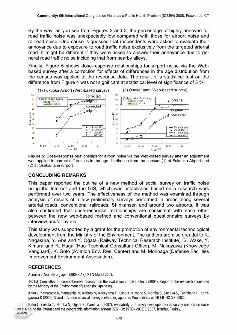
Community: 9th International Congress on Noise as a Public Health Problem (ICBEN) 2008, Foxwoods, CT
By the way, as you see from Figures 2 and 3, the percentage of highly annoyed for road traffic noise was unexpectedly low compared with those for airport noise and railroad noise. One cause is guessed that respondents were asked to evaluate their annoyance due to exposure to road traffic noise exclusively from the targeted arterial road. It might be different if they were asked to answer their annoyance due to ge-neral road traffic noise including that from nearby alleys. Finally, Figure 5 shows dose-response relationships for airport noise via the Web-based survey after a correction for effects of differences in the age distribution from the census was applied to the response data. The result of a statistical test on the difference from Figure 4 was not significant at statistical level of significance of 5 %.
Figure 5: Dose-response relationships for airport noise via the Web-based survey after an adjustment was applied to correct differences in the age distribution from the census: (1) at Fukuoka Airport and (2) at Osaka/Itami Airport
CONCLUDING REMARKS This paper reported the outline of a new method of social survey on traffic noise using the Internet and the GIS, which was established based on a research work performed over two years. The effectiveness of the method was examined through analysis of results of a few preliminary surveys performed in areas along several arterial roads, conventional railroads, Shinkansen and around two airports. It was also confirmed that dose-response relationships are consistent with each other between the new web-based method and conventional questionnaire surveys by interview and/or by mail. This study was supported by a grant for the promotion of environmental technological development from the Ministry of the Environment. The authors are also greatful to K. Nagakura, Y. Abe and Y. Ogata (Railway Technical Reserach Institute), S. Wake, Y. Kimura and R. Haga (Hao Technical Consultant Office), M. Nakazawa (Knowledge Vanguard), K. Goto (Aviation Env. Res. Center) and M. Morinaga (Defense Facilities Improvement Environment Assosiation).
REFERENCES Acoustical Society of Japan (2003). ASJ RTN-Model 2003.
INCE/J Committee on comprehensive research on the evaluation of noise effects (2004). Report of the research sponsored by the Ministry of the Environment of Japan (in Japanese).
Kaku J, Yamamoto K, Yamashita M, Kabuto M, Kageyama T, Kuno K, Kuwano S, Namba S, Sueoka S, Tachibana H, Kami-gawara K (2002). Standardization of social survey method in Japan. In: Proceedings of INTER-NOISE 2002.
Kaku J, Yokota T, Namba S, Ogata S, Yamada I (2007). Availability of a newly developed social survey method on noise using the Internet and the geographic information system (GIS). In: INTER-NOISE 2007, Istanbul, Turkey.
original corrected
corrected original original
original corrected
corrected
(2) Osaka/Itami (Web-based survey) (1) Fukuoka Airport (Web-based survey)
722

Community: 9th International Congress on Noise as a Public Health Problem (ICBEN) 2008, Foxwoods, CT
Kitagawa T et al. (1999). Estimation of prediction method for narrow-gauge railroads. In: Proceedings of the Meeting of ASJ 99 (in Japanese).
Nagakura K et al. (2002). Prediction method of noise from Shinkansen high-speed railroad. In: Report of the Meeting of ASJ Noise and Vibration Committee, N-2000-01 (in Japanese).
723

Community: 9th International Congress on Noise as a Public Health Problem (ICBEN) 2008, Foxwoods, CT
Reanalysis of dose-response curves of Shinkansen railway noise Shigenori Yokoshima1*, Takashi Morihara2, Atsushi Ota3, Akihiro Tamura3 1 Shonan Region Prefectural Administration Center, Kanagawa Prefectural Government, 1-3-39,
Shinomiya, Hiratsuka, 254-0014 Japan
2 Ishikawa National College of Technology, Tsubata cho Kitanakajo, Kawakita 929-0392., Japan
3 Department of Architecture, Yokohama National University, 79-5, Tokiwadai, Hodogaya, Yoko-hama, 240-8501 Japan
* corresponding author: e-mail: [email protected]
1 INTRODUCTION The Shinkansen railway has increased its transportation capacity since its opening in 1964. This has led to increased levels of vibrations and noise (including low fre-quency noise caused by running trains), annoying people living along the railway cor-ridor. For the purpose of helping to preserve living environments and for the protec-tion of inhabitants’ health against the adverse effect of noise, the “Environmental Quality Standards for Shinkansen Super-express Railway Noise” were introduced in 1975. Subsequently in 1976, the Director of the Environmental Agency recom-mended that “Shinkansen railway vibration countermeasures be taken urgently to ensure environmental preservation”. The noise level is to be evaluated by the energy mean of the top 10 values among 20 peak measurements. The vibration index is de-termined by the arithmetic mean instead of the energy mean. Several social surveys have been carried out so far in Japan on the community re-sponse to the Shinkansen noise issue. Sone et al. (1973) conducted social surveys on the Shinkansen noise in areas along the New Tokaido and Sanyo Lines. The re-sults were compared with the results of aircrafts noise measurements. They dis-cussed the application of several noise indices to evaluate Shinkansen noise annoy-ance levels. Subsequently, Tamura (1994) indicated that people along the Shinkan-sen railway rates more poorly than those along ordinary railways in the areas where railway noise is a major contributor to the total environmental noise. From 2001 to 2003, Yokohama National University and the Kanagawa Environmental Research Center carried out social surveys in residential areas along the New To-kaido Line in the Kanagawa Prefecture. Yokoshima & Tamura (2003) indicated that the inhabitants had more severe attitudes to the Shinkansen railway noise than those exposed to noise from other forms of ground-based transportation. Furthermore, ap-plying covariance structure analysis to the annoyance structure model of the noise and vibration, Yokoshima & Tamura (2005) revealed that there were synergetic ef-fects between the Shinkansen noise and vibrations on annoyance. In 2003, the Kumamoto and Hokkai Gakuen Universities carried out a joint social survey on the community response to Shinkansen railway noise in areas along the New Sanyo Line in the Fukuoka Prefecture. Yano et al. (2005) and Sato et al. (2004) suggested the presence of an interactive effect between the Shinkansen noise and vibration on annoyance. Recently, the “Environmental Quality Standards” regarding other noises have been amended in Japan. The “Environmental Quality Standards for Noise” are defined by the environmental conditions related to noise in general living and roadside areas. The standards were revised in 1999. The new standards prescribe LAeq as the noise
724

Community: 9th International Congress on Noise as a Public Health Problem (ICBEN) 2008, Foxwoods, CT
metric. In addition, in 2007, the Ministry of the Environment revised the “Environ-mental Quality Standards for Aircraft Noise”. These require aircraft noise to be evalu-ated using Lden instead of WECPNL. On the other hand, environmental quality stan-dards for conventional railway noise have yet to be legislated in Japan. However, the “Guidelines for Noise Measures with regard to Construction and/or Large-scale Im-provement of Conventional Railways” in 1995 use LAeq. Therefore, it is indispensable to discuss the application of noise metrics in the evaluation of Shinkansen railway noise annoyance. We discuss the dose-response curves of the Shinkansen railway noise using the re-sults of two surveys: the Fukuoka and the Kanagawa Surveys. To find an appropriate metric for Shinkansen railway noise, we compare the relationships between the maximum-based and energy-based noise metrics and community responses to noise. Furthermore, we examine whether or not non-auditory effects, distance and vibration exposure, affect Shinkansen railway noise annoyance.
2 SOCIAL SURVEYS
Table 1: Details of the Shinkansen railway and the surveys used in this study
Prefecture Kanagawa Survey Fukuoka Survey Railway line New Tokaido Line New Sanyo Line Survey Range 100 meters from the track 150 meters from the track Number of passing trains 287 trains 180 trains Train series Series 300,500,700 Series 0,100,300,500,700 Number of cars 16 cars 4-16 cars Survey date
October 2001 September – October 2002 October 2003
April 2003
Sample Size 1,784 1,100 Respondents 986 724
2.1 Description of the Shinkansen railway lines The operation of the Shinkansen train is prohibited from 12 midnight to 6 a.m. The total number of trains per day in the Kanagawa and Fukuoka Prefectures were 287 and 180, respectively. A maximum speed of above 250 km/h was observed at most sites for the Kanagawa Survey, in contrast to about 200 km/h for the Fukuoka Prefec-ture. In addition, the Sanyo Shinkansen trains have various numbers of cars ranging from 4 to 16, while 16 cars travelled on the New Tokaido Line (see Table 1).
2.2 The Kanagawa Survey The Kanagawa Survey was conducted in residential areas along the New Tokaido Line in the Kanagawa Prefecture, from 2001 to 2003. Questionnaires were distrib-uted to inhabitants 18 years of age and over at 98 survey sites. Each site, covering 100 square meters, was extracted at random from the areas within 100 meters of the railway. The survey used a distribution-by-mail method. However, the survey covered 10 survey sites in the vicinity of the Atsugi Naval Air Facility. Since noise generated by training flights may also have adversely affect people’s daily life in the areas sur-rounding the Atsugi Base, there is a possibility that their responses are biased by the aircraft noises. Consequently, 114 respondents in the 10 sites were eliminated from the sample. The sample size for people living in detached houses amounted to 872, and the response rate was about 55 %.
725

Community: 9th International Congress on Noise as a Public Health Problem (ICBEN) 2008, Foxwoods, CT
The contents of the questionnaire used in the Kanagawa Survey are as follows. Q1, satisfaction of residential environments included the degree of “outdoor quietness” and “house vibration”. These items were rated on a 5-point verbal scale. Q6, daily activity disturbances, including the following items related to noise and vibration: the rattling of fittings, listening disturbance, sleep disturbance, reading/thinking distur-bance and degree of restriction in opening windows. The answer format of Q6 was multiple choice. In Q7, the annoyance level of each of nine sources of noise, includ-ing the Shinkansen railway, was evaluated based on the ICBEN scale: not at all, slightly, moderately, very and extremely “bothered” by the noise. After the social survey was completed, noise and vibration measurements were made to estimate the actual noise exposures associated with each of the respon-dents’ dwellings at each site. The sound exposure level (LAE) and SLOW-peak sound level (LASmax) of each passing train was measured at several points at different dis-tances from the track. At each point, the 24-hour LAeq was determined based on the mean energy value of the LAE and the number of trains per day. Likewise, the energy mean value of the upper half of the measured SLOW-peak noise levels (LAmax) was also calculated. According to the noise metrics, one or more distance reduction equa-tions, logarithmic regression equations between distance and noise levels, were for-mulated. Noise exposures to each dwelling were estimated in every survey site by the corresponding formula. For Ldn and Lden, the exposures were estimated using the train schedule and the 24-hour LAeq values at each dwelling. Similarly, the peak vibration level in the vertical direction was measured at the same point as the noise measurement was taken. The vibration level was recorded on the ground using a vibration level meter. The vibration exposure (LVmax) was calculated from the arithmetic mean value of the upper half of the measurements (re 10-5 m/s2) at each point. The distance reduction equations were formulated based on the LVmax values, and the vibration exposure to each house was estimated from the equations.
2.3 Fukuoka Survey The Fukuoka Survey was conducted in 2003 in residential areas along the New Sanyo Line in the Fukuoka Prefecture. Since the Shinkansen line is elevated and noise barriers have been constructed along the line in almost all areas, essentially all of the detached houses within 150 m of the track were selected for the survey. When there was no house within the 150 m range, detached houses directly facing the rail-way were also included, up to a maximum distance of 680 m from the railway. Re-spondents aged between 20 and 75 years were randomly selected from a list of vot-ers on a one-person-per-family basis. The questionnaires were distributed and col-lected either by the staff or by mail. In total, 724 responses were obtained and the response rate was 66 %. The contents of the questionnaire, which were significantly different from those for the Kanagawa Survey, were as follows: housing factors, evaluation of the residential environment, annoyance caused by environmental factors including noise from the Shinkansen railway, interference in activities as a result of the Shinkansen trains, and personal factors. The annoyance and activity interferences in this case were also measured using the ICBEN scale. After the social survey was carried out, noise measurements were made. Shinkansen noise levels, LAE and LASmax, were recorded at least five times for each train type and for both near and far tracks at a reference point close to the Shinkansen line and points 5, 10, 20, 40 and 80 m apart from the reference point. Concurrent measure-
726

Community: 9th International Congress on Noise as a Public Health Problem (ICBEN) 2008, Foxwoods, CT
ments were made using integral sound level meters. Distance reduction equations, logarithmic regression equations between distance and noise reduction, were formu-lated separately for the near and far tracks based on the LAE and LASmax values. Noise exposures to each house were obtained from the LAeq,24h at the reference point and the noise reduction calculated using the formula. The values of Ldn and Lden, were estimated by the same method as used in the Kanagawa Survey. The peak vibration levels in the vertical direction were measured at points 12.5, 25, 50, 75, 100 and 150 m from the near track. The measurements were made at five sites along the line. The vibration level on the ground was recorded and the LVmax value was calculated from the measurements. The distance reduction equations of LVmax were formulated and the vibration exposure to each house was estimated. However, the number of the houses for which LVmax values were determined was only 358.
3 RESULTS Figure 1 indicates the averaged exposures (LAeq, LAmax, and LVmax) according to the distance categories. Analyses were done with LAeq as an energy-based noise index. This figure shows the results for respondents living within 100 m of the track. While the LAeq values for the Kanagawa Survey were higher within 25 m of the track, those for the Fukuoka Survey indicated the same or higher levels at distances over 25 m. For the LAmax, the Fukuoka Survey shows higher levels than found in the Kanagawa Survey for distances over 25 m. Since the number of and each duration time of the noise events and per day differed between the New Tokaido and Sanyo Lines, the LAeq value of the Kanagawa Survey was 5 dB larger than that of the Fukuoka Survey, even when the LAmax value was at the same level for both surveys. The Lden and Ldn values were about 4 dB and 3 dB higher than the LAeq value for both surveys, respec-tively. In contrast, the vibration level from the New Tokaido Line was higher compared with the New Sanyo Line. Figure 1: Averaged exposures according to the distance categories
Figure 2 compares the dose-response relationships for the Shinkansen noise annoy-ance between the two surveys. The “%HA” was defined here as the rate of respon-dents who answered in the top category (“extremely”) in each exposure range. For the LAeq, it was found that the difference in the %HA was significant at the 5 % level in the range of 46-50 dB using Fisher’s exact test. In contrast, there was a significant difference in %HA at the 5 % level in the LAmax range of 61-65 dB. These figures sug-
40.0
50.0
60.0
70.0
80.0
-25 26-50 51-75 76-100Distance (m)
Expo
sure
(dB
) LAeq [Kanagawa]LAmax [Kanagawa]LVmax [Kanagawa]LAeq [Fukuoka]LAmax [Fukuoka]LVmax [Fukuoka]
727

Community: 9th International Congress on Noise as a Public Health Problem (ICBEN) 2008, Foxwoods, CT
gest that the dose-response relationships between the surveys didn’t agree, espe-cially for LAeq. Likewise, Figure 3 compares the dose-response relationships for listening distur-bance between the two surveys. The “%LD” was defined here as the following: the rates of the respondents who answered the presence in listening disturbance. How-ever, the answer formats of listening disturbance differed between the surveys. Therefore, this paper regarded the responses in the top two categories, “very” and “extremely”, for the Fukuoka Survey as the presence of disturbance. For the LAeq, the Fukuoka Survey indicated a tendency towards a higher disturbance response rate than the Kanagawa Survey. A significant difference for the LAeq values was observed at the 5 % level in the range of 46-50 dB. However, no significant difference in the LAmax was found. Figure 2: Comparison of noise exposure –annoyance relationships between the surveys
Figure 3: Comparison of noise exposure –disturbance relationships between the surveys
Figure 4 shows the mean values of the LAeq and LAmax using a 5-point scale of noise annoyance according to the surveys. The X and Y axes are the noise exposure and annoyance scale (1=not at all, 2=slightly, 3=moderately, 4=very, 5=extremely), re-spectively. The LAmax values of the Kanagawa Survey were about 4 dB higher than those found in the Fukuoka Survey on every scale level from the “slightly” to the “ex-tremely” levels. For the “not at all” level, no difference was found between averaged LAeq values. In contrast, there was no difference in the LAeq between the two surveys except at the “not at all” level of the scale.
0
20
40
60
51-55 56-60 61-65 66-70 71-75 76-80 81-
L Amax (dB)
% H
A (%
)
Kanagawa
Fukuoka
0
20
40
60
80
31-35 36-40 41-45 46-50 51-55 56-60
L Aeq (dB)
% H
A (%
)
Kanagawa
Fukuoka
0%
20%
40%
60%
31-35 36-40 41-45 46-50 51-55 56-60L Aeq (dB)
%LD
(%)
Kanagawa
Fukuoka
0%
20%
40%
60%
51-55 56-60 61-65 66-70 71-75 76-80L Amax (dB)
%LD
(%)
Kanagawa
Fukuoka
728
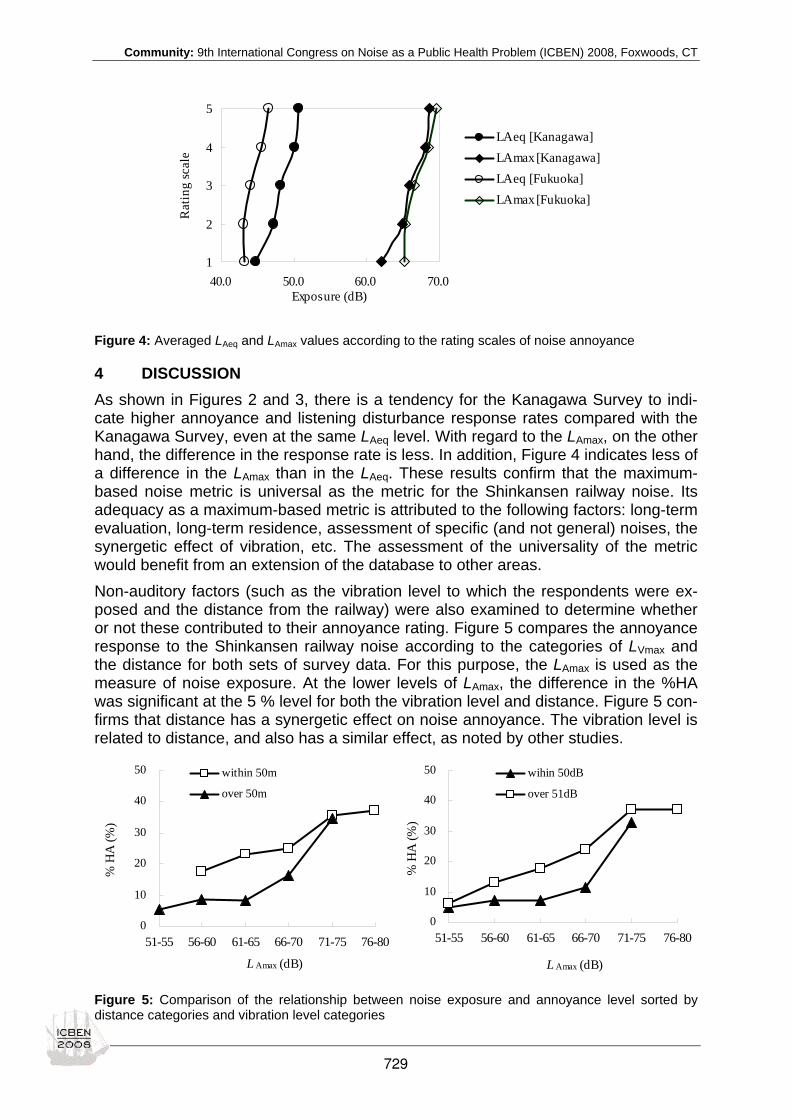
Community: 9th International Congress on Noise as a Public Health Problem (ICBEN) 2008, Foxwoods, CT
Figure 4: Averaged LAeq and LAmax values according to the rating scales of noise annoyance
4 DISCUSSION As shown in Figures 2 and 3, there is a tendency for the Kanagawa Survey to indi-cate higher annoyance and listening disturbance response rates compared with the Kanagawa Survey, even at the same LAeq level. With regard to the LAmax, on the other hand, the difference in the response rate is less. In addition, Figure 4 indicates less of a difference in the LAmax than in the LAeq. These results confirm that the maximum-based noise metric is universal as the metric for the Shinkansen railway noise. Its adequacy as a maximum-based metric is attributed to the following factors: long-term evaluation, long-term residence, assessment of specific (and not general) noises, the synergetic effect of vibration, etc. The assessment of the universality of the metric would benefit from an extension of the database to other areas. Non-auditory factors (such as the vibration level to which the respondents were ex-posed and the distance from the railway) were also examined to determine whether or not these contributed to their annoyance rating. Figure 5 compares the annoyance response to the Shinkansen railway noise according to the categories of LVmax and the distance for both sets of survey data. For this purpose, the LAmax is used as the measure of noise exposure. At the lower levels of LAmax, the difference in the %HA was significant at the 5 % level for both the vibration level and distance. Figure 5 con-firms that distance has a synergetic effect on noise annoyance. The vibration level is related to distance, and also has a similar effect, as noted by other studies. Figure 5: Comparison of the relationship between noise exposure and annoyance level sorted by distance categories and vibration level categories
1
2
3
4
5
40.0 50.0 60.0 70.0Exposure (dB)
Rat
ing
scal
e
LAeq [Kanagawa]LAmax [Kanagawa]LAeq [Fukuoka]LAmax [Fukuoka]
0
10
20
30
40
50
51-55 56-60 61-65 66-70 71-75 76-80
L Amax (dB)
% H
A (%
)
wihin 50dB
over 51dB
0
10
20
30
40
50
51-55 56-60 61-65 66-70 71-75 76-80
L Amax (dB)
% H
A (%
)
within 50m
over 50m
729

Community: 9th International Congress on Noise as a Public Health Problem (ICBEN) 2008, Foxwoods, CT
Figures 2 and 3 indicate that the slopes of the dose-response curves for the Fukuoka Survey are higher than those for the Kanagawa Survey. The difference can probably be attributed to the differences in distances between the track and the dwellings be-tween the surveys. While the level of noise annoyance in the vicinity of the railway is likely to have been affected by the distance, there is no synergetic effect on the an-noyance in the area distant from the source. Therefore, the difference in the distance brings about the steeper slope for the Fukuoka Survey.
5 CONCLUSION Using two social surveys of community responses, the Kanagawa and the Fukuoka Surveys, we reanalyzed the dose-response relationships for Shinkansen railway noise. For the noise metric LAmax, a maximum-based noise metric rather than LAeq has been found to be universal for assessing noise annoyance. In addition, we examined whether non-auditory effects affect annoyance or not. In particular, the distance from the source to the dwelling and the respondents’ vibration level of exposure showed significant effects on individual annoyance levels.
REFERENCES Sato T, Yano T, Morihara T (2004). Effects of situational variables on community response to Shinkansen noise: A survey in Kyushu, Japan. In: Proceedings of Inter-Noise 04.
Sone T, Kono S, Nimura T, Kameyama S, Kumagai M (1973). Effects of high speed train noise on the community along a railway’. J Acoust Soc Jpn 29: 214-224 (in Japanese).
Tamura A (1994). Comparison of community response to outdoor noise in the areas along Shinkansen and ordinary railroad. In: Proceedings of Inter-Noise 94, Vol. 2: 755-758.
Yano T, Morihara T, Sato T (2005). Community response to Shinkansen noise and vibration: a survey in areas along the Sanyo Shinkansen Line. In: Proceedings of Forum Acusticum Budapest.
Yokoshima S, Tamura A (2003). Community response to Shinkansen railway noise. In: Proceedings of Inter-Noise 03.
Yokoshima S, Tamura A (2005). Combined annoyance due to the Shinkansen railway noise and vibration. In: Proceedings of Inter-Noise 05.
730

Community: 9th International Congress on Noise as a Public Health Problem (ICBEN) 2008, Foxwoods, CT
Sound-masking technique for combined noise exposure in open public spaces Jin You, Jin Yong Jeon Department of Architectural Engineering, Hanyang university, Seoul 133-791, Korea
ABSTRACT A sound-masking technique was applied to minimize the annoyance in open public spaces exposed to combined noise sources. The noises were recorded binaurally through artificial head microphones from the building construction sites with nearby roads. Sound quality (SQ) parameters as well as spectral and temporal characteris-tics of the noises were investigated. For the auditory tests to evaluate the presence of the sound-masking system, sound maskers were manipulated and presented in the open public spaces. Psychoacoustical factors affecting subjective responses to the combined noise exposure were investigated and the effectiveness of the sound-masking system was examined.
INTRODUCTION Demands on favorable acoustic environment in open public spaces have been in-creasing with the increase of outdoor activities. Overall sound pressure level in the area has been thought as the most important aspect affecting the amenity of the en-vironment. However, most of the open areas are necessarily accompanied with heavy flux of transportation and people so that excessive noise threatens sound-scape of the environments. Many studies investigated the acoustical environment of exterior spaces in order to define the relationships between sound characteristics and subjective responses (Anderson et al. 1983; Skanberg & Ohrstrom 2002). Although classifying the charac-teristics of soundscape in open public space is important, active treatment on the sound environment is often needed to improve quality of the acoustical amenity of the areas. As an actual method to control the soundscape, several nature sounds were introduced with speaker systems to the open public spaces (Jang et al. 2003; Lee et al. 2005; Jeon et al. 2007). As most of the studies applied nature sounds with-out manipulation, hence masking effects on the environmental noise have been defi-cient. In the present study, the characteristics of combined exterior noises from road traffic and construction site were investigated. The preferences on the soundscape were sought before and after the application of the sound-masking system. Sound quality attributes of the combined noise were determined and sound maskers (to enhance the acoustical amenity) were produced.
MEASUREMENTS Sounds from building construction and nearby roads were recorded in eight open public areas which were chosen according to the volume of road traffic and the dis-tance from construction sites (see Table 1). Measured noise level ranged from 55.8 to 78.0 dBA during 10 minutes. Sites B and F were chosen and, as shown in Figure 1, HATS (Head and Torso simulator) was located at 33 m, 15 m from the roads in Sites B and F, respectively. Therefore, in Site F, HATS was located at 50 m apart from the construction site. The height of microphone was set at 1.5 m from the ground. The
731
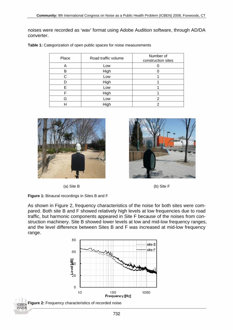
Community: 9th International Congress on Noise as a Public Health Problem (ICBEN) 2008, Foxwoods, CT
noises were recorded as ‘wav’ format using Adobe Audition software, through AD/DA converter.
Table 1: Categorization of open public spaces for noise measurements
(a) Site B (b) Site F
Figure 1: Binaural recordings in Sites B and F
As shown in Figure 2, frequency characteristics of the noise for both sites were com-pared. Both site B and F showed relatively high levels at low frequencies due to road traffic, but harmonic components appeared in Site F because of the noises from con-struction machinery. Site B showed lower levels at low and mid-low frequency ranges, and the level difference between Sites B and F was increased at mid-low frequency range.
Figure 2: Frequency characteristics of recorded noise
Place Road traffic volume Number of construction sites
A Low 0 B High 0 C Low 1 D High 1 E Low 1 F High 1 G Low 2 H High 2
732
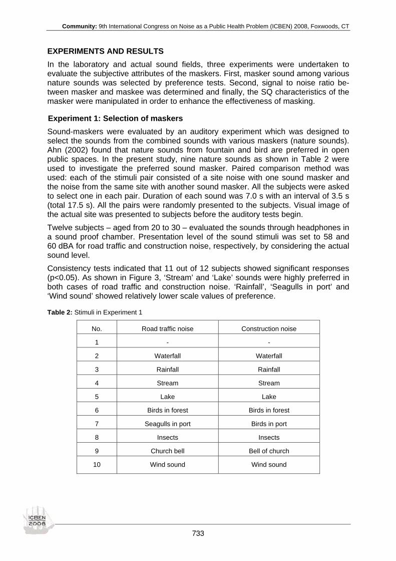
Community: 9th International Congress on Noise as a Public Health Problem (ICBEN) 2008, Foxwoods, CT
EXPERIMENTS AND RESULTS In the laboratory and actual sound fields, three experiments were undertaken to evaluate the subjective attributes of the maskers. First, masker sound among various nature sounds was selected by preference tests. Second, signal to noise ratio be-tween masker and maskee was determined and finally, the SQ characteristics of the masker were manipulated in order to enhance the effectiveness of masking.
Experiment 1: Selection of maskers Sound-maskers were evaluated by an auditory experiment which was designed to select the sounds from the combined sounds with various maskers (nature sounds). Ahn (2002) found that nature sounds from fountain and bird are preferred in open public spaces. In the present study, nine nature sounds as shown in Table 2 were used to investigate the preferred sound masker. Paired comparison method was used: each of the stimuli pair consisted of a site noise with one sound masker and the noise from the same site with another sound masker. All the subjects were asked to select one in each pair. Duration of each sound was 7.0 s with an interval of 3.5 s (total 17.5 s). All the pairs were randomly presented to the subjects. Visual image of the actual site was presented to subjects before the auditory tests begin. Twelve subjects – aged from 20 to 30 – evaluated the sounds through headphones in a sound proof chamber. Presentation level of the sound stimuli was set to 58 and 60 dBA for road traffic and construction noise, respectively, by considering the actual sound level. Consistency tests indicated that 11 out of 12 subjects showed significant responses (p<0.05). As shown in Figure 3, ‘Stream’ and ‘Lake’ sounds were highly preferred in both cases of road traffic and construction noise. ‘Rainfall’, ‘Seagulls in port’ and ‘Wind sound’ showed relatively lower scale values of preference.
Table 2: Stimuli in Experiment 1
No. Road traffic noise Construction noise
1 - -
2 Waterfall Waterfall
3 Rainfall Rainfall
4 Stream Stream
5 Lake Lake
6 Birds in forest Birds in forest
7 Seagulls in port Birds in port
8 Insects Insects
9 Church bell Bell of church
10 Wind sound Wind sound
733

Community: 9th International Congress on Noise as a Public Health Problem (ICBEN) 2008, Foxwoods, CT
Figure 3: Scale value of preference of sound maskers
Experiment 2: Investigation of effective signal to noise ratio Effective signal to noise ratio between masker and maskee was investigated for ‘Stream’ and ‘Lake’ sounds which were determined as sound maskers in Experiment 1. As shown in Table 3, the relative sound pressure levels of the sound maskers were varied. The signal to noise ratio between each of the neighboring stimuli was 3 dB and maximum level difference was 6 dB. Paired comparison method was also employed and ten subjects participated for the evaluations. Consistency tests indicated that 9 out of 10 subjects showed significant responses (p<0.05). As shown in Figure 4, in the case of construction noise, the scale value showed high preferences when the sound masker was presented 3 dB lower than that of the noise. In the case of road traffic noise, the scale value was high when the ‘Stream’ and ‘Lake’ were presented as the same level and 3 dB lower than the noise, respectively. The scale value was decreased when the level of sound masker was increased over the level of site noise.
Table 3: Stimuli of experiment 2
No. Road traffic noise Construction noise
1 Stream 52 dBA (-6 dB) Stream 56 dBA (-6 dB)
2 Stream 55 dBA (-3 dB) Stream 59 dBA (-3 dB)
3 Stream 58 dBA ( 0 dB) Stream 62 dBA (-0 dB)
4 Stream 61 dBA (+3 dB) Stream 65 dBA (+3 dB)
5 Stream 64 dBA (+6 dB) Stream 68 dBA (+6 dB)
6 Lake 52 dBA (-6 dB) Lake 56 dBA (-6 dB)
7 Lake 55 dBA (-3 dB) Lake 59 dBA (-3 dB)
8 Lake 58 dBA ( 0 dB) Lake 62 dBA ( 0 dB)
9 Lake 61 dBA (+3 dB) Lake 65 dBA (+3 dB)
10 Lake 64 dBA (+6 dB) Lake 68 dBA (+6 dB)
734

Community: 9th International Congress on Noise as a Public Health Problem (ICBEN) 2008, Foxwoods, CT
(a) Construction noise (b) Road traffic noise
Figure 4: Scale value of preference according to relative presentation level
Experiment 3: SQ characteristics of effective sound maskers The stimuli which were varied in sound quality characteristics were investigated in this experiment with the same experimental conditions as in Experiments 1 and 2. Psychoacoustical characteristics of the noise and sound masker are shown in Ta-ble 4. ‘Masker A’ and ‘Masker B’ are the sound maskers which were preferred in the previous experiments for construction noise and road traffic noise, respectively.
Table 4: Psychoacoustical characteristics of the stimuli used in Experiment 3
SPL [dBA]
Loudness [sone]
Sharpness [acum]
Roughness [asper]
Fluctuation Strength
[vacil]
Construction noise 62 17.6 1.41 1.67 1.05
Masker A 59 11.1 2.01 2.46 1.2
White noise A 59 12.3 3.14 1.43 0.74
Road traffic noise 58 12.1 1.43 1.34 0.76
Masker B 58 10.2 1.99 2.51 1.22
White noise B 58 11.5 3.15 1.44 0.75
Evaluation of sound masking system in actual condition Evaluations on the soundscape were conducted to verify the effectiveness of the sound masking system in actual condition. Subjects evaluated the sound masking system in the eight actual fields in order to validate the sound maskers in laboratory conditions.
DISCUSSION AND CONCLUSIONS Sound maskers have been applied in urban public spaces exposed to construction and road traffic noises. Subjective evaluations have been made to investigate noise annoyance to different combination of soundscape. Results which were taken both in laboratory and actual conditions, show that sound maskers such as ‘Stream’ and ‘Lake’ are effective for both road traffic and construction noises. When the presenta-tion level of the sound masker is up to 3 dB lower than that of the combined noise sources, the scale values of preferences actually increase.
735

Community: 9th International Congress on Noise as a Public Health Problem (ICBEN) 2008, Foxwoods, CT
Analyses of Zwicker’s parameters reveal that higher loudness factors in the pre-sented noises are perceptually lessened by other higher psychoacoustical factors in the maskers. The effectiveness of the sound masking-system will be further exam-ined in actual situations.
REFERENCES Ahn DS (2002). Analyses on the cognitive effects of masking traffic noise by sounds of water. J Korean Inst Forest Recreat 6(4): 9-19.
Anderson LM, Mulligan BE, Goodman LS, Regen HZ (1983). Effects of sounds on preferences for outdoor settings. Environ Behav 15: 539–566.
Guastavino C, Katz BFG, Polack JD, Levitin DJ, Dubois D (2005). Ecological validity of soundscape reproduction. Acta Acust 91: 333–341.
Jang GS, Kook C, Kim SW (2003). The preference and amenity factors of the environmental sounds suitable for urban spaces. Transact Korean Soc Noise Vibr Eng 13: 890–895.
Jeon JH, Shin YG, Kook C, Jang GS (2007). Study to propose the suitable reproducing sound level of SAFRS. Transact Korean Soc Noise Vibr Eng 17: 547–552.
Lee TG, Song MJ, Jang GS (2005). An experimental study on the effect of introducing sound in the city riversides for sound-scape application. Transact Korean Soc Noise Vibr Eng 15: 980–987.
Skanberg A, Ohrstrom E (2002). Adverse health effects in relation to urban residential soundscapes. J Sound Vibr 250: 151–155.
736
__________________________________________________________________________
__________________________________________________________________________
ICBEN 2008
Noise and Animals
737

Animals: 9th International Congress on Noise as a Public Health Problem (ICBEN) 2008, Foxwoods, CT
The costs of lost auditory awareness for wildlife and park visitors Kurt Fristrup1*, Jesse Barber2 1 Natural Sounds Program, National Park Service, 1201 Oakridge Drive, Suite 100, Fort Collins, CO,
80525, USA
2 Colorado State University, Fort Collins, CO, 80525, USA
* corresponding author: e-mail: [email protected]
Hearing provides omnidirectional environmental awareness in most animal species, and the auditory systems of many species enable them to fully exploit the quietest conditions that routinely occur in their environments. Although it is straightforward to compute reductions in alerting distance or listening area due to elevated noise in a particular frequency band, more work is needed to develop standardized methods for estimating masking effects when the noise sources and environmental signals have different spectral and temporal properties. Habituation, or learned deafness, also merits further investigation. Failure to notice environmental acoustic cues from either cause can have substantial consequences for survivorship, foraging efficiency, and reproduction. For park visitors, wildlife will be less likely to occur at times and places that are noisy, their behavior patterns will be less natural, and they will likely be less tolerant of human presence. Furthermore, visitors will be less likely to detect wildlife if they cannot hear subtle acoustic cues.
738

Animals: 9th International Congress on Noise as a Public Health Problem (ICBEN) 2008, Foxwoods, CT
Evolution of noise exposure criteria for fishes Mardi C. Hastings1*, Arthur N. Popper2
1 The Pensylvania State University, Applied Research Laboratory, State College, PA 16804
2 University of Maryland, Department of Biology, College Park, MD 20742
* corresponding author: e-mail: [email protected]
The first noise exposure criterion for fish was proposed in 1990 for a Navy test facility at Lake Pend Oreille in Idaho. Based on a study showing that goldfish had temporary threshold shift (TTS) after 4-hours exposure to pure tones with 149 dB re 1 µPa sound pressure level (SPL) (Popper & Clarke 1976), the recommendation for 'no harm' to fish was to limit SPL to 150 dB re 1 µPa (Hastings 1990). As concern about effects of human-generated sound in the ocean grew, damage to auditory tissue in fish was examined. Studies indicated that exposure to an SPL of 180 dB re 1 µPa for 1-2 hours could cause hair cell damage (Hastings 1995; Hastings et al. 1996). The site and extent of damage depended on species and sound frequency. The latest recommendation for direct injury is a sound exposure level (SEL) from 183 to 213 dB re 1 µPa^2-s, depending on fish body mass. These end points are based on data from a blast study on juvenile fish (Govoni et al. 2003) and a low frequency active sonar study on larger fish (Popper et al. 2007), respectively. Moreover dual criteria consisting of peak SPL and cumulative SEL are recommended for TTS based on the results of a riverine airgun study (Popper et al. 2005). These data indicate that some species will experience TTS of 20-25 dB at an SEL of 185 dB re 1 µPa^2-s that recovers within approximately 18 hours, whereas other species show no hearing loss.
Govoni JJ, Settle LR, West MA (2003). Trauma to juvenile pinfish and spot inflicted by submarine detonations. J Aquatic Animal Health 15: 111-119.
Hastings MC (1990). Comparison of a model for the dynamic response of the fish swimbladder with frequency responses measured in vivo. J Acoust Soc Am 88 (Suppl 1): S35
Hastings MC (1995). Physical effects of noise on fishes. In: InterNoise ’95 (p 979).
Hastings MC (1995). Acoustic stunning of marine animals. J Acoust Soc Am 98: 2940.
Hastings MC, Popper AN, Finneran JJ, Lanford PJ (1996). Effects of low-frequency underwater sound on hair cells of the inner ear and lateral line of the teleost fish Astronotus ocellatus. J Acoust Soc Am 99: 1759-1766.
Popper AN, Clarke NL (1976). The auditory system of the goldfish (Carassius auratus): effects of intense acoustic stimulation. Comp Biochem Physiol A 53: 11-18.
Popper AN, Smith ME, Cott PA, Hanna BW, MacGillivray AO, Austin ME, Mann DA (2005). Effects of exposure to seismic airgun use on hearing of three fish species. J Acoust Soc Am 117: 3958-3971.
Popper AN, Halvorsen MB, Kane A, Miller DL, Smith ME, Song J, Stein P, Wysocki LE (2007). The effects of high-intensity, low-frequency active sonar on rainbow trout. J Acoust Soc Am 122: 623-635.
739
Animals: 9th International Congress on Noise as a Public Health Problem (ICBEN) 2008, Foxwoods, CT
Introduction of the new ASA Subcommittee on Animal Bioacoustics David K. Delaney1*, Susan B. Blaeser2 1 U.S. Army CERL
2 Acoustical Society of America
* corresponding author: e-mail: [email protected]
In October 2007, the Accredited Standards Committee S3, Bioacoustics, approved the first ever formation of a new subcommittee in the Acoustical Society of America (ASA) Standards Program. The new subcommittee is designated S3/SC1 Animal Bioacoustics and is a "consensus body" which can vote to approve standards that subsequently can be approved as an American National Standard by the American National Standards Institute (ANSI). The main benefit of forming this subcommittee is that its voting members will have a direct and material interest in Animal Bioacoustics rather than the more general, human focused, subject matter of the parent committee, S3 Bioacoustics. This should result in a high-quality review of draft documents and ultimately in the production of standards that are useful to the scientfic community. One of the goals of the Subcommittee is to develop standards that improve the quality, uniformity, and applicability of research so that resource managers and regulatory agencies can better manage for the long-term sustainability of animal populations. Over the past several years, interest in standardization has grown in the animal bioacoustics technical area. Standards Working Groups began to be formed in both S3/S1. Under the formation of the new Subcommittee, S3 voted to move the three existing working groups into the new Subcommittee, which are: S3/SC1 1/WG1 - Animal Bioacoustics Terminology, S3/SC1 1/WG2 - Effects of Sound on Fish and Turtles, and S3/SC1 1/WG3 - Underwater Passive Acoustics Monitoring for Bioacoustic Applications. An update on the activities and future direction of the Subcommittee will be presented.
740

Animals: 9th International Congress on Noise as a Public Health Problem (ICBEN) 2008, Foxwoods, CT
Protecting horses from excessive music noise – a case study Cornelius (Neil) Huybregts Marshall Day Acoustics Pty Ltd, 6 Gipps Street, Collingwood VIC 3066, Australia [email protected]
ABSTRACT When Flemington Racecourse, the site of Australia’s most famous horse race – the Melbourne Cup – became the proposed venue for Australia’s largest touring music festival – the Big Day Out – there was concern expressed by the owners of the thor-oughbred race horses stabled at the racecourse that the horses may react badly to the potentially excessive music noise, and Marshall Day Acoustics was commis-sioned to assess the likely impact on the horses. The constraints of consulting allowed only a brief review of current knowledge re-garding the effect of noise on horses, which provided useful background information, but, predictably, little guidance on criteria. Nevertheless, a recommendation was made that, if possible, noise levels not exceed 65dBA LAeq. The noise exposure (LAeq,15 minutes) of horses during major race events was measured at 58-62 dBA in the stables (rising to 66-68 dBA during helicopter fly-overs), and 65-70 dBA in the stalls. The Clerk of the Course’s horse was exposed to 76 dBA LAeq,6h at Randwick Racecourse during the New Easter Carnival and 85 dBA LAeq,6h at Flemington during the Melbourne Cup, although this second fig-ure is difficult to reconcile with the measured noise levels at the various locations. During the Big Day Out, the noise exposure (LAeq,15 minutes) of horses in the sta-bles was measured at 54-70 dBA. The horses generally showed little response to the music noise except when the noise was associated with visible stimuli, or when the noise was of an alarming character such as short bursts of high-pitched singing.
INTRODUCTION Flemington Racecourse, in Melbourne, Australia, is a major horse racing venue. It is best known as the venue for the Melbourne Cup, a race for which a public holiday is declared in Melbourne and which is famously known to ‘stop the nation’. Because of its large size (1.3 square kilometres) and its relative isolation from noise-sensitive land uses, the racecourse is also sometimes used as a venue for outdoor concerts. The Big Day Out is a one-day touring music festival held annually in various cities in Australia and New Zealand. The 2008 Big Day Out event for Melbourne was held at Flemington Racecourse, and featured 72 bands playing at 8 stages, including 2 main stages adjacent to each other, with the major acts alternating between the two stages. The main stages were the loudest, and were located approximately 200m from the horse stables, facing away from the stables. The main stages were ap-proximately 300m from the nearest residence. When it was proposed to hold the Big Day Out at Flemington Racecourse, the own-ers of the thoroughbred race horses stabled at Flemington expressed some concern that the music noise levels in the stables would be excessive and that the horses may react badly. Marshall Day Acoustics (MDA) was commissioned by the Victoria Racing Club, the trustees of Flemington Racecourse, to review current knowledge regarding the effect of noise on horses, to measure the noise exposure of horses during a race event, to
741

Animals: 9th International Congress on Noise as a Public Health Problem (ICBEN) 2008, Foxwoods, CT
provide an opinion on the likely effect of the noise on the horses, and to measure music noise levels in the stables during the 2008 Big Day Out. This paper describes the investigations and findings of the study undertaken by MDA, but also looks at some of the difficulties encountered when the results of a somewhat obscure field of study are to be applied to the management of noise im-pacts on animals.
CURRENT KNOWLEDGE The budget for this project allowed only 8 hours for a review of current knowledge concerning the effects of noise on horses. The actual time spent was 12 hours. Understandably, the review was broad-brush, consisting of:
• A search of the MDA library (including ICBEN and other conference proceedings)
• Posting of queries on the MDA discussion forum (which brought out some previ-ous MDA projects where effects of noise on animals was considered, and which led to discussions with the flora and fauna experts involved in those previous studies)
• Google searches, including Google Scholar
• Discussions with horse handlers and the equine veterinarians at the racecourses
• Correspondence with Professor Rickye Heffner from the University of Toledo (Ohio, USA) Department of Psychology.
The findings were similarly broad brush, consisting mostly of a discussion of issues such as chronic versus acute exposure, energy conservation in wild animals, and habituation. There was some information gathered that turned out to be of practical benefit, or at least relevant to the manner in which the noise exposure of the horses was ultimately managed, namely:
• That horses may be startled by noise is common knowledge. One of the basic guides to horse care and management published by the Equine Centre in Wer-ribee, Victoria, entitled Horse Health Care – Management: Safety around Horses, states that when approaching a horse, “you should be aware that horses are most easily scared by sudden movements or loud noises, particularly outside of the animal's field of binocular vision. Quick movements or loud noises in these areas will trigger fear reactions such as spinning or bolting…”
• Discussions with flora and fauna experts have indicated that many animals are more likely to be concerned (ie, interrupt feeding or resting activity) about noise that is associated with visual stimuli.
• It appears that noise can be more unsettling when associated with unfamiliar situations. One comment from Rickye Heffner was that “horses (and other spe-cies) can be disturbed by anything new in their environment – after all, if things are going well and there is a change, that could signal a change for the worse; change is usually a bad thing until proven otherwise.”
• The United States National Park Service's 2004 Sheep Report provides a com-prehensive review of the likely effects of aircraft fly-over noise on animals, with particular emphasis on wildlife. The report differentiates between chronic expo-sure, for which the major concerns are related to the animals’ energy conserva-tion, and acute exposure, such as startle and panic behavior. The report states
742

Animals: 9th International Congress on Noise as a Public Health Problem (ICBEN) 2008, Foxwoods, CT
that “acute responses… occur in most wildlife species evaluated at noise levels greater than 95 dBA.”
• One other factor to consider is habituation. If the noise is familiar and not associ-ated with danger, the animals’ response will become moderated. This is most evi-dent in the (often ineffectual) use of scare guns to remove pest species such as cockatoos from crops or seagulls from airports.
• A review of research into the relative hearing ability of a wide variety of animals (in Comparative Psychology: A Handbook by Greenberg and Haraway) found that the hearing threshold of horses was 5-15 dB higher than humans – that is, horses are somewhat deaf compared to us.
• Discussions with the handlers at Randwick Racecourse in Sydney and Fleming-ton and the equine veterinarian at Flemington indicated a widely-held opinion that thoroughbred horses are likely to be sensitive to noise but without any indication of how much noise would be acceptable. However, most felt that loud bangs, such as that associated with fireworks, would not be acceptable.
• The connection between temperament and noise-sensitivity has been studied in cattle, with one study showing that cattle that were more flighty (faster gait, jerky movements, more vigilant) were more noise-sensitive.
These findings provided useful background information, but were of limited value in setting criteria for the exposure of horses to music noise. As with other reviews of the effects of noise on fauna undertaken by MDA, the information was lacking one or more of the aspects of the problem we were facing: the noise exposure was not quantified (eg, “high levels” or “loud bangs”) or was of the wrong type (eg, aircraft noise rather than music noise); the species was wrong (eg, orange-bellied parrots); or the information was not particularly well-supported, amounting to little more than expert speculation in some cases.
NOISE EXPOSURE AT RACE EVENTS Overview During race events, the horses are kept in stables until it is close to the time for the horse to race. The horses are then led to the stalls, where they are saddled up. A few minutes before the race, the horses are led to the pre-mounting yard to be lightly ex-ercised, then to the mounting yard, and then onto the race track. Noise levels were measured using several noise indices, including LAmax, LAeq, LAmin and various LAn. Results were reported almost exclusively in LAeq. Although the re-sults of the review of current knowledge indicated that startling noises may be of most concern – indicating that LAmax, or at least some form of Lmax – would be appro-priate, it was considered that LAmax would be ‘poorly behaved’ – that is, it would not always be clear during any particular sample period whether there were repeated noisy events or just one or two noisy events. The LAeq, on the other hand, would show some increase in level if there were repeated events and would give an indica-tion of noise dose. Also, it was considered that reporting of the results would be more easily understood if only one noise metric was used.
New Easter Carnival – Randwick Racecourse The first set of noise measurements during a race event was conducted during the 2006 Easter Carnival at Randwick Racecourse in Sydney on 15 April 2006. Noise
743

Animals: 9th International Congress on Noise as a Public Health Problem (ICBEN) 2008, Foxwoods, CT
levels were not measured in the stables, but there were noise monitors at several fixed locations about the venue, noise dosimeters attached to two of the Clerk of Course horses and on the consultant undertaking the measurements, and spot measurements at various locations during the event. Post-event analysis showed that the most useful information was obtained by the noise monitor in the stalls and the dosimeter attached to Yotis, one of the Clerk of Course horses. Figure 1 shows the measured noise levels in the stalls. Noise levels (LAeq,15 minutes) were in the range 64-70 dBA.
Noise level exposure in stalls Randwick Racecourse 15 April 2006
40
50
60
70
80
11:00 11:15 11:30 11:45 12:00 12:15 12:30 12:45 13:00 13:15 13:30 13:45 14:00 14:15 14:30 14:45 15:00 15:15 15:30 15:45 16:00 16:15 16:30 16:45 17:00
Time of day
Noi
se le
vel (
dBA
)
Leq (1 minute) Leq (15 minute) Figure 1: Measured noise levels in the stalls
Noise level exposure of Clerk of Course Randwick Racecourse 15 April 2006
50
60
70
80
90
100
11:15
:00
11:30
:00
11:45
:00
12:00
:00
12:15
:00
12:30
:00
12:45
:00
13:00
:00
13:15
:00
13:30
:00
13:45
:00
14:00
:00
14:15
:00
14:30
:00
14:45
:00
15:00
:00
15:15
:00
15:30
:00
15:45
:00
16:00
:00
16:15
:00
16:30
:00
16:45
:00
17:00
:00
17:15
:00
Time of day
Leq
(dB
A)
Leq (1 second) Leq (15 minute) Figure 2: Noise exposure of Yotis, a Clerk of the Course horse
744

Animals: 9th International Congress on Noise as a Public Health Problem (ICBEN) 2008, Foxwoods, CT
Figure 2 shows the noise exposure of Yotis, the Clerk of Course’s horse, moving be-tween stalls, the pre-mounting yard, the mounting yard and the race track for the whole event. Noise levels (LAeq,15 minutes) were in the range 69-84 dBA. The LAeq,6h noise level for the whole of the measurement period was 76 dBA.
Melbourne Cup Carnival – Flemington Racecourse Noise measurements at Flemington during the 2007 Melbourne Cup Carnival con-sisted of:
• Noise monitors situated near stables and on the roof of the stalls. These were in place during 3-12 November inclusive, taking in all of Derby Day, Melbourne Cup Day, Oaks Day and Stakes Day, as well as several non-race days
• A noise dosimeter attached to Subzero, the Clerk of the Course’s horse, on Mel-bourne Cup Day
• Spot measurements at various locations on Melbourne Cup Day. Figure 3 shows the measured noise levels at various locations on Melbourne Cup Day. Note that the race at 15:00 is the Melbourne Cup. This is the race that ‘stops the nation’.
Measured Leq noise levels Melbourne Cup Day
Race10:20
Race11:00
Race11:45
Race12:30
Race13:15
Race14:00
Race15:50
Race16:35
Race17:20
Race15:00
40
50
60
70
80
90
100
9:00 10:00 11:00 12:00 13:00 14:00 15:00 16:00 17:00 18:00
Time of day
Leq
(dBA
)
Stalls - logger on roof next to stand Stalls - next to stand Stalls - outside stall 92Stables - logger near west end Stables - west end Stables - centreStables - toward east end Pre-mounting yard Mounting yardSubzero - Clerk of the Course's horse Race
Figure 3: Measured noise levels – Melbourne Cup Day
Stables Results of the noise monitoring near the stables showed that on non-race days, the LAeq,15 minutes noise levels were in the range 50-65 dBA during the day. On race days, noise levels were about 51-68 dBA. The handheld measurements on Melbourne Cup Day showed similar noise levels to those at the monitoring position, except during helicopter arrivals and departures. Noise from helicopter arrivals and departures were measured at:
745

Animals: 9th International Congress on Noise as a Public Health Problem (ICBEN) 2008, Foxwoods, CT
• 66 dBA at the centre of the stables, about 8-14 dBA higher than at the monitoring position (which was at the west end of the stables, closer to the grandstand but further from the helipad) at the same time
• 67-68 dBA at the east end of the stables, about 10 dBA higher than at the moni-toring location at the same time.
Table 1 provides a summary of the measured LAeq noise levels near the stables.
Table 1: Summary of measured noise levels – stables
LAeq noise levels, dBA
Noise monitoring position Non-race days 50-65 Race days 51-68 Centre and east end During helicopter movements (Melbourne Cup Day) 66-68
Horses participating in races Results of the noise monitoring at the stalls showed that LAeq noise levels during the day were generally in the range 55-70 dBA on non-race days. On race days the noise levels were about 9 dBA higher than non-race days. Melbourne Cup Day Handheld measurements were undertaken at several locations around the stalls. Noise levels were similar to those at the noise monitor. In the mounting yard, LAeq noise levels were 76-78 dBA while there were horses in the yard. During Race 2, when there were no horses in the yard, the LAeq noise level was 84 dBA. The mounting yard is located in front of the grandstand and is exposed to high levels of noise from the crowd and the public address system. A dosimeter was attached to the collar of Subzero, a Clerk of the Course horse, from 11:00am until 4:45pm. He was exposed to LAeq noise levels of 75-90 dBA. The LAeq,6h noise level for the whole of the measurement period was 85 dBA. Table 2 provides a summary of the measured noise levels.
Table 2: Summary of measured noise levels. Horses involved in race events – Melbourne Cup Day
Location LAeq noise levels, dBA
Stalls 55-70 Mounting Yard 76-78 Clerk of the Course 75-90
Observations at the time of the measurements indicated that the noisiest area was the mounting yard, and that the major part of Subzero’s noise dose would be accu-mulated there. However, the LAeq,15 minutes at Subzero’s collar during Race 2 and dur-ing the noisy period prior to Race 3 was higher than the LAeq measured in the mount-ing yard. It appears that either Subzero was exposed to noise from other sources not apparent at the time, or that the dosimeter results are not reliable.
746
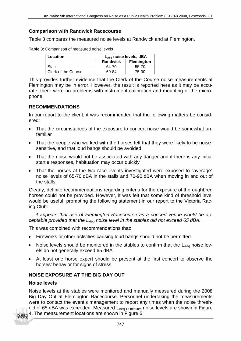
Animals: 9th International Congress on Noise as a Public Health Problem (ICBEN) 2008, Foxwoods, CT
Comparison with Randwick Racecourse Table 3 compares the measured noise levels at Randwick and at Flemington.
Table 3: Comparison of measured noise levels
LAeq noise levels, dBA Location Randwick Flemington
Stalls 64-70 55-70 Clerk of the Course 69-84 75-90
This provides further evidence that the Clerk of the Course noise measurements at Flemington may be in error. However, the result is reported here as it may be accu-rate; there were no problems with instrument calibration and mounting of the micro-phone.
RECOMMENDATIONS In our report to the client, it was recommended that the following matters be consid-ered:
• That the circumstances of the exposure to concert noise would be somewhat un-familiar
• That the people who worked with the horses felt that they were likely to be noise-sensitive, and that loud bangs should be avoided
• That the noise would not be associated with any danger and if there is any initial startle responses, habituation may occur quickly
• That the horses at the two race events investigated were exposed to “average” noise levels of 65-70 dBA in the stalls and 70-90 dBA when moving in and out of the stalls.
Clearly, definite recommendations regarding criteria for the exposure of thoroughbred horses could not be provided. However, it was felt that some kind of threshold level would be useful, prompting the following statement in our report to the Victoria Rac-ing Club: … it appears that use of Flemington Racecourse as a concert venue would be ac-ceptable provided that the LAeq noise level in the stables did not exceed 65 dBA. This was combined with recommendations that:
• Fireworks or other activities causing loud bangs should not be permitted
• Noise levels should be monitored in the stables to confirm that the LAeq noise lev-els do not generally exceed 65 dBA
• At least one horse expert should be present at the first concert to observe the horses’ behavior for signs of stress.
NOISE EXPOSURE AT THE BIG DAY OUT Noise levels Noise levels at the stables were monitored and manually measured during the 2008 Big Day Out at Flemington Racecourse. Personnel undertaking the measurements were to contact the event’s management to report any times when the noise thresh-old of 65 dBA was exceeded. Measured LAeq,15 minutes noise levels are shown in Figure 4. The measurement locations are shown in Figure 5.
747
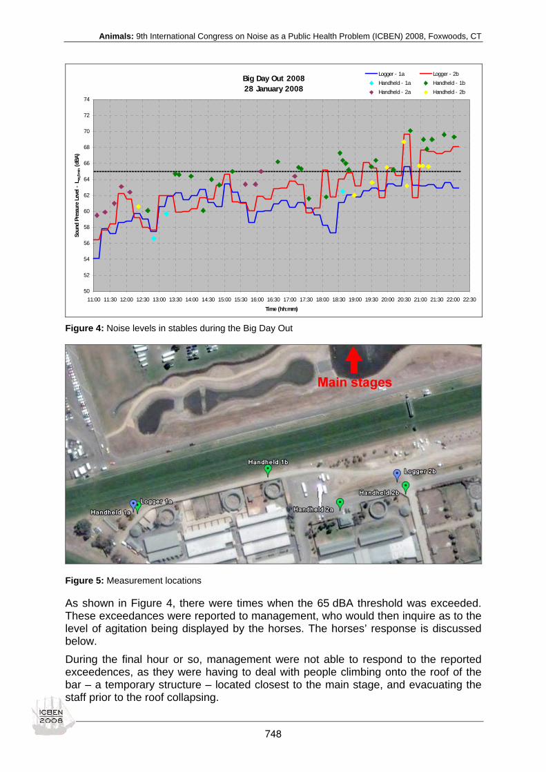
Animals: 9th International Congress on Noise as a Public Health Problem (ICBEN) 2008, Foxwoods, CT
Big Day Out 200828 January 2008
50
52
54
56
58
60
62
64
66
68
70
72
74
11:00 11:30 12:00 12:30 13:00 13:30 14:00 14:30 15:00 15:30 16:00 16:30 17:00 17:30 18:00 18:30 19:00 19:30 20:00 20:30 21:00 21:30 22:00 22:30
Time (hh:mm)
Soun
d Pr
essu
re L
evel
- L
eq,5
min (d
BA)
Logger - 1a Logger - 2bHandheld - 1a Handheld - 1bHandheld - 2a Handheld - 2b
Figure 4: Noise levels in stables during the Big Day Out
Figure 5: Measurement locations
As shown in Figure 4, there were times when the 65 dBA threshold was exceeded. These exceedances were reported to management, who would then inquire as to the level of agitation being displayed by the horses. The horses’ response is discussed below. During the final hour or so, management were not able to respond to the reported exceedences, as they were having to deal with people climbing onto the roof of the bar – a temporary structure – located closest to the main stage, and evacuating the staff prior to the roof collapsing.
748

Animals: 9th International Congress on Noise as a Public Health Problem (ICBEN) 2008, Foxwoods, CT
Horse behavior Discussions with the equine veterinarian and MDA staff indicated that the horses were aware of the music noise, but generally showed only low levels of agitation. The exceptions were:
• Two horses were stabled where they could see two of the rides – a ferris wheel and a giant slingshot ride. These horses had elevated heart rates and were not eating. The horses became noticeably calmer and began to eat when shade-cloth was used to enclose the stables so that the visual stimulation was reduced. How-ever, it was the vet’s opinion that it was not just the visual stimulation that was the problem. The horses’ state appeared to be due to a combination of the noise and the visual stimulation
• Some horses sometimes became noticeably agitated when the light-weight corru-gated steel sheeting on the enclosure walls vibrated in response to excitation by low-frequency airborne noise
• During the second last act (approximately 20:00-21:45), several of the horses re-acted to short bursts of high-pitched singing (squeals and screeches), even though these did not overly affect the LAeq,15 minutes.
The equine veterinarian’s overall opinion was that the impacts on the horses were acceptable, although there were concerns that the two horses that hardly ate may take a day or more to return to race-readiness. A recommendation has been made that, at next year’s Big Day Out, horse managers be given the option of moving horses to stables at the rear of the stabling complex where there will be no visual stimulation associated with the music noise.
CONCLUSIONS The findings of a brief literature review provided useful background, but little guid-ance on setting criteria. This is understandable given the likely significant effect of modifiers – such as visual stimulation – on the animals’ response. The most useful recommendations arising out of the review of current knowledge – that startling noises and associated visual stimulation should be avoided – were consistent with the observed response of the horses to music noise during the Big Day Out. The equine veterinarian’s recommendation to move horses to stables where there would be less visual stimulation appears to be worth implementing. Although the recommended 65 dBA LAeq criterion was somewhat arbitrary, it appears to have had value as a threshold for initiating action. However, the most effective ac-tion taken – to erect the shade-cloth to reduce visual stimulation – was done more as a response to the animals’ behavior than the measured noise level and would proba-bly have been done even if the threshold was not available as a trigger for action.
749

__________________________________________________________________________
__________________________________________________________________________
ICBEN 2008
Noise Policies: Regulations and Standards
750

Regulations: 9th International Congress on Noise as a Public Health Problem (ICBEN) 2008, Foxwoods, CT
Progress on development of noise policies from 2003-2008 Lawrence S. Finegold1*, Carl Oliva2, Jacques Lambert3 1 Finegold & So, Consultants, 1167 Bournemouth Court, Centerville, Ohio 45459 USA
2 Oliva & Co., Sociological Basic Research and Development Planning, CH-8050 Zürich-Oerlikon, Switzerland
3 INRETS-LTE (National Institute for Transport and Safety Research), 25 avenue François Mitter-rand, 69675 BRON, France
* corresponding author: e-mail: [email protected]
INTRODUCTION The purpose of ICBEN Team 9, Noise Policy is to promote and coordinate the dis-semination and utilization of scientific knowledge about the effects of noise, espe-cially as provided by the various ICBEN International Noise Teams (INTs), as scien-tific support to world-wide noise policy initiatives. These initiatives include activities intended to develop up-to-date noise policies, including noise regulations, guidelines and Standards. The ICBEN 2003 Congress was held in Rotterdam, the Netherlands, In addition to the 2003 Proceedings CD-ROM, overviews of that Congress have been published by Finegold et al. (2003) and Finegold (2004) for additional background materials. Since the last ICBEN Congress, there has been continuing progress on noise policy development around the globe, supported by the many improvements in available scientific data being reported at the current ICBEN 2008 Congress by the various ICBEN INTs. In addition, from 2003-2008 many national and international scientific conferences and workshops have provided forums for the discussion of a wide range of both noise research and noise policy topics, including progress on both noise source control (emission) and noise receiver (imission) issues. Reviews of pro-gress during the past five years on noise emission topics can readily be found in other sources, such as the web site of the Environmental Noise Program of the Euro-pean Commission (EC) at: http://ec.europa.eu/environment/noise/sources.htm, which lists the existing EC directives relating to noise sources. Because the emphasis of ICBEN is on the effects of noise, however, this paper focuses on the noise imission arena.
EUROPEAN UNION – PROGRESS SINCE PUBLICATION OF THE EC ENVIRON-MENTAL NOISE DIRECTIVE Since the publication of the European Commission Environmental Noise Directive (END) in 2002, the European Union has vigorously pursued an active research pro-gram on various environmental noise topics and continued to provide evolving guid-ance on implementation of the END. The EC Environmental Noise web site (http://ec.europa.eu/environment/noise/home.htm) provides a series of related docu-ments describing their progress. The bulk of the emphasis in the past five years has been on finalizing details of the required noise exposure modeling program for ag-glomerations (i.e., large urban areas with populations of over 100,000 people) and on development of Local Action Plans, both of which are required by the END. Since the last ICBEN Congress, the EC has also produced additional documents, mainly EC Position Papers, on various specific environmental noise policy topics such as noise metrics and indicators, noise computation methods, the economic val-uation of noise, night-time noise and sleep disturbance, environmental health indica-
751

Regulations: 9th International Congress on Noise as a Public Health Problem (ICBEN) 2008, Foxwoods, CT
tors, environmental impact assessment and public participation in this process, spa-tial information infrastructure, best practices for noise modeling, railway noise, and have continued to support technical publications on both community annoyance and sleep disturbance as these relate to noise policies. In addition, considerable effort and resources have been committed to development of the creation of a Noise Ex-pert Network, whose mission is to assist the commission in the development of its noise policy. All of these European Commission documents may be obtained from their environmental noise web sites.
THE UNITED STATES Very little progress on developing new noise policies has occurred in the past five years in the U.S., despite a strong interest in these activities within the scientific community and by the public. The best progress that can be reported has been the formation of several study groups looking at the needs and potential approaches for new national-level noise policies, continuing discussions about the appropriate metric for exposure to occupational noise, and the formation of a new study group looking at the possibilities for encouraging development of a national education and awareness program on the effects of noise and potential noise control options in communities.
JAPAN Few changes in national noise policies have likewise been seen in Japan during the past five years. The difference between Japan and the U.S. is that Japan has been involved in a rigorous and thorough reconsideration of its current environmental noise policies recently five years and significant changes are expected in the near future. For example, in the noise metrics arena, Japan is seriously considering changing from its current use of WECPNL (using the Japan version) to the use of an A-weigh-ted long-term average cumulative noise metric, such as some version of an LEQ-based metric. Their goal for this effort to update their noise policies is to develop a comprehensive, unified approach to describing exposure to environmental noise. These efforts are commended and Japan will hopefully be successful in their noise policy modernization program soon.
HONG KONG For a large, congested urban environment, the government of Hong Kong has main-tained an aggressive and comprehensive set of noise policies for some time and has made continued progress over the past five years. An overview of the Hong Kong program on noise pollution and noise control may be found at: http://www.epd.gov.hk/epd/english/environmentinhk/noise/noise_maincontent.html. Specific issues addressed by the Hong Kong government include aircraft noise, highway noise, construction noise, building codes, a noise ordinance, and urban planning. Without a strong set of national level noise policies in place, Hong Kong sets a good example for how to implement an effective and comprehensive noise pol-icy program at the local (city) level.
INTERNATIONAL INSTITUTE OF NOISE CONTROL ENGINEERING (I-INCE) Although the International Institute of Noise Control Engineering (I-INCE) does not develop noise policies such as a government body would implement, in addition to sponsoring annual international noise control Congresses, this professional organiza-tion also has a set of Technical Study Groups (TSGs) which address issues related
752

Regulations: 9th International Congress on Noise as a Public Health Problem (ICBEN) 2008, Foxwoods, CT
to noise policy development and produce highly useful summary reports. Below are two I-INCE TSGs which have been particularly active during the past five years.
INCE TSG3 – NOISE POLICIES AND REGULATIONS This I-INCE technical initiative deals with describing and assessing the effectiveness of noise policies and regulations around the world and involves a study of existing noise exposure policies and regulations in all countries which have recognized noise as a problem involving public health and welfare. To implement this study, a large-scale international survey was conducted of current noise policies in participating INCE Member Society countries and in other countries where information was avail-able from publications. The TSG3 Final Report, Survey of Legislation, Regulations, and Guidelines for Control of Community Noise, contains information from the 21 countries which responded to the set of two I-INCE questionnaires. At the present time, the Final Draft of this Report is undergoing its final review and is expected to be published in hard copy and on the I-INCE web site (http://www.i-ince.org/) later this year.
I-INCE TSG5 – GLOBAL NOISE POLICY This I-INCE Technical Study Group deals with noise as a global issue versus noise as a local issue and has been reviewing the arguments for and against consideration of Noise as a Global Policy Issue. It is expected that TSG5 will present a rationale for considering noise at the international level, based largely on the implications of how noise may become an important non-tariff trade barrier issue. The I-INCE description of the scope of the TSG5 effort, is part, is as follows: “Technical Study Group 5 shall consider a global approach to noise in order that an effective international noise control policy may be developed and implemented. “All vehicles, devices, machinery, and equipment that emit audible sound are manufac-tured products; most of these products are involved in international trade. Industrial enterprises with worldwide operations produce many products in two or more differ-ent countries. Noise emissions of such products are appropriately the subject of in-ternational agreements and regulations. Noise immissions resulting from the opera-tion of these products are growing in severity as vehicular traffic volume and the pace of industrialization continues to increase in many parts of the world. “An important aspect of the task charged to TSG 5 is to study the manner in which global policies were developed in the past and to make recommendations for improving current pro-cedures so that future policies may provide more effective control of the emission and immission of noise. The roles of international bodies, national governments and local authorities should be clearly identified and, if necessary, clarified.” To the current authors’ knowledge, the work of the TSG was completed in 2005 and the Final Report was circulated for final review and publication in 2006, although pub-lication of a final version could not be verified at the present time. Whenever it is, or was, published, however, this seminal document has the potential to provide much-needed guidance on a vital noise policy issue; namely, whether a general global noise policy can be developed. Implementation of a follow-on I-INCE Technical Study Group (TSG7) is currently being started, but no information of their progress is yet available.
753

Regulations: 9th International Congress on Noise as a Public Health Problem (ICBEN) 2008, Foxwoods, CT
INCREASING EMPHASIS ON AIRCRAFT NOISE One of the more interesting aspect of developments in noise policies globally in the past five years is the growing emphasis on aircraft noise, particularly night-time air-craft noise. In particular, sleep disturbance from night-time aircraft landings and take-offs around airports has become a topic of particular concern. Noise policies have to somehow balance the economic benefits to societies obtained when night-time air traffic is allowed with the public’s dislike of being awakened at night. At the current time, discussions are still continuing concerning the most appropriate sleep distur-bance metric, the most appropriate time frame for describing and assessing night-time noise, the best way to describe awakenings scientifically, and criteria for maxi-mum allowable awakenings. It is expected that the next five years will see new and updated noise policies in many countries, and particularly in the European Union.
WORKSHOPS (ICAO CAEP AND WHO/EUROPE) Some of the most important noise policy activities in the past several years have in-cluded a series of international workshops devoted to discussions of issues related to the development of noise policies, rather than specific new noise government policies themselves. As such, they are noise policy development support activities, rather than being government organizations which directly promulgate laws and regulations. Organizations such as the International Civil Aviation Organization (ICAO) Committee on Aviation Environmental Protection (CAEP) and the World Health Organization (WHO), which are both member organizations of the United Nations, have long had very active programs for a long period of time looking at both noise research and noise policy issues, although neither directly performs their own research. They do, however, sponsor their own study groups and committees and hold important interna-tional workshops. Several of the latter have been held during the past five years on critical noise issues, particularly those related to aviation noise impacts. For ICAO, their efforts often result in recommendations which are adopted as Standards and Recommended Practices and are incorporated, through the ICAO Council, as An-nexes to the Convention on International Civil Aviation, which was internationally de-veloped in 1944, (see: http://www.icao.int/icao/en/m_about.html for more information on ICAO). The WHO Noise Program for Europe is the only WHO effort related to noise which still remains and is located in Bonn, Germany (see: http://www.euro.who.int/Noise for more information on this program office.) In October 2007, the ICAO Committee on Aviation Environmental Protection (CAEP) held a Workshop in Montreal, Canada on “Assessing Current Scientific Knowledge, Uncertainties and Gaps Quantifying Climate Change, Noise and Air Quality Aviation Impacts”. Although the Final Report from this Workshop is still undergoing final de-velopment and review, it promises to provide excellent background scientific informa-tion relevant for future aircraft noise policies. In the meantime, several recent ICAO documents (ICAO 2004, 2006, 2007a, b) provide useful current noise policy docu-ments. Also in October 2007, the World Health Organization Regional Office for Europe held a somewhat similar Workshop in Bonn, Germany entitled “Aircraft Noise and Health: Evidence Review Meeting”. This Workshop will be covered during the ICBEN 2008 Congress. More recently, WHO/Europe also held another Workshop in Bonn, Ger-many during May 2008 entitled “Practical Guidelines for Risk Assessment of Envi-ronmental Noise”. Because this Workshop was only recently completed, no details are available at this time to describe the Final Report of this Workshop. Together, the
754
Regulations: 9th International Congress on Noise as a Public Health Problem (ICBEN) 2008, Foxwoods, CT
two WHO noise effects Workshops in 2007 and 2008 will make a quite valuable con-tribution to the development of future noise policies.
DEVELOPMENT OF NATIONAL AND INTERNATIONAL STANDARDS In addition to the development of national-level regulations, formal Standards devel-opment activities related to noise imission have also continued to evolve over the past five years, both at the national level in most developed countries and also in de-veloping countries, such as Brazil, Mexico, etc., and at the international level by or-ganizations such as the International Organization for Standardization (ISO). The most prominent and highly useful updated ISO Standard related to noise imission in the past five years has been ISO Standard 1996-1, “Acoustics — Description, meas-urement and assessment of environmental noise — Part 1: Basic quantities and as-sessment procedures”. The importance of the updated ISO Standard is that it pro-vides guidance on making Adjustments for sound source rating levels, describing and assessing high-energy impulse sounds, sounds with strong low-frequency content, annoyance caused by exposure to sound in multi-source environments, and – most importantly – predicting the estimated percentage of a population highly annoyed as a function of adjusted day/night sound levels. Although the details of these various methodologies cannot be described here because of ISO proprietary publication con-straints, all of them are very important for noise policy applications related to envi-ronmental noise impact assessments. This Standard, and other related ISO Stan-dards may be purchased from http://www.iso.org/iso/store.htm. Although they will not be covered here, the national Standards programs of many individual countries have also made considerable progress in the comprehensive-ness and adequacy of their noise Standards. Examples of just a few of these coun-tries include Brazil, Mexico and the United States.
STATUS OF NOISE POLICIES IN DEVELOPING COUNTRIES One rapidly evolving noise policy topic which has to date received inadequate atten-tion is the status of noise policies in developing countries in global areas such as Eastern Europe, Asia, South America and Africa. However, because countries in all these areas are in the process of developing “modern” technologies, including ex-panded industrial capabilities, noise in many cities in these regions of the world is quickly becoming excessive and adequate noise control policies are demonstrably lacking. This problem will only get worse in the near future. A recent Workshop during INTER-NOISE 2007 in Istanbul, Turkey was an initial attempt to begin to address this issue. During this Workshop, considerable agreement was easily reached concerning the importance of this growing problem and representatives of various “developing” countries agreed to work together in the future. What is needed now is for interna-tional organizations, such as the World Health Organization under the United Nations charter and others, to adopt this topic as a special focus item for future study groups. Much of the world’s population lives in “developing” countries and more attention needs to be given to their needs. One special topic within this general area concerns whether or not noise policy approaches being adopted in most “developed” countries and being considered for a Global Noise Policy are appropriate, affordable and tech-nically feasible for the “developing” countries. Obviously, much more work is needed in this area.
755

Regulations: 9th International Congress on Noise as a Public Health Problem (ICBEN) 2008, Foxwoods, CT
CONCLUSIONS Considerable effort has been expended by a great many people and through various organizations related to the development of noise policies between 2003-2008, since the last ICBEN Congress. In many countries and internationally there has been a good amount of progress has been made in the three relevant areas of noise regula-tions and laws, noise exposure guidelines, and noise Standards. As with the previous five-year period, the bulk of the progress still resides within the European Union, as represented by the European Commission. However, example are found for progress at the national level by many non-EU countries and internationally by many noise policy support organizations such as ICAO CAEP, WHO and I-INCE.
REFERENCES Finegold LS (2004). The effects of noise on public health: International congress explores global impact. Published by American Speech, Language and Hearing Association (ASHA): The ASHA Leader 13: 6-7.
Finegold LS, Job S, de Jong R, Griefahn B (2003). Overview of ICBEN 2003 Congress - Rotterdam, the Netherlands (2003). Special invited paper published in: Proceedings of INTER-NOISE 2003. The 32nd International Congress and Exposition on Noise Control Engineering (CD-ROM), 25-28 August, 2003, Seogwipo, Jeju Island, Korea. Abstract Book (p 50).
ICAO (2004). Appendix A: Resolution A35-5 “Consolidated statement of continuing ICAO policies and practices related to environmental protection”. ICAO, Montreal.
ICAO (2006). Keynote address by the President of the Council of ICAO, Singapore, December 2006 (see: www.icao.org).
ICAO (2007a). Update for “Recommended method for computing noise contours around airports” (ICAO Circular 205). ICAO, Montreal. (http://www.tc.gc.ca/civilaviation/International/ICAO/committee/pdf/working/Jan-22-07/CAEP7_WP22.pdf).
ICAO (2007b). Update for “Guidance on the balanced approach to aircraft noise management” (ICAO Document 9829, 1998). ICAO, Montreal. http://www.tc.gc.ca/civilaviation/International/ICAO/committee/pdf/working/Jan-22-07/CAEP7_WP17. pdf.
756

Regulations: 9th International Congress on Noise as a Public Health Problem (ICBEN) 2008, Foxwoods, CT
Overview of the World Health Organization Workshop on Aircraft Noise and Health Birgitta Berglund1*, Stephen Stansfeld2, Rokho Kim3 1 Department of Psychology, Stockholm University,SE-106 91 Stockholm, Sweden
2 Centre for Psychiatry, Barts and the London School of Medicine, London, United Kingdom
3 WHO/EURO Centre for Environment and Health, Hermann-Ehlers-Str. 10, 53113 Bonn, Germany
*corresponding author: e-mail: [email protected]
INTRODUCTION A workshop was convened by the WHO Centre for Environment and Health to exam-ine the evidence for the effects of aircraft noise exposure on physical and mental health in Bonn on October 11-12th 2007. A working group of experts on noise and health was asked to prepare draft chapters which were rigorously reviewed and dis-cussed at the meeting. The health topics, based on previous WHO projects, included annoyance, sleep, cardiovascular health, physiological (stress hormone) effects, ef-fects on cognition and mental health. Papers on exposure assessment and risk man-agement were also prepared. The workshop included experts from Europe, North America, Australia and Japan as well as representatives from the International Civil Aviation Organization (ICAO). The objective was to produce a WHO document ‘Evi-dence Review on Aircraft Noise and Health’ based on a systematic review of the sci-entific literature.
METHODS The working group was expected to apply the method of ‘health hazard identification’ to the issue of aircraft noise. Authors used systematic review techniques to assess the peer reviewed published literature on noise and health. Peer reviewed literature was supplemented by reports from significant studies and conference proceedings. When the published literature is limited, authors adopted narrative review of the available evidence. Each chapter was expected to follow a standard format, describ-ing the review protocol, search strategy and identification of relevant studies. Sys-tematic assessment of study validity included evidence for causal associations, char-acteristics of exposure-response associations, and discussion of whether the results could be explained by chance or bias such as confounding. For health topics where sufficient evidence was available, meta-analyses were carried out. Conclusions were drawn up taking account of high quality studies with the key results expressed in ta-bles.
RESULTS The results from each chapter were summarized as follows.
Annoyance Annoyance has been described as a feeling of displeasure associated with any agent or condition, known or believed by an individual or group to adversely affect them. This chapter focussed on meta-analyses by Miedema & Vos (1998), Finegold & Finegold (2002), Fidell & Silvati (2004), and van Kempen & van Kamp (2005), who provide comparable exposure-response relationships for aircraft noise. The relation-
757
Regulations: 9th International Congress on Noise as a Public Health Problem (ICBEN) 2008, Foxwoods, CT
ship shows a non-linear increase of the percentage of highly annoyed people with increased noise levels. However, they differ with respect to the degree of scatter, and with respect to the location of the maximum scatter. Today there are many more aircraft movements at civil airports, individual aircraft have become less noisy at the same engine power, although the mean engine power has increased. Although the trade-off between the levels of overflights in energy equivalent noise metrics like DNL proved to be approximately correct for the predic-tion of noise annoyance in a study around Amsterdam/Schiphol airport, it is plausible that several acoustic features that are not reflected in DNL level influence annoy-ance. There is evidence for an increasing trend of average annoyance responses over time (van Kempen & van Kamp 2005). That is, more recently, residents living near modern airports show more aircraft noise annoyance than in former times. One explanation for this trend may be that residents near modern airports are often sub-jected to large changes in noise exposure. The reviews do not distinguish between “low-rate changing” and “high-rate changing” airports, and there is evidence that noise situations changing at a high rate, espe-cially the mere expectation of an increase of aircraft movements in the near future, increases the degree of residential noise annoyance. Increased ambient road traffic near airports, population characteristics, changes in study design or response rate may also contribute to increased annoyance. Residents living near airports tend to say that “aircraft noise is getting louder” even when the LAeq or DNL goes down (Fi-dell et al. 1998). This may be because: (a) residents react to the increased number of aircraft movements, (b) residents react to the increase of the background noise levels due to the increased number of aircraft cruising in the vicinity of the airport at the same time. Several authors conclude that the energy-approach to the aircraft noise description puts too little weight to the increased number of movements (MVA Con-sultancy 2007). MVA Consultancy (2007) suggests in the final ANASE report that giving the number of aircraft movements a weighting more akin to NNI (i.e. 15) rather than 10 might be more appropriate for predicting annoyance from aircraft noise. The combination of expectancy effect and increased annoyance for a certain time period after the change is called “overshoot reaction”, because residents in high-rate change situations are considerably more annoyed than in low-rate change situations at comparable noise levels. After several years, the elevated annoyance tends to re-turn to levels expected from low-rate change situations (Breugelmans et al. 2007). The recent Schiphol longitudinal studies demonstrate that at all noise levels, the per-centages of highly annoyed residents is considerably higher than expected from es-tablished dose-response relationships, in anticipation of and even two years after the abrupt change.
Sleep This chapter focused on aspects of aircraft noise and sleep disturbance less exten-sively covered in the WHO European Night Noise Guidelines. There are many meth-odological issues in the measurement of sleep disturbance: polysomnography, re-mains the gold standard for measuring sleep. This method however is cumbersome and resource intensive and many studies have to rely on less reliable methods. EEG awakenings are probably the clearest indication of sleep disturbance.
758

Regulations: 9th International Congress on Noise as a Public Health Problem (ICBEN) 2008, Foxwoods, CT
Figure 1: Dose-response relationships between indoor maximum sound pressure level LA,max and the reaction of the sleeper. For “FICAN 1997”, “Finegold & Elias 2002” and “Passchier-Vermeer 2003”, SEL was converted to LA,max by subtracting 16.4 from the respective indoor SEL value and then divi-ding by 0.877.
All five dose-response curves show monotonously increasing reaction probabilities with simultaneously increasing LA,max. The dose-response curve for behavioral addi-tional awakening derived by Passchier-Vermeer predicts considerably fewer behav-ioral awakenings at the same LA,max compared to the FICAN and Finegold & Elias curves, most likely for two reasons. First, the FICAN curve predicts the maximum, not the average, percent of the exposed population expected to be behaviorally awak-ened. Second, the FICAN and the Finegold & Elias curves seem to include sponta-neous behavioral awakenings, whereas the Passchier-Vermeer curve concerns be-havioral awakenings additional to spontaneous awakenings. Dose-response curves are usually based on the average response in the investi-gated population. If protection concepts are based on this average response, the pro-tection will necessarily be too high for some and too low for other parts of the popula-tion. In order to ensure that all relevant parts of the population are well enough pro-tected, preventive measures can be taken, such as artificially elevating the dose-response curve or setting lower limit values than necessary (based on the average reaction in the population).
Cardiovascular effects Epidemiological studies or surveys directly related to associations between aircraft noise and cardiovascular disease (CVD) outcomes were reported distinguishing be-tween adults and children. Clinical manifestations of cardiovascular diseases are not very likely in young people. Therefore blood pressure is the major outcome that has been studied in children and adolescents. In adults, however, manifestations of high blood pressure (hypertension) and ischemic heart disease (myocardial infarction, an-
759

Regulations: 9th International Congress on Noise as a Public Health Problem (ICBEN) 2008, Foxwoods, CT
gina pectoris, ischemic signs in the ECG, heart failure) are major outcomes of inter-est. 61 epidemiological studies addressed the association between transportation noise and cardiovascular endpoints; 20 on commercial aircraft noise, 8 military aircraft noise. Repeated studies carried out around Schiphol airport revealed higher relative risks of cardiovascular medication ranging between 1.2 and 1.4 for a noise level dif-ference of approximately 10 dB(A). In the most recent phase of the Schiphol envi-ronment and health monitoring program a higher risk of approximately 1.8 was found for the same noise level difference. A recent cross-sectional study carried out around Cologne airport in Germany demonstrated higher individual prescriptions of anti-hypertensive and cardiac drugs in subjects exposed to high levels of aircraft noise, particularly, during the night and the early morning hours (3-5 hrs). Preliminary re-sults from a Swedish follow-up study carried out around Stockholm's airport suggest more use of antihypertensive medication in subjects exposed to noise levels ('FBN') of more than 55 dB(A) compared to less exposed (relative risk 1.6). In the later studies, no noise effects were found with respect to hospital admissions for cardiovascular disease. However, a statistically significant effect of Lden was found on self-reported hypertension. When the noise level increased by 3 dB(A) the odds ratio was 1.2, which corresponds with a relative risk of approximately 1.8 for a 10 dB(A) difference in noise level, confirming earlier studies. In a new multi-centre study carried out around six European airports a significant increase in the risk of hyperten-sion of 1.1 (95 % CI = 1.0-1.3) for a 10 dB(A) difference of aircraft noise during the night (Lnight) was found (Järup et al, 2007). Around Stockholm’s Arlanda airport an exposure-response association between aircraft noise and high blood pressure was found with relative risks ranging between 1.1 and 2.1 for noise levels between ap-proximately 'FBN' = 53 to 63 dB(A) (Rosenlund et al. 2001). In the single prospective study around this airport subjects exposed to weighted energy-averaged levels ('FBN') above 50 dB(A) had a significant relative risk of 1.2 for the development of hypertension over the 10-year follow-up period compared with less exposed (Erik-sson et al. 2007). The increase in risk per 10 dB(A) was 1.2 (95 % CI = 1.0-1.2). Meta-analysis of the HYENA, Stockholm, Okinawa and Amsterdam studies showed a pooled fixed effect estimate of 1.13 (95 %CI 1.06-1.20). Studies in children from Los Angeles and Munich found elevated systolic blood pressure in relation to aircraft noise, although these have not consistently confirmed by the recent RANCH Study (van Kempen et al. 2006). Overall, recently published powerful epidemiological stud-ies indicate that aircraft noise exposure around airports increases the risk of elevated blood pressure.
Stress hormone effects This chapter reviewed the evidence on aircraft noise exposure and hormonal re-sponses including adrenaline, noradrenaline and cortisol. A search on aircraft noise and various hormonal outcomes yielded 14 citations in Pubmed and 2 in PSYCinfo; these were supplemented by conference papers and reports. Among the five studies in children levels of adrenaline and noradrenaline were raised in both the cross sec-tional and longitudinal reports from the Munich Study in relation to aircraft noise ex-posure and increases in aircraft noise exposure around the newly opened Munich airport (Evans et al. 1998). By contrast urinary catecholamines were not raised in the larger noise exposed sample from the West London Schools Study (Haines et al. 2001). All the studies consistently showed no relationship between aircraft noise ex-posure and urinary cortisol. In eight adult studies four showed increased levels of
760

Regulations: 9th International Congress on Noise as a Public Health Problem (ICBEN) 2008, Foxwoods, CT
cortisol and two studies showed increased levels of catecholamines. Three experi-mental studies showed no increase in catecholamines and another field study showed no increase in relation to cortisol. A report from the German Aerospace Cen-ter (Maass & Basner 2003) found no effects of aircraft noise intensity or frequency on either free cortisol or catecholamines in parallel laboratory and field studies.
Mental health PSYCinfo yielded 4 studies on aircraft noise and mental disorders and Pubmed 57 articles on aircraft noise and mental disorders. Early studies of psychiatric hospital admissions around Heathrow airport show no convincing associations between air-craft noise exposure and admission to hospital. Community studies of aircraft noise suggest some association between aircraft noise exposure and acute symptoms of waking in the night, irritability, depression, difficulty getting to sleep, swollen ankles, burns, cuts, minor accidents and skin troubles. Aircraft noise exposure is associated with higher scores on a screening questionnaire for anxiety and depression in highly educated and professional groups but not in the general population. Franssen’s study around Schiphol Airport suggests an association between noise and non-prescribed sleep medication but no association with prescribed antidepressants and sedatives (Franssen et al. 2004). Japanese studies find that high levels of military aircraft noise are associated with depressive and anxiety symptoms but there are issues with the length of interval between assessment of noise exposure and depressive and anxiety symptoms. Using a standardised structured psychiatric interview Hardoy et al.’s (2005) study in Sardinia found an association between aircraft noise exposure and anxiety disorders. In contrast, van Kamp et al in a methodologically superior longitu-dinal panel study reported at Internoise 2007 found no relationship between change in aircraft noise exposure and mental health measured by screening questionnaire. The Munich Study (Evans et al. 1998) has shown that aircraft noise exposure is as-sociated with decreased quality of life both cross-sectionally and longitudinally. How-ever, more formal measures of anxiety and depression and parent assessed emo-tional and conduct disorders were not found to be related to aircraft noise in further studies (Haines et al. 2001; Stansfeld et al. 2005). Overall, there is reasonable evi-dence that noise impairs quality of life in children but does not cause more serious mental health problems.
Cognitive effects in children Aircraft noise exposure has been related to the fraction of students reading below grade level in schools around New York and in two elementary schools chronic air-craft noise exposure (65 dB LAeq) was associated with impairment of reading and speech perception. Around Heathrow Airport chronic aircraft noise exposure was as-sociated with poorer reading comprehension measured by standardized scales with adjustments for age, deprivation and main language spoken (Haines et al. 2001). In a further study of 451 children noise exposure was associated with impaired reading on difficult items, after adjustment for age, main language spoken and household depri-vation. High levels of noise exposure were not associated with impairments in mean reading score, memory and attention or stress responses. In the Munich airport study (Hygge et al. 2002) long–term memory and reading were impaired in the noise group at the new airport and improved in the formerly noise–exposed group at the old air-port. Short–term memory also improved in the latter group after the old airport was closed. At the new airport, speech perception was impaired in the newly noise–exposed group. Mediational analyses suggest that poorer reading was not mediated by speech perception, and that impaired recall was in part mediated by reading. In
761

Regulations: 9th International Congress on Noise as a Public Health Problem (ICBEN) 2008, Foxwoods, CT
the cross-national RANCH Study there was a linear exposure-effect associations be-tween exposure to chronic aircraft noise and impairment of reading comprehension (p=0·0097) and recognition memory (p=0·0141) maintained after adjustment for mother's education, socioeconomic status, longstanding illness, and extent of class-room insulation against noise (Stansfeld et al. 2005).
CONCLUSIONS Overall, despite a limited number of studies in some areas there is good evidence for exposure–response associations between aircraft noise and annoyance, sleep dis-turbance, high blood pressure, and children’s cognitive impairment. Evidence for the association with mental health and hormonal responses is limited. An important issue is the need for an accurate and reliable exposure assessment of aircraft noise rele-vant to the respective health outcomes. Conclusions on each topic are summarised below. Annoyance: Exposure-response relationships have been established predicting the percentages of people expressing annoyance given a certain level of noise exposure. Results of more recent studies show annoyance reactions to aircraft noise that are much higher than expected from the earlier established exposure-response curves. Research into the possible causes for the observed increase in annoyance is still continuing, but part of it may be due to the fact that many recent noise annoyance studies took place in airport situations with an increased rate of change, especially with respect to the number of aircraft movements. Thus, established exposure-response curves to predict annoyance reactions should be used with caution in changing noise situations. Sleep: Five dose-response curves show monotonously increasing reaction probabili-ties with simultaneously increasing aircraft LA,max in which behavioural awakenings, EEG measures and motility were the sleep outcomes. Laboratory studies consistently show stronger effects of noise exposure than field studies but field studies have greater ecological validity. Lnight is probably the most practical index for night time noise regulation as it is espoused by the European Noise Directive although energy-averaged measures do not take full account of impact of individual noise events on sleep disturbance. Cardiovascular Disease: There is sufficient evidence for a positive relationship be-tween aircraft noise and high blood pressure and the use of cardiovascular medica-tion. However, no single common exposure-response relationship or possible effect thresholds could be established for the association between aircraft noise and car-diovascular risk due to methodological differences between studies and the lack of continuous or semi-continuous (multi-categorical) noise data. There is some indica-tion of a stronger association between night time noise level and hypertension. Stress hormone responses: There is some consistent evidence that aircraft noise exposure in children is associated with raised levels of catecholamines but not corti-sol although there is a need for more studies to replicate these results. The associa-tions between aircraft noise levels and hormone responses in adults are unclear. Mental health: There is some evidence that aircraft noise is related to symptoms of common mental disorder such as depression or anxiety rather than more serious mental disorder but in general the results of these studies are inconsistent. Overall, there is reasonable evidence that noise impairs quality of life in children but does not cause more serious mental health problems.
762
Regulations: 9th International Congress on Noise as a Public Health Problem (ICBEN) 2008, Foxwoods, CT
Cognitive impairment: Aircraft noise has detrimental effects on learning, memory and reading in children. This conclusion is further strengthened by noting that more than twenty studies have shown detrimental effects of noise on children's reading and memory, and there is no study to the contrary. But even though a significant cause-effect relationship is established, it is still unclear how much impairment and at which noise level the impairing effects begin. Experimental noise studies demon-strate that acute (aircraft) noise exposure is a sufficient and efficient short term cause of impaired memory. Noise management: Successful noise management should be based on the funda-mental principles of precaution, the polluter pays and prevention. An integrated noise policy should include several control procedures: measures to limit the noise at the source, noise control within the sound transmission path, protection at the receiver’s site, land-use planning, education and raising of public awareness. With careful plan-ning, exposure to noise can be avoided or reduced. A sufficient distance between residential areas and an airport will make noise exposure minimal. Additional insula-tion of houses can help to reduce noise exposure from airports. For new buildings, standards or building codes should describe the position of houses and the ground plan of houses with respect to over-flight paths and also the required sound insula-tion of the façades. Unless legal constraints in a country proscribe a particular option, the evaluation of control options must take into account technical, financial, social, health and environmental factors, as well as the speed with which they can be im-plemented, and their enforceability. Environmental Noise Impact Assessment (ENIA) process is one of the major tools available for managing the risks associated with exposure to aircraft noise, in affected communities. The aim of this process is to pro-vide environmental protection for a planned project by foreseeing and preventing en-vironmental noise problems. Acknowledgements: We acknowledge the contribution of chapter authors: Wolf-gang Babisch, Matthias Basner, Martin van den Berg, Bernard Berry, Larry Finegold, Truls Gjestland, Barbara Griefahn, Rainer Guski, Staffan Hygge, Sabine Janssen, Irene van Kamp, Christian Maschke, Dieter Schwela, Stephen Stansfeld.
REFERENCES Breugelmans O, Houthuijs D, Kamp I, Stellato R, Wiechen C, Doornbos G (2007). Longitudinal effects of a sudden change in aircraft noise exposure on annoyance and sleep disturbance around Amsterdam airport. In: Proceedings of the 19th Interna-tional Congress on Acoustics (ICA 2007), Paper env-04-002. Madrid, Spain.
Eriksson C, Rosenlund M, Pershagen G, Hilding A, Östenson C-G, Bluhm G (2007). Aircraft noise and incidence of hyper-tension. Epidemiology 18: 716-721.
Evans GW, Bullinger M, Hygge S (1998). Chronic noise exposure and physiological response: a prospective study of chil-dren living under environmental stress. Psychol Sci 9: 75-77.
FICAN, Federal Interagency Committee on Aviation Noise (1997). Effects of aviation noise on awakenings from sleep.
Fidell S, Silvati L (2004). Parsimonious alternative to regression analysis for characterizing prevalence rates of aircraft noise annoyance. Noise Contr Eng J 5: 56-68.
Fidell S, Silvati L, Pearsons K (1998). Noticeability of a decrease in aircraft noise. Noise Contr Eng J 46: 49-56.
Finegold LS, Elias B (2002). A predictive model of noise induced awakenings from transportation noise sources. In: Proceed-ings of the 2002 International Congress and Exposition on Noise Control Engineering. Dearborn.
Finegold LS, Finegold MS (2002). Development of exposure-response relationships between transportation noise and com-munity annoyance. Internet-Symposium Noise Annoyance, Stress and Health Effects, http://www.netsympo.com
Franssen EA, van Wiechen CM, Nagelkerke NJ, Lebret E (2004). Aircraft noise around a large international airport and its impact on health and medication use. Occup Environ Med 61: 405-413.
763

Regulations: 9th International Congress on Noise as a Public Health Problem (ICBEN) 2008, Foxwoods, CT
Haines MM, Stansfeld SA, Brentnall S, Head J, Berry B, Jiggins M, Hygge S (2001). The West London Schools Study: the effects of chronic aircraft noise exposure on child health. Psychol Med 31: 1385-1396.
Hardoy MC, Carta MG, Marci AR, Carbone F, Cadeddu M, Kovess V, Dell'Osso L, Carpiniello B (2005). Exposure to aircraft noise and risk of psychiatric disorders: the Elmas survey-aircraft noise and psychiatric disorders. Soc Psychiatry Psychiatr Epidemiol 40: 24-26.
Hygge S, Evans GW, Bullinger M (2002). A prospective study of some effects of aircraft noise on cognitive performance in school children. Psychol Sci 13: 469-474.
Jarup L, Babisch W, Houthuijs D, Pershagen G, Katsouyanni K, Cadum E, Dudley M, Savigny P, Seiffert I, Swart W, Breugelmans O, Bluhm G, Selander J, Charalampidis AS, Dimakopoulou K, Sourtzi P, Velonakis M, Vigna-Taglianti F (2007). Hypertension and exposure to noise near airports - the HYENA study. Environ Health Perspect 113: 1473-1478.
Maass H, Basner M (2003). Effects of nocturnal aircraft noise, Vol. 3: Stress hormones. DLR-Forschungbericht 2004-09/E.
Miedema HME, Vos H. (1998). Exposure-response relationships for transportation noise. J Acoust Soc Am 104: 3432-3445.
MVA Consultancy (2007). Attitudes to noise from aviation sources in England (ANASE). MVA Project Number C34351. Woking, UK. http://www.mvaconsultancy.com
Passchier-Vermeer W (2003). Night-time noise events and awakening. TNO Inro report 2003-32. Delft, The Netherlands.
Rosenlund M, Berglind N, Pershagen G, Järup L, Bluhm G (2001). Increased prevalence of hypertension in a population exposed to aircraft noise. Occup Environ Med 58: 769-773.
Stansfeld SA, Berglund B, Clark C, Lopez-Barrio I, Fischer P, Öhrström E, Haines MM, Head J, Hygge S, van Kamp I, Berry BF (2005). Aircraft and road traffic noise and children’s cognition and health: a cross-national study. Lancet 365: 1942-1949.
van Kempen EEMM, van Kamp I (2005). Annoyance from air traffic noise. Possible trends in exposure-response relation-ships. Report 01/2005 MGO EvK, Reference 00265/2005. RIVM: Bilthoven (NL).
van Kempen E, van Kamp I, Fischer P, Davies H, Houthuijs D, Stellato R, Clark C, Stansfeld S (2006). Noise exposure and children's blood pressure and heart rate: the RANCH-project. Occup Environ Med 63: 632-639.
764

Regulations: 9th International Congress on Noise as a Public Health Problem (ICBEN) 2008, Foxwoods, CT
Airport noise policies in Europe: The contribution of human sciences research Michel Vallet Institute AEDIFICE, 59 Avenue Lacassagne 69 003 Lyon, France
corresponding author: e-mail: [email protected]
ABSTRACT Airport noise control regulations In Europe mainly consist into two Directives from the European Commission (EC) entered into force in 2002. The first one is EC D2002/30, which is specifically dedicated to Air Traffic Noise (ATN) and is inspired by the “Bal-anced Approach” adopted by ICAO for aircraft noise control worldwide. The second regulation is EC D2002/49, which deals with general environmental noise. These policies are required to be implemented between 5 and 7 years after their promulga-tion. In order to prepare a possible evolution in EC D 2002/30 and EC D 2002/49, the EU Commission has invited stakeholders from all bodies interested in noise airport poli-cies to participate to a working group (Working Group Airport Noise; WG-AN). Among various items which will be considered for possible modification or to be made more precise, the key points to be addressed concern the psychological and biological effects of aircraft noise on exposed populations, the noise indicators to be used in the future and exposure criteria levels. Experts have been invited to present their views on relevant topics, such as the proper philosophy to adopt and specify suggestions for the "Night Noise Guidelines" report from WHO, the EU RANCH pro-ject, and the role of holding a dialogue with airport neighbors concerning the expres-sion of community annoyance. This paper will present an overview of the critical issues under consideration, how new research data might be used in future aircraft noise policies, and the current comments from EU WG-AN experts and non specialist members.
Background on noise exposure around airports During last decades noise around airports has been gradually changing from that produced by a relatively small number of loud aircraft over flight events to a larger number of quieter events. The transition period from louder jets to the quieter (high by-pass engine) jets led to significant reduction in exposures around most airports that served commercial jet traffic. However, continued increases in passengers and in jet operations means that, rather than diminishing, noise exposure has begun to increase. Due to a general public sensitivity to aircraft noise and to concern about the effects of these exposures on the population, a large variety of efforts have been implemented to address noise issues at large airports around the world. These noise control and mitigation efforts have been implemented under the guidance of ICAO, national gov-ernment agencies, airports operators, local authorities and aircraft manufacturers. The situation of people exposed to noise around airports, as assessed by the most recent studies (ICAO 2007, EC 2008) show that:
765

Regulations: 9th International Congress on Noise as a Public Health Problem (ICBEN) 2008, Foxwoods, CT
• A significant reduction in exposure to aircraft noise has been achieved by the ICAO ban of the more noisy Chapter II aircraft in April 2002 and addi-tional decrease in noise at the source is expected from the present restric-tions of the ICAO Chapter III requirements. New discussions are now un-derway for consideration of additional Chapter IV restrictions, but this pos-sible policy change has not been adopted yet.
• Aircraft traffic is globally increasing by about 5 % a year for 2000-2005 (6.11 % for 2002-2005), although this estimate varies locally and regionally with the period of the day, the individual airport, and the geographic region internationally.
• Night traffic is increasing more rapidly than traffic during the day, especially for heavy aircraft and long range lines which increases night-time levels of noise, even though night traffic is restricted at some airports and more re-strictions on night traffic are being considered for the future. In Europe, be-tween 2002 and 2005, people exposed at 45Lnight have increased of 10 % (EC 2008).
A detailed assessment of people exposed to noise around airports in 2006, has been established by the EU report (MPD 2007) Data are roughly corresponding to the pre-dicted amount by ANOTEC study (2003) mean value of the baseline scenario # 1 % increase, with variation within airports : 25% have an increasing around 0,5 %, others at 2-3 % and others at 4 % by year. In 2006, the estimation of people exposed to Lden 55dBA and Lnight 45 dBA is given by the MPD Report: In 2002, 2.2 millions were exposed within Lden 55, and 2.7 within Lnight 45 In 2006 , 2.2 millions are exposed within Lden 55, and 3.0 within Lnight 45 The number of people exposed at night has increased by 10% (0.3 M) between 2002 and 2006. According the various scenarios of prevision in the MPD report, the population within 55Lden shall reach 2.3-2.4 Millions in 2010 and 2.6-2.7 in 2015. At night 3.1- 3.2 Millions within Ln, in 2010, and 3.1-3.2 in 2015. In conclusion EU-DGTREN (2008) reports that:
- More generally, the number of people affected by noise, particularly at night, has increased since the Directive came in force, due to a general increase in the number of movements, in spite of the possibility to introduce partial restric-tions.
- Our prediction is that the number of people affected by noise will continue to grow although the situation may differ between airports.
- For that reason the Commission intends to examine ways of clarifying the pro-visions of the Directive 2002/30 EC and its scope.
These conclusions invite to focus an analysis on noise at night.
766

Regulations: 9th International Congress on Noise as a Public Health Problem (ICBEN) 2008, Foxwoods, CT
Airport noise at night: metrics and criterion The metrics DNL and Lden continue to be used, but an informative supplemental metrics has to be defined and made available for states’ use, as deemed appropriate. Supplemental metrics can serve either as the only way to identify certain effects, such as the relationship between night-time noise events and sleep disturbance, or as informative to decision-makers and the public. Supplemental metrics deemed use-ful include Sound Exposure level (SEL), L(A)max and number of events. Other pos-sible metrics include: Number Above Threshold (NAT) at night, and Time Above a threshold level (TA). Meta analyses have been presented on the early 2000 years by Finegold and Elias (2002) and by Passchier-Vermeer (2003) as curves Noise indoor levels x percent of awakenings.
Figure 1: from Finegold 2008 (*Basner et al. (2006) data added)
New research data and new considerations have been presented on noise airport at night. Experimental results from Basner et al. in Germany (2006) and from Griefahn and Marks (2006) in Germany, too, are useful to confirm the need for a complemen-tary metric to the existing ones. Thoughts from the World Health Organisation (Night Noise Guidelines), from Miller (2007), Michaud et al. (2007) and Finegold (2008) are providing elements about metrics and criterion to be adopted as to progress in poli-cies In the study by Basner et al. (2006), 10,658 aircraft noise events (ANE) are consid-ered, occurring on a background level of 27 dBA Leq; short awakenings begin to arise at ANE 33dBA Lmax indoor: 2/000 awakenings occur in the same time of a noise, and 10 % at 40 dBA Lmax. Awakenings are longer when Lmax is exceeding 70dBA. Calculations have been performed as to assess the number and levels of
767

Regulations: 9th International Congress on Noise as a Public Health Problem (ICBEN) 2008, Foxwoods, CT
ANE to provoke “an awakening more per night” 58 ANE of 42 dBA Lmax are neces-sary to provoke this new awakening, 20 ANE at 57 dBA, and so on. In a laboratory study, Griefahn and Marks (2006) observed the sleep of young sub-jects during 4 nights, as to compare the effects of aircraft, trains and road vehicles; Leq levels are 39 and 50 dBA, and individual noises Lmax are 50-62 dBA for 262 cars,58-62 for 196 aircraft and 62-74 for 172 trains, in order to get the same Leq level. Train noises are more disruptive than aircraft and car noises. This highlights once again the influence of the Lmax level on awakenings. Another result is new in this research, that is dealing with a modification of the structure of the sleep WHO Europe is willing to propose strict Night Noise Guidelines (2007) and to precise the noise limit levels. The ad hoc Working Group, with experts from various areas (physiology, pathology of sleep, noise, sleep troubles in children), has been built. A synthesis by Muzet has begun to recommend the noise levels inside the bedrooms: a proposal of a peak of 42 dBA, as well as to take into account the number of noise events during the whole night; no number has been suggested at the moment. It can be observed that this recommendation is more severe than the previous one from the same organism, in 1995, that was 45 dBA. Vallet and Vernet (1991) concluded that increasing the number of noises at night would increase the probability of being awakened and that if this number is increasing, it is necessary to reduce the individ-ual noise levels, according the Griefahn model (Griefahn 1992). Analysing the effects of nocturnal aircraft noises around Paris-Charles-de-Gaulle airport, it was reported that in order to avoid 90 % of the awakenings there should be no more than 15 to 20 noises per night, with a maximum individual event level of 48 dBA (Lmax). This statement can be translated into a metric like NAT (Number of Noise Above Thresh-old) suggested by Southgate et al. (2001), here N is 15-20 and T is 45 dBA indoor. Michaud et al. (2007) have analyzed field studies carried out between 1990 and 2003; they pointed out that “sleep disturbance of night time aircraft noise are not dra-matic on the per-event basis” and that “linkages between outdoor aircraft noise expo-sure and sleep disturbance are tenuous”. To counter balance these conclusions, it can be reminded that complaints against aircraft noise are expressed in relationship with night noise (Hume et al. 2002) and that to live nearby an airport is a reason for increased sleep pills consumption (Greiser et al. 2007) and a trend in higher Arterial tension (Jarup et al. 2007). Anderson and Miller (2007) have observed that as a conclusion of most studies on sleep disturbance by aircraft noise is expressed as an “average person’s exposure to single aircraft events”. They propose a method to precise “what percent of a compos-ite population (all sensitivities) would likely to be awakened by a full night of single events” Sophisticated statistical analyses have been performed. One of the result, among others, consists in to show “that awakening depends upon time of night”: at the 8th hour the probability of awakening is increasing by 20%. These recent results confirm the interest of complementary noise metrics, for non continuous traffic, and for night disturbance. When locally promulgated, such policies are under control of noise monitoring sys-tems, airport by airport, and also a source of information for people living around air-port.
768
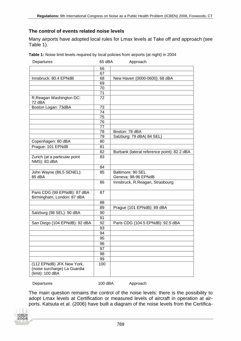
Regulations: 9th International Congress on Noise as a Public Health Problem (ICBEN) 2008, Foxwoods, CT
The control of events related noise levels Many airports have adopted local rules for Lmax levels at Take off and approach (see Table 1).
Table 1: Noise limit levels required by local policies from airports (at night) in 2004
Departures 65 dBA Approach
Departures 100 dBA Approach The main question remains the control of the noise levels: there is the possibility to adopt Lmax levels at Certification or measured levels of aircraft in operation at air-ports. Katsuta et al. (2006) have built a diagram of the noise levels from the Certifica-
66 67 Innsbruck: 80.4 EPNdB 68 New Haven (0000-0600): 68 dBA 69 70 71 R.Reagan Washington DC: 72 dBA
72
Boston Logan: 73dBA 73 74 75 76 77 78 Boston: 78 dBA 79 Salzburg: 79 dBA( 84 SEL) Copenhagen: 80 dBA 80 Prague: 101 EPNdB 81 82 Burbank (lateral reference point): 82.2 dBA Zurich (at a particular point NMS): 83 dBA
83
84 John Wayne (86,5 SENEL): 85 dBA
85 Baltimore: 90 SEL Geneva: 98-96 EPNdB
86 Innsbruck, R.Reagan, Strasbourg
Paris CDG (99 EPNdB): 87 dBA Birmingham, London: 87 dBA
87
88 89 Prague (101 EPNdB): 89 dBA Salzburg (98 SEL): 90 dBA 90 91 San Diego (104 EPNdB): 92 dBA 92 Paris CDG (104.5 EPNdB): 92.5 dBA 93 94 95 96 97 98 99 (112 EPNdB) JFK New York, (noise surcharge) La Guardia (limit): 100 dBA
100
769
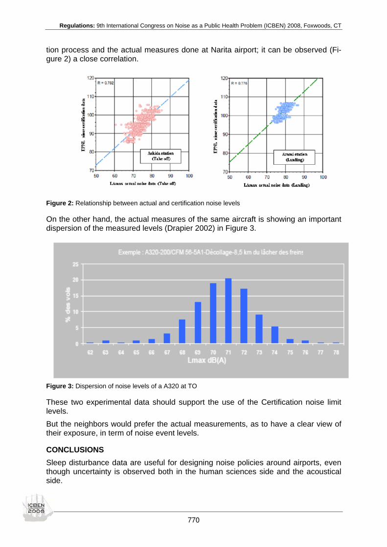
Regulations: 9th International Congress on Noise as a Public Health Problem (ICBEN) 2008, Foxwoods, CT
tion process and the actual measures done at Narita airport; it can be observed (Fi-gure 2) a close correlation.
Figure 2: Relationship between actual and certification noise levels
On the other hand, the actual measures of the same aircraft is showing an important dispersion of the measured levels (Drapier 2002) in Figure 3.
Figure 3: Dispersion of noise levels of a A320 at TO
These two experimental data should support the use of the Certification noise limit levels. But the neighbors would prefer the actual measurements, as to have a clear view of their exposure, in term of noise event levels.
CONCLUSIONS Sleep disturbance data are useful for designing noise policies around airports, even though uncertainty is observed both in the human sciences side and the acoustical side.
770

Regulations: 9th International Congress on Noise as a Public Health Problem (ICBEN) 2008, Foxwoods, CT
REFERENCES
Anderson G, Miller N (2007). Alternative analysis of sleep-awakening data. Noise Contr Engineering J 55: 224-245.
ANOTEC (2003). Study on current and future aircraft noise exposure at and around community airports. ANOTEC study. Report to the DG-TREN. Madrid: ANOTEC.
Babisch W (2006). Transportation noise and cardiovascular risks. Report. Berlin: Umweltbundesamt.
Basner M, Samel A, Isermann U (2006). Aircraft noise effects on sleep: application of the results of a large polysomno-graphic field study: J Acoust Soc Am 119: 2772-2784.
Drapier JL (2002). Etude de la dispersion des niveaux de bruit autour des aérodromes: Rapport DGAC. Paris.
EC (2008). Report from the Commission to the Council of the European parliament: Noise operation restrictions at EU air-ports. (Report on the application of the Directive 2002/30, EC). Brussels.
Finegold LS (2008). Noise report of the CAEP-ICAO Workshop Montreal (in press).
Finegold LS, Elias B (2002). A predictive model of noise induced awakenings from transportation noise source. In: Proceed-ings of the Congress Inter-noise 2002, Dearborn USA (CD Rom). [Basner data added]
Greiser E, Greiser C, Janhsen K (2007). Night-time aircraft noise increases prevalence of prescriptions of antihypertensive and cardiovascular drugs irrespective of social class - The Cologne-Bonn Airport study. J Public Health 15: 327-337.
Griefahn B (1992). Noise control during the night. Acoust Austral 20: 43-47.
Griefahn B, Marks A (2006). The significance of noises emitted by various modes: In: Hyrynen J (ed.): EURONOISE 2006. 6th European Conference on Noise Control in Tampere, Finland, 30 May – 1 June 2006. "Advanced solutions to noise con-trol” (6 pp on CD-ROM). Tampere.
Hume K, Morley H, Terranova D, Thomas C (2002). The influence of serial complainers on complaints profiles at airports. In: Proceedings of the Forum Acusticum , Sevilla, Spain.
ICAO, International Civil Aviation Organization (2007). Environmental Report 2007. Produced by the ICAO Environmental Unit in collaboration with FCM Communications Inc.
Jarup L, Babisch W, Houthuijs D, Pershagen G, Katsouyanni K, Cadum E, Dudley M, Savigny P, Seiffert I, Swart W, Breugelmans O, Bluhm G, Selander J, Charalampidis AS, Dimakopoulou K, Sourtzi P, Velonakis M, Vigna-Taglianti F (2007). Hypertension and exposure to noise near airports - the HYENA study. Environ Health Perspect 113: 1473-1478.
Katsuta K, Oshio K, Ogata S, Shinohara N (2006). New landing charge at Narita International Airport. In: Proceedings of the Congress Internoise , Honolulu.
Michaud DS, Fidell S, Pearsons K, Campbell KC, Keith SE (2007). Review of field studies of aircraft noise-induced sleep disturbance. J Acoust Soc Am 121: 32-41.
MPD (2007). Study of aircraft noise exposure at and around community airports: Evaluation of the effect of measures to reduce noise. Final report Tender N° TREN/F3/15-2006.
Passchier-Vermeer W (2003). Night-time noise events and awakening. Delft, The Netherlands, TNO Inro report 2003-32.
Southgate D, Fisher N, Perera D (2001). The Person-Events Index: a simple but invaluable aircraft noise assessment tool. In: Internoise 2001. Proceedings, The Hague, NL.
Vallet M, Vernet I (1991). Night noise index and sleep disturbance. In: Proceedings of the Internoise Congress, 1991, Syd-ney.
WHO Europe (2007). Night time noise guidelines. Report. Bonn: WHO Europe.
771
Regulations: 9th International Congress on Noise as a Public Health Problem (ICBEN) 2008, Foxwoods, CT
Aircraft noise effects on sleep: Substantiation of the DLR protection concept for airport Leipzig/Halle Mathias Basner* German Aerospace Center (DLR), Institute of Aerospace Medicine, 51170 Köln, Germany
* corresponding author: e-mail: [email protected]
ABSTRACT The Institute of Aerospace Medicine at the German Aerospace Center (DLR) investi-gated the influence of nocturnal aircraft noise on sleep in polysomnographical labora-tory and field studies between 1999 and 2004. The results of the field study were used by the Regional Council of Leipzig (Germany) for the establishment of a noise protection plan in the official approval process for the expansion of Leipzig/Halle air-port to an international freight hub. Of the results, special attention is given to the ex-posure-response relationship between the maximum sound pressure level of an air-craft noise event and the probability to wake up, which was used to establish noise protection zones directly related to the effects of noise on sleep. These protection zones differ qualitatively and quantitatively from zones that are solely based on acoustical criteria. The noise protection plan for Leipzig/Halle airport is presented and substantiated: (1) on average, there should be less than one additional awakening induced by aircraft noise, (2) awakenings recalled in the morning should be avoided as much as possible, and (3) aircraft noise should interfere as little as possible with the process of falling asleep again. Issues concerned with the representativeness of the study sample are discussed.
INTRODUCTION Between 1999 and 2004, the DLR-Institute of Aerospace Medicine in Cologne, Ger-many, performed extensive laboratory and field studies on the effects of aircraft noise on sleep, mood and performance in the DLR/HGF-project "Quiet Air Traffic". The Re-gional Council of Leipzig (RCL) asked DLR to propose a concept for the protection of residents of airport Leipzig/Halle against the adverse effects of nocturnal aircraft noise on sleep based on the findings of the field studies. Leipzig/Halle airport was recently extended to an international freight hub with air traffic predominantly occur-ring during the night. The southern runway was turned and extended to a length of 3,600 m. Together with the northern runway, this independent parallel runway system allows for simultaneous takeoffs and landings. The traffic volume is predicted with 81,000 aircraft movements during the six busiest months in the year 2015. Of these, 45,600 will take place during the day between 6:00 und 22:00 and 35,400 will occur during the night between 22:00 und 6:00. Thus, a large part of aircraft movements will take place during night. This situation distinguishes Leipzig/Halle airport from most other airports worldwide.
772

Regulations: 9th International Congress on Noise as a Public Health Problem (ICBEN) 2008, Foxwoods, CT
DLR-INVESTIGATIONS AND RESULTS Methods Since the concepts of the noise protection plan for Leipzig/Halle airport are mainly based on the results of the DLR field study, study design and methods of the field study are briefly described. A detailed description is provided in the executive sum-mary of the study (Basner et al. 2004). The field study was conducted in 2001 and 2002 with 64 residents of Cologne-Bonn airport, which is one of the German airports with the highest nighttime freight traffic densities. Subjects were investigated for 9 consecutive nights, starting on Mondays. They were selected in a multi-level process, and were between 19 and 61 years old (average: 38 years). 56 % of the participants were female. Subjects had to be free of intrinsic sleep disorders and had to have normal hearing thresholds according to age. The study protocol was approved by an ethics committee. Subjects were instructed according to the Helsinki declaration, par-ticipated voluntarily, and were free to discontinue their participation at any time with-out explanation. Electroencephalogram (EEG), electrooculogram (EOG), electromyogram (EMG), electrocardiogram (ECG), respiratory movements, finger pulse amplitude, position in bed and actigraphy were sampled continuously during the night. With the EEG, EOG and EMG signals (also called polysomnography), sleep can be classified into differ-ent sleep stages (Rechtschaffen et al. 1968). In the field study, sound pressure levels (SPL) and actual sounds were recorded in-side the bedroom (at the sleeper's ear) and outside (2 m in front of the window) with class-1 sound level meters. All events (e.g. aircraft noise, road traffic noise, snoring, etc.) were identified by a human scorer. The start and the end of each event were marked. The simultaneous recording of acoustical and electrophysiological signals allowed for an event-related analysis with a maximum resolution of 125 ms. Reactions to aircraft noise and spontaneous reactions (undisturbed by external stim-uli) during sleep are non-specific. Hence, reactions observed during an aircraft noise event (ANE) cannot be differentiated from spontaneous reactions according to elec-trophysiological criteria. Furthermore, spontaneous reactions occur irregularly. There-fore, a reaction during an ANE occurs, it is important to examine how often this reac-tion would have taken place spontaneously anyway, i.e. without the influence of air-craft noise. The probability of spontaneous reactions can be estimated from periods without aircraft noise. In epidemiology the term attributable risk is often used in this context. Thus, the probability of a reaction additionally induced by aircraft noise ac-cording to Brink et al. (2006) is calculated as: Padditional = PANE – Pspontaneous (1)
Results In total, 61 of 64 subjects contributed to the final analysis with 483 subject nights. The data of 3 subjects were discarded due to constant snoring (2 subjects) or an in-trinsic sleep disorder (1 subject). The first night was not analyzed because of the so called first-night effect (Agnew Jr. et al. 1966). 10,658 ANEs met the inclusion criteria and contributed to the regression analyses.
773

Regulations: 9th International Congress on Noise as a Public Health Problem (ICBEN) 2008, Foxwoods, CT
0 %
5 %
1 0 %
1 5 %
2 0 %
2 5 %
3 0 %
2 5 3 0 3 5 4 0 4 5 5 0 5 5 6 0 6 5 7 0 7 5
M a xum um S P L L A S ,m a x in dB
Prob
abili
ty o
f Sle
ep S
tage
Cha
nge
to A
wak
e or
S1
Figure 1: Probability of sleep stage change to Stage 1 or Awake depending on maximum SPL LAS,max. Assumptions: Background noise level 27.1 dB, prior sleep stage Stage 2, elapsed sleep time 5 hours. Point estimates (black line), 95 % confidence limits (grey lines), and spontaneous reaction probabilities (dashed line) are shown.
Figure 1 illustrates the relationship between the maximum SPL of an ANE and the percentage awakened (black line). The background noise level was assumed con-stant with 27.1 dB (median of all measurements in the field study). For preventive reasons, the sleep stage prior to the ANE was assumed to be Stage 2 in all cases, i.e. the most sensitive sleep stage. Likewise, elapsed sleep time was set to the mid-dle of the more sensitive second half of the night (about 5 hrs after sleep onset). The highest SPL measured in the field inside the bedroom was 73.2 dB. Spontaneous changes to Wake or Stage S1 occurred with a probability of 8.6 % (dashed line). A threshold value of about 33 dB was found, i.e. awakening probability increased only for ANEs with maximum SPL above 33 dB compared to spontaneous awakening probability (see Figure 1). This threshold was only 6 dB above the background noise level, which seems physiologically plausible: First noise induced awakenings should be observed when the auditory system is able to differentiate the ANE from the back-ground noise. It must be emphasized that the awakening probability just above the threshold is very low: only 2 of 1,000 people exposed to an ANE with a maximum SPL of 34 dB will show a noise induced awakening. Due to the large number of sub-jects and ANEs, the precision of the point estimate is very high, i.e. the width of the 95 % confidence interval is very narrow (3.1 % at 39 dB and 10.5 % at 73.2 dB). The probability of additional noise induced awakenings or changes to Stage 1 (ac-cording to equation 1) can be approximated with a second-degree polynomial be-tween 32.7 dB and 73.2 dB. Awakening probability in percent is calculated as:
3243,3L10008,4L10894,1P max.AS22
max,AS3
AWR −⋅+⋅= −−
(2) The probabilities calculated by the polynomial deviate less than 0.1 % from the origi-nal regression line within the specified interval.
774

Regulations: 9th International Congress on Noise as a Public Health Problem (ICBEN) 2008, Foxwoods, CT
0%
10%
20%
30%
40%
50%
60%
70%
0,5 1,0 1,5 2,0 2,5 3,0 3,5 4,0 4,5 5,0Elapsed Time after Awakening [min]
Perc
enta
ge n
ot y
et fa
llen
asle
ep a
gain
spontaneous
45-65 dB
70-80 dB
Figure 2: Duration of noise induced awakenings depending on maximum SPL and compared to spon-taneous awakenings
Both number and duration of aircraft noise induced awakenings play an important role for the evaluation of the effects of aircraft noise on sleep, because the probability of a recalled awakening in the morning increases with awakening duration. Results of the DLR laboratory study showed that awakening duration increased with the maxi-mum SPL of an ANE (see Figure 2). Awakenings induced by ANEs with maximum SPLs of 65 dB or lower were relatively short. After 1.5 min, descriptively no difference in the percentage of subjects having fallen asleep again compared to spontaneous awakenings was observed. In contrast to that, awakenings induced by ANEs with maximum SPLs of 70 dB or higher were markedly longer than spontaneous awaken-ings.
DLR-CONCEPT FOR NIGHTTIME PROTECTION Objectives of the concept Adequate protection of people affected by nocturnal aircraft noise has to be the main objective of a protection concept in order to prevent negative health consequences. Changes in sleep structure that may lead to a non-restorative sleep are the primary effects of nocturnal aircraft noise. Sleepiness and impaired mental capacities are two of the possible immediate consequences (Basner 2008). Furthermore, annoyance may be induced by consciously perceived noise events during the night. It is also be-ing discussed whether repeatedly (over years) occurring noise induced sleep distur-bances may lead to other health impairments, such as an increased risk for high blood pressure or myocardial infarction (Babisch 2000; Babisch et al. 2005; Jarup et al. 2008; Morrell et al. 1997). If established, these noise impacts on health would be of major societal importance. However, in practice it is very difficult to substantiate a causal link between noise and long term health effects, as many different and well proven risk factors lead to the same diseases and induction periods are usually very long. In order to overcome this dilemma, the DLR-concept is based on two assump-tions: (i) Because of biological plausibility, it is hypothesized that a causal link be-tween noise induced sleep disturbances and long term health effects exists. Vice versa, long term health effects can be prevented with a high probability if noise in-
775

Regulations: 9th International Congress on Noise as a Public Health Problem (ICBEN) 2008, Foxwoods, CT
duced sleep disturbances are minimized. (ii) It is assumed that humans – like any organism – represent an adaptive system, which is able to compensate for certain strains without negative effects for the organism. Hence, it is not necessary to elimi-nate strains completely.
Description of the concept The DLR-concept is founded on three objectives reflecting three highly correlated dimensions of sleep: (i) On average, there should be less than one additional awakening induced by
aircraft noise. Here, awakenings are defined as an electrophysiological phe-nomenon classified according to the rules of Rechtschaffen et al. (1968).
(ii) Awakenings recalled in the morning should be prevented as much as possible. (iii) There should be no relevant impairment of the process of falling asleep again.
4488 92 96 4500 04 08 12 16 20 24 28 32 36 45405692
96
5700
04
5708
Figure 3: Noise protection zone for airport Leipzig/Halle (traffic prognosis for 2015), consisting of the combination of two areas: (1) area outside of which less than one additional awakening induced by aircraft noise is expected on average (light grey, expected distribution of directions of flight move-ments); (2) area outside of which maximum SPLs of 80 dB or higher (measured outside) occur less than once (dark grey, 100:100 distribution of directions of flight movements)
Figure 3 illustrates the proposed noise protection zone for Leipzig/Halle airport for the night (22:00 until 06:00), based on a traffic prognosis for 2015. Two contours are combined: Outside of the light grey area on average less than one additional awak-ening induced by aircraft noise is expected. This contour is based on the expected, average distribution of flight movements on the two operation directions. Outside of the dark grey area, maximum SPLs of 80 dB or higher (measured outside) occur less than once. This contour is the envelope of two contours estimated for a 100 % distri-bution of flight movements in both operating directions. This leads to an overestima-tion of effects, which was intended as awakenings recalled in the morning are re-garded especially serious sleep disturbances. An individual wakes up or does not. Thus, criterion (i) must be interpreted as a statis-tical value which has a distribution over nights and persons. If an individual is awak-ened by aircraft noise more than once in one night, there must be other nights with no additional awakening for compensation. Summarizing e.g. over a year, the crite-rion allows not more than 364 additional awakenings. This number has to be kept in mind compared to about 24 spontaneous awakenings to be expected per night on average and therefore about 8,760 spontaneous awakenings per year (Basner et al. 2004).
776

Regulations: 9th International Congress on Noise as a Public Health Problem (ICBEN) 2008, Foxwoods, CT
Criterion (ii) considers the risk of recalled awakenings in the morning. Recalled awakenings are correlated with subjective sleep quality and quantity ratings: The higher the number of recalled awakenings, the worse the estimation of sleep quality and quantity. ANEs during a sleep period influence the assessment of annoyance only when they are perceived consciously, and longer awakenings are a prerequisite for regaining consciousness (Health Council of the Netherlands 2004). Recalled awakenings not only fragment sleep. They have psychological disadvantages as well and therefore form a major sleep disturbance. Psychosomatic disorders cannot be excluded if recalled awakenings are induced over longer time periods. Therefore, from a medical point of view, recalled awakenings induced by aircraft noise should be prevented as much as possible. The 1st criterion limits the number of noise induced awakenings irrespective of the duration of the awakenings, and, thus, limits the num-ber of recalled awakenings as well. Analyses of the laboratory study showed that the duration of noise induced awakenings increases with the maximum SPL of ANEs. Relevant differences compared to spontaneous awakenings were observed for maximum SPLs of more than 65 dB (see Figure 2). For this reason, maximum SPLs of more than 65 dB should be avoided in the bedroom. For a tilted window with an assumed difference in SPLs of 15 dB between inside and outside, the 1 x 80 dBoutside-contour of Figure 3 (dark grey) assures that outside this area maximum SPLs of 65 dB are exceeded less than once per night inside the bedroom on average. As re-called awakenings should be avoided as much as possible, this contour is based on a 100 % flight movements in one direction estimation, i.e. the worst case. The problem of falling asleep again (criterion (iii)) has practically not been considered in the literature of noise effects on sleep so far, disregarding the fact that about 7 % of the sleep period are spent awake (Basner & Samel 2005). ANEs can prevent the sleeper from falling asleep again in these situations, and therefore have a negative impact on sleep structure (Basner et al. 2004). The traffic prognosis for Leipzig/Halle airport in 2015 forecasts two very busy periods during the night caused by freight traf-fic. Between 0:00 and 1:30 up to 60 approaches per hour and between 4:00 and 5:30 up to 50 starts per hour are expected. The short time period between two noise events in these peak hours leads to an increased risk of preventing the affected population from falling asleep again. If a subject already regained consciousness, annoyance reactions may result from consciously perceived noise events. Indeed, many airport residents complain about ANEs in early morning hours. A complex model was built, based on extensive analyses of the data of the field study to assess the impact of aircraft noise on falling asleep again, depending on maximum SPL LAS,max of the ANE, elapsed sleep time, the current state (awake/sleep) and the elapsed time spent in the same sleep stage (Basner & Siebert 2006). The results in-dicated that maximum SPLs of ANEs in the second half of the night should receive a malus of 1.4 dB, i.e. they should be artificially elevated by 1.4 dB, in order to assure an undisturbed process of falling asleep again similarly in all regions around Leip-zig/Halle airport.
REPRESENTATIVENESS ISSUES In the DLR field study, 64 subjects were studied for 576 subject nights, resulting in the largest polysomnographical study with identical methodological approach so far. Nevertheless, the study does not claim representativeness for the whole population. It is impossible to be representative for a whole population in a study with huge methodological expenses for a single subject like the DLR study. Additionally, some inclusion criteria had to be met in order to be eligible for study participation, leading to
777

Regulations: 9th International Congress on Noise as a Public Health Problem (ICBEN) 2008, Foxwoods, CT
a higher internal validity of the results. This is a prerequisite for external validation, but also restricts it to some extent (Basner et al. 2004). Therefore, the results of the field study were not transferred 1:1 to the population liv-ing in the vicinity of Leipzig/Halle airport. Instead, several preventive measures were taken in order to protect those parts of the population that were not represented in the DLR field study and/or that are more sensitive to aircraft noise than the average sleeper. Some of these measures shall be briefly summarized: • Subjects assessing themselves as sensitive to and annoyed by aircraft noise were in-
cluded preferably into the study. 75 % of study subjects assessed themselves as moder-ately, strongly or very strongly annoyed, which compares well to a recent representative survey at Frankfurt airport (Schreckenberg & Meis 2006).
• Not only awakenings, but also sleep stage changes to Stage 1 were regarded as relevant noise induced sleep disturbances, increasing the probability of reactions to aircraft noise.
• For the calculation of the dose-response curve based on the regression results it was assumed that the sleeper spent the whole night in the most sensitive sleep stage S2 and in the middle of the more sensitive second half of the night. In reality, an average night contains only about 50 % of sleep Stage 2. Hence, the dose-response curve is shifted to higher probabilities compared to calculations were the actual sleep stage distribution is used. Because of this measure alone the noise protection zone increases from 156 km² by 28 % to 199 km².
• Subjects with illnesses lowering noise sensitivity (e.g. Hypakusis, Hypersomnolence) were excluded from study participation.
• The calculations for the noise protection zone were based on the six busiest months of the year according to air traffic.
• Sound insulation was increased by 3 dB for sensitive institutions (e.g. hospitals) and indi-viduals with relevant diseases accompanied by higher noise sensitivity.
The proposal of allowing only one additional awakening induced by aircraft noise makes sense in terms of preventive medicine. It has to be taken into account that on average 24 spontaneous awakenings can be observed in an otherwise undisturbed night anyway.
SUMMARY AND CONCLUSIONS The DLR-Institute of Aerospace Medicine investigated the influence of aircraft noise on sleep, mood and performance in an extensive polysomnographical field study be-tween 1999 and 2004 as part of the DLR/HGF-project "Quiet Air Traffic". The dose-response relationship developed in this study was used to establish a concept for the protection of subjects against the adverse effects of nocturnal aircraft noise on sleep. The Regional Council of Leipzig decided to use the results of the DLR field study for developing a new noise protection concept at Leipzig/Halle airport. This concept cul-minates in the three propositions and reflects three correlated dimensions of sleep: There should be on average less than one additional awakening induced by aircraft noise, noise induced awakenings recalled in the morning should be prevented as much as possible, and no relevant impairments of the process of falling asleep again should occur. These three provisions have been proposed in order to consider the special conditions under which Leipzig/Halle airport will operate: (i) construction of a second independent runway, (ii) settlement of a night cargo hub for a big service pro-vider, (iii) heavy air traffic during night including peak hours with up to 60 movements per hour and (iv) practically no nocturnal air traffic in the present. These circum-
778

Regulations: 9th International Congress on Noise as a Public Health Problem (ICBEN) 2008, Foxwoods, CT
stances necessitate a special concept for the protection of the affected population against the adverse effects of nocturnal aircraft noise on sleep. With the decision to implement the results of the DLR field study, fresh ground was broken, as noise protection zones solely depended on acoustical criteria so far. The noise protection zone for nocturnal air traffic proposed by DLR exceeds the one of a current law amendment under discussion, which should come in force in 2011, by 60 km². Shortly after the publication of the official documents of the approval process for the extension of Leipzig/Halle airport in November 2004, the integrator DHL decided to move its European freight hub from Brussels to Leipzig/Halle. Despite of the very conservative approach taken in constructing the noise protection zones, some resi-dents living in the vicinity of Leipzig/Halle airport are still not satisfied with the con-cept: They sued in order to prevent the start of constructions at the airport. The Fed-eral Administrative Court rebutted this sue in May 2005, and the construction meas-ures started in August 2005. The final decision by the Federal Administrative Court from 09 November 2006 supports the DLR protection concept in every aspect. Re-cently, Leipzig/Halle freight hub commenced its work.
REFERENCES
Agnew HW Jr., Webb WB, Williams RL (1966). The first night effect: an EEG study of sleep. Psychophysiology 2: 263-266.
Babisch W (2000). Traffic noise and cardiovascular disease: epidemiological review and synthesis. Noise & Health 2: 9-32.
Babisch W, Beule B, Schust M, Kersten N, Ising H (2005). Traffic noise and risk of myocardial infarction. Epidemiology 16: 33-40.
Basner M (2008). Nocturnal aircraft noise increases objectively assessed daytime sleepiness. Somnologie 12: 110-117.
Basner M, Samel A (2005). Effects of nocturnal aircraft noise on sleep structure. Somnologie 9: 84-95.
Basner M, Siebert U (2006). Markov-Prozesse zur Vorhersage fluglärmbedingter Schlafstörungen. Somnologie 10: 176-191.
Basner M, Buess H, Elmenhorst D, Gerlich A, Luks N, Maaß H, Mawet L, Müller EW, Müller U, Plath G, Quehl J, Samel A, Schulze M, Vejvoda M, Wenzel J (2004). Effects of nocturnal aircraft noise (Vol. 1): Executive summary. FB2004-07/E. Co-logne: Deutsches Zentrum für Luft- und Raumfahrt (DLR).
Brink M, Schierz C, Basner M, Samel A, Spreng M, Scheuch K, Stahel W, Bögli H (2006). Bericht zum Workshop "Auf-wachwahrscheinlichkeit". Bestimmung lärminduzierter Aufwachwahrscheinlichkeiten in der Nachtlärmwirkungsforschung und Anwendung entsprechender Wirkungsmodelle für Prognosezwecke. Zürich: Zentrum für Organisations- und Arbeitswissen-schaften. http://e-collection.ethbib.ethz.ch/show?type=bericht&nr=485].
Health Council of the Netherlands (2004). The influence of night time noise on sleep and health. Publication no. 2004/14E. The Hague: Health Council of the Netherlands.
Jarup L, Babisch W, Houthuijs D, Pershagen G, Katsouyanni K, Cadum E, Dudley ML, Savigny P, Seiffert I, Swart W, Breugelmans O, Bluhm G, Selander J, Haralabidis A, Dimakopoulou K, Sourtzi P, Velonakis M, Vigna-Taglianti F (2008). Hypertension and exposure to noise near airports: the HYENA study. Environ Health Perspect 116: 329-333.
Morrell S, Taylor R, Lyle D (1997). A review of health effects of aircraft noise. Aust N Z J Public Health 21: 221-236.
Rechtschaffen A, Kales A, Berger RJ, Dement WC, Jacobsen A, Johnson LC, Jouvet M, Monroe LJ, Oswald I, Roffwarg HP, Roth B, Walter RD (19689. A manual of standardized terminology, techniques and scoring system for sleep stages of human subjects. Washington, DC: Public Health Service, U.S. Government, Printing Office.
Schreckenberg D, Meis M (2006). Belästigung durch Fluglärm im Umfeld des Frankfurter Flughafens - Endbericht.
779

Regulations: 9th International Congress on Noise as a Public Health Problem (ICBEN) 2008, Foxwoods, CT
A strategic approach on environmental noise management in developing countries Dieter Schwela1*, Larry S. Finegold2, John Stewart3 1 Stockholm Environment Institute, University of York, Heslington, York, UK
2 Finegold & So, Consultants, 1167 Bournemouth Court, Centerville, Ohio 45459 USA and Tokyo, Japan
3 13 Stockwell Road, London SW9 9AU, United Kingdom
* corresponding author: e-mail: [email protected]
INTRODUCTION Environmental noise continues to pose a significant threat to human health and the quality of life of millions of people throughout developing countries. Urbanization and associated growth in mobility and industrialization has resulted in the intensification of noise in densely populated areas, causing deterioration in noise exposure. Many cities in developing countries are now having to take action to enhance their institu-tional and technical capabilities to monitor and control noise exposure and implement preventive actions in order to reduce the risks that noise poses to their citizens. This document introduces to and outlines a Strategic Approach (SA) on Environmental Noise Management (ENM) in developing countries to assist decision makers and stakeholders to formulate and implement effective ENM strategies. The severity of environmental noise problems in cities of developing countries re-flects the level and speed of development. As cities undergo economic and industrial development environmental noise becomes an increasing problem. In the past, the major causes of environmental degradation occurred sequentially rather than simul-taneously. However, nowadays many cities of developing countries are having to suf-fer the pressure of a combination of different driving forces (e.g. motorization, indus-trialization and increase in urban population density), each with a greater intensity than has occurred elsewhere or in the past and without the well-developed civil infra-structure and financial resources to control them. The result is that the ability of many cities to cope with the combined pressures is often exceeded leading to a deteriora-tion in environmental quality in many cities of developing countries. Environmental noise in developing countries has a number of impacts on human health and the environment, which have social and economic implications. These in-clude:
o Cardiovascular diseases o Increases in cardiovascular symptoms (e.g. blood pressure) o Hearing impairment o Cognitive effects o Speech interference o Sleep disturbance o Performance deficits o Annoyance o Mental health effects.
This paper is an overview of the SA on environmental noise management (ENM) in developing countries the outline of which was discussed at the Workshop on Envi-ronmental Noise Management in Developing Countries at the internoise 2007 con-
780
Regulations: 9th International Congress on Noise as a Public Health Problem (ICBEN) 2008, Foxwoods, CT
ference, held in Istanbul, 28-31 August 2007. At this workshop the following observa-tions were made:
The importance of an overall strategy Although a step-by-step program of implementation of environmental noise policies is probably the realistic way forward, it is critical that it is done in the context of a clear, strategic approach. Many developed countries lack this as do most developing coun-tries. China appears to be the exception to this. The seminar heard about the im-pressive strategy which the Chinese Government has developed to tackle noise. In many ways, this could act as a model for other developing countries.
The importance of the implementation and enforcement of noise policies The seminar heard that quite a few developing countries have theoretical noise poli-cies, but that the implementation and enforcement of them is poor. This is partly the result of a lack of political will and it is partly because of the cost. It is probably unre-alistic to expect a rapid improvement in implementation and enforcement, so a step-by-step approach would be more realistic.
The importance of active citizens’ groups There is little pressure on governments from citizens groups for action to be taken on environmental noise. This is, in part, due to a lack of understanding of the impacts of environmental noise. But the seminar did hear of some pressure. Here are citizens groups in China protesting about aircraft noise and about increase noise from traffic on existing roads. When people are annoyed and stressed out by noise they don’t need to fully understand the impact it is having on them in order to protest! It is likely that these protests will grow as development brings with it an increase in noise. The seminar also heard that ‘new’ noises will emerge as countries acquire more consumer goods. In particular, many of the new consumer goods will result in increases in low-frequency noise. In China low-frequency noise has become one of the problems which the responsible stakeholders have yet to tackle successfully. Al-though citizens groups in developed countries have only had limited success in put-ting pressure on their governments to tackle environmental noise, it is important that citizens groups from developing countries link up with their counterparts in the devel-oped world.
The importance of improved understanding of the impacts of noise It came across at the seminar that there is a lack of understanding in many develop-ing countries amongst both politicians and the general public of the impacts of envi-ronmental noise – the effect on stress levels, health, quality of life etc. It is only when these impacts are better understood will governments be motivated to tackle envi-ronmental noise and will citizens demand that noise be taken seriously.
The importance of low-cost solutions At present tackling environmental noise is not a political priority for most developing countries. It is going to be particularly difficult to persuade them to give some priority to environmental noise and put an effective noise strategy in place if they believe it is going to cost a lot of money. Therefore low-cost solutions are important. For exam-ple, noise mapping would be expensive – and probably unnecessary since most people know where the noisiest areas are. It also means it is important to highlight the cost-benefit advantages of tackling environmental noise, for example, money
781

Regulations: 9th International Congress on Noise as a Public Health Problem (ICBEN) 2008, Foxwoods, CT
spent on noise reduction could result in savings on health costs. But this does require an understanding of the health effects of noise (see previous section).
The importance of not re-inventing research, policy and practice This means developing countries using the research that has already been done (of-ten by countries in the developed world) but also, importantly, by the WHO. It also means examining, and adopting where relevant, the noise reduction policies and practices which have been shown to work in developed countries. And it means link-ing into international bodies like ICAO, even though many of these bodies are flawed. In fact, it may be because they are flawed that developing nations should get in-volved as they may bring a new fresh, perspective to their deliberations.
ENVIRONMENTAL NOISE MANAGEMENT The aim of Environmental Noise Management (ENM) is to maintain a low noise sound-scape that protects human health and wellbeing but also provides protection of animals. ENM is a tool which enables governmental authorities to set objectives to achieve and maintain a low noise sound-scape and reduce the impacts on human health and animals. Governmental authorities in collaboration with other stakeholders can determine the individual steps of the implementation of this process according to:
o local circumstances with respect to background noise levels and technological feasibilities;
o cultural and social conditions; and o financial and human resources available.
An effective ENM strategy is dependent of a number of factors such as source knowledge, noise monitoring networks, transmission of noise prediction models, ex-posure and damage assessments, health based standards together with a range of cost-effective noise exposure control measures and the legislative powers and re-sources to implement and enforce them. Figure 1 presents a simplified cycle of ENM.
Figure 1: Model of policy process for community noise (Hede 1998; WHO 2000)
ENM as envisaged in the SA a process which enables governmental authorities, in collaboration with other stakeholders, to:
o identify and establish appropriate policies on environmental noise; o identify relevant legislative and regulatory requirements; o identify all sources of environmental noise caused by human activities;
782

Regulations: 9th International Congress on Noise as a Public Health Problem (ICBEN) 2008, Foxwoods, CT
o set appropriate objectives and targets for human (and animal) health; o set priorities for achieving objectives and targets; o establish a structure and programs to implement policies and achieve objec-
tives and targets; o facilitate the monitoring of environmental noise and effects on human health; o facilitate urban planning, corrective action and the prevention of adverse ef-
fects; o ensure compliance with emission and noise standards; o account for changing circumstances.
Figure 2 depicts the policy cycle in a slightly different form but of same content and the stakeholders involved in the different stages of the cycle.
POLICY STAGES ACTORS
Figure 2: Policy stages and actors (stakeholders) (Hede 1998; WHO 2000)
STRATEGIC APPROACH The Strategic Approach (SA) on Environmental Noise Management in Developing Countries aims to provide an approach to mitigating noise by facilitating the setting of noise priorities and providing direction on institutional development and capacity en-hancement. The SA is being proposed by the Stockholm Environment Institute in col-laboration with Tamer Elnady, Egypt, Lawrence Finegold, USA, Samir Gerges, Brazil, John Stewart, UK, Tian Jing PR China.
Noise problem identification Politicians + Political Advisors + Expert-officials + Policy analysts + Community + Researchers +
Interest groups + Acoustic professionals
Noise impact assessment Expert-officials + Acoustic professionals + Re-searchers + Community + Interest groups
Noise control options Politicians + Political Advisors + Expert-officials + Policy analysts + Community + Researchers +
Interest groups + Acoustic professionals
Decision on noise regulation Politicians + Political Advisors
Implementation of noise regulation
Expert-officials + Acoustic professionals + Com-munity + Interest groups
Policy evaluation Expert-officials + Policy analysts + Commu-
nity + Researchers + Interest groups + Acoustic professionals
Policy revision
783

Regulations: 9th International Congress on Noise as a Public Health Problem (ICBEN) 2008, Foxwoods, CT
The SA is a strong follow up of the recommendations of Agenda 21, derived from the 1992 United Nations Conference on Environment and Development, and the Plan of Implementation of the 2002 World Summit on Sustainable Development (WSSD 2002) which requests States to strengthen capacities of developing countries to measure, reduce and assess the impacts of noise, including health impacts, and pro-vide financial and technical support for these activities. In addition, the SA supports the UN Habitat Agenda on the Urban Environment and the UNHABITAT/UNEP Sus-tainable Cities Program which notes the health hazards of exposure to excessive noise and recommends develop criteria for maximum permitted and safe levels of noise exposure and promote noise assessment control as part of environmental pro-grams (UNHabitat 2008). The SA is intended to help developing countries and mega and major cities in devel-oping countries to develop and/or improve their actions in preventing further deterio-ration of noise levels by a rational noise management. The deterioration of noise lev-els observed in many cities of developing countries is a consequence of industrializa-tion, urban growth, and migration of people into urban areas as a consequence of poverty. Environmental noise management aims at maintaining and/or re-installing levels of environmental noise that protect human health. Reduction of excess noise levels is necessary to support further development of developing countries because noise heavily affects public health and the costs on public health associated with noise can be huge. As in air quality management where the benefits of emissions re-ductions usually are much higher than the costs of source controls in environmental noise abatement the benefits of emissions reductions may also be much higher than the costs of reducing noise emissions. Moreover there may be co-benefits of noise and air pollution (including greenhouse gases) reduction. The SA is a broad high-level approach that is flexible and adaptable to the needs of different countries and cities. It is based on a set of guiding principles, which include precautionary and polluter pays principles, sustainability, stakeholder commitment, application of best practices, cost-effectiveness, risk awareness, and access to envi-ronmental information. The Strategic Approach highlights the challenges existing in cities of developing countries and gives recommendations with respect to the most important components of a comprehensive noise management system in a rational and systematic manner. Challenges in environmental noise management in develop-ing countries refer to government commitment and stakeholder participation, to weakness in policies, standards and regulations, to deficiencies in data for emis-sions, noise and public health impacts. Precise knowledge on noise emissions is of-ten missing, incomplete or inaccurate. Noise emission standards are sometimes ob-solete and do not reflect best technical practice. Measures to prevent and reduce noise emissions are often hampered by lack of source apportionment. Low cost and effective alternative technologies are rarely available. Noise monitoring systems are often limited in spatial coverage, not harmonised to each other, or are absent alto-gether. There is a lack in or absence of quality assurance/quality control plans, the data quality is unknown or poor. Little information exists in many developing coun-tries on health and economic impacts of environmental noise. Risk perception, risk communication, information dissemination and awareness raising are issues to be addressed. A major challenge is the availability of funding with good governance missing and low priority funding for environmental noise management. Key barriers to the adoption and implementation of the SA include lack of sufficient political will, lack of public awareness, inadequate infrastructure, lack of good data for emissions and noise levels and poor surveillance of health impacts due to noise. All these is-
784

Regulations: 9th International Congress on Noise as a Public Health Problem (ICBEN) 2008, Foxwoods, CT
sues have been addressed in the Strategic Approach and tools have been recom-mended to resolve the challenges and overcome the barriers. The SA is aimed at all stakeholders who have a role to play in ENM, especially na-tional and local governmental authorities. Governmental authorities in collaboration with a range of stakeholders can use the tools outlined in the SA document. The stakeholders also include: judiciary; private sector; civil society, non-governmental agencies; media, academia and development agencies.
GUIDING PRINCIPLES OF ENVIRONMENTAL NOISE MANAGEMENT Guiding principles related to ENM ensure the protection of human health from envi-ronmental noise (see Box 1). However, a number of economic, institutional and po-litical constraints may hamper the full implementation of these principles.
Box 1: The Guiding Principles of ENM
Access to Environmental Information: all stakeholders should have access to information regarding Noise
Awareness: Provision of information to all stakeholders
Best practice: application of state of the tech-nology
Co-benefits: consideration of the benefits of integrated ENM, air pollution management in-cluding greenhouse gas reduction
Coherence: orientation of the efforts of all stakeholders including different neighbouring jurisdictions towards a common objective.
Concerted effort: discussion and co-operation among all stakeholders involved
Compatibility: development of ENM compatible with regional, national and local needs
Continual Improvement: to promote the con-tinual improvement of ENM as well as reduction of noise itself
Cost-effectiveness: ENM measured at least cost and highest effectiveness
Decentralization: implementation of decentral-ised ENM with regional, national and local com-ponents with due consideration to local capacity
Equity: fair and equal protection of all people from noise exposure and consideration of indi-vidual vulnerability
Integrated approach: development of integrated ENM (prevention, monitoring of adverse impacts, control of sources, and education)
Opportunity: sound solutions to noise problems at the suitable moment
Participation: active participation of the population in the development and implementation of the plans to minimise noise pollution and prevent the increase of noise levels
Polluter Pays Principle: individuals responsible for noise pollution should bare the cost of its conse-quential impacts
Precautionary Principle: where there are threats of serious or irreversible health damage, lack of full scientific certainty should not be used as a reason for postponing cost effective measures to prevent higher noise levels
Stakeholder: Commitment of all stakeholders to noise management
Sustainability: development of economically and socially compatible ENM which is sustainable over the long term and future generations
Stepwise approach: ENM following a target and milestone approach
Universality: comprehensive ENM including human health
For each component, challenges in developing countries are listed and an objective and tools for improvement of ENM is outlined. The final section identifies the issues relating to the adoption and implementation of the Strategic Approach.
785

Regulations: 9th International Congress on Noise as a Public Health Problem (ICBEN) 2008, Foxwoods, CT
STRUCTURE OF THE DOCUMENT The document is divided into eight sections which cover the key components of ENM:
o Introduction o Environmental Noise Policies o Environmental Noise Governance o Emission o Environmental Noise Modelling o Environmental Noise Monitoring o Human (and Animal) Health and Economic Risk Assessments o Financing of Environmental Noise Management
USE OF THE DOCUMENT The SA can only be implemented if the ideas developed in it are generally accepted by all stakeholders. It is, therefore, logical to bring the SA to the attention of inter- and supranational organizations, governments, environmental protection agencies, indus-try, academia, media, aid agencies, and non-governmental organizations. Although some developing countries have made progress in addressing urban noise, they are still vulnerable to the actions taken by neighboring jurisdictions. This is par-ticularly the case with regard to the export and import of reconditioned vehicles which are unsuitable to meet current and future emission standards. In addition, the effects of global trade in noisy consumer products can inhibit a country’s progress in ad-dressing noise. Global cooperation is therefore necessary to facilitate a more harmonised approach to ENM, especially with regard to the adoption of environmental noise and emission standards. One key tool is the need to establish a flexible mechanism for the ex-change and sharing of environmental noise data among neighboring jurisdictions.
OVERCOMING THE CHALLENGES The ideas in the SA have been developed under the viewpoint of helping countries and cities to overcome barriers to development:
• lack of sufficient political will • inadequate infrastructure, training and resources • lack of good quality noise data • lack of necessary knowledge on emissions • poor assessment of the health impacts of environmental noise • need for the document to be translated into different languages.
These barriers can be overcome as described above by:
• gaining ministerial support in developing countries for the SA • gaining support from international agencies especially with regard to technical
and financial support • undertaking cost-benefit analyses and health impact studies • translation of the document into different regional languages
786

Regulations: 9th International Congress on Noise as a Public Health Problem (ICBEN) 2008, Foxwoods, CT
CONCLUSION This paper gives an overview over the Strategic Approach for Environmental Noise Management in Developing Countries. A first draft of the Strategic Approach has been compiled by SEI and a final draft will be produced in collaboration with several international experts from developing countries in the near future. This draft will be used as background paper for regional policy dialogues and to help cities in develop-ing countries develop action plans for noise mitigation.
REFERENCES Hede A (1998). Environmental noise regulation: A public policy perspective. In: Carter NL, Job RFS (eds.): Noise as a public health problem (Noise Effects ’98), Vol. 2 (pp 687-696). Sydney, Australia.
UNHabitat (2008). Section IV C. Sustainable human settlements development in an urbanizing world. 5. Environmentally sustainable, healthy and liveable human settlements. http://ww2.unhabitat.org/declarations/ch-4c-5.htm.
WHO 2000. Guidelines for community noise. Geneva: World Health Organization.
WSSD (2002). World Summit on Sustainable Development – Plan of Implementation. World Summit on Sustainable Devel-opment, Johannesburg, South Africa (see www.johannesburgsummit.org).
787

Regulations: 9th International Congress on Noise as a Public Health Problem (ICBEN) 2008, Foxwoods, CT
Road noise charges based on the marginal cost principle Mikael Ögren1*, Henrik Andersson2 1 The Swedish National Road and Transport Research Institute (VTI), Box 8077, SE-40278, Gothen-
burg, Sweden
2 VTI, Box 55685, SE-10215, Stockholm, Sweden, [email protected]
* corresponding author: e-mail: [email protected]
INTRODUCTION Noise emission from traffic is a growing environmental problem. The growth is both due to increasing traffic volumes, but also due to urbanization. In the end more peo-ple are being exposed to higher noise levels in their dwellings (Nijland et al. 2003). To try to mitigate the effects of the noise the European Comission (EC) has decided that infrastructure use charges in the European Union (EU) should be based on the short-run marginal costs, which includes environmental costs such as noise, air pollu-tion, global warming etc. If this is implemented in a manner where vehicles that cause less emissions and wear on the infrastructure pay less for the infrastructure use it will create an incentive to develop and use environmentally friendly technology. In the case of noise emissions this will lead to a demand for low noise technology such as low noise tires. It will also put a focus on the noise source itself, instead of solutions such as noise barriers and insulation windows. This is a positive development since it has been known for a long time that reducing the noise at the source is more cost effective than building barriers or improving façade insulation (Oertli 2000; de Vos 2003). One key issue is of course to make relevant and accurate estimations of the social cost of noise, which is difficult since there are no easily observed market prices. Sev-eral approaches to evaluate the costs exist, either based on observed costs such as property prices or health care costs; or based on costs determined indirectly through questionnaires or interviews. In this paper the official valuations used in Sweden for cost/benefit analysis of infrastructure investments will be used (SIKA 2005). Two ex-amples of other values that could have been used are the NEF system used in Den-mark (Larsen 2005) and the European HEATCO values (Navrud 2005).
THE MARGINAL COST OF NOISE As discussed above there are several possibilities to evaluate the cost of noise, or inversely the value of silence. Such models normally show the cost for one individual during one year whose dwelling is exposed to a certain noise level. This cost is de-pendant on the total traffic, which determines the total noise level. The marginal cost is the change in the social cost caused by adding the vehicle to be evaluated to the already present traffic. Thus it depends not only on the noise emission of the vehicle under study, but on the total traffic volume also. Expressed in mathematical terms the total social cost S of noise for a certain section of a road or railway line is
)1(,)(∑= LCS
788

Regulations: 9th International Congress on Noise as a Public Health Problem (ICBEN) 2008, Foxwoods, CT
where C(L) is the cost function describing the cost for one individual at sound level L and the sum is carried out over all inhabitants in the area. In other words it is simply the sum of the cost for all individuals exposed. If we add one single vehicle to the traffic the noise level will increase, and we denote this increase L∆ . Then the marginal cost M can be calculated as
)2(,)(∑ ∆′= LLCM
where )(LC′ is the marginal cost function, the derivative of the total cost function, and the sum is again carried out over all exposed inhabitants. The marginal cost function as Euro per person and year used here is plotted in Figure 1, note that the marginal cost is higher for high noise levels and that it is zero for noise levels below 50 dB (A-weighted equivalent level), and undefined above 75 dB. For a more detailed mathe-matical description see Andersson and Ögren (2007).
Figure 1: Marginal cost function )(LC′ in € per exposed person and year as a function of the equiva-lent A-weighted noise level
Adding a single vehicle to a large traffic flow such as a busy highway will only change the noise level by a tiny amount, but a lot of inhabitants can be exposed to this small change. On the other hand adding a freight train to a railway line with a low traffic volume, perhaps only a few freight train passages each day, may substantially in-crease the noise level. However, since the traffic is low fewer persons may be ex-posed. Thus the combined effect in economical terms is not straightforward to esti-mate.
THE MARGINAL ACOUSTICAL EFFECT Calculating the marginal cost according to formula (2) requires that we know the sound level at the dwelling of each individual exposed to noise from the infrastructure section we are studying. Such data is normally obtained by using standardized noise calculation methods that calculate the noise level based on traffic volumes, the pres-ence of screening terrain or buildings, meteorological conditions and so on. The change in sound level can also be calculated using the same methods, except if the
789
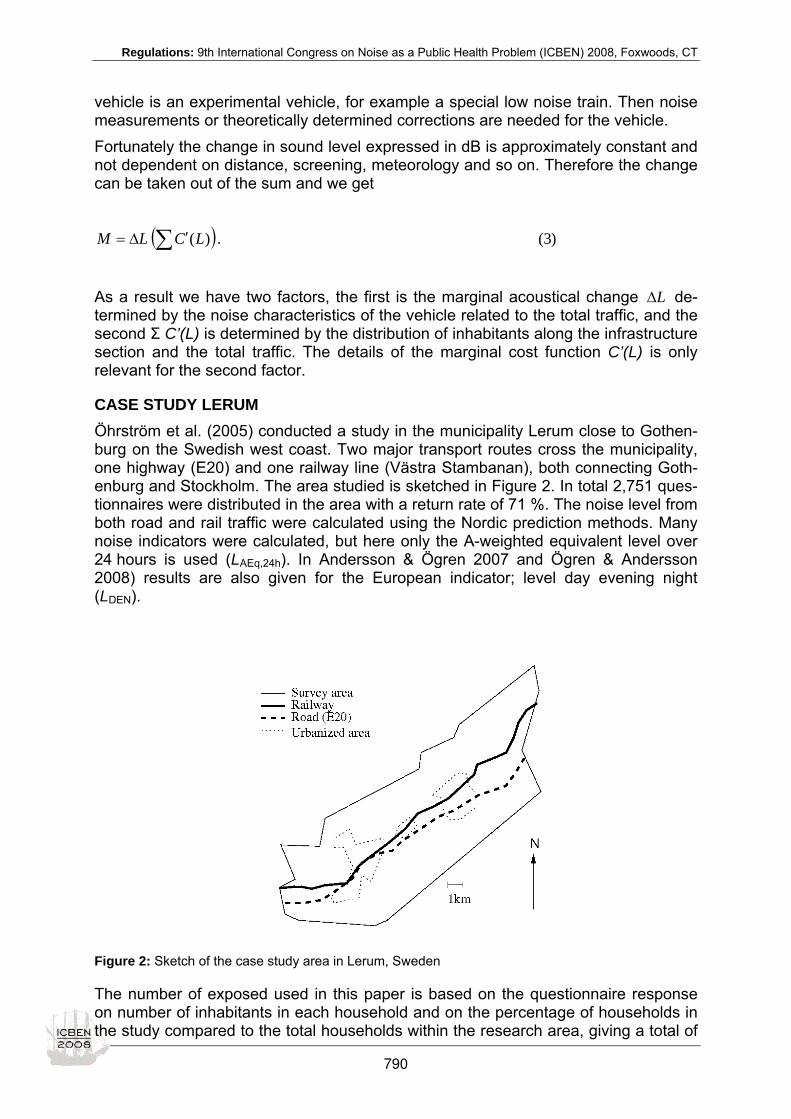
Regulations: 9th International Congress on Noise as a Public Health Problem (ICBEN) 2008, Foxwoods, CT
vehicle is an experimental vehicle, for example a special low noise train. Then noise measurements or theoretically determined corrections are needed for the vehicle. Fortunately the change in sound level expressed in dB is approximately constant and not dependent on distance, screening, meteorology and so on. Therefore the change can be taken out of the sum and we get
( ) )3(.)(∑ ′∆= LCLM
As a result we have two factors, the first is the marginal acoustical change L∆ de-termined by the noise characteristics of the vehicle related to the total traffic, and the second Σ C’(L) is determined by the distribution of inhabitants along the infrastructure section and the total traffic. The details of the marginal cost function C’(L) is only relevant for the second factor.
CASE STUDY LERUM Öhrström et al. (2005) conducted a study in the municipality Lerum close to Gothen-burg on the Swedish west coast. Two major transport routes cross the municipality, one highway (E20) and one railway line (Västra Stambanan), both connecting Goth-enburg and Stockholm. The area studied is sketched in Figure 2. In total 2,751 ques-tionnaires were distributed in the area with a return rate of 71 %. The noise level from both road and rail traffic were calculated using the Nordic prediction methods. Many noise indicators were calculated, but here only the A-weighted equivalent level over 24 hours is used (LAEq,24h). In Andersson & Ögren 2007 and Ögren & Andersson 2008) results are also given for the European indicator; level day evening night (LDEN).
Figure 2: Sketch of the case study area in Lerum, Sweden
The number of exposed used in this paper is based on the questionnaire response on number of inhabitants in each household and on the percentage of households in the study compared to the total households within the research area, giving a total of
790

Regulations: 9th International Congress on Noise as a Public Health Problem (ICBEN) 2008, Foxwoods, CT
4,956 (4,671) persons exposed to LAEq,24h > 50 dB for road (rail) traffic noise. The sound level at each exposed dwelling is determined from the calculations mentioned above, and finally the second term in equation (3) can be calculated for road and railway traffic noise. In order to calculate the marginal cost the first term in (3) we need the marginal change in sound level L∆ . In this study it is determined using the common European method HARMONOISE (de Vos et al. 2005) for road traffic and using the Nordic method for railway noise. The resulting marginal costs are given as noise charge per km in Table 1 together with the total traffic volumes.
Table 1: Estimated noise charges as Euro per km through the example area (Lerum, Sweden) in price level 2002
Cars 2 axles
110 km/h
Trucks 5 axles 90 km/h
High speed train200 m
135 km/h
Typical freight train650 m
90 km/h
Total traffic 24 h
17 600
1740
34 (1491)
41
SRMC Euro/km
0.00051
0.0059
0.033
0.30
1 34 high speed trains, and 149 counting all passenger trains together.
Note that it is difficult to use the calculated noise charges published here to compare the effects of railway noise and road traffic noise. One relevant comparison would be to compare the noise emission effect only, and then it is important to ensure that the number of exposed and length of the sections are identical, i.e. to remove the road and insert the railroad at the same position in the landscape. When comparing the two in the scope of a whole country or region, data for more than just one municipal-ity would be necessary, and it would also be important to take factors such as trans-port volumes, mean velocity and so on into account.
DISCUSSION The calculated values on the noise charges presented here are of limited value as such, since they only are relevant to the case study area, or other areas with similar population distribution, geography and so on. However, the approach as such shows that it is possible to estimate the marginal cost using standardized calculations meth-ods for traffic noise combined with published valuation methods. The noise calcula-tion method used in this paper is normally put to use for example during city planning, and the noise valuation method is in official use when performing cost benefit analy-sis of new road sections. As both methods are considered accurate and reliable enough to be usable in these contexts, the same should apply for estimation of rele-vant noise charges. One interesting experiment is look at what economic incentives are available if road or rail noise charges are implemented in a way that permits lower charges for low noise vehicles. If we assume that the charges are based on the marginal cost princi-ple, then using equation (3) we can easily estimate the effect of a vehicle with lower noise emission. Lowering the noise level with 5 dB gives a 70 % lower noise charge, a powerful incentive for the vehicle operator to introduce low noise technology. As examples 5 dB can be achieved by using low noise truck tires, and 8 dB is what the
791

Regulations: 9th International Congress on Noise as a Public Health Problem (ICBEN) 2008, Foxwoods, CT
international railway union UIC estimates as the average reduction if a freight train is retrofitted from cast iron to composite brake blocks.
ACKNOWLEDGEMENTS The authors gratefully acknowledge Evy Öhrström for the generous support with data from the Lerum study.
REFERENCES Andersson H, Ögren M (2007). Noise charges in rail infrastructure: a pricing schedule based on the marginal cost principle. Transport Policy 14: 204-213.
de Vos P (2003). How the money machine may help to reduce railway noise in Europe. J Sound Vibr 267: 439–445.
de Vos P, Beuving M, Verheijen E (2005). Harmonised accurate and reliable methods for the EU Directive on the assess-ment and management of environmental noise. Final technical report. http://www.harmonoise.org.
Larsen L (2005). Cost benefit analysis on noise-reducing pavements. Danish Road Institute report 146.
Navrud S (2005): Value transfer and environmental policy. Environmental and Resource Economics 2004/2005.
Navrud S, Trædal Y, Hunt A, Longo A, Greßmann A, Leon C, Espino Espino R, Markovits-Somogyi R, Meszaros F (2006). Economic values for key impacts valued in the stated preference studies. Deliverable 4 of HEATCO “Developing Harmonised European Approaches for Transport Costing and Project Assessment”. http://heatco.ier.uni-stuttgart.de/HEATCO_D4.pdf
Nijland HA, van Kempen EEMM, van Wee GP, Jabben J (2003). Costs and benefits of noise abatement measures. Transport Policy 10: 131-140.
Ögren M, Andersson H (2008). Noise charges in road traffic: a pricing schedule based on the marginal cost principle. Trans-port Policy (submitted).
Öhrström E, Barregård L, Skånberg A, Svennson H, Ängerheim P, Holmes M, Bonde E (2005). Undersökning av hälsoeffekter av buller från vägtrafik, tåg och flyg i Lerums kommun (in Swedish). ISSN 1400-5808.
Oertli J (2000). Cost-benefit analysis in railway noise control. J Sound Vibr 231: 505–509.
SIKA (2005). Kalkylvärden och kalkylmetoder – En sammanfattning av Verksgruppens rekommendationer 2005. SIKA (Swedish Institute for Transport and Communication Analysis) report 2005: 16.
792

Regulations: 9th International Congress on Noise as a Public Health Problem (ICBEN) 2008, Foxwoods, CT
Maslow’s hierarchy of needs as a model for the process of the development of national noise regulations George A. Luz Luz Social and Environmental Associates, 4910 Crowson Avenue, Baltimore, Maryland 21212, USA
e-mail: [email protected]
INTRODUCTION The subject matter of this paper arose out of a request received to write an article on international noise regulations for the Encylopedia of Environmental Health. The au-thor’s initial thought was to update Appendix 2, Examples of Regional Noise Situa-tions, in the World Health Organization (WHO) Guidelines on Environmental Noise (Berglund et al. 1999). However, upon revisiting the WHO Appendix, which covers Latin America, USA, South Africa, the Eastern Mediterranean, Southeast Asia and the Western Pacific, no unifying principles were apparent. In an attempt to find a uni-fying organizing principle, the author turned to a psychological theory known as Maslow’s hierarchy of needs.
METHOD The idea that the psychological development of humans proceeds from concern with basic physiological needs to self-actualization was introduced in 1943 by an Ameri-can behavioral psychologist, Abraham Maslow. Dissatisfied with the concept of American academic psychology that the end goal of the organism is homeostasis as well as Freud’s concept that the end goal of psychotherapy is the resolution of neu-rotic symptoms, Maslow argued that all human beings operate out of what he termed “an inborn hierarchy of needs.” The five stages of this hierarchy are physiological needs (breathing, food, water, sex, sleep, homeostasis, excretion), safety needs (se-curity of body, employment, resources, morality, family, health and property), love and belonging needs (friendship, family, sexual intimacy), need for esteem (self es-teem, confidence, achievement, respect for others, respect by others), and self-actualization (morality, creativity, spontaneity, spiritual enlightenment). Fulfillment of a lower stage in this hierarchy is a prerequisite for an individual to move toward ful-fillment of the next higher stage. Although Maslow intended his framework to apply to individuals, several social scientists have used it to predict developments within indi-vidual nations. Recent examples include strategies for eco-development in national parks in India (Rishi et al. 2008), institutional child care in developing countries (Tan-ner 2005) and annual quality of life in 88 countries over the period 1960 to 1994 (Hagerty 1999). Hagerty’s analysis confirmed that quality-of-life improvements within nations proceed along a temporal sequence of developmental stages. The temporal sequence of developmental stages is an essential element of Maslow’s theory, and the method used here was to look at the dates of milestones in the development of global noise regulations. A review of reviews was conducted (Bragdon 1970; Burton 2004; Concha-Barrientos et al. 2004; Flindell & McKenzie 2000; Finegold 2002; Johnson et al. 2001; Schwela 2000; Noise News International Editorial Staff 2000; Schultz 1982; Tachibana & Lang 2007; Wikipedia 2008). From these reviews, the correspondences between Maslow’s hierarchy and categories of noise regulation listed in Table 1 were developed.
793

Regulations: 9th International Congress on Noise as a Public Health Problem (ICBEN) 2008, Foxwoods, CT
Table 1: Comparison of the proposed stages of national noise regulations and Maslow’s hierarchy of needs
Maslow’s Hierarchy Individual Needs Corresponding Noise Regulations
Physiological Sleep Sleep disturbance
Safety Security of body Occupational hearing loss
Love/Belonging Friendship and family Community and low noise products
Esteem Respect of others Protecting children, noise sensitive
Self-actualization Creativity and spontaneity Preservation of natural quiet
RESULTS Regulating Sleep Disturbance Regulations against sleep disturbance predated the technology for noise measure-ment (Bragdon 1970). Chariots in ancient Rome were banned from the streets at night to prevent the noise of iron rims on paved streets that disrupted sleep. Similarly, in Beverley, England, a market town which drew buyers and sellers from all over me-dieval England, a fine was imposed on persons driving iron-wheeled carts wherever stone pavement existed. By the thirteenth century, some English towns enacted laws prohibiting blacksmiths from working in the early morning hours because of sleep disturbance from noise. In Japan, a country which was relatively isolated from the European technology until the rise of modern industrialization during the Meiji Restoration in 1868, the first nui-sance noise ordinance was enacted by Tokyo in 1871. This ordinance, which was the beginning of noise ordinances in Japan, prohibited unacceptable behaviors such as breaking serenity by unnecessarily loud sounds in the street or in other public places after midnight. After World War II, such nuisances as loud voices, loud music per-formances and loud radio sounds were restricted by the Minor Offenses Act in 1947. In the United States, the first attempts to deal with urban noise (including sleep dis-turbing noise) began after the Civil War (Smilor 1979). The most prominent and suc-cessful of these efforts was led by a physician, Julia Barnett Rice, in New York City, who, in 1906, founded the Society for the Suppression of Unnecessary Noise. Even after technology for noise measurement became available, non-quantitative regulation of nighttime noise, such as curfews, are common. The reason is that sleep disturbance is difficult to predict on the basis of noise measurements. Two major problems are the context effect and the definition of sleep disturbance. (1) Context Effect: Meta-analyses of field and laboratory studies have established that normal subjects are most likely to awaken to a specific decibel value of aircraft sound when sleeping in a sleep laboratory and least likely to awaken when sleeping in their own bedrooms in the vicinity of an airport. Subjects sleeping in their own bed-rooms but not accustomed to nighttime aircraft sounds fall between those two ex-tremes. (2) Definition of Sleep Disturbance: Within the U.S.and U.K, there is a tradition of de-fining sleep disturbance as an awakening in which the subject is alert enough to push a button indicating a wakened status. Within Germany and some other European countries, there is a tradition of defining sleep disturbance as a physiological arousal,
794

Regulations: 9th International Congress on Noise as a Public Health Problem (ICBEN) 2008, Foxwoods, CT
such as a shift in EEG toward a shallower stage of sleep. Use of physiological arousal is justified by evidence that subjects experience aftereffects during the next day, such as irritability and fatigue, even if they never fully awaken. At the same time, this difference has led to more conservative guidelines in some European countries than in the U.S.
Regulating Hearing Hazardous Noise Concerns about noise-induced hearing loss arise with industrialization. The recogni-tion that excessive exposure to noise in the workplace can lead to permanent loss of hearing appears to have first emerged during the 1870’s with the observations of English physicians (Roosa & St John 1873) in regards to “Boilermakers’ Deafness”, but a critical mass of patients with noise-induced hearing loss did not emerge until World War I. Shortly before World War I, German researchers were on the cutting edge of understanding noise-induced hearing loss (Hawkins 1976), but their progress was limited by not having effective technology to measure sound or to evaluate hear-ing sensitivity. Both technologies became available in the U.S. and U.K. during World War II. At the Harvard Biological Laboratory, Dr. Hallowell Davis’ wartime experi-ments in noise-induced hearing loss were facilitated by the availability of the sound level meter and the audiometer (Western Electric 6-B). In addition, the burst of re-search initiated by Bell Laboratories and other innovators in electro-acoustics during the inter-war period allowed access to oscillators, amplifiers, attenuators and ear-phones of sufficient quality for scientific work. At the end of WW II, the U.S. had a legacy of veterans with hearing loss, an active duty military force which was continuing to develop hearing loss, and a military budget with the luxury to address the problem. Consequently, world leadership in this stage of regulation came out of the U.S. Department of Defense. The Air Force pub-lished the first hearing conservation regulation which set limits to noise exposures from jets and rocket power plants, and mandated audiometric testing procedures (US Air Force 1948) and the Navy published a comparable regulation (US Navy 1953). DoD funded a group of experts to come together as the Armed-Forces National Re-search Council Committee on Hearing and Bio-Acoustics who issued their first report in 1954 (CHABA 1954). In October 1956, AFR 160-3 was updated and titled, “Haz-ardous Noise Exposure”. This publication became the first recognized comprehen-sive hearing conservation program (HCP), both within and outside the military and served as the template used by successive government and non-government organi-zations for establishing HCP’s within their respective agencies. The first U.S. legal limits for industrial noise exposure were not written into the Walsh Healy Public Contracts Act until 1969. This long standing resistance of the U.S. in-dustrial base to noise regulation was aided and abetted by two scientific issues. The first was the definition of “normal hearing.” European data on the sensitivity of the healthy young ear showed greater sensitivity than U.S. data. This resistance was broken through political maneuvering by the Executive Secretary of CHABA, a ma-neuver referred to as “tricky Hallowell’s end run” (Washington University 1977). The second scientific issue was the mathematical model used to predict hearing loss. In AFR 160-3, the U.S. Air Force adopted a model published by W.A. Rosenblith and K.N. Stevens in 1953 who adopted their model from earlier work by Dr. Karl Kryter in 1950 on using the “critical band concept” as a predictor of hearing hazard. The limits specified by AFR 160-3 for life-time exposures to broad band noise included four oc-tave bands: 300-600. 600-1200, 1200-2400. and 2400 to 4800 Hz. The risk of hear-ing impairment was stated to be slight if the octave-band level did not exceed 85 dB,
795
Regulations: 9th International Congress on Noise as a Public Health Problem (ICBEN) 2008, Foxwoods, CT
but to be excessive at 95 decibels (dB) Within the private sector, the mathematical model adopted in AFR 160-3 was considered to be inadequate. For example, in 1954, an exploratory committee (Z24-X-2) of the American Standards Association surveyed all available data on hearing loss among the industrial workforce and con-cluded that the data could not be sufficiently validated for regulating industrial noise exposures of the U.S. workforce. The mathematical model of hearing loss which became incorporated into the 1969 amendment to the U.S. Walsh-Healy Act required that hearing protection be worn when average noise levels exceeded 90 decibels, A-weighted (dBA) in an 8 hour pe-riod (using a 5 dB exchange rate), and when impulse/impact noise exceeded 140 dB Peak. In 1971, this standard was incorporated into the Occupational Safety and Health Act of 1970, eventually leading to the OSHA Hearing Conservation Amend-ment in 1983. The theoretical basis for this model was the observation by Dr. W. Dixon Ward and others that the amount of temporary threshold shift at two minutes after the cessation of an exposure to a continuous noise (TTS2) could be mapped onto the amount of permanent threshold shift (PTS) among factory workers after a lifetime of exposure to workplace noise of a comparable spectrum and level. In labo-ratory experiments, recovery from TTS2 was observed to proceed as a function of the logarithm of post-recovery time, and experimentation with different exposures led to the 5 decibel rule. Thus, an 8 hour exposure to 90 dBA was considered to be equally hazardous as a 4 hour exposure to 95 dBA and a 2 hour exposure to 100 dBA. The mathematical model was clearly superior to the Rosenblith-Stevens model, and in 1970, the Navy adopted the OSHA noise standard as part of their HCP in BUMEDINST 6260.6B, mandating enrollment in HCPs when the noise levels ex-ceeded 90 dBA. Subsequently, dozens of laboratory tests of the 5 dB rule in which multidisciplinary teams looked at the behavioral thresholds, electrophysiological functioning and co-chlear histology of noise-exposed animals failed to demonstrate the reliability of the 5 dB time-intensity relationship, and the majority of experts came to support a 3 dB rule for continuous noise exposures, which is known as the “equal energy rule” or “equivalent noise level (Leq).”
Regulating Community Noise Exposures Quantitative national laws for community noise tend to begin at the municipal or pro-vincial level prior to enactment of national occupational noise laws, later culminating in national community noise guidelines. For example, the U.S. Congress passed the Noise Control Act in 1972, five years after the occupational noise amendment to the Walsh Healy Act. Japan’s Occupational Health Association set down permissible noise criteria consisting of three band levels (500 – 2000 Hz) in 1966; the Basic Law for Environmental Pollution was issued in 1968 with guideline values for general envi-ronmental noise, aircraft noise and Shinkansen railway noise in 1971, 1973 and 1975, respectively. Although South Africa had provided community noise guidance to local jurisdictions in the Environment Conservation Act of 1989, their first national noise law was the Occupational Health and Safety Act of 1993. Australia published the National Code of Practice for Noise Management and Protection of Hearing at Work in 1992 but did not introduce the Sydney Airport Demand Management Plan until 1997. As with the third stage of Maslow’s hierarchy, the focus of most community noise regulations is the family and community and, typically, the first sources to be ad-dressed are motor vehicles and aircraft.
796

Regulations: 9th International Congress on Noise as a Public Health Problem (ICBEN) 2008, Foxwoods, CT
The historical record suggests that the first country to consider a methodology for regulating the noise of motor vehicles was the U.K. in 1934 (Berry 1998). Interrupted by World War II, National Physical Laboratory researchers did not return to this sub-ject until 1959. In the meantime, the growth of the commercial airline business, par-ticularly in the U.S., led to a new regulatory challenge. The history of regulations for aircraft noise began with a single question asked (at the municipal level) by the New York Port Authority in 1956, “How loud is the Boeing 707 jet aircraft compared with the propeller-driven airplanes which have been using the New York International Airport at Idlewild, now JFK, Airport?” (Beranek 2007). The Boeing Company, which had compared the noise levels of both types of aircraft using the linear scale of the sound level meter, concluded that there was not a significant difference between aircraft. However, the acoustical engineering firm, Bolt, Beranek and Newman, which employed a psychologist, Dr. Karl Kryter, to compare the two types of aircraft, concluded that the jet aircraft would be perceived as significantly louder than the propeller-driven aircraft. Kryter based his analysis on the loudness model developed by another psychologist, Dr. S.S. Stevens of the Harvard Psycho-acoustic Laboratory. This application yielded the basic measure, Perceived Noise Level (PNL) which was later improved to become the Effective Perceived Noise Level (EPNL) and incorporated into a technology for land-use planning, Noise Exposure Forecast (NEF). When, sixteen years later, the U.S. Congress authorized the US Environmental Pro-tection Agency to regulate community noise, EPNL was set aside in favor of a more convenient European approach, the Equivalent Level, a measure which achieved nearly global acceptance toward the end of the 20th Century.
Protecting the Most Vulnerable As a human matures to a stage where he or she experiences self esteem, a concern for others, particularly for the most vulnerable, also emerges. Similarly, as a safe and secure society matures, there is a growing concern for the most vulnerable members of that society. In regards to noise exposures, two vulnerable groups are children and people who are “noise-sensitive.” Within the U.S., the first experimental demonstration that noise has an adverse im-pact on children in classrooms was published in 1932 (Hartmann 1946), but over 25 years passed before a municipal government in the U.S. used its regulatory powers to protect children from noise (Bronzaft 1981). At the U.S. Federal level, the USEPA never addressed the needs of this vulnerable group, despite a credible body of scien-tific literature. Not until the adoption of the Americans with Disabilities Act (ADA) of 1990 was there an opportunity for noise regulation benefiting children. The trigger was a petition from a parent of a child with hearing loss who requested that the ADA Accessibility Guidelines be amended to include acoustical standards for classrooms. In June 1998, the ADA Board requested public input on this issue, a request an-swered by the Acoustical Society of America. The result was American National Standard S12.60-2002 on Classroom Acoustics. Although the standard is voluntary, it was written to be easily incorporated in building codes, and some U.S. cities and states have done so. As to the needs of the approximately one-in-five adults who can be categorized as “noise-sensitive”, there has been no activity whatsoever by any level of government within the United States. With the exception of an influential study by an American psychologist in the late 1970’s (Weinstein 1978), the research in this area has been
797

Regulations: 9th International Congress on Noise as a Public Health Problem (ICBEN) 2008, Foxwoods, CT
dominated by scientists from Europe and the Western Pacific regions. A search of the American Psychological Association’s PsycNet data base suggests that the earli-est reference to noise sensitivity came from a Spanish journal (Suils 1942), but the first serious consideration of the subject appears to have developed in the UK (Broadbent 1972). Although it would be economically infeasible for any society to tailor community noise regulations for this most vulnerable segment of the population, it is still possible to give consideration to the noise-sensitive within a regulatory environment. For exam-ple, the Sydney Airport supplements Australian Noise Exposure Forecast maps with maps showing areas where the levels of individual flights are in excess of 70 dBA (Southgate 2000). These maps include information on the number of daily flights and the times of day when the flights occur. Although such maps are not used to prohibit people from living in a noise-exposed neighborhood, the information facilitates noise-sensitive persons in making informed decisions about choosing a residence. This approach to protecting the noise-sensitive individual is consistent with the political philosophy known in the U.S. as “libertarian” government.
Preservation of Natural Quiet The preservation of the natural quiet and natural soundscapes is a relatively recent development in noise regulation. It is the last stage of development, and it is unlikely to be undertaken unless a country is relatively wealthy and contains a critical mass of citizens who will lobby to preserve natural quiet. Anecdotal evidence suggests that creativity and spontaneity, characteristics of Maslow’s self-actualization stage, are important to these citizens. Within the U.S., the initiative for the regulation of noise in quiet outdoor areas came from Public Law 100-91, The National Park Service Overflights Act of 1987. This ini-tiative was driven by citizens concerned about Grand Canyon National Park, which, within the span of a single generation, has suffered visual degradation from air pollu-tion and noise pollution from tour aircraft, particularly helicopters. The passage of PL 100-91 led to a burst of creativity among experts in noise regula-tion. Up to that point, noise regulations had been focused on achieving a specific decibel value while following a measurement procedure prescribed in a national or international standard. For the regulation of natural quiet, there cannot be a single number. In Table 4-1 of its Guidelines for Community Noise, the WHO recommends that existing quiet outdoor areas should be preserved and that the ratio of intruding noise to natural background sound be kept low. This goal precludes using Leq, be-cause a single value cannot preserve the fine structure of the soundscape. With two decades having passed since the passage of PL 100-91, it is clear that some progress has been made. The noise signatures of touring aircraft and helicop-ters in U.S. National Parks have been greatly reduced. New computer models have been introduced which provide more accurate predictions of the spectra of aircraft at longer distances than had been available from the older computer models used to calculate average noise levels around airports (e.g. the U.S. Federal Aviation Ad-ministration’s INM). Measurements and analyses of the propagation of sound through various terrains have been published, to include studies of natural masking sounds (e.g. wind in the trees). Because of the large expanse of U.S. National Parks, Na-tional Forests and designated wilderness areas, there is a growing consensus that management and preservation of the soundscape can only be achieved through computer modeling. Using Geographical Information System (GIS) technology, it has
798

Regulations: 9th International Congress on Noise as a Public Health Problem (ICBEN) 2008, Foxwoods, CT
been demonstrated that the probability of noticing highway traffic, rail traffic or jet air-craft traffic during the daytime can be calculated by county across the entire U.S. (Miller 2003). In Europe, which has relatively few areas of natural quiet compared to North America, the emphasis has been on a companion concept, the soundscape. The technology for the analysis of soundscapes is applicable to urban as well as ru-ral areas (Schulte-Fortkamp et al. 2007). Lessons learned in the preservation of natural quiet and soundscapes are applicable to unique acoustic environments, such as found in Australia, Africa and South Amer-ica. To date, grass roots efforts in this direction have been sporadic (and undocu-mented in published literature). Examples include an attempt to address the impact of the noise from tourist boats in the Periyar Tiger Reserve in India (Sidhu & Sebas-tian 1998) and activism over the noise of helicopter flights in the Capertee Valley, New South Wales, Australia (Hut News 2007).
CONCLUSIONS Within the U.S., the development of noise regulations followed the sequence outlined in Table 1. Specifically, Stage 1 (sleep disturbance) took place during the period 1865-1930, Stage 2 (hearing loss) during the period 1953-1969, Stage 3 (community) in 1972, Stage 4 (protection of the most vulnerable) in 1981, and Stage 5 (Protection of natural quiet) in 1987. Similar sequences of development have been observed among many of the countries in the European and Western Pacific regions. It is logi-cal to expect that this sequence will be followed in other nations. At the same time, developing countries have the opportunity to benefit from the lessons already learned from successes and failures in Europe and North America.
REFERENCES Beranek LL (2007). The noisy dawn of the jet age. Sound and Vibration 4: 94-100.
Berry B (1998). Standards for a quieter world: some acoustical reflections from the UK National Physical Laboratory. Noise News Int 6: 74-83.
Berglund B, Lindvall T, Schwela, D, Goh K-T (1999). Guidelines for community noise. Geneva: World Health Organization.
Bragdon C (1970). Noise pollution: the unquiet crisis. Philadelphia, PA: Univ. of Pennsylvania Press.
Broadbent (1972). Individual differences in annoyance by noise. Sound 6: 56-61.
Bronzaft A (1981). The effect of a noise abatement program on reading ability. J Environ Psychol 1: 215-222.
Burton N (2004). Methods of assessment of aircraft noise. Thesis submitted to Department of Engineering Systems, London South Bank University, Department of Engineering Systems.
CHABA (1954). High-intensity noise and military operations: an evaluation, CHABA report no. 1, Saint Louis, MO: Armed Forces National Research Council Committee on Hearing and Bio-Acoustics.
Concha-Barrientos M, Campbell-Lendrum D, Steenland K (2004). Occupational noise: assessing the burden of disease from work-related hearing impairment of national and local levels. Environmental burdens of disease Series No. 9. Geneva: World Health Organization.
Finegold L (2002). An overview of U.S. noise policy. Noise News Int 10: 51-63.
Flindell I, McKenzie A (2000). An inventory of current European methodologies and procedures for environmental noise management. Technical Report, Contract No. 3213/B1999.EEA.37044. Copenhagen: European Environment Agency.
Hagerty M (1999). Testing Maslow’s hierarchy of needs: national quality-of-life across time. Soc Indicators Res 46: 249-271.
Hartmann G (1946). The effects of noise on school children: an interpretative digest and recommendation. J Educ Psychol 37: 149-160.
Hawkins J (1976). Experimental noise deafness: recollections and ruminations. In: Hirsh SK, Eldredge DH, Hirsh IJ, Silverman SR (eds.): Hearing and Davis: essays honoring Hallowell Davis. St. Louis, MO: Washington Univ. Press.
799

Regulations: 9th International Congress on Noise as a Public Health Problem (ICBEN) 2008, Foxwoods, CT
Hut News (2007). Capertee Valley heliflights. Issue 236 (http://www.bluemountains.org.au/HutNews/0706news.pdf).
Johnson D, Papadopoulos P, Watfa N, Takala J (2001). Exposure criteria, Occupational exposure levels. In: Goelzer B et al. (eds.): Occupational exposure to noise: evaluation, pevention and control (pp 79-102). Geneva: World Health Organization.
Maslow A (1943). A theory of human motivation. Psychol Rev 50: 370-396.
Miller NP (2003). Transportation noise and recreational lands. Noise News Int 11: 19-21.
Noise News International Editorial Staff (2000). Overview of Japanese environmental regulations on noise. Noise News Int 8: 64-76.
NPS (1995). Report on effects of aircraft overflights on the National Park System: executive summary, report to Congress, appendixes. Washington, DC: National Park Service: U.S. Department of the Interior.
Rishi P, Moghe S, Upadhyay B (2008). Analysis of hierarchy of needs and motivational strategies for eco-development plan-ning in two national parks of India. Resources, Conservation & Recycling 52: 707-718.
Roosa D, St John B (1873). Treatise on the diseases of the ear. New York: William Wood & Co.
Schulte-Fortkamp B, Brooks B, Bray W (2007). Soundscape: an approach to rely on human perception and expertise in the post-modern community noise era. Acoust Today 3: 7-14.
Schultz T (1982). Community noise rating (2nd ed.). London: Elsevier Science Publications.
Schwela D (2000). The World Health Organization guidelines for environmental noise. Noise News Int 8: 9-22.
Sidhu R, Sebastian J (1998). Letter to Asia-Pacific editor. Noise News Int 6: 104.
Smilor R (1979). Personal boundaries in the urban environment: the legal attack on noise: 1865-1930. Environ Rev 3: 24-86.
Southgate D (2000). Expanding ways to assess and describe aircraft noise. Paper given as part of the Value of Supplemen-tal Noise Metrics in Aircraft Noise Analysis at Year 2001 International Airport Noise Symposium, February 28, 2000, San Diego, CA (available at www.fican.org).
Suils A (1942). Sobre las llamadas "neurosis del ruido." / The so-called "noise neuroses." Psicotecnia 3: 327-336.
Tachibana H, Lang W (2007). Survey of policies and regulations for control of community noise: Draft final report 0X-Y of the I-INCE Technical Study Group on Noise Policies and Regulations (TSG 3).
Tanner R (2005). Applied sociology and institutionalized professionalism. Some reflections on the pragmatics of child care in developing societies. An adaptation of Maslow’s hierarchy of needs. J Soc Sci 11: 15-20.
US Air Force (1948). Air Force Regulation (AFR) 160-3. Precautionary Measures Against Noise Hazards.
US Navy (1953). Bureau of Medicine and Surgery (BUMED) Instruction. Hearing Conservation Program.
Washington University (1977). Transcript: Hallowell Davis, 1977, Washington University School of Medicine: oral history project (http:beckerexhibits.wustl.edu/oral/transcripts/davis.html).
Weinstein N (1978). Individual differences in reactions to noise: a longitudinal study in a college dormitory. J Appl Psychol 63: 458-466.
Wikipedia (2008). Noise regulation (http:/en.wikipedia.org/wiki/Noise_regulation).
800
Regulations: 9th International Congress on Noise as a Public Health Problem (ICBEN) 2008, Foxwoods, CT
Acoustical design of hospitals: Standards and priority indexes Sergio Luzzi1*, Raffaella Bellomini1, Claudia Romero2 1 Vie En.Ro.Se. Ingegeneria, Via Stradivari 23, 50134 Florence, Italy
2 Politecnica, Viale Amendola 6, 50121 Florence, Italy
* corresponding author: e-mail: [email protected]
INTRODUCTION Improving acoustic conditions will result in a shorter or better hospital stay for pa-tients? And will it result in a better performance of medical teams? Possible answers to these questions can be derived from scientific literature and confirmed by recent experiences here reported. Unfortunately the patients’ stay in hospital areas is often characterized by long peri-ods of inactivity where they spend their time doing nothing and so becoming more sensitive towards environmental quality and comfort of their staying. In his/her hospi-tal lifetime a patient can find a very short number of distractions as compared to nor-mal life. This paper refers to a methodological approach that aims to reduce noise in design-ing new hospital settings, with special attention to the most sensitive areas. Starting from a review of international studies and papers on acoustic conditions in healthcare buildings, as well as on international standards and national provisions, a group of architects, engineers and acousticians with different backgrounds and affilia-tions, have joined with medical doctors working in and managing hospitals. The main aim of the group is to produce proposals for a guideline for acoustic comfort design of sensitive areas and activities, relating to new buildings and refurbished ones. Models and indexes for the identification of hotspots and critical factors in health structure acitivities (and consequent priorities) have been investigated with special attention to those based on time of exposure and severity of illness. Indexes have been proposed and tested, giving, as first result of the research, information about acoustical comfort or discomfort in existing hospitals.
METHODS In the Italian experience, according to European and National laws and standards, Public Administration and Control Authorities ask the designers of new healthcare buildings for careful and accurate studies of the acoustic behavior of new settle-ments, considering problems of compatibility in areas with different destinations. The predictive assessment of environmental noise pollution is obtained from the cor-rect estimation of the impact of plants, activities, traffic and other sources and then adapting algorithms provided for. But a healthcare building is a system of sources and receivers of noise pollution it-self; there are rooms and areas where sources and receivers must co-exist and the annoyance is produced by noise generated inside the area combined with noise coming from outside. In 1992 the United Nations Conference on Environment and Development of Rio de Janeiro established the principle of sustainable development. From the diffusion of
801

Regulations: 9th International Congress on Noise as a Public Health Problem (ICBEN) 2008, Foxwoods, CT
this cultural approach derives the need of a definition of rules and procedures for the correct designing of buildings and living spaces. Every building could have been de-signed in such a way to be comfortable and non-inducing pathologies like Sick Build-ing Syndrome (SBS), also called Tight Building Syndrome (TBS), and Building Re-lated Illness (BRI). The final aim for designers must be to provide building occupants with a healing environment free of disruptive levels of sound. In this context, wellness and eco-compatibility in the designed buildings are consid-ered also in terms of simultaneous reduction of noise breakings in. Thus healthcare facilities represent a challenge and an opportunity in the development and implemen-tation of sustainable design, construction and operations practices. Several methodological approaches consider the assessment and the improvement of acoustic atmosphere and acoustic comfort in internal areas, where sensitive re-ceivers (patients) usually live, starting from information about territory and structure of buildings, considering case scenarios with various levels of complexity, due to dif-ferent compositions of sources and receivers. The structure of buildings and the re-lated structure-borne sound propagation in the internal areas can be analyzed using the ISO methods and models concerning the acoustic properties of buildings. A general designing scheme starts from the acoustic climate “ante operam” and con-sider: acoustic analysis of inner and external sources; measurement and computa-tion of acoustic impact on the inner and external receivers; analysis of acoustic re-quirement of the building; final designing.
Figure 1: Example of internal sources of a General Hospital
Noise impact of a new building on the acoustic atmosphere of the surrounding re-ceivers has to be measured and analyzed in advance. Italian City Administrators ask for noise impact prediction, as a necessary preliminary document, to authorize each potentially pollutant activity or building. The International Standard references (ISO 8297 for the determination of sound power levels of multisource industrial plants, ISO 9613-2 for the method of calculation of the attenuation of sound during propagation outdoors) can be considered. The analysis of the acoustic quality of the building has to be carried on measuring and calculating all the significant parameters, such as Rw, Ln, w, D2m,nT,w also de-fined by the ISO standards. This methodological approach brings to a view of the acoustic performance of a building, based upon the modeling of sources and receivers located inside and out-side it.
802

Regulations: 9th International Congress on Noise as a Public Health Problem (ICBEN) 2008, Foxwoods, CT
In Table 1 the step by step sequence of activities that take to an acoustically com-patible way of sensitive building designing has been schematically shown. It can be assumed as a minimum required roadmap for healthcare building designers
Table 1: The acoustical design procedure flowchart for a generic health care building
Also considering the contents of recently published documents and guidelines like Design Guidelines for Hospital and Healthcare Facilities, drafted by Technical Com-mittees for Architectural Acoustics and Noise of the Acoustical Society of America, it is possible to make the reasons of environmental quality and high performance join together in a new healthcare units design philosophy. Not forgetting that besides the importance of acoustic comfort, there are the positive reasons of Music Therapy: good sound atmosphere may give to patients a physiological benefit but unfortu-nately, as we will see in the following paragraphs, it is often obscured by all the ran-dom (and often) unnecessary sounds that affect patients, even in the most noise sensitive units. Recent UK measurement campaigns (see Boulter 2007) where the intention was to follow a typical patient journey through the hospital areas and activities, result that in all the locations visited, occupational noise dominates the environment. Daytime LAeq noise levels in ICU (from the patient side, very sensitive unit) were significantly higher (from 62 to 64 dB LAeq), mostly as a result of noise from the medical equip-ment.
CRITICAL AREA MODELS AND THEIR APPLICATION TO CASE STUDIES A model based on a special index of acoustical sensitivity has been introduced by authors, see Luzzi (2004). It is a parametric index describing the need for particular conditions of acoustical comfort in sensitive areas of buildings. It is related to some other indexes representing time of staying inside the considered area (i.e. hospitali-zation) and the gravity of the potential annoyance (i.e. heaviness of noise exposure in a working place, severity of illness of patients in a hospital unit).
ACOUSTICAL STUDY - ante operam assessment - simulations A1 acoustical ante operam climate assessment in the interested area
A2 noise impact prediction of internal sources on internal and external poten-tially annoyed receivers
B1 noise impact prediction of outdoors sources on internal potentially annoyed receivers according to de-signed layout
B2 prediction of the acoustical behavior of wall, ceilings and other building elements
ACOUSTICAL DESIGN - corrections A DEFINITION OF ENVIRONMENTAL ASSESSMENT OF BUILDING
B DESIGN OF ACOUSTICAL OPTIMISATION OF INNER SPACES
ACOUSTICAL TEST - post operam assessment - measurements A1 acoustical post operam climate assessment in the interested area
A2 noise impact assessment of internal sources on internal and external potentially an-noyed receivers
B1 noise impact assessment of outdoors sources on internal potentially annoyed receivers according to de-signed layout
B2 acoustical analysis of structure and materials acoustic behavior of wall, ceilings and other building elements
ACOUSTICAL CERTIFICATION - qualification of building A COMPATIBILITY WITH ENVIRONMENT
B COMFORT OF INTERNAL AREAS
803

Regulations: 9th International Congress on Noise as a Public Health Problem (ICBEN) 2008, Foxwoods, CT
The acoustical criticity index c is a two variables functional, capable to represent with good level of approximation the need of acoustical comfort as a function of noise ex-posure time and annoyance severity. The proposed model is supported by some series of statistical data collected from literature and directly tested by authors in contexts where noise-generated discomfort and annoyance had produced physiological or psychological effects and influenced performance and concentration. For example in sensitive areas of hospital, like in-tensive care units, a strong correlation between acoustical comfort and effectiveness of therapy has been found. Acoustical analysis of internal critical areas with different destination and with differ-ent sources has been developed and standard values for constants and parameters have been found. Sound levels measurements, frequency and statistic analysis, computation of in-dexes and definition of the acoustical environment during standard activities, study of acoustic quality of building, furniture, materials, means of sound propagation and ra-diation have been considered. Case studies referred to different Italian hospitals can show the behavior of index c associated to a specific context (hospital area or activity), and its relationships with: - t: time of patient-stationing in that area or of patient-subjection to that activity. - g: gravity or severity of an illness or, more general, physiological state of the pa-
tient. The aim is to represent the discomfort and annoyance level of each significant hospi-tal area or activity using c index. The functional c = f (t,g) has been defined and the combined dependence on t and g has been derived from simple mathematical equations that take in account the para-metric relative weight of places and activities. In some hospitals a group of sample contexts, like operating theater, recovery room, delivery room, intensive care unit, and others have been considered as applicative sceneries of the model. For each of them, statistical data about the standard time of patient staying in the unit and about the distribution of values of the main scoring sys-tems, like GLASGOW and APACHE (Acute Physiology, Age, and Chronic Health Evaluation) have been found and put in the validation algorithm of the model, with the aim to find approximately the best fitting functional relationship c = f (t,g) in agree-ment with the two variables standard trend equations, summarized in Table 2. Index c gives a measure of the acoustical comfort or discomfort of areas and activi-ties carried on in healthcare buildings. The model has shown its efficiency above all in hospital contexts where hospitalization time of patients could be easily foreseen and activity cycles could be easily standardized. In all the case studies, time interval series, scales and units are chosen as the best fitting for the referred place or acti-vity.
804
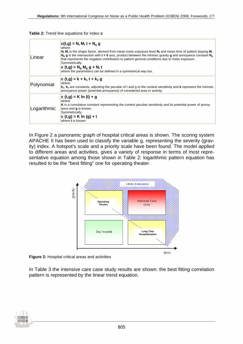
Regulations: 9th International Congress on Noise as a Public Health Problem (ICBEN) 2008, Foxwoods, CT
Long TimeHospitalization
Operating Theatre
Table 2: Trend line equations for index c
Linear
c(t,g) = Nt Mt t + Ng g where: Nt Mt is the shape factor, derived from mean noise exposure level Nt and mean time of patient staying Mt Ng g is the intersection with t = 0 axis, product between the intrinsic gravity g and annoyance constant Ng that represents the negative contribution to patient general conditions due to noise exposure. Symmetrically, c (t,g) = Ng Mg g + Nt t where the parameters can be defined in a symmetrical way too.
Polynomial c (t,g) = k + k1 t + k2 g where: k1, k2 are constants, adjusting the peculiar of t and g to the context sensitivity and k represent the intrinsic annoyance power (potential annoyance) of considered area or activity.
Logarithmic
c (t,g) = K ln (t) + g where: K is a cumulative constant representing the context peculiar sensitivity and its potential power of annoy-ance and g is known. Symmetrically, c (t,g) = K ln (g) + t where t is known
In Figure 2 a panoramic graph of hospital critical areas is shown. The scoring system APACHE II has been used to classify the variable g, representing the severity (grav-ity) index. A hotspot’s scale and a priority scale have been found. The model applied to different areas and activities, gives a variety of response in terms of most repre-sentative equation among those shown in Table 2: logarithmic pattern equation has resulted to be the “best fitting” one for operating theater.
Figure 2: Hospital critical areas and activities
In Table 3 the intensive care case study results are shown: the best fitting correlation pattern is represented by the linear trend equation.
805

Regulations: 9th International Congress on Noise as a Public Health Problem (ICBEN) 2008, Foxwoods, CT
Table 3: Index c in the intensive care unit case study
THE SIX SIGMA APPROACH Six Sigma is a quality management philosophy and a business discipline that aim to improve processes so that they could perform at their highest possible levels. In healthcare buildings levels of performance can be related to environmental comfort indexes, like the acoustical one described in the previous paragraph. Six Sigma is based on two models, depending upon the nature of involved proc-esses. The improvement of existing processes follows a DMAIC (Define, Measure, Analyze, Improve and Control) model; the development of a new process follows the DMADV (Define, Measure, Analyze, Design and Verify) model. A case study, see Luchsinger (2008), illustrates how a healthcare Six Sigma project team applied the DMAIC approach to improving the care of open-heart surgery pa-tients by reducing their post-operative length of stay. The result was an increase of the quality of patient care while reducing the average length of stay and costs for pa-tients. Another case study, see Bertels (2007), leads with the problem of excessive cycle times for processing orthopedic disability claims. As a result of Six Sigma approach the total cycle time was reduced from an average of seventeen to less than six days, variation was reduced by 60 %, and less than 16 % of all cases took longer than ten days. It’s possible to adapt the critical area models described above to the Six Sigma ap-proach. For example, the fishbone diagram in Figure 3 represents the quality pattern of the possible contributors to post-op length of stay. It is used in identifying all the potential contributors to process variations, a fundamental principle of the Six Sigma approach.
806
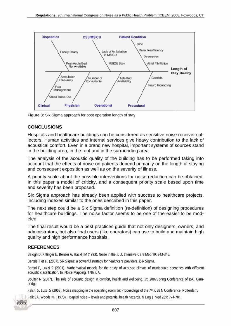
Regulations: 9th International Congress on Noise as a Public Health Problem (ICBEN) 2008, Foxwoods, CT
Figure 3: Six Sigma approach for post operation length of stay
CONCLUSIONS Hospitals and healthcare buildings can be considered as sensitive noise receiver col-lectors. Human activities and internal services give heavy contribution to the lack of acoustical comfort. Even in a brand new hospital, important systems of sources stand in the building area, in the roof and in the surrounding area. The analysis of the acoustic quality of the building has to be performed taking into account that the effects of noise on patients depend primarily on the length of staying and consequent exposition as well as on the severity of illness. A priority scale about the possible interventions for noise reduction can be obtained. In this paper a model of criticity, and a consequent priority scale based upon time and severity has been proposed. Six Sigma approach has already been applied with success to healthcare projects, including indexes similar to the ones described in this paper. The next step could be a Six Sigma definition (re-definition) of designing procedures for healthcare buildings. The noise factor seems to be one of the easier to be mod-eled. The final result would be a best practices guide that not only designers, owners, and administrators, but also final users (like operators) can use to build and maintain high quality and high performance hospitals.
REFERENCES Balogh D, Kittinger E, Benzer A, Hackl JM (1993). Noise in the ICU. Intensive Care Med 19: 343-346.
Bertels T et al. (2007). Six Sigma: a powerful strategy for healthcare providers. iSix Sigma.
Bertini F, Luzzi S (2001). Mathematical models for the study of acoustic climate of multisource sceneries with different acoustic classification. In: Noise Mapping, 17th ICA.
Boulter N (2007). The role of acoustic design in comfort, health and wellbeing. In: 2007Spring Conference of IoA, Cam-bridge.
Falchi S, Luzzi S (2003). Noise mapping in the operating room. In: Proceedings of the 7th ICBEN Conference, Rotterdam.
Falk SA, Woods NF (1973). Hospital noise – levels and potential health hazards. N Engl J Med 289: 774-781.
807

Regulations: 9th International Congress on Noise as a Public Health Problem (ICBEN) 2008, Foxwoods, CT
Hodge B, Thompson JF (1990). Noise pollution in the operating theatre. Lancet 335: 891-894.
Kam PCA, Kam AC, Thompson JF (1994). Noise pollution in the anaesthetic and intensive care environment. Anaesthesia 49: 982-986.
Liu EHC, Tan S-M (2000). Patients perceptions of sound levels in the surgical suites. J Clin Anesth 12: 298-302.
Luchsinger J et al. (2008). Six Sigma catapults hospitals to next level of quality. iSix Sigma.
Luzzi S (2005). Mapping and reducing noise pollution in hospitals. ELPIT Togliatti City (Russia).
Luzzi S, Falchi S (2002). Noise pollution in a general hospital. Canad Acoust 30: 128-129.
Luzzi S et al. (2003). Sound analysis of noise pollution in operating rooms. In: Proceedings of Euronoise 2003, Naples.
Luzzi S et al. (2004). Receivers comfort in the acoustic design of buildings. In: 33rd International Congress and Exposition on Noise Control Engineering.
Moore MM et al (1998). Interventions to reduce decibel levels on patient care units. 66o s Surgical Congress, Atlanta.
Novaes MAFP, Aronovich A, Ferraz MB, Knobel E (1997). Stressors in ICU: patients’ evaluation. Intensive Care Med 23: 1282-1285.
Seecof D (2007). Applying the Six Sigma approach to patient care. iSix Sigma.
Shapiro RA, Berland T (1972). Noise in the operation room. New Engl J Med 287: 1236-1239.
Topf J (2000). Hospital noise pollution: an environmental stress model to guide research and clinical intervention. J Adv Nurs 31: 520-528.
Walder B, Francioli D, Meyer JJ, Lançon M, Romand JA (2000). Effects of guidelines implementation in a surgical intensive care unit to control nighttime light and noise levels. Crit Care Med 28: 2242-2247.
808

Regulations: 9th International Congress on Noise as a Public Health Problem (ICBEN) 2008, Foxwoods, CT
Requirements for criteria and emission limits in view of social adequacy – codified law aspects Peer Jansen ABMZ Arbeitsmedizin GmbH, Florastrasse 55 b, D-40217 Düsseldorf, Germany, Tel: +49 211 58 666 10, Fax: +49 211 58 666 111
corresponding author: e-mail: [email protected]
INTRODUCTION Noise has a significant impact on the quality of life and in that sense is a health prob-lem in accordance with the World Health Organization's (WHO) definition of health. WHO's definition of health includes total physical and mental well-being, as well as the absence of disease. The effects of noise are seldom openly catastrophic and are often only transitory, but adverse effects can be cumulative with prolonged or repeated exposure. Although it may causes discomfort and sometimes pain, noise does not cause ears to bleed and noise-induced hearing loss usually takes years to develop. Noise-induced hearing loss can impair the quality of life through a reduction in the ability to hear important sounds and in communication with people. Some of the other effects of noise, such as sleep disruption, the masking of speech and television, and the inability to enjoy one's property or leisure time also impair the quality of life. In addition, noise can in-terfere with the teaching and learning process, disrupt the performance of certain tasks and increase the incidence of antisocial behaviour. There is also some evi-dence that it can adversely affect general health and well-being in the same manner as chronic stress. Through decades parliaments, law developing and research institutions struggle to find effective ways to eliminate noise induced effects on people by setting standards or limits. Most codified law systems focus on setting limits in a very general way by giving cer-tain figures, numbers or quantities for emissions that are regarded as tolerable in re-spect of the health of human beings or the environment. Basing on scientific knowl-edge and according to the research progress these laws are adjusted in respect of the emission limits. More or less the simple message of these laws is: How much emissions are we al-lowed to produce or apply legally.
PRELIMINARIES Noise-induced hearing loss is probably the most well-defined of the effects of noise. Predictions of hearing loss from various levels of continuous and varying noise have been extensively researched. Some discussion still remains on the extent to which intermittencies ameliorate the adverse effects on hearing and the exact nature of dose-response relationships from impulse noise. It appears that some members of the population are somewhat more susceptible to noise-induced hearing loss than others, and there is a growing body of evidence that certain drugs and chemicals can enhance the auditory hazard from noise. Although the incidence of noise-induced hearing loss from industrial populations is more extensively documented, there is growing evidence of hearing loss from leisure
809

Regulations: 9th International Congress on Noise as a Public Health Problem (ICBEN) 2008, Foxwoods, CT
time activities, especially from sport shooting, but also from loud music, noisy toys, and other manifestations of our "civilized" society. Because of the increase in expo-sure to recreational noise, the hazard from these sources needs to be more thor-oughly evaluated. The latter is one of the most difficult fields to deal in law settings, as most of these noise sources are reflected by the personal interest of the exposed people, either in the way of acceptance, either in the way of denying. Interference with speech communication and other sounds is one of the most compli-cated components of noise-induced annoyance. The resulting disruption can consti-tute anything from an annoyance to a serious safety hazard, depending on the cir-cumstance. Research over the past two decades has expanded and refined methods for predict-ing communication interference. Criteria for determining acceptable background lev-els in rooms have also been expanded and refined, and progress has been made on the development of effective acoustic warning signals. Noise can interfere with the educational process, and the result has been dubbed "jet-pause teaching" around some of the noisier airports, but railroad and traffic noise can also produce scholastic decrements. Noise-induced sleep interference is one of the critical components of community an-noyance. It can produce short-term adverse effects, such as mood changes and dec-rements in task performance the next day, with the possibility of more serious effects on health and well-being if it continues over long periods. Noise can cause adverse effects on task performance and behaviour at work and in non-occupational and social settings. These effects are the subject of some contro-versy, however, since they do not always occur as predicted. Sometimes noise actu-ally improves performance, and sometimes there are no measurable differences be-tween performance in noisy and quiet conditions. The presence and degree of effects depends on a variety of intervening variables. Noise can adversely affect task per-formance in a variety of circumstances. More moderate noise levels are a must, es-pecially when speech is the disruptive noise stimulus. Some research indicates that noise can also produce disruptive after-effects, commonly manifested as a reduced tolerance and the presence and timing of control over the noise are critical to the prediction of after-effects. Even moderate noise levels can increase anxiety, de-crease the incidence of helping behaviour, and increase the risk of hostile behaviour in experimental subjects. Annoyance is the complex expression of a defined community's response to survey questions on various environmental and other factors, such as noise exposure. Al-though annoyance of individuals is sometimes explored in laboratory or field evalua-tions, community annoyance is most useful for predicting the consequences of planned actions involving highways, airports, road traffic, railroads and other noise sources. Factors directly affecting annoyance from noise include interference with communication and sleep disturbance as described above. Other minor are effects are the disturbance of one's peace of mind, the enjoyment of one's property and the enjoyment of solitude. The consequences of noise-induced annoyance are privately felt dissatisfaction, publicly expressed complaints to authorities and potential adverse health effects, as mentioned before. "Annoyance" has been the term used to describe the community's collective feelings about noise ever since the early noise surveys in the 1950s and 1960s, although some have suggested that this term tends to minimize the impact. While "aversion" or
810

Regulations: 9th International Congress on Noise as a Public Health Problem (ICBEN) 2008, Foxwoods, CT
"distress" might be the more appropriate descriptors, over the years it has been a common suitable description of the social and physical affects. It should be clear, however, that annoyance can result in more than a slight irritation; it can mean a sig-nificant degradation in the quality of life. This represents a degradation of health in accordance with the WHO's definition of health, meaning total physical and mental well-being, as well as the absence of disease. Mostly a level of 55 dB (A) is meanwhile considered as an acceptable level of out-door environmental noise. It is a level defined by a negotiated scientific consensus without concern for economic and technological feasibility or the needs and desires of any particular community. The sources of noise producing community annoyance are primarily aircraft, road traffic, and railroad noise, although noise from industry, construction, and within buildings can also be problematical. The leading offenders are usually aircraft and road traffic noise, although the hierarchy depends upon many factors, such as ur-banization, numbers of noise events, and proximity to the sources. Recent research indicates that, despite equivalent noise levels, some sources of community noise are more annoying than others. Impulse noise also appears to be more annoying than continuous noise of equivalent energy. Although it is a fact that community annoyance is positively correlated with noise ex-posure level, other variables also appear to be important, such as ambient noise level, time of day and year, location, and socio-economic status. None of these other variables, however, is as powerful as the attitude of the residents surveyed.
SYSTEMS With regard to the prior mentioned facts environmental laws, especially those con-cerned with noise give guidance by setting limits of emissions. This system has no evaluation of the fact whether these emissions are tolerable in respect of social adequacy. Despite the fact that almost all law systems use social adequacy in undetermined terms such as “public order”, environmental law mostly is designed without any context to social acceptance to specific social contexts. To gain certain values there are some systems that might give a guideline to develop more flexibility in judging noise effects legally.
Indicator Systems 1. Determination and function of Indicators Indicators in general could be defined as the characteristics which are selected to the description of certain not directly measurable and often complicated circumstances (Indikandum) (SRU 1998, p. 93). National developed indicators should be able to give the information whether a Nation moves in the direction of an effective develop-ment. To develop suitable indicators or to select, it is to be cleared at first which de-velopments are to be considered in society, environment and economy as relevant about an development. 2. Functions of Indicators Indicators have different functions or tasks which can be distinguished in descriptive and normative ones (SRU 1998, p. 93). The following list of tasks base on an evalua-tion of different sources, but are in fact developed as sustainability indicators (SRU
811

Regulations: 9th International Congress on Noise as a Public Health Problem (ICBEN) 2008, Foxwoods, CT
1998; Walz et al. 1996; Lüdeke & Reusswig 1999; Opschoor & Reijnders 1991; UK Department of the Environment 1996). Indicators should have on one side descriptive tasks:
• the description of condition of a country regarding the effectivity of its noise avoiding development (actual condition analysis)
• the collection of expected future trends regarding a noise avoiding develop-ment (prognosis function)
• the evaluation of the condition and expected trends in the background of quali-tative and quantitative aims for a noise avoiding development (identification of deficits and appropriate action needed)
• the assistance in specifying and quantification of these goals • the support of political decision making and priority-setting • the evaluation of suggested strategies and measures for the promotion of a
noise avoiding development • the progress control of a policy (control function), directed toward noise avoid-
ing • the clearing-up and communication of politics and society over central of prob-
lem areas for a lasting development (communication function) • international comparisons of the progress, which obtained • different countries towards a noise avoiding development, and thus the • evaluation, to what extent different countries follow their obligations for the
promotion of a national and global lasting development. On the other hand indicators should have normative tasks: In order to become appropriate to these tasks, a system of national noise indicators must above all meet the following requirements:
• It must consist of a visible number of indicators, i.e. the abundance of existing relevant information and data must be consolidated (compression). In coun-tries with comparatively highly developed statistics, for example Germany, a collection of relevant data and items of information is present, for example from the environment -, social and economic report refunding, which are of large value for different purposes, e.g. for scientific analyses and sectored politics. However a bare unification of these data records constitutes still no national system of noise avoiding indicators. To fulfill the task a strong focus-ing and/or compression necessary, in order to reduce for politics and public institutions a manageable set of indicators. Such a compression means natu-rally a reduction of the complex reality. The necessary degree of the compres-sion depends thereby on the use of an indicator system. For the policy and public communication over lastingness a high degree of compression is nec-essary for example, while for scientific analyses a smaller degree of compres-sion might be adequate. One can speak in this connection also of a hierarchy of indicators, which serve different purposes or users.
• It must ensure a relation to quantitative and qualitative aims for a noise devel-opment, which exist in a society and/or a country (goal relation and/or stan-dardization of indicators). Only with appropriate relation to the goal they can be used directly as instrument for the examination of the trend of a society. They differ thereby from descriptive indicators which serve first, like environ-mental indicators or social indicators, only the description of condition of the ecological or social systems, by having a normative character. Occasionally it
812

Regulations: 9th International Congress on Noise as a Public Health Problem (ICBEN) 2008, Foxwoods, CT
is even demanded that they should be formulated from the beginning as tar-get- actual is and/or Distance to target indicators (z. B. Opschoor & Reijnders 1991, S. 9). In the field of environmental indicator systems often used is the PSR System (pressure-state-response) developed by the OECD. The PSR-framework is based on a concept of causality: human activities exert pres-sures on the environment and change its quality and its quantity of natural re-sources. Society responds to these changes through environmental, general economic and sectoral policies (OECD 1994, S. 9). A more detailed version of the PSR indicator system is the Driving-force-Pressure-State-Impact-Response-Model (DPSIR-Model) used by the EUROSTAT. It focuses on the causes (driving forces) of environmental impacts (stress), such as polluting social activities, like mobility, power production, agriculture, tourism and on the other hand the effects (impacts) from environmental condition changes.
Noise as an environmental problem is meanwhile on of the major problems in envi-ronmental policy and should be therefore implemented in indicator systems.
Implementation in Codified Law Systems Basing on these above facts, environmental law, standards and regulations should be linked to these premises: 1. Evaluation of the impact of emissions on the specific social structure.
Necessary is to collect data, what specific social structures are existing. Al-though the data structure of the effects of noise is scientifically advanced, the data structure of the existing noise emission is by far not sufficient enough. Basis for an exact evaluation is a specific noise register, according to the in-habited areas.
2. Evaluation of the quantity and necessity of the allowed emissions in a specific social context. Basing on the data structure of a noise register, the combined effects of differ-ent noise impacts have to be evaluated. For the infrastructure necessary re-sources are to be designated with a priority of the level 1. Units or projects, which are not vital or necessary, however grew there with the time, receive the priority level 2. They enjoy protection of continuance but are limited in expan-sion. New settlements or projects are assigned in principle to the priority level 3. Their admissibility depends on the intensity of the impact and their avoid-ableness. The evaluation proceeds after the following steps.
3. Evaluation of the social acceptance and annoyance. To gain verified data, specific research results have to be applied to the pro-ject. These are findings of similar projects, scientific research findings and standards that are already implemented in law codes. Age structure, cultural characteristics, technical and structural conditions and particularly protection-needy institutions are to determine. The larger the agreements with structures already existing are, the smaller is the social im-pairment.
4. Definition of avoidable emissions in respect of the actual economic and tech-nical demand by setting infringement steps such as public safeguard vs. pri-vate interests. The higher the public interest the less barriers are to be put for exposition by emissions.
813

Regulations: 9th International Congress on Noise as a Public Health Problem (ICBEN) 2008, Foxwoods, CT
Despite the fact that almost all law systems use social adequacy in undeter-mined terms such as “public order”, environmental law mostly is designed without any context to social acceptance to specific social contexts. Tolerable emission levels are diligently researched in wide areas of noise sources such as air traffic, road traffic, industrial complexes. But meanwhile wide complexes of the leisure time noise influence daily noise disturbances. Therefore codified noise laws need the undetermined correction for the social adequateness of a noise emission.
The requirement of the mutual consideration is a by the jurisdiction developed princi-ple, after which the regulations of law are to be laid out. Special meaning is attached to the requirement of the mutual consideration in the evaluation of the approvability of a project. So an otherwise permissible project (for example a project, which lies in the area of application of a development plan and corresponds to this) can inadmissibly its, if from it in the concrete case unreasonable impairments to proceed and the re-quired consideration is not kept. Thus the defaults of the law and/or the legal rules issued on its basis (everything in front the development plans) separate it from their rigid application and experience a certain making flexible in view to the individual case. The special development of the requirement of the mutual consideration determines that in the area of application otherwise permissible projects are inadmissible, if they – after number, situation, range or purpose of the characteristic of the construction site stir up annoyances or disturbances, which are unreasonable in concern of its environment or expose themselves to such annoyances or disturbances. Its status is a single legal typos, with whose assistance the respective noise emission standards are to be laid out. For instance an open concert stadium may be used for different types of music, such as Rock, Classic or Western. Each type of music might have their social acceptance in certain numbers of community inhabitants. As a point of cultural meeting it might have socially effects such as attractivity of this region, intellectual feeding or simply social life. But it has no imperative need for the existing of the inhabitants. Within short distance it has severe noise impacts, the neighbourhood is disturbed. Although their might be accordance with noise emission standards and in addition with prob-able passive noise protection a technical approvable planning which even meets the requirements of non-physically effects to the health, it arises mental and psychically effects on the inhabitants nearby. In respect of the requirements of mutual considera-tion it has no justification to be build in surroundings that are used for housing or rec-reation but might be justified in commercial areas as well in industrial areas. The main concern is to achieve the protection of a status quo in certain areas as noise reduced or noise free clusters depending on its actual use. On the other side technical and economic needs had to be considered if the noise emitting project or unit is placed in areas which are historically for commercial or in-dustrial use and the status quo is containing noise emissions. The need is a strict diversion between noisy areas and quiet areas. This requires empiric data collection of the noise levels at the time of collection. Step 2 is the evaluation about the avoidability or more or less the search for alterna-tive settings.
814

Regulations: 9th International Congress on Noise as a Public Health Problem (ICBEN) 2008, Foxwoods, CT
If there are no alternative settings Step 3 requires high general and inevitable inter-ests such as public safeguard or economic inevitable needs accompanied by state of the technique noise protection. The principal guideline is no additional noise, if it has to be, could it be locally dislo-cated with less effects, if not is it inevitable.
SUMMARY Despite the fact that almost all law systems use social adequacy in undetermined terms such as “public order”, environmental law mostly is designed without any con-text to social acceptance to specific social contexts. Basing on this fact, environ-mental law, standards and regulations should be linked to these premises: Evaluation of the impact of emissions on the specific social structure Evaluation of the quantity and necessity of the allowed emissions in a specific social context Evaluation of the social acceptance and annoyance Definition of avoidable emissions in respect of the actual economic and technical demand by setting infringement steps such as public safeguard vs. private interests. The higher the public interest the less barriers are to be put for exposition by emis-sions. Basis for the evaluation is the specification of noise indicators and noise registers as a global task.
REFERENCES Lüdeke M, Reusswig F (1999). Das Dust-Bowl-Syndrom in Deutschland. Potsdam: Institut für Klimafolgenforschung.
OECD (1994). Environmental endicators - OECD Core Set. Paris: OECD.
Opschoor H, Reijnders L (1991). Towards sustainable development indicators. In: Kuik O, Verbruggen H: In search of indica-tors of sustainable development. Dordrecht: Kluwer Academic Publ.
SRU, Der Rat von Sachverständigen für Umweltfragen (1998). Umweltgutachten 1998. Stuttgart: Metzler-Poeschel.
UK Department of the Environment (1999). Indicators of sustainable development of the United Kingdom. London: HSMO.
Walz R, Block N, Eichhammer W, Hiessl H, Nathani C, Ostertag K, Schön M, Herrchen M, Keller D, Köwener D, Rennings K, Rosemann M (1996). Weiterentwicklung von Indikatorensystemen für die Umweltberichterstattung. Abschlussbericht. Karlsruhe: Fraunhofer-Institut für Systemtechnik und Innovationsforschung.
815

__________________________________________________________________________
__________________________________________________________________________
ICBEN 2008
Noise Policies: Regulations and Standards
816

Regulations: 9th International Congress on Noise as a Public Health Problem (ICBEN) 2008, Foxwoods, CT
Community response to military shooting noise immissions - preliminary results
Mark Brink1*, Jean-Marc Wunderli2, Hans Boegli3
1 ETH Zürich, MTEC-ZOA, Public and Organizational Health, LEO B 9.1, 8092 Zürich, Switzerland
2 Empa Materials Science and Technology, Ueberlandstr. 129, 8600 Dübendorf, Switzerland
3 Swiss Federal Office for the Environment BAFU, 3003 Bern, Switzerland
* corresponding author: e-mail: [email protected]
INTRODUCTION
The assessment of the impact of noise exposure on the population is a fundamental step in noise abatement. It includes the establishment of exposure-response relation-ships with the use of empirical studies and the setting of an exposure limit that speci-fies the protection level for the population and eventually triggers mitigating measures to reduce noise exposure. Exposure-response relationships are common for most kinds of traffic or industrial noise. They usually relate noise exposure to the percent-age of highly annoyed persons (%HA). As military shooting noise (as a result of mili-tary training activities in times of peace) is less of a problem for the majority of the population, there are relatively few studies investigating its effects to be found in the literature and hence the impact of military shooting noise from training grounds of armies is far less well understood than effects of traffic or industrial noise.
Background and study objectives
Noise abatement in Switzerland started in the early sixties with a parliamentary pro-posal to deal with the increasing noise exposure of the population and its negative effects on public health. An environmental protection law was established 1983 in-cluding regulations for noise protection that were later laid down in the Noise Abate-ment Ordinance in 1987 (Schweizerische Eidgenossenschaft 1986). In the following years this policy was supplemented with exposure limits for roads, railways, civil shooting ranges, industry and trade installations, civil and military airports. While all the effort in noise abatement in the last decades has remarkably reduced noise ex-posure from the most dominant sources, there are still missing exposure limits as well as actions plans for military shooting grounds. Military shooting noise annoyance is not among the most widespread in Switzerland, even though gun shots from light and sometimes heavy weapons can be frequently heard in some mountain valleys. The biggest part of military shooting takes place on eight important shooting grounds that contain small infantry shooting ranges as well as expanded artillery and tank training facilities. Every year, the shooting training of the army consists of about 120'000 large caliber shots (>50mm) and over 25 million small caliber shots. Despite of, or maybe even because of (rifle) shooting, which is closely related to the militia army system, has a long standing tradition in Switzerland, no systematic studies have so far been carried out that researched the impact of military shooting noise on the population. The present study aimed at filling this knowledge gap. The main study goals were the following:
817

Regulations: 9th International Congress on Noise as a Public Health Problem (ICBEN) 2008, Foxwoods, CT
1. Establish a statistical model that explains as most as possible variation of annoy-ance by acoustical and/or operational factors
2. Provide an exposure-effect function for high annoyance among residents in the vicinity of the eight largest military training/shooting grounds in Switzerland
3. Provide the decisional basis for defining an exposure limit value by policy
METHODS
Sampling procedure
Eight large training grounds of the Swiss army that were located sufficiently close to inhabited areas to potentially evoke annoyance reactions from shooting noise were selected as study sites. At each of these sites, the exposure contours from prelimi-nary exposure calculations (without detailed modeling of terrain, elevation above ground, and shadowing effects) from the year 2006 were used to assign exposure values to building addresses which were derived using a geographical information system (GIS). The yearly exposure at each address was calculated as sound expo-sure level LEA, expressing the total acoustic energy resulting from shooting activity. Over all eight sites, a total of 5,901 building addresses within the 104 dB(A) contour were identified. Buildings not serving a residential purpose were deleted from the dataset. The remaining addresses were aligned with a commercially available ad-dress database to yield all available telephone numbers of private households. These telephone numbers were stored together with their exposure level category and served as the primary sample. The survey was carried out by computer assisted telephone interviews that were commissioned to a market research bureau. Within each household, one person over 16 years of age was randomly selected to be inter-viewed. The CATI software was configured to try to sample equal amounts of sub-jects in the different exposure categories, as far as possible. A total of 1,002 inter-views could be realized.
Telephone interviews
Interviews lasted about 15 to 20 minutes and took place during the evening hours of September, October and November 2007. Interviewers were blind to the pre-calculated exposure levels of the interviewees. Interviewers had to confirm the ad-dress and, if applicable, their floor if they lived in a multi-storeyed building. This in-formation was later used for the exact calculation of exposure levels that accounted for the elevation above ground and shading effects from neighboring buildings.
Considering that directly asking people about their perception of military noise expo-sure and annoyance could bias their responses, the description of the interview to follow given by the interviewers was not about "military shooting noise" but it was an-nounced as being about "factors influencing living quality". For the interviews, a ques-tionnaire was used that first asked about various factors of living quality of the res-pondent, among them, noise exposure and annoyance from different sources (5-point verbal scale, including military shooting noise). These were asked in random order, followed by the questions of the short form of the "Lärmempfindlichkeitsfrage-bogen" by Zimmer and Ellermeier (Zimmer & Ellermeier 1998) to assess noise sensi-tivity. In the middle of the interview was placed the main block about military shooting
818

Regulations: 9th International Congress on Noise as a Public Health Problem (ICBEN) 2008, Foxwoods, CT
noise immissions and annoyance. This main block of questions included the German version of the 11-point annoyance scale from 0 to 10 recommended by ICBEN (Fields et al. 2001), a question about self-assessment of the intensity of exposure by military shooting noise, a question about strategies to cope with the noise, and sev-eral questions about the respondent's attitude towards the army. In an open question, respondents could – if they wanted – indicate characteristics of the shooting noise they thought were particularly annoying.
Exposure assessment
After the selection of the eight shooting grounds at which the study took place, the input data for the noise exposure calculation were collected from army officials re-sponsible for the respective training facilities. Exposure calculations were performed separately for the years 2004, 2005, and 2006. For each single respondent's place of living, the exposure from all emplacement/weapon/ammunition combinations for each of the three years were calculated using a new calculation model being developed at Empa. The yearly sound exposure levels were calculated for the most exposed fa-cade of the respondents dwelling, using the sum of the energetic products of each weapon/ammunition exposure level with their corresponding number of shots fired in the respective year. For many decades, the C-weighting was widely used in conjunc-tion with shooting noise, but evidence exists, that A-weighted levels better reflect community annoyance due to shooting noise (Buchta & Vos 1998; Meloni & Rosen-heck 1995; Vos 2001). Therefore, no calculations using the C-weighting were per-formed and all calculations presented here use the A-weighting. Exposure values were calculated separately for daytime and evening shootings although the time pe-riods for day and evening were not strictly defined. The relevant factor for the as-signment of a particular amount of ammunition used during either the "day" or "eve-ning" period is the amount of light. Therefore – depending on season – during winter-time all shootings after about 17:00 h are usually considered "evening", in summer-time the evening period starts at about 20:30 h, amounting to an average beginning of the "evening" of 18:45 h. Shootings in the night past 23:00 h are very rare, as are shootings during weekends.
RESULTS
Sample description and distribution of exposure values
A total of 460 male and 542 female participants constituted the sample of 1,002 resi-dents. 232 interviews were made in the French speaking part of Switzerland. Re-spondents were in the age range from 16 to 94 years and experienced military shoot-ing noise exposure levels between 91 and 128 dB LAE.
Table 1 shows the yearly average number of shots as well as the average LAE expo-sure value per weapon class.
819

Regulations: 9th International Congress on Noise as a Public Health Problem (ICBEN) 2008, Foxwoods, CT
Table 1: Number of shots fired and average LAE of a single shot in the sample of 1002 inhabitants around eight army shooting grounds (yearly average between 2004 and 2006)
Type of weapon/ammunition # shots fired (Day)
# shots fired (Evening)
Average LAE,Day
Average LAE,Evng
Large caliber/tank 5,088 179 74 dB 75 dB Middle caliber 336,351 11,808 62 dB 65 dB Small caliber 8,554,533 532,128 46 dB 49 dB
Practice ammunition 32,650 4,862 27 dB 32 dB Grenades and explosive charges 17,163 1,065 64 dB 68 dB
Mortars 6,443 583 66 dB 70 dB
Distribution of annoyance ratings
The usefulness of a dose measure such as LAE or LA,eq to predict shooting noise an-noyance has repeatedly been demonstrated in the literature (Buchta 1990; Schomer 1985; Vos 2001). Therefore the first noise metric we analyzed in some detail is the energetic average LAE over three years (further referred to as LAE).
The degree of annoyance among residents was assessed in two ways: The first time during the interview using a 5-point verbal scale with the marks ("not at all", "slightly", "moderately", "very", "extremely") within a block of noise annoyance questions for different noise sources, the second time later during the interview using an 11-point numerical scale (both scales are described in Fields et al. 2001). Figure 1 shows the distribution of annoyance ratings in each level class.
-2
0
2
4
6
8
10
12
85 90 95 100 105 110 115 120 125 130
Ann
oyan
ce [n
umer
ical
sca
le]
LAE
0
1
2
3
4
5
6
85 90 95 100 105 110 115 120 125 130
Ann
oyan
ce [v
erba
l sca
le]
LAE Figure 1: Proportional distribution of annoyance ratings in the different exposure level classes (the class description on the x-axis refers to the lower boundary of the class) as bubble-plot. The diameter of the bubbles is proportional to the proportion of annoyance ratings for a particular level class. Left: 11-point numerical scale; Right: 5-point verbal scale
Data show considerable variability of annoyance ratings and the degree of explained variance was very limited. Linear regression results for the numerical scale yielded an adjusted R square value of 0.04, the verbal scale yielded an adjusted R square value of 0.08. The limitations of different noise metrics in explaining variance in an-noyance is a widespread phenomenon. While with transportation noise, on the indi-vidual level, R square values between 0.1 and 0.3 are common, the marginal rela-tionship found with military shooting noise is no surprise, assuming that individual moderators (such as the attitude towards the army) more strongly influence the an-noyance rating than would be the case with transportation noise. In our case, a sim-ple regression model using LAE, noise sensitivity, and a social image variable reflec-
820

Regulations: 9th International Congress on Noise as a Public Health Problem (ICBEN) 2008, Foxwoods, CT
ting the attitude towards the army (numerical index) explained about 17 % of the variation of the annoyance rating. Since, when it comes to setting a limiting value, individual factors and moderators of noise annoyance can not be accounted for, such type of variables will not be dealt with within the scope of this paper.
However, the low levels of explained variance could to some degree also be caused by having used an inadequate noise descriptor as predictor. Therefore, we computed several other potential exposure-related descriptor variables for each respondent. The following table shows the correlation coefficients of a range of noise descriptors with the annoyance rating of the 5-point and the 11-point ICBEN rating scales.
Table 2: Correlations of different acoustical noise descriptors with annoyance ratings on the 5-point verbal and the 11-point numerical scale
Noise Descriptor 5-point scale 11-point scale r p r p Arithmetic average sound exposure level [LAE] over three years 0.29 <.0001 0.20 <.0001Energetic average sound exposure level [LAE] over three years 0.29 <.0001 0.20 <.0001Energetic average sound exposure level [LAE] over three years dur-ing day
0.28 <.0001 0.19 <.0001
Energetic average sound exposure level [LAE] over three years dur-ing evenings
0.15 <.0001 0.07 0.0189
Sound exposure level [LAE] in 2004 0.29 <.0001 0.20 <.0001Sound exposure level [LAE] in 2005 0.29 <.0001 0.20 <.0001Sound exposure level [LAE] in 2006 0.27 <.0001 0.19 <.0001Energetic average sound exposure level [LAE] of small caliber shots 0.22 <.0001 0.11 0.0005Energetic average sound exposure level [LAE] of middle caliber shots 0.13 <.0001 0.08 0.0095Energetic average sound exposure level [LAE] of large caliber shots 0.03 0.4000 0.02 0.5814Energetic average sound exposure level [LAE] of other weapons 0.14 <.0001 0.08 0.0149Energetic average maximum level [LA,max] of shots during day 0.24 <.0001 0.17 <.0001Energetic average maximum level [LA,max] of shots during evenings 0.24 <.0001 0.17 <.0001Energetic average maximum level [LA,max] of shots 0.24 <.0001 0.17 <.0001Number of small caliber shots over 50 dB LAE during day 0.19 <.0001 0.13 <.0001Number of small caliber shots over 50 dB LAE on evenings 0.16 <.0001 0.11 0.0004Number of small caliber shots over 50 dB LAE 0.20 <.0001 0.13 <.0001Number of shots of other weapons/calibers over 50 dB LAE during day
0.10 0.0020 0.09 0.0062
Number of shots of other weapons/calibers over 50 dB LAE on eve-nings
0.10 0.0020 0.09 0.0062
Number of shots of other weapons/calibers over 50 dB LAE 0.10 0.0020 0.09 0.0062
We will not report about the model building process in more detail here. The ener-getic average sound exposure level LAE over the three years before the survey took place resulted as being the best acoustic/operational predictor for noise annoyance. It will further be used as main predictor for defining dose-response relationships with high annoyance.
821
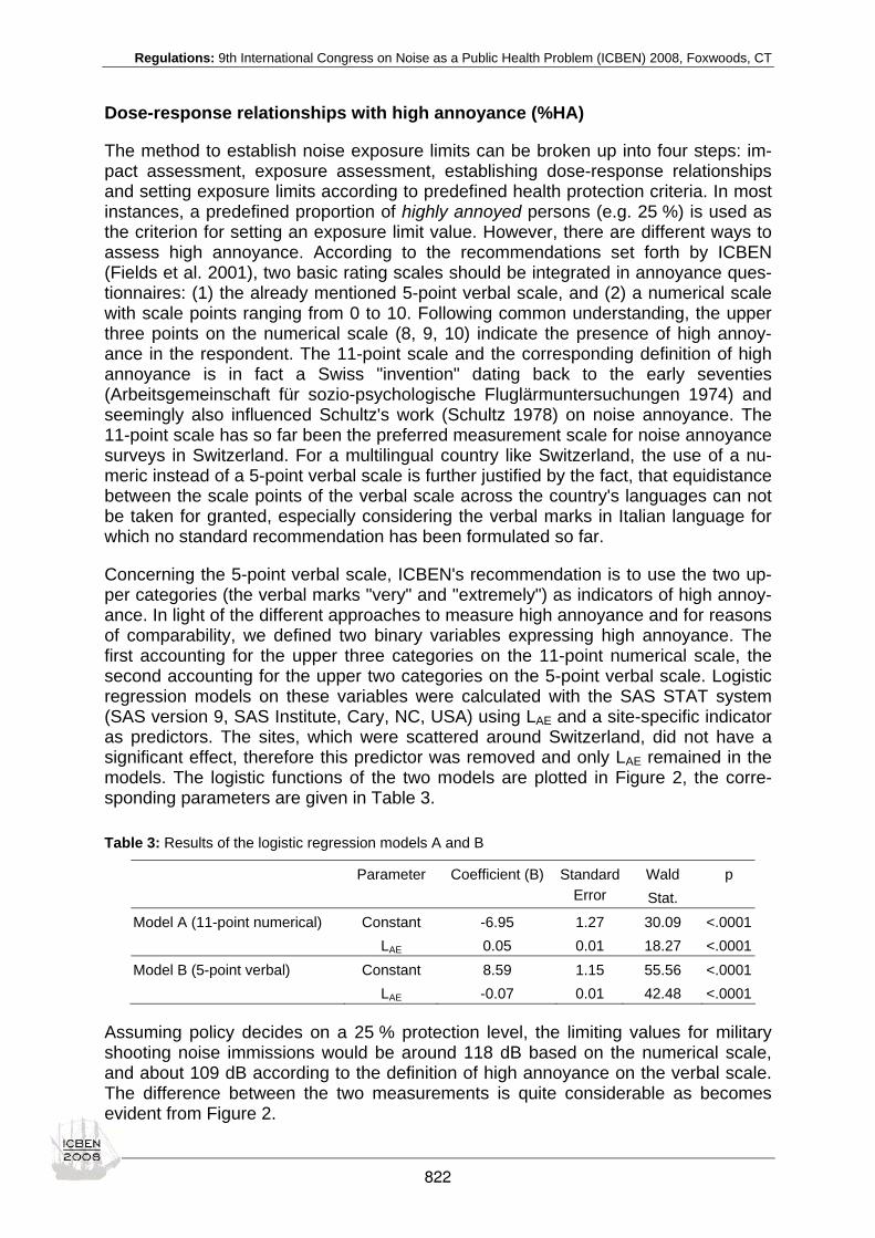
Regulations: 9th International Congress on Noise as a Public Health Problem (ICBEN) 2008, Foxwoods, CT
Dose-response relationships with high annoyance (%HA)
The method to establish noise exposure limits can be broken up into four steps: im-pact assessment, exposure assessment, establishing dose-response relationships and setting exposure limits according to predefined health protection criteria. In most instances, a predefined proportion of highly annoyed persons (e.g. 25 %) is used as the criterion for setting an exposure limit value. However, there are different ways to assess high annoyance. According to the recommendations set forth by ICBEN (Fields et al. 2001), two basic rating scales should be integrated in annoyance ques-tionnaires: (1) the already mentioned 5-point verbal scale, and (2) a numerical scale with scale points ranging from 0 to 10. Following common understanding, the upper three points on the numerical scale (8, 9, 10) indicate the presence of high annoy-ance in the respondent. The 11-point scale and the corresponding definition of high annoyance is in fact a Swiss "invention" dating back to the early seventies (Arbeitsgemeinschaft für sozio-psychologische Fluglärmuntersuchungen 1974) and seemingly also influenced Schultz's work (Schultz 1978) on noise annoyance. The 11-point scale has so far been the preferred measurement scale for noise annoyance surveys in Switzerland. For a multilingual country like Switzerland, the use of a nu-meric instead of a 5-point verbal scale is further justified by the fact, that equidistance between the scale points of the verbal scale across the country's languages can not be taken for granted, especially considering the verbal marks in Italian language for which no standard recommendation has been formulated so far.
Concerning the 5-point verbal scale, ICBEN's recommendation is to use the two up-per categories (the verbal marks "very" and "extremely") as indicators of high annoy-ance. In light of the different approaches to measure high annoyance and for reasons of comparability, we defined two binary variables expressing high annoyance. The first accounting for the upper three categories on the 11-point numerical scale, the second accounting for the upper two categories on the 5-point verbal scale. Logistic regression models on these variables were calculated with the SAS STAT system (SAS version 9, SAS Institute, Cary, NC, USA) using LAE and a site-specific indicator as predictors. The sites, which were scattered around Switzerland, did not have a significant effect, therefore this predictor was removed and only LAE remained in the models. The logistic functions of the two models are plotted in Figure 2, the corre-sponding parameters are given in Table 3.
Table 3: Results of the logistic regression models A and B
Parameter Coefficient (B) Standard Error
Wald Stat.
p
Model A (11-point numerical) Constant -6.95 1.27 30.09 <.0001 LAE 0.05 0.01 18.27 <.0001Model B (5-point verbal) Constant 8.59 1.15 55.56 <.0001
LAE -0.07 0.01 42.48 <.0001
Assuming policy decides on a 25 % protection level, the limiting values for military shooting noise immissions would be around 118 dB based on the numerical scale, and about 109 dB according to the definition of high annoyance on the verbal scale. The difference between the two measurements is quite considerable as becomes evident from Figure 2.
822
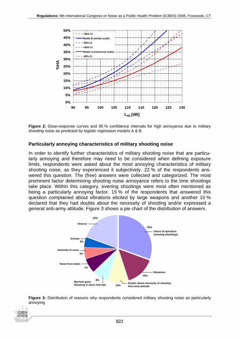
Regulations: 9th International Congress on Noise as a Public Health Problem (ICBEN) 2008, Foxwoods, CT
0%
5%
10%
15%
20%
25%
30%
35%
40%
45%
50%
90 95 100 105 110 115 120 125 130
+95% CI
Model B (verbal scale)
-95% CI
+95% CI
Model A (numerical scale)
-95% CI
LAE [dB]
%H
A
Figure 2: Dose-response curves and 95 % confidence intervals for high annoyance due to military shooting noise as predicted by logistic regression models A & B
Particularly annoying characteristics of military shooting noise
In order to identify further characteristics of military shooting noise that are particu-larly annoying and therefore may need to be considered when defining exposure limits, respondents were asked about the most annoying characteristics of military shooting noise, as they experienced it subjectively. 22 % of the respondents ans-wered this question. The (free) answers were collected and categorized. The most prominent factor determining shooting noise annoyance refers to the time shootings take place. Within this category, evening shootings were most often mentioned as being a particularly annoying factor. 15 % of the respondents that answered this question complained about vibrations elicited by large weapons and another 10 % declared that they had doubts about the necessity of shooting and/or expressed a general anti-army attitude. Figure 3 shows a pie chart of the distribution of answers.
30%
15%
10%
8%
7%
5%
5%
20%
Hours of operation(evening shootings)
Vibrations
Doubts about necessity of shootingAnti-army attitude
Machine gunsShooting in short intervals
Intensitiy of noise
Echoes
Diverse
Noise from tanks
Figure 3: Distribution of reasons why respondents considered military shooting noise as particularly annoying
823
Regulations: 9th International Congress on Noise as a Public Health Problem (ICBEN) 2008, Foxwoods, CT
A penalty for evening shootings?
The calculation of a penalty value for evening shootings appears to be rather difficult in the current case, because on one hand, the exposure data was not strictly related to specific time periods and on the other hand, evening shootings usually take place rather seldom (roughly about 8-10 times fewer shots fired than during day) and there-fore the empirical basis appears to be too weak for a sound statistical estimation of the time-of-day effect. However, due to the fact that evening shootings were rated among the top particularly annoying features of military shooting noise (cp. Figure 3), a penalty for the time evening shootings take place seems to be justified.
CONCLUDING REMARKS
The present study assessed the degree of military shooting noise annoyance around eight different shooting grounds in Switzerland. The reported results are to be termed "preliminary", as suggested by the title of this paper. Scientific experience as well as the body of literature concerning this kind of noise annoyance is rather scarce and the results therefore call for further discussion with experts in the field. Results showed a large variability among the annoyance responses for any given exposure class, adding to the complexity of the task of defining an exposure limit value. Total sound energy (LAE) appeared to be the best predictor for high annoyance.
The current study established two preliminary exposure-response relationships as a basis for setting a limiting value. Abatement measures for all military shooting grounds will be enforced as soon as the exposure limits are legally fixed in the Swiss noise abatement ordinance.
REFERENCES
Arbeitsgemeinschaft für sozio-psychologische Fluglärmuntersuchungen (Ed.) (1974). Sozio-psychologische Fluglärmunter-suchung im Gebiet der drei Schweizer Flughäfen Zürich, Genf, Basel. Bern: Eidgenössisches Luftamt.
Buchta E (1990). A field survey on annoyance caused by sounds from small firearms. J Acoust Soc Am 88: 1459-1467.
Buchta E, Vos J (1998). A field survey on the annoyance caused by sounds from large firearms and road traffic. J Acoust Soc Am 104: 2890-2902.
Fields JM, de Jong RG, Gjestland T, Flindell IH, Job RFS, Kurra S, Lercher P, Vallet M, Yano T, Guski R, Felscher-Suhr U, Schumer R (2001). Standardized general-purpose noise reaction questions for community noise surveys: research and a recommendation. J Sound Vibr 242: 641-679.
Meloni T, Rosenheck A (1995). Choice of frequency-weighting for the evaluation of weapon noise. J Acoust Soc Am 97: 3636-3641.
Schomer PD (1985). Assessment of community response to impulsive noise. J Acoust Soc Am 77: 520-535.
Schultz TJ (1978). Synthesis of social surveys on noise annoyance. J Acoust Soc Am 64: 377-405.
Schweizerische Eidgenossenschaft (1986). Lärmschutz-Verordnung vom 15. Dezember 1986 (LSV) [SR 814.41], http://www.admin.ch/ch/d/sr/8/814.41.de.pdf.
Vos J (2001). On the annoyance caused by impulse sounds produced by small, medium-large, and large firearms. J Acoust Soc Am 109: 244-253.
Zimmer K, Ellermeier W (1998). Ein Kurzfragebogen zur Erfassung der Lärmempfindlichkeit. Umweltpsychologie 2: 54-63.
824

Regulations: 9th International Congress on Noise as a Public Health Problem (ICBEN) 2008, Foxwoods, CT
Effects of science-based noise control laws, standards and policies Wayne R. Lundberg* Aerospace Engineer, 3312 Braddock St., Kettering OH 45420-1203, USA
*corresponding author: e-mail: [email protected]
ABSTRACT The US Noise Control Act of 1972 (NCA 1972) directs the US Federal Aviation Ad-ministration (FAA) and Department of Defense (DoD) to develop separate standards and polices regulating source noise. The current Federal Aviation Regulation Part 36 (FAR 2002) compels use of Aerospace Recommended Practices (ARP) and noise exposure methods which compare with scientifically developed and approved Inter-national Organization for Standardization (ISO) methods. Annual average noise met-rics also do not afford the public the full benefits of scientific research. This paper will advocate advances in two areas: 1- atmospheric attenuation of aeroacoustic noise using the acoustical model ISO 9613-1 (1993); 2- seasonal averaged noise exposure level policies and practices. Scientific improvements in either area would provide more fidelity for estimating biological effects and human response. (1) Atmospheric attenuation discrepancies primarily affect noise analyses of high-performance aircraft and rockets. Aerospace noise predictions are effected by range-dependant high-frequency discrepancies from all louder (than ~stage 3) sources. Aviation noise ex-posure estimates applying SAE (1975) ARP 866A under-predict levels affecting nearby communities under most weather conditions. Studies of high-performance military aircraft and rockets indicate that ISO 9613-1 may be extended for application to all aerospace sources. (2) Annual-averaged noise exposure fails to account for seasonal variations in atmospheric effects, aircraft performance and airport opera-tions. Science-based noise control laws, standards and policies are thus practicable, compelled by Environmental Management Systems, and benefit aviation and com-munity noise control.
INTRODUCTION Biological effects of noise in the environment are often predicted using Effective Per-ceived Noise Level (EPNL) or Day-Night average noise Level (DNL) metrics. This paper considers two primary approaches that could improve the fidelity of community noise prediction metrics in comparison to actual noise environs and sources. It is as-serted without discussion that the proposed methods, when refined for standard ap-plication, would serve to better predict biological effects and thus enable an improved regulatory approach for future aerospace noise sources. The historical development of aircraft noise regulations preceded scientific under-standing of aerospace sources and environmental propagation effects. Nonetheless, the compelling need to regulate aircraft noise led the US Congress to direct Federal agencies to prescribe standards and regulations respecting noise (NCA 1972 section 4). Military weapons were exempted from explicit regulation (NCA 1972 section 3) but their community noise is limited by the practical application of the National Environ-mental Policy Act (NEPA 1969). Application of noise estimates for NEPA planning activities has the potential to avoid science-based environmental impact assess-ments to the extent that public agencies allow. Empirical modeling of aircraft noise propagation was employed using many aircraft measurements that were available in the 1970’s. The US Society of Automotive En-
825

Regulations: 9th International Congress on Noise as a Public Health Problem (ICBEN) 2008, Foxwoods, CT
gineers developed a series of Aerospace Recommended Practices designed to measure aircraft noise and to model environmental propagation to the extent that it was able. Atmospheric attenuation of sound is fundamental to all empirical, and sci-entific, acoustical methods and was modeled by SAE (1975) ARP 866A. The FAA prescribes it explicitly in US aviation regulations (FAR 2002) at section H36.113. Air-craft noise propagation models of excess ground attenuation and lateral attenuation require modeling of atmospheric attenuation during data analyses. The sciences of aeroacoustics and sound propagation in the outdoor environment have progressed considerably since SAE (1975) was developed. Ray-tracing acous-tics has been studied and validated to model atmospheric refraction of acoustic noise (Pierce 1994). Atmospheric absorption has been researched sufficiently to produce both US national (ANSI 1995) and international (ISO 1993) standard models. Excess ground attenuation and lateral attenuation are known to be the result of source-receiver geometry and ground absorption (Delany & Bazley 1971; Chessell 1977), although time-averaged propagation through turbulent air reduces ground-absorption effects. Nonetheless, US aircraft noise compatible-use prediction models have not yet adopted a science-based approach in their implementation. This is partly due to a known discrepancy in model predictions of high-frequency noise measured from high-amplitude sources. The term high-amplitude sources generally refers to aero-space propulsion systems capable of powering supersonic flight. Development and fielding of high-speed civil transport aircraft is dependent on accu-rate flight noise prediction models applicable to their high-performance engines, as well as acceptance of the well-understood science of sonic boom propagation. Su-personic civil aircraft airframe and engine designs benefit directly from the acoustical science derived for use with military high-performance jet aircraft. The sciences of aeroacoustics and outdoor noise propagation are well-developed and, with adequate support, capable of being implemented in aerospace laws, stan-dards and policies. This paper will discuss the extent to which the fidelity of commu-nity noise predictions are influenced by current purely empirical methods. To that ex-tent, existing regulatory approaches effect aerospace engineering and devel-opment of the international air transport system including supersonic civil aviation.
ATMOSPHERIC ATTENUATION Atmospheric absorption theory and practice has long been suspected as the cause of discrepancies between theory and aircraft noise measurements at high frequencies (Bass et al. 1995). Although Morfey & Howell (1981) concluded that nonlinear propa-gation effects were responsible, the extremely complex time-domain computations required, coupled with legitimate concerns about measurement instrumentation (Joppa et al. 1994), effectively delayed productive research of this acoustic phe-nomenon. Nonlinear propagation of noise is a finite-amplitude effect in which the waveform steepens with distance. It appears in flight/launch noise measurements initially as a broadening of high-amplitude spectra (weak nonlinearity), and with higher amplitudes small shocks form at long ranges (strong nonlinearity). In the trans-sonic regime, these small shocks join with near-field shock waves created by supersonic flight, which would otherwise dissipate, yielding sonic boom (pure nonlinear) propagation.
826

Regulations: 9th International Congress on Noise as a Public Health Problem (ICBEN) 2008, Foxwoods, CT
Further evidence of weak nonlinear effects was afforded by Lundberg (1994a) and eventually confirmed by (Gee et al. 2005; Falco et al. 2006). The computationally in-tense time-domain methods of Gee et al. (2005) and others substantiate the fre-quency-domain methods proposed by Lundberg (2003, 2006). Although the empirical SAE ARP 866A model incorporates nonlinear effects owing to the use of C-135A high-amplitude noise data, it cannot be extended to account for this source-dependent effect. Figure 1 shows the nature of the discrepancy at high frequencies for an old fighter aircraft, and that both ANSI S1.26-95 and ISO 9613-1 models are able to be extended to incorporate nonlinear atmospheric attenuation.
Figure 1: Comparison of SAE ARP 866A to ANSI S1.26-78, (then-proposed) ANSI S1.26-95 and ANSI S1.26-95 with inclusion of weak nonlinear effects (Lundberg 1994a). ISO 9613-1 is closely com-parable to ANSI S1.26-95.
The difference between ANSI S1.26-78 and -95 results are due to extensive research of atmospheric absorption and filter effects (Joppa et al. 1994; Bass et al. 1995).
SCIENCE OF NOISE CONTROL OF AEROSPACE SOURCES The regulatory distinction between civil, military aircraft and rocket noise emissions becomes increasingly blurred with the advance of aerospace engineering. As the sci-ence of aeroacoustics of high-performance aircraft engine/airframes advances to fa-cilitate practical designs, environmental noise prediction methods must also advance to facilitate the fielding of supersonic civil and military vehicles. The following subsections briefly discuss legal, technological and economic factors that presently apply to military and civil aircraft noise constraints and roughly how the respective programs would be affected by science-based noise control laws.
Civil Aircraft The FAR Part 36 approach to regulating civil aircraft limits noise produced by individ-ual aircraft. Noise-reducing technology often takes the form of higher engine bypass ratios, in which cool air is mixed with hot combustion jet before being ejected. Civil aircraft powered by lower bypass engine designs (e.g. JT8D series) require ad-vanced noise suppression retrofitting to comply with Stage 4 (ICAO Chapter 4). This retrofit technology is currently designed into proposed supersonic business jets.
827
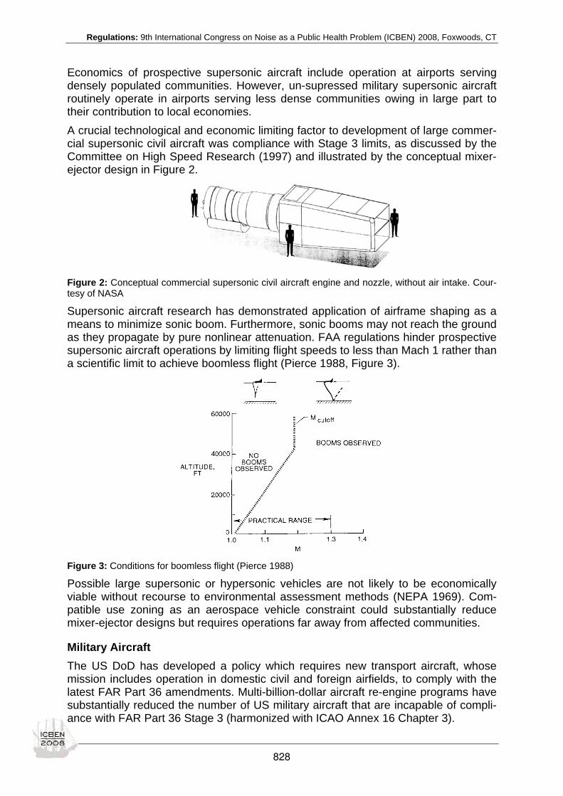
Regulations: 9th International Congress on Noise as a Public Health Problem (ICBEN) 2008, Foxwoods, CT
Economics of prospective supersonic aircraft include operation at airports serving densely populated communities. However, un-supressed military supersonic aircraft routinely operate in airports serving less dense communities owing in large part to their contribution to local economies. A crucial technological and economic limiting factor to development of large commer-cial supersonic civil aircraft was compliance with Stage 3 limits, as discussed by the Committee on High Speed Research (1997) and illustrated by the conceptual mixer-ejector design in Figure 2.
Figure 2: Conceptual commercial supersonic civil aircraft engine and nozzle, without air intake. Cour-tesy of NASA
Supersonic aircraft research has demonstrated application of airframe shaping as a means to minimize sonic boom. Furthermore, sonic booms may not reach the ground as they propagate by pure nonlinear attenuation. FAA regulations hinder prospective supersonic aircraft operations by limiting flight speeds to less than Mach 1 rather than a scientific limit to achieve boomless flight (Pierce 1988, Figure 3).
Figure 3: Conditions for boomless flight (Pierce 1988) Possible large supersonic or hypersonic vehicles are not likely to be economically viable without recourse to environmental assessment methods (NEPA 1969). Com-patible use zoning as an aerospace vehicle constraint could substantially reduce mixer-ejector designs but requires operations far away from affected communities.
Military Aircraft The US DoD has developed a policy which requires new transport aircraft, whose mission includes operation in domestic civil and foreign airfields, to comply with the latest FAR Part 36 amendments. Multi-billion-dollar aircraft re-engine programs have substantially reduced the number of US military aircraft that are incapable of compli-ance with FAR Part 36 Stage 3 (harmonized with ICAO Annex 16 Chapter 3).
828

Regulations: 9th International Congress on Noise as a Public Health Problem (ICBEN) 2008, Foxwoods, CT
Other military transport and supersonic aircraft must comply with the US National Environmental Policy Act (NEPA 1969) by preparing Environmental Impact State-ments using DNL contours. The noise produced by each aircraft model is combined with their operations model to predict DNL contours. Local communities develop compatible-use zoning ordinances accordingly. There is a common perception that military aircraft are ‘unregulated’ noise sources, due to their exemption from NCA 72. However, the combination of local compatible-use zoning ordinances and determina-tion to maximize flight operations compels use of noise abatement procedures. Thus, the number of operations of modern turbojets is affected by historic noisiness and compatible uses of predecessor aircraft. It is thus beneficial from a flight training op-erations standpoint to implement noise reduction technologies (e.g. Nesbitt et al. 2006) in developmental engines and require designs capable of noise abatement departures. Figure 4 shows an example of the new F-35 fighter aircraft engine with chevron nozzles. An engineering policy to design-in noise abatement approaches could be applied to future civil aerospace vehicles, particularly any that are over-constrained by Stage 4.
Figure 4: F135-PW-100 engine test illustrating noise-reducing chevron nozzle implementation in a high-performance jet engine (courtesy wikipedia)
NOISE CONTROL OF AEROSPACE OPERATIONS BY SEASON Both EPNL and DNL metrics average sound exposure over the entire year, while in-cluding night-time sleep disturbance penalties. There are essentially three reasons to consider regulatory implementation of seasonal-averaged noise exposure metrics. First, regional weather affects atmospheric propagation through both attenuation and refraction. Second, colder winter air is more dense, which is beneficial to both air-frame lift and engine performance. Third, daily operations at most major airports vary by a few percent between summer and winter seasons. Overall departures tend to be slightly more frequent in summer when aircraft are less able to gain altitude. The first two effects warrant discussion in the context of advocating regulatory changes.
Weather effects sound propagation The FAA conducted studies (Rickley & Fleming 1998; Reherman et al. 2002) to con-sider application of ISO 9613-1 in the US civil aircraft noise certification and predic-tion programs. These studies determined that the SAE ARP 866A method is nearly as accurate for civil aircraft except at “the extreme limits of the current FAR part 36 test window” (Rickley & Fleming 1998). A similar discrepancy exists in noise predic-tion models. Figure 5 shows representative results of analyses pertaining to turbofan aircraft, where weather conditions adversely affect the results at long range. Although “the exact method presented in both the ISO and ANSI standards was considered
829

Regulations: 9th International Congress on Noise as a Public Health Problem (ICBEN) 2008, Foxwoods, CT
the reference or ‘gold standard’..,” it yields increases in predicted DNL or EPNL which would slightly adversely impact compatible use zoning.
Figure 5: Comparison of noise-distance curves: ANSI/ISO Pure-Tone Mid-band Frequency Method minus SAE ARP 866A, reference 25oC, 70 % relative humidity (Rickley & Fleming 1998)
Sound exposures predicted by applying the science behind ISO/ANSI methods yield more significant results for high-performance aircraft engines. Earlier sensitivity analysis for low-bypass turbojet engines (Lundberg 1994a) show similarly increased predictions using the ISO/ANSI method. The incomplete atmospheric attenuation (neglecting nonlinear propagation) model for high-amplitude aerospace sources ap-pears to exacerbate the discrepancy near the source (Figure 6). Since nonlinear propagation shifts acoustic energy into more hearing-sensitive high-frequencies, ex-tension of the ISO/ANSI methods to correctly account for nonlinear propagation would both eliminate the near-field model discrepancy while exacerbating increased sound exposures at long ranges relevant to communities’ planning for compatible uses. The empirical SAE ARP 866A method cannot effectively be extended to ac-count for nonlinear effects since that would require extensive measurement and data-reduction of many different high-performance aircraft.
Figure 6: Discrepancy between SAE ARP 866A method prediction of SEL attenuation from laboratory measurements as modeled by the (then-proposed) ANSI S1.26-95, for an F-4C aircraft in takeoff power (Lundberg 1994a)
830

Regulations: 9th International Congress on Noise as a Public Health Problem (ICBEN) 2008, Foxwoods, CT
Weather affects acoustic refraction
Acoustic refraction depends on atmospheric wind-vector and temperature gradients. Since these meteorological variables change statistically of any season, scientifically exact methods for determining representative refractive atmospheres for each sea-son are quite complex. Such methods must account for acoustic energy averaging over the season. Calculations by Lundberg (1994b) estimate seasonal acoustic re-fractive effects using the TRAPS 89 sonic boom model (Figure 7).
Figure 7: Estimation of seasonal acoustic refraction effects using sonic boom ray-tracing methods for F-111 operations at Edwards AFB Military Operating Area, summer (left) and winter (right) (Lundberg 1994b)
Weather effects aircraft performance The International Center for Air Transportation (Huber et al. 2003, Figure 8) devel-oped a single-event aircraft noise simulator, NOISIM, which implements modern sci-ences of acoustic propagation in the outdoor environmental as well as weather ef-fects on aircraft performance. While dramatic reductions in community noise expo-sure were documented for specific departures, such results are tempered by the mul-tiple aircraft operations involved in long-term average noise exposure predictions.
Figure 8: SEL contours for a single departure in summer (left) with standard climb rate, winter (center) with cold-air climb rate and winter (right) taking advantage of additional lift produced by colder air to turn seaward earlier (Huber et al. 2003; reproduced with permission by MIT)
831

Regulations: 9th International Congress on Noise as a Public Health Problem (ICBEN) 2008, Foxwoods, CT
RECOMMENDATIONS Minor technical issues remain to be resolved to establish science-based noise control laws, standards and policies. Supersonic overland boomless flight is understood. Use of ISO 9613-1 for certification requires analysis of various third-octave band filters. Frequency-domain calculation of nonlinear aeroacoustic effects is achievable. Meth-ods for seasonal-averaged noise exposure levels require further study.
REFERENCES ANSI (1995). ANSI S1.26-Method for calculation of the absorption of sound by the atmosphere. New York, N.Y.: American National Standards Institute, Committee S1, Acoustics.
Bass HE, Sutherland LC, Zuckerwar AJ, Blackstock DT, Hester DM (1995). Atmospheric absorption of sound: further devel-opments. J Acoust Soc Am 97: 680-683.
Chessell CI (1977). Propagation of noise along a finite impedance boundary. J Acoust Soc Am 62: 825-834.
Committee on High Speed Research, Aeronautics and Space Engineering Board (1997). U.S. Supersonic Commercial Air-craft: Assessing NASA’s High Speed Research Program. Washington, DC: National Academy of Sciences, Division on Engi-neering and Physical Sciences.
Delany ME, Bazley EN (1971). A note on the effect of ground absorption in the measurement of aircraft noise. J Sound Vibr 16: 315-322.
Falco LE, Atchley AA, Gee KL (2006). Investigation of a single-point nonlinearity indicator in the propagation of high-amplitude jet noise. In: 12th AIAA/CEAS Aeroacoustics Conference, Conf Paper 2529. Washington, DC: AIAA.
FAR, Federal Aviation Regulation (2002). Part 36: Noise Standards: Aircraft Type and Airworthiness Certification. Washing-ton, DC: US Federal Aviation Administration.
Gee KL, Gabrielson TB, Atchley AA, Sparrow VW (2005). Preliminary analysis of nonlinearity in military jet aircraft noise propagation. AIAA J 43: 1398-1401.
Huber J, Clarke JB, Maloney S (2003). Aircraft noise impact under diverse weather conditions. In: 9th AIAA/CEAS Aeroacoustics Conference, Conf Paper 3276.
ISO (1993). ISO 9613-1: Acoustics – Attenuation of sound during propagation outdoors – Part 1: Calculation of the absorp-tion of sound by the atmosphere. Geneva: International Organization for Standardization, Committee ISO/TC 43, Acoustics, Sub-Committee SC 1, Noise.
Joppa PD, Sutherland LC, Zuckerwar AJ (1994). Filter effects in analysis of noise bands. In: 128th Acoustical Society of America meeting, Paper 2aNS5, Austin, TX.
Lundberg WR (1994a). Nonlinear aeroacoustics: Experimental evidence from the F-4C. In: Havelock DI, Stinson MR (eds.): Proceedings of the 6th International Symposium on Long-Range Sound Propagation: 1-20.
Lundberg WR (1994b). Seasonal sonic boom propagation prediction. AL/OE-TR-1994-0132. Wright-Patterson Air Force Base, OH: US Dept of Defense, Armstrong Laboratory.
Lundberg WR (2003). Prediction of nonlinear acoustic propagation effects for high-intensity aerospace noise sources in the natural far-field environment. PhD Dissertation, University of Dayton, Dayton, OH.
Lundberg WR (2006). Extent of nonlinear aeroacoustic propagation from single frequency-domain measurements. In: 12th AIAA/CEAS Aeroacoustics Conference, Conf Paper 2702, AIAA, Washington, DC.
Morfey CL, Howell GP (1981). Nonlinear propagation of aircraft noise in the atmosphere. AIAA J 19: 986-992.
NCA, Noise Control Act (1972). 42 US Code 4901 et seq. Public Law 92-574, amended 1976, 1978, 1988.
NEPA, National Environmental Policy Act (1969). 42 US Code 4321-4347, Public Law 91-190, amended 1975, 1982.
Nesbitt E, Mengle V, Czech M, Callender B, Thomas R (2006). Flight test results for uniquely tailored propulsion-airframe aeroacoustic Chevrons: community noise. In: 12th AIAA/CEAS Aeroacoustics Conference, Conf Paper 2438, AIAA, Washing-ton, DC.
Pierce AD (1988). Atmospheric effects. In: Status of sonic boom methodology and understanding. NASA Conference Publi-cation 3027. Hampton, VA.
Pierce AD (1994). Acoustics, an introduction to its physical principles and applications. American Institute of Physics, College Park, MD.
832

Regulations: 9th International Congress on Noise as a Public Health Problem (ICBEN) 2008, Foxwoods, CT
Reherman CN, Roof CJ, Fleming GG (2002). SAE ARP 866A vs. ISO 9613-1/ANSI S1.26-1995: A sensitivity analysis com-paring two procedures for adjusting as-measured spectra to reference conditions. Cambridge, MA: US Dept of Transporta-tion, Volpe National Transportation Systems Center.
Rickley EJ, Fleming GG (1998). Computing the absorption of sound by the atmosphere and its applicability to aircraft noise certification. Cambridge, MA: US Dept of Transportation, Volpe National Transportation Systems Center.
SAE (1975). ARP 866A Standard values of atmospheric absorption as a function of temperature and humidity. Warrenville, PA: Society of Automotive Engineers, Committee A-21, Aerospace Recommended Practice No. 866A.
833

Regulations: 9th International Congress on Noise as a Public Health Problem (ICBEN) 2008, Foxwoods, CT
Consideration elements for a legislation on the airport noise: The Italian experience Salvatore Curcuruto, Rosalba Silvaggio*, Francesca Sacchetti, Giuseppe Marsico APAT, Italian National Agency for Environmental Protection and Technical Services
* corresponding author: e-mail: [email protected]
INTRODUCTION The management of the airport noise in Italy is based on a specific regulation that takes into account also the Italian morphologic characteristics of the territory and the high urbanization which do not allow to have wide free areas to be used for the de-velopment of the airports. The Italian law which rules the noise caused by the air transport has to manage sev-eral requirements, i.e. the needs of the inhabitants who live near the airports, the de-velopment needs of the airport traffic, which generally causes also the growth of the airport infrastructures, the possible limitations to the territorial planning near the towns. As a consequence, the related law is quite complex and it is proved by the big amount of the Italian decrees on this subject and by the fact that it has taken a long time to get a full capacity. The national legislative approach is based on different lines of action, concerning the characterization of areas close to the airport, with noise limit values fixed, the defini-tion of measurement methodology and anti-noise procedures, the duty of utilization of monitoring system, the classification of the national airports on the basis of the noise let out on the surrounding areas, the duty of adoption of reclamation measures in case of the overcoming of the limits, the restrictions of the air traffic at night.
ITALIAN FRAMEWORK RULES Over the years air transportation and the related air movement have became more and more huge and a specific regulation must be adopted to manage the item in a strategic and sustainable way according also to the growth of the towns and the needs of the population. In Italy, two years later the issue of the framework law n. 447 of the 1995 on acoustic pollution, several decrees have been published in order to make operative this law. The entire Italian legislation has got the aim to get the following lines of action: - characterization of areas close to the airport, in order to fix noise limit for each
area according to the different uses of the areas; - definition of specific measurement methodology of the air transport noise; - definition of anti-noise procedure for each airport which must be respected by
airplanes during taking off and landing phases and during land operations; - duty of utilization of monitoring system in continuous of the airport noise in order
to guarantee and check the respect of the limits for protecting people, controlling noise let out by the airplanes, verifying the actions achieved against noise;
- classification of the national airports on the basis of the noise let out on the sur-rounding areas;
- duty of adoption of reclamation measures in case of the overcoming of the lim-its;
834
Regulations: 9th International Congress on Noise as a Public Health Problem (ICBEN) 2008, Foxwoods, CT
- restrictions of the air traffic at night. All the above lines of action are included into the following decrees. - Decree 31/10/97 on Measurement methodology of airport noise; - Decree n.496, 11th December 1997, on regulations for the reduction of acoustic
pollution caused by civil aircrafts; - Decree 20/5/99 which defines criteria for the design of monitoring systems for
controlling acoustic pollution levels close to the airports and criteria for the air-port classification related to the acoustic pollution level;
- Decree 3/12/99 regarding anti noise measures and respect areas in the airports; - Decree n.476, 9th November 1999, on the ban of air traffic at night. According to these decrees, each Italian airport devoted to civil transportation must provide a set up of a continuous monitoring system around the airport area able to get possible overtaking of fixed limits connecting this information with data and flight path of the aircraft which has generated the overtaking. This measure allows to control the acoustic climate around the airport areas and al-lows to impose economic sanctions if the fixed limits or the anti noise measures are not respected. Moreover, each airport must constitute a Commission whose duties are the follow-ings: - classification of the airport according to the acoustic pollution produced, on the
basis of the following parameters: extension of the airport area, extension of the three acoustic areas, extension of the residential areas which are into the perti-nence zones, house density in each pertinence zone. On the basis of these pa-rameters it is possible to get indices which allow to classify the airport;
- provide the anti noise measures for the airport on the basis of general criteria of the Italian decrees; the main objective is the optimisation of the noise aircraft noise at land in order to safeguard as best it is possible the exposed population;
- provide the definition of the three pertinence zones as requested by the specific decree 3/12/99, according to the different noise limit established by the decree itself.
Moreover, it is the duty of the airport managing Company to identify and to propose to the Municipality where the airport is located a noise reclamation plan, whereas it will be duty of the Municipality the adoption of the plan and its adaptation according to the Municipality acoustic reclamation plan as stated by the framework law n. 447/1995 on acoustic pollution. The last act of the airport regulation is the restriction of the air traffic at night, except for medical or emergency or Italian State flights, or if there is a specific Ministerial authorization.
EXPERIENCES Since 1997, when the first decree on air noise was published, each airport has work-ed with the above said aims. During these ten years, many experiences have been carried out, both positive and negative, useful to analyse the legislation itself. Particularly, for some of them the development of the airports and their infrastruc-tures in a sustainable way, increasing the value of the airport, as a power of eco-nomic and social development, respecting the territory and improving the environ-mental conditions, has represented the main objective.
835

Regulations: 9th International Congress on Noise as a Public Health Problem (ICBEN) 2008, Foxwoods, CT
This is the experience of the Bologna “G. Marconi” airport, which has evaluated the actions for reducing noise in a balanced approach, known, at now, at world level. The elements examined have been the following: - Technologic development; - Procedures of flight; - Airport infrastructures; - Acoustic monitoring; - Use of sound adsorbing barriers; - ISO 14001 certification; - Acoustic zoning; - Environmental communication. All of the elements of the balanced approach have been managed in a participative way, taking into account the input of the all stakeholders involved in the building up of the G. Marconi airport. The aim has been to share the principles of sustainability like the following: - Balance between the law for noise reduction, need of flight security, and objec-
tives of airport and air space capability; - Effective politics for land use around the airport area and for land-side accessi-
bility in order to reduce local emissions; - Balance between disturb reduction, economic aspects and free competition,
protection of employment; - Scientific evaluation of local source of atmospheric pollution in order to under-
stand reasons and responsibilities and realistic attribution of mitigation duties; - Flight path and procedures which make more efficient the use of the air space,
shortening the distance in order to reduce consumptions and global emissions. The International Airport of Naples represents another good experience. According to the Italian law, the Commission had realized the main objectives as: - Definition of the noise procedures; - Acoustic zoning; - Indices of acoustic classification of the airport; - Achievement of a noise monitoring system; - Collection of economic sanctions. The zones of Capodimonte, Vomero, Posillipo, characterized by a high density of population, are nearest the airport, and they are interested by take off and landing operations (Figure1).
836

Regulations: 9th International Congress on Noise as a Public Health Problem (ICBEN) 2008, Foxwoods, CT
AIRPORT
Figure 1: Airport of Naples and the areas interested. Source: Noise Airport Commission
The noise abatement procedures and the administrative sanctions, started in 2006, avoid the high dispersion of the routes of the airplanes in the areas mentioned above (Figurers 2 and 3), with a percentage of procedures respected that grown up from 26 % in May 2001 to 97 % in May 2007. More than 5,000 sanctions have been ap-plied, whose 60 % have been paid.
Figures 2 and 3: The situation before (on the left, Figure 2) and after (on the right, Figure 3) the appli-cation of the noise abatement procedures. Source: Noise Airport Commission
The airport of Milano Malpensa has carried out an experience regarding the health effects associated with exposure to aircraft noise. The airport was included in the pro-ject HYENA (Hypertension and Exposure to Noise near Airports), developed in 2003-2006 period. The project aim is to assess the impacts on cardiovascular health of noise generated by aircraft and road traffic. In particular, two of the specific objectives are the analysis of the exposure-response relationship in adults between long-term exposure to airport related noise and high blood pressure and the analysis of the impact of aircraft noise on stress hormone levels. The research includes cross-sectional studies near six major European air-ports: Germany (Berlin Tegel), Italy (Milano Malpensa), Greece (Athens), Nether-lands (Amsterdam Schiphol), Sweden (Stockholm Arlanda), United Kingdom (London Heathrow). A total of 4,861 persons between 45 and 70 years old, who have lived at least 5 years near the selected airports, have been selected using noise contours related to the acoustic characterization of the airports. In Italy the study, coordinated by ARPA Piemonte, in cooperation with ASL Novara, ASL Varese, ARPA Lombardia, had in-
837
Regulations: 9th International Congress on Noise as a Public Health Problem (ICBEN) 2008, Foxwoods, CT
volved 12 Municipalities, with 753 persons selected from different aircraft noise expo-sure categories, in order to have a wide range of exposures. For the assessment of the noise exposure and health effects the blood pressure and stress hormones (corti-sol in saliva) were collected and investigated. Some interesting results are: - the percentage of persons affected by hypertension in the areas analysed is,
respectively, 48.8 % in the UK, 54.6 % in Germany, 51.9 % in the Netherlands, 52.0 % in Sweden, Greece 57.0 % and 52.1 % in Italy. These values are greater than the data, up to now, published;
- there was a statistically significant relationship between exposure to noise, con-sidering air and road traffic, and the risk of hypertension;
- considering the A weighted noise equivalent level of 1 minute (LAeq1min) and 15 minutes (LAeq15min), in night-time noise exposure, an increase in blood pressure was observed over 15 minutes intervals in which an aircraft event oc-curs.
The HYENA study, which is the first multicenter research designed to assess the ef-fects of exposure to aircraft and road traffic noise on blood pressure and cardiovas-cular disease, has confirmed the presence of the effects of long-term noise exposure on the prevalence of hypertension and the acute effects analysed in night-time expo-sure.
STATE OF ART During these ten years, since the publication of the framework law n. 447 on acoustic pollution, the environmental acoustic Commission about air noise were established in all national airports, in different periods and with different progresses reached in the activities carried out. Particularly: - the definition of the airport area, which represents the most important act of
planning, able to allow subsequently the optimisation of the extension of the considered area and the population involved, was defined by the infrastructure in percentage of 60 %;
- 30 % of the airport infrastructure have started a noise monitoring system, in some case fully operative, in other case in the phase of start up;
- the noise abatement measures were defined only in few airports; - the definition of the three areas according to the different limit values estab-
lished by law was carried out by three airports; - the indices able to classify the airport were identified only by an infrastructure; - there is any Noise Containment and Abatement Plan for the air infrastructures.
Positive elements Even though in presence of a complex legislative system, there are many facts, un-doubtedly positive, which may suggest interesting proposals, i.e.:
- the possibility, supplied by the law, to develop and to share the process with the stakeholders, especially with the Local Administrations, even though this may introduce more difficulties in the processes;
- the characterization of the territory, where the presence of the airport infrastruc-ture is undoubtedly a problem, searching a balance between sustainable envi-ronmental impacts and the possibility of a future growth of the infrastructure;
838

Regulations: 9th International Congress on Noise as a Public Health Problem (ICBEN) 2008, Foxwoods, CT
- the continuous control of the noise emissions allowed by the monitoring system; - the possibility to inform the community, using the monitored data, about the
noise characterization of the area, trough web site dedicated, reports or news-letters;
- the application of economic sanctions towards air companies, in the presence of the non-observance of the abatement noise measures, causing excessive noise emissions. The amount may be used to projects noise abatement plans and to achieve a better acoustic quality of the area close to the airport.
In Italy the implementation of the legislation system has allowed, in a few years, to create specific acoustic competences, especially in the air traffic noise, permitting the development of the specific topic, also it has allowed to define, with the cooperation of the technicians working in the airport managing Companies and in the Local Agencies for Environmental Protection, instruments and methodologies for the con-tinuous noise monitoring, making the methods of acquisition, analysis and manage-ment of the noise data more accurate and appropriate.
Critical aspects The enforcement of the national law underlines also the problems and the critical as-pects existing, i.e.:
- in some experiences the presence of many local municipalities which empha-sizes the own interests, due to the complexity of the territory, inside Noise Air-port Commissions, causes conflict of interests and delay in the activities, but also a chance for an implementation of the different hypothesis proposed by the administrations;
- another reason of conflict inside working Commissions is the obligation to share all the choices, regarding the input noise data for the mathematical program util-ized, i.e.: flows and entities of air traffic, airplanes paths, stops of airplanes, technical characteristics of the airplanes;
- the utilization of an acoustical air traffic noise parameter, Lva, which is different from environmental noise parameter, Leq, using to evaluate the acoustic classi-fication of the areas close to the airport, causes difficulties, especially drawing comparison in boundary situations and in presence of actions belonging to the different policy makers;
- the insufficient knowledge of the distribution of the population does not allow a correct and adequate valuation of the people exposed to the air traffic noise;
- the need to improve studies on the effects of noise exposure on human health; - the lack of a deadline about the duties provided by law and the absence of the
economic sanctions creates delay in the process; - the implementation of END 2002/49/CE, carried out in Italy by the Decree
194/2005, makes changes in different aspects regarding the current national law, for instance the use of new acoustical parameter Lden.
CONCLUSIONS According to the Italian national legislative actions there are some airport experi-ences which can be shared among the other Italian airport or to foreign Countries. Particularly, when the aim to develop the airports and their infrastructures in a sus-tainable way, increasing the value of the airport, as a power of economic and social development, looking also at the territory and improving the environmental conditions has been respected.
839

Regulations: 9th International Congress on Noise as a Public Health Problem (ICBEN) 2008, Foxwoods, CT
Especially, in one of these experiences, the activities carried out essentially involving Companies, with specific meeting, with information towards new operators, with the involvement and participation of the pilots and with the presence of economic sanc-tions, have allowed to obtain, in two years, the respect of the noise abatement meas-ures with a percentage of 97 %. In another experience, the implementation of some aspects provided by the Euro-pean Directive 2002/30/CE, which introduces duties and procedures for the operative restrictions in order to control the noise airport emission in the Community, with par-ticular reference to the idea of “Balanced Approach”, has been realized. Many activi-ties were carried out in order to achieve the control of the noise emissions: a continu-ous monitoring system, new flight procedures, structural modification and noise abatement action in the airport, but the more interesting action concerning the plan-ning of the districts close to the infrastructure, in cooperation with the local municipal-ity. In this case, in six years, a reduction of 5 dB of medium value Lva is achieved, with an increase of the air traffic of 50 %. The research related to health effects associated with public exposure to aircraft noise carried out in Milano Malpensa surrounding is very important for the coopera-tion and the comparison with other airports situations, for the methods carried out and for the results obtained and it may be a reference frame for other studies and for a thorough analysis of the problem. These experiences emphasize the aspects of an effective management, able to manage an important noise source without excessive penalization on it, searching a balance between noise abatement measures, needs of flight safety, targets about the growth of the airport infrastructure, effective policy of the land use of the territory close to the airport, mitigation of the annoyance, economic aspects regarding the competitive system and the security of the employment.
REFERENCES Decree 31/10/97 on Measurement methodology of airport noise.
Decree n.496, 11th December 1997, on regulations for the reduction of acoustic pollution caused by civil aircrafts.
Decree 20/5/99 on criteria for the design of monitoring systems for controlling acoustic pollution levels close to the airports and criteria for the airport classification related to the acoustic pollution level.
Decree 3/12/99 on anti noise measures and respect areas in the airports.
Decree n.476, 9th November 1999, on the ban of air traffic at night.
Haralabidis AS, Dimakopoulou K, Vigna-Taglianti F, Giampaolo M, Borgini A, Dudley ML, Pershagen G, Bluhm G, Houthuijs D, Babisch W, Velonakis M, Katsouyanni K, Jarup L, HYENA Consortium (2008). Acute effects of night-time noise exposure on blood pressure in populations living near airports. Eur Heart J 29: 658-664.
http://www.hyena.eu.com/
http://www.arpa.piemonte.it/upload/dl/Rapporto_Stato_Ambiente/Rapporto_Stato_Ambiente_2006/cap_11_rumore.pdf
http://www3.imperial.ac.uk/newsandeventspggrp/imperialcollege/newssummary/news_13-2-2008-10-14-29?newsid=27774
Italian National Framework Law n. 447 of the 1995 on acoustic pollution.
Jarup L, Dudley ML, Babisch W, Houthuijs D, Swart W, Pershagen G, Bluhm G, Katsouyanni K, Velonakis M, Cadum E, Vigna-Taglianti F, HYENA Consortium (2005). Hypertension and exposure to noise near airports (HYENA) - Study design and noise exposure assessment. Environ Health Perspect 113: 1473-1478.
Jarup L, Babisch W, Houthuijs D, Pershagen G, Katsouyanni K, Cadum E, Dudley M-L, Savigny P, Seiffert I, Swart W, Breugelmans O, Bluhm G, Selander J, Haralabidis A, Dimakopoulou K, Sourtzi P, Velonakis M, VignaTaglianti F, HYENA study team (2008). Hypertension and exposure to noise near airports - the HYENA study. Environ Health Perspect 116: 329-333.
840
Regulations: 9th International Congress on Noise as a Public Health Problem (ICBEN) 2008, Foxwoods, CT
Using acoustic data to manage air tour noise in national parks Frank Turina National Park Service Natural Sounds Program
Correspondence: [email protected]
In 2000, Congress passed the National Parks Air Tour Management Act (NPATMA) requiring the National Park Service (NPS) and Federal Aviation Administration (FAA) to cooperatively develop air tour management plans for all nation parks where sight-seeing air tours were offered. Since NPATMA was passed, FAA and NPS have worked together to develop monitoring protocols, acoustic metrics, and methods for modeling and analyzing acoustic conditions. In addition, procedures for characteriz-ing noise impacts from air tour aircraft were developed. Impact analysis includes the development of acceptable thresholds for noise impacts to wildlife, cultural resources, visitor experience, and other park resources and values. This paper discusses meth-ods used to determine natural and existing ambient sound levels in national parks and to identify, measure and describe impacts from air tour noise. The result of the process is the development of policies and plans for determining air tour routes, op-eration levels (number of flights/year), and other operating parameters that air tour operators must follow over national parks. Examples developed for Mount Rushmore National Memorial will be presented.
841

Regulations: 9th International Congress on Noise as a Public Health Problem (ICBEN) 2008, Foxwoods, CT
Airborne ultrasonic standards for hearing protection, 2008 Martin L. Lenhardt Program in Biomedical Engineering:
Virginia Commonwealth University, P.O. Box 980168 Richmond, Virginia 23298-0168, USA
*corresponding author: e-mail: [email protected]
INTRODUCTION The American Conference of Governmental Industrial Hygienists (ACGIH) increased the threshold level Values (TLVs) for airborne ultrasound and these levels were adopted by Occupational Safety and Health Administration (OSHA) in 2003. The European community, Australia and Canada have retained the more stringent levels that stemmed from reports of “ultrasonic sickness” in the 1960s. Ultrasound can be solely airborne, or it can be fluid and/or solid-coupled. The substantial impedance mismatch between the air and the body prevents absorption of most of the airborne ultrasound energy. When airborne ultrasound impacts on human skin, less than 0.1 % of the energy is absorbed (Wiernicki & Karoly 1985). Partially on this basis, the ACGIH voted to raise the TLVs by 30 dB; unless solid or liquid coupling is also possi-ble allowing increased transmission through these paths into the body. A source of risk in industrial applications is the unintended transfer of acoustic energy into the human operator through solid or liquid coupling. Current exposure standards are based on the concept that detectability and the po-tential for damage to hearing are related. The current ACGIH TLVs, accepted by OSHA, offer guidelines based on two lines of argument: the bottom up approach ad-dressing detectability of directly coupled ultrasound and the top down approach based on evidence of damage from exposure. The current ultrasonic standard has four components:
• TLVs for high audio frequencies (10-20 kHz) in air and in water, • TLVs for airborne ultrasound (25-100 kHz) without coupling to other media
(i.e., fluid, substrate), • TLVs for airborne ultrasound with coupling to other media, • TLVs for waterborne ultrasound (25-100 kHz) with full body coupling.
Because of the nature of ultrasound propagating in three possible media, one or more of three types of analysis are required, i.e., airborne sound pressure level up to 100 kHz, water sound pressure up to 100 kHz and high frequency vibration. The cur-rent ultrasonic TLVs are presented in Table 1.
842

Regulations: 9th International Congress on Noise as a Public Health Problem (ICBEN) 2008, Foxwoods, CT
Table 1: The current ACGIH and OSHA standard
Frequency
Measured in Air in dB re: 20 µPa; Head in Air
Measured in Water in dB re: 1 µPa; Head in Water
Mid-Frequency of Third-Octave Band
(kHz) Ceiling Values 8-Hour TWA Ceiling Values
10 105A 88A 167 12.5 105A 89A 167
16 105A 92A 167 20 105A 94A 167 25 110B -- 172
31.5 115B -- 177 40 115B -- 177 50 115B -- 177 63 115B -- 177 80 115B -- 177 100 115B -- 177
ASubjective annoyance and discomfort may occur in some individuals at levels between 75 and 105 dB for the frequencies from 10 kHz to 20 kHz especially if they are tonal in nature. Hearing protection or engineering controls may be needed to prevent subjective effects. Tonal sounds in frequencies below 10 kHz might also need to be reduced to 80 dB. BThese values assume that human coupling with water or other substrate exists. These thres-holds may be raised by 30 dB when there is no possibility that the ultrasound can couple with the body by touching water or some other medium. [When the ultrasound source directly con-tacts the body, the values in the table do not apply. The vibration level at the mastoid bone must be used.] Acceleration Values 15 dB above the reference of 1g rms should be avoided by reduction of exposure or isolation of the body from the coupling source. (g = acceleration due to the force of gravity, 9.80665 meters/second; rms = root-mean-square). Source: ACGIH® Worldwide. 2003 TLVs® and BEIs®: Threshold Limit Values for Chemical Substances and Physical Agents & Biological Exposure Indices, p.107. 6500 Glenway Ave, D7 Cincinnati OH, USA 45211-4438
The ceiling value increase from 110-115 to 140-145 dB SPL for 25-100 kHz dis-played in Table 1 reflect the philosophy that the prior TLVs were too stringent, based on the impedance mismatch between skin and airborne ultrasound. The higher TLVs are below the level Parrack (1966) reported temporary threshold shifts. Possible ele-vation of the thresholds was a topic of a conversation on ultrasonic auditory effects among Drs. Henning von Gierke, Daniel Johnson and the author in the late 1990s at National Institute of Safety and Occupational Health (NISOH). The elevated TLVs are only applied if there is no possibility that the ultrasound can couple to the body through water or some other medium. If there is coupling, the TLVs are 110-115 dB SPL for 25-100 kHz. Ultrasonic energy in the coupling medium is not measured. The possibility of coupling alone triggers the lower TLVs; with no coupling, the TLVs are 140-145 dB.
843

Regulations: 9th International Congress on Noise as a Public Health Problem (ICBEN) 2008, Foxwoods, CT
Table 2: TLVs with no fluid or substrate coupling possible
Mid-Frequency of Third-Octave Band (kHz)
Ceiling Values
25 140 dB SPL 31.5 145
40 145 50 145 63 145 80 145
100 145
If there is coupling in a medium other than air, i.e. fluid or substrate, or the potential for coupling, then lower ceiling values apply. The measure is sound pressure level in air, and the assumption is made that the airborne sound pressure levels are an indi-rectly related to possible coupling energy.
Table 3: TLVs when fluid or substrate coupling is possible
Mid-Frequency of Third-Octave Band (kHz)
Ceiling Values
25 110 dB SPL 31.5 115
40 115 50 115 63 115 80 115 100 115
There may be circumstances when the source of the ultrasound directly contacts the body. Under these circumstances the TLVs are not to be used since the main ultra-sonic exposure is not airborne. “When the ultrasound source directly contacts the body, the values in the table do not apply. The vibration level at the mastoid bone must be used. Acceleration Values 15 dB above the reference of 1g rms should be avoided by reduction of exposure or isolation of the body from the coupling source. (g = acceleration due to the force of gravity, 9.80665 meters/second; rms = root-mean-square).” The measurement of choice is the vibration level at the mastoid bone. Acceleration values 15 dB above the reference of 1g rms should be avoided. This value is based on subjective detection of ultrasound applied to the head or neck as vibration (Len-hardt et al. 1991). The goal it to limit exposure to levels below detectability. There is no standard guidance on making acceleration measurements on the head for high frequencies. For example, measurements could be made on either mastoid or both (Lenhardt et al. 2002). The occiput is another potential measurement site. Bone conduction levels are measured as force (mass X acceleration) for the audio-metric frequencies (< 6 kHz). Caution should always be exercised in that slight
844
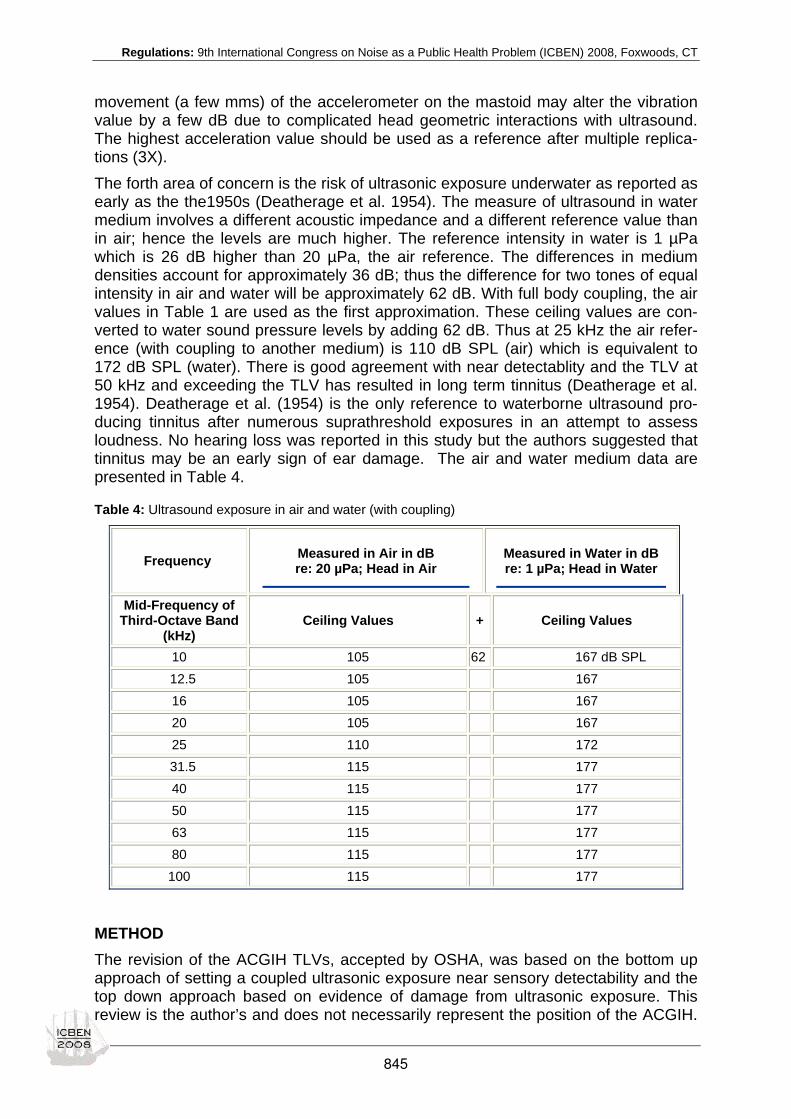
Regulations: 9th International Congress on Noise as a Public Health Problem (ICBEN) 2008, Foxwoods, CT
movement (a few mms) of the accelerometer on the mastoid may alter the vibration value by a few dB due to complicated head geometric interactions with ultrasound. The highest acceleration value should be used as a reference after multiple replica-tions (3X). The forth area of concern is the risk of ultrasonic exposure underwater as reported as early as the the1950s (Deatherage et al. 1954). The measure of ultrasound in water medium involves a different acoustic impedance and a different reference value than in air; hence the levels are much higher. The reference intensity in water is 1 µPa which is 26 dB higher than 20 µPa, the air reference. The differences in medium densities account for approximately 36 dB; thus the difference for two tones of equal intensity in air and water will be approximately 62 dB. With full body coupling, the air values in Table 1 are used as the first approximation. These ceiling values are con-verted to water sound pressure levels by adding 62 dB. Thus at 25 kHz the air refer-ence (with coupling to another medium) is 110 dB SPL (air) which is equivalent to 172 dB SPL (water). There is good agreement with near detectablity and the TLV at 50 kHz and exceeding the TLV has resulted in long term tinnitus (Deatherage et al. 1954). Deatherage et al. (1954) is the only reference to waterborne ultrasound pro-ducing tinnitus after numerous suprathreshold exposures in an attempt to assess loudness. No hearing loss was reported in this study but the authors suggested that tinnitus may be an early sign of ear damage. The air and water medium data are presented in Table 4.
Table 4: Ultrasound exposure in air and water (with coupling)
Frequency
Measured in Air in dB re: 20 µPa; Head in Air
Measured in Water in dB re: 1 µPa; Head in Water
Mid-Frequency of Third-Octave Band
(kHz) Ceiling Values + Ceiling Values
10 105 62 167 dB SPL 12.5 105 167
16 105 167 20 105 167 25 110 172
31.5 115 177 40 115 177 50 115 177 63 115 177 80 115 177
100 115 177
METHOD The revision of the ACGIH TLVs, accepted by OSHA, was based on the bottom up approach of setting a coupled ultrasonic exposure near sensory detectability and the top down approach based on evidence of damage from ultrasonic exposure. This review is the author’s and does not necessarily represent the position of the ACGIH.
845

Regulations: 9th International Congress on Noise as a Public Health Problem (ICBEN) 2008, Foxwoods, CT
The focus is only on any current evidence that airborne ultrasound may pose a risk to hearing. To assess risk, an indirect method will be applied which includes:
• understanding the hearing processes / hearing organs, and • the types of physical ultrasound measurements relating to hearing detection
and non-auditory effects.
RESULTS The bottom up approach of setting the coupled ultrasonic exposure near sensory de-tectability remains unchanged. For direct contact with the source, the TLV is 15 dB above 1g rms; which is about 5 dB below average threshold at 25 kHz (Lenhardt et al. 1991). The underwater TLV at 50 kHz is approximately 11 dB below threshold (Deatherage et al. 1954).The top down approach to assessing risk is based on evi-dence of ear damage from ultrasound. In the only such report of ultrasonic hearing damage, Grzesik and Pluta (1986) compared audiometric tests performed twice, three years apart in workers exposed to airborne ultrasound. Thresholds from 13 to 17 kHz revealed an average increase of 2-5 dB, beyond the hearing loss corrected for aging. The highest permanent threshold shifts were in the highest audible fre-quencies. This was interpreted as the cochlea was susceptible to hearing loss at the highest frequencies. More recently, workers exposed to ultrasonic welders, beyond the safe limit at 10-40 kHz, for 3-13 years, have revealed no progressive hearing loss in the 2-6 kHz range. Ultrasonic welders and lace sewing machines are a major source of intense airborne ultrasound (Pawlacyk-Luszczynska et al. (2007a, b). If contact ultrasound, centered at either 26 or 39 kHz, is applied directly to the head at five dB sensation level (SL), air conduction thresholds from 12 to 18 kHz are in-creased by 2-29 dB (Lenhardt 2003) paralleling the pattern of permanent hearing loss reported by Grzesik and Pluta (1986) but to a greater degree. When the ultra-sonic noise was terminated, normal threshold were again recorded, thus there was only a temporary effect in the cochlea (Lenhardt 2003). Kee et al. (2001) performed the inverse experiment by mixing 20 and 24 kHz tones (5 dB SL) and narrow-bands of audio noise (3-6, 6-9, 9-12, 12-15, 12-18 kHz) at 10-40 dB SL. Distortion product otoacoustic emissions (DPOAEs) were obtained prior to and following the task; there was no change after ultrasonic stimulation. The ultrasonic tones masked the audio noise for only the higher frequency bands. These masking experiments indicating interaction of ultrasound with high audio frequencies (12-18 kHz) is consistent with the pitch matching of ultrasound with high frequency audio tones (Lenhardt et al. 1991; Lenhardt 2003) and thus ultrasound activates first few mm (<4) of cochlear base. Wilson et al. (2002) reported audiograms in dental hygienists, who used ultrasonic scalers. There was loss of hearing at 3 kHz but not at conventional higher and lower audiometric frequencies. The spectra of ultrasonic drills were broad with the most energy in the 40 kHz range peaking at 80-89 dB SPL (Sorainen & Rytkönen (2002). Noise intensity was measured up to 82 dB A. Thus, the loss at 3 kHz may not be solely due to ultrasound. Further, ultrasonic hearing may be a more common phe-nomenon that first realized. A series of experiments have been carried out indicating that subjects respond behaviorally and physiologically (electroencephalograms and imaging) to the airborne ultrasonic components in some pieces of music (Oohashi et al. 2000, 2006). The auditory ultrasonic pathway for music was not specified. Ultra-sound was subsequently found to pass first through the eyes and brain then into the inner ear (Lenhardt 2007a). The eye is a mechanical structure capable of ultrasound propagation (Görig et al. 2006) and eye conduction of airborne sound could nicely
846

Regulations: 9th International Congress on Noise as a Public Health Problem (ICBEN) 2008, Foxwoods, CT
explain hearing loss and tinnitus in young workers exposed to intense ultrasound re-ported more than 40 years ago (Parrak 1966). Acoustic impedance (Z) is a function of density (kg/m3) and ultrasonic velocity (/m2s). The transmission coefficient (TC) of air (1.29 kg/m3) to the skull (1,900 kg/m3) is 59 dB. The TC from air to the eye (1,090 kg/m3) is 33 dB. The eye density is approximate the same as brain and the cochlear fluids (1,004 kg/m3) suggesting little attenuation inside the head. The fre-quency response of the eye is ultrasonic with a pass band from about 25 to 60 kHz. There remains only one report of some modest very high frequency hearing loss as a possible result of intense airborne exposure. However, now there is evidence that the eye is a window to the ear for airborne ultrasound, the high impedance of skin may not be as solid foundation for TLVs as previously argued.
DISCUSSION The US OHSA accepted the ACGIH recommended limits to prevent possible hearing loss caused by subharmonics of the ultrasonic frequencies rather than the ultrasonic sound itself. The masking data suggests ultrasound can directly affect the base of the cochlea. It was von Gierke (1950) who first proposed that audible subharmonics of ultrasound and the middle ear (air volume and/or ossicular displacement) were so-mehow involved in the response of workers to ultrasonic exposure. Displacement of the round and oval windows as release mechanisms for eye induced brain vibration could certainly interact with the ossicular chain, producing audio components that are detectable. Dallos and Linnell (1966) demonstrated intense stimulation can induce subharmonics at the eardrum, but not for ultrasound in humans. Contact ultrasound, at a comfortable level of 15 dB SL, will not produce subharmonics in the canal (Staab et al. 1997). Thus, threshold shifts in the high audio frequencies (10-20 kHz) could be due to high audio noise, ultrasonic subharmonics, ultrasound itself (via the eye) and even lower spectra noise. Because of this ambiguity, the TLVs for high audio fre-quencies are probably appropriate using time weighted averages (TWAs) at 88-94 dB (Table 1). Some fraction of workers may experience subjective effects between 75-105 dB, thus hearing protection, engineering controls (reflection or absorption barri-ers) and goggles may be needed. A novel vacuum earplug which distends the ear-drum outward and damps the ossicles would attenuate possible ultrasonic subhar-monics (Lenhardt 2007b). Worker exposure maintained under the TLVs should pre-vent adverse effects on their hearing and ability to understand speech. Nonetheless, a review of the high audio frequency ceiling values and possible adjustment might be considered if future evidence supports any increased hearing risk.
REFERENCES Dallos PJ, Linnell CO (1966). Even-order subharmonics in the peripheral auditory system. J Acoust Soc Am 40: 561-564.
Deatherage BH, Jeffress LA, Blodgett HC (1954). A note on the audibility of intense ultrasonic sound. J Acoust Soc Am 26: 582.
Görig C, Varghese T, Stiles T, van den Broek J, Zaqzebski JA, Murphy CJ (2006). Evaluation of acoustic wave propagation velocities in the ocular lens and vitreous tissues of pigs, dogs, and rabbits. Am J Vet Res 67: 288-295.
Grzesik J, Pluta E (1986). Dynamics of high-frequency hearing loss of operators of industrial ultrasonic devices. Int Arch Occup Environ Health 57: 137-142.
Kee R, Eddins D, Burkard R (2001). Perceptual and physiological manifestations of ultrasonic bone conduction in normal hearing subjects: Preliminary observations. ARO Abstracts 21383.
Lenhardt ML (2003). Ultrasonic hearing in humans: Applications for tinnitus treatment. Int Tinnitus J 9: 69-75.
Lenhardt ML (2007a). Eyes as fenestrations to the ears; a novel mechanism for high frequency hearing. Int Tinnitus J 13: 3-10.
847

Regulations: 9th International Congress on Noise as a Public Health Problem (ICBEN) 2008, Foxwoods, CT
Lenhardt ML (2007b). Novel vacuum personal hearing protection device. In: Proceedings of the National Hearing Conserva-tion Association, Savannah, GA, February 18-20. www.biosectech.com.
Lenhardt ML, Skellett R, Wang P, Clarke AM (1991). Human ultrasonic speech perception. Science 253: 82-85.
Lenhardt ML, Richards DG, Madsen AG, Goldstein BA, Shulman A, Guinta R (2002). Measurement of bone conduction levels for high frequencies. Int Tinnitus J 8: 9-12.
Occupational Safety Health Administration Technical Manual (2002). Sec III, Chapt. 5, subchapt. V, Ultrasonics. US Depart-ment of Labor.
Oohashi T, Nishina E, Honda M, Yonekura Y, Fuwamoto Y, Kawai N, Maekawa T, Nakamura S, Fukuyama H, Shibasaki H (2000). Inaudible high frequency sounds affect brain activity: hypersonic effect. J Neurophysiol 83: 3548-3558.
Oohashi T, Kawai N, Nishina E, Honda M, Yagi R, Nakamura S, Morimoto M, Maekawa T, Yonekura Y, Shibasaki H (2006). The role of biological system other than auditory air-conduction in the emergence of the hypersonic effect. Brain Res 1073: 339-347.
Parrack HO (1966). Effects of airborne ultrasound on humans. Int Audiol 5: 294-308.
Pawlaczyk-Łuszczyńska M, Dudarewicz A, Sliwińska-Kowalska M (2007a). Theoretical predictions and actual hearing thres-hold levels in workers exposed to ultrasonic noise of impulsive character--a pilot study. Int J Occup Saf Ergon 13: 409-418.
Pawlaczyk-Luszczyńska M, Dudarewicz A, Sliwińska-Kowalska M (2007b). Sources of occupational exposure to ultrasonic noise. Med Pr 58: 105-116.
Sorainen E, Rytkönen E (2002). Noise level and ultrasound spectra during burring. Clin Oral Investig 6: 133-136.
Staab WJ, Polashek T, Nunley J, Green RS, Brisken A, Dojan R, Taylor C, Katz R (1997). Audible ultrasound for profound losses. Hear Rev 4: 28-36. von Gierke HE (1950). Subharmonics generated in human and animal ears by intense sound. J Acoust Soc Am 22: 675-679.
Wiernicki C, Karoly WJ (1985). Ultrasound: biological effects and industrial hygiene concerns. Am Ind Hyg Assoc J 46: 488-496.
Wilson JD, Darby ML, Tolle SL, Sever JC Jr (2002). Effects of occupational ultrasonic noise exposure on hearing of dental hygienists: a pilot study. J Dent Hyg 76: 262-269.
848

Index of Authors
Ahmad R, 124Al Osman R, 197Albin M, 489Anderson G, 335Andersson H, 788Arcand R, 188Ardö J, 489Armstrong B, 294Asutay E, 428Au W-h, 662Ayas M, 252Aylward R, 427Ayob A, 124
Babisch W, 272Backenroth-Ohsako G, 150Barber J, 738Basner M, 463, 488, 499, 503, 510, 772Baulac M, 670Baumgartner W-D, 140Beelen R, 294Bellomini R, 801Belojevic G, 287, 639, 684Belt L, 433Belzile D, 188Berger EH, 71Berglund B, 617, 757Bergman P, 428Bernstein ER, 228Björk J, 489Blaeser SB, 740Blesser B, 254Blood GW, 169Blood IM, 169Boegli H, 817Boman E, 387
Botteldooren D, 322, 562, 617, 670Brammer AJ, 228Brauer M, 334Breugelmans ORP, 594Brink M, 817Bröde P, 510Brown L, 600Browne R, 707Brunekreef B, 294Burrows D, 151Buzzelli M, 334
Cadum E, 272Calvert GM, 149Campo P, 98, 182Canlon B, 150Chai D-L, 108Chen H, 429Chen S-s, 89Cheng X-r, 89Cherniack MG, 228Chiu M-C, 80Christensen KB, 302Clark C, 355Clausen T, 302Cluydts R, 550Cowan JP, 626Curcuruto S, 834
Davies HW, 263, 295, 334Davis A, 46, 53, 140Davis B, 89Davis R, 149De Coensel B, 617de Greve B, 322, 562, 670de Kluizenaar Y, 293
849

De Valck E, 550Defrance J, 670Dekoninck L, 322Delaney DK, 740Demers PA, 334Deshaies P, 188Dhamani I, 134, 252Dice N, 141Dobie RA, 52Dockrell J, 369Downs D, 152, 433Dudarewicz A, 137
Eagan ME, 335Ecob R, 53Eldred KM, 36Elmenhorst E-M, 463, 503Enmarker I, 387Ernst A, 140Esterhuizen H, 427Ezzatian P, 219
Feeney P, 90Ferry G, 138Finegold LS, 751, 780Fischer P, 294Fleischer G, 117Fligor B, 79Folsom R, 90Fontana Zocoli AM, 139Fortier P, 188Fransen E, 137Fransson N, 428Fristrup K, 738Fuente A, 135, 136
Gagné J-P, 125, 220Gardner RC, 526Genell A, 428Gentry RL, 47Gidlöf-Gunnarsson A, 471, 631Giguère C, 197, 210Girard S-A, 188Gjestland T, 556Gladstone VS, 151
Goldbohm RA, 294Gonzalez B, 433Goto K, 571Graham MA, 487Grandori F, 140Green A-M, 450Grevstad P, 205Griefahn B, 17, 38, 479, 503, 510Griest SE, 62, 91, 148, 176Gürtunca G, 149
Haapakangas A, 395, 418, 434Hager LD, 71Hagerman B, 150Haka M, 395, 418Halin N, 410Hamernik RP, 89Hashimoto Y, 688, 699Hastings MC, 739Hayashi N, 314Helenius R, 434Hiramatsu K, 314, 348Hoek G, 294Hong J, 587Hong O, 159Hongisto V, 395, 418, 434, 442Horonjeff R, 335Houthuijs D, 272, 294Howarth LC, 62, 91Hughes R, 362Hume KI, 456Huybregts C, 741Hygge S, 387, 410
Ilic J, 287Ishlah W, 124
Jakobsson K, 489Jakovljevic B, 287, 639, 684Jansen G, 40Jansen P, 809Janssen SA, 487, 594, 644, 653Janssen T, 140Jarup L, 272Jensen A, 307
850

Jeon JY, 583, 595, 731Jerson T, 471, 542Job RFS, 280, 347Johnson A-C, 106, 150Jones D, 362Jutras B, 220
Kailash, 454Kaku J, 715Kanekama Y, 152, 433Kaneko T, 571Katsouyanni K, 272Kendrick P, 707Kerr MJ, 159Kerry G, 707Keskinen E, 395, 434Kim J, 587Kim K, 587Kim R, 757Kjellberg A, 403, 450Konings A, 137Kovalchik P, 149Kramer S, 140Krieg E, 106Kristiansen GB, 182Kristiansen J, 205, 302, 489Kroesen M, 644, 653Kujawa SG, 51, 90
Lacerda A, 125Lagacé J, 220Lam K-c, 662Lambert J, 576, 751Lambert WE, 176Laroche C, 188, 197, 210Lee PJ, 583, 595Lee S, 587Lei Z, 108Lenhardt ML, 842Lercher P, 322, 562, 617, 670Leroux T, 125, 188Li H-J, 108, 518Li L, 219Li N, 518
Lim C, 587Ljung R, 403, 450Lonsbury-Martin BL, 133Lu J-Q, 518Lücke T, 307Lund SP, 182, 205, 307Lund T, 302Lundberg WR, 825Lusk SL, 159Luz GA, 534, 793Luzzi S, 801Lyon RH, 236
Ma H, 678Maass H, 463Macken W, 362Mackenbach JP, 293Maguin K, 98Marks A, 479Marsh J, 362Marsico G, 834Martin GK, 133Martin GY, 176, 177Martin R, 188Martin WH, 62, 91, 148, 176, 177Matetic RJ, 149Matsui T, 314, 348Meinke DK, 62, 91, 133, 141Mendes Marques J, 139Miedema HME, 293, 487, 594, 644, 653Miller NP, 526Mills D, 90Miyakawa M, 314Miyakita T, 348Mokhtar RH, 124Molin EJE, 644, 653Morata TC, 106, 139Morihara T, 679, 724Morio K, 314Morita I, 314Müller O, 80Müller R, 117Müller U, 463, 503Muirhead M, 707
851

Murphy WJ, 149
Namba S, 715Neitzel R, 90Nélisse H, 188Nguyen TL, 699Nicholas B, 335Nilsson ME, 617Nishimura T, 688, 699Novak CC, 402Nykaza ET, 534Nylen P, 106
Ögren M, 471, 542, 788Öhrström E, 471, 542, 631Östergren P-O, 489Oettl D, 322Ogata S, 715Ohashi S, 314Oliva C, 751Ota A, 608, 724
Passchier-Vermeer W, 487Pater LL, 534Paunovic K, 287, 639, 684Pawelczyk M, 137Pawlas K, 106Payton KL, 243Pedersen NL, 150Pershagen G, 272Persson R, 489Petersen DE, 228Phan HAT, 688, 699Phan HYT, 688, 699Philipps-Bertin C, 576Picard M, 188Pichora-Fuller K, 219Pirrera S, 550Popper AN, 739Poulin M, 188Prasher D, 106Probst R, 140Purvis GO, 151
Qiu W, 89
Quehl J, 463
Rajashekar B, 134Rajashekhar B, 252Rajkowska E, 137Randolph R, 149Rell MJ, 35Robens S, 479, 510Romero C, 801Rosenhall U, 150Rüdisser J, 322, 562, 670
Sacchetti F, 834Sakashita C, 280Salter L-R, 254Sato T, 679, 688, 699Scarlotta T, 62Schneider BA, 219Schouten LJ, 294Schulz TY, 149Schwela D, 780Seixas N, 90Shanker AS, 134Sheppard L, 90Shield B, 369Shrestha M, 243Shrivatava SK, 454Siebert U, 499Sikström S, 378Silvaggio R, 834Simmons JA, 48Sköld A, 428Sliwinska-Kowalska M, 50, 106, 136, 137,
140Smith P, 53Sobel JL, 62, 91, 148, 160Söderlund G, 378Sörqvist P, 410Soli SD, 210Stagner BB, 133Stallen PJM, 653Stansfeld S, 757Starck J, 106Stenfelt S, 140
852

Stephenson M, 149Stewart J, 780Stojanov V, 287Strasser H, 80Stroh E, 489
Tajadura A, 428Tamura A, 608, 724Theorell T, 150Tivnan T, 335Toppila E, 106Tufts J, 138Turina F, 841
Uchiyama I, 314Uehara T, 348Uhrner U, 322Ulfendahl M, 150
Västfjäll D, 428Vaillancourt V, 210Vallet M, 765van Camp G, 137van den Brandt PA, 294van Kamp I, 263, 295, 600van Kempen EEMM, 594van Laer L, 137van Lenthe FJ, 293van Wee B, 644, 653Vejvoda M, 463Velonakis M, 272Voix J, 71Vos H, 487, 594, 644, 653Vos J, 496
Waddington D, 707Wang LM, 402Weathersby PK, 138Wunderli J-M, 817
Yamada I, 715Yamamoto T, 348Yamashita K, 314Yano T, 678, 679, 688, 699Yokoshima S, 608, 724
Yokota T, 715You J, 583, 731Yu G, 228Yu W-B, 518
Zamyslowska-Szmytke E, 106, 136Zeng L, 89, 108, 518Zhao Y-M, 89, 108, 518Zheng Y, 197
853