ISMIR 2008
692
ISMIR 2008 Proceedings of the 9th International Conference on Music Information Retrieval Drexel University – Philadelphia, USA September 14-18, 2008 ISMIR
-
Upload
khangminh22 -
Category
Documents
-
view
2 -
download
0
Transcript of ISMIR 2008

ISMIR 2008
Proceedings of the 9th International Conference on Music Information Retrieval
Drexel University – Philadelphia, USA September 14-18, 2008
ISMIR

ISMIR 2008 is organized by
Drexel University
Columbia University
New York University
University of Southern California
COLUMBIA UNIVERSITYIN THE CITY OF NEW YORK
2

Edited by Juan Pablo Bello, Elaine Chew, Douglas Turnbull
ISMIR 2008
Proceedings of the 9th International Conference on Music Information Retrieval
© Copyright 2008, ISMIR. Permission is hereby granted to reproduce and distribute copies of individual works from this publication for research, library, and nonprofit educational purposes, provided that copies are distributed at or below cost, and that the author, source, and copyright notice are included on each copy. This permission is in addition to rights granted under Sections 107, 108, and other provisions of the U.S. Copyright Act.
ISBN: 978-0-615-24849-3
3
ISMIR 2008 gratefully acknowledges support from the following sponsors:
4

Conference Committee General Chairs: Dan Ellis, Columbia University, USA Youngmoo Kim, Drexel University, USA Program Chairs: Juan Pablo Bello, New York University, USA Elaine Chew, Radcliffe Institute for Advanced Study / University of Southern California, USA
Publication Chair: Douglas Turnbull, Swarthmore College, USA Tutorials Chair: Michael Mandel, Columbia University, USA Demos & Exhibits Chair: Arpi Mardirossian, University of Southern California, USA Sponsorship Chair: Jeremy Pickens, FX Palo Alto Laboratory, USA
5
Program Committee
Christina Anagnostopoulou, University of Athens, Greece Sally Jo Cunningham, University of Waikato, New Zealand
Roger Dannenberg, Carnegie Mellon University, USA Simon Dixon, Queen Mary, University of London, UK Stephen Downie, University of Illinois, USA Michael Fingerhut, Institut de Recherche et Coordination Acoustique/Musique, France Ichiro Fujinaga, McGill University, Canada
Masataka Goto, National Institute of Advanced Industrial Science and Technology, Japan Katayose Haruhiro, Kwansei Gakuin University, Japan Aline Honingh, City University, London, UK
Özgür �zmirli, Connecticut College, USA Anssi Klapuri, Tampere University of Technology, Finland Paul Lamere, Sun Microsystems, USA Kjell Lemström, University of Helsinki, Finland
Emilia Gómez, Universitat Pompeu Fabra, Spain Connie Mayer, University of Maryland, USA
François Pachet, Sony Research Labs, France Christopher Raphael, University of Indiana, Bloomington, USA Gaël Richards, École Nationale Supérieure des Télécommunications, France Malcolm Slaney, Yahoo! Research, USA George Tzanetakis, University of Victoria, Canada Anja Volk, University of Utrecht, the Netherlands Gerhard Widmer, Johannes Kepler University, Linz, Austria
6

Reviewers Samer Abdallah Kamil Adiloglu Miguel Alonso Xavier Amatriain Christina Anagnostopoulou John Anderies Josep Lluis Arcos Gerard Assayag Jean-Julien Aucouturier Wolfgang Auhagen David Bainbridge Stephan Bauman Mert Bay Juan Pablo Bello Nancy Bertin Rens Bod Carola Boehm Roberto Bresin Donald Byrd Emilios Cambouropoulos Antonio Camurri Pedro Cano Michael Casey Oscar Celma A. Taylan Cemgil Elaine Chew Parag Chordia Chinghua Chuan Darrell Conklin Arshia Cont Perry Cook Tim Crawford Sally Jo Cunningham Roger Dannenberg Laurent Daudet Matthew Davies Elizabeth Davis Francois Deliege Simon Dixon J. Stephen Downie Shlomo Dubnov Jon Dunn Jean-Louis Durrieu Douglas Eck Jana Eggink
Andreas Ehmann Alexandros Eleftheriadis Dan Ellis Slim Essid Morwaread Farbood Michael Fingerhut Derry FitzGerald Arthur Flexer Muriel Foulonneau Alexandre Francois Judy Franklin Hiromasa Fujihara Ichiro Fujinaga Jörg Garbers Martin Gasser Olivier Gillet Simon Godsill Emilia Gomez Michael Good Masataka Goto Fabien Gouyon Maarten Grachten Stephen Green Richard Griscom Catherine Guastavino Toni Heittola Marko Helen Stephen Henry Perfecto Herrera Keiji Hirata Henkjan Honing Aline Honingh Julian Hook Xiao Hu José Manuel Iñesta Charlie Inskip Eric Isaacson Akinori Ito Özgür Izmirli Roger Jang Tristan Jehan Kristoffer Jensen M. Cameron Jones Katsuhiko Kaji Hirokazu Kameoka Kunio Kashino Haruhiro Katayose Robert Keller Youngmoo Kim
Tetsuro Kitahara Anssi Klapuri Peter Knees Frank Kurth Mika Kuuskankare Mathieu Lagrange Pauli Laine Paul Lamere Gert Lanckriet Olivier Lartillot Kai Lassfolk Cyril Laurier Jin Ha Lee Kyogu Lee Marc Leman Kjell Lemström Micheline Lesaffre Pierre Leveau Mark Levy David Lewis Beth Logan Lie Lu Veli Mäkinen Arpi Mardirossian Matija Marolt Alan Marsden Francisco Martín Luis Gustavo Martins Connie Mayer Cory McKay Martin Mckinney David Meredith Dirk Moelants Meinard Müeller Daniel Mullensiefen Peter Munstedt Tomoyasu Nakano Teresa Marrin Nakra Kerstin Neubarth Kia Ng Takuichi Nishimura Beesuan Ong Nicola Orio Alexey Ozerov Francois Pachet Rui Pedro Paiva Elias Pampalk Bryan Pardo Richard Parncutt
7

ISMIR 2008 – Reviewers
Jouni Paulus Marcus Pearce Paul Peeling Geoffroy Peeters Henri Penttinen Jeremy Pickens Anna Pienimäki Aggelos Pikrakis Mark Plumbley Tim Pohle Laurent Pugin Ian Quinn Rafael Ramirez Christopher Raphael Andreas Rauber Josh Reiss Gäel Richard Jenn Riley David Rizo Stephane Rossignol Robert Rowe Matti Ryynänen Makiko Sadakata
Shigeki Sagayama Mark Sandler Craig Sapp Markus Schedl Xavier Serra Joan Serrà William Sethares Klaus Seyerlehner Malcolm Slaney Paris Smaragdis Leigh Smith Peter Somerville Neta Spiro Mark Steedman Sebastian Streich Kenji Suzuki Haruto Takeda David Temperley Atte Tenkanen Belinda Thom Dan Tidhar Renee Timmers Søren Tjagvad Madsen
Petri Toiviainen Yo Tomita Charlotte Truchet Douglas Turnbull Rainer Typke George Tzanetakis Alexandra Uitdenbogerd Erdem Unal Vincent Verfaille Fabio Vignoli Emmanuel Vincent Tuomas Virtanen Anja Volk Ye Wang Kris West Tillman Weyde Nick Whiteley Brian Whitman Gerhard Widmer Frans Wiering Geraint Wiggins Matt Wright Kazuyoshi Yoshii
8

Preface It is the great pleasure of the ISMIR 2008 Organizing Committee to welcome you all to Philadelphia for the Ninth International Conference on Music Information Retrieval. Since its inception in 2000, ISMIR has become the premiere venue for the presentation of research in the multidisciplinary field of accessing, analyzing, and managing large collections and archives of music information. We are proud to host the ninth ISMIR at Drexel University in Philadelphia, Pennsylvania, USA from September 14-18, 2008. The continuing expansion of the Music IR community reflects the enormous challenges and opportunities presented by the recent and tremendous growth in digital music and music-related data. ISMIR provides a forum for the exchange of ideas amongst representatives of academia, industry, entertainment, and education, including researchers, developers, educators, librarians, students, and professional users, who contribute to this broadly interdisciplinary domain. Alongside presentations of original theoretical research and practical work, ISMIR 2008 provides several introductory and in-depth tutorials, and a venue for the showcase of current MIR-related products and systems. This year, we introduced several changes over recent ISMIR conferences aimed at elevating the prominence and breadth of appeal of the paper presentations, and at encouraging broad participation from all MIR researchers: • Emphasis on Cross-disciplinary or Interdisciplinary Research: While ISMIR has always been
inherently interdisciplinary in nature, ISMIR 2008 places a singular premium on scholarly papers that span two or more disciplines, and encouraged submissions that appealed to the widest possible portion of the community. The preference for cross-disciplinary contributions was applied to the balancing of the overall program, and influenced the selection of papers for plenary presentations.
• Uniform Paper Status: Every accepted paper has up to six pages in the proceedings, and all papers are
presented as posters, reflecting the particular value of poster presentations in facilitating discussion between researchers; there is no ‘tiering’ of papers. A subset of papers has been selected for oral presentation in addition to their poster slots, specifically on the basis of their broad appeal to the whole community. By reducing the number of oral papers to around one quarter of all papers, compared to more than half in previous ISMIRs, we are able to keep ISMIR 2008 as single track and avoid obliging people to ‘label’ themselves by choosing between alternative sessions.
• Authorship Limitations: We introduced authorship limits to encourage authors to focus on preparing
their most distinctive work for submission and to cultivate a broad range of work by diverse researchers. Any individual could submit only one paper as first author, and his or her name could appear as an author or co-author on only three submissions in total. The goal of these limitations was to increase the diversity of viewpoints represented at ISMIR and to avoid the proceedings being unduly slanted towards any specific aspect of MIR. Author limits are common practice in many scholarly communities who view their gatherings as too valuable to allow any individual more than one opportunity to present their views at the assembly. In our view, this will help establish ISMIR not only as a place to publish, but also as a well-balanced public forum for scholars to stand before an international gathering of peers to present their ideas.
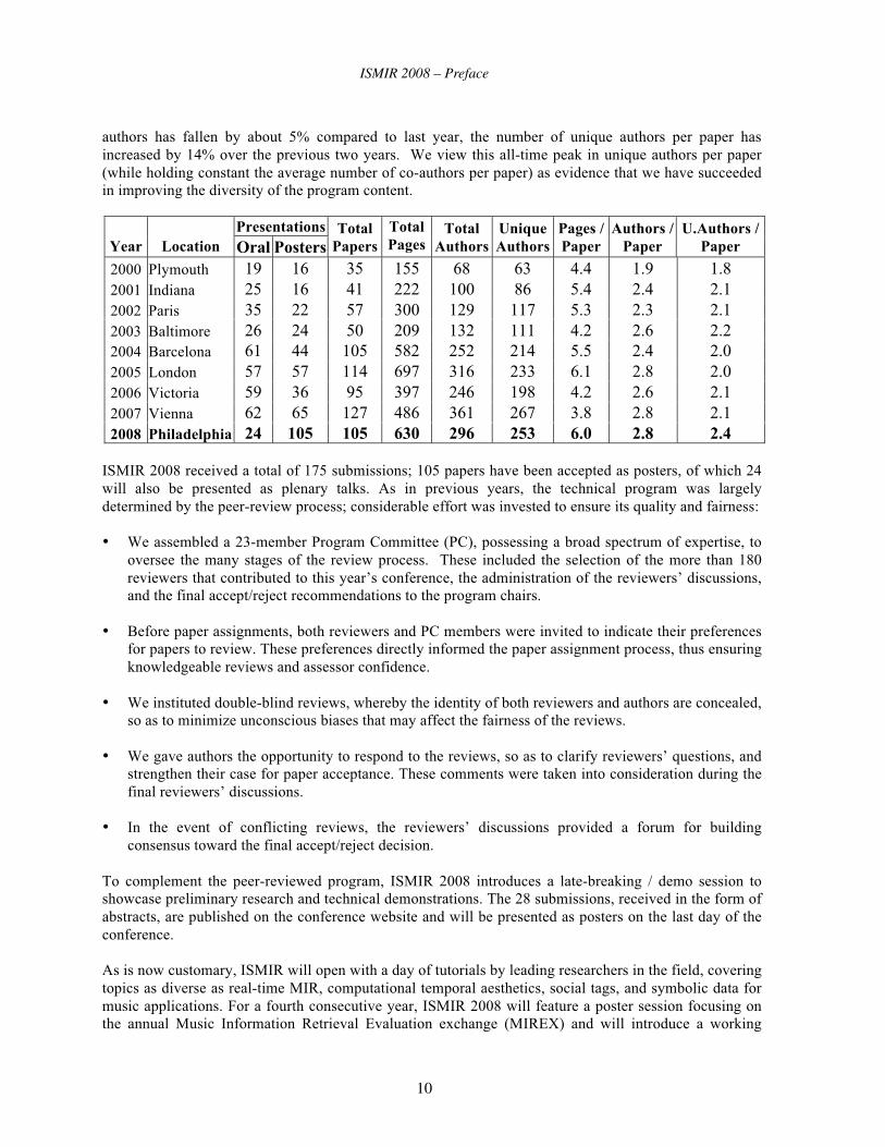
The following table shows some statistics from all the ISMIR conferences (data from the Cumulative ISMIR Proceedings on www.ismir.net). We see the impact of these changes has been to reduce slightly the total number of papers presented at the conference compared to 2007, but a substantial increase in the total proceedings length due to the absence of short papers. Although the absolute number of unique
9
ISMIR 2008 – Preface
authors has fallen by about 5% compared to last year, the number of unique authors per paper has increased by 14% over the previous two years. We view this all-time peak in unique authors per paper (while holding constant the average number of co-authors per paper) as evidence that we have succeeded in improving the diversity of the program content.
ISMIR 2008 received a total of 175 submissions; 105 papers have been accepted as posters, of which 24 will also be presented as plenary talks. As in previous years, the technical program was largely determined by the peer-review process; considerable effort was invested to ensure its quality and fairness: • We assembled a 23-member Program Committee (PC), possessing a broad spectrum of expertise, to
oversee the many stages of the review process. These included the selection of the more than 180 reviewers that contributed to this year’s conference, the administration of the reviewers’ discussions, and the final accept/reject recommendations to the program chairs.
• Before paper assignments, both reviewers and PC members were invited to indicate their preferences for papers to review. These preferences directly informed the paper assignment process, thus ensuring knowledgeable reviews and assessor confidence.
• We instituted double-blind reviews, whereby the identity of both reviewers and authors are concealed, so as to minimize unconscious biases that may affect the fairness of the reviews.
• We gave authors the opportunity to respond to the reviews, so as to clarify reviewers’ questions, and strengthen their case for paper acceptance. These comments were taken into consideration during the final reviewers’ discussions.
• In the event of conflicting reviews, the reviewers’ discussions provided a forum for building consensus toward the final accept/reject decision.
To complement the peer-reviewed program, ISMIR 2008 introduces a late-breaking / demo session to showcase preliminary research and technical demonstrations. The 28 submissions, received in the form of abstracts, are published on the conference website and will be presented as posters on the last day of the conference. As is now customary, ISMIR will open with a day of tutorials by leading researchers in the field, covering topics as diverse as real-time MIR, computational temporal aesthetics, social tags, and symbolic data for music applications. For a fourth consecutive year, ISMIR 2008 will feature a poster session focusing on the annual Music Information Retrieval Evaluation exchange (MIREX) and will introduce a working
Presentations Year Location Oral Posters
Total Papers
Total Pages
Total Authors
Unique Authors
Pages / Paper
Authors / Paper
U.Authors / Paper
2000 Plymouth 19 16 35 155 68 63 4.4 1.9 1.8 2001 Indiana 25 16 41 222 100 86 5.4 2.4 2.1 2002 Paris 35 22 57 300 129 117 5.3 2.3 2.1 2003 Baltimore 26 24 50 209 132 111 4.2 2.6 2.2 2004 Barcelona 61 44 105 582 252 214 5.5 2.4 2.0 2005 London 57 57 114 697 316 233 6.1 2.8 2.0 2006 Victoria 59 36 95 397 246 198 4.2 2.6 2.1 2007 Vienna 62 65 127 486 361 267 3.8 2.8 2.1 2008 Philadelphia 24 105 105 630 296 253 6.0 2.8 2.4
10

ISMIR 2008 – Preface
lunch that serves to discuss the current state of MIREX and the necessary steps to sustain and increase these evaluation efforts in years to come. Additionally, the program will feature a panel discussion on the topic of music discovery and recommendation. Expert panelists, drawn from industry, will discuss the links between academic MIR research and commercial applications, providing an opportunity for them to give any feedback on the direction of the whole community. This year’s keynote address will be given by Jeanne Bamberger (MIT/UC-Berkeley), who will speak on how humans retrieve music, from perception to action to representation and back, and how information retrieval is involved in each of these steps. A student of Artur Schnabel and Roger Sessions, Prof. Bamberger’s work in music cognition and education is also influenced by her background in philosophy. The conference program also includes an invited talk by Dmitri Tymoczko of Princeton University. Prof. Tymoczko is a music theorist and composer who has received considerable recent attention for his work on geometric modeling of the relationship between chords and scales, which has proven to be insightful and provocative. The technical program is complemented by a social program including, on Monday evening, the conference banquet at Philadelphia’s National Constitution Center. At the museum, which opened in 2003, we will have a view over the iconic Liberty Bell and Independence Hall, site of the approval and first public reading of the United States’ Declaration of Independence on July 4th, 1776. All information on ISMIR 2008, including the full conference and social program, is available at the conference website: http://ismir2008.ismir.net. We would like to thank everyone who contributed to the planning, preparation, and administration of ISMIR 2008. In particular, we acknowledge the expert help of the program committee members and reviewers who have given their time and experience to ensure the high quality of the scientific program. Our corporate sponsors, Gracenote, Sun Microsystems, and MusicIP, are worthy of a special mention. It is due to their generous support that we are able to offer a complete program and additional services without compromising the affordability of the conference. In addition, Sun’s sponsorship provided the means to award 10 travel grants to assist students with transportation to ISMIR 2008. Finally, we are extremely grateful to the myriad student volunteers and Drexel support staff who have offered their time and knowledge to ensure the smooth operation of the conference. We are very happy and pleased to see you here in Philadelphia to jointly witness the continuing growth and strength of the Music Information Retrieval community. Thank you for your support and contributions, and we wish you all a successful and productive conference!
Dan Ellis, Youngmoo Kim ISMIR 2008 General Chairs Juan Pablo Bello, Elaine Chew ISMIR 2008 Program Chairs
11


Contents
Host Institutions 2
Sponsors 4
Conference Committee 5
Reviewers 7
Preface 9
Keynote Talk 21Human Music Retrieval: Noting Time
Jeanne Bamberger . . . . . . . . . . . . . . . . . . . . . . . . . . . . . . . . . . . . . . . 21
Invited Talk 22The Geometry of Consonance
Dmitri Tymoczko . . . . . . . . . . . . . . . . . . . . . . . . . . . . . . . . . . . . . . . . 22
Tutorials 23Music Information Retrieval in ChucK; Real-Time Prototyping for MIR Systems & Performance
Ge Wang, Rebecca Fiebrink, Perry R. Cook . . . . . . . . . . . . . . . . . . . . . . . . . . 23
Computational Temporal Aesthetics; Relation Between Surprise, Salience and Aesthetics in Mu-
sic and Audio Signals
Shlomo Dubnov . . . . . . . . . . . . . . . . . . . . . . . . . . . . . . . . . . . . . . . . . 23
Social Tags and Music Information Retrieval
Paul Lamere, Elias Pampalk . . . . . . . . . . . . . . . . . . . . . . . . . . . . . . . . . . 24
Survey of Symbolic Data for Music Applications
Eleanor Selfridge-Field, Craig Sapp . . . . . . . . . . . . . . . . . . . . . . . . . . . . . . 24
Session 1a – Harmony 25COCHONUT: Recognizing Complex Chords from MIDI Guitar Sequences
Ricardo Scholz, Geber Ramalho . . . . . . . . . . . . . . . . . . . . . . . . . . . . . . . . 27
Chord Recognition using Instruments Voicing Constraints
Xinglin Zhang, David Gerhard . . . . . . . . . . . . . . . . . . . . . . . . . . . . . . . . . 33
Automatic Chord Recognition Based on Probabilistic Integration of Chord Transition and Bass
Pitch Estimation
Kouhei Sumi, Katsutoshi Itoyama, Kazuyoshi Yoshii, Kazunori Komatani, Tetsuya Ogata,Hiroshi G. Okuno . . . . . . . . . . . . . . . . . . . . . . . . . . . . . . . . . . . . . . . . 39
A Discrete Mixture Model for Chord Labelling
Matthias Mauch, Simon Dixon . . . . . . . . . . . . . . . . . . . . . . . . . . . . . . . . . 45
Tonal Pitch Step Distance: a Similarity Measure for Chord Progressions
Bas de Haas, Remco Veltkamp, Frans Wiering . . . . . . . . . . . . . . . . . . . . . . . . . 51
Evaluating and Visualizing Effectiveness of Style Emulation in Musical Accompaniment
Ching-Hua Chuan, Elaine Chew . . . . . . . . . . . . . . . . . . . . . . . . . . . . . . . . 57

ISMIR 2008 – Contents
Characterisation of Harmony with Inductive Logic Programming
Amèlie Anglade, Simon Dixon . . . . . . . . . . . . . . . . . . . . . . . . . . . . . . . . . 63
Structured Polyphonic Patterns
Mathieu Bergeron, Darrell Conklin . . . . . . . . . . . . . . . . . . . . . . . . . . . . . . . 69
A Music Database and Query System for Recombinant Composition
James Maxwell, Arne Eigenfeldt . . . . . . . . . . . . . . . . . . . . . . . . . . . . . . . . 75
Session 1b – Melody 81Detection of Stream Segments in Symbolic Musical Data
Dimitris Rafailidis, Alexandros Nanopoulos, Emilios Cambouropoulos, Yannis Manolopoulos 83
A Comparison of Statistical and Rule-Based Models of Melodic Segmentation
Marcus Pearce, Daniel Müellensiefen, Geraint Wiggins . . . . . . . . . . . . . . . . . . . . 89
Speeding Melody Search with Vantage Point Trees
Michael Skalak, Jinyu Han, Bryan Pardo . . . . . . . . . . . . . . . . . . . . . . . . . . . . 95
A Manual Annotation Method for Melodic Similarity and the Study of Melody Feature Sets
Anja Volk, Peter van Kranenburg, Jörg Garbers, Frans Wiering, Remco C. Veltkamp, LouisP. Grijp . . . . . . . . . . . . . . . . . . . . . . . . . . . . . . . . . . . . . . . . . . . . . 101
Melody Expectation Method Based on GTTM and TPS
Masatoshi Hamanaka, Keiji Hirata, Satoshi Tojo . . . . . . . . . . . . . . . . . . . . . . . 107
Session 1c – Timbre 113Automatic Identification of Simultaneous Singers in Duet Recordings
Wei-Ho Tsai, Shih-Jie Liao, Catherine Lai . . . . . . . . . . . . . . . . . . . . . . . . . . . 115
Vocal Segment Classification in Popular Music
Ling Feng, Andreas Brinch Nielsen, Lars Kai Hansen . . . . . . . . . . . . . . . . . . . . . 121
Learning Musical Instruments from Mixtures of Audio with Weak Labels
David Little, Bryan Pardo . . . . . . . . . . . . . . . . . . . . . . . . . . . . . . . . . . . . 127
Instrument Equalizer for Query-by-Example Retrieval: Improving Sound Source Separation
Based on Integrated Harmonic and Inharmonic Models
Katsutoshi Itoyama, Masataka Goto, Kazunori Komatani, Tetsuya Ogata, Hiroshi G. Okuno 133
A Real-time Equalizer of Harmonic and Percussive Components in Music Signals
Nobutaka Ono, Kenichi Miyamoto, Hirokazu Kameoka, Shigeki Sagayama . . . . . . . . . . 139
Session 1d – MIR Platforms 145The PerlHumdrum and PerlLilypond Toolkits for Symbolic Music Information Retrieval
Ian Knopke . . . . . . . . . . . . . . . . . . . . . . . . . . . . . . . . . . . . . . . . . . . 147
Support for MIR Prototyping and Real-Time Applications in the ChucK Programming Language
Rebecca Fiebrink, Ge Wang, Perry Cook . . . . . . . . . . . . . . . . . . . . . . . . . . . . 153
Session 2a – Music Recommendation and Organization 159A Comparison of Signal Based Music Recommendation to Genre Labels, Collaborative Filtering,
Musicological Analysis, Human Recommendation and Random Baseline
Terence Magno, Carl Sable . . . . . . . . . . . . . . . . . . . . . . . . . . . . . . . . . . . 161
Kernel Expansion for Online Preference Tracking
Yvonne Moh, Joachim Buhmann . . . . . . . . . . . . . . . . . . . . . . . . . . . . . . . . 167
14

ISMIR 2008 – Contents
Playlist Generation using Start and End Songs
Arthur Flexer, Dominik Schnitzer, Martin Gasser, Gerhard Widmer . . . . . . . . . . . . . . 173
Accessing Music Collections Via Representative Cluster Prototypes in a Hierarchical Organiza-
tion Scheme
Markus Dopler, Markus Schedl, Tim Pohle, Peter Knees . . . . . . . . . . . . . . . . . . . . 179
Development of a Music Organizer for Children
Sally Jo Cunningham, Edmond Zhang . . . . . . . . . . . . . . . . . . . . . . . . . . . . . 185
Session 2b – Music Recognition and Visualization 191Development of an Automatic Music Selection System Based on Runner’s Step Frequency
Masahiro Niitsuma, Hiroshi Takaesu, Hazuki Demachi, Masaki Oono, Hiroaki Saito . . . . . 193
A Robot Singer with Music Recognition Based on Real-Time Beat Tracking
Kazumasa Murata, Kazuhiro Nakadai, Kazuyoshi Yoshii, Ryu Takeda, Toyotaka Torii, Hi-roshi G. Okuno, Yuji Hasegawa, Hiroshi Tsujino . . . . . . . . . . . . . . . . . . . . . . . . 199
Streamcatcher: Integrated Visualization of Music Clips and Online Audio Streams
Martin Gasser, Arthur Flexer, Gerhard Widmer . . . . . . . . . . . . . . . . . . . . . . . . 205
Music Thumbnailer: Visualizing Musical Pieces in Thumbnail Images Based on Acoustic Fea-
tures
Kazuyoshi Yoshii, Masataka Goto . . . . . . . . . . . . . . . . . . . . . . . . . . . . . . . 211
Session 2c – Knowledge Representation, Tags, Metadata 217Ternary Semantic Analysis of Social Tags for Personalized Music Recommendation
Panagiotis Symeonidis, Maria Ruxanda, Alexandros Nanopoulos, Yannis Manolopoulos . . . 219
Five Approaches to Collecting Tags for Music
Douglas Turnbull, Luke Barrington, Gert Lanckriet . . . . . . . . . . . . . . . . . . . . . . 225
MoodSwings: A Collaborative Game for Music Mood Label Collection
Youngmoo Kim, Erik Schmidt, Lloyd Emelle . . . . . . . . . . . . . . . . . . . . . . . . . . 231
Collective Annotation of Music from Multiple Semantic Categories
Zhiyao Duan, Lie Lu, Changshui Zhang . . . . . . . . . . . . . . . . . . . . . . . . . . . . 237
MCIpa: A Music Content Information Player and Annotator for Discovering Music
Geoffroy Peeters, David Fenech, Xavier Rodet . . . . . . . . . . . . . . . . . . . . . . . . . 243
Connecting the Dots: Music Metadata Generation, Schemas and Applications.
Nik Corthaut, Sten Govaerts, Katrien Verbert, Erik Duval . . . . . . . . . . . . . . . . . . . 249
The Quest for Musical Genres: Do the Experts and the Wisdom of Crowds Agree?
Mohamed Sordo, Òscar Celma, Martin Blech, Enric Guaus . . . . . . . . . . . . . . . . . . 255
Session 2d – Social and Music Networks 261A Web of Musical Information
Yves Raimond, Mark Sandler . . . . . . . . . . . . . . . . . . . . . . . . . . . . . . . . . . 263
Using Audio Analysis and Network Structure to Identify Communities in On-Line Social Net-
works of Artists
Kurt Jacobson, Mark Sandler, Ben Fields . . . . . . . . . . . . . . . . . . . . . . . . . . . 269
Uncovering Affinity of Artists to Multiple Genres from Social Behaviour Data
Claudio Baccigalupo, Enric Plaza, Justin Donaldson . . . . . . . . . . . . . . . . . . . . . 275
Hyperlinking Lyrics: A Method for Creating Hyperlinks Between Phrases in Song Lyrics
Hiromasa Fujihara, Masataka Goto, Jun Ogata . . . . . . . . . . . . . . . . . . . . . . . . 281
15
ISMIR 2008 – Contents
Oh Oh Oh Whoah! Towards Automatic Topic Detection In Song Lyrics
Florian Kleedorfer, Peter Knees, Tim Pohle . . . . . . . . . . . . . . . . . . . . . . . . . . 287
Session 3a – Content-Based Retrieval, Categorization and Similarity 1 293A Text Retrieval Approach to Content-Based Audio Hashing
Matthew Riley, Eric Heinen, Joydeep Ghosh . . . . . . . . . . . . . . . . . . . . . . . . . . 295
A Music Identification System Based on Chroma Indexing and Statistical Modeling
Riccardo Miotto, Nicola Orio . . . . . . . . . . . . . . . . . . . . . . . . . . . . . . . . . . 301
Hubs and Homogeneity: Improving Content-Based Music Modeling
Mark Godfrey, Parag Chordia . . . . . . . . . . . . . . . . . . . . . . . . . . . . . . . . . 307
Learning a Metric for Music Similarity
Malcolm Slaney, Kilian Weinberger, William White . . . . . . . . . . . . . . . . . . . . . . 313
Clustering Music Recordings by Their Keys
Yuxiang Liu, Ye Wang, Arun Shenoy, Wei-Ho Tsai, Lianhong Cai . . . . . . . . . . . . . . . 319
Multi-Label Classification of Music into Emotions
Konstantinos Trohidis, Grigorios Tsoumakas, George Kalliris, Ioannis Vlahavas . . . . . . 325
A Study on Feature Selection and Classification Techniques for Automatic Genre Classification
of Traditional Malay Music
Shyamala Doraisamy, Shahram Golzari, Noris Mohd. Norowi, Nasir Sulaiman, Nur IzuraUdzir . . . . . . . . . . . . . . . . . . . . . . . . . . . . . . . . . . . . . . . . . . . . . . 331
Rhyme and Style Features for Musical Genre Classification by Song Lyrics
Rudolf Mayer, Robert Neumayer, Andreas Rauber . . . . . . . . . . . . . . . . . . . . . . . 337
Armonique: Experiments in Content-Based Similarity Retrieval using Power-Law Melodic and
Timbre Metrics
Bill Manaris, Dwight Krehbiel, Patrick Roos, Thomas Zalonis . . . . . . . . . . . . . . . . 343
Content-Based Musical Similarity Computation using the Hierarchical Dirichlet Process
Matthew Hoffman, David Blei, Perry Cook . . . . . . . . . . . . . . . . . . . . . . . . . . . 349
Hit Song Science Is Not Yet a Science
François Pachet, Pierre Roy . . . . . . . . . . . . . . . . . . . . . . . . . . . . . . . . . . 355
Session 3b – Computational Musicology 361A Framework for Automated Schenkerian Analysis
Phillip Kirlin, Paul Utgoff . . . . . . . . . . . . . . . . . . . . . . . . . . . . . . . . . . . 363
Music Structure Analysis Using a Probabilistic Fitness Measure and an Integrated Musicological
Model
Jouni Paulus, Anssi Klapuri . . . . . . . . . . . . . . . . . . . . . . . . . . . . . . . . . . . 369
Towards Quantitative Measures of Evaluating Song Segmentation
Hanna Lukashevich . . . . . . . . . . . . . . . . . . . . . . . . . . . . . . . . . . . . . . . 375
Towards Structural Alignment of Folk Songs
Jörg Garbers, Frans Wiering . . . . . . . . . . . . . . . . . . . . . . . . . . . . . . . . . . 381
Session 3c – OMR, Alignment and Annotation 387Joint Structure Analysis with Applications to Music Annotation and Synchronization
Meinard Müeller, Sebastian Ewert . . . . . . . . . . . . . . . . . . . . . . . . . . . . . . . 389
Segmentation-Based Lyrics-Audio Alignment using Dynamic Programming
Kyogu Lee, Markus Cremer . . . . . . . . . . . . . . . . . . . . . . . . . . . . . . . . . . . 395
16

ISMIR 2008 – Contents
Machine Annotation of Sets of Traditional Irish Dance Tunes
Bryan Duggan, Brendan O’ Shea, Mikel Gainza, Pádraig Cunningham . . . . . . . . . . . . 401
Enhanced Bleedthrough Correction for Early Music Documents with Recto-Verso Registration
John Ashley Burgoyne, Johanna Devaney, Laurent Pugin, Ichiro Fujinaga . . . . . . . . . . 407
Automatic Mapping of Scanned Sheet Music to Audio Recordings
Christian Fremerey, Meinard Müeller, Frank Kurth, Michael Clausen . . . . . . . . . . . . . 413
Gamera Versus Aruspix: Two Optical Music Recognition Approaches
Laurent Pugin, Jason Hockman, John Ashley Burgoyne, Ichiro Fujinaga . . . . . . . . . . . 419
Session 4a – Data Exchange, Archiving and Evaluation 425Using the SDIF Sound Description Interchange Format for Audio Features
Juan José Burred, Carmine-Emanuele Cella, Geoffroy Peeters, Axel Röbel, Diemo Schwarz . 427
Using XQuery on MusicXML Databases for Musicological Analysis
Joachim Ganseman, Paul Scheunders, Wim D’haes . . . . . . . . . . . . . . . . . . . . . . 433
Application of the Functional Requirements for Bibliographic Records (FRBR) to Music
Jenn Riley . . . . . . . . . . . . . . . . . . . . . . . . . . . . . . . . . . . . . . . . . . . . 439
Online Activities for Music Information and Acoustics Education and Psychoacoustic Data Col-
lection
Travis Doll, Raymond Migneco, Youngmoo Kim . . . . . . . . . . . . . . . . . . . . . . . . 445
The Latin Music Database
Carlos N. Silla Jr., Alessandro L. Koerich, Celso A. A. Kaestner . . . . . . . . . . . . . . . 451
The Liner Notes Digitization Project: Providing Users with Cultural, Historical, and Critical Mu-
sic Information
Megan Winget . . . . . . . . . . . . . . . . . . . . . . . . . . . . . . . . . . . . . . . . . . 457
The 2007 MIREX Audio Mood Classification Task: Lessons Learned
Xiao Hu, J. Stephen Downie, Cyril Laurier, Mert Bay, Andreas F. Ehmann . . . . . . . . . . 462
Audio Cover Song Identification: MIREX 2006-2007 Results and Analyses
J. Stephen Downie, Mert Bay, Andreas F. Ehmann, M. Cameron Jones . . . . . . . . . . . . 468
Session 4b – Musical Expression and Meaning 475Music, Movies and Meaning: Communication in Film-Makers’ Search for Pre-Existing Music,
and the Implications for Music Information Retrieval
Charlie Inskip, Andy MacFarlane, Pauline Rafferty . . . . . . . . . . . . . . . . . . . . . . 477
Performer Identification in Celtic Violin Recordings
Rafael Ramirez, Alfonso Perez, Stefan Kersten . . . . . . . . . . . . . . . . . . . . . . . . . 483
A New Music Database Describing Deviation Information of Performance Expressions
Mitsuyo Hashida, Toshie Matsui, Haruhiro Katayose . . . . . . . . . . . . . . . . . . . . . 489
Using Expressive Trends for Identifying Violin P erformers
Miguel Molina-Solana, Josep Lluı́s Arcos, Emilia Gomez . . . . . . . . . . . . . . . . . . . 495
Hybrid Numeric/Rank Similarity Metrics for Musical Performance Analysis
Craig Sapp . . . . . . . . . . . . . . . . . . . . . . . . . . . . . . . . . . . . . . . . . . . 501
Creating and Evaluating Multi-Phrase Music Summaries
Konstantinos Meintanis, Frank Shipman . . . . . . . . . . . . . . . . . . . . . . . . . . . . 507
Session 4c – Automatic Music Analysis and Transcription 513
17

ISMIR 2008 – Contents
Multiple-Feature Fusion Based Onset Detection for Solo Singing Voice
Chee-Chuan Toh, Bingjun Zhang, Ye Wang . . . . . . . . . . . . . . . . . . . . . . . . . . . 515
Multi-Feature Modeling of Pulse Clarity: Design, Validation and Optimization
Olivier Lartillot, Tuomas Eerola, Petri Toiviainen, Jose Fornari . . . . . . . . . . . . . . . . 521
Fast MIR in a Sparse Transform Domain
Emmanuel Ravelli, Gaël Richard, Laurent Daudet . . . . . . . . . . . . . . . . . . . . . . . 527
Detection of Pitched/Unpitched Sound using Pitch Strength Clustering
Arturo Camacho . . . . . . . . . . . . . . . . . . . . . . . . . . . . . . . . . . . . . . . . . 533
Resolving Overlapping Harmonics for Monaural Musical Sound Separation using Fundamental
Frequency and Common Amplitude Modulation
John Woodruff, Yipeng Li, DeLiang Wang . . . . . . . . . . . . . . . . . . . . . . . . . . . 538
Non-Negative Matrix Division for the Automatic Transcription of Polyphonic Music
Bernhard Niedermayer . . . . . . . . . . . . . . . . . . . . . . . . . . . . . . . . . . . . . 544
Perceptually-Based Evaluation of the Errors Usually Made When Automatically Transcribing
Music
Adrien Daniel, Valentin Emiya, Bertrand David . . . . . . . . . . . . . . . . . . . . . . . . 550
Session 5a – Content-Based Retrieval, Categorization and Similarity 2 557Social Playlists and Bottleneck Measurements: Exploiting Musician Social Graphs Using
Content-Based Dissimilarity and Pairwise Maximum Flow Values
Benjamin Fields, Christophe Rhodes, Michael Casey, Kurt Jacobson . . . . . . . . . . . . . 559
High-Level Audio Features: Distributed Extraction and Similarity Search
François Deliege, Bee Yong Chua, Torben Bach Pedersen . . . . . . . . . . . . . . . . . . . 565
Extending Content-Based Recommendation: The Case of Indian Classical Music
Parag Chordia, Mark Godfrey, Alex Rae . . . . . . . . . . . . . . . . . . . . . . . . . . . . 571
Multiple-Instance Learning for Music Information Retrieval
Michael Mandel, Daniel Ellis . . . . . . . . . . . . . . . . . . . . . . . . . . . . . . . . . . 577
Music Genre Classification: A Multilinear Approach
Ioannis Panagakis, Emmanouil Benetos, Constantine Kotropoulos . . . . . . . . . . . . . . 583
Direct and Inverse Inference in Music Databases: How to Make at Song Funk?
Patrick Rabbat, François Pachet . . . . . . . . . . . . . . . . . . . . . . . . . . . . . . . . 589
Session 5b – Feature Representation 595Combining Features Extracted from Audio, Symbolic and Cultural Sources
Cory McKay, Ichiro Fujinaga . . . . . . . . . . . . . . . . . . . . . . . . . . . . . . . . . . 597
On the Use of Sparce Time Relative Auditory Codes for Music
Pierre-Antoine Manzagol, Thierry Bertin-Mahieux, Douglas Eck . . . . . . . . . . . . . . . 603
A Robust Musical Audio Search Method Based on Diagonal Dynamic Programming Matching of
Self-Similarity Matrices
Tomonori Izumitani, Kunio Kashino . . . . . . . . . . . . . . . . . . . . . . . . . . . . . . 609
Combining Feature Kernels for Semantic Music Retrieval
Luke Barrington, Mehrdad Yazdani, Douglas Turnbull, Gert Lanckriet . . . . . . . . . . . . 614
Using Bass-line Features for Content-Based MIR
Yusuke Tsuchihashi, Tetsuro Kitahara, Haruhiro Katayose . . . . . . . . . . . . . . . . . . 620
Timbre and Rhythmic TRAP-TANDEM Features for Music Information Retrieval
Nicolas Scaringella . . . . . . . . . . . . . . . . . . . . . . . . . . . . . . . . . . . . . . . 626
18
ISMIR 2008 – Contents
Session 5c – Rhythm and Meter 633Quantifying Metrical Ambiguity
Patrick Flanagan . . . . . . . . . . . . . . . . . . . . . . . . . . . . . . . . . . . . . . . . 635
On Rhythmic Pattern Extraction in Bossa Nova Music
Ernesto Trajano de Lima, Geber Ramalho . . . . . . . . . . . . . . . . . . . . . . . . . . . 641
Analyzing Afro-Cuban Rhythms using Rotation-Aware Clave Template Matching with Dynamic
Programming
Matthew Wright, W. Andrew Schloss, George Tzanetakis . . . . . . . . . . . . . . . . . . . 647
Beat Tracking using Group Delay Based Onset Detection
Andre Holzapfel, Yannis Stylianou . . . . . . . . . . . . . . . . . . . . . . . . . . . . . . . 653
Using Statistic Model to Capture the Association between Timbre and Perceived Tempo
Linxing Xiao, Aibo Tian, Wen Li, Jie Zhou . . . . . . . . . . . . . . . . . . . . . . . . . . . 659
Rhythm Complexity Measures: A Comparison of Mathematical Models of Human Perception and
Performance
Eric Thul, Godfried Toussaint . . . . . . . . . . . . . . . . . . . . . . . . . . . . . . . . . 663
Session 5d – MIR Methods 669N-Gram Chord Profiles for Composer Style Representation
Mitsunori Ogihara, Tao Li . . . . . . . . . . . . . . . . . . . . . . . . . . . . . . . . . . . 671
Fast Index Based Filters for Music Retrieval
Kjell Lemström, Niko Mikkilä, Veli Mäkinen . . . . . . . . . . . . . . . . . . . . . . . . . . 677
A Tunneling-Vantage Indexing Method for Non-Metrics
Rainer Typke, Agatha Walczak-Typke . . . . . . . . . . . . . . . . . . . . . . . . . . . . . . 683
Author Index 689
19

20

Keynote Talk “Human Music Retrieval: Noting Time”
Jeanne Bamberger Professor of Music and Urban Education, MIT emerita Visiting Professor, UC-Berkeley School of Education Abstract “The unhappy fate of music...to fade away as soon as it is born.” - Leonardo Da Vinci “The notes don’t seem to go with what I’m hearing.” - Paul McCartney
These two quotes are a prompt for further inquiry: Why does music notation, the common conduit for human music retrieval, often become problematic, even irrelevant, even for those who may be identified as "gifted?" I will argue that the problem arises because we do not distinguish between our familiar units of description, the notes shown in a score, and the intuitive, contextual units of perception that we attend to in making sense of the music all around us. Notations transform the continuousness of music as it disappears in time, into symbols that refer consistently to events as stable, measurable, properties disengaged from context and function. Notational systems bring with them much more than pitches and rhythms: ”…they transmit a whole way of thinking about music.” How can we respond to the utility of notational invariance while still being responsive and responsible to the unique context and function of events as they unfold in the passing present? I will follow a group of 10 year old children as they transform their action knowledge, seamlessly guiding their hearing and playing, into noted “things” that hold still to be looked at and upon which to reflect: What’s a “thing?” “A thing as grasped is itself abstracted from any context. A thing endures for us, temporally, by virtue
of abstraction from changes-of-context.” - John Rahn Biography Jeanne Bamberger is Professor of Music emerita at the Massachusetts Institute of Technology where she teaches music theory and music cognition. She is also currently Visiting Professor of Education at UC-Berkeley. Her research is interdisciplinary: integrating music theory and practice, modes of representation, and recent approaches to cognitive development, she focuses on close analysis of children and adults in moments of spontaneous learning. Professor Bamberger, was a student of Artur Schnabel and Roger Sessions, performed extensively in the US and Europe as piano soloist and in chamber music ensembles. She attended Columbia University and the University of California at Berkeley receiving degrees in philosophy and music theory. Her most recent books include The mind
behind the musical ear, and Developing musical intuitions: A project based introduction to making and
understanding music.

Invited Talk "The Geometry of Consonance" Dmitri Tymoczko Associate Professor of Music, Princeton University Abstract In my talk, I will describe five properties that help make music sound tonal -- or "good," to most listeners. I will then show that combining these properties is mathematically non-trivial, with the consequence that space of possible tonal musics is severely constrained. This leads me to construct higher-dimensional geometrical representations of musical structure, in which it is clear how the various properties can be combined. Finally, I will show that Western music combines these five properties at two different temporal levels: the immediate level of the chord, and the long-term level of the scale. The resulting music is hierarchically self-similar, exploiting the same basic procedures on two different time scales. In fact, one and the same twisted cubic lattice describes the musical relationships among common chords and scales. Biography Dmitri Tymoczko is a composer and music theorist who is an Associate Professor at Princeton University. He was born in 1969 in Northampton, Massachusetts. He studied music and philosophy at Harvard University, where his primary teachers were Milton Babbitt, Leon Kirchner, Bernard Rands, Stanley Cavell, and Hilary Putnam. In 1992 he received a Rhodes Scholarship to do graduate work in philosophy at Oxford University. He received a Ph. D. in music composition from the University of California, Berkeley, where his teachers included Jorge Liderman, Olly Wilson, David Milnes, Steve Coleman, Richard Taruskin, and Edmund Campion. Dmitri’s music has won numerous prizes and awards, including a Guggenheim fellowship, a Charles Ives Scholarship from the American Academy of Arts and Letters, two Hugh F. MacColl Prizes from Harvard University, and the Eisner and DeLorenzo prizes from the University of California, Berkeley. He has received fellowships from Tanglewood, the Ernest Bloch festival, the Mannes Institute for Advanced Studies in Music Theory, and has been the composer in residence at the Radcliffe Institute for Advanced Study, and was awarded the Arthur Scribner Bicentennial Preceptorship from Princeton University. His music has been performed and by the Brentano Quartet, the Pacifica Quartet, Ursula Oppens, the Network for New Music, the Synergy Vocal Ensemble, the Gregg Smith Singers, the Janus Trio, the Cleveland Contemporary Youth Orchestra, the San Francisco Contemporary Players, and others. In addition to composing concert music, Dmitri enjoys playing rock and jazz. Dmitri’s writing has appeared in the Atlantic Monthly, Boston Review, Civilization, Integral, Lingua Franca, Music Theory Online, Music Theory Spectrum, and Transition. His 2006 article “The Geometry of Musical Chords” was the first music theory article published by Science in its 127-year history, and was discussed in Time, Nature, The Washington Post, The Boston Globe, NPR, Physics Today, and elsewhere. As a result of this work, he has been invited to speak to audiences of physicists, musicians, philosophers, mathematicians, and geneticists. He is currently writing a book for Oxford University Press about what makes music sound good.
22

Tutorials “Music Information Retrieval in ChucK; Real-Time Prototyping for MIR Systems & Performance” Ge Wang, Stanford University Rebecca Fiebrink, Princeton University Perry R. Cook, Princeton University This hands-on ISMIR tutorial focuses on the free, open-source ChucK programming language for music analysis, synthesis, learning, and prototyping. Our goal is to familiarize the ISMIR audience with ChucK’s new capabilities for MIR prototyping and real-time performance systems, and to stimulate discussion on future directions for language development and toolkit repository contents.built-in classifiers and implement their own. We will discuss exciting issues in applying classification to real-time performance, including on-the-fly learning.
“Computational Temporal Aesthetics; Relation Between Surprise, Salience and Aesthetics in Music and Audio Signals” Shlomo Dubnov, UC San Diego In this tutorial we will link measures of aesthetics to expectancies, creating a bridge between meaning and beauty in music. We will present an up to date account of different models of expectancies and dynamic information in musical signals, tying this to and generalizing upon the notions of aesthetics, surprisal and salience in other domains. It also shows the importance of tracking the dynamics of the listening process to account for the time varying nature of musical experience, suggesting novel description schemes that capture experiential profiles. The tutorial presents a survey of methods that recently appeared in the literature that try to measure the dynamic complexity in temporal signals. Measures such as entropy and mutual information are used to characterize random processes and were recently extended as a way to characterise temporal structure in music. These works are also related to research on surprisal and salience in other types of signals, such as Itti and Baldi image salience using Bayesian modeling framework of interest point detection, predictive information in machine learning, and surprisal in text based on grammatical approaches.

ISMIR 2008 – Tutorials
“Social Tags and Music Information Retrieval” Paul Lamere, Sun Labs Elias Pampalk, Last.fm Social Tags are free text labels that are applied to items such as artists, playlists and songs. These tags have the potential to have a positive impact on music information retrieval research. In this tutorial we describe the state of the art in commercial and research social tagging systems for music. We explore some of the motivations for tagging. We describe the factors that affect the quantity and quality of collected tags. We present a toolkit that MIR researchers can use to harvest and process tags. We look at how tags are collected and used in current commercial and research systems. We explore some of the issues and problems that are encountered when using tags. We present current MIR-related research centered on social tags and suggest possible areas of exploration for future research.
“Survey of Symbolic Data for Music Applications" Eleanor Selfridge-Field, Stanford University Craig Sapp, University of London The primary aim of this tutorial is to show how symbolic data usage has been broadened and deepened over the past ten years, carrying it far beyond the confines of program-specific data encoding schemes (principally for musical notation). However, one size does not fit all when dealing with musical data, and an encoding choice will depend on the intended application. Data formats to be discussed include: Humdrum (for music analysis), MusicXML (for data transfer), the Music Encoding Initiative’s XML format (for archival symbolic scores), SCORE (for graphical score layout), as well as legacy musical codes such as Plaine & Easie (used to encode RISM incipits), and pre-computer era notational codes.
24

Session 1a – Harmony

.

ISMIR 2008 – Session 1a – Harmony
COCHONUT: RECOGNIZING COMPLEX CHORDS FROM MIDI GUITAR SEQUENCES
Ricardo Scholz Geber Ramalho Federal University of Pernambuco
[email protected] Federal University of Pernambuco
ABSTRACT
Chord recognition from symbolic data is a complex task, due to its strong context dependency and the large number of possible combinations of the intervals which the chords are made of, specially when dealing with dissonances, such as 7ths, 9ths, 13ths and suspended chords. None of the current approaches deal with such complexity. Most of them consider only simple chord patterns, in the best cases, including sevenths. In addition, when considering symbolic data captured from a MIDI guitar, we need to deal with non quantized and noisy data, which increases the difficulty of the task. The current symbolic approaches deal only with quantized data, with no automatic technique to reduce noise. This paper proposes a new approach to recognize chords, from symbolic MIDI guitar data, called COCHONUT (Complex Chords Nutting). The system uses contextual harmonic information to solve ambiguous cases, integrated with other techniques, such as decision theory, optimization, pattern matching and rule-based recognition. The results are encouraging and provide strong indications that the use of harmonic contextual information, integrated with other techniques, can actually improve the results currently found in literature.
Keywords: Chord recognition, MIDI Guitar, music analysis, bossa nova, music segmenting, music information retrieval.
1. INTRODUCTION
The project “A Country, A Guitar”1 aims to study the Brazilian interpretation of acoustic guitar when accompanying Brazilian repertoire, in particular bossa nova. It is intuitively recognized by experts that there is a sort of “Brazilian accent” in acoustic guitar interpretation. In order to translate this intuition into formal data, getting a deeper understanding of the phenomena, the use of computer-based retrieval techniques is imperative. In the context of this project, chord recognition has a key role. Given that bossa nova has a jazz-like harmony, favoring high utilization of dissonances, and musicians often carry through re-harmonization, these aspects can be an 1 “Um País, Um Violão”, inspired on the beginning of the lyrics of Corcovado, by Tom Jobim.
important information on characterizing a given musician and understanding his/her interpretation. Therefore, for the purpose of this study, requirements on chord recognition are far more rigorous than the requirements considered in current literature. In addition, current approaches for chord recognition from symbolic data do not consider non quantized data [12] or force its quantization to a particular grid [17]. Finally, given that most of the current approaches for chord recognition on audio signals use MIDI synthesis to generate large labeled data sets for supervised learning, a MIDI chord recognition approach that deal with complex chords can be very useful.
In this paper, chord recognition from MIDI sequences is split into three phases: first, a segmentation algorithm is run to identify the possible points where chords change. Then, a utility function is applied to identify the most probable chords for each segment. After that, a graph is built representing the possible chords, and it is split into uncertainty regions, i.e., regions in which there are more than one candidate chord for a given segment, surrounded by certainty regions. A rule base containing common chord sequences patterns in jazz harmony is used to solve ambiguous cases.
2. COMPLEX CHORD RECOGNITION
The data set of the project “A Country, A Guitar” is made of several simultaneous recorded MIDI sequences and audio signals of bossa nova played by musicians on a MIDI guitar. This symbolic input data set is made of several non quantized and noisy MIDI sequences. The ideal output of the process should be the complete information about the chord sequences played, such as chord attack times, types and specially dissonances.
There are two main problems in chord recognition. The first one is segmenting the song in excerpts corresponding to a unique chord, i.e., the identification of chord changes. The second problem is the classification of such segments as representing one of the several chords that a given set of notes may represent. Such tasks can be solved simultaneously or sequentially.
The existence of grace notes is one of the main challenges in segmenting the sequences. Most of the musicians make use of grace notes during execution. Due
27

ISMIR 2008 – Session 1a – Harmony
to their out-of-chord nature, such notes make chord changes identification and segments classification harder, given the difficulty of telling a priori which notes are part of the chord, and which ones are grace notes.
The classification of the segments as chords is a hard task due to the ambiguity and context dependency of chords, i.e., a given set of notes may represent several chords, depending on the context in which they are inserted. A classical example of ambiguous set of notes is the set {E, G, Bb, D}, which can represent a Em7(b5) or a Gm6. More complex situations may occur when the amount of considered dissonances is larger, as in the set {C, D, F, A}, which can represent a Dm7, a Csus4(9)(13), a F6 or even a Asus4(#9)(b13) depending on its context. In addition, bossa nova execution on acoustic guitars has strong constraints regarding the maximum number of simultaneous notes being played, which very often is limited to four. Therefore, chord shapes on guitar tend to prefer using root and dissonances, and discard notes with low harmonic importance, such as fifths. This also increases ambiguity, since some notes of the chords may not be present at all times.
A good solution to harmony extraction must involve temporal and harmonic correctness requirements. Temporal correctness states that all chord changes must be recognized with a minimum time difference to the real chord change time. For most of the musical genres, classification of major, minor and diminished chords may be considered as a good model of the chord recognition problem [10]. However, for bossa nova study, which harmony is predominantly jazzistic, and specially for the study of bossa nova execution on acoustic guitars, it is necessary the complete recognition of chords, including all possible dissonances, given that the way they are used has a key role on characterizing interpretation. Thus, it is interesting that the proposed solution is harmonically correct, i.e., the recognition of chords include not only its basic notes (root, third and fifth), but all possible dissonances: sevenths, ninths, thirteenths and suspensions. We call these 4-note, 5-note and even 6-note chords, complex chords.
3. CURRENT CHORD RECOGNITION TECHNIQUES
Chord recognition literature considers two main input data types: audio signals and symbolic data, such as MIDI sequences. There are several techniques for chord recognition on audio signals, which use different approaches, such as pattern matching [8, 10] and many machine learning techniques, including supervised learning with labeled datasets acquired from symbolic data [9], genetic programming [16] and search through a hypothesis space [19]. We will not discuss these approaches here, since our focus is on symbolic data.
Considering chord recognition from symbolic data (typically MIDI), Birmingham and Pardo [12] proposed a chord pattern matching and graph search based approach for partition, segmentation and chord detection. First, partition points are created for every NOTE ON and NOTE OFF events. Then, a directed acyclic graph is built such that each partition point is mapped to a node and linked to all other subsequent nodes. The weights of the edges are calculated through a utility function applied to a set of chord patterns and roots, considering the notes which are being played between the partition points mapped by the starting and ending nodes of the edge. Finally, they use the HarmAn [12] algorithm to find the best path in the graph, i.e., the most plausible chords. This way, some nodes may be discarded along the path finding, allowing neighbor segments to be classified as belonging to the same chord. This technique simultaneously segments and detects chords in the sequence.
Also using symbolic data as input, Melisma Music Analyser [17] is one of the most used systems to build labeled data sets by supervised learning approaches [9]. Melisma uses some policies during harmony extraction, such as the preference for seeking a cycle of fifths between consecutive chords, or consider harmony changes in strong beats. However, Melisma does not actually recognize the chords; it only recognizes the root of each segment and outputs a list of notes which are present in the given segment.
All current approaches, symbolic or audio-based [2, 3, 8, 9, 12, 15, 16, 17, 19], are focused in recognizing only simple chords (basically, root, third and fifth, and, sometimes seventh). None of the approaches is capable of recognizing the complete set of complex chords recurrent in jazzistic harmony, with all their dissonances. In addition, supervised learning approaches [9] need large sets of labeled data for training and validation, suggesting the use of symbolic data approaches to automatically generate such sets. Then, harmonic correctness of such approaches is limited to the amount of chord patterns that symbolic data approaches can identify. Finally, although current symbolic approaches can reach good results, they are not able to deal with non quantized data [12, 17].
4. COMPLEX CHORD RECOGNITION THROUGH COCHONUT
The approach proposed by COCHONUT process splits chord recognition problem into three:
• the segmentation of the sequence through the identification of partition points which correspond to chord changes in the song;
• the identification of a set of more probable chords, according to local information;
• and finally, the choice of the best chord for each
28

ISMIR 2008 – Session 1a – Harmony
segment, considering contextual information. Our approach is inspired from Birmingham and
Pardo’s, but we introduce several technical and conceptual changes/extensions, getting better results. A sequential approach has been chosen, despite of a simultaneous one, because in the later, the use of contextual information would be harder. However, we do agree that a simultaneous approach, using contextual information, could be more appropriate, and we are currently working on improvements with this purpose.
Input data used as training and testing sets for this work have been recorded by two musicians executing bossa nova pieces in a MIDI acoustic guitar, and subsequently hand labeled. Chord grids have been made available; however it has been allowed that musicians made changes in harmony during their interpretations.
It is important to mention that symbolic data generated by MIDI guitars contains noise. We have developed a rule based approach to semi-automatically clean such noises by using local partial harmonic information. Unfortunately, due to space limitations, a more detailed description of the noise reduction process is out of the scope of this paper.
Also due to space limitations, we could not include a complete working example of the technique in the article, although it can be found on [14].
A priori, the method can be applied over any genre which have jazz-like harmony. Moreover, by changing the sets of chord patterns and chord sequences patterns, the method may succeed with other genres.
4.1. Partitioning and Segmentation Technique
As discussed in this section, we introduced several modifications to the Birmingham and Pardo’s original algorithm [12] aiming to increase its performance on partitioning the training MIDI acoustic guitars sequences acquired from our guitar players.
The partitioning technique we adopted has a more restrictive policy for partition points’s (chord changes) detection, in comparison to Birmingham and Pardo’s [12]. The partition algorithm considers as valid partition points only the ones where there are at least three or more simultaneous attacks within a predefined time window.
It is possible to justify such an approach since bossa nova accompaniment recordings on acoustic guitars are basically composed of chord changes, where three or more strings are pulled together. Although this may seem too specific for bossa nova, it can also be applied to non quantized inputs from other popular genres, since chord changes also tend to happen when many notes are played within a small time window.
Experiments have been done considering two, three and four simultaneous notes. The considered time window guarantees a duration between a sixteenth note and an eighth note, depending on the tempo actually used by the
musician while recording the song. Given that chord changes very often occur in strong beats, whose granularity is not greater than a quarter note, we believe that this time window is very reasonable.
Best results were obtained when policy considered a threshold of three simultaneous notes. This approach has improved the classification of correct partition points, although it still provided a large number of false-positives. However, most of the incorrectly detected partition points had a particularity: they resulted in consecutive identical state segments. Then, a post processing of the found segments have been defined, aiming to merge consecutive identical segments. This approach has significantly improved results.
4.2. More Probable Chords Identification
Aiming to choose a set of more probable chords for each segment, a set of chord patterns is confronted with the state of the segments, using each of the twelve notes of the chromatic scale as roots. Then, a numeric adaptation value is calculated for each chord (i.e., each pair root/pattern) at each segment.
Pattern matching approaches have been used before [10, 12], however the chord patterns previously defined did not reach good results in jazzistic songs due to the lack of complex chord patterns.
We opted for using a set of chord patterns which included basic chord patterns together with jazzistic harmony [1, 5, 6]. Several experiments have been carried through, from an initial set of chord patterns, built from all partterns on [12] and other more complex ones, aiming to remove patterns not appropriated to jazz harmony and keep or include patterns that leaded to best results on the training set.
The utility function proposed by Birmingham and Pardo [12] was used without any changes to calculate the fitness of each segment to an ordered pair {root, pattern}. Results obtained by Birmingham and Pardo approach using our richer chord patterns set were better than the ones obtained using the initial chord patterns set, although it was not enough to achieve expected results.
Then, all chords which score is lower than 85% of the winner score are discarded, and the remaining chords are considered as candidate chords. Such a threshold was obtained empirically, through the performance on the training set. After that, a graph is built in such a way that each segment is mapped to a layer in the graph, and each layer contains all candidate chords for its segment. Then, every layer is totally and uniquely linked to its next layer. The resulting graph G is a k-partite graph, having as disjoint vertex sets the candidate chords for each segment, where k is the number of segments found during partitioning phase as shown in figure 1.
29

ISMIR 2008 – Session 1a – Harmony
Figure 1. Example of graph built from candidate chords for each segment.
It is important to highlight that this graph, by definition,
is much different from Birmingham and Pardo’s, since its nodes are connected to all nodes in the immediately subsequent layer, and no other nodes. In addition, Birmingham and Pardo’s nodes map to partition points, while nodes in our graph map to segments (defined between two consecutive partition points). And finally, in opposition to Birmingham and Pardo’s graph, edges in our graph have no weights.
The problem is then reduced to the choice of a path in the graph G which represents more adequately the harmonic information of the musical piece.
4.3. Contextual Analysis
Local analysis was not enough to resolve ambiguous cases, i.e., it was not possible to choose the best chord for each segment by the application of the utility function, as proposed by Birmingham and Pardo. Then, we assumed that, together with the fitness of the set of notes to a given chord pattern and a given root, we had to make use of the context in which the segment was inserted.
Context is modeled through a set of chord sequence patterns. We defined a set of rules, trying to find recurrent paths over the graph, i.e., the chord sequence patterns. Formally, each sequence pattern defines a set of twelve paths on the graph, one for each possible root of the chromatic scale. In addition, they map recurrent chord sequences in jazzistic harmony, turning the problem of finding the more appropriate path into a problem of matching recurrent paths into the graph. The chord sequence patterns used are a subset of the patterns used in
other works related to automatic functional harmonic analysis [13].
Each rule can only apply in layers which nodes had not being used by other rules to fire. After the execution of the inference engine, all non used nodes in each layer are deleted, and the remaining nodes make the chosen path. Priority among rules follows two criterions: the recurrence of the chord sequence and its length, larger chord sequences having greater priority. Results obtained using this approach were very satisfactory.
5. RESULTS
The experiments aimed to measure the quality of the proposed approach according to the requirements defined on section two. The testing dataset contained four songs recorded by two guitar players, in a total of 270 chords. All MIDI sequences have been manually labeled by an expert.
Experiments consisted of the automatic chords recognition through the use of several combinations of COCHONUT and Birmingham and Pardo’s approach, varying partitioning algorithm, chord patterns set and graph construction and building technique. The results were then compared with the labeled data set.
The policy for chords comparison aimed to measure the correctness of the whole recognition, and considers the exact comparison with labeled chords, including all dissonances. Differences between enharmonic chords were not considered as errors, given that there are functional harmonic analysis techniques which are able to fix these information very well [13].
Some metrics were defined to obtain more accurate
30
ISMIR 2008 – Session 1a – Harmony
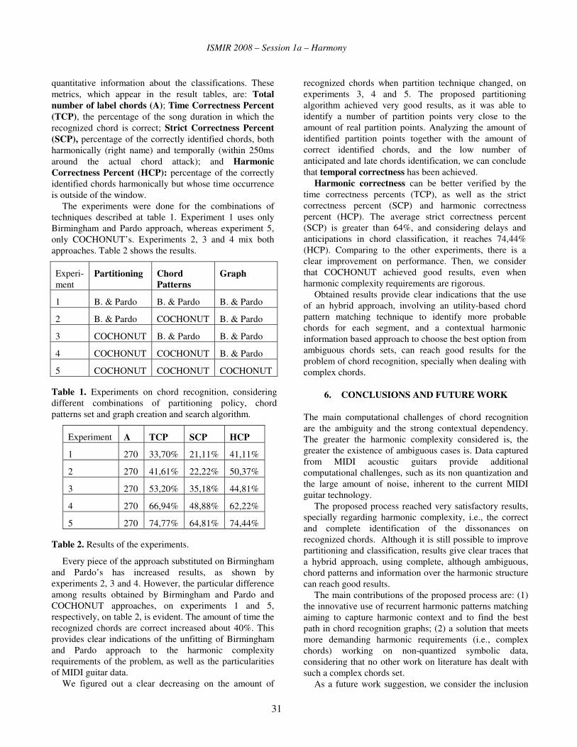
quantitative information about the classifications. These metrics, which appear in the result tables, are: Total number of label chords (A); Time Correctness Percent (TCP), the percentage of the song duration in which the recognized chord is correct; Strict Correctness Percent (SCP), percentage of the correctly identified chords, both harmonically (right name) and temporally (within 250ms around the actual chord attack); and Harmonic Correctness Percent (HCP): percentage of the correctly identified chords harmonically but whose time occurrence is outside of the window.
The experiments were done for the combinations of techniques described at table 1. Experiment 1 uses only Birmingham and Pardo approach, whereas experiment 5, only COCHONUT’s. Experiments 2, 3 and 4 mix both approaches. Table 2 shows the results.
Experi-ment
Partitioning Chord Patterns
Graph
1 B. & Pardo B. & Pardo B. & Pardo
2 B. & Pardo COCHONUT B. & Pardo
3 COCHONUT B. & Pardo B. & Pardo
4 COCHONUT COCHONUT B. & Pardo
5 COCHONUT COCHONUT COCHONUT
Table 1. Experiments on chord recognition, considering different combinations of partitioning policy, chord patterns set and graph creation and search algorithm.
Experiment A TCP SCP HCP
1 270 33,70% 21,11% 41,11%
2 270 41,61% 22,22% 50,37%
3 270 53,20% 35,18% 44,81%
4 270 66,94% 48,88% 62,22%
5 270 74,77% 64,81% 74,44%
Table 2. Results of the experiments.
Every piece of the approach substituted on Birmingham and Pardo’s has increased results, as shown by experiments 2, 3 and 4. However, the particular difference among results obtained by Birmingham and Pardo and COCHONUT approaches, on experiments 1 and 5, respectively, on table 2, is evident. The amount of time the recognized chords are correct increased about 40%. This provides clear indications of the unfitting of Birmingham and Pardo approach to the harmonic complexity requirements of the problem, as well as the particularities of MIDI guitar data.
We figured out a clear decreasing on the amount of
recognized chords when partition technique changed, on experiments 3, 4 and 5. The proposed partitioning algorithm achieved very good results, as it was able to identify a number of partition points very close to the amount of real partition points. Analyzing the amount of identified partition points together with the amount of correct identified chords, and the low number of anticipated and late chords identification, we can conclude that temporal correctness has been achieved.
Harmonic correctness can be better verified by the time correctness percents (TCP), as well as the strict correctness percent (SCP) and harmonic correctness percent (HCP). The average strict correctness percent (SCP) is greater than 64%, and considering delays and anticipations in chord classification, it reaches 74,44% (HCP). Comparing to the other experiments, there is a clear improvement on performance. Then, we consider that COCHONUT achieved good results, even when harmonic complexity requirements are rigorous.
Obtained results provide clear indications that the use of an hybrid approach, involving an utility-based chord pattern matching technique to identify more probable chords for each segment, and a contextual harmonic information based approach to choose the best option from ambiguous chords sets, can reach good results for the problem of chord recognition, specially when dealing with complex chords.
6. CONCLUSIONS AND FUTURE WORK
The main computational challenges of chord recognition are the ambiguity and the strong contextual dependency. The greater the harmonic complexity considered is, the greater the existence of ambiguous cases is. Data captured from MIDI acoustic guitars provide additional computational challenges, such as its non quantization and the large amount of noise, inherent to the current MIDI guitar technology.
The proposed process reached very satisfactory results, specially regarding harmonic complexity, i.e., the correct and complete identification of the dissonances on recognized chords. Although it is still possible to improve partitioning and classification, results give clear traces that a hybrid approach, using complete, although ambiguous, chord patterns and information over the harmonic structure can reach good results.
The main contributions of the proposed process are: (1) the innovative use of recurrent harmonic patterns matching aiming to capture harmonic context and to find the best path in chord recognition graphs; (2) a solution that meets more demanding harmonic requirements (i.e., complex chords) working on non-quantized symbolic data, considering that no other work on literature has dealt with such a complex chords set.
As a future work suggestion, we consider the inclusion
31

ISMIR 2008 – Session 1a – Harmony
of more complex contextual information, such as harmonic field and modal loans. Such modifications may allow the use of more chord patterns on the first phase, increasing harmonic completeness.
The use of musical structural information (e.g., sections) could also help to improve results [18], as well as the use of optimization techniques to find the best path over the graph [4], and a different way to build the graph such that partitioning and classification are done simultaneously.
Finally, it would be interesting to propose an adaptation of the approach for audio chord recognition. However, identification of partition points could be hard to adapt. The other phases could be adapted by comparing the Pitch Class Profiles of each segment with the chord patterns, and generating a graph with the high scored chords, in which the search technique proposed by COCHONUT could be applied.
7. REFERENCES
[1] Ferrara, J. Jazz Piano and Harmony: A Fundamental Guide. John Ferrara Music Pub. 2000.
[2] Bello, J. and Pickens, J. “A robust mid-level representation for harmonic content in music signals”, Proceedings of the International Symposium on Music Information Retrieval, London, UK, 2005.
[3] Cabral, G. Briot, J. and Pachet, F. “Impact of distance in pitch class profile computation”, Proceedings of the 10th Brazilian Symposium on Computer Music. Belo Horizonte, Brazil, 2005.
[4] Cook, W., Cunningham W., Pulleyblank W. and Schrijver, A. Combinatorial Optimization. John Wiley and Sons. Nova York, USA, 1998.
[5] D’Accord Music Software. Guitar Dictionary – Demo Version. www.daccord.com.br. September, 2007.
[6] Faria, N. Acordes, Arpejos e Escalas para Violão e Guitarra. Lumiar Editora. Brazil. 1999.
[7] Figueira Filho, C. and Ramalho, G. Jeops – the Java embedded object production system. In M. Monard and J. Sichman (eds). Advances in Artificial Intelligence. IBERAMIA-SBIA 2000. London, United Kingdom, 2000.
[8] Fujishima, T. “Realtime chord recognition of musical sound: a system using common Lisp music”, Proceedings of International Computer Music Conference. Beijing, China, 1999.
[9] Lee, K. and Slaney, M. “Automatic chord recognition from audio using an HMM with supervised learning”,
Proceedings of the 7th International Conference on Music Information Retrieval. Victoria, PAIS, 2006.
[10] Lee, K. “Automatic chord recognition from audio using enhanced pitch class profile”, Proceedings of the International Computer Music Conference. New Orleans, USA, 2006.
[11] Lima, E., Madsen, S., Dahia, M., Widmer, G. and Ramalho, G. “Extracting patterns from Brazilian guitar accompaniment data”, Proceedings of the 1st European Workshop on Intelligent Technologies for Cultural Heritage Exploitation at the 17th European Conference on Artificial Intelligence. Riva del Garda, Italy, 2006.
[12] Pardo, B. and Birmingham, W. “The chordal analysis of tonal music”, Technical report CSE-TR-439-01. The University of Michigan, Dept. of Electrical Engineering and Computer Science. Ann Arbor, PAIS, 2001.
[13] Scholz, R., Dantas, V. and Ramalho, G. “Automating functional harmonic analysis: the Funchal system”, Proceedings of the Seventh IEEE International Symposium on Multimedia. Irvine, USA, 2005.
[14] Scholz, R. COCHONUT References Home Page. www.cin.ufpe.br/~reps/msc/. September/2008.
[15] Sheh, A. and Ellis, D. “Chord segmentation and recognition using EM-trained Hidden Markov Models”, Proceedings of the International Symposium on Music Information Retrieval. Baltimore, PAIS, 2003.
[16] SONY Computer Science Lab. Holistic Signal Processing. http://www.csl.sony.fr/items/2004/holistic-signal-processing/. January, 2008.
[17] Temperley, D. and Sleator, D. “The Melisma Music Analyser”. http://www.link.cs.cmu.edu/music-analysis/. January, 2008.
[18] Widmer, G. “Learning expressive performance: the structure-level approach”, Journal of New Music Research 25(2), 179-205. 1996.
[19] Yoshioka, T. et al. “Automatic chord transcription with concurrent recognition of chord symbols and boundaries”, Proceedings of the 5th International Conference in Music Information Retrieval. Barcelona, Spain, 2004.
32

ISMIR 2008 – Session 1a – Harmony
CHORD RECOGNITION USING INSTRUMENT VOICING CONSTRAINTS
Xinglin ZhangDept. of Computer Science
University of ReginaRegina, SK CANADA S4S [email protected]
David GerhardDept. of Computer Science, Dept. of Music
Univeristy of ReginaRegina, SK CANADA S4S [email protected]
ABSTRACT
This paper presents a technique of disambiguation for chord
recognition based on a-priori knowledge of probabilities of
chord voicings in the specific musical medium. The main
motivating example is guitar chord recognition, where the
physical layout and structure of the instrument, along with
human physical and temporal constraints, make certain chord
voicings and chord sequences more likely than others. Pitch
classes are first extracted using the Pitch Class Profile (PCP)
technique, and chords are then recognized using Artificial
Neural Networks. The chord information is then analyzed
using an array of voicing vectors (VV) indicating likelihood
for chord voicings based on constraints of the instrument.
Chord sequence analysis is used to reinforce accuracy of in-
dividual chord estimations. The specific notes of the chord
are then inferred by combining the chord information and
the best estimated voicing of the chord.
1 INTRODUCTION
Automatic chord recognition has been receiving increasing
attention in the musical information retrieval community,
and many systems have been proposed to address this prob-
lem, the majority of which combine signal processing at the
low level and machine learning methods at the high level.
The goal of a chord recognition system may also be low-
level (identify the chord structure at a specific point in the
music) or high level (given the chord progression, predict
the next chord in a sequence).
1.1 Background
Sheh and Ellis [6] claim that by making a direct analogy
between the sequences of discrete, non-overlapping chord
symbols used to describe a piece of music and word se-
quence used to describe speech, much of the speech recog-
nition framework in which hidden Markov Models are pop-
ular can be used with minimal modification. To represent
the features of a chord, they use Pitch Class Profile (PCP)
vectors (discussed in Section 1.2) to emphasize the tonal
content of the signal, and they show that PCP vectors outper-
formed cepstral coefficients which are widely used in speech
recognition. To recognize the sequence, hidden Markov Mod-
els (HMMs) directly analogous to sub-word models in a
speech recognizer are used, and trained by the Expectation
Maximization algorithm. Bello and Pickens [1] propose a
method for semantically describing harmonic content di-
rectly from music signals. Their system yields the Major
and Minor triads of a song as a function of beats. They
also use PCP as the feature vectors and HMMs as the classi-
fier. They incorporate musical knowledge in initializing the
HMM parameters before training, and in the training pro-
cess. Lee and Slaney [5] build a separate hidden Markov
model for each key of the 24 Major/Minor keys. When
the feature vectors of a musical piece are presented to the
24 models, the model that has the highest possibility rep-
resents the key to that musical piece. The Viterbi algo-
rithm is then used to calculate the sequence of the hidden
states, i.e. the chord sequence. They adopt a 6-dimensional
feature vector called the Tonal Centroid [4] to detect har-
monic changes in musical audio. Gagnon et al [2] pro-
pose an Automatic Neural Network based pre-classification
approach to allow a focused search in the chord recogni-
tion stage. The specific case of the 6-string standard gui-
tar is considered. The feature vectors they use are calcu-
lated from the Barkhausen Critical Bands Frequency Dis-
tribution. They report an overall performance of 94.96%
accuracy, however, a fatal drawback of their method is that
both the training and test samples are synthetic chords con-
sisting of 12 harmonic sinusoids for each note, lacking the
noise and the variation caused by the vibration of the strings
where partials might not be in the exact multiple of their fun-
damental frequencies. Yoshioka et al [7] point out that there
exists mutual dependency between chord boundary detec-
tion and chord symbol identification: it’s difficult to detect
the chord boundaries correctly prior to knowing the chord;
and it’s also difficult to identify the chord name before the
chord boundary is determined. To solve this mutual de-
pendency problem, they propose a method that recognizes
chord boundaries and chord symbols concurrently. PCP vec-
tor is used to represent the feature. When a new beat time
is examined (Goto’s[3] method is used to obtain the beat
times), the hypotheses (possible chord sequence cadidate)
are updated.
33

ISMIR 2008 – Session 1a – Harmony
1.2 Pitch Class Profile (PCP) Vector
A musical note can be characterized as having a global pitch,
identified with a note name and an octave (e.g. C4) or a pitch
color or pitch class, identified only by the note name inde-
pendent of octave. The pitch class profile (PCP) technique
detects the color of a chord based on the relative content of
pitch classes. PCP begins from a frequency representation,
for example the Fourier transform, then maps the frequency
components into the 12 pitch classes. After the frequency
components have been calculated, we get the corresponding
notes of each frequency component and find its correspond-
ing pitch class.
2 CHORD ANALYSIS
Our approach deviates from the approaches presented in Sec-
tion 1 in several key areas. The use of voicing constraints
(described below) is the primary difference, but our low-
level analysis is also somewhat different from current work.
First, current techniques will often combine PCP with Hid-
den Markov Models. Our aproach analyzes the PCP vector
using Neural Networks, using a viterbi algorithm to model
chord sequences in time. Second, current techniques nor-
mally use window sizes on the order of 1024 samples (23.22
ms). Our technique uses comparatively large window sizes
(22050 samples, 500ms). Unlike Gagnon, Larouche and
Lefebvre [2], who use synthetic chords to train the network,
we use real recordings of chords played on a guitar. Al-
though the constraints and system development are based
on guitar music, similar constraints (with different values)
may be determined for other ensemble music.
2.1 Large Window Segmentation
Guitar music varies widely, but common popular guitar mu-
sic maintains a tempo of 80–120 beats per minute. Because
chord changes typically happen on the beat or on beat frac-
tions, the time between chord onsets is typically 600–750
ms. Segmenting guitar chords is not a difficult problem,
since the onset energy is large compared to the release en-
ergy of the previous chord, but experimentation has shown
that 500ms frames provide sufficient accuracy when applied
to guitar chords for a number of reasons. First, if a chord
change happens near a frame boundary, the chord will be
correctly detected because the majority of the frame is a sin-
gle pitch class profile. If the chord change happens in the
middle of the frame, the chord will be incorrectly identified
because contributions from the previous chord will contam-
inate the reading. However, if sufficient overlap between
frames is employed (e.g. 75%), then only one in four chord
readings will be inaccurate, and the chord sequence recti-
fier (see Section 2.3) will take care of the erroneous mea-
sure: based on the confidence level of chord recognition and
changes in analyzed feature vectors from one frame to the
next, the rectifier will select the second-most-likely chord if
it fits better with the sequence.
The advantages of the large window size are the accu-
racy of the pitch class profile analysis, and, combined with
the chord sequence rectifier, outweigh the drawbacks of in-
correct analysis when a chord boundary is in the middle of
a frame. The disadvantage of such a large window is that it
makes real-time processing impossible. At best, the system
will be able to provide a result half a second after a note is
played. Offline processing speed will not be affected, how-
ever, and will be comparable to other frame sizes. In our
experience, real-time guitar chord detection is not a prob-
lem for which there are many real-world applications.
2.2 PCP with Neural Networks
We have employed an Artificial Neural Network to analyze
and characterize the pitch class profile vector and detect the
corresponding chord. A network was first constructed to
recognize seven common chords for music in the keys of C
and G, for which the target chord classes are [C, Dm, Em, F,G, Am, D]). These chords were chosen as common chords
for “easy” guitar songs. The network architecture was set
up in the following manner: 1 12-cell input layer, 2 10-cell
hidden layers, and 1 7-cell output layer. With the encourag-
ing results from this initial problem (described in Section 4),
the vocabulary of the system was expanded to Major (I, III,
V), Minor (I, iii, V) and Seventh (I, III, V, vii) chords in the
seven natural-root(�) keys (C, D, E, F, G, A, B), totaling 21
chords. Full results are presented in Section 4.
A full set of 36 chords (Major, Minor and Seventh for all
12 keys) was not implemented, and we did not include fur-
ther chord patterns (Sixths, Ninths etc.). Although the ex-
pansion from seven chords to 21 chords gives us confidence
that our system scales well, additional chords and chord pat-
terns will require further scrutiny. With the multitude of
complex and colorful chords available, it is unclear whether
it is possible to have a “complete” chord recognition system
which uses specific chords as recognition targets, however a
limit of 4-note chords would provide a reasonably complete
and functional system.
2.3 Chord Sequence Rectification
Isolated chord recognition does not take into account the
correlation between subsequent chords in a sequence. Given
a recognized chord, the likelihood of a subsequent frame
having the same chord is increased. Based on such informa-
tion, we can create a sequence rectifier which corrects some
of the isolated recognition errors in a sequence of chords.
For each frame, the neural network gives a rank list of the
possible chord candidates. From there, we estimate the chord
transition possibilities for each scale pair of Major and rel-
34

ISMIR 2008 – Session 1a – Harmony
ative Minor through a large musical database. The Neural
Network classification result is provided in the S matrix of
size N × T , where N is the size of the chord dictionary and
T is the number of frames. Each column gives the chord
candidates with ranking values for each frame. The first row
of the matrix contains the highest-ranking individual candi-
dates, which, in our experience, are mostly correct identi-
fications by the neural network. Based on the chords thus
recognized, we calculate the most likely key for the piece.
For the estimated key we develop the chord transition proba-
bility matrix A of size N×N . Finally, we calculate the best
sequence fom S and A using the Viterbi Algorithm, which
may result in a small number of chord estimations being re-
vised to the second or third row result of S.
2.4 Voicing Constraints
Many chord recognition systems assume a generic chord
structure with any note combination as a potential match,
or assume a chord “chromaticity,” assuming all chords of
a specific root and color are the same chord, as described
above. For example, a system allowing any chord combina-
tion would identify [C-E-G] as a C Major triad, but would
identify a unique C Major triad depending on whether the
first note was middle C (C4)or C above middle C (C5). On
the other hand, a system using chromaticity would identify
[C4-E4-G4] as identical to [E4-G4-C5], the first voicing 1
of a C Major triad. Allowing any combination of notes pro-
vides too many similar categories which are difficult to dis-
ambiguate, and allowing a single category for all versions
of a chord does not provide complete information. What is
necessary, then, is a compromise which takes into account
statistical, musical, and physical constraints for chords.
The goal of our system is to constrain the available chords
to the common voicings available to a specific instrument or
set of instruments. The experiments that follow concentrate
on guitar chords, but the technique would be equally appli-
cable to any instrument or ensemble where there are specific
constraints on each note-production component. As an ex-
ample, consider a SATB choir, with standard typical note
ranges, e.g. Soprano from C4 to C6. Key, musical context,
voice constraints and compositional practice means that cer-
tain voicings may be more common. It is common compo-
sitional practice, for example, to have the Bass singing the
root (I), Tenor singing the fifth (V), Alto singing the major
third (III) and Soprano doubling the root (I).
This a-priori knowledge can be combined with statisti-
cal likelihood based on measurement to create a bayesian-
type analysis resulting in greater classification accuracy us-
ing fewer classification categories. A similar analysis can be
performed on any well-constrained ensemble, for example a
string quartet, and on any single instrument with multiple
1 A voicing is a chord form where the root is somewhere other than the
lowest note of the chord
variable sound sources, for example a guitar. At first, the
Piano does not seem to benefit from this method, since any
combination of notes is possible, and likelihoods are ini-
tially equal. However, if one considers musical expectation
or human physiology (hand-span, for example), then similar
voicing constraints may be applied.
One can argue that knowledge of the ensemble may not
be reasonable a priori information—will we really know if
the music is being played by a wind ensemble or a choir?
The assumption of a specific ensemble is a limiting factor,
but is not unreasonable: timbre analysis methods can be ap-
plied to detect whether or not the music is being played by
an ensemble known to the system, and if not, PCP com-
bined with Neural Networks can provide a reasonable chord
approximation without voicing or specific note information.
For a chord played by a standard 6-string guitar, we are
interested in two features: what chord is it and what voicing
of that chord is it 2 . The PCP vector describes the chro-
maticity of a chord, hence it does not give any information
on specific pitches present in the chord. Given knowledge
of the relationships between the guitar strings, however, the
voicings can be inferred based the voicing vectors (VV) in
a certain category. VVs are produced by studying and ana-
lyzing the physical, musical and statistical constraints on an
ensemble. The process was performed manually for the gui-
tar chord recognition system but could be automated based
on large annotated musical databases.
Thus the problem can be divided into two steps: deter-
mine the category of the chord, then determine the voicing.
Chord category is determined using the PCP vector com-
bined with Artificial Neural Networks, as described above.
Chord voicings are determined by matching harmonic par-
tials in the original waveform to a set of context-sensitive
templates.
3 GUITAR CHORD RECOGNITION SYSTEM
The general chord recognition ideas presented above have
been implemented here for guitar chords. Figure 1 provides
a flowchart for the system. The feature extractor provides
two feature vectors: a PCP vector which is fed to the input
layer of the neural net, and an voicing vector which is fed to
the voicing detector.
Table 1 gives an example of the set of chord voicing ar-
rays and the way they are used for analysis. The fundamen-
tal frequency (f0) of the root note is presented along with
the f0 for higher strings as multiples of the root f0.
The Guitar has a note range from E2 (82.41Hz, open low
string) to C6 (1046.5Hz, 20th fret on the highest string).
Guitar chords that is above the 10th fret (D) are rare, thus
we can restrict the chord position to be lower than the 10th
2 Although different voicings are available on guitar, a reasonable as-
sumption is that they are augmented with a root bass on the lowest string
35

ISMIR 2008 – Session 1a – Harmony
Figure 1. Flowchart for the chord recognition system.
fret, that is, the highest note would be 10th fret on the top
string, i.e. D5, with a frequency of 587.3Hz. Thus if we
only consider the frequency components lower than 600Hz,
the effect of the high harmonic partials would be eliminated.
Each chord entry in Table 1 provides both the frequen-
cies and first harmonics of each note. “Standard” chords
such as Major, Minor and Seventh, contain notes for which
f0 is equal to the frequency of harmonic partials of lower
notes, providing consonance and a sense of harmonic rela-
tionship. This is often be seen as a liability, since complete
harmonic series are obscured by overlap from harmonically
related notes, but our system takes advantage of this by ob-
serving that a specific pattern of harmonic partials equates
directly to a specific chord voicing. Table 1 shows this by
detailing the pattern of string frequencies and first harmonic
partials. First harmonic partials above G6 are ignored since
they will not interact with higher notes. Harmonic partials
above 600Hz are ignored, since there is no possibility to
overlap the fundamental frequency of higher notes (as de-
scribed above). These are indicated by the symbol “ø”. In
this way, we construct a pattern of components that are ex-
pected to be present in a specific chord as played on the
guitar. A string that is not played in the chord is indicated
by “–”. Boxes and underlines are detailed below. Table 2
shows the same information for voicings of a single chord
in three different positions, showing how these chords can
be disambiguated.
Chord S1 S2 S3 S4 S5 S6
f0 (Hz) H1 H2 H3 H4 H5 H6
F 1 1.5 2 2.52 3 4
87.31 2 3 4 ø ø ø
Fm 1 1.5 2 2.38 3 4
87.31 2 3 4 ø ø ø
F7 1 1.5 1.78 2.52 3 4
87.31 2 3 3.56 ø ø ø
G 1 1.26 1.5 2 2.52 4
98 2 2.52 3 4 ø ø
Gm 1 1.19 1.5 2 3 4
98 2 2.38 3 4 ø ø
G7 1 1.26 1.5 2 2.52 3.56
98 2 2.52 ø ø ø ø
A – 1 1.5 2 2.52 3
110 – 2 3 ø ø ø
Am – 1 1.5 2 2.38 3
110 – 2 3 ø ø ø
A7 – 1 1.5 1.78 2.52 3
110 – 2 3 ø ø ø
C – 1 1.26 1.5 2 2.52
130.8 – 2 2.52 ø ø ø
Cm – 1 1.19 1.5 2 –
130.8 – 2 ø ø ø –
C7 – 1 1.26 1.78 2 2.52
130.8 – 2 2.52 ø ø ø
D – – 1 1.5 2 2.52
146.8 – – 2 ø ø ø
Dm – – 1 1.5 2 2.38
146.8 – – 2 ø ø ø
D7 – – 1 1.5 1.78 2.52
146.8 – – 2 ø ø ø
Table 1. Chord pattern array, including three forms of five
of the natural-root chords in their first positions. S1–S6 are
the relative f0 of the notes from the lowest to highest string,
and H1–H6 are the first harmonic partial of those notes. See
text for further explanation of boxes and symbols.
Chord S1 S2 S3 S4 S5 S6
f0 (Hz) H1 H2 H3 H4 H5 H6
G 1 1.26 1.5 2 2.52 4
98 2 2.52 3 4 ø ø
G(3) 1 1.5 2 2.52 3 4
98 2 3 4 ø ø ø
G(10) – 1 1.5 2 2.52 3
196.0 – 2 3 ø ø ø
Table 2. Voicing array for the Gmaj chords played on dif-
ferent positions on the guitar.
36

ISMIR 2008 – Session 1a – Harmony
3.1 Harmonic Coefficients and Exceptions
It can be seen from Table 1 that there are three main cate-
gories of chords on the guitar, based on the frequency of the
second note in the chord. The patterns for the three cate-
gories are: (1.5), where the second note is (V): F, Fm, F7,E, Em, E7, A, Am, A7, B, Bm, D, Dm, D7; (1.26), where the
second note is (III): B7, C7, G, G7; and (1.19), where the
second note is (iii): Cm, Gm.
Thus, from the first coefficient (the ratio of the first har-
monic peak to the second) we can identify which group a
certain chord belongs to. After identifying the group, we
can use other coefficients to distinguish the particular chord.
In some situations (e.g., F and E; A and B ), the coefficients
are identical for all notes in the chord, thus they cannot be
distinguished in this manner. Here, the chord result will be
disambiguated based on the result of the Neural Network
and the f0 analysis of the root note. Usually, all first har-
monic partials line up with f0 of higher notes in the chord.
When the first harmonic falls between f0 of higher notes in
the chord, they are indicated by boxed coefficients.
Underlined coefficients correspond to values which may
be used in the unique identification of chords. In these cases,
there are common notes within a generic chord pattern, for
example the root (1) and the fifth (1.5). String frequen-
cies corresponding to the Minor Third (1.19, 2.38) and Mi-
nor Seventh (2.78) are the single unique identifiers between
chord categories in many cases.
4 RESULTS
Chord detection errors do not all have the same level of
“severity”. A C chord may be recognized as an Am chord
(the relative Minor), since many of the harmonic partials are
the same and they share two notes. In many musical situa-
tions, although the Am chord is incorrect, it will not produce
dissonance if played with a C chord. Mistaking an C chord
for a Cm chord, however, is a significant problem. Although
the chords again differ only by one note, the note in question
is more harmonically relevant and differs in more harmonic
partials. Further, it establishes the mode of the scale being
used, and, if played at the same time as the opposing mode,
will produce dissonance.
4.1 Chord Pickout
Chord Pickout 3 is a popular off-the-shelf chord recognition
system. Although the algorithm used in the Chord Pick-out system is not described in detail by the authors, it is
reasonable to compare with our system since Chord Pick-
out is a commercial system with good reviews. We applied
the same recordings to both systems and identified the ac-
curacy of each system. We were more forgiving with the
3 http://www.chordpickout.com
analysis for Chord Pickout in order to better detail the types
of errors that were made. If Chord Pickout was able to
identify the root of the chord, ignoring Major, Minor or
Seventh, it is described as “correct root.” If the chord and
the chord type are both correct, it is described as “correct
chord.” Errors between correct root and correct chord in-
cluded Major→Minor, Major→Seventh, and Minor→Major.
For our system, all chord errors regardless of severity, are
considered incorrect. The complete results for 6 trials are
presented in Table 3.
4.2 Independent accuracy trials
To detect the overall accuracy of our system, independent
of a comparison with another system, we presented a set
of 40 chords of each type to the system and evaluated its
recognition accuracy. Two systems were trained for specific
subsets of chord detection.
The first system was trained to detect chords in the a sin-
gle key only assuming key recognition has already taken
place. Seven chord varieties are available as classification
targets, and the system performed well, producing 96.8%
accuracy over all trials. Misclassifications were normally
toward adjacent chords in the scale.
The second system was trained to recognized Major, Mi-
nor and Seventh chords of all seven natural-root keys, result-
ing in 21 chord classification targets. This system produced
good results: 89% for Major versus Minor, and 75% accu-
racy for Major versus Seventh chords. Table 4 provides a
confusion matrix between single-instance classification of
Major and Seventh chords, which had the lower recogni-
tion rate. There are two reasons for this: in some cases
the first three notes (and correspondingly the first three har-
monic partials detected) are the same between a chord and
its corresponding Seventh; and in some cases the first har-
monic of the root note does not line up with an octave and
thus contributes to the confusion of the algorithm. Recogni-
tion accuracy is highest when only the first two notes are the
same (as in C and G chords). Recognition accuracy is low in
the case of F7,when the root is not doubled, and the pattern
can be confused with both the corresponding Major chord
and the adjacent Seventh chord. Recognition accuracy is
also low in the case of G7, where the difference between the
Major and the Seventh is in the third octave, at 3.56 times the
fundamental of the chord. In this case, the Seventh chord is
frequently mistaken for the Major chord, which can be con-
sidered a less “severe” error since the Seventh chord is not
musically dissonant with the Major chord.
A more severe case is with D7, which contains only 4
sounded strings, one of which produces a harmonic that
does not correspond to a higher played string. From Ta-
ble 1, we can see that the string frequency pattern for D7 is
[1, 1.5, 1.78, 2.25], and the first harmonic partial of the root
note inserts a 2 into the sequence, producing [1, 1.5, 1.78,
37

ISMIR 2008 – Session 1a – Harmony
Voicing Constraints Chord Pickout
Trial Frames Correct Rate Correct Root Rate Correct Chord Rate
1 24 23 95.8% 20 83.3% 1 5.0%
2 46 44 95.6% 30 65.2% 12 26.1%
3 59 54 91.5% 38 64.4% 7 11.9%
4 50 49 98.0% 31 62.0% 30 60.0%
5 65 51 78.4% 51 78.4% 21 32.3%
Table 3. Comparison of our system to Chord Pickout, an off-the-shelf chord recognition system.
Chord Rate C C7 D D7 E E7 F F7 G G7 A A7
C 40/40 40
C7 35/40 35 2 2 1
D 40/40 40
D7 13/40 1 13 1 3 20 2
E 40/40 40
E7 37/40 37 3
F 38/40 1 1 38
F7 5/40 3 16 16 5
G 40/40 40
G7 17/40 2 21 17
A 30/40 1 8 30 1
A7 25/40 5 2 8 25
Table 4. Confusion Matrix for Major and Seventh chords of natural-root keys. Overall accuracy is 75%.
2, 2.25]. This is very similar to the sequence for F7, which
is why the patterns are confused. It would be beneficial, in
this case, to increase the weight ascribed to the fundamen-
tal frequency when the number of strings played is small.
Unfortunately, detecting the number of sounded strings in a
chord is a difficult task. Instead, f0 disambiguation can be
applied when a chord with fewer strings is one of the top
candidates from the table, since that information is known.
5 CONCLUSIONS
A chord detection system is presented which makes use of
voicing constraints to increase accuracy of chord and chord
sequence identification. Although the system is developed
for guitar chords specifically, similar analysis could be per-
formed to apply these techniques to other constrained en-
sembles such as choirs or string, wind, or brass ensembles,
where specific chords are more likely to appear in a particu-
lar voicing given the constraints of the group.
6 REFERENCES
[1] J. P. Bello and J. Pickens. A robust mid-level representa-
tion for harmonic content in music signals. In Proceed-ings of the International Symposium on Music Informa-tion Retrieval, London, UK, 2005.
[2] T. Ganon, S. Larouche, and R. Lefebvre. A neural net-
work approach for preclassification in musical chord
recognition. In 37th Asilomar Conf, Signals, Systemsand Computers, volume 2, pages 2106–2109, 2003.
[3] M. Goto. An audio-based real-time beat tracking system
for music with or without drum-sounds. Journal of NewMusic Research, 30(2):159–171, 2001.
[4] C. Harte, M. Sandler, and M. Gasser. Detecting har-
monic change in musical audio. In AMCMM ’06: Pro-ceedings of the 1st ACM workshop on Audio and musiccomputing multimedia, 2006.
[5] K. Lee and M. Slaney. A unified system for chord tran-
scription and key extraction using hidden markov mod-
els. In Proceedings of International Conference on Mu-sic Information Retrieval, 2007.
[6] A. Sheh and D. P. Ellis. Chord segmentation and recog-
nition using em-trained hidden markov models. In Pro-ceedings of the International Symposium on Music In-formation Retrieval, Baltimore, MD, 2003.
[7] T. Yoshioka, T.Kitahara, K. Komatani, T. Ogata, and
H. Okuno. Automatic chord transcription with concur-
rent recognition of chord symbols and boundaries. In
Proceedings of the 5th International Conference on Mu-sic Information Retrieval (ISMIR), 2004.
38

ISMIR 2008 – Session 1a – Harmony
AUTOMATIC CHORD RECOGNITION BASED ON PROBABILISTICINTEGRATION OF CHORD TRANSITION AND BASS PITCH ESTIMATION
Kouhei Sumi,† Katsutoshi Itoyama,† Kazuyoshi Yoshii,‡
Kazunori Komatani,† Tetsuya Ogata,† and Hiroshi G. Okuno†
†Dept. of Intelligence Science and Technology ‡National Institute of Advanced IndustrialGraduate School of Informatics, Kyoto University Science and Technology (AIST)
Sakyo-ku, Kyoto 606-8501 Japan Tsukuba, Ibaraki 305-8568 Japan{ksumi, itoyama, komatani, ogata, okuno}@kuis.kyoto-u.ac.jp [email protected]
ABSTRACT
This paper presents a method that identifies musical chordsin polyphonic musical signals. As musical chords mainlyrepresent the harmony of music and are related to othermu-sical elements such as melody and rhythm, the performanceof chord recognition should improve if this interrelation-ship is taken into consideration. Nevertheless, this inter-relationship has not been utilized in the literature as far asthe authors are aware. In this paper, bass lines are utilizedas clues for improving chord recognition because they canbe regarded as an element of the melody. A probabilis-tic framework is devised to uniformly integrate bass linesextracted by using bass pitch estimation into a hypothesis-search-based chord recognition. To prune the hypothesisspace of the search, the hypothesis reliability is defined asthe weighted sum of three reliabilities: the likelihood ofGaussian Mixture Models for the observed features, the jointprobability of chord and bass pitch, and the chord transi-tion N-gram probability. Experimental results show thatour method recognized the chord sequences of 150 songsin twelve Beatles albums; the average frame-rate accuracyof the results was 73.4%.Keyword: chord recognition, bass line, hypothesis search,probabilistic integration
1 INTRODUCTION
In recent years, automatic recognition of musical elementssuch as melody, harmony, and rhythm (Figure 1) from poly-phonic musical signals has become a subject of great inter-est. The spread of high-capacity portable digital audio play-ers and online music distribution has allowed a diverse userbase to store a large number ofmusical pieces on these play-ers. Information on the content of musical pieces such astheirmusical structure,mood and genre can be used togetherwith text-based information to make music information re-trieval (MIR) more efficient and effective. Manual annota-tion requires an immense amount of effort, and maintaininga consistent level of quality is not easy. Thus, techniques
Melody Harmony Rhythm
Chord BeatBass lines
Music
Melody Harmony Rhythm
Chord BeatBass lines
Music
Figure 1. Musical elements
for extracting musical elements are essential for obtainingcontent-based information from musical signals.
A key principle in analyzing musical signals is that mu-sical elements are related to each other. Because composersexploit the interrelationship among musical elements, thisinterrelationship should be considered when analyzing theelements as well. Most studies in the literature have dealtwith these elements independently.
This paper exploits the interrelationship between chordsequences and bass lines to improve the performance of chordrecognition. The chord sequence is regarded as an elementof the harmony, while bass lines are regarded as an elementof the melody. The chord sequence consists of a chord sym-bol sequence and chord boundary sequence. As the chordsequence may represent the mood of music, it can be usedto calculate the similarity in mood between musical pieces.This similarity is important in MIR and music recommen-dation. On the other hand, the bass line represents a melodyin the bass register; thus, it leads the chord progression.
A recent approach adopted recently by many researchersfor automated description of the chord sequence is the useof Hidden MarkovModels (HMMs). Several methods havebeen suggested to explore the analogy between speech recog-nition and chord recognition and to consider the temporalconnection of chords [1, 2, 3]. Sheh et al. [1] proposed amethod that uses the extended Pitch Class Profile (PCP) [4]as a feature vector. They used an HMM that had one stateper chordwith a large set of classes (147 chord types). How-ever, they were not able to obtain good enough results forrecognition. Bello et al. [2] used chroma features and anHMM; they improved accuracy by incorporating musical
39

ISMIR 2008 – Session 1a – Harmony
knowledge into the model. Lee et al. [3] built key-specificmodels for automatic chord transcription. They used a 6-dimensional feature vector, called Tonal Centroid that is basedon Tonnetz [5]. Higher accuracies were obtained by limitingthe number of chord types that could be recognized.Yoshioka et al. pointed out that chord symbols affect chord
boundary recognition and vice versa [6]. They developeda method that concurrently recognizes chord symbols andboundaries by using a hypothesis search that recognizes thechord sequence and key.
While previous studies have treated only the features ofchords, we focus on the interrelationship among musical el-ements and integrate information about bass lines into chordrecognition in a probabilistic framework. The frameworkenables us to deal with multiple musical elements uniformlyand integrate information obtained from statistical analysesof real music.
This paper is organized as follows: Section 2 describesour motivation for developing an automatic chord recogni-tion system, the issues in involved in doing so, and our so-lution. Section 3 explains our method in concrete terms.Section 4 reports the experimental results and describes theeffectiveness of our method. Our conclusions are discussedin Section 5.
2 CHORD RECOGNITION USING BASS PITCHESTIMATION
2.1 Motivation
A bass line is a series of tonal linear events in the bass regis-ter. We focus on it specifically because it is strongly relatedto the chord sequence. Bass sounds are the most predomi-nant tones in the low frequency region, and bass lines havethe following important properties:
• They are comprised of the bass register of the musicalchords.
• They lead the chord sequence.
• They can be playedwith a single tone and have a pitchthat is relatively easy to estimate.
We improve chord recognition by exploiting the above prop-erties. Information about bass lines is obtained through basspitch estimation.
To processmultiple musical elements simultaneously, weuse a probabilistic framework that enables us to deal withthem uniformly because each evaluation value is scaled from0 to 1. In addition, with statistical training based on prob-ability theory, it is possible to apply information obtainedfrom the analysis of real music to the recognition. Thus, theframework has both scalability and flexibility.
2.2 Issues
We use the hypothesis-search-based (HSB) method proposedby Yoshioka et al. to recognize chord symbols and chordboundaries simultaneously. We chose this method over theHMM-based one because it expressly solves the mutual de-pendency problem between chord symbols and chord bound-aries. Furthermore, theHSBmethod makes it easier to prob-abilistically integrate various musical elements. That is, weare able to integrate bass pitch estimation into the chordrecognition. In this paper, Yoshioka’s HSB method is calledthe baseline method. However, two issues remain in using itto calculate the evaluation value of the hypothesis.
2.2.1 Usage of bass pitch estimation
Although information about bass sounds is used in the base-line method, it is not used in a probabilistic framework.When the predominant single tone estimated is different fromthe harmonic tones of the chord, penalties are imposed onthe certainty based on bass sounds. Errors in estimating sin-gle tones also tend to produce errors in chord recognition.
2.2.2 Non-probabilistic certainties
The certainties based on musical elements for the evaluationfunction are not probabilistic in the baseline method. Whenthe observation distribution of chroma vectors [7] is approx-imated with a single Gaussian, the Mahalanobis generalizeddistance between acoustic features is used as the certainty.Another certainty based on chord progression patterns is de-fined as a penalty. The criterion for applying this penaltyis related to progression patterns that appear several times.However, as the scales of the values was inconsistent, it be-comes difficult to integrate multiple elements. Additionally,optimizing the weighting factors of each value takes a lot oftime and effort.
2.3 Our Solution
To resolve the above issues, we use bass pitch probability(BPP) and define hypothesis reliability by using a proba-bilistic function.
2.3.1 Bass Pitch Probability
We utilize BPP as information about bass lines to reduce theeffect of bass pitch estimation errors on chord recognition.BPP can be estimated using a method called PreFEst [8].Because BPP is uniform in non-bass-sound frames, it doesnot significantly affect chord recognition in these frames.
2.3.2 Probabilistic design of hypothesis reliability
It is necessary to reformulate hypothesis reliability in orderto use BPP in the reliability calculation. Like the baseline
40

ISMIR 2008 – Session 1a – Harmony
Musical SignalsC major
C Am F G
12-dimensional
Chroma VectorMusical Signals
in Search Interval
Bass Pitch Probability
Searched Chord
Symbol Sequence
Hypothesis Reliability
Likelihood Evaluation
using GMM
Joint Probability
of Chord and Bass
Chord Transition
N-gram Probability
Bass pitch estimation
Hypothesis-Search
Beat
Tracking
Input Output
A minorEmAm F
C majorC Am F
C majorC Em Am F
C majorC Am F
Musical Key
Musical SignalsC major
C Am F G
12-dimensional
Chroma VectorMusical Signals
in Search Interval
Bass Pitch Probability
Searched Chord
Symbol Sequence
Hypothesis Reliability
Likelihood Evaluation
using GMM
Joint Probability
of Chord and Bass
Chord Transition
N-gram Probability
Bass pitch estimation
Hypothesis-Search
Beat
Tracking
Input Output
A minorEmAm F
C majorC Am F
C majorC Em Am F
C majorC Am FA minor
EmAm FA minor
EmAm F
C majorC Am F
C majorC Am F
C majorC Em Am F
C majorC Em Am F
C majorC Am F
C majorC Am F
Musical Key
Figure 2. System Overview
method, we use acoustic features and chord progression pat-terns. However, we define the reliabilities based on thesefeatures by using a probabilistic framework. The values ofthe acoustic features are based on the likelihood ofGaussianMixture Models (GMMs) for 12-dimensional chroma vec-tors. The values for the progression patterns are based onthe transition probability obtained from statistical N-grammodels. This reformulation enables three reliabilities to beintegrated: those based on acoustic features, on BPP, and ontransition probability.
3 SYSTEM
By applying information about BPP when calculating hy-pothesis reliability, we integrate the baseline method andbass pitch estimation in our chord recognition system. Thethree reliabilities based on the three elements are formu-lated probabilistically so that the system deals with themuniformly.Figure 2 shows an overview of our automatic chord recog-
nition system. First, the beat tracking method from [9] isused to detect the eighth note level beat times of an inputmusical piece. Second, the hypotheses are expanded overthis beat time, and hypothesis reliability is calculated basedon these three reliabilities. Third, a beam-search methodusing hypothesis reliability as the cost function is used toprune the expanded hypotheses. These operations are re-peated until the end of the input signal. Finally, we obtain atuple comprising the chord symbol sequence, chord bound-ary sequence, and key from the hypothesis that has the high-est reliability.
3.1 Specification of Chord Recognition System
We define automatic chord recognition as a process of auto-matically obtaining a chord symbol sequence, a chord bound-ary sequence, and a key. These elements are defined as fol-lows:
• Chord symbol sequencec = [c1 · · · cM ], ci ∈ C ≡ R× T
The system uses 48 classes (major,minor, diminished,and sus4 for each of the 12 roots). Triads, sevenths,and so on are included as subclasses of these largerclasses. we focused on discriminating the larger classes.For MIR applications we believe the larger classeswould be sufficient to capture the characteristics ormoods of accompaniments of musical pieces.
• Chord boundary sequencet = [t0 · · · tM ], ti ∈ N
where M is the number of chord symbols,ti denotes the boundary time of ci and ci+1,t0 denotes the beginning time of the input signal,and tM denotes the end time of the input signal.
• Keyk, k ∈ K ≡ R×M
R,M, T are defined as follows:R ≡ {C, C#, · · · ,B}, M ≡ {Major, Minor},T ≡ {Major, Minor,Diminished,Sus4}
We also assume the tempo stays constant, the beat is acommon measure (four-four time), and the key does notmodulate.
3.2 Formulating of Hypothesis Reliability
Denoting the observed feature sequence over frames τ =(τs, τe) as Xτ , we can probabilistically define hypothesisreliability Relτ as follows:
Relτ = p(cτ |Xτ ) (Xτ = [xτs· · ·xτe
]) (1)
The BPP, βτf , during a duration τ is defined from the frame-
by-frame BPP, w(t)(f), as follows:
βτf =
τe∑i=τs
w(i)(f)/α = {w(τs)(f) + · · ·+ w(τe)(f)}/α (2)
where f denotes the frequency of the bass pitch and α isa normalization constant. Hypothesis reliability integratingBPP on the duration τ is defined as follows:
Relτ = p(cτ |Xτ ) =∑
f
p(cτ , βτf |Xτ ) (3)
This hypothesis reliability is converted with Bayes’ theoreminto another form as follows:∑
f
p(cτ , βτf |Xτ ) ∝
∑f
p(Xτ |cτ , βτf )p(cτ , βτ
f ) (4)
=∑
f
p(Xτ |cτ , βτf )p(cτ |βτ
f )p(βτf ) (5)
We use 12-dimensional chroma vectors as the observationfeatures. Since the vectors only depend on the chord sym-bol, we set the following expression.
p(Xτ |cτ , βτf ) = p(Xτ |cτ ) (6)
41

ISMIR 2008 – Session 1a – Harmony
Thus, hypothesis reliability over τ becomes as follows:
Relτ = p(Xτ |cτ )∑
f
p(cτ |βτf )p(βτ
f ) (7)
where p(Xτ |cτ ) denotes the reliability based on acousticfeatures, and
∑f p(cτ |βτ
f )p(βτf ) denotes the reliability based
on BPP.The key k is independent of chord boundaries. With the
conditional probability of a chord symbol sequence given akey, overall hypothesis reliability Relall is defined as fol-lows:
Relall = p(c|k)∏τ
Relτ (8)
= p(c|k)∏τ
p(Xτ |cτ )∑
f
p(cτ |βτf )p(βτ
f ) (9)
where p(c|k) denotes the reliability based on transition prob-ability of chords.
3.3 Reliability based on Acoustic Features
We use 12-dimensional chroma vectors as acoustic features;these vectors approximately represent the intensities of the12-semitone pitch classes. As the chord symbols are identi-fied by the variety of tones, it is essential for chord recogni-tion.Because we focus on four chord types, major, minor, di-
minished and sus4, we use four M -mixture GMMs (Maj-GMM, Min-GMM, Dim-GMM, and Sus4-GMM). The pa-rameters of each GMM, λt, are trained on chroma vectorscalculated at the frame level. Note that chords of differ-ent roots are normalized by rotating chroma vectors. Thisnormalization reduces the number of GMMs to four and ef-fectively increases the number of training samples. The EMalgorithm is used to determine the mean, covariance matrix,and weight for each Gaussian.
After chroma vectors from the input signals are rotatedto adapt to the 12 chords having different root tones, wecalculate the log likelihood between them and the 4 GMMs.The likelihood is equal to p(Xτ |cτ ). Thus, the reliabilitydivided by the number of frames in the hypothesis, gc isdefined as follows:
gc = log p(Xτ |cτ ) = log p(Xr|λt), (10)
where r denotes the number of rotating chroma vector in-dexes and t denotes the number of GMM types.
3.4 Reliability based on Bass Pitch Probability
BPP is obtained by bass pitch estimation, and it is used torepresent the degree of each pitch of bass sounds. Since thebass lines determine the chord sequence, they should be si-multaneously analyzed for recognizing the chord sequence.
Musical signals
Bass-Pitch-Probability frame-by-frame
Bass Pitch Probability in search interval
Bass pitch estimation
Summation Conditional Probability of
chords given bass-pitch
Joint Probability of chord and bass-pitch
Learning-based value
Multiplication Multiplication
Musical signalsMusical signals
Bass-Pitch-Probability frame-by-frame
Bass Pitch Probability in search interval
Bass pitch estimation
Summation Conditional Probability of
chords given bass-pitch
Joint Probability of chord and bass-pitch
Learning-based value
Multiplication Multiplication
Figure 3. Bass-Pitch Processing
Figure 3 shows an overview of the process for calculatingthe reliability based on BPP. The prior probability of basssounds p(βτ
f ) is defined by using BPP w(t)(f) as follows:
p(βτf ) = w(τ)(f) =
τe∑j=τs
w(j)(f) (11)
On the other hand, the conditional probability of chordci given bass pitch βτ
f is obtained from real music by usingcorrect chord labels and the results of PreFEst for the par-ticular duration. We statistically calculate the frequency ofappearance of each bass pitch for each chord.
As the reliability based onBPP is the log joint probabilityof the chord and bass pitch, the reliability gb is defined interms of the BPP w(τ)(f) and the conditional probabilityp(ci|βτ
f ).
gb = log(∑
f
p(ci|βτf )w(τ)(f)) (12)
3.5 Reliability based on Transition Probability
Music theory indicates that the genre and the artist usuallydetermine the chord progression patterns for a given musi-cal piece. The progression patterns are obtained from thekey and scale degree. We probabilistically approximate thefrequency of a chord symbol appearing, thus reducing theambiguity of chord symbols.
We use two 2-gram models, one for major keys and onefor minor keys. They are obtained from real music in ad-vance. In the learning stage, we obtain the 2-gram probabil-ities from common chord symbol sequences consisting ofthe key and correct chord labels. We calculate the 2-gramprobability p(ci|c(−1)
i ) from the number of progression pat-terns and use smoothing to handle progression patterns notappearing in the training samples.
We estimate the transition 2-gram probability on a logscale by using the hypothesis’s key. The reliability gp isdefined as follows:
gp = log p(ci|k) = log p(ci|c(−1)i ) (13)
42

ISMIR 2008 – Session 1a – Harmony
C majorC Am
C AmC major
New 48 hypotheses
C AmC major
C AmC major
Eighth-note level
Beat times
New 48 hypotheses
Expanding hypothesisC majorC AmC Am
C AmC AmC major
New 48 hypotheses
C AmC AmC major
C AmC AmC major
Eighth-note level
Beat times
New 48 hypotheses
Expanding hypothesis
Figure 4. Hypothesis Expansion
3.6 Integrating three reliabilities
Because hypothesis reliability on a log scale is the weightedsum of the three log reliabilities described above, Rel is de-fined as follows:
Rel = wc × gc + wb × gb + wp × gp (14)
where wc, wb, and wp are weight constants.
3.7 Updating the Hypothesis
3.7.1 Hypothesis Expansion
Figure 4 shows the hypothesis expansion process. We con-sider the minimum size of boundary intervals to be eighth-note level beat times, which is the same as the baselinemethod. For each unit between one and eight beats, 48 hy-potheses are generated for 48 chord symbols.
3.7.2 Hypothesis Pruning
We use a beam search to prune the expanded hypotheses;this prevents the number of hypotheses from expanding ex-ponentially. In the beam search, hypotheses are pruned us-ing a beam width BS. After the pruning, the BS hypothe-ses with higher reliability than the rest of the hypotheses areexpanded. Furthermore, by delaying the expansion of hy-potheses until it comes time to evaluate them, we can applypruning to newly generated hypotheses. As a result, by de-creasing wasteful expansions of hypotheses we can reduceboth the amount of computation and memory required.
3.7.3 Update of Hypothesis Reliability
When a hypothesis is expanded, we need to update hypothe-sis reliability. To treat hypotheses with different numbers ofintervals fairly, the reliability of a new hypothesis Relnew isdefined as follows:
Relnew =Relprev
Nh+ Relnext, (15)
Table 1. Parameter values
BS = 25 M = 16wc = 1.0 wb = 2.0 wp = 0.3
Table 2. Results of 5-fold cross validation[1]:Baseline Method, [2]:Ac, [3]:Ac+Ba, [4]:Ac+Pt, [5]:Our Method
Groups [1] [2] [3] [4] [5]1st 65.1 62.9 71.7 68.3 78.32nd 62.7 62.6 70.6 65.7 74.93rd 57.7 60.4 66.8 61.2 69.54th 61.0 61.3 70.2 64.0 72.75th 61.6 60.9 69.2 64.8 71.4
Total 61.6 61.6 69.7 64.8 73.4
where Relprev denotes the reliability of the previously ex-panded hypothesis, Relnext denotes the hypothesis reliabil-ity of the newly expanded interval, and Nh denotes the num-ber of previously expanded intervals.
4 EXPERIMENTAL RESULTS
We tested our system on one-minute excerpts from 150 songsin 12 Beatles albums (a total of 180 songs), which have theproperties described in Section 3.1. These songs were sep-arated into 5 groups at random for 5-fold cross validation.For training the parameters of the GMMs, we used chromavectors calculated from audio signals of 120 of these songsand audio signals of each chord played on aMIDI tone gen-erator. These songs were also used to train the conditionalprobability of chords given the bass pitch (Section 3.4). Weutilized 150 songs (137 in the major key, 13 in the minorkey) as training data for the 2-gram models. As the correctchord labels, we used ground-truth annotations of theseBea-tles albums made by C. A. Harte [10]. The implementationfor experiments used the parameters listed in Table 1.
To evaluate the effectiveness of our method, we com-pared the frame-rate accuracies of the following five meth-ods of computing the hypothesis reliability:
1. Baseline method2. Using only acoustic features3. Using acoustic features and BBP4. Using acoustic features and transition probability5. Our method (three elements)
The results are listed in Table 2. With our system, the av-erage accuracy for the 150 songs was 73.4%. Comparedwith using only acoustic features, the method using bothacoustic features and bass pitch probability improved therecognition rate by 8.1 points. Furthermore, the methodusing acoustic features, BBP, and transition probability im-proved the recognition rate by 11.8 points. In addition, oursystem’s accuracywas higher than that of the baseline method.This is because the probabilistic integration enabled us to
43

ISMIR 2008 – Session 1a – Harmony
0 10 20 3035
40
45
50
55
60
65
70
75
80
85
90
95
100
0 10 20 3035
40
45
50
55
60
65
70
75
80
85
90
95
100
Acc
urac
y(%
)
Number of songs
0 10 20 3035
40
45
50
55
60
65
70
75
80
85
90
95
100
0 10 20 3035
40
45
50
55
60
65
70
75
80
85
90
95
100
0 10 20 3035
40
45
50
55
60
65
70
75
80
85
90
95
100
Acc
urac
y(%
)
Number of songs
Figure 5. Accuracy Histograms.(Left) Histogram for thesongs with correct key. (Right)Histogram for the songs withincorrect key.
utilize information about bass lines as a clue in chord recog-nition. Thus, the results prove both the importance of con-sidering the interrelationship between chord sequence andbass lines and the effectiveness of the probabilistic integra-tion of these elements.
We compared our results with those obtained from othersystems proposed by Bello [2] and Lee [3]. They used twoBeatles albums (Please Please Me, Beatles for Sale) as thetest data set. Our system had an average accuracy of 77.5%.Although both Bello’s and Lee’s system used different train-ing data from those that we used, their systems had 75.0%and 74.4% accuracy, respectively.
Upon investigating the accuracy distribution for all songs,we fount that the accuracy histogram for all songs is polar-ized with two peaks split at approximately 70%. Figure 5shows two accuracy histograms, one for songs where thekey was estimated correctly and another where it was in-correct. As these histograms describe the polarization, itis clearly important to correctly estimate the key for chordrecognition. To improve key estimation, we plan to developa method that searches the hypotheses by using not only aforward search but also backtracking.
5 CONCLUSION
We presented a chord recognition system that takes into ac-count the interrelationship amongmusical elements. Specif-ically, we focus on bass lines and integrate hypothesis-search-based chord recognition and bass pitch estimation in a prob-abilistic framework. To evaluate hypotheses, our systemcalculates the hypothesis reliability, which is designed bythe probabilistic integration of three reliabilities, based onacoustic features, bass pitch probability, and chord transi-tion probability. The experimental results showed that oursystem had a 73.4% frame-rate accuracy of chord recogni-tion in 150 songs. They also showed an increase in accu-
racy when the three reliabilities were integrated comparedwith the baseline method and a method using only acous-tic features. This shows that to recognize musical elements(not only musical chords but also other elements), it is im-portant to consider the interrelationship among musical el-ements and to integrate them probabilistically. To obtainmore information about how to recognize chord sequencesmore effectively, wewill design a way to integrate othermu-sical elements such as rhythm.
6 ACKNOWLEDGEMENTS
This research was partially supported by the Ministry of Ed-ucation, Culture, Sports, Science and Technology (MEXT),the Global Century of Excellence (GCOE) Program, andthe CrestMuse Project of the Japan Science and Technol-ogy Agency (JST). The authors thank Takuya Yoshioka forhis valuable discussion and comments, C. A. Harte for pro-viding us ground-truth annotations of the Beatles albums,and Graham Neubig for his careful reading of our Englishmanuscript.
7 REFERENCES
[1] A. Sheh and D. P. W. Ellis, “Chord Segmentation and Recog-nition Using EM-Trained Hidden Markov Models,” Proc.ISMIR, pp. 183-189, 2003.
[2] J. P. Bello and J. Pickens, “A Robust Mid-level Representationfor Harmonic Content in Music Signals,” Proc. ISMIR, pp.304-311, 2005.
[3] K. Lee and M. Slaney, “A Unified System for Chord Tran-scription and Key Extraction Using Hidden Markov Models,”Proc. ISMIR, pp. 245-250, 2007.
[4] T. Fujishima, “Realtime Chord Recognition ofMusical Sound:a System Using Common Lisp Music,” Proc. ICMC, pp.464-467, 1999.
[5] C. A. Harte, M. B. Sandler, and M. Gasser, “DetectingHarmonic Change in Musical Audio,” Proc. Audio and MusicComputing for Multimedia Workshop, pp. 21-26, 2006.
[6] T. Yoshioka, T. Kitahara, K. Komatani, T. Ogata, and H. G.Okuno, “Automatic Chord Transcription with ConcurrentRecognition of Chord Symbols and Boundaries,” Proc. ISMIR,pp. 100-105, 2004.
[7] M. Goto, “A Chorus-Section Detecting Method for MusicalAudio Signals,” Proc. ICASSP, V, pp. 437-440, 2003.
[8] M. Goto, “A Real-time Music-scene-description System:Predominant-F0 Estimation for Detecting Melody and BassLines in Real-world Audio Signals,” Speech Comm., 43:4, pp.311-329, 2004.
[9] M. Goto, “An Audio-based Real-time Beat Tracking Systemfor Music With or Without Drum-sounds,” Journal. of NewMusic Research, 30:2, pp. 159–171, 2001.
[10] C. A. Harte, et al., “Symbolic Representation of MusicalChords: A Proposed Syntax for Text Annotations,” Proc.ISMIR, pp. 66-71, 2005.
44

ISMIR 2008 – Session 1a – Harmony
A DISCRETE MIXTURE MODEL FOR CHORD LABELLING
Matthias Mauch and Simon DixonQueen Mary, University of London,
Centre for Digital [email protected]
ABSTRACT
Chord labels for recorded audio are in high demand both
as an end product used by musicologists and hobby musi-
cians and as an input feature for music similarity applica-
tions. Many past algorithms for chord labelling are based on
chromagrams, but distribution of energy in chroma frames
is not well understood. Furthermore, non-chord notes com-
plicate chord estimation. We present a new approach which
uses as a basis a relatively simple chroma model to represent
short-time sonorities derived from melody range and bass
range chromagrams. A chord is then modelled as a mix-
ture of these sonorities, or subchords. We prove the prac-
ticability of the model by implementing a hidden Markov
model (HMM) for chord labelling, in which we use the dis-
crete subchord features as observations. We model gamma-
distributed chord durations by duplicate states in the HMM,
a technique that had not been applied to chord labelling. We
test the algorithm by five-fold cross-validation on a set of
175 hand-labelled songs performed by the Beatles. Accu-
racy figures compare very well with other state of the art
approaches. We include accuracy specified by chord type as
well as a measure of temporal coherence.
1 INTRODUCTION
While many of the musics of the world have developed com-
plex melodic and rhythmic structures, Western music is the
one that is most strongly based on harmony [3]. A large
part of harmony can be expressed as chords. Chords can
be theoretically defined as sets of simultaneously sounding
notes, but in practice, including all sounded pitch classes
would lead to inappropriate chord labelling, so non-chord
notes are largely excluded from chord analysis. However,
the question which of the notes are non-chord notes and
which actually constitute a new harmony is a perceptual
one, and answers can vary considerably between listeners.
This has also been an issue for automatic chord analysers
from symbolic data [16]. Flourishing chord exchange web-
sites 1 prove the sustained interest in chord labels of ex-
isting music. However, good labels are very hard to find,
1 e.g. http://www.chordie.com/
arguably due to the tediousness of the hand-labelling pro-
cess as well as the lack of expertise of many enthusiastic
authors of transcriptions. While classical performances are
generally based on a score or tight harmonic instructions
which result in perceived chords, in Jazz and popular mu-
sic chords are often used as a kind of recipe, which is then
realised by musicians as actually played notes, sometimes
rather freely and including a lot of non-chord notes. Our
aim is to translate performed pop music audio back to the
chord recipe it supposedly has been generated from (leadsheet), thereby imitating human perception of chords. A
rich and reliable automatic extraction could serve as a basis
for accurate human transcriptions from audio. It could fur-
ther inform other music information retrieval applications,
e.g. music similarity. The most successful past efforts at
chord labelling have been based on an audio feature called
the chromagram. A chroma frame, also called pitch class
profile (PCP), is a 12-dimensional real vector in which each
element represents the energy of one pitch class present in a
short segment (frame) of an audio recording. The matrix of
the chroma frame columns is hence called chromagram. In
1999, Fujishima [5] introduced the chroma feature to music
computing. While being a relatively good representation of
some of the harmonic content, it tends to be rather prone
to noise inflicted by transients as well as passing/changing
notes. Different models have been proposed to improve es-
timation, e.g. by tuning [6] and smoothing using hidden
Markov models [2, 11]. All the algorithms mentioned use
only a very limited chord vocabulary, consisting of no more
than four chord types, in particular excluding silence (nochord) and dominant 7th chords. Also, we are not aware of
any attemps to address chord fragmentation issues.
We present a novel approach to chord modelling that ad-
dresses some of the weaknesses of previous chord recogni-
tion algorithms. Inspired by word models in speech process-
ing we present a chord mixture model that allows a chord to
be composed of many different sonorities over time. We
also take account of the particular importance of the bass
note by calculating a separate bass chromagram and inte-
grating it into the model. Chord fragmentation is reduced
using a duration distribution model that better fits the actual
chord duration distribution. These characteristics approxi-
mate theoretic descriptions of chord progressions better than
45

ISMIR 2008 – Session 1a – Harmony
previous approaches have.
The rest of this paper is organised as follows. Section 2
explains the acoustical model we are using. Section 3 de-
scribes the chord and chord transition models that constitute
the hierarchical hidden Markov model. Section 4 describes
how training and testing procedures are implemented. The
result section 5 reports accuracy figures. Additionally, we
introduce a new scoring method. In section 6 we discuss
problems and possible future developments.
2 ACOUSTIC MODEL
2.1 Melody and Bass Range Chromagrams
We use mono audio tracks at a sample rate of 44.1 kHz and
downsample them to 11025 kHz after low-pass filtering. We
calculate the short-time discrete Fourier transform for win-
dows of 8192 samples (≈ 0.74s) multiplied by a Hamming
window. The hop-size is 1024 samples (≈ 0.09s), which
corresponds to an overlap of 7/8 of a frame window. In
order to map the Fourier transform at frame t to the log-
frequency (pitch) domain magnitudes Qk(t) we use the con-
stant Q transform code written by Harte and Sandler [6].
Constant Q bin frequencies are spaced 33 13 cents (a third of
a semitone) apart, ranging from 110 Hz to 1760 Hz (four
octaves), i.e. the kth element of the constant Q transform Qk
corresponds to the frequency
2k−136 · 110 Hz, (1)
where k ∈ 1, . . . , (4 · 36). In much the same way as Peeters
[15], we smooth the constant Q transform by a median filter
in the time direction (5 frames,≈ 0.5s), which has the effect
of attenuating transients and drum noise.
For every frame t we wrap the constant Q magnitudes
Q(t) to a chroma vector y∗(t) of 36 bins by simply sum-
ming over bins that are an octave apart,
y∗j (t) =
4∑i=1
|Q36·(i−1)+j(t)|, j = 1, . . . , 36. (2)
Similar to Peeters [15], we use only the strongest of the three
possible sets of 12 semitone bins, e.g. (1, 4, 7, . . . , 34), thus
“tuning” the chromagram and normalise the chroma vector
to sum to 1,
yk(t) = y∗3k+ν(t)
/12∑
i=1
y∗3i+ν(t) , (3)
where ν ∈ {0, 1, 2} indicates the subset chosen to maximise∑t
∑k y∗
3k+ν(t). A similar procedure leads to the calcula-
tion of the bass range chromagrams. The frequency range is
55 Hz to 220 Hz. The number of constant Q bins per semi-
tone is 1, not 3. We linearly attenuate the bins at the fre-
quency range borders, mainly to prevent a note just above
the bass frequency range from leaking into the bass range.
2.2 Data
Harte has provided chord transcriptions for 180 Beatles re-
cordings [7], the entirety of the group’s 12 studio albums.
Some of the songs have ambiguous tuning and/or do not per-
tain to Western harmonic rules. We omit 5 of these songs 2 .
In a classification step similar to the one described by Mauch
et al. [13] we map all chords to the classes major, minor,
dominant, diminished, suspended, and no chord (which ac-
count for more than 94% of the frames) as well as other for
transcriptions that do not match any of the classes. We clas-
sify as dominant the so-called dominant seventh chords and
others that feature a minor seventh. We exclude the chords
in the other class from all further calculations. Hence, the
set of chords has n = 12× 6 elements.
2.3 Subchord Model
We want to model the sonorities a chord is made up of men-
tioned in Section 1 and call them subchords. Given the data
we have, it is convenient to take as set of subchords just the
set of chords introduced in the previous paragraph, denoting
them Si, i = 1, ..., n. In this way, we have a heuristic that
allows us to estimate chroma profiles for every subchord 3 ;
in fact, for every such subchord Si we use the ground truth
labels Gt to obtain all positive examples
Yi = {yt : Gt = Si}
and calculate the maximum likelihood parameter estimates
θ̂i of a Gaussian mixture with three mixture components by
maximising the likelihood∏y∈Yi
L(θi|y).
Parameters are estimated using a MATLAB implementation
of the EM algorithm by Wong and Bouman 4 with the de-
fault initialisation method. From the estimates θ̂i, we obtain
a simple subchord score function
p(Si|y) =L(θ̂i,y)∑j L(θ̂j ,y)
(4)
and hence a subchord classification function
s(y) := argmaxSi
p(Si|y) ∈ {S1, ..., Sn}. (5)
These will be used in the model with no bass information.
2 Revolution 9 (collage), Love You Too (Sitar-based), Wild Honey Pie(tuning issues), Lovely Rita (tuning issues), Within You Without You (Sitar-
based)3 We only fit one Gaussian mixture for each chord type (i.e. major,
minor, diminished, dominant, suspended, and no chord) by rotating all the
relevant chromagrams, see [15]).4 http://web.ics.purdue.edu/˜wong17/gaussmix/gaussmix.html
46

ISMIR 2008 – Session 1a – Harmony
0
0.02
0.04
0.06
0.08
0.1
0.12
0.14C DIMINISHED
F#(Gb) DIMINISHED
G#(Ab) DOMINANTA DIMINISHEDD#(Eb) MINOR
Relative subchord frequencies for chord C DIMINISHED
Figure 1. Example of subchord feature relative frequen-
cies bS|C for the diminished chord. The five most frequent
features are labelled. The subchord corresponding to C di-minished most likely to be the best-fitting feature is indeed
C diminished.
2.4 Subchord Model including Bass
In order to model the bass from the bass range chroma-
grams, every subchord Si has a set Bi ⊂ {1, . . . , 12} of
valid pitch classes coinciding with chord notes. The score
for the bass range chromagram of subchord Si at a bass
chroma frame yb is the maximum value
pb(Si|yb) =maxj∈Bi
{yb
j
}∑k maxj∈Bk
{yb
j
} ∈ [0, 1], (6)
the bass chromagram assumes in any of the pitch classes in
Bi, b stands for bass range.
In order to obtain a model using both melody range and
bass range information the two scores are combined to a
single score
p(Si|y,yb) = pb(Si|yb) · p(Si|y). (7)
Analogous to Equation 5 we obtain a second subchord clas-
sification function
s(y,yb) := argmaxSi
p(Si|y,yb) ∈ {S1, ..., Sn}. (8)
2.5 Discrete HMM Observations
We discretise the chroma data y (and yb) by assigning to
each frame with chroma y the relative subchord, i.e. s(y,yb),or s(y) depending on whether we want to consider the bass
chromagrams or not. That means that in the HMM, the only
information about a frame y we keep is which subchord fits
best.
3 LANGUAGE MODEL
In analogy to speech processing the high-level processing in
our model is called language modelling, although the lan-
guage model we are employing is a hidden Markov model
(HMM, see, e.g. [9]). Its structure can be described in terms
of a chord model and a chord transition model.
3.1 Chord Model
The chord model represents one single chord over time. As
we have argued above, a chord can generate a wealth of very
different subchords. The HMM takes the categorical data
s(y) ∈ {S1, . . . , Sn} as observations, which are estimations
of the subchords. From these, we estimate the chords. The
chords C1, . . . , Cn take the same category names (C major,
C# major,...) as subchords, but describe the perceptual con-
cept rather than the sonority 5 . Given a chord Ci the off-line
estimation of its emission probabilities consists of estimat-
ing the conditional probabilities
P (Ci|Sj), i, j ∈ 1, . . . , n (9)
of the chord Ci conditional on the subchord being Sj . The
maximum likelihood estimator is simply the relative condi-
tional frequency
bi|k =|{t : s(yt) = Si ∧ Ck = Gt}|
|{t : Ck = Gt}|, (10)
where Gt is the ground truth label at t. These estimates
are the (discrete) emission distribution in the hidden Markov
model. A typical distribution can be seen in Figure 1, where
Ck is a C diminished chord.
In hidden Markov models, state durations follow an ex-
ponential distribution, which has the undesirable property
of assigning the majority of probability mass to short dura-
tions as is shown in Figure 2. The true distribution of chord
durations is very different (solid steps), with no probabil-
ity assigned to very short durations, and a lot between one
and three seconds. To circumvent that problem we apply
a variant of the technique used by Abdallah et al. [1] and
model one chord by a left-to-right model of three hidden
states with identical emission probabilities bi|k. The chord
duration distribution is thus a sum of three exponential ran-
dom variables with parameter λ, i.e. it is gamma-distributed
with shape parameter k = 3 and scale parameter λ. Hence,
we can use the maximum likelihood estimator of the scale
parameter λ of the gamma distribution with fixed k:
λ̂ =1k
d̄N , (11)
where d̄N is the sample mean duration of chords. The obvi-
ous differences in fit between exponential and gamma mod-
elling are shown in Figure 2. Self-transitions of the states
in the left-to-right model within one chord will be assigned
probabilities 1− 1/λ (see also Figure 3).
5 In fact, the subchords could well be other features, which arguably
would have made the explanation a little less confusing.
47
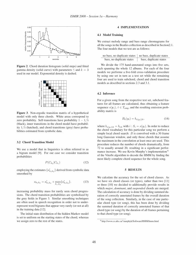
ISMIR 2008 – Session 1a – Harmony
1 2 3 4 50
0.01
0.02
0.03
0.04
0.05
0.06
seconds
rela
tive
freq
uenc
y/de
nsity
Figure 2. Chord duration histogram (solid steps) and fitted
gamma density (solid curve) with parameters γ̂ and k = 3used in our model. Exponential density is dashed.
Cho
rd 1
Cho
rd 2
Cho
rd 3
Figure 3. Non-ergodic transition matrix of a hypothetical
model with only three chords. White areas correspond to
zero probability. Self-transitions have probability 1 − 1/λ̂(black), inner transitions in the chord model have probabil-
ity 1/λ̂ (hatched), and chord transitions (grey) have proba-
bilities estimated from symbolic data.
3.2 Chord Transition Model
We use a model that in linguistics is often referred to as
a bigram model [9]. For our case we consider transition
probabilities
P (Ck2 |Ck1) (12)
employing the estimates {a′k1k2
} derived from symbolic data
smoothed by
ak1k2 = a′k1k2
+ maxk1,k2
{a′k1k2
}. (13)
increasing probability mass for rarely seen chord progres-
sions. The chord transition probabilities are symbolised by
the grey fields in Figure 3. Similar smoothing techniques
are often used in speech recognition in order not to under-
represent word bigrams that appear very rarely (or not at all)
in the training data [12].
The initial state distribution of the hidden Markov model
is set to uniform on the starting states of the chord, whereas
we assign zero to the rest of the states.
4 IMPLEMENTATION
4.1 Model Training
We extract melody range and bass range chromagrams for
all the songs in the Beatles collection as described in Section2.1.
The four models that we test are as follows:
no bass, no duplicate states no bass, duplicate states
bass, no duplicate states bass, duplicate states
We divide the 175 hand-annotated songs into five sets,
each spanning the whole 12 albums. For each of the four
models we performe a five-fold cross-validation procedure
by using one set in turn as a test set while the remaining
four are used to train subchord, chord and chord transition
models as described in sections 2.3 and 3.1.
4.2 Inference
For a given song from the respective test set, subchord fea-
tures for all frames are calculated, thus obtaining a feature
sequence s(yt), t ∈ Tsong, and the resulting emission prob-
ability matrix is
Bk(yt) = bs(yt)|k, (14)
where bs(yt)|k = bi|k with i : Si = s(yt). In order to reduce
the chord vocabulary for this particular song we perform a
simple local chord search: B is convolved with a 30 frame
long Gaussian window, and only those chords that assume
the maximum in the convolution at least once are used. This
procedure reduces the number of chords dramatically, from
72 to usually around 20, resulting in a significant perfor-
mance increase. We use Kevin Murphy’s implementation 6
of the Viterbi algorithm to decode the HMM by finding the
most likely complete chord sequence for the whole song.
5 RESULTS
We calculate the accuracy for the set of chord classes. As
we have six chord classes (or types), rather than two [11]
or three [10] we decided to additionally provide results in
which major, dominant, and suspended chords are merged.
The calculation of accuracy is done by dividing summed du-
ration of correctly annotated frames by the overall duration
of the song collection. Similarly, in the case of one partic-
ular chord type (or song), this has been done by dividing
the summed duration of correctly annotated frames of that
chord type (or song) by the duration of all frames pertaining
to that chord type (or song).
6 http://www.cs.ubc.ca/˜murphyk/Software/HMM/hmm.html
48

ISMIR 2008 – Session 1a – Harmony
5.1 Song-Specific Accuracy
It is obvious that any chord extraction algorithm will not
work equally well on all kinds of songs. Table 1 shows over-
all accuracy figures in both the merged and full evaluation
mode for all four models. The models including bass in-
without bass with bass
std. dupl. std. dupl.
mer
ged mean 64.74 64.96 66.46 66.84
std. deviation 11.76 13.21 11.59 13.00
max 86.35 89.15 86.99 88.81
full
mean 49.87 49.37 51.60 51.17
std. deviation 13.70 14.85 13.93 15.65
max 79.55 82.19 78.82 81.93
Table 1. Accuracy with respect to songs. Full and merged
refer to the evaluation procedures explained in Section 5.
The labels “without bass” and “with bass” denote if infor-
mation from the bass chromagrams has been used or not,
whereas “dupl.” denotes the model in which the duplicated
states have been used (see Section 3).
formation perform slightly better, though not significantly,
with a mean chord recognition rate (averaged over songs)
of 66.84% / 51.6% in the case of merged / full evaluation
modes. The use of duplicate states has very little effect on
the accuracy performance.
5.2 Total and Chord-specific Accuracy
Our top performance results (50.9 % for full evaluation mode,
65.9 % for merged evaluation mode) lie between the top
scoring results of Lee and Slaney [11] (74 %) and Burgoyne
et al. [4] (49 %). This is encouraging as we model more
chord classes than Lee and Slaney [11], which decreases
accuracy for either of the classes, and their figures refer to
only the first two Beatles albums, which feature mainly ma-jor chords. Unfortunately, we cannot compare results on
individual chords. We believe that such an overview is es-
sential because some of the chord types appear so rarely that
disregarding them will increase total accuracy, but delivers
a less satisfying model from a human user perspective.
5.3 Fragmentation
For a human user of an automatic transcription not only the
frame-wise overall correctness of the chord labels will be of
importance, but also—among others properties—the level
of fragmentation, which would ideally be similar to the one
in the ground truth. As a measure for fragmentation we
used the relative number of chord labels in the full evalu-
ation mode. One can see in Table 3, the gamma duration
modelling has been very successful in drastically reducing
without bass with bass
std. dupl. std. dupl.
mer
ged
total 63.85 64.04 65.59 65.91major (merged) 70.31 72.04 72.58 74.43minor 48.57 43.93 50.27 45.63
diminished 14.63 13.22 11.51 10.35
no chord 34.58 27.42 25.59 19.48
full
total 49.17 48.64 50.90 50.37
major 52.16 52.92 54.56 55.45minor 48.57 43.93 50.27 45.63
dominant 44.88 46.42 46.51 46.42
diminished 14.63 13.22 11.51 10.35
suspended 16.61 11.04 13.22 9.04
no chord 34.58 27.42 25.59 19.48
Table 2. Accuracy: Overall relative duration of correctly
recognised chords, see also Table 1.
without bass with bass
std. dupl. std. dupl.
fragmentation ratio 1.72 1.12 1.68 1.13
Table 3. Fragmentation.
the fragmentation of the automatic chord transcription. This
sheds a new light on the results as presented in Tables 1 and
2: the new duration modelling retains the level of accuracy
but reduces fragmentation.
6 DISCUSSION
6.1 Different Subchord Features
In the model presented in this paper, the subchord features
coincide with the chords and emission distributions are dis-
crete. This is not generally necessary, and one could well
imagine trying out different sets of features, be they based
on chromagrams or not. Advances in multi-pitch estima-
0 10 20 30 40 50 60 70 80 90 1000
5
10
15
20
accuracy in %
num
ber
of s
ongs
Figure 4. Histogram of recognition accuracy by song in
the model using both gamma duration modelling and bass
information, merged major, minor, and suspended chords,
with mean and standard deviation markers.
49

ISMIR 2008 – Session 1a – Harmony
tion 7 may make it feasible to use features more closely re-
lated to the notes played.
6.2 Hierarchical Levels and Training
While our duration modelling is a very simple form of hier-
archical modelling, additional approaches are conceivable.
Modelling song sections is promising because they could
capture repetition, which is arguably the most characteris-
tic parameter in music [8, p. 229]. Another option is key
models, and a combination of the algorithms proposed by
Noland and Sandler [14] and Lee and Slaney [11] is likely
to improve recognition and enable key changes as part of the
model. Such higher level models are needed to make on-line
training of transition probabilities sensible as otherwise fre-
quent transitions will be over-emphasised.
7 CONCLUSIONS
We have devised a new way of modelling chords, based on
the frequency of subchords, chord-like sonorities that char-
acterise a chord by their frequency of occurrence. A hidden
Markov model based on this chord model has been imple-
mented to label chords from audio with 6 chord classes (re-
sulting in an overall vocabulary of 6 × 12 chords), while
previous approaches never used more than four. The algo-
rithm has shown competitive performance in five-fold cross-
validation on 175 Beatles songs, the largest labelled data set
available. In addition to the chord model we used a bass
model, and more sophisticated state duration modelling. The
use of the latter results in a reduction of the fragmentation
in the automatic trancription while maintaining the level of
accuracy. We believe that the novelties presented in this pa-
per will be of use for future chord labelling algorithms, yet
improvement in feature and model design provide plenty of
room for improvement.
References[1] Samer Abdallah, Mark Sandler, Christophe Rhodes,
and Michael Casey. Using duration models to reduce
fragmentation in audio segmentation. Machine Learn-ing, 65:485–515, 2006.
[2] Juan P. Bello and Jeremy Pickens. A Robust Mid-
level Representation for Harmonic Content in Music
Signals. In Proc. ISMIR 2005, London, UK, 2005.
[3] Herbert Bruhn. Allgemeine Musikpsychologie, vol-
ume 1 of VII Musikpsychologie, chapter 12. Mehrstim-
migkeit und Harmonie, pages 403–449. Hogrefe,
Göttingen, Enzyklopädie der Psychologie edition,
2005.
7 e.g. http://www.celemony.com/cms/index.php?id=dna
[4] John Ashley Burgoyne, Laurent Pugin, Corey Kere-
liuk, and Ichiro Fujinaga. A Cross-Validated Study
of Modelling Strategies for Automatic Chord Recog-
nition in Audio. In Proceedings of the 2007 ISMIRConference, Vienna, Austria, 2007.
[5] Takuya Fujishima. Real Time Chord Recognition of
Musical Sound: a System using Common Lisp Music.
In Proceedings of ICMC 1999, 1999.
[6] Christopher Harte and Mark Sandler. Automatic
Chord Identifcation using a Quantised Chromagram.
In Proceedings of 118th Convention. Audio Engineer-
ing Society, 2005.
[7] Christopher Harte, Mark Sandler, Samer A. Abdallah,
and Emilia Gomez. Symbolic representation of musi-
cal chords: A proposed syntax for text annotations . In
Proc. ISMIR 2005, London, UK, 2005.
[8] David Huron. Sweet Anticipation: Music and the Psy-chology of Expectation. MIT Press, 2006.
[9] Frederick Jelinek. Statistical Methods for SpeechRecognition. MIT Press, Cambridge, Massachusetts,
1997.
[10] Kyogu Lee and Malcolm Slaney. Acoustic Chord
Transcription and Key Extraction From Audio Using
Key-Dependent HMMs Trained on Synthesized Au-
dio. IEEE Transactions on Audio, Speech, and Lan-guage Processing, 16(2), February 2008.
[11] Kyogu Lee and Malcolm Slaney. A Unified System for
Chord Transcription and Key Extraction Using Hidden
Markov Models. In Proceedings of the 2007 ISMIRConference, Vienna, Austria, 2007.
[12] Christopher D. Manning and Hinrich Schütze. Foun-dations of Natural Language Processing. MIT Press,
1999.
[13] Matthias Mauch, Simon Dixon, Christopher Harte,
Michael Casey, and Benjamin Fields. Discovering
Chord Idioms through Beatles and Real Book Songs.
In ISMIR 2007 Conference Proceedings, Vienna, Aus-tria, 2007.
[14] Katy Noland and Mark Sandler. Key Estimation Using
a Hidden Markov Model. In Proceedings of the 2006ISMIR Conference, Victoria, Canada, 2006.
[15] Geoffroy Peeters. Chroma-based estimation of mu-
sical key from audio-signal analysis. In ISMIR 2006Conference Proceedings, Victoria, Canada, 2006.
[16] David Temperley and Daniel Sleator. Modeling Meter
and Harmony: A Preference-Rule Approach. Com-puter Music Journal, 25(1):10–27, 1999.
50
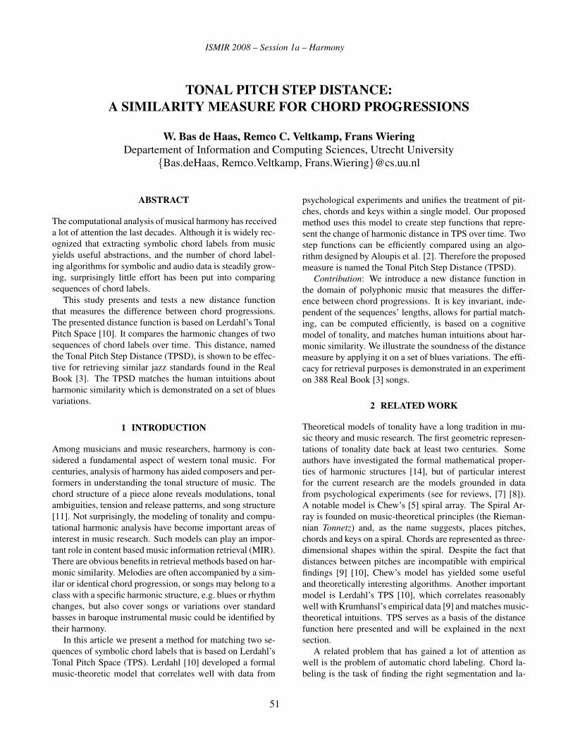
ISMIR 2008 – Session 1a – Harmony
TONAL PITCH STEP DISTANCE:A SIMILARITY MEASURE FOR CHORD PROGRESSIONS
W. Bas de Haas, Remco C. Veltkamp, Frans WieringDepartement of Information and Computing Sciences, Utrecht University
{Bas.deHaas, Remco.Veltkamp, Frans.Wiering}@cs.uu.nl
ABSTRACT
The computational analysis of musical harmony has received
a lot of attention the last decades. Although it is widely rec-
ognized that extracting symbolic chord labels from music
yields useful abstractions, and the number of chord label-
ing algorithms for symbolic and audio data is steadily grow-
ing, surprisingly little effort has been put into comparing
sequences of chord labels.
This study presents and tests a new distance function
that measures the difference between chord progressions.
The presented distance function is based on Lerdahl’s Tonal
Pitch Space [10]. It compares the harmonic changes of two
sequences of chord labels over time. This distance, named
the Tonal Pitch Step Distance (TPSD), is shown to be effec-
tive for retrieving similar jazz standards found in the Real
Book [3]. The TPSD matches the human intuitions about
harmonic similarity which is demonstrated on a set of blues
variations.
1 INTRODUCTION
Among musicians and music researchers, harmony is con-
sidered a fundamental aspect of western tonal music. For
centuries, analysis of harmony has aided composers and per-
formers in understanding the tonal structure of music. The
chord structure of a piece alone reveals modulations, tonal
ambiguities, tension and release patterns, and song structure
[11]. Not surprisingly, the modeling of tonality and compu-
tational harmonic analysis have become important areas of
interest in music research. Such models can play an impor-
tant role in content based music information retrieval (MIR).
There are obvious benefits in retrieval methods based on har-
monic similarity. Melodies are often accompanied by a sim-
ilar or identical chord progression, or songs may belong to a
class with a specific harmonic structure, e.g. blues or rhythm
changes, but also cover songs or variations over standard
basses in baroque instrumental music could be identified by
their harmony.
In this article we present a method for matching two se-
quences of symbolic chord labels that is based on Lerdahl’s
Tonal Pitch Space (TPS). Lerdahl [10] developed a formal
music-theoretic model that correlates well with data from
psychological experiments and unifies the treatment of pit-
ches, chords and keys within a single model. Our proposed
method uses this model to create step functions that repre-
sent the change of harmonic distance in TPS over time. Two
step functions can be efficiently compared using an algo-
rithm designed by Aloupis et al. [2]. Therefore the proposed
measure is named the Tonal Pitch Step Distance (TPSD).
Contribution: We introduce a new distance function in
the domain of polyphonic music that measures the differ-
ence between chord progressions. It is key invariant, inde-
pendent of the sequences’ lengths, allows for partial match-
ing, can be computed efficiently, is based on a cognitive
model of tonality, and matches human intuitions about har-
monic similarity. We illustrate the soundness of the distance
measure by applying it on a set of blues variations. The effi-
cacy for retrieval purposes is demonstrated in an experiment
on 388 Real Book [3] songs.
2 RELATED WORK
Theoretical models of tonality have a long tradition in mu-
sic theory and music research. The first geometric represen-
tations of tonality date back at least two centuries. Some
authors have investigated the formal mathematical proper-
ties of harmonic structures [14], but of particular interest
for the current research are the models grounded in data
from psychological experiments (see for reviews, [7] [8]).
A notable model is Chew’s [5] spiral array. The Spiral Ar-
ray is founded on music-theoretical principles (the Rieman-
nian Tonnetz) and, as the name suggests, places pitches,
chords and keys on a spiral. Chords are represented as three-
dimensional shapes within the spiral. Despite the fact that
distances between pitches are incompatible with empirical
findings [9] [10], Chew’s model has yielded some useful
and theoretically interesting algorithms. Another important
model is Lerdahl’s TPS [10], which correlates reasonably
well with Krumhansl’s empirical data [9] and matches music-
theoretical intuitions. TPS serves as a basis of the distance
function here presented and will be explained in the next
section.
A related problem that has gained a lot of attention as
well is the problem of automatic chord labeling. Chord la-
beling is the task of finding the right segmentation and la-
51

ISMIR 2008 – Session 1a – Harmony
(a) octave (root) level: 0 (0)
(b) fifths level: 0 7 (0)
(c) triadic (chord) level: 0 4 7 (0)
(d) diatonic level: 0 2 4 5 7 9 11 (0)
(e) chromatic level: 0 1 2 3 4 5 6 7 8 9 10 11 (0)
Table 1. The basic space of the tonic chord in the key of C
Major (C = 0, C# = 1, . . . , B = 11), from Lerdahl [10].
bels for a musical piece. A chord label consists of a chord
root, triadic quality, inversion, and extensions (additional
chord notes). Nowadays, several algorithms can correctly
segment and label approximately 80 percent of a symbolic
dataset (see for reviews [20] [16]). Within the audio domain,
hidden Markov Models are frequently used for chord label
assignment [17] [18]. It is widely accepted that chord in-
formation from symbolic or audio data yields a relevant and
musicological valid abstraction that can aid in discerning the
structure of a piece and making similarity judgments.
Both research areas previously touched upon are impor-
tant matters when it comes to MIR. Although the value of
chord descriptions is generally recognized, and various mod-
els about the cognition of tonality are available, surprisingly
little research has focused on how similar chord sequences
relate to each other. Attempts include string matching [12]
as a measure of similarity, and analyzing a chord sequences
on the basis of rewrite rules [15] [19]. Mauch [13] analyzed
the frequencies of chord classes, chord progression patterns
within the Real Book data [3] that is used in this study as
well. Still, we argue that similarity of chord sequences is
underexposed within the MIR field, which is also evident
from the fact that there is no MIREX track for chord pro-
gression similarity.
3 TONAL PITCH SPACE
The TPS is a model of tonality that fits human intuitions and
is supported by empirical data from psychology [9] 1 . The
TPS model can be used to calculate the distances between
all possible chords and to predict corresponding tension and
release patterns. Although the TPS can be used for defining
relationships between chords in different keys, it is more
suitable for calculating distances within local harmonies [4].
Therefore our here presented distance measure only utilizes
the parts of TPS needed for calculating the chordal distances
within a given key (this is motivated in section 4).
The basis of the TPS model is the basic space (see Ta-
ble 1) which comprises five hierarchical levels consisting of
pitch class subsets ordered from stable to unstable. Pitch
classes are categories that contain all pitches one or more
octaves apart. The first and most stable level (a) is the root
level, containing only the root of the analyzed chord. The
1 The TPS is an elaborate model; due to space limitation we have to
refer to [10], chapter 2, pages 47 to 59, for a more detailed explanation and
additional examples.
next level (b) adds the fifth of the chord. The third level (c)
is the triadic level containing all pitch classes of the chord.
The fourth (d) level is the diatonic level consisting of all
pitch classes of the diatonic scale of the current key. The
last and least stable level (e) is the chromatic level contain-
ing all pitch classes. The shape of the basic space of C major
strongly resembles Krumhansl and Kessler’s [9] C major-
key profile. For every chord change, the levels (a-c) must
be adapted properly and for a change of key, level d must
be adapted. The basic space is hierarchical: if a pitch class
is present at a certain level, it is also present at subsequent
levels.
The basic spaces of chords can be used to calculate dis-
tances between these chords. First, the basic space is set
to match the key of the piece (level d). Then the levels
(a-c) can be adapted to match the chords to be compared.
The distance between two chords is calculated by applying
the Chord distance rule. Some examples of calculation are
given in Tables 2 and 3.
The proposed distance measure uses a Chord distance
rule that is slightly different from the Chord distance rule
defined in TPS [10] and is defined as follows:
CHORD DISTANCE RULE: d(x, y) = j + k,
where d(x, y) is the distance between chord xand chord y. j is the minimal number of appli-
cations of the Circle-of-fifths rule in one direc-
tion needed to shift x into y. k is the number
of non-common pitch classes in the levels (a-d)
within the basic spaces of x and y together di-
vided by two 2 . A pitch class is non-common if
it is present in x or y but not in both chords.
CIRCLE-OF-FIFTHS RULE: move the levels
(a-c) four steps to the right or four steps to the
left (modulo 7) on level d 3 .
When plotted geometrically, the distances exhibit a reg-
ular pattern combining the diatonic circle of fifths horizon-
tally and the common tone circle vertically (see Figure 1). If
the chordal space is extended, it forms a toroidal structure.
Because we are interested in the metrical properties of the
chord distance rule it is good to observe that it has a maxi-
mum of 13 (see Table 4) 4 . This maximum can be obtained,
for instance, by calculating the distance between a C major
chord and an E chord containing all notes of the chromatic
scale.
2 This calculation of k deviates from the calculation described in [10].
Lerdahl defined k as the number of non-common pitch classes in the levels
(a-d) within the basic space of y compared to those in the basic space of x.
This definition has the undesirable side effect of making the distance func-
tion non-symmetrical. Our proposed calculation preserves the symmetry of
the distance function and yields equal or similar scores.3 If the chord root is non-diatonic j receives the maximum penalty of 3.4 Chords with a TPS score of 13 are not musically realistic, but it is
useful from a computational point of view to observe that the TPS, and
hence the TPSD, has a maximum score.
52

ISMIR 2008 – Session 1a – Harmony
0 7
0 2 70 2 4 5 7 11
0 2 4 5 7 9 11
0 1 2 3 4 5 6 7 8 9 10 11
Table 2. The distance between the C and G7 in the context
of a C major key. The bold numbers in the basic space are
specific for the C major chord and the underlined numbers
are specific for the G7 chord. The only common pitch class
is G (7). All other 9 pitch classes in the levels (a-c) are non-
common, therefore k = 92 . j = 1 because the Circle-of-
fifths rule is applied once. The total score is: 1 + 4.5 = 5.5.
22 92 5 6 9
1 2 4 5 6 7 9 11
0 1 2 3 4 5 6 7 8 9 10 11
Table 3. The distance of a D and a Dm chord in the context
of a D major key. The non-common pitch classes are the
minor and major thirds (5 and 6), therefore k = 32 = 1.5.
Note that the minor third does not belong to the D major
scale and adds 2 non-common pitch classes. There is no
application of the Circle-of-fifths rule (j = 0), hence the
total score is 1.5 + 0 = 1.5.
Figure 1. A portion of Lerdahl’s chordal space with the
roman numbers denoting the seven basic chords in an arbi-
trary key. The arrows denote the distances as calculated by
the Chord distance rule.
0 4
0 4 7 11
0 1 2 3 4 5 6 7 8 9 10 11
0 1 2 3 4 5 6 7 8 9 10 11
0 1 2 3 4 5 6 7 8 9 10 11
Table 4. Maximum chordal distance, demonstrated by com-
paring a C major chord with a chord on E chord containing
all pitch classes. The bold numbers are specific for the C
major chord and the underlined numbers are specific for the
chord on E. The numbers that are underlined and bold are
the common pitch classes, the remaining pitch classes are
non-common, hence k = 20. j = 3 because the Circle-
of-fifths rule is applied three times and yields its maximal
value. The total score is d(x, y) = 202 + 3 = 13.
Two Blues Variations
Blues variation 1 Blues variation 9
0 4 8 12 16 20 24 28 32 36 40 44 48
Beat
0
1
2
3
4
5
6
7
8
9
10
11
12
13
TP
S S
co
re
Figure 2. A plot of the step functions of Blues variation 1
and 9 (see Table 5). The TPSD is defined as the hatched
area between Blues variation 1 and 9 divided by the length
of the shortest step function (which can be either one in this
example).
4 TONAL PITCH STEP DISTANCE
On the basis of the Chord distance rule, we define a dis-
tance function for chord sequences, called the Tonal Pitch
Step Distance (TPSD). The TPSD compares two chord se-
quences and outputs a number between 0 and the maximum
chordal distance 13. A low score indicates two very similar
chord sequences and a high score indicates large harmonic
differences between two sequences.
The central idea behind the TPSD is to compare the
change of chordal distance to the tonic over time. This is
done by calculating the chordal distance between each chord
of the song and the triadic tonic chord of the key of the song.
The reason for doing so, is that if the distance function is
based on comparing subsequent chords, the chord distance
depends on the exact progression by which that chord was
reached. This is undesirable because very similar but not
identical chord sequences can then produce radically differ-
ent scores.
Plotting the chordal distance against the time results in a
step function. The difference between two chord sequences
can then be defined as the minimal area between the two
step functions f and g over all possible horizontal shifts t of
f over g (see Figure 2). These shifts are cyclic and to pre-
vent longer sequences from yielding higher scores, the score
is normalized by dividing it by the length of the shortest
step function. Trivially, the TSPD can handle step functions
of different length since the area between non-overlapping
parts is always zero.
The calculation of the area between f and g is straightfor-
ward. It can be calculated by summing all rectangular strips
between f and g, and trivially takes O(n+m) time where nand m are the number of chords in f and g, respectively. An
important observation is that if f is shifted along g, a min-
53

ISMIR 2008 – Session 1a – Harmony
imum is always obtained when two vertical edges coincide.
Consequently, only the shifts of t where two edges coincide
have to be considered, yielding O(nm) shifts and a total run-
ning time of O(nm(n + m)). For the results presented here
we used this simple algorithm, but the running time can be
further improved to O(nm log(n + m)) by applying an al-
gorithm proposed by Aloupis et al. [2]. They present an al-
gorithm that minimizes the area between two step functions
by shifting it horizontally as well as vertically.
We do not use the functionality of TPS to calculate dis-
tances between chords in different keys. We choose to do
so for two reasons. First, modulation information is rarely
present in chord sequence data. Second, we are interested
in the harmonic similarity of chord sequences regardless of
their keys. This implies that to analyze a chord sequence,
the key of the sequence must be provided. The TSPD is not
a metric, it does not satisfy the property of identity of in-discernibles; since two different chords can have the same
Lerdahl distance (see Figure 1), it is possible to construct
two different chord sequences with the same TPSD.
5 EXAMPLES
To illustrate how our measure behaves in practice, the dis-
tances are calculated for a number of blues progressions.
Table 5 shows seventeen variations on a twelve bar blues
(the last 12 columns) by Dan Hearle found in [1]. The pro-
gressions read from left to right with the numbers in the
header denoting the bar. The progression in the top row is a
very simple blues and as one moves down the progressions
become more complex, more altered, and more difficult to
play. The second column displays the distance between the
progression in first row and the progression in the current
row. The third column shows the distance between two sub-
sequent progressions.
We can make the following observations. The scores
correspond well to our intuitive idea of similarity between
chord progressions. The scores between similar progres-
sions are small and as progressions become more complex
the calculated distance with respect to the most simple blues
progression becomes higher.
6 EXPERIMENT
We tested the efficacy of the TPSD for retrieval purposes
in an experiment. We used a collection of 388 sequences
of chord labels that describe the chords of 242 jazz stan-
dards found in the Real Book [3]. The chord label data
comes from a collection of user-generated Band-in-a-Box
files; Band-in-a-Box is a commercial software package that
can be used for generating musical accompaniment. The au-
thors manually checked the files for consistency, quality and
correct key. Within this collection, 85 songs contain two or
more similar versions, forming 85 classes of songs. These
songs have the same title and share a similar melody, but can
differ in a number of ways. They can, for instance, differ
in key and form, they may differ in the number of repeti-
tions, or have a special introduction or ending. The richness
of the chords descriptions can also diverge, i.e. a C7b9b13
may be written instead of a C7, and common substitutions
frequently occur. Examples of the latter are relative substi-
tution, i.e. Am instead of C, or tritone substitution, i.e. F#7
instead of C7.
Although additional information about timing and tempo
in jazz can contain valuable cues that could be helpful for
MIR [6], we only used the chord-per-beat information in our
step functions. All songs with multiple versions are used as
queries and all other 387 songs are ranked on their TPSD
score. We then evaluate the ranking of the other versions.
7 RESULTS
Table 6 shows the results of the experiment. The second
and seventh columns display the average first tier per song
class. The first tier is the number of correctly retrieved songs
within the best (C − 1) matches divided by (C − 1), where
C is the size of the song class. Trivially, by using all songs
within a class as a query, C first tiers are calculated and aver-
aged for every class of songs. The third and eighth columns
show the average second tier. The second tier is the num-
ber of correctly retrieved songs within the best (2C − 1)
matches, divided by (2C − 1).
The grand averages 5 of the average first and second tiers
are 74 and 77 percent, respectively. This implies that in 74
percent of the song classes the songs searched for are on top
of the ranking. Seven song classes in Table 6 contain one
or more matches with a TPSD score of 0.00; such a per-
fect match occurs when two step functions are identical for
at least the length of the shortest chord sequence. If these
matches are removed from the results, the grand averages of
the first and second tiers become 71 and 75 percent, respec-
tively.
8 CONCLUSION
We introduced a new distance function, the Tonal Pitch Step
Distance, for chord progressions on the basis of harmonic
similarity. The distance of a chord to the tonic triad of its key
was determined by using a variant of Lerdahl’s Tonal Pitch
Space. This cognitive model correlates with empirical data
from psychology and matches music-theoretical intuitions.
A step function was used to represent the change of chordal
distance to its tonic over time. The distance between two
chord progressions was defined as the minimal area between
two step functions.
5 Song classes are not weighted on the basis of their size in the calcula-
tion of the grand average.
54

ISMIR 2008 – Session 1a – Harmony
i d(1,i) d(i,i-1) 1 2 3 4 5 6 7 8 9 10 11 12
1 0.00 0.00 F7 Bb7 F7 C7 F7
2 0.42 0.42 F7 Bb7 F7 C7 Bb7 F7 C7
3 1.00 0.67 F7 Bb7 F7 Bb7 F7 G7 C7 F7 C7
4 1.58 0.58 F7 Bb7 F7 Bb7 F7 D7 G7 C7 F7 C7
5 1.62 0.12 F7 Bb7 F7 Bb7 F7 D7 Gm7 C7 F7 Gm7 C7
6 2.31 0.69 F7 Bb7 F7 Bb7 Eb7 F7 D7 Db7 C7 F7 Db7 C7
7 2.75 1.10 F7 Bb7 F7 Cm7 F7 Bb7 Eb7 F7 Am7 D7 Gm7 C7 Am7 D7 Gm7 C7
8 3.31 0.56 F7 Bb7 F7 Cm7 F7 Bb7 Eb7 Am7 D7 Gm7 C7 Am7 D7 Gm7 C7
9 3.17 0.56 F7 Bb7 F7 Cm7 F7 Bb7 Bm7 E7 F7 E7 Eb7 D7 Gm7 C7 Bb7 Am7 D7 Gm7 C7
10 4.29 2.12 FM7 Em7 A7 Dm7 G7 Cm7 F7 Bb7 Bdim7 Am7 D7 Abm7 Db7 Gm7 C7 Dbm7 Gb7 F7 D7 Gm7 C7
11 5.12 2.08 FM7 Em7 Ebm7 Dm7 Dbm7 Cm7 Cb7 BbM7 Bbm7 Am7 Abm7 Gm7 C7 Am7 Abm7 Gm7 Gb
12 4.88 1.50 FM7 BbM7 Am7 Gm7 Gbm7 Cb7 BbM7 Bbm7 Am7 Abm7 Gm7 Gb7 FM7 Abm7 Gm7 Gb
13 5.23 1.48 FM7 BbM7 Am7 Gm7 Gbm7 Cb7 BbM7 Bbm7 Eb7 AbM7 Abm7 Db7 GbM7 Gm7 C7 Am7 D7 Dbm7 Gb
14 4.40 1.79 FM7 Em7 A7 Dm7 G7 Cm7 F7 BbM7 Bbm7 Eb7 Am7 Abm7 Db7 Gm7 C7 Am7 D7 Gm7 C7
15 4.98 0.75 FM7 Em7 A7 Dm7 G7 Gbm7 Cb7 BbM7 Bm7 E7 Am7 Abm7 Db7 Gm7 C7 Bb7 Am7 D7 Gm7 C7
16 5.42 1.94 F#m7 B7 Em7 A7 Dm7 G7 Cm7 F7 BbM7 Bbm7 Eb7 AbM7 Abm7 Db7 GbM7 Gm7 C7 Am7 D7 Gm7 C7
17 5.71 2.88 FM7 F#m7 B7 EM7 EbM7 DbM7 BM7 BbM7 Bm7 E7 AM7 Am7 D7 GM7 GbM7 FM7 AbM7 GM7 Gb
Table 5. Seventeen blues variations and the TPSD scores between each progression and the first one (second column), and
between each progression and the preceding one (third column).
nr. 1st Tier 2nd Tier Class size Title of the song class nr. 1st Tier 2nd Tier Class size Title of the song class
1 1.00 1.00 2 A Child is Born 44 1.00 1.00 2 Miyako
2 0.00 0.00 2 A Fine Romance 45 0.50 0.50 2 Moment Notice
3 1.00 1.00 2 A Night In Tunisia 46 1.00 1.00 3 Mood Indigo
4 0.50 0.50 2 All Blues 47 0.73 0.73 6 More I See You, The
5 0.67 0.83 3 All Of Me 48 0.33 0.33 3 My Favorite Things
6 0.50 0.50 2 Angel Eyes 49 1.00 1.00 4 My Funny Valentine
7 0.50 1.00 2 April In Paris 50 1.00 1.00 3 My Romance
8 0.00 0.00 2 Blue in Green 51 0.50 0.50 2 Nefertiti
9 0.50 0.50 4 Corcovado (Quiet Nights of Quiet Stars) 52 0.67 0.83 3 Nica’ Dream
10 1.00 1.00 2 Days of Wine and Roses, The 53 1.00 1.00 2 Night Dreamer
11 1.00 1.00 2 Dearly Beloved 54 0.00 0.00 2 Night Has a Thousand Eyes, The
12 0.00 0.00 2 Desafinado 55 0.33 0.33 3 Oleo
13 1.00 1.00 2 Don’t Get Around Much Anymore 56 1.00 1.00 3 Once I Loved
14 0.33 0.33 3 Easy to Love 57 1.00 1.00 3 One Note Samba
15 1.00 1.00 2 E.S.P. 58 0.50 0.50 2 Ornithology
16 0.60 0.60 5 Girl from Ipanema 59 1.00 1.00 2 Peace
17 1.00 1.00 2 Green Dolphin Street 60 1.00 1.00 2 Pensativa
18 1.00 1.00 2 Have You Met Miss Jones 61 0.00 0.00 2 Peri’s Scope
19 0.70 0.80 5 Here’s That Rainy Day 62 1.00 1.00 4 Satin Doll
20 1.00 1.00 4 Hey There 63 1.00 1.00 2 Scrapple from the Apple
21 0.63 0.67 6 How High the Moon 64 0.67 1.00 3 Shadow of Your Smile, The
22 1.00 1.00 3 How Insensitive 65 1.00 1.00 3 Solar
23 1.00 1.00 3 If You Never Come To Me 66 0.33 0.50 3 Some Day My Prince Will Come
24 0.00 0.00 2 I Love You 67 0.33 0.33 3 Song is You, The
25 1.00 1.00 2 I Mean You 68 1.00 1.00 3 Sophisticated Lady
26 1.00 1.00 2 In A Sentimental Mood 69 0.67 1.00 3 So What
27 0.00 0.00 2 Isotope 70 1.00 1.00 3 Stella by Starlight
28 1.00 1.00 3 Jordu 71 1.00 1.00 3 Stompin’ at the Savoy
29 1.00 1.00 2 Joy Spring 72 0.67 1.00 3 Straight, No Chaser
30 1.00 1.00 2 Just Friends 73 1.00 1.00 2 Take the “A” Train
31 1.00 1.00 2 Lament 74 1.00 1.00 3 There is No Greater Love
32 1.00 1.00 2 Like Someone In Love 75 0.50 0.50 2 They Can’t Take That Away From Me
33 1.00 1.00 3 Limehouse Blues 76 1.00 1.00 2 Triste
34 1.00 1.00 2 Little Waltz 77 1.00 1.00 2 Tune Up
35 0.83 1.00 4 Long Ago and Far Away 78 0.33 0.33 3 Wave
36 1.00 1.00 2 Look to the Sky 79 1.00 1.00 3 We’ll Be Together Again
37 0.33 0.33 3 Lucky Southern 80 1.00 1.00 3 Well You Needn’t
38 1.00 1.00 3 Lullaby of Birdland 81 1.00 1.00 3 When I Fall In Love
39 1.00 1.00 2 Maiden Voyage 82 0.17 0.25 4 Yesterdays
40 0.33 0.33 3 Meditation 83 0.45 0.60 5 You Are the Sunshine of My Life
41 1.00 1.00 2 Memories of Tommorow 84 1.00 1.00 3 You Are Too Beautiful
42 0.00 0.17 3 Michelle 85 1.00 1.00 2 You Don’t Know What Love Is
43 1.00 1.00 2 Misty avg. 0.74 0.77
Table 6. 78 song classes of jazz standards found in the Real Book. The first and second tier results show the retrieval efficacy
of the TPSD.
55

ISMIR 2008 – Session 1a – Harmony
We showed that the TPSD as a retrieval method yields
promising results. Similar versions of the same jazz stan-
dard found in the Real Book can be successfully retrieved
on the basis of their chord progressions. The soundness of
the TPSD was demonstrated on a series of blues variations.
9 FUTURE WORK
The problem in analyzing the retrieval quality of the TPSD
is the lack of good ground truth data. We do not know of
any collection of chord sequences that contain user gen-
erated similarity labels. It would be interesting to acquire
such similarity data and further explore the performance of
the TPSD. This could very well be done in a MIREX track.
Another issue concerns the used dataset. The Real Book
collection is a small collection and only contains songs of
a specific musical genre: jazz standards. It would be inter-
esting to explore the performance of the TPSD on a larger
dataset and in other musical domains.
We can suggest several improvements of the TPSD as
well. Currently, the TPSD does not treat modulations in
a musical way. If a modulation occurs within a piece, the
scores of the TPSD become very high, and although this
enables the TPSD to recognize these modulations, the step
function loses nuance. Applying a key finding algorithm
locally might yield more subtle results. Another idea is to
further exploit the fact that TPSD is very suitable for partial
matching by using it for tracing repetitions within a query
or matching meaningful segments of a query instead of the
query as a whole.
We believe that further improvement of chord labeling
algorithms and the development of tools that analyze these
labels should be high on the research agenda because chord
labels form an abstraction of musical content with substan-
tial explanatory power. In the future we expect TPSD based
methods to help users find songs in large databases on the
Internet, or in their personal collections. We believe that re-
trieval on basis of harmonic structure is crucial for the next
generation of content based MIR systems.
10 ACKNOWLEDGMENTS
This research was supported by the Dutch ICES/KIS III Bsik
project MultimediaN. The authors wish to thank Matthias
Mauch (Centre for Digital Music, Queen Mary, University
of London) for providing the Real Book data used in this
study.
11 REFERENCES
[1] J. Aebersold. Jazz Handbook. Jamey Aebersold Jazz,Inc., 2000.
[2] G. Aloupis, T. Fevens, S. Langerman, T. Matsui,A. Mesa, Y. Nuñez, D. Rappaport, and G. Toussaint.
Algorithms for Computing Geometric Measures ofMelodic Similarity. Computer Music Journal, 30(3):67–76, 2004.
[3] Various Authors. The Real Book. Hal Leonard Corpora-tion, 6th edition, 2004.
[4] E. Bigand and R. Parncutt. Perceiving Musical Ten-sion in Long Chord Sequences. Psychological Research,62(4):237–254, 1999.
[5] E. Chew. Towards a Mathematical Model of Tonal-ity. PhD thesis, Massachusetts Institute of Technology,2000.
[6] H. Honing and W.B. de Haas. Swing Once More: Relat-ing Timing and Tempo in Expert Jazz Drumming. MusicPerception, 25(5):471–476, 2008.
[7] C.L. Krumhansl. The Cognition of Tonality - as WeKnow it Today. Journal of New Music Research,33(3):253–268, 2004.
[8] C.L. Krumhansl. The Geometry of Musical Structure: aBrief Introduction and History. Computers in Entertain-ment (CIE), 3(4):3–14, 2005.
[9] C.L. Krumhansl and E.J. Kessler. Tracing the DynamicChanges in Perceived Tonal Organization in a SpatialRepresentation of Musical Keys. Psychological Review,89(4):334–68, 1982.
[10] F. Lerdahl. Tonal Pitch Space. Oxford University Press,2001.
[11] F. Lerdahl and C.L. Krumhansl. Modeling Tonal Ten-sion. Music Perception, 24:329–366, 2007.
[12] C.C. Liu, J. L. Hsu, and A.L.P. Chen. An ApproximateString Matching Algorithm for Content-Based MusicData Retrieval. Proceedings ICMCS, 1999.
[13] M. Mauch, S. Dixon, C. Harte, M. Casey, and B. Fields.Discovering Chord Idioms Through Beatles And RealBook Songs. Proceedings ISMIR, pages 255–258, 2007.
[14] T. Noll and J. Garbers. Harmonic Path Analysis. In Maz-zola G. Lluis-Puebla, E. and T Noll, editors, Perspec-tives in Mathematical and Computer-Aided Music The-ory. Verlag epOs-Music, Osnabrück, 2004.
[15] F. Pachet. Computer Analysis of Jazz Chord Sequences.Is Solar a Blues? Readings in Music and Artificial Intel-ligence, 1997.
[16] B. Pardo and W.P. Birmingham. Algorithms for ChordalAnalysis. Computer Music Journal, 26(2):27–49, 2002.
[17] J Pickens. Harmonic Modeling for Polyphonic Mu-sic Retrieval. PhD thesis, University of MassachusettsAmherst, 2004.
[18] A. Sheh and D.P.W. Ellis. Chord Segmentation andRecognition using EM-Trained Hidden Markov Models.Proceedings ISMIR, 3:185–191, 2003.
[19] M.J. Steedman. A Generative Grammar for Jazz ChordSequences. Music Perception, 2(1):52–77, 1984.
[20] D. Temperley. The Cognition of Basic Musical Struc-tures. Cambridge, MA, MIT Press, 2001.
56

ISMIR 2008 – Session 1a – Harmony
EVALUATING AND VISUALIZING EFFECTIVENESS OF STYLEEMULATION IN MUSICAL ACCOMPANIMENT
Ching-Hua Chuan∗ and Elaine Chew†
University of Southern California Viterbi School of Engineering∗Department of Computer Science and †Epstein Department of Industrial and Systems Engineering
†Radcliffe Institute for Advanced Study at Harvard University{chinghuc, echew}@usc.edu
ABSTRACT
We propose general quantitative methods for evaluating andvisualizing the results of machine-generated style-specificaccompaniment. The evaluation of automated accompani-ment systems, and the degree to which they emulate a style,has been based primarily on subjective opinion. To quan-tify style similarity between machine-generated and orig-inal accompaniments, we propose two types of measures:one based on transformations in the neo-Riemannian chordspace, and another based on the distribution of melody-chordintervals. The first set of experiments demonstrate the meth-ods on an automatic style-specific accompaniment (ASSA)system. They test the effect of training data choice on styleemulation effectiveness, and challenge the assumption thatmore data is better. The second set of experiments comparethe output of the ASSA system with those of a rule-basedsystem, and random chord generator. While the examplesfocus primarily on machine emulation of Pop/Rock accom-paniment, the methods generalize to music of other genres.
1 INTRODUCTION
Automatic generation of music in a specific style has been afocal topic in computational music research since the earlydays of computing. Many researchers have designed sys-tems that emulate music styles in compositions. The evalu-ation of the musical output, the degree to which it achievesits goal of emulating a particular style remains a challenge.Evaluation is often in the form of subjective opinion. It isour goal to fill this gap in quantitative evaluation of styleemulation in automatic accompaniment systems.In [1], Meyer states that “style is a replication of pattern-
ing, . . . , that results from a series of choices made withinsome set of constraints.” Accompaniment can be consideredthe outcome of a series of choices over possible chords un-der certain contextual constraints, such as melody, phrase,and key. For example, in four-part harmonization, the com-position must follow the counterpoint and voice-leading rulesin music theory. In contrast, modeling of the accompani-ment style in Pop/Rock tends to be vague and difficult be-
cause, according to Stephenson [2], “in rock, . . . , melody isallowed to interact with harmony more freely,” and the pro-cess becomes more complex because, as Everett states [3],“many different tonal systems are now practiced by the sameartist, on the same album.”
In this paper we propose methods to visualize, measure,and quantify the quality of an accompaniment generatedwiththe goal of emulating an original accompaniment, the “groundtruth”. These measures are designed to evaluate automaticstyle-specific accompaniment (ASSA) systems. We exam-ine the style as captured by the musical relations betweenmelody and harmony, and between adjacent chords. We de-velop six metrics based on these two types of measures.
Using these quantitativemethods, we design experimentsto explore training set selection strategies that further theASSA system’s style emulation goals. For machine learningtasks, it is often the case that more training data guaranteebetter results. For ASSA goals, more training songs may notnecessarily improve the output quality if the training set isnot consistent with the desired style. The first set of experi-ment explores the factors impacting style emulation success.
A second set of experiments compare the degree of style-specificity between the best ASSA systems, a rule-basedharmonization system, and a random chord generator. Weconduct the experiments on five well known Pop/Rock al-bums by Green Day, Keane, and Radiohead, providing de-tailed statistics and case studies for the resulting accompani-ments. The findings we report generalize to genres outsideof Rock music, and to some extent to simulation of style inmusic in general.
The paper is organized as follows: Section 2 describesrelated automatic accompaniment systems, with and with-out style requirements, and their evaluations. It concludeswith a brief description of an ASSA system, which formsthe basis of much of our evaluations. We present the eval-uation methods in Section 3. Intra-system comparisons areshown in Sections 4, and inter-system results in 5, followedby the conclusions.
57

ISMIR 2008 – Session 1a – Harmony
2 RELATED WORK
Baroque style four-part harmonization has been a popularaccompaniment generation application since the earliest daysof computing. Recent examples include [4, 5]. Many rulesgovern these Chorale-type harmonizations, which can be ap-plied in their synthesis and evaluation. Sixteenth centurycompositions in the style of Palestrina have also be emulatedusing Markov models [6]. Such compositions are similarlyand strictly circumscribed by a host of rules, which can beused in the evaluation of their correctness [7]. Temperleyand Sleator proposed a set of preference rules to harmoniz-ing melodies in the Western classical style [8]; these rulesare implemented in their Harmonic Analyzer [9].In the popular realm, the i-Ring system [10] generates
an accompaniment for any eight-measure melody. The ac-companiment is based on state transition probabilities cal-culated from a training set of 150 songs. For evaluation, 10participants were asked to rate the accompaniment as Good,Medium, or Bad.More recently, MySong [11] uses Hidden Markov Mod-
els, training on 298 popular songs in genres including Pop,Rock, R&B, Jazz, and Country Music. Users can choosebetween two style-related modes: ‘Jazz,’ which uses lesscommon triads, or ‘Happy,’ which selects more major-modechord transitions. 26 sample accompaniments by MySongwere evaluated subjectively by 30 volunteer musicians.While the output of the above systems fit the melody, be-
cause the systems learn from general training sets, the stylecaptured by the output lacks specificity. Thus, these sys-tems do not address the emulation of specific accompani-ment styles, as embodied in a distinctive song or a partic-ular band’s output. Evaluations take the form of subjectiveopinion, and lack an objective or quantitative component.In [12], Chuan & Chew proposed an ASSA system that
can generate style-specific accompaniment to a melody givenonly a few examples. The system consists of a chord tonedetermination and a chord progression module. The chordtone determination module applies machine learning to de-termine which notes in a melody are likely chord tones basedon the specified style. The system then constructs possi-ble chord progressions using neo-Riemannian transforms,representing them in a tree structure, and selects the high-est probability path based on the learned probabilities in aMarkov chain. This system was rated informally by subjec-tively judgement via a Turing test.
3 QUANTIFYING ACCOMPANIMENT DISTANCE
This section first presents ways to quantify and visualize dis-tance between two chords, and metrics to evaluate distancebetween two different accompaniments to the same melody.The examples are generated by the ASSA system of [12].
3.1 Visualization
Two visualization models are described as follows. The firstconsiders musical distance between two chords based onneo-Riemannian transforms, the second addresses the dif-ference between chord choices in relation to the melody.
3.1.1 Neo-Riemannian Distance in Chord Space
Music theorists have used neo-Riemannian transformationsto analyze harmonic diversity in Pop/Rock music [13]. Inthe neo-Riemannian chord space, chords are connected bythree types of neo-Riemannian operations (NROs), P (par-allel), L (leading-tone exchange), and R (relative).Figure 1 shows the three types of NROs in chord space,
where chords are represented in Roman numerals. Verticalneighbors are connected by P/R operations, and horizontalneighbors have Dominant/Subdominant (D/S) relationships.
ii v i iv bvii
vii iii vi ii v
II V I IV bVII
R L P
VII III VI II V
Figure 1. Neo-Riemannian transforms in chord space.
To quantify the distance between two chords − for ex-ample, to determine how well a generated chord comparesto the original − we can compute the shortest distance be-tween the two chords in the neo-Riemannian space. Twochords connected by an NRO share two tones, with the thirdbeing one or two half steps apart. The fewer NROs betweenthe chords, the closer they are perceptually.
Chord Space Distance-Time Plot: To visualize the dis-tance between a machine-generated and an original accom-paniment, we can graph this distance in chord space overtime. Figure 2 shows one such graph for comparing the gen-erated and original accompaniments.The x-axis marks the chord count; the yz-axes represent
chord space. The plot charts a given accompaniment’s dis-tance from the baseline (original), according to chord spacedistance. If the two accompaniments are identical, the graphwould be a horizontal line defined by y = z = 0. The ad-vantage of this visualization is that we can see the qualityof each generated chord by observing its neo-Riemanniandistance from the original, and we can observe their chordrelation by examining the direction of the deviation.
Chord Map Distribution: The second visualization em-ploys the key map idea proposed in [14]. A chord map (Fig-
58
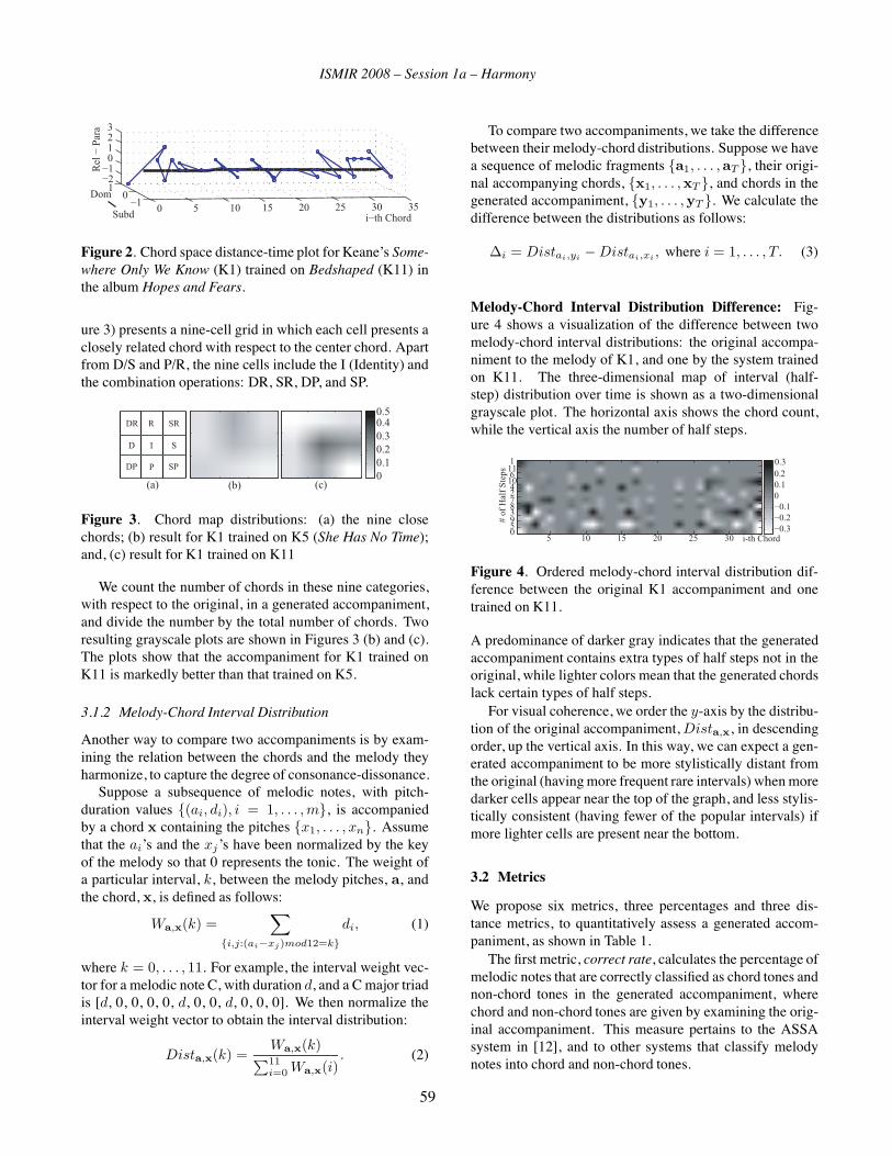
ISMIR 2008 – Session 1a – Harmony
0 5 10 15 20 25 30 35−10
1−2−1
0123
i−th Chord
Dom
Subd
Rel
− P
ara
Figure 2. Chord space distance-time plot for Keane’s Some-where Only We Know (K1) trained on Bedshaped (K11) inthe album Hopes and Fears.
ure 3) presents a nine-cell grid in which each cell presents aclosely related chord with respect to the center chord. Apartfrom D/S and P/R, the nine cells include the I (Identity) andthe combination operations: DR, SR, DP, and SP.
00.10.20.30.40.5
(c)(b)
P
I
R
D S
DP
DR SR
SP
(a)
Figure 3. Chord map distributions: (a) the nine closechords; (b) result for K1 trained on K5 (She Has No Time);and, (c) result for K1 trained on K11
We count the number of chords in these nine categories,with respect to the original, in a generated accompaniment,and divide the number by the total number of chords. Tworesulting grayscale plots are shown in Figures 3 (b) and (c).The plots show that the accompaniment for K1 trained onK11 is markedly better than that trained on K5.
3.1.2 Melody-Chord Interval Distribution
Another way to compare two accompaniments is by exam-ining the relation between the chords and the melody theyharmonize, to capture the degree of consonance-dissonance.Suppose a subsequence of melodic notes, with pitch-
duration values {(ai, di), i = 1, . . . , m}, is accompaniedby a chord x containing the pitches {x1, . . . , xn}. Assumethat the ai’s and the xj ’s have been normalized by the keyof the melody so that 0 represents the tonic. The weight ofa particular interval, k, between the melody pitches, a, andthe chord, x, is defined as follows:
Wa,x(k) =∑
{i,j:(ai−xj)mod12=k}di, (1)
where k = 0, . . . , 11. For example, the interval weight vec-tor for a melodic note C, with duration d, and a Cmajor triadis [d, 0, 0, 0, 0, d, 0, 0, d, 0, 0, 0]. We then normalize theinterval weight vector to obtain the interval distribution:
Dista,x(k) =Wa,x(k)∑11i=0 Wa,x(i)
. (2)
To compare two accompaniments, we take the differencebetween their melody-chord distributions. Suppose we havea sequence of melodic fragments {a1, . . . ,aT }, their origi-nal accompanying chords, {x1, . . . ,xT }, and chords in thegenerated accompaniment, {y1, . . . ,yT }. We calculate thedifference between the distributions as follows:
Δi = Distai,yi −Distai,xi , where i = 1, . . . , T. (3)
Melody-Chord Interval Distribution Difference: Fig-ure 4 shows a visualization of the difference between twomelody-chord interval distributions: the original accompa-niment to the melody of K1, and one by the system trainedon K11. The three-dimensional map of interval (half-step) distribution over time is shown as a two-dimensionalgrayscale plot. The horizontal axis shows the chord count,while the vertical axis the number of half steps.
5 10 15 20 25 3005938724106111
−0.3−0.2−0.100.10.20.3
i-th Chord
# of
Hal
f S
teps
Figure 4. Ordered melody-chord interval distribution dif-ference between the original K1 accompaniment and onetrained on K11.
A predominance of darker gray indicates that the generatedaccompaniment contains extra types of half steps not in theoriginal, while lighter colors mean that the generated chordslack certain types of half steps.For visual coherence, we order the y-axis by the distribu-
tion of the original accompaniment,Dista,x, in descendingorder, up the vertical axis. In this way, we can expect a gen-erated accompaniment to be more stylistically distant fromthe original (havingmore frequent rare intervals) whenmoredarker cells appear near the top of the graph, and less stylis-tically consistent (having fewer of the popular intervals) ifmore lighter cells are present near the bottom.
3.2 Metrics
We propose six metrics, three percentages and three dis-tance metrics, to quantitatively assess a generated accom-paniment, as shown in Table 1.The first metric, correct rate, calculates the percentage of
melodic notes that are correctly classified as chord tones andnon-chord tones in the generated accompaniment, wherechord and non-chord tones are given by examining the orig-inal accompaniment. This measure pertains to the ASSAsystem in [12], and to other systems that classify melodynotes into chord and non-chord tones.
59

ISMIR 2008 – Session 1a – Harmony
Table 1. Metric values’ names, meanings and ranges
name meaning max mincorrect rate % correct chord/non-chord tone classification 100 0
same chords % of generated chords identical with original 100 0
chords-in-grid % of generated chords in chord map 100 0
NR distance ave NR distance bet generated/original chords 7 0
HS distance MSE between interval (half-step) dist 2 0
wHS dist weighted MSE bet interval distributions 2 0
The second metric, same chords, records the percentageof chords generated that are identical to the original. Notethat this is also the value in the center cell of the chord mapsshown in Figure 3. The third metric, chords in grid, givesthe percentage of chords generated that are closely related tothe original on the chord map; this value can be computedby summing all values in the cells of the chord map.The NR distance metric shows the average shortest neo-
Riemannian distance between the generated chord and theoriginal, i.e., the average minimum neo-Riemannian dis-tance between each data-point and the center line in thechord space distance-time plot shown in Figure 2. Note thatthe maximum NR distance between any two chords is 7.The last two metrics are generated from the melody-
chord interval distribution described in Section 3.1.2. TheHS distance is the mean squared difference between the in-terval (half-step) distributions of the generated and the orig-inal accompaniments:
HS =1T
T∑i=1
11∑k=1
Δi(k)2. (4)
The worst case occurs when only one type of half step dom-inates the generated and original accompaniments’ distribu-tions, but the types are different, causing a distance of 2.The final metric wHS distance is like the HS distance,
except that Δi is multiplied by the inverse of the half-step distribution value for the original accompaniment. Theweighted HS distance increases the weight for infrequenthalf steps, reflecting the fact that rare, dissonant intervalscan significantly impact the perceived accompaniment style.Let Dista,x be the half-step distribution of the original
accompaniment for melody fragment a. The weighting fac-tor for each half step, k = 0, . . . , 11, can be calculated as:
w(k) =
{1/Dista,x(k), ifDista,x(k) > 00.001, ifDista,x(k) = 0
(5)
The weighted HS distance is then calculated as:
wHS =1T
T∑i=1
11∑k=1
w(k)×Δi(k)2, (6)
All Best Worst35
45
55
65
75
85
(a) Correct Rate (%) (b) Same Chord (%)All Best Worst
(c) Chord in Grid (%)
All Best Worst(d) NR Distance
All Best Worst(e) Half-Step Distance
All Best Worst(f) Wt. H-S Distance
10
20
30
40
All Best Worst50
60
70
80
90
0.8
1.2
1.6
2
0.5
0.7
0.9
1.1
0.3
0.5
0.7
Figure 5. Summary statistics for generated accompani-ments over five albums
4 INTRA-SYSTEM COMPARISONS
This section describes experiments involving only theASSA system of [12]. Recall that this system has a chordtone determination (CTD) module, and a chord progressionmodule. We examine the general quality of the results gen-erated by the system, focussing on the impact of trainingdata on the quality of the machine-generated accompani-ment, so as to improve the choice of training songs.The data set consists of songs from the five albums:
Green Day’s Dookie and American Idiots, Keane’s Hopesand Fears, and Radiohead’s Pablo Honey and Hail to theThief. We use commercial lead sheets for the ground truth.
4.1 One-Song v.s. All-Except-One Training Policy
To test whether more data is indeed better in ASSA, theseexperiments compare two training song choices. The firstselects one song from an album for training, and tests themodel on another song in the same album. The second usesall except one song for training, and tests the model on theheld out song.Figure 5 shows the statistics. “Best” and “Worst” report
the performance by the model that is trained on a single-song in the same album, and that has the highest and lowestcorrect CTD rates, respectively. “All” refers to results whereall other songs in the same album form the training set.Note that except for the correct CTD rate, Figure 5(a), the
statistics for Worst-CTD consistently outperform those forAll. The results indicate that more data is not always better,and that the use of neo-Riemannian transforms offer a robustway to generate chord progressions, even when chord toneinformation is poor.
4.2 Correct Chord Tones vs. Best Chord Overlap
To test the ASSA system’s sensitivity to different parame-ters, we compare the Best-CTD performance in the previ-ous section with two other training data selection policies.
60

ISMIR 2008 – Session 1a – Harmony
The first uses the three songs in the same album with thebest CTD correct rates; the second uses the three songs thatshare the most common chords (CC) with, and having theleast extra chords over, the test song.Figure 6 shows the summary statistics for these tests. We
observe that the CC training set achieves the highest samechord and chords in grid percentages, and reports the lowesthalf-step distance metrics.
Best CTD CC(a) Correct Rate (%)
10
20
30
40
Best CTD CC(b) Same Chord (%)
70
80
90
Best CTD CC(c) Chord in Grid (%)
0.5
1
1.5
2
2.5
Best CTD CC(d) NR Distance
0.5
0.6
0.7
0.8
0.9
1
Best CTD CC(e) Half-Step Distance
0.1
0.3
0.5
0.7
Best CTD CC(f) Wt. H-S Distance
45
55
65
75
85
Figure 6. Summary statistics for accompaniments gener-ated using Best, CTD and Common Chord training data sets
4.3 Case Study: Visualization of Details of Two Results
In this section we examine two accompaniments by visualiz-ing their chord space distance-time plots, and their melody-chord interval distribution difference graphs. We comparethe output of systems trained on the CC set (the best train-ing set), and on all other songs in the same album (theworst training set.) Figure 7 shows the first 12 bars of themelody and the original accompaniment on Keane’s YourEyes Open, and the chords generated by ASSA with the CCand All training sets.Figure 8 shows the neo-Riemannian distance plots over
time. Observe that the accompaniment generated by Allcontains larger deviations from the original than that by theCC training set. Figure 9 shows the melody-chord intervaldistribution visualizations of the two generated accompani-ments. Note that Figure 9(b) has more dark cells near thetop than Figure 9(a). These darker cells indicate that theaccompaniment generated by the All training set containsmore melody-chord intervals that are rare in the original.
Em Cmaj7 Am
Fmaj7 Em Cmaj7
Em Bm CEm Cmaj7 G
Am
Em D C Am
B A Bm
Em A Em
Orig.CCAll
Figure 7. The first 12 bars of Keane’s Open Your Eyes
5 10 15 20 25 30−2−1
01
−1
0
1
2
ith chord(a) Common Chords
Dom.
Subdom.
Par
a. −
Rel
.
5 10 15 20 25 30−2−1
01
−4−3
−2
−1
0
1
2
ith chord(b) All
Par
a. −
Rel
.
Dom.
Subdom.
Figure 8. Chord space distance-time plot for Keane’s OpenYour Eyes
ith Chord#
of H
alf
Ste
ps
5 10 15 20 25 30
186
11104352790
ith Chord(b) ALL5 10 15 20 25 30
# of
Hal
f S
teps
186
11104352790
(a) Common Chords
Figure 9. Interval distribution distance graphs for Keane’sOpen Your Eyes
5 INTER-SYSTEM COMPARISONS
In this section we compare the ASSA system [12] with tworule-based harmonization systems, Temperley and Sleator’s(T-S) Harmonic Analyzer [8], and a random harmonizerwith only one constraint.The Harmonic Analyzer [9] generates the root of the
chords for harmonization without indicating their modes(major or minor). For comparison, we interpret the chordsas being the common ones as described in [15]. For exam-ple, when G is reported by the Harmonic Analyzer in a songin C major, we assign a G major instead of a G minor chord.We further design a simple random chord selector as the
base case for the comparisons. In order to construct a rea-sonable accompaniment system, we add one constraint tothe random chord generator: an accompaniment chord mustcontain at least one of the melody notes it harmonizes, andare randomly assigned if the bar has no melody note.Figure 10 shows summary statistics comparing the ASSA
with the Best-CTD and the CC training sets, the T-S Har-monic Analyzer, and the random chord selector (Rand). Thefigure shows that (a) the ASSA and T-S systems report sim-
61

ISMIR 2008 – Session 1a – Harmony
ilar neo-Riemannian distances, (b) and (c) T-S generatesshorter half-step distances, and (e) achieves a higher per-centage of chords in grid; however, (d) ASSA with bothtraining sets outperforms T-S on same chord percentage.
Best CC T-S Rand1
1.5
2
2.5
(a) Avg NR Distance
0.4
0.6
0.8
1
1.2
Best CC T-S Rand(b) Avg Half-Step Distance
0.1
0.3
0.5
0.7
0.9
Best CC T-S Rand(c) Avg Wt. H-S Distance
0
10
20
30
40
%
Best CC T-S Rand(d) Avg % of Same Chord
40
50
60
70
80
90
100
%
Best CC T-S Rand(e) Avg % of Chords in Grid
Figure 10. Overall statistics over systems.
(a) Best Dom. SubD.
Par
.R
el.
(b) Com. Chord (c) T-S
00.050.10.150.20.250.3
(d) RandomDom. SubD. Dom. SubD. Dom. SubD.
Figure 11. Chord map distributions of systems.
Figure 11 shows the chord map distributions for the foursystems. (a) and (b) show that more chords generated by theASSA system match the original exactly. They also showthat ASSA tends to generate chords that are parallel or rel-ative to the original. In (c), we observe that the T-S systemgenerates almost equal numbers of chords in R, S, and SR.In (d), the chords generated by the random chord selectorare relatively evenly distributed among the close chords.
6 CONCLUSIONS
We have proposed quantitative methods for evaluatingand visualizing machine-generated style-specific accompa-niments. Using these methods, we showed that a trainingset with more chords in common with original leads to bet-ter style emulation. In the inter-system comparisons, weshowed that the ASSA system produces more chords iden-tical to those in the original song than the T-S system.
7 ACKNOWLEDGEMENTS
This material is based in part upon work supported by aUSC Digital Dissertation Fellowship and NSF Grant No.0347988. Any opinions, findings, and conclusions or rec-ommendations expressed herein are those of the authors,and do not necessarily reflect the views of USC or NSF.
8 REFERENCES
[1] Meyer, L.B. Style and Music: Theory, History, and Ide-ology, University of Pennsylvania Press, 1990.
[2] Stephenson, K. What To Listen For In Rock: A StylisticAnalysis, pp. 75, New Haven: Yale U. Press, 2002.
[3] Everett, W. “Making Sense of Rock’s Tonal Systems,”Music Theory Online, Vol. 10, No. 4, 2004.
[4] Allan, M. and Williams, C.K.I. “Harmonising Choralesby Probabilistic Inference,”Proc. of the Neural Informa-tion Processing Systems Conf., Vancouver, 2004.
[5] Phon-Amnuaisuk, S., Tuwson, A., and Wiggins, G.“EvolvingMusic Harmonisation,” Artificial Neural Netsand Genetic Algorithms: Proc. of the 4th Intl. Conf.,Portoroz, 1999.
[6] Farbood, M. and Schoner, B. “Analysis and Synthesisof Palestrina-Style Counterpoint UsingMarkov Chains,”Proc. of the Intl. Computer Music Conf., Havana, 2001.
[7] Huang, C.Z.A. and Chew, E. “Palestrina Pal: A Gram-mar Checker for Music Compositions in the Style ofPalestrina,” Proc. of the 5th Conf. on Understanding andCreating Music, Caserta, 2005.
[8] Temperley, D. and Sleator, D. “Modeling Meter andHarmony: A Preference Rule Approach,” ComputerMusic Journal, Vol. 15, No. 1, pp. 10 - 27, 1999.
[9] Temperley − Sleator Harmonic Analyzer,www.cs.cmu.edu/ sleator/harmonic-analysis.
[10] Lee, H.R. and Jang, J.S. “i-Ring: A System for Hum-ming Transcription and Chord Generation,” Proc. of theIEEE Intl. Conf. on Multimedia and Expo, Taipei, 2004.
[11] Morris, D., Simon, I., and Basu, S. “MySong: Auto-matic Accompaniment Generation for Vocal Melodies,”Proc. of Computer-Human Interaction, Florence, 2008.
[12] Chuan, C.H. and Chew, E. “A Hybrid System for Au-tomatic Generation of Style-Specific Accompaniment,”Proc. of the 4th Intl. Joint Workshop on ComputationalCreativity, London, 2007.
[13] Capuzzo, G. “Neo-Riemannian Theory and the Analysisof Pop-Rock Music,” Music Theory Spectrum, Vol. 26,No. 2, pp. 177-199, 2004.
[14] Chuan, C.H. and Chew, E. “Audio Key Finding: Con-siderations in System Design, and Case Studies on 24Chopin’s Preludes,” EURASIP Journal on Applied Sig-nal Processing, Vol. 2007, Article ID 56561, 15 pages.
[15] Kostka, S. and Payne, D. Tonal Harmony, McGraw-Hill:New York, 2003.
62

ISMIR 2008 – Session 1a – Harmony
CHARACTERISATION OF HARMONYWITH INDUCTIVE LOGIC PROGRAMMING
Amélie Anglade, Simon DixonQueen Mary University of London
Centre for Digital Music{amelie.anglade, simon.dixon}@elec.qmul.ac.uk
ABSTRACT
We present an approach for the automatic characterisation of
the harmony of song sets making use of relational induction
of logical rules. We analyse manually annotated chord data
available in RDF and interlinked with web identifiers for
chords which themselves give access to the root, bass, com-
ponent intervals of the chords. We pre-process these data
to obtain high-level information such as chord category, de-
gree and intervals between chords before passing them to an
Inductive Logic Programming software which extracts the
harmony rules underlying them. This framework is tested
over the Beatles songs and the Real Book songs. It gen-
erates a total over several experiments of 12,450 harmony
rules characterising and differentiating the Real Book (jazz)
songs and the Beatles’ (pop) music. Encouragingly, a pre-
liminary analysis of the most common rules reveals a list of
well-known pop and jazz patterns that could be completed
by a more in depth analysis of the other rules.
1 INTRODUCTION
The explosion of the size of personal and commercial mu-
sic collections has left both content providers and customers
with a common difficulty: organising their huge musical li-
braries in such a way that each song can be easily retrieved,
recommended and included in a playlist with similar songs.
Most of the metadata provided are hand-annotated by ex-
perts such as in AllMusicGuide 1 or the result of a commu-
nity effort such as in MusicBrainz 2 . Because classifying
large amounts of data is expensive and/or time-consuming,
people are gaining interest in the automatic characterisation
of songs or groups of songs. Songs can be characterised by
their rhythm, harmony, structure, instrumentation, etc. In
this article we present the first step towards a framework
able to automatically induce rules characterising songs by
various musical phenomena. For this study we are interested
in the automatic extraction of harmony patterns.
Many of the existing approaches for pattern extraction
and recognition make use of statistical descriptions [14].
1 http://www.allmusic.com/2 http://musicbrainz.org/
However some of the attempts to automatically build de-
scriptors of music explore the idea of using logical rules [6].
Such rules could be expressed as follows:
(X1 ∧X2...Xn) ⇒ Musical Phenomenon (1)
where the Xi are structured descriptions of local musical
content and Musical Phenomenon is the high level prop-
erty we are interested in. The logical framework offers sev-
eral advantages over the statistical framework, for example
temporal relations between local musical events can easily
be expressed. Moreover, logical rules are human-readable.
Thus, automatically extracted musical patterns expressed in
logical formulae can be transmitted as they are to musicolo-
gists who can in turn analyse them.
To induce such logical rules we can either use statistical
methods such as the C4.5 algorithm, a statistical decision
tree learning algorithm, or relational methods such as Induc-
tive Logic Programming (ILP) [5]. We choose to focus on
relational induction of harmony rules with ILP. To test our
framework we study the chord sequences of the Beatles and
Real Book songs starting from a symbolic representation of
these songs. However, the primary focus of this paper is on
methodology and knowledge representation, rather than on
the presentation of new musical knowledge extracted by the
system.
The paper is organised as follows: In Section 2, we re-
view some existing studies using logical rules for MIR. In
Section 3 we explain our methodology to automatically ex-
tract logical harmony rules from manually annotated chords.
In Section 4 the details and results of our automatic analysis
of the Beatles and Real Book songs with ILP are presented
and discussed before concluding in Section 5.
2 RELATED WORK
We now review some previous work in which automatically
induced logical rules are used for musical retrieval tasks.
In [6] logical rules for characterising melody in MIDI
files are built with random forest classifiers, a statistical ap-
proach. A pattern-based first order inductive system called
PAL set up by Morales [4] learns counterpoint rules. The
63

ISMIR 2008 – Session 1a – Harmony
system looks for patterns in the notes (described by their
tone, height and voice) using a background knowledge re-
stricted to the classification of intervals between two notes
into perfect or imperfect consonant and dissonant, valid and
invalid intervals.
Also many research projects have focused on automat-
ically building expressive performance rules. For instance
Widmer [16] develops an inductive rule learning system iden-
tifying both relevant and unknown rules of expressive per-
formance from MIDI recordings of Mozart’s sonatas per-
formed by different pianists. His rules are based on the
tempo, dynamics and articulation properties of the notes.
Dovey [1] analyses and extracts rules from piano perfor-
mances of Rachmaninoff using ILP. Subsequently, Van Bae-
len and De Readt [13] extend this work by transforming the
characterisation rules into generative rules for MIDI.
Finally several musical rule derivation studies were con-
ducted by Ramirez et al. [8, 10, 9]. In [8] an ILP based ap-
plication learns rules in popular music harmonisation. They
are constructed at a bar level (and not at a note level) to cap-
ture chord patterns. The structure (i.e. musical phrases) of
the songs given as examples is manually annotated, which
provides the system with a rich background knowledge con-
taining not only local but also global information. Subse-
quently, Ramirez et al. [10] study Jazz performance from
audio data with an ILP system. The system induces rules
related to the duration transformation, onset deviation and
energy of a note and the alteration of the score melody by
adding or deleting notes. A background knowledge com-
posed of information about the neighboring notes and the
Narmour group(s) to which each note belongs is provided
to the system. Finally, Ramirez et al. [9] implements a
framework which analyses classical violin performance by
means of both an ILP technique (the relational decision tree
learner called TILDE) and a numerical method. Another
component then uses these results to synthesise expressive
performance from unexpressive melody descriptions.
3 METHODOLOGY
In search of chord idioms, Mauch et al. [3] made an in-
ventory of chord sequences present in the Real Book and in
the Beatles’ studio albums. Their approach is entirely sta-
tistical and resulted in an exhaustive list of chord sequences
together with their relative frequencies. To compare the re-
sults of our relational methodology with their results ob-
tained with a statistical method we examine RDF (Resource
Description Framework) descriptions of the two manually
annotated collections from [3]:
• Harte’s transcriptions [2] of the 180 songs featured on
the Beatles’ studio albums,
• transcriptions of 244 Jazz standards from the Real
Book [15] 3 .
These transcriptions constitute a compact symbolic repre-
sentation of the songs: the chords are manually labelled in
a jazz/pop/rock shorthand fashion and their start and end
times are provided.
The steps to extract harmony rules from these songs tran-
scriptions are summarised as follows: First the RDF repre-
sentation of the harmonic events is pre-processed and tran-
scribed into a logic programming format that can be un-
derstood by an Inductive Logic Programming system. This
logic programming representation is passed to the ILP soft-
ware Aleph [11] which induces the logical harmony rules
underlying the harmonic events.
3.1 Harmonic content description
The RDF files describing the Beatles and Real songs we
study contain a structured representation of the harmonic
events based on the Music Ontology [7]. Each harmonic
event (or chord) is associated with a start time, an end time
and a web identifier we can crawl to get the RDF description
of the chord based on the Chord Ontology 4 .
We implemented a RDF chord parser to transcribe RDF
chord representation into Prolog files that can be directly
given as input to Aleph. For each of these chords it extracts
the root note, bass note, component intervals, start time and
end time from the RDF description. It then computes the
chord category and degree of a chord and the root interval
and bass interval between two consecutive chords. Intervals
are measured upwards.
For this study we limit the chord categories (or chord
types) to ‘Major’, ‘minor’, ‘augmented’, ‘diminished’, ‘sus-
pended’, ‘Dominant’, ‘neutral’ (when the 3rd is neither pre-
sent nor suspended) and ‘unknown’ (for every chord that
does not belong to the previous categories). For each chord,
the intervals are analysed by the RDF chord parser which
then assigns the chord to one of these categories. First it
reduces the chord to a 7th chord and checks if this reduced
chord is a dominant 7th, in which case the chord is labeled
‘Dominant’. Otherwise the chord is reduced to a triad and
the type of this triad is kept as the chord category.
The degrees are computed by our RDF chord parser using
the current key. Key information was added by hand when
available. We only had access to tonality information for the
Beatles, so no degree details were added for the Real Book
songs. For the Beatles we performed two studies: one with-
out degree over the whole set of songs and one with degree
in which only the songs where there was no key modula-
tion were kept. We also filtered out the songs which were
not tonal songs (i.e. songs that were not following major or
minor scales). The remaining songs constitute 73.9% of the
Beatles’ songs.
3 these RDF files are available on http://chordtranscriptions.net/4 http://purl.org/ontology/chord
64

ISMIR 2008 – Session 1a – Harmony
Our sole interest is in sequences of chords between which
there is a harmonic modification (i.e. at least the root, bass
or chord category differs from one chord to the next one).
Although harmonic rhythm is important we leave it for fu-
ture work.
3.2 Rule induction with ILP
The inductive concept learning task of Inductive Logic Pro-
gramming can be described as follows. We provide a set of
examples E containing positive (set E+) and negative (set
E−) examples of a concept C and a background knowledge
B all expressed in logic programs. Given this we find a hy-
pothesis H (also expressed in logic program form) such that
every positive example e ∈ E+ is covered by H ∧B (com-
pleteness) and no negative example e ∈ E− is covered by
H ∧B (consistency).
We are interested in chord sequences of length 4 as in
Mauch et al. [3]. Four chord sequences is a typical phrase
length for the studied corpora. This choice is also the result
of an empirical process: we also studied shorter sequences,
but the results were less interesting, i.e. characteristic of the
corpus and presenting well-known patterns. For longer se-
quences, the extracted patterns are less general, i.e. have a
smaller coverage and thus less characteristic of the corpus.
The concept we want to characterise is the harmony of a
set of songs e.g. all the Beatles songs, all the Real Book
songs. Therefore the positive examples given to the ILP
system are all the chord sequences of length 4 (predicate
chord prog 4/4) found in such a set of songs. These
chord sequences overlap. For instance from a chord se-
quence of length 8 we extract 5 overlapping chord sequences
of length 4. The background knowledge is composed of the
descriptions of all the chords previously derived by the RDF
chord parser.
In the ILP system we use to induce harmony rules (Aleph
[11]), we can either provide negative examples of a concept
(in our case, chord progressions of length 4 from another
set of songs) or force Aleph to explain the positive exam-
ples using a well-designed negative example (we will refer
to this mode as the one negative example mode). In the lat-
ter case our negative example consists of the first chord se-
quence of our corpus in which we exchanged the position of
the first and second chords. It is a valid negative example
because in our background knowledge each chord in each
song is uniquely identified by a Prolog atom and the posi-
tion of each individual chord relative to the other chords is
stored. We found out that by limiting the set of negative
examples to this very simple one we obtained a more com-
plete set of rules than when using the positive examples onlymode of Aleph which randomly generates a limited number
of negative examples.
To generate hypotheses Aleph uses inverse entailment.
It consists of selecting an uncovered example, saturating it
to obtain a bottom clause and searching the space of clauses
that subsumes this bottom clause in a top-down manner start-
ing from the shortest clauses. Saturating an example means
looking for all the facts that are true about this example (us-
ing the example itself and the background knowledge). The
bottom clause is the disjunction of all these facts. The clause
that covers the maximum number of examples and the min-
imum number of negative examples (i.e. which maximises
a score function based on the number of positive and nega-
tive examples covered by this clause) is kept as a hypothesis.
The examples covered by the found hypothesis are removed
and the next uncovered example is selected to be saturated,
and so on until no uncovered example is left. Finally Aleph
returns a set of hypotheses that covers all the positive exam-
ples. This process is not deterministic. The set of generated
rules depends on the order in which the examples are se-
lected by Aleph (which is the order in which the examples
are given to Aleph). So the resulting set of rules is only one
of the sets of rules that could be induced from the set of ex-
amples. However since Aleph looks for the most general
rules at each step, the final set of rules is a sufficient de-
scription of the data (it explains all chord sequences) and is
non-redundant (no subset of the rules explains all the chord
sequences). This minimal sufficient description of a data
set could be very useful for classification purposes since
only a few characteristics needs to be computed to classify
a new example. This is one of the advantages of our method
against the purely statistical method employed in [3] which
only computes the frequencies of each chord sequence and
does not try to build a sufficient model of the corpora.
To obtain meaningful rules we also constrain Aleph to
look for a hypothesis explaining the chord progressions in
terms of root note progressions (root prog 4/8), bass
note progressions (bassNote prog 4/8), chord category
progressions (category prog 4/8), root interval progres-
sions (rootInterval prog 3/7), bass interval progres-
sions (bassInterval prog 3/7) and degree progres-
sions (degree prog 4/8).
4 EXPERIMENTS AND RESULTS
4.1 Independent characterisation of the Beatles and RealBook chord sequences
We run two experiments. In the first experiment we want
to characterise the chord sequences present in the Beatles’
songs and compare them to the chord sequences present in
the Real Book songs. Therefore we extract all the chord se-
quences of length 4 in the Beatles’ tonal songs with no mod-
ulation (10,096 chord sequences), all the chord sequences of
length 4 in all the Beatles’ songs (13,593 chord sequences)
and all the chord sequences of length 4 from the Real Book
songs (23,677 chord sequences). Then for each of these sets
65

ISMIR 2008 – Session 1a – Harmony
Rule C1 C2
1. maj→ maj→ maj→ maj 4752 (35%) 3951 (39%)
2. maj→ maj→ maj→ min 632 (4.65%) 431 (4.27%)
3. min→ maj→ maj→ maj 628 (4.62%) 448 (4.44%)
4. • perf4th−→ • perf5th−→ • perf4th−→ • 586 (4.31%) -
5. • /perfU−→ • /perfU−→ • /perfU−→ • 584 (4.30%) -
6. maj→ min→ maj→ maj 522 (3.84%) 384 (3.80%)
7. maj→ maj→ min→ maj 494 (3.63%) 363 (3.60%)
8. • /perf5th−→ • /perf4th−→ • /perf5th−→ • 463 (3.41%) 346 (3.43%)
9. maj→ maj→ min→ min 344 (2.53%) 217 (2.15%)
10. • perfU−→ • perfU−→ • perfU−→ • 336 (2.47%) 237 (2.38%)
11. min→ min→ maj→ maj 331 (2.44%) 216 (2.14%)
12. maj→ min→ min→ maj 308 (2.27%) 197 (1.95%)
13. • perf4th−→ • maj2nd−→ • perf4th−→ • 260 (1.91%) 209 (2.07%)
14. • maj2nd−→ • perf4th−→ • perf4th−→ • 251 (1.85%) 195 (1.93%)
Table 1. Beatles harmony rules whose coverage is larger
than 1.75%. C1 and C2 represent the positive coverage over
all the Beatles songs and over the Beatles tonal songs with
no modulation respectively. “perfU” means perfect unison.
of chord sequences we induce rules characterising them us-
ing the one negative example mode in Aleph.
Our system induces a set of 250 rules for each of the Bea-
tles collections (tonal songs, all songs) and a set of 596 rules
for the Real Book. The positive coverage of a rule is the
number of positive examples covered by this rule. We want
to consider only the patterns occurring in multiple songs (i.e.
the ones characteristic of the corpus). For that we leave out
the rules with a too small coverage (smaller than 0.5%). Be-
cause of space limitation we also only show the top rules for
each experiment but a complete list of rules is available upon
request. The top rules for our first experiment are shown in
Tables 1 and 2.
For readability purposes we only show a compact repre-
sentation of the body of rules:
• degrees are represented with roman numerals,
• “/ ” refers to the bass note as in jazz chord notation,
• the intervals between roots (written first) or bass notes
of the chords (symbolised by “/”) are put on top of the
arrows,
• a bullet symbolises the absence of information about
some characteristics of the chord.
In accordance with conclusions in [3], some patterns ex-
tracted in these experiments are very common pop and jazz
harmonic patterns. For instance, the Beatles rule with the
highest coverage (more than a third of the chord sequences)
is maj→maj→maj→maj. The minor chord is the second
Rule C
1. • perf4th−→ • perf4th−→ • perf4th−→ • 1861 (7.86%)
2. min→ dom→ min→ dom 969 (4.09%)
3. min→ dom→ maj→ min 727 (3.07%)
4. dom→ min→ dom→ min 726 (3.07%)
5. min→ min→ min→ min 708 (2.99%)
6. dom→ dom→ dom→ dom 674 (2.85%)
7. • perf4th−→ • perf4th−→ • perfU−→ • 615 (2.60%)
8. • maj6th−→ • perf4th−→ • perf4th−→ • 611 (2.58%)
9. • perf4th−→ • perf5th−→ • perf4th−→ • 608 (2.57%)
10. dom→ min→ dom→ maj 594 (2.51%)
11. dom→ maj→ min→ dom 586 (2.47%)
12. • perf4th−→ • perfU−→ • perf4th−→ • 579 (2.45%)
13. • /maj6th−→ • /perf4th−→ • /perf4th−→ • 547 (2.31%)
14. maj→ min→ dom→ maj 478 (2.02%)
15. • /maj7th−→ • /perf4th−→ • /perf4th−→ • 477 (2.01%)
16. • /perf4th−→ • /maj6th−→ • /perf4th−→ • 440 (1.86%)
17. • perf4th−→ • perf4th−→ • maj6th−→ • 436 (1.84%)
18. min→ dom→ maj→ dom 424 (1.79%)
Table 2. Real Book harmony rules whose coverage is larger
than 1.75%. C is the positive coverage.
Rule C1 C2
1. majperf4th−→ maj
perf5th−→ majperf4th−→ maj 3.13% 3.79%
I maj→ IV maj→ I maj→ IV maj - 2.47%
V maj→ I maj→ V maj→ I maj - 1.00%
2. majperf5th−→ maj
perf4th−→ majperf5th−→ maj 2.94% 3.61%
IV maj→ I maj→ IV maj→ I maj - 2.43%
I maj→ V maj→ I maj→ V maj - 0.84%
3. majperf4th−→ maj
maj2nd−→ majperf4th−→ maj 1.38% 1.75%
I maj→ IV maj→ V maj→ I maj - 1.59%
4. majmaj2nd−→ maj
perf4th−→ majperf4th−→ maj 1.21% 1.47%
IV maj→ V maj→ I maj→ IV maj - 1.15%
5. majperf5th−→ maj
min7th−→ majperf5th−→ maj 1.04% 1.28%
I maj→ V maj→ IV maj→ I maj - 0.69%
IV maj→ I maj→ bVII maj→ IV maj - 0.52%
6. majperf4th−→ maj
perf4th−→ majmaj2nd−→ maj 0.93% 1.11%
V maj→ I maj→ IV maj→ V maj - 1.03%
7. majperf4th−→ maj
perf4th−→ majperf5th−→ maj 0.91% 1.09%
V maj→ I maj→ IV maj→ I maj - 0.83%
Table 3. Beatles root interval and chord category rules
(whose coverage is larger than 1%) and the associated de-
gree and chord category rules. C1 and C2 represent the pos-
itive coverage over all the Beatles songs and over the Beatles
tonal songs with no modulation respectively.
66

ISMIR 2008 – Session 1a – Harmony
Rule C
1. majmaj6th−→ min
perf4th−→ minperf4th−→ dom 190 (0.80%)
2. domperf4th−→ min
perf4th−→ domperf4th−→ maj 176 (0.74%)
3. minperf4th−→ dom
perf4th−→ minperf4th−→ dom 174 (0.73%)
4. minperf4th−→ min
perf4th−→ domperf4th−→ maj 171 (0.72%)
5. minperf4th−→ dom
perf4th−→ majmaj6th−→ min 170 (0.72%)
6. domperfU−→ min
perf4th−→ domperf4th−→ maj 133 (0.56%)
7. majmaj2nd−→ min
perf4th−→ domperf4th−→ maj 126 (0.53%)
8. minperf4th−→ dom
perf5th−→ minperf4th−→ dom 124 (0.52%)
9. minperfU−→ min
perfU−→ minperfU−→ min 124 (0.52%)
10. domperf4th−→ maj
maj6th−→ minperf4th−→ min 121 (0.51%)
Table 4. Top ten Real Book harmony rules when consider-
ing root interval progressions and chord category progres-
sions. C is the positive coverage.
most frequent chord category in the Beatles and the domi-
nant chord ranks quite low in the chord category rules (rule
25 not shown here). For the Real Book, the rule with the
highest coverage is • perf4th−→ • perf4th−→ • perf4th−→ •. An inter-
pretation of this rule is that for most of the instances it cer-
tainly is ii-V-I-IV (a very common jazz chord progression).
Another common jazz chord progression, I-VI-II-V (often
used as “turnaround” in jazz), is captured by rule 8 in Table
2. Moreover the dominant chord is the most frequent chord
category in the Real Book which clearly distinguishes the
jazz standards of the Real Book from the pop songs of the
Beatles.
Note that due to the fact that the chord sequences overlap
and due to the cyclic nature of some of the pop and jazz
songs, many rules are not independent. For instance rules 2,
3, 6 and 7 in Table 1 can represent the same chord sequence
maj-maj-maj-min repeated several times.
Moreover Aleph can also derive rules that contain some
degree information. For that we constrain Aleph to derive
rules about the intervals between the chord roots which we
believe capture degree patterns. The top root interval and
category rules for each corpus are presented in Tables 3 and
4. Furthermore, since we have key information for some
of the Beatles songs we can actually obtain degree rules for
them and an analysis of the degree rules allows us to match
each root interval rule (with no tonal centre information)
with the degree rules which are covered by it. The result
of this matching process between degree and root interval
rules is presented in Table 3 (top rules only). So for instance
in Table 3 the instances of the root interval rule 5:
majperf5th−→ maj
min7th−→ majperf5th−→ maj
Rule C
1. majperf4th−→ maj
maj2nd−→ majperf4th−→ maj 188 (1.38%)
2. majmaj2nd−→ maj
perf4th−→ majperf4th−→ maj 165 (1.21%)
3. majperf5th−→ maj
min7th−→ majperf5th−→ maj 141 (1.04%)
4. majperf4th−→ maj
perf4th−→ majmaj2nd−→ maj 126 (0.93%)
5. A maj→ D maj→ A maj→ D maj 114 (0.84%)
6. maj/A → maj/A → maj/A → maj/A 110 (0.81%)
7. majmin7th−→ maj
perf5th−→ majperf5th−→ maj 108 (0.79%)
8. majperf5th−→ maj
perf5th−→ majmin7th−→ maj 102 (0.75%)
9. majperfU−→ maj
perf4th−→ majperf5th−→ maj 99 (0.73%)
10. D maj→ G maj→ D maj→ G maj 92 (0.68%)
Table 5. Top ten Beatles harmony rules when the Real Book
is taken as negative example. C is the positive coverage.
are for 54% of them instances of the degree rule:
I maj → V maj → IV maj → I maj
and for 41%, instances of the degree rule:
IV maj → I maj → bVII maj → IV maj
4.2 Characterisation of the Beatles vs. Real Book songs
For the second experiment we want to know the Beatles
chord sequences that are not present in the Real Book. Aleph
is provided with all the Beatles chord sequences of length 4
as positive examples and all the Real Book chord sequences
of length 4 as negative examples. It returns 1679 rules which
characterise all the chord sequences that only appear in the
Beatles songs. The top ten rules are shown in Table 5. Some
of these rules are correlated. For instance the 3 chord cyclic
pattern I-IV-V-I-IV-V-I..., very common in the early com-
positions of the Beatles (see for instance the song PleasePlease Me of the album Please Please Me), is covered by
rules 1, 2 and 4. Similarly the cyclic pattern I-V-IV-I-V-IV-
I... is covered by rules 3, 7 and 8. Note also that the “back
and forth” pattern between the first and fourth degree men-
tioned in [3] and identified in rule 1 of Table 3 appears in
rules 5 and 10 of Table 5.
As in the previous experiment we also try to characterise
the chord sequences in terms of root intervals and chord cat-
egories and obtain a set of 1520 rules which are not pre-
sented here.
4.3 Considerations about the size of the corpora and thecomputation time
Such an ILP approach has never been applied on such a
scale: we dealt with data sets a musicologist would typically
67

ISMIR 2008 – Session 1a – Harmony
be interested in studying (unified corpora of songs com-
monly accepted as representative of a composer/band/genre).
Although ILP systems are known to usually be resource
intensive, the computation time of the ILP system was not
a limiting factor in this work. Aleph computed all the rules
in less than a minute on a regular desktop computer. We see
our framework as a useful tool for musicologists since man-
ual harmonic annotation and analysis of the whole Beatles
corpus takes several years of musicological work whereas
the automatic extraction of the chord progression patterns
using ILP takes only seconds, allowing the user to concen-
trate on the interpretation of the results.
5 CONCLUSION AND FUTURE WORK
In this paper we presented a framework to automatically ex-
tract harmony rules from manually labelled chords using In-
ductive Logic Programing. We also gave an overview of the
most common harmony rules extracted on the Beatles and
Real Book songs using this framework. This first analysis
shows that very common jazz and pop patterns are present in
these rules. We hope that an in-depth musicological analy-
sis of the other rules will reveal other less common and more
specific harmonic patterns. We identified patterns listed in
[3] but our methodology does more than listing and count-
ing chord sequences, it also builds a minimal rule set which
describes a data set. We believe this technique can be used
by musicologists to automatically characterise the harmony
of large sets of songs in few seconds.
Furthermore, since our system builds a sufficient model
of a data set in future work we intend to test whether such
logical rules can efficiently be used for classification and
clustering purposes. We also plan to use this technique to
characterise other musical phenomena such as rhythm, melo-
dy, structure from symbolic data. In order to deal with more
data and to avoid the time consuming task of manual an-
notation of collections we intend to use automatic symbolic
analysis systems such as Melisma [12]. A further step will
be to adapt our ILP framework to audio data.
6 ACKNOWLEDGMENTS
This work is part of the OMRAS2 project funded by EPSRC
grant EP/E017614/1.
7 REFERENCES
[1] M. J. Dovey. Analysis of Rachmaninoff’s piano perfor-
mances using inductive logic programming. In Proceed-ings of the European Conference on Machine Learning,
pages 279–282. Springer-Verlag, 1995.
[2] C. Harte, M. Sandler, S. Abdallah, and E. Gómez. Sym-
bolic representation of musical chords: a proposed syn-
tax for text annotations. In Proceedings of ISMIR 2005,
pages 66–71, London, UK, 2005.
[3] M. Mauch, S. Dixon, C. Harte, M. Casey, and B. Fields.
Discovering chord idioms through Beatles and Real
Book songs. In Proceedings of ISMIR 2007, pages 255–
258, Vienna, Austria, 2007.
[4] E. F. Morales. PAL: A pattern-based first-order inductive
system. Machine Learning, 26:227–252, 1997.
[5] S. Muggleton. Inductive logic programming. New Gen-eration Computing, 8(4):295–318, 1991.
[6] P. J. Ponce de León, D. Rizo, and J. M. Iñesta. Towards
a human-friendly melody characterization by automat-
ically induced rules. In Proceedings of ISMIR 2007,
pages 437–440, Vienna, Austria, 2007.
[7] Y. Raimond, S. Abdallah, and M. Sandler. The Music
Ontology. In Proceedings of ISMIR 2007, pages 417–
422, Vienna, Austria, 2007.
[8] R. Ramirez. Inducing musical rules with ILP. In Pro-ceedings of the International Conference on Logic Pro-gramming, pages 502–504. Springer-Verlag (LNCS)),
2003.
[9] R. Ramirez and A. Hazan. A tool for generating and ex-
plaining expressive music performances of monophonic
jazz melodies. International Journal on Artificial Intel-ligence Tools, 15(4):673–691, 2006.
[10] R. Ramirez, A. Hazan, E. Gómez, and E. Maestre.
Understanding expressive transformations in saxophone
jazz performances using inductive machine learning. In
Proceedings Sound and Music Computing InternationalConference, Paris, 2004.
[11] A. Srinivasan. The Aleph Manual (version 4), 2003.
[12] D. Temperley and D. Sleator. Modeling meter and har-
mony: A preference-rule approach. Computer MusicJournal, 23(1):10–27, 1999.
[13] E. Van Baelen and L. De Raedt. Analysis and prediction
of piano performances using Inductive Logic Program-
ming. In Proceedings of the International Conference inInductive Logic Programming, pages 55–71, 1996.
[14] P. van Kranenburg. Composer attribution by quantifying
compositional strategies. In Proceedings of ISMIR 2006,
Victoria, Canada, 2006.
[15] various. The Real Book. Hal Leonard Corporation, 6th
edition, 2004.
[16] G. Widmer. Discovering simple rules in complex data:
A meta-learning algorithm and some surprising musi-
cal discoveries. Artificial Intelligence, 146(2):129–148,
2003.
68

ISMIR 2008 – Session 1a – Harmony
Structured Polyphonic Patterns
Mathieu Bergeron Darrell ConklinDepartment of Computing
City University London{bergeron,conklin}@soi.city.ac.uk
ABSTRACT
This paper presents a new approach to polyphonic musicretrieval, based on a structured pattern representation. Poly-phonic patterns are formed by joining and layering patterncomponents into sequences and simultaneities. Pattern com-ponents are conjunctions of features which encode eventproperties or relations with other events. Relations betweenevents that overlap in time but are not simultaneous are sup-ported, enabling patterns to express many of the temporalrelations encountered in polyphonic music. The approachalso provides a mechanism for defining new features. It isillustrated and evaluated by querying for three musicolog-ical patterns in a corpus of 185 chorale harmonizations byJ.S.Bach.
1 INTRODUCTION
1.1 Motivation
The concept of pattern in music is very important for di-verse computational problems: database query and index-ing; statistical modeling of musical style; and computer as-sisted musical analysis. Recently, there have been efforts toextend monophonic patterns to the general polyphonic case.Though there is agreement on the expressive requirementsof monophonic patterns (e.g. transposition invariance), aconsensus is yet to emerge in the polyphonic case. It is clearthat patterns must be able to represent sequences of simul-taneous events (simple first species counterpoint) and noteagainst note counterpoint (second, third species). In addi-tion, it is important that patterns represent relations betweenevents that are overlapping but not simultaneous (fourth,fifth species).
Formalizing the knowledge found in treatises on coun-terpoint is a promising way to propose key features of poly-phonic music, which can then be reused in other applica-tions such as machine learning. This paper introduces struc-tured polyphonic patterns (SPP) and shows how they canbe used to define polyphonic features and patterns for themusicological notions of parallel fifth, suspension, and ca-dential voice leading.
The concept of a suspension in counterpoint provides auseful case study for the expressive power required for poly-
time
C3
A2
F2
E4F4
pitch
s
d
r
Figure 1. A 4-3 suspension between bass and alto voices inbars 16-17 of Bach’s chorale BWV 283 (left) and a piano-roll representation of the alto and bass voices (right).
phonic patterns. In a suspension (see Figure 1, left), a dis-sonance formed on a strong beat is resolved by step to aconsonance. The pattern presented here is restricted to asimpler “proto-suspension” pattern for ease of exposition.The temporal relations and consonance and dissonance arecaptured, but features that refer to strong and weak beats,stepwise resolution, and relative duration of preparation andresolution notes are omitted.
Figure 1 (right) shows the notes involved in the suspen-sion in piano-roll notation. The pattern involves three notes:the suspended note s; the note d introducing a dissonance;and the resolution note r (respectively F4, C3 and E4). Asuspension pattern must precisely represent the temporal re-lations between these three notes. In particular, the patternmust represent that d starts while s is unfolding and thatr starts while d is unfolding. At the same time, the pat-tern must represent harmonic pitch class intervals and alsogroup these into classes of consonant and dissonant inter-vals. In addition, the suspension might occur between anytwo voices in a multiple voice texture, hence the patternmust capture voice combinations.
The Humdrum toolkit [5] supports polyphonic patternrepresentation and retrieval. However, the development of apolyphonic pattern can be a prohibitively complex task. Torepresent the suspension, the encoding of the source needsto be first transformed to a form where a single regular ex-pression can test for the “starts while” temporal relation and
69

ISMIR 2008 – Session 1a – Harmony
bass tenor alto sop.8AA [4c [4f 4a8FF . . .= = = =4C 8.c] 8f] 4g. . 4e .
bass alto hint pc consAA f -20 8 TFF (f) -24 0 TC (f) -17 5 F(C) e -16 4 T
[a-g A-G]+[- # n]*[ˆ)]*[(] [a-g A-G]+[- # n]*.*F$[a-g A-G]+[- # n]*[)] [ˆ(]*[a-g A-G]+[- # n]*.*T$
Figure 2. Hudrum/kern representation of the 4-3 suspensionof Figure 1 before (top left) and after (top right) preprocess-ing. Simplified suspension pattern in Humdrum (bottom).
the occurrence of a consonance. Consider, for example, thelast line of the top left of Figure 2. The E4 in the alto voicestarts while the C3 in the bass voice is unfolding, introduc-ing a consonant interval. The null token “.”, used to indicatethat C3 is still unfolding, must be replaced by the dupli-cated C3 (to allow harmonic interval computation), but alsoplaced in round brackets to indicate that it is a continua-tion and does not represent the onset of a new event (thiscan be done with the Humdrum “ditto” command). Severaladditional preprocessing steps are necessary, for example:ties must be removed (otherwise the second component ofa tie will not appear as an unfolding event); slurs must beremoved (as slurs are also denoted by round brackets); andlines containing only null markers “.” must be removed (oth-erwise, a suspension could span three lines instead of two).
Once preprocessing steps are executed, the musical con-tent at the top left of Figure 2 is transformed into a formready for querying, shown at the top right of Figure 2, whichincludes all additional columns needed in the pattern match-ing phase. These additional columns can be computed usingHumdrum commands such as “hint”, “pc”, and “recode”.
The pattern matching itself is executed by searching fortwo successive lines that respectively satisfy the regular ex-pressions shown at bottom of Figure 2. Note that this willonly find instances in which the d note appears in the firstcolumn (the bass voice in Figure 2). To capture every sus-pension in Humdrum, one must iterate the preprocessingsteps, extracting every two voice combination, and testingfor both ordering of those two voices. This must be pro-grammed at a scripting language level above Humdrum.
2 METHODS
As the example above illustrated, the expression of even asimple polyphonic pattern is difficult in Humdrum. A cen-tral aim of this research is a pattern description and matchingalgorithm that is a more usable and efficient alternative toHumdrum. This section describes SPP , a polyphonic pat-
tern language inspired by algebraic representations of mu-sic [1, 4] and music knowledge representation methods [2].
2.1 Pattern components
Pattern components in SPP are represented using featuresets. A feature f has a feature name τ , a feature value v,and optionally a voice γ:
Definition 1 f ::= τ : v | τ(γ) : v
A specific feature name is taken from a set of featurenames (e.g. pitch). A feature value is either a value (e.g.60) or a value variable. A voice is either a voice name or avoice variable. A feature of the form τ : v can be primitive(e.g. pitch : 60) or can encode a relation with an eventoccurring in the same voice (e.g. melodic interval mi : −1).A feature of the form τ(γ) : v is used to encode a relationwith an event occurring in some other voice; for example,the feature vi(alto) : −5 encodes a vertical interval of −5with some event in the alto voice.
A pattern component α has a feature set and a voice:
Definition 2 α ::= {f, . . . , f}γ
Example E1 below illustrates a component containingtwo value variables (in upper case) and one voice variable(in lower case):
{duration : D, pitch : P}y (E1)
An event is a component with no variables, whose fea-ture set uses at least the following feature names: onset,duration and pitch (omitted if the event is a rest). Forexample, the following event encodes the r note of Figure 1(using MIDI pitch numbers and MIDI ticks at a resolutionof 24 ticks per quarter note):
{onset : 36, duration : 24, pitch : 64}alto (E2)
A component α matches an event if, after assignments ofthe variables of α to values, the feature set of α is a subsetof the feature set of the event and their voices are equal. Forexample, the component E1 matches the event E2 with thevariable assignments D → 24, P → 64 and y → alto.
2.2 Pattern construction
Patterns in SPP are formed by joining components sequen-tially using the “;” operator and by layering components ver-tically using the “==” operator. In addition, a component
70

ISMIR 2008 – Session 1a – Harmony
may be modified by the “−” operator. Formally, the set ofSPP patterns is defined inductively as follows:
Definition 3
φ ::= α
| −α
| φ ; φ
| φ
φ
To illustrate SPP semantics, the “proto-suspension” pat-tern will now be developed in multiple steps. First, the fol-lowing pattern captures the sequence formed by the s and rnotes in Figure 1:
{pitch : 65}alto ; {pitch : 64}alto (E3)
This construction enforces a single temporal relation: theevent matching the left component must directly precede theevent matching the right component (i.e. the event matchingthe left component must end exactly as the event matchingthe right component starts). To capture both the alto andbass voice of Figure 1 (in particular to capture the d note ofthe suspension), two layers are joined as follows:
{pitch : 65}alto{}bass
;{pitch : 64}alto{pitch : 48}bass
(E4)
This construction enforces four temporal relations: i) theevent matching the top left component must directly pre-cede the event matching the top right component; ii) theevent matching the bottom left component must directly pre-cede the event matching the bottom right component; iii) theevents matching the top and bottom right components muststart together; and iv) the events matching the top and bot-tom left components must start together. Consequently, ex-ample E4 does not correctly capture the temporal relationsof a suspension, and the “−” operator is used to extend thepattern as follows:
−{pitch : 65}alto−{}bass
;{pitch : 64}alto
−{pitch : 48}bass(E5)
This construction also enforces four temporal relations.The first two are unchanged. As a modified component islayered with a non-modified component (E5, right), the thirdcondition becomes: iii) the event matching the top rightcomponent must start while the event matching the bottomright component is unfolding. As two modified componentare layered (E5, left), the fourth condition becomes: iv) theevents matching the top and bottom left components mustoverlap. Note how the “−” does not represent a tie between
the two bass components. The construction correctly cap-tures the temporal relations between the s, d and r notes inthe suspension example of Figure 1. Example E5 can nowbe generalized to account for transposition invariance. Thisis done by replacing the concrete pitch features by more ab-stract vertical interval features:
−{}alto−{}bass
;{vi(bass) : −16}alto
−{vi(alto) : 17}bassd
rs
(E6)
The feature vi(alto) : 17 specifies that the d note formsa vertical interval of 17 semitones with some overlappingnote in the alto voice. This correctly represents the verticalinterval between the d note and the s note. However, it lacksprecision as it could also represent an interval between thed note and the r note. The feature vi(bass) : −16 alsolacks precision as it specifies that the r note forms a verticalinterval of −16 with any overlapping note in the bass voice.Therefore, the vertical interval feature must be specializedto the the “start while” temporal context:
−{}alto−{}bass
;{sw vi(bass) : −16}alto
−{sw vi(alto) : 17}bass(E7)
The feature sw vi(alto) : 17 is restricted to vertical in-tervals formed when the d note starts while some note in thealto voice unfolds. Therefore, it unambiguously representsthe interval between the d note and the s note. Similarly,the feature sw vi(bass) : −16 unambiguously representsthe vertical interval between the r note and the d note. Fur-ther generalization is achieved by replacing vertical inter-vals with classes of consonant and dissonant intervals:
−{}alto−{}bass
;{sw cons(bass) : t}alto
−{sw dis(alto) : t}bass(E8)
The sw cons/sw dis features are similar to the sw vifeature, except that the absolute value of the vertical inter-val is tested for inclusion (respectively exclusion), modulotwelve, in the following set : {0, 3, 4, 7, 8, 9}. Finally, voicevariables are used to capture suspensions between any twovoices, resulting in the final “proto-suspension” pattern P1:
−{}x
−{}y;
{sw cons(y) : t}x
−{sw dis(x) : t}y(P1)
In any instance, all three occurrences of the voice vari-able x (respectively y) must be assigned to the same voicename (i.e. the scope of variables is the whole pattern).
71

ISMIR 2008 – Session 1a – Harmony
2.3 Defining polyphonic features
A strength of SPP is that the polyphonic features used inthe previous section are given precise formulations in termsof feature definition rules. For example, the sw vi feature isdefined as follows:
where add{pitch : P}∗x
−{pitch : Q}ysw vi(y) : Q− P
(R1)
The where part uses a pattern to indicate that the sw vifeature is formed wherever a note in voice x starts while anote in voice y is unfolding. The value variable P (respec-tively Q) is used to capture the pitch of the note in voice x(respectively y). The add part defines the feature to add. It isevaluated after the variables of the where part have been as-signed. The resulting feature is added to the event matchingthe distinguished component in the where part (indicatedwith an asterisk in rule R1).
The same mechanism can also accommodate horizontalfeatures, such as the melodic interval:
where add{pitch : Q}x ; {pitch : P}∗x mi : P −Q
(R2)
Applying the rules R1 and R2 to the source excerpt ofFigure 1 would add the following features to the r note:
mi : −1sw vi(bass) : −16 (E9)
Matching the where part of a feature definition rule isdone with the same algorithm used for SPP pattern match-ing.
2.4 Pattern matching algorithm
The matching algorithm proceeds in two phases. In thefirst phase, the corpus is scanned and every component ofthe pattern is given an instance list (i.e. a list of matchingevents and corresponding variable assignments). In the sec-ond phase, the pattern is recursively analyzed and instancelists are joined, either according to a “;” operator or a “==”operator. Joins that do not respect SPP semantics or resultin inconsistent variable assignments are simply discarded.The joining of two instance lists is done efficiently usingdata structures that take advantage of the fact that pairs ofinstances resulting in valid joins are always neighbors in thetime dimension.
Figure 3. Examples of the two most frequent kinds of sus-pension found in the chorales: 2-3 suspension in BWV 272bar 1 (left), and 4-3 suspension in BWV 262 bar 6 (middle).In addition, a 7-(5)-6 suspension in BWV 328 bars 32-33(right).
3 RESULTS
An SPP parser and matching algorithm has been imple-mented in Ocaml and tested with 3 polyphonic patterns ona corpus of 185 chorale harmonizations by J.S.Bach. Thecorpus, originally encoded in the Humdrum format, was re-trieved from www.kernscores.net [9] and saturated with thefeatures described in Table 1.
3.1 Suspension
A total of 1177 instances of the suspension pattern P1 devel-oped in Section 2 were found in the corpus. Some instancesof the suspension pattern are shown in Figure 3. The firsttwo instances are examples of two of the four most frequentkinds of suspension found: 2-3 (509 instances), 4-3 (278 in-stances), 7-6 (128 instances) and 4-5 (98 instances). Notehow the d note (the note introducing a dissonance) can beeither in the upper voice (Figure 3, left) or lower voice (Fig-ure 3, middle): components layered with the “==” operatormay freely match any voice permutation.
An interesting instance of the pattern is illustrated at theright of Figure 3. In this example, a 7-6 suspension (A4-G4 in soprano) is delayed by an intermediate F4 in the so-prano voice, forming a (consonant) interval of a fifth whichmatches the consonance captured by the sw cons featurefound in the top right component of P1. If desired, this typeof match could be easily removed by introducing a featurerepresenting stepwise motion in the same component.
3.2 Parallel fifth pattern
The second pattern selected for illustration is the parallelfifth, a voice leading structure avoided by Renaissance andtonal composers. In the corpus, 5 instances were discovered.Figure 4 presents two instances. The remaining instancescan be found in BWV 263 bar 6, BWV 301 bar 3, and BWV361 bar 12. The results here are identical (on a smaller dataset) to those reported by Fitsioris and Conklin [3] who use
72

ISMIR 2008 – Session 1a – Harmony
Feature name Range Descriptionpc {0, . . . , 11} Modulo twelve of pitch (pitch class)pc r B True if the last pc is repeatedmi Z Melodic interval (pitch difference with previous note)mi m {0, . . . , 11} Modulo twelve of mi (pitch class interval)
vi(x) Z Vertical interval with an overlapping note in voice xst vi(x) Z Vertical interval with a note in voice x that starts together with the current notesw vi(x) Z Vertical interval with a note in voice x that is unfolding while the current note startset vi(x) Z Vertical interval with a note in voice x that ends together with the current notevi r(x) B True if the last vertical interval with voice x is repeatedet vi am(x) {0, . . . , 11} Modulo twelve of the absolute value of et visw cons(x) B True if sw vi(x) corresponds to a consonant intervalsw dis(x) B True if sw vi(x) corresponds to a dissonant interval
Table 1. List of user-defined features used in this paper (top: horizontal features; bottom: vertical features). The ranges Z andB respectively refer to integers and booleans.
Figure 4. Selected instances of the parallel fifth pattern:BWV 323 bar 8 (left) and BWV 355 bar 15 (right).
a Prolog encoding of the parallel fifth pattern and provide amusicological interpretation of all instances.
The SPP pattern of the parallel fifth was carefully de-signed to avoid false positives (e.g. antiparallel fifths, casesseparated by rests):
{et vi am(y) : 7}x ; {vi r(y) : t, pc r : f}x (P2)
The first component of P2 captures a vertical interval of aperfect fifth (7 semitones modulo twelve, hence compoundfifths are also captured). The second component ensures thatthe fifth is repeated (vi r(y) : t feature) and that thereis melodic motion (pc r : f feature). The vi r(y) : tfeature uses a voice variable to ensure that the successivefifths occur between the same two voices (the current voicex and some other voice y).
3.3 Cadential melodic interval pattern
The final pattern reported in this paper was initially reportedin the context of the discovery of vertical patterns in theBach chorales [1]. It was observed that a particular structureof two simultaneous pitch class intervals (2-5 in the bass and
G:
Figure 5. Instance of the cadential pattern in the bass andtenor voices: BWV 293 bar 8
11-8 in a higher voice; Figure 5) occurs at many cadences.Interestingly, in these cadences the leading tone falls to thefifth scale degree rather than rising to the tonic. Here, a two-voice fragment of that pattern is encoded as follows:
{}x
{}bass;{mi m : 11}x
{mi m : 2}bass;{mi m : 8}x
{mi m : 5}bass(P3)
The query on the corpus returned a total of 70 instances.In most (64) of the instances, the first chord is a ii65. Thefirst instance of Figure 6 illustrates such a case. It containsthe pattern in the bass and alto lines, with extensive melodicand rhythmic elaboration occurring in the surrounding tenorand soprano voices. In the remaining 6 cases a IV or IV7
is formed on the first chord. Figure 6 (right) illustrates sucha IV7 case. Note that these latter cases could easily be ex-cluded by adding the feature st vi(y) : 9 to the componentat the bottom left of P3. This would capture the vertical in-terval of a major sixth (9 semitones) between the bass noteand some note in another voice, which has to occur in a ii65chord.
73

ISMIR 2008 – Session 1a – Harmony
d: ii65 A�: IV7
Figure 6. Selected instances of the two-voice cadential pat-tern: BWV 297 bar 11 (left) and BWV 354 bar 6 (right).
4 DISCUSSION
The paper introduced SPP , a structured polyphonic patternlanguage and matching algorithm. An important feature ofSPP is that voicing is handled in a general way and thatvoice permutations are explored automatically. It also pro-vides a simple feature definition mechanism to offer a greatdeal of flexibility.
Most existing approaches to polyphonic pattern represen-tation lack the expressiveness to accurately capture the pat-terns discussed in this paper. For example, vertical patterns[1] can only match polyphonic sources that have been ex-panded and sliced to yield a homophonic texture. A point setpattern representation [7, 8] can only encode a class of sus-pensions for which the duration ratios and the vertical inter-vals are always the same (capturing every suspension wouldrequire a set of patterns, the size of which can grow quicklyas many different ratios and vertical intervals are likely to befound in the source). Techniques that rely on approximatematching to a source fragment [6] can confuse simultaneousnotes with notes that overlap without being simultaneous.This can result in a significant loss of precision when retriev-ing patterns such as the suspension in which events overlapbut are not simultaneous. In comparison with Humdrum,SPP shifts the kind of understanding required from opera-tional (understanding the processing steps required to searchfor a pattern) to denotational (understanding the meaningof particular features and patterns). This shift offers manyadvantages, such as the ease to specialize a pattern, and agreater confidence in the precision of the query. Finally,SPP is much easier to extend for a researcher, as addinga new operator can be done without significantly modifyingthe pattern matching algorithm.
In the future, the formal properties of the language willbe explored, e.g. the possibility of reasoning about pat-tern equivalence. Also, the expressiveness of SPP will beformally investigated (including a comparison with Hum-drum). Further evaluation of the approach will be achievedby encoding more patterns (e.g. appoggiatura, chained sus-pensions, neighbor tones and passing tones, cross relation)
and analyzing the result of matching in wider more diversecorpora, including corpora of piano music where voices canappear or disappear (this paper used a corpus that had anunchanging four-voice texture). The resulting catalog ofpolyphonic patterns might be used as global piece featuresfor machine learning. Finally, the topic of pattern discoverybased on the SPP language will be explored.
5 REFERENCES
[1] D. Conklin. Representation and discovery of verticalpatterns in music. In C. Anagnostopoulou, M. Ferrand,and A. Smaill, editors, Music and Artificial Intelligence:Lecture Notes in Artificial Intelligence, number 2445,pages 32–42. Springer-Verlag, 2002.
[2] D. Conklin and M. Bergeron. Representation and dis-covery of feature set patterns in music. Computer MusicJournal, 32(1):60–70, 2008.
[3] G. Fitsioris and D. Conklin. Parallel successions of per-fect fifths in the Bach chorales. In Fourth Conferenceon Interdisciplinary Musicology. Thessaloniki, Greece,2008.
[4] P. Hudak, T. Makucevich, S. Gadde, and B. Whong.Haskore music notation - an algebra of music. Journalof Functional Programming, 6(3):465–483, 1996.
[5] D. Huron. Music research using Humdrum: A user’sguide. Stanford, California: Center for Computer As-sisted Research in the Humanities, 414 pages. 1999.
[6] S. T. Madsen and G. Widmer. Evolutionary search formusical parallelism. In Applications of EvolutionaryComputing, proceedings of the EvoWorkshops 2005,Lecture Notes in Computer Science, pages 488–497.Springer Verlag, 2005. Lausanne, Switzerland, 2005.
[7] D. Meredith, K. Lemström, and G. A. Wiggins. Algo-rithms for discovering repeated patterns in multidimen-sional representations of polyphonic music. Journal ofNew Music Research, 31(4):321–345, 2002.
[8] C. A. Romming and E. Selfridge-Field. Algorithms forpolyphonic music retrieval: the Hausdorff metric andgeometric hashing. In International Conference on Mu-sic Information Retrieval (ISMIR), pages 457–462. Vi-enna, Austria. 2007.
[9] C. Sapp. Online database of scores in the Humdrum fileformat. In International Conference on Music Informa-tion Retrieval (ISMIR), pages 664–665. London, UnitedKingdom. 2005.
74
ISMIR 2008 – Session 1a – Harmony
A MUSIC DATABASE AND QUERY SYSTEM FOR
RECOMBINANT COMPOSITION
James B. Maxwell Arne Eigenfeldt
School for the Contemporary Arts Simon Fraser University, Burnaby, B.C.
School for the Contemporary Arts Simon Fraser University, Burnaby, B.C.
ABSTRACT
We propose a design and implementation for a music information database and query system, the MusicDB, which can be used for Music Information Retrieval (MIR). The MusicDB is implemented as a Java package, and is loaded in MaxMSP using the mxj external. The MusicDB contains a music analysis module, capable of extracting musical information from standard MIDI files, and a search engine. The search engine accepts queries in the form of a simple six-part syntax, and can return a variety of different types of musical information, drawing on the encoded knowledge of musical form stored in the database.
1. INTRODUCTION
Inspired by the analysis techniques developed by David Cope for his work in the field of algorithmic composition by “music recombinance”, the MusicDB [11] was originally designed as an analysis and data-retrieval back-end for an interactive music composition system. One of the primary motivations behind the design of this system was to allow the user to create original musical works, drawing on the musical language exemplified by their existing works, but maintaining as much flexibility as possible. We were drawn to Cope’s notion of music recombinance because of its proven capacity to replicate musical style, which we felt would allow the user to easily incorporate the software into their existing compositional practice, and provide the greatest continuity between new works composed with the system and existing works. However, since the principle of paraphrasing which underlies the notion of “strict” recombinance can be somewhat of a limitation on originality, we felt it was important to develop a system that could promote musical continuity without relying exclusively on verbatim quotations of musical fragments for its base materials.
As the music recombinance approach to composition is clearly “data-driven” [6], the fundamental design of the MusicDB is well suited for use in the field of MIR. The software was designed to parse, analyse, and store information from symbolic musical representations—
specifically, from standard MIDI files of ‘scored’ musical works—in a way which acknowledges similarities across multiple source works, but which also retains a formal ‘map’ of the original structure of each individual work. Single MIDI files of works are analysed by the software, and the analysis output is saved in the form of proprietary “.speac” data files. These files can then be loaded into a “session”, consisting of an arbitrary number of analysed works. The database built during a session represents the compilation all of the analysed musical material into a single data structure, making it possible for the system to reveal inter-relationships between the elements of a potentially large body of analysed works.
1.1. Organization by Hierarchy
The MusicDB uses Cope’s “SPEAC analysis” system to build a hierarchical analysis of each source work. A more detailed description of SPEAC is given later in the paper, and can also be found in numerous publications [3, 4, 5, 6]. This hierarchical analysis builds a tree-like structure for the representation of the musical form, in which the formal development of the music is segmented according to continuous changes observed over a variety of analysis parameters. In the MusicDB, this type of analysis is applied to each individual work, and is also used as an organizational system for the final session database. The end result is a data structure that associates the content of all the analysed works according to their overall pattern of formal development, regardless of their unique surface details. That is, the introductory, developmental, and concluding formal sections of all the stored works will be grouped together, regardless of the specific style or characteristics of each individual work. This allows the user to look at the formal contour of works, and find formal correlations between works, regardless of superficial and/or perceptual differences in musical content.
1.2. MusicDB Objectives
The MusicDB differs from Cope’s work in that we have sought to develop a component for data analysis, storage, and recall, to be used as a tool by algorithmic composition
75

ISMIR 2008 – Session 1a – Harmony
system designers. In particular, we have designed the MusicDB to accept input searches, and provide output data, at varying degrees of musical abstraction. While the system can provide complete, verbatim quotations of musical fragments from the analysed source works, it is not limited to such quotations. It can also be queried for more abstract representations, like melodic contour [12], chroma [13], kinesis [6], periodicity [10], and so on, thus offering the possibility of using musical knowledge provided by example works as a formal guideline for composition systems which are not otherwise based in music recombinance. In this sense, the MusicDB could be used strictly as a music analysis tool, or as a parameter control module for an agent-based [1, 7, 8], or fuzzy logic-based, system [2]—i.e., if such a system took kinesis (general activity level) and harmonic tension as parameters, such parameters could be provided by the MusicDB in a way which modelled the formal development exhibited by the analysed works.
2. IMPLEMENTATION
2.1. Music Analysis
The MusicDB breaks music apart using a hierarchical structuring of objects, which describe the score both vertically and horizontally. Beginning at the lowest level in the horizontal hierarchy, there are Events, Chords, and VoiceSegments. The vertical view of the score is described primarily by Group objects (though Chords obviously imply a vertical aspect as well), and at the top of the hierarchy both horizontal and vertical elements of the score are combined into a composite object called a Phrase (see Figure 1).
Figure 1. Music descriptors used by the MusicDB
An Event is a singular musical sound, occurring at a specific point in time1. Chords are two or more events, which occur at the same onset time (ED)2, and a VoiceSegment is a horizontal sequence of Events and/or Chords, confined to a single MIDI channel. The decision to keep the voices in polyphonic parts together, where such parts are confined to a single MIDI channel, was a consequence of our desire to preserve, wherever possible, any special characteristics of idiomatic instrumental writing present in the source music. In the current implementation, VoiceSegments are confined to durations of 3 to 8 Chords or Events.
Groups constitute vertical ‘slices’ of the score, marked by static harmonic structures. In the MusicDB, the smallest Group duration is 1/8th-note. If the harmony remains static, Groups will extend for the entire duration of that harmony, and will always be lengthened in 1/8th-note increments. Groups are identified by an entryPitch
vector, which is a sorted set of all pitches in the Group's harmonic structure.
Phrases are the largest component objects in the MusicDB, and are generally made from a combination of VoiceSegments and Groups. As the name suggests, a Phrase is a complete, semantically integrated, segment of music. Phrases are determined as sequences of Groups3, and also hold references to all VoiceSegments found to intersect their Group sequence.
Cope’s technique of SPEAC analysis [6] provides a segmentation of symbolic, or ‘scored’ music4, based on the relative tensions of Groups. Groups are given a tension score derived from a set of analysis parameters, and are then assigned SPEAC ‘labels’ (Statement, Preparation, Extension, Antecedent, Consequent) based on their relative scores. A new segment, or Phrase, is created at each A to C label transition. The same process is then applied to the segmentation of the entire sequence of “foreground” Phrases, thus deriving a sequence of “background” Phrases (see Figure 4) and so on. The resulting SPEAC hierarchy provides a clear formal topography for the analysed work, giving the MusicDB access to the musical materials therein at the level of individual Groups, Phrases (and their component VoiceSegments), or sequences of Phrases (i.e., ‘sections’), and also as a complete formal ‘tree.’ The hierarchical nature of SPEAC analysis is exploited by the MusicDB's search engine, which will be discussed later.
1 The event’s time is taken directly from the MIDI file, and is defined as the event’s location in MIDI ticks (i.e., “timestamp”). 2 We use the concept of Entry Delay (ED), to identify the onset time of an event, calculated as the time passed since the previous event's onset. 3 Phrases can also be made from sequences of other Phrases, as will be shown later in the paper. 4 The SPEAC system is well-suited to the analysis of symbolic representations of music, not to audio recordings.
76

ISMIR 2008 – Session 1a – Harmony
The MusicDB performs horizontal segmentation of Groups into Phrases (and Phrases into background Phrases) following the above SPEAC method, however, unlike in Cope, the MusicDB also uses a SPEAC-like system for segmenting sequences of events and/or chords on a single MIDI channel to form VoiceSegments. For this purpose, in addition to Cope’s analysis parameters of rhythmic tension, duration tension, and “approach tension” (melodic interval tension), we’ve added measures for dynamic stress and pitch symmetry. Dynamic stress is simply a scaling of the current MIDI velocity value against the running mean velocity, in order to draw attention to strongly accented events. Pitch symmetry is a scaled interval measurement, which returns the absolute value of the current interval divided by 12. The intention is to show the “leapiness” of the melodic line, where low values indicate step-wise movement or repetitions, and values closer to 1.0 indicate leaps (intervals greater than an octave are set to 1.0).
2.2. Data Structure
The three primary objects used in the MusicDB's data structure—VoiceSegments, Groups, and Phrases—are tightly linked by object referencing. VoiceSegments hold a reference to the Phrase in which they originally appeared (their “root” Phrase), and also hold references to the sequence of Groups found to occur over their musical duration. Further, each VoiceSegment stores references to its “preceding” and “target” (following) VoiceSegment. In a similar manner, Groups hold a reference to their root Phrase, references to preceding and target Groups, and a list of VoiceSegments found to be playing during the vertical ‘slice’ from which the Group was taken. Phrases store references to all VoiceSegments active during their total duration, and the sequence of either Groups (in the case of “foreground” Phrases), or Phrases (in the case of “background” Phrases) from which they are made. Phrases also store references to their parent Phrases, where appropriate. This proliferation of references makes it computationally trivial to locate and extract a great deal of information about the musical form of a piece, given even the smallest aspect of its content. For example, it would be possible, using an iterative search process, to extract an entire instrumental part from a single musical work in the database, given only a short sequence of pitches, rhythmic values (EDs), chords, etc., as input. It is this interconnectivity by object referencing that is exploited by the MusicDB during the search process. As a convenience, all of the above objects also store the name of the source work in which they originally appeared, and VoiceSegments additionally store the instrument name
assigned to the MIDI channel from which the VoiceSegment was derived.1
We would like to draw attention to the manner in which pitch-related searches are carried out in the MusicDB. For search processes involving specific pitch content—Pitch Lists and Chords—we have adopted Cope’s scale of harmonic tension, rather than using Euclidean distance, or some other linear distance metric, as a measure for what we call “pitch distance.” Cope assigns float values to each of the intervals within one octave, as follows [6]:
Interval Value
0 0.0 1 1.0 2 0.8 3 0.225 4 0.2 5 0.55 6 0.65 7 0.1 8 0.275 9 0.25 10 0.7 11 0.9
All intervals greater than one octave are constrained to
pitch-classes before their tension value is calculated. This sequence of values is based on the relative consonance of intervals within the octave, roughly following the harmonic series. It should not be viewed as a set of strictly ‘tonal’ relationships, though tonality generally follows a similar pattern, but rather as a measure of the degree to which a new note could be substituted for a given note, in an existing musical setting. It should be clear, therefore, that this is a metric chosen to apply to a broad range of compositional situations, but which would not be appropriate for most serial procedures, or for set theoretic analysis. Our application of the above harmonic tension scale as a pitch distance metric has the positive effect of relating searched items by a more acoustically founded notion of distance2 than would be reflected by a linear distance measure. For example, using the above scale to find a match for the Pitch List {60, 62, 67} would return the list {67, 69, 60} as a “closer” match than the list {61, 64, 66}, in spite of the fact that the numeric values are clearly more distant, and the melodic contour is not the same. Assuming that this searched Pitch List was extracted from a supporting harmonic context, such a result would likely offer a more suitable alternative than would be provided by a linear distance metric. A search
1 The instrument name is taken from the “name” metadata item in the MIDI file. 2 Again, we would like to stress the fact that we sought to find a solution for a wide number of cases, and we are aware that serial and set theoretic compositional approaches will benefit less from the use of this distance metric.
77

ISMIR 2008 – Session 1a – Harmony
for Pitch Contour, on the other hand, would use Euclidean distance to compare the Pitch Lists, and would thus have the opposite result.
2.3. Query System
Data is extracted from the MusicDB using a six-part query syntax (see Figure 2).
Figure 2. Format of a search query
Searches are carried out on VoiceSegment, Group, and Phrase objects, which hold the following fields1:
• VoiceSegment: Pitch List, Melodic Interval List, Pitch Contour, Chroma, ED List, ED Contour, Kinesis, Periodicity
• Group: Harmonic Interval List, Harmonic Tension, Harmonic Motive
• Phrase: Harmonic Tension, Kinesis, Periodicity, Chroma, Pitch Grid
The search Type can be chosen from a number of options:
1) PitchList: an ordered list of pitch values
2) MelodicIntervalList: an ordered list of interval values (signed integers)
3) PitchContour: a series of indices giving the relative “height” of each unique pitch in a Pitch List
4) Chroma: a 12-member vector indicating the occurrence-rate of pitch classes
5) EDList: an ordered list of ED values
6) EDContour: contour applied to an ED List
7) Kinesis: the general activity level (0. to 1.)
8) Periodicity: the rhythmic regularity of an ED list (0. to 1.)
9) Chord: an ascending list of pitches
10) HarmonicIntervalList: the intervals between adjacent pitches in a chord (i.e., a major triad is [0, 4, 3])
11) HarmonicTension: the interval tension of a given Chord2 (0. to 1.)
The search Data is a vector of float values, used to represent the search Type.
1 All objects also hold a field for their Statistical Representation. 2 The precise weighting of interval values used to calculate Harmonic Tension is taken from Cope [9].
The return Agenda (Figure 3) indicates the formal 'motivation' for the search. There are three options: Preceding, Current, and Following. A setting of Current will cause the search to return the requested field (indicated by the return Type) from the object containing the match, while Preceding and Following will return the same field from the preceding or following object, respectively. Beyond returning the matched field itself, the flexibility of the Agenda system makes it possible to extrapolate formal ‘causes’ and ‘effects’ relating to the searched data.
Figure 3. Search Agenda
The return Context indicates the immediate musical context of the object holding the requested field. There are three options: Element, Accompaniment, and Setting. A return Context of Element will return only the requested field from the matched object. The Setting option will attempt to provide data for a complete Phrase (i.e., a musical “setting”) and will thus return the requested field from all objects referenced by the root Phrase holding the matched object3. If the requested field is held by a Group object, the Group sequence of that object’s root Phrase will be returned4. For fields held by Groups the Accompaniment option is handled identically to Setting, but for fields held by VoiceSegments, Accompaniment removes the VoiceSegment in which the match was found, returning only the fields from the ‘accompanying’ VoiceSegments.
Return Types include all of the Search Types, with the addition of three more: PitchGrid, HarmonicMotive, and StatisticalRepresentation. A PitchGrid is a 128-member vector indicating the rate of occurrence for each available pitch. A HarmonicMotive is a sequence of Chords (these correspond to the entryPitch vectors used to identify Groups5), and a StatisticalRepresentation is a vector of statistical analysis values, used internally by the database to measure the similarity between instances of a given class (VoiceSegment, Group, or Phrase).
The final argument, Scope (Figures 4 and 5), controls the way in which searches are constrained by the formal structure of the database. A setting of Static (Figure 4) will
3 This is the case whenever the requested field belongs to a VoiceSegment or Group. If it belongs to a Phrase, the Phrase itself provides the return. 4 The result is equivalent to a “Harmonic Motive”. 5 This is different from the Chord object, used by the VoiceSegment class for storing simultaneous pitch events. The term “chord” is used here to fit easily into musical parlance.
78

ISMIR 2008 – Session 1a – Harmony
search the entire database, beginning at the top of the SPEAC hierarchy, and working its way through the tree. A setting of Progressive (Figure 5) will limit the scope of the search to a particular branch of the tree1, and thus to a certain ‘section’ of the encoded musical form. With each completed Progressive search, the focus of the search ‘steps forward’, moving through the formal plan of the database. Static scoping can be useful for finding the best possible match for a desired search, while Progressive scoping would generally by used to move through a large-scale musical form.
Figure 4. Static scoping of SPEAC hierarchy2
Figure 5. Progressive scoping of SPEAC hierarchy
Figure 6 demonstrates the way in which the MusicDB would handle searches with an input type of PitchList. It will be noticed that the actual data used for the return is always extracted in relation to the match found for the searched type. In the example, because PitchList is a field of the VoiceSegment object, the search for a best matching PitchList is carried out on VoiceSegments. From there, different return types (Chord, Contour, EDList) can be called, in relation to the VoiceSegment holding the match. In this case, the Contour and ED List are both stored by the VoiceSegment itself, whereas the Chord is stored by a Group, which is referenced by the VoiceSegment.
1 The branch chosen is dependent upon the last leaf to return a search. In the Figure 4 hierarchy, A0-1 would be followed by E0-2. 2 This representation shows the tree-like pattern provided by SPEAC analysis. The label given to each node indicates the Phrase’s formal function [9].
Figure 6. The system of references used to extract information from a given query
2.4. User Experience
Because input and output types are not required to match, the system offers great flexibility in the manner in which data is found and extracted. Take the following query as an example:
“PitchList 60 64 70 61 Current Accompaniment
PitchContour Progressive”
This query would return all the Pitch Contours which accompanied the VoiceSegment that best matched the input Pitch List {60, 64, 70, 61}, given the current Scope, and would step ‘forward’ in the database once the search was returned. On the other hand, a query such as:
“PitchList 60 64 70 61 Following Element
HarmonicMotive Static”
would search the entire database (due to the Static scoping) and return the harmonic sequence used by the Phrase following the VoiceSegment with the best matching Pitch List. Figure 7 shows a basic MaxMSP patch for querying the MusicDB.
Figure 7. The MusicDB in MaxMSP. The second outlet reports the return data, the fourth return type, and outlets 1 and 3 provide Group count and voice number
79

ISMIR 2008 – Session 1a – Harmony
Composite searches are also possible, by entering multiple search queries before sending out the result. When queries are concatenated in this way, each query serves to narrow the scope of the search for the following query.
3. FUTURE DIRECTIONS
The MusicDB has been designed as a component for a larger system with the working title “ManuScore.” This system will be a music notation-based application for interactive composition using principles of music recombinance. We will be working to extend the MusicDB itself by including the capacity for adding new material to the stored database dynamically, during the composition process. The other area we are working to develop concerns the discrimination of “quantized” versus “performed” rhythm. In particular, we are interested in refining the system in such a way as to make it more sensitive to the differences between quantized and performed rhythm, so that it may be given the capacity to apply a performed quality to otherwise quantized music, or to match the performance quality of fragments from two or more source works. One way we have thought to do this is by storing an event’s ED as a pair of values, rather than a single value. The first value would indicate the quantized rhythmic position, and the second would indicate the offset of the performed rhythmic position from the quantized position. Analysis could be carried out using the quantized values, as in the current implementation, and the offsets could be used to reconstruct the rhythmic quality of the original performance. We are also considering the idea of integrating search categories more directly related to set theoretical analysis—perhaps a return type of “Set Similarity”, for example—which could offer more flexibility in searching for materials based on specific pitch content.
Further, in order to introduce a more legitimate form of musical inference to the ManuScore system1, we are also currently investigating the integration of Hierarchical Temporal Memory networks, modelled after those proposed by Jeff Hawkins, Dileep George, and Bobby Jaros at Numenta Inc. [9]. It is our feeling that the structural organization of the MusicDB could provide a useful pre-processing step in building the data representations used to train HTM networks, and could also provide category information for supervised training of the HTMs.
1 Strictly speaking, the MusicDB is incapable of inference, being limited only to retrieving explicitly requested information from the data stored during analysis.
4. REFERENCES
[1] Assayag, G., Bloch, G., Chemellier, M., Cont, A., Dubnov, S. “OMax Brothers: a Dynamic Topology of Agents for Improvisation Learning”, Workshop on Audio and Music Computing for Multimedia, ACM Multimedia 2006, Santa Barbara, 2006.
[2] Cadiz, R. “Fuzzy logic in the arts: applications in audiovisual composition and sound synthesis”, Fuzzy
Information Processing Society, Ann Arbor, Michigan, 2005.
[3] Cope, D. New Directions in Music, W. C. Brown, Dubuqe, Iowa, 1984.
[4] Cope, D. Virtual Music, MIT Press, Cambridge, MA, 2001.
[5] Cope, D. “Computer Analysis of Musical Allusions”, Computer Music Journal, 27/1, 2003.
[6] Cope, D. Computer Models of Musical Creativity, MIT Press, Cambridge, MA, 2005.
[7] Dahlstedt, P., McBurney, P. “Musical Agents” Leonardo, 39 (5): 469-470, 2006.
[8] Eigenfeldt, A. “Drum Circle: Intelligent Agents in Max/MSP”, Proceedings of the International Computer Music Conference, Copenhagen, Denmark, 2007.
[9] George, D. and Jaros, B. “The HTM Learning Algorithms”, Numenta, Inc., Menlo Park, CA, 2007.
[10] Lerdahl, F. and Jackendoff, R. “On the Theory of Grouping and Meter”, The Musical Quarterly, 67/4, 1981.
[11] Maxwell, J., Eigenfeldt, A. “The MusicDB: A Music Database Query System for Recombinance-based Composition in Max/MSP” Proceedings of the International Computer Music Conference, Belfast, Ireland, 2008.
[12] Morris, R. “New Directions in the Theory and Analysis of Musical Contour”, Music Theory
Spectrum, 15/2, 1993.
[13] Roederer, Juan G. Introduction to the Physics and
Psychophysics of Music, Springer, New York, NY, 1973.
80

Session 1b – Melody

.

ISMIR 2008 – Session 1b – Melody
DETECTION OF STREAM SEGMENTS IN SYMBOLIC MUSICAL DATA
Dimitris
Rafailidis* Alexandros
Nanopoulos* Emilios
Cambouropoulos# Yannis
Manolopoulos*
* Dept of Computer Science, Aristotle Univ. of Thessaloniki, {draf, ananopou, manolopo}@csd.auth.gr # Dept. of Music Studies, Aristotle University of Thessaloniki, [email protected]
ABSTRACT
A listener is thought to be able to organise musical notes into groups within musical streams/voices. A stream segment is a relatively short coherent sequence of tones that is separated horizontally from co-sounding streams and, vertically from neighbouring musical sequences. This paper presents a novel algorithm that discovers musical stream segments in symbolic musical data. The proposed algorithm makes use of a single set of fundamental auditory principles for the concurrent horizontal and vertical segregation of a given musical texture into stream segments. The algorithm is tested against a small manually-annotated dataset of musical excerpts, and results are analysed; it is shown that the technique is promising.
1. INTRODUCTION
Voice separation algorithms [6, 8, 12, 13, 14, 16, 17, 18] attempt to model computationally the segregation of polyphonic music into separate voices; music segmentation algorithms [1, 4, 5, 7, 15] on the other hand, segment music voices/streams into smaller coherent groups. A common assumption underlying computational models of musical structure is that, firstly voices (or at least the melody) have to be identified and, then, segmentation can be applied to individual voices. For instance, Temperley [17] states that ‘once the voices of a texture are identified, the grouping problem becomes more tractable. … polyphonic grouping cannot be done without first grouping the notes into contrapunctal lines.’ (pp.81, 83).
In the current paper, the concept of stream segment is introduced, i.e. a relatively small number of tones grouped together into a coherent ‘whole’ perceived independently from other adjacent tones. Such stream segments may be organised into longer streams in case streams are relatively stable for a period of time, or may remain independent structural units. The advantage of adopting the concept of stream segments is that they are meaningful in any type of music, not only when music has a relatively ‘fixed’ number of voices, as in fugues, choral music, string quartets (see example of stream segments in Figure 1). The proposed algorithm makes use of a single set of auditory principles for the concurrent horizontal and vertical segregation of a musical texture into stream segments.
An algorithm capable of detecting stream segments can be very useful as it enables the organisation of tones into coherent groups that are musically meaningful, allowing thus more efficient and higher quality analytic processing. Most music analytic methodologies (from traditional harmonic analysis to pc-set theory and semiotic analysis) rely on an initial breaking down of the music into relevant (hierarchic) groups/segments/spans (we would say stream segments). In terms of MIR, for instance, a melodic pattern should be identified not spread across different voices or melodic boundaries (perceptally implausible), but within meanigful musical units, or cover-song detection algorithms may be enhanced if they can identify pertinent structural similarities between stream segments (e.g. between melodic segments rather than accompanimental segments).
Figure 1 Excerpt from Mozart’s Sonata K332, Allegro Assai. Potential stream segments are circled (other options: third
segment broken into two pseudopolyphonic voices, and last two segments seen as a single homophonic segment).
83

ISMIR 2008 – Session 1b – Melody
2. STREAM SEGMENTS
Most voice separation algorithms such as algorithms [6, 8, 12, 13, 14, 16, 17, 18] model computationally the segregation of polyphonic music into separate voices. Such algorithms commonly assume that ‘voice’ is a monophonic sequence of successive non-overlapping musical tones. Karydis et al. [12] adopt a perceptual view of musical ‘voice’ that corresponds to the notion of auditory stream and develop a computational model that automatically splits a musical score into different voices/streams (fewer voices than the maximum number of notes in the greatest chord can be detected manually in [13]).
An underlying assumption of such algorithms is that a fixed number of voices/streams evolve throughout an individual piece of music (sometimes a voice may pause for a certain period and, then, reappear again later - see more on voice and stream in [3]). Most of these algorithms are tested against groundtruth that consists of musical pieces that have a ‘fixed’ number of voices/streams, such as fugues, choral music, string quartets, songs (melody and accompaniment).
The above assumption, however, is limiting. There exists a significant amount of music that is not composed of a steady number of voices/streams. In many musical works, homophonic, polyphonic, heterophonic elements are mixed together not allowing a listener to trace musical streams throughout the duration of a piece. This fact has led us to hypothesize a novel music theoretic concept, which we will refer to as a stream segment (we are not aware of any equivalent music theoretic notion). A stream segment is a relatively short coherent sequence of tones that is separated horizontally from co-sounding streams and, vertically from neighbouring musical sequences.
Grouping relies essentially on fundamental cognitive mechanisms that enable a listener to perceive individual entities as gestalts/wholes [2, 9, 10]. Such mechanisms are based on the principles of proximity and similarity: proximal or similar entities in terms of time, space, pitch, dynamics, timbre to be grouped perceptually together. Such principles are applied locally (e.g. a large pitch interval in-between smaller ones signifies a potential local boundary) or at a higher-level (e.g. a repeating pitch pattern gives rise to a higher level structural unit delimited by pattern boundaries) [4]. In this paper we will discuss segmentation only in relation to the application of gestalt principles at the local level.
In the temporal domain, the most important perceptual principles are the following: T1 – Synchronous Note Principle: ‘Notes with synchronous
onsets and same IOIs (durations) tend to be merged into a single sonority.’ ([12], p.446)
T2 – Principle of Temporal Continuity: ‘Continuous or recurring rather than brief or intermittent sound sources’ evoke strong auditory streams ([10], p.12).
In essence, these two principles indicate that concurrent sounds and sounds following closely one another tend to be merged into the same group/stream, and that asynchronous overlapping tones and sounds occurring at a distance from one another tend to be perceived as belonging to different groups.
In the pitch domain, the most important principles are: P1 – Principle of Tonal Fusion: The perceptual
independence of concurrent tones is weakened when they are separated by intervals (in decreasing order: unisons, octaves, perfect fifths…) that promote tonal fusion [10].
P2 – Pitch Co-modulation Principle: ‘The perceptual union of concurrent tones is encouraged when pitch motions are positively correlated.’ ([10], p.31)
P3 – Pitch Proximity Principle: ‘The coherence of an auditory stream is maintained by close pitch proximity in successive tones within the stream.’ ([10], p.24)
The first two of these principles apply in the case of synchronous concurrent tones, whereas the third principle applies for successive non-overlapping tones.
By combining the principles we get the following: a. (T1 & P1 & P2) Synchronous notes tend to be merged; merging is stronger when the notes are separated by intervals that promote tonal fusion and when the pitch motions of concurrent notes are positively correlated, b. (T2 & P3) Successive notes tend to be grouped together when they follow each other closely and the pitch intervals separating them are relatively small. In all other cases, groupings are discouraged and potential segmentation boundaries are introduced.
3. THE ALGORITHM
Following the above discussion a stream segment detection algorithm has been developed. The algorithm is based on the k-nearest neighbor clustering algorithm, where the distances between notes are computed based on four of the above auditory perceptual organisation principles (only the Tonal Fusion principle is not taken into account at this stage). The algorithm accepts as input a musical piece in symbolic format (quantised piano-roll) and outputs a list of musical stream segments.
The stream segment detection algorithm is illustrated in Figure 3. Procedure Segment gets the list of notes N of the examined piece, and three parameters, k (number of nearest neighbors), cL (chain length; see below), and w (window length; see below). It first computes the distance matrix D between each pair of notes. For the computation of D, we examine three cases: (i) If two notes, ni and nj, fully coincide, they are checked by a procedure called verifyCoincide, which examines whether the vertical structure in the temporal neighborhood of these notes is strong or not (this case examines notes in accordance to the Synchronous Note and the Pitch Co-Modulation principles).
84

ISMIR 2008 – Session 1b – Melody
In particular, for each coinciding notes ni and nj, verifyCoincide forms two separate ‘chains’ centered at ni and nj, which contain preceding and following notes that coincide with each other and have the smallest absolute pitch difference with the center notes. Procedure verifyCoincide tries to form chains with length up to cL. Figure 2a illustrates an example of two such chains with length 3, centered at notes n2 and n5. If two such chains can be formed this means that there exists vertical homophonic structure, as several nearby notes coincide. Additionally, verifyCoincide examines the direction in the movement of chains, by checking the deviation in the pitch differences between the corresponding chain elements. This way, cases like the one depicted in Figure 2b, where the two chains containing concurrent notes move in non-parallel directions, are distinguished and merging is avoided according to the Pitch Co-modulation Principle.
Figure 2 Parallel (a) and non-parallel (b) note chains.
(ii) The second case in the computation of distance matrix D, examines asynchronous notes that overlap in time; such notes are considered to have infinite distance. (iii) The final case examines notes that neither overlap nor coincide and their distance is set equal to their normalized pitch difference (normPD) plus their normalized IOI (normIOI), divided by two (in accordance to the Temporal Continuity and Pitch Proximity Principles). A normalized pitch difference (IOI, respectively) is taken by dividing with the maximum occurring pitch difference (IOI, respectively) between notes occurring within the same time window of length less than w.
Next, clustering is performed with procedure kNNCluster. This procedure implements the k-nearest neighbor clustering algorithm [11], which finds for each note, the list of its k-nearest neighbors (sorted in increasing order of distance). The kNNCluster procedure is able to detect clusters of various shapes and sizes. It assigns to each pair of notes ni and nj, a mutual neighborhood value (MVN) that is equal to p + q, where p is the position of nj in the list of ni and q is the position of ni in the list of nj. If nj or ni do not belong to the list of each other, then MVN equals infinity. Therefore, if MVN is small, then the corresponding notes are close to each other. For this reason, the procedure joins in the same cluster, notes with MVN = 2, 3, …, 2k.
The main characteristic of our stream segment detection algorithm (procedure Segment) is that it places a pair of
objects (notes) in the same cluster, if they are mutual k-nearest neighbors. Due to this characteristic, as will be verified experimentally, this algorithm is able to detect segments of various shapes and sizes, as it is based only on the coherency within clusters. In contrast to several other clustering algorithms, the proposed algorithm does not require that the number of final clusters be determined a priori. This is very suitable for the case of musical stream segment detection as the number of clusters is difficult to be defined correctly in advance. The complexity of the algorithm is O(N2) for N notes.
Procedure Segment(N, k, cL, w) foreach ni ∈ N foreach nj ∈ N if coincide(ni,nj,cL) if verifyCoincide(ni,nj) D(ni,nj) = 0; else if nonoverlap(ni,nj)
D(ni,nj) = 0.5*(normPD(ni,nj) + normIOI(ni,nj));
else D(ni,nj) = ∞; kNNCluster(N, D, k);
end; Procedure kNNCluster(N, D, k)
foreach ni ∈ N L(ni) = kNN(k, N, D); foreach ni ∈ N foreach nj ∈ N if nj ∈ L(ni) and ni ∈ L(nj) MVN(ni,nj) = pos(nj,L(ni)) +
pos(ni,L(nj)); else MVN(ni,nj) = ∞; for m = 2 to 2*k find all ni,nj∈N with MVN(ni,nj)==m assign ni,nj to the same cluster
end; Figure 3 Algorithmic description of the proposed method.
Regarding the tuning of parameters, for several types of musical pieces, like sonatas, mazurkas, waltzes, parameter cL takes small values (not more than 2), whereas for others, like fugues, it takes relatively high values (around 10). The reason is that cL is responsible for detecting vertical structure. Thus, in musical genres that contain vertical homophonic structures (like sonatas, mazurkas, waltzes), a relatively low value suffices. In contrast, for genres for which this does not hold (polyphonic music like fugues), a higher value is required to avoid false drops.
The tuning of parameter k depends on the characteristics of each particular piece, thus has to be tuned accordingly. In our experiments, values within the range 1 to 5 were adequate. In contrast, when considering the stream segment detection algorithm for voice/stream separation (for instance, in Figure 6 the algorithm finds two streams, i.e. melody and accompaniment), higher k values should be used. The reason is that, in order to detect entire voices, which can be considered as concatenations of
85

ISMIR 2008 – Session 1b – Melody
smaller segments, a higher k value enables the algorithm to combine more small segments into larger ones, and eventually to voices/streams. For the detection of smaller, localized segments, small values of k, as those mentioned previously, have to be used. Finally, the length of window w is set constant to a value equal to half a second, in order to capture local variance of pitch and IOI differences.
4. EXPERIMENTS AND RESULTS
The proposed algorithm has been tested on a small set of musical extracts for piano.1 The dataset has been annotated by a music theory research student that was instructed to indicate non-overlapping low-level groups of notes that may be perceived as ‘wholes’ (not to indicate phrases, themes) - the example of figure 1 was discussed before preparing the groundtruth. This small dataset acted as groundtruth for testing the algorithm in this first experiment. Seven extracts were selected from different musical styles: from the openings of Bach’s Fugue No.14 in F# major, WTCI, BWV859, Chopin’s Mazurkas Op6, No.2 & Op.7, No.5 and Waltz Op.69, No.2 and Beethoven’s Sonatas Op.2, No.1, Op.13 (Pathétique) & Op.31, No.3 (overall 1500 notes). The small size of this dataset allowed a more detailed qualitative analysis as well (see discussion below and Figures 4, 5, 6 and 7), in addition to a quantitative analysis.
We studied experimentally the performance of the proposed method (henceforth denoted as kNNClust). For comparison purposes, we also examined a segmentation method that is based on a hierarchical clustering algorithm (henceforth denoted as HierarchicalClust). We considered the following variations of hierarchical clustering: single link, complete link, and Ward’s. We found significant differences in the performance of the variations. Thus, we examined all of them, and for each measurement we present the best result among them. Hierarchical methods run on the same distance matrix produced by Procedure Segment, whereas the number of clusters was tuned to give the best results for these methods.
For each music piece and for each segmentation method, we measured accuracy against the groundtruth in terms of the Jaccard Coefficient. Let f11 denote the number of notes that belong to the same segment in the groundtruth and have been assigned to the same segment by the segmentation method. In the same manner, f10 denotes the number of notes that belong to the same segment in the groundtruth but have not been assigned to the same segment by the segmentation method, whereas f01 denotes the number of notes that do not belong to the same segment in the groundtruth but have been assigned to the same segment by the segmentation method. The Jaccard Coefficient is computed as the ratio: f11/(f10+f01+f11) 1 These pieces were downloaded in Melisma format from the Kern collection (http://kern.humdrum.org)
Segments vary significantly in size, i.e., the number of notes they contain. Jaccard Coefficient tends to penalize excessively incorrect assignments of notes to larger segments and, in contrast, it tends to underestimate errors in smaller segments. To cope for this factor and, thus, to treat equally segments of various sizes, we examined a local Jaccard Coefficient, by computing the f11, f10, and f01 numbers only for notes that belong within a time-window. As mentioned, in the proposed method we use a time window to measure normalized pitch and IOI distances. Therefore, we naturally select the length of this window when measuring the local Jaccard Coefficient. Comparison results between kNNClust and HierarchicalClust in terms of the local Jaccard Coefficient are presented in Table 1. Clearly, due to its special characteristics, the proposed method kNNClust compares favorably against HierearchicalClust.
Title kNNClust HierClust Beethoven, Sonata, Op31, No3 0.96 0.82 Beethoven, Sonata, Op2 No1 0.82 0.59 Beethoven, Sonata, Op13, No8 0.84 0.60 Chopin, Mazurka, Op7, No5 0.86 0.62 Chopin, Mazurka, Op6, No2 0.83 0.75 Chopin, Waltz Op.69, No.2 0.94 0.51 Bach, Fugue No14 BWV859 0.84 0.73
Table 1 Accuracy (0 worst, 1 best) by local Jaccard Coefficient. The algorithm was also tested on a dataset of complete
pieces similar to the dataset used as groundtruth in [12]. In this dataset only voices/streams are annotated - not stream segments. A different measure was, therefore, used to evaluate the performance of the algorithm, that rated how well the detected stream segments fall within the voices/streams of the groundtruth, i.e. stream segments are penalised if they are shared across different streams (stream segments are detected for each piece using similar parametric settings as in the previous test). We measured the voice-crossing penalty as the ratio of the number of note pairs that were assigned to the same segment whilst they belong to different voices, divided by the number of note pairs that were assigned to the same segment. The voice-crossing penalty is presented in Table 2. In all cases, the measured error is low.
Title kNNClust Bach, Fugue No. 7 in E-flat major, BWV 852 0.09 Bach, Fugue No. 11 in F major, BWV 856 0.10 Bach, Fugue No. 1 in C major, BWV 846 0.14 Bach, Fugue No. 14 in F#minor, BWV 859 0.09 Joplin, Harmony Club Waltz 0.02 Chopin, Mazurka in C Major, Op7, No5 0.00 Chopin, Mazurka in C-sharp Minor, Op6, No2 0.02 Chopin, Waltz in D-flat Major, Op. 64, No. 1 0.09
Table 2 Results for voice-crossing penalty (0 best, 1 worst).
86

ISMIR 2008 – Session 1b – Melody
The results were examined in detail (qualitative analysis) in order to understand the kinds of mistakes produced by the algorithm. In the example of Figure 4, the algorithm detects coherent groups of notes such as melodic segments, harmonic accompanimental fragments, homophonic passages. Sometimes the algorithm over-segments, e.g. right hand in mm. 1-2, 10-11, 18-19 (these can be seen as single segments due to motivic similarity), or left hand in mm. 8, 18-19 (isolated chords). In m.10, the first note should be grouped with the following notes due to motivic repetition (NB. the current algorithm does not incorporate procedures for detecting parallelism). In the example of Figure 5, it is interesting that the algorithm groups together in stream segments the rhythmically independent notes that are ‘sandwiched’ in-between the homophonic top and lower notes (note that the algorithm ‘mistakenly’ does not group the top notes with the lower notes at the end of the passage). In Figure 6, the accompaniment should be segmented at the beginning of m.9 (not beginning of m.8) due to the fact that mm.9-12 are essentially a repetition of mm.5-8 (note that the algorithm does not detect repetitions). There are also mistakes at the edges of stream segments as in the ending of the first segment. Finally, in Figure 7, the algorithm ‘correctly’ groups together different contrapunctal lines in m.10 (perceptually they may be seen as a single stream), but makes serious mistakes in m.9 where independent voices are merged in the same segments (this type of mistake is under investigation).
5. CONCLUSIONS AND FUTURE WORK
This paper introduces the notion of stream segment, i.e., a relatively short coherent sequence of tones that is separated horizontally from co-sounding streams and, vertically from neighbouring musical sequences. A novel algorithm has been proposed that discovers musical stream segments in symbolic musical data based on a set of fundamental auditory principles. The algorithm has been tested against a small manually-annotated dataset of musical excerpts, and the results have been analysed; it was shown that the technique generates promising results.
The proposed concept is new in the sense that it views streaming and segmentation as linked to the same fundamental perceptual principles and that a single algorithm can generate ‘stream segments’. Further study, however, is required to make this concept clearer and to provide a crisp definition. Links to appropriate music theoretic notions are important, along with detailed theoretical and empirical analyses of a large number of actual musical examples. Such analyses can form the necessary ground truth on which alrgorithms are tested. Ambiguity, overlapping between stream segments, hierarchic segmentations have to be considered in the future studies of stream segments. We hope that this paper will initiate further research on this topic.
6. REFERENCES
[1] Barry, D., Gainza, M., & Coyle, E. (2007) Music Structure Segmentation using the Azimugram in conjunction with Principal Component Analysis, Proc. 123rd Audio Engineering Society Convention, Jacob Javitz Centre, Manhattan, New York.
[2] Bregman, A (1990) Auditory Scene Analysis: The Perceptual Organisation of Sound. The MIT Press, Cambridge (Ma).
[3] Cambouropoulos, E. (2006) ‘Voice’ Separation: theoretical, perceptual and computational perspectives. In Proceedings of ICMPC’06, 22-23 August, Bologna, Italy.
[4] Cambouropoulos E. (2006) Musical Parallelism and Melodic Segmentation: A Computational Approach. Music Perception 23(3):249-269.
[5] Cambouropoulos E. (2001). The Local Boundary Detection Model (LBDM) and its application in the study of expressive timing. In Proc. of ICMC01, Havana, Cuba.
[6] Cambouropoulos, E. (2000) From MIDI to Traditional Musical Notation. In Proceedings of the AAAI Workshop on Artificial Intelligence and Music, Austin, Texas.
[7] Chew, E. and Wu, X. (2004) Separating voices in polyphonic music: A contig mapping approach. In Computer Music Modeling and Retrieval: Second International Symposium (CMMR 2004), pp. 1-20.
[8] Conklin, D. and Anagnostopoulou, C. (2006). Segmental Pattern Discovery in Music. INFORMS Journal of Computing,18(3), pp. 285-293.
[9] Deutsch, D. (1999) Grouping Mechanisms in Music. In D. Deutsch (ed.), The Psychology of Music (revised version). Academic Press, San Diego.
[10] Gowda, K.C. and G. Krishna, G. (1978) Agglomerative clustering using the concept of mutual nearest neighborhood. Pattern Recognition, 10:105-112.
[11] Huron, D. (2001) Tone and Voice: A Derivation of the Rules of Voice-Leading from Perceptual Principles. Music Perception, 19(1):1-64.
[12] Karydis, I., Nanopoulos, A., Papadopoulos, A.N. & Cambouropoulos, E., (2007) VISA: The Voice Integration/Segregation Algorithm. In Proceedings of ISMIR’07, pp. 445-448, Vienna, Austria
[13] Kilian J. and Hoos H. (2002) Voice Separation: A Local Optimisation Approach. In Proceedings of ISMIR’02, pp.39-46.
[14] Kirlin, P.B. and Utgoff, P.E. (2005) VoiSe: Learning to Segregate Voices in Explicit and Implicit Polyphony. In Proceedings of ISMIR’05, Queen Mary, Univ. of London, pp. 552-557.
[15] Levy, M. and Sandler, M. (2006). Extraction of High-Level Musical Structure from Audio Data and its Application to Thumbnail Generation. In Proc. ICASSP 2006
[16] Madsen, S. T. and Widmer, G. (2006) Separating Voices in MIDI. In Proceedings ICMPC06, Bologna, Italy.
[17] Szeto, W.M. and Wong, M.H. (2003) A Stream Segregation Algorithm for Polyphonic Music Databases. In Proceedings of IDEAS’03.
[18] Temperley, D. (2001) The Cognition of Basic Musical Structures. The MIT Press, Cambridge (Ma).
87

ISMIR 2008 – Session 1b – Melody
Figure 4 Stream segments detected by algorithm in the opening of Beethoven’s Sonata Op.31, No.3 (see text for details).
Figure 5 Stream segments detected by algorithm in the opening of Chopin’s Mazurka Op.6, No.2 (see text for details)
Figure 6 Stream segments detected by algorithm in the opening of Chopin’s Mazurka Op.7, No.5 (see text for details)
Figure 7 Stream segments detected by algorithm in the opening of Bach’s Fugue in F# major No.14, WTCI, BWV859 (see text
for further details)
88

ISMIR 2008 – Session 1b – Melody
A COMPARISON OF STATISTICAL AND RULE-BASEDMODELS OF MELODIC SEGMENTATION
M. T. Pearce, D. Müllensiefen and G. A. WigginsCentre for Computation, Cognition and Culture
Goldsmiths, University of London{m.pearce,d.mullensiefen,g.wiggins}@gold.ac.uk
ABSTRACT
We introduce a new model for melodic segmentation basedon information-dynamic analysis of melodic structure. Theperformance of the model is compared to several existingalgorithms in predicting the annotated phrase boundaries ina large corpus of folk music.
1 INTRODUCTION
The segmentation of melodies into phrases is a fundamen-tal (pre-)processing step for many MIR applications includ-ing melodic feature computation, melody indexing, and re-trieval of melodic excerpts. In fact, the melodic phrase isoften considered one of the most important basic units ofmusical content [16] and many large electronic corpora ofmusic are structured or organised by phrases, for example,the Dictionary of Musical Themes by Barlow and Morgen-stern [2], the Essen Folksong Collection (EFSC) [33] or theRISM collection [28].
At the same time, melodic grouping is thought to be animportant part of the perceptual processing of music [11,14, 27]. It is also fundamental to the phrasing of a melodywhen sung or played. Melodic segmentation is a task thatmusicians and musical listeners perform regularly in theireveryday musical practice.
Several algorithms have been proposed for the auto-mated segmentation of melodies. These algorithms differin their modelling approach (supervised learning, unsuper-vised learning, music-theoretic rules), and in the type of in-formation they use (global or local).
In this paper, we introduce a new statistical model ofmelodic segmentation and compare its performance to sev-eral existing algorithms on a melody segmentation task. Themotivation for this model comparison is two-fold: first, weare interested in the performance differences between dif-ferent types of model; and second, we aim to build a hy-brid model that achieves superior performance by combin-ing boundary predictions from different models.
2 BACKGROUND
2.1 Evaluation Measures
In modern information retrieval, Precision, Recall, and F1have become standard measures for assessing model perfor-mance. These measures are usually defined in terms of True
Positives, TP (i.e. the number of times a model predictsa specific outcome correctly), False Positives, FP (i.e. thenumber of times a model predicts a specific outcome incor-rectly), and False Negatives, FN (i.e. the number of times amodel incorrectly does not predict a specific outcome):
precision =TP
TP + FPrecall = TP
TP+FN
F1 =2 · precision · recall
precision + recall
2.2 Models of Melodic Segmentation
GTTM: Melodic grouping has traditionally been modelledthrough the identification of local discontinuities or changesbetween events in terms of temporal proximity, pitch, du-ration and dynamics [6, 16, 36]. Perhaps the best knownexamples are the Grouping Preference Rules (GPRs) of theGenerative Theory of Tonal Music (GTTM) [16]. The mostwidely studied of these GPRs predict that phrase boundarieswill be perceived between two melodic events whose tem-poral proximity is less than that of the immediately neigh-bouring events due to a slur, a rest (GPR 2a) or a relativelylong inter-onset interval or IOI (GPR 2b) or when the transi-tion between two events involves a greater change in regis-ter (GPR 3a), dynamics (GPR 3b), articulation (GPR 3c) orduration (GPR 3d) than the immediately neighbouring tran-sitions. Some of these GPRs have been quantified [14] andstudied in psychological experiments [11, 14].LBDM: Cambouropoulos [6] proposes a related model inwhich boundaries are associated with any local change ininterval magnitudes. The Local Boundary Detection Model(LBDM) consists of a change rule, which assigns bound-ary strengths in proportion to the degree of change betweenconsecutive intervals, and a proximity rule, which scales theboundary strength according to the size of the intervals in-volved. The LBDM operates over several independent para-metric melodic profiles Pk = [x1, x2, . . . , xn] where k ∈{pitch, ioi, rest}, xi > 0, i ∈ {1, 2, . . . , n} and the bound-ary strength at interval xi is given by:
si = xi × (ri−1,i + ri,i+1)
where the degree of change between two successive inter-vals:
89

ISMIR 2008 – Session 1b – Melody
ri,i+1 =
{ |xi−xi+1|xi+xi+1
if xi + xi+1 �= 0 ∧ xi, xi+1 ≥ 00 if xi = xi+1 = 0.
For each parameter k, the boundary strength profile Sk =[s1, s2, . . . , sn] is calculated and normalised in the range[0, 1]. A weighted sum of the boundary strength profilesis computed using weights derived by trial and error (0.25for pitch and rest, and 0.5 for ioi), and boundaries arepredicted where the combined profile exceeds a predefinedthreshold.Grouper: Temperley [36] introduces a model calledGrouper which accepts a melody, in which each note is rep-resented by its onset time, off time, chromatic pitch andlevel in a metrical hierarchy, and returns a single, exhaus-tive partitioning of the melody into non-overlapping groups.The model operates through the application of three PhraseStructure Preference Rules (PSPRs):
PSPR 1 (Gap Rule): prefer to locate phrase boundaries at(a) large IOIs and (b) large offset-to-onset intervals(OOI); PSPR 1 is calculated as the sum of the IOI andOOI divided by the mean IOI of all previous notes;
PSPR 2 (Phrase Length Rule): prefer phrases with about10 notes, achieved by penalising predicted phrases by|(log2 N)− 3| where N is the number of notes in thepredicted phrase;
PSPR 3 (Metrical Parallelism Rule): prefer to begin suc-cessive groups at parallel points in the metrical hier-archy.
The first rule is another example of the Gestalt principle oftemporal proximity (cf. GPR 2 above); the second was de-termined through an empirical investigation of the typicalphrase lengths in a collection of folk songs. The best anal-ysis of a given piece is computed offline using a dynamicprogramming approach where candidate phrases are evalu-ated according to a weighted combination of the three rules.The weights were determined through trial and error. Byway of evaluation, Temperley used Grouper to predict thephrase boundaries marked in 65 melodies from the EFSCachieving a recall of 0.76 and a precision 0.74.Other Models: Tenney and Polansky [37] were perhapsthe first to propose models of melodic segmentation basedon Gestalt-like rules. Other authors have combined Gestalt-like rules with higher-level principles based on parallelismand music structure [1, 7]. Ferrand et al. [13] introduce anapproach based on the idea of ’melodic density’ (i.e., seg-ment at points of low cohesion between notes) and comparethe methods performance to the LBDM. In contrast, Bod[3] argues for a supervised learning approach to modellingmelodic grouping structure. A model based on data-orientedparsing (DOP) yielded F1 = 0.81 in predicting unseenphrase boundaries in the EFSC. A qualitative examinationof the data revealed that 15% of the phrase boundaries pre-dicted by the Markov-DOP parser cannot be accounted forby Gestalt principles. These models are mentioned for com-pleteness, but are not included in our comparison.
2.3 The IDyOMModel
We present a new model of melodic grouping (the Infor-mation Dynamics Of Music model) that is inspired by pre-vious research in musicology, music perception, computa-tional linguistics and machine learning.
From a musicological perspective, it has been proposedthat perceptual groups are associated with points of closurewhere the ongoing cognitive process of expectation is dis-rupted either because the context fails to stimulate strongexpectations for any particular continuation or because theactual continuation is unexpected [21, 22]. These proposalsmay be given precise definitions in an information-theoreticframework which we define by reference to a model of un-supervised inductive learning of melodic structure. Briefly,the models we propose output conditional probabilities ofan event e, given a preceding sequential context c. Givensuch a model, the degree to which an event appearing in agiven context in a melody is unexpected can be defined asthe information content, h(e|c), of the event given the con-text:
h(e|c) = log2
1p(e|c) .
The information content can be interpreted as the contextualunexpectedness or surprisal associated with an event. Givenan alphabet E of events which have appeared in the priorexperience of the model, the uncertainty of the model’s ex-pectations in a given melodic context can be defined as theentropy or average information content of the events in E :
H(c) =∑e∈E
p(e|c)h(e|c).
We propose that boundaries will occur before events forwhich unexpectedness (h) and uncertainty (H) are high.
In addition to the musicological basis, there is a prece-dent for these ideas in experimental psychology. Empiricalresearch has demonstrated that infants and adults use the im-plicitly learnt statistical properties of pitch [32], pitch inter-val [30] and scale degree [29] sequences to identify segmentboundaries on the basis of higher digram (n = 2) transitionprobabilities within than between groups.
There is also evidence that related information-theoreticquantities are important in cognitive processing of language.For example, it has recently been demonstrated that the diffi-culty of processing words is related both to their informationcontent [17] and the induced changes in entropy of gram-matical continuations [15]. More specifically, experimentalwork has demonstrated that infants and adults reliably iden-tify grouping boundaries in sequences of synthetic syllables[31] on the basis of higher transition probabilities withinthan between groups.
Furthermore, research in machine learning and compu-tational linguistics has demonstrated that algorithms thatsegment before unexpected events can successfully iden-tify word boundaries in infant-directed speech [4]. Simi-lar strategies for identifying word boundaries have been im-plemented using recurrent neural networks [12]. Recently,Cohen et al. [8] proposed a general method for segmenting
90

ISMIR 2008 – Session 1b – Melody
sequences based on two principles: first, so as to maximisen-gram frequencies to the left and right of the boundary; andsecond, so as to maximise the entropy of the conditional dis-tribution across the boundary. The algorithm was able tosuccessfully identify word boundaries in text from four lan-guages and episode boundaries in the activities of a mobilerobot.
IDyOM itself is based on n-gram models commonly usedin statistical language modelling [18]. An n-gram is a se-quence of n symbols and an n-gram model is simply acollection of such sequences each of which is associatedwith a frequency count. During the training of the statis-tical model, these counts are acquired through an analysisof some corpus of sequences (the training set) in the targetdomain. When the trained model is exposed to a sequencedrawn from the target domain, it uses the frequency countsassociated with n-grams to estimate a probability distribu-tion governing the identity of the next symbol in the se-quence given the n − 1 preceding symbols. The quantityn− 1 is known as the order of the model and represents thenumber of symbols making up the context within which aprediction is made.
However, n-gram models suffer from several problems,both in general and specifically when applied to music. Thefirst difficulties arise from the use of a fixed-order. Low-order models fail to provide an adequate account of thestructural influence of the context. However, increasing theorder can prevent the model from capturing much of thestatistical regularity present in the training set (an extremecase occurring when the model encounters an n-gram thatdoes not appear in the training set and returns an estimatedprobability of zero). In order to address these problems,the IDyOM model maintains frequency counts during train-ing for n-grams of all possible values of n in any givencontext. During prediction, distributions are estimated us-ing a weighted sum of all models below a variable orderbound. This bound is determined in each predictive con-text using simple heuristics designed to minimise uncer-tainty. The combination is designed such that higher-orderpredictions (which are more specific to the context) receivegreater weighting than lower-order predictions (which aremore general).
Another problem with n-gram models is that a trainedmodel will fail to make use of local statistical structure ofthe music it is currently analysing. To address this prob-lem, IDyOM includes two kinds of model: first, the long-term model that was trained over the entire training set inthe previous step; and second, a short-term model that istrained incrementally for each individual melody being pre-dicted. The distributions returned by these models are com-bined using an entropy weighted multiplicative combinationscheme [26] in which greater weights are assigned to mod-els whose predictions are associated with lower entropy (oruncertainty) at that point in the melody.
A final issue regards the fact that music is an inherentlymulti-dimensional phenomenon. Musical events have manyattributes including pitch, onset time, duration, timbre andso on. In addition, sequences of these attributes may havemultiple relevant dimensions. For example, pitch interval,
pitch class, scale degree, contour and many other derivedfeatures are important in the perception and analysis of pitchstructure. In order to accommodate these properties, themodelling process begins by choosing a set of basic fea-tures that we are interested in predicting. As these basicfeatures are treated as independent attributes, their proba-bilities are computed separately and in turn, and the prob-ability of a note is simply the product of the probabilitiesof its attributes. Each basic feature (e.g., pitch) may then bepredicted by any number of models for different derived fea-tures (e.g., pitch interval, scale degree) whose distributionsare combined using the same entropy-weighted scheme.
The use of long- and short-term models, incorporatingmodels of derived features, the entropy-based weightingmethod and the use of a multiplicative as opposed to aadditive combination scheme all improve the performanceof IDyOM in predicting the pitches of unseen melodies[24, 26]. Full details of the model and its evaluation canbe found elsewhere [9, 23, 24, 26].
The conditional probabilities output by IDyOM in agiven melodic context may be interpreted as contextual ex-pectations about the nature of the forthcoming note. Pearceand Wiggins [25] compare the melodic pitch expectationsof the model with those of listeners in the context of sin-gle intervals [10], at particular points in British folk songs[34] and throughout two chorale melodies [19]. The resultsdemonstrate that the statistical system predicts the expec-tations of listeners as least as well as the two-factor modelof Schellenberg [35] and significantly better in the case ofmore complex melodic contexts.
In this work, we use the model to predict the pitch, IOIand OOI associated with melodic events, multiplying theprobabilities of these attributes together to yield the over-all probability of the event. For simplicity, we don’t useany derived features. We then focus on the unexpectednessof events (information content, h) using this as a bound-ary strength profile from which we compute boundary loca-tions (as described below). The role of entropy (H) will beconsidered in future work. The IDyOM model differs fromthe GPRs, the LBDM and Grouper in that it is based onstatistical learning rather than symbolic rules and it differsfrom DOP in that it uses unsupervised rather than supervisedlearning.
2.4 Comparative evaluation of melody segmentation al-gorithms
Most of the models described above were evaluated to someextent by their authors and, in some cases, compared quan-titatively to other models. In addition, however, there exista small number of studies that empirically compare the per-formance of different models of melodic grouping. Thesestudies differ in the algorithms compared, the type of groundtruth data used, and the evaluation metrics applied. Melucciand Orio [20], for example, collected the boundary indi-cations of 17 music scholars on melodic excerpts from 20works by Bach, Mozart, Beethoven and Chopin. Havingcombined the boundary indications into a ground truth, theyevaluated the performance of the LBDM against three base-
91

ISMIR 2008 – Session 1b – Melody
line models that created groups containing fixed (8 and 15)or random (between 10 and 20) numbers of notes. Melucciand Orio report false positives, false negatives, and a mea-sure of disagreement which show that the LBDM outper-forms the other models.
Bruderer [5] presents a more comprehensive study of thegrouping structure of melodic excerpts from six Westernpop songs. The ground truth segmentation was obtainedfrom 21 adults with different degrees of musical training;the boundary indications were summed within consecutivetime windows to yield a quasi-continuous boundary strengthprofile for each melody. Bruderer examines the performanceof three algorithms: Grouper, LBDM and the summed GPRsquantified in [14] (GPR 2a, 2b, 3a and 3d). The output ofeach algorithm is convolved with a Gaussian window to pro-duce a boundary strength profile that is then correlated withthe ground truth. Bruderer reports that the LBDM achievedthe best and the GPRs the worst performance.
Another study [38] compared the predictions of theLBDM and Grouper to segmentations at the phrase and sub-phrase level provided by 19 musical experts for 10 melodiesin a range of styles. The performance of each model oneach melody was estimated by averaging the F1 scores overthe 19 experts. Each model was examined with parame-ters optimised for each individual melody. The results indi-cated that Grouper tended to outperform the LBDM. LargeIOIs were an important factor in the success of both models.In another experiment, the predictions of each model werecompared with the transcribed boundaries in several datasetsfrom the EFSC. The model parameters were optimised overeach dataset and the results indicated that Grouper (withmean F1 between 0.6 and 0.7) outperformed the LBDM(mean F1 between 0.49 and 0.56).
All these comparative studies used ground truth segmen-tations derived from manual annotations by human judges.However, only a limited number of melodies can be testedin this way (ranging from 6 in the case of [5] to 20 by [20]).Apart from Thom et al. [38], Experiment D, there has beenno thorough comparative evaluation over a large corpus ofmelodies annotated with phrase boundaries.
3 METHOD
3.1 The Ground Truth Data
We concentrate here on the results obtained for a subset ofthe EFSC, database Erk, containing 1705 Germanic folkmelodies encoded in symbolic form with annotated phraseboundaries which were inserted during the encoding processby folk song experts. The dataset contains 78,995 soundingevents at an average of about 46 events per melody and over-all about 12% of notes fall before boundaries. There is onlyone hierarchical level of phrasing and the phrase structureexhaustively subsumes all the events in a melody.
3.2 Making Model Outputs Comparable
The outputs of the algorithms tested vary considerably.While Grouper marks each note with a binary indicator (1 =
boundary, 0 = no boundary), the other models output a pos-itive real number for each note which can be interpreted asa boundary strength. In contrast to Bruderer [5] we choseto make all segmentation algorithms comparable by pick-ing binary boundary indications from the boundary strengthprofiles.
To do so, we devised a method called Simple Picker thatuses three principles. First, the note following a boundaryshould have a greater or equal boundary strength than thenote following it: Sn ≥ Sn+1. Second, the note followinga boundary should have a greater boundary strength thanthe note preceding it: Sn > Sn−1. Whilst these principles,simply ensure that a point is a local peak in the profile, thethird specifies how high the point must be, relative to ear-lier points in the profile, to be considered a peak. Thus thenote following a boundary should have a boundary strengthgreater than a threshold based on the linearly weighted meanand standard deviation of all notes preceding it:
Sn > k
√∑n−1i=1 (wiSi − Sw,1...n−1)2∑n−1
1 wi
+∑n−1
i=1 wiSi∑n−11 wi
The third principle makes use of the parameter k whichdetermines how many standard deviations higher than themean of the preceding values a peak must be to be picked.In practice, the optimal value of k varies between algorithmsdepending on the nature of the boundary strength profilesthey produce.
In addition, we modified the output of all models to pre-dict an implicit phrase boundary on the last note of a melody.
3.3 The Models
The models included in the comparison are as follows:
Grouper: as implemented by [36]; 1
LBDM: as specified by [6] with k = 0.5;
IDyOM: with k = 2;
GPR2a: as quantified by [14] with k = 0.5;
GPR2b: as quantified by [14] with k = 0.5;
GPR3a: as quantified by [14] with k = 0.5;
GPR3d: as quantified by [14] with k = 2.5;
Always: every note falls on a boundary;
Never: no note falls on a boundary.
Grouper outputs binary boundary predictions but the out-put of every other model was processed by SimplePicker using a value of k was chosen from the set{0.5, 1, 1.5, 2, 2.5, 3, 3.5, 4} so as to maximise F1 (and sec-ondarily Recall).
4 RESULTS
The results of the model comparison are shown in Table 1.The four models achieving mean F1 values of over 0.5
1 Adapted for use with Melconv 2 by Klaus Frieler.
92

ISMIR 2008 – Session 1b – Melody
Model Precision Recall F1Hybrid 0.87 0.56 0.66Grouper 0.71 0.62 0.66LBDM 0.70 0.60 0.63GPR2a 0.99 0.45 0.58IDyOM 0.76 0.50 0.58GPR2b 0.47 0.42 0.39GPR3a 0.29 0.46 0.35GPR3d 0.66 0.22 0.31Always 0.13 1.00 0.22Never 0.00 0.00 0.00
Table 1. The model comparison results in order of mean F1scores.
(Grouper, LBDM, GPR2a, IDyOM) were chosen for furtheranalysis. Sign tests between the F1 scores on each melodyindicate that all differences between these models are sig-nificant at an alpha level of 0.01, with the exception of thatbetween GPR2a and LBDM. In order to see whether furtherperformance improvements could be achieved by a com-bined model, we constructed a logistic regression model in-cluding Grouper, LBDM, IDyOM and GPR2a as predictors.Backwards stepwise elimination using the Bayes Informa-tion Criterion (BIC) failed to remove any of the predictorsfrom the overall model. The performance of the resultingmodel is shown in the top row of Table 1. Sign tests demon-strated that the Hybrid model achieved better F1 scores onsignificantly more melodies than each of the other models.
5 DISCUSSION
We would like to highlight four results of this evaluationstudy. First, we were surprised by the strong performanceof one of the GTTM preference rule, GPR2a. This points tothe conclusion that rests, perhaps above all other melodicparameters, have a large influence on boundaries in thismelodic style. Consequently, all of the high-performingrule-based models (Grouper, LBDM, GPR2a) make use of arest or temporal gap rule while IDyOM includes rests in itsprobability estimation. Future research should undertake amore detailed qualitative comparison of the kinds of musi-cal context in which each model succeeds or fails to predictboundaries.
Second, it is interesting to compare the results to thosereported in other studies. In general, the performance ofGrouper and LBDM are comparable to their performanceon a different subset of the EFSC reported by Thom et al.[38]. The performance of Grouper is somewhat lower thanthat reported by Temperley [36] on 65 melodies from theEFSC. The performance of all models is lower than that ofthe supervised learning model reported by Bod [3].
Third, the hybrid model which combines Grouper,LBDM, GPR2a and IDyOM generated better performancevalues than any of its components. The fact that the F1value seems to be only slightly better than Grouper is due tothe fact that logistic regression optimises the log-likelihoodfunction for whether or not a note is a boundary given the
boundary indications of the predictor variables (models). Ittherefore uses information about positive boundary indica-tions (P) and negative boundary indications (N) to an equaldegree, in contrast to F1. This suggests options, in futureresearch, for assigning different weights to P and N in-stances or including the raw boundary profiles of LBDMand IDyOM in the logistic regression procedure. Anotherpossibility is to use boosting to combine the different mod-els which may lead to better performance enhancementsthan logistic regression.
Finally, it is interesting to note that an unsupervisedlearning model (IDyOM) that makes no use of music-theoretic rules about melodic phrases performed as well asit does, in comparison to sophisticated rule-based models.In comparison to supervised learning methods such as DOP,IDyOM does not require pre-segmented data as a trainingcorpus. This may not be an issue for folk-song data wherewe have large corpora with annotated phrase boundaries butis a significant factor for other musical styles such as pop.IDyOM learns regularities in the melodic data it is trained onand outputs probabilities of note events which are ultimatelyused to derive an information content (unexpectedness) foreach note event in a melody. In turn, this information-theoretic quantity (in comparison to that of previous notes)is used to decide whether or not the note falls on a boundary.
We argue that the present results provide preliminary ev-idence that the notion of expectedness is strongly related toboundary detection in melodies. In future research, we hopeto achieve better segmentation performance by providingthe statistical model with more sophisticated melodic rep-resentations and examining the role of entropy (uncertainty)in melodic boundary detection.
6 REFERENCES
[1] S. Ahlbäck. Melody beyond notes: A study of melodycognition. PhD thesis, Göteborg University, Göteborg,Sweden, 2004.
[2] H. Barlow and S. Morgenstern. A dictionary of musicalthemes. Ernest Benn, 1949.
[3] R. Bod. Memory-based models of melodic analysis:Challenging the Gestalt principles. Journal of NewMusic Research, 30(3):27–37, 2001.
[4] Michael R. Brent. An efficient, probabilistically soundalgorithm for segmentation and word discovery. Ma-chine Learning, 34(1-3):71–105, 1999.
[5] M. J. Bruderer. Perception and Modeling of Seg-ment Boundaries in Popular Music. PhD thesis,J.F. Schouten School for User-System Interaction Re-search, Technische Universiteit Eindhoven, Neder-lands, 2008.
[6] E. Cambouropoulos. The local boundary detectionmodel (LBDM) and its application in the study of ex-pressive timing. In Proceedings of the InternationalComputer Music Conference, pages 17–22, San Fran-cisco, 2001. ICMA.
[7] E. Cambouropoulos. Musical parallelism and melodic
93

ISMIR 2008 – Session 1b – Melody
segmentation: A computational approach. Music Per-ception, 23(3):249–269, 2006.
[8] P. R. Cohen, N. Adams, and B. Heeringa. Voting ex-perts: An unsupervised algorithm for segmenting se-quences. Intelligent Data Analysis, 11(6):607–625,2007.
[9] D. Conklin and I. H. Witten. Multiple viewpoint sys-tems for music prediction. Journal of New Music Re-search, 24(1):51–73, 1995.
[10] L. L. Cuddy and C. A. Lunny. Expectancies generatedby melodic intervals: Perceptual judgements of conti-nuity. Perception and Psychophysics, 57(4):451–462,1995.
[11] I. Deliège. Grouping conditions in listening to mu-sic: An approach to Lerdahl and Jackendoff’s group-ing preference rules. Music Perception, 4(4):325–360,1987.
[12] J. L. Elman. Finding structure in time. Cognitive Sci-ence, 14:179–211, 1990.
[13] M. Ferrand, P. Nelson, and G. Wiggins. Memory andmelodic density: a model for melody segmentation. InN. Giomi F. Bernardini and N. Giosmin, editors, Pro-ceedings of the XIV Colloquium on Musical Informat-ics, pages 95–98, Firenze, Italy, 2003.
[14] B. W. Frankland and A. J. Cohen. Parsing of melody:Quantification and testing of the local grouping rulesof Lerdahl and Jackendoff’s A Generative Theory ofTonal Music. Music Perception, 21(4):499–543, 2004.
[15] J. Hale. Uncertainty about the rest of the sentence.Cognitive Science, 30(4):643–672, 2006.
[16] F. Lerdahl and R. Jackendoff. A Generative Theory ofTonal Music. MIT Press, Cambridge, MA, 1983.
[17] R. Levy. Expectation-based syntactic comprehension.Cognition, 16(3):1126–1177, 2008.
[18] C. D. Manning and H. Schütze. Foundations of Statis-tical Natural Language Processing. MIT Press, Cam-bridge, MA, 1999.
[19] L. C. Manzara, I. H. Witten, and M. James. On theentropy of music: An experiment with Bach choralemelodies. Leonardo, 2(1):81–88, 1992.
[20] M. Melucci and N. Orio. A comparison of manualand automatic melody segmentation. In Proceedingsof the International Conference on Music InformationRetrieval, pages 7–14, 2002.
[21] L. B. Meyer. Meaning in music and information the-ory. Journal of Aesthetics and Art Criticism, 15(4):412–424, 1957.
[22] E. Narmour. The Analysis and Cognition of Ba-sic Melodic Structures: The Implication-realisationModel. University of Chicago Press, Chicago, 1990.
[23] M. T. Pearce. The Construction and Evaluation ofStatistical Models of Melodic Structure in Music Per-ception and Composition. PhD thesis, Department of
Computing, City University, London, UK, 2005.
[24] M. T. Pearce and G. A. Wiggins. Improved methodsfor statistical modelling of monophonic music. Jour-nal of New Music Research, 33(4):367–385, 2004.
[25] M. T. Pearce and G. A. Wiggins. Expectation inmelody: The influence of context and learning. Mu-sic Perception, 23(5):377–405, 2006.
[26] M. T. Pearce, D. Conklin, and G. A. Wiggins. Meth-ods for combining statistical models of music. InU. K. Wiil, editor, Computer Music Modelling and Re-trieval, pages 295–312. Springer Verlag, Heidelberg,Germany, 2005.
[27] I. Peretz. Clustering in music: An appraisal of taskfactors. International Journal of Psychology, 24(2):157–178, 1989.
[28] RISM-ZENTRALREDAKTION. Répertoire in-ternational des scources musicales (rism). URLhttp://rism.stub.uni-frankfurt.de/index\_e.htm.
[29] J. R. Saffran. Absolute pitch in infancy and adulthood:The role of tonal structure. Developmental Science, 6(1):37–49, 2003.
[30] J. R. Saffran and G. J. Griepentrog. Absolute pitch ininfant auditory learning: Evidence for developmentalreorganization. Developmental Psychology, 37(1):74–85, 2001.
[31] J. R. Saffran, R. N. Aslin, and E. L. Newport. Statis-tical learning by 8-month old infants. Science, 274:1926–1928, 1996.
[32] J. R. Saffran, E. K. Johnson, R. N. Aslin, and E. L.Newport. Statistical learning of tone sequences by hu-man infants and adults. Cognition, 70(1):27–52, 1999.
[33] H. Schaffrath. The Essen folksong collection. InD. Huron, editor, Database containing 6,255 folksongtranscriptions in the Kern format and a 34-page re-search guide [computer database]. CCARH, MenloPark, CA, 1995.
[34] E. G. Schellenberg. Expectancy in melody: Tests ofthe implication-realisation model. Cognition, 58(1):75–125, 1996.
[35] E. G. Schellenberg. Simplifying the implication-realisation model of melodic expectancy. Music Per-ception, 14(3):295–318, 1997.
[36] D. Temperley. The Cognition of Basic Musical Struc-tures. MIT Press, Cambridge, MA, 2001.
[37] J. Tenney and L. Polansky. Temporal Gestalt percep-tion in music. Contemporary Music Review, 24(2):205–241, 1980.
[38] B. Thom, C. Spevak, and K. Höthker. Melodic seg-mentation: Evaluating the performance of algorithmsand musical experts. In Proceedings of the 2002 Inter-national Computer Music Conference, San Francisco,2002. ICMA.
94

ISMIR 2008 – Session 1b – Melody
SPEEDING MELODY SEARCH WITH VANTAGE POINT TREES
Michael Skalak, Jinyu Han, Bryan Pardo Electrical Engineering and Computer Science
Ford Engineering Design Center, Room 3-323 Northwestern University
2133 Sheridan Road, Evanston, IL, USA 60208 847.491.7184
[email protected], [email protected], [email protected]
ABSTRACT
Melodic search engines let people find music in online collections by specifying the desired melody. Comparing the query melody to every item in a large database is prohibitively slow. If melodies can be placed in a metric space, search can be sped by comparing the query to a limited number of vantage melodies, rather than the entire database. We describe a simple melody metric that is customizable using a small number of example queries. This metric allows use of a generalized vantage point tree to organize the database. We show on a standard melodic database that the general vantage tree approach achieves superior search results for query-by-humming compared to an existing vantage point tree method. We then show this method can be used as a preprocessor to speed search for non-metric melodic comparison.
1. INTRODUCTION
Music is a popular category of online multimedia. Example collections include the millions of recordings in iTunes, emusic, and amazon.com. New melodic search engines let one search a music collection by specifying the desired melody. Typically, the query is entered by singing, playing a virtual piano keyboard or entering a symbolic representation, such as notes on a music staff. For an overview of recent approaches to melodic search, see [1, 2] or the results of the MIREX competitions [3].
Currently deployed systems compare the query melody to each melodic search key in the database. While this works for small collections, direct comparison to every database element becomes prohibitively slow as the size of the collection increases. Placing database melodies in a metric space lets one leverage a large body of research on efficiently finding objects [4].
Given a metric for melodies, we can pre-compute the distance of each melody in the database to a small set of melodies taken from the database, called vantage points. By comparing the query’s distance to the vantage points with those of the database melodies, many melodies can
be removed from consideration without need for direct comparison to the query, speeding search.
Recently, several authors [5-7] have organized melodic databases with vantage points and a metric. Typke et al [6] made an excellent first step, encoding melodies as a piecewise constant functions on the pitches of the chromatic scale and then applying a variant of Earth Mover Distance (EMD) [8]. EMD forms a pseudometric (non-identical elements may have a distance of 0). Their work did not, however, use a true metric, nor did it focus on learning to optimize the metric from real query data. They also did not explore the potential benefits of organizing vantage points in a structure.
Parker et al. [5] approximated an edit-distance-based metric for melodies based on a data set. They used a recursively organized structure, called a vantage point tree [4, 9], to prune the search space. Their system showed good results, but they did not learn a true metric, potentially compromising effectiveness. As with Typke et al., their pitch quanta are the notes on the chromatic scale. Such quantization can introduce error when used with pitch-tracker output from audio recordings (like sung queries) [10]. Also, they only tested a single tree structure, leaving open the possibility that other tree structures could improve performance.
This paper describes an un-quantized melodic encoding (Section 2) and a simple metric for melodic comparison (Section 3). We use this metric to organize a melodic database with a more general vantage point tree architecture than previous work has used (Section 4). The simplicity of the metric lets us tune its parameters (Section 6) from a small set of sung queries (Section 7). We explore the space of vantage point trees to find architectures that greatly improve search speed while sacrificing little in terms of search quality (Section 8). We then show a vantage point tree can be an effective preprocessor to speed search for a non-metric melodic comparison approach (Sections 5 and 9).
95

ISMIR 2008 – Session 1b – Melody
2. MELODIC ENCODING
In a typical melodic search system, the query is provided to the computer quantized to some musical alphabet (e.g. the note staff entry at http://musipedia.org) or as a sung example (http://midomi.com). In the case of a sung example, the melody is typically transcribed into a time-frequency representation where the fundamental frequency and amplitude of the audio is estimated at short fixed intervals (on the order of 10 milliseconds).
Our system accepts both music-staff entry and sung queries, so we use a representation scheme that is useful for both these cases. We encode all queries and all melodies in the database as sequences (strings) of note intervals. Each note interval is represented by a pair of values: the pitch interval (PI) between adjacent notes (measured in units of musical half-steps) and the log of the ratio between the length of a note and the length of the following note (LIR) [11] (where note lengths are inter-onset-intervals). We use note intervals because they are transposition invariant (melodies that differ only in key appear the same) and tempo invariant (melodies that differ only in tempo appear the same).
Figure 1. Encoding of a sung query
Figure 1 shows a transcription of a sung query by our system. Dots show the initial transcription. Horizontal lines show notes derived from the transcription. The rounded rectangle surrounding two notes indicates a single note interval derived from those two notes.
3. THE METRIC
A metric is a function d(x,y) that defines the distance between elements x and y of a set. A metric must satisfy the following conditions: ( , ) 0d x y (non negativity);
( , ) 0 iff d x y x y ; ( , ) ( , )d x y d y x (symmetry); and ( , ) ( , ) ( , )d x y d y z d x z (triangle inequality). While there are any number of functions that satisfy the
requirements of a metric, most are unsuitable for meaningful melodic comparison. Since our focus is on speeding melodic search, a good metric for melodies must
be quick to calculate and one where d(X,Y) is small when a person would say melodies X and Y are similar and d(X,Y) is large when a person would call X and Y dissimilar. We now describe a simple metric that has proven effective for melodic comparison.
We represent a melody X as a string of note intervals. We denote note intervals as lower case letters. Equation 1 defines a simple metric between note intervals x and y, with pitch intervals xp and yp and LIRs xl and yl.
( , ) l l p pd x y a x y b x y (1)
Here, a and b are non-negative values chosen to optimize performance on a set of example queries for a given database. This simple approach, when paired with the differential melodic encoding described in Section 2 (this encoding is crucial to the use of such a simple note metric), has been shown to produce comparable search performance to more complex distance measures, without the need to optimize large numbers of parameters [2].
The proof that this is a metric is straightforward: the absolute difference between two values is a metric. So is the weighted sum of two metrics. Thus, our distance measure is a metric on note intervals. Note this metric does not force quantization of the note values to a finite alphabet. Such quantization has been shown to introduce errors in melodic search using sung queries [10].
The distance between the query and each database element determines its ranking in search results. Of course, when searching in a melodic database, one is not comparing individual note intervals, but full melodies. To compare melodic strings, we use global edit distance. The edit distance between two strings is the cost of the least expensive way of transforming one string into the other. Here, transformation cost depends on a comparison function for the individual string elements. We have a fixed insertion/deletion cost of one, effectively forcing the other parameters to be in these units. If the comparison function for string elements is a metric (like Equation 1) then edit distance is also a metric. For a more in depth description and proof, see [12, 13].
4. VANTAGE POINT TREES
We now give an overview of the vantage point tree algorithm [9] for speeding search. We organize a database by choosing v elements at random from the database. These elements are the vantage points. Each element in the database has its distance measured to each vantage point using a metric. Around each vantage point, we partition the space into r concentric rings. We choose the size of these rings so that each contains nearly equal numbers of elements.
Given v vantage points with r rings per vantage point, this divides the metric space into rv regions of intersection between rings, called branches. Each branch can be
0 1 2 3 446 A#
48 C
50 D
52 E
54 F#
56 G#
58 A# MID
I PITC
H (m
usical half steps)
TIME (seconds)
One Note IntervalPitch Interval = +2.1 half stepsLog of Rhythm Ratio = log2(0.3/0.9)
131 Hz
FREQ
UEN
CY
116 Hz
147 Hz
165 Hz
185 Hz
208 Hz
233 Hz
0 1 2 3 446 A#
48 C
50 D
52 E
54 F#
56 G#
58 A# MID
I PITC
H (m
usical half steps)
TIME (seconds)
One Note IntervalPitch Interval = +2.1 half stepsLog of Rhythm Ratio = log2(0.3/0.9)
131 Hz
FREQ
UEN
CY
116 Hz
147 Hz
165 Hz
185 Hz
208 Hz
233 Hz
96

ISMIR 2008 – Session 1b – Melody
uniquely identified by a v-tuple where the ith element specifies the ring for the ith vantage point. This tuple is the branchID. All database elements in the same branch are assigned the same branchID. BranchID values for database elements are computed prior to search.
Figure 2. One level of a vantage point tree
Figure 2 shows one level of a vantage point tree with two vantage points and two rings per vantage points. Points in the graph indicate database elements (i.e. melodies). Each vantage point in this example has only two rings: a close inner region and a far outer region. This splits the space into four branches. In Figure 2, each branch ID is a binary duple.
To search the database, we find all branches that intersect the spherical region within an empirically-determined error margin around the query. This set of branches contains the only points we need to consider when searching the database. In Figure 2, this eliminates all melodies in branch (0,1) and (0,0), leaving the melodies in branches (1,0) and (1,1) as possible matches.
The error margin around the query represents our uncertainty about how well the metric corresponds to the choices a human would make in selecting the most similar melody. We are guaranteed to find all targets that are within the error margin of the query. However, the smaller the error margin, the fewer branches fall within it, speeding search. The larger the error margin, the less likely we are to accidentally remove the correct target from consideration.
Even a single-layer tree can eliminate a large number of database elements from consideration. The true power of this approach, however, lies in creating levels. Within any branch at level l, one can partition the space again by selecting vantage points within that branch and creating a set of branches at level l+1. This recursive structure is called a vantage point tree. We apply the algorithm at each level, until a maximum depth is reached or the leaves are too small to split further. At this depth, the remaining database elements are directly compared to the query to find the best match. The cost of searching the tree is negligible other than the comparisons to the vantage points; at worst, it requires a number of hash table lookups equal to the non-eliminated branches at each level. Given a poor metric (no branches are eliminated at
any level) worst case performance is O(n). Typical performance is O(logB(n)). Log base B depends on the metric and tree structure. Different structures can have similar search quality, while varying in speed by an order of magnitude. This is shown in Section 8.
The vantage point tree used by Parker et al [5] is a special case with one vantage point per level (v=1) and two rings per vantage point (r=2). Similarly, the structure used by Typke et al [6, 7] can be realized with setting of v to the desired number of vantage points, r equal to the number of elements in the database, and only a single level (maximal tree depth d=1). Setting v=1, r=1 and d= 1 results in only one ring and all melodies must be directly compared to the query. This is linear search.
5. VANTAGE POINT TREE AS PREPROCESSOR
The metric in Section 3 is based on edit distance. Recent MIREX competitions show that recursive alignment (RA) generates a higher MRR than does the string-edit approach we can prove is a metric [14]. Unfortunately, RA is not a metric. Thus, we cannot directly apply vantage point trees to recursive alignment. We can, however, still use a vantage point tree preprocessor to speed search for a non-metric.
Let distance measure M(a,b) be a metric. Let H(a,b) be a slow non-metric we assume is ground-truth. If M and H agree within error bound e, we can build a vantage point tree with M and search with an error radius based on e. This precludes false negatives due to differences between M and H. The remaining database elements can be sorted using H. This lets us speed search by preprocessing with a vantage point tree built with M. We can progressively shrink the error bound to further speed search at the cost of increasing numbers of false negatives.
If we could find a vantage point tree able to put most queries in the same branches as their targets, it could be a useful preprocessor for any melodic search engine. Because each branch contains only a small portion of the database, the preprocessing could greatly speed up search, while still giving a high probability that the targets are within the search scope. Section 9 describes an experiment to find a good vantage point tree for this purpose.
6. DATA SET
Although there is nothing inherent in our approach that requires sung queries, we focus our experiments on the query-by-humming melodic search case, where queries are audio recordings of people humming or signing melodies. Our query set was drawn from the QBSH corpus [15] used in the 2006 MIREX comparison of query-by-humming melodic search systems [3]. We used 15 singers, each singing the same 15 songs from this dataset for a total of 225 queries. Our melody database
VantagePoint 1
(0,1) Query
Target
VantagePoint 2
(1,1)
(1,0)(0,0)
BranchID Error margin
VantagePoint 1
(0,1) Query
Target
VantagePoint 2
(1,1)
(1,0)(0,0)
BranchID Error margin
97

ISMIR 2008 – Session 1b – Melody
contained 2348 folk melodies from the Essen database (http://www.esac-data.org/) plus the 15 target melodies corresponding to the sung melodies in the query set, for a total of 2363 melodies. This database was chosen to emulate the database used in the 2006 MIREX competition.
The median melody length was 40 notes. Melodies were split into 10 note-interval subsequences with 3 note-intervals between the start of each subsequence and the search rank of the best subsequence was used as the rank of the melody. Melodies were broken into 11 subsequences, on average, resulting in 34,000 total database elements. While this is small compared to the millions of songs available in iTunes, the dataset used is a standard one used in the music search community. Copyright issues and the need to hand-vet melodies have limited the size of data sets used by this community.
7. TUNING THE METRIC
The metric from Section 3 may be tuned to favor pitch or rhythm similarity. Given the small number of parameters to be tuned, the model may be tuned using a relatively small set of examples. We learned parameters for a note segmenting preprocessor [10] and the note interval metric from Equation 1 using a simple genetic algorithm (GA) [16]. For tuning the metric, we selected five singers and used five of their songs for a total of 25 queries in our training set. Our testing set consisted of all 15 songs from each of the remaining 10 singers (150 queries). The GA used fitness proportional reproduction and single-point crossover. Each individual in the population was one set of segmentation and metric parameter values. To test the fitness of a set of parameter values, we ran a search engine using those values on the database from Section 6. Fitness for the GA was determined by MRR (see Section 8) on the training set and final results were validated on the testing set. Once good values for the metric were found, these values were used consistently in the experiments reported in this paper.
8. COMPARING TREES
We are interested in effect of tree architecture on the performance of a vantage point tree. To explore the space of the parameters for the vantage point tree, we generated 1736 random four-tuples (v,r,d,e). These represent the number of vantage points per level (v), rings per vantage point (r), maximal tree depth (d), and radius of the error margin around the query (e). Here d ranged from 1 to 20 levels, v ranged from 1 to 10, r ranged from 2 to 50, and e ranged from 0 to 10.
Trees were evaluated by the performance of a search-engine in finding correct targets for queries using the database from section 6. Given a vantage point tree, each
query was processed. Once the final leaf branch was reached, all database melodies in the leaf were ranked for similarity to the query using the metric from Section 3. If the correct target was not in the same leaf as the query, we treated it as having been ranked 100th.
Call c the rank of the correct target for a query. Here, c = 1 indicates the correct target was ranked first. The mean rank for a trial is the average value for c over all queries in the trial. This measure can be sensitive to poorly ranking outliers. The mean reciprocal rank (MRR) is less sensitive to outliers. The reciprocal rank is 1/c. MRR (see Equation 2) is the mean of the reciprocal rank over all queries in a trial. Here, Q is the number of queries and N is the size of the database.
1
111 =
Q
q qcMRR
Q N (2)
If the system always ranks a correct answer first, the MRR will be 1. If the system gives random similarity values to targets, the MRR will be roughly log(N)/N. Chance MRR performance on our database is 0.03.
Figure 3. Performance of vantage point trees plus the metric as a stand-alone melodic search method.
Results for the 1736 vantage point trees are shown in Figure 3. Each point represents the performance of the search engine on the dataset from Section 6, given vantage tree parameter settings (v,r,d,e). Results show mean values for the 200 query melodies not used in training the metric. Parameter settings conforming to the simple vantage point tree method described in Parker et al [5] (Single Vantage Point Trees) are shown as solid squares. Trees with more than two rings per vantage point and/or more than one vantage point per level are shown as open circles (General Vantage Point Trees). The vertical dimension shows the proportion of the database compared directly to the query. Thus, a value of 1% means that 99% of the database was removed through use of the vantage
Mean Reciprocal Rank (MRR)0 0.05 0.1 0.15 0.2 0.25 0.3 0.35
100%
10%
1%
0.1%% o
f dat
abas
e co
mpa
red
dire
ctly
to q
uery
BetterWorse
Wor
seB
ette
r
Cha
nce
perfo
rman
ce
Mean Reciprocal Rank (MRR)0 0.05 0.1 0.15 0.2 0.25 0.3 0.35
100%
10%
1%
0.1%% o
f dat
abas
e co
mpa
red
dire
ctly
to q
uery
BetterWorse
Wor
seB
ette
r
Mean Reciprocal Rank (MRR)0 0.05 0.1 0.15 0.2 0.25 0.3 0.35
100%
10%
1%
0.1%% o
f dat
abas
e co
mpa
red
dire
ctly
to q
uery
Mean Reciprocal Rank (MRR)0 0.05 0.1 0.15 0.2 0.25 0.3 0.35
100%
10%
1%
0.1%% o
f dat
abas
e co
mpa
red
dire
ctly
to q
uery
BetterWorse
Wor
seB
ette
r
Cha
nce
perfo
rman
ce
98

ISMIR 2008 – Session 1b – Melody
point tree, prior to the direct comparison of the final 1% to the query.
As Figure 3 shows, for every Single Vantage Point Tree, there is a General Vantage Point Tree that eliminates the same proportion of the database, while achieving a higher MRR. This indicates that using more complex vantage point tree structures can significantly improve search performance.
Figure 3 shows a general vantage point tree allows a string-alignment based method to achieve an MRR of 0.33 by comparing only 10% of the melodies in the database to the query melody. Full search of the database using the same method achieves an MRR of 0.346. This is an advance for edit-distance based search. Other search methods may also benefit from the metric and vantage point tree by using it as a front end. We now describe an experiment that explores this possibility.
9. FINDING A GOOD FRONT-END TREE
When a query is processed with a vantage point tree, we find which branches intersect the spherical region described by the error margin around the query. These branches are then divided into smaller branches at the next level. The tree is traversed until some depth limit is reached. At this point, we say the target song is still in our vantage point tree if at least one subsequence of the target melody is in one of the non-eliminated branches at the final level. The melodies in these branches may then be compared to the query by any desired search method.
By varying the value of error margin around the query (see Figure 2), we can change the number of the branches in the tree under consideration. Generally speaking, the larger the error margin is, the fewer branches will be eliminated from consideration. We wish to find an error margin that eliminates the largest portion of the database without removing the target melody.
To find a good tree architecture as a front-end for melodic search, we randomly generated 80 vantage point tree architectures by setting the number of vantage points and number of rings per point (v, r). For each pair of parameter settings, we then organized the database from Section 6 with a vantage point tree, recursively creating branches until reaching a level where the branches contain less than 2(v+r) melodies.
We then chose 150 queries and randomly selected 100 queries (the selecting set) from these 150 queries. We queried each tree with each query in the selecting set and counted the number times the correct target remained in the database after applying the vantage point tree. Call this t. We then calculated the percentage of database left after applying the tree, p. For each tree, we took the ratio t/p as a measure of the effectiveness of the tree. We then ranked the trees by this ratio and took the best one as the good vantage tree. This “good vantage tree” architecture
was tested using the remaining 50 queries. We repeated this selecting and testing process three times using 3-fold cross validation. The best tree architecture from each of the three trials was Trial1: v=4 ,r=3, Trial2: v=3, r=5, and Trial3: v=3, r=5.
Figure 4 shows average performance over the three trials. Open circles with the dashed line show performance on the testing set. Solid circles with the solid line show performance on the selecting (training) set. The numeral by each point indicates the error margin around the query (see Section 4). The diagonal line shows the effect of shrinking the database by randomly removing a given percentage of the elements.
Figure 4. Performance of vantage point trees as a front-end for a melodic search system.
One may select the appropriate trade-off between search quality and search speed by choosing the appropriate error margin. For example, an error margin of 2.4 leaves 90% of the targets in the database, while eliminating 50% of the other database elements. An error margin of 1.7 retains 80% of the correct targets, but only 20% of the database, speeding search by a factor of five.
After narrowing the search scope by the vantage point tree preprocessor, one could use any melodic comparison approach for the remaining elements. This could make some time-consuming comparison methods practical in current computing-limited systems. If the errors made by the vantage point tree are uncorrelated with errors the subsequent search method makes, we could even improve MRR, since the tree could eliminate database elements that might confuse the other search method.
10. CONCLUSIONS
This paper describes a way to speed melodic database search. We apply a simple parameterized approach to building a metric for melodies. This simplicity lets us
melodies remaining in the database
Better Worse
Bet
ter
Wor
se
0% 20% 40% 60% 80% 100%
100%
80%
60%
40%
20%
0%targ
ets
rem
aini
ng in
the
data
base
melodies remaining in the database
Better Worse
Bet
ter
Wor
se
0% 20% 40% 60% 80% 100%
100%
80%
60%
40%
20%
0%targ
ets
rem
aini
ng in
the
data
base
99

ISMIR 2008 – Session 1b – Melody
learn good metric parameter values from a small set of queries. We use this metric to organize a database to speed search, employing a more general vantage-tree approach than existing work has used. This results in significantly improved search times while sacrificing very little search quality. Previous methods used to index a melodic database with vantage point trees are special cases in this framework. Any melody metric can be used with this approach to database organization. For example, one could choose one metric for skilled musicians and another for the general public.
One can also use a vantage point tree preprocessor to speed search for a non-metric. By choosing the correct parameters for the vantage point tree, one can balance search speed against the likelihood of eliminating the correct target from the database.
Optimal tree architecture for a particular application depends on the metric and the content of the database. In future work, we will explore the relationships between tree architecture, metric and dataset to improve our ability to select the right tree architecture.
11. ACKNOWLEDGEMENTS
This work was funded in part by National Science Foundation Grant number IIS-0643752.
12. REFERENCES
[1] Typke, R., F. Wiering, and R.C. Veltkamp. A Survey of Music Information Retrieval Systems. in ISMIR 2005: 6th International Conference on Music Information Retrieval. 2005. London, England.
[2] Dannenberg, R., W. Birmingham, B. Pardo, N. Hu, C. Meek, and G. Tzanetakis, A Comparative Evaluation of Search Techniques for Query-by-Humming Using the MUSART Testbed. Journal of the American Society for Information Science and Technology, 2007: p. 687 - 701.
[3] Downie, J.S., K. West, A. Ehmann, and E. Vincent. The 2005 music information retrieval evaluation exchange (MIREX 2005): Preliminary overview. in Proceedings of the 6th International Conference on Music Information Retrieval (ISMIR). 2005. London, England.
[4] Chavez, E., G. Navarro, and J.L. Marroquin, Searching in Metric Spaces. ACM Computing Surveys, 2001. 33(3): p. 273-321.
[5] Parker, C., A. Fern., and P. Tadepalli. Learning for Efficient Retrieval of Sturctured Data with Noisy Queries. in Proceedings of the 24th International Conference on Machine Learning (ICML). 2007. Corvalis, Oregon.
[6] Typke, R., R.C. Veltkamp, and F. Wiering. Searching Notated Polyphonic Music Using Transportation Distances. in Proceedings of ACM Multimedia 2004. 2004. New York, NY, USA.
[7] Vleugels, J. and R.C. Veltkamp. Efficient Image Retrieval through Vantage Objects. in Proceedings of the Third International Conference on Visual Information and Information Systems. 1999.
[8] Typke, R., P. Giannopoulos, R.C. Veltkamp, F. Wiering, and R. van Oostrum. Using transportation distances for measuring melodic similarity. in ISMIR 2003, 4th International Conference on Music Information Retrieval. 2003. Balitmore, MD.
[9] Yianilos, P.N. Data Structures and Algorithms for Nearest-neighbor Search in General Metric Spaces. in Proceedings of the Fourth annual ACM-SIAM Symposium on Discrete Algorithms. 1993.
[10] D. Little, D.R., B. Pardo, User specific training of a music search engine, in Machine Learning and Multimodal Interaction: Fourth International Workshop, MLMI 2007, Lecture Notes in Computer Science. 2007, Springer: Brno, CZ.
[11] Pardo, B. and W.P. Birmingham. Encoding Timing Information for Musical Query Matching. in ISMIR 2002, 3rd International Conference on Music Information Retrieval. 2002. Paris, France.
[12] Levenshtein, V.I., Binary Codes Capable of Correcting Deletions Insertions and Reversals. Soviet Physics Doklady, 1966. 10(8): p. 707-710.
[13] Wagner, R. and M. Fischer, The string-to-string correction problem. Journal of the ACM, 1974. 21(1): p. 168-173.
[14] Wu, X., Li, M., Liu, J. , Yang, J. , and Yan, Y. A Top-down Approach to Melody Match in Pitch Contour for Query by Humming. in International Symposium on Chinese Spoken Language Processing. 2006.
[15] Jyh-Shing and R. Jang, QBSH: A corpus for designing QBSH (query by singing/humming) systems. 2006, Available at the http://www.cs.nthu.edu.tw/˜jang.
[16] Parker, J. Genetic Algorithms for Continuous Problems. in 15th Conference of the Canadian Society for Computational Studies of Intelligence on Advances in Artificial Intelligence. 2002.
100

ISMIR 2008 – Session 1b – Melody
A MANUAL ANNOTATION METHOD FOR MELODIC SIMILARITY ANDTHE STUDY OF MELODY FEATURE SETS
Anja Volk, Peter van Kranenburg, Jörg Garbers, Frans Wiering, Remco C. Veltkamp, Louis P. Grijp*Department of Information and Computing Sciences, Utrecht University and *Meertens Institute, Amsterdam
ABSTRACT
This paper describes both a newly developed method for
manual annotation for aspects of melodic similarity and its
use for evaluating melody features concerning their contri-
bution to perceived similarity. The second issue is also ad-
dressed with a computational evaluation method. These ap-
proaches are applied to a corpus of folk song melodies. We
show that classification of melodies could not be based on
single features and that the feature sets from the literature
are not sufficient to classify melodies into groups of related
melodies. The manual annotations enable us to evaluate var-
ious models for melodic similarity.
1 INTRODUCTION
The long term goal of the WITCHCRAFT-project is to
create computational methods that support folk song re-
search. 1 This paper takes an essential step towards this goal
by investigating the similarity of songs that have been clas-
sified by humans into groups of similar melodies.
For the computational modeling of melodic similarity
numerous features of melody could be taken into account.
However, for a specific problem such as classification only
a few features might be sufficient. Hence, we need a means
to evaluate which features are important. Once a similar-
ity measure is designed that uses a single feature or a few
features, we also need a means to evaluate that similarity
measure.
Therefore, we have developed a manual annotation
method that gathers expert judgments about the contribution
of different musical dimensions to perceived similarity. We
use this method to characterize the similarity of selected folk
songs from our corpus. The human perception of melodic
similarity is a challenging topic in cognition research (see
e.g. [1] and [4]). The establishing of the annotation data in
this paper is a first step to study the similarity as perceived
by humans in the special case of similarity between melo-
dies belonging to the same melody group. We evaluate in
how far available computational features contribute to the
characterization of similarity between these songs.
1 http://www.cs.uu.nl/research/projects/witchcraft
Contribution: With these two methods we address the
following questions:
1. Is there a small subset of features, or even one single
feature, that is discriminative for all melody groups?
2. Is the membership of a melody group based upon the
same feature for all member melodies?
3. Are the feature sets provided in earlier research sufficient
for classification of the melodies?
1.1 Human classification of melodies
The Meertens Institute in Amsterdam hosts and researches
folk songs of the corpus Onder de groene linde that have
been transmitted through oral tradition. Musicological ex-
perts classify these songs into groups called melody normssuch that each group is considered to consist of melodies
that have a common historic origin. Since the actual his-
toric relation between the melodies is not known from doc-
umentary evidence, the classification is based on similarity
assessments. If the similarity between two melodies is high
enough to assume a plausible genetic relation between them,
the two melodies are assigned to the same melody norm. In
the human process of assigning melody norms some mel-
odies receive the status of a prototypical melody of their
norms as the most typical representative. All other melody
candidates are then compared to this prototypical melody in
order to decide whether they belong to this norm.
The classification of melodies into groups of related mel-
odies is a special case of human categorization in music. In
order to be able to retrieve melodies belonging to the same
melody norm we have to investigate whether all melodies
belonging to a melody norm share a set of common features
or vary in the number and kind of characteristic features they
possess. Two different views of categorization are relevant
for this.
The classical view on categorization goes back to Aristo-
tle and defines a category as being constituted of all entities
that posses a common set of features. In contrast to this, the
modern view claims that most natural concepts are not well-
defined but rather that individual exemplars may vary in the
number of characteristic features they possess. The most
prominent models according to this view are Wittgenstein’s
family resemblance model (see [10]) and Rosch’s prototype
101

ISMIR 2008 – Session 1b – Melody
model (see [6]). Deliege in [2] and Ziv & Eitan in [11] pro-
vide arguments that the family resemblance and the proto-
type model are most appropriate to describe the categories
built in Western classical music.
2 SIMILARITY ANNOTATIONS
The study of melodic similarity in this paper contributes to
the development of a search engine for the collection of
Dutch folk songs Onder de groene linde, which contains
both audio data, metadata and paper transcriptions. The test
collection employed consists of 1198 encoded songs (MIDI
and **kern formats) segmented into phrases. The songs
have been classified into melody norms. Three experts an-
notated four melody norms in detail. For each melody group
one expert determined a reference melody that is the most
prototypical melody. All other melodies of the group were
compared to the reference melody.
The annotation data consists of judgements concerning
the contribution of different musical dimensions to the sim-
ilarity between the melody and the prototype of its melody.
In daily practice, the experts mainly perform the similar-
ity evaluation in an intuitive way. In order to analyze this
complex and intuitive similarity evaluation, we specified the
musical dimensions of the annotations in close collabora-
tion with the experts. These dimensions are rhythm, con-
tour, motifs, form and mode. 2 In order to be used as a
ground truth for computational algorithms we standardized
the human evaluation such that numeric values are assigned
to most of the dimensions. We distinguish three different
numeric values 0, 1 and 2: 3
0. The two melodies are not similar, hence according to this
dimension a relation cannot be assumed.
1. The two melodies are somewhat similar, a relation ac-
cording to this dimension is not implausible.
2. The two melodies are obviously similar, a relation ac-
cording to this dimension is highly plausible.
For each dimension we defined a number of criteria that
the human decision should be based upon when assigning
the numeric values. These criteria are as concrete as neces-
sary to enable the musicological experts to give reliable rat-
ings that are in accordance with their intuitive assignments.
2.1 Criteria for the similarity annotations
2.1.1 Rhythm
• If the two songs are notated in the same, or a comparable
meter (e.g. 2/4 and 4/4), then count the number of trans-
2 Text often provides cues as to whether songs are recognized as being
genetically related; hence this dimension is annotated too. Form is an aux-
iliary criterion in order to make reductions possible, such as from ABCC
to ABC. Text and form are not discussed here; for their description see [8].3 Differentiating more than three values proved to be an inadequate ap-
proach for the musicological experts.
formations needed to transform the one rhythm into the
other (see Figure 1 for an example of a transformation):
– If the rhythms are exactly the same or contain a per-
ceptually minor transformation: value 2.– If one or two perceptually major transformations
needed: value 1.– If more than two perceptually major transformations
needed: value 0.
• If the two songs are not notated in the same, or a compa-
rable meter (e.g. 6/8 and 4/4), then the notion of transfor-
mation cannot be applied in a proper manner (it is unclear
which durations correspond to each other). The notation
in two very different meters indicates that the rhythmic
structure is not very similar, hence a value of 2 is not ap-
propriate.
– If there is a relation between the rhythms to be per-
ceived: value 1.– If there is no relation between the rhythms to be per-
ceived: value 0.
Figure 1. Example of a rhythmic transformation: In the
first full bar one transformation is needed to transform the
rhythm of the upper melody into the rhythm of the lower
melody.
In all cases “rhythm” refers to the rhythm of one line.
Hence the songs are being compared line-wise.
2.1.2 Contour
The contour is an abstraction of the melody. Hence it re-
mains a subjective decision which notes are considered im-
portant for the contour. From the comparison of the lines we
cannot automatically deduct the value for the entire melody
via the mean value. Therefore we also give a value for the
entire melody that is based on fewer points of the melody
and hence on a more abstract version of the melody than the
line-wise comparison.
• For the line-wise comparison:
– Determine begin (if the upbeat is perceptually unim-
portant, choose the first downbeat as begin) and end of
the line and 1 or 2 turning points (extreme points) in
between.– Based on these 3 or 4 points per line determine whether
the resulting contour of the lines are very similar (value
2), somewhat similar (value 1) or not similar (value 0).
• For the comparison of the global contour using the entire
song:
102

ISMIR 2008 – Session 1b – Melody
– Decide per line: if the pitch stays in nearly the same
region choose an average pitch for this line; if not,
choose one or two turning points.– Compare the contour of the entire song consisting of
these average pitches and turning points.– If the melody is too long for this contour to be memo-
rized, then choose fewer turning points that character-
ize the global movements of the melody.
2.1.3 Motifs
The decision to assign a certain norm to a melody is of-
ten based on the detection of single characteristic motifs.
Hence it is possible that the two melodies are different on
the whole, but they are recognized as being related due to
one or more common motifs.
• If at least one very characteristic motif is being recog-
nized: value 2.
• If motifs are shared but they are not very characteristic:
value 1.
• No motifs are shared: value 0.
Characteristic in this context means that the motif serves
as a basic cue to recognize a relation between the melodies.
2.1.4 Mode
We distinguish two groups of modes based on major vs. mi-
nor characteristics. Major/Ionian, Lydian and Mixolydian
hence form one group, while Minor/Aeolian, Dorian and
Phrygian from another group.
• If the two melodies have exactly the same mode: value 2.
• If the modes of the two melodies are different but belong
to the same group: value 1.
• If the modes of the two melodies belong to different
groups: value 0.
3 EXPERIMENT ON CREATING ANNOTATIONS
From the set of 1198 encoded melodies 4 melody norms
containing 11–16 melodies each have been selected to be
annotated by three musicological experts for an initial ex-
periment on the similarity annotation. These are the mel-
ody norms Frankrijk buiten de poorten 1 (short: Frankrijk),
Daar was laatst een boerinnetje (short: Boerinnetje), Daarwas laatst een meisje loos 1 (short: Meisje) and Toen ikop Neerlands bergen stond (short: Bergen). For each mel-
ody norm one musicological expert determined the refer-
ence melody. Similarity ratings were assigned to all other
melodies of the same norm with respect to the reference
melody. In a first stage of the experiment Frankrijk and
Boerinnetje were annotated, in a second stage Meisje and
Bergen. After the first stage the results were discussed with
all experts.
3.1 Agreement among the experts
Table 1 gives an overview of the agreement among the three
experts for all musical dimensions using three categories.
Category A counts the number of total agreement, i.e. all
three experts assigned the same value. Categories PA1 and
PA2 count the number of partial agreements such that two
experts agreed on one value while the third expert chose a
different value. In PA1 the difference between the values
equals 1 (e.g. two experts assigned a 1 while one expert as-
signed a 2). In PA2 the difference between the values equals
2 (e.g. two experts assigned 0 while one expert assigned a 2).
Category D counts the cases in which all experts disagree.
Melody Norm A PA1 PA2 D
Frankrijk 58.7 38.1 1.6 1.6
Boerinnetje 50.8 42.6 0.5 6.1
Meisje 70.4 27.6 1 1
Bergen 77.5 18.5 1.1 2.9
Average 64.3 31.7 1.1 2.9
Table 1. Comparison of agreement among three experts: A
for total agreement, PA1 and PA2 for partial agreement D
for disagreement (see section 3.1 for further details). Num-
bers are percentages.
Both the percentage of disagreement in category D and
the percentage of partial agreement PA2 containing both
values for not similar and very similar are quite low. The
category of total agreement A comprises the majority of the
cases with 64.3%. Moreover, comparing the values obtained
for Frankrijk and Boerinnetje to those for Meisje and Bergenreveals that the degree of agreement is much higher within
the second stage of the experiment after the discussion of
the results of the first stage. Hence, this experiment indi-
cates that the musical dimensions have been established in
such a way that there is considerable agreement among the
musical experts as to how to assign the similarity values.
3.2 Comparing dimensions across melody norms
Table 2 lists the distribution of the assigned values within
each musical dimension for all melody norms. In three mel-
ody norms the dimension mode receives in 100% of the
cases the value 2, since all melodies of the norm belong
to the same mode. However, mode as an isolated dimen-
sion can hardly function as a discriminative variable for the
classification of the melodies. In the following we study the
values for the other musical dimensions.
Both Frankrijk and Meisje score highest for rhythm con-
cerning the value 2, while Boerinnetje scores highest for
motifs and Bergen for global contour. Hence the importance
of the different musical dimensions regarding the similarity
assignment of melodies belonging to one norm varies be-
103

ISMIR 2008 – Session 1b – Melody
Melody Norm Frankrijk Boerinnetje Meisje BergenValue 0 1 2 0 1 2 0 1 2 0 1 2
Rhythm 0 1.3 98.7 11.2 51.6 37.2 3.3 8.2 88.5 3.5 15.8 80.7
Global contour 0 31.7 68.3 12.8 48.7 38.5 33.3 13.3 53.4 2.5 10.3 87.2
Contour per line 5.6 52.5 40.9 41.9 26.4 31.7 20.7 31.8 47.5 4.8 22.5 72.7
Motifs 0 36.6 63.4 0 20.5 79.5 13.3 16.7 70 0 17.9 82.1
Mode 13.3 13.3 83.4 0 0 100 0 0 100 0 0 100
Table 2. Distribution of the assigned values within each dimension per melody norm as percentages.
tween the norms. Moreover, in most of the cases single di-
mensions are not characteristic enough to describe the sim-
ilarity of the melodies belonging to one melody norm.
The best musical feature (excluding mode) of Boerin-netje scores 79% for value 2, the other musical dimensions
score below 40%. From this perspective, the melodies of
Boerinnetje seem to form the least coherent group of all four
melody norms. While Frankrijk receives the highest rating
in a single dimension for value 2, all other dimensions score
relatively low. Bergen scores in all dimensions above 72%
for the value 2. Hence these melodies seem to be consider-
ably similar to the reference melody across all dimensions.
For Meisje two dimensions receive scores above 70% for
value 2, on the other hand three dimensions have consider-
ably high scores (between 13% and 33%) for the value 0.
Hence this norm contains melodies with both very similar
and very dissimilar aspects.
Comparing the contribution of the musical dimensions
reveals that the contour scores for only one melody norm
(Bergen) above 70% for value 2. Both rhythm and mo-
tifs score above 70% for value 2 in three out of four cases.
Hence rhythm and motifs seem to be more important than
contour for the human perception of similarity in these ex-
periments.
3.3 Similarity within melody norm
As a measurement for the degree of similarity of each mel-
ody within the norm to the reference melody we calculated
the average over the dimensions rhythm, global contour,
contour per line and motifs. The results show that the de-
gree of similarity within the norm can vary to a considerable
amount. For instance, in the melody norm Meisje two melo-
dies score higher than 95% for value 2, while two melodies
score lower than 20% for value 2 with corresponding high
scores for value 0.
The evaluation of single dimensions shows that also
within these single features the degree of similarity to the
reference melody varies. For instance, Meisje scores for the
dimension rhythm on average 88.5% for value 2. However,
one melody scores for rhythm only 42% for value 2 and 33%
for value 0. Hence we conclude that there is not one char-
acteristic (or one set of characteristics) that all melodies of
a melody norm share with the reference melody.
3.4 Discussion
From sections 3.2 and 3.3 we conclude that both across and
within the melody norms the importance of the musical di-
mensions for perceived similarity varies.
There is not one characteristic (or one set of character-
istics) that all melodies of a melody norm share with the
reference melody. Therefore, the category type of the mel-
ody norms cannot be described according to the classical
view on categorization, but rather to the modern view. This
agrees with the studies in [2] and [11] on categorization in
Western classical music.
4 EVALUATING COMPUTATIONAL FEATURES
This section complements the preceding one by an evalua-
tion of computational features related to melodic similarity.
4.1 Global Features
We evaluate the following three sets of features:
• 12 features provided by Wolfram Steinbeck [7].
• 40 features provided by Barbara Jesser [3].
• 40 rhythm, pitch and melody features implemented in
jSymbolic by Cory McKay [5].
The sets of Steinbeck and Jesser were specifically assem-
bled to study groups of folk songs within the Essen Folk
Song Collection that are related through the process of oral
transmission. Because our corpus consists of folk song mel-
odies, the evaluation of especially these two feature sets is
important to get an indication of the value of computational
features in general. McKay’s set has a general purpose. For
the complete list of features we refer to [8].
All features for which absolute pitch is needed (e.g.
Steinbeck’s Mean Pitch) were removed because not all mel-
odies in our corpus have the same key. Also the multidi-
mensional features from the set of jSymbolic were removed
because they are primarily needed to compute other fea-
tures. Thus we have 92 features, which are characterized
as ‘global’ because for each feature an entire song is repre-
sented by only one value.
104

ISMIR 2008 – Session 1b – Melody
These features can be considered aspects of the musi-
cal dimensions that were chosen for the manual annotations.
For example, features like the fraction of descending minor
seconds, the size of melodic arcs and the amount of arpeg-
giation contribute to contour, but they do not represent the
holistic phenomenon of contour exhaustively.
4.2 Feature evaluation method
For the four melody norms that were examined in the pre-
vious sections, the discriminative power of each individual
feature is evaluated. The songs are divided into two groups:
one group contains the songs from the melody norm un-
der consideration and the other group all other songs from
the test collection. The intersection of the normalized his-
tograms of both groups is taken as a measure for the dis-
criminative power of a feature:
Imn = 1−
n∑i=1
∣∣∣Hmn [i]−Hother [i]∣∣∣
n∑i=1
Hmn [i]
where Hmn [i] is the value for bin i of the histogram of the
songs belonging to the melody norm mn and Hother is the
histogram for all other songs. Both histograms have n bins,
with the same edges. For the nominal features n is the num-
ber of possible values, and for real valued features, n = 11,
which is the size of the smallest class.
The smaller the intersection, the larger the discriminative
power of the feature. The intersection therefore indicates
whether a search algorithm that makes use of a certain fea-
ture could be successful or not retrieving the songs of the
melody norm from the entire corpus.
Normalization of the histograms is needed for the inter-
section to get comparable values between 0 and 1. Because
the four melody norms all have very few melodies compared
to the entire corpus, this involves heavy scaling. As a conse-
quence, the intersection value only serves as an indicator for
the achievable recall of a retrieval system using the feature.
If both Hmn [i] > 0 and Hother [i] > 0 the absolute number
of songs in Hother [i] is almost certainly larger. Therefore,
to get an indication of the precision as well, the absolute
values of Hother should be considered.
4.3 Results
Table 3 lists the best scoring features. For both Boerinnetjeand Meisje none of the features have low values for the in-
tersections. According to the annotation data the similarity
of the melodies in these norms to their respective reference
melody is less obvious; Boerinnetje is the least character-
istic of all melody norms, while Meisje contains melodies
with both very similar and dissimilar aspects.
Feature IF IB IM IN
JESdminsecond 0.068 0.764 0.445 0.686
STBAmbitus 0.739 0.720 0.622 0.183Range 0.739 0.720 0.622 0.183JESprime 0.197 0.575 0.574 0.719
Repeated Notes 0.197 0.575 0.574 0.719
JESmeter 0.211 0.540 0.632 0.269
Table 3. Imn for the six best scoring features sorted ac-
cording to the smallest intersection (in bold) for any of the
melody norms Frankrijk (F ), Boerinnetje (B), Meisje (M )
and Bergen (N ). The prefixes JES- and STB- mean that the
feature is in the set of Jesser or Steinbeck.
We observe that the best feature for Frankrijk, JESdmin-
second, has quite high values for the other melody norms,
which means that it is only discriminative for Frankrijk.
This feature measures the fraction of melodic intervals that
is a descending second. Apparently a large number of de-
scending minor seconds is a distinctive characteristic of
Frankrijk, but not of the other melody norms. Melodic sam-
ples are shown in Figure 1 and the histograms for this feature
are shown in Figure 2. While for the normalized histograms
the largest bin of HFrankrijk is much larger than the corre-
sponding bin of Hother, the absolute values are 7 for Hother
and 8 for HFrankrijk. This means that a retrieval engine
using only this feature would achieve a quite low precision.
The annotations suggest that rhythm contributes most to
the similarity of the songs in the melody norm Frankrijk.
Furthermore, the investigation of a set of melody norms us-
ing a rhythmic similarity approach in [9] indicates that the
melodies of Frankrijk are rhythmically more similar to each
other than to melodies of other norms. However, none of the
rhythmic features of the three sets is discriminative.
Figure 2. Unnormalized histograms for JESdminseconds
for both Frankrijk and the other songs.
Most of the lowest values in Table 3 are for Frankrijk.
STBAmbitus and Range (which are actually the same fea-
ture, but from different sets) receive low values for Bergen.
According to the annotation data, Bergen is the only mel-
105
ISMIR 2008 – Session 1b – Melody
ody norm with high ratings for both the global contour and
the line-wise contour. Range is an aspect of contour. The
melodies of Bergen typically have a narrow ambitus. For all
other features not shown in Table 3, Imn ≥ 0.211, which
indicates that these are not discriminative.
4.4 Discussion
The evaluation of the individual features from the three fea-
ture sets shows that there is no single feature in the current
set that is discriminative for all four melody norms. Most
of the few features that proved discriminative are only so
for Frankrijk. Therefore, it is not even the case that we find
per melody norm a good feature. None of the three sets of
features is sufficiently complete for this.
In the manual annotations we observed that motifs are
important for recognizing melodies. There are many kinds
of motifs: a rhythmic figure, an uncommon interval, a leap,
a syncopation, and so on. Therefore it is not possible to
grasp the discriminative power of motifs in only a few fea-
tures. Besides that, global features are not suitable to reflect
motifs, which are local phenomena. This is an important
shortcoming of the approach based on global features.
It proves difficult to find clear links between the musical
dimensions used in the manual annotations and the com-
putational features. The two approaches reside on differ-
ent levels of abstraction. Computational features have to be
computed deterministically. Hence, low level and countable
characteristics of melodies are more suited than the more
intuitive and implicit concepts that are used by the human
mind. Nevertheless, computational features provided com-
plementary insights to the manual annotations, such as the
characteristic descending minor second for Frankrijk.
5 CONCLUDING REMARKS
With the results of both approaches, we are able to provide
answers to the questions stated in the introduction. First,
there is no single feature or musical dimension that is dis-
criminative for all melody norms. Second, it is not guaran-
teed that one single feature or musical dimension is suffi-
cient to explain the similarity of each individual melody to
the melody norm. Third, although two of the sets of compu-
tational features were specifically assembled for folk song
melodies, none of the involved sets provides features that
are generally useful for the classification task at hand. A
next step would be to evaluate subsets of features instead of
individual ones. Although these might prove more discrimi-
native than single features, the importance of the dimension
‘motifs’ indicates strongly that local model-based features
are needed rather than adding more global statistic ones.
The manual annotation of melodic similarity proved a
valuable tool to analyze the complex and intuitive similarity
assessment of the experts by specifying the constituent parts
that contribute to the specific perception of melodic similar-
ity that underlies folksong classification. Therefore a larger
set of such annotations is now being created. The annota-
tion data can also be used to evaluate similarity measures
that are based on one or more of the musical dimensions.
Acknowledgments. This work was supported by the Netherlands Or-
ganization for Scientific Research within the WITCHCRAFT project NWO
640-003-501, which is part of the CATCH-program. We thank musicolo-
gists Ellen van der Grijn, Mariet Kaptein and Marieke Klein for their con-
tribution to the annotation method and for creating the annotations.
6 REFERENCES
[1] Ahlbäck, S. Melody beyond notes. PhD thesis Göteborgs
Universitet, 2004.
[2] Deliege, I. “Prototype effects in music listening: An em-
pirical approach to the notion of imprint”, Music Percep-tion, 18 (2001), 371–407.
[3] Jesser, B. Interaktive Melodieanalyse. Bern, 1991.
[4] Müllensiefen, D. & Frieler, K. “Cognitive Adequacy in
the Measurement of Melodic Similarity: Algorithmic
vs. Human Judgements”, Computing in Musicology, 13
(2004), 147–177.
[5] McKay, C. & Fujinaga, I. “Style-independent computer-
assisted exploratory analysis of large music collections”,
Journal of Interdisciplinary Music Studies, 1 (2007),
63–85.
[6] Rosch, E. “Natural Categories”, Cognitive Psychology,
4 (1973), 328–350.
[7] Steinbeck, W. Struktur und Ähnlichkeit: Methoden au-tomatisierter Melodieanalyse. Kassel, 1982.
[8] Volk, A., van Kranenburg, P., Garbers, J., Wiering, F.,
Veltkamp, R., Grijp, L. “The Study of Melodic Similar-
ity using Manual Annotation and Melody Feature Sets”,
Technical Report UU-CS-2008-013, Utrecht University.
[9] Volk, A., Garbers, J., Van Kranenburg, P., Wiering, F.,
Veltkamp, R., Grijp, L. “Applying Rhythmic Similarity
based on Inner Metric Analysis to Folksong Research”,
Proceedings of the 8th International Conference on Mu-sic Information Retrieval, Vienna, 2007, 293–296.
[10] Wittgenstein, L. Philosophical investigations. London,
1953.
[11] Ziv, N. & Eitan, Z. “Themes as prototypes: Similar-
ity judgments and categorization tasks in musical con-
texts”, Musicae Scientiae, Discussion Forum 4A, 99–
133, 2007.
106

ISMIR 2008 – Session 1b – Melody
MELODY EXPECTATION METHOD BASED ON GTTM AND TPS
Masatoshi Hamanaka Keiji Hirata Satoshi Tojo University of Tsukuba
1-1-1, Tenodai, Tsukuba, Ibaraki,
Japan [email protected]
NTT Communication Science Laboratories
2-4, Hikaridai, Seikacho, Kei-hanna Science City, Kyoto, Japan [email protected]
Japan Advanced Institute of Science and Technology
1-1, Asahidai, Nomi, Ishikawa, Japan
[email protected] ABSTRACT
A method that predicts the next notes is described for assisting musical novices to play improvisations. Melody prediction is one of the most difficult problems in musical information retrieval because composers and players may or may not create melodies that conform to our expectation. The development of a melody expectation method is thus important for building a system that supports musical novices because melody expectation is one of the most basic skills for a musician. Unlike most previous prediction methods, which use statistical learning, our method evaluates the appropriateness of each candidate note from the view point of musical theory. In particular, it uses the concept of melody stability based on the generative theory of tonal music (GTTM) and the tonal pitch space (TPS) to evaluate the appropriateness of the melody. It can thus predict the candidate next notes not only from the surface structure of the melody but also from the deeper structure of the melody acquired by GTTM and TPS analysis. Experimental results showed that the method can evaluate the appropriateness of the melody sufficiently well.
1. INTRODUCTION
We have developed a method for predicting the next notes in a melody that uses the generative theory of tonal music (GTTM) [1] and the tonal pitch space (TPS) [2]. Our melody prediction method helps a novice construct a melody or play an improvisation by displaying candidates for the next notes. This method is designed to be used with a “prediction piano” (Figure 1), which was developed to assist musical novices play improvisations. On the lid of this piano, there is a 32 × 25 full-color LED matrix that displays a piano roll view that scrolls down in time with the music.
We identified two key requirements for our melody expectation method to make it useful to musical novices playing an improvisation on the expectation piano.
1) Candidate notes are predicted and output even if the input melody is novel.
2) The output is appropriate from a musical point of view. Two approaches were considered when developing this
method: statistical learning and music theory. With the statistical learning approach, the predictions depend on the characteristics of the data used for learning: composer, genre, period, country, etc. [3, 4]. Moreover, predicting candidate notes for a novel melody is problematic because the system may not be able to find a similar melody in the learning data and thus may be unable to evaluate whether the notes are appropriate or not. With the music theory approach, the predictions do not depend on the characteristics of the data used for learning. It can thus be applied to novel melodies.
Although many music theories have been proposed [5–8], GTTM is the most suitable for predicting notes in a melody because it can be used to represent the various aspects of music in a single framework. Furthermore, it includes a concept of stability, meaning that it can be used to evaluate the appropriateness of the predicted notes.
This paper is organized as follows. Section 2 briefly explains GTTM and the analyzers we constructed. Section 3 explains our melody prediction method. In Section 4, we describe the expectation piano, and, in Section 5, we present some experimental results. We conclude in Section 6 with a summary of the main points and mention of future work.
2. GTTM AND ANALYZERS
The GTTM is composed of four modules, each of which assigns a separate structural description to a listener’s understanding of a piece of music. These four modules output a grouping structure, a metrical structure, a time-span tree, and a prolongational tree, respectively (Figure 2). The time-span tree is a binary tree with a hierarchical structure that describes the relative structural importance of the notes that differentiate the essential parts of the melody from the ornamentation.
There are two types of rules in GTTM, i.e., “wellformedness rules” and “preference rules”. Wellformedness rules are the necessary conditions for assigning structures and restrictions on the structures. When more than one structure satisfies the well-formedness rules, the preference rules indicate the superiority of one structure over another.
Figure 2. Time-span tree, metrical structure, and grouping structure.
Time-span Tree
Metrical Structure
Grouping Structure
Figure 1. Expectation Piano.
107

ISMIR 2008 – Session 1b – Melody
…3a
1 2 3 4 5 6 7 8 9 10 11 12 13 14
3a6 6 3a,6
2.1. Problems in implementing GTTM In this section, we specify the problems with the GTTM rules in terms of computer implementation.
2.1.1. Ambiguous concepts defining preference rules GTTM uses some undefined words that can cause ambiguities in the analysis. For example, GTTM has rules for selecting structures for discovering similar melodies (called parallelism), but does not have the definition of similarity itself. To solve this problem, we attempted to formalize the criteria for deciding whether each rule is applicable or not.
2.1.2. Conflict between preference rules Conflict between rules often occurs and results in ambiguities in the analysis because there is no strict order for applying the preference rules. Figure 3 shows a simple example of a conflict between grouping preference rules (GPR). GPR3a (register) is applied between notes 3 and 4 and GPR6 (parallelism) is applied between notes 4 and 5. A boundary cannot be perceived at both 3-4 and 4-5, because GPR1 (alternative form) strongly prefers that note 4, by itself, cannot form a group.
To solve this problem, we introduced adjustable parameters that enable us to control the strength of each rule.
2.1.3. Lack of working algorithm
Knowledge represented in the rule form is in general declarative, which is advantageous in the sense that a knowledge programmer does not need to take into account an algorithm for reasoning. A system is required to perform automatic reasoning on the declaratively described knowledge.
Unfortunately, GTTM has few descriptions of the reasoning and working algorithms needed to compute analysis results.
2.2. exGTTM In our previous work [9], we extended the GTTM theory through full externalization and parameterization and devised a machine-executable extension of GTTM, exGTTM. The externalization includes introducing an algorithm for generating a hierarchical structure of the time-span tree in a mixed top-down/bottom-up manner. Such an algorithm has not previously been represented for GTTM. The parameterization includes a parameter for controlling the priorities of rules to avoid conflicts among them as well as parameters for controlling the shape of the hierarchical time-span tree. Although it has been suggested that such parameters are required in GTTM, they were not explicitly presented. Here, we distinguish two kinds of ambiguity in music analysis: one involves the musical understanding by humans, and the other concerns the representation of a music theory. The former kind of ambiguity derives from the ambiguity of the music itself. For the latter type of ambiguity, related to GTTM, either no concept for mechanization has been presented, or it has only been presented in an implicit way. Therefore, due to the former kind of ambiguity, we assume there is more than one correct result. We avoid the latter kind of ambiguity as much as possible by performing full externalization and parameterization.
2.2.1. Full externalization and parameterization The significance of full externalization and parameterization
is twofold: precise controllability and coverage of the manual results. Whenever we find a correct result that exGTTM cannot generate, we introduce new parameters and give them appropriate values so that it can generate the correct result. In this way, we repeatedly externalize and introduce new parameters until we can obtain all of the results that people consider correct. In total, we introduced 15 parameters for grouping-structure analysis, 18 for metrical-structure analysis, and 13 for time-span reduction (Table 1).
We appropriately supply lacking parameters and make implicit parameters explicit1. The parameters introduced by exGTTM are categorized into identified, implied, and unaware.
A parameter in the first category is identified in GTTM but it is not assigned concrete values. Hence, we valuate such a parameter. For example, since the resulting value of the GPR2a application, DGPR2a, is binary, if the rule holds, DGPR2a makes 1, and 0 if it does not hold. On the other hand, since GPR6 holds indefinitely, the resulting value of GPR6, DGPR6, varies continuously between 0 and 1.
A parameter of the second category is implied in GTTM. Hence, we make it explicit. For example, to resolve the preference rule conflict, we introduce parameters to express the priority for each preference rule (SGPR R, SMPR R, and STSRPR R in Table 1). Since each preference rule has its own priority, all of the priority patterns are realized. This is an example of full-parameterization.
For the third category, we need to complement parameters that are not recognized in the original theory, since some of them may nearly lack any musicological meaning. For example, GPR6 in exGTTM needs to add parameters for controlling the properties of parallel segments, including the weights for pitch-oriented matching or timing-oriented matching.
We add a comment to the domain of intermediate variables, denoted as D and B. The domain of all the intermediate variables is constrained within the range of 0 to 1, and for this purpose, these variables are normalized at every computing stage. Thanks to this property, exGTTM can flexibly combine any intermediate variables (and possibly parameters) and cascade as many weighted-mean calculations as needed. This facilitates precise controllability.
2.2.2. Algorithm for acquiring hierarchy
Among the issues that require working algorithms, the problems for acquiring hierarchical structures in the grouping- and metrical-structure analyses and the time-span tree reduction can be all regarded as constraint satisfaction problems (CSP). This is because only the properties to be satisfied for the hierarchical structures are represented in the form of a rule; that is, neither constraint nor order of generating hierarchical structures is determined in advance.
The constraints stipulated by the GTTM rules are divided into two categories: local and global. The former includes GPR2 (proximity) and TSRPR1 (strong metrical position),
1 In the paper, the word ``parameter'' is used not only for
parameters used in controlling a system externally but also for internal variables (intermediated variables) connecting submodules. Figure 3. Simple example of conflict between rules.
108

ISMIR 2008 – Session 1b – Melody
and the latter GPR5 (symmetry) and MPR1 (parallelism). We need to handle global constraints carefully when generating hierarchical structures. For the example of GPR5 in Figure 4, given a group at Layer 1, an inner boundary likely occurs around the center of the group, that is, either between Notes 1 and 2 or between Notes 2 and 3. Here, we can consider two cases. In Case 1, the boundary between Notes 1 and 2 is selected, taking into account the effects of some other rules. Then in each subgroup in Layer 2, the inner boundary of the subgroup may occur on the left-hand side of a center note. On the other hand, in Case 2, the boundary between Notes 2 and 3 is selected. Therefore, the inner boundary may occur on the right-hand side of a center note. Consequently, in computing GPR5, the determined boundary position influences the identifications of remote boundaries in lower layers, and we have to take into account up-to-date global information every time. That is, a global constraint is inevitably dynamic. In light of the above considerations, we are developing algorithms for generating hierarchical structures for exGTTM so that nodes are generated either from the bottom-most nodes
or the top-most node incrementally and so that every time the nodes at a layer are calculated, global information is re-calculated before moving onto an adjacent layer.
2.3. FATTA: Fully Automatic Time-span Tree Analyzer We implemented a time-span tree analyzer, called automatic time-span analyzer (ATTA), based on exGTTM. Although ATTA can automatically acquire a time-span tree, because the parameters are manually controlled, it takes too much time to find a set of optimal parameters. Therefore, we developed a method for automatically estimating the optimal parameters [10].
Two rules in GTTM [1] are not implemented in ATTA: GPR7 and TSRPR5.
These rules require that information from later processes, such as time-span/prolongational reductions, be sent back to earlier processes.
To estimate the optimal parameters automatically, we evaluate the structural stability of the analysis results derived by ATTA. We use GPR7 and TSRPR5 to calculate the level of stability. Figure 5 shows the process flow of the FATTA, which consist of the ATTA and a loop by the GPR7 and TSRPR5.
Parameters Description
Grouping structure SGPR R (0 SGPR R 1) Strength of each grouping preference rule. The larger the value is, the stronger the rule acts. R 2a, 2b, 3a, 3b, 3c, 3d, 4, 5, and 6
(0 0.1) Standard deviation of a Gaussian distribution, the average of which is the boundary by GPR5. The larger the value is, the wider its skirt becomes.
Wm (0 Wm 1) Balance between temporal similarity of attack points and that of pitch difference in GPR6. The larger the value is, the more the system estimates the pitch difference.
Wl (0 Wl 1) Weight for the length of parallel phrases. The larger the values is, the more the length of parallel phrases is prioritized in GPR6.
Ws (0 Ws 1) Balance determining whether the note i becomes the ending note of a group or the beginning note of the following group in GPR6. The larger the value is, the more the note tends to be the ending note.
TGPR4 (0 TGPR4 1) Threshold at which the effects of GPR2,3 are considered to be salient in GPR4. The smaller the value is, the more probably GPR4 is applied.
Tlow (0 Tlow 1) Threshold in the lower-level boundary. The smaller the value is, the more salient the boundary becomes.
Metrical structure SMPR R(0 SMPR R 1) Strength of each metrical preference rule. The larger the value is, the stronger the rule acts. R 1,2,3,4,5a, 5b, 5c, 5d, 5e, and 10)
Wm (0 Wm 1) Balance between temporal similarity of attack points and that of pitch difference in MPR1. The larger the value is, the more the system estimates the pitch difference.
Wl (0 Wl 1) Weight for the length of parallel phrases. The larger the value is, the more the length of parallel phrases is prioritized in MPR1.
Ws (0 Ws 1) Balance determining whether the note i becomes the ending note of a group or the beginning note of the following group in MPR1. The larger the value is, the more the note tends to be the ending note.
TMPR R(0 TMPR R 1) Value of the threshold that decides whether each rule is applicable. R 4, 5a, 5b, 5c
Time-span tree STSRPR R(0 STSRPR R 1) Strength of each rule. The larger the value is, the stronger the rule acts. R {1, 2, 3, 4, 5a, 5b,5c, 5d, 5e, and 10}
Wm (0 Wm 1) The balance between the temporal similarity of attack points and that of the pitch difference in TSRPR4. The larger the value is, the more the system estimates the pitch difference.
Wl (0 Wl 1) The weight for the length of parallel phrases. The larger the values is, the more the length of parallel phrases is estimated in TSRPR4.
Ws (0 Ws 1) The balance determines whether the note i becomes the ending note of a group or the beginning note of the following group in TSRPR4. The larger the value is, the more the note tends to be the ending note.
Layer 1
Layer 2
Boundary around the center
Group
Subgroup
Case 1: Boundary between Notes 1 & 2 selected
Note 1 2 3
Layer 2
Case 2: Boundary between Notes 2 & 3 selected
Subgroup
Figure 4. Simple example of conflict between rules.
GPR7 (time-span and prolongational stability): prefer a grouping structure that results in a more stable time-span and/or prolongational reductions. TSRPR5 (metrical stability) In choosing the head of time-span T, prefer a choice that results in a more stable choice of metrical structure.
Table 1. Adjustable parameters of the exGTTM and ATTA.
109

ISMIR 2008 – Session 1b – Melody
2.3.1. Implementation of GPR7 with Tonal Pitch Space GPR7 is applied to the loop between the time-
span/prolongational reduction and grouping structure analysis. This rule leads to a preference for a grouping structure that results in a more stable time-span and/or prolongational reductions. The holding level of GPR7, which varies continuously between 0 and 1, is defined as
i
iGPR
i
iisip
D2
2
7 )(size
)(size))(),((distance
,
(1)
where i indicates the head of the time-span, which has primary and secondary branches, denoted by p(i) and s(i), respectively. Distance (x, y) indicates the distance between notes x and y in the tonality of the piece, which are defined using Lerdahl’s tonal pitch space [2]. We normalized the distance from 0 to 1. The size(i) indicates the length of the time-span with head i. When calculating DGPR7, we use the square of size(i) for the weighting for empirical reasons.
In the tonal pitch space, the distance between chord x = C1/R1 and chord y = C2/R2 is defined as follows:
kjiyx )( , (2) where i is region distance, j is chord distance, and k is basic space difference. The region distance is the smallest number of steps along the regional circle of fifth between R1 and R2. The chord distance is the smallest number of steps along the chordal circle of fifth between the roots of C1 and C2 within each region. The basic space distance is a specially weighted to define each chord and region. Note that pitch class only has a meaning in terms the elements of the sets that define chords and regions, and chords are always understood as functioning within some region.
2.3.2. Implementation of TSRPR5 TSRPR5 is applied to the loop between the time-span
reduction and metrical structure analyzer and results in a more stable metrical structure when choosing the head of a time-span. The holding level of TSRPR5, which varies continuously between 0 and 1, is defined as
i
i
TSRPRisdotipdot
isdotipdoti
iD
))(())((0
))(())(()(size
)(size
1 2
25
, (2)
where dot(x) indicates the number of metrical dots of note x.
2.3.3. Optimization of adjustable parameters The set of optimal ATTA parameters is obtained by
maximizing the average of DGPR7 (0 ≤ DGPR7 ≤ 1) and DTSRPR5 (0 ≤ DTSRPR5 ≤1). The parameters and default values are Srules = 0.5, Trules = 0.5, Ws = 0.5, Wr = 0.5, Wl = 0.5, and σ = 0.05. Because there are 46 parameters, a great amount of time is needed to calculate all parameter combinations. To minimize the calculation time, we constructed an algorithm that does the following:
(1) Maximize average of DGPR7 and DTSRPR5 by changing a parameter from its minimum to its maximum value.
(2) Repeat (1) for all parameters. (3) Iterate (1) and (2) as long as the average of DGPR7 and
DTSRPR5 is higher than after the previous iteration.
3. MELODY EXPECTATION METHOD
Our melody expectation method predicts candidate notes by using the level of stability of the time-span tree defined in FATTA. Our position is that we cannot always specify a single expected, following tone; and thus, we developed anexpectation piano that simply suggests multiple candidatesamong stable pitch events with higher stability. The functions of FATTA are restricted as follows; FATTA only treats monophonic western tonal music. Thus, our expectation method can predict only monophonic musical structures of western tonal music.
3.1. Expectation Method based on FATTA The main advantage of our melody expectation method is that, the stability of a melody is calculated by analyzing the whole melody from the beginning note to the expected note, not from only the local melody(a few notes previous to a relevant note) ; previous melody expectation methods based on music theory (eg. Steve Larson's theory of musical forces [8]) derive the
Adjustable parameters for grouping structure analyzer
Adjustable parameters for metrical structure analyzer
Adjustable parameters for time-span tree analyzer
Applying TSRPR5DTSRPR5
Applying GPR7 DGPR 7
Level of time-span tree stability
noitazimitponoitazimitponoitazimitpo
ATTA
FATTAFeedback loop
Figure 5. Processing flow of fully automatic time-span tree analyzer (FATTA). 110

ISMIR 2008 – Session 1b – Melody
Figure 6. Level of stability over time. Time
Level of stability
0
1.0
expected note from the local melody. Music tends to be more interesting when it does not match the listener’s expectations, such as a delayed note, and this may result in tension and relaxation. A composer can deliberately construct such music, which can make it difficult to predict the next notes in the melody with accuracy. For example, an ornamentation note is often inserted before the expected note. In such cases, our method can predict candidate notes fairly well because FATTA can evaluate the stability of the entire structure of the time-span trees, which includes branches connected to essential notes and leaves connected to ornament notes.
3.2. Real-time Extension for FATTA To be able to predict notes on the basis of GTTM, FATTA must run in real time. However, FATTA needs several minutes to finish the analysis, so running in real time is difficult. Therefore, we extended the algorithm to enable real-time operation. First, to speed up the iteration described in 2.2, we use the set of optimal parameter values for the last melody, which is one note shorter than the present melody, as the initial parameter set. Second, to reduce the time used by ATTA, we introduce a window for analysis. The size of the window is the longest group length within 16 measures of the present position. This length can be acquired through preprocessing using the grouping structure analyzer in ATTA. If there is no grouping boundary in 16 measures from the present position, we use 16 measures as the window size.
3.3. Calculation Level of Stability of Melodies by FATTA Our method evaluates the appropriateness of each candidate melody to occur after the present one by calculating its stability. We use the average of DGPR7 and DTSRPR5 as the level of stability acquired by FATTA.
Figure 6 shows the calculated level of stability from the primary note to the present note. The level of stability can be calculated after the third note because GTTM analysis needs at least four notes. In the score, the primary note is a tonic of the region, and the tail note is also a tonic of the region. This means that the levels of stability indicate a large value at the tail of the melody and a smaller value in the middle of the melody. Therefore, the higher the level of stability, the relatively closer the tonic of the region. The region of the melody and chord progression were estimated in the implementation of GPR7 by applying the tonal pitch space.
4. EXPECTATION PIANO
Our expectation piano assists novices with musical improvisation by displaying the predicted notes on the piano lid. When the novice finds it hard to continue playing the melody, she/he can continue the improvisation by playing a note displayed on the lid, without impairing tonality.
4.1. Overview The processing flow of the prediction piano is as follows.
First, the MIDI signals for the music played on the piano are sent to a computer. The signals are quantized, and a MusicXML version of the performed melody is created. A learning-based quantization method [11] is used to eliminate the deviation in onset times, which are then aligned to the normalized positions. The predicted notes are acquired by inputting the MusicXML into FATTA. Finally, the predicted notes are displayed on the piano lid.
4.2. LED Scrolling Piano Roll The predicted notes are displayed in piano roll format within the range of view of the keyboard. The roll scrolls down at a constant speed. Below the piano lid, which is made of semitransparent acrylic resin, there is a 32 × 25 full-color LED matrix for displaying the scrolling piano roll. The 32 represents two measures when the resolution is a sixteenth note, and 25 is the number of keys on the keyboard. The color of each LED in the matrix is determined under the assumption that the onset of the next note will start at the corresponding position on the piano roll and by calculating the level of stability. When the level of stability is high, the LEDs show yellow, when it is low, they show black, and when it is neither, they show red. There is also a 32 × 20 blue LED matrix that displays the bar lines of the piano roll.
4.3. Construction The piano is 953 mm long and 710 mm wide and resembles a grand piano. It contains a MIDI keyboard, the LED display, a microcomputer, a power supply, and four speakers. The LED display is 630 mm long and 390 mm wide. The colors of the LEDs are controlled by MAX6972 which is 16-output 12-bit pulse-width-modulation (PWM) LED drivers. There is a 5-mm gap between the LEDs and piano lid to protect the acrylic resin lid from the heat of the LEDs. A half-mirror sheet is bonded to the back side of the acrylic resin so that the lights of the LEDs show on the surface of the piano lid rather than 5 mm below it. The LED drivers are controlled using a microcomputer connected to the computer with a network cable. The computer sends the data for the LED colors by using the user datagram protocol.
5. EXPERIMENTAL RESULTS
It is difficult to compare the performance of our system with those of previous systems, which are mostly based on statistical learning, because the approaches taken are completely different. Our method, which is based on music theory, evaluates the appropriateness of the notes from a musical point of view. Therefore, we first quantitatively evaluate each step in our method and then describe an example result.
5.1. Evaluation of FATTA We evaluated the performance of FATTA using an F-measure given by the weighted harmonic mean of precision P (proportion of selected groupings/dots/heads that are correct) and recall R (proportion of correct groupings/dots/heads that are identified). In calculating the F-measure of the grouping analyzer and time-span tree analyzer, we did not consider the possibility that a low-level error is propagated up to a higher level—we simply counted wrong answers without regard to the differences in grouping or time-span levels.
This evaluation required preparation of accurate data for the grouping structure, metrical structure, and time-span tree. We collected 100 pieces of 8-barlength,
111

ISMIR 2008 – Session 1b – Melody
monophonic, classical music and asked people with expertise in musicology to analyze them manually with faithful regard to the GTTM. These manually produced results were cross-checked by three other experts.
The grouping, metrical, and time-span tree structures change depending on the parameter settings. To evaluate the baseline performance of the ATTA, we used Srules = 0.5, Trules = 0.5, Ws= 0.5, Wr = 0.5, Wl = 0.5, and = 0.05. The range of Trules, Ws, Wr, and Wl was 0 to 1.0, and the resolution was 0.1. The range of was 0 to 0.1, and the resolution was 0.01.
After the set of parameters was optimized using FATTA, the average F-measure was 0.48, 0.89, and 0.49, respectively, for grouping, metrical, and time-span tree structures, all better than the baseline performance of ATTA (Table 2).
5.2. Evaluation of region estimation by TPS The tonal pitch space is used by FATTA to estimate the region and chord progression. We evaluated the performance of the region estimation by using the same 100 musical pieces. The TPS correctly estimated the regions for 96 pieces.
5.3. Example of Melody Expectation Figure 7 shows the results for Haydn’s andante. The graph below the musical staff indicates the level of melody stability, corresponding each above note. The number under each note indicates the level of stability for selecting a pitch of 25 possible ones. Stability of a pitch event is calculated from the partial melody between its beginning and the relevant event, and not by the sole event. As a result, the F# in measure 7 does not have the lowest stability, and that of C in measure 5 is lower than that of G in the previous measure, even in C major. Although this may contradict intuition, the calculated result is faithful to our algorithm. At the end of the 4th and 8th measures, the level of stability is high. This is because a dominant chord’s note that wants resolve to a tonic chord’s note occurs. In contrast, at the beginning of the 5th measure, the level of stability is relatively low. This is because a tonic chord’s root note at the beginning of the 5th measure occurs, and various progressions can follow the root note. These results show that our prediction method works well from a musical point of view.
6. CONCLUSION
We devised a melody expectation method that predicts candidate notes on the basis of the generative theory of tonal music (GTTM) and the tonal pitch space (TPS). It is designed to be used with an expectation piano, which displays the predicted notes on its lid, thereby supporting musical novices in playing improvisations. We experimentally evaluated our method and got the following results. (1) The performance of the fully automatic time-span tree
analyzer (FATTA) outperformed the baseline F-measure of the automatic time-span tree analyzer (ATTA).
(2) Region estimation by using a tonal pitch space (TPS) worked sufficiently well for predicting the melody.
(3) Our expectation method works well from a musical point of view.
We plan to evaluate the ability of our expectation piano to assist musical novices play improvisations with this method. We have not included the prolongational reduction in FATTA, because the search space of prolongational tree would explosively expand and this large search space would make it hard to acquire a solution within a practical time. Development of an efficient algorithm for the prolongational reduction would be one of our future tasks.
7. REFERENCES [1] Lerdahl, F. and Jackendoff, R.. A Generative Theory of
Tonal Music. MIT Press, Cambridge, Massachusetts, 1983. [2] Lerdahl, F. Tonal Pitch Space, Oxford University Press, 2001. [3] Mozer, M. Neural Network Music Composition by
Prediction: Exploring the Benefits of Psychoacoustic Constraints and Multi-Scale Processing. Connection-Science. Vol. 6, No. 2-3, pp. 247-280, 1994.
[4] Yen, G., Lucas, S., Fogel, G., Kendall, G., Salomon, R., Zhang, B., Coello, C., and Runarsson, T. ''Evolving Musical Sequences with N-Gram Based Trainable Fitness Functions'', Proceedings of the 2006 IEEE Congress on Evolutionary Computation, pp. 604-614, 2006.
[5] Cooper, G., and Meyer, L. B. The Rhythmic Structure of Music. The University of Chicago Press, 1960.
[6] Narmour, E. The Analysis and Cognition of Basic Melodic Structure. The University of Chicago Press, 1990.
[7] Temperley, D. The Cognition of Basic Musical Structures. MIT press, Cambridge, 2001.
[8] Larson, S. Musical Forces and Melodic Expectations: Comparing Computer Models with Experimental Results. Music Perception. 21/4, 457-498.
[9] Hamanaka, M., Hirata, K., Tojo, S.: Implementing "A Generating Theory of Tonal Music", Jornal of New Music Reserch (JNMR), Vol. 35, No. 4, pp. 249-277, 2006.
[10] Hamanaka, M., Hirata, K., and Tojo, S.: ''FATTA: Full Auto-matic Time-span Tree Analyzer'', Proceedings of ICMC2007, Vol. 1, pp. 153-156, 2007.
[11] Hamanaka, M., Goto, M., Asoh, H., and Otsu, N.: ''A Learning-Based Quantization: Unsupervised Estimation of the Model Parameters'', Proceedings of ICMC2003, pp. 369-372, 2003.
Melodies Grouping Metrical Time-Span
Baseline FATTA Baseline FATTA Baseline FATTA
1. Grande Valse Brillante
2. Moments Musicaux
3. TrukishMarch
4. Anitras Tanz
5. Valse du Petit Chien
0.21 0.24
0.67
0.29 0.04
:
0.32 0.60
0.67
0.71 0.28
:
0.88 0.95
0.91
0.82 0.87
:
0.88 1.00
0.96
0.82 0.95
:
0.37 0.58
0.68
0.55 0.17
:
0.41 0.74
0.80
0.52 0.57
:
Total (100 melodies) 0.46 0.48 0.84 0.89 0.44 0.49
Level of stability
0 Time
1.0
Figure 7. Example of melody expectation.
2 2 4 8 7 4 4 2 4 8 4 7 4 5 5 6 4 3 5 4 5 3 4 3
Table 2. F-measure for baseline and FATTA.
112

Session 1c – Timbre

.

ISMIR 2008 – Session 1c – Timbre
AUTOMATIC IDENTIFICATION OF SIMULTANEOUS SINGERS IN DUET RECORDINGS
Wei-Ho Tsai Shih-Jie Liao Catherine Lai
Graduate Institute of Computer and Communication Engineering, National Taipei University of Technology, Taipei, Taiwan
Graduate Institute of Computer and Communication Engineering, National Taipei University of Technology, Taipei, Taiwan
Open Text Corporation
Ottawa, ON, Canada
[email protected] [email protected] [email protected]
ABSTRACT
The problem of identifying singers in music recordings has received considerable attention with the explosive growth of the Internet and digital media. Although a number of studies on automatic singer identification from acoustic features have been reported, most systems to date, however, reliably establish the identity of singers in solo recordings only. The research presented in this paper attempts to automatically identify singers in music recordings that contain overlapping singing voices. Two approaches to overlapping singer identification are proposed and evaluated. Results obtained demonstrate the feasibility of the systems.
1. INTRODUCTION
In music recordings, the singing voice usually catches the listener's attention better than other musical attributes such as instrumentation or tonality. The singer’s information, therefore, is essential to people for organizing, browsing, and retrieving music recordings. Most people use singer’s voice as a primary cue for identifying songs, and performing such a task is almost effortless. However, building a robust automatic singer identification system is a difficult problem for machine learning. One of the challenges lies in training the system to discriminate among the different sources of sounds in music recordings, which may include background vocal, instrumental accompaniment, background noise, and simultaneous, or overlapping singings.
Although studies on automatic singer identification from acoustic features have been reported, most systems to date, however, reliably establish the identity of singers from recordings of solo performances only [1][2][3]. Tsai et al., in [4], investigated automatic detection and tracking of multiple singers in music recordings. However, the study only considered singing by multiple singers who performed in a non-overlapping matter. Other works related to the problem of singer identification include speech overlapping [5][6] in multi-speakers environments and voice separation from music accompaniment [7][8].
The research presented here attempts to automatically identify singers in music recordings that contain both simultaneous and non-simultaneous singings. We refer to this problem as overlapping singer identification (OSID).
2. APPLICATIONS
OSID can be applied in a number of areas. For example, a successful OSID system can be used as an automatic tool to locate, identify, and index singers in music recordings, thus reducing, if not replacing, human documentation efforts. OSID, moreover, can be applied in the context of karaoke. A personalized Karaoke system has been developed by Hua et al. [9] to create background visual content using home video and/or photo collections. As an extension to the current Karaoke system, OSID can be used to identify and index singers in their recorded karaoke songs, and using intelligent transformation and transition effects, the singing portions can be aligned with the respective singer's home video and/or photo collections to create a seamless personalize music video. In addition, OSID can be applied in the area of copyright protection and enforcement. Content description such as singer names, among many other metadata, is fundamental to the content and rights managements of digital music. OSID can be applied to generate singer information automatically and be integrated into the existing protection technologies to enhance the current copyright protection solutions.
3. PROBLEM FORMULATION
Since it is difficult to consider all application scenarios in an initial development stage, we began this research by identifying the important factors that influence the effectiveness of OSID. We then defined the scope of this preliminary study. The factors we identified include the following:
i) Multiplicity. Depending on the number of singers, a music recording may be classified as a pure instrumental, solo, duet, trio, band, or choral performance. In general, the complexity of an OSID
115

ISMIR 2008 – Session 1c – Timbre
problem grows as the number of singers in a music recording increases. This study focuses on vocal duets, i.e., the OSID system determines the identity of a singer or singers who sang in a given music recording.
ii) Overlapping duration percentage. Although two singers perform a duet, they may not always be singing simultaneously. Therefore, an excerpt from a music recording can be a) an instrument-only segment, b) a solo-singing segment, or c) an overlapping-singing segment. To simplify the problem, the test recordings used in this study are either b) or c), with the overlapping duration percentages of 0% or 100%, respectively.
iii) Overlapping energy ratio. As in many bands, one or more musicians in addition to the lead singer often sing background vocal while they play their instruments. The audio signal energy of the background singer(s), therefore, may be very low compared to that of the lead singer. In such a case, identifying the background singers would be more difficult. For this preliminary study, no test recordings have background singers, and the singers in our test recordings all sing with roughly equal signal energies.
iv) Tune/lyrics variations. Multiple singers performing simultaneously may sing in a) exactly the same tune and lyrics, b) exactly the same tune but different lyrics, c) different tunes but exactly the same lyrics, or d) different tunes and different lyrics. We consider only cases a) and d) for this study.
v) Background accompaniment. A majority of popular music contains background accompaniment that inextricably intertwines singers’ voice signals with a loud, non-stationary background music signal. During this initial stage of the development, we do not attempt to solve the problem of background interference but only deal with vocal music that has no background accompaniments.
vi) Open-set/close-set. The OSID problem at hand is a close-set classification problem, which identifies the singer(s) among a set of candidate singers. This study does not discuss the problem of open-set classification, which determines whether the singer(s) identified is/are among the candidate singers performed in a set of test recordings.
vii) Audio quality. Although most test recordings are taken from high quality sources such as CDs, many often undergo signal degradation due to audio filtering, encoding/decoding, or noise corruption. A successful OSID system should be robust against various signal distortions. This study, however, places this issue aside because audio quality is an inevitable problem for most music classification research. The music data we use for this study are all of high-quality audio recorded on PC.
4. DATA
Since no public corpus of music recordings meets the specific constraints of the OSID problem defined here, a small database of test recordings was created. The database contains vocal recordings by ten male amateur singers, aged between 20 and 35. Every singer was asked to perform 30 passages of Mandarin pop songs with a Karaoke machine. The duration of each passage ranges from 13 to 20 seconds.
The database was divided into two subsets, one for training the OSID system and the other for evaluating the system. The training subset consists of the first 15 passages, while the evaluation subset consists of the remaining 15 passages. Passages of the pop songs were recorded in a quiet room. The Karaoke accompaniments were output to a headset, and thus not recorded. All the passages were recorded at 22.05 kHz, 16 bits, in mono PCM wave.
Test recorindgs of duets were then obtained by mixing the wave files sung by a pair of singers. Two sets of recordings (i.e., for training and evaluation), sung by 45 (C2
10 =45) different pairs of singers, were created. One set
included 675 (C210
15 =675) recordings of duets sung in exactly the same tune and with the same lyrics; the other set included 4,725 (C2
10 C2
15 =4,725) recordings of duets
sung in different tunes and with different lyrics. To facilitate the discussions in the following sections,
thereafter, recordings of duets sung in exactly the same tune and with the same lyrics are referred to as “STSL duet recordings.” Similarly, recordings of duets sung in different tunes and with different lyrics are referred to as “DTDL duet recordings.”
5. METHODOLOGY
Following the most popular paradigm of stochastic pattern recognition, we propose two approaches to OSID system design.
5.1. Two-Stage OSID System Figure 1 shows the block diagram of our two-stage OSID system. The system first consists of a “Solo/Duet Recognition” component. If a solo singing is recognized, the problem becomes the conventional single singer identification. If a duet singing is recognized, a “Duet Singer Identification” component handles the case. Each of the components in this system is a Gaussian mixture classifier [9].
Test
Recording
Solo
Hypothesized
Singer Pair
Duet
Single Singer
Identification
Duet Singer
Identification
Hypothesized
SingerSolo/Duet
Recognition
Figure 1. Two-stage OSID system.
116

ISMIR 2008 – Session 1c – Timbre
5.1.1. Solo/Duet Recognition
Figure 2 shows the block diagram of the “Solo/Duet Recognition” component. The component is divided into two phases: training and testing. During the training phase, two Gaussian Mixture Models (GMMs), s and d, are created, where s represents the acoustic pattern of a solo singing passage while d represents the acoustic pattern of a duet singing passage. Combinations of Gaussian densities generate a variety of acoustic classes, which, in turn, reflect certain vocal tract configurations. The GMMs provide good approximations of arbitrarily shaped densities of spectrum over a long span of time [9]. Parameters of a GMM consist of means, covariances, and mixture weights. s is generated from all solo singing passages and d is generated from all duet singing passages. Then prior to Gaussian mixture modeling, singing waveforms are converted into Mel-scale frequency cepstral coefficients (MFCCs). In the testing phase, an unknown test recording is converted into MFCCs and then tested for s and d. The results are based on likelihood probabilities, Pr(X| s) and Pr(X| d), where the recording is hypothesized as a duet singing passage (or a solo singing passage) if logPr(X| d) logPr(X| s) is larger (or smaller) than a pre-set threshold .
All Solo Singing
Passages
s
Training
Testing
Unknown
Recording
Feature
Extraction
Likelihood
ComputationFeature
Extraction
s
d
Likelihood
Computation
Duet
or
Solo
All Duet Singing
Passages
d
)|Pr(
)|Pr(log
s
d
X
X
X
<>Duet
Solo
Feature
Extraction
Gaussian
Mixture Modeling
Gaussian
Mixture Modeling
Figure 2. Solo/Duet recognition.
5.1.2. Single Singer Identification
Figure 3 shows the “Single Singer Identification” component. If there are N different candidates singers, then N GMMs, 1, 2, …, N, are created to represent the acoustic patterns of their singings. When an unknown recording is received at the system input, the component calculates and decides in favor of singer I* when the condition in Eq. (1) is satisfied:
)|Pr(maxarg1
*i
Ni
I X (1)
5.1.3. Duet Singer Identification
The “Duet Singer Identification” component is similar to the “Single Singer Identification” component. The only difference between the two is that the GMMs of solo
singers are replaced with the GMMs of pairs of singers. However, generating the GMMs of pairs of singers is not as straightforward as generating the GMMs of solo singers, because it may be impractical to collect singing data from every possible combination of pairs of singers. Hence, two approaches were taken to sidestep the collection of real simultaneous singing data. The first approach uses direct waveform mixing, which is shown in Figure 4.
Passages of
the i-th Singer
Gaussian
Mixture Modelingi
Training
Testing
Unknown
Recording
Feature
Extraction
Likelihood
Computation
Feature
Extraction
1
N
2
Likelihood
Computation
ML
Decision
Most
Likely
Singer
Likelihood
Computation
Figure 3. The “Single Singer Identification” component.
Passages of the i-th Singer
Passage-by-Passage Mixing
Gaussian
Mixture
Modeling
ki,Training
Testing
Unknown
Recording
Feature
Extraction
Likelihood
Computation
Feature
Extraction
2,1
NN ,1
3,1
Likelihood
Computation
ML
Decision
Most
Likely
Pair of
Singers
Passages of the k-th Singer
Likelihood
Computation
Figure 4. The “Duet Singer Identification” component using direct waveform mixing.
In the training phase of this system, audio waveforms
from every pairs of singers are mixed, based on roughly equal energies, to simulate real duet singings. The resulting waveforms are then converted into MFCCs. For each pair of singers, a GMM is built using these features. Hence, for a population of N candidate singers, a total of C2
N = N! / [2!(N 2)!] singer-pair GMMs i,j, i j, 1 i, j
N are created. In the testing phase, an unknown audio recording is converted into MFCCs and then tested for each of the C2
N GMMs. The system then determines the
most-likely singer pair (I*, J*) performed in the recording based on the maximum likelihood decision rule:
).|Pr(maxarg),( ,,,1
**ji
jiNji
JI X (2)
One shortcoming of the direct waveform mixing approach is that the training process can become very cumbersome if the number of candidate singers is large or
117

ISMIR 2008 – Session 1c – Timbre
if a new singer needs to be added. As an alternative to this problem, a second approach based on Parallel Model Combination (PMC) technique [10] is used, as shown in Figure 5. Given a set of N solo singer GMMs, each GMM is used to generate C2
N singer-pair GMMs. Since duet
singing signals overlap in the time/frequency domain while the GMMs are in the cepstral/quefrency domain, the parameters of the GMMs need to be converted to the linear spectral/frequency domain before they can be added.
In addition, since two K-mixture GMMs would result in a large K K-mixture GMM, UBM-MAP [11] is used to control the size of the resulting GMM K-mixture. The basic strategy of UBM-MAP is to generate a universal GMM using all solo singers’ data, and then adapt the universal GMM to each solo singer GMM based on maximum a posterior (MAP) estimation. Since all of the solo singer GMMs are adapted from the universal GMM, the mixtures of the GMMs are aligned. Thus, we do not need to consider the combination of the k-th Gaussian of one GMM with the -th Gaussian of another GMM, where k , but we only need to consider the case when k = . For a pair of singers i and j, the combined mean and covariance of the k-th mixture is computed by
i , k
j = D{log{ exp(D-1i
k) + exp(D-1
jk) }}, (3)
i, k
j = D{log{exp[D-1ik(D-1) ] + exp[D-1
jk(D-1) ]}}, (4)
where ik and i
k are the mean vector and covariance
matrix of GMMs i, respectively; D represents the discrete cosine transform matrix; prime ( ) denotes the transpose.
Passages of the
i-th Singersi
k
PMC ki,
Gaussian
Mixture Modeling
Feature
Extraction
Passages of the
k-th Singers
Gaussian
Mixture Modeling
Feature
Extraction
Figure 5. The training phase of “Duet Singer Identification” component based on parallel model
combination.
5.2. Single-Stage OSID System As an alternative approach, we present a second system that combines the three components in the Two-Stage OSID system. The system unifies the three components into a Single-Stage system, eliminating the stage of first determining if a test recording is a solo or duet singing performance. This is done by using the N single-singer GMMs from the Single-Singer Identification and the C2
N
singer-pair GMMs from the Duet-Singer Identification to build a unified classifier with (N + C2
N) GMMs. In the
testing phase, an unknown recording is converted into MFCCs and then tested for each of the (N + C2
N) GMMs.
Then, if we denote each single-singer GMM i as i,i, 1
i N, the system should decide in favor of singer(s) (I*,J*) if the condition in Eq. (5) is satisfied.
),|Pr(maxarg),( ,,1
**ji
Nji
JI X (5)
Note that if I* = J*, then the recording is hypothesized to be performed by a single singer I*.
6. EXPERIMENTS AND RESULTS
6.1. Solo/Duet Recognition Experiments
The first experiment conducted examined the validity of the solo/duet recognition component. There were 150 solo test recordings, 675 STSL duet test recordings, and 4,725 DTDL duet test recordings, with a total of 5,550 test recordings. The recognition accuracy was measured by
100%.Recordings Testing#
Recordings recognizedCorrectly#
Table 1 shows the recognition results with respect to the different numbers of Gaussian mixtures in s and d. We can see that most of the recordings were correctly recognized.
No. of Mixtures Accuracy 16 96.1% 32 94.2% 64 95.2%
(a) Recognition accuracy
Actual Classified Solo Duet
Solo 99.3% 4.6% Duet 0.7% 95.4%
(b) Confusion matrix of the 16-mixture caseTable 1. Solo/duet recognition results.
6.2. Single-Singer Identification Experiments
For the purpose of comparison, experiments of the conventional SID for solo recordings were also conducted. The identification accuracy was measured by
100%.Recordings Testing#
Recordings identifiedCorrectly#
Table 2 shows the results of singer identification in 150 recordings sung by 10 different singers. As the singer population was small, the result obtained was almost perfect.
No. of Mixtures SID Accuracy 16 96.7% 32 98.7% 64 100.0%
Table 2. Results of singer identification for solo recordings.
118

ISMIR 2008 – Session 1c – Timbre
6.3. Duet-Singer Identification Experiments
Then the feasibility of OSID in duet recordings was examined. In these experiments, test data consisted of 675 + 4,725 duet singing wave files, i.e., no solo recordings were considered. Here the performances of the direct waveform mixing and the PMC methods of Duet-Singer Identification component were evaluated.
Depending on the context of application, the performance of OSID is evaluated differently. This study considers two types of OSID accuracy. The first one takes into account the number of singer pairs identified correctly. Specifically,
100%.Recordings Testing#
PairsSinger identifiedCorrectly#%)(in 1 Acc.
The second one takes into account the number of singers identified correctly. Specifically,
%.100Singers Testing#
Singers identifiedCorrectly#%)in ( 2 Acc.
For example, if a recording contains simultaneous singings by two performers, s1 and s2, and the identified singers are s1 and s4, then #Correctly-identified Singer
Pairs = 0 and #Correctly-identified Singers = 1. Consequently, Acc. 2 is always higher than Acc. 1.
Tables 3 shows the OSID result obtained with direct waveform mixing methods. Here, the OSID results for four cases are presented: i) both training and testing data consist of STSL duet recordings; ii) training data consist of STSL duet recordings, while testing data consist of DTDL duet recordings; iii) training data consist of DTDL duet recordings, while testing data consist of STSL duet recordings; iv) both training and testing data consist of DTDL duet recordings.
It can be seen from Table 3 that OSID using STSL duet recordings for training always outperformed than those that using DTDL duet recordings for training. Similarly, the performance of OSID using STSL duet recordings for testing was always better than those that using DTDL duet recordings for testing. When both training and testing data consist of STSL duet recordings, we obtained the best OSID performance, showing that 85.0% of singer pairs or 92.5% of singers in the testing data can be correctly identified.
Tables 4 shows the OSID result obtained with the PMC method. In this experiment, since no duet singing is required in the training process, we considered two cases: i) testing data consist of STSL duet recordings; ii) testing data consist of DTDL duet recordings. It can be observed in Table 4, that similar to the results in Table 3, the performance of OSID was always better when STSL duet recordings were used for testing. Comparing Table 4 with Table 3 (a) and (b), it can also be found that the direct
waveform mixing method was superior to the PMC method when STSL duet recordings were used for testing. However, the PMC method performed better than the direct waveform mixing method when DTDL duet recordings were used for testing. This indicates that the PMC method is not only better at scaling up the singer population, but it is also better at generalizing the singer identification problem than the direct waveform mixing method.
No. of Mixtures Acc. 1 Acc. 2 16 80.7% 90.1% 32 84.3% 92.1% 64 85.0% 92.5%
(a) Both training and testing data consist of STSL duet recordings
No. of Mixtures Acc. 1 Acc. 2 16 67.9% 83.7% 32 69.8% 84.8% 64 73.6% 86. 7%
(b) Training data consist of STSL duet recordings, while testing data consist of DTDL duet recordings
No. of Mixtures Acc. 1 Acc. 2 16 77.3% 88.7% 32 78.4% 89.3% 64 80.7% 90.4%
(c) Training data consist of DTDL duet recordings, while testing data are STSL duet recordings
No. of Mixtures Acc. 1 Acc. 2 16 52.3% 75.8% 32 47.1% 73.4% 64 43.6% 71.6%
(d) Both training and testing data consist of DTDL duet recordings
Table 3. Results of identifying duet recordings based on direct waveform mixing method.
No. of Mixtures Acc. 1 Acc. 2 16 75.1% 87.1% 32 75.1% 87.3% 64 78.1% 88.7%
(a) Testing data consist of STSL duet recordings
No. of Mixtures Acc. 1 Acc. 2 16 71.1% 85.0% 32 69.9% 85.0% 64 75.3% 87.6%
(b) Testing data consist of DTDL duet recordingsTable 4. Results of identifying duet recordings based on
PMC method.
119
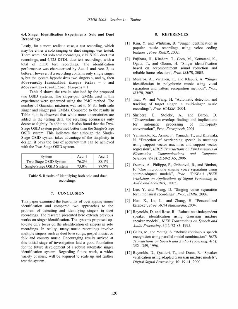
ISMIR 2008 – Session 1c – Timbre
6.4. Singer Identification Experiments: Solo and Duet Recordings
Lastly, for a more realistic case, a test recording, which may be either a solo singing or duet singing, was tested. There were 150 solo test recordings, 675 STSL duet test recordings, and 4,725 DTDL duet test recordings, with a total of 5,550 test recordings. The identification performance was characterized by Acc. 1 and Acc. 2, as before. However, if a recording contains only single singer s1 but the system hypothesizes two singers s1 and s4, then #Correctly-identified Singer Pairs = 0 and #Correctly-identified Singers = 1.
Table 5 shows the results obtained by the proposed two OSID systems. The singer-pair GMMs used in this experiment were generated using the PMC method. The number of Gaussian mixtures was set to 64 for both solo singer and singer pair GMMs. Compared to the results in Table 4, it is observed that while more uncertainties are added in the testing data, the resulting accuracies only decrease slightly. In addition, it is also found that the Two-Stage OSID system performed better than the Single-Stage OSID system. This indicates that although the Single-Stage OSID system takes advantage of the simplicity in design, it pays the loss of accuracy that can be achieved with the Two-Stage OSID system.
System Acc. 1 Acc. 2 Two-Stage OSID System 76.2% 88.1%
Single-Stage OSID System 73.0% 87.9%
Table 5. Results of identifying both solo and duet recordings.
7. CONCLUSION
This paper examined the feasibility of overlapping singer identification and compared two approaches to the problem of detecting and identifying singers in duet recordings. The research presented here extends previous works on singer identification. The systems proposed up-to-date only focus on the identification of singers in solo recordings. In reality, many music recordings involve multiple singers such as duet love songs, gospel music, or folk and country music. Encouraging results arrived at this initial stage of investigation laid a good foundation for the future development of a robust automatic singer identification system. Regarding future work, a wider variety of music will be acquired to scale up and further test the system.
8. REFERENCES
[1] Kim, Y. and Whitman, B. “Singer identification in popular music recordings using voice coding features”, Proc. ISMIR, 2002.
[2] Fujihara, H., Kitahara, T., Goto, M., Komatani, K., Ogata, T., and Okuno, H. “Singer identi-fication based on accompaniment sound reduction and reliable frame selection”, Proc. ISMIR, 2005.
[3] Mesaros, A., Virtanen, T., and Klapuri, A. “Singer identification in polyphonic music using vocal separation and pattern recognition methods”, Proc.
ISMIR, 2007.
[4] Tsai, W. and Wang, H. “Automatic detection and tracking of target singer in multi-singer music recordings”, Proc. ICASSP, 2004.
[5] Shriberg, E., Stolcke, A., and Baron, D. “Observations on overlap: findings and implications for automatic processing of multi-party conversation”, Proc. Eurospeech, 2001.
[6] Yamamoto, K., Asano, F., Yamada, T., and Kitawaki, N. “Detection of overlapping speech in meetings using support vector machines and support vector regression”, IEICE Transactions on Fundamentals of
Electronics, Communications and Computer
Sciences, 89(8): 2158-2165, 2006.
[7] Ozerov, A., Philippe, P., Gribonval, R., and Bimbot, F. “One microphone singing voice separating using source-adapted models”, Proc. WASPAA (IEEE
Workshop on Applications of Signal Processing to
Audio and Acoustics), 2005.
[8] Lee, Y. and Wang, D. “Singing voice separation form monaural recordings”, Proc. ISMIR, 2006.
[9] Hua, X., Lu, L., and Zhang, H. “Personalized karaoke”, Proc. ACM Multimedia, 2004.
[10] Reynolds, D. and Rose, R. “Robust text-independent speaker identification using Gaussian mixture speaker models”, IEEE Transactions on Speech and
Audio Processing, 3(1): 72-83, 1995.
[11] Gales, M. and Young, S. “Robust continuous speech recognition using parallel model combination”, IEEE
Transactions on Speech and Audio Processing, 4(5): 352 - 359, 1996.
[12] Reynolds, D., Quatieri, T., and Dunn, R. “Speaker verification using adapted Gaussian mixture models”, Digital Signal Processing, 10: 19-41, 2000.
120
ISMIR 2008 – Session 1c – Timbre
VOCAL SEGMENT CLASSIFICATION IN POPULAR MUSIC
Ling Feng, Andreas Brinch Nielsen, Lars Kai HansenTechnical University of Denmark
Department of Informatics and Mathematical Modelling{lf, abn, lkh}@imm.dtu.dk
ABSTRACT
This paper explores the vocal and non-vocal music classifi-
cation problem within popular songs. A newly built labeled
database covering 147 popular songs is announced. It is de-
signed for classifying signals from 1sec time windows. Fea-
tures are selected for this particular task, in order to capture
both the temporal correlations and the dependencies among
the feature dimensions. We systematically study the per-
formance of a set of classifiers, including linear regression,
generalized linear model, Gaussian mixture model, reduced
kernel orthonormalized partial least squares and K-means
on cross-validated training and test setup. The database is
divided in two different ways: with/without artist overlap
between training and test sets, so as to study the so called
‘artist effect’. The performance and results are analyzed in
depth: from error rates to sample-to-sample error correla-
tion. A voting scheme is proposed to enhance the perfor-
mance under certain conditions.
1 INTRODUCTION
The wide availability of digital music has increased the in-
terest in music information retrieval, and in particular in
features of music and of music meta-data, that could be
used for better indexing and search. High-level musical fea-
tures aimed at better indexing comprise, e.g., music instru-
ment detection and separation [13], automatic transcription
of music [8], melody detection [2], musical genre classifica-
tion [10], sound source separation [18], singer recognition
[16], and vocal detection [4]. While the latter obviously is
of interest for music indexing, it has shown to be a surpris-
ingly hard problem. In this paper we will pursue two ob-
jectives in relation to vocal/non-vocal music classification.
We will investigate a multi-classifier system, and we will
publish a new labeled database that can hopefully stimulate
further research in the area.
While almost all musical genres are represented in digital
forms, naturally popular music is most widely distributed,
and in this paper we focus solely on popular music. It is
not clear that the classification problem can be generalized
between genres, but this is a problem we will investigate in
later work.
Singing voice segmentation research started less than a
decade ago. Berenzweig and Ellis attempted to locate the
vocal line from music using a multi-layer perceptron speech
model, trained to discriminate 54 phone classes, as the first
step for lyric recognition [4]. However, even though singing
and speech share certain similarities, the singing process in-
volves the rapid acoustic variation, which makes it statisti-
cally different from normal speech. Such differences may
lie in the phonetic and timing modification to follow the
tune of the background music, and the usage of words or
phrases in lyrics and their sequences. Their work was in-
spired by [15] and [19], where the task was to distinguish
speech and music signals within the “music-speech” corpus:
240 15s extracts collected ‘at random’ from the radio. A set
of features have been designed specifically for speech/music
discrimination, and they are capable of measuring the con-
ceptually distinct properties of both classes.
Lyrics recognition can be one of a variety of uses for vo-
cal segmentation. By matching the word transcriptions, it
is applicable to search for different versions of the same
song. Moreover, accurate singing detection could be po-
tential for online lyrics display by automatically aligning
the singing pieces with the known lyrics available on the
Internet. Singer recognition of music recordings has later
received more attention, and has become one of the pop-
ular research topics within MIR. In early work of singer
recognition, techniques were borrowed from speaker recog-
nition. A Gaussian Mixture Model (GMM) was applied
based on Mel-frequency Cepstral Coefficients (MFCC) to
detect singer identity [20]. As briefly introduced, singing
voices are different from the conventional speech in terms
of time-frequency features; and vocal and non-vocal fea-
tures have differences w.r.t. spectral distribution. Hence
the performance of a singer recognition system has been
investigated using the unsegmented music piece, the vocal
segments, and the non-vocal ones in [5]. 15% improve-
ment has been achieved by only using the vocal segments,
compared to the baseline of the system trained on the un-
segmented music signals; and the performance became 23%worse when only non-vocal segments were used. It demon-
strated that the vocal segments are the primary source for
recognizing singers. Later, work on automatic singer recog-
nition took vocal segmentation as the first step to enhance
121
ISMIR 2008 – Session 1c – Timbre
the system performance, e.g. [16].
Loosely speaking, vocal segmentation has two forms. One
is to deal with a continuous music stream, and the locations
of the singing voice have to be detected as well as classi-
fied, one example is [4]. The second one is to pre-segment
the signals into windows, and the task is only to classify
these segments into two classes. Our work follows the sec-
ond line, in order to build models based on our in-house Pop
music database. A detailed description of the database will
be presented in section 4. The voice is only segmented in
the time domain, instead of the frequency domain, mean-
ing the resulting vocal segments will still be a mixture of
singing voices and instrumental background. Here we will
cast the vocal segments detection in its simplest form, i.e. as
a binary classification problem: one class represents signals
with singing voices (with or without background music); the
other purely instrumental segments, which we call accom-
paniment.
In this paper we study this problem from a different an-
gle. Several classifiers are invoked, and individual perfor-
mance (errors and error rates) is inspected. To enhance per-
formance, we study the possibility of sample-to-sample cross-
classifier voting, where the outputs of several classifiers are
merged to give a single prediction. The paper is organized as
follows. Section 2 explains the selection of features. Clas-
sification frameworks are covered by section 3. With the
purpose of announcing the Pop music database, we intro-
duce the database design in section 4. In section 5, the ex-
periments are described in depth, and the performance char-
acteristics are presented. At last, section 6 concludes the
current work.
2 ACOUSTIC FEATURES
2.1 Mel-Frequency Cepstral Coefficients
MFCCs are well-known in the speech and speaker recog-
nition society. They are designed as perceptually weighted
cepstral coefficients, since the mel-frequency warping em-
ulates human sound perception. MFCCs share two aspects
with the human auditory system: A logarithmic dependence
on signal power and a simple bandwidth-to-center frequency
scaling so that the frequency resolution is better at lower fre-
quencies. MFCCs have recently shown their applicability
in music signal processing realm, e.g. [1] for music genre
classification, [16] and [5] for singer recognition, and [14]
for vocal segmentation, and many more exist.
Features are extracted from short time scales, e.g. 20ms,
due to the stationarity of music signals. To process win-
dows at longer time scales, temporal feature integration is
needed. Features at different time scales may contain dif-
ferent information. A small frame size may result in a noisy
estimation; and a long frame size may cover multiple sounds
(phonemes) and fail to capture appropriate information.
2.2 Multivariate AR
During the course of searching for appropriate features, re-
searchers have realized that system performance can be im-
proved by combining short-time frame-level features into
clip-level features. Feature integration is one of the meth-
ods to form a long-time feature, in order to capture the dis-
criminative information and characterize how frame-level
features change over longer time periods for a certain task.
Often the mean and variance of several short-time features
are extracted as the clip-level features [17], using multi-
variate Gaussian model or a mixture of them. However,
both the mean-variance and mean-covariance model fail to
capture the temporal correlations. A frequency band ap-
proach has been proposed in [9], and the energy of the fea-
tures was summarized into 4 frequency bands. Even though
this method can represent temporal development, it does not
model the feature correlations.
The multivariate autoregressive model (MAR) was re-
cently introduced to music genre classification [11], and a
detailed comparison of different temporal feature integra-
tion methods was reported. MAR being able to capture both
the temporal correlations and the dependencies among the
feature dimensions, has shown its superiority for represent-
ing music. We adapt this model in the feature extraction
phase on top of short-time MFCCs. Here, a brief descrip-
tion of MAR will be given, for detail, see [11].
Assume the short-time MFCC at time t is denoted as xt,
which is extracted from a short period of stationary signals.
The MAR can be stated as,
xt =P∑
p=1
Apxt−p + ut, (1)
where ut is the Gaussian noise N (v,Σ), assumed i.i.d. Ap
is the coefficients matrix for order p; and if it is defined as
a diagonal matrix, dependencies among dimensions will not
be considered. P indicates the order of the multivariate auto
regressive model, meaning that xt is predicted from the pre-
vious P short-time features. It is worth to mention that the
mean of MFFCs m is related to the mean of the noise v in
the following way (note: I is an identity matrix),
m = (I−P∑
p=1
Ap)−1v. (2)
3 CLASSIFICATION FRAMEWORKS
We have examined a number of classifiers: linear regres-
sion model (LR), generalized linear model (GLM), Gaus-
sian mixture model (GMM), reduced kernel orthonormal-
ized partial least squares (rKOPLS) and K-means.
As the problem is a binary task, only a single dimension
is needed for linear regression, and the labels are coded as
122

ISMIR 2008 – Session 1c – Timbre
5 10 15 20 25 30 35 40 450
500
1000
1500
2000
2500
3000
3500
4000
ARTISTS
SE
CO
ND
S
Figure 1. Distribution of Pop music among artists
±1. The model is ln = wTy. A 1 is added to the fea-
ture vector to model offset. Least squares is used as the
cost function for training, and the minimum solution is the
pseudo inverse. The prediction is made based on the signof the output: we tag the sample as a vocal segment if the
output is greater than zero; and as a non-vocal segment oth-
erwise.
Generalized linear model relates a linear function of the
inputs, through a link function to the mean of an exponential
family function, μ = g(wT xn), where w is a weight vector
of the model and xn is the n’th feature vector. In our case
we use the softmax link function, μi = ewTi xn
i∑j e
wTj
xnj
. w is
found using iterative reweighted least squares [12].
GMM as one of the Bayesian classifiers, assumes a known
probabilistic density distribution for each class. Hence we
model data from each class as a group of Gaussian clus-
ters. The parameters are estimated from training sets via the
standard Expectation-Maximization (EM) algorithm. For
simplicity, we assume the covariance matrices to be diago-
nal. Note that although features are independent within each
mixture component due to the diagonal covariance matrix,
the mixture model does not factorize over features. The di-
agonal covariance constraint posits the axes of the resulting
Gaussian clusters parallel to the axes of the feature space.
Observations are assigned to the class having the maximum
posterior probability.
Any classification problem is solvable by a linear classi-
fier if the data is projected into a high enough dimensional
space (possibly infinite). To work in an infinite dimensional
space is impossible, and kernel methods solve the problem
by using inner products, which can be computed in the orig-
inal space. Relevant features are found using orthonormal-
ized partial least squares in kernel space. Then a linear clas-
sifier is trained and used for prediction. In the reduced form,
rKOPLS [3] is able to handle large data sets, by only using
a selection of the input samples to compute the relevant fea-
tures, however all dimensions are used for the linear classi-
fier, so this is not equal to a reduction of the training set.
K-means uses K clusters to model the distribution of each
class. The optimization is done by assigning data points
to the closest cluster centroid, and then updating the clus-
ter centroid as the mean of the assigned data points. This
is done iteratively, and minimizes the overall distances to
cluster centroids. Optimization is very dependent on the ini-
tial centroids, and training should be repeated a number of
times. Prediction is done by assigning a data point to the
class of the closest cluster centroid.
4 DATABASE
The database used in the experiments is our recently built
in-house database for vocal and non-vocal segments classi-
fication purpose. Due to the complexity of music signals and
the dramatic variations of music, in the preliminary stage of
the research, we focus only on one music genre: the pop-
ular music. Even within one music genre, Berenzweig et
al. have pointed out the ‘Album Effect’. That is songs from
one album tend to have similarities w.r.t. audio production
techniques, stylistic themes and instrumentation, etc. [5].
This database contains 147 Pop mp3s: with 141 singing
songs and 6 pure accompaniment songs. The 6 accompani-
ment songs are not the accompaniment of any of the other
singing songs. The music in total lasts 8h 40min 2sec. All
songs are sampled at 44.1 kHz. Two channels are averaged,
and segmentation is based on the mean. Songs are man-
ually segmented into 1sec segments without overlap, and
are annotated second-by-second. The labeling is based on
the following strategy: if the major part of this 1sec music
piece is singing voice, it is tagged as vocal segment; oth-
erwise non-vocal segment. We believe that the long-term
acoustic features are more capable of differentiating singing
voice, and 1sec seems to be a reasonable choice based on
[14]. Furthermore labeling signals at this time scale is not
only more accurate, but also less expensive.
Usually the average partition of vocal/non-vocal in Pop
music is about 70%/30%. Around 28% of the 141 singing
songs is non-vocal music in the collection of this database.
Forty-seven artists/groups are covered. By artists in Pop mu-
sic we mean the performers (singers) or bands instead of
composers. The distribution of songs among artists is not
even, and Figure 1 gives the total number of windows (sec-
onds) each artist contributes.
5 EXPERIMENTS AND RESULTS
We have used a set of features extracted from the music
database. First, we extracted the first 6 original MFCCs over
a 20ms frame hopped every 10ms. The 0th MFCC repre-
senting the log-energy was computed as well. The means
were calculated on signals covering 1sec in time. MAR
were afterwards computed on top of the first 6 MFCCs with
P = 3, and we ended up with a 6-by-18 Ap matrix, a 1-by-6
123

ISMIR 2008 – Session 1c – Timbre
0 10 20 30 40 50 60 70 80 90 100
0.15
0.2
0.25
0.3
0.35
SPLIT INDEX
ER
RO
R R
AT
ES
TEST CLASSIFICATION ERROR
lr
glm
gmm
rkopls
kmeans
Figure 2. Classification error rates as a function of splits of
five classifiers on test sets.
vector v and a 6-by-6 covariance matrix Σ. Since Σ is sym-
metric, repetitions were discarded. Ap, v and Σ all together
form a 135-dimensional feature set. The choice for 6 MFCC
is on one hand empirical, and on the other hand to reduce the
computational complexity. All in all, for 1sec music signal
we concatenated 135-d MAR, the means of both 0th and 6original MFCCs to form a 142-d feature vector.
5.1 Data Dependency and Song Variation
We used one type of cross-validation, namely holdout vali-
dation, to evaluate the performance of the classification frame-
works. To represent the breadth of available signals in the
database, we kept 117 songs with the 6 accompaniment songs
to train the models, and the remaining 30 to test. We ran-
domly split the database 100 times and evaluated each clas-
sifier based on the aggregate average. In this way we elimi-
nated the data set dependencies, due to the possible similar-
ities between certain songs. The random splitting regarded
a song as one unit, therefore there was no overlap song-wise
in the training and test set. On the other hand artist overlap
did exist. The models were trained and test set errors were
calculated for each split. The GLM model from the Netlab
toolbox was used with softmax activation function on out-
puts, and the model was trained using iterative reweighted
least squares. As to GMM, we used the generalizable gaus-
sian mixture model introduced in [7], where the mean and
variance of GMM are updated with separate subsets of data.
Music components have earlier been considered as ‘noise’
and modeled by a simpler model [16], thus we employed
a more flexible model for the vocal than non-vocal parts: 8
mixtures for the vocal model, and 4 for the non-vocal model.
For rKOPLS, we randomly chose 1000 windows from the
training set to calculate the feature projections. The average
error rates of the five classification algorithms are summa-
rized in the left column of Table 1.
A bit surprisingly the performance is significantly better
for the linear models. We show the performance of the cho-
Error Rates
Artists overlap no overlap
LR 19.03±2.25% 20.52±3.5%
GLM 18.46±2.02% 19.82±2.81%
GMM 23.27±2.54% 24.50±2.99%
rKOPLS 22.62±1.85% 24.60±3.14%
K-means 25.13±2.11% NA
Table 1. The average error rates (mean ± standard devia-
tion) of 5 classifiers on test sets.
20 40 60 80 100 120 1400
0.1
0.2
0.3
0.4
0.5
0.6
SONGSE
RR
OR
RA
TE
S
AVERAGE TEST ERROR OF 141 SONGS
Figure 3. Test classification error rates for individual songs
by GLM model. The dash line gives the average error rates
of the 100-split cross-validation.
sen classifiers as a function of splits in Figure 2. Each curve
represents one classifier, and the trial-by-trial difference is
quite striking. It proved our assumption that the classifica-
tion performance depends heavily on the data sets, and the
misclassification varies between 13.8% and 23.9% for the
best model (GLM). We envision that there is significant vari-
ation in the data set, and the characteristics of some songs
may be distinguishing to the others. To test the hypothesis,
we studied the performance on individual songs. Figure 3
presents the average classification errors of each song pre-
dicted by the best model: GLM, and the inter-song variation
is obviously revealed: for some songs it is easy to distin-
guish the voice and music segments; and some songs are
hard to classify.
5.2 Correlation Between Classifiers and Voting
While observing the classification variation among data splits
in Figure 2, we also noticed that even though classification
performance is different from classifier to classifier, the ten-
dency of these five curves does share some similarity. Here
we first carefully studied the pair-to-pair performance corre-
lation between the classification algorithms. In Table 2 the
degree of matching is reported: 1 refers to perfect match; 0
to no match. It seems that the two linear classifiers have a
very high degree of matching, which means that little will
be gained by combining these two.
The simplest way of combining classification results is
124

ISMIR 2008 – Session 1c – Timbre
LR GLM GMM rKOPLS K-means
LR 1.0000 0.9603 0.8203 0.8040 0.8110
GLM 0.9603 1.0000 0.8141 0.8266 0.8091
GMM 0.8203 0.8141 1.0000 0.7309 0.7745
rKOPLS 0.8040 0.8266 0.7309 1.0000 0.7568
K-means 0.8110 0.8091 0.7745 0.7568 1.0000
Table 2. A matrix of the degree of matching.
10 20 30 40 50 60 70 80 90 100
0.2
0.25
0.3
0.35
0.4
SPLIT INDEX
ER
RO
R R
AT
ES
TEST CLASSIFICATION ERROR
gmm
rkopls
kmeans
voting
baseline
Figure 4. Voting results. It gives the voting performance
among GMM, rKOPLS and K-means. The light dash line
shows the baseline of random guessing for each data split.
by majority voting, meaning that the class with the most
votes is chosen as the output. The voting has been done
crossing all five classifiers, unfortunately the average voting
results (error rates) on the test sets was 18.62%, which is
slightly worse than the best individual classifier. The reason
seems to be that even though the other classifiers are not so
correlated with the linear ones, the miss classification rate is
too high to improve performance.
However voting does help enhance the performance, if
it performs among not so correlated classification results.
Figure 4 demonstrates the sample-to-sample majority voting
among three classifiers: GMM, rKOPLS and K-means. The
similar tendency was preserved in the voting results, and
there were only 10 splits out of 100, where the voting results
were worse than the best ones among these three. The aver-
age performance of voting on test sets was 20.90± 2.02%.
Here we will elaborate on the performance on individual
songs, by looking at the predicted labels from each classifier
and voting predictions. Figure 5 demonstrates how voting
works, and how the prediction results correlate. Two songs:
‘Do You Know What You Want’ by M2M, and ‘A Thousand
Times’ by Sophie Zelmani, have been chosen to illustrate
the ‘good’ and ‘bad’ cases, i.e. when voting helps and fails.
Vocal segments are tagged with ‘1’, and ‘0’ for non-vocal
ones. The ground truth is given as a reference. The voting
was carried out among GMM, rKOPLS and K-means, and
their predictions are shown. If the classifiers make mistakes
in a similar pattern, the voting cannot recover the wrong pre-
dictions, e.g. area B. If the predictions are not correlated to
a high degree voting helps, e.g. area A.
50 100 150 200 250 300−1
0
1
2
TR
UE
Do You Know What You Want A Thousand Times
50 100 150 200 250 300−1
0
1
2
GM
M
50 100 150 200 250 300−1
0
1
2
RK
OP
LS
50 100 150 200 250 300−1
0
1
2
KM
EA
NS
50 100 150 200 250 300−1
0
1
2
VO
TE
24.85%15.52%
19.54%
17.24%
30.44%20.12%
31.06%
21.12%
B
A
Figure 5. Sample-to-sample errors and voting results. Two
songs represent the ‘good’ and ‘bad’ voting cases. Individ-
ual error rates for each classifier and voting results are given.
Two areas marked A & B indicate the scenarios when voting
helps and fails.
20 40 60 80 100 120 140 160 180−1
0
1
2
BIRD GUHL
SECONDS
20 40 60 80 100 120 140 160 180−1
0
1
2
SECONDS
NON−VOCAL
VOCAL
NON−VOCAL
VOCAL
Figure 6. Two manual label results of the same song: ‘Bird
Guhl’. It is obvious that the disagreement only appears in
the transition parts.
Moreover, we noticed that it is very likely for classifiers
to make wrong predictions in the transition sections, mean-
ing the changing from vocal to non-vocal parts, and vice
versa. We found this is reasonable comparing with man-
ual labels by different persons, shown in Figure 6. The song
was labeled carefully by both people, the absence of mind or
guessing should not be a concern. The mismatch indicates
the perception or judging difference, and it only happens in
the transition parts. The total mismatch is about 3% for this
particular song: ‘Bird Guhl’ by Antony and the Johnsons.
5.3 ‘Artist Effect’
In previous experiments, we randomly selected songs to form
training and test sets, hence the same artist may appear in
both sets. Taking the previous results as a baseline, we stud-
ied the ‘artist effect’ in this classification problem. We tried
to keep the size of test sets the same as before, and care-
fully selected around 30 songs in order to avoid artist over-
lap for each split, and formed 100 splits. The second column
of Table 1 summarizes the average error rates for 4 classi-
125

ISMIR 2008 – Session 1c – Timbre
fiers. The average results are a little worse than the previous
ones, and they also have bigger variance along the splits.
Therefore we speculate that artists do have some influence in
vocal/non-vocal music classification, and the influence may
be caused by different styles, and models trained on partic-
ular styles are hard to be generalized to other styles.
6 CONCLUSION AND DISCUSSION
We have investigated the vocal/non-vocal popular music clas-
sification. Experiments were carried out on our database,
containing 147 popular songs. To be in line with the label
set, the classifiers were trained based on features at 1sectime scale. We have employed 142-d acoustic features, con-
sisting MFCCs and MAR, to measure the distinct properties
of vocal and non-vocal music. Five classifiers have been
invoked: LR, GLM, GMM, rKOPLS and K-means.
We cross-validated the entire database, and measured the
aggregate average to eliminate the data set dependency. GLM
outperformed all the others, and provided us with 18.46%error rate on the baseline of 28%. The performance has great
variation among data splits and songs, indicating the vari-
ability of popular songs. The correlations among classifiers
have been investigated, and the proposed voting scheme did
help among less correlated classifiers. Finally we looked
into the ‘artist effect’, and it did degrade the classification
accuracy a bit by separating artists in training and test sets.
All in all vocal/non-vocal music classification was found to
be a difficult problem, and it depends heavily on the music
itself. Maybe classification within similar song styles can
improve the performance.
7 REFERENCES
[1] Ahrendt, P., Meng, A. and Larsen, J. “Decision time horizon
for music genre classification using short time features”, Pro-ceedings of EUSIPCO, pp. 1293-1296, 2004.
[2] Akeroyd, M. A., Moore, B. C. J. and Moore, G. A. “Melody
recognition using three types of dichotic-pitch stimulus”, TheJournal of the Acoustical Society of America, vol. 110, Issue
3, pp. 1498-1504, 2001.
[3] Arenas-Garcı́a, J., Petersen, K.B., Hansen, L.K. “Sparse Ker-
nel Orthonormalized PLS for feature extraction in large data
sets”, Proceedings of NIPS, pp. 33-40, MIT Press, Cambridge,
MA, 2007.
[4] Berenzweig, A. L., Ellis, D. P. W., and Lawrence, S. “Locating
Singing Voice Segments Within Music Signals”, Proceedingsof IEEE Workshop on Applications of Signal Processing to Au-dio and Aoustics, New Paltz, NY, 2001.
[5] Berenzweig, A. L., Ellis, D. P. W., and Lawrence, S. “Using
Voice Segments to Improve Artist Classification of Music”,
Proceedings of the International Conference on Virtual, Syn-thetic and Entertainment Audio, Espoo, Finland, 2002.
[6] Eronen, A. “Automatic musical instrument recognition”. Mas-
ter Thesis, Tampere University of Technology, 2001.
[7] Hansen, L. K., Sigurdsson, S., Kolenda, T., Nielsen, F. .,
Kjems, U., Larsen, J. “Modeling text with generalizable gaus-
sian mixtures”, Proceedings of ICASSP, vol. 4, pp. 3494-3497,
2000
[8] Heln, M. and Virtanen, T. “Separation of Drums From Poly-
phonic Music Using Non-Negative Matrix Factorization and
Support Vector Machine”, Proceedings of EUSIPCO, Antalya,
Turkey, 2005.
[9] McKinney, M. F. and Breebart, J. “Features for audio and mu-
sic classification”, Proceedings of ISMIR, Baltimore, Mary-
land (USA), pp.151-158, 2003.
[10] Meng, A., Shawe-Taylor J., “An Investigation of Feature Mod-
els for Music Genre Classification using the Support Vector
Classifier”, Proceedings of ISMIR, London, UK, pp. 604-609,
2005.
[11] Meng, A., Ahrendt, P., Larsen, J. and Hansen, L. K. “Tempo-
ral Feature Integration for Music Genre Classification”, IEEETransactions on Audio, Speech, and Language Processing,
vol. 15(5), pp. 1654-1664, 2007.
[12] Nabney, I., Bishop, C. “Netlab neural network software”, ver.
3.2, 2001
[13] Nielsen, A. B., Sigurdsson, S., Hansen, L. K., and Arenas-
Garca, J. “On the relevance of spectral features for instrument
classification”, Proceedings of ICASSP, Honolulu, Hawaii,
vol. 5, pp. 485-488, 2007.
[14] Nwe, T. L. and Wang, Y. “Automatic Detection of Vocal Seg-
ments in Popular Songs” Proceedings of the ISMIR, Barcelona,
Spain, 2004.
[15] Scheirer, E. and Slaney, M. “Construction and Evaluation fo A
Robust Multifeature Speech/Music Discriminator”, Proceed-ings of ICASSP, Munich, 1997.
[16] Tsai W.-H. and Wang, H.-M. “Automatic singer recognition of
popular music recordings via estimation and modeling of solo
vocal signals”, IEEE Trans. on Audio, Speech, and LanguageProcessing, vol. 14, no. 1, pp. 330–341, 2006.
[17] Tzanetakis, G. “Manipulation, analysis and retrieval systems
for audio signal”, Ph.D. dissertation , Faculty of Princeton
University, Department of Computer Science, 2002
[18] Virtanen, T. “Separation of Sound Sources by Convolutive
Sparse Coding”, Proceedings of ISCA Tutorial and ResearchWorkshop on Statistical and Perceptual Audio Processing,SAPA, 2004.
[19] Williams, G. and Ellis, D. P. W. “Speech/Music Discrimina-
tion Based on Posterior Probability Features”, Proceedings ofEurospeech, Budapest, 1999.
[20] Zhang, T. “Automatic singer identification”, Proceedings ofICME, Baltimore, 2003.
126

ISMIR 2008 – Session 1c – Timbre
LEARNING MUSICAL INSTRUMENTS FROM MIXTURES OF AUDIO WITHWEAK LABELS
David Little and Bryan PardoEECS Department
Northwestern UniversityEvanston, IL 60208
d-little,[email protected]
ABSTRACT
We are interested in developing a system that learns to rec-
ognize individual sound sources in an auditory scene where
multiple sources may be occurring simultaneously. We fo-
cus here on sound source recognition in music audio mix-
tures. Many researchers have made progress by using iso-
lated training examples or very strongly labeled training data.
We consider an alternative approach: the learner is presented
with a variety of weaky-labeled mixtures. Positive exam-
ples include the target instrument at some point in a mix-
ture of sounds, and negative examples are mixtures that do
not contain the target. We show that it not only possible to
learn from weakly-labeled mixtures of instruments, but that
it works significantly better (78% correct labeling compared
to 55%) than learning from isolated examples when the task
is identification of an instrument in novel mixtures.
1 INTRODUCTION
We are interested in developing a system that can learn to
recognize individual sound objects in an auditory scene where
multiple sound sources may be occurring simultaneously. A
system able to identify what particular sound sources are
present in a mixture would enable automatic tagging of au-
dio recordings with meta-data. A system capable of model-
ing sources in audio mixtures, without having to first learn
the sounds in isolation, would be useful to researchers work-
ing on separating audio mixtures into their component sources.
In a typical supervised learning paradigm, isolated in-
stances of a particular class of data are presented to a learner.
Learning in this case is mostly limited to a stage of the de-
sign process. With a more ecologically realistic set of re-
quirements, where learning can occur in an environemnt af-
ter deployment, this isolation of training instances can not be
guaranteed. While similar problems have already been stud-
ied in the field of computer vision [1], auditory data presents
its own unique problems because mixtures of sound can re-
sult in a composite of multiple sources at a given time.
In this paper, we focus on identification of musical instru-
ments in a musical mixture. Almost all systems that learn
to identify musical instruments require isolated examples of
the target instrument at some stage in the training process
(see [9] for a review). This could mean, isolated notes [12],
or more recently, solo phrases from an instrument [11]. A
number of these systems have been evaluated using poly-
phonic audio [5, 11, 15], i.e. audio with multiple simulta-
neous notes, but this work is still limited by the requirement
that instruments be learned in isolation.
We are aware of two systems that learn solely from poly-
phonic audio. However, they differ significantly from the
task we consider here. In [6] the system is trained on poly-
phonic audio, but each unique combination of instruments
must be learned individually. The authors admit this ap-
proach is only realistic when learning is done before deploy-
ment. Given n instruments, this results in 2n possible com-
binations that must be individually learned, significantly in-
creasing the number of required training examples. This ap-
proach also leaves open the question of how to recognize
individual instruments when presented in novel audio con-
texts. In addition, the training data requires labels indicating
all instruments currently playing for every two second seg-
ment of audio, a fairly intensive labeling task. This is true
even if a score is available (since it must be correctly aligned
with a particular audio recording).
Kitahara et al [10] learn from polyphonic data, avoiding
the combinatorial problems of [6]. However, they require
the user to input a musical score for the recording that ex-
actly labels every note with pitch, onset time and offset time,
i.e. perfect segmentation of each instrument into individual
notes is assumed.
What we would really like is a system that can learn from
weakly labeled mixtures. We call a label weak if only the
presence or absence of the target sound object is indicated
for some N second length of audio. A weakly labeled pos-
itive example will contain the target object at some point
in the example, but a significant portion of the time may
not contain audio from the target. A weakly labeled neg-
ative example does not contain the target sound object at
any point in the example. In this scenario a useful posi-
tive training example for the “saxophone” class would be
127

ISMIR 2008 – Session 1c – Timbre
an acoustic recording of a saxophone and bass duo playing
at a gallery opening. A negative example would be some
other audio clip that contains no saxophone in the record-
ing. Training could be accomplished on-line by recording
a few audio clips that contain the desired sound. Our pro-
posed input and output have important differences from that
of previous systems that learn from polyphonic audio [6, 10]
(weakly vs. strongly labeled input and multi-class vs. a
presence/absence label as output).
As a first step towards our objective, in this paper we
evaluate a system that provides presence/absence labels for
a single instrument over short time intervals (~2 seconds).
We do not require labeling all instruments in the mixtures at
short intervals, nor do we require detailed scores. Instead,
the system learns from weakly labeled examples that include
distractor sounds.
Our instrument classes are learned independently of the
background sounds: the classifier can be trained in one back-
ground environment and used in another. Although all the
tools we use to accomplish this task already exist (as de-
scibed in Section 2), we are not aware of anyone who has
yet put these pieces together the way we do. In our exper-
iments (in Section 4), we show that it is not only possibleto learn from a mixture of instruments (constructed as in
Section 3), but that it works significantly better than learn-
ing from isolated examples when identifying instruments in
novel mixtures.
2 CLASSIFICATION METHOD
We use the segment-and-combine [7] framework for our clas-
sification system, defined below.
1. Segment each example Xi by selecting n potentially
overlapping segments {xi1,xi2, . . . ,xin} ∈ Xi at
random (as per [7]), using the piece extraction opera-
tor described below.
2. Learn a classifier function f(x) ∈ [0, 1] which re-
turns higher values for segments more likely to be part
of the target object.
3. Classify segments with the learned function f(x).
4. Combine each of the classifications of f(x), F (Xi) =C[f(xi1), f(xi2), · · · , f(xin)] ∈ {0, 1}. The combi-
nator C[·] returns a positive result if the average of
f(x) for all segments is greater than 0.5 (as per [7]).
We chose this approach because it has shown promise, even
compared to more sophisticated approaches, in similar prob-
lems, such as learning to recognize visual objects from clut-
tered data [7]. We describe the extraction operator in Sec-
tion 2.1 and the segment classifiers f(x) in Section 2.2.
Feature Description/Details
MFCCs Mel frequency cepatral coefficients
Brightnes Ratio of energy above 1500Hz to energy
below.
Spectral Stats First four statistical moments of
spectrum
Flatness Ratio of geometric to arithmetic mean of
spectrum
Pitch Calculated using first peak of
autocorrelation function.
Amplitude Root mean squared average.
Flux Difference of spectrum between
subsequent frames.
Inharmoncity The strength of the pitch: amount of
energy far from f0 · n
Table 1. The features used to represent each audio segment.
2.1 Extraction Operator
Our extraction operator to select possibly overlapping audio
segments in Step 1 selects a sub-portion of the audio, based
on two parameters: time(t) and length(l). The range of pos-
sible values for our start time (t) is from 0 to the length of
the file in frames. The length of the extracted segment (l)ranges from 0.1 seconds to 0.5 seconds. Given an audio ex-
ample Xi, we select 5 segments per second of audio in the
example. Thus, for a 10 second example there would be 50
segments. We randomly select these segments, picking val-
ues for t and l using a uniform probability distribution over
time.
The jth segment drawn from example i is represented as a
vector of features xij ∈ Rd.In this case d = 22 (13 MFCCs,
4 spectral statistics, plus the other 6 features). We choose
to use a set of features found to be commonly useful in past
work on musical instrument identification. All features used
are listed in Table 1.
2.2 Segment Classifiers
We compare three classifiers: Extra Trees [8], which, as we
will explain, should be fairly appropriate for this task, to
a very simple classifier, the K-nearest neighbors algorithm
[4], and a fairly sophisticated classifier, the Support Vector
Machine [2] with a radial basis kernel. This comparison is
detailed in Section 4.
It is important to recognize the noisy nature of the label-
ing data: it is possible that a segment from a positive exam-
ple, which would be labeled positively, contains no energey
from the target instrument. Since labels are weak, a positive
example for “saxophone” could be a jazz recording contain-
ing many portions where the saxophone is silent.
The results in [3] suggest that methods such as bagging
or randomization work well under such noisy labeling con-
128
ISMIR 2008 – Session 1c – Timbre
ditions. The Extra Tree algorithm [8] is an ensemble method
that uses randomized decision trees. It differes from other
randomized decision trees, in that, with the lowest parameter
setting, the algorithm would completely randomize both the
split and the attribute selected at each decision node, yield-
ing a tree completely independent of training data (Extra
Tree is short for extremley randomized tree). The construc-
tion of a single Extra Tree is summarized below.
1. Let the subset of training examples be S, the feature-
split pool size be K and the minimum subset be nm.
2. If |S| < nm or if all features values are constant, or
all examples in S share the same label.
(a) Define this tree’s output f(x) as the value of the
most frequent label in S.
3. Otherwise:
(a) Select K randomly uniform split si and feature
fi pairs.
(b) Select the best split-feature pair smax, fmax by
entropy measures.
(c) Let the output f(x) be the output of the right
tree if fmax < smax for x and the output of the
left tree if fmax ≥ smax.
(d) Create the right tree, with S equal to the subset
of examples with fmax < smax.
(e) Create the left tree, with S equal to the subset of
examples with fmax ≥ smax.
Results in [8] suggest that with appropriate parameter set-
tings, as detailed in Section 4.1.1, the Extra Tree ensemble
outperforms other random tree ensemble methods.
3 DATA
For our initial tests we wanted to tightly control the diffi-
culty of our examples, allowing us to observe how each of
our classifiers degrades as the data becomes more challeng-
ing. So, rather than use commercial recordings, we trained
and tested on synthesized mixtures of randomly selected
notes from four instruments. Each positive example con-
tains a mixture of instruments, one of which corresponds
to the label the system should learn. Thus, a positive ex-
ample for “Cello” might contain a Cello, Violin and Oboe.
The four instrument classes used for our source sounds were
Cello, Violin, Oboe, and Bb Clarinet. Instrument recordings
were taken from a set of instrument samples made available
by the University of Iowa 1 . The ranges of pitches used in
our experiments for the instruments were as follows: for
1 http://theremin.music.uiowa.edu/index.html
Cello we used notes from C2 to C7, for Violin from G3 to
Db7, for Clarinet from D3 to B6, and for Oboe from Bb3
to C6. These were played at three different dynamic lev-
els, pp, mf and ff. All samples were encoded as linear PCM
16bit wav files at a sampling rate of 44100Hz. The Iowa
recordings were segmented into individual notes. Training
and testing examples were constructed as follows.
1. Select a set of instruments
2. For each instrument, create a melody by randomly
picking a series of note recordings from the database
3. For each instrument melody, intersperse the notes with
silences of random length from 0 to some maximum
value.
4. Adjust instrument volumes to obfuscate the target in-
strument to the desired level.
5. Sum the melodies to create a mixture.
Examples were a minimum of 10 seconds long. The aver-
age length of an example was 11.5 seconds and the longest
example was 17.3 seconds. To vary the a level of target ob-
fuscation we varied the maximum spacing between notes in
the target instrument melody (st) and notes in the distrac-
tor instrument melodies(sd), as well as the relative ampli-
tude of the distractors notes (ad) across three target obfus-
cation conditions. These values were selected so that we
would obtain a range of target to mixture ratios, as defined
in Section 4.2. For easy obfuscation, st = 0.5, sd = 1and ad = 1; for medium obfuscation, st = 1.5, sd = 1and ad = 1; and for hard obfuscation st = 1.5, sd = 0.5,
and ad = 1.5. Thus, for easy obfuscation, target instrument
notes were more frequent than distractors and of equal am-
plitude. For hard obfuscation, distractors were significantly
more frequent and louder than targets.
Conditions varied along three dimensions: target instru-
ment (one of the four instruments), ensemble of distractor
instruments (one to two of the other instruments in all pos-
sible combinations), and target obfuscation (from easy to
hard): this resulted in a total of 4 × 6 × 3 = 72 data con-
ditions. We created 10 positive examples and 10 negative
examples for each of the conditions, yielding a total of 1440
example audio files.
Some examples of typical correctly and incorrectly clas-
sified examples for the mixed condition (from Section 4.1)
can be found at the following URL:http://www.cs.northwestern.edu/~dfl909/ismir2008sounds
4 EVALUATION
In our evaluation we sought to answer to the following ques-
tions.
129

ISMIR 2008 – Session 1c – Timbre
1. What effect does training on mixtures, rather than iso-
lated notes have on accuracy when identifying instru-
ments in novel mixtures of sound?
2. How does accuracy degrade across our three segment
classifiers as the target class is increasingly obfus-
cated by the distractors in the mixture?
3. How does performance using weak labels compare to
performance using stronger labels?
We begin our evaluation by addressing questions 1 and 2 in
Section 4.1. Questions 3 is addressed in Section 4.2.
4.1 Experiment 1
In this experiment, we wanted to compare performance across
isolated and mixture training conditions, across our three
different segment classifiers (ExtraTrees, K-nearest neigh-
bor and SVM).
We constructed the various ensembles of instruments as
described in Section 3. We then ran an experiment under
two conditions, mixed and isolated training , using the segment-
and-combine algorithm descibed in Section 2 with f(x) learned
using one of the three segment classifiers (Section 2.2).
4.1.1 Parameter Settings
To select parameters for our K-nearest-neighbor (KNN) and
the radial basis kernel SVM classifiers we evaluated a range
of parameters using the data for our most challenging tar-
get obfuscation condition (the hard obfuscation condition
as described in Section 3). We evaluated the KNN classi-
fier with K = 1, 2, 5, 10, 20, or 50, of which 5 was the
best K we found. For the parameters of the SVM, γ (vari-
ance of the Gaussian in the radial basis kernel) and C (the
error penality), we considered γ= 0.001, 0.01, 0.1, 1, 10,
100, or 1000, and C=0.001,0.01,1,10,100, or 1000 (yield-
ing 6 × 6 = 36 possible parameters settings for the SVM),
we found γ = 0.1 and C = 100 was the best setting.
For our ensemble of ExtraTree’s we used the recomended
parameters, as described in [8]: thus K =√
N where Nis the number of features (22), and nmin = 5. Generally
the more trees in the ensemble the better this algorithm, so
we chose a large number that did not unduely compromise
speed (100).
We extracted segments from the audio files at a rate of
5 segments per second. This value was chosen based on a
run of the Extra Tree algorithm using the hard obfuscation
condition.
4.1.2 Procedure
In the first (mixed) training condition, we used the following
procedure for each target instrument class T and each target
obfuscation condition.
1. Train the learner on the example from 5 of the 6 pos-
sible ensembles of distractors using target T , totaling
50 positive and 50 negative examples.
2. Test on the remaining 20 examples from the final en-
semble condition.
3. Repeat steps 1-2, excluding a different condition each
time.
In the second (isolated) training condition, we used this pro-
cedure for each target instrument class T and each target
obfuscation condition:
1. Train the learner on all isolated notes of an instru-
ment. For negative examples, we use an equal number
of randomly selected notes from the remaining instru-
ments.
2. Test on the 10 negative and 10 positive mixture exam-
ples with target T , for each of the 6 ensemble condi-
tions, for a total of 120 examples tested.
This condition included from 138-170 unique isolated notes
(depending on the instrument) during training: this is as
many or more notes than used in the polyphonic training
condition.
Thus for each classifier we had a total of 24 × 3 = 72trials of our system (24 mixture conditions× 3 target obfus-
cation conditions).
4.1.3 Results
We calculated system accuracy in each trial based on how
well the system could identify approximately every two sec-
onds of audio: each example being tested was divided into
sixths: for every sixth (or about two seconds) of an example
given a correct label we noted that as a success. Successes
were then tallied across all examples in a trial. Note that
for all obfuscation conditions there was no more than 1.5
second silence between target notes.
Since this is a balanced binary labeling task, random chance
performance for a given condition is 50%. Overall perfor-
mance for the systems across the various target obfuscation
conditions is shown in Figure 1.
We performed a 2 × 3 × 3 repeated measures ANOVA
within the 24 mixture conditions, across the training condi-
tion, segment classification method, and target obfuscation
condition. This analysis showed main effects for training
condition (F = 124.90, p < 0.001), classification method
(F = 48.51, p < 0.001), and target obfuscation condition
(F = 57.48, p < 0.001), as well as interactions between
training condition with classification method (F = 12.27,
p < 0.001) and training condition with target obfuscation
(F = 7.72, p = 0.006). Since results were poor for the
130

ISMIR 2008 – Session 1c – Timbre
●
●●●
●
●●
●●
●
●●
●
●●
svm
extr
a.tr
ee knn
svm
extr
a.tr
ee knn
svm
extr
a.tr
ee knn
easy obf. med. obf. hard obf.
0.3
0.5
0.7
0.9
Mixed training condition
prop
ortio
n co
rrec
t
svm
extr
a.tr
ee knn
svm
extr
a.tr
ee knn
svm
extr
a.tr
ee knn
easy obf. med. obf. hard obf.
0.3
0.5
0.7
0.9
Isolated training condition
prop
ortio
n co
rrec
t
Figure 1. Performance across the three segment classifica-
tion methods for both the isolated and mixed training con-
ditions. Chance performance is indicated by the dotted line.
Here, “obf.” stansds for “obfuscation.”
isolated conditions, it is not surprising that the other main
effects should interact with the training condition.
Post-hoc permutation tests [13] showed that there was no
statistically significant difference in performance between
the ExtraTree and SVM segment classifiers (p = 0.845) on
the mixture case, but performance with the KNN classifier
was worse from both SVMs and Extra Trees (p < 0.001).
The the KNN method is known to be sensitive to irrelevant
features, since we have yet to consider feature selection, this
is one possible reason the KNN method failed to work. All
three obfuscation conditions differed from each other (p <0.02). We also confirmed the that the isolated condition was
worse than the mixed training condition (p < 0.001). We
also examined the pattern of performance across different
sorts of mixtures: not surprisingly the more similar a target
is to its distractors the worse performance is: due to space
considerations we have left the breakdown of performance
by instrument out.
Only in the mixed training condition was performance
better than chance (0.5), and then only for the SVM and
Extra Tree classifier (p < 0.001). Taken togethor, these re-
sults suggest that the SVM and the Extra Tree algorithm can
be used to classify instruments in novel mixtures using the
segment-and-combine algorithm when the training data are
mixtures of sound rather than isolated notes. As obfusca-
tion of the target became greater, accuracy dropped similarly
across the three segment classifiers.
4.2 Experiment 2
We performed a second experiment to determine how a more
exact labeling of segments would affect our results. To do
this we determined the ratio of the target instrument to the
total mixture (R) in each segment selected for classification.
This was found using the following equation:
R =‖projtm‖2‖m‖2 (1)
The linear projection of the target onto the mixture, projtm,
is used as an estimate of the target that remains in the mix-
ture as per [14]. An R of 0.5 means half the energy in a
segment is from the target. Given an R for each segment
our system is provided a positive label only if it is above
some threshold t. This new labeling will be more accurate
because segments from positive examples that contain no
energy from the target instrument will not be included as a
labeled segment. Using this procedure, we trained the Extra-
Tree classifier as per the mixture condition in Experiment 1
with the data from the hardest target obfuscation condition.
Thus each test at a given threshold consists of 24 trials: 4
instruments with 6 possible arrangements of distractors. Re-
sults across various values for the threshold t can be seen in
Figure 2.
0.0005 0.005 0.05 0.5
0.5
0.7
0.9
threshold
prop
ortio
n co
rrec
t
Figure 2. Classification accuracy as a function of the thresh-
old R used to label segments. Dotted lines indicate the max-
imum and minimum; the solid line indicates the mean.
We can conclude from this that although performance
can be improved if we select a fairly inclusive t (i.e. one that
includes any segment that has even a small fraction of the
target), this will will not yield performance gains of much
more than about 4-6%. We would note that the poor perfor-
mance for high values of t may be attributable to the small
sample of segments that actually have a high enough R. For
example with t = 0.5 only about 19% of the segments from
positive examples were included.
5 CONCLUSIONS AND FUTURE WORK
Many researchers have tried to address the problem of iden-
tifying instruments in mixtures of sound by trying to miti-
gate the effect the other instruments have on the target in-
131

ISMIR 2008 – Session 1c – Timbre
strument to be identified, through, for instance, source sepa-
ration methods [15], missing feature approaches [5] or weight-
ing of features [10]. Here we presented an alternative ap-
proach: rather than being smart about how we use isolated
training data, we have simply used a variety of mixtures as
our training data.
This simple method makes classificiation possible in mix-
tures of random notes using only weakly labeled data, when
it is not possible to do so when trained with isolated training
data, without one of the above mentioned methods. We be-
lieve this is because the training data, in the mixed case, is
more representative of the testing data, even when the train-
ing mixtures do not use the same set of instruments as the
testing mixtures. It’s possible that the use of mixtures during
training could be used in conjuction with these other meth-
ods to further improve performance.
We found that when using more strongly labeled data,
our results did not improve much (Section 4.2). We believe
the most likely explanation of this result is that we have hit
a performance ceiling for the chosen features set. This may
also explain the similar performance of Extra Trees and the
SVM. In future work, now that we have identified a poten-
tially useful training method and learning algorithm for this
task, we will begin to explore a more effective set of fea-
tures.
We will also need to confirm these results on more mu-
sical arrangements, and more challenging recordings (e.g.
varied articualation, echoes and non-instrumental background,
etc...). Since our algorithm does not a priori depend on these
simplifications, we suspect the conclusions drawn here will
be meaningful in more challenging environments.
6 ACKNOWLEDGEMENTS
We’d like to thank Josh Moshier for his time preparing in-
strument data. This work was funded by National Science
Foundation Grant number IIS-0643752.
7 REFERENCES
[1] P. Carbonetto, G. Dorko, C. Schmid, H. Kück, N. de Fre-
itas, and M. Vision. Learning to recognize objects with
little supervision. International Journal of Computer Vi-sion, 2007.
[2] Corinna Cortes and Vladimir Vapnik. Support-vector
networks. Machine Learning, 20(3):273–297, 1995.
[3] Thomas G. Dietterich. An experimental comparison of
three methods for constructing ensembles of decision
trees: Bagging, boosting, and randomization. MachineLearning, 40(2):139–157, 2000.
[4] R.O. Duda, P.E. Hart, and D.G. Stork. Pattern Classifi-cation, chapter 4.4. Wiley-Interscience, 2000.
[5] J. Eggink and G. J. Brown. A missing feature approach
to instrument identification in polyphonic music. In
IEEE International Conference on Acoustics, Speech,and Signal Processing (ICASSP ’03), volume 5, pages
553–556, 2003.
[6] S. Essid, G. Richard, and B. David. Instrument recog-
nition in polyphonic music based on automatic tax-
onomies. IEEE Transactions on Audio, Speech and Lan-guage Processing, 14(1):68–80, 2006.
[7] P. Geurts, R. Maree, and L. Wehenkel. Segment and
combine: a generic approach for supervised learn-
ing of invariant classifiers from topologically structured
data. Machine Learning Conference of Belgium and TheNetherlands (Benelearn), 2006.
[8] Pierre Geurts, Damien Ernst, and Louis Wehenkel. Ex-
tremely randomized trees. Machine Learning, 63(1):3–
42, 2006.
[9] Perfecto Herrera-Boyer, Anssi Klapuri, and Manuel
Davy. Automatic classification of pitched musical in-
strument sounds. In Anssi Klapuri and Manuel Davy,
editors, Signal Processing Methods for Music Transcrip-tion, pages 163–200. Springer Sciences+Business Me-
dia LLC, New York, NY, 2006.
[10] T. Kitahara, M. Goto, K. Komatani, T. Ogata, and H. G.
Okuno. Instrument identification in polyphonic music:
Feature weighting to minimize influence of sound over-
laps. EURASIP Journal on Advances in Signal Process-ing, 2007.
[11] A. Livshin and X. Rodet. Musical instrument identifica-
tion in continuous recordings. In 7th International Con-ference on Digital Audio Effects, 2004.
[12] Keith D. Martin and Youngmoo E. Kim. 2pmu9. musi-
cal instrument identification: A pattern-recognition ap-
proach. In 136th meeting of the Acoustical Society ofAmerica, 1998.
[13] J. Menke and TR Martinez. Using permutations in-
stead of student’s t distribution for p-values in paired-
difference algorithm comparisons. IEEE InternationalJoint Conference on Neural Networks, 2, 2004.
[14] E. Vincent, R. Gribonval, and C. Fevotte. Performance
measurement in blind audio source separation. Audio,Speech and Language Processing, IEEE Transactionson [see also Speech and Audio Processing, IEEE Trans-actions on], 14(4):1462–1469, 2006.
[15] Emmanuel Vincent and Xavier Rodet. Instrument iden-
tification in solo and ensemble music using independent
subspace analysis. In International Conference on Mu-sic Information Retrieval, 2004.
132

ISMIR 2008 – Session 1c – Timbre
INSTRUMENT EQUALIZER FOR QUERY-BY-EXAMPLE RETRIEVAL:IMPROVING SOUND SOURCE SEPARATION BASED ONINTEGRATED HARMONIC AND INHARMONIC MODELS
Katsutoshi Itoyama†* Masataka Goto‡ Kazunori Komatani†
Tetsuya Ogata† Hiroshi G. Okuno†
† Graduate School of Infomatics, Kyoto University * JSPS Research Fellow (DC1)
‡ National Institute of Advanced Industrial Science and Technology (AIST)
{itoyama,komatani,ogata,okuno}@kuis.kyoto-u.ac.jp [email protected]
ABSTRACT
This paper describes a music remixing interface, called In-strument Equalizer, that allows users to control the volumeof each instrument part within existing audio recordingsin real time. Although query-by-example retrieval systemsneed a user to prepare favorite examples (songs) in general,our interface gives a user to generate examples from exist-ing ones by cutting or boosting some instrument/vocal parts,resulting in a variety of retrieved results. To change the vol-ume, all instrument parts are separated from the input soundmixture using the corresponding standard MIDI file. Forthe separation, we used an integrated tone (timbre) modelconsisting of harmonic and inharmonic models that are ini-tialized with template sounds recorded from a MIDI soundgenerator. The remaining but critical problem here is to dealwith various performance styles and instrument bodies thatare not given in the template sounds. To solve this problem,we train probabilistic distributions of timbre features by us-ing various sounds. By adding a new constraint of maxi-mizing the likelihood of timbre features extracted from eachtone model, we succeeded in estimating model parametersthat better express actual timbre.
1 INTRODUCTION
One of promising approaches of music information retrievalis the query-by-example (QBE) retrieval [1, 2, 3, 4, 5, 6, 7]where a user can receive the list of musical pieces rankedby their similarity to a musical piece (example) that the usergives as a query. Although this approach is powerful anduseful, a user has to prepare or find favorite examples andsometimes feels difficulty to control/change the retrievedpieces after seeing them because the user has to find anotherappropriate example to get better results. For example, if auser feels that vocal or drum sounds are too strong in theretrieved pieces, the user has to find another piece that hasweaker vocal or drum sounds while keeping the basic moodand timbre of the piece. It is sometimes very difficult to findsuch a piece within a music collection.
We therefore propose yet another way of preparing an ex-ample for the QBE retrieval by using a music remixing inter-
face. The interface enables a user to boost or cut the volumeof each instrument part of an existing musical piece. Withthis interface, a user can easily give an alternative query witha different mixing balance to obtain refined results of theQBE retrieval. The issue in the above example of findinganother piece with weaker vocal or drum sounds can thusbe resolved. Note that existing graphic equalizers or tonecontrols on the market cannot control each individual instru-ment part in this way: they can adjust only frequency char-acteristics (e.g., boost or cut for bass and treble). Althoughremixing stereo audio signals [8] had reported previously,it had tackled to control only harmonic instrument sounds.Our goal is to control all instrument sounds including bothharmonic and inharmonic ones.
This paper describes our music remixing interface, calledInstrument Equalizer, in which a user can listen to and remixa musical piece in real time. It has sliders correspondingto different musical instruments and enables a user to ma-nipulate the volume of each instrument part in polyphonicaudio signals. Since this interface is independent of the suc-ceeding QBE system, any QBE system can be used. In ourcurrent implementation, it leverages the standard MIDI file(SMF) corresponding to the audio signal of a musical pieceto separate sound sources. We can assume that it is relativelyeasy to obtain such SMFs from the web, etc. (especially forclassical music). Of course, given a SMF, it is quite easy tocontrol the volume of instrument parts during the SMF play-back, and readers might think that we can use it as a query.Its sound quality, however, is not good in general and userswould lose their drive to use the QBE retrieval. Moreover,we believe it is important to start from an existing favoritemusical piece of high quality and then refine the retrievedresults.
2 INSTRUMENT EQUALIZER
The Instrument Equalizer enables a user to remix existingpolyphonic musical signals. The screenshot of its interfaceis shown in Figure 1 and the overall system is shown in Fig-ure 2. It has two features for remixing audio mixtures asfollows:
133

ISMIR 2008 – Session 1c – Timbre
Figure 1. Screenshot of main window.
Figure 2. Instrument Equalizing System.
1. Volume control function. It provides the remixingfunction by boosting or cutting the volume of eachinstrument part, not by controlling the gain of a fre-quency band. A user can listen to the remixed soundmixture as soon as the user manipulates the volume.
2. Interlocking with the hardware controller. In additionto a typical mouse control on the screen, we allowa user to use a hardware controller shown in Figure2 with multiple faders. It enables the user to manipu-late the volume intuitively and quickly. This hardwarecontroller makes it easy to manipulate the volume ofmultiple parts at the same time, while it is difficult ona mouse control.
To remix a polyphonic musical signal, the signal must beseparated into each instrument part. We use an integratedweighted mixture model consisting harmonic-structure andinharmonic-structure tone models [9] for separating the sig-nal, but improve the parameter estimation method of thismodel by introducing better prior distributions. This sep-aration method needs a standard MIDI file (SMF) that issynchronized to the polyphonic signal. We assume thatthe SMF has already been synchronized with the inputsignal by using audio-to-score alignment methods such as[10, 11, 12]. For the separation using the integrated model,the parameters of the model are initialized by templatesounds recorded from a MIDI sound generator. and grad-
Figure 3. System architecture.
ually improved to represent actual sounds in the sound mix-ture.2.1 Internal architectures
This section describes the internal architectures of control-ling the volume of each instrument part. The proceduresdescribed in this section are performed in real time underthe assumption that the musical signals of each instrumentpart already have been obtained in advance from the targetpolyphonic musical signal, as described in Section 3. Letxk(c, t) and yk(c, t) be a separated signal and the volume ofinstrument k at channel c and time t, respectively. yk(c, t)satisfies the following condition:
∀k, c, t : 0 ≤ yk(c, t) ≤ 1,
and yk(c, t) is obtained as
yk(c, t) = (value of volume slider k) · (value of the pan c).
The overview of the architecture is shown in Figure 3.
1. Volume control function. The output signal, x(c, t), isobtained as
x(c, t) =∑
k
yk(c, t) · xk(c, t).
Each yk(t) is obtained in real-time from the volumesliders in the GUI in Figure 1.
2. Interlocking with the hardware controller. The GUIand the hardware controller communicate by MIDI.If users control the hardware fader, a MIDI messagewhich represents the new volume is sent to the GUI,and vice varsa. Since a motor is embeded in the fader,MIDI messages from the GUI move the fader to theposition corresponding value of the volume.
3 SOUND SOURCE SEPARATION CONSIDERINGTIMBRE VARIETIES
In this section, we first define our sound source separationproblem and the integrated model. We then describe tim-bre varieties and timbre feature distributions for estimatingparameters of the model.
134

ISMIR 2008 – Session 1c – Timbre
3.1 Integratedmodel of harmonic and inharmonic mod-els
The sound source separation problem is to decompose theinput power spectrogram, X(c, t, f), into the power spec-trogram corresponding to each musical note, where c, t, andf are the channel (e.g., left and right), the time, and the fre-quency, respectively. We assume that X(c, t, f) includes Kmusical instruments and the k-th instrument performs Lk
musical notes. We use the tone model, Jkl(c, t, f), to rep-resent the power spectrogram of the l-th musical note per-formed by the k-th musical instrument ((k, l)-th note), andthe power spectrogram of a template sound, Ykl(t, f), to ini-tialize the parameters of Jkl(c, t, f). Each musical note ofthe SMF is played back on a MIDI sound generator to recordthe corresponding template sound. Ykl(t, f) is monaural be-cause SMFs may not include any sound localization (chan-nel) information. Ykl(t, f) is normalized to satisfy the fol-lowing relation, where C is the total number of the channels:∑
c
∫∫X(c, t, f) dt df = C
∑k,l
∫∫Ykl(t, f) dt df.
For this source separation, we define an integrated model,Jkl(c, t, f), as the sum of harmonic-structure tone models,Hkl(t, f), and inharmonic-structure tone models, Ikl(t, f),multiplied by the whole amplitude of the model, w
(J)kl , and
the relative amplitude of each channel, rkl(c):
Jkl(c, t, f) = w(J)kl rkl(c)
(Hkl(t, f) + Ikl(t, f)
),
where w(J)kl and rkl(c) satisfy the following constraints:
∑k,l
w(J)kl =
∫∫X(c, t, f) dt df, ∀k, l :
∑c
rkl(c) = C.
All parameters of Jkl(c, t, f) are listed in Table 1. Theharmonic model, Hkl(t, f), is defined as a constrainedtwo-dimensional Gaussian mixture model (GMM), which isa product of two one-dimensional GMMs,
∑E
(H)kl (m, t)
and∑
F(H)kl (n, t, f), and is designed by referring to
the harmonic-temporal-structured clustering (HTC) sourcemodel [13]. The inharmonic model, Ikl(t, f), is defined asa product of two nonparametric functions. The definition ofthese models is as follows:
Hkl(t, f) = w(H)kl
M∑m=1
N∑n=1
E(H)kl (m, t)F (H)
kl (n, t, f),
E(H)kl (m, t) =
ukl(m)√2πφkl
exp(− (t− τkl −mφkl)2
2φ 2kl
),
F(H)kl (n, t, f) =
vkl(n)√2πσkl
exp(− (f − nωkl(t))2
2σ 2kl
), and
Ikl(t, f) = w(I)kl E
(I)kl (t)F (I)
kl (t, f),
Table 1. Parameters of the integrated model.Symbol Description
w(J)kl overall amplitude
rkl(c) relative amplitude of each channelw(H)kl , w
(I)kl relative amplitude of harmonic and inharmonic
tone modelsukl(m) coefficient of the temporal power envelopevkl(n) relative amplitude of n-th harmonic componentτkl onset timeφkl diffusion of a Gaussian of power envelopeωkl(t) F0 trajectoryσkl diffusion of a harmonic component along the
freq. axisE(I)kl (t) power envelope of inharmonic tone model
F(I)kl (t, f) relative amplitude of frequency f at time t of
inharmonic tone model
where M is the number of Gaussian kernels representing thetemporal power envelope and N is the number of Gaussiankernels representing the harmonic components. ukl(m),vkl(n), E
(I)kl (t), F
(I)kl (t, f), w
(H)kl , and w
(I)kl satisfy the fol-
lowing conditions:
∀k, l :∑m
ukl(m) = 1, ∀k, l :∑
n
vkl(n) = 1,
∀k, l :∫
E(I)kl (t) dt = 1, ∀k, l, t :
∫F
(I)kl (t, f) df = 1,
and ∀k, l : w(H)kl + w
(I)kl = 1.
The goal of this separation is to decompose X(c, t, f)into Jkl(c, t, f) by estimating a spectrogram distributionfunction, Δ(J)(k, l; c, t, f), which satisfies
∀k, l, c, t, f : 0 ≤ Δ(J)(k, l; c, t, f) ≤ 1 and
∀c, t, f :∑k,l
Δ(J)(k, l; c, t, f) = 1.
With Δ(J)(k, l; c, t, f), the separated power spectrogram,X
(J)kl (c, t, f), is obtained as
X(J)kl (c, t, f) = Δ(J)(k, l; c, t, f)X(c, t, f).
Furthermore, let Δ(H)(m,n; k, l, t, f) and Δ(I)(k, l, t, f)be spectrogram distribution functions which decomposeX
(J)kl (c, t, f) into each Gaussian distribution of the har-
monic model and the inharmonic model, respectively. Thesefunctions satisfy
∀k, l,m, n, t, f : 0 ≤ Δ(H)(m,n; k, l, t, f) ≤ 1,
∀k, l, t, f : 0 ≤ Δ(I)(k, l, t, f) ≤ 1, and
∀k, l, t, f :∑m,n
Δ(H)(m,n; k, l, t, f) + Δ(I)(k, l, t, f) = 1.
135

ISMIR 2008 – Session 1c – Timbre
To evaluate the ‘effectiveness’ of this separation, we canuse a cost function defined as the Kullback-Leibler (KL) di-vergence from X
(J)kl (c, t, f) to Jkl(c, t, f):
Q(J)kl =
∑c
∫∫X
(J)kl (c, t, f) log
X(J)kl (c, t, f)
Jkl(c, t, f)dt df.
By minimizing the sum of Q(J)kl over (k, l) pertaining to
Δ(J)(k, l; c, t, f), we obtain the spectrogram distributionfunction and model parameters (i.e., the most ‘effective’ de-composition).
By minimizing the Q(J)kl pertaining to each parameter of
the integrated model, we obtain model parameters estimatedfrom the distributed spectrogram. This parameter estimationis equivalent to a maximum likelihood estimation. The pa-rameter update equations are described in appendix A.
3.2 Timbre varieties within each instrument
Even within the same instrument, different instrument bod-ies have different timbres, although its timbral difference issmaller than the difference among different musical instru-ments. Moreover, in live performances, each musical notecould have slightly different timbre according to the perfor-mance styles. Instead of preparing a set of many templatesounds to represent such timbre varieties within each instru-ment, we represent them by using a probabilistic distribu-tion.
We use parameters of the integrated model, ukl(m),vkl(n), and F
(I)kl (t, f), to represent the timbre variety of in-
strument k by training a diagonal Gaussian distribution withmean μ
(u)k (m), μ
(v)k (m), μ
(F )k (f) and variance Σ(u)
k (m),Σ(v)
k (n), Σ(F )k (f), respectively. Note that other probability
distributions, such as a Dirichlet distribution, are availablein this case. The model parameters for training the prior dis-tribution are extracted from instrument sound database [14](i.e., the parameters are estimated without any prior distri-butions).
By minimizing the cost function,
Q(p)kl =
∑c
∫∫X
(J)kl (c, t, f) log
X(J)kl (c, t, f)
Jkl(c, t, f)dt df
+12
∑m
(ukl(m)− μ(u)k (m))2/Σ(u)
k (m)
+12
∑n
(vkl(n)− μ(v)k (n))2/Σ(v)
k (n)
+12
∫∫(F (I)
kl (t, f)− μ(F )k (f))2/Σ(F )
k (f) dt df,
where the last term is an additional cost by using the priordistribution, we obtain the parameters by taking into accountthe timbre varieties. This parameter estimation is equivalentto a maximum A Posteriori estimation.
3.3 Cost function without considering timbre featuredistributions
In Itoyama’s previous study [9], they used template soundsinstead of timbre feature distributions to evaluate the ‘good-ness’ of the feature vector. The cost function, Q
(Y )kl , used in
[9] can be obtained by replacing the negative log-likelihood,Q
(p)kl , with the KL divergence, Q
(Y )kl , from Ykl(t, f) (the
power spectrogram of a template sound) to J ′kl(t, f):
Q(Y )kl =
∑c
∫∫X
(J)kl (c, t, f) log
X(J)kl (c, t, f)
Jkl(c, t, f)dt df
+∑
c
∫∫rkl(c)Ykl(t, f) log
rkl(c)Ykl(t, f)Jkl(c, t, f)
dt df.
4 EXPERIMENTAL EVALUATION
We conducted experiments to confirm whether the perfor-mance of the source separation using the prior distribution isequivalent to the one using the template sounds. In the firstexperiment, we separated the sound mixtures which weregenerated from a MIDI sound generator. In the other one,the sound mixtures were created from the signals with mul-tiple tracks [15] which were before mixdown. In this exper-iment, we compared the following two conditions:
1. using the log-likelihood of timbre feature distribu-tions (proposed method, section 3.2),
2. using the template sounds (previous method [9], sec-tion 3.3).
4.1 Experimental conditions
We used 5 SMFs from the RWC Music Database (RWC-MDB-P-2001 No. 1, 2, 3, 8, and 10) [16]. We recorded allmusical notes of these SMFs by using two different MIDIsound generators made by different manufacturers. We usedone of them for the test (evaluation) data and the other forobtaining the template sounds or training the timbre featuredistributions in advance.
The experimental procedure is as follows:
1. initialize the integrated model of each musical note byusing the corresponding template sound,
2. estimate all the model parameters from the inputsound mixture, and
3. calculate the SNR in the frequency domain for theevaluation.
The SNR is defined as follows:
SNR =1
C(T1 − T0)
∑c
∫SNRkl(c, t) dt,
SNRkl(c, t) = log10
∫X
(J)kl (c, t, f)2(
X(J)kl (c, t, f)−X
(R)kl (c, t, f)
)2 df,
136

ISMIR 2008 – Session 1c – Timbre
Table 2. Experimental conditions.Frequency Sampling rate 44.1 kHzanalysis Analyzing method STFT
STFT window 2048 points GaussianSTFT shift 441 points
Parameters C 2M 10N 30
MIDI sound Test data YAMAHA MU-2000generator Template sounds Roland SD-90
Table 3. SNRs of the signals separated from sound mixturesgenerated from a MIDI tone generator. P1, P2, and P3 arethe SNRs which are based on the prior distribution trainedusing 1, 2, and 3 instrument bodies, respectively. T is theSNR which is based on the template sounds.
P1 P2 P3 TP001 11.5 12.1 11.6 14.0P002 12.3 12.3 12.5 12.3P003 11.5 11.8 12.4 10.8P008 8.1 7.8 8.3 4.9P010 9.1 8.8 8.9 12.2Ave. 10.5 10.6 10.8 10.8
Table 4. SNRs of the signals separated from sound mixturesgenerated from CD recordings.
P1 P2 P3 TP001 9.3 9.4 9.4 9.0P002 11.4 11.5 11.7 11.6P003 4.0 4.1 4.2 3.1P008 7.1 7.2 7.3 6.1P010 8.4 8.5 8.5 8.0Ave. 8.1 8.2 8.3 7.6
where T0 and T1 are the beginning and ending times ofthe input power spectrogram, X(c, t, f), and X
(R)kl (c, t, f)
is the ground-truth power spectrogram corresponding to the(k, l)-th note (i.e., the spectrogram of an actual sound beforemixing). We used a 40-parameters for the prior distributions(1–10 dimensions: ukl(1), . . ., ukl(M), 11–40 dimensions:vkl(1), . . ., vkl(N)), where M = 10 and N = 30. Otherexperimental conditions are shown in Table 2.
4.2 Experimental results
The results are listed in Tables 3 and 4. In both experiments,the SNRs were improved by increasing the number of in-strument bodies for training the prior distributions. Further-more, the average SNR of P3 is equal to that of T in Table 3and the average SNRs in Table 4 is improved from the aver-age SNR of T. This means that although the SNRs decreasein some cases where the timbre difference between templatesounds and input sounds is large, it can be resolved by using
the better prior distributions.
5 CONCLUSION
In this paper, we have proposed the novel use of a musicremixing interface for generating queries for the QBE re-trieval, explained our Instrument Equalizer on the basis ofsound source separation using an integrated model consist-ing of harmonic and inharmonic models, and described anew parameter estimation method for the integrated modelby using the timbre feature distributions. We confirmed thatthis method increased separation performance for most in-strument parts simply by using the basic timbre features.
Although the use of the timbre feature distributions ispromising, it has not been fully exploited in our experi-ments. For example, we have not tried to use training dataincluding various performance styles and instrument bodies.We plan to evaluate our method by using such various train-ing data as well as more advanced timbre features. Someperformance benchmark for audio source separation [17]will helpful to compare our separation method with otherones. Future work will also include the usability evaluationof the Instrument Equalizer for the use of the QBE retrieval.
6 ACKNOWLEDGEMENTS
This research was partially supported by the Ministry ofEducation, Science, Sports and Culture, Grant-in-Aid forScientific Research of Priority Areas, Primordial Knowl-edge Model Core of Global COE program and CrestMuseProject.
7 REFERENCES
[1] Rauber, A., Pampalk, E., Merkl, D., “Using Psycho-acousticModels and Self-organizing Maps to Create a HierarchicalStructuring of Music by Sound Similarity”, Proc. ISMIR, pp.71–80, 2002.
[2] Yang, C., “The MACSIS Acoustic Indexing Framework forMusic Retrieval: An Experimental Study”, Proc. ISMIR, pp.53–62, 2002.
[3] Allamanche, E., Herre, J., Hellmuth, O., Kastner, T., Ertel, C.,“A Multiple Feature Model for Musical Similarity Retrieval”,Proc. ISMIR, 2003.
[4] Feng, Y., Zhuang, Y., Pan, Y., “Music Information Retrieval byDetecting Mood via Computational Media Aesthetics”, Proc.of Web Intelligence, pp. 235–241, 2003.
[5] Thoshkahna, B. and Ramakrishnan, K. R., “Projekt Quebex: AQuery by Example System for Audio Retrieval”, Proc. ICME,pp. 265–268, 2005.
[6] Vignoli, F. and Pauws, S., “A Music Retrieval System Basedon User-driven Similarity and Its Evaluation”, Proc. ISMIR,pp. 272–279, 2005.
[7] Kitahara, T., Goto, M., Komatani, K., Ogata, T., Okuno, H.G., “Musical Instrument Recognizer “Instrogram” and Its Ap-plication to Music Retrieval based on Instrumentation Similar-ity”, Proc. ISM, pp. 265–274, 2006.
137

ISMIR 2008 – Session 1c – Timbre
[8] Woodruff, J., Pardo, B., and Dannenberg, R., “RemixingStereo Music with Score-informed Source Separation”, Proc.ISMIR, pp. 314–319, 2006.
[9] Itoyama, K., Goto, M., Komatani, K., Ogata, T., Okuno,H.G., “Integration and Adaptation of Harmonic and Inhar-monic Models for Separating Polyphonic Musical Signals”,Proc. ICASSP, pp. 57–60, 2006.
[10] Cano, P., Loscos, A., and Bonada, J., “Score-performanceMatching using HMMs”, Proc. ICMC, pp. 441–444, 1999.
[11] Adams, N., Marquez, D., and Wakefield, G., “Iterative Deep-ening for Melody Alignment and Retrieval”, Proc. ISMIR, pp.199–206, 2005.
[12] Cont, A., “Realtime Audio to Score Alignment for PolyphonicMusic Instruments using Sparce Non-negative Constraints andHierarchical HMMs”, Proc. ICASSP, pp. 641–644, 2006.
[13] Kameoka, H., Nishimoto, T., Sagayama, S., “Harmonic-temporal Structured Clustering via Deterministic AnnealingEM Algorithm for Audio Feature Extraction”, Proc. ISMIR,pp. 115–122, 2005.
[14] Goto, M., Hashiguchi, H., Nishimura, T., and Oka, R., “RWCMusic Database: Music Genre Database and Musical Instru-ment Sound Database”, Proc. ISMIR, pp. 229-230, 2003.
[15] Goto, M., “AIST Annotation for the RWC Music Database”,Proc. ISMIR, pp. 359–260, 2006.
[16] Goto, M., Hashiguchi, H., Nishimura, T., and Oka, R.,“RWC Music Database: Popular, Classical, and Jazz MusicDatabases”, Proc. ISMIR, pp. 287–288, 2002.
[17] Vincent, E., Gribonbal, R., Févotte, C., “Performance Mea-surement in Blind Audio Source Separation”, IEEE Trans. onASLP, vol. 14, No. 4, pp. 1462–1469, 2006.
A DERIVATION OF THE PARAMETER UPDATEEQUATION
In this section, we describe the update equations of eachparameter derived from the M-step of the EM algorithm.By differentiating the cost function about each parameter,the update equations were obtained. Let X
(H)klmn(c, t, f) and
X(I)kl (c, t, f) be the decomposed power:
X(H)klmn(c, t, f) = Δ(H)(m,n; k, l, t, f)X(J)
kl (c, t, f)
and X(I)kl (c, t, f) = Δ(I)(k, l, t, f)X(J)
kl (c, t, f).
A.1 w(J)kl : overall amplitude
w(J)kl =
∑c
∫∫ (∑m,n
X(H)klmn(c, t, f) + X
(I)kl (c, t, f)
)dt df.
A.2 rkl(c): relative amplitude of each channel
rkl(c) =C∫∫ (∑
m,n X(H)klmn(c, t, f) + X
(I)kl (c, t, f)
)dt df∑
c
∫∫ (∑m,n X
(H)klmn(c, t, f) + X
(I)kl (c, t, f)
)dt df
.
A.3 w(H)kl , w
(I)kl : amplitude of harmonic and inhar-
monic tone models
w(H)kl =
∑c,m,n
∫∫X
(H)klmn(c, t, f) dt df∑
c
∫∫ (∑m,n X
(H)klmn(c, t, f) + X
(I)kl (c, t, f)
)dt df
and
w(I)kl =
∑c
∫∫X
(I)kl (c, t, f) dt df∑
c
∫∫ (∑m,n X
(H)klmn(c, t, f) + X
(I)kl (c, t, f)
)dt df
.
A.4 ukl(m): coefficient of the temporal power envelope
ukl(m) =
∑c,n
∫∫X
(H)klmn(c, t, f) dt df + μ
(u)k (m)∑
c,m,n
∫∫X
(H)klmn(c, t, f) dt df + 1
.
A.5 vkl(n): relative amplitude of n-th harmonic com-ponent
vkl(n) =∑
c
∫∫X
(H)klmn(c, t, f) dt df + μ
(v)k (m)∑
c,n
∫∫X
(H)klmn(c, t, f) dt df + 1
.
A.6 τkl: onset time
τkl =
∑c,m,n
∫∫(t−mφkl)X
(H)klmn(c, t, f) dt df∑
c,m,n
∫∫X
(H)klmn(c, t, f) dt df
.
A.7 ωkl(t): F0 trajectory
ωkl(t) =
∑c,m,n
∫∫nfX
(H)klmn(c, t, f) df∑
c,m,n
∫∫n2X
(H)klmn(c, t, f) df
.
A.8 φkl: diffusion of a Gaussian of power envelope
φkl =−A
(φ)1 +
√A
(φ)21 + 4A(φ)
2 A(φ)0
2A(φ)1
, where
A(φ)2 =
∑c,m,n
∫∫X
(H)klmn(c, t, f) dt df,
A(φ)1 =
∑c,m,n
∫∫m(t− τkl)X
(H)klmn(c, t, f) dt df, and
A(φ)0 =
∑c,m,n
∫∫(t− τkl)2X
(H)klmn(c, t, f) dt df.
A.9 σkl: diffusion of harmonic component along thefrequency axis
σkl =
√√√√∑c,m,n
∫∫(f − nωkl(t))2X
(H)klmn(c, t, f) dt df∑
c,m,n
∫∫X
(H)klmn(c, t, f) dt df
.
A.10 E(I)kl (t), F (I)
kl (t, f): inharmonic tone model
E(I)kl (t) =
∑c
∫X
(I)kl (c, t, f) df∑
c
∫∫X
(I)kl (c, t, f) dt df
and
F(I)kl (t, f) =
∑c X
(I)kl (c, t, f) + μ
(F )k (f)∑
c
∫X
(I)kl (c, t, f) df + 1
.
138

ISMIR 2008 – Session 1c – Timbre
A REAL-TIME EQUALIZER OF HARMONIC AND PERCUSSIVECOMPONENTS IN MUSIC SIGNALS
Nobutaka Ono, Kenichi Miyamoto, Hirokazu Kameoka and Shigeki SagayamaDepartment of Information Physics and Computing,
Graduate School of Information Science and Technology, The University of Tokyo7-3-1 Hongo Bunkyo-ku, Tokyo, 113-8656, Japan
E-mail: {onono,miyamoto,kameoka,sagayama}@hil.t.u-tokyo.ac.jp
ABSTRACTIn this paper, we present a real-time equalizer to control avolume balance of harmonic and percussive components inmusic signals without a priori knowledge of scores or in-cluded instruments. The harmonic and percussive compo-nents of music signals have much different structures in thepower spectrogram domain, the former is horizontal, whilethe latter is vertical. Exploiting the anisotropy, our methodsseparate input music signals into them based on the MAP es-timation framework. We derive two kind of algorithm basedon a I-divergence-based mixing model and a hard mixingmodel. Although they include iterative update equations,we realized the real-time processing by a sliding analysistechnique. The separated harmonic and percussive com-ponents are finally remixed in an arbitrary volume balanceand played. We show the prototype system implemented onWindows environment.
1 INTRODUCTION
A graphic equalizer is one of the most popular tools on anaudio player, which allows an user to control the volumebalance between frequency bands as its preference by sep-arating an input audio signal by several band-pass filtersand remixing them with different gains. Recently, basedon other kinds of separation, more advanced audio equal-izations have been discussed and developed [1, 2, 3], whichincrease the variety of modifying audio sounds and enrichfunctions of audio players.
In this paper, focusing on two different components in-cluded in music signals: harmonic and percussive ones, wepresent a technique to equalize them in real-time without apriori knowledge of the scores or the included instruments.Not only as an extended audio equalizer, the technique shouldyield the useful pre-processing for various tasks related tomusic information retrieval from audio signals [4]. It cansuppress percussive tones, which often interfere multipitchanalysis, while, suppression of harmonic component will fa-cilitate drum detection or rhythm analysis. We have cur-rently applied this technique to automatic chord detectionbased on emphasized chroma features [5], rhythm pattern
extraction and rhythm structure analysis [6], and melody ex-traction.
For independently equalizing the harmonic and percus-sive components, it is required to separate them. This kindof separation problem has been widely discussed in the lit-erature. Uhle et al. applied Independent Component Anal-ysis (ICA) to the magnitude spectrogram, and classified theextracted independent components into a harmonic and apercussive groups based on the several features like percus-siveness, noise-likeness, etc [7]. Helen et al. utilized Non-negative Matrix Factorization (NMF) for decomposing thespectrogram into elementary patterns and classified them bypre-trained Support Vector Machine (SVM) [8]. Throughmodeling harmonic and inharmonic tones on spectrogram,Itoyama et al. aimed to an instrument equalizer and pro-posed separation of an audio signal to each track based onthe MIDI information synchronized to the input audio signal[1].
The contribution of this paper is to derive a simple andreal-time algorithm specifically for the harmonic/percussiveseparation without any pre-learning or a priori knowledgeof score or included instruments of the input audio signals.We present the formulation of the separation in MaximumA Priori (MAP) estimation framework, derive the fast iter-ative solution to it by auxiliary function approach, imple-ment it with sliding update technique for real-time process-ing, and examine the performance by experiments to popu-lar and jazz music songs.
2 FORMULATION OF HARMONIC/PERCUSSIVESEPARATION
2.1 MAP Estimation Approach
Let Fω,τ be a Short Time Fourier Transform (STFT) of amonaural audio signal f(t), and Wω,τ = |Fω,τ |2 be a shorttime power spectrum, where ω and τ represent frequencyand time bins. Let Hω,τ and Pω,τ be a harmonic and a per-cussive component of Wω,τ , respectively. The variables W ,H , and P denote a set of Wω,τ , Hω,τ , and Pω,τ , respec-tively.
139

ISMIR 2008 – Session 1c – Timbre
The separation of W into H and P is a kind of under-determined blind source separation problem. One way tomathematically formulate this kind of problems is puttingit on MAP (Maximum A Posteriori) estimation frameworkthrough representing desired source properties as a prioriprobabilities. Assuming that H and P are independent, theobjective function of MAP estimation in our problem can bewritten as
J(H , P )= log p(H, P |W )= log p(W |H , P ) + log p(H, P ) + C
= log p(W |H , P ) + log p(H) + log p(P ) + C, (1)
where the first term represents the log-likelihood, the secondand the third terms represent the prior probabilities, and Cis a constant term not including H and P , hereafter, we willomit it since it is not used for MAP estimation.
A harmonic component on the spectrogram usually has astable pitch and form parallel ridges with smooth temporalenvelopes, while the energy of a percussive tone is concen-trated in a short time frame, which forms a vertical ridgewith wideband spectral envelopes. Then typically, the ver-tical and horizontal structure emerges in the spectrogram ofaudio signals shown in the top of Fig. 3.
Focusing on the horizontal and vertical smoothed enve-lope of Hω,τ and Pω,τ , we model their a priori distributionas functions of spectrogram gradients as:
p(H)∝∏ω,τ
1√2πσH
exp
(−
(Hγω,τ−1 −Hγ
ω,τ )2
2σ2H
), (2)
p(P )∝∏ω,τ
1√2πσP
exp
(−
(P γω−1,τ − P γ
ω,τ )2
2σ2P
), (3)
where σ2H and σ2
P are the variance of the spectrogram gradi-ents, probably depending on the frame length or frame shiftof STFT, and γ represents a range-compression factor suchthat (0 < γ ≤ 1), which we introduced for increasing thedegree of freedom of our model with holding the assumptionof the Gaussian distribution.
2.2 Method 1: I-divergence-based mixing model
Although Hω,τ and Pω,τ are the power spectrograms the ad-ditivity of them is not rigorously hold, Hω,τ + Pω,τ shouldbe close to the observation Wω,τ . In several power-spectrogram-based signal processing methods NMF [9, 10, 11], the dis-tance between power spectrograms Aω,τ and Bω,τ can bemeasured by I-divergence:
I(A, B) =∑ω,τ
(Aω,τ log
Aω,τ
Bω,τ−Aω,τ + Bω,τ
), (4)
which is almost equivalent to the assumption that p(W |H , P )is Poisson distribution [11]. Assuming that observation ateach time-frequency is independent, the log-likelihood termcan be written as
log p(W |H, P )−C (5)
= −∑ω,τ
{Wω,τ log
Wω,τ
Hω,τ + Pω,τ−Wω,τ + Hω,τ + Pω,τ
},
where C is a constant term for normalization.In the MAP estimation, the balance between a log-likelihood
term and a prior distribution term is significant. Specificallyin our problem, the relationship between them should be in-variant for scaling. The property is satisfied by setting therange-compression factor as γ = 0.5. Then, the objectivefunction can be written as
J1(H, P )
= −∑ω,τ
{Wω,τ log
Wω,τ
Hω,τ + Pω,τ−Wω,τ + Hω,τ + Pω,τ
}− 1
σ2H
(√
Hω,τ−1 −√
Hω,τ )2
− 1σ2
P
(√
Pω−1,τ −√
Pω,τ )2). (6)
Note that, when Hω,τ , Pω,τ , and Wω,τ are multiplied by ascale parameter A, the objective function is also just multi-plied by A and the function form is invariant.
2.3 Method 2: hard mixing model
Since the intersection of the horizontal and vertical ridgesis small, we can make a more strong assumption that theyare approximately disjoint. In the case, Wω,τ = Hω,τ orWω,τ = Pω,τ are exclusively satisfied at each (ω, τ ). How-ever, the sparse mixing model leads us to a large number ofcombination problem. For avoiding it and obtaining an ap-proximative solution, we cast it to a hard mixing model onthe range-compressed power spectrum as
Ŵω,τ = Ĥω,τ + P̂ω,τ , (7)
where
Ŵω,τ = W γω,τ , Ĥω,τ = Hγ
ω,τ , P̂ω,τ = P γω,τ . (8)
Eq. (7) is hold if Hω,τ and Pω,τ are actually disjoint. Al-though the model is rough, this assumption leads us to sim-ple formulation and solution. Since the deterministic mixingmodel of eq. (7) vanishes the log-likelihood term, the objec-tive function is given by
J2(Ĥ, P̂ ) = − 12σ2
H
∑ω,τ
(Ĥω,τ−1 − Ĥω,τ )2
− 12σ2
P
∑ω,τ
(P̂ω−1,τ − P̂ω,τ )2, (9)
under the constraint of eq. (7).
140

ISMIR 2008 – Session 1c – Timbre
3 DERIVATION OF UPDATE EQUATIONSTHROUGH AUXILIARY FUNCTION
3.1 Method 1
Maximizing eq. (6) is a nonlinear optimization problem. Inorder to derive an effective iterative algorithm, we introducean auxiliary function approach, which has been recently uti-lized in several signal processing techniques such as NMF[9] and HTC (Harmonic Temporal Clustering) [10].
Note that the following auxiliary function:
Q1(H, P , mP , mH)
= −∑ω,τ
mP ω,τWω,τ log(
mP ω,τ Wω,τ
Pω,τ
)−∑ω,τ
mHω,τWω,τ log(
mHω,τWω,τ
Hω,τ
)− 1
σ2H
(√
Hω,τ−1 −√
Hω,τ )2
− 1σ2
P
(√
Pω−1,τ −√
Pω,τ )2)
(10)
holds
J1(H , P ) ≥ Q1(H, P , mP , mH), (11)
for any H , P , mP , and mH under the condition that
mP ω,τ + mHω,τ = 1, (12)
where mP ω,τ and mHω,τ are auxiliary variables and mP
and mH are sets of mP ω,τ and mHω,τ , respectively. Theequality of eq. (10) is satisfied for
mXω,τ =Xω,τ
Hω,τ + Pω,τ, (13)
for X = H or X = P . Then, updating mH and mP by eq.(13) increases the auxiliary function Q1 and it achieves to J .After that, updating H and P by solving ∂Q1/∂Pω,τ = 0and ∂Q1/∂Hω,τ = 0 increases Q1 again and J1 increasestogether because of the inequality of eq. (10). Hence, theiterations increases J1 monotonically.
From ∂Q1/∂Pω,τ = 0, ∂Q1/∂Hω,τ = 0, and eq. (13),we have the following update equations:
Hω,τ ←
⎛⎝bHω,τ +√
bH2ω,τ + 4aHω,τ cHω,τ
2aHω,τ
⎞⎠2
(14)
Pω,τ ←
⎛⎝bP ω,τ +√
bP2ω,τ + 4aP ω,τcP ω,τ
2aP ω,τ
⎞⎠2
(15)
mHω,τ ←Hω,τ
Hω,τ + Pω,τ(16)
mP ω,τ ←Pω,τ
Hω,τ + Pω,τ(17)
where
aHω,τ =2
σ2H
+ 2, cHω,τ = 2mHω,τ Wω,τ , (18)
bHω,τ =(√
Hω,τ−1 +√
Hω,τ+1)σ2
H
, (19)
aP ω,τ =2
σ2P
+ 2, cP ω,τ = 2mP ω,τWω,τ , (20)
bP ω,τ =(√
Pω−1,τ +√
Pω+1,τ)σ2
P
. (21)
3.2 Method 2
Since eq. (9) is a quadrature form of Hω,τ and Pω,τ with alinear constraint, the optimal H and P , m can be obtainedby solving a simultaneous equation but it includes a largenumber of variables equal to the number of time-frequencybins. To avoid it and derive a simple iterative solution, wederived the following auxiliary function:
Q2(H, P , U , V )
= − 1σ2
H
∑ω,τ
{(Ĥω,τ−1 − Uω,τ )2 + (Ĥω,τ − Uω,τ )2
}− 1
σ2P
∑ω,τ
{(P̂ω−1,τ − Vω,τ )2 + (P̂ω,τ − Vω,τ )2
}(22)
satisfies
J2(H, P ) ≥ Q2(H , P , U , V ), (23)
where Uω,τ and Vω,τ are auxiliary variables and U and Vare sets of Uω,τ and Vω,τ , respectively. The equality ofeq. (10) is satisfied for Uω,τ = (Ĥω,τ−1 + Ĥω,τ )/2 andVω,τ = (P̂ω−1,τ + P̂ω,τ )/2. By taking the constraint of eq.(7) into consideration and organizing variables, we have thefollowing update rules, which guarantees to monotonicallyincrease the objective function J2. The detailed derivationis presented in [12].
Δω,τ ← α
(Ĥω,τ−1 − 2Ĥω,τ + Ĥω,τ+1
4
)
−(1− α)
(P̂ω−1,τ − 2P̂ω,τ + P̂ω+1,τ
4
),(24)
Ĥω,τ ← min(Ŵω,τ , max(Ĥω,τ + Δω,τ , 0)), (25)
P̂ω,τ ← Ŵω,τ − Ĥω,τ , (26)
where
α =σ2
P
σ2H + σ2
P
. (27)
In method 2, any γ is allowable. According to our experi-ments, setting γ to be about 0.3 gives a good performance.
141

ISMIR 2008 – Session 1c – Timbre
time
sliding analysis block
fre
qu
en
cy
before-processed
time
fre
qu
en
cy
harmonic
percussive
after-processed
being-processed
Figure 1. The process of the sliding block analysis
4 REAL-TIME PROCESSING BY SLIDING BLOCKANALYSIS
Although the objective functions eq. (6) and eq. (9) shouldinclude all time-frequency bins, the iterative updates for thewhole bins are much time-consuming. In order to obtainan approximate solution in real-time, we propose a slidingupdate algorithm. Based on the assumption that the separa-tion of a certain time-frequency bin is weakly affected by farbins, we limit the processed frames to n ≤ τ ≤ n + B − 1,where B is the size of the analysis block, and slide n itera-tively. The real-time version of the Method 1 is summarizedas follows.
1. Set the new frame as Hω,n+B−1 = Pω,n+B−1 =Wω,n+B−1/2.
2. Update variables by eq. (14), eq. (15), eq. (16), andeq. (17) for n ≤ τ ≤ n + B − 1.
3. Convert the nth frame to a waveform by the inverse-STFT.
4. Increment n to slide the analysis block.
The real-time version of the Method 2 is in the same way.In step 3, the original phase is used for converting the STFTdomain to the time domain. Note that the overlap of theframe shift should actually be considered for the conversion.
Each time-frequency bin is updated only once at step 2.Then, it is totally updated B times after passing through theanalysis block shown in Fig. 1. Although the larger blocksize B shows better performance, the processing time fromstep 1 to step 4 must be less than the length of the frameshift for real-time processing.
5 IMPLEMENTATION AND EVALUATIONS
We implemented our algorithms in VC++ on Microsoft Win-dows environment. The GUI of the prototype system is
shown in Fig. 2. After clicked a start button, the separa-tion process begins. The processing steps are as folllows.
1. Loading a frame-shift-length fragment of the inputaudio signal from a WAV-formated file.
2. Calculating FFT for a new frame.
3. Updating stored frames as described in the previoussection.
4. Calculating inverse FFT for the oldest frame.
5. Overlap-adding the waveform and playing it.
6. Go to Step 1.
The two bar graphs shown in Fig. 2 represent the powerspectra of the separated harmonic and percussive compo-nent. The sliding bar named “P-H Balance” enables an userto change the volume balance between the harmonic andpercussive components on play. The examples of the sep-arated two spectrogram sequences are shown in Fig. 3. Wecan see that the input power spectrogram is sequentially sep-arating in passing through the analysis block. In auditoryevaluation, we observed:
• The pitched instrument tracks and the percussion tracksare well separated in both of method 1 and 2.
• Under the same analysis block size, the method 1 givesa little better performance than method 2.
• The method 1 requires about 1.5 ∼ 2 times compu-tational time than the method 2 because of the calcu-lation of square root. Thus, the method 2 allows thelarger block size.
• The separation results depend on several parametersas σH , σP , the frame length, and the frame shift. Butthe dependency is not so large.
In order to quantitatively evaluate the performance of theharmonic/percussive separation and the relationship to theblock size, we prepared each track data of two music pieces(RWC-MDB-J-2001 No.16 and RWC-MDB-P-2001 No.18in [13]) by MIDI-to-WAV conversion and inputed the sum-mation of all tracks to our algorithms. As a criterion of theperformance, the energy ratio of the harmonic componenth(t) and the percussive component p(t) included in eachtrack was calculated as
rh =Eh
Eh + Ep, rp =
Ep
Eh + Ep, (28)
where
Eh =< fi(t), h(t) >2, Ep =< fi(t), p(t) >2, (29)
and <> represents the cross correlation operation and fi(t)represents a normalized signal of each track. The resultsare shown in Fig. 4. The pitched instrument tracks and thepercussion tracks are represented by solid and dotted lines,
142

ISMIR 2008 – Session 1c – Timbre
Figure 2. The GUI of the harmonic/percussive equalizer
Table 1. Experimental conditionssignal length 10ssampling rate 16kHzframe size 512frame shift 256range-compression factor (method 1) γ = 0.5range-compression factor (method 2) γ = 0.3gradient variance σP = σH = 0.3
respectively. We can see that the separation was almost wellperformed. Only the bass drum track has a tendency to be-long to the harmonic component, which can be considereddue to the long duration. Fig. 4 also shows that a largeblock size is not required and the separation performanceconverges at the block size of 30 or 40 frames in this condi-tion.
6 CONCLUSION
In this paper, we presented a real-time equalizer of harmonicand percussive components in music signals without any apriori knowledge of score and included instruments. In au-ditory evaluation and experiments, we confirmed the goodperformance. Based on our equalizer, applying existing au-dio modification technique as conventional equalizing, re-verb, pitch-shift, etc., to harmonic/percussive componentsindependently will yield more interesting effect. Applyingit as pre-processing for multi-pitch analysis, chord detec-tion, rhythm pattern extraction, is another interesting futurework.
7 REFERENCES
[1] K. Itoyama, M. Goto, K. Komatani, T. Ogata, and H. Okuno,“Integration and Adaptation of Harmonic and InharmonicModels for Separating Polyphonic Musical Signals,” Proc,ICASSP, pp. 57–60, Apr. 2007.
[2] J. Woodruff, B. Pardo, and R. Dannenberg, “Remixing stereomusic with score-informed source separation,” Proc.ISMIR,2006.
[3] K. Yoshii, M. Goto, and H. G. Okuno, “INTER:D: A drumsound equalizer for controlling volume and timbre of drums,”Proc. EWIMT, pp. 205–212, 2005.
[4] http://www.music-ir.org/mirex2007/index.php
[5] Y. Uchiyama, K. Miyamoto, T. Nishimoto, N. Ono, andS. Sagayama, “Automatic Chord Detection Using HarmonicSound Emphasized Chroma from Musical Acoustic Signal,”Proc. ASJ Spring Meeting, pp.901-902, Mar., 2008. (injapanese)
[6] E. Tsunoo, K Miyamoto, N Ono, and S. Sagayama, “Rhyth-mic Features Extraction from Music Acoustic Signals us-ing Harmonic/Non-Harmonic Sound Separation,” Proc. ASJSpring Meeting, pp.905-906, Mar., 2008. (in japanese)
[7] C. Uhle, C. Dittmar, and T. Sporer, “Extraction of drumtracks from polyphonic music using independent sub-space analysis,” Proc. ICA, pp. 843–847, Apr. 2003.
[8] M. Helen and T. Virtanen, “Separation of drums frompolyphonic music using non-negative matrix factoriza-tion and support vecotr machine,” Proc. EUSIPCO, Sep.2005.
[9] D. D. Lee and H. S. Seung, “Algorithms for Non-Negative Matrix Factorization” Proc. NIPS, pp. 556–562, 2000.
[10] H. Kameoka, T. Nishimoto, S. Sagayama, “A Multip-itch Analyzer Based on Harmonic Temporal StructuredClustering,” IEEE Trans. ASLP, vol. 15, no. 3, pp.982-994, Mar. 2007.
[11] J. Le Roux, H. Kameoka, N. Ono, A. de Cheveigne, S.Sagayama, “Single and Multiple F0 Contour EstimationThrough Parametric Spectrogram Modeling of Speechin Noisy Environments,” IEEE Trans. ASLP, vol. 15, no.4, pp.1135-1145, May., 2007.
[12] N. Ono, K. Miyamoto, J. Le Roux, H. Kameoka, andS. Sagayama, “Separation of a Monaural Audio Signalinto Harmonic/Percussive Components by Complemen-tary Diffusion on Spectrogram,” Proc. EUSIPCO, Aug.,2008. (to appear)
[13] M. Goto, H. Hashiguchi, T. Nishimura, and R. Oka,“RWC music database: Popular, classical, and jazz mu-sice databases,” Proc. ISMIR, pp. 287-288, Oct. 2002.
143

ISMIR 2008 – Session 1c – Timbre
Figure 3. The spectrograms of separated harmonic compo-nent (left) and percussive component (right) by sliding blockanalysis. The first frame of the analysis block is 0, 10, 50,100, 150, 200, and 250 from top to bottom, respectively.
0
0.1
0.2
0.3
0.4
0.5
0.6
0.7
0.8
0.9
1
0 5 10 20 30 40 50 60
ener
gy r
atio
of h
arm
onic
com
pone
nt
block size
pianobass
snare drumhigh-hat 1high-hat 2bass drum
0
0.1
0.2
0.3
0.4
0.5
0.6
0.7
0.8
0.9
1
0 5 10 20 30 40 50 60
ener
gy r
atio
of h
arm
onic
com
pone
nt
block size
pianobass
snare drumhigh-hat 1high-hat 2bass drum
0
0.1
0.2
0.3
0.4
0.5
0.6
0.7
0.8
0.9
1
0 5 10 20 30 40 50 60
ener
gy r
atio
of h
arm
onic
com
pone
nt
block size
pianobass
synthesizerbell 1
snare drumhigh-hatmelody
brass
0
0.1
0.2
0.3
0.4
0.5
0.6
0.7
0.8
0.9
0 5 10 20 30 40 50 60
ener
gy r
atio
of h
arm
onic
com
pone
nt
block size
pianobass
synthesizerbell 1
snare drumhigh-hatmelody
brass
Figure 4. The energy ratio of the separated harmonic com-ponent in each track (rh) for different block sizes. Their re-sults from top to bottom are obtained by method 1 for RWC-MDB-J-2001 No.16, by method 2 for RWC-MDB-J-2001No.16, by method 1 for RWC-MDB-P-2001 No.18, and bymethod 2 for RWC-MDB-P-2001 No.18, respectively.
144

Session 1d – MIR Platforms

.

ISMIR 2008 – Session 1d – MIR Platforms
THE PERLHUMDRUM AND PERLLILYPOND TOOLKITS FOR SYMBOLICMUSIC INFORMATION RETRIEVAL
Ian KnopkeGoldsmiths Digital Studios
ABSTRACT
PerlHumdrum is an alternative toolkit for working with largenumbers of Humdrum scores. While based on the originalHumdrum toolkit, it is a completely new, self-contained im-plementation that can serve as a replacement, and may be abetter choice for some computing systems. PerlHumdrum isfully object-oriented, is designed to easily facilitate analy-sis and processing of multiple humdrum files, and to answercommon musicological questions across entire sets, collec-tions of music, or even the entire output of single or multiplecomposers. Several extended capabilities that are not avail-able in the original toolkit are also provided, such as transla-tion of MIDI scores to Humdrum, provisions for construct-ing graphs, a graphical user interface for non-programmers,and the ability to generate complete scores or partial musicalexamples as standard musical notation using PerlLilypond.These tools are intended primarily for use by music theo-rists, computational musicologists, and Music InformationRetrieval (MIR) researchers.
1 INTRODUCTION
Humdrum [5, 3, 4] is a computer-based system pioneeredby David Huron for manipulating and querying symbolicrepresentations of music. Unlike notation-based systemssuch as GUIDO or MusicXML, Humdrum is primarily in-tended as a set of analytical tools to aid music theorists, mu-sicologists, acousticians, cognitive scientists, and MIR re-searchers, among others. Also, Humdrum data files are dif-ferentiated from stored-performance formats such as MIDI,in that almost all have been encoded by hand from musicalscores; more than 40,000 Humdrum files have been encodedto date, the majority of which are freely available online[1, 6].
The original motivation for this research was the desireto use the Humdrum resources in a series of music analysisprojects, coupled with a certain frustration with the lack offunctionality of some of the original tools which were relianton older Unix environments and were difficult to make workunder current versions of Linux. Other Humdrum tools,such as those for entering MIDI information, are associatedwith hardware that currently unavailable in most operating
systems. Also, many of the problems that the project ex-plored required writing additional programs that worked di-rectly with the Humdrum data, such as data collection andextraction across large numbers of scores, and it was sim-ply easier to write them fresh in Perl than to try to accom-plish the same thing based on one of the older Awk tools.Over time a collection of alternate tools, extensions, and re-placements began to take shape, and at some point it simplymade sense to collect everything under a single code basethat shared methods for common tasks in a object orientedframework. In the process, it became possible to rethinksome aspects of the original Humdrum Toolkit, and intro-duce some new possibilities that are useful when workingon these sorts of problems.
Additionally, from working with various musicologists,it became clear that a system was needed for automaticallyproducing musical excerpts in common musical notation, asa method for displaying search results. This led to the cre-ation of the PerlLilypond programs, that provide a scriptableenvironment for generating notation. The two systems aredesigned to complement one another.
The author refers to the two systems as PerlHumdrumand PerlLilypond. This is primarily to differentiate theirnames the original programs. However, within the Perl envi-ronment, the module names Humdrum and Lilypond areused. This is partially because of traditional naming con-ventions in Perl, but also because the author doesn’t see thenecessity of repeatedly inflicting an extra syllable on devel-opers and users during tasks such as multiple object cre-ation.
2 OVERVIEW OF HUMDRUM
The overall Humdrum system is comprised of two main parts:a set of file-based storage formats for time-aligned symbolicdata, and the accompanying collection of UNIX-based toolsfor manipulating and querying this data. The PerlHumdrumsystem discussed in this paper is designed to simplify oper-ations on the former, while providing an alternative to thelatter.
Humdrum data files consist of symbols representing mu-sical or other symbolic information, arranged in time-alignedcolumns known as spines. As an example, the first measures
147

ISMIR 2008 – Session 1d – MIR Platforms
of a Bach chorale and the representative Humdrum excerptare shown in Figure 1 and Table 1 respectively.
�
� �������� �
����
����
������
� � �� � �
Figure 1. Uns ist ein Kindlein heut’ gebor’n, J. S. Bach
**kern **kern **kern **kern*bass *tenor *alto *soprn*k[f#] *k[f#] *k[f#] *k[f#]4GG 4d 4g 4b#=1 =1 =1 =14G 4d 4g 8b#. . . 8cc4F# 4d 4a 4dd4G 4d 4g 4b4E 8d 4g 4g. 8c# . .
Table 1. A Humdrum Kern encoding of Figure 1
Humdrum files consist only of ASCII characters, includ-ing tabs and spaces, and are easy to create, view and editin any standard text editor. Each vertical spine represents asingle stave of music from the original score. Where newevents in the original score occur horizontally, moving fromleft to right. In the Humdrum version, new events are addedto the bottom of each spine. In many ways, Humdrum en-codings can be seen as normal scores rotated clockwise by90 degrees. Items aligned horizontally occur at the sametime, and a single horizontal line of data is known as arecord. Items marked with asterisks (*,**) are metadataevents or interpretations that give instructions as to how dataspines are to behave. For instance, spines can be added, sub-tracted, or exchanged, among other operations. Interpreta-tions are also used to indicate key and time signature.
The first item in each column indicates the type of Hum-drum format in use. In this case the standard Kern formatthat is more or less analogous to common-practice musicnotation is being employed, with notes encoded as a combi-nation of numeric value and letter, representing the rhythmicand pitch values. Measure numbers are preceded by equalsigns and are repeated in all columns. The letter c indicatesmiddle c (261.63 Hz), with lower octaves being represented
by upper-case letters, higher octaves by lower-case letters,and larger distances from middle c by accumulated letter-ing. A set of c notes going from lower to higher octaveswould be encoded as “CCC, CC, C, c, cc, ccc”.
While the Kern format is the most common type of Hum-drum encoding, many other types of encodings exist, includ-ing frequency, scale degrees, melodic and harmonic inter-vals, solfege symbols, set-theory representations, and evenpsychoacoustical representations such as barks or criticalband rates. Spines may be added or removed from a fileas necessary, or manipulated in various other ways. Multi-ple encoding schemes can also be used in a single file, andthe user can define their own types to accommodate specificneeds.
Coupled with data storage part of Humdrum is the toolkit,a set of programs for working with Humdrum data files. Theprograms encompass a rich set of functionality, includingdevices for manipulating and querying, and summarizingthis kind of data. It is difficulties with these tools in par-ticular that PerlHumdrum is designed to address.
3 PERLHUMDRUM USAGE
The original Humdrum toolkit operates using the standardUNIX command line paradigm. Commands in Humdrumgenerally consist of Awk scripts that take command lineoptions and an input Humdrum file, and produce anotherHumdrum file. Multiple commands can be strung togetherusing pipes, and intermediate results can be stored as tem-porary files to undergo further processing. For instance, oneof the simplest of all Humdrum programs is the censuscommand, used here to obtain a list of overall statistics fora kern file called bach.krn:
census -k bach.krn
This produces a text file containing various statistics aboutthe original piece, such as the number of notes, number ofcomments, and other basic information.
In PerlHumdrum, the basic ingredient is the Humdrumobject. The equivalent program to the above using PerlHum-drum is shown below.
use Humdrum;
my $c=Humdrum->new(’bach.krn’);my $dat=$c->census(k=>1);
Command line options from the original programs areavailable as parameters to the PerlHumdrum methods. Greatcare has been taken to ensure the best possible compatibilitybetween the original toolkit and this one; most of the orig-inal programs have been converted to methods, and great
148

ISMIR 2008 – Session 1d – MIR Platforms
care has been taken to ensure that all options have been ac-counted for and behave identically.
Applying this command to multiple files, to get a sum ofnotes for instance, is almost as simple:
use Humdrum;
my $sum=0;
foreach my $file(@filelist){my $c=Humdrum->new($file);my $dat=$c->census(k=>1);$sum+=$dat->get_datatokens();
In the original toolkit, processes could be chained to-gether by saving the results of each stage as a temporary fileand using it as input to the next, or by using the pipe sym-bol. The example below demonstrates a short processingchain that removes the non-note elements from the kernfile “bach.krn” and then performs a similar census opera-tion.
kern -x bach.krn | census -k
In PerlHumdrum, under normal circumstances, a Humdrumobject is considered immutable; that is, the output of one op-eration produces another Humdrum object.
The previous set of commands can be translated into aPerlHumdrum program as follows:
use Humdrum;
my $c=Humdrum->new(’bach.krn’);my $k=$c->kern(x=>1);my $dat=$k->census(k=>1);
Here is an even more succinct version:
use Humdrum;
my $c=Humdrum->new(’bach.krn’);my $dat=$c->kern(x=>1)->census(k=>1);
Obviously, much more complex examples are possible.
4 ADVANTAGES
The PerlHumdrum toolkit has several advantages over theoriginal Humdrum toolkit.
The primary advantage is that the object oriented paradigmmakes it simple to apply complex data analysis and modifi-cation operations to multiple files, through the use of loopsor other control structures. While this is possible in the orig-inal command-line syntax using command-line bash shellloops and judicious use of piping, the results are often brit-tle and not well-suited to large-scale analyses of symbolic
data as is often required in MIR research. We believe thatthese limitations of the current toolkit have limited the usesof existing Kern repositories in many MIR research areas.
A second, perhaps less-obvious advantage is that the orig-inal Humdrum toolkit makes complete sequential passes throughentire Humdrum files and then passes that data on to furthercommands through pipes. While many operations are possi-ble in this way, others are extremely difficult. Consider thesituation of trying to analyze all of the cadences in a piece orset of pieces. Cadences are most easily-identified by work-ing backwards through a file, finding the resolution in re-verse (I-V) and then working back until the “start” of thecadence is detected. Doing such work using only forwardsequential passes, perhaps with an additional operation oncethe cadence is located, is extremely difficult. PerlHumdrumprovides several different methods of proceeding through aHumdrum file, including reverse iteration and ranged itera-tion. The array of objects is also available to the user, mak-ing it possible to define any kind of non-sequential operationthe user might like (only even tokens, for instance).
Other advantages are:
• consistent use of OOP principles, instead of “impera-tive” Awk-style scripts simplifies the addition of newcommands.
• The use of perl provides a common base for other“data-munging” operations that Perl is commonly usedfor. This makes it easy to connect Humdrum oper-ations to databases, linear algebra libraries, or evenCGI scripts for web pages, to give just a few exam-ples.
• Unlike the Awk and C basis of the original toolkit,PerlHumdrum runs natively on many different com-puting platforms, including Unix, Macintosh, and Win-dows systems without recompiling.
5 PERLLILYPOND
A parallel package, PerlLilypond, has been developed thatcan take information from a Humdrum object and convertit into common practice music notation. As the name sug-gests, PerlLilypond uses LilyPond [14] as the underlying no-tation engine.
PerlLilypond has two primary virtues. First, PerlLily-pond can be easily scripted and called within other pro-grams. While PerlLilypond can be used to generate entirescores, and can function as an alternative, non-proprietarynotation system. The intended use is for displaying multipleexcerpts from a collection of Humdrum scores, such as all ofthe cadences across a corpus, without individual human in-tervention and editing. This is extremely difficult to do withany of the more-familiar commercial notation programs.
149

ISMIR 2008 – Session 1d – MIR Platforms
Secondly, and perhaps more importantly, PerlLilyponddisplays the results of symbolic searches in a form that isaccessible to most musicians. Experience has shown thatmany traditional musicologists and theorists without a back-ground in MIR have difficulties with non-traditional nota-tion formats. Displaying results in a traditional notationformat makes it much easier for many music researchersto use this technology, and we feel that the lack of such asystem has probably been the single biggest impedement tothe adoption of these technologies within that community.Also, MIR researchers themselves, with traditional musictraining, may find it much easier and more succinct to dis-play results in this format.
There are two ways to use PerlLilypond. The easiest issimply to pass it a PerlHumdrum object, which is the com-mon output of most Humdrum operations, and PerlLilypondwill do all the work of converting the object into its owninternal format. Thus, the entire process of printing a Hum-drum score or any Humdrum data can be reduced to the pro-cedure outlined below.
use Humdrum;use LilyPond;
my $humdrumexcerpt=Humdrum->new(’Bach.krn’);my $l=Lilypond->new($humdrumexcerpt);$l->print();
A second way is to gradually build up an object by addingnotes, staves, and other musical structures sequentially. Inthis mode, a PerlLilypond object can be considered a kind oflong pipe that we keep pushing objects into until our excerptis finished. Other “container” objects, such as chords or tu-plets, can be created as needed and added to a stave. No fa-cility is provided for editing materials inside a PerlLilypondobject once they have been allocated, although referencesto the underlying raw arrays is available for end users whowish to build their own subroutines. This is because suchediting tools are already in PerlHumdrum.
The procedure for creating a short excerpt consisting ofa note, a chord, and a final note is shown below:
my $ll=Lilypond->new();$ll->addstave(’soprano’);$ll->addnote(’soprano’,{step=>’d’});
my $lh=Lilypond::Chord->new;$lh->add(Lilypond::Note->new(
{duration=>8}));$lh->add(Lilypond::Note->new(
{step=>’e’,duration=>8}));$lh->add(Lilypond::Note->new(
{step=>’g’,duration=>8}));$ll->addchord(’soprano’,$lh);
$ll->addnote(’soprano’,{step=>’g’,duration=>4,dots=>1});
$ll->makeexcerpt();
First, a new Lilypond object is created and a stavenamed soprano is added. Following the addition of the firstnote, a Lilypond::Chord object is created and threenotes are “poured” into it in sequence. The resulting objectis then added to the stave, followed by a final note. Finally,the makexcerpt method is called, calling the Lilypond bi-nary, and generating the excerpt in all output formats.
Once a user is finished constructing a PerlLilypond ob-ject, various commands are available to actually get outputas PNG or postscript output, transparently created by callingthe actual LilyPond binary.
Facilities are also provided for displaying large numbersof excerpts as PNG graphics on an HTML page. HTMLwas chosen as the primary output format for excerpts be-cause web pages are essentially unlimited in length, can eas-ily align images, and can be easily viewed in practically anycomputing environment. An example of some output gen-erated directly from a Humdrum file is shown in Figure 2.Here, a cadence has been automatically detected and markedwith an ‘X’.
Figure 2. A simple example of web page output
One especially useful facility of PerlLilypond is the abil-ity to introduce “hidden” elements that are not seen, but in-stead act as spacers between other notes. This is extremelyuseful for displaying the results of aligned sequences of notes,such as those that might be produced by musical applica-tions of various alignment algorithms [17, 9]. At present,PerlLilypond captures about 60 percent of the capabilitiesof LilyPond, including almost everything connected to com-mon notation. Development is ongoing to add the remainingalternate notation styles such as percussion notation.
6 EXTENSIONS
PerlHumdrum also provides a number of additional capabil-ities that are not present in the regular Humdrum toolkit.
6.1 Support for Analyses of Multiple Scores
With the exception of the patt and grep tools, Humdrumis cumbersome for the analysis of large scores. Such pro-cedures, in the original toolkit, often involves some tricky
150

ISMIR 2008 – Session 1d – MIR Platforms
shell scripting, writing the results to a log file, and thenproviding an additional program to process these separately.This is especially difficult if the cumulative results need tobe recorded, or if the results of each analysis needed to beinserted into a database (for instance). PerlHumdrum pro-vides several “meta-tools” that make it simple to apply areferenced procedure or set of procedures to a collection offiles. Figure 3 shows the final results of one such operation,in which the number of common rule violations in the origi-nal Bach Chorales have been accumulated as percentages offiles of the original collection ([2, 10]).
B rangeB ext. range
A rangeT range
BT 15th spacingBT 12th spacing
TA spacingAS spacing
Parallel 8veParallel 5th
Hidden 8veHidden 5th
Uneq. comp. 5thVoice overlap
4-Part Chorale Writing Rule Violations
0
10
20
30
40
50
Perc
enta
ge o
f C
hora
les
Figure 3. Common rule violations in Bach Chorales
6.2 Graphing Capabilities
In a similar vein as the above, a set of procedures has beenprovided to facilitate easy graphing of extracted results. Themost common variety of this is the “scatterplot” diagram,such as that shown in Figure 4. This provides an easy wayto visualize aspects of entire collections, and such graphsare of great interest to musicologists ([7, 8, 18]).
0
0.02
0.04
0.06
0.08
0.1
0.12
0.14
0.16
0.18
0.5 1 1.5 2 2.5 3
Leap
Mov
emen
t
Event Density
attributed worksanonymous works
Figure 4. Comparing an entire collection
6.3 MIDI File Conversion
The original toolkit has the ability to convert Humdrum filesto MIDI format. There is also a limited facility for con-verting direct MIDI input from a MIDI-in port into Hum-drum, but this relies on a specific hardware library and onlyfunctions under Microsoft DOS. PerlHumdrum provides aMakeMidi method that will convert a MIDI file into Hum-drum notation. MakeMidi is not currently very good atmaking assumptions, and relies heavily on the MIDI filesbeing well-behaved To get good results, MIDI files mustinclude tempo and key signature, isolate each stave to adifferent track, and should probably be heavily quantized.It currently does not handle more complicated tuplets suchas quintuplets. However, the current capabilities work wellenough for most common music notation scores, and addi-tional improvements are being implemented.
6.4 Integration with Other MIR Systems
While not technically an aspect of PerlHumdrum, one veryunique aspect of Perl is the Inline facility, which allows pro-grammers to actually include foreign code directly inside aPerl source code file. This makes it possible to mix C, Java,Octave, and many other languages directly into Perl. TheMIR field currently has many different disparate toolkits de-signed to handle specific problems, but very few completesystems. Nor do such systems seem likely in the future, aswriting programs in multiple languages is usually extremelycomplex. Using Inline and Perl, it is possible to constructlarger programs combined of multiple languages and sourcecode files, including PerlHumdrum. We have used this fa-cility in the past, and found it extremely effective, yet it stillremains unknown in the MIR community as a whole.
7 FUTURE WORK
Most of the functionality of the original toolkit has been im-plemented in PerlHumdrum. However, a few of the moreobscure options of some of the original toolkit programsare currently unsupported, have undergone changes in func-tion in this new context, or have unfortunately been recentlydemonstrated as somewhat less than robust. Regression test-ing has helped considerably with these situations, and theentire toolkit is approaching something close to a real, dis-tributable replacement for the original.
It is intended that PerlHumdrum be made freely avail-able as is the original Humdrum toolkit, probably under theGnu Public License [13]. The standard method for mak-ing code available to the Perl community is by distributingthe modules through the CPAN network [15]. This makes itextremely easy for Perl users to download and install the en-tire set of modules from within Perl itself. This conversionhas yet to be completed; however, current versions of Perl-
151

ISMIR 2008 – Session 1d – MIR Platforms
Humdrum are available through direct email contact withthe author.
Several other extensions to PerlHumdrum are currentlyplanned or in progress, including: conversion classes to othernotation formats such as GUIDO, connections to databasessuch as PostGreSQL [16] for large-scale storage of musicfragments, better integration with the Perl MIDI classes, andthe ability to synthesize and play fragments directly usingTimidity.
The PerlLilypond notational facility is still under devel-opment and has difficulty with some advanced notationalsituations. It has not been well-tested on many types of con-temporary music, primarily because there are fewer exam-ples of this style of music in the various Humdrum reposito-ries.
The object-oriented nature of PerlHumdrum makes it nat-ural to consider building a graphical interface for Humdrum.This has been attempted before [12, 11, 19], but the resultshave never been satisfactory. Development of such a re-source would also be extremely helpful in aiding the adop-tion of these tools by musicologists and music theorists.
Finally, the set of operations available in Humdrum areprobably the most comprehensive set of symbolic music op-erations in the MIR world. We would like to adapt thesetools to operate on other possible file formats. The best can-didate at this time is the MusicXML format. In fact a rudi-mentary version of this already exists, and will be completedas time and necessity permit.
8 ACKNOWLEDGMENTS
The author wishes to express his sincere thanks to FraukeJürgensen for her ongoing and enthusiastic support of thisproject; her advice and patience have been invaluable. Ad-ditionally, I would like to acknowledge the encouragementof both Craig Stuart Sapp and Don Byrd in these efforts.
9 REFERENCES
[1] CCARH. Humdrum virtual scores, 2006. http://kern.ccarh.org/.
[2] B. Gingras and I. Knopke. Evaluation of voice-leadingand harmonic rules of j.s. bach’s chorales. In Proceed-ings of the Conference on Interdisciplinary Musicology,pages 60–1, March 2005.
[3] D. Huron. The Humdrum Toolkit: Software for musicresearchers. Software package, 1993.
[4] D. Huron. Humdrum and Kern: selective feature en-coding. In E. Selfridge-Field, editor, Beyond MIDI:The Handbook of Musical Codes, pages 375–401. MITPress, Cambridge, MA, 1997.
[5] D. Huron. Music information processing using the Hum-drum Toolkit: Concepts, examples, and lessons. Com-puter Music Journal, 26(1):15–30, 2002.
[6] David Huron. Humdrum scores, 2006. http://www.music-cog.ohio-state.edu/Humdrum/.
[7] F. Jürgensen and I. Knopke. A comparison of automatedmethods for the analysis of style in fifteenth-centurysong intabulations. In Proceedings of the Conference onInterdisciplinary Musicology, page n.p., 2004.
[8] F. Jürgensen and I. Knopke. Automated phrase parsingand structure analysis in fifteenth-century song intabu-lations. In Proceedings of the Conference on Interdisci-plinary Musicology, pages 69–70, March 2005.
[9] J. Kilian and H. Hoos. MusicBLAST - Gapped sequencealignment for MIR. In Proceedings of the InternationalConference on Music Information Retrieval, pages 38–41, October 2004.
[10] I. Knopke and B. Gingras. New approaches for the anal-ysis and teaching of chorale harmonizations. Presenta-tion at the Royal Conservatory of Music Art of ListeningConference in Toronto, Ontario, Canada, 2005.
[11] Andreas Kornstädt. Score-to-humdrum: A graphicalenvironment for musicological analysis. Computing inMusicology, 10:105–22, 1996.
[12] Andreas Kornstädt. The jring system for computer-assisted musicological analysis. In Proceedings of theInternational Symposium on Music Information Re-trieval, 2001.
[13] GNU Public License. Homepage, 2006. http://www.gnu.org/copyleft/gpl.html.
[14] Lilypond. Homepage, 2006. http://www.cs.wisc.edu/condor/.
[15] Comprehensive Perl Archive Network. Cpan, 2006.http://www.cpan.org.
[16] PostGreSQL. Homepage, 2006. http://www.postgresql.org/.
[17] L. Smith, R. J. McNab, and I. H. Witten. Sequence-based melodic comparison: A dynamic-programmingapproach. Computing in Musicology, (11):101–18,1998.
[18] Jan Stevens. Meme hunting with the humdrum toolkit:Principles, problems, and prospects. Computer MusicJournal, 28(4):68–84, 2004.
[19] M. Taylor. Humdrum graphical user interface. Master’sthesis, Queen’s University, Belfast, 1996.
152

ISMIR 2008 – Session 1d – MIR Platforms
SUPPORT FOR MIR PROTOTYPING AND REAL-TIME APPLICATIONS IN THE CHUCK PROGRAMMING
LANGUAGE
Rebecca Fiebrink Ge Wang Perry Cook Princeton University
Stanford University [email protected]
Princeton University [email protected]
ABSTRACT
In this paper, we discuss our recent additions of audio analysis and machine learning infrastructure to the ChucK music programming language, wherein we provide a complementary system prototyping framework for MIR researchers and lower the barriers to applying many MIR algorithms in live music performance. The new language capabilities preserve ChucK’s breadth of control—from high-level control using building block components to sample-level manipulation—and on-the-fly re-programmability, allowing the programmer to experiment with new features, signal processing techniques, and learning algorithms with ease and flexibility. Furthermore, our additions integrate tightly with ChucK’s synthesis system, allowing the programmer to apply the results of analysis and learning to drive real-time music creation and interaction within a single framework. In this paper, we motivate and describe our recent additions to the language, outline a ChucK-based approach to rapid MIR prototyping, present three case studies in which we have applied ChucK to audio analysis and MIR tasks, and introduce our new toolkit to facilitate experimentation with analysis and learning in the language.
1. INTRODUCTION
ChucK [13] began as a high-level programming language for music and sound synthesis, whose design goals included offering the musician user a wide breadth of programmable control—from the structural level down to the sample level—using a clear and concise syntax, and employing a set of abstractions and built-in objects to facilitate rapid prototyping and live coding. We have recently expanded the language to provide support for audio analysis and machine learning, with two primary goals: first, to offer real-time and on-the-fly analysis and learning capabilities to computer music composers and performers; and second, to offer music information retrieval (MIR) researchers a new platform for rapid prototyping and for easily porting algorithms to a real-time performance context. We address the former goal in [6]; here, we focus on the latter.
We begin in Section 2 by reviewing prototyping in MIR and motivating the need for additional shared tools between MIR and performance. We describe the ChucK
language as it is used for music creation, including prototyping and live coding systems. In Section 3, we describe in some detail how we have incorporated analysis and learning into the language, with attention both to preserving the flexible and powerful control that makes ChucK suited for prototyping and experimentation, and to tightly and naturally integrating the new functionality with ChucK’s synthesis framework. Sections 4 and 5 illustrate the new potential of ChucK as an MIR rapid prototyping workbench, introducing an example working pipeline for prototyping an MIR task and presenting three examples of how we have used ChucK to perform and teach music analysis. Finally, in Section 6 we discuss ongoing work to improve ChucK as an MIR tool and announce the release of a toolkit containing examples and supporting code for MIR researchers desiring to experiment with the language.
2. BACKGROUND AND MOTIVATION
2.1. MIR Prototyping
One primary goal in this work is to provide a new rapid prototyping environment for MIR research. Our definition of an MIR prototyping environment includes: the ability to design new signal processing algorithms, audio feature extractors, and learning algorithms; the ability to apply new and existing signal processing, feature extraction, and learning algorithms in new ways; and the ability to do these tasks quickly by taking advantage of high-level building blocks for common tasks, and by controlling the system either via a GUI or through concise and clear code. Furthermore, a prototyping system should encourage experimentation and exploration. There exist several programming environments for MIR that accommodate many of the above requirements, including Matlab, M2K1, MARSYAS [12], CLAM [1], and Weka [15], and their popularity suggests that they meet the needs of many MIR research tasks. We propose that ChucK also meets all of these requirements and inhabits a complementary place in the palette of tools at the MIR researcher’s disposal. In particular, ChucK features real-time support for analysis and synthesis, easy accommodation of concurrency and auditory feedback, and a syntax and running environment
1 http://www.music-ir.org/evaluation/m2k/index.html
153

ISMIR 2008 – Session 1d – MIR Platforms
that encourage a development cycle rapid enough for live-coding, in which the performer modifies the code in a live performance [14]. As we discuss below, ChucK is therefore able to facilitate a rapid, feedback-driven, real-time and performance-enabled approach to MIR prototyping that is not a primary concern of other tools.
2.2. MIR and Music Performance
Research in MIR has primarily focused on analyzing and understanding recorded audio, static symbolic representations (e.g., MIDI or Humdrum files) and other non-performative musical representations and metadata. There is some exceptional work, notably real-time score-following and accompaniment systems such as [8], [11]. However, many other popular music information retrieval tasks, such as mood and style analysis and instrumentation and harmony identification, are directly pertinent to real-time interactive performance, and the relevance of core MIR work to live music remains under-exploited.
For one thing, a primary focus of MIR is building computer systems that understand musical audio at a semantic level (e.g., genre, rhythm, mood, harmony), so that humans can search through, retrieve, visualize, and otherwise interact with musical data in a meaningful way. Making sense of audio data at this higher level is also essential to machine musicianship, wherein the performing computer—like any musically trained human collaborator—is charged with interacting with other performers in musically appropriate ways [10].
Despite the shared need to extract useful features from audio, and to bridge the gap between low-level audio features and higher-level musical properties, there does not exist a shared tool set for accomplishing these tasks in both computer music and MIR. On one hand, most computer music languages do not readily accommodate analysis of audio in the language; for example, highly custom spectral analysis and processing tasks must be coded in C++ externals in order to be used in SuperCollider or Max/MSP. Externals’ development overhead, enslavement to the audio and control rates and APIs of the associated music language, and unsuitability as recursive building blocks within larger analysis algorithms make them an unattractive choice for MIR researchers (not to mention musicians). On the other hand, most MIR toolkits and frameworks do not support real-time audio processing or synthesis. Those that do (namely MARSYAS [3] and CLAM [1]) do not offer the full-fledged synthesis and interaction support of a computer music language, so while popular among MIR researchers, they do not have widespread adoption among computer musicians.
Computer musicians would undoubtedly benefit from lower barriers to adapting state-of-the-art MIR algorithms for pitch tracking, beat tracking, etc. for their real-time performance needs. We additionally posit that MIR researchers can benefit from increased collaboration with
musicians and composers, which does not suffer from the common challenges of copyright restrictions on obtaining data or releasing systems to the public, nor the difficulty and expense in obtaining reasonable ground truth to perform evaluations. Additionally, applying MIR research in music performance can offer researchers outside of industry a greater potential to directly impact people’s experiences with music.
We realize that no single tool will meet the needs of everyone in computer music and MIR, but we propose to lower barriers to working at the intersection of these fields—in analysis-driven computer music and real-time, potentially performance-oriented MIR—via a full-fledged computer music language that allows for arbitrarily complex signal processing and analysis tasks within a user-extensible, object oriented framework.
2.3. ChucK
ChucK is a cross-platform, open-source computer music programming language [13] whose primary design goals include the precise programmability of time and concurrency, with an emphasis on encouraging concise, readable code. System throughput for real-time audio is an important consideration, but first and foremost, the language was designed to provide maximal control and flexibility for the audio programmer. In particular, key properties of the language are as follows: • Flexibility: The programmer may specify both high-
level (e.g., patching an oscillator to a filter, or initiating structural musical events) and low-level, time-based operations (e.g., inspecting and transforming individual samples) in a single unified language mechanism, without any need for externals.
• Readability: The language provides a strong correspondence between code structure, time, and audio building blocks; as a result, the language is increasingly being used a teaching tool in computer music programs, including at Princeton, Stanford, Georgia Tech, and CalArts.
• Modularity: Like many other languages, ChucK encapsulates behaviors of synthesis building blocks (filters, oscillators, etc.) using the “Unit Generator” model. Its object-oriented nature also supports modular user code.
• A “do-it-yourself” approach: By combining the ease of high-level computer music environments with the expressiveness of lower-level languages, ChucK supports high-level musical representations, as well as the prototyping and implementation of low-level, “white-box” signal-processing elements in the same language.
• Explicit treatment of time: There is no fixed control rate. It’s possible to assert control on any unit generator at any point in time, and at any rate, in a sub-sample-precise manner.
154

ISMIR 2008 – Session 1d – MIR Platforms
• Concurrency: Parallel processes (called shreds) share a notion of time, so one can precisely synchronize and easily reason about parallel code modules according to each’s treatment of time. Parallelism is easy and expressive.
• On-the-fly programming: Programs can be edited as they run; this functionality is supported and encouraged in the miniAudicle development environment1.
The following example synthesis code illustrates several of these concepts. In it, an impulse train is synthesized, and its frequency is modified in a concurrent parallel function at an arbitrary “control rate.”
Figure 1: Simple concurrent ChucK code. Note that ‘… => now’ acts to control program execution
in time, and ‘=>’ alone acts as a left-to-right assignment operator.
3. ADDITIONS TO CHUCK
3.1. Unit Analyzers
In previous work, we introduced a language-based solution to combining audio analysis and synthesis in the same high-level programming environment of ChucK [15]. The new analysis framework inherited the same sample-synchronous precision and clarity of the existing synthesis framework, while adding analysis-specific mechanisms where appropriate. The solution consisted of three key components. First, we introduced the notion of a Unit Analyzer (UAna), similar to its synthesis counterpart, the Unit Generator (UGen), but augmented with a set of operations and semantics tailored towards analysis. Next, we introduced an augmented dataflow model to express dependencies among unit analyzers (UAnae), and to
1 http://audicle.cs.princeton.edu/mini/
manage caching and computation accordingly. Third, we ensured that the analysis framework made use of the existing timing, concurrency, and on-the-fly programming mechanisms in ChucK as a way to precisely control analysis processes.
Figure 2: An example analysis patch
For example, it’s possible to instantiate an FFT object for spectral analysis, instantiate spectral centroid and spectral rolloff objects that compute using the output of the FFT, and trigger the extraction of each feature at its own rate. Code for this task appears in Figure 2. The programmer has dynamic, sample-precise control over analysis parameters such as FFT/IFFT sizes, analysis windows, hop sizes, feature extraction rates, etc. The primary advantages of using ChucK for analysis are threefold: • Conciseness: ChucK implicitly manages real-time
audio and buffering, and the language is tailored for audio, so analysis system implementation time and code length are greatly reduced.
• Rapid turnaround experimentation: Through the application of on-the-fly programming and ChucK’s concise audio programming syntax, one can quickly prototype systems and sub-systems, changing parameters as well as the underlying system structure, and experience the results almost immediately.
• Concurrency: Parallel management of feature extraction, even at multiple rates, is straightforward in ChucK. This sample-synchronous concurrency would be extremely challenging and/or inefficient in C++, Java, or a library built in these languages, due to their support for preemptive, thread-based concurrency, and the consequent need to contend with thread-instantiation, synchronization, bookkeeping, etc.
155

ISMIR 2008 – Session 1d – MIR Platforms
These highly useful flexibilities come with a tradeoff: system performance and throughput. A system implemented in reasonable ChucK code would likely run much less efficiently than an optimized C++ implementation. In this regard, it may be desirable to leverage the flexibility and rapid experimentation abilities of ChucK to prototype systems and components, and if needed, then implement “production” code in a low-level language with an optimizing compiler. But for researchers experimenting with new MIR algorithms, such a prototyping stage can be instrumental in crafting new systems and testing the feasibility of new ideas.
3.2. Learning Framework
A natural consequence of ChucK’s analysis capabilities is that analysis results can be treated as features whose relationship to high-level musical concepts can be learned via labeled examples and standard classification algorithms. Classification is a common and powerful technique in MIR, and it has been applied successfully to MIR problems such as genre [2], mood [7], and transcription [5]. Classification has also been widely used in computer music for tasks such as pitch tracking [9], and learning is a key component of the aforementioned accompaniment and score-following systems. ChucK’s learning framework was designed with the recognition that a general tool for learning could be useful for accomplishing both MIR analysis tasks and creative compositional tasks, and with acknowledgment that classification of streaming audio is a task that should be natural to perform in real time.
We have built an object-oriented classification framework in ChucK, modeled on the architecture and naming conventions of Weka [16], a popular Java framework for applied machine learning. Classification algorithms such as k-nearest-neighbor and AdaBoost are implemented as ChucK classes which inherit from a parent Classifier class. Each Classifier can be trained on a dataset, represented by an Instances class, and trained Classifiers can be used to assign class predictions to new Instance objects. Because this infrastructure is all written in ChucK, users can easily add their own Classifier child classes in Chuck, as well as modify not just classification parameters but also the underlying algorithms on-the-fly. We have also implemented a suite of standard MIR features, listed in Table 1.
Note that the implementation of ChucK’s analysis and learning capabilities preserves its suitability for rapid prototyping, and extends this capability to many MIR tasks. In particular, the user retains sample-level control over audio processing, allowing easy implementation of new feature extraction methods and signal processing algorithms directly in the language. Learning algorithms are also implemented in the language, affording the user arbitrary modification of these algorithms at any time,
without the need to recompile. Additionally, the user can choose from standard MIR features and standard classifiers that have already been implemented, and use these out-of-the-box. Furthermore, the ability to code features and algorithms precisely in ChucK, within its object-oriented framework, means that the user can create new “white-box” features and classifiers for immediate usage. In short, ChucK meets the requirements we believe to be important to a prototyping environment.
FFT, IFFT, DCT, IDCT Spectral centroid, spread, rolloff, and flux Mel- and real-frequency cepstral coefficients
LPC coefficients Zero crossing rate RMS Cross- and auto- correlation
Table 1: MIR features in ChucK
4. AN MIR PROTOTYPING PIPELINE
Here we provide an example of how an MIR student or researcher might approach working with the MIR prototyping system of ChucK. Perhaps someone has an idea for an audio analysis task. One can use ChucK to write relevant code immediately: in particular, the programmer can 1) quickly instantiate and connect together essential unit analyzers (FFT’s, feature extractors, etc.), then 2) specify any initial parameters, and 3) write control code, potentially in concurrent chuck processes (shreds). If a learning algorithm is part of the task, the programmer will additionally instantiate a classifier and set its parameters, and include control code for passing the extracted feature vectors to the classifier during training and testing stages. The programmer can ignore issues of audio buffering, dependencies among analysis results (e.g., spectral centroid requires an FFT), concurrency management, etc., as these are handled by ChucK, and instead focus on the content of the algorithm.
As soon as a basic skeleton for the algorithm is written, the programmer can immediately run the code and observe the output (which can easily be sonified, if desired). At this point, the programmer can augment or tweak the parameters and underlying structures of the system via on-the-fly programming. For example, the programmer can easily change STFT window type, size, zero-padding, and hop size, or add and remove the features used in classification, and immediately observe the consequences of these changes. It is in this focal stage of prototyping, wherein the programmer interactively tunes system performance and logic, that ChucK is most uniquely powerful as a prototyping tool, aided by its live-coding support in miniAudicle.
5. EXAMPLES
We now present three examples of music analysis systems that have been built in ChucK. The first is a trained vowel
156

ISMIR 2008 – Session 1d – MIR Platforms
identification system with a GUI interface, which illustrates the conciseness of interactive ChucK code and ease with which GUIs can be incorporated. The second is an implementation of a genre and artist classification system described in [2], which illustrates the ease of porting a complex MIR feature extraction and classification system to ChucK and applying it to real-time audio input. The third is a discussion of our experiences employing ChucK’s MIR capabilities as an educational tool, illustrating its usefulness to MIR and computer music novices. The code for case studies 1 and 2 is publicly available (see Section 6).
5.1. Simple Visualizations and Classifier
In order to visualize spectral properties of a sound in real-time, a filter-based sub-band spectral analyzer was implemented in ChucK using MAUI, miniAudicle’s framework for graphical widgets. The GUI appears in Figure 3(a); sliders update to indicate the power in each octave sub-band in real-time. The entire code for this task is 25 lines, 15 of which manage the display.
With a simple modification, this code and display can be used to train a classifier on any task for which sub-band power is a useful feature, then perform classification (and useful visual feedback) on new inputs. For example, code that uses 1/3-octave sub-bands from 200Hz to 4kHz to train a nearest-neighbor classifier to recognize each of 5 vowels spoken by the user (and silence), to classify the vowel of new inputs, and to construct the training and feedback graphical interface shown in Figure 3(b), requires under 100 lines of code. This includes the nearest-neighbor classifier coded from scratch (i.e., the KNN ChucK class was not used here). Clearly, ChucK allows for concise specification of signal processing analysis tasks and for real-time GUI display and input.
Figure 3: GUIs for (a) octave-band spectral analysis and (b) trained vowel recognition
5.2. Artist Classification
Of obvious concern to MIR researchers interested in ChucK is whether more complex systems are possible. To address this, we have implemented one of the genre and artist classification systems of Bergstra et al. described in [2]. It uses eight types of standard audio features, including FFT coefficients, real cepstral coefficients, mel-
frequency cepstral coefficients, zero-crossing rate, spectral spread, spectral centroid, spectral rolloff, and LPC coefficients (all are available in ChucK). Means and variances are computed for each feature over a segment of consecutive frames, then classified by an AdaBoost classifier using decision stumps as the weak learners. Bergstra’s system performed in the top two submissions for both genre and artist classification at MIREX 2005 [4].
We have embedded this classification approach in a simple interface for real-time, on-the-fly training and classification of audio. The user can specify via a keyboard or graphical interface that the incoming audio provides examples of a particular class (thereby initiating the construction of labeled Instances from features extracted from this audio), initiate the training rounds of AdaBoost using all available Instances, and then direct the trained classifier to classify the incoming audio and output the class predictions to the screen.
Our experimental on-the-fly application of this system reveals the impressive strength of the features and classifier; in fact, training on only 6 seconds of audio from each of two artists, the system is able to classify new songs’ artists with over 80% accuracy. Furthermore, it is easy to use the keyboard interface to experiment with applying this system to new tasks, for example speaker identification and instrument identification, without modification to the algorithm or features.
5.3. ChucK as Introductory MIR Teaching Tool
We have used ChucK to teach audio analysis and basic MIR in introductory computer music courses at Princeton and Stanford. By leveraging the clarity and flexibility of representing analysis and MIR concepts in the language, as well as ChucK’s rapid prototyping and on-the-fly programming capabilities, we were able to teach the following topics to students familiar with the basics of the language: • Practical real-time, short-time Fourier analysis on
audio signals (both recorded and live), with on-the-fly demonstration of the effects of window type, window size, FFT size, and hop size
• Standard spectral- and time-domain audio features, their extraction algorithms, and real-time exploration of relationships between audio signals and feature values
• Classification, including applications to speaker identification, vowel/consonant analysis, and physical gesture recognition
• Basic pitch and beat tracking using spectral processing
Additionally, at Stanford, these concepts were taught in conjunction with a large class project to design a computer-mediated performance. Although the use of analysis and MIR algorithms was not a project requirement, more than one-third of the class integrated the extraction of some high-level musical information as a
157
ISMIR 2008 – Session 1d – MIR Platforms
component of their final projects. These ranged from real-time algorithmic processes that employed extracted features to create compelling accompaniments to a live flutist, to real-time speech analysis that was transformed into gestures controlling a Disklavier, to amplitude and pitch event-triggered generative “sonic clouds.” While these projects used very basic MIR components, it was encouraging to witness the students (most of whom had not worked with MIR or audio analysis before) eagerly and efficiently experiment in a 2–3 week period and craft successful musical performances from these investigations.
6. ONGOING WORK AND CONCLUSIONS
We have made available the ChucK learning infrastructure described in Section 3.2, code for the first and second examples described in Section 5, as well as code for several other example tasks, as part of the Small Music Information Retrieval toolKit (SMIRK)1. SMIRK will provide a permanent and growing open-source repository for music information retrieval infrastructure and examples using ChucK, targeted at researchers, educators, and students.
Several improvements to ChucK’s MIR capabilities are currently underway. First, support for asynchronous file I/O will allow the reading and writing of large datasets in a way that does not interfere with audio production. Second, we are adding more classifiers and support for modeling, beginning with hidden Markov models.
Our recent additions to ChucK have greatly expanded its capabilities beyond the realm of sound synthesis and music performance. Through the integration of analysis and learning tools, we hope to lower the barriers to applying MIR algorithms in real-time settings and suggest a new prototyping paradigm for signal processing, feature extraction, and learning components of MIR systems. We are excited by the nascent potential for new creative and technical work by researchers, musicians, educators, and students using this new framework.
7. ACKNOWLEDGEMENTS
We thank our students for bravely and creatively experimenting with ChucK. This material is based upon work supported under a National Science Foundation Graduate Research Fellowship.
8. REFERENCES
[1] Amatriain, X., P. Arumi, and D. Garcia, “CLAM: A framework for efficient and rapid development of cross-platform audio applications,” Proceedings of
ACM Multimedia, Santa Barbara, CA, 2006.
1 http://smirk.cs.princeton.edu
[2] Bergstra, J., N. Casagrande, D. Erhan, D. Eck, and B. Kégl, “Aggregate features and AdaBoost for music classification,” Machine Learning, vol. 65, pp. 473–84, 2006.
[3] Bray, S., and G. Tzanetakis, “Implicit patching for dataflow-based audio analysis and synthesis,” Proc.
ISMIR, 2005.
[4] Downie, J. S., K. West, A. Ehmann, and E. Vincent, “The 2005 Music Information Retrieval Evaluation exchange (MIREX2005): Preliminary overview,” Proc. ISMIR, 2005, pp. 320–3.
[5] Ellis, D. P. W., and G. E. Poliner, “Classification based melody transcription,” Machine Learning, vol. 65, 2006, pp. 439–56.
[6] Fiebrink, R., G. Wang, and P. R. Cook, “Foundations for on-the-fly learning in the ChucK programming language,” Proc. ICMC, 2008.
[7] Liu, D., L. Lu, and H.-J. Zhang, “Automatic mood detection from acoustic music data,” Proc. ISMIR, 2003.
[8] Raphael, C., “A Bayesian network for real-time musical accompaniment,” Proceedings of Neural
Information Processing Systems, Vancouver, Canada, 2001.
[9] Rodet, X., “What would we like to see our music machines capable of doing?” Computer Music
Journal, vol. 15, no. 4, Winter 1991, pp. 51–4.
[10] Rowe, R., Machine musicianship. Cambridge, MA: The MIT Press, 2001.
[11] Schwarz, D., A. Cont, and N. Schnell, “From Boulez to ballads: Training IRCAM’s score follower,” Proc.
ICMC, 2005.
[12] Tzanetakis, G., and P. R. Cook, “MARSYAS: A framework for audio analysis,” Organized Sound, vol. 4, no. 3, 2000.
[13] Wang, G., and P. R. Cook, “ChucK: A concurrent, on-the-fly audio programming language,” Proc.
ICMC, 2003.
[14] Wang, G. and P. R. Cook, “On-the-fly programming: Using code as an expressive musical instrument,” Proceedings of the 2004 International Conference on
New Interfaces for Musical Expression (NIME), Hamamatsu, Japan, June 2004.
[15] Wang, G., R. Fiebrink, and P. R. Cook, “Combining analysis and synthesis in the ChucK programming language,” Proc. ICMC 2007.
[16] Witten, I. H., and E. Frank, Data mining: Practical
machine learning tools and techniques, 2nd ed. San Francisco: Morgan Kaufmann, 2005.
158

Session 2a – Music Recommendation and Organiza-tion

.

ISMIR 2008 – Session 2a – Music Recommendation and Organization
A COMPARISON OF SIGNAL-BASED MUSIC RECOMMENDATION TOGENRE LABELS, COLLABORATIVE FILTERING, MUSICOLOGICALANALYSIS, HUMAN RECOMMENDATION, AND RANDOM BASELINE
Terence MagnoCooper Union
Carl SableCooper Union
ABSTRACT
The emergence of the Internet as today’s primary medium
of music distribution has brought about demands for fast
and reliable ways to organize, access, and discover music
online. To date, many applications designed to perform
such tasks have risen to popularity; each relies on a spe-
cific form of music metadata to help consumers discover
songs and artists that appeal to their tastes. Very few of
these applications, however, analyze the signal waveforms
of songs directly. This low-level representation can provide
dimensions of information that are inaccessible by metadata
alone. To address this issue, we have implemented signal-
based measures of musical similarity that have been opti-
mized based on their correlations with human judgments.
Furthermore, multiple recommendation engines relying on
these measures have been implemented. These systems rec-
ommend songs to volunteers based on other songs they find
appealing. Blind experiments have been conducted in which
volunteers rate the systems’ recommendations along with
recommendations of leading online music discovery tools
(Allmusic which uses genre labels, Pandora which uses mu-
sicological analysis, and Last.fm which uses collaborative
filtering), random baseline recommendations, and personal
recommendations by the first author. This paper shows that
the signal-based engines perform about as well as popular,
commercial, state-of-the-art systems.
1 INTRODUCTION
The nature of online music distribution today is character-
ized by massive catalogs of music unbounded by physical
constraints. As pointed out in [1], current technology has
offered music listeners “massive, unprecedented choice in
terms of what they could hear”. The number of songs avail-
able on-line is in the billions, and many millions of users
are continuing to flock from traditional means of obtaining
music (e.g., CD stores) to online alternatives [11].
With such a vast amount of music available on the Inter-
net, end users need tools for conveniently discovering mu-
sic previously unknown to them (whether recently released
or decades old). In the context of electronic music distribu-
tion, it is the goal of today’s online discovery tools to au-
tomatically recommend music to human listeners. This is
no simple task; a program must have an automated way of
computing whether or not one song is, in some sense, simi-
lar to some other set of songs (i.e., to songs that are already
liked by the user to whom the program is recommending
new music). In accordance with this goal, we have designed
and implemented three systems that use signal-based music
similarity measures to recommend songs to users.
In this paper, we first discuss existing methods of au-
tomatic music recommendation, including a discussion of
commercial, state-of-the-art systems that use them, in Sec-
tion 2. Next, we discuss techniques for automatically com-
puting signal-based music similarity, including a description
of our own similarity measures, in Section 3; the optimiza-
tion of the measures is discussed in Section 4. In Section 5,
we discuss how these similarity measures have been used
to design and implement three automatic, signal based mu-
sic recommendation engines. Section 6 describes experi-
ments in which volunteers have rated the recommendations
of these systems, along with those of the popular systems
described in Section 2, a baseline system, and human rec-
ommendations. We evaluate the results of these experiments
in Section 7. We then state some general conclusions in Sec-
tion 8.
2 STRATEGIES FOR AUTOMATIC MUSICRECOMMENDATION
Three possible strategies of automatic music recommenda-
tion involve expert opinions, collaborative filtering, and mu-
sicological analysis. Recommendation by expert opinion of-
ten relies on the application of genre labels to songs and
artists. The wide variety of music genre labels has arisen
through a multifaceted interplay of cultures, artists, music
journalists, and market forces to make up the complex hi-
erarchies that are in use today [16]. Currently, the largest
database of music that is organized by genre is Allmusic 1 ,
1 http://www.allmusic.com/
161

ISMIR 2008 – Session 2a – Music Recommendation and Organization
where professional editors compose brief descriptions of pop-
ular musical artists, often including a list of similar artists
[6]. In the context of automatic music recommendation, re-
cent research has effectively pointed out significant deficien-
cies of the traditional genre labeling methodology. For one,
as discussed in [16], there is no general agreement in the
music community as to what kind of music item genre clas-
sification should be consistently applied: a single song, an
album, or an artist. Second, as discussed in [14], there is
no a general agreement on a single taxonomy between the
most widely-used music databases on the Internet. Lastly,
it is noted in [16] that the criteria for defining music genres
have, for countless years, been inconsistent; some labels are
geographically defined, some are defined by a precise set
of musical techniques, while others arise from the lexical
whims of influential music journalists.
Given these inconsistencies, musicological analysis aims
to determine music similarity in a way that transcends con-
ventional genre labels, focusing primarily on music theo-
retic description of the vocal and instrumental qualities of
songs. This technique was spearheaded by the Music Genome
Project (MGP) in 2000, whose research culminated in the
music discovery website/tool Pandora 2 [10]. The automatic
recommendation algorithm behind Pandora involves com-
parisons of very particular descriptions of songs. The de-
scription process involves analysis of songs by a team of
professional music analysts, each song being represented by
about 150 “genes,” where each gene describes a musicolog-
ical quality of the song. Perhaps the most apparent draw-
back of musicological analysis — especially in the context
of Pandora — is that while the recommendation process is
automated, the description aspect is not. It is this aspect that
contributes to the relatively slow rate at which new content
is added to the Pandora database.
Also designed within the context of online music discov-
ery, collaborative filtering works according to the principle
that if songs or artists you like occur commonly in other
users’ playlists, then you will probably also like the other
songs or artists that occur in those playlists. According to
[8], “if your collection and somebody else’s are 80% alike,
it’s a safe bet you would like the other 20%”. One of the
most popular on-line recommendation engine to use collab-
orative filtering is Last.fm 3 , which boasts 15 million active
users and 350 million songs played every month [12]. One
problem with collaborative filtering systems is that they tend
to highlight popular, mainstream artists. As noted in [8],
Last.fm “rarely surprises you: It delivers conventional wis-
dom on hyperdrive, and it always seems to go for the most
obvious, common-sense picks.” In other words, collabora-
tive filtering is not helpful for discovering lesser known mu-
sic which a user might highly appreciate.
The past several years have seen considerable progress in
2 http://www.pandora.com/3 http://www.last.fm/
the development of mathematical methods to quantify mu-
sical characteristics of song waveforms based on the con-
tent of their frequency spectra. In particular, these methods
have enabled the extraction of features of a song’s waveform
that are correlated with the song’s pitch, rhythmic, and tim-
bral content. Timbre can be said to be the most important
of these three elements when subjectively assessing musical
similarity between a pair of songs; indeed, it may even be
said that the global timbral similarity between two pieces of
music is a reasonable — and often sufficient — estimate of
their overall musical similarity [4].
These research efforts have also gone on to evaluate and
test several different timbre-based music similarity measures
applied to a number of signal-based music information re-
trieval tasks, including supervised and unsupervised classi-
fication of entire music databases and the segmentation and
summarization of individual songs [16]. Following the lead
of these efforts, we have applied signal-based measures of
music similarity to the task of automatic recommendation
of music. An automatic recommendation engine built on
a signal-based music similarity measure would possess the
advantages that current online music discovery tools merely
trade off. It would boast the ability to describe and compare
pieces of music based purely on their musical qualities, and
would also facilitate the rapid addition of new content to a
music database that does not require human intervention.
3 COMPUTING MUSIC SIMILARITY
Our signal based recommendation engines rely on the abil-
ity to automatically compute the similarity of two songs.
First, the relevant information about each song — features
— is computationally derived from its waveform data. Sec-
ond, a compact representation of the song is obtained by
modeling the distribution of its feature data using mixture
and clustering algorithms. Third, a metric for comparing
mixture models of songs is used to estimate the similarity
between the feature distributions of two different songs. In
effect, the timbral similarity between the two songs is math-
ematically computed.
As a whole, this music similarity measure framework
allows a user to present a song query to the signal-based
recommendation engine and receive a set of song recom-
mendations (i.e., similar songs) drawn from a target music
database. The similarities of the recommended songs to the
query song are determined via signal processing alone, with-
out human intervention. In this section, a general overview
is given of the three similarity measures examined in this pa-
per. Our implementations of these measures are based partly
on those proposed in [9, 15, 17].
The music feature dataset extracted by the measures’ anal-
ysis front-ends are the Mel-frequency cepstral coefficients
(MFCC’s). These perceptually-motivated features capture
the “spectral shape” — and effectively, the timbral quality
162

ISMIR 2008 – Session 2a – Music Recommendation and Organization
— of a music signal within a small frame of the waveform
[18, 6]. In the literature, the MFCC feature set has already
shown effective performance for various audio classification
experiments [6, 18, 13, 3].
3.1 K-Means Clustering with Earth Mover’s Distance
The first similarity measure used in our work was origi-
nally proposed by Logan and Salomon in their work in [13].
In this architecture, K-means clustering of a target song’s
feature vectors is performed during the statistical model-
ing stage, with each data cluster being subsequently fit with
a Gaussian component to form a Gaussian Mixture Model
(GMM). Also in line with what was proposed in [13], the
distance metric stage of the first similarity measure incor-
porates the Earth Mover’s Distance (EMD). The EMD ex-
pands the Kullback-Leibler divergence — a distance met-
ric for comparing individual probability distributions — to
the comparison of mixtures of distributions (in this case,
GMM). For the remainder of the paper, this similarity mea-
sure combining K-means training of GMM’s with the Earth
Mover’s Distance for GMM comparison is referred to by the
shorthand term KM+EMD.
3.2 Expectation-Maximization with Monte Carlo Sam-pling
The second similarity measure that we have relied on uses
the Expectation-Maximization (EM) algorithm to train the
parameters of each GMM component. Aucouturier and Pa-
chet introduced and refined the use of EM to model music
feature distributions in [2, 3, 4]. This method makes use of
vectors sampled directly from the GMM’s of the two songs
to be compared; the sampling is performed computationally
via random number generation. This sampling process cor-
responds roughly to recreating a song from its timbre model
[4], and is known as Monte Carlo Sampling (MCS). Using
MCS in conjunction with GMM training via Expectation-
Maximization is in line with what was originally proposed
by Aucouturier and Pachet in [2, 3, 4]. For the remainder of
the paper, the similarity measure based on this approach is
referred to as EM+MCS.
3.3 Average Feature Vector with Euclidean Distance
In the early work of Tzanetakis and Cook [18], a simple way
is presented to construct an averaged vector representation
of a song’s MFCC’s. They propose that low-order statistics
such as mean and variance should be calculated over seg-
ments called texture windows that are more meaningful per-
ceptually. With respect to human auditory perception, the
length of a so-called texture window roughly corresponds to
the minimum duration of time required to identify a partic-
ular sound or music “texture” that corresponds to its overall
timbral character. This has led us to test a simpler similarity
measure which does not involve the training of a GMM. For
each song, a single “average feature vector” is constructed
from means and variances taken across the texture windows
of the song’s waveform. The song’s representative vector
may then be compared to that of another song by taking the
Euclidean distance between them. The similarity measure
based on this approach is referred to as AV+EUC.
4 PARAMETER OPTIMIZATION
In order to use any of the similarity measures discussed
in Section 3, the values of several parameters must be se-
lected. Perhaps most importantly are the dimensionality of
the MFCC vectors (N) and the number of Gaussian com-
ponents in a GMM (M). The parameter M is not applicable
when using AV+EUC as a similarity measure. Other param-
eters include the sampling frequency of the song waveforms
(fs), the frame length (Nf ), and for the case of EM+MCS,
the distance sample rate (NDSR). It has been hypothesized
in [4] that these later three parameters are independent of
N and M, and we have decided to use the values that were
obtained in [4] and [5]; namely, fs = 44,100 Hz (44.1 kHz),
Nf = 1,102 samples (corresponding to a frame duration of
25 ms), and NDSR = 2,000.
In order to optimize the first two parameters, two authors
of this paper have subjectively evaluated the similarity of
200 song pairs that were randomly selected from a corpus
containing approximately 10,000 songs spanning 40 differ-
ent genres. Each author has rated each pair of songs using a
one to four scale explained in Table 1; half ratings (e.g., 2.5)
were also allowed. For the similarity measures KM+EMD
and EM+MCS, N was varied from 5 to 25 in steps of 5, and
M was varied from 5 to 30 in steps of 5. For the similarity
measure AV+EUC, N was taken from the set {3, 4, 5, 8, 10,
15, 20, 23, 30, 40, 50}.Two-fold cross validation has been used to evaluate each
parameter configuration. The 200 song pairs are randomly
divided into two disjoint subsets with 100 song pairs each.
Similarity measures are computed for the each of the first
100 song pairs; these pairs are then sorted according to their
similarities and grouped into ten bins with ten song pairs
each. Each bin is then labeled with an average rating, ac-
cording to the authors, of the ten songs in the bin, rounded
to the nearest 0.5. Next, similarity measures are computed
for the other 100 song pairs, and each is assigned a rating
according to the bin from the first 100 song pairs into which
the current song pair would fall. These automatically as-
signed ratings for the second subset of 100 songs are used
to compute the average computer-to-human correlation for
the current parameter configuration. The entire process is
then repeated, swapping the two subsets of 100 songs, and
the two correlations computed for each parameter configu-
ration are averaged together. Correlation has been used as
defined in [7].
163

ISMIR 2008 – Session 2a – Music Recommendation and Organization
Rating Meaning Description
4 “Extremely Similar”If a person likes one of the songs,
it would be rare they wouldn’t like the other.
3 “Similar”If a person likes one of the songs,
it’s fairly likely they would like the other.
2 “Not Similar”Liking the first song does not increase or
decrease the chances of liking the other.
1 “Totally Different”It is highly unlikely that a person
would like both songs at the same time.
Table 1: Subjective scale for rating music similarity.
The optimal values of N and M for KM+EMD were N=20
and M=15 leading to a computer-to-human correlation of
0.496. The optimal values of N and M for EM+MCS were
N=5 and M=25 leading to a computer-to-human correlation
of 0.547. The optimal value of N for AV+EUC was 4 lead-
ing to a computer-to-human correlation of 0.484. Accord-
ing to [7], these numbers represent medium to large correla-
tions. Note that the correlation between the two authors was
0.613, a large correlation, and since it is unlikely that an au-
tomatic similarity measure would outperform humans, this
could be considered a reasonable upper bound on the achiev-
able correlations. For the remainder of the paper, the opti-
mized configurations of the three approaches are referred to
as KM+EMD(20,15), EM+MCS(5,25) and AV+EUC(4).
5 SIGNAL-BASED MUSIC RECOMMENDATION
Three self-sufficient music recommendation engines have
been implemented, each incorporating one of the three opti-
mized music similarity measures. The same corpus of 10,000
songs mentioned in Section 4 serves as the source from which
each engine draws its recommendations. Each engine ac-
cepts a single music query from a user in the form of a dig-
ital file. The song’s MFCC features are then extracted, and
a representative mixture model or vector is computed from
the feature distribution.
To begin the recommendation process, the distance be-
tween the query song model and the model of each song
in the target music corpus is computed, resulting in a total
of approximately 10,000 distances generated for the query.
Since the corpus is organized by album, the songs in each
album are then arranged in order of least to greatest dis-
tance from the query song (i.e., “most timbrally similar” to
“least timbrally similar”). The most similar song is then
chosen from each album; in this way, we are not allowing
two recommendations from the same album. The represen-
tative songs from each album are sorted in order of least
to greatest distance from the query, and three songs are se-
lected at random from the top 2% of songs in the sorted list.
During this process, any song selection bearing the same
artist as one of the previous selections is discarded, and ran-
dom selection is repeated as necessary. The final three song
selections are considered to be the recommendations based
on the query song.
The authors found it justified to present the user with only
one song from each artist according to the reasonable as-
sumption that most artists’ songs are, generally speaking,
timbrally and stylistically consistent. In the case that many
of an artist’s songs are computed to be extremely close to a
query song, the respective artist would be overrepresented in
the resulting recommendations. It suffices to assign the role
of “gateway song” to the closest song from such an artist
to introduce a user to the artist and their discography, and it
gives other possibly relevant songs the chance to find a place
in the recommendation set.
6 EXPERIMENTAL DESIGN
We have conducted experiments to compare our recommen-
dation engines to today’s leading online music discovery
tools (i.e., Pandora, Last.fm, and Allmusic). 15 volunteers
not involved with the research were recruited, and each vol-
unteer was requested to submit one song based on which
three recommendations would be generated by every sys-
tem. Each volunteer was instructed to verify that Pandora.com,
Last.fm, and Allmusic.com all recognize the title and artist
of their chosen song prior to submission. The 15 submitted
songs were well distributed in terms of their Allmusic genre
classification — one belonged to the Proto-Punk genre, one
to Hip-Hop, one to Hard Rock, one to MPB (Música Popu-
lar Brasileira), one to Jazz, one to Alternative Rock, one to
Indie Pop, two to Punk Rock, two to Classical, and three to
Rock-n-Roll.To generate recommendations from Pandora, the title of
the volunteer’s song was submitted to the Pandora website,
and the first three songs returned were used (unless any sin-
gle artist happened to be repeated, in which case the lat-
ter song by the artist would be skipped and the next song
by a new artist was used in its place). To generate recom-
mendations from Last.fm, which uses artists as opposed to
songs to generate suggestions, the artist of the volunteer’s
song was submitted and the first three recommended songs
(also excluding songs from identical artists) were used. To
generate recommendations from Allmusic, three songs were
randomly chosen from the same narrow genre as the volun-
teer’s submission (not allowing duplicate artists). As a base-
line, we also created a simple engine that randomly chooses
three songs from the entire corpus (not allowing duplicate
artists). As an upper bound, the first author of this paper
suggested three personal recommendations.
The three systems described in Section 5, the three on-
line discover tools, the baseline system, and the first author
each generated three recommendations based on every sub-
mitted song, so 24 total recommendations were generated
for each volunteer. These recommendations were returned
to the volunteer in a randomized order, without indicating
which recommendation was produced by which method; in
164

ISMIR 2008 – Session 2a – Music Recommendation and Organization
the rare instance that multiple engines would choose the
same song, that song would only be included in the list once.
Each volunteer was then asked to rate each recommendation
on a one to five scale explained in Table 2; half ratings were
also allowed.
Rating Description
5 “A top-notch recommendation”
4 “A good recommendation”
3 “An OK recommendation”
2 “Not a good recommendation”
1 “A very bad recommendation”
Table 2: Subjective scale for rating recommendations.
7 RESULTS AND EVALUATION
Ultimately, 13 of the 15 volunteers submitted their subjec-
tive ratings of the recommendations for their query song.
For each volunteer, the performance of each of the eight rec-
ommendation engines have been assessed by computing the
average of the ratings given to the three songs recommended
by that particular engine. These averages have also been
used to determine the rank (from first to eighth place) of
each engine; engines which tied were assigned equal ranks.
To evaluate the performance of all eight recommendation
methods across the entire set of volunteers, the ratings and
rankings assigned by all volunteers for each method have
been averaged; the results are shown in Figure 1 and Fig-
ure 2.
Figure 1: Average ratings for all music recommendation
engines, computed across the entire set of volunteers.
It can be seen from Figures 1 and 2 that all of the software-
based recommendation engines significantly outperform the
baseline random recommender (which received the lowest
average rating and worst average rank value), but none per-
Figure 2: Average rankings of all music recommendation
engines, computed across the entire set of volunteers.
form quite as well as the human recommender (who re-
ceived the highest average rating and best average rank).
According to average ratings, the order of automatic recom-
mendation engines, from best to worst, is Pandora, Last.fm,
EM+MCS(5, 25), AV+EUC(4), KM+EMD(20,15), and All-
music. According to average ranks, the order, from best to
worst, is EM+MCS(5, 25), Pandora, Last.fm, AV+EUC(4),
KM+EMD(20,15), and Allmusic.
The red bars in Figure 1 represent 95% confidence inter-
vals, assuming normal distrubutions for ratings. Note that
the confidence interval for random recommendations has no
overlap with that of any other approach; the closest gap is
of size approximately 0.4. With the exception of Pandora
compared to Allmusic, the confidence intervals of the au-
tomatic recommendation engines all overlap, and even for
the one exception, the confidence intervals miss each other
by only a few hundredths of a point. The top three auto-
mated systems - Pandora, Last.fm, and EM+MCS(5, 25) -
have confidence intervals that partially overlap with that of
the human recommender.
It is not surprising that the two professional online mu-
sic tools - Pandora and Last.fm - are rated the highest by
the 13 volunteers. Note, however, that our signal based rec-
ommendation engines trail closely behind, and in particular,
EM+MCS(5,25) achieves an average rating only 6% lower
than that of Pandora and 2.5% lower than that of Last.fm.
In fact, based on average rank, EM+MCS(5,25) performs
the best of all the automated systems, indicating that al-
though its average rating is not as high, it beats the profes-
sional systems more often than it loses to them. Among the
three signal-based recommendation engines, it is not sur-
prising that EM+MCS(5,25) performs the best. The mer-
its of a music similarity measure that utilizes expectation-
maximization and Monte Carlo sampling have already been
established in the literature [2, 3, 4].
165

ISMIR 2008 – Session 2a – Music Recommendation and Organization
8 CONCLUSIONS
This paper has shown that a signal-based recommendation
engine can perform comparably to popular, state-of-the-art
commercial music discovery applications when subjected to
human evaluation. This fact further highlights the impor-
tant role that timbre plays in subjective judgment of music
similarity; a timbre similarity measure that relies on signal
analysis alone appears to be approximately as robust a mu-
sical descriptor as musicological analysis or collaborative
filtering, and moreso than conventional genre taxonomies.
The results also show that music recommendations given
by a fellow human do not satisfy the sensibilities of a music
consumer all of the time. Accurately predicting a person’s
musical tastes is highly dependent on several cultural, soci-
ological, and psychoacoustic factors. Nevertheless, it may
be seen that, acting independently, each recommendation
engine — whether signal-based or not — produces signif-
icantly more accurate recommendations than a baseline ran-
dom recommender. We can thus say that the particular as-
pects of music highlighted by each recommendation method
are all integral parts of whatever holistic sense of music sim-
ilarity a person may be said to possess.
Sun Microsystems’ Paul Lamere, who is one of the lead-
ing researchers in music information retrieval, has dubbed
the ideal music discovery engine the “celestial jukebox” [8].
It may be posited this ideal hypothetical engine would be
one that somehow combines all the similarity measurement
techniques evaluated in this paper, and others as well. Given
the positive results discussed in this paper, there is little
doubt in the minds of the authors that signal-based music
similarity measures will be a sine qua non feature of the ce-
lestial jukebox of the future.
9 REFERENCES
[1] Anderson C. “The Rise and Fall of the Hit”, Wired Mag-azine, vol. 14, no. 7, July, 2006.
[2] Aucouturier, J.-J. and Pachet, F. “Finding songs that
sound the same” Proceedings of the IEEE BeneluxWorkshop on Model-Based Processing and Coding ofAudio, 2002.
[3] Aucouturier, J.-J. and Pachet, F. “Music similarity mea-
sures: What’s the use?”. Proceedings of the 3rd Interna-tional Conference on Music Information Retrieval (IS-MIR), Paris, France, October 2003.
[4] Aucouturier, J.-J. and Pachet, F. “Improving Timbre
Similarity: How high is the sky?”, Journal of Nega-tive Results in Speech and Audio Sciences, vol. 1, no.
1, 2004.
[5] Aucouturier, J.-J. and Pachet, F. and Sandler, M. “The
Way It Sounds: Timbre Models for Analysis and Re-
trieval of Music Signals”, IEEE Transactions on Multi-media, vol. 7, no. 6, December 2005.
[6] Berenzweig, A., Logan, B., Ellis, D.P.W. and Whit-
man, B. “A large-scale evaluation of acoustic and sub-
jective music similarity measures.”, Proceedings of theAES 22nd International Conference on Virtual, Syn-thetic, and Entertainment Audio, Espoo, Finland, June
2002.
[7] Cohen J. “Statistical Power Analysis for the Behavioral
Sciences”, Lawrence Erlbaum Associates, 1988.
[8] Dahlen, C. “Better Than We Know Ourselves”,
http://www.pitchforkmedia.com/article/feature/36524-
better-than-we-know-ourselves, May, 2006. [Online;
last accessed March 2008].
[9] Ellis, D.P.W. “PLP and RASTA (and MFCC, and
inversion) in MATLAB”. http://www.ee.columbia.edu/
dpwe/resources/matlab/rastamat/, 2005. [Online; last
accessed March 2008]
[10] Folini, F. “An Interview with Tim Westergren,
Pandora Founder and Chief Strategy Officer”,
http://blog.novedge.com/2007/10/an-interview-wi.html,
October, 2007. [Online; last accessed March 2008].
[11] Gupta, R. “The New, New Music Industry”, http://
gigaom.com/2007/02/15/the-new-new-music-industry/,
February, 2007. [Online; last accessed March 2008].
[12] Lake, C. “Interview with Martin Stiksel of Last.fm”,
http://www.e-consultancy.com/news-blog/362081/
interview-with-martin-stiksel-of-last-fm.html, Novem-
ber, 2006. [Online, last accessed March 2008].
[13] B. Logan and A. Salomon. “A music similarity function
based on signal analysis”, Proceedings of the 2001 In-ternational Conference on Multimedia and Expo (ICME’01), 2001.
[14] Pachet, F. and Cazaly, D. “A taxonomy of musical gen-
res”. Proceedings of the Content-Based Multimedia Ac-cess Conference (RIAO), Paris, France, 2000.
[15] Pampalk, E. “A MATLAB Toolbox to Compute Music
Similarity From Audio”. Technical Report, Austrian Re-
search Institute for Artificial Intelligence, 2004.
[16] Scaringella, N., Zoia, G. and Mlynek, D. “Automatic
Genre Classification of Music Content: A survey”. IEEESignal Processing Magazine, pp. 133-141, March 2006.
[17] Slaney, M. “Auditory Toolbox, Version 2”. Technical
Report, Interval Research Corporation, 1998.
[18] Tzanetakis, G. and Cook, P. ”Musical Genre Classifica-
tion of Audio Signals”. IEEE Transactions on Speechand Audio Processing, vol. 10, no. 5, July 2002.
166

ISMIR 2008 – Session 2a – Music Recommendation and Organization
KERNEL EXPANSION FOR ONLINE PREFERENCE TRACKING
Yvonne Moh JoachimM.BuhmannInstitute of Computational Science
Swiss Federal Institute of Technology (ETH) Zurich{tmoh,jbuhmann}@inf.ethz.ch
ABSTRACT
User preferences of music genres can significantly changesover time depending on fashions and the personal situationof music consumers. We propose a model to learn user pref-erences and their changes in an adaptive way. Our approachrefines a model for user preferences by explicitly consid-ering two plausible constraints of computational costs andlimited storage space. The model is required to adapt itselfto changing data distributions, and yet be able to compress“historical” data. We exploit the success of kernel SVM,and we consider an online expansion of the induced spaceas a preprocessing step to a simple linear online learner thatupdates with maximal agreement to previously seen data.
1 INTRODUCTION
Adaptivity is an indispensable prerequisite for personaliza-tion of acoustic devices like hearing aids. Hearing instru-ments, for instance, are often expected to suppress distract-ing or even annoying acoustic background sounds, whereasenjoyable acoustic scenes should be enhanced.Such acoustic scenes can often be differentiated in a fairly
fine-grained way, e.g. users might like some specific popartists, but dislikes other pop entertainers. We currently livein a constantly changing world, and the amount of person-alization that can be predicted and implemented in advanceis quite limited. This pre-training of device parameters can-not cover all possible acoustic scenes (databases) to provideuser specific settings. Furthermore, new acoustic scenesmight evolve (e.g. new music types), and the user mightchange his preference over time. Hence, we need to look atreal-time online adaptive algorithms.Many classification results are based on batch learning,
where the training set with complete or partial labeling isstatic and given at the training time. State-of-the-art meth-ods for classification are Support Vector Machines (SVM)[1] which have been successfully employed in genre/artistclassification [2] as well as in active learning [3]. A SVMclassifier is a kernel method which finds an optimal separat-ing hyperplane of the data points x in a high-dimensionalprojection space Φ(x), without having to explicitly expandthe data representation in this high-dimensional space. This
computational advantage is achieved via the kernel trick,i.e., the scalar product in this high dimensional space as-sumes a functional form defined by the kernel. The largemargin discriminatory hyperplane in this high dimensionalspace accounts for the success of SVM in batch classifiers.In our scenario we deal with the user’s preference. Here,
batch algorithms are no longer applicable since data are notavailable in advance, nor can the system select data pointsfrom a known database for querying (e.g. in active learn-ing). Furthermore, temporal preference changes can not bemodeled via batch learning, since the time information isdiscarded.Hence we need to consider a sequential online learning
paradigm. In sequential online learning [4], the data areprocessed as a stream, and the algorithm updates the clas-sifier parameters online. Here, we use two online-learningalgorithms: an incremental SVM (LASVM) [5] and onlinepassive-aggressive algorithms (PA) [6]. Both algorithms arediscriminative kernel algorithms that learn sequentially. Adrawback of kernelized online large margin methods is thetendency to invoke more and more support vectors which in-evitably will violate the constraints on computational costsand space.To maintain the advantages of kernelization without the
space/computational violations, we introduce a infinite mem-ory extension of kernel machines (specifically to PA) whichintegrates the advantages of kernelization with the memoryspace limitations.
2 BACKGROUND
In sequential learning, the data is accessible at times t =1, ..., T , where the horizon T can be arbitrarily large. Ateach time step t, a new observation xt is presented to thesystem, which predicts a label ft(xt). After this prediction,the correct label yt is revealed to the system which uses thisinformation to update the classifier ft+1. The new classifierft+1 is used for the next time step t + 1.This paper presents an extension of the passive-aggressive
algorithm (PA) [6] for online preference learning and it com-pares it with an incremental SVM learning system (LASVM)[5]. Both algorithms learn discriminative classifiers in a se-quential manner, i.e., LASVM optimizes a quadratic cost
167

ISMIR 2008 – Session 2a – Music Recommendation and Organization
function, whereas PA implements gradient descent. Ourvariation of PA replaces the scalar product in the linear formof PA by a kernel expansion.
2.1 Incremental SVM
For comparison purposes, we consider an incremental ver-sion of SVM, the LASVM [5]. SVM optimization solves aquadratic programming problem for the dual objective func-tion of large margin classifiers. One commonly used solveris the sequential minimal optimization (SMO) [7] whichcomputes a τ -approximate solution. The LASVM imple-mentation reorganizes the SMO sequential direction searchesby considering pairs of examples (the new data point and ex-isting support vectors (SVs)). In a second step, it repeats thesearch between pairs of SVs and eliminates redundant SVs.We modified the code provided by the authors 1 to pro-
cess the data in order of input. Simultaneously, we computethe cumulative error of the training in one epoch.
2.2 Online Passive-Aggressive Algorithms
Online passive-aggressive algorithms (PA) define a familyof margin-based online learning algorithms [6] which arebased on the hinge-loss for large margin classification
l(w; (x, y)) ={
0 y(w · x) ≥ 11− y(w · x) otherwise.
(1)
This constrained optimization is formulated as
wt+1 = arg minw∈RD
12||w−wt||2 s.t. l(w; (xt, yt)) = 0. (2)
This procedure can be interpreted as follows: At each updatestep, if the current hyperplane misclassifies the current sam-ple x (within a margin), then the hyperplane is adjusted tothe next nearest hyperplane that resolves this problem. Thenearest hyperplane is the one that deviates the least from theoriginal hyperplane.
Algorithm 1 PARequire: Input: aggressive parameter C > 0, initial classi-
fier w1
1: for t = 1, 2, ... do2: Predict: ŷt = sign(w′
txt) for current data xt
3: Obtain yt: loss lt = max{0 , 1 − yt(w ′txt)}
4: Update:
αt = min{
C,lt
||xt||2}
wt+1 = wt + αtytxt
5: end for
1 http://leon.bottou.org/projects/lasvm/
The PA algorithm is outlined above. Its kernel counter-part is obtained by replacing the scalar product with a kernelfunction. The update step
wt+1 = wt + αtytxt (3)
of the classifier function is replaced by
ft+1(x) =t∑
i=1
αiyiK(xi, x). (4)
Comparing the Eq 3 and Eq 4, we see that the kernel for-mulation requires an explicit storage of the data points withαi �= 0 (“SVs”). These SVs are accumulated during thelearning phase and their number may grow arbitrarily large.Apart from violating storage constraints, a large number ofSVs also leads to an increased computational cost for theprediction step, when the kernel function has to be evalu-ated for each of the many “SVs”. Contrary to this growthof the computational complexity for kernel machines, thelinear support vector machines (Eq 3) implicitly encode theSVs with the normal vector wt+1, which leaves the storagerequirements and the computational costs unchanged duringupdate.
2.3 Limiting the Kernel PA
When the cache for the kernel storage is limited, two alter-natives are available for discarding exemplars: removal ofthe oldest “SV”, or removal of the worst performing “SV”.By removing the oldest sample, we penalize the systemwherememory is needed. If the data shows cyclical behavior, thenthe “SVs” used to model a certain phase might have beendiscarded by the time this phase is revisited. In expulsion ofthe worst performing “SV”, we discard “SVs”, as advocatedin [8]. If a loss is incurred, we find the “SV” for which theremoval decreases the loss maximally:
arg maxj
yt(ft(xt)− αjyjK(xj , xt)) =
arg minj
ytαjyjK(xj , xt) (5)
3 KERNEL EXPANSION FOR THE PASSIVEAGGRESSIVE ALGORITHM
Mercer’s theorem states that a continuous, symmetric, posi-tive semi-definite kernel function represents a scalar productin an appropriately high-dimensional space. Via the kerneltrick [9], observations xi of a non-linearly separable prob-lem are mapped to a high-dimensional space Φ(xi), suchthat these data becomes linearly separable. The scalar prod-uct in the linear function is replaced with the kernel func-tion, such that it is not necessary to explicitly computeΦ(x):
K(x, z) = Φ(x) · Φ(z). (6)
168

ISMIR 2008 – Session 2a – Music Recommendation and Organization
Two commonly used kernels are the radial basis function(RBF) kernel
K(x, z) = e−γ||x−z||2 , (7)
where γ is the kernel width, and the polynomial kernel
K(x, z) = (γx′z + c)δ, (8)
for some scale factor γ, bias c and degree δ. For instance,the polynomial kernel emulates the scalar product of a finiteinduced feature space. Consider the polynomial kernel ofdegree 2,K(x, z) = (x · z′)2. We obtain
Φ(x) = (x21, ..., x
2D,√
2x1x2, ...,√
2xdxd+j , ...,√
2xD−1xD)(9)
where d = 1, ..., D, and j = 1, ..., D − d indexes an ex-haustive pairing of all features. This transformation yields aD(D + 1)/2 dimensional space, i.e. Φ(x) ∈ R
D(D+1)/2.We can now modify the algorithm PA to derive the algo-
rithm passive-aggressive linear (expanded) PA-L-EX (Table3)which requires an additional input: function Φ which mapsthe input data to a different (higher) dimensional space in-duced by the kernel. Whilst this high dimensional repre-sentation is infeasible for batch-learning algorithms (datasetrepresentation has to be stored for ALL data points whichmay be infeasible for large datasets), it is readily integratedin the online scenario. Since the data points are processedindividually, this high dimensional expansion is calculatedon the fly and, therefore, it is practical. In general, this ex-tension holds for any kernel with a finite expansion for theinduced feature space, or which admits some approximationof this induced feature space.
Algorithm 2 PA-L-EXRequire: Input: aggressive parameter C > 0, Expansion
function Φ : RD → R
M ,M � D, initial classifierw1 ∈ R
M
1: for t = 1, 2, ... do2: Expand data xt ∈ R
D : Φ(xt) ∈ RM
3: Predict: ŷt = sign(w′tΦ(xt)) for current data xt
4: Obtain yt: loss lt = max{0 , 1 − yt(w ′tΦ(xt))}
5: Update:
αt = min{
C,lt
||Φ(xt)||2}
wt+1 = wt + αtytΦ(xt)
6: end for
4 EXPERIMENTAL SETUP
Our experiments use a subset of the uspop2002 2 dataset.This subset of 18 pop artists 1 each with 5 or 6 albums is
2 http://labrosa.ee.columbia.edu/projects/musicsim/uspop2002.html
Rolling Stones Aerosmith BeatlesDave Matthews Band Metallica QueenFleetwood Mac Garth Brooks MadonnaDepeche Mode Green Day RoxetteBryan Adams Pink Floyd Genesis
Creedence Clearwater Revival Tina Turner U2
Table 1. Artists in the 18-artist subset of uspop2002.
Set Artist Album SongTrain 18 3× 18 650Test 18 2× 18 448Valid 9 1× 9 102Phase1 ⊂ Train 18 2× 18 431Phase2 = Valid ∪ Train\Phase1 18 2× 9 + 1× 9 321
Table 2. Number of artists, albums and songs covered ineach subset of the dataset. Phase1 and Phase2 data is arepartition of the combined Train and Valid sets.
described in [3]. We use these authors’ training and test setpartition definition, which takes into account the producer’seffect. The validation set has not been used during training.In one experiment, we combined the validation and train-ing set to created a large 2-phase-training set to simulateuser-preference change. Table 2 shows the statistics for thevarious database partitions.
4.1 Feature Extraction
We employed the 20 dimensional MFCC features distributedwith the database (some songs were corrupt and discardedfrom the database), and we generated song level features.This grouping is achieved by vectorizing the sufficient statis-tics of the MFCC features per song, yielding a 230 dimen-sional input feature vector per song. We normalized 3 eachfeature dimension using the training data. High level fea-tures were not considered but can be readily integrated.
4.2 Verification and Simulation
To verify our dataset, we repeated the artist classificationtask outlined in [3] and we obtained the same accuracy rates.For our experiments, we simulated random user profiles
by splitting the 18 artists into two categories (like/dislike).The user likes a random subset of 3 to 15 artists, and dis-likes the remaining artists. In this manner, we cover bothbalanced (same number of artists in each class) and unbal-anced (one class having more artists) scenarios. For each
3 For real-life scenario, approximate normalization factors can be esti-mated for a small dataset.
169

ISMIR 2008 – Session 2a – Music Recommendation and Organization
Kernel K(x, z) Test AccLinear x′z 77.8± 6.6Poly2 (x′z)2 81.4± 5.2RBF e−0.01∗||x−z||2 82.7± 4.7
Table 3. Results for batch SVM models. Hyper-parametersare optimized.
profile, we run 10 fold cross validation by using 10 permu-tations of the order in which the data is presented to the user.While the assumption of random selection might not cor-rectly model the preferences of most users (preferences mayoccur in more structured groupings, e.g. mood or style), therandom choice is certainly a difficult setting, since the clas-sifier might be required to learn potential quirks.
4.3 Evaluation Measure
We consider two evaluation measure. For testing, we reportaccuracy rates 1
n
∑ni=1 11(f(xi), yi)∗100% where 11 denotes
the indicator function. For online learning scenarios, wereport the cumulative accuracy
CumAcc =1T
T∑t=1
11(ft(xt−1), yt) ∗ 100%, (10)
which is the accuracy during the learning phase. The in-curred error (100% − CumAcc) indicates how often theuser was required to correct the system by responding withthe correct label.
5 EXPERIMENTAL RESULTS
We first consider static random user preferences by simu-lating 100 randomly sampled user profiles. The results forbatch learning algorithms (Sec 5.1) are analyzed for com-parison purposes, then we consider sequential learning withindependent and identically-distributed (i.i.d.) drawing ofthe data (Sec 5.2). In Sec 5.3 we further analyze the situa-tion when the data are no longer presented randomly, rather,they occur in cycles. Here, the simulations considered bal-anced preferences (liking 50% of the artists). Finally, inSec 5.4 the users change their preferences after an initialtraining phase. During the second training phase some pref-erences are flipped, and the classifier should adapt for suchopinion changes.
5.1 Batch Conditions
We first test the “best” case when all training data are knownin advance. For this batch learning, we use a SVM classi-fier using libsvm 4 . Comparing the different kernel types,
4 http://www.csie.ntu.edu.tw/cjlin/libsvm
Figure 1. Illustration of SVM boundaries for RBF kernels.Circled data points are SVs. A high proportion of the obser-vations serve as SVs.
Model Kernel, Details CumAcc Test Acc
PA-L Linear, D=230 75.0± 3.9 77.5± 5.7PA-L-EX Linear, Expand 80.8± 5.9 81.8± 5.7PA-R200 RBF, 200 SV 77.5± 6.8 76.6± 7.6PA-R RBF,∞ SV 81.6± 5.2 83.3± 5.1LASVM RBF,∞ SV 80.8± 4.3 81.7± 4.6
Table 4. Descriptions of different incremental models andtheir performances during training (CumAcc) and for a holdout set (Test Acc). Sequential online learning on i.i.d. data.First three rows implement limited memory space. The lasttwo rows are not truly online learners since no memory lim-itations is imposed on them.
the linear kernel performs poorly, whereas the RBF kernelshows the best performance, as can be seen in Table 3. Theless frequently evaluated polynomial kernel, here with de-gree 2, almost matches the performance of RBF kernels.Observing the models, we note that a large proportion
of the training data was almost always retained within themodel as support vectors, with almost all SVs located withinthe margin. For the RBF model, this 84.5 ± 6.5% of thetraining data were retained as SVs. This high proportion ofSVs can be visualized as in Figure 1. New subcategoriesof data mark out new regions. As the amount of trainingdata increases, it is possible that this growth in number ofSV will level off. However, it is likely that new preferences(sub-categories) will require more SVs. Hence, for a fixed,batch training scenario, SVM may perform well, but for anequivalent online scenario, the algorithm may face resourceproblems such as infinitely large storage of SVs.
5.2 Sequential i.i.d. Conditions
To test the online learning under sequential i.i.d. conditions,we present the training data in a randomly permuted order.To ensure strict comparison, permutations were preservedacross all systems, and 10 permutations were simulated foreach different random preference.Table 4 shows the descriptions and results for the various
170

ISMIR 2008 – Session 2a – Music Recommendation and Organization
Figure 2. Detailed results on 20 randomly selected user pro-files. Left: Train cumulative results. Right: Test accuracyon hold-out test set. Models are explained in Table 4.
models tested. The first three models are online sequentialmodels which operate on a limited memory-storage, whilethe last two models (with ∞ SV) assume infinite storagespace, and are not practical, and serve as a reference.Comparing the performance sequential algorithms with
that of the batch SVM classifiers (Table 3), we see that theperformances are similar. LASVM attains a 81.7% perfor-mance which is 1.0% poorer than that of the SVM-RBFcounterpart. PA-R even shows better performance at 83.3%.Similarly for the linear classifiers, PA-L performs 0.3%worsethan that of the linear SVM.While RBF-based algorithms are superior over the linear
models for batch models, and also under impractical con-ditions of infinite memory, we see that this advantage nolonger holds when memory is limited. Limiting the numberof SV to 200SV (30% of the training set) as in PA-R200, wesee a significant drop in performance, Instead, we observethat our approach of space expansion (PA-L-EX) combinedwith a linear classifier achieves similar performance levelsto the kernel based classifiers with infinite storage.Figure 2 demonstrates detailed results for 20 of the 100
random user profiles, both during training and on the hold-out test set. Note that while LASVM show slightly betterresults in the more difficult cases where accuracy is lower,it starts to show instable behavior when the sets are easy,resulting in large error bars. A detailed analysis shows thatLASVM’s stability depends on the sequence in which thedata is presented. On the other hand, PA-algorithms aremore stable for the same “unfavorable” sequences.
5.3 Sequential Non-i.i.d. Conditions
For common real world scenarios, data are no longer gener-ated under i.i.d. conditions, rather, they show some patterns.
Model Train CumAcc Test AccPA-L 84.0± 1.6 65.7± 4.3PA-L-EX 76.5± 1.5 73.1± 2.4PA-R200 73.3± 2.6 59.1± 4.4PA-R 79.7± 1.8 73.4± 4.2LASVM 78.5± 2.0 78.5± 1.7SVM (rbf) batch 78.7± 1.7
Table 5. Performance when learning occur in an orderedmanner (non-i.i.d.). Classes are balanced.
Artist ID Phase 1 Phase 2 Test
a1 likes likes likesa2 likes likes likesa3 likes dislikes dislikesa4 dislikes likes likesa5 dislikes likes likesa6 dislikes dislikes dislikes
Table 6. Simulation example for user preference change
For example, Christmas songs are usually popular only overChristmas, or some artist are more frequently played whenthey have released a new album. We have a learning phasethat records the behavior of the user over a cycle, and hopethat this preference is still represented during the evaluationcycle, where user feedback is no longer provided.In this experiment, we have generated 10 random user
profiles. Each user likes a random subset of 9 artists, result-ing in a balanced class problem. The data is presented inphases, at each phase, only data from one “like” artist andone “dislike” artist is exhaustively presented, yielding a totalof 9 phases during the training simulation.Table 5 summarizes the results. Again, we show results
for two online systems PA-L-EX and PA-R200. Results arealso reported for PA-R and LASVM, but since they requireinfinite memory, they are impractical and serve as bounds.Comparing the PA-L-EX and PA-R200 (limited storage),
we see that the kernelized version does not perform wellwhen data from previous phases are presented to the sys-tem during the evaluation phase, resulting in a low accuracyof 59.1%. PA-L-EX, on the other hand, still retains goodclassification accuracy, performing slightly worse at 73.1%.However, this almost equals the performance of a PA-RBFwith infinite memory. We see that LASVM performs better,but is not feasible due to its requirement of large SV storage.
5.4 Adaptation to Preference Change over Time
In this experiment, we simulate a very adverse scenario.There are two phases during learning. During phase one,data from the set Phase1 are streamed i.i.d. to the system,
171
ISMIR 2008 – Session 2a – Music Recommendation and Organization
Model Train CumAcc Test AccPA-L-EX 75.8± 3.3 68.9± 3.6LASVM 71.5± 1.6 61.1± 4.7
Table 7. Simulation for adverse (50%) preference change.
with the same 100 user profiles generated in the first exper-iment (i.i.d. data). Upon completion, data from set Phase2are streamed with a 50% preference change. The 9 artistswith 2 albums in the set Phase2 now have their labels (userpreference) flipped. At the end of phase two, we test the fi-nal model on the test set, where the artist preference reflectsthat of phase two. Table 6 shows an example.The performance of the two models LASVM and PA-L-
EX are presented in Table 7. Recall that LASVM stores allthe SVs that it accumulates. Its learning strength is greatlyundermined by the change in user preference, which lead toconflicting SVs that greatly weakens the performance. Assuch, it breaks down and shows poor behavior (61.1% testaccuracy). Even during the learning phase, it is already ex-periencing difficulties, degrading significantly from previ-ous scenarios. PA-L-EX tries to accommodate for the newdata by adjusting the hyperplane while trying to compromisefor the previously learnt information. It shows weakenedperformance, but still retains information at 68.9%. Thissimulation models a severe 50% change in the classificationclasses, which takes its toll. Nevertheless, we notice thatPA-L-EX does not break down which is in contrast to thecomplete failure of LASVM.
6 CONCLUSION
We have presented a user preference tracking system thatexploits the advantages of using kernels for learning, with-out having to store potentially infinite numbers of supportvectors. Our preference tracking system uses a simple algo-rithm PA-L-EX which can be efficiently implemented intosmall devices with limited storage and computational power.Despite these constraints, the algorithm has shown to becapable of recalling historically learnt events, and further-more, adapt well to changes in concepts. These are neces-sary ingredients in adjusting and learning user preferencesover time.Our focus was primarily on song-level features, based on
low level MFCC features. We experimented with 30 secondmusic segments, which had slightly degraded performance(76.9% versus 81.8% test accuracy for i.i.d. case). Nev-ertheless, the results are encouraging given the simplicityof the features. There is potential for this algorithm to beused in combination with more sophisticated higher levelfeatures, and also online features.We have addressed the case where the system learns and
adjusts to the true label after each prediction. Future workcould encompass the consideration of stream-based activelearning ([10], [11]) where the data arrives in a stream, butlabels must be procured. Other scenarios can include sparsefeedback and inconsistent feedback.Acknowledgements. This work is part of a project fundedby KTI, Nr8539.2;2EPSS-ES.
7 REFERENCES
[1] N. Cristianini and J. Shawe-Taylor, Eds., Support Vec-tor Machines and other kernel-based learning methods,Cambridge University Press, 2000.
[2] M. Mandel and D. Ellis, “Song-level features and sup-port vector machines for music classification,” Proc.Int. Conf. on Music Information Retrieval, pp. 594–599,Sept. 2005.
[3] M. Mandel, G. Poliner, and D. Ellis, “Support vectormachine active learning for music retrieval,”MultimediaSystems, special issue on Machine Learning Approachesto Multimedia Information Retrieval, vol. 12, no. 1, pp.3–13, Aug. 2006.
[4] N. Cesa-Bianchi and G. Lugosi, Prediction, learningand games, Cambridge University Press, 2006.
[5] A. Bordes, S. Ertekin, J. Weston, and L. Bottou, “Fastkernel classifiers with online and active learning,” Jour-nal of Machine Learning Research, vol. 6, pp. 1579–1619, 2005.
[6] K. Crammer, O. Dekel, J. Keshet, S. Shalev-Schwartz,and Y. Singer, “Online passive-aggressive algorithms,”Journal of Machine Learning Research, vol. 7, pp. 551–585, 2006.
[7] John C. Platt, Advances in Kernel Methods: SupportVector Learning, chapter Fast Training of Support Vec-tor Machines using Sequential Minimal Optimization,pp. 185–208, MIT Press, 1999.
[8] Koby Crammer, Jaz S. Kandola, and Yoram Singer,“Online classification on a budget,” in NIPS, 2003.
[9] M. Aizerman, E. Braverman, and L. Rozonoer, “Theo-retical foundations of the potential function method inpattern recognition learning.,” Automation and RemoteControl, vol. 25, pp. 821 – 837, 1964.
[10] H. S. Seung, M. Opper, and H. Sompolinsky, “Query bycommittee,” in Computational Learning Theory, 1992,pp. 287–294.
[11] Y. Freund, H. S. Seung, E. Shamir, and N. Tishby, “Se-lective sampling using the query by committee algo-rithm,” Journal of Machine Learning, vol. 28, pp. 133–168, 1997.
172
ISMIR 2008 – Session 2a – Music Recommendation and Organization
PLAYLIST GENERATION USING START AND END SONGS
Arthur Flexer1, Dominik Schnitzer1,2, Martin Gasser1, Gerhard Widmer1,2
1Austrian Research Institute for Artificial Intelligence (OFAI), Vienna, Austria2 Department of Computational PerceptionJohannes Kepler University, Linz, Austria
[email protected], [email protected],[email protected], [email protected]
ABSTRACT
A new algorithm for automatic generation of playlists with
an inherent sequential order is presented. Based on a start
and end song it creates a smooth transition allowing users to
discover new songs in a music collection. The approach is
based on audio similarity and does not require any kind of
meta data. It is evaluated using both objective genre labels
and subjective listening tests. Our approach allows users
of the website of a public radio station to create their own
digital “mixtapes” online.
1 INTRODUCTION
This work is concerned with the creation of playlists with
an inherent sequential order. Such a playlist consists of a
start and an end song, both chosen by a user. The songs in
between should form a smooth transition, with songs at the
beginning sounding similar to the start song, songs at the
end similar to the end song and songs in the middle similar
to both start and end songs. Our approach is based solely
on audio analysis and does not require any kind of meta-
data. It could therefore easily replace or at least support
manual creation of playlists. It allows to explore audio col-
lections by simply choosing two songs and a desired length
for the playlist. It also enables efficient discovery of new
music if applied to collections of yet unknown songs by au-
tomatically creating a smooth transition between only two
supporting songs.
Most existing approaches to playlist generation rely on
the usage of one seed song or a group of seed songs. The
playlist then consists of songs which are somehow simi-
lar to this seed. Some authors use different kinds of audio
similarity to create the playlists [7, 10]. Others work with
some kind of metadata [11, 14, 16]. Seed based creation of
playlists has the problem of producing too uniform lists of
songs if applied to large data bases with lots of similar mu-
sic. If a data base does not contain enough similar music
to a seed song there is the danger of “playlist drift” towards
music that sounds very different.
Few authors report about generating playlists with an in-
herent sequential order. Most approaches are solely based
on metadata and not audio similarity. Case Based Reason-
ing has been applied to create new playlists with inherent
temporal structure based on patterns of subsequences of a
collection of existing playlists [4]. Creation of playlists sat-
isfying user constraints based on rich metadata has also been
reported [3]. These constraints may also concern the tem-
poral order of the playlists (e.g. rising tempo, change of
genre). This constraint based approach has been extended
[2] to include notions of audio similarity as yet another con-
straint (e.g. timbre continuity through a playlist). Related
approaches have been formulated based on simulated an-
nealing [12] and linear programming [1]. Travelling Sales-
man algorithms applied to audio similarity have been used
to generate a sequential order of all songs in a data base
[15]. Since all songs have to be part of the playlist, this is a
quite different kind of organising principle for the playlist.
Direct interaction with a two dimensional mapping of mu-
sic spaces based on audio similarity also allows creation of
playlists with inherent sequential structure [9]. Computa-
tions are based on the lower dimensional representations and
not directly on the audio models of the songs themselves. A
related approach also using a two dimensional display which
is enriched with various kinds of meta data has also been
presented [5].
Contrary to the work reviewed above, our approach is (i)
based on audio similarity, (ii) requires very little user in-
teraction and (iii) results in playlists with smooth temporal
transitions potentially including songs previously unknown
to the users. Our playlist generation algorithm has been de-
veloped for the internet portal of an Austrian radio station to
allow creation of digital “mixtapes” online.
2 DATA
This work is part of a project aiming at providing novel
ways of accessing the music of an Austrian music portal.
The FM4 Soundpark is an internet platform 1 of the Aus-
1 http://fm4.orf.at/soundpark
173

ISMIR 2008 – Session 2a – Music Recommendation and Organization
HiHo Regg Funk Elec Pop Rock
No. 226 60 56 918 158 1148
% 9 2 2 36 6 45
Table 1. Number of songs and percentages across genres
in our data base. Genres are Hip Hop, Reggae, Funk, Elec-
tronic, Pop and Rock.
trian public radio station FM4. This internet platform allows
artists to present their music free of any cost in the WWW.
All interested parties can download this music free of any
charge. At the moment this music collection contains about
10000 songs but it is only organised alphabetically and in
a coarse genre taxonomy. The artists themselves choose
which of the six genre labels “Hip Hop, Reggae, Funk, Elec-
tronic, Pop and Rock” best describe their music. We use a
development data base of 2566 songs for our experiments.
Number of songs and percentages across genres are given in
Tab. 1. The distribution of genres is quite unbalanced with
“Electronic” and “Rock” together taking up 81%. This is
representative of the full data base.
From the 22050Hz mono audio signals two minutes from
the center of each song are used for further analysis. We di-
vide the raw audio data into non-overlapping frames of short
duration and use Mel Frequency Cepstrum Coefficients
(MFCC) to represent the spectrum of each frame. MFCCs
are a perceptually meaningful and spectrally smoothed rep-
resentation of audio signals. MFCCs are now a standard
technique for computation of spectral similarity in music
analysis (see e.g. [6]). The frame size for computation of
MFCCs for our experiments was 46.4ms (1024 samples).
We used the first 20 MFCCs for all our experiments.
3 METHODS
Our playlist generation algorithm consists of two basic parts:
(i) computation of similarities between songs, (ii) computa-
tion of the actual playlists based on these similarities. Please
note that the actual generation of playlists does not rely on a
specific similarity function and could therefore also be done
using different approaches towards computation of similar-
ity.
3.1 Computing spectral similarity of songs
We use the following approach to music similarity based on
spectral similarity. For a given music collection of songs, it
consists of the following steps:
1. for each song, compute MFCCs for short overlapping
frames as described in Sec. 2
2. train a single Gaussian (G1) to model each of the songs
3. compute a similarity matrix between all songs using
the Kullback-Leibler divergence between respective
G1 models
We use one single Gaussian (G1) with full covariance to
represent the MFCCs of each song [8]. For single Gaus-
sians, p(x) = N (x; μp, σp) and q(x) = N (x; μq, σq), there
is a closed form of the Kullback-Leibler divergence [13]:
KLN (p‖q) = 0.5 log(
det (Σp)det (Σq)
)+ 0.5Tr
(Σ−1
p Σq
)+ 0.5 (μp − μq)
′ Σ−1p (μq − μp)−
d
2(1)
where Tr(M) denotes the trace of the matrix M , Tr(M) =Σi=1..nmi,i. Dropping constants and symmetrizing the di-
vergence yields the following approximation [17]:
DKL(p, q) = Tr(Σ−1
p Σq
)+ Tr
(Σ−1
q Σp
)+ Tr
((Σ−1
p + Σ−1q
)(μp − μq) (μq − μp)
′)(2)
Please note that this approximation is symmetric, i.e.
DKL(p, q) = DKL(q, p), and that the self-similarity is
non-zero, i.e. DKL(p, p) �= 0. Actually, DKL(p, p) =2d with d being the dimensionality of the data vectors (20
MFCCs in our case).
3.2 Computing playlists
Our algorithm for computation of a playlist of length p (ex-
cluding start and end song) for a database of n songs Si,
starting at song Ss and ending at song Se consists of the
following steps:
1. for all i = 1, ..., n songs compute the divergences to
the start song DKL(i, s) and the end song DKL(i, e)
2. find the d% songs with greatest divergence DKL(i, s)to the start song Ss; find the d% songs with greatest
divergence DKL(i, e) to the end song Se; discard all
songs which are in both of these groups; keep remain-
ing m songs for further processing
3. for all i = 1, ...,m songs compute a divergence ratio:
R(i) =DKL(i, s)DKL(i, e)
(3)
4. compute step width for playlist:
step =R(s)−R(e)
p + 1(4)
174
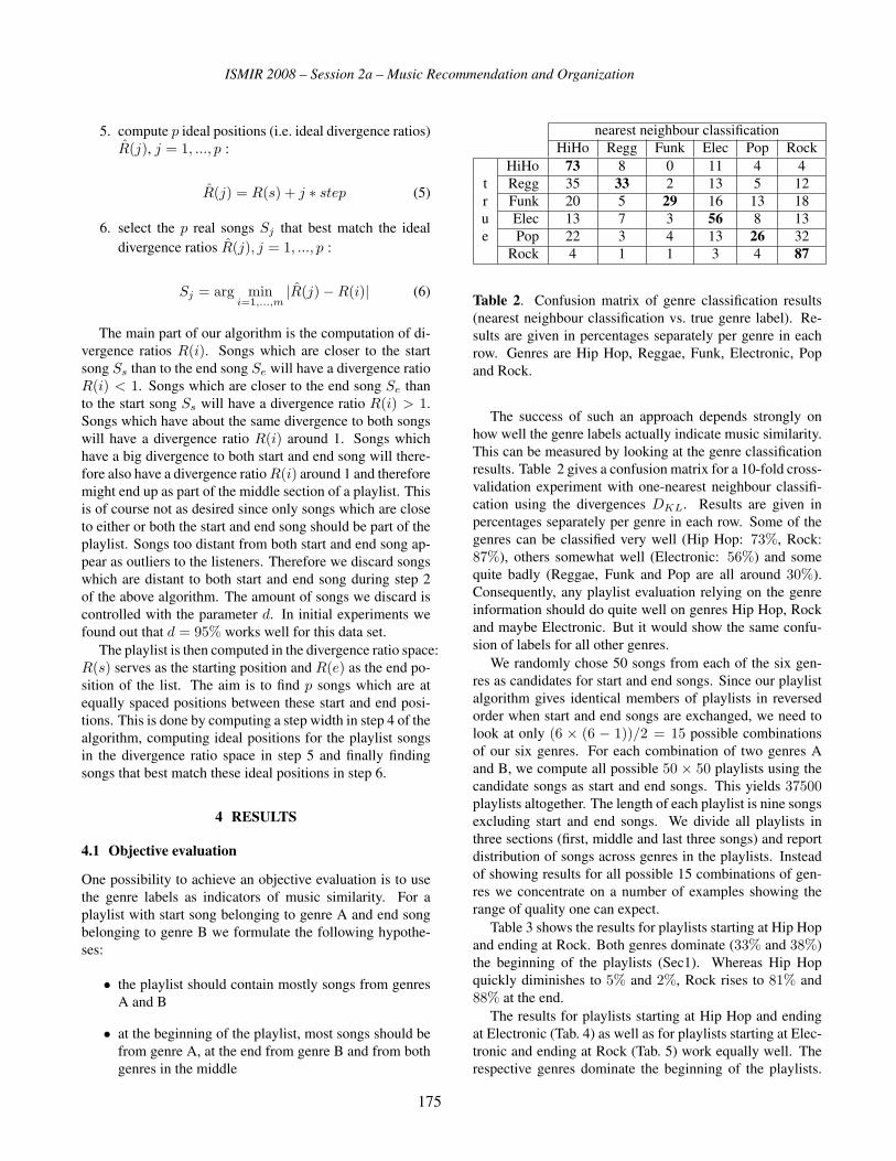
ISMIR 2008 – Session 2a – Music Recommendation and Organization
5. compute p ideal positions (i.e. ideal divergence ratios)
R̂(j), j = 1, ..., p :
R̂(j) = R(s) + j ∗ step (5)
6. select the p real songs Sj that best match the ideal
divergence ratios R̂(j), j = 1, ..., p :
Sj = arg mini=1,...,m
|R̂(j)−R(i)| (6)
The main part of our algorithm is the computation of di-
vergence ratios R(i). Songs which are closer to the start
song Ss than to the end song Se will have a divergence ratio
R(i) < 1. Songs which are closer to the end song Se than
to the start song Ss will have a divergence ratio R(i) > 1.
Songs which have about the same divergence to both songs
will have a divergence ratio R(i) around 1. Songs which
have a big divergence to both start and end song will there-
fore also have a divergence ratio R(i) around 1 and therefore
might end up as part of the middle section of a playlist. This
is of course not as desired since only songs which are close
to either or both the start and end song should be part of the
playlist. Songs too distant from both start and end song ap-
pear as outliers to the listeners. Therefore we discard songs
which are distant to both start and end song during step 2
of the above algorithm. The amount of songs we discard is
controlled with the parameter d. In initial experiments we
found out that d = 95% works well for this data set.
The playlist is then computed in the divergence ratio space:
R(s) serves as the starting position and R(e) as the end po-
sition of the list. The aim is to find p songs which are at
equally spaced positions between these start and end posi-
tions. This is done by computing a step width in step 4 of the
algorithm, computing ideal positions for the playlist songs
in the divergence ratio space in step 5 and finally finding
songs that best match these ideal positions in step 6.
4 RESULTS
4.1 Objective evaluation
One possibility to achieve an objective evaluation is to use
the genre labels as indicators of music similarity. For a
playlist with start song belonging to genre A and end song
belonging to genre B we formulate the following hypothe-
ses:
• the playlist should contain mostly songs from genres
A and B
• at the beginning of the playlist, most songs should be
from genre A, at the end from genre B and from both
genres in the middle
nearest neighbour classification
HiHo Regg Funk Elec Pop Rock
HiHo 73 8 0 11 4 4
t Regg 35 33 2 13 5 12
r Funk 20 5 29 16 13 18
u Elec 13 7 3 56 8 13
e Pop 22 3 4 13 26 32
Rock 4 1 1 3 4 87
Table 2. Confusion matrix of genre classification results
(nearest neighbour classification vs. true genre label). Re-
sults are given in percentages separately per genre in each
row. Genres are Hip Hop, Reggae, Funk, Electronic, Pop
and Rock.
The success of such an approach depends strongly on
how well the genre labels actually indicate music similarity.
This can be measured by looking at the genre classification
results. Table 2 gives a confusion matrix for a 10-fold cross-
validation experiment with one-nearest neighbour classifi-
cation using the divergences DKL. Results are given in
percentages separately per genre in each row. Some of the
genres can be classified very well (Hip Hop: 73%, Rock:
87%), others somewhat well (Electronic: 56%) and some
quite badly (Reggae, Funk and Pop are all around 30%).
Consequently, any playlist evaluation relying on the genre
information should do quite well on genres Hip Hop, Rock
and maybe Electronic. But it would show the same confu-
sion of labels for all other genres.
We randomly chose 50 songs from each of the six gen-
res as candidates for start and end songs. Since our playlist
algorithm gives identical members of playlists in reversed
order when start and end songs are exchanged, we need to
look at only (6 × (6 − 1))/2 = 15 possible combinations
of our six genres. For each combination of two genres A
and B, we compute all possible 50 × 50 playlists using the
candidate songs as start and end songs. This yields 37500playlists altogether. The length of each playlist is nine songs
excluding start and end songs. We divide all playlists in
three sections (first, middle and last three songs) and report
distribution of songs across genres in the playlists. Instead
of showing results for all possible 15 combinations of gen-
res we concentrate on a number of examples showing the
range of quality one can expect.
Table 3 shows the results for playlists starting at Hip Hop
and ending at Rock. Both genres dominate (33% and 38%)
the beginning of the playlists (Sec1). Whereas Hip Hop
quickly diminishes to 5% and 2%, Rock rises to 81% and
88% at the end.
The results for playlists starting at Hip Hop and ending
at Electronic (Tab. 4) as well as for playlists starting at Elec-
tronic and ending at Rock (Tab. 5) work equally well. The
respective genres dominate the beginning of the playlists.
175

ISMIR 2008 – Session 2a – Music Recommendation and Organization
HiHo Regg Funk Elec Pop RockSec1 33 5 2 15 8 38
Sec2 5 1 2 7 4 81
Sec3 2 0 3 4 2 88
Table 3. Distribution of songs across genres in playlists
starting at Hip Hop and ending at Rock. Results given for
first, middle and last section of playlists (Sec1 to Sec3).
HiHo Regg Funk Elec Pop Rock
Sec1 30 5 2 35 8 19
Sec2 6 2 3 66 5 18
Sec3 2 2 3 70 4 18
Table 4. Distribution of songs across genres in playlists
starting at Hip Hop and ending at Electronic. Results given
for first, middle and last section of playlists (Sec1 to Sec3).
The start genres diminish quickly and the end genres are
most prominent in the last sections (Sec3). Tables 3 to 5
give results for the three genres which also achieve the best
classification results (see Tab. 2). The results are basically in
line with the two hypotheses we formulated at the beginning
of this section. Only the fact that the end genre is already
very prominent at the beginning of the playlists (Sec1) is a
bit surprising. This might be due to the fact that the end gen-
res in Tables 3 to 5 are also the most numerous in our data
base (Electronic 36% and Rock 45% of all songs in the data
base, see Tab. 1).
Table 6 shows the results for playlists starting at Reggae
and ending at Rock. The amount of songs from genre Rock
rises from 38% to 80% to 88% going from Sec1 to Sec3 as
expected. Genre Reggae is somewhat under-represented in
all sections of the playlists. Going back to the genre classi-
fication confusion matrix in Tab. 2, it is clear that there is a
lot of mix-up between genres Reggae and Hip Hop. Conse-
quently, Tab. 6 shows a considerable amount of Hip Hop in
Sec1, diminishing towards Sec3.
The results for playlists starting at Funk and ending at
Pop given in Tab. 7 are even less satisfactory. The genre
classification confusion matrix in Tab. 2 shows that genre
HiHo Regg Funk Elec Pop RockSec1 13 3 2 42 6 34
Sec2 8 2 2 8 5 77
Sec3 5 1 3 3 3 85
Table 5. Distribution of songs across genres in playlists
starting at Electronic and ending at Rock. Results given for
first, middle and last section of playlists (Sec1 to Sec3).
HiHo Regg Funk Elec Pop RockSec1 26 7 2 20 7 38
Sec2 6 1 2 7 4 80
Sec3 3 0 2 4 2 88
Table 6. Distribution of songs across genres in playlists
starting at Reggae and ending at Rock. Results given for
first, middle and last section of playlists (Sec1 to Sec3).
HiHo Regg Funk Elec Pop Rock
Sec1 19 3 8 28 13 29
Sec2 17 4 4 20 19 36
Sec3 12 3 4 22 16 42
Table 7. Distribution of songs across genres in playlists
starting at Funk and ending at Pop. Results given for first,
middle and last section of playlists (Sec1 to Sec3).
Funk is confused with almost all other genres and genre
Pop strongly with genre Rock. As a result, the only visi-
ble trend in Tab. 7 is a rising amount of songs from genres
Pop and Rock going from Sec1 to Sec3. This clearly indi-
cates the limits of our approach to objective evaluation of
playlist generation. Such an evaluation only makes sense
with reliable genre label information.
The amount of songs which are being excluded from be-
coming members of the playlist because of being too dis-
similar from both start and end song was set to d = 95% for
all experiments (see step 2 in Sec. 3.2). Relaxing this con-
straint to smaller values leads to less clear distribution of
genres (i.e. less songs in the playlists have the same genre
label as the start and end songs).
4.2 Subjective evaluation
Our playlist generation algorithm can be utilised by users
of the FM4 Soundpark website 2 to create their own digital
“mixtapes” online. Therefore the best evaluation would be
a user study with people actually using this service on the
internet. Such a user study is planned for the future. During
the development phase of the project, we decided to do an
internal form of user study by having one of the authors lis-
ten to a number of playlists and judge their quality. This one
person has considerable experience with popular music for
having been a record collector and DJ for about two decades.
While this approach has the problem of being highly subjec-
tive it does have the advantage of actually judging the “raw”
playlists instead of a certain implementation and user inter-
face.
As pointed out in Sec. 4.1, our playlist algorithm gives
identical members of playlists in reversed order when start
2 http://fm4.orf.at/soundpark
176

ISMIR 2008 – Session 2a – Music Recommendation and Organization
and end songs are exchanged. Therefore, we look at only
(6× (6− 1))/2 = 15 possible combinations of our six gen-
res (see two leftmost columns in Tab. 8). For each combi-
nation of two genres A and B, we randomly choose three
of the 50 × 50 playlists computed as described in Sec. 4.1.
This gives 45 playlists for evaluation. Our evaluator listened
to all the playlists using the “XMMS 1.2.10 - Cross plat-
form multimedia player” 3 . He would first listen to the start
song, then the end song and then the songs in between in
the correct order. The evaluator was allowed to freely move
through a song by skipping parts and moving back and forth
in time. He was also allowed to re-listen to songs in the
playlist if necessary.
For each playlist, the evaluator was asked to answer the
following two questions which are tightly connected to our
two hypotheses formulated in Sec. 4.1:
• How many outliers are in the playlist which do not fit
the overall flavour of the playlist?
• Is the order of songs in the playlist from the start to
the end song apparent?
The first question should allow to judge whether all the
songs in a playlist really are similar to either the start or the
end song, or are located somewhere in the intended middle.
The second question aims at the sequential ordering of the
songs. Songs at the beginning should be more similar to the
start song, songs at the end to the end song. The second
question can be answered with either “yes”, “somewhat” or
“no”.
The results of the evaluation are given in Tab. 8. For
each combination of genres, the average number of outliers
is given (average taken over three playlists). It is also in-
dicated how the second question has been answered for the
three playlists of a certain combination of genres. Each “x”
in a column stands for the respective answer given for one
playlist. So for each row (i.e. combination of genres) three
“x” indicate three answers to the second question. At the
bottom row, the average number of outliers is given as well
as the percentages of different answers to the question about
the sequential order of the playlists is given.
The average number of outliers in a playlist is quite low
at 1.1 out of possible 9. This means that on average, a user
might want to delete one song from an automatically cre-
ated playlist. While for a lot of combinations of genres this
number is 0 and therefore perfect, for some genre combina-
tions the number of outliers is quite high. E.g. for playlists
starting at Hip Hop and ending at Reggae, an average of 4.7songs are rated as outliers. The reasons seems to be that
for a listener, the defining part of a Reggae song is the off-
beat percussion which is not well conserved in our timbral
representation of music. Instead, the rhythm guitar seems
3 http://www.xmms.org
Genres # of order apparent
from to outliers yes somewhat no
HiHo Regg 4.7 x xx
HiHo Funk 1.7 xx x
HiHo Elec 1.3 xxx
HiHo Pop 2.7 xx x
HiHo Rock 0 xxx
Regg Funk 0.7 xx x
Regg Elec 1.3 xxx
Regg Pop 1.3 xxx
Regg Rock 0.3 xx x
Funk Elec 1.0 xx x
Funk Pop 1.7 xx x
Funk Rock 0 xx x
Elec Pop 0 xxx
Elec Rock 0 xx x
Pop Rock 0 xxx
average 1.1 71.1% 17.8% 11.1%
Table 8. Results of the subjective evaluation. For each com-
bination of genres, the average number of outliers and the
answers to the question concerning the order in the playlist
is given. At the bottom row, average number of outliers as
well as the percentages of different answers to the question
about order are given.
to dominate the models giving rise to high similarities with
certain types of rock songs. Other sources of mistakes are
recordings of poor acoustic quality which are found to be
similar to each other no matter what the genres of the songs
are. The sequential order of the playlists seems to work
very well with it being apparent in 71% of all playlists and
“somewhat” apparent in another 17.8%. One problem with
the sequential ordering that we noticed is a kind of “tilting”-
effect at the middle of playlists: the first half would be very
close to the start song, the second half to the end song but
a sort of smooth transition is missing. This was sometimes
the case if start and end songs are very different and the data
base might not even contain songs fitting in between. An-
other problem are too many outliers obscuring the overall
order of a playlist.
As with the objective evaluation in Sec. 4.1, relaxing the
amount of songs which are being excluded from becoming
members of the playlist below d = 95% (see step 2 in Sec.
3.2) results in more outliers and less clear sequential order
of the playlists.
177

ISMIR 2008 – Session 2a – Music Recommendation and Organization
5 CONCLUSION
We have presented a new approach for the generation of
playlists using start and end songs and showing inherent se-
quential order. Our approach is based on audio similarity
and requires very little user interaction. Both objective eval-
uation based on genre labels of songs and subjective evalua-
tion based on listening tests showed that the concept works
well.
Our playlist generation algorithm can be utilised by users
of the website of a public radio station to create their own
digital “mixtapes” online. Since our evaluation showed that,
on average, at least one song does not fit the overall playlist,
an editing functionality might be added to the user interface.
6 ACKNOWLEDGEMENTS
Parts of this work have been funded by the “Österreichische
Forschungsförderungsgesellschaft (FFG)” (Bridge-project
815474 and “Advanced Knowledge Technologies: Ground-
ing, Fusion, Applications AKT:GFA”-project).
7 REFERENCES
[1] Alghoniemy M., Tewfik A.: A network flow model for
playlist generation, IEEE International Conference onMultimedia and Expo (ICME’01), 2001.
[2] Aucouturier J.-J., Pachet F.: Finding songs that sound
the same, Proceedings of IEEE Benelux Workshop onModel based Processing and Coding of Audio, Leuven,
Belgium, Nov. 2002, 2002.
[3] Aucouturier J.-J., Pachet F.: Scaling up music playlist
generation, Proceedings of IEEE International Con-ference on Multimedia and Expo (ICME), Lausanne,
Switzerland, 2002.
[4] Baccigalupo C., Plaza E.: Case-Based Sequential Or-
dering of Songs for Playlist Recommendation, Euro-pean Conference on Case Based Reasoning (ECCBR’06), Lecture Notes in Computer Science, Springer
Berlin/Heidelberg, Volume 4106/2006, 2006.
[5] Gulik R., Vignoli F.: Visual Playlist Generation on the
Artist Map, Proceedings of the 6th International Confer-ence on Music Information Retrieval (ISMIR’05), Lon-
don, UK, 2005.
[6] Logan B.: Mel Frequency Cepstral Coefficients for Mu-
sic Modeling, Proc. of the International Symposium onMusic Information Retrieval (ISMIR’00), 2000.
[7] Logan B.: Music Recommendation from Song Sets,
Proceedings of the 5th International Conference on Mu-sic Information Retrieval (ISMIR’04), Barcelona, Spain,
October 10-14, 2004.
[8] Mandel M.I., Ellis D.P.W.: Song-Level Features and
Support Vector Machines for Music Classification, Pro-ceedings of the 6th International Conference on Mu-sic Information Retrieval (ISMIR’05), London, UK,
September 11-15, 2005.
[9] Neumayer R., Dittenbach M., Rauber A.: PlaySOM
and PocketSOMPlayer: Alternative Interfaces to Large
Music Collections, Proceedings of the 6th InternationalConference on Music Information Retrieval (ISMIR’05),London, UK, September 11-15, pp. 618-623, 2005.
[10] Pampalk E., Pohle T., Widmer G.: Dynamic Playlist
Generation Based on Skipping Behaviour, Proceedingsof the 6th International Conference on Music Informa-tion Retrieval (ISMIR’05), London, UK, September 11-
15, 2005.
[11] Pauws S., Eggen B.: PATS: Realization and User Evalu-
ation of an Automatic Playlist Generator, Proceedings ofthe 3rd International Conference on Music InformationRetrieval (ISMIR’02), Paris, France, pp. 222-230, 2002.
[12] Pauws S., Verhaegh W., Vossen M.: Fast Generation of
Optimal Music Playlists using Local Search, Proceed-ings of the 7th International Conference on Music Infor-mation Retrieval (ISMIR’06), Victoria, Canada, 2006.
[13] Penny W.D.: Kullback-Liebler Divergences of Normal,
Gamma, Dirichlet and Wishart Densities, Wellcome De-partment of Cognitive Neurology, 2001.
[14] Platt J.C., Burges C.J.C., Swenson S., Weare C., Zheng
A.: Learning a Gaussian Process Prior for Automatically
Generating Music Playlists, Advances in Neural Infor-mation Processing Systems 14, pp. 1425-1432, 2002.
[15] Pohle T., Knees P., Schedl M., Pampalk E., Widmer G.:
”Reinventing The Wheel”: A Novel Approach to Music
Player Interfaces, IEEE Multimedia, 14(3), pp. 46-54,
2007.
[16] Ragno R., Burges C.J.C., Herley C.: Inferring Similar-
ity Between Music Objects with Application to Playlist
Generation, Proc. 7th ACM SIGMM International Work-shop on Multimedia Information Retrieval, 2005.
[17] Schnitzer D.: Mirage - High-Performance Music Simi-
larity Computation and Automatic Playlist Generation,
Vienna University of Technology, Austria, Master The-
sis, 2007.
178

ISMIR 2008 – Session 2a – Music Recommendation and Organization
ACCESSING MUSIC COLLECTIONS VIA REPRESENTATIVE CLUSTERPROTOTYPES IN A HIERARCHICAL ORGANIZATION SCHEME
Markus Dopler Markus Schedl Tim Pohle Peter KneesDepartment of Computational Perception
Johannes Kepler UniversityLinz, Austria
ABSTRACT
This paper addresses the issue of automatically organizinga possibly large music collection for intuitive access. Wepresent an approach to cluster tracks in a hierarchical man-ner and to automatically find representative pieces of musicfor each cluster on each hierarchy level. To this end, audiosignal-based features are complemented with features de-rived via Web content mining in a novel way. Automatichierarchical clustering is performed using a variant of theSelf-Organizing Map, which we further modified in order tocreate playlists containing similar tracks.The proposed approaches for playlist generation on a hier-archically structured music collection and finding prototyp-ical tracks for each cluster are then integrated into the Trav-eller’s Sound Player, a mobile audio player application thatorganizes music in a playlist such that the distances betweenconsecutive tracks are minimal. We extended this player todeal with the hierarchical nature of the playlists generatedby the proposed structuring approach.As for evaluation, we first assess the quality of the clusteringmethod using the measure of entropy on a genre-annotatedtest set. Second, the goodness of the method to find proto-typical tracks for each cluster is investigated in a user study.
1 INTRODUCTION AND MOTIVATION
Increased storage capabilities, high-speed Internet access,and novel techniques for music compression have tremen-dously increased the size of private as well as commercialmusic collections over the past few years. Due to the largenumber of audio tracks in private repositories, it is virtuallyimpossible for users to keep track of every piece. Hence,elaborate methods for organizing large music collections be-come increasingly important. The enormous economic suc-cess of high-capacity mobile music players, such as Ap-ple’s “iPod”, necessitates intelligent methods for automatedstructuring of music collections.The paper at hand presents a possible solution to this prob-lem. The approach proposed here employs an unsupervisedhierarchical clustering algorithm, more precisely the Grow-ing Hierarchical Self-Organizing Map (GHSOM) [3], onaudio features extracted from the music collection. Each
cluster of the resulting hierarchical organization is then la-beled automatically with a typical track from the cluster tofacilitate exploration. To this end, we elaborated an origi-nal approach that not only relies on audio features, but in-corporates Web-based information on the prototypicality ofartists to determine a representative track for each cluster.The main motivation for this is the bad quality of straightfor-ward methods to find a representative for a set of data items.Indeed, choosing for example the music track whose audiofeature representation is closest to the average feature vectorof the cluster may give a mathematically sound prototype forthe cluster. However, in preliminary experiments that em-ployed this selection approach, we encountered many rep-resentatives that were either songs by barely known artists(even though the cluster contained very well known artists)or barely known tracks by popular artists. In any case, usingsuch tracks as representative for a cluster seems counterin-tuitive to guide the user in exploring his music collection.The main contributions of this work are the novel approachto determine cluster prototypes, based not only on the au-dio features, but also on Web mining techniques, in order toomit “average” cluster representatives that are unknown tomost users. In addition, we reimplemented the GHSOM al-gorithm and modified it in order to generate playlists. Fur-thermore, a novel version of the Traveller’s Sound Playerapplication, which uses the cluster prototypes to facilitatenavigating the collection, is proposed. The approaches togenerate playlists and finding cluster prototypes are furtherevaluated thoroughly.The remainder is structured as follows. Section 2 brieflydiscusses related work. In Section 3, the acquisition of fea-ture data to describe artists and pieces of music is elabo-rated. Our approaches to hierarchically cluster a given mu-sic collection and creating playlists from these clusters canbe found in Section 4, whereas finding representative pro-totypes for each cluster is addressed in Section 5. The ex-periments conducted to evaluate the proposed approachesare detailed in Section 6. Finally, Section 7 gives some re-marks on the integration of the presented approaches in theTraveller’s Sound Player application, and in Section 8, con-clusions are drawn.
179

ISMIR 2008 – Session 2a – Music Recommendation and Organization
2 RELATED WORK
This paper was mainly motivated by the work done in [9],where Pohle et al. employ different heuristics to solve aTraveling Salesman Problem on a track-level audio simi-larity matrix. The resulting tour represents a playlist withminimized distances between consecutive pieces of music.The playlist generated for a complete music collection isthen made accessible via a special music player. In [8], thisapproach is modified in that the audio similarity matrix isadapted according to artist similarity estimations, which arederived from TF×IDF features computed on artist-relatedWeb pages. In contrast to [9, 8], we do not model a Trav-eling Salesman Problem to generate playlists. Instead wefollow a recursive approach that builds upon the GHSOMalgorithm to hierarchically break down the tracks of a mu-sic collection until every track is represented by a sole mapunit. The playlist is then generated by successively visitingeach such unit.As we build our playlist generation approach upon a variantof the GHSOM, a hierarchical version of the Self-OrganizingMap, this work is certainly also related to [3, 4], where theGHSOM is presented.
3 FEATURE EXTRACTION
As we combine features extracted from the audio signal withcultural features from the Web in order to determine pro-totypical pieces of music for each cluster, we perform thefollowing two feature extraction stages.
3.1 Audio-based Features
First, we extract audio features using a well-established ap-proach. For each piece of music, Mel Frequency CepstralCoefficients (MFCCs) are extracted on short-time audio seg-ments to obtain a coarse description of the spectral shape.Details on this procedure can be found, for example, in [2, 1,7]. Gaussian Mixture Models (GMMs) are then used to ag-gregate the MFCCs of each individual piece of music. Thesimilarity between two arbitrary pieces is calculated as theinverse of the distance between their GMMs. For our exper-iments, we used parameters similar to those proposed in [1](19 MFCCs, 30 clusters per GMM). Performing this proce-dure for a collection of n music pieces eventually yields ann× n distance matrix.
3.2 Web-based Features
In order to estimate the prototypicality of each artist in thecollection, and thus his or her suitability to serve as repre-sentative for a cluster, we make use of information foundon artist-related Web pages. To this end, we follow the ap-proach backlink/forward link ratio with exorbitant popular-ity penalization as proposed in [11, 12]. The basic assump-tion underlying this approach is that the probability that a
popular artist is mentioned on a Web page about a ratherunknown artist is higher than vice versa. This seems rea-sonable if one thinks, for example, of references of the form“Band X sounds like band Y.”. Such phrases are more likelyto occur on a Web page of a rather unknown band X, whichpoints to a popular band Y than vice versa.For each artist, we retrieve up to 150 Web pages returned byGoogle for queries of the form "artist name"+music+review. This query scheme was originally pro-posed in [13] for retrieving artist-related Web pages. Sub-sequently, the Web pages of each artist are analyzed for oc-currences of all other artist names in the collection, and therespective document frequency dfa,B (i.e., the number ofWeb pages in the set B of retrieved pages for artist b onwhich the name of artist a occur) is stored for all combina-tions of artists.To estimate the prototypicality of an artist a for a specificset of tracks given by cluster u 1 , we compare the documentfrequencies dfa,B and dfb,A for all b’s in the same clusteru as a. We count for how many of these b’s the inequalitydfa,B ≥ dfb,A holds. The higher this count, the more proto-typical artist a. Performing this calculation for all artists ofa specific cluster u, we obtain an artist prototypicality rank-ing ru(a). However, this ranking is usually quite distortedas artist names like “Genius”, “Kiss”, or “Bush” are alwaysoverrated. Addressing this issue, a penalization term thatdownranks artists whose prototypicality is extremely highfor all clusters (which actually cannot be the case) is intro-duced. This eventually gives a corrected ranking functionruw(a). For a more detailed elaboration on the prototypical-
ity ranking function, please see [12].
4 ADAPTING THE GHSOM FOR PLAYLISTGENERATION
Structuring the music collection under consideration is per-formed using an unsupervised neural network algorithm thatautomatically organizes a given data set in a hierarchicalmanner. More precisely, we reimplemented in Java a hier-archical extension of the Self-Organizing Map, namely theGrowing Hierarchical Self-Organizing Map (GHSOM), asproposed in [3]. The GHSOM has been integrated in theCoMIRVA framework [10].The GHSOM extends the widely used Self-Organizing Map[6] in a way that during training, new map units are auto-matically inserted into the existing grid between the mapunit whose data items show the highest deviation from themap unit’s model vector and its most dissimilar neighboringunit. This is performed until the mean quantization error ofall map units is reduced to a certain threshold τ1. Hence,τ1 controls the final size of the individual SOMs. A secondthreshold τ2 determines the quantization error a particularmap unit must exceed in order to reorganize its data items on
1 In our case, the clusters are given by the map units of the Self-Organizing Map that we use to organize the collection (cf. Section 4).
180

ISMIR 2008 – Session 2a – Music Recommendation and Organization
a newly generated SOM at a deeper hierarchy level. A moredetailed explanation of the GHSOM algorithm is given, forexample, in [3].In order to suit our need for playlist generation, we hadto modify the original GHSOM algorithm in two regards.First, we redefined the neighborhood function used in thetraining process. In particular, we defined a cyclic neighbor-hood relation that extends its range over the map’s borders,i.e., considers the last row/column of the map whenever amap unit in the first row/column is modified and vice versa.Second, each time a map unit u is expanded to a new SOMat a deeper hierarchy level, this new SOM is initialized us-ing the model vectors of u’s neighboring units.These two modifications allow for a very simple playlistgeneration approach in that we just have to train a 1-dim-ensional GHSOM on the input data and ensure the recursiveexpansion of map units until each track is represented byits sole unit. Traversing the resulting GHSOM tree in pre-order while successively storing all tracks represented by theleave nodes eventually yields a playlist containing all piecesof the collection. As for training the GHSOM, we use theaudio similarity matrix, whose creation is described in Sub-section 3.1. For performance reasons, however, we applyPrincipal Components Analysis (PCA) [5] to reduce the di-mensionality of the feature space to 30. 2
5 FINDING CLUSTER PROTOTYPES
One of the main goals of this work is determining proto-typical tracks that can serve as representatives to describeeach cluster, i.e., map unit, of the GHSOM. However, pre-liminary experiments showed that relying solely on audio-based information to calculate a representative piece of mu-sic for each cluster yields unsatisfactory results, as alreadyexplained in Section 1. To alleviate this problem, we in-corporate artist prototypicality information extracted as de-scribed in Subsection 3.2 into an audio-based prototypical-ity ranking. The resulting ranking function thus combinesaudio features of all tracks in the cluster under consider-ation with Web-based artist prototypicality information asdetailed in the following.Denoting the map unit under consideration as u, the rankingfunction ru(p) that assigns a prototypicality estimation tothe representation in feature space of each 3 piece of musicp by artist a is calculated as indicated in Equation 1, whererus (p) denotes the audio signal-based part of the ranking
function (cf. Equation 2) and ruw(a) is the corrected Web-
based ranking function from Subsection 3.2. In the signal-based ranking function, u denotes the mean of the featurevectors represented by u, | · | is the Euclidean distance, andnorm(·) is a normalization function that shifts the range to
2 30 dimensions seemed appropriate for our test collection of 2,545pieces of music. Employing the approach on larger collections, most prob-ably requires increasing this number.
3 More precisely, “each” refers to those pieces of music that are repre-sented by the map unit u under consideration.
[1, 2]. Finally, each piece of music p represented by map unitu is assigned a prototypicality value, which is the higher, themore prototypical p is for u.
ru(p) = rus (p) · ru
w(a) (1)
rus (p) = norm
(1
1 + ln(1 + |p− u|)
)(2)
6 EVALUATION
We conducted two sets of evaluation experiments. The firstaimed at comparing our GHSOM-based playlist generationapproach to the ones proposed in [9, 8]. In accordance with[9], the quality of the playlist was evaluated by calculatingthe genre entropy for a number of consecutive tracks. Sec-ond, we assessed the quality of our approach to detectingprototypical tracks via a user study.For evaluation, we used the same collection as used in [8].This collection contains 2,545 tracks by 103 artists, groupedin 13 genres. For details on the genre distribution, pleaseconsider [8].
6.1 Entropy of the Playlist
To evaluate the coherence of the playlists generated by ourGHSOM-based approach, we compute the entropy of thegenre distribution on sequences of the playlists. More pre-cisely, using each piece of the collection as starting point,we count how many of n consecutive tracks belong to eachgenre. The result is then normalized and interpreted as aprobability distribution, on which the Shannon entropy iscalculated, according to Equation 3, where log2 p(x) = 0 ifp(x) = 0.
H(x) = −∑
x
p(x) log2 p(x) (3)
In Figure 1, the entropy values for n = 2 . . . 318 aregiven (plot “audio ghsom”), averaged over the whole play-list, i.e., each track of the playlist is chosen once as the start-ing track for a sequence of length n. 4
Comparing the entropy values given by the GHSOM ap-proach to the ones presented in [8] reveals that the GH-SOM approach performs very similar to the SOM-based ap-proach followed in [8]. This is obviously no surprise, butshows that the automated splitting of clusters by the GH-SOM does not harm the entropy of the generated playlists,while at the same time offers the additional benefit of auto-matically structuring the created playlists in a hierarchicalmanner. Like those created by the recursive SOM approachin [8], the GHSOM-based playlists show quite good long-term entropy values (for large values of n), but rather poorvalues for short playlists.
4 318 tracks correspond to an angular extent of 45 degrees on the circulartrack selector in the Traveller’s Sound Player application.
181

ISMIR 2008 – Session 2a – Music Recommendation and Organization
Figure 1. Genre entropy values for n consecutive tracks ofthe GHSOM-based playlist.
We also experimented with incorporating Web-based fea-tures directly into the playlist generation algorithm, as pro-posed in [8]. This improved on the one hand the entropy val-ues (cf. plot “combined ghsom” in Figure 1). On the otherhand, taking a critical look at the resulting playlists showedthat using Web-based artist features as proposed in [8] yields“too perfect” playlists in that often one and the same artistcontributes 20 or more consecutive tracks. Hence, this ap-proach may be suited well for creating very consistent, butsometimes boring, playlists.
6.2 Quality of the Prototype Estimation
To evaluate the quality of the cluster representatives as deter-mined by the approach proposed in Section 5, we performeda user study. The evaluation sets for the user study werecreated by training a 1-dimensional GHSOM with an initialnumber of 5 rows and gradient initialization. The growingthreshold τ1 was set to 0.5, the expansion threshold τ2 to 0.1.We performed sequential training with a training length of 5epochs. This setting resulted in a GHSOM with 11 clusterson the first level. 5
We had 16 participants in the study, each of which evalu-ated 11 sets of tracks, consisting of 10 tracks each. 10 outof these 11 sets were constructed as follows. The most pro-totypical track of each cluster, according to our approach,was added to the corresponding set. The remaining 9 trackswere selected by drawing a random sample from their re-spective cluster. The 11th set (for cluster 6) in contrastcontained exactly the same pieces of music for all partici-
5 Level 1 is the first distinctive level of the GHSOM as level 0 containsall data items.
pants. 6 . The reason for this different creation method forcluster 6 is that we also wanted to take a qualitative look atsome of the results, which would have been barely feasiblefor a large number of differing track sets, each of which isevaluated by only one user. We followed this rather com-plicated procedure of track set generation in order to raisethe total number of evaluated sets. This procedure yielded161 different track sets (16 participants · 10 sets + 1 invari-ant set for all participants). Each participant was instructedto select one track from each set that should be best suitedto represent the corresponding set. We offered the partici-pants the artist and song names as well as the audio files incase they were uncertain or unfamiliar with artist or track.In total, we received 176 prototype selections, which wereanalyzed as follows.
To obtain a general performance measure, we first calcu-lated the overall concordance between the prototypes foundby our automated approach and those indicated by the par-ticipants. Table 1 gives these overall concordance valuesover the 176 evaluated track sets. We assessed the concor-dances on different levels. The first row depicts the exactconcordance of the tracks, i.e., in order to be consideredconcordant, the track given by our approach must be thesame as the one selected by the user. This definition ofconcordance is weakened for rows two and three as our ap-proach and the user judgment must, in this case, agree onlyon the artist or on the genre, respectively.At first glance, these results may not seem very promising.However, taking the difficult nature of the user task into ac-count (choosing between 10 probably quite similar tracks,many of which are by the same artists), it must be regarded asuccess that the concordance values considerably exceededthe baseline. The difficulty of the task is also reflected bythe relatively high mean genre entropy of 1.95 over all tracksets. This number is obviously higher than the entropy valuegiven in Figure 1 for n = 10 because of the randomized se-lection process involved in the creation of the track sets.Taking a closer look at the individual track sets, we often en-countered the problem that the sets contained approximatelyequal numbers of tracks from two or three different genres.To analyze the influence this may have had on the evaluationresults, Table 2 shows, for each group of sets (created fromclusters 1 to 11 of the GHSOM), the absolute number ofusers that agreed with the prototype found by our approach(column “hits”) and the mean genre entropy of the respec-tive track set. Note that the entries are ordered by their aver-age entropy. The baseline is 1.6 as each group was evaluatedby 16 participants; a random guesser would have yielded ahit rate of 10% in the long run. From Table 2, we can seethat high entropy values in fact tend to correspond to low hitrates and vice versa. The low hit rate of 2 for the group withthe lowest entropy, however, can be explained by the fact
6 Cluster 6 also contained the prototype and a random sample of 9 othertracks, but this sample remained constant for all participants
182

ISMIR 2008 – Session 2a – Music Recommendation and Organization
level baseline concordance
track 10.00 17.61artist 15.17 26.14genre 35.34 50.57
Table 1. Overall concordance of the prototype finding algo-rithm and the user judgments, in percent.
that this group subsumed music by different, but all famous,metal bands. Furthermore, in most track sets of this group,2 or 3 tracks by “Cannibal Corpse” were included, one ofwhich was also rated the prototype by our approach. But theothers were usually no less famous tracks by this band.The identical composition of cluster 6 for all participantsallowed us to take a qualitative look at the ranking resultson the level of individual tracks. Table 3 summarizes theseresults. In this table, the evaluated tracks of cluster 6 aredisplayed in decreasing order of their prototypicality as de-termined by our approach. The leftmost column gives thenumber of times the respective track was selected as clus-ter representative by a participant. As for the compositionof cluster 6, it mainly contained punk rock and folk rocksongs, but also a metal song by “Pantera”, which somehowalso fits into this cluster, and a real outlier by the Germanelectronic music producer “Scooter”. From Table 3, it canbe seen that about 56% (9 out of 16) of the user hits accountfor the top 3 rankings by our approach. On the other hand,also the lowest ranked two tracks by “Bad Religion” werechosen by 25% of the users. This is no surprise as this bandmay be seen as equally prototypical for the punk rock genreas the top ranked band “Offspring”. The remaining 3 userhits were given to the tracks by “Subway to Sally”. Sincethe randomly drawn sample included 3 tracks of this bandin the evaluation set, it seems that some users considered theset best represented by a track by this artist. None of the par-ticipants, however, selected one of the outliers by “Pantera”or “Scooter” as representative.To summarize the results, even though they certainly leaveenough room for improvement, most users at least roughlyagreed with the prototypicality ratings given by the pro-posed approach. Moreover, taking into account the espe-cially difficult task the participants in the user study had toperform and the quite heavy mixtures of different genres inthe track sets, the results are surprisingly good.
7 A NOVEL VERSION OF THE TRAVELLER’SSOUND PLAYER
The basic idea of the Traveller’s Sound Player (TSP) pre-sented in [9] is to arrange the tracks in a music collectionaround a wheel that serves as track selector. The authorsof [9] aim at performing this arrangement in a way suchthat consecutive tracks are maximally similar. To this end,a large circular playlist is created by solving a TravelingSalesman Problem on an audio similarity matrix. A draw-
group hits entropy
4 2 0.96095 7 1.33856 4 1.68553 4 1.75162 2 2.01897 5 2.10688 2 2.17851 3 2.27630 2 2.27729 0 2.434310 0 2.5372
Table 2. Number of correctly found prototypes and meanentropy values for each of the 11 playlists.
hits ranking track name
4 0 offspring - hypodermic2 1 offspring - leave it behind3 2 blink 182 - don’t leave me0 3 pantera - strength beyond strength0 4 scooter - back in the u.k.2 5 subway to sally - mephisto1 6 subway to sally - ohne liebe0 7 subway to sally - böses erwachen3 8 bad religion - let them eat war1 9 bad religion - markovian process
Table 3. Detailed results of the user study for group 6, i.e.,the group containing identical tracks for all participants.
back of the original version of the TSP is, however, that itdoes not guide the user in finding a particular style of musiche or she is interested in. Indeed, the user has to explore dif-ferent regions of the playlist by randomly selecting differentangular positions with the wheel. It is also very hard to ex-actly position the wheel at a specific track as thousands oftracks are placed around one wheel, which corresponds toan angular representation in the magnitude of tenths of onedegree for each track.Addressing these shortcomings, we propose to integrate theprototype information found by our GHSOM-based approachpresented in Section 5 into the TSP. To this end, we elabo-rated an extension to the TSP that allows for hierarchicallyexploring the music collection by means of the cluster pro-totypes. More precisely, the novel user interface maps thestructure of the collection, as given by the trained GHSOM,to the wheel. It thus reflects the hierarchical organization inthat the user is first only presented the prototypes of the firstlevel clusters. He or she can then either opt for playing therepresentative track or for descending to a lower hierarchylevel. On each level, the user is presented a playlist con-taining the most prototypical tracks of all clusters (be themeither single map units or other GHSOMs at a deeper level)that make up the GHSOM at the current level.
183

ISMIR 2008 – Session 2a – Music Recommendation and Organization
8 CONCLUSIONS AND FUTURE WORK
We presented an approach to automatically cluster the tracksin a music collection in a hierarchical fashion with the aimof generating playlists. Each track is represented by similar-ities calculated on MFCC features, which are used as inputto the clustering algorithm. To this end, we reimplementedand modified the Growing Hierarchical Self-Organizing Map(GHSOM). We further proposed an approach to determine,for each of the clusters given by the GHSOM, the most rep-resentative track. This is achieved by combining the MFCC-based audio features with artist-related information extractedfrom the Web. We finally integrated the two approachesinto a music player software called the “Traveller’s SoundPlayer”, for which we elaborated an extension to deal withthe hierarchical data.We carried out evaluation experiments in two ways. First,we aimed at assessing the coherence of the playlists gen-erated by the GHSOM approach by measuring their genreentropy. We compared these entropy values to those givenby other playlist generation approaches and found that theylargely correspond to a similar approach based on standardSOMs. In addition, our approach also yields a hierarchicallyorganization of the collection and determines a representa-tive for each cluster, while at the same time the good long-term entropy values of the (GH)SOM-based playlist gener-ation are retained. Second, we conducted a user study to as-sess the quality of the found cluster prototypes. Even thoughthe results are still improvable, we could exceed the baselineconsiderably. Especially when taking into account the chal-lenging setup of the user study, the results are promising.As for future work, we are thinking of integrating the artistdistribution of the clusters into the ranking function, as theuser study showed that users tend to prefer representativetracks by artists who occur often in the cluster under con-sideration. Similar considerations would probably also besuited to filter out outliers. Furthermore, we have to experi-ment with different user interfaces for hierarchically access-ing music collections as the integration of the cluster repre-sentatives into the Traveller’s Sound Player is currently donein a quite experimental fashion. Our special concern in thiscontext will be the usability of the user interface for mobiledevices.
9 ACKNOWLEDGMENTS
This research is supported by the Austrian Fonds zur Förder-ung der Wissenschaftlichen Forschung (FWF) under projectnumbers L112-N04 and L511-N15.
10 REFERENCES
[1] J.-J. Aucouturier and F. Pachet. Improving Timbre Sim-ilarity: How High is the Sky? Journal of Negative Re-sults in Speech and Audio Sciences, 1(1), 2004.
[2] J.-J. Aucouturier, F. Pachet, and M. Sandler. ”The WayIt Sounds”: Timbre Models for Analysis and Retrievalof Music Signals. IEEE Transactions on Multimedia,7(6):1028–1035, 2005.
[3] M. Dittenbach, D. Merkl, and A. Rauber. The Grow-ing Hierarchical Self-Organizing Map. In Proc. of theInt’l Joint Conference on Neural Networks, Como, Italy,2000. IEEE Computer Society.
[4] M. Dittenbach, A. Rauber, and D. Merkl. UncoveringHierarchical Structure in Data Using the Growing Hier-archical Self-Organizing Map. Neurocomputing, 48(1–4):199–216, 2002.
[5] H. Hotelling. Analysis of a Complex of Statistical Vari-ables Into Principal Components. Journal of Educa-tional Psychology, 24:417–441 and 498–520, 1933.
[6] T. Kohonen. Self-Organizing Maps, volume 30 ofSpringer Series in Information Sciences. Springer,Berlin, Germany, 3rd edition, 2001.
[7] B. Logan. Mel Frequency Cepstral Coefficients for Mu-sic Modeling. In Proc. of the Int’l Symposium on MusicInformation Retrieval, Plymouth, MA, USA, 2000.
[8] T. Pohle, P. Knees, M. Schedl, E. Pampalk, and G. Wid-mer. “Reinventing the Wheel”: A Novel Approach toMusic Player Interfaces. IEEE Transactions on Multi-media, 9:567–575, 2007.
[9] T. Pohle, E. Pampalk, and G. Widmer. GeneratingSimilarity-based Playlists Using Traveling Salesman Al-gorithms. In Proc. of the 8th Int’l Conference on DigitalAudio Effects, Madrid, Spain, 2005.
[10] M. Schedl, P. Knees, K. Seyerlehner, and T. Pohle. TheCoMIRVA Toolkit for Visualizing Music-Related Data.In Proc. of the 9th Eurographics/IEEE VGTC Sympo-sium on Visualization, Norrköping, Sweden, 2007.
[11] M. Schedl, P. Knees, and G. Widmer. Improving Proto-typical Artist Detection by Penalizing Exorbitant Popu-larity. In Proc. of the 3rd Int’l Symposium on ComputerMusic Modeling and Retrieval, Pisa, Italy, 2005.
[12] M. Schedl, P. Knees, and G. Widmer. InvestigatingWeb-Based Approaches to Revealing Prototypical Mu-sic Artists in Genre Taxonomies. In Proc. of the 1st IEEEInt’l Conference on Digital Information Management,Bangalore, India, 2006.
[13] B. Whitman and S. Lawrence. Inferring Descriptionsand Similarity for Music from Community Metadata.In Proc. of the 2002 Int’l Computer Music Conference,Göteborg, Sweden, 2002.
184
ISMIR 2008 – Session 2a – Music Recommendation and Organization
DEVELOPMENT OF A MUSIC ORGANIZER FOR CHILDREN
Sally Jo Cunningham, Yiwen (Edmond) Zhang Dept of Computer Science
University of Waikato Hamilton, New Zealand
{sallyjo, ez1} @ cs.waikato.ac.nz ABSTRACT
Software development for children is challenging; children have their own needs, which often are not met by ‘grown up’ software. We focus on software for playing songs and managing a music collection—tasks that children take great interest in, but for which they have few or inappropriate tools. We address this situation with the design of a new music management system, created with children as design partners: the Kids Music Box.
1. INTRODUCTION
Digital documents such as music, movies, and pictures have become widely available; it is not uncommon for an individual’s hard drive to contain hundreds of songs and videos, and thousands of photos. However, both the interface and usability of digital document organizers are aimed for adults, and far less attention has been focused on the development of applications that are suitable for primary school children (six to ten years old). Children are as information thirsty as adults; they want to access their favourite songs and movies as much as adults do, and prize the ability to independently select and enjoy their entertainment ‘just like a big person’. But at present children are forced to use computer software that requires complex interaction, good spelling, and reading skills beyond their current abilities.
A number of music-related systems aimed at children are described in the research literature. They primarily focus on supporting children in creating music (eg, [4]), often in the context of formal music education (eg, [6]). MIR research attention has not yet turned to supporting children in playing, browsing, searching, and organizing collections of existing music. This paper describes the design and prototyping of such an organizer, the Kids
Music Box (KMB). The development of KMB was grounded in previous research on creating software for children (Section 2), and follows the Participatory Design [10] model for software development (Section 3). Structured techniques for matching functionality and interface/interaction design to the target users were also employed (eg, expert review and usability testing). The major contribution of this paper is to demonstrate this principled approach to developing music-interaction software for children.
2. DESIGNING SOFTWARE FOR CHILDREN
Children are not miniature adults [4]; they have different needs, capabilities and expectations of computer technologies. Making cosmetic changes to adult software does not adequately adapt it for children [3]. To guide development of KMB, we first reviewed existing literature regarding software design for children.
2.1. Cognitive Development
Chiasson et al. [3] found that most adult user-interfaces assume that users are proficient readers with fairly extensive vocabularies; most children, however, have not reached this level of proficiency. Older children may not fully understand text-based instructions, while young children may not even know the alphabet. Children are creative spellers and it is hard for an interface to recognise their text input [6]. Given these difficulties in interpreting on-screen text, it is particularly important that icons be meaningful and intuitive. Where possible, the icons should represent familiar, real-world objects [5].
Children expect to see the results of their actions. If nothing happens after an action has been performed, it is very likely that children will repeat their action until there is some response from the application. Although constant visual or audio feedback might be annoying for adult users, children often expect and enjoy it [9].
Young children have difficulty with abstract concepts, and may not be able to navigating complex interfaces. Their most common method for learning to use new software is trail-and-error. Once they have found a method that works, it is very likely that they will keep using it, instead of searching for a more efficient method.
To summarise: • Interfaces should be strongly visual, avoiding text
where possible [4] • Content specific metaphors are useful in helping
children navigate interfaces [4]. • Where possible, allow children to select input from a
list rather than directly enter text [6]. • Children are impatient and want instant feedback on
their actions [9]. • Icons should be visually meaningful [5].
185

ISMIR 2008 – Session 2a – Music Recommendation and Organization
• Interfaces should take into account the fact that children may not yet understand abstract concepts [4].
• Interfaces should not make use of menus and sub-menus as children may not have the ability to categorize so as to navigate efficiently [4].
• Rollover audio, animation, and highlighting should be used to indicate where to find functionality [4].
2.2. Physical Development
Since children’s motor control skills develop over time, until fully developed, it is difficult to perform tasks such as controlling the mouse and targeting small areas on the screen. For example, tasks requiring them to hold down mouse for extended period are tiring and difficult [5]. Typing on a standard keyboard is also an issue for children as their strategy is “hunt-and-peck”.
Children find it challenging to accurately drag an item on screen [11]. They may also lack the fine-motor control needed to target small items on screen. It is important to have icons big enough for children to identify and at the same time, icons should be spaced to minimise the chance that children accidentally press the wrong button [4].
To summarise: • Mousing should be as simple as possible [4]. • Screen items should be big enough and distanced
from each other to compensate inaccuracy in targeting [4].
• Dragging is difficult for children [5].
3. KMB DESIGN AND DEVELOPMENT
We base our work on the Participatory Design model , the essence of which is to respect users as partners in the design process, by giving them a significant role in the design phase [10]. However, it is unreasonable to expect that that children can have the same level of explicit input as an adult. Since children are usually unable to clearly verbally articulate their feelings and reactions to software designs, the onus is on designers to identify these reactions from the child partners’ emotional displays and physical actions during participatory design exercises [5]. To that end, we videotaped design exercises.
That said, it is also central to the Participatory Design model to empower the users to negotiate team decisions with the designers. This can be a significant issue when working with children, as the children must learn to trust that adults will listen to their contributions, and adults must learn to elaborate on children’s ideas rather than dismissing them [1].
3.1. Evaluation of suitability of existing organizers Our initial step was to evaluate existing digital music organizers for their suitability with our target age group (6
to 10 years old). We identified one organizer intended specifically for children (KidsPlayer, developed by SororSoft); for contrast, we also examined the suitability of two organizers intended for adults (Windows Media
Player v10 and iTunes v7.01). These three organizers were investigated in a focus
group study involving eight participants aged between six and ten years old. Three of the participants were female and five were male; the average age was 7.8 years. All participants had regularly used a computer. For the study, the participants used all three organizers to: import songs; manage a playlist by deleting songs, assigning genre and ratings, and so forth; loading a saved playlist; and selecting and playing one or more songs. These tasks include the minimum requirements of a digital music organizer. The study included a debriefing, and ‘homework’ in the form of an opportunity to draw a design for an ideal music organizer.
This evaluation study uncovered significant usability problems in all three organizers. The most significant barriers were in importing music and creating a new playlist, primarily because these require the user to understand the Windows file system. All participants required assistance from the researcher to locate specific folders for songs—a difficulty corroborated by the children in the debriefing. When asked the question, “Do
you look after the songs on your computer yourself?”, all participants responded that their parents or other family members help them look after both their physical (CDs and tapes) and digital music.
The children liked KidsPlayer’s big and colorful buttons, corroborating suggestions in the literature review that children prefer vibrant colors and large controls [6]; the iTunes interface was dismissed as ‘boring’ with its small buttons and grayscale windows. However, KidsPlayer uses a ‘bubble wrapping’ effect on buttons that causes them to look like part of the background graphics, and the children had difficulties in identifying its clickable objects. An attractive interface must still adhere to basic usability principles—and in particular, the children had difficulty with small fonts, small buttons and ‘handles’, right clicks, drag-and-drop, and double-clicking.
A major difficulty with the products designed for adults (Media Player and iTunes) is that they provide too much information and functionality for children. Children simply do not know what to focus on when too many details are presented to them—and so, for example, the presentation of many columns of metadata turned the task of locating a single song by its title into a frustrating chore. The children also responded positively to the ‘clear and simple’ layout of Media Player, which more cleanly groups related features than do the other two organizers.
The children were particularly enthusiastic about two functionalities: the ability to rate songs in iTunes (“So I
can give five stars to my favourite songs!”), and the Media
Player visualization that synchronizes with the music (“I
186

ISMIR 2008 – Session 2a – Music Recommendation and Organization
like to see those colourful and moving graphics when I
play my song”).
3.2. Prototyping and Expert Review
Based on the background research into effective interface/interaction designs for children (Section 2) and the evaluation of existing music organizers (Section 3.1), a list of essential design requirements emerged: clear navigation paths; access to visualizations and games while listening to music; features grouped by functionality, and clear guidance through multi-step processes; use of point-and-click rather than double-clicking, right-clicking, or drag-and-drop; and a colorful design with large clickable areas. These principles guided the creation of a C# based horizontal prototype (ie, a largely non-functional demonstration of the design) [7].
With adult users, at this point a ‘walkthrough’ of Use Cases is staged with a group of potential users to refine the interface and interaction design. Children, however, find it overwhelmingly difficult to provide feedback from a non-functional prototype, particularly when the most engaging design aspects (eg, playing songs, viewing visualizations) are not supported. For this reason the initial design was instead the subject of an expert evaluation [7] by two design experts with significant experience in creating interfaces for children. The expert review identified many minor improvements to the interface design (for example, in the choice of colors and shape of the frames distinguishing spaces within a window). The most significant changes were to further simplify the interface and clarify the interaction flow, and to support a variety of ‘skins’ for KMB (discussed in Section 3.4).
3.3. Design Overview and Implementation
Kids Music Box was developed with C#, MySQL and
Macromedia Flash. C# was selected for its support of rapid development. MySQL database was used to store all the account and song information and to provide responses to user queries. Macromedia Flash was used to construct all the interactive features, such as the buttons and the ‘playground’ of games and visualizations.
The ‘box’ was chosen as the primary visual interface metaphor for KMB. The real world analogy is to children and their toys – children are taught early that toys cannot be scattered all over the house; they needed to be sorted in a box or a drawer, so the toys can be retrieved when needed and the house is not cluttered. Digital organizers in many aspects are the counterpart to storage boxes and drawers that hold children’s toys.
KMB has a multi-coloured and non-rectangular interface; children from the focus group study have agreed that colours and shapes were more interesting. The main display area has multiple functionalities; it is able to display both pictures and text, display visualisations and it is also an interactive playground. The main reason why MediaPlayer’s visualisation was so well received in the
initial user study (Section 3.1) is that it offered children “something to do” while listening to music [7]; children are not interested in sitting quietly and listening to songs. One real-world example occurs in music classes for kids, which often involve several activities (dancing, clapping, games) while singing or listening.
Children enjoy making and receiving presents: every parent’s refrigerator is covered with art given proudly by their child, school art classes help children create cards and gifts for every occasion, and children (particularly girls) exchange handmade tokens of friendship. Music–related gifts hold a special position for adult, who may give gifts of songs and CDs or create elaborate and emotionally meaningful playlists or compilation CDs [4]. To support this behavior, users can create a ‘gift’ music box that can be opened by another KMB.
Participants in the study of existing organizers (Section 3.1) liked the idea of organizing their songs as playlists or groups of ‘favorites’, but found it difficult to manipulate files. KMB takes an approach to managing playlists that is similar to that of iTunes (the playlist manager that the children found to be most usable): users do not have to know where the playlists are stored, since both saving and loading is handled by the organizer.
The final KMB interface relies heavily on images—each button or functional area has an associated icon. Children aged 6 – 10 are often still learning to read, and find it easier to process information from pictures rather than text. Tool tips and brief onscreen explanations clarify the functions attached to icons, and support the children in associating images with functionality. The Comic Sans MS font in 14 point is used in KMB, as it is the font that is most attractive and easiest/fasted to read for children [2].
3.4. Expert and Participant Design Review
A second expert review was conducted on an ‘alpha’ prototype of KMB, uncovering a few minor issues with functionality (eg, the lack of an exit button) and icons (the rating system was changed from stars to an image more familiar to children: the smiley face). Appropriate modifications were made, to create a ‘beta’ prototype.
All participants in the initial design evaluation study (Section 3.1) took part in a formal review of the KMB beta. The goals were: to uncover remaining usability problems; to investigate how well the KMB design addresses the issues and desires raised by the children in the initial study; and to examine the ‘learnability’ of KMB (the extent to which it can be sued without formal training) [7]. Learnability is particularly important for entertainment-oriented software—struggling through a tutorial detracts from the user experience.
Again, minor usability problems were uncovered. The most significant insights gained were in the use of skins, the suitability of the icons, the song metadata displayed, and the box metaphor. One of the older participants (10 years old), dismissed all of the skins provided as being
187

ISMIR 2008 – Session 2a – Music Recommendation and Organization
“too kiddie” and “not cool”; the boys thought that some skins were “too girlie”. A child’s interests and tastes change dramatically from six to ten, as the child begins to aspire to a more mature appearance and activities. A full version of KMB should allow the user many more possibilities for tailoring the interface to support their emerging image of themselves.
For each of the icons, the participants were asked to speculate on the functionality represented. All of the participants were able to identify the function represented by most of the icons, and the children felt that any remaining uncertainty could be easily cleared up by reading the tooltips text.
Another concern was the minimal song metadata displayed by KDM (song title, artist, and user-provided rating). The expert reviewers speculated that children might wish to view additional descriptors. The participants, however, were emphatic that they found the larger amount of metadata to be confusing.
Participants did not find the ‘box’ metaphor to be compelling; given that users do not physically drag items into a box, the analogy is indeed weak. Two of the children did, however, suggest reinforcing the visual link to the metaphor by always including an image within box outlines—a suggestion that we adopted.
4. THE KMB INTERFACE
4.1. Login Window and Parental Settings
The Login window allows multiple users to create their own account for the organizer—each user will have their own music collections, and can organize music the way they like. Before a user can access KBM by logging into in their account, the parental settings must be configured (Figure 1). Only songs stored within the folders specified in the Music settings section folders are imported to the organizer window automatically; this aids children in importing music into their organizer while giving parents control over the songs that KMB contains. The Picture
setting similarly restricts the images used in KMB (for to identify playlists and users). Parents can further restrict the import of songs whose metadata contain terms specified in the Filter settings. Gift setting identifies the default directory where KMB ‘gift boxes’ are to be stored. The grayscale, standard ‘adult software’ appearance of the Parental Settings window was deliberately chosen to make the adults feel more comfortable using that part of the software, and to make it less appealing to children.
4.2. The Organizer Window
Before the primary organizer window displays, KMB loads all the songs from the music folders that were added from the Parental Settings window into the Music Library. The Organizer window comprises the music box
(Playlists) manager, the music library display, visualisation and global control (Figure 2).
Figure 1. Parental Settings Window
Figure 2. The Organizer window
The main function of the Music Box area is to display all the music boxes (playlists) that the user has created. The music boxes are displayed by a picture along with the name for the box. There will always be one box that is selected. All the songs that belong to this box will be displayed in the Music Library area. To change to another box, the user simply clicks on the box’s icon.
The four vertical buttons in the Music Box area are, from top to bottom, the remove music box, search for
songs, make a new music box and get songs from CDs.
4.3. Searching for songs
Users can search for songs by the title, artist, playlist (“music box”), and song rating (Figure 3). Search fields that are not expected to include very large numbers of values (artist, music box, and rating) prompt the user with a pull-down list of values. Metadata for songs matching the query are listed immediately below the query.
188

ISMIR 2008 – Session 2a – Music Recommendation and Organization
Figure 3. Searching for songs by The Tomato Collection Friends
4.4. The Music Library area
The music library displays all the songs that are contained in the currently selected music box. The main functionalities for the Music Library are: sort songs within
a music box, move songs to different music boxes, assign
ratings to songs, performing the quick search function, import songs and remove songs (Figure 4a)
Figure 4a. The Music Library area
Figure 4b. Move a song to a different music box
Song metadata is limited to song title, artist and the song
rating. Songs can be sorted by all these attributes. To move a song to a different music box, the user clicks on the Favourites label for the song and selects a new music box from the drop down box (Figure 4b). Users can similarly assign ratings (smiley faces) to individual songs. To remove a song, the user clicks on the song to select it and then clicks the Remove button. A song is added by clicking the Add button, and then following through the import dialog that appears.
4.5. The Visualisation area
The Visualisation area occupies largest screen area of the interface. This area has multiple functionalities: image
viewer, a playground with a number of Macromedia Flash
games and music visualisations by using the embedded Window’s Media Player (Figure 5). The games and visualisations in the current KMB are essentially samples – in a non-prototype version, it would be more appropriate for users to manually insert their own games. The user can switch between different image albums, games and visualizations by clicking on the Switch Display button or using the large arrows to scroll between possibilities. The music playing buttons (play, pause, go to beginnning/end) are included in this area to reinforce the connection between the song and the playground activity. Note that we use the conventional music/video player icons; while these are not intuitive, it seems more reasonable to support children in learning standard icons than to require them to learn controls idiosyncratic to KMB.
Figure 5. A range of games, image albums, and visualizations
4.6. Making a Gift
Clicking on the Make a Gift button (middle vertical button in the Music Library window) invokes a wizard that guides the user through selecting the songs, cover image, item for the visualization area, and a message to the recipient (Figure 6). The gift is packaged as a single file that is transferred to the recipient’s computer. When opened, the gift is stored in KMB as a new music box within the recipient’s music box library.
5. CONCLUSIONS
This paper has described the design, and the design process, for a music organizer for children. The most significant design features to adapt the organizer concept
189

ISMIR 2008 – Session 2a – Music Recommendation and Organization
for children are: a ‘playground’ to interact with while listening to songs; a set of themed interface skins to allow children to tailor the interface to their own tastes; a parental assistance window to support the child’s caregiver in ensuring that appropriate images/music are included in KMB; the movement of difficult file management tasks from the user to the system; and an appealing and usable interface and interaction design.
Figure 6. An opened gift However, the true test of a design lies in its use (or
lack of use) over time [7]. To further evaluate the acceptability of KMB to its target users, it was installed on three of the participants’ personal computers in their homes for a month, together with a logging application. The logging software created a timestamped log entry for each user action, and also created a screenshot every 20 so that the researchers could manually clarify ambiguous log states. This version of KDM also included popups triggered by starting up and exiting the software; the popups contained brief questions about why the child was using the system and the quality of the user experience.
The three participants engaged in a total of 85 sessions, with a median session length of about 15 minutes. The users’ first few sessions were with their parents, but they began using KMB independently as they became more familiar with it. This pattern was expected, as parental assistance is necessary to set up the songs and images that the children can use. Tooltips were used extensively in earlier sessions, but then their display rapidly tapered off—indicating that the icons are indeed well linked to functionality, and that the system learnability is acceptable. For over 80% of the usage sessions, the participants reported that KMB was fun and easy to use.
The ‘playground’ was well received; for 33 of the 85 sessions the main reason for using KMB was to play with the games, rather than to organize or listen to music. In retrospect, this should not have been surprising—adults frequently listen to music as they play computer games or browse the Web [8]. This does point to the need for a variety of games and visualizations—and perhaps to make
it easier to run KMB in the background to other games or physical activities.
None of the participants used the ‘make a gift’ feature, likely because a KMB gift can only be opened by another KMB. Evaluation of this feature has to wait until a significant user base develops—or the gift feature is redesigned to be compatible with conventional organizers.
Participant Design has enabled us to create a music organizer tailored to the eight children who worked with us in this study. The next step is to test our design with a larger pool of potential users. To this end, we plan to make KMB available as Open Source, perhaps as a One Laptop Per Child resource (www.olpc.org).
6. REFERENCES
[1] Alborzi, H., et al., “Designing Story Rooms: Interactive Storytelling Technologies to Encourage Collaboration Between Young Children”, Proceedings of CHI 2000, 2000, 95-104.
[2] Bernard, M., Mills, M., Frank, T., and McKown, J. “Which fonts do children prefer to read online?”, Usability News 3(1), Jan 2006, 24.
[3] Chiasson, S. and C. Gutwin, “Design Principles for Children's Technology”, Technical Report HCI-TR-2005-02, Computer Science Department, University of Saskatchewan, 2005.
[4] Druin, A. “What children can teach us: developing digital libraries for children with children”, The
Library Quarterly, 2003.
[5] Hanna, L., Risden, K., and Alexander, K. “Guidelines for usability testing with children”. Interactions 4(9), 1997, 9-14.
[6] Hutchinson, H., B.B. Bederson, and A. Druin, “Interface Design for Children's Searching and Browsing”, Report No. HCIL-2005-24, College Park, MD: University of Maryland, 2005.
[7] Nielsen, J. Usability Engineering. Morgan Kaufmann, 1993.
[8] Roberts, D.F., U.G. Foehr, V. Rideout, Generation
M: Media in the Lives of 8 to 18 year-old. Menlo Park, CA: Kaiser Family Foundation, 2005.
[9] Said, N., An Engaging Multimedia Design Model. Proceedings of ACM IDC, 2004, 169-172.
[10] Schuler, D. and A. Mamioka, Participatory Design:
Principles and Practices. 1993, Hillsdale, NJ: Lawrence Earlbaum.
[11] Strommen, E. “Children's use of mouse-based interfaces to control virtual travel”, Proceedings of
ACM CHI, 1994, 405-410.
190

Session 2b – Music Recognition and Visualization

.

ISMIR 2008 – Session 2b – Music Recognition and Visualization
DEVELOPMENT OF AN AUTOMATIC MUSIC SELECTION SYSTEMBASED ON RUNNER’S STEP FREQUENCY
Niitsuma Masahiro†1, Hiroshi Takaesu†, Hazuki Demachi, Masaki Oono†, and Hiroaki Saito††Department of Computer Science, Keio University
Yokohama, Japan1 [email protected]
ABSTRACT
This paper presents an automatic music selection systembased on runner’s step frequency. Recent development ofportable music players like iPod has increased the numberof those who listen to music while exercising. However,few systems which connect exercises with music selectionhave been developed. We propose a system that automati-cally selects music suitable for user’s running exercises. Al-though many parameters can be taken into account, as a firststep we focus on runner’s step frequency. This system se-lects music with tempo suitable for runner’s step frequencyand when runner’s step frequency changes, it executes an-other music selection. The system consists of three mod-ules: step frequency estimation, music selection, and musicplaying. In the first module, runner’s step frequency is esti-mated from data derived from an acceleration sensor. In thesecond module, appropriate music is selected based on theestimated step frequency. In the third module, the selectedmusic is played until runner’s step frequency changes. Inthe experiment, subjects ran on a running machine at dif-ferent paces listening to the music selected by the proposedsystem. Experimental results show that the system can es-timate runner’s SPM accurately and on the basis of the es-timated SPM it can select music appropriate for users’ ex-ercises with more than 85.0% accuracy, and makes runningexercises more pleasing.
1 INTRODUCTION
Recently, people can collect massive volumes of digital mu-sic data easily due to efficient audio compression techniqueslike MP3 and online music distribution services. Portablemusic players like iPod have enabled people to listen to mu-sic while doing other things: driving, browsing, or sporting.These circumstances have brought great demand for a sys-tem that selects music data suitable for their listening envi-ronments from among massive volumes of music data.
There are some commercial products concerning auto-matic music selection. Portable music players for exercisingsuch as NW-S203F [13] and Nike+iPod Sport Kit [2] haveattracted public attention. NW-S203F has an acceleration
sensor, with which it can count steps, measure distance trav-eled, and track calories burned. Nike+iPod Sport Kit con-sists of a wireless sensor attached to a shoe and a receiverplugged into a portable music player. The sensor sends in-formation such as pace, distance, and calories burned to thereceiver, and the music player can store and display thisdata. These products function not only as portable musicplayers but also as exercise equipment. However, these func-tions are independent and the information which is obtainedwhile exercising does not influence music selection.
There are also some previous studies on automatic mu-sic selection systems using user’s information. MPTrain[9, 10, 11] is designed as a mobile and personal system(hardware and software) that users wear while exercisingsuch as walking, jogging or running. MPTrain’s hardwareincludes a set of physiological sensors wirelessly connectedto a mobile phone carried by the user. MPTrain does nottake any action until about 10 seconds before the end of thecurrent song. It then determines whether the user needs toincrease, decrease or keep the running pace, by comparingthe user’s current heart-rate with the desired heart-rate fromthe desired workout for that day. Once it has determined theaction to take, it searches the user’s digital music library(DML) for the optimal song to play. The context-awaremobile music player PersonalSoundtrack described in [4]works with its owner’s library to select music in real-timebased on a taxonomy of attributes and contextual informa-tion derived from an accelerometer connected wirelessly toa laptop carried under the arm. On the basis of user feedbackand analysis, a hand-held device is implemented for testingin less constrained mobile scenarios.
These systems select music automatically based on user’slistening environments, however, these studies do not in-vestigate in detail how the musical tempo influences user’spleasingness, nor do an objective evaluation to show how ac-curately their system can estimate runner’s step frequency.
In this paper, we propose an automatic music selectionsystem that interacts with user’s running exercises. Manyparameters can be taken into account, but as a first step wefocus on runner’s step frequency. We conducted a prelim-inary experiment to investigate how actual musical tempo
193

ISMIR 2008 – Session 2b – Music Recognition and Visualization
influences runner’s pleasingness in the relation with his stepfrequency. On the basis of the result, we develop a sys-tem that automatically selects music with appropriate tempobased on runner’s step frequency. This paper is structured asfollows: in Section 2 we investigate how actual BPM influ-ences user’s pleasingness. In Section 3 we propose an au-tomatic music selection system reflecting runner’s step fre-quency. In Section 4 we present experiments to evaluate theproposed system. Finally in Section 5 we offer concludingremarks and discuss future work.
2 PRELIMINARY EXPERIMENT
In this paper, the developed system which automatically se-lects music by tempo is described. Tempo is defined asspeed at which a musical composition is played [12], andrepresented by BPM (Beat Per Minute). Some experimentshave shown that musical tempo has a great effect on peoplein the areas of performance of track athletes [3] and on gen-eral spatial awareness, arousal and mood [7]. This previouspaper [1] studies the influence of the tempo of various piecesof music on SPM (Step Per Minute) of users running whilelistening to them. It concludes that there is no correlationbetween tempo and SPM, but there is significant correlationbetween tempo and subjective rating. These experimentsimply that musical tempo is strongly connected with humanperception.
In order to investigate how actual BPM influences user’spleasingness, we conducted a preliminary experiment. Inthe preliminary experiment, six subjects (university students)ran at constant step frequency (150 SPM) listening to twodifferent kinds of music: one is calm and melodious andhas a weak beat (Track1), while the other is rhythmical andhas a strong beat (Track2). They were composed for the ex-periment, and BPM of each song was changed at each time:150±5, 10, 35, 40, 45, 70, and 80.
Figure 1 indicates the result of the experiment. Corre-lation coefficient between the difference between SPM andBPM and evaluated pleasingness of Track1 was -0.589 andthat of Track2 was -0.634. This result leads us to the con-clusion that people tend to feel pleased when BPM is neartheir SPM.
3 AUTOMATIC MUSIC SELECTION SYSTEM
3.1 Overview of the proposed system
In this section, we propose a system which selects musicby BPM based on the result of the preliminary experiment.Figure 2 indicates an overview of the proposed system. Theproposed system consists of three modules: step frequencyestimation, music selection, and music playing. First, it es-timates runner’s step frequency based on data derived froman acceleration sensor (step frequency estimation module).
0 20 40 60 80
12
34
5
Difference between SPM and BPM(SPM = 150)
Eva
luat
ed p
leas
ingn
ess
Figure 1. Evaluated pleasingness as a function of differencebetween SPM and BPM
Next, it selects music based on the estimated step frequency(music selection module). Finally, it plays the selected mu-sic (music playing module). We explain each module in de-tail in the following sections.
3.2 Step Frequency Estimation Module
Our preliminary experimental results show that human stepfrequency ranges from 70 to 220 SPM. We set sampling fre-quency of an acceleration sensor at 100Hz, in order to detectsteps even if the rate is 600 SPM. We assume that the usertakes a step when the acceleration sensor indicates the max-imum value. We can calculate an interval between two stepsΔt as Equation (1).
Δt = tn − tn−1 (1)
where tn is the time (sec) the user takes n steps. We canestimate SPM as Equation (2).
SPM � 60Δt
(2)
SPM is updated every time the acceleration sensor indi-cates the maximum value.
3.3 Music Selection Module
We assume BPM does not change throughout the entire pieceand group pieces of music according to its BPM. Each groupconsists of pieces of music whose BPM are between n and
194

ISMIR 2008 – Session 2b – Music Recognition and Visualization
Figure 2. An overview of the proposed system
Figure 3. A mobile acceleration sensor:WAA-001
Figure 4. A description of the music selection module
n+4, which is labeled as n. Music selection module searchesfor the music group whose label n is the closest in value touser’s SPM and selects one piece of music at random fromthe group. The pieces of music selected by the system in thelast ten selections are logged, and are not selected again toavoid repetition.
We give an example in Figure 4. The input (step fre-quency) to the music selection module is 87 and data1, data2,data3 and data4 are music data. In this case, data1, data2,data3 and data4 are candidates because they are included inthe music group labeled as 85, which is the closest in valueto 87. Data2 is not selected because it is in the record. Thesystem selects one at random from data1, data3 and data4.In this example, data3 is selected and input into the musicplaying module.
3.4 Music Playing Module
In the music playing module, the music selected in the previ-ous module is played. When runner’s step frequency changes,the system executes another music selection using currentSPM. This function enables the runner to always listen tomusic with tempo suitable for his step frequency withoutmanual control. Let P be the estimated SPM, P be the av-erage of the last 10 P , bNow be BPM of the playing music,E be the allowable gap between BPM and SPM, Count bea counter, and uBound be upper bound of the times P or Pcan be out of range of bNow. Then the algorithm Play isdescribed as follows:step (S-1):initialize the counter
Count = 0step (S-2):input runner’s step frequency
Input P and P .step (S-3):calculate the gap
If |P − bNow| > E and |P − bNow| > E
195

ISMIR 2008 – Session 2b – Music Recognition and Visualization
then Count++;else if |P − bNow| ≤ E and |P − bNow| ≤ Ethen Count−−;
step (S-4):judge the close conditionIf Count > uBoundthen stop music and select another piece of music.
step (S-5):repeatBack to (S-2).First, we assign a beginning value ”0” to Count. When
both P and P are less than bNow−E or more than bNow+E, we increment Count. When both P and P are morethan or equal to bNow − E which is less than or equal tobNow + E, we decrement Count. Otherwise, Count isnot changed. If Count exceeds the upper bound, the sys-tem stops the playing music, and executes another musicselection using the current SPM (music selection module).Using both P and P , this module can detect changes of run-ner’s step frequency exactly and avoid frequent changes ofmusic. By default E is 10 and uBound is 20. The usercan change these values. In the proposed system, a phase-synchronization[8] method is not implemented, and the nextmusic just cuts in. This method will be implemented in fu-ture work.
4 EXPERIMENT
We carried out two experiments in order to confirm avail-ability of the proposed system. In the first experiment, wedetermined how accurate the estimated SPM was and howlong it took for music to change. In the second experiment,five subjects used and evaluated the proposed system. Musicdata used in the experiments was taken from the RWC Mu-sic Database: Popular Music [5, 6]. We used 100 pieces ofmusic and BPM of each piece was calculated manually inadvance. The experiment platform was Windows XP pro-fessional SP2 with an intel Pentium M 2.13GHz and 2GBmemory.
4.1 Experiment to determine the accuracy of SPM esti-mation
In the first experiment, one subject ran on a running machine(Figure 5) changing his SPM. First, he ran at 80SPM andwhen music was played, he started to run at 120SPM. Whenthe music changed, he started to run again at 80SPM. Herepeated this until the music changed nine times. He alsoran at 80 - 160SPM, 120 - 160SPM, and 120 - 200SPM.To determine the accuracy of SPM estimation, we definedprecision ratio as Equation (3).
precisionk =∑N
i=1 Ik(rSPMi, eSPMi)N
(3)
where k is the allowable range, N is the number of musicselection, eSPM is the estimated SPM, rSPM is the actual
SPM, and Ik(x, y) is the function which returns 1 if |y −x| ≤ k, otherwise 0. We calculated both precision5 andprecision10.
Table 1 shows the precision ratio of each set. Table 2shows the average precision ratio at each SPM and howlong it took for music to change. One can observe in Ta-ble 1 that Precision10 is more than 80% in all cases, whilePrecision5 is too low at 80 - 120SPM, which results fromthe low precision ratio of 80SPM as indicated in Table 2.This might be due to the difficulty in running just at 80SPMsince 80SPM is too slow for most people to run at keepingtheir step frequency fixed.
Table 2 indicates that the proposed system can select thenext music at every SPM within 20 seconds after runner’sSPM changes. The lower SPM is, the longer it takes formusic to change. The user can shorten the time by changingthe value of uBound, however, too small uBound may leadto frequent changes of music at higher SPM. In order that itmay take the same amount of time for music to change atevery SPM, we should make uBound change automaticallyassociated with SPM in future work.
SPM 80-120 80-160 120-160 120-200Precision10(%) 100.00 100.00 90.91 81.82Precision5(%) 50.00 90.00 81.82 81.82
Table 1. The precision ratio of music selection of each set
SPM 80 120 160 200 Over allPrecision10(%) 100.00 87.50 90.00 83.33 90.21Precision5(%) 40.00 81.25 90.00 83.33 73.65Time for music change(sec) 19.90 14.70 11.56 9.32 13.87
Table 2. The precision ratio at each SPM and the time formusic change (average)
4.2 Experiment to investigate how the user feels
In the second experiment, we investigated whether the userfelt pleased with the music selected by the proposed system.Five subjects (university students) ran on a running machineat different paces listening to the music selected by the pro-posed system and continued to run until music changed fivetimes. They also ran at different paces listening to the mu-sic selected by a random selection system. In the randomselection system, music was selected randomly. Music dataused in the random selection system was the same as in theproposed system. In both cases, they answered how suitableeach music had been for exercises (“suitability”) and howpleasant the whole exercise had been (“pleasingness”) on ascale of one to five (Table 3, Table 4). Table 5 illustrates a
196

ISMIR 2008 – Session 2b – Music Recognition and Visualization
Evaluation Criteria5 very suitable4 suitable3 no opinion2 unsuitable1 not suitable at all
Table 3. Evaluation criteria for “suitability”
Evaluation Criteria5 very pleasing4 pleasing3 no opinion2 boring1 very boring
Table 4. Evaluation criteria for ”pleasingness”
comparison with the random selection system. In both cri-teria, the proposed system achieved higher scores than therandom selection system. The high score of “suitability” in-dicates that the proposed system can select music suitablefor runner’s step frequency. The high score of “pleasing-ness” indicates that the proposed system can give pleasureto people listening to music while running.
Suitability PleasingnessThe proposed system 4.3 4.4Random 2.7 2.6
Table 5. Evaluated ”Suitability” and ”Pleasingness” (aver-age)
The distribution of the number of pieces of music judgedsuitable by the users in one experimental session is shownin Table 6. In Table 6, we can find that 86.0% of the musicselected by the proposed system was evaluated as suitablefor their exercises, while only 35.0% of the music selectedby the random selection system was evaluated as suitable.These results suggest that the proposed system can selectmusic suitable for user’s running exercises.
Table 7 shows the relation between BPM and “suitabil-ity” of the music selected by the proposed system. Table7 implies that BPM is positively correlated with “suitabil-ity”. One subject remarked that he had felt comfortablewhile listening to the music selected by the proposed sys-tem especially when running at high SPM. It suggests thatthe proposed system is especially effective when the user isrunning at high SPM. This may be partly because at highSPM, phase-shifts are less obtrusive than at low SPM. Moredetailed research will be needed for a complete understand-ing of this reason.
Figure 5. A scene of the experiment
Suitability 1 2 3 4 5Proposed System (%) 0.0 0.0 13.0 43.0 43.0Random (%) 20.0 33.0 13.0 28.0 7.0
Table 6. The distribution of the number of pieces of musicjudged suitable by the users
5 CONCLUSION
In this paper, we proposed an automatic music selection sys-tem for those who listen to music while running. We fo-cused on runner’s step frequency and succeeded in devel-oping a system that automatically selects music appropri-ate for running exercises by making a correlation betweenmusical tempo and runner’s step frequency. Experimentalresults show that the system can estimate runner’s SPM ac-curately, and on the basis of the estimated SPM it can selectmusic appropriate for users’ exercises with more than 85.0%accuracy, and makes running exercises more pleasing. Toimprove the proposed system, we need to use cross-fadingtechnique to make transition between beats of both piecesof music seamless and have music phase-synchronized toincrease user satisfaction. Future work will be dedicatedto use other musical elements: musical genre, musical key,meter, timbre, melody, and harmony. And taking this stepa bit further, we intend to correlate blood pressure, bodilytemperature, or some other health information with variousmusical elements to make exercises not only amusing butalso effective to improve human health.
6 REFERENCES
[1] Teemu Ahmaniemi. Influence of tempo and subjectiverating of music in step frequency of running. Proc. of
197

ISMIR 2008 – Session 2b – Music Recognition and Visualization
Suitability 1 2 3 4 5Averages of BPM - - 115 119 153
Table 7. The relation between BPM and “suitability” of themusic selected by the proposed system
the 8th International Conference on Music InformationRetrieval, 2007.
[2] Apple computer.http://www.apple.com/.
[3] J.R. Brown. The Effects of Stressed Tempo Music on Per-formance Times of Track Athletes. Florida, 2005.
[4] Greg T. Elliott and Bill Tomlinson. Personalsoundtrack:context-aware playlists that adapt to user pace. CHI’06extended abstracts on Human factors in computing sys-tems, 2006.
[5] Masataka Goto, Hiroki Hashiguchi, TakiuchiNishimura, and Ryuichi Oka. Rwc music database:Popular, classical, and jazz music databases. Proceed-ings of the 3rd International Conference on MusicInformation Retrieval, pages 287–288, 2002.
[6] Masataka Goto, Hiroki Hashiguchi, TakiuchiNishimura, and Ryuichi Oka. Music genre databaseand musical instrument sound database. Proceedings ofthe 4th International Conference on Music InformationRetrieval, pages 229–230, 2003.
[7] G. Husain, W. F. Thompson, and E. G. Schellenberg.Effects of musical tempo and mode on arousal on moodand spatial abilities. Music Perception, 20(2):151–171,2002.
[8] Tristan Jehan, Michael Lew, and Cati Vaucelle. Catidance: self-edited, self-synchronized music video. SIG-GRAPH Technical Sketch, Conference Abstracts andApplications, 2003.
[9] Nuria Oliver and Fernando Flores-Mangas. Mptrain: amobile, music and physiology-based personal trainer.Proceedings of the 8th conference onHuman-computerinteraction with mobile devices and services, 2006.
[10] Nuria Oliver and Lucas Kreger-Stickles. Enhancingexercise performance through real-time physiologicalmonitoring and music: A user study. Proc. of PervasiveHealth Conference and Workshops, 2006, 2006.
[11] Nuria Oliver and Lucas Kreger-Stickles. Papa: Physick-ing and purpose-aware automatic playlist generation.Proc. of the 7th International Conference on Music In-formation Retrieval, 2006.
[12] Orio. A tutorial and review. Foundations and Trends inInformation Retrieval, 1(1):1–90, 2006.
[13] Sony.http://www.walkman.sony.co.jp/.
198

ISMIR 2008 – Session 2b – Music Recognition and Visualization
A ROBOT SINGERWITH MUSIC RECOGNITIONBASED ON REAL-TIME BEAT TRACKING
Kazumasa Murata†, Kazuhiro Nakadai‡,†, Kazuyoshi Yoshii∗, Ryu Takeda∗,Toyotaka Torii‡, Hiroshi G. Okuno∗, Yuji Hasegawa‡ and Hiroshi Tsujino‡
† Graduate School of Information Science and Engineering, Tokyo Institute of Technology‡ Honda Research Institute Japan Co., Ltd., ∗ Graduate School of Informatics, Kyoto [email protected], {nakadai, tory, yuji.hasegawa, tsujino}@jp.honda-ri.com, {yoshii,rtakeda,okuno}@kuis.kyoto-u.ac.jp
ABSTRACT
A robot that can provide an active and enjoyable user inter-face is one of the most challenging applications for musicinformation processing, because the robot should cope withhigh-power noises including self voices and motor noises.This paper proposes noise-robust musical beat tracking byusing a robot-embedded microphone, and describes its ap-plication to a robot singer with music recognition. The pro-posed beat tracking introduces two key techniques, that is,spectro-temporal pattern matching and echo cancellation.The former realizes robust tempo estimation with a shorterwindow length, thus, it can quickly adapt to tempo changes.The latter is effective to cancel self periodic noises suchas stepping, scatting, and singing. We constructed a robotsinger based on the proposed beat tracking for Honda ASIMO.The robot detects a musical beat with its own microphone ina noisy environment. It tries to recognize music based on thedetected musical beat. When it successfully recognizes mu-sic, it sings while stepping according to the beat. Otherwise,it performs scatting instead of singing because the lyrics areunavailable. Experimental results showed fast adaptation totempo changes and high robustness in beat tracking evenwhen stepping, scatting and singing.
1 INTRODUCTION
Music information processing draws attention of researchersand industrial people for recent years. Many techniques inmusic information processing such as music information re-trieval are mainly applied to music user interfaces for cellu-lar phones, PDAs and PCs, and various commercial serviceshave been launched[12]. On the other hand, robots like hu-manoid robots are recently getting popular. They are ex-pected to help us in a daily environment as intelligent phys-ical agents in the future. This means that the robot shouldnot only perform tasks but also make us more enjoyable thanPDA or PC based interface. Thus, music is important mediafor such rich human-robot interaction because music is oneof the popular hobbies for humans. This will contribute toMIR society in a sense that robot provides real-world MIRapplications. Therefore, we started to apply music informa-tion processing to robots. As a first step, we focused on
musical beat tracking because it is a basic function to recog-nize music. However, to be applied to a robot , three issuesshould be considered for beat tracking as follows:
1. real-time processing by using a robot-embedded mi-crophone,
2. quick adaptation to tempo changes, and3. high noise-robustness for environmental noises, a robot’sown voices and motor noises.
The first issue is crucial to realize natural user interface.A lot of beat-tracking methods have been studied in the fieldof music information processing [6]. They focus on extrac-tion of complicated beat structures with off-line processing,although there are some exceptions like [5, 8]. Nakadaiet al. reported the importance of auditory processing byusing robots’ own ears. They proposed “robot audition”as a new research area[14]. Some robot audition systemswhich achieved highly noise-robust speech recognition havebeen reported [7, 18]. However, beat tracking for noisy sig-nals such as robot-noise-contaminated music signals has notbeen studied so far. The second issue is essential for real-world applications like a robot. For example, in [19], Goto’salgorithm was used. It was able to cope with real recordingdata such as CD music and to apply it to software robotdancer called Cindy[3], because it integrates 12 differentagents to track musical beats. However, this approach to im-prove robustness results in insensitivity of tempo changes.This is because a self-correlation-based method requires alonger window to improve noise-robustness, while a shortwindow is necessary to adapt to drastic tempo changes quickly.Thus, they reported that it took around ten seconds to adapt astepping cycle to tempo changes. Indeed, some probabilisticmethods were proposed to cope with tempo changes [10, 2],but these methods tend to require high computational costsand the large amount of memory. Thus, they have difficultyin embedded applications. The last issue is similar to thefirst one in terms of a noise problem. However, when weconsider singing, scatting and stepping functions synchro-nizing to musical beats, a new problem arises. The noisescaused by such functions are periodic because they are gen-erated according to “periodic” beat signals. If the noises andthe beats are synchronized, there will be no problem. How-
199

ISMIR 2008 – Session 2b – Music Recognition and Visualization
ever, because scatting/singing is based on estimated beats,entrainment can occur between real and estimated beats intempo and phase. Thus, it takes a while for them to attainfully synchronization, that is, there is no error between thesetwo beats. This means that the noises affect the performanceof beat tracking badly. Scatting and singing cause a muchbigger problem than stepping, because the loudspeaker em-bedded in a robot is usually closer to a robot-embedded mi-crophone than motors and fans. These noises should be sup-pressed.In this paper, we proposed a new real-time beat-tracking
algorithm by using two techniques to solve the above threeissues. One is spectro-temporal pattern matching to real-ize faster adaptation to tempo changes. The other is noisecancellation based on semi-blind Independent ComponentAnalysis (semi-blind ICA)[16]. We then developed a robotsinger with a music recognition function based on proposedreal-time beat-tracking for Honda ASIMO. When music isplayed, the developed robot first detects its beat, secondlyrecognizes the music based on musical beat information toretrieve the lyrics information from a lyrics database, and fi-nally sings with stepping synchronizing to its musical beat.We evaluated the performance of the proposed beat trackingmethod in terms of adaptation speed, and noise-robustnessthrough the developed robot system.
2 RELATEDWORK IN ROBOTICS
In robotics, music is a hot research topic[1]. Sony exhib-ited a singing and dancing robot called QRIO. Kosuge et al.showed that a robot dancer, MS DanceR, performed socialdances with a human partner [17]. Nakazawa et al. reportedthat HRP-2 imitated the spatial trajectories of complex mo-tions of a Japanese traditional folk dance by using a mo-tion capture system [15]. Although these robots performeddances and/or singing, they were programmed in advancewithout any listening function. Some robots have musiclistening functions. Kotosaka and Schaal [11] developeda robot that plays drum sessions with a human drummer.Michalowski et al. developed a small robot called Keeponwhich can move its body quickly according to musical beats[13]. Yoshii et al. developed a beat tracking robot usingHonda ASIMO [19]. This robot was able to detect musicalbeats by using a real-time beat tracking algorithm [3], andthe robot that times its steps to the detected musical beatswas demonstrated. These robots worked well only when amusic signal is given. However, it is difficult for them tocope with noises such as environmental noises, self voices,and so on. Thus, they have difficulties in singing and scat-ting that make high power noises.
3 REAL-TIME BEAT TRACKING ALGORITHM
Figure 1 shows an overview of our newly-developed real-time beat tracking algorithm. This algorithm has two input
Frequency Analysis
Musical Audio Signals
Short Time Fourier Transform
Mel-scale Filter Bank
Pattern Matting
Extracting Onset Components
Most Reliable Interval
Cross-Corelation Analysis
Beat Interval Prediction
Beat Time Prediction
Interval Beat Time
Onset-Time Vector
Interval Reliabirity
Interval
Singing Voice Signals
Echo Cancel
Figure 1. Overview of our real-time beat-trackingsignals. One is a music signal which is usually contaminatedby noise sources such as self-noises. The other is a self-noise signal such as a scatting or a singing voice. Becausethe self-noise is known in advance for the system, pure self-noise can be directly obtained from line-in without using amicrophone. The outputs are predicted beat time, and tempovalue. It consists of three stages – frequency analysis, beatinterval prediction and beat time prediction.
3.1 Frequency AnalysisSpectra are consecutively obtained by applying the shorttime Fourier transform (STFT) to two input signals sam-pled at 44.1 kHz. The Hanning window of 4,096 points isused as a window function, and its shift length is 512 points.Echo canceling is, then, applied. It is essential to elimi-nate self-noises such as singing and scatting voices to im-prove beat tracking. We introduced semi-blind ICA for echocancellation[16] which was proposed by our group for self-voice cancellation. We also extended this method to supportmulti-channel input signals. We used a two-channel versionof semi-blind ICA. One channel takes the spectra contami-nated by self-noises as an input, and the other channel takesa pure self-noise as an input. The noise-suppressed spectraare sent to Mel-scale Filter Bank. It reduces the number offrequency bins from 2,049 linear frequency bins to 64 mel-scale frequency bins to reduce computational costs in laterprocesses. A frequency bin where a spectral power rapidlyincreases is detected as an onset candidate at the mel-scalefrequency domain. We used the Sobel filter, which is usedfor visual edge detection, to detect frequency bins only withrapid power increase. Let ds(t, f ) be the spectral power atthe t-th time frame and the f -th mel-filter bank bin after theSobel filtering. An onset belief d(t, f ) is estimated by
d(t, f ) ={
ds(t, f ) if ds(t, f) > 0,0 otherwise
(1)
200

ISMIR 2008 – Session 2b – Music Recognition and Visualization
500 520 540 560 580 600 620 640 660 680 700
10
20
30
40
50
60
Pattern Matching
Pattern Matching Width00
Onset-Time Vector
Figure 2. Spectro-Temporal Pattern Matching
where f = 1,2, ...,62. Thus, a 62-dimensional onset timevector is extracted for each time frame.
3.2 Beat Interval PredictionTo estimate a beat interval defined as the temporal differ-ence between two neighboring beats, spectro-temporal pat-tern matching is performed by using the onset time vector.As a pattern matching function, we used Normalized Cross-Correlation (NCC) defined by
R(t, i)=
62
∑j=1
Pwidth−1∑k=0
d(t− k, j)d(t− i− k, j)√√√√ 62
∑j=1
Pwidth−1∑k=0
d(t− k, j)2 ·62
∑j=1
Pwidth−1∑k=0
d(t− i− k, j)2
(2)where Pwidth is window length for pattern matching, and i isthe shift parameter (Fig. 2).Frequency-line-based self-correlation is often used for
interval estimation. It requires a longer window length forthe self-correlation function to improve robustness. Thisleads to insensitivity to tempo changes. The proposed methoduses NCC defined in Eq.(), which corresponds to a kindof whitening in signal processing. This improves noise-robustness, even when a window length is as short as 1 sec1 .Therefore, faster adaptation to tempo changes is achieved.A set of local peaks is, then, extracted by
Rp(t, i) ={
R(t, i) if R(t, i−1) < R(t, i) < R(t, i+1),0 otherwise.
(3)When two peaks have comparable reliabilities, mis-detection
of beat interval occurs. To avoid this mis-detection, beat in-terval is limited from 61 to 120 M.M.2 When beat intervalsfor the first and the second biggest local peaks in Rp(t, i) areI1 and I2, beat interval at time t is estimated by
I(t) =
⎧⎨⎩ 2|I1− I2| (|In2− I1|< δ or |In2− I2|< δ )3|I1− I2| (|In3− I1|< δ or |In3− I2|< δ )I1 otherwise,
(4)
In2 = 2|I1− I2|, In3 = 3|I1− I2|,1 This is minimum window length because the lower tempo limit is
60BPM due to a hardware specification of our robot.2 Mälzel’s Metronome: the number of quarter notes per minute. For
example, if the tempo is 60 M.M., the quarter-note length is 1,000 [ms].
500 520 540 560 580 600 620 640 660 680 700
10
20
30
40
50
60
Beat Interval
Onset-Time Vector
Neighouring Beat Reliability
i
tFigure 3. Neighboring Beat Reliability.
I(t) tI(t)/3
I(t)
Beat Time
Beat Time Reliability
T(n)T(n+1)
Figure 4. Beat Time Detection
where δ means an error margin parameter. This formula-tion are defined empirically to avoid mis-estimation such asdouble and triple tempos.
3.3 Beat Time Prediction
Beat reliability is estimated from two types of reliabilities –neighboring beat reliability and continuous beat reliability.Beat time is predicted according to beat reliability.Neighboring beat reliability is a reliability on beat exis-
tence, and is calculated at the current time and at the previ-ous beat time by using the beat interval shown in Fig. 3. Aneighboring beat reliability Sc(t, i) for time t− i at time t isdenoted by
Sc(t, i)=
⎧⎪⎨⎪⎩62
∑f=1
d(t− i, f )+62
∑f=1
d(t− i− I(t), f ) (i≤ I(t))
0 (i> I(t)).(5)
Continuous beat reliability is a reliability of a temporalbeat sequence. It is calculated from neighboring beat relia-bilities.
Sr(t, i) =NSr
∑mSc(Tp(t,m), i) (6)
Tp(t,m) ={
t− I(t) (m= 0)Tp(t,m−1)− I(Tp(t,m)) (m≥ 1)
where Sr(t, i) denotes continuous beat reliability for timet − i at time t. Tp(t,m) means the m-th previous beat timefor time t, and NSr is the number of beats to calculate con-tinuous beat reliability. This reliability is effective to decidethe best beat sequence such as strong beats when multiplebeat sequences are detected.The neighboring beat reliability and the continuous beat
reliability are integrated into a beat reliability defined by
S(t) = ∑i(Sc(t− i, i)Sr(t− i, i)). (7)
201

ISMIR 2008 – Session 2b – Music Recognition and Visualization
Beat time is then detected. Let the n-th beat time beT (n). When T (n) ≥ t− 3
4 I(t), three-best peaks in S(t) areextracted from T (n)+ 1
2 I(t) to T (n)+ 32 I(t). The peak which
is closest to T (n) + I(t) is estimated as the next beat timeT (n+ 1) shown in Fig. 4. In case that no peak is foundfrom T (n)+ 2
3 I(t) to T (n)+ 43 I(t), T (n)+ I(t) is regarded
as T (n+ 1). This beat time detection process was definedempirically. The detected beat time T (n+1) is a past beat,that is, t > T (n+ 1). To apply beat tracking to scatting orsinging, a future beat time T ′ should be predicted. By usingthe following extrapolation, a future beat time is predicted.
T ′ ={
Ttmp if Ttmp ≥ 32 Im(t)+ t
Ttmp+ Im(t) otherwise.(8)
Ttmp =T (m)+Im(t)+(t−T (m))−{(t−T (m)) mod Im(t)}where Im(t) is a median value of a set of I(t), and T (m) isthe latest beat time detected in beat time detection.
4 IMPLEMENTATION OF ROBOT SINGER
Fig. 5 shows the architecture of our robot singer based onthe proposed beat-tracking. The system mainly consists offour components – Real-time Beat Tracker, Music Recog-nizer, Robot Controller, and Humanoid Robot. The Real-time Beat Tracker estimates predicted beat time and a beatinterval from a noise-contaminated music signal capturedby a robot’s microphone as described in Sec. 3. The otherthree components are described in the following sections. Interms of implementation, Real-time Beat Tracker and Mu-sic Recognizer were implemented by C++ on Linux. Thesecomponents work in real time on a remote PC with Pentium4. In Robot Controller, scatting and stepping are running thesame PC as the above two components, which only singingfunction is running on Windows PC.
4.1 Specifications of Humanoid Robot
We used Honda ASIMOwith a microphone embedded in thehead for a singer robot. It has two legs like humans and canstamp its feet on the floor, i.e., perform steps in a stationarylocation. The step interval is limited to between 1,000 and2,000 [ms]. If the tempos of musical pieces are between 61and 120 M.M., The robot records these signals with its ownsingle microphone embedded in the front of the head. It hasa loudspeaker for singing at the position of its chest.
4.2 Music Recognizer
Music recognizer consists of two parts – music activity de-tection and music retrieval. In music activity detection, beatstability is estimated as a ratio of a stable beat period in3 seconds. When the time difference between the currenttempo and the estimated beat interval is within 55 ms, thebeat is estimated as stable. When the ratio is higher than0.8, such a 3-second period is regarded as music. These
MixMusicNoise Ear
MixedSound RealTime BeatTracker
Beat TimeTempo
Step Pattern
ActionPlanning
MusicDetector
Speaker
Legs
Song DBSong DB
Music DBMusic DB
Scat DBScat DB
Voice
Stepping
Singing
ScattingVocaloid To MIDI
Scat VoiceScat Voice
Transforn to Control
Robot Control
RealTimeBeatTracker Music Recognizer
Voice
Voice
Interval
Tempo
Music Reliability
LyrisPitchDuration
Tempo
Music No.
Not Match
Figure 5. Architecture of a robot singer
thresholds were empirically obtained. Music retrieval re-turns music ID in the music database by retrieving musicwhich has the closest beat to the estimated one. We sim-ply used tempo information in this retrieval. Practically,when the tempo difference between music and the estimatedtempo was within 11 ms, such music was selected. Whensuch music was not found, “unknown music” was returnedas a music ID. Music retrieval then obtained the lyrics andnotes for the music ID from a song database. In case ofunknown music, scatting sounds such as “Zun” and “Cha”were obtained from a scat database in order to utter theminstead of singing. Finally, this information was sent to aRobot Control.
4.3 Robot ControllerRobot Controller controls ASIMO to time its steps to mu-sical beats, and to synchronize singing or scatting with thebeat. The voices are outputted from a loudspeaker insideASIMO. The control of stepping is done by using a com-mand via a TCP/IP network.The stepping function is used to adjust step timings to
musical beats only by using a command of specifying a stepinterval. Because an accurate target value is unavailable, itis theoretically difficult to control a robot even when sophis-ticated feedback control is used in this case. Thus, we useda simple feedback control to reduce the errors of step timingand interval.Singing means that a robot sings according to musical
beats. Thus, when a music tempo decreases, the robot cansing slowly. As prior information, the melody and lyrics ofthe music are given to the system asMIDI data. VOCALOIDdeveloped by YAMAHA is used as a singing engine. Itachieves a singing function with around 200ms latency. Therobot outputs singing voices synchronizing to musical beatsby taking such latency into account.Scatting is used when any appropriate music is not found.
Scatting means, here, that a robot outputs sounds accordingto a beat pattern. In this paper, “zun” was outputted for astrong beat, and “cha” for a weak beat. Since these wordshave some durations, synchronization between these wordsand beat time includes some ambiguities. When their cor-respondence is slightly changed, people easily feel that it isunnatural or the robot is tone deaf. We empirically decided
202
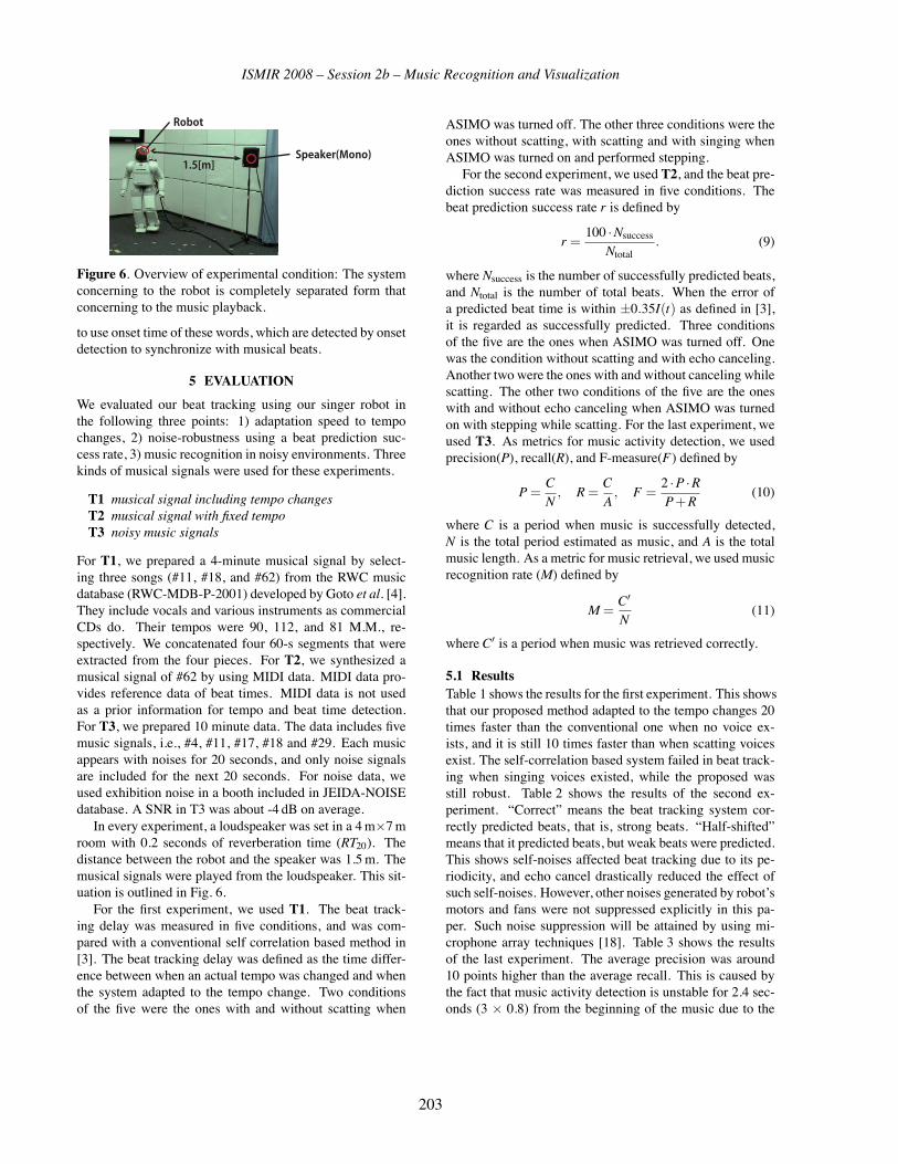
ISMIR 2008 – Session 2b – Music Recognition and Visualization
Robot
Speaker(Mono)1.5[m]
Figure 6. Overview of experimental condition: The systemconcerning to the robot is completely separated form thatconcerning to the music playback.
to use onset time of these words, which are detected by onsetdetection to synchronize with musical beats.
5 EVALUATION
We evaluated our beat tracking using our singer robot inthe following three points: 1) adaptation speed to tempochanges, 2) noise-robustness using a beat prediction suc-cess rate, 3) music recognition in noisy environments. Threekinds of musical signals were used for these experiments.
T1 musical signal including tempo changesT2 musical signal with fixed tempoT3 noisy music signals
For T1, we prepared a 4-minute musical signal by select-ing three songs (#11, #18, and #62) from the RWC musicdatabase (RWC-MDB-P-2001) developed by Goto et al. [4].They include vocals and various instruments as commercialCDs do. Their tempos were 90, 112, and 81 M.M., re-spectively. We concatenated four 60-s segments that wereextracted from the four pieces. For T2, we synthesized amusical signal of #62 by using MIDI data. MIDI data pro-vides reference data of beat times. MIDI data is not usedas a prior information for tempo and beat time detection.For T3, we prepared 10 minute data. The data includes fivemusic signals, i.e., #4, #11, #17, #18 and #29. Each musicappears with noises for 20 seconds, and only noise signalsare included for the next 20 seconds. For noise data, weused exhibition noise in a booth included in JEIDA-NOISEdatabase. A SNR in T3 was about -4 dB on average.In every experiment, a loudspeaker was set in a 4m×7m
room with 0.2 seconds of reverberation time (RT20). Thedistance between the robot and the speaker was 1.5m. Themusical signals were played from the loudspeaker. This sit-uation is outlined in Fig. 6.For the first experiment, we used T1. The beat track-
ing delay was measured in five conditions, and was com-pared with a conventional self correlation based method in[3]. The beat tracking delay was defined as the time differ-ence between when an actual tempo was changed and whenthe system adapted to the tempo change. Two conditionsof the five were the ones with and without scatting when
ASIMO was turned off. The other three conditions were theones without scatting, with scatting and with singing whenASIMO was turned on and performed stepping.For the second experiment, we used T2, and the beat pre-
diction success rate was measured in five conditions. Thebeat prediction success rate r is defined by
r =100 ·Nsuccess
Ntotal. (9)
where Nsuccess is the number of successfully predicted beats,and Ntotal is the number of total beats. When the error ofa predicted beat time is within ±0.35I(t) as defined in [3],it is regarded as successfully predicted. Three conditionsof the five are the ones when ASIMO was turned off. Onewas the condition without scatting and with echo canceling.Another two were the ones with and without canceling whilescatting. The other two conditions of the five are the oneswith and without echo canceling when ASIMO was turnedon with stepping while scatting. For the last experiment, weused T3. As metrics for music activity detection, we usedprecision(P), recall(R), and F-measure(F) defined by
P=CN
, R=CA
, F =2 ·P ·RP+R
(10)
where C is a period when music is successfully detected,N is the total period estimated as music, and A is the totalmusic length. As a metric for music retrieval, we used musicrecognition rate (M) defined by
M =C′
N(11)
whereC′ is a period when music was retrieved correctly.
5.1 ResultsTable 1 shows the results for the first experiment. This showsthat our proposed method adapted to the tempo changes 20times faster than the conventional one when no voice ex-ists, and it is still 10 times faster than when scatting voicesexist. The self-correlation based system failed in beat track-ing when singing voices existed, while the proposed wasstill robust. Table 2 shows the results of the second ex-periment. “Correct” means the beat tracking system cor-rectly predicted beats, that is, strong beats. “Half-shifted”means that it predicted beats, but weak beats were predicted.This shows self-noises affected beat tracking due to its pe-riodicity, and echo cancel drastically reduced the effect ofsuch self-noises. However, other noises generated by robot’smotors and fans were not suppressed explicitly in this pa-per. Such noise suppression will be attained by using mi-crophone array techniques [18]. Table 3 shows the resultsof the last experiment. The average precision was around10 points higher than the average recall. This is caused bythe fact that music activity detection is unstable for 2.4 sec-onds (3 × 0.8) from the beginning of the music due to the
203

ISMIR 2008 – Session 2b – Music Recognition and Visualization
Table 1. Tracking Delay for Tempo Changes (in second)ASIMO power off ASIMO with step
scatting off on off on offsinging off off off off on
self-correlation 11.24 29.91 14.66 20.43 N/Aproposed 1.31 1.31 1.29 1.29 1.29
Table 2. Beat Prediction Success RateASIMO power off ASIMO power on
(with step)scatting off on on
echo cancel off on off on off
Correct 95% 97% 68% 95% 64%Half shifted 5% 1% 40% 4% 40%
Table 3. Music Recognition Result (P: precision, R: recallrate, F: f-measure)
with noise cleanID bpm P (%) R (%) F P (%) R (%) F
#4 86 94.7 84.9 0.90 94.8 81.2 0.87#11 90 74.3 67.3 0.71 96.1 72.1 0.82#17 97 88.0 83.1 0.85 95.3 81.6 0.88#29 103 93.4 81.5 0.87 95.9 82.2 0.88#18 112 89.6 82.8 0.86 95.9 83.2 0.89
3-second window. In #11 and #17, precision was affectedby noises. This is because the noise includes a periodic sig-nal between 90 and 97 bpms. M was 95.8% for clean data,and 88.5% for noisy data. We can say that music recog-nition worked well for a small number of songs althoughusing only tempo information. To improve the scalability ofmusic recognition, we will use higher information such asrhythmic features such as [9].
6 CONCLUSIONS
We presented a real-time beat-tracking method for robotswhich is noise-robust and quickly-adaptable to musical beatchanges. The method uses spectro-temporal pattern match-ing to improve the adaptation speed against tempo changes,and echo canceling based on semi-blind independent com-ponent analysis to suppress self periodic noises such as scat-ting and singing. We showed a singer robot using HondaASIMO as an application of the proposed beat-tracking. Itsings or scats while stepping synchronized to musical beatsdetected by using robot-embedded microphones, and also ithas a simple function to recognize music based on musicalbeat information. Performance evaluation of the proposedbeat tracking method showed high noise-robustness, quickadaptation to tempo changes, high music recognition per-formance. We believe that the proposed method and its ex-tension will help to realize more active and enjoyable userinterface through music, although further evaluation withbenchmark datasets is necessary to know its performance
precisely. More sophisticated robot motions such as danc-ing, improvements of robustness of beat tracking, introduc-tion of other music information processing are remainingfuture work.
7 REFERENCES
[1] J. J. Aucouturier et al. Cheek to Chip: Dancing Robots and AI’s Future.Intelligent Systems, IEEE, 23(2):74–84, 2008.
[2] A. Cemgil and B. Kappen. Monte carlo methods for tempo trackingand rhythm quantization. J. of Artificial Intelligence Research, 18:45–81, 2003.
[3] M. Goto. An audio-based real-time beat tracking system for music withor without drum-sounds. J. of New Music Research, 30(2):159–171,2001.
[4] M. Goto et al. RWCmusic database: Popular, classical, and jazz musicdatabases. In Int. Conf. Music Info. Retrieval, pages 287–288, 2002.
[5] M. Goto and Y. Muraoka. A real-time beat tracking system for audiosignals. In Proc. of the Int’l Computer Music Conf., pages 171–174,San Francisco CA, 1995. International Computer Music Association.
[6] F. Gouyon et al. An experimental comparison of audio tempo induc-tion algorithms. IEEE Trans. Audio, Speech and Language Processing,14(5):1832–1844, 2006.
[7] I. Hara et al. Robust speech interface based on audio and video infor-mation fusion for humanoid HRP-2. In Proc. of IEEE/RSJ Int’l Conf.on Intel. Robots and Systems (IROS 2004), pages 2404–2410. IEEE,2004.
[8] K. Jensen and T.H. Andersen. Real-time beat estimation using featureextraction. Proc. Computer Music Modeling and Retrieval Symposium,Lecture Notes in Computer Science. Springer Verlag, 2003.
[9] D. Kirovski and H. Attias. Beat-ID: Identifying music via beat analysis.
[10] A. P. Klapuri et al. Analysis of the meter of acoustic musical signals.IEEE Trans. Audio, Speech, and Language Processing, 14(1), 2006.
[11] S. Kotosaka and S. Schaal. Synchronized robot drumming by neuraloscillators. In Proc. of Int’l Sympo. Adaptive Motion of Animals andMachines, 2000.
[12] T. Kurozumi et al.A robust audio searching method for cellular-phone-based music information retrieval. In Proc. of Int’l Conf. on PatternRecognition (ICPR’02), volume 3, page 30991, 2002.
[13] M. P. Michalowski et al. A dancing robot for rhythmic social interac-tion. In Proc. of ACM/IEEE Int’l Conf. on Human-Robot Interaction(HRI 2007), pages 89–96. IEEE, 2007.
[14] K. Nakadai et al. Active audition for humanoid. In Proc. of NationalConf. on Artificial Intelligence (AAAI-2000), pages 832–839. AAAI,2000.
[15] A. Nakazawa et al. Imitating human dance motions through motionstructure analysis. In Proc. of IEEE/RSJ Int’l Conf. on Intel. Robot sand Systems (IROS-2002), pages 2539–2544, 2002.
[16] R. Takeda et al. Exploiting known sound sources to improve ica-based robot audition in speech separation and recognition. In Proc. ofIEEE/RSJ Int’l Conf. on Intel. Robots and Systems (IROS-2007), pages1757–1762, 2007.
[17] T. Takeda et al. Hmm-based error detection of dance step selection fordance partner robot –MS DanceR–. In Proc. of IEEE/RSJ Int’l Conf.on Intel. Robots and Systems (IROS-2006), pages 5631–5636, 2006.
[18] S. Yamamoto et al., T. Ogata, and H. G. Okuno. Real-time robot au-dition system that recognizes simultaneous speech in the real world.In Proc. of IEEE/RSJ Int’l Conf. on Intel. Robots and Systems (IROS2006), pages 5333–5338. IEEE, 2006.
[19] K. Yoshii et al. A biped robot that keeps steps in time with musicalbeats while listening to music with its own ears. In Proc. of IEEE/RSJInt’l Conf. on Intel. Robots and Systems (IROS-2007), pages 1743–1750, 2007.
204

ISMIR 2008 – Session 2b – Music Recognition and Visualization
STREAMCATCHER: INTEGRATED VISUALIZATION OF MUSIC CLIPSAND ONLINE AUDIO STREAMS
Martin Gasser, Arthur FlexerAustrian Research Institute
for Artificial Intelligence (OFAI)Freyung 6/6
A-1010 Vienna, Austria
Gerhard WidmerDepartment of Computational Perception
Johannes Kepler UniversityLinz, Austria
ABSTRACT
We propose a content-based approach to explorative visu-
alization of online audio streams (e.g., web radio streams).
The visualization space is defined by prototypical instances
of musical concepts taken from personal music collections.
Our system shows the relation of prototypes to each other
and generates an animated visualization that places repre-
sentations of audio streams in the vicinity of their most simi-
lar prototypes. Both computation of music similarity and vi-
sualization are formulated for online real time performance.
A software implementation of these ideas is presented and
evaluated.
1 INTRODUCTION
A massive amount of music is already available on the web
in the form of internet radio streams. At the time of writ-
ing this paper, the “radio-locator” website 1 lists more than
2500 entries in its directory of free internet radio stations, a
number that is likely to increase rapidly in the future. Be-
cause it is infeasible for users to keep an overview of avail-
able radio streams, software that recommends possibly in-
teresting radio streams would be desirable.
When talking about music, humans usually use exam-
ples of similar music to describe new and unknown songs
or artists. For example, one might characterize Nirvana as a
combination of the Pixies’ and Sonic Youth’s guitar sound,
the Beatles’ sense for catchy melody lines, and the heritage
of American folk-rock music in the style of Neil Young. So,
instead of resorting to predefined taxonomies for music cat-
egorization (e.g., by Genre), an alternative is to present a
“query by example” based user interface directly to the user.
To support the user in finding new music he or she might
like in audio streams, we propose a simple interactive visu-
alization approach that incorporates the user’s musical vo-
cabulary into the definition of semantic spaces for music
similarity judgement. The user defines her own semantic
1 http://www.radio-locator.com/
space by supplying, coloring and labeling an arbitrary num-
ber of reference songs from her own music collection. In
this way, she can define her personal musical concepts via
examples she is familiar with.
In our application, songs from personal music collections
are imported in an incremental, user-feedback based man-
ner: (1) A new sound clip (concept prototype) is loaded
into the system and it is compared to already loaded clips
with a content-based music similarity measure, (2) the soft-
ware shows the user what it thinks the new music is similar
to and puts a preliminary label on it, (3) the user refines
the software suggestion by correcting the label, (4) go back
to (1). When the user decides that the concepts he or she
is interested in are sufficiently well represented, unknown
music from internet radio streams can be compared to the
sound prototypes (using the same similarity metric), and a
visualization is generated by means of a multidimensional
scaling [4] technique. The visualization also provides di-
rect interaction facilities that allow the playback of streams
and clips to interactively explore the audio streams audio-
visually.
Additionally to mapping acoustic similarity to proximity
information in the 2D visualization, color is used to encode
the user’s view of what the music sounds like. Colors can be
assigned to songs upon loading them into the system by the
user. This idea is motivated by the neurologically based phe-
nomenon of synesthesia [1, 14], in which stimulation of one
sense automatically triggers experiences in another sense.
2 RELATED WORK
Berenzweig et al. [3] construct an Anchor Space by training
N classifiers to prototypical instances of concepts, classify-
ing unknown music, and mapping posterior probabilities to
the individual dimensions of vectors in an N -dimensional
space. Distances in this space have been shown to better
reflect the user’s notion of music similarity.
Lidy and Rauber [7] calculated features derived from long-
term observations of (terrestrial) radio stations and used a
SOM to generate a 2D visualization of the types of music
205

ISMIR 2008 – Session 2b – Music Recognition and Visualization
PersonalMusic
Collection
Stream Stream Stream
Distancecalculation
User Interface+
Visualization+
Playback
Prototype selection
Feature Extraction
Feature Extraction
Figure 1. System components
played in different radio stations. However, they do not per-
form online analysis of radio streams.
Tzanetakis [13] extracted features from audio streams in
real time and displayed genre membership of the streams
in a real time visualization. By reducing dimensionality of
the feature space with a Principal Component Analysis, he
also mapped audio signals from high-dimensional timbre-
similarity space into a three-dimensional visualization space.
To the authors’ knowledge, this was the first published im-
plementation of online/real time audio signal classification
and similarity analysis.
Lamere [6] uses a technique based on acoustic similarity
and multidimensional scaling to visualize and explore music
collections in 3D space. This work is related to our work in
that it also shows the disparity between acoustic and high-
level similarity.
Lübbers [9] derives prototypical songs by hierarchically
clustering music collections, and proposes a multi-modal
user interface for interactively exploring the cluster centers’
neighborhood.
Recently, some work in the field of Human-Computer In-
teraction has been published (see also [1, 14]) that gives rise
to the presumption that organizing music by color is quite
intuitive. We also used this idea in our application to iden-
tify music that belongs to a common abstract concept, which
could be a genre, a particular kind of instrumentation, a cer-
tain guitar sound, and so on.
3 SYSTEM OVERVIEW
To evaluate our approach, we implemented an application
prototype that performs online (a) feature extraction, (b)
similarity calculation, and (c) visualization. Figure 1 sketches
the main components of the application.
The feature extraction subsystems are responsible for ex-
tracting feature frames from offline clips and online streams
of audio data. The distribution of these feature frames is
then modeled as a single Gaussian with full covariance [10]
per clip/stream.
Central to our framework is the similarity calculation com-
ponent that calculates distance matrices holding clip-to-clip
and stream-to-clip similarities by calculating the symmetric
Kullback-Leibler (KL) divergence [5] between each pair of
Gaussians.
Distances between clips are then projected to a 2D visu-
alization space with a Multidimensional Scaling [4, 2] algo-
rithm, whereas streams are linearly embedded into a local
subspace spanned by the 3 nearest neighbors of a stream
model in feature space.
3.1 Implementation notes
The application was implemented in C++ using the Open-
Source QT 2 toolkit , and we use OpenGL 3 for the visu-
alizations. All signal processing and statistical computing
was implemented within the FLOWer framework, a portable
and efficient C++ library for data flow-oriented media pro-
cessing, which is being developed by the first author of this
paper.
4 FEATURE EXTRACTION & SIMILARITYCALCULATION
In order to be able to extract features from offline files as
well as from live streams, the system contains two feature
extraction pipelines. In both pipelines, Mel Frequency Cep-
stral Coefficients (MFCCs) [8] are computed for each frame
of audio data. The main difference between online and of-
fline analysis is the way statistics (means and covariances)
are calculated. While in the offline case, the distribution
of MFCC’s in an entire audio file is estimated, the online
scenario requires more diligence; since the distribution of
features in an internet radio stream is not likely to stay con-
stant, we only take the most recent feature frames into ac-
count. For performance reasons, we decided to use a recur-
sive estimator for means and covariances instead of a sliding
window approach.
The input to the feature extraction stage is either an MP3
file or an MP3 stream (which can be transmitted over an
HTTP connection). This data is decoded to PCM at a sample
rate of 44.1kHz, converted to mono, and sliced into frames
of size 2048 samples with 50% overlap. Then, the frames
are multiplied with a Hamming window, the magnitude spec-
trum and MFCCs are calculated, and a statistical model is
derived from the data.
2 http://www.trolltech.com/products/qt3 http://www.opengl.org
206

ISMIR 2008 – Session 2b – Music Recognition and Visualization
4.1 Offline processing
In the offline case, the calculation the mean vector μ and the
covariance matrix Σ in the stream processing framework is
straighforward. Let X be a vector of random variables, and
xi a concrete instantiation (sample) of X (in our case an
MFCC vector from frame i).Since
Σ = E(XX�)− μμ� (1)
and
μ =1n
Σxi (2)
E(XX�) =1n
Σxixi� (3)
all that is needed is one accumulation vector and one accu-
mulation matrix for the sums and the sums of products of
observations, respectively.
4.2 Online processing
Since in an online scenario the complete sequence of feature
frames is not available beforehand, we use a recursive esti-
mate of mean and covariance to parameterize the distribu-
tion of timbral features (we preferred a recursive estimator
to windowed statistics for performance reasons).
The recursive estimate of the mean vector μ is calculated as:
μn = (1− α)μn−1 + αxn (4)
The covariance matrix Σ of a multidimensional vector of
random variables X can be written as
Σ = E(XX�)− μμ� (5)
E(XX�) can be estimated recursively as
E(XX�) = Rn = (1− α)Rn−1 + αxx� (6)
and
Σn = Rn − μμ� (7)
which can be refactored to
Σn = (1− α)Rn−1 + αxx� − μμ�
= (1− α)[Rn−1 − μn−1μ�n−1︸ ︷︷ ︸
Σn−1
+
. . . α (xnx�n − μn−1μ
�n−1 − xnμ�
n−1 + x�n μn−1)︸ ︷︷ ︸
(xn−μn−1)(xn−μn−1)�
]
Thus,
Σn = (1− α)[Σn−1 + α(xn − μn−1)(xn − μn−1)�] (8)
Small values of the parameter α assign small weights to
present values, thus the sequence of estimates is smoother
with smaller α. In experiments, we found α = 0.001 to be
a reasonable setting.
For the implementation of the recursive estimation algo-
rithms only one vector and one matrix accumulator are nec-
essary. This is a clear advantage over windowed estimation
approaches, where all measurements that fall inside the win-
dow must be memorized.
4.3 Distance calculation
Clip-to-clip distance is calculated upon loading of a new clip
by storing the Kullback-Leibler (KL) divergences between
each clip pair to a distance matrix. Clip-to-stream distances
must be recalculated continuously because the distribution
of stream features can change at any time.
4.4 Evaluation of the incremental similarity measure
In figure 2, we have plotted the similarities of a set of music
clips to a music stream. We used the 4 reference clips listed
in table 1.
The 4 plots correspond to the 4 clips, each plot shows the
similarity of the current stream content to the reference clip
(x axis is in audio frame numbers, 1 frame corresponds to
the FFT hop size of 1024 samples). We calculate the simi-
larity of the stream at time t to the clip Ci as the reciprocal
value of the KL divergence between the stream model and
the clip model, and we normalize the sum of clip-to-stream
similarities over all clips at time t to one.
Artist/Composer TitleAbsolute Beginner Rock On
Metallica The Four Horsemen
Al Green Listen
Heitor Villa-Lobos Etude n. 1 en mi mineur
Table 1. Reference clips used for the evaluation
Artist/Composer Title FramesA Tribe Called Quest Buggin Out 0–9388
Megadeth This was my Life 9389–18776
Al Green Listen 18777–25150
Heitor Villa-Lobos Etude n.2 en la majeur 25151–29715
Male Speech 29716–34539
Table 2. Stream used for the evaluation
207

ISMIR 2008 – Session 2b – Music Recognition and Visualization
The similarity measure successfully identifies music from
the same genre, style, or artist (“A Tribe Called Quest” have
the highest similarity with the “Absolute Beginners” clip,
“Megadeth” are most similar to “Metallica”, and the clip-to-
stream self-similarity for Al Green’s “Listen” stays at∼ 0.8almost over the entire duration of the song). However, the
system tends to confuse Rap vocals with pure speech al-
though it should emit low similarity scores with respect to
all reference clips (last part of the stream versus the “Abso-
lute Beginner” song) - this observation seems to be related
to the fact that simple timbral similarity based on MFCC
statistics wrongly classifies “Rap” and “Speech” as similar.
Another shortcoming can be observed using the Absolute
Beginner’s and Al Green’s songs as examples - both yield
high similarity scores in the beginning of the Al Green tune,
which seems to be related to the use of strong percussion in
both pieces.
Figure 2. Online stream similarity to offline reference clips
5 GRAPHICAL USER INTERFACE
Figure 4 shows a screenshot of the running StreamCatcherapplication. The GUI of the application currently consists
of a visualization that allows direct manipulation (zooming,
panning, rotating, playback of clips and streams) of the visu-
alized objects via a pointing device like a mouse or a touch
screen.
By pressing the ”Load Clip” button, a new sound clip
is loaded into the application. After analyzing and k-NN-
classifying the clip, a label (consisting of a textual descrip-
tion and a color) is suggested by the software in a dialog
window. Now the user has the possibility to accept the sug-
gestion, to change the label to another – already existing
A B C D
A 0 dab dac dad
B dab 0 dbc dbd
C dac dbc 0 dcd
D dad dbd dcd 0
MD
S
Stream S
A daS
B dbS
C dbS
D ddS
Clip-to-clip distance Clip-to-stream distance
NN
daS dbS
dcS
Stream position
Figure 3. Placement of online streams in visualization space
– label or create a new label. Furthermore, it is always
possible to alter the labeling of the clips later on. If the
“Open Stream” button is pressed, the user can load an MP3
stream, which is subsequently visualized with the algorithm
described below.
5.1 Visualization algorithm
It is well known that the symmetric KL divergence between
Gaussians does not satisfy the requirements to a proper dis-
tance measure [12]. Therefore, we use a visualization tech-
nique that seeks to preserve the KL divergence values in
a low-dimensional visualization space and relaxes this de-
mand if that is not possible. A classic distance-preserving
data mining/visualization technique is Multidimensional Scal-
ing [4], which aims at placing data points in low dimen-
sional visualization space while approximating the distances
in feature space as closely as possible. Multidimensional
scaling can be implemented as a spring model [2, 11], a
physically inspired model of spring-connected nodes aiming
at finding a node placement that minimizes the cumulative
deflection from the springs’ resting states. By mapping dis-
tances in feature space to spring lengths, the spring model
solves the MDS problem approximately.
We chose to use a spring model variant of MDS because
of its ease of implementation and because of the attractive
visualizations that can be generated by constantly drawing
the gradual relaxation of the system. By using a gradient-
descent based solution algorithm (see algorithm 1), a place-
ment of the nodes that minimizes the overall stress (the de-
flection from the springs’ resting state) is constructed.
While the overall stress in the model (Scum) is larger than
a threshold (Sthresh), the algorithm loops over all nodes and
determines for each node a force acting upon the node by
calculating a weighted sum of unit vectors pointing from
the current node to all other nodes. The weights can be pos-
itive or negative, depending on the difference between high-
and low-dimensional distances. Then, a velocity vector is
208

ISMIR 2008 – Session 2b – Music Recognition and Visualization
Figure 4. Screenshot showing the running application
Algorithm 1 Spring model layout algorithm
repeatScum = 0for Ca ∈ C do−→
f =−→0
for Cb ∈ C do−→u ← unit(p(Ca)− p(Cb))S ← dhigh(Ca, Cb)− dlow(Ca, Cb)−→f ← −→
f +−→u ∗ SScum ← Scum + |S|
end forv(CA) ← v(CA) +
−→f
p(Ca) ← p(Ca) + v(CA)v(CA) ← v(CA) ∗ dampingFactor
end foruntil Scum < Sthresh
Scum : Cumulative stress in the model
C : Set of clip nodes
unit : Function returning a unit vector
p : Vector-valued function returning the 2D position of a clip node
dhigh : Distance of clips in feature space
dlow : Distance of clips nodes in visualization space
v : Vector-valued function returning the current velocity of a clip node
−→f : Force acting upon a node
updated for the current node by adding the force vector to
its current value. Finally, the node’s position is updated by
moving it into the direction of its velocity, and the node’s
velocity is multiplied with a damping factor.
We use spring model MDS to place the static clips in
a 2D visualization. Upon loading of a new clip, an MDS
procedure is executed until the cumulative stress goes below
a threshold value. The placement of the dynamic streams
is determined by calculating the distances to the 3 nearest
neighbors in the feature space and using the reciprocal value
of those distances to calculate a convex combination of the
positions of the nearest neighbors that have been placed by
the MDS algorithm (see figure 3). Additionally, the true
distances to the anchor clips are visualized by drawing the
audio waveform of the stream’s audio signal between the
stream’s position and the clips’ positions, and by modulating
the opacity of this waveform with the feature space distance.
The smaller the feature space distance, the more opaque is
the drawing of the waveform.
In the screenshot (figure 4), example clips for four dif-
ferent styles/genres of music are loaded (Heavy Metal: Red,
HipHop: Yellow, Jazz Guitar: Green, Classical Guitar: Blue).
The green outlier, which is closer to the Classic Guitar clus-
ter than to Jazz Guitar, is a solo guitar piece by Pat Metheny,
which makes the placement quite reasonable. The two streams
(the loudspeaker-like symbols emanating the waveforms) play
Heavy Rock music and Soul/Funk. The Rock stream is
placed near the Heavy Metal-cluster, whereas the Soul stream
209

ISMIR 2008 – Session 2b – Music Recognition and Visualization
is placed close to the HipHop clusters, which characterizes
the music quite well.
6 CONCLUSIONS & FUTURE WORK
We have presented an application prototype for similarity
analysis and visualization of audio files and online audio
streams in a common framework. Music clips from personal
music collections are used as prototypical instances of musi-
cal concepts that define a visualization space in which online
streams are embedded. For the online calculation of mu-
sic similarity from streams we derived a similarity measure
which is based on incrementally updated statistical models.
The system comprises a user interface that supports the user
in identifying prototypical examples of high level musical
concepts. Acoustic similarity is mapped to proximity data
in a 2D visualization, which in turn is derived from a high
dimensional timbre similarity space by means of multidi-
mensional scaling. Sound prototypes can be labeled with
user-definable colors as well as textual labels.
The system successfully identifies streams that sound sim-
ilar to prototypical clips. Thus, it can be used to get a rough
overview of audio stream content, e.g., of internet radio sta-
tions. By exploring the suggestions of the software, the user
may find music he or she likes faster than by just blindly
trying radio stations.
We are currently working on improving the underlying
distance measure and on special cases like speech-music
discrimination, which could be a very useful feature for this
application.
7 ACKNOWLEDGEMENTS
This research is supported by the Austrian Research Promo-
tion Agency (FFG) under project number 815474 B1, and
by the Austrian Science Fund (FWF) under project number
L511-N15.
8 REFERENCES
[1] S. Baron-Cohen and J. Harrison. Synaesthesia: Classicand Contemporary Readings. Oxford: Blackwell Pub-
lishers, 1997.
[2] G. Di Battista, P. Eades, R. Tamassia, and I. G. Tol-
lis. Graph Drawing: Algorithms for the Visualization ofGraphs. Prentice Hall, 1999.
[3] A. Berenzweig, D. P. W. Ellis, and S. Lawrence. An-
chor space for classification and similarity measurement
of music. In ICME ’03: Proceedings of the 2003 In-ternational Conference on Multimedia and Expo, pages
29–32, Washington, DC, USA, 2003. IEEE Computer
Society.
[4] M.F. Cox and M.A.A Cox. Multidimensional Scaling.
Chapman and Hall, 2001.
[5] S. Kullback and R. A. Leibler. On information and suf-
ficiency. Annals of Mathematical Statistics, 22:79–86,
1951.
[6] Paul Lamere and Douglas Eck. Using 3d visualizations
to explore and discover music. In Proceedings of the8th International Conference on Music Information Re-trieval, Vienna, Austria, September 2007.
[7] Thomas Lidy and Andreas Rauber. Visually profiling
radio stations. In Proceedings of the 7th InternationalConference on Music Information Retrieval, 2006.
[8] Beth Logan. Mel frequency cepstral coefficients for mu-
sic modeling. In Proceedings of the 1st InternationalConference on Music Information Retrieval, Plymouth,
Massachusetts, 2000.
[9] Dominik Lübbers. Sonixplorer: Combining visualiza-
tion and auralization for content-based exploration of
music collections. In Proc. of the 6th International Con-ference on Music Information Retrieval, London, UnitedKingdom, 2005.
[10] Michael Mandel and Dan Ellis. Song-level features and
support vector machines for music classification. In Pro-ceedings of the 6th International Conference on MusicInformation Retrieval, London, United Kingdom, 2005.
[11] Alistair Morrison, Greg Ross, and Matthew Chalmers.
Fast multidimensional scaling through sampling,
springs and interpolation. Information Visualization,
2(1):68–77, 2003.
[12] Elias Pampalk. Computational Models of Music Similar-ity and their Application in Music Information Retrieval.PhD thesis, Vienna University of Technology, Vienna,
Austria, March 2006.
[13] George Tzanetakis and Perry Cook. Marsyas3d: A pro-
totype audio browser-editor. In Proceedings of the 7thInternational Conference on Auditory Display (ICAD),Helsinki, Finland, 2001.
[14] M. Voong and R. Beale. Music organisation using colour
synesthesia. In CHI ’07 Extended Abstracts on HumanFactors in Computing Systems, San Jose, CA, USA,
April 28 - May 03 2007.
210

ISMIR 2008 – Session 2b – Music Recognition and Visualization
MUSIC THUMBNAILER: VISUALIZING MUSICAL PIECESIN THUMBNAIL IMAGES BASED ON ACOUSTIC FEATURES
Kazuyoshi Yoshii Masataka GotoNational Institute of Advanced Industrial Science and Technology (AIST)
{k.yoshii,m.goto}@aist.go.jp
ABSTRACT
This paper presents a principled method called MusicThumb-nailer to transform musical pieces into visual thumbnail im-
ages based on acoustic features extracted from their audio
signals. These thumbnails can help users immediately guess
the musical contents of audio signals without trial listening.
This method is consistent in ways that optimize thumbnails
according to the characteristics of a target music collection.
This means the appropriateness of transformation should be
defined to eliminate ad hoc transformation rules. In this pa-
per, we introduce three top-down criteria to improve mem-
orability of thumbnails (generate gradations), deliver infor-
mation more completely, and distinguish thumbnails more
clearly. These criteria are mathematically implemented as
minimization of brightness differences of adjacent pixels
and maximization of brightness variances within and be-
tween thumbnails. The optimized parameters of a modified
linear mapping model we assumed are obtained by minimiz-
ing a unified cost function based on the three criteria with a
steepest descent method. Experimental results indicate that
generated thumbnails can provide users with useful hints as
to the musical contents of musical pieces.
1 INTRODUCTION
Music recommender systems are increasingly important in
online music-distribution services to help users discover their
favorite pieces among a huge music collection. For instance,
recommender systems based on collaborative filtering [1, 2]
recommend musical pieces to the user by taking into ac-
count someone else’s ratings of those pieces. Content-based
filtering systems [3, 4] select musical pieces that are similar
to the user’s favorites in terms of musical content (acous-
tic features). Recently, several hybrid systems that integrate
these two techniques have been proposed to enable more ac-
curate recommendations [5, 6].
An important problem that has not been resolved is that
users cannot immediately grasp the musical contents of rec-
ommended pieces after these pieces are listed. Users have
to listen to all listed pieces, including those they do not like,
to find which pieces are worth listening to. This often pre-
vents users from seamlessly listening to their favorite pieces.
Worse still, trial listening is time-consuming because the in-
formation of audio signals (temporal media) is not simul-
taneously delivered to users whereas visual images (spatial
W. Houston
M. Carey J. Jackson
Mozart
Beethoven
Haydn
Thumbnails the user has ever seen before
This piece would have pops features
The generated thumbnail
of an unknown piece
Figure 1. Expected scenario: A user can roughly guess the
musical contents of unknown pieces by seeing only thumb-
nails and without time-consuming trial listening.
media) can be easily skimmed through.
To solve this problem, we propose an audio-visual trans-
formation method called MusicThumbnailer that generates
compact images corresponding to the audio signals of indi-
vidual pieces. This helps users guess the musical contents
of audio signals without trial listening. For example, this
method will work well in recommender systems, as shown
in Fig. 1. Initially, users only glance at compact thumbnails
attached to recommended pieces when they actually listen
to these pieces. While accumulating this experience, users
will unconsciously associate particular types of thumbnail
with their preferred music. Users thus learn to understand
the musical meanings of the thumbnails’ features. Finally,
users will be able to efficiently select audio signals of their
desired pieces by using their eyes rather than their ears.
One advantage of our method is that the visual features
(colors and patterns) of thumbnails are automatically opti-
mized for a given collection. To achieve this, it is necessary
to eliminate ad hoc rules that arbitrarily associate acoustic
features with visual features, because these rules lack a prin-
cipled justification that is consistent for different collections.
In this paper, we define some top-down criteria on generated
thumbnails from the viewpoint of usability, independently
of the characteristics of music collections. We then mathe-
matically represent these criteria in a unified cost function.
Audio-visual associations are obtained in a self-organized
way so that the cost function is minimized.
211

ISMIR 2008 – Session 2b – Music Recognition and Visualization
The rest of this paper is organized as follows. Section 2
introduces related work. Section 3 explains the principles of
our audio-visual transformation method and its implemen-
tation. Section 4 reports on our experiment using the RWC
Music Database [7]. Section 5 summarizes the key findings
of this paper.
2 RELATED WORK
Many visualization methods have been proposed for spatial
representation, organization, and browsing of music collec-
tions [8–16]. These methods typically locate musical pieces
in a two- or three-dimensional space so that musical pieces
that have similar musical contents (acoustic features) are ar-
ranged close to each other. This enables users to easily un-
derstand relationships between musical pieces because sim-
ilarity in acoustic features can be observed as spatial dis-
tance. From a mathematical viewpoint, this kind of visu-
alization can be interpreted as information compression of
high-dimensional feature vectors according to some crite-
ria. The self-organizing map (SOM) is often used for this
purpose (e.g., Islands of Music [8]).
In a music-playback interface called Musicream [17], in-
dividual musical pieces are visualized as colored discs using
an ad hoc rule. The disc color (hue and saturation) is deter-
mined from the color circle whose circumference and radius
correspond to hue and saturation, respectively. Each piece is
mapped into the circle according to its feature vector. Princi-
pal component analysis (PCA) is used to reduce the dimen-
sionality of acoustic feature vectors to a two-dimensional
vector on a plane. Musicovery [18] uses arbitrary rules for
associating genres with colors specified in advance.
In the work described in this paper, we aimed to visualize
individual pieces, rather than a collection, as compact im-
ages (thumbnails) without using ad hoc rules. In general, vi-
sual images are represented as super-high-dimensional vec-
tors that contain the color values of numerous pixels. There-
fore, our objective was to find an appropriate mapping from
a low-dimensional acoustic space (several-tens dim.) to a
high-dimensional visual space (several-thousands dim.). A
unique feature of this problem lies in this drastic increase in
degrees of freedom. To solve such an ill-posed problem by
using an optimization method, it is necessary to incorporate
some criteria on the appropriateness of the mapping.
3 MUSIC THUMBNAILER
This section describes our method of generating thumbnails
of musical pieces based on acoustic features.
3.1 Problem Specification
Given a collection of musical pieces (audio signals) as in-
put data, our objective is to output appropriate thumbnails
(visual images) that reflect acoustic features extracted from
these pieces. We first prepare some criteria to evaluate the
appropriateness of the generated thumbnails as discussed
later. In this paper, we focus on generating gray-scale thumb-
nails as the first step towards obtaining full-color thumbnails
in the future. This means we have only to deal with the
brightness of pixels contained in each thumbnail.
We first define constant values in advance. Let N be the
number of musical pieces. Let S be the number of acoustic
features taken into account. Let T be the number of pix-
els contained in each thumbnail, where T is the product of
width, W , and height, H; i.e., T = WH .
The input data is given by X = [x1x2 · · ·xN ], which
is a collection of feature vectors extracted from all musical
pieces. Here, xn = (xn,1, · · · , xn,S)T is an S-dimensional
feature vector of piece n (1 ≤ n ≤ N), where xn,s (1 ≤s ≤ S) represents the value of feature s in piece n.
The output data is represented as Y = [y1y2 · · ·yN ],which is a set of brightness vectors of generated thumbnails.
yn = (yn,1,1, · · · , yn,1,H , yn,2,1, · · · , yn,2,H , · · · , yn,W,1,· · · , yn,W,H )T is a T -dimensional brightness vector of piece
n, where yn,w,h (1 ≤ w ≤W, 1 ≤ h ≤ H) is the brightness
of pixel (w, h) in thumbnail n. The range of yn,w,h is given
by 0 < yn,w,h < 1.
3.2 Top-down Criteria for Principled Transformation
To evaluate the appropriateness of the generated thumbnails,
we introduce three top-down criteria from the viewpoint of
user friendliness (usability) as follows:
1. Memorability: Each thumbnail should be easily re-
membered by users. The visual pattern is an impor-
tant factor that affects the ease of remembering thumb-
nails, as shown in Fig. 2. This is related to how easily
users can understand the musical meanings of visual
patterns based on their memories. We assume that
gradation images are suitable to our purpose.
2. Informational delivery: Each thumbnail should pro-
vide a large amount of information to users. This is
achieved if thumbnail’s pixels have a wide variety of
brightness, as shown in Fig. 3. This enables users to
associate a thumbnail with detailed information about
the music content.
3. Distinguishability: Users should be able to easily dis-
tinguish thumbnail images of different pieces. To en-
able this, each thumbnail should have a distinctive vi-
sual pattern that explicitly reflects the content of mu-
sic, as shown in Fig. 4. This enables users to effi-
ciently find their favorite pieces based on thumbnails
they recognize.
Note that these criteria mention neither specific genres of
music nor specific colors of thumbnails.
212

ISMIR 2008 – Session 2b – Music Recognition and Visualization
Hard to remember
W1 2
1
2
H
W
1
2
H
1 2
Easy to remember
Figure 2. Difference in ease of remembering thumbnails.
Both thumbnails have the same histogram of brightness.
Small amount of info.
W1 2
1
2
H
W
1
2
H
1 2
Large amount of info.
Figure 3. Difference of the amount of information obtained
from thumbnails.
Easy to distinguish Hard to distinguish
Figure 4. Difference in ease of distinguishing thumbnails
of different pieces.
These top-down criteria enable us to design thumbnails
in a non-ad-hoc way. In general, system designers tend to
define ad hoc rules that directly associate musical contents
of musical audio signals with specific colors of visual im-
ages (e.g., rock-red, jazz-green, and classic-blue). However,
the appropriateness of these arbitrary rules cannot be guar-
anteed. In contrast, the criteria we proposed only regulate
the appropriateness of transformation. The actual colors and
patterns of thumbnails are optimized for a given collection
in a self-organized way so that the criteria are best satisfied.
Therefore, our approach is methodologically and mathemat-
ically sound.
A remaining problem here is how to mathematically im-
plement these criteria. In this paper, we will present a simple
implementation of the three criteria below.
3.3 Mathematical Formulation
From a mathematical point of view, the objective is to ob-
tain optimal parameters of a mapping model that transforms
a S-dimensional space to a T -dimensional space so that a
cost function defined according to the three criteria is mini-
mized. This transformation has a high degree of freedom; a
higher-dimensional space can always preserve the complete
information of an original space. We thus incorporate linear
mapping into a mapping model. This is reasonable because
linear mapping can strongly limit the degree of freedom in
transformation. In addition, musical pieces which are close
to each other in an acoustic space are expected to be mapped
still close to each other in a visual space. This effect is suit-
able to achieve the expected scenario shown in Fig. 1. We
define the mapping model as
Y = Sig(AX), (1)
where A is a T -by-S transformation matrix to be optimized,
which is given by⎡⎢⎢⎢⎢⎢⎢⎢⎢⎢⎢⎢⎢⎣
AT1,1...
AT1,H...
ATW,1...
ATW,H
⎤⎥⎥⎥⎥⎥⎥⎥⎥⎥⎥⎥⎥⎦=
⎡⎢⎢⎢⎢⎢⎢⎢⎢⎢⎢⎢⎣
A1,1,1 A1,1,2 · · · A1,1,S
......
A1,H,1 A1,H,2 · · · A1,H,S
......
AW,1,1 AW,1,2 · · · AW,1,S
......
AW,H,1 AW,H,2 · · · AW,H,S
⎤⎥⎥⎥⎥⎥⎥⎥⎥⎥⎥⎥⎦(2)
and Sig is the sigmoid function given by
Sig(x) =1
1 + e−x(−∞ < x <∞). (3)
In Eq. (1), we applied the sigmoid function to each cell of
matrix AX so that the value of each cell of matrix Y ranges
from 0 to 1. Note that the differential of the sigmoid func-
tion is given by Sig’(x) = Sig(x) (1− Sig(x)) .To evaluate the appropriateness of the mapping model,
we define a cost function, C, as
C = Cs + αwCw + αbCb, (4)
where Cs, Cw, and Cb are the costs corresponding to the
three criteria described in Section 3.2, and αw and αb are
the weighting parameters. We mathematically define these
three costs below.
3.3.1 Minimization of adjacent-pixel distances
To generate gradation images, we focus on a necessary con-
dition that the brightness values of adjacent pixels should be
close to each other. One way to mathematically implement
this condition is to minimize the differences of the bright-
ness values of adjacent pixels included in each thumbnail.
213

ISMIR 2008 – Session 2b – Music Recognition and Visualization
However, this calculation is not efficient because it would
have to be repeated for all thumbnails. To solve this prob-
lem, we directly define the cost function, Cs, for the trans-
formation matrix, A, as follows:
Cs =1
WHS
∑w,h,s
Dw,h,s, (5)
where Dw,h,s is the average of the following eight distances:
Dw,h,s =18
∑i,j=±1
(Aw,h,s −Aw+i,h+j,s)2
(6)
+18
∑i=±1
(Aw,h,s −Aw+i,h,s)2
(7)
+18
∑j=±1
(Aw,h,s −Aw,h+j,s)2. (8)
3.3.2 Maximization of within-thumbnail variances
To increase the amount of information delivered by a thumb-
nail, the brightness variance within the thumbnail should be
maximized. We formulate this condition for each thumbnail
and define the cost function, Cw, based on the average of
brightness variances over all thumbnails:
Cw = − 1N
∑n
1WH
∑w,h
(yn,w,h − ȳn)2 , (9)
where ȳn is an average of the brightness values of wh pixels
within a thumbnail of piece n, given by
ȳn =1
WH
∑w,h
yn,w,h. (10)
Note that maximization of within-thumbnail variances is equiv-
alent to minimization of the cost function Cw.
3.3.3 Maximization of between-thumbnail variances
To enable users to clearly distinguish generated thumbnails,
the brightness vectors of these thumbnails should be far from
each other. A simple way to satisfy this condition is to max-
imize the brightness variance between all thumbnails, where
the between-thumbnail variance is calculated in each posi-
tion, (w, h). We define the cost function, Cb, based on the
average of brightness variances over all positions as
Cb = − 1WH
∑w,h
1N
∑n
(yn,w,h − ȳw,h)2 , (11)
where ȳw,h is an average of the brightness values of n pixels
in the same position (w, h), given by
ȳw,h =1N
∑n
yn,w,h. (12)
Note that maximization of between-thumbnail variances is
equivalent to minimization of the cost function Cb.
3.4 Parameter Optimization
To minimize the total cost function, C, as an optimization
method, we use a steepest descent method that iteratively
updates the parameters until the cost reduction is converged.
The updating formula is given by
Aw,h,s ← Aw,h,s − η∂C
∂Aw,h,s, (13)
where η is a learning parameter (0 < η < 1) and ∂C∂Aw,h,s
is
decomposed into three terms:
∂C
∂Aw,h,s=
∂Cs
∂Aw,h,s+ αw
∂Cw
∂Aw,h,s+ αb
∂Cb
∂Aw,h,s. (14)
3.4.1 Derivation of updating formula
We now explain how to derive the updating formula. The
first term in Eq. (14) is obtained by
∂Cs
∂Aw,h,s=
2WHS
(Aw,h,s − Āw,h,s
), (15)
where Āw,h,s is an average of the values in the vicinity of
Aw,h,s, given by
Āw,h,s =Aw,h±1,s + Aw±1,h,s + Aw±1,h±1,s
8. (16)
The second and third terms are calculated as
∂Cw
∂Aw,h,s=
∂Cw
∂yn,w,h· ∂yn,w,h
∂Aw,h,s, (17)
∂Cb
∂Aw,h,s=
∂Cb
∂yn,w,h· ∂yn,w,h
∂Aw,h,s, (18)
where
∂Cw
∂yn,w,h= − 2
NWH(yn,w,h − ȳn) , (19)
∂Cb
∂yn,w,h= − 2
NWH(yn,w,h − ȳw,h) , (20)
∂yn,w,h
∂Aw,h,s= Sig’(AT
h,wxn)xn,s (21)
= Sig(ATh,wxn)
(1− Sig(AT
h,wxn))
xn,s.
(22)
3.4.2 Visual effects of updating formula
Next, we will discuss the visual effects of the three terms
of Eq. (14) in the mathematically derived updating formula.
Eq. (15) means the first term tries to make transformation
coefficients close to their smoothed versions. Eq. (16) cor-
responds to a visual processing algorithm that is used for
smoothing images by using a convolution matrix. Eq. (19)
and Eq. (20) mean the second and third terms try to make
the brightness value of each pixel far from the within- and
between-thumbnail averages. This enhances the dynamic
range of each thumbnail and the variety of generated thumb-
nails. These effects intuitively match our expectation.
214

ISMIR 2008 – Session 2b – Music Recognition and Visualization
4 EXPERIMENT
This section reports on a thumbnail-generation experiment
done to evaluate the usefulness of MusicThumbnailer.
4.1 Experimental Conditions
As a music collection, we used the “RWC Music Database:
Music Genre” (RWC-MDB-G-2001) [7], which consists of
100 pieces (N = 100) in total with three pieces prepared for
each of 33 genres and one for a cappella. This database is
divided into 10 main genre categories (popular, rock, dance,
jazz, Latin, classical, march, world, vocal, and traditional
Japanese music) and 33 subcategories (pops, ballad, rock,
heavy metal, rap/hip-hop, house, techno, funk, soul/R&B,
big band, modern jazz, fusion, bossa nova, samba, reggae,
tango, baroque, classic, romantic, modern, brass band, blues,
folk, country, gospel, African, Indian, flamenco, chanson,
canzone, traditional-style Japanese popular music, Japanese
folk music, and ancient Japanese court music).
To extract acoustic features, we used the MARSYAS [19].
We obtained a 42-dimensional feature vector for each piece,
which consists of the average and variance of local spec-
tral features (centroid, rolloff, and flux) and zero-crossings
across the entire piece (8 dimensions), average and variance
of Mel-frequency cepstral coefficients (MFCC) across the
entire piece (26 dimensions), and rhythmic content features
reflecting periodicity in beat (8 dimensions). We then used
PCA to reduce the dimensionality; the 42-dimensional space
was transformed into a 20-dimensional space still account-
ing for 95% of the variance of the original data (S = 20).
The size of thumbnails was 50× 50 (W = H = 50, T =2500). In this experiment, gray-scale thumbnails were con-
verted to full-color ones according to a lookup table shown
in Table 1 (called “Jet” color scheme in MATLAB) from an
aesthetic point of view. Note that this is just for convenience
because we should essentially eliminate such an ad hoc rule.
The values of parameters, αw, αb, and η were empirically
set to 0.4, 0.4, and 0.1.
4.2 Experimental Results
The experimental results indicate that the generated thumb-
nails are useful for guessing the musical contents, as shown
in Fig. 5. At the main-category level, thumbnails of pop-
ular/rock pieces, those of classical (orchestra) pieces, and
those of marches seem to be close to each other, respec-
tively. In the dance category, similar thumbnails were ob-
tained in each subcategory, where we can find the simi-
larity between rap/hip-hop and funk. The thumbnails of
funk pieces somewhat resemble those of reggae and African
pieces across the main category. This corresponds with the
fact that funk music has been developed while absorbing
the characteristics of African music and reggae. In the cat-
egories of Latin, world, and traditional Japanese, we can
Table 1. Lookup table for converting brightness to RGB.
Brightness 0.00 0.33 0.66 1.00
RGB (0,0,1) (0,1,1) (1,1,0) (1,0,0)
roughly say that similar thumbnails were obtained in each
subcategory. In the vocal category, each subcategory yielded
the similar thumbnails, which have especially unique pat-
terns among the database. In the jazz category, however,
there were comparatively wide variations in thumbnails of
each category. Moreover, fusion pieces tend to reflect and
mix the styles of other pieces.
5 CONCLUSION
We presented an audio-visual transformation method called
MusicThumbnailer that generates thumbnail images reflect-
ing acoustic features of audio signals. To achieve principled
transformation free from ad hoc rules, we designed three
top-down criteria regarding memorability, informational de-
livery, and distinguishability. These criteria are used to eval-
uate the appropriateness of generated thumbnails from the
viewpoint of usability rather than to associate specific acous-
tic features with actual colors and patterns of thumbnails.
From a mathematical viewpoint, we formulated this prob-
lem as a constrained minimization of a cost function based
on the three criteria. The experiment showed promising re-
sults as to the usefulness of MusicThumbnailer.
Many issues still remain regarding the refinement of our
method through subjective experiments. First, we plan to in-
troduce a new criterion to preserve the topological relations
of feature vectors in audio-visual transformation. Then, we
will improve the mathematical implementation of each cri-
terion and attempt to use a more sophisticated optimization
algorithm that can achieve fast convergence while avoiding
the local-minimum problem. Several experiments using dif-
ferent features and collections would be important. An in-
teresting application of our method would be to generate a
visual effect (a temporal sequence of visual images) that dy-
namically represents the local musical contents in a musical
piece. This can be done by interpreting feature vectors ex-
tracted from individual time frames in a musical piece in the
same way as for those extracted from individual pieces in a
music collection. Such a visualizer will give users a practi-
cal overview of structures within a musical piece.
6 REFERENCES
[1] Shardanand, U. and Maes, P., “Social Information Filtering:Algorithms for Automating “Word of Mouth”,” ACM Conf. onHuman Factors in Computing Systems, 1995, pp. 210–217.
[2] Cohen, W. and Fan, W., “Web-Collaborative Filtering: Recom-mending Music by Crawling the Web,” Computer Networks,Vol. 33, No. 1–6, pp. 685–698, 2000.
215

ISMIR 2008 – Session 2b – Music Recognition and Visualization
Pops Ballad
Rock Heavy metal
Rap/Hip-hop House
Techno Funk
Soul/R&B Big band
Modern jazz Fusion
Bossa nova Samba
Reggae Tango
Baroque Classic Romantic Modern
Brass band
Blues Folk
Baroque Classic Romantic Modern
Country Gospel
African Indian
Flamenco
ChansonCanzone
Popular (Enka) Folk (Min’you)
Court (Gagaku)
A Cappella
Popular
#1~#6
Rock
#7~#12
Dance
#13~#27
Jazz
#28~#36
Latin
#37~#48
Classical
(Orchestra)
#49~#53
March
#54~#56
World
#64~#84
Vocal
#85~#90
Traditional
Japanese
#91~#99
A Cappella
#100
Classical
(Solo/Chamber)
#57~#63
Figure 5. Experimental results of generating thumbnail images of 100 pieces included in RWC-MDB-G-2001 [7].
[3] Hoashi, K., Matsumoto, K., and Inoue, N., “Personalizationof User Profiles for Content-based Music Retrieval based onRelevance Feedback,” ACM Multimedia, 2003, pp. 110–119.
[4] Logan, B., “Music Recommendation from Song Sets,” ISMIR,2004, pp. 425–428.
[5] Celma, O., Ramirez, M., and Herrera, P., “Foafing the Music:A Music Recommendation System based on RSS Feeds andUser Preferences,” ISMIR, 2005, pp. 464–457.
[6] Yoshii, K., Goto, M., Komatani, K., Ogata, T., andOkuno, H. G., “An Efficient Hybrid Music Recommender Sys-tem Using an Incrementally-trainable Probabilistic GenerativeModel,” IEEE Trans. on Audio, Speech and Language Process-ing, Vol. 16, No. 2, pp. 435–447, 2008.
[7] Goto, M., Hashiguchi, H., Nishimura, T., and Oka, R., “RWCMusic Database: Music Genre Database and Musical Instru-ment Sound Database,” ISMIR, 2005, pp. 229-230.
[8] Pampalk, E., Dixon, S., and Widmer, G., “Exploring MusicCollections by Browsing Different Views,” ISMIR, Vol. 28,Mo. 2, pp. 49–62, 2004.
[9] Torrens, M., Hertzog, P., and Arcos, J., “Visualizing and Ex-ploring Personal Music Libraries,” ISMIR, 2004, pp. 421–424.
[10] Mörchen, F., Ultsch, A., Nöcker, M., and Stamm, C.,“Databionic Visualization of Music Collections According toPerceptual Distances,” ISMIR, 2005, pp. 396–403.
[11] Mayer, R., Dittenbach, M., and Rauber, A., “PlaySOM andPocketSOMPlayer: Alternative Interfaces to Large Music Col-lections,” ISMIR, 2005, pp. 618–623.
[12] Mayer, R., Lidy, T., Rauber, A., “The Map of Mozart,” ISMIR,2006, pp. 351–352.
[13] Knees, P., Schedl, M., Pohle, T., and Widmer. G., “An Inno-vative Three-dimensional User Interface for Exploring MusicCollections Enriched with Meta-Information from the Web,”ACM Multimedia, 2006, pp. 17–24.
[14] Leitich, S. and Topf, M., “Globe of Music: Music Library Vi-sualization Using GEOSOM,” ISMIR, 2007, pp. 167–170.
[15] Donaldson, J. and Knopke, I., “Music Recommendation Map-ping and Interface based on Structual Network Entropy,” IS-MIR, 2007, pp. 181–182.
[16] Lamere, P. and Eck, D., “Using 3D Visualizations to Exploreand Discover Music,” ISMIR, 2007, pp. 173–174.
[17] Goto, M. and Goto, T., “Musicream: New Music Playback In-terface for Streaming, Sticking, Sorting, and Recalling MusicalPieces,” ISMIR, 2005, pp. 404–411.
[18] Musicovery: http://musicovery.com/.
[19] Tzanetakis, G. and Cook, P., “MARSYAS: A Framework forAudio Analysis,” Organized Sound, No. 4, Vol. 3, pp. 169–175, 2000.
216

Session 2c – Knowledge Representation, Tags, Meta-data

.

ISMIR 2008 – Session 2c – Knowledge Representation, Tags, Metadata
TERNARY SEMANTIC ANALYSIS OF SOCIAL TAGS FORPERSONALIZED MUSIC RECOMMENDATION
Panagiotis Symeonidis1 Maria Ruxanda2 Alexandros Nanopoulos1 Yannis Manolopoulos1
1. Department of Informatics 2. Department of Computer ScienceAristotle Univ. of Thessaloniki, Greece Aalborg University, Denmark
ABSTRACT
Social tagging is the process by which many users addmetadata in the form of keywords, to annotate informationitems. In case of music, the annotated items can be songs,artists, albums. Current music recommenders which em-ploy social tagging to improve the music recommenda-tion, fail to always provide appropriate item recommen-dations, because: (i) users may have different interests fora musical item, and (ii) musical items may have multiplefacets. In this paper, we propose an approach that tacklesthe problem of the multimodal use of music. We developa unified framework, represented by a 3-order tensor, tomodel altogether users, tags, and items. Then, we recom-mend musical items according to users multimodal per-ception of music, by performing latent semantic analysisand dimensionality reduction using the Higher Order Sin-gular Value Decomposition technique. We experimentallyevaluate the proposed method against two state-of-the-artrecommendations algorithms using real Last.fm data. Ourresults show significant improvements in terms of effec-tiveness measured through recall/precision.
1 INTRODUCTION
Social tagging is the process by which many users addmetadata in the form of keywords to annotate and catego-rize information items such as songs, pictures, products.In general, social tagging is associated to the “Web 2.0”technologies and has already become an important sourceof information for recommendation. In the music domain,popular web systems such as Last.fm and MyStrands pro-vide possibility for users to tag with free text labels anitem of interest - e.g., artist, song, album. Such systemscan further exploit these social tags to improve the searchmechanisms and the personalized music recommendation.Recent research in the music field has also focused on
exploiting the social tags in various ways. For example,a partial solution to the cold-start problem of music rec-ommenders has been proposed in [4]: social tags are usedfor the automatic generation of new tags, which then can
THIS RESEARCH WAS SUPPORTED IN PART BY THE DAN-ISH RESEARCH COUNCIL FOR TECHNOLOGY AND PRODUC-TION SCIENCES PROJECT 26-04-0092 INTELLIGENT SOUND,AND BY GREEK SECRETARIAT FOR RESEARCH AND TECH-NOLOGY ΠABET (05ΠAB216) PROJECT.
be used to label the untagged music. In [9], the socialtags are investigated as a source of semantic metadata formusic, which can be used to generate a psychologically-motivated search-space representing musical emotion.However, the social tags carry useful information not
only about the musical items they label, but also aboutthe users who tagged. This aspect is not being fully ex-ploited, neither by the music recommenders, neither in theresearch field. Music is an artistic concept, and the musi-cal items (artists, songs, albums) have a rich and complexview, which is only partially perceived by particular users,depending on their emotional and cultural perspective onmusic. Social tags are a powerful mechanism that reveal3-dimensional correlations between users–tags–items. Thistriplet information can project for each user his perceptionof a particular musical item. However, the current musicrecommender systems are commonly using collaborativefiltering techniques, which traditionally exploit only pairsof 2-dimensional data. Thus, they are not capable of cap-turing well the multimodal use of music.As a simple example, let us consider the social tag-
ging system of artists in Last.fm. Assume two users. Oneis very fond of young female singers and therefore hastagged Christina Aguilera as “sexy” and Beyonce as “sen-sual”. Another is fond of male singers and has taggedLenny Kravitz as “sexy” and “male vocalists”. When want-ing to listen to “sexy” music, both users are recommendedmale and female singers, while the first user is expectingfemale singers and the other prefers the opposite.Recent research has focused on developing recommen-
dation algorithms [7, 14], which try to exploit tags givenby users on specific items. However, the existing algo-rithms do not consider the 3 dimensions of the problemaltogether, and therefore they miss a part of the semanticsthat is carried by the 3-dimensions.In this paper, we address the problem of music recom-
mendation by capturing the multimodal perception of mu-sic by particular users. We perform 3-dimensional analy-sis on the social tags data, attempting to discover the la-tent factors that govern the associations among the tripletsuser–tag–item. Consequently, the musical items (artists,songs or albums) can be recommended according to thecaptured associations. That is, given a user and a tag, thepurpose is to predict whether and how much the user islikely to label with this tag a specific musical item.Our strategy in dealing with the 3-dimensional social
219

ISMIR 2008 – Session 2c – Knowledge Representation, Tags, Metadata
tagging data, is to develop a unified framework to modelthe three dimensions. Thus, user-tag-item data is rep-resented by a 3-order tensor. Consequently, we have todeal with the data sparsity problem: the three-way data ishighly sparse, especially that each user only tags a smallnumber of items. Latent Semantic Indexing (LSI) hasbeen proved useful to address the data sparseness in 2-dimensional data recommender systems, however, it is stillan open problem for the 3-dimensional data case. There-fore, we perform 3-mode analysis, using the Higher OrderSingular Value Decomposition (HOSVD) technique.The contributions of our approach are as follow: (1)
we provide a method to improve music recommendationby capturing users multimodal perception of music; (2)wedevelop a unified framework, represented by a 3-order ten-sor, to model the three types of entities that exist in socialtagging data; (3) we apply dimensionality reduction in 3-order tensors to reveal the latent semantic associations be-tween users, tags, and items; (4) we perform experimentalcomparison of the proposed method against two state-of-the-art recommendations algorithms, using Last.fm data;our results show significant improvements in terms of ef-fectiveness measured through recall/precision.The rest of this paper is organized as follows. Section 2
summarizes the related work, whereas Section 3 briefly re-views background techniques employed in our approach.A motivating example and the proposed approach are de-scribed in Section 4. Experimental results are given inSection 5. Finally, Section 6 concludes this paper.
2 RELATEDWORK
Music recommendation has been addressed in various work.For example, in Logan [11] music recommendation is donebased solely on using acoustic-based similarity measure.Other approaches try to bridge the semantic gap and em-ploy hybrid music recommendation methods. Thus, Yoshiiet al. [15] model collaborative filtering (CF) data and audio-content data together, and unobservable user preferencesare statistically estimated. Li et al. [10] employ a proba-bilistic model estimation for CF, where musical items areclustered based on audio-content and user rating, and pre-dictions are made considering the Gaussian distribution ofratings. Celma [2] mines music information from the Web(album releases, MP3 blogs, etc.) and is using it togetherwith user profiling and audio-content descriptions.The above work can be used to improve the music rec-
ommendation by addressing the cold-start problem andthe bias of CF towards mainstreammusic. Along the samelines, an innovative use of social tags has been recentlyproposed in [4]. Eck et al. [4] predict new tags using au-dio features extracted frommusic and supervised learning.These automatically-generated tags resemble the charac-teristics of those generated by social taggers, and can beused to label new or poorly tagged music.However, current music recommenders fail to always
provide good recommendations, because they do not cap-ture well the interest of particular users in musical itemsthat have multiple facets. Recent research work [4] envis-
aged that musical items have multiple facets, but it did notaddress their multimodal perception by particular users.Since social tagging data carry simultaneous informationabout both the items and the users who tagged them, wepropose to use such data as means to improve music rec-ommendation by capturing the multimodal use of music.The characteristics of social tagging systems have been
already studied in the literature. Halpin et al. [6] claimedthat there are three main entities in any tagging system:users, items, and tags. In contrast to the above ternary re-lation, recommender systems apply collaborative filteringon 2-dimensional spaces. For example, the approach ofprojecting the 3-dimensional space of social tagging intopair relations {user, item}, {user, tag}, {tag, item}, isapplied in well-known recommendation algorithms suchas Penalty-Reward and FolkRank. The Collaborative TagSuggestions algorithm [14], also known as Penalty-Reward(PR), uses an authority score for each user, which mea-sures how well each user has tagged in the past. This au-thority score can be computed via an iterative algorithmsuch as HITS [8]. FolkRank algorithm [7] is inspired bythe seminal PageRank [12] algorithm. The key idea ofFolkRank is that an item, which is tagged with importanttags by important users, becomes important itself (and thesame holds for tags and users).However, the above state-of-art algorithms miss a part
of the total interaction between the three dimensions of thesocial tagging space. In contrast, our approach develops aunified framework to concurrently model the three dimen-sions by employing a 3-order tensor, on which latent se-mantic analysis is performed using HOSVD technique [3].The HOSVD technique has been successfully applied forcomputer vision problems. We also use in our approachthe work proposed in Wang and Ahuja [13], which presenta novel multi-linear algebra-based method to reduce thedimensionality representation of multi-dimensional data.
3 PRELIMINARIES - TENSORS AND HOSVD
In the following, we denote tensors by calligraphic up-percase letters (e.g., A, B), matrices by uppercase letters(e.g., A, B), scalars by lowercase letters (e.g., a, b), andvectors by bold lowercase letters (e.g., a, b).
SVD and Latent Semantic IndexingThe singular value decomposition (SVD) [1] of a ma-
trix FI1×I2 can be written as a product of three matrices,as shown in Equation 1:
FI1×I2 = UI1×I1 · SI1×I2 · V TI2×I2, (1)
where U is the matrix with the left singular vectors of F ,V T is the transpose of the matrix V with the right singularvectors of F , and S is the diagonal matrix of (ordered)singular values of F .By preserving only the largest c < min{I1, I2} sin-
gular values of S, SVD results to matrix F̂ , which is anapproximation of F . In Information Retrieval, this tech-nique is used by Latent Semantic Indexing (LSI) [5], todeal with the latent semantic associations of terms in texts
220

ISMIR 2008 – Session 2c – Knowledge Representation, Tags, Metadata
Figure 1. Visualization of the three unfoldings of a 3-order tensor.
and to reveal the major trends in F . The tuning of c is em-pirically determined by the information percentage that ispreserved compared to the original matrix [3].
TensorsA tensor is a multi-dimensional matrix. AN -order ten-
sor A is denoted as A ∈ RI1...IN , with elements ai1,...,iN.
In this paper, for the purposes of our approach, we onlyuse 3-order tensors.
HOSVDThe high-order singular value decomposition [3] gen-
eralizes the SVD computation to multi-dimensional matri-ces. To apply HOSVD on a 3-order tensorA, three matrixunfolding operations are defined as follows [3]:
A1 ∈ RI1×I2I3 , A2 ∈ RI2×I1I3 , A3 ∈ RI1I2×I3
where A1, A2, A3 are called the 1-mode, 2-mode, 3-modematrix unfoldings ofA, respectively. The unfoldings ofAin the three modes is illustrated in Figure 1.
Example: Define a tensor A ∈ R3×2×3 by a111 =a112 = a211 = −a212 = 1, a213 = a311 = a313 =a121 = a122 = a221 = −a222 = 2, a223 = a321 =a323 = 4, a113 = a312 = a123 = a322 = 0. The ten-sor and its 1-mode matrix unfolding A1 ∈ RI1×I2I3 areillustrated in Figure 2.
Next, we define the n-mode product of anN -order ten-sor A ∈ RI1×...×IN by a matrix U ∈ RJn×In , which isdenoted as A ×n U . The result of the n-mode product isan (I1× I2× . . .× In−1×Jn× In+1× . . .× IN )-tensor,the entries of which are defined as follows:
(A×n U)i1i2...in−1jnin+1...iN=∑
in
ai1i2...in−1inin+1...iNujnin
(2)
Since we focus on 3-order tensors, n ∈ {1, 2, 3}, weuse 1-mode, 2-mode, and 3-mode products.
1 2
1 2
2 4
0
2 4
2 4
1
-1 -2
0 0
2
0
1 1 0 2 2 0
1 -1 2 2 -2 4
2 0 2 4 0 4
A1 =
Figure 2. Visualization of tensor A ∈ R3×2×3 and its1-mode matrix unfolding.
In terms of n-mode products, SVD on a regular two-dimensional matrix (i.e., 2-order tensor), can be rewrittenas follows [3]:
F = S ×1 U (1) ×2 U (2) (3)
where U (1) = (u(1)1 u
(1)2 . . . u
(1)I1
) is a unitary (I1 × I1)-
matrix, U (2) = (u(2)1 u
(2)2 . . . u
(2)I1
) is a unitary (I2 × I2)-matrix, and S is a (I1 × I2)-matrix with the properties of:(i) pseudo-diagonality: S = diag(σ1, σ2, . . . , σmin{I1,I2})(ii) ordering: σ1 ≥ σ2 ≥ . . . ≥ σmin{I1,I2} ≥ 0.
By extending this form of SVD, HOSVD of 3-ordertensor A can be written as follows [3]:
A = S ×1 U (1) ×2 U (2) ×3 U (3) (4)
where U (1), U (2), U (3) contain the orthonormal vectors(called the 1-mode, 2-mode and 3-mode singular vectors,respectively) spanning the column space of theA1, A2, A3
matrix unfoldings. S is the core tensor and has the prop-erty of all orthogonality.
4 THE PROPOSED APPROACH
We first provide the outline of our approach, which wename Tensor Reduction, through a motivating example.Next, we analyze the steps of the proposed algorithm.
4.1 Outline
When using a social tagging system, to be able to retrieveinformation items easily, a user u labels with a tag t anitem i. After some time of usage, the tagging system ac-cumulates a collection of data – hence, usage data, whichcan be represented by a set of triplets {u, t, i}.Our Tensor Reduction approach applies HOSVD on
the 3-order tensor constructed from these usage data. Inaccordance with the HOSVD technique introduced in Sec-tion 3, the Tensor Reduction algorithm receives as inputthe usage data of A and outputs the reconstructed tensorÂ. Âmeasures the associations among the users, tags, anditems. The elements of  can be represented by a quadru-plet {u, t, i, p}, where p measures the likeliness that useru will label with tag t an item i . Therefore, items can berecommended to u according to their weights associatedwith {u, t} pair.
221

ISMIR 2008 – Session 2c – Knowledge Representation, Tags, Metadata
Figure 3. Usage data of the running example
In order to illustrate how our approach works, we ap-ply the Tensor Reduction algorithm to a running example,which is illustrated in Figure 3. As it can be seen, 4 userstagged 4 different items. In the figure, the arrow lines andthe numbers on them give the correspondence betweenthe three types of entities. For example, user U1 taggedwith tag “sensual” (denoted as T1) the item “Beyonce”(denoted as I1). From Figure 3, we can see that users U1
and U2 have common interests on female singers, whileusers U3 and U4 have common interests in male singers.A 3-order tensorA ∈ R4×4×4 can be constructed from
these usage data. We use the co-occurrence frequency ofuser, tag and item as the elements of tensor A, which aregiven in Table 1.
Arrow Line User Tag Item Weight1 U1 T1 I1 12 U2 T1 I1 13 U2 T2 I2 14 U2 T3 I3 15 U3 T3 I4 16 U3 T4 I4 17 U4 T4 I4 1
Table 1. Tensor Constructed from the usage Data of therunning example.
After performing the Tensor Reduction analysis (de-tails are given in the section 4.2), we get the reconstructedtensor of Â. Table 2 gives the output of the Tensor Reduc-tion algorithm, which is also illustrated in Figure 4.We can notice that the algorithm outputs new associa-
tions among the involved entities (see the last rows in theTable 2 and the dotted lines in Figure 4). Even though inthe original data, user U1 did not tag items I2 and I3, thealgorithm is capable to infer that if U1 would tag them,then U1 would likely (likelihood 0.35) use tags “femalevocalists”, and respectively “sexy”. As well, the algorithmcan infer that if U4 would tag item I4 with another tag,then U4 would likely (likelihood 0.44) use the tag “sexy”.We judge the obtained results as reasonable since U1
appears to be concerned with female singers rather than
Figure 4. Illustration of the Tensor Reduction Algorithmoutput for the running example
with male singers, and viceversa for U4 . That is, the Ten-sor Reduction approach is able to capture the latent associ-ations among the multi-type data entities: users, tags andmusical items. These associations can further be used toimprove the recommendation procedure of musical items.
Arrow Line User Tag Item Weight1 U1 T1 I1 0.502 U2 T1 I1 1.203 U2 T2 I2 0.854 U2 T3 I3 0.855 U3 T3 I4 0.726 U3 T4 I4 1.177 U4 T4 I4 0.728 U1 T2 I2 0.359 U1 T3 I3 0.3510 U4 T3 I4 0.44
Table 2. Tensor Constructed from the usage data of therunning example.
4.2 The Tensor Reduction Algorithm
In this section, we elaborate on how HOSVD is applied ontensors and on how the recommendation of musical itemsis performed according to the detected latent associations.Our Tensor Reduction algorithm initially constructs a
tensor, based on usage data triplets {u, t, i} of users, tagsand items. The motivation is to use all three entities thatinteract inside a social tagging system. Consequently, weproceed to the unfolding of A, where we build three newmatrices. Then, we apply SVD in each new matrix. Fi-nally, we build the core tensor S and the resulting tensorÂ. All these can be summarized in 6 steps, as follows.
Step 1. The initial construction of tensor AFrom the usage data triplets (user, tag, item), we con-
struct an initial 3-order tensor A ∈ Ru×t×i, where u, t,i are the numbers of users, tags and items, respectively.Each tensor element measures the preference of a (user u,tag t) pair on an item i.
222

ISMIR 2008 – Session 2c – Knowledge Representation, Tags, Metadata
Step 2. Matrix unfolding of tensor AAs described in Section 3, a tensor A can be matri-
cized i.e., to build matrix representations in which all thecolumn (row) vectors are stacked one after the other. Inour approach, the initial tensorA is matricized in all threemodes. Thus, after the unfolding of tensor A for all threemodes, we create 3 new matrices A1, A2, A3, as follows:
A1 ∈ RIu×ItIi , A2 ∈ RIt×IuIi , A3 ∈ RIuIt×Ii
Step 3. Application of SVD in each matrixWe apply SVD on the three matrix unfoldings A1, A2,
A3. We result to total 9 new matrices.
A1 = U (1) · S1 · V T1 (5)
A2 = U (2) · S2 · V T2 (6)
A3 = U (3) · S3 · V T3 (7)
For tensor dimensionality reduction, there are three pa-rameters to be determined. The numbers c1, c2, and c3 ofleft singular vectors of matrices U (1), U (2), U (3) whichare retained, are determinative for the final dimension ofthe core tensor S. Since each of the three diagonal singularmatrices S1, S2, and S3 are calculated by applying SVDon matrices A1, A2 and A3 respectively, we use differentc1, c2, and c3 values for each matrix U (1), U (2), U (3).The numbers c1, c2, and c3 are empirically chosen by
preserving a percentage of information of the original S1,S2, S3 matrices after appropriate tuning (usually the per-centage is set to 50% of the original matrix).
Step 4. The core tensor S constructionThe core tensor S governs the interactions among user,
item and tag entities. Since we have selected the dimen-sions of U (1), U (2), and U (3) matrices, we proceed to theconstruction of the core tensor S, as follows:
S = A×1 U c1(1)T ×2 U c2
(2)T ×3 U c3(3)T
, (8)
where A is the initial tensor, U c1(1)T
is the transpose ofthe c1-dimensionally reduced U (1) matrix, U c2
(2)T
is thetranspose of the c2-dimensionally reducedU (2), andU c3
(3)T
is the transpose of the c3-dimensionally reduced U (3).
Step 5. The tensor  constructionFinally, tensor  is build by the product of the core
tensor S and the mode products of the three matricesU (1),U (2) and U (3) as follows:
 = S ×1 U c1(1) ×2 U c2
(2) ×3 U c3(3), (9)
where S is the c1, c2, c3 reduced core tensor, U c1(1) is
the c1-dimensionally reduced U (1) matrix, U c2(2) is the
c2-dimensionally reduced U (2) matrix, U c3(3) is the c3-
dimensionally reduced U (3) matrix.
Step 6. The generation of the item recommendationsThe reconstructed tensor  measures the associations
among the users, tags and items, so that the elements of Â
represent a quadruplet {u, t, i, p} where p is the likelinessthat user u will tag musical item i with tag t. Therefore,musical items can be recommended to u according to theirweights associated with {u, t} pair.
5 EXPERIMENTAL CONFIGURATION
In this section, we study the performance of our approachagainst two well-known recommendation algorithms: Col-laborative Tag Suggestions [14] (known as Penalty-Reward)and FolkRank [7], denoted as PR and FolkRank, respec-tively. We denote our algorithm as Tensor Reduction.
5.1 Data Set
To evaluate the aforementioned algorithms we have cho-sen a real data set mined from Last.fm. The data was gath-ered during October 2007, by using Last.fm web services.The musical items correspond to artist names, which arealready normalized by the system. There are 12,773 tripletsin the form user–tag–artist. To these triplets correspond4,442 users, 2,939 tags and 1,620 artists. (We only kepttags expressing positive preference.)To get more dense data, we follow the approach of [7]
and we adapt the notion of a p-core to tri-partite hyper-graphs. The p-core of level k has the property, that eachuser, tag and item occurs in at least k posts. We use k = 5,and we finally retain 112 users, 567 tags, and 234 artists.
5.2 Evaluation Metrics
We perform 4-fold cross validation and the default size ofthe training set is 75% – we pick, for each user, 75% of hisposts randomly. The task of each item recommendationalgorithm is to predict the items of the user’s 25% remain-ing posts. As performance measures we use precision andrecall, which are standard in such scenarios.For a test user that receives a list of N recommended
items (top-N list), the following are defined:– Precision: is the ratio of the number of relevant items inthe top-N list (i.e., those items in the top-N list that areused/tagged by the test user) relative to N .– Recall: is the ratio of the number of relevant items in thetop-N list relative to the total number of relevant items (allitems used/tagged by the test user).
5.3 Settings of the Algorithms
Tensor Reduction algorithm: The numbers c1, c2, and c3
of left singular vectors of matrices U (1), U (2), U (3) afterappropriate tuning are set to 40, 80 and 190. Due to lackof space we do not present experiments for the tuning ofc1, c2, and c3 parameters. The core tensor dimensions arefixed, based on the aforementioned c1, c2, and c3 values.FolkRank algorithm: We set the damping factor d = 0.7and stop computation after 10 iterations or when the dis-tance between two consecutive weight vectors is less than10−6. For the preference vector p, we give higher weightsto the user and the tag from the post which is chosen.While each user, tag and item gets a preference weight
223

ISMIR 2008 – Session 2c – Knowledge Representation, Tags, Metadata
0
10
20
30
40
50
60
70
80
10 20 30 40 50 60 70
Recall
Tensor Reduction FolkRank PR
precision
Figure 5. Comparison of the Tensor Reduction, FolkRankand the PR algorithms for the Last.fm data set
of 1, the user and tag from that particular post gets a pref-erence weight of 1 + |U | and 1 + |T |, respectively.PR algorithm: Initially, we set the uniform authority scorefor each user equal to 1.0. Then, the authority score ofusers is computed via an iterative algorithm similar to HITS.
5.4 Comparison Results
We compare the Tensor Reduction algorithmwith FolkRankand PR, in terms of precision and recall. This reveals therobustness of each algorithm in attaining high recall withminimal losses in terms of precision. We examine thetop-N ranked list, which is recommended to a test user,starting from the top item. In this situation, the recall andprecision vary as we proceed with the examination of thetop-N list. For our data set, N is between [1..5].In Figure 5, we plot a precision versus recall curve for
all three algorithms. As it can be seen, Tensor Reductionalgorithm attains the best performance. The reason is thatTensor Reduction exploits altogether the information thatconcerns the three entities (users, tags, items) and thus, itis able to provide more accurate recommendations.
6 CONCLUSIONS
We developed a unified framework to model the three typesof entities that exist in social tagging systems: users, tagsand items. This data is represented by a 3-order tensor,on which latent semantic analysis and dimensionality re-duction is applied using the higher-order singular valuedecomposition technique. Our approach can be used togenerate personalized recommendations of musical items,which can capture users multimodal perception of music.We performed thorough experimental comparison of ourapproach against two state-of-the-art recommendations al-gorithms on real Last.fm data. Our method achieves sig-nificant improvements measured through recall/precision.As future work, we intend to apply different weight-
ing schemes for the initial construction of a tensor. Also,we will adjust our Tensor Reduction framework so thatthe newly emerged users, tags or items of a social taggingsystem, can be handled online.
7 REFERENCES
[1] M. Berry, S. Dumais, and G. O’Brien. Using linearalgebra for intelligent information retrieval. SIAM Re-view, 37(4):573–595, 1994.
[2] O. Celma. Foafing the music: Bridging the semanticgap in music recommendation. In Proc. ISWC Conf.,pages 927–934, 2006.
[3] L. De Lathauwer, B. De Moor, and J. Vandewalle. Amultilinear singular value decomposition. SIAM Jour-nal of Matrix Analysis and Applications, 21(4):1253–1278, 2000.
[4] D. Eck, P. Lamere, T. Bertin-Mahieux, and S. Green.Automatic generation of social tags for music recom-mendation. In Proc. NIPS Conf., 2007.
[5] G. Furnas, S. Deerwester, and S. Dumais. Informa-tion retrieval using a singular value decompositionmodel of latent semantic structure. In Proc. ACM SI-GIR Conf., pages 465–480, 1988.
[6] H. Halpin, V. Robu, and H. Shepherd. The complexdynamics of collaborative tagging. In Proc. WWWConf., pages 211–220, 2007.
[7] A. Hotho, R. Jaschke, C. Schmitz, and G. Stumme. In-formation retrieval in folksonomies: Search and rank-ing. In The Semantic Web: Research and Applications,pages 411–426, 2006.
[8] J. Kleinberg. Authoritative sources in a hyperlinkedenvironment. Journal of the ACM, 46:604–632, 1999.
[9] M. Levy and M. Sandler. A semantic space for musicderived from social tags. In Proc.ISMIR Conf., pages411–416, 2007.
[10] Q. Li, S. H. Myaeng, D. H. Guan, and B. M. Kim. Aprobabilistic model for music recommendation con-sidering audio features. In Proc. AIRS Conf., pages72–83, 2005.
[11] B. Logan. Music recommendation from song sets. InProc. ISMIR Conf., pages 425–428, 2004.
[12] L. Page, S. Brin, R. Motwani, and W. T. The pagerankcitation ranking:bringing order to the web. In Techni-cal Report, 1998.
[13] H. Wang and N. Ahuja. A tensor approximationapproach to dimensionality reduction. InternationalJournal of Computer Vision, 2007.
[14] Z. Xu, Y. Fu, J. Mao, and D. Su. Towards the seman-tic web: Collaborative tag suggestions. CollaborativeWeb Tagging Workshop at WWW2006, 2006.
[15] K. Yoshii, M. Goto, K. Komatani, T. Ogata, and H. G.Okuno. Hybrid collaborative and content-based musicrecommendation using probabilistic model with latentuser preferences. In Proc. ISMIR Conf., pages 296–301, 2006.
224

ISMIR 2008 – Session 2c – Knowledge Representation, Tags, Metadata
FIVE APPROACHES TO COLLECTING TAGS FOR MUSIC
Douglas TurnbullUC San Diego
Luke BarringtonUC San Diego
Gert LanckrietUC San Diego
ABSTRACT
We compare five approaches to collecting tags for music:conducting a survey, harvesting social tags, deploying anno-tation games, mining web documents, and autotagging audiocontent. The comparison includes a discussion of both scala-bility (financial cost, human involvement, and computationalresources) and quality (the cold start problem & popularitybias, strong vs. weak labeling, vocabulary structure & size,and annotation accuracy). We then describe one state-of-the-art system for each approach. The performance of eachsystem is evaluated using a tag-based music informationretrieval task. Using this task, we are able to quantify theeffect of popularity bias on each approach by making useof a subset of more popular (short-head) songs and a set ofless popular (long-tail) songs. Lastly, we propose a simplehybrid context-content system that combines our individualapproaches and produces superior retrieval results.
1 INTRODUCTION
Tags are text-based tokens, such as “happy”, “classic rock”,and “distorted electric guitar”, that can be used to annotatesongs. They represent a rich source of semantic informationthat is useful for text-based music retrieval (e.g., [19]), aswell as recommendation, discovery, and visualization [11].Tags can be collected from humans using surveys [19, 5],social tagging websites [13], or music annotation games[20, 14, 12]. They can also be generated by text mining web-documents [10, 24] or by autotagging audio content [19, 7,21]. In Section 2, we introduce key concepts associated withtag collection, and use them to highlight the strengths andweaknesses of each of these five approaches. In Section 3, wedescribe one implementation of a system for each approachand evaluate its performance on a tag-based music retrievaltask. In the final section, we describe a simple hybrid systemthat combines the output from each of our individual systems.
2 COLLECTING TAGSIn this section, we describe five approaches to collectingmusic tags. Three approaches (surveys, social tags, games)rely on human participation, and as such, are expensive interms of financial cost and human labor. Two approaches(text mining, autotagging) rely on automatic methods thatare computationally intense, but require less direct humaninvolvement.
There are a number of key concepts to consider when com-paring these approaches. The cold start problem refers to thefact songs that are not annotated cannot be retrieved. Thisproblem is related to popularity bias in that popular songs (inthe short-head) tend to be annotated more thoroughly thanunpopular songs (in the long-tail) [11]. This often leadsto a situation in which a short-head song is ranked abovea long-tail song despite the fact that the long-tail song maybe more semantically relevant. We prefer an approach thatavoids the cold start problem (e.g., autotagging). If this isnot possible, we prefer approaches in which we can explic-itly control which songs are annotated (e.g., survey, games),rather than an approach in which only the more popular songsare annotated (e.g., social tags, web documents).
A strong labeling [3] is when a song has been explicitlylabeled or not labeled with a tag, depending on whether ornot the tag is relevant. This is opposed to a weak labeling inwhich the absence of a tag from a song does not necessarilyindicate that the tag is not relevant. For example, a songmay feature drums but is not explicitly labeled with the tag“drum”. Weak labeling is a problem if we want to designa MIR system with high recall, or if our goal is to collecta training data set for a supervised autotagging system thatuses discriminative classifiers (e.g., [7, 24]).
It is also important to consider the size, structure, andextensibility of the tag vocabulary. In the context of text-based music retrieval, the ideal vocabulary is a large anddiverse set of semantic tags, where each tag describes somemeaningful attribute or characterization of music. In thispaper, we limit our focus to tags that can be used consistentlyby a large number of individuals when annotating novelsongs based on the audio content alone. This does not includetags that are personal (e.g., “seen live”), judgmental (e.g.,“horrible”), or represent external knowledge about the song(e.g., geographic origins of an artist). It should be noted thatthese tags are also useful for retrieval (and recommendation)and merit additional attention from the MIR community.
A tag vocabulary can be fixed or extensible, as well asstructured or unstructured. For example, the tag vocabu-lary associated with a survey can be considered fixed andstructured since the set of tags and the grouping of tagsinto coherent semantic categories (e.g., genres, instruments,emotions, usages) is predetermined by experts using domainknowledge [19, 20]. By contrast, social tagging communitiesproduce a vocabulary that is extensible since any user can
225
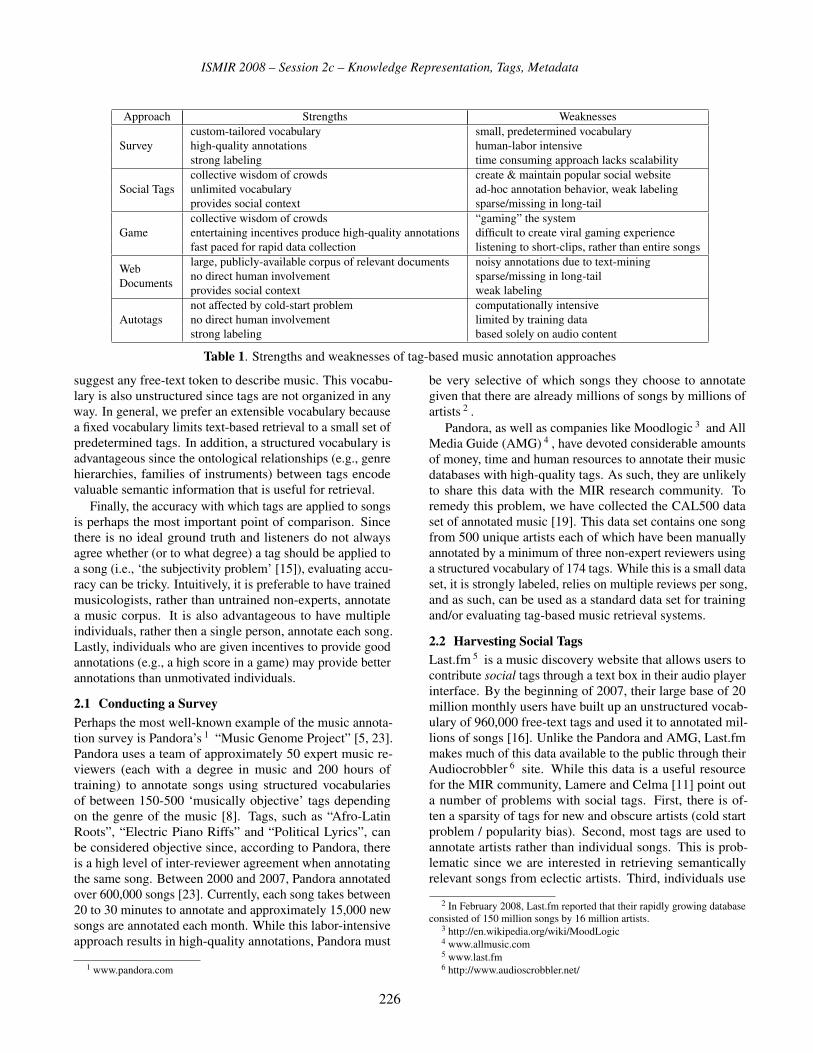
ISMIR 2008 – Session 2c – Knowledge Representation, Tags, Metadata
Approach Strengths Weaknesses
custom-tailored vocabulary small, predetermined vocabulary
Survey high-quality annotations human-labor intensive
strong labeling time consuming approach lacks scalability
collective wisdom of crowds create & maintain popular social website
Social Tags unlimited vocabulary ad-hoc annotation behavior, weak labeling
provides social context sparse/missing in long-tail
collective wisdom of crowds “gaming” the system
Game entertaining incentives produce high-quality annotations difficult to create viral gaming experience
fast paced for rapid data collection listening to short-clips, rather than entire songs
Web
Documents
large, publicly-available corpus of relevant documents noisy annotations due to text-mining
no direct human involvement sparse/missing in long-tail
provides social context weak labeling
not affected by cold-start problem computationally intensive
Autotags no direct human involvement limited by training data
strong labeling based solely on audio content
Table 1. Strengths and weaknesses of tag-based music annotation approaches
suggest any free-text token to describe music. This vocabu-lary is also unstructured since tags are not organized in anyway. In general, we prefer an extensible vocabulary becausea fixed vocabulary limits text-based retrieval to a small set ofpredetermined tags. In addition, a structured vocabulary isadvantageous since the ontological relationships (e.g., genrehierarchies, families of instruments) between tags encodevaluable semantic information that is useful for retrieval.
Finally, the accuracy with which tags are applied to songsis perhaps the most important point of comparison. Sincethere is no ideal ground truth and listeners do not alwaysagree whether (or to what degree) a tag should be applied toa song (i.e., ‘the subjectivity problem’ [15]), evaluating accu-racy can be tricky. Intuitively, it is preferable to have trainedmusicologists, rather than untrained non-experts, annotatea music corpus. It is also advantageous to have multipleindividuals, rather then a single person, annotate each song.Lastly, individuals who are given incentives to provide goodannotations (e.g., a high score in a game) may provide betterannotations than unmotivated individuals.
2.1 Conducting a SurveyPerhaps the most well-known example of the music annota-tion survey is Pandora’s 1 “Music Genome Project” [5, 23].Pandora uses a team of approximately 50 expert music re-viewers (each with a degree in music and 200 hours oftraining) to annotate songs using structured vocabulariesof between 150-500 ‘musically objective’ tags dependingon the genre of the music [8]. Tags, such as “Afro-LatinRoots”, “Electric Piano Riffs” and “Political Lyrics”, canbe considered objective since, according to Pandora, thereis a high level of inter-reviewer agreement when annotatingthe same song. Between 2000 and 2007, Pandora annotatedover 600,000 songs [23]. Currently, each song takes between20 to 30 minutes to annotate and approximately 15,000 newsongs are annotated each month. While this labor-intensiveapproach results in high-quality annotations, Pandora must
1 www.pandora.com
be very selective of which songs they choose to annotategiven that there are already millions of songs by millions ofartists 2 .
Pandora, as well as companies like Moodlogic 3 and AllMedia Guide (AMG) 4 , have devoted considerable amountsof money, time and human resources to annotate their musicdatabases with high-quality tags. As such, they are unlikelyto share this data with the MIR research community. Toremedy this problem, we have collected the CAL500 dataset of annotated music [19]. This data set contains one songfrom 500 unique artists each of which have been manuallyannotated by a minimum of three non-expert reviewers usinga structured vocabulary of 174 tags. While this is a small dataset, it is strongly labeled, relies on multiple reviews per song,and as such, can be used as a standard data set for trainingand/or evaluating tag-based music retrieval systems.
2.2 Harvesting Social TagsLast.fm 5 is a music discovery website that allows users tocontribute social tags through a text box in their audio playerinterface. By the beginning of 2007, their large base of 20million monthly users have built up an unstructured vocab-ulary of 960,000 free-text tags and used it to annotated mil-lions of songs [16]. Unlike the Pandora and AMG, Last.fmmakes much of this data available to the public through theirAudiocrobbler 6 site. While this data is a useful resourcefor the MIR community, Lamere and Celma [11] point outa number of problems with social tags. First, there is of-ten a sparsity of tags for new and obscure artists (cold startproblem / popularity bias). Second, most tags are used toannotate artists rather than individual songs. This is prob-lematic since we are interested in retrieving semanticallyrelevant songs from eclectic artists. Third, individuals use
2 In February 2008, Last.fm reported that their rapidly growing databaseconsisted of 150 million songs by 16 million artists.
3 http://en.wikipedia.org/wiki/MoodLogic4 www.allmusic.com5 www.last.fm6 http://www.audioscrobbler.net/
226
ISMIR 2008 – Session 2c – Knowledge Representation, Tags, Metadata
ad-hoc techniques when annotating music. This is reflectedby use of polysemous tags (e.g., “progressive”), tags that aremisspelled or have multiple spellings (e.g., “hip hop”, “hip-hop”), tags used for self-organization (e.g., “seen live”), andtags that are nonsensical. Finally, the public interface allowsfor malicious behavior. For example, any individual or groupof individuals can annotate an artist with a misleading tag.
2.3 Playing Annotation GamesAt the 2007 ISMIR conference, music annotation gameswere presented for the first time: ListenGame [20], Tag-a-Tune [12], and MajorMiner [14]. ListenGame is a real-timegame where a large group of users is presented with a songand a list of tags. The players have to choose the best andworst tags for describing the song. When a large group ofplayers agree on a tag, the song has a strong (positive ornegative) association with the tag. This game, like a musicsurvey, has the benefit of using a structured vocabulary oftags. It can be considered a strong labeling approach sinceit also collects information that reflects negative semanticassociations between tags and songs. Like the ESPGame forimage tagging [22], Tag-a-Tune is a two-player game wherethe players listen to a song and are asked to enter “free text”tags until they both enter the same tag. MajorMiner is similarin nature, except the tags entered by the player are comparedagainst the database of previously collected tags in an offlinemanner. Like social tagging, the tags collected using bothgames result in a unstructured, extensible vocabulary.
A major problem with this game-based approach is thatplayers will inevitably attempt to game the system. For exam-ple, the player may only contribute generic tags (e.g., “rock”,“guitar”) even if less common tags provide a better seman-tic description (e.g., “grunge”, “distorted electric guitar”).Also, despite the recent academic interest in music annota-tion games, no game has achieved large scale success. Thisreflects the fact that it is difficult to design a viral game forthis inherently laborious task.
2.4 Mining Web DocumentsArtist biographies, album reviews, and song reviews areanother rich source of semantic information about music.There are a number of research-based MIR systems thatcollect such documents from the Internet by querying searchengines [9], monitoring MP3 blogs [4], or crawling a musicsite [24]. In all cases, Levy and Sandler point out that suchweb mined corpora can be noisy since some of the retrievedwebpages will be irrelevant, and in addition, much of the textcontent on relevant webpages will be useless [13].
Most of the proposed web mining systems use a set of oneor more documents associated with a song and convert theminto a single document vector (e.g., tf-idf representation)[10, 25]. This vector space representation is then useful fora number of MIR tasks such as calculating music similarity[25] and indexing content for a text-based music retrievalsystem [10]. More recently, Knees et. al. [9] have proposed apromising new web mining technique called relevance scor-
ing as an alternative to the vector space approaches. Bothrelevance scoring and vector space approaches are subject topopularity bias since short-head songs are generally repre-sented by more documents than long-tail songs.
2.5 Autotagging Audio ContentAll previously described approaches require that a song beannotated by humans, and as such, are subject to the coldstart problem. Content-based audio analysis is an alternativeapproach that avoids this problem. Early work on this topicfocused (and continues to focus) on music classification bygenre, emotion, and instrumentation (e.g., [21]). Theseclassification systems effectively ‘tag’ music with class labels(e.g., ‘blues’, ‘sad’, ‘guitar’). More recently, autotaggingsystems have been developed to annotate music with a larger,more diverse vocabulary of (non-mutually exclusive) tags[19, 7, 17]. In [19], we describe a generative approach thatlearns a Gaussian mixture model (GMM) distribution over anaudio feature space for each tag in the vocabulary. Eck et. al.use a discriminative approach by learning a boosted decisionstump classifier for each tag [7]. Finally, Sordo et. al. presenta non-parametric approach that uses a content-based measureof music similarity to propagate tags from annotated songsto similar songs that have not been annotated [17].
3 COMPARING SOURCES OF TAGSIn this section, we describe one system for each of the tagcollection approaches. Each has been implemented based onsystems that have been recently developed within the MIRresearch community [19, 9, 20]. Each produces a |S|x|T |annotation matrix X where |S| is the number of songs in ourcorpus and |T | is the size of our tag vocabulary. Each cellxs,t of the matrix is proportional to the strength of semanticassociation between song s and tag t.
We set xs,t = ∅ if the relationship between song s andtag t is missing (i.e., unknown). If the matrix X has manyempty cells, then we refer to the matrix as sparse, otherwisewe refer to it as dense. Missing data results from both weaklabeling and the cold start problem. Sparsity is reflected bythe tag density of a matrix which is defined as the percentageof non-empty elements of a matrix.
Our goal is to find a tagging system that is able to ac-curately retrieve (i.e., rank-order) songs for a diverse set oftags (e.g., emotions, genres, instruments, usages). We quan-titatively evaluate music retrieval performance of system aby comparing the matrix Xa against the CAL500 matrixXCAL500 (see Section 2.1). The XCAL500 matrix is a binarymatrix where xs,t = 1 if 80% of the individuals annotatesong s with tag t, and 0 otherwise (see Section V.a of [19]for details). For the experiments reported in this section, weuse a subset of 109 of the original 174 tags. 7 We willassume that the subset of 87 songs from the Magnatunes [6]
7 We have merged genre-best tags with genre tags, removed instrument-solo tags, removed some redundant emotion tags, and pruned other tags thatare used to annotate less than 2% of the songs. For a complete list of tags,see http://cosmal.ucsd.edu/cal.
227

ISMIR 2008 – Session 2c – Knowledge Representation, Tags, Metadata
Approach Songs Tag Density AROC Avg. Prec R-Prec Top10 Prec
Survey (CAL500) All Songs 1.00 1.00 1.00 1.00 0.97
Ground Truth Long Tail 1.00 1.00 1.00 1.00 0.57
Baseline All Songs 1.00 0.50 0.15 0.14 0.13
Random Long Tail 1.00 0.50 0.18 0.15 0.12
Social Tags All Songs 0.23 0.62 0.28 0.30 0.37
Last.fm Long Tail 0.03 0.54 0.24 0.20 0.19
GameAll Songs 0.37 0.65 0.28 0.28 0.32
ListenGame†
Web Documents All Songs 0.67 0.66 0.29 0.29 0.37
SS-WRS Long Tail 0.25 0.56 0.25 0.20 0.18
Autotags All Songs 1.00 0.69 0.29 0.29 0.33
SML Long Tail 1.00 0.70 0.34 0.30 0.27
Rank-based All Songs 1.00 0.74 0.32 0.34 0.38
Interleaving (RBI) Long Tail 1.00 0.71 0.33 0.27 0.28
Table 2. Tag-based music retrieval: Each approach is compared using all CAL500 songs and a subset of 87 more obscure long-tail songs from
the Magnatunes dataset. Tag Density represents the proportion of song-tag pairs that have a non-empty value. The four evaluation metrics
(AROC, Average Precision, R-Precision, Top-10 Precision) are found by averaging over 109 tag queries. †Note that ListenGame is evaluated
using half of the CAL500 songs and that the results do not reflect the realistic effect of the popularity bias (see Section 3.2).
collection that are included in the CAL500 data set are repre-sentative of long-tail music. As such, we can use this subsetto gauge how the various tagging approaches are affected bypopularity bias. 8
Each system is compared to the CAL500 data set usinga number of standard information retrieval (IR) evaluationmetrics [9]: area under the receiver operation characteristiccurve (AROC), average precision, R-precision, and Top-10precision. An ROC curve is a plot of the true positive rateas a function of the false positive rate as we move downthis ranked list of songs. The area under the ROC curve(AROC) is found by integrating the ROC curve and is upper-bounded by 1.0. A random ranking of songs will producean expected AROC score of 0.5. Average precision is foundby moving down our ranked list of test songs and averagingthe precisions at every point where we correctly identifya relevant song. R-Precision is the precision of the top R-ranked songs where R is the total number of songs in theground truth that have been annotated with a given tag. Top-10 precision is the precision after we have retrieved the top10 songs for a given tag. This metric is designed to reflectthe 10 items that would be displayed on the first results pageof a standard Internet search engine.
Each value in Table 2 is the mean of a metric after averag-ing over all 109 tags in our vocabulary. That is, for each tag,we rank-order our 500 song data set and calculate the valueof the metric using CAL500 data as our ground truth. Wethen compute the average of the metric using the 109 valuesfrom the 109 rankings.
3.1 Social Tags: Last.fmFor each of our 500 songs, we attempt to collect two listsof social tags from the Last.fm Audioscobbler website. Onelist is related specifically to the song and the other list isrelated to the artist. For the song list, each tag has a score
8 It should be noted that 87 songs is a small sample.
(xLast.fm Songs,t ) that ranges from 0 (low) to 100 (high) and is
a secret function (i.e., trade secret of Last.fm) of both thenumber and diversity of users who have annotated song swith tag t. For the artist list, the tag score (xLast.fm Artist
s,t )is again a secret function that ranges between 0 and 100,and reflects both tags that have been used to annotate theartist or songs by the artist. We found one or more tagsfor 393 and 472 of our songs and artists, respectively. Thisincluded at least one occurrence of 71 and 78 of the 109tags in our vocabulary. While this suggests decent coverage,tag densities of 4.6% and 11.8%, respectively, indicate thatthe annotation matrices, XLast.fm Song and XLast.fm Artist,are sparse even when we consider mostly short-head songs.These sparse matrices achieve AROC of 0.57 and 0.58.
To remedy this problem, we create a single Last.fm anno-tation matrix by leveraging the Last.fm data in three ways.First, we match tags to their synonyms. 9 For example, asong is considered to be annotated with ‘down tempo’ if ithas instead been annotated with ‘slow beat’. Second, weallow wildcard matches for each tag. That is, if a tag appearsas a substring in another tag, we consider it to be a wildcardmatch. For example, “blues” matches with “delta electricblues”, “blues blues blues”, “rhythm & blues”. Althoughsynonyms and wildcard matches add noise, they increase therespective densities to 8.6% and 18.9% and AROC perfor-mance to 0.59 and 0.59. Third, we combine the song andartist annotation matrices in one annotation matrix:
XLast.fm = XLast.fm Song + XLast.fm Artist.
This results in a single annotation matrix that has a density of23% and AROC of 0.62. 95 of the 109 tags are representedat least once in this matrix. However, the density for theMagnatunes (e.g., long-tail) songs is only 3% and producesretrieval results that are not much better than random.
9 Synonyms are determined by the author using a thesaurus and by ex-ploring the Last.fm tag vocabulary.
228

ISMIR 2008 – Session 2c – Knowledge Representation, Tags, Metadata
3.2 Games: ListenGameIn [20], Turnbull et al. describe a music annotation gamecalled ListenGame in which a community of players listento a song and are presented with a set of tags. Each player isasked to vote for the single best tag and single worst tag todescribe the music. From the game, we obtain the annotationmatrix XGame by letting
[XGame]s,t = #(best votes)−#(worst votes)
when song s and tag t are presented to the players.
During a two-week pilot study, 16,500 annotations (bestand worst votes) were collected for a random subset of 250CAL500 songs. Each of the 27,250 song-tag pairs werepresented to users an average of 1.8 times. Although thisrepresents a very small sample size, the mean AROC for thesubset of 250 songs averaged over the 109-tag vocabularyis 0.65. Long-tail and short-head results do not accuratelyreflect the real-world effect of popularity bias since all songswere selected for annotation with equal probability. As such,these results have been omitted.
3.3 Web Documents: Weight-based Relevance ScoringIn order to extract tags from a corpus of web documents, weadapt the relevance scoring (RS) algorithm that has recentlybeen proposed by Knees et. al. [9]. They have shown thismethod to be superior to algorithms based on vector spacerepresentations. To generate tags for a set of songs, the RSworks as follows:
1. Collect Document Corpus: For each song, repeat-edly query a search engine with each song title, artistname, or album title. Collect web documents in searchresults. Retain the (many-to-many) mapping betweensongs and documents.
2. Tag Songs: For each tag
(a) Use the tag as a query string to find the relevantdocuments, each with an associated relevanceweight (defined below) from the corpus.
(b) For each song, sum the relevance scores for allthe documents that are related to the song.
We modify this algorithm in two ways. First, the relevancescore in [9] is inversely proportional to the rank of the rele-vant document. We use a weight-based approach to relevancescoring (WRS). The relevance weight of a document given atag can be a function of the number of times the tag appearsin the document (tag-frequency), the number of documentswith the tag (document frequency), the number of total wordsin the document, the number of words or documents in thecorpus, etc. For our system, the relevance weights are deter-mined by the MySQL match function. 10
We calculate an entry of the annotation matrix XWRS as,
XWRSs,t =
∑d∈Dt
wd,tId,s
10 http://dev.mysql.com/doc/refman/5.0/en/fulltext-natural-language.html
where Dt is the set of relevant documents for tag t, wd,t isthe relevance weight for document d and tag t, and Id,s is anindicator variable that is 1 if document d was found whenquerying the search engine with song s (in Step 1) and 0otherwise. We find that weight-based RS (WRS) producesa small increase in performance over rank-based RS (RRS)(AROC of 0.66 vs. 0.65). In addition, we believe that WRSwill scale better since the relevance weights are independentof the number of documents in our corpus.
The second modification is that we use site-specificqueries when creating our corpus of web documents (Step 1).That is, Knees et. al. collect the top 100 documents returnedby Google when given queries of the form:
• “<artist name>” music
• “<artist name>” “<album name>” music review
• “<artist name> ” “<song name>” music review
for each song in the data set. Based on an informal study ofthe top 100 webpages returned by non-site-specific queries,we find that many pages contain information that is onlyslightly relevant (e.g., music commerce site, ticket resellers,noisy discussion boards, generic biographical information).By searching music-specific sites, we are more likely to finddetailed music reviews and in-depth artist biographies. Inaddition, the webpages at sites like Pandora and AMG AllMusic specifically contain useful tags in addition to naturallanguage content.
We use site-specific queries by appending the substring‘site:<music site url>’ to the three query templates, where<music site url> is the url for a music website that isknown to have high quality information about songs, al-bums or artists. These sites include allmusic.com, ama-zon.com, bbc.co.uk, billboard.com, epinions.com, mu-sicomh.com, pandora.com, pitchforkmedia.com, rolling-stone.com, wikipedia.org. For these 10 music sites and onenon-site-specific query, we collect and store the top 10 pagesreturned by the Google search engine. This results in a maxi-mum of 33 queries and a maximum of 330 pages per song.On average, we are only able to collect 150 webpages persong since some of the long-tail songs are not well repre-sented by these music sites.
Our site-specific weight-based relevance scoring (SS-WRS) approach produces a relatively dense annotation ma-trix (46%) compared with the approach involving Last.fmtags. However, like the Last.fm approach, the density of theannotation matrix is greatly reduced (25%) when we consideronly long-tail songs.
3.4 Autotagging: Supervised Multiclass LabelingIn [19], we use a supervised multiclass labeling (SML) modelto automatically annotate songs with a diverse set of tagsbased on audio content analysis. The SML model is parame-terized by one Gaussian mixture model (GMM) distributionover an audio feature space for each tag in the vocabulary.The parameters for the set of GMMs are trained using anno-tated training data. Given a novel audio track, audio features
229

ISMIR 2008 – Session 2c – Knowledge Representation, Tags, Metadata
are extracted and their likelihood is evaluated using eachof the GMMs. The result is a vector of probabilities that,when normalized, can be interpreted as the parameters of amultinomial distribution over the tag vocabulary. This se-mantic multinomial distribution represents a compact andinterpretable index for a song where the large parametervalues correspond to the most likely tags.
Using 10-fold cross validation, we can estimate a semanticmultinomial for each of the CAL500 songs. By stacking the50 test set multinomials from each of the 10 folds, we canconstruct a strongly-labeled annotation matrix XSML that isbased purely on the audio content. As such, this annotationmatrix is dense and not affected by the cold start problem.
3.5 SummaryComparing systems using a two-tailed, paired t-test (N = 109,α = 0.05) on the AROC metric, we find that all pairs of thefour systems are significantly different, with the exception ofGame and Web Documents. 11 If we compare the systems us-ing the other three metrics (Average Precision, R-Precision,and Top 10 Precision), we no longer find statistically sig-nificant differences. It is interesting that Social Tags andWeb Documents (0.37) have slightly better Top 10 precisionthan Autotags (0.33). This reflects the fact that for some ofthe more common individual tags, we find that Social Tagsand Web Documents have exceptional precision at low recalllevels. For both Web Documents and Social Tags, we findsignificant improvement in retrieval performance of short-head songs over long-tail songs. However, as expected, thereis no difference for Autotags. This confirms the intuition thatsystems based on web documents and social tags are influ-enced by popularity bias, whereas content-based autotaggingsystems are not.
4 COMBINING SOURCES OF TAGSWhile the purpose of this paper is to compare various ap-proaches for collecting tags for music, our ultimate goal isto combine these approaches in order to create a more pow-erful tag-based music retrieval system. For example, if weinterleave the top ranked songs from each of the four ap-proaches (See Rank-based Interleaving (RBI) in Table 2), weobserve a significant increase in performance (AROC 0.74)over the performance of the best single approach (Autotagswith AROC = 0.69). Our improvement is consistent withthe findings of Yoshii et. al. [26] and Aucountier et. al. [1],both of whom have recently proposed hybrid context-contentsystems for music recommendation and music classification,respectively. We explore alternative hybrid systems in someof our related work [2, 18].
5 ACKNOWLEDGEMENTSWe would like to thank our anonymous reviewers who had a large
impact on this paper. This work is supported by NSF IGERT DGE-
0333451 and NSF grant DMS-MSPA 062540922.11 Note that when we compare each system with the Game system, we
compare both systems using the reduced set of 250 songs.
6 REFERENCES
[1] J.J. Aucouturier, F. Pachet, P. Roy, and A. Beurive. Signal + context =better classification. ISMIR, 2007.
[2] L. Barrington, M. Yazdani, D. Turnbull, and G. Lanckriet. Combiningfeature kernels for semantic music retrieval. ISMIR, 2008.
[3] G. Carneiro, A. B. Chan, P. J. Moreno, and N. Vasconcelos. Supervisedlearning of semantic classes for image annotation and retrieval. IEEEPAMI, 29(3):394–410, 2007.
[4] O. Celma, P. Cano, and P. Herrera. Search sounds: An audio crawlerfocused on weblogs. In ISMIR, 2006.
[5] S. Clifford. Pandora’s long strange trip. Inc.com, 2007.
[6] J. S. Downie. Music information retrieval evaluation exchange(MIREX), 2005.
[7] D. Eck, P. Lamere, T. Bertin-Mahieux, and S. Green. Automatic genera-tion of social tags for music recommendation. In Neural InformationProcessing Systems Conference (NIPS), 2007.
[8] W. Glaser, T. Westergren, J. Stearns, and J. Kraft. Consumer itemmatching method and system. US Patent Number 7003515, 2006.
[9] P. Knees, T. Pohle, M. Schedl, D. Schnitzer, and K. Seyerlehner. Adocument-centered approach to a natural language music search engine.In ECIR, 2008.
[10] P. Knees, T. Pohle, M. Schedl, and G. Widmer. A music search enginebuilt upon audio-based and web-based similarity measures. In ACMSIGIR, 2007.
[11] P. Lamere and O. Celma. Music recommendation tutorial notes. ISMIRTutorial, September 2007.
[12] E. L. M. Law, L. von Ahn, and R. Dannenberg. Tagatune: a game formusic and sound annotation. In ISMIR, 2007.
[13] M. Levy and M. Sandler. A semantic space for music derived fromsocial tags. In ISMIR, 2007.
[14] M. Mandel and D. Ellis. A web-based game for collecting music meta-data. In ISMIR, 2007.
[15] C. McKay and I. Fujinaga. Musical genre classification: Is it worthpursuing and how can it be improved? ISMIR, 2006.
[16] F. Miller, M. Stiksel, and R. Jones. Last.fm in numbers. Last.fm pressmaterial, February 2008.
[17] M. Sordo, C. Lauier, and O. Celma. Annotating music collections: Howcontent-based similarity helps to propagate labels. In ISMIR, 2007.
[18] D. Turnbull. Design and Development of a Semantic Music DiscoveryEngine. PhD thesis, UC San Diego, 2008.
[19] D. Turnbull, L. Barrington, D. Torres, and G. Lanckriet. Semanticannotation and retrieval of music and sound effects. IEEE TASLP, 16(2),2008.
[20] D. Turnbull, R. Liu, L. Barrington, and G Lanckriet. Using games tocollect semantic information about music. In ISMIR ’07, 2007.
[21] G. Tzanetakis and P. R. Cook. Musical genre classification of audiosignals. IEEE Transaction on Speech and Audio Processing, 10(5):293–302, 7 2002.
[22] L. von Ahn and L. Dabbish. Labeling images with a computer game. InACM CHI, 2004.
[23] T. Westergren. Personal notes from Pandora get-together in San Diego,March 2007.
[24] B. Whitman and D. Ellis. Automatic record reviews. ISMIR, pages470–477, 2004.
[25] B. Whitman and S. Lawrence. Inferring descriptions and similarity formusic from community metadata. ICMC, 2002.
[26] K. Yoshii, M. Goto, K. Komatani, T. Ogata, and H. G. Okuno. Anefficient hybrid music recommender system using an incrementallytrainable probabilistic generative model. IEEE TASLP, 2008.
230

ISMIR 2008 – Session 2c – Knowledge Representation, Tags, Metadata
MOODSWINGS: A COLLABORATIVE GAME FOR MUSIC MOOD LABELCOLLECTION
Youngmoo E. Kim Erik Schmidt Lloyd EmelleElectrical & Computer Engineering
Drexel University{ykim,eschmidt,lte22}@drexel.edu
ABSTRACT
There are many problems in the field of music infor-
mation retrieval that are not only difficult for machines to
solve, but that do not have well-defined answers. In labeling
and detecting emotions within music, this lack of specificity
makes it difficult to train systems that rely on quantified la-
bels for supervised machine learning. The collection of such
“ground truth” data for these subjectively perceived features
necessarily requires human subjects. Traditional methods
of data collection, such as the hiring of subjects, can be
flawed, since labeling tasks are time-consuming, tedious,
and expensive. Recently, there have been many initiatives to
use customized online games to harness so-called “Human
Computation” for the collection of label data, and several
such games have been proposed to collect labels spanning
an excerpt of music. We present a new game, MoodSwings
(http://schubert.ece.drexel.edu/moodswings), which differs
in that it records dynamic (per-second) labels of players’
mood ratings of music, in keeping with the unique time-
varying quality of musical mood. As in prior collaborative
game approaches, players are partnered to verify each oth-
ers’ results, and the game is designed to maximize consensus-
building between users. We present preliminary results from
an initial set of game play data.
1 INTRODUCTION
The detection and labeling of the emotional content (mood)
of music is one of many music information retrieval prob-
lems without a clear “ground truth” answer. The lack of eas-
ily obtained ground truth for these kinds of problems further
complicates the development of automated solutions, since
classification methods often employ a supervised learning
approach relying on such ground truth labels. The collec-
tion of this data on subjectively perceived features, such as
musical mood, necessarily requires human subjects. But tra-
ditional methods of data collection, such as the hiring of
subjects, have their share of difficulties since labeling tasks
can be time-consuming, tedious, error-prone and expensive.
Recently, a significant amount of attention has been placed
on the use of collaborative online games to collect such
ground truth labels for difficult problems, harnessing so-
called “Human Computation”. For example, von Ahn et al.
have created several such games for image labeling: the ESPGame, Peekaboom [1], and Phetch. More recently, several
such games have been been proposed for the collection of
music data, such as MajorMiner [2], Listen Game [3], and
TagATune [4]. These implementations have primarily fo-
cused on the collection of descriptive labels for a relatively
short audio clip.
We present a new game, MoodSwings, designed to ex-
plore the unique time-varying nature of musical mood. Of
course, one of the joys of music is that the mood of a piece
may change over time, gradually or suddenly. According
to Huron [5], this combination of anticipation and surprise
may be at the core of our enjoyment of music. Thus, our
game is targeted at collecting dynamic (per-second) labels
of users’ mood ratings, which are collected in real-time as
a player hears the music using the two-dimensional grid of
emotional components: valence and arousal. As in other
collaborative games, players are partnered in order to verify
each others’ results, providing a strong incentive for pro-
ducing high-quality labels that others can agree upon. Ac-
cordingly, game scoring is designed to maximize consensus-
building between partners. In this paper, we present data
from an initial pilot phase of the game and demonstrate the
utility of this approach for the collection of high-quality, dy-
namic labels of musical affect.
2 BACKGROUND
Models of affect and the categorization and labeling of spe-
cific emotions has received significant attention from a vari-
ety of research areas including psychology, physiology, neu-
roscience, as well as musicology. With the advent of digital
music and very large music collections, recent work has fo-
cused on the problem of automatic music mood detection.
Next, we briefly summarize some of the related work.
2.1 Mood models
Early work on the quantification of musical affect focused
on the formation of ontologies using clusters of common
231

ISMIR 2008 – Session 2c – Knowledge Representation, Tags, Metadata
emotional adjectives and labels (e.g., “bright”, “gloomy”,
“contemplative”, “angry”). Ontologies proposed by Hevner
[6] and Farnsworth [7] proposed eight and ten such mood
clusters, respectively. All Music Guide [8], a large edited
music information database, also uses a descriptive approach
with a total of 179 distinct (but not unrelated) mood labels.
An alternative approach to the modeling of human emo-
tions views affect as a combination of orthogonal continu-
ous sub-features. The most popular such representation of
musical affect is Thayer’s two-dimensional valence-arousal
space [9], which itself is derived from Russell’s general mo-
del of human emotions (pleasant-unpleasant vs. arousal-
sleep) [10]. Thayer’s model decomposes emotion in music
according to two principal dimensions:
• valence: positive vs. negative (e.g., happy vs. sad)
• arousal: high- vs. low-energy (e.g., energetic vs. calm)
According to this model, music can be broadly catego-
rized into one of four quadrants: high valence and arousal
(joy, exuberance), high valence and low arousal (content-
ment), low valence and high arousal (anger), and low va-
lence and arousal (depression). But the model also views the
axes as continuous features, allowing for an unlimited com-
bination of overall moods. The continuous valence-arousal
model is at the core of MoodSwings.
2.2 Ground truth label collection
The tedium and expense of label collection has presented a
significant obstacle for researchers seeking such labels in or-
der to train automatic systems for mood classification. When
employing subjects specifically for the collection of mood
labels for music, prior systems have used alternatively ex-
pert and non-expert populations.
The Pandora service [11] is an example of a well-known
expert labeling system that employs a large team of musi-
cians to manually label tracks according to hundreds of fea-
tures (their “music genome”), some of which relate to mood.
The former MoodLogic service used questionnaires given to
their users to collect mood metadata. The data from these
services is, sadly, not available to the public. Other com-
mercial tools allow users to tag their own collections, such
as the Moody plug-in for iTunes, which uses a quantized
4x4 valence-arousal grid.
More recently, online services that allow users to input
free-form (unconstrained) tags, such as Last.fm [12], have
collected myriad tags (some of which represent mood la-
bels) across very large music collections. The accessibil-
ity of this data has led to a recent trend towards using such
free-form tags as the basis for mood labeling by aggregating
results from many users. Hu, Bay, and Downie collected la-
bels and tags from AMG, Last.fm, and epinions.com to form
the ground-truth mood “clusters” used in the 2007 MIREX
mood detection evaluation [13].
2.3 Automatic mood classification of music
The general approach to automatic mood detection from au-
dio has been to use supervised machine learning to train sta-
tistical models of acoustic features. Li and Ogihara [14]
used acoustic features related to timbre, rhythm, and pitch
to train Support Vector Machines (SVMs) to classify music
into 13 mood categories derived from Farnsworth’s emo-
tion groupings. Using a hand-labeled library of 499 mu-
sic clips (30-seconds each), they achieved an accuracy of
∼45%, with 50% of the database used for training and test-
ing, respectively.
Lu, Liu, and Zhang [15] pursued mood detection and
tracking (following dynamic mood changes during a song)
using a variety of acoustic features related to intensity, tim-
bre, and rhythm. Their classifier used Gaussian Mixture
Models (GMMs) for Thayer’s four principal mood quad-
rants in the valence-arousal representation. The system was
trained using a set of 800 classical music clips (from a data
set of 250 pieces), each 20 seconds in duration, hand labeled
to one of the 4 quadrants. Their system achieved an accu-
racy of ∼85% when trained on 75% of the clips and tested
on the remaining 25%.
In 2007, the Music Information Research Evaluation eX-
change (MIREX) first included a “beta” task on audio mu-
sic mood classification with 8 systems submitted. The audio
clips used for this task were assigned to one of 5 mood clus-
ters, aggregated from AMG mood labels (adjectives), and
600 30-second hand-labeled clips distributed equally among
the 5 mood clusters were used in the evaluations. All partic-
ipants performed reasonably well (far higher than chance)
with the highest performing system [16] achieving correct
classifications slightly over 60% of the time. It should be
noted that several of the systems were primarily designed for
the genre classification and then appropriated to the mood
classification task as well [17].
3 MOODSWINGS
MoodSwings is a collaborative, two-player game that incor-
porates each listener’s subjective judgements of the emo-
tional content (mood) of music into the game play. At the
start of a match, a player is partnered with another player
anonymously across the internet. The goal of the game is
for the players to dynamically and continuously reach agree-
ment on the mood of 5 short (30-second) music clips drawn
from a database of popular music.
The MoodSwings game board (Figure 1) is a direct rep-
resentation of the valence-arousal space. The board repre-
sents a continuum of possible mood ratings, with arousal on
the horizontal axis and valence on the vertical axis. During
gameplay, players simultaneously listen to identical short
music clips. Each player positions their circular cursor dy-
namically on the game board, indicating their instantaneous
232

ISMIR 2008 – Session 2c – Knowledge Representation, Tags, Metadata
Figure 1. The MoodSwings game board
assessment of the mood of the music. A player’s position is
sampled once per second, indicated by the pulsing of their
cursor. The partner’s cursor is visible only intermittently,
every few seconds. Scoring is based on the amount of over-
lap between the partners’ circles, with greater congruency
resulting in a greater number of points scored. The size of
the players’ cursors decreases over time as the clip plays, in-
creasing the difficulty of scoring points as time elapses (the
players must agree on their ratings more precisely to overlap
and thus score points).
3.1 Game play sequence
A MoodSwings match consists of 5 rounds, each consisting
of a different music clip with a duration of 30 seconds. Once
a partner pairing is established and verified, each round com-
mences after a short 3-second countdown. The partner pair-
ing remains consistent for all 5 rounds. The game board
remains inactive until the round begins.
1. Once the round begins, the player’s cursor (colored
yellow circle) becomes visible. The cursor “throbs”
every second indicating the sampled position, but the
player is free to continuously alter the cursor position
between pulses.
2. After an initial period of 5 seconds, the partner’s cur-
sor becomes visible for the first time (again pulsing
for one second). This allows a player to make an
initial mood assessment independently, without influ-
ence from their partner.
3. Afterwards, the partner’s cursor is visible once every
3 seconds. This interval is designed to prevent play-
ers from simply “chasing” their partners in order to
accumulate more points.
4. The size of both cursors decreases continuously dur-
ing the course of the round.
At the end of each round, the player is presented with
their score for the round and their total points for the match
thus far. Likewise, at the conclusion of a match, a list is
presented with performing artist and title for each music clip
(offering a link to a search engine for each piece), as well as
the points for each round and the total score for the match
(Figure 2).
Figure 2. The MoodSwings post-match wrapup
3.2 Game scoring
The primary score calculation is based upon the amount of
overlap between the player’s cursor and that of their partner,
which is designed to encourage maximum agreement in the
mood assessments from both parties. This score is only ac-
cumulated whenever the partner’s cursor is visible. When
points accumulate, they are displayed on top of the partner’s
cursor (shown in Figure 1).
Players can also accumulate bonus points by “convinc-
ing” their partner to agree with a particular mood assessment
(position). This provides an incentive for players to remain
firm in a position and not to be capricious in their move-
ments. It also encourages them to respond to a change in
mood rapidly in order to “stake out” the new position before
their partner. The rules for bonus points are as follows:
• A player is eligible to accumulate bonus points after
remaining stationary for 1 second. This is indicated
by a yellow square around the player’s cursor. Bonus
points will only be awarded while the player remains
stationary.
• If a partner moves towards a player’s location achiev-
ing overlap between the cursors, the stationary player
233

ISMIR 2008 – Session 2c – Knowledge Representation, Tags, Metadata
is awarded 5 bonus points. This is indicated by the
cursor changing color to green (Figure 3).
• Bonus points may be awarded every second, even when
the partner’s cursor is not visible to the player.
The overall point system is designed so that a “good”
score for a round is approximately 100 points, and a par-
ticularly good match total is 500 points. High scores for
the top five players as well as the top five individual match
scores are visible when first logging onto the MoodSwings
website.
Figure 3. MoodSwings bonus scoring
3.3 Music database
The music for MoodSwings is drawn randomly from the
well-known uspop2002 database, a collection of over 8000
popular music tracks from approximately 400 performing
artists [18]. This database was chosen because of the com-
position of the corpus (popular music spanning several dec-
ades) and its potential appeal to a mass audience, the size
of the database, and the fact that it includes a range of fa-
miliar and obscure tunes. In addition, since the corpus is
well-known, a great deal of acoustic feature data and mu-
sic metadata have already been calculated and compiled for
the database, such as MFCCs [19]. This will allow other re-
searchers to rapidly and easily deploy their algorithms using
the labels collected from the game.
The uspop2002 database, however, is not without its is-
sues. A fair number of the songs contain explicit lyrics,
which may be objectionable to some players. Some of the
clips randomly selected for the game will not include music
at all because of extended applause from live recordings and
other unusual spoken-word tracks from a few albums. Be-
cause such metadata (explicit lyrics, non-music sections) for
tracks is not readily available, the game interface also offers
players the opportunity to mark such tracks. In particular,
beneath the game board for each round are the following
options that a player may voluntarily select:
• Clip does not contain music: for selections that do not
contain music (so that we can filter these tracks out in
the future).
• Song contains explicit lyrics: this will help us create
a future version of the game appropriate for all ages
that excludes these songs.
• Report a bug in this game: for any other problem en-
countered during the current round.
3.4 Technical implementation
A primary goal during the development of MoodSwings was
to allow access to the game through a standard web browser
interface, so that the game would be widely accessible and
would not require the installation of any additional software.
In particular, our lab works closely with several K-12 school
environments where the computers may be out of date and
additional software is difficult to install.
The end-user interface for MoodSwings is principally
coded using Asynchronous JavaScript and XML (AJAX),
which also makes use of Dynamic HTML. Audio playback
is handled through the Flash plug-in, which is included with
all browsers. The browser portion communicates with a web
server hosted by our laboratory that is used to synchronize
players, record the collected mood assessments, and admin-
ister the game. A diagram of the overall architecture of the
system is given in Figure 4.
Web server
PHP game scripts
HTTP/XML
mp3database
MySQL game
database
Player web browser
DHTML
JavaScript
Flash(audio)
mp3file
MoodSwings user interface MoodSwings game synchronizationand data recording
Figure 4. MoodSwings game architecture for a single
player. Each player interacts with the server independently.
The web server uses scripts written in PHP to respond to
client requests for game data, such as music clip information
and partner mood coordinates, in XML format. The game
data is stored in a MySQL database running on the server
that tracks all of the following information:
• Valence and arousal assessments from each player for
each second of the song.
• Game and match scores.
234

ISMIR 2008 – Session 2c – Knowledge Representation, Tags, Metadata
70 75 80 85 90
Am
plitu
de
Time (s)
0
0
Arousal
Val
ence
0
0
Arousal
Val
ence
0
0
Arousal
Val
ence
Figure 5. Progression of valence-arousal labels over a clip spanning the end of the first chorus and beginning of the second
verse of “American Pie” (Don McLean). The ellipses represent the standard deviation across different players.
• Game and match parameters (song clips used, clip
starting locations).
• Music metadata (artist, album, song title).
• User scores and high scores.
3.4.1 Technical limitations and single-player matches
Obviously, with simultaneous listening between the players
there will be some latency in the data received from one’s
partner during a game. Since the mood assessments are only
sampled once per second, it is likely that the partner’s data
received by a player will be at least one second out of date.
In practice, this does not affect gameplay very much, since
a player normally takes a second or two to react to sudden
mood changes.
Even when other players are not available online, a player
may still play a match against data previously recorded from
another player’s match. No distinction is made to the player
to indicate a match against a live player vs. a pre-recorded
match. In some ways, such single-player matches against
recorded data may be preferred because the partner’s labels
can be pre-fetched so that synchronization between ratings
and time samples is not an issue.
4 MOOD DATA COLLECTION
In our initial one week pilot phase, we attracted approxi-
mately 100 users and collected over 50,000 valence-arousal
point labels spanning more than 1000 songs. Of course,
given the collaborative structure of the game, many of the
valence-arousal labels refer to the same locations in a song.
4.1 Example data from song clip in database
Figure 5 shows a sample of collected valence-arousal la-
bels for a short section of the song “American Pie” by Don
McLean, between the first chorus and second verse. The
change in instrumentation and tempo within the segment
(drums are added to voice and guitar) is generally marked
by players as a change in intensity in the song, as well as a
slight increase in valence.
4.2 Summary of labels collected to date
Figure 6 depicts the distribution of the collected points in
the valence-arousal space. It is clear that the songs labeled
thus far have bias towards high valence and arousal, which
is consistent with a database of popular music. The plot
also shows that players for the most part favor locations near
the middle of each “quadrant” in the valence-arousal space,
largely avoiding extreme values.
5 FUTURE WORK
The initial implementation of MoodSwings and the prelim-
inary data collected thus far suggest the potential of such
a collaborative system with many users in providing high-
quality labels. We are currently investigating modifications
to make the gameplay more fun, with the hope of drawing
a greater number of repeat visits from users. A question
arises in examining live matches vs. those played against
recorded data. Qualitatively, the labels collected in single
and two-player games appear equally valid, but we plan to
verify their consistency by more closely examining the data.
235

ISMIR 2008 – Session 2c – Knowledge Representation, Tags, Metadata
Arousal
Val
ence
−100 0 100−100
0
100
Figure 6. Contour plot of the distribution of ∼50,000
valence-arousal labels collected over one-week pilot period.
An issue in dealing with popular music is that the mood
of most songs simply doesn’t change very much or often,
which can lead to rather static games (perhaps this is a com-
ment on the state of popular music!). We plan to add an
option for additional simultaneous players (3 or even more)
that may produce more interesting group labeling dynam-
ics. We also plan on augmenting the uspop2002 databse
with a collection of classical music clips, which will have
the added benefit of removing some of the lyric vs. audio
confusion that arises in labeling some pop songs.
As our collection of labels grows, we intend to use the
data to train a system for mood classification of short audio
segments using a Hidden Markov Model to capture time-
varying mood transitions. Once the entire database has been
labeled, the data collected from MoodSwings will be made
available to the music information retrieval research com-
munity through the game website.
6 REFERENCES
[1] L. von Ahn, “Games with a purpose,” Computer, vol. 39,
no. 6, pp. 92–94, 2006.
[2] M. I. Mandel and D. P. W. Ellis, “A web-based game for
collecting music metadata,” in Proceedings of the 8th In-ternational Conference on Music Information Retreival,Vienna, Austria, 2007, pp. 365–366.
[3] D. Turnbull, R. Liu, L. Barrington, and L. G., “A game-
based approach for collecting semantic annotations of
music,” in Proc. 8th International Conference on Music
Information Retreival, Vienna, Austria, 2007, pp. 535–
538.
[4] E. L. M. Law, L. von Ahn, R. B. Dannenberg, and
M. Crawford, “TagATune: a game for music and sound
annotation,” in Proc. of the 8th International Conferenceon Music Information Retreival, Vienna, Austria, 2007.
[5] D. Huron, Sweet Anticipation: music and the psychologyof expectation. Cambridge, MA: MIT Press, 2006.
[6] K. Hevner, “Experimental studies of the elements of ex-
pression in music,” American Journal of Psychology,
no. 48, pp. 246–268, 1936.
[7] P. R. Farnsworth, “The social psychology of music,” TheDryden Press, 1958.
[8] “The All Music Guide.” [Online]. Available:
http://www.allmusic.com
[9] R. E. Thayer, The Biopsychology of Mood and Arousal.Oxford, U.K.: Oxford Univ. Press, 1989.
[10] J. A. Russell, “A complex model of affect,” J. Personal-ity Social Psychology, vol. 39, pp. 1161–1178, 1980.
[11] “Pandora.” [Online]. Available: www.pandora.com
[12] “Last.fm.” [Online]. Available: http://www.last.fm
[13] X. Hu, M. Bay, and J. S. Downie, “Creating a simplified
music mood creating a simplified music mood classifi-
cation ground-truth set,” in Proc. 8th International Con-ference on Music Information Retreival, Vienna, Aus-
tria, 2007, pp. 309–310.
[14] T. Li and O. M., “Detecting emotion in music,” in Proc.4th International Conference on Music Information Re-treival, Baltimore, Maryland, 2003.
[15] L. Lu, D. Liu, and H.-J. Zhang, “Automatic mood detec-
tion and tracking of music audio signals,” IEEE Trans.on Audio, Speech, and Language Processing, vol. 14,
no. 1, pp. 5–18, 2006.
[16] G. Tzanetakis, “Marsyas submissions to MIREX 2007,”
MIREX 2007.
[17] J. S. Downie, “The 2007 MIREX results overview.” [On-
line]. Available: http://www.music-ir.org/mirex2007/
[18] A. Berenzweig, B. Logan, D. Ellis, and B. Whitman, “A
large-scale evaluation of acoustic and subjective music
similarity measures,” Computer Music Journal, vol. 28,
no. 2, pp. 63–76, June 2004.
[19] D. P. W. Ellis, A. Berenzweig, and B. Whitman,
“The uspop2002 pop music data set.” [Online]. Avail-
able: http://labrosa.ee.columbia.edu/projects/musicsim/
uspop2002.html
236

ISMIR 2008 – Session 2c – Knowledge Representation, Tags, Metadata
COLLECTIVE ANNOTATION OF MUSICFROM MULTIPLE SEMANTIC CATEGORIES
Zhiyao Duan1,2 Lie Lu1 Changshui Zhang2
1Microsoft Research Asia (MSRA), Sigma Center, Haidian District, Beijing 100080, China.2State Key Laboratory of Intelligent Technology and Systems,
Tsinghua National Laboratory for Information Science and Technology (TNList),Department of Automation, Tsinghua University, Beijing 100084, China.
[email protected], [email protected], [email protected]
ABSTRACT
Music semantic annotation aims to automatically annotate a
music signal with a set of semantic labels (words or tags).
Existing methods on music semantic annotation usually take
it as a multi-label binary classification problem, and model
each semantic label individually while ignoring their rela-
tionships. However, there are usually strong correlations
between some labels. Intuitively, investigating this corre-
lation can be helpful to improve the overall annotation per-
formance. In this paper, we report our attempts to collective
music semantic annotation, which not only builds a model
for each semantic label, but also builds models for the pairs
of labels that have significant correlations. Two methods
are exploited in this paper, one based on a generative model
(Gaussian Mixture Model), and another based on a discrim-
inative model (Conditional Random Field). Experiments
show slight but consistent improvement in terms of preci-
sion and recall, compared with the individual-label model-
ing methods.
1 INTRODUCTION
Semantic annotation of music signals have become an im-
portant direction in music information retrieval. With music
annotation approaches, a music signal is associated with a
set of semantic labels (text, words), which is a more com-
pact and efficient representation than the raw audio or low
level features. It can also potentially facilitate a number of
music applications, such as music retrieval and recommen-
dation, since it is more natural for a user to describe a song
by semantic words, and it is more flexible to measure music
similarities with vectors of semantic labels.
Several methods have been proposed for automatic mu-
sic semantic annotation, which basically can be classified
into two categories: non-parametric and parametric. Non-
parametric methods model the text-audio relations implic-
This wok was performed when the first author was a visiting student
in Microsoft Research Asia.
itly. For example, Slaney [10] created separate hierarchi-
cal models in the acoustic and text spaces and then linked
the two spaces for annotation and retrieval. Cano and Kop-
penberger [2] proposed an approach to predict the semantic
words based on nearest neighbor classification. On the other
hand, parametric methods explicitly model the text-audio re-
lations. For instance, Whitman et al. [14, 13] trained a one-
versus-all discriminative model (a regularized least-square
classifier or a support vector machine) for each word, based
on which the audio frames were classified. Turnbull et al.[11] built a generative model for each semantic word, and
calculated a multinomial distribution over the word vocabu-
lary for each song. Eck et al. [3] used AdaBoost to predict
the strength of the occurrence of each social tag (a word) on
a large audio data set.
The methods abovementioned achieve good results by
modeling the text-audio relations, however, they share two
drawbacks. First, there lacks of a taxonomy to organize
the semantic labels. Music has a number of important as-
pects affecting music perception and music similarity, such
as genre, instrumentation, emotion, and tempo, etc. The
classification or detection of these aspects, were also inves-
tigated in many previous methods [12, 4, 8, 9]. Semantic
labels used for music annotation can be also naturally di-
vided into groups corresponding to these aspects. However,
although most of the annotation methods use a rather large
semantic vocabulary that covers almost all the aspects, the
words are not structurally organized. One consequence is
that they cannot make sure that a song is annotated from all
the aspects. For example, Turnbull et al. [11] calculated the
posterior probability for each word in the vocabulary given a
song, and selected the A (a constant) words with the largest
posterior probability to annotate the song. Thus, suppose
for some songs, the posterior probabilities of some words
describing genre are larger than those of all the words de-
scribing instrumentation, this may cause the words describ-
ing instrumentation being absent in the annotation.
Second, in the previous methods, semantic labels are mod-
eled individually, that is, the methods only build text-audio
237

ISMIR 2008 – Session 2c – Knowledge Representation, Tags, Metadata
relations, but ignore the text-text relations between two la-
bels. However, some labels do have strong correlations, and
this information can be investigated to improve annotation
schemes. For example, “hard rock” and “electronic guitar”
tend to co-occur in the annotations of a song, while “happy”
and “minor key”, “fast tempo” and “gloomy” tend rarely to
co-occur. Using the text-text relation information, strong
evidence for the occurrence of “hard rock” may help to pre-
dict the presence of “electronic guitar”. On the other hand,
conflicts in the annotated labels such as the co-occurrence
of “fast tempo” and “gloomy”, which may happen using the
individually annotation methods, could be mostly avoided
by employing the text-text correlation.
To address the two issues above, this paper divides the
semantic vocabulary into a number of categories, and pro-
poses two collective annotation methods by exploiting the
correlations within label pairs. Specifically, 50 web-parsed
semantic labels are used to form the vocabulary, and are
divided into 10 categories, each of which describes an as-
pect of music attributes, including genre, instrumentation,
texture, vocal, arousal, affectivity, tempo, rhythm, tonality
and production process. We also pose the restriction that
the obtained annotation should contain labels from all the
categories. In order to estimate the text-text relations, the
normalized mutual information (NormMI) between the la-
bels in the vocabulary is calculated. The label pairs whose
NormMI values are larger than a threshold are selected to
be modeled. Two methods are then exploited to integrate
correlation modeling: one is a generative method, in which
each selected label pair is modeled by a Gaussian Mixture
Model (GMM); the other is a discriminative method, which
is based on Conditional Random Field (CRF).
The rest of the paper is organized as follows: Section 2
describes the semantic vocabulary and the selection process
of important word pairs. Section 3 describes audio feature
extraction. The two proposed annotation methods are pre-
sented in Section 4. Section 5 presents the experimental re-
sults, and Section 6 concludes this paper.
2 SEMANTIC VOCABULARY
A vocabulary lists all the labels that can be used for semantic
annotation. Currently there is not a standard vocabulary, and
most researchers build their own vocabularies. Cano and
Koppenberger [2] used the taxonomy provided by Word-
Net 1 . Whitman and Rifkin [14] extracted about 700 words
from web documents associated with artists. Turnbull et al.[11] extracted 135 musically relevant words spanning six
semantic categories from song reviews. These vocabular-
ies are usually large enough to cover all the aspects of mu-
sic. However, due to the large vocabulary, it is usually hard
to avoid preference over words when acquiring the ground
1 http://wordnet.princeton.edu/
Category Words NumGenre Blues, Country, Electronica, Folk, 1-2
Funk, Gospel, HardRock, Jazz,
Pop, Punk, Rap, R&b, Rock-roll,
SoftRock
Instrument Acoustic guitar, Acoustic piano, 1-5
Bass, Drum, Electric guitar,
Electric piano, Harmonica, Horn,
Organ, Percussion, Sax, String
Texture Acoustic, Electric, Synthetic 1-2
Vocal Group, Male, Female, No 1-2
Affective Positive, Neutral, Negative 1
Arousal Strong, Middle, Weak 1
Rhythm Strong, Middle, Weak 1
Tempo Fast, Moderato, Slow 1
Tonality Major, Mixed, Minor 1
Production Studio, Live 1
Table 1. The vocabulary contains 50 quantized labels span-
ning 10 semantic categories. Each song is annotated using
labels from all the categories with a number limitation.
truth annotations.
In this paper, we build a simplified (but still general) vo-
cabulary from a list of web-parsed musically relevant words.
50 commonly used labels are manually selected and quan-
tized, covering 10 semantic categories (aspects) to describe
characteristics of music signals. Table 1 lists the vocabulary.
Using this vocabulary, each song will be annotated by la-
bels from each category with label number limitations. This
solves the problem that the annotations of a music signal are
missing in some music aspects when the vocabulary is not
organized as categories. It is noticed that multiple labels can
be selected from the categories of genre, instrument, texture
and vocal, while the labels within the other categories are
exclusive with each other.
The same as existing methods, each label can be viewed
as a binary variable in modeling and annotation. As men-
tioned previously, some labels have strong relations: posi-tive or negative correlations. For example, the labels within
some categories (e.g. Rhythm and Tempo) have negative
correlations and are exclusive with each other. Moreover,
some labels from different categories may have positive or
negative correlations. For example, “Genre.HardRock” and
“Arousal.Strong” tend to co-occur, while “Tonality.Major”
and “Affective.Negative” tend rarely to co-occur.
The normalized mutual information (NormMI) is used to
measure the correlations of each label pair (X, Y ) as
NormMI(X, Y ) =I(X, Y )
min{H(X),H(Y )} (1)
238

ISMIR 2008 – Session 2c – Knowledge Representation, Tags, Metadata
Word pair NormMI(Production.Live, Production.Studio) 1.00
(Vocal.Female, Vocal.Male) 0.79
(Tonality.Major, Tonality.Minor) 0.69
(Tempo.Fast, Tempo.Moderato) 0.62
(Rhythm.Middle, Rhythm.Strong) 0.56
(Genre.Electronica, Texture.Synthetic) 0.25
(Arousal.Weak, Rhythm.Weak) 0.24
(Instrument.AcousticGuitar, Texture.Acoustic) 0.23
(Instrument.Drum, Rhythm.Weak) 0.23
(Genre.HardRock, Instrument.ElectricGuitar) 0.19
Table 2. Selected word pairs and their normalized mutual
information. The label pairs in the first five rows are from
the same semantic category, and those in the last five rows
are from different categories.
where I(X, Y ) is the mutual information between X and Y
I(X, Y ) =∑
x∈{+1,−1}
∑y∈{+1,−1}
P (x, y) logP (x, y)
PX(x)PY (y)
(2)
and H(x) is the entropy of label X defined by
H(X) = −∑
x∈{+1,−1}PX(x) log PX(x) (3)
Here +1 and −1 represents the presence and absence of a
label, respectively. The probability PX(x) and PY (y), and
P (X, Y ) can be estimated from a training set.
NormMI(X, Y ) has the following properties:
1. 0 ≤ NormMI(X, Y ) ≤ 1;
2. NormMI(X, Y ) = 0 when X and Y is statistically
independent;
3. NormMI(X, X) = 1.
NormMI considers label correlations only, and is irrelevant
to the distributions of individual labels. The larger NormMI
is, the stronger the correlation is. In our approach, only the
label pairs whose NormMI values are larger than a threshold
are selected to be modeled (see in Section 4). Table 2 lists
some of the selected pairs and their NormMI values.
3 AUDIO FEATURE EXTRACTION
Each song is divided into frames with 20ms length and 10ms
overlap. Tempo and beats are detected, then the song is di-
vided into beat segments. Each segment contains a number
of successive frames. A bag of beat-level feature vectors
are used to represent a song. Each vector contains two sets
of features: timbre features and rhythm features. Beat-level
timbre features are the mean and standard deviation of the
timbre features extracted in each frame. Rhythm features
are extracted from the beat segments.
The reason to use beat-level features is that they are much
more compact than the frame-level features to represent a
song, and hence result in much lower computational com-
plexity. Besides, the beat-level features cover a long period
information, and may represent some high-level music char-
acteristics so that it may be helpful for the annotation task.
3.1 Timbre Features
For each audio frame, three classes of spectral features are
calculated. They are 8-order Mel-frequency cepstral coef-
ficients (MFCCs), spectral shape features and spectral con-
trast features. The spectral shape features, including bright-
ness, bandwidth, rolloff, and spectral flux, are commonly
used in genre classification [12]. The spectral contrast fea-
tures which was originally proposed in [6], are designed to
be a complement of MFCCs on the sub-band information,
and are shown successful in mood classification [8]. These
three classes of features constitute a 47-dimensional vector.
Finally, the mean and standard deviation of the frame-level
timbre features in each beat segment compose the beat-level
timbre feature vector, which is a 94-dimensional vector.
3.2 Rhythm Features
Rhythm is an important aspect of music. In our approach,
a 20-second window (with current beat-segment in the mid-
dle) is used for rhythm feature extraction. Following Lu
et al. [8], eight rhythm features are extracted, including
average tempo, average onset frequency, rhythm regularity,
rhythm contrast, rhythm strength, average drum frequency,
drum amplitude and drum confidence.
In the end, a 102-dimensional (timbre plus rhythm) beat-
level feature vector for each beat segment is extracted. Then
the vectors are normalized to zero mean and unit variance
along each dimension. Principle Component Analysis (PCA)
is further employed to reduce the dimensionality of the fea-
ture vectors to 65, reserving 95% energy.
4 SEMANTIC ANNOTATION
Given a vocabulary V consisting of |V| labels (or words)
wi ∈ V , and a song s represented by a bag of T real-valued
feature vectors X = {x1, · · · ,xT }, the goal of semantic
annotation is to find a set W = {w1, · · · , wA} of A words
describing the song. It is convenient to represent the set Was an annotation vector y = (y1, ..., y|V|). Here yi is a bi-
nary variable, valued 1 or -1 to represent “presence” or “ab-
sence” of label wi. Therefore, a data set D is a collection of
song-annotation pairs D = {(X1,y1), · · · , (X|D|,y|D|)}.
239

ISMIR 2008 – Session 2c – Knowledge Representation, Tags, Metadata
In general, this annotation problem can be addressed by
Maximum A Posterior (MAP), that is, to choose an annota-
tion vector with maximum posterior: ŷ = arg maxP (y|X )[11]. In existing methods, the labels are treated independent,
so that the posterior probability of the annotation vector can
be decomposed into the multiplication of the posterior prob-
ability of each label as
P (y|X ) =|V|∏i
P (yi|X ) ∝|V|∏i
p(X|yi)P (yi) (4)
If further assume that feature vectors x1, · · · ,xT in the bag
X are independent, then
p(X|yi) =T∏t
p(xt|yi) (5)
where T is the number of feature vectors in the bag X .
The likelihood p(xt|yi) can be estimated using a paramet-
ric model such as a GMM from the training data. The prior
probability P (yi) can also be estimated or as usual set to a
uniform distribution.
However, as mentioned above, the labels are not indepen-
dent, and we need to consider their correlations. In the fol-
lowing subsections, two approaches are exploited for corre-
lation modeling: a GMM-based method, and a Conditional
Random Field (CRF)-based method.
4.1 The GMM-based method
When the labels are not independent, the joint posterior prob-
ability P (y|X ) cannot be decomposed into single label pos-
teriors. Instead, we approximate it using the multiplication
of single label posteriors and label-pair posteriors.
P (y|X ) ∼|V|∏i
P (yi|X )
⎛⎝ |E|∏j
P (ye1j, ye2
j|X )
⎞⎠α
(6)
∝|V|∏i
p(X|yi)P (yi)⎛⎝ |E|∏j
p(X|ye1j, ye2
j)P (ye1
j, ye2
j)
⎞⎠α
(7)
where E is the set of the selected label pairs that have large
normalized mutual information; e1j and e2
j are the two la-
bels in the pair; α is a the trade off between label posteriors
and label pair posteriors. In our experiments it is set to 1
typically.
The likelihood p(X|yi) and p(X|ye1j, ye2
j) can be com-
puted based on Eq.(5), assuming the feature vectors within
a bag are independent. The likelihood of each feature vec-
tor is estimated using a GMM model, where 8 kernels are
arbitrarily selected in this paper.
Although the right part of Eq.(6) is not the exact decom-
position of P (y|X ), it represents the intuitive idea that the
annotation should not only maximize the posterior probabil-
ities of individual words, but should also consider the pos-
teriors of the correlated label pairs.
4.2 The CRF-based method
Conditional Random Field (CRF) was firstly proposed by
Lafferty et al. [7] to segment and label sequence data such as
natural language. It is an undirected graphical model, where
the nodes represent the label variables and the edges repre-
sent the relations between labels. Compared with Hidden
Markov Model (HMM), one advantage of the chain CRF
model is that it relaxes the strong independence assump-
tions. In fact, a general CRF can naturally model arbitrary
dependencies between features and labels. Further, Gham-
rawi and McCallum [5] proposed two multi-label classifi-
cation models based on CRF, which directly parameterized
correlations among labels and features.
Generally, given a sample x and its output label vector y,
using the multi-label classification CRF models, the poste-
rior probability p(y|x) can be written as
p(y|x) =1
Z(x)exp
(∑k
λkfk(x,y) +∑
l
μlgl(x,y)
)(8)
where Z(x) is the normalizing factor. fk(x,y) and gl(x,y),are two predefined real-valued functions, corresponding to a
node and an edge respectively. They are usually referred to
as features of the CRF. In principle, any real-valued func-
tion of sample x and label y can be treated as a feature. For
example, it can be the frequency of a phrase in a text docu-
ment, or one dimension of the beat-level feature in a music
signal. λk and μl are the parameters to be estimated to max-
imize Eq. (8) using training data, where k and l enumerate
the following indexes of features,
k ∈ < ri, yj >: 1 ≤ i ≤ |R|, 1 ≤ j ≤ |Y| (9)
l ∈ < ri, yj , yj′ >: 1 ≤ i ≤ |R|, 1 ≤ j, j′ ≤ |Y| (10)
where R is a set of music characteristics (we do not call
them features in order to avoid confusion with CRF features
like fk and gl above), and ri ∈ R; |Y| is the length of the
label vector, and yj is a label variable. It can be seen that
each feature fk corresponds to a pair consisting of a label
and a characteristic, and each feature gl corresponds to a
triplet consisting of a label pair and a characteristic.
Note that k in Eq.(9) enumerates all the nodes, and l in
Eq.(10) enumerates all the edges. Therefore, Eq. (8) cor-
responds to a full connected graph, where∑
k λkfk(x,y)represents the overall potential of nodes, and
∑l μlgl(x,y)
represents the overall potential of edges. However, in prac-
tice, not all the label pairs have close relations, and we only
240

ISMIR 2008 – Session 2c – Knowledge Representation, Tags, Metadata
% Individual GMM Collective GMM Individual CRF Collective CRF
Overall 60.7 / 61.0 / 60.8 61.2 / 61.0 / 61.1 68.0 / 60.5 / 64.0 68.4 / 61.0 / 64.5Genre 43.4 / 50.9 / 46.9 44.5 / 50.2 / 47.2 54.2 / 40.9 / 46.6 55.4 / 41.8 / 47.7Instrument 54.3 / 53.5 / 53.9 54.9 / 53.8 / 54.3 72.8 / 48.4 / 58.1 72.9 / 48.6 / 58.3Texture 73.2 / 71.8 / 72.5 74.0 / 71.7 / 72.8 75.1 / 71.0 / 73.0 75.2 / 71.0 / 73.1Vocal 76.5 / 71.3 / 73.8 76.7 / 71.2 / 73.8 80.6 / 84.3 / 82.4 80.6 / 85.4 / 82.9Affective 46.8 47.5 42.1 43.1
Arousal 56.5 56.6 57.0 58.5Rhythm 63.0 62.3 64.0 64.5Tempo 59.2 59.4 63.3 63.0
Tonality 56.9 57.4 60.4 60.1
Production 93.0 93.0 94.5 94.6
Table 3. Average per-category performance in the whole vocabulary and each semantic category. For each item, the three
numbers are arranged in the format “Precision / Recall / F-measure”. Note that for the lower 6 semantic categories, precision,
recall and F-measure are the same, and hence written as one number.
consider those with strong correlations. In this case, the
edges of the graph are sparse. Suppose the number of edges
is E, and all the label variables have C possible values (in
our case, C is 2, representing the presence and absence of
each label.), then the number of parameters to be estimated
in total is |R||Y |C + |R|EC2.
In Eq.(10), the potential of edges are feature-dependent.
It can also be degenerated to feature-independent as
l ∈ < yj , yj′ >: 1 ≤ j, j′ ≤ |Y| (11)
In this case, the number of parameters to be estimated in
total is |R||Y |C + EC2.
In order to reduce the computational complexity, we adopt
the degenerated CRF model, where the edges are feature-
independent, as in Eq.(11). Besides, each song is treated as
a sample, and a 115-dimensional song-level feature vector is
calculated and set as the characteristic set R. It consists of
two parts: a 65-dimensional vector, which is the mean of the
beat-level features, and a 50-dimensional vector, with each
dimension representing the likelihood of the song given an
semantic label in vocabulary, calculated using Eq.(5). The
50-dimensional vector can also be seen as a song represen-
tation in an anchor space [1], where each anchor represents
one of the 50 semantic labels in the vocabulary.
5 EXPERIMENTS
In this section, the two proposed collective annotation meth-
ods are evaluated and compared with two individual anno-
tation methods: the individual GMM-based method with
Eq.(4), and the individual CRF-based method which does
not consider the edges (or label pairs) in the graph. The ex-
perimental data set consists of 4,951 Western popular songs,
each of which was manually annotated with semantic labels
from the vocabulary in Table 1, as described in Section 2.
25% of the songs are randomly selected as the training set
and the left as the test set. For the collective methods, 49
label pairs in total, whose NormMI values in the training set
are larger than 0.1, are selected to be modeled.
The annotation performance is measured from two as-
pects: the category aspect and the song aspect. From the
category aspect, the annotation performances in different
categories are measured. From the song aspect, the aver-
age annotation performance of each song is evaluated. For
both aspects, the average precision, recall and F-measureare used as evaluation metrics, where F-measure is defined
as
F-measure =2× precision× recall
(precision + recall)(12)
Table 3 lists the average per-category performances of
the four methods. It can be seen that the CRF-based meth-
ods outperform the GMM-based methods generally, which
accords with previous experiences that discriminative meth-
ods generally outperform generative methods in classifica-
tion problems. Besides, the collective annotation methods
slightly but consistently improve the performance, compared
with their individual counterpart, both for GMM-based meth-
ods and CRF-based methods. This indicates that the label
pair modeling helps annotatoin in some cases.
Table 4 presents the performances of song annotations,
comparing with four methods. It can be seen that, while the
recalls are similar for all the methods, the precision is im-
proved significantly from the generative models to discrimi-
native models. Besides, the collective methods slightly out-
perform their individual counterparts, which are consistent
with the observations made above.
However, the performance improvements from individ-
ual modeling to collective modeling is not so much. Al-
though the level of improvement accords with the experi-
ments in [5], we still need to further discover reasons and
241

ISMIR 2008 – Session 2c – Knowledge Representation, Tags, Metadata
% Precision Recall F-measure
Individual GMM 60.9 61.4 60.9
Collective GMM 61.4 61.4 61.2
Individual CRF 68.1 60.9 64.0
Collective CRF 68.5 61.3 64.4
Table 4. Performance of song annotation, comparing with
four methods.
exploit solutions. One possible reason may be that, in in-
dividual modeling methods, although each label is modeled
individually, the labels which are “correlated” share many
songs in their training set (since each song has multiple la-
bels). This makes the trained models of “correlated” labels
are also “correlated”, or in other words, the correlation is
implicitly modeled.
6 CONCLUSION
In this paper, we presents our attempts to collective annota-
tion of music signals, which not only models individual se-
mantic labels , but also their correlations. In our approach,
50 musically relevant labels are manually selected for music
annotation, covering 10 semantic aspects of music percep-
tion. Then, normalized mutual information is employed to
measure the correlation between two semantic labels, and
those label pairs with strong correlation are selected and
modeled in two methods, one based on GMM, and the other
based on CRF. Experimental results show slight but consis-
tent improvement compared with individual label modeling
methods.
There is still considerable room to improve the proposed
approach. First, we need further exploit better methods to
model label correlation in order to get higher performance
improvement. Second, we need also exploit better features.
In current approach, only a song-level feature vector is used
for CRF-based methods. How to choose effective song-level
features or to adapt the bag of features to CRF-based meth-
ods is still a challenging task. Finally, we will also try to
apply the obtained annotations in various applications, such
as music similarity measure, music search or music recom-
mendation. We are also like to check the impact of annota-
tion accuracy in these applications.
7 REFERENCES
[1] Berenzweig, A., Ellis, D.P.W. and Lawrence, S. “An-
chor space for classification and similarity measurement
of music,” in Proc. IEEE International Conference onMultimedian and Expo (ICME), 2003, pp. I-29–32.
[2] Cano, P. and Koppenberger, M. “Automatic sound an-
notation,” in Proc. IEEE Workshop Mach. Learn. SignalProcess., 2004, pp. 391-400.
[3] Eck, D., Lamere, P., Bertin-Mahieux, T. and Green, S.,
“Automatic generation of social tags for music recom-
mendation, ” in Proc. Neural Informaiton ProcessingSystems (NIPS), 2007.
[4] Essid, S., Richard, G. and David, B. “Instrument recog-
nition in polyphonic music based on automatic tax-
onomies,” IEEE Trans. Audio, Speech and Lang. Pro-cess., vol. 14, no. 1, 2006.
[5] Ghamrawi, N. and McCallum, A. “Collective multi-
label classification,” in Proc. the 14th ACM Interna-tional Conference on Information and Knowledge Man-agement (CIKM), 2005, pp. 195-200.
[6] Jiang, D.N., Lu, L., Zhang, H.J., Tao, J.H. and Cai, L.H.,
“Music type classification by spectral contrast features,”
in Proc. IEEE International Conference on Multimedianand Expo (ICME), vol. 1, 2002, pp. 113-116.
[7] Lafferty, J., McCallum, A. and Pereira, F. “Conditional
random fields: Probabilistic models for segmenting and
labeling seqeunce data,” in Proc. the Eighteenth Interna-tional Conference on Machine Learning (ICML), 2001,
pp. 282-289.
[8] Lu, L., Liu, D. and Zhang, H.J. ”Automatic mood detec-
tion and tracking of music audio signals”, IEEE Trans.on Audio, Speech and Lang. Process., vol. 14, no. 1, pp.
5-18, 2006.
[9] Peeters, G. “Time variable tempo detection and beat
marking,” in Proc. International Computer Music Con-ference (ICMC), 2005.
[10] Slaney, M. “Mixtures of probability experts for audio re-
trieval and indexing,” in Proc. IEEE International Con-ference on Multimedian and Expo (ICME), 2002, pp.
345-348.
[11] Turnbull, D., Barrington, L., Torres, D. and Lanck-
riet, G. “Semantic annotation and retrieval of music and
sound effects,” IEEE Trans. Audio, Speech and Lang.Process., vol. 16, no. 2, pp. 467-476, 2008.
[12] Tzanetakis, G. and Cook, P. “Musical genre classifica-
tion of audio signals,” IEEE Trans. Speech and AudioProcess., vol. 10, no. 5, pp. 293-302, 2002.
[13] Whitman, B. and Ellis, D.P.W. “Automatic record re-
views,” in Proc. ISMIR, 2004, pp. II-1002 - II-1009.
[14] Whitman, B. and Rifkin, R. “Musical query-by-
description as a multiclass learning problem,” in IEEEWorkshop Multimedia Signal Process., 2002, pp. 153-
156.
242

ISMIR 2008 – Session 2c – Knowledge Representation, Tags, Metadata
MCIPA: A MUSIC CONTENT INFORMATION PLAYER AND ANNOTATORFOR DISCOVERING MUSIC
Geoffroy PeetersIrcam - CNRS STMS
David FenechIrcam
Xavier RodetIrcam - CNRS STMS
ABSTRACT
In this paper, we present a new tool for intra-document brows-ing of musical pieces. This tool is a multimedia playerwhich represents the content of a musical piece visually.Each type of musical content (structure, chords, downbeats/beats, notes, events) is associated which a distinct visualrepresentation. The user sees what he/ she is listening too.He can also browse inside the music according to the vi-sual content. For this, each type of visual object has a ded-icated feedback, either as an audio-feedback or as a play-head feedback. Content information can be extracted auto-matically from audio (using signal processing algorithms)or annotated by hand by the user. This multimedia playercan also be used as an annotator tool guided by the content.
1 INTRODUCTION
Content description of music based on audio signal anal-ysis has been the subject of many researches over the lastfew years. Applications such as query over large music col-lections for specific music characteristics (melody, genre,mood, singer type . . . ) or search-by-similarity (based onmelody, chord progression or timbre . . . ) have now becomepossible. However, few works address the problem of usingcontent-information to guide the user during its listening, toallow him/ her to have a better understanding of the musi-cal content, to help him/ her to browse inside a track by thecontent (intra-document browsing) or to help him compar-ing several pieces of music visually.
On the other side, the development of music content-extraction algorithms relies for a large part on the availabil-ity of annotated music-audio. These annotations are usedto learn concepts such as audio structure, audio chords orto check the performances of developed algorithms (multi-pitch or beat-positions estimation algorithms). Tools that al-low annotating music audio files in terms of specific musiccharacteristics (chords, beats, structure) are still missing.
In this paper, we present a tool which has been developedin order to allow both user interaction with the music contentand annotation of the music content. The paper is organizedas follows. In part 2, we give an overview of currently ex-isting music player and audio annotation tools. From thisoverview we give a set of requirements for our tool. In part3, we detail the various parts of our tool: its general architec-ture, the various types of content described and explain howthe tool is used for annotation. In part 4, we give technicaldetails about the development of our tool.
2 RELATED WORKS AND REQUIREMENTS
Computer based media players are numerous (iTunes, Win-dows Media Player, Real Player, Win Amp . . . ). However,currently none of them propose a visualization of the con-tent of the music track in order to allow browsing of thedocument by its content. On the opposite, there exist sev-eral tools dedicated to the annotation of audio. “AS (Au-dioScuplt) Annotation” [12] is a free software developedby Ircam for Mac-OS-X . The main paradigm of this soft-ware is annotation over the visualization of the spectrogram.Many algorithms are integrated into the software such astransient detection, pitch detection . . . Annotation is doneover the spectrogram using temporal markers or by drawingmidi notes over a note-scaled spectrogram. “Sonic Visu-alizer” [5] is an open source software (Linux/ Mac-OS-X/Windows) developed by Queen Mary University of London.It is also based on annotation over the visualization of eitherthe waveform or the spectrogram. The various annotationscan be super-imposed using a set of visual masks. Contentanalysis is performed using external plug-ins (Vamp format)so that the user can plug-in its favourite content-analyzer.“CLAM annotator” [1] is an open source software (Linux/Mac-OS-X/ Windows) developed by IUA-UPF. It is a frame-work for developing graphical interfaces and signal analy-sis algorithms. “MUCOSA” [11] also developed by IUA-UPF is an online system for global (a single descriptionassigned to the whole file duration) annotations of musictracks. “Wavesurfer” [19] is an open source software (Linux/Mac-OS-X/ Windows) developed by KTH. It is based onwaveform and spectrogram visualization. Some algorithmsfor energy, pitch or formant estimation are included. An-notation is done by placing markers over the file duration.Some plug-ins for music content analysis (such as beat anal-ysis [9]) have been developed. Wavesurfer has functionali-ties for browsing by content (markers) over the file duration.“Praat” [3] is an open source software (Linux/ Mac-OS-X/Windows) developed by IPS. It includes many signal anal-ysis algorithms (pitch, formant) but is mostly dedicated tospeech analysis. “Acousmographe” [10] is a Windows XPsoftware developed by the GRM. It is mainly based on anno-tation over spectrogram and includes a wide range of graph-ical tools in order to facilitate annotation reading (specificshape and colour for each annotation). “Transcriber” [6]is an open source software (Linux/ Mac-OS-X/ Windows)developed by the French DGA. It is mostly dedicated tothe transcription of speech to text. It has functionalities forbrowsing by content (text) over the file duration. “Audac-
243

ISMIR 2008 – Session 2c – Knowledge Representation, Tags, Metadata
Figure 1. MCIpa interface: [left] large view of the interface with music track browser (similarity matrix and structure rep-resentation) and music database browser, [right] detailed view of the music track browser (chord progression, drum events,downbeat/ beat positions and multi-pitch).
ity” [2] [13] is an open source audio multi-tracks recorderwith MIDI integration. Because of the audio/ MIDI syn-chronization it is used for annotation although no specifictools are dedicated to annotation.
2.1 Discussion
According to the previous list, there are currently no toolsdedicated specifically to the annotation of music in terms ofmusic content (structure, chords . . . ). Most of the tools in-deed aim to annotate generic audio or speech and proposea representation of the signal (waveform or spectrogram) tohelp this annotation. A signal representation is useful to an-notate a file in low-level audio terms (transients, onsets, fun-damental frequency . . . ) but not to annotate it in high-levelmusic terms (structure, chords . . . ). Our tool only concen-trates on high-level music description. We mean by high-level music description a description that an every-day usercan understand (a spectrogram still requires some knowl-edge about signal processing). Our point of view is that thevisualization of one type of music content can help the an-notation of another type of music content. Therefore theground visualization of our interface is the music contentdescription itself (by default it is a similarity matrix rep-resenting the global structure of the track) and not a sig-nal representation. However some functionalities presentin the list of softwares described above are also interest-ing in our case: - visual masking and transparency system(AS-Annotation, Sonic Visualizer, Acousmographe), - useof specific colour and shape for each type of annotations(Acousmographe), - separation between the graphical in-terface and the content-extraction tools (Sonic Visualizer,Wavesurfer), - possibility to quickly browse the files by an-notations (Wavesurfer, Transcriber). In our tool, each typeof music content is displayed on the same panel and hasa specific colour and shape. A large use is made of vi-sual masking and transparency. The content-extraction al-gorithms are not part of the tool and are provided to it by
a set of XML files. These files can be generated by anycontent-extraction algorithms or annotated by hand. Thetool acts either as a media player with music-content visual-ization or as an annotator of music-content. In the followingof this paper, we call Music Content Information (MCI)object a description of the music-content that has a specificvisual representation, a specific interface-feedback, a dedi-cated content-extraction algorithm and a dedicated file for-mat.
2.2 Semantic HIFI intra-document player
In the Semantic HIFI project, a first intra-document-playerbased on the visualization of/ and the interaction with themusical structure has been integrated into the remote-controllerof an HIFI system (see Fig. 2). User testing of this interfacehas been performed and are presented in [4]. The resultsof this study show that users found the interface “interest-ing, useful and innovating”. However, some weak pointswere specified by the users: • no possibility to assign a labelto each block of the structure, • no possibility to exchangestructure annotations among user, • no possibility to assigna colour to each block, • a timeline with tempo annotationwould be welcome. These user-comments were taken as thebasis for the development of the MCIpa interface.
2.3 Requirements
Generic requirements: The tool must be easy to use, tounderstand and to install. The same tool is used for bothannotation and visualization. The automatic extraction isnot part of the tool (the content-description is provided by aset of XML files). This allows the user to use its favouriteextraction algorithm and allows the application to remainlight. The tool must be cross-platform. The interface shouldread and play directly the most currently used music for-mats, mp3 included.
244

ISMIR 2008 – Session 2c – Knowledge Representation, Tags, Metadata
Figure 2. PDA used as a remote-controller for theSemantic-HIFI system: music structure representation.
Figure 3. Schema of communication between the MCIpainterface, the database, the audio and content-descriptionfiles and the corresponding automatic estimation tools.
Interface requirements: The interface must be intuitive.The action must be quick and quickly reachable (keyboardshortcuts are used extensively in order to do that). The mainparadigm is “click and listen to what/where you have clickedon”. It should be easy for the user to navigate in the repre-sentation and to change the type of representations beingdisplayed.
3 DEVELOPED INTERFACE ANDFUNCTIONALITIES
The interface is composed of two main parts: the “musicdatabase browser” and the “music track browser” (see Fig. 1).
3.1 Music database browser
The music database browser (MDB) allows searching insidea music database by music genre, artist-name, track-nameor album-name. The result of the query is displayed as alist of music tracks. Clicking on any item of this list willautomatically load the corresponding music track into the“music track browser”.
3.2 Music track browser
The music track browser (MTB) represents graphically allMusic Content Information of a given track and allows nav-
igation inside it. The top part of the MTB groups the ac-tions for loading directly the file (when not using the “mu-sic database browser”), for displaying the editorial meta-data (ID3 tags) and for performing the basic playing actions(play, pause, stop, forward/backward).
The middle panel of the MTB represents visually the mu-sical content of the track. Time is represented horizontally.The current playing time is represented as a play-head (redvertical bar) sliding from left to right over the file duration.In this panel are superimposed the various visual objectsrepresenting the musical content of the track (the MCI ob-jects). The main paradigm of this panel is “click and listento what/where you have clicked on”. For this, each type ofMCI object has a specific behaviour, either as an audio feed-back or as a play-head positioning feedback. We have de-cided to represent all information on the same panel in orderto allow comparison between the various MCIs and high-light their musical dependencies.The MCI objects representthe music-content with decreasing temporal scales: simi-larity matrix, temporal structure, chord progression, musictemporal grid (downbeat and beat positions), various notesoccurring over time and various sound events occurring overtime (musical instruments or percussive sounds). Each typeof MCI object has a specific visual representation (shapeand colour). They are super-imposed graphically thanks to amasking and transparency system (see Fig. 1 [left] with thetransparent structure over the similarity matrix). The usercan quickly change the kind of representation during playingusing either interface buttons or keyboard shortcuts (show-ing/masking similarity matrix, structures, chords, beats, notes,sound-events representation).
The bottom part of the MTB represents the time-line ofthe track. It allows the user to zoom in/ out or to scroll overthe track. In this case, the time-line indicates the currentlydisplayed content with a darker rectangle. Auto-scroll func-tionality is included and can be turned on and off.
3.3 Overall architecture and file formats
The interface directly reads the mp3 format. The descrip-tions of the various music-contents are stored as a set ofXML files. These files are organized in a hierarchical way:a “top” XML file contains a list of pointers to the describedmp3 file and to the various content-description files (one fileper type of description). The description can • come frommanual annotations (either done externally or using the in-terface itself), • be generated using a set of automatic music-content extraction tools (which are not part of the applica-tion). The interface only displays existing data in the XMLfiles (not all of them are mandatory). The XML formats readby MCIpa are described at the following URL 1 . It should benoted that we choose not to use the MPEG-7 Audio XMLschema [15] here. This is because, for the kind of musicdescription used here, implementing MPEG-7 is too heavy,morevover MPEG-7 lacks several important music descrip-tions used here. The proposed XML format has been chosento be very simple to use and to read. The general schema ofthe tool is represented in Fig. 3.
1 http://recherche.ircam.fr/equipes/analyse-synthese/peeters/mcipa/
245

ISMIR 2008 – Session 2c – Knowledge Representation, Tags, Metadata
3.4 Various types of Music Content Information objects
We now describe the various types of Music Content In-formation (MCI) displayed on the interface, their meaning,their visual representation, their interface-feedback, and theway they can be obtained (by automatic extraction or man-ual annotation). Table 1 summaries the various MCIs, theirrepresentations and corresponding actions.
3.4.1 Similarity matrix
Meaning: The default representation of the music track(representation loaded by default on the background of theMTB) is the similarity matrix [7]. This matrix describesthe similarity between the content at the various times of amusic track. A point (x,y) in the matrix represents the sim-ilarity between the content of the track at time x and timey. Visual representation: This matrix is represented as a2D-image, low similarity values are represented with brightcolours, high similarity values with dark colours. Dark linesparallel to the main-diagonal in the matrix represents rep-etition of segments of times (for example repetition of thesame melody). Extraction and annotations: This matrixis automatically generated by analyzing the audio signal. Itrepresents the similarities of timbre (instrumentation) andharmony (melodies and chords) as well as their evolutionover short periods of time [17]. The similarity matrix can-not be manually generated. Storage: The similarity matrixis stored either as an SDIF file or directly as a bitmap file(for faster loading). Interface feedback: The user can clickanywhere inside the matrix, the playing will starts immedi-ately at the given position. The user can therefore quicklycompare several occurrences of a melody by clicking on thevarious diagonals.
3.4.2 Music structure
Meaning: The music structure represents a music track asa succession of parts (verse, chorus, bridge . . . ) that can berepeated over time. Visual representation: The structureis represented visually as a set of rectangles placed insidevarious corridors. Each corridor represents a specific typeof part; the width of the rectangle inside it represents thetime extend of a specific part. The accuracy of the structure(number of corridors used for the decomposition) can bechosen by the user (“structure accuracy” buttons in Fig. 1).The structure can be super-imposed to the similarity matrixin order to allow comparison between the estimated struc-ture and the similarity between the individual times. Ex-traction and annotations: The structure can be estimatedautomatically from the audio signal using for example thealgorithms described in [17] or any algorithm conformingto the proposed XML format definition. The structure canalso be manually annotated (or corrected) using the markersystem explained in part 3.5. Storage: The structure isstored in an XML files describing the decomposition spe-cific to each “structure accuracy” level. Interface feedback:Clicking anywhere inside a rectangle starts immediately theplaying at the beginning of the corresponding part. The usercan therefore quickly compare several parts or several oc-
Table 1. Music Content Information (MCI) objects.
currences of the same part. Functionality of forward/ back-ward by part is also included.
3.4.3 Chord progression
Meaning: Chord progression denotes the location and du-ration of each chord of the music track (C Major . . . B Major,c minor . . . b minor). Visual representation: Each chord isrepresented as a TAB on the top of the middle panel with aspecific location and extent. On each TAB is indicated thename of the chord (GM, DM . . . ). Extraction and annota-tions: The chord progression (chord positions and labels)can be estimated automatically from the audio signal usingfor example the algorithm described in [16] or any algorithmconforming to the proposed XML format definition. Thechords can also be manually annotated (or corrected) usingthe marker system explained in part 3.5. Storage: Thechord progression is stored in an XML files. Interface feed-back: When the user clicks on a specific TAB, the play-ing starts immediately at the beginning of the correspondingchord. The user can thus quickly skip by chords inside thetrack. Another feedback, currently under development, isthe audio feedback. Clicking on a TAB automatically playsthe corresponding prototype chord.
3.4.4 Downbeat and beat positions
Meaning: The downbeats and beats represent the musicaltemporal grid of a music track. This information is nec-essary to understand the role of the various musical eventsexisting in the music track. Visual representation: There-fore, the downbeats and beats are represented as verticallines crossing all other types of description. Thick verticallines are used for downbeats, thin ones for the other beats.Extraction and annotations: The beat positions can be esti-mated automatically from the audio signal using for exam-
246

ISMIR 2008 – Session 2c – Knowledge Representation, Tags, Metadata
ple the algorithm described in [18], the downbeat positionsusing the one described in [16] or any algorithm conformingto the proposed XML format definition. Beat positions canbe corrected manually using the marker system explained inpart 3.5. They can also be manually “annotated while lis-tening” by putting “on the fly” markers. This is done usingkeyboard shortcuts. Storage: The downbeat and beat posi-tions are stored on a XML file. Interface feedback: The in-terface provides an audio feedback each time the play-headcrosses a beat marker. This allows to “check by listening”the accuracy of the beat marker positions.
3.4.5 Multi-pitch information
Meaning: The multi-pitch information represents the vari-ous pitches occurring over time. Visual representation: Theyare represented in a piano-roll way as in most current midi-sequencers. Each line represents a specific pitch; the pres-ence of a note at a given time is indicated by a rectangle atthis time and this pitch. Up to 16 different note-channels(based on the 16 midi-channels) can be displayed simulta-neously. In order to distinguish the various channels, eachnote-channel has its own specific colour. The left part of theinterface displays the number of existing channels in the de-scription loaded. It allows the user to select which channelsto display. Extraction and annotations: The multi-pitchinformation can come from an aligned midi file (convertedto the XML format) or can be estimated automatically fromthe audio signal using for example the algorithm describedin [20] or any algorithm conforming to the proposed XMLformat definition. No multi-pitch annotation or correctionis possible in the current version of the interface. Storage:The various multi-pitch of the note-channels are stored inan XML files. Interface feedback: When the user clicks ona specific note-rectangle, a piano sound at the correspond-ing pitch is immediately played. This allows, for example,comparing a transcription to the original audio file.
3.4.6 Sound-events information
Meaning: Sound events represent the various sound occur-rences over time (instruments, percussive sounds). Visualrepresentation: The various occurrences over time of soundevents are represented in a “sound-event-roll”: each linerepresents a specific type of sound; the presence of a spe-cific sound is represented by a rectangle at the correspond-ing line and time. Extraction and annotations: This infor-mation can be estimated automatically from the audio signalusing for example the algorithm described in [8] for drum-event sounds and [14] for instruments or any algorithm con-forming to the proposed XML format definition. No sound-events annotation or correction is possible in the current in-terface. Storage: The instrument and drum sound-eventsare stored in XML files. Interface feedback: No interfacefeedback has been implemented so far.
3.5 Specific actions for annotation
An extension of the music track browser has been realizedin order to allow annotation by the user: enter or correct thedisplayed content description. Indeed, it has been showed
Figure 4. Annotation using the MCIpa interface: markersedition and XML generation
that annotating the content of a music track is greatly fa-cilitated by the knowledge (visualization) of other types ofcontent information. For example, annotating the tempo-ral structure of a track is greatly facilitated by the knowl-edge (visualization) of the similarity matrix, annotating thechord progression by the knowledge of structure and beatpositions . . . Annotation is performed using a marker sys-tem. The markers can be generated using various methods:• create a marker at the current mouse-cursor position • put“on the fly” markers while listening at the play-head posi-tions (beat annotation) • create a marker at the beginningof the currently selected MCI • generate automatically allthe markers corresponding to a specific type of MCI. Themarkers can then be moved or deleted. Each marker has anassociated text label which is editable. If the markers aregenerated from an existing MCI, the label will be the oneof the MCI (for example the one of the chord TAB). An an-notation can start from scratch (by generating manually themarkers) or by correcting an existing annotation (by gener-ating automatically all the MCI markers and then correctingthe markers position and labels). Once finished, the XMLcode corresponding to the given annotation can be automat-ically generated and reloaded (see Fig. 4).
4 DEVELOPMENT DETAILS
Graphical interface: The graphical interface has been de-veloped using the FlashDevelop ActionScript 3 environment.The interface is written in the Flash/ ActionScript 3 lan-guage, for faster display of numerous items and easy userinteraction with the displayed objects. It can easily be runon any platform supporting the Adobe Flash 9 plugin (LinuxPC, Windows PC, Mac-OS-X apple computers, portable de-vices . . . ). A standalone version can also be run on Mac-OS-X or Windows PC.
Database management: The database management part(music database browser) is calling a PHP script that auto-matically polls a MySQL database of music titles. This PHPscript returns the polled information under the form of a topXML file, which is then read back into the Flash interface.
247

ISMIR 2008 – Session 2c – Knowledge Representation, Tags, Metadata
Any music title has 4 identifiers: title, album, author, music-genre and the path to the top XML file. The top XML fileprovides the path to the mp3 file and to the various contentdescription XML files (see Fig. 3). When the user asks fora specific title, he just has to click in the list of tracks. ThePHP / MySQL / Apache management has been done usingthe XAMPP environment.
5 CONCLUSION
In this paper, we presented “MCIpa” a Music Content In-formation player and annotator. The “MCIpa” is a Flash-based (cross-platform) graphical interface that allows intra-document browsing of music track based on content-description.It is also a music-content annotator tool guided by the visu-alization of other music-contents. The tool represents eachtype of music-content (similarity matrix, music structure,chord progression, downbeat and beat positions, multi-pitches,sound-events) by a specific Music Content Information ob-ject with a specific meaning, visual representation, interface-feedback, extraction-algorithm and XML file format. TheXML formats used by MCIpa as well as the software it-self are available 2 . We hope this will help people use theirfavourite content-extraction algorithm with this tool. Be-cause new types of content-description can easily be addedto this tool, it could be used as a standard music-content-description player and annotator.
Future works: The paradigms used by MCIpa have beenpartially tested during the user-testings of the Semantic HIFIintra-document “player” [4]. However they still need to betested for annotation tasks. Future works will therefore con-centrate on that. For this, an experimental protocol for an-notation (choice of a set of annotation tasks to be performedand a set of music items) must first be established. Futureworks will also concentrate on extending the current archi-tecture of MCIpa to a plug-in architecture.
MCIpa usages: We believe that MCIpa can be used formany different purposes since the visual representations usedcan be easely understand by a large number of people with-out dedicated signal processing or musical knowledge. MCIpacould be used as a standard media player, for musical edu-cation, for comparative musicology (some of the graphicalrepresentations of MCIpa are currently used by musicolo-gist at Ircam to compare various interpretations of the samepiece; integration into Ircam online mediatheque is also un-der study), as a musician practicing tools (when playing overmusic -such as with Aebersold methods- being able to vi-sually locate “theme”, “chorus”, bars and repetitions is ofgreat help), for research purposes (for quick visualization ofresults obtained with content-extraction tools) and of courseto create annotated training or test-sets.
2 http://recherche.ircam.fr/equipes/analyse-synthese/peeters/mcipa/
6 ACKNOWLEDGEMENTS
This work was supported by the French projects ANR “Mu-sic Discover” 3 and Oseo “Quaero” 4 . Thanks to Koen Tangheand to Frederic Cornut for comments and helps.
7 REFERENCES
[1] X. Amatriain, J. Massaguer, D. Garcia, and I. Mosquera.The clam annotator: A cross-platform audio descriptorsediting tool. In ISMIR, London, UK, 2005.
[2] Audacity-Development-Team. Audacity: Free audio ed-itor and recorder, 2006.
[3] P. Boersma and D. Weenink. Praat: Doing phonetics bycomputer, 2006.
[4] G. Boutard, S. Goldszmidt, and G. Peeters. Browsinginside a music track, the experimentation case study. InLSAS, Athens, Greece, 2006.
[5] C. Cannam, C. Landone, el al. The sonic visualiser: Avisualisation platform for semantic descriptors from mu-sical signals. In ISMIR, Victoria, Canada, 2006.
[6] DGA. Transcriber, 2007.[7] J. Foote. Visualizing music and audio using self-
similarity. In Proc. of ACM Int. Conf. on Multimedia,pages 77–84, Orlando, Florida, USA, 1999.
[8] O. Gillet and G. Richard. Supervised and unsupervisedsequence modelling for drum transcription. In Proc. ofISMIR, Vienna, Austria, 2007.
[9] F. Gouyon, N. Wack, and S. Dixon. An open sourcetool for semi-automatic rhytmic annotation. In Proc. ofDAFX, Naples, Italy, 2004.
[10] GRM. Acousmographe, 2007.[11] P. Herrera, O. Celma et al. Mucosa: A music content
semantic annotator. In ISMIR, London, UK, 2005.[12] Ircam. As (audioscuplt) annotation, 2007.[13] B. Li, J. A. Burgoyne, and I. Fujinaga. Extending au-
dacity for audio annotation. In ISMIR, Victoria, Canada,2006.
[14] A. Livshin and X. Rodet. Musical instrument identifica-tion in continuous recordings. In Proc. of DAFX, Naples,Italy, 2004.
[15] MPEG-7. Information technology - multimedia contentdescription interface - part 4: Audio, 2002.
[16] H. Papadopoulos and G. Peeters. Simultaneous estima-tion of chord progression and downbeats from an audiofile. In IEEE ICASSP, Las Vegas, USA, 2008.
[17] G. Peeters. Sequence representation of music struc-ture using higher-order similarity matrix and maximum-likelihood approach. In Proc. of ISMIR, Austria, 2007.
[18] G. Peeters. Template-based estimation of time-varyingtempo. EURASIP Journal on Advances in Signal Pro-cessing, 2007 Article ID 67215
[19] K. Sjolander and J. Beskow. Wavesurfer - an opensource speech tool. In ICSLP, 2000.
[20] C. Yeh, A. Roebel, and X. Rodet. Multiple fundamen-tal frequency estimation of polyphonic music signals. InProc. of IEEE ICASSP, Philadelphia, PA, USA, 2005.
3 http://recherche.ircam.fr/equipes/analyse-synthese/musicdiscover/4 http://www.quaero.org
248

ISMIR 2008 – Session 2c – Knowledge Representation, Tags, Metadata
CONNECTING THE DOTS: MUSIC METADATA GENERATION, SCHEMAS AND APPLICATIONS
Nik Corthaut, Sten Govaerts, Katrien Verbert, Erik Duval
Katholieke Universiteit Leuven, Dept. Computer Science {nik.corthaut, sten.govaerts, katrien.verbert, erik.duval}@cs.kuleuven.be
ABSTRACT
With the ever-increasing amount of digitized music becoming available, metadata is a key driver for different music related application domains. A service that combines different metadata sources should be aware of the existence of different schemas to store and exchange music metadata. The user of a metadata provider could benefit from knowledge about the metadata needs for different music application domains. In this paper, we present how we can compare the expressiveness and richness of a metadata schema for an application. To cope with different levels of granularity in metadata fields we defined clusters of semantically related metadata fields. Similarly, application domains were defined to tackle the fine-grained functionality space in music applications. Next is shown to what extent music application domains and metadata schemas make use of the metadata field clusters. Finally, we link the metadata schemas with the application domains. A decision table is presented that assists the user of a metadata provider in choosing the right metadata schema for his application.
1. INTRODUCTION
Metadata plays an important role in MIR research. In 2007, we proposed a semi-automatic approach for the generation of music metadata [2] in the rockanango project [1]. In this approach, we bundled the power of computational techniques, the wisdom of the crowds and the experience of the music experts of Aristo Music (www.aristomusic.com), the company with whom we collaborate. This was needed because of the increasing volume of music that needs annotation within a reasonable amount of time and cost.
A diversity of available metadata web services can be used to facilitate the annotation process. Amazon.com has a substantial web API to retrieve metadata about their products. Available music metadata for CD’s includes reviews from editors and customers, track listings, release dates, genres, labels, popularity and similar items. Last.fm (http://last.fm), the well-known social recommendation music service, provides a web service to retrieve user, artist, group and tag data. The All Music Guide is also a
very rich source of music metadata. MusicBrainz (http://www.musicbrainz.org) is a community based music metadata database used for CD recognition. It contains artists, tracks, labels and releases. Discogs (http://discogs.com) offers a neat web service with good pointers to different production houses and publishers.
Another kind of web service is available that, given an audio file, returns the results of different signal processing algorithms. Echo Nest (http://analyze.echonest.com/) recently released a web service that returns a set of musical features, like timbre, pitch, and rhythm. It is aiming at different applications, such as visualizations, games and DJ-software. Furthermore, Echo Nest has been developing software that ‘listens’ to music and tries to predict which songs will become hits. The MIR Group of the Vienna University of Technology (http://www.ifs.tuwien.ac.at/mir/webservice/) also made a web service available that returns a set of musical features for a given song (e.g. rhythm patterns, statistical spectrum descriptors and rhythm histograms) and allows the training of self-organizing music maps. In conclusion, these systems provide diverse and useful metadata, however not without a substantial amount of overlap.
Figure 1. Internals of the metadata framework.
We want to build a framework that makes use of the strength of the different systems (see Figure 1). The input is a musical object (MO) that consists of an audio file (the signal) and possibly some initial metadata (MD). When it enters the system, a federated request for metadata among available generators is done. Generators can use available a priori metadata to enhance predictions. To cope with potentially conflicting results, [3] suggests different conflict resolution approaches. The resulting metadata is
249

ISMIR 2008 – Session 2c – Knowledge Representation, Tags, Metadata
stored in an internal format. The generated metadata can cover the full range from low-level features, over factual data e.g. the arrangement of the band, to affective metadata e.g. the mood, similar songs or popularity.
By offering the choice between different existing music metadata formats (OF), we enable the reuse of existing tools and parsers to handle the generated metadata. To be able to store all the generated metadata we are looking for a suitable metadata schema for internal use in the metadata framework. In this paper we will select a set of metadata standards relevant for the task, investigate in which application domains they are useful and evaluate their descriptive richness.
The description of large music works, e.g. the complete opus of a composer, is beyond the scope of this paper. Likewise metadata schemas for metadata exchange (e.g. METS [18]) or rights (e.g. ODRL [19]) are also out of the scope. We focus on descriptive metadata schemas.
2. COMPARISON OF METADATA SCHEMAS
The goal of collecting metadata is to enable functionalities in an application. To understand the usefulness of a metadata schema in different cases, we will investigate which metadata is involved in different use cases. This will be the foundation for defining music application domains and selecting a number of relevant metadata schemas. For the sake of easier comparison, we introduce a level of abstraction to the metadata fields by means of field clustering. The three elements: the selected metadata standards, the different application domains and categories of metadata fields will be introduced in this section. The question which metadata schemas to use when building an application that offers a certain functionality can then be answered through the comparison of the three elements.
2.1. Application domains
Music metadata can be anywhere in the production cycle of music, whether it be copyright information about a drum loop while composing or the number of searches for a musical piece at an online store. For the use of metadata schemas, we limit our application domains to software.
Clustering software applications into application domains allows easier comparison between different applications. The actual clustering is based on the actions people perform when handling music [4] [14]. The eight clusters cover the production cycle from conception (composition) over consumption to transactions.
• Music library/encyclopedia: software systems for physical libraries, encyclopediae or companies that license music, describing factual knowledge for large collections of music, e.g. AllMusic Guide.
• Personal collection management: software to organize your music collection, e.g. iTunes, Winamp media library, Collectorz.com Music Collector.
• Commerce and transactions: applications involved in the act of shopping for music, this includes presenting songs, searching and trading, e.g. iTunes Music Store, Amazon, Magnatune.
• Music editing/production: the tools deployed in the creation and adaptation of music, e.g. Logic Pro.
• Music playback: applications that render music files to its audible form, e.g. your favorite music player.
• Music recommendation: services for discovery of new and similar music, e.g. Pandora, Last.fm.
• Music retrieval: search and identification tools with different query interfaces in all their forms, e.g. query by humming.
• Musical notation: creation and manipulation tools for musical scores, e.g. Sibelius, WAV2Midi.
A real-life application will most likely use a number of application domains, e.g. playlist generation can be classified as music recommendation and library functionality, some music players also offer management of the personal music collection.
2.2. Metadata standards
Metadata standards originate from different sources: it can evolve out of the design of an application and through wide adoption become a de facto standard, it can be focused on interoperability or it can be designed as a standard from the start. No single metadata standard is at the moment available for music covering all the possible requirements. Based on industry standards and the use in ongoing research we selected eight music metadata standards. The methodology presented in this paper is applicable to the many other available standards (e.g. MARC [20], MODS [21]). Future work includes extending the comparison with other relevant schemas.
• ID3: An ID3-tag is a data container of a prescribed format embedded within an audio file. The stored data can contain the artist name, song title and genre of the audio file. ID3 has a wide spread use in music players and devices like iTunes, iPod and Winamp.
• FreeDB: is an online database to look up CD information by calculating a unique ID for a CD to query the database. FreeDB is a community version of the commercial Gracenote service; both are used in a variety of playback and MP3-ripping software.
• MusicBrainz: the scope of MusicBrainz [6] is the same as FreeDB, but they have a moderated database and use identification on track level. MusicBrainz is an RDF-based [7] web service.
• Dublin Core: is a standard for cross-domain information resource description, which provides a simple and standardized set of conventions for
250

ISMIR 2008 – Session 2c – Knowledge Representation, Tags, Metadata
describing things online [11]. It is widely used to describe digital multimedia materials.
• Music Vocabulary: describes classic musical works and performances in an RDF-ontology [8], defining classes for musical works, events, instruments, performers and relationships between them.
• Music Ontology: the goal is to link information about artists, albums and tracks together and express relationships between musical information for the Semantic Web [10]. The Music Ontology is based on Functional Requirements for Bibliographic Records (FRBR) [13], but removes the Expression entity to be able to model the creational process behind music and is available as an RDF-ontology.
• MPEG-7: is a multimedia content description standard. MPEG-7 [9] provides standardized tools for describing different aspects of multimedia at different levels of abstraction. The XML-based syntax enables interchange across applications, but without precise semantics metadata interoperability can be a problem.
2.3. Metadata field clusters
Different metadata standards describe different things. To facilitate the comparison of the standards we clustered the metadata fields in an iterative process. First we clustered the elements of ID3 in semantically related clusters. Next, we tried to map Music Ontology onto the ID3 clustering. This resulted in a small adjustment in the clusters. The same procedure was used to add the remaining metadata standards. The final clustering defines semantically related elements, independent of metadata schemas or metadata fields. The following clusters are defined:
• Musical info: musical properties of the audio signal, e.g. bpm, duration, key.
• Classifiers: categorizers for music organization, e.g. genre.
• Performance: descriptions of the people that are involved in a musical performance, e.g. artists, conductor, engineers.
• Versioning: descriptions for different versions of the musical work and relationships between the involved people and the related works, e.g. original artists, contains sample from, remix of.
• Descriptor: describing the musical work, e.g. title.
• Rights & ownership: information about intellectual property management, e.g. license, owner.
• Playback rendition: information useful for rendering of the music file, e.g. relative volume adjustment.
• Lyrics: text of the musical work and related information, e.g. translated lyrics, synched lyrics.
• Grouping & referencing: data clustering structures and linking to web sites and other works, e.g. wikipedia link, album listing structure.
• Identifiers: identification keys, e.g. ISRC-code.
• Record-info: information about the recording and the involved people, e.g. recording type, album name.
• Instrumentation & arrangement: about the used instruments and orchestration, e.g. instrument type.
• Sound & carrier: information about the available media of a musical work, e.g. media type.
• Event: information about public performances of the musical work, e.g. festival program, place.
• Time-modeling: metadata structures to express points in time, e.g. interval, at duration.
• Musical notation: everything for a symbolic representation of music, e.g. clefs, measures, notes.
• Attention-metadata & usage: information about the user’s attention to music, e.g. times played.
• Publishing: information about the publishing process, e.g. record label.
• Composition: information about the composition process, e.g. movement, composer.
• Production: information about the creative process of the production and its actors, e.g. producer.
• Meta-metadata: information about the metadata, e.g. who annotated the metadata.
2.4. Comparison
In this subsection we determine how the clusters, the schemas and the application domains relate to one another. As said in 2.1, we are mainly interested in determining which metadata schema to use for some desired functionality. We use the level of abstraction of the metadata clusters to join metadata schemas and application domains.
2.4.1. Application domains vs. metadata field clusters
In table 1 we compared the music metadata fields with the application domains. When assigning music metadata field clusters to application domains, the different domains are considered from the perspective of the provider of the functionality. We used the results of survey [4] on how users search for the library and encyclopedia domain. For the personal music collection management domain, we used a combination of the survey presented in [5] and we looked at the applications in the
251

ISMIR 2008 – Session 2c – Knowledge Representation, Tags, Metadata
domain. For the other domains, we investigated the metadata usage of different applications in these domains to determine to what degree which clusters are used.
Table 1. Metadata field clusters vs. application domains
Based on Table 1, we can conclude that library and encyclopedia, personal collection management, commercial applications and recommendation make use of the largest set of metadata clusters. The bibliographical nature of libraries strives for completeness and accounts for a wider range of clusters. For collections, recommendation and commercial use, [16] and [4] suggest wide ranges of user goals, often with a focus on enjoyment that require a broad range of information. In the latter case, rights management and information about the carrier is relevant. Information closely describing the actual audio signal found in musical info is not so relevant here as opposed to e.g. playback where descriptive metadata typically is not needed to render an audio file.
Recommendation and retrieval rely both on signal and metadata in order to function. Pachet [16] defines 3 music metadata categories: editorial, cultural and acoustic. Music recommendation techniques can make use of elements out of these 3 categories [17].
Music notation is useful, either during composition, early in the music creation cycle, or while describing already existing music by means of transcription.
Information about publishing, producing, recording, etc. are not immediately relevant.
The table can be used as a reference for the metadata needed when building an application.
2.4.2. Metadata standards vs. metadata field clusters
Table 2. Metadata field clusters vs. metadata standards
By doing the clustering of the metadata fields for each metadata standard (see 2.3), we obtain a table with the fields of each metadata standard in the corresponding clusters. This table enables us to determine how good the metadata clusters are represented in the different metadata standards, as can be seen in table 2.
From table 2, we can clearly see that the scope of Dublin Core is more general than music alone, because the clusters typically related to music are not present. MPEG-7 and Music Ontology are the most versatile schemas that are present in almost all clusters. MusicBrainz and freeDB have similar fields and scope.
Some clusters are better represented in some standards, like the performance cluster in Music Vocabulary, Music Ontology and MPEG-7.
libr
./enc
.
pers
. col
l.
com
m.
edit
./pro
d.
play
back
reco
mm
.
retr
ieva
l
nota
tion
musical info - +/- - + +/- + + +classifiers + + + - - + - -performance + + + + +/- + + -versioning + + + +/- - + + -descriptor + + + + + + + +rights & ownersh. + + + + +/- - - -playback rendition +/- +/- - - +/- - - -lyrics + + - + +/- + + +group. & refs. + + + +/- - + - -identifiers + + + - - +/- +/- -record-info + + + - - + +/- -instr. & arrang. + +/- +/- - - + - +sound & carrier + + + - +/- - - -event + +/- +/- - - +/- - -time-modelling - - - + - - +/- +notation - - - +/- - - + +attention-metadata - + - - + + +/- -publishing + + + - - +/- - -composition + + + + - + - +production + + + + - + - -meta-metadata + + + + - - - -
ID3
free
DB
Mus
icB
rain
z
Dub
lin
Cor
e
Mus
ic V
ocab
ular
y
Mus
ic O
ntol
ogy
MP
EG
-7
Mus
icX
ML
musical info + +/- +/- - +/- + + +classifiers +/- +/- - +/- +/- +/- + +/-performance + +/- +/- + + + + +/-versioning + - - + +/- + + -descriptor + + + + + + + +rights & ownersh. + - - + - + + +playback rendition + - - - - + + +lyrics + - - - + + + +group. & refs. + - - + +/- + + +identifiers + + + + - + + -record-info + + + - - + + -instr. & arrang. +/- - - - + + + +sound & carrier - - - + - + + +/-event - - - - + + + -time-modelling - - - - - + + +notation - - - - +/- +/- - +attention-metadata + - - - - + + -publishing + - - - - + + -composition + - - +/- + + + +production - - - - - + + -meta-metadata - + - - - - + -
252

ISMIR 2008 – Session 2c – Knowledge Representation, Tags, Metadata
2.4.3. Application domains vs. metadata standards
Table 3. Application domains vs. metadata standards in %
We use the first two tables to determine which metadata schema is most apt, given the application domain.
To be able to compute the decision table we formalized table 1 and 2. The +, +/- and - signs are converted to 1, 0.5 and 0 respectively. This results in 2 matrices: MCAD (table 1) of dimension (#metadata field clusters (MC) x #application domains) and a matrix MCMS (table 2) of dimension (#metadata field clusters x #metadata standards). The sum of the columns of MCAD results in the maximum score any metadata standard can reach for an application domain, a vector mssum.
mssum j = MCADi ,ji=1
#MC
(1)
We now calculate the product of the transposed MCAD and MCMS in (2). This measures how well a metadata standard covers the clusters for each application domain.
Ri ,j = MCADi ,xT .MCMSx ,j
x=1
#MC
(2)
The mssum vector is used to normalize the values for the different schemas (3) and this results in a matrix MFAD, comparing metadata schemas with application domains, see table 3 for the actual values.
MFADi ,j =Ri ,j
mssum j
(3)
Note that we do not penalize excess information, because most of the metadata fields are not obligatory. If they are not needed, they can be omitted.
3. ANALYSIS OF THE DECISION TABLE
It is clear that MPEG-7 scores well for all application domains. Does this mean that this is the über music metadata standard that should be the only output format for a metadata generation framework? No, though it is possible to store any kind of information in MPEG-7 through the use of description schemas and the description definition language. It might be the case that the more
limited set of e.g. Dublin Core is sufficient. The same is valid for MusicOntology.
Some interoperability issues with MPEG-7 have been signaled [15]. Semantically identical data can be represented in multiple ways, e.g by keywords, free text and a structured annotation with labels. Another issue is that the intended semantics of description structures are not always clear in MPEG-7.
FreeDB and MusicBrainz seem to score low overall, but seem best suited for music retrieval. Both are deployed in online services focus on identification of songs/albums. The available information linked to the identifier consists mainly about artist, track and album related metadata. Applications will use that data to fill in other metadata schemas, for example an ID3 tag.
As expected, MusicXML is extremely relevant for notation. This is the main goal of the standard. With the existence of tools that convert MusicXML to MIDI, it can also be used in playback.
Music Vocabulary’s goal is to define a vocabulary to describe classical music masterworks and performances/concerts [6]. This limited scope has severe consequences for the general expressiveness of the schema. The fact that it scores relatively high on music notation is mainly because of its elaborate description of composition and orchestration/instrumentation. It could be used together with Music Ontology, to enrich its classical work descriptions.
Dublin core is designed to offer simple cross-domain metadata fields. This leaves very little margin for music domain specific information. However, often a simple, interoperable description is desired for an application. MusicXML, Music Ontology and Music Vocabulary use parts of Dublin Core, for example dc:author.
The creators of ID3 use ‘The audience is informed’ as their motto. This is visible in the good performance in the playback application domain. It scores equally well for recommendation applications, due to its expressiveness in classifiers, descriptors, performance and versioning.
4. FUTURE WORK
The implementation of a music metadata framework as described in Figure 1 is currently under development. It will be integrated in the SAmgI framework [3], where metadata for learning content is gathered, combined and presented to the end user in multiple formats, e.g. LOM, Dublin Core and human readable. The fundamentals for conflict resolution and management of different generators are already present. Furthermore SAmgI runs as a Java web service that embraces distributed metadata generation. The main challenge is adapting the internal structure for music specific metadata fields.
libr
./enc
.
pers
. col
l.
com
m.
edit
./pro
d.
play
back
reco
mm
.
retr
ieva
l
nota
tion
ID3 70 75 70 67 90 81 81 64freeDB 30 31 36 29 30 30 38 21MusicBrainz 21 22 25 19 30 26 38 21Dublin Core 48 47 57 43 50 41 44 21Music Vocabulary 45 40 39 50 45 56 56 71Music Ontology 91 91 89 88 100 96 94 93MPEG-7 100 100 100 95 100 100 88 86MusicXML 48 47 43 71 70 52 63 100
253

ISMIR 2008 – Session 2c – Knowledge Representation, Tags, Metadata
5. CONCLUSION
In conclusion of this study on the expressiveness and richness of different music metadata schemas and their relation with application domains, we can state that the formalization of these relations offers two practical uses in the context of music metadata generation. Firstly, once an application developer has decided on the functionality, he can determine what parameters (clusters) he should retrieve from a metadata generation framework based on the desired application domains. Secondly, the metadata framework developer can decide on the metadata formats to be returned given the set of requested parameters.
The scope of this work is not to provide a metadata schema decision table to the detail of individual fields of the metadata schemas. However it provides useful insights in whether schemas are relevant for certain application domains. The granularity of functionality can be refined after a first selection, but this requires deep knowledge of the considered application.
6. ACKNOWLEDGEMENT
We gratefully acknowledge the funding by IWT-Vlaanderen under grant: IWT 060237 Music Metadata Generation.
7. REFERENCES
[1] N. Corthaut, S. Govaerts, E. Duval. “Moody Tunes: The Rockanango Project”, Proceedings of the 7th
International Conference on Music Information
Retrieval, Victoria, Canada, 2006, pp. 308-313.
[2] S. Govaerts, N. Corthaut, E. Duval. “Mood-ex-Machina: Towards Automation of Moody Tunes”, Proceedings of the 8th International Conf. on Music
Information Retrieval, Vienna, 2007, pp. 347-350.
[3] C. Kardinaels, M. Meire, E. Duval. “Automating Metadata Generation: the Simple Indexing Interface“, Proceedings of the 14th international conference on
World Wide Web, pp. 548-556, 2005.
[4] J. H. Lee, J. S. Downie. “Survey of Music Information Needs, Uses and Seeking Behaviours: Preliminary Findings”, Proceedings of the 5th
International Conference on Music Information
Retrieval, 8 pages, Barcelona, Spain, 2004.
[5] S. J. Cunningham, M. Jones, S. Jones. “Organizing Digital Music for Use: an Examination of Personal Music Collections”, Proceedings of the 5th
International Conference on Music Information
Retrieval, 8 pages, Barcelona, Spain, 2004.
[6] A. Swartz. “MusicBrainz: A Semantic Web Service”, IEEE Intelligent Systems, vol.17, no.1, pp.76-77, 2002.
[7] O. Lassila and R. Swick, “Resource description framework (RDF) model and syntax speci�cation”, 1998, W3C, available: citeseer.ist.psu.edu/article/lassila98resource.html
[8] Masahide Kanzaki, Music Vocabulary, available: http://www.schemaweb.info/schema/SchemaDetails.aspx?id=162
[9] J.M. Martinez, R. Koenen, F. Pereira, “MPEG-7: the generic multimedia content description standard, part 1”, Multimedia, IEEE, vol.9, no.2, pp.78-87, 2002.
[10] Y. Raimond, A. S. Abdallah, M. Sandler, F. Giasson. “The Music Ontology”, Proceedings of the 8th
International Conference on Music Information
Retrieval, Vienna, Austria, 2007, pp. 417-422.
[11] Dublin Core Metadata Element set, 2008-01-14, http://dublincore.org/documents/dces/
[12] M. Good, “MusicXML: An Internet-Friendly Format for Sheet Music”, XML Conf. & Expo, 2001, pp. 12.
[13] M.-F. Plassard. “Functional Requirements for Bibliographic Records - Final Report”, IFLA Study Group on the Functional Requirements for Bibliographic Records, K.G. Saur Verlag GmbH & Co. KG, München 1998, ISBN 3-598-11382-X.
[14] B. Brown, E. Geelhoed, and A. Sellen, “The Use of Conventional and New Music Media: Implications for Future Technologies”, In Hirose and M., editors, Proceedings Interact'2001, 67-75.
[15] O. Celma, S. Dasiopoulou, M. Hausenblas, S. Little, C. Tsinaraki, R.Troncy, “MPEG-7 and the Semantic Web”, W3C Incubator Grp. Editor's Draft 08/14/07, http://www.w3.org/2005/Incubator/mmsem/XGR-mpeg7/
[16] F. Pachet. “Knowledge Management and Musical Metadata”, 2005, Encyclopedia of Knowledge
Management, Schwartz, D. Ed. Idea Group, 9 pages.
[17] O. Celma. “Music Recommendation: a multi-faceted approach”, Doctoral Pre-Thesis Work, 2006, Universitat Pompeu Fabra, Barcelona, 139 pages.
[18] L. Cantara. “METS: The Metadata Encoding and Transmission Standard”, 2005, Cataloging &
Classification Quarterly, 40 (3-4), 237-253.
[19] R. Iannella. “Open Digital Rights Language”, v1.1, 2002, http://www.odrl.net/1.1/ODRL-11.pdf
[20] B. Furrie. “Understanding MARC Bibliographic: Machine-readable Cataloging”, The Library of Congres, Follet Software Co., 1988.
[21] R. Gartner. “MODS: Metadata Object Description Schema”, Pearson New Media Librarian, Oxford University Library Services, October 2003.
254

ISMIR 2008 – Session 2c – Knowledge Representation, Tags, Metadata
THE QUEST FOR MUSICAL GENRES: DO THE EXPERTS AND THEWISDOM OF CROWDS AGREE?
Mohamed Sordo, Òscar Celma, Martı́n Blech, Enric GuausMusic Technology GroupUniversitat Pompeu Fabra
{msordo, ocelma, mblech, eguaus}@iua.upf.edu
ABSTRACT
This paper presents some findings around musical genres.The main goal is to analyse whether there is any agree-ment between a group of experts and a community, whendefining a set of genres and their relationships. For this pur-pose, three different experiments are conducted using twodatasets: the MP3.com expert taxonomy, and last.fm tags atartist level. The experimental results show a clear agree-ment for some components of the taxonomy (Blues, Hip-Hop), whilst in other cases (e.g. Rock) there is no correla-tions. Interestingly enough, the same results are found inthe MIREX2007 results for audio genre classification task.Therefore, a multi–faceted approach for musical genre usingexpert based classifications, dynamic associations derivedfrom the wisdom of crowds, and content–based analysis canimprove genre classification, as well as other relevant MIRtasks such as music similarity or music recommendation.
1 INTRODUCTION
Music genres are connected to emotional, cultural and socialaspects, and all of them influence our music understanding.The combination of these factors produce a personal orga-nization of music which is, somehow, the basis for (human)musical genre classification. Indeed, musical genres havedifferent meanings for different people, communities, andcountries [2].The use of musical genres has been deeply discussed by
the MIR community. A good starting point is the review byMcKay [5]. The authors suggested that musical genres arean inconsistent way to organize music. Yet, musical genresremain a very effective way to describe and tag artists.Broadly speaking, there are two complementary approa-
ches when defining a set of genre labels: (i) the definitionof a controlled vocabulary by a group of experts or musi-cologists, and (ii) the collaborative effort of a community(social tagging). The goal of the former approach is thecreation of a list of terms, organised in a hierarchy. A hi-erarchy includes the relationships among the terms; suchas hyponymy. The latter method, social tagging, is a lessformal bottom–up approach, where the set of terms emerge
during the (manual) annotation process. The output of thisapproach is called folksonomy.The aim of this paper is, then, to study the relationships
between these two approaches. Concretely, we want to studywhether the controlled vocabulary defined by a group of ex-perts concord with the tag annotations of a large community.Section 2 introduces the pros and cons of expert–based
taxonomies and music folksonomies. To compare the simi-larities between both approaches, we gathered data from twodifferent websites: a musical genre taxonomy fromMP3.com,and a large dataset of artists’ tags gathered from the last.fmcommunity. Section 3 presents these datasets. The experi-mental results, presented in section 4, are conducted in or-der to analyse the relationships between the genres used intheMP3.com taxonomy, and the genre–tags annotated in theartist dataset from last.fm. Finally, section 5 concludes andsummarizes the main findings.
2 MUSICAL GENRES CLASSIFICATION
2.1 Expert–based taxonomies
Depending on the application, taxonomies dealing with mu-sical genres can be divided into different groups [6]: Musicindustry taxonomies, Internet taxonomies, and specific tax-onomies.Music industry taxonomies are created by recording com-
panies and CD stores (e.g. RCA, Fnac, Virgin, etc.). Thegoal of these taxonomies is to guide the consumer to a spe-cific CD or track in the shop. They usually use four dif-ferent hierarchical levels: (1) Global music categories, (2)Sub-categories, (3) Artists (usually in alphabetical order),and (4) Album (if available).Internet taxonomies are also created under commercial
criteria. They are slightly different from the music indus-try taxonomies because of the multiple relationships thatcan be established between authors, albums, etc. The mainproperty is that music is not exposed in a physical space(shelves). Obviously, exploiting the relationships among theitems allows the end–user a richer navigation and personal-ization of the catalogue.
255
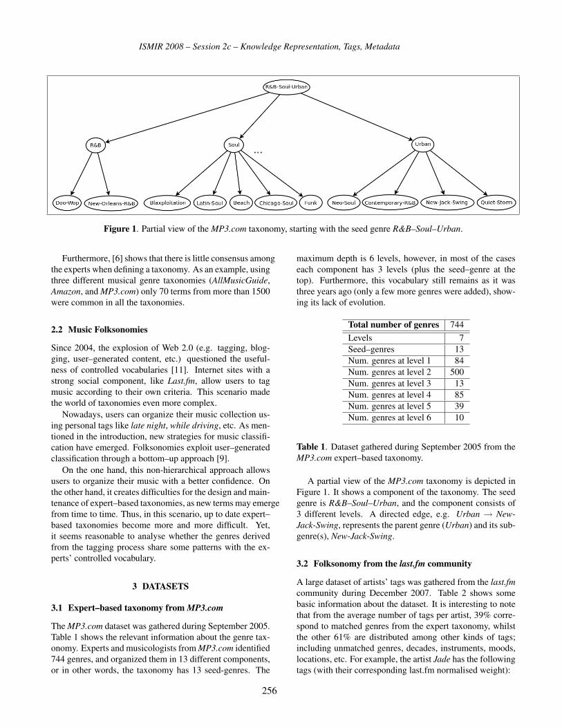
ISMIR 2008 – Session 2c – Knowledge Representation, Tags, Metadata
Figure 1. Partial view of the MP3.com taxonomy, starting with the seed genre R&B–Soul–Urban.
Furthermore, [6] shows that there is little consensus amongthe experts when defining a taxonomy. As an example, usingthree different musical genre taxonomies (AllMusicGuide,Amazon, andMP3.com) only 70 terms from more than 1500were common in all the taxonomies.
2.2 Music Folksonomies
Since 2004, the explosion of Web 2.0 (e.g. tagging, blog-ging, user–generated content, etc.) questioned the useful-ness of controlled vocabularies [11]. Internet sites with astrong social component, like Last.fm, allow users to tagmusic according to their own criteria. This scenario madethe world of taxonomies even more complex.Nowadays, users can organize their music collection us-
ing personal tags like late night, while driving, etc. As men-tioned in the introduction, new strategies for music classifi-cation have emerged. Folksonomies exploit user–generatedclassification through a bottom–up approach [9].On the one hand, this non-hierarchical approach allows
users to organize their music with a better confidence. Onthe other hand, it creates difficulties for the design and main-tenance of expert–based taxonomies, as new terms may emergefrom time to time. Thus, in this scenario, up to date expert–based taxonomies become more and more difficult. Yet,it seems reasonable to analyse whether the genres derivedfrom the tagging process share some patterns with the ex-perts’ controlled vocabulary.
3 DATASETS
3.1 Expert–based taxonomy fromMP3.com
TheMP3.com dataset was gathered during September 2005.Table 1 shows the relevant information about the genre tax-onomy. Experts and musicologists fromMP3.com identified744 genres, and organized them in 13 different components,or in other words, the taxonomy has 13 seed-genres. The
maximum depth is 6 levels, however, in most of the caseseach component has 3 levels (plus the seed–genre at thetop). Furthermore, this vocabulary still remains as it wasthree years ago (only a few more genres were added), show-ing its lack of evolution.
Total number of genres 744
Levels 7Seed–genres 13Num. genres at level 1 84Num. genres at level 2 500Num. genres at level 3 13Num. genres at level 4 85Num. genres at level 5 39Num. genres at level 6 10
Table 1. Dataset gathered during September 2005 from theMP3.com expert–based taxonomy.
A partial view of the MP3.com taxonomy is depicted inFigure 1. It shows a component of the taxonomy. The seedgenre is R&B–Soul–Urban, and the component consists of3 different levels. A directed edge, e.g. Urban → New-Jack-Swing, represents the parent genre (Urban) and its sub-genre(s), New-Jack-Swing.
3.2 Folksonomy from the last.fm community
A large dataset of artists’ tags was gathered from the last.fmcommunity during December 2007. Table 2 shows somebasic information about the dataset. It is interesting to notethat from the average number of tags per artist, 39% corre-spond to matched genres from the expert taxonomy, whilstthe other 61% are distributed among other kinds of tags;including unmatched genres, decades, instruments, moods,locations, etc. For example, the artist Jade has the followingtags (with their corresponding last.fm normalised weight):
256

ISMIR 2008 – Session 2c – Knowledge Representation, Tags, Metadata
Jade: urban(100), rnb(81), 90s(68),new jack swing(55), illinois(50),r and b(36), ...
Number of mapped genres 511
Number of artists 137,791Number of distinct tags 90,078Avg. tags per artist 11.95Avg. MP3.com genres per artist 4.68
Table 2. Dataset gathered from the last.fm community dur-ing December 2007.
Nevertheless, since the experiments aim to analyse theagreement between expert genres and genre–tags, we needto match artists’ tags with the expert defined genres.
3.2.1 Matching MP3.com genres and last.fm artist tags
In order to match those tags from the folksonomy that corre-spond to a genre in the expert taxonomy, a two-step processis followed:
• Compute a normalised form for all the folksonomytags and expert genres, by:
– converting them into lowercase,
– unifying separators to a single common one,
– treating some special characters (such as “&”,which can be expanded to “and” and “n”).
• Compute a string matching between the normalisedfolksonomy tags and expert genres.
The former step is inspired from [3]. For the latter, astring matching algorithm by Ratcliff and Metzener [8] isused to get all possible matches of a tag against a genre fromthe taxonomy. The similarity value goes from 0 to 1. Valuesclose to 0mean that the two strings are very dissimilar, and a1 value means that the strings are identical. Deciding whichis the threshold for identifying “nearly-identical” words isnot trivial. Yet, [10] shows that a threshold of 0.85 gives thehighest F-measure.The following example shows artist Jade’s tags that are
mapped to an MP3.com genre (90s and illinois tags dis-appear, and rnb and r and b are merged, combining theirweights—with a maximum value of 100):
Jade: Urban(100), R&B(100),New-Jack-Swing(55)
Once the matching process is complete, the next step isto analyse whether the tagging behaviour of the communityshares any resemblance with the expert taxonomy. The fol-lowing section presents the experimental results.
4 EXPERIMENTAL RESULTS
In order to measure the agreement between expert genresand the genre–tags defined by the wisdom of crowds, weperform several experiments. Beforehand, we have to com-pute the similarities among genres. Section 4.1 explains theprocess of computing distances in the expert taxonomy (us-ing the shortest path between two genres), and the tag dis-tances in the folksonomy (by means of a classic InformationRetrieval technique, called Latent Semantic Analysis).The experiments are divided in two main groups. The
first set of experiments deal with measuring the agreementat component level (a seed–genre and its subgenres). Thatis, to validate whether this taxonomy partition (13 compo-nents) correspond to the view of the community. Section 4.2present these experiments. The other experiment focuses onthe hierarchical structure (levels) of the expert taxonomy.In this experiment the goal is to reconstruct the taxonomybased on the genre distances from the folksonomy (section4.3).
4.1 Computing genre distances
4.1.1 Expert taxonomy
To compute genre distances in the expert taxonomy we sim-ply choose the shortest path between two genres, as an anal-ogy with the number of mouse clicks to reach one genrefrom a given one (e.g. distance between genres New–Jack–Swing and Soul is 3, according to Figure 1). Since the tax-onomy contains 13 seed genres, a virtual root node is addedat the top, thus making the graph fully connected. This waywe can compute the path between any genre in the graph.Whenever a path traverses the virtual root node, a penalty inthe distance is added to emphasize that the two genres comefrom different components.
4.1.2 Folksonomy
Latent Semantic Analysis (LSA), plus cosine similarity, isused as a measure of distance among genres within the folk-sonomy. LSA assumes a latent semantic structure that liesunderneath the randomness of word choice and spelling in“noisy” datasets [1], such as the one we are using. A sig-nificant paper that applies LSA in the music domain is [4].The authors show the usefulness of social tags—in a low102 space—to several relevant MIR problems, such as mu-sic similarity and mood analysis.LSA makes use of algebraic techniques such as Singular
Value Decomposition (SVD) to reduce the dimensionalityof the Artist–Genres matrix. After this step, either artist orgenre similarity can be computed using a cosine distance.Moreover, Information Retrieval literature [1, 7] states that,after raw data has been mapped into this latent semanticspace, topic (in our case, genre) separability is improved.
257

ISMIR 2008 – Session 2c – Knowledge Representation, Tags, Metadata
Electronic- Rock- R&B-Soul- Gospel- Vocal-Easy- World-
Folk Bluegrass Country Dance New-Age Pop Jazz Hip-Hop Urban Spiritual Listening Blues Reggae
Folk 0.184 0.144∗ 0.048 0.002 0.040 -0.022 0.007 -0.005 0.003 0.095 0.001 -0.002 0.107
Bluegrass 0.144 0.987 0.738∗ 0.006 -0.018 0.008 -0.019 -0.006 -0.022 0.096 0.014 0.019 -0.033
Country 0.048 0.738 0.430 0.001 -0.034 0.048 0.007 0.007 0.009 0.054 0.031 0.008 -0.042
Electronic-Dance 0.002 0.006 0.001 0.056 0.019 0.012 0.025 0.004 0.019 0.036 0.171 0.002 -0.007
New-Age 0.040 -0.018 -0.034 0.019 0.306 0.125 0.001 0.022 0.018 0.068 0.102 0.037 0.303∗
Rock-Pop -0.022 0.008 0.048 0.012 0.125∗ 0.043 0.036 0.005 0.006 0.040 0.043 0.006 0.132
Jazz 0.007 -0.019 0.007 0.025 0.001 0.036 0.211 -0.008 0.030 -0.036 0.150 0.046 0.018
Hip-Hop -0.005 -0.006 0.007 0.004 0.022 0.005 -0.008 0.599 -0.005 0.027 0.003 -0.005 0.021
R&B-Soul-Urban 0.003 -0.022 0.009 0.019 0.018 0.006 0.030 -0.005 0.393 0.355∗ 0.009 0.002 0.005
Gospel-Spiritual 0.095 0.096 0.054 0.036 0.068 0.040 -0.036 0.027 0.355 0.134 0.003 0.163 -0.015
Vocal-Easy-Listening 0.001 0.014 0.031 0.171 0.102 0.043 0.150 0.003 0.009 0.003 0.167 0.012 0.040
Blues -0.002 0.019 0.008 0.002 0.037 0.006 0.046 -0.005 0.002 0.163 0.012 0.657 -0.004
World-Reggae 0.107 -0.033 -0.042 -0.007 0.303 0.132 0.018 0.021 0.005 -0.015 0.040 -0.004 0.142
Table 3. Confusion matrix for the inter–components coarse grained similarity. For clarification purposes, the diagonal containsthe intra–component similarity. The values marked with an asterisk are as significative as the highest value (in bold).
For each artist we create a vector based on their (last.fmnormalised) genre–tags’ frequencies. Once the matrix is de-composed by columns, using SVD with 50 dimensions, weobtain genre similarities. For example, the closest genres toHeavy Metal in the semantic space are Power Metal, BritishMetal and Speed Metal, all with a similarity value above 0.6.On the other hand, similarity between Heavy Metal and Popyields a near–zero value.
4.2 Agreement between expert and community genres
Tomeasure the agreement between expert defined genre com-ponents and community genres we perform two experiments.The first one carries out a coarse–grained similarity (at genrecomponent level), where the main goal is to separate theexpert genre clusters according to the genre distances inthe folksonomy. The second experiment performs a fine–grained similarity (at genre node level) in order to see thecorrelations between the genre distance in the taxonomy andthe distance in the LSA space derived from the folksonomy.
4.2.1 Coarse-grained similarity
The first experiment aims to check how separable are theexpert defined genre components according to the genre dis-tances in the folksonomy (as defined in section 4.1.2). Theexperiment is performed in two steps: (i) compute the LSAcosine similarity among all the subgenres within a com-ponent (intra–component similarity); and (ii) compute theLSA cosine similarity among components, using the cen-troid of each component (inter–component similarity).The results for intra–component similarity are presented
in Figure 2. The most correlated components are Bluegrass,
Figure 2. Intra–component coarse grained similarity.
Hip-Hop and Blues. Note however that the Bluegrass com-ponent has only 3 subgenres mapped in our last.fm dataset.The components with less community–expert agreement areElectronic-Dance and Rock-Pop. For the latter genre, it isworth noting that it is an ill–defined seed-genre, and it is alsothe one including the highest number of subgenres. Some ofthese Rock-Pop subgenres are so eclectic that they could be-long to more than one component. For instance, Obscurosubgenre is defined in Allmusic 1 as “...a nebulous categorythat encompasses the weird, the puzzling, the ill-conceived,the unclassifiable, the musical territory you never dreamed
1 http://www.allmusic.com/
258

ISMIR 2008 – Session 2c – Knowledge Representation, Tags, Metadata
existed”.Regarding the inter–component similarity, we proceed as
follows: we compute the centroid vector of each compo-nent, and then compare it with the remaining components’centroids. The results are presented in table 3. Note thatthe results in the diagonal represent the intra–componentssimilarity. For each row, we mark in bold the highest value.Subgenres of Bluegrass, Hip-Hop and Blues, as it has beenobserved for the intra–component case, are highly correlatedin the semantic space. Thus, they are the ones with moreagreement between the community and the experts classifi-cation. However, only Hip-Hop and Blues are clearly dis-tinguishable from the rest. Furthermore, according to thecommunity, Bluegrass and Country genres are very similar.Indeed, other available internet taxonomies, such as Amazonor Allmusic, include Bluegrass as a subgenre of Country.Similarly, Gospel-Spiritual genre is merged into R&B-Soul-Urban.
4.2.2 Fine-grained similarity
In this experiment we focus on the genre node level (insteadof components). The hypothesis is that genres closer in thesemantic space of the folksonomy should also be closer inthe expert taxonomy, and vice versa. To validate this for-mulation a one–way Anova is performed. The independentgroups are considered the path distances in the expert tax-onomy (ranging from 1..10, the diameter of the taxonomy),whilst the dependent variable is the LSA cosine distance.Figure 3 depicts the box–and–whisker plot. Indeed, a
large value of the F–statistic as well as a p–value � 0.05corroborates the hypothesis. Furthermore, to determine thedistances that are statistically significant we perform the Tukey’spairwise comparisons test. The results show that path dis-tances 1 and 2 are significant among the rest of the distances,at 95% family–wise confidence level.
4.3 Reconstructing the taxonomy from the folksonomy
In this experiment we try to reconstruct the taxonomy fromthe folksonomy’s inferred semantic structure. The recon-struction of the expert taxonomy from the folksonomy isbased on the correct selection of a parent genre, accordingto the LSA cosine similarity derived from the folksonomy.We follow a bottom–up approach, starting from the leaves ofeach component. At each step of the process, we record thedifferences between the inferred and original taxonomies inorder to have a similarity metric between them.The metrics used are: mean reciprocal rank, and root hit.
The mean reciprocal rank (MRR) is a statistic widely usedin Information Retrieval. The reciprocal rank (RR) is de-fined as the inverse of the correct answer’s rank,RR(tag) =1/ranktag . For instance, given the New–Jack–Swing genre,see Figure 4, the closest genre parents (according to the LSA
Figure 3. Box–and–whisker plot depicting the correlationbetween genre path distances in the taxonomy and semanticLSA cosine similarity. The Anova experiment (p−value�0.05) shows that there is a statistical significance amongpath distances.
Figure 4. Reconstruction of the expert taxonomy from thefolksonomy. Selection of a parent is made according to theLSA cosine similarity derived from the folksonomy.
cosine distance) are: (1) R&B, (2) Urban, (3) Traditional–Gospel, etc. The correct parent genre, Urban, is found in thesecond position, thus RR(New − Jack − Swing) = 1
2 =0.5. Furthermore we compute whether the top–1 parent be-longs to the same component as the child genre (root hit).In this example, it is a root hit because both the genre New–Jack–Swing and the selected (wrong) parent, R&B, belongto the same component, R&B–Soul–Urban.
Table 4 shows the results for each component. Bluegrass’perfect hit rate should be ignored, as the component hasonly 3 subgenres mapped. The lowest MRR is in Rock–Pop genre, which is also the highest (153 subgenres), andleast cohesive component (lowest inter-genre similarity, seeTable 3). Hip–Hop, on the other hand, is a highly cohesivecomponent with a very high MRR. Finally, a lower MRRin Folk and World–Reggae could be interpreted as a con-sequence of the taxonomy being too geographically biasedto English spoken territories. At the same time, disparategenres of all kinds, and from all over the world, are to beconsidered sub–genres of Folk and World–Reggae.
259

ISMIR 2008 – Session 2c – Knowledge Representation, Tags, Metadata
Component (size) Root Hits (%) MRRFolk (22) 36.3 0.447Bluegrass (3) 100 1.000Country (35) 85.8 0.636Electronic-Dance (36) 30.6 0.391New-Age (5) 40.0 0.700Rock-Pop (135) 48.2 0.295Jazz (83) 83.2 0.638Hip-Hop (22) 81.8 0.894R&B-Soul-Urban (26) 75.4 0.694Gospel-Spiritual (7) 38.6 0.558Vocal-Easy-Listening (11) 27.3 0.446Blues (43) 81.4 0.455World-Reggae (83) 53.0 0.389
Weighted Avg. (511) 60.4 0.478
Table 4. Reconstruction of the expert–taxonomy, usinggenre similarity derived from the folksonomy.
5 CONCLUSIONS
This paper presented some interesting findings around mu-sical genres. First of all, the consensus from a group of ex-perts to create a universal taxonomy seems difficult. Whileexpert taxonomies are useful for cataloguing and hierarchi-cal browsing, the flat view of folksonomies allows betterorganization and access of a personal collection.
We presented three different experiments to analyse theagreement between expert–based controlled vocabulary andbottom–up folksonomies. The first two experiments focusedon measuring the agreement between genres from the folk-sonomy and expert genres. A third experiment emphasizedthe hierarchical structure of a taxonomy, but using the in-formation from a folksonomy. In all the experiments theconclusions were the same: some genres are clearly definedboth from the experts and the wisdom of crowds, reaching ahigh agreement between these two views, while other genresare difficult to get a common consensus of its meaning.
All in all, experts, wisdom of crowds, and machines 2
agree in the classification and cohesion of some genres (e.g.Blues, Hip-Hop), and clearly disagree in others (e.g. Rock).A multi–faceted approach for musical genre using expertbased classifications, dynamic associations derived from thecommunity driven annotations, and content–based analysiswould improve genre classification, as well as other relevantMIR tasks such as music similarity or music recommenda-tion.
2 See the results of MIREX 2007 in http://www.music-ir.org/mirex/2007/index.php/Audio Genre Classification Results
6 ACKNOWLEDGMENTS
This research has been partially supported by the e-Contentplus project VARIAZIONI 3 .
7 REFERENCES
[1] J.R. Bellegarda. Latent semantic mapping. Signal Pro-cessing Magazine, IEEE, 22(5):70–80, Sept. 2005.
[2] F. Fabbri. A theory of musical genres: Two applications.Popular Music Perspectives, 1981.
[3] G. Geleijnse, M. Schedl, and P. Knees. The quest forground truth in musical artist tagging in the social webera. In Proceedings of the Eighth International Confer-ence on Music Information Retrieval, pages 525 – 530,Vienna, Austria, September 2007.
[4] M. Levy andM. Sandler. A semantic space for music de-rived from social tags. In Proceedings of the Eighth In-ternational Conference on Music Information Retrieval,Vienna, Austria, September 2007.
[5] C. Mckay and I. Fujinaga. Musical genre classification:Is it worth pursuing and how can it be improved? InProceedings of the Seventh International Conference onMusic Information Retrieval, Victoria, Canada, 2006.
[6] F. Pachet and F. Cazaly. A taxonomy of musical genres.In Proc. Content-Based Multimedia Information Access,2000.
[7] C. H. Papadimitriou, H. Tamaki, P. Raghavan, andS. Vempala. Latent semantic indexing: A probabilis-tic analysis. In Proocedings of the ACM Conference onPrinciples of Database Systems (PODS), pages 159–168, Seattle, 1998.
[8] JW Ratcliff and D. Metzener. Pattern matching: TheGestalt approach. Dr. Dobb’s Journal, page 46, 1988.
[9] N. Scaringella, G. Zoia, and D. Mlynek. Automaticgenre classification of music content: a survey. SignalProcessing Magazine, IEEE, 23(2):133–141, 2006.
[10] A. Schuth, M. Marx, and M. de Rijke. Extracting thediscussion structure in comments on news-articles. In9th ACM International Workshop on Web Informationand Data Management (WIDM 2007), pages 97–104,November 2007.
[11] C. Shirky. Ontology is overrated: Categories, Links,and Tags. Online: http://shirky. com/writings/ontologyoverrated. html, 2005.
3 http://www.variazioniproject.com
260

Session 2d – Social and Music Networks

.

ISMIR 2008 – Session 2d – Social and Music Networks
A WEB OF MUSICAL INFORMATION
Yves Raimond, Mark SandlerCentre for Digital Music
Queen Mary, University of London
ABSTRACT
We describe our recent achievements in interlinking several
music-related data sources on the Semantic Web. In partic-
ular, we describe interlinked datasets dealing with Creative
Commons content, editorial, encyclopedic, geographic and
statistical data, along with queries they can answer and tools
using their data. We describe our web services, provid-
ing an on-demand access to content-based features linked
with such data sources and information pertaining to their
creation (including processing steps, applied algorithms, in-
puts, parameters or associated developers). We also provide
a tool allowing such music analysis services to be set up and
scripted in a simple way.
1 INTRODUCTION
Information management has become a primary concern for
multimedia-related technologies, from personal collections
management to the construction of large content delivery
services. However, the solutions that have emerged still ex-
ist in isolation. For example, large online databases (such as
Musicbrainz, MyStrands, etc.) and personal music collec-
tion management tools such as iTunes or Songbird do not
interact with each other, although they actually deal with the
same kind of data. The information one of these solutions
manages does not benefit from the information another may
hold.
The problem becomes acute when narrowing our view
to the exchange of results between music technology re-
searchers. If providing access to content-based feature ex-
traction through web services is a first step [10, 6], the re-
sults they produce, in order for them to be meaningful, must
be interlinked with other data sources. Just giving back a
set of results from a particular digital audio item is useless
unless we know what has been processed, and how.
In this paper, we show the benefits of using a set of
web standards, often referred to as Semantic Web technolo-
gies, to achieve these goals. First, we give an overview
of these standards and how they can be used to create a
‘web of data’—a distributed, domain-independent, web-
scale database. We give a brief summary of the Seman-
tic Web ontology we described in [12], able to deal with
music-related data. We then focus on the music-related in-
terlinked datasets we published since, and give examples of
the type of queries they can answer and of tools consum-
ing their data. We describe our lightweight extension of this
music ontology to make content-based features part of this
‘web of data’. We also describe our web services, providing
on-demand access to such resources, as well as the frame-
work underlying them.
2 TOWARDS A MUSIC-RELATED WEB OF DATA
2.1 Web identifiers and structured representations
The web is built around the concept of URI (Uniform Re-
source Identifier 1 ). A URI can identify anything, not just
a document: a person, a particular performance, a signal,
a particular content-based feature, etc. Web resources can
have multiple associated representations. For example, to a
URI identifying a particular signal, we may want to asso-
ciate an HTML representation of it (providing some textual
information about its characteristics) or an image depicting
the actual waveform. The web aspect comes into place when
other web identifiers are mentioned within such a represen-
tation. For example, the HTML representation of our sig-
nal URI might link to an URI identifying the corresponding
recording device.
Now, these representations can be structured: they can
provide explicit machine-processable information. The Re-
source Description Framework (RDF 2 ) allows such repre-
sentations to be made, by expressing statements about web
resources in the form of triples: subject, predicate and ob-
ject. When such representations quote other resource identi-
fiers, enabling access to corresponding structured represen-
tation, we create a ‘web of data’.
For example, starting from the URI of a
band available in our Jamendo dataset 3 : http://dbtune.org/jamendo/artist/5, two possi-
ble representations are available. One is in HTML and can
be rendered for human consumption through a traditional
web browser; the other is structured and machine readable,
holding explicit statements about this band. The RDF
representation, requested via the HTTP Accept header, is
1 http://www.ietf.org/rfc/rfc2396.txt2 http://www.w3.org/RDF/3 See http://dbtune.org/ for all our DBTune datasets.
263

ISMIR 2008 – Session 2d – Social and Music Networks
as follows: 4
<http://dbtune.org/jamendo/artist/5>a mo:MusicGroup;foaf:made <http://dbtune.org/jamendo/record/174>;foaf:made <http://dbtune.org/jamendo/record/33>;owl:sameAs <http://zitgist.com/music/artist/0781a3f3-
645c-45d1-a84f-76b4e4decf6d>;foaf:based near <http://sws.geonames.org/2991627/>;foaf:homepage <http://www.both-world.com>;foaf:img <http://img.jamendo.com/artists/b/both.jpg>;foaf:name ”Both”ˆˆxsd:string.
Using this representation, we can for example follow the
foaf:based near link to a resource in the Geonames
dataset 5 in order to get detailed information about the place
where this band is based.
2.2 Accessing and querying Semantic Web data
The new SPARQL W3C recommendation 6 gives a way
to access and query such data, through a simple SQL-like
syntax allowing requests ranging from simple DESCRIBEs
(“return all information about resource x”) to complex struc-
tured queries (eg. “return the latest album from artists lo-
cated in Mexico, produced by a French person”).
SPARQL allows us to specify explicitly the location of
the RDF data, access a particular aggregation of data, or
drive a Semantic Web “user agent”, such as the Semantic
Web Client Library 7 , which crawls and aggregates data in
order to satisfy a particular query. A place on the web ac-
cepting SPARQL queries is called an end-point.
2.3 The Music Ontology
The Music Ontology we described in [12] aims at providing
a set of web identifiers and corresponding structured repre-
sentations for an ontology (defining the main concepts and
relationships) of the music domain. It is divided into three
different parts, respectively dealing with editorial informa-
tion (track names, people, labels, releases, etc.), production
workflow information (compositions, arrangements, perfor-
mances, recording, etc.) and event decomposition (eg. “the
piano player was playing in that particular key at that time”)
The following Music Ontology example describes a set of
resources involved in the description of a performance of
Antonio Vivaldi’s Four Seasons:
:vivaldi a mo:MusicArtist;foaf:name ”Antonio Vivaldi”;
4 All our RDF examples are written in RDF/Turtle: http://www.w3.org/TeamSubmission/turtle/. Each block corresponds to a
set of statements (subject, predicate, object) about one subject. Web iden-
tifiers are either between angle brackets or in a prefix:name notation (with
the namespaces defined at the end of the paper). Literals are enclosed in
double quotes and can hold an explicit typing information.5 http://geonames.org/.6 http://www.w3.org/TR/rdf-sparql-query/7 http://sites.wiwiss.fu-berlin.de/suhl/bizer/
ng4j/semwebclient/
Figure 1. Available interlinked dataset, as of March 2008.
owl:sameAs <http://dbpedia.org/resource/Antonio Vivaldi>.:compositionevent a mo:Composition;
mo:composer :vivaldi;mo:produced work :thefourseasons;event:time [time:year ”1723”].
:thefourseasons a mo:MusicalWork;dc:title ”The Four Seasons”;owl:sameAs
<http://dbpedia.org/resource/The Four Seasons (Vivaldi)>;mo:part :spring.
:spring a mo:MusicalWork;dc:title ”Concerto No. 1 in E major, Op. 8, RV 269, La primavera”;mo:movement :largo.
:largo a mo:Movement;dc:title ”Largo”.
:performance a mo:Performance;owl:sameAs <http://dbtune.org/magnatune/performance/369>;mo:perfomer :american baroque;mo:performance of :largo.
:americanbaroque a mo:MusicalGroup;foaf:name ”American Baroque”;owl:sameAs
<http://dbtune.org/magnatune/artist/american baroque>.
Following the principles outlined above, this example in-
terlinks two datasets: DBpedia and Magnatune, which we
study in the next section.
3 CURRENT DATASETS
The “Linking Open Data on the Semantic Web” project [3]
hosted by the W3C Semantic Web Education and Outreach
group aims at publishing a wide range of datasets on the
Semantic Web, and creating links between them. The cur-
rently available interlinked datasets (regardless of their do-
main) can be depicted as in fig. 1. In this section, we discuss
a few of these datasets and their links to other datasets. We
especially focus on the music-related datasets we published
within our DBTune service, using the Music Ontology men-
tioned above. We illustrate their use by examples of queries
they can answer, or by tools using their data.
264

ISMIR 2008 – Session 2d – Social and Music Networks
3.1 DBpedia
The DBpedia project described by Auer et al. in [1] ex-
tracts structured information from Wikipedia, and repub-
lishes it on the Semantic Web, together with links to other
datasets. The whole DBpedia dataset holds around 100 mil-
lion RDF statements, describing 2.4 million entities across
a wide range of domains, and 2 million links (statements
that quote an identifier outside DBpedia). For example, the
following SPARQL query issued on the DBpedia dataset re-
turns names, descriptions and birth dates of guitarists born
in Paris between 1939 and 1945: 8
SELECT ?name ?birth ?description ?person WHERE {?person
p:birthPlace <http://dbpedia.org/resource/Paris> ;a yago:Guitarist110151760 ;p:birth ?birth ;foaf:name ?name ;rdfs:comment ?description .FILTER (LANG(?description) = ’en’ &&?birth > "1939-01-01"ˆˆxsd:date &&?birth < "1945-01-01"ˆˆxsd:date ) . }
The DBpedia relationship finder [9] allows this dataset to
be queried for arbitrary RDF ‘paths’ between two different
resources. For example, it would answer the query ‘what
do Mozart and Metallica have in common?’ as depicted in
fig. 2.
3.2 DBTune
We created the DBTune service to experiment with hetero-
geneous music-related datasets published as Music Ontol-
ogy linked data. We published the Magnatune record label
catalogue, and we interlinked it with corresponding DBpe-
dia identifiers (as illustrated in § 2.3). We also published
the Jamendo music platform database, and we interlinked
it with Geonames and Musicbrainz identifiers. DBTune re-
publishes on the Semantic Web data coming from Audio-
Scrobbler and MySpace, therefore allowing different social
networks as well as listening habits to be interlinked. DB-
Tune also hosts a Semantic Web version of the BBC John
Peel sessions, interlinked with DBpedia.
Musicbrainz is a community-maintained music database
holding detailed editorial information about 300,000 artists,
500,000 releases and 6 million tracks. We published a linked
data version of this dataset. Artists, records and countries
are interlinked with corresponding DBpedia web identifiers.
For example, the identifier corresponding to Madonna in
DBTune is stated as being the same as the corresponding
identifier in DBpedia. We also interlinked artist resources
with corresponding web identifiers on our linked data pub-
lication of the MySpace social network.We provide a number of SPARQL end-points, for each
dataset (except AudioScrobbler and MySpace, as the RDF
8 This query returns, among others, Babik Reinhardt, one of Django
Reinhardt’s sons.
documents are generated dynamically). For example, thefollowing query can be issued to our Jamendo end-point:
SELECT DISTINCT ?an ?lat ?long WHERE {?a a mo:MusicArtist;foaf:based_near ?place;foaf:name ?an;foaf:made ?alb.
?alb tags:taggedWithTag<http://dbtune.org/jamendo/tag/jazz>.
?placegeo:name ?name;geo:population ?population;wgs:lat ?lat;wgs:long ?long } ORDER BY ?population
This returns artists who made at least one album tagged as
‘jazz’ by a Jamendo user, sorted by the number of inhab-
itants of the places they are based near. Overall, DBTune
gives access to approximately 13 billion RDF triples, thus
making it one of the largest dataset on the Semantic Web.
3.3 Use-case: personal collection management
Such interlinked music-related data sources can be used
for a wide range of use-cases, including personal collec-
tion management. We developed two tools to aggregate Se-
mantic Web data describing arbitrary personal music col-
lections. GNAT 9 finds, for all tracks available in a collec-
tion, the corresponding web identifiers in the Semantic Web
publication of the Musicbrainz dataset mentioned earlier.
GNAT uses primarily a metadata-based interlinking algo-
rithm described in [13], which was also used to interlink the
above described music-related datasets. GNARQL crawls
the web of data from these identifiers and aggregate struc-
tured information about them, coming from heterogeneous
data sources. GNAT and GNARQL then automatically cre-
ate a tailored database, describing different aspects of a per-
sonal music collection. GNARQL provides a SPARQL end-
point, allowing this aggregation of Semantic Web data to be
queried. For example, queries such as “Create a playlist of
performances of works by French composers, written be-
tween 1800 and 1850” or “Sort European hip-hop artists in
my collection by murder rates in their city” can be answered
using this end-point. GNARQL also gives a faceted brows-
ing interface based on /facet [8], as illustrated in fig. 3.
4 ON-DEMAND FEATURE EXTRACTION ANDINTERLINKING
4.1 Why web services are not enough
Although providing web service access through technolo-
gies such as SOAP or WSDL is a first step towards a dis-
tributed framework for performing music analysis tasks (as
highlighted in [10] and [6]), this is not enough. In order
for results to be easily re-usable, it is desirable to prevent
9 GNAT and GNARQL are available at http://sourceforge.net/projects/motools.
265

ISMIR 2008 – Session 2d – Social and Music Networks
Figure 2. What do Mozart and Metallica have in common?
Figure 3. Management of personal music collections using
GNAT and GNARQL. Here, we plot our collection on a map and
display a particular artist.
the client software from having to explicitly adapt to the pe-
culiarities of each web service. This is particularly impor-
tant when trying to combine several web services (known
as the ‘choreography’ problem). The results of various ser-
vices must be interlinked with additional resources supply-
ing information pertaining to their creation. The information
could include processing steps, applied algorithms, inputs
and the parameters, associated developers, etc.
The technologies described in § 2 provide a way to ad-
dress this issue. The results of a music analysis task can be
described in an RDF document which provides such links.
The results are then part of the data web, and can be queried
through their relationships to further data. For example, one
could issue a SPARQL query such as “Give me a struc-
tural segmentation obtained using an implementation of al-
gorithm x developed by y, on the signal identified by z”.
In the rest of this section, we describe our framework to
express music analysis results in RDF, and a tool provid-
ing on-demand access to such interlinked results. We also
describe a way to easily script and publish combinations of
music analysis results made available on the Semantic Web.
4.2 Representing features in RDF
We extended the Music Ontology framework to describe a
wide range of musical audio features in RDF 10 . Features
describing the whole audio signal (whose concept is iden-
tified by the URI mo:Signal) can be directly attached to
10 http://purl.org/ontology/af/
the signal resource. Moreover, an audio signal is associated
with a temporal extent (tl:Interval) defined on a time-
line (tl:TimeLine). Then, events (event:Event) can
be defined in order to classify particular points or intervals
on such time-lines. Defining new types of audio features
is then just a matter of subsuming the event concept. For
example, the following defines a new zero-crossing rate
feature type:
:ZeroCrossingRatea owl:Class;rdfs:subClassOf event:Event;rdfs:label ”Zero Crossing Rate event”.
:zcra owl:DatatypeProperty;rdfs:subPropertyOf event:literal factor;rdfs:domain :ZeroCrossingRate;rdfs:label ”Associated zero-crossing rate”.
Then, an instance of such a feature on the time-line of
a particular signal (here, a track from the Jamendo dataset)
would be represented as:
<http://dbtune.org/audio/Den-Nostalia.ogg> mo:encodes :sig.:sig a mo:Signal;
mo:time [ # Temporal extent of the signaltl:timeline :tl; # Time-line on which this extent is definedtl:duration ”PT4M50S” ]. # 4 minutes and 50 seconds
:e1 a :ZeroCrossingRate;:zcr ”27”; # Zero-crossing rateevent:time [
tl:start ”PT0S”; # Starts at 0tl:end ”PT0.046439912S”; # Ends at 1024/22050 secondstl:timeline :tl ]. # Defined on the time-line backing our signal
4.3 Evaluating music analysis predicates
We model music analysis processes as RDF properties, as-
sociating their results with the inputs and parameters used.
Predicates involving these properties can be considered as
built-in predicates, within particular SPARQL end-points.
For example, the decoding of an audio file and the evalua-
tion of a musical key detection Vamp plugin 11 implement-
ing the template-based algorithm described by Noland and
Sandler in [11] could be triggered while evaluating the fol-
lowing query:
SELECT ?sig ?resultWHERE {<http://dbtune.org/audio/Den-Nostalia.ogg>
mo:encodes ?sig.?sig vamp:qm-keydetector ?result }
The audio file is discovered at querying time. The corre-
sponding signal resource is associated to the ?sig variable,
11 http://www.vamp-plugins.org/.
266
ISMIR 2008 – Session 2d – Social and Music Networks
and the results given by the Vamp plugin are associated to
the ?result variable. The predicates mo:encodes and
vamp:qm-keydetector both correspond to a particular
process, which is triggered when the predicate is evaluated.
Moreover, in the representations of mo:encodes and
vamp:qm-keydetector, we can access two statements
specifying that these are functional properties 12 . For one
subject of these properties, there is only one correspond-
ing object. Results corresponding to the evaluation of such
predicates are therefore cached, to prevent repeating similar
evaluations.
In these representations, we might also have links to ac-
tual implementations. We can therefore discover at querying
time how to evaluate a new predicate by retrieving such im-
plementations.
4.4 Combining music analysis and structured web data
N3 [2] provides a way to publish rules over RDF data on
the Semantic Web, by extending the RDF data model in
two ways: quoting facilities (the ability to consider an RDF
graph as a literal resource) and universal quantification. A
particular RDF predicate then captures the notion of impli-
cation: log:implies (denoted by the => symbol in our
example). N3, in our context, allows to easily script how
combination of predicates (which resolution might trigger
some analysis tools, or some querying of RDF data) can
lead to further predicates. A N3 rule can express “state-
ments linking two similar audio signals can be derived by
computing a MFCC model for both and thresholding their
Kullback-Leibler divergence”, or “statements linking two
similar audio signals can be derived by thresholding the co-
sine distance of the corresponding beat spectra” 13 . A N3
rule can also merge contextual queries and content analy-
sis, as suggested in [7]: “A danceable track has an average
tempo of around 120 beats per minute, a high loudness, and
is in the playlist of a disc jockey.”.
Our previous key detection example can be mashed
up with an identification process (captured by the
gnat:match predicate which, from an audio file,
finds out the corresponding identifier in the Musicbrainz
dataset) and be translated into Music Ontology terms using
the following rule:
{ ?af mo:encodes ?sig; gnat:match ?mbzsig. ?sig vamp:qm-keydetector ?results.?mbzsig mo:time [tl:timeline :tl ].(?start ?duration ?key) list:in ?results. } => {
:keyevent a to:Tonality;rdfs:label ”key event”; to:key ?key; event:time [
tl:start ?start; tl:duration ?duration; tl:timeline :tl ]. }
12 individuals of owl:FunctionalProperty13 Using the approach described in [5], we can trace back what has been
achieved to derive such similarity statements.
4.5 On-demand extraction and interlinking: Henry
We developed an interpreter of such rules combining mu-
sic analysis processes and contextual data: Henry 14 . Henry
handles two persistent stores: an RDF and N3 store m (han-
dling, among other things, computation metadata and RDF
statements gleaned from the web) and a binary store b (han-
dling binary representations of resources described in the
RDF store: signals, features, etc.). The underlying logic of
this software builds on top of Transaction Logic [4] over b.
Henry provides the ability to register new built-in predicates
written in a variety of languages.The main interface to inter-
act with Henry is its SPARQL end-point. When processing
a SPARQL query q, Henry executes the following steps:
1. For every newly appearing web identifier i in q, deref-
erence it, and then:
(a) If the representation is RDF, store it in m. If i is
a property and its representation links to a built-
in implementation matching the current platform,
retrieve it ;
(b) If the representation is N3, store it in m and reg-
ister the corresponding rules ;
(c) If the representation is binary, cache it in b ;
2. For every triple pattern p in q, the possible solutions
are:
(a) Instantiations of p in m ;
(b) If p is in the conclusion part of a rule, the so-
lutions correspond to the possible evaluations of
the premises ;
(c) if p=(sp, pp, op) where pp is a built-in predicate,
solutions are derived using this built-in, updat-
ing b accordingly.
4.6 Available services
An available Henry instance 15 provides access to a number
of such results. It wraps a Vamp plug-in host, so new built-in
predicates and the corresponding Vamp implementation can
be discovered at querying time. This instance also discovers
new audio files at querying time. It provides a SPARQL end-
point, although a future version will also include a simplified
HTTP interface.
The above defined rule for key events and a number of
others are pre-loaded. For example, the following query se-
lects several attributes of key events on the time-line of an
audio signal (start time, end time and corresponding key):
14 Henry source code is available at http://code.google.com/p/km-rdf/
15 Available at http://dbtune.org/henry/
267

ISMIR 2008 – Session 2d – Social and Music Networks
SELECT ?start ?end ?key WHERE {<http://dbtune.org/audio/Den-Nostalia.ogg>
mo:encodes ?sig.?sig mo:time ?time.?time tl:timeline ?tl._:evt a to:Tonality;
event:time [tl:start ?start; tl:end ?end; tl:timeline ?tl] ;
to:key ?key }
This query triggers a call to a key detection Vamp plugin
if the results have not yet previously been computed for the
mentioned audio file. As the predicate corresponding to the
Vamp call is functional, the Vamp results are cached. The
results bound with the variable ?key are resources within
the Tonality Ontology 16 , which allows us to access further
information about the keys themselves.
5 CONCLUSION AND FUTURE WORK
Publishing web resources and corresponding RDF represen-
tations providing links to further resources is a big step to-
wards a shared information space for music enthusiasts. The
web environment allows us to link together heterogeneous
types of information: from music analysis results to edito-
rial or social data, but also data that we often don’t include
in a music information system, such as geographical, statis-
tical or encyclopedic data. This web of data is now a reality,
which is concretely used in a number of applications such
as GNAT and GNARQL. We developed a tool called Henry,
which dynamically creates and publishes such linked data,
by working on top of on-the-fly discovery of content, con-
tent analysis processes, logical rules, and external data. Pub-
lishing a new range of music analysis results on the data web
is therefore as simple as publishing a small amount of RDF
specifying new processing tools (if we need any), and some
N3 rules combining them together. We are now in the posi-
tion of answering hybrid queries such as ‘find me all works
composed in New York in 1977, performed at an average
tempo of 130 bpm and with an overall C major key’.
Future work includes publishing and interlinking more
music-related datasets. It also includes delegating the res-
olution of predicates within Henry: it might be inefficient
to allow every instance to be dynamically patched with the
same set of plugins, handling a similar range of processing.
Moreover, some plugin providers may not want to distribute
their implementation, but just provide web access to it.
6 ACKNOWLEDGEMENTS
The authors acknowledge the support of both the Centre
For Digital Music and the Department of Computer Sci-
ence at Queen Mary University of London for the stu-
dentship for Yves Raimond. This work has been partially
16 http://purl.org/ontology/tonality/
supported by the EPSRC-funded ICT project OMRAS-2
(EP/E017614/1).
Namespaces@prefix rdfs: <http://www.w3.org/2000/01/rdf-schema#>.@prefix owl: <http://www.w3.org/2002/07/owl#>.@prefix geo: <http://www.geonames.org/ontology#>.@prefix wgs: <http://www.w3.org/2003/01/geo/wgs84 pos#>.@prefix yago: <http://dbpedia.org/class/yago/>.@prefix foaf: <http://xmlns.com/foaf/0.1/>.@prefix p: <http://dbpedia.org/property/>.@prefix xsd: <http://www.w3.org/2001/XMLSchema#>.@prefix dc: <http://purl.org/dc/elements/1.1/>.@prefix mo: <http://purl.org/ontology/mo/>.@prefix event: <http://purl.org/NET/c4dm/event.owl#>.@prefix tl: <http://purl.org/NET/c4dm/timeline.owl#>.@prefix to: <http://purl.org/ontology/tonality/>.@prefix vamp: <http://purl.org/ontology/vamp/>.@prefix list: <http://www.w3.org/2000/10/swap/list#>.@prefix gnat: <http://motools.sourceforge.net/doap.rdf#>.@prefix tags: <http://www.holygoat.co.uk/owl/redwood/0.1/tags/>.
7 REFERENCES
[1] S. Auer, C. Bizer, J. Lehmann, G. Kobilarov, R. Cyganiak, and Z. Ives. Dbpedia:A nucleus for a web of open data. In Proceedings of the International SemanticWeb Conference, Busan, Korea, November 11-15 2007.
[2] Tim Berners-Lee, Dan Connolly, Lalana Kagal, Yosi Scharf, and Jim Hendler.N3Logic : A logical framework for the world wide web. Theory and Practice ofLogic Programming, 2007. To appear in Theory and Practice of Logic Program-ming (TPLP). Available at http://arxiv.org/abs/0711.1533. Last ac-cessed September 2007.
[3] Chris Bizer, Tom Heath, Danny Ayers, and Yves Raimond. Interlinking open dataon the web. In Demonstrations Track, 4th European Semantic Web Conference,Innsbruck, Austria, 2007.
[4] Anthony J. Bonner and Michael Kifer. An overview of transaction logic. Theoret-ical Computer Science, 133:205–265, 1994.
[5] Jeremy J. Carroll, Christian Bizer, Pat Hayes, and Patrick Stickler. Named graphs.Journal of Web Semantics, 2005.
[6] Andreas F. Ehmann, J. Stephen Downie, and M. Cameron Jones. The music infor-mation retrieval evaluation exchange “Do-It-Yourself” web service. In Proceed-ings of the International Conference on Music Information Retrieval, 2007.
[7] Roberto Garcia and Òscar Celma. Semantic integration and retrieval of multime-dia metadata. In Proceedings of the 5th International Workshop on KnowledgeMarkup and Semantic Annotation, 2005.
[8] Michiel Hildebrand, Jacco van Ossenbruggen, and Lynda Hardman. The SemanticWeb - ISWC 2006, volume 4273/2006 of Lecture Notes in Computer Science,chapter /facet: A Browser for Heterogeneous Semantic Web Repositories, pages272–285. Springer Berlin / Heidelberg, 2006.
[9] Jens Lehmann, Jrg Schppel, and Sren Auer. Discovering unknown connections -the dbpedia relationship finder. In Proceedings of the First Conference on SocialSemantic Web (CSSW), pages 99–110, 2007.
[10] Daniel McEnnis, Cory McKay, and Ichiro Fujinaga. Overview of OMEN. In Pro-ceedings of the International Conference on Music Information Retrieval, 2006.
[11] K. Noland and M. Sandler. Signal processing parameters for tonality estimation.In Proceedings of AES 122nd Convention, Vienna, 2007.
[12] Yves Raimond, Samer Abdallah, Mark Sandler, and Frederick Giasson. The mu-sic ontology. In Proceedings of the International Conference on Music Informa-tion Retrieval, pages 417–422, September 2007.
[13] Yves Raimond, Christopher Sutton, and Mark Sandler. Automatic interlink-ing of music datasets on the semantic web. In Proceedings of the LinkedData on the Web workshop, colocated with the World-Wide-Web Conference,2008. Available at http://events.linkeddata.org/ldow2008/papers/18-raimond-sutton-automatic-interlinking.pdf.Last accessed June 2008.
268

ISMIR 2008 – Session 2d – Social and Music Networks
USING AUDIO ANALYSIS AND NETWORK STRUCTURE TO IDENTIFYCOMMUNITIES IN ON-LINE SOCIAL NETWORKS OF ARTISTS
KURT JACOBSON, MARK SANDLER
Centre for Digital MusicQueen Mary, University of London
BEN FIELDS
Goldsmiths Digital StudiosGoldsmiths, University of London
ABSTRACT
Community detection methods from complex network the-
ory are applied to a subset of the Myspace artist network
to identify groups of similar artists. Methods based on the
greedy optimization of modularity and random walks are
used. In a second iteration, inter-artist audio-based simi-
larity scores are used as input to enhance these community
detection methods. The resulting community structures are
evaluated using a collection of artist-assigned genre tags.
Evidence suggesting the Myspace artist network structure is
closely related to musical genre is presented and a Semantic
Web service for accessing this structure is described.
1 INTRODUCTION
The dramatic increase in popularity of online social net-
working has led hundreds of millions of individuals to pub-
lish personal information on the Web. Music artists are no
exception. Myspace 1 has become the de-facto standard
for web-based music artist promotion. Although exact fig-
ures are not made public, recent blogosphere chatter sug-
gests there are well over 7 million artist pages 2 on Mys-
pace. Myspace artist pages typically include some stream-
ing audio and a list of “friends” specifying social connec-
tions. This combination of media and a user-specified social
network provides a unique data set that is unprecedented in
both scope and scale.
However, the Myspace network is the result of hundreds
of millions individuals interacting in a virtually unregulated
fashion. Can this crowd-sourced tangle of social network-
ing ties provide insights into the dynamics of popular mu-
sic? Does the structure of the Myspace artist network have
any relevance to music-related studies such as music recom-
mendation or musicology?
In an effort to answer these questions, we identify com-
munities of artists based on the Myspace network topology
and attempt to relate these community structures to musical
1 http://myspace.com2 http://scottelkin.com/archive/2007/05/11/
Myspace-Statistics.aspx∼25 million songs, ∼3.5 songs/artist, ∼7 million artists
genre. To this end, we examine a sample of the Myspace so-
cial network of artists. First we review some previous work
on the topics of artist networks, audio-based music anal-
ysis, and complex network community identification. We
then describe our methodology including our network sam-
pling method in Section 3.1 and our community detection
approaches in Section 3.2. In Section 3.3 we describe the
concept of genre entropy - a metric for evaluating the rele-
vance of these community structures to music. Finally, we
include a discussion of the results, suggestions for future
work, and describe a Semantic Web service that can be used
to access some of the data in a structured format.
2 BACKGROUND
2.1 Complex Networks
Complex network theory uses the tools of graph theory and
statistical mechanics to deal with the structure of relation-
ships in complex systems. A network is defined as a graph
G = (N, E) where N is a set of nodes connected by a set
of edges E. We will refer to the number of nodes as n and
the number of edges as m. The network can also be defined
in terms of the adjacency matrix G = A where the elements
of A are
Aij ={
1 if nodes i and j are connected,
0 otherwise.(1)
In this work, we restrict our analysis to the undirected case
where edges are not considered directional and A is a sym-
metric matrix. For a summary of recent developments in
complex networks see [7, 17].
2.2 Music Networks
Networks of musicians have been studied in the context of
complex network theory - viewing the artists as nodes in the
network and using either collaboration, influence, or some
measure of similarity to define network edges [4, 5, 9, 19].
However the networks studied are generally constructed based
on expert opinions (e.g. AllMusicGuide 3 ) or proprietary
3 http://www.allmusic.com/
269

ISMIR 2008 – Session 2d – Social and Music Networks
algorithms based on user listening habits (e.g. Last.fm 4 ).
The Myspace artist network is unique in that the edges -
the “friend” connections - are specified by the artists them-
selves. This makes the Myspace artist network a true social
network. It has been shown that significantly different net-
work topologies result from different approaches to artist
network construction [4]. Since the Myspace artist network
is of unique construction - owing its structure to the deci-
sions and interactions of millions of individuals - we are
motivated to analyze its topology and explore how this net-
work structure relates to music.
It should be noted that networks of music listeners and bi-
partite networks of listeners and artists have also been stud-
ied [2, 13]. While such studies are highly interesting in the
context of music recommendation, and while the Myspace
network could potentially provide interesting data on net-
works of listeners, we restrict our current investigation to
the Myspace artist network.
Previous analysis of the Myspace social network (includ-
ing artists and non-artists) suggests that it conforms in many
respects to the topologies commonly reported in social net-
works - having a power-law degree distribution and a small
average distance between nodes [1]. Previous analysis of
the Myspace artist network sample used in this work shows
a multi-scaling degree distribution, a small average distance
between nodes, and strong assortative mixing with respect
to genre [11].
2.3 Community Detection
Recently, there has been a significant amount of interest in
algorithms for detecting community structures in networks.
These algorithms are meant to find dense subgraphs (com-
munities) in a larger sparse graph. More formally, the goal is
to find a partition P = {C1, . . . , Cc} of the nodes in graph
G such that the proportion of edges inside Ck is high com-
pared to the proportion of edges between Ck and other par-
titions.
Because our network sample is moderately large, we re-
strict our analysis to use more scalable community detec-
tion algorithms. We make use of the greedy modularity op-
timization algorithm [6] and the walktrap algorithm [20].
These algorithms are described in detail in Section 3.2.
2.4 Signal-based Music Analysis
A variety of methods have been developed for signal-based
music analysis, characterizing a music signal by its timbre,
harmony, rhythm, or structure. One of the most widely used
methods is the application of Mel-frequency cepstral coeffi-
cients (MFCC) to the modeling of timbre [15]. In combina-
tion with various statistical techniques, MFCCs have been
4 http://last.fm
successfully applied to music similarity and genre classifi-
cation tasks [18, 16, 3, 10]. A common approach for com-
puting timbre-based similarity between two songs or col-
lections of songs creates Gaussian mixtures models (GMM)
describing the MFCCs and comparing the GMMs using a
statistical distance measure. Often the earth mover’s dis-
tance (EMD), a technique first used in computer vision, is
the distance measure used for this purpose [21]. The EMD
algorithm finds the minimum work required to transform
one distribution into another. We use a set of inter-artist
EMD values as a means of enhancing our community detec-
tion methods as described in Section 3.2.3.
3 METHODOLOGY
We will review our methodology beginning with a descrip-
tion of our network sampling method in Section 3.1. We
then describe the various community detection approaches
applied to the network in Section 3.2 and how we incorpo-
rate audio-based measures. Finally, we describe our metric
for evaluating the relevance of the Myspace artist network
structure with respect to musical genre in Section 3.3.
3.1 Sampling Myspace
The Myspace social network presents a variety of challenges.
For one, the massive size prohibits analyzing the graph in its
entirety, even when considering only the artist pages. There-
fore we sample a small yet sufficiently large portion of the
network as described in section 3.1.2. Also, the Myspace so-
cial network is filled with noisy data - plagued by spammers
and orphaned accounts. We limit the scope of our sampling
in a way that minimizes this noise.
3.1.1 Artist Pages
It is important to note we are only concerned with a subset
of the Myspace social network - the Myspace artist network.
Myspace artist pages are different from standard Myspace
pages in that they include a distinct audio player application.
We use the presence or absence of this player to determine
whether or not a given page is an artist page.
A Myspace page will always include a top friends list.
This is a hyperlinked list of other Myspace accounts ex-
plicitly specified by the user. The top friends list is lim-
ited in length with a maximum length of 40 friends (the
default length is 16 friends). In constructing our sampled
artist network, we use the top friends list to create a set of
directed edges between artists. Only top friends who also
have artist pages are added to the sampled network; stan-
dard Myspace pages are ignored. We also ignore the re-
mainder of the friends list (i.e. friends that are not specified
by the user as top friends), assuming these relationships are
not as relevant. This reduces the amount of noise in the
270

ISMIR 2008 – Session 2d – Social and Music Networks
sampled network but also artificially limits the outdegree of
each node. This approach is based on the assumption that
artists specified as top friends have some meaningful musi-
cal connection for the user – whether through collaboration,
stylistic similarity, friendship, or artistic influence.
Each Myspace artist page includes between zero and three
genre tags. The artist selects from a list of 119 genres spec-
ified by Myspace. We include this information in our data
set.
The audio files associated with each artist page in the
sampled network are also collected for feature extraction as
described in Section 3.2.3.
3.1.2 Snowball Sampling
For the Myspace artist network, snowball sampling is the
most appropriate method [1]. Alternative methods such as
random edge sampling and random node sampling would
result in many small disconnected components and not pro-
vide any insight to the structure of the entire network [14].
In snowball sampling, a first seed node (artist page) is in-
cluded in the sample. Then the seed node’s neighbors (top
friends) are included in the sample. Then the neighbors’
neighbors. This breadth-first sampling is continued until a
particular sampling ratio is achieved. We randomly select
one seed node 5 and perform 6 levels of sampling - such
that in an undirected view of the network, no artist can have
a geodesic distance greater than 6 with respect to the seed
artist - to collect 15,478 nodes. If the size of the Myspace
artist network is around 7 million, then this is close to the
0.25% sampling ratio suggested in [12].
3.1.3 Conversion to Undirected Graph
With the sampling method described above, the edges in our
Myspace artist network are directional. If j is a top friend
of i, this does not mean i is a top friend of j ((i, j) �= (j, i)).However, many community detection algorithms operate on
undirected graphs where (i, j) = (j, i). For this reason we
convert our directed graph to an undirected graph. Where a
single directed edge exists it becomes undirected and where
a reflexive pair of directed edges exist a single undirected
edge replaces both edges. This process reduces the edge
count from 120, 487 to 91, 326.
3.2 Community Detection
We apply two community detection algorithms to our net-
work sample - the greedy optimization of modularity [6]
and the walktrap algorithm [20]. Both of these algorithms
are reasonably efficient and both algorithms can be easily
adapted to incorporate audio-based similarity measures.
5 our randomly selected artist is French rapper Karna Zoo http://www.myspace.com/karnazoo
3.2.1 Greedy Modularity Optimization
Modularity is a network property that measures the appro-
priateness of a network division with respect to network
structure. Modularity can be defined in several different
ways [7]. In general, modularity Q is defined as the number
of edges within communities minus the expected number of
such edges. Let Aij be an element of the network’s adja-
cency matrix and suppose the nodes are divided into com-
munities such that node i belongs to community Ci. We
define modularity Q as the fraction of edges within commu-
nities minus the expected value of the same quantity for a
random network. Then Q can be calculated as follows:
Q =1
2m
∑ij
[Aij −
didj
2m
]δCiCj (2)
where the δCiCj function is 1 if Ci = Cj and 0 otherwise, mis the number of edges in the graph, and di is the degree of
node i - that is, the number of edges incident on node i. The
sum of the termdidj
2m over all node pairs in a community
represents the expected fraction of edges within that com-
munity in an equivalent random network where node degree
values are preserved.
If we consider Q to be a benefit function we wish to max-
imize, we can then use an agglomerative approach to detect
communities - starting with a community for each node such
that the number of partitions |P| = n and building com-
munities by amalgamation. The algorithm is greedy, find-
ing the changes in Q that would result from the merge of
each pair of communities, choosing the merge that results
in the largest increase of Q, and then performing the corre-
sponding community merge. It can be proven that if no com-
munity merge will increase Q the algorithm can be stopped
because no further modularity optimization is possible [6].
Using efficient data structures based on sparse matrices, this
algorithm can be performed in time O(m log n).
3.2.2 Random Walk: Walktrap
The walktrap algorithm uses random walks on G to iden-
tify communities. Because communities are more densely
connected, a random walk will tend to be ‘trapped’ inside a
community - hence the name “walktrap”.
At each time step in the random walk, the walker is at a
node and moves to another node chosen randomly and uni-
formly from its neighbors. The sequence of visited nodes
is a Markov chain where the states are the nodes of G. At
each step the transition probability from node i to node j is
Pij = Aij
diwhich is an element of the transition matrix P
for the random walk. We can also write P = D−1A where
D is the diagonal matrix of the degrees (∀i, Dii = di and
Dij = 0 where i �= j).
The random walk process is driven by powers of P : the
probability of going from i to j in a random walk of length
271

ISMIR 2008 – Session 2d – Social and Music Networks
t is (P t)ij which we will denote simply as P tij . All of the
transition probabilities related to node i are contained in the
ith row of P t denoted as P ti•. We then define an inter-node
distance measure:
rij =
√√√√ n∑k=1
(P tik − P t
jk)2
dk= ‖D− 1
2 P ti• −D− 1
2 P tj•‖ (3)
where ‖.‖ is the Euclidean norm of �n. This distance can
also be generalized as a distance between communities: rCiCj
or as a distance between a community and a node: rCij .
We then use this distance measure in our algorithm. Again,
the algorithm uses an agglomerative approach, beginning
with one partition for each node (|P| = n). We first com-
pute the distances for all adjacent communities (or nodes in
the first step). At each step k, two communities are chosen
based on the minimization of the mean σk of the squared
distances between each node and its community.
σk =1n
∑Ci∈Pk
∑i∈Ci
r2iCi
(4)
Direct calculation of this quantity is known to be NP-hard,
so instead we calculate the variations Δσk. Because the al-
gorithm uses a Euclidean distance, we can efficiently calcu-
late these variations as
Δσ(C1, C2) =1n
|C1||C2||C1|+ |C2|
r2C1C2
(5)
The community merge that results in the lowest Δσ is per-
formed. We then update our transition probability matrix
P t(C1∪C2)• =
|C1|P tC1• + |C2|P t
C2•|C1|+ |C2|
(6)
and repeat the process updating the values of r and Δσ then
performing the next merge. After n−1 steps, we get one par-
tition that includes all the nodes of the network Pn = {N}.The algorithm creates a sequence of partitions (Pk)1≤k≤n.
Finally, we use modularity to select the best partition of the
network, calculating QPkfor each partition and selecting
the partition that maximizes modularity.
Because the value of t is generally low (we use t = 4),
this community detection algorithm is quite scalable. For
most real-world networks, where the graph is sparse, this
algorithm runs in time O(n2 log n) [20].
3.2.3 Audio-based Community Detection
Both algorithms described above are based on the adjacency
matrix A of the graph. This allows us to easily extend these
algorithms to include audio-based similarity measures. We
simply insert an inter-node similarity value for each non-
zero entry in A. We calculate these similarity values using
audio-based analysis.
For the audio analysis, MFCCs are extracted resulting
in 100ms non-overlapping frames. For each artist node a
GMM is built from the concatenation of MFCC frames for
all songs found on each artist’s Myspace page (generally be-
tween 1 and 4 songs although some artists have more). For
each non-zero value in the adjacency matrix Aij a dissim-
ilarity value is calculated using the earth mover’s distance
λij between the GMMs corresponding to nodes i and j.
These dissimilarity values must be converted to similarity
values to be successfully applied to the community detection
algorithms. This is achieved by taking the reciprocal of each
dissimilarity.
Aij ={
λ−1ij if nodes i and j are connected,
0 otherwise.(7)
3.3 Genre Entropy
Now that we have several methods for detecting commu-
nity structures in our network, we need a means of evaluat-
ing the relevance of these structures in the context of music.
Traditionally, music and music artists are classified in terms
of genre. If the structure of the Myspace artist network is
relevant to music, we would expect the communities identi-
fied within the network to be correlated with musical genres.
That is, communities should contain nodes with a more ho-
mogenous set of genre associations than the network as a
whole.
As mentioned in Section 3.1, we have collected genre
tags that are associated with each artist. In order to measure
the diversity of each community with respect to genre we
use a variant of Shannon entropy we call genre entropy S.
This approach is similar to that of Lambiotte [13]. For a
given community Ck we calculate genre entropy as:
SCk= −
∑γ∈Ck
Pγ|Cklog Pγ|Ck
(8)
where Pγ|Ckis the probability of finding genre tag γ in com-
munity Ck. As the diversity of genre tags in a community
Ck increases, the genre entropy SCkincreases. As the genre
tags become more homogenous, the value of SCkdecreases.
If community Ck is described entirely by one genre tag then
SCk= 0. We can calculate an overall genre entropy SG
by including the entire network sample. In this way, we
can evaluate each community identified by comparing SCk
to SG. If the community structures in the network are re-
lated to musical genre, we would expect the communities
to contain more homogenous mixtures of genre tags. That
is, in general, we would expect SCk≤ SG. However, as
community size decreases so will the genre entropy because
fewer tags are available. To account for this, we create a ran-
dom partitioning of the graph that results in the same num-
ber of communities and calculate the corresponding genre
entropies Srand to provide a baseline.
272
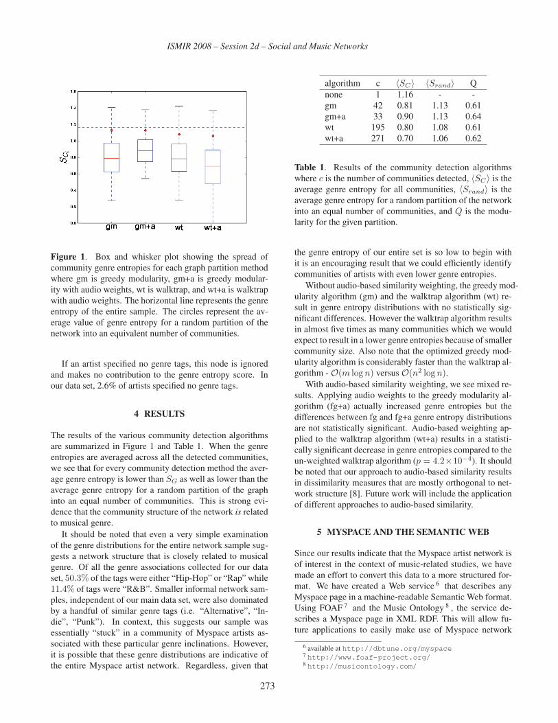
ISMIR 2008 – Session 2d – Social and Music Networks
Figure 1. Box and whisker plot showing the spread of
community genre entropies for each graph partition method
where gm is greedy modularity, gm+a is greedy modular-
ity with audio weights, wt is walktrap, and wt+a is walktrap
with audio weights. The horizontal line represents the genre
entropy of the entire sample. The circles represent the av-
erage value of genre entropy for a random partition of the
network into an equivalent number of communities.
If an artist specified no genre tags, this node is ignored
and makes no contribution to the genre entropy score. In
our data set, 2.6% of artists specified no genre tags.
4 RESULTS
The results of the various community detection algorithms
are summarized in Figure 1 and Table 1. When the genre
entropies are averaged across all the detected communities,
we see that for every community detection method the aver-
age genre entropy is lower than SG as well as lower than the
average genre entropy for a random partition of the graph
into an equal number of communities. This is strong evi-
dence that the community structure of the network is related
to musical genre.
It should be noted that even a very simple examination
of the genre distributions for the entire network sample sug-
gests a network structure that is closely related to musical
genre. Of all the genre associations collected for our data
set, 50.3% of the tags were either “Hip-Hop” or “Rap” while
11.4% of tags were “R&B”. Smaller informal network sam-
ples, independent of our main data set, were also dominated
by a handful of similar genre tags (i.e. “Alternative”, “In-
die”, “Punk”). In context, this suggests our sample was
essentially “stuck” in a community of Myspace artists as-
sociated with these particular genre inclinations. However,
it is possible that these genre distributions are indicative of
the entire Myspace artist network. Regardless, given that
algorithm c 〈SC〉 〈Srand〉 Q
none 1 1.16 - -
gm 42 0.81 1.13 0.61
gm+a 33 0.90 1.13 0.64
wt 195 0.80 1.08 0.61
wt+a 271 0.70 1.06 0.62
Table 1. Results of the community detection algorithms
where c is the number of communities detected, 〈SC〉 is the
average genre entropy for all communities, 〈Srand〉 is the
average genre entropy for a random partition of the network
into an equal number of communities, and Q is the modu-
larity for the given partition.
the genre entropy of our entire set is so low to begin with
it is an encouraging result that we could efficiently identify
communities of artists with even lower genre entropies.
Without audio-based similarity weighting, the greedy mod-
ularity algorithm (gm) and the walktrap algorithm (wt) re-
sult in genre entropy distributions with no statistically sig-
nificant differences. However the walktrap algorithm results
in almost five times as many communities which we would
expect to result in a lower genre entropies because of smaller
community size. Also note that the optimized greedy mod-
ularity algorithm is considerably faster than the walktrap al-
gorithm - O(m log n) versus O(n2 log n).With audio-based similarity weighting, we see mixed re-
sults. Applying audio weights to the greedy modularity al-
gorithm (fg+a) actually increased genre entropies but the
differences between fg and fg+a genre entropy distributions
are not statistically significant. Audio-based weighting ap-
plied to the walktrap algorithm (wt+a) results in a statisti-
cally significant decrease in genre entropies compared to the
un-weighted walktrap algorithm (p = 4.2×10⁻⁴). It should
be noted that our approach to audio-based similarity results
in dissimilarity measures that are mostly orthogonal to net-
work structure [8]. Future work will include the application
of different approaches to audio-based similarity.
5 MYSPACE AND THE SEMANTIC WEB
Since our results indicate that the Myspace artist network is
of interest in the context of music-related studies, we have
made an effort to convert this data to a more structured for-
mat. We have created a Web service 6 that describes any
Myspace page in a machine-readable Semantic Web format.
Using FOAF 7 and the Music Ontology 8 , the service de-
scribes a Myspace page in XML RDF. This will allow fu-
ture applications to easily make use of Myspace network
6 available at http://dbtune.org/myspace7 http://www.foaf-project.org/8 http://musicontology.com/
273

ISMIR 2008 – Session 2d – Social and Music Networks
data (i.e. for music recommendation).
6 CONCLUSIONS
We have presented an analysis of the community structures
found in a sample of the Myspace artist network and shown
that these community structures are related to musical genre.
We have applied two efficient algorithms to the task of par-
titioning the Myspace artist network sample into communi-
ties and we have shown how to include audio-based similar-
ity measures in the community detection process. We have
evaluated our results in terms of genre entropy - a measure
of genre tag distributions - and shown the community struc-
tures in the Myspace artist network are related to musical
genre.
In future work we plan to examine community detection
methods that operate locally, without knowledge of the en-
tire network. We also plan to address directed artist graph
analysis, bipartite networks of artists and listeners, different
audio analysis methods, and the application of these meth-
ods to music recommendation.
7 ACKNOWLEDGEMENTS
Thanks to Zhijia Huang, Chris Sutton, Matthew Davies, Amelie
Anglade and Yves Raimond for their input. This work is
supported as a part of the OMRAS2 project, EPSRC num-
bers EP/E02274X/1 and EP/E017614/1.
8 REFERENCES
[1] Y. Ahn, S. Han, H. Kwak, S. Moon, and H. Jeong. Anal-
ysis of topological characteristics of huge online social
networking services. In WWW ’07: Proceedings of the16th international conference on World Wide Web, pages
835–844, New York, NY, USA, 2007. ACM.
[2] A. Anglade, M. Tiemann, and F. Vignoli. Virtual com-
munities for creating shared music channels. In Proc. ofISMIR, pages 95–100, 2007.
[3] A. Berenzweig, B. Logan, D. P. W. Ellis, and B. P. W.
Whitman. A large-scale evaluation of acoustic and sub-
jective music-similarity measures. Computer Music J.,28(2):63–76, 2004.
[4] P. Cano, O. Celma, M. Koppenberger, and J. M.
Buldu. The topology of music recommendation net-
works. arXiv.org:physics/0512266, 2005.
[5] O. Celma and P. Lamere. Music recommendation. IS-
MIR Tutorial, 2007.
[6] A. Clauset, M. E. J. Newman, and C. Moore. Finding
community structure in very large networks. Phys. Rev.E, 70(6):066111, Dec 2004.
[7] L. F. Costa, F. A. Rodrigues, G. Travieso, and P. R. Vil-
las Boas. Characterization of complex networks: A sur-
vey of measurements. Advances In Physics, 56:167,
2007.
[8] B. Fields, K. Jacobson, M. Casey, and M. Sandler. Do
you sound like your friends? exploring artist similarity
via artist social network relationships and audio signal
processing. In Proc. of ICMC, August 2008.
[9] P. Gleiser and L. Danon. Community structure in jazz.
Advances in Complex Systems, 6:565, 2003.
[10] K. Jacobson. A multifaceted approach to music similar-
ity. In Proc. of ISMIR, 2006.
[11] K. Jacobson and M. Sandler. Musically meaningful or
just noise, an analysis of on-line artist networks. In Proc.of CMMR, pages 306–314, 2008.
[12] H. Kwak, S. Han, Y. Ahn, S. Moon, and H. Jeong. Im-
pact of snowball sampling ratios on network characteris-
tics estimation: A case study of cyworld. Technical Re-
port CS/TR-2006-262, KAIST, November 2006.
[13] R. Lambiotte and M. Ausloos. On the genre-fication of
music: a percolation approach (long version). The Euro-pean Physical Journal B, 50:183, 2006.
[14] S. H. Lee, P. J. Kim, and H. Jeong. Statistical properties
of sampled networks. Physical Review E, 73:102–109,
January 2006.
[15] B. Logan. Mel frequency cepstral coefficients for music
modeling. In Proc. of ISMIR, 2000.
[16] B. Logan and A. Salomon. A music similarity function
based on signal analysis. Multimedia and Expo ICME,
pages 745–748, 2001.
[17] M. E. J. Newman. The structure and function of complex
networks. SIAM Review, 45:167, 2003.
[18] E. Pampalk. Computational Models of Music Similar-ity and their Application in Music Information Retrival.PhD thesis, Technischen Universität Wien, May 2006.
[19] J. Park, O. Celma, M. Koppenberger, P. Cano, and J. M.
Buldu. The social network of contemporary popular mu-
sicians. arXiv:physics/0609229, 2006.
[20] P. Pons and M. Latapy. Computing communities in
large networks using random walks (long version).
arXiv:physics/0512106v1, 2005.
[21] Y. Rubner, C. Tomasi, and L. J. Guibas. The earth
mover’s distance as a metric for image retrieval. Interna-tional Journal of Computer Vision, 40(2):99–121, 2000.
274

ISMIR 2008 – Session 2d – Social and Music Networks
UNCOVERING AFFINITY OF ARTISTS TO MULTIPLE GENRESFROM SOCIAL BEHAVIOUR DATA
Claudio Baccigalupo Enric PlazaIIIA, Artificial Intelligence Research InstituteCSIC, Spanish Council for Scientific Research
{claudio,enric}@iiia.csic.es
Justin DonaldsonIndiana University
School of [email protected]
ABSTRACT
In organisation schemes, musical artists are commonly iden-
tified with a unique ‘genre’ label attached, even when they
have affinity to multiple genres. To uncover this hidden cul-
tural awareness about multi-genre affinity, we present a new
model based on the analysis of the way in which a commu-
nity of users organise artists and genres in playlists.
Our work is based on a novel dataset that we have elabo-
rated identifying the co-occurrences of artists in the playlists
shared by the members of a popular Web-based community,
and that is made publicly available. The analysis defines
an automatic social-based method to uncover relationships
between artists and genres, and introduces a series of novel
concepts that characterises artists and genres in a richer way
than a unique ‘genre’ label would do.
1 INTRODUCTION
Musical genres have typically been used as a ‘high level’
classification of songs and artists. However, many musical
artists cannot be described with a single genre label. Artists
can change style throughout their career, and perform songs
that do not entirely fall into single categories such as ‘Rock’,
‘R&B’ or ‘Jazz’. In general terms, artists can be said to have
a certain degree of affinity to each specific genre.
In this paper we propose to model relationships from
artists to genres as fuzzy sets, where the membership degreeindicates the affinity of an artist to a genre. This is in con-
trast to conventional labelling approaches, in which artists
either belong or do not belong to a genre, and allows for a
sentence like “Madonna is Pop and R&B, not Jazz” to be
rephrased as “Madonna belongs with a membership degree
of 0.8 to Pop genre, with 0.6 to R&B and with 0.1 to Jazz”.
To uncover the affinity of different artists to different gen-
res, we follow a social approach: we exploit information
about how people aggregate and organise artists and genres
in playlists. Playlists are the predominant form of casual
This research is partially supported by the MID-CBR (TIN2006-
15140-C03-01) project, by the Generalitat de Catalunya under the grant
2005-SGR-00093, and by a MyStrands scholarship.
music organisation. When playlists are collected in aggre-
gate over a large sampling of the music listening populace,
they reflect current cultural sensibilities for the association
of popular music. Our assumption about large repositoriesof playlists is that when two artists or genres co-occur to-
gether and closely in many playlists, they have some form
of shared cultural affinity. For example, if we observe that
a large number of songs by an artist x co-occur often and
closely with songs whose artists are classified in the ‘Jazz’
genre, then we argue that x has a certain affinity with Jazz,
independently from the original ‘genre’ label attached to x.
On the basis of this assumption, we build a model of
multi-genre affinity for artists, grounded on data about the
usage of music objects by real people. We suggest this kind
of analysis can provide results which are complementary to
those provided by other content-based or social techniques,
which we discuss in the following subsection.
In this paper, we first discuss different approaches to-
wards musical genre analysis, and provide arguments for
the consideration of a community-based approach. Next,
we report on the analysis we performed on a novel dataset,
which lists the co-occurrences of 4,000 artists in a large col-
lection of playlists, to uncover associations between artists
and genres. Finally, we depict possible applications, such as
affinity-based generation of ‘smooth sequences’ of songs.
1.1 Related work about genre analysis
Genre analysis has been a constant theme in the MIR com-
munity, and researchers have had some success in classi-
fying or predicting genre using either content-analytic ap-
proaches or social behaviour approaches.
Content-analytic methods are broken into two distinct ap-
proaches. The ‘acoustic-analytic’ approach was introduced
by Tzanetakis and Cook [9], and investigates the acoustic
signature of music according to a battery of relevant cogni-
tive and musicological descriptors, such as beats per minute,
timbre, and frequency spectrum. The ‘score-analytic’ ap-
proach concerns itself with symbolic representations of mu-
sic as sequences of notes and events making up a musical
score, generally as MIDI files, as in McKay and Fujinaga [6].
Social behaviour approaches classify music objects
275

ISMIR 2008 – Session 2d – Social and Music Networks
based upon the actions that a community of people perform
with them. A large amount of effort has been directed to-
wards harvesting textual correlations (of names of artists,
songs, etc.) that co-occur on public Web sites. This has
been the focus of Schedl et al. [8], who analysed artist-
based term co-occurrences, Knees et al. [4], and Whitman
and Smaragdis [10]. Text-based Web mining, however, can
suffer from a lack of precision, mistaking band name terms
with non-associated content as mentioned in [8].
Other attempts at providing richer representations for
musical artists include describing an artist with a set of
tags [2], with a set of moods [3] or identifying term profiles
that characterise a specific cluster of similar artists [4]. All
of these techniques maintain a ‘Boolean’ approach, identi-
fying whether each artist matches specific tags, moods or
clusters, while we seek to identify ‘fuzzy’ membership val-
ues relating each artist to each genre.
The social-based approach that we follow is the analy-
sis of co-occurrences in playlists, which is currently not a
common method of analysis. This is because playlists are
not often publicly indexed or made available. Previously, a
smaller public collection of about 29,000 playlists was used
by Logan et. al [5] to analyse a set of 400 popular artists,
and by Cano and Koppenberger [1] to provide a study of
artists networks, while we work on a novel and much larger
dataset of 1,030,068 human-compiled playlists.
Playlists have a special utility for social analysis of gen-
res in that they are specific to music, with no extraneous
“noise” information such as on arbitrary Web pages. They
are also intentional in their creation, as opposed to a simple
record of an individual’s play history which may have been
generated randomly.
2 A DATASET OF ARTISTS CO-OCCURRENCES
MusicStrands (http://music.strands.com) is a Web-based
music recommendation community which allows members
to publish playlists from their personal media players, such
as Apple iTunes and Windows Media Player. Every pub-
lished playlist is made of a sequence of IDs that univocally
identify the songs and artists that the playlist contains.
On July 31st, 2007, we gathered the 1,030,068 user
playlists published so far. We discarded playlists made by a
single song or by a single artist. We also removed any in-
formation related to the creators (user name, creation date,
playlist title, rating) to focus on the sequential nature of
playlists in terms of co-occurrences of artists.
For each pair of artists (x, y), we extracted the number
of times that a song by x occurs together with a song by y,
and at what distance (i.e., how many other songs are in be-
tween). To reduce the dimension of the dataset, we consid-
ered only the co-occurrences of songs from the 4,000 most
popular artists, where the popularity of an artist equals the
number of playlists in which occurs. We also excluded non-
specific popular artist labels such as “Various Artists” or
“Original Soundtrack”, and any co-occurrence with a dis-
tance larger than 2, to obtain the dataset sketched in Table 1,
where each record contains: the ID of the first artist x, the
ID of the second artist y, and the numbers d0(x, y), d1(x, y),and d2(x, y) of playlists where y co-occurs after x at dis-
tance 0, 1, and 2 respectively.
x y d0(x, y) d1(x, y) d2(x, y)
11 11 137 96 77
11 27 0 0 1
11 91 0 1 2
. . . . . . . . . . . . . . .
Table 1. A portion of the provided dataset
An auxiliary table in the dataset lists the 4,000 artists IDs,
together with their genre IDs and their Musicbrainz artist
IDs. Both artist IDs and genre IDs can be easily translated
to actual names using the OpenStrands developers API. 1
Thanks to the support of MusicStrands, we now make
public the complete dataset that we have elaborated, which
is freely available to researchers wishing to perform social
based analysis on music behaviour data from real users. 2
3 GENRES AND AFFINITY
The artists in the previously described dataset already have a
genre label attached. However, our motivation is to provide
a richer representation, which overcomes the limitation of
having only one genre per artist.
We denote with G the set of m genres, and with Athe set of n artists in the dataset, where m = 26 and
n = 4,000. Our goal is to describe each artist x as a
vector [Mx(g1), Mx(g2), . . . , Mx(gm)], where each value
Mx(gi) ∈ [0, 1] indicates how much x has affinity to the
genre gi. We call Mx(gi) the genre affinity degree of artist
x to genre gi.
The process to calculate the genre affinity degrees is the
following. First we measure the association from each artist
x ∈ A to each other artist, based on their co-occurrences in
the authored playlists. Then we aggregate these associations
by genre to obtain the degree in which each artist x is asso-
ciated with each genre g ∈ G. Finally we combine artist-to-
artist and artist-to-genre associations to measure the degree
Mx(g) of affinity between artist x and genre g.
The first step is to consider how much an artist x is asso-
ciated with any other artist y. Let X be set of n − 1 artists
other than x: X = A − {x}. We define the artist-to-artistassociation Ax : X → R as an aggregation of the number
1 API available at http://my.strands.com/openstrands2 Dataset available at http://labs.strands.com/music/affinity
276

ISMIR 2008 – Session 2d – Social and Music Networks
of co-occurrences of x with any artist y ∈ X :
Ax(y) = α · [d0(x, y) + d0(y, x)]+ β · [d1(x, y) + d1(y, x)]+ δ · [d2(x, y) + d2(y, x)] .
This metric aggregates the number of playlists in which
artists x and y co-occur, with different weights according
to the distance at which x and y occur. Co-occurrences
at distance 0 (d0), distance 1 (d1), and distance 2 (d2) are
weighted with α, β and δ respectively. These parameters,
with values in [0, 1], can be tuned to reflect the importance
that the authors of the playlists assign to the distance be-
tween associated artists in their playlists. In the case of
MusicStrands, we have observed that some authors com-
pile playlists grouping together associated artists one afterthe other (for example, DJs for dance playlists), while most
users create playlists as unordered sets of associated songs,
where the distance between two artists is not related to their
association. Based on this mixed behaviour, in our analysis,
we have assigned values of α = 1, β = 0.8, and δ = 0.64.
According to the metric defined, the values of Ax are
heavily influenced by the popularity of x. In fact, an artist xwho is present in many playlists co-occurs with many artists,
and has a generally higher artist-to-artist association than an
uncommon artist. Therefore, we perform a normalisation
and obtain an artist-to-artist association Âx : A → [−1, 1]independent from the popularity of x, such that:
Âx(y) =Ax(y)−Ax
|max(Ax(y)−Ax)|
where Ax = 1n−1
∑y∈X Ax(y), and Âx(x) = 0 by con-
vention. A positive (resp. negative) value Âx(y) indicates
that the artist-to-artist association of x with y is above (resp.
below) the average artist-to-artist association of x.
Now we turn to estimate the affinity of artists with re-
spect to genres. First, let us consider how much an artist xis associated with any genre g. We define the association
Px : G → R by cumulating the artist-to-artist association
Ax from x to any artist of genre g:
Px(g) =∑
y∈X :γ(y)=g
Ax(y)
where γ(y) denotes the genre of y. Again, we normalise
this association to counter-effect the uneven distribution of
genres in the playlists (e.g., Rock/Pop artists occur in almost
any playlist, while Folk artists are quite rare). The result is
a normalised association P̂x(g) : G → [0, 1], independent
from the popularity of genre g, defined as:
P̂x(g) =
∑y∈X :γ(y)=g Ax(y)∑
y∈X Ax(y).
This function P̂ measures the degree in which artists as-
sociated with artist x belong to the genre g. Finally we ob-
tain the genre affinity degree Mx : G → [0, 1] by weighting
the association P̂ with the artist-to-artist association Â, and
normalising the result to the range [0, 1]:
Mx(g) =12
(∑y∈A Âx(y)P̂y(g)
n+ 1
).
Notice that Mx(g) is high when artists that often co-
occur with x belong to genre g and when artists that
rarely co-occur with x do not belong to genre g. Each
artist can be characterised by a genre affinity vector[Mx(g1), Mx(g2), . . . , Mx(gm)] ∀gi ∈ G, which is a multi-
dimensional representation of an artist in terms of genres.
For example, Table 2 shows , for three famous artists
of the dataset labelled as ‘Rock/Pop’ (Madonna, Metal-
lica and Bruce Springsteen), their artist-to-artist associa-
tion Âx(y), their association P̂x(g) and their genre affin-
ity degrees Mx(g) with respect to three popular genres
(Rock/Pop, Country and R&B).
The ‘Rock/Pop’ genre is very common in our data (la-
belling 2,286 of the 4,000 artists in the dataset), so having
these three artists generically labelled as ‘Rock/Pop’ is not
very informative of their style. However, by observing the
differences in their genre affinity degrees Mx(g), we can
spot their differences. For instance, Bruce Springsteen has
a higher genre affinity to Country, while Madonna has a
higher affinity to R&B. By plotting their Mx(g) values with
respect to these three genres on a graph, we can visually
observe such difference in Fig. 1.
Figure 1. Genre affinity of 3 artists with 3 genres
4 ANALYSIS AND DISCUSSION
4.1 Genres and core artists
One advantage of describing artists in terms of affinity vec-
tors, rather than with unique genre labels, is that we can
identify how central an artist is to a genre. For each artist x,
we define its genre-centrality Cg : A → [0, 100] to a genre
g ∈ G as the percentage of artists whose genre affinity to g
277

ISMIR 2008 – Session 2d – Social and Music Networks
Âx(y) Madonna Metallica Bruce Spr.
Mad. 0 0.0026 0.0516
Met. 0.0322 0 0.0106
B. Spr. 0.0602 0.0063 0
P̂x(g) Rock Country R&B
Mad. 0.628 0.028 0.065
Met. 0.892 0.013 0.034
B. Spr. 0.790 0.041 0.026
Mx(g) Rock Country R&B
Mad. 0.49997 0.49998 0.50007Met. 0.50040 0.49995 0.49997
B. Spr. 0.50038 0.50001 0.49991
Table 2. Associations and affinities between artists and genres, shown only for a subset of 3 artists and 3 genres
is lower or equal than the genre affinity of x to genre g:
Cg(x) =100n· card {y ∈ A : My(g) ≤ Mx(g)} .
For instance, the Country-centrality of Bruce Springsteen is
79.3%, because as many as 3,172 out of the 4,000 artists in
the dataset have an affinity degree to Country lower than his,
while his R&B-centrality is 39.5%, since only 1,580 artists
have a genre affinity degree to R&B lower than his.
We will call those artists which are the most central to a
genre g the core artists of g. Core artists are good represen-
tatives of a genre, since they occur very often in the set of
playlists with artists from that genre and seldom with artists
from other genres. For instance, we interestingly observe
that the top core artists for the genre labelled ‘Soundtrack’
are James Horner, Alan Silvestri and Michael Giacchino,
who are famous composers of original movie scores (e.g.,
James Horner’s “Titanic Original Soundtrack”), and not
Pop artists who have only sporadically performed famous
songs which appeared in movies (e.g., Celine Dion’s “MyHeart Will Go On”).
The top core artists for other three genres are: (Folk)
Luka Bloom, Greg Brown, The Chieftains; (Blues) Muddy
Waters, Taj Mahal, Dr. John; (Jazz) Bob James, Donald
Byrd, Peter White; (Electronic) Kaskade, Sasha, Junkie XL.
4.2 Centrality and cross-genre artists
Table 3 shows four artists originally labelled as Electronic
and their genre-centrality with respect to four genres. From
this table, we learn that St. Germain has a high Jazz-
centrality (94%), Soul II Soul have a high R&B-centrality
(94%) and M83 have a high Rock/Pop-centrality (95%).
This is not surprising, since St. Germain is “a French elec-
tronica and nu jazz musician”, 3 Soul II Soul is a “U.K. R&Bcollective”, 4 and M83 offer “a luscious blend of shoegaze
aesthetics, ambient pop, and progressive textures”. 5 This
is an example of how, using genre-centrality, we can ob-
tain richer descriptions of the affinity of artists to multiple
genres, without employing expert knowledge, but analysing
the way in which each artists’ works were employed by real
users in playlists, in combination with other artists.
Table 3 also shows that Cameron Mizell, originally la-
belled as Electronic, has a higher genre-centrality to Jazz
3 Excerpt from http://last.fm/music/St.+Germain4 Excerpt from http://music.strands.com/artist/152465 Excerpt from http://music.aol.com/artist/m83/1655884
Cg(x) St. Germain Soul II Soul M83 C.Mizell
Electronic 98% 96% 98% 90%
Jazz 94% 10% 6% 99%R&B 41% 94% 8% 62%
Rock/Pop 37% 1% 95% 17%
Table 3. Genre-centrality of 4 artists to 3 genres
(99%) than to Electronic (90%). The reason is that Cameron
Mizell is a cross-genre artist, whose creations mostly fall in
the Electronic category, and mostly occur together with Jazz
songs. Indeed, Cameron Mizell is labelled as ‘Electronic’
in MusicStrands, but as ‘Jazz’ according to other exter-
nal musical sources, such as AMG (http://allmusic.com),
iTunes Music Store (http://apple.com/itunes) and Amazon
(http://amazon.com). This is not such a strange case, for
several artists exist which behave as a sort of musical bridgefrom a genre to another. Formally, we call bridge artistany artist x whose original genre label γ(x) differs from
the genre φ(x) for which x has the highest genre-centrality,
where φ(x) = g ∈ G : Cg(x) ≥ Ch(x) ∀h ∈ G.
Table 4 reports the number of bridge artists, aggregated
by genre, for six of the 26 genres (with the main diagonal
containing artists which are not bridge artists). According
to our data, the distribution of bridge artists is uneven and
depends on genres; for instance there are no bridge artists
from Reggae to Country and vice versa, while there are 90
bridge artists from Rap to R&B (37% of all the Rap artists).
This suggests that genres like Country and Reggae are “dis-
tinct”, in the sense that artists from the two genres tend not
to “play well together”, while genres like R&B and Rap are
“adjoining”, meaning that artists from the two genres tend
to “play well together”. These abstract concepts are defined
more precisely hereafter, with different typologies of asso-
ciations between genres characterised.
g \ h Country Blues Jazz Reggae R&B Rap
Country 162 - 1 - - -
Blues - 3 - - - -
Jazz - 2 101 - - -
Reggae - - - 24 - -
R&B 1 1 9 6 334 11
Rap - - - 9 90 226
Table 4. Number of artists labelled as genre g, whose genre-
centrality is maximum for genre h, for 6 different genres
278

ISMIR 2008 – Session 2d – Social and Music Networks
4.3 Correlation between two genres
After having analysed associations from artists to genres, we
draw some observations about how genres relate with each
other. The goal is to discern for each pair of genres (g, h)whether they are or not correlated. The idea is that two gen-
res are correlated when artists belonging to one genre nat-
urally tend to be played together with artists of the other
genre. Using the genre affinity degree Mx(g), we can more
precisely state that two genres g and h are correlated (resp.
exclusive) when artists with a high Mx(g) (genre affinity
degree to g) tend to have a high (resp. low) Mx(h) (genre
affinity degree to h); and two genres are independent when
their affinity degrees do not show any sign of correlation.
As an example, consider Figure 2 (above) showing, for
each of the 4,000 artists in the dataset, its affinity degree to
Country (x axis), to Reggae (y axis), and its original genre
label (point type). Artists with high affinity to Country (in
the lower right section) tend to have a ‘neutral’ affinity to
Reggae (with most values close to 0.5). Similarly, artists
with high affinity to Reggae (in the upper left section) tend
to have a ‘neutral’ affinity to Country. This is an exam-
ple of independent genres, since the genre affinity degree to
Country and to Reggae of an artist look unrelated. Figure 2
(below) shows instead that artists with high affinity to R&B
often have a high affinity to Rap as well (in the upper right
section), suggesting that the two genres are correlated.
Figure 2. Comparing Country vs. Reggae (above), and
R&B vs. Rap (below) genre-centralities
To measure the correlation between any two genres g and
h, we employ Pearson’s coefficient ρg,h ∈ [−1, 1], which
assesses the linear correlation between the affinity degree of
artists from two genres, and has values close to 1 in the case
of a positive relationship (i.e., artists with high affinity to galso have high affinity to genre h), and close to −1 in the
case of a negative relationship (i.e., artists with high affinity
to g have low affinity to genre h). Table 5 reports these co-
efficients for six genres, showing for instance that R&B and
Rap (0.6) are positively correlated (as suggested by Fig. 2),
as well as Jazz and Blues (0.4), while Blues and Rap (−0.2)
are negatively correlated: artists with a high affinity to Blues
tend to have a low affinity to Rap.
This social analysis of genres exposes cultural correla-
tions between music that is often not present in an acoustic
or score analysis. Most importantly, this analysis does not
require expert human knowledge of genre relationships. In-
stead, relationships emerge from a larger cultural consensus.
ρg,h Country Blues Jazz Reggae R&B Rap
Country 1 0.2 0.1 0 0.1 -0.1
Blues 0.2 1 0.4 0.1 0 -0.2Jazz 0.1 0.4 1 0.1 0.2 -0.1
Reggae 0 0.1 0.1 1 0.4 0.4R&B 0.1 0 0.2 0.4 1 0.6Rap -0.1 -0.2 -0.1 0.4 0.6 1
Table 5. Pearson coefficient ρ for 6 genre-centrality vectors
5 APPLICATIONS
The analysis we have performed allows to describe artists
in terms of affinity vectors and to uncover relations among
genres. This knowledge is useful for many applications,
some of which are presented hereafter.
First, consider the case of a Web radio, with a large
repository of available music, and with the need to sched-
ule different channels with different sequences of songs.
The most common approach is to programme each chan-
nel with a randomly ordered selection of songs from the
repository, matching the definition of each channel (e.g., a
random sequence of jazz songs is played on a ‘Jazz chan-
nel’). This method may work well for channels limited to
a single genre, but may sound inadequate when multiple
genres are permitted (e.g., in a channel generically defined
as “Music from the ‘80s”), since unpleasant musical transi-
tions could occur from one genre to another (e.g., a song by
Abba, followed by a song by Metallica, and by a song by
B.B. King). To procure smooth transitions from a song to
the next one, the knowledge we have uncovered about affin-
ity of each artist to each genre can be exploited, to generate
better musical sequences that move, for example, from the
core artists of ‘Rock’, to less central and cross-genre artists
279

ISMIR 2008 – Session 2d – Social and Music Networks
(‘Rock’/‘R&B’), to core artists of ‘R&B’, and so on, avoid-
ing disturbing disruptions in the path. The same approach
can work to generate playlists.
Another possible application of our analysis is to per-
form similarity assessments among artists. Having artists
described as affinity vectors, we can obtain a measure of
how close two artists are, independently from their ‘genre’
label. For instance, we can spot for each artist its near-
est neighbour using Euclidean distance among these vec-
tors. The results are interesting: in most cases we find
that the nearest neighbour artists have the same genre la-
bel attached (e.g., Donna Summer goes to Diana Ross, both
R&B), while sometimes they are differently labelled but still
culturally associated, for example Nelly Furtado (Rock/Pop)
goes to Missy Elliott (Rap), and Bob Sinclair (R&B) goes
to Sonique (Rock/Pop). In this way, we exploit affinity
fuzzy values to uncover associated artists, independently
from their ‘genre’ label.
A third possible application is the creation of user pro-
files in music recommender systems. Rather than asking
a user which musical genres she prefers, the system could
ask her to name a few of her favourite artists, and then lo-
cate them on a multi-dimensional map of affinity degrees, to
identify which styles of music the user seems to favour.
6 CONCLUSIONS
Music is a complex form of information that can be ad-
dressed both as an acoustic and a cultural phenomenon.
Genre labels serve as simple and easily communicated clas-
sifications of musical style, but it can be shown that pop-
ular music often does not avail itself to such simple clas-
sifications. Musicians can share affinity with different gen-
res, although in most organisational schemes (such as record
stores) they have a unique genre label attached.
Our first contribution is providing a way to automatically
uncover a richer relationship between artists and genres,
based on social data in the form of playlists. Our proposal
is moving from a Boolean concept of genres as exclusive
categories to a view where artists have a degree of affinity
with respect to each genre, and thus genres are conceptu-
alised as fuzzy categories where affinity is represented as
membership degrees in fuzzy set theory.
Our second contribution is developing a richer ontology
for describing artist-to-genre and genre-to-genre associa-
tions, defining new concepts useful to better organise and
understand large collections of music metadata. To enrich
the characterisation of artists based on our first contribu-
tion (moving from Boolean categories to the notion of genre
affinity), the ontology introduces the concepts of genre affin-
ity degree, genre affinity vector, and genre centrality. To
better characterise genres, the ontology introduces the con-
cepts of core artists of a genre, bridge artists, and correlation
or independence among genres.
To promote further social-based music analysis, we make
publicly available the dataset of artists co-occurrences that
we have produced from a very large repository of playlists.
Since we identify each artist with its unique Musicbrainz ID,
researchers have the chance to mash-up this dataset with a
large number of other inter-linked music-related semantic
Web datasets, following the methodology described in [7].
Future work includes expanding this approach to elu-
cidate relationship between songs, tags and genres, view-
ing tags as user-provided fuzzy categories to determine the
affinity of artists to tags, the core tags of genres and artists,
the affinity and centrality of songs to genres, the relationship
of songs with their artists, and the relationships among tags.
7 REFERENCES
[1] P. Cano and M. Koppenberger. The emergence of com-
plex network patterns in music artist networks. In Proc.of ISMIR, pages 466–469, 2004.
[2] D. Eck, T. Bertin-Mahieux, and P. Lamere. Autotagging
music using supervised machine learning. In Proc. of IS-MIR, pages 367–368, 2007.
[3] X. Hu and J. Downie. Exploring mood metadata: Rela-
tionships with genre, artist and usage metadata. In Proc.of ISMIR, pages 67–72, 2007.
[4] P. Knees, E. Pampalk, and G. Widmer. Artist classifi-
cation with web-based data. In Proc. of ISMIR, pages
517–524, 2004.
[5] B. Logan, D. Ellis, and A. Berenzweig. Toward eval-
uation techniques for music similarity. The MIR/MDLEvaluation Project White Paper Collection, 3:81–85,
2003.
[6] C. McKay and I. Fujinaga. Automatic genre classifica-
tion using large high-level musical feature sets. In Proc.of ISMIR, pages 525–530, 2004.
[7] Y. Raimond, S. Abdallah, M. Sandler, and F. Giasson.
The Music Ontology. In Proc. of ISMIR, pages 417–422,
2007.
[8] M. Schedl, P. Knees, and G. Widmer. Discovering
and visualizing prototypical artists by web-based co-
occurrence analysis. In Proc. of ISMIR, pages 21–28,
2005.
[9] G. Tzanetakis, G. Essl, and P. Cook. Automatic musical
genre classification of audio signals. In Proc. of ISMIR,
pages 205–210, 2001.
[10] B. Whitman and S. Lawrence. Inferring descriptions and
similarity for music from community metadata. In Proc.of ISMIR, pages 591–598, 2002.
280

ISMIR 2008 – Session 2d – Social and Music Networks
HYPERLINKING LYRICS: A METHOD FOR CREATING HYPERLINKSBETWEEN PHRASES IN SONG LYRICS
Hiromasa Fujihara,Masataka Goto, and Jun OgataNational Institute of Advanced Industrial Science and Technology (AIST), Japan
{h.fujihara, m.goto, jun.ogata} [at] aist.go.jp
ABSTRACTWe describe a novel method for creating a hyperlink from aphrase in the lyrics of a song to the same phrase in the lyricsof another song. This method can be applied to various ap-plications, such as song clustering based on the meaning ofthe lyrics and a music playback interface that will enablea user to browse and discover songs on the basis of lyrics.Given a song database consisting of songs with their textlyrics and songs without their text lyrics, our method firstextracts appropriate keywords (phrases) from the text lyricswithout using audio signals. It then finds these keywordsin audio signals by estimating the keywords’ start and endtimes. Although the performance obtained in our experi-ments has room for improvement, the potential of this newapproach is shown.
1 INTRODUCTION
The goal of this study is to enable a Music Web wheresongs are hyperlinked to each other on the basis of theirlyrics (figure 1). Just as some hypertext phrases on the webare hyperlinked, so some phrases of lyrics (which we callhyperlyrics) on the Music Web can be hyperlinked. Sucha hyperlinked structure of the Music Web can be used as abasis for various applications. For example, we can clus-ter songs based on the meanings of their lyrics by analyzingthe hyperlinked structure or can show relevant informationduring music playback by analyzing the hyperlinked songs.We can also provide a new active music listening interface[1] where a user can browse and discover songs by clickinga hyperlinked phrase in the lyrics of a song to jump to thesame phrase in the lyrics of another song. Although we canthink of many possible ways to hyperlink musical pieces onthe Music Web, focusing on song lyrics is natural becausethe lyrics are one of the most important elements of songsand often convey their essential messages.
Most approaches for analyzing inter-song relationshiphave been based on musical similarity between songs, andvarious music interfaces based on such song-level similarityhave been proposed [2, 3, 4, 5, 6]. the methods of musicbrowsing for intra-song navigation have also been studied,such as music browsing based on the structure [7, 8] and thelyrics [9, 10, 11]. However, hyperlinking lyrics — i.e., acombination of inter-song and intra-song navigations basedon lyrics phrases — has not been proposed.
In this paper, we propose a method for hyperlinking iden-tical keywords (phrases) that appear in the lyrics of differentsongs. Hyperlinking lyrics enables us to benefit from vari-ous studies dealing with sung lyrics in musical audio signals.For example, by using methods for automatic synchroniza-tion of lyrics with musical audio signals[9, 10], we can firstfind a keyword pair in the text lyrics for two different songs
Music Web
HyperlinkHyperlyrics
Songs are hyperlinked to each other on the basis of their lyrics.
Figure 1. Hyperlinking lyrics. on Music Web
and then locate (i.e., estimate the start and end times of) thekeyword in the audio signals of each song. However, it isstill difficult to achieve accurate automatic lyrics recogni-tion that enables us to find a keyword pair in sung lyricsthat are recognized in polyphonic musical audio signals, de-spite the achievements made by studies on automatic lyricsrecognition for musical audio signals [12, 13, 14]. Whilestudies have also been done on analyzing text lyrics withoutusing audio signals [15, 16], we cannot use their results tohyperlink lyrics.
Figure 2 shows the strategy our method uses to hyperlinklyrics. We assume that a user has a song database that isa set of audio files (e.g., MP3 files) and that we can pre-pare text files of the lyrics for some of the songs. Notethat we do not require text lyrics for all the songs — i.e.,a song database consists of songs with their text lyrics andsongs without them. We therefore apply two different strate-gies for hyperlinking: one for hyperlinking from a phrase inother text lyrics to the same phrase in the text lyrics, and onefor hyperlinking from a phrase in the text lyrics to the samephrase in the sung lyrics in a song (polyphonic music sig-nals) without its text lyrics. Here, “text lyrics” means a textdocument containing the lyrics of a song, and “sung lyrics”means audio signals containing the lyrics sung by a singerin a polyphonic sound mixture. Although hyperlinking fromtext lyrics to text lyrics is relatively easy with the support ofLyricSynchronizer [10, 1], hyperlinking from text lyrics tosung lyrics is more difficult.
2 OUR METHOD FOR HYPERLINKING LYRICS
Our method hyperlinks phrases that appear in the lyricsof different songs. In other words, if different songs share
281

ISMIR 2008 – Session 2d – Social and Music Networks
Keywords extraction
Hyperlink from
text lyrics to text lyrics
Hyperlink from
text lyrics to sung lyrics
Songs with text lyrics Songs without text lyrics
Each keyword is hyperlinked in the text/sung lyrics
Song database
easier than
like a dream
take me higher
make me cry fall in love
you don’t need to
Figure 2. Two different strategies for hyperlinking: hyper-link from text lyrics to text lyrics and hyperlink from textlyircs to sung lyrics.
the same phrase (what we call a keyword1 ) in their lyrics,a section (temporal region) corresponding to the keywordin one song is hyperlinked with a section corresponding tothe same keyword in another song. This method shoulddeal with polyphonic music mixtures containing sounds ofvarious instruments as well as singing voices. If a songdatabase consists of songs with text lyrics and songs withouttext lyrics, this approach creates two different types of bidi-rectional hyperlinks: a hyperlink between songs with textlyrics and a hyperlink from a song with text lyrics to a songwithout them. The former hyperlink can be created by ex-tracting potential keywords from all the text lyrics and find-ing sections corresponding to them (i.e., temporally locat-ing them) in audio signals with the help of their lyrics. Thisestimation can be done using an automatic lyrics synchro-nization method described in [10]. For the latter hyperlink,our method looks for sections including voices that sing thekeywords by using a keyword spotting technique for poly-phonic music mixtures.
2.1 Hyperlinking from text lyrics to text lyricsThis section describes our method for hyperlinking from
text lyrics to text lyrics. By using text lyrics of all the songs,the method first extracts as many keywords that can resultin meaningful hyperlinks as possible. It then estimates sec-tions (the start and end times) of each keyword in audio sig-nals. Finally, it creates bidirectional hyperlinks between theestimated keyword sections.
2.1.1 Keyword extraction from the text lyricsWe would like to create as many hyperlinks as possible
while ensuring that they are meaningful and useful. Wetherefore have to accordingly extract keywords. From theviewpoint of inter-song hyperlinks, each keyword must ap-
1 In this paper, the term “keyword” means a lyrics phrase consisting ofone or more consecutive words.
pear in multiple songs (the more songs, the better). Inaddition, since long keywords tend to convey importantmeanings, longer keyword lengths are preferred. Longerkeywords are also advantageous for improving the accu-racy of keyword detection, in Sec. 2.2. In contrast, shortwords/phrases, such as an article and a preposition, are notappropriate as keywords.
The requirements for appropriate keywords can be sum-marized as follows:(a) A larger number of songs sharing a keyword is better.(b) A larger number of phonemes in a keyword is better.Note the trade-off between these requirements: a longerphrase is less likely to appear many times. We therefore tryto maximize the number of phonemes provided each key-word appears in two songs or more.
According to these requirements, we developed the key-word extraction algorithm shown below.1. Initialize a keyword dictionary as empty. Each keyword
registered to this dictionary in the following will have aflag called a ”finalized” flag only when it cannot be con-nected with an adjacent word to make a longer keyword(phrase).
2. Register every word of all text lyrics to the keyworddictionary.
3. Count the number of different songs whose lyrics in-clude each keyword of the keyword dictionary. The key-word with the largest number of corresponding songs isconsidered the most frequent keyword.
4. Remove all keywords that appear in less than M songsfrom the keyword dictionary.
5. Select the most frequently occurring keyword withoutthe ”finalized” flag. If all the keywords have this flag,this algorithm is finished.
6. Try to combine adjacent words with the selected key-word. The former word and the latter word of eachlyrics are respectively combined to make a longerphrase.
7. Only the best combination that results in the most fre-quent phrase is registered as a new keyword to the key-word dictionary, provided it appears in M songs ormore. Note that the original keyword is not removedeven if a combined one is thus registered.
8. If any combination for the selected keyword does notappear in M songs or more, the ”finalized” flag is at-tached to the keyword when the number of phoneme ofit is more than ”N” and the keyword is removed whenthe number of phoneme of it is under ”N”.
9. Go back to 5.First, the algorithm uses a dictionary to prepare the pronun-ciation of each word of all text lyrics so that each word canbe represented as a sequence of phonemes and the numberof phonemes can be calculated. 2
Two parameters, M and N , correspond to the above re-quirements. Since their appropriate values will depend onthe total volume of all lyrics, in Sec. 2.2 we discuss howthey are set.
2 For songs sung in the Japanese language, we need to apply a prepro-cessing, called morphological analysis, so that text lyrics can be dividedinto a sequence of words. Unlike English, a word boundary is not explic-itly specified by a space character in Japanese.
282

ISMIR 2008 – Session 2d – Social and Music Networks
2.1.2 Hyperlinking keywordsEach keyword in the keyword dictionary is used to create
bidirectional hyperlinks. Given the text lyrics, our methodcan easily find all the positions of each keyword througha string search. At each found position, the method thenfinds the keyword’s section (temporal region) by estimatingits start and end times in the corresponding musical audiosignals. This can be done by using an automatic lyrics syn-chronization method [10] which estimates the start and endtimes of all words in the lyrics, including the keywords.
2.2 Hyperlinking from text lyrics to sung lyricsThis section describes our method for hyperlinking from
songs with text lyrics to songs with only the sung lyrics (au-dio signals). Each keyword in the keyword dictionary isagain used to create bidirectional hyperlinks, but our methodshould find each keyword in polyphonic musical audio sig-nals without text lyrics. The method first judges whetherthe sung lyrics of each song (without text lyrics) includes akeyword, and then finds the keyword section by estimatingits start and end times. We enable this through a methodbased on a keyword spotting technique [17]. This techniqueuses two different statistical acoustic models: a model forthe keyword pronunciation (called the keyword model) and amodel for other sounds (called the garbage model). By find-ing the best matching of these models to singing voices seg-regated from polyphonic audio signals, we can find keywordsections described by the keyword model. More specifi-cally, we first detect many candidate sections of keywordsand then narrow the candidates down by rescoring them.
2.2.1 Feature extraction for singing voices in polyphonicmixtures
To use the acoustic models, we extract a sequence of fea-ture vectors from each song without the text lyrics. Sincethe audio signals are polyphonic, we have to reduce variousinfluences of the accompaniment sounds to extract featurevectors that represents only the singing voice. We thereforeuse the feature extraction method described in [10]. Thismethod estimates and resynthesizes the singing voice (thesung melody) in polyphonic mixtures through three steps:(1) estimate the most predominant F0 as the melody line
(singing voice candidate) by using the PreFEst method[18]
(2) extract the harmonic structure corresponding to the es-timated F0
(3) use sinusoidal synthesis of the harmonics to resynthe-size the audio signal (waveform) corresponding to themelody line.
After resynthesizing the singing voice, we extract theMFCCs, ΔMFCCs, and Δ Power as feature vectors.
2.2.2 Preparing acoustic models by training phone modelsThe keyword and garbage models are represented as the
hidden Markov models (HMMs). In the keyword HMMs,the pronunciation of each keyword is represented as a se-quence of phone models as shown in Figure 3. The garbageHMM is defined as a phoneme typewriter in which anyphonemes can appear in any order as shown in Figure 4.The keyword HMMs and garbage HMM are integrated inparallel as shown in Figure 5.
The phone models that represent acoustic characteris-tics of the phonemes of singing voices significantly affect
Keyword 1 �
Keyword 2 �
Keyword 3 �
t cha i od m ra u
n na i om k ma u
m ia n ich g a
Figure 3. Keyword models (HMMs).
Garbage�
a i u e o k s t
ε
ε
Figure 4. Garbage model (HMM).
the performance of keyword spotting. Because we can-not directly use phone models for typical automatic speechrecognition, we built from scratch our own phone mod-els for singing voices. We prepared precise phoneme-level annotation for 79 Japanese songs of the RWC MusicDatabase: Popular Music (RWC-MDB-P-2001) [19], andthen trained monophone models with 3-state left-to-rightHMMs on those songs.
2.2.3 Keyword candidate detection and score calculationFor each song without the text lyrics, the method de-
tects candidate sections of each keyword by applying aViterbi decoder to the feature vectors. As a result, the key-word HMMs can be expected to match with candidate sec-tions where the singer sings the keyword, while the garbageHMM can be expected to match with all other sections.In this decoding, the likelihood of each candidate sectionagainst the corresponding keyword HMM can also be ob-tained, which represents acoustic matching between singingvoices and the HMM. This decoding needs to use a wordinsertion penalty; each keyword in the keyword HMMs andeach phoneme in the garbage HMM is regarded as a word.The word insertion penalty prevents long keywords from be-ing substituted by short keywords of other keyword HMMsor phonemes of the garbage HMM. This decoding frame-work is based on typical automatic speech recognition tech-niques, except that the language model (Figure 5) was de-signed specifically to detect the keywords.
After the candidate sections of keywords are detected,we calculate the score of each candidate to narrow down thenumber of candidates. First, the Viterbi decoder using onlythe garbage HMM is applied to each candidate section toobtain its likelihood against the garbage HMM. Since thelikelihood of each candidate section against the correspond-ing keyword HMM has already been obtained as explainedabove the score can be defined as the difference in the av-erage log likelihood between the keyword HMM and the
283

ISMIR 2008 – Session 2d – Social and Music Networks
Keyword 1
Keyword 2
Keyword 3
Garbage
εStart Endε
Figure 5. Integration of the keyword models and thegarbage model.
garbage HMM.
2.2.4 Hyperlinking keywordsFor each keyword, we select several songs that include
detected keyword candidate sections with high scores. Wethen create bidirectional hyperlinks from keyword sectionsin songs with the text lyrics to the selected candidate sec-tions in songs without the text lyrics.
3 EXPERIMENTS
We conducted preliminary experiments to evaluate ourhyperlinking method by using 79 Japanese songs taken fromthe RWC Music Database: Popular Music (RWC-MDB-P-2001) [19].
3.1 Evaluation of hyperlinking lyricsFirst, we evaluated the performance of the keyword ex-
traction described in Sec. 2.1.1. We set parameters M andN to 2 (songs) and 10 (phonemes), respectively. As a result,84 keywords were automatically extracted and the averagenumber of phonemes of those keywords was 11.1. 3 Figure6 shows a distribution of the number of phonemes and Table1 shows examples of the extracted keywords. We found thatappropriate phrases that could result in meaningful hyper-links were chosen as the keywords.
Next, we evaluated the performance of hyperlinking fromtext lyrics to sung lyrics, as described in Sec. 2.2 by intro-ducing a new evaluation measure link success rate 4 . Thelink success rate indicates the percentage of hyperlinks thatcorrectly connected a phrase in a song to the same phraseappearing in another song. Our evaluation procedures wereas follow:1. Assuming that the lyrics of the 79 songs were unknown,
we executed the keyword candidate detection and scorecalculation described in Sec. 2.2.3.
2. For each song in the 79 songs, we again assumed thatwe obtained the text lyrics of this song only and cre-
3 Since the lyrics used here were written in Japanese, we used a prepro-cessing morphological analyzer MeCab[20] to divide the input text lyricsinto word sequences.
4 In this paper, we have omitted any evaluation of the hyperlinking fromtext lyrics to text lyrics, described in Sec. 2.1, because its accuracy dependson only the performance of LyricSynchronizer [10, 1]
The number of phonemes
Frequency
�
��
��
��
��
��
�� �� �� �� �� �� �� � �
Figure 6. Distribution of the number of phonemes of ex-tracted keywords.
ated the hyperlinks of the above 84 keywords from thissong to the other 78 songs. In this experiment, the hy-perlinks were created only for the keyword candidatesection with the highest score.
3. We evaluated these hyperlinks by using the link successrate and averaged the rate over all 79 songs.
The link success rate, r, of a song is expressed as
r =∑K
k=1
∑Ik
i=1 s(w(k, i))∑Kk=1 Ik
, (1)
s(w(k, i)) ={ 1 if w(k, i) is appropriate
0 if w(k, i) is not appropriate,(2)
where k denotes a different keyword, K denotes the numberof keywords appearing in the song, Ik denotes the numberof occurences of the k-th keyword within this song (notethat the same keyword is sometimes repeated in the samesong), and w(k, i) expresses the i-th hyperlink of the k-thkeyword. A hyperlink w(k, i) is judged to be appropriatewhen more than half of the detected region (in the other 78songs) hyperlinked from the k-th keyword overlaps with theground truth region (given by the annotation we used in Sec.2.2.2. The experimental result showed that the link successrate was 30.1%.
3.2 Number of phonemes and occurrences of keywordsWe then evaluated the appropriateness of parameters M
(= 2 songs) and N (= 10 phonemes). As described in Sec.2.1.1, M indicates the minimum number of songs in whicheach keyword should appear and N indicates the minimumnumber of phonemes of each keyword (i.e., the minimumlength of each keyword). Because we would like to createas many hyperlinks as possible, we first fixed M as 2 songsfor this evaluation with a small number of songs. We thenmeasured the link success rate by increasing N . Table 2shows the dependence of the link success rate and the num-ber of extracted keywords on the number of phonemes in thekeywords. Taking the trade-off between the two parametersinto consideration, we set N as 10 phonemes.
3.3 Validation of our experimental conditionsIn the experiments described in Secs. 3.1 and 3.2, the
79 songs used for the evaluation of hyperlinks were the
284
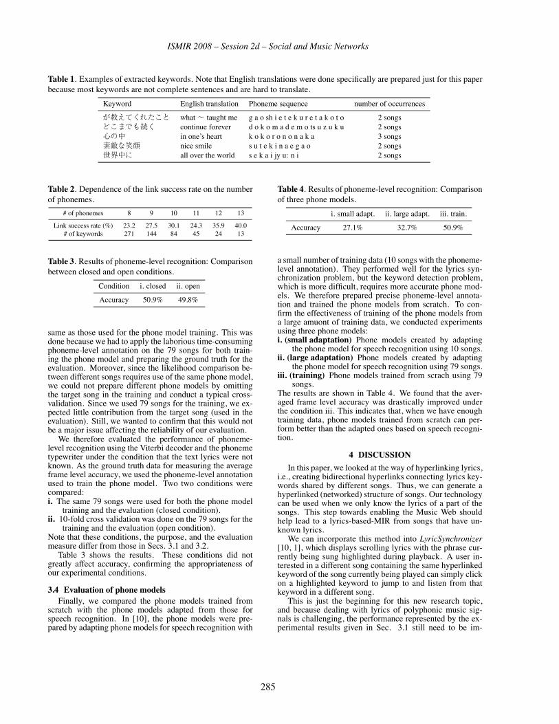
ISMIR 2008 – Session 2d – Social and Music Networks
Table 1. Examples of extracted keywords. Note that English translations were done specifically are prepared just for this paperbecause most keywords are not complete sentences and are hard to translate.
Keyword English translation Phoneme sequence number of occurrences
が教えてくれたこと what~ taught me g a o sh i e t e k u r e t a k o t o 2 songsどこまでも続く continue forever d o k o m a d e m o ts u z u k u 2 songs心の中 in one’s heart k o k o r o n o n a k a 3 songs素敵な笑顔 nice smile s u t e k i n a e g a o 2 songs世界中に all over the world s e k a i jy u: n i 2 songs
Table 2. Dependence of the link success rate on the numberof phonemes.
# of phonemes 8 9 10 11 12 13
Link success rate (%) 23.2 27.5 30.1 24.3 35.9 40.0# of keywords 271 144 84 45 24 13
Table 3. Results of phoneme-level recognition: Comparisonbetween closed and open conditions.
Condition i. closed ii. open
Accuracy 50.9% 49.8%
same as those used for the phone model training. This wasdone because we had to apply the laborious time-consumingphoneme-level annotation on the 79 songs for both train-ing the phone model and preparing the ground truth for theevaluation. Moreover, since the likelihood comparison be-tween different songs requires use of the same phone model,we could not prepare different phone models by omittingthe target song in the training and conduct a typical cross-validation. Since we used 79 songs for the training, we ex-pected little contribution from the target song (used in theevaluation). Still, we wanted to confirm that this would notbe a major issue affecting the reliability of our evaluation.
We therefore evaluated the performance of phoneme-level recognition using the Viterbi decoder and the phonemetypewriter under the condition that the text lyrics were notknown. As the ground truth data for measuring the averageframe level accuracy, we used the phoneme-level annotationused to train the phone model. Two two conditions werecompared:i. The same 79 songs were used for both the phone model
training and the evaluation (closed condition).ii. 10-fold cross validation was done on the 79 songs for the
training and the evaluation (open condition).Note that these conditions, the purpose, and the evaluationmeasure differ from those in Secs. 3.1 and 3.2.
Table 3 shows the results. These conditions did notgreatly affect accuracy, confirming the appropriateness ofour experimental conditions.
3.4 Evaluation of phone modelsFinally, we compared the phone models trained from
scratch with the phone models adapted from those forspeech recognition. In [10], the phone models were pre-pared by adapting phone models for speech recognition with
Table 4. Results of phoneme-level recognition: Comparisonof three phone models.
i. small adapt. ii. large adapt. iii. train.
Accuracy 27.1% 32.7% 50.9%
a small number of training data (10 songs with the phoneme-level annotation). They performed well for the lyrics syn-chronization problem, but the keyword detection problem,which is more difficult, requires more accurate phone mod-els. We therefore prepared precise phoneme-level annota-tion and trained the phone models from scratch. To con-firm the effectiveness of training of the phone models froma large amuont of training data, we conducted experimentsusing three phone models:i. (small adaptation) Phone models created by adapting
the phone model for speech recognition using 10 songs.ii. (large adaptation) Phone models created by adapting
the phone model for speech recognition using 79 songs.iii. (training) Phone models trained from scrach using 79
songs.The results are shown in Table 4. We found that the aver-aged frame level accuracy was drastically improved underthe condition iii. This indicates that, when we have enoughtraining data, phone models trained from scratch can per-form better than the adapted ones based on speech recogni-tion.
4 DISCUSSION
In this paper, we looked at the way of hyperlinking lyrics,i.e., creating bidirectional hyperlinks connecting lyrics key-words shared by different songs. Thus, we can generate ahyperlinked (networked) structure of songs. Our technologycan be used when we only know the lyrics of a part of thesongs. This step towards enabling the Music Web shouldhelp lead to a lyrics-based-MIR from songs that have un-known lyrics.
We can incorporate this method into LyricSynchronizer[10, 1], which displays scrolling lyrics with the phrase cur-rently being sung highlighted during playback. A user in-terested in a different song containing the same hyperlinkedkeyword of the song currently being played can simply clickon a highlighted keyword to jump to and listen from thatkeyword in a different song.
This is just the beginning for this new research topic,and because dealing with lyrics of polyphonic music sig-nals is challenging, the performance represented by the ex-perimental results given in Sec. 3.1 still need to be im-
285

ISMIR 2008 – Session 2d – Social and Music Networks
proved. We expect to improve the overall performance byrefining the phone model. As shown in Sec. 3.4, we can im-prove it by preparing the annotation for more songs. More-over, as speech recognition technologies have shown, oncewe obtain good initial phone models, we can improve themthrough transcribing audio signals (i.e., lyrics) without re-quiring precise phoneme-level annotation.
Our experience in developing the keyword extractionmethod described in Sec. 2.1.1 has shown that the wellknown tf-idf (term frequency-inverse document frequency)is not useful for extracting keywords that have as manyphonemes as possible but appear in two songs or more. Thetf-idf is designed based of the assumptions that the impor-tance of a keyword for a document is proportional to thenumber of occurrences of the keyword in the document isand inversely proportional to the number of occurrences ofthe keyword in all documents. However, the number of key-word occurrences in a song in our problem is unimportant.Even if a keyword appears only once, a user can jump fromthat keyword to other songs of interest. Therefore, we de-veloped our own keyword extraction method.
5 CONCLUSION
This paper described a method for creating hyperlinksbetween different songs at the level of lyrics phrases. Wepresented a method for dealing with an important problemthat has received little attention. We created two kinds ofhyperlinks: hyperlinks between songs where the text lyricsare known and those from songs with text lyrics to songswithout text lyrics. We created these hyperlinks by extract-ing keywords from the text lyrics of all songs and by de-tecting the keywords in polyphonic audio signals by using aHMM-based keyword spotting technique. Our experimentalresults show that the approach is promising, but better per-formance is needed for practical application. We will applyour method to a much larger database in the future. We alsoplan to develop useful applications for this method, includ-ing song clustering based on the songs’ lyrics, and a MusicWeb browser that enables users to browse and discover in-teresting songs by clicking the hyperlyrics of songs.
6 ACKNOWLEDGEMENTS
This work was partially supported by CrestMuse,CREST, JST. We used the HTK (Hidden Markov ModelToolkit) [21] for training the phone models. We thankKatunobu Itou (Hosei University) for helping us to createthe phoneme label annotation of the RWC Music Database[19]. We also thank everyone who has contributed to build-ing and distributing the atabase.
7 REFERENCES
[1] Masataka Goto, “Active music listening interfaces based on signalprocessing,” in Proceedings of the 2007 IEEE International Confer-ence on Acoustics, Speech, and Signal Processing (ICASSP 2007),2007, pp. IV–1441–1444.
[2] George Tzanetakis and Perry Cook, “MARSYAS: A framework foraudio analysis,” Organised Sound, vol. 4, no. 30, pp. 169–175, 1999.
[3] Robert Neumayer, Michael Dittenbach, and Andreas Rauber,“Playsom and pocketsomplayer: Alternative interfaces to large musiccollections,” in Proceedings of the 6th International Conference onMusic Information Retrieval (ISMIR 2005), 2005, pp. 618–213.
[4] Takayuki Goto and Masataka Goto, “Musicream: New music play-back interface for streaming, sticking, sorting, and recalling musical
pieces,” in Proceedings of the 6th International Conference on MusicInformation Retrieval (ISMIR 2005), 2005, pp. 404–411.
[5] Elias Pampalk and Masataka Goto, “Musicrainbow: A new user in-terface to discover artists using audio-based similarity and web-basedlabeling,” in Proceedings of the 7th International Conference on Mu-sic Information Retrieval (ISMIR 2006), 2006, pp. 367–370.
[6] Paul Lamere and Douglas Eck, “Using 3D visualizations to exploreand discover music,” in Proceedings of the 8th International Confer-ence on Music Information Retrieval (ISMIR 2007), 2007, pp. 173–174.
[7] Masataka Goto, “A chorus-section detection method for musical au-dio signals and its application to a music listening station,” IEEETransactions on Audio, Speech and Language Processing, vol. 14,no. 5, pp. 1783–1794, 2006.
[8] Meinard Müller and Frank Kurth, “Enhancing similarity matrices formusic audio analysis,” in Proceedings of the 2006 IEEE InternationalConference on Acoustics, Speech, and Signal Processing (ICASSP2006), 2006, pp. V–9–12.
[9] Ye Wang, Min-Yen Kan, Tin Lay Nwe, Arun Shenoy, and Jun Yin,“Lyrically: Automatic synchronization of acoustic musical signalsand textual lyrics,” in Proceedings of the 12th ACM InternationalConference on Multimedia, 2004, pp. 212–219.
[10] Hiromasa Fujihara, Masataka Goto, Ogata Jun, Kazunori Komatani,Tetsuya Ogata, and Hiroshi G. Okuno, “Automatic synchronizationbetween lyrics and music CD recordings based on viterbi alignmentof segregated vocal signals,” in Proceedings of the IEEE Interna-tional Symposium on Multimedia (ISM 2006), 2006, pp. 257–264.
[11] Meinard Müller, Frank Kurth, David Damm, Christian Fremerey, andMichael Clausen, “Lyrics-based audio retrieval and multimodal nav-igation in music collections,” in Proceedings of the 11th EuropeanConference on Digital Libraries (ECDL 2007), 2007.
[12] Chong-Kai Wang, Ren-Yuan Lyu, and Yuang-Chin Chiang, “An au-tomatic singing transcription system with multilingual singing lyricrecognizer and robust melody tracker,” in Proceedings of the 8th Eu-ropean Conference on Speech Communication and Technology (Eu-rospeech2003), 2003, pp. 1197–1200.
[13] Toru Hosoya, Motoyuki Suzuki, Akinori Ito, and Shozo Makino,“Lyrics recognition from a singing voice based on finite state automa-ton for music information retrieval,” in Proceedings of the 6th Inter-national Conference on Music Information Retrieval (ISMIR 2005),2005, pp. 532–535.
[14] Matthias Gruhne, Konstantin Schmidt, and Christian Dittmar,“Phoneme recognition in popular music,” in Proceedings of the8th International Conference on Music Information Retrieval (ISMIR2007), 2007, pp. 369–370.
[15] Peter Knees, Markus Schedl, and Gerhard Widmer, “Multiple lyricsalignment: Automatic retrieval of song lyrics,” in Proceedings of the6th International Conference on Music Information Retrieval (ISMIR2005), 2005, pp. 564–569.
[16] Bin Wei, Chengliang Zhang, and Mitsunori Ogihara, “Keyword gen-eration for lyrics,” in Proceedings of the 8th International Conferenceon Music Information Retrieval (ISMIR 2007), 2007, pp. 121–122.
[17] Kate Knill and Steve Young, “Speaker dependent keyword spottingfor accessing stored speech,” Tech. Rep. CUED/F-INFENG/TR 193,Cambridge University, 1994.
[18] Masataka Goto, “A real-time music-scene-description system:Predominant-F0 estimation for detecting melody and bass lines inreal-world audio signals,” Speech Communication, vol. 43, no. 4, pp.311–329, 2004.
[19] Masataka Goto, Hiroki Hashiguchi, Takuichi Nishimura, and RyuichiOka, “RWC Music Database: Popular, classical, and jazz musicdatabases,” in Proceedings of the 3rd International Conference onMusic Information Retrieval (ISMIR 2002), 2002, pp. 287–288.
[20] MeCab: Yet Another Part of Speech and Morphological Analyzer,“http://mecab.sourceforge.net/,” .
[21] HTK: The Hidden Markov Model Toolkit,“http://htk.eng.cam.ac.uk/,” .
286

ISMIR 2008 – Session 2d – Social and Music Networks
OH OH OHWHOAH!TOWARDS AUTOMATIC TOPIC DETECTION IN SONG LYRICS
Florian KleedorferStudio Smart Agent Technologies
Research Studios [email protected]
Peter Knees Tim PohleDept. of Computational Perception
Johannes Kepler University Linz, Austria{peter.knees,tim.pohle}@jku.at
ABSTRACT
We present an algorithm that allows for indexing music bytopic. The application scenario is an information retrievalsystem into which any song with known lyrics can be in-serted and indexed so as to make a music collection browse-able by topic. We use text mining techniques for creating avector space model of our lyrics collection and non-negativematrix factorization (NMF) to identify topic clusters whichare then labeled manually. We include a discussion of thedecisions regarding the parametrization of the applied meth-ods. The suitability of our approach is assessed by measur-ing the agreement of test subjects who provide the labels forthe topic clusters.
1 INTRODUCTION
The past few years have seen a tremendous amount of scien-tific work in the field of music information retrieval. Much,if not most of this work was concentrated on the acousticproperties of music, while the semantic content conveyedby the words of the songs was mostly ignored. There hasbeen some work on song lyrics, but the field has not gainedmomentum comparable to work on acoustic features of mu-sic. In much of the older work lyrics were used to side orcontrast with acoustic-based techniques in genre classifica-tion of songs [8] or artists [7]. In newer work, lyrics havebecome sources for metadata generation [9] and, probablyinspired by the evolution of Web 2.0, lyrics were found use-ful as a basis for keyword generation for songs, a techniquethat may ultimately lead to automatic tagging [12].
In our view, any music browsing or recommendation sys-tem is incomplete if it does not incorporate the dimension ofthe songs’ semantic content. It is therefore our goal to cre-ate elements of such a system based on the analysis of songlyrics. In the work at hand, we present the building blocksof a system that allows for searching a collection of lyrics byselecting from a set of topics. We describe the formal detailsof the procedure which we propose for making a collectionof songs browseable by topic. Centrally to our algorithm,we apply NMF for clustering the lyrics documents as pro-posed in [13]. The resulting clusters are labeled manually
so that they can be used as the dimensions of a topic spacein which the documents are arranged.
The remainder of this paper is organized as follows: Sec-tion 2 describes the dataset we work with, in Section 3 weexplain the details of our algorithm. Section 4 gives an ac-count of the quality assessment we performed.
2 THE DATA
The music archive we work with is a subset of the collec-tion marketed through Verisign Austria’s 1 content down-load platform. This subset comprises approximately 60.000of the most popular audio tracks 2 by some 6.000 artists.The tracks are affiliated with one or more of 31 genres. Themost important genres are “Pop” (10817 songs), “Alter-native” (9975 songs), “Hip-Hop” (4849), “Rock” (4632),“Country” (3936) and “Dance/Electronic” (3454).
The lyrics to these songs were extracted from the inter-net using the method presented in [5], which worked forroughly two thirds of the songs. The reason for this ratherlow rate of success is that the method we employed is notsuitable for some classes of tracks. Such classes compriseof course the purely instrumental songs, but also works thatbear a composite artist attribute, e.g., “Mint Condition/feat.Charlie Wilson of the Gap Band” or older and only locallyknown music. After removal of duplicates, which are alsopresent in our dataset, we get a corpus of 33863 lyrics.
The lyrics are in 15 different languages, though the vastmajority is in English. We found about 300 Spanish songs,roughly 30 in Italian, French, Gaelic and Latin; all otherlanguages are even less frequent.
3 ALGORITHM
The method we propose requires the lyrics collection to betransformed into a vector space model in which each doc-ument is represented as a vector defining its affiliation to aset of topics. This transformation encompasses the follow-ing steps:
1 http://www.verisign.at/2 i.e., the most frequently accessed tracks within a certain time span
287
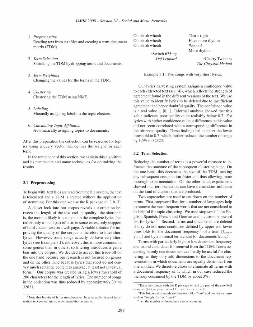
ISMIR 2008 – Session 2d – Social and Music Networks
1. PreprocessingReading text from text files and creating a term-documentmatrix (TDM).
2. Term SelectionShrinking the TDM by dropping terms and documents.
3. Term WeightingChanging the values for the terms in the TDM.
4. ClusteringClustering the TDM using NMF.
5. LabelingManually assigning labels to the topic clusters.
6. Calculating Topic AffiliationAutomatically assigning topics to documents.
After this preparation the collection can be searched for top-ics using a query vector that defines the weight for eachtopic.
In the remainder of this section, we explain this algorithmand its parameters and name techniques for optimizing theresults.
3.1 Preprocessing
To begin with, text files are read from the file system, the textis tokenized and a TDM is created without the applicationof stemming. For this step we use the R package tm [10, 3].
A closer look into our corpus reveals a correlation be-tween the length of the text and its quality: the shorter itis, the more unlikely it is to contain the complete lyrics, butrather only a small part of it or, in some cases, only snippetsof html code or text on a web page. A viable solution for im-proving the quality of the corpus is therefore to filter shortlyrics. However, some songs actually do have very shortlyrics (see Example 3.1); moreover, this is more common insome genres than in others, so filtering introduces a genrebias into the corpus. We decided to accept this trade-off onthe one hand because our research is not focused on genresand on the other hand because lyrics that short do not con-vey much semantic content to analyze, at least not in textualform. 3 Our corpus was created using a lower threshold of200 characters for the length of lyrics. The number of songsin the collection was thus reduced by approximately 3% to32831.
3 Note that brevity of lyrics may, however, be a valuable piece of infor-mation in a general music recommendation scenario.
Oh oh oh whoahOh oh oh whoahOh oh oh whoah
“Switch 625” by
Def Leppard
That’s rightHave more rhythmWoooo!More rhythm
“Cherry Twist” by
The Chrystal Method
Example 3.1: Two songs with very short lyrics.
Our lyrics harvesting system assigns a confidence valueto each extracted text (see [4]), which reflects the strength ofagreement found in the different versions of the text. We usethis value to identify lyrics to be deleted due to insufficientagreement and hence doubtful quality. The confidence valueis a real value ∈ [0, 1]. Informal analysis showed that thisvalue indicates poor quality quite realiably below 0.7. Forlyrics with higher confidence value, a difference in this valuedid not seem correlated with a corresponding difference inthe observed quality. These findings led us to set the lowerthreshold to 0.7, which further reduced the number of songsby 1.5% to 32323.
3.2 Term Selection
Reducing the number of terms is a powerful measure to in-fluence the outcome of the subsequent clustering stage. Onthe one hand, this decreases the size of the TDM, makingany subsequent computation faster and thus allowing morethorough experimentation. On the other hand, experimentsshowed that term selection can have tremendous influenceon the kind of clusters that are produced.
Two approaches are used to cut down on the number ofterms. First, stopword lists for a number of languages helpto remove the most frequent words that are not considered tobe helpful for topic clustering. We used stopwords 4 for En-glish, Spanish, French and German and a custom stopwordlist for lyrics 5 . Second, terms and documents are deletedif they do not meet conditions defined by upper and lowerthresholds for the document frequency 6 of a term (fmax,fmin) and by a minimal term count for documents (tmin).
Terms with particularly high or low document frequencyare natural candidates for removal from the TDM. Terms oc-curring in only one document can hardly be useful for clus-tering, as they only add dimensions to the document rep-resentation in which documents are equally dissimilar fromone another. We therefore chose to eliminate all terms witha document frequency of 1, which in our case reduced thememory consumed by the TDM by about 3%.
4 These lists come with the R package tm and are part of the snowballstemmer (http://snowball.tartarus.org/)
5 This list contains mainly exclamations like “uuh” and non-lyrics termssuch as “songlyrics” or “inurl”
6 i.e., the number of documents a term occurs in.
288

ISMIR 2008 – Session 2d – Social and Music Networks
Terms with a very high document frequency account fordimensions of the document representation in which a greatamount of documents are similar. With respect to cluster-ing, these dimensions may be regarded as noise that makesthe real clusters more difficult to discern. This rationalesuggests that the clustering result improve when frequentterms are removed. Moreover, removing the frequent termsgreatly reduces the space consumed by the TDM: in ourcase, deleting terms with a document frequency > 500 re-duced the memory consumption by 42%. However, the dis-advantage of this strategy may be that clusters mainly de-fined by frequent terms are lost.
Early findings suggested that the use of an upper limit forthe document frequency makes the resulting clusters morediverse, but more systematic experimentation convinced usthat it was better to use fmax =∞.
3.3 Term Weighting
It has been proposed to use TF×IDF [11] as the weightingscheme prior to NMF clustering [13]. In text retrieval appli-cations, the purpose of the weighting function is to amplifythe weights of the terms that are most typical for a docu-ment and to lower the weights of the other terms. This isbecause the main use case of the method is retrieval, i.e.,finding documents that match a user-defined query. In ouralgorithm, however, the use case to optimize for is not re-trieval but clustering. During our experiments, we learnedthat this requires different properties of the weighting func-tion.
We investigated the usefulness of three different weigh-ing schemes in our context: term frequency weighting (i.e.,no change to the TDM at all), TF×IDF and binary (i.e., re-placing all nonzero entries in the TDM by 1). We found thatbinary weighting yielded the best results both in terms ofindividual cluster quality and evenness of the document-to-cluster distribution. Clustering using term frequency weight-ing produces term clusters in which the frequent terms areclearly overrepresented. Similarly, when applying TF×IDFweighting before clustering, the terms with low documentfrequency are too important in the resulting term clusters.
3.4 Clustering
We decided to use NMF [6, 13] for automatic topic detec-tion as it is a clustering technique that results in additiverepresentation of items 7 [6], a property that distinguishes itfrom most other clustering techniques. We also evaluatedlatent semantic analysis (LSA) [2], but found that it is not asuitable techniques for large sparse matrices due to its spacecomplexity. Using NMF, the TDM is approximated by the
7 e.g., song X is represented as 10% topic A, 30% topic B and 60% topicC
do
cum
ents
terms
clusters
clu
ster
s
do
cum
ents
terms
W
H
Figure 1. Non-negative factorization of the TDM. TheTDM is approximated by the product WH.
matrix product of two matrices of appropriate dimensional-ity. NMF is parametrized most prominently by the numberof clusters that it shall produce, k. More formally, let T bethe TDM, W and H the factor matrices, and
Tdocuments×terms = Wdocuments×kHk×terms (1)
The parameter k is the inner dimension of the factorization,i.e. the dimension that both factor matrices share. The ap-proximation of the TDM by the NMF is depicted in Figure1. For our purposes, the more important matrix of the twofactor matrices is H , which contains the weight of each termin each cluster.
A low value for k causes NMF to produce clusters thatare actually mixtures of multiple topics, which may be re-lated hierarchically, but this is not neccessarily the case. Forinstance, one cluster may describe the topic “love”, and ona closer look, the sub-topics “loss”, “happy” and “family”are recognizable, while another cluster could at first glancecontain only the “gangsta” topic but at the same time be thestrongest cluster for all spanish songs. In the first case, theclustering result is acceptable - none of the songs that fallinto the cluster would really be misclassified; the only validcriticism is the lack of exactness. In the latter case, a portionof the lyrics that fall into that cluster are clearly misclassi-fied because the cluster combines multiple different “real”topics.
When using high values for k, NMF tends to producemore specific clusters, most of which are quite interestingand useful. One of the drawbacks of this setting, however,is a tendency of NMF to find the same topics multiple times.Another noticeable side effect of high k values is that the im-portant terms simply tend to be strong co-occurrents of thefirst term in the cluster, so the cluster represents not really atopic but rather contains the standard result of co-occurrenceanalysis.
289

ISMIR 2008 – Session 2d – Social and Music Networks
lovep
artylo
ss
do
cum
ents
terms
document affiliation
do
cum
ents
terms
terms
clu
ster
s
a b
Figure 2. Computation of the documents’ affiliationstrength to the clusters. The manually assigned cluster la-bels in this example are ’love’, ’party’ and ’loss’.
After carefully weighing the benefits and drawbacks ofboth approaches, we decided to use a high value for thenumber of clusters in NMF. We conducted experiments foroptimizing fmax and k, and as a result, we chose to set k to60 (and fmax to∞, as stated above).
3.5 Labeling
In order to make the clustering useful to an end user, theclusters need some kind of identifiers associated with themthat hint at the nature of each cluster’s content. Labelinga cluster was done manually by reading its most impor-tant terms and assigning one or more words that best sum-marised those terms. The exact procedure followed in label-ing the clusters, and the results are described in Section 4.
3.6 Calculating Topic Affiliation
The degree of membership of a document in each cluster iscomputed using the orginal TDM weighted with term fre-quencies. This step is shown in Figure 2. First, only thecolumns (i.e. terms) that were used in the NMF are se-lected ( �a ). The resulting matrix is multiplied by the trans-posed factor matrix H from the NMF that contains the termweights per cluster ( �b ). Hence, for each cluster and eachdocument, each term belonging to the document is multi-plied by the weight of the term in the cluster and the sumover these products is regarded as the weight of the clusterfor the document. After the calculation of this document af-filiation matrix, its rows are normalized to a length of 1 inthe euclidean norm.
3.7 Query Formulation and Document Retrieval
Retrieval of documents requires defining a query specifiyingwhich clusters the documents should belong to. Resultingdocuments are ranked with respect to that query. A queryvector is defined, assigning a weight to each cluster. Thecosine similarity values between the rows of the documentaffiliation matrix and the query vector define the rank of alldocuments in the query result. The result is sorted in de-scending order; the first results are the most relevant ones.
4 ASSESSMENT OF LABELING
4.1 Setup
Stages 1-4 of the described algorithm were applied to ourlyrics database with the settings k = 60 and fmax =∞,as explained above. The resulting 60 clusters were used asbasis for a two-phased experiment that was inspired by thedelphi method [1] which is a common method for obtainingopinion consensus from a group of experts.
In the first phase, test subjects were shown the most im-portant terms 8 of each cluster and were asked to providetags that summarise the terms.
In the second phase, the same word lists were shown tothe same test subjects, but this time the task was to choosethe best tags from those collected during the first phase, butnot more than two. These tests were carried out with 6 sub-jects, all male between 20 and 32 years of age with strongbackground in computer science and little in music.
4.2 Evaluation Measure
The strength of agreement among test subjects cannot bemeasured after the first phase because they are completelyfree in their production of tags, so it is very unlikely thatidentical tags be used. In phase 2, when the subjects have tochoose from the tags produced during phase 1, this is pos-sible because everyone has to perform the very same task.For estimating the significance of the labeling outcome, wecompute the probability of the actual result being attained bycompletely random behaviour on behalf of the subjects. Therationale is similar to that of methods for assessing inter-coder agreement: The lower this probability is, the moreevidence there is that the result is due to intelligible featuresof the data.
During phase 2, there was a given number of tags (m)associated with a given cluster 9 . If a person chose a tagat first position, we assigned a grade of 1 to that tag. Ifthe person chose it for the second position, the grade was
8 Those terms with a weight stronger than mean + std.dev. of all termweights in the cluster, sorted by weight. Not more than 30 terms wereshown.
9 There were at least 2 tags for each cluster, at most 10; mean tag countper cluster was 6.25.
290

ISMIR 2008 – Session 2d – Social and Music Networks
2, all other tags were assigned grade 3. Thus, In the wholesession, a (n × m) grading matrix was created containingthe grades for all m tags created by all n test subjects.
The behaviour of the subjects was modeled as follows:For a given cluster, i.e., for a given m, a subject could chooseone of the tags as the best tag with a probability of P (first) =p1 and chose none with probability P (none) = 1 − p1.If a tag was chosen best, each tag was equally probableto be chosen with a probability of 1/m. Then, the per-son could pick another tag as second best with probabilityP (second|first) = p2 and no second best tag with prob-ability P (nosecond|first) = 1 − p2. If a tag was chosenas second best, again, all tags were equally probable for thischoice with probability 1/(m− 1).
The model parameters p1 and p2 are computed based onthe behaviour of the test subjects. p1 is defined as the per-centage of cases in which at least one tag was chosen, p2 asthe percentage of the former cases in which also a secondtag was picked.
Consequently, given m, p1 and p2, the probability p(g)for a tag to get grade g ∈ {1, 2, 3} is
p(1) = p1p2m + p1(1−p2)
m (2)
p(2) = p1p2m (3)
p(3) = p1p2(m−2)m + p1(1−p2)(m−1)
m + 1− p1 (4)
As the result of phase 2, we get a grading matrix for eachcluster. The strength of agreement is assessed by comput-ing how probable the column means of such a matrix are apriori. As each value in each column takes the values 1,2 or3 with the probabilities explained above, the probability fora column to contain g1 times the grade 1, g2 times 2 and g3
times 3 isn!
g1!g2!g3!p(1)g1p(2)g2p(3)g3 (5)
The likelihood of reaching a given column mean (i.e.,average grade for a tag) is the sum of the probabilities of allgrade combinations that result in the same or a better mean.
4.3 Discussion
The result of the assesment procedure is a number of tagsfor each cluster. The tags are associated with a grade and avalue which indicates the likelihood for the grade to resultfrom chance agreement among subjects. Table 1 shows thebest-graded tag of each cluster, provided that the said like-lihood is at most 10%. Due to this selection criterion, only41 out of 60 tags are shown. As stated in Section 3.4, thesame topic are found multiple times; this is reflected here intags occurring more than once (e.g., “dream”, “emotion”or “gangsta”).
appearance boys and girls boys and girls broken heartedclubbing conflict crime dancedance depression dream dreamemotion emotion family feelingsfuture gangsta gangsta gangstagangsta going out gospel hard timeshiphop home leave listenloneliness loss love lovelove music music natureparty sorrow talk weatherworld
Table 1. Winning tags at a significance level of 10%
significance level#
clus
ters
0.0 0.2 0.4 0.6 0.8 1.0
015
30Figure 3. Number of clusters per significance level of thewinning tag
Figure 3 shows the levels of significance for the mostpopular tag of each cluster in 5% steps. In 31 out of 60clusters, the best tag was agreed on with a less than 5% like-lihood of chance agreement. For another 10 clusters, thesignificance level was between 5 and 10%.
These results suggest that a reasonable portion of theclusters describes discernable topics and that they are re-liably tagged.
5 CONCLUSION
The work at hand explains the structure and parametriza-tion of an algorithm for the application of NMF to songlyrics. The focus is on showing the distinct stages of the al-gorithm and the considerations concerning the choice of pa-rameter values for each stage. The most interesting choicesfor parameter values, in our view, are a) the high value fork (60 may still not be high enough) and b) the use of binaryweighting prior to NMF clustering.
We also present an assessment of the clustering outcomeindicating that most of the topic clusters resulting from ouralgorithm are useful for indexing our music collection. Theprocedure used for assessment is at the same time an integralpart of the algorithm, the labeling stage, which has the con-venient property that a statistically interpretable confidencevalue is calculated for each cluster so that it can be rejectedor accepted for use in the subsequent stages.
291

ISMIR 2008 – Session 2d – Social and Music Networks
6 FUTUREWORK
We plan to integrate the proposed method into an exisingMIR system 10 . Only then the effects of certain parametersettings can be evaluated effectively. We also plan on eval-uating our system in a user study with more test subjectsthan in the work at hand so as to produce statistically sig-nificant results. In addition to that, the question arises howsimilar clusters can be combined or hierarchically arrangedfor display to end users. Another interesting route of inquiryis hierarchical or iterative NMF clustering with the goal offinding less frequent topics. Taking the whole approach onestep further, using NMF may turn out to be only one ap-proach among many for creating weighted word lists (i.e.,clusters) for indexing song collections. We consider the useof term co-occurrences most promising for the semi-manualdefinition of such lists for topics that are known to be con-tained in the archive but are not found by clustering. Ulti-mately, this task could be done by end users, allowing themto define and fine-tune topic classifiers themselves.
7 ACKNOWLEDGEMENTS
This work was supported by the Austrian Federal Ministryof Economics and Labor and Austria Wirtschaftsservice (”Im-pulsprogramm Creativwirtschaft”); the Austrian ResearchPromotion Agency (FFG) (FIT-IT project SEMPRE); andthe Austrian Science Fund (FWF) under project number L511-N15.
8 REFERENCES
[1] Norman Dalkey and Olaf Helmer. An experimental ap-plication of the delphi method to the use of experts.Management Science, 9(3):458–467, 1963.
[2] Scott C. Deerwester, Susan T. Dumais, Thomas K. Lan-dauer, George W. Furnas, and Richard A. Harshman.Indexing by latent semantic analysis. Journal of theAmerican Society of Information Science, 41(6):391–407, 1990.
[3] Ingo Feinerer. tm: Text mining package, 2007. R pack-age version 0.2-3.7.
[4] Peter Knees. Addendum to “Multiple Lyrics Alignment:Automatic Retrieval of Song Lyrics”. Technical Re-port CPJKU-TR-2008-MLA, Dept. of ComputationalPerception, Johannes Kepler University, Linz, Austria,2008.
[5] Peter Knees, Markus Schedl, and Gerhard Widmer.Multiple lyrics alignment: Automatic retrieval of songlyrics. In Proceedings of 6th International Conference
10 http://musicexplorer.researchstudio.at/
on Music Information Retrieval (ISMIR’05), pages 564–569, London, UK, September 2005.
[6] Daniel D. Lee and Sebastian H. Seung. Learning theparts of objects by non-negative matrix factorization.Nature, 401(6755):788–791, October 1999.
[7] Tao Li and Mitsunori Ogihara. Music artist style iden-tification by semi-supervised learning from both lyricsand content. In MULTIMEDIA ’04: Proceedings of the12th annual ACM international conference on Multime-dia, pages 364–367, New York, NY, USA, 2004. ACMPress.
[8] B. Logan, A. Kositsky, and P. Moreno. Semantic analy-sis of song lyrics. In Proceedings of the 2003 IEEE In-ternational Conference on Multimedia and Expo, vol-ume 2, pages 827–830, Baltimore,Maryland, USA,2004.
[9] Jose P. G. Mahedero, Álvaro Martı́nez, Pedro Cano,Markus Koppenberger, and Fabien Gouyon. Natural lan-guage processing of lyrics. In Proceedings of the 13thACM International Conference on Multimedia (MUL-TIMEDIA ’05), pages 475–478, New York, NY, USA,2005. ACM Press.
[10] R Development Core Team. R: A language and environ-ment for statistical computing, 2006. ISBN 3-900051-07-0.
[11] Gerard Salton and Christopher Buckley. Term-weighting approaches in automatic text retrieval.Information Processing and Management, 24(5):513–523, 1988.
[12] Bin Wei, Chengliang Zhang, and Mitsunori Ogihara.Keyword generation for lyrics. In Proceedings of theEighth International Conference on Music InformationRetrieval (ISMIR’07), pages 121–122, Vienna, Austria,September 2007.
[13] Wei Xu, Xin Liu, and Yihong Gong. Document clus-tering based on non-negative matrix factorization. In SI-GIR ’03: Proceedings of the 26th annual internationalACM SIGIR conference on Research and developmentin informaion retrieval, pages 267–273, New York, NY,USA, 2003. ACM.
292

Session 3a – Content-Based Retrieval, Categorizationand Similarity 1

.
ISMIR 2008 – Session 3a – Content-Based Retrieval, Categorization and Similarity 1
A TEXT RETRIEVAL APPROACH TO CONTENT-BASED AUDIORETRIEVAL
Matthew RileyUniversity of Texas at Austin
Eric HeinenUniversity of Texas at Austin
Joydeep GhoshUniversity of Texas at Austin
ABSTRACT
This paper presents a novel approach to robust, content-
based retrieval of digital music. We formulate the hash-
ing and retrieval problems analogously to that of text re-
trieval and leverage established results for this unique ap-
plication. Accordingly, songs are represented as a ”Bag-
of-Audio-Words” and similarity calculations follow directly
from the well-known Vector Space model [12]. We evaluate
our system on a 4000 song data set to demonstrate its prac-
tical applicability, and evaluation shows our technique to be
robust to a variety of signal distortions. Most interestingly,
the system is capable of matching studio recordings to live
recordings of the same song with high accuracy.
1 INTRODUCTION
Large digital music libraries are becoming commonplace on
consumer computer systems, and with their growth our abil-
ity to automatically analyze and interpret their content has
become increasingly important. The ability to find acousti-
cally similar, or even duplicate, songs within a large audio
database is a particularly important task with numerous po-
tential applications. For example, an automated system sim-
ilar to MusicBrainz [11] might organize a user’s music col-
lection by properly naming each file according to artist and
song title. Another application could attempt to retrieve the
artist and title of a song given a short clip recorded from a
radio broadcast or perhaps even hummed into a microphone.
Due to the rich feature set of digital audio, a central task
in this process is that of extracting a representative audio fin-
gerprint that describes the acoustic content of each song. We
hope to extract from each song a feature vector that is both
highly discriminative between different songs and robust to
common distortions that may be present in different copies
of the same source song. With the multitude of compres-
sion formats and signal extraction processes, two copies of
the same song can sound perceptually identical while hav-
ing very different digital representations. Additionally, it is
desirable for the audio fingerprint to compress the existing
audio information into a much smaller representation, thus
enabling efficient retrieval and requiring less storage than
that of the initial data set.
In this paper, we present a novel hashing methodology
that satisfies these constraints. We show that a technique
based on methods for text retrieval performs well for the
desired applications, and benefits from established research
results in the area. Section 2 reviews existing work related
to our application and section 3 details our application of
the text retrieval techniques to content-based audio retrieval.
Section 4 details our experimental evaluation of the pro-
posed algorithm. Section 5 discusses practical implemen-
tation considerations and section 6 concludes with final re-
marks and suggestions for future work.
2 RELATED WORK
The problem of audio fingerprinting has been studied widely.
In 2002, Haitsma and Kalker proposed a method for ex-
tracting audio fingerprints that they showed were robust to
a variety of signal distortions. In addition, they outlined a
database searching algorithm for locating a fingerprint most
similar to a given target fingerprint [7]. One of the draw-
backs of their system is the amount of memory required
to store an audio fingerprint (approx. 100 KBytes for a 5
minute song). In addition, it was unclear whether or not
their fingerprints could feasibly be used to match a studio
recording to a live performance or a cover version (i.e. a
performance of the original composition by another artist,
possibly rearranged).
Existing work on cover song detection was presented for
a competition at The Music Information Retrieval Evalua-
tion eXchange (MIREX). In 2006, Dan Ellis’ team from
Columbia University won the competition by posting ac-
curacy of about 60% using a method that computed sim-
ilarities between songs by cross-correlating sequences of
their so-called Chroma features [5]. Their similarity mea-
sure is equally applicable to the problem of matching a stu-
dio recording to a live performance. However, the high com-
putational complexity of cross-correlating Chroma feature
vector sequences does not make sense in an audio retrieval
context.
We have not found previous research that directly applies
text retrieval methods to the task of audio retrieval, but a
similar approach has been taken for Object Recognition in
images [13]. Further, Casey and Slaney [3] present a system
295

ISMIR 2008 – Session 3a – Content-Based Retrieval, Categorization and Similarity 1
������������ ��������� ����������������������
����������������
�������������������
Digital Audio Bag-of-Audio-Words
Representation
Figure 1. Block diagram for ”Bag-of-Audio-Words” Representation
for discovering derivative audio works and describe a local-
ity sensitive hashing procedure for matching similar songs
that is derived from the ”text shingles” method originally
proposed in [2]. Finally, A vector quantization scheme sim-
ilar to ours but using self-organizing maps is described in
[14].
3 BAG-OF-AUDIO-WORDS REPRESENTATION
Our basic framework for extracting a song’s Bag-of- Audio-
Words representation is depicted in Figure 1. First, the song
is converted from its original digital audio format into a
22.05 kHz, 16-bit, mono wav file. Next, the signal is di-
vided into non-overlapping time segments and audio fea-
tures are extracted from each segment. Then, a vector quan-
tization (VQ) technique is used to map audio feature vec-
tors to cluster numbers in the set {1, 2, . . . , k}, where each
cluster corresponds to what we refer to as an audio-word.
Finally, each song is represented by a histogram of audio-
word occurrences.
3.1 Audio Segmentation
In the segmentation process we extract non-overlapping 200
millisecond clips. We originally explored aligning audio
segments to detected beats, which were extracted using the
beat tracking algorithm proposed by Ellis and Poliner [5],
but experimentally determined there to be little difference in
system performance between the segmentation approaches.
Additionally, uniform segmentation has the advantage of re-
quiring less computational complexity.
3.2 Audio Feature Extraction
Several papers have characterized the suitability of numer-
ous audio features for a variety of scenarios [5, 6, 10]. For
our application, we chose the so-called normalized Chroma
feature.
The Chroma feature is a 12-dimensional, real-valued vec-
tor that approximates an audio signal’s strength at each mu-
sical note (e.g. A, A#, B, etc.), regardless of octave. Nor-
malization of a Chroma is then performed by dividing by its
vector norm.
We chose normalized Chroma features because it is very
important to the performance of our audio-word histogram
representations that the feature vectors for an audio seg-
ment and a distorted version are very similar. First, Chroma
features are invariant to types of distortions that affect tim-
bre because they only attempt to capture tonal information.
Second, Chroma features are useful in detecting live/cover
songs because they disregard information about octave, and
are therefore somewhat invariant to certain differences be-
tween renditions or arrangements. Finally, the normaliza-
tion of these Chroma features reduces the effects of a partic-
ular recording’s loudness.
A song’s chromagram is the sequence of the audio seg-
ment’s Chroma features. Example chromagrams, with and
without normalization, for the original and live performance
recordings of the same song are depicted in Figure 2. We
can see here the importance of normalization as the fading
in volume from the original recording does not appear in
the live performance. The normalization of Chroma vectors
helps to eliminate the differences between the chromagrams
of the two renditions.
3.3 Vector Quantization and Song-Level Histograms
Vector quantization primarily consists of performing clus-
tering in the 12-dimensional Chroma space. The clustering
process identifies k dense regions within a set of Chroma
features extracted from our data set, which we collectively
refer to as audio-words. Thereafter, when a Chroma feature
is extracted from a song segment we calculate the nearest
audio-word and consider the segment to be an occurrence of
that audio-word. This quantization procedure forms the ba-
sis of matching distorted signals – song segments that sound
very similar will have slightly different Chroma feature vec-
tors but are expected to be assigned to the same audio-word.
For clustering we first collect a large sample of Chroma
vectors from a variety of songs that are separate from our
test set (approx. 100,000 vectors). We use K-Means to com-
pute the k cluster centers, or audio-words.
The vector quantization procedure takes as input a song’s
sequence of Chroma vectors, and for each outputs one or
more numbers in {1, 2, . . . , k} corresponding to the closest
audio-word(s), as measured by Euclidean distance. Finally,
the song x is mapped to a k-dimensional vector encoding
the frequency of occurrence of each audio-word in the song:
φ(x) = [f1, f2, . . . , fk] where fi denotes the number of oc-
currences of the i-th audio-word in song x.
296

ISMIR 2008 – Session 3a – Content-Based Retrieval, Categorization and Similarity 1
(a) Original Recording (b) Live Recording
Figure 2. Chromagrams (with and without normalization) of the original and live performance of the same song.
Figure 3. Audio-word histograms for the original and live
recordings of Alice in Chains’ ”No Excuses”
By representing individual Chroma vectors by the clus-
ter center to which they belong, we make equivalent in the
histogram representation any segments that were musically
very similar but may have had slightly different Chroma
vectors. In terms of text retrieval, this is analogous to the
stemming procedure often performed on the words of a text
document [9].
3.4 Audio-Word Histogram Term Weighting
After forming the audio-word histograms we weight each
of the k terms according to the term-frequency inverse doc-
ument frequency (TF-IDF) scheme. We determine the term
weightings ti, i ∈ {1, 2, . . . , k}, according to the following
equation [1]:
ti =nid
ndlog
N
ni(1)
Here nid is the number of times the feature i occurs in
song d, nd is the total number of features in song d, N is the
total number of songs in the database, and ni is the number
of songs in which feature i is present. The log term is larger
for features that occur in few songs (rare features) and the
leading term is large for features that occur many times in a
given song. The nd term serves to normalize the weights so
that songs with many features can match songs with fewer
features.
3.5 Calculating Song Similarity
Three different measures were considered and tested for com-
puting the similarity between chord-histograms. We con-
sidered Cosine Similarity, Chi-Squared Similarity, and Eu-
clidean distance (with normalization), given in equations
(2), (3), and (4) respectively. In each of these equations, Aand B represent the k-dimensional histogram vectors φ(a)and φ(b) of songs a and b.
simab = cos−1
(A ·B
||A|| ||B||
)(2)
simab =12
k∑i=1
(Ai −Bi)2
Ai + Bi(3)
simab =
√√√√ k∑i=1
(Ai
|A| −Bi
|B|
)2
(4)
For each of these similarity measures, a smaller value in-
dicates a better song match. The cosine similarity measure
helps when calculating the similarity between two songs
without TF-IDF weightings because the dot product is nor-
malized by the vector magnitudes, thus allowing songs of
297

ISMIR 2008 – Session 3a – Content-Based Retrieval, Categorization and Similarity 1
different lengths to be similar. Analogously to a typical in-
ternet search engine query, given a query song or song clip,
we use this similarity measure to return a ranked list of sim-
ilar songs from the database. For our application we use
the original WAV of the studio recording of a song as the
query and expect the top results returned to be the distorted
versions of the same song.
4 EXPERIMENTAL EVALUATION
We evaluated our system on a data set of 4000 songs drawn
randomly from a variety of musical genres. A 4000 song
data set under mp3 compression is roughly 40 gigabytes in
size, which, if we use the size of current portable mp3 play-
ers as a guide, is a generous estimation of the size of a ran-
dom user’s music collection. In addition to the base 4000
tracks, we selected 60 additional tracks as query songs and
quantify the system’s ability to correctly retrieve distorted
versions of the tracks from within the 4060 total song set.
The idea here is to determine the discriminative power of
the song-level feature vectors in a practical setting.
4.1 Vector Quantization
We experimented with several types of clustering algorithms
besides K-Means, including hierarchical agglomerative clus-
tering (HAC) and Gaussian mixture modeling (GMM) with
expectation maximization. However, most of these other
clustering algorithms involved greater computational com-
plexity without improving the VQ and resulting song match-
ing. We determined experimentally that k = 500 works
well. Figure 4 depicts the Chroma vectors belonging to four
different, and shows how some of the clusters resemble mu-
sical chords with two to three significant notes (lighter color
indicates greater signal strength).
In addition, we determined experimentally that our match-
ing performance could be improved by modifying the way
in which we built our audio-word histograms. Instead of
assigning a Chroma vector to the single closest cluster cen-
ter, we assigned each one to the three closest centroids. We
also tried some other soft assignment techniques. For ex-
ample, instead of simply adding 1 to a Chroma’s assigned
histogram bins, we tried adding values weighted by how
close the Chroma was to the cluster center. However, this
approach actually hurt our results, especially in the case of
identifying live/cover songs.
4.2 Robustness to Signal Distortion
The main experiment we performed in order to evaluate our
Bag-of-Audio-Words song representation is as follows. First,
we computed audio-word histograms for each of our 4060
songs. We then applied a signal distortion (overdrive, echo,
etc.) using Adobe Audition to each of the 60 query songs,
Figure 4. Four example clusters showing chord structure.
(C major, C minor, D minor, D# power chord)
Similarity MeasureDistortion Type Chi-Sq Cosine Euclidean
Overdrive 100% 100% 100%
Echo 98.3% 98.3% 98.3%
Reverb 100% 100% 100%
Speedup (1%) 98.3% 98.3% 98.3%
mp3 (32 Kbps) 100% 100% 100%
Live/Cover 67.8% 50.8% 50.8%
Table 1. Retrieval results
and computed the audio-word histograms for those distorted
versions. Next, we computed our three similarity measures
between each of the 4120 audio-word histograms. Finally,
we calculated, for each similarity measure, the percentage
at which the distorted query songs were most similar to the
original query songs. Our results are outlined in Table 1.
4.3 Live/Cover Song Identification
In addition to facilitating matching between original and dis-
torted recordings, our audio-word histogram representation
was found to be useful in matching original studio record-
ings with live performances and cover songs to a lesser de-
gree. To test this type of matching, we performed the same
procedure as described in the previous section, but used a
different set of 59 query songs for which we had live/cover
versions (only a quarter of these were actually covers).
The results of this test are given in Table 1. It is some-
what surprising how good our live/cover song detection re-
sults were when compared to low-bitrate mp3 compression.
In addition, it is interesting to note that our audio-word his-
tograms were used to correctly match several cover songs.
298

ISMIR 2008 – Session 3a – Content-Based Retrieval, Categorization and Similarity 1
Figure 5. Similarity matrix for live performance retrieval.
For example, we correctly matched Stevie Ray Vaughn’s
cover version of ”Little Wing” (6:49) to the original by Jimi
Hendrix (2:24). The cover version is significantly longer
and includes a much longer guitar solo.
Figure 5 shows a cosine similarity matrix for the query
songs and their live/cover versions. In this matrix, a song
at an odd index represents an original query song, and the
song at the following even index is the live/cover version.
If you look closely at this figure, you can see dark 2x2
squares along the diagonal, indicating that the original and
live/cover versions have high similarity measures.
In addition to testing live/cover song retrieval from within
a 4060 total song-set, we performed some other tests in the
framework used by Ellis and Poliner [5]. Their procedure
is as follows. First, they collected a set of approximately
80 original songs, and a separate set of cover versions of
those 80. Then, their goal was to match a given song in the
set of originals to its corresponding cover in the other set.
For their 80 songs, they had a matching accuracy of around
60%. When we tested our matching algorithm on these same
songs and in their framework, we only achieved an accuracy
of 37.5% (using chi-squared similarity).
We then repeated the same procedure using our 59 songs,
and the performance achieved by Ellis and Poliner’s match-
ing scheme was 70%, whereas our algorithm gave 90%.
Our explanation for these surprising results is the follow-
ing. Suppose we consider a cover song whose arrangement
is such that every E minor chord (E, G, B) from the origi-
nal version is replaced by an E power chord (E, B). In the
case where song matching is based on chromagram cross-
correlations, the matching between original and cover will
be affected but not significantly. Under our scheme, these
two chords would result in Chroma vectors that would map
to different audio-word bins. Thus, our audio-word his-
togram representation can effectively be used to identify live
song performances, but perform poorly on cover songs whose
arrangements are significantly different from the original.
5 IMPLEMENTATION CONSIDERATIONS
Scalability was a central concern in the design of our pro-
posed system. Here we discuss two implementation consid-
erations – the Inverted Index and Locality Sensitive Hashing
– that extend naturally to our application, and indicate that
our algorithm will scale well to very large data sets.
5.1 Query Processing with an Inverted Index
The Inverted Index data structure is critical to the rapid pro-
cessing speed of many text retrieval systems. This index
contains all words in the text corpus and with each stores a
list of every document in which that word is present. When
performing a retrieval operation, the system looks at the in-
verted index to quickly retrieve a list of documents contain-
ing one or more of the words present in the query. When
using the cosine similarity metric, only the words present in
the query will affect the similarity measure, so documents
not returned by a lookup in the inverted index can be safely
ignored. In practice, this usually results a dramatic perfor-
mance increase because the computationally expensive sim-
ilarity metric must only be computed on a small subset of
the entire database. Analogously, an Inverted Index for our
application would contain each audio word and with each
store a list of every song in which that word is present. This
would be especially useful for an application in which only
a short clip of a song is used to query the system.
5.2 Fast Search with Locality Senstive Hashing
The task of nearest-neighbor calculation in high-dimensional
data can be efficiently implemented using Locality Sensi-
tive Hashing (LSH). LSH is a hashing technique in which
the probability that two objects are hashed to the same bin
is proportional their similarity according to some metric.
Hence, songs with very similar song-level histograms will
likely be hashed to the same bin, allowing sub-linear deter-
mination of the nearest-neighbor of a given song within the
data set, and therefore very rapid retrieval. LSH techniques
exist for a number of similarity measures, including cosine
similarity [4] and euclidean distance [8].
6 CONCLUSIONS
We have shown that a Bag-of-Audio-Words approach to au-
dio retrieval can be both discriminative in a large data set
299

ISMIR 2008 – Session 3a – Content-Based Retrieval, Categorization and Similarity 1
and robust to common signal distortions. We have also dis-
cussed numerous considerations for the practical application
of our approach, addressing issues of scalability and effi-
ciency. Excellent retrieval accuracy for a wide variety of
distortions indicates that our approach will be useful for nu-
merous applications. A natural extension of this work would
be to add temporal information into the song-level feature
vectors. Presently, the Bag-of-Audio-Words approach ig-
nores all time-series information present in the initial song.
Perhaps augmenting the song-level vectors to be a pyramid
of audio word histograms, formed at different resolutions of
song division, would lead to even better performance results.
7 REFERENCES
[1] Baeza-Yates, R. and Ribeiro-Neto, B. Modern Informa-tion Retrieval. Addison-Wesley Longman Publishing,
USA, 1999.
[2] Broder, A.Z., Glassman, S. C., Manasse, M. S. and
Zweig G. “Syntactic clustering of the Web”, Proceed-ings of the 6th International World Wide Web Confer-ence, pp. 391-404, 1997.
[3] Casey, M. and Slaney, M. “Song Intersection by Ap-
proximate Nearest Neighbour Retrieval”, Proceedingsof the 7th International Conference on Music Informa-tion Retrieval, 2006.
[4] Charikar, M. “Similarity Estimation Techniques from
Rounding Algorithms”, ACM Symposium on Theory ofComputing, 2002.
[5] Ellis, D. and Poliner, G. “Identifying Cover Songs
with Chroma Features and Dynamic Programming Beat
Tracking”, Proceedings of the International Conferenceon Acoustics, Speech, and Signal Processing, 2007.
[6] Flexer, A., Gouyon, F., Dixon, S. and Widmer, G. “Prob-
abilistic Combination of Features for Music Classifica-
tion”, Proceedings of the 7th International Conferenceon Music Information Retrieval, 2006.
[7] Haitsma, J. and Kalker, T. “A Highly Robust Audio
Fingerprinting System”, Proceedings of the 3rd Inter-national Conference on Music Information Retrieval,2002.
[8] Indyk, P. and Motwani, R. “Approximate Nearest Neigh-
bors: towards removing the curse of dimensionality”,
Proceedings of the 30th Symposium on Theory of Com-puting, pp. 604-613, 1998.
[9] Lovins, J. “Development of a stemming algorithm”,
Mechanical Translation and Computational Linguistics,
vol. 11, pp. 22-31, 2006.
[10] Mandel, M. and Ellis, D. “Song-Level Features and Sup-
port Vector Machines for Music Classification”, Pro-ceedings of the 6th International Conference on MusicInformation Retrieval, 2005.
[11] MusicBrainz, http://www.musicbrainz.org
[12] Salton, G., Wong, A. and Yang, C. S. “A Vector Space
Model of Automatic Indexing”, Commun. ACM, Ply-
mouth, USA, 2000.
[13] Sivic, J. and Zisserman, A. “Video Google: A Text Re-
trieval Approach to Object Matching in Videos”, Pro-ceedings of the International Conference on ComputerVision, 2003.
[14] Vignoli, F. and Pauws, S. “A Music Retrieval System
Based on User Driven Similarity and Its Evaluation”,
Proceedings of the 6th International Conference on Mu-sic Information Retrieval, 2005.
300

ISMIR 2008 – Session 3a – Content-Based Retrieval, Categorization and Similarity 1
A MUSIC IDENTIFICATION SYSTEM BASED ON CHROMA INDEXINGAND STATISTICAL MODELING
Riccardo Miotto and Nicola OrioDepartment of Information Engineering, University of Padova
{miottori,orio}@dei.unipd.it
ABSTRACT
A methodology is described for the automatic identificationof classical music works. It can be considered an exten-sion of fingerprinting techniques because the identificationis carried out also when the query is a different performanceof the work stored in the database, possibly played by differ-ent instruments and with background noise. The proposedmethodology integrates an already existing approach basedon hidden Markov models with an additional componentthat aims at improving scalability. The general idea is tocarry out a clustering of the collection to highlight a limitednumber of candidates to be used for the HMM-based iden-tification. Clustering is computed using the chroma featuresof the music works, hashed in a single value and retrievedusing a bag of terms approach. Evaluation results are pro-vided to show the validity of the combined approaches.
1 INTRODUCTION
This paper presents a methodology and its Web-based im-plementation for the automatic identification of music works.The approach is an extension of audio fingerprinting tech-niques. As it is well known, an audio fingerprint is a uniqueset of features that allows to identify digital copies of a givenaudio file because it is robust to the presence of noise, dis-tortion, lossy compression and re-sampling. Identificationis carried out by comparing the fingerprint of the unknownaudio file with the fingerprints stored in a database, nor-mally using indexing techniques. A comprehensive tutorialon methods and techniques for audio fingerprinting can befound in [3].
The main difference between the proposed approach andtypical fingerprinting techniques is that the goal is to iden-tify any possible recording of a given music work throughstatistical modeling. This representation is automaticallycomputed from audio recordings, which are stored in a data-base. To this end, the methodology is strictly related to re-search work on cover identification. Yet, the envisaged ap-plication scenario is the automatic identification of baroque,classical, and romantic music or of any music genre wherea written score is assumed to be the starting point of perfor-mances. In all these cases, the term “cover” is misleading
because it assumes the existence of a prototype recordingfrom which all the others derive. For this reason, the moregeneral term music identification is used in this paper; forsimplicity, the term “classical music” is used to address allthe aforementioned repertories.
An automatic system able to identify performances ofclassical music may be helpful in a variety of situations. Forinstance, most theaters and concert halls routinely recordall the rehearsals. This valuable material may totally lackmetadata, with the possible exception of the date of the re-hearsals, and the reconstruction of how a particular produc-tion has been created may become a difficult task. Similarconsiderations apply to the recordings of concerts that havebeen broadcasted and archived by radio and television com-panies. Most of the times, metadata are uninformative aboutthe content of each single audio track, if not totally missing.From the end user point of view, automatic labeling of clas-sical music can be helpful because many compositions havebeen recorded in a number of different CDs that, apart fromthe recordings made by well known artists, may not be listedin online services such as Gracenote [9], in particular for thetypical case of compilations containing selected movementsof recordings already released.
Automatic identification of classical music can be con-sidered also a viable alternative to fingerprinting. In orderto effectively identify a recording, fingerprinting techniquesneed to access the original audio files. For classical musicthis means that all the different recordings of a given workshould be present, with an increase in computational costs,not mentioning the economical aspects in creating such alarge reference collection.
The proposed methodology integrates an approach forthe identification of orchestral live music [14] based on hid-den Markov models (HMMs). A HMM is generated foreach music work, starting from an audio recording. Theapproach showed to be effective but not scalable, becausethe recording has to be compared to all the recordings inthe database. The identification becomes clearly unfeasiblewhen the database contains a large number of music works.
To this end, an additional component has been designedwith the aim of improving scalability. The idea is to carryout a clustering of the collection to highlight a limited num-ber of candidates to be used for the HMM based identifi-
301
ISMIR 2008 – Session 3a – Content-Based Retrieval, Categorization and Similarity 1
cation. The main requirement of clustering is efficiency,while effectiveness can be modulated by carefully selectingthe size of the cluster.
2 CHROMA-BASED DESCRIPTION
Chroma features have been extensively used in a numberof music retrieval applications. The concept behind chromais that octaves play a fundamental role in music perceptionand composition [1]. For instance, the perceived quality –e.g. major, minor, diminished – of a given chord dependsonly marginally on the actual octaves where it spans, whileis strictly related by the pitch classes of its notes. Followingthis assumption, a number of techniques have been proposedbased on chroma features, for chord estimation [7, 18], de-tection of harmonic changes [11], and the extraction of re-peating patterns in pop songs [8]. The application of chromafeatures to an identification task has been already been pro-posed for classical [15] and for pop [12] music.
2.1 Indexing
We propose to use chroma features as indexes for a col-lection of classical music recordings. These recordings arestored in a database system, and are used to create statisti-cal models aimed at identification as described in Section 3.The basic idea is that information retrieval techniques can begenerally employed outside the textual domain, because theunderlying models are likely to be shared by different me-dia [13]. Chroma features are considered as pointers to therecordings they belong to, playing the same role of words intextual documents. The information on the time position ofchroma features is used to directly access to relevant audioexcerpts.
One major advantage of indexing in text retrieval is thatthe list of index terms can be accessed in logarithmic, oreven constant, time. The same cannot apply to feature vec-tors, because exact match has to be replaced by similaritysearch, which is less efficient. A number of research workshas been carried out to effectively carry out similarity searchin high dimensional spaces, achieving good results in differ-ent tasks such as K-nearest neighbors search, clustering, andrange searches [20]. In particular, a promising technique isLocality Sensitive Hashing [6]. This techniques aims at ap-plying to feature vectors a carefully chosen hashing functionwith the aim of creating collisions between vectors that areclose in the high dimensional space. The hashing functionitself becomes then an effective tool to measure the similar-ity between two vectors.
It can be noted that fingerprint techniques, such as theone described in [10], can be considered variants of Local-ity Sensitive Hashing. Following this idea we propose torepresent the 12-dimensional chroma vector with a single
integer value, obtained through an hashing function. In par-ticular, the actual hash depends on the ranks of the chromapitch classes, and on on their absolute values.
More formally, a chroma vector c(i) is an array of pitchclasses, where i ∈ {1 . . .12}, which are computed from theFourier transform S(f) of a windowed signal according toequation
c(i) =∑
f
Bi(f) · S(f) (1)
where Bi(f) is a bank of bandpass filters, each filter cen-tered on the semitones belonging to pitch class i and with abandwidth of a semitone. The filterbanks may range over allthe audible octaves, even if it is common practise to limit itssupport. In our case the minimum and maximum frequen-cies are respectively 20 and 5000 hertz.
Once vector c(i) is computed for a window of the signal,we proposed to compute its rank-based quantization q(i)through the following rule
q(i) = { rank[c(i)] if rank[c(i)] ≤ k0 elsewhere
(2)
where k is the number of quantization levels that are takeninto account and rank[c(i)] is a function that outputs therank of the value of the energy in pitch class i over the valuesof the whole array, that is rank[c(j)] = 1 if pitch class j hasthe highest energy and so on.
Finally, a non negative integer hash h is computed fromq(i) according to equation
h =12∑
i=1
ki−1q(i) (3)
where common hashing techniques can be additionally ap-plied to store the values h in one array, which can be ac-cessed in constant time. In particular, we simply computethe reminder of h divided by a carefully chosen prime num-ber.
Indexing is applied both to the recordings in the databaseand to the queries. One of the problems that may affect re-trieval effectiveness is that chroma-based representation issensible to transpositions. If the recording used as a queryand the recording stored in the database are played in dif-ferent tonalities, they have totally different sets of chroma.We addressed this problem by considering that a transposi-tion of s semitones will result in a rotation of vector c(i)of s steps (the direction of the rotation depending on thedirection of the transposition). The value of hs of quan-tized chroma h transposed by s ascending semitones, wheres ∈ {1 . . .11} can be computed through equation
hs = k12−s(h % ks) + � h
ks� (4)
where % gives the reminder of a division and �·� is thefloor function. Thus a query is represented by twelve sets
302

ISMIR 2008 – Session 3a – Content-Based Retrieval, Categorization and Similarity 1
of hashes Hs, that is the representation H0 in the originaltonality and eleven additional ones that take into account allthe possibile transpositions. This representation can be con-sidered as an application of query extension techniques.
2.2 Retrieval
With the main goal of efficiency, continuing the parallel withtextual information retrieval techniques, retrieval is carriedout using the bag of words paradigm. Thus the similarity be-tween the query and the recordings in the collection is car-ried out by simply counting the number of hashes of quan-tized chroma they have in common. No attempt to align,not even to consider the relative ordering of the quantizedchroma, is made. The only additional processing is to high-light the excerpts of each recordings that potentially corre-spond to the query. This is simply made by using the timinginformation contained in the indexes to divide the record-ings in overlapping frames.
The similarity Mq between the query and the recordingsis computed by simply counting the number of hashes theyhave in common, that is by performing an intersection be-tween the set H0 representing the query – or one of its trans-posed versions Hs with s ∈ {1 . . . 11} – with the set Hjf
representing the frame f of the recording j in the database.This can be expressed through equation
Mq(s, j, f) = ‖Hs ∩Hjf‖ (5)
where || · || returns the cardinality of a set, that is the numberof its elements. The approach allows us to sort the record-ings in the dataset according to the value of M and, at thesame time, to highlight the frames f that more likely corre-spond to the query and the difference in semitones betweenthe two tonalities.
The proposed similarity value is not very common in in-formation retrieval, where more complex measures are ex-ploited, such as the cosine of the angle between the vectorsrepresenting the query and the items in the database. More-over, the similarity does not take into account the number ofoccurrences of a given hash value within the query and therecordings, which is normally exploited through the tf · idfweighting scheme. The choice of this particular similaritymeasure has been motivated by a number of tests showingthat this simple measure outperformed more complex ones.It has to be considered that the distribution of a given hashvalue inside the database, which is taken into account by theinverse document frequency element idf , does not have aclear effect on the similarity between two recordings of thesame music work. At the same time, the distribution of agiven hash within a recording, the term frequency elementtf , can be affected by the rate at which chroma vectors arecomputed and give different similarity values depending onthe difference in tempo between two recording.
The top A retrieved recordings are considered as the clus-ter of candidates that are used in the second step, as dis-cussed in the next section. It is important to note that quan-tized chroma are used only in the clustering step, where re-call is much more important than precision. It is likely thatmore sophisticated techniques will increase precision, by as-signing a higher rank to the recording that corresponds to aquery, but will have a minor impact on recall.
2.3 Chroma Evaluation
The indexing methodology has been evaluated with a test-bed composed by a database of 1000 recordings and by aquery set of 50 different performances of a subset of theworks in the database. The audio files were all polyphonicrecordings of orchestral music, with a sampling rate of 44.1kHz. We segmented the recordings in frames, as discussedin the previous section, with a length of 10 seconds. Subse-quent frames had an overlap of 50%. Queries were made ofaudio excerpts of about the half of the length of the frames,taken at random within the audio query files. Testing wascarried out by extracting random frames of the 50 queries,matching them with all the frames of the recordings in thedatabase and measuring the rank of the recording that corre-sponded to the query. This experimental setup aims at sim-ulating a real situation, where the user can query the systemusing any part of an unknown recording. The purpose of theevaluation was to prove the validity of hashes of the quan-tized chroma features as index terms, to highlight the bestconfiguration of the parameters, and to select the size of thecluster.
We tested the effectiveness of the approach depending onthe size of the window used to compute the chroma features.According to this value, the precision of chroma featureswould increase or decrease, affecting the clustering rates.We tested the system with different window sizes, whilethe hopsizes between windows consistently set to 1/4 ofthe window size. Results showed that the optimal windowlength, with this experimental setup, is 1024 points (about23 milliseconds). Moreover, we tested different sizes of thehashing map by varying the quantization level k, that is thenumber of pitch classes that are used to compute the hash-ing function, as explained in Section 2.1. The results high-lighted the optimal number of levels used for quantization,which is k = 6. With this value, and with this experimentalsetup, a cluster of the first 100 recordings is enough to assurethat the correct document will be processed in the followingHMM-based identification step. A cluster size of only 50elements contains the correct document in 96% of the cases.
These results are particularly encouraging, because theyare obtained with a compact representation of audio record-ings – which allows us to compute an exact match betweenfeatures – and a retrieval based on a simple bag of terms ap-proach – which does not require any alignment technique.
303

ISMIR 2008 – Session 3a – Content-Based Retrieval, Categorization and Similarity 1
Table 1 reports the percentage of times the correct recordinghas been ranked within predefined thresholds.
method = 1 ≤ 10 ≤ 50 ≤ 100 ≤ 200
chroma 69 88 96 100 100
Table 1. Identification rates using the quantized chroma
3 A COMPLETE IDENTIFICATION SYSTEM
The first system architecture was proposed in [14], wherethe results of a set of experimental tests have been presented.Identification is based on a audio to audio matching pro-cess, which goal is to retrieve all the audio recordings thatrepresents the same music content as the audio query. Theaudio recordings used for the identification are stored in arelational database, together with a set of relevant metadata.Audio to audio matching has been also proposed in [15],where a chroma representation was used to identify clas-sical music. Another application of chroma features to anidentification task, this time on pop music, has been pro-posed in [12] where chroma features of the query song andthe songs in the database are aligned using Dynamic TimeWarping (DTW). Global similarity, obtained through DTW,between audio excerpts has been used in [5] to align in realtime two different performances of the same music work.
The current retrieval architecture, which is depicted inFigure 1, is based on two main components: a clusteringblock (on the left) that selects efficiently a number of candi-date compositions and an identification block (on the right)that computes the probability that the audio query corre-spond to each of the candidates.
audio query
index
feature extraction
Locality SensitiveHashing
candidates HMM-basedidentification
retrieved songs
Figure 1. Structure for a music identification system
In this section, for the sake of completeness, the main el-ements of the identification block are briefly summarized.A more detailed description can be found in [14]. In a firststep, the segmentation process extracts audio subsequences
that have a coherent acoustic content. Segmentation exploitsa technique that has been proposed for the segmentationof textual documents in coherent parts, a task also calledtopic segmentation [4]. The aim of segmentation is to dividethe music signal into subsequences that are bounded by thepresence of music events, where an event occurs wheneverthe current pattern of a music piece is modified, typicallyone or more new notes being played or stopped.
Coherent segments of audio are analyzed through a sec-ond step in order to compute a set of acoustic parametersthat are general enough to match different performances ofthe same music work. To this aim each segment needs tobe described by a compact set of features that are automat-ically extracted. Considering pitch as the most relevant pa-rameter for music identification and because pitch is relatedto the presence of peaks in the frequency representation ofan audio frame, the parameter extraction step is based onthe computation of local maxima in the Fourier transform ofeach segment, averaged over all the frames in the segment.
In a final step a HMM is automatically built from seg-mentation and parameterization to model music productionas a stochastic process. HMMs are stochastic finite-state au-tomata, where transitions between states are ruled by proba-bility functions. At each transition the new state emits a ran-dom vector with a given probability density function [19].The basic idea is that music recordings can be modeled withHMMs providing that states are labeled with events in theaudio recording and their number is proportional to the num-ber of segments, transitions model the temporal evolution ofthe audio recording and observations are related to the audiofeatures previously extracted that help distinguishing differ-ent events.
At identification time, an unknown recording of a perfor-mance is pre-processed in order to extract the features mod-eled by the HMMs. All the models are ranked according tothe probability of having generated the acoustic features ofthe performance to be identified.
3.1 Evaluation of the Complete System
We evaluate the effectiveness and the efficiency of a systemimplementing the methodology by using the same experi-mental collection described in Section 2.3. Clustering hasbeen carried out by selecting, for each query, 100 frames ofthe recordings in the database according to their similaritywith the query or its transposed versions. Hashes have beencomputed using an analysis window of 1024 points and us-ing k = 6 levels of quantization. The queries had a lengthof 7 seconds, while recordings in the database have beensegmented in overlapping frames of 10 seconds.
Results are shown in Table 2, which compares the ef-fectiveness of the complete approach with the one based onHMM. As it can be seen, clustering improves effectivenessbecause the complete method gave a Mean Reciprocal Rank
304

ISMIR 2008 – Session 3a – Content-Based Retrieval, Categorization and Similarity 1
(MRR) of 90.2, which is significantly higher than MRR forthe pure HMM-based approach. Moreover, for the completeapproach, every query gives the correct work ranked amongthe first 10 positions, which is an important result for manyof the applications of supervised music identification thathave been described in Section 1.
method = 1 ≤ 3 ≤ 5 ≤ 10 ≤ 20 MRR
only HMM 84 88 90 94 94 86.7
complete 86 94 94 100 100 90.2
Table 2. Identification rates using the HMM-based ap-proach and the complete methodology
The complete approach gives clear improvements alsoon efficiency. Because chroma-based clustering can be car-ried out efficiently, its computational cost is negligible com-pared to HMM-based identification. Thus the reduction ofthe number of candidates gives an improvement of orders ofmagnitude, because the cluster contains a fixed number ofexcerpts of recordings while, without clustering, the queryshould compared against all the experts of all the record-ings. In our experiments, identification of an audio excerptsof about 7 seconds is carried out in 2.5 seconds.
It is interesting to note that most of the queries have adifferent tempo than the corresponding recordings in thedatabase. The approach seems to be robust to tempo differ-ences, even if commercial recordings, especially of orches-tral music, do not present large deviations from the tempowritten in the score. In order to test robustness to tempo,queries have been stretched from 0.8 to 1.2 of their origi-nal bpms (larger deviations were totally unrealistic with thisparticular dataset). Results with this artificial dataset didnot showed changes in the identification rate, yet more ex-periments should be carried out with real data to effectivelymeasure the robustness to tempo deviations
3.2 A Prototype for Music Identification
The system in Section 3 has been implemented in a Web-oriented prototype available on-line [16], which works asa demonstrator of the proposed approach. The core en-gine of the application, which include indexing, modelingand identification steps, has been implemented in C++. Themusic collection is composed by the indexed music record-ings and is stored in a PostgreSQL database, including boththe metadata and the music content information. A numberof queries are available for the user to test the system, in-cluding some recordings where different noisy sources havebeen added to the original queries, such as environmentalnoises, and typical noises of analog equipments (i.e., clicks,hisses). Additional queries are available with piano soloversion of orchestral music and dramatic changes in tempo,
both faster and slower than the original, in order to show theeffect of changes in orchestration and in tempo, althoughthe approach has not been tested extensively with changesin orchestration.
All the examples are coded with lossy compression, inorder to be easily listened also through the Web. The usercan access to the metadata associated to the recordings inthe database and listen to the rank list of music works re-turned by the prototype. For this reason, only copyright freerecordings are stored in the database, which thus has a lim-ited size of about 1000 music works.
At the current state the prototype allows to test the sys-tem with the supplied examples, by visualizing the first 20results of the whole rank list. In order to find the rightmatch, the user can listen to the resulting elements to findthe most similar one. Considering all the experimental re-sults reported in the previous sections, the user has goodprobability of listening just the first retrieved music worksto find the relevant one. The approach is thus to perform asupervised identification, because the final choice of whichis the correct music work is left to the user.
4 CONCLUSIONS
This paper describes a methodology for the identificationof works of classical music. It is based on two steps. Atfirst it carries out a clustering of a database of recordingsin order to select a set of candidates music works. Cluster-ing is based on the introduction of an hashing function thatmaps the chroma features on integer numbers. The secondstep computes the similarity between the audio query andthe recordings in the database by exploiting an applicationof HMMs. Thus identification is carried out using two dif-ferent strategies, the first to achieve efficiency, the second torefine effectiveness.
The methodology has been implemented in a Web-basedprototype that allows the user to identify even short audioexcerpts of classical music. The identification rate, whichhas been computed using a database of 1000 recordings oforchestral music, is encouraging. Already using the firststep, the system was able to correctly identify the query in69% of the times. The second step introduces an additionalrefinement of the identification rate that reaches, in our ex-periments, 86%.
It is important to note that the proposed approach as-sumes that different performances are based on a similarmusic score, even if played with different instrumentation,tempo, or key signature. The system has not been tested onmusic genres where improvisation is a predominant feature,such as jazz music, or where the music score can be sub-stantially modified through arrangements. Yet, some resultson the effectiveness of the individual techniques show thatthe general approach could be extended also, at least, to popand rock music. For instance, many works on cover song
305

ISMIR 2008 – Session 3a – Content-Based Retrieval, Categorization and Similarity 1
identification are based on the use of chroma vectors [18]while HMM-based identification has been applied also topop music with encouraging results [17].
It could be argued that the proposed methodology canhardly be extended to the identification of recordings of allthe music genres. One of the lessons learnt by the informa-tion retrieval community is that some of the techniques fortext retrieval (i.e., stemming), are not equally effective forall the languages and all the retrieval tasks. Nevertheless,we aim at extending the proposed approach to other musicgenres, by introducing different descriptors that are relatedto the main features of each music genre. For instance, themain melody in the case of pop and rock or the chord pro-gression in the case of jazz.
5 ACKNOWLEDGMENTS
This work was partially supported by the SAPIR project,funded by the European Commission under IST FP6 (SixthFramework Programme, Contract no. 45128), and by theproject “Analysis, design, and development of novel method-ologies for the study and the dissemination of music works”,funded by the University of Padova.
6 REFERENCES
[1] M.A. Bartsch and G.H. Wakefield “Audio Thumbnail-ing of Popular Music Using Chroma-based Representa-tions”, IEEE Transactions on Multimedia, 1996.
[2] L. Boney and A. Tewfik and K. Hamdy “Digital Water-marks for Audio Signals”, IEEE Proceedings Multime-dia, 1996.
[3] P. Cano and E. Batlle and T. Kalker and J. Haitsma “AReview of Audio Fingerprinting”, Journal of VLSI Sig-nal Processing, 2005.
[4] F.Y.Y. Choi “Advances in domain independent lineartext segmentation”, Proceedings of the Conference onNorth American chapter of the Association for Compu-tational Linguistics, 2000.
[5] S. Dixon and G. Widmer “MATCH: a Music AlignmentTool Chest”, Proceedings of the International Con-ference of Music Information Retrieval, London, UK,2005.
[6] A. Gionis and P. Indyk and R. Motwani “SimilaritySearch in High Dimensions via Hashing”, Proceedingsof the International Conference on Very Large DataBases, Edinburgh, UK, 1999.
[7] E. Gómez and P. Herrera “Automatic Extraction of TonalMetadata from Polyphonic Audio Recordings”, Pro-ceedings of the Audio Engineering Society, London,UK, 2004.
[8] M. Goto “A Chorus Section Detection Method for Musi-cal Audio Signals and Its Application to a Music Listen-ing Station”, IEEE Transactions on Audio, Speech, andLanguage Processing, 2006.
[9] Gracenote http://www.gracenote.com/, June2008.
[10] J. Haitsma and T. Kalker and J. Oostveen “Robustaudio hashing for content identification”, Proceedingsof the Content-Based Multimedia Indexing Conference,Firenze, IT, 2001.
[11] C.H. Harte and M. Sandler and M. Gasser “DetectingHarmonic Changes in Musical Audio”, Proceedings ofthe ACM Multimedia Conference, Santa Barbara, USA,2006.
[12] N. Hu and R.B. Dannenberg and G. Tzanetakis “Poly-phonic Audio Matching and Alignment for Music Re-trieval”, Proceedings of the IEEE Workshop on Applica-tions of Signal Processing to Audio and Acoustics, 2003.
[13] M.S. Lew and N. Sebe and C. Djeraba and R.Jain “Content-based Multimedia Information Retrieval:State of the Art and Challenges”, ACM Transactions onMultimedia Computing, Communications, and Applica-tions, 2006.
[14] R. Miotto and N. Orio “A Methodology for the Segmen-tation and Identification of music Works”, Proceedingsof the International Conference of Music InformationRetrieval, Vienna, A, 2007.
[15] M. Müller and F. Kurth and M. Clausen “Audio Match-ing Via Chroma-based Statistical Features”, Proceed-ings of the International Conference of Music Informa-tion Retrieval, London, UK, 2005.
[16] Music Identification Prototype http://svrims2.dei.unipd.it:8080/musicir/, June 2008.
[17] N. Orio and C. Zen “Song Identification through HMM-based Modeling of the Main Melody”, Proceedings ofthe International Computer Music Conference, Copen-hagen, DK, 2007.
[18] G. Peeters “Chroma-based Estimation of Musical Keyfrom Audio-signal Analysis”, Proceedings of the In-ternational Conference of Music Information Retrieval,Victoria, CA, 2006.
[19] L.R. Rabiner “A Tutorial on Hidden Markov Models andSelected Application”, Proceedings of the IEEE, 1989.
[20] H. Samet “Foundations of Multidimensional and Met-ric Data Structures.”, Morgan Kaufmann Publishers Inc.,San Francisco, USA, 2006.
306

ISMIR 2008 – Session 3a – Content-Based Retrieval, Categorization and Similarity 1
HUBS AND HOMOGENEITY:IMPROVING CONTENT-BASED MUSIC MODELING
Mark T. GodfreyGeorgia Institute of Technology
Music Technology [email protected]
Parag ChordiaGeorgia Institute of Technology
Music Technology [email protected]
ABSTRACT
We explore the origins of hubs in timbre-based song mod-
eling in the context of content-based music recommenda-
tion and propose several remedies. Specifically, we find
that a process of model homogenization, in which certain
components of a mixture model are systematically removed,
improves performance as measured against several ground-
truth similarity metrics. Extending the work of Aucouturier,
we introduce several new methods of homogenization. On
a subset of the uspop data set, model homogenization im-
proves artist R-precision by a maximum of 3.5% and agree-
ment to user collection co-occurrence data by 7.4%. We
also explore differences in the effectiveness of the various
homogenization methods for hub reduction. Further, we ex-
tend the modeling of frame-based MFCC features by using a
kernel density estimation approach to non-parametric mod-
eling. We find that such an approach significantly reduces
the number of hubs (by 2.6% of the dataset) while improv-
ing agreement to ground-truth by 5% and slightly improving
artist R-precision as compared with the standard parametric
model.
1 INTRODUCTION
Content-based music similarity is a promising but under-
developed approach to automatic music recommendation.
To date, most work in this area has been focused on cal-
culating similarity through comparison of song-level statis-
tical models. However, such systems have thus far yielded
only limited results [2], regardless of modeling method. It
is thought that this may be connected to the existence of
“hubs”, songs that are found to be inaccurately similar to a
large number of songs in a database. The origin of these
hubs has been conjectured, yet no clear strategy for combat-
ing them has been established.
We conjecture that some songs are modeled particularly
poorly, in effect leaving them far from other songs in the
database and thus unlikely to be recommended. These songs,
which we call “anti-hubs”, are shown to be identifiable from
certain properties of their models. In this paper, we propose
a method to systematically reduce the incidence of anti-hubs.
Another modeling approach suggested by the goal of hub re-
duction was also explored.
2 METHODOLOGY
2.1 Prior Work
Gaussian mixture models (GMMs) of short-time MFCC frames
have been explored extensively and are considered the state-
of-the-art approach to content-based song modeling [10, 7,
4, 8, 1]. Typically, the symmetric Kullback-Leibler (KL)
divergence is found between these models and is used as a
similarity measure. Since there is no closed-form solution
for mixture models, this distance must be approximated,
usually by a Monte Carlo method [1] or the Earth Mover’s
distance (EMD) [11].
2.2 Modeling
Following this work, we also use the MFCC-GMM approach
for song modeling. While Aucouturier [2] showed 50 com-
ponents to be optimal, for speed we chose to use 32 compo-
nents, and empirically deemed these to have sufficient mod-
eling power.
For experiments using non-parametric modeling, we em-
ployed kernel density estimation (KDE) [9, 6] as imple-
mented by MATLAB’s ksdensity routine. Our mod-
els therefore consist of a sampled density function for each
MFCC dimension, considering each to be independent. We
empirically determined a resolution of 1,000 points per den-
sity function was sufficient to represent the distributions.
The kernel bandwidth, which depends on the number of
frames and their median absolute deviation, is scaled to con-
trol the smoothness of the density estimate, and this scaling
can be varied to explore its effect on model performance.
2.3 Distance
Initial experiments showed the Monte Carlo-based distance
to be prohibitively slow for comparing GMMs, and EMD
was used instead. For KDE models, we adopted the Bhat-
tacharyya distance [5], a common measure of similarity be-
307

ISMIR 2008 – Session 3a – Content-Based Retrieval, Categorization and Similarity 1
tween two discrete probability distributions. Note that be-
cause each density is sampled over different ranges, we lin-
early interpolate over the maximum range of the two given
models so that each density is defined and compared for
common x values.
2.4 Data
These experiments used a subset of the uspop collection
consisting of 617 songs from 40 artists. This set was in-
tended to match the relative size of Berenzweig’s subset [3],
while not hand-picking tracks based on intra-class timbral
homogeneity and inter-class heterogeneity as with Aucou-
turier’s set [1].
2.5 Hubness
In measuring a kernel’s hubness, we adopted the N -occurrences
measure used by Aucouturier [1] and Berenzweig [3], choos-
ing N to be 100. This measure is a count of the number of
times a song appears in the top-N list of other tracks, in that
a large value indicated a hub. Like Aucouturier, we consid-
ered a track a hub if its 100-occurrences are greater than 200
(2 times the mean) and an anti-hub if its 100-occurences is
less than 20.
2.6 Ground-truth Agreement
In measuring agreement to ground-truth, we first measured
each kernel’s artist R-precision. This is the percentage of
retrieved the R nearest neighbors with the same artist as the
seed, where R is the number of the artist’s songs in the data
set. This corresponds to the common k-NN classifier with
leave-one-out cross-validation, except that k is dependent
on the size of each seed’s class.
As another measure of ground-truth agreement, we used
the OpenNap user collection co-occurrence data accompa-
nying the uspop collection [4]. Using the top-N rank agree-
ment score, we found how well our computed kernels’ neigh-
bor rankings matched the kernel computed from the Open-
Nap data.
3 HUBS OR ANTI-HUBS?
Berenzweig discovered that models with very few near neigh-
bors, which we now refer to as anti-hubs (and classified by
Pampalk as “always dissimilar” [8]), had certain characteris-
tic properties [3]. It was hypothesized that perhaps the focus
in the quest for understanding hubs was on the wrong side
of the hub distribution: “... hubs may actually be the only
songs behaving nicely, while non-hubs [are] pathologically
far away from everything else.” Because we base our rec-
ommendations and, in result, notions of hubness, on nearest
neighbors in kernel space, anti-hubs could actually be con-
sidered as problematic as hubs. In other words, anti-hubs
Correlation
Trace of single Gauss. covar. −0.2432Max. intra-comp. dist. −0.3272
Max. comp. dist from centroid −0.3156
Table 1. Pearson correlation coefficients between 100-
occurences count and measures of model spread
are absent from their rightful timbral neighborhoods, leav-
ing their would-be neighbors near other songs that are per-
haps not perceptually suitable.
We speculate that these anti-hubs originate not from what
would be considered perceptually anomalous timbres, but
from a relative small number of frames representing tran-
sient timbral sections. Because the algorithms used to train
song models are musically agnostic (i.e. silence is as musi-
cally valid as a chorus), we have found several components
of mixture models are spent modeling these unrepresenta-
tive timbral sections.
This section demonstrates that models of anti-hubs tend
to contain outlier mixture components that can prove detri-
mental to their parent models’ discriminative power. We
also propose that anti-hubs are at least easier to identify
through measuring attributes of these components and there-
fore more easily treatable.
3.1 Model Variance
By measuring the overall “variance” of his GMMs, Aucou-
turier found no correlation with hubness and this measure
of model “spread” [1], disproving his hypothesis that hubs
are well-connected to other models simply due to a rela-
tively large distribution of frames. However, using three
other measures of model spread, we found a negative corre-
lation between model size and hubness, as seen in Table 1.
This suggests hubs actually have small spreads compared
to anti-hubs, likely indicating that anti-hubs have largely
multi-modal distributions.
3.2 Outlier Components
But, as Berenzweig observed [3], the large spread of anti-
hubs can be attributed to relatively few mixture components.
Berenzweig observed anti-hubs contain components with very
small variance, leading to models that are overly specific to
a certain region in feature-space and thus making them less
likely to match other models. He also found these com-
ponents tend to have other common attributes: relatively
significant prior probabilities so they cannot be ignored as
“mathematical nuisances”, large distance from the mixture’s
centroid meaning they are most likely to blame for anti-
hubs’ overall “wide diameter” models, and close proxim-
ity to the origin, suggesting these components are primarily
308

ISMIR 2008 – Session 3a – Content-Based Retrieval, Categorization and Similarity 1
Correlation
Min. log-det. of covar. 0.2247Max. dist. from centroid −0.3113
Min. dist. from origin 0.3253Min. prior probability 0.0908
Table 2. Pearson correlation coefficients between 100-
occurences count and measures of component attributes
modeling low-energy frames. We found that components
of anti-hubs in general can be characterized with the same
attributes. To verify, we calculated the Pearson correlation
between each model’s 100-occurrences count and measure-
ments of the most extreme component according to these
attributes. Table 2 shows these correlations, which were all
found to be statistically significant.
4 HOMOGENIZATION
Aucouturier concurred that a significant amount of model-
ing power was being occupied by certain outlier frames, as
seen through his experiments with “homogenizing” mod-
els [1]. His experiments were based on the idea that compo-
nents with high prior probabilities model statistically impor-
tant frames, so that we can, in effect, associate these com-
ponent weights with component “importance”. He then re-
moved components whose prior probabilities fell below a
given threshold, producing a “homogenized” version of the
original model. Through this experiment, he claimed that
most of the variance of a GMM is accounted for by the least
5-10% of the statistically weighted components. Also, he
argued that the hubness of a song is based primarily on the
least statistically “important” components, as the hubness
of his collection increased by nearly a factor of 3 when the
models were homogenized to just 90%.
Mixture models, however, typically contain components
that are highly overlapped. In this way, the prior probability,
or “weight”, of a particular component may be low, but to-
gether with its neighbor components, could comprise a large
mode in the overall density function. Therefore, the prior
probabilities alone cannot be assumed to correlate with a
component’s “importance”.
Therefore, we claim that component prior probabilities
are not a reliable feature to effectively homogenize mixture
models. We instead make use of the correlates to hubness
highlighted in the previous section. In particular, we pro-
pose to base homogenization around procedures aimed at
removing the components characterized by the above fea-
tures. In each case, practically the same algorithm described
by Aucouturier is used: components not meeting a certain
defined threshold requirement are discarded and the compo-
nent weights (prior probabilities) are re-normalized.
Figure 1. Influence of homogenization by distance from
mixture centroid on number of hubs (top) and anti-hubs
(bottom) for different thresholds. The un-homogenized
amounts are plotted as horizontal lines for reference.
4.1 Homogenization by Distance from Centroid
The first method of homogenization explored was based on
the observation that anti-hubs tend to have components that
are distant from a main mode of the frame distribution. We
therefore discarded components whose Euclidean distance
from the component center to the mixture’s centroid was
greater than a given threshold. The threshold values were
determined empirically by observing many activation se-
quences (showing the likelihood that each frame occurred
from each GMM component) of models found from all sec-
tions of the hub distribution, as inspired by Berenzweig [3].
4.1.1 Effects on hubness
Figure 1 shows the effects of homogenization on the oc-
currence of hubs and anti-hubs. Note the symmetry of the
un-homogenized distributions: there are approximately the
same number of hubs and anti-hubs (71 and 70, respec-
tively). It is clear that the number of hubs and anti-hubs
decreased only for severe homogenization levels.
Interestingly, the number of anti-hubs greatly increased
after mild homogenization. If anti-hubs become more cen-
tralized in distribution space after homogenization as in-
tended, they should attain more neighbors. But would these
neighbors be new or are anti-hubs simply getting closer to
their previous nearest neighbors? To answer this, we ob-
served where in the hub distribution each song’s nearest
neighbors existed. It was clear that anti-hubs’ only near
neighbors tended to be other anti-hubs. Because of this, if
we treat some anti-hubs with homogenization, their former
neighbors, who were generally unaffected by this procedure,
become more severe anti-hubs. Therefore, while several
309

ISMIR 2008 – Session 3a – Content-Based Retrieval, Categorization and Similarity 1
Figure 2. Influence of homogenization by distance from
mixture centroid on artist R-precision. The R-precision
level before homogenization is plotted as a horizontal line
for reference.
anti-hubs are clearly being introduced into the song pool,
increasing not only their similarity accuracy but also that
of their new neighbors, we see many borderline anti-hubs
dropping into the anti-hub region after homogenization.
4.1.2 Effects on agreement to ground-truth
Figure 2 shows the artist R-precision computed for each
homogenization by distance from centroid threshold. R-
precision increased monotonically until a threshold of 0.875
with a maximum increase of 3.50% (absolute) above the un-
homogenized baseline (R-precision with a random kernel
was found to be 0.03). This was likely due to anti-hubs be-
ing brought nearer to their appropriate perceptual neighbors,
as songs by the same artist are generally similar timbrally.
After this threshold, the R-precision drops dramatically. The
decrease with severe homogenization was no doubt due to
song models disintegrating into generic distributions with
little discriminating information.
We then computed the top-39 (our dataset contains 40
artists) rank agreement scores against the OpenNap user co-
occurrence kernel for each level of homogenization. Each
score was averaged over 1,000 runs to smooth out incon-
sistencies resulting from ties. A Wilcoxon signed-rank test
showed that agreement scores for homogenization distance
thresholds from 3.0 to 0.875 were significantly higher than
the un-homogenized score, where a maximum increase of
5.95% (absolute) over the GMM-EMD kernel was found.
4.2 Homogenization by Variance
We next examined homogenization by variance. With this
method, we removed components whose log-determinant
did not meet a minimum threshold. The determinant of a
covariance matrix can be thought of as a measure of a com-
ponent’s volume, so we were in effect removing components
that cover a small region of the timbral space. Again, the
existence of such components was shown to be negatively
correlated with a model’s hubness, so we again expected
homogenization to primarily affect models on the lower end
of the hub distribution.
Note we were unable to affect all models with this ap-
proach without removing all of certain models’ components.
Therefore, our most severe homogenization level with this
method affected only 70% of the models. This highlights
an advantage in the use of relative component features (e.g.
distance from centroid) in defining the homogenizing func-
tion, as opposed to absolute cut-offs (e.g. log-determinant).
4.2.1 Effects on hubness
Unlike the previously discussed homogenization method,
this method did not show improvement in hubness at any
level. The number of hubs increased by 2 for weak homog-
enization and remained unchanged for more severe thresh-
olds. The number of anti-hubs, in fact, increased by 16
(2.6% of the dataset) for most homogenization levels. This
was assumed to be a result of the aforementioned abandon-
ment of borderline anti-hubs.
4.2.2 Effects on agreement to ground-truth
Despite its apparent detriment to hubness, this homogeniza-
tion improved agreement to ground-truth. All levels ex-
cept for the most severe were found to significantly increase
over the un-homogenized level, with a maximum increase
of 1.26% at the -110 threshold. Note this is only about half
of the improvement seen with homogenization by distance
from mixture centroid.
Significant improvement was also seen in agreement to
the OpenNap user co-occurrence data, fairly consistently
across homogenization levels. The maximum increase of
6.18% (absolute) was seen at a log-determinant threshold of
-105.
4.3 Homogenization by Distance from Origin
The last homogenization method explored was based on the
observation that anti-hubs tend to have components near the
origin. These are likely modeling frames with low energy
(e.g. silence) and can reasonably be considered not percep-
tually relevant in relation to the song’s timbre. As before,
several thresholds were found empirically, and components
less than this distance away from the origin were discarded
from the model. Like with homogenization by variance, we
were only able to treat at most 60% without fulling collaps-
ing certain models whose components were all fairly near
the origin.
310

ISMIR 2008 – Session 3a – Content-Based Retrieval, Categorization and Similarity 1
4.3.1 Effects on hubness
Hubness was not improved for any homogenization level
with this method. In fact, like with homogenization by vari-
ance, we saw a slight increase in hubs and a considerable
increase in anti-hubs, by more than 15 (2.4% of the dataset)
for each threshold.
4.3.2 Effects on agreement to ground-truth
We saw that artist R-precision also improved with this ho-
mogenization, increasing monotonically with distance from
origin threshold. The maximum increase of 3.09% (abso-
lute) was found when discarding components less than 5.5
units from the origin (in MFCC space). All changes were
found to be significant under the Wilcoxon signed-rank test.
Agreement with the OpenNap data significantly increased
as well with this type of homogenization, increasing mono-
tonically and reaching a maximum of 7.38% (absolute) above
the un-homogenized baseline at a threshold of 5.5.
5 NON-PARAMETRIC MODELING
We discussed in Section 3 that using algorithms such as
Expectation-Maximization to train parametric mixture mod-
els such as GMMs can result in mixture components that are
devoted to modeling timbral frames that are not related to
perceptually salient sections. This tends to result in models
with poor representative power that in turn leads to inaccu-
rately low similarity scores with other models. However, in-
stead of iteratively training a parametric model to fit a given
distribution, non-parametric approaches can be used to ex-
plicitly model these complex distributions of MFCC frames.
In particular, using kernel density estimation (KDE), we are
given some control over the effect spurious frames have on
a model by increasing the kernel bandwidth. Wider band-
widths yield smoother density functions, effectively reduc-
ing the multi-modal behavior shown to be consistent with
songs containing outlier frames (i.e. anti-hubs).
Aucouturier compares a type of non-parametric model-
ing to other modeling algorithms in his thesis [1]. Using
three methods (independent histograms and two vector quan-
tization methods), he shows that each performs much worse
than the GMM approach, in both R-precision and hubness.
Interestingly, our approach here is similar to his indepen-
dent histograms modeling (which scored 24% lower in R-
precision than GMM), in that we treat each MFCC dimen-
sion independently, but since we use estimated density func-
tions, we use the Bhattacharyya distance or the Monte Carlo
approximated divergence to compare these models instead
of Euclidean distance.
We verified that our KDE models were consistent with
the GMM models by computing the top-N rank agreement
between kernels. We chose N to be 616 and slowly de-
caying rank weights to allow for a large set of neighbors
Agreement
Bhattacharyya 0.8940Monte Carlo 0.8866
Random 0.3218
Table 3. Top-N rank agreement scores for KDE kernels and
the standard GMM kernel using different distance metrics
and unity bandwidth scaling
to impact the scores. The agreement scores are shown in
Table 3 and show KDE kernels from both distance metrics
agree well with the GMM kernel.
5.1 Hubness
Looking at hubness, however, here was a large discrepancy
between the GMM kernel and the KDE-BD kernels. A large
decrease was found in both the number of hubs and anti-
hubs, as high as 16 and 29 respectively or 23% and 41%
of the un-homogenized GMM levels. It seems there is no
strong relationship between hubness and the smoothness of
the density function. After examining this in more detail, it
was shown that the anti-hub region is unaffected by smooth-
ing of the density functions. This goes against our earlier hy-
pothesis that anti-hubs are severely multi-modal, which first
led to our experiments with homogenization. We speculated
that the smoother the density functions (i.e. the more ho-
mogenized the underlying distribution), the more hub-like
the model would become. We did see the amount of hubs
decrease 9.8% (61 to 55) with increased smoothing, sug-
gesting, if anything, we were decreasing hubs. This could
be a result of more models from the middle of the hub distri-
bution moving nearer hubs, thus splitting the former hubs’
neighbors amongst the new hubs. In this way, a song simply
occupying a centralized region in space (or as Aucouturier
calls a “center of mass”) does not make it a hub; the song
must be relatively alone in this region.
It was also shown that there is a strong correlation (0.788)
between the hubness values of GMM and KDE models. In
other words, songs that appear as hubs in the GMM ker-
nel are likely to appear as hubs in the KDE kernel. This
is contrary to Aucouturier’s experiment [1] where he finds
a much weaker correlation between hubs appearing from
GMMs and his non-parametric histogram models.
5.2 Agreement to ground-truth
No significant difference was found for artist R-precision
scores on the KDE kernels as compared to the GMM ker-
nels. However, KDE modeling improved agreement to the
OpenNap data, where we saw an improvement of about 5%
(absolute) for all bandwidth sizes. Similar results were seen
311

ISMIR 2008 – Session 3a – Content-Based Retrieval, Categorization and Similarity 1
with the Monte Carlo distance, with a maximum increase
over the GMM-EMD baseline of 6% (absolute).
5.3 Computation Time
Aside from apparently better discriminative power, KDE-
BD models also showed advantages in necessary compu-
tation time. The total computation time to train the KDE
models on all 617 songs of the uspop subset was found
to decrease exponentially with kernel bandwidth. For very
small bandwidths, we saw modeling time increase by over
a factor of 15 over GMMs, with no apparent detriment to
modeling power.
As far as distance computation time, the Bhattacharyya
distance (with linear interpolation and 2,000-point density
functions) took on average 83 ms. per pair of KDE mod-
els, compared to 30 ms. for finding the distance between
two GMMs via the Earth Mover’s distance 1 . This means
computing a KDE-BD kernel took about 2.7 times longer
(262 minutes) than the GMM-EMD kernel (95 minutes) on
our 617-song uspop subset. Speed of the BD computa-
tion could of course be improved by employing lower order
interpolation and more sparsely sampling the density func-
tions.
The Monte Carlo distance, on the other hand, took signif-
icantly longer, averaging 586 ms. per pair (generating 2,000
samples per model), meaning the entire kernel took 31 hours
to compute, which is entirely unacceptable in a real-world
scenario. Granted, measures could be taken to increase its
efficiency, but since the results on the above performance
tasks were comparable to the BD kernel, no reason is seen
to further use the computationally expensive Monte Carlo-
based distance.
6 CONCLUSION
Homogenization of GMMs was shown to improve the hub-
ness of several models, particularly anti-hubs. While the
overall amounts of hubs and anti-hubs generally increased
after this procedure, this was assumed to be a result of the
abandonment of anti-hub neighbors who were themselves
untreatable by the given homogenization method. Each method
showed significant improvements, however, in agreement to
ground-truth data, as shown in Table 4. This is encouraging,
since the improved representative power of the models af-
fected by homogenization seems to outweigh the expected
loss in models left untreated.
Non-parametric modeling by kernel density estimation
proved to offer not only significant reduction in hubness but
considerable improvement in computation time and ground-
truth agreement.
1 Computed on a MacPro with 2 2.66 GHz Dual-Core Intel Xeon pro-
cessors and 2 GB of RAM
Homogenization Artist OpenNap
Method R-precision Agreement
Dist. from centroid 3.50% 5.95%Variance 1.26% 6.15%
Dist. from origin 3.10% 7.40%
Table 4. Maximum percent improvement (absolute) of
agreement to ground-truth data for different homogeniza-
tion methods.
Overall, the work presented here suggests approaches to
solutions to fundamental problems found in content-based
music modeling.
7 REFERENCES
[1] J.-J. Aucouturier. Ten Experiments on the Modelling of Poly-phonic Timbre. PhD thesis, University of Paris 6, Paris, France,
May 2006.
[2] J.-J. Aucouturier and F. Pachet. Improving timbre similiarity:
How high is the sky? Journal of Negative Results in Speechand Audio Sciences, 1(1), 2004.
[3] A. Berenzweig. Anchors and Hubs in Audio-based Music Simi-larity. PhD thesis, Columbia University, New York City, USA,
May 2007.
[4] A. Berenzweig, B. Logan, D. Ellis, and B. Whitman. A large-
scale evaluation of acoustic and subjective music similarity
measures. Computer Music Journal, 28(2):63–76, June 2004.
[5] A. Bhattacharyya. On a measure of divergence between two
statistical populations defined by their probablity distribu-
tions. Bulletin of the Calcutta Mathematics Society, 35:99–
110, 1943.
[6] R. Duda, P. Hart, and D. Stork. Pattern Classification. John
Wiley and Sons, 2001.
[7] Z. Liu and Q. Huang. Content-based indexing and retrieval-by-
example in audio. In IEEE International Conference on Multi-media and Expo., pages 877–880, 2000.
[8] E. Pampalk. Computational Models of Music Similarity andtheir Application in Music Information Retrieval. PhD the-
sis, Vienna University of Technology, Vienna, Austria, March
2006.
[9] E. Parzen. On the estimation of a probability density function
and mode. Annals of Mathematical Statistics, 33:1065–1076,
1962.
[10] D. Pye. Content-based methods for the management of digital
music. In Proc. IEEE International Conference on Acoustics,Speech and Signal Processing (ICASSP ’00), volume 4, pages
2437–2440, Istanbul, Turkey, June 2000.
[11] Y. Rubner, C. Tomasi, and L. J. Guibasg. A metric for dis-
tributions with applications to image databases. In Proc. of theIEEE International Conference on Computer Vision, pages 59–
66, Bombay, India, 1998.
312

ISMIR 2008 – Session 3a – Content-Based Retrieval, Categorization and Similarity 1
LEARNING A METRIC FOR MUSIC SIMILARITY
Malcolm SlaneyYahoo! Research
2821 Mission College Blvd.Santa Clara, CA 95054
Kilian WeinbergerYahoo! Research
2821 Mission College Blvd.Santa Clara, CA [email protected]
William WhiteYahoo! Media Innovation
1950 University Ave.Berkeley, CA 94704
ABSTRACT
This paper describe five different principled ways to em-
bed songs into a Euclidean metric space. In particular, we
learn embeddings so that the pairwise Euclidean distance
between two songs reflects semantic dissimilarity. This al-
lows distance-based analysis, such as for example straight-
forward nearest-neighbor classification, to detect and poten-
tially suggest similar songs within a collection. Each of the
six approaches (baseline, whitening, LDA, NCA, LMNN
and RCA) rotate and scale the raw feature space with a lin-
ear transform. We tune the parameters of these models using
a song-classification task with content-based features.
1 INTRODUCTION
Measuring the similarity of two musical pieces is difficult.
Most importantly, two songs that are similar to two lovers
of jazz, might be very different to somebody that does not
listen to jazz. It is inherently an ill-posed problem.
Still, the task is important. Listeners want to find songs
that are related to a song that they like. Music programmers
want to find a sequence of songs that minimizes jarring dis-
continuities. A system based on measurements from hun-
dreds of thousands of users is perhaps the ultimate solution
[8], but there is still a need to find new songs, before an
item-to-item system has enough data.
It is difficult to construct a distance calculation based on
arbitrary features. A simple approach places the feature
values into a vector and then calculates an Euclidean dis-
tance between points. Such a calculation implies two things
about the features: their independence and their scale. Most
importantly, a Euclidean metric assumes that features are
(nearly) orthogonal so the distance along different axis can
be summed. A Euclidean metric also assumes that each fea-
ture is equally important. Thus a distance of 1 unit in the
X direction is perceptually identical to one unit in the Y di-
rection. This is unlikely to be true, and this paper describes
principled means of finding the appropriate weighting.
Much work on music similarity and search calculates a
feature vector that describes the acoustics of the song, and
then computes a distance between these features. In this
work we describe six means of assigning weights to the di-
mensions and compare their performance. The purpose of
this paper is not to determine the best similarity measure—
after all evaluation of a personal decision such as similarity
is difficult—but instead to test and compare several quan-
titative approaches that MIR practitioners can use to create
their own similarity metric. West’s recent paper provides a
good overview of the problem and describes successful ap-
proaches for music similarity [11]. We hope to improve the
performance of future systems by describing techniques for
embedding features in a metric space.
We measure the performance of our system by testing
identification ability with a k-nearest neighbor (kNN) clas-
sifier. A kNN classifier is based on distances between the
query point and labeled training examples. If our metric
space is “good” then similar songs will be close together
and kNN classification will produce the right identification.
In our case, we try to identify the album, artist or blog asso-
ciated with each song.
A kNN classifier has several advantages for our task. A
kNN classifer is simple to implement, and with large amounts
of data they can be shown to give an error rate that is no
worse than twice the optimal recognizer [2]. Simple clas-
sifiers have often been shown to produce surprisingly good
results [5]. The nearest-neighbor formulation is interesting
in our application because we are more interested in find-
ing similar songs, than we are in measuring the distance
between distant songs or conventional classification. Thus
kNN classification is a good metric for measuring our ability
to place songs into a (linear) similarity space.
2 DATA
Our data comes from the top 1000 most-popular mp3 blogs
on the Web, as defined by music blog aggregator, The Hype
Machine’s “TOP MUSIC BLOGS On The Net” 1 . We an-
alyzed each new mp3 track that was posted on these mp3
blogs during the first three weeks of March 2008.
In the ongoing quest to discover new music, music blogs
provide an engaging and highly useful resource. Their cre-
1 http://hypem.com/toplist
313

ISMIR 2008 – Session 3a – Content-Based Retrieval, Categorization and Similarity 1
ators are passionate about music, given that they’re blogging
about it all the time. And unlike a traditional playlist or set
of recommended tracks, music blogs also provide personal
commentary which gives the blog consumer a social context
for the music.
We’re interested in comparing the similarity across music
posted on the same blog to the similarity between different
tracks by the same artist or from the same album.
One of the difficulties in gathering this type of data is
the large amount of uncertainty and noise that exists within
the metadata that describes mp3s. Our general experience
analyzing Web mp3s has been that less than a third of the
tracks we encounter have reliable (if any) metadata in their
ID3 tags. Therefore the metadata we used for our artists and
album calculations is limited to what we were able to parse
out of valid ID3 tags or information we could infer from the
filename, or the HTML used to reference the track.
In these 1000 blogs, we found 5689 different songs from
2394 albums and 3366 artists. Just counting blogs for which
we found labeled and unique songs, we were left with 586
different blogs in our dataset. After removing IDs for which
we did not have enough data (less than 5 instances) we were
left with 74 distinct albums, 164 different artists, and 319
blogs. The style of music represented in this collection dif-
fers from blog to blog. Many mp3 blogs could be broadly
classified as “Indie” or “Indie Rock”, but music shared on a
specific blog is more representative of the blogger’s personal
taste than any particular genre.
3 FEATURES
We characterized each song using acoustic analysis provided
via a public web API provided by The Echo Nest [4]. We
send a song to their system, they analyze the acoustics and
provide 18 features to characterize global properties of the
songs. Although we did not test it, we expect that features
from a system such as Marsyas [9] will give similar results.
The Echo Nest Analyze API splits the song into seg-ments, each a section of audio with similar acoustic qual-ities. These segments are from 80ms to multiple seconds inlength. For each segment they calculate the loudness, attacktime and the other measures of the variation in the segment.There are also global properties such as tempo and time sig-nature. The features we used are as follows [4]:
• segmentDurationMean: mean segment duration (sec.).
• segmentDurationVariance: variance of the segment dura-
tion (sec.2)—smaller variances indicate more regular seg-
ment durations.
• timeLoudnessMaxMean: mean time to the segment maxi-
mum, or attack duration (sec.).
• loudnessMaxMean: mean of segments’ maximum loudness
(dB).
• loudnessMaxVariance: variance of the segments’ maximum
loudness (dB2). Larger variances mean larger dynamic range
in the song.
• loudnessBeginMean: average loudness at the start of seg-
ments (dB).
• loudnessBeginVariance: variance of the loudness at the start
of segments (dB2). Correlated with loudnessMaxVariance
• loudnessDynamicsMean: average of overall dynamic range
in the segments (dB).
• loudnessDynamicsVariance: segment dynamic range vari-
ance (dB2). Higher variances suggest more dynamics in
each segment.
• loudness: overall loudness estimate of the track (dB).
• tempo: overall track tempo estimate (in beat per minute,
BPM). Doubling and halving errors are possible.
• tempoConfidence: a measure of the confidence of the tempo
estimate (beween 0 and 1).
• beatVariance: a measure of the regularity of the beat (secs.2).
• tatum: estimated overall tatum duration (in seconds). Tatums
are subdivisions of the beat.
• tatumConfidence: a measure of the confidence of the tatum
estimate (beween 0 and 1).
• numTatumsPerBeat: number of tatums per beat
• timeSignature: estimated time signature (number of beats
per measure). This is perceptual measures, not what the
composer might have written on the score. The description
goes as follows: 0=None, 1=Unknown (perhaps too many
variations), 2=2/4, 3=3/4 (eg waltz), 4=4/4 (typical of pop
music), 5=5/4, 6=6/4. 7=7/4 etc.
• timeSignatureStability: a rough estimate of the stability of
the time signature throughout the track
4 ALGORITHMS
We create a feature vector by concatenating the individual
feature-analysis results (we used the order described in Sec-
tion 3, but the order is irrelevant). Let us denote all input
features as the matrix f , which is an mxn array of n m-
dimensional feature vectors, one vector for each song’s anal-
ysis results. Further let fi be the ith feature (column-)vector
in f . To measure the distances between different feature
vectors, we use learned Mahalanobis metrics [6].
A Mahalanobis (pseudo-)metric is defined as
d(fi, fj) = (fi − fj)�M(fi − fj), (1)
where M is any well-defined positive semi-definite matrix.
From Eq. (1) it should be clear that the Euclidean distance
is a special case of the Mahalanobis metric with M = I,
the identity matrix. We considered five different algorithms
from the research literature to learn a Mahalanobis matrix to
convert the raw features into a well-behaved metric space.
Each of the algorithms either learns a positive semi-definite
314

ISMIR 2008 – Session 3a – Content-Based Retrieval, Categorization and Similarity 1
matrix M or a matrix A, such that M = A�A. We can
uniquely decompose any positive semi-definite matrix as
M = A�A, for some real-valued matrix A (up to rotation).
This reduces Eq. (1) to
d(fi, fj) = ‖A(fi − fj)‖2, (2)
the Euclidean metric after the transformation fi → Afi.
One of the approaches—whitening—is unsupervised, i.e.
the algorithm does not require any side-information in addi-
tion to the pure feature vectors f . The other four use labels
to tune the Mahalanobis matrix A so that similar songs are
likely to be close to each other in the metric space. In this
study we use album, artist and blog labels for each song as
a measure of similarity. We evaluate our algorithm by test-
ing the performance of a nearest-neighbor classifier in these
new spaces.
The output of our algorithms is F = Af . The learned
matrix A is of size m × m in this paper, but also can be
m′ × m, where m′ < m, in which case it reduces the di-
mensionality of the output space. The result matrix F has
n points arrayed so similar points are close together. We
partition the algorithms that we discuss into two groups: al-
gorithms based on second-order statistics, and algorithms
based on optimization. We will discuss each in turn.
4.1 Algorithms based on second-order statistics
The first three algorithms learn a linear transformation of
the input space based on second-order statistics of the fea-
ture vectors. These methods rely heavily on the spread of
information as captured by an outer product in the covari-
ance calculation
cov(f) =1n
∑i
(fi − f̄i)(fi − f̄i)� (3)
where f̄i is the mean of the feature vector over all songs.
This equation is used in two different ways. The within-
class covariance function is calculated from all vectors within
one class and the between-class covariance is calculated from
the means of all class clusters.
Whitening
The easiest way to massage the data is to normalize each
dimension of the feature vector so that they all have the same
energy. A more sophisticated approach adds rotations so
that the covariance matrix of the whitened data is diagonal.
We do this by computing
Aw = [cov(f)]−1/2 (4)
where cov(·) is the covariance of a matrix. The covari-
ance of fAw is the identity matrix. This approach is com-
pletely unsupervised because whitening does not take into
account what is known about the songs and their neighbors.
Whitening is important as it removes any arbitrary scale
that the various features might have. To use whitening as a
pre-processing for distance computation was originally pro-
posed by Mahalanobis [6] and is the original formulation of
the Mahalanobis metric. A potential draw-back of whiten-
ing is that it scales all input features equally, irrespective of
whether they carry any discriminative signal or not.
LDA
Linear discriminant analysis (LDA) is a common means to
find the optimal dimensions to project data and classify it. It
is often used as a means of rotating the data and projecting
it into a lower-dimensional space for dimensionality reduc-
tion.
LDA assumes that the data is labeled with (normally) two
classes. It further assumes that the data within each class is
distributed with a Gaussian distribution and further assumes
that each class of data shares the same covariance matrix.
This is likely not true in our case since some artists or al-
bums are more diverse that others. In this work we use a
multi-class formulation for LDA proposed by Duchene [3].
LDA optimizes class distinctions, maximizing the
between-class spread while minimizing the within-class
spread. This procedure is based on the assumption that each
class is independently sampled from a single uni-modal dis-
tribution so the distribution is characterized by a single mean
and variance, which may not apply in many more compli-
cated real world scenarios.
RCA
Relevant component analysis (RCA) [1] is related to whiten-
ing and LDA as it is entirely based on second-order statistics
of the input data. One can view RCA as local within-class
whitening. Different from LDA, it does not maximize the
between-class spread and therefore makes no uni-modal as-
sumption on the data.
4.2 Algorithms based on optimization
The next two algorithms explicitly learn a matrix A by min-
imizing a carefully constructed objective function that mim-
ics the kNN leave-one-out classification error.
The problem with optimizing a nearest-neighbor classi-
fier is that the objective function is highly non-continuous
and non-differentiable. Many changes to the solution, the
A matrix in this case, make no change to a point’s near-
est neighbors and thus no change to the objective function.
Then an infinitesimally small change to A will shift the
nearest neighbors and the objective function will make a
large jump. The two algorithms we consider next introduce
two different surrogate loss functions whose minimization
315

ISMIR 2008 – Session 3a – Content-Based Retrieval, Categorization and Similarity 1
loosely translates into the minimization of the kNN leave-
one-out classification error.
NCA
In neighborhood component analysis (NCA) the hard de-
cisions incumbent in identifying nearest neighbors are re-
placed with a soft decision based on distance to the query
point [7]. Instead of defining the nearest neighbor as
the closest feature vector, Goldberger et al. use a soft-
neighborhood assignment. For a given feature vector fi, the
nearest neighbor fj is picked at random with probability
pij =e−d(fi,fj)∑k e−d(fi,fk)
. (5)
In other words, the probability that fj is a nearest-neighbor
of fi decreases exponentially with the distance between
them. Given this objective function, one can compute the
probability, pi, of a data point fi within class Ci has a near-
est neighbor within the same class:
pi =∑
fj∈Ci
pij . (6)
The objective of NCA is to maximize the probability that
each point has neighbors in the same class,
Anca = argmin∑
i
pi(A) (7)
where the point probabilities depend implicitly on M . In
words, the algorithm maximizes the expected number of
classified input feature vectors under a probabilistic 1-NN
classification. As Eq. (5) is continuous and differentiable
so is the objective in Eq. (6), which can be maximized with
standard hill-climbing algorithms such as gradient descent,
or conjugate gradient.
The O(N2) cost of the calculation is mitigated because
the exponential weighting falls off quickly so many distant
pairs can be safely ignored.
LMNN
The last approach we investigated is large-margin nearest
neighbor (LMNN) [10]. Similar to NCA, LMNN is also
based on an optimization problem. However, instead of
a smooth, non-convex objective, LMNN mimics the kNN
leave-one-out classification error with a piecewise linear
convex function. This minimization can be solved with
well-studied semidefinite programs, which can be solved
with standard optimiziation algorithms such as interior-
point or sub-gradient descent. A key step in making the
objective convex is to fix target neighbors for each input
vectors prior to learning. These target neighbors must be of
the same class and should be close under some reasonable
Los
s
Squared distance from data point i
1 unit
target neighbor j(class 1)
data point i(class 1)
data point p(class 2)
(outside the margin)
data point q(class 2)
(inside the margin)
Figure 1. The loss function for LMNN. The loss (or error)
increases rapidly for points not in class 1 that encroach too
close to a point in the query class.
metric. The objective tries to minimize the distance of an
input vector to its target neighbors, while enforcing that no
differently labeled inputs come closer than 1 unit from the
target neighbor.
Partially inspired by support vector machines (SVM), the
objective consists of two parts: One that forces target neigh-
bors to be close, and a second that forces a margin between
an input vector and differently-labeled vectors. Let j � idenote that fj is a target neighbor of fi, then we write the
objective as∑j�i
d(fi, fj) +∑j�i
∑k/∈Ci
[d(fi, fj)+1− d(fi, fk)]+ , (8)
where Ci is the class of fi and [a]+ = max(a, 0). The sec-
ond term of this objective function pushes dissimilar points
at least one unit away, as illustrated in Figure 1.
As the objective function in Eq. (8) is piece-wise linear,
it can be efficiently minimized over large data sets N >60000. One potential weakness of LMNN is the fact that
the target neighbors are fixed before the optimization and
their choice significantly impacts the final metric. In this
paper we chose them to be the nearest neighbors under the
Euclidean metric after whitening.
5 EVALUATION
We evaluate each metric algorithm by testing a kNN clas-
sifier’s ability to recognize the correct album, artist or blog
that describe each song. We do this by organizing all data
by ID, and then selecting enough IDs so that we have more
than 70% of all songs in a training set. The remaining data,
slightly less than 30%, is a test set. The classifier’s task is to
look at each test point, and see if at least 2 of its 3 neighbors
have the desired ID.
Thus we train a Mahalanobis matrix on a large fraction
of our data, and test the matrix by measuring identification
316

ISMIR 2008 – Session 3a – Content-Based Retrieval, Categorization and Similarity 1
Figure 2. Summary of Mahalanobis matrices derived by
each algorithm based on album similarity. The whitened
matrix has both positive and negative terms centered around
the gray of the background. The other matrices have been
scaled so that white is at 0 and black represents the maxi-
mum value. All features are in the same order as described
in Section 3.
performance on data it has never seen. We do this for album
and artist ID, and also try to predict the blog that mentions
this song.
We found that adding a whitening stage before all algo-
rithms improved their performance. Thus each of the four
algorithms we investigated (LDA, NCA,LMNN, RCA) are
preceded by a full whitening step. We also compare these
algorithms to two strawman: a baseline using the original
(unweighted) feature space, and the whitened feature space
with no other processing.
We are interested in the robustness of these algorithms to
noise. To test this, we measured performance as we added
noisy features. Each feature is a zero-mean Gaussian ran-
dom variable with a standard deviation that is 10% of the
average for the real features. This level is arbitrary since
all algorithms performed best, in testing, when the data is
whitened first. This removes the level dependence on all but
the baseline data.
6 RESULTS
Figure 2 shows all 6 Mahalanobis matrices. The four entries
in the whitening matrix with the largest values are the four
loudness features. Except for LDA, the other matrices make
relatively small changes to the feature space.
Yet, these small changes in the Mahalanobis matrices
have significant difference in performance. Figure 3 shows
the performance of all six approaches on all three identifi-
cation tasks. We performed 10 trials for each classification
Figure 3. Summary of metric algorithms kNN performance.
The results for each of the six metrics are offset horizontally,
in the order shown in the legend, to facilitate comparison.
Note, the performance of the blog-identification task was
very poor, and we have reduced each blog error by 0.5 to fit
them on the same graph as the others.
test, in each case choosing at random new (non-overlapping)
training and testing sets. In these tests, NCA did best, but
LMNN and RCA were close seconds on the album-match
and artist-match tasks respectively. In our tests, both album
and artist ID are relatively easy, but identifying the blogger
who referenced the song was problematic. This suggests
that album and artists are better defined than a blogger’s mu-
sical interests.
Figure 4 shows the performance as we add noisy fea-
tures. In this experiment we added noisy dimensions to
simulate the effect of features that are not relevant to the
musical queries. The error for the baseline quickly grows,
while the other methods do better. This test was done for the
album-recognition task. In this case NCA and RCA perform
best, and this is significant because the computational cost
of RCA is trivial compared to that of NCA and LMNN.
One explanation for the relative win of RCA over LMNN
(and LDA) is that the later algorithms try to push different
classes apart. This might not be possible, or even a good
idea when there are as many classes as in our experiment.
There just isn’t any room for the classes to separate. Thus
in our tests, especially when noise is added, the overlapping
classes are not amenable to separation.
All of these algorithms have the ability to do feature se-
lection and reduce the dimensionality of the feature space.
LDA and RCA order the dimensions by their ability to pre-
dict the data clouds, so it’s natural to cut off the smaller di-
mensions. Both NCA and LMNN are essentially optimiza-
tion problems, and by posing the problem with a rectangu-
lar instead of a square A matrix one can calculate a low-
317

ISMIR 2008 – Session 3a – Content-Based Retrieval, Categorization and Similarity 1
Figure 4. Summary of metric algorithms kNN performance
with additional noisy features. We have augmented the orig-
inal 18 features with additional purely noise features to mea-
sure the ability of each algorithm to ignore the noisy dimen-
sions. The results for each of the six metrics are offset hori-
zontally, in the order shown in the legend, to facilitate com-
parison.
dimensional embedding. We illustrate this kind of dimen-
sionality reduction in Figure 5. Dimensionality reduction
can be important in a nearest-neighbor recognizer because
one must store all the prototypes, and the dimensionality of
the feature space directly links to the amount of memory
needed to store each song’s feature vector.
7 CONCLUSIONS
In this paper we have described and demonstrated 6 differ-
ent means to embed acoustic features into a metric space.
In the best-performing cases the algorithms use meta data
about the songs—in our case album, artist, or blog IDs— to
tune the space so that songs with the same ID are close to
each other. With our data, more than 5000 songs described
on music blogs, we found that all algorithms lead to a signif-
icant improvement in kNN classification and, in particular,
NCA and RCA perform by far most robustly with noisy in-
put features. More work remains to be done to verify that
these results produce sensible playlists and pleasing transi-
tions. We would also like to investigate which features are
important for these problems.
8 REFERENCES
[1] A. Bar-Hillel, T. Hertz, N. Shental, D. Weinshall. Learning a
Mahalanobis metric from equivalence constraints. J. of Ma-chine Learning Research, 6, pp. 937–965, 2005.
Figure 5. We used NCA to find the optimal projection of the
9 most common artists. Each image indicates the location of
one or more songs by that artist in a two-dimensional space.
[2] T. Cover and P. Hart. Nearest neighbor pattern classification.
IEEE Trans. in Information Theory, IT-13, pp. 21–27, 1967.
[3] J. Duchene and S. Leclercq. An Optimal transformation for
discriminant principal component analysis. IEEE Trans. onPattern Analysis and Machine Intelligence, 10(6), Nov. 1988.
[4] The Echo Nest Analyze API.
http://developer.echonest.com/docs/analyze/xml xmlde-
scription, downloaded March 31, 2008.
[5] R. Holte. Very simple classification rules perform well on
most commonly used datasets. Mach. Learn., 11(1), pp. 63–
90, 1993.
[6] P. Mahalanobis. On the generalized distance in statistics. Proc.Nat. Inst. Sci. India (Calcutta), 2, pp. 49–55, 1936.
[7] J. Goldberger, S. Roweis, G. Hinton, and R. Salakhutdinov.
Neighbourhood components analysis. In Advances in NeuralInformation Processing Systems (NIPS), 2004.
[8] M. Slaney and W. White. Similarity based on rating data.
Proc. of the International Symposium on Music InformationRetrieval, Vienna, Austria, 2007.
[9] George Tzanetakis and Perry Cook. Music analysis and re-
trieval systems. Journal of American Society for InformationScience and Technology, 55(12) 2004.
[10] Kilian Q. Weinberger, John Blitzer, Lawrence K. Saul. Dis-
tance metric learning for large margin nearest-neighbor clas-
sification. in Advances in Neural Information Processing Sys-tems 18, Vancouver, BC, Canada, December 5–8, 2005.
[11] Kris West and Paul Lamere. A model-based approach to con-
structing music similarity functions. EURASIP Journal on Ad-vances in Signal Processing, vol. 2007.
318

ISMIR 2008 – Session 3a – Content-Based Retrieval, Categorization and Similarity 1
CLUSTERING MUSIC RECORDINGS BY THEIR KEYS
Yuxiang Liu1,2
Ye Wang2 Arun Shenoy Wei-Ho Tsai
3Lianhong Cai
1
1 Department of Computer Science & Technology, Tsinghua University, Beijing, China 2
School of Computing, National University of Singapore, Singapore 3
Department of Electronic Engineering, National Taipei University of Technology, Taipei, Taiwan [email protected], [email protected],
[email protected], [email protected], [email protected]
ABSTRACT
Music key, a high level feature of musical audio, is an effective tool for structural analysis of musical works. This paper presents a novel unsupervised approach for clustering music recordings by their keys. Based on chroma-based features extracted from acoustic signals, an inter-recording distance metric which characterizes diversity of pitch distribution together with harmonic center of music pieces, is introduced to measure dissimilarities among musical features. Then, recordings are divided into categories via unsupervised clustering, where the best number of clusters can be determined automatically by minimizing estimated Rand Index. Any existing technique for key detection can then be employed to identify key assignment for each cluster. Empirical evaluation on a dataset of 91 pop songs illustrates an average cluster purity of 57.3% and a Rand Index of close to 50%, thus highlighting the possibility of integration with existing key identification techniques to improve accuracy, based on strong cross-correlation data available from this framework for input dataset.
1. INTRODUCTION
Musical key which specifies the tonal center (also called tonic), describes the hierarchical pitch relationship in a composition. Tonic refers to the most stable pitch in a music piece, upon which all other pitches are referenced and scale implies pitch set which occur in a passage and interval between them. Therefore, key is extremely important for music representation and conveys semantic information about a composition. Automatic key estimation can be applied to many problems in content-based analysis of music, such as structure analysis and emotion detection, and also in music retrieval & recommendation systems.
Although considerable work can be found in the literature addressing the problem of estimating music key from audio signal automatically, it is still a challenging task. Major difficulties lie in the fact that key is a high level feature and difficult to extract from audio signals based on complexities of polyphonic audio analysis. Krumhansl [9]
This work was performed in National University of Singapore
proposed a Maximum key-profile correlation(MKC) method that compares spectrum of music piece with key profiles which are derived by probe tone rating task and represent perceived stability of each chroma within the context of a particular key. The key that provides the maximum correlation with the music piece is considered as the solution[13]. Some modifications of MKC are involved, such as [19] which introduces Bayesian probabilistic model to infer key profiles from a pattern of notes. In [2], Chew described a mathematical model called Spiral Array, where pitch class, chord and key are spatially aligned to points in 3D space using a knowledge-based approach. The distance from tonal center of the music piece to the key representation acts as a likely indicator, and key estimation is performed through finding the nearest neighbor of the music piece. zmirli[6] calculated similarity of tonal evolution among music pieces via dynamic time warping. Martens et. al.[12] compared decision tree methods with distance-based approaches. However, supervised classification approaches need a large scale of annotated data to train a model and new samples can’t be reliably detected. Shenoy and Wang[16] adopted a rule-based method that combines higher level musical knowledge with lower level audio features. Based on a chromagram representation for each beat spaced frame of audio, triads are detected and matched against templates of key patterns, to identify the key with the highest ranking. Zhu and Kankanhalli[23] attempted to extract precise pitch profile features for key finding algorithms, considering the interference of pitch mistuning and percussive noise. Gómez and Herrera [4] extracted kinds of descriptors which can represent tonal content of a music piece and introduced machine learning models into key estimation. HMM based models have also been used to identify keys[11,14] and to detect key changes[1] by modeling timing and context information during a music performance. Most of the techniques discussed above suffer from the fact that complexities in polyphonic audio analysis make it rather difficult to accurately determine the actual template or position for each key.
In this paper, we propose a novel, unsupervised method to cluster music recordings into several categories without performing actual key identification. We believe that
319
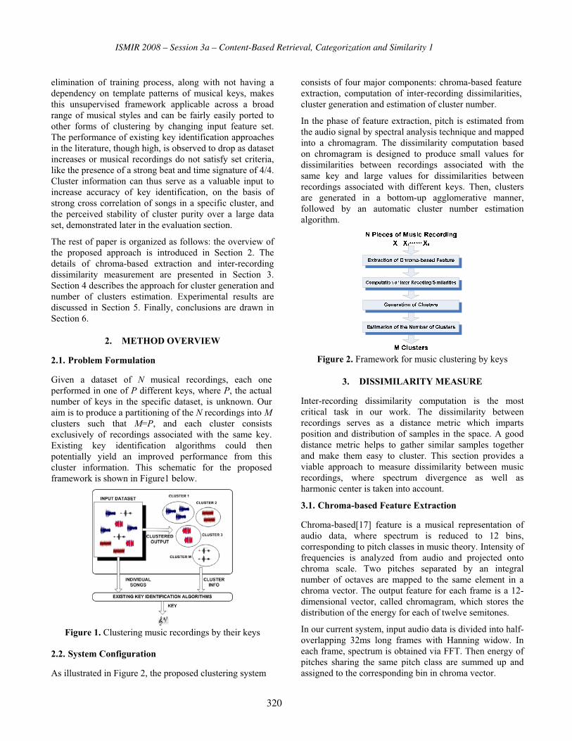
ISMIR 2008 – Session 3a – Content-Based Retrieval, Categorization and Similarity 1
elimination of training process, along with not having a dependency on template patterns of musical keys, makes this unsupervised framework applicable across a broad range of musical styles and can be fairly easily ported to other forms of clustering by changing input feature set. The performance of existing key identification approaches in the literature, though high, is observed to drop as dataset increases or musical recordings do not satisfy set criteria, like the presence of a strong beat and time signature of 4/4. Cluster information can thus serve as a valuable input to increase accuracy of key identification, on the basis of strong cross correlation of songs in a specific cluster, and the perceived stability of cluster purity over a large data set, demonstrated later in the evaluation section.
The rest of paper is organized as follows: the overview of the proposed approach is introduced in Section 2. The details of chroma-based extraction and inter-recording dissimilarity measurement are presented in Section 3. Section 4 describes the approach for cluster generation and number of clusters estimation. Experimental results are discussed in Section 5. Finally, conclusions are drawn in Section 6.
2. METHOD OVERVIEW
2.1. Problem Formulation
Given a dataset of N musical recordings, each one performed in one of P different keys, where P, the actual number of keys in the specific dataset, is unknown. Our aim is to produce a partitioning of the N recordings into M clusters such that M=P, and each cluster consists exclusively of recordings associated with the same key. Existing key identification algorithms could then potentially yield an improved performance from this cluster information. This schematic for the proposed framework is shown in Figure1 below.
Figure 1. Clustering music recordings by their keys
2.2. System Configuration
As illustrated in Figure 2, the proposed clustering system
consists of four major components: chroma-based feature extraction, computation of inter-recording dissimilarities, cluster generation and estimation of cluster number.
In the phase of feature extraction, pitch is estimated from the audio signal by spectral analysis technique and mapped into a chromagram. The dissimilarity computation based on chromagram is designed to produce small values for dissimilarities between recordings associated with the same key and large values for dissimilarities between recordings associated with different keys. Then, clusters are generated in a bottom-up agglomerative manner, followed by an automatic cluster number estimation algorithm.
Figure 2. Framework for music clustering by keys
3. DISSIMILARITY MEASURE
Inter-recording dissimilarity computation is the most critical task in our work. The dissimilarity between recordings serves as a distance metric which imparts position and distribution of samples in the space. A good distance metric helps to gather similar samples together and make them easy to cluster. This section provides a viable approach to measure dissimilarity between music recordings, where spectrum divergence as well as harmonic center is taken into account.
3.1. Chroma-based Feature Extraction
Chroma-based[17] feature is a musical representation of audio data, where spectrum is reduced to 12 bins, corresponding to pitch classes in music theory. Intensity of frequencies is analyzed from audio and projected onto chroma scale. Two pitches separated by an integral number of octaves are mapped to the same element in a chroma vector. The output feature for each frame is a 12-dimensional vector, called chromagram, which stores the distribution of the energy for each of twelve semitones.
In our current system, input audio data is divided into half-overlapping 32ms long frames with Hanning widow. In each frame, spectrum is obtained via FFT. Then energy of pitches sharing the same pitch class are summed up and assigned to the corresponding bin in chroma vector.
320
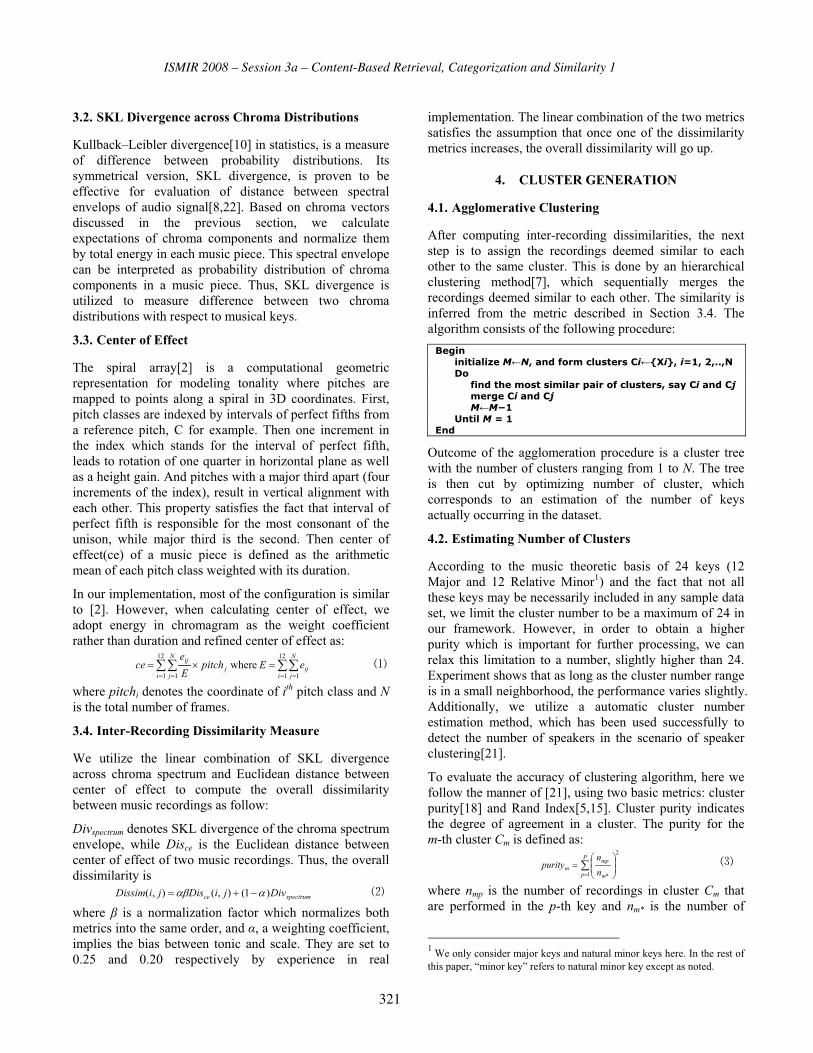
ISMIR 2008 – Session 3a – Content-Based Retrieval, Categorization and Similarity 1
3.2. SKL Divergence across Chroma Distributions
Kullback–Leibler divergence[10] in statistics, is a measure of difference between probability distributions. Its symmetrical version, SKL divergence, is proven to be effective for evaluation of distance between spectral envelops of audio signal[8,22]. Based on chroma vectors discussed in the previous section, we calculate expectations of chroma components and normalize them by total energy in each music piece. This spectral envelope can be interpreted as probability distribution of chroma components in a music piece. Thus, SKL divergence is utilized to measure difference between two chroma distributions with respect to musical keys.
3.3. Center of Effect
The spiral array[2] is a computational geometric representation for modeling tonality where pitches are mapped to points along a spiral in 3D coordinates. First, pitch classes are indexed by intervals of perfect fifths from a reference pitch, C for example. Then one increment in the index which stands for the interval of perfect fifth, leads to rotation of one quarter in horizontal plane as well as a height gain. And pitches with a major third apart (four increments of the index), result in vertical alignment with each other. This property satisfies the fact that interval of perfect fifth is responsible for the most consonant of the unison, while major third is the second. Then center of effect(ce) of a music piece is defined as the arithmetic mean of each pitch class weighted with its duration.
In our implementation, most of the configuration is similar to [2]. However, when calculating center of effect, we adopt energy in chromagram as the weight coefficient rather than duration and refined center of effect as:
12
1 1
12
1 1
wherei
N
jij
i
N
jj
ijeEpitch
E
ece
where pitchi denotes the coordinate of ith pitch class and N is the total number of frames.
3.4. Inter-Recording Dissimilarity Measure
We utilize the linear combination of SKL divergence across chroma spectrum and Euclidean distance between center of effect to compute the overall dissimilarity between music recordings as follow:
Divspectrum denotes SKL divergence of the chroma spectrum envelope, while Disce is the Euclidean distance between center of effect of two music recordings. Thus, the overall dissimilarity is spectrumce DivjiDisjiDissim )1(),(),(
where is a normalization factor which normalizes both metrics into the same order, and , a weighting coefficient, implies the bias between tonic and scale. They are set to 0.25 and 0.20 respectively by experience in real
implementation. The linear combination of the two metrics satisfies the assumption that once one of the dissimilarity metrics increases, the overall dissimilarity will go up.
4. CLUSTER GENERATION
4.1. Agglomerative Clustering
After computing inter-recording dissimilarities, the next step is to assign the recordings deemed similar to each other to the same cluster. This is done by an hierarchical clustering method[7], which sequentially merges the recordings deemed similar to each other. The similarity is inferred from the metric described in Section 3.4. The algorithm consists of the following procedure:
Begin initialize M N, and form clusters Ci {Xi}, i=1, 2,..,N Do find the most similar pair of clusters, say Ci and Cj merge Ci and Cj M M 1 Until M = 1 End
Outcome of the agglomeration procedure is a cluster tree with the number of clusters ranging from 1 to N. The tree is then cut by optimizing number of cluster, which corresponds to an estimation of the number of keys actually occurring in the dataset.
4.2. Estimating Number of Clusters
According to the music theoretic basis of 24 keys (12 Major and 12 Relative Minor1) and the fact that not all these keys may be necessarily included in any sample data set, we limit the cluster number to be a maximum of 24 in our framework. However, in order to obtain a higher purity which is important for further processing, we can relax this limitation to a number, slightly higher than 24. Experiment shows that as long as the cluster number range is in a small neighborhood, the performance varies slightly. Additionally, we utilize a automatic cluster number estimation method, which has been used successfully to detect the number of speakers in the scenario of speaker clustering[21].
To evaluate the accuracy of clustering algorithm, here we follow the manner of [21], using two basic metrics: cluster purity[18] and Rand Index[5,15]. Cluster purity indicates the degree of agreement in a cluster. The purity for the m-th cluster Cm is defined as:
P
p m
mp
mn
npurity
1
2
*
where nmp is the number of recordings in cluster Cm that are performed in the p-th key and nm* is the number of
1 We only consider major keys and natural minor keys here. In the rest of
this paper, “minor key” refers to natural minor key except as noted.
321

ISMIR 2008 – Session 3a – Content-Based Retrieval, Categorization and Similarity 1
recordings in the cluster of Cm. Deriving from Equation 3,
purity follows 11
*m
m
purityn
and is proportion to the
probability that two music recordings in a cluster are in the same key. Specifically, the overall performance can be evaluated using average purity for all clusters:
M
mmm purityn
Mpurity
1
)(1
The average purity is monotonically increasing with cluster number. This is based on the fact that as the number of clusters increases, average count of recordings in each cluster decreases, which leads to a higher purity. Hence, purity is not suitable for evaluating clustering performance, when the number of clusters is uncertain.
In contrast, Rand index, implying the extent of divergence of clustering result, is the number of incorrect pairs, actually performed in the same key but are placed in different clusters and vice versa.
Let n*p denotes the number of recordings associated with the p-th key. Rand index can be calculated by:
M
m
P
pmp
P
pp
M
mm nnnMR
1 1
2
1
2*
1
2* 2)(
Rand index can also be represented as a mis-clustering rate:
%100
2
percentage in )(
1
2*
1
2*
1 1
2
1
2*
1
2*
P
pp
M
mm
M
m
P
pmp
P
pp
M
mm
nn
nnn
MR
It’s obvious that the smaller the value of R(M) is, the better the cluster performance will be. It has been proven that the approximately minimal value will be achieved, when the number of cluster is equal to the actual number of keys occurring in the dataset[21]. So our task is to search for a proper cluster number, such that Rand Index is minimized.
Recalling the Rand Index in Equation 5, the first term in
the right side of the equation, , can be computed
based on the clustering result. Meanwhile the second
term, , is a constant irrelevant to clustering. The third
term, requires that the true key attribute of each
recording is known in advance, which cannot be computed directly. To solve this problem, we represent it by
M
mmn
1
2*
P
ppn
1
2*
M
m
P
p
n1 1
2mp
N
i
N
j
jiji
M
m
P
p
N
i
N
j
jjii
M
m
P
p
N
j
jj
N
i
ii
M
m
P
p
N
i
ii
M
m
P
p
mp
oohh
pomhpomh
pomhpomh
pomhn
1 1
1 1 1 1
1 1 11
1 1
2
11 1
2
),(),(
),(),(),(),(
]),(),(][),(),([
]),(),([
where (·) is Kronecker Delta function, hi is the index of cluster where the i-th recording is located, and oi is the true
key attribute of the i-th recording. Note that hi, 1 i N, is an integer between 1 and M, if M clusters are generated. The term (oi,oj) in Equation 7 is then approximated by the similarity between Xi and Xj.
jiXXS
jioo
jiji if ),,(
if ,1 ),(
where S(Xi, Xj) is a similarity measure between Xi and Xj, and 0 S(Xi, Xj) 1, which derives from dissimilarity metric(Equation 2). Hence, the optimal set of cluster indices can be determined by )('minarg* MRM
where is
the estimated Rand Index.
N
i
N
j
jiji
M
m
mXXShhnMR
1 11
2
* ),(),(2)('
5. EXPERIMENT
The evaluation of the framework has been carried out in two phases - effectiveness of the dissimilarity metrics, and the clustering algorithm. The test dataset consists of 91 pop songs, which include 21 out of 24 keys. The audio has been collected from CD recordings and contain the singing voice together with musical instrument accompaniment. The files are stored as 44 kHz, 16 bit, mono PCM waveform. Ground truth for the actual key information has been obtained from commercially available sheet music1.
5.1. Dissimilarity efficiency validation
For convenience, we denote the relationship between music pieces as intra-class, relative-class, parallel-class and inter-class. Musical pieces with the same key are intra-class; share the same Major/Relative Minor combination of keys are relative-class (for example C Major and A Minor); share the same tonic but are in Major and Minor modes are parallel-class (e.g. A Major vs. A Minor), while inter-class means two pieces are in unrelated keys. The Dissimilarity evaluation is carried out using SKL Divergence of chroma spectrum and Euclidian Distance between center of effect, of two music recordings. The results are discussed below:
SKL Divergence
of chroma spectrum
Euclidian Distance between Center of
Effect
average 0.1402 0.2917Stat. lower bound2 0.0004 0.0193
Intra class
Stat. upper bound 0.2177 0.4419average 0.1860 0.3344
Stat. lower bound 0.0330 0.0675Relative
class Stat. upper bound 0.4777 0.5224
average 0.2715 0.5160Parallel class Stat. lower bound 0.0740 0.2317
1 http://www.musicnotes.com/, Commerical Sheet Music Archive 2 Stat. lower/upper bound stands for the bound of interval, which contains 80 percentile of the total samples
322

ISMIR 2008 – Session 3a – Content-Based Retrieval, Categorization and Similarity 1
Stat. upper bound 0.4092 0.8670average 0.3681 0.5637
Stat. lower bound 0.1292 0.2087Inter class
Stat. upper bound 1.1042 1.6324Table 1. Dissimilarity between music with various keys
From Table 1 it is seen that average SKL Divergence for inter-class samples (0.36) and parallel-class samples (0.27) is much higher than that of the intra-class (0.14). This difference can be further demonstrated by Figure 3a, which shows the percentage distribution of SKL Divergence. It is observed that the total percentage of the intra-class distances less than 0.2 is 78%, while 80% of inter-class and parallel-class distances are greater than 0.2. A similar trend is observed for Euclidian Distance between Centre of Effect in Table 1 and Figure 3b.
05
101520253035404550
0.05 0.1 0.15 0.2 0.25 0.3 0.35 0.4
(3a) SKL Divergence between chromagram
perc
enta
ge
intra class relative classparallel class inter class
0
10
20
30
40
50
60
0.2 0.3 0.4 0.5 0.6 0.7
(3b) Euclidian Distance between center of effect
perc
enta
ge
intra class relative class
parallel class inter class
Figure 3. Proportion of dissimilarity metric in various intervals
These results corroborate significant confidence in distinguishing intra-class samples from parallel-class and inter-class samples. However, relative-class distances are observed to be much more difficult to distinguish as the SKL Divergence and Euclidian Distance, are both observed to be fairly close to the intra-distance. This can be explained by the music theoretic knowledge that relative keys share the same scale and similar harmonic structure. Thus, chroma features of relative-class pieces have similar distribution. In addition, modulations between relative modes are common in tonal music, which makes it harder to identity whether a song is primarily structured around a Major or its Relative Minor key (for example, a song with the verse sections in C Major and the Chorus sections in A Minor).
5.2. Clustering performance evaluation
The accuracy of clustering results is evaluated via cluster purity and Rand Index. Figure 4 reveals cluster purity and Rand Index as well as their correlation with the number of clusters. It can be observed that the cluster purity is always above 50%. On the other hand, the Rand index is relatively stable around 50% and reaches minima of 48% when the number of clusters is 21 (the actual number of keys occurring in the test dataset as per ground truth). This follows the discussion in Section 4.2 that Rand Index will reach its minimal value, when the number of cluster is equal to the actual number of keys occurring in the data.
0
10
20
30
40
50
60
70
15 16 17 18 19 20 21 22 23 24 25 26 27 28 29
number of clusterpe
rcen
tage
Purity RI
Figure 4. Clustering accuracy evaluation
The number of clusters predicted by our system for the test dataset is observed to be 24 based on a minimum of estimated Rand Index(computed by Equation 8), while the cluster purity is observed to be 57.2%. It can be seen that this is fairly close to the actual number of clusters - 21.
On further analysis of the clustering result, we find that quite a few errors are caused because of the Major/ Relative Minor ambiguity. A straightforward approach to reduce the confusion here would be to merge such keys into key groups[12], which implies that the signature for each cluster is a combination of 2 keys - the Major and its Relative Minor. In our experiments, the cluster purity has been observed to be as high as 70% with this change. Furthermore, errors are also caused because the algorithm is sometimes unable to distinguish the tonic from the dominant (perfect fifth interval). The overlap of harmonic components makes it difficult to identify the chroma component the harmonic belongs to. Besides, perfect fifth is a basic element when construction of triads is concerned in harmony. Similar errors were also observed in [3,12].
6. CONCLUSION
In this paper, a framework has been presented to cluster a higher level feature of music, the key, in an unsupervised way, discarding prior training information and music theoretic based rules. To the best of our knowledge this is the first attempt in this direction and hence there is no strong basis for evaluation against existing techniques. An empirical evaluation shows that accuracy of the existing
323

ISMIR 2008 – Session 3a – Content-Based Retrieval, Categorization and Similarity 1
rule-based key estimation approach[16] suffers a decrease from over 80% to around 60% as the dataset has been scaled from 30 to 91 songs. From the discussion above, it is observed that the clustering performance is still stable as the data set grows because the dependency on specific higher level musical knowledge is not present. This gives us sufficient confidence that clustering, if involved as a preprocessing component in key detection tasks, will contribute in improving the accuracy for key estimation in large music databases. Future work will focus on integrating the clustering framework with key detection techniques to evaluate performance and scalability. Although the clustering framework is not yet sufficient to output the actual key assignment for each music recording or cluster, we believe it could provide useful information for further structure analysis of musical work, in addition to music retrieval & recommendation systems, and emotion recognition systems.
7. ACKNOWLEDGEMENT
This work was supported by Singaporean Ministry of Education grant with the Workfare Bonus Scheme No. R-252-000-267-112 and National Science Foundation of China (No. 60433030).
8. REFERENCES
[1] Chai, W. and Vercoe, B., Detection of key change in classical piano music, Proc. of the International
Symposium on Music Information Retrieval, 2005
[2] Chew, E., The spiral array: an algorithm for determining key boundaries, Music and Artificial
Intelligence, Vol. 2445, 2002
[3] Chuan, C. H. and Chew, E., Fuzzy Analysis in pitch-class determination for polyphonic audio key finding, Proc. of the International Symposium on Music
Information Retrieval, 2005
[4] Gómez, E. and Herrera, P., Estimating the tonality of polyphonic audio files cognitive versus machine learning modelling strategies, Proc. of the
International Symposium on Music Information
Retrieval, 2004
[5] Hubert, L. and Arabie, P., Comparing partitions, Journal of Classification, Vol. 2, Issue 1, 1985
[6] zmirli, O., Tonal similarity from audio using a template based attractor model, Proc. of the
International Symposium on Music Information
Retrieval, 2005
[7] Kaufman, L. and Rousseuw, P. J., Finding Groups in Data: An Introduction to Cluster Analysis, John Wiley and Sons, New York, 1990
[8] Klabbers, E. and Veldhuis, R., Reducing audible spectral discontinuities, IEEE Trans. on Speech and
Audio Processing, Vol. 9, Issue 1, 2001.
[9] Krumhansl, C., Cognitive Foundations of Musical
Pitch, Oxford University Press, New York, 1990
[10] Kullback, S. and Leibler, R. A., On information and sufficiency, Annals of Mathematical Statistics Vol. 22, Issue 1, 1951
[11] Lee, K., Slaney M., Acoustic chord transcription and key extraction from audio using key-dependent HMMs trained on synthesized audio, IEEE Trans. on
Audio, Speech, and Language Processing, Vol. 16, No. 2, 2008
[12] Martens, G., De Meyer, H., etc. Tree-based versus distance-based key recognition in musical audio, Soft
Computing- a Fusion of Foundations, Methodologies
and Applications archive, Vol. 9, Issue 8, 2005
[13] Pauws, S., Extracting the key from music, Intelligent
Algorithms in Ambient and Biomedical Computing, Springer, Netherlands, 2006
[14] Peeters, G., Musical key estimation of audio signal based on HMM modeling of chroma vectors, Proc.
of DAFX, McGill, Montreal, Canada, 2006.
[15] Rand, W. M., Objective criteria for the evaluation of clustering methods, Journal of the American
Statistical Association, Vol. 66, No. 336, 1971.
[16] Shenoy, A. and Wang, Y., Key, chord, and rhythm tracking of popular music recordings”, Computer
Music Journal, Vol. 29, No. 3, 2005
[17] Shepard, R., “Circularity in judgments of relative pitch”, The Journal of the Acoustical Society of
America, Vol. 36, Issue 12, 1964
[18] Solomonoff, A., Mielke, A., etc. Clustering speakers by their voices, Proc. of the IEEE International Conf.
on Acoustics, Speech, and Signal Processing, 1998.
[19] Temperley, D., A Bayesian approach to key-finding, Proc. of the Second International Conf. on Music
and Artificial Intelligence, 2002
[20] Tsai, W. H., Rodgers, D. and Wang, H. M., Blind clustering of popular music recordings based on singer voice characteristics, Computer Music
Journal, Vol. 28, No. 3: 2004
[21] Tsai, W. H., and Wang, H. M., Speaker Clustering Based on Minimum Rand Index, Proc. of the IEEE
International Conf. on Acoustics, Speech, and Signal
Processing, 2007
[22] Veldhuis, R. and Klabbers, E., On the computation of the Kullback–Leibler measure for spectral distances, IEEE Trans. on Speech and Audio
Processing, Vol. 11, No. 1, 2003.
[23] Zhu, Y. W. and Kankanhalli, M. S., Precise pitch profile feature extraction from musical audio for key detection, IEEE Trans. on Multimedia, Vol. 8, No. 3, 2006.
324

ISMIR 2008 – Session 3a – Content-Based Retrieval, Categorization and Similarity 1
MULTI-LABEL CLASSIFICATION OF MUSIC INTO EMOTIONS
Konstantinos TrohidisDept. of Journalism &Mass CommunicationAristotle University
Grigorios TsoumakasDept. of InformaticsAristotle University
George KallirisDept. of Journalism &Mass CommunicationAristotle University
Ioannis VlahavasDept. of InformaticsAristotle University
ABSTRACT
In this paper, the automated detection of emotion in music is
modeled as a multilabel classification task, where a piece of
music may belong to more than one class. Four algorithms
are evaluated and compared in this task. Furthermore, the
predictive power of several audio features is evaluated using
a new multilabel feature selection method. Experiments are
conducted on a set of 593 songs with 6 clusters of music
emotions based on the Tellegen-Watson-Clark model. Re-
sults provide interesting insights into the quality of the dis-
cussed algorithms and features.
1 INTRODUCTION
Humans, by nature, are emotionally affected by music. Who
can argue against the famous quote of the German philoso-
pher Friedrich Nietzsche, who said that “without music, lifewould be a mistake”. As music databases grow in size and
number, the retrieval of music by emotion is becoming an
important task for various applications, such as song selec-
tion in mobile devices [13], music recommendation systems
[1], TV and radio programs 1 and music therapy.
Past approaches towards automated detection of emotions
in music modeled the learning problem as a single-label
classification [9, 20], regression [19], or multilabel classi-
fication [6, 7, 17] task. Music may evoke more than one dif-
ferent emotion at the same time. We would like to be able
to retrieve a piece of music based on any of the associated
(classes of) emotions. Single-label classification and regres-
sion cannot model this multiplicity. Therefore, the focus of
this paper is on multilabel classification methods.
A secondary contribution of this paper is a new multil-
abel dataset with 72 music features for 593 songs catego-
rized into one or more out of 6 classes of emotions. The
dataset is released to the public 2 , in order to allow com-
parative experiments by other researchers. Publicly avail-
able multilabel datasets are rare, hindering the progress of
research in this area.
1 http://www.musicovery.com/2 http://mlkd.csd.auth.gr/multilabel.html
The primary contribution of this paper is twofold:
• A comparative experimental evaluation of four multi-
label classification algorithms on the aforementioned
dataset using a variety of evaluation measures. Previ-
ous work experimented with just a single algorithm.
We attempt to raise the awareness of the MIR commu-
nity on some of the recent developments in multilabel
classification and show which of those algorithms per-
form better for musical data.
• A new multilabel feature selection method. The pro-
posed method is experimentally compared against two
other methods of the literature. The results show that
it can improve the performance of a multilabel clas-
sification algorithm that doesn’t take feature impor-
tance into account.
The remaining of this paper is structured as follows. Sec-
tions 2 and 3 provide background material on multilabel
classification and emotion modeling respectively. Section 4
presents the details of the dataset used in this paper. Section
5 presents experimental results comparing the four multi-
label classification algorithms and Section 6 discusses the
new multilabel feature selection method. Section 7 presents
related work and finally, conclusions and future work are
drawn in Section 8.
2 MULTILABEL CLASSIFICATION
Traditional single-label classification is concerned with learn-
ing from a set of examples that are associated with a single
label λ from a set of disjoint labels L, |L| > 1. In multil-abel classification, the examples are associated with a set of
labels Y ⊆ L.
2.1 Learning Algorithms
Multilabel classification methods can be categorized into
two different groups [14]: i) problem transformation meth-
ods, and ii) algorithm adaptation methods. The first group
325

ISMIR 2008 – Session 3a – Content-Based Retrieval, Categorization and Similarity 1
contains methods that are algorithm independent. They trans-
form the multilabel classification task into one or more single-
label classification, regression or ranking tasks. The second
group contains methods that extend specific learning algo-
rithms in order to handle multilabel data directly.
2.2 Evaluation Measures
Multilabel classification requires different evaluation mea-
sures than traditional single-label classification. A taxon-
omy of multilabel classification evaluation measures is given
in [15], which considers two main categories: example-basedand label-based measures. A third category of measures,
which is not directly related to multilabel classification, but
is often used in the literature, is ranking-based measures,
which are nicely presented in [21] among other publications.
3 MUSIC AND EMOTION
Hevner [4] was the first to study the relation between mu-
sic and emotion. She discovered 8 clusters of adjective sets
describing music emotion and created an emotion cycle of
these categories. Hevner’s adjectives were refined and re-
grouped into ten groups by Farnsworth [2].
Figure 1 shows another emotion model, called Thayer’s
model of mood [12], which consists of 2 axes. The horizon-
tal axis described the amount of stress and the vertical axis
the amount of energy.
Figure 1. Thayer’s model of mood
The model depicted in Figure 2 extends Thayer’s model
with a second system of axes, which is rotated by 45 degrees
compared to the original axes [11]. The new axes describe
(un)pleasantness versus (dis)engagement.
4 DATASET
The dataset used for this work consists of 100 songs from
each of the following 7 different genres: Classical, Reggae,
Rock, Pop, Hip-Hop, Techno and Jazz. The collection was
created from 233 musical albums choosing three songs from
Figure 2. The Tellegen-Watson-Clark model of mood (fig-
ure reproduced from [18])
each album. From each song a period of 30 seconds after the
initial 30 seconds was extracted. The resulting sound clips
were stored and converted into wave files of 22050 Hz sam-
pling rate, 16-bit per sample and mono. The following sub-
sections present the features that were extracted from each
wave file and the emotion labeling process.
4.1 Feature Extraction
For the feature extraction process, the Marsyas tool [16] was
used. The extracted features fall into two categories: rhyth-
mic and timbre.
4.1.1 Rhythmic Features
The rhythmic features were derived by extracting periodic
changes from a beat histogram. An algorithm that identi-
fies peaks using autocorrelation was implemented. We se-
lected the two highest peaks and computed their amplitudes,
their BMPs (beats per minute) and the high-to-low ratio of
their BPMs. In addition, 3 features were calculated by sum-
ming the histogram bins between 40-90, 90-140 and 140-
250 BPMs respectively. The whole process led to a total of
8 rhythmic features.
4.1.2 Timbre Features
Mel Frequency Cepstral Coefficients (MFCCs) are used for
speech recognition and music modeling [8]. To derive MFCCs
features, the signal was divided into frames and the ampli-
tude spectrum was calculated for each frame. Next, its log-
arithm was taken and converted to Mel scale. Finally, the
discrete cosine transform was implemented. We selected
the first 13 MFCCs.
Another set of 3 features that relate to timbre textures
were extracted from the Short-Term Fourier Transform (FFT):
Spectral centroid, spectral rolloff and spectral flux.
For each of the 16 aforementioned features (13 MFCCs,
3 FFT) we calculated the mean, standard deviation (std),
326
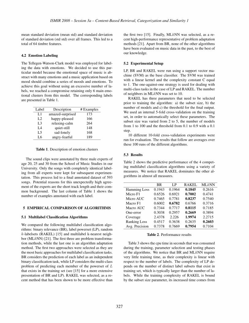
ISMIR 2008 – Session 3a – Content-Based Retrieval, Categorization and Similarity 1
mean standard deviation (mean std) and standard deviation
of standard deviation (std std) over all frames. This led to a
total of 64 timbre features.
4.2 Emotion Labeling
The Tellegen-Watson-Clark model was employed for label-
ing the data with emotions. We decided to use this par-
ticular model because the emotional space of music is ab-
stract with many emotions and a music application based on
mood should combine a series of moods and emotions. To
achieve this goal without using an excessive number of la-
bels, we reached a compromise retaining only 6 main emo-
tional clusters from this model. The corresponding labels
are presented in Table 1.
Label Description # Examples
L1 amazed-surprised 173
L2 happy-pleased 166
L3 relaxing-calm 264
L4 quiet-still 148
L5 sad-lonely 168
L6 angry-fearful 189
Table 1. Description of emotion clusters
The sound clips were annotated by three male experts of
age 20, 25 and 30 from the School of Music Studies in our
University. Only the songs with completely identical label-
ing from all experts were kept for subsequent experimen-
tation. This process led to a final annotated dataset of 593
songs. Potential reasons for this unexpectedly high agree-
ment of the experts are the short track length and their com-
mon background. The last column of Table 1 shows the
number of examples annotated with each label.
5 EMPIRICAL COMPARISON OF ALGORITHMS
5.1 Multilabel Classification Algorithms
We compared the following multilabel classification algo-
rithms: binary relevance (BR), label powerset (LP), random
k-labelsets (RAKEL) [15] and multilabel k-nearest neigh-
bor (MLkNN) [21]. The first three are problem transforma-
tion methods, while the last one is an algorithm adaptation
method. The first two approaches were selected as they are
the most basic approaches for multilabel classification tasks.
BR considers the prediction of each label as an independent
binary classification task, while LP considers the multi-class
problem of predicting each member of the powerset of Lthat exists in the training set (see [15] for a more extensive
presentation of BR and LP). RAKEL was selected, as a re-
cent method that has been shown to be more effective than
the first two [15]. Finally, MLkNN was selected, as a re-
cent high-performance representative of problem adaptation
methods [21]. Apart from BR, none of the other algorithms
have been evaluated on music data in the past, to the best of
our knowledge.
5.2 Experimental Setup
LP, BR and RAKEL were run using a support vector ma-
chine (SVM) as the base classifier. The SVM was trained
with a linear kernel and the complexity constant C equal
to 1. The one-against-one strategy is used for dealing with
multi-class tasks in the case of LP and RAKEL. The number
of neighbors in MLkNN was set to 10.
RAKEL has three parameters that need to be selected
prior to training the algorithm: a) the subset size, b) the
number of models and c) the threshold for the final output.
We used an internal 5-fold cross-validation on the training
set, in order to automatically select these parameters. The
subset size was varied from 2 to 5, the number of models
from 1 to 100 and the threshold from 0.1 to 0.9 with a 0.1
step.
10 different 10-fold cross-validation experiments were
run for evaluation. The results that follow are averages over
these 100 runs of the different algorithms.
5.3 Results
Table 2 shows the predictive performance of the 4 compet-
ing multilabel classification algorithms using a variety of
measures. We notice that RAKEL dominates the other al-
gorithms in almost all measures.
BR LP RAKEL MLkNN
Hamming Loss 0.1943 0.1964 0.1845 0.2616
Micro F1 0.6526 0.6921 0.7002 0.4741
Micro AUC 0.7465 0.7781 0.8237 0.7540
Macro F1 0.6002 0.6782 0.6766 0.3716
Macro AUC 0.7344 0.7717 0.8115 0.7185
One-error 0.3038 0.2957 0.2669 0.3894
Coverage 2.4378 2.226 1.9974 2.2715
Ranking Loss 0.4517 0.3638 0.2635 0.2603Avg. Precision 0.7378 0.7669 0.7954 0.7104
Table 2. Performance results
Table 3 shows the cpu time in seconds that was consumed
during the training, parameter selection and testing phases
of the algorithms. We notice that BR and MLkNN require
very little training time, as their complexity is linear with
respect to the number of labels. The complexity of LP de-
pends on the number of distinct label subsets that exist in
training set, which is typically larger than the number of la-
bels. While the training complexity of RAKEL is bound
by the subset size parameter, its increased time comes from
327

ISMIR 2008 – Session 3a – Content-Based Retrieval, Categorization and Similarity 1
the multiple models that it builds, since it is an ensemble
method. RAKEL further requires a comparatively signifi-
cant amount of time for parameter selection. However, this
time is still affordable (2.5 minutes), as it is only run offline.
BR LP RAKEL MLkNN
Training 0.77 3.07 6.66 0.51
Parameter selection 0 0 151.59 0
Testing 0.00 0.02 0.03 0.06
Table 3. Average training, parameter selection and testing
cpu time in seconds
Concerning the test time, we notice that BR is the fastest
algorithm, followed by LP and RAKEL. MLkNN is the most
time-consuming algorithm during testing, as it must calcu-
late the k nearest neighbors online after the query.
Table 4 shows the classification accuracy of the algo-
rithms for each label (as if they were independently pre-
dicted), along with the average accuracy in the last column.
We notice that based on the ease of predictions we can rank
the labels in the following descending order L4, L6, L5, L1,
L3, L2. L4 is the easiest with a mean accuracy of approx-
imately 87%, followed by L6, L5 and L1 with mean accu-
racies of approximately 80%, 79% and 78% respectively.
The hardest labels are L2 and L3 with a mean accuracy of
approximately 73% and 76% respectively.
BR LP RAKEL MLkNN Avg
L1 0.7900 0.7906 0.7982 0.7446 0.7809
L2 0.7115 0.7380 0.7587 0.7195 0.7319
L3 0.7720 0.7705 0.7854 0.7221 0.7625
L4 0.8997 0.8992 0.9031 0.7969 0.8747
L5 0.8287 0.8093 0.8236 0.7051 0.7917
L6 0.8322 0.8142 0.8238 0.7422 0.8031
Table 4. Accuracy per label
Based on the results, one can see that the classification
model performs better for emotional labels such as label 4
(quiet) rather than label 2 (happy). This can be interpreted
due to the fact that emotions such as quietness can be eas-
ily perceived and classified by humans in a musical context,
as it is more objective than more difficult and abstract emo-
tional labels such as happiness, which is more subjective.
6 EMPIRICAL FEATURE EVALUATION
Multilabel feature selection has been mainly applied to the
domain of text categorization, due to the typically high di-
mensionality of textual data. The standard approach is to
consider each label separately, use an attribute evaluation
statistic (such as χ2, gain ratio, etc) for each label, and then
combine the results using an averaging approach. Two aver-
aging approaches that appear in the literature are max, which
considers the maximum score for each feature across all la-
bels and avg, which considers the average of the score of
each feature across all labels, weighted by the prior proba-
bility of each label. The disadvantage of these approaches,
similarly to BR, is that they do not consider label correla-
tions.
We propose a different approach in this paper, which has
not been discussed in the literature before, to the best of our
knowledge. At a first step, we apply the transformation of
the LP method in order to produce a single-label classifica-
tion dataset. Then, we apply a common attribute evaluation
statistic. We argue that this approach could be more benefi-
cial than the others, as it considers label correlations.
In order to evaluate our hypothesis we compare the Ham-
ming loss of the MLkNN algorithm (known to suffer from
the curse of dimensionality) using the best 1 to 71 features
according to the three feature selection approaches using the
χ2 statistic. Figure 3 shows the results.
0 2 4 6 8 10121416 182022242628303234 363840424446485052 545658606264666870 720.23
0.24
0.25
0.26
0.27
0.28
0.29
AVGMAXLP
Figure 3. Hamming loss of the MLkNN classifier using the
best 1 to 71 features as ordered by the χ2 feature selection
method, using the max and avg averaging approaches and
the proposed method.
We notice that all approaches have similar performance
for most of the horizontal axis (number of features retained),
apart from the section from 36 to 50 features, where the pro-
posed method leads to better results. It is in this area that
the best result is achieved for MLkNN, which is a Ham-
ming loss of approximately 0.235. This is an indication that
taking label correlations may be fruitful, especially for se-
lecting important features beyond those that are correlated
directly with the labels.
7 RELATED WORK
We discuss past efforts on emotion detection in music, mainly
in terms of emotion model, extracted features and the kind
328

ISMIR 2008 – Session 3a – Content-Based Retrieval, Categorization and Similarity 1
of modeling of the learning problem: a) single label classi-
fication, b) regression, and c) multilabel classification.
7.1 Single-label Classification
The four main emotion classes of Thayer’s model were used
as the emotion model in [9]. Three different feature sets
were adopted for music representation, namely intensity, tim-
bre and rhythm. Gaussian mixture models were used to
model each of the four classes. An interesting contribution
of this work, was a hierarchical classification process, which
first classifies a song into high/low energy (vertical axis of
Thayer’s model), and then into one of the two high/low stress
classes.
The same emotion classes were used in [20]. The au-
thors experimented with two fuzzy classifiers, using the 15
features proposed in [10]. They also experimented with a
feature selection method, which improved the overall accu-
racy (around 78%), but they do not mention which features
were selected.
The classification of songs into a single cluster of emo-
tions was a new category in the 2007 MIREX (Music Infor-
mation Retrieval Evaluation eXchange) competition. The
top two submissions of the competition 3 were based on
support vector machines. The model of mood that was used
in the competition, was 5 clusters of moods proposed in
[5], which was compiled based on a statistical analysis of
the relationship of mood with genre, artist and usage meta-
data. Among the many interesting conclusion of the compe-
tition, was the difficulty to discern between certain clusters
of moods, due to their semantic overlap. A multilabel classi-
fication approach could overcome this problem, by allowing
the specification of multiple finer-grain emotion classes.
7.2 Regression
Emotion recognition is modeled as a regression task in [19].
Volunteers rated a training collection of songs in terms of
arousal and valence in an ordinal scale of 11 values from
-1 to 1 with a 0.2 step. The authors then trained regression
models using a variety of algorithms (again SVMs perform
best) and a variety of extracted features. Finally, a user could
retrieve a song by selecting a point in the two-dimensional
arousal and valence mood plane of Thayer.
Futhermore, the authors used a feature selection algo-
rithm, leading to an increase of the predictive performance.
However, it is not clear if the authors run the feature se-
lection process on all input data or on each fold of the 10-
fold cross-validation used to evaluate the regressors. If the
former is true, then their results may be optimistic, as the
feature selection algorithm had access to the test data. A
similar pitfall of feature selection in music classification is
discussed in [3].
3 http://www.music-ir.org/mirex/2007
7.3 Multilabel Classification
Both regression and single-label classification methods suf-
fer from the same problem: No two different (clusters of)
emotions can be simultaneously predicted. Multilabel clas-
sification allows for a natural modeling of this issue.
Li and Ogihara [6] used two emotion models: a) the 10
adjective clusters of Farnsworth (extended with 3 clusters of
adjectives proposed by the labeler) and b) a further cluster-
ing of those into 6 super-clusters. They only experimented
with the BR multilabel classification method using SVMs
as the underlying base single-label classifier. In terms of
features, they used Marsyas [16] to extract 30 features re-
lated to the timbral texture, rhythm and pitch. The predic-
tive performance was low for the clusters and better for the
super-clusters. In addition, they found evidence that genre
is correlated with emotions.
In an extension of their work, Li and Ogihara [7] consid-
ered 3 bipolar adjective pairs (Cheerful vs Depressing), (Re-
laxing vs Exciting), and (Comforting vs Disturbing). Each
track was initially labeled using a scale ranging from -4 to
+4 by two subjects and then converted to a binary (posi-
tive/negative) label. The learning approach was the same
with [6]. The feature set was expanded with a new extraction
method, called Daubechies Wavelet Coefficient Histograms.
The authors report an accuracy of around 60%.
The same 13 clusters as in [6] were used in [17], where
the authors modified the k Nearest Neighbors algorithm in
order to handle multilabel data directly. They found that the
predictive performance was low, too.
Compared to our work, none of the three aforementioned
approaches discusses feature selection from multilabel data,
compares different multilabel classification algorithms or uses
a variety of multilabel evaluation measures in its empirical
study.
8 CONCLUSIONS AND FUTURE WORK
The task of multi-label mapping of music into emotions was
investigated. An evaluation of four multi-label classifica-
tion algorithms was performed on a collection of 593 songs.
Among these algorithms, RAKEL was the most effective
and is proposed for emotion categorization. The overall pre-
dictive performance was high and encourages further inves-
tigation of multilabel methods. The performance per each
different label varied. The subjectivity of the label may be
influencing the performance of its prediction.
In addition, a new multilabel feature ranking method was
proposed, which seems to perform better than existing meth-
ods in this domain. Feature ranking may assist researchers
working on feature extraction by providing feedback on the
predictive performance of current and newly designed indi-
vidual features. It also improves the performance of multi-
label classification algorithms, such as MLkNN, that don’t
329

ISMIR 2008 – Session 3a – Content-Based Retrieval, Categorization and Similarity 1
take feature importance into account.
Multilabel classifiers such as RAKEL could be used for
the automated annotation of large musical collections with
multiple emotions. This in turn would support the imple-
mentation of music information retrieval systems that query
music collections by emotion. Such a querying capability
would be useful for song selection in various applications.
Future work will explore the effectiveness of new fea-
tures based on time frequency representation of music and
lyrics, as well as the hierarchical multilabel classification
approach, which we believe has great potential in this do-
main.
9 REFERENCES
[1] Rui Cai, Chao Zhang, Chong Wang, Lei Zhang, and
Wei-Ying Ma. Musicsense: contextual music recom-
mendation using emotional allocation modeling. In
MULTIMEDIA ’07: Proceedings of the 15th interna-tional conference on Multimedia, pages 553–556, 2007.
[2] P Farnsworth. The social psychology of music. The Dry-
den Press, 1958.
[3] R. Fiebrink and I. Fujinaga. Feature selection pitfalls
and music classification. In Proceedings of the Interna-tional Conference on Music Information Retrieval (IS-MIR 2006), pages 340–341, 2006.
[4] K. Hevner. Experimental studies of the elements of ex-
pression in music. American Journal of Psychology,
48:246–268, 1936.
[5] X Hu and J.S. Downie. Exploring mood metadata: rela-
tionships with genre, artist and usage metadata. In Pro-ceedings of the 8th International Conference on Mu-sic Information Retrieval (ISMIR 2007), pages 67–72,
2007.
[6] T. Li and M. Ogihara. Detecting emotion in music. In
Proceedings of the International Symposium on Mu-sic Information Retrieval, pages 239–240, Washington
D.C., USA, 2003.
[7] T. Li and M. Ogihara. Toward intelligent music in-
formation retrieval. IEEE Transactions on Multimedia,
8(3):564–574, 2006.
[8] B. Logan. Mel frequency cepstral coefficients for music
modeling. In Proceedings of the 1st International Sym-posium on Music Information Retrieval (ISMIR 2000),Plymouth, Massachusetts, 2000.
[9] L. Lu, D. Liu, and H.-J. Zhang. Automatic mood detec-
tion and tracking of music audio signals. IEEE Trans-actions on Audio, Speech, and Language Processing,
14(1):5–18, January 2006.
[10] E. Schubert. Measurement and Time Series Analysis ofEmotion in Music. PhD thesis, University of New South
Wales, 1999.
[11] A. Tellegen, D. Watson, and L.A. Clark. On the dimen-
sional and hierarchical structure of affect. PsychologicalScience, 10(4):297–303, July 1999.
[12] R.E. Thayer. The Biopsychology of Mood and Arousal.Oxford University Press, 1989.
[13] M. Tolos, R. Tato, and T. Kemp. Mood-based naviga-
tion through large collections of musical data. In 2ndIEEE Consumer Communications and Networking Con-ference (CCNC 2005), pages 71–75, 3-6 Jan. 2005.
[14] G. Tsoumakas and I. Katakis. Multi-label classification:
An overview. International Journal of Data Warehous-ing and Mining, 3(3):1–13, 2007.
[15] G. Tsoumakas and I. Vlahavas. Random k-labelsets:
An ensemble method for multilabel classification. In
Proceedings of the 18th European Conference on Ma-chine Learning (ECML 2007), pages 406–417, Warsaw,
Poland, September 17-21 2007.
[16] G. Tzanetakis and P. Cook. Musical genre classification
of audio signals. IEEE Transactions on Speech and Au-dio Processing, 10(5):293–302, July 2002.
[17] A. Wieczorkowska, P. Synak, and Z.W. Ras. Multi-label
classification of emotions in music. In Proceedings ofthe 2006 International Conference on Intelligent Infor-mation Processing and Web Mining (IIPWM’06), pages
307–315, 2006.
[18] D. Yang and W. Lee. Disambiguating music emotion us-
ing software agents. In Proceedings of the 5th Interna-tional Conference on Music Information Retrieval (IS-MIR’04), Barcelona, Spain, 2004.
[19] Y.-H. Yang, Y.-C. Lin, Y.-F. Su, and H.-H. Chen. A re-
gression approach to music emotion recognition. IEEETransactions on Audio, Speech and Language Process-ing (TASLP), 16(2):448–457, February 2008.
[20] Y.-H. Yang, C.-C. Liu, and H.-H. Chen. Music emo-
tion classification: A fuzzy approach. In Proceedingsof ACM Multimedia 2006 (MM’06), pages 81–84, Santa
Barbara, CA, USA, 2006.
[21] M-L Zhang and Z-H Zhou. Ml-knn: A lazy learning
approach to multi-label learning. Pattern Recognition,
40(7):2038–2048, 2007.
330

ISMIR 2008 – Session 3a – Content-Based Retrieval, Categorization and Similarity 1
A Study on Feature Selection and Classification Techniques for Automatic Genre Classification of Traditional Malay Music
Shyamala Doraisamy Shahram Golzari Noris Mohd. Norowi Md. Nasir B Sulaiman Nur Izura Udzir
Faculty of Computer Science and Information Technology University Putra Malaysia
ABSTRACT
Machine learning techniques for automated musical genre classification is currently widely studied. With large collections of digital musical files, one approach to classification is to classify by musical genres such as pop, rock and classical in Western music. Beat, pitch and temporal related features are extracted from audio signals and various machine learning algorithms are applied for classification. Features that resulted in better classification accuracies for Traditional Malay Music (TMM), in comparison to western music, in a previous study were beat related features. However, only the J48 classifier was used and in this study we perform a more comprehensive investigation on improving the classification of TMM. In addition, feature selection was performed for dimensionality reduction. Classification accuracies using classifiers of varying paradigms on a dataset comprising ten TMM genres were obtained. Results identify potentially useful classifiers and show the impact of adding a feature selection phase for TMM genre classification.
1. INTRODUCTION
Interest on music information retrieval systems for the storage, retrieval and classification of large collections of digital musical files has grown in recent years. Metadata such as filename, author, file size, date and genres are commonly used to classify and retrieve these documents. Such manual classification is highly labour-intensive and costly both in terms of time and money [1].
An automatic classification system that is able to analyse and extract implicit knowledge of the musical files is therefore highly sought. One approach to musical classification that is currently being widely studied is classification by musical genres. Musical genres are labels created and used by humans for categorizing and describing music [2].
Examples of a few Western musical genres are such as Pop, Rock, Hip-hop, and Classical. Several systems for automated genre classification and retrieval of musical files have been researched and developed [2,3]. However, most of these studies were conducted using only western dataset and we focus on non-Western musical genres, and more specifically Traditional Malay Music (TMM).
TMM encompasses all traditional music from Malaysia, both West Malaysia (on the Peninsular) and the states on the Borneo Island (Sabah and Sarawak) [4].
Genre examples include Dikir Barat, Joget, Wayang Kulit, Gamelan, Etnik Sabah and Inang. In general, these musical genres have a strong sense of rhythm, partly due to the fact that TMM is traditionally played by ear as opposed to reading from written musical scores. Having the beat or rhythm clearly audible helps when the musical piece is being passed down orally through generations in the villages such as having clear gong hits. The significance of beat features for TMM genre classification in comparison to Western musical genres was investigated in a previous study using a two-phase methodology – feature extraction and classification [5]. In this paper we study the impact of adding a feature selection phase for TMM genre classification.
Feature extraction is a process where a segment of an audio is characterized into a compact numerical representation. Due to the high dimensionality of these feature sets, feature selection can be performed to reduce the dimensionality of the data as a preprocessing step prior to classification. With audio data, several studies have investigated the significance of this phase and the performance of several feature selection methods [21]. A comprehensive discussion on feature selection is available in Saeys et. al [6].
A large number of the studies performed on music classification have looked more closely at the feature extraction step, and in this study we investigate the classification phase more closely. The rest of this paper is organised as follows: Section 2 presents background information about music genre classification and TMM. An overview of feature selection is presented in Section 3. Section 4 presents the experimental framework and results are discussed in Section 5.
2. BACKGROUND
2.1. Music Genre Classification
Digital audio in general is categorized as speech, music and noise. Wold, et al[3] analyse and compare audio features such as rhythms, pitch, duration, loudness and instrument identification to classify various groups of audio such as speech, gender, animal sounds and sound
331

ISMIR 2008 – Session 3a – Content-Based Retrieval, Categorization and Similarity 1
effects. However, music classification was not emphasized in their study.
There has been great interest of classification of audio based on musical genres in recent years [2, 7,8]. Tzanetakis and Cook [2] and Aucoturier and Pachet[8] categorized audio features into three categories; timbral related features, rhythmic related features, and pitch related features. Audio data that are to be classified cannot be represented as raw audio data, such as samples of amplitude value of digital audio signals. Hence, some form of parameterisation is required. Parameterisation of audio data is based on audio analysis, which can be done using several methods such as Fourier transform, wavelet transform, statistical methods, etc. [9].
Timbral related features are based on the Short Time Fourier Transform (STFT), which is used to determine the phase content of short local sections in a signal as it changes over time. The features are used in music-speech discrimination and speech recognition. Examples of timbral related features are such as spectral centroid, spectral roll off and time domain zero crossing, which measure the spectral shape, the changes in spectral shape and the noisiness of a signal respectively. Another feature, Mel-Frequency Cepstral Coefficients (MFCC), is also based on the STFT, but is typically used to provide compact representation of the spectral envelope, especially in speech recognition. Tzanetakis and Cook [2] provide a detailed discussion on timbral related features and the account of their experiment.
Beat features analyses the signals that calculate the rhythmic structure of music based on their wavelet transform [2]. It involves time-frequency analysis, which is useful to music classification as its algorithm is similar to human hearing. The main beat can be defined as the regular periodic sequence of pulses corresponding to where a human would tap his foot whilst listening to music. Although achievable, extraction of beat features is very difficult. Whilst it is trivial for human to do so to a music, it is not so with machines. Kosina[10] and Dixon[11] give good overviews on beat tracking methods. Li and Tzanetakis[12] investigate the effects of different feature set combinations for optimum classification performance. Features incorporated in the study were: FFT, MFCC, Pitch and Beat. Although suitable feature set combinations from this study was obtained, it was also suggested that they might not be generic to all genres but applicable only to western genres that was used in their study.
With classification, classifiers vary in terms of robustness, speed, memory usage and complexity. Several studies investigate the use of existing classifiers for musical genre classification [2,3,12]. For instance, OneR is a primitive form of classifier as it produces simple rule based on one attribute only, but it is useful in determining a baseline performance as a benchmark for other learning
schemes [13]. Emphasis on the importance of understanding different classifiers is also discussed at length by [7,14].
2.2. Traditional Malay Music
Traditional Malay music is mainly derivative, influenced by the initial overall Indian and Middle Eastern music during the trade era and later from colonial powers such as Thailand, Indonesia, Portuguese and British who introduced their own culture including dance and music. A thorough overview on the origin and history of TMM can be found in [17]. The taxonomy of TMM depends on the nature of the theatre forms they serve and their instrumentations. Categorization of TMM genres has been studied extensively by Ang[18]. Music of these genres is usually disseminated non-commercially, usually performed by persons who are not highly trained musical specialists, undergoes change arising from creative impulses and exists in many forms. The musical ensembles usually include gendangs or drums that are used to provide constant rhythmic beat of the songs and gongs to mark the end of a temporal cycle at specific part of the song [19].
One common attribute that is shared by most TMM genres is that they are generally repetitive in nature and exist in ‘gongan’-like cycle. ‘Gongan’ is defined as a temporal cycle marked internally at specific points by specific gongs and at the end by the lowest-pitched gong of an ensemble [17]. It is an important structural function as it divides the musical pieces into temporal sections. Once every measure has been played, musicians continue playing in a looping motion by repeating the cycle from the beginning again until one of the lead percussionists signals the end of the song by varying their rhythms noticeably. Traditional Malay music does not have a chorus that plays differently than other parts of the songs, which is the usual occurrence in western music. Its repetitiveness and constant rhythms are two aspects that are taken into account to facilitate classification by genre later.
Very little study has been conducted on automatic traditional Malay music genre classification in the literature. Norowi, et al[20] study the effects of various factors and audio feature set combinations towards the classification of TMM genres. Results from experiments conducted in several phases show that factors such as dataset size, track length and location ̧ together with various combinations of audio feature sets comprising Short Time Fourier Transform (STFT), Mel-Frequency Cepstral Coefficients (MFCCs) and Beat Features affect classification. Based on parameters optimized for TMM genres, classification performances were evaluated against three groups of human subjects:
332

ISMIR 2008 – Session 3a – Content-Based Retrieval, Categorization and Similarity 1
experts, trained and untrained. Based on the result of this study performances of both machine and human were shown to be comparable. However, only the J48 classifier was used with 66.3% classification accuracy [5]. In this study, we assess the practical usefulness of a wide range of classifiers and identify potential classifiers that would improve the performance of TMM genre classification. We confine our study to the classifiers within WEKA which is discussed further in section 4.2.
3. FEATURE SELECTION
Feature selection is the process of removing features from the data set that are irrelevant with respect to the task that is to be performed. Feature selection can be extremely useful in reducing the dimensionality of the data to be processed by the classifier, reducing execution time and improving predictive accuracy (inclusion of irrelevant features can introduce noise into the data, thus obscuring relevant features). It is worth noting that even though some machine learning algorithms perform some degree of feature selection themselves (such as classification trees), feature space reduction can be useful even for these algorithms. Reducing the dimensionality of the data reduces the size of the hypothesis space and thus results in faster execution time.
In general, feature selection techniques can be split into two categories - filter methods and wrapper methods. Wrapper methods generally result in better performance than filter methods because the feature selection process is optimized for the classification algorithm to be used. However, they are generally far too expensive to be used if the number of features is large because each feature set considered must be evaluated with the trained classifier. For this reason, wrapper methods will not be considered in this study. Filter methods are much faster than wrapper methods and therefore are better suited to high dimensional data sets. Diverse feature ranking and feature selection techniques have been proposed in the machine learning literature, Such as: • Correlation-based Feature Selection (CFS) [21] • Principal Component Analysis (PCA) [21] • Gain Ratio (GR) attribute evaluation [21] • Chi-square Feature Evaluation [21] • Support Vector Machine Feature Elimination (SVM-RFE) [22]
Some of these methods does not perform feature selection but only feature ranking, they are usually combined with another method when one needs to find out the appropriate number of attributes. Forward selection, backward elimination, bi-directional search, best-first search [13], genetic search [23], and other methods are often used on this task.
Fiebrink et. al [23] investigated the significance of the addition of feature selection with classification of Western musical genres. The results showed an almost similar classification accuracy using forward selection and PCA, a wrapper and filter method respectively. Classification utilized a fraction of time with PCA. We evaluate several filter methods for TMM genre classification in this study to achieve to our purpose: choose the best combination of feature selection and classification to classify the TMM genre.
4. EXPERIMENTS
The aim of this study is to investigate the impact of the addition of feature selection towards TMM classification. For this purpose some experiments were designed and conducted and explained in this section.
4.1. Data Set
The data collection and pre-processing stages of this study are described in these following sub-sections.
4.1.1. Data Collection Ten TMM genres were involved in this study. The breakdown for each genre and its number of musical files are listed in Table 1. A relatively small dataset was used in this experiment due to the difficulty in obtaining digital files of TMM, as traditional Malay musical culture is fast corroding with little preservation in digital format. Whilst it was much easier to obtain dataset for western music, the number was also kept small to match the size of TMM dataset.
NO Genre Number 1 Dikir Barat 31 2 Etnik Sabah 12 3 Gamelan 23 4 Ghazal 17 5 Inang 10 6 Joget 15 7 Keroncong 43 8 Tumbuk Kalang 13 9 Wayang Kulit 17
10 Zapin 10 Table 1. Overall number of musical files for each genre
Musical files for this experiment were obtained from the Malaysia Arts Academy, Sultan Salahuddin Abdul Aziz Shah’s Cultural and Arts Centre at Universiti Putra Malaysia, Student’s Cultural Centre at Universiti Malaya and also personal collections of audio CDs from many individuals. The dataset became available in both digital and analog format. Quite a number of musical data for TMM genres were in analog format and were digitized manually. All of the digital music files were then
333

ISMIR 2008 – Session 3a – Content-Based Retrieval, Categorization and Similarity 1
converted into wav files; the only audio format supported by the existing feature extraction tool used at the time of study. The whole dataset was later trimmed to specific length and location in the file by executing certain audio commands through batch processing before extraction began.
4.2. Genre Classification Component
This section discusses feature extraction and classification using Musical Research System for Analysis ad Synthesis (MARSYAS) [2] and Waikato Environment for Knowledge Analysis (WEKA) [13]. We use MARSYAS for feature extraction and WEKA for feature selection and classification. 4.2.1. Feature Extraction The features were extracted from the music files through MARSYAS-0.2.2; a free framework that enables the evaluation of computer audition applications. MARSYAS is a semi-automatic music classification system that is developed as an alternative solution for the existing audio tools that are incapable of handling the increasing amount of computer data [2]. It enables the three feature sets for representing the timbral texture, rhythmic content and pitch content of the music signals and uses trained statistical pattern recognition classifiers for evaluation. The feature extractor will produce numerical outputs in the form of Attribute Related File Format (ARFF) files. In this study we extracted STFT + MFCC + Beat Feature because this combination of features had been achieved best accuracy for TMM genre classification in [5] and also includes the complete set of features (73 features ).
Scenario Description S1 No Feature selection S2 Correlation-based Feature Selection
with best first search strategy S3 Correlation-based Feature Selection
with genetic search strategy S4 Correlation-based Feature Selection
with greedy stepwise search strategy S5 Principal Component Analysis S6 Chi-square Feature Evaluation S7 Gain Ratio Feature Evaluation S8 SVM based Feature Evaluation
Table 2. Description of scenarios
4.2.2 Feature Selection
We used seven feature selection methods in the experiments of study. There are eight scenarios at the experiments in which one scenario does not incorporate a
feature selection steps. The description of scenario is shown in Table 2.
4.2.3 Classification To compare the performance of classification
algorithms, the list of classifiers chosen included a wide range of paradigms. The code written was based on the WEKA data mining package and the default parameters used for each algorithm. All experiments were carried out using a ten-fold cross validation approach and to control the validity of experiments. The list of classifiers and results of the experiments are shown in Table 3. These include AIRS (a classifier based on the Artificial Immune System (AIS) paradigm [25,26]), Bagging, Bayesian Network, Cart, Conjunctive rule learner (Conj-Rules), Decision Stump, Decision Table, IB1, J48 (an implementation of C4.5), Kstar, Logistic, LogitBoost, Multi-layer neural network with back propagation (MLP), Naïve Bayesian, Nbtree, PART (a decision list [27]), RBF Network, and SMO (a support vector machine [28]).
Of these classifiers, AIRS is discussed a little further. It’s performance for musical genre classification has not been widely investigated. AIS is a computational method inspired by the biology immune system. It is progressing slowly and steadily as a new branch of computational intelligence and soft computing [29]. One of the AIS based algorithms is the Artificial Immune Recognition System (AIRS). AIRS is a supervised immune-inspired classification system capable of assigning data items unseen during training to one of any number of classes based on previous training experience. AIRS is probably the first and best known AIS for classification, having been developed in 2001. [29]. This study also investigates the performance of this algorithm for musical genre classification.
5. RESULTS
Table 5 lists the classifiers that obtained highest classification accuracies for each of the described scenarios. The descriptive details of the classification are shown in Table 4.
The highest accuracy was obtained with MLP using the Correlation-based Features Selection and a genetic search strategy. Although none of the evaluated classifiers and feature selection methods provided us with a combination that outperforms a particular combination, useful knowledge was gained regarding combinations that do not contribute significantly to the task. The functional-based classifiers, MLP and SMO prove to be superior to the other classifiers. The combination of MLP and Correlation-based Feature Selection with genetic search strategies has achieved best accuracy of 88.6%.
334

ISMIR 2008 – Session 3a – Content-Based Retrieval, Categorization and Similarity 1
� min max Avg S1 32.64 86 68.13 S2 33.68 87 71.96 S3 33.68 88.6 71.36 S4 33.68 87 72.25 S5 35.23 83.42 60.88 S6 31.6 87.05 71.45 S7 31.6 87.05 72.37 S8 31.6 84.46 69.89
Table 4. Descriptive statistics of scenarios
Scenario Max Accuracy (%) Classifier S1 86 MLP S2 87 MLP S3 88.6 MLP S4 87 MLP S5 83.42 SMO S6 87.05 AIRS-SMO S7 87.05 AIRS S8 84.46 SMO
Table 5. Max accuracy achieved by classifiers in each scenario
Table 3. The classifier’s accuracies Another significant observation that can be made is that the addition of the feature selection step has significantly improved the performance accuracy of the AIRS accuracy, an immune-based system. An improvement of almost
30% is obtained. However, the use of PCA did not still improve the performance of AIRS.
6. CONCLUSION
A comprehensive study evaluating the performance of a wide range of classifiers for automating TMM genre classification was performed. Features that were found to be useful for TMM genre classification in comparison to Western genres continued to be used in this study. Results obtained clearly identify potentially useful classifiers -- the functional-based classifiers MLP and SMO. The impact of including a feature selection phase for TMM genre classification was investigated. The results show that the addition of this phase did improve the performance of most classifiers by at least 1%. This addition however improved the performance of the immune-based classifier, AIRS very much as discussed above. Future work will include further experiments to investigate these findings on improved musical genre classification with AIRS and a comparative study to Western Musical genres.
7. REFERENCES
[1] R. Dannenberg, J. Foote, G. Tzanetakis, and C. Weare, “Panel: New Directions in Music Information Retrieval,” International Computer Music Conference,
Accuracy (%) Classifier S1 S2 S3 S4 S5 S6 S7 S8 Avg
AIRS 51.81 84.97 82.90 84.97 59.10 87.05 87.05 83.41 77.66 Bagging 73.57 74.61 75.13 75.65 61.66 75.13 76.68 68.91 72.67 Bayesian Network
78.24 78.76 77.20 78.76 49.22 78.24 80.83 75.13 74.55
Cart 58.55 60.10 62.18 63.73 60 60.62 61.67 61.14 61 Conj-Rules 32.64 33.68 33.68 33.68 35.23 31.60 31.60 31.60 32.96
Decision Stump 33.68 33.68 33.68 33.68 35.75 33.69 33.68 33.68 33.94 Decision Table 60 53.36 56.48 53.37 45.60 51.81 52.85 55.96 53.68
IB1 75.65 84.45 82.38 84.46 67.36 84.97 84.97 80.83 80.63 J48 68.39 66.84 71.50 68.91 56.48 72.53 73.06 66.84 68.07
Kstar 76.68 83.41 82.38 83.42 60.62 82.38 80.83 79.79 78.69 Logistic 83.41 76.16 75.67 76.16 76.68 81.87 86.01 79.79 79.47
LogitBoost 77.20 82.90 81.34 82.90 70.98 76.17 81.35 76.69 78.69 MLP 86 87 88.60 87 82.90 82.90 84.47 83.94 85.35
Naïve Bayesian 78.24 80.82 79.79 80.82 75.65 75.13 77.72 79.79 78.50 Nbtree 63.73 74.61 70.47 74.61 48.70 77.72 75.13 69.43 69.3 PART 66.84 73.10 70.47 71.50 58 68.91 68.39 67.87 68.14 RBF 76.68 80.83 78.24 80.82 68.40 78.24 80.31 78.76 77.79 SMO 84.97 86 82.38 86 83.42 87.05 86.01 84.46 85.04
335

ISMIR 2008 – Session 3a – Content-Based Retrieval, Categorization and Similarity 1
International Computer Music Association, pp. 52-59, 2001.
[2] G. Tzanetakis and P. Cook, “Musical Genre Classification of Audio Signals,” IEEE Transactions on Speech and Audio Processing, vol. 10, no. 5. 2002.
[3] E. Wold, T. Blum, D. Keislar, and J. Wheaton, “Content-based Classification, Search, and Retrieval of Audio,” IEEE Multimedia, vol.3, no.3, pp. 27-36, 1996.
[4] M. G. Nasuruddin, The Malay Traditional Music. Kuala Lumpur: Dewan Bahasa dan Pustaka, 1992.
[5] N. Norowi, S. Doraisamy and R.W. Rahmat, Journal of Information Technology in Asia, JITA, Vol. 2, 2007.
[6] Y. Saeys, I. Inza, and P. Larranaga, A Review of Feature Selection Techniques in Bioinformatics, Bioinformatics Advance Access, and Oxford University press, pgs, Aug. 2007.
[7] K. West, and S. Cox, Features and Classifiers for the Automatic Classification of Musical Audio Signals, In Proceedings of the International Conference on Music Information Retrieval, ISMIR 2006.
[8] J. Aucouturier and F. Pachet, “Representing Musical Genre: A State of the Art”’, Journal of New Music Research. vol. 32, no. 1, pp. 83-93, 1993.
[9] A. Wieczorkowska, “Towards Musical Data Classification via Wavelet Analysis,” In Proceedings of 12th International Symposium on Methodologies for Intelligent Systems, pp. 292-300, 2000.
[10] K. Kosina, Music Genre Recognition. Diplome Thesis, Hagenberg University, 2002.
[11] S. Dixon, “A Beat Tracking System for Audio Analysis,” In Proceedings of the Diderot Forum on Mathematics and Music, Austrian Computer Society, pp. 101-110, 1999.
[12] T. Li and G. Tzanetakis, “Factors in Automatic Musical Genre Classification of Audio Signals,” IEEE Workshop on Applications of Signal Processing and Audio Acoustics, WASPAA 2003, pp. 143-146, 2003.
[13] H. Witten and E. Frank, Data Mining: Practical Machine Learning Tools and Techniques. Morgan Kaufmann, San Francisco, 2nd Edition, 2005.
[14] I. Kaminskyj, “Multi-feature Musical Instrument Sound Classifier,” Mikropolyphonie, WWW Journal, Melbourne, Australia, Vol.6, 2001.
[15] S. Lippens, J. Martens, T. Mulder, and G. Tzanetakis, “A Comparison of Human and Automatic Musical Genre Classification,” In Proceedings of IEEE International Conference on AcousticSpeech and Signal Processing, Montreal, Canada, 2004.
[16] D. Perrot and R. Gjerdigen, “Scanning the Dial: An Exploration of Factors in Identification of Musical Styles,” In Proceedings of Society for Music Perception and Cognition. pp. 88, 1999.
[17] P. Matusky, Malaysian Shadow Play and Music: Continuity of an Oral Tradition. Kuala Lumpur: Oxford University Press, 1993.
[18] M. Ang, A Layered Architectural Model for Music: Malaysian Music on the World Wide Web. Ph.D. dissertation: UPM, 1998.
[19] J. Becker, “The Percussive Patterns in the Music of Mainland Southeast Asia,” Ethnomusicology, vol. 2, no. 2, pp. 173-191, 1968.
[20] N.M. Norowi, S. Doraisamy, and R. Wirza, “ Factors Affecting Automatic Genre Classification: an Investigation Incorporating Non-Western Musical Forms”, In Proceeding of the 6th International Conference on Music Information retrieval, pp. 13-21, 2005.
[21] M.A. Hall, and L.A. Smith, “Practical feature subset selection for machine learning”, In Proceedings of the 21st Australian Computer Science Conference, pp. 181–191, 1998.
[22] I. Guyon, J. Weston, S. Barnhill, and V. Vapnik, “Gene selection for cancer classification using support vector machines,” Machine Learning, Vol.46, pp. 389–422, 2002.
[23] D.E. Goldberg, Genetic algorithms in search, optimization and machine learning, Addison-Wesley, 1989.
[24] R. Fiebrink and I. Fujinaga, Feature Selection Pitfalls and Music Classification, In Proc. Of the International Conference on Music Information Retrieval, ISMIR 2006, pgs 340-341, 2006.
[25] A. Watkins, J. Timmis, and L. Boggess. Artificial Immune Recognition System (AIRS): An Immune-Inspired Supervised Learning Algorithm. Genetic Programming and Evolvable Machines, 5(3):291-317, 2004.
[26] J. Brownlee. WEKA Classification Algorithms, Version 1.6, http://sourceforge.net/projects/wekaclassalgos., Accessed December 2007.
[27] E. Frank and I. H. Witten. Generating Accurate Rule Sets without Global Optimization. In Fifteenth International Conference on Machine Learning, Morgan Kaufmann, 1998.
[28] S. S. Keerthi, et al. Improvements to Platt's SMO Algorithm for SVM Classifier Design. Neural Computation, 13(3):637-649, 2001.
[29] De Castro, L.N. Timmis, J, Articial Immune System as a novel soft computing paradigm, Soft Computing Journal 7 (7), 2003.
[30] Watkins, A., AIRS: A Resource Limited Artifiial Immune Classifier, M.S. thesis, Dept. of Comp. Sc, Mississippi State University, 2001.
336

ISMIR 2008 – Session 3a – Content-Based Retrieval, Categorization and Similarity 1
RHYME AND STYLE FEATURES FOR MUSICAL GENRE CLASSIFICATIONBY SONG LYRICS
Rudolf Mayer1, Robert Neumayer1,2, and Andreas Rauber1
1Department of Software Technology and Interactive Systems,
Vienna University of Technology, Vienna, Austria2Department of Computer and Information Science,
Norwegian University of Science and Technology, Trondheim, Norway
ABSTRACT
How individuals perceive music is influenced by many dif-
ferent factors. The audible part of a piece of music, its
sound, does for sure contribute, but is only one aspect to
be taken into account. Cultural information influences how
we experience music, as does the songs’ text and its sound.
Next to symbolic and audio based music information re-
trieval, which focus on the sound of music, song lyrics, may
thus be used to improve classification or similarity ranking
of music. Song lyrics exhibit specific properties different
from traditional text documents – many lyrics are for exam-
ple composed in rhyming verses, and may have different fre-
quencies for certain parts-of-speech when compared to other
text documents. Further, lyrics may use ‘slang’ language or
differ greatly in the length and complexity of the language
used, which can be measured by some statistical features
such as word / verse length, and the amount of repetative
text. In this paper, we present a novel set of features devel-
oped for textual analysis of song lyrics, and combine them
with and compare them to classical bag-of-words indexing
approaches. We present results for musical genre classifica-
tion on a test collection in order to demonstrate our analysis.
1 INTRODUCTION
The prevalent approach in music information retrieval is to
analyse music on the symbolic or audio level. Songs are
therein represented by low level features computed from the
audio waveform or by transcriptions of the music. Addi-
tionally, all songs but instrumental tracks can be treated as
textual content by means of song lyrics. This information
can be exploited by methods of classical text information
retrieval to provide an alternative to music processing based
on audio alone. On the one hand, lyrics provide the means
to identify specific genres such as ‘love songs’, or ’Christ-
mas carols’, which are not acoustic genres per se, but, to a
large degree, defined by song lyrics [10]. Christmas songs,
for instance may appear in a wide range of genres such as
‘Punk Rock’ or ‘Pop’ in addition to the classic ‘Christmas
carol’. On the other hand, song lyrics might sometimes be
the only available option for extracting features, for exam-
ple, when audio files are not available in an appropriate for-
mat, or only via a stream when bandwith is a limiting factor.
Further, processing of audio tracks might be too time con-
suming compared to lyrics processing.
Song lyrics may differ to a great extent from the docu-
ments often dealt with in traditional text retrieval tasks such
as searching the web or office documents. In addition to its
plain text content, song lyrics exhibit a certain structure, as
they are organised in blocks of choruses and verses. Also,
lyrics might feature other specific properties, such as slang
language in ‘Hip-Hop’ or ‘Rap’ music, or other statistical
information such as (average) line lengths, or words per
minute. Also special characters, e.g. the number of excla-
mation marks used, might be of interest.
In this paper, we present a set of features composed of
these various textual properties. We then use them for genre
classification, and compare and combine them with features
resulting from standard bag-of-words indexing of the song
texts. We aim to show the following: a) rhyme, part-of-
speech, and simple text statistic features alone can be used
for genre classification, and b) the combination of bag-of-
words features and our feature sets is worthwile.
The remainder of this paper is structured as follows. We
first give an overview of related work on music information
retrieval focusing on lyrics processing in Section 2. Then,
we give an introduction to lyrics analysis and explain our
feature sets in detail in Section 3. In Section 4, we report
from experiments performed on a manually compiled col-
lection of song lyrics. Finally, we draw conclusions and give
an overview of future work in Section 5.
2 RELATED WORK
In general, music information retrieval (MIR) is a broad and
diverse area, including research on a magnitude of topics
such as classic similarity retrieval, genre classification, visu-
alisation of music collections, or user interfaces for access-
ing (digital) audio collections. Many of the sub-domains of
MIR – particularly driven by the large-scale use of digital
337
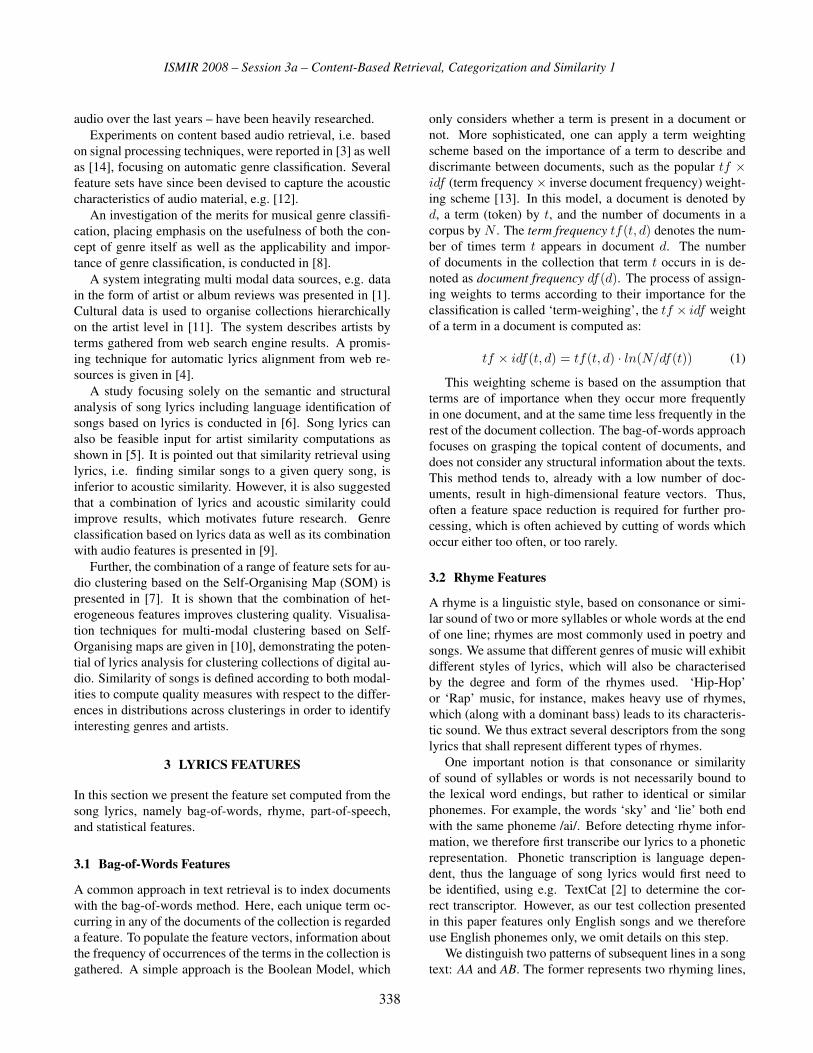
ISMIR 2008 – Session 3a – Content-Based Retrieval, Categorization and Similarity 1
audio over the last years – have been heavily researched.
Experiments on content based audio retrieval, i.e. based
on signal processing techniques, were reported in [3] as well
as [14], focusing on automatic genre classification. Several
feature sets have since been devised to capture the acoustic
characteristics of audio material, e.g. [12].
An investigation of the merits for musical genre classifi-
cation, placing emphasis on the usefulness of both the con-
cept of genre itself as well as the applicability and impor-
tance of genre classification, is conducted in [8].
A system integrating multi modal data sources, e.g. data
in the form of artist or album reviews was presented in [1].
Cultural data is used to organise collections hierarchically
on the artist level in [11]. The system describes artists by
terms gathered from web search engine results. A promis-
ing technique for automatic lyrics alignment from web re-
sources is given in [4].
A study focusing solely on the semantic and structural
analysis of song lyrics including language identification of
songs based on lyrics is conducted in [6]. Song lyrics can
also be feasible input for artist similarity computations as
shown in [5]. It is pointed out that similarity retrieval using
lyrics, i.e. finding similar songs to a given query song, is
inferior to acoustic similarity. However, it is also suggested
that a combination of lyrics and acoustic similarity could
improve results, which motivates future research. Genre
classification based on lyrics data as well as its combination
with audio features is presented in [9].
Further, the combination of a range of feature sets for au-
dio clustering based on the Self-Organising Map (SOM) is
presented in [7]. It is shown that the combination of het-
erogeneous features improves clustering quality. Visualisa-
tion techniques for multi-modal clustering based on Self-
Organising maps are given in [10], demonstrating the poten-
tial of lyrics analysis for clustering collections of digital au-
dio. Similarity of songs is defined according to both modal-
ities to compute quality measures with respect to the differ-
ences in distributions across clusterings in order to identify
interesting genres and artists.
3 LYRICS FEATURES
In this section we present the feature set computed from the
song lyrics, namely bag-of-words, rhyme, part-of-speech,
and statistical features.
3.1 Bag-of-Words Features
A common approach in text retrieval is to index documents
with the bag-of-words method. Here, each unique term oc-
curring in any of the documents of the collection is regarded
a feature. To populate the feature vectors, information about
the frequency of occurrences of the terms in the collection is
gathered. A simple approach is the Boolean Model, which
only considers whether a term is present in a document or
not. More sophisticated, one can apply a term weighting
scheme based on the importance of a term to describe and
discrimante between documents, such as the popular tf ×idf (term frequency× inverse document frequency) weight-
ing scheme [13]. In this model, a document is denoted by
d, a term (token) by t, and the number of documents in a
corpus by N . The term frequency tf(t, d) denotes the num-
ber of times term t appears in document d. The number
of documents in the collection that term t occurs in is de-
noted as document frequency df(d). The process of assign-
ing weights to terms according to their importance for the
classification is called ‘term-weighing’, the tf × idf weight
of a term in a document is computed as:
tf × idf(t, d) = tf(t, d) · ln(N/df(t)) (1)
This weighting scheme is based on the assumption that
terms are of importance when they occur more frequently
in one document, and at the same time less frequently in the
rest of the document collection. The bag-of-words approach
focuses on grasping the topical content of documents, and
does not consider any structural information about the texts.
This method tends to, already with a low number of doc-
uments, result in high-dimensional feature vectors. Thus,
often a feature space reduction is required for further pro-
cessing, which is often achieved by cutting of words which
occur either too often, or too rarely.
3.2 Rhyme Features
A rhyme is a linguistic style, based on consonance or simi-
lar sound of two or more syllables or whole words at the end
of one line; rhymes are most commonly used in poetry and
songs. We assume that different genres of music will exhibit
different styles of lyrics, which will also be characterised
by the degree and form of the rhymes used. ‘Hip-Hop’
or ‘Rap’ music, for instance, makes heavy use of rhymes,
which (along with a dominant bass) leads to its characteris-
tic sound. We thus extract several descriptors from the song
lyrics that shall represent different types of rhymes.
One important notion is that consonance or similarity
of sound of syllables or words is not necessarily bound to
the lexical word endings, but rather to identical or similar
phonemes. For example, the words ‘sky’ and ‘lie’ both end
with the same phoneme /ai/. Before detecting rhyme infor-
mation, we therefore first transcribe our lyrics to a phonetic
representation. Phonetic transcription is language depen-
dent, thus the language of song lyrics would first need to
be identified, using e.g. TextCat [2] to determine the cor-
rect transcriptor. However, as our test collection presented
in this paper features only English songs and we therefore
use English phonemes only, we omit details on this step.
We distinguish two patterns of subsequent lines in a song
text: AA and AB. The former represents two rhyming lines,
338

ISMIR 2008 – Session 3a – Content-Based Retrieval, Categorization and Similarity 1
Feature Name Description
Rhymes-AA A sequence of two (or more)
rhyming lines (‘Couplet’)
Rhymes-AABB A block of two rhyming se-
quences of two lines (‘Cleri-
hew)
Rhymes-ABAB A block of alternating rhymes
Rhymes-ABBA A sequence of rhymes with
a nested sequence (‘Enclosing
rhyme’)
RhymePercent The percentage of blocks that
rhyme
UniqueRhymeWords The fraction of unique terms
used to build the rhymes
Table 1. Rhyme features for lyrics analysis
while the latter denotes non-rhyming. Based on these basic
patterns, we extract the features described in Table 1.
A ‘Couplet’ AA describes the rhyming of two or more
subsequent pairs of lines. It usually occurs in the form of
a ‘Clerihew’, i.e. several blocks of Couplets AABBCC...ABBA, or enclosing rhyme denotes the rhyming of the first
and fourth, as well as the second and third lines (out of four
lines). We further measure ‘RhymePercent’, the percent-
age of rhyming blocks, and define the unique rhyme words
as the fraction of unique terms used to build rhymes ‘Uni-
queRhymeWords’.
Of course, more elaborate rhyming patterns, especially
less obvious forms of rhymes, could be taken into account.
In order to initially investigate the usefulness of rhyming
at all, we do not take into account rhyming schemes based
on assonance, semirhymes, or alliterations, amongst others.
Initial experimental results lead to the conclusions that some
of these patterns may well be worth studying. However, the
frequency of such patterns in popular music is doubtful.
3.3 Part-of-Speech Features
Part-of-speech tagging is a lexical categorisation or gram-
matical tagging of words according to their definition and
the textual context they appear in. Different part-of-speech
categories are for example nouns, verbs, articles or adjec-
tives. We presume that different genres will differ also in the
category of words they are using, and therefore we addition-
ally extract several part of speech descriptors from the lyrics.
We count the numbers of: nouns, verbs, pronouns, rela-tional pronouns (such as ‘that’ or ‘which’), prepositions, ad-verbs, articles, modals, and adjectives. To account for dif-
ferent document lengths, all of these values are normalised
by the number of words of the respective lyrics document.
Feature Name Description
exclamation mark, colon,
single quote, comma, ques-
tion mark, dot, hyphen,
semicolon
simple count
d0 - d9 counts of digits
WordsPerLine words / number of lines
UniqueWordsPerLine unique words / number
of lines
UniqueWordsRatio unique words / words
CharsPerWord number of chars / num-
ber of words
WordsPerMinute the number of words /
length of the song
Table 2. Overview of text statistic features
3.4 Text Statistic Features
Text documents can also be described by simple statistical
measures based on word or character frequencies. Measures
such as the average length of words or the ratio of unique
words in the vocabulary might give an indication of the com-
plexity of the texts, and are expected to vary over different
genres. The usage of punctuation marks such as exclama-
tion or question marks may be specific for some genres. We
further expect some genres to make increased use of apos-
trophes when omitting the correct spelling of word endings.
The list of extracted features is given in Table 2.
All features that simply count character occurrences are
normalised by the number of words of the song text to ac-
commodate for different lyrics lengths. ‘WordsPerLine’ and
‘UniqueWordsPerLine’ describe the words per line and the
unique number of words per line. The ‘UniqueWordsRa-
tio’ is the ratio of the number of unique words and the to-
tal number of words. ‘CharsPerWord’ denotes the simple
average number of characters per word. The last feature,
‘WordsPerMinute’ (WPM), is computed analogously to the
well-known beats-per-minute (BPM) value 1 .
4 EXPERIMENTS
In this section we report on experiments performed for a
test collection of 397 song lyrics. We used classical bag-of-
words indexing as well as the feature sets introduced in Sec-
tion 3. Genre classification was done for a range of setups
with Naı̈ve Bayes, k-Nearest Neighbour with different val-
ues for k, SVMs with linear and polynomial kernels (more
complex kernels did not improve accuracy), and a Decision
1 Actually we use the ratio of the number of words and the song length
in seconds to keep feature values in the same range. Hence, the correct
name would be ‘WordsPerSecond’, or WPS.
339
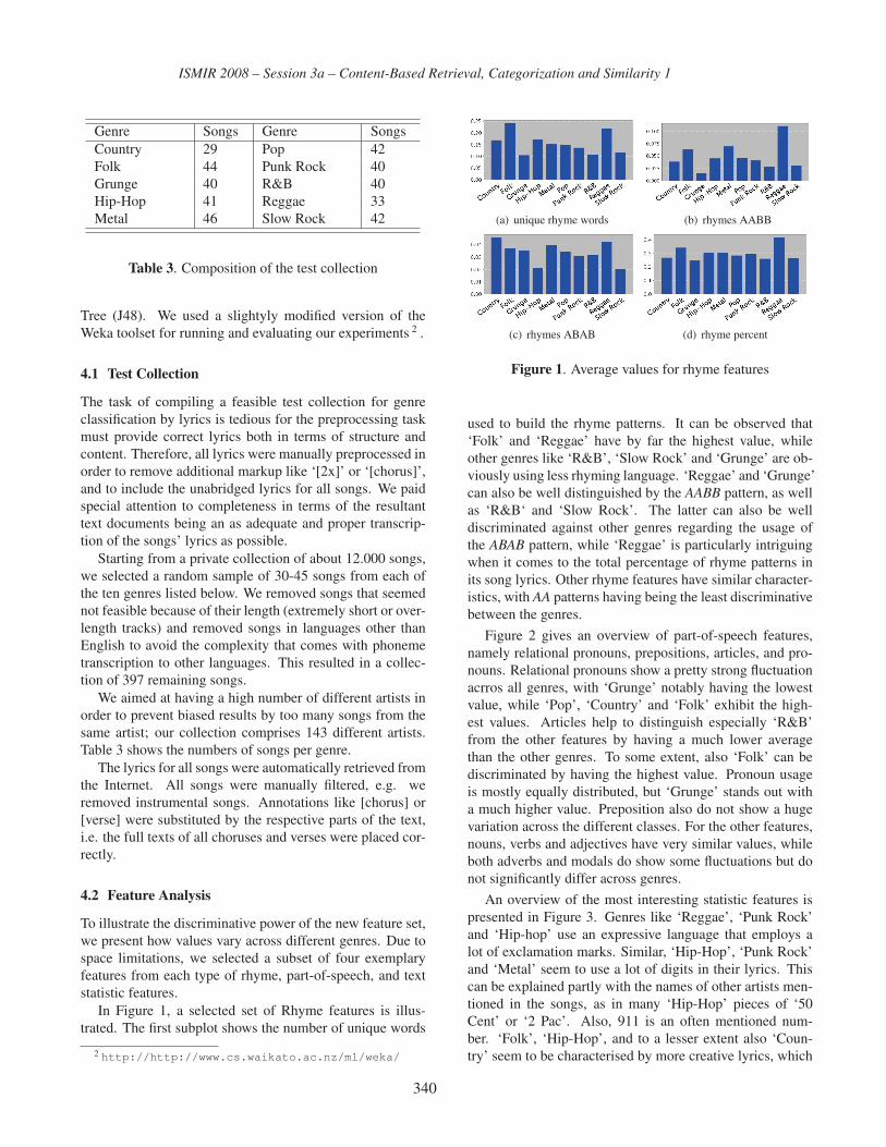
ISMIR 2008 – Session 3a – Content-Based Retrieval, Categorization and Similarity 1
Genre Songs Genre Songs
Country 29 Pop 42
Folk 44 Punk Rock 40
Grunge 40 R&B 40
Hip-Hop 41 Reggae 33
Metal 46 Slow Rock 42
Table 3. Composition of the test collection
Tree (J48). We used a slightyly modified version of the
Weka toolset for running and evaluating our experiments 2 .
4.1 Test Collection
The task of compiling a feasible test collection for genre
classification by lyrics is tedious for the preprocessing task
must provide correct lyrics both in terms of structure and
content. Therefore, all lyrics were manually preprocessed in
order to remove additional markup like ‘[2x]’ or ‘[chorus]’,
and to include the unabridged lyrics for all songs. We paid
special attention to completeness in terms of the resultant
text documents being an as adequate and proper transcrip-
tion of the songs’ lyrics as possible.
Starting from a private collection of about 12.000 songs,
we selected a random sample of 30-45 songs from each of
the ten genres listed below. We removed songs that seemed
not feasible because of their length (extremely short or over-
length tracks) and removed songs in languages other than
English to avoid the complexity that comes with phoneme
transcription to other languages. This resulted in a collec-
tion of 397 remaining songs.
We aimed at having a high number of different artists in
order to prevent biased results by too many songs from the
same artist; our collection comprises 143 different artists.
Table 3 shows the numbers of songs per genre.
The lyrics for all songs were automatically retrieved from
the Internet. All songs were manually filtered, e.g. we
removed instrumental songs. Annotations like [chorus] or
[verse] were substituted by the respective parts of the text,
i.e. the full texts of all choruses and verses were placed cor-
rectly.
4.2 Feature Analysis
To illustrate the discriminative power of the new feature set,
we present how values vary across different genres. Due to
space limitations, we selected a subset of four exemplary
features from each type of rhyme, part-of-speech, and text
statistic features.
In Figure 1, a selected set of Rhyme features is illus-
trated. The first subplot shows the number of unique words
2 http://http://www.cs.waikato.ac.nz/ml/weka/
(a) unique rhyme words (b) rhymes AABB
(c) rhymes ABAB (d) rhyme percent
Figure 1. Average values for rhyme features
used to build the rhyme patterns. It can be observed that
‘Folk’ and ‘Reggae’ have by far the highest value, while
other genres like ‘R&B’, ‘Slow Rock’ and ‘Grunge’ are ob-
viously using less rhyming language. ‘Reggae’ and ‘Grunge’
can also be well distinguished by the AABB pattern, as well
as ‘R&B‘ and ‘Slow Rock’. The latter can also be well
discriminated against other genres regarding the usage of
the ABAB pattern, while ‘Reggae’ is particularly intriguing
when it comes to the total percentage of rhyme patterns in
its song lyrics. Other rhyme features have similar character-
istics, with AA patterns having being the least discriminative
between the genres.
Figure 2 gives an overview of part-of-speech features,
namely relational pronouns, prepositions, articles, and pro-
nouns. Relational pronouns show a pretty strong fluctuation
acrros all genres, with ‘Grunge’ notably having the lowest
value, while ‘Pop’, ‘Country’ and ‘Folk’ exhibit the high-
est values. Articles help to distinguish especially ‘R&B’
from the other features by having a much lower average
than the other genres. To some extent, also ‘Folk’ can be
discriminated by having the highest value. Pronoun usage
is mostly equally distributed, but ‘Grunge’ stands out with
a much higher value. Preposition also do not show a huge
variation across the different classes. For the other features,
nouns, verbs and adjectives have very similar values, while
both adverbs and modals do show some fluctuations but do
not significantly differ across genres.
An overview of the most interesting statistic features is
presented in Figure 3. Genres like ‘Reggae’, ‘Punk Rock’
and ‘Hip-hop’ use an expressive language that employs a
lot of exclamation marks. Similar, ‘Hip-Hop’, ‘Punk Rock’
and ‘Metal’ seem to use a lot of digits in their lyrics. This
can be explained partly with the names of other artists men-
tioned in the songs, as in many ‘Hip-Hop’ pieces of ‘50
Cent’ or ‘2 Pac’. Also, 911 is an often mentioned num-
ber. ‘Folk’, ‘Hip-Hop’, and to a lesser extent also ‘Coun-
try’ seem to be characterised by more creative lyrics, which
340

ISMIR 2008 – Session 3a – Content-Based Retrieval, Categorization and Similarity 1
(a) rel. pronouns (b) prepositions
(c) articles (d) pronouns
Figure 2. Average values for part-of-speech features
manifests in a bigger word pool used in these genres. Last,
‘Words per Minute’ is the most discriminative feature for
‘Hip-Hop’, which indeed is characterised by fast language,
and in most of the cases has very short lead-in and fade-out
sequences. Also ‘R&B’ and ‘Punk Rock’ have these char-
acteristics, while ‘Grunge’, ‘Slow Rock’ and ‘Metal’ feature
long instrumental parts or a more moderate singing tempo.
4.3 To Stem or Not to Stem
We used Porter’s stemming algorithm to remove word end-
ings. Its impact on classification accuracies varies; in some
cases, it lowers classification accuracy. We performed ex-
periments for a standard Naı̈ve Bayes classifier, and Support
Vector Machines (SVM) with linear kernel and Decision
Trees (J48) for three different dimensionalities computed by
document frequency thresholding feature selection. For the
Bayes classifier and SVMs, stemming improved the results
for all three dimensionalities (full set, 3000, 300). For the
Decision Tree setup, it did not yield improvements. Overall,
we did not find significant differences in accuracies, yet, we
had expected setups without stemming to be superior caused
by word endings in ‘slang’ language.
4.4 Classification Results
We performed a set of classification experiments, a sum-
marisation of the results is given in Table 4. It shows the
experiments we performed on the test collection, omitting
results on different values for k for the k-Nearest Neigh-
bour and kernels other than the linear one for SVMs, as
they showed the same trends, but had a worse overall perfor-
mance. For a set of ten genres, we assume the absolute base-
line for classification experiments to be the relative number
of tracks in the largest class, i.e. 46/397 = 11.59%. How-
ever, we rather consider the results obtained with the bag-of-
words approach as the baseline to compare to. The values
given are macro-averaged classification accuracies for the
(a) question marks (b) digits
(c) unique words per line (d) words per minute
Figure 3. Average values for statistic features
correctly classified tracks computed with ten-fold cross val-
idation. We want to point out that classification accuracies
are lower than comparable results based on audio content,
yet we show that genre classification by lyrics features can
be complementary for they might classify different genres
better than audio only.
For all three classifiers, feature sets including our pro-
posed features achieved the best results (experiments 6, 4,
and 3). The addition to the bag-of-words approach (with
stemming) always yields better results, this becomes even
clearer in the case of the SVM (experiments 6, 8, and 10).
The best result of all experiments was achieved with a di-
mensionality of 38, which is sa significantly lower dimen-
sionality than the one of the best performing bag-of-words
approach (experiment 6, dimensionality: 3336). We want to
point out the improvement in performance of about 7.5% ab-
solute between 24.83 and 33.47 (relative increase of about
a third). We also performed the same set of experiments
with non-stemmed bag-of-words features and combinations
thereof; they revealed the same trends but are omitted due to
space limitations.
5 CONCLUSIONS
In this paper, we introduced style and rhyme features for
lyrics processing. We showed that all our feature sets out-
perform the baseline in terms of classification accuracies in
a set of experiments. Further, we showed that the combi-
nation of style features and classical bag-of-words features
outperforms the bag-of-words only approach and in some
cases reduces the needed dimensionality.
These results indicate that style and rhyme features can
contribute to better music classification or a reduction in di-
mensionality for similar classification accuracies. Hence,
we plan to investigate more sophisticated rhyme patterns.
As the classification experiments reported in this paper were
based on a simple concatenation approach, more elaborate
341

ISMIR 2008 – Session 3a – Content-Based Retrieval, Categorization and Similarity 1
Exp. Feature Combination Dim 5-NN Naı̈ve Bayes SVM Decision Tree
1 rhyme 6 13.17 13.67 − 12.83 − 13.82 -
2 part-of-speech (pos) 9 15.99 20.79 16.04 − 15.89 -
3 text statistic 23 28.53 + 20.6 − 30.12 26.724 rhyme / pos / text statistic 38 25.33 + 23.37 33.47 + 24.60
5 bag-of-words #1 3298 13.63 25.89 24.83 23.63
6 bag-of-words / rhyme / pos / text statistic #1 3336 13.88 27.58 29.44 + 24.39
7 bag-of-words #2 992 12.34 25.13 21.96 23.11
8 bag-of-words / rhyme / pos / text statistic #2 1030 16.56 25.78 27.37 23.77
9 bag-of-words #3 382 14.06 22.74 22.27 22.17
10 bag-of-words / rhyme / pos / text statistic #3 420 15.06 24.50 29.36 24.05
Table 4. Classification results for different feature combinations. The highest accuracies per column are printed in bold face;
statistically significant improvement or degradation over the base line experiment (5, column-wise) is indicated by (+) or (−),
respectively
methods such as ensemble learning will be taken into con-
sideration. Finally, we plan on improve lyrics preprocessing
by heuristics for rhyme detection and automatic alignment
thereof.
References[1] Stephan Baumann, Tim Pohle, and Shankar Vembu.
Towards a socio-cultural compatibility of mir systems.
In Proc. of the 5th Int. Conf. of Music Information Re-trieval (ISMIR’04), pages 460–465, Barcelona, Spain,
October 10-14 2004.
[2] William B. Cavnar and John M. Trenkle. N-gram-
based text categorization. In Proc. of SDAIR-94, 3rdAnnual Symposium on Document Analysis and Infor-mation Retrieval, pages 161–175, Las Vegas, USA,
1994.
[3] Jonathan Foote. An overview of audio information re-
trieval. Multimedia Systems, 7(1):2–10, 1999.
[4] Peter Knees, Markus Schedl, and Gerhard Widmer.
Multiple lyrics alignment: Automatic retrieval of song
lyrics. In Proc. of 6th Int. Conf. on Music InformationRetrieval (ISMIR’05), pages 564–569, London, UK,
September 11-15 2005.
[5] Beth Logan, Andrew Kositsky, and Pedro Moreno. Se-
mantic analysis of song lyrics. In Proc. of the 2004IEEE Int. Conf. on Multimedia and Expo (ICME’04),pages 827–830, Taipei, Taiwan, June 27-30 2004.
[6] Jose P. G. Mahedero, Álvaro Martı́nez, Pedro Cano,
Markus Koppenberger, and Fabien Gouyon. Natural
language processing of lyrics. In Proc. of the 13thannual ACM Int. Conf. on Multimedia (ACMMM’05),pages 475–478, Singapore, 2005.
[7] Tamsin Maxwell. Exploring the music genome: Lyric
clustering with heterogeneous features. Master’s the-
sis, University of Edinburgh, 2007.
[8] Cory McKay and Ichiro Fujinaga. Musical genre clas-
sification: Is it worth pursuing and how can it be im-
proved? In Proc. of the 7th Int. Conf. on Music In-formation Retrieval (ISMIR’06), pages 101–106, Vic-
toria, BC, Canada, October 8-12 2006.
[9] Robert Neumayer and Andreas Rauber. Integration of
text and audio features for genre classification in music
information retrieval. In Proc. of the 29th EuropeanConf. on Information Retrieval (ECIR’07), pages 724–
727, Rome, Italy, April 2-5 2007.
[10] Robert Neumayer and Andreas Rauber. Multi-modal
music information retrieval - visualisation and evalua-
tion of clusterings by both audio and lyrics. In Proc. ofthe 8th RIAO Conf. (RIAO’07), Pittsburgh, PA, USA,
May 29th - June 1 2007.
[11] Elias Pampalk, Arthur Flexer, and Gerhard Widmer.
Hierarchical organization and description of music
collections at the artist level. In Research and Ad-vanced Technology for Digital Libraries ECDL’05,
pages 37–48, 2005.
[12] Elias Pampalk, Arthur Flexer, and Gerhard Widmer.
Improvements of audio-based music similarity and
genre classificaton. In Proc. of the 6th Int. Conf. onMusic Information Retrieval (ISMIR’05), pages 628–
633, London, UK, September 11-15 2005.
[13] Gerald Salton. Automatic text processing – The Trans-formation, Analysis, and Retrieval of Information byComputer. Addison-Wesley Longman Publishing Co.,
Inc., 1989.
[14] George Tzanetakis and Perry Cook. Marsyas: A
framework for audio analysis. Organized Sound,
4(30):169–175, 2000.
342

ISMIR 2008 – Session 3a – Content-Based Retrieval, Categorization and Similarity 1
ARMONIQUE: EXPERIMENTS IN CONTENT-BASED SIMILARITY RETRIEVAL USING POWER-LAW
MELODIC AND TIMBRE METRICS
Bill Manaris 1, Dwight Krehbiel 2, Patrick Roos 1, Thomas Zalonis 1 1 Computer Science Department, College of Charleston, 66 George Street, Charleston, SC 29424, USA
2 Psychology Department, Bethel College, 300 E. 27th Street, North Newton, KS 67117, USA
ABSTRACT
This paper presents results from an on-going MIR study utilizing hundreds of melodic and timbre features based on power laws for content-based similarity retrieval. These metrics are incorporated into a music search engine prototype, called Armonique. This prototype is used with a corpus of 9153 songs encoded in both MIDI and MP3 to identify pieces similar to and dissimilar from selected songs. The MIDI format is used to extract various power-law features measuring proportions of music-theoretic and other attributes, such as pitch, duration, melodic intervals, and chords. The MP3 format is used to extract power-law features measuring proportions within FFT power spectra related to timbre. Several assessment experiments have been conducted to evaluate the effectiveness of the similarity model. The results suggest that power-law metrics are very promising for content-based music querying and retrieval, as they seem to correlate with aspects of human emotion and aesthetics.
1. INTRODUCTION
We present results from an on-going project in music information retrieval, psychology of music, and computer science. Our research explores power-law metrics for music information retrieval.
Power laws are statistical models of proportions exhibited by various natural and artificial phenomena [13]. They are related to measures of self-similarity and fractal dimension, and as such they are increasingly being used for data mining applications involving real data sets, such as web traffic, economic data, and images [5]. Power laws have been connected with emotion and aesthetics through various studies and experiments [8, 9, 12, 14, 16, 18].
We discuss a music search engine prototype, called Armonique, which utilizes power-law metrics to capture both melodic and timbre features of music. In terms of input, the user selects a music piece. The engine searches for pieces similar to the input by comparing power-law proportions through the database of songs. We provide an on-line demo of the system involving a corpus of 9153 pieces for various genres, including baroque, classical, romantic, impressionist, modern, jazz, country, and rock among others. This corpus was originally encoded in
MIDI, which facilitated extraction of melodic features. It was then converted to MP3 for the purpose of extracting timbre features.
In terms of assessment, we conducted an experiment by measuring human emotional and physiological responses to the music chosen by the search engine. Analyses of data indicate that people do indeed respond differently to pieces identified by the search engine as similar to the participant-chosen piece, than to pieces identified by the engine as different. For similar pieces, the participants’ emotion while listening to the music is more pleasant, their mood after listening is more pleasant; they report liking these pieces more, and they report them to be more similar to their own chosen piece. These results support the potential of using power-law metrics for music information retrieval.
Section 2 presents relevant background research. Sections 3 and 4 describe our power-law metrics for melodic and timbre features, respectively. Sections 5 and 6 discuss the music search engine prototype, and its evaluation with human subjects. Finally, section 7 presents closing remarks and directions for future research.
2. BACKGROUND
Tzanetakis et al. [15] performed genre classifications using audio signal features. They performed FFT analysis on the signal and calculated various dimensions based on the frequency magnitudes. Also, they extracted rhythm features through wavelet transforms. They reported classification success rates of 62% using six genres (classical, country, disco, hiphop, jazz and rock) and 76% using four classical genres.
Aucouturier and Packet [1] report the most typical audio similarity technique is timbre via spectral analysis using Mel-frequency cepstral coefficients (MFCCs). Their goal was to improve on the overall performance of timbre similarity by varying parameters associated with these techniques (e.g. sample rate, frame size, number of MFCCs used, etc.) They report that there is a “glass ceiling” for timbre similarity that prevents any major improvements in performance via this technique. Subsequent research on this seems to either be a verification of this ceiling or an attempt to pass it using additional similarity dimensions (e.g., [10]).
343

ISMIR 2008 – Session 3a – Content-Based Retrieval, Categorization and Similarity 1
Lidy et al. [6] discuss a genre classification experiment utilizing both timbre and melodic features. They utilize the typical timbre measures obtained through spectral analysis. They also employ a music transcription system they developed to generate MIDI representations of audio music files. From these files, they extract 37 different features, involving attributes of note pitches, durations and non-diatonic notes. The combined timbre and melodic features are used to conduct genre classification experiments. They report classification accuracies with combined feature sets ranging from 76.8% to 90.4% using standard benchmarks (e.g., ISMIR 2004 audio data).
Cano et al. [4] report on a music recommendation system called MusicSurfer. The primary dimensions of similarity used are timbre, tempo and rhythm patterns. Using a corpus of 273,751 songs from 11,257 artists their system achieves an artist identification rate of 24%. On the ISMIR 2004 author identification set they report a success rate of 60%, twice as high as that of the next best systems. MusicSurfer has a comprehensive user interface that allows users to find songs based on artist, genre, and similarity among other characteristics, and allows selection of different types of similarity. However, it does not include melodic features.
2.1. Power Laws and Music Analysis Our music recommender system prototype employs both melodic and timbre features based on power-laws. Although power laws, fractal dimension, and other self-similarity features have been used extensively in information retrieval (e.g., [5]), to the best of our knowledge, there are no studies of content-based music recommendation systems utilizing power law similarity metrics.
A power law denotes a relationship between two variables where one is proportional to a power of the other. One of the most well-known power laws is Zipf’s
law: P(f) ~ 1 / f
n (1)
where P(f) denotes the probability of an event of rank f, and n is close to 1. Zipf’s law is named after George Kingsley Zipf, the Harvard linguist who documented and studied natural and social phenomena exhibiting such relationships [18]. The generalized form is:
P(f) ~ a / f b (2)
where a and b are real constants. This generalized form is known as the Zipf-Mandelbrot law, after Benoit Mandelbrot.
Numerous empirical studies report that music exhibits power laws across timbre and melodic attributes (e.g., [8, 16, 18]). In particular, Voss and Clarke [16] demonstrate that music audio properties (e.g. loudness and pitch fluctuation) exhibit power law relationships. Using 12 hours worth of radio recordings, they show that power fluctuations in music follow a 1/f distribution.
Manaris et al. [8] report various classification experiments with melodic features based on power laws. These studies include composer identification with 93.6% to 95% accuracy. They also report an experiment using emotional responses from humans. Using a corpus of 210 music excerpts in a 12-fold cross-validation study, artificial neural networks (ANNs) achieved an average success rate of 97.22% in predicting (within one standard deviation) human emotional responses to those pieces.
3. MELODIC FEATURE EXTRACTION
As mentioned earlier, we employ hundreds of power-law metrics that calculate statistical proportions of music-theoretic and other attributes of pieces.
3.1. Melodic Metrics We have defined 14 power-law metrics related to proportion of pitch, chromatic tone, duration, distance between repeated notes, distance between repeated durations, melodic and harmonic intervals, melodic and harmonic consonance, melodic and harmonic bigrams, chords, and rests [9]. Each metric calculates the rank-
frequency distribution of the attribute in question, and returns two values: • the slope of the trendline, b (see equation 2), of the
rank-frequency distribution; and • the strength of the linear relation, r2. We also calculate higher-order power law metrics. For
each regular metric we construct an arbitrary number of higher-order metrics (e.g., the difference of two pitches, the difference of two differences, and so on), an approach similar to the notion of derivative in mathematics.
Finally, we also capture the difference of an attribute value (e.g., note duration) from the local average. Local variability, locVar[i], for the ith value is
locVar[i] = abs(vals[i] – avg(vals, i)) / avg(vals, i) (3)
where vals is the list of values, abs is the absolute value, and avg(vals, i) is the local average of the last, say, 5 values. We compute a local variability metric for each of the above metrics (i.e., 14 regular metrics x the number of higher-order metrics we decide to include).
Collectively, these metrics measure hierarchical aspects of music. Pieces without hierarchical structure (e.g., aleatory music) have significantly different measurements than pieces with hierarchical structure and long-term dependencies (e.g., fugues).
3.2. Evaluation Evaluating content-based music features through classification tasks based on objective descriptors, such as artist or genre, is recognized as a simple alternative to listening tests for approximating the value of such features for similarity prediction [7, 11].
We have conducted several genre classification experiments using our set of power-law melodic metrics to extract features from music pieces. Our corpus
344

ISMIR 2008 – Session 3a – Content-Based Retrieval, Categorization and Similarity 1
consisted of 1236 MIDI-encoded music pieces from the Classical Music Archives (www.classicalarchives.com). These pieces were subdivided into 9 different musical genres (listed here by timeline): Medieval (57 pieces), Renaissance (150 pieces), Baroque (160 pieces), Classical (153 pieces), Romantic (91 pieces), Modern (127 pieces), Jazz (118 pieces), Country (109 pieces), and Rock (271 pieces).
First, we carried out a 10-fold cross validation experiment training an ANN to classify the corpus into the 9 different genres. For this, we used the Multilayer Perceptron implementation of the Weka machine learning environment. Each piece was represented by a vector of 156 features computed through our melodic metrics. The ANN achieved a success rate of 71.52%.
Figure 1 shows the resulting confusion matrix. It is clear that most classification errors occurred between genres adjacent in timeline. For example, most Renaissance pieces misclassified (32/43) were either falsely assigned to the Medieval (7) or Baroque (25) period. Most misclassified Baroque pieces (40/64) were incorrectly classified as Renaissance (23) or Classical (17), and so on. This is not surprising, since there is considerable overlap in style between adjacent genres.
To verify this interpretation, we ran several binary classification experiments. In each experiment, we divided the corpus into two classes: class 1 consisting of a particular genre (e.g., Baroque), and class 2 consisting of all other genres non-adjacent in timeline (e.g., all other genres minus Renaissance and Classical). For Jazz, as well as Rock, the other class included all other genres.
Table 1 shows the classification accuracies for all of these experiments. Since the two output classes in each experiment were unbalanced, the ANN accuracy rates should be compared to a majority-class classifier.
4. TIMBRE FEATURE EXTRACTION
We calculate a base audio metric employing spectral analysis through FFT. This metric is then expanded through the use of higher-order calculations and variations of window size and sampling rate. Since we are interested in power-law distributions within the human hearing range, assuming CD-quality sampling rate (44,1KHz), we use window sizes up to 1-sec. Interestingly, given our technique, the upper frequencies in this range do not appear to be as important for calculating timbre similarity; the most important frequencies appear to be from 1kHz to 11kHz.
For each of these windows we compute the power spectrum per window and then average the results, across frequencies. We then extract various power-law proportions from this average power spectrum. Again, each power-law proportion is captured as a pair of slope and r2 values.
We have explored various ways to calculate higher-
order quantities involving both signal amplitudes and power spectrum (i.e., frequency) magnitudes. Again, the idea of a higher-order is similar to the use of derivatives in mathematics where one measures the rate of change of a function at a given point. Through this approach, we have created various derivative metrics, involving raw signal amplitude change, frequency change within a window, and frequency change across windows.
To further explore the proportions present in the audio signal, we vary the window size and the sampling rate. This allows us to get measurements from multiple “views” or different levels of granularity of the signal. For each new combination of window size and sampling rate, we recompute the above metrics, thus getting another pair of slope and r
2 values. Overall, we have defined a total of 234 audio features.
4.1. Evaluation To evaluate these timbre metrics, we conducted a classification experiment involving a corpus of 1128 MP3 files containing an equal number of classical and non-classical pieces.
We carried out a 10-fold cross-validation, binary ANN classification experiment using a total of 234 audio features. For comparison, each classification was repeated using randomly assigned classes. The ANN achieved a success rate of 95.92%. The control success rate was 47.61%. We are in the process of running additional classification experiments to further evaluate our timbre metrics (e.g., ISMIR 2004 audio data).
a b c d e f g h i <-- classified as 92 17 1 2 4 4 23 8 9 | a = baroque
20 107 0 1 2 5 5 4 9 | b = classical 1 1 96 0 0 0 0 9 2 | c = country
0 3 1 96 0 2 1 13 2 | d = jazz
8 3 0 0 28 0 15 3 0 | e = medieval 9 9 1 0 0 78 2 10 18 | f = modern
25 8 1 0 7 0 107 1 1 | g = renaissance
1 2 7 11 0 4 1 242 3 | h = rock
9 12 3 3 1 19 1 5 38 | i = romantic
Figure 1. Confusion matrix from 9 genre multi-classification ANN experiment.
Class 1 Class 2 ANN Accuracy
Majority Classifier
Baroque Non-Adjacent 91.29 % 82.85 % Classical Non-Adjacent 92.08 % 84.46 % Rock Non-Rock 92.88 % 78.07 % Jazz Non-Rock 96.66 % 90.45 %
Table 1. ANN success rates for binary
classification experiments.
345
ISMIR 2008 – Session 3a – Content-Based Retrieval, Categorization and Similarity 1
5. A MUSIC SEARCH ENGINE PROTOTYPE
Musicologists consider melody and timbre to be independent/complementary aesthetic dimensions (among others, such as rhythm, tempo, and mode). We have developed a music search-engine prototype, called Armonique, which combines melodic and timbre metrics to calculate sets of similar songs to a song selected by the user. For comparison, we also generate a set of dissimilar songs. A demo of this prototype is available at http://www.armonique.org.1
The corpus used for this demo consists of 9153 songs from the Classical Music Archives (CMA), extended with pieces from other genres such as jazz, country, and rock. These pieces originated as MIDI and were converted for the purpose of timbre feature extraction (and playback) to the MP3 format. As far as the search engine is concerned, each music piece is represented as a vector of hundreds of power-law slope and r2 values derived from our metrics. As input, the engine is presented with a single music piece. The engine searches the corpus for pieces similar to the input, by computing the mean squared error (MSE) of the vectors (relative to the input). The pieces with the lowest MSE are returned as best matches.
We have experimented with various selection algorithms. The selection algorithm used in this demo, first identifies 200 similar songs based on melody, using an MSE calculation across all melodic metrics. Then, from this set, it identifies the 10 most similar songs based on timbre, again, using an MSE calculation across all timbre metrics. Each song is associated with two gauges providing a rough estimate of the similarity across the two dimensions, namely melody and timbre. It is our intention to explore more similarity dimensions, such as rhythm, tempo, and mode (major, minor, etc.).
6. EVALUATION EXPERIMENT
We conducted an experiment with human subjects to evaluate the effectiveness of the proposed similarity model. This experiment evaluated only the melodic metrics of Armonique, since the timbre metrics had not been fully incorporated at the time.2
6.1. Participants
Twenty-one undergraduate students from Bethel College participated in this study. The participants consisted of 11 males and 10 females, with a mean age of 19.52 years and a range of 5 years. They had participated in high school or college music ensembles for a mean of 3.52 years with a standard deviation of 2.21, and had received private music lessons for a mean of 6.07 years with a standard deviation of 4.37.
1 Due to copyright restrictions, some functionality is password-protected. 2 We are planning a similar assessment experiment involving both melodic and timbre metrics.
6.2. Design
A single repeated-measures variable was investigated. This variable consisted of the seven different excerpts, one of them participant-chosen (hereafter referred to as the original piece), three of them computer-selected to be similar to the participant-chosen piece, and three selected to be different (see next section). Of primary interest was the comparison of responses to the original with those to the three similar pieces, of the original to the three different pieces, and of the three similar to the three different pieces.
6.3. Data Set At the time they were recruited, participants were asked to list in order of preference three classical music compositions that they enjoyed. The most preferred of these three compositions that was available in the CMA corpus was chosen for each participant. The search engine was then employed to select three similar and three different pieces. Similarities were based upon the first two minutes of each composition. This corpus is available at http://www.armonique.org/melodic-search.html .
6.4. Procedure The resulting seven two-minute excerpts (original plus
six computer-selected pieces), different for each participant, were employed in a listening session in which participant ratings of the music were obtained during and after the music, and psychophysiological responses were monitored (i.e., skin conductance, heart rate, corrugator supercilii electromygraphic recording, respiration rate, and 32 channels of electroencephalographic recording). The physiological data are not reported here. In some instances the entire piece was shorter than two minutes. A different random order of excerpts was employed for each participant.
Ratings of mood were obtained immediately prior to the session using the Self-Assessment Manikin [3] represented as two sliders with a 1-9 scale, one for pleasantness and one for activation, on the front panel of a LabVIEW (National Instruments, Austin, TX) virtual instrument. Physiological recording baseline periods of one minute were included prior to each excerpt. By means of a separate practice excerpt, participants were carefully instructed to report their feelings during the music by using a mouse to move a cursor on a two-dimensional emotion space [2]. This space was displayed on the front panel of the LabVIEW instrument, which also played the music file and recorded x-y coordinates of the cursor position once per second. After each excerpt participants again rated their mood with the Self-Assessment Manikin, and then rated their liking of the previous piece using another slider on the front panel with a 1-9 scale ranging from “Dislike very much” to “Like very much.”
At the conclusion of the listening session, participants rated the similarity of each of the six computer-selected
346

ISMIR 2008 – Session 3a – Content-Based Retrieval, Categorization and Similarity 1
excerpts to the original; these ratings were accomplished on a LabVIEW virtual instrument with six sliders and 0-10 scales ranging from “Not at all” to “Extremely.”
6.5. Data Analysis Data from the ratings during the music were averaged over time, yielding an average pleasantness and activation measure for each excerpt. A procedural error resulted in loss of data for two participants on these measures. Data from each behavioral measure were subjected to planned contrasts based upon a repeated-measures analysis of variance (SYSTAT software, SYSTAT, Inc., San Jose, CA). These contrasts compared the original song with each of the other two categories of music, and each of those categories with each other.
6.6. Results The results for similarity ratings are shown in Figure 2. A contrast between the three similar and three different pieces indicated that the similar pieces were indeed judged to be more similar than were the different ones (F(1, 20) = 20.98, p < 0.001). Interestingly, the similar songs recommended by the search engine were ordered by humans the same way as by the search engine.1
In terms of the average ratings for pleasantness recorded during the music, the contrast between the similar pieces and the original was significant (F(1, 18) = 5.85, p = 0.026), while that between the different pieces and the original showed an even more marked difference (F(1, 18) = 11.17, p = 0.004). The contrast between similar and different pieces approached significance (F(1, 1 It should be noted that the different songs used in this corpus were not the most dissimilar songs. These selections were used to avoid a cluster of most dissimilar songs, which was the same for most user inputs. However, they also somewhat reduced the distance between similar and dissimilar songs.
18) = 3.04, p = 0.098). No significant differences were found for these contrasts on the average activation measure.
In terms of the ratings for pleasantness recorded after the music, the contrast between the similar pieces and the original was not significant (F(1, 20) = 1.21, p = 0.285), while that between the different pieces and the original was significant (F(1, 20) = 7.64, p = 0.012). The contrast between similar and different pieces again approached significance (F(1, 20) = 4.16, p = 0.055). No significant differences were found for these contrasts on the activation measure recorded after the music.
Finally, in terms of the ratings for liking recorded after the music, the contrast between the similar pieces and the original showed a clear difference (F(1, 20) = 20.31, p < 0.001), as did that between the different pieces and the original (F(1, 20) = 42.09, p < 0.001). The contrast between similar and different pieces was not significant (p > 0.2).
7. CONCLUSION AND FUTURE WORK
These assessment results involving human subjects suggest that the model under development captures significant aesthetic similarities in music, evidenced through measurements of human emotional and, perhaps, physiological responses to retrieved music pieces. At the same time they indicate that there remains an important difference in affective responses – greater liking of the piece chosen by the person. Thus, these data provide new insights into the relationship of positive emotion and liking.
It is well documented experimentally that liking increases with exposure to music up to some moderate number of exposures and then decreases as the number of exposures becomes very large [17]. It may be that the pieces chosen by our participants are near that optimum number of exposures whereas the aesthetically similar pieces are insufficiently (or perhaps excessively) familiar to them. Thus, different degrees of familiarity may account for some of the liking differences that were found. It may be desirable in future studies to obtain some independent measure of prior exposure to the different excerpts in order to assess the contribution of this factor.
We plan to conduct additional evaluation experiments involving humans utilizing both melodic and timbre metrics. We also plan to explore different selection algorithms, and give the user more control via the user interface, in terms of selection criteria.
Finally, it is difficult to obtain high-quality MIDI encodings of songs (such as the CMA corpus). However, as Lidy et al. demonstrate, even if the MIDI transcriptions are not perfect, the combined (MIDI + audio metrics) approach may still have more to offer than timbre-based-only (or melodic-only) approaches [6].
This paper presented results from an on-going MIR study utilizing hundreds of melodic and timbre metrics
Figure 2. Boxplots of similarity ratings across all subjects for the three similar songs recommended by the search
engine and the three different songs.
347

ISMIR 2008 – Session 3a – Content-Based Retrieval, Categorization and Similarity 1
based on power laws. Experimental results suggest that power-law metrics are very promising for content-based music querying and retrieval, as they seem to correlate with aspects of human emotion and aesthetics. Power-law feature extraction and classification may lead to innovative technological applications for information retrieval, knowledge discovery, and navigation in digital libraries and the Internet.
8. ACKNOWLEDGEMENTS
This work is supported in part by a grant from the National Science Foundation (#IIS-0736480) and a donation from the Classical Music Archives (http://www.classicalarchives.com/). The authors thank Brittany Baker, Becky Buchta, Katie Robinson, Sarah Buller, and Rondell Burge for assistance in conducting the evaluation experiment. Any opinions, findings and conclusions or recommendations expressed in this material are those of the author(s) and do not necessarily reflect the views of the sponsors.
9. REFERENCES
[1] Aucouturier, J.-J. and Pachet, F. (2004). “Improving Timbre Similarity: How High Is the Sky?”, Journal
of Negative Results in Speech and Audio Sciences, 1(1), 2004.
[2] Barrett, L. F. and Russell, J. A. (1999). “The Structure of Current Affect: Controversies and Emerging Consensus”, Current Directions in
Psychological Science, 8, pp. 10-14.
[3] Bradley, M.M. and Lang, P.J. (1994). “Measuring Emotion: The Self-Assessment Manikin and the Semantic Differential”, Journal of Behavioral
Therapy and Experimental Psychiatry, 25(1), pp. 49-59.
[4] Cano, P. Koppenberger, M. Wack, N. (2005). “An Industrial-Strength Content-based Music Recommendation System”, in Proceedings of 28th
Annual International ACM SIGIR Conference, Salvador, Brazil, p. 673.
[5] Faloutsos, C. (2003). “Next Generation Data Mining Tools: Power Laws and Self-Similarity for Graphs, Streams and Traditional Data”, Lecture Notes in
Computer Science, 2837, Springer-Verlag, pp. 10-15.
[6] Lidy, T., Rauber, A., Pertusa, A. and Iñesta, J.M. (2007). “Improving Genre Classification by Combination of Audio and Symbolic Descriptors Using a Transcription System”, in Proceedings of the
8th International Conference on Music Information
Retrieval (ISMIR 2007), Vienna, Austria, pp. 61-66.
[7] Logan, B. and Salomon, A. (2001). “A Music Similarity Function Based on Signal Analysis”, in
Proceedings of the 2001 IEEE International
Conference on Multimedia and Expo (ICME ‘01), Tokyo (Japan ), pp. 745-748.
[8] Manaris, B., Romero, J., Machado, P., Krehbiel, D., Hirzel, T., Pharr, W., and Davis, R.B. (2005), “Zipf’s Law, Music Classification and Aesthetics”, Computer Music Journal, 29(1), pp. 55-69.
[9] Manaris, B., Roos, P., Machado, P., Krehbiel, D., Pellicoro, L., and Romero, J. (2007). “A Corpus-based Hybrid Approach to Music Analysis and Composition”, in Proceedings of the 22
nd Conference
on Artificial Intelligence (AAAI-07), Vancouver, BC, pp. 839-845.
[10] Pampalk, E. Flexer, A., and Widmer, G. (2005). “Improvements of Audio-Based Music Similarity and Genre Classification”, in Proceedings of the 6th
International Conference on Music Information
Retrieval (ISMIR 2005), London, UK.
[11] Pampalk, E. (2006). “Audio-Based Music Similarity and Retrieval: Combining a Spectral Similarity Model with Information Extracted from Fluctuation Patterns”, 3rd Annual Music Information Retrieval
eXchange (MIREX'06), Victoria, Canada, 2006.
[12] Salingaros, N.A. and West, B.J. (1999). “A Universal Rule for the Distribution of Sizes”, Environment and Planning B: Planning and Design, 26, pp. 909-923.
[13] Schroeder, M. (1991). Fractals, Chaos, Power Laws:
Minutes from an Infinite Paradise. W. H. Freeman and Company.
[14] Spehar, B., Clifford, C.W.G., Newell, B.R. and Taylor, R.P. (2003). “Universal Aesthetic of Fractals.” Computers & Graphics, 27, pp. 813-820.
[15] Tzanetakis, G., Essl, G., and Cook, P. (2001). “Automatic Musical Genre Classification of Audio Signals”, in Proceedings of the 2nd International
Conference on Music Information Retrieval (ISMIR
2001), Bloomington, IN, pp. 205-210.
[16] Voss, R.F. and Clarke, J. (1978). “1/f Noise in Music: Music from 1/f Noise”, Journal of Acoustical
Society of America , 63(1), pp. 258–263.
[17] Walker, E. L. (1973). “Psychological complexity and preference: A hedgehog theory of behavior”, in Berlyne, D, E., & Madsen, K. B. (eds.), Pleasure,
reward, preference: Their nature, determinants, and
role in behavior, New York: Academic Press.
[18] Zipf, G.K. (1949), Human Behavior and the
Principle of Least Effort, Hafner Publishing Company.
348

ISMIR 2008 – Session 3a – Content-Based Retrieval, Categorization and Similarity 1
CONTENT-BASED MUSICAL SIMILARITY COMPUTATION USING THEHIERARCHICAL DIRICHLET PROCESS
Matthew HoffmanPrinceton University
Dept. of Computer Science
David BleiPrinceton University
Dept. of Computer Science
Perry CookPrinceton University
Dept. of Computer ScienceDept. of Music
ABSTRACT
We develop a method for discovering the latent structure in
MFCC feature data using the Hierarchical Dirichlet Process
(HDP). Based on this structure, we compute timbral simi-
larity between recorded songs. The HDP is a nonparametric
Bayesian model. Like the Gaussian Mixture Model (GMM),
it represents each song as a mixture of some number of
multivariate Gaussian distributions However, the number of
mixture components is not fixed in the HDP, but is deter-
mined as part of the posterior inference process. Moreover,
in the HDP the same set of Gaussians is used to model all
songs, with only the mixture weights varying from song to
song. We compute the similarity of songs based on these
weights, which is faster than previous approaches that com-
pare single Gaussian distributions directly. Experimental re-
sults on a genre-based retrieval task illustrate that our HDP-
based method is both faster and produces better retrieval
quality than such previous approaches.
1 INTRODUCTION
We develop a new method for estimating the timbral sim-
ilarity between recorded songs. Our technique is based on
the hierarchical Dirichlet process, a flexible Bayesian model
for uncovering latent structure in high-dimensional data.
One approach to computing the timbral similarity of two
songs is to train a single Gaussian or a Gaussian Mixture
Model (GMM) on the Mel-Frequency Cepstral Coefficient
(MFCC) feature vectors for each song and compute (for
the single Gaussian) or approximate (for the GMM) the
Kullback-Leibler (K-L) divergence between the two models
[1]. The basic single Gaussian approach with full covariance
matrix (“G1” [2]) has been successful, forming the core of
the top-ranked entries to the MIREX similarity evaluation
task two years running [3, 4].
Although MFCC data are not normally distributed within
songs, using a richer model such as the GMM to more ac-
curately represent their true distribution provides little or
no improvement in numerous studies [2, 5, 1]. This sug-
gests that a “glass ceiling” has been reached for this type
of representation. Moreover, the computational cost of the
Monte Carlo estimation procedure involved in comparing
two GMMs is orders of magnitude more than that incurred
by computing the K-L divergence between two single Gaus-
sians exactly. This is a very significant issue if we want to
compute similarity matrices for large sets of songs, since the
number of comparisons between models that must be done
grows quadratically with the number of songs.
Another approach [6] produced results statistically indis-
tinguishable from the other top algorithms in MIREX 2007
by using a mid-level semantic feature representation to com-
pute similarity. Using painstakingly human-labeled data,
Barrington et al. trained GMMs to estimate the posterior
likelihood that a song was best characterized by each of 146
words. These models then produced a vector for each test
song defining a multinomial distribution over the 146 se-
mantic concepts. To compute the dissimilarity of two songs,
the K-L divergence between these multinomial distributions
for the songs was computed.
The success of this method suggests that alternative sta-
tistical representations of songs are worth exploring. Rather
than take a supervised approach requiring expensive hand-
labeled data, we make use of the Hierarchical Dirichlet Pro-
cess (HDP), which automatically discovers latent structure
within and across groups of data (songs, in our case). This
latent structure generates a compact alternative representa-
tion of each song, and the model provides a natural and ef-
ficient way of comparing songs using K-L divergence.
2 HDP-BASED SIMILARITY USING LATENTFEATURES
The hierarchical Dirichlet process (HDP) is an extension of
the Dirichlet process (DP), a nonparametric Bayesian model
of mixtures of an unknown number of simple densities. We
first outline the DP and then describe how we model songs
with an HDP.
2.1 Dirichlet Process Mixture Models
The Gaussian Mixture Model (GMM) is a generative pro-
cess that assumes that each of our feature vectors was gen-
erated by one of K multivariate Gaussian distributions. To
349
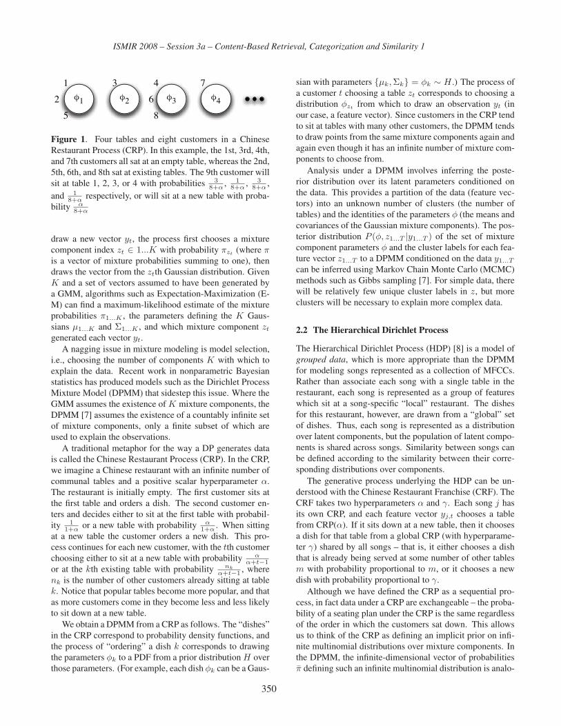
ISMIR 2008 – Session 3a – Content-Based Retrieval, Categorization and Similarity 1
�1 �2 �3 �4
1
2
3 4
5
6
7
8
Figure 1. Four tables and eight customers in a Chinese
Restaurant Process (CRP). In this example, the 1st, 3rd, 4th,
and 7th customers all sat at an empty table, whereas the 2nd,
5th, 6th, and 8th sat at existing tables. The 9th customer will
sit at table 1, 2, 3, or 4 with probabilities 38+α , 1
8+α , 38+α ,
and 18+α respectively, or will sit at a new table with proba-
bility α8+α
draw a new vector yt, the process first chooses a mixture
component index zt ∈ 1...K with probability πzt (where πis a vector of mixture probabilities summing to one), then
draws the vector from the ztth Gaussian distribution. Given
K and a set of vectors assumed to have been generated by
a GMM, algorithms such as Expectation-Maximization (E-
M) can find a maximum-likelihood estimate of the mixture
probabilities π1...K , the parameters defining the K Gaus-
sians μ1...K and Σ1...K , and which mixture component zt
generated each vector yt.
A nagging issue in mixture modeling is model selection,
i.e., choosing the number of components K with which to
explain the data. Recent work in nonparametric Bayesian
statistics has produced models such as the Dirichlet Process
Mixture Model (DPMM) that sidestep this issue. Where the
GMM assumes the existence of K mixture components, the
DPMM [7] assumes the existence of a countably infinite set
of mixture components, only a finite subset of which are
used to explain the observations.
A traditional metaphor for the way a DP generates data
is called the Chinese Restaurant Process (CRP). In the CRP,
we imagine a Chinese restaurant with an infinite number of
communal tables and a positive scalar hyperparameter α.
The restaurant is initially empty. The first customer sits at
the first table and orders a dish. The second customer en-
ters and decides either to sit at the first table with probabil-
ity 11+α or a new table with probability α
1+α . When sitting
at a new table the customer orders a new dish. This pro-
cess continues for each new customer, with the tth customer
choosing either to sit at a new table with probability αα+t−1
or at the kth existing table with probability nk
α+t−1 , where
nk is the number of other customers already sitting at table
k. Notice that popular tables become more popular, and that
as more customers come in they become less and less likely
to sit down at a new table.
We obtain a DPMM from a CRP as follows. The “dishes”
in the CRP correspond to probability density functions, and
the process of “ordering” a dish k corresponds to drawing
the parameters φk to a PDF from a prior distribution H over
those parameters. (For example, each dish φk can be a Gaus-
sian with parameters {μk, Σk} = φk ∼ H .) The process of
a customer t choosing a table zt corresponds to choosing a
distribution φzt from which to draw an observation yt (in
our case, a feature vector). Since customers in the CRP tend
to sit at tables with many other customers, the DPMM tends
to draw points from the same mixture components again and
again even though it has an infinite number of mixture com-
ponents to choose from.
Analysis under a DPMM involves inferring the poste-
rior distribution over its latent parameters conditioned on
the data. This provides a partition of the data (feature vec-
tors) into an unknown number of clusters (the number of
tables) and the identities of the parameters φ (the means and
covariances of the Gaussian mixture components). The pos-
terior distribution P (φ, z1...T |y1...T ) of the set of mixture
component parameters φ and the cluster labels for each fea-
ture vector z1...T to a DPMM conditioned on the data y1...T
can be inferred using Markov Chain Monte Carlo (MCMC)
methods such as Gibbs sampling [7]. For simple data, there
will be relatively few unique cluster labels in z, but more
clusters will be necessary to explain more complex data.
2.2 The Hierarchical Dirichlet Process
The Hierarchical Dirichlet Process (HDP) [8] is a model of
grouped data, which is more appropriate than the DPMM
for modeling songs represented as a collection of MFCCs.
Rather than associate each song with a single table in the
restaurant, each song is represented as a group of features
which sit at a song-specific “local” restaurant. The dishes
for this restaurant, however, are drawn from a “global” set
of dishes. Thus, each song is represented as a distribution
over latent components, but the population of latent compo-
nents is shared across songs. Similarity between songs can
be defined according to the similarity between their corre-
sponding distributions over components.
The generative process underlying the HDP can be un-
derstood with the Chinese Restaurant Franchise (CRF). The
CRF takes two hyperparameters α and γ. Each song j has
its own CRP, and each feature vector yj,t chooses a table
from CRP(α). If it sits down at a new table, then it chooses
a dish for that table from a global CRP (with hyperparame-
ter γ) shared by all songs – that is, it either chooses a dish
that is already being served at some number of other tables
m with probability proportional to m, or it chooses a new
dish with probability proportional to γ.
Although we have defined the CRP as a sequential pro-
cess, in fact data under a CRP are exchangeable – the proba-
bility of a seating plan under the CRP is the same regardless
of the order in which the customers sat down. This allows
us to think of the CRP as defining an implicit prior on infi-
nite multinomial distributions over mixture components. In
the DPMM, the infinite-dimensional vector of probabilities
π̄ defining such an infinite multinomial distribution is analo-
350

ISMIR 2008 – Session 3a – Content-Based Retrieval, Categorization and Similarity 1
�1 �1 �2 �1
1
2
3 4
5
6
7
8
�2 �3 �3
1 2 3
4
5
67
8
�4 �1 �2 �1
1
2
3
4 5 6
7
8
�1 �2 �3 �4
1,1
1,2
1,4
3,2
3,4
1,3
2,1
3,2 2,2
2,3
3,1
Figure 2. Chinese Restaurant Franchise (CRF) for three
songs with eight observations. Below are three CRPs (cor-
responding to the three songs), and above is the global CRP
from which the CRPs get their dishes. Each customer j, isitting at a table in the global CRP corresponds to table iin restaurant j, and customer j, i’s table membership in the
global CRP determines the dish that is served at table i in
restaurant j. If a new customer coming into a restaurant jsits down at a new table, then the dish for that table will
be φ1, φ2, φ3, or φ4 with probability 5γ+11 , 3
γ+11 , 2γ+11 , or
1γ+11 respectively, or a new dish with probability γ
γ+11 .
gous to the K-dimensional vector π in the GMM. The HDP
has J such vectors π̄1...J , each of which defines a different
distribution over the same mixture components.
We use Gibbs sampling to approximate the posterior dis-
tribution over the latent variables conditioned on observed
data. The distribution is over the cluster partition assign-
ing feature vectors to clusters and a truncated vector πj
defining the mixture proportions for each song over the fi-
nite subset of K mixture components that are actually as-
signed to observations. We let πj,1...K = π̄j,1...K , and
πj,K+1 = 1 −∑Kk=1 π̄j,k, where πj,K+1 is the probability
of drawing an observation from a mixture component that
has not been used to explain any feature vector in any song.
For a complete exposition of the HDP, including how to
infer the posteriors for its parameters conditioned on data,
see [8].
2.3 Representing Songs Using the HDP
The mixture components parameterized by φ1...K capture
the latent structure in the feature data, and the mixture pro-
portion vectors π1...J express the feature data for songs 1...Jin terms of that latent structure. φ and πj together can de-
scribe the empirical distribution of feature vectors for a song
j as richly as a GMM can, but the HDP does not require that
we choose a fixed value of K, and represents the songs in a
more compact way.
To compute the distance between two songs i and j, we
can compute the symmetrized KL divergence between the
posterior distributions P (πi|β,m) and P (πj |β,m) which
are of the form
P (πj |β,m) = Dir(β1 + mj,1, ..., βK + mj,K , βK+1) (1)
where mj,k is the number of tables in restaurant j serving
dish k, βk is the likelihood of choosing a dish k from the
global CRP, and βK+1 is 1 −∑Kk=1 βk, the likelihood of
choosing a previously unseen dish in the global CRP.
This allows us to compare two songs in terms of the latent
structure of their feature data, rather than directly comparing
their distributions over the low-level features as the G1 algo-
rithm and GMM-based algorithms do. The KL divergence
between these two posteriors can be efficiently computed.
The KL divergence between two Dirichlet distributions with
parameters v and w each of length K is [9]:
D(Dir(v)||Dir(w)) = logΓ(∑
v)Γ(∑
w)+
K∑s=1
log(Γ(ws))log(Γ(vs))
+
K∑s=1
((vs − ws)(Ψ(vs)−Ψ(∑
v))
where Γ(x) is the gamma function, Ψ(x) is the digamma
function (the first derivative of the log gamma function), and∑v and
∑w denote the sum of the K elements of v and w
respectively.
This is less expensive to compute than the KL divergence
between two high-dimensional multivariate Gaussian densi-
ties. It can be sped up further by computing the gamma and
digamma terms offline for each song.
2.4 Generalizing to New Songs
It is important that our approach be scalable to new songs
not seen during training. Once we have inferred the global
dish likelihoods β and the mixture component parameters
φ1...K , we can infer the posterior distribution over the mix-
ture proportions πJ+1 for a new song J + 1 conditioned on
β, φ, and the new data yJ+1 using the same Gibbs sam-
pling techniques originally used to train the model, holding
all other parameters constant.
351

ISMIR 2008 – Session 3a – Content-Based Retrieval, Categorization and Similarity 1
3 EVALUATION
In this section we describe the experiments we performed to
evaluate our approach against G1, GK (the analogous algo-
rithm for K-component GMMs), and an approach based on
Vector Quantization (VQ).
3.1 South by Southwest Dataset
We test our approach on a dataset that we compiled from
the South by Southwest (SXSW) 2007 and 2008 festivals’
freely distributed “artist showcase” mp3s [10]. We selected
a set of up to twenty mp3s (all by different artists to avoid bi-
asing the results) for seven genres: country, electronic, hip-
hop, jazz, metal, punk, and rock. Songs that we felt were un-
representative of their genre were removed or replaced prior
to any quantitative evaluations. There were fewer than 20
usable songs available for country (12), jazz (14), and metal
(15), so those genres are slightly underrepresented. There
are a total of 121 songs in the dataset.
3.2 Features
All models were trained on the same sets of feature vectors,
which for each frame consisted of 13 MFCCs (extracted us-
ing jAudio [11]) combined with 26 delta features computed
by subtracting the MFCCs for frame t from those at frame
t − 1 and t − 2, for a total of 39 dimensions. Each frame
was approximately 23 ms long, or 512 samples at the files’
sampling rate of 22050 Hz, with a hop size of 512 samples
(no overlap). 1000 feature vectors were extracted from the
middle of each song.
3.3 Models Evaluated
3.3.1 G1
As described above, G1 models each song’s distribution
over feature vectors with a single multivariate Gaussian dis-
tribution with full covariance matrix. Models are compared
using the symmetrized KL divergence.
3.3.2 K-component GMMs
We train K-component GMMs for each song using the E-M
algorithm. The symmetrized KL divergence between mod-
els is approximated by drawing 1000 synthetic feature vec-
tors from the trained models and evaluating their log likeli-
hoods under both models [1]. This approach is evaluated for
K = 5, 10, 20, and 30.
3.3.3 VQ Codebook
This algorithm is meant to be a simple approximation to
the HDP method we outlined above. First, we cluster all
of the feature vectors for all songs into K groups using the
k-means algorithm, renormalizing the data so that all dimen-
sions have unit standard deviation. This defines a codebook
of K cluster centers that identifies every feature vector with
the cluster center to which it is closest in Euclidean space.
For each song j, we compute the vector πj,1...K of the rela-
tive frequencies of each cluster label. Each πj,1...K defines a
multinomial distribution over clusters, and we compute the
distance between songs as the symmetrized KL divergence
between these multinomial distributions (smoothed by a fac-
tor of 10−5 to prevent numerical issues).
This algorithm, like our HDP-based method, represents
each song as a multinomial distribution over latent cluster
identities discovered using an unsupervised algorithm, and
lets us see how a much simpler algorithm that uses similar
ideas performs compared with the HDP.
3.3.4 HDP
We train an HDP on all of the data using the direct assign-
ment method [8], inferring the posterior distributions over
the πj’s for each song j and computing the distance between
two songs i and j as the KL divergence between the posteri-
ors over πi and πj . We place vague gamma priors on α and
γ [8]:
α ∼ gamma(1, 0.1), γ ∼ gamma(1, 0.1) (2)
and learn them during inference. For the prior H over φ,
we use the normal-inverse-Wishart distribution [12] with pa-
rameters κ0 = 2, ν0 = 41 (the number of dimensions plus
two), and μ0 = ȳ (the mean of all feature vectors across
songs). The normal-inverse-Wishart matrix parameter Λ0
was chosen by averaging the covariance matrices from 100
clusters of feature vectors, each of which was obtained by
choosing a feature vector at random and choosing the 24,200
feature vectors closest to it under a Euclidean distance met-
ric. (The number 24,200 was chosen because it was 1/5 of
the total number of points.) The goal of this process is to
choose a matrix Λ0 that resembles the covariance matrix of
fairly large cluster of points, encouraging the model to find
similarly shaped clusters. Using smaller (larger) clusters to
choose Λ0 would result in the model creating more (fewer)
latent topics to explain the data.
3.4 Experiments
Since human-labeled ground truth similarity data is inher-
ently expensive and difficult to acquire, we follow previous
researchers [1, 2] in using genre as a proxy for similarity.
We assume that all songs labeled with the same genre are
“similar,” which allows us to use evaluation metrics from
the information retrieval literature. We first compute a full
121x121 distance matrix between all songs using each al-
gorithm. For each query song sq, each other song si is
352

ISMIR 2008 – Session 3a – Content-Based Retrieval, Categorization and Similarity 1
G1 G5 G10 G20 G30 VQ5 VQ10 VQ30 VQ50 VQ100 HDP
13.24 829 1487 2786 4072 0.58 0.59 0.63 0.686 0.85 0.25
Table 1. Time in seconds required to compute a 121x121 distance matrix for G1, GMM-based (K = 5, 10, 20, 30), VQ-based
(K = 5, 10, 30, 50, 100), and HDP-based algorithms.
G1 G5 G10 G20 G30 VQ5 VQ10 VQ30 VQ50 VQ100 HDP
RP 0.3254 0.3190 0.3287 0.3144 0.3146 0.2659 0.2997 0.3191 0.340 0.3313 0.3495AP 0.3850 0.3761 0.3746 0.3721 0.3706 0.3171 0.3546 0.3850 0.3989 0.3910 0.3995AUC 0.6723 0.6712 0.6687 0.6679 0.6661 0.6513 0.6675 0.6846 0.6893 0.6758 0.7002
Table 2. Three measures of retrieval quality: mean R-Precision (RP), mean Average Precision (AP), and mean Area Under
ROC Curve (AUC) for G1, GMM-based (K = 5, 10, 20, 30), VQ-based (K = 5, 10, 30, 50, 100), and HDP-based algorithms
on the large SXSW dataset.
G1 HDP
RP 0.5486 0.6000AP 0.6807 0.7154AUC 0.8419 0.8983
Table 3. Mean R-Precision (RP), mean Average Precision
(AP), and mean Area Under ROC Curve (AUC) for G1 and
our HDP-based algorithm on the smaller dataset.
given a rank rq,i based on its similarity to sq. The qual-
ity of this ranking, i.e. how well it does at ranking songs
of the same genre as sq more similar than songs of differ-
ent genres, is summarized using R-Precision (RP), Average
Precision (AP), and the Area Under the ROC Curve (AUC),
which are standard metrics from the information retrieval
literature [13]. All experiments were conducted on a Mac-
Book Pro with a 2.0 GHz Intel Core Duo processor and 2
GB of RAM. All models were implemented in MATLAB.
3.4.1 Testing on Additional Data
To test our HDP-based method’s ability to generalize to un-
seen data using the method in section 2.4, we use the HDP
trained on the large SXSW set to compute a similarity ma-
trix on a smaller set consisting of 5 artist-filtered songs per
genre (35 in all) by artists not in the training set. The elec-
tronic, punk, rap, and rock songs came from the SXSW artist
showcase collection, and the country, jazz, and metal songs
came from a dataset previously used by George Tzanetakis
[14]. We also compute a similarity matrix on this dataset
using G1, and compare the RP, AP, and AUC metrics for
retrieval quality obtained using both algorithms.
4 RESULTS
Tables 1, 2, and 3 summarize the results of our experiments.
The best results in each row are in bold.
The amount of time required to compute the distance ma-
trices for the GMMs was, as expected, enormous by com-
parison to the other models. The cost of computing the KL
divergence for the VQ-based and HDP-based models was
more than an order of magnitude lower even than the cost of
computing the KL divergence between single Gaussians.
The HDP performed better than the other models for all
three standard information retrieval metrics, although the
VQ model with K = 50 was a very close second. None
of the GMMs outperformed G1.
The results in table 3 show that the HDP-based approach
does generalize well to new songs, showing that the al-
gorithm can be scaled up efficiently to databases of many
songs.
4.1 SIMILARITY HUBS
The G1 and GK approaches are known to produce “hubs”
[1] – an undesirable phenomenon where certain songs are
found to be similar to many other songs. The hub phe-
nomenon is a potentially serious concern, since it can re-
sult in very bad matches being selected as similar to a query
song.
Our HDP-based approach does not suffer from this prob-
lem. Figure 3 shows how often each song is ranked in the top
five of another song’s similarity list for similarity matrices
obtained from G1, the HDP, and choosing distances at ran-
dom. The randomly generated histogram shows the sort of
distribution of hubs one would expect to see due to chance
in a dataset of this size. The HDP’s histogram closely re-
sembles the random one, indicating an absence of abnormal
hubs. G1’s histogram, by contrast, shows more severe and
more numerous hubs than the other two histograms.
353

ISMIR 2008 – Session 3a – Content-Based Retrieval, Categorization and Similarity 1
0 50 1000
5
10
15
20
25
0 50 1000
5
10
15
20
25
0 50 1000
5
10
15
20
25
Figure 3. Histograms of how often each song is ranked in
the top five of another song’s similarity list for similarity
matrices obtained using G1 (left), the HDP (center), and by
choosing distances at random (right).
5 CONCLUSION
We developed a new method for assessing the similarity
between songs. Our HDP-based approach outperformed
the G1 algorithm, can compute large distance matrices ef-
ficiently, and does not suffer from the “hub” problem where
some songs are found to be similar to all other songs.
Since our approach does not have access to any informa-
tion about temporal structure beyond that provided by the
MFCC deltas (about 69 ms in total), we expect that com-
bining the distances it provides with fluctuation patterns or
some similar feature set would provide an improvement in
similarity performance, as it does for the G1C algorithm [2].
One area of future work involves relaxing the bag-of-
feature-vectors assumption. For example, we might learn
distributions over texture patches of feature vectors instead
of individual feature vectors. Hidden Markov models can
also be fit into the HDP framework [8], and may yield im-
proved results.
6 REFERENCES
[1] Aucouturier, J-J and Pachet, F. “Improving Timbre Sim-
ilarity: How High’s the Sky?,” Journal of Negative Re-sults in Speech and Audio Sciences 1 (2004), no. 1,
http://journal.speech.cs.cmu.edu/articles/2004/3.
[2] Pampalk, E. “Computational Models of Music Simi-
larity and Their Application to Music Information Re-
trieval.” Ph.D. Dissertation, Vienna Inst. of Tech., Aus-
tria, 2006.
[3] Pampalk, E. “Audio-Based Music Similarity and Re-
trieval: Combining a Spectral Similarity Model with
Information Extracted from Fluctuation Patterns,” Pro-ceedings of the International Symposium on Music In-formation Retrieval, Victoria, BC, Canada, 2006.
[4] Pohle, T. and Schnitzer, D. “Striving for an Improved
Audio Similarity Measure,” Proceedings of the Interna-tional Symposium on Music Information Retrieval, Vi-
enna, Austria, 2007.
[5] Jensen, J., Ellis, D.P.W., Christensen, M., and Jensen,
S. “Evaluation of Distance Measures Between Gaus-
sian Mixture Models of MFCCs,” Proceedings of the In-ternational Symposium on Music Information Retrieval,Vienna, Austria, 2007.
[6] Barrington, L., Turnbull, D., Torres, D., and Lanckriet,
G. “Semantic Similarity for Music Retrieval,” Proceed-ings of the International Symposium on Music Informa-tion Retrieval, Vienna, Austria, 2007.
[7] Neal, R. “Markov chain sampling methods for Dirichlet
process mixture models,” Journal of Computational andGraphical Statistics, 9(2):249-265, 2000.
[8] Teh, Y., Jordan, M., Beal, M., and Blei, D. “Hierarchical
Dirichlet processes,” Journal of the American StatisticalAssociation, 101(476):1566-1581, 2007.
[9] Penny, W.D. “Kullback-Liebler Divergences of Normal,
Gamma, Dirichlet and Wishart Densities.” Technical re-
port, Wellcome Department of Cognitive Neurology,
2001.
[10] http://2008.sxsw.com/music/showcases/alpha/0.html
[11] McEnnis, D., McKay, C., Fujinaga, I., and Depalle, P.
“jAudio: A Feature Extraction Library,” Proceedings ofthe International Symposium on Music Information Re-trieval, London, UK, 2005.
[12] Gelman, A., Carlin, J., Stern, H., and Rubin, B.
Bayesian Data Analysis CRC Press, New York, 2004.
[13] Manning, C., Raghavan, P., and Schütze, H. Intro-duction to Information Retrieval. Cambridge University
Press, Cambridge, UK, 2008.
[14] Tzanetakis, G. “Manipulation, Analysis and Retrieval
Systems for Audio Signals.” PhD thesis, Computer Sci-
ence Department, Princeton University, 2002.
354

ISMIR 2008 – Session 3a – Content-Based Retrieval, Categorization and Similarity 1
� �
�
�������������������������� ������
���������������� ��������������������
�� �����������������������
����������������
���� ��
� �� ����� ����� ���� � � ��� ���������������������� � ����� ���� ���� �� � �������� ��� ������ ���� �� ��� � �� ���� ������������������������������ ��� ���� ��� �� !"�$$$� ���� � ���� � '���� <!"� ������� �� � �� �� ��� �� ���� � ����������!� � �� �� ��� �� ������������ �� � ���� ��>��� � ��� ����� ���'�������� ��� �� ��?���' ������� �� �� ��� ��� �� � ������� �� � �� �� ��� ���� �� � ���������� ��� \� � � ��� ��� ���'�� ���� ��� � ���^ ���� � �� ������ ��� �� � � � ������� ' ���� �� �� ��� �� � �� ����_� �?������������������\���������������� � ������������ ���������� ������ �`|~�������������� ��� �� �� ���������� � ���� �� ����������������� �� ���
��� �����!"�����
������ �� � � � ����� � �� ������� �� ����� �� ������������ ��� � ����� ��� �� �� ���� ���� �� � ��������'� �� ������ ������������ �?� ������������������ ?�'����� � � ���?� ����� ��� ���� �������������� ����� ������ �� � � ���� � ��� �� � ������� ��� ������ ���� �� ' ��� �� ���� � ���?����� ��� ������������������ ���������� �� �����?�������
`�� � � ��� ��?� �� � ����� ��� ���� �������� �� ��� '������� �� �����?�� �������� ��� �������� ��� ��� � �� ����� � �^������ ��� �� ?� �������� �� � ���� ��������������������� ��� � � � �� �� �<��� \� � � � ��� �� ������ � � ����� ������������������ ���� �������� ��� �� ����������� ��� ����� � ��� �?� �������� � '� �� �� �� ����� ��� ����� ��� �������
��� ������ ���' �� �� � ��� � ��� ��� ����������� �������������� ��� ������\� ���� �����������'�� ���'�� ����� �� ����� � �������� � ����� � ��� ������ ������ �� �� ���� \� � ������ ���� ���� ������� ?� ��' � �?� ���� �� � �'�� ��� ��^ ���� � ������� � ��� �� �� � � � �� �?� ����� ������� ���� � ���� �� ������ � � �� ������������� ��'� ���� ���� � ��� �����^���� ��������� ��������
\���� ������ �� �� �� ��� '����� �� ��� ����� ����� ������ ���������������� ������� ���������������?��� �����' � ������ ����������� � ��� �� ���������� ���� ������������?� � ���� ��� ��� �� � �������� ��� �� ��� �� �����������
|�� �������?� ���� � ����� � �� � ��� ��� ��� '����� ����� �� ��� ���� �� ��� � ��� � ����� � �' �� �������������� � ��� �� ����� �� ����� �� � �������� ������ �������� �� � ������?� ��� �� � �������� ��� �� � ������ \� ��������� � ����� ����� � ��� ��� ���� �� ������� �� � ������� ������������������?����������������������� �� ������� �������� ��
��' � �?��� ��� ����������������� ���� �� ������������� �������� ��� ��������������� ������������������������������������� ������� ����
|�� ����� �?� ' � � ����� � � ��� ����� � ��� ��� ����� � � � ��� ��� � ���� �� ��� ����� �� ����� � ����������� � � �� � � !"�$$$� ����� ���� � ��� ����� ���������� �?������� ��'������� ����� �������� ���?������ ������� ��� �� � ������ ������ ��<��� \�� ���� � ���� �� � � ��� ��� ��� ���� ��� �?� ' � �� � ��� � � ��� ��� ���� � ���� ��� ���� �� ����� � �� �������� � ��� ���� ������� ����� ������� � ���� �������� ��� �������� ���� � �� �� ����������� � �� ��� �� ����
#�� �$�� ����%�� %�!����������
\� � ����� '�� ��� �� �� ����� ��� ������ ����������������� ����� �������� ������� ��� ��� �� ������ � ��� �� ������� ������ �� � � ����� ���������������������������� �� ��� �� � �����?� ��� ��� ����� ������� ��� ����� ����`���������� �����`���� ������������������ ������������� ����\� � �������� ���� ��� ��� �� �?��������������� ������ ������ ������ ��?������ ��� ������� ���� ���� ���|���� � � ��� ������ ����� ��'���������� �?������� ������� ������ �������� ��� ��������� � � ��� �� �� ������ � ���� ������� ��� � ����������� �������� ����� ������������������ ����������
|������� ��' �� ����� ��� � ��� ��������������������� ���� ��� ���� ��� � !"?$$$� ����� ���� �� � � �� � ��� ����� � ��� � ��� � � ��� ��� ����� ���� ������� ���� � ��������������� � �� � ��� `�����?� � ��������� �������� � �� ���������� ���� ���������?� ��� � � �� ��� ������ � �� � ��������� ������������\� � � � ��� � � ��� � �� ����� �� ����� �� ���� ��������
#����������� &'�������&����
\� �������� ��� �� ��' ������� ������ �� ������� ������� �������������� ��>��� ������ \� � �>�� ����� �'���
355

ISMIR 2008 – Session 3a – Content-Based Retrieval, Categorization and Similarity 1
� �
����� ���� ��� ��� ���� ���������� ��� � � �����?� �� ��� ��� � ?���� ��� � �?� �� �� ���� ��������� ��� ������ � ������� �������� ���� ���� \� � �>�� ����� ��������� ������ �������� ���������������� �������������������������������� � ��� �� ����� �� ��� ���������?� ������ � �� �����\ ��������?� �� � ������ ��� � �� �� �� ����� ���� ���� ?����������� ��������� �?������'������� ��� �� �������� ����� ��� \� � � ��� �� � � �� �� ��� �� �� ��� �� �������������������������� �����?������������������������ � � �������� � ��� �� � � ��� �� ������ ��� ��� �� ������ � ���� �� ��� ������ ����� �� ������� `����� �`�� ��� ��``���� |�� � �� ���� �� ������������� ���� ��?��� � ���� �� ��� ��� ��� ��� ������������������ ���\� ��>����������� ��� � ��� ���������'������� �� ����� ��� �� ��?� ����� ���� � ��� �� ��� � ��� �� �������� �����?� ����� � ��� ���������� � �������� � ����������������� ��� ���� ��� ������� `����� � `�� ���?� �������� � ��� �� � ������� �� �� ������� \� �?� ������ � �����`���� �?� �``� ������� ��?� ������ `��� ��� ��� �� �`|~���� ���� �� ���� � ��� ����'�����������������>���� � ��� ��� ��� �� ����� ������������� ���� ��� ���?����?� ��"�?� ������ ��������� �� ��� � ������ � � �� ���� ��� �?��� � �'������ ������� ������� ��>���������� � � ���� ���� ��������� � '�� � ��� � ��� ������ ������� ����������
\� ��������� ��� �� ��' ������� ��� � ��������������������� � ��� �� �� �� ������� ����� �� � `������ ������������ ������ \���� � �� ������ �� � ����� ����� ���������� ����� � ������?� ��������� ��� �� '� ��?� ���?� ` ���� _� ����� �������� ����� ����?� � ��������~?�|�� �������� �~�� �?� ����������� ���������\� � � � ��� ��� � ��� ��������� ���� �� ���� �� ��� � � �����?� �� �� �� �� ��������������� ��������������������������������������� ���������������
������� � ��� ���� �����' � � ����� �� ��� �� ��� �� ������� �>�� �� � ��� ���� ����� � ��� � � ��� ��������������������������� ������?�������������� ������� �������� �� ��� � ��� � ��� ���������?� ��� � ��� � ��� �� ����\� �� ������ ������ �' ������������������������� ���� ��� � �� '���� �� � �����'���� �� � ���� "$��� ��� ���� �������?�$$�����'������$ ��� �������� ������"������ ������� ����� ��������� ������ ��������� ����� ?��� � � ��� �� � � �� � �'�� ������ ���������� ��� ���� ��� �����������������?� �� �� �� � � �� ��� ����� ?� � � ������ � �?��� ������������� ��� �� ����������� �������������� ���¡��������� ����
#�#���(���)��� &'�������&����
\� ������������������������������������� ��� ����`��������� �� '���� � � �� ��� ����������� �������� � ��� ��� � �� �� � ������ ��������������� ������� ������������� ����������� \� � � ���� ���� � ��� �� �� � � ���� �� ��� ���� ����� ��������� ����� ������������� �������� ���� ���� ����� �� �?� �� � � ������ � ��� � � �� ������ ������ ��� �� ����������� ��������?�'����������� ��
��������������'������ �� � ����� ��� �� ��������� ����� �� � � � ���� � �?� �� � � ������ � �� �� �� ���� �� � �� � ��� ������ ��� � ��� � ��� ����� �� ��� �� � '��� � �����?��������� ��� ������� � ������ ������� ������������ ���������� ?� �� � � ��� � � ����� �� �� � ��������� ��� �� ����� �� �� ��� �� � ���������� ��� �� � ���� ��������� ��� �� �'��� � ���� �� ����� �� �� � � � � ���� �� � ��������� ��� ������� ���������������������������� ������������ �� � � � � ��� �� � ��������� ��� �� � � � ��� �� �� ' � � �������� ��� � �� �� ��� �������� �� � ������� �� ����������� ������� ��� ��� �'�� � ����� ?� ���� ���� � ���� ��� �� ����
#�+���&/�������&����
�����?� ' � ���� �� � ������� �� '���� ������ � �� ��� ��� ���� ��� ��� �<!"����� ���� �������� ���������������� ����� �� ���� � �� � �����'���� � ������� ���������� �������� ����\�������������� ����������� ������ ���� ����� � ��� �� �� �� � � �� ��� � � ���� �� ���� ������������ ������' � �?���' �'����� ?��� � �� ��� ��� ������������ ������������������� � ������ ��� ������������������������ �������������' ���� ���������� ��� �� ����� ��������� �����������������
+�� ���������!�! � � ���
+���� ������::�'����;���<��������������
� � ������� ���������� ���������� �� ������ ������� �`|~����������?���������� �~������� ����?��� �������� ���� �� �� � �� ���� �� � `|~�¢� � ���� �!�����' � �?���� ������ ������� ���� �������� ������� ���� � ������ ������������ ��������������������' ��� ��� ��� ������ ��� � ���� ���� � ����� �� ��� �� � ������������� ��$��� \���� ���� � ��� � ��� ��� �� ������ ����� � � ��� ������� � ��� � � �������� ��� ��� ����� ���������� �������� ��� ����������������������������������� ��?� ����� �� ������� � � �����?� � ���� ������?����� �� ������ ���'����?� ���� \� � ������� �� ��� � ��������$������ ������� ���������\� ��� ����� ������<��� ���� �?� � � � ������ � � ������ ��� ������ ��� �����������?� �����?� �������� ����?� ����� ���������?� ������?�!�������?������?�"��#"����?������?�$�����?��������?�����?� $�������?� %�����?� &����� ��� '������������ ��� � ����� � � ��� � ��� � ��� ������� ��������������^ ���� � ����������� ����� �� �� � �� � �� � ��� ��������������?������ ��� ������ ������� �����?���' �������� ����^ ���� � ����� �������� ����� �� ����� �?� ������ ��� ���������� ��� �� � ������ \� � '��������� �� ����� ����������� � ����� ��� �� ��?� ��*?� ������� ��� ����� |��� � � ������ �������������� ����� ?������ �� �� ����������������������� ������������������������\� � ���� ��� ���� ?���������� ?��������� ������� ��
\� ��� ������������� �����'������������������������������� ��� ���� ���� � ��� ���� � �� ��� ���� ��� ��� �� �
356

ISMIR 2008 – Session 3a – Content-Based Retrieval, Categorization and Similarity 1
� �
��� ����� ����� ������� �� ���������� �� � �� ������������9���� �� ���������� ����'� �� �� �� �� ���� �� � ������� � �� ��� ��� � � ������ ��� ��� ������� � �� ����?���� ���� ������������� � ������ ������������������ ��� ��� � � � � �� ��� \� � ��� � �� �?� ���� � ���� ���� ����� �?������ ����� ������� ����� ���������<������ ���\� � �� ����� �� ���� �� � � �� �� ������ � �� ��� ��� ���������� �� ������?� '��� �� ���?� ����� ��� ��������?� � ���� ����� �� ������� ���� ��� ��� � �� � ��� ���� ������� �� ����������������� ��� �' ������ ���������� ������ �� ������� ����� ������ �� � �� ���������� � ������������ ������ ��� ��������� ��� �� ��� � � �� � ������������ ��� ��?� ��� � � ��� � ��� ������ �� � � ���� � ������_����������������� ��������� �� ���?������ ������������ � ��� ���������� � ������� ���� �� ��� '������� � � ��� ��� �� ��������� ������������ �� � � ��������� �� ��� ��� � ��� � ��� � ��� ��� ���� �� ��� ��� � ������� � �� �� ���� �?� � � ������� '����� ��� ���������� ������ � �'�������������� ������������ ���
\� � � ��� ��� ���� ����� '�� ��� ���� � ���� �� ��� ���������� ����� �� ������ ��� ���� ��� ��� ������� �������������?����' ������������� ���� ����� ������'������� �� �� ������� ������� ��� � ������ ��� �� ��� '�� ����� �� � ��� � �� ?� ��� ���������� ���� �� '���� � ������� ���������� ��� ��'� _������� ���� ������ ?� ' � ������ �������� ������ ����� � ��� �� ��� � �� ��� ���� �� ���� �� �� �� � �!���������������?� ' �� ������� ���� � �� ��� ����'����� ' � ��� � ����������� ������ ��� ���� �� ���� � "$��'������ ����������������� �?���������������������� ������� ������������� ������ ������� ��������������� ��?��� ���������� ��������� �������� � �������������������!"���?������ ����� ����� �� ���<!"�� �£�� � ���� ���� � �� ��� ���� ���������� �<!"������� ��� �������� � � ��� ���� ����� ������ ������"�!������������������' � ���� ������� ����������*��� ��� � �� �"�� ����� \���� ���� � '�� �� �� ����� ���������������� ������� ������ ���� � ������ �� �?���� ����� ������ �����������
+�#��!���=������'&�'�����
\� ������������ �������������� �� ������ ������� ���� �������� � ������������������������������ ���� ��!������ ��������<!"������ � ������� ���� �� ��������� ��� ������ � ��� ���� ���� ������� �������� ���� ���� �������� ��� �� ������ |�� ��� ���� ���������� ���� ������ ?� �� ���¤�������� �� � ¥� ��� ¤����� � �� �¥� � � ' ������� �� ��� \���� � �������� ��� � �� ���� �� ��� ����� ������ ���������������������� � �� ?� ���������� �������'�� ������� �� ����� � ����� � ��������� ��� ����������� ?������������ �������������������������
+�+�� �������;�:����)�����
\��������� ����� ������ � �������� ���� ��� ����� ���������� � ���?� �� � ���������� ����� ��� ����� ����������� ����� ����� � ������� ����������� ������������ ���� �?��� ���������� ��� �� � ��������� ��� ������ � ��� �� ��� �� �� �
���� �� ���� � � ���� ���� ����� �� ��� ���� ' � � ���� ������ ���� ��� \� � ���������� �� ��� �� � ��������� ��� �� �� ���� �� ������ � ��� �� ���� ' � � ���� ���� �� �� �� ������������������� � ��� �� ��� ��������� �� ��� ������� � ���� � ��� �?� �� � � ������� '���� ������� � ������������� ������������� �� ����� �����'?�� ���� �������� � ����� _������ ��� �� � ������� ��� \� � ��� ��� ���� �� ����������� �������� ��� �����
� � � � � � � � � � ���' � �?� ��� ���� �� ?� ' � �� � ��� �� � '���� �
���������������� ��"�������������������������� ����� �� �� ����� ���� �� ���� ��� ����� ���������������������������������� ������������������\���������������?�' ��� ����� � ������� ��������������� ���'������ ���� �� ���������� ���������?�� ��� ������ ������������ ���� �� � ��� ��� � ���� �� � ������ � ��� � ���� � �� ��� ����������������� ������������ ���� ��� ����� ��������� ��'������ ������������������� �' ���� ���� ���
>�� �$����?����
>�����@(���/����!���;��
� �������������� �;���������� �����'������� ������������� ������?� ��� ���������� �������� ������ ��� �� ��� � ��������� ��� ��� �� ��� ����� �� ��� �� ���� ����� ����������� ������ ���������� ���� ���������� � �� ������ ������ ������ � ���� �� �������� '����� �� ���� ����� ����� �������� ��?��� ����� ���� ��� �� �� �������?� ��������� ��� �������� \� � � ������� ��� ����� �� �������� �����`���� � ���`�����������'���� �~�������������������~����� �� �?����' � ����� ������ �� �� ������ ������ ��� ����� `�� � � ��� ��?� ���������� �?� ���� � ��� �� �� �?� ��� ���� �� ��� � ������������� ������� ����������?��� ���� ���� ������� �����������'������ ��� ����� ������\�� ��������� ������ ������������� �����������%�*?�����������;�����|������� ��� ���� ���� �� � � ���������� ��������� ����� �� �����"$� ����<!"$�� \���� ����� ���� � ��� � ��� ��'� � � � ���� �� ������������������ ����� ���������� ���\� �������� ���� ��� ��� �� ������� �'��� ������� ��£�� ������� ������� ������������������� ��'����� ����� ������������ �� �?�'�����^������ ���� ��� ������ �������������������� ����� � ������� ���� ���������� ���
>�#�����'�/�����:���
\���� ����� � ������� ��������������� ��?�' ����� ��� ������������������ ��������� ��� ���������'������ ���� �� �� '���� �� ������ � ��� �� ���� �� � ��� � <���� ���� ��� �?�'����<� �� � ��� ������ �� ���� ��?� ��������� �� ����������'����������������#<��
��� � ��������?� �� � ������� ��� � ��� � ������ ���� ������ � ���� ��� �� � ��������� ��� ������ � ��� � ���� � ��� ������� �� ������� ��
357

ISMIR 2008 – Session 3a – Content-Based Retrieval, Categorization and Similarity 1
� �
����� ������ ?� ���� � �� �� '���� ���� �� ������ � ���
� ���� � ��� �?� �� � ������ ���� � � ��� �� �� ��� ���� � �������������� ��� �$ �� �� �� �� '���� "$$� ������ � ��� �� ���� �� � ��� � ������ �<?$$$� � ���� � ��� ���� ����������������� �'������������ ��� ���� "�! �� ��� �� � ������� � ��� �� � ������ ���� � ��� ������ ��������� ��� �� � ��� � ��� �� � ����� � �?� ��� ����� � ��� �� ��� ��������������������� �����' �'����� �� ��'��
>�+���Q�:&������ �)� ���� ���)��/����� �)� ��&�����:����)�����
>?@?G?� $��������� *�� ������ �������
\� ��������������� � ������� ������������������� ���'���� ������ ���� �� ���'�� ���� �� � ������� ��� ��� ��� ��� ��� ��� ������ ����� ���� ��� �� � ������� �� ���� `�� �������$?��������<!"?�� �� �� �� � �� ��'���� �� ���������������� �������'������������������ ��\�� ��������� �?����� ��� � ��� � � �?� �� � ������������� ��� �� � � ���� � ������� �� ��� �������� ������� ��� '���� � ����� ������������� ���
|���� � ��� � ������ � � �����$� �� $��$� �"� ���!$� �!� "$�"$� ���� ����$� !!$� !<$�$� �"�� ����
��=:�����£��� ������� �������'���������������������� ������� �� �� �� � ������ ������� �� ��� � � ����� �������������� �|���� � ���� � ��� �� �����'��� �� � � � � ������ �������'������� ��������������������� ����� ��������������������� �����¡"$������������ ��� ���
\�� ����������'�������������!$������$��� ���� �������'� ������� �������� ��?��� ����������������� ���������� ���� ������ ������������� � �� �� ���� � ������ ���� ���� �������'������ ���� �¦������� ������������ ��� ���� ������������ ������������ ��� ���� � ������� ����������� ������� �� ��� � ��� ���� �$¦� �� � � ��� ���� ��'����� ���� ��� ������ � ������ ���� ?� �� �� �� �� � � ' ������ � �������������������� ����
>?@?K?� !��������� �� ������������ ��� ������� �����������
������������?���������� � ������������������ ������������������� � ������� �� ��� �� � � �������� ������� ���� \� � � ������� ������ �����$ � ��������� � ��� �� ��� ����� ������� �� � ����� ��� ������< ������� �� �������� ���\� ����������� ������������� ��� �� � ������� �� ��� ���� � ��� ��' ���'�������������?����������� ������� ������������������;&������
�
��;&��� ��� �������� ���� ��� �� � ������������� ��� �� � ������� � ��� �������� ������� ��� ���� ����� � ��� � � ����\���������������������� � ������� ����������� ���������� ������' ���'��
\� � � �' �� �'�� ���� ��� ���� � ������ �������������� ��� ��� ������ �� � ��� �� � � � � ������� ��� ������������ ���'� �� ?� ��� ���� �� � ��� ��� ��� ���������������������������������������������������
>?@?@?� �������� ������� ������ ��������� ������ �������
£��������������?�' ����� ������ ������� ��� �� �������'���� �� �������� �� � ������ ���\��������������� �������;&���#������ ��� �������� ���� �������� ������� ��� ���`�� �� �?� �� � ���� � �� � ��� ����� ��� � ����� ��� �� ������� ��� �� ����� �����"���� ���� ������� ������������ � � � ���� � ��� �?� �� � ��� ������ ��� �� �� ��� � ������ � �� �� �� �� ��� �� � � �� ���� ��� �� � ������ ���� �� �� ������� ��� �?��� ���� ����������� �����
�
��;&��� #�� ������ �� ������������� ��� �� � ������� � ����������� ������� ��� ���� �� � � � ���� ��� � ������ � ��� �� ����\� � �� ���� �������� ���'������'� ������� ������� �� � ����� ��� �� ����� ���������� ������ �������
���������
���������
�
��
�
��
�
��
� �� � �� �
�������
������
�����������
�������
�
�� ������������������������ ���� !��������������� ���� ����� ��������� ���!�������
�
���
���
"��
#��
��
$��
� �� � �� � "� " #� # � $� $ �� �
%��
�����
�������&�������
������
�
'������� �����������&����������������� �����������
!������ �� ����
358

ISMIR 2008 – Session 3a – Content-Based Retrieval, Categorization and Similarity 1
� �
�>?@?>?� U������ ����������� ������� ���� ��� ���� ������ ���
�����?� ' � ��� ��� �� � �� � � ��������� � �' �� �� � ������� � ��� �� � ��� � ��� �� � �������� � ��� \� � �� ������ �� �������� �!� ���'� ���� �� � ������� ����� ��������������� ��� ���� � � '���� �� � �������� ��� �� ��� ?�� ���� ��� ��� �� � � ��� � � ��� \���� ��� ������� ��� '���� �� �����'� �� �� ���� ���� ����� �� ������ ����������� _��� � ��� � ���� ��� ��� �������� ��� �?� � ������ ������������ �������� ��� �� ����
�
��;&���+��\� � � ���� � ������� ����� �� �<!"� ��������������� ������ ���� ����� � �� �� �' ���� �������� ��� ������� �������� ���������� ����� ������������������ ������ � ������ ��� � � ���� � ��� �?� �� � ��������� ��� �� ��������� ���� � ��� �� \� � ������� � ��� �� � ��������������� ������� � ��'������ ���� ������ ������������� ��
\� � � � ��� ���� ���'� ���� �������� ������� ���� ����� ��� � ��� ��� � ������� ����������?� '���� �������� �� ����� ������� �� |�� ���� ���'������ �� � ���^ ���� ����� ������ ��� ���������� ���������� �� ��� ������������ � � � �� �� ��� ����� � ��� ��� ���� ������ ?� �� � �� ���`������������������ ����'������ � ������� ������� ��� ������ � ��� ��?� ��� �! � �� � ���� � ��� ��?� ��� � ����� ������� �< ������ ����������� ����������?��� ������������ � ����� ������ ��� � ���� '���� <" � ��� �< �� � ���� ��?�������!< ����������������������� ��?�� ������?�������� ������� ���������������
>�>����)�������)��/��&/���!����
\���� ����� � � ��� � � ��� ��� ��� ���� � �� �� ������� �� � ��� ������'�����' �������������� ������������� ���������� ��������� ������������ ���\�������^������ ������� ���'� ����������� ����� ���������� ������ ������!�"�� ���������� ��� �� � �������� ������� ��?� ' � ��� ����� � ��� � � � �� � ������� �� ��� �� � ������� ��� ���� ���������� �� ���� |�� �?� ��� � ���� ��� ������� �� ��� � � �� ����� ' ��� ���� �� �� ��� ����� ��� � � '����� �� ������������� ?����������� ������������� � �������� ��������� ���������� ���� ���������������� ������ ���\� ��� ������ #
������� ��� �� ����� ����� ��� ��'������ �<"���������������� ������������ ������ ������'����� ���������������������� �� � �'���������%�*�?� !� � �'��������������������! ��'���������;�����
>�Z���&//�����)����&:���)�����)�����;���(&:������
\� � � ������ ���� ������ �� � ��������� �� ��� � �������� �����\�� �"��
���
����
���
� ��
� �
���
��
���
��
� �
�����
� �
�� �
�
���
� ��
��
� �
�����
���
��
� �
�� �
�
���
���
���
��
~�
���
���
��
�
��'�� !<� !�� !�� ��� !"� "��` ������ !<� !�� !�� !�� "�� ""������ �� !� !� !� !� !�
��=:�� #�� \� � ������� �� �������� ��� ��� ��� �� �������� ������� ��� ���� �� � ��� � ��������� �� ���� £������������� ����� � ��� ��� �� � ������ ���� � ������ �� ���
\� � �� ���������'��� ���������� ������������ �������� ���� ' ������ � �� ��� �������� ������� ���� ���� � �� ������� � ��� ��� �� ������� ���� ��� �<� �� ���� �������� � �?� ���� '���� �� � � ����� ��' ��� ������� ��� �������� ���� ���
����������� � � ������� �� ������ �������������� ��� ���� �� � ���'�� �� �?� �� � ��������� '���� �� ������� �� ������ ������� ��� ���'�� ���� �������� ��� ������� ��������� ���� � ����� |���� �����?� �� � � ������� �� � � ���� ����� �� '���� �� � ��������� ������?� � � ����� ���� ������� ��� ��� ������� � �' ���� ��� ��� ���� ��� �� � � ������ ����?� ��� �� � ������ ��� �� ����� ����������� ����� ������"���
|�� � �������?��� ��� ���������� ��� ��������������� ������ ���������'� ��� ���������������� ������� ���
�����?� ' � ���� ������ � �� � ������� ��� � ���������������������������������� ������ �� �� �������� ���������� ?��� ���� ��� �� ����������� �"<?������������� ����� ����� ������ �� �� ��� ��� � �� �� ��� �� � ����� ���� �� \� � ������� �� ��� �� � ���� �������� ������� ��� � �� � ���� ���!" �"� ����! �������� ���'?�� ����������������������� ��?�� �\�� �"���\�������'������ � �������������� �������������������� ��� � ������� ������������������ �������� ����������� ������� �� ����������'��������� �� ���?� ���� ���� ����� ������������� ������� ��������������������� ����� ����������
\� � � � ������ ���� ��� ���� �� � � � � ��� ��������������������� �� ���� ���� ������ �������� ������ �� � �� ��� ��� ����
Z�� ��%"�����
� � �� � ���'�� ���� �� � �������� ��� � ����� ������ � �� ���� ��� ������ ��� ������ ���� ����� � � ������
���
��
����
���
����
���
(���������
�!������
� �����
� ����
�������
%���������&��� � �����!���
!������ �� ����
359

ISMIR 2008 – Session 3a – Content-Based Retrieval, Categorization and Similarity 1
� �
�� ����_� �� '���� �'�� � ��� ��� � ����� � ����� � ��� ���\���� � ����� ��� ������� �� '� �� ������ ���� ���� ���� ��� � �� ����� � ����� \���� ��� ���� � �������?� �������� � � ��� ����� �� ������ � ����_� �� ����� � ��� �������'� �� ?�������������� ����������������������� �� �?��� �� ���� �� � �������� ��� � ������ ���� � ��� � � � �� �� �� ���� ��� ����� ���'�� � ��� �� ��� ������ ���� �?� ��� ������������� ������� � ������ ���� �� � � ������ � � ��� ���� �� ��� �������� ��� ��� ��� ��� �� � ��� ����� \���� � ��� ��� ��� ��� �� � ��� � ����������� ���� ��� � ��� �����^ ���� � �� ��� ��� ��� �� � � � ���� � ������� ' ��������� �� � � ��� �� � ��� � ����� �� � � � � ���� �� � ������������������ ����
\���� � ��� ��� �� �� ���� � �?� ��' � �?� ������������ ������ � � � ���� ����� �� � ������� ��� � ������������ ��� ����� ��� �� � ��� ��� |�� ��� �� ���� ���� ���� �� �� ��� �� �� �� ��������� ���� ������ ������� � � ������������� � ������ ��� ���� �������� � �� �� ��� ��������^ ���� � ��� ���� ^���� ����� ���� ��� '����� � � ������� ��� ��� � � ���� � ������ � ��� ��� ������ � ��� �� � ������ � ����_� �� ��!�?� '����� �� � � �� ���'�� ������ ������ ������� � ���� �� � ��� �� ���� � ���������������������' � �?���� �'����� ��������� ���� ������� ������ �� � � ��� �� ��� ���^ �������� ���� � �� ���� �����������^ �������������������������������� ���� ������� ����� ��� �� � ��� ���� � �� � ��� �� ?� ���� � '�� � � ���� ����
[�� \��]%�!�?����
\���� � � ���� ��� � �� ����� ����� �� ��� �� � \�������^ ������� ����� �� ������ ������ ������\ �������� ��������|�\���\�� ��� �� � ���� �� ����������� ��� ���� � �������� |�\�!��"��� \� � ����������� ����� �� ��� �� ���� � � ��������������� �� � ������������ ������ � �� ��� �� �����������§����������\� �������������������� ������� ����� ��� �� � ���� ��� � � �� � ��� ��� ����� ��� ����������������
^�� ����������
���� ��������� �?� ¨��¨�� ��� ��� �?� ��� |�������� \���� ������������ ��'� ����� ��� �� � ���©� ¨�� ��� £ ���� �~ ���������� ��������������� �� �?�����?�"$$���
�"�� ��������� �?�¨��¨�?���� �?���?�~��?�������� ����ª?���������� ¡� ���� ��� «� � �� �� �������������� '���? �� Z���� K[[\?��� ��?���������
�!�� ���?� ��� �¬� �?� ��� ������?� ��� � �� �?� ����� �� �� �?� `�� >��?� ��� � ��?� ¢�� ��� ���?� ������?� £�� �"$$<��� Z��Z& K[[> U���� !��������� $����?���� ��������� &����] `\��\~�"$$<�$"��
���� ����^?�~���������?��������������� ��������������������?�'���? �� Z���� K[[^?�������?����
���� �����?� ��� ~�����?� ��� ��� ����?� ��� |������ ���~ ���������� ��� ���������� `����� �� �� ������������ \������ �?� �Z""" �����? �� ������_ U���� ��� %��? '����?������?�<���$?�"$$<��
�<�� ����?� ~�� ��� ����?� ��� ¨�� \� � ���� ��\� ��������� ��?��� ��� ��?�£ '�®���?�£®?�������
���� ���' ��?�`��\� ������������ <�* `��j��?�"$$<��
���� ����?� `�� ���������?� ��?� £�������?� \�?� >�?� ~���~��� `��������� �� �����?��������� ��� ¨���`����� ���� ��?� '���? �� Z���� K[[K?� ����?����� ��
���� ������'''����������� �� �����
��$��������'''������������
��������?� ��� ��� `�� �?� £�� �����?� \�� `������ ���������� ���������������� ��� |�� ��������~ ��� ��?���� ��¯�����?�"$$���
��"�����?� ��� ��?� ��� ����?� ���¨�� ��������� ������ � ��������� ����������������� ������������� Z""" �����? �� ������ U���� ��� %����� '��������?������?������?�"$$<��
��!����� �?� ��� ��� ~��?� ��� ��������� ��������� ��� ������ ��� ��� |�� �����?� �����?� '���? �� $��Z [\?����� ��?����� ��
�������� �?� ��� ��� ~��?� ��� |�������� `������� ���������� ��� `����� \��� ��� �� ��� ���� � ������������ �� � ���� ������ ����� ���?� ������� �� ��� Z""" �U%�'_ "$$���
���������?���?��� � �?���?����� �����|���� � ��������������� �� `����� ���������� ��� � �� �������������?� �� <"��<!!?� '���? �� Z���� K[[^?�������?����
��<��������'''����������
����� ������'''���������� ���������
�����~���?� ��� ��� ��� �?� ��� ���������� |�� � �� � ������ ���� ����� �����'����`� �����������©�'���? �� Z���� K[[{?������ ��?�����
�����������?� `�� ¨�� �����?� ��� ��� ����?� ��� ¨���� ��� ���� ������ ��� |� _������ ����� ����������� ��� �� ���������� �������� `�� �?��������?�!��?�������<?�"$$<��
360

Session 3b – Computational Musicology

.

ISMIR 2008 – Session 3b – Computational Musicology
A FRAMEWORK FOR AUTOMATED SCHENKERIAN ANALYSIS
Phillip B. Kirlin and Paul E. UtgoffDepartment of Computer Science
University of Massachusetts AmherstAmherst, MA 01003
{pkirlin,utgoff}@cs.umass.edu
ABSTRACT
In Schenkerian analysis, one seeks to find structural de-pendences among the notes of a composition and organizethese dependences into a coherent hierarchy that illustratesthe function of every note. This type of analysis revealsmultiple levels of structure in a composition by construct-ing a series of simplifications of a piece showing variouselaborations and prolongations. We present a frameworkfor solving this problem, called IVI, that uses a state-spacesearch formalism. IVI includes multiple interacting compo-nents, including modules for various preliminary analyses(harmonic, melodic, rhythmic, and cadential), identifyingand performing reductions, and locating pieces of the Ur-satz. We describe a number of the algorithms by which IVIforms, stores, and updates its hierarchy of notes, along withdetails of the Ursatz-finding algorithm. We illustrate IVI’sfunctionality on an excerpt from a Schubert piano composi-tion, and also discuss the issues of subproblem interactionsand the multiple parsings problem.
1 SCHENKERIAN ANALYSIS
A number of types of music analysis are concerned with “la-beling” individual objects in a musical score. In harmonicanalysis, labels are assigned to chords and notes correspond-ing to harmonic function; in contrapuntal voice segregation,labels are assigned to notes indicating voice assignment. Arhythmic analysis may assign different levels of metrical im-portance to notes. These styles of analysis are similar in thatthey often describe musical components in isolation, or onlyin relation to their immediate neighbors on the musical sur-face.
Structural analysis, on the other hand, emphasizes dis-covering relationships among notes and chords in a com-position, rather than studying individual tones in a vacuum.The word “structure” here refers to “the complete fabric ofthe composition as established by melody, counterpoint, andharmony in combination” [1].
Schenkerian analysis is the most well-developed type ofstructural analysis. This type of analysis examines the “in-terrelationships among melody, counterpoint, and harmony”
[1] in a hierarchical manner. Schenker’s theory of music al-lows one to determine which notes in a passage of musicare more structurally significant than others. It is importantnot to confuse “structural significance” with “musical im-portance;” a musically important note (e.g., crucial for artic-ulating correctly in a performance) can be a very insignifi-cant tone from a structural standpoint. Judgments regardingstructural importance result from finding dependences be-tween notes or sets of notes: if a note X derives its musicalfunction or meaning from the presence of another note Y ,then X is dependent on Y and Y is deemed more structuralthan X .
The process of completing a Schenkerian analysis pro-ceeds in a recursive manner. Starting from the musical scoreof a composition, one may locate any number of structuraldependences. After no more can be found, an abstractedscore is produced by rearranging or removing the less struc-tural notes. The new abstracted score will reveal new de-pendences: when their subservient neighbors are moved oreliminated, various structurally important notes in the origi-nal score will be deemed less significant to their new neigh-bors.
This iterative process illustrates Schenker’s conceptionthat tonal compositions consist of a “continuum of interre-lated structural levels,” [1] where each structural level of themusic represents that composition at a different level of ab-straction. Each successively abstract level expands or pro-longs various aspects of the previous one. The most abstractlevel of the piece is the background level. At the other end ofthe spectrum is the foreground level: an analysis at this levelusually still contains most of the notes of the score and mostclosely represents the musical surface. Between these levelsis the middleground level. While Schenker’s own analysesusually only contain these three levels, there can be manylevels in between the surface level music and the ultimatebackground level; rarely are the levels clearly delineated.
Schenker theorized that at the background level, all tonalworks could be represented by one of three basic outlines,consisting of a three chord harmonic progression (the Bass-brechung or bass arpeggiation) supporting a three-, five-,or eight-note descending melodic line (the Urlinie or funda-mental line). Together, these form the Ursatz or fundamen-
363

ISMIR 2008 – Session 3b – Computational Musicology
tal structure. The Ursatz is a basic structure that appearsover most of the length of a single composition, though itoften manifests itself at other levels in the structural hier-archy as well. While the Ursatz is an important facet ofSchenkerian analysis, the idea of structural levels is moreencompassing, as the Ursatz can be seen as another musicaldevice that may appear at multiple levels of abstraction [2].
2 PREVIOUS WORK AND STATE OF THE ART
The most widely known formalization of musical structurein a hierarchical fashion similar to Schenker’s is that of Ler-dahl and Jackendoff [8]. The authors attempt to describethe structure of music from a linguistic perspective by pro-viding preference-rule systems that govern various aspectsof musical structure. They present a set of rules for group-ing of notes in a voice, and another for deducing metricalstructure in term of strong beats and weak beats. Their mostintriguing contributions here, however, are the preference-rule systems for two recursive reductive systems, one basedon “time-span analysis” that is governed by metrical andgrouping structure, and another based on “prolongationalanalysis” that is controlled by the ideas of rising and fallingmusical tension in a piece. These reductions can be illus-trated by trees, where the leaves are the surface-level notesof the piece and higher-level branches represent the morestructural tones, or by an equivalent musical depiction as asequence of staves showing successive levels of the resultanthierarchy of pitches.
Though Lerdahl and Jackendoff frame their discussionin terms of discovering a grammar of music, they acknowl-edge that their system is incomplete and probably cannotbe directly turned into a formal algorithm. This is mainlydue to the lack of weightings for the preference rules andthat the authors’ representations are based primarily on ver-tical segmentation of the input music as chords, and do notgive enough weight to voice-leading considerations. Never-theless, a number of people have undertaken formalizationof Lerdahl and Jackendoff’s system, though the results usu-ally require tweaking of parameters. For example, Hirataand Aoyagi [6] present a framework for the representationof musical knowledge in the spirit of Lerdahl and Jackend-off, while Hamanaka et al. [4, 5] describe an implementa-tion that can automatically make reductions according to aset of preference rules, but the weights on the rules must beadjusted by hand for each piece.
Temperley [15] presents models for meter, phrase struc-ture, voice segregation, pitch spelling, harmonic structure,and key structure using a preference rule system very simi-lar to that of Lerdahl and Jackendoff. Temperley, however,went further and was able to use his models in algorithmsthat “implement Lerdahl and Jackendoff’s initial concep-tion.” The models and algorithms vary in level of successand sophistication [13]. All of the models developed could
be useful in automating Schenkerian analysis, though theconcept of hierarchical reductions is not discussed. Temper-ley later re-developed some of these modules and a numberof new ones with a Bayesian statistics slant [16]; here hedoes present a high-level discussion on how to test or verifySchenker’s ideas from a Bayesian viewpoint.
Schenkerian analysis has largely resisted formalizationbecause it was not presented in any sort of formal man-ner by Schenker himself. Indeed, many textbooks illustrateconcepts largely through examples and long paragraphs ofprose [1, 3] rather than by giving a recipe for constructingan analysis step-by-step. There have only been three large-scale initiatives in developing a computational procedurefor Schenkerian analysis; other relevant work (e.g., Meehan[12]) was undertaken on a smaller scale and was restrictedto models, not algorithms. The first large project, the workof Smoliar [14], resulted in a tool used to assist a humanin performing an analysis, largely by confirming the valid-ity of reductions; the system did not perform any analysison its own. The second, by Kassler [7], described a modelthat took the analysis from the middleground level to thebackground, but did not work directly with the surface-levelmusical notes (what one sees in the actual score). The thirdproject in Schenkerian analysis is more current: an under-taking by Marsden [9, 10, 11], which seeks to derive ananalysis directly from a MIDI-style music representation.This project, however, is still in its infancy and is focusedon calculating all possible reductions using a dynamic pro-gramming algorithm and scoring each analysis. For exam-ple, it makes no mention of locating the Ursatz (a criticalstep), does not take advantage of other notational informa-tion that would be given by a higher-level representation of ascore such as MusicXML, and the published research makesno mention of harnessing previous research in voice segre-gation, key finding, or harmonic analysis to bootstrap theprocess.
3 THE IVI FRAMEWORK
We now explain the functionality of the IVI framework, asystem to perform automated Schenkerian analysis. The IVIname (pronounced like ivy, the plant) was chosen for the I-V-I (tonic-dominant-tonic) harmonic structure that Schenkertheorized was at the background level of all tonal composi-tions. The framework consists of numerous components,which we detail in the following section.
We have chosen MusicXML as the input format for IVI.While the MIDI file format is more widely used for musicfile storage than MusicXML, the richer score format of Mu-sicXML facilitates the analysis process. A MIDI file giveslittle information to the user other than pitch and timinginformation; even such vital clues as the spelling of acci-dentals is lost. Though hierarchical music analysis is de-signed to reflect processes in tonal music that are aurally
364

ISMIR 2008 – Session 3b – Computational Musicology
1
2 2
Figure 1. The DAG structure illustrating how the middlenote in a neighbor tone musical figure is dependent on theouter tones.
perceived by music theorists and average listeners alike (andso the process could conceivably use MIDI as input), hav-ing as much of the printed score as possible available toIVI removes many of the preprocessing steps that otherwisewould be inevitable. MusicXML gives us key and time sig-natures, clefs, beaming information, stem directions, slurs,ornaments, barlines, and written repeats, all of which are po-tentially useful for Schenkerian analysis, and most of whichare not included in a MIDI file.
3.1 Data Structures
The primary data structure that IVI uses to store an analysis(in any state of completeness) is the directed acyclic graph,or DAG. A DAG is an abstract data type consisting of a setof nodes (or vertices) and arcs (or edges). An arc is a con-nection between two nodes.
We augment the basic DAG definition to support two dif-ferent kinds of arcs:
• Regular (directed) arcs: An arc directed from node xto node y specifies that the note(s) represented by yare dependent on those represented by x. That is, anode’s children are its dependents.
• Equivalence arcs: These arcs are non-directional. Anequivalence arc connecting nodes x and y representsthe claim that x and y must be at the same structurallevel. These arcs are inserted to force nodes to be atthe same level.
Note that with equivalence arcs as well as regular arcsbetween nodes, we can enforce both dependences and struc-tural level equivalences. We show the DAG for a neighbornote idiom in Figure 1,where regular arcs are shown as solidlines, and equivalence arcs are shown as dashed lines.
Initially, the DAG contains one node for each note inthe input composition and no arcs; this corresponds to thesurface-level information before any analysis has occurred.
3.2 The Informed Search Paradigm
We can formalize Schenkerian analysis as a computationalsearch problem. The search space consists of all possibleempty, intermediary, and completed Schenkerian analysesof a piece; since we are using DAGs, this is the space of
all possible DAGs over n nodes. This space is prohibitivelylarge for an exhaustive search; Marsden [11] showed thateven if we restrict ourselves to DAGs that resemble binarytrees, the size of the search space is still factorial in n, thenumber of notes in the input piece. Therefore, we employvarious informed (heuristic) search methods.
A state in the search space consists of an individual DAG,corresponding to a partial Schenkerian analysis. Goal statesare completed analyses, where there are only a small num-ber of nodes at the top-most level of the DAG; these nodeswill correspond to the tones of the Ursatz. The variousoperators that IVI can apply correspond to either individ-ual Schenkerian reductions, which transform the DAG byadding new nodes and edges, or adding properties to thesearch state. A property is an attribute-value pair that storesadditional information about the the state of the analysis notcaptured by the DAG; the attributes are name-note pairings.The most important property is called level and may beattached to any note. This is an integer that represents theimportance of that note in the structural hierarchy. Highernumbers represent higher levels of structure. Initially, allnotes are assigned a level of 1. There is a procedure (de-tailed later) that updates these values as the analysis pro-gresses. Additional properties correspond to marks an ana-lyst would make on a physical musical score, such as har-monic analysis chord symbols. Since there are myriad prop-erty assignments and reductions possible at numerous lo-cations in the analysis, we are investigating using variousranking algorithms to evaluate possible reductions and de-termine the musical plausibility of each.
Two metrics are needed to perform an intelligent search.If n is a state in the search tree, we need a metric ĝ(n) totell us the distance from the start state (a “blank” analysis)to n, and ĥ(n) to tell us the estimated distance from n to agoal state. ĝ depends primarily on the number of reductionsapplied and the aggregate musical plausibility level of thosereductions. ĥ takes into account more global measurements,such as the plausibility of the current analysis as a whole(rather than individual reductions), the levels of each ofthe most structural notes in the DAG, and the probability offurther reductions.
Before the intelligent search begins, however, IVI needsto perform a number of preliminary analyses: a harmonicanalysis to determine the initial chord structure, a melodicanalysis to determine voice leading, a rhythmic analysis tolocate strong beats and weak beats, and a cadential analysisto locate cadences. While we already have basic algorithmsin place for these first two analyses, we plan on harnessingthe wealth of existing published algorithms for harmonic,melodic, and rhythmic analyses to improve IVI. We havefound no existing systems for explicitly finding cadences,however, and so we are currently implementing our owncadence-locating algorithm that will use the results from theother three analysis modules and measurements of harmonic
365

ISMIR 2008 – Session 3b – Computational Musicology
rhythm to identify cadences.After the preprocessing steps, the search control algo-
rithm begins its work. Once a goal state is found, IVI cansave the resulting analysis and backtrack to locate other plau-sible analyses if desired by the user. We embrace the ideaof multiple musically-plausible analyses. Because we areoperating with numerical parameters, there will be a singleanalysis that is deemed the best (or most-likely). Still,muchmusical knowledge and insight can be gleaned from seeingthe “second tier” of analyses.
4 IMPLEMENTATION DETAILS
4.1 Memory Issues
One of the major problems facing a naı̈ve implementation ofIVI’s search control is that of memory management. Storinga complete DAG and all the properties of all the notes atevery search state in the search tree would be infeasible, asthe computer would quickly run out of RAM. While we areinvestigating using beam search to ameliorate this situation,there is a fundamental data structure change we use to lowerour memory requirements.
First, we choose to implement the storage of the DAGitself as a collection of properties in a search state. Weuse properties named “children” and “parents” to store aset of regular arcs indicating structural dependences, and an“equivalent-to” property to store equivalence arcs. By doingthis, all local information about a search state is combinedinto a collection of properties. We cannot store a global setof properties in a central location as we need to support mul-tiple (possibly conflicting) analyses that may interpret thesame musical structures in different fashions, leading to dif-ferent values for the same name-note property attribute.
Because properties are local to a search state, one may betempted to copy the property set (currently implemented asa hash table) when creating successor states of a particularsearch state. However, much memory can be saved (with asmall sacrifice in time) if we allow properties to be implic-itly inherited from a search state’s predecessor. When IVIneeds to look up a property, it checks the property set ofthe current search state, and if the property attribute in ques-tion is not found, it walks up the search state’s chain of pre-ceding states, looking for the appropriate attribute. This in-heritance model prevents us from copying properties manytimes over and wasting memory. We plan on investigatingthe loss in efficiency due to time spent traversing the searchtree, and possibly implementing a compromising solutionwhere properties are duplicated, but only at certain states inthe search tree.
4.2 Updating the Structural Levels
Updating the level of nodes in the DAG must take placeafter reductions are performed that modify the DAG in some
fashion. If one temporarily coalesces nodes connected byequivalence edges into “meta-nodes,” then the pure DAGstructure is restored while preserving equivalence relations.It is then possible to assign new level values by usinga dynamic programming algorithm to find the longest pathfrom each node to a node with no parents; these path lengthsbecome the new level values.
4.3 Voice Segregation and Searching for the Ursatz
IVI’s current voice segregation algorithm works by find-ing voice-leading connections between individual notes. Itprefers stepwise connections between notes, and thereforedoes very well at identifying cases of implicit polyphony,where voice changes are often signaled by leaps. The pro-cedure also can detect voices being doubled at the octave;instead of creating separate voices for each musical line inthe doubling, properties are stored in the current search stateindicating the notes are part of a doubling.
Our computational procedure for finding the Ursatz in apiece requires we already have the soprano line extracted,which IVI’s voice segregation algorithm does for us. IVIfirst identifies the final most structural cadence (the one withthe highest values for level) and locates the 2̂-1̂ and V-Ipieces. (We use an integer with a circumflex accent to in-dicate a scale degree.) Next, one must locate possible loca-tions for the primary tone of the Urlinie. A method for ac-complishing this is to search for candidate primary tones bylocating all notes on scale degrees 3̂, 5̂, and 8̂, and selectingthe most structural of each scale degree. Now that potentialbeginning and ending points are determined, the last step isto locate the intermediary tones of the Urlinie (not neededfor a 3̂-line). This can be viewed as an optimization proce-dure: we have a notescape of candidate tones with variouslevels of structure indicated by the level property, and wemust pick the descending sequence that maximizes, say, thesum of the levels of structure of each individual tone. Thisis a variant of the longest decreasing subsequence problem,where the items are weighted, and can be solved with dy-namic programming. After the Urlinie is found, the last re-maining note to locate is the initial tone of the bass arpeg-giation, which is contained in the initial tonic chord of thecomposition. Note that as the analysis proceeds, levels ofstructure may change, so it is possible to run this procedurewhenever a new level is created in the analysis.
5 A SHORT EXAMPLE
We illustrate running a few of IVI’s implemented compo-nents on the first eight measures of Schubert’s Impromptuin B� major, Opus 142, Number 3, depicted in Figure 2.IVI’s extraction of the soprano line is shown in Figure 3.Notice how IVI correctly separated the voices in the im-plied polyphony, leaving only the upper voice in the right
366
ISMIR 2008 – Session 3b – Computational Musicology
hand part. Though it may appear that in measures 5–7, IVIsimply took the top note of the right-hand octave doubling,IVI actually detected this doubling (as described earlier) andtransfered the register of the soprano voice up an octave.
IVI also correctly locates the manifestation of the Ursatzat this level of the Impromptu, as displayed in Figure 4. Forthe primary tone, IVI chose the D6 in measure 5 over theD5 in measure 1 as it prefers later-occurring notes to earlierones when structural levels cannot be distinguished, as wasthe case here. (We use scientific pitch notation; C4 is middleC.) We told IVI to look for a 3̂-line as the Ursatz-findingalgorithm currently requires specifying the scale degree ofthe primary tone.
6 FUTURE WORK
6.1 Multiple Parsings
There is no single correct Schenkerian analysis for any givenmusical composition. Because this type of analysis is basedin part on how a listener perceives a piece, different analystsmay produce (sometimes significantly) different analyses.For example, a single piece may admit two different typesof Urlinie (e.g., a 3̂-line and a 5̂-line).
IVI must detect when there are multiple musically-validinterpretations of some collection of notes in a piece andconsider possible analyses continuing from each of the view-points. At the crux of this issue is the problem of conflictingreductions, where two or more reductions can be applied butnot independently; applying one precludes the later possi-bility of applying another. Furthermore, there is also the is-sue of backtracking if either reduction should lead to a non-musically-valid analysis later on in the process. This is in-evitable even when humans perform Schenkerian analysis;reductional decisions can have far-reaching consequencesand may occasionally lead to dead ends.
We are considering a number of approaches to the multi-ple parsings problem. Weighted preference rules are a stan-dard option, having been used with success by Lerdahl andJackendoff [8], Temperley and Sleator [17], and Temper-ley [15] in their music analysis formalisms. Our currentmodel for preference rules uses a weighted system for mea-suring the amount of “evidence” supporting various reduc-tions. The intelligent search framework around which IVI isbased can use this evidence metric in its heuristics to choosewhich analysis paths to follow. The backtracking compo-nent of intelligent search gives us a method for handlingmultiple interpretations and also any dead ends encountered:because the search proceeds down multiple possible paths atonce by saving intermediate states in a queue, the algorithmis always currently investigating the state most likely to leadto the most musically-probable analysis.
6.2 Subproblem Interactions and Levels of Influence
Music analysis involves multiple interacting subproblems ofvarious levels of influence. It is impossible to isolate andsolve each problem in a vacuum; they are intertwined andcannot (and should not) be separated. This, however, createsa situation of seemingly circular dependences among theproblems. For example, doing a complete harmonic analysiswithout knowing anything about the melodic and contrapun-tal aspects of a composition is challenging at best, whereasan analysis of the voice leading of the piece is informedgreatly by knowing the underlying chord structure. Mu-sic theorists analyze compositions opportunistically, solv-ing the easier cases within a subproblem before tackling theharder ones (within the same subproblem or a different one),as often the easier instances will shed new light on how tosolve the harder cases.
Every reduction in IVI has some amount of evidence as-sociated with it. We have already discussed using this ev-idence measurement to handle the multiple parsings prob-lem; it gives us a method for choosing between multiplenon-independent reductions. The evidence for various pos-sible reductions and property assignments, however, is anever-fluctuating quantity. Each reduction performed has thepotential to guide new ones, and so these evidence vari-ables must be updated after every reduction. This suggestsa method for improving the performance of the preliminaryanalyses (melodic, harmonic, rhythmic, and cadential), asone can execute an iterative process by which the next mostlikely property attribute-value pair is added at every step,and evidence values are updated, possibly causing changesto other property values. This contrasts with other methodsfor, e.g., harmonic analysis, where often all of the chord la-bels are assigned in an order that is independent of the actualmusic being examined.
7 REFERENCES
[1] A. Cadwallader and D. Gagné. Analysis of TonalMusic: A Schenkerian Approach. Oxford UniversityPress, Oxford, 1998.
[2] A. Forte. Schenker’s conception of musical structure.Journal of Music Theory, 3(1):1–30, Apr. 1959.
[3] A. Forte and S. E. Gilbert. Introduction to Schenke-rian Analysis. W.W.Norton and Company, New York,1982.
[4] M. Hamanaka, K. Hirata, and S. Tojo. ATTA: Au-tomatic time-span tree analyzer based on extendedGTTM. In Proceedings of the Sixth International Con-ference on Music Information Retrieval, pages 358–365, 2005.
367

ISMIR 2008 – Session 3b – Computational Musicology
����
�
���� �
� 7
I
�
���� ��
��
�
�
��
�����
���
�
�I6
�� �� �VII7/V
�
�
��
��
V7
�
��� �
�
��
���
5
������
�
�8
V
���
�
� �
�
�
����
�������
���
I
��
��
���
��
I
�
�� ��� ��
6
V43
�
�
3�
II65
��
�
��V��
��
I6
��
��
��
�
�
����
���
��
� � ��
2
V43 I
��
�
��
����
�
��� �� �
��
��
�
���
�
�
��
� �B�:
��
��
����
V7��
� �
�
4
V65/V
��
���� �
��
��
��
��
���
�
I
����
���� �
Figure 2. The input score to IVI, with harmonic labels.
5
� �8 �
�� �31 � � ��� �4� 2 � �
�� �� � �7 � �� � �6
Figure 3. IVI’s extraction of the soprano line. (Numbers above notes indicate corresponding measures from Figure 2.)
���
5
�
��
��
�
�
8
�
�Figure 4. IVI’s extraction of the Ursatz. (Numbers abovenotes indicate corresponding measures from Figure 2.)
[5] M. Hamanaka, K. Hirata, and S. Tojo. ATTA: Im-plementing GTTM on a computer. In Proceedings ofthe Eighth International Conference on Music Infor-mation Retrieval, pages 285–286, 2007.
[6] K. Hirata and T. Aoyagi. Computational music repre-sentation based on the generative theory of tonal musicand the deductive object-oriented database. ComputerMusic Journal, 27(3):73–89, 2003.
[7] M. Kassler. APL applied in music theory. APL QuoteQuad, 18(2):209–214, 1987. ISSN 0163-6006.
[8] F. Lerdahl and R. Jackendoff. A Generative Theory ofTonal Music. MIT Press, Cambridge, Massachusetts,1983.
[9] A.Marsden. Extending a network-of-elaborations rep-resentation to polyphonic music: Schenker and speciescounterpoint. In Proceedings of the First Sound andMusic Computing Conference, pages 57–63, 2004.
[10] A. Marsden. Generative structural representation oftonal music. Journal of New Music Research, 34(4):409–428, Dec. 2005.
[11] A. Marsden. Automatic derivation of musical struc-ture: A tool for research on Schenkerian analysis. InProceedings of the Eighth International Conference onMusic Information Retrieval, pages 55–58, 2007. Ex-tended Version.
[12] J. R. Meehan. An artificial intelligence approach totonal music theory. Computer Music Journal, 4(2):60–64, 1980.
[13] D. Meredith. Review of The Cognition of Basic Musi-cal Structures by David Temperley. Musicae Scientiae,6(2):287–302, 2002.
[14] S. W. Smoliar. A computer aid for Schenkerian analy-sis. Computer Music Journal, 2(4):41–59, 1980.
[15] D. Temperley. The Cognition of Basic Musical Struc-tures. MIT Press, Cambridge, Massachusetts, 2001.
[16] D. Temperley. Music and Probability. MIT Press,Cambridge, Massachusetts, 2007.
[17] D. Temperley and D. Sleator. Modeling meter and har-mony: A preference-rule approach. Computer MusicJournal, 23(1):10–27, 1999. ISSN 0148-9267.
368

ISMIR 2008 – Session 3b – Computational Musicology
MUSIC STRUCTURE ANALYSIS USING A PROBABILISTIC FITNESSMEASURE AND AN INTEGRATED MUSICOLOGICAL MODEL
Jouni Paulus and Anssi KlapuriInstitute of Signal Processing
Tampere University of Technology, Tampere, Finland{jouni.paulus,anssi.klapuri}@tut.fi
ABSTRACT
This paper presents a system for recovering the sectional
form of a musical piece: segmentation and labelling of mu-
sical parts such as chorus or verse. The system uses three
types of acoustic features: mel-frequency cepstral coeffi-
cients, chroma, and rhythmogram. An analysed piece is
first subdivided into a large amount of potential segments.
The distance between each two segments is then calculated
and the value is transformed to a probability that the two
segments are occurrences of a same musical part. Different
features are combined in the probability space and are used
to define a fitness measure for a candidate structure descrip-
tion. Musicological knowledge of the temporal dependen-
cies between the parts is integrated into the fitness measure.
A novel search algorithm is presented for finding the de-
scription that maximises the fitness measure. The system is
evaluated with a data set of 557 manually annotated pop-
ular music pieces. The results suggest that integrating the
musicological model to the fitness measure leads to a more
reliable labelling of the parts than performing the labelling
as a post-processing step.
1 INTRODUCTION
Western popular music pieces tend to follow a sectional form
where the piece can be thought to be constructed of smaller
parts (e.g., verse or chorus) which may be repeated during
the piece, often with slight variations. The analysis of mu-
sic structure is the process of recovering a description of this
kind from audio input.
Automatic music structure analysis enables several ap-
plications, including a structure-aware music player [4] and
music summarisation or thumbnailing [3, 12, 9] (see [8] for
a discussion of further applications). A popular aim has
been to locate a representative clip of the piece, such as the
chorus, but there are also systems which aim to describe the
structure of the whole piece, for example [2, 7].
In the proposed method (block diagram illustrated in Fig-
ure 1), the audio content is described using three sets of fea-
This work was supported by the Academy of Finland, project No.
5213462 (Finnish Centre of Excellence pr ogram 2006 - 2011).
INPUTAUDIO
BEAT SYNC.FEATURE EXT.
SELF-DISTANCECALCULATION
DISTANCE
FEATURES
MATRICES
SEGMENTGENERATION SEGMENT LIST
PAIRWISEMATCHING
PAIRPROBABILITIES
EXPLANATIONSEARCH
LABELLING
STRUCTUREDESCRIPTION
MUSICALKNOWLEDGE
Figure 1. Analysis system block diagram.
tures: mel-frequency cepstral coefficients (MFCCs), chroma,
and rhythmogram, to address different perceptual dimen-
sions of music. 1 The use of multiple features is motivated
by [1], which suggests that changes in timbre and rhythm
are important cues for detecting structural boundaries in ad-
dition to repetitions. A large set of candidate segmentations
of the piece is first constructed. All non-overlapping seg-
ment pairs are then compared based on the features and two
different distance measures: one based on the average value
of a feature over a segment and the other matching the two
temporal sequences of features in the segments. Utilising
the distance values we calculate the probability of the two
segments to be occurrences of same musical part (i.e., re-
peats). The values are used as terms in a fitness measure
which is used to rank different candidates for the piece struc-
ture description.
The found structural description consists of subdivision
of the piece into segments and of forming groups of seg-
ments that are occurrences of the same musical part. To
make the description more informative, the segment groups
are automatically named using musical part labels, such as
“verse” or “chorus”. The labelling is done by utilising a mu-
sicological model, in practice an N-gram model for musical
parts estimated from a manually annotated data set. Two dif-
ferent strategies for the labelling are evaluated: either per-
1 A similar set of three features have been used earlier in [5], but the
features were considered individually instead using a combination of them.
369

ISMIR 2008 – Session 3b – Computational Musicology
forming it as a post-processing step after the segments and
their grouping has been decided, or by integrating it into the
fitness measure for the descriptions. The latter method al-
lows assigning the labels already while searching for the de-
scription, and enable utilising the potentially useful musical
information of the part N-grams in the search.
The main original contributions of this paper concern the
last two blocks in Figure 1, the pairwise matching of seg-
ments, the search algorithm, and musicological model for
naming the found parts.
The performance of the proposed system is evaluated us-
ing a data set of 557 popular music pieces with manually
annotated structure information. Different configurations of
the overall system are studied in order to determine potential
points for improvement.
2 PROPOSED METHOD
Different parts of the proposed method are described now in
more detail.
2.1 Feature Extraction
The system uses three sets of acoustic features, all of them
with two different time scales to provide the necessary in-
formation for further analysis. The extraction starts by esti-
mating the locations of beat (tactus) pulses using the method
from [6]. The pulse periods are halved by inserting an extra
pulse between the estimated location to alleviate problems
due to possible π-phase errors. The pulses are used to cre-
ate a beat-synchronised time grid for making the features
less sensitive to tempo variations.
MFCCs are used to describe the timbral content of the
signal. They are calculated using 42-band filter bank ener-
gies which are decorrelated with discrete cosine transform.
The lowest coefficient is discarded, and the following 12 co-
efficients are used as the feature. The MFCCs are calculated
with 92.9 ms frames with 50% overlap.
The harmonic content is described with chroma, which
is calculated using the method described in [14]. First, the
saliences of fundamental frequencies in the range 80–640 Hz
are estimated. The linear frequency scale is transformed to
a musical one by retaining only the largest salience value
in each semitone range. The chroma vector of length 12 is
obtained by summing the octave equivalence classes. The
frame division is the same as with MFCCs.
The rhythmic content is described with rhythmogram pro-
posed in [5], but replacing the original perceptual spectral
flux front-end with an onset accent signal obtained as a by-
product of the beat estimation. After removing the mean
value from the accent signal, it is divided into several sec-
onds long, overlapping frames with spacing corresponding
to the 46.4 ms frame hop on MFCCs and chroma calcula-
tion. From each frame, autocorrelation is calculated and the
0
0
0
0
100
100
100
100
200
200
200
200
300
300
300
300
II CCCCCC VVVV OO SS TTTTTT
Figure 2. Examples of SDMs calculated using chroma fea-
tures with two different time-scale parameters. The SDM
on the left was calculated with a low cut-off frequency mak-
ing different parts resemble blocks, and the SDM on right
was calculated with a high cut-off making −45◦ stripes vis-
ible. All axes show time in seconds and a darker pixel value
denotes lower distance. The overlaid grid illustrates the an-
notated part borders. The part labels are indicated as: intro
(I), theme (T), verse (V), chorus (C), solo (S), outro (O).
values below the lag of 2 seconds are retained. The values
are normalised to produce value 1 on lag 0.
Beat-synchronised feature vectors are obtained by calcu-
lating the average value of a feature between each two beat
pulses. From each feature, two versions focusing on dif-
ferent time scales are produced. With MFCCs and chroma,
this is done by low-pass filtering the feature vector series
over time with second order Butterworth IIR filters. The fil-
ter cut-off frequency ω is determined by ω = 1/τ , where
τ is the time scale parameter. The used values of τ for
MFCCs are 8 for finer time scale and 64 for coarse time
scale, for chroma the values are 0.5 and 64. The filtering is
done twice along time, first forward and then backwards to
double the magnitude response of the filters and to cancel
out phase distortions. The rhythmogram feature is not fil-
tered, but instead the length of the autocorrelation window
is adjusted to a length which corresponds to 4 beat frames
for the shorter time scale and 32 beat frames for the longer
one. Each feature is normalised to zero mean and unity vari-
ance over the whole piece. The feature vector in beat frame
k is denoted by fk. As the remaining operations are similar
for all features and time scales, the same notation is used for
all feature vectors. The above-mentioned time scale param-
eter values were selected based on the results from [10].
2.2 Self-distance Matrices
Using the extracted feature vector series, self-distance ma-
trices (SDMs) are calculated. Each element in the SDM
denotes the distance between feature vectors in frames kand l, and is calculated with the cosine distance measure
Dk,l = d (fk, fl). Figure 2 illustrates the SDMs calculated
for an example pieces using the chroma features.
370

ISMIR 2008 – Session 3b – Computational Musicology
2.3 Formal Model of Structure Description
The method searches for a description E for the structure of
a piece S, which is represented as a sequence of beat framesS = c1, c2, . . . , cK , K being the length of the piece in beats.
The sequence S can be divided into M subsequences of one
or more consecutive frames S = s1, s2, . . . , sM , where each
subsequence is a segment sm = ck, ck+1, . . . , ck+L−1. A
segment represents an individual occurrence of a musical
part. For each segment sm, there is also associated infor-
mation about the group gm where it belongs to. The com-
bination of segment and group information is denoted by
(s, g)m. All possible segmentations and groupings of the
piece form a set S = {(s, g)1, (s, g)2, . . . , (s, g)Z}, where
Z is the total number of all segments and groupings. The
set of segments with the same group assignment represents
all occurrences of a musical part (for example a chorus).
A structure description E ⊂ S consists of the division of
the entire piece into non-overlapping segments and of the
grouping of the segments.
2.4 Border Candidates
Because the number of possible segmentations is very high,
a set of potential segment border candidates is generated to
narrow the search space. Not all of the candidates have to
be used in the final segmentation, but the final segment bor-
ders have to be selected from the set. The main requirement
for the border candidate generation method is to be able to
detect as many of the true borders as possible while keeping
the total amount of the borders still reasonable.
The border candidates are generated using the novelty
detection method from [3]. A Gaussian tapered checker-
board kernel is correlated along the main diagonal of the
SDMs to produce novelty vectors. The vectors from differ-
ent features are summed and peaks in the resulting vector
are searched using a median based dynamic thresholding.
2.5 Segment Distance Measures
All segments between all pairs of border candidates are gen-
erated. These segments, when replicated with all possible
groupings, form the set S, from which the final description
is a subset. The fitness measure for the structure descrip-
tion operates on probabilities that two segments in the piece
are occurrences of the same musical part. The probability is
obtained by matching the features of the segments.
The matched two segments sm and sn define a submatrix
D̃[m,n] of the SDM. Two distance measures for the segment
pair are defined using this submatrix: stripe and block dis-
tances. The stripe distance dS (sm, sn) is calculated by find-
ing the minimum cost path through D̃[m,n] with dynamic
programming. No transition cost is applied, but instead the
total path cost is the sum of the elements along the path.
The local path constraint forces the path to take one step in
one or both directions at a time. The distance measure is
obtained by normalising the total path cost with the maxi-
mum of the two submatrix dimensions. The block distance
dB (sm, sn) is calculated as the average element value in the
submatrix D̃[m,n].
2.6 Probability Mapping
Given the acoustic distance d (sm, sn) 2 between two seg-
ments sm and sn, it is possible to define the probability
p (sm, sn) that the segments belong to the same group (are
occurrences of the same part) using a sigmoidal mapping
p (sm, sn) = p(gm = gn|d (sm, sn) = δ) (1)
=1
1 + eAδ+B, (2)
where δ is the observed distance value. The sigmoid pa-
rameters A and B are determined using two-class logistic
regression with Levenberg-Marquardt algorithm [13].
The probabilities obtained from the mapping of all six
distance values are combined with geometric mean. Heuris-
tic restrictions on the segment groupings can be enforced by
adjusting the pairwise probabilities. An example of such re-
striction is to set the segment pair probability to zero if the
segment lengths differ too much (ratio 6/5 was used as the
limit in the evaluations). The aggregated probability value
after adjustments is denoted by p̂ (sm, sn).
2.7 Fitness of a Description
A probabilistic fitness measure for different structure de-
scription candidates is defined using the segment pair prob-
abilities in the description E by
P (E) =M∑
m=1
M∑n=1
A (sm, sn)L (sm, sn), (3)
where
L (sm, sn) =
{log (p̂ (sm, sn)) , if gm = gn
log (1− p̂ (sm, sn)) , if gm �= gn
. (4)
The weighting factor A (sm, sn) is the number of elements
in the submatrix D̃[m,n] defined by the two segments. It is
used to enable comparing descriptions with different num-
ber of segments, and its intuitive motivation is “the need to
cover the whole area of the SDM”.
The main concepts related to the calculation are illus-
trated in Figure 3. The short ticks in top and left side of
the figure are the locations of chunk borders. The descrip-
tion claims that the piece consists of five segments (A1, A2,
B1, B2, C) of varying lengths, and that segments A1 and
2 Similar definition applies to all three feature sets and two distance mea-
sures.
371

ISMIR 2008 – Session 3b – Computational Musicology
A1
A1
A2
A2
B1
B1
B2
B2
C
C
c1c2c3c4c5c6c7c8c9c10c11c12c13
Figure 3. Illustration of the concepts regarding the calcula-
tion of the overall probability of a description. See text for
details.
A2 belong to same group as well as B1 and B2. There is
a probability value assigned to each of the 25 submatrices,
denoting the acoustic probability that the segments defining
the submatrix belong to the same group. When evaluating
Eq. (4), the upper alternative is used with the shaded subma-
trices, whereas the lower alternative is used for all the other
submatrices.
The task to solve is to find the description E maximis-
ing the total log-probability of Eq. (3), given the acoustic
information embedded to the pairwise probabilities
EOPT = argmaxE
{P (E)} . (5)
2.8 Segment Labelling
The found description EOPT defines a segmentation of the
piece to musical sections and grouping of the segments which
are occurrences of the same part. However, the groups have
no musically meaningful labels. From the application point
of view, the knowledge of the “musical role” of each part
would be valuable. Musical pieces tend to follow certain
forms when considering the sequences formed by the part
names, e.g., “intro, verse, chorus, verse, chorus, chorus”.
These sequential dependencies are here modelled with N-
grams of length 3. The 12 most often occurring musical
part labels cover 90% of all part occurrences in the data set
and are retained; the other labels are replaced with an arti-
ficial label “MISC”. The estimated trigrams are smoothed
using Witten-Bell smoothing [15]. The musicological infor-
mation can be used in a post-processing stage to label the
segments, or integrated into the fitness measure.
2.8.1 Labelling as Post-processing
In post-process labelling, the description found using Eqs. (3)–
(4) is handled as a sequence of parts. Each of the groups
in the description is mapped on trial with a unique musical
part label in the trained vocabulary. The probability over the
resulting label sequence is evaluated by calculating the cu-
mulative Markov probability over the sequence and the most
probable labelling is chosen. The post-processing labelling
method is described in more detail in [11].
2.8.2 Integrated Labelling Model
As earlier experiments have shown the N-gram model to
be informative in labelling the structural descriptions, an
attempt is made to utilise this information already in the
search of the descriptions. This is done by modifying the
fitness measure of Eq. (3) to include a term containing the
probabilities pN from the N-grams:
P (E) =M∑
m=1
M∑n=1
A (sm, sn)L (sm, sn) (6)
+w
M − 1
M∑o=1
log(pN (go|g1:(o−1))
) M∑m=1
M∑n=1
A (sm, sn),
where w is the relative weight given for the labelling model. 3
In effect, the additional term is the average part label tran-
sition log-probability weighted with the total area of the
SDM. The labelling model likelihoods are normalised with
the number of transitions (M−1) to ensure that descriptions
with different number of parts would have equal weight for
the musicological model.
3 SEARCH ALGORITHM
Given all segments, segment pairs, and the probabilities that
a pair of segments are from the same group, the search al-
gorithm attempts for find the description EOPT maximising
the total fitness of Eq. (3) or Eq. (6). This section describes a
novel search algorithm Bubble token passing (BTP) solving
the optimisation task. An exhaustive search over all descrip-
tions as is possible, but it is computationally too heavy for
practical applications even with admissible search bound-
ing. The exhaustive search was used to verify the operation
of the greedy BTP algorithm presented next.
The proposed BTP can be seen as a variant of the N-best
token passing (TP). The states in the algorithm are formed
by the set S of all segments and all possible group assign-
ments to each segment. In other words, the problem is find-
ing the best path in a directed acyclic graph where the ver-
tices are the segments with group information and there is
an edge from a segment to the segments that start from the
same border the previous ends. Because of the form of the
total fitness measure of Eq. (3) or Eq. (6), the edge weights
depend on the earlier vertices occupied by the path. There-
fore, more efficient dynamic programming algorithms can
not be used.
In the conventional TP, tokens are propagated between
states time synchronously. Tokens record the travelled path
and the associated path probabilities. At each time instant,
the states take the best contained token, copy it and propa-
gate it to all connecting states updating the token path and
3 Values in the range 0.02–0.3 were noted to be most suitable in experi-
ments with a subset of the evaluation data.
372

ISMIR 2008 – Session 3b – Computational Musicology
probability. When tokens are arriving to a state, they are
sorted and only the best one is retained to be propagated at
the next iteration. In N-best TP the N best tokens are prop-
agated. [16]
The BTP operates as follows: an initial token is set to
a start state, it is replicated and propagated to all connect-
ing states updating the token information. The states store βbest tokens that have arrived and propagate α tokens at the
next iteration. If α < β, the tokens not propagated remain
in the state and they are considered for propagation in the
next iteration. After some iterations, tokens start arriving to
the end state. They contain the found paths (structural de-
scriptions) and the related probabilities (fitness measures).
As iterations are continued, more tokens “bubble” through
the states to the end state and more description alternatives
are found. It is likely that the found paths initially improve,
but after a while the improving stops. The iterations can be
stopped at any time, e.g., if the solution has converged or
there are no more tokens in the system.
The proposed algorithm contains some beneficial proper-
ties mostly based on the two parameters α and β. As the to-
kens are propagated in a best-first order, the algorithm finds
some reasonable solution fast and then continues improving
it. The search “beam width” can be controlled with α, while
β controls the the overall greediness. If the two are equal
the algorithm is approximately the N-best TP. If β is set to
infinity and the search is run until all tokens are out of the
system, the search is exhaustive and guaranteed to find the
global optimum. In experiment it was found to be sufficient
to propagate a moderate amount (α = 5− 50) of tokens at a
time while retaining larger amount of them (β = 50− 500).
With these values, the BTP was noted to find the same result
as the exhaustive search in almost all of the test cases with
considerably less computational cost. The exact values de-
pend on the number of possible states and their connectivity.
When the description labelling done as a post-processing
step, the search can be optimised by occupying different
groups in order which eliminates much of the search space. 4
4 RESULTS
The proposed algorithm is evaluated using 557 manually an-
notated pieces. The evaluation metrics are calculated from
different evaluation aspects. The effect of the segmentation
and border candidate generation is evaluated. In addition
to them, both alternatives for the musical part labelling are
evaluated. By comparing these two results, it is possible to
test if the musicological knowledge is able to provide useful
information for deciding which description is the best.
4 With the number of border candidates used in the evaluations (32), and
possible labels (13), there are approximately 3.1 · 1035 different descrip-
tions E. With post-processing labelling the amount is reduced to 1.1·1026.
4.1 Data
The evaluation data set consists of 557 Western popular mu-
sic pieces. 5 The pieces were selected to provide a represen-
tative sample of the music played on mainstream radio. The
pieces are mainly from the pop/rock genre, but also some
pieces from jazz, blues and schlager are present. For each
piece, the sectional form was annotated by hand by seg-
menting and labelling the musical parts. The annotations
were made by two research assistants with some musical
background. The simulations were run using 10-fold cross-
validation scheme. At each iteration, the training subset was
used to train the labelling model N-grams and the distance
to probability mapping function parameters. The presented
results are averaged over all folds.
4.2 Evaluation Metrics
Two different metrics are used in the evaluations: frame
pairwise grouping F-measure, and total frames labelled cor-
rectly. The first measure has been used in evaluation of a
structure analysis algorithm in [7]. It considers all beat-
frame pairs and whether or not the frames in the pair are
assigned correctly in the same group. The recall rate Rr is
calculated as the ratio of correctly found frame pairs with
the frames assigned to the same group to the number of all
segments pair from the same group. The precision rate Rp
is the ratio of correctly found frame pairs to the claimed
frame pairs. The F-measure is calculated from these two as
F = 2RpRr/(Rp + Rr).The second used evaluation metric is motivated by the
desired final output of the system: the result should be a
segmentation to musical parts and the labelling of each seg-
ment with the appropriate musical part name. The measure
is the amount of the piece assigned with the correct musical
part name.
4.3 Evaluation Results
The evaluation results are given in Table 1. Results are
shown for six different system configurations. First, the ef-
fect of segment boundary candidate generation (see Sec. 2.4)
is studied by considering three different cases:
• “full”: Fully automatic system which generates the
segment border candidates using the novelty vector.
The system has to decide at each candidate border
should is be included, group the created segments,
and label the groups. (This configuration uses all fea-
tures except rhythmogram stripes.)
• “bord”: The border candidate set is taken from the
annotated segmentation points. Otherwise the same
as above. (Uses MFCC and chroma stripes.)
5 Full list of the pieces is available at
<http://www.cs.tut.fi/sgn/arg/paulus/TUTstructure07_files.html>.
373

ISMIR 2008 – Session 3b – Computational Musicology
System F (%) Rp (%) Rr (%) label hit (%)
full w/ LM 61.4 64.2 63.9 39.1
full post-LM 61.7 65.9 63.1 36.1
bord w/ LM 77.0 80.5 77.8 46.8
bord post-LM 77.9 81.8 78.2 45.4
segs w/ LM 86.1 96.0 80.6 49.3
segs post-LM 86.2 95.6 81.1 46.5
Table 1. Evaluation results for six different system configu-
rations and four evaluation measure. See text for details.
• “segs”: The segmentation is taken from the ground
truth. The system has to group the different occur-
rences of a part together and label the groups. (Uses
MFCC and chroma stripes.)
Secondly, the strategies of using the musicological model
are: “w/ LM” when then labelling is done during the de-
scription search using Eq. (6), and “post-LM” when the de-
scription search is done with Eq. (3) and the labelling is done
as post-processing.
The results indicate that the method for generating the
border candidates is currently a bottle-neck for the system,
and should be considered in future work. The integrated us-
age of musicological model in the fitness measure does not
seem to have a big effect on the result when looking at the F-
measure (the difference is statistically insignificant, the level
of p < 0.05 would require F-measure difference of at least
1.5 %-units). From the point of view of the label hit mea-
sure, the integrated labelling improves the results slightly,
but the improvement is statistically significant (p < 0.05)
only in the results obtained from fully automatic system.
Comparing the results for “full” with [7] where the same F-
measure was used, the performance is very similar, although
it should be noted that differring data sets were used.
5 CONCLUSIONS
A method for analysing the sectional form of a music piece
was presented. The method uses a probabilistic fitness mea-
sure for comparing different structural descriptions. This
allows the focus of the development work to be concen-
trated on the definition of the fitness measure and its terms
which is typically more intuitive and conceptually simpler
than algorithm development. A musicological model of the
sequential dependencies of musical parts was integrated to
the proposed fitness measure. The integration improves the
performance of the system when measuring the amount of
time where the piece is assigned with the correct musical
part label. A novel algorithm was presented for searching
a description which maximises the defined fitness measure.
The algorithm can be controlled with two intuitive param-
eters and its average- and worst-case performance is con-
siderably better than that of an exhaustive search. Future
work will concentrate on improving the method that gener-
ates segment border candidates since it seems to be a bottle-
neck of the current system.
6 REFERENCES
[1] M. J. Bruderer, M. McKinney, and A. Kohlrausch.
Structural boundary perception in popular music. In IS-
MIR, Victoria, B.C., Canada, 2006.
[2] W. Chai. Automated Analysis of Musical Structure. PhD
thesis, Massachusetts Institute of Technology, 2005.
[3] M. Cooper and J. Foote. Summarizing popular music via
structural similarity analysis. In WASPAA, New Platz,
N.Y., USA, 2003.
[4] M. Goto. A chorus-section detecting method for musical
audio signals. In ICASSP, Hong Kong, 2003.
[5] K. Jensen. Multiple scale music segmentation using
rhythm, timbre, and harmony. EURASIP Journal on Ad-vances in Signal Processing, 2007.
[6] A. Klapuri, A. Eronen, and J. Astola. Analysis of the
meter of acoustic musical signals. IEEE Transactions onAudio, Speech, and Language Processing, 2006.
[7] M. Levy and M. Sandler. Structural segmentation of mu-
sical audio by constrained clustering. IEEE Transactionson Audio, Speech, and Language Processing, 2008.
[8] N. C. Maddage. Automatic structure detection for pop-
ular music. IEEE Multimedia, 2006.
[9] B. S. Ong. Structural analysis and segmentation of mu-sical signals. PhD thesis, Universitat Pompeu Fabra,
Barcelona, 2006.
[10] J. Paulus and A. Klapuri. Acoustic features for music
piece structure analysis. In DAFx, Espoo, Finland, 2008.
[11] J. Paulus and A. Klapuri. Labelling the structural parts of
a music piece with Markov models. In CMMR, Copen-
hagen, 2008.
[12] G. Peeters. Deriving musical structure from signal anal-
ysis for music audio summary generation: "sequence"
and "state" approach. In Lecture Notes in Computer Sci-ence, vol. 2771. Springer-Verlag, 2004.
[13] J. C. Platt. Probabilistic outputs for support vector ma-
chines and comparisons to regularized likelihood meth-
ods. In A. J. Smola, P. Bartlett, B. Schölkopf, and
D. Schuurmans, editors, Advances in Large MarginClassifiers. MIT Press, 1999.
[14] M. P. Ryynänen and A. P. Klapuri. Automatic transcrip-
tion of melody, bass line, and chords in polyphonic mu-
sic. Computer Music Journal, 2008.
[15] I. H. Witten and T. C. Bell. The zero-frequency problem:
Estimating the probabilities of novel events in adap-
tive text compression. IEEE Transcations on Informa-tion Theory, 1991.
[16] S. J. Young, N. H. Russell, and J. H. S. Thornton. To-
ken passing: a simple conceptual model for connected
speech recognition systems. Tech Report CUED/F-
INFENG/TR38, Cambridge, UK, 1989.
374

ISMIR 2008 – Session 3b – Computational Musicology
TOWARDS QUANTITATIVE MEASURES OF EVALUATINGSONG SEGMENTATION
Hanna LukashevichFraunhofer IDMT, Ilmenau, Germany
ABSTRACT
Automatic music structure analysis or song segmentation
has immediate applications in the field of music information
retrieval. Among these applications is active music naviga-
tion, automatic generation of audio summaries, automatic
music analysis, etc. One of the important aspects of a song
segmentation task is its evaluation. Commonly, that implies
comparing the automatically estimated segmentation with a
ground-truth, annotated by human experts. The automatic
evaluation of segmentation algorithms provides the quanti-
tative measure that reflects how well the estimated segmen-
tation matches the annotated ground-truth. In this paper we
present a novel evaluation measure based on information-
theoretic conditional entropy. The principal advantage of
the proposed approach lies in the applied normalization, which
enables the comparison of the automatic evaluation results,
obtained for songs with a different amount of states. We dis-
cuss and compare the evaluation scores commonly used for
evaluating song segmentation at present. We provide sev-
eral examples illustrating the behavior of different evalua-
tion measures and weigh the benefits of the presented metric
against the others.
1 INTRODUCTION
Automatic analysis of digital audio content has become an
important research field in the last years. The rapid growth
of music structure analysis also poses a question of sufficient
evaluation of the proposed algorithms. Commonly the auto-
matically estimated segmentation is compared to a ground-
truth, provided by human experts. Music structure annota-
tion is a challenging task even for the human experts. Its
results might strongly vary depending on a particular appli-
cation or even on the cultural background of the experts. For
example, for popular western music the distinguishable and
repeated parts could be “intro”, “verse”, “chorus”, “bridge”
and “outro”.
There are two principal approaches to the music struc-
ture analysis, namely sequence and state representation [1].
In the present work we refer only to the state representa-
tion, i.e. we consider the music audio signal as a sequence
of states. Each state is characterized by a consequent time
region with a similar acoustical content and is assigned to a
distinct label. Thus if the similar acoustical content appears
once again in the music piece it is assigned to the same la-
bel. Especially for popular western music, the semantically
distinguishable and repeated parts like “chorus” or “verse”
generally have constant acoustical characteristics.
Evaluating song segmentation algorithms is not a trivial
task. Possible solutions for the case of state representation
have been already proposed by [2], [3] and [4]. According
to the knowledge of the author, up to now there is no com-
monly established standard way of performing a segmenta-
tion evaluation. One of the key challenges is the unknown
number of possible states which might vary depending on
the song. Having just one state of interest (e.g. “chorus”)
[5] allows the use of precision, recall and F-measure, origi-
nally proposed in [6].
An ideal evaluation measure for song segmentation should
possess the following properties:
• to provide the possibility to compare the results ob-
tained by different authors andor for different algo-
rithms;
• to be easily and intuitively understandable;
• to be insensitive to some particular properties varying
for different songs, such as the number of states in the
ground-truth segmentation.
It is not generally required that the estimated labels them-
selves should match the annotated ones, i.e. an additional
stage of mapping the estimated labels into annotated ones is
required. The architecture of the song segmentation system
could imply that a given kind of mismatch between anno-
tated and estimated segmentations is not considered to be
a failure. For instance in [4] several annotated sequences
are allowed to be mapped to a unique estimated one. Thus
the evaluation measure should be able to treat this case cor-
rectly.
Representing a song as a sequence of possibly repeated
states is in fact a classical clustering procedure. The same
challenges appear while evaluating Speaker Clustering or
Image Segmentation algorithms. As such similar evalua-
tion measures can be used. Solomonoff et al. introduced the
purity concept for Speaker Clustering evaluation [8], which
was later extended by Ajmera et al. [9]. Another measure
375

ISMIR 2008 – Session 3b – Computational Musicology
was originally proposed by Huang and Dom [10] for eval-
uating Image Segmentation. Abdallah et al. [2] adapted it
to the song segmentation task. The detailed explanation and
the discussion of these evaluation measures are given in the
next section.
In this paper we introduce a novel evaluation measure
based on the information-theoretic conditional entropy. Gen-
erally, the number and the distribution of the states is differ-
ent for each song in the test set. As such the evaluation
scores, obtained for different songs are not directly compa-
rable. The proposed evaluation measure is designed to over-
come this challenge. Obviously, the more states there are in
the song, the more “difficult” it is to get the true segmenta-
tion by chance, or randomly. If the song has just two states
of equal duration, even a “random” segmentation with two
states can lead to 50% of matching between the annotated
and the estimated segmentations. This percentage decreases
while the number of the states is increased . The absolute
value of conditional entropy itself is strongly influenced by
the number and by the distribution of the states in the an-
notated and the estimated segmentations. Therefore an ad-
ditional normalization is required. We propose using two
values of normalized conditional entropies as two indepen-
dent scores corresponding to the over-segmentation (errors
caused by false fragmentation) and to the under-segmentation
(errors caused by false merge of the segments).
2 PREVIOUS WORK
2.1 Common notations
The usual form to represent the segmentation information
is to provide the starting and the ending time of each seg-
ment and to associate each segment with a particular label
of the state. The same information can also be represented
as a sequence of numeric labels. Estimating the automatic
segmentation usually includes feature extraction from the
original acoustic signal which is accompanied by a time-
domain windowing. On the later stages of the segmentation
algorithm additional modeling or smoothing might be done
leading to the change of time discretization unit. We can ap-
ply discretization with the same time unit to the annotated
ground-truth segmentation. Thus, the segmentation infor-
mation can also be represented via a discrete time sequence
of numeric labels. In the present work A is a sequence of la-
bels for each unit of time discretization (for each frame) for
the annotated segmentation, and likewise E is a sequence of
numerical labels for the estimated segmentation.
Additionally we denote:
N - total number of frames, equal for both annotated and
estimated segmentations;
Na - number of states in the annotated segmentation;
Ne - number of states in the estimated segmentation;
nij - number of frames that simultaneously belong to the
state i in the annotated segmentation and to the state j in the
estimated one;
nai - total number of frames, that belong to the state i in the
ground-truth segmentation;
nej - total number of frames belonging to the state j in the
automatic segmentation.
Note, that conventionally the subscript a and the running
index i are assigned to the annotated segmentation. Corre-
spondingly, the subscript e denotes the estimated segmenta-
tion and the running index j is associated to its states.
2.2 Pairwise precision, recall, and F-measure
One of the standard metrics for clustering evaluation is pair-
wise precision, recall and F-measure. This technique was
used for Song Segmentation evaluation by Levy and Sandler
[7]. Let Ma be a set of identically labeled pairs of frames
in the ground-truth segmentation, i.e. pairs of frames that
belong to the same state. Likewise let Me be a set of iden-
tically labeled frames in the estimated segmenation. Then
pairwise precision (Pp), pairwise recall (Rp), and pairwise
F-measure (Fp) are defined as
Pp =|Me ∩Ma||Me|
(1)
Rp =|Me ∩Ma||Ma|
(2)
Fp =2 · Pp ·Rp
Pp + Rp(3)
where | · | denotes the number of the corresponding pairs.
The pairwise precision shows the accuracy of the applied
segmentation algorithm due to under-segmentation, while
the pairwise recall indicates the over-segmentation accuracy.
2.3 Purity concept
The purity concept was first proposed in [8] for the evalua-
tion of the Speaker Clustering. Solomonoff et al. introduced
a quantity measure which describes “to what extent all the
utterances from the cluster came from the same speaker”
[8]. The score is designed to be maximal (equal to 1) if
all utterances of the cluster come from the same speaker. It
reaches the lowest level of 1/k if the utterances are evenly
distributed between k speakers. Note, that the purity con-
cept can be easily adapted to the case of song segmentation.
In our case, the word ‘speaker’ corresponds to the states of
the annotated segmentation, and ‘cluster’ is assigned to the
states of the estimated one.
According to the above mentioned notations the cluster
purity [8] is defined as
rej =
Na∑i=1
n2ij/(ne
j)2 . (4)
376

ISMIR 2008 – Session 3b – Computational Musicology
Ajmera et al. [9] extended this evaluation measure using the
average cluster purity (acp)
acp =1N
Ne∑j=1
rej · ne
j (5)
providing a weighted sum of single cluster purities. Further-
more they introduced the measures of speaker purity (rai )
and average speaker purity (asp)
rai =
Ne∑j=1
n2ij/(na
i )2 (6)
asp =1N
Na∑i=1
rai · na
i . (7)
The speaker purity estimates how well a speaker is limited
to only one automatically estimated cluster. This measure
is necessary to penalize a case of assigning each input ut-
terance to a separate cluster. Ajmera et al. also suggested
using a final score given as K =√
asp · acp.
In the case of song segmentation the above given aspmeasure corresponds to the over-segmentation (how well the
segmentation is done due to the possible fragmentation mis-
takes) and likewise the acp depicts the accuracy due to the
possible under-segmentation errors.
2.4 Concept of directional Hamming distance
An alternative approach to the segmentation evaluation was
applied in [10] for the task of Image Segmentation. It was
adapted and applied for the song segmentation task by Ab-
dallah et al. [2].
Let T ia be a sequence of all frames forming a i-th state in
the annotated ground-truth segmentation and T je likewise a
frame sequence belonging to the j-th state in the automati-
cally estimated segmentation. The basic idea of the method
is to establish the correspondence between the labels of two
given segmentations by finding the sequence T ia with the
maximum overlap for each sequence T je of the estimated
segmentation. The directional Hamming distance (dae) be-
tween annotated and estimated segmentations is given as
dae =∑T j
e
∑T k
a =T ia
|T je ∩ T k
a | (8)
where |·| denotes the duration of the overlapping parts. Nor-
malizing the measure dae by the track length N gives a mea-
sure of the missed boundaries, m = dae/N . Accordingly
the inverse directional Hamming distance
dea =∑T i
a
∑T l
e =T je
|T ia ∩ T l
e| (9)
and its normalization by the track length give a measure of
the segment fragmentation, f = dea/N . The accuracy of
the applied segmentation algorithm can be estimated using
1− f value for the under-segmentation and 1−m value for
the over-segmentation.
We note that the evaluation measure identical to the 1−fscore was independently proposed and applied in [4]. The
author uses different mathematical expression leading to the
identical numerical result. The over-segmentation mistakes
were tolerated in [4], since several annotated states had been
allowed to be mapped to an unique estimated one, due to an
architecture of the segmentation system.
2.5 Mutual Information
In [2] Abdallah et al. proposed the information-theoretic
measure (namely mutual information) for the segmentation
evaluation. As we already mentioned in section 2.1 the seg-
mentation information can also be represented via a discrete
time sequence of numeric labels. In our notations, these
are the sequences A and E for annotated and estimated seg-
mentations correspondingly. The normalized 2D histogram
of the mutual occurrence of the numeric labels in annotated
and estimated segmentations can be treated as a joint dis-tribution over the labels. Abdallah et al. suggested using
the mutual information I(A, E) as an evaluation score to
measure the information in the class assignments. The mu-
tual information is maximal when each state of the estimated
segmentation maps to one and only one state of the ground-
truth segmentation and it approaches zero value when the
joint distribution over the labels is uniformly random. The
biggest disadvantage of using the mutual information as an
evaluation score is the unrestricted maximum value, which
is dependent on the number of label classes and their distri-
bution. As such the results, obtained for the songs with a
different number of clusters or different distribution of the
ground-truth labels, are incomparable.
3 PROPOSED METHOD
A possibility of using the conditional entropies as an eval-
uation score was first proposed in [2]. The authors noted
that H(A|E) measures the amount of ground-truth segmen-
tation information that is missing in the estimated segmen-
tation, while H(E|A) measures the amount of the spuriousinformation. Both H(A|E) and H(E|A) turn to zeros in
the case of ideal segmentation. Some results of applying the
conditional entropies as an evaluation score were presented
in [11]. Likewise the mutual information score, discussed in
section 2.5, the conditional entropies do not have a restricted
maximum boundary. The higher the number of states in the
segmentations (and the more uniformly these states are dis-
tributed) the higher conditional entropies.
377
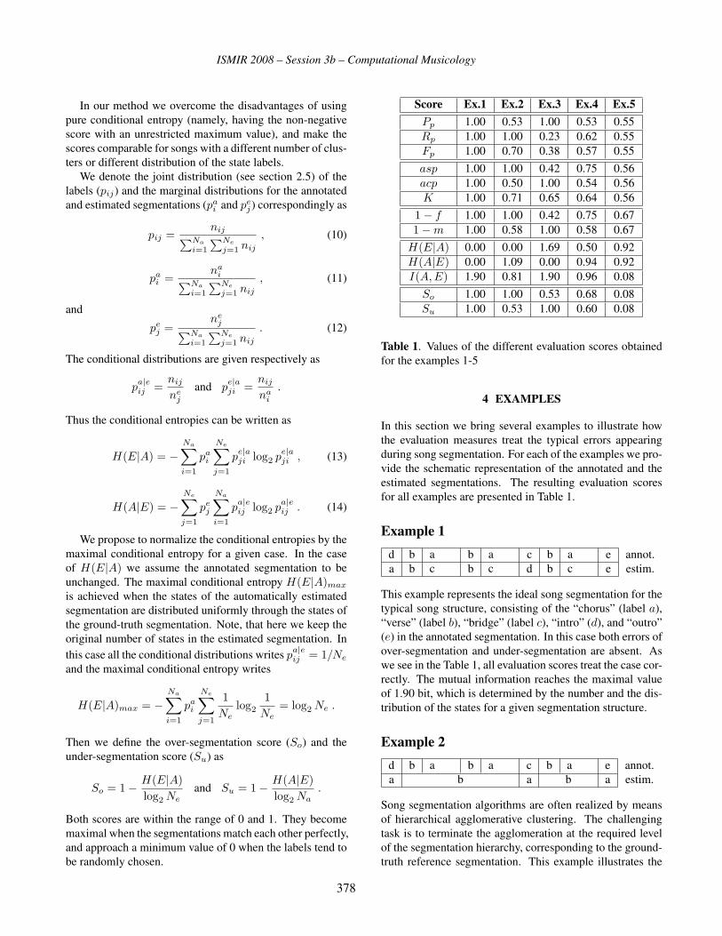
ISMIR 2008 – Session 3b – Computational Musicology
In our method we overcome the disadvantages of using
pure conditional entropy (namely, having the non-negative
score with an unrestricted maximum value), and make the
scores comparable for songs with a different number of clus-
ters or different distribution of the state labels.
We denote the joint distribution (see section 2.5) of the
labels (pij) and the marginal distributions for the annotated
and estimated segmentations (pai and pe
j) correspondingly as
pij =nij∑Na
i=1
∑Ne
j=1 nij
, (10)
pai =
nai∑Na
i=1
∑Ne
j=1 nij
, (11)
and
pej =
nej∑Na
i=1
∑Ne
j=1 nij
. (12)
The conditional distributions are given respectively as
pa|eij =
nij
nej
and pe|aji =
nij
nai
.
Thus the conditional entropies can be written as
H(E|A) = −Na∑i=1
pai
Ne∑j=1
pe|aji log2 p
e|aji , (13)
H(A|E) = −Ne∑j=1
pej
Na∑i=1
pa|eij log2 p
a|eij . (14)
We propose to normalize the conditional entropies by the
maximal conditional entropy for a given case. In the case
of H(E|A) we assume the annotated segmentation to be
unchanged. The maximal conditional entropy H(E|A)max
is achieved when the states of the automatically estimated
segmentation are distributed uniformly through the states of
the ground-truth segmentation. Note, that here we keep the
original number of states in the estimated segmentation. In
this case all the conditional distributions writes pa|eij = 1/Ne
and the maximal conditional entropy writes
H(E|A)max = −Na∑i=1
pai
Ne∑j=1
1Ne
log2
1Ne
= log2 Ne .
Then we define the over-segmentation score (So) and the
under-segmentation score (Su) as
So = 1− H(E|A)log2 Ne
and Su = 1− H(A|E)log2 Na
.
Both scores are within the range of 0 and 1. They become
maximal when the segmentations match each other perfectly,
and approach a minimum value of 0 when the labels tend to
be randomly chosen.
Score Ex.1 Ex.2 Ex.3 Ex.4 Ex.5Pp 1.00 0.53 1.00 0.53 0.55
Rp 1.00 1.00 0.23 0.62 0.55
Fp 1.00 0.70 0.38 0.57 0.55
asp 1.00 1.00 0.42 0.75 0.56
acp 1.00 0.50 1.00 0.54 0.56
K 1.00 0.71 0.65 0.64 0.56
1− f 1.00 1.00 0.42 0.75 0.67
1−m 1.00 0.58 1.00 0.58 0.67
H(E|A) 0.00 0.00 1.69 0.50 0.92
H(A|E) 0.00 1.09 0.00 0.94 0.92
I(A, E) 1.90 0.81 1.90 0.96 0.08
So 1.00 1.00 0.53 0.68 0.08
Su 1.00 0.53 1.00 0.60 0.08
Table 1. Values of the different evaluation scores obtained
for the examples 1-5
4 EXAMPLES
In this section we bring several examples to illustrate how
the evaluation measures treat the typical errors appearing
during song segmentation. For each of the examples we pro-
vide the schematic representation of the annotated and the
estimated segmentations. The resulting evaluation scores
for all examples are presented in Table 1.
Example 1d b a b a c b a e annot.
a b c b c d b c e estim.
This example represents the ideal song segmentation for the
typical song structure, consisting of the “chorus” (label a),
“verse” (label b), “bridge” (label c), “intro” (d), and “outro”
(e) in the annotated segmentation. In this case both errors of
over-segmentation and under-segmentation are absent. As
we see in the Table 1, all evaluation scores treat the case cor-
rectly. The mutual information reaches the maximal value
of 1.90 bit, which is determined by the number and the dis-
tribution of the states for a given segmentation structure.
Example 2d b a b a c b a e annot.
a b a b a estim.
Song segmentation algorithms are often realized by means
of hierarchical agglomerative clustering. The challenging
task is to terminate the agglomeration at the required level
of the segmentation hierarchy, corresponding to the ground-
truth reference segmentation. This example illustrates the
378

ISMIR 2008 – Session 3b – Computational Musicology
case, when the agglomeration algorithm is terminated too
late, and the resulting states are too generalized. As such
there is no over-segmentation errors, but under-segmentation
scores are rather poor. Note, that the mutual information
score (0.81 bit) is informative only in comparison to the
maximal mutual information for a given ground-truth seg-
mentation, obtained in Example 1.
Example 3d b a b a c b a e annot.
a b c d e f g h i j k l estim.
The opposite situation occurs if the automatically estimated
segmentation tends to assign each input utterance to a sepa-
rate state. That could happen if the agglomerative clustering
is terminated at a very early stage. In this case there are no
under-segmentation errors, but the over-segmentation scores
are low.
Note, that the over-segmentation scores (asp, 1 − f and
So) and the under-segmentation scores (acp, 1−m and Su)
are in good correspondence for both Example 2 and Exam-
ple 3. Contrastingly, the mutual information score for the
Example 3 is close to the one obtained for the “ideal” seg-
mentation in Example 1. The mutual information I(A, E)can be written as
I(A, E) = H(E)−H(E|A) (15)
where H(E) is a marginal entropy of the automatically es-
timated segmentation. In this case a marginal entropy for 12
uniformly distributed states is really high (3.59 bit). As such
even a high value of conditional entropy H(E|A) (1.69 bit)
cannot compensate it. The comparison of the Example 1 and
Example 3 shows that a single score of mutual information
is not directly applicable as an evaluation measure when the
number of the states in the segmentations is changed.
Example 4d b a b a c b a e annot.
a b c b c b c a estim.
In most cases the estimated segmentation contains both over-
segmentation and under-segmentation errors. For instance
it happens when the borders of the segments are not deter-
mined correctly. In the presented example the second half of
the “chorus” together with the “bridge” (label c in the esti-
mated segmentation) is recognized as a distinct state, while
the first half of the “chorus” is merged with the “verse” (la-
bel b in the estimated segmentation).
Clearly, the obtained estimated segmentation in Exam-
ple 4 is not ideal, but it is obviously more appropriate than
the estimated segmentation in Example 3. Note, that the
measure K stays nearly unchanged, and even slightly de-
creases.
Example 5b a b a annot.
a b a b a b a b a b a b estim.
The structure of the ground-truth segmentation in Exam-
ples 1-4 is typical (but not obligatory!) for Rock or Pop
songs. This example depicts an annotated segmentation that
could often appear e.g. for Jazz or Classical music pieces.
As it was noted in section 1, the evaluation score should
provide a possibility to compare the segmentation efficiency
for different songs. In this case the estimated segmentation
tends to be random. Obviously, this estimated segmenta-
tion is not of use in practical applications. In Table 1 we
see, that the over-segmentation and the under-segmentation
scores (So and Su) are really low while the other evalua-
tion measures (asp, acp, 1− f , 1−m) keep relatively high
values. As such the values of 1 − f and 1 − m become
comparable for the Examples 4 and 5, nevertheless that the
estimated segmentation in Example 5 evidently carries less
information about the corresponding ground-truth segmen-
tation.
5 DISCUSSION
Analyzing the results listed in Table 1 we can summarize
the following trends. First of all, the evaluation scores dis-
cussed in section 2 are strongly dependent on the amount
and the distribution of the states in both annotated and esti-
mated segmentations. Even within one musical genre these
parameters differ for each song in the test set. Evaluating a
song segmentation algorithm commonly implies calculating
the evaluation scores for every entry of the test set and then
providing the overall results. The latter becomes impossible
if the evaluation score depends on the parameters that are
different for every item of the test set.
We should mention that the higher the number of the
states in the segmentations the more reliable the evaluation
scores asp, acp, 1− f and 1−m. Contrastingly, if the song
consists only of a few states, even a “random” segmentation
yields relatively high values.
The results show the benefits of treating the over-segmen-
tation and the under-segmentation scores independently. If
one of the scores is close to 1 and the other is relatively
low, then we can assume that the automatic segmentation
is performed on the other level of the segmentation hierar-
chy. In the worst, all states of the annotated segmentation
are mapped into one state of the estimated segmentation, or
vice versa each frame (time discretization unit) of the song
forms a distinct state in the estimated segmentation. In the
379

ISMIR 2008 – Session 3b – Computational Musicology
latter cases the merging score K leads to the spurious re-
sults. For instance in the Examples 2 and 3 the score Kindicates inconsistently high results. Therefore we believe
using two independent scores So and Su to be more appro-
priate for the case.
The comparison of the Examples 1 and 3 shows that the
mutual information I(A, E) is an unreliable evaluation score,
especially if the number and the distribution of the states
in both annotated and estimated segmentations are changed
significantly.
The proposed evaluation score shows reliable results for
all five presented examples. It is insensitive to changing
the number of states in the segmentations and as such en-
ables the comparison of automatic evaluation results, ob-
tained from different songs. The scores can be loosely treated
as an accuracy rate of the applied segmentation indicating
the over-segmentation and under-segmentation errors. As a
disadvantage of the So and Su scores one can point out that
in the strict sense these scores cannot be treated as the ac-
curacy rates. The proposed normalization only restricts the
boundaries of the scores and brings it within the range of 0
and 1. In point of fact the conditional entropies H(E|A) and
H(A|E) are not a linear functions and thus a boundary re-
striction does not form the accuracy rate out of it. Therefore
further investigations and a more complicated normalization
scheme are needed.
6 CONCLUSION
In this paper we presented a novel approach to the song
segmentation evaluation. The proposed evaluation score is
based on the information-theoretic conditional entropies for
comparing the estimated song segmentation with the one
annotated by human experts (in the case of a state repre-
sentation). Having applied the normalization scheme we
formed the over-segmentation and the under-segmentation
scores reflecting the accuracy rate of the obtained automatic
segmentation given the annotated ground-truth. We com-
pared our evaluation method to the commonly used approa-
ches. By providing the illustrating examples we demon-
strated the challenging points of the evaluation procedure
and showed that the proposed over-segmentation and under-
segmentation scores depicted more reliable results in com-
parison to the other evaluation measures.
By means of over-segmentation and under-segmentation
scores one can compare the song segmentation efficiency
obtained for the different songs, even when the number and
the distribution of the states for these songs are various.
Since song segmentation is a particular case of classi-
cal clustering procedure, the proposed approach can be also
applied for evaluating other clustering tasks like Image Seg-
mentation or Speaker Clustering.
7 ACKNOWLEDGMENTS
This work has been partly supported by the PHAROS and
the DIVAS projects, funded under the EC IST 6th Frame-
work Program. Furthermore, the work on this publication is
supported by grant No. 01QM07017 of the German THE-
SEUS program.
8 REFERENCES
[1] Peeters, G. “Deriving Musical Structures from Signal
Analysis for Music Audio Summary Generation: Se-
quence and State Approach”, in Lecture Notes in Com-puter Science, Springer-Verlag, 2004.
[2] Abdallah, S. Noland, K., Sandler, M., Casey, M., and
Rhodes, C. “Theory and evaluation of a Bayesian music
structure extractor”, in Proc. ISMIR, London, UK, 2005.
[3] Paulus, J. and Klapuri, A. “Music structure analysis by
finding repeated parts”, in Proc. AMCMM, Santa Bar-
bara, California, USA, 2006.
[4] Peeters, G. “Sequence Representation of Music
Structure Using Higher-Order Similarity Matrix and
Maximum-Likelihood Approach”, in Proc. ISMIR, Vi-
enna, Austria, 2007.
[5] Goto, M. “A Chorus Section Detection Method for Mu-
sical Audio Signals and Its Application to a Music Lis-
tening Station”, IEEE Transactions on Audio, Speech,and Language Processing, 2006.
[6] van Rijsbergen, C. J. Information Retrieval, Butter-
worths, London, UK, 1979.
[7] Levy, M., Sandler, M. “Structural Segmentation of mu-
sical audio by constrained clustering”, IEEE Transac-tions on Audio, Speech and Language Processing, 2008.
[8] Solomonoff, A., Mielke, A., Schmidt, M., and Gish, H.
“Clustering Speakers by Their Voices”, in Proc. IEEEICASSP, Piscataway, New Jersey, 1998.
[9] Ajmera, J., Bourlard, H., Lapidot, I., and McCowan, I.
“Unknown-Multiple Speaker Clustering Using HMM”,
in Proceedings of the International Conference on Spo-ken Language Processing, Denver, Colorado, USA,
2002.
[10] Huang, Q. and Dom, B. “Quantitative methods of evalu-
ating image segmentation”, in Proceedings of the Inter-national Conference on Image Processing, Washington,
DC, USA, 1995.
[11] Abdallah, S., Sandler, M., Rhodes, C., and Casey, M.
“Using duration models to reduce fragmentation in au-
dio segmentation”, Machine Learning, 2006.
380

ISMIR 2008 – Session 3b – Computational Musicology
TOWARDS STRUCTURAL ALIGNMENT OF FOLK SONGS
Jörg Garbers and Frans WieringUtrecht University
Department of Information and Computing Sciences{garbers,frans.wiering}@cs.uu.nl
ABSTRACT
We describe an alignment-based similarity framework
for folk song variation research. The framework makes
use of phrase and meter information encoded in Hum-
drum scores. Local similarity measures are used to
compute match scores, which are combined with gap
scores to form increasingly larger alignments and
higher-level similarity values. We discuss the effects
of some similarity measures on the alignment of four
groups of melodies that are variants of each other.
1 INTRODUCTION
In the process of oral transmission folk songs are re-
shaped in many different variants. Given a collection
of tunes, recorded in a particular region or environ-
ment, folk song researchers try to reconstruct the ge-
netic relation between folk songs. For this they study
historical and musical relations of tunes to other tunes
and to already established folk song prototypes.
It has often been claimed that their work could ben-
efit from support by music information retrieval (MIR)
similarity and alignment methods and systems. In prac-
tice however it turns out that existing systems do not
work well enough out of the box [5]. Therefore the re-
search context must be analyzed and existing methods
must be adapted and non-trivially combined to deliver
satisfying results.
1.1 Similarity and alignment
Similarity and alignment can be considered two sides
of the same coin. In order to produce an automatic
alignment we need a measure for the relatedness of
musical units. Conversely, in order to compute the (lo-
cal) similarity between two melodies we must know
which parts of the melody should be compared.
Alignment can also be a prerequisite for higher-level
similarity measures. In a previous paper we derived
generalized queries from a group of folk song vari-
ants [3]. For a given group of musically related query
melodies aligned by the user, we were able to retrieve
melodies from a database that are good candidate mem-
bers for this group.
Making a manual alignment is time-consuming and
involves edit decisions, e.g. ‘shall one insert a rest in
one melody or delete a note in the other?’. When look-
ing for good additional group members in a database,
one should allow both options. However, keeping track
of all options quickly becomes impracticable. In this
paper we therefore look into automatic alignment of
corresponding score positions and ways of controlling
the alignment with basic similarity measures.
1.2 Overview and related work
In this paper we first discuss why automatic detection
of (genetically related) folk song variants is very de-
manding and is a major research topic in its own. Next,
to support research into similarity measures based on
musically meaningful transformations, we develop a
framework that helps to model the influence of local
similarity measures on variation detection and align-
ment. Starting from the information encoded in our
folk song collection, we motivate the use of available
structural and metrical information within alignment
directed similarity measures. Finally we compare au-
tomatically derived alignments with alignments anno-
tated by an expert.
Generally, we follow a similar approach to Mon-
geau and Sankoff’s [6], who tackled selected transfor-
mational aspects in a generic way. They set up a frame-
work to handle pitch contour and rhythm in relation to
an alignment-based dissimilarity (or quality) measure.
They based their framework assumptions on musical
381
ISMIR 2008 – Session 3b – Computational Musicology
common sense and based their model parameter esti-
mations on the discussion of examples.
We agree with them that musical time (as repre-
sentated in common music notation) is a fundamen-
tal dimension in variant similarity. This distinguishes
our approach from ones that deal with performance-
oriented timing deviation problems. A shortcoming of
Mongeau and Sankoff’s global alignment algorithm is
that it cannot handle aspects of musical form, such as
repeats or reordering of parts. They are also criticized
for sometimes ignoring barlines [2].
Contribution: In this paper we present an approach
to tackle these shortcomings by proposing a phrase-
and meter-based alignment framework. By using sim-
ple and out-of-the-box local similarity measures within
the framework and studying the resulting alignments
we prove that the framework is useful.
2 MUSICOLOGICAL MOTIVATION
For folk song researchers, an important question is to
identify which songs or melodies are genetically re-
lated. A way for them to tackle this question is to order
melodies into groups that share relevant musical fea-
tures. We assume that in the process of incrementally
building those melody groups, researchers construct a
sort of mental alignment of related parts of the candi-
date melodies. The detection of relevant relationships
between variants is affected by the perceived similarity
of the material, the knowledge of common transforma-
tion phenomena and the discriminative power of the
shared features with respect to the investigated corpus.
Researchers have identified transformations that
range from a single note change to changes of global
features like mood. A mood change can for example
affect the tonality (major/minor), the number of notes
(due to liveliness) and ambitus (due to excitation) [10].
2.1 Modeling musical similarity
To support folk song variation research, one could
choose to model expert reasoning using rule systems.
Such a system would consist of transformation rules
and transformation sequences that taken together model
the relation between melodic variants. A fundamental
problem with this approach is that we are still a long
way from sufficiently understanding music perception
and cognition. Therefore it is impossible to fully for-
malize the necessary expert knowledge and model the
rules of musicological discourse.
Also, it is difficult to find out which approaches to
folk song variation are the most promising, because
there is little scholarly documentation about music
transformations. An exception is Wiora’s catalog of
transformation phenomena [10]. It describes musical
features and related transformations and is a good in-
spirational source for models of similarity and human
reasoning about it. But it lacks descriptions of the con-
texts in which certain transformations are permissible.
It also does not provide the means to estimate the plau-
sibility of one transformation chain as compared to an-
other when explaining a certain variation. It is common
in folk song research to reason about the relatedness
of specific songs rather than to provide comprehensive
models. However, what is needed for MIR is a com-
prehensive theory about this kind of reasoning.
We chose a different approach to model variant re-
lationships, namely to investigate local similarity. This
closely follows musicological practice. Often some
striking similarities between some parts are considered
sufficient evidence for a variant relationship. This
seems to leave MIR with the task to design local sim-
ilarity measures for variation research. However we
also need to model what is striking and what are rele-vant parts and we must find ways to turn local similar-
ity values into overall relevance estimates.
2.2 Structural, textual and metrical alignment
In this section we mention some relations between the
parts of a song and between parts of variant songs that
support or inhibit the detection of variants. By doing
so, we motivate the structure-based alignment frame-
work that we describe in the next sections. Our as-
sumptions stem from general experience with folk
songs and from dealing with a collection of Dutch folk
songs that we currently help making searchable. [9]
Strophes: In songs, music is tightly bound to the
lyrics. When two different songs have similar lyrics,
we can often simply use textual similarity to relate mu-
sical parts with high confidence. However, we cannot
rely on text alone: if textually different variants or dif-
ferent strophes are encoded, we need to make use of
musical similarities. This should be unproblematic in
principle, since different strophes of a song typically
382

ISMIR 2008 – Session 3b – Computational Musicology
share the same basic melody.
Phrases: Musical phrases in a folk song are typically
related to the verse lines of a poem. When dealing with
automatic alignment we must be aware that the level
of phrase indication might differ: one phrase in song A
might match with two shorter phrases in song B, or the
same rhythm can be notated with different note values.
Accents: Word accents in a verse typically follow a
common scheme, such as dactyl and trochee. These
accents often correspond to the metrical accents of the
notes, which can be found by looking at the barlines
and measure signatures. We cannot always assume the
same meter across variants, since different durations
can turn a 2-foot verse scheme into a 3-accent melody.
Also, extra syllables in the lyrics may make it neces-
sary to insert notes.
Accent (beat position) and phrase position may also
be important for musical similarity of variants: in our
previous work we found that pitches on stronger beat
positions tend to be more stable across variants than
less accented notes. There also seems to be a higher
agreement between variants at the beginning and end
of a strophe or a phrase (cadence notes), while inner
variation is higher [4]. We will study these claims fur-
ther in future research.
3 A STRUCTURE-BASED ALIGNMENTFRAMEWORK
In this section we describe three components for struc-
ture-based folk song alignment: hierarchical segmen-
tation, phrase-level alignment and strophe alignment.
The general idea of the proposed framework is to use
alignments and alignment scores of smaller musical
parts in the alignment process on higher levels. The
more part A from the first melody resembles part B
from the second melody according to a similarity mea-
sure, the more preferable is it to align A with B rather
than with another part of the second melody with a
lower similarity. However, constraints in higher level
alignments can overrule this preference.
3.1 Hierarchical song structure
In accordance with the analysis given in the previous
section, we split songs hierarchically into smaller parts.
We work on manually encoded musical scores in which
meter information and phrases that correspond to the
lyrics are indicated. For each song, at least one stro-
phe is encoded. For some songs two or more stro-
phes are separately encoded. We convert our encod-
ings to Humdrum **kern format with the usual = bar
line markers and special !!new phrase comments.
We use the Humextra [7] toolkit to access the rele-
vant information in Humdrum **kern files (one file
per strophe). In our data model, each strophe contains a
sequence of phrases. We currently do not deal with re-
peat structures, since they are not encoded in our data,
but written out. Each phrase is split into bar segmentsusing the given bar lines.
A bar in turn is recursively split into smaller beatsegments delimited by metrically strong beat positions.
These are not encoded and need not coincide with note
events, but are inferred from the bar lines and the mea-
sure signature.
To each structural unit we attach both the correspond-
ing Humdrum fragment, which can be used to retrieve
notes and extra information such as the syllables, and
a beat range, which identifies the start and duration of
the segment measured in beats.
When retrieving the notes for a structural unit, spe-
cial care is taken to handle boundaries: incomplete bars
can occur not only at the beginning or end of a strophe
but also at the beginning or end of a phrase. A bar
segment will only return those notes of the bar that are
part of the parent phrase segment, and likewise for a
beat segment.
3.2 Phrase level alignment
The user of the framework chooses an elementary sim-
ilarity measure sim that is defined on either bar seg-
ments or beat segments. The framework computes a
similarity value for any pair of segments (one segment
from melody A, the second from melody B).
To combine segments of two phrases into a phraselevel alignment, we use standard global string align-
ment techniques with match scores and deletion and
insertion related gap scores [11]. We define the match
score of two segments a and b as being equal to
sim(a, b). The scaling of gap scores with respect to
sim is left to the user.
To cope with the common phenomenon of different
durations of the upbeat bar and the last bar in the same
phrase in two variants, we support different gap scores
for inner and (left/right) outer gaps. Also, we could
383

ISMIR 2008 – Session 3b – Computational Musicology
use local instead of global alignment methods to look
for motivic similarity instead of phrase similarity [6].
Future improvements will support augmentation, di-minution, fragmentation and consolidation as described
in [6] in combination with segment constraints. We
will also look into inner-phrase form deviations, such
repeats of a bar or beat segment. (See section 5.)
3.3 Strophe alignment
For the strophe level alignment the framework em-
ploys phrase alignments: from the alignment scores
similarity values are calculated for all possible pairs of
phrases (one phrase from melody 1, one from melody
2). Different phrase-level similarity values from alter-
native elementary similarity measures and from non-
alignment similarity measures (e.g. on cadence tones)
can be consolidated into one similarity value. Then a
string alignment technique can be used again to find
the best alignments of the phrase sequences based on
these similarity values. This handles transformations
from ABCD to ABD.
To assume sequential similarity and to use phrases
only once on the strophe level would sometimes be
misleading. Consider simple transformations from
AABB to AAB or BBAA. Therefore the framework
supports the creation of alignments where one strophe
is fixed and each phrase p of it can be matched against
any of the phrases q of the phrase set S variant strophe:
MatchScore(p, S) = maxqεS{similarity(p, q)}To cover cases where strophes of one song differ
significantly, the framework simply performs all pair-
wise comparisons between all strophes from one vari-
ant with all strophes from the other variant.
4 EVALUATION
To study the usefulness of our framework, we com-
pared alignments produced by framework-based mod-
els with manual alignments (annotations). One of the
authors selected sets of similar phrases from a vari-
ant group and produced for each set a multiple align-
ment of their segments in a matrix format (one line
per phrase, one column per set of corresponding seg-
ments). Segments are identified by their starting met-
rical position (e.g. 3.2 for bar 3, second part) and all
segments in a bar must be of the same size.
From each multiple alignment annotation of N phra-
ses we derived N(N-1)/2 pairwise alignments. We com-
pared these to automatic alignments derived from spe-
cific framework setups. Each setup consists of:
A basic distance measure (seed) acting on segments
defined by the expert annotation. The segments usually
stem from the first subdivision of the bar (one half of a
bar in 6/8, one third of a bar in 9/8 measure). Excep-
tion: a 4/4 variant in a 6/8 melody group is split into
four segments per bar.
A normalization to turn the segment distance values
into match scores between 0 and 1. We employ
e−distance as the match score for this experiment.
Gap penalty scores for inner and outer gaps (between
0 and 1.5 for this experiment). Note: gap scores are
subtracted and match scores are added in an alignment.
For each setup we generated a log file. For overall
performance comparisons we produced summary fit-
ness values per variant group and across all tested vari-
ant groups. For the fitness of a setup for a particular
variant group (group fitness), we counted all pairwise
alignments in which the automatic alignment has the
same gap positions as the annotation and divided this
number by N(N-1)/2. For the overall fitness of a setup,
we took the average of the group fitnesses.
4.1 Results
Four (not necessarily representative) groups of variant
phrases were manually aligned and used for evaluation.
We only present a summary about the lessons learned
from studying the log files [1], which contain anno-
tations, links to the musical scores, alignment results,
failure analysis information and summaries.
The overall performance of selected setups is shown
in table 4.1 and discussed in the next sections.
4.2 Discussion of distance seeds
In this section we discuss the performance of increas-
ingly complex elementary distance measures (seeds).
Baselines are provided by trivial and random.
The trivial distance 0 turns into a match score of
1 to any pair of segments. As a consequence the ac-
tual alignment depends on the gap scores and the al-
gorithm execution order only. In our test setup this
always means that the algorithm always chooses left
384

ISMIR 2008 – Session 3b – Computational Musicology
Seed IG OG G1 G2 G3 G4 A1 A2
trivial 0.0 0.0 33 50 20 10 28 34
random 0.5 0.3 50 16 30 20 29 32
random 1.5 1.0 83 50 20 10 40 51
beatPos 0.0 0.0 33 16 20 10 19 23
beatPos 0.5 0.3 33 50 20 10 28 34
beatPos 1.5 1.0 100 50 20 10 45 56
events 0.5 0.3 100 50 40 30 55 63
events 1.5 0.5 100 50 20 30 50 56
ptdAbs 0.5 0.3 66 83 50 30 57 66
ptdAbs 1.5 1.0 100 83 40 20 60 74
ptdRel 0.5 0.3 66 50 50 20 46 55
ptdRel 1.5 1.0 100 50 50 20 55 66
Table 1. Alignment fitness. IG/OG: inner/outer gap
scores. G1-4: percentage of well-aligned phrases per
group. A1: average of G1-4; A2: average of G1-3.
(outer) gaps to compensate for the beat segment count
difference of the variants.
A random distance between 0 and 1 leads to a more
even distribution of gaps. When outer gaps are cheaper,
there is a preference for outer gaps. Interestingly in
our examples random performs better than trivial, be-
cause the manual alignments contain more right than
left outer gaps. As a consequence we should consider
to lower the right outer gap penalty with respect to the
left in future experiments.
To study the performance using phrase and meter in-
formation only, we defined the beatPos distance as the
difference of the segment number relative to the pre-
vious barline. The second segment of a bar thus has
distance 1 to the first segment. The algorithm should
prefer to align barlines this way. Surprisingly it per-
formed worse than trivial. However, we found that too
many (relatively cheap) gaps were introduced to match
as many segments as possible. We compensated this in
another test run with gap penalties greater than 1 and
achieved much higher fitness than trivial. In general
there were only few examples where both phrases were
supposed to have inner gaps at different positions.
The next distance measure events measures the dif-
ference of the number of notes in a segment. Tied notes
that begin before the segment starts count for both the
current and the preceding segment. The effect of this
measure is that regions of same event density (related
to tempo or rhythm) are preferred matches. Events per-
forms overall better in the alignment than beatPos.
To take both onset and pitch into account at the same
time, we used proportional transportation distance
(PTD) [8]: we scaled the beat segment time into [0..1]
and weighted the note events according to their scaled
duration. As the ground distance we used (4Δpitch2+Δonset2)−2 with pitches measured as MIDI note num-
bers modulo 12. Our distance measure ptdAbsolutetakes advantage of the fact that the given melodies are
all in the same key. It performs best in comparison with
the previous measures.
If we do not assume the same key, it does not make
sense to employ absolute pitch, but instead one can
compare only the contours. One approach to tackle this
is ptdRelative, which takes the minimum over 12 ptd-Absolute distances. However, it performs much worse.
The reason for this is that, given this distance measure,
two segments that each contain a single note always
have a distance 0. One should therefore apply this mea-
sure only on larger segments or model the tonal center
in the state of the alignment process (see section 5).
4.3 Discussion of annotation groups
The four variant groups were chosen to display differ-
ent kind of alignment problems.
The manual alignment of the group G1 (Wat hoor ikhier...) does not contain any inner gaps. There is lit-
tle variation in absolute pitch, so ptdAbsolute achieves
100% the same alignments. The framework proves to
be useful and handles different kind of measures (6/8
and 9/8) correctly.
Group G2 (Ik ben er ...) contains one inner gap. Ac-
cording to the annotation, the final notes d,c,b of one
variant (72564) are diminished (d,c lasts one beat in-
stead of two beats). Because the framework does not
handle such transformations yet, this was annotated as
a gap. For the similarity measures this gap is hard to
find, probably because the neighboring segments pro-
vide good alternative matches and often a right outer
gap is preferred. Lowering the gap penalties leads to
the introduction of unnecessary extra gaps. However,
ptdAbsolute with high gap penalties achieves 83% suc-
cess and misses only one pair (72564 and 72629), be-
cause it matches d with e. The framework deals well
with aligning 4/4 with 6/8 measures.
Group G3 (Moeder ik kom ...) contains a repeated
segment. Variants that have no repeat are annotated
with a gap at the first occurrence of the segment. How-
ever, there is no compelling reason why this gap cannot
385

ISMIR 2008 – Session 3b – Computational Musicology
be assigned to the second occurrence. This ambiguity
accounts for many “failures” in the test logs.
Group G4 (Heer Halewijn) was chosen because of
its complexity. Only when looking at the annotation
for a while the chosen alignment becomes understand-
able. It is mainly based on tonal function of pitches and
contains many inner gaps. For pairs of phrases, other
alignments are plausible as well, but in the multiple
alignment several small hints together make the given
annotation convincing. Therefore there are only few
correct automatic alignments. Interestingly, however,
the algorithm manages to align a subgroup (72256,
74003, and 74216) without failure.
5 CONCLUSION
We have presented a structure-based alignment and sim-
ilarity framework for folk song melodies represented
as scores. We have done initial tests that show both the
usefulness and limitations of our segmentation, align-
ment and evaluation approach. We see two continu-
ations. First, we should use the framework to study
similarity seeds that take the observed stability of be-
ginnings and endings into account (see section 2.2).
Second, the alignment framework needs to be de-
veloped further into several directions. 1) We did not
so far pay any attention to the relationship between the
statistical properties of the distance measure, its nor-
malization and the value of the gap penalties. 2) We
should support the modeling of states and non-linear
gap costs. 3) Multiple alignment strategies should be
incorporated in order to relate more than two melodies.
The need for this became apparent in the last alignment
group. Multiple alignments are particularly needed for
group queries [3]. Therefore we will not only evaluate
the quality of the alignments but also the performance
of melody retrieval using these alignments.
Acknowledgments. This work was supported by the
Netherlands Organization for Scientific Research within the
WITCHCRAFT project NWO 640-003-501, which is part
of the CATCH-program.
6 REFERENCES
[1] Log files for this paper. http://pierement.zoo.cs.uu.nl/misc/ISMIR2008/.
[2] University Bonn Arbeitsgruppe Multimedia-
Signalverarbeitung. Modified Mongeau-Sankoff
algorithm. http://www-mmdb.iai.uni-bonn.de/forschungprojekte/midilib/english/saddemo.html.
[3] J. Garbers, P. van Kranenburg, A. Volk, F. Wier-
ing, L. Grijp, and R. C. Veltkamp. Using pitch sta-
bility among a group of aligned query melodies
to retrieve unidentified variant melodies. In Si-
mon Dixon, David Bainbridge, and Rainer Typke,
editors, Proceedings of the eighth InternationalConference on Music Information Retrieval, pages
451–456. Austrian Computer Society, 2007.
[4] J. Garbers, A. Volk, P. van Kranenburg, F. Wier-
ing, L. Grijp, and R. C. Veltkamp. On pitch and
chord stability in folk song variation retrieval. In
Proceedings of the first International Conferenceof the Society for Mathematics and Computation inMusic, 2007. (http://www.mcm2007.info/pdf/fri3a-garbers.pdf).
[5] P. van Kranenburg, J. Garbers, A. Volk, F. Wiering,
L.P. Grijp, and R. C. Veltkamp. Towards integra-
tion of MIR and folk song research. In ISMIR 2007proceedings, pages 505–508, 2007.
[6] M. Mongeau and D. Sankoff. Comparison of mu-
sical sequences. In Computers and the Humanities,
volume 24, Number 3. Springer Netherlands, 1990.
[7] C. Sapp. Humdrum extras (source code). http://extras.humdrum.net/download/.
[8] Rainer Typke. Music retrieval based on melodicsimilarity. PhD thesis, Utrecht University, 2007.
[9] A. Volk, P. van Kranenburg, J. Garbers, F. Wiering,
R. C. Veltkamp, and L.P. Grijp. A manual annota-
tion method for melodic similarity and the study of
melody feature sets. In ISMIR 2008 proceedings.
[10] Walter Wiora. Systematik der musikalischen Er-
scheinungen des Umsingens. In Jahrbuch fürVolksliedforschung 7, pages 128–195. Deutsches
Volksliedarchiv, 1941.
[11] D. Yaary and A. Peled. Algorithms for
molecular biology, lecture 2. http://www.cs.tau.ac.il/˜rshamir/algmb/01/scribe02/lec02.pdf, 2001.
386

Session 3c – OMR, Alignment and Annotation

.

ISMIR 2008 – Session 3c – OMR, Alignment and Annotation
JOINT STRUCTURE ANALYSIS WITH APPLICATIONS TO MUSICANNOTATION AND SYNCHRONIZATION
Meinard MüllerSaarland University and MPI Informatik
Campus E1 4, 66123 Saarbrücken, [email protected]
Sebastian EwertBonn University, Computer Science IIIRömerstr. 164, 53117 Bonn, [email protected]
ABSTRACT
The general goal of music synchronization is to automati-cally align different versions and interpretations related toa given musical work. In computing such alignments, re-cent approaches assume that the versions to be aligned cor-respond to each other with respect to their overall globalstructure. However, in real-world scenarios, this assump-tion is often violated. For example, for a popular song thereoften exist various structurally different album, radio, or ex-tended versions. Or, in classical music, different recordingsof the same piece may exhibit omissions of repetitions orsignificant differences in parts such as solo cadenzas. In thispaper, we introduce a novel approach for automatically de-tecting structural similarities and differences between twogiven versions of the same piece. The key idea is to performa single structural analysis for both versions simultaneouslyinstead of performing two separate analyses for each of thetwo versions. Such a joint structure analysis reveals the re-petitions within and across the two versions. As a furthercontribution, we show how this information can be used forderiving musically meaningful partial alignments and anno-tations in the presence of structural variations.
1 INTRODUCTION
Modern digital music collections contain an increasingnumber of relevant digital documents for a single musicalwork comprising various audio recordings, MIDI files, orsymbolic score representations. In order to coordinate themultiple information sources, various synchronization pro-cedures have been proposed to automatically align musi-cally corresponding events in different versions of a givenmusical work, see [1, 7, 8, 9, 14, 15] and the referencestherein. Most of these procedures rely on some variant ofdynamic time warping (DTW) and assume a global corre-spondence of the two versions to be aligned. In real-worldscenarios, however, different versions of the same piece mayexhibit significant structural variations. For example, in thecase of Western classical music, different recordings often
The research was funded by the German Research Foundation (DFG)and the Cluster of Excellence on Multimodal Computing and Interaction.
exhibit omissions of repetitions (e. g., in sonatas and sym-phonies) or significant differences in parts such as solo ca-denzas of concertos. Similarly, for a given popular, folk, orart song, there may be various recordings with a differentnumber of stanzas. In particular for popular songs, theremay exist structurally different album, radio, or extendedversions as well as cover versions.
A basic idea to deal with structural differences in thesynchronization context is to combine methods from mu-sic structure analysis and music alignment. In a first step,one may partition the two versions to be aligned into musi-cally meaningful segments. Here, one can use methods fromautomated structure analysis [3, 5, 10, 12, 13] to derive sim-ilarity clusters that represent the repetitive structure of thetwo versions. In a second step, the two versions can then becompared on the segment level with the objective for match-ing musically corresponding passages. Finally, each pair ofmatched segments can be synchronized using global align-ment strategies. In theory, this seems to be a straightforwardapproach. In practise, however, one has to deal with severalproblems due to the variability of the underlying data. Inparticular, the automated extraction of the repetitive struc-ture constitutes a delicate task in case the repetitions revealsignificant differences in tempo, dynamics, or instrumen-tation. Flaws in the structural analysis, however, may beaggravated in the subsequent segment-based matching stepleading to strongly corrupted synchronization results.
The key idea of this paper is to perform a single, jointstructure analysis for both versions to be aligned,which pro-vides richer and more consistent structural data than in thecase of two separate analyses. The resulting similarity clus-ters not only reveal the repetitions within and across the twoversions, but also induce musically meaningful partial align-ments between the two versions. In Sect. 2, we describe ourprocedure for a joint structure analysis. As a further con-tribution of this paper, we show how the joint structure canbe used for deriving a musically meaningful partial align-ment between two audio recordings with structural differ-ences, see Sect. 3. Furthermore, as described in Sect. 4,our procedure can be applied for automatic annotation of agiven audio recording by partially available MIDI data. InSect. 5,we conclude with a discussion of open problems and
389

ISMIR 2008 – Session 3c – OMR, Alignment and Annotation
0 100 200 3000
50
100
150
200
250
300
350
0
0.1
0.2
0.3
0.4
0.5
0.6
0.7
0.8
0.9
1
0 100 200 3000
50
100
150
200
250
300
350
0
0.1
0.2
0.3
0.4
0.5
0.6
0.7
0.8
0.9
1
0 100 200 300
1
2
1 2 3 4
1
2
20406080100120
0 100 200 300
1
2
0 100 2000
50
100
0
50
100
150
200
0 100 2000
50
100
0
0.5
1
(a) (b)
(c)
(d)
(e)
(f)
(g)
A1 B1 A21 A2
2 B21 B2
2
A1
B1
A21
A22
B21
B22
A1 B1 A21 A2
2 B21 B2
2 A1 B1 A21 A2
2 B21 B2
2
Figure 1. Joint structure analysis and partial synchronization for two structurally different versions of the Aria of the Goldberg VariationsBWV 988 by J.S. Bach. The first version is played by G. Gould (musical form A1B1) and the second by M. Perahia (musical formA21A
22B
21B
22 ). (a) Joint similarity matrix S . (b) Enhanced matrix and extracted paths. (c) Similarity clusters. (d) Segment-based score
matrixM and match (black dots). (e) Matched segments. (f) Matrix representation of matched segments. (g) Partial synchronization result.
prospects on future work.The problem of automated partial music synchronization
has been introduced in [11], where the idea is to use the con-cept of path-constrained similarity matrices to enforce mu-sically meaningful partial alignments. Our approach carriesthis idea even further by using cluster-constraint similaritymatrices, thus enforcing structurally meaning partial align-ments. A discussion of further references is given in thesubsequent sections.
2 JOINT STRUCTURE ANALYSIS
The objective of a joint structure analysis is to extract the re-petitive structure within and across two different music rep-resentations referring to the same piece of music. Each ofthe two versions can be an audio recording, a MIDI version,or a MusicXML file. The basic idea of how to couple thestructure analysis of two versions is very simple. First, oneconverts both versions into common feature representationsand concatenates the resulting feature sequences to form asingle long feature sequence. Then, one performs a com-mon structure analysis based on the long concatenated fea-ture sequence. To make this strategy work, however, onehas to deal with various problems. First, note that basi-cally all available procedures for automated structure analy-sis have a computational complexity that is at least quadraticin the input length. Therefore, efficiency issues becomecrucial when considering a single concatenated feature se-quence. Second, note that two different versions of thesame piece often reveal significant local and global tempodifferences. Recent approaches to structure analysis suchas [5, 12, 13], however, are built upon the constant tempoassumption and cannot be used for a joint structure analysis.Allowing also tempo variations between repeating segmentsmakes the structure analysis problem a much harder prob-lem [3, 10]. We now summarize the approach used in thispaper closely following [10].
Given two music representations, we transform them
into suitable feature sequences U := (u1, u2, . . . , uL) andV := (v1, v2, . . . , vM ), respectively. To reduce differenttypes of music data (audio, MIDI, MusicXML) to the sametype of representation and to cope with musical variationsin instrumentation and articulation, chroma-based featureshave turned out to be a powerful mid-level music repre-sentation [2, 3, 8]. In the subsequent discussion, we em-ploy a smoothed normalized variant of chroma-based fea-tures (CENS features) with a temporal resolution of 1 Hz,see [8] for details. In this case, each 12-dimensional featurevector u�, � ∈ [1 : L], and vm, m ∈ [1 : M ], expressesthe local energy of the audio (or MIDI) distribution in the12 chroma classes. The feature sequences strongly correlateto the short-time harmonic content of the underlying musicrepresentations. We now define the sequence W of lengthN := L + M by concatenating the sequences U and V :
W := (w1, w2, . . . , wN ) := (u1, . . . , uL, v1, . . . , vM ).
Fixing a suitable local similarity measure— here,we use theinner vector product—the (N×N)-joint similarity matrix Sis defined by S(i, j) := 〈wi, wj〉, i, j ∈ [1 : N ]. Each tuple(i, j) is called a cell of the matrix. A path is a sequence p =(p1, . . . , pK) with pk = (ik, jk) ∈ [1 : N ]2, k ∈ [1 : K],satisfying 1 ≤ i1 ≤ i2 ≤ . . . ≤ iK ≤ N and 1 ≤ j1 ≤j2 ≤ . . . ≤ jK ≤ N (monotonicity condition) as well aspk+1 − pk ∈ Σ, where Σ denotes a set of admissible stepsizes. In the following, we use Σ = {(1, 1), (1, 2), (2, 1)}.
As an illustrative example, we consider two differentaudio recordings of the Aria of the Goldberg VariationsBWV 988 by J.S. Bach, in the following referred to as Bachexample. The first version with a duration of 115 seconds isplayed by Glen Gould without repetitions (corresponding tothe musical form A1B1) and the second version with a du-ration of 241 seconds is played by Murray Perahia with re-petitions (corresponding to the musical form A2
1A22B
21B2
2 ).For the feature sequences hold L = 115, M = 241, andN = 356. The resulting joint similarity matrix is shown in
390

ISMIR 2008 – Session 3c – OMR, Alignment and Annotation
0 100 200 300 400 500 6000
100
200
300
400
500
600
0
0.1
0.2
0.3
0.4
0.5
0.6
0.7
0.8
0.9
1
0 100 200 300 400 500 600
5
10
15
10 20 30
5
10
15
20
25
30
0
20
40
60
80
100
0 100 200 300 4000
50
100
150
200
250
0
100
200
300
400
500
0 100 200 300 4000
50
100
150
200
250
0
0.2
0.4
0.6
0.8
1
(a) (b)
(c)
(d)
(e)
Figure 2. Joint structure analysis and partial synchronization for two structurally modified versions of Beethoven’s Fifth Symphony Op. 67.The first version is a MIDI version and the second one an audio recording by Bernstein. (a) Enhanced joint similarity matrix and extractedpaths. (b) Similarity clusters. (c) Segment-based score matrixM and match (indicated by black dots). (d) Matrix representation of matchedsegments. (e) Partial synchronization result.
Fig. 1a, where the boundaries between the two versions areindicated by white horizontal and vertical lines.
In the next step, the path structure is extracted from thejoint similarity matrix. Here, the general principle is thateach path of low cost running in a direction along the maindiagonal (gradient (1, 1)) corresponds to a pair of similarfeature subsequences. Note that relative tempo differencesin similar segments are encoded by the gradient of the path(which is then in a neighborhood of (1, 1)). To ease thepath extraction step, we enhance the path structure of S bya suitable smoothing technique that respects relative tempodifferences. The paths can then be extracted by a robust andefficient greedy strategy, see Fig. 1b. Here, because of thesymmetry of S, one only has to consider the upper left partof S. Furthermore, we prohibit paths crossing the bound-aries between the two versions. As a result, each extractedpath encodes a pair of musically similar segments, whereeach segment entirely belongs either to the first or to the sec-ond version. To determine the global repetitive structure,weuse a one-step transitivity clustering procedure, which bal-ances out the inconsistencies introduced by inaccurate andincorrect path extractions. For details, we refer to [8, 10].
Altogether, we obtain a set of similarity clusters. Eachsimilarity cluster in turn consists of a set of pairwise similarsegments encoding the repetitions of a segment within andacross the two versions. Fig. 1c shows the resulting set ofsimilarity clusters for our Bach example. Both of the clus-ters consist of three segments, where the first cluster corre-sponds to the three B-parts B1, B2
1 , and B22 and the sec-
ond cluster to the three A-parts A1, A21, and A2
2. The jointanalysis has several advantages compared to two separateanalyses. First note that, since there are no repetitions in thefirst version, a separate structure analysis for the first version
would not have yielded any structural information. Second,the similarity clusters of the joint structure analysis naturallyinduce musically meaningful partial alignments between thetwo versions. For example, the first cluster shows that B1
may be aligned to B21 or to B2
2 . Finally, note that the deli-cate path extraction step often results in inaccurate and frag-mented paths. Because of the transitivity step, the joint clus-tering procedure balances out these flaws and compensatesfor missing parts to some extent by using joint informationacross the two versions.
On the downside, a joint structural analysis is computa-tionally more expensive than two separate analyses. There-fore, in the structure analysis step, our strategy is to use arelatively low feature resolution of 1 Hz. This resolutionmay then be increased in the subsequent synchronizationstep (Sect. 3) and annotation application (Sect. 4). Our cur-rent MATLAB implementation can easily deal with an over-all length up to N = 3000 corresponding to more then fortyminutes of music material. (In this case, the overall com-putation time adds up to 10-400 seconds with the path ex-traction step being the bottleneck, see [10]). Thus, our im-plementation allows for a joint analysis even for long sym-phonic movements of a duration of more than 20 minutes.
Another drawback of the joint analysis is that local in-consistencies across the two versions may cause an over-fragmentation of the music material. This may result ina large number of incomplete similarity clusters contain-ing many short segments. As an example, we consider aMIDI version as well as a Bernstein audio recording of thefirst movement of Beethoven’s Fifth Symphony Op. 67. Westructurally modified both versions by removing some sec-tions. Fig. 2a shows the enhanced joint similarity matrixand Fig. 2b the set of joint similarity clusters. Note that
391

ISMIR 2008 – Session 3c – OMR, Alignment and Annotation
some of the resulting 16 clusters contain semantically mean-ingless segments stemming from spuriously extracted pathfragments. At this point, one could try to improve the over-all structure result by a suitable postprocessing procedure.This itself constitutes a difficult research problem and is notin the scope of this paper. Instead, we introduce a proce-dure for partial music alignment, which has some degree ofrobustness to inaccuracies and flaws in the previously ex-tracted structural data.
3 PARTIAL SYNCHRONIZATION
Given two different representations of the same underlyingpiece of music, the objective of music synchronization is toautomatically identify and link semantically correspondingevents within the two versions. Most of the recent synchro-nization approaches use some variant of dynamic time warp-ing (DTW) to align the feature sequences extracted fromthe two versions, see [8]. In classical DTW, all elementsof one sequence are matched to elements in the other se-quence (while respecting the temporal order). This is prob-lematic when elements in one sequence do not have suit-able counterparts in the other sequence. In the presence ofstructural differences between the two sequences, this typ-ically leads to corrupted and musically meaningless align-ments [11]. Also more flexible alignment strategies such assubsequence DTW or partial matching strategies as used inbiological sequence analysis [4] do not properly account forsuch structural differences.
A first approach for partial music synchronization hasbeen described in [11]. Here, the idea is to first constructa path-constrained similarity matrix, which a priori con-stricts possible alignment paths to a semantically meaning-ful choice of admissible cells. Then, in a second step, apath-constrained alignment can be computed using standardmatching procedures based on dynamic programming.
We now carry this idea even further by using the seg-ments of the joint similarity clusters as constraining ele-ments in the alignment step. To this end, we consider pairsof segments, where the two segments lie within the samesimilarity cluster and belong to different versions. Moreprecisely, let C = {C1, . . . , CM} be the set of clusters ob-tained from the joint structure analysis. Each similarity clus-ter Cm, m ∈ [1 : M ], consists of a set of segments (i. e.,subsequences of the concatenated feature sequence W ). Letα ∈ Cm be such a segment. Then let �(α) denote thelength of α and c(α) := m the cluster affiliation. Recallthat α either belongs to the first version (i. e., α is a subse-quence of U ) or to the second version (i. e., α is a subse-quence of V ). We now form two lists of segments. The firstlist (α1, . . . , αI) consists of all those segments that are con-tained in some cluster of C and belong to the first version.The second list (β1, . . . , βJ) is defined similarly, where thesegments now belong to the second version. Both lists are
sorted according to the start positions of the segments. (Incase two segments have the same start position, we breakthe tie by also considering the cluster affiliation.) We definea segment-based I × J-score matrixM by
M(i, j) :={
�(αi) + �(βj) for c(αi) = c(βj),0 otherwise,
i ∈ [1 : I], j ∈ [1 : J ]. In other words,M(i, j) is positiveif and only if αi and βj belong to the same similarity clus-ter. Furthermore,M(i, j) depends on the lengths of the twosegments. Here, the idea is to favor long segments in thesynchronization step. For an illustration, we consider theBach example of Fig. 1, where (α1, . . . , αI) = (A1, B1)and (β1, . . . , βJ ) = (A2
1, A22, B
21 , B2
2). The resulting matrixM is shown in Fig. 1d. For another more complex example,we refer to Fig. 2c.
Now, a segment-based match is a sequence μ =(μ1, . . . , μK) with μk = (ik, jk) ∈ [1 : I] × [1 : J ] fork ∈ [1 : K] satisfying 1 ≤ i1 < i2 < . . . < iK ≤ Iand 1 ≤ j1 < j2 < . . . < jK ≤ J . Note that a matchinduces a partial assignment of segment pairs, where eachsegment is assigned to at most one other segment. Thescore of a match μ with respect to M is then defined as∑K
k=1M(ik, jk). One can now use standard techniques tocompute a score-maximizing match based on dynamic pro-gramming, see [4, 8]. For details, we refer to the litera-ture. In the Bach example, the score-maximizing match μ isgiven by μ = ((1, 1), (2, 3)). In other words, the segmentα1 = A1 of the first version is assigned to segment β1 = A2
1
of the second version and α2 = B1 is assigned to β3 = B21 .
In principle, the score-maximizing match μ constitutesour partial music synchronization result. To make the pro-cedure more robust to inaccuracies and to remove clusterredundancies,we further clean the synchronization result ina postprocessing step. To this end, we convert the score-maximizing match μ into a sparsepath-constrained simi-larity matrix Spath of size L × M , where L and M arethe lengths of the two feature sequences U and V , re-spectively. For each pair of matched segments, we com-pute an alignment path using a global synchronization algo-rithm [9].Each cell of such a path defines a non-zero entryof Spath, where the entry is set to the length of the path (thusfavoring long segments in the subsequent matching step).All other entries of the matrix Spath are set to zero. Fig. 1fand Fig. 2d show the resulting path-constrained similaritymatrices for the Bach and Beethoven example, respectively.Finally, we apply the procedure as described in [11] us-ing Spath (which is generally much sparser than the path-constrained similarity matrices as used in [11])to obtain apurified synchronization result, see Fig. 1g and Fig. 2e.
To evaluate our synchronization procedure, we per-formed similar experiments as described in [11]. In oneexperiment, we formed synchronization pairs each consist-ing of two different versions of the same piece. Each pair
392

ISMIR 2008 – Session 3c – OMR, Alignment and Annotation
(a)
0 100 200 300 400 5000
100
200
300
400
0 100 200 300 400 500D
C
B
AS1 S2 S3 S4 S5 S6
P1 P2 P3
(b)
0 50 100 150 200 2500
50
100
150
0 50 100 150 200 250D
C
B
AS1 S2 S3 S4
P1 P2
(c)
0 50 100 150 200 2500
100
200
300
0 50 100 150 200 250D
C
B
AS1 S2 S3 S4 S5 S6 S7
P1 P2 P3
(d)
0 50 1000
20
40
60
80
0 50 100D
C
B
AS1 S2 S3 S4 S5 S6 S7
P1
Figure 3. Partial synchronization results for various MIDI-audio synchronization pairs. The top figures show the final path componentsof the partial alignments and the bottom figures indicate the ground truth (Row A), the final annotations (Row B), and a classification intocorrect (Row D) and incorrect annotations (Row C), see text for additional explanations. The pieces are specified in Table 1. (a) Haydn (RWCC001), (b) Schubert (RWC C048, distorted), (c) Burke (P093), (d) Beatles (“Help!”, distorted).
consists either of an audio recording and a MIDI version orof two different audio recordings (interpreted by differentmusicians possibly in different instrumentations). We man-ually labeled musically meaningful sections of all versionsand then modified the pairs by randomly removing or dupli-cating some of the labeled sections, see Fig. 3. The partialsynchronization result computed by our algorithm was ana-lyzed by means of its path components. A path componentis said to be correct if it aligns corresponding musical sec-tions. Similarly, a match is said to be correct if it covers(up to a certain tolerance) all semantically meaningful cor-respondences between the two versions (this information isgiven by the ground truth) and if all its path components arecorrect. We tested our algorithm on more than 387 differentsynchronization pairs resulting in a total number of 1080path components. As a result, 89% of all path componentsand 71% of all matches were correct (using a tolerance of 3seconds).
The results obtained by our implementation of thesegment-based synchronization approach are qualitativelysimilar to those reported in [11]. However, there is one cru-cial difference in the two approaches. In [11], the authorsuse a combination of various ad-hoc criteria to constructa path-constrained similarity matrix as basis for their par-tial synchronization. In contrast, our approach uses only thestructural information in form of the joint similarity clustersto derive the partial alignment. Furthermore, the availabil-ity of structural information within and across the two ver-sions allows for recovering missing relations based on suit-able transitivity considerations. Thus, each improvement ofthe structure analysis will have a direct positive effect on thequality of the synchronization result.
4 AUDIO ANNOTATION
The synchronization of an audio recording and a corre-sponding MIDI version can be regarded as an automatedannotation of the audio recording by means of the explicitnote events given by the MIDI file. Often, MIDI versionsare used as a kind of score-like symbolic representation of
the underlying musical work, where redundant informationsuch as repetitions are not encoded explicitly. This is a fur-ther setting with practical relevance where two versions tobe aligned have a different repetitive structure (an audio ver-sion with repetitions and a score-like MIDI version withoutrepetitions). In this setting, one can use our segment-basedpartial synchronization to still obtain musically adequate au-dio annotations.
We now summarize one of our experiments, which hasbeen conducted on the basis of synchronization pairs con-sisting of structurally equivalent audio and MIDI versions. 1
We first globally aligned the corresponding audio and MIDIversions using a temporally refined version of the synchro-nization procedure described in [9]. These alignments weretaken as ground truth for the audio annotation. Similar tothe experiment of Sect. 3, we manually labeled musicallymeaningful sections of the MIDI versions and randomly re-moved or duplicated some of these sections. Fig. 3a il-lustrates this process by means of the first movement ofHaydn’s Symphony No. 94 (RWC C001). Row A of thebottom part shows the original six labeled sections S1 toS6 (warped according to the audio version). In the modi-fication, S2 was removed (no line) and S4 was duplicated(thick line). Next, we partially aligned the modified MIDIwith the original audio recording as described in Sect. 3.The resulting three path components of our Haydn exampleare shown in the top part of Fig. 3a. Here, the vertical axiscorresponds to the MIDI version and the horizontal axis tothe audio version. Furthermore, Row B of the bottom partshows the projections of the three path components onto theaudio axis resulting in the three segments P1, P2, and P3.These segments are aligned to segments in the MIDI thusbeing annotated by the corresponding MIDI events. Next,we compared these partial annotations with the ground truthannotations on the MIDI note event level. We say that analignment of a note event to a physical time position of theaudio version is correct in a weak (strong) sense, if there is
1 Most of the audio and MIDI files were taken from the RWC musicdatabase [6]. Note that for the classical pieces, the original RWC MIDIand RWC audio versions are not aligned.
393

ISMIR 2008 – Session 3c – OMR, Alignment and Annotation
Original DistortedComposer Piece RWCweak strong weak strong
Haydn Symph. No. 94, 1st Mov. C001 98 97 97 95Beethoven Symph. Op. 67, 1st Mov. C003 99 98 95 91Beethoven Sonata Op. 57, 1st Mov. C028 99 99 98 96Chopin Etude Op. 10, No. 3 C031 93 93 93 92Schubert Op. 89, No. 5 C048 97 96 95 95Burke Sweet Dreams P093 88 79 74 63Beatles Help! — 97 96 77 74
Average 96 94 91 87
Table 1. Examples for automated MIDI-audio annotation (mostof files are from the RWC music database [6]). The columns showthe composer, the piece of music, the RWC identifier, as well as theannotation rate (in %) with respect to the weak and strong criterionfor the original MIDI and some distorted MIDI.
a ground truth alignment of a note event of the same pitch(and, in the strong case, additionally lies in the same musicalcontext by checking an entire neighborhood of MIDI notes)within a temporal tolerance of 100 ms. In our Haydn exam-ple, the weakly correct partial annotations are indicated inRow D and the incorrect annotations in Row C.
The other examples shown in Fig. 3 give a representa-tive impression of the overall annotation quality. Generally,the annotations are accurate—only at the segment bound-aries there are some larger deviations. This is due to ourpath extraction procedure, which often results in “frayed”path endings. Here, one may improve the results by cor-recting the musical segment boundaries in a postprocessingstep based on cues such as changes in timbre or dynamics.A more critical example (Beatles example) is shown Fig. 3d,where we removed two sections (S2 and S7) from the MIDIfile and temporally distorted the remaining parts. In this ex-ample, the MIDI and audio version also exhibit significantdifferences on the feature level. As a result, an entire sec-tion (S1) has been left unannotated leading to a relativelypoor rate of 77% (74%) of correctly annotated note eventswith respect to the weak (strong) criterion.
Finally, Table 1 shows further rates of correctly anno-tated note events for some representative examples. Ad-ditionally, we have repeated our experiments with sig-nificantly temporally distorted MIDI files (locally up to±20%). Note that most rates only slightly decrease (e. g.,for the Schubert piece, from 97% to 95% with respectto the weak criterion), which indicates the robustness ofour overall annotation procedure to local tempo differ-ences. Further results as well as audio files of sonificationscan be found at http://www-mmdb.iai.uni-bonn.de/projects/partialSync/
5 CONCLUSIONS
In this paper, we have introduced the strategy of performing ajoint structural analysis to detect the repetitive structure within andacross different versions of the same musical work. As a corecomponent for realizing this concept, we have discussed a struc-ture analysis procedure that can cope with relative tempo differ-ences between repeating segments. As further contributions, we
have shown how joint structural information can be used to dealwith structural variations in synchronization and annotation appli-cations. The tasks of partial music synchronization and annotationis a much harder then the global variants of these tasks. The rea-son for this is that in the partial case one needs absolute similaritycriteria, whereas in the global case one only requires relative cri-teria. One main message of this paper is that automated musicstructure analysis is closely related to partial music alignment andannotation applications. Hence, improvements and extensions ofcurrent structure analysis procedures to deal with various kinds ofvariations is of fundamental importance for future research.
6 REFERENCES
[1] V. Arifi,M. Clausen, F. Kurth, and M.Müller. Synchronizationof music data in score-,MIDI- and PCM-format. Computing inMusicology, 13, 2004.
[2] M.A. Bartsch, G.H. Wakefield: Audio thumbnailing of popu-lar music using chroma-based representations. IEEE Trans. onMultimedia 7(1) (2005) 96–104.
[3] R. Dannenberg, N. Hu, Pattern discovery techniques for musicaudio, Proc. ISMIR, Paris, France, 2002.
[4] R. Durbin, S. Eddy, A. Krogh, and G. Mitchison, BiologicalSequence Analysis : Probabilistic Models of Proteins and Nu-cleic Acids, Cambridge Univ. Press, 1999.
[5] M. Goto, A chorus section detection method for musical au-dio signals and its application to a music listening station,IEEE Transactions on Audio, Speech & Language Processing14 (2006), no. 5, 1783–1794.
[6] M. Goto, H. Hashiguchi, T. Nishimura, and R. Oka. RWC mu-sic database: Popular, classical and jazz music databases. Proc.ISMIR, Paris, France, 2002.
[7] N. Hu, R. Dannenberg, and G. Tzanetakis. Polyphonic audiomatching and alignment for music retrieval. In Proc. IEEEWASPAA, New Paltz, NY, October 2003.
[8] M. Müller: Information Retrieval for Music and Motion.Springer (2007).
[9] M. Müller, H. Mattes, and F. Kurth. An efficient multiscaleapproach to audio synchronization. In Proc. ISMIR, Victoria,Canada, pages 192–197, 2006.
[10] M. Müller, F. Kurth, Towards structural analysis of audiorecordings in the presence of musical variations, EURASIPJournal on Advances in Signal Processing 2007, Article ID89686, 18 pages.
[11] M. Müller, D. Appelt: Path-constrained partial music syn-chronization. In: Proc. International Conference on Acoustics,Speech, and Signal Processing, Las Vegas, USA (2008).
[12] G. Peeters, Sequence representation of music structure usinghigher-order similarity matrix and maximum-likelihood ap-proach, Proc. ISMIR, Vienna, Austria, 2007.
[13] C. Rhodes, M. Casey, Algorithms for determining and la-belling approximate hierarchical self-similarity, Proc. ISMIR,Vienna, Austria, 2007.
[14] F. Soulez, X. Rodet, and D. Schwarz. Improving polyphonicand poly-instrumental music to score alignment. In Proc. IS-MIR, Baltimore, USA, 2003.
[15] R. J. Turetsky and D. P. Ellis. Force-Aligning MIDI Synthe-ses for Polyphonic Music Transcription Generation. In Proc.ISMIR, Baltimore, USA, 2003.
394

ISMIR 2008 – Session 3c – OMR, Alignment and Annotation
SEGMENTATION-BASED LYRICS-AUDIO ALIGNMENT USING DYNAMICPROGRAMMING
Kyogu LeeMedia Technology Lab, Gracenote
Emeryville, CA [email protected]
Markus CremerMedia Technology Lab, Gracenote
Emeryville, CA [email protected]
ABSTRACT
In this paper, we present a system for automatic alignmentof textual lyrics with musical audio. Given an input audiosignal, structural segmentation is first performed and simi-lar segments are assigned a label by computing the distancebetween the segment pairs. Using the results of segmenta-tion and hand-labeled paragraphs in lyrics as a pair of inputstrings,we apply a dynamic programming (DP) algorithm tofind the best alignment path between the two strings, achiev-ing segment-to-paragraph synchronization. We demonstratethat the proposed algorithm performs well for various kindsof musical audio.
1 INTRODUCTION
As the market for portable media players increases rapidly,more and more manufacturers and multimedia content providersare searching for outstanding features that will set their of-fering apart from the rest. At the same time the rush to-wards online distribution of digital assets has stripped mostcontent of rich metadata such as album artwork and lyrics.While artwork is gaining a lot of traction with the introduc-tion of higher resolution color displays in devices, only fewhigh end devices offer the ability to display lyrics in a read-able form along with music. As devices tend to get smallerand smaller with advancing technology, there is not muchhope for displays to become large enough for the user tocomfortably follow song lyrics without some form of syn-chronized presentation. Some devices are already capableof displaying lyrics synchronized to the playback of musicusing manually inserted time stamps into the lyrics file.
However, this approach does not scale well for large col-lections, so an automated approach to align lyrics with mu-sic is the strongly preferable approach. It is notable thatword-by-word level synchronization for most applications isnot necessary. A paragraph or line-by-line synchronization,whatever is more appropriate for the device display resolu-tion, will be sufficient. As this promises to be a fairly solv-able problem, to which a scalable automated solution couldbe provided, it has recently attracted a number of researchersin the music information retrieval (MIR) community.
Wang et al., for example, have proposed a hierarchicalapproach for automatic alignment of acoustic musical sig-nals with textual lyrics [11, 9]. They decompose the prob-lem into two separate tasks — a higher-level section-basedalignment followed by lower-level per-line alignment. Tothis end, they first process audio to obtain high-level struc-tural information such as Measure,Chorus and Singing VoiceSection. In parallel, textural lyrics are analyzed and eachsection is labeled with one of the pre-defined section types.In this text processing stage, they also compute approximatedurations of each section and line. However, their algorithmis limited by strong assumptions about the song structure aswell as the fixed rhythmic structure.
A different approach has been taken by Chen et al. whohave presented an automatic lyrics-audio synchronizationsystem using the low-level acoustic features only [3]. Theiralgorithm has two main components: 1) vocal/non-vocal de-tector and 2) alignment of the audio signal with its lyricsat multiple levels using acoustic models. Given a musicalaudio signal, a vocal/non-vocal classifier detects candidatesfor the singing voice sections. In parallel, they constructthe grammar net from the lyrics and force an alignment uti-lizing the previously obtained acoustic model units with amaximum likelihood linear regression technique. They havetested their algorithm on a small set of Chinese song seg-ments and achieve a boundary accuracy of 81.5% at thephrase level.
Fujihara et al. tackle the lyrics-audio alignment chal-lenge by solving three sub-problems in series [8]: i.e., 1)separation of singing voice, 2) singing voice detection, and3) alignment of segregated vocal signals with lyrics usinga Viterbi-based matching technique. At the final alignmentstage, they first build a language model from the lyrics usingonly vowel phonemes and short pauses between word, sen-tence or phrase boundaries. They also employ an adaptationof a phone model to the specific singer of the input audiosignal to improve performance. Using 10 Japanese popularsongs as test bed, they have achieved over 90% accuracy foreight songs.
The ultimate goal of the lyrics-audio alignment systemsdescribed so far is to automate karaoke-style synchroniza-tion at a line or word level. Although a word-level or even
395

ISMIR 2008 – Session 3c – OMR, Alignment and Annotation
syllable-level synchronization may appear to be ideal, it isextremely challenging to achieve and usually involves solv-ing other difficult problems such as singing voice separationor constructing proper speech models.
In this paper, we deviate from this goal and propose asolution to a simpler, more basic problem: we aim to alignsong lyrics to the corresponding audio signal at a segment-to-paragraph level. Paragraph-level alignment may not besufficient for karaoke applications, but as stated initially webelieve this will help users follow the lyrics as they lis-ten to music by providing them with referential points overtime. Furthermore, as reported by Wang et al. [11, 9],section- or segment-level alignment provides an initial solu-tion that makes lower-level alignment such as line- or word-level alignment easier and more robust.
This publication is organized as follows. We describeour proposed method for automatic lyrics-audio alignmentin detail in the next Section. Thereafter, in Section 3, wepresent experimental results with several real examples. Fi-nally, in Section 4,we draw conclusions from the previouslypresented results, and give an outlook on future work in thisdomain.
2 METHOD
As mentioned in Section 1, our system for lyrics-audio align-ment strives to achieve paragraph-to-segment level synchro-nization. The motivations for this are as follows. First, wefind that the segment structure in musical audio correspondsapproximately to the paragraphs in lyrics. For example, averse and/or chorus section is found in both audio andlyrics for most popular music, even when investigating onewithout knowledge of the other. Therefore, if we can dividean entire song into the appropriate segments, we can searchfor the corresponding paragraphs in lyrics.
Second, paragraph-to-segment level alignment is far eas-ier and more robust than word-level or syllable-level align-ment because the latter usually depends on other complexalgorithms such as singing voice separation and/or speechrecognition, which are very challenging problems by them-selves. On the other hand, structural music segmentationhas achieved fairly good performance with relatively simpleand straightforward techniques, as previously discussed bymany other researchers [7, 5, 1, 10].
Therefore, the first stage in our system consists of a seg-mentation of musical audio, and is described in the nextparagraph.
2.1 Structural Segmentation
Structural music segmentation is one of the major researchtopics in the current field of MIR.We do not intend to solvethis problem in this paper, however, and thus we briefly de-scribe the algorithm we use for segmentation as an example.
Most contemporary and classical music has a certain struc-ture or pattern with regard to its temporal evolution that con-tains systematic change and repetition; for example, a pat-tern like {intro-verse-chorus-verse-chorus-bridge-solo-chorus-outro} is observed to be verycommon in rock or pop music. Structural music segmenta-tion is referred to as finding the boundaries between thesesections. Many algorithms have been proposed so far tofind the section boundaries in musical audio. We use anapproach that is based on the self-similarity matrix of low-level features derived from the audio signal [6, 7].
In this algorithm, the entire song or musical piece is pro-cessed using common spectral analysis methods, and a se-quence of feature frames is obtained. A 2-dimensional self-similarity matrix S is then computed,where an element S(i, j)represents a similarity measure between the feature-framepair (fi, fj). A cosine distance is used as similarity met-ric. Then a kernel correlation is performed on the simi-larity matrix S to generate a 1-dimensional novelty score,whereby peaks indicate significant changes in musical au-dio. The novelty score is smoothed in order to suppress spu-rious peaks. Subsequently, the final segment boundaries areobtained by choosing the peaks whose values are above acertain heuristically determined threshold. Foote and Cooperalso use the self-similarity matrix and the segmentation re-sults to cluster the segments and summarize music [4, 5],where similar segments are grouped as a cluster like chorusor verse.
The final output of the segmentation algorithm resultstherefore in a sequence of segment labels and their corre-sponding time boundaries. For example, using the algo-rithm for segmentation outlined above, the final output of“Super Trouper” by A*Teens is {G-B-D-C-A-B-D-C-A-C-A}, where each label or letter represents a segment, and thesegments with the same label represent a cluster. At the clus-tering stage,we locate the cluster within which the segmentsare closest to each other, and label it as chorus, which isdenoted as ‘A’ in the above example. This simplified heuris-tic is based on the observation that in by large most pop-ular music the chorus section remains mostly unalteredthroughout the entire song, as it represents the main themeor hook of the song which is emphasized by repetition asmuch as other musical techniques.
In the following sections, we explain how we align theparagraphs found in lyrics with the segments that our seg-mentation algorithm was able to retrieve.
2.2 Paragraph-to-Segment Alignment
As is mentioned above, the segmentation algorithm outputsa sequence of labels with additional clustering information.This and the location of chorus sections in particular, yieldpartial but useful information about how to coarsely alignlyrics with audio, provided that we have lyrics that have
396

ISMIR 2008 – Session 3c – OMR, Alignment and Annotation
been hand-labeled at a paragraph or section level. That is,we can synchronize lyrics with audio using one or multi-ple chorus sections as anchoring points. For instance,the structure of lyrics in the above example by A*Teens is{intro-verse-verse-chorus-chorus-verse-verse-chorus-chorus-bridge-chorus-chorus-chorus}. Although there are seven chorus paragraphsin lyrics, we can group the consecutive chorus paragraphsto obtain three of them, as many as have been derived fromthe audio segmentation.
However, there are usually many other segments in theaudio signal that we don’t have any knowledge of as to theircorrespondence with the appropriate paragraphs within thelyrics. For example, using the above mentioned exampleagain, a segment ‘G’ could be an instrumental intro or anintro with some lyrics content. For repetitive segmentssuch as ‘B’, ‘C’, or ‘D’,we can assume them to be a versesection because the verse theme or themes usually repeatin most popular music. However, ‘B’, ‘C’, or ‘D’ may bea repetitive instrumental section, as well. Therefore, even ifwe achieve some basic alignment using chorus sections aspoints of reference we still will have many other segmentsunaligned, about which we have too little information as totheir contents. We propose in the next section a simple so-lution to this alignment problem using a dynamic program-ming (DP) algorithm.
2.3 Dynamic Programming
In a dynamic programming (DP) algorithm an optimiza-tion problem is first divided into smaller sub-problems, andthe optimal scores for the solution of every sub-problemare stored and used to solve an entire problem, without re-solving the sub-problems over and over again [2]. DP al-gorithms are widely used in applications such as DNA se-quence matching to efficiently and optimally align two stringsof different length, and compute the distance between them.
We can use a DP algorithm for our task because, afterstructural segmentation of audio, we have obtained two se-quences of input strings — one derived directly from the au-dio signal and the other extracted from the structural clueswithin the lyrics text — whereby both sequences are of dif-ferent length. In order to find the minimum-cost alignmentpath using DP, however, we first need to compute an errormatrix E from the two input sequences, where an elementE(i, j) represents the distance between the ith element of asequence S1 and the jth element of a sequence S2. Hence,it is critical to appropriately define the pairwise distancebetween an audio segment and a lyrics paragraph so as toachieve meaningful alignment results.
Therefore, we first simplify the input string describingthe audio structure by reducing the number of label types.That is, we re-label the audio segments so that there are onlythree labels — ‘C’ for chorus, ‘V’ for verse and ‘O’ for
all others. However, as mentioned above, we don’t knowfor certain which segment within the audio structure corre-sponds to which in the lyrics except for the chorus. Thuswe label the segments that repeat twice or more as verseor ‘V’, and those that appear only once as ‘others’ or ‘O’.As to labeling lyrics, we define four different labels — ‘C’for chorus, ‘V’ for verse, ‘I’ for intro and ‘B’ forbridge — which cover all of the lyrics in our experimentdata set.
The next step consists of defining a distance measure be-tween every paragraph-segment pair. First, we determinethe minimum distance between a chorus pair to use it asan anchor in the alignment process. This is essential be-cause a chorus section is the most representative part inmost popular music and therefore we would like to avoidmisalignment there. Secondly, we assign the second small-est distance to a verse pair, but with less confidence thanchorus pairs, because we are less certain about it beinga true verse segment from our segmentation results thanwith the chorus segments — these segments can moreoften be confused with introductory solo parts, bridges orother sections aligned with the verses in one fashion or an-other. We define the distance between every further pair ina similar manner. Table 1 shows a distance matrix that hasbeen generated as part of our experiments for every possiblelyrics-audio pair.
Table 1. Distance matrix between paragraph-segment pairs����������������audio segments
lyrics paragraphC V I B
C 0.0 0.5 0.3 0.5V 0.5 0.2 0.5 0.3O 0.7 0.5 0.3 0.3
After the error matrix E is computed using the pairwisedistance matrix in Table 1, an accumulated error matrix iscalculated by storing the minimum cost of the three pos-sible directions from the previous step (i.e., →, ↓,↘). Bybacktracking, the DP algorithm then retrieves the optimalalignment path with minimum accumulated error.
3 EXPERIMENTS
Using the paragraph-to-segment level alignment algorithmdescribed so far, we have performed experiments on a num-ber of musical items representing a variety of genres andstyles of popular music. Figure 1 shows the alignment re-sults of “Super Trouper” by A*Teens. Shown is the er-ror matrix between the alignment of lyrics and audio at aparagraph-to-segment level, which is computed using thedistance measure in Table 1. The minimum-cost alignmentpath found by the DP algorithm is also displayed in thick,solid lines.
397

ISMIR 2008 – Session 3c – OMR, Alignment and Annotation
Audio Segments
Lyric
s P
arag
raph
s
(A*Teens) The ABBA Generation [03] Super Trouper
G B D C A B D C A C A
I
V
V
C
C
V
V
C
C
B
C
C
C
Tonight the Super Trouper lights are gonna find meShining like the sun (Sup−p−per Troup−p−per)Smiling, having fun (Sup−p−per Troup−p−per)Feeling like a number one
So imagine I was glad to hear you’re coming (Glad to hear you’re coming)Suddenly I feel all right(And suddenly it’s gonna be)And it’s gonna be so differentWhen I’m on the stage tonight
Figure 1. Alignment results of “Super Trouper” byA*Teens. At the top is shown the error matrix along withthe optimal alignment path. At the bottom is displayed lyricsparagraphs corresponding to previous and current audio seg-ments being played.
As shown in Figure 1, chorus sections (‘C’ for lyricsand ‘A’ for audio) are always aligned since the distance be-tween the two is 0 by definition. Thereby anchoring pointsare provided which will help to align the entire song sub-sequently. This also allows for automatic grouping of con-secutive chorus paragraphs in lyrics and mapping them tocorresponding chorus segments in audio.
However, some issues can be observed in these alignmentresults. First of all, we can never guarantee a one-to-onemapping between lyrics paragraphs and audio segments be-cause the number of paragraphs in lyrics seldom match thenumber of segments in audio. Therefore, there are caseswhere two or more paragraphs are assigned to one audiosegment or vice versa. We approximately resolve the firstcase by equally dividing the audio segment by the number
of lyrics paragraphs so that both lyrics and audio have thesame number of paragraphs/segments. For example, we ob-serve in Figure 1 that two chorus (‘C’) paragraphs are as-signed to the first chorus (‘A’) segment. Here, we displaythe first ‘C’ in the beginning of ‘A’ and the second ‘C’ atthe half the duration of ‘A’. This approach results in a morerealistic though still somewhat inaccurate alignment.
The more serious issue occurs when there are more thantwo audio segments assigned to one lyrics paragraph, suchas ‘B’ and ‘D’ assigned to the first ‘V’, as shown in Figure1. The same solution we use for the first case — i.e., sub-dividing ‘V’ into two equal paragraphs and mapping themto ‘B’ and ‘D’ — won’t work because ‘B’ is an instrumen-tal segment in this example. Therefore, correct mappingwould result in {V-V}–{D-C}, and in this case by skippingthe instrumental ‘B’ segment. However, we are unable toconclude from the segmentation results which segment con-tains the singing voice and which is purely instrumental, orif indeed both contain part of the sung lyrics.
We therefore increase the alignment accuracy by first clas-sifying the audio segments into vocal and non-vocal parts,and then applying the alignment algorithm only on the audiosegments that have a higher likelihood of containing vocals.We perform segment-level vocal/non-vocal discriminationusing the state-of-the-art classification algorithm. Table 2shows the vocal/non-vocal classification results on “SuperTrouper” by A*Teens.
Table 2. Vocal/non-vocal classification results
Segment G B D C A B D C A C AV/NV
V NV V V V NV V V V V Vclassification
Using the above referenced vocal/non-vocal classifica-tion results, we can simplify the problem significantly byignoring the non-vocal audio segments in the alignment pro-cess. That is, we replace the original segmentation with {G-D-C-A-D-C-A-C-A} and apply the DP algorithm to obtainthe final alignment results as shown in Figure 2.
As shown in Figure 2, two instrumental audio segments(denoted by ‘B’) are not assigned any lyrics, and this pro-vides a much increased accuracy for following the lyricsalong the audio during playback. We also notice that di-viding ‘A’ segments into sub-segments of equal length simi-larly leads to more precise alignment (indicated in dash-dotlines).
Our alignment algorithm has been tested on 15 popu-lar music items of different musical styles, including pop,rock, R&B, punk and so on. The number of paragraphsin the lyrics for each song of this set varies from 5 to 27.Table 3 displays more specific information about the songsin the test bed. Because the algorithm proposed in this pa-per has been designed to obtain paragraph-to-segment align-ment,we have evaluated the alignment accuracy by compar-
398

ISMIR 2008 – Session 3c – OMR, Alignment and Annotation
0 50 100 150 200
Lyr
ics
Alignment results
0 50 100 150 200Time (seconds)
Aud
io
B
I V
G D A1C A2 B D C A1 CA2 A1 A2 A3
V C C V V C C B C C C
Figure 2. Final alignment results of “Super Trouper” by A*Teens. chorus sections in audio (‘A’) are sub-divided by dash-dotlines as explained in the text.
ing the manually-marked starting point of each paragraph inthe corresponding audio file to that of the automatically se-lected audio segment.
Using 174 paragraphs in total in the test bed detailed inTable 3, overall we have obtained an average error of 3.50seconds and a standard deviation of 6.76 seconds. These re-sults reflect the robustness of our alignment algorithm, eventhough the test songs’ styles and lyrical/musical structuresvary to a great degree, and the segmentation/clustering re-sults are noticeably different from song to song. The songyielding the best result is “Hand In My Pocket” by AlanisMorissette, which achieved an average error of 0.91 secondswith a standard deviation of 1.19 seconds. “I Ran (So FarAway)” by A Flock Of Seagulls produced the least satisfy-ing outcome of 11.25 and 10.48 seconds in average errorand standard deviation, respectively.
4 CONCLUSIONS
In this publication, we have presented an algorithm to alignsong lyrics with a corresponding musical audio recordingat a paragraph-to-segment level, as we believe that multipleapplications in the entertainment market can benefit fromsuch an alignment. To this avail, we first perform a struc-tural segmentation and clustering of the audio signal, whichoutputs a sequence of labels where similar segments havebeen assigned the same label. Lyrics has been hand-labeledat a paragraph level, and we use this pair of label strings asan input to a dynamic programming algorithm. Based onthe paragraph-segment distance measure that has been con-structed to precisely fit the requirements, the DP algorithm
finds the minimum-cost alignment path between lyrics andaudio. In addition, we improve the alignment performanceby detecting the vocal segments in audio and discarding thenon-vocal segments in the alignment process.
Experiments on various kinds of popular music show thatthe proposed algorithm successfully synchronizes lyrics toaudio with all the unintended variations caused by the inac-curacy of the segmentation and clustering of the audio sig-nal.
In the near future, we consider a hierarchical system forlyrics-audio alignment as suggested by Wang et al. [11, 9].In other words, we plan to develop an algorithm for lower-level per-line alignment based on the paragraph-level align-ment we achieved in this paper. We believe this hierarchicalapproach, or an equivalent “divide-and-conquer” method,will be more robust and accurate than performing line-levelalignment for an entire song without additional intermedi-ate steps. In addition, a vocal/non-vocal classifier whichoperates on a finer time grid will allow to more preciselylocate the singing voice sections, which we believe will fur-ther correct the mis-alignment caused by false segmentationboundaries.
5 REFERENCES
[1] Jean-Julien Aucouturier and Mark Sandler. Segmenta-tion of musical signals using hidden markov models. InProceedings of the Audio Engineering Society, 2001.
[2] Richard Bellman. Dynamic Programming. PrincetonUniversity Press, 1957.
399

ISMIR 2008 – Session 3c – OMR, Alignment and Annotation
Table 3. Songs in the test bed
Song ID Title Artist Genre # of paragraphs # of segments1 Hold On Loosely .38 Special Rock 9 132 I Ran (So Far Away) A Flock Of Seagulls Pop 9 123 Try Again Aaliyah R&B 27 134 Don’t Turn Around Ace Of Base Pop 17 125 Hand In My Pocket Alanis Morissette Rock 11 106 Save Me American Hi-Fi Alternative Rock 12 97 There’s A Star Ash Punk 7 108 Super Trouper A*Teens Pop 13 119 Like Dylan In The Movies Belle & Sebastian Indie Rock 7 12
10 Summer House Better Than Ezra Alternative Rock 5 911 Crazy In Love Beyoncé Feat. Jay-Z R&B 24 912 White Wedding Billy Idol Pop 13 1113 That’s Cool Blue County Country & Folk 7 1014 Parklife Blur Rock 10 715 Here Comes My Baby Cat Stevens Pop 7 6
[3] Kai Chen, Sheng Gao, Yongwei Zhu, and Qibin Sun.Popular song and lyrics synchronization and its appli-cation to music information retrieval. In Proceedings ofSPIE, 2006.
[4] Matthew Cooper and Jonathan Foote. Automatic musicsummarization via similarity analysis. In Proceedings ofthe International Conference on Music Information Re-trieval, Paris, France, 2002.
[5] Matthew Cooper and Jonathan Foote. Summarizing pop-ular music via structural similarity analysis. In Proceed-ings of IEEE Workshop on Applications of Signal Pro-cessing to Audio and Acoustics, New Paltz, NY, 2003.
[6] Jonathan Foote. Visualizing music and audio using self-similarity. In Proceedings of ACM International Confer-ence on Multimedia, Orlando, Florida, 1999.
[7] Jonathan Foote. Automatic audio segmentation using ameasure of audio novelty. In Proceedings of Interna-tional Conference on Multimedia and Expo, New York,NY, 2000.
[8] Hiromasa Fujihara, Masataka Goto, Jun Ogata,Kazunori Komatani, Tetsuya Ogata, and Hiroshi G.Okuno. Automatic synchronization between lyrics andmusic cd recordings based on viterbi alignment of seg-regated vocal signals. In Proceedings of IEEE Interna-tional Symposium on Multimedia, San Diego, CA, 2006.
[9] Min-Yen Kan, Ye Wang, Denny Iskandar, Tin Lay Nwe,and Arun Shenoy. Lyrically: Automatic synchronizationof textual lyrics to acoustic music signals. IEEE Trans-actions on Acoustics, Speech, and Signal Processing,16(2):338–349, 2008.
[10] Mark Levy and Mark Sandler. New methods in struc-tural segmentation of musical audio. In Proceedingsof European Signal Processing Conference, Florence,Italy, 2006.
[11] Ye Wang, Min-Yen Kan, Tin Lay Nwe, Arun Shenoy,and Jun Yin. Lyrically: Automatic synchronization ofacoustic musical signals and textual lyrics. In Proceed-ings of ACM Conference on Multimedia, pages 212–219,New York, NY, 2004.
400

ISMIR 2008 – Session 3c – OMR, Alignment and Annotation
����������������������� ��������� ����������������
������������������� ��������
�|\��������������������� ����������������|� ����
°������������������������±��������������
��������������
������~ � ����������|\�� �������
���������|� ����
���������������������
�
²�����!�����������
����������|������������������� ����� �� �
����������|� ����
�������������������������
"��#$"�#��� ���� ��� ���������� |����� ������ ��� � � _� �� � ��� �'�� ������ ���� � ��� �� ��� �� ��� � ��� �������� ?�'� � � ������ � ���� � ���������������� �������� ����� ����� ����� ��� � � ������ ��������'����� ��� ������ �� �������� '���� ������������ ���\�� ������ ���� ��� ������������'���������� ��������� � �������� ������������������������� �� �� \���� �� � � ���� �� � `�\�� ��������?� ���� �� ������������� �� ��������� ������ ��� � ������ ����������|����� ������� `�\�� '����� ��� ������� �� ����� ��� �� ����������������� ��������'����� ���������� ������'������������ ��������������������������������������� ����� � ��� ���� � ������ ��������� �� � `�\�� ��������� � �� � �� �����
%��&'#$�(�#&'��� � ��� ��� ��� ��� �� � � � ������ ��� � � ������ `|~��`�����|����������~ ��� �������� �������� ��� ������� � � ������ � _��� � ���� ��� ������ ������ ��� ���� ��� �� �� ����������������������������� ���������������!������� ��� � � � � `|~� ���� ��� ���� ���'� �� ��� ��� � ���� �������������� |����� ��� � ��� �� ������ � ��� �� �� �������_� �� ����?�������� � �� �`|~����� ����������'��� ������� ��������� ���� �������������_� �� ���<?��?� �� � �� ����`|~����� �������' �� �'� �����������'�������������� ���� ���� ���������� |����� ��� � ��� �� ������ _� �� ���� �� ��� ���������� ������� ����� ��� � ��� �� ��� �� ���� � ������ � �� � ' ���� � �� � ���������� ���� '������������� �� �� ���� � ���� ������ ��� �� �� � � �� ������������������ ��� � ��� �� ��� �� � ���� ����� ¦� �� � ���� ��������� � ��� _� �� �� ��� ��� ��� �� � � ���� ������ ��'���� � ��� � ��� � ������ _� �� �� ��� �� � ���� ����� ����������?� ` ���������� �<�� � �������� �� ����� � `|~����� �� ���� ������� ����� _� �� �� ��� �������� � ��� ����� �������������������|�������� ���� ���� ������� � �� ������� �� ������'� ��_� �� ��� �� � �� ������� ���������� ���� ���� ������� �����'����� ����'��� ������ ��� ���������� ��'������� ������������������� ��� ������ ������ ��������� ��� � ��� ��?� ���������� ��� �� �� ����� ��������� ��� ������ ��� ����� � ������ ���� �� �� ��������������� ������ �� ��� �� � ���������� ��� ���������������� ����� �� £� �³����³� ��� ��?� �������� � ���¬��³�´�� �������� �|�����\���������`����������� �������������� ��� ������� �� ���������� ������ � ������?� � ������ ���
� ��������� ������ ���������������� ������ ��� ���������� �'������� �� �� '� �� �� � ��� � ��� _� ������ �� �� ������� �� � � �� ?� ����� �� ��� ��������� ���� � ������ ��� �� ��� ����� ��������������� �� ������'�������� ��`�\\"��`���� ��������������\��������� \�� ��� �� � ���� �� ���� ��� �� ������ ��� ���� �� ��� ��� �� �� � ���� � ��� �� � ���� '����� � ����� `�\\"��� �� ����� � ��� � ���� �� ��� ��� �� ������� ��� ����������������� ���� � � �������� ������� ���� ������������� �� �� �� ��� � ��� ��� ��� � ������ ���� �� ��� ���� � ������������� \� � � ������ � �� ��� �� � � ������ ���������� � �� �� ���� '������'�� ������� ���?� �� ���� ���������� ������������������ ��������������������?���'���������� ��� � ������ ��� ��� �� ��� �� � ���� ����� � �������� ���� ���� ���������� ������� ��� � � ������������������������������������� �� ��� �� ������������ � '�� �� �� ������ � � �� �� ��� � ����� ���������`�\\"� ��� � ����� �� ��� � ���� ��� ���� ��� ' � � � ��� ���� ��� '����� ������!��\� ��������� ��������� ��������� � ��� ���� ���� � ���� ��� �� � `�\\"� ���� �� ���� ������������� � ����� '������������������������ ����������������|�������� ���� ������ ������ � ������� ���`�\\"� ������ ����� ����� � ����� � ��� �?� ��' � �� ������������� ������ ��� �� � � �� ��� �� �� �������� `�� ������������� ��� ��� ����������������� ����'����� �����'�� �� � ���� ��� ��� ��� �� � �� �������� ��������� ��� �'����� ������������ ���� ��������� ������'������������ ������$?���� \������� ��� ��� � ��� �� � � �� ��� �� �� �'�� � ������ � ��� �� � ��� � ��������� ���� � ��� �� � ���� _� ������ ������ �� ������ ��������������� � ������� ���� ������ �� ��� ��� � � �� ��� ���'���� � ��������� ��� �� ��� � ��� � ��'��� ��� �� � �� � ��� � ������� � ��� ��� �� ��� �� � �� �� �?� �� � ���� �� � �� � ��� � ��� ��� � �� ������ � ��� �������� ������ ���������\� ������� � �� ���������� ������ �� ����� ���� ������������� ����� ������ ���������������� �� ������ � ������ ��� �� � ����� ��������� ��������������� ��������� � ����� �� ��� � ������ !�� \� � `�\������������ ����� ���������� ������� �������� ��������� ������ ��� � ����������� ��� ?���������� �� � � ����������� ��� �� ������ �� � ���� � ��� ������ �� � ���������� ��'���� ������ ������ ���� � ������ "� ��� ����� �� ��� ���� ������ �� � ������ �������������|�������� ��������|��� ������!� ��������'��������� �`�\\"����� ������ � �� ���� ��������� � ����`�\���`���� � ���������� ��� \��������� � ���?� � ��� ��
401

ISMIR 2008 – Session 3c – OMR, Alignment and Annotation
��������� ��������� '����� ����� �� � ��� ��� ������������� ��� � ������ �� � � ���� � ��� ���� � ������ '����� �������� �� � �� ���� � ��� ��� ����� � '� ��������� ���� ������<�� � ������������������������ �'������
)��#$"�&#&'"*�&$&�+��"'�,��(�&���
\� ������������������������� �������� ��������������-�����������������>�� �� ��� � �� �� ������ ��������?�����������?� ���������������� ����� -��� ������ -������� ������.�����������������������������������������������������/������� ������\� � � ������ ���� �� ��� ��� � ������� ?� � �������������� ������ ��� ��� �� ��� � � ������� �������� ��� � ��� ��� ��� ��� ���� ��� � ������ ����� ��� ��� � ��?����������������������� ���� �����_�� ����������?�'��� �� '���� ��� � � ����� �� �� �� ���' �� � � ��� ��� ��� !������ �� `���� ��� �� �������� ��� � ������� �������� � ��� �'������ ��� �� �� � �� ��� ��� �� ���� \�� �� � � ���������� �� �� ������ � ����� ������� � ��� ' � � ���������� ������ �� �� ��� ������� � �� ��� �� ��$�?� '��� � ��� �� � ����� � � ��� � ����� �� � � ����� ��� � ���� � ���� �� ��� �������|������������������� ��������� � ������������ ��' ��� ���� �������� � ����������������������������������������� � � � � � � � � � � � � � � � � � � � � � � � � � � � � � � �
��
�����
�����������0������������������ �����������������!��µ����������! �µ��!"����������� �����������������!��µ���������������0������µ� ��#�"��!�������
� \� � ������� ��� ���� � ��� ��� ��� �� ��� �����'�� ������������ ��� �� ����� � � '� � ��� ���� �� � ����� �������������������� ������������� ������'���'� ���������������'����� ���� ������� ���\� ���� ��' � ��� ������'��� �� ���� � ��� �� ��� � � � �� ��� �� � ���?� �� � � ��� ������ ���� � �' �� �� � ������ �� � ������ ��� � ��� �� � ����� ����� � � ����� ��� �� `��� � ������� � ��� ��� �� � �� ����������� ��� � ��������������� ����� ��� �������������� ����������"���\������������� ��� ������������?�'� � � ������ ������ �� ������ ��� ����� ����������� ���� �� �� � ���������� �������� ���� � ��� ?� ��� ��� �� ����� �� ������ �� �������� ��� |�� ���� �� � �� �� ���������� � � �� ���� �� � �� � ��� � �'�� � �� �������?� ���������� ������ �� �������������������������������������� �� �� �� � ��� � ������ ���� � ����������� ��� �� � �� � ������� ��������������������������' �� � ��������?�!?������ >��� ������� ���� � � �� ��� � ��� �� � ������������� �� �������������������|�������������$���\� ���� ����
���� ����������������� ������������ ���������� ���������� � ����� ���������� ������������� ��������� ����?�������� ��� ��� ������� ��� ��� ����� �������� ��� ���������\�� �� ������������ � ����� �� ���� ������� ��� �� ������'����'����
�������������������������������������������������������������������� ����!�����"�����������!����������������������� ���� �����������!� ���� ���� ��� ���� ���� ���� ������#���� �������� ��� ���� #�������#� ������� ��� "�������������������������#�����¶�������
�� >��� ������������������������ � ������� ����������� ������ �������� �������� � ����������������� ��������� ����� � ��� ^���� �$ � ���� ��������� � ���� ���� ��<?�������������?�� �� ��'������������������������� ���������� �������������� ����������� ���� ���� _��� ������������� ����������������� ��� ���������� |������� ��������������� ���������������������`|~����� ������������������� �������������� � ��� �� ��'��������� �������� ��?�������������������������� � ��'�������� ��� � ������ � ��� � ��� ?� �� � �� � ��� ���� ������� '���������� '�� ����������������� ��� ������� ����� ������������ �� ����� � ��� �� ����� � �� ������� ���� ����\����������� ������� � ��� ���� � � _��� � ��� ���� `|~� ������������� ������ �� ��� ��� ��������� ���� ��� �� ��� � ������� ����������� � ���� �����<����$��%"�&&'(�"'')*"*&)'�)��*+",&*&)'"-�
*.'(/�0%"**12��
`�\\"� '����� ��� ����?� ������� ����� ��� �� ��� �� � ���������� � ���� �� �� ������� �� ����� � � �� ������ ��� �� �������� ��������� ���`�\\"�� �� � �� ����������� �"�� `�\\"� ��� � ����� �� ��� � ���� ��� ���� ��� ��� � ��� ��� ������������� � �� ��� � ��
���������������� ����������
���������������
���������������������
���������������
����������������
��������������������� ��
����������������
��������!"����
�����$%%$����
���&����'�������
���&����'�������
���������������
����*������������� �������'���,-�:��;���-�
��������!"����
�����$%%$����
�������������������������
��������1�&������0���"��������������%"**1���!���!!�������
� \� � ����� ��� � ��� � � ����� �� ��� ������ � �� �� �� ����������� � ��� � ��� ��� ������ �� ��� �� � � ������ ���������
402

ISMIR 2008 – Session 3c – OMR, Alignment and Annotation
�� ��������������<?�����\� ���� ��� � ���������������>���� ��� �� �� ��� ��� � ������ �|~� ������ � |���� �~ ���� �� ����� ���� ���� >���� ������ ��� ������������� �������� ��� �� � ����� ������ ��� ��� �� � ��� � �� ��������� � ��������� ��������#�������������������'������'������������������� ������������� ����� ������ �����'����� ���
� |�� ��� �� ���� � ��� �� � �� �� �� �������� � ��� ?� �� ������� � �������������� �� ���������\�\� �������\ ������� ����� �� \��������� ��� � �� ���� ����� �� ��� ��� ���� � �� ������� ���� ��� � ���������� ���\� ������������ �������� �� �� ��������� ���� �� � ��� ����� �' ���� � �'������� ����� ��� ��� ��� �� � ��\� ����� \���� ���� ������'�����' ��������� ��������������� �'��� ������ ������ �����'����� ��� `�\\"� �������� �� � �� ��� � � ����� ������� �� ����������� � � �� ��� ��� �� � ������� �� �� ��� ��� ��� �� ��� ��� �� �� ������� � �� ����� �� ������� � ����� ��� � ��� �����$$�������� �� �� ������� ����������� ���� ���� ���� ��� ���� � �$ � ��� ������ ������ �� � � �� � ������ ������ � ���� ������������ ����� � �� ��� ��� ��� ������������������ ����������� ����� �������� � �������� �������������� ������ ������� ����� ���� `�\\"��� ���� �������� ���� � ���� � ��� �� � ����� ������'�� � � �� �� ��� � ���� '����� � ��� � '��� �� ���� �� �� ����'����� ������ �� �������������� �� �������� ����� ���� �� ���� � ��� �� � � �� ��� �?� ��� ��� �� � ��������� ������� ��� ���� �� '���� � ����� ��� � ��� ���!������� ���� � ��'� ��?��� ���� ����������������� �������� �������������������������'����� ������ ����� ������� ������� ���������������� ������ ����������������� ������� �'��� ������ ������ �����'����� ��� ����� �����'�� ���� �?� ������� ����� ��� � � �� �� �� ��� ���������� ����� � ����_� �� ���?��?�!��� \�� ��� ��� ������ ���� ����'����������� ��������1��2?� ��������� ����� ��� _� ����������� ��'������ ��� _� ��� ������� ���� ������� �� ��������`^���������`^���3����������� ��'������ ������ �����'��� ������ ���� \� ����� �� ������ ����� ��'��� ����������� ����� ����� ��� ��� � ������ �� ��� ��������� '���� ���� _� ��� ��� ���\��������� � �� ������ �������������� ����� ���� ������� ������� �� ��� �� � >��� ��� �� ��� ������ ��� ���� ��� ���� ���������� ���� ������� ��� �� ����� �� ���� � ������ �������?����� ������ ���������������������|��������������?"$?��?�!?����� \�� ��� � � ����?� �� � _����������������� �� ������ � � �� �� � ��������� ��� ��� �� � ��� ������������\� � ��������� ���� '���� �� � ���� ��� ��� � ��������� � �� ��� � � �� � � ����� ��� � _�� �� ��� �� \� ���������� ������� ��� �� '������ ¡��!$ � � ��� �� � ���� '������\� � ��������� ���� ��� �� �� � ���� '����� ��� ��� � ������� � ��� ����� �?� ��� ���� �� � ���� '������ � � � ��� �� ��������� � � �� � � ������ ��� ��� �� ����� ��� �������������� �� ��� �� �� � � �� �� ��� �� � ���� ����� � ����� � ����� ������ ����� �� � � ��� �� ����� �� ��� �� �������� ������`�\\"��
`�\\"������������� ��� �'�� �����������'����� ������ ���������� ��� �� � ���� ����� � ��'�� ����� �� �
���� ������� ��� £��� ��� �"���� \�� �� ������ � ��� ?� `�\\"���������������� ��������� ������������������ ���������������� \���� ��� ��� ��� � ����� �� ��� � ���� ��� �����£������������������ �� �� � �� ��� ��� ������������ ��������� ���������� �������� ��� �� � ���������� ��� � ����������������� \� � ����� ��� ��� ��� �� �� ������ �� ���� �� ��� � �������� ��� �� � ��� �'���� �� � ��' ��� ���� ������ � ���� ���� ������������ ����� ������ ?� ���� ���'�� �� ����������� ��� ��� ������������ ��� ��� ��� �""?"!�?� ��� � ���� �� ���������������� � ��� ��� ��� ��� � ����� �� �� ����� ����� ��������� ������?� � � ������ ��� ��������������� ���� �� � ��� � ��� � ��� ��� �� ��� ���� � �� � ������� ��� ���� ��� |�� ��� �� �������������� ��� ���� ��� ��� ������������ �' ��"������������ \� � ���������� ����������� �' ������������������������������ ���� ��?� '� � � ��� �� ����� ��� �� � �������� ����� ��� �� _� �� ���� ��������� ��� _��� ��������� �������������������� ���� ����������� ������ ��������������� �� �������������� � � _� �� �� ��� �� ����� ����� ������ � ��� � ������� ������������������������� �"!���\������� ��� � ���� ������ � �������� � ������ ����������������� ������������ �� '� � � ��� � ��� �� � �������� ���� �� ��� ����� �������� � ������������������������� ��� ���� ������ � � ��� ��� � � ��� ������ �� �� �� ����� \� � �������� ���������� � � �' �� �� ��� �� ��� ��� �� ��� �� � ������ ����� ������������������������� � � � � � �� � � � � ��� � � � ���� ���
� ��������� ��� ���� � �� ��������������� �� �
�����
�� \� � ��������� ��� � � �� �� ��� ����� �� � ��' ��� ���������� �� ���� �� ��� ����������� ��� ��� \���� ��� ��� � �� ���� ������ ��� � «� $� ���� ��� ������������ |�� �������� ��� �� � ���������� ����������� ����� ����� ?� �� � ���� ��'������ � ����� �� �� �� ��� ��� � � �����!� "����"� ���� ������ � ���� �� ��������������������"!������ �� �� �� �� �� �� � �� � !� "� �� #� ���� $ $� $� $ $� $� $� $ $� $� $� $� $� $��� % %� %� % %� %� %� $ %� %� %� %� %� $��� & %� &� & &� %� &� % $� %� &� &� &� %�! ' &� &� ' '� &� &� & %� $� %� &� '� &�! ( '� '� ' (� '� '� ' &� %� %� &� '� '�
�#�$����%�&"���"����!$��'�����������!��()&&��!�)***)*()&+*,(��#��������!���� ����!�������'������-�!�����'����������!��µ.���/�����!0�µ��!�!��������"�,(/�'������
� ��� ��� ���������������������� � ���������� ��� ����� � ���� ���� �� � �� ��� ������� ������������������� ��� ��� �� ��� \�� � ��� \� �
403

ISMIR 2008 – Session 3c – OMR, Alignment and Annotation
�������� ���� ������ � ��������� � � ��������� ���� ��������� ��� �� � ���� ������ � ��������� �� � � ���� �� ���������� ����� ���£��������� ��� ����� ��� ��� �� ������ ��� � � ��������� �� �� ��� `|~� ���� �����?"�����
������ ����������'��������� ����������� ������ � ���������������������� ?�'����� ��������� ?��� ����� ��'���� �������� ������� �������� ���� �����< ������ ���|���< ������ �?��� ����� ������ �'���� ����� ��'�������� ������� ����� ������� �������� �
1��%,/234&�,445#,#354�5+�#6,)3#354,-�/&#/�,-*563#2%�0%,#/2�
�|�� ����� � ������ `�\�� ��� � ����� ��� `�\�� ��� �� ���� � ������`�\\"�� ����� ������� �� ������� �������\� ����� ����`�\������������� ���� ���� ������ ����� \� � ����� ��� ��� � ��� �� � ������ �� �� �� ��� `�\\"� ��� ������ � ^����������� � ^��� � ��� � ��� � ���<��� ��� � '���� �������������� �������������_�� ����� ���������������\� ������ ��� ������ � � �� �� � ��� � '����� ������� �'�� ����� �^������<���� ����� ��'�������� ���������\������� ��� ����� ��� �?� `�\�� ������ �� �� � � �������� ��� � � ���� � ��� �� ������������������� ����� ����������� �������� �� ���������� ������ ���� �����!��� �·7���� � �� �� ����� ��� �� � �� ?� �� � `�\�� ��������� ��� �� ������ ����� �� ��������� ���������� ����������� ����� ����� � ������ !�� �� ������ � ���� �� � `�\�� ��������� ���� � �� ���������� �!��
� � `�\�������� ���������������������������� ������������������ ���� ���!����� �� ���!��� �� �� �������� ���� ��� ���`�\�� �� �� � ��� �� �� ��������������� �� � ���������� ����������� ����� ������ ������!������������ ����� ���������������� ����������� ������`�\�����'���� ��� ������ ������� ��� �������4?������������������� ���� ��� ��'���� ��� � �������� ����� �� � ������ ��� `�\�� �� ��� � �� ���� ���������� ������ ����� ����4�� �� ������������ ?���� ���� ������������������ ������ ������ �������'������ � ���� ������ � ������ ��� ��� � � ��� ������� �� �� ����������'� � ����������������������4�'������ ��������� ���������� ����
� � ����� � �� ���'�� �� � ���� ������ � ����� �� ���� �� � � �� ������ �� �¨��� ��� ��¥��?� �� ��� � ���� �� ������� �� ������ ������������ ������� ���\� ��������������� ����� ���� � ������ ��� � �� �¨��� ��� ��¥��� ��� ��� ���� _� ������ � �� ���� ���������� ������ ���� ���������������� �������� �� � ������ ��� � ��� �� � ������������� \� � �'�� �������� �������� ���� ������ � �� � ��� ��� �� � �'�� � �������� ��� �� ���� ������ ��������������\� � ����� ������� � ��������������� �� ���
� � \� � `�\�� ��������� �� �� ������� �� �� � ���� ������ ������ ����� ����� ���� ����������������'�������� ���������� ��� �� _� ��� ��� ��������$����\������� �� � �� ������ ���������� �� � ����� ��� ��� � ��� � ������ �� ���������� ������ ������� ���������� ����\���������������� ���� ���������������� ����� ������ ��������� ���� ���
� � \� ������������ ��� � ����������������� ������ ����������� ���������������� �������8�3��\� ������������� ���������� ������ ���������� ��� ������� ���� � ��� ��� �� ������ �� ����� ������������������ ��������� �' ���� ������� ��|����� �� � ��������������������������� ����� �� � ����� �������� ���� ������� ���
�� ����������������� ������������� ������������������ ������������ ��������������� �������� ��������� ������� � � ��!������ �� ��������� � � ��� ��!��"���!����� � � ������� � � � ��!�������!��� � � � �#������ � � ����� ����� �������� �#������ �������������� ������ ������������ �����$���� ������%&�� '��������� ���������� �������� ������'��� ������� � ��'���-�-��� ����� ����� �������� '��� ����'/�1�� ������3����� ���������� ������������+������-%�9���"�$�"��'�������%,#/������!!������!�����������
� � \� ��������� � ������������������`�\��� �������� ������������������?�������������!������� ����� ����� ������������������ � � � ����������� ��� ��������������� ������������� ����������������������`�\��� ��������� ��� �� ������'������������������������ �� � ���������� ����� �� ������������������� ������'������� ��� �������������� ������������������� �����
� � \� ����������� ����������� ���'������ '������ ������ � ���� ����� ��� �� � �������� � ����� ��� ������ �� � � ������������ _� ������ ������� �� ��������������������� �������� ���� ������ � ���������� � ��� � ����� ���!��� �� �������� �� ��� ��� �' ��� �� �� ���� � ���������\� �� �������� ������ � � �?� �� ��� � ���� �� ������� �� '�� �� �� ��� � ����� � � ���� ���� ������������� � ������� ��� �� �������� �� � ���������� ������������� ������ ������������� ���������� ���� �������� �������4������ ����������������\� ���������� ���� � ��������� '�� � � �� �'�� � ��� ��� �� � � � � �'��������������� �������������������� ����
���
404

ISMIR 2008 – Session 3c – OMR, Alignment and Annotation
:��6&/;-#/��
� � |�� ��� �� ��� � ��� �� � ������� ��� ��� `�\�� ' � ��� ����������� �������� � ����� � �� ����� ��� �� ��� ���� � ��� ���� �� ��� � ���� \� � � ���� �� ��� �� � � ����� � ��������'''���������� ������������� \� � � ��� �� �� ����� �����������' � ��� ��������� �������� ���¸��� �� ����������������� �������������� ���¬��³�´�� ����"�����
�
����
:�����'����-�
<�'�,���>���?
@������B����-��
J�K�������<����?
����S�������<�'�,���>���?
��
+������1%�&"���"����!$�� ��'�����'�����������!��� ��#�"��!�������
�
�+������:%�+������"�0�����!��'�'�������� ���!�+������1��#���"#!���$���������"��!"�"���$��"����������������%�"�
\� � � ��� ������� �� ��� ����� � ��� ����� � ^���� ��� � ����� �������� ���� ������ ����|������?��� �� ��������� ��"!�� �� � ��� �� '���� ��� ������ ' � ' � � ��� � �� �� ������������� |�� �������� ���� ����� � ��� ��?� ' � ' � ���� � �� ����� ��������������`�\\"����������� ���������� ������� ����������������������������� �������� ��� ������� ���� �����
/����$��#��"�!��'��"� �< �3!$����$��#��"�!��'��"� � �
�#�$���1%�/����$��#��!"��!$����$��#��"�!��'��"���!��� �
� `�\\"� ���� �������� �� ����� �� ""� ���� ��� �� � "!� ��� �?���� � ������ �� ��� ���������� ��� ���� � ���������� ���� �`�\��� ���������������������\�� �"���� \�� � !� ���'�� � ��� � ��� �� � ��� ���� �� �� ��� ����� � ��� ��������� ��������� ��� ������ � �� ������ ����������� ����\�� ���������������������������� � � ��� ��?������������� � ��������������� ���� � ����������� �� ��������� ���|���� �������������� ���������� ����� ���� ���� ����� ���������������� �� ���>�� ����� ���������� ��������� ���� ������ �� ���� ���������� ���������������� �������� �� ���������� �� �`�\��'��'����������� ����������� �������������������
#�!�� 2���!� %�$��!�� )�''���!$���� "$�<�� "���$� $��!��� ����"� ����� $����1� �"��"� �!���� $��!�-� �"!���� �"����� $��<�-� �<����� �<<���� "�!<�,0������ � � $����
�#�$���-%�2���!�<���$��!���!!�����"����!��
� \� � �� ���� ��������� ������� ��� ����� �� ������������� �'�� ���� � ��� � ��� �� �������� ��� �� ����\� � ��� � ��� �������� ��� ������ �� �� �� �"�� '� � ������� ��� � � �� � ��� � ������ �� ����� ����� �� ����� �� ���������� ��� � ������ �� ������� ����� �� ����� �� �������� ����� ��������� ���� �� _������ �!��'� � ��� ��� �� ����� �������� � � ���� �� ������� ��� �� � ����� ������ ���� � � �� �� ����� �������������
� !"�#�$% � &�&� � ��� �"��
��
!"'(( � &�&� � �)�
�!��
�#9� +4� +9� ��$����!�� � ��$����� �!�� �� <� �� � �� �
�#���������!!������!��$$���$��
� \�� � �� ���'�� �� � ��������� �������� |�� ��� � � � ������� ���������� ��� ����� ���� �� � ��������� ����� �� ������ � �� � ��� ������� �� � � ������ ������� � ��� � �� ���������� ��� ���� �������� �� ������ �����?� ��� ��� �������� ����� ������������� �� ����������� ����� _� ������ ���� �� �� �� ��������� �� ������ �� � ��� ���¥��' � ���� ������� ������������������������ ������� �������� ������������� �' �� ��� �� ��� � � ��� �� �� ����� � ��� �� � ��������������� ������ � � � � ����� � � ���� ����� �� � � ��� ��� �������������� _� ���������� ������������� ����� ����|��
405

ISMIR 2008 – Session 3c – OMR, Alignment and Annotation
��� � �� �?� ��¥�� ' � � '������ � � '� � ������ ��� �� � �'��� �������� ������' ����� ����
�����4���� �4��!�+�#�"#�$�"%��\���� �� � � �� �� � ��� �� ��������� ���� ��� �� �� ����� �� ��� �� � ������ ��� |����� ���������� ��� � �����?����� ��� ��������� � ��� ��� ��� ��� ��� � � �� ��� ������� �������������� �������� ���� ��� �� �'������������ ������� �� ��� �� ��� � ��� � � � � �� �� �������� ���� �� ������ �?�� � �'��� ��� �� � �� � ��� �������� � ������ �� ����� ��� �� �?��� ���������������� �� ������������� ��������� ����������'� � ��� � ��� � ������� �� �� ��� ��� ��������\� � � ������ � � �� �� ��� � ���� `�\�� ��� �� ���� � ��� �� ������ � ��?� ��������� � �������� ��� �� ���������������������� ���� ������� ���\���������'� �� ����������� � ������ ��� � ��������� ������ �� ��� �� �� ��� ��`|~����� �����' ����� ��������� ����� ����������� ��� �� ��� � �� ������ � � �� ��� �� ����� ��� �� � �� ���� ������� �� ��� \� ��������� ������ ������������� � ������ ^������� �������� �'�������'����� ���� �� ��'������ ���������� � ������ ���������� ��� �� ��� ���� � ��� ��� � ������� ��� >� ���� � ������ � ��� � ���� � �� ����� �� ��� �� � � ������������� � ��� ��� ������ ���������������� ���� ��� �� ���� � ��� � �� ������� � ��� �� ����� ����� ��� � ��� � �� � ���� �����&��'�����&�������'��������'����� ��\�������� � ����� ������ � ������ � ������'�����������?������ ���������� ������ ��' � ����� ��� ����� ������ �?��� �� ������������ _� ������ ������ ������ ������ ��?������� ��������������������� �� ��?��������� ������ ���' � ����� ��� ����� �� ��� � � �� ��� � ����� � ��� � ��� � ���� � ��� ��� �������� �'������ ��� ����� �������������� �� ������ ������� ����� �������
(��"#+#"#4�#���
���� ����������?��������?����£��£���'�?��\�'�����`|~����� ������`������`����?��=�)��������������!��*����������+�������*��&������������������� ��������������������� ����������
�"�� ���¨ �� �?�¨��¢�?����`�������� �?��~�������� ��� �� ������������������� � ������?���� ��������� ��������������� ���� ��������� ��� ������� �!��� �����������"�#���$�%&?���!���!�$��
�!�� ���£ ����?�������� �� ��?�������� ����?��\�'�������������\���������������������������������`����?��%������������ ���� ��������� ��� �������� �!��� �����������'���� ���#(������� ��������)����)��
���� �\� �� ������¦�������'''��� � ���������������� ����������?��� ������\���������|�����`�����
����������?���*+�#�� ����,��������� ���������-�����.�� ����+ ���?�¨����"$$<��
�<�� �` ����������¦�������'''�� ��������������_� ��¹��¹��������$�������
���� ������������� ����?��`������`�����~ ��� ������������� �� �?��*���*�� �?��������$$�?������$��"��$��
���� £���' � �?��\� ������������������ �����?��"$$������� ��������?����>§�� ?����������������?����
���� ����������������������������\���������|�����`������� ���~ ��������?��#�/������������ ���0 �1�� (� ��� ������'������ ��!���������/����2 �������.�3��������.� ��, �� ��34?�¨����"$$���
��$�������� ��?�-���� !(��� ��� �������-������ ���� ���?�£ '�®������� �������� ��?�������
�������������?�-���5��������6 ����� �������7 �������-���0�����?�` ����������������?�|���?�"$$!��
��"��£��`��� � ����?������ ����� ���������������� ��������'����������������������� ���������� ��������?���� ��������� �������������� ��*������������ ���� ��������� ��� ��!����?�"$$�?�����"������
��!�������� ��?�-�!���8�-���0 ����7 ���- � ����������������?�������?����������������?��`�\\�����
���� ������`�� �������� ����������\���������|��������� �������?��-�����5�*��0 �1�� (� ��� !( ���� ������������.?��~���� �����?�|�����"$$<��
��������\�� �?�-���'������*( ����� �����������?�\���������������?�������
��<��̀ ������?�� ����-�������(�� ��9������������-������ ���� ���?�����\� ���?��������|������� ����\ ��������?���������������� ����?�"$$<��
�����̀ ����������������� ?������������>��� �������\����������?��*� ������#(���������#������� �����������:;���*##�����:;��555���������� ���� ��������� �?��������?�"$$���
�����~��\�� ?��`�����~ ��� ����� �����` ���������������?��+ �� ����������3�������3��������.�?�"$$���
���������������?�-���������7 �����.����<���� 1?���������� �������������?����$��
�"$��£��� ��?�-���0 ���� ��-������ ���7 ���#�.�?�`�����\� ���?���� ���������� � �����?�`������ ��� ��?����"��
�"������£��� ��?������\�� �?��"$$�¦�������'''����� ������������ ������?�
�""������ � ���� ��?����������� ����� �������� ������� � �����?�|�� ����������~ � ����?��# �������.�����+ 1��.?��������$?���<<?����$���
�"!�����£��������`��~������?�7�/������������������������#������8�������������,����#������*� ����!��� ��-�/�������'� �����#�= �����?�������� ���� �������� ��?�"$$"��
�"������� �������������� ����?����`�¢���������� ���`�����~ ��� ���������� ?��7�������������� ���#.!( �� !� ��� ������� �!��� �����������"�#���&?�"$$$��
�"����������?�7 ����#����>��?���������� ���¬��³�´�� ��?�"$$���
406

ISMIR 2008 – Session 3c – OMR, Alignment and Annotation
ENHANCED BLEEDTHROUGH CORRECTION FOR EARLYMUSIC DOCUMENTS WITH RECTO-VERSO REGISTRATION
John Ashley Burgoyne Johanna Devaney Laurent Pugin Ichiro FujinagaCentre for Interdisciplinary Research in Music and Media Technology
Schulich School of Music of McGill UniversityMontréal (Québec) Canada
{ashley,devaney,laurent,ich}@music.mcgill.ca
ABSTRACT
Ink bleedthrough is common problem in early music doc-uments. Even when such bleedthrough does not pose prob-lems for human perception, it can inhibit the performanceof optical music recognition (OMR). One way to reducethe amount of bleedthrough is to take into account what isprinted on the reverse of the page. In order to do so, thereverse of the page must be registered to match the front ofthe page on a pixel-by-pixel basis. This paper describes ourapproach to registering scanned early music scores as wellas our modifications to two robust binarization approachesto take into account bleedthrough and the information avail-able from the registration process. We determined that al-though the information from registration itself often makeslittle difference in recognition performance, other modifica-tions to binarization algorithms for correcting bleedthroughcan yield dramatic increases in OMR results.
1 MOTIVATION AND BACKGROUND
1.1 Fostering Interdisciplinary Research with OMR
“We stand at a moment of opportunity,” opened NicholasCook at his invited talk for ISMIR 2005 in London. Theopportunity is for historical musicologists and music infor-mation scientists to work together and revitalize the sub-discipline of computer-assisted empirical musicology [6].This subdiscipline began in the 1960s [15], and although ithas developed into a thriving discipline in several regions,it is largely moribund in North America, where a signif-icant amount of other musicological research takes place.While Cook assigned musicologists a great deal of the re-sponsibility for realizing this moment of interdisciplinaryopportunity, he challenged researchers in music informa-tion retrieval to create large databases of the “highly reduceddata”—e.g., scores—upon which musicological research re-lies. Such electronic databases are especially important forthose older documents that are available in only a limitednumber of locations and for which archivists often restrict
physical access, making it difficult to engage in large-scalecomparative research.
Entering musical sources into such databases by handis highly labor-intensive, which renders music digitizationprojects prohibitively costly for most institutions [3]. Opti-cal music recognition (OMR), the musical analog to opticalcharacter recognition (OCR), is the most practical means bywhich to create such databases. The potential for opticalrecognition to transform research approaches has alreadybeen demonstrated by the recent explosion in the numberof searchable electronic texts available for older books andjournal articles, (e.g., JSTOR 1 ). When treating historicaldocuments, however, OMR and OCR systems struggle withvarious types of document degradation, including ink bleed-through from the reverse side of the page [1]. Because thesesystems rely on the ability to distinguish foreground (ink)from background (paper), the darker the bleedthrough, themore likely it is that the bleedthrough will be classified asforeground and thereby corrupt the recognition process.
1.2 Binarization and Bleedthrough
Binarization is the common name for separating an imageinto its foreground and background. It is notoriously dif-ficult to evaluate, leading most authors to resort to coarsesubjective distinctions such as “better,” “same,” or “worse,”e.g., [12]. As binarization is typically a preprocessing stepin an automated image-processing pipeline with some othergoal, e.g., OMR, one can use the evaluation metric for theultimate goal, e.g.,minimizing the amount of time necessaryfor a human editor to correct recognition errors, to evaluatethe quality of the binarization algorithm. This paper uses asimilar method to that described in our recently-publishedsurvey of binarization algorithms for music documents [4]to evaluate extensions to the algorithms we found to be best-performing.
Although there has been some previous work on bina-rization in the presence of bleedthrough that focuses specif-ically on historical documents [9, 10], a larger body of work
1 http://www.jstor.org/
407

ISMIR 2008 – Session 3c – OMR, Alignment and Annotation
exists on the related problem of showthrough from the re-verse side caused by the bright light used in photoreproduc-tion (e.g., photocopying or scanning). Many approaches toshowthrough (and bleedthrough) require that the recto andverso sides of each page be aligned, or registered, prior tothe removal of showthrough [5, 8, 11, 20]. In addition to“blind” extensions to existing algorithms for the treatmentof bleedthrough, i.e., those that do not take into account in-formation from the reverse side of the page, we have devel-oped our own technique for registering the recto and versoand extended the top-performing blind binarization algo-rithms for music to account for this information.
2 IMAGE PROCESSING
2.1 Binarization
2.1.1 KL Thresholding
In most cases, binarization algorithms seek to identify aglobal threshold for a given image. All pixels with graylevels below this threshold are classified as foreground andall pixels with gray levels above it are classified as back-ground. The motivation for this simple classification tech-nique, known as thresholding, is its computational speed.
Previous studies have demonstrated that thresholding ap-proaches based on Shannon entropy are strong performers[4, 7]. For music documents in particular, [4] shows that apair of related algorithms, [2] and [13], are optimal. Thesetwo algorithms consider images to be probability densityfunctions, the so-called “monkey model,” under which graylevels represent the probability that imaginary balls of lu-minance tossed by monkeys in a uniformly-distributed fash-ion would land on a particular pixel. Given a threshold T ,the binarization of an image is represented not as zeros andones but as the average gray levels of the foreground andbackground pixels in the original image: μ0(T ) and μ1(T ).Under this representation, the total luminance of the origi-nal image and the binarized image is identical. Thus, onecan minimize the cross-entropy between the two images,or equivalently, minimize the Kullback-Leibler (KL) diver-gence, by minimizing
θ(T ) =∑
f(x,y)≤T
f(x, y) logf(x, y)μ0(T )
+∑
f(x,y)>T
f(x, y) logf(x, y)μ1(T )
(1)
where f(x, y) represents the gray level of the image at pixel(x, y). This algorithm is the one proposed in [13] and is re-ferred to in this paper as asymmetric KL thresholding. Thealgorithm proposed in [2] is very similar except that it min-
imizes the symmetrized form of the KL divergence:
θ(T ) =∑
f(x,y)≤T
f(x, y) logf(x, y)μ0(T )
+∑
f(x,y)≤T
μ0(T ) logμ0(T )f(x, y)
+∑
f(x,y)>T
f(x, y) logf(x, y)μ1(T )
+∑
f(x,y)>T
μ1(T ) logμ1(T )f(x, y)
. (2)
We call this technique symmetric KL thresholding. Bothalgorithms are analogous to Otsu’s famous thresholding al-gorithm, [17], which also seeks to minimize the differencebetween the original image and a binarized representation ofmean gray levels μ0(T ) and μ1(T ) but uses mean squarederror as opposed to the KL divergence.
In an attempt to account for bleedthrough, which is usu-ally lighter than foreground, we have added a third classto these algorithms by adding a second threshold U . Pix-els with gray levels between T and U are considered tobe bleedthrough and pixels with gray levels above U areconsidered to be true background. A new gray-level mean,μ2(T,U) is computed for the bleedthrough pixels. For theasymmetric case, we minimize over both thresholds thus:
θ(T,U) =∑
f(x,y)≤T
f(x, y) logf(x, y)μ0(T )
+∑
T<f(x,y)≤U
f(x, y) logf(x, y)
μ2(T,U)
+∑
f(x,y)>U
f(x, y) logf(x, y)μ1(U)
. (3)
We also implemented the analogous modification to (2). Inthis paper, these variants are referred to as three-class sym-metric and three-class asymmetric KL thresholding. Sam-ples of the output from these algorithms appear in Figure1.
2.1.2 Gatos et al. 2004
Gatos et al. [10] is an adaptive technique for digital imagebinarization consisting of three stages: preprocessing, roughforeground estimation, background surface estimation, andfinal thresholding. In our earlier experiments [4], it wasthe only locally adaptive algorithm to perform well for mu-sic documents. Rough foreground estimation is achievedthrough the application of the adaptive thresholding methodin [16], which tends to produce an over-complete (noisy)estimate of the foreground. A background surface is ini-tially created from pixels classified as background during
408

ISMIR 2008 – Session 3c – OMR, Alignment and Annotation
(a) Original recto image (b) Asymmetric KL: 2 classes (c) Symmetric KL: 2 classes
(d) Gatos et al. (21-px window) (e) Gatos et al. (31-px window) (f) Symmetric KL: 3 classes
Figure 1: Binarization output from selected algorithms on a page of the Occo Codex.
(a) Original recto image (b) Original verso image (c) Absolute difference between the original rectoimage and the registered, flipped verso image
Figure 2: Registration output for RISM M-0539
(a) Original verso image (b) Symmetric KL: recto-verso (c) Gatos et al. (31-px window): recto-verso
Figure 3: Binarization output from selected recto-verso algorithms on the same page of the Occo Codex.
409

ISMIR 2008 – Session 3c – OMR, Alignment and Annotation
this preliminary thresholding, and the values for the remain-ing pixels are derived by interpolating between the valuesof neighboring pixels. The final binarization is achieved byfirst calculating the distance between the background sur-face estimate with the original grayscale image: when anoriginal pixel’s gray level is greater than a threshold valuederived from the corresponding background estimate, it isconsidered to be part of the foreground. Samples of the out-put from this algorithm also appear in Figure 1.
2.2 Registration
As the recto and verso side of a page are scanned separately,there is often some degree of misalignment and distortionbetween them. In order to take advantage of knowledgeof the verso when correcting for bleedthrough, it is neces-sary to register the verso to the recto. We employ a feature-based registration technique, following from [8], that usesan affine transformation to minimize the total squared differ-ence between pixels of recto and verso. In our experimentswe constrained the affine transformation to avoid excessivetranslation or rotation. We also optimized the technique withthe simulated-annealing approach described in [11]. Basedon the success of the KL-based thresholding algorithms formusic images, however, we replaced the sum-of-squares er-ror metric used in [8] and [11] with symmetrized KL diver-gence.
Incorporating registration information into KL threshold-ing algorithms is similar to the three-class variant of the al-gorithms. Again, we minimize over two thresholds, T forthe original image and U for the registered version of thereverse side. The bleedthrough class of pixels is restrictedto those for which U classifies the pixel on the reverse sideas foreground:
θ(T,U) =∑
f(x,y)≤T
f(x, y) logf(x, y)μ0(T )
+∑
f(x,y)>T & g(x,y)≤U
f(x, y) logf(x, y)
μ2(T,U)
+∑
f(x,y)>T & g(x,y)>U
f(x, y) logf(x, y)
μ1(T,U), (4)
where g(x, y) represents the gray level of the image at thepixel from the registered reverse side corresponding to front-side pixel (x, y). Again,we also implemented the analogousmodification to (2) for the symmetric form.
In order to take advantage of the registered verso in Gatoset al., we added an additional stage to the process betweenthe foreground and background surface estimations. In thisstage, both grayscale and binarized versions of the regis-tered verso are used to guide removal of bleedthrough fromthe foreground estimation. If the pixel in the recto grayscaleimage is less than or equal to the corresponding pixel in the
grayscale registered reverse, the corresponding pixel in thebinary reverse is equal to 1, and the value of the pixel in thesource grayscale image is less than a heuristically definedlimit, then the value of the corresponding pixel in the fore-ground estimation is set to 0. Samples of this variant and arecto-verso variant from the KL thresholding family appearin Figure 1.
3 RESULTS
The data set we used for our experiments includes a to-tal of 167 pages from three different books: two printedbooks of music by Luca Marenzio from 1581 and 1598,RISM M-0539 and RISM M-0582 [19], and one manuscript(handwritten book) compiled by the Alamire scriptoriumin 1534, the Occo Codex. The 1581 Marenzio book con-tains significantly more bleedthrough than the 1598 book,and its landscape layout presented the registration processwith additional challenges. The Occo Codex, where theamount of bleedthrough is comparable to the 1581 book butthe layout is the same as the 1598 book, presented furtherchallenges because most OMR systems, including our own(Aruspix [18]), are designed for printed scores rather thanmanuscripts.
The performance of recognition systems is traditionallypresented in terms of recall and precision, but in the case ofOMR, a more relevant statistic is the amount of time it willtake a human to correct recognition errors. We present ourresults using a variant of our editing cost formula in [18],specifically
V = 1−(
1/4 I + 1/2 S + D
N
), (5)
where I is the number of musical symbols wrongly insertedby the OMR process, S is the number of musical symbolsincorrectly classified by the OMR process, D is the num-ber of musical symbols missed by the OMR process, andN is the total number of symbols on the page. The quan-tity V represents the savings in human editing time relativeto transcribing a page by hand, i.e., V = 0.75 would meanthat only a quarter of the human labor necessary for a mu-sic digitization project without OMR would be needed afterintroducing the OMR system. Perfect OMR would yieldV = 1.00.
As the results in Table 1 show, all of these algorithms aregood (as one would expect considering that top performerswere selected for the experiments). Excepting the specialcases of symmetric and asymmetric KL thresholding withthree classes, which will be discussed below, the minimumaverage cost saving is 71 percent (asymmetric KL thresh-olding with two classes on the Occo Codex). For moreaccurate comparisons among algorithms, we also providethe odds multipliers (model coefficients transformed withthe inverse link function) from a binomial regression model
410

ISMIR 2008 – Session 3c – OMR, Alignment and Annotation
AlgorithmRISM M-0539 RISM M-0582 Occo Codex
Rate Odds multiplier Rate Odds multiplier Rate Odds multiplierSymmetric KL: 2 classes 0.88 0.56 (0.46, 0.67) 0.87 0.70 (0.65, 0.75) 0.75 0.81 (0.74, 0.87)Symmetric KL: 3 classes 0.93 1.00 – 0.90 1.00 – 0.17 0.05 (0.05, 0.06)Symmetric KL: recto-verso 0.89 0.66 (0.54, 0.81) 0.88 0.78 (0.71, 0.86)) 0.76 0.86 (0.79, 0.93)Asymmetric KL: 2 classes 0.88 0.57 (0.47, 0.69) 0.87 0.69 (0.64, 0.74)) 0.71 0.65 (0.60, 0.70)Asymmetric KL: 3 classes 0.93 0.99 (0.81, 1.22) 0.90 0.99 (0.92, 1.06) 0.11 0.03 (0.03, 0.04)Asymmetric KL: recto-verso 0.89 0.63 (0.52, 0.77) 0.88 0.75 (0.69, 0.83) 0.76 0.85 (0.78, 0.92)Gatos et al. (31-px window) 0.87 0.52 (0.43, 0.62) 0.89 0.86 (0.80, 0.92) 0.79 1.00 –Gatos et al. (21-px window) 0.75 0.23 (0.19, 0.27) 0.88 0.81 (0.75, 0.87) 0.77 0.89 (0.82, 0.97)Gatos et al. (31-px window): recto-verso 0.90 0.68 (0.56, 0.83) 0.89 0.88 (0.80, 0.97) 0.76 0.83 (0.77, 0.90)Gatos et al. (21-px window): recto-verso 0.86 0.46 (0.38, 0.56) 0.88 0.81 (0.73, 0.89) 0.75 0.80 (0.74, 0.87)
Table 1: Average savings rates over manual transcription time for each algorithm and book. The corresponding odds multipliers(inverse-link-transformed regression coefficients), given here with their 95-percent-confidence intervals, take into account thevariable difficulty of OMR for the different books and are scaled relative to a baseline of the best-performing algorithm for eachbook. Where the confidence intervals do not overlap, the differences are statistically significant.
over all pages in our experiment [4, 14], which take into ac-count the fact that some books in the set are more difficultthan others, a fact which is highly statistically significant(p < 0+). The baseline for the odds multipliers is set rela-tive to the highest-performing algorithm for each book; thusthey range from 0 to 1 and represent the proportion of themaximum recognition performance produced by any givenalgorithm. The 95-percent confidence intervals for the oddsmultipliers are also included. Where these intervals over-lap, there is no statistically significant difference betweenthe two algorithms.
The first point to note about the results is that althoughthe symmetric KL thresholding family seems to performslightly better than the asymmetric KL thresholding fam-ily on average, there is no statistically significant differencebetween them. For the printed music (RISM M-0539 andRISM M-0582), the three-class variants of KL thresholdingare the clear winners. In the case of the Occo Codex, how-ever, this pair of algorithms performs abysmally. The rea-son is clear from Figure 1f: in the presence of uneven light-ing and variable ink density (e.g., from a quill pen ratherthan a printing press) these algorithms suffer a strong ten-dency to overclean. Curiously, our experiments showed thatthere was no statistically significant difference between theperformance of the originally published version of the sym-metric two-class KL algorithm [2], which contains an errorin the normalization for mean foreground and backgroundvalues, and the three-class variants of KL thresholding inour experiments. This unexpected similarity was true bothfor the Marenzio prints, for which these algorithms performextremely well, and for the Occo Codex, for which thesealgorithms overclean and thus perform extremely poorly.
Although the global thresholds chosen by the two-classKL algorithms yield fair results, our adaptive algorithm set,based on [10], performs the best on the Occo Codex. In con-trast to [4], for which the ideal window size was 21 pixels,
a window size of 31 pixels works best on this manuscript.Looking at the performance of these algorithms for the printbooks, however, the preference for a 31-px window is notalways statistically significant, which is in keeping with ourearlier finding that choosing a single ideal window size foradaptive thresholding algorithms is impossible [4].
Incorporating information from the verso did not help theKL thresholding algorithms significantly. Although thereare small improvements in the savings rate for all booksin our data set, the confidence intervals for two-class KLthresholding and recto-verso KL thresholding all overlapconsiderably. For the Gatos-style algorithms, however, theregistration does make a difference for RISM M-0539, thebook with the most severe bleedthrough in our data set, al-though the improvement is only statistically significant for awindow size of 21 pixels. Considering the computational re-sources necessary to register images, however, the improve-ments are unlikely to be worth the computational cost for allbut the most bleedthrough-ridden OMR projects.
4 SUMMARY AND FUTURE WORK
On account of their computational speed and ease of imple-mentation, we would recommend our new symmetric three-class KL thresholding algorithm for printed music and Gatoset al.’s algorithm for documents with uneven lighting or inkdistribution, such as most manuscripts. Several techniqueshave also been presented in the literature for treating unevenlighting (e.g., [21]), and it is worth exploring whether cor-recting for uneven lighting before thresholding with a three-class KL algorithm would temper the overcleaning problem.
A very different technique for document binarization hasalso been published recently, based on independent compo-nent analysis (ICA) [22]. Early work with ICA for binariza-tion was restricted to color images because multiple imagechannels are required for ICA to be meaningful. The more
411

ISMIR 2008 – Session 3c – OMR, Alignment and Annotation
recent work uses recto-verso registration to yield the two-channel minimum necessary for ICA. Because this algo-rithm is so markedly different from traditional approaches,we have not yet had an opportunity to compare it to ourown algorithms. We expect that the presence of staves onboth sides of the page will be too strong a violation of theindependence assumption for ICA to work well for musicimages, but because the authors claim that the technique ismore sensitive to the quality of registration than the con-tent of the recto and verso pages, we are planning to exploretheir technique on our database of music images in the nearfuture.
5 ACKNOWLEDGEMENTS
We would like to thank the Canada Foundation for Inno-vation and the Social Sciences and Humanities ResearchCouncil of Canada for their financial support. We wouldalso like to thank Marnie Reckenberg, Tristan Matthews,and Jane Hatter for their contributions to the project.
6 REFERENCES
[1] BAIRD, H. S. The state of the art of document image degrada-tion modeling. In Proceedings of the 4th IAPR InternationalWorkshop on Document Analysis Systems (Rio de Janeiro,Brazil, 2000), pp. 1–16.
[2] BRINK, A. D., AND PENDOCK, N. E. Minimum cross-entropy threshold selection. Pattern Recognition 29, 1 (1996),179–88.
[3] BRUDER, I., FINGER, A., HEUER, A., AND IGNATOVA,T. Towards a digital document archive for historical hand-written music scores. In Digital Libraries: Technology andManagement of Indigenous Knowledge for Global Access,T. M. T. Sembok, H. B. Zaman, H. Chen, S. Urs, and S. H.Myaeng, Eds., vol. 2911 of Lecture Notes in Computer Sci-ence. Springer, Berlin, 2003, pp. 411–14.
[4] BURGOYNE, J. A., PUGIN, L., EUSTACE, G., AND FUJI-NAGA, I. A comparative survey of image binarisation algo-rithms for optical recognition on degraded musical sources. InProceedings of the 8th International Conference on Music In-formation Retrieval (Vienna, Austria, 2007), pp. 509–12.
[5] CASTRO, P., ALMEIDA, R. J., AND PINTO, J. R. C. Restora-tion of double-sided ancient music documents with bleed-through. In Progress in Pattern Recognition, Image Analysis,and Applications, vol. 4756 of Lecture Notes in Computer Sci-ence. Springer, Berlin, 2007, pp. 940–49.
[6] COOK, N. Towards the compleat musicologist? Invited talk,6th Annual Conference on Music Information Retrieval, Lon-don, England, September 2005.
[7] DA SILVA, J. M. M., LINS, R. D., AND DA ROCHA, V. C.Document engineering (DE): Binarizing and filtering histori-cal documents with back-to-front interference. In Proceedingsof the 2006 ACM Symposium on Applied Computing (Dijon,France, 2006), ACM Special Interest Group on Applied Com-puting, ACM Press, pp. 853–58.
[8] DANO, P. Joint restoration and compression of document im-ages with bleed-through distortion. Master’s thesis, Universityof Ottawa, Ottawa, Canada, 2003.
[9] FADOUA, D., LE BOURGEOIS, F., AND EMPTOZ, H. Restor-ing ink bleed-through degraded document images using a re-cursive unsupervised classification technique. In DocumentAnalysis Systems VII,H.Bunke and A. L. Spitz, Eds., vol. 3872of Lecture Notes in Computer Science. Springer, Berlin, 2006,pp. 38–49.
[10] GATOS, B., PRATIKAKIS, I., AND PERANTONIS, S. J. Anadaptive binarization technique for low quality historical doc-uments. In Document Analysis Systems VI, S. Marinai andA. Dengel, Eds., vol. 3163 of Lecture Notes in Computer Sci-ence. Springer, Berlin, 2004, pp. 102–13.
[11] JOHANSSON, M. Image registration with simulated anneal-ing and genetic algorithms.Master’s thesis, Kungliga TekniskaHögskolan, Stockholm, Sweden, 2006.
[12] LEEDHAM, G., VARMA, S., PATANKAR, A., AND GOVIN-DARAYU, V. Separating text and background in degraded doc-ument images – a comparison of global threshholding tech-niques for multi-stage threshholding. In Proceedings of theEighth International Workshop on Frontiers in HandwritingRecognition (IWFHR’02) (2002).
[13] LI, C. H., AND LEE, C. K. Minimum cross-entropy thresh-olding. Pattern Recognition 26, 4 (1993), 617–25.
[14] MCCULLAGH, P., AND NELDER, J. A. Generalized LinearModels, 2nd ed. Chapman and Hall, London, 1989.
[15] MENDEL, A. Some preliminary attempts at computer-assistedstyle-analysis in music. Computers and the Humanities 4, 1(1969), 41–52.
[16] NIBLACK, W. An Introduction to Digital Image Processing.Prentice Hall, Englewood Cliffs, NJ, 1986, pp. 115–16.
[17] OTSU, N. A threshold selection method from gray-level his-tograms. IEEE Transactions on Systems, Man, and Cybernet-ics 9, 1 (1979), 62–66.
[18] PUGIN, L., BURGOYNE, J. A., AND FUJINAGA, I. Reduc-ing costs for digitising early music with dynamic adaptation.In Research and Advanced Technology for Digital Libraries,L. Kovács, N. Fuhr, and C.Meghini, Eds., vol. 4675 of LectureNotes in Computer Science. Springer, Berlin, 2007, pp. 471–74.
[19] RÉPERTOIRE INTERNATIONAL DES SOURCES MUSICALES
(RISM). Single Prints Before 1800. Series A/I. Bärenreiter,Kassel, 1971–81.
[20] SHARMA, G. Show-through cancellation in scans of duplexprinted documents. IEEE Transactions on Image Processing10, 5 (May 2001), 736–754.
[21] SHI, Z., AND GOVINDARAJU, V. Historical document imageenhancement using background light intensity normalization.In Proceedings of the 17th International Conference on PatternRecognition (Cambridge, United Kingdom, August 2004).
[22] TONAZZINI, A., SALERNO, E., AND BEDINI, L. Fast cor-rection of bleed-through distortion in grayscale documents bya blind source separation technique. International Journal ofDocument Analysis 10, 1 (May 2007), 17–25.
412

ISMIR 2008 – Session 3c – OMR, Alignment and Annotation
AUTOMATIC MAPPING OF SCANNED SHEET MUSIC TOAUDIO RECORDINGS
Christian Fremerey∗, Meinard Müller†,Frank Kurth‡, Michael Clausen∗
∗Computer Science IIIUniversity of Bonn
Bonn, Germany
†Max-Planck-Institut (MPI)for Informatics
Saarbrücken, Germany
‡Research Establishment forApplied Science (FGAN)
Wachtberg, Germany
ABSTRACT
Significant digitization efforts have resulted in large multi-modal music collections comprising visual (scanned sheetmusic) as well as acoustic material (audio recordings).In this paper, we present a novel procedure for mappingscanned pages of sheet music to a given collection of au-dio recordings by identifying musically corresponding au-dio clips. To this end, both the scanned images as well as theaudio recordings are first transformed into a common featurerepresentation using optical music recognition (OMR) andmethods from digital signal processing, respectively. Basedon this common representation, a direct comparison of thetwo different types of data is facilitated. This allows for asearch of scan-based queries in the audio collection. We re-port on systematic experiments conducted on the corpus ofBeethoven’s piano sonatas showing that our mapping pro-cedure works with high precision across the two types ofmusic data in the case that there are no severe OMR errors.The proposed mapping procedure is relevant in a real-worldapplication scenario at the Bavarian State Library for auto-matically identifying and annotating scanned sheet music bymeans of already available annotated audio material.
1 INTRODUCTION
The last years have seen increasing efforts in building uplarge digital music collections. These collections typicallycontain various types of data ranging from audio data suchas CD recordings to image data such as scanned sheet music,thus concerning both the auditorial and the visual modal-ities. In view of multimodal searching, navigation, andbrowsing applications across the various types of data, onerequires powerful tools that support the process of analyz-ing, correlating, and annotating the available material. In thecase of digitized audio recordings, first services have beenestablished to automate the annotation process by identify-ing each recording and assigning available metadata such astitle, artist, or lyrics. Here, the metadata is drawn from spe-cialized annotation databases provided by commercial ser-vices such as Gracenote [6] or DE-PARCON [9].
Opposed to acoustic music data, which is increasinglyavailable in digital formats, most sheet music is still pro-duced and sold in printed form. In the last years, dig-ital music libraries have started to systematically digitizetheir holdings of sheet music resulting in a large numberof scanned raster images. To make the raw image dataavailable to content-based retrieval and browsing, meth-ods for automatically extracting and annotating semanti-cally meaningful entities contained in the scanned docu-ments are needed. In this context, optical music recogni-tion (OMR) [3] is a key task. Here, the goal is to convertscanned sheet music into a computer readable symbolic mu-sic format such as MIDI or MusicXML [13]. Even thoughsignificant progress has been made in the last years, cur-rent OMR algorithms are substantially error-prone, resultingin systematic errors that require subsequent correction [2].Similarly, there is still a high demand for reliable solutionsfor the more general task of automatic sheet music annota-tion in the digital library community.
In this paper, we present a novel approach for automat-ically annotating scanned pages of sheet music with meta-data. Our approach is based on a new procedure for mappingthe scanned sheet music pages to an existing collection ofannotated audio recordings. The mapping allows for iden-tifying and subsequently annotating the scans based on themetadata and annotations that are already available for theaudio recordings. In particular, as it is the case in the spe-cific application scenario at the Bavarian State Library, weassume the existence of an audio collection containing an-notated digitized audio recordings for all pieces to be con-sidered in the sheet music digitization process. The con-version of both the audio recordings (by employing filteringmethods) and the scanned images (by employing OMR) toa common feature representation allows for a direct com-parison of the two different types of data. Using the featuresequence obtained from a few consecutive staves or an en-tire page of the scanned sheet music as query, we computethe top match within the documents of the audio database.The top match typically lies within a musically correspond-ing audio recording, which then allows for identifying thescanned page and for transferring all available audio anno-
413

ISMIR 2008 – Session 3c – OMR, Alignment and Annotation
0 10 20 30
C C#D D#E F
F#G
G#A
A#B
0
0.2
0.4
0.6
0.8
1
AnnotatedAudioDatabase
Sheet MusicIdentification &Annotation
Figure 1. Overview of the mapping procedure for automatic identification and annotation of scanned sheet music using an annotated audiodatabase. The first page of the second movement of Beethoven’s piano sonata Op. 2 No. 1 and the resulting scan chromagram are shown.
tations to the scanned sheet music domain. This procedureis described in Sect. 2 and illustrated by Fig. 1. We havetested and analyzed our mapping procedure by means of areal-world application scenario using the corpus of the 32piano sonatas by Ludwig van Beethoven. In Sect. 3, wediscuss the outcome of our experiments showing that themapping across the two music domains is robust even in thepresence of local OMR errors, but suffers in the presence ofsevere global OMR errors. We also describe a postprocess-ing procedure that allows for detecting most of the misclas-sifications and automatically reveals most of the passageswithin the scanned pages where the severe OMR errors oc-curred. In Sect. 4, we conclude this paper with prospects onfuture work and indicate how to improve the identificationrate by correcting and compensating for severe OMR errorsprior to the mapping stage.
2 MAPPING PROCEDURE
One key strategy of our mapping procedure is to reduce thetwo different types of music data, the audio recordings aswell as the scanned sheet music, to the same type of featurerepresentation, which then allows for a direct comparisonacross the two domains. In this context, chroma-based fea-tures have turned out to be a powerful mid-level music rep-resentation [1, 7, 12]. Here, the chroma correspond to thetwelve traditional pitch classes of the equal-tempered scaleand are commonly indicated by the twelve pitch spelling at-tributes C, C�, D, . . .,B as used in Western music notation.In the case of audio recordings, normalized chroma-basedfeatures indicate the short-time energy distribution amongthe twelve chroma and closely correlate to the harmonic pro-gression of the underlying piece. Based on signal processingtechniques, the transformation of an audio recording into achroma representation (or chromagram) may be performedeither by using short-time Fourier transforms in combina-tion with binning strategies [1] or by employing suitablemultirate filter banks [12]. In our implementation, we usea quantized and smoothed version of chroma features, re-ferred to as CENS features, see [12]. The transformationof scanned sheet music into a corresponding chromagram
requires several steps, see [11]. First, each scanned pageis analyzed using optical music recognition (OMR) [2, 3].In our system, we use the commercially available Sharp-Eye software [8] to extract musical note parameters (onsettimes, pitches, durations) along with 2D position parame-ters as well as bar line information from the scanned im-age. Assuming a fixed tempo of 100 BPM, the explicitpitch and timing information can be used to derive a chro-magram essentially by identifying pitches that belong to thesame chroma class. A similar approach has been proposedin [7] for transforming MIDI data into a chroma represen-tation. Fig. 1 shows a resulting scan chromagram obtainedfor the first page of the second movement of Beethoven’s pi-ano sonata Op. 2 No. 1. Note that the tempo assumption (ofalways choosing 100 BPM) is not a severe restriction sincethe mapping algorithm to be described next can handle localand global tempo variations anyway.
For the actual scan-audio mapping, we use a match-ing procedure similar to the one described in [10]. First,in a preprocessing step, all recordings of the given audiodatabase are converted into sequences of CENS vectors. (Inour implementation, we use a feature sampling rate of 1Hz.) While keeping book on document boundaries, all theseCENS sequences are concatenated into a single audio fea-ture sequence. Then, each scanned page of sheet music tobe identified is also converted into a sequence of CENS fea-tures. The resulting scan feature sequence is then comparedto the audio feature sequence using subsequence dynamictime warping (DTW). For a detailed account on this variantof DTW we refer to [12]. In our experiments, it turned outthat the DTW step sizes (2, 1), (1, 2), (1, 1) (instead of theclassical step sizes (1, 0), (0, 1), (1, 1)) lead to more robustmatching results, and are hence used in the remainder ofthis paper. As a result of the DTW computation, one obtainsa matching curve. The ith position of the matching curvecontains the costs for matching the scan feature sequence tothe most similar subsequence of the audio feature sequenceending at position i. Therefore, the curve’s local minimaclose to zero correspond to audio feature subsequences sim-ilar to the scan feature sequence. These subsequences arereferred to as matches. Because of the book-keeping, doc-
414

ISMIR 2008 – Session 3c – OMR, Alignment and Annotation
ument numbers and positions of matches within each au-dio document can be recovered easily. Note that DTW cancompensate for possible temporal differences between scanfeature sequences and corresponding audio feature subse-quences thus also relativizing the above tempo assumption.
3 EXPERIMENTS AND EVALUATION
The basic identification and annotation procedure of a givenscanned page of sheet music can be summarized as follows.First, map a given scanned page against the audio databaseand derive the top match of lowest cost. Then determine theaudio recording that contains the top match and transfer allannotations available for the audio recording to the imagedomain. Note that in the ideal case the top match not onlyidentifies the scanned page but also indicates the time posi-tion within the audio recording where the music notated onthe page is actually played.
We now show to which extent this approach also worksin practice by discussing a real-world application scenariousing the musically relevant corpus of Beethoven’s pianosonatas. Our test database and some technical details aredescribed in Sect. 3.1. In Sect. 3.2, we discuss a baselineexperiment using MIDI versions instead of extracted OMRdata. This experiment indicates which identification ratesone may expect in the optimal (but unrealistic) case whereno OMR extraction errors have occurred. Then, in Sect. 3.3,we describe several experiments performed on the actualOMR data. Here, we also discuss various types of OMR er-rors that significantly degrade the mapping quality. Finally,in Sect. 3.4, we describe a postprocessing strategy that au-tomatically reveals most of the misclassifications.
3.1 Test Database
Our experiments have been conducted on the basis of the 32piano sonatas by Ludwig van Beethoven, which play a keyrole in the evolution of the sonata form and are considered asone of the greatest treasures in the music literature. Becauseof its outstanding musical significance and the large numberof available digitized audio recordings, the automated anal-ysis and organization of the corpus of Beethoven’s pianosonatas is highly relevant to musicologists and librarians.
Our audio database consists of a complete recording ofthe 32 piano sonatas conducted by Daniel Barenboim, com-prising 101 audio documents (basically corresponding to themovements) and 11 hours of audio material. Furthermore,we have a scanned version of the corresponding sheet music(Volume 1 & 2, G. Henle Verlag) at our disposal amount-ing to a total number of 604 digitized pages (3693 two-stavesystems). In the following, dealing with piano music, theterm line is used to denote a two-stave system consistingof a stave for the right and a stave for the left hand. Thescanned pages, which are available as 600dpi b/w images in
the TIFF format, have been processed by the OMR Engineof SharpEye 2.68 and saved in the MusicXML file formatas one file per page. Finally, each of the 604 MusicXMLfiles was transformed into a sequence of CENS vectors (onefeature per second) assuming a fixed tempo of 100 BPM.Subsequently, using the extracted OMR information on thenotated systems, the CENS sequences were segmented into3693 subsequences corresponding to the lines.
3.2 Baseline Experiment: MIDI-Audio Mapping
In a baseline experiment, we investigated what identifica-tion rates one may expect in the case that there are no se-vere OMR extraction errors. To this end, we used a com-plete set of MIDI files for the 32 Beethoven sonatas and ran-domly generated a large number of MIDI fragments of vari-ous lengths, which were used instead of the OMR extractionresults. Then, for each of these MIDI fragments we com-puted a matching curve with respect to the audio databaseand determined the topmost audio match. Recall that in theidentification scenario the objective is to determine the pieceof music underlying the respective MIDI fragment by usingthe audio recordings of the database as an identifier. There-fore, we consider a match as correct if it lies within the au-dio document that corresponds to the same movement as theMIDI document from which the respective query is taken.Otherwise the match is considered as incorrect.
In particular, we investigated the dependence of the num-ber of correct audio matches subject to the length L (givenin seconds) of the MIDI query. To this end, we randomlygenerated 1000 MIDI queries for each of the seven param-eters L ∈ {10, 20, 30, . . . , 70}. Each of the queries lieswithin a single MIDI file and therefore has a unique cor-rect assignment to one of the 101 movements. The secondcolumn of Table 1 shows the number of correct matches. Asan example, consider the case L = 10, where 823 of the1000 matches were correct. Note that the number of correctmatches increases significantly with the query length. Forexample, for L = 40 only 3 of the 1000 queries were mis-classified. To give a more detailed picture of the matchingquality, Table 1 additionally provides various cost and con-fidence values. The third, fourth, and fifth column show theaverage cost values, the standard deviations, and the maxi-mal cost values for the correct top matches. For example,in the case L = 10, the average cost value (standard de-viation/maximal cost value) for the 823 correct matches is0.059 (0.024/0.223). The latter cost values are with respectto a range from 0 (no costs) to 1 (maximum costs). Increas-ing L leads to slightly higher cost values stabilizing aroundthe value 0.07 even for long queries.
Similarly, the sixth, seventh, and eighth columns of Ta-ble 1 show the corresponding values for the incorrect topmatches. For example, in the case L = 10, the average costof the 177 incorrect top matches is 0.084 with a standard de-
415

ISMIR 2008 – Session 3c – OMR, Alignment and Annotation
Length #(Cor.) Cost (correct) Cost (incorrect) Gap(in sec.) (in %) av. std. max. av. std. max. av.
10 82.3 0.059 0.024 0.223 0.084 0.034 0.207 0.04420 96.7 0.068 0.026 0.206 0.102 0.031 0.196 0.07030 99.2 0.070 0.024 0.189 0.139 0.040 0.214 0.09340 99.7 0.071 0.024 0.218 0.177 0.027 0.198 0.10650 99.9 0.072 0.023 0.204 0.117 0.000 0.117 0.11860 99.9 0.071 0.021 0.193 0.159 0.000 0.159 0.12870 99.9 0.071 0.022 0.196 0.229 0.000 0.229 0.135
Table 1. Results for the baseline experiment of mapping MIDIfragments of various lengths L ∈ {10, 20, . . . , 70} (given in sec-onds) to the audio database. Each line shows the length L, thepercentage of correct matches for the 1000 MIDI fragments of therespective length, the average values (av.), the standard deviations(std.), and the maximum values (max.) of the correct matches andincorrect matches, and the average confidence gap.
viation of 0.034. Note that in the case of incorrect matches,when increasing the query length, the average cost increasesat a much higher rate than in the case of correct matches.
We also investigated how well the correct matches wereseparated by successive matches that do not lie in the respec-tive correct audio document. To this end, we computed foreach query the minimal cost value of a restricted matchingcurve, where the correct audio document had been removed.Then, for all correctly identified queries, we computed thedifference of this minimal value and the cost of the correcttop match. This difference value, which we refer to as con-fidence gap, indicates the identification reliability based onthe top match. The average confidence value is shown in thelast column of Table 1. For example, in the case L = 10the average confidence gap amounts to the value 0.044. In-creasing L leads to a significant increase of the confidencegap up to the value of 0.135 for L = 70. In conclusion, onemay say that one obtains very good identification rates (withan error rate of less than 1%) for MIDI fragments of at least30 seconds of duration.
3.3 OMR-Audio Mapping
Next, we describe a similar experiment, now using the(potentially flawed) OMR extraction results instead of the“clean” MIDI data. For each of the 604 scanned pages, wecomputed a CENS feature sequence as explained in Sect. 2.Then, from these sequences, we randomly generated 1000subsequences of length L for each of the length parametersL ∈ {10, 20, . . . , 70}. Table 2 summarizes the OMR-audiomapping results. Obviously, the identification rate dropssignificantly compared to the pure MIDI case. For exam-ple, in the case L = 10 only 484 out of the 1000 OMRquery fragments appear as top match in the correct audiodocument (opposed to the 823 correct matches in the MIDIcase). The identification rate increases to roughly 87% forOMR feature sequences that correspond to a duration of 50
Length #(Cor.) Cost (correct) Cost (incorrect) Gap(in sec.) (in %) av. std. max. av. std. max. av.
10 48.4 0.080 0.033 0.198 0.104 0.040 0.247 0.03420 67.9 0.103 0.039 0.261 0.147 0.051 0.285 0.05030 78.4 0.114 0.044 0.292 0.173 0.049 0.317 0.06240 84.9 0.120 0.043 0.356 0.192 0.051 0.340 0.07250 87.1 0.132 0.043 0.305 0.208 0.051 0.367 0.08060 87.0 0.143 0.050 0.304 0.232 0.044 0.356 0.08070 87.1 0.153 0.052 0.316 0.247 0.049 0.373 0.078
Table 2. Experimental results mapping OMR fragments of var-ious lengths (given in seconds) to the audio database. For eachlength parameter L ∈ {10, 20, . . . , 70} we randomly generated1000 OMR chroma subsequences, each corresponding to a sub-part of exactly one of the scanned pages. The table has the sameinterpretation as Table 1.
seconds and above. A comparison with Table 1 shows that,in the OMR case, the average costs of the correct matchesare much higher than the ones in the MIDI case. Further-more, the confidence gap is much smaller.
All these numbers indicate that the OMR-audio map-ping procedure significantly suffers from the artifacts thatare mainly caused by OMR extraction errors. In particu-lar, a manual investigation of samples of the OMR extrac-tion results revealed that there are two prominent types ofOMR errors that significantly degrade the quality of theCENS feature sequences. First, for roughly 7% of the lines(two-stave systems) the key signature was extracted incor-rectly. In particular, one or even more accidentals notatedat the beginning of each stave were missing. Such an er-ror generally distorts the CENS subsequence for an entireline, since a missing accidental causes all notes of a spe-cific pitch class to be shifted upwards or downwards byone semitone, which may significantly corrupt the chromadistribution. Second, in almost 5% of the measures therewere some note or beam extraction errors that resulted ininconsistencies with respect to the notated time signature.In such cases, the conversion tool of our OMR software,which transforms the OMR extraction parameters into a Mu-sicXML file, simply discards all voices within those mea-sures that reveal such inconsistencies. This also results ina significant corruption of the chroma distribution. Obvi-ously, the automated detection and correction of such OMRextraction errors would overcome these problems resultingin significantly improved identification rates. These issuesare left for future work and are further discussed in Sect. 4.
We continue the analysis of our OMR-audio mappingprocedure based on the raw OMR material. Instead of usingrandomly chosen OMR fragments of a specific duration, wenow investigate the mapping quality based on musical unitssuch as pages or lines. Using entire pages in the OMR-audiomapping leads to an identification rate of roughly 82.5%.The average length of the corresponding CENS sequences
416

ISMIR 2008 – Session 3c – OMR, Alignment and Annotation
Lines Length k = 1 k = 2 k = 5 k = 10 k = 20 k = 50(in sec.) (in %) (in %) (in %) (in %) (in %) (in %)
1 9.133 44.57 52.97 65.77 76.20 84.59 92.263 27.099 71.30 76.66 83.62 88.06 92.45 96.135 45.053 77.04 81.23 86.41 90.12 93.37 96.867 62.995 77.74 81.83 86.84 90.85 93.83 96.89
Table 3. Identification rates depending on the number of linesused in the OMR-audio mapping. The columns indicate the re-call percentage (out of 3693 mappings, respectively) of the correctaudio document within the top k matches.
amounts to 55 seconds yielding robust mappings if there areno severe OMR errors. Another problem that often leadsto misclassifications is that a single scanned page may re-fer to more than one pieces of music. In particular for ourBeethoven corpus, a single page may contain both the endand the beginning of two consecutive movements. To over-come this problem, one may use single lines in the mappingprocess instead of entire pages. This also yields the advan-tage of having several identifiers per page. On the downside,the average length of the CENS sequences corresponding tothe lines lies below a duration of 10 seconds yielding anidentification rate of only 44.57%, see Table 3. To improvethe identification rate of the line-based mapping strategy, wequery each line in the context of � preceding and � subse-quent lines. In other words, instead of using a single linewe use a block of 2� + 1 subsequent lines with the refer-ence line positioned in the middle. Here, we assume thatall pages belonging to one movement are in the correct or-der, hence allowing us to consider blocks of lines rangingacross two consecutive pages. To systematically investigatethe identification rate depending on the number of lines usedin the OMR-audio mapping, for each of the 3693 lines of ourscanned Beethoven material, we generated CENS query se-quences corresponding to 1, 3, 5, and 7 lines. Table 3 showsboth the resulting identification rates based on the top match(k = 1) and the recall values for the correct audio documentfor the top k matches with k ∈ {1, 2, 5, 10, 20, 50}. For ex-ample, using three lines, the top match (k = 1) was correctin 71.30% of the 3693 OMR-audio mappings. Consideringthe top 5 matches (k = 5), at least one of these matches wascorrect in 83.62% of the mappings.
3.4 Postprocessing
We now show how the additional information of consider-ing the k top matches (instead of considering only the topmatch) can be used to detect most of the incorrect identi-fications. The only assumption we use is that the scannedpages that correspond to a specific movement are given asa sequence of consecutive pages, i. e., pages of differentmovements are not interleaved. We explain our postprocess-ing procedure by means of our Beethoven scenario using
Q = 3693 OMR queries each consisting of 7 subsequentlines and considering the k = 5 top matches. Recall that theobjective is to map each of the queries to one of the P = 101audio documents (representing the pieces or movements).We construct a P × Q mapping matrix M , where the rowscorrespond to the pieces and the columns to the queries.Then an entry M(p, q), 1 ≤ p ≤ P , 1 ≤ q ≤ Q, is non-zero if and only if the pth audio document appears amongthe top k matches for the qth query. In this case M(p, q) isset to 1 − c, where c ∈ [0, 1] denotes the cost of the corre-sponding match. In case there are several matches for theentry (p, q) among the top k matches, we define c to be theminimal cost value over these matches. Note that M(p, q)expresses a kind of confidence that the qth query belongs thepth piece. Furthermore, M indicates the kind of confusionthat occurred in the identification procedure. Fig. 2 showsthe mapping matrix for the Beethoven scenario.
For our Beethoven corpus, both the audio recordings andthe scanned pages are sorted with respect to increasing opusand movement numbers. Therefore, a correct mapping ofall queries corresponds to a diagonal staircase-like structurein M . In the following, we do not assume that the scannedpages are given in the same order (on the piece and move-ment level) as the audio recordings, since this assumptionis often violated in real-world digitization applications. Forexample, many music books contain a more or less unsortedmixture of various pieces and movements. Therefore, weonly make the assumption that the pages that correspond to aspecific audio document (referring to a specific movement)are given in the correct order. Then, in case of a correctidentification of the OMR queries, the matrix M reveals astructure of horizontal line segments, where each such seg-ment corresponds to an audio document.
In the following, a tuple (p, q) is referred to as positiveif the entry M(p, q) is non-zero. Furthermore, a positivetuple (p, q) is referred to as true positive if the qth querysemantically corresponds to the pth audio document, other-wise (p, q) is called false positive. Now, the idea is that pos-itive tuples included in long horizontal line segments withinM are likely to be true, whereas isolated positive tuples arelikely to be false. Intuitively, our procedure classifies thepositive tuples by looking for groups of tuples included inlong horizontal line segments (these tuples are classified astrue) and discards isolated positives tuples (these tuples areclassified as false). Due to space limitations, we do not givetechnical details and refer to Fig. 2 for an illustration.
We have applied this postprocessing procedure to theBeethoven scenario using Q = 3693 queries each consistingof 7 subsequent lines and considering the top match only.As a result, 78.42% of the queries were mapped correctlyand 17.17% of the queries were not mapped (by discardingfalse positives). The remaining 4.41% are incorrect map-pings. Note that the result of this type of postprocessing isthe detection rather than the correction of incorrect identifi-
417

ISMIR 2008 – Session 3c – OMR, Alignment and Annotation
1000 2000 3000
20
40
60
80
100
1100 1200 1300 1400
34
36
38
40
42
1100 1200 1300 1400
34
36
38
40
42
0
0.2
0.4
0.6
0.8
1(a) (b) (c)
Figure 2. (a) Mapping matrix M for the Beethoven scenario. The rows correspond to the audio documents (P = 101) and the columns tothe OMR queries (Q = 3693). (b) Enlargement of the marked region of M . (c) The same region after applying the postprocessing procedure.
cations. Having identified incorrect mappings allows to bothfurther improve the identification process and to automati-cally reveal passages within the sheet music where severeOMR errors have occurred.
Rather than identifying incorrect mappings, one may alsoincrease the number of correct identifications. For this, cer-tain tuples are specified as true positives by “filling” smallgaps within horizontal line segments. Thus, OMR queriesare assigned to a specific audio document if neighboringOMR queries are consistently assigned to the same audiodocument. Using k = 3 in our example increases the num-ber of correct identifications to 86.70% (instead of 77.74%without postprocessing). Note that there is a natural trade-off between eliminating the incorrect identifications andboosting the correct identifications.
4 CONCLUSIONS
In this paper, we have introduced the problem of mappingsheet music to audio recordings. Based on an automatedmapping procedure, we have presented a novel approach forautomatically identifying scanned pages of sheet music bymeans of a given audio collection. Such a procedure, whichconstitutes an important component in the digitization andannotation process of multimodal music material, is neededfor building up the Probado music repository [4] currentlyset up at Bavarian State Library in Munich, Germany. Thismusic repository, which contains digitized sheet music andaudio data for a large collection of classical and romanticpiano sonatas (Haydn, Mozart, Beethoven, Schubert, Schu-mann, Chopin, Liszt, Brahms) as well as German 19th cen-turies piano songs, is continuously expanded requiring au-tomated procedures for music processing and annotation.
As our experiments show, the proposed procedure formapping scanned sheet music and audio material works wellin the case that there are no severe OMR extraction errors.Our postprocessing procedure allows for automatically re-vealing most of the critical passages containing these OMRerrors. In the future, we will use various heuristics to correcttypical OMR errors prior to the mapping step. For exam-ple, in the case of piano music, different key signatures for
the left and right hand staves can be assumed to be invalidand easily corrected by considering neighboring stave lines.Furthermore, similar to the strategy suggested in [2], onecan simultaneously employ various OMR extraction resultsobtained from different OMR software packages to stabilizethe mapping result. Based on these strategies, we expect toachieve a significant improvement of the identification ratesreaching the ones reported in our MIDI baseline experiment.
5 REFERENCES
[1] Bartsch, M.A., Wakefield, G.H.: Audio thumbnailing of popu-lar music using chroma-based representations. IEEE Trans. onMultimedia 7(1), pp. 96–104 (2005).
[2] Byrd, D., Schindele, M.: Prospects for improving OMR withmultiple recognizers. Proc. ISMIR, Victoria, CA (2006).
[3] Choudhury, G., DiLauro, T., Droettboom, M., Fujinaga, I.,Harrington, B., MacMillan, K.: Optical music recognition sys-tem within a large-scale digitization project. Proc. ISMIR, Ply-mouth, MA, US. (2000).
[4] Diet, J., Kurth, F.: The Probado Music Repository at theBavarian State Library. Proc. ISMIR, Vienna, AT (2007).
[5] Dunn, J.W., Byrd, D., Notess, M., Riley, J., Scherle, R.: Vari-ations2: Retrieving and using music in an academic setting.Special Issue, Commun. ACM 49(8), pp. 53–48 (2006).
[6] Gracenote: http://www.gracenote.com (2008)[7] Hu, N., Dannenberg, R., Tzanetakis, G.: Polyphonic audio
matching and alignment for music retrieval. Proc. IEEE WAS-PAA, New Paltz, US (2003).
[8] Jones, G.: SharpEye Music Reader, http://www.visiv.co.uk (2008)
[9] Krajewski, E.: DE-PARCON software technology, http://www.deparcon.de (2008)
[10] Kurth, F., Müller, M.: Efficient Index-based Audio Match-ing. IEEE Trans. on Audio, Speech, and Language Processing16(2), pp. 382–395 (2008).
[11] Kurth, F., Müller, M., Fremerey, C., Chang, Y., Clausen, M.:Automated Synchronization of Scanned Sheet Music with Au-dio Recordings. Proc. ISMIR, Vienna, AT (2007).
[12] Müller, M.: Information Retrieval for Music and Motion.Springer (2007).
[13] Recordare LLC: Music XML, http://www.recordare.com/xml.html (2008).
418

ISMIR 2008 – Session 3c – OMR, Alignment and Annotation
GAMERA versus ARUSPIXTWO OPTICAL MUSIC RECOGNITION APPROACHES
Laurent Pugin Jason Hockman John Ashley Burgoyne Ichiro FujinagaCentre for Interdisciplinary Research in Music and Media Technology
Schulich School of Music of McGill UniversityMontréal (Québec) Canada
{laurent,hockman,ashley,ich}@music.mcgill.ca
ABSTRACT
Optical music recognition (OMR) applications are pre-
dominantly designed for common music notation and as such,
are inherently incapable of adapting to specialized notation
forms within early music. Two OMR systems, namely Ga-
mut (a Gamera application) and Aruspix, have been pro-
posed for early music. In this paper, we present a novel
comparison of the two systems, which use markedly dif-
ferent approaches to solve the same problem, and pay close
attention to the performance and learning rates of both appli-
cations. In order to obtain a complete comparison of Gamut
and Aruspix, we evaluated the core recognition systems and
the pitch determination processes separately. With our ex-
periments, we were able to highlight the advantages of both
approaches as well as causes of problems and possibilities
for future improvements.
1 INTRODUCTION
Optical music recognition (OMR) enables document images
to be encoded into digital symbolic music representations.
The encoded music can then be used and processed within a
wide range of applications, such as music analysis, editing
and music information retrieval. Over the years, multiple
approaches have addressed this difficult task, in some cases
focusing exclusively on one type of music document, such
as keyboard music, orchestral scores, or music manuscripts
[1]. Most commercial tools today are non-adaptive, act-
ing as black-boxes that do not improve their performance
through usage: when a symbol is misread, it continues to
be misread in the subsequent pages, even if the user corrects
the results by hand on every page. Attempts have been made
to remedy this situation by merging multiple OMR systems,
yet this remains a challenge [4].
Two research projects have taken an innovative approach
to OMR by adopting adaptive strategies, namely Gamut,
built based on the Gamera framework, and Aruspix. The
main idea behind the adaptive approach in OMR is to en-
able the tools to improve themselves through usage by tak-
ing benefits from the training data that becomes available
as the user corrects recognition errors. Adaptive approaches
have been proven to be very promising with historical doc-
uments, because the very high variability within the data re-
quires the tools to constantly adapt and retarget themselves.
This is particularly true for early music prints from the six-
teenth and seventeenth centuries, for which Aruspix was de-
signed, as they contain an unpredictable variability of font
shape, page noise, brightness and contrast [14].
This study is a first attempt at a comparison between Ga-
mut and Aruspix. We specifically address the accuracy of
the tools and their capability to adapt themselves to a new
dataset. This paper is structured as follows. In section 2
we present a brief overview of the two OMR applications in
comparison. In section 3 we present the experiments under-
taken to enable such a comparison at different stages of the
recognition process. Results are presented in section 4, and
conclusions and future work are discussed in section 5.
2 INFRASTRUCTURE
2.1 Gamera and Gamut
Gamera is an open-source framework for the creation of
structured document analysis applications by domain ex-
perts [8]. This system is designed for use with any type
of image documents, and provides tools for preprocessing,
segmentation, and classification of symbols within a docu-
ment. The environment, structured as a composite of C++
and Python, provides facilities for developers to integrate
plugins or toolkits suited for the specific type of documents
being analyzed. Its framework is accessible enough to pro-
vide the tools for the development of an application for a
specific domain without requiring a strong programming back-
ground. Within a Gamera application, individual symbols
may be extracted by connected-component (CC) analysis
and recognized using the k-nearest neighbour (kNN) clas-
sifier. If the symbols themselves are split during CC anal-
ysis, the kNN classifier is capable of automatic regrouping
and recognition, which has been shown to be a necessary
feature when working with degraded documents [7].
419

ISMIR 2008 – Session 3c – OMR, Alignment and Annotation
Gamut is an OMR application built with the Gamera frame-
work [10]. It is comprised of several plugins and toolkits
that provide procedures specific to the task. As in most
OMR systems, Gamut requires additional preprocessing to
remove staff lines prior to symbol recognition, a task that
is especially important for subsequent pitch detection from
classified symbols [5]. Within Gamut, staff detection and
removal is performed by the MusicStaves toolkit, a collec-
tion staff-removal algorithms specialized for specific types
of musical documents.
2.2 Aruspix
Aruspix is a cross-platform software program for OMR of
early music prints. Aruspix performs the entire OMR pro-
cess, from preprocessing to score encoding. The preproc-
essing stage includes document deskewing, border removal,
binarization, and a heuristic approach to preclassify each re-
gion of the image as text, music, or an ornate letter. Once
preprocessing is complete, Aruspix reads the musical con-
tent of each page and converts it into an editable digital
music format. Early music has been a challenge for tradi-
tional approaches to OMR [11], and so Aruspix has taken a
unique approach based on hidden Markov models (HMMs)
[12, 13]. The two key features of the method are that it
does not require staff removal and that pitch detection is in-
tegrated within the recognition process. Aruspix also pro-
vides a built-in music editor to assist in correcting recogni-
tion mistakes. Features like this one make Aruspix usable
not only as a research tool but also as an end-user applica-
tion.
3 EXPERIMENTS
To perform our comparison, we evaluated both systems on
the same set of pages to measure their accuracy. In par-
ticular, we were interested in comparing individual symbol
recognition rates in addition to the overall performance of
both applications. For these experiments, we used a data
set built from four books of madrigals for four voices, com-
posed by Luca Marenzio (1533–99). The books were printed
in Venice and Antwerp between 1587 and 1607 (RISM [15]
M-0579, M-0580, M-0583 and M-0585). As they are all
re-editions of the same collection of madrigals, they contain
the same musical content, with very few exceptions. The
uniformity of content ensures that performance variations
across books within our experiments are mainly related to
the graphical appearance of the music fonts and document
degradation, rather than the musical content itself.
From each book, we selected 40 pages for the training
sets and 30 pages for the testing sets, resulting in total of
280 pages. For the training sets, we chose the first 20 pages
of both the Canto and the Alto parts. This was not an ar-
bitrary decision, as it is in this order that the pages would
(a) RISM M-0579 (R. Amadino, Venice, 1587)
(b) RISM M-0580 (G. Vincenti, Venice, 1587)
(c) RISM M-0583 (A. Gardano, Venice, 1603)
(d) RISM M-0585 (P. Phalèse, Antwerp, 1607)
Figure 1: Prints used for the experiments
logically appear if either Gamut or Aruspix were used in a
real-life project, as one would most likely start from the be-
ginning of the books and continue onward. For this reason,
and as the intent of the experiment was to reflect a com-
parison of tools rather than their absolute performance, we
opted not to cross-validate our results. Further, it has been
shown that cross-validated results do not vary significantly
in such experiments [14].
Within Aruspix, each image underwent preprocessing with
skew-removal and binarization, and all borders and non-
musical symbols (e.g., titles, lyrics, and ornate letters) were
removed. Because some image features used for classifica-
tion are size dependent, the image size was then normalized
to a staff height of 100 pixels. Ground-truth data were gen-
erated by transcribing the entire dataset using the Aruspix
integrated editor.
3.1 Preprocessing in Gamut: staff removal
Staff-line removal is known to be very difficult within early
documents due to numerous printing irregularities and fre-
quent document degradations [9]. Dalitz et al. have recently
presented an extensive comparison of several staff removal
algorithms using self-generated degraded images and three
different error metrics to gauge their performance [5]. This
study clearly demonstrates that of the six algorithms tested,
no single algorithm outperforms the others across all the
data. As this evaluation does not focus on early music doc-
uments in particular, it was not possible to assume which
algorithm would be most suitable for our printed sources.
420
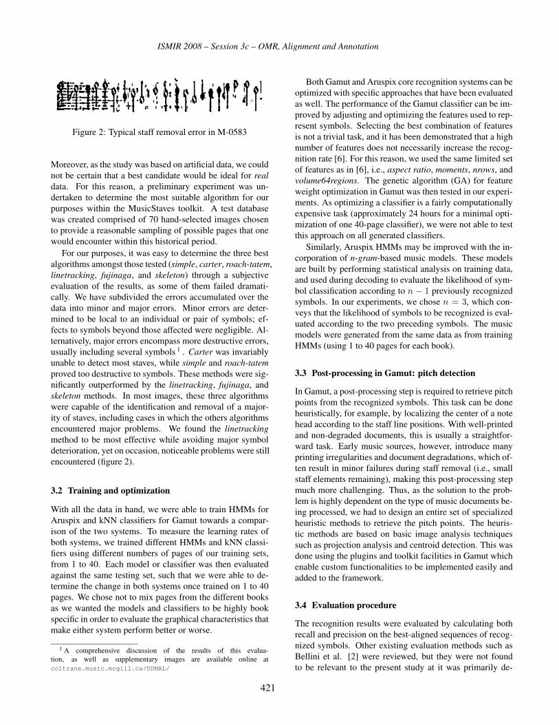
ISMIR 2008 – Session 3c – OMR, Alignment and Annotation
Figure 2: Typical staff removal error in M-0583
Moreover, as the study was based on artificial data, we could
not be certain that a best candidate would be ideal for realdata. For this reason, a preliminary experiment was un-
dertaken to determine the most suitable algorithm for our
purposes within the MusicStaves toolkit. A test database
was created comprised of 70 hand-selected images chosen
to provide a reasonable sampling of possible pages that one
would encounter within this historical period.
For our purposes, it was easy to determine the three best
algorithms amongst those tested (simple, carter, roach-tatem,
linetracking, fujinaga, and skeleton) through a subjective
evaluation of the results, as some of them failed dramati-
cally. We have subdivided the errors accumulated over the
data into minor and major errors. Minor errors are deter-
mined to be local to an individual or pair of symbols; ef-
fects to symbols beyond those affected were negligible. Al-
ternatively, major errors encompass more destructive errors,
usually including several symbols 1 . Carter was invariably
unable to detect most staves, while simple and roach-tatemproved too destructive to symbols. These methods were sig-
nificantly outperformed by the linetracking, fujinaga, and
skeleton methods. In most images, these three algorithms
were capable of the identification and removal of a major-
ity of staves, including cases in which the others algorithms
encountered major problems. We found the linetrackingmethod to be most effective while avoiding major symbol
deterioration, yet on occasion, noticeable problems were still
encountered (figure 2).
3.2 Training and optimization
With all the data in hand, we were able to train HMMs for
Aruspix and kNN classifiers for Gamut towards a compar-
ison of the two systems. To measure the learning rates of
both systems, we trained different HMMs and kNN classi-
fiers using different numbers of pages of our training sets,
from 1 to 40. Each model or classifier was then evaluated
against the same testing set, such that we were able to de-
termine the change in both systems once trained on 1 to 40
pages. We chose not to mix pages from the different books
as we wanted the models and classifiers to be highly book
specific in order to evaluate the graphical characteristics that
make either system perform better or worse.
1 A comprehensive discussion of the results of this evalua-
tion, as well as supplementary images are available online at
coltrane.music.mcgill.ca/DDMAL/
Both Gamut and Aruspix core recognition systems can be
optimized with specific approaches that have been evaluated
as well. The performance of the Gamut classifier can be im-
proved by adjusting and optimizing the features used to rep-
resent symbols. Selecting the best combination of features
is not a trivial task, and it has been demonstrated that a high
number of features does not necessarily increase the recog-
nition rate [6]. For this reason, we used the same limited set
of features as in [6], i.e., aspect ratio, moments, nrows, and
volume64regions. The genetic algorithm (GA) for feature
weight optimization in Gamut was then tested in our experi-
ments. As optimizing a classifier is a fairly computationally
expensive task (approximately 24 hours for a minimal opti-
mization of one 40-page classifier), we were not able to test
this approach on all generated classifiers.
Similarly, Aruspix HMMs may be improved with the in-
corporation of n-gram-based music models. These models
are built by performing statistical analysis on training data,
and used during decoding to evaluate the likelihood of sym-
bol classification according to n − 1 previously recognized
symbols. In our experiments, we chose n = 3, which con-
veys that the likelihood of symbols to be recognized is eval-
uated according to the two preceding symbols. The music
models were generated from the same data as from training
HMMs (using 1 to 40 pages for each book).
3.3 Post-processing in Gamut: pitch detection
In Gamut, a post-processing step is required to retrieve pitch
points from the recognized symbols. This task can be done
heuristically, for example, by localizing the center of a note
head according to the staff line positions. With well-printed
and non-degraded documents, this is usually a straightfor-
ward task. Early music sources, however, introduce many
printing irregularities and document degradations, which of-
ten result in minor failures during staff removal (i.e., small
staff elements remaining), making this post-processing step
much more challenging. Thus, as the solution to the prob-
lem is highly dependent on the type of music documents be-
ing processed, we had to design an entire set of specialized
heuristic methods to retrieve the pitch points. The heuris-
tic methods are based on basic image analysis techniques
such as projection analysis and centroid detection. This was
done using the plugins and toolkit facilities in Gamut which
enable custom functionalities to be implemented easily and
added to the framework.
3.4 Evaluation procedure
The recognition results were evaluated by calculating both
recall and precision on the best-aligned sequences of recog-
nized symbols. Other existing evaluation methods such as
Bellini et al. [2] were reviewed, but they were not found
to be relevant to the present study at it was primarily de-
421

ISMIR 2008 – Session 3c – OMR, Alignment and Annotation
signed for common music notation. Our first evaluation was
to measure the performance of the core recognition engines
by determining symbol recognition rates for both the Ga-
mut kNN and Aruspix HMM methods, without pitch detec-
tion. This was a trivial alteration within Gamut, as we only
needed to consider the output of the classifier, prior to pitch
point detection. For Aruspix, however, it was necessary to
short-circuit the system, as symbol and pitch recognition is
normally performed concurrently. The HMMs were modi-
fied in such a way that pitches were ignored, reducing the
number of different symbols to be recognized from more
than 130 to less than 30, hence enabling a direct comparison
with Gamut classifiers. We also evaluated and compared
improvement rates of both systems through incorporation of
their specific optimization schemes, i.e., the genetic algo-
rithm for Gamut and n-gram-based music models for Arus-
pix. Finally, we assessed the complete recognition process
including pitch detection, yielding a full comparison of both
OMR approaches for early music prints.
4 RESULTS
4.1 Evaluation of the recognition systems
Training the recognition systems of Gamut and Aruspix nei-
ther yields similar results nor generates the same learning
curves. After 40 pages of training, Aruspix HMMs out-
perform the Gamut kNN classifiers for all four books, as
shown in table 1. Only within the fourth book (M-0585)
does the kNN classifier produce similar results to those of
the HMMs, with more than 93% recall and more than 94%
precision. Overall, the HMMs appears to be more robust and
reliable, as the variability across the results is far smaller
than within the kNN classifiers. While learning rates for
Aruspix HMMs are fairly consistent across the four books,
the Gamut kNN classifiers varies significantly from one book
to another.
Figure 3 shows the learning curves for Aruspix HMMs
and Gamut kNN classifiers for the book M-0579 and for
the book M-0585. When the Gamut kNN classifiers per-
form well, they learn quicker than the HMMs, as demon-
strated within the fourth book M-0585 (figure 3, bottom). In
all cases, the kNN classifiers reach a plateau after 10 to 20
BookRecall Precision
kNN HMMs kNN HMMs
M-0579 86.90 95.99 86.63 95.63
M-0580 86.76 93.51 89.36 97.32
M-0583 77.30 87.58 81.04 93.95
M-0585 93.35 94.72 93.47 96.80
Table 1: Recall and precision for the core recognition sys-
tems after 40 pages
75
80
85
90
95
100
5 10 15 20 25 30 35 40
Rec
all
Number of pages
Aruspix HMMs (without pitch detection)Gamut kNN
75
80
85
90
95
100
5 10 15 20 25 30 35 40
Rec
all
Number of pages
Aruspix HMMs (without pitch detection)Gamut kNN
Figure 3: Learning curves (recall) of the core recognition
systems on M-0579 and M-0585
pages, whereas the HMMs continue to improve gradually
even after 30 pages.
For both Gamut kNN classifiers and Aruspix HMMs, the
third book (M-0583) appears to be the most difficult. It is the
most degraded book in our set, with strong bleed-through
showing printed characters of the verso through the page.
This book was printed with a very similar music font to that
in book M-0585 (see figure 1), upon which both systems
performed quite well: the best results for Gamut were found
within this book. We may therefore conclude that document
degradation, and not font shape, is the main cause of dif-
ficulty for both systems encountered with this book. Such
degradations make the binarization step, which is critical
in such applications, much more challenging [3]. Figure 4
clearly illustrates the effects of binarization errors on subse-
quent staff removal and recognition.
4.2 Evaluation of the optimization techniques
GA optimization of Gamut kNN classifiers improved the re-
sults for each of the four books in our experiments. Further,
it appeared to be extremely influential when the number of
422

ISMIR 2008 – Session 3c – OMR, Alignment and Annotation
Figure 4: Original greyscale image and the same image after
binarization and staff removal in one page of M-0583
pages was very small. Even within kNN classifiers already
demonstrating steep (fast) learning curves, the GA optimiza-
tion led to markedly faster learning, as shown in figure 5.
Yet, in most cases, results were not significantly improved
when using 20 pages or more.
75
80
85
90
95
100
5 10 15 20 25 30 35 40
Rec
all
Number of pages
Gamut kNNGamut kNN with GA optimization
Figure 5: Improvement (recall) with GA optimization in Ga-
mut on M-0585
For Aruspix, the integration of the n-gram-based mod-
els also improved results for all books, but in a notably dif-
ferent way than GA optimization within Gamut. First, the
n-gram-based models improve precision rates much more
so than recall rates. This verifies the logical intuition that
the introduction of the model will reduce the likelihood of
non-expected symbols during decoding, and thus reduce the
number of insertions. Secondly, the improvement curve is
also quite different than that of GA optimization within Ga-
mut, as n-gram integration requires more pages to be signif-
icant, but displays a longer stable growth period, as shown
in figure 6.
4.3 Evaluation of the OMR approaches
Table 2 presents the overall OMR recall and precision rates
of both applications after 40 pages. In Gamut, pitches were
determined heuristically in a post-processing step, whereas
Aruspix uses an all-inclusive approach directly at the HMM
level. On average, the differences for the complete OMR
process from one book to the next are very similar to the
those observed for the core recognition systems (see table
1), with a more significant loss in Gamut than in Aruspix.
���
���
���
���
���
����
�� ��� ��� �� �� �� �� ���
� �
����
��
����� ���������
� ����������� �����������!�"#���� �����$�%
Figure 6: Improvement (precision) with the n-gram-based
music models in Aruspix on M-0579
BookRecall Precision
Gamut Aruspix Gamut Aruspix
M-0579 79.34 92.44 84.13 95.60
M-0580 76.18 92.52 84.55 96.44
M-0583 68.13 86.75 76.54 92.76
M-0585 81.61 92.77 88.34 96.23
Table 2: Recall and precision for the complete OMR results
after 40 pages
These results distinctly show that retrieval of pitch points
after symbol recognition is far from trivial with early mu-
sic documents. In this task, the flexibility of Gamut could
have been leveraged more, as the heuristic approach may be
adjusted for a particular dataset.
In our experiment, Gamut failed to perform as well as
Aruspix, despite the fact that the all-inclusive approach of
Aruspix offer very few entry points for adjustment. Within
the fourth book (M-0585), for which the core recognition
systems performance is nearly equivalent, the final OMR
output decreases significantly with the addition of pitch de-
tection in Gamut (-11.71% for the recall rate) whereas the
decline is only minimal in Aruspix (-1.95%). This slight
reduction at the incorporation of pitch detection in Aruspix
is an intriguing aspect of these results, as the all-inclusive
approach of Aruspix has drastically inflated the number of
symbols to be recognized (from less than 30 to more than
130 with our datasets) without affecting the recognition rates
significantly.
5 CONCLUSIONS AND FUTURE WORK
The results of these experiments confirm the need for adapt-
ability within tools for optical early music recognition. Even
if the systems learn and perform differently, they both under-
423

ISMIR 2008 – Session 3c – OMR, Alignment and Annotation
performed on the same book (M-0585), which was by far the
most degraded in our experimental set. This clearly indi-
cates that binarization of degraded music documents is still
an area in which improvements must be made. The differ-
ence between the results of M-0582 and M-0585, two books
with the same content and quasi-identical music font, illus-
trates well the extent to which degradation may affect the
performance of the systems. This is a quite probable ex-
planation as to why our results obtained with Gamut are
significantly lower than those obtained by Dalitz et al. [6]
from a lute tablature application also built within the Gamut
framework, which was evaluated with retouched facsimile
images.
Our experiments with Gamut also demonstrate that staff
removal within early music sources cannot be considered
a solved problem. None of the algorithms tested worked
extraordinarily well, and even minor failures, such as re-
maining small staff elements, certainly affect performance
throughout the entire OMR process. Retrieving the pitch
from the recognized symbols appears to be a challenging
step within such documents, and the heuristic method cur-
rently used in Gamut could certainly be improved further.
The flexibility and the extensibility of the Gamut infras-
tructure proved its utility, as the system can easily be modi-
fied to improve its performance for a particular set of sources.
Additionally, the learning speed of Gamut is an asset to
the approach. The kNN classifiers learn quite rapidly, en-
abling a specific application to be built upon only a hand-
ful of pages. With the addition of the GA optimization, the
amount of data required to achieve the best performance is
reduced even further. Aruspix distinguishes itself by its per-
formance and robustness. Together, HMMs and integrated
pitch detection are an excellent approach with which to han-
dle noise introduced by printing irregularities and degrada-
tions in early printed sources. Aruspix also provides a built-
in editor specifically designed to assist in the correction of
recognition errors. To enhance performance, Aruspix im-
plements dynamic adaptation, which enables the amount of
training data to be significantly reduced through optimiza-
tion of previously trained HMMs.
Although both applications present distinct advantages,
Aruspix clearly benefits from having been optimized for early
music prints and may be used directly out-of-the-box, while
the adaptability of Gamut may be advantageous for projects
with a wider scope.
6 REFERENCES
[1] D. Baindridge and T. Bell. The challenge of optical music
recognition. In Computer and the Humanities, volume 35,
pages 95–121, 2001.
[2] P. Bellini, I. Bruno, and P. Nesi. Assessing optical music recog-
nition tools. Computer Music Journal, 31(1):68–93, 2007.
[3] J. A. Burgoyne, L. Pugin, G. Eustace, and I. Fujinaga. A com-
parative survey of image binarisation algorithms for optical
recognition on degraded musical sources. In Proceedings of the8th International Conference on Music Information Retrieval,pages 509–12, Vienna, Austria, 2007.
[4] D. Byrd and M. Schindele. Prospects for improving OMR with
multiple recognizers. In Proceedings of the 7th InternationalConference on Music Information Retrieval, pages 41–6, Vic-
toria, Canada, 2006.
[5] C. Dalitz, M. Droettboom, B. Czerwinski, and I. Fuji-
naga. A comparative study of staff removal algorithms. IEEETransactions on Pattern Analysis and Machine Intelligence,
30(5):753–66, May 2008.
[6] C. Dalitz and T. Karsten. Using the Gamera framework for
building a lute tablature recognition system. In Proceedingsof the 6th International Conference on Music Information Re-trieval, pages 478–81, London, UK, 2005.
[7] M. Droettboom. Correcting broken characters in the recogni-
tion of historical printed documents. In Proceedings of the 3rdACM/IEEE-CS Joint Conference on Digital Libraries, pages
364–6, Houston, Texas, 2003.
[8] M. Droettboom, K. MacMillan, I. Fujinaga, G. S. Choudhury,
T. DiLauro, M. Patton, and T. Anderson. Using the Gamera
framework for the recognition of cultural heritage materials.
In Proceedings of the 2nd ACM/IEEE-CS Joint Conference onDigital Libraries, pages 11–7, Portland, Oregon, 2002.
[9] I. Fujinaga. Staff detection and removal. In S. E. George, ed-
itor, Visual Perception of Music Notation: On-Line and Off-Line Recognition, chapter 1, pages 1–39. IRM Press, Hershey,
2005.
[10] K. MacMillan, M. Droettboom, and I. Fujinaga. Gamera: Op-
tical music recognition in a new shell. In Proceedings of the In-ternational Computer Music Conference, pages 482–5, 2002.
[11] J. C. Pinto, P. Vieira, M. Ramalho, M. Mengucci, P. Pina, and
F. Muge. Ancient music recovery for digital libraries. In 4thEuropean Conference on Digital Libraries, ECDL 2000, Lis-bon, Portugal, September 2000, Proceedings, volume 1923 of
LNCS, pages 24–34. Springer, Berlin, 2000.
[12] L. Pugin. Optical music recognition of early typographic prints
using hidden Markov models. In Proceedings of the 7th In-ternational Conference on Music Information Retrieval, pages
53–6, Victoria, Canada, 2006.
[13] L. Pugin, J. A. Burgoyne, and I. Fujinaga. Goal-directed evalu-
ation for the improvement of optical music recognition on early
music prints. In Proceedings of the ACM/IEEE Joint Confer-ence on Digital Libraries, pages 303–4, Vancouver, Canada,
2007.
[14] L. Pugin, J. A. Burgoyne, and I. Fujinaga. MAP adaptation to
improve optical music recognition of early music documents
using hidden Markov models. In Proceedings of the 8th In-ternational Conference on Music Information Retrieval, pages
513–6, Vienna, Austria, 2007.
[15] Répertoire international des sources musicales (RISM). SinglePrints Before 1800. Series A/I. Bärenreiter, Kassel, 1971–81.
424

Session 4a – Data Exchange, Archiving and Evalua-tion

.

ISMIR 2008 – Session 4a – Data Exchange, Archiving and Evaluation
USING THE SDIF SOUND DESCRIPTION INTERCHANGE FORMAT FORAUDIO FEATURES
Juan José Burred, Carmine Emanuele Cella, Geoffroy Peeters, Axel Röbel and Diemo SchwarzIRCAM - CNRS STMS
{burred,cella,peeters,roebel,schwarz}@ircam.fr
ABSTRACT
We present a set of extensions to the Sound Description In-terchange Format (SDIF) for the purpose of storage and/ortransmission of general audio descriptors. The aim is to al-low portability and interoperability between the feature ex-traction module of an audio information retrieval applicationand the remaining modules, such as training, classificationor clustering. A set of techniques addressing the needs ofshort-time features and temporal modeling over longer win-dows are proposed, together with the mechanisms that allowfurther extensions or adaptations by the user. The paper iscompleted by an overview of the general aspects of SDIFand its practical use by means of a set of existing program-ming interfaces for, among others, C, C++ and Matlab.
1 INTRODUCTION
The Sound Description Interchange Format (SDIF) [1, 2]is an established standard for the precise, well-defined andextensible storage and interchange of a variety of sound de-scriptions including representations of the signal for anal-ysis/synthesis like spectral, sinusoidal, time-domain, orhigher-level models, audio descriptors like loudness or fun-damental frequency, markers, labels, and statistical models.SDIF consists of a basic data format framework based ontime-tagged frames containing matrices of binary numbersor text, and an extensible set of standard type declarationscorresponding to different sound descriptions.
The SDIF standard was created in 1998 in collabora-tion between Ircam–Centre Pompidou in Paris, France, CN-MAT at the University of Berkeley, USA, and the MusicTechnology Group (MTG) of the Universitat Pompeu Fabra,Barcelona, Spain. It arose out of the need to be able tostore and exchange sound representation data between dif-ferent analysis/synthesis programs, research teams, and in-stitutions, and to enable anyone to interpret the informationin the files correctly, needing as little external information aspossible. With the previously widely used headerless ASCIIformats, this goal was seriously compromised, as well asprecision and space efficiency lost.
In the present contribution, we propose a set of exten-sions to the SDIF description types and conventions and bestpractices for the application of storing and/or transmitting awide range of audio descriptors, e.g. as generated by the fea-ture 1 extraction stage of an audio pattern recognition sys-
1 We will use the terms feature and descriptor interchangeably.
tem. In the Audio or Music Information Retrieval fields, thisis of interest to assure interoperability between feature ex-traction and further processing modules, such as feature se-lection, training, clustering or classification, possibly beingdeveloped independently from each other, or even by differ-ent institutions. Such a need for standardization can arise inthe context of multi-partner evaluation, such as in the MusicInformation Retrieval Evaluation eXchange (MIREX) [3].
SDIF is an open format, unhampered by licensing or in-tellectual property restrictions, made by the research com-munity for research and creation. There is a wide rangeof software available for its use: Libraries in C, C++,Java, Matlab, Perl, and Python, command-line and graph-ical tools, and plugins for audio-processing systems such asMax/MSP and PureData.
After an introduction to the basics of SDIF (section 2),and a general overview of common different types of audiodescriptors (section 3), we will propose several format con-ventions for storing general descriptor information (section4). The standard’s type declarations are completely exten-sible and modifiable by the user (section 5), which makesthe current proposal adaptable to special application needs.Finally, in section 7, we will present a selection of helpfultools distributed with the SDIF library, programming inter-faces for reading and writing SDIF files, a number of appli-cations and online resources.
2 OVERVIEW OF THE SDIF SPECIFICATION
SDIF is a binary meta-format based on streams, frames andmatrices. The matrix content representation can be chosento be text, integer, or floating point in different bit-widths.Several matrices are grouped into a frame, which has a pre-cise 64 bit floating point time tag in seconds relative to thestart of the file. Frames are always stored in increasing tem-poral order and are assigned to a stream. Streams separatedifferent entities of the same type, such as different soundfiles, channels, or different analyses or descriptors, thus al-lowing to unite a database of several source sound files, plusvarious stages of analysis and descriptor data, in one singleSDIF file. 2 For example, one could choose to store twochannels of audio, their STFT representation, fundamentalfrequency and sinusoidal partial representation, markers, la-bels, and harmonicity audio descriptors in one file.
2 This was formerly achieved by separate files with different file exten-sions, grouped in the same directory, with the risk of loss of single files,and a certain implicitness of their relationships.
427

ISMIR 2008 – Session 4a – Data Exchange, Archiving and Evaluation
Frame and matrix types are identified by 4-byte ASCIIsignatures, inspired by the IFF format. Each frame startswith a header containing the frame signature, the numberof matrices it contains, an integer identifying the stream itbelongs to, and the time tag. Each matrix’ header containsits signature, its content data type, and its number of rowsand columns. Matrices are padded to 8 byte boundaries toachieve 64 bit word alignment for fast access using memorymapped files.
Special header-frames can store global textual meta-datain so-called Name–Value Tables (NVTs), together with re-lationships of different streams (see section 6). However,global information that is needed to interpret the data, forinstance the sampling rate, is stored in information matri-ces, making SDIF files streamable.
There are a number of standard description types thatspecify the columns of matrices, and which matrices canoccur in which frame type. Examples include 1FQ0 to storefundamental frequencies and 1TRC to store partial tracksresulting from sinusoidal analysis. By convention, the sig-natures of standard frame and matrix signatures start with aversion number, mostly 1. It is always possible to declarenew experimental description types, or to extend existingtypes by new matrices for a frame, or new columns for a ma-trix. New experimental types have signatures starting withX. SDIF is designed such that programs can always ignoreadditional data they don’t know how to interpret.
3 OVERVIEW OF AUDIO DESCRIPTORS
Audio descriptors (also named audio features or audio at-tributes) are numerical values describing the contents ofan audio signal according to various points of view, e.g.temporal, spectral or perceptual characteristics. They areused nowadays in many areas such as for the developmentof query-by-example (search-by-similarity), automatic in-dexing, segmentation or identification applications. Thesefeatures are extracted from the audio signal using signalprocessing algorithms. Several taxonomies can be used toclassify them, for example according to the type of con-tent they can be applied to (single musical notes, percus-sion, sound effects, generic audio, etc.), the underlying sig-nal model they rely on (source-filter, sinusoidal harmonicmodels, etc.), their abstractness, i.e. what the audio featurerepresents (spectral envelope, temporal envelope, etc.), theirsteadiness or variability, i.e., the fact that they represent avalue extracted from the signal at a given time, or a param-eter from a model of the signal behavior along time (mean,standard deviation, derivative or Markov model of a param-eter), or the time extent of the description provided by them:some descriptors apply to only part of the object (e.g., de-scription of the attack of the sound) whereas others applyto the whole signal (e.g., loudness). On the computer side,an audio feature is represented by a numerical value or avector of numerical values when several audio features canbe linked together (such as the coefficients of the MFCC, orvarious definitions of the spectral centroid).
Each of such numerical values describes a specific prop-erty of the signal around a specific time (the time of thesegment corresponding to the analysis window). Most au-dio features are first computed on a small-time scale (oftencalled short-term analysis) which for most of them corre-spond to the length of the analysis window used for FFTanalysis (usually 40 ms to 80 ms). Other features are com-puted on a longer-time scale due to their semantics (the log-attack-time, the roughness or the fluctuation strength are as-sociated to a whole musical note) or due to computationalrequirements (the estimation of a vibrato or tremolo at a fre-quency of 6 Hz necessitates a window larger than 80 ms).In this case the numerical value needs to be associated ex-actly to the segment used to compute it. Finally, it has be-come frequent to model the behavior of an audio featureover time. Using long-term analysis (often with windowlengths of 500 ms or larger), it is common to compute themean, variance or derivative values of the feature over thesliding window. This type of description is often namedtemporal modeling, and the corresponding large frames aresometimes called texture windows or macroframes. In thiscase, the segment over which the temporal model is com-puted does not need to have a specific semantic (e.g., “every200 ms” has no meaning by itself), although it can have (forexample for beat-synchronous analysis).
In the proposed SDIF extensions, we address these spe-cific requirements concerning definition of different timehorizons, multidimensionality and addition of semantic in-formation. It is out of the scope of this article to presentdetailed mathematical definitions of the descriptors. A largeset of them can be found in [4].
4 EXTENDED TYPES FOR GENERALIZED AUDIODESCRIPTORS
A defining aspect of SDIF is its flexibility regarding datatypes. Using the data declaration syntax introduced laterin section 5, the user is able to define or redefine theframe/matrix grouping rules and to add or modify type dec-larations at will. Throughout the paper, we will present dif-ferent possibilities for different applications in the contextof descriptor extraction. At the same time, however, we areproposing a ready-to-use set of type declarations designedaccording to what we consider appropriate to most audiocontent analysis and retrieval applications. The proposedtype declarations, together with related documentation andseveral example SDIF files can be accessed online 3 .
In both short-time and temporal modeling cases, the val-ues of a given descriptor at a given time are stored in a sepa-rate matrix. For example, spectral centroid values are storedin matrices of signature 1SCN and for zero-crossing valuesthe matrix signature is 1ZCR. In analogy with the standardmatrix types (e.g., with sinusoidal modeling), the numberof rows of the matrix must correspond to the dimensionalityof the descriptor, i.e., with the number of frequency bands(such as with spectral flatness) or with the number of coef-ficients (such as with MFCCs or autocorrelation features).
3 http://sdif.sourceforge.net/descriptor-types
428

ISMIR 2008 – Session 4a – Data Exchange, Archiving and Evaluation
The columns are intended to store the values for differentdefinitions or implementations of the same descriptor. Forexample, the first column of the spectral centroid could con-tain the values for a centroid defined on linear frequency andamplitude scales, and the second the values using logarith-mic scalings. We will thus use dimensions to denote rowsand variations to denote columns.
Both the number of rows and of columns are not fixedbeforehand by the type declaration. In most cases, the num-ber of rows will depend on a user-defined feature extractionparameter, such as number of frequency bands or cepstralcoefficients. It is also most likely that the user will just storea single variation for each descriptor. In some training ex-periments, however, it can be interesting to store differentvariations at the same time and let an automatic feature se-lection algorithm select the most informative one.
Even if not strictly necessary for a clustering or statisti-cal training algorithm, the feature extraction program shouldstore additional information alongside the descriptor val-ues, such as bandwidths, thresholds or labels describing thecontents of the columns. This data will be included in in-formation matrices, whose signatures will be equal to thedescriptor matrix signatures, with the first character 1 re-placed by I. Entries on information matrices are alwaysstored column-wise. The next subsections will detail howto store such matrices.
To accommodate the different descriptor time-spansmentioned above (short-, mid-, long-term and temporalmodeling) we propose two different schemes for SDIF stor-age. In fact, we simplify such categorization by only con-sidering, on the one hand, the descriptors themselves (whichare directly based on the signal) and, on the other hand,temporal modelings (which are based on descriptors), whichwill respectively be addressed in the next two subsections.We deliberately avoid a categorical distinction between thelength of the time spans, since the only difference from theSDIF point of view is the definition of the time bound-aries. Also, we will avoid the terminology “low-level”or “high-level” feature because of the lack of consensusabout its meaning. By convention, an SDIF file containingonly audio descriptors should end with the double extension.descr.sdif.
4.1 Format for Descriptors
We propose the following procedure to store descriptors thatare directly based on the signal, independently of their timespan. Each data matrix corresponding to a given analysiswindow of a given descriptor is contained within a frame oftype 1DSC, a descriptor frame. In order to be able to per-form a one-to-one mapping between streams and descrip-tors, each descriptor frame must contain only a single de-scriptor data matrix. The time tag on each frame corre-sponds to the center of the analysis window. The optionalinformation matrices must be stored at the beginning ofthe corresponding descriptor stream, and are valid until anew information matrix of the same type appears on thesame stream. Figure 1 represents this approach schemati-cally for the case of a file storing spectral centroid (1SCN)
and perceptual tristimulus (1PTR) data. In this example,the spectral centroid is a unidimensional descriptor with asingle variation, and two different variations of the three-dimensional tristimulus have been stored, each one definedwith a different amplitude scaling.
The SDIF reading routines search first by frames, andthen by matrices. Thus, if the performance in accessing indi-vidual descriptors is critical, an alternative approach wouldbe to declare a pair of frame type and matrix type with thesame signature for each descriptor. Its disadvantage how-ever is that it requires to double the amount of type declara-tions.
4.2 Format for Temporal Modeling of Descriptors
There are three main reasons for considering temporal mod-eling of descriptors as a special case that requires dedicatedstoring conventions. First, they are derived features of typi-cally the same dimensionality than their shorter-term coun-terparts they are based on, and thus they can reuse their ma-trix type declarations. This results in each temporal modelbeing associated to a frame type, containing matrices of thetypes already declared for the descriptors. For example, atexture window of the weighted variance of the spectral cen-troid will correspond to a frame of type 1WVR containing amatrix of type 1SCN. An indicative list of types of temporalmodeling is: mean, variance, standard deviation, weightedmean, weighted standard deviation, amplitude modulation.
Second, it is possible to assume that their time-span willbe relatively long-term (in the range of seconds), and thusperformance when accessing them will rarely be critical. Ifstored together with their short-term descriptors, they willpredictably constitute a very small percentage of the filesize. This allows more freedom in choosing the most appro-priate way of frame and matrix grouping, depending on theapplication. This can be done either in the one-matrix-per-frame way, as before, or using compound frames, i.e. group-ing several matrices corresponding to different descriptorsunder the same frame. In the first case, individual assign-ment to streams, and different window sizes between dif-ferent descriptors will be possible. In the compound case,visual inspection of SDIF files (e.g., after ASCII conversionwith the sdiftotext tool) will be clearer. To leave both possi-bilities open, the provided type declaration lists all descrip-tor matrices as optional members of each temporal modelingframe. If visual inspection is not important, we recommendusing the one-matrix-per-frame alternative.
Finally, the third reason is that the segment the tempo-ral modeling works on is not necessarily of constant sizeand overlap. For example, one can define a sequence oflog-attack time features resulting from a note-wise segmen-tation of a melodic line. Thus, a mechanism must be pro-vided to indicate the segment on which the descriptor evo-lution is modeled. This mechanism makes use of the stan-dard frame type 1MRK that represents a marker at the timeof the frame, containing matrices 1BEG and/or 1END witha unique identifier of a segment. Now, the temporal model-ing frame will also contain a matrix with the identifier of thesegment whose descriptor evolution it models.
429

ISMIR 2008 – Session 4a – Data Exchange, Archiving and Evaluation
0.03111DSC
TimeStream# matr.Sign.
503.2
1141SCN
# cols.# rowsTypeSign.
0.03211DSC
TimeStream# matr.Sign.
0.0010.002
0.3510.619
0.6490.38
2341PTR
# cols.# rowsTypeSign.
0.06111DSC
TimeStream# matr.Sign.
503.2
1141SCN
# cols.# rowsTypeSign.
0.06211DSC
TimeStream# matr.Sign.
0.0020.005
0.2950.625
0.7040.374
2341PTR
# cols.# rowsTypeSign.
Figure 1. SDIF storage example for four consecutive frames of a short-time spectral centroid (1SCN) and a short-time percep-tual tristimulus (1PTR).
0.5121WMN
TimeStream# matr.Sign.
432.3
1141SCN
# cols.# rowsTypeSign.
1221MDA
TimeStream# matr.Sign.
0.0010.002
0.0320.024
0.0230.012
2341PTR
# cols.# rowsTypeSign.
171
214IWMN
# cols.# rowsTypeSign.
2
114IMDA
# cols.# rowsTypeSign.
1121WMN
TimeStream# matr.Sign.
461.54
1141SCN
# cols.# rowsTypeSign.
3.5221MDA
TimeStream# matr.Sign.
0.0020.001
0.0670.049
0.0370.023
2341PTR
# cols.# rowsTypeSign.
171
214IWMN
# cols.# rowsTypeSign.
3
114IMDA
# cols.# rowsTypeSign.
Figure 2. SDIF storage example for four consecutive temporal modeling segments: weighted mean (1WMN) of spectral centroidand modulation amplitude (1MDA) of perceptual tristimulus.
Each temporal modeling frame type has an associated in-formation matrix type, e.g. IWVR for the weighted varianceframe type 1WVR. Then, each temporal modeling frame con-tains one information matrix indicating the duration, in sec-onds, of the window as its first element. For regularly spacedtexture windows, the time tag of the frames corresponds tothe middle of the temporal modeling segment. For irregularsegments given by markers, the temporal modeling frameis written at the start time of the segment. Figure 2 showsan example of this approach, using single-matrix grouping.It shows the storage for two consecutive texture windowscontaining the weighted mean (1WMN) of the spectral cen-troid, and the amplitude modulation (1MDA) of the percep-tual tristimulus. Like with any other matrix, the meaningof the columns is contained in the type declaration. As inthe plain descriptors case, it is possible to store descriptor-related information matrices at the beginning of the corre-sponding streams. It should be noted that some temporalmodelings, such as log-attack time or temporal increase, arealmost always based on a very specific descriptor, in thiscase the energy envelope. It would be however possible toattach them to no matter which shorter-time feature (for in-stance, the temporal increase of the fundamental frequencycould be an informative “sweep descriptor”).
5 USER-DEFINED TYPES
SDIF allows to define new description types by declaringframe and matrix signatures, and matrix columns, or to ex-tend existing types by new matrices, or new columns. Thedeclaration of extended types is included in a special typedeclaration frame of signature 1TYP. Each SDIF file mustinclude a 1TYP frame declaring the non-standard types, andis therefore self-contained. The standard types must not bedeclared in such a frame, since they are already recognizedby the library. The following is an example of the type dec-laration for some existing types:
1TYP{1MTD 1SCN {SpectralCentroid}1MTD 1ZCR {ZeroCrossingRate}1MTD IWMN {WindowLength}1FTD 1WMN
{1SCN SpectralCentroidWeightedMean;1ZCR SignalZeroCrossingRateWeightedMean;1FQ0 FundamentalFrequencyWeightedMean;IWMN WeightedMeanInfo;
}}
Each line starting with 1MTD is a matrix type declaration,containing the new matrix signature and, between curly
430

ISMIR 2008 – Session 4a – Data Exchange, Archiving and Evaluation
brackets, a list of the declared column names, separated bycommas. The lines starting with 1FTD are frame type decla-rations; after the frame signature (1WMN in the example), be-tween the curly brackets, there is the list of the matrices thatcan appear inside that frame with their role, terminated by asemicolon. A matrix type must be declared before the frametype containing it. As a side note, we point out that even forstandard types (like 1FQ0 in the example), the associationwith a non-standard frame must be created. All the descrip-tor types proposed here contain only one declared column.This does not hinder the user to store as many additionalcolumns as needed.
6 DECLARATION OF STREAM RELATIONSHIPS
In the previous section we have seen that the proposed SDIFrepresentation of audio descriptors will distribute the dataover several streams of SDIF frames. For instance, we couldhave a stream of temporal modeling frames 1WMN, model-ing segments given by a stream of 1MRK frames, based onvarious descriptors in different streams, that were extractedfrom the audio data in a stream of 1TDS files.
While the relationships between these streams are clearin our context of use, we would like them to be expressedexplicitly, in a machine-readable format, in order to be ex-ploited by tools, visualisers, and other applications. Theexplicitness of the relationships and meanings of streamsbecomes even more important when several source sounds,channels, or analyses are included in the same SDIF file.
At the beginning of the SDIF standard, there has been anattempt [5] to formalise the relationships between streamsin an XML based language, which has not been followed byconcrete implementations. This is possibly due to the com-paratively simple SDIF files that were used at that time, pos-ing no real need for an explicit representation, and, what’smore, to the problem of adding a dependency on an externallibrary to parse XML to all SDIF tools.
We propose here a new, simple approach how to definerelationships, meaning, and content of streams in a tabulartext format, not unlike the existing Name–Value Tables. Wewill start with expressing only those relationships that areindeed needed for the applications described in this article,but we strive to keep the format open enough for other rela-tionships to be added in the future.
The format associates one entity by a relationship to a listof entities. The possible entities are listed in table 1, the listof defined relationships in table 2. For stream IDs and frameand matrix signatures, the notation of entities follows theSDIF-selection syntax [2] to ease understanding and pars-ing, all other entities are labels, starting with a letter. Wepropose to store this table in a 2IDS frame with text matrix.
7 SDIF USAGE INFORMATION
7.1 SDIF Tools
In order to easily manipulate the produced SDIF files, thelibrary provides some command-line tools together with the
Entity Example Description# stream id #23 Stream number 23: frame / matrix :1WMN/1SCN stream contains
weighted mean ofspectral centroid
identifier left-channel Label
Table 1. List of entities in the proposed stream relationshipdeclaration.
Relationship Descriptioncontains left stream contains frame, matrix types
given rightgroup left label groups labels or streams to the
rightsegments left stream contains segmentation infor-
mation for right entityderives left entity is derived (by analysis or tem-
poral modeling) from right entity
Table 2. List of relationships between two entities.
source code. Basically, there are tools to display, to extractand to convert the stored data; the most important are:• querysdif: prints out a summary of the information storedin the file, e.g. the number and the types of stored framesand matrices,• sdifextract: extracts selected data from a file; the outputcan be stored in many formats like SDIF itself, multi-bpf(text lines of frame time and all selected columns), etc.,• sdiftotext, tosdif: convert data between SDIF and plaintext, preserving frame-matrix relationships. These also ex-ist as droplets for Macintosh, onto which one can drop a file,generating the complementary text or SDIF file.
7.2 Programming Interfaces
This section will describe the existing possibilities to ma-nipulate SDIF data using the SDIF libraries that are pub-licly available on the SourceForge software repository (seelocation below). There exist a C-library (denoted just asthe SDIF library) and a C++ library (called Easdif). Eas-dif incorporates the complete interface of the SDIF library.Additionally Easdif provides a high level programming in-terface to SDIF files, frames, and matrices including itera-tors over SDIF files. These iterators allow easy and efficientnavigation within the SDIF file using an internal cache ofthe meta data (frame and matrix headers). The SDIF andEasdif libraries are designed to work on all major platforms(Linux, Mac OS X and Windows), and thanks to the useof the cmake 4 project generator they can be compiled withmost common compilers (gcc, MSVC, Intel, . . .).
The Easdif library cannot only be used in C++ applica-tions, it comes as well with a number of bindings for otherapplications and languages. A recent achievement is the ad-
4 http://www.cmake.org
431

ISMIR 2008 – Session 4a – Data Exchange, Archiving and Evaluation
dition of sources for Matlab and Octave bindings (mex) thatallow access to data stored in SDIF files for these two pro-graming environments. The Matlab/Octave interface makesuse of the frame and matrix header cache of Easdif to allowefficient random access to SDIF frames and matrices.
Additionally, the Easdif library includes support for theSWIG 5 wrapper generator and interface descriptions forbindings for python, perl and java. Starting from the ex-isting interface descriptions the addition of other scriptinglanguages that are supported by SWIG should be easy.
7.3 Applications using SDIF
Many applications developed nowadays integrate a general-purpose SDIF reader/writer. Here is a partial list:
•AudioSculpt 6 : tool to analyse and modify sounds througha visual approach,• ASAnnotation 7 : sound analysis, visualisation and anno-tation, based on AudioSculpt,• CLAM 8 : C++ library for music information retrieval,• Csound 9 : language for sound manipulation and analysis,• Diphone Studio 10 : tool for sonic morphing,• FTM 11 for Max/MSP, jMax, PureData: realtime visualprogramming environment for sound analysis/synthesis,• Loris 12 : sound modeling and processing package,•OpenMusic 13 : visual programming language for computer-aided composition,• Open Sound World 14 : programming environment toprocess sound in real-time,• SDIF-Edit 15 : SDIF editor and visualisation tool,• SPEAR 16 : sinudoidal analysis/resynthesis.
Moreover, in the developer tools included with the lat-est version of the Mac OS X operating system (version10.5, Leopard), SDIF support has been included for the Au-dioUnit called AdditiveSynth.
7.4 Availability and Online Resources
SDIF is an open source project hosted on the SourceForgerepository. The following resources are available:
• SDIF Homepage. (http://sdif.sourceforge.net)Includes the format specification and main documents, andpointers to all other resources.• SDIF Download. (http://sourceforge.net/projects/sdif)
5 http://www.swig.org6 http://forumnet.ircam.fr/691.html7 http://www.ircam.fr/anasyn/ASAnnotation8 http://clam.iua.upf.edu9 http://www.csounds.com
10 http://forumnet.ircam.fr/703.html11 http://ftm.ircam.fr12 http://www.cerlsoundgroup.org/Loris/13 http://recherche.ircam.fr/equipes/repmus/OpenMusic/14 http://osw.sourceforge.net15 http://recherche.ircam.fr/equipes/repmus/bresson/sdifedit/
sdifedit.html16 http://www.klingbeil.com/spear/
Includes the sources and several binaries for the SDIF andEasdif libraries. For developers, CVS access is possible.• SDIF Wiki. (http://sdif.wiki.sourceforge.net)is intended for the documentation of application-specificusages, the proposal of extensions, and additional user-oriented documentation.• SDIF mailing lists. There is one mailing list for users(http://listes.ircam.fr/wws/info/sdif) and one for developers(https://lists.sourceforge.net/lists/listinfo/sdif-devel).
8 CONCLUSION
In the context of the growing needs for standardizationwithin the fields of audio-based content analysis and re-trieval, we have proposed the use of the well-establishedand open SDIF format for storing, transmitting and sharinggeneral audio features. We made use of SDIF’s extensioncapabilities to declare a set of extended types addressing theneeds of general short-term and temporal modeling descrip-tors. We are hoping to initiate a discussion among interestedresearchers, e.g. via the wiki and the mailing lists, to furtherassess the general needs, and eventually update the type pro-posals. Concerning future work, we are studying the use ofSDIF for other audio-related pattern recognition data, suchas feature transformation data and statistical models.
9 ACKNOWLEDGMENTS
This work was supported by the French National Agency ofResearch (ANR) within the RIAM project Sample Orches-trator.
10 REFERENCES
[1] M. Wright, A. Chaudhary, A. Freed, S. Khoury and D.Wessel, “Audio Applications of the Sound DescriptionInterchange Format Standard”, Proc. of the 107th Con-vention of the Audio Engineering Society (AES), NewYork, USA, 1999.
[2] D. Schwarz and M. Wright, “Extensions and Applica-tions of the SDIF Sound Description Interchange For-mat”, Proc. of the Int. Computer Music Conference(ICMC), Berlin, Germany, 2000.
[3] J. S. Downie, “The Music Information Retrieval Evalua-tion eXchange (MIREX)”, D-Lib Magazine, Volume 12,Number 12, 2006.
[4] G. Peeters, “A Large Set of Audio Features forSound Description (Similarity and Classification) in theCUIDADO Project”, CUIDADO I.S.T. Project Report,2004.
[5] M. Wright, A. Chaudhary, A. Freed, S. Khoury, A.Momeni, D. Schwarz, D. Wessel, “An XML-basedSDIF Stream Relationships Language”, Proc. of the Int.Computer Music Conference (ICMC), Berlin, Germany,2000.
432

ISMIR 2008 – Session 4a – Data Exchange, Archiving and Evaluation
USING XQUERY ON MUSICXML DATABASES FOR MUSICOLOGICALANALYSIS
Joachim Ganseman, Paul ScheundersIBBT - Visionlab
Dept. of Physics, University of AntwerpUniversiteitsplein 1, building N
B-2610 Wilrijk (Antwerp), Belgium{joachim.ganseman, paul.scheunders}@ua.ac.be
Wim D’haesMu Technologies NVSingelbeekstraat 121
B-3500 Hasselt, [email protected]
ABSTRACT
MusicXML is a fairly recent XML-based file format for mu-
sic scores, now supported by many score and audio editing
software applications. Several online score library projects
exist or are emerging, some of them using MusicXML as
main format. When storing a large set of XML-encoded
scores in an XML database, XQuery can be used to re-
trieve information from this database. We present some
small practical examples of such large scale analysis, using
the Wikifonia lead sheet database and the eXist XQuery en-
gine. This shows the feasibility of automated musicological
analysis on digital score libraries using the latest software
tools. Bottom line: it’s easy.
1 INTRODUCTION
MusicXML is an open file format developed by Recordare
LLC [1]. Its development started around the year 2000 [2].
Some design decisions on the format are well explained in
[3].
In 2002 a paper was presented on the XML conference
[4] explaining how XQuery can be used to search for struc-
tures in a MusicXML document, but since then it has been
very quiet on the front. In a 2007 poster, Viglianti [5] points
out the possibilities of using XQuery for musicological anal-
ysis. Unfortunately, his text contains some errors - the most
important one being the remark that XQuery would not sup-
port arrays. XQuery definitely does support arrays, it is
even proved to be a Turing complete language [6]. There-
fore has the same expressive power as languages like C++
or Java, and any computable function can be performed us-
ing XQuery.
In the meantime, XQuery 1.0 has made it to a W3C rec-
ommendation [7]. Galax [8] strives to be a reference im-
plementation. eXist [9], Sedna [10], and Oracle’s Berkeley
DB XML [11] are native XML database management sys-
tems incorporating their own XQuery engines. All of those
are open source and free. Both standards and software have
thus matured.
Digital score libraries already exist, emanating from re-
search (e.g. KernScores [12], based on HumDrum [13]) or
the open source community (e.g. Mutopia [14], using Lily-
pond [15]). The Wikifonia project [16] uses MusicXML. It
is a wiki-style collaborative environment for publishing lead
sheets - i.e. reduced scores where arrangement details have
been removed and only melody, lyrics and chord progres-
sion information is available. Wikifonia is at the moment
of writing still relatively small. We worked with a database
downloaded on April 1st 2008, which contained just over
200 songs.
To do automated musicological analysis, the HumDrum
toolkit [13] is probably the most widely used today. It is
very powerful, but it has its drawbacks. It works with in-
put and output in its own plain text (ASCII) file format.
Formatting output, converting to and from other formats,
dynamically generating queries etc., require the creation of
dedicated software or advanced scripts. To use it effectively,
HumDrum requires a good deal of knowledge of UNIX style
scripting, which is even more difficult to use on Windows
platforms. On the other hand, XML formats are so generic
that a huge set of software tools already exist to manipu-
late XML data in almost any way imaginable. Knowing that
XQuery is Turing complete, we can state that it is theoret-
ically possible to translate the whole HumDrum toolkit to
XQuery.
There is not much software around that is capable of
doing pattern analysis on MusicXML files: MelodicMatch
[17] is at the moment of writing probably the most complete
one. THoTH [18] also has some limited selection and ex-
traction functionality based on the contents of a MusicXML
file. Both software packages are closed source. Neverthe-
less, this kind of functionality is very desirable in music
score software. For example, in regular PDF files, we are
433
ISMIR 2008 – Session 4a – Data Exchange, Archiving and Evaluation
not impressed any more by functionality that allows us to
search for a text pattern, highlighting all occurrences in the
text itself. But in score editors, searching for a music pattern
and highlighting the results in the score, is a functionality
that is only noticeable by its absence.
In this paper we give some practical examples that illus-
trate how XQuery can be used to easily and quickly search
large collections of MusicXML scores for interesting data,
and return the results formatted in any way desired. We
will point out some interesting directions for future projects.
By showing that only a few proven, stable, off-the-shelf
software components are needed for advanced score analy-
sis, we think that advanced search and information retrieval
functionality can be incorporated in music score software
very quickly.
2 USED TECHNOLOGIES
It is not our goal to provide an in-depth tutorial on Mu-
sicXML [1], XPath [19] or XQuery [7]. Numerous excellent
books or online tutorials can be found on those subjects, and
the websites of the respective projects contain valuable in-
formation. Nevertheless, to understand the examples in this
paper, a small introduction is given in the next paragraphs.
MusicXML can encode scores in 2 ways: part-wise or
time-wise. In a part-wise score, the file is roughly struc-
tured as follows: a score contains a number of parts, a part
contains a number of measures, and a measure contains a
number of notes. For a time-wise score, measure and part
are switched in the hierarchy. An XSLT file (eXtensible
Stylesheet Language Transformation) can be used to convert
between the 2 formats, with a notable exception: multimet-
ric music - where different parts have different time signa-
tures - can only be properly encoded in part-wise scores. In
practice, most MusicXML files today are part-wise encoded,
and for the rest of this paper, we will assume part-wise file
structure. Example files of MusicXML documents can be
found on Recordare’s website [1].
XPath is a language for retrieving information from an
XML document. It is relatively easy to understand, and is
used by XQuery to traverse XML documents. A complete
reference of the latest W3C recommendation, version 2.0,
can be found online [19]. Next to the document traversal
functionality, XPath contains a wide range of operators for
union and intersection, comparison, arithmetic, etc. A list of
about 100 built-in functions completes the XPath language.
Important to note is that an XPath query preserves document
order.
XQuery extends XPath, making it more suitable for larger
queries than XPath is. The most important extension is the
so-called FLWOR (pronounce ’flower’) construct - acronym
for ’for, let, where, order by, return’ - describing the typ-
ical form of an XQuery query. This is roughly analogous
to the ’select, from, where’ structure used in SQL (Struc-
tured Query Language). Results of XQuery FLWORs can
be returned in any desired XML format, including XHTML,
allowing immediate inclusion in a dynamic webpage. A sec-
ond extension is the possibility to define functions yourself,
functions which may be recursive, making XQuery Turing
complete. Last but not least, (: comments look like this :).
eXist [9] is an open source XML database management
system, written in Java. It implements XPath 2.0, XQuery
1.0, and some other minor standards, recommendations and
drafts. Several HTTP interfaces are provided, eXist can be
easily deployed to run a whole database-driven website. In
this paper, we used the latest stable release at the moment of
writing, which is 1.2.0-rev7233. There was no specific rea-
son to choose eXist over alternatives. It is a small project,
easily set up on all kinds of platforms, with a very fast and
complete XQuery engine and a simple graphical user in-
terface. For a few queries to succeed, we needed to adapt
the standard settings of eXist first: the maximum result size
needed to be increased in the configuration file, and the max-
imum heap size of the Java virtual machine needed to be in-
creased in the startup batch file.
3 QUERYING WIKIFONIA
In the next examples, we show some simple queries to re-
trieve basic information from the database. They can even-
tually be wrapped in a function to be used in more complex
queries afterwards. To save the bandwidth of Wikifonia and
speed up processing, we made a local copy of the database
and worked from there. Wikifonia is at the moment of writ-
ing just a file repository, offering easy access to individual
files with URLs that can be generated automatically. Iter-
ating over all online documents and saving the results to a
local database was done on April 1st, 2008, using the query
in Listing 1, actually just a file dump.
Listing 1. Downloading the database. The URL of each
document is composed using the concat() function that is
built into XPath.<wfdb> {f o r $ i i n (0 t o 1000)
l e t $s := c o n c a t ( ” h t t p : / / s t a t i c . w i k i f o n i a . o rg / ” ,
$ i , ” / musicxml . xml ” )
r e t u r n doc ( $s )
} </wfdb>
434

ISMIR 2008 – Session 4a – Data Exchange, Archiving and Evaluation
A better approach when working with large databases,
is using ’collections’, storing each file separately into the
database. However, database manipulation functions are not
part of the XQuery standard and can differ depending on the
XQuery engine used. To keep things as uniform and clear as
possible, we will keep working on a single file here, which
we will call ’wfdb.xml’, that contains all songs. Since the
database is relatively small, this is not problematic here: the
file is only about 30 MB large and contains approximately
750000 lines of text.
3.1 Database contents and statistics
The number of note elements (this also includes rests, grace
notes and cue notes) in the each song can be counted using
the query in Listing 2. The largest song contains 1764 notes
and the smallest only 5. Wrapping that code in the built-
in sum() function and adapting it slightly informs us of a
total of 50846 <note> tags in the database. Only the tag
name needs to be adapted in the query to return the count
of any tag in a MusicXML file, parts of a file, or the whole
database.
Listing 2. Count the number of notes in each song. Element
and attribute constructors are used in the return clause for
mark-up.f o r $ i i n doc ( ” wfdb . xml ” ) / / s c o r e−p a r t w i s e
l e t $ j := c o u n t ( $ i / / n o t e )
o r d e r by $ j d e s c e n d i n g
r e t u r n e l e m e n t {” song ”}{ a t t r i b u t e {” t i t l e ”}{ $ i / / movement− t i t l e / t e x t ( ) } ,
a t t r i b u t e {” note−c o u n t ”}{ $ j }}
Next, we can retrieve songs that meet certain criteria. The
query in Listing 3 finds the song with the least number of
notes and prints all notes that occur in that song. At the same
time, it demonstrates the ability of XQuery to use nested
queries. The query in Listing 4 returns a list of titles of
those songs that have no rests in them.
Listing 3. Get the song with the least number of notesf o r $ i i n doc ( ” wfdb . xml ” ) / / s c o r e−p a r t w i s e
l e t $ j := $ i / / movement− t i t l e [ c o u n t ( $ i / / n o t e ) eq
min ( f o r $x i n doc ( ” wfdb . xml ” ) / / s c o r e−p a r t w i s e
r e t u r n c o u n t ( $x / / n o t e )
) ]
r e t u r n $ j / . . / / n o t e
Listing 4. Get the titles of songs with no restsf o r $ i i n doc ( ” wfdb . xml ” ) / / s c o r e−p a r t w i s e
r e t u r n $ i [ c o u n t ( $ i / / r e s t ) eq 0 ] / / movement− t i t l e
A music database will most likely contain some redun-
dancies. The same song can be present in different edi-
tions, covered by other musicians, or there can be reduc-
tions for other instruments in separate files. These are just
a few of the possibilities that cause the same song to be in-
cluded in the database multiple times. Executing the query
in Listing 5 checks only the titles, revealing that there are
3 songs called ”Summertime” stored in the database and 9
other songs stored 2 times - as shown in Listing 6. Similarly,
the query in Listing 7 allows us to find composers that have
several compositions in the database. We found 12 ”Tra-
ditional” songs in the database, 6 by Duke Ellington, 4 by
A.L. Webber, etc.
Listing 5. Get the songtitles that are stored more than once
in the database.f o r $ i i n d i s t i n c t −v a l u e s ( doc ( ” wfdb . xml ” ) / /
movement− t i t l e / t e x t ( ) )
l e t $c := c o u n t ( doc ( ” wfdb . xml ” ) / / movement− t i t l e
[ t e x t ( ) = $ i ] )
o r d e r by $c d e s c e n d i n g , $ i
r e t u r n ( e l e m e n t {” song ”}{ a t t r i b u t e {” c o u n t ”}{$c } , $ i } ) [ $c g t 1 ]
Listing 6. Part of the results of the query in Listing 5<song c o u n t =”3”>Summertime </ song><song c o u n t =”2”> Bern ie ’ s Tune </ song><song c o u n t =”2”>Cherokee </ song><song c o u n t =”2”>Could I t Be Magic </ song><song c o u n t =”2”>Everybody H u r t s c o n t i n u e d </ song>
Listing 7. Sort authors that have more than 1 song in the
database. The lower-case() function was used to iron out
inconsistencies in capital letter usage.l e t $ m u l t i s e t := doc ( ” wfdb . xml ” ) / / c r e a t o r
[ @type=” composer ” ] / lower−c a s e ( t e x t ( ) )
l e t $ s e t := d i s t i n c t −v a l u e s ( $ m u l t i s e t )
f o r $ i i n $ s e t
l e t $c := c o u n t ( index−of ( $ m u l t i s e t , $ i ) )
o r d e r by $c d e s c e n d i n g , $ i
r e t u r n ( e l e m e n t {” a u t h o r ”}{ a t t r i b u t e {” c o u n t ”}{$c } , $ i } ) [ $c g t 1 ]
Eventually, we want to go looking for musically signifi-
cant information. Using the same techniques as used above,
Listing 8 returns the titles of all songs that are written in
c minor. A more complex variant of this query, searching
through all chords in a piece, is of special interest to people
who are learning the guitar and only know a limited number
of chords. They could then search for songs that only con-
tain this limited set of chords, and thus find music they can
already play completely despite a limited knowledge.
Listing 8. Find titles of all songs in c minor.l e t $ f := ”−3”
l e t $m := ” minor ”
f o r $ i i n doc ( ” wfdb . xml ” ) / / key
435

ISMIR 2008 – Session 4a – Data Exchange, Archiving and Evaluation
[ f i f t h s / t e x t ( ) eq $ f ] [ mode / t e x t ( ) eq $m]
r e t u r n $ i / a n c e s t o r−or−s e l f : : s c o r e−p a r t w i s e / /
movement− t i t l e
3.2 Database statistics
Using the built-in aggregation and arithmetic functions, one
can generate very detailed statistics of the database contents.
A first rudimentary example is presented in Listing 9. It
iterates over the nominators and denominators of the time
signatures that are present in the database, and generates
all possible time signatures out of them. For each of these
time signatures is calculated how many times it occurs in the
database. This is converted to a percentage value and the re-
sults are ordered by that value. To keep the example simple,
Listing 9 does not contain code to keep non-occurring time
signatures from being generated. Instead, at the end the re-
sults having a count of 0 are removed from the list using the
selection [$c gt 0]. A part of the results is presented
in Listing 10. Note that time signatures can change in the
middle of a song. Due to the query requesting all time sig-
natures in the database wherever they occur, these time sig-
nature changes are also taken into account here.
Listing 9. Database statistics on time signatures.l e t $ t := c o u n t ( doc ( ” wfdb . xml ” ) / / t ime )
f o r $ i i n d i s t i n c t −v a l u e s ( doc ( ” wfdb . xml ” ) / / b e a t s )
f o r $ j i n d i s t i n c t −v a l u e s ( doc ( ” wfdb . xml ” ) / /
bea t−t y p e )
l e t $c := c o u n t ( doc ( ” wfdb . xml ” ) / / t ime
[ b e a t s eq $ i ] [ bea t−t y p e eq $ j ] )
l e t $p := $c d i v $ t ∗ 100
o r d e r by $p d e s c e n d i n g
r e t u r n e l e m e n t {” t ime ”} {a t t r i b u t e {” b e a t s ”}{ $ i } ,
a t t r i b u t e {” bea t−t y p e ”}{ $ j } ,
e l e m e n t {” c o u n t ”}{ $c } ,
e l e m e n t {” p e r c e n t a g e ”}{$p}} [ $c g t 0 ]
Listing 10. Results of the query in Listing 9<t ime b e a t s =”4” bea t−t y p e =”4”>
<count >238</ count><p e r c e n t a g e >49.6868475991649269 < / p e r c e n t a g e >
</ t ime><t ime b e a t s =”2” bea t−t y p e =”4”>
<count >98</ count><p e r c e n t a g e >20.4592901878914405 < / p e r c e n t a g e >
</ t ime><t ime b e a t s =”3” bea t−t y p e =”4”>
<count >88</ count><p e r c e n t a g e >18.37160751565762 </ p e r c e n t a g e >
</ t ime>
The same can be done for key signatures. In the code
in Listing 11, all key signatures from 7 flats to 7 sharps are
generated and both minor and major mode are considered.
The first part of the result of this query is presented in List-
ing 12. Here too, note that key signatures can change in the
middle of a song, and those key alterations are also present
in the results. With some extra code this can be avoided if
desired.
Listing 11. Database statistics on key signatures.l e t $ t := c o u n t ( doc ( ” wfdb . xml ” ) / / key )
f o r $ i i n (−7 t o 7 )
f o r $ j i n ( ” minor ” , ” major ” )
l e t $c := c o u n t ( doc ( ” wfdb . xml ” ) / / key
[ f i f t h s eq s t r i n g ( $ i ) ] [ mode eq $ j ] )
l e t $p := $c d i v $ t ∗ 100
o r d e r by $p d e s c e n d i n g
r e t u r n e l e m e n t {” key ”} {a t t r i b u t e {” f i f t h s ”}{ $ i } ,
a t t r i b u t e {”mode”}{ $ j } ,
e l e m e n t {” c o u n t ”}{ $c } ,
e l e m e n t {” p e r c e n t a g e ”}{$p}} [ $c g t 0 ]
Listing 12. Results of the query in Listing 11<key f i f t h s =”0” mode=” major”>
<count >64</ count><p e r c e n t a g e >21.3333333333333333 < / p e r c e n t a g e >
</key><key f i f t h s =”−1” mode=” major”>
<count >39</ count><p e r c e n t a g e >13</ p e r c e n t a g e >
</key><key f i f t h s =”−3” mode=” major”>
<count >34</ count><p e r c e n t a g e >11.3333333333333333 < / p e r c e n t a g e >
</key>
A last query which is quite complex, is shown in Listing
13. It requests all lyrics of each song, sorts them by verse
number, puts the syllables together if necessary so that they
form words and sentences, and outputs them into what can
be called a ’lyric library’. It can handle the special case that
when there is only 1 verse present, it does not need to be
numbered explicitly in MusicXML. Lyrics are only printed
if there are any.
Listing 13. Extracting lyrics from each song and compiling
them into a library.< l i b r a r y > {f o r $ i i n doc ( ” wfdb . xml ” ) / / s c o r e−p a r t w i s e
l e t $ t i t := $ i / / movement− t i t l e / t e x t ( )
l e t $ a u t := $ i / / c r e a t o r [ @type=” composer ” ] / t e x t ( )
r e t u r n
<song>{ a t t r i b u t e {” t i t l e ”}{ $ t i t }}{ a t t r i b u t e {” composer ”}{ $ a u t }}
{l e t $ l y r := $ i / / l y r i c
l e t $nrv := i f ( empty ( $ l y r / @number ) ) t h e n 1
e l s e xs : i n t e g e r ( max ( $ l y r / @number ) )
f o r $cu r i n (1 t o $nrv )
l e t $ve r := $ l y r [ i f ( $nrv g t 1 ) t h e n
436

ISMIR 2008 – Session 4a – Data Exchange, Archiving and Evaluation
@number = $cu r e l s e t r u e ( ) ] / t e x t
l e t $s := s t r i n g −j o i n (
f o r $ s y l i n $ve r r e t u r n c o n c a t ( $ s y l / t e x t ( ) ,
i f ( $ s y l / . . / s y l l a b i c = ( ’ begin ’ , ’ middle ’ ) )
t h e n ’ ’ e l s e ’ ’ ) , ’ ’ )
r e t u r n
< l y r i c >{ a t t r i b u t e {” v e r s e ”}{ $cu r }}{ $s}</ l y r i c > [ n o t ( empty ( $ l y r ) ) ]
} </ song>} </ l i b r a r y >
3.3 Querying musical structure
Finding all occurrences of a single rhythmic or melodic mo-
tive, or a chord sequence, is a basic task when making a
music theoretical analysis of a piece of music. In the next
example, we work on the score of the ’Blue Danube’ (’An
der schönen blauen Donau’), the well-known waltz by Jo-
hann Strauss jr. The code in Listing 14 extracts all occur-
rences of the rhythmic pattern consisting of three notes of
the same length followed by a note that is 3 times as long as
the previous ones. This allows not only to find the pattern
of 3 quarters followed by a dotted half note, but also faster
or slower occurrences of the same rhythm - the comparison
is based on relative duration values. This specific code ex-
ample requires that all notes appear next to each other and
in the same voice. The returned value indicates the position
where the motive can be found. By simply removing the se-
lection of a specific song, we can search the whole database
for the specified motive.
Listing 14. Finding a rhytmic motive in a single song.l e t $bd := doc ( ” wfdb . xml ” ) / / s c o r e−p a r t w i s e
[ movement− t i t l e = ’ Blue Danube ’ ]
l e t $ n o t e s := $bd / / n o t e
f o r $ i i n (0 t o c o u n t ( $ n o t e s ) )
l e t $s := s u b s e q u e n c e ( $n o te s , $ i , 4 )
( : now s e l e c t t h o s e s u b s e q u e n c e s wi th t h e
l a s t n o t e d u r a t i o n b e i n g 3 t i m e s t h a t o f
t h e p r e v i o u s ones : )
l e t $ d u r s := $s / d u r a t i o n
l e t $ v o i c := d i s t i n c t −v a l u e s ( $s / v o i c e )
where c o u n t ( $s / r e s t ) = 0
and c o u n t ( $ v o i c ) = ( 0 , 1 )
( : ’= ’ computes an i n t e r s e c t i o n ,
whereas ’ eq ’ compares s i n g l e v a l u e s : )
and $ d u r s [ 1 ] / t e x t ( ) eq $ d u r s [ 2 ] / t e x t ( )
and $ d u r s [ 2 ] / t e x t ( ) eq $ d u r s [ 3 ] / t e x t ( )
and number ( $ d u r s [ 4 ] ) eq number ( $ d u r s [ 1 ] ) ∗ 3
r e t u r n
<motive><measure−s t a r t >{$s [ 1 ] / . . / @number / s t r i n g ( ) }
</measure−s t a r t ><note−s t a r t >{index−of ( $s [ 1 ] / . . / no te , $s [ 1 ] ) }
</ no te−s t a r t ></ mot ive>
In [4] an XQuery function is presented that calculates
MIDI pitch values of notes. The where clause in Listing
14 can be replaced by the code in Listing 15 which uses
the aforementioned function. This example searches for the
melodic motive of a large triad, followed by repetition of
the last note. The triad can begin at any pitch, since only the
intervals are taken into account.
Listing 15. Code Excerpt: Finding a melodic motive.l e t $ p i t s := $s / p i t c h ( : a l l p i t c h v a l u e s : )
where c o u n t ( $s / r e s t ) = 0 ( : no r e s t s : )
and c o u n t ( $ v o i c ) = ( 0 , 1 )
and c o u n t ( $ p i t s ) = 4
and MidiNote ( $ p i t s [ 1 ] ) +4 eq MidiNote ( $ p i t s [ 2 ] )
and MidiNote ( $ p i t s [ 2 ] ) +3 eq MidiNote ( $ p i t s [ 3 ] )
and MidiNote ( $ p i t s [ 3 ] ) eq MidiNote ( $ p i t s [ 4 ] )
In [5] is pointed out that the generation of permutations
of a sequence is of importance in certain music analysis
tasks. A function can be written to generate all permuta-
tions of a sequence: XQuery allows defining recursive func-
tions. But since permutation generation has a time com-
plexity of order O(n!), this is only usable on a very small
scale. Also, when considering all possible permutations of
a chord, transpositions need to be eliminated: this can be
accomplished by calculating pitch values modulo 12.
4 FUTURE WORK
Musicological analysis is much more than just finding mo-
tives. The creation of an XQuery function database, a ’tool-
box’ for often used analysis tasks is one of the several practi-
cal projects that could (and, we think, needs) be undertaken
to further automate large-scale analysis. An example of a
practical tool that can be made available to the public is a
web interface on top of the code presented here. This is not
difficult to accomplish, since most XML database systems
can be run as database back-end.
Of special interest are also regular expressions, the main
power of the HumDrum toolkit [13]. The standard UNIX
tools that it uses provide advanced regular expression pro-
cessing on plain text files, but implementing this function-
ality in Xquery for XML files might be tricky - though it is
theoretically possible.
Beyond merely statistical and structural analysis lies the
domain of data mining. Here we try to isolate those patterns
in the database that occur often, without having to define
a specific pattern first. The Apriori algorithm [20] used to
mine association rules in transactional databases has been
translated to XQuery by Wan and Dobbie [21], and could
be applied to a MusicXML database to search for structures
that often appear together.
437

ISMIR 2008 – Session 4a – Data Exchange, Archiving and Evaluation
5 CONCLUSION
In this work we have shown the feasibility of using XQuery
to mine a repository of music scores. We gave several ex-
amples of simple queries that can be run on a MusicXML
database. They can form the basis for more complex queries.
The strength of the XQuery language, the scalability of XML
databases, the growing software support for the MusicXML
format, combined with an increasing availability of digital
scores, enable powerful musicological analysis with only a
few lines of code. Awareness of the possibilities is an impor-
tant factor in getting these XML-based technologies further
developed. They allow musicologists, musicians, and the
occasional music hobbyist to extract more significant infor-
mation from an ever growing set of available scores in a very
accessible way.
6 REFERENCES
[1] Recordare LLC, “MusicXML definition, version 2.0,”
Available at http://www.recordare.com/xml.html, ac-
cessed April 1, 2008.
[2] Michael Good, “Representing music using XML,” in
Proc. 1st International Symposium on Music Informa-tion Retrieval (ISMIR 2000), Plymouth, Massachusetts,
USA, Oct. 23-25 2000.
[3] Michael Good, “Lessons from the adoption of Mu-
sicXML as an interchange standard,” in Proc. XML2006 Conference, Boston, Massachusetts, USA, Dec. 5-
7 2006.
[4] Michael Good, “MusicXML in practice: issues in trans-
lation and analysis,” in Proc. 1st International Confer-ence on Musical Applications Using XML (MAX 2002),Milan, Italy, Sept. 19-20 2002, pp. 47–54.
[5] Raffaele Viglianti, “MusicXML: An XML based ap-
proach to automatic musicological analysis,” in Confer-ence Abstracts of the Digital Humanities 2007 confer-ence, Urbana-Champaign, Illinois, USA, Jun. 4-8 2007,
pp. 235–237.
[6] Stephan Kepser, “A simple proof for the turing-
completeness of XSLT and XQuery.,” in Proceedingsof the Extreme Markup Languages 2004 Conference,
Montréal, Quebec, Canada, Aug. 2-6 2004.
[7] World Wide Web Consortium (W3C), “XQuery
1.0: An XML Query Language - W3C Rec-
ommendation 23 January 2007,” Available at
http://www.w3.org/TR/xquery/, accessed April 1,
2008.
[8] The Galax Team, “Galax,” Available at
http://www.galaxquery.org/, accessed April 1, 2008.
[9] Wolfgang Meier and contributors, “eXist - open
source native XML database,” Available at
http://exist.sourceforge.net/, accessed April 1, 2008.
[10] Modis Team, “Sedna,” Available at
http://www.modis.ispras.ru/sedna, accessed March
31, 2008.
[11] Oracle Corporation, “Oracle Berke-
ley DB XML,” Available at
http://www.oracle.com/technology/products/berkeley-
db/xml/index.html, accessed June 19, 2008.
[12] Craig Stuart Sapp, “Online database of scores in the
Humdrum file format,” in Proc. 6th International Con-ference on Music Information Retrieval (ISMIR 2005),London, UK, Sept. 11-15 2005, pp. 664–665.
[13] David Huron, “Music information processing using the
Humdrum toolkit: Concepts, examples, and lessons,”
Computer Music Journal, vol. 26, no. 2, pp. 11–26,
2002.
[14] Chris Sawer and David Chan, “Mutopia,” Available at
http://www.mutopiaproject.org/, accessed April 1, 2008.
[15] Han-Wen Nienhuys, Jan Nieuwenhuizen, and contribu-
tors, “GNU Lilypond,” Available at http://lilypond.org/,
accessed April 1, 2008.
[16] Wikifonia Foundation, “Wikifonia,” Available at
http://www.wikifonia.org/, accessed April 1, 2008.
[17] Philip Wheatland, “MelodicMatch music analysis soft-
ware,” Available at http://www.melodicmatch.com/, ac-
cessed June 19, 2008.
[18] Steve Carter, “THoTH,” Available at
http://www.frogstoryrecords.com/dev/thoth, accessed
June 19, 2008.
[19] World Wide Web Consortium (W3C), “XML Path Lan-
guage (XPath) 2.0 - W3C Recommendation 23 January
2007,” Available at http://www.w3.org/TR/xpath20/, ac-
cessed April 1, 2008.
[20] R. Agrawal and R. Srikant, “Fast algorithms for mining
association rules in large databases,” in Proc. 20th Inter-national Conference on Very Large Data Bases, Santi-
ago, Chile, Sept. 12-15 1994, pp. 487–499.
[21] Jacky W. W. Wan and Gillian Dobbie, “Extracting as-
sociation rules from XML documents using XQuery,”
in Proc. 5th ACM international workshop on Web infor-mation and data management, New Orleans, Louisiana,
USA, Nov. 7-8 2003, pp. 94–97.
438

ISMIR 2008 – Session 4a – Data Exchange, Archiving and Evaluation
APPLICATION OF THE FUNCTIONAL REQUIREMENTS FOR BIBLIOGRAPHIC RECORDS (FRBR) TO MUSIC
Jenn Riley
Indiana University Digital Library Program
ABSTRACT
This paper describes work applying the Functional Requirements for Bibliographic Records (FRBR) model to music, as the basis for implementing a fully FRBR-compliant music digital library system. A detailed analysis of the FRBR and Functional Requirements for Authority Data (FRAD) entities and attributes is presented. The paper closes with a discussion of the ways in which FRBR is gaining adoption outside of the library environment in which it was born. This work benefits the MIR community by demonstrating a model that can be used in MIR systems for the storage of descriptive information in support of metadata-based searching, and by positioning the Variations system to be a source of robust descriptive information for use by third-party MIR systems.
1. THE FUNCTIONAL REQUIREMENTS FOR BIBLIOGRAPHIC RECORDS (FRBR)
Functional Requirements for Bibliographic Records (FRBR) is a conceptual model released in 1997 by the International Federation of Library Associations and Institutions (IFLA). FRBR provides a “framework that would provide a clear, precisely stated, and commonly shared understanding of what it is that the bibliographic record aims to provide information about, and what it is that we expect the record to achieve in terms of answering user needs” [9] (p. 2). In short, FRBR provides a model for the “bibliographic universe” by describing the entities and attributes that make up library metadata.
FRBR entities are divided into three groups. Group 1 entities are the “products of intellectual or artistic endeavour,” and include Work (“a distinct intellectual or artistic creation”), Expression (“the intellectual or artistic realization of a Work”), Manifestation (“the physical embodiment of an Expression of a Work”) and Item (“a single exemplar of a manifestation”), as seen in Figure 1 [9] (p. 13). The FRBR Group 2 entities are those that create or act upon Group 1 entities: Person and Corporate Body. FRBR Group 3 entities are the subjects of Works: Concept, Object, Event, and Place.
The application of FRBR to music has been described (though mostly in passing) at past ISMIR conferences
[4][8][18][19][22][23]. More in-depth studies of FRBR for musical materials appear in the library and information science literature. LeBoeuf performs a semiotic analysis of FRBR for musical works, raising crucial questions regarding the boundaries of Works and proposing revised definitions for the FRBR Group 1 entities [12]. Miller and LeBoeuf [14] analyze the application of the FRBR Group 1 entities to live events of performing arts, focusing on mixed-media works including drama or choreography. Vellucci, in the most systematic published analysis to date, considers what the Work and Expression entities and their various attributes mean for music [25].
Figure 1. The FRBR group 1 entities [9] (p. 14)
FRBR has also served as the underlying conceptual model for a small number of music digital libraries, most notably MusicAustralia [1] and the evolving Probado system at the Bavarian State Library [4]. While research reports from some of these initiatives are available, specific details needed as a guide to local FRBR adoption efforts are generally more difficult to obtain.
Despite the work that has been done to study and test implementation of FRBR in music digital libraries, it is still not clear how the model should be applied to a newly-developed system. Even taking into account the move of some FRBR implementations for music towards production-level systems, the music library and MIR communities’ understanding of FRBR exists largely at a theoretical rather than a practical level. The work presented in this paper represents a significant step forward in demonstrating how this theory can be turned into practice.
439
ISMIR 2008 – Session 4a – Data Exchange, Archiving and Evaluation
2. THE VARIATIONS SYSTEM AND FRBR
2.1. Variations music metadata
Like FRBR, the Variations digital music library system at Indiana University has been discussed at previous ISMIR conferences [5][6][8][19][22], demonstrating the value of contributions from the academic music library and digital library communities to MIR research. Variations2 was a research and development project investigating such wide areas as system architecture, metadata standards, component-based application architecture, and network services. A system that provides access to streaming audio and scanned scores developed as part of the Variations2 project has been put into production at the Cook Music Library in the Indiana University Jacobs School of Music. A follow-on project known as Variations3 is currently underway, which aims to provide a version of the software that can be deployed at other institutions, and continues some of the music metadata research started in the earlier project. The source code for the Variations Audio Timeliner1 and the Variations metadata model, described below, both show promise for use within MIR systems.
The Variations system uses a work-based metadata model which has been described in more detail at previous ISMIR conferences [8][22] and elsewhere [16]. While the Variations metadata model is similar in many ways to FRBR, it was not envisioned as a FRBR implementation at the time of its creation, relying heavily instead on the music modeling work of Richard Smiraglia [24]. Table 1 shows a partial summary of the differences between the Variations model and FRBR.
Variations2/3 Entity FRBR Group 1 Entity
Work (more concrete than FRBR Work)
Work
Instantiation (can only appear on one Container)
Expression
Container (includes some copy-specific data)
Manifestation
Media Object (defined as a digital file)
Item
Table 1. Comparison of Variations and FRBR models
The FRBR model is increasingly taking hold in the library environment, and shows promise for improving interoperability of data within libraries and beyond, including with the MIR community. The increasing uptake of FRBR led the Variations team to embark upon an in-depth study of how the FRBR model applies to
1 http://sourceforge.net/projects/variations/
musical materials. In order to make our work as useful as possible to others outside of our home institution, we structured our investigations as direct analysis of FRBR, rather than presenting our analysis as incremental changes to our existing data model.
We also limited our work to applying the FRBR model to scores and recordings, rather than to other types of material held by music libraries or managed by MIR systems. With this approach we did not model musical works as separate from texts included in them, in contrast to the method that some have proposed as ideal [1]. This decision is largely a practical one, limiting the scope of study to materials in the Variations system.
To function as a production service, Variations also requires a variety of structural and technical metadata. While some attributes described in the FRBR report could be used to support these functions, FRBR is primarily focused on descriptive metadata. Our team took the approach of using FRBR for the descriptive metadata in Variations only, with plans to model structural and technical metadata separately.
2.2. FRBR Group 1 Entities
The Variations team’s initial efforts to study the FRBR model focused on the FRBR Group 1 entities: Work, Expression, Manifestation, and Item. We created operational definitions of each of the Group 1 entities as they applied to music, evaluated each attribute and relationship for its utility for the description of musical materials, and noted areas of description needed for music that were not covered in the FRBR report. Detailed results of our analysis are documented in a white paper freely available on the project web site [20].
2.2.1. Defining Work and Expression
One area of particular interest for music is the boundary between FRBR Works and Expressions. Phrases in the FRBR report suggest a Work for music should be interpreted broadly rather than strictly, including passages such as “addition of parts or an accompaniment to a musical composition” and “musical transcriptions and arrangements” as referring to new Expressions rather than new Works [9] (p. 17). Based on this approach, our operational definition for a Work is liberal and abstract, following the FRBR characterization of “adaptation” as a relationship between two Works, and “arrangement” as a relationship between two Expressions of the same Work.
This basic definition functions well for music in the canon of Western art music, where the composition takes precedence over any given performance of it. For other types of music, the notion of an abstract work is less natural. The Variations team proceeded nevertheless to create definitions of “Work” for music from these other traditions, believing that compromises for the modeling of
440

ISMIR 2008 – Session 4a – Data Exchange, Archiving and Evaluation
specific cases are worth the benefits of using a single model throughout the system. For jazz, our operational definition of a FRBR Work for music is the “tune.” Performances of that tune, even widely diverging in nature, would be Expressions of that same Work. A fundamental transformation of the work would be considered a new Work. For pop music (itself a difficult-to-define category), we defined the “song” as a Work. Covers and different performances by the same artist or group are therefore considered separate Expressions of that same Work. An album, when it represents a cohesive artistic whole, can also be considered a Work, with a whole-part relationship to the individual songs on the album. World and non-Western music, including systems that operate in an oral rather than a written tradition, pose a particular challenge to a work-based model. The Variations team’s definition of a Work for music from these traditions is necessarily vague, and specifies that the cultural or ethnic group responsible for the music and the location and context in which the music is generally performed should be major factors in the decision as to whether two performances reflect two Works or different Expressions of the same Work.
A specific definition of Expression for music requires even more interpretation of the FRBR report than Works. It is clear from the FRBR report that Expressions have a defined form; that is, music represented in visual notation is a different Expression than music represented as an audio recording. Yet since different arrangements are considered different Expressions of the same Work, for audio recording Manifestations, each embodied Expression represents both an arrangement and a specific interpretation of that arrangement as a musical performance. The combining of the abstract notion of arrangement together with the slightly more concrete idea of realizing a Work in a particular notation or performance seems to reflect a weakness of the FRBR model for the performing arts. Vellucci in response to this issue proposes that FRBR entities have “subentities.” In this approach, notation and performance are separate Expressions, each with “sub-Expressions” for particular notations or performances [25] (p. 142-4). The Variations team did not take this approach, as it is possible to connect performances of the same arrangement Expression with mechanisms described in the FRBR report through the use of Expression-Expression relationships. While our solution might not give the notion of arrangement the intellectual primacy it holds in typical discussions of Western art music, it appears to be sufficient to support the requirements of Variations.
2.2.2. Balancing rigor with practicality
In our work applying FRBR to music, the Variations team faced difficult compromises between rigorous data
modeling and practical considerations. In some cases our team determined additional levels of complexity were not required, and in others we believed there was benefit to following the FRBR model to its fullest. We took the former approach in two notable cases. First, due to our early decision that our model would only create entities representing musical content, we decided to track language of liner notes and other material appearing on the Manifestation as an attribute of that Manifestation, although a different FRBR interpretation might model the liner notes as a separate Work with an Expression that appears together on the recording Manifestation. Second, although multiple volumes in a set can be modeled as separate Manifestations with whole-part relationships to a set-level Manifestation according to the FRBR report, the Variations team determined that this would not be necessary in most cases for our purposes.
We took the approach of following more complex features of FRBR more often, allowing for more robust services to be built on our data. The current Variations system allows us to track the date of first performance of a musical Work (i.e., its first performance Expression), as this data can be used to support a wider range of research questions than most current library catalogs. In order to support this type of discovery in a FRBR-based system, an Expression should be modeled for the original performance, even if the Variations system did not include a recording of that performance. We also determined that the recording held by the library should be modeled as a separate Manifestation than the WAV file generated from it, and that the MP3 file for streaming to end-users was a third Manifestation.
FRBR Items presented a challenge in our analysis. The FRBR report describes Items as physical entities, and does not explicitly cover the case where a Manifestation exists only as a digital file rather than in physical form. While there is some disagreement in the community as to how digital files should be handled [7], the Variations team concluded that the intent of the FRBR authors was that digital files should be FRBR Items. The Item-Item “reproduction” relationship will be used to record which copy of a physical recording was digitized to create a particular WAV file. For digitized scores, each individual page might be modeled as a separate Item2, although our team is reserving a final decision on this issue until we complete our work on specifying technical metadata needed for effective system operation. These decisions represent a fairly complex model for Items, beyond what is implied by the text of the FRBR report. We expect, however, that most Item attributes and relationships will be handled by Variations at the system level and not require manual intervention by a cataloger.
2 The Probado project’s implementation of FRBR introduces a “file” entity to avoid this situation. [4]
441
ISMIR 2008 – Session 4a – Data Exchange, Archiving and Evaluation
2.2.3. Additional attributes needed
The Variations team excluded a number of attributes and relationships defined in the FRBR report from local interpretation of the model, as they were not appropriate to the description of musical material. Our analysis also uncovered a few attributes that were not present in the FRBR model, but nevertheless would be necessary for the Variations system. The “missing” attributes generally fell into three categories: those necessary due to simplifications to FRBR we instituted for practical reasons, those needed for efficient system operation, and those that appear to have simply been overlooked in the development of the FRBR report.
The first case, attributes necessary due to our decision to preference musical content over other types, can be seen in the need to record a language for a Work, since text settings are an integral part of musical works and in our interpretation are not considered to be separate Works with their own Expressions. The second case, attributes to assist with system operation, represent both new attributes and refinements of FRBR-defined attributes. An identifier attribute for Work and location, call number, and copy number for Item are examples of this second case.
The third case, attributes missing entirely from FRBR, represent our most significant departure from the FRBR model. Based on initial reactions to our findings from members of the FRBR Review Group3, we are optimistic that our findings will influence the growth of the FRBR model into the future. The attributes we noted as necessary for our local implementation but not obviously present in the FRBR report are place of composition and genre/form/style for Works, and place of performance, key, and genre/form/style for Expressions. We also noted that data essential for the understanding of non-Western music, such as geography, culture, event, and function could be recorded within FRBR-defined Work attributes, but that FRBR could be adjusted to model this type of information in a more prominent way.
2.3. Next Steps and Implementation Plans
The Variations team’s initial study of the FRBR model extended only to the FRBR Group 1 Entities, assuming that if they matched the needs of the Variations system, then the rest of the FRBR model would as well. Our analysis demonstrated that moving the Variations system to a fully FRBRized model would be both possible and desirable. This decision was only the first step in what will be a much longer process.
Our next area of study was to extend our detailed analysis of the applicability of FRBR to musical material to the Group 2 (Person and Corporate Body) and Group 3 (Concept, Object, Event, and Place) entities and their attributes. We also considered in this second phase of our
3 http://www.ifla.org/VII/s13/wgfrbr/
analysis the model presented by the FRBR companion report Functional Requirements for Authority Data
(FRAD), released in draft in April 2007 [10]. This second phase of our FRBR analysis proved more straightforward than the first, with relatively little interpretation of FRBR/FRAD entities and attributes needed for musical materials. A report describing this phase two analysis is available from the Variations3 project web site [21].
The Variations team concluded that modeling Names/Identifiers and Controlled Access Points as separate entities, as outlined in FRAD, was not necessary for a single-language system of the scale of Variations. We adjusted our phase one interpretations in a few cases, modeling features such as form/genre and instrumentation as FRBR/FRAD Group 3 Concept entities rather than as attributes on Work or Expression, but stopped short of large-scale conversion of attributes to relationships to Group 3 entities, in keeping with the spirit of the FRBR report limiting Group 3 entities to “subjects” of Works.
We expect to embark upon a third planning stage in the late summer and fall of 2008, where we will adopt a FRBR encoding syntax, or develop our own if necessary. FRBR as a conceptual model does not define a formal data structure for recording FRBR data, and one has not emerged from the library community from a trusted maintenance agency that would represent an obvious choice for adoption by Variations. A few FRBR encodings have emerged from efforts outside of the core library community, however, and the Variations team plans to study each of these to determine if they meet the functional requirements for our system, and to analyze their likely sustainability and supportability over time.
3. ADOPTION OF FRBR AND IMPLICATIONS FOR MUSIC INFORMATION RETRIEVAL
While FRBR originated within libraries as an effort to better understand the bibliographic universe, it has also attracted attention from outside the library community. An expression of FRBR in RDF, allowing FRBR data to interact in Semantic Web environments, has arisen from a small but diverse group of information professionals [2].The museum community recognized similarities between FRBR and its CIDOC Conceptual Reference Model4, and organized an effort to create an object-oriented version of FRBR that aims to harmonize the two models [11]. The enthusiast- and researcher-driven Music Ontology, expressed in the OWL Web Ontology Language5, uses FRBR together with other existing frameworks such as Friend of a Friend (FOAF)6 to provide a “formal framework for dealing with music-related information on
4 http://cidoc.ics.forth.gr/index.html 5 http://www.w3.org/2004/OWL/ 6 http://www.foaf-project.org/
442

ISMIR 2008 – Session 4a – Data Exchange, Archiving and Evaluation
the Semantic Web, including editorial, cultural and acoustic information” [18] (p. 417). The Music Ontology especially falls within the area of interest for the MIR community, and these developments can be interpreted as a sign that the FRBR approach has proven useful beyond libraries, including in MIR research.
Within the library environment, the FRBR model is gaining significant traction as well. While a number of systems have implemented FRBR or FRBR-like models in test environments, more production-scale implementations are starting to emerge, such as OCLC’s WorldCat.org.7 A recent report made to the Library of Congress concerning the future of library cataloging recognized the potential of the FRBR model for enhancing library services, but called for more testing of it in production situations [13]. A new content standard for library cataloging records called Resource Description and Access (RDA)8 is in development, which will be based on FRBR principles. These and other changes are driving investigations into the use of record structures other than the current MARC standards in ubiquitous use in libraries [3][15]. It seems clear that FRBR has taken hold as a fundamental guiding model for ongoing metadata development in libraries. We expect that Variations, as a FRBR-based system, will serve as a model for these developments.
The library community has recognized that this time of change in our system architectures and standards presents us with an opportunity to participate more fully in the global information environment. The activity in this area most relevant to the ISMIR community is the work of the Dublin Core Metadata Initiative (DCMI)/RDA Task Group. This group has three primary goals: the definition of the “elements” presented by RDA as Resource Description Framework (RDF)9 properties and classes, the exposure of in-line vocabularies defined in RDA for use by Semantic Web tools, possibly in RDF Schema (RDFS)10 or Simple Knowledge Organization System (SKOS)11, and the development of a DCMI application profile for FRBR and FRAD.12 When library-generated metadata is openly exposed in formats such as these, communities such as MIR can benefit.
Indiana University’s plans to move Variations to a FRBR-based model, if a pending funding application is awarded to support the implementation phase of our work, would be of particular advantage to the MIR community in two ways. First, structured music metadata in standards-based and commonly-understood forms would be available to MIR researchers long before the vast
7 http://www.worldcat.org. Note that this system is not a full FRBR implementation; it lacks a robust Expression entity. 8 http://www.collectionscanada.ca/jsc/rda.html 9 http://www.w3.org/RDF/ 10 http://www.w3.org/TR/rdf-schema/ 11 http://www.w3.org/2004/02/skos/ 12 http://dublincore.org/dcmirdataskgroup/
amounts of library metadata as a whole could undergo a similar transformation. Such wide exposure of library-generated music metadata would allow it to be used in new environments, such as the emerging linked data movement [17]. This metadata could be used as a source of ground truth, as information for display to users in systems demonstrating MIR research, in support of production music discovery and use systems, or even as primary data worthy itself of analysis and study. Second, the interpretation of the FRBR model for musical materials that the Variations team has performed could serve as a model for MIR systems that wish to store descriptive metadata as the basis of metadata-based searching. The potential for advancing the state of MIR research as a result of the Variations/FRBR harmonization and other related initiatives in the library sector is indeed vast.
4. ACKNOWLEDGMENTS
This paper is based in part upon work supported by the Institute of Museum and Library Services. Any views, findings, conclusions, or recommendations expressed in this paper do not necessarily represent those of the Institute of Museum and Library Services.
5. REFERENCES
[1] Ayres, Marie-Louise. “Case Studies in Implementing Functional Requirements for Bibliographic Records (FRBR): AustLit and MusicAustralia.” ALJ: The
Australian Library Journal 54(1), 2005, pp. 43-54.
[2] Davis, Ian, Richard Newman, and Bruce D’Arcus. “Expression of Core FRBR Concepts in RDF.” August 10, 2005. http://vocab.org/frbr/core
[3] Delsey, Tom. “RDA Database Implementation Scenarios.” January 14, 2007. http://www. collectionscanada.gc.ca/jsc/docs/5editor2.pdf
[4] Diet, Jürgen and Frank Kurth. “The Probado Music Repository at the Bavarian State Library.” Proceedings of the International Conference on
Music Information Retrieval, Vienna, Austria, 2007. http://ismir2007.ismir.net/proceedings/ISMIR2007_p501_diet.pdf
[5] Dunn, Jon W. “Beyond VARIATIONS: Creating a Digital Music Library.” Proceedings of the
International Symposium on Music Information
Retrieval, Plymouth, Massachusetts, 2000. http:// ismir2000.ismir.net/papers/invites/dunn_invite.pdf
[6] Dunn, Jon W., Mary Wallace Davidson, and Eric J. Isaacson. “Indiana University Digital Music Library Project.” Proceedings of the International
Symposium on Music Information Retrieval,
443

ISMIR 2008 – Session 4a – Data Exchange, Archiving and Evaluation
Bloomington, Indiana, USA, 2001. http://variations2.indiana.edu/pdf/dml-ismir2001.pdf
[7] Floyd, Ingbert and Allen Renear. “What Exactly is a FRBR Item in the Digital World?” Grove, Andrew, Ed. Proceedings of the 70th Annual Meeting of the
American Society for Information Science and
Technology, Milwaukee, Wisconsin, 2007. http://hdl.handle.net/2142/5254
[8] Hemmasi, Harriette. “Why Not MARC?” Proceedings of the International Conference on
Music Information Retrieval, Paris, France, 2002. http://ismir2002.ismir.net/Proceedings/02-FP08-3.pdf
[9] IFLA Study Group on the Functional Requirements for Bibliographic Records. Functional Requirements
for Bibliographic Records. Munich: K.G. Saur, 1997, with amendments in 2008. http://www.ifla.org/VII/s13/frbr/frbr_2008.pdf
[10] IFLA Working Group on Functional Requirements and Numbering of Authority Records. Functional
Requirements for Authority Data: A Conceptual
Model. Draft, April 1, 2007. http://www.ifla.org/VII/d4/FRANAR-ConceptualModel-2ndReview.pdf
[11] International Working Group on FRBR and CIDOC CRM Harmonisation. “FRBR Object-oriented Definition and Mapping to FRBR-ER.” Version 0.9 draft, January 2008. http://cidoc.ics.forth.gr/docs/frbr_oo/frbr_docs/FRBR_oo_V0.9.pdf
[12] LeBoeuf, Patrick. “Musical Works in the FRBR Model or ‘Quasi la Stessa Cosa’: Variations on a Theme by Umberto Eco.” Cataloging and
Classification Quarterly 39(3/4), 2005, pp. 103-124.
[13] Library of Congress Working Group on the Future of Bibliographic Control. “On the Record.” January 9, 2008. http://www.loc.gov/bibliographic-future/news/lcwg-ontherecord-jan08-final.pdf
[14] Miller, David and Patrick Le Boeuf. “‘Such Stuff as Dreams are Made On’: How Does FRBR Fit Performing Arts?” Cataloging & Classification
Quarterly 39(3/4), 2005, pp. 151-178.
[15] Mimno, David, Gregory Crane, and Alison Jones. “Hierarchical Catalog Records: Implementing a FRBR Catalog.” D-Lib Magazine 11(10), October 2005. http://www.dlib.org/dlib/october05/crane/10crane.html
[16] Notess, Mark, Jenn Riley, and Harriette Hemmasi. “From Abstract to Virtual Entities: Implementation of Work-Based Searching in a Multimedia Digital Library.” Proceedings of the European Conference
on Digital Libraries, Bath, UK, 2004. http://mypage. iu.edu/~mnotess/ECDL/ecdl-04-reprint.pdf
[17] Raimond, Yves, Christopher Sutton, and Mark Sandler. “Automatic Interlinking of Music Datasets on the Semantic Web.” Linked Data on the Web
Conference, Beijing, China, 2008. http://events.linkeddata.org/ldow2008/papers/18-raimond-sutton-automatic-interlinking.pdf
[18] Raimond, Yves, Samer Abdallah, Mark Sandler, and Frederick Giasson. “The Music Ontology.” Proceedings of the International Conference on
Music Information Retrieval, Vienna, Austria, 2007. http://ismir2007.ismir.net/proceedings/ISMIR2007_p417_raimond.pdf
[19] Riley, Jenn. “Exploiting Musical Connections: A Proposal for Support of Work Relationships in a Digital Music Library.” Proceedings of the
International Conference on Music Information
Retrieval, London, England, 2005. http://ismir2005.ismir.net/proceedings/1108.pdf
[20] Riley, Jenn, Caitlin Hunter, Chris Colvard, and Alex Berry. “Definition of a FRBR-Based Metadata Model for the Indiana University Variations3 Project.” September 10, 2007. http://www.dlib.indiana.edu/projects/variations3/docs/v3FRBRreport.pdf
[21] Riley, Jenn, Casey Mullin, Chris Colvard, and Alex Berry. “Definition of a FRBR-Based Metadata Model for the Indiana University Variations3 Project. Phase 2: FRBR Group 2&3 Entities and FRAD.” July 23, 2008. http://www.dlib.indiana.edu/projects/variations3/docs/v3FRBRreportPhase2.pdf
[22] Scherle, Ryan and Don Byrd. “The Anatomy of a Bibliographic Search System for Music.” Proceedings of the International Conference on
Music Information Retrieval, Barcelona, Spain, 2004. http://ismir2004.ismir.net/proceedings/p089-page-489-paper241.pdf
[23] Smiraglia, Richard. “Musical Works as Information Retrieval Entities: Epistemological Perspectives.” Proceedings of the International Symposium on
Music Information Retrieval, Bloomington, Indiana, 2001. http://ismir2001.ismir.net/pdf/smiraglia.pdf
[24] Smiraglia, Richard. The Nature of ‘The Work.’
Lanham, Md: Scarecrow Press, 2001.
[25] Vellucci, Sherry L. “FRBR and Music.” In Understanding FRBR: What it Is and How it Will
Affect Our Retrieval Tools, ed. Arlene G. Taylor; pp. 131-151. Westport, CT: Libraries Unlimited, 2007.
444

ISMIR 2008 – Session 4a – Data Exchange, Archiving and Evaluation
ONLINE ACTIVITIES FOR MUSIC INFORMATION AND ACOUSTICSEDUCATION AND PSYCHOACOUSTIC DATA COLLECTION
Travis M. Doll Ray V. Migneco Youngmoo E. KimDrexel University, Electrical & Computer Engineering
{tmd47,rm443,ykim}@drexel.edu
ABSTRACT
Online collaborative activities provide a powerful plat-
form for the collection of psychoacoustic data on the per-
ception of audio and music from a very large numbers of
subjects. Furthermore, these activities can be designed to
simultaneously educate users about aspects of music infor-
mation and acoustics, particularly for younger students in
grades K-12. We have created prototype interactive activ-
ities illustrating aspects of two different sound and acous-
tics concepts: musical instrument timbre and the cocktail
party problem (sound source isolation within mixtures) that
also provide a method of collecting perceptual data related
to these problems with a range of parameter variation that
is difficult to achieve for large subject populations using tra-
ditional psychoacoustic evaluation. We present preliminary
data from a pilot study where middle school students were
engaged with the two activities to demonstrate the potential
benefits as an education and data collection platform.
1 INTRODUCTION
Recently, a number of web-based games have been devel-
oped for the purpose of large-scale data labeling [1]. Simi-
lar activities can be used to collect psychoacoustic data from
a large number of users, which is difficult to obtain using
traditional evaluations. We present two such activities that
explore the perception of audio (instrument timbre and the
cocktail party problem), with the additional aim of educat-
ing users, particularly K-12 students, about aspects of music
and acoustics. These web-based interfaces are designed as
game activities with minimal complexity so they can be eas-
ily used by students without previous training. To maintain
widespread accessibility, the activities require only internet
access through a web browser and run independently of ex-
ternal applications. We believe this platform will enable us
to collect a very large number of samples exploring myriad
parameter variations to better define perceptual boundaries
and quantitative models of perceived features.
2 BACKGROUND
Relatively little research has been conducted on human per-
formance in the identification of musical instruments after
timbral modifications. Saldanha and Corso demonstrated
that the highest performance is achieved when the test tone
consists of the initial transient and a short steady-state seg-
ment and the lowest performance occurs using test tones
consisting of only the steady-state component and the end-
ing transient [2]. Iverson examined the dynamic attributes
of timbre by evaluating the effects of the transient in sound
similarity tests. While results of instrument identification
experiments depended on the presence of the initial transient
in the sound, the results of similarity tests using tones with
and without the initial transient suggest that the initial tran-
sient is not required to imply similarity. This research sug-
gests that similarity judgments may be attributed to acoustic
properties of an instrument’s sound other than the transient
component [3]. Martin demonstrated that humans can iden-
tify an instrument’s family with greater accuracy than the
instrument itself [4]. Other studies on instrument identifi-
cation suggest that musically inclined test subjects perform
better than non-musically inclined subjects and in particular,
subjects with orchestra experience perform better than those
without [5].
The performance of automatic speaker and speech recog-
nition algorithms often use human performance as a bench-
mark, but it is difficult to obtain a large human subject popu-
lation for comparisons. Atal [6] provides a summary of hu-
man speaker recognition evaluations before 1976 in which
no more than 20 human listeners are employed for each
evaluation. Stifelman [7] performed a speech recognition
evaluation that simulated the environment of the cocktail
party problem, testing the listening comprehension and tar-
get monitoring ability of 3 pilot and 12 test subjects. Lipp-
mann [8] provides a summary of several human vs. machine
speech recognition comparisons, all of which distinctly show
humans outperforming machines with a limited number of
test subjects. In the area of speaker recognition, Schmidt-
Nielsen [9] conducted an evaluation in which 65 human lis-
teners were tested with speech data from the 1998 NIST
automatic speaker recognition evaluations. The experiment
was administered in the same manner as the automated sys-
445

ISMIR 2008 – Session 4a – Data Exchange, Archiving and Evaluation
tems to create a direct comparison, and the results show that
humans perform at the level of the best automated systems
and exceed the performance of typical algorithms.
3 DEVELOPED ACTIVITIES
3.1 Timbre Game
The Timbre Game is an online activity designed to illustrate
the effects of particular acoustic modifications on musical
instrument timbre and to collect evaluation data on the per-
ception of timbre. The user interface for the Timbre Game
was developed in Java and is accessed by downloading ap-
plets within a client’s web browser, requiring no additional
software. The Timbre Game has two user interfaces, la-
beled “Tone Bender” and “Tone Listener”. The objective
of Tone Bender is primarily educational in that a player
is allowed to modify time and frequency characteristics of
musical sounds and immediately hear how those sounds are
affected. Upon modification, the player submits the result-
ing sound they have created to a server database. In Tone
Listener, other players will listen to the sounds whose tim-
bre has been modified by a player in the prior component.
Players will then attempt to determine the original instru-
ment source from the modified timbre. Points are awarded
to both players (modifier and listener) if the listening player
enters the sound source’s identity correctly. A more detailed
description of each component of the activity follows.
3.1.1 Tone Bender
The Tone Bender game involves time and frequency analysis
of a single instrument sound and provides a visual interface
which allows a player to modify the sound’s timbre. The
sounds available for analysis are 44.1 kHz recordings of var-
ious musical instruments, each producing a single note with
a duration of less than five seconds.
Figure 1. The Tone Bender interface
A player starts a session in Tone Bender by requesting a
sound file from the server database. The sound is then an-
alyzed in both the time and frequency domains to generate
control points suitable for modifying the sound’s timbre. In
the time domain analysis, a heuristic method is employed to
approximate the sound’s amplitude envelope by picking am-
plitude peaks within small time intervals of the sound wave.
These peaks are used as the initial amplitude envelope con-
trol points.
In the frequency domain, the sound is analyzed via an
efficient Short-Time Fourier Transform (STFT) implemen-
tation optimized for Java, using 45 msec Hanning windows
with 50 percent overlap. The STFTs are used to generate
a time-averaged spectrum of the sound. Linear prediction
is employed to establish a threshold, which is used to ex-
tract twenty of the most prominent spectral peaks from the
time-averaged spectrum. These spectral peaks are used as
the initial control points for the harmonic weights that the
player will modify.
The visual representation of the sound’s timbre is dis-
played to the player in two separate ‘XY’ plots in the Java
applet as shown in Figure 1. In the amplitude plot, the sound
wave is shown with the extracted amplitude control points.
The player is allowed to manipulate the shape of the am-
plitude envelope as they wish by clicking and dragging the
control points within the plot window. In the frequency plot,
the time-averaged spectrum of the sound wave is shown with
the spectral control points. The player is allowed to move
the control points vertically so that they are only adjusting
the harmonic weights of the sound without affecting pitch.
After modifying the spectral envelope, the sound wave is re-
synthesized using additive sinusoidal synthesis and redrawn
in the time plot.
After each modification in Tone Bender, the player is pre-
sented with a potential score based on the difference be-
tween the original sound and the altered sound, calculated
using the signal-to-noise ratio (SNR):
SNR = 10 log10
∣∣∣∣∣N∑
n=0
p[n]2
(p[n]− p̂[n])2
∣∣∣∣∣ (1)
This score is intended to reflect the potential difficulty in
correctly identifying the original instrument from the modi-
fied sound where p[n] and p̂[n] are the original and modified
sounds, respectively. The resulting difficulty score ranges
from 1-25, where 1 corresponds to a high SNR (little change)
and 25 represents a low SNR (significant change). The player
has the incentive to modify the timbre of the sound as greatly
as possible while still maintaining the identity of the origi-
nal instrument. They will be awarded points based on the
difficulty score of their modifications only if a listener can
correctly guess the original instrument. This encourages the
player to be creative with their timbre adjustments yet still
produce recognizable musical sounds.
When a player is finished altering the timbre of a specific
instrument, they submit their information, including user
ID and modified time and spectral envelopes, to the server
446

ISMIR 2008 – Session 4a – Data Exchange, Archiving and Evaluation
database, which collects all the players’ modified sounds.
The player can then load another sound from the database
to continue with timbre modification.
3.1.2 Tone Listener
Figure 2. The Tone Listener interface
In the Tone Listener interface, a player is presented with
a Java applet that allows them to listen to sounds created by
other players in the Tone Bender component. A player’s ob-
jective is to correctly guess the family and identity of the in-
strument from the modified sound with which they are pre-
sented. The modified sounds are randomly selected from the
database and the sounds are re-synthesized in the applet us-
ing the amplitude and spectral envelope data. The player is
allowed to listen as many times as needed before submitting
their guess.
The listening player is allowed to classify the sound a-
mong three instrument families: strings, wind, and brass.
The player’s choice populates another list consisting of in-
dividual instruments. After the player has listened to the
sound and made a selection for the family and instrument,
they submit their guess. The player will receive points only
if they correctly guess either the instrument family or the
specific instrument. If the player correctly guesses an in-
strument, they receive a score proportional to the difficulty
rating. If the player correctly guesses within the instrument
family, they receive half of the potential point value. After
each guess, the results, including the user ID, original sound
information and the player response are uploaded to a server
database containing all players’ listening results.
3.1.3 Educational objectives
The Timbre Game is designed to educate players about sound
timbre, particularly the importance of time- and frequency-
domain envelopes. The interface does not require any previ-
ous background in engineering or music, and the ability to
listen to timbral changes in real-time encourages the user to
learn by experimentation. Additionally, the simple scoring
method is designed to provide players with an indication of
the degree of change imparted upon the sound, while con-
cealing technical details, such as SNR.
3.2 Cocktail Party Game
The Cocktail Party Game is a web-based activity designed
to collect data from listeners on how source locations and
acoustic spaces affect identification of a speaker and the in-
telligibility of speech. It also provides a method of examin-
ing the perception of complex timbres, such as the dynam-
ically varying sounds of voices. This game consists of two
components: room creation and listening room simulators.
The room creation component introduces the concepts of the
cocktail party problem and illustrates the effects of reverber-
ation and interfering sounds. The listening room component
evaluates the ability of a listener to detect a known person’s
voice within a room mixture. The two components are de-
scribed in further detail in the sections that follow.
3.2.1 Room Creation
Figure 3. The Room Creation interface
In this component of the game, the player simulates a
“cocktail party” situation by positioning multiple talkers, in-
cluding the target person of interest, in a reverberant room,
thus making it more difficult to hear the voice of the target
speaker. The goal is to create a situation where the speaker
of interest is obscured, but still identifiable, and more points
potentially will be awarded to the player based on the “de-
gree of difficulty” of the designed room. Initially, the game
displays a room (20’ x 20’ x 10’) containing two people: the
listener and the person of interest, represented as white and
red circles, respectively. The player has the option to add
or remove people from the room, change the strength of the
room reverberation, and alter the position of the people in
the room. Audio for each of the speakers in the room is ran-
domly drawn from the well-known TIMIT speech database
[10]. The browser-based user interface communicates with
the server to download the relevant speech files.
A room’s potential score is based on the resulting SINR,
treating the target voice as the signal and the others as inter-
ferers. These points are only added to the player’s score if
another player correctly determines if the speaker is in the
room.
447

ISMIR 2008 – Session 4a – Data Exchange, Archiving and Evaluation
3.2.2 Room Listening
Figure 4. The Listening Room interface
In the listening component of the game, the player’s goal
is simply to determine if the target person’s voice is in the
mixture of voices in the room. The game communicates
with the server to obtain parameters and sound sources for
a previously created room. The game randomly determines
whether or not the target voice will be present in the room.
The player then listens to the mixed room audio with the
option to graphically view the configuration of the people in
the room. The room audio is generated in exactly the same
manner as in the room creation component. Then the player
decides whether or not the sample person’s voice is in the
room.
After the player decides if the person of interest is in the
room, the response is sent to the server and the player is in-
formed of the correct answer. The points are based on the
difficulty of the room as calculated by the SINR and only
awarded when the person chooses the correct answer. Af-
ter the information is submitted, the player continues on to
the next round until all rounds are completed for the current
match.
3.2.3 Educational Objectives
The Cocktail Party Game is designed to educate and in-
form students about the cocktail party effect and basic room
acoustics. Like the Timbre Game, the controls are designed
to be simple and minimal so that players can easily exper-
iment with sound source locations and listen to the results.
The graphical layout of the game represents actual acoustic
space so that players can visually correlate speaker positions
with the resulting sound. The activity is intended for players
without any specific training in engineering or music, which
broadens its appeal.
3.3 Technical implementation details
Both the Timbre Game and Cocktail Party game employ a
client-server architecture that allows distributed online game
play, so that players of both games may be widely separated.
The data for both activities is stored and served from a web
server using a MySQL database. PHP web server scripts
on the server respond to client queries with XML format-
ted responses from the database, such as sound and room
parameters and audio file URLs.
The Timbre Game is a single Java applet, containing the
interface, sound processing, and server communication code.
The overall client-server architecture for the Timbre Game
shown in Figure 5.
Player 1: Tone Bender
1. Request audio file from server2. Return path and download file3. Analyze timbre4. Return control points to plot window5. Play back audio at user request6. Calculate and display SNR7. Player 1 submits sound information
PHPMySQL
Database
PHPMySQL
Database
Player 2: Tone Listener
8. Request modified sound9. Send sound information10. Synthesize and play audio11. Player 2 Listens and submits guess12. Calculate and return score13. Submit listening results to server
PHPMySQL
Database
PHPMySQL
Database
ServerBrowser
Java Applet
Figure 5. Diagram of Timbre Game
The user interface for the components of the Cocktail
Party Game is implemented in Adobe Flash, which has rather
limited audio processing and computational capabilities. There-
fore, it was necessary to also use a Java helper applet for au-
dio playback flexibility and its concurrent computation ca-
pabilities using threading, which is generally sufficient to
handle the computation required for room acoustics simu-
lation. Calculation and playback of the room audio in both
components of the game is initiated via a call in Flash that
sends the room configuration and speaker audio file paths
to the Java applet via a JavaScript bridge. The Flash appli-
cation also communicates with the server to obtain game pa-
rameters and audio file paths using Asynchronous JavaScript
and XML (AJAX) calls.
Player 1:Room
CreationFlash GUI
PHPMySQL
Database
1. Requesting audio file paths.
2. Sending audio file paths.
Javascript/Java
3. Playing mixed speech.
4. Returning SNR.5. Player 1 submits the room.
PHPMySQL
Database
Player 2:Listening
RoomFlash GUI
PHPMySQL
Database
6. Requesting room configuration.
7. Sending room configuration.
Javascript/Java
8. Playing mixed speech.
9. Player 2 submits choice.
PHPMySQL
Database
ServerBrowser
Figure 6. Diagram of Cocktail Party Game
The generation of the room audio for listening is a multi-
448

ISMIR 2008 – Session 4a – Data Exchange, Archiving and Evaluation
step process, requiring multiple components and conversions.
First, the room impulse response for each source speaker lo-
cation is determined based on the person’s position in the
room using a Java implementation of the well-known room
image model [11]. Next, the resulting room impulse re-
sponse is convolved with the respective speech audio us-
ing fast block convolution via the FFT in blocks of approx-
imately 8192 samples (∼ 0.5 seconds at 16 kHz sampling).
An efficient Java FFT library was used to optimize the calcu-
lation speed by employing concurrent threading. In the final
step, the convolved, reverberant speech from each source is
combined to obtain the overall room audio for the current
configuration. This audio is then played through the Java
applet in the client’s browser. The overall architecture of
the Cocktail Party Game is given in Figure 6.
4 ACTIVITY EVALUATIONS
Evaluations of both activities were performed on a popula-
tion of 56 eighth grade students attending a magnet school
specializing in music performance. Activity sessions fo-
cused on the Room Simulation Game and the Timbre Game
on separate days. The students were divided into groups of
approximately 10 students for each of six sessions lasting
40 minutes per day. The students were switched from the
creative component of the game to the listening component
midway through the session to have an opportunity to both
create and objectively listen to the sounds. The students
played the games alone using headphones to avoid confu-
sion in the sound creation and listening processes.
Prior to playing each component, the students were given
a 2-3 minute demonstration covering the game objectives,
instructions, and user controls. The students were given the
opportunity to ask questions throughout the sessions.
4.1 Quantitative results
4.1.1 Timbre Game
Figure 7 provides the results of 800 listening trials from the
Tone Listener game: percentage of correct identification of
the instrument and instrument family vs. varying SNR lev-
els. The plots demonstrate a very slight upward trend in
percentage of correct detection with increasing SNR, with
the percentage of correct family detection being greater than
correct instrument detection across all SNR values. This re-
sult is expected since, in general, it is easier for a listener
to identify an instrument’s family. The wide variation in
performance, however, is likely due to the difference be-
tween SNR as a measure of sound quality and actual per-
ceived sound quality. It should be noted that the majority of
sounds listened to were created with an SNR value under 20
dB due to players seeking to earn a high modification score
by creating more difficult instrument sounds.
−10 0 10 20 30 40 50
0
0.2
0.4
0.6
0.8
1
SNR (dB)
% o
f Cor
rect
Iden
tific
atio
n
Performance vs. SNR
Instrument Correctly IdentifiedFamily Correcctly Identified
Figure 7. Timbre Game Results
4.1.2 Cocktail Party Game
The results of 817 unique listening tests were analyzed and
the results are presented in Figure 8. As the figure shows, the
percentage of correct detection generally increased with the
SINR. This result is somewhat expected since rooms with
higher SINR indicate situations where the greater energy of
the target listener should make them easier to identify. This
upward trend, however, was not strictly monotonic, indicat-
ing that factors other than SINR affect overall performance.
The confusion matrix indicates that false negatives were far
more likely than false positives, an interesting result that
warrants further study.
−10 −8 −6 −4 −2 0
0.4
0.5
0.6
0.7
0.8
0.9
1Performance vs. SINR
SINR (dB)
Per
cent
of C
orre
ct D
etec
tion
Figure 8. Cocktail Party Game Results
Correct Answer
In Room Not In Room
Player GuessIn Room 229 84
Not In Room 215 289
Table 1. Cocktail Party Evaluation confusion matrix
449

ISMIR 2008 – Session 4a – Data Exchange, Archiving and Evaluation
4.2 Qualitative Observations
The Tone Listener interface had the broadest appeal among
the students and provided the most instant gratification. This
was likely due to the simple objective of the activity, which
only required them to listen to sounds and guess the original
instrument producing them. Additionally, the instant feed-
back and scoring added a distinct competitive aspect that en-
couraged the students to keep playing and comparing scores
with each other. In the case of Tone Bender, student reac-
tions to the game objective were mixed. Some students ap-
peared intimidated by or uninterested in the visual represen-
tations of instrument timbre. This behavior was evident in
students repeatedly asking the demonstrators (graduate stu-
dents) to explain the game or simply not participating. The
students who were more engaged with the activity, however,
attempted to modify many different sounds without assis-
tance.
Similarly, the room creation component of the Cocktail
Party Game raised more questions and requests for clarifi-
cation from the students than the listening component. This
was expected since the game requires students to be cre-
ative and to achieve some understanding of the task in or-
der to successfully design a challenging room. The activity
could be improved by altering the audio processing chain so
that the room audio responds in real-time to game param-
eter changes (position and number of sources, etc.). Then
the player would receive instant audio feedback, reducing
the time to iterate a particular room design. The lack of
information provided to room creators regarding the perfor-
mance of their rooms when listened to by other players was
also frustrating and reduced one of the motivating compet-
itive aspects of the game. Overall, the room creation com-
ponent may need to be simplified in order for middle school
students to better understand the objectives of the activity.
5 FUTURE WORK
The websites for both activities will eventually be made pub-
licly available through the web. Another improvement we
believe will enhance the activities is to allow players to record
their own sounds for immediate use in the games. For exam-
ples, an instrumentalist could record their own instrument to
be used in the Timbre Game, and players could record their
own voices for use in the Cocktail Party game. This feature
would enable continuous expansion of the sound databases,
keeping the game fresh for frequent users.
A relatively straightforward extension of the Cocktail Par-
ty Game would be to extend the sound sources to musical
instruments, providing a method of examining the percep-
tion of individual instruments within mixtures. We are also
investigating the utility of time limits for different phases
of the game, in order to keep the activity moving and to
increase competition. We particularly wish to pursue a de-
tailed analysis of acquired performance data for cases that
deviate from anticipated “difficulty” in terms of SNR. We
plan to investigate other acoustic factors affecting listening
performance as well as other metrics that may be better cor-
related to perceptual task performance than SNR.
6 ACKNOWLEDGEMENTS
This work is supported by NSF grants IIS-0644151 and DGE-
0538476.
7 REFERENCES
[1] L. von Ahn, “Games with a purpose,” Computer, vol. 39,
no. 6, pp. 92–94, 2006.
[2] E. Saldanha and J. Corso, “Timbre cues and the identi-
fication of musical instruments,” in Journal of AcousticSociety of Ameria, 1964, pp. 2021–2026.
[3] P. Iverson and C. L. Krumhansl, “Isolating the dynamic
attributes of musical timbre,” in Journal of Acoustic So-ciety of Ameria, vol. 94, no. 5, 1993, pp. 2595–2603.
[4] K. Martin, “Sound-source recognition: A theory
and computational model,” Ph.D. dissertation, Mas-
sachusetts Institute of Technology, 1999.
[5] A. Srinivasan, D. Sullivan, and I. Fujinaga, “Recogni-
tion of isolated instrument tones by conservatory stu-
dents,” in Proc. International Conference on Music Per-ception and Cognition, July 2002, pp. 17–21.
[6] B. S. Atal, “Automatic recognition of speakers from
their voices,” vol. 64, no. 4, 1976, pp. 460–475.
[7] L. J. Stifelman, “The cocktail party effect in auditory
interfaces: a study of simultaneous presentation,” in MITMedia Laboratory Technical Report, 1994.
[8] R. Lippmann, “Speech recognition by machines and hu-
mans,” in Speech Communication, vol. 22, no. 1, 1997,
pp. 1–16.
[9] A. Schmidt-Nielsen and T. H. Crystal, “Human vs. ma-
chine speaker identification with telephone speech,” in
Proc. International Conference on Spoken LanguageProcessing. ISCA, 1998.
[10] V. Zue, S. Seneff, and J. Glass, “Speech database devel-
opment at MIT: TIMIT and beyond,” Speech Communi-cation, vol. 9, no. 4, pp. 351–356, August 1990.
[11] J. Allen and D. Berkley, “Image method for efficiently
simulating small room acoustics,” in Journal of AcousticSociety of Ameria, April 1979, pp. 912–915.
450
ISMIR 2008 – Session 4a – Data Exchange, Archiving and Evaluation
THE LATIN MUSIC DATABASE
Carlos N. Silla Jr.University of Kent
Computing [email protected]
Alessandro L. KoerichPontifical Catholic
University of Paraná[email protected]
Celso A. A. KaestnerFederal University
of Technology of Paraná[email protected]
ABSTRACT
In this paper we present the Latin Music Database, a novel
database of Latin musical recordings which has been de-
veloped for automatic music genre classification, but can
also be used in other music information retrieval tasks. The
method for assigning genres to the musical recordings is
based on human expert perception and therefore capture their
tacit knowledge in the genre labeling process. We also present
the ethnomusicology of the genres available in the database
as it might provide important information for the analysis of
the results of any experiment that employs the database.
1 INTRODUCTION
The maturation of the music information retrieval (MIR)
field has required that researchers move beyond work in-
volving simplistic musical databases to more expansive stud-
ies that require much larger, more varied and carefully an-
notated collections [19]. McKay et al. [19] have suggested
a list of desired features for the development of new music
databases in order to have music databases that can be em-
ployed in different types of research instead of only a few
experiments. The suggested list of desired features in new
databases can be divided into three major groups: related to
the musical recordings, related to the underlying framework
to efficiently use the musical recordings and considering the
accessibility and distribution of the database.
The desired features related to the musical recordings
are: (1) The database should contain many different types
of music; (2) The database should include many thousands
of recordings; (3) The database should include a significant
amount of commercial music; (4) Each recording should be
annotated with as diverse a range of metadata fields as possi-
ble, in order to make the database usable as ground truth for
as wide a range of research as possible; (5) Entire record-
ings should be accessible, at least indirectly, not just short
excerpts; (6) Given that different compression methods can
influence extracted feature values, the audio format(s) most
commonly used by the public should be adopted in order to
reflect realistic conditions.
The desired features related to the underlaying frame-
work are: (7) It should ideally be possible to label segments
of recordings as well as recordings as a whole; (8) Anno-
tations of subjective fields such as genre or mood should
include a wide range of candidate categories; allowing ten
or so coarse categories is unrealistic; (9) It should be pos-
sible to assign multiple independent values to a single field
so that, for example, a recording could be classified as both
swing and blues; (10) The ability to construct ontological
structures between fields could be useful; (11) Metadata should
be made available to users in formats that are easy to both
manually browse and automatically parse; (12) Automatic
tools should be available to validate metadata and generate
profiles of the database; (13) It should be easy to add new
recordings and their metadata.
The last desired feature is concerned with the accessi-
bility and distribution of the database: (14) Data should be
freely and legally distributable to researchers.
Another question that often arises is how to assign a mu-
sic genre in order to create a musical genre database. In the
work of McKay and Fujinaga [18] this issue has been ex-
tensively covered. We consider the following definition of a
musical genre: “a kind of music, as it is acknowledged by a
community for any reason or purpose or criteria” [9].
In this paper we present the Latin Music Database (LMD),
a 3.227 musical recordings database from ten different gen-
res. This database was firstly developed to the task of musi-
cal genre classification, but it can be used by any MIR task
since it provides not only the full recordings in the MP3 for-
mat but also information about the music title and perform-
ing artist. The main motivation behind the development of
this database is due to the lack of ground-truth in the area.
Most of databases normally contains few musical record-
ings, sometimes only excerpts of the full music recording,
and also a small number of instances per class. One of the
reasons that hinders the development of novel databases is
the difficultly in distributing them due to copyright restric-
tions of musical recordings. However with the creation of
the OmeN (On-demand Metadata Extraction Network) tool
[17] researchers now have a tool to overcomes this limita-
tion and make databases widely available to the MIR com-
munity. In this work an approach to assign musical genres
that corroborates with the definition of [9] is used. We also
present information concerning how the LMD attends this
list of desired features along with a brief ethnomusicology
451

ISMIR 2008 – Session 4a – Data Exchange, Archiving and Evaluation
description of the musical genres used in the database.
This paper is organized as follows: Section 2 presents the
related work; Section 3 presents the development process
of the LMD; The concluding remarks and a brief discus-
sion about future work are presented in the last section; Ap-
pendix A presents the ethnomusicology of the genres used
in the LMD.
2 RELATED WORK
The work of Tzanetakis and Cook [22] have strongly moti-
vated the research in automatic music genre classification.
The contributions from this work were three fold: First, it
showed the task of an automatic music genre classification
as a pattern recognition problem; Second, it not only pro-
posed a feature set for the task but also developed an open
source software for feature extraction know as Marsyas; and
Third, the database used in the experiments is available.
This database contains 1.000 music pieces from 10 musi-
cal genres (Blues, Classic, Country, Disco, Hiphop, Jazz,
Metal, Pop, Reggae and Rock). In the remainder of this work
this database will be as referred the GTZAN database. From
this work onwards, different methods were developed based
on extracting features from the audio signal [12].
Current work in the field is trying to break through the
possible glass ceiling that content-based audio classifica-
tion using timbral features has reached [2]. In [3] the au-
thors proposed a method for considering context attributes
in order to improve classification accuracy. The experiments
were performed with database containing 4.936 songs with
801 boolean attributes grouped in 18 categories, some of
which being correlated with some acoustic aspect of the
sound (“Main Instrument”, “Dynamics”), while others seem
to result from a more cultural aspect of the sound (“Genre”,
“Mood”). This method achieved an improvement of 5% ac-
curacy in average when compared to using only features
extracted from the music signal. In [16] a framework for
augmenting genre classification accuracy using an ensemble
that considers two different views of the same audio signal.
The first view is based on the audio signal content, while
the second is based on a symbolic form that is obtained us-
ing a transcription system. The experiments were performed
on three databases: GTZAN, ISMIR Rhythm and ISMIR
Genre. The achieved results shown improvements over the
previous results on the same databases.
Another important aspect that concerns current research
is how the evaluation of music genre classification have been
performed. In [10] is verified that performing classification
without artist filters (i.e. using music pieces from the same
artist in both training and test sets) not only lower the clas-
sification accuracy but may also erode the differences in ac-
curacies between different techniques. In [7] is presented
a discussion on how to define ground-truth for the task of
music genre classification. In this work they define ground-
truth as an artefact of an individual response to music, not
an artefact of the audio itself; to establish any ground-truth
is therefore a cultural study. An approach that comply with
this definition is presented by Gouyon et al. [12]. In this
work they used the instantly ability that dancers have to rec-
ognize different ballroom musical genres (Jive, Quickstep,
Tango, Waltz, Viennese Waltz, Cha Cha Cha, Samba and
Rumba) to label their database. These approaches are sim-
ilar to the one used to define ground-truth for the LMD, as
we will see in section 3.1.
Despite the efforts on the development on new techniques
for the task of automatic music genre classification, rela-
tively less work have been done concerning the development
of music databases that can be used as ground-truth. Besides
the GTZAN database, other known databases are: the RWC
database [11], the CODAICH database [19], the magnatune
database which was used in the MIREX 2004 [8] genre con-
test, and the database developed by Homburg et al. [14].
3 THE DEVELOPMENT OF THE DATABASE
We start the development of the LMD 1 aiming to collect at
least 3.000 musical recordings from ten Latin musical gen-
res. However, there are many issues involved in the devel-
opment of a new audio database, as we will see in the fol-
lowing.
3.1 The Process of Assigning Musical Genres
In the development of the LMD we used an approach mo-
tivated by the human perception of how to assign musical
genres to the musical recordings. The genre is defined ac-
cording to how human listeners dance the musical record-
ings. The musical recordings were labeled by professional
teachers with over ten years of experience in teaching ball-
room and Brazilian cultural dances. In the first stage of
the process these professionals made a selection of the mu-
sical recordings that they judged representative of a spe-
cific genre, according to how that musical recording is dan-
ced. In the second stage of the process the first author of
this work verified each one of the selected songs in order
to avoid mistakes that were expected to happen due to the
stress produced by manually listening and labeling each one
of the songs. About 300 musical recordings were classified
by month, and the total duration of the development of the
LMD took a year.
As a result of this attempt, we developed the Latin Mu-
sic Database which currently has 3.227 musical recordings
from ten Latin music genres in MP3 format. Table 1 presents
information concerning the informetrics of the LMD. The
original source of the recordings are CD’s (which were en-
coded using 256 kbps and 44 kHz) and from different web-
sites.
1 Information available on: http://www.ppgia.pucpr.br/∼silla/lmd/
452

ISMIR 2008 – Session 4a – Data Exchange, Archiving and Evaluation
Track Duration
Genre Artists # Tracks # Min. Max. Length
Axé 37 313 01:22 08:37 19:09:07
Bachata 64 313 02:54 06:32 23:23:22
Bolero 99 315 01:50 05:45 19:19:44
Forró 27 313 01:17 07:50 18:38:16
Gaúcha 92 311 01:13 07:32 17:32:29
Merengue 96 315 01:39 07:30 20:21:39
Pagode 16 307 00:52 11:12 19:41:27
Salsa 54 311 01:55 09:12 28:53:48
Sertaneja 9 321 02:04 06:34 23:03:10
Tango 7 408 01:19 12:06 19:02:26
Table 1. Latin Music Database Informetrics
The employed protocol of human inspection based on the
perception about how that musical recordings are danced
contrasts with the suggestion given by Aucouturier and Pa-
chet [1]. They suggest to use complete CDs from collections
of a given genre or theme. We justify the approach because
the latter proposal, in the case of Latin music, is highly inef-
ficient for labeling. For example in the case of the four CD
collection Los 100 Mayores Exitos De La Musica Salsa only
half (50 out of 100) of the songs can be classified as Salsa,
the remaining of the collection belongs to other music gen-
res like Merengue, Lambada and even Samba.
Another approach that could be used for automatically
labeling the music is the classification of albums based on
the artist profile, a common practice in the area. However
this approach does not seems to be adequate again. For ex-
ample, if we want to add songs by Carlos Gardel (the fa-
mous Tango Composer), all his songs would be labeled as
Tango. Although he has over 500 compositions, only about
400 of them are actually Tangos, so the straightforward la-
beling introduces unnecessary noise from a machine learn-
ing perspective. Even with other artists from a specific genre
hardly ever all the tracks from an album are from the same
genre. One interesting fact that was perceived during the
database creation is that about one of three songs in each
album are not from the main style of the Artist profile.
3.2 Storage and Retrieval of the Musical Recordings
Besides the acquisition and genre labeling of the music pieces,
much effort was employed in order to develop a database
with the following characteristics: (1) it must be easily used
in other MIR tasks; (2) it must allow the reproducibility of
the performed experiments; (3) it must avoids duplicity in
the stored musical recordings; and (4) it must be easily ex-
tended, with the storage of new music pieces, new music
genres or any other kind of desired metadata (i.e. mood).
Taking this issues in consideration a prototype system for
storing, labeling and handling the musical recordings was
developed. The proposed system is in accordance with the
list of desirable features proposed by McKay et al. [19].
The process of adding a new music recording to the frame-
work is as follows. First, a musical genre is assigned to the
recording following the procedure explained at Section 3.1.
Next, the ID3v2 tag (which contains meta-information) of
the musical recording is manually inspected to verify if the
fields have been correctly fulfilled. Sometimes we need to
correct / adapt them according to a standardization proce-
dure, such as in the case of names that contain the special
character &, indicating more than one artist in the same
song. This procedure could be replaced by an automated
process like the one suggested by McKay et al. [19] as it
mainly involves converting the music titles and artists to a
pre-defined standard. To add a new music to the database
the mandatory fields in the ID3v2 tag are the artist and the
song title. The reason is simple: even if only one person
is working on adding new songs to the database, eventually
albums from the same artist can contain musical recordings
that also appear in other albums, e.g. in the case of albums
with greatest hits of a particular artist. The contribution of
this simple procedure is two-fold: first, it avoids having du-
plicate songs in the database; second, it enforces that all mu-
sic added to the database have the valuable metadata of song
artist and title.
Finally, the musical recording is stored in the database. In
this step the framework obtains the metadata from the ID3v2
tag of the musical recording and verify if the song is not
already present in the database, to avoid duplicity. If there
is no duplicity the framework assigns the song an identifier
code, associate this song to the defined genre and creates
an internal copy of the song. The information concerning
the music genre is stored into a relational database, because
the Genre field of ID3v2 tag is not reliable. Another reason
for this approach is flexibility, as it makes the assignment of
multiple genres per musical recording as simple as adding
another entry into the relational database.
The process of retrieval in the framework is straightfor-
ward: it is started by the user, who specifies how many
recordings from each musical genre should be retrieved. The
framework also implements other modules that execute spe-
cific tasks, such as the integration of the database with fea-
ture extraction frameworks – like Marsyas [22] – or to allow
the user to retrieve the feature set in a specific data format
– such as in the arff format for using the WEKA machine
learning tool [24].
Another important aspect of the framework is related to
the reproducibility of performed experiments. Since every
musical recording in the database has information concern-
ing the song artist and title, it is possible to create along the
output of the feature sets in arff format a list of the songs
in the same order in which they are used by classification
modules. The file used to store this list is called SAL (Song
Artist List). There are three reasons for representing this in-
formation in the SAL format: (1) Sometimes different artists
interpret the same songs using the same or a different style;
453

ISMIR 2008 – Session 4a – Data Exchange, Archiving and Evaluation
Database No. Songs No. Genres Commercial Music Meta Data Full Recordings
CODAICH 20.849 53 Yes Yes Yes
Homburg et al. 1.886 9 No Yes No
GTZAN 1.000 10 Yes No No
LMD 3.227 10 Yes Yes Yes
Magnatune 2.181 6 No Yes Yes
RWC 100 10 No Yes Yes
Table 2. Comparison of the existing databases for musical genre classification
(2) Using only the system assigned ID we cannot obtain a re-
liable information, because if for some reason (i.e. backup)
the musical recordings need to be restored in the system,
they will probably not be added in the same order they were
originally; (3) It might be easier to understand and interpret
the achieved results if one knows which songs / artists were
used in the experiment.
3.3 Analysis of the Database
In this section we present an explanation on how the LMD
deals with the list of desired features in new databases indi-
cated in [19]. As discussed in Section 1, the list of desired
features can be divided into three major groups: related to
the musical recordings, related to the underlying framework
to efficiently use the musical recordings and considering the
accessibility and distribution of the database.
Concerning the features related to the musical record-
ings, the LMD satisfy all the desired criteria because: (1)
it has 10 Latin music genres; (2) 3.227 music pieces; (3)
every musical recording in the LMD is commercial; (4) the
fields from artist, tile, and musical genre have all been care-
fully annotated; (5) only full recordings are available; (6)
every recoding is in the MP3 format.
Concerning the features related to the underlying frame-
work, some of them are not fully implemented yet. How-
ever, they are less critical than the features related to the mu-
sical recordings, because doing implementation improve-
ments is easier than doing carefully and correct annotation.
In the current framework the issues that can be handled are
as follows: features (7) and (9) can be handled by creating
a table in the relational database of the framework to con-
sider the segments of the music recordings, or to allow more
than one genre per musical recording; (8) Although only 10
Latin music genres are presented in the database, it is im-
portant to stress that the classification was done by human
experts and not using website listings in order to achieve
ground-truth. Therefore, we would like to encourage more
approaches as the one presented in this paper, even if few
genres are presented as the classification by human experts
is a really time-consuming task; (10) is beyond the scope
of the designed framework; (11) and (12) the framework
outputs information in arff and SAL formats, and could be
easily modified to deal with other formats as needed; (13) as
seen in section 3.2 it is a straightforward process.
The last desired feature is concerned with the accessi-
bility and distribution of the database. Due to copyright
reasons, the LMD cannot be made freely available to the
research community; however there are on-going efforts in
two directions to disseminate the use of the database. The
first direction is making the LMD available through the OmeN
tool [17]. The second direction is contributing the LMD to
the MIREX (Music Information Retrieval Evaluation eX-
change) community [8].
A summary of the different databases according to the
list of desired features related to the musical recordings as
seen in Section 1 is presented in Table 2. An analysis of this
table shows that besides CODAICH, only the LMD has all
the desired features related to the musical recordings, due
to its large number of entire commercial songs associated to
metadata.
4 CONCLUDING REMARKS
In this work we present a novel and carefully developed
database for the task of automatic music genre classification,
namely the Latin Music Database (LMD). An analysis of the
database shows that the LMD has all the desired features
listed in the work of McKay et al. [19], with one exception:
the legal questions related to music recording distribution.
However two efforts are being made in order to make the
LMD available to the research community: (a) contributing
the database to the MIREX community; and (b) using it in
the OMEN framework. The method for assigning musical
genres although similar in concept to the one used in [12]
differs from it for the following reasons: (1) the LMD has a
greater number of musical recordings; (2) the genre labeling
process is based on two human experts instead of assuming
that the classification given by a website is the ground-truth;
and (3) most of the genres used are different.
Another contribution of this work is that it presented briefly
the ethnomusicology aspects of the genres used in LMD.
This is an important aspect of the database, considering the
current state of the art in the field of automatic music genre
classification: understanding the ethnomusicology of the gen-
res being worked is crucial to understand the social context
to which the genres belong. This information along with the
full metadata for the music pieces in the database allow that
454

ISMIR 2008 – Session 4a – Data Exchange, Archiving and Evaluation
context information may be explored in novel ways. One
interesting aspect of future research is training a classifier
based on the lyrics of the musical recordings, in order to pro-
vide further information about the context of specific genres
or sub-genres. Another goal for future research is to expand
the LMD and further classify the existing songs into their
sub-genres categories.
5 REFERENCES
[1] Aucouturier, J. J.; Pachet, F. “Representing Musical Genre: A
State of the Art”, Journal of New Music Research, vol.32, no.1,
pp.1-12, 2003.
[2] Aucouturier, J. J.; Pachet, F. “Improving timbre similarity:
How high is the sky?”, Journal of Negative Results in Speechand Audio Sciences, vol. 1, no. 1, 2004.
[3] Aucouturier, J. J.; Pachet, F.; Roy, P.; Beurivé, A. “Signal +
Context = Better Classification”, Proc. 8th Intl Conf. on MusicInformation Retrieval, pp.425–430, 2007.
[4] Austerlitz, P.; Merengue: Dominican Music and DominicanIdentity. Temple University Press, 1997.
[5] Clark, W. A.; From Tejano to Tango: Latin American PopularMusic. Routledge, 2002.
[6] Collier, S.; Cooper, A.; Azzi, M. S.; Martin, R.; ¡Tango!.Thames and Hudson, 1997.
[7] Craft, A. J. D.; Geraint A.Wiggins, G. A.; Crawford, T. “How
Many Beans Make Five? The Consensus Problem in Music-
Genre Classification and a New Evaluation Method for Single-
Genre Categorization Systems”, Proc 8th Intl Conf. on MusicInformation Retrieval, 2007.
[8] Downie, J. Stephen. “The Music Information Retrieval Eval-
uation eXchange (MIREX)”, D-Lib Magazine, vol.12, no.12,
2006.
[9] Fabbri, A. “Browsing Music Spaces: Categories and the Mu-
sical Mind”, Proc. of the IASPM Conference, 1999.
[10] Flexer, A. “A Closer Look on Artist Filters for Musical Genre
Classification”, Proc. 8th Intl Conf. on Music Information Re-trieval, 2007.
[11] Goto, M.; Hashiguchi, Hashiguchi, H.; Nishimura, T.; Oka, R.
“RWC Music Database: Music Genre Database and Musical
Instrument Sound Database”.
[12] Gouyon, F.; Dixon, S.; Pampalk, E.; Widmer, G. “Evaluating
rhythmic descriptors for musical genre classification”, Proc.AES 25th Int. Conf., pp. 196-204, 2004.
[13] Hernandez, D. P.; Bachata: A Social History of a DominicanPopular Music. Temple University Press, 1995.
[14] Homburg, H.; Mierswa, I.; Möller, B.; Katharina, M.; Wurst,
M. “A Benchmark Dataset for Audion Classification and Clus-
tering”, Proc. 6th Intl Conf. on Music Information Retrieval,pp. 528–531, 2005.
[15] Koskoff, E.; Music Cultures in the United States: An Introduc-tion. Routledge, 2005.
[16] Lidy, T.; Rauber, A.; Pertusa, A.; Iñesta; “Improving Genre
Classification by Combination of Audio and Symbolic De-
scriptors Using a Transcription System”, Proc. 8th Intl Conf.on Music Information Retrieval, 2007.
[17] McEnnis, D.; McKay, K.; Fujinaga, I. “Overview of On-
demand Metadata Extraction Network (OMEN)”, Proc. 7thIntl Conf. on Music Information Retrieval, 2006.
[18] McKay, K.; Fujinaga, I. “Musical Genre Classification: Is it
worth pursuing and how can it be”, Proc. 7th Intl Conf. onMusic Information Retrieval, 2006.
[19] McKay, K.; McEnnis, D.; Fujinaga, I. “A Large Publicly Ac-
cessible Database of Annotated Audio for Music Research”,
Proc. 7th Intl Conf. on Music Information Retrieval, 2006.
[20] McGowan, C.; Pessanha, R. The Brazilian Sound: Samba,Bossa Nova, and the Popular Music of Brazil. Temple Uni-
versity Press, 1998.
[21] Steward, S.; ¡Musica!: Salsa, Rumba, Merengue, and More.
Chronicle Books, 1999.
[22] Tzanetakis, G.; Cook, P. “Musical genre classification of audio
signals”. IEEE Trans. on Speech and Audio Processing, vol.10,
no.5, pp.293-302, 2002.
[23] Waxer, L. Situating Salsa: Global Markets and Local Mean-ings in Latin Popular Music. Routledge, 2002.
[24] Witten, I. H.; Frank, E. Data Mining: Practical machine learn-ing tools and techniques. Morgan Kaufmann, 2005.
A ETHNOMUSICOLOGY OF THE DATABASE
One important aspect of the research on music genre classi-
fication that is often forgot is how it can contribute to music-
related fields like musicology. This might be due to the fact
that most approaches still use only content based informa-
tion extracted from the audio signal [12, 22]. However, as
any other application in data mining, in order to better un-
derstand the results achieved by the state of art algorithms,
prior knowledge about the data itself is needed. For the
task of music genre classification, this can be achieved from
the field of Ethnomusicology, which considers not only the
origin of the music genres but also the social and cultural
context in which it exists. In this section, we present a
brief analysis of the music genres used in the database in
the hope of: (a) a better understanding of any results using
the database; (b) a briefly description of what some of the
unknown genres are; (c) act as starting reference points to
books that discuss the social and cultural aspects of the mu-
sical genres used in the LMD.
Axé: It is a Brazilian music genre, originated in Sal-
vador, Bahia, where rhythm has been the key ingredient,
455

ISMIR 2008 – Session 4a – Data Exchange, Archiving and Evaluation
which typically feature simple melodies and harmonies. It
is energetic, good-time party music, designed for dancing
and Carnival. The lyrics usually focus on romance, sex, and
Carnival [20].
Bachata: Closely associated with poor rural migrants
residing in urban shantytowns in the Dominican Republic,
was considered too crude, too vulgar, and too musically rus-
tic to be allowed entrance into the mainstream musical land-
scape, since its emergence in the early 1960‘s. In 1991, Juan
Luis Guerra and his group were responsible for transforming
the genre into a success with the song Bachata Rosa. In his
album only 4 of the 10 musics were considered as bachata
because of the standard instrumentation (guitar, maracas and
bongos) although the arrangements were enhanced by syn-
thesizers and Guerra sang the romantic lyrics with the height-
ened emotion typical of bachata singers. Since 1990 the
most significant change is bachata is the instrumentation,
while still guitar led, bachata is increasingly being played
with hollow-body electric guitars rather than acoustic gui-
tars, which has dramatically changed its timbre[13].
Bolero: It has the same Afro-Cuban roots as the Rumba
and is thought to have originated from Cuban or Spanish
folk dances such as the Danzon and Beguine. However the
Bolero is strongly associated with Mexico, because of its
appropriation by the Mexican Trios Romanticos. Bolero po-
ems often deal with themes of bittersweet, unrequited, be-
trayed or eternal love. The music is frequently arranged with
Spanish vocals and a subtle percussion effect, usually imple-
mented with guitar, conga or bongos [5].
Forró: Originated in 1946 when Luiz Gonzaga recorded
the evolutionary song named baião, whose title become the
name of a new genre. The baião derived from an old north-
eastern circle dance of African origin. It has a steady beat
from beginning to end, making it easier to dance to. The ba-
sic instruments are the accordion, a triangle and a zabumba
bass drum which are used to create a syncopated 2/4 rhythm.
Around 1950, Luiz Gonzaga popularized others musical gen-
res such as Xaxado and Xote. Nowadays much of his music
is referred to as Forró, a word that originally meant a party
or place to play music, however the etymology of the word
is subject to much speculation [20].
Gaúcha: Is related to the southern states in Brazil and is
related to its cultural identity. As with the Forró, this label is
used to refer to different music genres such as the Vaneira,
Vaneirão, Buggio, Xote Gaúcho, among others. The lyrics
usually refer to a specific set of values like respect for the
women, the love for the countryside, the culture and the an-
imals.
Merengue: Is a century-old music has been used to tell
news and gossip an to spread political propaganda since the
birth and is also the national dance of the Dominican Re-
public. There is no mistaking its crisp.,zippy beat, hissed
and scratched out on a metal grater quira in jaunty 2/4 time,
or the bubbling triple beat roll of tambora rhythms and sharp
twitter of interlocked saxophone vamps[21]. The mainstream
Merengue is also called merengue cibaeño. There are other
types of Merengue like the merengue palo eacho (or pri-
prı̀) of the south and east. While few regional merengues
are played today, a vital pri-prı́ culture persists. This music
class for one singer, the single-headed basie drum, the guira,
and the one-row accordion and its 12/8 rhythm is markedly
different from the 4/4 of meregue cibaeño[4].
Pagode: It is a style of Brazilian samba, that surged in the
mid-1970’s, when a group of musicians associated with the
Carnival Block Cacique de Ramos started getting together
for a pagode, a party where people played samba. In these
informal get-togethers they introduced the tan-tan, a type of
atabaque, which replaced the larger and heavier surdo. This
was more practical for informal samba get-togethers, as the
tan-tan could be more easily carried on buses, the mode of
transportation for Rio de Janeiros‘ Working class. Almir
Guineto added a banjo, which was louder than a cavaquinho
and better for open-air gatherings. Ubirany started playing
a hand-held repique, called repique de mão and dispensed
with the usual use of drum sticks. And Bira played the pan-
deiro in unusual ways. The sound was intimate and earth
with new percussive textures. Their lyrics were unpreten-
tious, focusing on situations from their daily life [20].
Salsa: The term salsa did not come into common usage
until the early 1970s, when it appeared in Latin New York
magazine and was adopted as a category for the 1975 Latin
New York Music Awards [15]. There are different theories
around the origins of Salsa, one of them is that it surged
in Cuba and later went to Puerto Rico. However, studies
from the lyrics show that Puerto Rican musical identity and
salsa are inseparable, because Puerto Ricans in New York
made salsa a political movement in the 1970‘s. The most
important aspect of the instrumentation in Salsa is the Clave
as every musician in the band must understand it [23].
Sertaneja: A type of Brazilian country music, surged in
national popularity and was the single biggest category in
term of record sales. It is a pop-music version of músicacaipira, the rural folk music from Brazil‘s South, Southeast
and central regions. Most Sertaneja artists are duplas (duos)
who strum guitars and ten-strings violas, harmonizing plain-
tively as they croon about romance and rural life [20].
Tango: The etymology of the word tango cannot be traced
completely, but it seems high probable that it reached the
Western hemisphere with the slave-ships and on the lips
of slaves. Regardless of the origin, in many parts of the
Spanish-American empire, the word Tango acquired the stan-
dard meaning of a place where African Slaves assembled for
the purpose of dancing. The dance as we know today come
from a parodistic way of dancing the African-Argentine tangowhere the movements of Quebradas (an improvised dra-
matic contortion) and Cortes (a sudden break in the standard
figures of the dance) were incorporated into dances in which
the partners danced together [6].
456

ISMIR 2008 – Session 4a – Data Exchange, Archiving and Evaluation
THE LINER NOTES DIGITIZATION PROJECT: PROVIDING USERS WITH CULTURAL, HISTORICAL, AND CRITICAL
MUSIC INFORMATION
Megan A. Winget School of Information
University of Texas at Austin 1 University Station, D7000
Austin, TX 78712-0390 [email protected]
ABSTRACT
Digitizing cultural information is a complex endeavor. Not only do users expect to have access to primary information like digital music files; it is also becoming more important for digital systems to provide contextual information for the primary artifacts contained within. The Liner Notes Markup Language (LNML) was developed to provide an XML vocabulary for encoding complex contextual documents that include an album’s packaging, informational notes and inserts, liners, and album labels. This paper describes the development of the LNML framework, its major structural elements and functions, and some of the more pressing problems related to usability and purpose. The current LNML model is based on the examination and encoding of fifty albums from the 80s Rock genre. We are currently encoding fifty additional Jazz albums, which will provide data to augment and strengthen the model. Development of the LNML is ongoing, with plans to examine Classical and World Music examples to further augment the model.
1. DIGITIZING CONTEXTUAL INFORMATION
Digitizing cultural information is a complex endeavor. Not only do users expect to have access to primary information like the content of a literary work, or digital music files; it is also becoming more important for digital systems to provide contextual information for the primary artifacts contained within. When providing access to physical objects, communicating context is relatively straightforward: physical aesthetic cues give the user subtle but important contextual information about the object, while supporting information is available at a glance. This is not true for digital artifacts, which must have their implicit contextual information explicitly defined.
In addition to bibliographic information, album packaging includes information pertaining to the historical context and critical reception of music contained within. Liner notes often contain essays written by major critics or cultural figures; the notes record authoritative information on the group, its members, and recording details; and the
aesthetic design of the packaging helps scholars place the work historically in context. Unfortunately, in terms of vinyl collections, album packaging was often discarded when the artifact was added to an institutional collection, and if the notes were kept, the information contained in the packaging was unlikely to be digitized. The result is that unless users have access to an original pristine physical artifact, much of this important cultural and historical information is lost.
Musical album packaging (defined here as the entirety of the physical manifestation of a musical work: the album label, the outside jacket and the album sleeve) contains a significant amount of contextual information, which is rarely included with digital manifestations of that content. The supporting materials, like the physical packaging, liner notes, album label, album design, and album art are a valuable resource for people who want to delve deeper into the music they listen to. For example, Jazz albums typically use the physical album label to define the company that produced the record, the pressing and publisher’s catalog numbers, the genre, sub-genre, and instrumentation information, the title of the song, the composter, arranger, performing unit, and a full list of musicians, as illustrated in Figure 1. In contrast, popular music applications like iTunes typically include inadequate and incorrect or misleading information with their sound files. For example, the “Information” tab in iTunes provides access to Song Title, Artist, Album, and Year, and the “Year” element typically refers to the date the album was digitally re-mastered or released, not the original creation or release date (which is not represented anywhere).
Figure 1. Example album label with extensive bibliographic and artistic information.
457

ISMIR 2008 – Session 4a – Data Exchange, Archiving and Evaluation
The inadequate representation models used by
commercial music vendors are problematic not only because they introduce a level of confusion into the information seeking process, but also because they subvert the method by which music enthusiasts learn. Instead of relying on experts, Jazz aficionados can, and do, examine their album packaging to get a good idea of the musician / artistic networks involved in the production of a work. One of the ways in which Jazz, in particular, has remained an accessible and ever more popular art form is because fans can educate themselves through their music collections. Without a rich representational scheme to model the implicit contextual information contained in an album’s packaging, music runs the risk of losing its immediacy and appeal. Instead of remaining a popular and approachable artistic form, only those people with access to physical artifacts will be able to claim expert status.
2. CURRENT WORK
There are a number of academically based digitization projects that provide, or are concerned with providing, rich access to bibliographical information associated with an album or individual song. For example, the VARIATIONS 2 project at Indiana University provides extensive information about artists, conductors, arrangers, and instrumentalists for each recording [3]. The Handel Project at McGill [4] has developed a rigorous digitization process and proposed a metadata model for phonograph digitization, which includes album packaging and liner notes, but does not provide a method for providing encoded access to the notes themselves.
Industry players have also recognized the user need for access to the implicit contextual information contained in liner notes, and often include this type of information on websites for historically significant albums. In classical music, Naxos [5], for example often provides PDF images of the front and back cover of the albums in their catalog, and many of the albums also have contextualizing critical essays written for the website by music experts. Some of the albums in the Verve Vault contain complete instrumentalist listings [7] with cross listings to related albums. While many music lovers appreciate the rich interactive information resource provided by Naxos and Verve, many are impatient for the complete information from the liner notes themselves to become available [1].
To facilitate the preservation, study, and analysis of contextual musical information, the project team digitized original album packaging, including labels and liners, and developed an XML vocabulary suitable for encoding the varied and complex data and metadata found on these artifacts [9].
3. GOALS OF THE LINER NOTES MARKUP LANGUAGE
An album’s packaging was often designed to convey a specific mood or aesthetic impression, which fed into a deeper understanding of the album’s music. Design elements like layout, font choice, illustrations, photographs, and the varied juxtaposition of these elements imply creative and cultural decisions on the part of the group, producers, production label, and the design team. In the development of the LNML, the emphasis was to encode the information found in album packaging in such a way that would enable future access by laypeople, and research on musicological as well as artistic and design-oriented work.
4. DEVELOPMENT STRATEGY
4.1. Background Work Work done by the xipf working group [10] and the creators of the Comic Book Markup Language [8] provided a starting point for development of the LNML, which is based on the XML vocabulary developed by the Text Encoding Initiative (TEI) [6]. The TEI was originally designed to encode texts like novels, poems, drama, and dictionaries, and is the standard upon which most text encoding is done today. The TEI model provides an extensive vocabulary as well as a well-documented and standardized method for extending and modifying models to encode scholarly texts. It also provides a useful framework for encoding an album’s basic textual features. However, the TEI does not readily describe some of the more design-oriented elements of album packaging, like complex arrangement, the importance of physical layout of information in sequence, and the advertisements. While an argument could be made for developing an entirely new vocabulary to describe album packaging, that route would hinder interoperability and widespread utility of the LNML.
The first iteration of the LNML was developed using a single representative instance of a pop album: Culture Club’s Kissing to be Clever. This album was chosen because it contained a broad range of physical and conceptual elements present in rock album packaging at that time: the packaging opens up to reveal a “book,” the album’s liner was not blank and contained extra information about the band and the album’s creation process, and the album label contained musicological information not found anywhere else on the packaging. Using this album as a model ensured that many of the metadata, structural, and vocabulary issues involved in the encoding of album packaging would be encountered and addressed in the first iteration of the document model.
After developing the initial framework, fifty students were given fifty unique albums to encode using the LNML. The students were members of the iSchool
458

ISMIR 2008 – Session 4a – Data Exchange, Archiving and Evaluation
community at the University of Texas at Austin, enrolled in either “Organizing and Providing Access to Information,” or “Survey of Digitization,” in the Spring of 2007. The students were given “80s Rock” albums with genres spanning from straight commercial pop artists like Adam Ant and Duran Duran to post-punk groups such as The Talking Heads and The Clash. Students were asked to encode their album’s packaging using the LNML, and to record any cases where the model did not fit their particular album instance. Student comments were used to enhance and strengthen the descriptive properties of the LNML model. In an attempt to ensure the general applicability of the document model, the LNML is currently being tested against Jazz album packaging.
4.2. The Structure of Album Packaging
The physical format of album packaging is relatively static, and its purpose, and hence its intellectual content, tends to remain the same through genres and styles. While the design elements of an album’s packaging express a certain aesthetic principle, the content on that packaging generally remains focused on conveying information about the musical group, the music, and the production process.
Because placement of information on packaging is strategic (i.e., information on the outside jacket can be viewed through plastic wrap), the structure of the packaging forms the heart of the LNML framework. There are five major structural elements within an album framework: Outside Jacket, Album Sleeve, Album Label, Book, and Book Insert.
The names of the elements are fairly self-explanatory: the Outside Jacket contains that information which can be viewed if the album is encased in plastic wrap: the front and back covers, and the spine. The Album Sleeve, also called the “Liner,” protects the vinyl album from the cardboard packaging. The majority of “80s Rock” albums encoded in the first batch had sleeves that contained a great deal of extra information. This is not the case for the Jazz albums examined so far. The Album Label is the paper label placed at the center of the vinyl album. These first three elements are mandatory within the LNML framework, even if their value is “null.”
The last two elements are optional. The Book element would be encoded if the packaging opens up to reveal a scrapbook-like entity. This can simply be a verso of the front cover and the verso of the back cover, or can include more pages bound into the packaging.
The Book Insert is more unusual, and describes a separate booklet included with the packaging, often describing (in the initial set of albums) more biographical information, dance steps to try with the music, or a catalog of other albums produced by the same music label.
All of the structural elements allow for a combination of sub-elements: AlbumTitle, ChannelType, ArtistName,
BandList, CatNum, ContactInfo, ContribList, CreditStmt, SongList, and Thanks are the most common, and each has its own set of sub-elements and associated attributes.
4.3. Metadata
One of the major motivations in the development of the LNML was simply to provide access to the information on album packaging, which was either inaccessible or lost. However, there is also the expectation that development of the LNML will add value and functionality through the use of defining attributes not available in the original physical packaging. The LNML provides three methods for defining album metadata: through the LNML Header, element attributes, and through the use of IDREFs outside the document.
4.3.1. The LMNL Header
As with the TEI, the LNML requires bibliographic information about the artifact and the digitizing authority to be recorded in the Header. The LNML Header has four sections: 1) the File Description, which describes the artifact being encoded; 2) the Encoding Description, which describes the digitizing entity and the editorial and taxonomic decisions made as pertains to digitization of the artifact; 3) the Profile Description, which includes formal cataloging information and keywords; and 4) Revision Descriptions, which record any changes made to the file.
The LNML Header can be a large and complicated object, or it can be very simple. While much of the information included in the LNML Header is similar to common library bibliographic standards (like MARC), the Header does allow for the rich description of a number of elements not available in traditional library models. Specifically, disambiguating the description of the source from the creation of its digital counterpart is valuable, as is the ability to record a history of revision to the digital document. The Header provides a space that can augment and extend the MARC model, particularly for non-print sources.
4.3.2. Element Attributes and the use of IDREF
Digitizing and encoding a physical artifact using the LNML allows for the explicit definition of personal names, pseudonyms, and place names, as well as the addition of geographical information, and the disambiguation of relationships among musicians, engineers, arrangers, and studios. To give a simple example, one of Charlie Parker’s pseudonyms, in addition to “Bird,” was “Charlie Chan” [2]. This might be common knowledge among Jazz experts, but this particular pseudonym is not common knowledge among laypeople, and we cannot assume this information will be carried into
459

ISMIR 2008 – Session 4a – Data Exchange, Archiving and Evaluation
the future. LNML enables the clarification of names, places and terms in two ways: 1) through the use of object attributes, and 2) through the use of IDREF attributes, which point to a single authoritative and regularized name, biographical information, and a list of the multiple name and identity variations. Figure 2 illustrates the use of element attributes.
Figure 2. Name attributes for the Name Entity Charlie Parker.
Here the added metadata, not present in the original, allows a user to find songs written, arranged, or performed not only by Charlie Parker but also by his pseudonymous identity “Charlie Chan.” By then linking this information to an IDREF, denoted by the “ref” tag here, users will additionally be able to find all other pseudonyms associated with this person that have been included in the collection.
5. OUTSTANDING ISSUES WITH THE LMNL MODEL
The LNML provides a sound framework for encoding explicit information on album packaging. However, implicit information is still proving difficult to encode. There are three major issues that must be addressed in future iterations of the LNML model to ensure general usefulness: 1) the presence of unstated information; 2) the use of aesthetic objects to convey meaning; and 3) the seemingly limitless possibility of disambiguation.
5.1. Unstated Information A number of the “80s Rock” albums encoded in the first batch were “eponymous” albums, and did not explicitly include the album name anywhere on the physical album itself. Because eponymously named albums are somewhat common, it was relatively easy to add the “type= eponymous,” and “source=URL” attributes to the AlbumTitle Element, and disambiguate meaning (Figure 3) by placing the album title itself within brackets.
Figure 3. Eponymous Album Title.
The Jazz albums presented a different set of problems
concerning unstated information. One specific example was Marcus Belgrave’s Gemini II (Figure 4), which does not state the title anywhere on the album. To handle this type of problem, the LNML framework provides an
AlbumTitle attribute, “type=implicit,” which will allow encoders to provide the title, while encoding the physical reality of the album packaging.
Figure 4. Marcus Belgrave, Gemini II (1974). Album title never stated on the physical album packaging. Top: Front Cover Image; Bottom: Name attribute for implicitly named album
5.2. Aesthetic Design Conveys Meaning
In design-based information contexts like album packaging, text is often conceptually linked to an image, and often the design components carry meaning. Because of this relationship between text and image, it was impossible to sufficiently represent these objects using XML alone; future work involves development of an interface that integrates images with encoded textual data and metadata. In addition to this anticipated issue related to the limited ability of XML to encode design-oriented elements, a number of the Jazz albums from the test collection used aesthetic objects to convey primarily textual information like song titles (Figure 5).
Figure 5. Anthony Braxton, Duets (1976). Graphic information conveying primary textual information.
460

ISMIR 2008 – Session 4a – Data Exchange, Archiving and Evaluation
By doing research, we were able to ascertain that the second composition on the first side of Anthony Braxton’s Duets (illustrated in figure 5) is commonly called “Comp. 60,” and the third is called “Comp. 40 P.” In an attempt to encode as much information as possible, the next iteration of the LNML will augment the SongTitle, AlbumTitle and ArtistName elements by allowing for image links, and will also provide additional element attributes, such as “type=graphic,” “source=URL,” and “description= FreeText.”
5.3. Where Does it All Stop?
The above examples illustrate the richness and complexity of information found on album packaging. Even seemingly straightforward elements like “AlbumTitle” and “SongTitle” prove to be complex once real physical artifacts are encountered. Furthermore, the somewhat straightforward task of linking authoritative names with pseudonyms and nicknames will be time consuming and ongoing.
While the primary purpose of this project is to provide important contextual and implicit information to music users, the reality of providing this information for a large number of works is unrealistic. The traditional model of expert encoders working on single instances of digital artifacts simply will not scale.
6. FUTURE WORK & CONCLUSION
The current LNML model is based on examination of fifty albums from the 80s Rock genre, and is being augmented by the inspection of an additional fifty Jazz albums. Future work includes working with World Music and Classical Music examples. Development of the LNML is ongoing, but we believe that once the major issues raised by the inclusion of Jazz albums are resolved, the LNML framework will provide a valid means of encoding contextual information contained in album packaging for various genres and time periods.
As mentioned in part 5 of this paper, encoding album packing is both labor- and knowledge- intensive. Because of this, the project team has decided that the next phase of this research project will include a focus on the capabilities of social networking to generate data. Development will soon begin on an online application that will allow users to upload, augment, and share their iTunes XML libraries using the LNML framework. We believe that the promise of more powerful searching, the capability to create more interesting playlists, and the development of online communities around music collections will appeal to users, and will lead to extensive self-markup of their collections. We intend to initially target the Jazz community, because they tend to be the
community most actively calling for the digitization of packaging information.
The LNML was developed to provide an XML vocabulary for encoding complex contextual documents that include an album’s packaging, informational notes and inserts, liners, and album labels. Access to this information will facilitate new forms of musical scholarship, community, and self-education. This paper described the initial development of the LNML XML framework, its major structural elements and functions, and some of the more pressing problems related to usability and purpose. Future work will focus on innovative data generation techniques, using social classification and user-based markup.
7. REFERENCES
[1] Bremser, W. (2004). Jazz in 2500? iTunes versus preservation. Retrieved April 2, 2008, from http://www.harlem.org/itunes/index.html
[2] Goosty, F. (2004). Jazz Musician Pseudonyms. Retrieved January 28, 2008, from http://www.allaboutjazz.com/php/article.php?id=1405
[3] Indiana University. VARIATIONS 2 Project home page. Retrieved April 2, 2008, from http://www.dml.indiana.edu/
[4] Lai, C., Fujinaga, I., & Leive, C. A. (2005). The challenges in developing digital collections of phonograph records. Proceedings of the Annual Joint Conference on Digital
Libraries, 332-333. [5] Naxos Music. (2008). Naxos Website. Retrieved April 2,
2008, from http://www.naxos.com/ [6] Sperberg-McQueen, C. M., & Burnard, L. (Eds.). (2002).
TEI P4: Guidelines for Electronic Text Encoding and
Interchange XML-compatible edition (Vol. 2 vols). Oxford, UK: Published for the TEI Consortium by the Humanities Computing Unit, Oxford University.
[7] Verve Music Group. (2008). Oliver Nelson - Sound Pieces - Impulse Records. Retrieved April 2, 2008, from http://www.vervemusicgroup.com/artist/releases/default.aspx?pid=11039&aid=2789
[8] Walsh, J. (2006). Comic Book Markup Language. Retrieved April 2, 2008, from http://www.cbml.org/
[9] Winget, M.A. (2008). The Liner Notes Digitization Project. Retrieved January 31, 2008, from http://www.ischool.utexas.edu/~megan/LinerNotes/.
[10] Yahoo! Tech. (2007). XIPF-TALK. Retrieved April 2, 2008, from http://tech.groups.yahoo.com/group/xipf-talk/
461

ISMIR 2008 – Session 4a – Data Exchange, Archiving and Evaluation
THE 2007 MIREX AUDIO MOOD CLASSIFICATION TASK: LESSONS LEARNED
Xiao Hu1 J. Stephen Downie1 Cyril Laurier2 Mert Bay1 Andreas F. Ehmann1
1International Music Information Retrieval System Evaluation LaboratoryUniversity of Illinois at Urbana-Champaign
{xiaohu, jdownie, mertbay, aehmann}@uiuc.edu 2Music Technology Group, Universitat Pompeu Fabra [email protected]
ABSTRACT
Recent music information retrieval (MIR) research pays increasing attention to music classification based on moods expressed by music pieces. The first Audio Mood Classification (AMC) evaluation task was held in the 2007 running of the Music Information Retrieval Evaluation eXchange (MIREX). This paper describes important issues in setting up the task, including dataset construction and ground-truth labeling, and analyzes human assessments on the audio dataset, as well as system performances from various angles. Interesting findings include system performance differences with regard to mood clusters and the levels of agreement amongst human judgments regarding mood labeling. Based on these analyses, we summarize experiences learned from the first community scale evaluation of the AMC task and propose recommendations for future AMC and similar evaluation tasks.
1. INTRODUCTION
With the goal of systematically evaluating state-of-the-art algorithms for Music Information Retrieval (MIR) systems, the Annual Music Information Retrieval Evaluation eXchange (MIREX) included an Audio Mood Classification (AMC) task for the first time in 2007. It is inspired by MIR researchers’ growing interest in classifying music by moods (e.g. [4][7][8]), and the difficulty in the evaluation of music mood classification caused by the subjective nature of mood. Most previous experiments on music mood classification used different mood categories and datasets, raising a great challenge in comparing systems. MIREX, as the largest evaluation event in the MIR community, is a good venue to build an available audio dataset and ground-truth for AMC and to facilitate collaborations among MIR researchers around the world.
The first AMC task in MIREX was a success. A ground-truth set of 600 tracks distributed across five mood categories was built based on metadata analysis and human assessments. A total of nine systems from Europe and North America participated in the task. Resultant accuracies ranged from 25.67% to 61.50%, with an
average of 52.65%, a median of 55.83% and a standard deviation of 11.19%.
In this paper, we examine the evaluation process and explore the datasets in detail. We also analyze the system performances with a special focus on the possible effects that the data creation and evaluation process might have. The findings will help in organizing similar MIREX-style evaluations in the future.
The rest of the paper is organized as follows: Section 2 describes critical issues in preparing and carrying out the AMC evaluation task. Section 3 analyzes the human assessments made on candidate audio pieces for the purpose of building a ground-truth set. Statistical analyses on system performances from multiple angles are presented in Section 4, and Section 5 wraps up with discussions and recommendations based on the findings from the analyses.
2. EVALUATION SETUP
2.1. Dataset
A standard dataset used in evaluating a classification task should include a set of categories, a collection of samples distributed across these categories and ground-truth labels that ideally are given by agreements among multiple human judges. The AMC task adopted the set of five mood clusters proposed in [6] which effectively reduce the mood space into a manageable set. For clarity purposes, we present the mood clusters in Table 1. The words in each cluster collectively define the “mood spaces” associated with the cluster.
Cluster1 Cluster2 Cluster3 Cluster4 Cluster5Rowdy Literate Witty Volatile
RousingAmiable/
Good natured Wistful Humorous Fiery Confident Sweet Bittersweet Whimsical Visceral Boisterous Fun Autumnal Wry AggressivePassionate Rollicking Brooding Campy Tense/anxious
Cheerful Poignant Quirky Intense Silly
Table 1. Five mood clusters used in the AMC task
462

ISMIR 2008 – Session 4a – Data Exchange, Archiving and Evaluation
2.1.1. Audio Track Collection
Our previous study [6] shows that music mood, as a descriptive metadata type, is independent of music genre. Thus, it is desirable to evaluate mood classification algorithms against a collection of music pieces in a variety of genres. Furthermore, the ideal collection should have not been used in previous evaluations so as to avoid the overfitting problem caused by repetitive uses of the same collection. Keeping these criteria in mind, we chose the libraries of Associated Production Music (APM) as the candidate pool. The APM collection is “the world’s leading production music library… offering every imaginable music genre from beautiful classical music recordings to vintage rock to current indie band sounds”1. This collection is made available to the MIR community under a contract of academic use between APM and the IMIRSEL lab. It contains 206,851 tracks pooled from 19 libraries produced by APM and covers 27 genres. Each track is annotated with rich, descriptive metadata including instrument, tempo, style, etc. One such metadata field is called “category” which contains a list of descriptors including 32 mood-related ones (e.g. “Moods-Aggressive”, “Moods-Quirky”). Such descriptors are particularly useful in building the evaluation dataset using the following steps:
Step 1. Eliminate tracks without genre information, so that we can explicitly select tracks in diversified genres;
Step 2. A set of rules are manually designed according to statistics of the mood-related descriptors, and tracks matching the rules are selected and pre-labeled with the mood clusters specified by the rules. An exemplar rule is “if ‘Moods-Quirky’ ∈ Song1.category, then Song1 ∈Cluster 4”;
Step 3. Eliminate tracks shorter than 50 seconds, as a means to reduce the chances of including non-music content in the extracted 30 seconds clips (see below);
Step 4. Eliminate tracks from the same CDs or same libraries, for diversity purposes.
The result is a collection of 1250 tracks with 250 pieces in each mood cluster. These tracks were then truncated into 30-second clips and were taken as candidates to be judged by human evaluators.
The choice of using 30-second clips over whole tracks is due to several considerations. First, it lessens the burden on our human evaluators. Second, it reduces the runtime needed in audio processing. Finally, it alleviates variation caused by the changing nature of music mood, i.e., some pieces may start from one mood but end in another. The clips are extracted from the middle of the tracks which are assumed to be more representative than other parts.
1 www.apmmusic.com/pages/aboutapm.html
2.1.2. Ground-truth and Human Assessment
Our goal was to build a ground-truth set of 600 clips with 120 in each mood cluster. These numbers were decided by polling opinions from potential participants via the AMC task wiki 2 . We planned to have multiple human assessments on each of the 1250 candidates selected by the metadata statistics. Based on a pilot experiment on selecting exemplar songs, we estimated at least half of the candidates would achieve majority agreements on their mood labels among human assessments. We used the Evalutron 6000 [5], a Web-based device designed for collecting human judgments for MIREX evaluations. As music mood is very subjective and judging music mood is a new task for human evaluation, we designed concise but explicit instructions to help control variations among the human assessors. The most important instructions include:
1) Ignoring lyrics. Many clips have lyrics which often express certain moods and thus could affect listeners’ judgments. However, state-of-the-art audio music processing technology has not yet been developed to sufficiently transcribe lyrics. Hence, we should try our best to mitigate possible bias imposed by lyrics.
2) Mini-training on exemplar songs. In order to better articulate what the mood clusters mean, we prepared a set of exemplar songs in each mood cluster that were unanimously judged by 6 IMIRSEL members. We added special settings to the Evalutron to ensure an assessor cannot complete registration until finishing listening to the excerpts of the exemplar songs.
3) “Other” category. A human assessor can change the pre-selected label on a candidate piece if she does not agree with it. To better capture assessors’ opinions, we designed an “Other” category for the cases when none of the five clusters seems appropriate to the assessors.
2.2. Evaluation Method
As in many other evaluations on classification tasks, the submitted systems were trained, tested and evaluated using cross-validation. In particular, the AMC task was evaluated using 3-fold cross-validation. As a starting point for evaluating on music mood classification, the AMC task was defined as a single-label classification problem, i.e., each song can only be classified into one mood cluster. The classification results were evaluated and compared using classification accuracy as the measure. There is also an alternative evaluation approach proposed during task preparation that is discussed in Section 5. The audio format used in the task was 22KHz mono-channel wav files, as voted on by the majority of the potential participants on the AMC task wiki.
2 http://www.music-ir.org/mirex/2007/index.php/AMC
463
ISMIR 2008 – Session 4a – Data Exchange, Archiving and Evaluation
3. HUMAN ASSESSMENT ANALYSIS
3.1. Statistics on the Evalutron Data
Human assessment data were collected between 1 Aug. and 19 Aug., 2007, from volunteer assessors from the MIR/MDL research community, representing 5 different countries from Europe and the U.S. Among the 21 volunteers registered on the Evalutron, 15 of them provided at least one judgment and 8 of them finished assessing all assigned 250 clips while each of the remaining assessors completed 6 to 140 assessments.
Table 2 shows the number of human agreements for clips with at least two judgments for each of the mood clusters (denoted as “C1” to “C5”), produced by early September 2007. To build the ground-truth, we needed clips with at least two agreed judgments. As can be seen from the table, there were not enough such clips (< 120) for Cluster 1, 2 and 4. As a means to quickly compensate for the missing judgments, the IMIRSEL lab collected clips with only one judgment in these clusters and organized an in-house assessment on these clips.
# of clips with 3 or 2 agreements
# of clips with no agreement Total
C1 102 (57.6%) 75 (43.4%) 177C2 105 (64.0%) 59 (36.0%) 164C3 147 (79.9%) 37 (20.1%) 184C4 95 (60.5%) 62 (39.5%) 157C5 137 (75.3%) 45 (24.7%) 182
Total 586 (67.8%) 278 (32.2%) 864
Table 2. Agreements on clips with 3 or 2 judgments
The fact that Cluster 3 and 5 had enough agreed judgments and also allowed the highest agreement rate (> 70%) reflects that the clips pre-selected in these two clusters caused fewer confusions among human assessors. This possibly means the pre-labeling methods worked better for Cluster 3 and 5 than Cluster 1 (where agreement rate was the lowest) and/or that Cluster 3 and 5 were easier to assess than Cluster 1. In Section 4, we will see the participating systems performed better in Cluster 3 and 5 as well.
3.2. Effects on Reclassification
As human assessors were asked to change the pre-assigned labels whenever appropriate, it is interesting to see how aggregated human opinions differ from pre-assigned labels. We only consider pieces with at least two agreed human judgments. Table 3 shows how the agreed assessments concurred with or changed the pre-assigned labels. For example, among the clips pre-assigned to Cluster 1, 59.8% were kept in Cluster 1 by agreed human judgments while 40.2% of them were reclassified to other clusters including 17.6% to the “other” category (far higher than other mood clusters). For other clusters, more
than 84% of the clips kept their pre-assigned labels. Cluster 1 seemed to have caused the greatest confusion with other clusters, according to the human assessments.
C1 C2 C3 C4 C5 OtherC1 59.8% 11.8% 17.6% 6.9% 0.0% 17.6%C2 1.0% 89.5% 5.7% 1.0% 0.0% 2.9%C3 2.0% 1.4% 92.5% 0.7% 0.7% 2.7%C4 0.0% 7.4% 1.1% 84.2% 2.1% 5.3%C5 4.4% 0.0% 1.5% 1.5% 89.8% 2.9%
Table 3. Percentage distribution of agreed judgments (rows: pre-assigned labels, columns: human assessment)
3.3. Three Judgment Sets
Among the 600 audio pieces eventually used in the AMC task, 153 of them were agreed upon by 3 human judges (denoted as “Set 1”), 134 were assessed by 3 judges but only 2 of the judges reached agreement (“Set 2”), and 313 pieces were assessed by 2 judges who agreed on the mood label assignments (“Set 3”). Table 4 demonstrates the distribution of clips in these sets across mood clusters. In a later analysis (Section 4.4), we will investigate if the number of agreed judgments made a difference in system performances.
C1 C2 C3 C4 C5 TotalSet 1 21 24 56 21 31 153Set 2 41 35 18 26 14 134Set 3 58 61 46 73 75 313Total 120 120 120 120 120 600
Table 4. Number of audio pieces in different judgment sets across mood clusters
4. SYSTEM PERFORMANCE ANALYSIS
Nine systems participated in the AMC 2007 task. The average classification accuracy scores over a 3-fold cross-validation, as well as run time information were published on the MIREX results wiki1. Table 5 presents the accuracy results (∈[0, 1]) for each system broken down by fold, along with its overall average accuracy.
In this section, we examine the performance results from several different angles. We are interested in knowing the answers to the following questions:
1. Which system(s) performed better than the others in a statistically significant way? Is there any difference between systems a) across folds; or, b) across mood clusters?
2. Are there significant performance differences between the folds or between the mood clusters?
1http://www.music-ir.org/mirex/2007/index.php/MIREX2007_Results
464

ISMIR 2008 – Session 4a – Data Exchange, Archiving and Evaluation
3. Does the division of ground-truth into judgment Set 1, 2 and 3 (Section 3.1) have an effect on performance?
GT CL TL ME1 ME2 IM2 KL1 IM1 KL2 Avg.
Fold 1 0.70 0.66 0.67 0.63 0.62 0.58 0.52 0.51 0.22 0.57
Fold 2 0.56 0.59 0.58 0.57 0.51 0.55 0.52 0.45 0.26 0.51
Fold 3 0.58 0.57 0.56 0.53 0.55 0.54 0.46 0.46 0.29 0.50
Avg. 0.61 0.61 0.60 0.58 0.56 0.56 0.50 0.47 0.26 0.53Legend: GT: George Tzanetakis; CL: Cyril Laurier and Perfecto Herrera; TL: Thomas Lidy, Andreas Rauber, Antonio Pertusa andJosé Manuel Iñesta; ME1, ME2: Michael I. Mandel and Daniel P. W. Ellis; IM1, IM2: IMIRSEL M2K; KL1, KL2: Kyogu Lee
Table 5. System accuracies across folds
4.1. Comments on Statistical Testing
Exploratory data analyses of the result datasets consistently indicated that these data failed to meet the necessary assumptions of parametric statistical tests in that they exhibit non-normal distributions and non-equal variances. Therefore, we adopted the non-parametricFriedman’s ANOVA test [1] as our general tool to determine if significant differences were present among the groups of interest (e.g., among systems, among mood clusters, among judgment sets, etc.). If and only if a Friedman’s overall test showed the presence of a statistically significant difference (at p < 0.05) somewhere among the groups, would we then turn to the Tukey-Kramer Honestly Significantly Different (TK-HSD) analyses [1] to determine where the significant differences actually existed among the groups. The TK-HSD is used rather than the commonly mis-used multiple t-tests because TK-HSD properly controls for the experiment-wise Type I error rate whereas the naïve adoption of multiple t-tests does not. Failure to adjust for this experiment-wise inflation in Type I error in situations such as ours, where many pair-wise comparisons are made, all but guarantees that the null hypotheses of no differences in means between pairs of interest (i.e., H0: º(rank x) = º (rank y) will be falsely rejected somewhere within the set of comparisons being made.
4.2. System Performance Comparison
To explore question 1 outlined above, we looked at the results from two different viewpoints corresponding to questions 1.a (fold-based) and 1.b (cluster-based). In test 1.a, we ran the Friedman’s test using the accuracies shown in Table 5. In test 1.b we used accuracy scores in Table 6. Both tests proved significant (1.a: »2 (8, 16) = 21.42, p < 0.01; 1.b: »2 (8, 32) = 15.61; p = 0.048).
We then conducted the follow-up TK-HSD analysis on the two sets, to see exactly how the system performances differed. The results are displayed in Table 7 (for set 1.a)
and Table 8 (for set 1.b). The shaded areas in the tables represent the groups of systems which did not show significant differences within each group.
C1 C2 C3 C4 C5 All GT 0.43 (7) 0.53 (1) 0.80 (3) 0.52 (4) 0.80 (1) 0.62 (1)CL 0.46 (5) 0.50 (2) 0.83 (2) 0.53 (2) 0.71 (4) 0.61(2)TL 0.53 (2) 0.49 (3) 0.75 (4) 0.53 (3) 0.69 (6) 0.60 (3)ME 0.52 (3) 0.46 (4) 0.70 (5) 0.55 (1) 0.67 (7) 0.58 (4)IM_2 0.51 (4) 0.45 (5) 0.68 (7) 0.45 (6) 0.70 (5) 0.56 (5)ME2 0.55 (1) 0.43 (6) 0.65 (8) 0.51(5) 0.66 (8) 0.56 (5)KL1 0.25 (8) 0.37 (7) 0.84 (1) 0.25 (8) 0.78 (3) 0.50 (7)IM_1 0.45 (6) 0.22 (9) 0.70 (5) 0.19 (9) 0.80 (1) 0.47 (8)KL2 0.15 (9) 0.25(8) 0.33 (9) 0.27 (7) 0.28 (9) 0.26 (9)
Table 6. Accuracies cross mood clusters. Numbers in parenthesis are ranks within each cluster.
GT CL TL ME1 ME2 IM2 KL1 IM1 KL2
Group 1
Group 2
Table 7. System groups: fold-based performances
CL GT TL ME1 ME2 IM2 KL1 IM1 KL2
Group 1
Group 2
Table 8. System groups: cluster-based performances
The fact that KL2 is not grouped together with GT and CL for set 1.a (Table 7) indicates the two system pairs (GT, KL2) and (CL, KL2) are significantly different in the fold-based analysis. It is noteworthy that among all systems, CL has the best ranks across all mood clusters despite its average accuracy being the second highest. As the TK-HSD is based on ranks rather than the raw scores, CL is part of the only pair with difference in set 1.b, the cluster-based analysis.
4.3. Effects of Folds and Mood Clusters
In order to see whether there were any significant differences among folds or mood clusters, we transposed the datasets used in test 1.a and 1.b and conducted Friedmans’ tests on the transposed sets. Again, both tests were significant: test 2.a: »2 (2, 16) = 6.22, p < 0.01; test 2.b: »2 (4, 32) = 27.91; p < 0.01).
The follow-up TK-HSD analysis showed that Fold 1 and Fold 3 were significantly different. In general, using more folds would help alleviate the impact of one fold on the overall performances. In regard to the five clusters, there were two pairs of difference: (Cluster 3, Cluster 1) and (Cluster 5, Cluster 1). This is consistent with what we saw in human assessment analysis: Cluster 3 and 5 reached the best agreements among assessors and best performances among systems while Cluster 1 caused the most confusion both among assessors and systems.
465

ISMIR 2008 – Session 4a – Data Exchange, Archiving and Evaluation
4.4. System Performance and Human Agreement
In this section, we investigate whether the number of agreed judgments on the audio pieces affects system performances. We calculated accuracy scores on each of the three judgment sets described in Section 3.1 and present them in Table 9.
GT CL TL ME1 ME2 IM2 KL1 IM1 KL2 Avg.
Set 1 0.72 0.67 0.67 0.67 0.65 0.66 0.54 0.46 0.28 0.59
Set 2 0.41 0.43 0.37 0.4 0.39 0.47 0.39 0.36 0.19 0.38
Set 3 0.64 0.62 0.65 0.59 0.56 0.55 0.49 0.51 0.26 0.54
Table 9. System accuracies across three judgment sets
From the table, we can see that across all systems, accuracies on Set 1 are consistently the highest and those on Set 2 are always the lowest. A Friedman’s test on the scores in Table 9 indicated the existence of significant difference (»2 (2, 16) = 16.22, p < 0.01). The follow-up TK-HSD analysis showed two pairs of significant difference: (Set 1, Set 2) and (Set 3, Set 2). This means that the systems performed significantly better on Set 1 and Set 3 than on Set 2. Set 2 consisted of audio pieces involving disagreement among human judges while the other two sets contained only agreed judgments. This suggests pieces with discrepant human judgments impose greater challenges to the systems. In order to reduce such inherent ambiguity in the dataset, our recommendation for future evaluations is to exclude pieces with mixed labels when three judgments are collected for each piece.
Now we investigate the interactions between the 3 judgment sets and the 3 folds in cross-validation. The breakdown of the sets and folds is shown in Table 10. We can see that Fold 1 was dominated by Set 1, the set with best system performances, while Fold 3 contained none of the Set 1 pieces1. Also, Fold 1 included fewer pieces from the problematic Set 2 than Fold 3 did. These factors at least partially explain the observation that systems performed significantly better on Fold 1 than Fold 3. Again, this shows that the unanimity among human assessors on the dataset had an important influence on system performances, and suggests that one way to reduce variations among folds is to stratify audio pieces with different numbers of human agreements when splitting the dataset into training and testing sets.
Set 1 Set 2 Set 3 TotalFold 1 116 22 62 200 Fold 2 37 47 116 200 Fold 3 0 65 135 200 Total 153 134 313 600
Table 10. Number of audio pieces across judgment sets and cross-validation folds
1
The folds were split according to the result order of MySql queries on the collected human assessments. The impact of the levels of human agreements was not recognized until after the evaluation.
5. DISCUSSION AND RECOMMENDATIONS
5.1. Techniques Used in Systems
Comparing the abstracts of the submissions available on the task result wiki page, we found that most of the systems adopted Support Vector Machines (SVM) as the classifier2, but with different implementations, including the libsvm library [2], SMO algorithm [9] implemented in the WEKA machine learning software [12], and DAG-SVM for efficient n-way classification [10]. Table 11 shows the systems grouped by the classifiers they used, as well as the average accuracy within each group.
Weka SMO LibSVM DAG-SVM KNNSystem(s) IM2, TL CL, GT ME1, ME2 IM1
Avg. Acc. 0.58 0.61 0.57 0.47
Table 11. System groups w.r.t. classifiers (KNN signifies a K-nearest neighbor classification model)
The systems utilized a variety of audio and symbolic features, but spectral features were included in all systems. Among them, GT and ME2 were exclusively based on spectral features. ME1 added temporal features to ME2 and improved the overall accuracy by 2%. CL utilized fairly rich music descriptors including temporal, tonal, loudness and high level features (e.g., danceability) while TL added symbolic features capturing pitches and note durations. According to the analysis in Section 4, there were no significant differences among these systems. Thus, the (high-level) features other than the basic spectral ones did not show any advantage in this evaluation. One possible reason is that the training set is too small (for each fold, only 80 training clips exist in each mood cluster) to optimize models with a large feature space. In future AMC tasks, a larger training set is desirable for allowing possible improvements by using large feature spaces.
5.2. Evaluation Approaches
During the evaluation setup process, two evaluation approaches were proposed. One was to evaluate on a closed dataset with ground-truth labels, as adopted in AMC 2007. The advantages of this approach include rigorous evaluation metrics and the ability to conduct cross-validation. However, since labeling ground-truth is human labor intensive, both the sizes of training and testing sets are limited in this approach. The other proposed approach was to train systems on a labeled dataset, and subsequently test them on an unlabeled audio pool. After each system returns a ranked list of song candidates for each mood cluster, human assessors make judgments only on the top ranked candidates. This
2
As abstracts of KL1 and KL2 were not published on the task result wiki page, we do not know what techniques were used in these systems.
466

ISMIR 2008 – Session 4a – Data Exchange, Archiving and Evaluation
approach adopts the pooling mechanism first proposed in TREC, the annual evaluation event in the domain of text-focused information retrieval [11], and has been used in the Audio Similarity and Retrieval task in both MIREX 2006 and 2007. The obvious advantage is that the size of the testing set can be arbitrarily large because the number of judgments required is independent of the size of the test set. However, one downside of this approach is that traditional evaluation metrics (e.g. precision, recall, F-measure, accuracy) can only be used after careful modifications. For example, one cannot measure the absolute “recall” metrics, but can only compare systems using “relative recall” scores calculated by assuming all unjudged samples are irrelevant [11].
The AMC 2007 participants chose the first approach by voting on it: 8 voted for the first approach while only 1 voted for the second exclusively. However, 4 voters indicated they would prefer to have their systems evaluated using both approaches. Considering the second approach’s advantage of being able to test systems on a large scale dataset, we recommend adopting this approach in future AMC tasks and perhaps in other classification tasks as well.
5.3. Recommendations on Task Organization
Based on the analysis on the three judgment sets, we recommend that future AMC tasks exclude pieces where judges disagree. This would reduce ambiguity in the dataset and help measure the systems more accurately.
The methods of acquiring more ground-truth of high quality need to be validated and improved in the future. Formal studies are needed to guide choices such as whether to provide human assessors with pre-selected labels and exemplar songs. During the debates on how the evaluation should be done, the polls conducted through the AMC wiki drew votes from potential participants and helped make critical decisions. We recommend this polling method as it can collect opinions directly from participants in a timely manner, and can clearly present the distribution of all votes. In fact, 6 out of the 11 tasks in MIREX 2007 used polls to aid decision making.
6. ACKNOWLEDGEMENTS
MIREX has received considerable financial support from both the Andrew W. Mellon Foundation and the National Science Foundation (NSF) under grants NSF IIS-0340597 and NSF IIS-0327371.
7. REFERENCES
[1] Berenson, M. L., Goldstein, M. and Levine, D. Intermediate Statistical Methods and Applications: A Computer Package Approach. Prentice-Hall, 1983.
[2] Chang, C. and Lin, C. “LIBSVM: a library for support vector machines”, Software available at http://www.csie.ntu.edu.tw/˜cjlin/libsvm 2001.
[3] Downie, J. S. “The music information retrieval evaluation exchange (MIREX)”, D-Lib Magazine Vol. 12(12), 2006.
[4] Feng, Y., Zhuang, Y. and Pan, Y. “Popular music retrieval by detecting mood”, Proceedings of the. 26th annual international ACM SIGIR conference, Toronto, Canada, 2003.
[5] Gruzd, A. A., Downie J. S., Jones, M. C. and Lee, J. H. “Evalutron 6000: collecting music relevance judgments”, Proceedings of the Joint Conference on Digital Libraries (JCDL), Vancouver, Canada, 2007.
[6] Hu, X. and Downie, J. S. “Exploring mood metadata: relationships with genre, artist and usage metadata”, Proceedings of the 8th International Conference on Music Information Retrieval, ISMIR'07, Vienna, Austria, 2007.
[7] Lu, L., Liu, D. and Zhang, H. “Automatic mood detection and tracking of music audio signals”, IEEETransaction on Audio, Speech, and Language Processing, Vol.14 (1), 2006.
[8] Mandel, M. Poliner, G. and Ellis, D. “Support vector machine active learning for music retrieval”, Multimedia Systems, Vol.12 (1), 2006.
[9] Platt, J. “Machines using sequential minimal optimization”, In B. Schoelkopf and C. Burges and A. Smola, editors, Advances in Kernel Methods - Support Vector Learning, MIT Press, 1998.
[10] Platt, J., Cristianini, N. and Shawe-Taylor, J. “Large margin DAGs for multiclass classification”, In S.A. Solla, T.K. Leen, and K.-R. Mueller, editors, Advances in Neural Information Processing SystemsVol. 12, MIT Press, 2000.
[11] Voorhees, E. and D. Harmon. “The text retrieval conference,” in E. Voorhees and D. Harmon, editors TREC Experiment and Evaluation in Information Retrieval. MIT Press, 2005.
[12] Witten, I. H. and Frank, E. Data Mining: Practical machine learning tools and techniques. Morgan Kaufmann, San Francisco, 2nd edition, 2005.
467

ISMIR 2008 – Session 4a – Data Exchange, Archiving and Evaluation
AUDIO COVER SONG IDENTIFICATION: MIREX 2006-2007 RESULTS AND ANALYSES
J. Stephen Downie, Mert Bay, Andreas F. Ehmann, M. Cameron Jones International Music Information Retrieval Systems Evaluation Laboratory
University of Illinois at Urbana-Champaign{jdownie, mertbay, aehmann, mjones2}@uiuc.edu
ABSTRACT
This paper presents analyses of the 2006 and 2007 results of the Music Information Retrieval EvaluationeXchange (MIREX) Audio Cover Song Identification(ACS) tasks. The Music Information Retrieval Evaluation eXchange (MIREX) is a community-based endeavor to scientifically evaluate music information retrieval (MIR) algorithms and techniques. The ACS task was created to motivate MIR researchers to expand their notions of similarity beyond acoustic similarity to include the important idea that musical works retain their identity notwithstanding variations in style, genre, orchestration,rhythm or melodic ornamentation, etc. A series of statistical analyses were performed that indicate significant improvements in this domain have been made over the course of 2006-2007. Post-hoc analyses reveal distinct differences between individual systems and the effects of certain classes of queries on performance. This paper discusses some of the techniques that show promise in this research domain
1. INTRODUCTION
Founded in 2005, the annual Music Information Retrieval Evaluation eXchange (MIREX) is a community-based endeavor to scientifically evaluate music informationretrieval (MIR) algorithms and techniques. Since its inception, over 300 music information retrieval (MIR) algorithms have been evaluated across 19 distinct tasks. These tasks were defined by community input and range from such low-level tasks such as Audio Onset Detectionto higher-level tasks as Audio Music Similarity and Retrieval. More information about MIREX can be found at the MIREX wiki [8] where task descriptions and results are archived. This paper focuses on one specific task, namely Audio Cover Song Identification (ACS), which was first run in 2006 and repeated in 2007.
This paper is organized as follows: In Section 1.1, we discuss the motivation for conducting an ACS task. In Section 2, we introduce the task design and its evaluation dataset and the evaluation metrics used. In Section 3 we compare the results of the ACS 2006 and 2007 tasks. In Section 4, we focus on the ACS 2007 results and perform a set of statistical significance tests to investigate differences in system performance and the effects of the
data on these performances. Section 5 summarizes what has been learned from the examining the different approaches to cover song identification. Section 6 contains the conclusion and future work.
1.1. Motivation
Aucouturier and Pachet’s [1] seminal 2004 study identified the limitations of using audio-based timbral features to perform music similarity tasks. They performed more than one hundred machine learning experiments using spectral features and could only improve the performance 15% over a baseline. They called this problem the “glass ceiling”. Whitman, et al. [11] investigated the “album effect”, where they saw that the performances of artist identification systems were inflated by machine learning algorithms picking up on similarities in the production qualities of albums. The album effect has also been investigated by Kim, et al. [6]. Pampalk, et al. [9] addressed similar effects, where they evaluated genre classification systems on artist-filtered datasets and noted a marked reduction in performance.
The glass-ceiling, album and artist-filtering effects can also be seen throughout the MIREX 2005-2007 results. For example, comparing the best results for the Audio Genre Classification task of MIREX 2005, 82.34% (Bergstra, Casagrande and Eck), with the MIREX 2007 results, 68.29% (IMIRSEL (SVM)) [8] we see an apparent reduction in system performance across the two years. Similarly, the top Audio Artist Classification results for 2005, 72.45% (Mandel and Ellis) and 2007 48.14% (IMIRSEL (SVM)) also exhibit a seemingly large decline in performance. These performance drops can be partially explained by the fact that in 2005 there was no artist or album filtering of the test and training sets used these evaluations. In the 2007 Audio Genre Classification task, the data was filtered such that no track from the same artist could simultaneously exist in both the test and train sets in any cross-validation fold. Also, in the 2007 Audio Artist Identification task, the test collections did not include any track from the same album in test and training sets of any cross-validation folds.
The issues of an apparent glass ceiling, in conjunctionwith the absence of artist and album filtering in early MIR system evaluations overstating performance effectiveness,
468

ISMIR 2008 – Session 4a – Data Exchange, Archiving and Evaluation
indicated a need for the development and evaluation of methods using higher-order music descriptors in MIR similarity tasks. The ACS task was created to motivate MIR researchers to expand their notions of similarity beyond acoustic similarity to include the important idea that musical works retain their identity notwithstanding variations in style, genre, orchestration, rhythm or melodic ornamentation, etc. Because cover songs are known to span a range of styles, genres, and instrumentations, yet are often, in some sense, undeniably “similar,” the evaluation of cover song identification performance can address the distinction between timbral similarity and “musical similarity”. While identifying cover songs represents only a narrow scope of possible applications in regard to the use of higher-level features in MIR systems,it is an effective starting point in evaluating the usefulness of currently proposed “high-level musical descriptors”,like those being investigated in [5][7].
2. ACS TASK DESCRIPTION
2.1. Evaluation Dataset
The ACS task dataset consists of 1000 tracks. Thirty different “cover song” groups each having 11 different versions for a total of 330 tracks are embedded within the ACS database. The original works in the cover song collection come from a variety of genres such as pop, rock, classical, baroque, folk, jazz, etc. Furthermore, within each group, the versions of each work similarly span a wide range of genres with different styles and orchestrations. The total length of the 330 cover songs is 21.2 hours with an average track length of 232 seconds (σ= 77 sec.). The remaining 670 tracks in the database are “noise”. The noise tracks were chosen to be unrelated to any of the cover songs and their performing artists. The noise set also reflects a broad variety of genres and styles.The total length of the noise set is 45.8 hours with an average track length of 241 seconds (σ = 82 sec.). Thus the total length of the ACS dataset is 67 hours with an average track length of 242 seconds (σ = 72 sec.). Unlike many other MIREX tasks where 30 second clips were commonly used, the ACS task employed whole tracks to allow participants the opportunity to exploit the potentially important musical structure of the pieces.
All tracks in the dataset were encoded as 128 kbpsMP3s and then decoded back to 22.05 kHz 16-bit WAV files using the LAME codec. Since the cover songs came from variety of sources with different encoding parameters, the MP3 encoding/decoding step was necessary to normalize the dataset to minimize the influence of coding effects on system performance.
2.2. Evaluation Methods and Metrics
The goal of the ACS task is to use each cover song track as a "seed/query" for identifying the 10 other versions of
that piece in the dataset. All tracks in each cover song group are used as queries for a total of 330 queries. Since the underlying work of each individual cover song in a cover song group is known, the ground-truth for the ACS task is unambiguous and non-subjective. This distinguishes the ACS task from such other music similarity tasks as Audio Music Similarity, Audio Genre Classification, Audio Mood Classification, etc., which require the application of potentially subjective human judgments. The same dataset was used for both ACS 2006 and 2007. The identities of the pieces in the dataset have never been released to preclude the possibility of the a
priori tuning of the submitted systems. In ACS 2006, the overall evaluations were based on
average performance and mean reciprocal rank (MRR).Average performance was defined as the mean number of covers identified within the top 10 returned items by the system. Rescaling the average performance score to the range of [0, 1] yields the precision at 10 (P@10) value for that system. Reciprocal rank was calculated as 1 over the rank of the first correctly identified cover song. In 2006 the systems only returned their top 10 candidates.
In ACS 2007, the participants introduced a new evaluation metric: mean average precision (MAP). For each query, average precision is calculated from the full returned list (i.e., 999 returned songs) as the average of precisions when the ranked list is cut off at each true item:
(1)
where p(r) is precision at rank r
(2)
and I(j) is a binary indicator function which is 1 if the jth
returned item in the list is a cover song, and 0 otherwise. The MAP is calculated as the mean of average precisions across all 330 queries. MAP is a commonly used metric in the text information retrieval domain [3]. Using MAP has the advantage of taking into account the whole returned list where correct items ranked closer to rank 1 receive the largest weights.
3. COMPARISON OF 2006-2007 RESULTS
Eight systems participated in ACS 2006 resulting in atask-wide P@10 of 0.08 (σ = 0.067), and a task-wide MRR of 0.19 (σ = 0.13). Table 1 (see Appendix A for legend) shows the P@10 values for each system. It is quite important to note that the systems labeled with ‘*’were not specifically designed for the ACS task. These systems, which were originally designed to participate in the Audio Music Similarity task, were graciously
(r)I p(r)10
1ve.P
999
1r
A
r
1j r
I(j))(rp
469

ISMIR 2008 – Session 4a – Data Exchange, Archiving and Evaluation
volunteered to help the ACS organizers to determine whether standard music similarity algorithms would be adequate for the ACS task. Similarly, the task organizers included the IM system in the 2007 evaluations. The average P@10 of the top 4 (task-specific) systems in ACS 2006 was 0.13 (σ = 0.073). The average MRR of these 4 system was 0.28 (σ = 0.14).
Eight systems participated in ACS 2007 resulting in atask-wide MAP of 0.2062 (σ = 0.1674). The task-wide P@10 for ACS 2007 was 0.2057 (σ = 0.1675). The task-wide MRR was 0.38 (σ = 0.27). The average P@10 scores for the top 4 systems in 2007 were 0.34 with a standard deviation of 0.12.
Table 1 shows the P@10 values of the systems for both years. We can see a substantial improvement in ACS 2007 over 2006. The top 4 systems scores in 2007 are the same or better than the best score of 2006. After confirming that the top 4 mean P@10 values for both 2006 and 2007 are normally distributed using the Jarque-Bera (J-B) test [2](p < 0.05), we ran a one-way ANOVA on the top 4 systems from each year to see if there is a statistically significant difference in performance between the years. The ANOVA indicated a significant difference between the P@10 means with F(1,6) = 9.18, p = 0.023. This result highlights that there has been a ~270% improvement of the top performing ACS systems in one year.
2006 2007DE 0.23 SG 0.50KL1 0.11 EC 0.37KL2 0.10 JB 0.26CS 0.06 JEC 0.23LR* 0.05 KL1 0.13KWL* 0.04 KL2 0.09TP* 0.04 KP 0.06KWT* 0.03 IM** 0.01
Table 1. Precision at 10 for ACS 2006 – 2007 results
It is also important to look at the non-task-specific systems. For example, the IM system which had the lowest score of all systems over both years was based on the same naïvely constructed spectral feature set (i.e., MFCC’s, zero-crossing rates, spectral flux, spectral centroid, etc.) as the IM-SVM system that ranked amongst the top systems for the Audio Artist Identification, Audio Genre Classification and Audio Classical Composer Identification tasks in MIREX 2007. The weak performance of the non-task-specific systems strongly suggests that to capture the identity aspects of “music similarity,” one should go beyond simple spectral features. Top-performing systems in ACS 2007 used higher-level features (e.g., rhythm, tonality, tonal sequences, etc.) so as to capture the musically important structures.
4. ANALYSIS OF 2007 RESULTS
In this section we will focus exclusively on the ACS 2007 results since the overall performance of the 2007 systems is significantly better than the 2006 group. Furthermore, in 2007 all but one system (i.e., IM) were specifically designed for the ACS task.
4.1. Descriptive Analyses of ACS 2007 Results
0.1 0.2 0.3 0.4 0.5 0.6 0.7 0.8 0.9 10
0.1
0.2
0.3
0.4
0.5
0.6
0.7
0.8
Recall
Pre
cisi
on
SG
EC
JB
JECKL1
KL2
KP
IM
Figure 1. Precision-Recall curves for ACS 2007
The precision-recall graph in Figure 1 was generated by calculating the precision values at each recall level from 0.1 to 1 and averaging across all 330 queries for each system. Looking at the graph, we can see that SG and EC retrieved substantial numbers of relevant cover songs in early portions of their results list. In fact SG had 26 queries with perfect precision at recall equal to 1. SG had a further 10 queries where the entire relevant set was returned within the first 11 items. EC had 12 queries where 9 out of the 10 relevant cover songs were returned in the first 10 items. These results are quite remarkable because, given our dataset size (1000) and the number of relevant items per query (10), the probability of randomly returning the entire relevant set within the top 10 list once
in 330 queries is only 211026.1 ! Also noteworthy, is the extraordinarily flat performance curve of the IM system.
Figure 2 shows the box-whisker plot of the distributions of MAP values for each system across the 30 cover song groups. The bottom, middle and top of each box represent the lower quartile, median and upper quartile values, respectively. The ‘+’s are the outliers for each distribution. The data were amalgamated with respect to their cover song groups because ACS task is primarily interested in system performance with regard to the identification of the 30 underlying works rather than the 330 individual pieces. Thus, a MAP score was calculated
470

ISMIR 2008 – Session 4a – Data Exchange, Archiving and Evaluation
for each cover song group as the mean of the average precision values for each group’s 11 members.
In Figure 2, we see that there is a fair amount of variance across query groups with respect to system performance. This is especially noticeable in the top 4 performing systems (i.e., JB, JEC, EC, SG). This suggests that some query groups might have significant effects (positive or negative) on system performance.
IM KP KL2 KL1 JB JEC EC SG
0
0.1
0.2
0.3
0.4
0.5
0.6
0.7
0.8
0.9
1
Figure 2. Box whisker plot of MAP distributions for each system across cover groups (query groups).
4.2. Inferential Significance Testing
In this section, we analyze the results in several different perspectives. We are interested in determining the answers to the following questions:
1. a) Is there any significant difference in performance means among the systems? and, b) If such differences exist, between which systems do they occur?
2. a) Is there any significance difference among performance means in query groups? and, b) If such differences exist, between which query groups do they occur?
Following the procedures outlined in [3], we determined whether the by-query-group MAP data discussed above were normally distributed across query groups using the J-B test. Most of those data did not conform to the normal distribution. However, after applying the arcsine square-root transformation:
(3)
as recommended by [10], 7 out of 8 systems across query groups, and 28 out of 30 query groups across systems passed the J-B test (p < 0.05). Since the dataset is approximately normally distributed using arcsine square-root transformation, we selected a parametric test to investigate whether there are any significance differences among systems or query groups. Parametric tests are preferred, where appropriate, because they are more
powerful than their non-parametric counterparts: they better detect differences that might be overlooked (i.e., they have lower Type II error rates).
A two-way ANOVA was chosen because it can provide answers to both of our system (Q.1) and our query group (Q.2) questions simultaneously. Table 2 shows the results of the two-way ANOVA on the transformed data. As one can see, there are significant differences among both systems and query groups.
Table 2. Two-way ANOVA table
To further investigate the differences between individual system performance means (Q.1b), weperformed the Tukey-Kramer Honestly Significantly Different (TK-HSD) analysis on the system data. TK-HSD was used because it can properly control the experiment-wise Type-I error rate unlike the commonly misused multiple t-tests [10]. Figure 3 shows the results of the TK-HSD on the transformed by-query-group MAP data for each system. The circled items refer to individual groupings based on the absence of significant differences within the grouping. The answer to Q.1b can be seen in Figure 3. It is evident that the SG system is significantly better than the other systems in this task. Also EC, JB and JEC have formed their own grouping. It is important to note that these results differ from those presented ACS 2007 results wiki [8] where the non-parametricFriedman’s test was performed on the non-transformed data. The lower power of the Friedman’s test appears to have missed the significantly better performance of the SG system.
Figure 3. TK-HSD analysis on system effects based on the transformed by-query-group MAP data.
Source Sum Sq. D.F. Mean Sq. F-stat PSystems 10.51 7 1.50 54.64 0.00QueryGroups 6.53 29 0.23 8.20 0.00Error 5.58 203 0.027Total 22.62 239
0 0.1 0.2 0.3 0.4 0.5 0.6 0.7 0.8 0.9
IM
KP
KL2
KL1
JEC
JB
EC
SG
)xsin(arcy
471

ISMIR 2008 – Session 4a – Data Exchange, Archiving and Evaluation
To answer Q.2b, We ran the TK-HSD test to determine where differences in performance occur with regard to the query groups. Table 3 displays the results. The first column represents the anonymized IDs of the query groups which are rank ordered with respect to the by-query-group MAP across the systems. The second column presents the by-query-group MAP. The shaded regions indicate sets of query groups which are not significantly different in how the algorithms performed. For example, the first column indicates that query groups 1 through 10 are not significantly different from one another.
Group no.
Avg.MAP
1 0.522 0.423 0.414 0.355 0.356 0.347 0.338 0.309 0.29
10 0.2811 0.2712 0.2413 0.2414 0.2015 0.1816 0.1617 0.1618 0.1619 0.1320 0.1221 0.1022 0.1023 0.0824 0.0825 0.0826 0.0827 0.0628 0.0529 0.0530 0.03
Table 3. Significance sets of cover song groups.
Table 3 clearly illustrates the wide range from 0.03 to 0.52 (σ = 0.24) of by-query-group MAP performances.
Since there is such a large discrepancy between the best query group and the worst, we investigated the two extremes to explain attempt to explain how systems behave in response to different query groups.
The best performing group (Group 1 in Table 3) is a late 17th-century canon with a regular structure and harmonic progression. All versions of Group 1 share the same rhythmic structure as they should, since canons are composed of replication of the rhythms and intervals of the same main theme. We surmise this makes it easier for algorithms to accurately compare the rhythmic and tonal structures of the songs. There is not much variance in orchestration or tempo in Group 1. This was one of the query groups, in which SG achieved its near-perfect MAP scores (0.998). The SG method uses sequences of tonal descriptors where songs are matched using dynamic programming for local alignment. The EC system also performed very well (MAP of 0.838) for this group. It uses correlation of beat-synchronous chroma features.
The worst performing group (Group 30 in Table 3) is an 18th century hymn set to its now-traditional 19th century melody. All the song versions in this cover group vary greatly in their harmonies, chord progressions, rhythms,tempi and dynamic ranges. The performances encompass many different styles such as country, blues, jazz, hip-hop, rock, etc. Group 30 songs exhibit a great deal of widely varying melodic ornamentation and several different languages. Virtually all task-specific systems use tempo and key-independent matching of the underlying tonal or harmonic structure of the pieces. Because the variations of the Group 30 songs contain a wide range of embellishments and changes to the harmonic structure, we believe the systems are sensitive to the varying nature of this group. SG scored a MAP of 0.052. EC scored the highest MAP of 0.06 for Group 30.
5. DISCUSSION
In the design of audio cover song algorithms, the top performing algorithms share a variety of attributes. A majority of the four top performing algorithms use chromagrams or pitch class profiles as the predominant feature representation, with methods for addressing possible changes in key and tempo in matching songs.Chromagrams represent the distribution of spectral energy quantized to the chromatic scale. The EC algorithm addresses variations in tempo by performing a tempo induction stage and producing a beat-synchronous chromagram that contains a single chroma vector per beat, and uses cross correlation of the chromagrams for song matching. The SG system uses dynamic programming to align and match harmonic pitch class profiles. JEC also uses an underlying chromagram representation, but filters the logarithm of each of the 12 chroma channels into 25 logarithmically spaced bands.This 12×25 feature matrix captures the variation of each of the 12 chroma channel on scales of 1.5 to 60 seconds. Because a logarithm is used prior to filtering, large changes in tempo become apparent as simple shifts along the filter channel axis. Song matches are performed by calculating the Frobenius distance between feature matrices. JB also uses chromagrams, but these are used for performing HMM-based chord identification, with string alignment techniques being used to perform song matches on the chord transcription. To address changes in key, the top performing algorithms perform circular shifts of their underlying representations to address possible transpositions. Therefore to calculate a possible song match, similarity scores are calculated multiple times for each transposition. In contrast to the top performing algorithms, the worst performing algorithms across the two years are based predominantly on timbre features, which are highly effective for audio music similarity, genre identification, etc. However, for cover song identification, it is clear that
472

ISMIR 2008 – Session 4a – Data Exchange, Archiving and Evaluation
analysis of musical structure, and dealing with musical alterations to aspects such as key and tempo are necessary.
6. CONCLUSIONS AND FUTURE WORK
This paper presented an analysis of the evaluation of audio cover song identification systems. While the aim of identifying variations of musical pieces in audio collections is narrow in scope with regard to the overarching goals of MIR, it represents a necessary departure from a large portion of the MIR research done to date. In particular, we assert that cover song identification necessarily must explore “musical similarity” along structural dimensions, as opposed to those characterized merely by timbre. This is demonstrated by the poor performance of timbre-based audio similarity algorithms in identifying cover songs. However, we do not wish to imply that cover song identification is in some way superior to, or meant to serve as a replacement for related similarity and classification tasks (e.g. audio artist, audio genre, etc). Instead, it represents an interesting new direction of research because of its apparent need for analyzing underlying musical structure. The significant performance gains in a single year and the impressive performances of the top algorithms in 2007 suggest that some of the musical descriptors used by these algorithms are seemingly quite powerful. As discussed often in terms of the “glass ceiling” problem, it is our hope that such descriptors, in conjunction with all of the other research that has been carried out to date, can push the state of MIR research forward, and also allow musical similarity searches to be tailored along structural dimensions (e.g. “find me a song with a similar chord progression”).
In the broader context of music similarity, an interesting future direction would be to test the ability of “cover song” systems to retrieve “relevant” songs (not necessarily cover versions) from an audio collection given a query. While we have seen algorithms intended to retrieve similar songs in the MIREX audio music similarity task performed poorly in cover song identification, it would be interesting to see if the reverse is true. That is, it could be beneficial to note whether these cover song systems, which rely more on matching tonal or chord sequences, would produce results that a human judge would deem “similar.” This very topic is addressed by Ellis, Cotton and Mandel [4]. Although they found that traditional MFCC based approaches are superior to using only their beat synchronous chromagrams, the features used in cover song identification did perform significantly better than a random baseline.
7. ACKNOWLEDGEMENTS
MIREX has received considerable financial support from both the Andrew W. Mellon Foundation and the National Science Foundation (NSF) under grants NSF IIS-0340597
and NSF IIS-0327371. Additionally, we would like to thank Professor David Dubin for his statistical advice.
8. REFERENCES
[1] Aucouturier J-J, and Pachet F., “Improving timbre similarity: How high is the sky?” Journal of Negative
Results in Speech and Audio Sciences, 1(1), 2004. [2] Bera, A. K., Jarque, C. M., "Efficient tests for
normality, homoscedasticity and serial independence of regression residuals". Economics Letters 6 (3): 255–259. 1980.
[3] Di Nunzio, M. G., Ferro N., Mandl, T., and Peters, C. “CLEF 2007: Ad Hoc Track Overview”, In Nardi, A.
and Peters, C., editors, Working Notes for the CLEF
2007 Workshop, 2007 [4] Ellis, D. P. W., Cotton, C. V., Mandel, M. “Cross-
Correlation of Beat-Synchronous Representations for Music Similarity”, Proc. ICASSP-08, pp. 57-60, 2008.
[5] Gomez, E., “Tonal descriptions of music audio signals”, Ph.D Thesis. Barcelona, 2006.
[6] Kim, Y. E., Williamson D. S. and Pilli S. “Towards quantifying the ‘album effect’ in artist identification,” Proc. ISMIR 2006, pp. 393-394, 2006.
[7] Lidy, T., Rauber A., Pertusa A. and Iñesta, J. M. “Improving Genre Classification by Combination of Audio and Symbolic Descriptors Using a Transcription System”, Proc. ISMIR 2007, 2007.
[8] MIREX Wiki. Available: http://www.music-ir.org/mirexwiki/.
[9] Pampalk, E., Flexer, A., Widmer, G. “Improvements of audio-based music similarity and genre classification,” Proc. ISMIR 2005, pp. 260-263, 2005.
[10] Tague-Sutcliffe, J. and Blustein J. “The statistical analysis of the TREC-3 data”, Overview of the Third
Text Retrieval Conference, D. Harmon, Ed. (NIST, Gaithersburg, MD), pp. 385-398, 1995.
[11] Whitman B., Flake G. and Lawrence, S. "Artist detection in music with Minnowmatch", Proc. IEEE
Workshop on Neural Networks for Signal Processing,pp. 559-568, 2001.
9. APPENDIX
CS Christian Sailer and Karin Dressler DE Daniel P. W. Ellis KL(1,2) Kyogu Lee KW(L,T) Kris West (Likely), Kris West (Trans) LR Thomas Lidy and Andreas Rauber TP Tim Pohle EC Daniel P. W. Ellis, Courtenay V. CottonIM IMIRSEL M2KJB Juan BelloJEC Jesper Højvang Jensen, Daniel P. W. Ellis,
Mads G. Christensen, Søren HoldtKP Youngmoo E. Kim, Daniel PerelsteinSG Joan Serrà, Emilia Gómez
473

ISMIR 2008 – Session 4a – Data Exchange, Archiving and Evaluation
474

Session 4b – Musical Expression and Meaning

.

ISMIR 2008 – Session 4b – Musical Expression and Meaning
Music, Movies and Meaning: Communication in Film-makers’ Search for Pre-existing Music, and the Implications for Music
Information Retrieval.
CHARLIE INSKIP ANDY MACFARLANE PAULINE RAFFERTY Dept of Information Science,
City University London Dept of Information Science,
City University London Dept of Information Studies, University of Aberystwyth
ABSTRACT
While the use of music to accompany moving images is widespread, the information behaviour, communicative practice and decision making by creative professionals within this area of the music industry is an under-researched area. This investigation discusses the use of music in films and advertising focusing on communication and meaning of the music and introduces a reflexive communication model. The model is discussed in relation to interviews with a sample of music professionals who search for and use music for their work. Key factors in this process include stakeholders, briefs, product knowledge and relevance. Searching by both content and context is important, although the final decision when matching music to picture is partly intuitive and determined by a range of stakeholders.
1. INTRODUCTION
Although evidence from the period is sparse, it is likely that music has been used to accompany moving images since the Lumiere brothers’ presentations in 1896 [17]. Music was either written especially for the purpose, or consisted of a mixture of well-known favourites drawn from classical and popular repertoires. Gradually these ad hoc combinations of music and film have led to a multi-million dollar worldwide creative industry and there is an accompanying wealth of theory on how music works with film. Directors such as Quentin Tarrantino and the Coen Brothers spearhead a wave of film makers using existing music in their productions, and this widespread trend has spun off into television, advertising, and computer games. This widespread use raises the questions, ‘who chooses what, why and how?’, which this investigation attempts to answer. The research focuses on identifying the communicative practice and decision making undertaken by creative professionals who choose music for multimedia texts (films, adverts, television programmes). This set of professionals is an under-researched sub-group of the music industry, and this paper contributes to the literature by focussing on their work processes, which may inform the development of systems that attempt to meet those users’ information needs.
2. BACKGROUND
2.1. Use of music in films Although music was originally used as a mood enhancer and narrative aid for the cinema audience it gradually became an essential part of the film itself, ‘to colour a scene, to suggest a general mood, to intensify a narrative or emotional tension’ [17:145]. The interpretation of film music depends on the listener [21] and there are two main areas of analysis and interpretation, the music itself, and its interaction with the film [9]. The meaning of the music is successfully transmitted to the audience through means of agreed cultural codes – whether these are major/minor for happy/sad or consonance/dissonance as light/shade, as well as style topics, tonal design, leitmotiv, timbre and musical and filmic form [21]. Using pre-existing music means considering how the viewers’ familiarity with the music might determine meaning, and being aware that these meanings can change [23].
2.2. Communication And Meaning As the research subjects of this investigation describe their needs with words, a semiotic approach may be of value in successfully analysing the music in their collections. In semiotics, signs, (including words). are interpreted by the community according to agreed codes. Musical signs would include elements of notation (slurs, clefs), the music itself and its surrounding texts (cd sleeves, photos, videos), and genre names and theory terms [26]. Owing to the importance of connotational signification within music, where the use of signs/sounds such as a car horn sound effect within a piece is to act as music rather than to tell you a fast moving vehicle is approaching, in order to understand the meaning of music it is important to learn the cultural meanings encoded by the music. It is only through this that the intertextuality or dialogism of modern popular music, which frequently carries important codes by referencing other music, films and literature, can be fully appreciated.
If music retrieval systems are to effectively retrieve music for the end user then they need to be able to incorporate the listener’s meaning of music. Different listeners have varying ways of giving meaning to the music they hear [19], and historically this has affected the
477
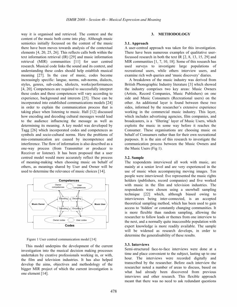
ISMIR 2008 – Session 4b – Musical Expression and Meaning
way it is organised and retrieved. The context and the content of the music both come into play. Although music semiotics initially focussed on the content of the music there have been moves towards analysis of the contextual elements [4, 20, 25, 26]. This reflects calls both within the text information retrieval (IR) [29] and music information retrieval (MIR) communities [11] for user centred research. Musical code links the sound and its context, and understanding these codes should help establish musical meaning [27]. In the case of music, codes become increasingly specific: langue, norms, sub-norms, dialects, styles, genres, sub-codes, idiolects, works/performances [4, 20]. Competences are required to successfully interpret these codes and these competences will vary according to experience, background and interests [25]. These can be incorporated into established communications models [24] in order to explain the communication process that is taking place when listening to music. Hall [12] discussed how encoding and decoding cultural messages would lead to the audience influencing the message as well as determining its meaning. A key model was developed by Tagg [26] which incorporated codes and competences as symbols and socio-cultural norms. Here the problems of mis-communication are caused by incompetence and interference. The flow of information is also described as a one-way process (from Transmitter or producer to Receiver or listener). It has been proposed that a user centred model would more accurately reflect the process of meaning-making when choosing music on behalf of others, as meanings shared by User and Owner will be used to determine the relevance of music choices [14].
Figure 1 User centred communication model [14]
This model underpins the development of the current investigation into the musical decision making processes undertaken by creative professionals working in, or with, the film and television industries. It has also helped develop the aims, objectives and methodology of the bigger MIR project of which the current investigation is one element [14].
3. METHODOLOGY
3.1. Approach A user-centred approach was taken for this investigation. There have been numerous examples of qualitative user-focussed research in both the text IR [2, 8, 13, 15, 29] and MIR communities [1, 7, 10, 18]. Some of this research has used surveys to investigate large populations of recreational users, while others interview users, and examine rich web queries and ‘music discovery’ diaries.
A breakdown of the music industry was derived from British Phonographic Industry literature [3] which showed the industry comprises two key areas: Music Owners (Artists, Record Companies, Music Publishers) on one side and Music Consumers (Recreational users) on the other. An additional layer is found between these two sides, informed by the researcher’s extensive experience working in the commercial music industry. This layer, which includes advertising agencies, film companies, and broadcasters, is a ‘filtering’ layer of Music Users, which exploits the music in some way before it reaches the Consumer. These organisations are choosing music on behalf of Consumers rather than for their own recreational purposes. It is the aim of this research to investigate the communication process between the Music Owners and the Music Users (Fig 1).
3.2. Sample The respondents interviewed all work with music, are mainly at a senior level and are very experienced in the use of music when accompanying moving images. Ten people were interviewed: five represented the music rights holders (publishers, record companies) and five worked with music in the film and television industries. The respondents were chosen using a snowball sampling technique [22] which, although biased owing to interviewees being inter-connected, is an accepted theoretical sampling method, which has been used to gain access to ‘hidden’ or constantly changing communities. It is more flexible than random sampling, allowing the researcher to follow leads or themes from one interview to the next, and a normally quite inaccessible population with expert knowledge is more readily available. The sample will be widened as research develops, in order to determine the generalisability of these results.
3.3. Interviews Semi-structured face-to-face interviews were done at a time and place convenient to the subject, lasting up to one hour. The interviews were recorded digitally and transcribed by the researcher. Before each interview the researcher noted a number of areas to discuss, based on what had already been discovered from previous interviews and other research. This flexible approach meant that there was no need to ask redundant questions
Codes
Competences
Music Owner
Music User
Encoding Decoding
Decoding Encoding
Owner competences
User competences
Owner codes
User codes
478

ISMIR 2008 – Session 4b – Musical Expression and Meaning
and allowed the interviewees to talk freely about the issues that were important to them.
3.4. Topics and Questions The exact wording of the questions varied, and sometimes the planned questions were not asked directly because answers had been given answering another question. However the researcher always had a list of areas to cover. These focussed on the process, the use, queries, communication, meaning, relevance and relationships. Areas of discussion included participant’s work role and relationships with other stakeholders; the extent to which they use and search for music in their job; queries and systems they use in searching; the type of material that satisfies their requests; and whether they could recommend improvements to the process.
3.5. Ethics University ethics guidelines were used as a framework, and all subjects were sent an explanatory statement and signed a consent form. Each interviewee was given a code to aid in anonymising their comments, and information which may identify them has been removed.
3.6. Analysis The transcribed texts and recordings were read and listened to, focussing on discussions of the process and the issues that were felt by the respondents to be of importance. Common areas which were raised are discussed in section 4. This is a preliminary analysis designed to inform the researcher of the main issues and how the process takes place, these are subsequently compared to the reflexive communication model in Figure 1. This research is part of an investigation into the information seeking behaviour of Users, which is significantly influenced by the world they are a part of. The discussion that follows highlights some of these real world issues and relates them to Figure 1.
4. RESULTS AND DISCUSSION
4.1. Stakeholders The interviews were started by discussing a subject the respondents knew well, their day-to-day work and their perceived role in the process. This allowed them to settle in comfortably to the interview process and relax. One of the key themes raised by this question were how on both sides there were large numbers of stakeholders involved in the process, in addition to the Consumers (Fig 2).
‘You get a creative team, who write the script, who are probably in their twenties, and invariably, whatever music they’re into, be it hiphop, electronica, grime, whatever, they’ll want that on the ad. You get a creative director, their boss, who’s probably a generation older, who wants something he’s never heard on an ad before, so it stands
out in the ad break and gets noticed, and then you’ve got the client, who’s probably into classical or jazz or something like that, and he’ll want that on it, and then you’ve got the target market, Debbie the housewife, who’s 35 got three kids and lives in Sheffield who’s into Madness. And you’ve got to find one track which all those people will buy into and say, ‘Yes, we want this track on our ad’. So it is difficult at the best of times.’ (003 music publisher)
Music Owners Music Users Synchronisation Dept, Legal / Business Affairs, Composer, Performer, Marketing & Promotions, Artists & Repertoire
Producer, Director, Film Editor, Music Editor, Music Supervisor, Client, Director, Ad Agency Creatives.
Figure 2 Stakeholders
Once a selection of pieces of music has been offered to the User, the stakeholders are brought in to reach a decision on the piece of music that will be used. Each of the stakeholders is likely to have different motivations, codes and competences, and these are not easily resolved. The criteria behind the decision making will include budget, clearance issues, aesthetic and commercial judgments. Whether the music enhances the picture seems to be the most important issue, although this will vary according to the producer (budget, market), director (picture as a whole), editor (the story), music supervisor (aesthetic and administrative) and audience (in test screenings). However this is not easily evaluated, most respondents resorting to ‘gut feeling’ when asked to describe what makes a great sync.
‘And I think I think the hardest thing about searching for music for an advert is it’s an opinion, and it’s a take on a brief. And it’s a take on visuals. And it’s what you think works.’ (007 record company)
4.2. Briefs The query comes generally from the User to the Owner as a brief, which may take the form of a short informal email, a more widely circulated document which has been approved by internal User stakeholders, a script element, a conversation, or a moving image in the form of a clip of a completed ad.
‘It’s very easy to actually try stuff against picture and know whether it works and know whether a really odd idea is really worth playing somebody. (002 independent music supervisor)
The Owner may have the opportunity to clarify key issues with the User. These issues would include budget, deadlines, more detailed information on the use and context, or guidelines on the type of music that is sought.
479

ISMIR 2008 – Session 4b – Musical Expression and Meaning
The User frequently works with a ‘temp’ track of music that is not going to be used in the final product, but can be used for similarity queries. Normally a range of Owners are approached with the same or a similar query. These will be drawn from favoured or targeted contacts within the industry who are likely to make an offer that meets the aesthetic, time and budget constraints of the User.
According to the model, different musical codes are likely to have varying relevance for each query. For example, while a director may require a particular song, a music supervisor may extract the codes from that recording that are important to the meaning the director is attempting to convey, and match them to other recordings that may be more affordable or are not so obvious, uniqueness being an important decision-making factor.
‘And sometimes if they want a track, for example, they can’t have – let’s say they want the Stones and there’s no way they can afford it, they’ve only got thirty grand or something, you have to find something that’s equally going to impress them as much as the Stones is. And I think that’s by finding something unique that’s going to work to picture.’ (007 record company)
These codes would have increasingly granular specificity, from highly specific (different artists performing the same song in a similar style) through to different artists from other musical traditions that may have important perceived similarity, not necessarily musical but more relating to image and status. User codes are conveyed to the Owner as a brief, which may focus on the qualities of a product (‘speed, power, control, ability’, ‘beauty, sophistication and intricacy of design’ (011 ad agency supervisor) or key words, such as ‘tension, mystery, playfulness and warmth’ (011 ad agency supervisor). The Owner may have different competences and interpret these emotive connotations of signification differently to the User, although a sharing of codes and competences will reduce this semantic gap. A selection of songs are offered that are deemed to match the brief and the User makes a choice. There are frequent references to a ‘left field’ suggestion, which does not appear to meet a brief, being chosen as the ‘perfect’ sync. In these instances it is possible that while the User felt the song did not ‘meet the brief’, because of a mis-match between competences, the Owner’s view of the track was that it was not at all left-field but an obvious match for this query.
4.3. Product knowledge The Owners then attempt to match the brief to their catalogue, which may consist of up to one million pieces of music. If the brief is clear – a specific piece of music is required, or a specific genre, era, tempo or style is described, and if the Owners’ catalogue is able to match those search terms to its metadata, the specific piece is found and terms negotiated, or a selection of pieces are offered to the User. These may be sent via email or ftp or
on a cd, played to picture in an editing suite with the User present, or sent already matched roughly to picture using consumer software. The choice offered will vary in quantity depending on the brief. A small number of Owners offer a web-based facility to Users whereby they log in to production folders of music put together by the Owner, which include downloadable tracks as mp3 and wav (for broadcast). Then either feedback is received from the User to guide further searches, one of the songs is chosen and a license is negotiated, or the User does not contact the Owner again, choosing material elsewhere.
The search by the Owner is of particular interest. During the interviews some described how, rather than search the whole catalogue, they would refer to existing searches that they had done for similar queries, and discussed how they usually browsed their own collection, which was narrowed-down from the catalogue in terms of it’s ‘sync-friendly’ nature. Removing material that was not likely to be used for synchronisation was very important to them, often citing narrative or offensive songs as being difficult to use owing to the lyrics obscuring the message of the picture. Their ‘bespoke’ collections are organized using very specific terms, such as ‘instrumental – surf’ and ‘female vocal – 1950s’ which they feel relate more to the queries they receive than the artist-album-title-genre format. An unclear brief means the Owner has to use their experience and product knowledge to ‘second guess’ the Users needs. Experience as a film maker helps in this area and some of the more successful practitioners have experience on ‘the other side’. Most of them used iTunes as their personal media library and when doing a search referred both to their company catalogue and to the outside world, including the iTunes store and their own collections, and bringing in expert advisors from within and outside their company when specialist music was required that lay outside their own product knowledge. Great importance is placed on ‘knowing the catalogue’ rather than relying on a bespoke search engine and the respondents spend a large amount of time listening to music in order to familiarise themselves with it in order to maximise any opportunities for exploitation.
‘A big part of my day is always every day at least fifty per cent will be listening to music. And if I can get more of the day to listen to music, I will. I mean there’s just so much..’ (005 independent music supervisor)
While the Owner is performing the search for the User, the User is exploring other avenues for music for use. They will not only be approaching other Owners, but will, again, search their own collections and look at their previous similar searches, use the iTunes store to listen to samples of tracks, and refer to web-based resources such as Google, All Music Guide, Pandora and last.fm. They also may have experience on ‘the other side’, are experienced in searching for music and are driven by a passion for music that is matched by in-depth knowledge.
480

ISMIR 2008 – Session 4b – Musical Expression and Meaning
4.4. Relevance When the User is supplied with a selection of material this is listened to in order to evaluate its relevance and narrow down the selection. The choices are then matched to the visual. Other stakeholders are involved in this process, their input varying by their importance and ability to argue their case. While the relevance appears mainly to be gauged by ‘gut-feeling’, a term used by many respondents, probing revealed contextual factors such as target audience, genre, uniqueness, budget, availability, recognisability and chart position, and content features such as tempo, structure, mood, instrumentation, texture are all considered. It is here that the query becomes more concrete, and a further iteration can be made much more specific, when the User can refer to features of offered material as reference points.
5. IMPLICATIONS FOR MIR AND COMMUNICATION MODEL
It can clearly be seen from the analysis of the process that this is similar to the interactive information retrieval system used in online databases. The system consists of a knowledgeable and expert User, an equally knowledgeable and expert intermediary (the Owner) and a system (the record company or publisher’s catalogue). It could be suggested that the expert intermediary be removed from the process (disintermediation) and the User allowed direct access to the collection [5]. This situation is discussed in a recent survey of graphic designers search for music [16] which indicated the value of online systems when looking for music to accompany presentations. This could reduce the problem with inadequately worded briefs as an interactive system would allow the User to adjust the query until a satisfactory result has been found. However it raises some problems. The Users have very limited time budgets and are reluctant to use these doing ‘narrowing down’ searches that can be delegated to others. Secondly, there are numerous Owners, so this approach would require the User doing searches on each Owner’s bespoke search engine. However it appears that the expert knowledge of the Owners is frequently invaluable, as they know their catalogue well, and some of them have real experience in the use of music in film, and are prepared to match music to picture themselves in order to encourage the User to choose that piece of music over the others available. This experience in each other’s world also means the Owner and User can encode and decode each other’s meanings more accurately, they are aware of the other’s codes and competences, and can accommodate these in forming their requests and results.
Mapping these results to the communications model in Figure 1, we have shown that there is a relationship between the Music Owners and the Music Users in terms of searching for and providing music. The Users have a
piece of film, and are attempting to communicate meanings with that footage. These meanings are encoded into a query, in the form of an informal note or a brief, which is generated by a number of stakeholders, all with competing codes and competences. This brief can be of any level of specificity, ranging from a specific piece of music, to offering the piece of footage itself and asking for the creative input of the Owner, who attempts to match codes and competences with those of the User. These offerings are then sent back to the User, who, depending on how much s/he shares codes and competences, may agree or disagree with the choices on offer.
6. CONCLUSION
While the communication between Owners and Users has been shown to be reflexive and interactive, representing an interactive information retrieval system, the professionals in this sample were not schooled in searching through large collections. Their primary motivation seems to be to find the ‘best’ piece of music to communicate their meaning. Although there are some search engines available for this type of use, human involvement is central in the process. Attempting to build systems that meet the information needs of these users should be flexible, incorporate queries by example as well as by matching established metadata (including lyrics), and allow searching by content as well as contextual information. It is often the use that determines the choice, and it is rare that the initial query will name a song or an artist except as an example of what would work but is not available. The clearest briefs appear to be moving images, so matching video features to music features could be a worthwhile avenue of exploration. Using musical meaning to enhance moving images requires an understanding of the contexts and contents of both media and further user research is required to inform successful systems development if these needs are to be met.
7. FUTURE WORK
This preliminary analysis of interviews has been used to describe the process in choosing music for work purposes in the music and film industry. It is planned to analyse these texts more closely over time, to draw out nuances and detail of the discourses, and investigate the interpretive repertoires that are used by the participants in the process when talking about searching for and using music. This will provide a view of ‘macrosociologically relevant cultural regularities’ [28:26] which are used by participants and will inform a wide ranging research project on searching for and using music from large collections across the music industry, including games, broadcasters and DJs, which will also investigate and evaluate key systems to provide a holistic evaluation of searching for music for work purposes.
481
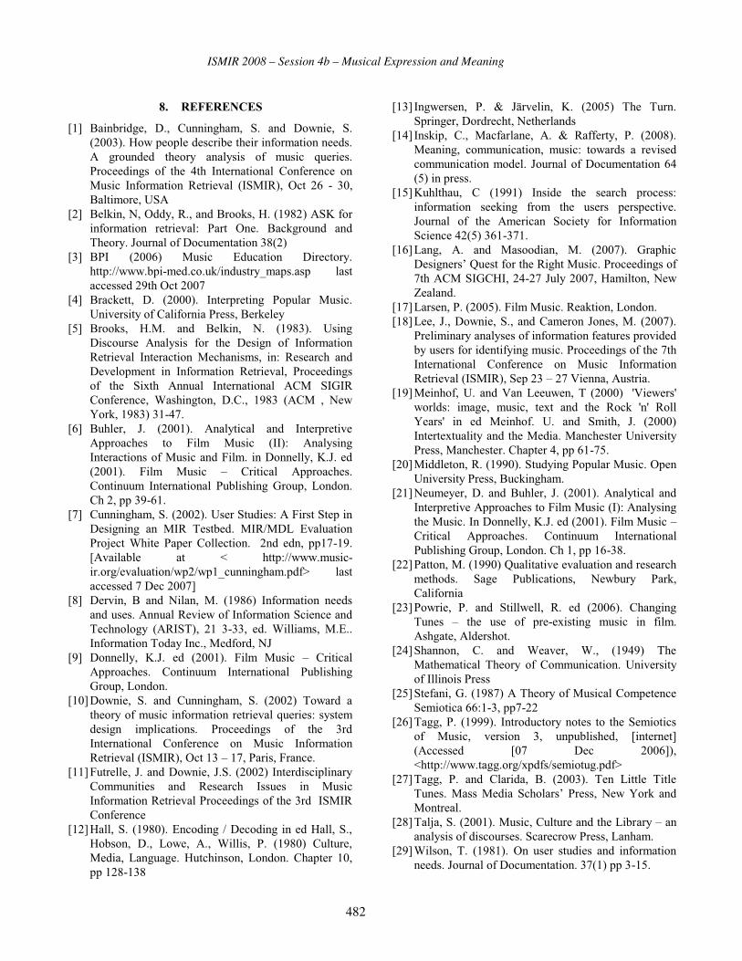
ISMIR 2008 – Session 4b – Musical Expression and Meaning
8. REFERENCES
[1] Bainbridge, D., Cunningham, S. and Downie, S. (2003). How people describe their information needs. A grounded theory analysis of music queries. Proceedings of the 4th International Conference on Music Information Retrieval (ISMIR), Oct 26 - 30, Baltimore, USA
[2] Belkin, N, Oddy, R., and Brooks, H. (1982) ASK for information retrieval: Part One. Background and Theory. Journal of Documentation 38(2)
[3] BPI (2006) Music Education Directory. http://www.bpi-med.co.uk/industry_maps.asp last accessed 29th Oct 2007
[4] Brackett, D. (2000). Interpreting Popular Music. University of California Press, Berkeley
[5] Brooks, H.M. and Belkin, N. (1983). Using Discourse Analysis for the Design of Information Retrieval Interaction Mechanisms, in: Research and Development in Information Retrieval, Proceedings of the Sixth Annual International ACM SIGIR Conference, Washington, D.C., 1983 (ACM , New York, 1983) 31-47.
[6] Buhler, J. (2001). Analytical and Interpretive Approaches to Film Music (II): Analysing Interactions of Music and Film. in Donnelly, K.J. ed (2001). Film Music – Critical Approaches. Continuum International Publishing Group, London. Ch 2, pp 39-61.
[7] Cunningham, S. (2002). User Studies: A First Step in Designing an MIR Testbed. MIR/MDL Evaluation Project White Paper Collection. 2nd edn, pp17-19. [Available at < http://www.music-ir.org/evaluation/wp2/wp1_cunningham.pdf> last accessed 7 Dec 2007]
[8] Dervin, B and Nilan, M. (1986) Information needs and uses. Annual Review of Information Science and Technology (ARIST), 21 3-33, ed. Williams, M.E.. Information Today Inc., Medford, NJ
[9] Donnelly, K.J. ed (2001). Film Music – Critical Approaches. Continuum International Publishing Group, London.
[10] Downie, S. and Cunningham, S. (2002) Toward a theory of music information retrieval queries: system design implications. Proceedings of the 3rd International Conference on Music Information Retrieval (ISMIR), Oct 13 – 17, Paris, France.
[11] Futrelle, J. and Downie, J.S. (2002) Interdisciplinary Communities and Research Issues in Music Information Retrieval Proceedings of the 3rd ISMIR Conference
[12] Hall, S. (1980). Encoding / Decoding in ed Hall, S., Hobson, D., Lowe, A., Willis, P. (1980) Culture, Media, Language. Hutchinson, London. Chapter 10, pp 128-138
[13] Ingwersen, P. & Järvelin, K. (2005) The Turn. Springer, Dordrecht, Netherlands
[14] Inskip, C., Macfarlane, A. & Rafferty, P. (2008). Meaning, communication, music: towards a revised communication model. Journal of Documentation 64 (5) in press.
[15] Kuhlthau, C (1991) Inside the search process: information seeking from the users perspective. Journal of the American Society for Information Science 42(5) 361-371.
[16] Lang, A. and Masoodian, M. (2007). Graphic Designers’ Quest for the Right Music. Proceedings of 7th ACM SIGCHI, 24-27 July 2007, Hamilton, New Zealand.
[17] Larsen, P. (2005). Film Music. Reaktion, London. [18] Lee, J., Downie, S., and Cameron Jones, M. (2007).
Preliminary analyses of information features provided by users for identifying music. Proceedings of the 7th International Conference on Music Information Retrieval (ISMIR), Sep 23 – 27 Vienna, Austria.
[19] Meinhof, U. and Van Leeuwen, T (2000) 'Viewers' worlds: image, music, text and the Rock 'n' Roll Years' in ed Meinhof. U. and Smith, J. (2000) Intertextuality and the Media. Manchester University Press, Manchester. Chapter 4, pp 61-75.
[20] Middleton, R. (1990). Studying Popular Music. Open University Press, Buckingham.
[21] Neumeyer, D. and Buhler, J. (2001). Analytical and Interpretive Approaches to Film Music (I): Analysing the Music. In Donnelly, K.J. ed (2001). Film Music – Critical Approaches. Continuum International Publishing Group, London. Ch 1, pp 16-38.
[22] Patton, M. (1990) Qualitative evaluation and research methods. Sage Publications, Newbury Park, California
[23] Powrie, P. and Stillwell, R. ed (2006). Changing Tunes – the use of pre-existing music in film. Ashgate, Aldershot.
[24] Shannon, C. and Weaver, W., (1949) The Mathematical Theory of Communication. University of Illinois Press
[25] Stefani, G. (1987) A Theory of Musical Competence Semiotica 66:1-3, pp7-22
[26] Tagg, P. (1999). Introductory notes to the Semiotics of Music, version 3, unpublished, [internet] (Accessed [07 Dec 2006]), <http://www.tagg.org/xpdfs/semiotug.pdf>
[27] Tagg, P. and Clarida, B. (2003). Ten Little Title Tunes. Mass Media Scholars’ Press, New York and Montreal.
[28] Talja, S. (2001). Music, Culture and the Library – an analysis of discourses. Scarecrow Press, Lanham.
[29] Wilson, T. (1981). On user studies and information needs. Journal of Documentation. 37(1) pp 3-15.
482

ISMIR 2008 – Session 4b – Musical Expression and Meaning
PERFORMER IDENTIFICATION IN CELTIC VIOLIN RECORDINGS
Rafael Ramirez, Alfonso Perez and Stefan KerstenMusic Technology GroupUniversitat Pompeu Fabra
Ocata 1, 08003 Barcelona, SpainTel:+34 935422864, Fax:+34 935422202{rafael, aperez, skersten}@iua.upf.edu
ABSTRACT
We present an approach to the task of identifying perform-ers from their playing styles. We investigate how violinistsexpress and communicate their view of the musical contentof Celtic popular pieces and how to use this information inorder to automatically identify performers. We study note-level deviations of parameters such as timing and amplitude.Our approach to performer identification consists of induc-ing an expressive performance model for each of the inter-preters (essentially establishing a performer dependent map-ping of inter-note features to a timing and amplitude expres-sive transformations). We present a successful performeridentification case study.
1 INTRODUCTION
Music performance plays a central role in our musical cul-ture today. Concert attendance and recording sales oftenreflect people’s preferences for particular performers. Themanipulation of sound properties such as pitch, timing, am-plitude and timbre by different performers is clearly distin-guishable by the listeners. Expressive music performancestudies the manipulation of these sound properties in an at-tempt to understand expression in performances. There hasbeen much speculation as to why performances contain ex-pression. Hypothesis include that musical expression com-municates emotions and that it clarifies musical structure,i.e. the performer shapes the music according to her ownintentions
In this paper we focus on the task of identifying violinperformers from their playing style using high-level descrip-tors extracted from single-instrument audio recordings. Theidentification of performers by using the expressive contentin their performances raises particularly interesting ques-tions but has nevertheless received relatively little attentionin the past.
The data used in our investigations are violin audio record-ings of Irish popular music performances. We use soundanalysis techniques based on spectral models [15] for ex-tracting high-level symbolic features from the recordings.
In particular, for characterizing the performances used inthis work, we are interested in inter-note features represent-ing information about the music context in which expres-sive events occur. Once the relevant high-level informationis extracted we apply machine learning techniques [9] toautomatically discover regularities and expressive patternsfor each performer. We use these regularities and patternsin order to identify a particular performer in a given audiorecording.
The rest of the paper is organized as follows: Section2 sets the background for the research reported here. Sec-tion 3 describes how we process the audio recordings in or-der to extract inter-note information. Section 4 describesour approach to performance-driven performer identifica-tion. Section 5 describes a case study on identifying per-formers based on their playing style and discusses the re-sults, and finally, Section 6 presents some conclusions andindicates some areas of future research.
2 BACKGROUND
Understanding and formalizing expressive music performanceis an extremely challenging problem which in the past hasbeen studied from different perspectives, e.g. [14], [4], [2].The main approaches to empirically studying expressive per-formance have been based on statistical analysis (e.g. [12]),mathematical modeling (e.g. [17]), and analysis-by-synthesis(e.g. [3]). In all these approaches, it is a person who isresponsible for devising a theory or mathematical modelwhich captures different aspects of musical expressive per-formance. The theory or model is later tested on real per-formance data in order to determine its accuracy. The ma-jority of the research on expressive music performance hasfocused on the performance of musical material for whichnotation (i.e. a score) is available, thus providing unam-biguous performance goals. Expressive performance stud-ies have also been very much focused on (classical) pianoperformance in which pitch and timing measurements aresimplified.
Previous research addressing expressive music performanceusing machine learning techniques has included a number of
483

ISMIR 2008 – Session 4b – Musical Expression and Meaning
approaches. Lopez de Mantaras et al. [6] report on SaxEx,a performance system capable of generating expressive solosaxophone performances in Jazz. One limitation of theirsystem is that it is incapable of explaining the predictionsit makes and it is unable to handle melody alterations, e.g.ornamentations.
Ramirez et al. [11] have explored and compared diversemachine learning methods for obtaining expressive musicperformance models for Jazz saxophone that are capableof both generating expressive performances and explainingthe expressive transformations they produce. They proposean expressive performance system based on inductive logicprogramming which induces a set of first order logic rulesthat capture expressive transformation both at an inter-notelevel (e.g. note duration, loudness) and at an intra-note level(e.g. note attack, sustain). Based on the theory generatedby the set of rules, they implemented a melody synthesiscomponent which generates expressive monophonic output(MIDI or audio) from inexpressive melody MIDI descrip-tions.
With the exception of the work by Lopez de Mantaraset al and Ramirez et al, most of the research in expressiveperformance using machine learning techniques has focusedon classical piano music where often the tempo of the per-formed pieces is not constant. The works focused on classi-cal piano have focused on global tempo and loudness trans-formations while we are interested in note-level tempo andloudness transformations.
Nevertheless, the use of expressive performance mod-els, either automatically induced or manually generated, foridentifying musicians has received little attention in the past.This is mainly due to two factors: (a) the high complexity ofthe feature extraction process that is required to character-ize expressive performance, and (b) the question of how touse the information provided by an expressive performancemodel for the task of performance-based performer iden-tification. To the best of our knowledge, the only groupworking on performance-based automatic performer iden-tification is the group led by Gerhard Widmer. Saunders etal [13] apply string kernels to the problem of recognizingfamous pianists from their playing style. The characteris-tics of performers playing the same piece are obtained fromchanges in beat-level tempo and beat-level loudness. Fromsuch characteristics, general performance alphabets can bederived, and pianists’ performances can then be representedas strings. They apply both kernel partial least squares andSupport Vector Machines to this data.
Stamatatos and Widmer [16] address the problem of iden-tifying the most likely music performer, given a set of per-formances of the same piece by a number of skilled candi-date pianists. They propose a set of very simple features forrepresenting stylistic characteristics of a music performerthat relate to a kind of ’average’ performance. A databaseof piano performances of 22 pianists playing two pieces by
Frdric Chopin is used. They propose an ensemble of sim-ple classifiers derived by both subsampling the training setand subsampling the input features. Experiments show thatthe proposed features are able to quantify the differences be-tween music performers.
3 MELODIC DESCRIPTION
First of all, we perform a spectral analysis of a portion ofsound, called analysis frame, whose size is a parameter ofthe algorithm. This spectral analysis consists of multiplyingthe audio frame with an appropriate analysis window andperforming a Discrete Fourier Transform (DFT) to obtainits spectrum. In this case, we use a frame width of 46 ms,an overlap factor of 50%, and a Keiser-Bessel 25dB win-dow. Then, we compute a set of low-level descriptors foreach spectrum: energy and an estimation of the fundamen-tal frequency. From these low-level descriptors we performa note segmentation procedure. Once the note boundariesare known, the note descriptors are computed from the low-level values. the main low-level descriptors used to charac-terize note-level expressive performance are instantaneousenergy and fundamental frequency.
Energy computation. The energy descriptor is computedon the spectral domain, using the values of the amplitudespectrum at each analysis frame. In addition, energy is com-puted in different frequency bands as defined in [5], andthese values are used by the algorithm for note segmenta-tion.
Fundamental frequency estimation. For the estimation ofthe instantaneous fundamental frequency we use a harmonicmatching model derived from the Two-Way Mismatch pro-cedure (TWM) [7]. For each fundamental frequency candi-date, mismatches between the harmonics generated and themeasured partials frequencies are averaged over a fixed sub-set of the available partials. A weighting scheme is used tomake the procedure robust to the presence of noise or ab-sence of certain partials in the spectral data. The solutionpresented in [7] employs two mismatch error calculations.The first one is based on the frequency difference betweeneach partial in the measured sequence and its nearest neigh-bor in the predicted sequence. The second is based on themismatch between each harmonic in the predicted sequenceand its nearest partial neighbor in the measured sequence.This two-way mismatch helps to avoid octave errors by ap-plying a penalty for partials that are present in the measureddata but are not predicted, and also for partials whose pres-ence is predicted but which do not actually appear in themeasured sequence. The TWM mismatch procedure hasalso the benefit that the effect of any spurious components orpartial missing from the measurement can be counteractedby the presence of uncorrupted partials in the same frame.
484

ISMIR 2008 – Session 4b – Musical Expression and Meaning
Note segmentation is performed using a set of frame de-scriptors, which are energy computation in different frequencybands and fundamental frequency. Energy onsets are firstdetected following a band-wise algorithm that uses somepsycho-acoustical knowledge [5]. In a second step, funda-mental frequency transitions are also detected. Finally, bothresults are merged to find the note boundaries (onset andoffset information).
Note descriptors. We compute note descriptors using thenote boundaries and the low-level descriptors values. Thelow-level descriptors associated to a note segment are com-puted by averaging the frame values within this note seg-ment. Pitch histograms have been used to compute the pitchnote and the fundamental frequency that represents each notesegment, as found in [8]. This is done to avoid taking intoaccount mistaken frames in the fundamental frequency meancomputation. First, frequency values are converted into cents,by the following formula:
c = 1200 ·log ( f
fref)
log2(1)
where fref = 8.176 (fref is a the reference frequency ofthe C0). Then, we define histograms with bins of 100 centsand hop size of 5 cents and we compute the maximum ofthe histogram to identify the note pitch. Finally, we com-pute the frequency mean for all the points that belong to thehistogram. The MIDI pitch is computed by quantization ofthis fundamental frequency mean over the frames within thenote limits.
Musical Analysis. It is widely recognized that humans per-form music considering a number of abstract musical struc-tures. In order to provide an abstract structure for the record-ings under study, we decided to use Narmour’s theory ofperception and cognition of melodies [10] to analyze theperformances.
The Implication/Realization model proposed by Narmouris a theory of perception and cognition of melodies. The the-ory states that a melodic musical line continuously causeslisteners to generate expectations of how the melody shouldcontinue. The nature of these expectations in an individualare motivated by two types of sources: innate and learned.According to Narmour, on the one hand we are all born withinnate information which suggests to us how a particularmelody should continue. On the other hand, learned fac-tors are due to exposure to music throughout our lives andfamiliarity with musical styles and particular melodies. Ac-cording to Narmour, any two consecutively perceived notesconstitute a melodic interval, and if this interval is not con-ceived as complete, it is an implicative interval, i.e. an in-terval that implies a subsequent interval with certain char-
Figure 1. Prototypical Narmour Structures
Figure 2. Narmour analysis of a melody fragment
acteristics. That is to say, some notes are more likely thanothers to follow the implicative interval. Two main prin-ciples recognized by Narmour concern registral directionand intervallic difference. The principle of registral direc-tion states that small intervals imply an interval in the sameregistral direction (a small upward interval implies anotherupward interval and analogously for downward intervals),and large intervals imply a change in registral direction (alarge upward interval implies a downward interval and anal-ogously for downward intervals). The principle of inter-vallic difference states that a small (five semitones or less)interval implies a similarly-sized interval (plus or minus 2semitones), and a large interval (seven semitones or more)implies a smaller interval. Based on these two principles,melodic patterns or groups can be identified that either sat-isfy or violate the implication as predicted by the principles.Such patterns are called structures and are labeled to denotecharacteristics in terms of registral direction and intervallicdifference. Figure 1 shows prototypical Narmour structures.A note in a melody often belongs to more than one struc-ture. Thus, a description of a melody as a sequence of Nar-mour structures consists of a list of overlapping structures.We parse each melody in the training data in order to au-tomatically generate an implication/realization analysis ofthe pieces. Figure 2 shows the analysis for a fragment of amelody.
4 PERFORMANCE-DRIVEN PERFORMERIDENTIFICATION
4.1 Note features
The note features represent both properties of the note itselfand aspects of the musical context in which the note appears.Information about the note includes note pitch and note du-ration, while information about its melodic context includesthe relative pitch and duration of the neighboring notes (i.e.previous and following notes) as well as the Narmour struc-tures to which the note belongs. The note’s Narmour struc-tures are computed by performing the musical analysis de-scribed before. Thus, each performed note is characterized
485

ISMIR 2008 – Session 4b – Musical Expression and Meaning
by the tuple
(Pitch, Dur, PrevPitch, PrevDur, NextPitch, NextDur, Nar1,Nar2, Nar3)
4.2 Algorithm
We are ultimately interested in obtaining a classification func-tion F of the following form:
F (MelodyFragment(n1, . . . , nk)) −→ Performers
where MelodyFragment(n1, . . . , nk) is the set of melodyfragments composed of notes n1, . . . , nk and Performersis the set of possible performers to be identified. For eachperformer i to be identified we induce an expressive per-formance model Mi predicting his/her timing and energyexpressive transformations:
Mi(Notes) → (PDur, PEner)
where Notes is the set of score notes played by performeri represented by their inter-note features, i.e. each note inNotes is represented by the tuple (Pitch, Dur, PrevPitch,PrevDur, NextPitch, NextDur, Nar1, Nar2, Nar3) as describedbefore, and the vector (PDur, PEner) contains the model’spredictions for note duration (PDur) and energy (PEner).Once a performance model is induced for each performer P i
we apply the following algorithm:
F([N1,...,Nm], [P1,...,Pn])for each performer Pi
Scorei = 0for each note Nk
FNk = inter-note_features(Nk)Mi(FNk) = (PDk,PEk)for each performer Pi
ScoreNKi = sqrt(((Dur(NK)-PDk)ˆ2)+ ((Ener(Nk)-PEk)ˆ2))
Scorei = Scorei + ScoreNKireturn Pj (j in {1,...,m}) with minimum score
This is, for each note in the melody fragment the classi-fier F computes the set of its inter-note features. Once thisis done, for each note Nk and for each performer Pi, perfor-mance model Mi predicts the expected duration and energyfor Nk. This prediction is based on the note’s inter-notefeatures. The score Scorei for each performer i is updatedby taking into account the Euclidean distance between thenote’s actual duration and energy and the predicted values.Finally, the performer with the lower score is returned.
Clearly, the expressive models Mi play a central role inthe output of classifier F . For each performer, M i is in-duced by applying Tildes top-down decision tree inductionalgorithm ([1]). Tilde can be considered as a first order
logic extension of the C4.5 decision tree algorithm: insteadof testing attribute values at the nodes of the tree, Tildetests logical predicates. This provides the advantages ofboth propositional decision trees (i.e. efficiency and prun-ing techniques) and the use of first order logic (i.e. in-creased expressiveness). The musical context of each noteis defined by predicates context and narmour. contextspecifies the note features described above and narmourspecifies the Narmour groups to which a particular note be-longs, along with its position within a particular group. Ex-pressive deviations in the performances are encoded usingpredicates stretch and dynamics. stretch specifies thestretch factor of a given note with regard to its durationin the score and dynamics specifies the mean energy of agiven note. The temporal aspect of music is encoded via thepredicates pred and succ. For instance, succ(A, B, C, D)indicates that note in position D in the excerpt indexed bythe tuple(A, B) follows note C.
5 CASE STUDY
5.1 Training data
In this work we are focused on Celtic jigs, fast tunes butslower that reels, that usually consist of eighth notes in aternary time signature, with strong accents at each beat. Thetraining data used in our experimental investigations are mono-phonic recordings of nine Celtic jigs performed by two pro-fessional violinists. Apart from the tempo (they played fol-lowing a metronome), the musicians were not given any par-ticular instructions on how to perform the pieces.
5.2 Results
Initially, we evaluated the expressive performance model foreach of the musicians we considered. Thus, we obtainedtwo expressive performance models M1 and M2. For M1
we obtained correlation coefficients of 0.88 and 0.83 forthe duration transformation and note dynamics predictiontasks, respectively, while we obtained 0.91 and 0.85 for M 2.These numbers were obtained by performing 10-fold cross-validation on the training data. The induced models seem tocapture accurately the expressive transformations the mu-sicians introduce in the performances. Figure 3 contraststhe note duration deviations predicted by model M 1 and thedeviations performed by the violinist. Similar results wereobtained for M2.
We then proceed to evaluate the classification function Fby spliting our data into a training set and a test set. We heldout approximately 30% of the data as test data while the re-maining 70% was used as training data (we held out 3 piecesfor each violinist). When selecting the test data, we left outthe same number of melody fragments per class. In order toavoid optimistic estimates of the classifier performance, we
486

ISMIR 2008 – Session 4b – Musical Expression and Meaning
Figure 3. Note deviation ratio for a tune with 89 notes.Comparison between performed and predicted by M 1
explicitly removed from the training set all melody fragmentrepetitions of the hold out fragments. This is motivated bythe fact that musicians are likely to perform a melody frag-ment and its repetition in a similar way. We tested our al-gorithm in each of the six test pieces (three pieces of eachclass) and obtained 100% accuracy (correctly classified in-stances percentage). This is, the six pieces in the test setwere classified correctly.
6 CONCLUSION
In this paper we focused on the task of identifying perform-ers from their playing style using note descriptors extractedfrom audio recordings. In particular, we concentrated inidentifying violinists playing Irish popular pieces (Irish jigs).We characterized performances by representing each note inthe performance by a set of inter-note features represent-ing the context in which the note appears. We then in-duced an expressive performance model for each of the per-formers and presented a successful performer identificationcase study. The results obtained seem to indicate that theinter-note features presented contain sufficient informationto identify the studied set of performers, and that the ma-chine learning method explored is capable of learning per-formance patterns that distinguish these performers. Thispaper present preliminary work so there is further work inseveral directions. Our immediate plans are to extend ourdatabase and to test different distance measures for updat-ing the performer scores in our algorithm. We also plan toevaluate our algorithm considering melody fragments of dif-ferent size and to evaluate the predictive power of timing ex-pressive variations relative to energy expressive variations.
7 REFERENCES
[1] H. Blockeel, L. D. Raedt, and J. Ramon. Top-down in-duction of clustering trees. In Proceedings of the 15thInternational Conference on Machine Learning, 1998.
[2] Bresin, R. (2000). Virtual Visrtuosity: Studies in Auto-matic Music Performance. PhD Thesis, KTH, Sweden.
[3] Friberg, A.; Bresin, R.; Fryden, L.; 2000. Music fromMotion: Sound Level Envelopes of Tones ExpressingHuman Locomotion. Journal of New Music Research29(3): 199-210.
[4] Gabrielsson, A. (1999). The performance of Music. InD.Deutsch (Ed.), The Psychology of Music (2nd ed.)Academic Press.
[5] Klapuri, A. (1999). Sound Onset Detection by ApplyingPsychoacoustic Knowledge, Proceedings of the IEEEInternational Conference on Acoustics, Speech and Sig-nal Processing, ICASSP.
[6] Lopez de Mantaras, R. and Arcos, J.L. (2002). AI andmusic, from composition to expressive performance, AIMagazine, 23-3.
[7] Maher, R.C. and Beauchamp, J.W. (1994). Fundamentalfrequency estimation of musical signals using a two-waymismatch procedure, Journal of the Acoustic Society ofAmerica, vol. 95 pp. 2254-2263.
[8] McNab, R.J., Smith Ll. A. and Witten I.H., (1996). Sig-nal Processing for Melody Transcription, SIG workingpaper, vol. 95-22.
[9] Mitchell, T.M. (1997). Machine Learning. McGraw-Hill.
[10] Narmour, E. (1990). The Analysis and Cognition ofBasic Melodic Structures: The Implication RealizationModel. University of Chicago Press.
[11] Rafael Ramirez, Amaury Hazan, Esteban Maestre,Xavier Serra, A Data Mining Approach to ExpressiveMusic Performance Modeling, in Multimedia Data min-ing and Knowledge Discovery, Springer.
[12] Repp, B.H. (1992). Diversity and Commonality in Mu-sic Performance: an Analysis of Timing Microstructurein Schumann’s ‘Traumerei’. Journal of the AcousticalSociety of America 104.
[13] Saunders C., Hardoon D., Shawe-Taylor J., and Wid-mer G. (2004). Using String Kernels to Identify Fa-mous Performers from their Playing Style, Proceedingsof the 15th European Conference on Machine Learning(ECML’2004), Pisa, Italy.
487

ISMIR 2008 – Session 4b – Musical Expression and Meaning
[14] Seashore, C.E. (ed.) (1936). Objective Analysis of Mu-sic Performance. University of Iowa Press.
[15] Serra, X. and Smith, S. (1990). ”Spectral Modeling Syn-thesis: A Sound Analysis/Synthesis System Based ona Deterministic plus Stochastic Decomposition”, Com-puter Music Journal, Vol. 14, No. 4.
[16] Stamatatos, E. and Widmer, G. (2005). Automatic Iden-tification of Music Performers with Learning Ensem-bles. Artificial Intelligence 165(1), 37-56.
[17] Todd, N. (1992). The Dynamics of Dynamics: a Modelof Musical Expression. Journal of the Acoustical Soci-ety of America 91.
488

ISMIR 2008 – Session 4b – Musical Expression and Meaning
A NEW MUSIC DATABASE DESCRIBING DEVIATION INFORMATION OFPERFORMANCE EXPRESSIONS
Mitsuyo Hashida Toshie Matsui Haruhiro KatayoseResearch Center for Human & Media, Kwansei Gakuin University
CrestMuse Project, JST, Japan{hashida, tmatsui, katayose}@kwansei.ac.jp
ABSTRACT
We introduce the CrestMuse Performance Expression Data-base (CrestMusePEDB), a music database that describes mu-sic performance expression and is available for academic re-search. While music databases are being provided as MIRtechnologies continue to progress, few databases deal withperformance expression. We constructed a music expres-sion database, CrestMusePEDB. It may be utilized in theresearch fields of music informatics, music perception andcognition, and musicology. It will contain music expressioninformation on virtuosis’ expressive performances, includ-ing those of 3 to 10 players at a time, on about 100 pieces ofclassical Western music. The latest version of the database,CrestMusePEDB Ver. 2.0, is available. The paper gives anoverview of CrestMusePEDB.
1 INTRODUCTION
Constructing music databases is one of the most importantthemes in the field of music studies. The importance of mu-sic databases has been recognized through the progress ofmusic information retrieval technologies and benchmarks.Since the year 2000, some large-scale music databases havebeen created, and they have had a strong impact on the globalresearch area [1, 2, 3].
Corpora of scores, audio recordings, and information onbooks of composers and musicians have been collected andused in the analysis of music styles, structures, and per-formance expressions. Meta-text information, such as thenames of composers and musicians, has been attached tolarge-scale digital databases and been used in the analysis ofmusic styles, structures, and performance expressions fromthe viewpoint of social filtering. In spite of there being manyactive music database projects, few projects have dealt withmusic performance expression, such as dynamics, tempo,and the progression of pitch. The performance expressionplays an important role in formulating impressions of music.Providing a performance expression database, especially de-scribing deviation information from neutral expression, canbe used as a research in MIR fields.
In musicological analysis, some researchers construct adatabase of the transition data of pitch and loudness and thenuse the database through statistical processing. Widmer etal. analyzed deviation of tempi and dynamics of each beatfrom Horowitz’s piano performances [4]. Sapp et al., work-ing on the Mazurka Project [5], collected as many record-ings of Chopin mazurka performances as possible in orderto analyze deviations of tempo and dynamics by each beat ina similar manner to Widmer. Their researches are expectedto provide the fundamental knowledge in the quantitativeanalysis of music style and performance expression. How-ever, their archives are focused on the specified composerand player but ignored all other types of music. And theyare not enough to be covered with the description of the de-viation of duration and loudness of each note from score.Toyoda et al. have provided a performance expression devi-ation database which is aimed to describe those of individ-ual note [6]. But their data format is limited to performancesrecorded by MIDI signals not audio signals. However, mostof the analysis of classical Western music expression is de-termined by the researchers’ acute musical sense; even lessresearch has quantitatively analyzed music performance ex-pression based on data [7, 8, 9, 10, 11]. One of the reasonsfor this absence of data is that this qualitative research hasbeen based on the field methods of music performance edu-cation up until now.
MIDI files of performances are prolific on the Internet;however, very few of these are actually created by profes-sional musicians, but rather by students and amateurs. Also,searching with the precise details on the performances is toodifficult, although the information on each piece (e.g., thetitle, composer, genre, and the composition of the musicalinstruments) is rich.
A database, which describes outlines of changes in tempo,dynamics, the delicate control of each note, the deviation re-garding starting time and duration to existing virtuoso per-formances in the form of acoustic signals as time-series data,can be used for new studies in the fields of music informat-ics, musicology and music education. To that end, we con-structed a performance expression database, ‘CrestMuse-PEDB,’ that covers classical Western music, especially pi-ano pieces performed by famous professionals.
489

ISMIR 2008 – Session 4b – Musical Expression and Meaning
2 CONSIDERATIONS IN THE DATABASE DESIGN
2.1 Ensuring the amount and quality of performances
A music database generally needs to contain high-qualityperformances. Goto et al. recorded performances by manyprofessional musicians as part of their RWC music database[12]. Copyright restrictions pose difficulties for performancedatabase creators. One method of avoiding such restrictionsis to have the collectors record musical performances specif-ically for the database. Financially this is a onerous task andcan compromise quality when extending a large database.For this problem, McEnnis et al. suggested an approach:collecting the parameters of audio features (covered in mu-sic information retrieval) in the real performances aroundthe world and showing those reference information[3]. Thisapproach is a rational way to avoid copyright problems andthat the system can deal with raw data of the real world. Weused the same approach.
2.2 Handling performance control data
The main information in a performance expression databasepertains to instrument control. It has various kinds and lev-els of information. For keyboard instruments such as thepiano, control data can be represented as the onset time,the offset time, the dynamics (velocity), and the depth ofthe damper pedal. The information on the instrument con-trol deals with the feature quantity at the MIDI level. De-scribing them in a database requires having really usefulinformation that can be extended in the future. Therefore,we constructed control information as XML-based data inCrestMusePEDB. We will extend and work out the detailsof these descriptions in accordance with the individual situ-ations and technology.
Another problem which deals with music information isto identify the intensity of each note from acoustic signal.We especially need to be careful in describing the loudnessof each note. To obtain the strict value of loudness of a note,we need to construct a sound model including the charac-teristics when recording the performance and architecturalacoustic characteristics. However, getting that informationfrom only the audio signal is quite difficult. Although someapproaches using non-negative matrix factorization (NMF)are suggested, the problem has not been radically resolvedyet in audio signal processing. In the view point of construc-tion of a useful database, those information of the perfor-mance data should be collected as correctly by auditory aspossible. Therefore, the velocity data is estimated approxi-mately in CrestMusePEDB based on a specific digital audiosource by well-trained experts using some support tools de-scribed in section 3.4.
2.3 Musical structure
A specific musical structure corresponds with a performance.CrestMusePEDB includes the data of the musical structuresin an analysis of each performance, and it provides supportto use the data in research on musicology, performance the-ories, and computational music systems.
The best solution is to interview a pianist and ask howhis/her performance was achieved based on the musical struc-ture. However, such an interview must be done immediatelybefore and after the recording. The musical structure datashould be collected by estimating the data from audio sig-nals. Our approach involves interviewing as many playersas possible to estimate the structures through discussion be-tween a few musicologists and asking an expert pianist toplay some performances with different musical structures.We aimed to get both the musical structure and the way it isexpressed from the original recording
3 OVERVIEW OF CRESTMUSE PEDB
3.1 Music pieces
The focus of the database is on classical music from theBaroque period through the early twentieth century, includ-ing music by Bach, Mozart, Beethoven and Chopin. Wechose around a hundred music pieces, including those re-ferred to often by previous music studies in the past coupleof decades. We also chose various existing performances byprofessional musicians; the database includes 3 to 10 per-formances for each musical score.
3.2 Contents of the database
The database consists of the following four kinds of compo-nent data. These kinds of data will sequentially be providedfrom SCR, DEV. The description of the database is based onXML files. CrestMusePEDB does not contain any acousticsignal data (WAV files, AIFF files, MP3 files.) except forPEDB-REC. Instead, it contains the catalogs of the perfor-mances from which expression data is extracted. The origi-nal audio sources can be purchased by the database users ifnecessary.
PEDB-SCR (score text information): The score data in-cluded in the database: files in MusicXML format and inSMF (standard MIDI file) format will be provided.
PEDB-IDX (audio performance credit): The catalogs ofthe performances from which expression data are extracted:album title, performer’s name, song title, CD number, yearof publication.
PEDB-DEV (performance deviation data): Tempo changesoutline changes in dynamics, the delicate control of eachnote, deviation regarding starting time, duration, and dy-namics extracted from expressive performances. Performancesfrom 3 to 10 performers are analyzed a piece, and plural
490

ISMIR 2008 – Session 4b – Musical Expression and Meaning
deviation data analyzed by different sound sources are pro-vided a performance. Each data is described in Deviation-InstanceXML format (see below).
PEDB-STR (musical structure data): This contains theinformation on a musical structure data (hierarchical phrasestructure and the top note of a phrase). The data is describedin compliant MusicXML format. The structure data corre-sponds with a performance expression data in PEDB-DEV.But if plural adequate interpretations exist in a piece, theplural structure data is provided in the performance data.
PEDB-REC (original recordings): The audio performancedata we will newly record based on PEDB-STR. The datawill be useful to analyze performance expression from theview of music structure. It provides an audio signal andMIDI data that an expert pianist plays.
3.3 DeviationInstanceXML format
DeviationInstanceXML describes the deviation informationfrom score information in a music performance as a subsetof CrestMuseXML (CMX)1 , which is the universal data for-mat for music informatics. The latest version (0.32) dealswith the control information of the piano playing, such asthe onset time, offset time, and the velocity in MIDI of eachnote, tempo control, and damper pedal control. This con-trol data is categorized into (1) common or multiple parts(non-partwise), (2) each part (partwise), and (3) each note(notewise) and is described as follows:
<deviation target="sample.xml" xmlns:xlink="http://www.w3.org/1999/xlink">
<non-partwise>...</non-partwise> (1)<partwise>...</partwise> (2)<notewise>...</notewise> (3)
</deviation>
The details of this description are shown in the site, but hereis the overview shown.
(1) <non-partwise> One of the common deviations ofplural parts is tempo information. It is described as a combi-nation of two XML tags: one is <tempo>, which describesthe fundamental impression such as Andante and Allegro. Itindicates the number of beats per minute (BPM). The otheris <tempo-deviation>, which describes the micro tempo perbeat; it is expressed as the ratio of the value of <tempo>.
(2) <partwise> The deviations of each part deal withthe fundamental dynamics and damper pedal control intoa <partwise> tag. The fundamental dynamics describe theglobal indication such as forte and piano. The pedal controlis available to be described in the MusicXML format, butthe control refers to the expression of the score and does notalways correspond to the performance. The pedal descrip-tion in DeviationInstanceXML handles the pedal control inan actual performance expression. Some people might think
1 http://www.crestmuse.jp/cmx/
that the pedal control should be described as the commondeviation of all the parts. For CrestMusePEDB, the pedalcontrol is sufficient because the only instrument in all ofthe performances is the piano. However, the DeviationIn-stanceXML will be used to describe the control with pluralinstruments in the future. This issue is controversial, buthere, the pedal control is described in <partwise>.
(3) <notewise> The deviation information of each notedeals with the deviation of the onset time and offset timefrom the score and the deviation of individual dynamics (thevelocity of each note key). The individual dynamics are fordescribing a micro-expression within a phrase to which thenote belongs. The actual loudness of the note is computedby multiplying the individual dynamics by the fundamentaldynamics at the score-time of the piece.
3.4 Procedure for making DEV data
Transcribing an audio-signal performance into MIDI-leveldata is the core issue for constructing the CrestMusePEDB.Although we have improved the automation of the proce-dure, at present, an iterated listening process by plural ex-perts with commercial audio editor and original alignmentsoftware possesses higher reliability. The data needs to beextracted from a recording as efficiently as possible. Wenow use an approach where four experts who have special-ized in music including piano, composition and musicologymanually identify the transcription/data in CrestMusePEDBusing their ears and three support tools that we have imple-mented for the procedure.
Figure 1 illustrates the procedure for generating PEDB-DEV information.
Step 1: identify the attack time in the beat level of a piecewhile listening to the CD audio.
Step 2: estimate the approximation of the onset time,offset time, velocity of each note, and whether or not thedamper pedal is used and whether or not it is fixed to thesound source.
Deviation
estimation
MusicXMLperformance deviation
data (MusicXML)
audio signal
Performance
alignment
MIDI file
score
MIDI data
Music editing software
(commarcial software)
Support software
(PEDB-TOOLs)
Raugh matching tool
Velocity Estimation Tool
Score Alignment Tool
Deviation Caluculation
tool
Manual data-approximation
* attack & release time
* damper pedal
* velocity
Support software
(automatic processing)
Score alignment
↓
Feature extraction
* metrical tempo
* metrical dynamics
* deviation of atack & release time of each note
* deviation of velocity of each note
Figure 1. The procedure to make PEDB-DEV.
491

ISMIR 2008 – Session 4b – Musical Expression and Meaning
Step 3: refine the estimation with repeating step2 untila expert accepts and have it cross-checked by other experts.This step needs the most time of all the steps and takes atleast five hours to a day a piece.
Step 4: match the expression data obtained through steps1-3 with the normal expression data.
Step 5: calculate the time transition of tempi and dynam-ics, the deviation of the onset and offset time of each note,and the deviation of velocity from the fundamental dynam-ics (nominal expression) to the whole score.
The velocity estimation in step 2 and step 3 is necessaryfor resolving the problem with the loudness range when anaudio signal differs because each audio CD was recordedusing different musical instruments and in different environ-ments. Here, we give priority to obtaining the value of thevelocity for each note approximated to the listening data ofthe audio signal by experts who listen to the data of the au-dio signal. After justifying the range of the loudness for allof the audio signals, the experts repeat refining the approxi-mated data with their headphones, which is always identical.
We have implemented three of support software to helpwith each step of the procedure.
Rough Matching Tool enables aligning the rough attacktime of each note of a score corresponding with audio spec-trogram, using Dynamic Programming.
Velocity Estimation Tool enables estimating the veloc-ity of each note based on the original audio signal, the onsettime of each note (which is roughly identified by the abovetool), and an audio source for the sound of the MIDI data.
Score Alignment and Deviation Calculation Tool sup-ports two procedures to extract the deviation information.The first one identifies all the notes of the score as those ofthe expressed performance. The second one calculates thedeviation information (the onset time, the offset time, andthe velocity) for each note. The deviation information is de-scribed in the DeviationInstanceXML format.
The rough matching tool and the velocity estimation tooldo not have to function at a very high accuracy in order tobe beneficial. The skill of experts is arguably higher thanthat of current systems. The former tool is used for step 1,and the latter is used when deciding the initial parameters instep 2. Meanwhile, the score alignment and deviation cal-culation tool seldom make errors. We determined the resultdata using these tools in step 4 and step 5. We will makethese tools public so that a community of CrestMusePEDBusers will grow.
3.5 Subset tools
The data description in the XML format has scalability anddata integrity. Meanwhile, it is not so useful for researchersexcept for those in computer science. Therefore, we providethe following sub-tools for CrestMusePEDB so that it can beeffectively utilized.
CrestMusePEDB player: a music player that inputs SCRand DEV data, then generates expressed performance datathrough the indicated audio source.
CrestMusePEDB time-line viewer: a deviation visual-izer that inputs SCR and DEV data then shows each note andthe data described in the DEV data to a piano-roll display.
CSV (Comma Separated Values) Converter: a plugintool for the CrestMusePEDB time-line viewer that outputsselected deviation information in the CSV format.
4 PUBLISHING OF CRESTMUSE PEDB
CrestMusePEDB has been available since November 2007.The version 1.0 and 2.0 have been released on the Inter-net2 and there are totally 60 performances included. Table1 and 2 shows the list of the music pieces included in thedatabase, and Table 3 shows a player list and a sound sourcecorresponding with each piece.
Each DEV data is given a unique number (PerfID) andan identification ID to discriminate itself along with a form.Identification ID is given by the combination of ScoreIDand DevID. For example, the database has three perfomanceDEV data (Gould, Nakamura and Shimizu) of the 1st move-ment of Mozart’s Piano Sonata K. 331. The IDs of theGould’s performance are described as “PEDB-DEV No. 22(snt331-1-003-b)”. The alphabet at the last of DevID meansa sound source used for extracting deviation data from au-dio source; ‘a’ is B osendolfer PIANO/GIGA by CryptonFuture Media Inc., ‘b’ is GPO-Concert-Steinway-ver2.sf2(a free source from SF2midi.com) and ‘c’ is Yamaha’s MO-TIF XS. The performances using ’c’ will be provided at thefuture version.
We have been preparing a listening contest for musicperformance rendering systems (Rencon) as part of anotherresearch project (http://www.renconmusic.org/).In the summer of 2008, the database is provided to the Ren-con competition as the standard learning set for autonomousperformance rendering systems that generate expressive per-formance. We have been already providing some sampledata on CrestMusePEDB to researchers who plan to enterthe Rencon contest.
5 DISCUSSION
5.1 Applied research area
CrestMusePEDB can be used in various research areas suchas musicology and music education, not only MIR fields.Next, we describe some cases for application.
Musicology In musicology, many analyses of expressiveperformance style examine the presence of legato/non-legatophrasing [13]. Many of them depend on a subjective verdictby an analyst. As well as these verdicts, we suppose that the
2 http://www.crestmuse.jp/pedb/
492

ISMIR 2008 – Session 4b – Musical Expression and Meaning
Table 1. CrestMusePEDB ver. 1.0 Performance Data (No.1-39)
Composer (ComposerID) (amount of performances)PerfID ScoreID Title
Player DevID CD index Track.J. S. Bach (1) (21 performances)
No. 1~2 inv001 Invention No. 1 BWV 772A. Schiff 001-a/b POCL-5099 Tr.01
No. 3 inv002 Invention No. 2 BWV 773A. Schiff 001-b POCL-5099 Tr.02
No. 4 inv008 Invention No. 8 BWV 779A. Schiff 001-b POCL-5099 Tr.08
No. 5 inv015 Invention No.15 BWV 786A. Schiff 001-b POCL-5099 Tr.15
No. 6-11 wtc101-p Das Wohltemperierte Klavier Vol. No.1 BWV 846 PreludeS. Richter 002-a/b BVCC-37139 Tr.01G. Gould 003-a/b SRCR9496 Tr.02F. Gulda 004-a/b 416-113-2 Tr.01
No. 12 wtc107-p Das Wohltemperierte Klavier Vol. I No. 7 BWV 852 PreludeS. Richter 002-b BVCC-37139 Tr.13
No. 13 wtc107-f Das Wohltemperierte Klavier Vol. I No. 7 BWV 852 FugaS. Richter 002-b BVCC-37139 Tr.14
No. 14 wtc113-p Das Wohltemperierte Klavier Vol. I No.13 BWV 858 PreludeS. Richter 002-b BVCC-37139 Tr.01
No. 15 wtc113-f Das Wohltemperierte Klavier Vol. I No.13 BWV 858 FugaS. Richter 002-b BVCC-37140 Tr.02
No. 16 wtc123-p Das Wohltemperierte Klavier Vol. I No.23 BWV 868 PreludeS. Richter 002-b BVCC-37140 Tr.21
No. 17 wtc123-f Das Wohltemperierte Klavier Vol. I No.23 BWV 868 FugaS. Richter 002-b BVCC-37140 Tr.22
No. 18 wtc202-p Das Wohltemperierte Klavier Vol. II No. 2 BWV 871 PreludeS. Richter 002-b BVCC-37141 Tr.03
No. 19 wtc202-f Das Wohltemperierte Klavier Vol. II No. 2 BWV 871 FugaS. Richter 002-b BVCC-37141 Tr.04
No. 20 wtc219-p Das Wohltemperierte Klavier Vol. II No.19 BWV 888 PreludeS. Richter 002-b BVCC-37142 Tr.11
No. 21 wtc219-f Das Wohltemperierte Klavier Vol. II No.19 BWV 888 FugaS. Richter 002-b BVCC-37142 Tr.12
W. A. Mozart (02) (8 performances)No. 22-24 snt011-1 Piano Sonata No.11, K. 331, 1st Mov.
G. Gould 003-b SRCR-9669 Tr.01H. Nakamura 005-b AVCL-25130 Tr.07N. Shimizu 006-b RWC-MDB-C-2001-M05 Tr.01
No. 25 snt011-2 Piano Sonata No.11, K. 331, 2nd Mov.H. Nakamura 005-b AVCL-25130 Tr.08
No. 26 snt011-3 Piano Sonata No.11, K. 331, 3rd Mov.H. Nakamura 005-b AVCL-25130 Tr.09
No. 27 snt016-1 Piano Sonata No.16, K. 545, 1st Mov.G. Gould 003-b UCCG-5029 Tr.10
No. 28 snt016-2 Piano Sonata No.16, K. 545, 2nd Mov.G. Gould 003-b UCCG-5029 Tr.11
No. 29 snt016-3 Piano Sonata No.16, K. 545, 3rd Mov.G. Gould 003-b UCCG-5029 Tr.12
L. V. Beethoven (03) (5 performances)No. 30 snt008-1 Piano Sonata No. 8, Op. 13, 1st Mov.
V. Ashkenazy 007-a POCL-5005 Tr.07No. 31 snt014-2 Piano Sonata No.14, Op. 27-2, 2nd Mov.
B. Brendel 008-b PHCP-21023 Tr.08F. Chopin (04) (7 performances)
No. 32 pld001 Prelude Op. 28, No. 1V. Ashkenazy 007-b POCL-5064 Tr.01
No. 33~34 pld004 Prelude Op. 28, No. 4V. Ashkenazy 007-b POCL-5064 Tr.04M. Argerich 009-b UCCG-5024 Tr.04
No. 35 pld007 Prelude Op. 28, No. 7V. Ashkenazy 007-b POCL-5064 Tr.07
No. 36 pld015 Prelude Op. 28, No. 15V. Ashkenazy 007-b POCL-5064 Tr.15
No. 37 pld020 Prelude Op. 28, No. 20V. Ashkenazy 007-b POCL-5064 Tr.20
No. 38 wlz007 Waltz Op. 64-2, No. 7V. Ashkenazy 007-b POCL-5024 Tr.07
R. Schuman (05) (1 performances)No. 39 kdz007 Kinderszenen Op. 15, No. 7 “Träumerei”
V. Ashkenazy 007-b POCL-5106 Tr.07
analysts can work more objectively by referring to qualifiedperformance expression data.
Music pedagogy in performance expression To quan-tify the information on performance expression clarifies itsfeatures and enables showing us the features objectively.CrestMusePEDB can be applied to a music-learning systemin music education and at rehearsal sessions for players.
Supporting the performance expression design Crest-MusePEDB will contain performance expression data of over100 pieces of music. The database will likely be used as adata set for learning expressive performances in a rendering
Table 2. CrestMusePEDB ver. 2.0 Performance Data (No.40-60)
Composer (ComposerID) (amount of performances)PerfID ScoreID Title
W. A. Mozart (02) (6 performances)No. 40~42 snt011-1 Piano Sonata No. 11, K. 331, 1st Mov.
C. Eschenbach 010-a UCCG-5029 Tr.07I. Haebler 011-a COCQ-83691 Tr.07L. Kraus 012-a SICC-487 Tr.04
No. 43 snt001-1 Piano Sonata No. 1, K. 279, 1st Mov.G. Gould 003-a SRCR-9667 Tr.01
No. 44 snt001-2 Piano Sonata No. 1, K. 279, 2nd Mov.G. Gould 003-a SRCR-9667 Tr.02
No. 45 snt001-3 Piano Sonata No. 1, K. 279, 3rd Mov.G. Gould 003-a SRCR-9667 Tr.03
L. V. Beethoven (03) (6 performances)No. 46 snt008-2 Piano Sonata No. 8, Op. 13, 2nd Mov.
V. Ashkenazy 007-a POCL-5005 Tr.08No. 47 snt008-3 Piano Sonata No. 8, Op. 13, 3rd Mov.
V. Ashkenazy 007-a POCL-5005 Tr.09No. 48 snt014-1 Piano Sonata No. 14, Op. 27-2, 1st Mov.
B. Brendel 008-a 438-862-2 Tr.09No. 49 snt014-2 Piano Sonata No. 14, Op. 27-2, 2nd Mov.
B. Brendel 008-b 438-862-2 Tr.10No. 50 snt014-3 Piano Sonata No. 14, Op. 27-2, 3rd Mov.
B. Brendel 008-a 438-862-2 Tr.11No. 51 snt017-1 Piano Sonata No. 17, Op. 31-2, 1st Mov.
M. Pollini 013-a UCCG-7069 Tr.02F. Chopin (04) (9 performances)
No. 52 wlz001 Waltz Op. 18, No. 1V. Ashkenazy 007-a POCL-5024 Tr.01
No. 53 wlz003 Waltz Op. 34-2, No. 3V. Ashkenazy 007-a POCL-5024 Tr.03
No. 54 wlz009 Waltz Op. 69-1, No. 9V. Ashkenazy 007-a POCL-5024 Tr.09
No. 55 wlz010 Waltz Op. 69-2, No. 10V. Ashkenazy 007-a POCL-5024 Tr.10
No. 56 etd003 Etude Op. 10, No. 3V. Ashkenazy 007-a POCL-5046 Tr.03
No. 57 etd004 Etude Op. 10, No. 4V. Ashkenazy 007-a POCL-5046 Tr.04
No. 58 etd023 Etude Op. 25-11, No. 23V. Ashkenazy 007-a POCL-5046 Tr.23
No. 59 nct002 Nocturne Op. 9-2, No. 2V. Ashkenazy 007-a POCL-3880 Tr.02
No. 60 nct010 Nocturne Op. 32-2, No. 10V. Ashkenazy 007-a POCL-3880 Tr.10
Table 3. Players’ list included in ver. 1.0 and 2.0.No. Player’s name Included performances
001 Andras Schiff 5002 Sviatoslav Richter 12003 Glenn Gould 9004 Friedrich Gulda 2005 Hiroko Nakamura 3006 Norio Shimizu 1007 Vladimir Ashkenazy 19008 Alfred Brendel 4009 Martha Argerich 1010 Christoph Eschenbach 1011 Ingrid Haebler 1012 Lili Kraus 1013 Maurizio Pollini 1
system and for referenced performances in a case-based mu-sic system. CrestMusePEDB will contain not only perfor-mance expression data but also musical structure informa-tion. Research on performance rendering and music analysisprogress can be conducted by utilizing both the performanceexpression data and the musical structure information.
5.2 Future works
Handling damper pedal It can be impossibly difficultto extract detailed damper pedaling information, including
493

ISMIR 2008 – Session 4b – Musical Expression and Meaning
Table 4. A part of music pieces the future versions willinclude.
Composer TitlesJ. S. Bach Sinfonia No. 3, 5, 8, 11W. A. Mozart Sonata No.8, K. 310L. v. Beethoven Sonata No. 9, 17, 19, 20, 23F. Chopin Mazurkas No. 5, 7, 13, 19, 23, 38
Polonaise No. 3, 6J. Brahms Rhapsody Op. 79, No. 1, 2
Rhapsody Op. 119-4R. Schumann Kinderszenen Op. 13, No. 1F. Schubert Moment Musicaux Op. 97, No. 3, 4G. Fauré Barcarolle No. 4, 6, 8, 12C. Debussey Suite Bergamasque (all)
Deux arabesques (both)Préludes 1er livre VIII ‘La fille aux cheveux de lin’Préludes1er livre X ‘La cathédrale engloutie’Préludes2e livre X ‘Canope’Children’s Corner No. 1
E. Granados 12 danzas españolas Op. 37-5I. Albéniz Cantos de España Op. 232S. Rakhmaninov Prelude Op. 3-2E. Satie Trois Gymnopédies No. 1G. Gershwin Three Preludes No. 1S. Prokofiev Sonata No. 7 (1st & 3rd mov.)
The Love for Three Oranges, ‘March’M. Ravel Sonatine (1st mov.)
Le Tombeau de Couperin I. Prelude
half pedaling, from audio signals. At present, we simply es-timate the position as being possible if the player changeshis pedaling, depending on the resonance in the audio sig-nal and the pianist’s experience for the performance method.Extracting and describing the information of pedal controlshould be discussed more in the future.
Handling audio (sound) sources In CrestMusePEDB,the velocity data is estimated approximately based on a cer-tain digital audio source. In the future, we should constructan acoustic model of the physical characteristics of the pi-ano and architectural acoustic characteristics. The databaseshould include these description.
Formation of a research community The most mean-ingful purpose of constructing an open database is to enablea lot of research to be conducted using the database and forthe global research area to be developed. At present, Crest-MusePEDB mainly consists of the members of the Crest-Muse Project. We are preparing some useful tools for writ-ing down musical notation. We intend to create a far-reachingcommunity for CrestMusePEDB.
6 CONCLUSION
We introduced CrestMusePEDB containing a description ofthe deviation of performance expression by many world vir-tuosos. This database is available to researchers around theworld free of charge through the Internet after the submis-sion procedure is completed. Information on obtaining thedatabase is described at http://www.crestmuse.jp/pedb/. We believe that it can be useful for research in,
but not limited to, music information retrieval, music appre-ciation, music structure analysis, music expression analy-sis, musical instrument analysis/identification, performancerendering systems, and music-related visualization. Withthis database, researchers can now use virtuosos’ perfor-mances for each stage of finding problems, obtaining so-lutions, implementing these solutions, and for conductingevaluations and presentations.
In the future, more expressive performances and variousmeta-data (descriptions of contents) will need to be addedto the database pieces through cooperation with several mu-sic databases on the Internet. Also, we are preparing sometools to facilitate using the database such as a data viewerand extracting the deviation data from audio signals so thatworld-wide users can add data to the database. Our goal forour database is for it to be widely used worldwide and toaccelerate progress in this field of research.
7 ACKNOWLEDGEMENT
This research is supported by the CrestMuse Project in theFoundation of technology supporting the creation of digitalmedia content Phase II, the Core Research for EvolutionalScience and Technology (CREST), JST, Japan.
8 REFERENCES
[1] RWC Music Database: http://staff.aist.go.jp/m.goto/RWC-MDB/[2] MIREX: http://www.music-ir.org/mirexwiki/index.php/Main Page[3] McEnnis, D., McKay, C. and Fujinaga, I. “Overview of
OMEN”, Proc. of ISMIR, pp. 7-12 2006.[4] Widmer, G., Dixon, S., Goebl, W., Pampalk, E. and Tobudic,
A. “In Research of the Horowitz Factor”, AI Magazine, FALL2003, pp. 111-130 2003.
[5] Sapp, C. “Comparative Analysis of Multiple Musical Perfor-mances”, Proc. of ISMIR, pp. 497-500, 2007.
[6] Toyoda, K., Noike, K. and Katayose, H. “Utility System forConstructing Database of Performance Deviations”, Proc. ofISMIR, pp. 373-380, 2004.
[7] Bel, B. “Symbolic and sonic representations of sound-objectstructures”, Understanding Music with AI, The AAAI Press,1992.
[8] Seashore, C. E.: Psychology of Music, McGraw-Hill 1938.[9] Clynes, M. “A Composing Program Incorporating Microstruc-
ture”, Proc. of International Computer Music Conference,pp.225-232, 1984.
[10] Friberg, A., Bresin, R., & Sundberg, J. “Overview of the KTHrule system for musical performance”, Advances in CognitivePsychology, Special Issue on Music Performance, Vol. 2, No.2-3, pp. 145-161, 2006.
[11] De Poli G., “Methodologies for expressiveness modelling ofand for music performance”, Journal of New Music ResearchVol. 33, No. 3, pp. 189-202, 2004.
[12] Goto, M., Hashiguchi, H., Nishimura, T., and Oka, R.“RWC Music Database: Popular, Classical, and Jazz MusicDatabases”, Proc. of ISMIR, pp.287-288, 2002.
[13] Badura-Skoda, E. and Badura-Skoda, P. Interpreting Mozart:The Performance of His Piano Works, Barrie and Jenkins,1963.
494

ISMIR 2008 – Session 4b – Musical Expression and Meaning
USING EXPRESSIVE TRENDS FOR IDENTIFYING VIOLIN PERFORMERS
Miguel Molina-SolanaComp. Science and AI Dep.
University of Granada18071 Granada, [email protected]
Josep Lluı́s ArcosIIIA, AI Research Institute
CSIC, Spanish National Res. Council08193 Bellaterra, Spain
Emilia GomezMusic Technology GroupUniversitat Pompeu Fabra08003 Barcelona, Spain
ABSTRACT
This paper presents a new approach for identifying profes-
sional performers in commercial recordings. We propose a
Trend-based model that, analyzing the way Narmour’s Im-
plication-Realization patterns are played, is able to charac-
terize performers. Concretely, starting from automatically
extracted descriptors provided by state-of-the-art extraction
tools, the system performs a mapping to a set of qualita-
tive behavior shapes and constructs a collection of frequency
distributions for each descriptor. Experiments were con-
ducted in a data-set of violin recordings from 23 different
performers. Reported results show that our approach is able
to achieve high identification rates.
1 INTRODUCTION
Expressive performance analysis and representation is cur-
rently a key challenge in the sound and music computing
area. Previous research has addressed expressive music per-
formance using machine learning techniques. For example,
Juslin et al. [6] studied how expressivity could be com-
putationally modeled. Ramirez et al. [12] have proposed
an approach for identifying saxophone performers by their
playing styles. Lopez de Mantaras et al. [9] proposed a
case based reasoning approach to deal with expressiveness.
Hong [7] investigated expressive timing and dynamics in
recorded cello. Dovey [2] analyzed Rachmaninoff’s piano
performances using inductive logic programming. Work on
automatic piano performer identification has been done by
the group led by Gerhard Widmer. To cite some, in [14]
they represent pianists’ performances as strings; in [16] they
study how to measure performance aspects applying ma-
chine learning techniques; and in [15], Stamatatos and Wid-
mer propose a set of simple features for representing stylis-
tic characteristics of piano music performers. Sapp [13]
work should also be cited as an interesting proposal for
representing musical performances by means of scape plots
based on tempo and loudness correlation. Goebl [3] is fo-
cused on finding a ‘standard performance’ by exploring the
consensus among different performers.
In this paper, we focus on the task of identifying violin-
ists from their playing style using descriptors automatically
extracted from commercial audio recordings by means of
state-of-the-art feature extraction tools. First, since we con-
sider recordings from quite different sources, we assume
a high heterogeneity in the recording conditions. Second,
as state-of-the-art audio transcription and feature extraction
tools are not 100% precise, we assume a partial accuracy in
the extraction of audio features.
Taking into account these characteristics of the data, our
proposal therefore identifies violin performers through the
following three stage process: (1) using a higher-level ab-
straction of the automatic transcription focusing on the mel-
odic contour; (2) tagging melodic segments according to the
E. Narmour’s Implication-Realization (IR) model [10]; and
(3) characterizing the way melodic patterns are played as
probabilistic distributions.
The rest of the paper is organized as follows: In Section 2
we present the data collection being used. In Section 3, we
describe the proposed Trend-Based model and the developed
system, including data gathering, representation of record-
ings and distance measurement. In Section 4, experiments
for the case study are explained and results are presented.
The paper concludes with final considerations and pointing
out to future work in Section 5.
2 MUSICAL DATA
We have chosen to work with Sonatas and Partitas for solo
violin from J.S. Bach [8]. Sonatas and Partitas for solo Vio-
lin by J.S. Bach is a six work collection (three Sonatas and
three Partitas) composed by the German musician. It is a
well-known collection that almost every violinist plays dur-
ing its artistic life. All of them have been recorded many
times by several players. The reason of using this work
collection is twofold: 1) we have the opportunity of test-
ing our model with existing commercial recordings of the
best known violin performers, and 2) we can constrain our
research on monophonic music.
In our experiments, we have extended the musical collec-
tion presented in [11]. We analyzed music recordings from
23 different professional performers. Because these audio
files were not recorded for our study, we have not interfered
at all with players’ style at the performance [5]. The scores
495

ISMIR 2008 – Session 4b – Musical Expression and Meaning
of the analyzed pieces are not provided to the system.
3 TREND-BASED MODELING
Our approach for dealing with the identification of violin
performers is based on the acquisition of trend models that
characterize each particular performer to be identified. Speci-
fically, a trend model characterizes, for a specific audio de-
scriptor, the relationships a given performer is establishing
among groups of neighbor musical events. We perform a
qualitative analysis of the variations of the audio descrip-
tors. Moreover, as we will describe in the next subsection,
we analyze these qualitative variations with a local perspec-
tive. We will be using two trend models in this paper: energy
and duration. The trend model for the energy descriptor re-
lates, qualitatively, the energy variation for a given set of
consecutive notes, while the trend model for duration indi-
cates, also qualitatively, how note durations change for note
sequences. Notice that trend models are not trying to char-
acterize the audio descriptors with respect to an expected
global behavior.
Given an input musical recording of a piece, the trend
analysis is performed by aggregating the qualitative varia-
tions on their small melody segments. Thus, in advance of
building trend models, input streams are broken down into
segments. As most of automatic melody segmentation ap-
proaches, we will perform note grouping according to a hu-
man perception model.
Our system has been designed in a modular way with
the intention of creating an easy extendable framework. We
have three different types of modules in the system: 1) the
audio feature extraction modules; 2) the trend analysis mod-
ules; and 3) the identification modules. Moreover, the sys-
tem may work in two different modes: in a training mode
or in a testing mode. Modules from (1) and (2) are used in
both modes. Modules from (3) are only used in the testing
mode. Figure 1 shows a diagram of the system modules. On
top, audio files in .wav format as input.
At the training stage, the goal of the system is to char-
acterize performers by extracting expressive features and
constructing trend models. Next, at the identification stage,
the system analyzes the input performance and looks for the
most similar previously learnt model. The training process
is composed of three main steps: 1) the extraction of audio
descriptors and the division of a performance in segments;
2) the tagging of segments according to IR patterns; and 3)
the calculus of probabilistic distributions for each IR pattern
and descriptor (trend generation).
3.1 Feature Extraction and Segmentation
The first step consists on extracting audio features. Our re-
search is not focused on developing new methods for ex-
tracting audio features, so that we employ existing tech-
Figure 1. System’s dataflow
niques. At the moment, we consider fundamental frequency
and energy, as these are the main low-level audio features
related to melody. These features are then used to identify
note boundaries and to generate melodic segments. The cur-
rent version of our system uses the fundamental frequency
estimation algorithm proposed by Arturo Camacho [1]. This
module provides a vector with instantaneous fundamental
frequency and energy values.
We have developed a post-processing module for deter-
mining the possible notes played by the performers. This
module first converts fundamental frequencies into quan-
tized pitch values, and then a pitch correction procedure is
applied in order to eliminate noise and sudden changes. This
correction is made by assigning to each sample the value
given by the mode of their neighbors around a certain win-
dow of size σ. With this process, a smooth vector of pitches
is obtained. By knowing on which frames pitches are chang-
ing, a note-by-note segmentation of the whole recording is
performed. For each note we collect its pitch, duration and
energy.
We assume that there might be some errors in this au-
tomatic segmentation, given the hetereogenity of recording
conditions. Our approach for dealing with this problem con-
sists of using a more abstract representation that the real
notes, but still close to the melody. That is, instead of fo-
cusing on the absolute notes, we are interested in modeling
the melodic surface.
We use the IR model by E. Narmour [10] to perform
melodic segmentation. This model tries to explicitly de-
scribe the patterns of expectations generated in the listener
with respect to the continuation of the melody. The IR model
describes both the continuation implied by particular melodic
496

ISMIR 2008 – Session 4b – Musical Expression and Meaning
intervals, and whether or not this expected continuation is
fulfilled by the following interval. Taking this cognitive
model as the basis for the melodic segmentation, each IR
pattern determine a different segment.
The IR model has been shown to be suitable for assessing
melodic similarity (see MIREX’05 [4]). Since our goal is to
characterize expressive trends, we analyze the way different
audio descriptors change in the different IR patterns. See
[10] for a detailed description of IR patterns.
3.2 Modeling Trends
A trend model is represented by a set of discrete probability
distributions for a given audio descriptor (e.g. energy). Each
of these probability distributions represents the way a given
IR pattern is played against that certain audio descriptor.
To generate trend models for a particular performer and
audio descriptor, we use the sequences of values extracted
from the notes identified in each segment. From these se-
quences, a qualitative transformation is first performed to
the sequences in the following way: each value is compared
to the mean value of the fragment and is transformed into
a qualitative value where + means ‘the descriptor value is
higher than the mean’, and - means ‘the descriptor value is
lower than the mean’. Being s the size of the segment and nthe number of different qualitative values, there are ns pos-
sible resulting shapes. In the current approach, since we are
segmenting the melodies in groups of three notes and using
two qualitative values, eight (23) different shapes may arise.
We note these possibilities as: —, –+, -+-, -++, +–, +-+, ++-
and +++.
Next, a histogram per IR pattern with these eight quali-
tative shapes is constructed by calculating the percentage of
occurrence of each shape. These histograms can be under-
stood as discrete probability distributions. Thus, trend mod-
els capture statistical information of how a certain performer
tends to play. Combining trend models from different audio
descriptors, we improve each performer characterization.
Since our goal is the identification of violin performers,
the collection of trend models acquired for each performer
is used as the patterns to compare with when a new audio
recording is presented to the system.
3.2.1 Current Trends
We have generated trend models for both duration and en-
ergy descriptors. Note durations are calculated as the num-
ber of samples between pitch changes. Qualitative devia-
tions are calculated by comparing the real and the average
duration for each note. Then, the trend model for the dura-
tion descriptor was calculated from the frequency distribu-
tions of each IR pattern. Figure 2 shows, for the duration
descriptor, the frequency distributions of the eight shapes
in P patterns (ascending or descending sequences of simi-
Figure 2. Frequency distribution of duration deviations for
the P pattern in the Sixth movement of Partita N.1. Only
four performers are shown
lar intervals) and for four violin performers (Ara Malikian,
Arthur Grumiaux, Brian Brooks, and Christian Tetzlaff).
We can observe that the way different professional per-
formers are playing is not equally distributed. For instance,
A. Malikian has a higher propensity to extend the durations
while an opposite behavior can be observed for A. Grumi-
aux (see his values for the two left qualitative shapes). It
should be noticed that more exact ways of obtaining this
measure could be used, as well as taking into account the
attack and release times, as other researchers do [12].
We have also acquired trend models for the energy de-
scriptor in an analogous way. The energy average for each
fragment is calculated and, given the energy of each note,
the qualitative deviations are computed. Next, from these
qualitative values, the trend models are constructed by cal-
culating the frequencies of the eight shapes for each IR pat-
tern.
3.3 Classifying new performances
A nearest neighbor (NN) classifier is used to predict the per-
former of new recordings. Trend models acquired in the
training stage, as described in the previous section, are used
as class patterns, i.e. each trained performer is considered a
different solution class. When a new recording is presented
to the system, the feature extraction process is performed
and its trend model is created. This trend model is compared
with the previously acquired models. The classifier outputs
a ranked list of performer candidates where distances de-
termine the order, with 1 being the most likely performer
relative to the results of the training phase.
497
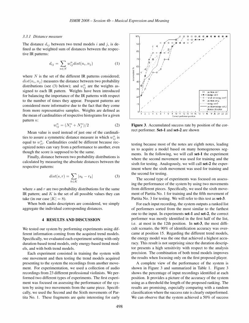
ISMIR 2008 – Session 4b – Musical Expression and Meaning
3.3.1 Distance measure
The distance dij between two trend models i and j, is de-
fined as the weighted sum of distances between the respec-
tive IR patterns:
dij =∑n∈N
wnijdist(ni, nj) (1)
where N is the set of the different IR patterns considered;
dist(ni, nj) measures the distance between two probability
distributions (see (3) below); and wnij are the weights as-
signed to each IR pattern. Weights have been introduced
for balancing the importance of the IR patterns with respect
to the number of times they appear. Frequent patterns are
considered more informative due to the fact that they come
from more representative samples. Weights are defined as
the mean of cardinalities of respective histograms for a given
pattern n:
wnij = (Nn
i + Nnj )/2 (2)
Mean value is used instead of just one of the cardinali-
ties to assure a symmetric distance measure in which wnij is
equal to wnji. Cardinalities could be different because rec-
ognized notes can vary from a performance to another, even
though the score is supposed to be the same.
Finally, distance between two probability distributions is
calculated by measuring the absolute distances between the
respective patterns:
dist(s, r) =∑k∈K
|sk − rk| (3)
where s and r are two probability distributions for the same
IR pattern; and K is the set of all possible values they can
take (in our case |K| = 8).
When both audio descriptors are considered, we simply
aggregate the individual corresponding distances.
4 RESULTS AND DISCUSSION
We tested our system by performing experiments using dif-
ferent information coming from the acquired trend models.
Specifically, we evaluated each experiment setting with only
duration-based trend models, only energy-based trend mod-
els, and with both trend models.
Each experiment consisted in training the system with
one movement and then testing the trend models acquired
presenting to the system the recordings from another move-
ment. For experimentation, we used a collection of audio
recordings from 23 different professional violinists. We per-
formed two different types of experiments. The first experi-
ment was focused on assessing the performance of the sys-
tem by using two movements from the same piece. Specifi-
cally, we used the Second and the Sixth movements of Par-
tita No. 1. These fragments are quite interesting for early
Figure 3. Accumulated success rate by position of the cor-
rect performer. Set-1 and set-2 are shown
testing because most of the notes are eighth notes, leading
us to acquire a model based on many homogeneous seg-
ments. In the following, we will call set-1 the experiment
where the second movement was used for training and the
sixth for testing. Analogously, we will call set-2 the exper-
iment where the sixth movement was used for training and
the second for testing.
The second type of experiments was focused on assess-
ing the performance of the system by using two movements
from different pieces. Specifically, we used the sixth move-
ment of Partita No. 1 for training and the fifth movement of
Partita No. 3 for testing. We will refer to this test as set-3.
For each input recording, the system outputs a ranked list
of performers sorted from the most similar to the farthest
one to the input. In experiments set-1 and set-2, the correct
performer was mostly identified in the first half of the list,
i.e. at most in the 12th position. In set-3, the most diffi-
cult scenario, the 90% of identification accuracy was over-
came at position 15. Regarding the different trend models,
the energy model was the one that achieved a highest accu-
racy. This result is not surprising since the duration descrip-
tor presents a high sensitivity with respect to the analysis
precision. The combination of both trend models improves
the results when focusing only on the first proposed player.
A complete view of the performance of the system is
shown in Figure 3 and summarized in Table 1. Figure 3
shows the percentage of input recordings identified at each
position. It provides a picture of the accuracy of the system
using as a threshold the length of the proposed ranking. The
results are promising, especially comparing with a random
classification where the success rate is clearly outperformed.
We can observe that the system achieved a 50% of success
498

ISMIR 2008 – Session 4b – Musical Expression and Meaning
set-1 set-2 set-31st 3rd 10th 1st 3rd 10th 1st 3rd 10th
duration 34.8 60.9 95.7 21.7 43.5 91.3 10.5 26.3 68.4
energy 21.7 69.6 91.3 30.4 47.8 91.3 15.8 31.6 73.7
both 52.2 65.2 91.3 34.8 47.8 95.7 15.8 26.3 68.4
Table 1. Success rate (%) in all experiments taking into
account three different ranking positions proposed for the
correct performer: 1st, 3rd, and 10th
using the four top candidates in set-1 and set-2.
Table 1 summarizes the performance of the system for
the three experimental sets and the three trend models. The
three columns of each experiment show, respectively, the
percentage of performers identified in the first position, at
least in the third position, and at least in the tenth position.
We can observe that for settings set-1 and set-2 the correct
performer is predicted, in the worst case, 20% of times as the
first candidate, clearly outperforming the random classifier
(whose success rate is 4.3%).
Figure 4 presents a matrix that summarizes the classi-
fier output for set-2 using both duration and energy trend
models. The figure shows, for each input recording (row),
the sorted list of predicted performers as squares. The gray
scale maps to the ranking values. The black color indicates
the first performer proposed and the gray degradation is used
to draw all the performers predicted until the correct one.
Notice that the success in the first position means a black
square in the diagonal. The matrix is not supposed to be
symmetric and each column can have the same color several
times because a predicted performer can occur in the same
position for several inputs. For instance, we can see that
Garret Fischbach’s performance (gar) for Sixth Movement
is very different from the rest of performers’ Second Move-
ment performances: all values correspond to last position
(i.e. the furthest). On the other hand, Christian Tetzlaff’s
(chr) and Rachel Podger’s (rac) performances are quite
similar to most of Second Movement performances since
there are many squares in their columns.
Finally, Figure 5 shows in which position the correct per-
former is ranked for each performer in the test set. This Fig-
ure complements the former two. The results came from set-1 using both trend models (‘duration+energy set-1’ curve in
Figure 3). Twelve right identifications were achieved at first
position (52% of success rate). The rest was correctly identi-
fied in positions 2 to 4 except three performers. Nathan Mil-
stein was identified at position 6. Finally, Sergiu Luca and
Shlomo Mintz were not clearly identified. After a detailed
analysis of the distances among all performers, we observed
that these two musicians are not clearly distinguished. We
mean, small variations in the trend models confuse the iden-
tification process.
Figure 4. Classifier output in matrix form for set-2 where
both trend models were used
5 CONCLUSIONS
This work focuses on the task of identifying violinists from
their playing style by building trend-based models that cap-
ture expressive tendencies. Trend models are acquired by
using state-of-the-art audio feature extraction tools and au-
tomatically segmenting the obtained melodies using IR pat-
terns. Performers were characterized by a set of probability
distributions, capturing their personal style with respect to a
collection of melodic patterns (IR patterns). We have shown
that, without a great analysis accuracy, our proposal is quite
robust.
The experiments were concentrated on identifying vio-
linists and using note durations and energies as descriptors.
We tested the system with 23 different professional perform-
ers and different recordings. Results obtained show that
the proposed model is capable of learning performance pat-
terns that are useful for distinguishing performers. The re-
sults clearly outperform a random classifier and, probably,
it would be quite hard for human listeners to achieve such
recognition rates. In order to assure the robustness of the
system, other sets of works should be used for learning and
testing.
We have presented a qualitative analysis using only two
qualitative values. We want to keep our model at this qual-
itative level but we plan to extend the model with the use
of fuzzy sets. This improvement will allow us to use the
capabilities of fuzzy theory for a better assessment in the
similarity measure.
Combining information from different music features have
been demonstrated to improve results. We are currently
working in increasing the number of descriptors. Since the
predictability of a given descriptor varies depending on the
499

ISMIR 2008 – Session 4b – Musical Expression and Meaning
Figure 5. Correct performer position for each performance
in set-1. Both trend models are used
performers, we are also interested in discovering relations
among the descriptors. Finally, the use of hierarchical clas-
sifiers or ensemble methods is a possible way of improving
the identification.
6 ACKNOWLEDGEMENTS
M. Molina-Solana is supported by the Spanish Ministry of
Education and Science under the project TIN2006-15041-
C04-01. J. Ll. Arcos is supported by the Spanish project
MID-CBR (TIN2006-15140-C03-01), EU-FEDER funds, and
by the Catalan Goverment (2005-SGR-00093). E. Gomez is
supported by EU-eContent-Plus project VARIAZIONI 1 (ECP-
2005-CULT-038264).
7 REFERENCES
[1] Camacho, A. SWIPE: A Sawtooth Waveform InspiredPitch Estimator for Speech and Music. PhD Disserta-
tion, University of Florida, USA, 2007.
[2] Dovey, M.J. “Analysis of Rachmaninoff’s piano perfor-
mances using inductive logic programming”, Proc. Eur.Conf. Machine Learning, pp. 279-282, 1995.
[3] Goebl, W. “Analysis of Piano Performance: Towards
a Common Performance Standard?”, Proc. of the So-ciety for Music Perception and Cognition Conference,
(SMPC99), 1999.
[4] Grachten, M., Arcos, J.L., Lopez de Mantaras, R.
“Melody retrieval using the Implication/Realization
Model”, Proc. of 6th Int. Conf. on Music Information
1 http://www.variazioniproject.org
Retrieval, (ISMIR 2005), (First prize of the MIREX
Symbolic Melodic Similarity Contest), 2005
[5] Juslin, P.N., Sloboda, J.A. Musical Emotion: Theoryand Research. New York: Oxford Univ. Press, 2001.
[6] Juslin, P.N., Frieberg, A., Bresin, R. “Toward a com-
putational model of expression in performance: The
GERM model”, Musicae Scientiae, special issue 2001-
2002, pp. 63-122.
[7] Hong, J. “Investigating expressive timing and dynamics
in recorded cello”, Psychology of Music, 31(3), pp. 340-
352, 2003.
[8] Lester, J. Bach’s Works for Solo Violin: Style, Structure,Performance. First published in 1999 by Oxford Univer-
sity Press, Inc.
[9] Lopez de Mantaras, R., Arcos, J.L. “AI and music, form
composition to expressive performance”, AI Magazine,
23(3), pp. 43-57, 2002.
[10] Narmour, E. The Analysis and Cognition of MelodicComplexity: The Implication Realization Model.Chicago, IL: Univ. Chicago Press, 1990.
[11] Puiggros, M. Comparative analysis of expressivity inrecorded violin performances. Study of the Sonatas andPartitas for solo violin by J. S. Bach. Master Thesis, Uni-
versitat Pompeu Fabra, Barcelona, 2007.
[12] Ramirez, R., Maestre, E., Pertusa, A., Gomez, E.,
Serra, X. “Performance-Based Interpreter Identification
in Saxophone Audio Recordings”, IEEE Trans. on Cir-cuits and Systems for Video Technology, 17(3), pp. 356-
264, 2007.
[13] Sapp, C.S. “Comparative Analysis of Multiple Musical
Performances”, Proc. of 8th Int. Conf. on Music Infor-mation Retrieval, (ISMIR 2007), Vienna, Austria, pp.
497-500, 2007.
[14] Saunders, C., Hardoon, D., Shawe-Taylor, J., Widmer,
G. “Using string kernels to identify famous performers
from their playing style”, 15th Eur. Conf. on MachineLearning, Pisa, Italy, 2004.
[15] Stamatatos, E., Widmer, G. “Automatic Identification of
Music Performers with Learning Ensembles”, ArtificialIntelligence, 165(1), pp. 37-56, 2005.
[16] Widmer, G., Dixon, S., Goebl, E., Pampalk, W., Tobu-
dic, A. “In search of the Horowitz factor”, AI Magazine,
24(3), pp. 111-130, 2003.
500

ISMIR 2008 – Session 4b – Musical Expression and Meaning
HYBRID NUMERIC/RANK SIMILARITY METRICS FORMUSICAL PERFORMANCE ANALYSIS
Craig Stuart SappCHARM, Royal Holloway, University of London
ABSTRACT
This paper describes a numerical method for examiningsimilarities among tempo and loudness features extracted fromrecordings of the same musical work and evaluates its effec-tiveness compared to Pearson correlation. Starting with corre-lation at multiple timescales, other concepts such as a perfor-mance “noise-floor” are used to generate measurements whichare more refined than correlation alone. The measurements areevaluated and compared to plain correlation in their ability toidentify performances of the same Chopin mazurka played bythe same pianist out of a collection of recordings by variouspianists.
1 INTRODUCTION
As part of the Mazurka Project at the AHRC Centre for the His-tory and Analysis of Recorded Music (CHARM), almost 3,000recordings of Chopin mazurkas were collected to analyze thestylistic evolution of piano playing over the past 100 years ofrecording history, which equates to about 60 performances ofeach mazurka. The earliest collected performance was recordedon wax cylinders in 1902 and the most recent posted as home-made videos on YouTube. Table 1 lists 300 performances offive mazurkas which will be used for evaluation later in this pa-per since they include a substantial number of recordings withextracted tempo and loudness features.
Table 1. Collection of musical works used for analysis.
For each of the processed recordings, beat timings in the per-formance are determined using the Sonic Visualiser audio edi-tor 1 for markup and manual correction with the assistance ofseveral vamp plugins. 2 Dynamics are then extracted as smoo-thed loudness values sampled at the beat positions.[3] Featuredata will eventually be extracted from all collected mazurkas inthe above list, but comparisons made in Section 3 are based on
1 http://www.sonicvisualiser.org2 http://sv.mazurka.org.uk/download
the processed performance counts in Table 1. Raw data usedfor analysis in this paper is available on the web. 3
Figure 1 illustrates extracted performance feature data as aset of curves. Curve 1a plots the beat-level tempo which iscalculated from the duration between adjacent beat timings inthe recording. For analysis comparisons, the tempo curve isalso split into high- and low-frequency components with lin-ear filtering. 4 Curve 1b represents smoothed tempo whichcaptures large-scale phrasing architecture in the performance(note there are eight phrases in this example). Curve 1c repre-sents the difference between Curves 1a and 1b which is calledhere the desmoothed tempo curve, or the residual tempo. Thishigh-frequency tempo component encodes temporal accentu-ation in the music used by the performer to emphasize par-ticular notes or beats. Mazurka performances contain signifi-cant high-frequency tempo information, since part of the per-formance style depends on a non-uniform tempo throughoutthe measure—the first beat usually shortened, while the secondand/or third beat are lengthened. Curve 1d represents the ex-tracted dynamics curve which is a sampling of the audio loud-ness at each beat location.
Other musical features are currently ignored here, yet areimportant in characterizing a performance. In particular, pi-anists do not always play left- and right-hand notes together,according to aural traditions, although they are written as si-multaneities in the printed score. Articulations such as legatoand staccato are also important performance features but areequally difficult to extract reliably from audio data. Nonethe-less, tempo and dynamic features are useful for developing nav-igational tools which allow listeners to focus their attention onspecific areas for further analysis.
Figure 1. Extracted musical features from a recording ofChopin’s mazurka in B minor, 30/2: a) tempo between beats;b) smoothed tempo; c) residual tempo (c = a− b); and d) beat-level dynamics.
3 http://mazurka.org.uk/info/excel4 The filtering method is available online at
http://mazurka.org.uk/software/online/smoother .
501

ISMIR 2008 – Session 4b – Musical Expression and Meaning
2 DERIVATIONS AND DEFINITIONS
Starting with the underlying comparison method of correlation(called S0 below), a series of intermediate similarity measure-ments (S1, S2, and S3) are used to derive a final measurementtechnique (S4). Section 3 then compares the effectiveness ofS0 and S4 measurements in identifying recordings of the sameperformer out of a database of recordings of the same mazurka.
2.1 Type-0 Score
As a starting point for comparison between performance fea-tures, Pearson correlation, often called an r-value in statistics,is used:
Pearson(x, y) =
∑n
(xn − x̄)(yn − ȳ)√∑n
(xn − x̄)2∑
n
(yn − ȳ)2(1)
This type of correlation is related to dot-product correlationused in Fourier analysis, for example, to measure similaritiesbetween an audio signal and a set of harmonically related sinu-soids. The value range for Pearson correlation is−1.0 to +1.0,with 1.0 indicating an identical match between two sequences(exclusive of scaling and shifting), and the value 0.0 indicat-ing no predictable linear relation between the two sequences xand y.
Correlation values between extracted musical features typi-cally have a range between 0.20 and 0.97 for different perfor-mances of mazurkas. Figure 2 illustrates the range of correla-tions between performances in two mazurkas. Mazurka 17/4 isa more complex composition with a more varied interpretationrange, so the mode, or most-expected value, of the correlationdistribution is 0.67. Mazurka 68/3 is a simpler compositionwith fewer options for individual interpretations so the mode ismuch higher at 0.87.
These differences in expected correlation values betweentwo randomly selected performances illustrate a difficulty ininterpreting similarity directly from correlation values. Thecorrelation values are consistent only in relation to a particu-lar composition, and these absolute values cannot be compareddirectly between different mazurkas. For example, a pair ofperformances which correlate at 0.80 in mazurka 17/4 indicatesa better than average match, while the same correlation valuein mazurka 68/3 would be a relatively poor match. In addition,correlations at different timescales in the same piece will havea similar problem, since some regions of music may allow for afreer interpretation while other regions may have a more staticinterpretation.
Figure 2. Different compositions will have different expectedcorrelation distributions between performances.
Figure 3. Scapeplot for the dynamics in Horowitz’s 1949 per-formance of mazurka 63/3 with the top eight matching perfor-mances labeled.
2.2 Type-1 Score
In order to compensate partially for this variability in correla-tion distributions, scapeplots were developed which only dis-play nearest-neighbor performances in terms of correlation atall timescales for a particular reference performance.[3] Ex-amples of such plots created for the Mazurka Project can beviewed online. 5
The S1 score is defined as the fraction of area each targetperformance covers in a reference performer’s scapeplot. Fig-ure 3 demonstrates one of these plots, comparing the dynamicsof a performance by Vladimir Horowitz to 56 other recordings.In this case, Rachmaninoff’s performance of the same piecematches better than any other performance, since his perfor-mance covers 34% of the scape’s plotting domain. At secondbest, Zak’s performance matches well towards the end of themusic, but covers only 28% of the total plotting domain. Notethat Zak’s performance has the best correlation for the entirefeature sequence (S0 score) which is represented by the point atthe top of the triangle. The S1 scores for the top eight matchesin Figure 3 are listed in Table 2. There is general agreement be-tween S1 and S0 scores since five top-level correlation matchesalso appear in the list.
2.3 Type-2 Score
Scape displays are sensitive to the Hatto effect: if an identicalperformance to the reference, or query, performance is presentin the target set of performances, then correlation values at alltime resolutions will be close to the maximum value for theidentical performance, and the comparative scapeplot will showa solid color. All other performances would have an S1 score ofapproximately 0 regardless of how similar they might otherwiseseem to the reference performance. This property of S1 scoresis useful for identifying two identical recordings, but not usefulfor viewing similarities to other performances which are hiddenbehind such closely neighboring performances.
One way to compensate for this problem is to remove thebest match from the scape plot in order to calculate the nextbest match. For example, Figure 4 gives a rough schematic for
5 http://mazurka.org.uk/ana/pcor-perf502

ISMIR 2008 – Session 4b – Musical Expression and Meaning
Figure 4. Schematic of nearest-neighbor matching methodused in comparative timescapes.
how scapeplots are generated. Capital ‘Q’ represents the query,or reference, performance, and lower-case lettered points repre-sent other performances. The scapeplot basically looks aroundin the local neighborhood of the feature space and displaysclosest matches as indicated by lines drawn towards the queryon the right side of Figure 4. Closer performances will tend tohave larger shadows on the query, and some performances canbe completely blocked by others, as is the case for point “a” inthe illustration.
An S2 score measures the coverage area of the most dom-inant performance which is assumed to be most similar to thereference performance. This nearest of the neighbors is thenremoved from the search database, and a new scapeplot is gen-erated with the remaining performances. Gradually, more andmore performances will be removed which allows for previ-ously hidden performances to appear in the plot. For example,point “a” in Figure 4 will start to become visible once point “b”is removed. S2 scores and ranks are independent. As fewerand fewer target matches remain, the S2 scores will increasetowards 1.0 while the S2 ranks decrease towards the bottommatch.
In Figure 3, Rachmaninoff is initially the best match in termsof S1 scores, so his performance will be removed and a newscapeplot generated. When this is done, Zak’s performancethen represents the best match, covering 34% of the scapeplot.Zak’s performance is then removed, a new scapeplot is calcu-lated, and Moravec’s performance will have the best coverageat 13%, and so on. Some of the top S2 scores for Horowitz’sperformance are listed in Table 2.
2.4 Type-3 Score
Continuing on, the next best S2 rank is for Chiu, who has 20%coverage. Notice that this is greater than Moravec’s score of13%. This demonstrates the occurrence of what might be calledthe lesser Hatto effect: much of Moravec’s performance over-lapped onto Chiu’s region, so when looking only at the near-est neighbors in this manner, there are still overlap problems.Undoubtedly, Rachmaninoff’s and Zak’s performances mutu-ally overlap each other in Figure 3 as well. Both of them aregood matches to Horowitz, so it is difficult to determine ac-curately which performance matches “best” according to S2
scores since they are interfering with each others scores andare both tied at 34% coverage.
In order to define a more equitable similarity metric and re-move the Hatto effect completely, all performances are firstranked approximately by similarity to Horowitz using either
Figure 5. Schematic of the steps for measuring an S3 score: (1)sort performances from similar to dissimilar, (2) remove mostsimilar performance to leave noise floor, (3) & (4) insert moresimilar performances one-by-one to observe how well they canocclude the noise-floor.
S0 values or the rankings produced during S2 score calcula-tions. Performances are then divided into two groups, with thepoorly-matching half defined as the performance “noise-floor”over which better matches will be individually placed.
To generate an S3 score, the non-noise performances are re-moved from the search database as illustrated in step 2 of Fig-ure 5, leaving only background-noise performances. Next, non-noise performances are re-introduced separately along with allof the noise-floor performances and scapeplot is generated. Thecoverage area of the single non-noise performance representedin the plot is defined as its S3 similarity measurement with re-spect to the query performance.
This definition of a performance noise-floor is somewhat ar-
Figure 6. Dynascapes for Horowitz’s performance of mazurka63/3. Top left is a plot of the noise-floor performances, andthe other three plots separate include one of the top matchingperformances which can cover most of the noise-floor.
503

ISMIR 2008 – Session 4b – Musical Expression and Meaning
Table 2. Scores and rankings for sample targets to Horowitz’s1949 performance of mazurka 63/3.
bitrary but splitting the performance database into two equalhalves seems the most flexible rule to use, and is used for theevaluation section later in this paper. But the cut-off point couldbe a different percentage, such as the bottom 75% of rankedscores, or an absolute cut-off number. In any case, it is prefer-able that the noise floor does not appear to have any favoredmatches, and should consist of uniform small blotches at alltimescales in the scapeplot representing many different per-formers as is the example shown in Figure 6 (top left part ofthe figure). While Rachmaninoff and Zak have equivalent S2
scores, Rachmaninoff’s performance is able to cover 74% ofthe noise-floor, while Zak’s is only able to cover 64%.
2.5 Type-4 Score
Type-3 scores require one additional refinement in order to beuseful since performances are not necessarily evenly distributedin the feature space. The plots used to calculate the S3 scoresare still nearest-neighbor rank plots, so the absolute numericdistances between performances are not directly displayed. Un-like correlation values between two performances, S3 scoresare not symmetric: the score from A to B is not the same valueas from B to A. It is possible for an outlier performance to matchwell to another performance closer to the average performancejust because it happens to be facing towards the outlier, withthe similarity just being a random coincidence.
Therefore, the geometric mean is used to mix the S3 scorewith the reverse-query score (S3r) as shown in Equation 4.
S3 = A ⇒ B measurement (2)
S3r = A ⇐ B measurement (3)
S4 =√
S3 S3r (4)
The arithmetic mean could also be used, but the geometricmean is useful since it penalizes the final score if the type-3and its reverse scores are not close to each other. For exam-ple, the arithmetic mean between 0.75 and 0.25 is 0.50, whilethe geometric mean is lower at 0.43. Greatly differing S3 andS3r scores invariably indicate a poor match between two perfor-mances, with one of them acting as an outlier to a more centralgroup of performances.
Table 2 shows several of the better matches to Horowitz’sperformance in mazurka 63/3, along with the various types ofscores that they generate. S0 is the top-level correlation be-tween the dynamics curves, and R0 is the corresponding sim-ilarity rankings generated by sorting S0 values. Likewise, S4
Table 3. Rankings for 17/4 Rubinstein performances. Shadednumbers indicate perfect performance of a similarity metric.
and R4 indicate the final proposed similarity metric, and theresulting rankings generated by sorting these scores.
3 EVALUATION
When evaluating similarity measurement effectiveness, a use-ful technique with a clear ground-truth is to identify recordingsby the same performer mingled among a larger collection ofrecordings.[5] Presumably pianists will tend to play more liketheir previous performances over time rather than like otherpianists. If this is true, then better similarity metrics shouldmatch two performances by the same pianist more closely toeach other than to other performances by different pianists.
3.1 Rubinstein performance matching
Arthur Rubinstein is perhaps the most prominent interpreter ofChopin’s compositions in the 20th century, and luckily he hasrecorded the entire mazurka cycle three times during his career:(1) in 1938–9, aged 51; (2) in 1952–4, aged 66, and (3) in 1966,aged 79.
Table 3 lists the results of ranking his performances to eachother in mazurka 17/4 where the search database contains anadditional 60 performances besides the three by Rubinstein.The first column in the table indicates which performance wasused as the query (Rubinstein’s 1939 performance, for exam-ple, at the top of the first row). The target column indicatesa particular target performance which is one of the other twoperformances by Rubinstein in the search database. Next, fivecolumns list three types of rankings for comparison. The fivecolumns represent four different extracted features as illustratedin Figure 1, plus the TD column which represents a 50/50 ad-mixture of the tempo and dynamics features.
For each musical feature, three columns of rankings are re-ported. R0 represents the rankings from the S0 scores; R3
being the type-3 scoring ranks, and R4 resulting from sortingthe S4 similarity values. In these columns, a “1” indicates thatthe target performance was ranked best in overall similarity tothe query performance, “2” indicates that it is the second bestmatch, and so on (see the search database sizes in Table 1). Inthe ranking table for mazurka 17/4 performances of Rubinstein,the shaded cells indicate perfect performance matches by a par-ticular similarity metric where the top two matches are bothRubinstein. Note that there is one perfect pair of matches inall of the R0 columns which is found in the full-tempo feature
504

ISMIR 2008 – Session 4b – Musical Expression and Meaning
Figure 7. Ability of metrics to identify the same performer in alarger set of performances, using 3 performances of Rubinsteinfor each mazurka. (Lower rankings indicate better results.)
when Rubinstein 1939 is the target performance. No columnsfor R3 contain perfect matching pairs, but about 1/2 of the R4
columns contain perfect matches: all of the full-tempo R4 rank-ings are perfect, and a majority of the desmoothed tempo andjoint tempo/dynamics rankings are perfect. None of the metricscontain perfect matching pairs for the dynamics features. Thisis perhaps due to either (1) the dynamics data containing mea-surement noise (due to the difficultly of extracting dynamicsdata from audio data), or (2) Rubinstein varying his dynamicsmore over time than his tempo features, or a combination ofthese two possibilities.
Figure 7 shows the average rankings of Rubinstein perfor-mances for all extracted features averaged by mazurka. The fig-ure shows S4 scores are best at identifying the other two Rubin-stein performances for all of the five mazurkas which were usedin the evaluation. Typically S4 gives three to four times betterrankings than the S0 values according to this figure. S3 scores(used to calculate S4 scores), are slightly better than plain cor-relation, but sometimes perform worse than correlation in somemazurkas.
Figure 8 evaluates the average ranking effectiveness by mu-sical feature, averaged over all five mazurkas. Again S4 scoresare always three to four times more effective than plain corre-lation. S3 scores are approximately as effective as S0 rankingsfor full and smoothed tempo, but perform somewhat better onresidual tempo and dynamics features, probably by minimizingthe effects of sudden extreme differences between comparedfeature sequences caused by noisy feature data.
Table 4. Performer self-matching statistics.
Figure 8. Ranking effectiveness by extracted musical fea-tures, using three performances of Rubinstein for each ma-zurka. (Lower values indicate better results.)
3.2 Other performers
Rubinstein tends to vary his performance interpretation morethan most other pianists. Also, other performers may tend toemulate his performances, since he is one of the more promi-nent interpreters of Chopin’s piano music. Thus, he is a diffi-cult case to match and is a good challenge for similarity metricevaluations.
This section summarizes the effectiveness of the S0 and S4
similarity metrics in identifying other pianists found in the fiveselected mazurkas for which two recordings by the same pi-anist are represented in the data collection (only Rubinstein isrepresented by three performances for all mazurkas).
Table 4 presents ranking evaluations for performance pairsin a similar layout to those of Rubinstein found in Table 3. Inall except two cases (for Fou) the S4 metrics perform perfectlyin identifying the other performance by the same pianist. Top-level correlation was able to generate correct matches in 75%of the cases. An interesting difference between the two met-rics occurs when Hor71 is the query performance. In this caseS0 yields a rank of 13 (with 12 other performance matchingbetter than his 1985 performance), while S4 identifies his 1985performance as the closest match.
Fou’s performance pair for mazurka 30/2 is also an interest-ing case. For his performances, the phrasing portion of the full-and smoothed-tempo features match well to each other, but thetempo residue does not. This is due to a significant change inhis metric interpretation: the earlier performance has a strongmazurka metric pattern which consists of a short first beat, fol-lowed by a lengthened second or third beat in each measure.His 2005 performance greatly reduces this effect, and beat du-rations are more uniform throughout the measure in compari-son to his 1978 performance.
Finally, it is interesting to note the close similarity betweenUninsky’s pair of performances listed in Table 4. These twoperformances were recorded almost 40 years apart, one in Rus-sia and the other in Texas. Also, the first was recorded onto 78RPM monophonic records, while the later was recorded onto33-1/3 RPM stereo records. Nonetheless, his two performancesindicate a continuity of performance interpretation over a longcareer.
505

ISMIR 2008 – Session 4b – Musical Expression and Meaning
Table 5. Comparison of Cortot performances of mazurka 30/2(m. 1–48).
4 APPLICATION
As an example application of the derived similarity metrics,two performances of mazurka 30/2 performed by Alfred Cortotare examined in this section. One complete set of his mazurkaperformances can be found on commercially release recordingsfrom a 1980’s-era issue on cassette tape “recorded at diverselocations and dates presumably in the period of 1950–1952.”[1]These recordings happen to be issued by the same record labelas the recordings of Joyce Hatto, which casts suspicion on otherrecordings produced on that label.[4]. A peculiar problem isthat no other commercial recordings exist of Cortot playing anymazurka, let alone the entire mazurka cycle.
In 2005, however, Sony Classical (S3K89698) released a 3-CD set of recordings by Cortot played during master classes heconducted during the late 1950’s, and in this set, there are sixpartial performances of mazurkas by Cortot where he demon-strates how to play mazurkas to students during the class. Hisrecording of mazurka 30/2 on these CDs is the largest contin-uous fragment, including 75% of the entire composition, stop-ping two phrases before the end of the composition.
Table 5 lists the S4 scores and rankings for these two record-ings of mazurka 30/2, with the Concert Artist’s rankings on theleft, and the Sony Classical rankings to the right. The five dif-ferent musical features listed by column in previous tables forRubinstein and other pianists are listed here by row. For eachrecording/feature combination, the top three matches are listed,along with the ranking for the complimentary Cortot recording.
Note that in all cases, the two Cortot recordings match verypoorly to each other. In two cases, the worst possible rankingof 35 is achieved (since 36 performances are being compared intotal). Perhaps Cortot greatly changes his performances style inthe span of 6 years between these two recordings late in his life,although data from Tables 3 and 4 would not support this viewsince no other pianists has significantly alter all musical fea-tures at once, and only Fou significantly changes one musicalfeature between performances.
Therefore, it is likely that this particular mazurka recording
on the Concert Artist label was not actually performed by Cor-tot. Results from further investigation of the other five partialmazurka performances on the Sony Classical recordings wouldhelp to confirm or refute this hypothesis, but the other examplesare more fragmentary, making it difficult to extract reasonableamounts of recital-grade performance material. In addition, noperformer in the top matches for the Concert Artist Cortot per-formance match well enough to have likely recorded this per-formance, so it is unlikely that any of the other 30 or so per-formers being compared to this spurious Cortot performance isthe actual source for this particular mazurka recording.
5 FUTURE WORK
Different methods of combining S3 and S3r scores, such asmeasuring the intersection between plot areas rather than mea-suring the geometric mean to calculate S4 should be examined.The concept of a noise floor when comparing multiple perfor-mances is useful for identifying features which are common orrare, and allows similarity measurements to be more consistentacross different compositions, which may aid in the identifica-tion of pianists across different musical works.[6]
Further analysis of the layout of the noise-floor as seen inFigure 6 might be useful in differentiating between directly andindirectly generated similarities between performances. For ex-ample in this figure, Rachmaninoff’s performance shows moreconsistent similarity towards smaller-scale features, which mayindicate a direct influence on Horowitz’s performance style.Zak’s noise-floor boundary in Figure 6 may demonstrate an in-direct similarity, such as a general school of performance.
Since the similarity measurement described in this paperworks well for matching the same performer in different record-ings, and examination of student/teacher similarities may bedone. The analysis techniques described here should be appli-cable to other types of features, and may be useful with otherunderlying similarity metrics besides correlation. For example,It would be interesting to extract musical features first fromthe data with other techniques such as Principle ComponentAnalysis[2] and use this derived feature data for characterizingthe similarities between performances in place of correlation.
6 REFERENCES
[1] Chopin: The Mazurkas. Alfred Cortot, piano. ConcertArtist compact disc CACD 91802 (2005).
[2] Repp, B.H. “A microcosm of musical expression: I. Quan-titative analysis of pianists’ timing in the initial measuresof Chopin’s Etude in E major,” Journal of the AcousticalSociety of America, 104 (1998). pp. 1085–1100.
[3] Sapp, C. “Comparative analysis of multiple musical perfor-mances,” Proceedings of the 8th International Conferenceon Music Information Retrieval, Vienna, Austria, 2007.pp. 497–500.
[4] Singer, M. “Fantasia for piano: Joyce Hatto’s incredible ca-reer,” New Yorker, 17 Sept. 2007. pp. 66–81.
[5] Stamatatos, E. and G. Widmer. “Automatic identification ofmusic performers with learning ensembles,” Artificial Intel-ligence, 165/1 (2005). pp. 37–56.
[6] Widmer, G., S. Dixon, W. Goebl, E. Pampalk, and A. Tobu-dic. “In search of the Horowitz factor,” AI Magazine, 24/3(2003). pp. 111–130.
506

ISMIR 2008 – Session 4b – Musical Expression and Meaning
�
�"#�# ?,��?-�#.����# ?,�%��# /90"��#�%�� ����%%�" #��
����������������` ���������������`��������
�� �� �������� ����������������������� ��¯�� ��� ����������� ����� �� �
\ ����¯`���� ������@��"���?������A�������� ���
��
�1�#"��#�
`����� ������������ ������ �� �� � ��� ��� ��� �� ������������ � � ������ � ����� ��� ��� �������� ������� �������������� ���� ������������� ��� � � �� ����� � ������ |������ ���� ����� ��������?� �� � ���� �� ��� ������������ � ��� ��� ��� ��� �� �� ��� ������ ������ � � ��� �� ������ ��� ��� ���� ��� �� � ����� ��� ��� ��������� � � '�� ������ ����� �� � ����¥�� �������������� ~ � ���� ��� �� ����������� �������������������� ���������� ������������� � �������������� ������� ��������� ����� ���� ����� � � � ��� �� �'��� � ������\���� �� ���� ��'� �� ���� � ����������� ��� ������ � ������ �������� ��� �� ����� � � � �� �� ��� � � ������� ���������� ��� �� � ���� �� '�������� � � �� �������¥�� �� ���� � ����\���� ��� � ������� ������������� �������������� ������� ����������������� ��� � ������ �� � �� �������� ���������� � ������������~ ������ ���' �� ���� �� � � ����������������� ������� �� ����� ��' ������� ����������� ��������� �� � � � �� �� �� � ��������� � ������ �� �� ��� � ������������� �������������������� ���������
2�� ?#"�-��# �?�
� �� � �� � ������ �� ��� ������ ��� � ����� � ��� ������������ � �^��� ������ ��� �� � � ���� � ��^ ���� |�� � ��?� ���� ��� ?� �� � ������� ��� � ��� ������� �� ������� � �� �� ������������� ���� � ������������������?���������� ���� � ��������� �� � ����� ��� �� ��� ��� � � ���� ����� ��� �����������?� ��� �����?� � ������ ��� ���� ��� �!������ ����������������� ��������� ���������������� ���� ����� ������ ��� � ��� � ������� '���� �� � ���� ���� ����������������������������� ����������� �������� ��������������?��������������� ��������� � �������� ����� ������������ �' ������������� �� ����������� �� � ���� ��������
��� �� � ��� �� ��� � ������ ?� � ������ ��������������������� ������������ ����������� ��������������������������� ������������������������ ����� ������ �������� ������������ ���� ������ ����������������������������� �������� �������������� ���������������� ��������������� ��������������� ���� � �� ��� � � ������� ������� ������� ��� ��� � ����?� �� � �� �¥�� �� ����� ��� ������ ��� �� � ���� ������ � ���� � � ������ ����� ���'�� ������ ��� � �������'� �� ��������������'������������������������������������������ �������������������� ��������� _��� ������ �� ��� �� � �����?� � ��� �� ��� �� ��� �?� ��� � ��� �� ���
�� � ����� `���� ���� ����� ������ � ������ ���� �� � �� '��� ��� ������ ��� ��� �� �� � ������������� ��� �� � ����?� ���������� � �� ����� ?������ ����� ���������� � �� ���� ������ \� � ���������� ��� �� � � ���� �� ��� �'�� �������� ���� >�� �� � ���?� �� � � ��� ��� ����� � ���� �� �� � �� ����� ����������� �������� ��������������'�������� ���������� �� � ������ >�� �� � ��� �� ���?� ������ ������ ����� �� ��� ����� �� � � ����� ���� ��������� ��� ������ �������������� ���������� ?� ������������ ���
`���� ��� �� � �������� '���� ��� ������ ����������������� �� ��� �� � � � ������ ��� �� � ����� � � �� ��� ������� �� ��� � ���� �� � ��� � ��� � � �� �?� ��� ��� � � ������ ��� � �� � � ��� �� ������� � ����� ��� ���� �� ���� �� ��� ����� �� � ����� ��� �� � �� �� � �� ��� ��� �� � ��� ��� ����� �� �� �� � � ��� ����� �� _� ��� � ���� ��� ��� ������������������� ��� ���� � �� ��� ������������ �� ������ ����� � � �����?� ' � ���� � ������ �� � ���� �� ��������� � ��� � ���� ���� �� � ����� ��� ��� ��� � ��� �� ������������������� �������\�� ���� ��� �� ������� ���������� ���������?� ' � ���� � ���������� ���� ����� � �������� ������ ��� ������ ����� ����� ���� ���� �� ���������� �� � ������������� ������ ����� �' ��� � ��������� �� ���� � � ��������� ���� � ��� ��� ��� �� ���� � �� � ����� ���� ���
�|�� ����� �� ' � � � ��� ��� � ���������������������� ���� �����'� �� � ������ �� ��� � ��� �� �������� �������� �� ��� ������� � ��� �� � ���� ��� ��������������������� ������"�������� �� �� �� �� ��'������� �������� ������������ ��� � ��������� ���� ����_� ��� � ������ !� � ����� �� �� � ����������������������� � ������ �� �������� �� �� � ������ ��� �� ���� ��� �� �����' ��� ��� ������� ��� �� � � ������ ���� � �� �� ��� � ������ ��� ������?� � ������ <� ������� �� �� �� ������ ��� � � ���� ��� ������� ���� ������ � ����� � ��������� ����� ���������������������'��������� ���� �
3�� "#��##-�$�"%�
~ � ���� ����� � ����_� �� ���� �� � ��������� ��� ������ �������� � ��� �� ��� �� � ��?� ������� ��?� ����� ������ _� ��� �?�������������� ������_��� � � ���� ��\����'������� ��� �� ����� � � ���� ���� � � ������ ������������ ������� ����������������� ����� ������� ���������������� ��� �� ��?� ��� �������?� �� � � ������� �� ?� �� ����� ��� ��� ������������ ���������� ��� � �� ��������
507

ISMIR 2008 – Session 4b – Musical Expression and Meaning
�
���� ���� �������'������ ����� ������ � ���� ��� ������� � ����� ��\� � �� ����� ���������� ������� ����������� �� ������
�� ���� �� ��� ���������� ��?� "�� �� � � �� ��� ������������� '� � � �� � �������� � ��� �� � ���� ��?� ��� ��� �� ��������� �� � ����� ��� ��� ��� ?� ��� � � ���� �� ����������� ������ � � �� ���� �� ��� �� � _� �� � ������ ���'���� �� �'��� � ��������� ��������� � �!�?� �� ���� � �� � �������� ��� �� � ������ '���� �� � ���������� ����� �` �� �� _� ���� � �������� ����� ���� �`�����?� ������� � ������ � ��� �� � �� � �� � ������ ��� ��� ��� ������������� ��� ���� � �� � � ������ ��� � �'����� �������� ��������������������\��� � ��� �� � � �� ��� �� _� �� ������� �������� ���� � � ������ � ���� �����?��� �������� ��� �������������� ���� �� �������� �'��� ��������� ��� ��� �'���� �� ����������� �� |�� �� ���� � ��������� ��������� �� ��� ��������?��� ������� �� ������� ������������� ������
>�� ������������� � ������ �������� ��������� �������� ������������� ������� �������� ������� � ����� �������������������� �� ��� ��� ���� ������� ����������� �� ����� ����� ��� �� �������� �����?��� ������� ���� �� �������� � �� ���� ������ � ������ �� ������ ������ ������������ ��� ������������� ������� ���� ��������� ������ ������ ��� �� �� ���� ���� � ��� ����� \� � � �� ��� � ��� �� ��� � �� �� �� �� ��� �� � �� _� ���� ��� ���� � �� ���� ��� ���������<���� ��� ��� _� ���?� � ������������������� � ����� � ������� �� ��� ������� ��� �� ��� �������� ������ ¥�� ����� �� � ��� ��� ��������� � ������ �� ���� ������ ���� �� �������� ����������� ����������� � �� � ��� ������ �������� ���� ��� ���������� ������?� ¢�����`��� ���"�������� �������� �� ��� ������� �� ��������� � ������� �� ��� �� � � �� �� �� ������ � ���� `����� ��������� � �� �� � ���� ������� ���� �����¦� ��� ��� �������� �� ����� ���� ������� ��� � ��� �� � �������� ����� ��������������$�������������������\��� �� ��� ��� ��� ���� ���������� ����� ������� ����?������ ������������ �� ���� �� � ��������� ��� �� � ����� � � � ����� � �� � ������ ����������� ����� ������ ��������������������������������������\� ��������� �� ����� ��������� ��������� ������ �������� ������� ��� �� ������ ������� ���`���������� ����� ��������� ������¥���������� ��� ����� �� � ������� ��� ��� � �� � ��� �� ��� �� � ������ ��� �� ������� �� �� � � �� ���� ��������� ��� �� ��� � ������� ��������� ���������� ��� ���� ����� �� ������� ��������� ������������ ���������������\� � ��� ���� �� ���������������� � ������� ��� �� �� '���� ��� � ��� ����� � � ����� ������� ����� ��� �� � � �� �� ���� �� � �� ����� ��� �� � ������������� `���������� ��� �� '� ���� � � �� � ������������������������ �� _� �� ������ �� ��������� ������ �� �� � ��� � ��� ��� � �� ��� � � ��� �� � ����� ����� ���� ������
� � ��� �� ��� ���� � � �� � � ��� � � � � ������� ��� �� ������ ��� ������ �� ���� ���������� ����� ����� ��� �������� ������� ��� �������� ������� ������?��� �������� ��� ����� ����� ��� ������ � ��� ��� � ��� �� � ��� �� �
������ � ����� ���������� ��`�����`�� ����``������� �������� ���� �� _� �� ��\� ���� �� � � ������������ ���� �� ���� �� � �� ����� ��� �� � ������� ��� ��������� ��� ������������������������������ ��� ����\� ��� ����� ���������� � ��� ������ � '��� ��� � � �� � � ��������� ���������� ������� ���������������
���� ����� �?����������� �'���������������������������� ����� �� ��� �� � �� ����������� ��� ������ ��� ��� >���'���� ��� ���� � ����� ��� ���� ��� ���� �� �� � � ����� ������������ ������� ����� ���� ���� �� ���� ����� ���
B�� ��,�" #0%��
���� �������� �� ���������������������������� ������� � � � �� ��� �� � ������ � �� ������������� ���� � ��� ������� � ���� �� ��� ���� � �� � ��� � ��� � �������� \� � �� � ���� ��� �� '� � � �� _� ����� ���������� ��� ����� �������� �� ������ � �� ���� ������ ��������������������������� � �� ������� ����������������������� �� ���� � � �� ����� ������� �� �� � ����� ��� ��� ��� � ��� �� ������|����������������¥����' ����� ������?����� ��� ?� �� � ������������� �� � ?� '����� ��� � � ������ �� ��� �� �����?� ����������� � �������� ��� �� �� �������� ����\�� ���� ���'������ ������� �� � ��������������������� �� �� ���� �� ��� �� ������ ��� �� � ������?� ���������� �� �������� ��� ��� � ����� �� � ����� ��� ��� ��� ��������� �� � � ������ ��� �'�� ��������� ��� ��� � ����� � ��� � ���������� ���� � � ������ �� � �'�� ������������ ��� \� � � ���������� ���� �� � ���� � �' �� ��� ������� �� � �������� ������� ��������������������
B�2� %���������!��9������-���$���!�
���� �� � ��������������� ��������������'������?���� �?����� ��� �� � ���������� ������ ��� � �� �� '���� ������ � ��� �� ���� �� ��� �� ������ ��� � ������� �� ��� � � ���� �� ��������� ���� ��� ���� ���� ���������� �����'�� ������������ ���� �� � � � ������ ��� �� � ����� ��� ��� ���� � ������ �� |�� �� � � ��� ������ �� ?� �� � �����?� �� �� �� �� ����� ��� ���� ������ ��� ���� �$� � ������ ����� ��� �� ����������� ���� �����������?� ��� � �� �� �� ����� ��� �?� ������ ������ ������� ��� $���� � ����� ���� �� �������'����'������ ����� ������������� � ��� ������������� ���������� ��\�����������\��'�������������� �������� ��� _� ���� ����� ���� ��� �� � ������� ��� �'���?� �� ���������� ������ �� �� � `����� ��� ��� ������ �� �� ������� � � � �� �� ��������� ��� ��'� ������ �� �� ��� _� ��� ����
|���� �� ����� ?���������� ��������� ���� ��������� ����� ��'� � ����� ���� ��������� ���$ ��� ������ �?��� ��������� ���� ��� ����� ' � � � ���� � ���� `����� ��������� �� � � �� � ��� �� � `����� ��� ���� �������� \� ������� �� ������ � � �' �� �� � `����� ��� ��� ��� ��������� ��� �� �� ������ �� ���������� ����������� '���� ���������� �������� �������� ���� �����?������ ���� ������ �������� ��� ����� �� � � �������� \� � ��� ��� � ������������� �� ��� �� �� � � �� ��� ����� ��� ���� ������ � �����
508

ISMIR 2008 – Session 4b – Musical Expression and Meaning
�
����������� � �� ���� ��� �� � ������ � � ���� ������ � ��� |���� � ��� ������ ��� ���� ������� ��� � � �� � ��� �������������������� ��?��� ���� ���� ���'�������� �� �� ����� ��������
>�� � �� � ��� ��� ����� �� ��� �� ����� �?� �� �� ����� � ���� � �� �� ��� �� ��������� �� � ������ '���� �� � ���� ��������� � ���' ��� ������ � � ��� '������ � ��� � ��� �������������<�� �������� ��� ��� ������������������ ����������� �� � ����� ���\� ������ '���� �� � ���� ��� ���� �������������� ����� � �� ���� ������ ���� ������������� ����������� ���� ������������������� ��\� ����������� �� ����� ���� ���� �� ���� �!� � ����������� ��� �� � � � �� ������������ �� ����� ������������� �������
\� �� ������� ������� � ����������� � ��� �������������� ���� ���������������� � �������� ����� � ������������ �� � �������� \���� ��� �����' �� ��� � ��� � � ��� ��� ��������������'��� ������������ ��������� ���
B�3� ��� ����!�����9���������$���!���4��4��5 �
\� � ��� � ����������� � �� ��� � ����� �� � � � ����������� ��'������ � ����������� �� ������������ ��������� ���������� ���������������������� �� �� ���¥������������������ ������� � � �' �� `�����?� �� � ���� �� ����� ����� �� � �������� ���� � ��� ����� ��?� ��� �� � � ������������� ��� �� � ������� � � �� ���� �����?� �� � ��������������� �����'�� �� ����� ��� �� �� ��� � ��� ������������ � ����� ���� ��������� ��� �� ��� �� _� ���� ��������� �� � ��� �� � ������ |�� ��������?� �� � � ������������������ � ���� �������� ������ ������������� ������ �� � ��������� ���'��� ��� ������������������ ������������ � ����������� ������������� ���
\� � ������ ��������� �~ ������� ������� ���������� ��~���� � � ���� �� � ���� � ����� ��� �� ��� ������ ��� �� ������ ��� �� � ���������� � �' �� �� � ��� � ��� ��������� �'�� �������� ������� � ����� ��������������� �� �� � �� ����� �� � �� ��� �� \� � � ����� ����������|�� �� ��� � ���������� �� |��� ���� � � ���� �� � ���������� � ����� ��� � ��� � � ������ �� � ����� � � ����� ������ ��� �� �� ����� � �������� ��������� � �������� ������� |�� � � ���� �� � � ����� ���� � ����� ��� � ��������� � �� � �������� ��� ��� �� � ���������� � �' �� �� �� �������� ������ �� ��������"���� ������������ �' ���� �� �������� ������ �������� � �� ����� ��|�������'�?��� � |�� ���� � ���� �� � � � �� � ��� �������� ���� � �� �� �' ����� ��� ������ �� � �� ���������� �� �������������������� �� �������� ¥��� ��������\� ����������������������� ���� � �� � ������� ���������� �� ������ �� �� ��� ������ ������ � �������� ��'������ � ������ �� �������� ������� � �� � ������� ���������� � �' �� �� � ��� �� �� ����'������������� �����'� �� ���� ����� � �������� ��' � �� � ����������
B�B� ��� ����!�����9���������$���!��-������ �
\� � ������ �'������������ ��� � �� ��� ����� ��� � � �������� ����������� � ���������\� �������� ���� �� � ������
��� �� � ������ ��� � ����� ���� � ����� ���� ��'���� ��� ������� �������������� �����?�� � ���� ����
��� �� �� � � � ������ ��� �� � � ����� � ����� �� � ��� �������� �����������?� �� � ������ ���� � �������� ��� � � �� ��������� �� ������ �������� ������� ��� �?���������� ?������ ���� ���� � �' �� �� � ����� ��� �� � ����� ��� �� � � ����� ���� ���� ��� ��� ��� � ���� � �������� ��� ������� \� ����� � �� � � �' �� �� � �'�� ����� ��� ��� �� � � �� ������ �� �' �� �� � `����� ��� ���� ������� \�� � � � ������ � ����� � �������������� � �������?��� �� �������� ������� ��� � �� ������ � ��� ����� ����������� ������ ������ � ������ �� ����� � � ��' �� ���� � � ������ ������� \� � ���� ������� � ��� � �� � ��� ������� ���� �� � ��������� '��������� ������� �������� �� ���� ������� ��� ������� ��� �� �� ����� ���� ���� �� �����'��������� ����� ���������������� �����>�� � �� �� ������ ��� ����� �� ����� ��� �� �`���������� �� _��� � �������� �������?��� ������������������������������������� �� ����� �������� ������������������� ����� �� � � ����� � ��� ���� �� �� �� � ���������� � ���������|���������������������� ����������� �� ����� ?��� ���� ����������� � ��������������� ������ ��� ��� ����� �������� � �������� ������������ ���������� �� ����� ���
\� � � � ��������� �� � � ��������� � �������� ��� �� �~��� ��� ��� ���������� ����?� �� � ��������� � � ���� �� �� ��� ��� ��� ����� �� '���� ����������� ���� � �� �� ��� `����� ��� ����� ����� �� � � ����� � ��� �� � ���������� � ����� ���� >�� � �� � ����� �� ��� �� ����� �?� �� ������ ��� ������� ���� ��� ��� �� � ��� ��� ����� ��� � � �� ����������� �� � ������ ���� � ����� ��� '�� ���� �� ������ ��� ��� �� ����� ?���� �'�� ����'����� � ����� �������������������� �������� ����������� ��������
|���� �|�?��� �� � ����������� ����������� � ���������� �� �� � � ����_� � � ����� �� ��� �� � ������ ������������' � �?� �� � � � ������ ��� ��� ��� �� � � ��������� � ����� ��� � ��� �� ������������� �� �� ���� �� �� ���� ��� ������ ����� �� ��� �� � ��� ���� � �' �� �� � � ����� ������ � �������� �������\� �� ��������� � ��������������� ������ ���������������� ���� �������������� ���� ������������������������
������«�����������?���������'� � �� � �������������«�¼����������?���� ����� ��� � ����"��������«�¼����������?������������� � �������������!���
'� � � ¼���?�"�� ��� �� � ������ �� ������ � ��� �� � `����� ������ ��?�"� ��� �� ��� �� � ���� �� ��� �� � ������ ���� �� ������������� ������� ���� ���� ����
\� ���������� ������������������� �� �� � �������������� � � ����� ?� �� � � �� � ��� ������� ������ ��� ������� ����� �������`����� ��������������������� �� ����� ��������� ������� � � �� �� �� ������ �� ���� �� � � � ������ ��� �� ���� ��� ����� �� � � �� ������ �?� �� � ��� '���� �� ��������������������������������� �������� ������� ������ �� � ��������� ��� �� � �'�� ���� � ����� ����� \���?����������������� ���� � �� ������������������� � �� ��
509

ISMIR 2008 – Session 4b – Musical Expression and Meaning
�
B��� ���������������!�
\���� � ��� ������������?�' ��� ��� ������ ��������� ������ �� � � �� ��� � ��� � ����� ����� ���� � ����� ��� ����� � �'�� ���� � ����� ���� ������ �' ���� � ������� ������ ���� ��� ������������ �� �������� �� ������������ ��� �' ���� �� �� ������������������ � �� ��������� �������'���� ��� ������ ��� ��� ���� ��� ���� ���� ����� �� �� ���� � ������ ���� �� ������� ����� � ��� � ����� �� � ����������' � �?� �� � �������� ������ �� ���� ���������� �� ������������ � �' �� ��� �� ��� �������� ��� �� ��� ���������� �� '���� � � ��� ��� ���� ����� � �������� \� � ��������������� � ����� �' ���� �'�� � ������ '����� ��� ������������������� ����� ����������� ���������
��� �#�-C�-#� ,?�
� � � ���� �� �� � ��� ���� ������ ��� ���� � ������� � ���� ��� � ������������ ���� �� ��� ��� � ����� ��� ������� ��� ���'�� ����� ��� ����_� ��\� �������'�� ������� �� ��� �� � � �� �� ���� �� � ������ ��� ������������� �� �� \ ��� �¯`� ��� ������� ���� �� ����������� ������ ������?����������� ���?�' � �� ����� �� ��� �� ���� �����������"�� �����!�'�� ���\� ��^������ �<� ����� ��� � �������� ������ �������� ��� ��� � ���� ���� ����� ���<� ������ ���������������� ������������ ����$������������������������� �����"$$���������
���������� ' � � �� �� ��� ���� �� �� ������ ��� �� ������� �� ��� �' ���� ����� ����� ��� �� ������ �������� � �� � ������� ���� � ��� � � � ���� ��� ������ |��������������� �������������� �����>������?����� ������������ ��� ����� �� ��� �� �� � � � �� � ��� ����������� � � ��� ������� ��� � ������ � ������� �� � ������� ������^ ���� �������������� ���� ���\� � �' � � �����""�� ����������� �� �� ����?� ��� � � � �� �� '���� ���� ��������������� � ����'��� � ��� �� � ������""�� ��������� �� � ������������������' � ���� �� ����������� ������ �_� ������������ �� � _������ ��� �� � � � �� �� ������� ��� �� ������������� '���� �� � ����� � ��� � ��� ����� ��� �� � � ����� �� \� � ������ �?� �� ' ��� �� �� � ������ ���� �� ��� ������ ������?� ' � � �� ����� � �������� � ' ���� �� ��� ��� ������������ ' � � �� � ��� ����� � �������� �� � ������ ������� ������� ������� ����������� ���� ��'�� ���\� � �'�������� ������������� ����� ���������� ������\� ���� ����� '����� �� � ������ ��� �� � ������ �� ' � � � � �� �� ����� ����������'������ �������������������
� ����������� ����� �� � ��������� '�� ���� �� ����� � � ����� _� �������� �� ��������?� � ����������� ����� ��� '�� ' � � �� �� ��� ��� �� ����������� ����� �� ���������¥� �� ����������� ����?��� ��� � �� �� �'������ ���������������� ����� ����������� ������ � �����
6�� �#�-C�"#���#��
\��� �� �� �� ���� '����� ��� � ����� ��� � �����������������' ��� ���� ������� ��� �����_� �������� ��
�� � ���� ��� � ��� �� ��� ������ �� �� ������ �� ����� ��������� ��������������'�������� ���������������
�V���������������������� �����������
"WX
Z[X
[\X
]ZX
^X^X
]^X
�^X
"^X
[^X
Z^X
\^X
S���'��_��������_������>����',����
����� `������ `�,���������������� ���
S����
����
b��
j ������
��
+�7����2��|���������������� ��������������
V��������������������� �����������������������
�ZX �ZX
[�X
]kX
qX
^X
]^X
�^X
"^X
[^X
Z^X
\^X
S���'��_��������_������>����',����
����� `������ `�,���������������� ���
S����
����
b��
j ������
��
+�7����3��|��������������� ��� ��������'�����������\� �� ������������� ������������� ������������������� �
� ����� � � � �� � �� ��� �� � �� �������� ��� � ��� �� ���� ��� ��� ��� ��������� ��� � ���������� ������ �� ������ ����¯�"�����' � �?��� � �'���������������� �' ���� ��'���� ���\� ������������������� ������'�������� ������� �������� ���� � � �� ����� ��������� '���� ��������� � �� � ����� �� � � ����� ���� '�� � ������ '��� � �� �� �����'����� ��� ��� ����� ��������_���� ��'���� �� ��������\� ����� ������ ������ ������������������� ������������������ ����������� ����������������� �� �� ����� ������ '�'����������� ������ �������� ��������� ���������������' � ���'� ���� ����� � ����� � ����������� ���� � ����� ' � ������� ���'�� ������?� ��� �� ������� ���� ��� � ����� �� ���� �� �� ���� ��� ��� ��'� ��� �� �� � � �� � ���������� ' � ������ ����� ������������ ������������
����� � !� ���'�� �� � ������������� ��� ��������¥�� � ������� ���� �� ��� ���� �� �������� ���������� ���� ��� ������������������������������! ������ ��� ������� �~��?� �� � ����� ����?� ��� !� ���� �� � �� ��� �������� ����� � ��� ���'�� �� � ���� � �� � ��� �� � � � ������ ��� �� � �����
510
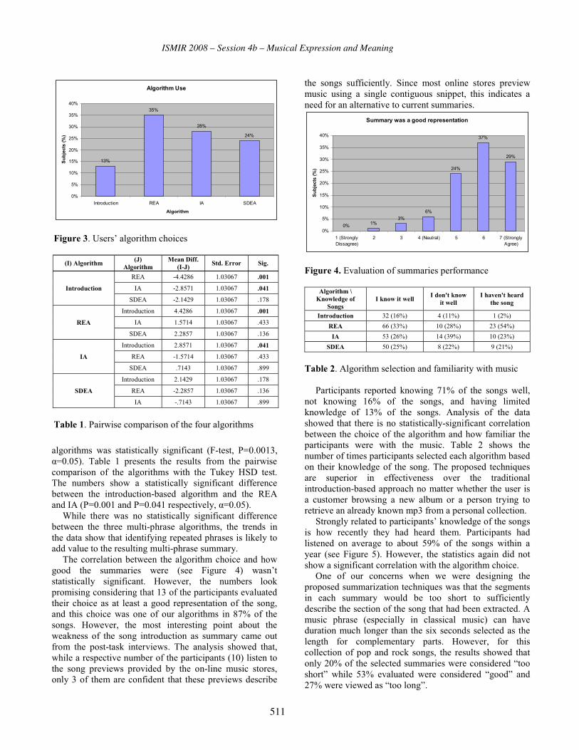
ISMIR 2008 – Session 4b – Musical Expression and Meaning
�
���������� '�� ������������ ����������� ���� ��?� �«$�$$�!?�½«$�$���� \�� � �� � � ���� �� � � ������ ����� �� � ��'�� ���������� ��� �� � ���������� '���� �� � \�� �� ���� � ����\� � ���� ��� ���'� � ������������ ����������� ���� � �� �� �' �� �� � ��������������� �� ��������� ��� �� � ~������|����«$�$$������«$�$���� � ���� ��?�½«$�$����
���� � �� � � '�� ��� ������������ ����������� ���� � �� �� �' �� �� � ��� � ��������� � ���������?� �� � �� ���� ����� �������'������� ���������� � ����� �������� ������������ ������ �� ����������������� ���������
\� ����� ������� �' �� �� ��������������� ������'������ �� � ������ �� ' � � �� � ����� � ��� '��¥�������������� ������������ ��' � �?� �� � ���� ��� �������������������� ����������!������ ���������� ���� ���� ��� ����� ����� � ��� � ����� � � � ���������� �� � ����?���� ����� ����� � '���� ���� ���� ���������� ����� ���� �� �������� ��' � �?� �� � ����� ��� � ������ ����� ����� �� �' �� ��� ��� �� � ����� ������������� �� ������� �� � ��������� �� � �������� ��� ��� '��� \� � ������� ���' �� ���?�'��� ��� � ���� ����� ������� ������������$������ ������� � ����� � �� '�� ����� �� ��� �� � ������ � ������ ���� �?������!���� �� ��� ������� ��� ���� �� � �� �� '��� ����� �
�� � ������ ������� ������ ���� � ����� ����� � ���� �� � �� '������� ������ � ����� � ����������� ��� �?� ����� ������ �� �� ���������� ����� �������� ��������� ���
b����������������� �� �������
^X ]X"X
\X
�[X
"kX
�WX
^X
ZX
]^X
]ZX
�^X
�ZX
"^X
"ZX
[^X
]�<������',���������?
� " [�<&�����'? Z \ k�<������',����?
b��
j ������
��+�7������������������������� �� ������� ��
��7�������¾�%!�5��"7���'�
��!7�� �8!�5����5���� �"�!D��8!�5�
���5���� ���4�!D������"�
������!7�
!���"�$���!� !"���< �� ����� �� ���" ��"#�� <<��!! �� �$��"� �� "!���� �� �� �!��"< �� ����!� �� �$��"! ��
�-#�� �$��"� �� ���"" �� ���"� ��
�#�����3������������� � �������������������'����������
����������� � ��� �� ���'���� �� � ��� �� � ������ ' ��?�
���� ���'���� �< � ��� �� � �����?� ��� ������ ����� �����'� �� � ��� �! � ��� �� � ������� �������� ��� �� � ������' �� ���� �� � � ��������������������������������� ������� �' �� �� ������ ���� �� ���������������'�������� �� ���������� ' � � '���� �� � ������� \�� � "� ���'�� �� ����� �������� ������������ � �� �� �������������� ����� �� ������'� �� ���� �� � ������\� ����� �� � ����_� ��� � �� ����� ��� �� ���� � ��� �� �� �� � ������������������������� ������������� ��'� �� ���� ��� ������ ������ �� ���'����� � � '� ����� ��� � ����� ������� ���� ��� � ����� ������'���!������� ���������� ��������
���������� �� �������������¥����'� �� ������ ���������� ��'� � � ����� �� �� ��� � ��� �� ��� ���������� ������� � �� ��� � �� � ��� ����� �� � ��� �� � ������ '������ �� �� �� � ����� � ���� ��' � �?� �� � ���������� ���� ���� �������'����������������� ������'������ ��������������� ���
>� � ��� ���� ���� ���� '� �� ' � ' � � � �������� �� ����� ��������������� ����_� ��'�������� �� �� ������� ��� ������� '����� � � ���� ������ ��� ������� ������ ����� ��� �� ����������� �������������� �� ����� ����������� ��� � � � ������ ��� �������� ������� ��� �� �������������� ���� �� ���� �� ������ ������� � �� ���� �� �� ����� ���� ���� � ����� ����� ��' � �?� ���� ��������� ��������� �� ��� ����� �����?� �� � � ������ ���' �� ���������"$ ������ �� � �� �������� ��' � ������� � �������������� '��� � �! � ���� �� ' � � ������ � �� ������� ���"� �' � ��� ' ����������������
���������x
]"X
"ZX
�qX
�[X
^X
ZX
]^X
]ZX
�^X
�ZX
"^X
"ZX
[^X
����������� `� � ���
��������
b��
j ������
��
+�7����B��� ��¥��������������� ���� ���7������� �E �
��7�������%��!�-�''��
� /E � ��"��#����� ��7��
� ~��� ����"�<� ��$!$<�� �992�
!���"�$���!� |�� �"������ ��$!$<�� �9�2�
� ����� �"���"�� ��$!$<�� �����
� |������������ ���"�<� ��$!$<�� �992�
"#�� |�� ������� ��$!$<�� ��!!�
� ����� "�"���� ��$!$<�� ��!<�
� |������������ "������ ��$!$<�� �9�2�
�� ~��� �������� ��$!$<�� ��!!�
� ����� ����!� ��$!$<�� �����
� |������������ "���"�� ��$!$<�� �����
�-#�� ~��� �"�"���� ��$!$<�� ��!<�
� |�� �����!� ��$!$<�� �����
�#�����2�����'�� ��������������� �����������������
�
511

ISMIR 2008 – Session 4b – Musical Expression and Meaning
�
��� - ����� �?�
\�� � ���������� ���� �� ����� ��������� � ������������ �� ��� � � � � �� �� ��� ���� ��� \� � � ����� ����� � ���������� � �� ���� � ��� � ��� ���� �� ���� ����� �' �� ����������� �� � ���������� � ����� ������� � � � ������ ��� ��������� ���� � ��� ��� ��� \� � ���������' �� ���� ��������� � �� � �� ���� �� � ��������� ������� �� � �� �� � � � �� �� �� � ����� ���� �� ������������������� ����������� ��� ����� � �� �� �' ���� ���� �����������'����������������?� �� � � ������ ������ ����� ��� � � � �� � ���� ���������� ���� ����� � �� �� � ��������� � � ����� �?� �� � ��� ��� �� �� �� ��������� ����� '� � � �� � ���������� ����� ���� ��� �� � � ������ ���� ��������� ������� ������� ���
\� � � � � � � ��� ������� ' � '��� ��� � ��� ��� ����� �������������������� ��� �� ������ ��>� ���� �� ������������������� ���������� �� � ���� '�� ���� �� � �'����� �������� ��� ��� ��� �� � ������ �� '�� ���� ����� ��� � �� ���������� � ��� � �� ��������� � � � ��� ��� � �������� � ������ ���� � � ������ �� � ����� ��� ��� �� ������ � �� �������� �� � �� � ��� �� ���� ��� �� ����� �� ����� �� �� �����������¥� � ����� ����� '����� ���� �� � ��� �� ��� �� �������� � �������?� ���'������ � ��� � ������ ��� ���� � ����� � ��� ������� ��� �� � ������������� ��� ���� ������ �� �������� � ��� �� � �� � �� � ��� ��� ��� � ������� �������'���� � '� ������� �� ��������� ��� �� � � ��� ��� ����� ����_� �� '���� ������ �� ���������� ����� �� � �������� ��� ��� � ��� �� � ����� ��� ���� ��� ���� ����� � �����������?� ' � '����� ��� � ��� ����� � �� � ������� ��� ���������������� ����� ��� � � ����� � ��� � �� �� ��� ������������������^���'� � ��� ���������������� ���������� � ������������������ ���������� ����� �������
(�� "#+#"#?�#��
���� ������?�`������� �� ��?�����\��������������������� �������� �� ~ � � ������� ���� ������\�����������?� �� �;� �� ���� ���;� 0 �1�� (� ��
*((����� ��� �� #����� �� �������� � � * �� � ����*� �����?�£ '�®���?���?�"$$���
�"�� ���?� ��� ��� � ��� ?� ��� �`����� \����������� ������������� ��������?� �� �;� �� *��� � ��!����?�� �� � �?���?�"$$!���
�!�� ��� �?� `�� ��� ���� ?� ¨�� ���������� `����������������� ��� ���������� �������?��� �;� �� �������;� #.!( �� !� �� � ���� ��� �!��� �� ��������?�����?����� ?�"$$"��
���� ���?���?����?���?��'��?���?� ������?�������`����������������� ��� � � ������ \ ��� \������� ���\'�� ��� � ����� �����?� �� �;� �� ���� �555� ����0 �1�� (� ����#�����?���?����?�"$$<��
���� ����?���� ������?���� �`����� ������������ ������� ����� ��?��� �;� �������555����;�� ��;� ��* �� �#(���������#������� �������?�>�����?���?�"$$$��
�<�� ��?� ��?� ��� ����?� ��� ������� �� ���������� ���`����� ��� ���?� �� �;� �� ���� *��� � ��!����?�� �� � �?���?�"$$!��
���� `���������?� ��?� ��� �� '?� ��� �`����������������� ��� � �� ��������������� ����� �� ������������� ��� ��� ��� ������� ���������?� �� �;� ������ ���;� � ��;� �� � ���� ��� �!��� �� ��������?��������?����������������?����?�"$$<��
���� >��?� ��� ����������� �������� ��� � �� ������� ���`����� �������?� ���� ������� ������� �� ��� �� �� ��� ��� ��� \ ��������� ��� ��� ������ ��� �����?�"$$<��
���� � � ��?� ��?� ����� ?� ��?� ��� ~�� �?� ¢�� �\�'����������� ������ ����� ������� � � ������ ����������� �������?� �� �;� �� ���� ���;� � ��;� �� � ������� �!��� ����������?�����?����� ?�"$$"��
��$��~��� �?� ��� ��� ¨���?� ���7 ���!������ �� #(�������� ����� �?� ���� '���� ������?� £¨�� �� ���� ����?����!��
��������?�¢�?�`��� ?�£�?�¢�?���������������?�`������������ `����� ������������ �� �� ��� `������������� ���������?��� �;� �� �����555����;�� ��;� ��*� ������ #(����� ���� #����� �� �������?������ ���?���?�"$$���
��"��¢�?� ��?� `��� ?� £�?� ��� ���?� ¢�� ����������`����� ������������� ��� ������������?� �555�-�������� ��� ��#(�����F�* �� ?��!��!�?�`�?�"$$���
� {������ �V�� ������ ���
"X
]\X
[^X
]qX]\X
kX
^X
ZX
]^X
]ZX
�^X
�ZX
"^X
"ZX
[^X
[ZX
����B��; ]�>��;����]���������
]����������],�������
�����������,�������
&�K�� ���|������ ��
b��
����
�+�7����6�����������¥�������� �������� ���������� ������
512

Session 4c – Automatic Music Analysis and Tran-scription

.

ISMIR 2008 – Session 4c – Automatic Music Analysis and Transcription
MULTIPLE-FEATURE FUSION BASED ONSET DETECTION FOR SOLO SINGING VOICE
Chee Chuan Toh Bingjun Zhang Ye Wang School of Computing
National University of Singapore [email protected], {bingjun, wangye}@comp.nus.edu.sg
ABSTRACT
Onset detection is a challenging problem in automatic singing transcription. In this paper, we address singing onset detection with three main contributions. First, we outline the nature of a singing voice and present a new singing onset detection approach based on supervised machine learning. In this approach, two Gaussian Mixture Models (GMMs) are used to classify audio features of onset frames and non-onset frames. Second, existing audio features are thoroughly evaluated for this approach to singing onset detection. Third, feature-level and decision-level fusion are employed to fuse different features for a higher level of performance. Evaluated on a recorded singing database, the proposed approach outperforms state-of-the-art onset detection algorithms significantly.
1. INTRODUCTION
Accurate monophonic singing voice transcription depends heavily on singing onset detection. Current onset detection algorithms applied on monophonic singing voice produced poor results [5][8]. In MIREX2007, the best result for onset detection of solo singing voice only managed an F-measure of 51.0% [2]. The singing voice is a pitched non-percussive (PNP) instrument [17], which is still a challenging category of instruments for onset detection. The case is further complicated by the nature of the singing voice, which is inherently inconsistent and prone to pitching and timing dynamics.
Current onset detection methods for PNP instruments, such as methods by spectral difference [7][10], phase deviation [6], pitch shift [9], and sub-band energy change [11][12] are targeted at detecting spectral changes based on certain rules. It has been observed on a spectrogram that in general, a musical note onset occurs at locations where there is a visible change in the spectrum, and within the duration of the note, the spectrum is relatively stable. A violin signal is shown as an example in Fig.1a.
However, for the case of singing voice, this observation may not always hold (Fig.1b). Unlike most other instruments, where there is usually a high level of timbre consistency in the duration of a note, the singing
voice is capable of producing much more variations of formant structures (for articulation); sometimes the formant structure may even change within the duration of a single note. Pitch irregularities, pitch modulations, and inadvertent noise also upset stability of the spectrum.
Figure 1: Comparison between spectrograms of violin and singing signal. Onsets are marked by red circles Onset detection in the singing voice is much more
complicated than in most other instruments. An onset detector that relies explicitly on a rule-based approach is bound to fail to capture the nuances of the singing onset. To address the difficulties in singing onset detection, we present a new onset detector based on supervised machine
515

ISMIR 2008 – Session 4c – Automatic Music Analysis and Transcription
learning, in order to capture the intricacies of singing note onsets, illustrated in Figure 2.
Figure 2: System diagram of the proposed system
Two GMMs are used to profile the distribution of
audio features of onset frames and non-onset frames, respectively. We thoroughly evaluate existing audio features for their effectiveness in distinguishing onset and non-onset frames, including Mel-frequency Cepstral Coefficients (MFCCs), Linear Predictive Cepstrum Coefficients (LPCCs), Equal loudness phon values along critical bands. Feature concatenation fusion in feature-level and linear weighted sum fusion in decision-level are then employed to achieve a high level of onset detection accuracy. Evaluated using our singing database, our proposed approach to singing onset detection outperforms state-of-the-art methods, including methods based on phase change [6], pitch change [9], equal loudness [12], and inverse-correlation [7]. Re-implementations of these methods are used in the evaluation.
2. DEFINITION OF A SINGING ONSET
In a non-percussive continuous-pitch instrument, such as the melodic singing voice, there is no clear definition of an onset. A definition is especially difficult to establish when taking into account glissandos1 and portamentos2, 1 Glissandos are glides from one pitch to another, by filling the slide with discrete intermediate pitches. In continuous-pitch instruments, glissando is often used interchangeably with the term portamento.
which are vocal expressions involving pitch glides. Traditionally, an onset is the beginning of a new note event [5][8], characterized by a change in pitch, amplitude envelope, spectral shape, phase, or a combination of the mentioned factors [14].
However, in a singing voice, which is plagued by accidental glissandos, slurring (melisma3) and imperfect vocalization, the definition of an onset is a less clear-cut one. It is very often that a singer performs a glissando (more accurately, portamento in the singing voice) at the beginning or ending of a note, even when a music score does not stipulate so. When a musician is tasked to transcribe the singing performance, these portamentos are not transcribed into notes. However, slurred performances, which also involve pitch glides, are usually transcribed as actual notes, albeit with a legato denotation. There is no real physical difference between a portamento and a slur in singing performances. In both cases, the singing voice undergoes a continuous change in pitch. However, perceptually many glissandos are not considered as note onsets. This is because when listening to a singer’s performance, a human subconsciously takes into account contextual cues like the rhythm, language and style of music.
The nature of singing onset is strongly related to the manner of articulation in speech. A singing voice has strong harmonic components producing numerous timbral differences, which are interpreted as different phonemes by the human ear. Singing onsets usually, though not always, occur during vowel-onsets.
Since there is no known existing definition for a singing onset, it is crucial to define one before even attempting to evaluate the effectiveness of a singing onset detector. In [5], an onset is defined as the start of the transient, but in a pitched singing voice (and many PNP instruments), there are numerous notes with no observable transient, particularly during slurs. A singing performance may also contain long stretches of unvoiced consonant segments, typically at the beginning or end of the note. These unvoiced segments are too varied and inconsistent to base the definition of a singing note onset on, and should simply be regarded as noise in the annotation process, not as part of a singing note. An onset should be marked at the end of a consonant, not before or during the consonant.
For practical purposes, it is intuitive and reasonable to define a singing onset as follows: The beginning of a new human-perceived note, taking into account contextual cues. This excludes erroneous portamentos during note beginnings, transitions and trail-offs, but includes pitch changes in slurring. The actual notes included in a slur
2 Portamentos are continuous glides from one pitch to another, usually produced as an effect by continuous-pitch instruments. 3 Melisma is the act of changing pitch on a single syllable of sung text.
516

ISMIR 2008 – Session 4c – Automatic Music Analysis and Transcription
may be subject to human interpretation, since it is possible that a singer reaches the correct pitch only very briefly during a slur. Slurred notes that occur too briefly for an average human auditory system to reliably detect should not be included. The precise location of an onset in a slur is also subjective, and allowances ought to be made for human bias.
3. FEATURE EXTRACTION
The effectiveness of any onset detection function ultimately depends on the audio features used in the system. It is necessary to employ features that provide useful information on whether or not a frame contains an onset.
Features capable of capturing timbral differences should provide a reliable measure for onset detection. Pitch and energy features could provide important information regarding onset detection as well, but are much less reliable. We have chosen to focus on features that provide information on the spectral shape, since a timbral change is the main characteristic of an onset.
3.1. Mel Frequency Cepstral Coefficients
MFCCs represent audio by a type of cepstral representation. In a mel-frequency cepstrum, the frequency bands are positioned on a mel-scale, which aims to approximate the human auditory system’s response.
It is a common feature used in speech recognition, and can be derived by first taking the Fourier transform of a (windowed) signal, mapping the log-amplitudes of the resulting spectrum into the mel-scale, then performing DCT on the mel log-amplitudes. The amplitudes of the resultant cepstrum are the MFCCs. Since DCT holds most of the signal information in the lower bands, the higher coefficients can be truncated without excessive information loss. In our system, we extracted MFCC features with 81 mel-scale filter banks and 23 DCT coefficients.
The coefficients are concatenated with their first and second-order derivatives to form a feature vector of 69 dimensions. This improves the performance of the system, due to the correlation of the MFCCs and the derivatives at feature-level.
3.2. Linear Predictive Cepstrum Coefficients
LPCCs are LPC coefficients transformed into cepstra, and are widely used in speech recognition systems. An efficient method of obtaining the coefficients using Levinsin-Durbin recursion is covered in detail in [1]. Once we obtain the LPC coefficients, they can be transformed into cepstra by [4]:
1
1
m
m m k m k
k
kc a c a
m (1)
where 1... Nc c is the set of cepstral coefficients of order
N. In our system, we used 22 cepstral coefficients, appended with 44 coefficients of the first and second order derivatives, similar to the feature-level fusion performed in the extraction of MFCCs.
3.3. Critical bands
Grouping frequency bins into critical bands is a psychoacoustically motivated principle. In [11], 36 bands of triangular-response bandwidth were used along the critical bands, and power in each band was used to derive a detection function. Detection functions based on equal-loudness changes in Equivalent Rectangular Bandwidth (ERB) bands have also been used in the past [8]:
1021.4 log (4.37 F + 1) (2)
where is the ERB band number, F is the bin frequency in kHz. By grouping frequency bins into ERB bands, we greatly reduce the dimensionality of the spectra. In [8], the power in individual ERB bands were mapped into phon values using equal-loudness contours [3]. In our system, we replicate the method introduced in [8], but only 36 ERB bands are used (includes frequencies of up to 11kHz) for audio files sampled at 22.05kHz.
3.4. Other Features Combined
Pitch-stability, zero-crossing rate and signal periodicity are all simple features which may contain information about note onsets. These features are commonly used, and can be concatenated into a combined feature vector. This feature-level data fusion is sensible for features which are characteristic of onset frames, especially if the features are of low dimensionality. Features which are of no value to the onset detection problem should not be included, as they corrupt the feature space and hence degrade the system performance. In our system, we used pitch stability, zero-crossing rate and signal periodicity and their derivatives as the combined vector.
4. GMM TRAINING AND SCORING
GMM-based modeling of speech signals has been the principal approach for speech and speaker recognition systems in recent years. It has been successfully implemented in [16] for speaker identification with very good results. Like speaker identification, onset detection can be modeled as a classification problem. At each time step, we need to classify a frame of audio into the onset class or a non-onset class.
517
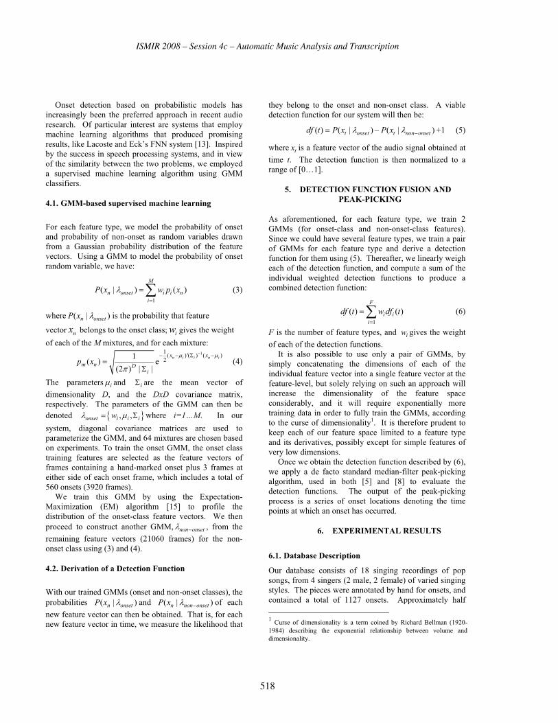
ISMIR 2008 – Session 4c – Automatic Music Analysis and Transcription
Onset detection based on probabilistic models has increasingly been the preferred approach in recent audio research. Of particular interest are systems that employ machine learning algorithms that produced promising results, like Lacoste and Eck’s FNN system [13]. Inspired by the success in speech processing systems, and in view of the similarity between the two problems, we employed a supervised machine learning algorithm using GMM classifiers.
4.1. GMM-based supervised machine learning
For each feature type, we model the probability of onset and probability of non-onset as random variables drawn from a Gaussian probability distribution of the feature vectors. Using a GMM to model the probability of onset random variable, we have:
1
( | ) ( )M
n onset i i n
i
P x w p x (3)
where ( | )n onsetP x is the probability that feature
vector nx belongs to the onset class; iw gives the weight
of each of the M mixtures, and for each mixture: 11
( ) '( ) ( )21
( ) e(2 ) | |
n i i n ix x
m n Di
p x (4)
The parameters i and i are the mean vector of
dimensionality D, and the DxD covariance matrix, respectively. The parameters of the GMM can then be denoted , ,onset i i iw where i=1…M. In our
system, diagonal covariance matrices are used to parameterize the GMM, and 64 mixtures are chosen based on experiments. To train the onset GMM, the onset class training features are selected as the feature vectors of frames containing a hand-marked onset plus 3 frames at either side of each onset frame, which includes a total of 560 onsets (3920 frames).
We train this GMM by using the Expectation-Maximization (EM) algorithm [15] to profile the distribution of the onset-class feature vectors. We then proceed to construct another GMM, non onset , from the
remaining feature vectors (21060 frames) for the non-onset class using (3) and (4).
4.2. Derivation of a Detection Function
With our trained GMMs (onset and non-onset classes), the probabilities ( | )n onsetP x and ( | )n non onsetP x of each
new feature vector can then be obtained. That is, for each new feature vector in time, we measure the likelihood that
they belong to the onset and non-onset class. A viable detection function for our system will then be:
( ) ( | ) ( | )t onset t non onsetdf t P x P x +1 (5)
where tx is a feature vector of the audio signal obtained at
time t. The detection function is then normalized to a range of [0…1].
5. DETECTION FUNCTION FUSION AND ..PEAK-PICKING
As aforementioned, for each feature type, we train 2 GMMs (for onset-class and non-onset-class features). Since we could have several feature types, we train a pair of GMMs for each feature type and derive a detection function for them using (5). Thereafter, we linearly weigh each of the detection function, and compute a sum of the individual weighted detection functions to produce a combined detection function:
1
( ) ( )F
i i
i
df t w df t (6)
F is the number of feature types, and iw gives the weight
of each of the detection functions. It is also possible to use only a pair of GMMs, by
simply concatenating the dimensions of each of the individual feature vector into a single feature vector at the feature-level, but solely relying on such an approach will increase the dimensionality of the feature space considerably, and it will require exponentially more training data in order to fully train the GMMs, according to the curse of dimensionality1. It is therefore prudent to keep each of our feature space limited to a feature type and its derivatives, possibly except for simple features of very low dimensions.
Once we obtain the detection function described by (6), we apply a de facto standard median-filter peak-picking algorithm, used in both [5] and [8] to evaluate the detection functions. The output of the peak-picking process is a series of onset locations denoting the time points at which an onset has occurred.
6. EXPERIMENTAL RESULTS
6.1. Database Description
Our database consists of 18 singing recordings of pop songs, from 4 singers (2 male, 2 female) of varied singing styles. The pieces were annotated by hand for onsets, and contained a total of 1127 onsets. Approximately half
1 Curse of dimensionality is a term coined by Richard Bellman (1920-1984) describing the exponential relationship between volume and dimensionality.
518

ISMIR 2008 – Session 4c – Automatic Music Analysis and Transcription
(560) of the onsets were used for training GMMs, and the other half (567) were used to evaluate the system.
Each recording was annotated and cross checked by two amateur musicians. Onsets were first identified by ear, and then marked at positions where the wave form was first observed to follow a periodic structure. Consonant noise and unintentional portamentos / glissandos do not constitute new onsets, as explained in Section 2. For legato, an onset was marked at the point where a pitch change was perceived to begin.
6.2. Evaluation of Individual Detection Functions
For evaluation of the individual onset detection functions, we extract all the features mentioned in Section 3 and score each feature type based on a pair of trained GMMs (onset and non-onset GMMs). From the detection function produced by (5) for each feature type, we apply the median-filter peak-picking process across different parameters. We evaluate the usefulness of the feature by the metrics of precision, recall and F-measure, based on an onset tolerance of 50ms. Based on an onset tolerance of 50ms. These evaluation conditions are identical to those in the annual MIREX Audio Onset Detection contest.
The onset detection results of individual features are shown in Figure 3. The best F-measure among the set of peak-picking parameters is selected for each feature. From our experiments, MFCC is revealed to be the best audio feature, producing the best results of 80.3% precision, 77.8% recall and 79.0% F-measure. LPCC is next best, with 72.9% precision, 77.7% recall, and F-measure 75.3%. ERB-bands produce 78.2% precision, 69.5% recall, and 73.6% F-measure. The combined vector produces 60.1% precision, 86.1% recall, and 70.8% F-measure.
0.790.753 0.736 0.708
0
0.2
0.4
0.6
0.8
1
M FCC LPCC ERB Combined
Precision Recall F-M easure
Figure 3: Evaluation results of individual detection function
6.3. Evaluation of Combined Detection Function Based on the performance of all evaluated detection functions, we search the best linear weights based on extensive experiments and compute an overall detection
function described by (6). The weight distribution is shown in Table 1.
Detection Function produced by: Weight
MFCC 0.76
LPCC 0.12
ERB-bands 0.10
Combined vector 0.02
Table 1: Weight distribution for detection functions
Using the sum of linearly-weighted detection functions,
we achieve the best performance of 86.5% precision, 83.9% recall, and 85.2% F-measure, which is superior to current state-of-the-art methods. As can be seen in Figure 4, most existing methods do not perform well on singing music. Equal loudness change based method produces an F-measure of 71.0% under the best set of parameters. Both the phase-based and pitch-based methods perform badly because the singing voice’s pitch track is very unstable, and contains many noisy segments.
0.243 0.224
0.442
0.71
0.852
0
0.1
0.2
0.3
0.4
0.5
0.6
0.7
0.8
0.9
1
Phase
Deviation
Pitch-Based Inverse
Correlation
Equal
Loudness
Linear-
Weighted
Precision Recall F-Measure
Figure 4: Results of linear-weighted sum detection function compared with state-of-the-art methods
The parameters for the system, especially those used in the GMM and individual features, were determined through extensive experimentation.
7. DISCUSSIONS AND FUTURE WORK
In our system, we have employed both feature-level and decision-level fusion. Feature-level fusion works well, but the higher dimensionality necessitates higher volume of training data. Our system was trained with only 560 onsets, due to the laborious process annotating pieces by hand. More training and testing data ought to be used to validate the system’s performance.
We utilized only 4 pairs of GMMs: for MFCC, LPCC, ERB-bands, and a combined feature. In reality, any number of feature types can be used, and fusion can be
519

ISMIR 2008 – Session 4c – Automatic Music Analysis and Transcription
done at the feature-level (e.g. concatenation) and/or at decision-level (e.g. linear weighted sum). As a rough guide, more feature types and detection functions usually produce better onset detection results. This is provided the features extracted are representative of the onset classification problem, i.e. there should be a discernible difference in feature between onset and non-onset frames.
Weight-assignments for linear-weighted sum fusion are usually based on heuristics, and require lengthy experiments to optimize. Even though it generally works well, the simple linear weighting method can cause false peaks in detection functions to propagate into the combined detection function, making the overall detection function noisy. Other decision-level fusion techniques exist, and ought to be explored and tested.
We also look forward to expanding the system by incorporating note segmentation, as well as more functions in the post-processing section.
8. CONCLUSION
As shown by our experiments, the proposed supervised machine-learning approach based on GMM modeling produces higher accuracy for singing onset detection. Clearly, the system produces better results than state-of-the-art singing voice onset detection algorithms. Further improvements by decision-level fusion of the system boost the overall accuracy and completeness of the system. The singing onset detection problem cannot be considered solved by our system, but its potential is promising.
9. ACKNOWLEDGEMENT
This work was supported by Singaporean Ministry of Education grant with the Workfare Bonus Scheme number of R-252-000-267-112.
10. REFERENCES
[1] Sung-Won Park, online DSP course, http://www.engineer.tamuk.edu/SPark/course.htm
[2] MIREX 2007 Audio Onset Detection Results: Solo Singing Voice, http://www.music-ir.org/mirex/2007/index.php/Audio_Onset_Detection_Results:_Solo_Singing_Voice
[3] ISO Acoustics: Normal-equal loudness contours. Technical Report ISO226:2203, International
Organisation for Standardization, 2003
[4] G. Antoniol, V. Rollo, G. Venturi “Linear Predictive Coding and Cepstrum coefficients for mining time variant information from software repositories” International
Workshop on Mining Software Repositories, ACM, 2005
[5] J. Bello, L. Daudet, S. Abdallah, C. Duxbury, M. Davies, M. Sandler “A Tutorial on Onset Detection in Music
Signals” IEEE Transactions on Speech and Audio
Processing, volume 13(5), September 2005
[6] J. Bello and M. Sandler “Phase-Based Onset Detection for Music Signals”, Proceedings of IEEE International
Conference on Acoustics, Speech, and Signal Processing, volume 5, pages 49-52, April 2003.
[7] W. Boo, Y. Wang and A. Loscos “A violin music transcriber for personalized learning.”, Proceedings of IEEE International Conference on Multimedia and Expo, pages 2081-2084, 2006
[8] N. Collins “A comparison of sound onset detection algorithms with emphasis on psycho-acoustically motivated detection functions”, Proceedings of AES118
Convention, 2005
[9] N. Collins “Using a Pitch Detector for Onset Detection”, Proceedings of 6th International Conference on Music Information Retrieval, 2005
[10] C. Duxbury, M. Sandler, M. Davies “A Hybrid Approach to Note Onset Detection”, Proceedings of the 5th Int.
Conference on Digital Audio Effects (DAFx-02), Hamburg, Germany, 2002
[11] A. Klapuri, A. Eronen, J. Astola “Analysis of the Meter of Acoustic Musical Signals”, IEEE Transactions on Speech
and Audio Processing,volume 14(1), pages 342-355,
January 2006
[12] A. Klapuri. “Sound onset detection by applying psychoacoustic knowledge.” In Proceedings of IEEE
International Conference on Acoustics, Speech, and Signal
Processing, volume 6, pages 3089–3092, 1999.
[13] A. Lacoste and D. Eck “A supervised classification algorithm for note onset detection” EURASIP Journal on
Advances in Signal Processing, August 2007
[14] A. Loscos “Spectral Processing of the Singing Voice”, Ph.D. Thesis submission to Pompeu Fabra University, Barcelona, Spain, 2007
[15] R. Redner, H. Walker. “Mixture densities, maximum likelihood and the EM algorithm” SIAM Review, volume 26(2), 1984
[16] D. A. Reynolds and R. C. Rose “Robust text-independent speaker identification using Gaussian mixture speaker models”, IEEE Transactions on Speech and Audio
Processing, volume 3(1), pages 72-83, January 1995
[17] J. Sundberg, The Science of the Singing Voice, Northern Illinois University Press, 1990.
520

ISMIR 2008 – Session 4c – Automatic Music Analysis and Transcription
MULTI-FEATURE MODELING OF PULSE CLARITY: DESIGN,VALIDATION AND OPTIMIZATION
Olivier Lartillot, Tuomas Eerola, Petri Toiviainen, Jose FornariFinnish Centre of Excellence in Interdisciplinary Music Research, University of Jyväskylä
<first.last>@campus.jyu.fi
ABSTRACT
Pulse clarity is considered as a high-level musical dimen-
sion that conveys how easily in a given musical piece, or a
particular moment during that piece, listeners can perceive
the underlying rhythmic or metrical pulsation. The objective
of this study is to establish a composite model explaining
pulse clarity judgments from the analysis of audio record-
ings. A dozen of descriptors have been designed, some of
them dedicated to low-level characterizations of the onset
detection curve, whereas the major part concentrates on de-
scriptions of the periodicities developed throughout the tem-
poral evolution of music. A high number of variants have
been derived from the systematic exploration of alternative
methods proposed in the literature on onset detection curve
estimation. To evaluate the pulse clarity model and select
the best predictors, 25 participants have rated the pulse clar-
ity of one hundred excerpts from movie soundtracks. The
mapping between the model predictions and the ratings was
carried out via regressions. Nearly a half of listeners’ rating
variance can be explained via a combination of periodicity-
based factors.
1 INTRODUCTION
This study is focused on one particular high-level dimen-
sion that may contribute to the subjective appreciation of
music: namely pulse clarity, which conveys how easily lis-
teners can perceive the underlying pulsation in music. This
characterization of music seems to play an important role
in musical genre recognition in particular, allowing a finer
discrimination between genres that present similar average
tempo, but that differ in the degree of emergence of the main
pulsation over the rhythmic texture.
The notion of pulse clarity is considered in this study
as a subjective measure that listeners were asked to rate
whilst listening to a given set of musical excerpts. The
aim is to model these behavioural responses using signal
processing and statistical methods. An understanding of
pulse clarity requires the precise determination of what is
pulsed, and how it is pulsed. First of all, the temporal evo-
lution of the music to be studied is usually described with
a curve – denominated throughout the paper onset detection
curve – where peaks indicate important events (considered
as pulses, note onsets, etc.) that will contribute to the evoca-
tion of pulsation. In the proposed framework, the estimation
of these primary representations is based on a compilation
of state-of-the-art research in this area, enumerated in sec-
tion 2. In a second step, the characterization of the pulse
clarity is estimated through a description of the onset detec-
tion curve, either focused on local configurations (section 3),
or describing the presence of periodicities (section 4). The
objective of the experiment, described in section 5, is to se-
lect the best combination of predictors articulating primary
representations and secondary descriptors, and correlating
optimally with listeners’ judgements.
The computational model and the statistical mapping have
been designed using MIRtoolbox [11]. The resulting pulse
clarity model, the onset detection estimators, and the statis-
tical routines used for the mapping, have been integrated in
the new version of MIRtoolbox, as mentioned in section 6.
2 COMPUTING THE ONSET DETECTIONFUNCTION
In the analysis presented in this paper, several models for
onset or beat detection and/or tempo estimation have been
partially integrated into one single framework. Beats are
considered as prominent energy-based onset locations, but
more subtle onset positions (such as harmonic changes) might
contribute to the global rhythmic organisation as well.
A simple strategy consists in computing the root-mean-
square (RMS) energy of each successive frame of the signal
(“rms” in figure 1). More generally, the estimation of the
onset positions is based on a decomposition of the audio
waveform along distinct frequency regions.
• This decomposition can be performed using a bank of
filters (“filterbank”), featuring between six [14], and
more than twenty bands [9]. Filterbanks used in the
models are Gammatone (“Gamm.” in table 1) and two
sets of non-overlapping filters (“Scheirer” [14] and
“Klapuri” [9]). The envelope is extracted from each
band through signal rectification, low-pass filtering
and down-sampling. The low-pass filtering (“LPF”) is
implemented using either a simple auto-regressive fil-
521

ISMIR 2008 – Session 4c – Automatic Music Analysis and Transcription
audio
frame
filterbank:Gammatone
ScheirerKlapuri
rms
autocor novelty
LPF:IIR
halfHanning
spectrum
bands
sum peaks
log
diff
hwr sum bef
sum adj
autocor sumafter
reson enhan
ENTR2HARM2
MAXMINKURTTEMPENTR1HARM1
ART
ATT2
ATT1VAR
+
Figure 1. Flowchart of operators of the compound pulse clarity model, where options are indicated by switches.
ter (“IIR”) or a convolution with a half-Hanning win-
dow (“halfHanning”) [14, 9].
• Another method consists in computing a spectrogram
(“spectrum”) and reassigning the frequency ranges into
a limited number of critical bands (“bands”) [10]. The
frame-by-frame succession of energy along each sep-
arate band, usually resampled to a higher rate, yields
envelopes.
Important note onsets and rhythmical beats are charac-
terised by significant rises of amplitude in the envelope. In
order to emphasize those changes, the envelope is differenti-
ated (“diff”). Differentiation of the logarithm (“log”) of the
envelope has also been advocated [9, 10]. The differentiated
envelope can be subsequently half-wave rectified (“hwr”) in
order to focus on the increase of energy only. The half-wave
rectified differentiated envelope can be summed (“+” in fig-
ure 1) with the non-differentiated envelope, using a specific
λ weight fixed here to the value .8 proposed in [10] (“λ=.8”
in tables 1 and 2).
Onset detection based on spectral flux (“flux” in table 1)
[1, 2] – i.e. the estimation of spectral distance between suc-
cessive frames – corresponds to the same envelope differ-
entiation method (“diff”) computed using the spectrogram
approach (“spectrum”), but usually without reassignment of
the frequency ranges into bands. The distances are hence
computed for each frequency bin separately, and followed
by a summation along the channels. Focus on increase of
energy, where only the positive spectral differences between
frames are summed, corresponds to the use of half-wave rec-
tification. The computation can be performed in the com-
plex domain in order to include phase information 1 [2].
Another method consists in computing distances not only
between strictly successive frames, but also between all frames
in a temporal neighbourhood of pre-specified width [3]. Inter-
frame distances 2 are stored into a similarity matrix, and
1 This last option, although available in MIRtoolbox, has not been in-
tegrated into the general pulse clarity framework yet and is therefore not
taken into account in the statistical mapping presented in this paper.2 In our model, this method is applied to frame-decomposed autocorre-
lation (“autocor”).
a “novelty” curve is computed by means of a convolution
along the main diagonal of the similarity matrix with a Gaus-
sian checkerboard kernel [8]. Intuitively, the novelty curve
indicates the positions of transitions along the temporal evo-
lution of the spectral distribution. We notice in particular
that the use of novelty for multi-pitch extraction [16] leads
to particular good results when estimating onsets from vi-
olin solos (see Figure 2), where high variability in pitch
and energy due to vibrato makes it difficult to detect the
note changes using strategies based on envelope extraction
or spectral flux only.
3 NON-PERIODIC CHARACTERIZATIONS OFTHE ONSET DETECTION CURVE
Some characterizations of the pulse clarity might be esti-
mated from general characteristics of the onset detection
curve that do not relate to periodicity.
3.1 Articulation
Articulation, describing musical performances in terms of
staccato or legato, may have an influence in the apprecia-
tion of pulse clarity. One candidate description of articu-
lation is based on Average Silence Ratio (ASR), indicating
the percentage of frames that have an RMS energy signif-
icantly lower than the mean RMS energy of all frames [7].
The ASR is similar to the low-energy rate [6], except the use
of a different energy threshold: the ASR is meant to charac-
terize significantly silent frames. This articulation variable
has been integrated in our model, corresponding to predictor
“ART” in Figure 1.
3.2 Attack characterization
Characteristics related to the attack phase of the notes can
be obtained from the amplitude envelope of the signal.
• Local maxima of the amplitude envelope can be con-
sidered as ending positions of the related attack phases.
A complete determination of each attack phase re-
quires therefore an estimation of the starting position,
522

ISMIR 2008 – Session 4c – Automatic Music Analysis and Transcriptionte
mpo
ral l
ocat
ion
of fr
ame
cent
ers
(in s
.)
temporal location of frame centers (in s.)
Similarity matrix
2 4 6 8 10 12 14
2
4
6
8
10
12
14
0 5 10 150
0.5
1Novelty
Temporal location of events (in s.)
coef
ficie
nt v
alue
Figure 2. Analysis of a violin solo (without accompani-
ment). From top to bottom: 1. Frame-decomposed general-
ized and enhanced autocorrelation function [16] computed
from the audio waveform; 2. Similarity matrix measured
between the frames of the previous representation; 3. Nov-
elty curve [8] estimated along the diagonal of the similarity
matrix with onset detection (circles).
through an extraction of the preceding local minima
using an appropriate smoothed version of the energy
curve. The main slope of the attack phases [13] is
considered as one possible factor (called “ATT1”) for
the prediction of pulse clarity.
• Alternatively, attack sharpness can be directly collected
from the local maxima of the temporal derivative of
the amplitude envelope (“ATT2”) [10].
Finally, a variability factor “VAR” sums the amplitude
difference between successive local extrema of the onset de-
tection curve.
4 PERIODIC CHARACTERIZATION OF PULSECLARITY
Besides local characterizations of onset detection curves,
pulse clarity seems to relate more specifically to the degree
of periodicity exhibited in these temporal representations.
4.1 Pulsation estimation
The periodicity of the onset curve can be assessed via auto-
correlation (“autocor”) [5]. If the onset curve is decomposed
into several channels, as is generally the case for ampli-
tude envelopes, the autocorrelation can be computed either
in each channel separately, and summed afterwards (“sum
after”), or it can be computed from the summation of the
onset curves (“sum bef.”). A more refined method consists
in summing adjacent channels into a lower number of wider
band (“sum adj.”), on each of which is computed the auto-
correlation, further summed afterwards (“sum after”) [10].
Peaks indicate the most probable periodicities. In order
to model the perception of musical pulses, most perceptually
salient periodicities are emphasized by multiplying the au-
tocorrelation function with a resonance function (“reson.”).
Two resonance curve have been considered, one presented
in [15] (“reson1” in table 1), and a new curve developed for
this study (“reson2”). In order to improve the results, redun-
dant harmonics in the autocorrelation curve can be reduced
by using an enhancement method (“enhan.”) [16].
4.2 Previous work: Beat strength
One previous study on the dimension of pulse clarity [17]
– where it is termed beat strength – is based on the compu-
tation of the autocorrelation function of the onset detection
curve decomposed into frames. The three best periodici-
ties are extracted. These periodicities – or more precisely,
their related autocorrelation coefficients – are collected into
a histogram. From the histogram, two estimations of beat
strength are proposed: the SUM measure sums all the bins
of the histogram, whereas the PEAK measure divides the
maximum value to the main amplitude.
This approach is therefore aimed at understanding the
global metrical aspect of an extensive musical piece. Our
study, on the contrary, is focused on an understanding of
the short-term characteristics of rhythmical pulse. Indeed,
even musical excerpts as short as five second long can easily
convey to the listeners various degrees of rhythmicity. The
excerpts used in the experiments presented in next section
are too short to be properly analyzed using the beat strength
method.
4.3 Statistical description of the autocorrelation curve
Contrary to the beat strength strategy, our proposed approach
is focused on the analysis of the autocorrelation function it-
self and attempts to extract from it any information related
to the dominance of the pulsation.
• The most evident descriptor is the amplitude of the
main peak (“MAX”), i.e., the global maximum of the
curve. The maximum at the origin of the autocorre-
lation curve is used as a reference in order to normal-
523

ISMIR 2008 – Session 4c – Automatic Music Analysis and Transcription
ize the autocorrelation function. In this way, the ac-
tual values shown in the autocorrelation function cor-
respond uniquely to periodic repetitions, and are not
influenced by the global intensity of the total signal.
The global maximum is extracted within a frequency
range corresponding to perceptible rhythmic period-
icities, i.e. for the range of tempi between 40 and 200
BPM.
��� ��� ��� ��� �� �� ������
����
�
���
���
������ ������ � �������
�������
� ���������
Figure 3. From the autocorrelation curve is extracted,
among other features, the global maximum (black circle,
MAX), the global minimum (grey circle, MIN), and the kur-
tosis of the lobe containing the main peak (dashed frame,
KURT).
• The global minimum (“MIN”) gives another aspect of
the importance of the main pulsation. The motivation
for including this measure lies in the fact that for pe-
riodic stimuli with a mean of zero the autocorrelation
function shows minima with negative values, whereas
for non-periodic stimuli this does not hold true.
• Another way of describing the clarity of a rhythmic
pulsation consists in assessing whether the main pul-
sation is related to a very precise and stable period-
icity, or if on the contrary the pulsation slightly os-
cillates around a range of possible periodicities. We
propose to evaluate this characteristic through a di-
rect observation of the autocorrelation function. In the
first case, if the periodicity remains clear and stable,
the autocorrelation function should display a clear peak
at the corresponding periodicity, with significantly sharp
slopes. In the second and opposite case, if the period-
icity fluctuates, the peak should present far less sharp-
ness and the slopes should be more gradual. This
characteristic can be estimated by computing the kur-
tosis of the lobe of the autocorrelation function con-
taining the major peak. The kurtosis, or more pre-
cisely the excess kurtosis of the main peak (“KURT”),
returns a value close to zero if the peak resembles
a Gaussian. Higher values of excess kurtosis corre-
spond to higher sharpness of the peak.
• The entropy of the autocorrelation function (“ENTR1”
for non-enhanced and ”ENTR2” for enhanced auto-
correlation, as mentioned in section 4.1) characterizes
the simplicity of the function and provides in partic-
ular a measure of the peakiness of the function. This
measure can be used to discriminate periodic and non-
periodic signals. In particular, signals exhibiting peri-
odic behaviour tend to have autocorrelation functions
with clearer peaks and thus lower entropy than non-
periodic ones.
• Another hypothesis is that the faster a tempo (“TEMP”,
located at the global maximum in the autocorrelation
function) is, the more clearly it is perceived by the
listeners. This conjecture is based on the fact that
fast tempi imply a higher density of beats, supporting
hence the metrical background.
4.4 Harmonic relations between pulsations
The clarity of a pulse seems to decrease if pulsations with
no harmonic relations coexist. We propose to formalize this
idea as follows. First a certain number N of peaks 3 are se-
lected from the autocorrelation curve. Let the list of peak
lags be P = {li}i∈[0,N ], and let the first peak l0 be re-
lated to the main pulsation. The list of peak amplitudes is
{r(li)}i∈[0,N ].
l0 l1 l2
r(l0)
r(l1) r(l2)
Figure 4. Peaks extracted from the enhanced autocorrela-
tion function, with lags li and autocorrelation coefficient
r(li).
A peak will be inharmonic if the remainder of the eu-
clidian division of its lag li with the lag of the main peak l0(and the inverted division as well) is significantly high. This
defines the set of inharmonic peaks H:
H ={
i ∈ [0, N ]∣∣∣∣ li ∈ [αl0, (1− α)l0] (mod l0)
l0 ∈ [αli, (1− α)li] (mod li)
}where α is a constant tuned to 0.15 in our implementation.
The degree of harmonicity is thus decreased by the cumu-
lation of the autocorrelation coefficients related to the inhar-
monic peaks:
HARM = exp(− 1
β
∑i∈H r(li)r(l0)
)where β is another constant, initially tuned 4 to 4.
3 By default all local maxima showing sufficient contrasts with respect
to their adjacent local minima are selected.4 As explained in the next section, an automated normalization of the
524

ISMIR 2008 – Session 4c – Automatic Music Analysis and Transcription
5 MAPPING MODEL PREDICTIONS TOLISTENERS’ RATINGS
The whole set of pulse clarity predictors, as described in the
previous sections, has been computed using various meth-
ods for estimation of the onset detection curve 5 . In order to
assess the validity of the models and select the best predic-
tors, a listening experiment was carried out. From an initial
database of 360 short excerpts of movie soundtracks, of 15
to 30 second length each, 100 five-second excerpts were se-
lected, so that the chosen samples qualitatively cover a large
range of pulse clarity (and also tonal clarity, another high-
level feature studied in our research project). For instance,
pulsation might be absent, ambiguous, or on the contrary
clear or even excessively steady. The selection has been
performed intuitively, by ear, but also with the support of a
computational analysis of the database based on a first ver-
sion of the harmonicity-based pulse clarity model.
25 musically trained participants were asked to rate the
clarity of the beat for each of one hundred 5-second ex-
cerpts, on a nine-level scale whose extremities were labeled
“unclear” and “clear”, using a computer interface that ran-
domized the excerpt orders individually [12]. These ratings
were considerably homogenous (Cronbach alpha of 0.971)
and therefore the mean ratings will be utilized in the follow-
ing analysis.
Table 1. Best factors correlating with pulse clarity ratings,
in decreasing order of correlation r with the ratings. Factor
with cross-correlation κ exceeding .6 have been removed.
var r κ parameters
MIN .59 Klapuri, halfHanning,
log, hwr, sum bef., reson1
KURT .42 .55 Scheirer, IIR, sum aft.
HARM1 .40 .53 Scheirer, IIR, log, hwr, sum aft.
ENTR2 -.4 .54 Klapuri, IIR,
log, hwr(λ=.8), sum bef., reson2
MIN .40 .58 flux, reson1
The best factors correlating with the ratings are indicated
in table 1. The best predictor is the global minimum of the
autocorrelation function, with a correlation r of 0.59 with
the ratings. Hence one simple description of the autocorre-
lation curve is able to explain already r2 = 36 % of the vari-
ance of the listeners’ ratings. For the following variables,
κ indicates the highest cross-correlation with any factor of
distribution of all predictions is carried out before the statistical mapping,
rendering the fine tuning of the β constant unnecessary.5 Due to the high combinatory of possible configurations, only a part has
been computed so far. More complete optimization and validation of the
whole framework will be included in the documentation of version 1.2 of
MIRtoolbox, as explained in the next section.
better r value. A low κ value would indicate a good in-
dependence of the related factor, with respect to the other
factors considered as better predictors. Here however, the
cross-correlation is quite high, with κ > .5. However, a
stepwise regression between the ratings and the best predic-
tors, as indicated in table 2, shows that a a linear combina-
tion of some of the best predictors enables to explain nearly
half (47%) of the variability of listeners’ ratings. Yet 53%
of the variability remains to be explained...
Table 2. Result of stepwise regression between pulse clar-
ity ratings and best predictors, with accumulated adjusted
variance r2 and standardized β coefficients.
step var r2 β parameters
1 MIN .36 .97 Klapuri, halfHanning,
log, hwr, sum bef., reson1
2 TEMP .43 -.5 Gamm., halfHanning,
log, hwr, sum aft., reson1
3 ENTR1 .47 -.55 Klapuri, IIR,
log, hwr(λ=.8), sum bef.
6 MIRTOOLBOX 1.2
The whole set of algorithms used in this experiment has
been implemented using MIRtoolbox 6 [11]: the set of op-
erators available in the version 1.1 of the toolbox have been
improved in order to incorporate a part of the onset extrac-
tion and tempo estimation approaches presented in this pa-
per. The different paths indicated in the flowchart in figure
1 can be implemented in MIRtoolbox in alternative ways:
• The successive operations forming a given process
can be called one after the other, and options related
to each operator can be specified as arguments. For
example,
a = miraudio(’myfile.wav’)
f = mirfilterbank(a,’Scheirer’)
e = mirenvelope(f,’HalfHann’)
etc.
• The whole process can be executed in one single com-
mand. For example, the estimation of pulse clarity
based on the MIN heuristics computed using the im-
plementation in [9] can be called this way:
mirpulseclarity(’myfile.wav’,
’Min’,’Klapuri99’)
6 Available at http://www.jyu.fi/music/coe/materials/mirtoolbox
525

ISMIR 2008 – Session 4c – Automatic Music Analysis and Transcription
• A linear combination of best predictors, based on the
results of the stepwise regression can be used as well.
The number of factors to integrate in the model can
be specified.
• Multiple paths of the pulse clarity general flowchart
can be traversed simultaneously. At the extreme, the
complete flowchart, with all the possible alternative
switches, can be computed as well. Due to the com-
plexity of such computation 7 , optimization mecha-
nisms limit redundant computations.
The routine performing the statistical mapping – between
the listeners’ ratings and the set of variables computed for
the same set of audio recordings – is also available in version
1.2 of MIRtoolbox. This routine includes an optimization
algorithm that automatically finds optimal Box-Cox trans-
formations [4] of the data, ensuring that their distributions
become sufficiently Gaussian, which is a prerequisite for
correlation estimation.
7 ACKNOWLEDGEMENTS
This work has been supported by the European Commission
(BrainTuning FP6-2004-NEST-PATH-028570), the Academy
of Finland (project 119959) and the Center for Advanced
Study in the Behavioral Sciences, Stanford University. We
are grateful to Tuukka Tervo for running the listening exper-
iment.
8 REFERENCES
[1] Alonso, M., B. David and G. Richard. “Tempo and beat
estimation of musical signals”, Proceedings of the In-ternational Conference on Music Information Retrieval,Barcelona, Spain, 2004.
[2] Bello, J. P., C. Duxbury, M. Davies and M. Sandler. “On
the use of phase and energy for musical onset detection
in complex domain”, IEEE Signal Processing. Letters,
11-6, 553–556, 2004.
[3] Bello, J. P., L. Daudet, S. Abdallah, C. Duxbury, M.
Davies and M. Sandler. “A tutorial on onset detection in
music signals”, Transactions on Speech and Audio Pro-cessing., 13-5, 1035–1047, 2005.
[4] Box, G. E. P., and D. R. Cox. “An analysis of transfor-
mations” Journal of the Royal Statistical Society. SeriesB (Methodological), 26-2, 211–246, 1964.
[5] Brown, J. C. “Determination of the meter of musical
scores by autocorrelation”, Journal of the Acoustical So-ciety of America, 94-4, 1953–1957, 1993.
7 In the complete flowchart shown in figure 1, as many as 4383 distinct
predictors can be counted.
[6] Burred, J. J., and A. Lerch. “A hierarchical approach
to automatic musical genre classification”, Proceedingsof the Digital Audio Effects Conference, London, UK,
2003.
[7] Y. Feng and Y. Zhuang and Y. Pan. ”Popular music re-
trieval by detecting mood”, Proceedings of the Inter-national ACM SIGIR Conference on Research and De-velopment in Information Retrieval, Toronto, Canada,
2003.
[8] Foote, J., and M. Cooper. “Media Segmentation using
Self-Similarity Decomposition”, Proceedings of SPIEConference on Storage and Retrieval for MultimediaDatabases, San Jose, CA, 2003.
[9] Klapuri, A. “Sound onset detection by applying psy-
choacoustic knowledge”, Proceedings of the Interna-tional Conference on Acoustics, Speech and Signal Pro-cessing, Phoenix, AZ, 1999.
[10] Klapuri, A., A. Eronen and J. Astola. “Analysis of the
meter of acoustic musical signals”, IEEE Transactionson Audio, Speech and Langage Processing, 14-1, 342–
355, 2006.
[11] Lartillot, O., and P. Toiviainen. “MIR in Matlab (II): A
toolbox for musical feature extraction from audio”, Pro-ceedings of the International Conference on Music In-formation Retrieval, Wien, Austria, 2007.
[12] Lartillot, O., T. Eerola, P. Toiviainen and J. Fornari.
“Multi-feature modeling of pulse clarity from audio”,
Proceedings of the International Conference on MusicPerception and Cognition, Sapporo, Japan, 2008.
[13] Peeters, G. “A large set of audio features for
sound description (similarity and classification) in the
CUIDADO project (version 1.0)”, Report, Ircam, 2004.
[14] Scheirer, E. D. “Tempo and beat analysis of acoustic
musical signals”, Journal of the Acoustical Society ofAmerica, 103-1, 588–601, 1998.
[15] Toiviainen, P., and J. S. Snyder. “Tapping to Bach:
Resonance-based modeling of pulse”, Music Perception,
21-1, 43–80, 2003.
[16] Tolonen, T., and M. Karjalainen. “A Computationally
Efficient Multipitch Analysis Model”, IEEE Transac-tions on Speech and Audio Processing, 8-6, 708–716,
2000.
[17] Tzanetakis, G.,G. Essl and P. Cook. “Human perception
and computer extraction of musical beat strength”, Pro-ceedings of the Digital Audio Effects Conference, Ham-
burg, Germany, 2002.
526

ISMIR 2008 – Session 4c – Automatic Music Analysis and Transcription
FAST MIR IN A SPARSE TRANSFORM DOMAIN
Emmanuel RavelliUniversité Paris 6
Gaël RichardTELECOM [email protected]
Laurent DaudetUniversité Paris 6
ABSTRACT
We consider in this paper sparse audio coding as an alter-
native to transform audio coding for efficient MIR in the
transform domain. We use an existing audio coder based
on a sparse representation in a union of MDCT bases, and
propose a fast algorithm to compute mid-level representa-
tions for beat tracking and chord recognition, respectively an
onset detection function and a chromagram. The resulting
transform domain system is significantly faster than a com-
parable state-of-the-art system while obtaining close perfor-
mance above 8 kbps.
1 INTRODUCTION
Music recordings are now widely available in coded format.
The reason is that state-of-the-art audio coders such as MP3
[6] or AAC [7] are able to reduce the size of a PCM au-
dio signal more than 10 times, while guaranteeing a near-
transparent quality. Consequently, such technology allows
users to easily exchange and store music on mobile devices
and networks.
On the other hand, state-of-the-art audio indexing algo-
rithms such as beat tracking [8, 2] and chord recognition
[1, 10] are designed to process PCM audio signals. Conse-
quently, to use them with coded audio, one has to decode
to PCM first and then apply the audio indexing algorithm
on the PCM signal (Processing in the time domain, see Fig.
1). To save computational cost, which is often required e.g.
when using such algorithms with mobile devices or on very
large databases, it would be more efficient to design audio
indexing algorithms that work directly with the coded data.
There are two ways to process coded data depending on
which stage of the decoding process we are working on (see
Fig. 1). The first way is to use directly the bitstream, this ap-
proach is called processing in the compressed domain. The
second way is to use the transform representation, this ap-
proach is called processing in the transform domain. The
first approach is faster as we avoid the cost of decoding the
transform representation, however, for certain cases the in-
formation available in the bitstream is not sufficiently ex-
plicit, and it it thus necessary to use the transform domain
representation.
We consider in this paper two audio indexing applica-
tions, beat tracking [8, 2] and chord recognition [1, 10].
Figure 1. Block diagram of a common audio decoder andthree possible audio indexing systems.
Beat tracking has already been investigated using MP3 au-
dio files in the transform domain [13] and in the compressed
domain [14]. However, no work related to chord recogni-
tion using coded data has been found in the literature. This
may be due to the limited frequency resolution of the time-
frequency analysis used in state-of-the-art transform audio
coders such as MP3 [6] and AAC [7].
Due to this limitation of the transform based coders, it is
interesting to consider other kinds of audio coders, such as
parametric coding (e.g. [3]) or sparse representation based
coding (e.g. [12]). We have chosen here to use a new pro-
totype audio coder based on a union of MDCT bases [12],
which has the advantage to provide a sparse representation
which has both precise time and frequency resolution, con-
trary to transform based coders. This coder, available for
testing in open source 1 , has also the interesting property of
fine-grain scalability.
We show in this paper that this new signal representa-
tion approach is not only useful for audio coding, but also
for audio indexing. We propose a fast method to calculate,
in the transform domain, mid-level representations similar
to those used in state-of-the-art systems, namely an onset
1 http://www.emmanuel-ravelli.com/downloads.html
527

ISMIR 2008 – Session 4c – Automatic Music Analysis and Transcription
detection function and a chromagram. The onset detection
function and the chromagram are then used to perform re-
spectively beat tracking and chord recognition using same
machine learning systems as used in state-of-the-art systems
[2, 1].
The remainder of this paper is as follows. In section 2,
we describe the signal representation used in [12]. In section
3, the details of the calculation of the mid-level representa-
tions are given. In section 4, the machine learning systems
we use to perform beat tracking and chord recognition are
briefly described. Finally, section 5 gives the performance
evaluation, section 6 discuss about computation times, and
we conclude in section 7.
2 SIGNAL REPRESENTATION IN A UNION OFMDCT BASES
In state-of-the-art audio coders such as AAC [7], the Mod-
ified Discrete Cosine Transform (MDCT) is used. While
such coders allow transparent quality at high bitrates, they
give limited performance at low bitrates. In [12], Ravelli
et al proposed a generalization of the transform coding ap-
proach where the signal is decomposed in a union of MDCT
bases with different scales. The results showed that this new
approach allows improved performance at low bitrates. We
briefly present in the following the signal model and the de-
composition algorithm.
2.1 Signal model
The signal is modeled using a union of 8 MDCT bases,
where the window length ranges from 128 to 16384 samples
(i.e. from 2.9 to 370 ms) in powers of 2. The smallest win-
dows are needed to model very sharp attacks while larger
windows are useful for modeling long stationary compo-
nents. The signal f ∈ RN is then decomposed as a weighted
sum of functions gγ ∈ RN plus a residual of negligible en-
ergy r
f =∑γ∈Γ
αγgγ + r (1)
where αγ are the weighting coefficients. The set of func-
tions D = {gγ , γ ∈ Γ} is called the dictionary and is a
union of M MDCT bases (called blocks). The functions g,
called atoms are defined as:
gm,p,k(n) = wm(u). (2)√2
Lmcos
[π
Lm
(u +
1 + Lm
2
)(k +
12
)]where u = n − pLm − Tm and m is the block index, p is
the frame index, k is the frequency index, Lm is the half of
the analysis window length of block m (defined as power
of two Lm = L02m), Pm is the number of frames of block
m, Tm is a time offset introduced to “align” the windows of
Figure 2. Block diagram of the proposed system for thecalculation of the mid-level representations.
different lengths (Tm = Lm
2 ) and wm(u) is the sine window
defined on u = 0, .., 2Lm − 1.
2.2 Decomposition algorithm
The signal is decomposed using Matching Pursuit (MP). MP
[11] is an iterative algorithm which select at each iteration
the atom in the dictionary that is the most correlated with
the residual; subtracts the selected atom from the residual;
and iterates until a stopping condition (e.g. target SNR) is
met. The decomposition algorithm has been implemented
in the Matching Pursuit ToolKit (MPTK) framework [9],
which is to date the fastest available generic implementation
of Matching Pursuit for audio signals.
3 CALCULATION OF MID-LEVELREPRESENTATIONS
The signal representation used in the audio coder of [12]
is based on a union of 8 MDCT bases with analysis win-
dow sizes from 128 to 16384 samples. We have remarked
that high amplitude atoms with small window sizes (128 and
256) are often located around attacks; consequently, we can
build a very cheap onset detection function by filtering the
decomposition such that we keep only small window sizes
atoms, and then sum the absolute value of the coefficients in
temporal bins to construct a downsampled signal with peaks
located at attacks. We have also remarked that strong tonal
components are modeled by the large window sizes atoms
(8192 and 16384) with a precise frequency resolution. Con-
sequently, it is possible to build a very cheap chromagram by
528

ISMIR 2008 – Session 4c – Automatic Music Analysis and Transcription
0 0.5 1 1.5 2 2.5 3 3.5 4 4.5 5−1
−0.5
0
0.5
1
Time (seconds)
Am
plitu
de
Signal
50 100 150 200 250 300 350 4000
2
4
x 10−4
Frame index
Am
plitu
de
Complex spectral difference onset detection function
50 100 150 200 250 300 350 4000
0.5
1
1.5
2 x 10⁻³
Frame index
Am
plitu
de
Proposed onset detection function
Figure 3. A 5 seconds signal of rock music; the complexspectral difference onset detection function of [2]; the pro-posed onset detection function.
summing the absolute value of the coefficients of the largest
atoms in time/frequency bins. The complete system is in
Fig. 2 and we describe it in more details in the following.
3.1 Onset detection function
The onset detection function Γ is computed on a frame-by-
frame basis. The length of one frame is defined such that the
corresponding time resolution is the same as in [2] and [8]
which is 11.6 ms and it is equivalent to tDF = 512 samples
at 44.1 kHz. The function Γ(q) at frame q is thus defined as
Γ(q) =∑
m,p,k
|αm,p,k| (3)
where we sum only the atoms satisfying the following two
conditions:
• the window size is 128 or 256 samples
m < 2 (4)
• the center is in the temporal support of the frame q
floor
((p + 1)Lm + Tm
tDF
)= q. (5)
0 5 10 15 20 25 30 35 40 45 50−1
−0.5
0
0.5
1
Time (seconds)
Am
plitu
de
Signal
Frame index
Fre
quen
cy b
in
Constant−Q transform 36−bin Chromagram
50 100 150 200 250
10
20
30
Frame index
Fre
quen
cy b
in
Proposed 36−bin Chromagram
50 100 150 200 250
10
20
30
Figure 4. A 50 seconds signal of rock music; the constant-Q transform 36-bin chromagram of [1]; the proposed 36-binchromagram
Fig. 3 shows the onset detection function obtained with a 5
seconds signal of rock music, and as a reference the onset
detection function of [2].
3.2 Chromagram
The chromagram is computed on a frame-by-frame basis
too. In [1], the time resolution is 92.9 ms, while in [10]
the time resolution is the double 185.8 ms. We decide to use
here a time resolution of 185.8 ms as this is the hop size of
the MDCT with largest window size. This is equivalent to a
frame size of tCH = 8192 samples at 44.1 kHz. The Chro-
magram CH(q, b) at frame q and frequency bin b is thus
defined as
CH(q, b) =∑
m,p,k
|αm,p,k| (6)
where we sum only the atoms satisfying the following three
conditions:
• the window size is 8192 or 16384 samples
m ≥ 6 (7)
529

ISMIR 2008 – Session 4c – Automatic Music Analysis and Transcription
• the center is in the temporal support of the frame q
floor
((p + 1)Lm + Tm
tCH
)= q. (8)
• the frequency value k maps to the frequency bin b of
the chromagram
mod
(round
(B log2
(22050 k/Lm
fmin
)), B
)= b
(9)
with B = 36 the number of bins per octave and fmin
is the minimum frequency.
Fig. 4 shows the chromagram obtained with a 50 seconds
signal of rock music, and as a reference the chromagram of
[1].
4 MACHINE LEARNING SYSTEMS
After calculation of the mid-level representation, it is passed
into a machine learning system to produce a symbolic repre-
sentation. The onset detection function produces a sequence
of beats (frame index of the detected beats) and the chroma-
gram produces a sequence of chords (one detected chord per
frame). We use the same machine learning as in other works
in order to compare only the mid-level representations in the
evaluation of the final system. We describe briefly in the fol-
lowing the machine learning systems.
4.1 Beat tracking
The same system as in [2] is used. The onset detection func-
tion is first post-processed using an adaptive moving average
threshold. Then the onset detection function is partitioned
into overlapping frames to allow variable tempo. In each
frame, the unbiased autocorrelation function of the onset
detection function is calculated. The autocorrelation func-
tion is then passed into a shift-invariant context-dependant
comb filterbank in order to estimate the tempo of the current
frame. Finally, a beat train at the estimated tempo is built
and aligned with the current frame by passing the detection
function into a tuned context-dependant comb filterbank.
4.2 Chord recognition
The same system as in [1] is used: the 36-bin chromagram
is first circularly shifted according to the estimated tuning
of the piece, low-pass filtered, and mapped to a 12-bin chro-
magram by simply summing within semitones. Then, the
Expectation Maximization (EM) algorithm is used to train
the initial states probabilities and the transition matrix of
an Hidden Markov Model (HMM). Finally, the sequence
of chords is estimated using the Viterbi algorithm with the
chromagram and the trained HMM.
5 EVALUATION
We evaluate in the following the performance of our pro-
posed system, in comparison with the reference systems [2,
1]. As the coding/decoding process is lossy, we also study
the influence of the codec bitrate on the system performance.
The audio files are coded with the coder described in [12],
using the standard matching pursuit with a target SNR of
60 dB, and the bitplane encoder with a bitrate of 128 kbps.
As we use an embedded coding method, the decoder simply
truncates the bitstream to obtain lower bitrates.
5.1 Beat tracking
We compare the performance of our system with the sys-
tem of Davies et al [2] on the same database provided by S.
Hainsworth [4]. There are 222 files of several music genres.
As we use the same beat tracking system, this evaluation
compares only the detection function used in the system.
Davies et al. use a complex spectral difference onset de-
tection function, which is sensitive not only for percussive
sounds but also for soft tonal onsets (contrary to our detec-
tion function). Results are in Fig. 5. We give four measures
of beat accuracy, as proposed in [8] and used also in [2]:
correct metrical level with continuity required (CML cont);
correct metrical level with continuity not required (CML to-
tal); allowed metrical levels with continuity required (AML
cont); allowed metrical levels with continuity not required
(AML total). The performance of our system is close to the
performance of the reference system at high bitrates (5-12%
less) and even at 8 kbps, with a very bad quality of the syn-
thesized audio, the performance is still high.
5.2 Chord recognition
We compare the performance of our system with the system
of Bello et al [2]. We use the same evaluation database as in
[1]. It consists of 2 albums of the Beatles: Please Please Me
(14 songs) and Beatles for Sale (14 songs). The database has
been annotated by C. Harte et al [5]. Only the chromagram
calculation is different, the machine learning system is ex-
actly the same. To calculate the 36-bin chromagram, Bello
et al use a constant-Q transform on a downsampled PCM
audio signal at 11.25 kHz, with a analysis window length of
8192 samples (32768 at 44.1 kHz, twice as ours). To obtain
a relevant comparison, we have modified the time resolution
of the Bello system such that it is the same as our system:
185.8 ms. Recognition rates (percentage of well detected
frames) for both Beatles CD are in Fig. 6. The performance
of our system is close to the performance of the reference
system at high bitrates (5-7% less) and even at 4 kbps, with
a very bad quality of the synthesized audio, the performance
is still high.
530

ISMIR 2008 – Session 4c – Automatic Music Analysis and Transcription
0.25 0.5 1 2 4 8 16 32 64 1280
50
100
Bitrate (kbps)
CM
L co
nt. (
%)
0.25 0.5 1 2 4 8 16 32 64 1280
50
100
Bitrate (kbps)
CM
L to
tal (
%)
0.25 0.5 1 2 4 8 16 32 64 1280
50
100
Bitrate (kbps)
AM
L co
nt. (
%)
0.25 0.5 1 2 4 8 16 32 64 1280
50
100
Bitrate (kbps)
AM
L to
tal (
%)
Figure 5. Performance of the proposed beat tracking systemin function of the decoding bitrate. The dotted line corre-sponds to the performance of the reference system (with thecomplex spectral difference onset detection function) on theoriginal PCM audio.
0.25 0.5 1 2 4 8 16 32 64 1280
20
40
60
80CD1: Please Please Me
Bitrate in kbps
Rec
ogni
tion
rate
in %
0.25 0.5 1 2 4 8 16 32 64 1280
20
40
60
80CD2: Beatles for Sale
Bitrate in kbps
Rec
ogni
tion
rate
in %
Figure 6. Performance of the proposed chord recogni-tion system in function of the decoding bitrate. The dottedline corresponds to the performance of the reference system(with the constant-Q transform chromagram) on the origi-nal PCM audio.
0.25 0.5 1 2 4 8 16 32 64 1280
0.02
0.04
0.06
0.08
0.1
0.12
0.14
Bitrate (kbps)
Nor
mal
ised
com
puta
tion
time
(sec
onds
/sec
onds
)
Decoding (+proposed DF/CH)Decoding + SynthesisDecoding + Synthesis + Reference CHDecoding + Synthesis + Reference DF
Figure 7. Computation times of the different stages: bit-stream decoding; signal synthesis; reference mid-level rep-resentations. The computation times for the proposed mid-level representations are not given as they are negligible incomparison with the bitstream decoding
6 COMPUTATION TIME
As stated in the previous section, the performance of our
transform domain systems is slightly lower than the one of
the reference systems. However, working in the transform
domain allows a huge gain in computation times.
As we are working with coded audio, there are two pos-
sibilities for a user to calculate mid-level representations
from the coded audio. The first possibility is to decode
the bitstream, synthesize the decoded transform represen-
tation, and calculate state-of-the-art mid-level representa-
tions on the synthesized PCM audio. This is the best ap-
proach in terms of performance. However, it requires sev-
eral operations with a non negligible computational cost:
the bitstream decoding; the transform representation synthe-
sis, which requires 8 IMDCT; the mid-level representation,
which requires a time-frequency analysis (FFT) plus addi-
tional computations. The second possibility is to compute
mid-level representations from the transform representation
as explained in the previous sections. This approach is a
bit less efficient in terms of performance but it requires less
operations that the first approach and thus is faster. Only
two operations are required: the bitstream decoding; and the
mid-level representation calculation, which involves only
histogram-like calculations and has thus small computation
cost as compared to the bitstream decoding cost.
Fig. 7 shows the computation times of the different oper-
ations: the bitstream decoding; the synthesis; the reference
chromagram from PCM audio; and the reference onset de-
tection function from PCM audio. The proposed mid-level
531

ISMIR 2008 – Session 4c – Automatic Music Analysis and Transcription
representations cost is not given as it is very small in com-
parison with the bitstream decoding. Results show that the
computation of the proposed transform-domain mid-level
representations is from 3 times (CH at high bitrates) to 24times (DF at low bitrate) faster than the computation of the
reference mid-level representations.
7 CONCLUSION
We have considered in this paper an alternative approach
for audio indexing in the transform domain. While common
approach use standard transform based coders, we show that
using sparse representation allows to go beyond the limita-
tions of the time-frequency resolution of the transform ap-
proach. We have chosen in this paper the audio coder of
[12], which is based on a union of MDCT bases and we
show that MIR in the sparse transform domain allows user
to trade performance and computational complexity.
We have considered in this paper two applications, beat
tracking and chord recognition. And we have proposed the
calculation of two mid-level representations for these appli-
cations; an onset detection function and a chromagram. We
have showed that the performance of the resulting systems
are close to the performance of the reference systems above
8kbps. We have also shown that the computation time of the
proposed systems depend mainly on the bitstream decoding
module, as the cost of the proposed mid-level representa-
tions is small in comparison. Moreover, the saving of the
synthesis and the time-frequency analysis allows a gain in
the computation time from 3 to 24 times.
Given the results of this work, it would be interesting
to consider in the future other audio indexing applications,
such as e.g. musical genre classification, by using equivalent
low level features such as e.g. MFCC. It would be also in-
teresting to try other signal representations, such as MDCT
with greater window sizes, or union of MCLT, and study the
influence of such representations on the audio coding and
audio indexing systems.
AcknowledgmentThe authors would like to thank M. Davies and J. P. Bello
for kindly providing their Matlab code, S. Hainsworth for
providing his annotated database, and C. Harte for providing
his annotations.
8 REFERENCES
[1] J. P. Bello and J. Pickens. A robust mid-level representa-
tion for harmonic content in music signals. In Proc. Int.Conf. Music Inf. Retrieval, pages 304–311, 2005.
[2] Matthew E. P. Davies and Mark D. Plumbley. Context-
dependant beat tracking of musical audio. IEEE trans.
on audio, speech and lang. proc., 15(3):1009–1020,
2007.
[3] A.C. den Brinker, E.G.P. Schuijers, and A.W.J. Oomen.
Parametric coding for high-quality audio. In Proc. of the112th AES Convention, 2002. Paper 5554.
[4] S. Hainsworth. Techniques for the Automated Analysisof Musical Audio. PhD thesis, Dept. Eng., Cambridge
University, 2004.
[5] C. Harte and M. Sandler. Automatic chord identification
using a quantized chromagram. In Proceedings of the118th AES Convention, May 2005.
[6] ISO/IEC, JTC1/SC29/WG11 MPEG. Information tech-
nology - coding of moving pictures and associated audio
for digital storage media at up to about 1.5 Mbit/s - part
3: Audio, IS11172-3 1992.
[7] ISO/IEC, JTC1/SC29/WG11 MPEG. Information tech-
nology - coding of audio-visual objects - part 3: Audio,
IS14496-3 2001.
[8] Ansi P. Klapuri, Antti J. Eronen, and Jaakko T. Astola.
Analysis of the meter of acoustic musical signals. IEEEtrans. on audio, speech and lang. proc., 14(1):342–355,
2006.
[9] S. Gribonval R. Krstulovic. MPTK: Matching pursuit
made tractable. In Proc. Int. Conf. on Acoustics, Speech,and Sig. Proc., volume 3, pages 496–499, 2006.
[10] K. Lee and M. Slaney. Acoustic chord transcription and
key extraction from audio using key-dependent HMMs
trained on synthesized audio. IEEE Transactions on Au-dio, Speech, and Language Processing, 16(2):291–301,
2008.
[11] S.G. Mallat and Zhifeng Zhang. Matching pursuits with
time-frequency dictionaries. IEEE Trans. on Signal Pro-cessing, 41(12):3397–3415, Dec. 1993.
[12] E. Ravelli, G. Richard, and L. Daudet. Extending fine-
grain scalable audio coding to very low bitrates using
overcomplete dictionaries. In Proc. IEEE Workshop onApplications of Signal Processing to Audio and Acous-tics (WASPAA’07), pages 195–198, Oct. 2007.
[13] Ye Wang and Miikka Vilermo. A compressed domain
beat detector using mp3 audio bitstreams. In ACM Mul-timedia, pages 194–202, 2001.
[14] Jia Zhu and Ye Wang. Pop music beat detection in
the huffman coded domain. In Proc. IEEE Interna-tional Conference on Multimedia and Expo, pages 60–
63, 2007.
532

ISMIR 2008 – Session 4c – Automatic Music Analysis and Transcription
DETECTION OF PITCHED/UNPITCHED SOUND USING PITCH STRENGTH CLUSTERING
Arturo Camacho Computer and Information Science and Engineering Department
University of Florida Gainesville, FL 32611, USA [email protected]
ABSTRACT
A method for detecting pitched/unpitched sound is presented. The method tracks the pitch strength trace of the signal, determining clusters of pitch and unpitched sound. The criterion used to determine the clusters is the local maximization of the distance between the centroids. The method makes no assumption about the data except that the pitched and unpitched clusters have different centroids. This allows the method to dispense with free parameters. The method is shown to be more reliable than using fixed thresholds when the SNR is unknown.
1. INTRODUCTION
Pitch is a perceptual phenomenon that allows ordering sounds in a musical scale. However, not all sounds have pitch. When we speak or sing, some sounds produce a strong pitch sensation (e.g., vowels), but some do not (e.g., most consonants). This classification of sounds into pitched and unpitched is useful in applications like music transcription, query by humming, and speech coding.
Most of the previous research on pitched/unpitched (P/U) sound detection has focused on speech. In this context, the problem is usually referred as the voiced/unvoiced (V/U) detection problem, since voiced speech elicits pitch, but unvoiced speech does not. Some of the methods that have attempted to solve this problem are pitch estimators that, as an aside, make V/U decisions based on the degree of periodicity of the signal [3,7,8,11]1. Some other methods have been designed specifically to solve the V/U problem, using statistical inference on the training data [1,2,10]. Most methods use static rules (fixed thresholds) to make the V/U decision, ignoring possible variations in the noise level. To the best of our knowledge, the only method deals with non-stationary noise makes strong assumptions about the distribution of V/U sounds2, and requires the
1 Pitch strength and degree of periodicity of the signal are highly correlated. 2 It assumes that the autocorrelation function at the lag corresponding to the pitch period is a stochastic variable whose
determination of a large number of parameters for those distributions [5].
The method presented here aims to solve the P/U problem using a dynamic two-means clustering of the pitch strength trace. The method favors temporal locality of the data, and adaptively determines the clusters’ centroids by maximizing the distance between them. The method does not make any assumption about the distribution of the classes except that the centroids are different. A convenient property of the method is that it dispenses with free parameters.
2. METHOD
2.1. Formulation
A reasonable measure for doing P/U detection is the pitch strength of the signal. We estimate pitch strength using the SWIPE algorithm [4], which estimates the pitch strength at (discrete) time n as the spectral similarity between the signal (in the proximity of n) and a sawtooth waveform with missing non-prime harmonics and same (estimated) pitch as the signal.
In the ideal scenario in which the noise is stationary and the pitch strength of the non-silent regions of the signal is constant, the pitch strength trace of the signal looks like the one shown in Figure 1(a). Real scenarios differ from the ideal in at least four aspects: (i) the transitions between pitched and non-pitched regions are smooth; (ii) different pitched utterances have different pitch strength; (iii) different unpitched utterances have different pitch strength; and (iv) pitch strength within an utterance varies over time. All these aspects are exemplified in the pitch strength trace shown in Figure 1(b).
The first aspect poses an extra problem which is the necessity of adding to the model a third class representing transitory regions. Adding this extra class adds significant complexity to the model, which we rather avoid and
p.d.f. follows a normal distribution for unvoiced speech, and a reflected and translated chi-square distribution for voiced speech.
533

ISMIR 2008 – Session 4c – Automatic Music Analysis and Transcription
Figure 1. Pitch strength traces. (a) Ideal. (b) Real.
instead opt for assigning samples in the transitory region to the class whose centroid is closest. The second and third aspects make the selection of a threshold to separate the classes non trivial. The fourth aspect makes this selection even harder, since an utterance whose pitch strength is close to the threshold may oscillate between the two classes, which for some applications may be even worst than assigning the whole utterance to the wrong class.
Our approach for solving the P/U detection problem is the following. At every instant of time n, we determine the optimal assignment of classes (P/U) to samples in the neighborhood of n, using as optimization criterion the maximization of the distance between the centroids of the classes. Then, we label n with the class whose pitch-strength centroid is closer to the pitch strength at time n.
To determine the optimal class assignment for each sample n in the neighborhood of n, we first weight the samples using a Hann window of size 2N+1 centered at n:
1
)'(cos1)'(
N
nnnnwN
, (1)
for | n n | N , and 0 otherwise. We represent an assignment of classes to samples by
the membership function (n ) {0,1} ( n ), where (n ) = 1 means that the signal at n is pitched ( n ), and (n ) = 0 means that the signal at n is unpitched ( n ).
Given an arbitrary assignment of classes to samples, an arbitrary N, and a pitch strength time series s(n ), we determine the centroid of the pitched class in the neighborhood of n as
N
Nn
N
N
Nn
N
nwnn
nwnnsnn
Nnc
'
'1
)'()'(
)'()'()'(),,(
, (2)
the centroid of the unpitched class as
Figure 2. Pitch and unpitched classes centroids and their midpoint.
N
Nn
N
N
Nn
N
nwnn
nwnnsnn
Nnc
'
'0
)'()'(1
)'()'()'(1),,(
, (3)
and the optimal membership function and parameter N as
. (4) ),,(),,(maxarg)](),([ 01],[
** NncNncnNnN
Finally, we determine the class membership of the signal at time n as
5.0))(),(,())(),(,(
))(),(,()()(
**0
**1
**0
nNnncnNnnc
nNnncnsnm ,
(6)
where [·] is the Iverson bracket (i.e., it produces a value of one if the bracketed proposition is true, and zero otherwise).
Figure 2 illustrates how the classes’ centroids and their midpoint vary over time for the pitch strength trace in Figure 1(b). Note that the centroid of the pitched class follows the tendency to increase over time that the overall pitch strength of the pitched sounds have in this trace. Note also that the speech is highly voiced between 0.7 and 1.4 sec (although with a gap at 1.1 sec). This makes the overall pitch strength increase in this region, which is reflected by a slight increase in the centroid of both classes in that region. The classification output for this pitch strength trace is the same as the one shown in Figure 1(a), which consists of a binary approximation of the original pitch strength trace.
2.2. Implementation
For the algorithm to be of practical use, the domains of N and in Equation 4 need to be restricted to small sets. In our implementation, we define the domain of N
534

ISMIR 2008 – Session 4c – Automatic Music Analysis and Transcription
recursively, starting at a value of 1 and geometrically increasing its value by a factor of 21/4, until the size of the pitch strength trace is reached. Non-integer values of N are rounded to the closest integer.
The search of * is performed using the Loyd’s algorithm (a.k.a. k-means) [6]. Although the goal of Loyd’s algorithm is to minimize the variance within the classes, in practice it tends to produce iterative increments in the distance between the centroids of the classes as well, which is our goal. We initialize the pitched class centroid to the maximum pitch strength observed in the window, and the unpitched class centroid to the minimum pitch strength observed in the window. We stop the algorithm when reaches a fixed point (i.e., when it stops changing) or after 100 iterations. Typically, the former condition is reached first.
2.3. Postprocessing
When the pitch strength is close to the middle point between the centroids, undesired switchings between classes may occur. A situation that we consider unacceptable is the adjacency of a pitched segment to an unpitched segment such that the pitch strength of the pitched segment is completely below the pitch strength of the unpitched segment (i.e., the maximum pitch strength of the pitched segment is less than the minimum pitch strength of the unpitched segment). This situation can be corrected by relabeling one of the segments with the label of the other. For this purpose, we track the membership function m(n) from left to right (i.e., by increasing n) and whenever we find the aforementioned situation, we relabel the segment to the left with the label of the segment to the right.
3. EVALUATION
3.1. Data Sets
Two speech databases were used to test the algorithm: Paul Bagshaw’s Database (PBD) (available online at http://www.cstr.ed.ac.uk/research/projects/fda) and Keele Pitch Database (KPD) [9], each of them containing about 8 minutes of speech. PBD contains speech produced by one female and one male, and KPD contains speech produced by five females and five males. Laryngograph data was recorded simultaneously with speech and was used by the creators of the databases to produce fundamental frequency estimates. They also identified regions where the fundamental frequency was inexistent. We regard the existence of fundamental frequency equivalent to the existence of pitch, and use their data as ground truth for our experiments.
Figure 3. Pitch strength histogram for each database/SNR combination.
3.2. Experiment Description
We tested our method against an alternative method on the two databases described above. The alternative method consisted in using a fixed threshold, which is commonly used in the literature [3,7,8,11]. Six different pitch strength thresholds were explored: 0, 0.01, 0.02, 0.05, 0.10, and 0.20., based on the plots of Figure 3. This figure shows pitch strength histograms for each of the speech databases, at three different SNR levels: , 10, and 0 dB.
3.3. Results
Table 1 shows the error rates obtained using our method (dynamic threshold) and the alternative methods (fixed thresholds) on the PBD database, for seven different SNRs and the six proposed thresholds. Table 2 shows the error rates obtained on the KPD database. On average, our method performed best in both databases (although for some SNRs some of the alternative methods outperformed our method, they failed to do so at other SNRs, producing overall a larger error when averaged over all SNRs). These results show that our method is more robust to changes in SNR.
The right-most column of Tables 1 and 2 shows the (one-tail) p-values associated to the difference in the average error rate between our method and each of the alternative methods. Some of these p-values are not particularly high compared to the standard significance levels used in the literature (0.05 or 0.01). However, it should be noted that these average error rates are based on 7 samples, which is a small number compared to the number of samples typically used in statistical analyses.
To increase the significance level of our results we combined the data of Tables 1 and 2 to obtain a total of 14 samples per method. The average error rates and their associated p-values are shown in Table 3. By using this
535

ISMIR 2008 – Session 4c – Automatic Music Analysis and Transcription
Error rate (%) Threshold \ SNR (dB) 0 3 6 10 15 20 Average P-value 0 41.0 11.0 7.4 8.7 13.0 16.0 33.0 18.6 0.10 0.01 51.0 17.0 7.7 7.4 10.0 12.0 23.0 18.3 0.14 0.02 56.0 30.0 9.6 6.9 8.1 9.4 15.0 19.3 0.14 0.05 58.0 57.0 30.0 8.9 6.5 6.6 7.6 24.9 0.09 0.10 58.0 58.0 58.0 39.0 10.0 7.5 5.7 33.7 0.03 0.20 58.0 58.0 58.0 58.0 57.0 36.0 14.0 48.4 0.00 Dynamic 24.0 13.0 9.3 7.7 7.2 7.2 8.4 11.0
Table 1. Error rates on Paul Bagshaw’s Database
Error rate (%) Threshold \ SNR (dB) 0 3 6 10 15 20 Average P-value 0 20.0 12.0 13.0 11.0 23.0 26.0 26.0 18.7 0.04 0.01 29.0 13.0 10.0 12.0 15.0 17.0 17.0 16.1 0.13 0.02 40.0 18.0 11.0 10.0 11.0 12.0 12.0 16.3 0.23 0.05 50.0 43.0 20.0 11.0 8.7 8.6 8.7 21.4 0.13 0.10 50.0 50.0 50.0 28.0 13.1 11.0 9.6 30.2 0.03 0.20 50.0 50.0 50.0 50.0 47.0 32.0 19.0 42.6 0.00 Dynamic 21.0 15.0 12.0 10.0 10.0 10.0 12.0 12.9
Table 2. Error rates on Keele Pitch Database
0
10
20
30
40
50
60
70
0 5 10 15 20
SNR (dB)
Erro
r rat
e (%
)
0
0.01
0.02
0.05
0.1
0.2
Dynamic
Figure 4. Error rates on Paul Bagshaw’s Database
0
10
20
30
40
50
60
0 5 10 15 20
SNR (dB)
Erro
r rat
e (%
)
0
0.01
0.02
0.05
0.1
0.2
Dynamic
Figure 5. Error rates on Keele Pitch Database
Threshold Average error rate P-value 0 18.7 0.02 0.01 17.2 0.06 0.02 17.8 0.08 0.05 23.2 0.03 0.10 32.0 0.00 0.20 45.5 0.00 Dynamic 11.9
Table 3. Average error rates using both databases (PBD and KPD)
Threshold Average error rate P-value 0 15.6 0.00 0.01 14.6 0.05 0.02 15.3 0.05 0.05 21.5 0.00 0.10 33.1 0.00 0.20 50.7 0.00 Dynamic 11.1
Table 4. Average interpolated error rates using both databases (PBD and KPD)
536

ISMIR 2008 – Session 4c – Automatic Music Analysis and Transcription
approach, the p-values were reduced by at least a factor of two with respect to the smallest p-value when the databases were considered individually.
Another alternative to increase the significance of our results is to compute the error rates for a larger number of SNRs. However, the high computational complexity of computing the pitch strength traces and the P/U centroids for a large variety of SNR makes this approach unfeasible. Fortunately, there is an easier approach which consists in utilizing the already computed error rates to interpolate the error rates for other SNR levels. Figures 4 and 5 show curves based on the error rates of Tables 1 and 2 (the error rate curve of our dynamic threshold method is the thick dashed curve). These curves are relatively predictable: each of them starts with a plateau, then the error decrease abruptly to a valley, and finally has a slow increase at the end. This suggests that error levels can be approximated using interpolation.
We used linear interpolation to estimate the error rates for SNRs between 0 dB and 20 dB, using steps of 1 dB, for a total number of 21 steps. Then, we compiled the estimated errors of each database to obtain a total of 42 error rates per method. The average of these error rates and the p-values associated to the difference between the average error rate of our method and the alternative methods are shown in Table 4. Based on these p-values, all differences are significant at the 0.05 level.
4. CONCLUSION
We presented an algorithm for pitched/unpitched sound detection. The algorithm works by tracking the pitch strength trace of the signal, searching for clusters of pitch and unpitched sound. One valuable property of the method is that it does not make any assumption about the data, other than having different mean pitch strength for the pitched and unpitched clusters, which allows the method to dispense with free parameters. The method was shown to produce better results than the use of fixed thresholds when the SNR is unknown.
5. REFERENCES
[1] Atal, B., Rabiner, L. “A pattern recognition approach to voiced/unvoiced/silence classification with applications to speech recognition”. IEEE
Transactions on Acoustics, Speech, and Signal
Processing, 24(3), 201-212, June 1976.
[2] Bendiksen, A., Steiglitz, K. “Neural networks for voiced/unvoiced speech classification”, Proceedings
of the International Conference on Acoustics,
Speech, and Signal Processing, Albuquerque, New Mexico, USA, 1990.
[3] Boersma, P. “Accurate short-term analysis of the fundamental frequency and the harmonics-to-noise ratio of a sampled sound”, Proceedings of the
Institute of Phonetic Sciences 17: 97–110. University of Amsterdam.
[4] Camacho, A. “SWIPE: A Sawtooth Waveform Inspired Pitch Estimator for Speech and Music”. Doctoral dissertation, University of Florida, 2007.
[5] Kobatake, H. “Optimization of voiced/Unvoiced decisions in nonstationary noise environments”, IEEE Transactions on Acoustics, Speech, and Signal
Processing, 35(1), 9-18, Jan 1987.
[6] Lloyd, S. “Least squares quantization in PCM”, IEEE Transactions on Information Theory, 28(2), 129-137, Mar 1982.
[7] Markel, J. “The SIFT algorithm for fundamental frequency estimation”, IEEE Transactions on Audio
and Electroacoustics, 5, 367-377, Dec 1972.
[8] Noll, A. M. “Cepstrum pitch determination”, Journal
of the Acoustical Society of America, 41, 293-309.
[9] Plante, F., Meyer, G., Ainsworth, W.A. “A pitch extraction reference database”, Proceedings of EUROSPEECH 95, 1995, 837-840.
[10] Siegel, L. J. “A procedure for using pattern classification techniques to obtain a voiced/unvoiced classifier”, IEEE Transactions on Acoustics, Speech,
and Signal Processing, 27(1), 83-89, Feb 1979.
[11] Van Immerseel, L. M., Martens, J. P. “Pitch and voiced/unvoiced determination with an auditory model”, Journal of the Acoustical Society of
America, 91, 3511-3526.
537

ISMIR 2008 – Session 4c – Automatic Music Analysis and Transcription
RESOLVING OVERLAPPING HARMONICS FOR MONAURAL MUSICALSOUND SEPARATION USING PITCH AND COMMON AMPLITUDE
MODULATION
John Woodruff and Yipeng LiDept. of Computer Science and Engineering
The Ohio State University{woodrufj, liyip}@cse.ohio-state.edu
DeLiang WangDept. of Computer Science and Engineering
& the Center for Cognitive ScienceThe Ohio State [email protected]
ABSTRACT
In mixtures of pitched sounds, the problem of overlappingharmonics poses a significant challenge to monaural musi-cal sound separation systems. In this paper we present anew algorithm for sinusoidal parameter estimation of over-lapping harmonics for pitched instruments. Our algorithm isbased on the assumptions that harmonics of the same sourcehave correlated amplitude envelopes and the phase changeof harmonics can be accurately predicted from an instru-ment’s pitch. We exploit these two assumptions in a least-squares estimation framework to resolve overlapping har-monics. This new algorithm is incorporated into a separa-tion system and quantitative evaluation shows that the re-sulting system performs significantly better than an existingmonaural music separation system for mixtures of harmonicinstruments.
1 INTRODUCTION
Musical sound separation attempts to isolate the sound ofindividual instruments in a polyphonic mixture. In recentyears this problem has attracted significant attention as thedemand for automatic analysis, organization, and retrievalof a vast amount of online music data has exploded. A so-lution to this problem allows more efficient audio coding,more accurate content-based analysis, and more sophisti-cated manipulation of musical signals [1]. In this paper, weaddress the problem of monaural musical sound separation,where multiple harmonic instruments are recorded by a sin-gle microphone or mixed to a single channel.
A well known difficulty in music separation arises whenthe harmonics of two or more pitched instruments have fre-quencies that are the same or similar. Since Western musicfavors the twelve-tone equal temperament scale [2], com-mon musical intervals have pitch relationships very close tosimple integer ratios (≈3/2, 4/3, 5/3, 5/4, etc.). As a conse-quence, a large number of harmonics of a given source maybe overlapped with another source in a mixture.
When harmonics overlap, the amplitude and phase of in-dividual harmonics become unobservable. To recover anoverlapped harmonic, it has been assumed that the ampli-
tudes of instrument harmonics decay smoothly as a functionof frequency [3]. Based on this assumption, the amplitudeof an overlapped harmonic can be estimated from the ampli-tudes of neighboring non-overlapped harmonics of the samesource. For example, Virtanen and Klapuri [4] estimatedan overlapped harmonic through non-linear interpolation ofneighboring harmonics. Every and Szymanski [5] used lin-ear interpolation instead. Recently, Virtanen [1] proposeda system which directly imposes spectral smoothness bymodeling the amplitudes of harmonics as a weighted sumof fixed basis functions having smooth spectral envelopes.However, for real instrument sounds, the spectral smooth-ness assumption is often violated (see Figure 1). Anothermethod of dealing with overlapping harmonics is to use in-strument models that contain the relative amplitudes of har-monics [6]. However, models of this nature have limitedsuccess due to the spectral diversity in recordings of differ-ent notes, different playing styles, and even different buildsof the same instrument type.
Although in general, the absolute value of a harmonic’samplitude with respect to its neighboring harmonics is diffi-cult to model, the amplitude envelopes of different harmon-ics of the same source exhibit similar temporal dynamics.This is known as common amplitude modulation (CAM)and it is an important organizational cue in human audi-tory perception [7] and has been used in computational au-ditory scene analysis [8]. Although CAM has been utilizedfor stereo music separation [9, 10], to our knowledge, thiscue has not been applied in existing monaural systems. Inthis paper we demonstrate how CAM can be used to resolveoverlapping harmonics in monaural music separation.
Many existing monaural music separation systems oper-ate only in the amplitude/magnitude domain [5, 6, 11, 12].However, the relative phase of overlapping harmonics playsa critical role in the observed amplitude of the mixture andmust be considered in order to accurately recover the ampli-tudes of individual harmonics. We will show that the phasechange of each harmonic can be accurately predicted fromthe signal’s pitch. When this and the CAM observation arecombined within a sinusoidal signal model, both the ampli-tude and phase parameters of overlapping harmonics can beaccurately estimated.
538

ISMIR 2008 – Session 4c – Automatic Music Analysis and Transcription
This paper is organized as follows. Section 2 presents thesinusoidal model for mixtures of harmonic instruments. InSection 3 we justify the CAM and phase change predictionassumptions and propose an algorithm where these assump-tions are used in a least-squares estimation framework forresolving overlapping harmonics. In Section 4 we presenta monaural music separation system which incorporates theproposed algorithm. Section 5 shows quantitative evalua-tion results of our separation system and Section 6 providesa final discussion.
2 SINUSOIDAL MODELING
Modeling a harmonic sound source as the summation of in-dividual sinusoidal components is a well established tech-nique in musical instrument synthesis and audio signal pro-cessing [13, 14]. Within an analysis frame m where sinu-soids are assumed constant, the sinusoidal model of a mix-ture consisting of harmonic sounds can be written as
xm(t) =∑
n
Hn∑hn=1
ahnn (m)cos(2πfhn
n (m)t + φhnn (m)),
(1)where ahn
n (m), fhnn (m), and φhn
n (m) are the amplitude,frequency, and phase of sinusoidal component hn, respec-tively, of source n at time frame m. Hn denotes the numberof harmonics in source n. The sinusoidal model of xm(t)can be transformed to the spectral domain by using the dis-crete Fourier transform (DFT). With an appropriately cho-sen time-domain analysis window (in terms of frequencyresolution and sidelobe suppression), and assuming perfectharmonicity, the spectral value of xm(t) at frequency bin kcan be written as
X(m, k) =∑
n
Shnn (m)W (kfb − hnFn(m)). (2)
Here, W is the complex-valued DFT of the analysis win-dow, fb is the frequency resolution of the DFT, and Fn(m)denotes the pitch of source n at time frame m. We callShn
n (m) the sinusoidal parameter of harmonic hn of source
n, where Shnn (m) = ahn
n (m)2 eiφhn
n (m). As a proof of con-cept, we further assume that pitches of individual sourcesare known.
3 RESOLVING OVERLAPPING HARMONICS
Given ground truth pitches of each source, one can identifynon-overlapped and overlapped harmonics. When a har-monic of a source is not overlapped, the estimation of thesinusoidal parameter, Shn
n (m), from observed spectral val-ues, X(m, k), in corresponding frequency bins is straight-forward (see Section 4). However, when harmonics fromdifferent sources overlap, finding Shn
n (m) for each activeharmonic is an ill-defined problem. To address this, wemake use of non-overlapped harmonics of the same source
1 3 5 7 9 11 13 15 17 19 1 6 11 16 21 26
0
1
2
3
4
5
6
Time FrameHarmonic Number
Log−
Am
plitu
de
Figure 1. Logarithm of the amplitude envelopes for the first20 harmonics of a clarinet playing a G#.
0 −3 −6 −9 −12 −15 −18 −21 −24 −27 −30−0.4
−0.2
0
0.2
0.4
0.6
0.8
1C
orre
latio
n C
oeffi
cien
t
Average Amplitude Difference (dB)
Figure 2. Box plots of correlation coefficient between dif-ferent harmonics of the same source. Results are calculatedusing 40 five second instrument performances, with correla-tion calculated for each note of each performance.
as well as the phase change estimated from the pitch infor-mation.
3.1 Common Amplitude Modulation (CAM)
CAM assumes that the amplitude envelopes of sinusoidalcomponents from the same source are correlated. Figure 1shows the envelopes of the first 20 harmonics of a clarinettone. We can see that in this case the CAM assumption holdswhile the spectral smoothness assumption does not. As fur-ther support for the CAM assumption, we calculated the cor-relation coefficient between the strongest harmonic of an in-dividual instrument tone with other harmonics in the sametone as a function of difference in amplitude. The ampli-tude envelope of each harmonic was calculated by predict-ing each harmonic’s frequency from the ground truth pitch
539

ISMIR 2008 – Session 4c – Automatic Music Analysis and Transcription
0.5 0.9 1.4 1.9 2.3 2.8 3.3 3.7 4.2 4.6−4
−3
−2
−1
0
1
2
3
Time (sec)
Cha
nge
in P
hase
(ra
dian
s)
True Phase ChangePredicted Phase Change
Figure 3. True and predicted phase change for harmonic 1from a five second excerpt of a flute recording.
and using the approach described in Section 4 for param-eter estimation of non-overlapped harmonics (since everyharmonic in a performance by a single instrument is non-overlapped).
Figure 2 shows box plots of the results obtained using40 five second instrument performances with the correlationcalculated for each note of each performance. The upperand lower edges of each box represent the upper and lowerquartile ranges, the middle line shows the median value andthe whiskers extend to the extent of the sample. For clar-ity, outliers are excluded from the plot. We can see that thecorrelation is high for harmonics with energy close to thatof the strongest harmonic and tapers off as the energy in theharmonic decreases. This suggests that the amplitude enve-lope of an overlapped harmonic could be approximated fromthe amplitude envelopes of non-overlapped harmonics of thesame source. Since the low-energy harmonics do not have astrong influence on the perception of a signal, the decreasedcorrelation between the strongest harmonic and lower en-ergy harmonics does not significantly degrade performance.
3.2 Predicting Phase Change using Pitch
According to the sinusoidal model in the time domain (seeEquation (1)), the phase of a sinusoid at frame m + 1 isrelated to the phase at frame m by
φhnn (m + 1) = 2πhnFn(m)T + φhn
n (m), (3)
where T denotes the frame shift in seconds. Equivalentlywe can write
Δφhnn (m) = 2πhnFn(m)T. (4)
Therefore the phase change can be predicted from the pitchof a harmonic source. Figure 3 shows the phase change be-tween successive time frames as measured from the first har-monic of a flute recording, and the predicted phase changeusing the true pitch of the signal. The predicted phase from
1 2 3 4 5 6 7 8 9 10 11 12 13 14 15 16 17 18 19 20
0
0.5
1
1.5
2
2.5
3
Pre
dict
ion
Err
or (
radi
ans)
Harmonic Number
Figure 4. Box plots of phase change prediction error as afunction of harmonic number. Results are calculated using40 five second instrument performances, with error (in radi-ans) calculated as absolute difference between true changein phase from frame m to m + 1 and predicted change inphase for frame m.
Equation (4) is wrapped to [−π, π]. This example clearlyshows that the phase change of a harmonic component canbe accurately predicted from the pitch.
In Figure 4 we show box plots of the error between thetrue phase change of a harmonic component and the pre-dicted phase change of a harmonic component as a functionof harmonic number. The results are taken over the sameperformances as in Figure 2. As can be seen, for lower-numbered harmonics, the predicted phase change matcheswell to the true changes.
3.3 Estimating Amplitudes and Phases of OverlappedHarmonics
Using the amplitude envelope and phase change informa-tion, we can express the sinusoidal parameter of harmonichn, Shn
n (m), in terms of a reference time frame m0 as fol-lows:
Shnn (m) = Shn
n (m0)rhnm0→mei
∑ml=m0
Δφhnn (l). (5)
Here, rhnm0→m = ahn
n (m)
ahnn (m0)
is the amplitude scaling factor
between frames m0 and m for harmonic hn. The discussionin Section 3.1 suggests that the scaling factor of harmonichn can be approximated from the scaling factor of another
harmonic of source n, i.e., rhnm0→m ≈ r
h∗nm0→m = a
h∗nn (m)
ah∗nn (m0)
,
where h∗n is a non-overlapped harmonic with strong energy.
As discussed in Section 3.2, the phase change of harmonichn can be predicted using the pitch Fn(m). If we write
Rn(m, k) = rh∗nm0→mei
∑ml=m0
Δφhnn (l)W (kfb − hnFn(m)),
(6)then Equation (2) becomes
X(m, k) =∑
n
Rn(m, k)Shnn (m0). (7)
540

ISMIR 2008 – Session 4c – Automatic Music Analysis and Transcription
If harmonics from different sources overlap in a time-frequency (T-F) region with time frames from m0 to m1 andfrequency bins from k0 and k1, we can write Equation (7)for each T-F unit in the region and the set of equations canbe represented as
X = RS, (8)
where,
X =
⎛⎜⎜⎜⎜⎜⎝X(m0, k0)
...X(m0, k1)
...X(m1, k1)
⎞⎟⎟⎟⎟⎟⎠ , (9)
R =
⎛⎜⎜⎜⎜⎜⎝R1(m0, k0) . . . RN (m0, k0)
......
R1(m0, k1) . . . RN (m0, k1)...
...R1(m1, k1) . . . RN (m1, k1)
⎞⎟⎟⎟⎟⎟⎠ , and (10)
S =
⎛⎜⎝ Sh11 (m0)
...
ShN
N (m0)
⎞⎟⎠ . (11)
The coefficient matrix R is constructed according to Equa-tion (6) for each T-F unit. X is a vector of the observedspectral values of the mixture in the overlapping region. Weseek a solution for S to minimize the sum of squared error
J = (X−RS)H(X−RS). (12)
The least-squares solution is given by
S = (RHR)−1RHX, (13)
where H denotes conjugate transpose. After Shnn (m0) is
estimated for each of the sources active in the overlappingregion, we use Equation (5) to calculate Shn
n (m) for all m ∈[m0,m1].
Figure 5 shows the effectiveness of the proposed algo-rithm in recovering two overlapping harmonics for two in-struments. In this case, the third harmonic of the first sourceoverlaps with the fourth harmonic of the second source. Fig-ure 5(c) shows the magnitude spectrum of the mixture in theoverlapping region. Note that the amplitude modulation re-sults from the relative phase of the two harmonics. The es-timated magnitude spectra of the two harmonics are shownin Figure 5(d) and (e). For comparison, the magnitude spec-tra of the two sources obtained from pre-mixed signals areshown in Figure 5(a) and (b). It is clear that the estimatedmagnitude spectra are very close to the true magnitude spec-tra.
4 A MONAURAL MUSIC SEPARATION SYSTEM
We incorporate the proposed algorithm into a monaural mu-sic separation system to evaluate its effectiveness. The dia-gram of the system is shown in Figure 6. The input to the
5 10 15 20 252
4
2060
100
(a)
Mag
nitu
de
5 10 15 20 252
4
2060
100
(b)
5 10 15 20 252
4
2060
100140
(c)
Mag
nitu
de
5 10 15 20 252
4
2060
100
Frame
(d)
Bin
Mag
nitu
de
5 10 15 20 252
4
2060
100
Frame
(e)
Bin
Figure 5. LS estimation of overlapped harmonics. (a) Themagnitude spectrum of a harmonic of the first source in theoverlapping T-F region. (b) The magnitude spectrum of aharmonic of the second source in the same T-F region. (c)The magnitude spectrum of the mixture at the same T-Fregion. (d) The estimated magnitude spectrum of the har-monic from the first source. (e) The estimated magnitudespectrum of the harmonic from the second source.
system is a polyphonic mixture and pitch contours of indi-vidual sources. As mentioned previously, we use groundtruth pitch estimated from the clean signals for each source.In the harmonic labeling stage, the pitches are used to iden-tify overlapping and non-overlapping harmonics.
To formalize the notion of overlapping harmonics, wesay that harmonics hn1 and hn2 for sources n1 and n2, re-spectively, overlap when their frequencies are sufficiently
close, |fhn1n1 (m)− f
hn2n2 (m)| < θf . If one assumes the sig-
nals strictly adhere to the sinusoidal model, the bandwidthof W determines how many frequency bins will contain en-ergy from a sinusoidal component and one can set an ampli-tude threshold to determine θf .
For non-overlapped harmonics, sinusoidal parameters areestimated by minimizing the sum of squared error betweenthe mixture and the predicted source energy,
J =∑
k∈Khnn (m)
|X(m, k)−W (kfb− hnFn(m))Shnn (m)|2,
(14)where Khn
n (m) is the set of frequency bins associated withharmonic hn in frame m. The solution is given by:
Shnn (m) =
∑k∈Khn
n (m) X(m, k)W (hFn(m)− kfb)∑k∈Khn
n (m) |W (hFn(m)− kfb)|2.
(15)As described in Section 3.3, we utilize the amplitude en-
velope of non-overlapped harmonics to resolve overlappingharmonics. Since the envelope information is sequential,
541

ISMIR 2008 – Session 4c – Automatic Music Analysis and Transcription
Harmonic
Labeling
LS Estimation
Resynthesis
Non-overlapping Harmonics
Phase
Estimated
EnvelopeSeparated
Sounds
Mixture
Pitches
Overlapping Harmonics
Figure 6. System diagram
we resolve overlapped hn for time frames [m0,m1] usinga non-overlapped harmonic h∗
n. To determine appropriatetime frames for this processing, we first identify sequencesof time frames for which a harmonic hn is overlapped withone or more other harmonics. If the pitch of any of thesources contributing to the overlapping region changes, webreak the sequence of frames into subsequences. Given asequence of frames, we choose the strongest harmonic foreach source that is unobstructed in the entire sequence ash∗
n. We use θf to determine the bin indices, [k0, k1], of theoverlapping region.
For each overlapping region, we perform least-squaresestimation to recover the sinusoidal parameters for each in-strument’s harmonics. To utilize the mixture signal as muchas possible, we estimate the source spectra differently forthe overlapped and non-overlapped harmonics. For all non-overlapped harmonics, we directly distribute the mixture en-ergy to the source estimate,
Ŷ non (m, k) = X(m, k) ∀k ∈ Khn
n (m). (16)
For the overlapped harmonics, we utilize the sinusoidalmodel and calculate the spectrogram using
Ŷ on (m, k) = Shn
n (m)W (kfb − fhnn (m)). (17)
Finally, the overall source spectrogram is Ŷn = Ŷ non + Ŷ o
n
and we use the overlap-add technique to obtain the time-domain estimate, ŷn(t), for each source.
5 EVALUATION
5.1 Database
To evaluate the proposed system, we constructed a databaseof 20 quartet pieces by J. S. Bach. Since it is difficult toobtain multi-track recordings, we synthesize audio signalsfrom MIDI files using samples of individual notes from theRWC music instrument database [15]. For each line se-lected from the MIDI file, we randomly assign one of fourinstruments: clarinet, flute, violin or trumpet. For each notein the line, a sample with the closest average pitch is se-lected from the database for the chosen instrument. We cre-ate two source mixtures (using the alto and tenor lines fromthe MIDI file) and three source mixtures (soprano, alto andtenor), and select the first 5-seconds of each piece for eval-uation. All lines are mixed to have equal level, thus lines in
SNR improvementVirtanen (2 sources, 2006) 11.1 dBProposed System (2 sources) 14.5 dBProposed System (3 sources) 14.7 dB
Table 1. SNR improvement
the two instrument mixtures have 0 dB SNR and those in thethree instrument mixtures have roughly -3 dB SNR. Detailsabout the synthesis procedure can be found in [16]. Admit-tedly, audio signals generated in this way are a rough ap-proximation of real recordings, but they show realistic spec-tral and temporal variations.
5.2 Results
For evaluation we use the signal-to-noise ratio (SNR),
SNR = 10 log10
∑t y2(t)∑
t(ŷ(t)− y(t))2, (18)
where y(t) and ŷ(t) are the clean and the estimated instru-ment signals, respectively. We calculate the SNR gain af-ter separation to show the effectiveness of the proposed al-gorithm. In our implementation, we use a frame length of4096 samples with sampling frequency 44.1 kHz. No zero-padding is used in the DFT. The frame shift is 1024 samples.We choose θf = 1.5fb, one and half times the frequencyresolution of the DFT. The number of harmonics for eachsource, Hn, is chosen such that fHn
n (m) < fs
2 for all timeframes m, where fs denotes the sampling frequency.
Performance results are shown in Table 1. The first rowof the table is the SNR gain for the two source mixturesachieved by the Virtanen system [1], which is also basedon sinusoidal modeling. At each frame, this approach usespitch information and the least-squares objective to simulta-neously estimate the amplitudes and phases of the harmon-ics of all instruments. A so-called adaptive frequency-bandmodel is used to estimate the parameters of overlapped har-monics. To avoid inaccurate implementation of this system,we asked the author to provide separated signals for our setof test mixtures. The second row in Table 1 shows the SNRgain achieved by our system. On average, our approachachieved a 14.5 dB SNR improvement, 3.4 dB higher thanthe Virtanen system. The third row shows the SNR gain ofour system on the three source mixtures. Note that all resultswere obtained using ground truth pitches. Sound demos ofthe our separation system can be found at: www.cse.ohio-state.edu/∼woodrufj/mmss.html
6 DISCUSSION AND CONCLUSION
In this paper we have proposed an algorithm for resolvingoverlapping harmonics based on CAM and phase changeestimation from pitches. We incorporate the algorithm in aseparation system and quantitative results show significantimprovement in terms of SNR gain relative to an existing
542

ISMIR 2008 – Session 4c – Automatic Music Analysis and Transcription
monaural music separation system. In addition to large in-creases in SNR, the perceptual quality of the separated sig-nals is quite good in most cases. Because reconstruction ofoverlapped harmonics is accurate and we utilize the mixturefor non-overlapped harmonics, the proposed system doesnot alter instrument timbre in the way that synthesis witha bank of sinusoids can. A weakness of the proposed ap-proach is the introduction of so-called musical noise as per-formance degrades. One aspect of future work will be toaddress this issue and create higher quality output signals.
In this study we assume that the pitches of sources areknown. However, for practical applications, the true pitchesof sources in a mixture are not available and must be esti-mated. Since our model uses pitch to identify overlappedand non-overlapped harmonics and pitch inaccuracy affectsboth the least-squares estimation and phase change predic-tion, good performance is reliant on accurate pitch estima-tion. We are currently investigating methods that relax theneed for accurate prior knowledge of pitch information. Pre-liminary results suggest that performance similar to the Vir-tanen system using ground truth pitch can still be achievedby our approach even with prior knowledge of only the num-ber of sources (when combining our system with multi-pitchdetection) or rough pitch information (as provided by MIDIdata).
AcknowledgmentThe authors would like to thank T. Virtanen for his assis-tance in sound separation and comparison. This researchwas supported in part by an AFOSR grant (F49620-04-1-0027) and an NSF grant (IIS-0534707).
7 REFERENCES
[1] T. Virtanen, “Sound source separation in monaural mu-sic signals,” Ph.D. dissertation, Tampere University ofTechnology, 2006.
[2] E. M. Burns, “Intervals, scales, and tuning,” in The Psy-chology of Music, D. Deutsch, Ed. San Diego: Aca-demic Press, 1999.
[3] A. Klapuri, “Multiple fundamental frequency estimationbased on harmonicity and spectral smoothness,” IEEETransactions on Speech and Audio Processing, vol. 11,no. 6, pp. 804–816, 2003.
[4] T. Virtanen and A. Klapuri, “Separation of harmonicsounds using multipitch analysis and iterative parameterestimation,” in IEEE Workshop on Applications of Sig-nal Processing to Audio and Acoustics, 2001, pp. 83–86.
[5] M. R. Every and J. E. Szymanski, “Separation of syn-chronous pitched notes by spectral filtering of harmon-ics,” IEEE Transactions on Audio, Speech, and Lan-guage Processing, vol. 14, pp. 1845–1856, 2006.
[6] M. Bay and J. W. Beauchamp, “Harmonic source sep-aration using prestored spectra,” in Independent Com-ponent Analysis and Blind Signal Separation, 2006, pp.561–568.
[7] A. S. Bregman, Auditory Scene Analysis. Cambridge,MA: MIT Press, 1990.
[8] D. L. Wang and G. J. Brown, Eds., Computational Au-ditory Scene Analysis: Principles, Algorithms, and Ap-plications. Hoboken, NJ: Wiley/IEEE Press, 2006.
[9] H. Viste and G. Evangelista, “Separation of harmonicinstruments with overlapping partials in multi-channelmixtures,” in IEEE Workshop on Applications of SignalProcessing to Audio and Acoustics, 2003, pp. 25–28.
[10] J. Woodruff and B. Pardo, “Using pitch, amplitudemodulation and spatial cues for separation of harmonicinstruments from stereo music recordings,” EURASIPJournal on Advances in Signal Processing, vol. 2007,2007.
[11] S. A. Abdallah and M. D. Plumbley, “Unsupervisedanalysis of polyphonic music by sparse coding,” IEEETransactions on Neural Networks, vol. 17, no. 1, pp.179–196, 2006.
[12] T. Virtanen, “Monaural sound source separation by non-negative matrix factorization with temporal continuityand sparseness criteria,” IEEE Transactions on Audio,Speech, and Language Processing, vol. 15, no. 3, pp.1066–1074, 2007.
[13] R. McAulay and T. Quatieri, “Speech analysis/synthesisbased on a sinusoidal representation,” IEEE Transac-tions on Acoustics, Speech, and Signal Processing,vol. 34, no. 4, pp. 744–754, 1986.
[14] X. Serra, “Musical sound modeling with sinusoids plusnoise,” in Musical Signal Processing, C. Roads, S. Pope,A. Picialli, and G. Poli, Eds. Lisse, The Netherlands:Swets & Zeitlinger, 1997.
[15] M. Goto, H. Hashiguchi, T. Nishimura, and R. Oka,“RWC music database: Music genre database and mu-sical instrument sound database,” in International Con-ference on Music Information Retrieval, 2003.
[16] Y. Li and D. L. Wang, “Pitch detection in polyphonicmusic using instrument tone models,” in IEEE Interna-tional Conference on Acoustics, Speech, and Signal Pro-cessing, 2007, pp. II.481–484.
543

ISMIR 2008 – Session 4c – Automatic Music Analysis and Transcription
NON-NEGATIVE MATRIX DIVISION FOR THE AUTOMATICTRANSCRIPTION OF POLYPHONIC MUSIC
Bernhard NiedermayerDepartment of Computational PerceptionJohannes Kepler University Linz, Austria
ABSTRACT
In this paper we present a new method in the style ofnon-negative matrix factorization for automatic tran-scription of polyphonic music played by a single instru-ment (e.g., a piano). We suggest using a fixed repos-itory of base vectors corresponding to tone models ofsingle pitches played on a certain instrument. This as-sumption turns the blind factorization into a kind ofnon-negative matrix division for which an algorithmis presented. The same algorithm can be applied forlearning the model dictionary from sample tones aswell. This method is biased towards the instrumentused during the training phase. But this is admissiblein applications like performance analysis of solo music.The proposed approach is tested on a Mozart sonatawhere a symbolic representation is available as well asthe recording on a computer controlled grand piano.
1 INTRODUCTION
Transcription of polyphonic music is a difficult taskeven for humans after several years of musical training.In the computational field people have been working onthe problem of extracting single note events from com-plex music recordings for more than three decades. Inspecial cases like monophonic music some systems haveproven to be successful [1]. But pieces where more thanone note is present at a time are much more challenging.Consonant tones in Western music often have frequencyrelations close to simple integer ratios and thereforecause overlapping harmonics. So when considering apower spectrum the mapping of found energies to cer-tain fundamental frequencies is usually ambiguous.
A review of transcription methods is given in [4] and[5], clustering them into three main approaches. Thefirst systems were built on pure bottom-up principleswithout considering any higher level knowledge. Al-though these algorithms used to fit very specific casesonly, recent works like [6] or [13] show that bottom-up methods have overcome those early restrictions. Asecond group of transcription methods, like used by[12], is based on blackboard systems. Here low-level
information gathered by digital signal processing andframe-wise description of the auditory scene as well ashigh-level prior knowledge is used to support or discardhypotheses at multiple levels.
The third major approach to music transcription ismade up of model based algorithms. Similar to black-board systems they also include high-level informationas well as low-level signal based features. The differ-ence is that prior knowledge is fed into the system byintroducing a model of the analyzed data. The signalis then processed in order to estimate the model’s pa-rameters. The results of these methods can only be asgood as the assumed model fits the actual data. Workslike [14] or [2] are examples of this class.
During the last years the methods of non-negativematrix factorization (NMF) [10], independent compo-nent analysis (ICA) [9] and sparse coding [13] becameof increasing interest in audio analysis. The basic ideais the introduction of hidden, not directly observableatoms. The above cited methods decompose an inputmatrix into two factors where one is a dictionary de-scribing the individual atoms and the other gives theactivation of these components as a function of time.The non-negativity constraint is derived from the areasof application where single observations linearly add upto the whole. For instance in audio analysis it would notmake sense to consider notes with negative loudness.Since the only prior knowledge is the maximum num-ber of independent components these algorithms arepart of the group of bottom-up methods as describedabove.
In this paper we propose a new method where theideas of matrix factorization and sparse, independentcomponents are adapted to follow a model based ap-proach. Studies on the human approach to music tran-scription [5] have shown that trained musicians use lotsof background information like the style of the pieceor the instruments playing. They expect certain tim-bres and therefore would for example never search fordistorted guitar tones in a classical piano piece. Apply-ing this principle to the non-negative matrix factoriza-tion, prior knowledge about the dictionary is incorpo-rated. The activation matrix will then remain the only
544

ISMIR 2008 – Session 4c – Automatic Music Analysis and Transcription
unknown component which needs an operation like anon-negative matrix division in order to be calculated.
Section 2 of this paper focuses on the NMF and itsshortcomings in the context of transcription of solo mu-sic as a motivation for our method that is then ex-plained in detail. Section 3 describes how the tonemodels representing a certain instrument can be ex-tracted from sample recordings. The post processingstep transforming the activation patterns yielded by thematrix division into discrete note events is described insection 4. Sections on the experimentation results andour conclusions complete the paper.
2 PITCH DECOMPOSITION
2.1 Non-negative matrix factorization
Non-negative matrix factorization as introduced in [9]decomposes a non-negative input V of size m× n intotwo non-negative output matrices W and H of size m×rand r × n respectively, such that
V ≈ W ·H (1)
where by convention W is regarded as a set of basisvectors and H as the aggregation of their activationpatterns.
Since perfect factorization is not possible in almostall cases, a solution to equation (1) with minimal errorof reconstruction is achieved by minimizing a cost func-tion over the difference between V and W ·H. Commonsuch functions are the Euclidean distance E(V,WH) orthe Kullback-Leibler divergence D(V ‖ WH).
Applied to a power spectrum, as obtained by theshort time Fourier transform, the basis components inW are weighted frequency groups that are found tosound together. Ideally they belong either to a sin-gle pitch played on a certain instrument or a groupof pitches that are normally played together like thenotes of a chord. If the number r of basis componentsis smaller than the number of different pitches played,some of the pitches have to be either omitted or groupedwithin one atom. In the reverse case where r is suffi-ciently large there can be atoms representing noise, orthere is more than one atom per one single pitch. Hereit is very likely that a component represents the sus-tained part of a note whereas another maps to the noteonset with much richer harmonics. A detailed investi-gation on these effects can be found in [13].
The component activation data in H contains thestrength of each atom at a certain time frame. Due tothe non-negativity constraint the combination is addi-tive only. This gives consideration to the fact that thereis nothing like negative loudness of notes.
Effective algorithms for the calculation of the NNMFhave been introduced in [10]. Multiplicative updaterules are used in order to find local minima startingform randomly initialized matrices W and H. Usingthe Kullback-Leibler divergence D(V ‖ WH) as costfunction these update rules are
Haμ ← Haμ
∑i WiaViμ/(WH)iμ∑
k Wka(2)
Wia ← Wia
∑μ HaμViμ/(WH)iμ∑
ν Haν(3)
In [10] a proof for the convergence of this algorithmtowards a local minimum is given. It is shown thatthe divergence is (i) non-increasing under above updaterules and (ii) invariant if and only if W as well as Hare at stationary points.
2.2 Drawbacks of NNMF
Several works like [13] or [15] have concentrated on ap-plying matrix factorization using non-negativity andsparseness constraints to automatic music transcrip-tion. Although there are numerous advantages, an in-herent problem of NMF based approaches is the de-termination of an appropriate number r of base com-ponents. This parameter has to be guessed since thenumber of different pitches present in a piece of mu-sic is not known in advance. An r that is too smallcannot represent each pitch individually whereas toolarge values cause increased computational expenses aswell as difficulties when mapping base vectors in W totranscribed pitches.
Another drawback is that there is no guarantee thateach played pitch is represented at all. [13] reports thatalthough using a more than sufficiently large number ofbase vectors in an NMF as well as in two sparse codingapproaches a few notes are not represented. This is thecase when chords or certain residual noise patterns be-come more significant than single tones that are playedonly very rarely.
Thirdly learning a dictionary of independent com-ponents while transcribing music played by a single in-strument does not seem to be a natural way of ap-proaching the problem. As shown in [5] humans startby detecting the genre and style of a piece, which al-lows them to limit the number of possible instrumentsand timbres to be expected. Learning the dictionaryof independent components along with their activationis, as pointed out above, likely to model noise as welland therefore prone to overfitting. Restricting dictio-nary vectors to feasible values in advance is a reasonablemeans of preventing overfitting as well as unnecessarycomputational costs.
545

ISMIR 2008 – Session 4c – Automatic Music Analysis and Transcription
2.3 Non-negative matrix division
To overcome the above drawbacks we propose fixing thenumber r of independent components to the numberof actual possibilities regarding the pitch range of theinstrument in focus, and the single atoms of the dictio-nary W to stereotypical tone models of the correspond-ing pitches. One approach would be to use multiplica-tive updates on a random initialization of H applyingthe rule in (2) while omitting (3) or defining constraintson its computation like done in [16]. But exploiting thefact that W is fixed and therefore single vectors of Vcan be processed independently, equation (1) resolvesto
v ≈ W · h (4)
where W is the fixed dictionary. v and h are columnvectors representing one time frame of the spectrogramand the pitch activation respectively. In order to mea-sure the quality of an approximation in (4) again a costfunction is needed. A convenient measure is the meansquare criterion where
f =12‖ Wh− v ‖2 (5)
has to be minimized while regarding the constraint ofnon-negativity. According to [8] this problem is solvedby an iterative algorithm as follows.
1. Initialize all elements of h to zero and introducetwo sets P and Z where P is empty and Z con-tains all indices within h.
2. Compute the gradient $hf = WT · (v − Wh)
where f is the cost function as defined in (5).
3. If Z = {} or ∀i : i ∈ Z ⇒ ($hf)i ≤ 0 thenterminate.
4. Find the maximum element of $hf and move itsindex from Z to P .
5. Solve the unconstrained linear least squares prob-lem W sub ·z = v where W sub is a copy of W whereall columns corresponding to indices in Z are setto zeros. Within the result z only those elementswith indices contained in P are significant. Theothers are set to zero.
6. If ∀i : i ∈ P ⇒ zi ≥ 0 then z is a feasible solutionto the subproblem, h is set to z and the main loopis continued at step 2.
7. If the above condition does not hold z can onlycontribute to the new temporary solution up to acertain amount. Therefore a factor α (a learning
rate) is calculated as α = argmini(hi/(hi − zi))where only the indices of negative elements in zare allowed as i.
8. Calculate the new temporary solution using αfrom the above step as h = h + α(z − h)
9. Move all indices for which the corresponding ele-ment in h is zero from P to Z. Continue workingon the subproblem at step 5.
Although the result of one frame is a useful hint forthe computation of the next frame, single time framescan now be independently processed. This makes themethod suitable for parallelization as well as online pro-cessing.
Reassembling the results of individual frames givesa complete activation matrix like H from equation (1)as an optimal non-negative quotient of an input powerspectrogram V and a given tone model dictionary W .The method can therefore be seen as a non-negativematrix division in contrast to the uninformed matrixfactorization.
3 TONE MODEL LEARNING
The method as pointed out so far requires a given dic-tionary of tone models that has to be learned in ad-vance. In this work an approach is explained wherethe same algorithm as for the pitch decomposition isused. The necessary training data consists of recordingsof single pitches played on the particular instrument.Starting from equation (1) again instead of fixing Wto a given dictionary, H is chosen to have a number ofcomponents r = 1. This does justice to the facts thatthere shall be exactly one basis vector per midi pitchand in a single training instance there is only one tonepresent. The values of H are set to the correspondingvalues of the amplitude envelope expressing the currentloudness of the sound. Then the tone model is calcu-lated as described in section 2.3 but having a fixed Hinstead of a fixed W .
In cases where only recordings of some notes and notthe whole pitch range are available interpolation is ap-plied. Given a fundamental frequency f0 for which thetone model is not known the starting point are the twonearest frequencies fl and fh with given energy distri-bution such that fl < f0 < fh. The interpolation isthen done in two steps. At first for each bin’s centerfrequency f within the spectrum of f0 the correspond-ing frequency within the known models is calculated.In the second step the energy of f ′ is estimated usingparabolic interpolation. Finally the approximations us-ing the lower and the upper frequency model are com-bined by taking the average.
546

ISMIR 2008 – Session 4c – Automatic Music Analysis and Transcription
4 FRAME-WISE CLASSIFICATION ANDTRANSCRIPTION
The steps described in sections 2.3 and 3 lead to apiano-roll-like representation of the activation of in-dividual pitches given by the matrix H. In order toclose the gap between this representation and a sym-bolic transcription in midi-format a final step of post-processing is still needed since the activation data (i)contains low energy noise as well as higher level outliersand (ii) is not separated into discrete note events.
All the above calculations have been at the level ofindividual frames. Since musical notes are in most casesstable over a certain amount of time it makes senseto use the information given within a local neighbor-hood. We do so by applying a median filter in order tosmooth the activation curves as well es to eliminate veryshort fragments. In our experiments window lengths ofaround 100 ms have been found to yield good results.
Since the smoothed activation data is very sparse,discrete note events can easily be extracted by identi-fying segments with above zero activation while fillingout very small gaps (up to 30 ms) that might be thereeven after smoothing.
5 EXPERIMENTAL RESULTS
5.1 Tone model learning
As our prime test environment we have chosen solo pi-ano music. In order to learn the dictionary for our ex-periments we took recordings of single tones played ona computer controlled Bösendorfer SE290 grand pianolike they were also used by Goebl [3]. Recordings wereavailable for every fourth midi pitch at different veloc-ity levels. The power spectrum was computed usinga short time Fourier transform with a window lengthof 4096 samples and a hop size of 441 frames or 10 mswhen having input data sampled at a rate of 44.1 kHz.Additional zero padding by a factor of 2 was used in or-der to get narrower frequency bins. The window usedwas a Hamming window.
The resulting spectrum was then preprocessed in twosteps. At first a silence detector sets all frames whichhave a total energy below a certain threshold to ze-ros. Then in order to further suppress noise as wellas to remove the bias due to the tone model learnedfrom one specific instrument, magnitude warping andspectral average subtraction as described in [7] is per-formed. The spectrum X(k) of the signal is assumed tobe a combination of S(k) representing the sound that isoriginally excited, H(k) being the frequency response ofthe environment like the instrument body and an addi-tional noise component N(k), giving the decomposition
X(k) = H(k)S(k) + N(k) (6)
In order to equalize the factor H(k) the power spec-trum X(k) is magnitude warped by applying
Y (k) = ln(
1 +1gX(k)
)(7)
The purpose of the term g is to normalize the spec-trum such that the level of the noise N(k) is close toone whereas the spectral peaks are much larger. As-suming that the major part of X(k) is just noise floorand the peaks of H(k)S(k) are quite sparse any outlierresistible average measure can be taken in order to finda feasible g. In our tests just using the minimum ofX(k) gave satisfying results as well. Due to this warp-ing the influence of H(k) is reduced.
The additive noise is suppressed by subtraction of amoving average N(k) within the logarithmic scale. Thesize of the sliding window has a width of 100 Hz but in-creases at higher frequency bands such that it alwayscovers at least a range of ±4 semitones with regard tothe currently processed coefficient k. The moving aver-age N(k) representing the noise floor is then subtractedfrom Y (k) leaving the preprocessed spectrum Z(k) as
Z(k) = max{0, Y (k)−N(k)
}(8)
According to [7] using the logarithmic scale givesclearly better results than the linear scale.
The preprocessed recordings of the single tones arethen passed to the model learner as described in sec-tion 3. Recordings were available for every fourth pitchusing velocities of 30, 50, 70, 90 and 110. The influenceof loudness of the training data is weakened by its ex-plicit consideration during the learning algorithm. Butsince individual harmonics fade out unequally the ini-tial loudness still influences the resulting model. Weovercome this effect by taking into account the modelslearned from all different velocities and calculating afinal one by taking the average spectral power at eachfrequency bin. To complete the dictionary containingall midi pitches from 21 to 108, which constitutes thewhole pitch range of the piano, the missing tone modelswere interpolated.
5.2 Transcription
As test data we use the recording of Mozart’s sonataKV279 played by a professional pianist on a computermonitored Bösendorfer SE290 grand piano, giving usa precise ground truth of played notes in a midi-likeformat. The test set of 10.000 time frames contains1087 keystrokes and continuous pedal events that areknown as well. Although this covers only less than the
547

ISMIR 2008 – Session 4c – Automatic Music Analysis and Transcription
first two minutes of the piece it is a respectable basisfor cross validation experiments as will be described inthis section.
The data was converted to be monaural and trans-formed into the frequency domain using the same pa-rameters and preprocessing as used for the dictionarylearning. The only difference was that the upper halfof the frequency bands were dropped in order to re-duce computational costs on further operations. Testshave shown that this reduction of data causes hardlyany loss of quality. The power spectrum was then pro-cessed using the non-negative matrix division approachincluding smoothing of the result as well as the extrac-tion of discrete note events. First tests have shown thatthe resulting set of identified notes includes 1077 out ofthe 1087 present notes, missing less than 1%. Howeverthe amount of spurious events being more than threetimes as high as the number of correct notes was unac-ceptable and made further post-processing necessary.
The data showed that the higher the pitches, thehigher are the activation levels of occurring spuriousevents. A reason might be that due to the disregard ofthe higher half of the spectrum the higher notes withinthe dictionary are only represented by the fundamentalfrequency and the first one or two harmonics. Such abase vector is more likely to match a noise pattern thanone containing the whole range of harmonics as is thecase with models of lower pitches.
For this reason it is not adequate to use a singlemagnitude threshold on the activation data in orderto distinguish correct note events from spurious ones.Instead we applied a very simple rule based classifier(RB) that has one magnitude threshold per frequencyband as the only rules.
We compared this classifier to a second, instancebased, one. We decided to use a nearest neighbor algo-rithm (IB) having a broader basis of decision-making.The features used were pitch, length, maximum energyand the sum of energy of a note. A 10-fold cross vali-dation on our data set was done to test the ability ofthese two classifiers to separate correct notes from spu-rious ones. The results are listed in table 1 showingthat the instance based classifier clearly outperformsthe rule based one on all measures defined as
precision =TP
TP + FP(9)
recall =TP
TP + FN(10)
f = 2 · precision · recall
precision + recall(11)
where TP are the correctly found notes, FN are themissed and FP the spurious notes. A note event is
precision recall fraw data 21.8% 99.1% 0.357classifier (RB, notes) 85.9% 85.4% 0.856classifier (IB, notes) 95.6% 88.1% 0.917classifier (frames) 42.3% 68.8% 0.524
Table 1. Classification results on solo piano music
counted as correct if the transcribed and the real notedo overlap. Cases where the sustain pedal is used arehandled in the way that notes are allowed to last as longas the pedal is pressed but they do not need to sincethe actual length of the note cannot be told exactly.
Determining note onsets and offsets by just consid-ering if the activation is above zero is simple. Howeverthis usually leads to transcriptions into notes that arelonger than the original ones. To overcome this draw-back we applied another classifier to the raw activationdata in order to decide whether a pitch is played or notfor each frame individually. In our test set of 10.000frames containing 88 pitches each, this leaves us with880.000 instances with more than 20.000 instances be-longing to an actually played note. The features givento the, again instance based, classifier were the onesused for note-wise processing with addition of the cur-rent activation of each instance.
The result is again shown in table 1. The recallmeans that almost 70% of the original sound is cov-ered in the transcription. 42% of the play time withinthe result match with a real note whereas the remain-der of 58% is made up by erroneous note elongationsand spurious notes.
6 CONCLUSIONS
In this work we have proposed a modification to exist-ing transcription approaches using non-negative matrixfactorization. Instead of tackling the problem in an un-informed way the new method makes use of an a pri-ori learned dictionary of base vectors or tone models.This transforms the problem from general factorizationto a division problem. The methods for the calcula-tion of activation magnitudes can also be applied to theinitial model learning in order to yield an appropriatedictionary. An advantage over uninformed matrix fac-torization is that single time frames can be processedindependently - a fact that can be utilized to reducecomputational complexity.
Applied to solo piano music, the raw resulting acti-vation patterns contained more than 99% of the origi-nal notes but more than three times as many spuriousnotes as well. A post processing step with quite simpleclassifiers achieved an overall f-value of about 90% for
548
ISMIR 2008 – Session 4c – Automatic Music Analysis and Transcription
note-wise detection of played notes. In comparison, theframe wise classification yields an f-value of about 0.5which is significantly less accurate.
We believe that additional information like high-levelmusical knowledge could help to improve the final stepof picking correct notes while neglecting spurious ones.Also the information from an additional onset detectioncould benefit the frame-wise detection accuracy. Steepslopes can be observed at the beginning of connectedparts within the activation data. Yet their reliabilityfor onset detection has not been investigated.
Another aspect that has not been considered yet ishow to cope with situations where there is more thanone instrument present, or pieces where the playing in-strument is not known a priori. Although the prepro-cessing that was applied in the test environment doessome spectral whitening and therefore reduces the in-fluence of timbre we still expect the timbral correlationbetween the instrument used for the dictionary learningand the one that shall be transcribed to be essential.
7 ACKNOWLEDGMENTS
This research is supported by the Austrian Fonds zurFörderung der Wissenschaftlichen Forschung (FWF) un-der project number P19349-N15.
8 REFERENCES
[1] Brown, J. C. and Zhang, B. “Musical frequencytracking using the methods of conventional and nar-rowed autocorrelation”, Journal of the AcousticalSociety of America 89 (5). pp. 2346–2354, 1991.
[2] Godsill, S. J. and Davy, M. “Bayesian harmonicmodels for musical signal analysis”, 7th Valencia In-ternational meeting on Bayesian statistics. Valen-cia, 2002.
[3] Goebl, W. “The Role of Timing and Intensity inthe Production and Perception of Melody in Ex-pressive Piano Performance”, Doctoral thesis. Karl-Franzens-Universität Graz, Graz, 2003.
[4] Hainsworth, S.W. “Analysis of musical audio forpolyphonic transcription”, 1st Year PhD Report.University of Cambridge, 2001.
[5] Hainsworth, S.W. and Macleod, M.D. “The Auto-mated Music Transcription Problem”, 2003.
[6] Klapuri, A. P.“Pitch estimation using multiple inde-pendent time-frequency windows”, IEEE Workshopon Applications of Signal Processing to Audio andAcoustics. New York, 1999.
[7] Klapuri, A. P. “Multiple fundamental frequency es-timation based on harmonicity and spectral smooth-ness”, IEEE Trans. Speech and Audio Processing11(6). pp. 804–816, 2003.
[8] Lawson, C. L. and Hanson R. J. Solving leastsquares problems. Prentice Hall, Lebanon, Indiana,1974.
[9] Lee, D.D. and Seung, H. S. “Learning the parts ofobjects by non-negative matrix factorization”, Na-ture 401. pp. 788–791, 1999.
[10] Lee, D. D. and Seung, H. S. “Algorithms for Non-Negative Matrix Factorization”, Neural InformationProcessing Systems. Denver, 2000.
[11] Lesser, V.; Nawab, H.; Gallastegi, I. and Klassner,F. “IPUS: An architecture for integrated signal pro-cessing and signal interpretation in complex envi-ronments”, Proceedings of the AAAI. Washington,1993.
[12] Martin, K.D. “A backboard system for automatictranscription of simple polyphonic music”, Technicalreport TR.385. Media Laboratory, MIT, 1996.
[13] Plumbley, M.D.; Samer, A. A.; Blumensath, T. andDavies, M. E. “Sparse Representation of PolyphonicMusic”, Signal Processing 86/3. pp. 417–431, 2006.
[14] Ryynänen, M. P. and Klapuri, A.“Polyphonic MusicTranscription using Note Event Modeling”, IEEEWorkshop on Applications of Signal Processing toAudio and Acoustics. New York, 2005.
[15] Smaragdis, P. and Brown, J. “Non-negative matrixfactorization for polyphonic music transcription”,IEEE Workshop on Applications of Signal Process-ing to Audio and Acoustics. New York, 2003.
[16] Vincent, E.; Bertin, N. and Badeau, R. “Har-monic and inharmonic nonnegative matrix factor-ization for polyphonic pitch transcription”, IEEEInt. Conf. on Acoustics, Speech and Signal Process-ing (ICASSP). Las Vegas, 2008.
549

ISMIR 2008 – Session 4c – Automatic Music Analysis and Transcription
PERCEPTUALLY-BASED EVALUATION OF THE ERRORS USUALLY MADEWHEN AUTOMATICALLY TRANSCRIBING MUSIC
Adrien DANIEL, Valentin EMIYA, Bertrand DAVIDTELECOM ParisTech (ENST), CNRS LTCI
46, rue Barrault, 75634 Paris cedex 13, France
ABSTRACT
This paper investigates the perceptual importance of typi-cal errors occurring when transcribing polyphonic music ex-cerpts into a symbolic form. The case of the automatic tran-scription of piano music is taken as the target applicationand two subjective tests are designed. The main test aims atunderstanding how human subjects rank typical transcrip-tion errors such as note insertion, deletion or replacement,note doubling, incorrect note onset or duration, and so forth.The Bradley-Terry-Luce (BTL) analysis framework is usedand the results show that pitch errors are more clearly per-ceived than incorrect loudness estimations or temporal devi-ations from the original recording. A second test presents afirst attempt to include this information in more perceptuallymotivated measures for evaluating transcription systems.
1 INTRODUCTION
In the benchmarking of Information Retrieval systems, per-formance is often evaluated by counting and classifying er-rors. Classically the ratio of relevant items that are re-turned out of the full set of original ones, referred to as re-call, measures the completeness of the system performancewhereas the proportion of relevant items that are retrieved,or precision, indicates the correctness of the answer. TheF-measure, combining precision and recall, offers a singlescore to assess the performance. When music processingsystems are involved, the question arises as to how to com-plement such a quantitative assessment by incorporating acertain amount of perceptually motivated criteria or weights.
This paper investigates the perceptual importance of typi-cal errors occurring when transcribing polyphonic music ex-cerpts into a symbolic form, e.g. converting a piece recordedin a PCM (.wav) format into a MIDI file. This particular
The authors thank all the subjects involved in the perceptive test fortheir participation. They also thank M. Castellengo, A. de Cheveigné, D.Pressnitzer and J. Benenson for their useful remarks, and M. Marolt, N.Bertin and P. Leveau for sharing their programs. The research leading tothis paper was supported by Institut TELECOM under the Automatic Tran-scription of Music: Advanced Processing and Implementation - TAMTAMproject and by the French GIP ANR under contract ANR-06-JCJC-0027-01, Décomposition en Éléments Sonores et Applications Musicales - DE-SAM.
Music Information Retrieval (MIR) task and its related sub-tasks (onset detection, multipitch estimation and tracking)have received a lot of attention [9] from the MIR commu-nity since the early works of Moorer [14] in the mid 70s.The approaches used to accomplish the goal are very di-verse [4, 5, 14, 15, 16] and the evaluation of the performancefor such systems is almost as varied. Some papers [4, 14] fo-cus on a couple of sound examples, to probe typical errorssuch as octave errors, or deviations from ground truth suchas duration differences, and so forth. However, the mostwidely used criteria for assessing automatic transcription arequantitative, even if the evaluation framework is not alwayssimilar (frame-based [15], note-based [16] or both [1]).
In the practical context of piano music for instance, theevaluation task is often handled by generating the PCM for-mat piece from an original MIDI file which makes it pos-sible to compare the input (ground truth) and output MIDIfiles. For that particular case, in this study, a perceptiontest has been designed for subjectively rating a list of typi-cal transcription errors (note insertions, deletions, incorrectonsets or duration...). The test is based on pairwise compar-isons of sounds holding such targeted errors. The results arethen analyzed by means of the Bradley-Terry-Luce (BTL)method [3].
In a second step, the question emerged of finding a wayto take into account the perceptual ranking of the discomfortlevels we obtained. Another test was designed to subjec-tively compare transcriptions resulting from different sys-tems. It aimed at deriving more perceptually relevant met-rics from the preceding BTL results by synthetically com-bining their main findings, and at checking their compliancewith the test results. We worked in two directions: percep-tually weighting typical errors, countable by comparing theinput and output MIDI files, and adaptating similarity met-rics [17].
2 THE EVALUATION MEASURES
The commonly-used F-measure is defined by:
f � 2rp
r + p=
#TP
#TP + 12#FN + 1
2#FP(1)
550

ISMIR 2008 – Session 4c – Automatic Music Analysis and Transcription
where r denotes the recall, p the precision, #TP the numberof true positives (TP), #FN the number of false negatives(FN) and #FP the number of false positives (FP). f is equiv-alent to the quantity a, that is referred to as either accuracyor score [5], since f = 2
1a +1
. The F-measure is useful to ob-
tain the error rate for individually counted errors, but doesnot consider aspects like sequentiality, chords, harmonic ortonal relationships, etc.
Another evaluation approach comes from the problem offinding the similarity between two (musical) sequences. Atthe moment, these methods are commonly used to search forsimilar melodies in large databases, rather than in the fieldof the evaluation of transcriptions.
Let us assume that one must compare two sequences ofsymbols, A and B. The Levenshtein’s distance, or edit dis-tance [11], is a metric that counts the minimal number ofoperations necessary to transform A to B. The possible op-erations on symbols are: deletion from A, insertion into B,or replacement of a symbol in A by another one in B.
Mongeau and Sankoff [13] proposed adapting this dis-tance to the case of monophonic musical sequences, in or-der to define a similarity metric between two melodies. Thetwo sequences of notes are ordered according to the onsetof each note. Each note is characterized by its pitch and du-ration, which are used to compute the cost of the followingpossible operations: insertion, deletion, replacement, withcosts depending on tonal criteria, fragmentation and consol-idation of several notes with the same pitch. These oper-ations reflect typical mistakes in transcriptions. The min-imum distance between the sets of notes is then estimatedusing the edit distance framework.
This melodic edit distance being applicable only to mo-nophonic sequences, an extension to the polyphonic casehas been recently proposed [8]. In order to represent thepolyphonic nature of musical pieces, quotiented sequencesare used. So far, this representation has only been appliedto chord sequences, which constitute a restricted class ofmusical pieces: the notes within a chord must have the sameonset and duration.
Another way to compute the similarity between two mu-sical sequences [17] consists in considering each set of notesas points in a multidimensional space, e.g. the pitch/timedomain. The algorithm is based on two choices. First, eachpoint must be assigned a weight, e.g. the note duration. Sec-ond, a distance between a point in the first set and a pointin the second one is defined, e.g. the euclidian distancein the time/pitch space. Then, the overall distance can becomputed with the Earth Movers Distance (EMD) or theProportional Transportation Distance (PTD). It is related tothe minimum amount of work necessary to transform oneset of weighted points to the other using the previously-defined distance, making it possible to transfer the weightof a source note towards several targets.
In all of these methods, the setting of the parameters is
a crucial point. Indeed, the weighting between the time andthe pitch dimensions, for instance, depends on music per-ception. The tests presented in this paper aim at assessingthe trends of the perceptive impact of typical errors and thedistribution of their related weights.
3 EXPERIMENTAL SETUP
3.1 Overview
The perception test consists of two tasks, which are detailedbelow. It was available on the Internet in the spring of 2007for two weeks and was announced by e-mail. Before ac-cessing the tasks, the subject is given instructions and in-formation on the recommended audio device (high-qualityheadphones or loudspeakers, and a quiet environment) andon the estimated duration of the test. He or she is then in-vited to complete the tasks. Both of them consist in hearinga musical excerpt and several transcriptions of it, and in fo-cusing on the discomfort caused by the transcriptions, withrespect to the original. Task 1 uses artificial transcriptions,i.e. some copies of the original piece into which errors wereinserted whereas task 2 uses transcriptions obtained by au-tomatic transcription systems. In both cases, the transcrip-tions are resynthesized in the same recording conditions asthe original piece in order to be heard and compared by thesubject. At the end, the subject was asked to describe thecriteria he used to compare files and to add any comments.Due to the total duration of the test a subject can possiblyendure (about 40’ here), we limited the scope of the study topieces of classical piano music, from different periods, withdifferent tempi and harmonic/melodic content.
3.2 Test 1: Subjective Evaluation of Typical Transcrip-tion Errors
3.2.1 Principle
Test 1 aims at obtaining a specific score for typical tran-scription errors. In order to achieve this, the transcriptionsto be evaluated are made by inserting one and only onekind of error into an original excerpt. The error is chosenamong the following list of typical errors: note deletion,random-pitched note insertion (1 to 11 half-tones), random-pitched note replacement (1 to 11 half-tones), octave inser-tion, octave replacement, fifth insertion, fifth replacement,note doubling, onset displacement, duration change (offsetmodification) and loudness modification (MIDI velocity).
These errors are inserted into three excerpts from Stud-ies, op 10 / Study 1 in C Major by Chopin (8 seconds), SuiteBergamasque / III. Clair de Lune by C. Debussy (20 sec-onds), and Sonata in D Major KV 311 / I. Allegro con Spiritoby W.A. Mozart (13 seconds).
Ideally, we would like to obtain a ranking of the typicalerrors. Due to the large number of files, asking the subjects
551
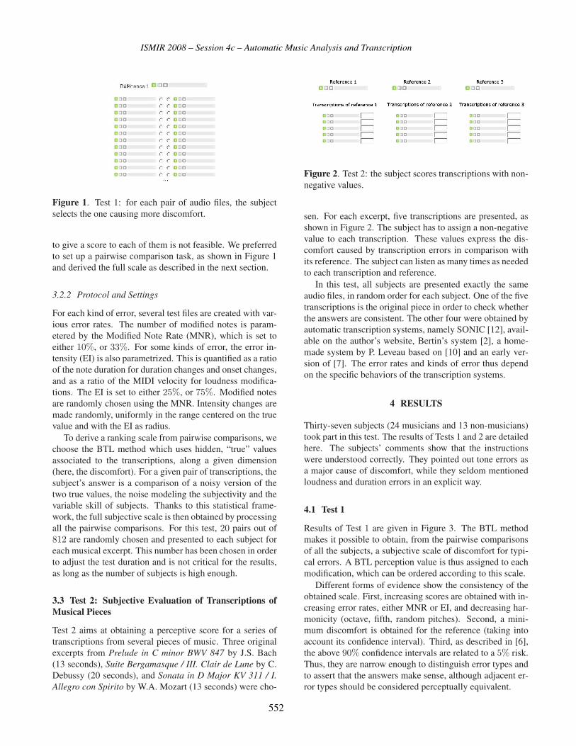
ISMIR 2008 – Session 4c – Automatic Music Analysis and Transcription
Figure 1. Test 1: for each pair of audio files, the subjectselects the one causing more discomfort.
to give a score to each of them is not feasible. We preferredto set up a pairwise comparison task, as shown in Figure 1and derived the full scale as described in the next section.
3.2.2 Protocol and Settings
For each kind of error, several test files are created with var-ious error rates. The number of modified notes is param-etered by the Modified Note Rate (MNR), which is set toeither 10%, or 33%. For some kinds of error, the error in-tensity (EI) is also parametrized. This is quantified as a ratioof the note duration for duration changes and onset changes,and as a ratio of the MIDI velocity for loudness modifica-tions. The EI is set to either 25%, or 75%. Modified notesare randomly chosen using the MNR. Intensity changes aremade randomly, uniformly in the range centered on the truevalue and with the EI as radius.
To derive a ranking scale from pairwise comparisons, wechoose the BTL method which uses hidden, “true” valuesassociated to the transcriptions, along a given dimension(here, the discomfort). For a given pair of transcriptions, thesubject’s answer is a comparison of a noisy version of thetwo true values, the noise modeling the subjectivity and thevariable skill of subjects. Thanks to this statistical frame-work, the full subjective scale is then obtained by processingall the pairwise comparisons. For this test, 20 pairs out of812 are randomly chosen and presented to each subject foreach musical excerpt. This number has been chosen in orderto adjust the test duration and is not critical for the results,as long as the number of subjects is high enough.
3.3 Test 2: Subjective Evaluation of Transcriptions ofMusical Pieces
Test 2 aims at obtaining a perceptive score for a series oftranscriptions from several pieces of music. Three originalexcerpts from Prelude in C minor BWV 847 by J.S. Bach(13 seconds), Suite Bergamasque / III. Clair de Lune by C.Debussy (20 seconds), and Sonata in D Major KV 311 / I.Allegro con Spirito by W.A. Mozart (13 seconds) were cho-
Figure 2. Test 2: the subject scores transcriptions with non-negative values.
sen. For each excerpt, five transcriptions are presented, asshown in Figure 2. The subject has to assign a non-negativevalue to each transcription. These values express the dis-comfort caused by transcription errors in comparison withits reference. The subject can listen as many times as neededto each transcription and reference.
In this test, all subjects are presented exactly the sameaudio files, in random order for each subject. One of the fivetranscriptions is the original piece in order to check whetherthe answers are consistent. The other four were obtained byautomatic transcription systems, namely SONIC [12], avail-able on the author’s website, Bertin’s system [2], a home-made system by P. Leveau based on [10] and an early ver-sion of [7]. The error rates and kinds of error thus dependon the specific behaviors of the transcription systems.
4 RESULTS
Thirty-seven subjects (24 musicians and 13 non-musicians)took part in this test. The results of Tests 1 and 2 are detailedhere. The subjects’ comments show that the instructionswere understood correctly. They pointed out tone errors asa major cause of discomfort, while they seldom mentionedloudness and duration errors in an explicit way.
4.1 Test 1
Results of Test 1 are given in Figure 3. The BTL methodmakes it possible to obtain, from the pairwise comparisonsof all the subjects, a subjective scale of discomfort for typi-cal errors. A BTL perception value is thus assigned to eachmodification, which can be ordered according to this scale.
Different forms of evidence show the consistency of theobtained scale. First, increasing scores are obtained with in-creasing error rates, either MNR or EI, and decreasing har-monicity (octave, fifth, random pitches). Second, a mini-mum discomfort is obtained for the reference (taking intoaccount its confidence interval). Third, as described in [6],the above 90% confidence intervals are related to a 5% risk.Thus, they are narrow enough to distinguish error types andto assert that the answers make sense, although adjacent er-ror types should be considered perceptually equivalent.
552

ISMIR 2008 – Session 4c – Automatic Music Analysis and Transcription
−200 −150 −100 −50 0 50 100 150 200
Duration EI=25% MNR=10%Reference
Duration EI=75% MNR=33%Duration EI=75% MNR=10%
Loudness EI=25% MNR=10%Duration EI=25% MNR=33%
Loudness EI=25% MNR=33%Onset EI=25% MNR=10%
Loudness EI=75% MNR=10%Deletion MNR=10%
Octave replac. MNR=10%Doubling MNR=10%
Octave insert. MNR=10%Octave insert. MNR=33%
Onset EI=25% MNR=33%Onset EI=75% MNR=10%
Loudness EI=75% MNR=33%Doubling MNR=33%
Fifth insert. MNR=10%Rand. insert. MNR=10%
Octave replac. MNR=33%Onset EI=75% MNR=33%
Fifth replac. MNR=10%Rand. replac. MNR=10%
Deletion MNR=33%Fifth replac. MNR=33%Fifth insert. MNR=33%
Rand. replac. MNR=33%Rand. insert. MNR=33%
BTL perception values of discomfort
BTL valuesReferenceTime modificationsLoudness ModificationsPitch modifications
Figure 3. Test 1 : perceptive scale for typical errors. Crosses account for the related BTL value. Horizontal bars depictthe 90% confidence intervals, obtained by a bootstrap method [6] using 100 resamplings of the data (because the data is notgaussian, confidence intervals may not be centered on BTL values).
Globally, as expected from the subjects’ comments, thehighest discomfort values are obtained with pitch modifica-tions; loudness and time modifications cause low to mediumdiscomfort. Regarding pitch changes, octave errors are jud-ged much less serious than fifth changes, which cause aslightly lower discomfort than random changes. In eachcase, replacements and insertions are judged as equivalent,which would indicate that the discomfort is more inducedby the added note than by the deleted note of a replace-ment. The lower values obtained for deletions confirm thishypothesis, which is commonly observed when working ontranscription systems: a false negative usually sounds betterthan a false positive.
Results with time errors show that the modified onsetscause much more discomfort than duration changes. Whileone can expect that moving the beginning of an event causesa significant subjective change, it seems that subjects justdid not perceive most of the modifications of duration. Thiscan be explained by a specific feature of the piano: the endsof sounds generated from its freely-vibrating strings are lessperceptible than for a musical instrument with forced vibra-tions. Thus current results for perception of note durationcannot be generalized to all instruments.
Finally, additional analysis of the results should be re-ported, which are not represented in Figure 3. First, similarresults were obtained from subjects that were musicians andfrom non-musicians. Second, the three scales obtained forthe three excerpts are also similar, with a little differencefor the excerpt by Debussy in which deletions have a lowerscore and duration changes cause higher discomfort, proba-bly because of the long durations in this slow piece of music.
4.2 Test 2
For each subject, scores of Test 2 are normalized by themaximum score he/she gave. Six subjects were removedsince they scored a discomfort greater than 20% for the ref-erence. Average scores and variances were then computed,with respect to the results from all the remaining subjects.
Results are represented in Figure 4. As the test is not acontest between existing algorithms, the systems were madeanonymous, numbered from 1 to 4. The confidence in the re-sults is assessed thanks to a 3 (composers) × 5 (algorithms)factorial ANOVA test, passed for each dimension and for in-teractions using a p = 0.01 test level. Thereby, the scoresand the ranking of the algorithms are very dependent on thepiece of music. This confirms that the performance of a tran-scription system is related to the musical content of piecesand thus depends on the test database. Large standard devi-ations indicate that the evaluation of a musical transcriptiondepends greatly on proper subjective criteria. An importantoverlap between the answers makes it impossible to obtain adefinitive ranking among the different algorithms even if foreach excerpt, systems 2 and 3 are judged as the worst andthe best one respectively.
5 EVALUATING THE TRANSCRIPTIONS
When comparing the results given by one of the objectiveevaluation methods proposed in Section 2 to the perceptiveresults of Test 1, several aspects are differentiated in the for-mer case while they are not in the latter case, and vice versa.For instance, octave, fifth and random pitch changes have
553
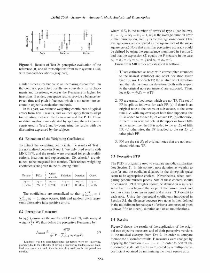
ISMIR 2008 – Session 4c – Automatic Music Analysis and Transcription
Bach Debussy Mozart
0
0.5
1
R R R
1
1
12
2
2
33 3
4
4 4
Dis
com
fort
Figure 4. Results of Test 2: perceptive evaluation of thereference (R) and of transcriptions from four systems (1-4),with standard deviations (gray bars).
similar F-measures but cause an increasing discomfort. Onthe contrary, perceptive results are equivalent for replace-ments and insertions, whereas the F-measure is higher forinsertions. Besides, perceptive results provide a balance be-tween time and pitch influences, which is not taken into ac-count in objective evaluation methods.
In this part, we estimate weighting coefficients of typicalerrors from Test 1 results, and we then apply them to adapttwo existing metrics: the F-measure and the PTD. Thesemodified methods are validated by applying them to the ex-cerpts used in Test 2 and by comparing the results with thediscomfort expressed by the subjects.
5.1 Extraction of the Weighting Coefficients
To extract the weighting coefficients, the results of Test 1are normalized between 0 and 1. We only used results withMNR 33%, and the results were averaged for pitch modifi-cations, insertions and replacements. Six criteria 1 are ob-tained, to be integrated into metrics. Their related weightingcoefficients are given in the following table:
Octave FifthOther
Deletion Duration Onsetintervals
α1 = α2 = α3 = α4 = α5 = α6 =0.1794 0.2712 0.2941 0.2475 0.0355 0.4687
The coefficients are normalized so that 13
∑3i=1 αi +∑6
i=4 αi = 1, since octave, fifth and random pitch repre-sents alternative false positive errors.
5.2 Perceptive F-measure
In eq.(1), errors are the number of FP and FN, with an equalweight ( 1
2 ). We thus define the perceptive F-measure by:
fpercept �#TP
#TP +∑6
i=1 αiwi#Ei
(2)
1 Loudness was not considered since the results were not satisfying,probably due to the difficulty of having a trustworthy loudness scale. Dou-bled notes were not used either because they could not be integrated intometrics.
where #Ei is the number of errors of type i (see below),w1 = w2 = w3 = w4 = 1, w5 is the average duration errorin the transcription, and w6 is the average onset error. (Theaverage errors are computed as the square root of the meansquare error.) Note that a similar perceptive accuracy couldbe defined by using the equivalence mentioned in Section 2and that the expression (2) equals the F-measure in the caseα1 = α2 = α3 = α4 = 1
2 and α5 = α6 = 0.Errors from MIDI files are extracted as follows:
1. TP are estimated as notes with correct pitch (roundedto the nearest semitone) and onset deviation lowerthan 150 ms. For each TP, the relative onset deviationand the relative duration deviation (both with respectto the original note parameters) are extracted. Then,let #E5 = #E6 = #TP.
2. FP are transcribed notes which are not TP. The set ofFP is split as follows: for each FP, (a) if there is anoriginal note at the octave or sub-octave, at the sametime (i.e. with any overlap of both time supports), theFP is added to the set E1 of octave FP; (b) otherwise,if there is an original note at the upper or lower fifthat the same time, the FP is added to the set E2 of fifthFP; (c) otherwise, the FP is added to the set E3 ofother pitch FP.
3. FN are the set E4 of original notes that are not asso-ciated with one TP.
5.3 Perceptive PTD
The PTD is originally used to evaluate melodic similarities(see Section 2). In this context, note duration as weights totransfer and the euclidian distance in the time/pitch spaceseem to be appropriate choices. Nevertheless, when com-paring generic musical pieces, both of these choices shouldbe changed. PTD weights should be defined in a musicalsense but this is beyond the scope of the current work andwe thus chose to assign an equal and unitary PTD weight toeach note. Using the perceptual coefficients introduced inSection 5.1, the distance between two notes is then definedin the multidimensionnal space of criteria composed of pitch(octave, fifth or others), duration and onset modifications.
5.4 Results
Figure 5 shows the results of the application of the origi-nal two objective measures and of their perceptive versionsto the musical excerpts from Test 2. In order to comparethem to the discomfort results, F-measures were changed byapplying the function x → 1 − x. In order to best fit thediscomfort scale, all results were scaled by a multiplicativecoefficient obtained by minimizing the mean square error.
554

ISMIR 2008 – Session 4c – Automatic Music Analysis and Transcription
Bach Debussy Mozart0
0.5
1
1.5
R R R
1
1
12
2
2
3 3 3
44 4
F−
mea
sure
Bach Debussy Mozart0
0.5
1
1.5
R R R
1
1
12
2 23 33
44 4
Per
cep.
F−
mea
s.
Bach Debussy Mozart0
0.5
1
1.5
R R R
1
1
122
2
3
3 3
44 4
PT
D
Bach Debussy Mozart0
0.5
1
1.5
R R R
1
1
122
2
3 3 3
44 4
Per
cep.
PT
D
Figure 5. Transcription evaluation results with several ob-jective and perceptive measures: in each case, crosses showthe normalized error related to a measure, and the gray barsindicate the discomfort obtained in Test 2.
Results with the perceptive F-measure are slightly closerto the discomfort values than the original F-measure. More-over, the ranking of the 15 excerpts is also closer to thediscomfort-based ranking. Results of the perceptive PTDdo not look better than the original, due to a high isolatedvalue for the excerpt with highest discomfort (Mozart, Sys-tem 2), that makes it difficult to scale the results adequately.However, the achieved ranking is dramatically better thanthe ranking by the original PTD, and also slightly betterthan the ranking by the perceptive F-measure. Thus, even ifthe relation between the discomfort and the perceptive PTDmay be non-linear, the latter is appropriate in a ranking task.
6 CONCLUSIONS
The main idea of these tests was to get a ranking of thetypical automatic transcription errors, to extract perceptionweights, and to integrate them into several musical sequencedistance metrics. These primary results are consistent andthe proposed perceptive metrics give satisfying results.
However further investigations should focus on a numberof aspects, such as non-linear relations between specific er-ror rates and discomfort, musical-based typical errors (tak-ing into account tonality, melody, chords, etc.), and morespecific algorithms to identify them.
References
[1] Multiple fundamental frequency estimation & track-ing. In Music Information Retrieval Evaluation eX-change (MIREX), 2007.
[2] N. Bertin, R. Badeau, and G. Richard. Blind signaldecompositions for automatic transcription of poly-
phonic music: NMF and K-SVD on the benchmark. InProc. of ICASSP, Honolulu, Hawaii, USA, April 2007.
[3] R.A. Bradley. Some statistical methods in taste testingand quality evaluation. Biometrics, 9(1):22–38, 1953.
[4] A.T. Cemgil, H.J. Kappen, and D. Barber. A genera-tive model for music transcription. IEEE Trans. Audio,Speech and Lang. Proces., 14(2):679–694, 2006.
[5] S. Dixon. On the computer recognition of solo pianomusic. Australasian Computer Music Conf., 2000.
[6] B. Efron and R. J. Tibshirani. An introduction to thebootstrap. In London: Chapman & Hall, 1993.
[7] V. Emiya, R. Badeau, and B. David. Automatic tran-scription of piano music based on HMM tracking ofjointly-estimated pitches. In Proc. of EUSIPCO, Lau-sanne, Switzerland, August 2008.
[8] P. Hanna and P. Ferraro. Polyphonic music retrievalby local edition of quotiented sequences. In Proc. ofCBMI, Bordeaux, France, June 2007.
[9] A. Klapuri and M. Davy. Signal Processing Methodsfor Music Transcription. Springer, 2006.
[10] P. Leveau, E. Vincent, G. Richard, and L. Daudet.Instrument-specific harmonic atoms for mid-level mu-sic representation. IEEE Trans. Audio, Speech andLang. Proces., 16(1):116–128, January 2008.
[11] V. I. Levenshtein. Binary codes capable of correctingspurious insertions and deletions of ones. Problems ofInformation Transmission, 1(1):8–17, 1965.
[12] M. Marolt. A connectionist approach to automatictranscription of polyphonic piano music. IEEE Trans.on Multimedia, 6(3):439–449, 2004.
[13] M. Mongeau and D. Sankoff. Comparison of mu-sical sequences. Computers and the Humanities,24(3):161–175, 1990.
[14] J.A. Moorer. On the Segmentation and Analysisof Continuous Musical Sound by Digital Computer.Dept. of Music, Stanford University, 1975.
[15] G. Poliner and D. Ellis. A discriminative model forpolyphonic piano transcription. EURASIP Journal onAdvances in Signal Processing, 8:1–9, 2007.
[16] M. Ryynänen and A.P. Klapuri. Polyphonic musictranscription using note event modeling. In Proc. ofWASPAA, pages 319–322, New Paltz, NY, USA, 2005.
[17] R. Typke, P. Giannopoulos, R. C. Veltkamp, F. Wier-ing, and R. van Oostrum. Using transportation dis-tances for measuring melodic similarity. In Proc. ofISMIR, Baltimore, Maryland, USA, 2003.
555

ISMIR 2008 – Session 4c – Automatic Music Analysis and Transcription
556

Session 5a – Content-Based Retrieval, Categorizationand Similarity 2

.

ISMIR 2008 – Session 5a – Content-Based Retrieval, Categorization and Similarity 2
SOCIAL PLAYLISTS AND BOTTLENECK MEASUREMENTS :EXPLOITING MUSICIAN SOCIAL GRAPHS USING CONTENT-BASED
DISSIMILARITY AND PAIRWISE MAXIMUM FLOW VALUES
BEN FIELDS, CHRISTOPHE RHODES, MICHAEL CASEY
Goldsmiths Digital StudiosGoldsmiths, University of London
KURT JACOBSON
Centre for Digital MusicQueen Mary, University of London
ABSTRACT
We have sampled the artist social network of Myspace and
to it applied the pairwise relational connectivity measure
Minimum cut/Maximum flow. These values are then com-
pared to a pairwise acoustic Earth Mover’s Distance mea-
sure and the relationship is discussed. Further, a means of
constructing playlists using the maximum flow value to ex-
ploit both the social and acoustic distances is realized.
1 INTRODUCTION
As freely–available audio content continues to become more
accessible, listeners require more sophisticated tools to aid
them in the discovery and organization of new music that
they find enjoyable. This need, along with the recent advent
of Internet based social networks and the steady progress of
signal based Music Information Retrieval have created an
opportunity to exploit both social relationships and acoustic
similarity in recommender systems.
Motivated by this, we examine the Myspace artist net-
work. Though there are a number of music oriented social
networking websites, Myspace 1 has become the de factostandard for web-based music artist promotion. Although
exact figures are not made public, recent estimates suggest
there are well over 7 million artist pages 2 on Myspace. For
the purpose of this paper, artist and artist page are used
interchangeably to refer to the collection of media and so-
cial relationships found at a specific Myspace page residing
in Myspace’s artist subnetwork, where this subnetwork is
defined as those Myspace user pages containing the audio
player application.
The Myspace social network, like most social networks,
is based upon relational links between friends designating
some kind of association. Further, a Myspace user has a
subset of between 8 and 40 top friends. While all friends
1 http://myspace.com/2 http://scottelkin.com/archive/2007/05/11/
MySpace-Statistics.aspx reports as of April 2007 ∼25 mil-
lion songs, our estimates approximate 3.5 songs/artist, giving ∼7 million
artists
are mutually confirmed, individual users unilaterally select
top friends. Additionally, pages by artists will usually con-
tain streaming and downloadable media of some kind either
audio, video or both.
Social networks of this sort present a way for nearly any-
one to distribute their own media and as a direct result, there
is an ever larger amount of available music from an ever
increasing array of artists. Given this environment of con-
tent, how can we best use all of the available information to
discover new music? Can both social metadata and content
based comparisons be exploited to improve navigation?
To work towards answers to these and related questions,
we explore the relationship between the connectivity of pairs
of artists on the Myspace top friends network and a measure
of acoustic dissimilarity of these artists.
We begin this paper by briefly reviewing graph theoretic
network flow analysis and previous work in related topics
including musician networks, content-based artist similarity.
We go on to explain our methodology including our network
sampling method in Section 3.1 and our connectivity analy-
sis techniques in Section 3.2. These connectivity measures
are then compared to acoustic artist similarity for the struc-
tured network in Section 4 and they are used to construct a
social playlist in Section 5. We finish with a discussion of
the results and what these results may mean for future work
in this space.
2 BACKGROUND
This work uses a combination of complex network theory,
network flow analysis and signal-based music analysis. Both
disciplines apply intuitively to Music Information Retrieval;
however, the two have only recently been applied simulta-
neously to a single data set [9].
2.1 Complex Networks
Complex network theory deals with the structure of relation-
ships in complex systems. Using the tools of graph theory
and statistical mechanics, physicists have developed models
559

ISMIR 2008 – Session 5a – Content-Based Retrieval, Categorization and Similarity 2
and metrics for describing a diverse set of real-world net-
works – including social networks, academic citation net-
works, biological protein networks, and the World-Wide Web.
In contrast to simple networks, all these networks exhibit
several unifying characteristics such as small worldness, scale-
free degree distributions, and community structure [19]. We
briefly introduce below some definitions and concepts that
will be used in this work.
A given network G is described by a set of nodes N con-
nected by a set of edges E. Each edge is defined by the pair
of nodes (i, j) it connects. This pair of nodes are neigh-bors via edge E(i, j). If the edges imply directionality,
(i, j) �= (j, i), the network is a directed network. Other-
wise, it is an undirected network. In this paper, all edges
are directed unless otherwise stated. In some graphs each
edge E(i, j) will have an associated label w(i, j) called the
weight. This weight is sometimes thought of as the cost of
traversing an edge, or an edge’s resistance. The number of
edges incident to a node i is the degree ki. In a directed
network there will be an indegree kini and an outdegree kout
i
corresponding to the number of edges pointing into the node
and away from the node respectively.
The degree distribution P (k) of a graph is the propor-
tion of nodes that have a degree k. The shape of the de-
gree distribution is an important metric for classifying a net-
work – scale-free networks have a power-law distribution
P (k) ∝ k−γ , while random networks have a Poisson distri-
bution [19]. Many real-world networks are approximately
scale-free over a wide range of scales. Conceptually, a scale-
free distribution indicates the presence of a few very-popular
hubs that tend to attract more links as the network evolves
[19].
2.2 Network Flow Analysis
The basic premise in network flow analysis is to examine a
network’s nodes as sources and sinks of some kind of traf-fic[2]. Typically, though not exclusively, flow networks are
directed, weighted graphs. A simple flow network can be
seen in Figure 1. Many useful strategies for determining the
density of edge connectivity between sources and sinks can
be found in this space[18]. One of the most common among
them is the Maximum Flow/Minimum Cut Theorem[8], which
is a means of measuring the maximum capacity for fluid to
flow between a source node to a sink node or, equivalently,
the smallest sum of edge weights that must be cut from the
network to create exactly two subgraphs, one containing the
source node and one containing the sink node. This will be
discussed in more detail in Section 3.2. The few examples
of network flow type analysis in music deal primarily with
constructing playlists using partial solutions to the Travel-
ing Salesman Problem [12] or use exhaustive and explicit
metadata[3].
� �
��
�
�
��
��
�
�
��
�
Figure 1. A simple flow network with directed weighted
edges. Here the source is node A and the sink is node F.
2.3 Musician Networks
Quite naturally, networks of musicians have been studied
in the context of complex network theory – typically view-
ing the artists as nodes in the network and using either col-
laboration, influence, or similarity to define network edges.
These networks of musicians exhibit many of the proper-
ties expected in social networks [7, 10, 21]. However, these
studies all examine networks created by experts (e.g. All
Music Guide 3 ) or via algorithmic means (e.g. Last.fm 4 ) as
opposed to the artists themselves, as is seen in Myspace and
other similar networks. Networks of music listeners and bi-
partite networks of listeners and artists have also been stud-
ied [4, 14].
2.4 Content-Based Music Analysis
Many methods have been explored for content-based mu-
sic analysis, attempting to characterizing a music signal by
its timbre, harmony, rhythm, or structure. One of the most
widely used methods is the application of Mel-frequency
cepstral coefficients (MFCC) to the modeling of timbre [16].
In combination with various statistical techniques, MFCCs
have been successfully applied to music similarity and genre
classification tasks [6, 17, 20]. A common approach for
computing timbre-based similarity between two songs or
collections of songs creates Gaussian Mixture Models (GMM)
describing the MFCCs and comparing the GMMs using a
statistical distance measure. Often the Earth Mover’s Dis-
tance (EMD), a technique first used in computer vision [22],
is the distance measure used for this purpose [5, 20]. The
EMD algorithm finds the minimum work required to trans-
form one distribution into another.
3 http://www.allmusic.com/4 http://www.lastfm.com/
560

ISMIR 2008 – Session 5a – Content-Based Retrieval, Categorization and Similarity 2
2.5 Bringing It Together
There has been some recent work attempting to bridge the
divide between content-based analysis and human gener-
ated metadata. Most of this work [12, 23] focuses on vari-
ous ways of exploiting the human-generated metadata to fil-
ter content prior to, or instead of, conducting content-based
analysis, similar to the techniques discussed in Section 2.4,
in order to reduce computational load.
3 METHODOLOGY
3.1 Sampling the Social Web
The Myspace social network presents a variety of challenges.
For one, the size of the network prohibits analyzing the graph
in its entirety, even when considering only the artist pages.
Therefore in the work we deal with a sample (of large ab-
solute size) of the network. Also, the Myspace social net-
work is filled with noisy data – plagued by spammers and
orphaned accounts. We limit the scope of our sampling in a
way that minimizes this noise. And finally, there currently
is no interface for easily collecting the network data from
Myspace 5 . Our data is collected using web crawling and
HTML scraping techniques 6 .
3.1.1 Artist Pages
It is important to note we are only concerned with a subset of
the Myspace social network – the Myspace artist network.
Myspace artist pages are different from standard Myspace
pages in that they include a distinct audio player application.
We use the presence or absence of this player to determine
whether or not a given page is an artist page.
A Myspace page will most often include a top friends
list. This is a hyperlinked list of other Myspace accounts
explicitly specified by the user. The top friends list is lim-
ited in length with a maximum length of 40 friends (the
default length is 16 friends). In constructing our sampled
artist network, we use the top friends list to create a set of
directed edges between artists. Only top friends who also
have artist pages are added to the sampled network; stan-
dard Myspace pages are ignored. We also ignore the re-
mainder of the friends list (i.e. friends that are not specified
by the user as top friends), assuming these relationships are
not as relevant. This reduces the amount of noise in the
sampled network but also artificially limits the outdegree of
each node. Our sampling is based on the assumption that
artists specified as top friends have some meaningful musi-
5 At time of writing Myspace has recently published a public API, this
may allow future work to occur without the need for html scraping, which
would greatly decrease the compute time required for graph generation.6 Myspace scraping is done using tools from the MyPySpace project
available at http://mypyspace.sorceforge.net
cal connection for the user – whether through collaboration,
stylistic similarity, friendship, or artistic influence.
The audio files associated with each artist page in the
sampled network are also collected for feature extraction.
Cached versions of the audio files are downloaded and audio
features are extracted.
3.1.2 Snowball Sampling
There are several network sampling methods; however, for
the Myspace artist network, snowball sampling is the most
appropriate method [1, 15]. In this method, the sample be-
gins with a seed node (artist page), then the seed node’s
neighbors (top friends), then the neighbors’ neighbors, are
added to the sample. This breadth-first sampling is contin-
ued until a particular sampling ratio is achieved. Here, we
randomly select a seed artist 7 and collect all artist nodes
within 6 edges to collect 15,478 nodes. This produces a
dataset where no more than six directed top friends links
need to be followed to get from the seed artist to any other
artist in the dataset. If the size of the Myspace artist net-
work is around 7 million, then this dataset approximates the
0.25% sampling ratio suggested for accurate degree distri-
bution estimation in sampled networks. However, it is in-
sufficient for estimating other topological metrics such as
the clustering coefficient and assortativity [13]. Of course, a
complete network topology is not our primary concern here.
With snowball sampling there is a tendency to over sam-
ple hubs because they have high indegree connectivity and
are therefore picked up disproportionately frequently in the
breadth-first sampling. This property would reduce the de-
gree distribution exponent γ and produce a heavier tail but
preserve the power-law nature of the network [15].
3.2 Minimum Cut/Maximum Flow
We use the Maximum Flow value as a means of determin-
ing the number of independent paths from a source node to
a sink node. Formally the Maximum Flow/Minimum Cut
theorem[8], it is used to calculate the highest weight in the
narrowest part of the path from source to sink. The the-
orem’s name comes from the equivalence in the smallest
weight of edges that must be removed in order to create two
subgraphs which disconnect the source and sink nodes. Fur-
ther, if the edges in the graph are unweighted, this value is
also equivalent to the number of paths from the source to
the sink which share no common edges. As this is a mature
algorithm there are a number of optimization strategies that
have been examined [2, 11].
An example of Maximum Flow can be seen on the net-
work in figure 1. It can been seen that the narrowest point
7 The artist is Karna Zoo, Myspace url: http://www.myspace.com/index.cfm?fuseaction=user.viewProfile&friendID=134901208
561

ISMIR 2008 – Session 5a – Content-Based Retrieval, Categorization and Similarity 2
from node A to node F is E(a, b) and E(a, c). The maxi-
mum flow can simply be found via Equation 1.
M =∑
m(i, j) (1)
Where m(i, j) is the magnitude of each edge in the min-
imum cut set.
In our Myspace top friends graph, the maximum flow is
measured on the unweighted directed graph from the source
artist node to the sink artist node.
4 CONNECTED SOUND
4.1 Experiment
We calculate the maximum flow value, using the snowball
sample entry point as the fixed source against every other
node in turn as a sink, yielding the number of edges con-
necting each sink node to the entry point node at the nar-
rowest point of connection. The acoustic distances can then
be compared to these maximum flow values.
4.1.1 Signal-based analysis
Cepstral coefficients are extracted from each audio signal
using a Hamming window on 8192 sample FFT windows
with 4096 sample overlap. For each artist node a GMM is
built from the concatenation of MFCC frames for all songs
found on each artist’s Myspace page (the mean number of
songs per artist is 3.5). We calculate the Earth Mover’s Dis-
tance between the GMMs corresponding to each source sink
pair in the sample. All MFCCs are created with the fftEx-
tract tool 8 .
4.1.2 Random Networks
In order to better understand a result from analysis of our
Myspace sample, a baseline for comparison must be used.
To that end, random permutations of the node locations are
examined. In order to preserve the overall topology present
in the network, this randomization is performed by random-
izing the artist label and associated music attached to a given
node on the network. This is done ten fold, creating a solid
baseline to test the null hypothesis that the underlining com-
munity structure is not responsible for any correlation be-
tween maximum flow values and Earth Mover’s Distance.
4.2 Result
The results of the first experiment show no simple relation-
ship between the sampled netwrok and the randomized net-
work. This can be seen in Table 1 and in Figures 2 and
3. There is an increase in the median EMD for the less well
connected (i.e. lower maximum flow value) node pairs in the
8 source code at http://omras2.doc.gold.ac.uk/software/fftextract/
Max Flow median deviation randomized deviation
1 40.80 1.26 39.10 −0.432 45.30 5.76 38.34 −1.193 38.18 −1.35 38.87 −0.664 38.21 −1.32 38.64 −0.895 40.00 0.47 39.11 −0.426 41.77 2.25 39.02 −0.517 39.94 0.41 39.24 −0.298 39.38 −0.15 38.76 −0.779 38.50 −1.03 38.87 −0.6610 39.07 −0.46 40.85 1.32
Table 1. Node pairs average EMD values grouped by actual
minimum cut values and randomized minimum cut values,
shown with deviations from the global median of 39.53.
Myspace sample graph, though this is not significant enough
to indicate a correlation, while the randomized permutations
are near flat. While the median EMD of the artist pairs with
a maximum flow of 10 is appreciably higher than all other in
the randomized graph, this is likely related to the relatively
large size of this group. Perhaps the easiest way to examine
the relationship between the sampled graph and randomized
one is through the deltas of each group’s median from the
entire dataset median. This data is shown in the second and
forth colum in Table 1 and Figure 4. Further, the Kruskal-
Wallis one-way ANOVA results for both the sample graph
and averaged across the 10 fold permutations are shown in
Table 2.
H-value P-value
From sample 12.46 0.19Random permutations 9.11 0.43
Table 2. The Kruskal-Wallis one-way ANOVA test results
of EMD against maximum flow for both the sampled graph
and it’s random permutations. The H-values are drawn from
a chi-square distribution with 10 degrees of freedom.
5 THE MAX FLOW PLAYLIST
In order to build playlists using both acoustic and social net-
work data, we use the Earth Mover’s Distance between each
pair of neighbors as weights on the Myspace sample net-
work. Two artists are then selected, a starting artist as the
source node and a final artist as the sink node. One or more
paths are then found through the graph via the maximum
flow value, generating the list and order of artists for the
playlist. The song used is the most popular at the time of
the page scrape. In this way playlists are constructed that
are both influenced by timbre similarity and bound by so-
562

ISMIR 2008 – Session 5a – Content-Based Retrieval, Categorization and Similarity 2
1 2 3 4 5 6 7 8 9 10
Maximum Flow Value
10
20
30
40
50
60
70
80
90
100
EarthMover'sDistance
Figure 2. The box and whisker plot showing the distribution
of EMD grouped by maximum flow value between artists on
the Myspace social graph.
1 2 3 4 5 6 7 8 9 10
Maximum Flow Value
20
30
40
50
60
70
80
90
100
EarthMover'sDistance
Figure 3. The box and whisker plot showing the distribution
of EMD grouped by maximum flow value between artists on
the randomized graph, maintaining the original edge struc-
ture.
cial context, regardless of any relationship found between
these two spaces found via the work discussed in Section
4. Playlists generated using this technique were informally
auditioned, and were found to be reasonable on that basis.
6 DISCUSSION AND FUTURE WORK
While an inverse relationship between Earth Mover’s Dis-
tance and the maximum flow value might be expected on the
basis of the conventional wisdom that a community of artists
tend to be somehow aurally similar, this does not appear to
be strictly the case. The evidence, at least in this sample set,
does not support this relationship, though it doesn’t disprove
it either. However, based upon the difference in result from
the Kruskal-Wallis one-way ANOVA test and simple obser-
0 2 4 6 8 10Maximum Flow Value
-2
-1
0
1
2
3
4
5
6
DeltaFrom
OverallMedian
sampled graph
randomized graph
Figure 4. The deltas from the global median for each max-
imum flow value group of EMD values, from the sampled
graph and the randomized graph.
vation of the deviation from the global median the maximum
flow values and Earth Mover’s Distances do seem affected
by the artist created social links, though it is not a simple re-
lationship and describing it precisely is difficult. This seems
to suggest that there may be no noticeable correlation be-
tween density of connection (maximum flow values) and
acoustic similarity (GMMs compared with EMD), at least
across an entire sample.
There does seem to be some potential in the idea of the
maximum flow playlist. When using the EMD as a weight
the results appear to be quite good, at least from a qualitative
perspective. The imposed constraint of the social network
alleviates to some extent short comings of a playlist built
purely through the analysis of acoustic similarity by moving
more toward the balance between completely similar works
and completely random movement.
Having shown the lack of a strong relationship between
the maximum flow values and acoustic artist similarity, where
do we go from here?
The most promise lies in the exploration of the maximum
flow based playlist. A network could be built which was
song to song exhaustive, having duplicate edges link each
song individually to an artist’s friends’ songs. These edges
would be weighted according to their acoustic similarity and
a more complete playlist generation system would be cre-
ated. A serious hurdle to the implementation of such a sys-
tem lies in the computational complexity of the maximum
flow value. Its compute time is typically dependent on both
the number of nodes and the number of edges making it very
slow to run on a network as dense as the one just described.
This is less of a concern if some form of localized subgraphs
were used, e.g. maximum flow is found against only friends
(the greedy approach) or friends of friends. That said, there
563

ISMIR 2008 – Session 5a – Content-Based Retrieval, Categorization and Similarity 2
may be strategies to get around these problems of complex-
ity leading to novel and interesting playlist generation.
7 ACKNOWLEDGEMENTS
This work is supported as a part of the OMRAS2 project,
EPSRC numbers EP/E02274X/1 and EP/E017614/1.
8 REFERENCES
[1] Y.-Y. AHN, S. HAN, H. KWAK, S. MOON, AND
H. JEONG, Analysis of topological characteristics ofhuge online social networking services, in Proceedings
of the 16th international conference on World Wide
Web, Alberta, Canada, May 2007, IW3C2.
[2] R. K. AHUJA, T. L. MAGNANTI, AND J. B. ORLIN,
Network flows: theory, algorithms, and applications,
Prentice-Hall, Inc., Upper Saddle River, NJ, USA, 1993.
[3] M. ALGHONIEMY AND A. TEWFIK, A network flowmodel for playlist generation, in Multimedia and Expo,
2001. IEEE International Conference on, 2001.
[4] A. ANGLADE, M. TIEMANN, AND F. VIGNOLI, Vir-tual communities for creating shared music channels,
in Proc. of Int. Symposium on Music Information Re-
trieval, 2007.
[5] J. AUCOUTURIER AND F. PACHET, Improving timbresimilarity : How high’s the sky?, J. Negative Results in
Speech and Audio Sciences, (2004).
[6] A. BERENZWEIG, B. LOGAN, D. P. W. ELLIS, AND
B. P. W. WHITMAN, A large-scale evaluation of acous-tic and subjective music-similarity measures, Computer
Music J., 28 (2004), pp. 63–76.
[7] P. CANO, O. CELMA, M. KOPPENBERGER,
AND J. M. BULDU, The topology of music rec-ommendation networks, Chaos: An Interdis-
ciplinary Journal of Nonlinear Science, (2006).
http://arxiv.org/abs/physics/0512266v1.
[8] P. ELIAS, A. FEINSTEIN, AND C. SHANNON, A noteon the maximum flow through a network, Information
Theory, IEEE Transactions on, 2 (Dec 1956), pp. 117–
119.
[9] B. FIELDS, K. JACOBSON, M. CASEY, AND M. SAN-
DLER, Do you sound like your friends? exploring artistsimilarity via artist social network relationships and au-dio signal processing, in Int. Computer Music Confer-
ence, August 2008.
[10] P. GLEISER AND L. DANON, Community structure injazz, Advances in Complex Systems, 6 (2003), pp. 565–
573.
[11] A. V. GOLDBERG AND R. E. TARJAN, A new approachto the maximum-flow problem, J. ACM, 35 (1988),
pp. 921–940.
[12] P. KNEES, T. POHLE, M. SCHEDL, AND G. WIDMER,
Combining audio-based similarity with web-based datato accelerate automatic music playlist generation, in
Proc. 8th ACM international workshop on Multimedia
information retrieval, 2006, pp. 147 – 154.
[13] H. KWAK, S. HAN, Y.-Y. AHN, S. MOON, AND
H. JEONG, Impact of snowball sampling ratios on net-work characteristics estimation: A case study of cy-world, Tech. Rep. CS/TR-2006-262, KAIST, November
2006.
[14] R. LAMBIOTTE AND M. AUSLOOS, On the genre-fication of music: a percolation approach (long version),The European Physical Journal B, 50 (2006), p. 183.
[15] S. H. LEE, P.-J. KIM, AND H. JEONG, Statisticalproperties of sampled networks, Physical Review E, 73
(2006), pp. 102–109.
[16] B. LOGAN, Mel frequency cepstral coefficients for mu-sic modeling, in Proc. of Int. Symposium on Music In-
formation Retrieval, 2000.
[17] B. LOGAN AND A. SALOMON, A music similarity func-tion based on signal analysis, in Multimedia and Expo,
2001. IEEE International Conference on, 22-25 Aug.
2001, pp. 745–748.
[18] H. NAGAMOCHI AND T. IBARAKI, Computing edge-connectivity in multigraphs and capacitated graphs,
SIAM J. Discret. Math., 5 (1992), pp. 54–66.
[19] M. E. J. NEWMAN, The structure and function of com-plex networks, SIAM Review, 45 (2003), p. 167.
[20] E. PAMPALK, Computational Models of Music Similar-ity and their Application in Music Information Retrival,PhD thesis, Technischen Universität Wien, May 2006.
[21] J. PARK, O. CELMA, M. KOPPENBERGER, P. CANO,
AND J. M. BULDU, The social network of contemporarypopular musicians, Int. J. of Bifurcation and Chaos, 17
(2007), pp. 2281–2288.
[22] Y. RUBNER, C. TOMASI, AND L. J. GUIBAS, The earthmover’s distance as a metric for image retrieval, Inter-
national Journal of Computer Vision, 40 (2000), pp. 99–
121.
[23] M. SLANEY AND W. WHITE, Similarity based on rat-ing data, in Proc. of Int. Symposium on Music Informa-
tion Retrieval, 2007.
564

ISMIR 2008 – Session 5a – Content-Based Retrieval, Categorization and Similarity 2
HIGH-LEVEL AUDIO FEATURES:DISTRIBUTED EXTRACTION AND SIMILARITY SEARCH
François Deliège, Bee Yong Chua, and Torben Bach PedersenDepartment of Computer Science
Aalborg University
ABSTRACT
Today, automatic extraction of high-level audio features suf-
fers from two main scalability issues. First, the extraction
algorithms are very demanding in terms of memory and com-
putation resources. Second, copyright laws prevent the au-
dio files to be shared among computers, limiting the use of
existing distributed computation frameworks and reducing
the transparency of the methods evaluation process. The
iSound Music Warehouse (iSoundMW), presented in this
paper, is a framework to collect and query high-level au-
dio features. It performs the feature extraction in a two-step
process that allows distributed computations while respect-
ing copyright laws. Using public computers, the extraction
can be performed on large scale music collections. How-
ever, to be truly valuable, data management tools to search
among the extracted features are needed. The iSoundMW
enables similarity search among the collected high-level fea-
tures and demonstrates its flexibility and efficiency by us-
ing a weighted combination of high-level features and con-
straints while showing good search performance results.
1 INTRODUCTION
Due to the proliferation of music on the Internet, many web
portals proposing music recommendations have appeared.
As of today, the recommendations they offer remain very
limited: manual tagging has proved to be time consuming
and often results in incompleteness, inaccuracy and incon-
sistency; automatic tagging systems based on web scanning
or relying on millions of users are troubled, e.g., by mind-
less tag copying practices, thus blowing bag tags. Automatic
extraction of music information is a very active topic ad-
dressed by the Music Information Retrieval (MIR) research
community. Each year, the Music Information Retrieval
Evaluation eXchange (MIREX) gives to researchers an op-
portunity to evaluate and compare new music extraction meth-
ods [9]. However, the MIREX evaluation process has proved
to be resource consuming and slow despites attempts to ad-
dress these scalability issues [4, 11]. So far, concerns with
copyright issues have refrained the community to distribute
the extraction among public computers as most algorithms
require the audio material to be available in order to per-
form the feature extraction 1 . The features are therefore ex-
tracted from a relatively small music collection that narrows
their generality and usefulness. Additionally, the feature ex-
traction, being run by private computers on a private music
collection, limits the transparency of the evaluation process.
These limitations call for the development of a system able
to extract meaningful, high-level audio features over large
music collections. Such a system faces data management
challenges. Noteworthily, the impressive amount of infor-
mation generated requires an adapted search infrastructure
to become truly valuable.
Our intention is to create a system able to cater for dif-
ferent types of features. Present literature mainly focuses on
features that have either absolute or relative values, thus mo-
tivating the handling of both kinds of features. In this paper,
the exact selection of the features is actually not as impor-
tant as it is to demonstrate how extraction can be handled
on public computers and enabling researchers to compare
results obtained by using different algorithms and features.
The contributions of this paper are two-fold. First, we
propose a framework for collecting high-level audio features
(that were recently proposed by [5, 6, 7, 13]) over a large
music collection of 41,446 songs. This is done by outsourc-
ing the data extraction to remote client in a two-step feature
extraction process: (1) dividing the audio information into
short term segments of equal length and distributing them
to various clients; and (2) sending the segment-based fea-
tures gathered during step one to various clients to compute
high-level features for the whole piece of music. Second, we
propose a flexible and efficient similarity search approach,
which uses a weighted combination of high-level features,
to enable high-level queries (such as finding songs with a
similar happy mood, or finding songs with a similar fast
tempo). Additionally, to support the practical benefits of
these contributions, we propose a short scenario illustrating
the feature extraction and search abilities of the iSoundMW.
For the general public, the iSoundMW music offers rec-
ommendation without suffering from a “cold start”, i.e., new
artists avoid the penalties of not being well known, and new
listeners obtain good music recommendation before being
profiled. For researchers, the iSoundMW (1) offers flexi-
1 https://mail.lis.uiuc.edu/pipermail/evalfest/2008-May/000765.html
565

ISMIR 2008 – Session 5a – Content-Based Retrieval, Categorization and Similarity 2
ble search abilities; (2) enables visual comparison of both
segment-based and aggregated high-level features; (3) pro-
vides a framework for large scale computations of features;
and (4) gives good search performances.
The remainder of the paper is organized as follows. Re-
lated work is presented in Section 2. Section 3 offers an
overview of the system, explains the process of collecting
the high-level audio features, describes how similarity search
with weighted coefficients is performed, and how the search
can be further optimized by using range searches. Section 4
illustrates the similarity search on a concrete example. Sec-
tion 5 concludes and presents future system improvements
and research directions.
2 RELATED WORK
Research on distributed computing has received a lot of at-
tention in diverse research communities. The Berkeley Open
Infrastructure for Network Computing framework (BOINC)
is a well-known middleware system in which the general
public volunteers processing and storage resources to com-
puting projects [1, 2] such as SETI@home [3]. However, in
its current state, BOINC does not address copyright issues,
does not feature flexible similarity search, and does not en-
able multiple steps processes, i.e., acquired results serve as
input for other tasks. Closer to the MIR community, the On-
demand Metadata Extraction Network system (OMEN) [15]
distributes the feature extraction among trusted nodes rather
than public computers. Furthermore, OMEN does not store
the computed results, and, like BOINC, does not allow sim-
ilarity search to be performed on the extracted features.
Audio similarity search is often supported by creating
indexes [10]. Existing indexing techniques can be applied
to index high dimensional musical feature representations.
However, as a consequence of the subjective nature of mu-
sical perception, the triangular inequality property of the
metric space is typically not preserved for similarity mea-
sures [14, 16]. Work on indexes for non-metric space is
presented in the literature [12, 17]. Although the similarity
function is non-metric, it remains confined in a pair of lower
and upper bounds specifically constructed. Therefore, us-
ing these indexes would impose restrictions on the similarity
values that would limit the flexibility of the iSoundMW.
3 SYSTEM DESCRIPTION
In this section, we present an overview of the system fol-
lowed by a more detailed description of a two-step process
for extracting high-level features. Later, we describe how
flexible similarity searches are performed and how they are
further optimized using user-specified constraints.
�������������������
:� ��������
�����������������
�������������������
����������������������
������������������
���������
�}�������
�}�������
�}�������
�}�������
��������������������� ���
��'�����������K��
���K������ �'��������
B� ��'�����������������%�B� ������'
������''������
��������*��'��
Figure 1. System architecture
3.1 iSoundMW Overview
The iSoundMW system has a client-server architecture, shown
in Figure 1. The server side is composed of a central data
repository and an application server that controls the extrac-
tion and similarity searches. The data repository stores all
the audio collection in MP3 format and uniquely identifies
each by a number. It also contains all the editorial informa-
tion, e.g., the artist name, the album name, the band name,
the song title, the year, the genre, and copyright license, and
the physical information, e.g., the file size, the format, the
bit rate, and the song length, that are stored in the music
information database. Additionally, the Music Information
Database holds all the extracted feature information.
The application server is composed of three distinct com-
ponents. First, the job manager assigns extraction or aggre-
gation tasks to the clients, collects the results, and prepares
progress reports about each extraction process. Second, the
segment handler splits the audio information into short term
segments overlapping or non-overlapping of equal length,
and makes them available to the clients they have been as-
signed. Future versions of the system will have multiple
segment handlers, enabling multiple music collections to be
analyzed without violating copyright for any of them. Third,
the music search engine serves requests such as finding the
most similar song to a given seed song with respect to a
combination of features.
The client side is composed of three different types of
clients. First, the segment extractors are receiving short term
segments, and extracting their high-level features, e.g., the
pitch, or the tempo. Second, the segment aggregators are
performing computations based on the high-level features
of the segments to produce other high-level features requir-
ing features over different segments, e.g., the mood. Third,
the music listeners perform similarity search queries on the
extracted high-level features.
566

ISMIR 2008 – Session 5a – Content-Based Retrieval, Categorization and Similarity 2
�}�������
`�~�����:�
����������&�}��:�
`�~������������
�}�������������������J�������
J���:�
���K�������
@�������'��
�����:� �������
��'�����������K��
`�~�����:�
����������&�}��:�
���������
� ������������������J�������
�}���������������J�������
]
�"
[
Z\
k
q
W
]^
�]
��
�"
�[
�Z
�\
�k�q
Figure 2. Two-step extraction process
3.2 Collecting the High-Level Features
The increasingly fast growth of music collections motivates
the adoption of a distributed approach to perform feature
extraction. Such approach, however, brings forward copy-
right issues, i.e., the copyrighted material in the music col-
lection prevents the audio content to be freely distributed.
We propose to address this issue by performing the feature
extraction in a two-step process. In the proposed two-step
extraction process, the full songs are not available to, or re-
constructible by, the computers performing the extraction of
the audio features.
Step 1, as illustrated by the A arrows in Figure 2, consists
of dividing the audio information into short term segments
of equal length and distributing them to the clients. Divid-
ing the songs into segments offers the following advantages.
First, it limits and normalizes the memory size and proces-
sor time needed on the client side to perform the feature ex-
traction, as most extraction methods require resources pro-
portional to the length of the audio source. Second, it avoids
copyright issues as the audio segments are very short and
distributing them falls under “fair use” since the segments
are only temporally stored in memory on the client, and the
full songs cannot be reconstructed by the clients.
Step 2, as illustrated by the B arrows in Figure 2, consists
of sending the segment-based features gathered during step
one to the clients. Using the features of step 1, the clients
are computing high-level features for the whole piece of mu-
sic. The computation of the aggregated features can be per-
formed over the features obtained from multiple segments,
as they are not subject to copyright issues. While having the
segment based and the aggregated high-level features com-
puted separately represents a potential overhead, it remains
insignificant compared to the resources needed to perform
each of the two feature extraction steps.
A job is the smallest atomic extraction or aggregation
task that a remote client has to perform. Each job is uniquely
identified for each extraction method and is composed of the
following attributes: a song reference, a segment number, a
starting point, an ending point, a lease time, a client ref-
erence, a counter of assignments, and a result holder. The
assignment of jobs to clients is a critical part of the seg-
ment extraction process. Some randomness in the jobs as-
signment prevents clients to reconstruct the full song from
the distributed segments as the segments assigned to a client
will belong to different songs. However, since all the seg-
ments of a song have to be processed by step 1 before mov-
ing to step 2, assigning the segments randomly to clients de-
lays the obtainment of results. Some locality constraints are
therefore enforced in order to quickly acquire preliminary
results and proceed to step 2.
In order to control which job should be assigned next,
jobs are assigned in sequence. To avoid all the clients trying
to obtain the same job, the assignment of a job is relaxed
from being the minimal sequence number to being one of the
lowest numbers in the sequence. Assigning jobs “nearly” in
sequence still allows the application server to control which
jobs should be prioritized for segment extraction and feature
aggregation, e.g., when a similarity search is requested for a
new song without any features extracted.
The current configuration of the system has shown its us-
ability on a music collection of 41,446 songs composed of
2,283,595 non-overlapping 5 seconds segments. In terms of
scalability, the job manager, supported by a PostgreSQL 8.3
database running on an Intel Core2 CPU 6700 @ 2.66GHz,
4GB of RAM under FreeBSD 7.0, was able to handle 1,766
job requests and submissions per second. Running on the
same computer, the job manager and the segment handler
were able to serve 87 clients per second; the bottleneck be-
ing the CPU consumption mostly due to the on-the-fly seg-
mentation of the MP3 files. At this rate, an average band-
width of 13,282 KB/s was consumed to transfer the seg-
mented files of the data collection. Given that, by expe-
rience, the average processing of a segment by a modern
desktop computer takes 5 seconds, the presented configura-
tion would be able to handle over 400 clients. In a setup
where the segment handler is run separately and not consid-
ering network limitations, the job manager could serve close
to 9000 clients.
3.3 Similarity Search
Search among the collected features is a valuable tool to
compare and evaluate extraction results. Similarity search
raises two main challenges. First, similarities are of two
types: similarities that can be computed rapidly on-the-fly
and similarities that have to be pre-computed. Second, each
similarity is tweaked dynamically with different user de-
fined weight coefficients in order to adjust the final similar-
ity value. In the following, we propose to find the 10 songs
the most similar, with respect to a user defined weighted
combination of features, to a given seed song.
Similarities that can be computed on the fly are stored in a
single table, abssim: (“songID”, “abs1”, “abs2”, ...), where
567

ISMIR 2008 – Session 5a – Content-Based Retrieval, Categorization and Similarity 2
������ ����� �����] ] ^� � "" " ���� ��� ���
������� '������ ������ ��� ��
] ] ^] � \] " ���� ��� ���� ] \� � ^
`�'������ '�
��� ��� ���
Figure 3. The absolute and relative similarity tables
the songID is the primary key identifying the song and abs1,
abs2, ..., are the different attributes. The table is composed
of 41,446 songs and 18 attributes, such as the tempo, the
motion, the articulation, the pitch, and the harmonic. Sim-
ilarities that cannot be computed on the fly have to be pre-
computed and stored for each pair of songs as some sim-
ilarities are not symmetric and do not fulfill the triangular
inequality. They are stored in a second table, relsim: (“see-
dID”,“songID”,“rel1”), where the “seedID” and “songID”
refers to a pair of songs and “rel1” is the similarities value
between the two songs. The relsim table has 1.7 billion rows
and a timbre attribute. The abssim and relsim tables are il-
lustrated in Figure 3.
The distance function, the similarity search is based on,
is as follows:
dist(x, y) = a× | pitch(x, y)|+ b× | tempo(x, y)|+ c× | timbre(x, y)|+ . . .
where x and y are two songs, tempo, pitch, and timbre are
the computed differences between x and y for each fea-
ture, and a, b, and c are their respective coefficients. The
pitch difference, like the tempo, can be computed on the fly:
pitch(x, y) = x.pitch − y.pitch. The timbre difference is
pre-computed and requires a lookup in the relsim table.
Assume the following query: find the 10 songs with the
lowest distance from a given seed song. First, we compute
the difference between the values of the seed song and the
values of all the other songs in the table “abssim”. This re-
quires a random disk access using an index on the “songID”
to read the values of the seed song, followed by a sequen-
tial scan to compute on the fly all the similarity values from
the “abssim” table. Second, using an index on the “seedID”,
we select all the pre-computed similarities that correspond
to the query songs. The song pairs with an identical “see-
dID” are contiguous on disk to minimize the number of disk
accesses. Third, the 41,446 similarities from both resulting
sets have to be joined. Fourth, the final distance function is
computed and the 10 closest songs are returned.
Table 1 shows the average query processing time of the
most costly operations involved in queries run on the MW
described in Section 3. The performance is acceptable;
Hash join 123 ms
Merge join 141 ms
Nested loop 163 ms
Top K 405 ms
Total runtime 575 ms
Table 1. Time Cost of
Similarity Search
most of the query process-
ing time is cause by the join
(20%) and the ordering (75%)
operations. Hash joins have
shown slightly better perfor-
mance than, merge sort and
nested loop joins. Merge
joins should provide the per-
formance results if the sort operation can be avoided by re-
specting the data organization on disk.
3.4 Similarity Search within a Range
The query cost is mainly due to the join and the Top-K op-
erations over the whole music set. We introduce similarity
searches within ranges to reduce the size of the set on which
the join and the Top-K are performed, thus decreasing the
search time. We propose to search, within a user specified
range for each feature, for the most similar songs to a given
seed song.
The abssim table is used for each similarity search. Its
small size allows sequential scans to be performed fast. There-
fore, filtering out the values outside the query range effec-
tively reduces the search time. Similarly, performing a filter-
ing of the selected rows from relsim contributes to reducing
the search time. However, several additional improvements
can be made, they are illustrated in Figure 4.
First, a partial index on the seedID for the similarity val-
ues that are below a given threshold can be created. If the
partial index has a good selectivity, speed is gained by trad-
ing the sequential scan for a few random disk access. This
is of critical importance as the database grows larger. Using
a threshold with a too high selectivity reduces the chances
of the partial index being used.
Second, to further improve the search, one can create ar-
rays containing pairs of songID and similarity value for each
seedID. Arrays offer the following advantages. As the par-
����� ������ ��� ��] ] ^] � \] " ���� ��� ���� ] \� � ^
`�'������ '�
�����
�'���
�}�
����
�����
��� ��� ���
]]^
"�
�^
����
������S�'��������S�'��
�����
�
��� ������
`�'�������,
���
}
Figure 4. Range queries with arrays or a partial index
568

ISMIR 2008 – Session 5a – Content-Based Retrieval, Categorization and Similarity 2
Table Array Table + PI
Query time (ms) 130 15 54
Query time (%) 100 12 42
Size (MB) 70000 71550 70200
Size (%) 100 112 100
Table 2. Cost of Similarity Search within a Range
tial index, only the similar values are accessed, thus greatly
reducing the cost of filtering. The similar values are clus-
tered on disk for each seed song, similarity values are stored
in the array in ascending order, and the array itself is com-
pressed, therefore allowing a complete array to be retrieved
in a single disk access. Accessing similarity values is done
in an efficient way: one index lookup for locating the array,
and one disk access to read the pairs of songID and value.
Table 2 presents the costs in search time and in disk space
of each approach for the same set of constraints. As ex-
pected, specifying ranges for the similarity search signifi-
cantly improves the response time compared to searching
in the complete music collection; a simple filtering can im-
prove the response time by a factor of 4. Using a partial
index or arrays, further decreases the search time but come
with a storage cost [8]. The search time improvements are
dependent on the selected range as well as the selectivity of
the threshold chosen for both the array and the partial index.
Similarity searches using the partial index are slower than
arrays due to the random disk accesses that are required to
read the values. However the partial index offers two major
advantages. First, it does not require any backstage process-
ing; the partial index is updated as new data is entered in the
relsim table. Updating the arrays requires some additional
processing that could be performed automatically with trig-
gers. Second, the choice of using the partial index or not is
delegated to the query planner, all queries are treated trans-
parently regardless of the range chosen, i.e., no extra manip-
ulation is needed to handle the array organization of the data
when a threshold is reached.
4 THE ISOUNDMW
A web interface is connected to the iSoundMW. It offers a
visual understanding of the functioning of the system and
gives an opportunity to observe the information extracted
from different songs and compare the result with the music
being played simultaneously.
The setup is as follows. The music collection has a size of
41,446 songs in MP3 format, segments are non-overlapping
and have a 5 seconds length. The Music Information Database
is partially loaded with some segments information and some
aggregated feature information, but some segments still have
to be extracted and aggregated. Some clients are connected
to the application server and are processing some segment
extraction and feature aggregation jobs. If all the segments
have not been extracted, the corresponding jobs will be pri-
[
"
\
�
]
Z
Figure 5. Web interface
oritized. to ensure that the extracted features are available.
The user interface, as shown in Figure 5, consists of a music
player and a graph showing the content of the extraction as
the music is being played.
The main steps of a short scenario are presented below.
Step 1: A user searches for a famous song and provides
its title, artist name, or album name, e.g., the user enters
“Madonna” for the artist and “Like” for the title. The sys-
tem retrieves a list of maximum 20 candidates present in the
database based on the ID3 tags of the MP3 in the music col-
lection, 3 songs in this scenario. The song “Like a Prayer”
is listed twice, as it belongs to two different albums. The
user selects one of the two “Like a Prayer” songs.
Step 2: The system searches for the 10 most similar songs to
the song selected, places them in the playlist, and starts play-
ing the songs. The most similar song to the song selected is
generally the song itself, therefore the song appears first in
the generated playlist. At this stage, the search is based on
569

ISMIR 2008 – Session 5a – Content-Based Retrieval, Categorization and Similarity 2
default coefficients and one the complete database. The sec-
ond version of the song “Like a Prayer” appears further in
the generated playlist.
Step 3: As the song is being played, the tempo analysis
based on the extracted segments and the aggregated features
is displayed in the graph. For each 5 seconds (corresponding
to a segment length), new points are placed on the graph. If
the segments have not been extracted, a request is sent to the
application server to prioritize the corresponding jobs. The
graph updates as new extraction results are arriving from the
extraction and aggregation clients.
Step 4: Any extracted features given on an absolute scale
can be displayed on the graph, e.g., the user has selected to
display the mood features.
Step 5: Moving to the playlist configuration panel, the user
can select, for each of the extracted features, the weight to
be used as a coefficient for the similarity search, e.g., we
choose to put a high coefficient on the pitch and the mood.
Once the tuning of the weights is done, when the user selects
a new song, the system searches for the songs that, with the
given coefficients, are the most similar to the song currently
being played. Additionally, the user can select a range of
values in which the search should be performed.
Step 6: When similar songs are being played, the user can
select to compare the currently played song with the song
originally selected to generate the playlist, e.g., the main
difference between the two versions of “Like a Prayer” rely
in the harmonic feature.
5 CONCLUSION AND FUTURE WORK
The automatic extraction of high-level features over a large
music collection suffers from two main scalability issues:
high computation needs to extract the features, and copy-
right restrictions limiting the distribution of the audio con-
tent. This paper introduces the iSoundMW, a framework
for extracting high-level audio features that addresses these
scalability issues by decomposing the extraction into a two-
step process. The iSoundMW has successfully demonstrated
its ability to efficiently extract high-level features on a mu-
sic collection of 41,446 songs. Furthermore, the iSoundMW
proves to be efficient and flexible for performing similarity
searches using the extracted features. This is done by allow-
ing users to constrain the search within a range and specify a
weighted combination of high-level features. To further op-
timize the search, three different approaches are compared
in terms of query time and storage. The threshold for build-
ing the partial index and arrays are decisive parameters to
obtain good search performance.
Future work encompasses integrating different similarity
functions in the features search, providing comparison be-
tween them, and enabling user feedback and its reuse for
user specific recommendation.
6 ACKNOWLEDGMENTS
The authors would like to thank Jesper Højvang Jensen for
participating in the distributed extraction and providing tim-
bre similarities between songs. This work was supported by
the Danish Research Council for Technology and Produc-
tion, through the framework project “Intelligent Sound” 2
(STVF No. 26-04-0092).
7 REFERENCES[1] The Berkeley Open Infrastructure for Network Computing.
http://boinc.berkeley.edu/.
[2] D. P. Anderson. BOINC: a system for public-resource comput-
ing and storage. In Proc. of the 5th IEEE/ACM InternationalWorkshop on Grid Computing, 2004.
[3] D. P. Anderson, J. Cobb, E. Korpela, M. Lebofsky, and
D. Werthimer. SETI@home: An experiment in public-
resource computing. Communications of the ACM, 45(11):56–
61, November 2002.
[4] S. Bray and G. Tzanetakis. Distributed audio feature extraction
for music. In Proc. of ISMIR, 2005.
[5] B. Y. Chua. Automatic Extraction of Perceptual Features andCategorization of Music Emotional Expression from Poly-phonic Music Audio Signals. PhD thesis, Monash University,
Victoria, Australia, 2007. http://www.cs.aau.dk/∼abychua.
[6] B. Y. Chua and G. Lu. Improved perceptual tempo detection
of music. In Proc. of MMM, 2005.
[7] B. Y. Chua and G. Lu. Perceptual rhythm determination of mu-
sic signal for emotion-based classification. In Proc. of MMM,
2006.
[8] F. Deliège and T. B. Pedersen. Using fuzzy song sets in Music
Warehouses. In Proc. of ISMIR, 2007.
[9] J. S. Downie. The music information retrieval evaluation ex-
change (MIREX). D-Lib Magazine, 12(12):795–825, Decem-
ber 2006.
[10] J. S. Downie and M. Nelson. Evaluation of a simple and ef-
fective music information retrieval method. In Proc. of ACMSIGIR, 2000.
[11] A. F. Ehmann, J. S. Downie, and M. C. Jones. The music in-
formation retrieval evaluation exchange “Do-It-Yourself” Web
Service. In Proc. of ISMIR, 2007.
[12] K.-S. Goh, B. Li, and E. Chang. DynDex: a dynamic and non-
metric space indexer. In Proc. of ACM Multimedia, 2002.
[13] H. Jensen, D. P. W. Ellis, M. G. Christensen, and S. H. Jensen.
Evaluation of distance measures between Gaussian mixture
models of MFCCs. In Proc. of ISMIR, 2007.
[14] B. Logan and A. Salomon. A music similarity function based
on signal analysis. In Proc. of ICME, 2001.
[15] C. McKay, D. McEnnis, and I. Fujinaga. Overview of OMEN.
In Proc. of ISMIR, 2006.
[16] T. Pohle, E. Pampalk, and W. G. Generating similarity-based
playlists using traveling salesman algorithms. In Proc. ofDAFx, 2005.
[17] M. M. Ruxanda and C. S. Jensen. Efficient similarity retrieval
in music databases. In Proc. of COMAD, 2006.
2 http://www.intelligentsound.org
570

ISMIR 2008 – Session 5a – Content-Based Retrieval, Categorization and Similarity 2
EXTENDING CONTENT-BASED RECOMMENDATION: THE CASE OFINDIAN CLASSICAL MUSIC
Parag ChordiaGeorgia Tech
Mark GodfreyGeorgia Tech
Alex RaeGeorgia Tech
ABSTRACT
We describe a series of experiments that attempt to create
a content-based similarity model suitable for making rec-
ommendations about North Indian classical music (NICM).
We introduce a dataset (nicm2008) consisting of 897 tracks
of NICM along with substantial ground-truth annotations,
including artist, predominant instrument, tonic pitch, raag,
and parent scale (thaat). Using a timbre-based similarity
model derived from short-time MFCCs we find that artist
R-precision is 32.69% and that the predominant instrument
is correctly classified 90.30% of the time. Consistent with
previous work, we find that certain tracks (“hubs”) appear
falsely similar to many other tracks. We find that this prob-
lem can be attenuated by model homogenization. We also
introduce the use of pitch-class distribution (PCD) features
to measure melodic similarity. Its effectiveness is evaluated
by raag R-precision (16.97%), thaat classification accuracy
(75.83%), and comparison to reference similarity metrics.
We propose that a hybrid timbral-melodic similarity model
may be effective for Indian classical music recommenda-
tion. Further, this work suggests that “hubs” are a general
features of such similarity modeling that may be partially
alleviated by model homogenization
1 INTRODUCTION AND MOTIVATION
North Indian classical music (NICM) has for the past forty
years become an increasingly international phenomenon. A
great number of people have had some exposure but other-
wise know little about the tradition. This presents an oppor-
tunity for a music discovery system that can suggest music
based either on known artists or on simple descriptive terms.
However, metadata for Indian classical music is often miss-
ing or inaccurate, and user-tagging of Indian classical mu-
sic tracks is uncommon. These problems suggest the use
of a content-based recommender. In addition to the goal
of exploring models that can be used for content-based rec-
ommendation, we hope to explore whether issues observed
with the standard timbre-based content-based recommenda-
tion (CBR) models, such as the prevalence of many false
hits due to a few tracks (“hubs”), are artifacts of the data or
appear more generally when novel music is considered. To
date, published work on CBR [1, 2, 12] has focused on a few
datasets that consist solely of a small slice of Western pop-
ular music. Finally we hope to show how properties of the
musical genre can be exploited to improve CBR. Because
NICM is significantly less polyphonic than most Western
music, it relatively easy for us to extract melodic informa-
tion which can be used in a similarity model.
2 BACKGROUND
NICM is one of the oldest continuous musical traditions
in the world and it is an active contemporary performance
practice. Since the 1960’s, due to the emigration of Indians
and the popularity of artists such as Ravi Shankar and Zakir
Hussain, it has become widely known to international audi-
ences. The repertoire of Indian classical music is extensive,
consisting of dozens of styles and hundreds of significant
performers. The most prevalent instruments, such as sitar,
sarod and tabla, are timbrally quite different from popular
Western instruments. NICM is an oral tradition and record-
ings therefore represent the primary materials.
The performance of Indian classical music typically in-
volves a soloist, either a vocalist or instrumentalist, accom-
panied by a tanpura (drone) throughout and a tabla (percus-
sion) in rhythmic sections. Most presentations begin with
an extended ametric melodic improvisation (alap) and build
in intensity throughout the performance. After this section,
several compositions are usually presented with tabla ac-
companiment. Here too, the majority of the music is impro-
vised. All NICM is based on raag, a melodic concept that
defines the melodic parameters of a given piece. There are
hundreds of raags, of which approximately 150 are widely
performed. Raags are typically defined by a scale and a set
of interrelated phrases. Although highly structured, they al-
low the performer tremendous scope for improvisation and
elaboration. It is this development that forms the core of
most NICM performances.
Another important, though quite distinct, performance
tradition is solo tabla, in which the tabla player becomes
the soloist. Here timbral and rhythmic patterns form the
core material, and the melodic accompaniment is used pri-
marily as a time-keeper.
571

ISMIR 2008 – Session 5a – Content-Based Retrieval, Categorization and Similarity 2
3 DATABASE
The database was assembled from the author’s personal mu-
sic collection. Recordings encompass both commercial and
non-commercial sources. Many of the non-commercial record-
ings are live concerts that are distributed informally amongst
NICM listeners. A substantial number of the most histori-
cally important recordings are of this type. The recordings
span a range from the early 20th century to present with
the vast majority of recordings being from the second half
of the century. Low fidelity is common due to the quality
of the initial recording or the number of intermediate ana-
log copies. Common degradations include hiss and crackle,
overloading, missing high and/or low frequency content, ar-
tifacts from excessive noise reduction processing, and wow
due to tape speed fluctuation. The balance of the accompa-
nying drone and tabla varies widely, in some cases barely
audible, in other cases overwhelming.
The database consist of 897 tracks. Only the first five
minutes of each track was used, leading to a total size of ap-
proximately seventy hours. This was done to reduce compu-
tation time since many of the tracks were over thirty minutes
long. A total of 141 artists are contained in the database as
well as 14 different instruments. The instruments include
sitar, sarod, tabla, shenai, flute, violin, and pakhawaj, with
the first three being the most common. There are 171 differ-
ent raags. The distribution of tracks amongst the raags was
uneven and 71 raags are represented by only one recording
in the database.
All the features used in this study, including MFCCs and
pitch-tracks, along with ground-truth annotation will be made
available at paragchordia.com/data/nicm08/.
3.1 Annotation
For each track the main artist, instrument and raag was an-
notated. In duet tracks, of which there were only fourteen,
both instruments were noted. A substantial difficulty in ana-
lyzing raag recordings is that there is no standard reference
scale, and each performer is free to choose any pitch for the
tonic. Thus, if frequency values are to be later interpreted
as scale degrees, the tonic must be known for each record-
ing. For each track an expert listener tuned an oscillator
while listening to the performance. The tracks were divided
amongst two experts, and tracks that were challenging or
ambiguous were reviewed by both. This annotation was not
done for solo tabla tracks, as they were excluded from the
melodic similarity experiments.
4 METHOD
We describe the feature extraction and statistical modeling
used to develop the timbral and melodic similarity models.
4.1 Timbre Modeling
Timbre modeling was done using MFCCs calculated on 20ms
windows overlapped by 50%. Twenty coefficients were used
excluding the 0th coefficient. As mentioned earlier, features
were only calculated on the first five minutes of each song.
A model was built for each track by assuming that each
MFCC feature vector was a sample from an underlying dis-
tribution for the current track. Because a given track is
likely to evolve over time, statistical models that are flexible
enough to represent multiple clusters in the feature space are
typically used. Following earlier approaches [1], a Gaussian
mixture model (GMM) was trained for each track based on
the frame-based MFCCs. The GMM was trained by initial-
izing the means using the k-means clustering algorithm and
then running the EM algorithm [10]. A total of thirty-two
components were used for each GMM, each with a diag-
onal covariance matrix. The model parameters, namely the
means and covariance matrices of the Gaussian components,
become our model of each track.
The similarity of two tracks was judged by comparing
the distributions that had been learned for each track [3, 12].
Although there are many intuitive ways to measure the dis-
tance of points in a feature space, it is less obvious how
to compare distributions. Several methods have been pro-
posed such as Kullback-Liebler (KL) divergence and Earth
Movers Distance (EMD) [13]. KL divergence measures the
relative entropy of two distributions: that is, the reduction in
uncertainty for one distribution if the other is known. EMD
has been widely applied to the comparison of GMMs. The
algorithm considers the minimum cost to “move” the prob-
ability mass of the first distribution so it resembles the sec-
ond. In one dimension it is easy to visualize: each GMM is
a set of hills and the hills are moved and probability mass
shifted from one to another until they are matched. Another
approach that is perhaps the most natural is to compute the
likelihood that the features vectors of one track are gener-
ated by the other tracks distribution. This last method, while
intuitive, is rarely used because of the computational cost.
Regardless of the method employed, the distance metric al-
lows us to calculate a scalar value representing the measure
of similarity between tracks. If we have n tracks then n2
distances must be calculated, or (n)(n+1)/2 if the distance
measure is symmetric, meaning that our computation time
will increase as a square of the number of tracks we wish to
analyze. The arrangement of all such distance pairs forms a
similarity matrix. For any given seed song in the database
the similarity matrix can then be used to retrieve the k near-
est neighbors, which can then be used as candidates for rec-
ommendation.
4.2 Melody Modeling
NICM, as noted in the introduction, is based on raag. In ad-
dition to specifying melodic constraints, raags are tradition-
572

ISMIR 2008 – Session 5a – Content-Based Retrieval, Categorization and Similarity 2
ally thought to elicit certain emotions in listeners. Chordia
[7] empirically demonstrated that certain raags consistently
elicit certain emotions, such as joy or sadness, even for lis-
teners with little or no prior exposure to NICM. Thus raagidentification is an important descriptor of both melodic and
emotional content of a track. Chordia [6] demonstrated that
pitch-class distributions (PCDs) could be used to recognize
raags using a variety of classification algorithms. Further,
PCDs might reveal connections or perceptual similarities
between particular recordings beyond those suggested by
raag name alone.
These insights are used in the current system to build a
melodic similarity model. First, each piece was pitch tracked
using the YIN [9] algorithm. Each pitch estimate was then
converted to a scale degree using the manually annotated
tonic. Given the tonic, the locations of the scale degrees
were computed using the ratios that define the chromatic
notes of a just intoned scale. The pitch estimate at each
frame was compared to the ideal scale values in the log do-
main and assigned to the nearest scale degree. The octave
information was then discarded, giving a sequence of pitch-
classes. A histogram was then computed yielding a pitch-
class distribution for the track. Because of the consistent
presence of the drone, the tonic value usually overwhelms
all other scale degrees without providing any useful discrim-
inative power and was therefore discarded. Thus each track
in the database was characterized by one eleven dimensional
feature vector.
In addition to a pitch estimate, the YIN algorithm returns
a pitch aperiodicity measure which was used to weight the
pitch estimates. In one case, which we call linear pitch
salience weighting, pitch aperiodicity was converted to a
pitch salience measure as 1 − pitchAperiodicty. In a sec-
ond case, called ratio weighting, the pitch salience was de-
fined as 1/pitchAperiodicity. Previous work [8] showed
improved performance on the raag classification task after
weighting, particularly for ratio weighting. In practice, such
weighting tends to eliminate or de-emphasize regions of the
track where the soloist is silent and the pitch track is there-
fore noisy and uninformative.
A melodic similarity matrix was constructed by evalu-
ating the distance between pairs of PCDs for each of the
conditions. Two distance metrics were used, Pearson corre-
lation and Euclidean distance, with each of these yielding a
distinct similarity matrix. The similarity models were then
used to retrieve the k nearest neighbors for each track.
5 EVALUATION
In the end, we are interested in how well such a similar-
ity engine might perform for such tasks as making purchase
recommendations, or suggesting songs in playlist. As such,
the final evaluation requires building an application and judg-
ing its success in terms of user engagement or purchases.
Accuracy Ratesmodel type
k = 1 k = 5 k = 10
GMM 81.27% 71.28% 65.64%
GMM - homogenized 90.30% 80.57% 73.36%
non-parametric 87.96% 75.96% 67.97%
Table 1. Instrument classification accuracy using three dif-
ferent modeling techniques with a k-NN classifier. GMMs
without homogenization using Earth Mover’s Distance, ho-
mogenized with log determinant threshold of -150, and non-
parametric modeling are shown.
However, before building such a system we would like to
have some sense of whether our similarity judgments are
appropriate. Various proxy tasks are used that hopefully
correlate with the ultimate utility of the system. For exam-
ple, Berenzweig [2] and Aucouturier [1] have used artist R-
precision and classification tasks to judge the quality of the
recommendations based on their timbre models.
Although it is true that an artist’s sound may change from
recording to recording, it is nevertheless likely that many
artists will be timbrally consistent and thus distinguishable
from each other . Therefore if our timbre model tends to
return hits of the same artist we would tend to think it is
doing better than if it does not. In addition to tasks based
on artist name, we also evaluated R-precision and classifica-
tion accuracy for the predominant instrument. Similarly, for
melodic evaluation, we considered raag R-precision, thaatclassification, and correlation with a ground-truth matrix ex-
pressing known relationships between raags.
5.1 Timbral Evaluation
Following the standard definition, we define R-precision to
be the number of relevant hits for a given seed divided by
the total possible relevant hits in the database. For example,
in the instrument task, we consider the relevant hits to be the
number of the R nearest neighbors that have the same instru-
ment label as the seed, where R represents the total number
of tracks with the same instrument as the seed. For the artist
task, average R-precision was 26.96% using a GMM model
and EMD compared with 2.08% for neighbors chosen ran-
domly. A related task is classification, in which the k near-
est neighbors are used to classify the seed track. Table 1
gives the classification performance for recognition of the
predominant instrument. Nearest neighbor (k = 1) classifi-
cation performs best with an accuracy of 81.27% for four-
teen instrument targets. In the rare case (14 tracks) where
there are two main instruments, we consider classification
successful if either of the main instruments is matched.
573

ISMIR 2008 – Session 5a – Content-Based Retrieval, Categorization and Similarity 2
Figure 1. Log of the determinant for the components of
GMMs. It can be seen that certain tracks have outlier com-
ponents where the log-determinant is very small.
5.2 Hubness
It has been previously observed that a substantial problem
with the standard timbre modeling strategies for CBR is the
existence of hubs, certain tracks which inappropriately ap-
pear as hits for many different seeds [1]. More precisely,
we define a hub to be a track that is a top one hundred hit
for at least 200 of the seeds in the database (twice the aver-
age). In our dataset a total of 105 tracks, or 11.71% of the
database, fit this definition. Recent work by Godfrey [11]
has shown that these hubs may arise because certain tracks,
termed “anti-hubs”, are effectively taken out of the pool of
possible neighbors due to poor modeling by the GMM. 121
tracks in our dataset (13.49%) were anti-hubs, which we de-
fined as those that match less than twenty seeds. Figure 1
shows the log-determinant of the covariance matrix for each
GMM component of each track. The determinant of the co-
variance matrix can be thought of as a measure of the vol-
ume of the Gaussian data cloud. We see that certain compo-
nents have nearly zero volume. By looking at an activation
matrix, which indicates when a GMM component is active
in a track, Godfrey found that such components are often
active only for very short segments of the track and are oth-
erwise unused.
A possible solution to this problem is the removal of de-
generate components of the GMM. This homogenized model
may then have a more evenly distributed hub histogram. To
see the effect of this, we reduced each GMM by removing
components where the log of the determinant was less than a
specified threshold. This was done for three levels as shown
in Table 2. The similarity matrix was then recomputed using
Threshold R-Precision
-300 0.3040
-200 0.3215
-150 0.3269
Table 2. Artist R-Precision results obtained using homoge-
nization
these new models. We find that artist R-precision increases
by 5.73 percentage points to 32.69% for the maximum level
of homogenization, and instrument classification accuracy
increases by 9.03 percentage points to 90.30%. This is con-
sistent with results on the uspop2002 dataset, and suggests
that the problems of hubs is general and may be ameliorated
by model homogenization [11].
An alternative approach to the hub problem is to use al-
ternative modeling strategies. One such approach is to model
feature vectors non-parametrically rather than using a GMM.
In kernel density estimation, the points in the feature space
representing observations (e.g. MFCC feature vectors) are
essentially convolved with a window such as a Gaussian,
and summed to yield the density estimate [10]. The esti-
mated densities are then compared using a metric such as
the Bhattacharya distance [5], defined as
B(p, q) = −log∑x∈X
√p(x)q(x). (1)
Using such an approach, we found that instrument R-
precision increased by 3.14 percentage points to 30.10% and
instrument classification accuracy improved 6.69 percent-
age points to 87.96% compared with the non-homogenized
GMM model. Again, this is consistent with experiments
performed on the uspop2002 dataset [11], suggesting that
this modeling approach may be broadly applicable. A fur-
ther advantage of this non-parametric approach is that com-
putation time is greatly reduced, primarily because the iter-
ative EM algorithm step can be skipped. The bandwidth of
the kernel was varied but was not found to have a significant
effect over a range of reasonable values.
5.3 Melody Evaluation
Raag, as noted above, is the most essential melodic descrip-
tion of NICM. Our first evaluation task was therefore raagR-precision. Accuracy was 16.97% compared to a random
baseline of 1.18%. We excluded tabla and pakhawaj solos
as well as a few semi-classical tracks that did not have a
clearly defined raag. The sparseness of the data, with re-
spect to certain raags, led us to additionally classify each
track according to parent scale, or thaat. The system of
abstract parent scale-types, developed by Bhatkande in the
early 20th century [4], consists of a mapping of the wide
variety of scale-types used in raags to a small set of seven
574
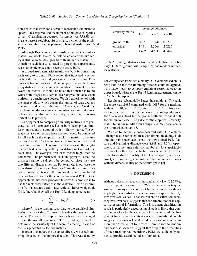
ISMIR 2008 – Session 5a – Content-Based Retrieval, Categorization and Similarity 2
note scales that were considered to represent basic melodic
spaces. This step reduced the number of melodic categories
to ten. Classification accuracy for thaats was 75.83% us-
ing the nearest neighbor. Surprisingly, neither of the pitch-
salience weighted vectors performed better than the unweighted
PCDs.
Although R-precision and classification tasks are infor-
mative, we would like to be able to compare the similar-
ity matrix to some ideal ground-truth similarity matrix. Al-
though no such data exist based on perceptual experiments,
reasonable references may nevertheless be built.
A ground-truth similarity matrix was built by converting
each raag to a binary PCD vector that indicated whether
each of the twelve scale degrees was used in that raag. Dis-
tances between raags were then computed using the Ham-
ming distance, which counts the number of mismatches be-
tween the vectors. It should be noted that a match is found
when both raags use a certain scale degree and also when
both omit a certain scale degree. We also experimented with
the inner product, which counts the number of scale degrees
that are shared between the raags. However, we found that
the Hamming distance matched intuitive notions of distance
better since the absence of scale degree in a raag is as im-
portant as its presence.
One approach to comparing similarity matrices is to gen-
erate lists of hits for each seed using both the empirical simi-
larity matrix and the ground-truth similarity matrix. The av-
erage distance of the hits from the seed would be computed
for all seeds in the empirical similarity matrix, for exam-
ple based on the Euclidean distance between each retrieved
track and the seed. Likewise the distances of the neigh-
bors fetched according to the ground-truth matrix could be
calculated. The averages over each model might then be
compared. The problem with such an approach is that the
distances cannot be directly be compared, since they use
two different distance metrics. For example, in our case the
ground-truth distances are based on Hamming distances be-
tween binary PCDs while the empirical distances are based
on correlation between the continuous-valued PCDs. One
approach that has been proposed to solve this problem is to
use the rank order rather than the distance. Taking inspira-
tion from measures used in text retrieval, Berenzweig et al.
[3] define what they call the Top-N Ranking agreement:
si =N∑
r=1
(αr)r(αc)kr
, (2)
where kr is the ranking according to the empirical sim-
ilarity matrix of the rth-ranked hit using the ground-truth
matrix. The score is computed for each seed and averaged
to give the overall agreement. The αc and αr parameters
determine the sensitivity of the score to ordering in each of
the lists generated by the two metrics.
In order to compare the distances directly we used Ham-
ming distance on the empirical results. This was done by
Average Distancessimilarity matrix
k = 1 k = 5 k = 10
ground-truth 0.0331 0.1444 0.2770
empirical 1.831 2.3669 2.6235
random 4.682 4.668 4.6442
Table 3. Average distances from seeds calculated with bi-
nary PCDs for ground-truth, empirical, and random similar-
ity matrices.
converting each track into a binary PCD vector based on its
raag label so that the Hamming distance could be applied.
This made it easy to compare empirical performance to an
upper bound, whereas the Top-N Ranking agreement can be
difficult to interpret.
Results are substantially better than random. The rank
list score was .1085 compared with .0087 for the random,
with N = 10, αc = .51/3, and αr = .52/3. Using our
method for direct distance comparison, the average distance
for k = 5 was .1444 for the ground truth matrix and 4.668
for the random case. The value for the empirical similarity
matrix fell in the middle of this range (2.367). These results
are summarized in table 3.
We also found that hubness occurred with PCD vectors,
although to a lesser extent than with timbral modeling. Hub
and anti-hub percentages using the unweighted PCD fea-
ture and Hamming distance were 8.9% and 4.7% respec-
tively, using the same definition as above. Not surprisingly
this was less than for the timbre models, most likely due
to the lower dimensionality of the feature space (eleven vs.
twenty). Berenzweig demonstrated that hubness increases
with the dimensionality of the feature space [2].
6 DISCUSSION
Although the artist R-precision is relatively low (32.69%),
this is expected because in NICM instrumentation is quite
similar for many artists. Without further annotation indicat-
ing higher-level artist clusters, we would expect relatively
low precision values. That instrument classification accu-
racy was over 90% suggests that the timbre model is cap-
turing essential information. The instrument classification
result is particularly encouraging since it is likely that con-
necting tracks with the same main instrument would be im-
portant for a recommendation system. Similarly, although
raag R-precision was low, thaat identification was correct in
more than three out of four cases. Comparisons to random
and best-case scenarios suggest that despite the difficulties
of pitch tracking real recordings, PCDs are sufficiently ro-
bust to provide useful melodic information.
575

ISMIR 2008 – Session 5a – Content-Based Retrieval, Categorization and Similarity 2
The results presented suggest that MFCC based timbre
modeling is effective for NICM and generalizes beyond West-
ern popular music. Further we find support for the idea
that hubs may be a general problem when models are con-
structed using GMMs on frame-based MFCC features. This
work also supports the observation that model homogeniza-
tion may lead to improved retrieval precision and classifica-
tion accuracy.
7 APPLICATION
We anticipate that the similarity modeling presented here
could be used as the basis for a music recommendation sys-
tem based on both timbral and melodic characteristics. One
way of combining them would be to create a global distance
metric. In the simplest case, one could weight timbre and
melody equally and simply sum the distances in the respec-
tive similarity matrices. More likely we might imagine giv-
ing users control over the extent to which recommendations
were controlled by one parameter or the other. This could
be done explicitly, for example through a slider interface,
or implicitly in a live application by tracking the perceived
quality of the recommendations, for example by allowing
users to rate the suggested tracks. We conjecture that this
combined model approach may also allow adaptation to dif-
ferent patterns of user preferences; timbre might dominate
the quality judgments of some users, while others might be
more responsive to melodic content.
8 FUTURE WORK
Although encouraging, the current models are clearly quite
simplistic and the results suggest there is ample room for
improvement. On the timbral side, although including more
features may improve performance incrementally, as is often
noted, significant improvement will require a more percep-
tually grounded model. For melodic modeling we intend to
generalize PCDs to include sequential structure though n-
gram modeling. Earlier work has shown that this markedly
improves raag classification performance [6]. Pitch tracking
could also be improved by suppression of accompaniment.
We hope to use the techniques discussed here to create
a CBR system for Indian classical music in which listeners
will be able to generate playlists based either on artists or
tracks, or alternatively based on simple emotional descrip-
tors. This would allow us to replace evaluation based on
measures such as R-precision and artificial ground-truth ma-
trices with more objective measures of the success of these
models in generating music streams.
9 REFERENCES
[1] J.-J. Aucouturier. Ten Experiments on the Modelling ofPolyphonic Timbre. PhD thesis, University of Paris 6,
Paris, France, May 2006.
[2] A. Berenzweig. Anchors and Hubs in Audio-based Mu-sic Similarity. PhD thesis, Columbia University, New
York City, USA, May 2007.
[3] A. Berenzweig, B. Logan, D. Ellis, and B. Whit-
man. A large-scale evaluation of acoustic and subjec-
tive music similarity measures. Computer Music Jour-nal, 28(2):63–76, June 2004.
[4] V.N. Bhatkande. Hindusthani Sangeet Paddhati.Sangeet Karyalaya, 1934.
[5] A. Bhattacharyya. On a measure of divergence between
two statistical populations defined by their probablity
distributions. Bulletin of the Calcutta Mathematics So-ciety, 35:99–110, 1943.
[6] Parag Chordia and Alex Rae. Raag recognition using
pitch-class and pitch-class dyad distributions. In Pro-ceedings of International Conference on Music Informa-tion Retrieval, 2007.
[7] Parag Chordia and Alex Rae. Understanding emotion in
raag music. In Proceedings of International ComputerMusic Conference, 2007.
[8] Parag Chordia, Alex Rae, and Jagadeeswaran
Jayaprakash. Automatic carnatic raag classification. In
Proceedings of the Digital Audio Effects Conference(sumbitted), 2008.
[9] Alain de Cheveigne and Hideki Kawahara. Yin, a funda-
mental frequency estimator for speech and music. Jour-nal of the Acoustical Society of America, 111(4):1917 –
1930, 2002.
[10] R. Duda, P. Hart, and D. Stork. Pattern Recognition andScene Analysis. John Willey, 2001.
[11] Mark Godfrey. Hubs and homogeneity: Improving
content-based modeling. Master’s thesis, Georgia Insti-
tute of Technology, Atlanta, Georgia, April 2008.
[12] E. Pampalk. Computational Models of Music Similarityand their Application in Music Information Retrieval.PhD thesis, Vienna University of Technology, Vienna,
Austria, March 2006.
[13] Y. Rubner, C. Tomasi, and L. J. Guibasg. A metric for
distributions with applications to image databases. In
Proc. of the IEEE International Conference on Com-puter Vision, pages 59–66, Bombay, India, 1998.
576

ISMIR 2008 – Session 5a – Content-Based Retrieval, Categorization and Similarity 2
MULTIPLE-INSTANCE LEARNING FOR MUSIC INFORMATIONRETRIEVAL
Michael I. MandelLabROSA, Dept. Elec. Eng.,Columbia University, NY, [email protected]
Daniel P. W. EllisLabROSA, Dept. Elec. Eng.,Columbia University, NY, [email protected]
ABSTRACT
Multiple-instance learning algorithms train classifiers from
lightly supervised data, i.e. labeled collections of items,
rather than labeled items. We compare the multiple-instance
learners mi-SVM and MILES on the task of classifying 10-
second song clips. These classifiers are trained on tags at
the track, album, and artist levels, or granularities, that have
been derived from tags at the clip granularity, allowing us
to test the effectiveness of the learners at recovering the clip
labeling in the training set and predicting the clip labeling
for a held-out test set. We find that mi-SVM is better than a
control at the recovery task on training clips, with an average
classification accuracy as high as 87% over 43 tags; on test
clips, it is comparable to the control with an average classifi-
cation accuracy of up to 68%. MILES performed adequately
on the recovery task, but poorly on the test clips.
1 INTRODUCTION
There are many high quality sources of metadata about mu-
sical material such as Last.fm, the All Music Guide, Pan-
dora.com, etc. Typically, however, each source provides
metadata only at certain granularities, i.e. describes the mu-
sic only at certain scales. For example, the All Music Guide
provides metadata about many artists and albums, but few
tracks. Similarly, Last.fm users have described a large pro-
portion of artists, a smaller proportion of albums, and an even
smaller proportion of tracks. Furthermore, there are no pub-
licly accessible, large-scale sources of metadata describing
parts of tracks known as clips, here taken to be 10-second
excerpts. This paper describes the use of clip-level classifiers
to refine descriptions from one granularity to finer granular-
ities, e.g. using audio classifiers trained on descriptions of
artists to infer descriptions of albums, tracks, or clips.
Many descriptions of music apply at multiple granulari-
ties, like rap, or saxophone, although certain descriptions are
valid only at specific granularities like seen live or albums Iown. Descriptions valid at one granularity, however, might
only apply to certain elements at a finer granularity. For
example, at the artist level, the Beatles could very reasonably
be tagged psychedelic. This tag would certainly apply to
an album like Sgt. Pepper’s Lonely Hearts Club Band but
would not apply to one like Meet the Beatles. Similarly, the
John Coltrane track “Giant Steps” could very reasonably be
tagged saxophone. While valid for most clips in the track, it
most notably is not valid during the piano solo. This paper
describes systems capable of deriving, from feature similarity
and a list of psychedelic artists or saxophone tracks, the clips
for which these tags are most appropriate.
By considering tags one at a time, as either being present
or absent from a clip, we pose the automatic tagging (autotag-
ging) problem as clip classification. In this framework, the
task of metadata refinement is known as multiple instancelearning (MIL) [6]. In MIL, classifiers are trained on labels
that are only applied to collections of instances, known as
bags. Positive bags contain one or more positive instances,
while negative bags contain no positive instances. Labeled
bags provide less information to the learner than labeled in-
stances, but are still effective at training classifiers. For the
purposes of this paper, clips are the instances to be classified,
and artists, albums, and tracks, in turn, are the bags.
There are two problems addressed in the multiple-instances
learning (MIL) literature, the classification of bags and the
classification of instances. As we are interested in refining
musical metadata from bags to the instances within them, we
only concern ourselves with multiple-instance learners that
are capable of classifying instances. A related problem that
we also examine is the training of a general instance-level
classifier from bag-level labels. This task is slightly different
in that the instances to be labeled are not in the training bags,
and are unseen at training time.
To evaluate the applicability of MIL to music, we use
the data from our MajorMiner game [10]. The game has
collected approximately 12,000 clip-level descriptions of ap-
proximately 2,200 clips from many different tracks, albums,
and artists. The most popular descriptions have been applied
to hundreds of clips, and there are 43 tags that have been
applied to at least 35 clips. Previous authors have generally
used datasets that were labeled at the bag level, making it
difficult to evaluate instance-level classification. Sometimes
a subset of the data was laboriously annotated to allow the
evaluation of instance-level classification. In the MajorMiner
dataset, however, tags are applied directly to clips, making it
577

ISMIR 2008 – Session 5a – Content-Based Retrieval, Categorization and Similarity 2
possible to test instance-level classification in both the train-
ing set and a separate test set. By deriving bag tags from
clip tags in the training set, we can directly test the ability
of multiple instance learners to recover metadata at the in-
stance level from the bag level. This derivation adheres to the
MIL formulation, labeling a given bag positive as a positive
example of a tag if any of its clips have been labeled with
that tag. In addition, a held-out test set allows us to evaluate
the generalization of these classifiers to instances outside the
training set.
1.1 Previous work
A number of authors have explored the link between mu-
sic and text. Whitman and Ellis [14] trained a system for
associating music with noun phrases and adjectives using a
collection of reviews from the All Music Guide and Pitchfork
Media. This work was based on the earlier work described
in [15]. More recently, [12] used a naive Bayes classifier
to both annotate and retrieve music based on an association
between the music and text. Eck et al. [7] used boosted
classifiers to identify the top k tags describing a particular
track, training the classifiers on tags that the users of Last.fm
had entered for the track’s artist.
The MIL problem was first formulated for the task of digit
recognition [8], in which a neural network was trained with
the information of whether a given digit was present, but not
where it was present. In this case, the bags were regions in
which the digit was known to be present and the instances
were shifted and windowed sub-regions. Another early ap-
plication of MIL was to the problem of drug discovery [6],
in which the bags were molecules and the instances were
conformations of those molecules.
MIL has also been applied to object detection in images,
in which the bags were images and the instances were either
automatically segmented image regions [5] or automatically
identified interest points [3]. It has been applied to video
classification to match names and faces [16], in which the
instances were (name, face) pairs, the bags were scenes, and
the task was to determine whether a face had any names
associated with it or not. And it has been applied to text
classification [1], in which the bags were documents and the
instances were sentences or paragraphs.
Many learning frameworks have been applied to MIL,
including boosting [13], Markov chain Monte Carlo [3], and
both 1-norm [4] and 2-norm support vector machines [1]. In
this work, we compare the performance of two SVM-based
MIL methods, mi-SVM [1] and MILES [4], on the task of
autotagging 10-second song clips. These two algorithms are
explained in greater detail in the next section.
2 MULTIPLE-INSTANCE LEARNING
The following notation is common to both mi-SVM and
MILES. We denote the ith bag as Bi, of size �i, and the
jth instance in that bag as xij where j ∈ 1 . . . �i. The label
for bag i is Yi ∈ {−1, 1} and the label for instance xij
is yij . The set of positive bag indices is defined as I+ ≡{i : Yi = 1} and similarly the set of negative bag indices
I− ≡ {i : Yi = −1}. All instances in a negative bag are
negative and a single positive instance in a bag forces the bag
to be positive, meaning that
Yi = maxj
yij . (1)
2.1 The mi-SVM algorithm
The mi-SVM algorithm is the instance-level MIL support
vector machine classifier presented in [1]. Support vector ma-
chines generally maximize the margin around a hyperplane
separating positive from negative examples. In the MIL set-
ting, however, the optimal labeling of the points in positive
bags must be computed as well, creating the following mixed
integer quadratic program (QP)
min{yij},w,b,ξ
12‖w‖22 + C
∑ij
ξij (2)
subject to ∀i : yij(〈w,xij〉+ b) ≥ 1− ξij
yij ∈ {−1, 1}ξij ≥ 0
∀i ∈ I+ :�i∑
j=1
12 (yij + 1) ≥ 1
∀i ∈ I− : yij = −1.
Unfortunately, it is difficult to solve this integer program
directly and [1] presents a heuristic means of approximating
it that converges to a local optimum. This heuristic solves the
standard SVM quadratic program with the labels fixed, and
then uses the solution of the QP to impute the missing labels
for instances in positive bags. This alternation continues
until the labels no longer change. The instance labels are
initialized from the bag labels, so that all instances in positive
bags are initially labeled positive and all instances in negative
bags are initially (and subsequently) labeled negative.
The number of iterations required for convergence de-
pended on the number of instances in each bag, but was
generally on the order of 10-20. We use the dual domain for-
mulation of the standard SVM QP so that a nonlinear kernel
could be used to define the similarity between instances; in
particular, we used the radial basis function (RBF) kernel. In
this dual domain, the classifier is a linear combination of a
hopefully sparse subset of the training instances, the support
vectors.
2.2 The MILES algorithm
Another SVM-based multiple-instance learner is Multiple-
Instance Learning via Embedded Instance Selection (MILES)
578

ISMIR 2008 – Session 5a – Content-Based Retrieval, Categorization and Similarity 2
[4]. While MILES is mainly a bag classifier, it is also able
to derive classifications for instances. Classification with
MILES proceeds in three steps. In the first step, bags are
projected into a large feature space by computing the similar-
ity between each bag and all of the training instances. The
similarity between a bag and an instance is defined as the
maximum similarity between any of the instances in that bag
and the instance in question,
K(Bi,x) ≡ maxk∈1...�i
K(xik,x). (3)
The feature vector for one bag is then
mi ≡ [K(Bi,x11) . . . K(Bi,xN�N)]T . (4)
In the second step, a 1-norm support vector machine [2]
simultaneously learns a classifier and selects discriminative
“features,” i.e. instances. The 1-norm SVM solves the follow-
ing linear program
minw,b,ξ
‖w‖1 + Cμ∑i∈I+
ξi + C(1− μ)∑i∈I−
ξi (5)
subject to ∀i : Yi(〈w,mi〉+ b) ≥ 1− ξi
ξi ≥ 0.
This optimization can be solved as written in the primal do-
main by representing w as the difference of two non-negative
vectors. The �1-norm in the objective function encourages
sparsity in the elements of w forcing many of them to 0.
Since w multiplies instance-similarities, only the instances
corresponding to nonzero elements of w affect the classifi-
cation of new bags. These instances can be considered the
support vectors in this case. Thus, the �1 SVM is also sparse
in its selection of instances.
In the third step, classifications of some of the instances
are derived from the bag classifications. There is one instance
in every bag selected by (3) as the closest to each support
vector. A bag’s classification is not affected by instances that
are not the closest to any support vector, and those instances
can be ignored. Any remaining instance that contributes
more than a threshold amount to the classification of the bag
is considered to be that class itself. We treat unclassified
instances as negatively classified even though [4] allows
instances to remain unclassified.
While MILES has a number of parameters that need to
be tuned, we found its performance quite consistent across a
wide range of parameter settings. The μ parameter controls
the penalty for misclassifying an instance from a positive
bag versus misclassifying an instance from a negative bag.
We found it to have little effect in our experiments except
when within 10−4 of 1, so we kept it at 0.5. The C parameter
controls the trade-off between increasing the margin and
violating class constraints. We found that it could affect
performance when it was small and determined that a value of
10 worked well. The σ parameters is the standard deviation
of the RBF kernel. With feature vectors of unit norm, as
described in the next section, σ = 1 worked well. Similarly,
mi-SVM has C and σ parameters for which C = 1 and σ = 1worked well. All of these parameters were tuned on a subset
of the tags using different train/test breakdowns of the artists
from our main experiments.
3 MUSICAL FEATURES
We use two types of features to describe musical audio. The
spectral features come from our earlier work [9] and capture
timbral aspects of the music related to instrumentation and
production quality. The temporal features are novel, and
summarize the beat, tempo, and rhythmic complexity of the
music in four different frequency bands. All of these features
are calculated on 10-second long clips of songs.
The temporal features are similar to those described in
[11]. They are calculated on the magnitude of the Mel spec-
trogram, including frequencies from 50 Hz to 10,000 Hz,
using a window size of 25 ms and a hop size of 10 ms.
The mel bands are combined into four large bands at low,
low-mid, high-mid, and high frequencies giving the total
magnitude in each band over time. The bands are windowed
and their Fourier transforms are taken, from which the mag-
nitude of the 0-10 Hz modulation frequencies are kept. The
DCT of these magnitudes is then taken and the bottom 50
coefficients of this envelope cepstrum are kept for each band.
The four bands’ vectors are then stacked to form the final,
200-dimensional feature vector.
The spectral features consist of the mean and unwrapped
covariance of a clip’s mel-frequency cepstral coefficients
(MFCCs). The MFCCs are calculated from the mel spec-
trogram used in the temporal features above. Since the
on-diagonal variance terms are strictly positive, their log
is taken to make their distribution more Gaussian. We use
18-dimensional MFCCs, and only keep the unique elements
of the covariance matrix, for a total of 189 dimensions.
The 0-th cepstral coefficient, the DC modulation fre-
quency, and the on-diagonal variance terms tend to be much
larger than other features. We therefore scale each feature to
be zero-mean and unit-variance across the set of all instances
to make the features more comparable to each other. This
scaling improves classification because those dimensions that
are biggest are generally not the most discriminative. After
the feature dimensions are scaled, the temporal features are
multiplied by 1√2
, a value that was determined empirically to
balance the spectral and temporal features well. Finally, the
feature vector for each clip is normalized to have unit length
to avoid problems with degenerate clips.
4 EXPERIMENTS
The data used in our experiments come from our MajorMiner
game [10]. In this game, players label 10-second clips with
579

ISMIR 2008 – Session 5a – Content-Based Retrieval, Categorization and Similarity 2
arbitrary textual descriptions called tags, scoring points when
others describe the same clips with the same tags. The rules
of the game encourage players to use original, yet relevant
tags. In our experiments, we only include tags that have
been verified by at least two different players on at least 35
clips, ensuring that the concept is relevant overall and to the
individual clips. There are 43 such tags and they have been
verified approximately 9000 times in total on approximately
2200 clips selected at random from 3900 tracks.
Note that these data do not include strict negative labels.
While many clips are tagged rock, none are tagged not rock.
Frequently, however, a clip will be tagged many times with-
out being tagged rock. We take this as an indication that
rock does not apply to that clip. More specifically, a negative
example of a particular tag is a clip on which another tag has
been verified, but the tag in question has not.
Certain data-handling issues required extra consideration.
Before using the tags in our experiments, we performed a
number of normalization steps on them, eliminating varia-
tions in punctuation, spelling, and suffixing. Around 45 silent
clips were culled from the dataset and the last clip in each
track was also discarded, as the irregular length of these clips
can cause problems and they are generally silent. Finally, a
number of tracks came from albums where the artist was in-
dicated as “Various Artists” and “Original Soundtrack.” We
excluded these clips from any bags used in our experiments,
but allowed them in the instance-level test set, where bags
were ignored anyway.
4.1 Procedure
The experiment was five repetitions of a two-fold cross-
validation procedure, where artists were assigned to one
fold or the other to make sure tags were learned independent
of artists. Each tag was evaluated independently as a binary
classification task. To create the training set for a particular
tag the positive bags with the most instances of that tag were
selected from the training fold until either they were all se-
lected or 400 instances had been selected. The negative bags
with the most instances were then selected until there were
at most as many negative instances as positive instances. On
average, the selected track, album, and artist bags contained
2.47, 4.44, and 8.17 instances, respectively. In the training
set, bag labels Yi were calculated from instance labels yij
according to (1).
As an illustration, to create the training and testing datasets
for the tag saxophone at the artist granularity, all of the artists
with any clips tagged saxophone are considered positive bags.
So Sonny Rollins would be one positive bag, John Coltrane
another, etc. All artists without any clips tagged saxophoneare considered negative bags. To create the training set, the
positive artists with the most labeled clips are selected, fol-
lowed by the negative artists with the most labeled clips.
In addition to mi-SVM and MILES, two control algo-
rithms were included in the evaluation. The first, referred to
as the naı̈ve approach, assumes that bag labels apply to all of
the instances in a bag and trains an instance-labeling SVM
on those labels directly. The second control, referred to as
the cheating approach, trains on instance labels directly and
serves as a ceiling on performance for instance classification
in the training set. Since there are many negative instances
in positive bags and this algorithm needs to train on an equal
number of positive and negative examples, it only selects a
subset of the negative instances to train on. This selection
causes its slightly imperfect performance.
The maximum number of positive instances, 400, was
chosen to give a reasonable running time for all algorithms.
With 400 labeled instances in positive bags, the largest data
sets would have 800 examples. Training an individual 1-
norm or 2-norm SVM on this many examples takes only a
few seconds, but there were about 5000 SVMs to be trained
over 10 repetitions, on 43 tags, with 3 different bag sizes
for each of 4 algorithms. The slowest algorithm was mi-
SVM, which took 6.7 hours to run on one Intel Xeon 1.89
MHz CPU. Second was the naı̈ve approach, which took 67
minutes, followed by MILES at 42 minutes and the cheating
approach at 24 minutes.
We evaluate the classifiers on two different tasks. The
first, is the recovery of instance labels in the training set.
Since the classifier is trained only on bag labels and not
directly on instance labels, this task is not trivial. To fix a
performance baseline of 0.5, accuracy is evaluated on an
equal number of positive and negative instances from the
training bags. To increase the precision of the measurement,
the maximum number of examples are selected while still
maintaining balance, although this causes the variance of the
estimates to differ between classes.
While recovering instance labels is one useful application
of MIL, it does not allow the classifiers’ performance on
novel instances to be measured accurately, because of the
partial supervision. We instead measure this using instances
from the held-out test set, ignoring any notion of bags. To
facilitate comparison between the accuracy of classifying
each tag, the same number of test examples are selected for
each tag, namely 11 positive and 11 negative (setting the
baseline accuracy again to 0.5). When combined across two
cross validation folds and five repetitions of the experiment,
each class is tested on 220 examples. Since MILES classifies
bags before classifying instances in those bags, each test
point is presented to MILES in its own bag.
5 RESULTS
The overall classification accuracy of the various algorithms
can be seen in Table 1. On the training instances, the cheating
algorithm was the most accurate, followed by mi-SVM, the
naı̈ve algorithm, and MILES. Since the cheating algorithm
is an upper bound on training set accuracy, mi-SVM is the
most accurate realistic classifier, if only by a small margin.
580
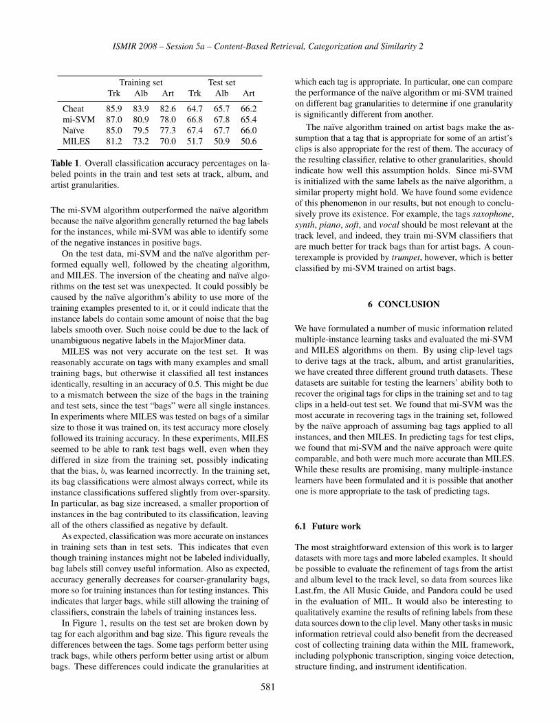
ISMIR 2008 – Session 5a – Content-Based Retrieval, Categorization and Similarity 2
Training set Test set
Trk Alb Art Trk Alb Art
Cheat 85.9 83.9 82.6 64.7 65.7 66.2
mi-SVM 87.0 80.9 78.0 66.8 67.8 65.4
Naı̈ve 85.0 79.5 77.3 67.4 67.7 66.0
MILES 81.2 73.2 70.0 51.7 50.9 50.6
Table 1. Overall classification accuracy percentages on la-
beled points in the train and test sets at track, album, and
artist granularities.
The mi-SVM algorithm outperformed the naı̈ve algorithm
because the naı̈ve algorithm generally returned the bag labels
for the instances, while mi-SVM was able to identify some
of the negative instances in positive bags.
On the test data, mi-SVM and the naı̈ve algorithm per-
formed equally well, followed by the cheating algorithm,
and MILES. The inversion of the cheating and naı̈ve algo-
rithms on the test set was unexpected. It could possibly be
caused by the naı̈ve algorithm’s ability to use more of the
training examples presented to it, or it could indicate that the
instance labels do contain some amount of noise that the bag
labels smooth over. Such noise could be due to the lack of
unambiguous negative labels in the MajorMiner data.
MILES was not very accurate on the test set. It was
reasonably accurate on tags with many examples and small
training bags, but otherwise it classified all test instances
identically, resulting in an accuracy of 0.5. This might be due
to a mismatch between the size of the bags in the training
and test sets, since the test “bags” were all single instances.
In experiments where MILES was tested on bags of a similar
size to those it was trained on, its test accuracy more closely
followed its training accuracy. In these experiments, MILES
seemed to be able to rank test bags well, even when they
differed in size from the training set, possibly indicating
that the bias, b, was learned incorrectly. In the training set,
its bag classifications were almost always correct, while its
instance classifications suffered slightly from over-sparsity.
In particular, as bag size increased, a smaller proportion of
instances in the bag contributed to its classification, leaving
all of the others classified as negative by default.
As expected, classification was more accurate on instances
in training sets than in test sets. This indicates that even
though training instances might not be labeled individually,
bag labels still convey useful information. Also as expected,
accuracy generally decreases for coarser-granularity bags,
more so for training instances than for testing instances. This
indicates that larger bags, while still allowing the training of
classifiers, constrain the labels of training instances less.
In Figure 1, results on the test set are broken down by
tag for each algorithm and bag size. This figure reveals the
differences between the tags. Some tags perform better using
track bags, while others perform better using artist or album
bags. These differences could indicate the granularities at
which each tag is appropriate. In particular, one can compare
the performance of the naı̈ve algorithm or mi-SVM trained
on different bag granularities to determine if one granularity
is significantly different from another.
The naı̈ve algorithm trained on artist bags make the as-
sumption that a tag that is appropriate for some of an artist’s
clips is also appropriate for the rest of them. The accuracy of
the resulting classifier, relative to other granularities, should
indicate how well this assumption holds. Since mi-SVM
is initialized with the same labels as the naı̈ve algorithm, a
similar property might hold. We have found some evidence
of this phenomenon in our results, but not enough to conclu-
sively prove its existence. For example, the tags saxophone,
synth, piano, soft, and vocal should be most relevant at the
track level, and indeed, they train mi-SVM classifiers that
are much better for track bags than for artist bags. A coun-
terexample is provided by trumpet, however, which is better
classified by mi-SVM trained on artist bags.
6 CONCLUSION
We have formulated a number of music information related
multiple-instance learning tasks and evaluated the mi-SVM
and MILES algorithms on them. By using clip-level tags
to derive tags at the track, album, and artist granularities,
we have created three different ground truth datasets. These
datasets are suitable for testing the learners’ ability both to
recover the original tags for clips in the training set and to tag
clips in a held-out test set. We found that mi-SVM was the
most accurate in recovering tags in the training set, followed
by the naı̈ve approach of assuming bag tags applied to all
instances, and then MILES. In predicting tags for test clips,
we found that mi-SVM and the naı̈ve approach were quite
comparable, and both were much more accurate than MILES.
While these results are promising, many multiple-instance
learners have been formulated and it is possible that another
one is more appropriate to the task of predicting tags.
6.1 Future work
The most straightforward extension of this work is to larger
datasets with more tags and more labeled examples. It should
be possible to evaluate the refinement of tags from the artist
and album level to the track level, so data from sources like
Last.fm, the All Music Guide, and Pandora could be used
in the evaluation of MIL. It would also be interesting to
qualitatively examine the results of refining labels from these
data sources down to the clip level. Many other tasks in music
information retrieval could also benefit from the decreased
cost of collecting training data within the MIL framework,
including polyphonic transcription, singing voice detection,
structure finding, and instrument identification.
581

ISMIR 2008 – Session 5a – Content-Based Retrieval, Categorization and Similarity 2
0.4 0.5 0.6 0.7 0.8 0.9 1
hornsvoicebass
trumpetdrums
keyboarddrum machine
acousticinstrumental
solostrings
ambient80s
britishelectronic
fastnoisefunk
vocalslowpopsoft
electronicapianoquiet
countrysynth
distortionpunk
drum and basshouseguitar
beatdance
r&brock
technomale
femalejazz
saxophonehip hop
rap
Classification accuracy
mi−SVM
0.4 0.5 0.6 0.7 0.8 0.9 1Classification accuracy
Cheat
0.4 0.5 0.6 0.7 0.8 0.9 1Classification accuracy
Naive
0.4 0.5 0.6 0.7 0.8 0.9 1Classification accuracy
MILES
Figure 1. Classification accuracy on the test set, broken down by tag. Each pane is an algorithm, and each style of dot is a
different bag granularity. Dots get larger and lighter for coarser granularities: track, album, artist. The tags are ordered by the
accuracy of mi-SVM with track bags. For every dot, N=220, meaning that a difference of around 0.06 is statistically significant.
AcknowledgementsThe authors would like to thank Stuart Andrews for his advice
and useful discussions. This work was supported by the
Fu Foundation School of Engineering and Applied Science
via a Presidential Fellowship, by the Columbia Academic
Quality Fund, and by the National Science Foundation (NSF)
under Grants IIS-0238301 and IIS-0713334. Any opinions,
findings and conclusions or recommendations expressed in
this material are those of the authors and do not necessarily
reflect the views of the NSF.
7 REFERENCES
[1] S. Andrews, I. Tsochantaridis, and T. Hofmann. Support vector ma-chines for multiple-instance learning. In S. Thrun and K. Obermayer,editors, Advances in Neural Information Processing Systems 15, pages561–568. MIT Press, Cambridge, MA, 2003.
[2] J. Bi, K. Bennett, M. Embrechts, C. Breneman, and M. Song. Dimension-ality reduction via sparse support vector machines. Journal of MachineLearning Research, 3:1229–1243, 2003.
[3] P. Carbonetto, G. Dorkó, C. Schmid, H. Kück, and N. de Freitas. Learn-ing to recognize objects with little supervision. International Journal ofComputer Vision, 77(1):219–237, May 2008.
[4] Y. Chen, J. Bi, and J. Z. Wang. MILES: Multiple-instance learning viaembedded instance selection. IEEE Transactions on Pattern Analysisand Machine Intelligence, 28(12):1931–1947, 2006.
[5] Y. Chen and J. Z. Wang. Image categorization by learning and reasoningwith regions. Journal of Machine Learning Research, 5:913–939, 2004.
[6] T. G. Dietterich, R. H. Lathrop, and T. Lozano-Perez. Solving the multi-ple instance problem with axis-parallel rectangles. Artificial Intelligence,89(1-2):31–71, January 1997.
[7] D. Eck, P. Lamere, T. B. Mahieux, and S. Green. Automatic generationof social tags for music recommendation. In J. C. Platt, D. Koller,
Y. Singer, and S. Roweis, editors, Advances in Neural InformationProcessing Systems 20. MIT Press, 2008.
[8] J. D. Keeler, D. E. Rumelhart, and W. K. Leow. Integrated segmenta-tion and recognition of hand-printed numerals. In Advances in NeuralInformation Processing Systems 3, pages 557–563, San Francisco, CA,1990. Morgan Kaufmann Publishers, Inc.
[9] M. I. Mandel and D. P. W. Ellis. Song-level features and support vectormachines for music classification. In J. D. Reiss and G. A. Wiggins,editors, Proc. Intl. Symp. Music Information Retrieval, pages 594–599,September 2005.
[10] M. I. Mandel and D. P. W. Ellis. A web-based game for collecting musicmetadata. In S. Dixon, D. Bainbridge, and R. Typke, editors, Proc. Intl.Symp. Music Information Retrieval, pages 365–366, 2007.
[11] A. Rauber, E. Pampalk, and D. Merkl. Using psycho-acoustic modelsand self-organizing maps to create a hie rarchical structuring of musicby sound similarity. In M. Fingerhut, editor, Proc. Intl. Symp. MusicInformation Retrieval, pages 71–80, 2002.
[12] D. Turnbull, L. Barrington, and G. Lanckriet. Modeling music andwords using a multi-class naive bayes approach. In Proc. Intl. Symp.Music Information Retrieval, October 2006.
[13] P. Viola, J. Platt, and C. Zhang. Multiple instance boosting for objectdetection. In Y. Weiss, B. Schölkopf, and J. Platt, editors, Advancesin Neural Information Processing Systems 18, pages 1417–1424. MITPress, Cambridge, MA, 2006.
[14] B. Whitman and D. Ellis. Automatic record reviews. In Proc. Intl. Symp.Music Information Retrieval, pages 470–477, 2004.
[15] B. Whitman and R. Rifkin. Musical query-by-description as a multiclasslearning problem. In IEEE Workshop on Multimedia Signal Processing,pages 153–156, 2002.
[16] J. Yang, R. Yan, and A. G. Hauptmann. Multiple instance learning forlabeling faces in broadcasting news video. In Proc. ACM Intl. Conf. onMultimedia, pages 31–40, New York, NY, USA, 2005. ACM.
582

ISMIR 2008 – Session 5a – Content-Based Retrieval, Categorization and Similarity 2
MUSIC GENRE CLASSIFICATION: A MULTILINEAR APPROACH
Ioannis Panagakis, Emmanouil Benetos, and Constantine KotropoulosDepartment of Informatics
Aristotle University of ThessalonikiBox 451 Thessaloniki GR-54124, Greece
E-mail: {panagakis, empeneto, costas}@aiia.csd.auth.gr
ABSTRACT
In this paper, music genre classification is addressed in amultilinear perspective. Inspired by a model of auditorycortical processing, multiscale spectro-temporal modulationfeatures are extracted. Such spectro-temporal modulationfeatures have been successfully used in various content-basedaudio classification tasks recently, but not yet in music genreclassification. Each recording is represented by a third-orderfeature tensor generated by the auditory model. Thus, theensemble of recordings is represented by a fourth-order datatensor created by stacking the third-order feature tensorsassociated to the recordings. To handle large data tensorsand derive compact feature vectors suitable for classifica-tion, three multilinear subspace techniques are examined,namely the Non-Negative Tensor Factorization (NTF), theHigh-Order Singular Value Decomposition (HOSVD), andthe Multilinear Principal Component Analysis (MPCA). Clas-sification is performed by a Support Vector Machine. Strat-ified cross-validation tests on the GTZAN dataset and theISMIR 2004 Genre one demonstrate the advantages of NTFand HOSVD versus MPCA. The best accuracies obtained bythe proposed multilinear approach is comparable with thoseachieved by state-of-the-art music genre classification algo-rithms.
1 INTRODUCTION
To manage large music collections, tools able to extract use-ful information about musical pieces directly from audiosignals are needed. Such information could include genre,mood, style, and performer [13]. Aucouturier and Pachet[1] indicate that music genre is probably the most populardescription of music content. Classifying music recordingsinto distinguishable genres is an attractive research topic inMusic Information Retrieval (MIR) community.
Most of the music genre classification techniques, em-ploy pattern recognition algorithms to classify feature vec-tors, extracted from short-time recording segments into gen-res. In general, the features employed for music genre clas-sification are roughly classified into three classes: timbraltexture features, rhythmic features, and pitch content fea-
tures [20]. Commonly used classifiers are Support VectorMachines (SVMs), Nearest-Neighbor (NN) classifiers, orclassifiers, which resort to Gaussian Mixture Models, Lin-ear Discriminant Analysis (LDA), etc. Several common au-dio datasets have been used in experiments to make the re-ported classification accuracies comparable. Notable resultson music genre classification are summarized in Table 1.
Reference Dataset AccuracyBergstra et al. [4] GTZAN 82.50%
Li et al. [12] GTZAN 78.50%Lidy et al. [14] GTZAN 76.80%
Benetos et al. [3] GTZAN 75.00%Holzapfel et al. [6] GTZAN 74.00%
Tzanetakis et al. [20] GTZAN 61.00%
Holzapfel et al. [6] ISMIR2004 83.50%Pampalk et al. [19] ISMIR2004 82.30%
Lidy et al. [13] ISMIR2004 79.70%
Bergstra et al. [4] MIREX2005 82.34%
Lidy et al. [14] MIREX2007 75.57%Mandel et al. [16] MIREX2007 75.03%
Table 1. Notable classification accuracies achieved by mu-sic genre classification approaches.
Recently, within MIR community, genre has been crit-icized as being a hopelessly, ambiguous, and inconsistentway to organize and explore music. Consequently users’needs would be better addressed by abandoning it in favor ofmore generic music similarity-based approaches [17]. Fromanother point of view, end users are more likely to browseand search by genre than either artist similarity or musicsimilarity by recommendation [11]. Furthermore, Aucou-turier et al. [2] have observed that recent systems, which as-sess audio similarity using timbre-based features, have failedto offer significant performance gains over early systemsand in addition their success rates make them unrealistic forpractical use. It is clear that new approaches are needed tomake automatic genre classification systems viable in prac-tice. McKay et al. [17] argues on the importance of con-tinuing research in automatic music genre classification and
583

ISMIR 2008 – Session 5a – Content-Based Retrieval, Categorization and Similarity 2
encourages the MIR community to approach the problem ina inter-disciplinary manner.
The novel aspects of this paper are as follows. First,we use bio-inspired multiscale spectro-temporal features formusic genre classification. Motivated by the fact that eachsound is characterized by slow spectral and temporal mod-ulations and investigations on the auditory system [22], weuse the auditory model proposed in [21] in order to extractfeatures that map a given sound to a high-dimensional repre-sentation of its spectro-temporal modulations. The auditoryhigh-dimensional representation can be viewed as a high-order tensor that is defined on a high-dimensional space.Note that in the field of multilinear algebra, tensors are con-sidered as the multidimensional equivalent of matrices orvectors [8]. In addition, cortical representations are highlyredundant [18]. Therefore, it is reasonable to assume thatthe tensors are confined into a subspace of an intrinsicallylow dimension.
Feature extraction or dimensionality reduction thus aimsto transform such a high-dimensional representation into alow-dimensional one, while retaining most of the informa-tion related to the underlying structure of spectro-temporalmodulations. Subspace methods are suitable for the afore-mentioned goal. Indeed subspace methods, such as Princi-pal Component Analysis (PCA), Linear Discriminant Anal-ysis (LDA), and Non-Negative Matrix Factorization (NMF)have successfully been used in various pattern recognitionproblems. The just mentioned methods deal only with vec-torized data. By vectorizing a typical three-dimensional cor-tical representation of 6 scales × 10 rates × 128 frequencybands results in a vector having dimension equal to 7680.Many pattern classifiers, can not cope with such a high-dimensionality given a small number of training samples. Inaddition, handling such high-dimensional samples is com-putationally expensive. Therefore, eigen-analysis or Singu-lar Value Decomposition cannot be easily performed. De-spite implementation issues, it is well understood that re-shaping a 3D cortical representation into a vector, breaks thenatural structure and correlation in the original data. Thus,in order to preserve natural structure and correlation in theoriginal data, dimensionality reduction operating directly ontensors rather than vectors is desirable. State-of-the-art mul-tilinear dimensionality reduction techniques are employed,e.g. Non-Negative Tensor Factorization (NTF) [3], High-Order Singular Value Decomposition (HOSVD) [9], and Mul-tilinear Principal Component Analysis (MPCA) [15] in or-der to derive compact feature vectors suitable for classifica-tion. Classification is performed by an SVM.
Stratified cross-validation tests on two well-known data-sets, the GTZAN dataset and the ISMIR2004Genre dataset,demonstrate that the effectiveness of the proposed approachis compared with that of state-of-the-art music genre classi-fication algorithms on the GTZAN dataset, while its accu-racy exceeds 80% on the ISMIR2004Genre one.
In Section 2, the computational auditory model and thecortical representation of sound are described. Basic multi-linear algebra and multilinear subspace analysis techniquesare briefly introduced in Section 3. The application of mul-tilinear subspace analysis to cortical representations is dis-cussed in this section as well. Datasets and experimentalresults are presented in Section 4. Conclusions are drawnand future research direction are indicated in Section 5.
2 COMPUTATIONAL AUDITORY MODEL ANDCORTICAL REPRESENTATION OF SOUND
The computational auditory model, proposed in [21], is in-spired by psychoacoustic and neurophysiological investiga-tions in the early and central stages of the human auditorysystem. An acoustic signal is analyzed by the human audi-tory model and a four-dimensional representation of soundis obtained, the so-called cortical representation. The modelconsists of two basic stages. The first stage converts theacoustic signal into a neural representation, the so-called au-ditory spectrogram. This representation is a time-frequencydistribution along a tonotopic (logarithmic frequency) axis.At the second stage, the spectral and temporal modulationcontent of the auditory spectrogram is estimated by mul-tiresolution wavelet analysis. For each frame, the multires-olution wavelet analysis is implemented via a bank of two-dimensional Gabor filters, that are selective to spectrotem-poral modulation parameters ranging from slow to fast tem-poral rates (in Hertz) and from narrow to broad spectralscales (in Cycles/Octave). Since, for each frame, the anal-ysis yields a scale-rate-frequency representation, thus theanalysis results in a four-dimensional representation of time,frequency, rate, and scale for the entire auditory spectro-gram. Mathematical formulation and details about the audi-tory model and the cortical representation of sound can befound in [18, 21].
Psychophysiological evidence justifies the choice of sca-les ∈ {0.25, 0.5, 1, 2, 4, 8} (Cycles / Octave) and posi-tive and negative rates ∈ {±2,±4,±8,±16,±32} (Hz) torepresent the spectro-temporal modulation of sound. Thecochlear model, employed by the first stage, has 128 fil-ters with 24 filters per octave, covering 5 1
3 octaves along thetonotopic axis. For each sound recording, the extracted four-dimensional cortical representation is averaged along timeand the average rate-scale-frequency cortical representationis thus obtained, that is naturally represented by a third-order tensor. Accordingly, the feature tensorD ∈ R
I1×I2×I3+ ,
where I1 = Iscales = 6, I2 = Irates = 10, and I3 =Ifrequencies = 128 results. During the analysis, we haveused the NSL Matlab toolbox 1 .
1 http:// www.isr.umd.edu/CAAR/pubs.html
584
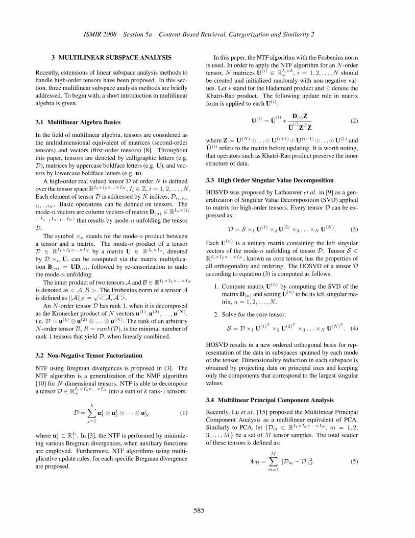
ISMIR 2008 – Session 5a – Content-Based Retrieval, Categorization and Similarity 2
3 MULTILINEAR SUBSPACE ANALYSIS
Recently, extensions of linear subspace analysis methods tohandle high-order tensors have been proposed. In this sec-tion, three multilinear subspace analysis methods are brieflyaddressed. To begin with, a short introduction in multilinearalgebra is given.
3.1 Multilinear Algebra Basics
In the field of multilinear algebra, tensors are considered asthe multidimensional equivalent of matrices (second-ordertensors) and vectors (first-order tensors) [8]. Throughoutthis paper, tensors are denoted by calligraphic letters (e.g.D), matrices by uppercase boldface letters (e.g. U), and vec-tors by lowercase boldface letters (e.g. u).
A high-order real valued tensor D of order N is definedover the tensor space R
I1×I2×...×IN , Ii ∈ Z, i = 1, 2, . . . , N .Each element of tensor D is addressed by N indices, Di1,i2,
i3,...,iN. Basic operations can be defined on tensors. The
mode-n vectors are column vectors of matrix D(n) ∈ RIn×(I1
...In−1In+1...IN ) that results by mode-n unfolding the tensorD.
The symbol ×n stands for the mode-n product betweena tensor and a matrix. The mode-n product of a tensorD ∈ R
I1×I2×...×IN by a matrix U ∈ RJn×In , denoted
by D ×n U, can be computed via the matrix multiplica-tion B(n) = UD(n), followed by re-tensorization to undothe mode-n unfolding.
The inner product of two tensorsA andB ∈ RI1×I2×...×IN
is denoted as < A,B >. The Frobenius norm of a tensor Ais defined as ||A||F =
√< A,A >.
An N -order tensor D has rank 1, when it is decomposedas the Kronecker product of N vectors u(1), u(2), . . . , u(N),i.e. D = u(1) ⊗ u(2) ⊗ . . .⊗ u(N). The rank of an arbitraryN -order tensorD, R = rank(D), is the minimal number ofrank-1 tensors that yield D, when linearly combined.
3.2 Non-Negative Tensor Factorization
NTF using Bregman divergences is proposed in [3]. TheNTF algorithm is a generalization of the NMF algorithm[10] for N -dimensional tensors. NTF is able to decomposea tensor D ∈ R
I1×I2×...×IN+ into a sum of k rank-1 tensors:
D =k∑
j=1
uj1 ⊗ uj
2 ⊗ · · · ⊗ ujN (1)
where uji ∈ R
Ii+ . In [3], the NTF is performed by minimiz-
ing various Bregman divergences, when auxiliary functionsare employed. Furthermore, NTF algorithms using multi-plicative update rules, for each specific Bregman divergenceare proposed.
In this paper, the NTF algorithm with the Frobenius normis used. In order to apply the NTF algorithm for an N -ordertensor, N matrices U(i) ∈ R
Ii×k+ , i = 1, 2, . . . , N should
be created and initialized randomly with non-negative val-ues. Let ∗ stand for the Hadamard product and& denote theKhatri-Rao product. The following update rule in matrixform is applied to each U(i):
U(i) = Ũ(i) ∗ D(i)Z
Ũ(i)
ZT Z(2)
where Z = U(N)& . . .&U(i+1)&U(i−1)& . . .&U(1) andŨ(i) refers to the matrix before updating. It is worth noting,that operators such as Khatri-Rao product preserve the innerstructure of data.
3.3 High Order Singular Value Decomposition
HOSVD was proposed by Lathauwer et al. in [9] as a gen-eralization of Singular Value Decomposition (SVD) appliedto matrix for high-order tensors. Every tensor D can be ex-pressed as:
D = S ×1 U(1) ×2 U(2) ×3 . . .×N U(N). (3)
Each U(n) is a unitary matrix containing the left singularvectors of the mode-n unfolding of tensor D. Tensor S ∈R
I1×I2×...×IN , known as core tensor, has the properties ofall orthogonality and ordering. The HOSVD of a tensor Daccording to equation (3) is computed as follows.
1. Compute matrix U(n) by computing the SVD of thematrix D(n) and setting U(n) to be its left singular ma-trix, n = 1, 2, . . . , N .
2. Solve for the core tensor:
S = D ×1 U(1)T ×2 U(2)T ×3 . . .×N U(N)T
. (4)
HOSVD results in a new ordered orthogonal basis for rep-resentation of the data in subspaces spanned by each modeof the tensor. Dimensionality reduction in each subspace isobtained by projecting data on principal axes and keepingonly the components that correspond to the largest singularvalues.
3.4 Multilinear Principal Component Analysis
Recently, Lu et al. [15] proposed the Multilinear PrincipalComponent Analysis as a multilinear equivalent of PCA.Similarly to PCA, let {Dm ∈ R
I1×I2×...×IN , m = 1, 2,3, . . . , M} be a set of M tensor samples. The total scatterof these tensors is defined as:
ΨD =M∑
m=1
||Dm −D||2F (5)
585

ISMIR 2008 – Session 5a – Content-Based Retrieval, Categorization and Similarity 2
where D is the mean tensor. MPCA aims to define a mul-tilinear transformation that maps the original tensor spaceR
I1×I2×...×IN onto a tensor subspace RP1×P2×...×PN with
Pn < In, n = {1, 2, . . . , N} such that most of the variationobserved in the original tensor objects is captured, assumingthat the variation can be measured by the total tensor scatter.Details and an algorithm for MPCA can be found in [15].
3.5 Multilinear Dimensionality Reduction of Cortical Re-presentations
In each step of a stratified cross-validation test, the datasetused in the experiments (see Section 4) is split into two sub-sets, one used for training and another used for testing. Asmentioned in Section 2, each recording is represented by athird-order feature tensor D ∈ R
Iscales×Irates×Ifrequencies
defining its average cortical representation. Thus, by stack-ing the third order feature tensors, associated to trainingrecordings, a fourth order data tensor T ∈ R
Isamples×Iscales××Irates×Ifrequencies is obtained, where samples is the num-ber of training set recordings.
3.5.1 Multilinear Dimensionality Reduction by NTF
The resulting data tensor T is approximated by k rank-1tensors obtained by NTF. Without loss of generality, NTFapproximation is expressed in matrix form as:
T(1) = U(1)(U(4) & U(3) & U(2))T ⇐⇒TT
(1) = (U(4) & U(3) & U(2))U(1)T
(6)
where T(1) ∈ Rsamples×(scales·rate·frequencies) is the mode-
1 unfolding of tensor T , U(1) ∈ Rsamples×k, U(2) ∈ R
scales×k, U(3) ∈ Rrates×k, and U(4) ∈ R
frequencies×k.From (6), it is clear that every column of TT
(1), i.e. vector-ized cortical representation of a sound, is a linear combina-tion of the basis vectors, which span the columns, of the ba-sis matrix W = U(4) & U(3) & U(2) with coefficients takenfrom the columns of coefficient matrix U(1)T
. PerformingGram-Schmidt orthogonalization on basis matrix W, an or-thogonal basis matrix Q can be obtained. The orthogonal-ized bases span the same space as that of learned bases. Theabove step was employed, because previous research [5] hasshown that orthogonality increases the discriminative powerof the projections. Thus, the suitable features for classifica-tion are derived from the projection x̃i = QT di, where di isthe vectorized cortical representation of the ith recording ofthe dataset.
3.5.2 Multilinear Dimensionality Reduction by HOSVD
The resulting data tensor T is decomposed to its mode-nsingular vectors using the algorithm described in Subsec-tion 3.3. Then, the singular matrices U(scales), U(rates), and
U(frequencies) are obtained. These matrices are orthonor-mal ordered matrices, which contain the subspace of singu-lar vectors. In order to produce a subspace that approxi-mates the original data, each singular matrix is truncated bysetting a threshold so as to retain only the desired principalaxes for each tensor mode.
Features suitable for classification are derived as follows.Each feature tensor Di corresponding to ith recording ofthe dataset is projected onto the truncated orthonormal axes
Û(scales)
, Û(rates)
, and Û(frequencies)
and a new featuretensor X̂i is derived:
X̂i = Di ×1 Û(scales) ×2 Û
(rates) ×3 Û(frequencies)
. (7)
The actual features for classification x̃i are derived from thevectorization of X̂i.
3.5.3 Multilinear Dimensionality Reduction by MPCA
In a similar manner to HOSVD, a multilinear transformationthat maps the original tensor space R
I1×I2×I3 onto a tensorsubspace R
P1×P2×P3 with Pn < In, n = {1, 2, 3}, suchthat the subspace captures most of the variation observed inthe original tensor objects is obtained by MPCA on T . Fea-tures for classification, x̃i, are derived from the vectorizedform of the projected Di using the multilinear transforma-tion obtained by MPCA.
4 EXPERIMENTAL RESULTS
Experiments are performed on two different datasets widelyused for music genre classification [4, 6, 12, 13, 19, 20].The first dataset, abbreviated as GTZAN, consists of fol-lowing ten genre classes: Blues, Classical, Country, Disco,HipHop, Jazz, Metal, Pop, Reggae, Rock. Each genre classcontains 100 audio recordings 30 seconds long. The sec-ond dataset, abbreviated as ISMIR 2004 Genre, is from theISMIR 2004 Genre classification contest and contains 1458full audio recordings distributed over six genre classes asfollows: Classical (640), Electronic (229), JazzBlues (52),MetalPunk (90), RockPop (203), World (244), where thenumber within parentheses refers to the number of record-ings belong to each genre class.
Features are extracted from the cortical representation ofsound using the aforementioned multilinear subspace anal-ysis techniques. The value of parameter k in NTF algorithmwas set to 150 and 140 for the GTZAN dataset and the IS-MIR 2004 Genre one, respectively. The number of retainedprincipal components for each subspace, when HOSVD isemployed for feature extraction, is set to be 5 out of 6 forrate, 7 out of 10 for scale, and 12 out of 128 for frequency.The features extracted by MPCA capture 98% of the totalvariation in each mode. In Figures 1 and 2, the number ofretained principal components in each subspace is shown as
586

ISMIR 2008 – Session 5a – Content-Based Retrieval, Categorization and Similarity 2
80 82 84 86 88 90 92 94 96 980
2
4
6
8
10
12
14
16
18
20
Variance (%)
Num
ber
of P
rinci
pal C
ompo
nent
s
Scale subspaceRate subspaceFrequency subspace
Figure 1. Total number of retained principal components ineach subspace (e.g. scale, rate, and frequency) as a functionof the portion of variance retained for the GTZAN dataset.
a function of the portion of variance retained for the GTZANand ISMIR2004 Genre dataset, respectively.
Classification was performed by SVM with an RBF ker-nel. In order to tune the RBF kernel parameters, a gridsearch algorithm similar to algorithm proposed in [7] wasused. Linear and polynomials kernels were also considered,but they achieve poor performance.
The classification accuracies reported in Table 2 are themean accuracies obtained by 10-fold stratified cross-valida-tion on the full datasets. They are obtained by the variousmultilinear subspace analysis techniques followed by SVM.The row marked by NTF contains the classification resultsachieved by features extracted using NTF for both datasets.The row marked by HOSVD contains the classification re-sults achieved by features extracted using HOSVD, whilethe row marked by MPCA contains the classification resultsachieved by features extracted using MPCA. The effective-ness of NTF and HOSVD as feature extraction techniques isself-evident in both datasets.
GTZAN ISMIR2004GenreNTF 78.20%(3.82) 80.47%(2.26)
HOSVD 77.90% (4.62) 80.95% (3.26)MPCA 75.01% (4.33) 78.53% (2.76)
Table 2. Classification accuracy on GTZAN and IS-MIR2004Genre datasets. The accuracy is calculated by ten-fold stratified cross-validation. The number within paren-theses is the corresponding standard deviation.
On the GTZAN dataset, the best classification accuracyoutperforms the rates reported by Tzanetakis et al. [20](61.0%), Lidy et al. [14] (76.8%), Holzapfel et al. [6]
80 82 84 86 88 90 92 94 96 980
2
4
6
8
10
12
14
16
18
20
22
Variance (%)
Num
ber
of P
rinci
pal C
ompo
nent
s
Scale subspaceRate subspaceFrequency subspace
Figure 2. Total number of retained principal components ineach subspace (e.g. scale, rate, and frequency) as a functionof the portion of variance retained for the ISMIR2004Genredataset.
(74%), and it is comparable to the rate achieved by Li etal. [12] (78.5%). Bergstra et al. in [4] reported a classifica-tion accuracy equal to 82.5% on the GTZAN database, butthey do not disclose details on the experimental setup (e.g.the number of folds).
On the ISMIR2004Genre dataset classification, accura-cies achieved for features extracted by NTF and HOSVDare comparable and exceed 80%. It is not possible to com-pare directly our results with the results obtained by otherresearchers on this dataset, because of the quite different ex-perimental settings [6, 13, 19].
5 CONCLUSIONS - FUTURE WORK
In this paper, the problem of automatic music genre clas-sification is examined in a multilinear framework. Featureshave been extracted from the cortical representation of soundusing three multilinear subspace analysis techniques. Thebest classification accuracies reported in this paper are com-parable with the best accuracies obtained by other state-of-the-art music genre classification algorithms. The effec-tiveness of spectro-temporal features obtained by NTF andHOSVD has been demonstrated. It is true, that multilineartechniques applied in straightforward manner, although theyprovide a more accurate representation to be exploited bythe subsequent classifier, do not yield a recognition accuracymuch higher than state-of-the-art linear algebra techniquesdo. Therefore, more effort is required toward addressing thesmall sample case in the multilinear algebra as well. It isworth noting that the multilinear dimensionality reductiontechniques employed in the paper are unsupervised. In thefuture, supervised multilinear subspace analysis techniques
587

ISMIR 2008 – Session 5a – Content-Based Retrieval, Categorization and Similarity 2
based on NTF will be developed and tested for the automaticmusic genre classification.
Finally, in our experiments, we have considered that eachsong belongs to only one genre class. Obviously, it is real-istic to use overlapping class labels for labelling music bystyle [4]. In general, high-order tensors are structures thatare suitable for a such multi-labelling classification prob-lem.
6 REFERENCES
[1] Aucounturier, J. J. and Pachet F. “Representing musical genre:A state of the art”, Journal of New Music Research, pp. 83-93,2005.
[2] Aucounturier, J. J. and Pachet F. “Improving timbre similarity:How high is the sky?”, Journal of Negative Results in Speechand Audio Sciences,Vol. 1, No. 1, 2004.
[3] Benetos, E. and Kotropoulos C. “A tensor-based approach forautomatic music genre classification”, Proceedings of the Eu-ropean Signal Processing Conference, Lausanne, Switzerland,2008.
[4] Bergstra, J., Casagrande, N., Erhan, D., Eck, D. and Kegl B.“Aggregate features and AdaBoost for music classification”,Machine Learning, Vol. 65, No. 2-3, pp. 473-484, 2006.
[5] Duchene, J. and Leclercq, S. “An optimal transformation fordiscriminant and principal component analysis”, IEEE Trans-actions on Pattern Analysis and Machine Intelligence, Vol. 10,No. 6, pp. 978-983, 1988.
[6] Holzapfel, A. and Stylianou Y. “Musical genre classificationusing nonnegative matrix factorization-based features”, IEEETransactions on Audio, Speech, and Language Processing,Vol.16, No. 2, pp. 424-434, 2008.
[7] Hsu, C., Chang, C. C. and Lin, C. J. A Practical Guide toSupport Vector Classi�cation. Technical Report, Departmentof Computer Science, National Taiwan University, 2003.
[8] Lathauwer, L. Signal Processing Based on Multilinear Alge-bra. Ph.D Thesis, K.U. Leuven, E.E. Dept. - ESAT, Belgium,1997.
[9] Lathauwer, L., Moor, B. and Vandewalle, J. “A multilinear sin-gular value decomposition”, SIAM Journal on Matrix Analysisand Applications, Vol. 21, No. 4, pp. 1253-1278, 2000.
[10] Lee, D. D. and Seung H. S. “Algorithms for non-negative ma-trix factorization”, Advances in Neural Information ProcessingSystems, Vol. 13, pp. 556-562, 2001.
[11] Lee, J. H. and Downie, J. S. “Survey of music informationneeds, uses and seeking behaviours: Preliminary findings”,Proceedings of the Fifth International Symposium on MusicInformation Retrieval, Barcelona, Spain, 2004.
[12] Li, T., Ogihara, M. and Li, Q. “A comparative study oncontent-based music genre classification”, Proceedings of the26th Annual International ACM SIGIR Conference on Re-search and Development in Informaion Retrieval, pp. 282-289,Toronto, Canada, 2003
[13] Lidy, T. and Rauber, A. “Evaluation of feature extractors andpsycho-acoustic transformations for music genre classifica-tion”, Proceedings of the Sixth International Symposium onMusic Information Retrieval, London, UK, 2005.
[14] Lidy, T., Rauber, A., Pertusa, A. and Inesta, J. “Combiningaudio and symbolic descriptors for music classification fromaudio”, Music Information Retrieval Information Exchange(MIREX), 2007.
[15] Lu, H., Plataniotis, K. N. and Venetsanopoulos, A. N. “MPCA:Multilinear principal component analysis of tensor objects”,IEEE Transactions on Neural Networks, Vol. 19, No. 1, pp 18-39, 2008.
[16] Mandel, M. and Ellis, D. “LABROSA’s audio music similarityand classification submissions”, Music Information RetrievalInformation Exchange (MIREX), 2007.
[17] McKay, C. and Fujinaga, I. “Musical genre classification: Isit worth pursuing and how can in be improved?”, Proceedingsof the Seventh International Symposium on Music InformationRetrieval, Victoria, Canada, 2006.
[18] Mesgarani, N., Slaney, M., and Shamma, S. A.“Discriminationof speech from nonspeech based on multiscale spectro-temporal modulations”, IEEE Transactions on Audio, Speech,and Language Processing, Vol. 14, pp. 920-930, 2006.
[19] Pampalk, E., Flexer, A. and Widmer, G. “Improvements ofaudio-based music similarity and genre classification”, Pro-ceedings of the Sixth International Symposium on Music In-formation Retrieval, London, UK, 2005.
[20] Tzanetakis, G. and Cook, P. “Musical genre classification ofaudio signal”, IEEE Transactions on Speech and Audio Pro-cessing, Vol. 10, No. 3, pp. 293-302, July 2002.
[21] Wang, K. and Shamma, S. A. “Spectral shape analysis in thecentral auditory system”, IEEE Transactions on Speech andAudio Processing, Vol. 3, pp. 382-396, 1995.
[22] Woolley, S., Fremouw, T., Hsu, A. and Theunissen, F. “Tuningfor spectro-temporal modulations as a mechanism for auditorydiscrimination of natural sounds”, Nature Neuroscience, Vol.8, pp. 1371-1379, 2005.
588

ISMIR 2008 – Session 5a – Content-Based Retrieval, Categorization and Similarity 2
DIRECT AND INVERSE INFERENCE IN MUSIC DATABASES:
HOW TO MAKE A SONG FUNK?
Patrick Rabbat François Pachet Sophis
[email protected] Sony CSL
ABSTRACT
We propose an algorithm for exploiting statistical properties of large-scale metadata databases about music titles to answer musicological queries. We introduce two inference schemes called “direct” and “inverse” inference, based on an efficient implementation of a kernel regression approach. We describe an evaluation experiment conducted on a large-scale database of fine-grained musical metadata. We use this database to train the direct inference algorithm, test it, and also to identify the optimal parameters of the algorithm. The inverse inference algorithm is based on the direct inference algorithm. We illustrate it with some examples.
1. INTRODUCTION
Large databases of metadata are now available in many domains of digital content such as music (allmusic) or films (imdb). However, the scaling up of content databases makes it increasingly difficult and expensive to maintain manually these metadata databases. The apparition of collaborative tagging addresses this issue by exploiting the power of large distributed networks of users. However, the basic issue of maintaining these repositories of information and coping with their possible incompleteness remains open.
The aim of our study is to design algorithms to turn large-scale databases of musical information into knowledge bases. More precisely, we wish to exploit these databases to perform statistical inferences from partial descriptions of items in order to infer new information about the content.
The inferences we target must be both statistically coherent with the data and computationally tractable. The inferences we consider in this study are of two sorts: direct and inverse. Direct inference consists in inferring the most plausible value of an attribute given a set of “observed attributes”. These inferences can be used typically to lower the maintenance cost of the database: when new items are encountered, only a subset of attributes would then be needed to be observed, and the other ones could be inferred with some degree of confidence. Inverse inference answers a different question: given a set of observed attributes (possibly
complete, i.e. a fully described title), and a target attribute value, we wish to know the minimal modifications to apply to this initial observation set to reach this target attribute value. An application of direct inference is algorithms for automatic music categorization. Some attributes like ‘Style Rap’ or ‘Distorted Guitar’ can be relatively well estimated from the analysis of the acoustic signal [2]. However, acoustic classifiers fail to compute more “high-level” attributes like “Mood sad” or “Lyrics cynical” with a satisfactory performance. The idea of such a hybrid approach is to first compute the best acoustic attributes and, in a second stage, infer the remaining attributes using direct inference.
As an example of inverse inference, we can consider a computer-aided composition tool that suggests musicians how to modify their compositions: starting from an initial composition, the system would observe some “low-level” attributes. The musician could then ask the system what attributes to change, and how, in order to, say, make his title sound “Funk”, or not “aggressive”, or “harmonious”. Inverse inference yields the minimal modifications of the initial title to increase optimally the corresponding probabilities.
In this paper, we propose an algorithm for direct and inverse inference, based on an efficient implementation of a kernel regression approach. We describe an evaluation experiment conducted on a large-scale database of fine-grained musical metadata. We use this database to train the direct inference algorithm, test it, and also to identify the optimal parameters of the algorithm. Inverse inference is based on the direct inference algorithm. We illustrate it with real world examples.
1.1. State-of-the-art
To perform our inferences, we would need ideally a statistical model of our attributes in the form of a Bayesian Network, yielding a compact representation of the underlying distribution of the attributes. If we had such a model inference would be carried out with approximate methods suitable for large networks. We tried to learn such a model of our random variables with the SBNS algorithm proposed in [3]: since our data is sparse, we can use frequent sets (i.e. sets of attributes co-
589
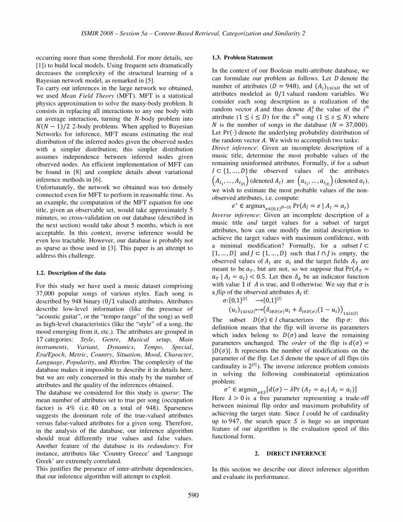
ISMIR 2008 – Session 5a – Content-Based Retrieval, Categorization and Similarity 2
occurring more than some threshold. For more details, see [1]) to build local models. Using frequent sets dramatically decreases the complexity of the structural learning of a Bayesian network model, as remarked in [5]. To carry out inferences in the large network we obtained, we used Mean Field Theory (MFT). MFT is a statistical physics approximation to solve the many-body problem. It consists in replacing all interactions to any one body with an average interaction, turning the �-body problem into ��� � ���� 2-body problems. When applied to Bayesian Networks for inference, MFT means estimating the real distribution of the inferred nodes given the observed nodes with a simpler distribution; this simpler distribution assumes independence between inferred nodes given observed nodes. An efficient implementation of MFT can be found in [8] and complete details about variational inference methods in [6]. Unfortunately, the network we obtained was too densely connected even for MFT to perform in reasonable time. As an example, the computation of the MFT equation for one title, given an observable set, would take approximately 5 minutes, so cross-validation on our database (described in the next section) would take about 5 months, which is not acceptable. In this context, inverse inference would be even less tractable. However, our database is probably not as sparse as those used in [3]. This paper is an attempt to address this challenge.
1.2. Description of the data
For this study we have used a music dataset comprising 37,000 popular songs of various styles. Each song is described by 948 binary (��valued) attributes. Attributes describe low-level information (like the presence of “acoustic guitar”, or the “tempo range” of the song) as well as high-level characteristics (like the “style” of a song, the mood emerging from it, etc.). The attributes are grouped in ��categories: Style, Genre, Musical setup, Main instruments, Variant, Dynamics, Tempo, Special, Era/Epoch, Metric, Country, Situation, Mood, Character, Language, Popularity, and Rhythm. The complexity of the database makes it impossible to describe it in details here, but we are only concerned in this study by the number of attributes and the quality of the inferences obtained. The database we considered for this study is sparse: The mean number of attributes set to true per song (occupation factor) is 4% (i.e.� on a total of 948). Sparseness suggests the dominant role of the true-valued attributes versus false-valued attributes for a given song. Therefore, in the analysis of the database, our inference algorithm should treat differently true values and false values. Another feature of the database is its redundancy. For instance, attributes like ‘Country Greece’ and ‘Language Greek’ are extremely correlated. This justifies the presence of inter-attribute dependencies, that our inference algorithm will attempt to exploit.
1.3. Problem Statement
In the context of our Boolean multi-attribute database, we can formulate our problem as follows. Let denote the number of attributes ( � ���), and ��������� the set of attributes modeled as ��valued random variables. We consider each song description as a realization of the random vector �and thus denote ���the value of the �th attribute (� � � � ) for the �th song (� � � � �) where � is the number of songs in the database (� � ���). Let �����denote the underlying probability distribution of the random vector�. We wish to accomplish two tasks: Direct inference: Given an incomplete description of a music title, determine the most probable values of the remaining uninformed attributes. Formally, if for a subset � !�� " � #the observed values of the attributes
$�%&� " � �%'(')(denoted�%) are $*%&� " � *%'(')(denoted*%), we wish to estimate the most probable values of the non-observed attributes, i.e. compute: +, - ������.-!/��#01'(' ����%2 � +'�% � *%� Inverse inference: Given an incomplete description of a music title and target values for a subset of target attributes, how can one modify the initial description to achieve the target values with maximum confidence, with a minimal modification? Formally, for a subset� !�� " � # and3 !�� " � # such that� 4 3is empty, the observed values of�% are *% and the target fields �5 are meant to be*5 , but are not, so we suppose that����5 �*5'�% � *%� 6 78. Let then 9: be an indicator function with value �if �is true, and otherwise. We say that ;is a flip of the observed attributes �%if: ;<!��#'%' =!��#'%'�>������'%'?@9�A��B�>� C 9�-��B��� � >��D����'%' The subset �;� - �characterizes the flip;: this definition means that the flip will inverse its parameters which index belong to �;�and leave the remaining parameters unchanged. The order of the flip isE�;� �' �;�'. It represents the number of modifications on the parameter of the flip. Let S denote the space of all flips (its cardinality is�'%'). The inverse inference problem consists in solving the following combinatorial optimization problem: ;, - ������B-FGE�;� � H����5 � *5'�% � *%�I Here H J is a free parameter representing a trade-off between minimal flip order and maximum probability of achieving the target state. Since �could be of cardinality up to���, the search space K is huge so an important feature of our algorithm is the evaluation speed of this functional form.
2. DIRECT INFERENCE
In this section we describe our direct inference algorithm and evaluate its performance.
590

ISMIR 2008 – Session 5a – Content-Based Retrieval, Categorization and Similarity 2
2.1. Description of the algorithm
Computing ����%2 � +'�% � *%� for all + - !��#�L'%'is combinatorial and computationally intractable for the dimensions we are dealing with ( � '�' M �), so the basic assumption to break the intractability is that the variables �%2&� " � �%2'(N' are independent given�%. It then
suffices to compute separately ����%2O � �'�% � *%� for all P - !�� " � '� 2'# to determine the most probable values of the inferred attributes�%2. Although this assumption might seem contradictory with our primary aim to model dependencies, the intuition is that the inferred�%2 attributes only depend on observed attributes�%, meaning that subjective attributes emerge solely from objective (possibly acoustic) attributes that will form our observation �. This independence assumption is less strong as the size of the observation set grows. However, the choice of the attributes �% will have to be dealt with carefully, and we discuss this issue later on. To compute ����%2O � �'�% � *%�we use a kernel regression estimator [4] and [7]:
QRS�*%� � T UV@E�*%� �%��D�%2O�W�X�T UV@E�*%� �%��DW�X�
where E�*%� �%��is a distance function indicating the ‘proximity’ between our observed attributes*% and the corresponding values of attributes �% for the �-th song in the database. For instance, E����� could be the Euclidian distance inY'%' counting the number of differences between two binary strings passed as arguments. However, the Euclidian distance treats equivalently both values and�. Yet the sparseness of the data indicates clearly that two binary strings are more similar if they have common 1s than if they have common 0s. To emphasize the important role of common ones, we rather use the Jaccard distance: E�>� Z� � E@�>������[� �Z������[D
� T 9\]^_][�X�T 9\]^_][�X� C T 9\]X�9_]X�[�X�
The numerator is the number of differences between the two arguments, and the denominator is composed of two terms: the first one is again the number of differences and the second term is the number of “1” the strings have in common. Notice that for all>� Z - Y[ � E�>� Z� � �. UV��� is a weighting function with a real parameter ` - Ya7 An obvious property of this function is that it decreases towards as its parameter increases. Intuitively, this means that the closer a song is from our observation *% (using distance E) the greater its weight should be. The integral of the weighting function UV��� should also be finite. Notice that the weighting function needs not be normalized since the estimator QRS is already normalized. A simple choice for UV is a Gaussian filter UV�b� �
cde $� fgVg) but since ` is a free parameter that we have to
tune, a nice property would be to have an intuitive understanding of the value`7For example, with a simple
linear decreasing functionUV�b� � $� � fV)a, the value of
` is just a threshold distance above which songs have a weight set to, and are thus not taken into account in the estimationQRS7 Note that if ` h � our estimator is an empirical mean on all the songs of the database, each song having identical importance, no matter the distance. If
` h athen UV�b� � i��b � �b j k and we are only
estimating the empirical distribution on the data.
2.2. Evaluation & Experiments
This section introduces experiments to assess the performance of our algorithm. We also study the influence of several parameters of the algorithm.
2.2.1. Performance criterion
Our database contains about�l of attributes set to�. This unbalancedness forbids the use of precision or recall to assess our classifiers (a dumb classifier that always predicts an attribute �%2Oto would have an accuracy of�ml). Instead, we use the more suited F-measure. For a given attribute, F-measure (for the true class) is defined as
the mean of precision and recall,n � opqpaq. A classifier
always responding false has a F-measure of 0.
2.2.2. Observed Attributes
In this paragraph we discuss the different choices for the observation set�. The choice can either be driven by applications, or by performance: if the goal is to complete an acoustic automatic categorization system, then there is a canonical order for all the attributes defined by the decreasing performance of some acoustic classifier. We call this order the acoustic order. Another possible choice for � is the set of modifiable attributes. This set of observations will be used in the inverse inference problem and has been determined by hand: modifiable attributes are low-level attributes that a musician can easily modify (like instruments, tempo, etc.). On the other hand, if what we are looking for is to increase the performance of our inference algorithm, the choice for� is not obvious. The simplest way to formulate the problem is to choose� as one of the subsets of !�� " � # of fixed cardinalityr maximizing some global performance criterions for inference:
�t, - ������% !��"��#'%'Xt s uGQRS�*%�I ��S�'%2'v(-!/��#wx
591

ISMIR 2008 – Session 5a – Content-Based Retrieval, Categorization and Similarity 2
The arguments of s are all possible responses to an inference query. The global performance criterion should ‘integrate’ in a certain sense all possible inference responses to all*% - !��#t. Of course, this optimization problem is completely intractable and we shall restrict our empirical study to the case of the acoustic and modifiable attributes.
2.2.3. Experiments
In this paragraph, we assess the influence of the free parameters of the algorithm, namely` andUV and the influence of the choice of the observation�. The performances were computed using leave-one-out cross-validation on the whole dataset.
2.2.3.1 Influence of the smoothing parameter
First, we evaluate the influence of the free parameter ` J on the overall performance. In this experiment, we thus fix the observation� to be the� first attributes in the acoustic order. On Figure 1, we show the performance of our algorithm with` varying in the intervalG��G. The reason we restrict the search to this interval is because intuitively we do not want to take into account all the songs in the database: songs with large distance (close to�) should be ignored and, as we mentioned earlier, ` can be interpreted as a threshold distance. We plotted the F-measure for several individual attributes versus the smoothing parameter` on the rangeG��G. All of the attributes exhibit a bell-shaped F-measure vs. ` curve. This shows that there exists a maximum of the performance for some optimal value of the smoothing parameter. The figure also shows that this optimal value is different from one attribute to another. If the smoothing parameter was unique for all attributes and chosen to maximize the performance of, say, attribute ‘Country France’, the performance of the attribute ‘Variant Wah-wah’ would be zero whereas it could be near�l with an individual fine smoothing tuning. This suggests that we should use one smoothing parameter per attribute to achieve maximum performance as opposed to the classic approach of maximizing a global performance criterion over all attributes. On figure 1 we plotted the cumulative distribution function (cdf) for the set of F-measures (over all inferred attributes) obtained for several choices of the smoothing parameter. A perfect classifier would have a cdf starting at the origin straight to point���� and from then straight to point�����. The worst classifier would have a cdf curve starting at the origin, straight to point���� and then straight to point�����. Visually, the best classifier among our choices for the smoothing parameter is thus the closest curve to that of the perfect classifier. Figure 2 confirms that choosing individually optimized smoothing parameters for
each attribute largely outperforms a global optimized parameter.
Figure 1: Influence of the smoothing parameter on the performance of several classifiers.
Figure 2: CDF of the F-measures over all inferred attributes for several choices of smoothing parameters. We select a unique parameter (for all attributes) that maximizes the sum of F-measures.
2.2.3.2 Influence of the weighting function
A well-known fact of kernel regression is that the choice of the smoothing parameter` is more important than the choice of the weighting function. To confirm this in our case, we computed the performances for all inferred attributes for several functional forms forUV and where ` was optimally chosen for each attribute as discussed above. The observation� is still the first� attributes in the acoustic order. On Figure 3, we plotted the cdf for each set of F-measures obtained for several choices of the weighting function. Figure 3 shows that although there is a slight performance increase for the Gaussian function over other functional forms (with individually optimized smoothing parameters),
�
���
���
���
���
���
��
��
���
� ��� ��� �� ���
��������
���� ������������θθθθ
� �� ����� ����� ������� ������������������� ��� ����!"�������#��$��� ��� �%��&���
�
���
���
���
���
���
��
��
���
��'
�
� ��� ��� �� ��� �
�������������������������������
��������
(�&�)�&�� �*+����, &���������-�.���� � �/��0� �*+����, &���������-�.���� � �1�2����(�&�)�&�� �3��&�����������-�.���� � ��/��0� ���������-�.���� � ��1��2�/��0� ���������-�.���� � ��1��2�
592
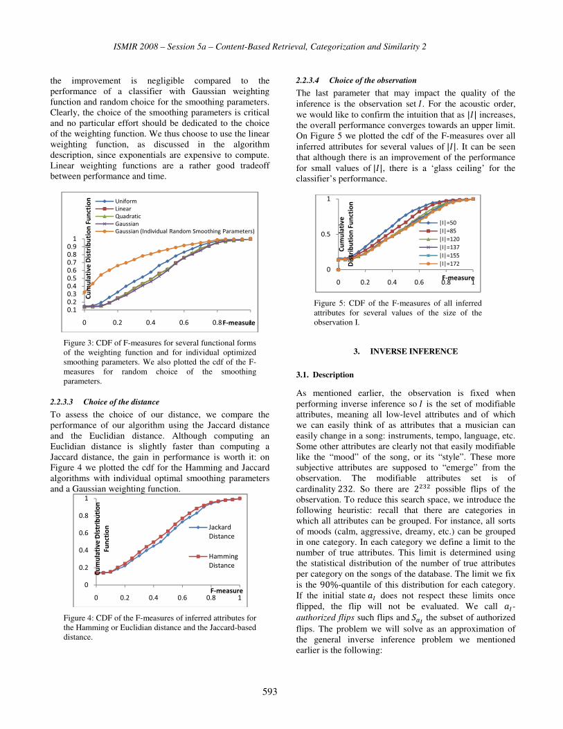
ISMIR 2008 – Session 5a – Content-Based Retrieval, Categorization and Similarity 2
the improvement is negligible compared to the performance of a classifier with Gaussian weighting function and random choice for the smoothing parameters. Clearly, the choice of the smoothing parameters is critical and no particular effort should be dedicated to the choice of the weighting function. We thus choose to use the linear weighting function, as discussed in the algorithm description, since exponentials are expensive to compute. Linear weighting functions are a rather good tradeoff between performance and time.
Figure 3: CDF of F-measures for several functional forms of the weighting function and for individual optimized smoothing parameters. We also plotted the cdf of the F-measures for random choice of the smoothing parameters.
2.2.3.3 Choice of the distance
To assess the choice of our distance, we compare the performance of our algorithm using the Jaccard distance and the Euclidian distance. Although computing an Euclidian distance is slightly faster than computing a Jaccard distance, the gain in performance is worth it: on Figure 4 we plotted the cdf for the Hamming and Jaccard algorithms with individual optimal smoothing parameters and a Gaussian weighting function.
Figure 4: CDF of the F-measures of inferred attributes for the Hamming or Euclidian distance and the Jaccard-based distance.
2.2.3.4 Choice of the observation
The last parameter that may impact the quality of the inference is the observation set�. For the acoustic order, we would like to confirm the intuition that as '�' increases, the overall performance converges towards an upper limit. On Figure 5 we plotted the cdf of the F-measures over all inferred attributes for several values of'�'. It can be seen that although there is an improvement of the performance for small values of'�', there is a ‘glass ceiling’ for the classifier’s performance.
Figure 5: CDF of the F-measures of all inferred attributes for several values of the size of the observation I.
3. INVERSE INFERENCE
3.1. Description
As mentioned earlier, the observation is fixed when performing inverse inference so� is the set of modifiable attributes, meaning all low-level attributes and of which we can easily think of as attributes that a musician can easily change in a song: instruments, tempo, language, etc. Some other attributes are clearly not that easily modifiable like the “mood” of the song, or its “style”. These more subjective attributes are supposed to “emerge” from the observation. The modifiable attributes set is of cardinality���. So there are �oyo possible flips of the observation. To reduce this search space, we introduce the following heuristic: recall that there are categories in which all attributes can be grouped. For instance, all sorts of moods (calm, aggressive, dreamy, etc.) can be grouped in one category. In each category we define a limit to the number of true attributes. This limit is determined using the statistical distribution of the number of true attributes per category on the songs of the database. The limit we fix is the �l-quantile of this distribution for each category. If the initial state*% does not respect these limits once flipped, the flip will not be evaluated. We call *%-authorized flips such flips andKv( the subset of authorized flips. The problem we will solve as an approximation of the general inverse inference problem we mentioned earlier is the following:
������������������������'
�
� ��� ��� �� ��� �
�������������������������������
��������
/��4���5�� ��6��&����������������������7(�&�)�&�� �3��&�����������-�.���� � ��8
�
���
���
��
���
�
� ��� ��� �� ��� �
�����������������������
��������
��������
9��!��&��������
%�����-��������
�
���
�
� ��� ��� �� ��� �
�����������
��������������������
��������
:(:1��:(:1��:(:1���:(:1��:(:1���:(:1��
593

ISMIR 2008 – Session 5a – Content-Based Retrieval, Categorization and Similarity 2
;, - ������B-Fz( {E�;� � H|QRS�*%�vO@� � QRS�*%�D�LvO}-~�
The product is just the estimated value of����5 �*5'�% � *%�.
Do flip = get next authorized flip If ( fitness(flip) is one of the M best fitness’s of order 1 ) Then add flip to M best flip list Until no more authorized flips of order 1 For k=2..max order Do flip = get next authorized flip If flip contains same attributes as at least an element of M best flip list And fitness(flip) is one of the M best Then add flip to temporary M best flip list Until no more authorized flips of order k M best flip list = temporary M best flip list End For
Table 1. The inverse inference algorithm.
We finally explore the search space with the following strategy: we scan through the *%-authorized order� flips and evaluate their fitness; we select the� best authorized order� flips (�is a parameter of the approximation method). We then loop on the order of the flip, and only consider *%-authorized flips that contain the same attributes as at least one of the M best flips of previous order, and update the � best flip list (Table 1).
3.2. Examples
We illustrate here inverse inference with an example. We tried to make “Black or White” by Michael Jackson sound ‘Funk’ (its style was initially tagged as ‘Pop’ and ‘Rock/Pop’). We set tradeoff parameter H � � so that in the optimization process, an additional modification is only accepted if it increases the probability of being ‘Funk’ by at least 0.01. This ‘Probability of Target’ is the probability of being ‘Funk’ given the 232 modifiable attributes of the song “Black or White” (or its flipped version). Initially, this probability is about 0.05 and even though we are not sure the flip we found is optimal, it yields a probability of being ‘Funk’ of about 0.87 which is much better. The set of attributes to flip is the following:
Main Instruments Vocals (Choir)=false Variant forming/shaping=true
Main Instruments Voice (Effects/Sample)=true Main Instruments SFX (Sound Effects)=true
Rhythm funky=true To confirm the funkiness of the song has been increased, we can verify that within the nearest neighbors (NN) of the modified song there are more ‘Funk’ songs than initially. Among the 20 NN of the initial “Black or White”, 4 songs are tagged as “Funk”. Among the 20 NN of its flipped version, 11 songs tagged as “Funk”. So the algorithm is indeed able to translate the high-level query “more funk” into a minimal set of low-level modifications.
4. CONCLUSION
We have presented an attribute inference algorithm for large-scale Boolean databases. The algorithm produces optimally plausible inferences in reasonable time. The algorithm can also be used to perform inverse inference, i.e. answering questions about how to modify a description to make it fit optimally a given attribute. The algorithm is particularly well suited to the exploitation of metadata databases, both for traditional search applications, and for applications that exploit these databases for creation purposes. As such, it can be seen as a first step in turning these databases into knowledge bases.
5. ACKNOWLEDGEMENT
This work was partially supported by the TAGora project (contract IST-34721), funded by the Future and Emerging Technologies program of the European Commission.
6. REFERENCES
[1] Agrawal, R., & Srikant, R. (1994). Fast Algorithms for Mining Association Rules. Proc. 20th Int. Conf. Very Large Data Bases (VLDB), pp. 487-499, Morgan Kaufmann.
[2] Aucouturier, J.-J., Pachet, F., Roy, P., & Beurivé, A. (2007). Signal + Context = Better Classification. Proc. of ISMIR 07, Vienna, Austria.
[3] Goldenberg, A., & Moore, A. (2004). Tractable Learning of Large Bayes Net Structures from Sparse Data. Proc. of the 21st int. conf. on Machine learning. New-York: ACM Int. Conf. Proc. Series.
[4] Nadaraya, E. (1964). On estimating regression. Theor. Probab. Appl., 9, 141-142.
[5] Pavlov, D., Mannila, H., & Smyth, P. (2001). Beyond independence: Probabilistic models for query approximation on binary transaction data. Technical report ICS TR-01-09, Information and Computer Science Department. UC Irvine.
[6] Wainwright, M., & Jordan, M. (2003). Graphical models, exponential families, and variational inference. Technical report, UC Berkeley, Department of Statistics, No. 649, September.
[7] Watson, G. (1964). Smooth regression analysis. Sankhya, Series A (26), 359-372.
[8] Winn, J. M., & Bishop, C. M. (2005). Variational Message Passing. Journal of Machine Learning, 6, 661-694.
594

Session 5b – Feature Representation

.

ISMIR 2008 – Session 5b – Feature Representation
COMBINING FEATURES EXTRACTED FROM AUDIO, SYMBOLIC AND CULTURAL SOURCES
Cory McKay Ichiro Fujinaga Music Technology Area and CIRMMT, Schulich School of Music, McGill University
Montreal, Quebec, Canada [email protected], [email protected]
ABSTRACT
This paper experimentally investigates the classification utility of combining features extracted from separate au-dio, symbolic and cultural sources of musical information. This was done via a series of genre classification experi-ments performed using all seven possible combinations and subsets of the three corresponding types of features.
These experiments were performed using jMIR, a soft-ware suite designed for use both as a toolset for perform-ing MIR research and as a platform for developing and sharing new algorithms.
The experimental results indicate that combining fea-ture types can indeed substantively improve classification accuracy. Accuracies of 96.8% and 78.8% were attained respectively on 5 and 10-class genre taxonomies when all three feature types were combined, compared to average respective accuracies of 85.5% and 65.1% when features extracted from only one of the three sources of data were used. It was also found that combining feature types de-creased the seriousness of those misclassifications that were made, on average, particularly when cultural features were included.
1. INTRODUCTION
Music is a multi-faceted area of inquiry, and there are many factors that influence any individual’s experience of music. Given the variety of possible approaches to study-ing music, researchers can have a tendency to focus their attentions on limited types of music or on particular spe-cialized approaches to studying music. One of the most exciting aspects of the contemporary music information retrieval (MIR) field is that it attempts to break down these barriers using a multi-disciplinary approach to music.
In the past, MIR research has tended to focus on study-ing either audio (e.g., MP3), symbolic (e.g., MIDI) or cul-tural (e.g., web data, user tags, surveys, etc.) sources of information about music. Traditionally, research using each of these sources has been relatively segregated based on whether a researcher had a corresponding background in signal processing, music theory or library sciences and data mining. In recent years, however, MIR researchers have increasingly begun to study these sources of informa-
tion in combination, with a particular emphasis on re-search combining audio and cultural sources of data.
Features extracted from all three types of data can pro-vide valuable information for use in music classification and similarity research. Audio is clearly useful because it is the essential way in which music is consumed, and cul-tural data external to musical content is well-known to have a large influence on our understanding of music [8].
Symbolic data has recently been receiving less attention from MIR researchers than it did in the past. The value of symbolic data should not be overlooked, however, as much of the information associated with high-level musi-cal abstractions that can be relatively easily extracted from symbolic formats is currently poorly encapsulated by the types of features that are typically extracted from audio, which tend to focus primarily on timbral information
Symbolic formats can thus, at the very least, be a pow-erful representational tool in automatic music classifica-tion. This characteristic will become increasingly valuable as polyphonic audio to symbolic transcription algorithms continue to improve. Even though such technologies are still error-prone, it has been found that classification sys-tems can be relatively robust to such errors [6].
This paper focuses on an experimental investigation of the extent to which combining features extracted from the three types of data can be advantageous in automatic mu-sic classification. If the orthogonal independence of the feature types is high, then performance boosts can poten-tially be attained in a variety of applications by combining features extracted from the different data types.
This investigation was performed via sets of automatic genre classification experiments. Genre classification in particular was chosen because it is a complex and difficult task that combines diverse musical variables. The experi-ments could just as easily have been performed using other types of classification, however, such as mood or artist classification. The essential issue being investigated re-mains the potential performance improvements attained by combining features extracted from the three types of data.
2. RELATED RESEARCH
There has been a significant amount of research on com-bining audio and cultural data. Whitman and Smaragdis
597

ISMIR 2008 – Session 5b – Feature Representation
[14] performed particularly important early work on com-bining audio features with cultural data mined from the web, and achieved substantial performance gains when doing so. Dhanaraj and Logan [3] took a more content-based approach by combining information extracted from lyrics and audio. Others have combined audio and cultural data for the purpose of generating music browsing spaces (e.g., [5]). Aucouturier and Pachet [2] used a hybrid train-ing approach based on acoustic information and boolean metadata tags. Research has also been done on using audio data to make correlations with cultural labels, which can in turn improve other kinds of classification (e.g., [12]).
There has been much less work on combining symbolic data with audio data. Lidy et al. [6] did, however, find that combining audio and symbolic data can result in improved performance compared to when only audio data is used.
To the best knowledge of the authors, no previous re-search has been performed on combining symbolic and cultural features or on combining all three feature types.
Far too many papers have been published on automatic genre classification in general to cite with any complete-ness here. One influential work that bears particular men-tion, however, is that of Tzanetakis and Cook [13].
3. THE JMIR SOFTWARE SUITE
jMIR is a suite of software tools developed for use in MIR research. It was used to perform the experiments described in this paper. jMIR includes the following components:
• jAudio [7]: An audio feature extractor that includes implementations of 26 core features. jAudio also in-cludes implementations of “metafeatures” and “aggre-gators” that can be used to automatically generate many more features from these core features (e.g., standard deviation, derivative, etc.).
• jSymbolic [10]: A symbolic feature extractor for proc-essing MIDI files. jSymbolic is packaged with 111 mostly original features [8].
• jWebMiner [11]: A cultural feature extractor that ex-tracts features from the web based on search engine co-occurrence page counts. Many user options are avail-able to improve results, including search synonyms, fil-ter strings and site weightings.
• ACE [9]: A meta-learning classification system that can automatically experiment with a variety of different dimensionality reduction and machine learning algo-rithms in order to evaluate which are best suited to par-ticular problems. ACE can also be used as a simple automatic classification system.
The jMIR components can be used either independently or as an integrated suite. Although the components can read and write to common file formats such as Weka ARFF, jMIR also uses its own ACE XML file formats that
offer a number of significant advantages over alternative data mining formats [9].
The components of jMIR were designed with the fol-lowing goals in mind:
• Provide a flexible set of tools that can easily be applied to a wide variety of MIR-oriented research tasks.
• Provide a platform that can be used to combine re-search on symbolic, audio and/or cultural data.
• Provide easy-to-use and accessible software with a minimal learning curve that can be used by researchers with little or no technological training.
• Provide a modular and extensible framework for itera-tively developing and sharing new feature extraction and classification technologies.
• Provide software that encourages collaboration between different research centers by facilitating the sharing of research data using powerful and flexible file formats.
In order to improve accessibility, each of the jMIR components is, with the temporary exception of ACE, packaged with an easy-to-use GUI. The jMIR components also include user manuals and help systems.
The jMIR components are all implemented in Java, in order to make them as platform-independent as possible. They are open-source and distributed free of charge.1
4. THE SAC DATASET
The SAC (Symbolic, Audio and Cultural) dataset was as-sembled by the authors in order to provide matching sym-bolic, audio and cultural data for use in the experiments described in Section 5. SAC consists of 250 MIDI files and 250 matching MP3s, as well as accompanying meta-data (e.g., title, artist, etc.). This metadata is stored in an iTunes XML file,2 which can be parsed by jWebMiner in order to extract cultural features from the web.
It was decided to acquire the matching MIDI and audio recordings separately, rather than simply synthesizing the audio from the MIDI. Although this made acquiring the dataset significantly more difficult and time consuming, it was considered necessary in order to truly test the value of combining symbolic and audio data. This is because audio generated from MIDI by its nature does not include any additional information other then the very limited data encapsulated by the synthesis algorithms.
SAC is divided into 10 different genres, with 25 pieces of music per genre. These 10 genres consist of 5 pairs of similar genres, as shown in Figure 1. This arrangement makes it possible to perform 5-class genre classification experiments as well as 10-class experiments simply by combining each pair of related genres into one class. An additional advantage is that it becomes possible to meas-
1 jmir.sourceforge.net 2 Contact [email protected] for access to the file.
598

ISMIR 2008 – Session 5b – Feature Representation
ure an indication of how serious misclassification errors are in 10-class experiments by examining how many mis-classifications are in an instance’s partner genre rather than one of the other 8 genres.
Blues: Modern Blues and Traditional Blues Classical: Baroque and Romantic
Jazz: Bop and Swing Rap: Hardcore Rap and Pop Rap Rock: Alternative Rock and Metal
Figure 1: The ten genres found in the SAC dataset.
5. EXPERIMENTAL PROCEDURE
The first step of the experiment was to use jMIR’s three feature extractors to acquire features from each matched audio recording, MIDI recording and cultural metadata. Details on the particular features extracted are available elsewhere ([7], [8], [10] and [11]).
To provide a clarifying example, features might be ex-tracted from a Duke Ellington MP3 recording of Perdido, from an independently acquired MIDI encoding of the same piece, and from automated search engine queries using metadata such as artist and title. Three types of fea-ture sets were therefore extracted for each piece, one cor-responding to each of the three data types.
These three types of features were then grouped into all seven possible subset combinations. This was done once for each of the two genre taxonomies, for a total of four-teen sets of features (as shown in Table 1), in preparation for fourteen corresponding classification experiments de-signed to measure how well the different feature sets per-formed relative to one another.
Feature Type 5-Genre Code 10-Genre Code Symbolic S-5 S-10 Audio A-5 A-10 Cultural C-5 C-10 Symbolic + Audio SA-5 SA-10 Audio + Cultural AC-5 AC-10 Symbolic + Cultural SC-5 SC-10 Symbolic + Audio + Cultural SAC-5 SAC-10
Table 1: The identifying codes for the 14 experiments.
ACE was then trained on and used to classify each of the fourteen feature sets in fourteen independent 10-fold cross-validation experiments. This resulted in two classifi-cation accuracy rates for each of the seven feature type combinations, one for each of the two genre taxonomies. As a side note, ACE includes dimensionality reduction functionality, so training was actually performed with automatically chosen subsets of the available features.
It is desirable not only to determine how effective each of the feature type combinations are at achieving correct classifications, but also how serious those misclassifica-
tions that do arise are. Two classifiers with similar raw classification accuracy rates can in fact be of very different value if the misclassifications made by one classifier result in classes that are more similar to the “correct” class.
A normalized weighted classification accuracy rate was therefore calculated for each of the 10-genre experiments in order to provide insight on error types. This was calcu-lated by weighting a misclassification within a genre pair (e.g., Alternative Rock instead of Metal) as 0.5 of an error, and by weighting a misclassification outside of a pair (e.g., Swing instead of Metal) as 1.5 of an error.
6. RESULTS AND DISCUSSION
6.1. Results
The average classification accuracy rates across cross-validation folds for each of the fourteen experiments out-lined in Table 1 are shown in Table 2, including weighted and unweighted results. Figures 2 and 3 illustrate the un-weighted results for the 5-genre and 10-genre experiments respectively. These results are summarized in Table 3 and Figure 4, which show the average results for all experi-ments using one feature type, all experiments using two feature types and all experiments using three feature types.
6.2. Effects of Combining Feature Types on Accuracy
As can be seen in Figures 2 and 3, all combinations of two or three feature types performed substantially better than all single feature types classified independently. Further-more, combining all three feature types resulted in better performance than most pairs of feature types.
This is illustrated in Figure 4, which shows important average increases in performance when feature types are combined. Combining all three feature types resulted in increases in performance of 11.3% on the 5-genre taxon-omy and 13.7% in the 10-genre taxonomy, compared to the average performances of each of the single feature types classified individually. Considered in terms of per-centage reduction in error rate, this corresponds to impres-sive improvements of 78.0% and 39.3% for the 5 and 10-genre taxonomies, respectively.
A Wilcoxon signed-rank test indicates that, with a sig-nificance level of 0.125, the improvements in performance of two or three feature types over one type were statisti-cally significant in all cases. However, the improvements when three feature types were used instead of two were not statistically significant. The corresponding average increases in performance were only 2.3% and 2.7% for the 5 and 10-genre taxonomies, respectively.
Overall, these results indicate that, at least to some ex-tent, the three different types of features contain or-thogonally independent information, and can therefore be profitably combined for a variety of purposes.
599
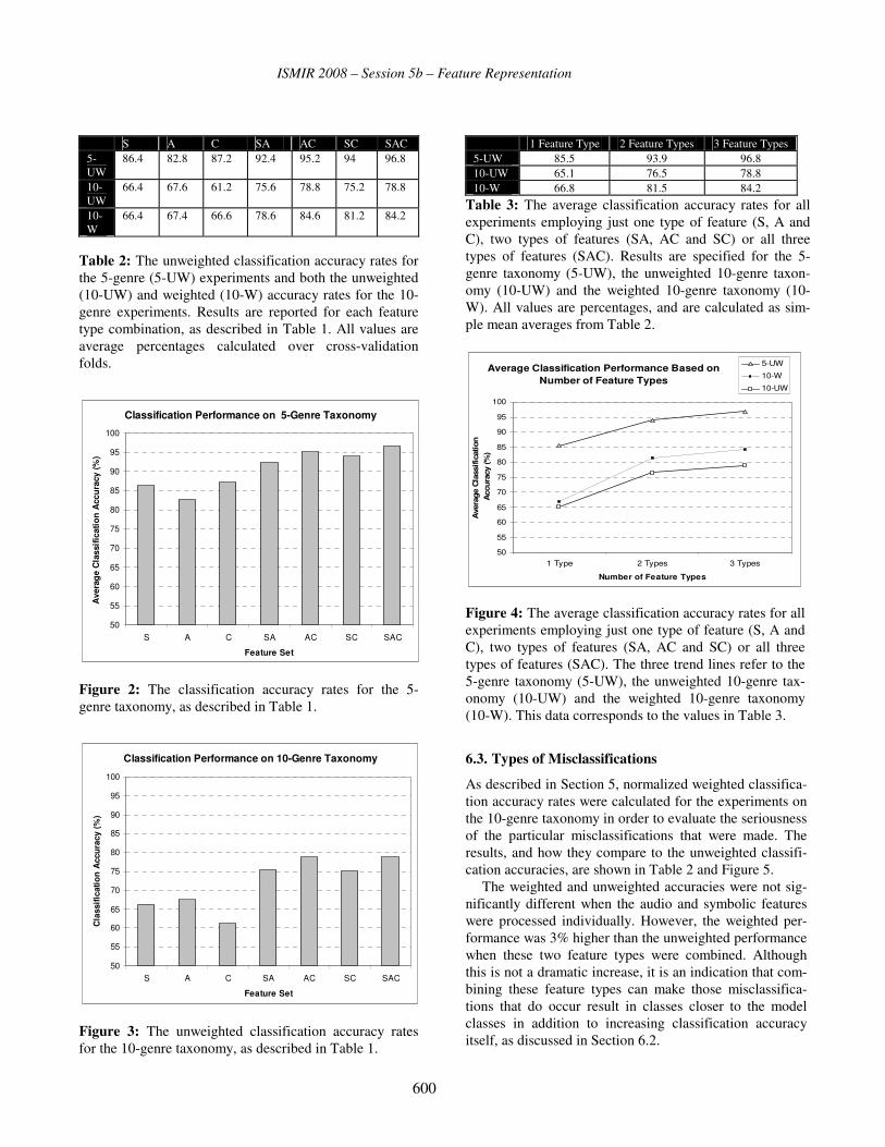
ISMIR 2008 – Session 5b – Feature Representation
S A C SA AC SC SAC 5-UW
86.4 82.8 87.2 92.4 95.2 94 96.8
10-UW
66.4 67.6 61.2 75.6 78.8 75.2 78.8
10-W
66.4 67.4 66.6 78.6 84.6 81.2 84.2
Table 2: The unweighted classification accuracy rates for the 5-genre (5-UW) experiments and both the unweighted (10-UW) and weighted (10-W) accuracy rates for the 10-genre experiments. Results are reported for each feature type combination, as described in Table 1. All values are average percentages calculated over cross-validation folds.
Classification Performance on 5-Genre Taxonomy
50
55
60
65
70
75
80
85
90
95
100
S A C SA AC SC SAC
Feature Set
Ave
rag
e C
lass
ific
atio
n A
ccu
racy
(%
)
Figure 2: The classification accuracy rates for the 5- genre taxonomy, as described in Table 1.
Classification Performance on 10-Genre Taxonomy
50
55
60
65
70
75
80
85
90
95
100
S A C SA AC SC SAC
Feature Set
Cla
ssif
icat
ion
Acc
ura
cy (
%)
Figure 3: The unweighted classification accuracy rates for the 10-genre taxonomy, as described in Table 1.
1 Feature Type 2 Feature Types 3 Feature Types 5-UW 85.5 93.9 96.8 10-UW 65.1 76.5 78.8 10-W 66.8 81.5 84.2
Table 3: The average classification accuracy rates for all experiments employing just one type of feature (S, A and C), two types of features (SA, AC and SC) or all three types of features (SAC). Results are specified for the 5-genre taxonomy (5-UW), the unweighted 10-genre taxon-omy (10-UW) and the weighted 10-genre taxonomy (10-W). All values are percentages, and are calculated as sim-ple mean averages from Table 2.
Average Classification Performance Based on Number of Feature Types
50
55
60
65
70
75
80
85
90
95
100
1 Type 2 Types 3 Types
Number of Feature Types
Ave
rage
Cla
ssific
atio
n
Acc
ura
cy (%
)
5-UW
10-W
10-UW
Figure 4: The average classification accuracy rates for all experiments employing just one type of feature (S, A and C), two types of features (SA, AC and SC) or all three types of features (SAC). The three trend lines refer to the 5-genre taxonomy (5-UW), the unweighted 10-genre tax-onomy (10-UW) and the weighted 10-genre taxonomy (10-W). This data corresponds to the values in Table 3.
6.3. Types of Misclassifications
As described in Section 5, normalized weighted classifica-tion accuracy rates were calculated for the experiments on the 10-genre taxonomy in order to evaluate the seriousness of the particular misclassifications that were made. The results, and how they compare to the unweighted classifi-cation accuracies, are shown in Table 2 and Figure 5.
The weighted and unweighted accuracies were not sig-nificantly different when the audio and symbolic features were processed individually. However, the weighted per-formance was 3% higher than the unweighted performance when these two feature types were combined. Although this is not a dramatic increase, it is an indication that com-bining these feature types can make those misclassifica-tions that do occur result in classes closer to the model classes in addition to increasing classification accuracy itself, as discussed in Section 6.2.
600

ISMIR 2008 – Session 5b – Feature Representation
The differences between the weighted and unweighted classification accuracies were greater in all feature sets that included cultural features. These weighted rates were higher than the unweighted rates by an average of 5.7%, a difference that, based on Student’s paired t-test, is statisti-cally significant with a significance level of 0.005.
Overall, these results indicate that the types of misclas-sifications that occur when cultural features are used are less serious than when audio or symbolic features are used alone. Quite encouragingly, it also appears that this im-provement in error quality carries through when cultural features are combined with audio and symbolic features.
Comparison of Unweighted and Weighted Accuracies
50
55
60
65
70
75
80
85
90
95
100
S-10 A-10 C-10 SA-10 AC-10 SC-10 SAC-10
Feature Set
Cla
ssif
icat
ion
Acc
ura
cy (
%)
Unmodified
Weighted
Figure 5: The differences between the unweighted and weighted classification accuracies on the 10-genre taxon-omy for each of the seven feature type combinations. This data corresponds to the last two rows of Table 2.
6.4. General Genre Classification Performance
In order to put the experimental results described here in context, it is appropriate to compare them with classifica-tion accuracies achieved by high-performing existing spe-cialized genre classification systems. It is important, how-ever, to keep in mind the essential caveat that different classification systems can perform dramatically differently on different datasets, so direct comparisons of classifica-tion accuracies calculated on different datasets can give only a very rough indication of comparative performance.
The MIREX (Music Information Retrieval Evaluation eXchange) evaluations offer the best benchmarking refer-ence points available. Although no evaluations of genre classification based on cultural data have been carried out yet at MIREX, both symbolic and audio genre classifica-tion evaluations have been held, most recently in 2005 and 2007, respectively. The highest accuracy for symbolic
classification was 84.4%, attained on a 9-genre taxonomy by McKay and Fujinaga’s Bodhidharma system [15]. The highest classification accuracy attained in audio classifica-tion was 68.3%, achieved by the University of Illinois’s International Music Information Retrieval Systems Evaluation Laboratory (IMIRSEL) team, on a 10-genre taxonomy [16].
The experiments described in this paper achieved clas-sification accuracies of 67.6% using only features ex-tracted from audio and 66.4% using only features ex-tracted from symbolic data. This is comparable to the best MIREX audio result of 68.3%, but significantly lower than the best MIREX symbolic result of 84.4%, which was achieved on a taxonomy only smaller by one class.
This latter result is intriguing, as jSymbolic uses the same features and feature implementations as Bodhid-harma. The difference is likely due at least in part to the specialized and sophisticated hierarchical and round-robin learning classification ensemble algorithms used by Bo-dhidharma [8], whereas ACE only experiments with gen-eral-purpose machine learning algorithms.
When all three feature types were combined, the jMIR experiments described in this paper achieved a success rate of 78.8% which was still lower than Bodhidharma’s performance, but significantly better than the best audio MIREX results to date.
Taken in the context of the particular difficulty of the SAC dataset, and when it is considered that the accuracy on the 10-genre taxonomy improves to 84.2% when weighted, the results attained here are encouraging, and may be an indication that the ultimate ceiling on perform-ance might not be as low as some have worried [1]. It may well be that the use of more sophisticated machine learn-ing approaches, such as those used by Bodhidharma or by DeCoro et al. [4], combined with the development of new features, could significantly improve performance further.
7. CONCLUSIONS AND FUTURE RESEARCH
The experimental results indicate that it is indeed substan-tively beneficial to combine features extracted from audio, symbolic and cultural data sources, at least in the case of automatic genre classification. Further research remains to be performed investigating whether these benefits general-ize to other areas of music classification and similarity research.
All feature groups consisting of two feature types per-formed significantly better than any single feature types classified alone. Combining all three feature types resulted in small further improvement over the feature type pairs on average, but these additional improvements were not as uniform nor were they statistically significant.
The results also indicate that combining feature types tends to cause those misclassifications that do occur to be less serious, as the misclassifications are more likely to be
601

ISMIR 2008 – Session 5b – Feature Representation
to a class that is more similar to the model class. Such improvements were particularly pronounced when cultural features were involved.
Encouragingly high genre classification accuracy rates were attained. The results of the experiments as a whole provide hope that any ultimate ceiling on genre classifica-tion performance might not be as low as has been worried.
The jMIR software suite was demonstrated to be an ef-fective and convenient tool for performing feature extrac-tion and classification research. The SAC dataset was also found to provide a good basis for performing combined audio, symbolic and cultural experiments.
An important next step is to repeat the experiments per-formed here with MIDI files transcribed from audio, in order to investigate more practically significant use cases where MIDI files do not have to be manually harvested. This would also enable experiments on larger datasets.
There are also plans to combine feature types in more sophisticated ways, such as by segregating them among different weighted specialist classifiers collected into blackboard ensembles. Sophisticated classification tech-niques that take advantage of ontological structuring, such as those utilized in Bodhidharma, also bear further inves-tigation, and could fruitfully be incorporated into ACE. There are also plans to expand SAC as well as to apply jMIR to a wider variety of MIR research applications, such as mood and artist classification.
8. ACKNOWLEDGEMENTS
The authors would like to thank the Centre for Interdisci-plinary Research in Music Media and Technology (CIRMMT), the Social Sciences and Humanities Research Council (SSHRC) and the Canadian Foundation for Inno-vation (CFI) for their generous financial support.
9. REFERENCES
[1] Aucouturier, J. J., and F. Pachet. 2004. Improving timbre similarity: How high is the sky?” Journal of Negative Results in Speech and Audio Sciences 1 (1).
[2] Aucouturier, J. J., and F. Pachet. 2007. Signal + context = better. Proceedings of the International Conference on Music Information Retrieval. 425–30.
[3] Dhanaraj, R., and B. Logan. 2005. Automatic prediction of hit songs. Proceedings of the International Conference on Music Information Retrieval. 488–91.
[4] DeCoro, C., Z. Barutcuoglu, and R. Fiebrink. 2007. Bayesian aggregation for hierarchical genre classification. Proceedings of the International Conference on Music Information Retrieval. 77–80.
[5] Knees, P., M. Schedl, T. Pohle, and G. Widmer. 2006. An innovative three-dimensional user interface for exploring music collections enriched with meta-information from the web. Proceedings of the ACM International Conference on Multimedia. 17–24.
[6] Lidy, T., A. Rauber, A. Pertusa, and J. M. Iñesta. 2007. Improving genre classification by combination of audio and symbolic descriptors using a transcription system. Proceedings of the International Conference on Music Information Retrieval. 61–6.
[7] McEnnis, D., C. McKay, and I. Fujinaga. 2006. jAudio: Additions and improvements. Proceedings of the International Conference on Music Information Retrieval. 385–6.
[8] McKay, C. 2004. Automatic genre classification of MIDI recordings. M.A. Thesis. McGill University, Canada.
[9] McKay, C., R. Fiebrink, D. McEnnis, B. Li, and I. Fujinaga. 2005. ACE: A framework for optimizing music classification. Proceedings of the International Conference on Music Information Retrieval. 42–9.
[10] McKay, C., and I. Fujinaga. 2006. jSymbolic: A feature extractor for MIDI files. Proceedings of the International Computer Music Conference. 302–5.
[11] McKay, C., and I. Fujinaga. 2007. jWebMiner: A web-based feature extractor. Proceedings of the International Conference on Music Information Retrieval. 113–4.
[12] Reed, J., and C. H. Lee. 2007. A study on attribute-based taxonomy for music information retrieval. Proceedings of the International Conference on Music Information Retrieval. 485–90.
[13] Tzanetakis, G., and P. Cook. 2002. Musical genre classification of audio signals. IEEE Transactions on Speech and Audio Processing 10 (5): 293–302.
[14] Whitman, B., and P. Smaragdis. 2002. Combining musical and cultural features for intelligent style detection. Proceedings of the International Symposium on Music Information Retrieval. 47–52.
[15] 2005 MIREX contest results – symbolic genre classification. Retrieved April 1, 2008, from http://www.music-ir.org/evaluation/mirex-results/sym-genre/index.html.
[16] Audio genre classification results - MIREX 2007. Retrieved April 1, 2008, from http://www.music-ir.org/mirex/2007/index.php/Audio_Genre_Classification_Results.
602
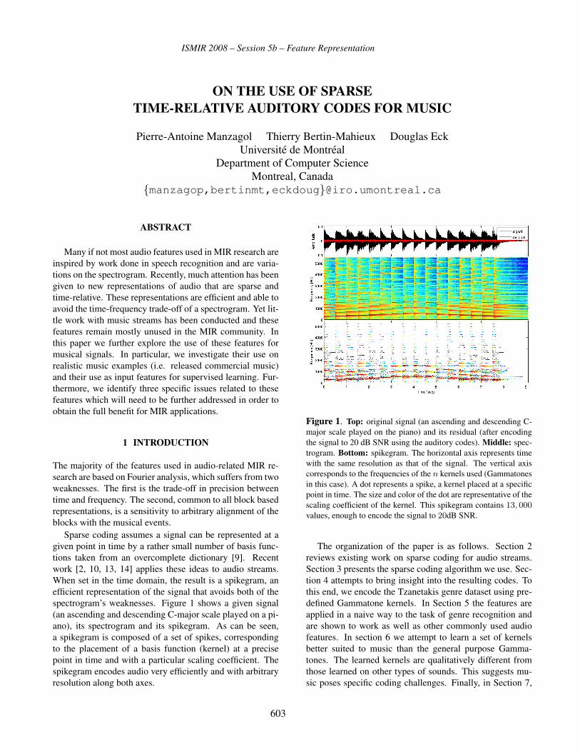
ISMIR 2008 – Session 5b – Feature Representation
ON THE USE OF SPARSETIME-RELATIVE AUDITORY CODES FOR MUSIC
Pierre-Antoine Manzagol Thierry Bertin-Mahieux Douglas EckUniversité de Montréal
Department of Computer ScienceMontreal, Canada
{manzagop,bertinmt,eckdoug}@iro.umontreal.ca
ABSTRACT
Many if not most audio features used in MIR research are
inspired by work done in speech recognition and are varia-
tions on the spectrogram. Recently, much attention has been
given to new representations of audio that are sparse and
time-relative. These representations are efficient and able to
avoid the time-frequency trade-off of a spectrogram. Yet lit-
tle work with music streams has been conducted and these
features remain mostly unused in the MIR community. In
this paper we further explore the use of these features for
musical signals. In particular, we investigate their use on
realistic music examples (i.e. released commercial music)
and their use as input features for supervised learning. Fur-
thermore, we identify three specific issues related to these
features which will need to be further addressed in order to
obtain the full benefit for MIR applications.
1 INTRODUCTION
The majority of the features used in audio-related MIR re-
search are based on Fourier analysis, which suffers from two
weaknesses. The first is the trade-off in precision between
time and frequency. The second, common to all block based
representations, is a sensitivity to arbitrary alignment of the
blocks with the musical events.
Sparse coding assumes a signal can be represented at a
given point in time by a rather small number of basis func-
tions taken from an overcomplete dictionary [9]. Recent
work [2, 10, 13, 14] applies these ideas to audio streams.
When set in the time domain, the result is a spikegram, an
efficient representation of the signal that avoids both of the
spectrogram’s weaknesses. Figure 1 shows a given signal
(an ascending and descending C-major scale played on a pi-
ano), its spectrogram and its spikegram. As can be seen,
a spikegram is composed of a set of spikes, corresponding
to the placement of a basis function (kernel) at a precise
point in time and with a particular scaling coefficient. The
spikegram encodes audio very efficiently and with arbitrary
resolution along both axes.
Figure 1. Top: original signal (an ascending and descending C-
major scale played on the piano) and its residual (after encoding
the signal to 20 dB SNR using the auditory codes). Middle: spec-
trogram. Bottom: spikegram. The horizontal axis represents time
with the same resolution as that of the signal. The vertical axis
corresponds to the frequencies of the n kernels used (Gammatones
in this case). A dot represents a spike, a kernel placed at a specific
point in time. The size and color of the dot are representative of the
scaling coefficient of the kernel. This spikegram contains 13, 000values, enough to encode the signal to 20dB SNR.
The organization of the paper is as follows. Section 2
reviews existing work on sparse coding for audio streams.
Section 3 presents the sparse coding algorithm we use. Sec-
tion 4 attempts to bring insight into the resulting codes. To
this end, we encode the Tzanetakis genre dataset using pre-
defined Gammatone kernels. In Section 5 the features are
applied in a naive way to the task of genre recognition and
are shown to work as well as other commonly used audio
features. In section 6 we attempt to learn a set of kernels
better suited to music than the general purpose Gamma-
tones. The learned kernels are qualitatively different from
those learned on other types of sounds. This suggests mu-
sic poses specific coding challenges. Finally, in Section 7,
603

ISMIR 2008 – Session 5b – Feature Representation
we conclude and identify three specific issues with sparse
coding for further research.
2 RELATED WORK
In this section we present existing work on creating a sparse
encoding of audio signals. First, we present work done in
the frequency domain, and secondly, methods in the time
domain.
2.1 Frequency Domain
Plumbley and Abdallah have many publications about sparse
coding using a code book. See [10] for one of their recent
articles. The main idea is to derive a dictionary of power
spectra from a corpus of audio. One assumes that the spectra
of the signal is a weighted sum of the dictionary elements.
Weights can be derived in number of ways. For example
in [10] a method employing non-negative matrix factoriza-
tion and one employing variance estimation are used. In
the same article, the authors apply their coding to the task
of note detection. However, the most sparse representation
they present is from a time domain method, discussed fur-
ther in Section 2.2.
Another recent approach is introduced by Gardner and
Magnesco [5]. The idea is to compute a transformation of
the spectrogram that gives it higher precision. Thus it is
possible to track a single signal efficiently.
2.2 Time Domain
The most used method in the time domain is based on a
dictionary of kernels that are mapped onto a signal using a
MAP estimate [2, 10, 13]. MAP gives the best reconstruc-
tion error, but is very computationally expensive. Thus, an
approximation is developed in [2], and in [13] MAP is used
as an optimization phase using only a subset of selected ker-
nels.
Two other methods of encoding are described by Smith
and Lewicki [13]. The first one uses a threshold on the cor-
relation between the signal and the kernels; the second one
uses matching pursuit. In experiments, matching pursuit
comes out as the best compromise between computational
complexity and Signal to Noise Ratio (SNR).
The kernels used can be either predefined or learned us-
ing a gradient ascent method. The first option is used by
Smith and Lewicki in [13]. They use Gammatones, which
are known to approximate the cochlear filters. The second
option requires a corpus on which to learn the kernels. In
[10], 57 kernels are learned on a recording of Beethoven’s
Bagatelle containing 57 played notes. Thus they expect each
kernel to model a particular note. In [14], learning is done
on environmental sounds (ambient and transient), mammalian
vocalizations, speech and reversed speech.
0 100 200 300 400 500-0.15
-0.10
-0.05
0.00
0.05
0.10
0.15
Figure 2. Example of a Gammatone kernel.
3 SPARSE TIME-RELATIVE CODING
In this section we describe the model we use for signal rep-
resentation as well as the encoding algorithm. The model is
the same as Smith and Lewicki’s [13] and is used in conjunc-
tion with the matching pursuit encoding, as done in [13, 14].
3.1 Model for signal representation
We represent a signal using a sparse representation based on
shiftable kernels [13]. This models the signal x as a linear
superposition of kernels φ that are placed at precise time
locations τ with a given scaling coefficient s. Formally:
x(t) =M∑
m=1
nm∑i=1
smi φm(t− τm
i ) + ε(t),
where m runs over the different kernels, i over the different
instances of a given kernel and ε represents additive noise.
The length of the kernels is variable.
3.2 Choice of encoding algorithm
Encoding a signal amounts to determining the placement
and scaling of kernels. This is a non-linear process and find-
ing the optimal sparse representation using a generic dictio-
nary of functions is NP-hard [3]. We choose to use matching
pursuit [7], an iterative greedy algorithm, which is shown to
offer a very good trade-off between computational resources
and efficiency of representation [13]. The algorithm works
iteratively in three steps. First, the signal is cross-correlated
with the kernels. The best fitting projection is then selected
and the corresponding kernel identity, placement and scal-
ing are recorded. The projection is then subtracted from the
signal and the procedure is repeated over the residual.
4 ENCODING USING GAMMATONE KERNELS
In this section, we attempt to bring insight into the encoding.
Basic characteristics and properties are illustrated through
604

ISMIR 2008 – Session 5b – Feature Representation
4.9 4.95 5 5.05 5.1 5.15 5.2 5.25 5.3−1
−0.5
0
0.5
1
4.9 4.95 5 5.05 5.1 5.15 5.2 5.25 5.30
10
20
30
40
50
60
Time (sec)
Ker
nel
Figure 3. Top: original signal (close-up of a piano sounding an
A4). Bottom: spikegram (using kernel shapes).
the encoding of the Tzanetakis genre dataset. We use Gam-
matone kernels (see Figure 2), which are motivated as bio-
logical general purpose kernels used in the cochlea. Their
characteristic sharp rise and slow decay also intuitively fit
many real phenomenons. The Gammatones are set accord-
ing to an equivalent rectangular band (ERB) filter bank cochlear
model using Slaney’s auditory toolbox for Matlab [12], as
done in [13]. Unless otherwise stated, we use 64 variable
length normalized Gammatone kernels, with frequencies rang-
ing from 20Hz to the Nyquist frequency.
An important characteristic of the coding is that kernels
are placed at precise time locations. This characteristic al-
lows for precise localisation of events. This is illustrated in
Figure 3, which shows the encoding of a note played on a
piano. The onset clearly stands out.
Another important property of the coding is the fact that
spikes are only used on a per-need basis. In Figure 4 we
see that most of the spikes are placed in the middle of the
song where the energy is. This contrasts with the uniform
distribution of encoding resources in the spectrogram and
illustrates a characteristic of sparse coding: it is adaptive in
the number of spikes for a given encoding ratio. Figure 5
shows the encoding of a metal song. Though the code is
still sparse, more spikes are needed than for the jazz exam-
ple, perhaps due to the constant presence of high-frequency
guitar with heavy distortion.
We further investigate the previous result, i.e. that jazz
seems easier to encode than metal. For this purpose we used
Tzanetakis’ genre dataset later presented in Section 5. In
top of Figure 6 we show the average number of spikes per
song needed to encode songs from different musical genres
to a given SNR. Some genres seem to require more spikes,
metal being the most needy. We placed an upper limit on the
Figure 4. Top: original signal (30 seconds from a jazz song)
and its residual (after encoding the signal to 20dB SNR using the
auditory codes). Middle: spectrogram. Bottom: spikegram.
# of kernels 103 104 2.5 × 10⁴ 5 × 10⁴
32 2.82 (0.97) 8.57 (2.17) 12.69 (2.87) 16.60 (2.88)
64 3.02 (1.03) 9.07 (2.29) 13.44 (2.98) 17.43 (2,70)
128 3.08 (1.04) 9.24 (2.31) 13.76 (2.99) 17.76 (2.52)
Table 1. Mean (standard deviation) of the SNR (dB) obtained
over 100 songs (ten from each genre), as a function of the number
of Gammatones in the codebook and of the maximum number of
spikes allowed to reach a maximal value of 20 dB SNR.
number of spikes computed (105), which is why the metal
box is compressed. To make sure the difficulty lies in the
high frequencies, we divide the 64 kernels in eight bins and
count them separately. The results are at the bottom of Fig-
ure 6. The highest frequencies are on the leftt, the lowest on
the right. As expected, many high frequency Gammatones
were used for metal songs, whereas classical or jazz songs
required few.
It is also interesting to determine the effect on the signal
to noise ratio of using different numbers of kernels in the
ERB and different numbers of spikes in the spikegram. The
results are presented in Table 1. Surprisingly, the number
of kernels has relatively little impact for the tested range of
values.
5 GENRE RECOGNITION
In order to explore the discriminative ability of the spikegram
representation, we apply it to the classification task of genre
recognition. As classifier, we use the AdaBoost meta-learning
algorithm. This choice is motivated by the fact that source
code [8] is available as well as published results for a set
of genre recognition experiments [1]. Those experiments
605

ISMIR 2008 – Session 5b – Feature Representation
Figure 5. Top: original signal (30 seconds from a metal song)
and its residual (after encoding the signal to 20dB SNR using the
auditory codes). Middle: spectrogram. Bottom: spikegram.
were performed on a freely available dataset from Tzane-
takis. (Similar datasets were used for previous MIREX con-
tests. However those datasets are not available for down-
load.)
The Tzanetakis genre dataset contains one thousand 30-
second songs evenly distributed among 10 genres and is
used in several papers [1, 16, 15, 6]. The dataset is very
small and is annotated with only a single winner-take-all
genre label. Though we believe the dataset is suitable for
exploring the predictive power of the spikegram, it is clearly
too small to reflect the challenges faced in finding structure
in large datasets of audio.
5.1 Algorithm
AdaBoost [4] is a meta-learning method that constructs a
strong classifier from a set of simpler classifiers, called weaklearners in an iterative way. Originally intended for bi-
nary classification, there exist several ways to extend it to
multiclass classification. We use AdaBoost.MH [11] which
treats multiclass classification as a set of one-versus-all bi-
nary classification problems. In each iteration t, the algo-
rithm selects the best classifier, called h(t) from a pool of
weak learners, based on its performance on the training set,
and assigns it a coefficient α(t). The input of the weaklearner is a d-dimensional observation vector x ∈ �d con-
taining audio features for one segment of data (5 seconds
in our experiments). The output of h(t) is a binary vector
y ∈ {−1, 1}k over the k classes. h(t)l = 1 means a vote for
class l by a weak learner while h(t), −1 is a vote against.
After T iterations, the algorithm output is a vector-valued
classical disco jazz pop rock blues countryhiphop metal reggae10000
20000
30000
40000
50000
60000
70000
80000
90000
100000
classical disco jazz pop rock blues countryhiphop metal reggae0
5000
10000
15000
20000
25000
30000
Figure 6. Top: box-and-whisker plot of the number of spikes (out
of a maximum of 105) required to encode songs from various gen-
res up to a SNR of 20dB. The red line represents the median and
the box extends from the lower quartile to the upper one. Bottom:Bar plot of the mean number of kernels used per song depending
on the genre. The 64 kernels are split into eight bins going from
the highest frequency Gammatones (left) to the lowest ones (right).
discriminant function:
g(x) =T∑
t=1
α(t)h(y)(x) (1)
We obtain a single label by taking the class with the “most
votes” i.e f(x) = arg maxl gl(x). As weak learner we use
single stumps, a simple threshold on one element of the fea-
ture vector.
We use an AdaBoost method for genre recognition based
on a method detailed in Bergstra et al. [1].
5.2 Features from the spikegram
The input of the classifier needs to be a feature vector of
fixed size for every segment of a song (5 seconds segments
here). Of course, a sparse code is designed to adapt to
specific audio signals. The number of spikes per segment
changes, and the spikes can be positioned at any given mu-
sic frame. Thus we have encode the information about the
spikes differently in order to use it as input to a typical clas-
sifier.
Here we try two types of features based on the spikes.
First, we simply count the number of times each spike is
used in every segment, and we also sum their scaling coeffi-
cients s. We also give the same information, but normalized
by the number of spikes in the segment. Finally, we give the
classifier the total number of spikes in this segment. For 64kernels, this yields an input vector of size 257 per segment.
606

ISMIR 2008 – Session 5b – Feature Representation
feat. SC feat. SC + MFCC MFCC (B.)
63.0% 68.2% 63%
Table 2. Genre recognition results on Tzanetakis dataset with 5-
fold cross-validation using the sparse code features (SC), the sparse
code features and our implementation of MFCC (SC + MFCC) and
result using MFCC from Bergstra et al. [1] (B.). Result from [1] is
approximate (taken from a graph).
5.3 Results
Results are reported using a 5-fold cross-validation. For
more details about reported results on this dataset in the lit-
erature, see Bergstra et al. [1].
Using AdaBoost.MH with single stumps as weak learn-
ers, and 5-second segments, Bergstra et al. [1] report an er-
ror per song of about 63% using MFCCs. Our results using
the features derived from the spikegrams are presented in
Table 2. We see that even with a naive use of the spikegram,
results are comparable with commonly used audio features.
The spikegrams also add information to the MFCC as can
be seen in Column 2 of Table 2.
6 LEARNING KERNELS
The spikegrams used in the previous sections were based
on the use of kernels of a specific predefined form (Gam-
matones). It is also possible to learn the kernels as done
in [10, 14] over different audio corpora. Here we investigate
the learning of kernels for western commercial music. There
are at least three motivations for this. First, we hope to better
encode music with learned kernels than with Gammatones.
Secondly, these kernels should be more efficient as input for
MIR tasks. Thirdly, perhaps these learned kernels can form
meaningful blocks representing concepts like compression,
note onsets or timber. This was the case in Plumbley et al.
[10] where the authors could relate the learned kernels to pi-
ano notes. The difference here is that we train on more com-
plex music and we put less constraint on the kernel lengths.
6.1 Algorithm
The learning is done by gradient ascent. The approximate
gradient of a signal x, given a kernel φ, is (from [14]):
∂
∂φp(x|φ) =
1σε
∑i
ŝi[x− x̂]τi (2)
We can then perform gradient ascent on every dimension
of the kernels using the residual signal at corresponding po-
sitions. The σε is constant and can be ignored as we set the
learning rate empirically.
In our experiments, 32 kernels are initialized using ran-
dom values drawn from a Gaussian distribution. Through-
out the learning, the kernels are kept normalized. We use
0.0 1500.0
0
0.0 2000.0
1
0.0 350.0
2
0.0 200.0
3
0.0 800.0
4
0.0 1600.0
5
0.0 800.0
6
0.0 100.0
7
0.0 500.0
8
0.0 1400.0
9
Figure 7. Examples of learned kernels
kernel 103 104 2.5 × 10⁴ 5 × 10⁴
gammatones 2.82 (0.97) 8.57 (2.17) 12.69 (2.87) 16.60 (2.88)
learned 1.86 (0.57) 6.06 (1.49) 8.86 (2.00) 11.53 (2,37)
Table 3. Mean (standard deviation) of the SNR (dB) obtained
over 100 songs (ten from each genre) with either 32 Gammatones
or 32 learned kernels in the codebook.
a database containing tens of thousands of MP3s. Learn-
ing proceeds by iteratively randomly choosing a song from
the database, encoding it using 1000 spikes, computing the
residual signal and performing gradient ascent on the ker-
nels. The learning rate was set to 0.01 and we did approx-
imately 2000 iterations. Figure 7 shows samples from the
32 kernels we learned. The learned kernels are qualitatively
different from Gammatones. They closely resemble those
learned by [10]. However, our kernels are of variable length
which may be better suited to encoding music with varying
note durations.
6.2 Learned Kernels versus Gammatones
As a first experiment, we evaluate how well the learned ker-
nels encode songs compared to the Gammatones. Results
are shown in Table 3. Unfortunately, Gammatones perform
significantly better at this task. This is a surprising result, as
the learned kernels are trained to optimize this specific cost,
suggesting that learning kernels for complex music poses
specific challenges.
As a second experiment, we use the 32 learned kernels as
input for genre recognition, and we compare the results with
those obtained using 32 Gammatones. Results are shown in
Table 4. We compare the results when encoding using 103
607

ISMIR 2008 – Session 5b – Feature Representation
gamma (1K) learn (1K) gamma(10K) learn (10K)
47.5 % 46.3 % 52.5 % 54.3 %
Table 4. Genre recognition results on Tzanetakis dataset
with 5-fold cross-validation. Number in parentheses is the
maximum number of spikes used to encode each song.
and 104 spikes for computational reasons. Learned kernels
seem to perform similarly as Gammatones. This shows that
the encoding capacity of kernels is different from their pre-
dictive property for a particular task.
7 DISCUSSION AND FUTURE WORK
Our goal with this work is to draw further attention to time-
relative sparse codings. These codes manage to avoid the
weaknesses of the spectrogram and encode an audio signal
very efficiently. Yet there are three issues related to their
use that will need to be addressed. The first is how to prop-
erly use them as input to MIR tasks. Indeed, in our genre
recognition experiments, we summarize spike counts and
scaling coefficients over a block. This destroys the useful
time-relative configurations of the spikes and reintroduces
a sensitivity to arbitrary block alignment. The fact that we
are still able to get results comparable to MFCCs shows the
potential of the features. The second issue relates to learn-
ing in the case of complex music. Our work seems to reveal
specific difficulties. In particular, kernels trained over mu-
sic tended to continually grow, and thus we had to enforce
some length constraints. The disappointing results are also
indicative that the learning problem becomes difficult with
complex music. Solutions might lie in using weight decays,
and starting from kernels trained on less complex signals.
Finally, there is an issue with the computational complex-
ity of the technique. Even with the use of matching pur-
suit, the computational requirements of encoding are above
real time, which may not suit all applications. Answers may
rely in performing approximate matching pursuit, or learn-
ing a function to do an approximate encoding using machine
learning.
8 ACKNOWLEDGEMENTS
We would like to thank James Bergstra for helpful discus-
sions. Pierre-Antoine Manzagol is supported by an FQRNT
scholarship. Thierry-Bertin Mahieux and Douglas Eck are
supported by an NSERC discovery grant.
9 REFERENCES
[1] J. Bergstra, N. Casagrande, D. Erhan, D. Eck, and B. Kégl.
Aggregate features and AdaBoost for music classification. Ma-chine Learning, 65(2-3):473–484, 2006.
[2] T. Blumensath and M. Davies. Sparse and shift-invariant repre-
sentations of music. IEEE Transactions on Speech and AudioProcessing, 2006.
[3] G. Davis, S. Mallat, and M. Avellaneda. Adaptive greedy
approximations. Constructive approximation, 13(1):57–98,
2004.
[4] Y. Freund and R.E. Shapire. Experiments with a new boost-
ing algorithm. In Machine Learning: Proceedings of the Thir-teenth International Conference, pages 148–156, 1996.
[5] T. J. Gardner and M. O. Magnasco. Sparse time-frequency rep-
resentations. Proceedings of the National Academy of Science,
103:6094–6099, April 2006.
[6] Tao Li and George Tzanetakis. Factors in automatic musical
genre classification. In IEEE Workshop on Applications of Sig-nal Processing to Audio and Acoustics, 2003.
[7] S.G. Mallat and Zhifeng Zhang. Matching pursuits with time-
frequency dictionaries. Signal Processing, IEEE Transactionson, 41(12):3397–3415, December 1993.
[8] Multiboost, a pure C++ implementation of Ad-
aBoost.MH by N. Casagrande available at
http://www.iro.umontreal.ca/˜casagran/.
[9] B. A. Olshausen and D. J. Field. Emergence of simple-cell re-
ceptive field properties by learning a sparse code for natural
images. Nature, 381:607–609, June 1996.
[10] M. Plumbley, S. Abdallah, T. Blumensath, and M. Davies.
Sparse representations of polyphonic music. Signal Process-ing, 86(3):417–431, March 2006.
[11] R. E. Schapire and Y. Singer. Improved boosting algo-
rithms using confidence-rated predictions. Machine Learning,
37(3):297–336, 1999.
[12] M. Slaney. Auditory toolbox, 1998. (Tech. Rep. No. 1998-
010). Palo Alto, CA:Interval Research Corporation.
[13] E. Smith and M. S. Lewicki. Efficient coding of time-relative
structure using spikes. Neural Computation, 17(1):19–45,
2005.
[14] E. Smith and M. S. Lewicki. Efficient auditory coding. Nature,
439:978–982, February 2006.
[15] George Tzanetakis and Perry Cook. Musical genre classifica-
tion of audio signals. IEEE Transactions on Speech and AudioProcessing, 10(5):293–302, Jul 2002.
[16] George Tzanetakis, Andrey Ermolinskyi, and Perry Cook.
Pitch histograms in audio and symbolic music information re-
trieval. In Michael Fingerhut, editor, Proceedings of the ThirdInternational Conference on Music Information Retrieval: IS-MIR 2002, pages 31–38, Oct 2002.
608

ISMIR 2008 – Session 5b – Feature Representation
A ROBUST MUSICAL AUDIO SEARCHMETHODBASED ON DIAGONAL DYNAMIC PROGRAMMINGMATCHING
OF SELF-SIMILARITY MATRICES
Tomonori IzumitaniNTT Communication Science Laboratories
Kunio KashinoNTT Communication Science Laboratories
ABSTRACT
We propose a new musical audio search method based onaudio signal matching that can cope with key and tempovariations. The method employs the self-similarity matrixof an audio signal to represent a key-invariant structure ofmusical audio. And, we use dynamic programming (DP)matching of self-similarity matrices to deal with time vari-ations. However, conventional DP-based sequence match-ing methods cannot be directly applied for self-similaritymatrices because they cannot treat gaps independently ofother time frames. We resolve this problem by introduc-ing “matched element indices,” which reflect the history ofmatching, to a DP-based sequence matching method. Weperformed experiments using musical audio signals. Theresults indicate that the proposed method improves the de-tection accuracy in comparison to that that obtained by twoconventional methods, namely, DP matching with chroma-based vector rotations and a simple matching of self-similarityfeature vectors.
1 INTRODUCTION
Musical audio search, that is, identifying the title and corre-sponding locations in an audio database from a short musi-cal audio excerpt of a query, has become important with therapid expansion of digital content utilization.
A technology known as audio fingerprinting has beenwidely used to search for identical audio signals to queries.Most audio fingerprinting systems can be applied to audiosignals with noises or other signal distortions. However, it isalso demanded to cope with other kinds of variations causedby different players, keys, tempi, arrangements, and so on.
We focus on a musical audio search task where audio sig-nals include key and tempo variations. For this task, manyapproaches have been reported. An early work using thechroma-based features was reported by Nagano et al., whoproposed a feature representation named the polyphonic bi-nary feature vector (PBFV) [1]. Their method deals withkey variations by rotating query vector elements. They usedbeat detection and dynamic programming for tempo varia-tions. Müller et al. also used chroma-based features for au-dio matching with different timbres played by various play-ers [2].
For similar purposes, cover song detection methods havebeen proposed. Typically, they detect the same title as thequery in the database by comparing music tracks. Ellis etal. proposed a method based on chroma-based features anda beat tracking technique [3]. Tsai et al. adopted melody ex-traction and a dynamic programming (DP) based matchingmethod, known as dynamic time warping (DTW) [4]. Forthe audio cover song identification task of MIREX1 , sev-eral methods have been proposed and evaluated using thesame test data.
In the above mentioned methods, chroma-based featureswith element rotation and key adjustment are often used todetect transposed musical pieces. The former needs twelvematching processes and the latter need schemes for accu-rate key adjustment, for example, when key changes are in-cluded in a piece. For tempo variations, DP-based matchingor time adjustment by beat tracking is commonly used.
In contrast, here we deal with key variation in terms offeatures invariant to it. We use a self-similarity matrix thathas elements defined by spectral (or other) similarities be-tween two different time points in an audio signal.
The self-similarity matrix has been used to represents theglobal structure of a musical piece. Foote used it for visu-alization [5] and audio segmentation [6]. Marolt used it todetect repeated parts within a musical piece for a musicalaudio retrieval system [7].
A self-similarity matrix also represents local structures,such as frame-wise relationships. And, it is insensitive tokey variations because the relationship between two timepoints within a musical audio signal tends to be kept evenwhen the music is played in a different key. In this work, weconstructed a musical audio search system using this prop-erty.
In our earlier work, self-similarity was applied for mu-sical audio search with key variations using simple vectormatching [8]. However, the detection accuracy degradeswhen tempo variations are significant.
As a solution to this problem, we utilize a DP-based match-ing scheme. However, conventional DP methods for se-quential data are not applicable because columns and rowsof self-similarity matrices, which include gaps, have to bematched simultaneously in each step of the DP calculation.
1 http://www.music-ir.org/mirex/2007/index.php/Main Page
609

ISMIR 2008 – Session 5b – Feature Representation
We propose a method for resolving this problem. The keyidea is the introduction of “matched element indices,” whichreflect the history of the matching process. This reduces theproblem to one that conventional DP-based sequence match-ing schemes can handle.
2 METHODS
2.1 Audio search framework based on self-similarity ma-trix
The proposed method searches the database for the sameparts as a query given as a short piece of musical audio sig-nal based on self-similarity matrices.
Self-similarity matrix A = (aij) represents audio sim-ilarity of two time points within an audio signal. Elementaij is a similarity value between i-th and j-th frame. In thisstudy, we define aij using spectral power of i-th and j-thframe and the radial basis function (RBF) as follows:
aij = exp(−C|pi − pj |2
), (1)
where C is a constant. Vectors pi and pj indicate spectralpowers of i-th and j-th frame, respectively.
RBF is related to the Euclidean distance between twovectors and its value ranges from 0 to 1. There are someother similarity measures, such as a cosine measure, for theself-similarity calculation. The reason we adopt the RBFis that it can control the distribution of similarity values byconstant C. In the experiments, we used C = 30, whichyields an average similarity value of around 0.5.
A schematic view of the proposed audio search methodis shown in Fig. 1, where (A) and (B) show self-similaritymatrices of the query and database musical audio signals, re-spectively. Elements represented by white pixels show sim-ilar frame pairs within an audio signal.
In Fig. 1, the query is played seven semitones higherand 20 % faster than the original music in the database. Wecan see that general patterns of corresponding regions of thequery and the database are very similar, which shows thatthe self-similarity measure affected very little by key vari-ations. We utilize this nature for our musical audio searchsystem.
The region corresponding to the query in the databaseis larger than the query self-similarity matrix because thequery is played faster. To find such variously sized patterns,we propose a method based on DP.
2.2 Self-similarity matching based on DP
DP-based methods that consider pixel-wise deletion and in-sertion have been developed for two-dimensional image match-ing [9]. However, in our approach, these methods are notsuitable for matching of self-similarity matrices because wedo not treat elements of a self-similarity matrix in the samerow or column independently. For example, when the i-th frame is deleted, the i-th row and column of the self-similarity matrix disappear together. Therefore, it is only
Figure 1. A schematic view of self-similarity matching.(A) Self-similarity matrix of the query. The query is playedseven semitones higher and 20 % faster than the original.(B) Self-similarity matrix of the database with the originalkey and speed. The square region within the thick white lineis matched with the query. The part outlined by the dashedline is the same size as the query self-similarity matrix.
Figure 2. Alignment of (A) sequences and (B) self-similarity matrices.
necessary to search the diagonal direction of database self-similarity matrices because the objective is to find locationsin the time direction. For this purpose, we can utilize analignment framework for a one-dimensional sequence.
DP has been commonly used for matching of two vec-tor or symbol sequences with different lengths. It has beenapplied for not only audio signals but also for sequences ofsymbols, such as amino or nucleic acids [10]. This methodaligns their elements, including gaps, and yields the align-ment score.
The alignment of (A) sequences and (B) self-similaritymatrices is illustrated in Fig. 2. When query and databasesequences are aligned, each query element corresponds toan element in the database. When self-similarity matricesare aligned, inverted L regions along the diagonal on thematrices are matched, instead of single elements.
The framework of the proposed method is shown in Fig.3(A). Self-similarity matrices of a database and a query aredenoted by S = (sij) and R = (rij), where sij and rij are
610

ISMIR 2008 – Session 5b – Feature Representation
Figure 3. The framework of the proposed method. (A)An illustration of the alignment procedure for two self-similarity matrices. (B) The calculation of matching scoreM(Qk, Dl) in eq. (2).
(i, j) elements of S and R, respectively. Diagonal elementsof S and R are not used because, having a constant value of1, they are not informative.
As well as conventional sequence alignment methods, weintroduce a m×n DP matrix F (k, l) where m and n denotethe lengths of the self-similarity matrices of the query anddatabase, respectively. F (k, l) means the score of an align-ment of the initial k query frames and l database frames.
F (k, l) is recursively calculated from adjacent elementsF (k−1, l−1), F (k−1, l), and F (k, l−1) in the followingway:
F (k, l) = max
⎧⎪⎨⎪⎩F (k − 1, l − 1) + M(Qk, Dl), . . . (a)F (k − 1, l)− g, . . . (b)F (k, l − 1)− g, . . . (c)
(2)where Qk and Dl denote features at the k-th frame of thequery and l-th frame of the database, respectively, M(Qk, Dl)is the matching score between Qk and Dl, and g is a penalty
for a gap.The thick line on the DP matrix in Fig. 3(A)(iii) shows
a history of the selections in eq. (2) from (1, 1) to (k, l).The vertical part of the line shows a gap in the query and thehorizontal parts shows gaps in the database.
When we search aligned subsequences in a query anda database, we can use local alignment technique, whereF (k, 0) = 0 and F (0, l) = 0 are set as initial conditions.This means that initial gaps in both the query and the databaseare omitted from the alignment.
In this study, we assume that the query is a short ex-cerpt of the database and that the whole query is used foran alignment. Moreover, we do not use the 0-th row andcolumn of F (k, l) because self-similarities are not definedfor the first frame of either the query or database. Then,F (k, 1) = −(k − 1) g and F (1, l) = 0 are used for theinitial conditions.
Finally, by backtracking the path on the DP matrix fromthe peaks of the final (m-th) row of F (k, l), we can find thelocations corresponding to the query on the database.
2.3 Calculating matching score from self-similarity ma-trices
For alignment of symbol or vector sequences, M(Qk, Dl)in eq. (2) is defined using similarity measures of vectors orsymbol substitution matrices.
On the other hand, for alignment of self-similarity ma-trices, the proposed method matches inverted L regions onself-similarity matrices. We consider only the left lower re-gion of self-similarity matrices, i.e., the gray regions withinthe thick lines in Fig. 3(A), since they are symmetrical.Consequently, Qk and Dl in eq. (2) can be represented asvectors:
Qk = (rk1, ..., rk,k−1),Dl = (sl1, ..., sl,l−1).
(3)
It is not appropriate to use all elements of Qk and Dl tocalculate M(Qk, Dl), since, generally, vectors Qk and Dl
have different lengths because they may include elementscorresponding to gaps.
To obtain the globally optimum matching score, an ex-haustive search for the optimum combination of non-gap el-ements in Qk and Dl is needed in each eq. (2)(a) calcula-tion. To reduce the computational cost, we use non-gap ele-ments that are determined by past DP calculations. Namely,we chose elements where the case (a) was selected in pasteq. (2) calculations. Rightward diagonal parts of the DPpath in Fig. 3(A)(iii) show these elements.
By this approximation, the order of eq. (2) calculationscomes down to O(m2n) in the worst case, considering theorder of M(Qk, Dl) calculation. In case of conventionalvector sequence alignment, by comparison, the order is O(dmn),where d is the vector dimension.
Fig. 3(B) shows the correspondence of elements of Qk
and Dl when the DP path from (1, 1) to (k, l) is that shown
611

ISMIR 2008 – Session 5b – Feature Representation
in Fig. 3(A)(iii). The sl3 , sl6, and sl7 correspond to rk1,rk2, and rk4, respectively. We call these elements “matchedelements.”
Matched elements of Qk and Dl are different at every po-sition of (k, l) in the DP matrix even if the k or l is the same.Then, we introduce “matched element indices” Iq(k, l) andId(k, l), which indicate sets of indices at each position of(k, l) for the query and database respectively. In Fig. 3(B),Iq(k, l) = {1, 2, 4} and Id(k, l) = {3, 6, 7}.
Using Iq(k, l) and Id(k, l), the same sized vectors qk(l)and dl(k) can be generated at each position of (k, l) on aDP matrix as follows:
qk(l) = (rkj) : j ∈ Iq(k, l),dl(k) = (slj) : j ∈ Id(k, l).
(4)
Using the above vectors, we define the matching score ineq. (2) as
M(Qk, Dl) = M ′(q,d) = 0.5− 1a
a∑i=1
|qi − di|, (5)
where q and d are simplified descriptions of qk(l) and dl(k),qi and di are their elements, and a denotes the number of di-mensions of q and d. M ′(q,d) ranges from −0.5 to 0.5.
Matched element indices Iq(k, l) and Id(k, l) can be de-termined recursively during the DP score calculations in eq.(2) in the following way.
1. Make temporary indices I ′q(k, l) and I ′d(k, l) from Iq(k−1, l − 1) and Iq(k − 1, l − 1) for the calculation ofM ′(qk(l),dl(k)).
I ′q(k, l) = {j, k − 1 | j ∈ Iq(k − 1, l − 1)},I ′d(k, l) = {j, l − 1 | j ∈ Id(k − 1, l − 1)}.
2. If case (a) is chosen in eq. (2),Iq(k, l) = I ′q(k, l) and Id(k, l) = I ′d(k, l).
3. If case (b) is chosen,Iq(k, l) = Iq(k − 1, l) and Id(k, l) = Id(k − 1, l).
4. If case (c) is chosen,Iq(k, l) = Iq(k, l − 1) and Id(k, l) = Id(k, l − 1).
As initial conditions, Iq(k, 1) = ∅ and Id(1, l) = ∅ areused.
2.4 Reducing memory by splitting databases
To make a self-similarity matrix, memory space of O(n2)is needed. When we use large databases generated fromlong musical audio signals, we can reduce memory spaceby splitting a large self-similarity matrix into multiple sub-matrices with comparatively small size along the diagonal(Fig. 4). This causes few problems because the left lowerand right upper parts of the matrix rarely match with a querymatrix. To avoid degradation around the boundaries of the
Figure 4. Splitting a self-similarity matrix into overlappingsubmatrices.
submatrices, we allocate the submatrices so that they over-lap each other. In experiments, we used 4,000 frames (200sec.) for the submatrix size with 2,000 (100 sec.) overlap-ping frames.
3 EXPERIMENTS
We evaluated the proposed method in a musical audio signalretrieval task with key and tempo variations.
To evaluate the method in a systematic way, we used per-formances controlled by MIDI data. That is, we used tenpieces of MIDI data in the RWC Music Database (RWC-MDB-C-2001) [11] to generate queries in various keys andtempi and a database.
For the database, we generated audio signals by playingten MIDI files using WinampTM 2 . For queries, we ran-domly extracted ten twelve-second-long excerpts.
For the query, we generated three variations of key andtempi: the original key and tempo, the original key with 20% faster tempo, and the key seven semitones higher thanthe original with 20 % faster tempo. These variations weremade by modifying the original MIDI files.
Each audio signal was sampled at 11,025 Hz and a spec-trogram was generated by 144 second-order-IIR bandpassfilters with a frame rate of 20 Hz. Central frequencies ofthese filters were set between 55 and 3,520 Hz with halfsemitone intervals. Spectral powers were represented in alog scale and normalized to be |pi| = 1.
The ground truth was determined from the original MIDIfiles by comparing the constitution of twelve chromatic notesat each frame between the query and database. In total, 15locations in the database were extracted as the ground truthfor ten queries. For five queries, two parts were found inthe database and two of them were played seven semitoneshigher than the original parts.
Accuracies were measured by the percentage of correctidentification in top Ni candidate locations, where Ni is thenumber of correct locations in the database correspondingto the i-th query.
We also examined two existing methods for accuracy com-parisons. One is a variant of Nagano et al.’s method [1]
2 http://www.winamp.com
612

ISMIR 2008 – Session 5b – Feature Representation
based on alignment of chroma vector sequences and thatalso employs the same DP calculation as the proposed method[eq. (2)]. A chroma vector represents the constitution oftwelve chromatic note at each frame. Then, we can dealwith key variation by applying DP alignment calculationstwelve times, rotating the elements of the vector one by one.We call this method “chroma+DP” in this study.
As was done by Nagano et al., we represented a chromavector as a binary vector. We used a threshold μ + σ, whereμ and σ are the average and the standard deviation of theoriginal chroma vector elements at each frame. For simplic-ity, we did not apply harmonics elimination or other conver-sions, which is the same as for the proposed method.
To calculate matching scores in eq. (2) for each frame,we used a measure based on the Dice’s coefficient and de-fined as
2nqd/(nq + nd)− 0.5, (6)
where nq and nd are the numbers of elements of chromavectors that exceed the threshold for the query and database,respectively. The nqd denotes the number of elements thatexceed the threshold for both the query and database. It isequivalent to the similarity measure used in [1] except thatour measure is made by subtracting 0.5.
The other previous method we examined is the one wehave proposed [8], which also uses self-similarity of au-dio signals. The method simply matches two vector se-quences without considering gaps. Instead, it weights vec-tors according to time distance from start points. We callthis method “self-similarity vector matching.”
We tested three variations of gap penalty, namely, g = 0.1,0.3, and 0.5, for the proposed method and for chroma+DP.Neither method was sensitive to g, and g=0.1 for the pro-posed method and g=0.5 for chroma+DP yielded the lowesterror rate in total.
Fig. 5 shows the search accuracy for each method usingthe best g values as described above. The proposed methodyield high accuracy for all three key and tempo patterns.Noteworthy is that it outperforms the other methods whenboth key and tempo variations are large.
The accuracy for original key and the original tempo area little lower than in other cases using the proposed method.This is because the proposed method using queries with theoriginal keys and tempi failed to identify the two positionsin the database played in the key seven semitones higher.
Totally, the results indicate that the self-similarity fea-tures are robust to key variations and that the alignmentmethod based on DP works effectively for the self-similaritymatrix matching.
4 CONCLUSION
We have proposed a musical audio signal search methodbased on DP matching of self-similarity matrices. By in-troducing indices that represents the history of the DP path,the problem is reduced to the one that a sequence alignmentscheme can be applied. The experimental results show that a
0
0.2
0.4
0.6
0.8
1
Accuracy
±0 (key), ±0(tempo)+7 (key), ±0(tempo)+7 (key), +20%(tempo)
(A)chroma+DP (B) self-sim.
vec. matching(C)Proposed method
Figure 5. Search accuracy of (A) chroma + DP, (B) self-similarity vector matching, and (C) the proposed method.The “+7 (key)” and “20 % (tempo)” mean the queries areplayed in a key seven semitones higher at a 20 % fastertempo, respectively.
self-similarity matrix can represent a key-invariant structureof musical audio signal and that the DP framework worksvery effectively for dealing with tempo variations. We willevaluate the method using larger data sets, including setscontaining acoustically played musical signals and improveit to deal with other musical variations, such as variations ofinstruments and arrangements.
5 REFERENCES
[1] Nagano, H. et al. “Fast Music Retrieval Using Polyphonic Bi-nary Feature Vectors,” Proc. of ICME, Vol. 1, 101–104, 2002.
[2] Müller, M. et al. “Audio Matching via Chroma-Based Statisti-cal Features,” Proc. of ISMIR, 2005.
[3] Ellis, D. P. W. and Poliner, G. E. “Identifying ‘Cover Songs’with Chroma Features and Dynamic Programming Beat Track-ing,” Proc. of ICASSP, IV-1429–IV-1432, 2007.
[4] Tsai, W.-H. et al. “A Query-by-Example Technique forRetrieving Cover Versions of Popular Songs with SimilarMelodies,” Proc. of ISMIR, 2005.
[5] Foote, J. “Visualizing Music and Audio using Self-Similarity,”Proc. of ACM Multimedia, 77–80, 1999.
[6] Foote, J. “Automatic Audio Segmentation using a Measure ofAudio Novelty,” Proc. of ICME, Vol. 1, 452–455, 2000.
[7] Marolt, M. “A Mid-level Melody-based Representation forCalculating Audio Similarity,” Proc of ISMIR, 2006.
[8] Izumitani, T. and Kashino, K. “A Musical Audio SearchMethod Based on Self-Similarity Features,” Porc. of ICME,68–71, 2007.
[9] Uchida, S. and Sakoe, H. “A Monotonic and ContinuousTwo-Dimensional Warping Based on Dynamic Programming,”Proc. of ICASSP, Vol. 1, 521–524, 1998.
[10] Durbin, R. et al. “Biological Sequence Analysis,” CambridgeUniversity Press, 1998.
[11] Goto, M. et al. “RWC Music Database: Popular, Classical, andJazz Music Databases,” Proc. of ISMIR, 287–288, 2002.
613

ISMIR 2008 – Session 5b – Feature Representation
COMBINING FEATURE KERNELS FOR SEMANTIC MUSIC RETRIEVAL
Luke Barrington Mehrdad Yazdani Douglas Turnbull∗ Gert LanckrietElectrical & Computer Engineering, ∗Computer Science & Engineering
University of California, San [email protected] [email protected] [email protected] [email protected]
ABSTRACT
We apply a new machine learning tool, kernel combination,to the task of semantic music retrieval. We use 4 differenttypes of acoustic content and social context feature sets todescribe a large music corpus and derive 4 individual kernelmatrices from these feature sets. Each kernel is used to traina support vector machine (SVM) classifier for each seman-tic tag (e.g., ‘aggressive’, ‘classic rock’, ‘distorted electricguitar’) in a large tag vocabulary. We examine the individualperformance of each feature kernel and then show how tolearn an optimal linear combination of these kernels usingconvex optimization. We find that the retrieval performanceof the SVMs trained using the combined kernel is superiorto SVMs trained using the best individual kernel for a largenumber of tags. In addition, the weights placed on indi-vidual kernels in the linear combination reflect the relativeimportance of each feature set when predicting a tag.
1 INTRODUCTION
A significant amount of music information retrieval (MIR)research has focused on signal processing techniques thatextract features from audio content. Often, these featuresets are designed to reflect different aspects of music suchas timbre, harmony, melody and rhythm [15, 9]. In addition,researchers use data from online sources that places musicin a social context [6, 16]. While individual sets of audiocontent and social context features have been shown to beuseful for various MIR tasks (e.g., classification, similarity,recommendation), it is unclear how to combine multiplefeature sets for these tasks.
This paper presents a principled approach to combiningmultiple feature sets by applying a useful machine learningtechnique: kernel combination [7]. A kernel function foreach feature set measures the similarity between pairs ofsongs. Kernel functions can be designed to accommodateheterogeneous feature representations such as vectors [8],sets of vectors [4], distributions [10], or graphs [1]. We usethe kernel function to compute a kernel matrix that encodesthe similarity between all pairs of songs. From multiplefeature sets, we compute multiple kernel matrices for a setof songs. We find the optimal linear combination of thekernel matrices using quadratically-constrained quadratic-
programming (i.e., convex optimization). The result is asingle kernel matrix that is used by a support vector machine(SVM) to produce a decision boundary (i.e., a classifier).
In this paper, we use kernel combination to integrate musicinformation from two audio content and two social contextfeature sets. For each semantic tag (e.g., “aggressive”, “clas-sic rock”, “distorted electric guitar”) in our vocabulary, welearn the linear combination of the four kernel matrices thatis optimal for SVM classification and rank-order songs basedon their relevance to the tag. The weights that are used toproduce the combined kernel reflect the importance of eachfeature set when producing an optimal classifier.
In the following subsection, we discuss related work onmusic feature representations, kernel methods in MIR re-search, and the origins of kernel combination. We continuein Section 2 with an overview of kernel methods and the ker-nel combination algorithm. Section 3 introduces a number offeatures that capture information about musical content andcontext and describes how to build song-similarity kernelsfrom these features. Section 4 describes our experimentsusing individual and combined heterogenous feature kernelsfor semantic music retrieval. Section 5 concludes with adiscussion of our findings.
1.1 Related Work
McKinney and Breebaart [9] use 4 different feature sets torepresent audio content and evaluate their individual per-formance on general audio classification and 7-way genreclassification. They determine that features based on the tem-poral modulation envelope of low-level spectral features aremost useful for these tasks but suggest that intelligent combi-nations of features might improve performance. Tzanetakisand Cook [15] present a number of content-based featuresand concatenate them to produce a single vector to representeach song for use in genre classification.
Knees et al. [6] use semantic data mined from the resultsof web-searches for songs, albums and artists to generatea contextual description of the music based on large-scale,social input, rather than features that describe the audio con-tent. Using this context data alone achieves retrieval resultscomparable to the best content-based methods. Whitman andEllis [16] also leverage web-mined record reviews to developan unbiased music annotation system.
614

ISMIR 2008 – Session 5b – Feature Representation
Flexer et al. [3] combine information from two featuresources: tempo and MFCCs. They use a nearest-neighborclassifier on each feature space to determine an independentclass-conditional probability for each genre, given each fea-ture set. Using a naı̈ve Bayesian combination, they multiplythese two probabilities and find that the resulting probabilityimproves 8-way genre classification of dance music.
Lanckriet et al. [7] propose a more sophisticated methodfor combining information from multiple feature sources.They use a kernel matrix for each feature set to summarizesimilarity between data points and demonstrate that it ispossible to learn a linear combination of these kernels thatoptimizes performance on a discriminative classification task.They show that, for a protein classification task, an optimalcombination of heterogenous feature kernels performs betterthan any individual feature kernel.
Discriminative SVM classifiers have been successfullyapplied to many MIR tasks. Mandel and Ellis [8] use pat-terns in the mean and co-variance of a song’s MFCC featuresto detect artists. Meng and Shawe-Taylor [10] use a multi-variate autoregressive model to describe songs. Using Jebaraet al.’s probability product kernels [5], they kernelize theinformation contained in these generative models and thenuse an SVM to classify songs into 11 genres.
2 KERNEL METHODS
A simple solution for binary classification problems is to finda linear discriminant function that separates the two classesin the data vector space. In practice, the data may not lie in avalid vector space or may not be linearly separable. A lineardiscriminant may still be learned using a kernel function tomap the data items into a new kernel-induced vector (Hilbert)space, called the feature space F.
If we consider mapping a pair of data items xi, xj ∈ Ωwith Φ : Ω → F, kernel methods only require the innerproduct of the data features Φ(xi), Φ(xj) ∈ F. The kernelfunction K(xi, xj) = 〈Φ(xi), Φ(xj)〉 completely specifiesthis inner product relationship. Thus, a data set {xi, i ∈1, ..., n} can be specified in the feature space with the kernelmatrix K where each element (i, j) is obtained by the kernelfunction K(xi, xj). See [12] for details.
If we use a valid kernel function, the resulting kernelmatrix K must be positive semi-definite. Henceforth, kernelmatrix and kernel function will be referred to as “kernel” withthe meaning being clear from the context. Many differentkernels are used in practice and we have experimented withseveral of them. A natural question that arises is which kernelto use. Our work and the work of Lanckriet et al. [7] suggeststhat settling for a single kernel may not be optimal and that acombination of kernels can improve results.
2.1 Kernelizing Feature Data
2.1.1 Radial Basis Function
The Radial Basis Function (RBF) kernel is one of the mostcommonly used kernels. It is defined as:
Ki,j = exp(−‖xi − xj‖22σ2
).
The hyper-parameter σ is learned by cross validation [12].
2.1.2 Probability Product Kernel
The Probability Product Kernel (PPK) is a natural candi-date for data items that have been modeled with probabilitydistributions [5]. We have found experimentally that thePPK tends to outperform other distribution-capturing kernels(such as the Kullback-Leibler divergence kernel space[11]),and is easier and more elegant to compute. We model eachdata item xi with a distribution p(x; θi) specified by parame-ters θi and compute the PPK as:
Ki,j =∫
p(x; θi)ρp(x; θj)ρdx,
where ρ > 0. When ρ = 1/2, the PPK corresponds to theBhattacharyya distance between two distributions. This casehas a geometric interpretation similar to the inner-product be-tween two vectors. That is, the distance measures the cosineof the angle between the two distributions. Another advan-tage of the PPK is that closed-form solutions for Gaussianmixture models (GMM’s) are available [5], whereas this isnot the case for the Kullback-Leibler divergence.
2.1.3 Normalized Kernels
It can also be useful to “normalize” the kernel matrix. Thisprojects each entry in the kernel matrix onto the unit sphereand entries can be geometrically interpreted as the cosine ofthe angle between the two data vectors. Furthermore, whencombining multiple kernels, normalized kernels will become“equally” important. We normalize K by setting:
Knormi,j =
Ki,j√Ki,iKj,j
.
The resulting kernel matrix has all ones on its diagonal, help-ing ensure numerical stability in the combination algorithmbelow. Henceforth all kernels are assumed to be normalized.
2.2 Support Vector Machine (SVM)
The SVM learns the separating hyperplane that maximizesthe margin between two classes. We present the SVM hereto establish notation and clarify the formulation of kernelcombination. The algorithm considered is the 1-norm soft
615

ISMIR 2008 – Session 5b – Feature Representation
margin SVM which can be cast as the following optimizationproblem:
minw,b,ζ�0
wT w + C
n∑i=1
ζi
subject to: yi(wT Φ(xi) + b) ≥ 1− ζi,∀i,(1)
where xi is the data point we wish to classify and yi ∈{+1,−1} is its corresponding label. Φ(xi) is the data pointmapped to the feature space. w is the normal vector tothe hyperplane that defines the discriminant boundary inthe feature space and b is the hyperplane offset. C is aregularization parameter that penalizes misclassifications orwithin-margin points and ζi are slack variables that “relax”the hard-margin constraints of the SVM.
The the dual formulation of 1-norm soft margin optimiza-tion in Equation 1 is:
max0≤α≤C,αT y=0
2αT e− αT diag(y)Kdiag(y)α, (2)
where e is an n-vector of ones and α ∈ Rn is the vector ofLagrange multipliers. The solution to this dual problem is afunction of K and results from the point-wise maximum ofa series of affine functions in alpha. Because the point-wisemaximum of affine functions is convex, the solution to thedual problem is convex in K.
The SVM classifies a new, unlabeled data point xnew
based on the sign of the linear decision function:
f(xnew) = wT Φ(xi) + b =n∑
i=1
αiK(xi,xnew) + b. (3)
For example, the classification task might be to determinewhether a given song represents the tag “guitar” or not. It iscommon to associate positive examples (e.g. those classifiedas “guitar”) with the label “+1” and negative examples with “-1.” This labeling is achieved by taking the sign of the decisionfunction sign(f(x)).
2.3 Kernel Combination SVM
Lanckriet et al. [7] propose a linear combination of m differ-ent kernels, each encoding different features of the data:
K =m∑
i=1
μiKi,
where Ki are the individual kernels formulated via feature ex-traction methods described in Section 3. A useful property ofkernel matrices is that, since they are positive semi-definite,a positive linear combination of a set of kernels will also bea positive semi-definite kernel [12]. That is,
K =∑
i
μiKi, μi > 0, Ki ' 0 ∀i ⇒ K ' 0.
The kernel combination problem reduces to learning the setof weights, μ, that combine the feature kernels, Ki, into the“optimum” kernel. To ensure the positive semi-definitenessof K, the weights are restricted to be positive, μi ≥ 0.
We wish to ensure that the weights μ sum to one. Thisprevents any weight from growing too large, forces the kernelmatrices to be combined convexly and gives interpretabilityto the relative importance of each kernel. We can achievethis with the constraint μT e = 1. The optimum value of thedual problem in Equation 2 is inversely proportional to themargin and is convex in K. Thus, the optimum K can belearned by minimizing the function that optimizes the dual(thereby maximizing the margin) with respect to the kernelweights, μ.
minμ
{max
0≤α≤C,αT y=02αT e− αT diag(y)Kdiag(y)α
}subject to: μT e = 1
μi ≥ 0 ∀i = 1, ...,m,(4)
where K =∑m
i=1 μiKi.
Since the objective function is linear in μ, and henceconvex, we can write this min-max problem equivalentlyas a max-min problem [2]. We may recast this problemin epigraph form and deduce the following quadraticallyconstrained quadratic program (QCQP)[7]:
maxα,t
2αT e− t
subject to: t ≤ αT diag(y)Kidiag(y)α, i = 1, . . . , m
0 ≤ α ≤ C, αT y = 0.
(5)
The solution to this QCQP will return the optimum convexcombination of kernel matrices. For a more complete deriva-tion of the kernel combination algorithm, see [7].
3 KERNEL CONSTRUCTION FROM AUDIOFEATURES
We experiment with a number of popular MIR feature setswhich attempt to represent different aspects of music: timbre,harmony and social context.
3.1 Audio Content Features
Audio content features are extracted directly from the audiotrack. Each track is represented as a set of feature vectors,X = {x1, ...,xT}, where each feature vector xt representsan audio segment, and T depends on the length of the song.We integrate the set of feature vectors for a song into a singlerepresentation by estimating the parameters of a probabilitydistribution, approximated with a Gaussian mixture model,over the audio feature space. Finally, we compute a kernelmatrix using set of song GMMs with the probability productkernel technique [5] described in Section 2.1.2.
616

ISMIR 2008 – Session 5b – Feature Representation
3.1.1 Mel-Frequency Cepstral Coefficients
Mel-frequency cepstral coefficients (MFCCs) are a popularfeature for a number of music information retrieval tasks[8, 10, 3]. For a 22050Hz-sampled, monaural song, we com-pute the first 13 MFCCs for each half-overlapping short-time(∼23 msec) segment and append the first and second instan-taneous derivatives of each MFCC. This results in about5,000 39-dimensional MFCC+delta feature vectors per 30seconds of audio content.
We summarize an entire song by modeling the distributionof its MFCC+delta features with an 8-component GMM. Wesample 5,000 feature vectors from random times throughouta song, learn a MFCC+delta GMM for each song and convertthe GMM parameters of every song into a probability productkernel matrix. For our semantic music retrieval task, we findthat using GMMs with diagonal covariances results in bet-ter performance than using single, full-covariance Gaussiandistributions.
3.1.2 Chroma
Chroma features [4] represent of the harmonic content ofa short-time window of audio by computing the spectralenergy present at frequencies that correspond to each of the12 notes in a standard chromatic scale. We extract a 12-dimensional chroma feature every 1
4 second and, as with theMFCCs above, model the distribution of a song’s chromafeatures with a GMM and create a probability product kernelmatrix. We also investigated features that describe a song’skey (estimated as the mean chroma vector) and tempo (inbeats per minute) but found that these features performedpoorly for semantic music retrieval.
3.2 Social Context Features
We can also summarize each song in our dataset with asemantic feature vector. Each element of this vector indicatesthe relative strength of association between the song and asemantic tag. We propose two methods for collecting thissemantic information: social tags and web-mined tags. Giventhese semantic feature vectors, we compute an RBF kernelfor each data source as described in Section 2.1.1. Thesemantic feature vectors tend to be sparse as most songs areannotated with only a few tags. When tags are missing for asong, we set that dimension of the semantic feature to zero.In addition to being sparse, many semantic context featuresare noisy and do not always reflect an accurate semanticrelationship between a song and a tag. Songs which havenot been annotated with any tags are assigned the averagesemantic feature vector (i.e., the estimated prior probabilitiesof the tags in the vocabulary).
3.2.1 Social Tags
For each song in our dataset, we attempt to collect twolists of social (raw-text) tags from the Last.fm website(www.last.fm). The first list relates the song to a set oftags where each tag has a score that ranges from 0 (low) to100 (high) as a function of both the number and diversityof users who have annotated that song with the tag. Thesecond list associates the artist with tags and aggregates thetag scores for all the songs by that artist. We find the scoresfor all relevant song and artist tags as well as their synonyms(determined by the authors). For example, a song is consid-ered to be annotated with “down tempo” if it has instead beenannotated with “slow beat”. We also allow wildcard matchesfor tags so that, for example, “blues” matches with “deltaelectric blues” and “rhythm & blues”. To create the Last.fmsemantic feature vector, we add the song and artist tag scoresinto a single vector.
3.2.2 Web-Mined Documents
We extract tags from a corpus of web documents using therelevance scoring (RS) algorithm [6]. To generate tags for aset of songs, RS works by first repeatedly querying a searchengine with each song title, artist name and album title toobtain a large corpus of relevant web-documents. We restrictthe search to a set of musically-relevant sites (see [13] fordetails). From these queries, we retain the (many-to-many)mappings between the songs and the documents. Then weuse each tag as a query string to find all the relevant docu-ments from our corpus, each with an associated relevanceweight. By summing the relevance weights for the docu-ments associated with a song, we calculate a score for eachsong-tag pair. The semantic feature vector for a song is thenthe vector of song-tag scores for all tags in our vocabulary.
4 SEMANTIC MUSIC RETRIEVAL EXPERIMENTS
We experiment on the CAL-500 data set [14]: 500 songsby 500 unique artists, each annotated by a minimum of 3individuals using a 174-tag vocabulary representing genres,instruments, emotions and other musically relevant concepts.The kernel combination algorithm requires at least 50 datapoints (and often more) from each class to learn a reliableclassifier so, for the experiments reported here, we requirethat each tag be associated with at least 50 songs and removesome redundant tags, reducing the vocabulary to 61 tags 1 .
Given a tag (e.g., “jazz”), the goal is to rank all songsby their relevance to this query (e.g. jazz songs at the top).We learn a decision boundary for each tag (e.g., a boundarybetween jazz / not jazz) and rank all test songs by theirdistance (positive or negative) from this boundary, calculatedusing Equation 3. The songs which most strongly embodythe query tag should have a large positive distance from
1 For the list of tags used, see http://cosmal.ucsd.edu/cal
617

ISMIR 2008 – Session 5b – Feature Representation
the boundary. Conversely, less semantically relevant songsshould have a small or negative distance from the boundary.
We compare the SVM results to the human-annotatedlabels provided in the CAL-500 dataset where a song ispositively associated with a tag if 80% of test subjects agreethat the tag is relevant. We quantify the ranking returnedby the discriminative SVM classifier using the area underthe receiver operating characteristic (ROC) curve. The ROCcompares the rate of correct detections to false alarms ateach point in the ranking. A perfect ranking (i.e., all therelevant songs at the top) results in an ROC area equal to one.Ranking songs randomly, we expect the ROC area to be 0.5.We also compute mean average precision (MAP) by movingdown the ranked list of test songs and averaging precisionsat every point where we correctly identify a new song.
One benefit of using ROC area as a metric to evaluaterankings is that it is immune to differences in the tags’ priorprobabilities. The tag frequencies in the data set roughlyfollow an exponential distribution with most terms havingfar more negative than positive examples. The average priorprobability over all tags is 16.9%. While measuring binaryclassification performance would have to overcome a biastowards the negative class, evaluating ranking performance(using ROC area) is a better measure of what’s importantfor real MIR applications and does not suffer from this im-balance. For example, 339 of the 500 songs were annotatedas having “Male Lead Vocals” while only 56 songs werejudged to be from the “Electronica” genre. In the latter case,a classifier could achieve 88% accuracy by never labelingany songs as “Electronica” while its average ROC area wouldbe 0.5 (random).
4.1 Single Kernel Results
For each of the four features described in Section 3, we con-struct a kernel and train a one-vs-all SVM classifier for eachtag where the negative examples are all songs not labeledwith that tag. We train SVMs using 400 songs, optimize reg-ularization parameter, C, using a validation set of 50 songsand use this final model to report results on a test set of 50songs. The performance of each kernel, averaged over alltags and 10-fold cross validation (so that each song appearsin the test set exactly once), is shown in Table 1. The right-most column of Table 1 shows the number of tags for whicheach of the different features resulted in the best single ker-nel for ranking songs. The bottom row of Table 1 showsthe theoretical upper bound that an ‘oracle’ could achieveby choosing the single best feature for each tag, based ontest-set performance.
Table 1 demonstrates that the MFCC content features aremost useful for about 60% of the tags while social contextfeatures are best for the other 40%. However the facts thatall kernels individually perform well above random and thatthree of four perform best for many tags indicate that allfeatures can be useful for semantically ranking songs.
Feature ROC area MAP Best Kernel
MFCC 0.71 0.50 37Chroma 0.60 0.40 0Last.fm 0.68 0.49 16Web Docs 0.67 0.48 8
Single Oracle 0.73 0.54
Table 1. Individual feature kernel SVM retrieval results andthe number of tags for which each kernel was the best.
4.2 Kernel Combination Results
The kernel combination SVM can integrate the four sourcesof feature information to enhance our music retrieval system.In practice, we find that some tags do not benefit from thisintegration since they have reached maximum performancewith their individual best feature kernel. With appropriatesetting of the regularization parameter, C, it is generallypossible to get the combined kernel to correctly place allweight on this single best kernel and the result in these casesis the same as for the single best kernel. 31 of the 61 tags(51%) show an improvement in ROC area of 0.01 or morewhile 14 tags (23%) show no significant change. 16 tags(26%) get worse, we suspect due to insufficient data to trainand optimize the parameters of the combined kernel SVM.
Table 2 shows the average retrieval ROC area and MAPresults for the combined kernel as well as those that couldbe obtained if the single best feature were known in advance.We break down results by tag category and show how manytags from each category benefit from kernel combination.Despite the facts that some tags perform worse using kernelcombination and that knowing which single feature is bestrequires looking at the test set, the combined kernel improve-ment is significant (paired t-test, N = 61, α = 0.05).
Though all kernels are normalized, the absolute value ofa weight does not give direct insight into the relevance ofthat feature to the classification task. If its weight is zero(as happens if we include a randomly-generated kernel), thefeature is truly useless but even a small positive weight canallow a feature kernel to have a large impact. However,examining the relative feature weights in Figure 1 for the 45words where the algorithm succeeds does allow us to makesome interesting comparisons of how the features’ utilityvaries for different tags. The simplex in Figure 1 shows thatthe MFCC kernel tends to get most weight, unsurprising sinceit is the single most reliable feature. We also see a preferencefor Last.fm over Web Docs and both get more weight thanChroma, in accordance with their individual performancesin Table 1. The spectral MFCC features are most useful forgenres like “Rock” as well as the ubiquitous “Drum Set”which most web users neglect to tag. The human-derivedcontext information gets more weight for nebulous tags like“Powerful” as well as both “Male” & “Female Lead Vocals”which, while only represented in a few MFCC vectors, areeasily identified by human listeners.
618

ISMIR 2008 – Session 5b – Feature Representation
Tag Single Oracle Kernel Combo ImproveCategory ROC MAP ROC MAP / Total
All tags 0.73 0.54 0.74 0.54 31 / 61
Emotion 0.71 0.51 0.72 0.52 14 / 28
Genre 0.80 0.58 0.82 0.58 3 / 5
Instrument 0.74 0.55 0.76 0.56 8 / 10
Song 0.73 0.60 0.73 0.60 5 / 15
Usage 0.70 0.34 0.69 0.35 0 / 1
Vocals 0.69 0.37 0.69 0.39 1 / 2
Table 2. Music retrieval results for 61 CAL500 tags. “Sin-gle Oracle” picks the single best feature for each tag, basedon test set performance. “Kernel Combo” learns the optimumcombination of feature kernels from the training set.
It may be possible to enhance these results by adding evenmore feature kernels. In practice however, as the numberof kernels grows, over-fitting can be a problem. KeepingC low ensures the optimum solution is well regularized.In the experiments reported here, optimum results for bothsingle and combined kernel SVMs are found by optimizinga different value of C for the positive and negative classexamples.
5 DISCUSSION
This paper uses a novel machine learning tool to combine anumber of existing MIR features in a manner that optimizesretrieval performance for a variety of semantic tags. The re-sults show significant improvement in retrieval performancefor 51% of the 61 tags considered. Although discriminativeSVM classification may not be the best solution for semanticretrieval problems, the results reported here (ROC area of0.71 for MFCC+delta, 0.73 for the single best feature, 0.74for kernel combination) compare favorably to the genera-tive framework in [14] which reports retrieval ROC area of0.71 on the CAL-500 data using the MFCC+delta features(although that work used a larger vocabulary of 174 tags).
6 ACKNOWLEDGEMENTS
Thanks to Shlomo Dubnov, Lawrence Saul and our reviewersfor helpful comments. LB and DT are supported by NSFIGERT fellowship DGE-0333451. We also acknowledgesupport from NSF grant DMS-MSPA 062540922.
7 REFERENCES
[1] A. Berenzweig, B. Logan, D. Ellis, and B. Whitman. A large-
scale evalutation of acoustic and subjective music-similarity
measures. Computer Music Journal, pages 63–76, 2004.
[2] S. Boyd and L. Vandenberghe. Convex Optimization. Cambridge
University Press, March 2004.
[3] A. Flexer, F. Gouyon, S. Dixon, and G. Widmer. Probabilistic
combination of features for music classification. ISMIR, 2006.
Figure 1. Optimal feature weights for 45 tags from the CAL-500 data set. Five tags are named for illustrative purposes.
[4] M. Goto. A chorus selection detection method for musical audio
singals and its application to a music listening station. IEEETASLP, 2006.
[5] T. Jebara, R. Kondor, and A. Howard. Probability product ker-
nels. Journal of Machine Learning Research, 5:819–844, 2004.
[6] P. Knees, T. Pohle, M. Schedl, D. Schnitzer, and K. Seyerlehner.
A Document-centered Approach to a Natural Language Music
Search Engine. European Conference on Information Retrieval,2008.
[7] G. Lanckriet, N. Cristianini, P. Bartlett, L. El Ghaoui, and M.I.
Jordan. Learning the kernel matrix with semi-definite program-
ming. Journal of Machine Learning Research, 5:27–72, 2004.
[8] M.I. Mandel and D.P.W. Ellis. Song-level features and support
vector machines for music classification. ISMIR, 2005.
[9] M.F. McKinney and J. Breebaart. Features for audio and music
classification. ISMIR, 2003.
[10] A. Meng and J. Shawe-Taylor. An investigation of feature mod-
els for music genre classification using the support vector clas-
sifier. ISMIR, 2005.
[11] P.J. Moreno, P.P. Ho, and N. Vasconcelos. A Kullback-Leibler
divergence based kernel for SVM classification in multimedia
applications. NIPS, 2004.
[12] J. Shawe-Taylor and N. Cristianini. Kernel Methods for PatternAnalysis. Cambridge University Press, New York, USA, 2004.
[13] D. Turnbull, L. Barrington, and G. Lanckriet. Five approaches
to collecting tags for music. ISMIR, 2008.
[14] D. Turnbull, L. Barrington, D. Torres, and G. Lanckriet. Seman-
tic annotation and retrieval of music and sound effects. IEEETASLP, 16(2):467–476, February 2008.
[15] G. Tzanetakis and P. Cook. IEEE Transactions on Speech andAudio Processing, 10(5), 2002.
[16] B. Whitman and D. Ellis. Automatic record reviews. ISMIR,
2004.
619

ISMIR 2008 – Session 5b – Feature Representation
USING BASS-LINE FEATURES FOR CONTENT-BASED MIR
Yusuke Tsuchihashi† Tetsuro Kitahara†,‡ Haruhiro Katayose†,‡† Kwansei Gakuin University, Japan ‡ CrestMuse Project, CREST, JST, Japan
ABSTRACT
We propose new audio features that can be extracted frombass lines. Most previous studies on content-based musicinformation retrieval (MIR) used low-level features such asthe mel-frequency cepstral coefficients and spectral centroid.Musical similarity based on these features works well tosome extent but has a limit to capture fine musical charac-teristics. Because bass lines play important roles in bothharmonic and rhythmic aspects and have a different stylefor each music genre, our bass-line features are expected toimprove the similarity measure and classification accuracy.Furthermore, it is possible to achieve a similarity measurethat enhances the bass-line characteristics by weighting thebass-line and other features. Results for applying our fea-tures to automatic genre classification and music collectionvisualization showed that our features improved genre clas-sification accuracy and did achieve a similarity measure thatenhances bass-line characteristics.
1 INTRODUCTION
Content-based music information retrieval (MIR) is ex-pected to be a key technology for developing sophisticatedMIR systems. One of the main issues in content-based MIRis the design of music features to be extracted from musicdata. The effectiveness of various features has been exam-ined by several researchers. For audio data, Tzanetakis etal., for example, used spectral shape features (e.g., the spec-tral centroid, rolloff, flux, and mel-frequency cepstral coeffi-cients (MFCCs)), rhythm content features (e.g., the beat his-togram), and pitch content features [1]. Pampalk used fea-tures as zero crossing rates, mel spectral features, and fluc-tuation patterns (the amplitude modulation of the loudnessper frequency band) [2]. Aucouturier et al. used MFCCswith various pre- and post-processing techniques [3]. Beren-zweig et al. also used MFCCs [4]. Some researchers usedchroma features, also known as pitch-class profiles, in addi-tion to or instead of MFCCs [5, 6].
Most studies handling audio data have used low-levelfeatures, as described above. Low-level features such asthe MFCCs and spectral centroid can be easily calculatedand can capture coarse characteristics of musical content tosome extent, but they have a clear limit to their ability tocapture fine characteristics of musical content; it is not clear,for example, which musical aspects, such as chord voicingand instrumentation, affect the similarity of two vectors ofMFCCs. The limit of low-level features was also pointed
out by Pampalk [2]. Hence, trying to discover new featuresbeyond such low-level features is a common theme in effortto improve content-based MIR.
We focus on bass lines to design new features. Bass partsplay an important role for two (rhythm and harmony) of thethree basic elements of music. The base lines of each musicgenre proceed in their own style. Moreover, a method forextracting the pitch of bass lines has been proposed [7].
In this paper, therefore, we propose new audio featuresthat can be extracted from bass lines and describe appli-cations of them to automatic genre classification and mu-sic collection visualization. Section 2 discusses the char-acteristics of bass parts and the design of audio features tobe extracted from bass lines. Section 3 describes an algo-rithm for extracting the features. Section 3 also describesthe other conventional low-level features used in the exper-iments. Section 4 examines the effectiveness of the pro-posed features in automatic genre classification tasks. Sec-tion 5 describes an application of the proposed features tomusic collection visualization using Music Islands [2]. Wegenerate different views of Music Islands by switching theweights given to the features. The differences are discussed.
2 DESIGNING BASS-LINE FEATURES
2.1 Characteristics of Bass Lines
Bass lines are contained in almost all genres of music andplay important roles in both harmonic and rhythmic aspects.Bass lines usually emphasize the chord tones of each chord,while they work along with the drum part and the otherrhythm instruments to create a clear rhythmic pulse [8].
Bass lines have a different style for each genre. In pop-ular music, for example, bass lines often use “riffs”, whichare usually simple, appealing musical motifs or phrases thatare repeated, throughout the musical piece [8]. In jazz mu-sic, a sequence of equal-value (usually quarter) notes, calleda walking bass line, with a melodic shape that alternatelyrises and falls in pitch over several bars, is used [9]. In rockmusic, a simple sequence of eighth root notes is frequentlyused. In dance music, a repetition of a simple phrase thatsometimes involves octave pitch motions is used.
2.2 Basic Policy for Designing Bass-line Features
As described above, bass lines for each genre have a dif-ferent style in both pitch and rhythm. However, we designonly pitch-related features due to technical limitations. We
620

ISMIR 2008 – Session 5b – Feature Representation
use the PreFEst-core [7] for extracting bass lines. It detectsthe pitch of the bass part, specifically the most predominantpitch in a low-pitch range, for each frame. Because it doesnot contain the process of sequential (temporal) grouping,the rhythm of the bass line may not be recognized.
Our pitch-related bass-line features are divided into twokinds: features of pitch variability and those of pitch mo-tions. We design as many features as possible because wereduce the dimensionality after the feature extraction. It isknown that pitch estimation techniques sometimes generateoctave errors (double-pitch or half-pitch errors). We there-fore extract features not only from specific pitches but alsofrom note names (pitch classes) to avoid the influence of oc-tave pitch-estimation errors.
2.3 Features of Pitch Variability
The following 11 features are used:
• Fv1: Number of different pitches that appear in at leastone frame in the musical piece.
• Fv2: Number of pitches from Fv1 excluding those withan appearance rate of less than 10% or 20%.
• Fv3: Temporal mean of the numbers of differentpitches within a sliding short-term (2 s in the currentimplementation) window.
• Fv4: Percentage of appearance frequencies of the imost frequently appearing pitches (i = 1, · · · 5).
• Fv5: Pitch interval between the two most frequentlyappearing pitches.
• Fv6: Period of the most frequently appearing pitch.
Fv1 was designed to distinguish rock music, which tendsto use a comparatively small number of notes in bass lines,and jazz music, which tends to use passing notes frequently.Fv2 was prepared to improve the robustness to pitch mises-timation. Fv3 was designed to distinguish electronic music,which tends to repeat short phrases moving in pitch, fromrock music, which tends to play root notes in bass lines. Fv4will have high values when the same short phrase is simplyrepeated throughout the piece. Such repetetion is sometimesused in some types of music such as dance music. Fv5 andFv6 were designed by referring to the pitch content featuresof Tzanetakis et al. [1].
2.4 Features of Pitch Motions
The following 10 features are used:
• Ft1: Mean of the numbers of pitch motions (thechanges of the bass pitches) per unit time.
• Ft2: Percentage of each of the following kinds of pitchmotions: chromatic, conjunct (i.e., either choromatic ordiatonic), disjunct (i.e., leaps), and octave.
• Ft3: Percentage of each of the following kindsof successive pitch motions: conjunct+conjunct,
conjunct+disjunct, disjunct+conjunct, and dis-junct+disjunct.
Similarly to Fv1, Fv2, and Fv3, we designed Ft1 to dis-tinguish jazz music, which tends to involve frequent pitchmotions, from rock music, which tends to maintain the samenote (usually the root note) within a chord. Ft2 and Ft3 wereintended to distinguish walking bass lines from bass riffs in-volving octave motions used in electronic music.
3 ALGORITHM OF BASS-LINE FEATUREEXTRACTION
Our bass-line features and conventional low-level featuresare extracted through the following steps.
3.1 Extracting Pitch Trajectory of Bass line
Given an audio signal, the spectrogram is first calculated.The short-time Fourier transform shifted by 10 ms (441points at 44.1-kHz sampling) with an 8,192-point Hammingwindow is used. The frequency range is then limited by us-ing a bandpass filter to deemphasize non-bass-part features.The same filter setting as that used by Goto [7] is used.
After that, PreFEst-core [7], a multi-pitch analysis tech-nique, is used. PreFEst-core calculates the relative predom-inance of a harmonic structure with every pitch in everyframe. The most highly predominant pitch for each frameis basically extracted as the result of pitch estimation, butthe second most highly predominant pitch is extracted if itis the same as the top one in the previous frame.
3.2 Extracting Bass-line Features
The 21 bass-line features defined in Section 2 are extractedfrom the pitch trajectory of the bass line. In addition, thesame features are extracted from the note name trajectory(i.e., the octave is ignored) to avoid the influence of octavepitch-estimation errors; however, the percentage of octavepitch motions is excluded. The total number of bass-linefeatures is 41.
3.3 Extracting Timbral Features
The timbral features used by Lu et al. [10] are used. Thefeatures are listed in Table 1. These features are extractedfrom the power spectrum in every frame and their temporalmeans and variances are then calculated.
3.4 Extracting Rhythmic Features
We designed rhythmic features by referring to previous stud-ies, including that of Tzanetakis et al. [1]. For each 3-s win-dow, auto-correlation is analyzed. The following featuresare then extracted:
621

ISMIR 2008 – Session 5b – Feature Representation
Table 1. Timbral features used in our experimentsIntensity Sum of intensities for all frequency binsSub-band intensity Intensity of each sub-band (7 sub-bands were prepared)Spectral centroid Centroid of the short-time amplitude spectrumSpectral rolloff 85th percentile of the spectral distributionSpectral flux 2-norm distance of the frame-to-frame spectral ampli-
tude difference)Bandwidth amplitude weighted average of the differences between
the spectral components and the centroidSub-band peak Average of the percent of the largest amplitude values
in the spectrum of each sub-bandSub-band valley Average of the percent of the lowest amplitude values
in the spectrum of each sub-bandSub-band contrast Difference between Peak and Valley in each sub-band
• Fr1: Ratio of the power of the highest peak to the totalsum.
• Fr2: Ratio of the power of the second-highest peak tothe total sum.
• Fr3: Ratio of Fr1 and Fr2.• Fr4: Period of the first peak in BPM.• Fr5: Period of the second peak in BPM.• Fr6: Total sum of the power for all frames in the win-
dow.
3.5 Dimensionality Reduction
The dimensionality of the feature space is reduced to avoidthe so-called curse of dimensionality. The dimensionalityreduction is performed through the following three steps:
1. For every feature pair, if its correlation is higher thana threshold r, the feature that has a lower separationcapacity is removed. The separation capacity is calcu-lated as the ratio of the between-class variance to thewithin-class variance.
2. The s1 features having the highest separation capacitiesare chosen.
3. The dimensionality is further reduced from s1 to s2 byusing principal component analysis (PCA).
The parameters r, s1, s2 are determined experimentally.
4 APPLICATION TO GENRE CLASSIFICATION
In this section, we mention an application of our bass-linefeatures to automatic genre classification. Automatic genreclassification [1, 11] is a representative task in the content-based MIR field because genre labels can describe coarsecharacteristics of musical content despite their ambigu-ous definitions and boundaries. In fact, many researchershave attempted to perform automatic genre classificationand entered their classification accuracies in competitionsat the Music Information Retrieval Evaluation Exchange(MIREX). However, bass-line features were not used in pre-vious audio-based genre classification studies. In this sec-
tion, we show that our bass-line features are effective at im-proving the accuracy of automatic genre classification.
4.1 Experimental Conditions
We used an audio data set consisting of 300 musical pieces(50 for each genre) of six different genres: Pop/Rock,Metal/Punk, Electronic, Jazz/Blues, Classical, and World.This was taken from the data set distributed on the Web forthe ISMIR 2004 Audio Description Contest1 . To reducecomputational costs, we used only a one-minute term foreach piece. The one-minute term right after the first oneminute was excerpted to avoid lead-ins, which sometimesdo not contain bass lines.
Given an audio signal, the feature vector x consisting ofthe bass-line, timbral, and rhythmic features was extractedusing the algorithm described in Section 3. The Maha-lanobis distance of the feature vector x to the feature dis-tribution of each genre c was calculated as follows:
D2c = (x− μc)
tΣ−1c (x− μc),
where t is the transposition operator, and μc and Σc are themean vector and covariance matrix, respectively, of the fea-ture distribution for the genre c. Finally, the genre mini-mizing the Mahalanobis distance, that is, argmincD
2c , was
determined as the classification result.The experiments were conducted using the leave-one-out
cross validation method for each of the with- and without-bass-line conditions. The parameters r, s1, s2 were deter-mined as the best parameters found through preliminaryexperiments for each condition: we used r = 0.5, s1 =7, s2 = 2 for the with-bass-line condition and r =0.65, s1 = 8, s2 = 2 for the without-bass-line condition.
4.2 Experimental Results
Experimental results are listed in Table 2. The classificationaccuracy was improved from 54.3% to 62.7% on average.In particular, the result for Electronic was greatly improved,from 10% to 46%. The feature distribution for each genreis shown in Figure 1. Here, the second dimension in thewith-bass-line condition contributes to the separation of thedistributions for Electronic and other genres. The seconddimension represents the pitch variability of bass lines.
The features selected through the dimensionality reduc-tion process for the with- and without-bass-line conditionsare listed in Table 3. In the with-bass-line condition, Fv1(the number of different pitches that appear in at least oneframe) and Ft3 (the ratio of successive pitch transition pat-terns) were selected instead of the temporal mean of the 2ndsub-band intensity and the temporal variance of the 4th sub-band contrast, which were selected in the without-bass-linecondition. The temporal mean of the 2nd sub-band inten-sity was extracted from a low-pitch sub-band, so it can be
1 http://ismir2004.ismir.net/genre contest/index.htm
622

ISMIR 2008 – Session 5b – Feature Representation
Table 2. Results of automatic genre classification(a) without bass-line features Avg: 54.3%
P/R M/R El. J/B Cl. Wo. Acc.Pop/Rock 21 13 3 7 2 4 42%Metal/Punk 6 42 1 1 0 0 84%Electric 11 8 5 12 9 5 10%Jazz/Blues 0 0 0 48 0 2 98%Classical 0 0 0 4 31 15 62%World 3 4 0 7 20 16 32%
(b) with bass-line features Avg: 62.7%P/R M/R El. J/B Cl. Wo. Acc.
Pop/Rock 23 10 8 5 0 4 46%Metal/Punk 5 42 0 2 0 1 84%Electric 10 1 23 6 3 7 46%Jazz/Blues 5 1 1 37 1 5 74%Classical 0 0 0 2 45 3 90%World 7 1 6 10 8 18 36%Vertical axis: ground truth, horizontal axis: classification results
Table 3. Features selected with dimensionality reduction.Without bass-line features With bass-line features
Mean of intensity Mean of intensity[Mean of 2nd sub-band intensity] Mean of 5th sub-band contrastMean of 5th sub-band contrast Fv1: # of pitches that appearVar of 6th sub-band intensity Var of 6th sub-band intensity[Var of 4th sub-band contrast] Var of 6th sub-band valleyVar of 6th sub-band valley Mean of spectral flux
Ft3: % of disjunct+conjunct motions[ ] denotes features selected for the without-bass-line condition.Underline denotes selected bass-line features.
regarded as an implicit bass-line feature. This result showsthat our explicit bass-line features contribute to improve sep-aration capacity much more than such an implicit bass-linefeature.
One possible reason for genre classification errors is mis-estimation of bass-line pitches. The misestimation tended tooccur at on-beat times when drum instruments sound. Onepossible solution to this problem is to use drum-sound re-duction techniques [12, 13].
4.3 Examination of Ground Truth by Human Subjects
Another possible reason for genre classification errors lies inambiguous definitions and boundaries of music genres. Byconducting a listening test with human subjects, we discussthe appropriateness of the ground truth for pieces whosegenres were or were not successfully identified.
We first chose one piece each at random from genre-identified pieces and mis-identified pieces for each genre;the total number of chosen pieces was 12. We then askedhuman subjects the most likely genre for each piece. Thehuman subjects were 10 people who often listened to mu-sic in everyday life. The results are listed in Table 4. ForPop/Rock, Metal/Punk, Electronic, and Classical, at leasthalf the subjects chose the same genres as our system, whichwere different from the official ground truth. This result im-plies that these pieces lie on the boundaries of the genres
Figure 1. Feature distributions. While the distributions for Elec-tronic and World spreaded out all over the feature space withoutthe bass-line features, those gathered with the bass-line features.
Table 4. Results of listening test by human subjectsP/R M/P El. J/B Cl. Wo.
T F T F T F T F T F T FPop/Rock [ 7 ] 4 3 [ 6 ] 4 [ 5 ] [ ] 2 1Metal/Punk 3 [ 7 ] 3Electric [ 6 ] 1 [ 4 ] 5 2Jazz/Blues 1 [10 ] 8 [ 2 ]Classical [10 ] 1World 1 [ 7 ] [10 ] 7
T/F denotes the piece whose genre is correctly/incorrectly identified.[ ] denotes the result of automatic genre classification.
Underline denotes the case that at least half the subjects chose the samegenre as the system’s output although the ground truth is different.
and that their genre classification is essentially difficult.
5 APPLICATION TOMUSIC ISLANDS
Music genres are useful concepts, but they are essentiallyambiguous. Some pieces categorized into Rock/Pop couldbe very similar to Electronic, and others could be similarto Metal/Punk. We therefore need a mechanism for distin-guishing pieces that have such different characteristics eventhough they are categorized into the same genre. One solu-tion to this is to visualize music collections based on musicalsimilarity. Because different listeners may focus on differ-ent musical aspects (e.g. melody, rhythm, timbre, and bass-line), it should be possible to adapt music similarity to suchusers’ differences. We therefore choose to use the MusicIslands technique developed by Pampalk [2] as a music col-lection visualizer and generate different views by switchingweights given to the features.
623

ISMIR 2008 – Session 5b – Feature Representation
Table 5. Settings of feature weightingBass-line features Timbral/rhythmic features
All Mix 1.0 1.0Timbre&Rhythm 0.0 1.0Bass Only 1.0 0.0
5.1 What are Music Islands
The key idea of Music Islands is to organize music collec-tions on a map such that similar pieces are located closeto each other. The structure is visualized using a metaphorof geographic maps. Each island represent a different style(genre) of music. This representation is obtained with an un-supervised clustering algorithm, the Self-organizing Map.
5.2 Switching Views of Music Islands
As Pampalk pointed out [2], there are various aspects of sim-ilarity. It is thus better to allow users to adjust the aspectsthat they are interested in exploring in their music collec-tions. He therefore used three different aspects of features:periodicity histograms related to rhythmic characteristics,spectrum histograms related to timbre, and metadata spec-ified manually by users. Different combinations of theseaspects successfully generated different views, but there isroom for improvement if features that are more clearly re-lated to specific musical aspects are available.
In this paper, we introduce our bass-line features to gen-erate Music Islands. By switching the weights given to thebass-line and other features, we produce music similaritymeasures and collection views that enhance different aspectsof music.
5.3 Implementation
We implemented a system for visualizing a music collectionusing Matlab (Figure 2). This system generates three differ-ent views called All Mix, Timbre&Rhythm, and Bass Only.The settings of feature weights are listed in Table 5. Theusers are allowed to select one view based on their inter-ests and to click any cell in a view to select and play back amusical piece. We used SOM Toolbox [14] and SDH Tool-box [15].
5.4 Experiments and Discussions
We conducted experiments on the generation of music col-lection maps to discuss the difference among three kinds ofviews. We used the 300 musical pieces (50 pieces per genre× 6 genres), which were the same as those used in the ex-periments described in the previous section. The map sizewas set to 14× 14.
The results of generating music collection maps, shownin Figure 3, can be summarized as follows:
Figure 2. Prototype system of music collection visualizer.
• All MixFor Classical, Electronic, Jazz/Blues, and Metal/Punk,pieces in the same genre tended to be located close toeach other. This is because these genres have compar-atively clear characteristics in timbral, rhythmic, andbass-line aspects. Pop/Rock and World pieces, on theother hand, were spread throughout the map. Thisis because these genres cover a wide range of music,so their correspondence to acoustic characteristics isunclear. In fact, rock is sometimes treated as a su-per category of metal and punk. Pop music is widelyused to classify any kinds of musical pieces that havea large potential audience and world music to classifyany kinds of non-western music.
• Timbre&RhythmThe basic tendency was similar to that of All Mix.The major difference was that islands of Classical andJazz/Blues were connected by a land passage. This isbecause music of both genres is played on similar in-struments and has a comparatively weak beat. More-over, Electronic pieces tended to spread much morethroughout the map than All Mix ones. This resultmatches the improvement in genre classification.
• Bass OnlyJazz/Blues pieces that had high pitch variability in theirbass lines were located at the bottom of the map. Onthe other hand, pieces that have low pitch variability intheir bass lines were located at the top of the map. Thusthe map enhanced the characteristics of bass lines.
From these results, we consider that aspects enhanced in
624
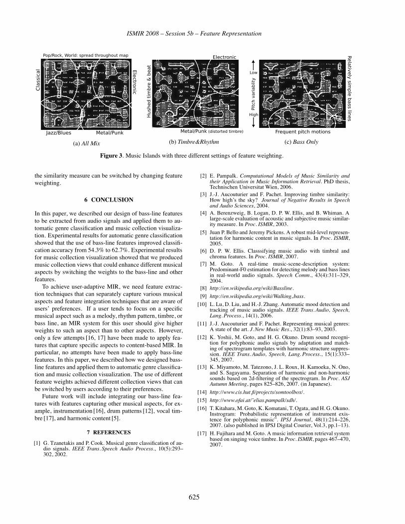
ISMIR 2008 – Session 5b – Feature Representation
(a) All Mix (b) Timbre&Rhythm (c) Bass Only
Figure 3. Music Islands with three different settings of feature weighting.
the similarity measure can be switched by changing featureweighting.
6 CONCLUSION
In this paper, we described our design of bass-line featuresto be extracted from audio signals and applied them to au-tomatic genre classification and music collection visualiza-tion. Experimental results for automatic genre classificationshowed that the use of bass-line features improved classifi-cation accuracy from 54.3% to 62.7%. Experimental resultsfor music collection visualization showed that we producedmusic collection views that could enhance different musicalaspects by switching the weights to the bass-line and otherfeatures.
To achieve user-adaptive MIR, we need feature extrac-tion techniques that can separately capture various musicalaspects and feature integration techniques that are aware ofusers’ preferences. If a user tends to focus on a specificmusical aspect such as a melody, rhythm pattern, timbre, orbass line, an MIR system for this user should give higherweights to such an aspect than to other aspects. However,only a few attempts [16, 17] have been made to apply fea-tures that capture specific aspects to content-based MIR. Inparticular, no attempts have been made to apply bass-linefeatures. In this paper, we described how we designed bass-line features and applied them to automatic genre classifica-tion and music collection visualization. The use of differentfeature weights achieved different collection views that canbe switched by users according to their preferences.
Future work will include integrating our bass-line fea-tures with features capturing other musical aspects, for ex-ample, instrumentation [16], drum patterns [12], vocal tim-bre [17], and harmonic content [5].
7 REFERENCES
[1] G. Tzanetakis and P. Cook. Musical genre classification of au-dio signals. IEEE Trans. Speech Audio Process., 10(5):293–302, 2002.
[2] E. Pampalk. Computational Models of Music Similarity andtheir Application in Music Information Retrieval. PhD thesis,Technischen Universitat Wien, 2006.
[3] J.-J. Aucouturier and F. Pachet. Improving timbre similarity:How high’s the sky? Journal of Negative Results in Speechand Audio Sciences, 2004.
[4] A. Berenzweig, B. Logan, D. P. W. Ellis, and B. Whiman. Alarge-scale evaluation of acoustic and subjective music similar-ity measure. In Proc. ISMIR, 2003.
[5] Juan P. Bello and Jeremy Pickens. A robust mid-level represen-tation for harmonic content in music signals. In Proc. ISMIR,2005.
[6] D. P. W. Ellis. Classsifying music audio with timbral andchroma features. In Proc. ISMIR, 2007.
[7] M. Goto. A real-time music-scene-description system:Predominant-F0 estimation for detecting melody and bass linesin real-world audio signals. Speech Comm., 43(4):311–329,2004.
[8] http://en.wikipedia.org/wiki/Bassline.
[9] http://en.wikipedia.org/wiki/Walking bass.
[10] L. Lu, D. Liu, and H.-J. Zhang. Automatic mood detection andtracking of music audio signals. IEEE Trans. Audio, Speech,Lang. Process., 14(1), 2006.
[11] J.-J. Aucouturier and F. Pachet. Representing musical genres:A state of the art. J. New Music Res., 32(1):83–93, 2003.
[12] K. Yoshii, M. Goto, and H. G. Okuno. Drum sound recogni-tion for polyphonic audio signals by adaptation and match-ing of spectrogram templates with harmonic structure suppres-sion. IEEE Trans. Audio, Speech, Lang. Process., 15(1):333–345, 2007.
[13] K. Miyamoto, M. Tatezono, J. L. Roux, H. Kamoeka, N. Ono,and S. Sagayama. Separation of harmonic and non-harmonicsounds based on 2d-filtering of the spectrogram. In Proc. ASJAutumn Meeting, pages 825–826, 2007. (in Japanese).
[14] http://www.cis.hut.fi/projects/somtoolbox/.
[15] http://www.ofai.at/˜elias.pampalk/sdh/.
[16] T. Kitahara, M. Goto, K. Komatani, T. Ogata, and H. G. Okuno.Instrogram: Probabilistic representation of instrument exis-tence for polyphonic music”. IPSJ Journal, 48(1):214–226,2007. (also published in IPSJ Digital Courier, Vol.3, pp.1–13).
[17] H. Fujihara and M. Goto. A music information retrieval systembased on singing voice timbre. In Proc. ISMIR, pages 467–470,2007.
625

ISMIR 2008 – Session 5b – Feature Representation
TIMBRE AND RHYTHMIC TRAP-TANDEM FEATURES FOR MUSICINFORMATION RETRIEVAL
Nicolas ScaringellaIdiap Research Institute, Martigny, Switzerland
Ecole Polytechnique Fédérale de Lausanne (EPFL), Lausanne, [email protected]
ABSTRACT
The enormous growth of digital music databases has led to
a comparable growth in the need for methods that help users
organize and access such information. One area in partic-
ular that has seen much recent research activity is the use
of automated techniques to describe audio content and to
allow for its identification, browsing and retrieval. Con-
ventional approaches to music content description rely on
features characterizing the shape of the signal spectrum in
relatively short-term frames. In the context of Automatic
Speech Recognition (ASR), Hermansky [7] described an in-
teresting alternative to short-term spectrum features, the TRAP-
TANDEM approach which uses long-term band-limited fea-
tures trained in a supervised fashion. We adapt this idea
to the specific case of music signals and propose a generic
system for the description of temporal patterns. The same
system with different settings is able to extract features de-
scribing either timbre or rhythmic content. The quality of
the generated features is demonstrated in a set of music re-
trieval experiments and compared to other state-of-the-art
models.
1 INTRODUCTION
As discussed in [2], most state-of-the-art algorithms dedi-
cated to the high-level description of music signals rely on
the same basic architecture with different algorithm variants
and parameters, i.e. short-term audio features extraction fol-
lowed by some supervised or unsupervised machine learn-
ing algorithm. The most successful approaches rely on fea-
tures describing the shape of short-term spectral frames of
audio signal. Spectral shape is indeed known to be corre-
lated with the perceived timbre of sounds as confirmed by
recent experiments in isolated instrument recognition (see
notably [8]). As a matter of fact, short-term spectral en-
velopes have dominated similar research fields for years,
like e.g. ASR. These short-term spectral envelopes are typi-
cally transformed in accordance with some constraining prop-
erties of human hearing such as the nonlinear (critical-band
like) frequency resolution (Bark, Mel), the compressive non-
linearity between acoustic stimulus and its percept (loga-
rithm) or the decreasing sensitivity of hearing at lower fre-
quencies (equal-loudness curves). Moreover, these modified
spectral frames are typically projected on spectral basis that
decorrelate the feature space (cepstrum).
In both speech and music signals, the smallest unit of in-
formation, i.e. phonemes on the one hand and notes on the
other hand (not only pitched notes but also hits of percussive
instruments or whatever that produces sounds), spread on
longer time intervals than the usual short-term audio frame.
Indeed, typical ASR/MIR (Music Information Retrieval) sys-
tems considers slices of audio signals of length 20 to 50 ms
(slightly longer when accurate pitch estimates are needed
in the lower frequencies). On the contrary, phonemes were
demonstrated to spread at least over the interval 200-300ms
[26]. As a matter of fact, the minimum discriminable in-
ter onset interval (IOI) is estimated to lie within the range
50-100ms (i.e. two sounds separated by less than the min-
imum IOI will be perceived as one) so that it is likely that
at least 50-100ms of information is needed by a human lis-
tener to interpret the incoming sound. Studies on rhythm
perception show that the rate of information in music sig-
nals is even less. Experiments [16] have indicated that pulse
sensation cease to exist outside of the period range of 200-
2000ms which is known as the region of pulse sensationwhile the most natural foot-tapping period is approximately
500-600ms. Given these observations, it is reasonable to
think that it is probably more perceptually relevant to model
audio signals with a longer context than the usual 20-50ms
spectrum frames. To preserve information related to the
short-term dynamics of sounds and to keep sufficient time-
resolution when detecting e.g. musical note onsets, a trade-
off consists in building a model of the sequence of short-
term feature vectors over a longer time-scale. This process
is sometimes referred to as temporal feature integration [14].
The simplest approach consists in computing simple statis-
tics of feature vectors (means and variances) over texture-windows. This has been shown [25] to significantly improve
music genres classification accuracy when using windows
of approximately 1.0 second as opposed to the direct use of
short-term frames. However, simple statistics discard dy-
namical changes of short-term features while the dynamics
of sound and notably the attack time and the fluctuations
626

ISMIR 2008 – Session 5b – Feature Representation
of the spectral envelope over time have proved to be of a
great importance in the perception of individual instrument
notes (see [11]). Meng [14] modeled the evolution of fea-
tures over a texture window with an auto-regressive (AR)
model and got improved genre classification results than
with simple statistics. McKinney and Breebart [12] com-
puted a periodogram for each short-term feature dimension
over a frame corresponding to roughly 768ms. Each peri-
odogram was then summarized by its power in 4 predefined
frequency bands using a fixed filter bank. This approach
was pursued by Arenas-Garcia et al. [1] who trained the
filter-bank in a supervised fashion to optimally suit a partic-
ular music organization task. Rauber et al. [20] used crit-
ical band energies periodograms with a much longer con-
text, i.e. 6 seconds. This longer context was considered to
model rhythmic patterns and the range 0-10Hz was consid-
ered as higher values are beyond what humans can perceive
as rhythm (see again the region of pulse sensation). These
approaches to temporal feature integration model the dy-
namics of each feature independently. Though Meng [14]
describes a general multivariate autoregressive model that
does take into account correlations between feature trajec-
tories, for the sake of simplicity he experiments in practice
with a diagonal multivariate autoregressive model, i.e. an
AR model of each feature dimension. Pohle et al. [19] use
independent component analysis on short sequences of crit-
ical band energies and obtain time-frequency 2D filters that
are reminiscent of cortical receptive fields [4]. Though this
approach seems more appropriate to take into account cor-
relations between feature trajectories, it is at best of similar
quality as short-term features in genre classification experi-
ments.
As a matter of fact, the use of long-term features has
been investigated more in depth in the context ASR, notably
by Hermansky [7]. These features are extracted in 2 steps.
Firstly, rather long-term TempoRAL Patterns (TRAPs) of
band-limited (1-3 Bark) spectral energies are considered.
Though, a context of 200-300ms seems needed for ASR,
an even longer time interval of 1 second is considered so
that information about slowly varying noise can be removed
from the data (i.e. mean/standard deviation normalization).
Hermansky [7] argues that, consistently with color separa-
tion in vision, it seems likely that the frequency selectiv-
ity of the hearing system is used for separating the reliable
(high SNR) part of the signals from the unreliable ones, so
that it seems reasonable to use independent frequency lo-
calized processors. Consequently, each band-limited TRAP
is processed individually by a specifically trained system to
build as much knowledge as possible into the feature extrac-
tion module to minimize the complexity of the subsequent
stochastically trained models. The second step, referred to
as the TANDEM part, consists in training a system aiming at
the combination of frequency-localized evidence into a set
of robust features that can be used in conventional HMM-
based ASR systems.
To our knowledge, there’s been only one application of
these TRAP-TANDEM features to music signals in the con-
text of drum transcription [17]. In this paper, we further in-
vestigate some possible applications of the TRAP-TANDEM
approach in the context of music information retrieval. More
specifically, we describe in section 2 our own implemen-
tation of the TRAP-TANDEM feature extraction module,
which slightly differs from the original method. As a matter
of fact, we propose two different implementations to focus
on two different aspects of music signals, namely timbre and
rhythm. In section 3, we evaluate the validity of these fea-
tures for music information retrieval in a set of music clus-
tering experiments. Section 4 reaches conclusion.
2 MUSICAL TRAP-TANDEM FEATURES
The first step of the processing consists in converting the au-
dio signal into some time-frequency representation. In prac-
tice, we use the typical short-term Fourier transform (STFT)
with Hann windowing of the short-term audio frames. The
resulting short-term spectra are projected onto the Mel scale
to simulate human critical bands of hearing [13]. The per-
ceptual relevance of this time-frequency representation is
further improved by exploiting masking properties of the
human ear (see [22]) and frequency response of the outer
and middle ear (see [23]). The loudness in Sone of the spec-
tra is finally evaluated according to [3].
These short-term spectra will be later used to build tim-
bre related TRAPs. Rhythmic TRAPs are based on a slightly
different representation. More specifically, each critical band
of the time-frequency plane is smoothed with a kernel, which
width is taken in the range of the minimum IOI so that
rhythmically irrelevant details of the band envelopes will
be smoothed while the peaks corresponding to two differ-
ent note onsets will not be merged. The first order deriva-
tive of each smoothed critical band is then taken to empha-
size sudden changes. Critical bands are finally combined as
suggested by Scheirer [21] who demonstrated that the per-
ceived rhythmic content of many types of musical excerpts
was mainly contained in 4 to 6 larger critical bands.
To reduce further processing, we deploy a note onset de-
tection algorithm and we will only compute one TRAP fea-
ture vector per onsets instead of using a constant and faster
rate of feature extraction. By synchronizing the analysis on
detected onsets, an important factor of variability of the data
is strongly reduced, i.e. the data is made translation invari-
ant, and consequently, we can expect that the task of learn-
ing relevant features will be simplified. The differentiated
signals computed for rhythm description are used as a basis
to detect note onsets. The signals are first half-wave rectified
and peaks are detected by using an adaptive threshold to ac-
count for possible loudness changes over the course of the
musical piece. Peaks are first combined over the different
627

ISMIR 2008 – Session 5b – Feature Representation
Figure 1. From audio signal to critical band spectra and
onset positions.
bands and those closer than the minimum IOI are merged
together. Figure 1 illustrates the processing chain that goes
from the audio signal to both critical band spectra and onset
positions.
The data from each critical band and differentiated criti-
cal band surrounding each onset is then parameterized with
the cosine transform, which has the good property of pro-
ducing decorrelated signals. The cosine transform is simple
to deploy since it does not need any training phase, plus
it has the interesting property that it closely resembles the
Principal Component Analysis (PCA) of such critical band
signals [7]. The cosine transform also allows for a signifi-
cant reduction of the dimensionality of the input data. The
range of modulation frequencies of the cosines is carefully
selected. For timbre description, modulations between 4 and
up to 100 Hz can be considered. The lower limit of 4 Hz is
set in accordance with the smallest perceivable sound unit
discussed in section 1. The higher limit is in the range of
modulations contributing to perceptual roughness, which is
generally thought to be a primary component of musical dis-
sonance [24]. As a matter of fact, the percept of roughness
is considered to correlate with temporal envelope modula-
tions in the range of about 20-150 Hz and maximal at 70
Hz. For rhythm description, lower frequencies are consid-
ered. Modulations between 1 and 4 Hz are interesting since
they are of the order of typical beat rates, i.e. 60 to 240
Beats Per Minute (BPM).
In the original TRAP approach, for each critical band
some algorithm, typically a non-linear feedforward multi-
layer perceptron (MLP), is trained to estimate posterior prob-
abilities of the classes under consideration. In ASR, the
targets are phonemes and there exist plenty of annotated
datasets. Ideally, we would like to have instrument annota-
tions to translate the TRAP idea to the case of music signals.
Figure 2. The TRAP-TANDEM feature extraction process-
ing chain.
Unfortunately, no such dataset exists for real-world poly-
phonic music and as a matter of fact, the annotation problem
would become even more complex since we’re considering
mixture of instruments. For the time being, we left aside the
use of critical band MLPs.
The TANDEM part of the system is in charge of combin-
ing evidence from the different frequency bands into a sin-
gle estimate. A MLP is typically trained to combined these
band limited features into a set of class posterior probabili-
ties. Again, we lack appropriate annotated datasets. As an
alternative, we use music genres annotations that are much
cheaper to obtain, using e.g. some online music guide such
as the AllMusic guide 1 . The merging MLP is fed with
the concatenation of all band limited features, which are
whitened with PCA to make them decorrelated. The MLP is
trained to associate acoustic evidence with 50-dimensional
binary vectors for which each dimension corresponds to a
particular music genres. Notice that one song may be char-
acterised by multiple genres. Once properly trained, the out-
puts of the MLP are decorrelated by PCA and can be used
as a feature vector describing the different genres in which
the acoustic data has been observed. Figure 2 illustrates the
processing chain that goes from the critical band or differ-
entiated critical band spectra to the final TRAP-TANDEM
like features.
3 EVALUATIONS
The TRAP-TANDEM features describe the timbre and rhyth-
mic context of a note onset. They may need to be aggregated
into a song-level model in e.g. song retrieval applications.
One application scenario consists in retrieving sets of songs
1 http://www.allmusic.com
628

ISMIR 2008 – Session 5b – Feature Representation
similar to some query song according to some similarity
measure between song-level models. Though listening tests
have proved to be a valid evaluation method of such music
retrieval systems due to the consistency of judgements ob-
served over different listeners [15], they are very demanding
in terms of time and human resources. Previous works have
shown that evaluations based on genre data correspond to
evaluations based on similarity ratings gathered in listening
tests [15]. Consequently, we will base our evaluation of the
descriptive quality of our features on some genre annotated
data. However, since we are more interested in music re-
trieval than automatic genre labelling, we will use measures
of the ranking quality of the system rather than classification
accuracy.
3.1 Timbre TRAP-TANDEM evaluation
To evaluate the timbre TRAP-TANDEM features, we have
gathered a set of 210 songs annotated with genre and styles
from the AllMusic guide. The quality of the labels was
cross-checked by systematic listening tests. Each selected
song is performed by a different artist to avoid the album ef-fect [9] in the evaluation. Moreover, the songs selected were
not previously used while training the TRAP-TANDEM fea-
ture extractor. Six main genre clusters of songs are consid-
ered and each genre cluster is composed of a set of smaller
style clusters with 10 songs per style. The Rock cluster
is composed of the Grunge, British-Invasion, Punk-Blues,
Glam-Rock, New-Wave, Folk-Rock sub-clusters. The Jazzcluster is composed of the Soul-Jazz, Swing, Hard-Bop, Free-Jazz sub-clusters. The Hip-Hop cluster is composed of the
West-Coast, East-Coast, Turntablism, Old-School sub-clusters.
The Electronica cluster is composed of the House, Trip-Hop, Drum’n’Bass sub-clusters. The last two clusters, Souland Adult Contemporary, are both divided into two sub-
clusters according to the gender of the lead singer.
We will measure how well the timbre TRAP-TANDEM
features are able to recover this organisation in terms of
genre/style clusters. In practice, we summarize the distri-
bution of TRAP-TANDEM feature vectors over each song
by a simple average. Though more complex models, like
e.g. HMM, could be deployed, our goal is to demonstrate
the descriptive quality of the TRAP-TANDEM features so
that we leave more complex song-level modelling strate-
gies to future work. Two songs can then be compared by
evaluating the cosine similarity of their average song-level
TRAP-TANDEM vectors. The similarity between each pair
of songs of the dataset is computed and the quality of the
system is assessed by comparing the labels of a song and its
nearest neighbours. More specifically, the precision at 1, 2
and 3 are computed for each query and averaged over the
dataset. The precision at n is a quality measure commonly
used to evaluate information retrieval systems. It accounts
1 1
Table 1. Timbre TRAP-TANDEM features.Prec. at 1 Prec. at 2 Prec. at 3
Genre 72.86 71.90 69.84
Style 50.00 43.10 39.37
Table 2. Full Gaussian of MFCCs.Prec. at 1 Prec. at 2 Prec. at 3
Genre 65.24 57.62 54.13
Style 35.71 30.00 25.87
for the quality of ranking, i.e. it is high if the most relevant
hits are in the top documents returned for a query. It is mea-
sured by computing the precision at different cut-off points
(for example, if the top 10 documents are all relevant to the
query and the next ten are all nonrelevant, we have 100%
precision at a cut off of 10 documents but a 50% precision
at a cut off of 20 documents).
To ease the comparison of our approach with the state-of-
the-art, we have implemented one of the most popular tim-
bre similarity measure based on spectral shape features. It
simply consists of a Mel-Frequency Cepstrum Coefficients
(MFCCs) frame-based parameterization of the audio signal
(20 coefficients including the energy coefficient). These
features are aggregated over the song as a Gaussian with
full covariance matrix and compared using the symmetric
version of the Kullback-Leibler (KL) divergence. This ap-
proach has been originally introduced by Mandel and El-
lis [10] and was used in the winning algorithm of the 1st
Annual Music Information Retrieval Evaluation exchange
(MIREX 2005) 2 artist identification contest and ranked 3rd
on 13 at the MIREX 2005 music genres classification con-
test while being almost 3 times faster than the first two win-
ning algorithms. It can be considered as a simplified, yet
competitive, implementation of Aucouturier’s timbre model
[2].
Tables 1 and 2 summarize the average precision at 1, 2
and 3 for both models. Results are given for both genres
and styles targets, i.e. in the first case precision increases
if the nearest neighbours are of the same genre, and in the
second case precision increases if the nearest neighbours are
of the same style.
It is clear from this experiment that the TRAP-TANDEM
features are more reliable than the short-term spectral shape
features in a music retrieval context. It is worth noticing that
MFCCs with a simple average and cosine similarity leads
to poorer results than MFCCs with mean, full covariance
matrix and KL divergence, while for the TRAP-TANDEM
features, the use of a KL-based distance function leads to
slightly inferior results than the simpler cosine similarity.
2 http://www.music-ir.org/mirex2005/index.php/Main Page
629

ISMIR 2008 – Session 5b – Feature Representation
Table 3. Rhythm TRAP-TANDEM features.
Prec. at 1 Prec. at 2 Prec. at 3
Style 79.37 77.01 76.36
Table 4. 10-fold 1-NN classification accuracy.
Accuracy
Rhythm TRAP-TANDEM features
(without annotated tempo)
79.49
Gouyon & Dixon (without anno-
tated tempo
67.60
Gouyon & Dixon (with annotated
tempo)
82.10
Peeters (with annotated tempo) 90.40
Dixon et al. (with annotated tempo
and semi-automated beat tracking)
96.00
This suggests that it is possible to have better retrieval re-
sults with a simpler—and especially faster—similarity func-
tion. Indeed, even if we’re considering here 50-dimensional
TRAP-TANDEM vectors against 20-dimensional MFCC vec-
tors, the cosine similarity remains much faster than the sym-
metric KL of two full Gaussians since the later requires
some matrix multiplications. This advantage becomes cru-
cial when dealing with industrial databases with millions of
songs.
3.2 Rhythm TRAP-TANDEM evaluation
We will evaluate the descriptive power of the rhythm TRAP-
TANDEM features in a similar fashion. Rhythm TRAP-
TANDEM features are averaged over each song and two
songs are compared with the cosine similarity. We used
here a well known dataset that contains 698 pieces of ball-
room dance music divided into 8 sub-styles having differ-
ent rhythmic characteristics, namely Cha Cha Cha, Jive,
Quickstep, Rumba, Samba, Tango, Viennese Waltz and
Waltz. It is interesting to notice that the TRAP-TANDEM
system for rhythm was trained with the same 50 genres tar-
gets as the system for timbre, and that these genres are far
from being as restricted as Jive or Cha Cha Cha. Table 3
summarizes the results obtained.
To ease the comparison with state-of-the-art algorithms,
we also computed the classification accuracy on a 10-fold
cross validation experiment with a 1-Nearest Neighbour clas-
sifier since various authors have reported results on this dataset
using this particular evaluation procedure (see table 4). Gouyon
and Dixon [6] reports up to 82.10% accuracy using a set of
rhythmic features including the manually annotated tempo.
The accuracy drops to 67.60% when using the tempo auto-
matically extracted by their algorithm. Peeters [18] reaches
up to 90.40% using spectral rhythm patterns normalised by
the manually annotated tempo. While these two algorithms
extract features from some periodicity representation of the
audio signal, Dixon et al. [5] characterise the amplitude
envelope of musical patterns, synchronised on musical bar
positions and normalised to a reference tempo. They ob-
tain an impressive 96.00% accuracy, but they also make use
of the annotated tempo and a semi-automated beat track-
ing algorithm. On the contrary, our approach is fully au-
tomatic and reaches 79.49% classification accuracy. More-
over the results obtained by Dixon et al. with tempo nor-
malised/bar synchronised temporal patterns suggest that the
TRAP-TANDEM rhythmic features could become even more
effective if synchronised on higher level musical events (mu-
sical bar positions instead of note onsets) and if made in-
dependent of the tempo. However, though on this particu-
lar dataset, a tempo normalisation may be needed since the
clusters exhibit clearly defined rhythmic patterns with vari-
able tempi, a tempo normalisation may not be so crucial for
a general purpose music similarity engine since slow/fastsongs should probably be similar to other slow/fast songs
independently from the rhythmical pattern they’re built on,
i.e. the percept of speed would be more important than the
perception of a particular rhythmical pattern.
4 CONCLUSION
We have presented a new set of features for music content
description based on the work by Hermansky [7] in the con-
text of ASR. The original approach has been adapted to the
specific case of music signals and two different implemen-
tations based on the same architecture have been proposed
to describe two apparently dissimilar dimensions of music,
namely timbre and rhythmic patterns. Instead of using a
relatively simple low-level characterization of the audio sig-
nal (like e.g. MFCCs), the TRAP-TANDEM approach is
a complex feature extraction module that encodes tempo-
ral patterns and as much prior knowledge as possible. The
distribution of TRAP-TANDEM features over a song can be
described with simple models that can be used together with
fast similarity measures. First experimental results confirm
that the TRAP-TANDEM approach is competitive against
state-of-the-art algorithms. Future work will focus on ex-
perimenting at a larger scale to confirm—or infirm—the de-
scriptive quality of the TRAP-TANDEM features.
5 REFERENCES
[1] J. Arenas-Garcia, J. Larsen, L. Kai Hansen, A. Meng,
“Optimal filtering of dynamics in short-time features for
music organization”, in Proc. ISMIR 2006, pp. 290-295,
Victoria, Canada, 2006.
[2] J.J. Aucouturier, “Dix Expériences sur la Modélisation
630
ISMIR 2008 – Session 5b – Feature Representation
du Timbre Polyphonique”, Ph.D. Dissertation, Univer-
sité Paris 6, France, 2006.
[3] R.A.W. Bladon, B. Lindblom, “Modeling the judgment
of vowel quality differences”, in J. Acoustical Society of
America, vol. 69, no.5, pp. 1414-1422, 1981.
[4] D.D. Depireux, J.Z. Simon, D.J. Klein, S.S. Shamma,
“Spectro-temporal response fields characterization with
dynamic ripples in ferret primary auditory cortex”, in J.
Neurophysiology, vol. 85, pp. 1220-1234, 2001.
[5] S. Dixon, F. Gouyon, G. Widmer, “Towards Characteri-
sation of Music via Rhythmic Patterns”, in Proc. ISMIR
2004, pp. 509-516, Barcelona, Spain, 2004.
[6] F. Gouyon, S. Dixon, “Dance Music Classification: a
Tempo-Based Approach”, in Proc. ISMIR 2004, pp.
501-504, Barcelona, Spain, 2004.
[7] H. Hermansky, “TRAP-TANDEM: Data-driven extrac-
tion of temporal features from speech”, in Proc. IEEE.
ASRU-2003, no. 50, St. Thomas, Virgin Islands, 2003.
[8] P. Herrera-Boyer, G. Peeters, S. Dubnov, “Automatic
classification of musical instrument sounds”, in J. of
New Music Research, no. 32 (2), pp. 3-21, 2003.
[9] Y.E. Kim, D.S. Williamson, S. Philli, “Towards quanti-
fying the Album Effect in artist identification”, in Proc.
ISMIR 2006, pp. 393-394, Victoria, Canada, 2006.
[10] M. Mandel, D. Ellis, “Song-level Features and Support
Vector Machines for Music Classification”, in Proc. IS-
MIR 2005, pp. 594-599, London, UK, 2005.
[11] S. McAdams, S. Winsberg, S. Donnadieu, G. De Soete,
J. Krimphoff, “Perceptual scaling of synthesized musi-
cal timbres: common dimensions, specificities and la-
tent subject classes”, in Psychological Research, no. 58,
pp.177-192, 1995.
[12] M.F. McKinney, J. Breebart, “Features for audio and
music classification”, in Proc. ISMIR 2003, Baltimore,
Maryland, USA, 2003.
[13] S. Stevens, J. Volkman, E. Newman, “A scale for the
measurement of the psychological magnitude of pitch”,
in J. of the Acoustical Society of America, vol. 8(3) pp.
185-190, 1937.
[14] A. Meng, “Temporal feature integration for music or-
ganisation”, Ph.D. Dissertation, IMM Technical Univer-
sity of Denmark, Denmark, 2006.
[15] E. Pampalk, “Computational models of music similar-
ity and their application in music information retrieval”,
Ph.D. Dissertation, Vienna Institute of Technology, Aus-
tria, 2006.
[16] R. Parncutt, “The perception of pulse in musical
rhythm”, in Action and Perception in Rhythm and Mu-
sic, pp. 127-138, Stockholm, Sweden, 1987.
[17] J. Paulus, A. Klapuri, “Combining Temporal and Spec-
tral Features in HMM-Based Drum Transcription”, in
Proc. ISMIR 2007, Vienna, Austria, 2007.
[18] G. Peeters, “Rhythm Classification using Spectral
Rhythm Patterns”, in Proc. ISMIR 2005, pp. 644-647,
London, UK, 2005.
[19] T. Pohle, P. Knees, M. Schedl, G. Widmer, “Indepen-
dent Component Analysis for Music Similarity Com-
putation”, in Proc. ISMIR 2006, pp. 228-233, Victoria,
Canada, 2006.
[20] A. Rauber, E. Pampalk, D. Merkl, “Using psycho-
acoustic models and self-organizing maps to create a hi-
erarchical structuring of music by sound similarity”, in
Proc. ISMIR 2002, Paris, France, 2002.
[21] E. Scheirer, “Tempo and beat analysis of acoustic musi-
cal signals”, in J. of the Acoustical Society of America,
103(1): 588-601, 1998.
[22] M.R. Schroeder, B.S. Atal, J.L. Hall, “Optimizing Dig-
ital Speech Coders by Exploiting Masking Properties of
the Human Ear”, in J. of the Acoustical Society of Amer-
ica, vol. 66, issue 6, pp. 1647-1652, December 1979.
[23] E. Terhardt, “Calculating virtual pitch”, in Hearing Re-
search, vol. 1, pp. 155-182, 1979.
[24] E. Terhardt, “On the perception of periodic sound fluctu-
ations (roughness)”, in Acustica, 30, pp. 201-213, 1974
[25] G. Tzanetakis, P. Cook, “Musical genre classification of
audio signals”, in IEEE Trans. Speech Audio Process-
ing, vol.10, no.5, pp. 293-302, July 2002.
[26] H.H. Yang, S. Sharma, S. van Vuuren, H. Hermansky,
“Relevance of Time Frequency Features for Phonetic
and Speaker/Channel Classification”, in Speech Com-
munication, vol. 31, issue 1, pp. 35-50, August, 2000.
631

ISMIR 2008 – Session 5b – Feature Representation
632

Session 5c – Rhythm and Meter

.
ISMIR 2008 – Session 5c – Rhythm and Meter
QUANTIFYING METRICAL AMBIGUITY
Patrick Flanagan
ABSTRACT
This paper explores how data generated by meter induc-
tion models may be recycled to quantify metrical ambigu-
ity, which is calculated by measuring the dispersion of met-
rical induction strengths across a population of possible me-
ters. A measure of dispersion commonly used in economics
to measure income inequality, the Gini coefficient, is intro-
duced for this purpose. The value of this metric as a rhyth-
mic descriptor is explored by quantifying the ambiguity of
several common clave patterns and comparing the results to
other metrics of rhythmic complexity and syncopation.
1 INTRODUCTION
This study initially grew out of an interest in modeling lis-
tener responses of a tapping study in which listeners tapped
to the beat of sections of Steve Reich’s Piano Phase [17].
For some sections, tapping rate and phase varied widely
among listeners, and for others they displayed relative con-
sistency. Accordingly, the goal of the study was to model
metrical ambiguity as the degree of variety of listener re-
sponses to a given rhythm.
This task, however, would be complicated by a lack of
simplified experimental data; the experiments of [17] in-
volved pitched music, which added a layer of complexity
I wanted to avoid. I therefore turned my attention to a corol-
lary kind of metrical ambiguity, which is the amenability of
a rhythm to gestalt flip, in which a listener reevaluates the
location of the beat. This amenability has been convinc-
ingly advanced as one reason for the pull of African and
African-derived rhythms on listeners [7]. Data on metrical
gestalt flips is no easier to come by, but orientating the study
around the proverbial average listener instead of groups of
listeners allowed it to interface with the voluminous litera-
ture on syncopation. While metrical ambiguity is not equiv-
alent to syncopation, the results of this study suggest that it
roughly correlates to syncopation and offers an interesting
rhythmic descriptor in its own right that could be used for
theoretical analysis, genre classification, and the production
of metrically ambiguous music.
To describe the ambiguity of the metrical scene, the am-
biguity model recycles data that existing models of meter
and beat induction often discard, the data about the induc-
tion strengths of all potential meters. The central idea of the
model is that a more even distribution of induction strengths
across a group of potential meters will cause greater am-
biguity in the perception of meter. The model of ambigu-
ity, therefore, requires a model of meter induction that, for
a given rhythm, produces numerical values for an array of
potential meters, with each meter defined by its period and
phase relation to some arbitrary point in the rhythm. For the
sake of simplicity, this study uses a hybrid model based on
older models of meter induction that operate on quantized
symbolic data, but the theory of ambiguity presented here
is extensible to any model, including those that work with
audio, that produces such an array.
In this paper the term “meter” refers to an isochronous,
tactus-level pulse, characterized by a period and phase ex-
pressed in discrete integer multiples of some smallest unit of
musical time. The more common term for this isochronous
pulse is, of course, “the beat.” “Meter,” however, is the
preferable term because this paper uses the conventionally
understood downbeat of musical examples as a reference
point for the tactus-level pulse.
2 METER INDUCTION MODEL
2.1 Influences on the Model
While the intent of this paper is not to advance a new model
of meter induction, the existing models are either too com-
plex for the purposes of this study or otherwise flawed. I
therefore employ a hybrid meter induction model that calcu-
lates an induction strength for each candidate meter by sum-
ming the values of phenomenal accents that a given meter
encounters, a strategy inherited from [12; 9; 2; 10]. Parn-
cutt’s model is the most sophisticated of the four in that it
incorporates durational accent and tempo preference. For
this reason, I largely adopt Parncutt’s model.
Parncutt’s model, however, has one flaw that prevents its
full deployment in this study. In calculating what he called
“pulse-match salience,” which is the degree of match be-
tween phenomenal accents and an isochronous pulse stream,
Parncutt summed the product of the phenomenal accents
that occur on neighboring pulses. The problem with mul-
tiplying the phenomenal accents that occur on neighboring
pulses is that some rhythms contain no inter-onset intervals
(IOIs) that map onto candidate meters that we know to be
viable meters. In this case, the metrical induction score, or
pulse-match salience, of a viable meter turns out to be 0. For
example, consider the Bossa Nova pattern in Figure 2.
The rhythm contains no inter-onset intervals of 4 tatums
that begin on what, according to musical practice, is the
635
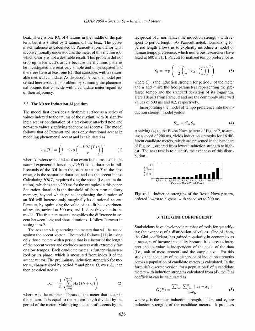
ISMIR 2008 – Session 5c – Rhythm and Meter
beat. There is one IOI of 4 tatums in the middle of the pat-
tern, but it is shifted by 2 tatums off the beat. The pulse-
match salience as calculated by Parncutt’s formula for what
is conventionally understood as the meter of this rhythm is 0,
which clearly is not a desirable result. This problem did not
crop up in Parncutt’s article because the rhythmic patterns
he investigated are relatively simple and unsyncopated and
therefore have at least one IOI that coincides with a reason-
able metrical candidate. As discussed below, the model pre-
sented here avoids this problem by summing the phenome-
nal accents that coincide with a candidate meter regardless
of their adjacency.
2.2 The Meter Induction Algorithm
The model first describes a rhythmic surface as a series of
values indexed to the tatums of the rhythm, with 0s signify-
ing a rest or continuation of a previously attacked note and
non-zero values signfiying phenomenal accents. The model
follows that of Parncutt and uses only durational accent in
modeling phenomenal accent and is calculated as
Ad (T ) =(
1− exp(−IOI (T )
r
))i
(1)
where T refers to the index of an event in tatums, exp is the
natural exponential function, IOI(T) is the duration in mil-
liseconds of the IOI from the onset at tatum T to the next
onset, r is the saturation duration, and i is the accent index.
Calculating IOI(T) requires fixing the speed (i.e., tatum du-
ration), which is set to 200 ms for the examples in this paper.
Saturation duration is the threshold of short term auditory
memory, beyond which point lengthening the duration of
an IOI will increase only marginally its durational accent.
Parncutt, by optimizing the value of r to fit his experimen-
tal results, arrived at 500 ms, and I adopt this value in the
model. The free parameter i magnifies the difference in ac-
cent between long and short durations. I follow Parncutt in
setting it to 2.
The next step is generating the meters that will be tested
against the accent vector. The model follows [11] in using
only those meters with a period that is a factor of the length
of the accent vector and excludes meters with extremely fast
or slow tempos. Each candidate meter is further character-
ized by its phase, which is measured from index 0 of the
accent vector. The preliminary induction strength S for me-
ter m, characterized by period P and phase Q, over Ad, can
then be calculated as
Sm =1n
(n−1∑i=0
Ad (Pi + Q)
)(2)
where n is the number of beats of the meter that occur in
the pattern. It is equal to the pattern length divided by the
period of the meter. Multiplying the sum of accents by the
reciprocal of n normalizes the induction strengths with re-
spect to period length. As Parncutt noted, normalizing for
period length allows us to explicitly introduce a model of
human tempo preference, which numerous researchers have
fixed at 600 ms [5]. Parcutt formalized tempo preference as
Sp = exp
(−1
2
(1σ
log10
( p
u
))2)
(3)
where Sp is the induction strength for period p of the meter
and u and σ are the free parameters representing the pre-
ferred tempo and the standard deviation of its logarithm.
Here I depart from Parncutt and use the commonly observed
values of 600 ms and 0.2, respectively.
Incorporating the model of tempo preference into the in-
duction strength model yields
S′m = SmSp (4)
Applying (4) to the Bossa Nova pattern of Figure 2, assum-
ing a speed of 200 ms, yields induction strengths for 16 dif-
ferent candidate meters, which are presented in the bar chart
of Figure 1, ordered from lowest induction strength to high-
est. The next task is to quantify the evenness of this distri-
bution.
8,7 8,4 8,1 1,0 8,5 8,3 8,2 8,0 8,6 2,1 4,3 4,1 4,0 2,0 4,20
0.1
0.2
0.3
Candidate Meter (Period, Phase)
Indu
ctio
nSt
reng
th
Figure 1. Induction strengths of the Bossa Nova pattern,
ordered lowest to highest, with speed set to 200 ms.
3 THE GINI COEFFECIENT
Statisticians have developed a number of tools for quantify-
ing the evenness of a distribution of values. One of them,
the Gini coefficient, has gained popularity in economics as
a measure of income inequality because it is easy to inter-
pret and its value is independent of the scale of the data
(i.e., unit of measurement) and the sample size. For this
study, the inequality of the dispersion of induction strengths
across a population of candidate meters is calculated. In the
formula’s discrete version, for a population P of n candidate
meters with induction strengths calculated from (4), the Gini
coefficient can be calculated as
G(P ) =
∑ni=1
∑nj=1 | xi − xj |2n2μ
(5)
where μ is the mean induction strength, and xi and xj are
induction strengths of the candidate meters. It produces
636

ISMIR 2008 – Session 5c – Rhythm and Meter
values with a range of 0 to 1, where 1 signifies perfect in-
equality and 0 signifies perfect equality. In music theoretical
terms, lower values denote greater metrical ambiguity, and
vice versa. In practice, values for metrical ambiguity range
from the high 0.20s for high metrical ambiguity up to the
mid 0.70s for low metrical ambiguity. With the necessary
tools in hand, we may now proceed to assess the metrical
ambiguity of some rhythms.
4 METRICAL AMBIGUITY AND CLAVERHYTHMS
4.1 Comparison to Syncopation Measures
Thus far the Gini coefficient has been described as a mea-
sure of metrical ambiguity, which is not necessarily syn-
onymous with rhythmic complexity or syncopation. A fast
isochronous pulse stream is metrically ambiguous because it
is amenable to subjective rhythmization, but it is also rhyth-
mically simple. Nevertheless, it is fruitful to compare the
Gini coefficient to existing measures of syncopation.
Toussaint has tested several metrics of complexity and
syncopation against clave rhythms in [16; 15], with partic-
ular attention paid to six of the most popular 4/4 timelines:
the Bossa Nova, Gahu, Rumba, Soukous, Son, and Shiko
patterns (Figure 2). Histograms of the induction strengths
according to (4), ordered lowest to highest, of each rhythm
with a moderate tatum duration of 200 ms are presented in
Figure 3 (except for the Bossa Nova pattern, the histogram
of which is presented in Figure 1). Note that the bars are
labelled by their period and phase, and that the candidate
meter that is most commonly understood to orgranize the
rhythm in musical practice is 4,0. A simple visual inspec-
tion of the histograms reveals variation in the evenness of
the distribution of induction strengths; to the eye, Shiko is
the most uneven, and Bossa Nova the most even. As one
would expect, these differences are reflected in the Gini co-
efficients of each rhythm, which are displayed in the first
row of Table 1 alongside several metrics of rhythmic com-
plexity and syncopation. In reading Table 1, be mindful that
the Gini coefficient measures inequality of metrical induc-
tion strengths and therefore is inversely related to metrical
ambiguity. A low value implies higher metrical ambiguity.
A word about the different metrics of complexity in Table
1. “Gini Syncopation” is derived from the Gini coefficient
as explained in section 4.2. Michael Keith’s measure of syn-
copation assigns each note to one of four categories: unsyn-
copated, hesitation, anticipation, and syncopation. Each cat-
egory is associated with a different value or degree of syn-
copation, and the total syncopation of a passage equals the
sum of its constituent notes’ values. The reader is referred to
[15] for more information. Pressing’s measure [13] is sim-
ilar in that it parses a rhythm into six basic units and sums
their values.
(a) Bossa Nova (b) Gahu
(c) Rumba (d) Soukous
(e) Son (f) Shiko
Figure 2. Six common 4/4 timelines.
Bossa Gahu Rumba Soukous Son Shiko
Nova
Gini 0.583 0.719 0.679 0.683 0.679 0.803
Gini 0.894 0.841 0.733 0.876 0.571 0.492
Syncopation
Keith 3 3 2 3 2 1
Off-Beatness 2 1 2 2 1 0
Pressing 22 19.5 17 15 14.5 6
Metrical 6 5 5 6 4 2
Complexity
LHL 6 5 5 6 4 2
WNBD 4 3.6 3.6 3.6 2.8 1.2
Table 1. A comparison of measures of rhythmic complexity
and syncopation for six clave rhythms.
Two different measures of rhythmic syncopation were
proposed in [15]. The first is off-beatness, which is equal
to the number of onsets that occur at indices of the mea-
sure that share no factors other than 1 with the length of the
measure (a measure in usually indexed in 16th notes). The
second measure of syncopation, called “metrical complex-
ity,” employs the metrical accent grid of [6]. In this scheme,
the level of syncopation is related to the coincidence of on-
sets and shallow levels in Lerdahl and Jackendoff’s metrical
accent grid. The Longuet-Higgins Lee syncopation measure
(LHL) also employs a metrical accent grid while consider-
ing whether an onset is followed a rest (or continuation) or
another onset [8]. Finally, the Weighted Note-to-Beat Mea-
sure (WNBD) relates syncopation to the distance from each
onset to the nearest beat [4].
The extreme Gini values in Table 1 correspond well to the
other metrics of syncopation and to intuition; Bossa Nova
is the most syncopated pattern and Shiko the least. Most
of the metrics, however, have different interpretations of
Gahu, Soukous, Son, and Rumba. According to [16], the
patterns should be ordered in decreasing degree of syncopa-
tion as Bossa Nova, Gahu, Rumba/Soukous, Son, and Shiko,
which is exactly the order of Pressing’s model. I would have
637
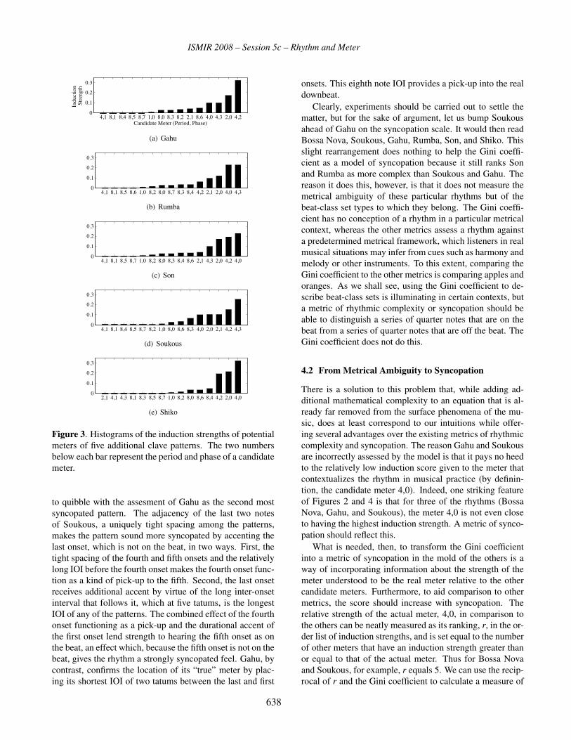
ISMIR 2008 – Session 5c – Rhythm and Meter
4,1 8,1 8,4 8,5 8,7 1,0 8,0 8,3 8,2 2,1 8,6 4,0 4,3 2,0 4,20
0.1
0.2
0.3
Candidate Meter (Period, Phase)
Indu
ctio
nSt
reng
th
(a) Gahu
4,1 8,1 8,5 8,6 1,0 8,2 8,0 8,7 8,3 8,4 4,2 2,1 2,0 4,0 4,30
0.1
0.2
0.3
(b) Rumba
4,1 8,1 8,5 8,7 1,0 8,2 8,0 8,3 8,4 8,6 2,1 4,3 2,0 4,2 4,00
0.1
0.2
0.3
(c) Son
4,1 8,1 8,4 8,5 8,7 8,2 1,0 8,0 8,6 8,3 4,0 2,0 2,1 4,2 4,30
0.1
0.2
0.3
(d) Soukous
2,1 4,1 4,3 8,1 8,3 8,5 8,7 1,0 8,2 8,0 8,6 8,4 4,2 2,0 4,00
0.1
0.2
0.3
(e) Shiko
Figure 3. Histograms of the induction strengths of potential
meters of five additional clave patterns. The two numbers
below each bar represent the period and phase of a candidate
meter.
to quibble with the assesment of Gahu as the second most
syncopated pattern. The adjacency of the last two notes
of Soukous, a uniquely tight spacing among the patterns,
makes the pattern sound more syncopated by accenting the
last onset, which is not on the beat, in two ways. First, the
tight spacing of the fourth and fifth onsets and the relatively
long IOI before the fourth onset makes the fourth onset func-
tion as a kind of pick-up to the fifth. Second, the last onset
receives additional accent by virtue of the long inter-onset
interval that follows it, which at five tatums, is the longest
IOI of any of the patterns. The combined effect of the fourth
onset functioning as a pick-up and the durational accent of
the first onset lend strength to hearing the fifth onset as on
the beat, an effect which, because the fifth onset is not on the
beat, gives the rhythm a strongly syncopated feel. Gahu, by
contrast, confirms the location of its “true” meter by plac-
ing its shortest IOI of two tatums between the last and first
onsets. This eighth note IOI provides a pick-up into the real
downbeat.
Clearly, experiments should be carried out to settle the
matter, but for the sake of argument, let us bump Soukous
ahead of Gahu on the syncopation scale. It would then read
Bossa Nova, Soukous, Gahu, Rumba, Son, and Shiko. This
slight rearrangement does nothing to help the Gini coeffi-
cient as a model of syncopation because it still ranks Son
and Rumba as more complex than Soukous and Gahu. The
reason it does this, however, is that it does not measure the
metrical ambiguity of these particular rhythms but of the
beat-class set types to which they belong. The Gini coeffi-
cient has no conception of a rhythm in a particular metrical
context, whereas the other metrics assess a rhythm against
a predetermined metrical framework, which listeners in real
musical situations may infer from cues such as harmony and
melody or other instruments. To this extent, comparing the
Gini coefficient to the other metrics is comparing apples and
oranges. As we shall see, using the Gini coefficient to de-
scribe beat-class sets is illuminating in certain contexts, but
a metric of rhythmic complexity or syncopation should be
able to distinguish a series of quarter notes that are on the
beat from a series of quarter notes that are off the beat. The
Gini coefficient does not do this.
4.2 From Metrical Ambiguity to Syncopation
There is a solution to this problem that, while adding ad-
ditional mathematical complexity to an equation that is al-
ready far removed from the surface phenomena of the mu-
sic, does at least correspond to our intuitions while offer-
ing several advantages over the existing metrics of rhythmic
complexity and syncopation. The reason Gahu and Soukous
are incorrectly assessed by the model is that it pays no heed
to the relatively low induction score given to the meter that
contextualizes the rhythm in musical practice (by definin-
tion, the candidate meter 4,0). Indeed, one striking feature
of Figures 2 and 4 is that for three of the rhythms (Bossa
Nova, Gahu, and Soukous), the meter 4,0 is not even close
to having the highest induction strength. A metric of synco-
pation should reflect this.
What is needed, then, to transform the Gini coefficient
into a metric of syncopation in the mold of the others is a
way of incorporating information about the strength of the
meter understood to be the real meter relative to the other
candidate meters. Furthermore, to aid comparison to other
metrics, the score should increase with syncopation. The
relative strength of the actual meter, 4,0, in comparison to
the others can be neatly measured as its ranking, r, in the or-
der list of induction strengths, and is set equal to the number
of other meters that have an induction strength greater than
or equal to that of the actual meter. Thus for Bossa Nova
and Soukous, for example, r equals 5. We can use the recip-
rocal of r and the Gini coefficient to calculate a measure of
638
ISMIR 2008 – Session 5c – Rhythm and Meter
syncopation. For an accent vector Ad that produces a pop-
ulation P of meter induction strengths, its syncopation Syncmay be described as
Sync(Ad) = 1−(G(P )(1− e−
1r ))
(6)
Inputting the values for the Gini coefficient and meter in-
duction strengths calculated above yields the scores in the
second row of Table 1.
These values correspond with what I have argued above
is the most reasonable ranking of the patterns. This metric
enjoys two other advantages over the others. The first is that
it is invariant to scale. The other metrics invariably increase
with the length of the rhythm being measured, making it
impossible to compare rhythms of different lengths. The
syncopation measure proposed here, on the other hand, al-
ways produces a value between 0 and 1. Second, it has a
much finer grain of discrimination than the others. On the
downside, it depends on a large number of free parameters,
a circumstance that prevents fixing a final value for the syn-
copation of a rhythm conceived in the abstract; there is no
single score for the Bossa Nova pattern. This fault could,
however, be turned into an advantage if it allowed analysts
to probe the effects of tempo and various kinds of phenom-
enal accent on syncopation.
4.3 Correspondence to Experimental Results
In [14], Spearman rank correlations were calculated between
the experimental data of [12] and [3], which measured the
difficulty of performing a set of rhythms, and the values
produced by various models of syncopation for the same
rhythms. The correlations give an indication of how well
the models predict performance difficulty, which is assumed
to be a reasonable proxy for syncopation. For the models
tested, which were those listed in Table 1 (excluding the
Gini coefficient models presented here), correlations ranged
from 0.224 to 0.787. The procedure of [14] was repeated for
the Gini coefficient and the Gini syncopation metrics, with
the following results: The Gini coefficient showed correla-
tions of 0.51 and 0.42 for the data of [12] and [3], respec-
tively. The Gini syncopation measure produced correlations
of 0.56 and 0.51.
These figures should treated cautiously. The Essens study
[3] was a small experiment with only six participants and
high p-values (i.e., low confidence). That said, the results
indicate that the Gini coefficient and Gini syncopation mea-
sure are decent but not good predictors of performance diffi-
culty. Considering that the best performing models in [14],
the LHL and metrical complexity models, operate in refer-
ence to a full metrical hierarchy, one could speculate that
the performance of the Gini measures could be improved by
replacing the modified Parncutt beat induction model with
one that uses a metrical hierarchy. It is also noteworthy that
these same two models produced rankings of the six clave
rhythms in Table 1 that agree with my own assessment and
that of the Gini syncopation measure.
5 METRICAL AMBIGUITY OF BEAT-CLASS SETTYPES
The concept of the beat-class set was (re)introduced in [1]
in order to analyze the properties and transformations of
rhythmic material in Steve Reich’s phase-shifting music (the
concept originated in Babbitt’s timepoint system). At issue
in [1] was the transformational potential of rhythmic ma-
terial, a topic that the Gini coefficient addresses because it
describes how amenable a beat-class (bc) set type might be
to various metrical interpretations. To investigate what the
Gini coefficient might reveal about metrical ambiguity and
beat-class sets, Gini coefficients for all mod 12 bc set types
at three different speeds were calculated.
The most striking feature of the results is that the bc types
with the highest ambiguity are those formed by one of the
generator cycles of the modulo 12 system, the 5- (or 7-) cy-
cle, the generator of the diatonic scale. In another interesting
twist, if one skips applying rules for phenomenal accent and
calculates induction strengths over an accent vector of 1s
and 0s, the Gini coefficients of bc set types are invariant un-
der M operation. Under M operation, the 5 cycle transforms
into the 1-cycle, which means that, at least when accent rules
are ignored, the two most famous scales of Western music,
when transformed into rhythms, also turn out to be, at least
according to the model developed here, the most metrically
ambiguous bc set types. It might seem surprising that the
dispersion of values produced by this model of meter in-
duction, which was designed to reflect human preference
for aligning isochronous downbeats with note onsets, would
intersect so directly with set theory, but the explanation is
almost intuitive.
By definition, the candidate meters have periods that are
factors of the length of the meter. The generators cycles, by
definition, have periods that are prime relative to the length
of the meter and therefore prime relative to the periods of
the candidate meters. The relative primeness of the candi-
date meters and the cycle generators ensures that the gener-
ator will cycle through all of the meters of a different phase
and the same period before coinciding with the same me-
ter twice. This cycling over candidate meters produces the
most even distribution of onsets among the candidate me-
ters, which in turn assures a low Gini coefficient.
It should be obvious from the status of cycle 1 generated
beat-class sets as highly ambiguous that maximal ambigu-
ity is hardly a guarantor of musical interest. As Cohn [1]
noted in a parenthetical aside, these sets are “inherently less
interesting for other reasons as well, although to articulate
these reasons is not an easy task.” One possible reason is
that while bc sets generated from the 1-cycle are metrically
ambiguous, their grouping structure is all too obvious. The
639

ISMIR 2008 – Session 5c – Rhythm and Meter
maximally even dispersion of onsets in the 5-cycle gener-
ated sets creates the potential for ambiguity of grouping as
well as metrical structure, allowing grouping and metrical
structures to interact in interesting ways. Alternatively, per-
haps the maximally even sets are more interesting because
they constantly flip the beat around, forcing the listener to
retrospectively reevaluate the location in the metrical grid
of what has already been heard. In this sense, the metrical
ambiguity of maximally even rhythms is like that of the fa-
miliar visual phenomenon, in which the image of two faces
opposite one another can be flipped to the background to
produce an image of a vase. The perceptual gestalt is fragile
but clearly delineated. The 1-cycle generated rhythms are
more like looking at a fuzzy image. The gestalt is not so
much ambiguous as amorphous. To be precise, their metri-
cal structure is amorphous while the larger scale grouping
structure is clear. One is confronted with a blob of notes
followed by silence, a sonic image both blunt and vague.
6 CONCLUSION
The use of the Gini coefficient to quantify metrical ambigu-
ity holds promise as a means to assess the syncopation of
short, repeated rhythmic patterns and the perceptual quali-
ties of beat-class set types. While a model of meter induc-
tion, based on older models, was introduced here for the
purpose of creating input data for the Gini coefficient, the
principle of using a dispersion of probabilities over candi-
date meters to calculate metrical ambiguity is in no way de-
pendent on this model of meter induction. It may be fruitful
to apply this principle to data from the more recent mod-
els that work with audio in order to use metrical ambiguity
as a rhythmic descriptor of audio tracks. As it stands, the
Gini coefficient may help analysts discuss rhythmic mate-
rial in repetitive compositions and possibly serve as a utility
for composers and other creators of rhythmically complex
music.
7 REFERENCES
[1] R. Cohn, “Transpositional Combination of Beat-Class
Sets in Steve Reich’s Phase-Shifting Music,” Perspec-tives of New Music, vol. 30, no. 2, pp. 146–177, 1992.
[2] D. Eck, “A Positive-Evidence Model for Rhythmi-
cal Beat Induction,” Journal of New Music Research,
vol. 30, no. 2, pp. 187–200, 2001.
[3] P. Essens, “Structuring temporal sequences: Compari-
son of models and factors of complexity,” Perception &Psychophysics, vol. 57, no. 4, pp. 519–532, 1995.
[4] F. Gomez, A. Melvin, D. Rappaport, and G. Tous-
saint, “Mathematical Measures of Syncopation,” Proc.
BRIDGES: Mathematical Connections in Art, Musicand Science, pp. 73–84, 2005.
[5] S. Handel, Listening. MIT Press Cambridge, Mass,
1989.
[6] F. Lerdahl and R. Jackendoff, A Generative Theory ofTonal Music. MIT Press, 1996.
[7] D. Locke, Drum Gahu!: A Systematic Method for anAfrican Percussion Piece. White Cliffs Media Co.,
1987.
[8] H. Longuet-Higgins and C. Lee, “The rhythmic interpre-
tation of monophonic music,” Music Perception, vol. 1,
no. 4, pp. 424–441, 1984.
[9] J. McAuley and P. Semple, “The effect of tempo and mu-
sical experience on perceived beat,” Australian Journalof Psychology, vol. 51, no. 3, pp. 176–187, 1999.
[10] R. Parncutt, “A perceptual model of pulse salience and
metrical accent in musical rhythms,” Music Perception,
vol. 11, no. 4, pp. 409–464, 1994.
[11] D. Povel and P. Essens, “Perception of temporal pat-
terns,” Music Perception, vol. 2, no. 4, pp. 411–440,
1985.
[12] D. Povel and H. Okkerman, “Accents in equitone se-
quences.” Perception and Psychophysics, vol. 30, no. 6,
pp. 565–72, 1981.
[13] J. Pressing, “Cognitive complexity and the structure of
musical patterns,” Proceedings of the 4th Conference ofthe Australasian Cognitive Science Society, Newcastle,Australia, 1997.
[14] E. Thul and G. T. Toussaint, “On the relation between
rhythm complexity measures and human rhythmic per-
formance,” in C3S2E ’08: Proceedings of the 2008C3S2E conference. New York, NY, USA: ACM, 2008,
pp. 199–204.
[15] G. Toussaint, “Mathematical features for recognizing
preference in Sub-Saharan African traditional rhythm
timelines,” Proceedings of the 3rd International Con-ference on Advances in Pattern Recognition, pp. 18–27,
2005.
[16] ——, “A mathematical analysis of African, Brazilian,
and Cuban clave rhythms,” Proceedings of BRIDGES:Mathematical Connections in Art, Music and Science,
pp. 157–168, 2002.
[17] S. Wilson, “Pattern perception and temporality in the
music of Steve Reich: An interdisciplinary approach,”
Ph.D. dissertation, University of New South Wales,
1999.
640

ISMIR 2008 – Session 5c – Rhythm and Meter
ON RHYTHMIC PATTERN EXTRACTION IN BOSSA NOVA MUSIC
Ernesto Trajano de Lima Geber RamalhoCentro de Informática (CIn)—Univ. Federal de Pernambuco
Caixa Postal 7851—50732-970—Recife—PE—Brazil{etl,glr}@cin.ufpe.br
ABSTRACT
The analysis of expressive performance, an important re-
search topic in Computer Music, is almost exclusively de-
voted to the study of Western Classical piano music. Instru-
ments like the acoustic guitar and styles like Bossa Nova and
Samba have been little studied, despite their harmonic and
rhythmic richness. This paper describes some experimen-
tal results obtained with the extraction of rhythmic patterns
from the guitar accompaniment of Bossa Nova songs. The
songs, played by two different performers and recorded with
the help of a MIDI guitar, were represented as strings and
processed by FlExPat, a string matching algorithm. The re-
sults obtained were then compared to a previously acquired
catalogue of “good” patterns.
1 INTRODUCTION
It is common sense that playing music in the exact way it is
written in the score results in a mechanical and uninteresting
succession of sounds. To make written music interesting,
the musician is required to make variations on low level mu-
sical parameters, such as: Local tempo (accelerandi, ritar-dandi, rubato); dynamics; notes articulation (staccati, liga-
tures, etc.); micro-silences between the notes, etc. [12].
Several researchers stress the importance, as well as the
the difficulties, of studying this phenomenon, also known
as expressive performance [14]. These researches, in gen-
eral, focus on building relationships between different mu-
sical elements (such as harmony and melody or even the
low level parameters previously mentioned), and expressive
performance itself. These relationships can be described in
many ways, from different points of view or levels of ab-straction, and including various musical parameters. Exam-
ples of such relationships are rules like “lengthen a note ifit is followed by a longer note and if it is in a metricallyweak position” or “stress a note by playing it louder if it ispreceded by an upward melodic leap larger that a perfectfourth” [13].
With some exceptions [3, 6], the role of rhythm in ex-
pressive performance has not been thoroughly studied so
far, despite its intuitive importance. Moreover, the research
is almost exclusively devoted to the Western Classical Mu-
sic composed for the piano. We are interested in studying
the Música Popular Brasileira (Brazilian Popular Music)—
MPB, represented by artists like João Gilberto, Tom Jobim,
Caetano Veloso, Gilberto Gil, etc. We are particularly inter-
ested in the guitar accompaniment, that is, in how the guitar
player accompanies the singer or solo instrument.
This paper presents an experiment that focus on the dis-
covery of rhythmic patterns in Bossa Nova music. For this,
two different performers played several songs on a MIDI
guitar, which were processed in the form of strings. These
strings were then processed using FlExPat, a pattern match-
ing algorithm [8], and the results were then compared to a
catalogue of patterns that reflects the rhythmic patterns used
by João Gilberto, the “inventor” of the Bossa Nova style.
The remainder of the paper is organized as follows: In
Section 2, we discuss what motivated us to try such an ex-
periment. In Section 3, we describe how the data was ac-
quired and the representation we used. In Section 4, we
present the experiment itself and discuss the results we ob-
tained. Finally, in Section 5, we present some conclusions
and future directions for this work.
2 MOTIVATION
Apart from obvious differences (instrument, genre/style and
player’s role), there is a much more fundamental difference
between research focusing on Western Classical Music and
research that deals with MPB: While in the Western Classi-
cal Music case there is some sort of “official” notated ver-
sion of musical pieces (the score, namely), in MPB there
is no such thing. What may be available is the chord grid
(chord sequence that should be played), and, in some rare
cases, the score of the melody. Even when the chord grid is
available, the musician is usually allowed to change the har-
mony and play something different from what was initially
notated. Considering that, it becomes clear that the guitar
player has a major role in the accompaniment’s construc-
tion.
This importance becomes even clearer when the rhythm
is taken into consideration, because, although the musi-
cian may have the chord sequence notated (i.e., informa-
tion about the harmony may be somehow specified), there is
no indication whatsoever of the rhythm the musician should
641

ISMIR 2008 – Session 5c – Rhythm and Meter
play. It is entirely up to him/her to decide about the rhythm.
Some studies pointed out, however, that the guitar ac-
companiment in styles like Bossa Nova and Samba is built
by the concatenation of certain rhythmical groups or pat-terns [4, 9]. There are, however, several aspects of the
accompaniment construction that are only known by prac-
titioners of these styles. Moreover, the knowledge about
the accompaniment construction is mainly subjective. Due
to this lack of formalized knowledge, there are many open
questions such as:
• Are there rhythmic patterns that are preferred by a cer-
tain performer or required for a certain musical style?
In which situations and in which frequency do they
show up?
• Are there variations of these patterns? Is it possible
to group these variations in meaningful way? Which
variations (timing, dynamics, etc.) are acceptable
within a pattern?
• Is it really the case that everything is a pattern, i.e.,
are there parts that are not recurrent?
• Is it possible to justify the choice of a pattern in terms
of other musical features (melody, harmony, tempo,
musical structure, style, etc.)?
• Is it possible to build a dictionary of patterns for a
given player? Does this dictionary changes when the
style changes (Bossa Nova and Samba, for instance)?
Do different players have different dictionaries?
• Is it possible to build a grammar or a set of rules
that is able to describe formally how the patterns are
chained and/or the rhythmical transformations done
by a given performer? If so, what are the relations
between grammars from performers p1 and p2?
More general questions could also be posed: To which
extent patterns used in Bossa Nova music are different from
patterns used in Samba? How different is Samba today
(in terms of patterns and pattern usage) from Samba in the
1920’s or 1930’s? Is Bossa Nova today still played as it was
in the 1950’s, when it was created? How can we describe
those differences, if any?
3 DATA ACQUISITION AND REPRESENTATION
For the experiment, two different players, referred to from
now on as G1 and G2, were invited to record the accompa-
niment of some Bossa Nova songs on a MIDI guitar 1 . G11 The equipments we used in the recordings were the following
ones: An acoustical guitar with an RMC Poly-Drive II pick-up in-
stalled (http://www.rmcpickup.com/polydriveii.html) that
was connected to a Roland GR-33 guitar synthesizer responsible for the
pitch to MIDI conversion (http://www.roland.com/products/en/GR-33/index.html).
performed the following songs: Bim Bom, O Barquinho, In-sensatez (How Insensitive), Garota de Ipanema (Girl from
Ipanema), Só Danço Samba, and Wave. From G2, we
recorded A Felicidade, Chega de Saudade, Corcovado, De-safinado, Eu Sei Que Vou Te Amar, Samba de uma Nota Só,
Garota de Ipanema, Só Danço Samba, Insensatez, Tarde emItapoã, and Wave. In the total, we collected 16 recordings
(ca. 30 minutes of music). It was requested for the perform-
ers to play the songs according to a provided notation (the
chord grid as notated by Chediak [1]).
The acquired data was, however, not ready for usage.
Probably due to technological restrictions, the resulting
MIDI files were noisy and it was necessary to clean the col-
lected songs before using them. Noisy files contained notes
that were not played by the guitarist and these notes could
be grouped into two basic types: Very short notes (usually
high pitched) and notes with very low volume (loudness).
There was yet a second type of problem, namely events that
were somehow misplaced by the recording equipment (usu-
ally a semitone up or down the actually played note). The
first type of noise was removed automatically, but the sec-
ond one required manual correction, which was done with
the help of the recording’s audio files 2 . After this step, the
data was beat tracked at the eighth note level using Beat-Root [3], an interactive system that outputs the MIDI file
beat tracked.
As we are interested in the discovery of rhythmic pat-
terns, an essential information is the moment when a note
is played or its onset. It would be very hard, however, to
use this information only in a meaningful way. We should,
then, associate some other information with onsets in or-
der to better represent the songs. Pitches may come to the
reader’s mind as the most relevant information that could be
used with onsets, but they are not intrinsically linked to the
rhythm. If we, however, observe how sound is produced by
the guitar player, we may link each onset to the finger that
generated it. So, the finger used to pluck the string and pro-
duce sound may prove a much more interesting abstractionthan, for instance, the pitches.
But, this abstraction was not readily available in the files
we collected 3 . So, we had to develop an algorithm to auto-
matically determine the right hand fingering [11]. Roughly
speaking, we first introduced the concept of hand position,
that is, the fingers’ position regarding the string or strings
they are about to pluck. Then, we created a hand positionset that contains all relevant hand positions. Considering
that the fingering is formed by transitions between consecu-
tive hand positions, we assigned a cost to each transition 4 .
2 We recorded, at the same time, MIDI and audio information.3 Note that the MIDI files we had at hand contained no information at
all about the fingering. But, we collected them in a way that each string
was recorded separately on its own MIDI channel.4 This cost represents, in fact, the amount of effort required to change
from hand position HPi to hand position HPi+1.
642
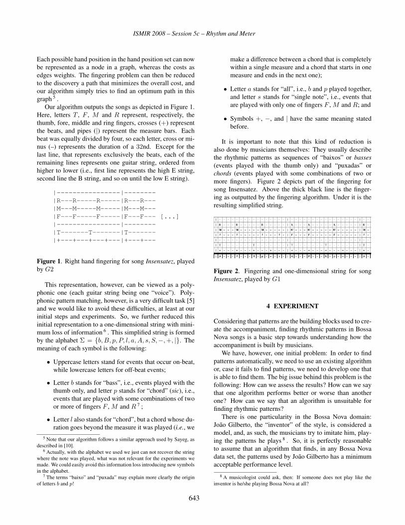
ISMIR 2008 – Session 5c – Rhythm and Meter
Each possible hand position in the hand position set can now
be represented as a node in a graph, whereas the costs as
edges weights. The fingering problem can then be reduced
to the discovery a path that minimizes the overall cost, and
our algorithm simply tries to find an optimum path in this
graph 5 .
Our algorithm outputs the songs as depicted in Figure 1.
Here, letters T , F , M and R represent, respectively, the
thumb, fore, middle and ring fingers, crosses (+) represent
the beats, and pipes (|) represent the measure bars. Each
beat was equally divided by four, so each letter, cross or mi-
nus (–) represents the duration of a 32nd. Except for the
last line, that represents exclusively the beats, each of the
remaining lines represents one guitar string, ordered from
higher to lower (i.e., first line represents the high E string,
second line the B string, and so on until the low E string).
|----------------|--------|R---R-----R-----|R---R---|M---M-----M-----|M---M---|F---F-----F-----|F---F--- [...]|----------------|--------|T-------T-------|T-------|+---+---+---+---|+---+---
Figure 1. Right hand fingering for song Insensatez, played
by G2
This representation, however, can be viewed as a poly-
phonic one (each guitar string being one “voice”). Poly-
phonic pattern matching, however, is a very difficult task [5]
and we would like to avoid these difficulties, at least at our
initial steps and experiments. So, we further reduced this
initial representation to a one-dimensional string with mini-
mum loss of information 6 . This simplified string is formed
by the alphabet Σ = {b, B, p, P, l, a, A, s, S,−, +, |}. The
meaning of each symbol is the following:
• Uppercase letters stand for events that occur on-beat,
while lowercase letters for off-beat events;
• Letter b stands for “bass”, i.e., events played with the
thumb only, and letter p stands for “chord” (sic), i.e.,
events that are played with some combinations of two
or more of fingers F , M and R 7 ;
• Letter l also stands for “chord”, but a chord whose du-
ration goes beyond the measure it was played (i.e., we
5 Note that our algorithm follows a similar approach used by Sayeg, as
described in [10].6 Actually, with the alphabet we used we just can not recover the string
where the note was played, what was not relevant for the experiments we
made. We could easily avoid this information loss introducing new symbols
in the alphabet.7 The terms “baixo” and “puxada” may explain more clearly the origin
of letters b and p!
make a difference between a chord that is completely
within a single measure and a chord that starts in one
measure and ends in the next one);
• Letter a stands for “all”, i.e., b and p played together,
and letter s stands for “single note”, i.e., events that
are played with only one of fingers F , M and R; and
• Symbols +, −, and | have the same meaning stated
before.
It is important to note that this kind of reduction is
also done by musicians themselves: They usually describe
the rhythmic patterns as sequences of “baixos” or basses(events played with the thumb only) and “puxadas” or
chords (events played with some combinations of two or
more fingers). Figure 2 depicts part of the fingering for
song Insensatez. Above the thick black line is the finger-
ing as outputted by the fingering algorithm. Under it is the
resulting simplified string.
Figure 2. Fingering and one-dimensional string for song
Insensatez, played by G1
4 EXPERIMENT
Considering that patterns are the building blocks used to cre-
ate the accompaniment, finding rhythmic patterns in Bossa
Nova songs is a basic step towards understanding how the
accompaniment is built by musicians.
We have, however, one initial problem: In order to find
patterns automatically, we need to use an existing algorithm
or, case it fails to find patterns, we need to develop one that
is able to find them. The big issue behind this problem is the
following: How can we assess the results? How can we say
that one algorithm performs better or worse than another
one? How can we say that an algorithm is unsuitable for
finding rhythmic patterns?
There is one particularity in the Bossa Nova domain:
João Gilberto, the “inventor” of the style, is considered a
model, and, as such, the musicians try to imitate him, play-
ing the patterns he plays 8 . So, it is perfectly reasonable
to assume that an algorithm that finds, in any Bossa Nova
data set, the patterns used by João Gilberto has a minimum
acceptable performance level.
8 A musicologist could ask, then: If someone does not play like the
inventor is he/she playing Bossa Nova at all?
643

ISMIR 2008 – Session 5c – Rhythm and Meter
But, what are the patterns João Gilberto plays? In the
literature we were able to find several transcriptions of pat-
terns played by João Gilberto [4, 9]. So, we have built a
catalogue containing 21 different patterns (labeled P1, P2,
etc.), all manually transcribed by musicologists from João
Gilberto’s recordings. Examples of patterns in this cata-
logue are showed in Figure 3.
Chord
Bass
Pattern P1
Chord
Bass
Pattern P15
Chord
Bass
Pattern P17
Figure 3. Examples of patterns in the catalogue
The experiment was, then, to explore the data set we had
acquired, verifying if patterns from this catalogue could be
found in the data set. For the experiment the algorithm
FlExPat [8] was chosen. It is an inexact string matching
algorithm that was inspired by algorithms from the Com-
putational Biology field, but that also incorporates results
from previous research on musical similarity [7]. Given an
input (here the simplified string previously described) and
using the edit distance as its similarity measure 9 , the algo-
rithm outputs a collection of patterns, organized in classes.
Each class has a prototype, that is the most representative
pattern of the class, and several occurrences, possibly inex-
act, of this prototype. It is also possible for the user to pro-
vide the algorithm with some constraints, such as the maxi-
mal and minimal length of patterns, the similarity threshold,
the maximum difference between two candidates to be com-
pared, etc.
In our first experiment FlExPat was used “as is”, that
is, we used the algorithm without any sort of modifica-
tions and/or adaptations. Although the algorithm found pat-
terns from the catalogue, including patterns with some small
modifications, the results, in this case, were not so good as
we previously expected. Table 1 summarizes the results we
obtained with FlExPat.
The algorithm’s configuration we used was the follow-
ing: mmin = 17 (minimal pattern length), mmax = 34(maximal pattern length), and similarity threshold of 0.75(normalized values). The lengths mmin and mmax corre-
spond to patterns varying from one to two measures 10 . On
9 Dynamic programming is used to compute it efficiently.10 It does not mean, however, that the patterns necessarily start at the
Pat G1 G2 Pat G1 G2P1 × × P12P2 × P13P3 P14P4 × P15 ×P5 P16P6 P17P7 P18P8 P19P9 × × P20P10 × × P21P11 / / /
Table 1. Patterns from the catalogue found in data set
average, each song has 48 classes of patterns (smallest num-
ber of classes was 40 and greatest number was 78).
In song Garota de Ipanema, played by G2, the
algorithm was able to identify the following pat-
tern: |A---P---B-p-+---|P---P---Bp--+l.
The corresponding pattern in the catalogue is
|A---P---B-p-+---|A---P---B-p-+-l-. Look-
ing closer at the modifications done by the performer, it is
possible to notice that he usually substitutes A by P in the
second measure of the pattern, and that he anticipates both
final chords in this same measure. Figure 4 depicts these
variations.
Chord
Bass
Original pattern Pattern found by FlExPat
Figure 4. Pattern found by FlExPat
In song Wave, as played by G1, FlExPat identi-
fied as the prototype of class 18 the following pat-
tern: |A---P---B-p-+l--|B---P---Bp--+p-.
The corresponding pattern in the catalogue is
|A---P---B-p-+-l-|B---P---B-p-+-l-. As
in the previous case, the modifications done by the
performer are mainly anticipations.
The main problem we found was that the extracted pat-
terns, many times, start from the middle of a measure, such
as in --B---B---+---|P---B---B---+---|P(FlExPat also found the expected pattern,
|P---B---B---+---|P---B---B---+--). This
brings some problems to the evaluation of the results: Due
to the great number of patterns with this kind of structural
malformation, it becomes difficult to validate the patterns.
beginning of the measure. There is no way to specify such a constraint in
FlExPat.
644

ISMIR 2008 – Session 5c – Rhythm and Meter
This problem is even bigger when most of a class is formed
by such patterns (it happened many times, unfortunately).
From these results we may rush and conclude that FlEx-
Pat performed poorly, since it found just a few patterns from
the catalogue in the data set and because these patterns were
grouped into too many classes. However, as pointed out in
the previous paragraph, there was a sort of structural malfor-
mation in many patterns found by FlExPat. So, what would
happen if we could “help” the algorithm, somehow provid-
ing it with some structural information about the patterns?
Unfortunately, it is not possible to describe for the al-
gorithm the desired aspect of the pattern: We can not say
that it should only consider patterns that begin on the mea-
sure bar, for instance. We can only describe the minimum
and maximum pattern lengths, as well as the minimum sim-
ilarity threshold. If we, however, look more carefully at the
patterns in the catalogue, it is possible to identify some com-
mon structure: They are all two measures long and they start
either at the measure bar or at a “puxada” right before the
measure bar 11 .
We then introduced a step just before the actual pattern
matching where all songs were segmented according to this
structure. It is important to note that with this modification,
we changed the abstraction level at which the pattern extrac-
tion happens: Instead of comparing event by event (basses
or chords), now we compare groups of events (i.e., the seg-
ments).
After we adjusted our implementation of the algorithm
to accept the segments described before as input, we ran the
experiment again. In this case, differently from the previ-
ous one, the algorithm found systematically in every song
patterns from the catalogue. This time, more than half of
the catalogue’s patterns was found, which significantly im-
proves the results we obtained before. On average, each
song had 14 classes of patterns (smallest number was 6 and
greatest number was 34). Table 2 shows the patterns found
in this second part of the experiment.
After running the experiments and having in mind that
we have used a small data set, it is now possible to discuss a
little bit the results we obtained. First of all, let us examine
the patterns used by the performers. As described by Dahia
et al. [2], patterns in the catalogue belong to one of four
groups: cyclical (P2 to P8), beginning (P9 to P12), spe-
cial (P13 and P14) and fill-in patterns (P15 to P21). Pat-
tern P1 is the main Bossa Nova pattern and forms its own
group. From the results presented before (Tables 1 and 2),
it is possible to see that the players used patterns belong-
ing to all groups, but the special one. This group, however,
contains patterns that are rarely used and it would not be a
problem if they do not show up. Given that the catalogue
contains Bossa Nova patterns, we can say, then, that the per-
11 It means that all segments look like |<pattern> or like
l*|<pattern>, where the * symbol represents a sequence of zero or
more minuses only.
Pat G1 G2 Pat G1 G2P1 × × P12P2 × × P13P3 × × P14P4 × P15 ×P5 × P16 × ×P6 × P17P7 P18 ×P8 P19 ×P9 × × P20P10 × × P21P11 / / /
Table 2. Patterns found by the modified version of FlExPat
formers do follow the Bossa Nova style in the rhythmic ac-
companiment construction.
There are occasions, however, that the pattern used does
not belong to the catalogue. G1, for instance, uses the pat-
tern |P---B---B---+---|P---B---B---+--- in
song Eu Sei Que Vou Te Amar. We can interpret this fact
in many ways, such as: the player deliberately used a non
Bossa Nova pattern, the catalogue may not be complete, or
even that Bossa Nova style has changed over the time and
players started to use or create their own patterns.
5 FINAL REMARKS AND FUTURE WORK
This paper described an experiment that dealt with the ex-
traction of rhythmic patterns from Bossa Nova songs. Six-
teen beat tracked MIDI files, representing the recording of
several songs by two different players, were represented as
a string and thereafter processed by a string matching al-
gorithm called FlExPat. The objective was to identify in
the data set patterns from a previously acquired catalogue of
patterns.
First results showed that, although FlExPat could find
some patterns, many patterns, including some that could be
clearly heard, were not found. After examining the struc-
ture of the catalogue’s patterns, we were able to pre-segment
the songs and use the pre-segmented version of the song as
input for the algorithm. This time the results were much
better, and more than half of the patterns was found by the
algorithm.
It is important to stress the relevance of the abstractions
we have built. First of all, we could reduce the complexity of
the pattern matching process by rewriting a polyphonic song
as a monophonic line, with minimum information loss. This
first abstraction was, however, not sufficient, as can be seen
with the first experiment we made, and we had to build a
second abstraction, going up one structural level: From sin-
gle events to groups of events (segments). Only due to these
645
ISMIR 2008 – Session 5c – Rhythm and Meter
abstractions we could explore the data set we collected.
Of course, there are several points for improvement. One
that is particularly important is the representation. We used
a very simple representation of the events. Attributes like
tempo, structural or harmonic information are not repre-
sented. The more attentive reader may have even noticed
that the actual duration of the events is not represented at
all. We just used the onset information, which turned out to
work for this experiment. To further investigate the particu-
larities of the patterns, however, we surely need to represent
appropriately the duration of each event. Another point re-
lated to the representation is the following: what kind of
results would we have if we had represented the downbeat
explicitly? Would they be better than the ones we presented
here?
The evaluation of the algorithm’s results was done in an
ad hoc manner: Results were compared, one by one, to the
patterns in the catalogue. This procedure takes too much
time, is error prone, and, therefore, must be improved. We
plan to implement a tool to help us with this task.
The data acquisition is an important and non-trivial prob-
lem. It is important because if we want to draw relevant and
significant conclusions about Bossa Nova (and any musical
style, in fact), we must have a much more representative
data set. And it is non-trivial because there are many fac-
tors involved varying from the availability and willingness
of certain performer to record for us, to copyright issues of
the collected material. One possible way to remedy this
problem is to use audio recordings as start point, but, un-
fortunately, there are other problems (separating guitar and
singing voice signals most notably).
FlExPat’s problem (structural malformation) should be
examined more carefully, since, instead of a problem, it can
mean another thing. Several patterns of the catalogue have
a common substructure (i.e., sub-parts of these patterns are
equal). It may be the case that the second measure of pat-
terns whose second measure are equal, are frequently con-
catenated with patterns whose first measure are similar. So,
it may be the case that these concatenations are so typical
that they are “promoted” to patterns by the algorithm.
Finally, we hope that the questions previously formulated
were provocative enough. We do believe that answers to
them will bring much more understanding of how the musi-
cians bring their genres to life, as well as register how they,
musicians and styles, evolved through the years.
6 REFERENCES
[1] Chediak, A. editor. Songbook: Bossa Nova, volume 1–5.
Lumiar Editora, Rio de Janeiro, 1990.
[2] Dahia, M., Santana, H., Trajano de Lima, E., Sandroni,
C., Ramalho, G., and Cabral, G. “Using patterns to gen-
erate rhythmic accompaniment for guitar”, In Proc. of
Sound and Music Computing (SMC’04), pages 111–115,
2004.
[3] Dixon, S. “Automatic extraction of tempo and beat from
expressive performances”, Journal of New Music Re-search, 30(1):39–58, 2001.
[4] Garcia, W. Bim Bom: A Contradição sem Conflitos deJoão Gilberto. Editora Guerra e Paz, 1999.
[5] Meredith, D., Lemström, K., and Wiggins, G. “Algo-
rithms for discovering repeated patterns in multidimen-
sional representations of polyphonic music”, Journal ofNew Music Research, 31(4):321–345, 2002.
[6] MMM. Music, mind, machine group, 2003.
http://www.nici.kun.nl/mmm/. Last ac-
cess date Mar 12 2004.
[7] Mongeau, M., and Sankoff, D. “Comparision of musical
sequences”, Computer and the Humanities, 24:161–175,
1990.
[8] Rolland, P.-Y. “FlExPat: Flexible extraction of sequen-
tial patterns”, In Nick Cercone, Tsau Young Lin, and
Xindong Wu, editors, Proceedings of the 2001 IEEEInternational Conference on Data Mining (ICDM’01),pages 481–488. IEEE Computer Society, 2001.
[9] Sandroni, C. Feitiço Decente: Transformações doSamba no Rio de Janeiro (1917–1933). Jorge Zahar Ed-
itor, Rio de Janeiro, 2001.
[10] Sayegh, S. “Fingering for string instruments with the op-
timum path paradigm”, In Peter M. Todd and D. Gareth
Loy, editors, Music and Connectionism, pages 243–255,
Cambridge (MA), 1991. The MIT Press.
[11] Trajano de Lima, E., Dahia, M., Santana, H., and Ra-
malho, G. “Automatic discovery of right hand fingering
in guitar accompaniment”, In Intern. Comp. Mus. Conf.(ICMC), pages 722–725, 2004.
[12] Widmer, G. “Applications of machine learning to music
research: Empirical investigations into the phenomenon
of musical expression”, In R. S. Michalski, I. Bratko,
and M. Kubat, editors, Machine Learning, Data Miningand Knowledge Discovery: Methods and Applications.
Wiley & Sons, Chichester (UK), 1998.
[13] Widmer, G. “Machine discoveries: A few simple, robust
local expression principles”, Journal of New Music Re-search, 31(1):27–50, 2002.
[14] Widmer, G., Dixon, S., Goebl, W., Pampalk, E., and To-
budic, A. “In search of the Horowitz factor”, AI Maga-zine, 24(3):111–130, 2003.
646

ISMIR 2008 – Session 5c – Rhythm and Meter
ANALYZING AFRO-CUBAN RHYTHM USING ROTATION-AWARE CLAVETEMPLATE MATCHING WITH DYNAMIC PROGRAMMING
Matthew Wright, W. Andrew Schloss, George TzanetakisUniversity of Victoria, Computer Science and Music [email protected], [email protected], [email protected]
ABSTRACT
The majority of existing research in Music Information Re-
trieval (MIR) has focused on either popular or classical mu-
sic and frequently makes assumptions that do not generalize
to other music cultures. We use the term Computational Eth-
nomusicology (CE) to describe the use of computer tools to
assist the analysis and understanding of musics from around
the world. Although existing MIR techniques can serve as
a good starting point for CE, the design of effective tools
can benefit from incorporating domain-specific knowledge
about the musical style and culture of interest. In this pa-
per we describe our realization of this approach in the con-
text of studying Afro-Cuban rhythm. More specifically we
show how computer analysis can help us characterize and
appreciate the complexities of tracking tempo and analyz-
ing micro-timing in these particular music styles. A novel
template-based method for tempo tracking in rhythmically
complex Afro-Cuban music is proposed. Although our ap-
proach is domain-specific, we believe that the concepts and
ideas used could also be used for studying other music cul-
tures after some adaptation.
1 INTRODUCTION
We present a set of techniques and tools designed for study-
ing rhythm and timing in recordings of Afro-Cuban music
with particular emphasis on “clave,” a rhythmic pattern used
for temporal organization. In order to visualize timing in-
formation we propose a novel graphical representation that
can be generated by computer from signal analysis of audio
recordings and from listeners’ annotations collected in real
time. The proposed visualization is based on the idea of Bar
Wrapping, which is the breaking and stacking of a linear
time axis at a fixed metric location.
The techniques proposed in this paper have their origins
in Music Information Retrieval (MIR) but have been adapted
and extended in order to analyze the particular music cul-
ture studied. Unlike much of existing work in MIR in which
the target user is an “average” music listener, the focus of
this work is people who are “experts” in a particular music
culture. Examples of the type of questions they would like
to explore include: how do expert players differ from each
other, and also from competent musicians who are not fa-
miliar with the particular style; are there consistent timing
deviations for notes at different metric positions; how does
tempo change over the course of a recording etc. Such ques-
tions have been frequently out of reach because it is tedious
or impossible to explore without computer assistance.
Creating automatic tools for analyzing micro-timing and
tempo variations for Afro-Cuban music has been challeng-
ing. Existing beat-tracking tools either don’t provide the re-
quired functionality (for example only perform tempo track-
ing but don’t provide beat locations) or are simply not able
to handle the rhythmic complexity of Afro-Cuban music
because they make assumptions that are not always appli-
cable, such as expecting more and louder notes on met-
rically “strong” beats. Finally the required precision for
temporal analysis is much higher than typical MIR appli-
cations. These considerations have motivated the design of
a beat tracker that utilizes domain-specific knowledge about
Cuban rhythms.
The proposed techniques fall under the general rubric
of what has been termed Computational Ethnomusicology(CE), which refers to the design and usage of computer tools
that can assist ethnomusicological research [14] . Futrelle
and Downie argued for MIR research to expand to other
domains beyond Western pop and classical music [9]. Re-
trieval based on rhythmic information has been explored in
the context of Greek and African traditional music [1].
Our focus here is the analysis of music in which percus-
sion plays an important role, specifically, Afro-Cuban mu-
sic. Schloss [13] and Bilmes [4] each studied timing nu-
ances in Afro-Cuban music with computers. Beat tracking
and tempo induction are active topics of research, although
they have mostly focused on popular music styles [11]. Our
work follows Collins’ suggestion [5] to build beat trackers
that embody knowledge of specific musical styles.
The clave is a small collection of rhythms embedded in
virtually all Cuban music. Clave is a repeated syncopated
rhythmic pattern that is often explicitly played, but often
only implied; it is the essence of periodicity in Cuban music.
An instrument also named “clave” (a pair of short sticks hit
together) usually plays this repeating pattern. Clave is found
mainly in two forms: rumba clave and son clave. (One way
of notating clave is shown in Figure 1.)
647

ISMIR 2008 – Session 5c – Rhythm and Meter
Figure 1. Son (left) and rumba (right) clave
Our study of timing requires knowing the exact time of
every note played by the clave. We can then decompose this
data into an estimate of how tempo changes over time (what
is called the tempo curve) and a measure of each individual
note’s deviation from the “ideal” time predicted by a metro-
nomic rendition of the patterns shown in Figure 1.
Unfortunately, we do not know of any databases of Afro-
Cuban music with an exact ground-truth time marked for
every clave note or even for every downbeat. 1 Therefore
we constructed a small four-song database 2 and gathered
ground truth clave timing data by having an expert percus-
sionist with Afro-Cuban experience tap along with the clave
part. Custom sample-accurate tap detection/logging soft-
ware automatically timestamps the taps.
Recordings of Afro-Cuban music challenge existing state-
of-the-art beat-tracking algorithms because of the complex
and dense rhythm and the lack of regular approximately
isochronous pulses. Figure 2 shows how two recent state-
of-the-art beat-tracking systems (BeatRoot [7] and a beat
tracker using dynamic programming proposed by Ellis [8])
do not generate an accurate tempo curve for the recording
CB. The plots in the figure are shown only in order to moti-
vate the proposed approach. The comparison is not fair, as
the other algorithms are more generally applicable and de-
signed with different assumptions, but in any case it demon-
strates the advantage of a domain-specific method to deal
with these recordings: our method is specifically designed
to take into account clave as the rhythmic backbone.
2 DATA PREPARATION
It is common for Afro-Cuban songs to begin with just the
sound of the clave for one or two repetitions to establish the
initial tempo. However as other instruments (both percus-
sive and pitched) and voices enter the mix the sound of the
clave tends to become masked. The first step of data prepa-
ration is to enhance the sound of the clave throughout the
song using a matched filter approach. In addition onset de-
tection is performed.
1 Bilmes recorded about 23 minutes of Afro-Cuban percussion at MIT in
1992, and performed sophisticated analysis of the timing of the guagua and
conga (but not clave) instruments [4]; unfortunately these analog record-
ings are not currently available to the research community.2 Here is the name, artist, and source recording for each song, along
with the two-character ID used later in the paper: LP: La Polemica, Los
Muñequitos de Matanzas, Rumba Caliente 88. CB: Cantar Bueno, Yoruba
Andabo, El Callejon De Los Rumberos. CH: Chacho, Los Muñequitos de
Matanzas, Cuba: I Am Time (Vol. 1). PD: Popurrit de Sones Orientales,
Conjunto de Sones Orientales, Son de Cuba.
Figure 2. Four estimates of the tempo curve for our record-
ing CB: Ground truth calculated from a human expert’s tap
times (upper left), curve from our method (top right), curve
from BeatRoot (lower left), and curve from Ellis’ dynamic
programming approach (lower right).
2.1 Clave enhancement using Matched-Filtering
A matched filter detects or enhances the presence of an apriori known signal within an unknown signal. Its impulse
response is a time-reversed copy of the known signal, which
in our case is the beginning portion of one isolated clave
note. The clave instrument affords little timbral variety and
therefore every note of clave in a given recording sounds
substantially like all the others, so a matched filter made
from any single note (frequently easily obtained from the
beginning of the song) will enhance the presence of the clave
throughout the song and suppress the remaining signal. One
free parameter is the filter order, i.e., the duration of the seg-
ment of the clave note; in each case we selected a “good”
matched filter experimentally by listening to the output of
different configurations. All the curves in Figure 2 and
results in this paper have been calculated on audio signals
output by matched filtering.
2.2 Onset detection
Onset detection aims at finding the starting time of musical
events (e.g. notes, chords, drum events) in an audio signal;
see [3],[6] for recent tutorials. We used spectral flux as the
onset detection function, defined as:
SF (n) =N/2∑k=0
HWR(|X(n, k)| − |X(n− 1, k)|) (1)
648

ISMIR 2008 – Session 5c – Rhythm and Meter
where HWR(x) = x+|x|2 is the half-wave rectifier function,
X(n, k) represents the k-th frequency bin of the n-th frame
of the power magnitude (in dB) of the short time Fourier
transform, and N is the corresponding Hamming window
size. For the experiments performed in this work all data
had a sampling rate fs = 44100 Hz and we used a window
size of 46 ms (N = 2048) and a hop size of about 11ms
(R = 512). The onsets are subsequently detected from the
spectral flux values by a causal peak-picking algorithm that
finds local maxima as follows. A peak at time t = nRfs
(the
time of the beginning of the nth frame) is selected as an
onset if it fulfills the following conditions:
1. SF (n) ≥ SF (k) ∀k : n− w ≤ k ≤ n + w
2. SF (n) >Pn+w
k=n−mw SF (k)
mw+w+1 × thres + δ
where w = 6 is the size of the window used to find a local
maximum, m = 4 is a multiplier so that the mean is calcu-
lated over a larger range before the peak, thres = 2.0 is a
threshold relative to the local mean that a peak must reach in
order to be sufficiently prominent to be selected as an onset,
and δ = 10−20 is a residual value to avoid false detections
on silent regions of the signal. All these parameter values
were derived from preliminary experiments using a collec-
tion of music signals with varying onset characteristics.
In order to reduce the false detection rate, we smooth the
detection function SF (n) with a Butterworth filter to reduce
the effect of spurious peaks:
H(z) =0.1173 + 0.2347z−1 + 0.1174z−2
1− 0.8252z−1 + 0.2946z−2(2)
(These coefficients were found by experimentation based on
the findings in [3],[6].) In order to avoid phase distortion
(which would shift the detected onset time away from the
SF (n) peak) the signal is filtered in both the forward and
reverse directions.
3 TEMPLATE-BASED TEMPO TRACKING
We propose a new method to deal with the challenges of
beat tracking in Afro-Cuban music. The main idea is to use
domain specific knowledge, in this case the clave pattern,
directly to guide the tracking. The method consists of the
following four basic steps: 1) Consider each detected onset
time as a potential note of the clave pattern. 2) Exhaustively
consider every possible tempo (and clave rotation) at each
onset by cross-correlating each of a set of clave-pattern tem-
plates against an onset strength envelope signal beginning
at each detected onset. 3) Interpret each cross-correlation
result as a score for the corresponding tempo (and clave ro-
tation) hypothesis. 4) Connect the local tempo and phase
estimates to provide a smooth tempo curve and deal with
errors in onset detection, using dynamic programming.
The idea of using dynamic programming for beat track-
ing was proposed by Laroche [10], where an onset func-
tion was compared to a predefined envelope spanning mul-
tiple beats that incorporated expectations concerning how
a particular tempo is realized in terms of strong and weak
beats; dynamic programming efficiently enforced continu-
ity in both beat spacing and tempo. Peeters [12] developed
this idea, again allowing for tempo variation and matching
of envelope patterns against templates. An approach assum-
ing constant tempo that allows a simpler formulation at the
cost of more limited scope has been described by Ellis [8].
3.1 Clave pattern templates
At the core of our method is the idea of using entire rhyth-
mic patterns (templates) for beat tracking rather than indi-
vidual beats. First we construct a template for each possible
tempo. We take the ideal note onset times in units of beats
(e.g., for rumba clave, the list 0, 0.75, 1.75, 2.5, 3) and mul-
tiply them by the duration of a beat at each tempo, giving
ideal note onset times in seconds. We center a Gaussian en-
velope on each ideal note onset time to form the template.
The standard deviation (i.e., width) of these Gaussians is a
free parameter of this method. Initial results with a constant
width revealed a bias towards higher tempi, so widths are
specified in units of beats, i.e., we scale the width linearly
with tempo. Better results were obtained by making each
template contain multiple repetitions of the clave, e.g., three
complete patterns. Figure 3 shows a visual representation
of the template rotations for all considered tempi.
Figure 3. Clave Templates for all rotations and tempi
With a 5-note clave pattern, any given note played by the
clave could be the 1st, 2nd, 3rd 4th or 5th note of the pattern.
Therefore we make templates for all “rotations” of the clave,
i.e., for the repeating pattern as started from any of the five
notes. For example, rotation 0 of rumba clave is [0, 0.75,
1.75, 2.5, 3], and rotation 1 (starting from the second note)
is [0.75 1.75 2.5 3 4] - 0.75 = [0 1 1.75 2.25 3.25]. Time 0always refers to the onset time of the current note.
649

ISMIR 2008 – Session 5c – Rhythm and Meter
Figure 4. Matching different templates (filled grey) to the
CB recording’s energy envelope (black line). The X-axis is
time (seconds), with zero the time of the onset under consid-
eration. The score for each template match represents how
well that template lines up with the energy envelope.
We cross-correlate (in other words, take the dot product
of) these templates against segments of an onset strength
envelope (in our case, simply the total energy in each 1024-
sample window of the matched filter output) beginning at
the time of each detected onset. We interpret the dot prod-
uct between the onset strength signal O(t) and a template
Tj,k(t) with tempo j and rotation k as the strength of the
hypothesis that the given onset is the given note of clave at
the given tempo. Figure 4 depicts this process for some
tempi and rotations and the corresponding scores. We ex-
haustively compute these dot products for every candidate
tempo j (e.g,. from 95 to 170 BPM in 1 BPM increments),
for all five rotations of the clave pattern k , for every detected
onset i at time ti to produce a score grid:
score(i, j, k) =LTj,k−1∑
t=0
Tj,k(t)O(ti + t) (3)
where LTj,k is the length of template Tj,k .
3.2 Rotation-blind dynamic programming
It is trivial to look at a given onset, pick the tempo and ro-
tation with the highest score, and call that the short-term
tempo estimate. However, due to the presence of noise, in-
evitable onset detection errors, and the matched filter’s far-
from-perfect powers of auditory source separation, simply
connecting these short-term tempo estimates does not pro-
duce a usable estimate of the tempo curve. Better results can
be achieved by explicitly discouraging large tempo changes.
We use dynamic programming [2] as an efficient means to
estimate the best tempo path (i.e., time-varying tempo). In
the next section we will consider the rotations of the tem-
plate; for now let the “rotation-blind” score be:
scoreRB(i, j) = max(score(i, j, k)) k : 1..5 (4)
We convert each score scoreRB to a cost Ci,j with a
linear remapping so that the highest score maps to cost 0and the lowest score maps to cost 1. We define a path Pas a sequence of tempo estimates (one per onset), so that
P (i) is P’s estimate of the tempo at time ti. Our algorithm
minimizes the path cost PC of the length n path P :
PC(P ) =∑
i=0:n−1
Ci,P (i)+∑
i=0:n−2
F (P (i), P (i+1)) (5)
where F (tempo1, tempo2) is a “tempo discontinuity cost
function” expressing the undesirability of sudden changes
in tempo. F is simply a scalar times the absolute difference
of the two tempi. Dynamic programming can efficiently find
the lowest-cost path from the first onset to the last because
the optimal path up to any tempo at time ti depends only
on the optimal paths up to time ti−1. We record both the
cost PC(i, j) and the previous tempo Previous(i, j) for
the best path up to any given onset i and tempo j.
3.3 Rotation-aware dynamic programming
Now we will extend the above algorithm to consider rota-
tion, i.e., our belief about which note of clave corresponds
to each onset. Now our cost function Ci,j,k is also a func-
tion of the rotation k. Our path tells us both the tempo
Ptempo(i) at time ti and also the rotation Prot(i), so we
must keep track of both previous Previoustempo(i, j) and
Previousrot(i, j) (corresponding to the best path up to iand j). Furthermore, considering rotation will also give us a
principled way for the path to skip over “bad” onsets, so in-
stead of assuming that every path reaches onset i by way of
onset i− 1 we must also keep track of Previousonset(i, j).The key improvement in this algorithm is the handling of
rotation. Rotation (which indexes the notes in the clave pat-
tern) is converted to phase, the proportion (from 0 to 1) of
the distance from one downbeat to the next. (So the phases
for the notes of rumba clave are [0, 0.1875, 0.4375, 0.625,
0.75]). The key idea is predicting what the phase of the next
note “should be”: Given phase φ1 and tempo j1 for onset
i1, a candidate tempo j2 for onset i2, and the time between
onsets ΔT = t2 − t1, and assuming linear interpolation of
650

ISMIR 2008 – Session 5c – Rhythm and Meter
LP CB CH PD LPWT PDWT
RB 40 26 22.9 63.1 39.96 62.7
RA 1.75 11 1.54 3.10 2.043 57.9
Table 1. RMS (in BPM) results for tempo curve estimation
tempo during the (short) time between these nearby onsets,
we can use the fact that tempo (beat frequency) is the deriva-
tive of phase to estimate the phase φ̂2:
φ̂2 = φ1 + ΔT ((j1 + j2)/2)/(4× 60) (6)
Dividing by 4× 60 converts from BPM to bars per second.
Now we can add an extra term to our cost function to ex-
press the difference between the predicted phase φ̂2 and the
actual phase φ2 corresponding to the rotation of whatever
template we’re considering for the onset at time t2 (being
careful to take this difference modulo 1, so that, e.g., the dif-
ference between 0.01 and .98 is only 0.03, not 0.97). We’ll
call this phase distance the “phase residual” R, and add the
term α ∗R to our cost function.
Now let’s consider how to handle “false” detected onsets,
i.e., onsets that are not actually notes of clave. For onset n,
we consider not just onset n − 1 as the previous onset, but
every onset i with ti > tn −K, i.e., every onset within Kseconds before onset n, where K is set heuristically to 1.5
times the largest time between notes of clave (one beat) at
the slowest tempo. We introduce a “skipped onset cost” βand include β × (n − i − 2) in the path cost when the path
goes from onset i to onset n.
Table 1 shows the Root-mean-square (RMS) error be-
tween the ground truth tempocurve and the tempocurves es-
timated by the rotation-blind (RB) and rotation-aware (RA)
configurations of our method. In all cases the rotation-aware
significantly outperforms the rotation-blind method (which
usually tracks correctly only parts of the tempo curve). The
first three recordings (LP, CB, CH) have rumba-clave and
the fourth piece (PD) has son-clave. The last two columns
show the results when using the “wrong” template. Essen-
tially when the template is not correct the matching cost of
the beat path is much higher and the tempo curve estimation
is wrong. Figure 5 shows the score grid for the rotation-
blind (top) and rotation-aware (bottom) configurations over-
laid with the estimated and ground truth tempocurves.
4 BAR-WRAPPING VISUALIZATION
A performance typically consists of about 625-1000 clave
“notes”. Simply plotting each point along a linear time axis
would require either excessive width, or would make the fig-
ure too small to see anything; this motivates bar wrapping.
Conceptually, we start by marking each event time (in this
Figure 5. Rotation-blind (top) and rotation-aware (bottom)
beat tracking
case, each detected onset) on a linear time axis. If we imag-
ine this time axis as a strip of magnetic tape holding our
recording, then metaphorically we cut the tape just before
each downbeat, so that we have 200 short pieces of tape,
which we then stack vertically, so that time reads from left
to right along each row, and then down to the next row, like
text in languages such as English. Each of these “strips” is
then stretched horizontally to fill the figure width, adding a
tempo curve along the right side to show the original dura-
tion of each bar. Figure 6 depicts the times of our detected
onsets for LP with this technique. The straight lines show
the theoretical clave locations. By looking at the figure one
can notice that the 5th clave note is consistently slightly later
than the theoretical location. This would be hard to notice
without precise estimation of the tempocurve.
Rotation-aware dynamic programming is used to find the
downbeat times. An explicit downbeat estimate occurs when-
ever the best path includes a template at rotation 0. But there
might not be a detected onset at the time of a downbeat, so
we must also consider implicit downbeats, where the current
onset’s rotation is not 0 but it is lower than the rotation of
the previous onset in the best path. The phase is interpolated
to estimate the downbeat time that “must have occurred” be-
tween the two onsets.
651

ISMIR 2008 – Session 5c – Rhythm and Meter
1 1.5 2 2.5 3 3.5 4 4.5
0
20
40
60
80
100
120
140
160
bar number
120140
0
20
40
60
80
100
120
140
160
Figure 6. Bar-wrapping visualization
5 DISCUSSION AND CONCLUSIONS
Our beat-tracking method works particularly well for Afro-
Cuban clave for many reasons: 1) The clave part almost
never stops in traditional Afro-Cuban music (although it can
be hard to hear when many other percussion instruments
are playing). 3 2) The clave pattern almost never changes
in Afro-Cuban music. 4 3) The clave instrument produces
an extremely consistent timbre with every note, so matched
filtering does a good job emphasizing it. 5 4) Songs often
begin with the clave alone, making it easy to construct our
matched filter. 6 5) The clave plays one of a few prede-
termined syncopated parts, favoring the use of predefined
templates rather than assumptions of isochrony.
There are many future work directions. Rhythmic analy-
sis can be used to categorize recordings into different styles
and possibly identify particular artists or even percussion-
ists. We also plan to apply the method to more record-
ings and continue working with ethnomusicologists and per-
formers interested in exploring timing. It is our belief that
our template-based rotation-aware formulation can also be
applied to popular music by utilizing different standard drum
patterns as templates. All the code implementing the method
can be obtained by emailing the authors.
3 Our method’s phase- and tempo-continuity constraints allow it to stay
on track in the face of extra or missing onsets and occasional unduly low
template match scores, so we expect that it would still perform correctly
across short gaps in the clave part.4 One subtlety of Afro-Cuban music is the notion of “3-2” versus “2-3”
clave, which refers to a 180-degree phase shift of the clave part with respect
to the ensemble’s downbeat. Our method has no notion of the ensemble’s
downbeat and “doesn’t care” about this distinction. Some songs change
between 3-2 and 2-3 in the middle, but never by introducing a discontinuity
in the clave part (which would be a problem for our algorithm); instead the
other instruments generally play a phrase with two “extra” beats that shifts
their relationship to the clave.5 In rare cases a different instrument carries the clave part; this should
not be a problem for our method as long as a relatively isolated sample can
be located.6 As future work we would like to explore the possibility of creating a
“generic” clave enhancement filter that doesn’t rely on having an isolated
clave note in every recording, a weakness of the current method.
6 REFERENCES
[1] I. Antonopoulos et al. Music retrieval by rhythmic simi-
larity applied on greek and african traditional music. In
Proc. Int. Conf. on Music Information Retrieval(ISMIR),2007.
[2] R. Bellman. Dynamic Programming. Princeton Univer-
sity Press, 1957.
[3] J.P. Bello et al. A tutorial on onset detection in music
signals. IEEE Trans. on Speech and Audio Processing,
13(5):1035–1047, September 2005.
[4] J. Bilmes. Timing is of the essence: Perceptual and com-
putational techniques for representing, learning and re-
producing timing in percussive rhythm. Master’s thesis,
Massachusetts Institute of Technology, 1993.
[5] N. Collins. Towards a style-specific basis for computa-
tional beat tracking. In Int. Conf. on Music Perceptionand Cognition, 2006.
[6] S. Dixon. Onset detection revisited. In Proc. Interna-tional Conference on Digital Audio Effects (DAFx),Montreal, Canada, 2006.
[7] S. Dixon. Evaluation of audio beat tracking system beat-
root. Journal of New Music Research, 36(1), 2007.
[8] D. Ellis. Beat tracking by dynamic programming. Jour-nal of New Music Research, 36(1), 2007.
[9] J. Futrelle and S. Downie. Interdisciplinary communi-
ties and research issues in music information retrieval. In
Proc. Int. Conf. on Music Information Retrieval(ISMIR),2002.
[10] J. Laroche. Efficient tempo and beat tracking in audio
recordings. Journal of the Audio Engineering Society,
51(4):226–233, 2003.
[11] M.F. McKinney et al. Evaluation of audio beat tracking
and music tempo extraction algorithms. Journal of NewMusic Research, 36(1), 2007.
[12] G. Peeters. Template-based estimation of time-varying
tempo. EURASIP Journal of Advances in Signal Pro-cessing, 2007.
[13] W.A. Schloss. On the Automatic Transcription of Per-cussive Music: From Acoustic Signal to High-LevelAnalysis. PhD thesis, Stanford University, 1985.
[14] G. Tzanetakis, A. Kapur, W.A. Schloss, and M. Wright.
Computational ethnomusicology. Journal of Interdisci-plinary Music Studies, 1(2):1–24, 2007.
652

ISMIR 2008 – Session 5c – Rhythm and Meter
BEAT TRACKING USING GROUP DELAY BASED ONSET DETECTION
Andre Holzapfel and Yannis StylianouInstitute of Computer Science, FORTH, Greece,
and Multimedia Informatics Lab, Computer Science Department, University of Crete{hannover, yannis}@csd.uoc.gr
ABSTRACT
This paper introduces a novel approach to estimate onsets
in musical signals based on the phase spectrum and specif-
ically using the average of the group delay function. A
frame-by-frame analysis of a music signal provides the evo-
lution of group delay over time, referred to as phase slope
function. Onsets are then detected simply by locating the
positive zero-crossings of the phase slope function. The pro-
posed approach is compared to an amplitude-based onset de-
tection approach in the framework of a state-of-the-art sys-
tem for beat tracking. On a data set of music with less per-
cussive content, the beat tracking accuracy achieved by the
system is improved by 82% when the suggested phase-based
onset detection approach is used instead of the amplitude-
based approach, while on a set of music with stronger per-
cussive characteristics both onset detection approaches pro-
vide comparable results of accuracy.
1 INTRODUCTION
The task of estimating the times at which a human would
tap his foot to a musical sound is known as beat tracking
[1]. All state-of-the-art approaches ([1, 2, 3, 4]) for this task
first conduct an onset detection. The output of the onset de-
tection is a signal with a lower time resolution than the input
signal, which has peaks at the time instances where a musi-
cal instrument in the input started playing a note. Usually,
this onset signal is derived from the amplitude of the signal,
as in [1, 2, 3]. Only in [4], phase information is consid-
ered, by computing the phase deviation between neighbor-
ing analysis frames. Several approaches of computing on-
sets from musical signals are compared in [5], resulting in
the conclusion that in general the moments of big positive
change in the amplitude spectrum of the signal provide the
most preferable estimators for the onsets. This is because
using information contained in the complex spectrum or in
the phase changes might lead to similar onset estimations,
but using only the amplitude spectrum is preferred for com-
putational reasons [5]. A similar conclusion can be drawn
from the results of the MIREX 2007 Audio Onset Detection
contest 1 , where most systems use only the amplitude infor-
1 http://www.music-ir.org/mirex/2007/index.php/Audio Onset Detection
mation. Considering the results on complex music mixtures,
which are the signals of interest in beat tracking, the usage
of phase deviation by some systems does not improve the
onset estimation accuracy [6].
As can be seen in the results depicted in [7] (Table II), the
state-of-the-art approaches for beat tracking decrease sig-
nificantly in accuracy, when applied to folk music. These
music signals contain weaker percussive content than music
of rock or disco styles. This problem is of particular impor-
tance when dealing with traditional dances as well, as they
are often played using string or wind instruments only [8].
Based on the results obtained in [7], it is necessary to im-
prove beat tracking on music with little percussive content.
While a decrease in the case of jazz and classical music can
partly be attributed to the complex rhythmic structure, rhyth-
mic structure of folk music is simpler, and thus the decrease
in this forms of music may be attributed solely to the prob-
lem of detecting onsets.
In [9], the negative derivative of the unwrapped phase, i.e.the group delay, is used to determine instants of significant
excitation in speech signals. This approach has been fur-
ther developed and used for the detection of clicks of ma-
rine mammals in [10]. There, it has been shown that pulses
can be reliably detected by using group delay, even when the
pulses have been filtered by a minimum phase system. Moti-
vated by these works, we suggest the use of the group delay
function for onset estimation in musical signals, and then
use this estimation as input to a beat tracker based on the
state-of-the-art system presented in [2]. The goal of this pa-
per is to provide an improved beat tracking performance on
musical signals with simple rhythmic structure and little or
no percussive content. The proposed approach to consider
phase information is novel in Music Information Retrieval,
as previous approaches computed a time derivative of phase
[5], while the suggested approach makes use of group de-
lay, which is a derivative of phase over frequency. The
group delay function is computed in frame-by-frame analy-
sis and its average is computed for each frame. This results
in time-domain signal referred to as phase slope function
[10]. Onsets are then simply estimated by detecting the pos-
itive zero-crossings of the phase slope function. Therefore,
the suggested approach does not require the use of time-
dependent (adaptive) energy-based thresholds as the ampli-
653
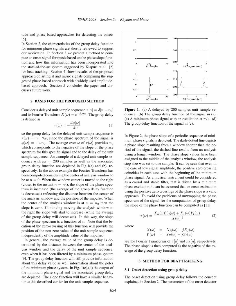
ISMIR 2008 – Session 5c – Rhythm and Meter
tude and phase based approaches for detecting the onsets
[5].
In Section 2, the characteristics of the group delay function
for minimum phase signals are shortly reviewed to support
our motivation. In Section 3 we present a method to com-
pute an onset signal for music based on the phase slope func-
tion and how this information has been incorporated into
the state-of-the-art system suggested by Klapuri et al. [2]
for beat tracking. Section 4 shows results of the proposed
approach on artificial and music signals comparing the sug-
gested phase-based approach with a widely used amplitude-
based approach. Section 5 concludes the paper and dis-
cusses future work.
2 BASIS FOR THE PROPOSED METHOD
Consider a delayed unit sample sequence x[n] = δ[n− n0]and its Fourier Transform X(ω) = e−jωn0 . The group delay
is defined as:
τ(ω) = −dφ(ω)dω
(1)
so the group delay for the delayed unit sample sequence is
τ(ω) = n0 ∀ω, since the phase spectrum of the signal is
φ(ω) = −ωn0. The average over ω of τ(ω) provides n0
which corresponds to the negative of the slope of the phase
spectrum for this specific signal and to the delay of the unit
sample sequence. An example of a delayed unit sample se-
quence with n0 = 200 samples as well as the associated
group delay function are depicted in Fig.1(a) and (b), re-
spectively. In the above example the Fourier Transform has
been computed considering the center of analysis window to
be at n = 0. When the window center is moved to the right
(closer to the instant n = n0), the slope of the phase spec-
trum is increased (the average of the group delay function
is decreased) reflecting the distance between the center of
the analysis window and the position of the impulse. When
the center of the analysis window is at n = n0 then the
slope is zero. Continuing moving the analysis window to
the right the slope will start to increase (while the average
of the group delay will decreased). In this way, the slope
of the phase spectrum is a function of n. Note that the lo-
cation of the zero-crossing of this function will provide the
position of the non-zero value of the unit sample sequence
independently of the amplitude value of the impulse.
In general, the average value of the group delay is de-
termined by the distance between the center of the anal-
ysis window and the delay of the unit sample sequence,
even when it has been filtered by a minimum phase system
[9]. The group delay function will still provide information
about this delay value as well information about the poles
of the minimum phase system. In Fig. 1(c),(d) the output of
the minimum phase signal and the associated group delay
are depicted. The slope function will have a similar behav-
ior to this described earlier for the unit sample sequence.
Figure 1. (a) A delayed by 200 samples unit sample se-
quence. (b) The group delay function of the signal in (a).
(c) A minimum phase signal with an oscillation at π/4. (d)
The group delay function of the signal in (c).
In Figure 2, the phase slope of a periodic sequence of mini-
mum phase signals is depicted. The dash-dotted line depicts
a phase slope resulting from a window shorter than the pe-
riod of the signal, the dashed line results from an analysis
using a longer window. The phase slope values have been
assigned to the middle of the analysis window, the analysis
step size was set to one sample. It can be seen that even in
the case of low signal amplitude, the positive zero crossing
coincides in each case with the beginning of the minimum
phase signal. As a musical instrument could be considered
as a causal and stable filter, that is driven by a minimum
phase excitation, it can be assumed that an onset estimation
using the positive zero crossings of the phase slope is a valid
approach. To avoid the problems of unwrapping the phase
spectrum of the signal for the computation of group delay,
the slope of the phase function can be computed as [11]:
τ(ω) =XR(ω)YR(ω) + XI(ω)YI(ω)
|X(ω)|2 (2)
whereX(ω) = XR(ω) + jXI(ω)Y (ω) = YR(ω) + jYI(ω)
are the Fourier Transforms of x[n] and nx[n], respectively.
The phase slope is then computed as the negative of the av-
erage of the group delay function.
3 METHOD FOR BEAT TRACKING
3.1 Onset detection using group delay
The onset detection using group delay follows the concept
explained in Section 2. The parameters of the onset detector
654

ISMIR 2008 – Session 5c – Rhythm and Meter
Figure 2. (a) A sequence of impulses of constant amplitude
and the associated phase slope function using long (dashed
line) and short (dash-dotted line) window (b) A sequence
of impulses with linearly time varying amplitudes and the
associated phase slope function using long (dashed line) and
short (dash-dotted line) window.
have been evaluated on two development data sets: The first
data set, referred to as D1, consists of periodic artificial sig-
nals like those depicted in Figure 2, with periods from 0.3s
to 1s, which is related to the typical range for the tempo of
musical pieces (60bpm-200bpm). This data set is also use-
ful in evaluating the robustness of the suggested approach
against additive noise. For this purpose, a Transient to Noise
Ratio (TNR) is defined in the same way as the usual Signal
to Noise Ratio (SNR):
TNR = 10 log10
1L
∑L−1n=0 x2(n)σ2
u
(3)
where x denotes a signal of length L and σ2u denotes the
variance of the noise. The artificial signals have been mixed
with white noise at different TNR. For each artificial sig-
nal a corresponding text file has been created containing the
onset times of the impulses. The second development set,
referred to as D2, is a data set of 28 song excerpts of 30
seconds length. This data set has been compiled and beat
annotated by the authors. From these annotations, a unit
sample sequence, a[n], may be obtained with pulses located
at the annotated onset or beat time instance. In the same
way, a unit sample sequence y[n] may be generated from
the estimated onset times. The quality of an onset estima-
tion was judged based on the function used in the MIREX
2006 Audio Beat Tracking contest 2 :
PM =1S
S∑s=1
1NP
W∑m=−W
N∑n=1
y[n]as[n−m] (4)
2 http://www.music-ir.org/mirex2006/index.php/Audio Beat Tracking
where N is the length of the two pulse trains in samples,
S is the number of different annotations per sound sample
(equal to one for the development data), NP is the maxi-
mum number of impulses in the two pulse trains, NP =max (
∑y[n],
∑as[n]), and W is equal to 20% of the aver-
age distance between the impulses in as[n] in samples. This
function represents an estimator, of how much two pulse
trains are correlated, accepting some inaccuracy regarding
the placement of the onset estimation impulses. Note that
for the development set containing music signals (i.e., D2),
no onset annotations exist but beat annotations.
The most crucial parameter in the click or onset detection
using phase slope is the length of the analysis window. As
it is indicated in [10], a large window is appropriate for de-
tecting major sound events in an audio signal while shorter
windows may be used in case additional sound events are
needed to be detected. In this paper, the optimum length
of the analysis window has been determined by trials and
errors on the two (development) training data sets, D1 and
D2. Figure 3 shows the phase slopes from a short excerpt
of a music sample from D2 computed with three different
analysis window lengths. The optimum analysis window
was found to be 0.2s, thus slightly shorter than the shortest
considered signal period (i.e., 0.3 s). A typical window like
Hanning was used while the step size of the analysis was set
to 5.8ms which corresponds to a sample rate, fl, of 172 Hz
for the onset signal, as suggested in [2].
Two further refinements of the approach as explained in
Section 2 have been found to be necessary for music sig-
nals. The first is a zero crossing selection. In Figure 3 it can
be observed that the shorter the analysis window the more
positive zero-crossings are detected. It was observed that ac-
cepting only the zero crossings that are surrounded by large
oscillations improves the accuracy on the development sets.
Such oscillations can easily be detected by thresholding, as
shown by the dotted lines in each sub plot of Figure 3. The
positive threshold has been determined by the mean of the
absolute values of the phase slope for a whole sample; the
negative threshold is simply the negative of this value. A
zero-crossing is selected if the minimum and the maximum
amplitude of the phase slope function, before and after the
zero-crossing, respectively, pass the corresponding thresh-
olds. For example, the zero crossing at sample 800 in the
middle plot was rejected, because it is not followed by a
large maximum.
The second refinement is the usage of a multi band analy-
sis. Dividing the spectrum into a number of bands has been
shown to be meaningful for beat tracking [12, 13]. For this,
the spectrum has been divided into four equally sized bands
on logarithmic frequency scale. In each band, an onset de-
tection using the phase slope method was performed. In or-
der to get a single vector representation, the four band-wise
onset signals, yc[n], c = 1...4, have been fused in the same
655

ISMIR 2008 – Session 5c – Rhythm and Meter
0 100 200 300 400 500 600 700 800 900
−150
−100
−50
0
50
100
Analysis window of 0.05s
0 100 200 300 400 500 600 700 800 900−600
−400
−200
0
200
400
600
Analysis window of 0.2s
0 100 200 300 400 500 600 700 800 900−1500
−1000
−500
0
500
1000
1500
2000
Analysis window of 0.8s
Figure 3. Influence of the analysis window length on the
phase slope of a music sample from D2 (x-axis: samples, y-
axis: phase slope amplitude, onsets: bold peaks with circle
markers, annotation: dashed peaks with triangle markers,
threshold for zero crossing selection: dotted lines)
way as in [2]:
y[n] =4∑
c=1
(6− c)yc[n] (5)
giving more weight to lower bands. Indeed, the subband
splitting as well as the fusion of bands have been found to
improve the performance of the beat tracker as measured by
(4).
3.2 Beat tracking
For the estimation of beat times from the band-wise onset
signals an algorithm based on the method proposed by Kla-
puri et al. in [2] has been used. The algorithm had to be
adapted to the type of onset signals that are obtained using
the phase slope function. This modified beat tracker will be
referred to as M-KLAP in the rest of the paper. Experiments
for the development of M-KLAP have been conducted using
the music data set, D2, described in Section 3.1.
3.2.1 Beat Period
For beat period estimation, Klapuri et al. suggest the com-
putation of comb filter responses on each of the four bands
separately, and summing afterwards. In M-KLAP, the band
wise onset signals, yc, are simply summed using (5). After-
wards, the obtained onset vector is weighted with the sum
of the spectral flux at each sample n:
yflux[n] = y[n]∑ω
HWR(|X(ω, n)| − |X(ω, (n− 1))|)
(6)
where HWR denotes a half wave rectification and X(ω, n)denotes the (short time) Fourier transform of the signal as
used in the group delay computation in (2). Weighting the
detected onsets in this way slightly but consistently improves
performance.
The sample autocorrelation of the vector yflux[n] is then
computed in a rectangular window of twin = 8s length
with a step size of one second. The maximum lag consid-
ered is 4s × fl, which is equal to 688, since fl = 172Hz.
The centers of the analysis windows are positioned at times
[1s, 2s, ..., TN ], where TN = �N/fl�, zero padding has
been applied. In the following, the beat periods β have
been estimated using a Hidden Markov Model(HMM) as de-
scribed in [2], where the beat period is referred to as tactus
period. This results in a sequence of beat period estimations
β[k], with k = 1...TN/s. The only change in the HMM is
the use of flat priors for the beat periods, and that the beat
periods do not depend on the simultaneous measure periods
((24) in [2]) in the Viterbi algorithm.
3.2.2 Beat Phase
In the phase estimation of the beat pulse ((27) in [2]), the
computation of the likelihood of a phase Φ[k] in analysis
frame k has been changed to
P (r̂ỹy|Φ[k] = l) =4∑
c=1
(6−c)8fl∑n=0
ỹk[n+l]yc[kfL+n−4fl]
(7)
where ỹk is a reference pulse train of twinfl + 1 samples
length, having an impulse at the middle position and a pe-
riod equal to β[k]. Thus, just like in the estimation of the
beat period, an eight second length window has been used.
The weighted sum of the band wise correlations as com-
puted in (7) is then used in an HMM framework as sug-
gested in [2]. Again, incorporating spectral flux as in (6)
has been tried, combined with an impulse selection instead
of a Viterbi in order to get the final beat pulse. This would
656

ISMIR 2008 – Session 5c – Rhythm and Meter
have the advantage of avoiding the relatively long (8s) anal-
ysis window. However, results were slightly inferior to those
achieved using the Viterbi algorithm. Because of this, this
improvement was postponed for now. Note that the accuracy
of measure and tatum periods [2] have not been evaluated,
as the focus is the derivation of the beat information.
4 EXPERIMENTS
This Section compares the performance of the system as
suggested by Klapuri et al.[2], denoted as KLAP, with the
performance phase slope detected onsets as input to the mod-
ified beat tracker, which will be referred to as PS/M-KLAP.
Two data sets of beat annotated pieces of music have been
used for evaluation. The first has been used as a training
set for the MIREX 2006 Audio Beat Tracking task 3 , and
consists of twenty 30 second excerpts from popular music
songs. Each song has been beat annotated by several listen-
ers, who were asked to tap the beat of the piece of music.
In the following, this data set is referred to as T1. The sec-
ond data set, (T2), consists of twenty 30 second excerpts
from pieces of traditional Cretan music, downloaded from
the Institute of Mediterranean Studies 4 . The beat for these
pieces has been annotated by the first author. In contrast to
T1, none of the songs contain percussive instruments, but
only string instruments and vocals. It is worth to note, that
none of the mentioned data sets have been used to find the
optimal parameters of the system. For this purpose, only the
development sets, D1 and D2, mentioned in Section 3, have
been used.
As detailed in [2], the most appropriate estimator for the
performance of a beat tracking system is the length of the
longest continuous correct estimated section of the song, di-
vided by the duration of the whole song. For example, for
30s duration of a song and 12s to be the longest continu-
ously correct beat estimation duration, the accuracy is 40%.
Furthermore, the beat estimation is judged as correct when
its period is half or double the period of the annotation as
well. A deviation of 0.175 times the annotated period length
is tolerated. Note that a beat pulse train with the same pe-
riod as the annotation pulse train is considered as incorrect
whenever it has a half period offset (off-beat). Accuracies
measured with this method will be referred to as Acont. For
convenience, also the accuracies as computed by (4) will be
shown, denoted as Amir, in order to be able to compare with
scores achieved at the MIREX contest.
4.1 Proof of concept
In this Section, the KLAP and PS/M-KLAP beat trackers
are applied to D1, the development set containing artificial
signals. For each TNR level, the accuracies of the two beat
3 http://www.music-ir.org/mirex/2006/index.php/Audio Beat Tracking4 http://gaia.ims.forth.gr/portal/
INF 28 20 14 6 0
50
100
TNR/dB
AC
CU
RA
CY
/%
PS/M−KLAPKLAP
Figure 4. Accuracy of the beat tracking using the proposed
method (PS/M-KLAP) and the algorithm of [2] (KLAP), on
artificial signals of varying TNR
tracking systems have been computed using (4) for all the
signal periods in D1 (0.3s to 1s). Then the mean values and
the standard errors have been computed for each TNR level.
The mean accuracy values along with their corresponding
standard errors, shown as error bars, are depicted in Figure
4. Without the addition of noise both approaches estimate a
beat pulse train that is perfectly correlated with the position
of the impulses in the signal. When the TNR decreases, the
presented approach PS/M-KLAP is persistently more accu-
rate. This proofs the hypothesis, that using the proposed
approach, beat tracking will be more robust against noise
which is important if an audio recording is noise corrupted.
Also the presence of noise makes some of the possible per-
cussion components found in music to soften. Based on the
above results we expect the proposed approach to be also ap-
propriate for musical signals without strong percussive com-
ponents.
4.2 Results
The accuracies of the beat trackers applied to the music data
sets T1 and T2 are depicted in Tables 1 and 2 for the ac-
curacy measures Acont and Amir, respectively. On T1, the
KLAP beat tracker is superior. The advantage of using the
phase slope in the proposed way is distinct on T2. Here,
the improvement compared to the state-of-the-art approach
is 82%. This shows that using the proposed method, beat
tracking in a signal with weak or no percussive content can
be improved, while approaches using the amplitude infor-
mation clearly fail on this data. Since the difference between
the KLAP and PS/M-KLAP system, doesn’t solely rely on
the onset detection approach (there are modifications in beat
tracking approach as well), it may be assumed that the dif-
ferences in accuracy cannot be solely attributed to the onset
detection method. To check this we decided to provide as in-
put to the M-KLAP system the standard input of the KLAP
657

ISMIR 2008 – Session 5c – Rhythm and Meter
PS/M-KLAP KLAP
T1 54.3(0.058) 58.4(0.063)
T2 48.0(0.171) 26.3(0.122)
Table 1. Accuracies Acont of the beat tracking on the two
data sets, mean value/%(variance)
PS/M-KLAP KLAP
T1 45.0(0.028) 50.0(0.026)
T2 39.3(0.071) 21.4(0.085)
Table 2. Accuracies Amir of the beat tracking on the two
data sets, mean value/%(variance)
system, i.e. that derived from spectral flux [2]. For T1
and T2 data sets, the obtained results are 48%/43.1% and
22%/27.8%, respectively for Acont/Amir measures. This
shows the importance of the phase slope function in onset
detection and in the context of beat-tracking. The slightly
lower performance of PS/M-KLAP in T1 as compared to
the standard system (KLAP) may be attributed to the imple-
mentation of beat tracking and we expect to further improve
that part in the near future.
5 CONCLUSIONS
In this paper a new method to detect onsets using the av-
erage of the group delay was introduced and evaluated in a
beat tracking framework. Advantages are the immediate de-
tection of the onsets by locating the positive zero crossings
of the phase slope, and the robustness for signals with little
percussive content as shown in the experiments. The next
steps to improve the method are a more efficient implemen-
tation of the phase slope computation and refinements of the
beat tracker. Also, evaluation on different data sets of folk
music will be performed.
6 ACKNOWLEDGEMENTS
The authors would like to thank Anssi Klapuri for providing
his meter estimation code.
7 REFERENCES
[1] Daniel P. W. Ellis, “Beat tracking by dynamic program-
ming,” Journal of New Music Research, vol. 36, no. 1,
pp. 51–60, 2007.
[2] A. P. Klapuri, A. J. Eronen, and J. T. Astola, “Analysis
of the meter of acoustic musical signals,” IEEE Trans-actions on Acoustics Speech and Signal Processing, in
press.
[3] Simon Dixon, “Mirex 2006 audio beat tracking evalu-
ation: Beatroot,” in MIREX at 7th International ISMIR2006 Conference, 2006.
[4] M. E. P. Davies and M. D. Plumbley, “Tempo estima-
tion and beat tracking with adaptive input selection,”
in MIREX at 7th International ISMIR 2006 Conference,
2006.
[5] Simon Dixon, “Onset detection revisited,” in Proceed-ings of the 9th International Conference on Digital Au-dio Effects, 2006.
[6] Dan Stowell and Mark Plumbley, “Adaprive whitening
preprocessing applied to onset detectors,” in MIREX at8th International ISMIR 2007 Conference, 2007.
[7] Matthew E. P. Davies and Mark D. Plumbley, “Context-
dependent beat tracking of musical audio,” Audio,Speech, and Language Processing, IEEE Transactionson [see also Speech and Audio Processing, IEEE Trans-actions on], vol. 15, no. 3, pp. 1009–1020, March 2007.
[8] Andre Holzapfel and Yannis Stylianou, “Rhythmic sim-
ilarity of music based on dynamic periodicity warping,”
in ICASSP 2008, 2008.
[9] R. Smits and B. Yegnanarayana, “Determination of in-
stants of significant excitation in speech using group de-
lay function,” IEEE Trans. on Speech and Audio Pro-cessing, vol. 3, no. 5, pp. 325–333, 1995.
[10] V. Kandia and Y. Stylianou, “Detection of clicks based
on group delay,” Accepted in Canadian Acoustics, 2008.
[11] A.V. Oppenheim, R.W. Schafer, and J.R. Buck,
Discrete-Time Signal Processing, Prentice Hall, 1998.
[12] E. D. Scheirer, “Tempo and beat analysis of acoustic
musical signals,” J. Acoust. Soc. Am., vol. 103, no. 1,
pp. 588–601, 1998.
[13] M. Goto and Y. Muraoka, “Music understanding at the
beat level: Real-time beat tracking for audio signals,” in
Proceedings of IJCAI 95 Workshop on ComputationalAuditory Scene Analysis, 1995, pp. 68–75.
658
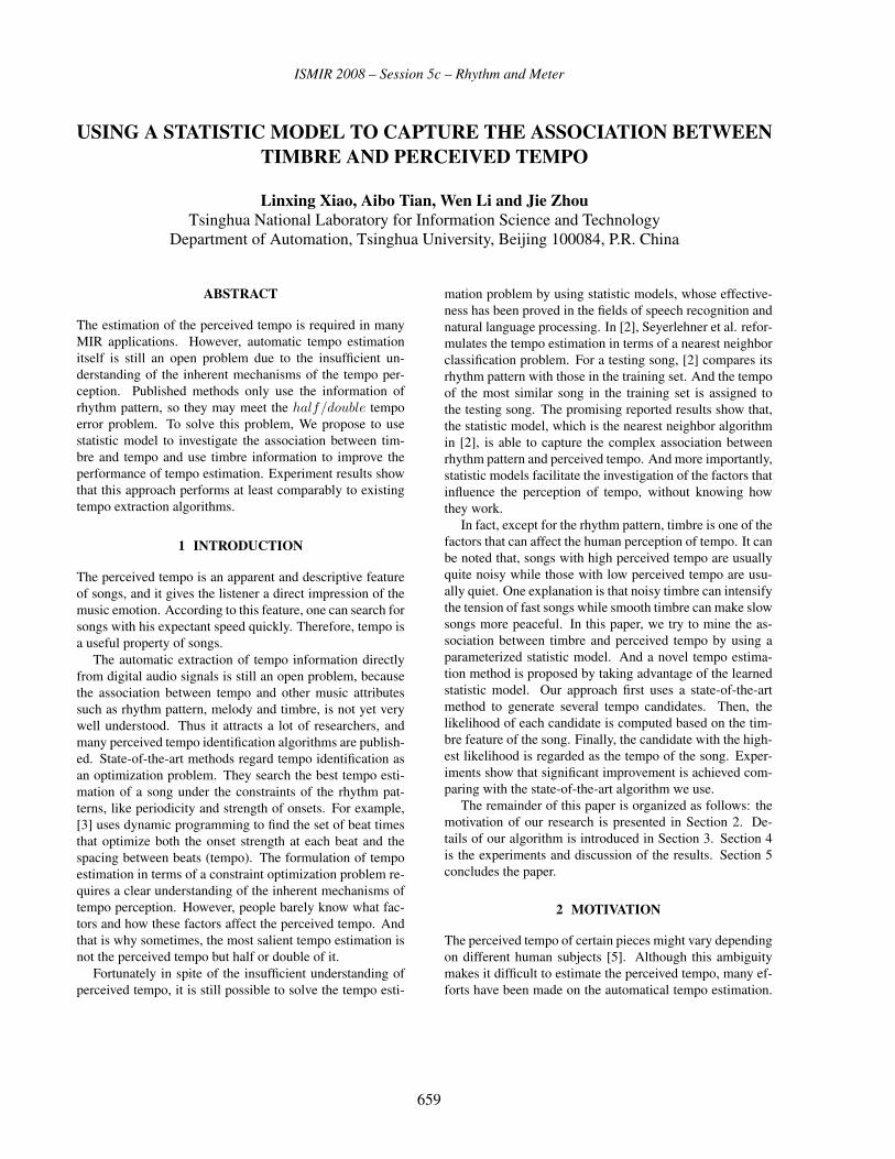
ISMIR 2008 – Session 5c – Rhythm and Meter
USING A STATISTIC MODEL TO CAPTURE THE ASSOCIATION BETWEENTIMBRE AND PERCEIVED TEMPO
Linxing Xiao, Aibo Tian, Wen Li and Jie ZhouTsinghua National Laboratory for Information Science and Technology
Department of Automation, Tsinghua University, Beijing 100084, P.R. China
ABSTRACT
The estimation of the perceived tempo is required in many
MIR applications. However, automatic tempo estimation
itself is still an open problem due to the insufficient un-
derstanding of the inherent mechanisms of the tempo per-
ception. Published methods only use the information of
rhythm pattern, so they may meet the half/double tempo
error problem. To solve this problem, We propose to use
statistic model to investigate the association between tim-
bre and tempo and use timbre information to improve the
performance of tempo estimation. Experiment results show
that this approach performs at least comparably to existing
tempo extraction algorithms.
1 INTRODUCTION
The perceived tempo is an apparent and descriptive feature
of songs, and it gives the listener a direct impression of the
music emotion. According to this feature, one can search for
songs with his expectant speed quickly. Therefore, tempo is
a useful property of songs.
The automatic extraction of tempo information directly
from digital audio signals is still an open problem, because
the association between tempo and other music attributes
such as rhythm pattern, melody and timbre, is not yet very
well understood. Thus it attracts a lot of researchers, and
many perceived tempo identification algorithms are publish-
ed. State-of-the-art methods regard tempo identification as
an optimization problem. They search the best tempo esti-
mation of a song under the constraints of the rhythm pat-
terns, like periodicity and strength of onsets. For example,
[3] uses dynamic programming to find the set of beat times
that optimize both the onset strength at each beat and the
spacing between beats (tempo). The formulation of tempo
estimation in terms of a constraint optimization problem re-
quires a clear understanding of the inherent mechanisms of
tempo perception. However, people barely know what fac-
tors and how these factors affect the perceived tempo. And
that is why sometimes, the most salient tempo estimation is
not the perceived tempo but half or double of it.
Fortunately in spite of the insufficient understanding of
perceived tempo, it is still possible to solve the tempo esti-
mation problem by using statistic models, whose effective-
ness has been proved in the fields of speech recognition and
natural language processing. In [2], Seyerlehner et al. refor-
mulates the tempo estimation in terms of a nearest neighbor
classification problem. For a testing song, [2] compares its
rhythm pattern with those in the training set. And the tempo
of the most similar song in the training set is assigned to
the testing song. The promising reported results show that,
the statistic model, which is the nearest neighbor algorithm
in [2], is able to capture the complex association between
rhythm pattern and perceived tempo. And more importantly,
statistic models facilitate the investigation of the factors that
influence the perception of tempo, without knowing how
they work.
In fact, except for the rhythm pattern, timbre is one of the
factors that can affect the human perception of tempo. It can
be noted that, songs with high perceived tempo are usually
quite noisy while those with low perceived tempo are usu-
ally quiet. One explanation is that noisy timbre can intensify
the tension of fast songs while smooth timbre can make slow
songs more peaceful. In this paper, we try to mine the as-
sociation between timbre and perceived tempo by using a
parameterized statistic model. And a novel tempo estima-
tion method is proposed by taking advantage of the learned
statistic model. Our approach first uses a state-of-the-art
method to generate several tempo candidates. Then, the
likelihood of each candidate is computed based on the tim-
bre feature of the song. Finally, the candidate with the high-
est likelihood is regarded as the tempo of the song. Exper-
iments show that significant improvement is achieved com-
paring with the state-of-the-art algorithm we use.
The remainder of this paper is organized as follows: the
motivation of our research is presented in Section 2. De-
tails of our algorithm is introduced in Section 3. Section 4
is the experiments and discussion of the results. Section 5
concludes the paper.
2 MOTIVATION
The perceived tempo of certain pieces might vary depending
on different human subjects [5]. Although this ambiguity
makes it difficult to estimate the perceived tempo, many ef-
forts have been made on the automatical tempo estimation.
659

ISMIR 2008 – Session 5c – Rhythm and Meter
Hz
Bar
k sc
ale
freq
uenc
y ba
nks
0 5 10
5
10
15
20
Hz
Bar
k sc
ale
freq
uenc
y ba
nks
0 5 10
5
10
15
20
Figure 1. Illustration of FPs of two songs. The upper pane
is the FP of a song with tempo value 208 bpm (3.4 Hz); the
lower pane is the FP of a song with tempo value 104 bpm
(1.7 Hz).
A common approach of state-of-the-art methods [1] is to
analyze the extracted rhythm patterns under the assumption
that one of the periodicities present in the rhythm patterns
corresponds to the perceived tempo. [1] evaluates eleven
algorithms by using two evaluation metrics as follows:
• Accuracy 1: the percentage of tempo estimates within
4 % (the precision window) of the ground-truth tempo.
• Accuracy 2: the percentage of tempo estimates within
4 % of either the ground-truth tempo, or half, double,
three times or one third of the ground-truth tempo.
In the evaluation of [1], for all eleven algorithms, accu-
racies 2 are much higher than accuracies 1. The average
increment is about 30%. This result shows that state-of-the-
art methods mainly suffer from the half/double and one−third/triple tempo error problems (We will use ”half/do−uble” for both kind of errors). One possible reason is that
sometimes it is quite hard to pick the ”most salient tempo”
from the rhythm pattern, as shown in the upper pane of Fig-
ure 1, which illustrates the Fluctuation Pattern (FP)[4] of a
song. The left light bar corresponds to a possible tempo of
104 bpm (1.7 Hz) and right light bar corresponds to a pos-
sible tempo of 208 bpm (3.4 Hz). It is hard to determine
which tempo is more salient.
Merely using rhythm pattern as the feature, the instance
based method [2] may meet the half/double tempo error
problem as well, because sometimes the rhythm pattern of
a song is very similar to that of a song with double tempo,
but different from a song with the same tempo. As shown in
Figure 1, the upper pane illustrates the FP of a song whose
tempo is 208 bpm and the lower one illustrates the FP of a
song whose tempo is 104 bpm.
Since the tempo is an important parameter that reflects
the mood of a song, an estimated tempo which is half or
double of the ground truth might give the user a terrible ex-
perience. For example, a sad user intends to search a slow
song, but gets a bright one with double of the desired tempo.
In order to solve the half/double tempo error problem, we
decide to investigate possible factors that influence the per-
ception of tempo except for rhythm patterns. And we hope
these factors can be used to improve the accuracy of tempo
estimation. Noticing the phenomenon that songs with high
perceived tempo are usually quite noisy while those with
low perceived tempo are usually quiet, we choose timbre as
the factor into which we want to get deeper insights.
3 OUR METHOD
Without knowing how the timbre affects the perception of
tempo, we build a statistic model to capture the association
between tempo and timbre. Then, the statistic model is com-
bined with a state-of-the-art method to estimate the tempo of
a piece of music.
3.1 Training the statistic model
We train a statistic model as follows: (1) For each song in
the training set, we divide it into several 10-second seg-
ments, with neighboring segments overlapping 1/2 of the
length. (2) Each 10-second segment is further windowed
into 0.1-second frames. After extracting a 12-dimension
MFCC vector from each frame, the mean MFCC vector of
each 10-second segment is computed. Then the annotated
tempo is combined with the mean MFCC vector to form a
13-dimension tempo-timbre feature. (3) Finally, the aggre-
gate of tempo-timbre features of all songs in the training set
are used to train a GMMs model, which describes the prob-
ability distribution of tempo-timbre feature.
3.2 Tempo prediction
We propose a tempo estimation method by using the pre-
trained statistic model. The process of predicting is given
below:
1. Partition a testing song into several 10-second seg-
ments with 5-second overlapping.
2. For each segment, use [3] to get a possible tempo.
Then, four additional tempi are generated by multi-
plying the original tempo with factor 0.33, 0.5, 2 and
3. Thus, there are five candidate tempi for a piece of
music, denoted as Ti, i = 1, ..., 5.
3. Compute the 12-dimension mean MFCC vector of each
segment, denoted as M .
660

ISMIR 2008 – Session 5c – Rhythm and Meter
60 80 100 120 140 160 180 200 220 2400
50
100
150
Tempo [BPM]
Num
ber
of in
stan
ces
Ballroom data (N = 698)
0 50 100 150 200 2500
10
20
30
40
50
Tempo [BPM]
Num
ber
of in
stan
ces
Songs data (N = 465)
Figure 2. Histograms of ground truth tempo values for ball-
room, songs data sets.
4. For each 10-second segment, compute the probabil-
ity of the combination of Ti and M in the pre-trained
statistic model. The candidate with the highest proba-
bility is determined as the tempo of the segment. The
mathematic expression is in equation(1).
T ∗ = arg maxTi
P (Ti|M), (1)
where P (x|y) is the likelihood of x with respect to y.
5. Select the median of the tempi of all segments as the
estimated tempo of the testing song.
4 EXPERIMENTS AND DISCUSSION
Our experiments are based on two data sets that have been
used in [1, 2]. The ballroom data set consists of 698 thirty-
second audio excerpts, and the songs data set contains 465
audio clips from nine genres. Both data sets are publicly
available 1 . The distributions of the annotated tempi in both
data sets are shown in Figure 2.
To make the results comparable to [1], we use the accu-
racy 1 mentioned in Section 2 as the evaluation criterion.
The error measure of [2] is used to visualize the errors, as
defined in equation (2).
e ={
t∗t − 1, t∗ > t;−( t
t∗ − 1), t∗ < t,(2)
1 http://www.iua.upf.es/mtg/ismir2004/contest/tempoContest/
A1 A2 D1 D2 D3 KL SC T1 T2 T3 UH S1 S2 E OT0
20
40
60
80
100
Acc
urac
ies(
%)
Ballroom data (N = 698)
A1 A2 D1 D2 D3 KL SC T1 T2 T3 UH S1 S2 E OT0
20
40
60
80
100
Acc
urac
ies(
%)
Song data (N = 465)
Figure 3. Comparative experiment results on ballroom and
songs data sets.
where t∗ is the predicted tempo value and t is the ground
truth.
In our experiment, an 8-center GMMs model is used to
describe the probability distribution of the tempo-timbre fea-
ture. We use the well-known 10-fold cross validation strat-
egy to evaluate the proposed method on each data set.
Firstly, the results of our timbre-related method are com-
pared with those of Ellis’ method [3]. Our approach achieves
accuracies of 68.4% and 60.51% for ballroom data set and
songs data set respectively, while [3] only achieves 57.7%
and 34%. The visualization of the prediction results of both
methods on ballroom data set is illustrated in Figure 4, in
which the upper pane is the prediction error of proposed al-
gorithm and the medium pane is the error of [3]. We can see
that many half/double errors made by [3] are corrected by
our algorithm.
Secondly, in order to show the effectiveness of timbre-
related method, we compare our approach with algorithms
in [1, 2, 3]. The comparative experiment results are illus-
trated in Figure 3. The prediction results of eleven algo-
rithms , namely Miguel Alonso (A1, A2), Simon Dixon (D1,
D2, D3), Anssi Klapuri (KL), Eric Scherier (SC), GeorgeTzanetakis (T1, T2, T3) and Christian Uhle (UH), are ob-
tained from [1]. And the results of the instance based al-
gorithm, namely Klaus Seyerkehner (S1, S2), are obtained
from [2]. The last two darker bars represent the results of
Ellis’ method [3] (E) and our timbre related method (OT).
Our method has apparently higher accuracies in both data
sets than other state-of-the-art algorithms, in spite of a little
weakness in comparison with instance based approaches, S1
661

ISMIR 2008 – Session 5c – Rhythm and Meter
0 100 200 300 400 500 600 700−2
0
2
Err
or
Ballroom data set (N = 698)
0 100 200 300 400 500 600 700−2
0
2
Err
or
0 100 200 300 400 500 600 7000
100
200
300
Instances [sorted from slow to fast tempo]
Tem
po [B
PM
]
Figure 4. Visualization of errors on ballroom data set, sorted in ascending order according to ground truth tempo. Upper pane
is the prediction errors of the proposed algorithm. Medium pane is the prediction errors of Ellis’ method [3]. Bottom pane is
the ground truth tempo.
and S2, on ballroom set. However, for the instance based ap-
proach, the high accuracy in ballroom data set relates much
to the tempo distribution of the data set. As it shows in Fig-
ure 2, data in the ballroom set concentrate on several certain
values-such as 100 bpm and 120 bpm-which makes it facile
to find the correct tempo using the nearest neighbor classi-
fication algorithm. This ascendency of S1 and S2 does not
occur in the songs data set, since the tempo distribution of
this set is close to normal distribution. And the result of our
method in songs set is equally good as, even better than, that
of S1 and S2. Thus, we may draw the conclusion that, our
timbre related algorithm performs at the same level as the
best current tempo estimation algorithms.
5 CONCLUSION
Current tempo estimation methods often meet the half/do−uble tempo problem because it’s hard to pick the most salient
tempo merely by using the rhythm information of the indi-
vidual song. Noticing the fact that the timbre of a song is
relevant to its tempo, we use a statistic model to capture
the association between the two attributes. We also pro-
pose a novel tempo estimation approach by using the tim-
bre information. Experimental results based on two differ-
ent data sets show that our approach efficiently reduces the
half/double errors made by a sate-of-the-art tempo esti-
mation method, and performs at least equally well as other
tempo identification methods.
As with each supervised learning approach, the good per-
formance of the proposed tempo estimation method requires
a large annotated training set that covers a wide tempo range
as well as various genres and musical styles. However, ap-
plying the statistic model to tempo extraction can help inves-
tigating the factors that affect tempo perception and improve
the accuracy of perceived tempo estimation.
6 REFERENCES
[1] Gouyon, F. Klapuri, A. Dixon, S. Alonso, M.Tzanetakis,
G. Uhle, C. Cano, P. ”An experimental comparison of
audio tempo induction algorithms”, IEEE Transactionson Audio, Speech and Language Processing,vol.14,
no.5, pp. 1832-1844, 2006.
[2] Seyerlehner, K. Widmer, G. Schnitzer, D. ” From
Rhythm patterns to perceived tempo”, ISMIR’07, Vi-
enna, Austria, 2007.
[3] Ellis, D.P.W. ”Beat Tracking with Dynamic Program-
ming”, MIREX’06,2006.
[4] Pampalk, E. Rauber, A. Merkl, D. ”Content-based orga-
nization and visualization of music archives”, Proceed-ings of the 10th ACM MM, Juan les Pins, France, pp.
570-579, 2002.
[5] McKinney, M. F. Moelants, D. ”Tempo Perception and
Musical Content: What makes a piece fast, slow or
temperally ambiguous?”, ICMPC’04, Evanston, USA,
2004.
662

ISMIR 2008 – Session 5c – Rhythm and Meter
RHYTHM COMPLEXITY MEASURES:A COMPARISON OF MATHEMATICAL MODELS OF
HUMAN PERCEPTION AND PERFORMANCE
Eric ThulSchool of Computer Science
Schulich School of MusicMcGill University, Montréal
Godfried T. ToussaintSchool of Computer Science
Schulich School of MusicMcGill University, Montréal
ABSTRACT
Thirty two measures of rhythm complexity are comparedusing three widely different rhythm data sets. Twenty-twoof these measures have been investigated in a limited con-text in the past, and ten new measures are explored here.Some of these measures are mathematically inspired, somewere designed to measure syncopation, some were intendedto predict various measures of human performance, someare based on constructs from music theory, such as Press-ing’s cognitive complexity, and others are direct measures ofdifferent aspects of human performance, such as perceptualcomplexity, meter complexity, and performance complex-ity. In each data set the rhythms are ranked either accord-ing to increasing complexity using the judgements of humansubjects, or using calculations with the computational mod-els. Spearman rank correlation coefficients are computedbetween all pairs of rhythm rankings. Then phylogenetictrees are used to visualize and cluster the correlation co-efficients. Among the many conclusions evident from theresults, there are several observations common to all threedata sets that are worthy of note. The syncopation measuresform a tight cluster far from other clusters. The human per-formance measures fall in the same cluster as the syncopa-tion measures. The complexity measures based on statisti-cal properties of the inter-onset-interval histograms are poorpredictors of syncopation or human performance complex-ity. Finally, this research suggests several open problems.
1 INTRODUCTION
Many music researchers consider rhythm to be the most im-portant characteristic of music. Furthermore, one of themain features of rhythm is its complexity. Threfore mea-sures of the complexity of a rhythm constitute key featuresuseful for music pattern recognition and music informationretrieval, as well as ethnomusicological analyses of worldmusic [17, 18]. Since the notion of complexity is flexible, itis not surprising that in the past a variety of different mea-sures of complexity has appeared in the literature. Areas
where such measures have been applied range from psychol-ogy, enginneering, computer science and mathematics, tomusic theory. Given such a wide range of applicable fields,different techniques for measuring complexity have beendeveloped. For example, one can analyze a rhythm’s bi-nary sequence representation, ask listeners to rate a rhythm’scomplexity, or ask musicians to perform a rhythm. There-fore, in our work, we include measures of information andcoding complexity, performance complexity, and cognitivecomplexity. Furthermore, there are traditional concepts inmusic such as syncopation [10] which may also be consid-ered as measures of rhythm complexity [7, 8].
With the exception of [7, 8], previous research on rhythmcomplexity has been limited to determining how good a fea-ture it is for music pattern recognition, or how well it mod-els human judgements of complexity [17, 18]. Moreover, forsuch studies researchers have used data (families of rhythms)that were generated artificially and randomly with some con-straints. Here, we not only use a large group comprised of32 measures of complexity that employ a wide variety ofmeasurement techniques, but we also validate these mea-sures against human judgements of perceptual, meter, andperformance complexity using three diverse data sets.
2 COMPLEXITY MEASURES
One can broadly categorize the complexity measures usedin this study into two distinct categories: human perfor-mance measures directly obtained from psychological ex-periments, and measures obtained from mathematical mod-els of rhythm complexity. The human performance mea-sures can be subdivided into three types: perceptual com-plexity, meter complexity, and performance complexity. Per-ceptual complexity is obtained by asking human subjects tojudge complexity as they listen to rhythms. Meter complex-ity is obtained by measuring how well the human subjectsare able to track the underlying metric beat of a rhythm. Itis worth noting that some researchers, for example in mu-sic psychology [4], refer to the metric beat as the pulse.
663

ISMIR 2008 – Session 5c – Rhythm and Meter
Here we reserve the word pulse for the largest duration in-terval that evenly divides into all the inter-onset onsets (IOI)present in a family of rhythms. This is common terminologyin ethnomusicology and music technology. Performancecomplexity measures pertain to how well the subjects canreproduce (execute, play-back) the rhythms, usually by tap-ping. The mathematical models can be subdivided into twomain categories: those that are designed to measure synco-pation, and those that are designed to measure irregularity.The irregularity measures can be divided into statistical andminimum-weight-assignment measures.
Due to lack of space, we cannot provide a detailed de-scription of all the complexity measures tested. Thus welist the complexity measures with each corresponding es-sential reference in the literature for further information,along with a label in parentheses pertaining to the phylo-gentic tree labels used in Figures 1, 2, and 3. Measures ofsyncopation are listed first. The Longuet-Higgins and Leemeasure (lhl) [4, 14], along with Smith and Honing’s ver-sion (smith) [19], take advantage of a metric hierarchy ofweights [13] to calculate syncopation. A variation of Tous-saint’s metrical complexity (metrical) [21] and Keith’s mea-sure (keith) [10] also use this hierarchy to judge syncopa-tion. The Weighted Note-to-Beat Distance (wnbd, wnbd2,wnbd4, wnbd8) [7] uses the distance from onsets to metricbeats to gauge syncopation.
Second, we list the measures regarding mathematical ir-regularity. IOI histogram measures for entropy (ioi-g-h, ioi-l-h), standard deviation (ioi-g-sd, ioi-l-sd), and maximumbin height (ioi-g-mm, ioi-l-mm) were used to determine thecomplexity of both global (full) IOIs [24] and local (relative,adjacent) IOIs [18]. Also, pertaining to entropy calculationsare the Coded Element Processing System (ceps) [26], H(k-span) complexity (hk) [25], and the H(run-span) complexity(hrun) [25], which all measure the uncertainty [5] of ob-taining sub-patterns in a rhythm. The directed swap dis-tance (dswap, dswap2, dswap4, dswap8) [1] computes theminimum weight of a linear assignment between onsets of arhythm and a meter with an onset at every second, fourth, oreigth pulse, and also the average over each meter. Two othermeasures, Rhythmic Oddity (oddity) [22] and Off-Beatness(off-beatness) [22] take a geometric approach.
Third, those measures which do not easily fall into a cat-egory are listed. These include the Lempel-Ziv compres-sion measure (lz) [12], Tanguiane’s [20] complexity mea-sure, which looks at sub-patterns at each metrical beat level,and Pressing’s Cognitive Complexity measure (pressing) de-signed on the basis of music theory principles, which gen-erates rhythmic patterns at each metrical beat, assigning ap-propriate weights to special patterns [16]. Furthermore, Tan-guiane’s measure uses the max (tmmax) and average (tmavg)complexities over different metrical beat levels. In addition,derivatives (tmuavg, tmumax) without the restriction of sub-patterns starting with an onset, were tested.
3 EXPERIMENTAL DATA
The measures of complexity in § 2, were compared usingthree rhythm data sets. Each data set had been compiled totest human judgements regarding the perceptual, meter, andperformance complexities of the rhythms. The first data setshown in Table 1 was synthesized by Povel and Essens in1985 [15] and then later studied by Shmulevich and Povelin 2000 [17]. The second data set shown in Table 2 wascreated by Essens in 1995 [2]. The third data set shown inTable 3 was generated by Fitch and Rosenfeld in 2007 [4].In addition to the rhythms themselves, the results of severalhuman performance complexity measures used in this workare contained in Tables 1, 2, and 3. In the following we de-scribe the methodologies of Povel and Essens [15], Shmule-vich and Povel [17], Essens [2], and Fitch and Rosenfeld [4],used to obtain the human judgements of complexity.
3.1 Povel and Essens 1985
Previous work by Povel and Essens [15] studied the repro-duction quality of temporal patterns. The rhythms, shownin Table 1, were presented to the participants in randomorder. For each presentation, the participant was asked tolisten to the pattern, and then reproduce the pattern by tap-ping [15]. Once the participant had felt they could repro-duce the rhythm, they stopped the audio presentation andproceeded to then tap the pattern they just heard, repeat-ing the pattern 4 times. Afterwards, they could choose tomove to the next rhythm or repeat the one they had justheard [15]. From this experiment, we derive an empiricalmeasure for the reproduction difficulty of temporal patterns;i.e., rhythm performance complexity. This was based onPovel and Essens’ mean deviation percentage which cal-culates the amount of adjacent IOI error upon reproduc-tion [15]. See column 3 of Table 1.
3.2 Shmulevich and Povel 2000
Shmulevich and Povel [17] studied the perceptual complex-ity of rhythms using the same data as Povel and Essens [15].All participants were musicians with musical experience av-eraging 9.2 years [17]. A pattern was repeated four timesbefore the next was randomly presented. The resulting per-ceptual complexity in column 4 of Table 1 represents theaverage complexity of each rhythm across all participants.
3.3 Essens 1995
A study of rhythm performance complexity was conductedby Essens [2]. The rhythms used for that study are shown inTable 2. The procedure Essens used to test the reproductionaccuracy of rhythms was very similar to that of Povel andEssens [15]. We use the mean deviations of Essens to rankthe rhythms by increasing complexity, as seen in column 3
664

ISMIR 2008 – Session 5c – Rhythm and Meter
of Table 2. Essens also studied the perceptual complexityof rhythms [2]. Participants were asked to judge the com-plexity of each rhythm in Table 2 on a 1 to 5 scale where 1means very simple and 5 means very complex [2]. Note thatsome participants had been musically trained for at least 5years. The order of the patterns was random. The perceptualcomplexity in column 4 of Table 2 is the average complexityover the judgements from each subject.
3.4 Fitch and Rosenfeld 2007
Most recently, Fitch and Rosenfeld [4] conducted an experi-mental study of metric beat-tracking or, in their terminology,pulse-tracking (i.e., rhythmic meter complexity) and rhythmreproduction (i.e., performance complexity). The rhythmsused in the experiments are shown in Table 3. These rhythmswere generated in such a way as to vary the amount of syn-copation among the rhythms, as measured by the Longuet-Higgins and Lee syncopation measure [14].
The metric beat-tracking experiment yielded two mea-sures of meter complexity [3]. The first pertained to howwell participants could tap a steady beat (beat tapping erroradjusted for tempo) when different rhythms were played.The second counted the number of times (number of resets)the participant tapped the metric beat exactly in between thepoints where the metric beat should be [4]. The values areshown in columns 3 and 4 of Table 3. The second experi-ment for rhythm reproduction accuracy was interleaved withthe metric beat-tracking experiment. Hence the subject nowtaps the rhythm just heard from experiment 1 while the com-puter provides the metric beat [4]. The adjacent IOI errorof the target and reproduced rhythms gives a performancecomplexity shown in column 5 of Table 3.
4 RESULTS
We adhered to the following procedure to validate the com-plexity measures in § 2 using the three rhythm data sets.The complexity scores were obtained using the rhythms asinput for each measure. The Spearman rank correlation co-efficients [11] between all pairs of rankings of the rhythmsaccording to the computational and empirical measures foreach rhythm data set were calculated.
Phylogenetic trees were used to visualize the relation-ships among the correlation coefficients. This technique hasproved to be a powerful analytical tool in the computationalmusic domain [1, 8, 21, 22, 23]. The program SplitsTree [9]was used to generate the phylogenetic trees using the BioNJalgorithm [6]. Figures 1, 2, and 3, picture the phylogenetictrees where the distance matrix values are the correlationcoefficients subtracted from one. Each tree yields a fitnessvalue greater than or equal to 94.0 on a 100.0 scale. Theleast-squares fitness is the ratio of A/B where A is the sumof the squared differences between the geodesic distances
No. RhythmPerformance Complexity Perceptual Complexity
Povel and Essens Shmulevich and Povel
1 x x x x x . . x x . x . x . . . 5 1.562 x x x . x . x x x . . x x . . . 1 2.123 x . x x x . x x x . . x x . . . 0 2.084 x . x . x x x x x . . x x . . . 2 1.885 x . . x x . x . x x x x x . . . 3 1.806 x x x . x x x . x x . . x . . . 9 2.447 x . x x x x . x x . . x x . . . 7 2.208 x x . . x x x x x . x . x . . . 4 2.569 x x . . x . x x x . x x x . . . 14 3.00
10 x . x x x . x x x x . . x . . . 18 2.0411 x x x . x x . . x x . x x . . . 19 2.7612 x x . x x x x . x . . x x . . . 15 2.7213 x x . x x . x x x x . . x . . . 13 3.0014 x x . . x x . x x . x x x . . . 27 3.1615 x . . x x x . x x x . x x . . . 10 2.0416 x x . x x x x . x x . . x . . . 11 2.8817 x x . x x x . x x x . . x . . . 17 2.6018 x x . x x x . . x x . x x . . . 22 2.6019 x x . . x x . x x x x . x . . . 21 2.6420 x x . . x x . x x x . x x . . . 25 3.2421 x x x x x . x x . x . . x . . . 29 3.0822 x x x x . x . . x x x . x . . . 20 3.0423 x x x . . x x . x x x . x . . . 16 3.0424 x . x x x . . x . x x x x . . . 6 2.5625 x . x . . x x x x . x x x . . . 8 2.5626 x x x x . x . x . . x x x . . . 26 2.8427 x x . x x x . x . . x x x . . . 23 3.6028 x x . x . . x x x . x x x . . . 32 2.6829 x . x x x x . x . . x x x . . . 28 3.2830 x . . x x x x x . x x . x . . . 21 3.0831 x x x x . x x x . . x . x . . . 30 3.5232 x x x x . . x x . x x . x . . . 31 3.6033 x x . x x x x . . x x . x . . . 24 3.0434 x x . x . . x x x x x . x . . . 33 2.8835 x . x . . x x x . x x x x . . . 12 3.08
Table 1. Thirty-five rhythms from Povel and Essens withthe Performance Complexity and Perceptual Complexity.
No. RhythmPerformance Complexity Perceptual Complexity
Essens Essens
1 x x x . x x x . x x x . x x . . 0 2.22 x x x . x . x x x . x x x x . . 8 3.13 x . x x x . x x x . . x x x . . 4 3.24 x . x x x . . x x . x x x x . . 19 2.95 x x x . x x x . x x . x x . . . 2 2.26 x x x . x . . x x . x . x x . . 7 3.17 x x x x x x x . x x x . x x x . 10 2.68 x x x . x x x x x . . x x x . . 5 4.29 x x x x x x . x x . x x x . . . 13 2.9
10 x . x . x . x . x x x . x x . . 6 2.811 x x x x x x x . x x x . x . x . 1 3.112 x x x . x x . . x . x . x . . . 3 2.513 x . . x x x x . x x . . x x . . 20 3.514 x . x x x x . x x x . x x x . . 12 2.515 x . . x x x . x x x . x x x . . 14 2.416 x . . x x x . x x x x . x x . . 11 3.017 x x . x x x . x x x x . x . . . 17 3.018 x . . x x x x x x x . x x x . . 18 3.119 x . x . x x . x x x . x x x . . 22 2.420 x x . x x x x . x x . x x . . . 16 3.221 x x . x x x . x x x x x x . . . 15 2.422 x x . . x x . x x x x x x . . . 11 2.923 x . x . x x . x x x x x x x . . 21 2.724 x x . x x x x x x . x . x x . . 9 3.8
Table 2. Twenty-four rhythms from Essens with Perfor-mance Complexity and Perceptual Complexity.
between pairs of leaves in the tree, and their correspondingdistances in the distance matrix, and B is the sum of thesquared distances in the distance matrix. Then this value issubtracted from 1 and multiplied by 100 [27]. Note that thephylogenetic tree is used here as a visualization tool, and notin order to obtain a phylogeny of complexity measures.
5 DISCUSSION AND CONCLUSION
There are several noteworthy observations common to allthree data sets. The syncopation measures form a tight clus-ter far from the other clusters. The human performance mea-
665

ISMIR 2008 – Session 5c – Rhythm and Meter
Figure 1. BioNJ of measures compared to Shmulevich and Povel and Povel and Essens human judgements.
Figure 2. BioNJ of measures compared to Essens’ human judgements.
666

ISMIR 2008 – Session 5c – Rhythm and Meter
Figure 3. BioNJ of measures compared to Fitch and Rosenfeld’s human judgements.
No. RhythmMeter Complexity
Beat Tapping AdjustedMeter ComplexityNumber of Resets
PerformanceComplexity
Play-back Error
1 x . . . . . x . x . . . . . x . 0.075 2.500 0.1382 x . . . x . . . x . . . x . x . 0.082 2.250 0.1453 x . x . x . . . . . . . x . x . 0.075 2.313 0.1534 x . . . x x x . . . . . x . . . 0.119 8.750 0.2575 . . x . . . x . x . x . x . . . 0.103 5.500 0.1336 . . x . . . x . x . . . x . x . 0.082 3.063 0.2357 x . . . . . x . . x . . . . x . 0.112 6.000 0.2158 x . . x . . . x . . x . x . . . 0.110 5.188 0.2089 x . . . . x . . . x . . . x x . 0.141 6.938 0.250
10 x . . . . x . . . x . . . x . . 0.144 10.375 0.17111 . . x . . . x . . . x x . x . . 0.130 6.875 0.22012 . x . . . x . . . x . . x . x . 0.124 6.438 0.22613 . . x . . . x x . . . x . x . . 0.130 6.965 0.38714 . . x . . x . . . . . x . . . x 0.159 11.688 0.23915 . . . x . x . . . . x x . . . x 0.172 13.688 0.48516 x . . . x . x x x . . . . . . . 0.085 2.625 0.17317 x . x . x . . . . . x . x . . . 0.077 2.313 0.17918 . . x . x . . . x . x . x . . . 0.077 2.438 0.18219 x . x . . . x . x . . x . . . . 0.074 1.938 0.25220 . . x . . . x . x . . . x . . . 0.098 3.375 0.14221 x . . . . x . x . . x . x . . . 0.161 11.063 0.30522 . . x . . . x . x . x . . . x . 0.129 8.500 0.32123 x x . . . x . . . . x . . . x . 0.145 7.375 0.32024 . x . . . x . . . x x . x . . . 0.134 7.188 0.26525 . . x . . . x . . . x . . x . . 0.146 8.625 0.17626 . . x . . . x . . . x x . . . x 0.118 6.500 0.32627 . . x . . x . . . . x . . x . x 0.117 6.188 0.36828 . . x x . . . x . . . x . x . . 0.154 10.813 0.34429 . x . x . x . x . . . x . . . . 0.191 15.750 0.18530 . x . x . . . x . . . x . . . x 0.164 11.938 0.158
Table 3. Thirty rhythms from Fitch and Rosenfeld with Me-ter Complexity and Performance Complexity.
sures fall in the same cluster as the syncopation measures.The complexity measures based on statistical properties ofthe inter-onset-interval histograms appear to be poor predic-tors of syncopation or of human performance complexity.
There are also some important differences between the threefigures. The overall appearance of clusters is much strongerin Figure 3 than in the other two. This is perhaps due tothe fact that the rhythms used in Figure 3 are much morerealistic and sparser than the rhythms used in Figures 1 and2. Similarly, the six IOI (inter-onset-interval) measures arescattered in Figures 1 and 2, but are in one cluster in Figure3. The cognitive complexity measure of Pressing, designedon the basis of principles of music perception falls squarelyin the group of syncopation measures in Figures 1 and 3.However, in Figure 2, although it falls into the syncopationcluster, it is quite distant from the other measures, proba-bly because of the great density of the rhythms in this dataset. Also worthy of note is a comparison of the human me-ter complexity measures with the human performance (play-back) measure. In Figure 3 we see that the meter complex-ity is considerably closer to the syncopation measures thanthe play-back performance measure. This suggests that themathematical syncopation measures are better predictors ofhuman meter complexity than performance complexity.
6 ACKNOWLEDGEMENT
The authors would like to thank W. T. Fitch for making theirdata set available.
667

ISMIR 2008 – Session 5c – Rhythm and Meter
7 REFERENCES
[1] J. M. Dı́az-Báñez, G. Farigu, F. Gómez, D. Rappaport,and G. T. Toussaint. El compás flamenco: a phyloge-netic analysis. In BRIDGES: Mathematical Connectionsin Art, Music and Science, Jul 2004.
[2] P. Essens. Structuring temporal sequences: Compari-son of models and factors of complexity. Perception andPsychophysics, 57(4):519–532, 1995.
[3] W. T. Fitch. Personal communication, 2007.
[4] W. T. Fitch and A. J. Rosenfeld. Perception andproduction of syncopated rhythms. Music Perception,25(1):43–58, 2007.
[5] W. R. Garner. Uncertainty and Structure as Psychologi-cal Concepts. John Wiley & Sons, Inc., 1962.
[6] O. Gascuel. BIONJ: an improved version of the NJ algo-rithm based on a simple model of sequence data. Molec-ular Biology and Evolution, 14(7):685–695, 1997.
[7] F. Gómez, A. Melvin, D. Rappaport, and G. T.Toussaint. Mathematical measures of syncopation. InBRIDGES: Mathematical Connections in Art, Musicand Science, pages 73–84, Jul 2005.
[8] F. Gómez, E. Thul, and G. T. Toussaint. An experimen-tal comparison of formal measures of rhythmic syncopa-tion. In Proceedings of the International Computer Mu-sic Conference, pages 101–104, Aug 2007.
[9] D. H. Huson and D. Bryant. Applications of phyloge-netic networks in evolutionary studies. Molecular Biol-ogy and Evolution, 23(2):254–267, 2006.
[10] M. Keith. From Polychords to Pólya: Adventures in Mu-sical Combinatorics. Vinculum Press, 1991.
[11] M. Kendall and J. D. Gibbons. Rank Correlation Meth-ods, Fifth Edtion. Oxford Univ. Press, New York, 1990.
[12] A. Lempel and J. Ziv. On the complexity of finite se-quences. IEEE Transactions on Information Theory, IT-22(1):75–81, 1976.
[13] F. Lerdahl and R. Jackendoff. A Generative Theory ofTonal Music. MIT Press, 1983.
[14] H. C. Longuet-Higgins and C. S. Lee. The rhythmicinterpretation of monophonic music. Music Perception,1(4):424–441, 1984.
[15] D.-J. Povel and P. Essens. Perception of temporal pat-terns. Music Perception, 2:411–440, 1985.
[16] J. Pressing. Cognitive complexity and the structure ofmusical patterns. http://www.psych.unimelb.edu.au/staff/jp/cog-music.pdf, 1999.
[17] I. Shmulevich and D.-J. Povel. Measures of temporalpattern complexity. Journal of New Music Research,29(1):61–69, 2000.
[18] I. Shmulevich, O. Yli-Harja, E. Coyle, D.-J. Povel, andK. Lemström. Perceptual issues in music pattern recog-nition: complexity of rhythm and key finding. Comput-ers and the Humanities, 35:23–35, February 2001.
[19] L. M. Smith and H. Honing. Evaluating and extendingcomputational models of rhythmic syncopation in mu-sic. In Proceedings of the International Computer MusicConference, pages 688–691, 2006.
[20] A. S. Tanguiane. Artificial Perception and Music Recog-nition. Springer-Verlag, 1993.
[21] G. T. Toussaint. A mathematical analysis of African,Brazilian, and Cuban clave rhythms. In BRIDGES:Mathematical Connections in Art, Music and Science,pages 157–168, Jul 2002.
[22] G. T. Toussaint. Classification of phylogenetic analy-sis of African ternary rhythm timelines. In BRIDGES:Mathematical Connections in Art, Music and Science,pages 23–27, Jul 2003.
[23] G. T. Toussaint. A comparison of rhythmic similaritymeasures. In Proc. International Conf. on Music Infor-mation Retrieval, pages 242–245, Universitat PompeuFabra, Barcelona, Spain, October 10-14 2004.
[24] G. T. Toussaint. The geometry of musical rhythm. In JinAkiyama, Mikio Kano, and Xuehou Tan, editors, Proc.Japan Conf. on Discrete and Computational Geometry,volume 3742 of Lecture Notes in Computer Science,pages 198–212. Springer Berlin/Heidelberg, 2005.
[25] P. C. Vitz. Information, run structure and binary patterncomplexity. Perception and Psychophysics, 3(4A):275–280, 1968.
[26] P. C. Vitz and T. C. Todd. A coded element model of theperceptual processing of sequential stimuli. Psycologi-cal Review, 75(6):433–449, Sep 1969.
[27] R. Winkworth, D. Bryant, P. J. Lockhart, D. Havell,and V. Moulton. Biogeographic interpretation of splitsgraphs: least squares optimization of branch lengths.Systematic Biology, 54(1):56–65, 2005.
668

Session 5d – MIR Methods

.

ISMIR 2008 – Session 5d – MIR Methods
N-GRAM CHORD PROFILES FOR COMPOSER STYLE REPRESENTATION
Mitsunori OgiharaDepartment of Computer Science
University of [email protected]
Tao LiSchool of Computer ScienceFlorida International University
ABSTRACT
This paper studies the problem of using weighted N-grams of chord sequences to construct the profile of a com-poser. The N-gram profile of a chord sequence is the col-lection of all N-grams appearing in a sequence where eachN-gram is given a weight proportional to its beat count. TheN-gram profile of a collection of chord sequences is the sim-ple average of the N-gram profile of all the chord sequencesin the collection.Similarity of two composers is measured by the cosine of
their respective profiles, which has a value in the range [0, 1].Using the cosine-based similarity, a group of composers isclustered into a hierarchy, which appears to be explicable.Also, the composition style can be identified using N-gramsignatures.
1 INTRODUCTION
The chord progression is an important component in music.Musicians and listeners speak of novel and influential chordprogressions, typified in the First Act Prelude of “Tristanund Isolde” by Richard Wagner, in “Because” by The Bea-tles, and in “Giant Steps” by John Coltrane. Among manygenres of music the role of chord progressions is the mostsignificant in Jazz, where performances are improvisationaland thus performers often choose to play tunes with interest-ing chord progressions. While many jazz compositions areconstructed based on well-known chord progressions, suchas 12-bar blues progressions and “I Got Rhythm” by GeorgeGershwin, there are composers, such as Thelonius Monkand Wayne Shorter, whose chord progressions are thoughtof as unique. The importance of chord progressions in Jazzraises the questions of whether they can be effectively usedfor music retrieval and whether they can be used to charac-terize composers, which we will address in this paper.An approach to the problem of comparing two chord pro-
gressions is sequence alignment, as often used in melody-based music retrieval (see, e.g., [2, 6, 11, 12]). The ba-sis for the sequence-alignment approach is a theory thatexplains transformation of a chord progression to another(see, e.g., [8, 10]). Such a generative theory offers musi-cal understanding of how two progressions are similar, but
has a limitation that not all pairs of progressions are neces-sarily comparable. Also, for comparing multiple progres-sions with each other, generative-theory-based comparisonsmay be too computation-intensive. This consideration sug-gests the use of N-grams—the patterns consisting of N-consecutive chords that appear in a chord sequence. Theuse of N-grams is very popular in natural language under-standing (see, e.g., [5]). In music information retrieval, N-grams have been shown effective for melodic contour anal-ysis [3, 4, 9]. Also, the recent work of Mauch et al. [7] use4-grams to examine the chord sequences of The Beatles.
While the chord sequences are an important subject inmusicology, we believe that they can be incorporated into atune retrieval system where the tunes are indexedwith meta-data and chord sequence. In such a system, a user providesa chord sequence (either typed or copy-pasted from a se-quence on screen) as input and the system retrieves tunesthat contain a part with either exactly the same as (with thepossibility of allowing transposition of the key) or similarto the input sequence, where the input chord progression isspecified using an unambiguous notation system (such asthe one in [1]).
Highly prominent in the Jazz harmony are the 6th, 7thand major 7th notes and the tensions (the 9th, the 11th, andthe 13th notes). The former signify the functions that chordspossess while the latter add color to triads. Chord progres-sion analysis in terms of triads is likely to enable fundamen-tal understanding of the chord structure, but perhaps deeperunderstanding can be obtained by examining these non-triadnotes. Our work extends [7] by considering functional andadditional notes such as the 6th, 7th, and tensions, by creat-ing a profile out of N-gram data, and then by assigning thesimilarity between two profiles.
1.1 Organization of the paper
The rest of the paper is organized as follows: Section 2 de-scribes the method for obtaining an N-gram profile of chordsequences; Section 3 describes the experiments; and Sec-tion 4 describes conclusions and discusses future work.
671

ISMIR 2008 – Session 5d – MIR Methods
2 THE METHOD
2.1 N-Grams
2.1.1 N-Grams
Let U denote the universe of chords. For integers N ≥ 1,an N -gram is an ordered N -tuple (u1, . . . , uN ) such thatu1, . . . , uN ∈ U . We say that anN -gram (u1, . . . , uN ) suchthat u1, . . . , uN ∈ U is proper if for all i, 1 ≤ i ≤ N − 1,ui �= ui+1.
2.1.2 Chord simplification
The universe, U , of chord names is vast. There are twelvepossible choices for the root (without distinguishing be-tween sharps and flats); four for the 3rd (Minor, Major,Sus4, Omitted 3rd); four for the 5th (�5, �5, �5, Omitted 5th);four for the 6th/7th (the 6th, Minor 7th, Major 7th, no 6th or7th); four for the 9th (�9, �9, �9, no 9th); three for the 11th(�11, �11, no 11th); and three for the 13th (�13, �13, �13, no13th). These make the total number of choices more than27,000, and so, the total number of possible N-grams be-comes 761millions forN = 2 and 21 trillions forN = 3. Inaddition, chords can be augmented with a use of a bass notedifferent than the root of the chord, which further increasesthe number of N-grams. While the space of N-grams canbe enormous, the N-grams are sparse. In fact, the N-gramsappearing in a progression with M chord changes is onlyM − N + 1. Even though the distributions of chords areoften very skewed (towards certain keys and towards chordswithout tension notes), the vastness may make it unlikelyfor the N-gram profile of a chord progression with highlyenriched chords to intersect with the N-gram profile of an-other chord progression. This problem can be overcome bysimplifying chords.The concept of simplification corresponds well with that
of stemming in document processing, which is the processof removing modifiers of words thereby making words gen-erated from the same root with difference modifiers treatedas identical words. We divide of the process of simplify-ing a chord into two parts: (1) turning a fractional chord (achord with an attached bass note, such as AMI7 on B) intoa non-fractional chord and (2) simplifying the tensions andthe 6th/7th. We consider three options for the first part:
• (B0) simply removing the bass note (for example,AMI7 on B is turned into AMI7),
• (B1) reorganizing the notes so that the bass note be-comes the root (for example, AMI7 on B is turned intoB7sus4 (�5, �9)), and
• (B2) incorporate the bass note as a tension (for ex-ample, AMI7 on B is turned into AMI9).
We consider three options for the second part:
• (T 0) removing entirely the tensions and the 6th/7thnote,
• (T 1) removing entirely the tensions but keeping the6th/7th note, and
• (T 2) replacing the whole tension notes with a sin-gle bit of information as to whether the chord has anytension and keeping the 6th/7th note.
We also consider the possibility of keeping all the tensionsintact and keeping the 6th/7th note. We will denote this op-tion (not a form of simplification though) by T3. Then oursimplification method is expressed as a pair (Bi, T j) suchthat 0 ≤ i ≤ 2 and 0 ≤ j ≤ 3. The most aggressivesimplifications are (Bi, T0), 0 ≤ i ≤ 3. Each of these sim-plifications reduces a chord to a triad and thus reduces thenumber of possibilities for a chord name to 192. For a pro-gression Π and a simplification method τ , we will use τ(Π)to denote the progressionΠ after applying τ .We will be interested only in proper N-grams. So, given
an input chord progression, after simplification we collapseall the consecutive entries whose chord names are identicalto each other into one entry whose duration is the total ofthe durations of the subsequence. After this modificationevery block of N-consecutive entries corresponds to an N-gram, so we call such a chord progression a proper chordprogression. Note that simplification applied to a proper N-gram may produce a non-proper N-gram.
2.1.3 N-gram transposition
Also, since popular songs are transposed to different keys,in our analysis of N-grams we are only interested in howchords are changed after the first chord. We will thus trans-pose each N-gram locally, in such a way that each N-gramstarts with a code having A as the root. For example, froma five-chord sequence [FMI7, B�7, E�MA7, CMI7, B7], weobtain three 3-grams, FMI7 – B�7 – E�MA7, B�7 – E�MA7– CMI7, and E�MA7 – CMI7 – B7, which are then trans-posed respectively to AMI7 – D7 – GMA7 A7 – DMA7 –BMI, and AMA7 – F�MI7 – F7. We call this process A-transpose.
2.1.4 Chord sequences and Weight of N-grams
We assume that each chord progression is a series of chordnames each accompanied by a positive rational, which rep-resents the number of beats during which its chord is tobe played. In other words, a progression Π is a sequence[(u1, d1), . . . , (um, dm)] such that for all i, 1 ≤ i ≤ m,ui is a chord name (belonging to the universe U of chordnames) and di is a nonnegative rational.We next assign a weight to each N-gram produced from a
proper chord progression, for the purpose of considering thecontribution that the chord progression makes to the tune.
672

ISMIR 2008 – Session 5d – MIR Methods
For example, we consider that the contribution of a 4-chordpattern DMI7 - G7 - EMI7 - A7 when one beat is allocatedto each chord is different from that when four beats are al-located to each. We approximate the contribution of an N-chord pattern by the total number of beats assigned to thechords. For an N-gram (ai, ai+1, . . . , ai+N−1) of a properchord progression Π = [(a1, �1), . . . , (aN , �N )], its contri-bution is thus �i + · · ·+ �i+N−1.
2.1.5 N-gram profile of chord sequences
For a chord progressionΠ, a simplification method τ , and apositive integerN , the N -gram profile of the progressionΠwith respect to τ , denoted Θ[τ, N ](Π), is the set of all pairs(w, c), where w is a proper N-gram appearing in Π and cis the total contribution of w (since w may appear at morethan one place in Π) divided by the total contribution of allN-grams appearing in Π. By assuming that the weight is0 for each N-gram not appearing in Π, Θ[τ, N ](Π) can beviewed as the set
{(w, c) | w is an A-transposed properN -gramappearing in τ(Π) after applying simplification τ
and c is the weight of w in τ(Π)}.Given a collection C of chord sequences Π1, . . . ,Πs,the N -gram profile of C with respect to τ , Θ[τ, N ](C),is the average of Θ[τ, N ](Π1), . . . ,Θ[τ, N ](Πs), that is,1s
∑sj=1 Θ[τ, N ](Πj).Figure 1 shows the melody and the chord progression
of “Yesterdays” composed by Jerome Kern. Due to thespace constraint on the drawing software, the minus signis used for minor chords. With the B0-simplification, thetwo fractional chords at the end of the first line, DMI/C�
and DMI7/C, are respectively turned into DMI and DMI7.The chord progression has the following 3-grams after A-transpose: AMI–BMI7(�5)–E7 (16 beats), AMI7(�5)–D7–GMI (14 beats), A7–DMI–EMI7(�5) (8 beats), A7–DMI–DMI7 (8 beats), AMI–AMI7–F�7(�5) (8 beats), AMI7–F�7(�5)–B7 (12 beats), AMI7�7–D7–G7(�5) (12 beats),A7–D7(�5)–G7 (12 beats), A7(�5)–D7–G7 (12 beats), A7–D7–G7 (24 beats), A7–D7–GMA7 (12 beats), A7–DMA7–G�7(�5) (12 beats), AMA7–D�7(�5)–G�7 (12 beats).
2.2 Profile Comparison Using Cosine-based SimilarityMeasure
Given two profiles Π1 and Π2, we compute the similaritybetween them by the cosine of the two. More precisely, ifΠ1 = (u1, . . . , uk) and Π2 = (v1, . . . , vk), then the simi-larity between the two is:
u1v1 + · · ·+ ukvk√u2
1 + · · ·+ u2k
√v21 + · · ·+ v2
k
.
The cosine can be thought of as representing the similaritybetween the two because the value of cosine is 1 for two
� � ������� �� � � �� � � � � � � � � � �
� � �� � � �� � � �� � � �� � � � � �
� � � �
��������� � �������� �������� ���
���� �� ���� � �� �� �� ����
����� ��
Figure 1. The melody and the chord progression of aJerome Kern composition “Yesterdays”.
identical N-gram profiles and 0 for two N-gram profiles withno common N-gram patterns.
3 EXPERIMENTS
3.1 Data
We collect from jazz fake books (Real Book 1, 2, and 3;New Real Book 1, 2, and 3; Jazz Limited) 218 chord pro-gressions of the following modern jazz composers: JohnColtrane (28 tunes), Chick Corea (25 tunes), Duke Elling-ton (25 tunes), Herbie Hancock (16 tunes), Freddie Hub-bard (17 tunes), Thelonius Monk (27 tunes), Wayne Shorter(47 tunes), and Horace Silver (33 tunes). We exclude Fu-sion compositions of them, in particular, the Wayne Shortercompositions for the Weather Report and the later periods,the Herbie Hancock compositions for The Headhunters, andthe Chick Corea compositions for The Elektric Band, fear-ful that addition of such tunes would make these composerstoo different from the rest of the composers. We also col-lect 63 “standard” tunes from Real Book 1. These arerestricted to contain neither compositions by modern jazzmusicians, nor Bossa Nova. Finally, we collect 20 com-positions of The Beatles from the Hal Leonard Publish-ing “Anthology Volume 3”. We consider these 20 compo-sitions to be something not similar to the Jazz Fakebooktunes. An archive of the data files can be obtained at:www.cs.miami.edu/∼ogihara/chord-sequence-files.zip.
3.2 Comparison of the simplification methods
3.2.1 The choice of N and bass note simplification
To determine the value for N and and to choose the bassnote simplification, we examine the cosine-based similar-ity between the standards and D. Ellington with respect toeach of the twelve simplification methods. The similarityvalues are shown in Table 1. Since D. Ellington played the
673

ISMIR 2008 – Session 5d – MIR Methods
most prominent role in founding the modern jazz theory andthe chord progressions of the Fakebook standard tunes insome sense summarize the chord sequences resulting fromJazz reharmonization, it is anticipated that the two groupsare very similar, in particular, when the tension notes areexcluded (namely, T 0 simplification). So this comparisonsuggests that N = 3 or N = 4 will be a good choice.The choice of the bass note simplification (the B-part)
does not seem to affect much the similarity measure, whilethe choice for the tension note simplification (the T -part)makes a substantial difference, in particular, for the 3- and4-gram similarity. The phenomenon that the selection on
Method NT B 1 2 3 4
T 0B0 0.990 0.950 0.818 0.579B1 0.990 0.950 0.818 0.579B2 0.990 0.950 0.818 0.576
T 1B0 0.954 0.835 0.628 0.319B1 0.953 0.836 0.630 0.320B2 0.952 0.834 0.626 0.310
T 2B0 0.950 0.798 0.504 0.197B1 0.949 0.797 0.500 0.190B2 0.947 0.796 0.497 0.187
T 3
B0 0.952 0.805 0.502 0.194B1 0.951 0.804 0.500 0.189B2 0.950 0.804 0.500 0.185
Table 1. The cosine-based similarity between the standardsand D. Ellington with respect to various simplification meth-ods.
the bass note simplification doesn’t affect similarity muchcan be explained by the fact that only a small fraction (lessthan 5%) of the chords appearing the data had a bass note.This observation leads us to chooseB0 (bass note omission)for the bass note simplification, because it is the simplestoperation.
3.2.2 Tension simplification
We next examine how different the similarity value is de-pending on the choice for the T -part in the method. It is an-ticipated that the more aggressive the simplification is, thehigher similarity values become, and this is clearly exhib-ited in Table 1 that shows comparisons between the stan-dards and the D. Ellington tunes. According to the table,there is much difference between the T 2 and T 3 simplifica-tions. Since T 2 is more aggressive than T 3, and thus, theresulting chord notation is generally simpler with T 2 thanwith T 3, we should choose T 2 over T 3.We then compare T 0 and T 1 using the songs by The
Beatles and those by the others. The numbers are shownin Table 2. There is a substantial difference in the similarity
���
�� ��
��
�
�
��
��
Figure 2. The similarity graph of the Jazz composers.
value between T 0 and T 1. Given that The Beatles is in thePop/Rock genre and the rest are in Jazz, we feel that T 1 ismore appropriate than T 0. Since the similarity of The Beat-
Composer 1-gram 2-gramT 0 T 1 T 0 T 1
CC 0.933 0.594 0.527 0.250DE 0.993 0.521 0.715 0.239FH 0.921 0.570 0.456 0.114HH 0.827 0.354 0.346 0.078HS 0.962 0.483 0.621 0.178JC 0.983 0.562 0.790 0.241TM 0.998 0.551 0.691 0.243WS 0.950 0.373 0.500 0.164
Table 2. Comparison between T 0 and T 1.
les to these composers seems very high for T 0, we considerusing T 1 instead of T 0.These observations narrow our choices down to (B0, T 1)
and (B0, T 2).Table 3 shows the comparison of The Beatles, T. Monk,
and H. Hancock with respect to the (B0, T 1)-simplificationand the (B0, T 3)-simplification. We note that as N in-creases the similarity of the standards more quickly decayswith The Beatles and Herbie Hancock than with TheloniusMonk and the decay is more dramatic with the 6th/7th keptin the chord names and further more dramatic with the ten-sions kept.Figure 2 shows the cosine-based similarity of the pro-
files among the Jazz composers with respect to 3-grams and(B0, T 2)-simplification. Two composers are connected ifthe similarity is 0.2500 or higher. The thicker the line is, thehigher the similarity value is. The actual similarity valuesof these lines are summarized in Table 4. Since the similar-ity is symmetric, the upper right portion of the table is leftblank and the two <’s appearing in the last line indicate that
674

ISMIR 2008 – Session 5d – MIR Methods
Standards VersusN The Beatles T. Monk H. Hancock1 0.430 0.922 0.8752 0.163 0.716 0.3903 0.040 0.437 0.1144 0.017 0.199 0.038
Standards VersusN The Beatles T. Monk H. Hancock1 0.414 0.886 0.8292 0.162 0.676 0.1853 0.040 0.378 0.0514 0.018 0.1580 0.010
Table 3. Cosine-based comparison of N-gram profiles be-tween the standards and each of The Beatles, T. Monk, andH. Hancock. for N = 1, 2, 3, 4. Top: with respect tothe (B0, T 1)-simplification. Bottom: : with respect to the(B0, T 3)-simplification.
STD DE HSDE 0.504HS 0.349 0.376TM 0.379 0.422 0.363JC 0.402 0.278 0.349WS 0.267 < <
Table 4. Composer Similarity
the similarity value is not more than 0.2500.This graph coincides seems to reflect well the rela-
tions among the composers from the historical perspec-tive. According to the year of the first recording ses-sion as a leader, these composers are ordered as follows:Ellington (1924), Monk (1947), Silver (1955), Coltrane(1957), Shorter (1959), Hubbard (1960), Hancock (1962),and Corea (1966). The graph connects among the firstfive along with the standards and disconnects the remainingthree from every one else.
3.3 Artist clustering using profiles
This historical is more strongly represented in hierarchicalclustering of the composers. Figures 3 and 4 show the hier-archical clusters of the composers generated using 3-grams,the former with the (B0, T 1)-simplification and the latterwith the (B0, T 2)-simplification.
3.4 Unique N-gram signatures
We also consider the question of whether N-gram profilescan be used to identify a composition style. To study this
�������
���������
�������
����������
���������
���������
�����
����������
����������
�����
�����
����
�����
���
��
�����
Figure 3. Hierarchical clustering of the composers with re-spect to the (B0, T 1)-simplification. The Beatles is not in-cluded.
�������
���������
�������
����������
���������
���������
�����
����������
���������
�����
�����
����
�����
����
����
���
Figure 4. Hierarchical clustering of the composers with re-spect to the (B0, T 3)-simplification. Again, The Beatles isnot included.
question, for each composer we look for an N-gram w suchthat the frequency value of w with respect to that com-poser has a large positive gap from the frequency value of wwith respect to any other composer. For each simplificationmethod and for each N = 1, 2, 3, 4, we compute top 20 N -grams in terms of the narrowest positive gap from the valuewith respect to any other composer.
Table 5 shows the most distinctive 4-grams of the com-posers when compared against the rest. We note that themost prominent patterns in the standards in contrast with therest are perfect-4th movements. This agrees with the obser-vation of Mauch et al. [7] that the standard jazz tunes havefrequent occurrences of perfect-4th movements. Also, thedistinctive patterns of other composers contain chromatic,major 2nd, and minor 3rd movements.
675

ISMIR 2008 – Session 5d – MIR Methods
Name 4-gram Freq. Max.Value Others
STD
AMI7–DMI7–G7–CMA7 0.891 0.304A7–DMI7–G7–CMA7 0.789 0.225AMI7–D7–GMA7–EMI7 0.815 0.300AMI7–D7–GMA7–CMA7 0.776 0.291
BTLSA–E–A–E 4.396 0.345A–D–A–D 3.964 0.357
FHAMI7–C7–B7–A�MA7 6.250 0.000
A7–G7–A7–G7 3.274 0.823
CCAMI–DMI–AMI–F7 1.000 0.000AMI7–EMI–C–D 0.680 0.000
DEAdim.–A�MI7–D�7–D�MI7 0.799 0.000A7–DMI6–A7–DMI6 0.785 0.000
HHAMI7–F7–F�SUS7–AMI7 3.125 0.000A7–A�SUS7–C�MI7–A7 1.563 0.000
WSA7–G7–A7–AMI7 1.084 0.000A7–F�7–B–A�MI7 1.042 0.000
HSAMI–D7–AMI–G�7 1.299 0.000AMI6–F7–AMI6–E7 1.299 0.000
JCA7–G7–A7–CMI7 1.587 0.000
A7–DMA7–F7–A�MA7 1.449 0.210
Table 5. The most distinctive 4-grams of the composerswith respect to the (B0, T 1)-simplification. For each 4-gram, the “Freq. Value” column shows its frequency in thecomposer and the “Max. Others” column shows its maxi-mum frequency in any other composer.
4 CONCLUSIONS AND FUTUREWORK
In this paper we explored the use of N-gram profiles gen-erated from chord progressions to find a composition style.Of the twelve possible methods of chord simplification, weidentified two to be the most promising. We used the chordprofile to cluster artists in a hierarchy, which seems to beconsistent with the composition styles from the historicalperspective. It will be interesting to conduct more extensivestudies to examine usefulness of chord progression profileswith more genres and more composers. The fact that thefrequencies are very small for most of the N-grams raisesthe question of whether there is a more appropriate alterna-tive for the distance measure that accounts for the sparse-ness. Another interesting direction will be to study the rela-tion between the melody line and the chord progression andquestion whether the relation shows unique characteristicsof composers.
5 REFERENCES
[1] C. Brandt and C. Roemer. Standardized chord symbolnotation: a uniform system for the music profession. Ro-erickMusic Co., Sherman Oaks, CA, 2nd. edition, 1976.
[2] M. Cahill and D. O’Maidı́n. Melodic similarity algo-
rithms – using similarity ratings for development andearly evaluation. In Proceedings of the 6th InternationalConference on Music Information Retrieval, pages 450–453, 2005.
[3] S. C. Doraisamy and S. M. Rüger. Robust polyphonicmusic retrieval with n-grams. Journal of Intelligent In-formation Systems, 21(1):53–70, 2003.
[4] J. S. Downie. Evaluating a simple approach to musicinformation retrieval: Conceiving melodic n-grams astext. PhD thesis, University ofWestern Ontario, London,Ontario, Canada, 1999.
[5] D. Jurafsky and J. H. Martin. Speech and Language Pro-cessing. Prentice Hall, Upper Saddle River, NJ, 2000.
[6] R. L. Kline and E. P. Glinert. Approximate matching al-gorithms for music information retrieval using vocal in-put. In Proceedings of the Eleventh ACM InternationalConference on Multimedia, pages 130–139, 2003.
[7] M. Mauch, S. Dixon, M. Casey, C. Harte, and B. Fields.Discovering chord idioms through Beatles and RealBook songs. In Proceedings of the International Sym-posium on Music Information Retrieval, pages 255–258,2007.
[8] J.-F. Paiement, D. Eck, S. Bengio, and D. Barber. Agraphical model for chord progressions embedded in apsychoacoustic space. In Proceedings of the 22nd Inter-national Conference on Machine Learning, Bonn, Ger-many, 2005.
[9] R. Swanson, E. Chew, and A. Gordon. Supporting mu-sical creativity with unsupervised syntactic parsing. InCreative Intelligent Systems, AAAI Spring SymposiumSeries, 2008.
[10] S. Tojo, Y. Oka, and M. Nishida. Analysis of chord pro-gression by HPSG. In AIA’06: Proceedings of the 24thIASTED International Conference on Artificial Intelli-gence and Applications, pages 305–310, Anaheim, CA,USA, 2006. ACTA Press.
[11] A. L. Uitdenbogerd and J. Zobel. Matching techniquesfor large music databases. In Proceedings of the SeventhACM International Conference on Multimedia, pages57–66, 1999.
[12] A. Volk, J. Garbers, P. van Kranenborg, F. Wiering, R. C.Veltkamp, and L. P. Grijp. Applying rhythmic similaritybased on inner metric analysis to folksong research. InProceedings of the Eighth International Symposium onMusic Information Retrieval, pages 293–300, 2007.
676

ISMIR 2008 – Session 5d – MIR Methods
FAST INDEX BASED FILTERS FOR MUSIC RETRIEVAL
Kjell Lemström, Niko Mikkilä and Veli MäkinenUniversity of Helsinki, Department of Computer Science
ABSTRACT
We consider two content-based music retrieval problemswhere the music is modeled as sets of points in the Eu-clidean plane, formed by the (on-set time, pitch) pairs. Weintroduce fast filtering methods based on indexing the un-derlying database. The filters run in a sublinear time in thelength of the database, and they are lossless if a quadraticspace may be used. By taking into account the application,the search space can be narrowed down, obtaining practi-cally lossless filters using linear size index structures. Forthe checking phase, which dominates the overall runningtime, we exploit previously designed algorithms suitable forlocal checking. In our experiments on a music database,our best filter-based methods performed several orders of amagnitude faster than previous solutions.
1 INTRODUCTION
In this paper we are interested in content-based music re-trieval (CBMR) of symbolically encoded music. Such set-ting enables searching for excerpts of music, or query pat-terns, that constitute only a subset of instruments appearingin the full orchestration of a musical work. Instances of thesetting include the well-known query-by-humming applica-tion, but our framework can also be used for more complexapplications where both the query pattern searched for andthe music database to be searched may be polyphonic.The design of a suitable CBMR algorithm is always a
compromise between robustness and efficiency. Moreover,as robustness means high precision and recall, the similar-ity/distance measure used by the algorithm should not betoo permissive to detect false matches (giving low precision)and not too restrictive to omit true matches (giving low re-call). In this paper, we concentrate on a modeling of musicthat we believe is robust in this sense, and at the same timeprovides computationally feasible retrieval performance.As symbolically encoded monophonic music can easily
be represented as a linear string, in literature several solu-tions for monophonic CBMR problems are based on an ap-propriate method from the string matching framework (seee.g. [4, 6]). Polyphony, however, imposes a true challenge,especially when no voicing information is available or theoccurrence is allowed to be distributed across the voices. Insome cases it may suffice to use some heuristic, as for an ex-ample the SKYLINE algorithm [8], to achieve a monophonic
reduction out of the polyphonic work. This, however, doesnot often provide musically meaningful results.In order to be able to deal with polyphonic music,
geometric-based modeling has been suggested [1, 7, 9, 10].Most of these provide also another useful feature, i.e., ex-tra intervening elements in the musical work, such as gracenotes, that do not appear in the query pattern can be ig-nored in the matching process. The downside is that the ge-ometric online algorithms [2, 5, 9, 10] are not computation-ally as efficient as their counterparts in the string matchingframework. Moreover, the known offline (indexing) meth-ods [1, 7] compromise on crucial matters.These downsides are not surprising: the methods look at
all the subsequences and the number of them is exponentialin the length of the database. Thus, a total index would alsorequire exponential space.We deal with symbolically encoded, polyphonic music
for which we use the pitch-against-time representation ofnote-on information, as suggested in [10] (see Figs. 1 and 2).The musical works in a database are concatenated in a sin-gle geometrically represented file, denoted by T . In a typicalcase the query pattern P to be searched for is often mono-phonic and much shorter than the database T to be searched.If P and T are readily not given in the lexicographic order,the sets can be sorted in |P | log |P | and |T | log |T | times,respectively. The problems of interest are the following:
(P1) Find translations of P = p1, p2, . . . , pm such thateach point in P match with a point in T =t1, t2, . . . , tn (pi, tj ∈ R
2 for 1 ≤ i, j ≤ m,n).
(P2) Find translations of P that give a partial match of thepoints in P with the points in T .
Notice that the partial matches of interest in P2 need tobe defined properly, e.g. one can use a threshold k to limitthe minimum size of partial matches of interest.Ukkonen et al. [9] presented algorithms PI and PII solv-
ing problems P1 and P2 in worst case times O(mn) andO(mn log m), respectively. Their algorithms require O(m)space. Noteworthy, the algorithm solving P1 has an O(n)expected time complexity. Clifford et al. [2] showed thatproblem P2 is 3SUM-hard, i.e., it is unlikely that an exactsolution could run faster than in quadratic time O(mn), andgive an approximation algorithm, called MSM, for P2, thatruns in time O(n log n).In this paper we introduce index-based filtering algo-
rithms for the problems presented above. Our contribution
677

ISMIR 2008 – Session 5d – MIR Methods
Figure 1. A musical excerpt.
is twofold. Firstly, our methods outperform its competitors;in particular, the algorithms are output sensitive, i.e., therunning time depends more on the output than on the in-put. This is achieved by exploiting a simple indexing struc-ture that is not a total index. Secondly, we show how tokeep the index of a practical, linear size. The index enablesfast filtering; best results are obtained with filters running inO(f(m) log n + s) time. The found s (s ≤ n) candidatepositions are subsequently checked using Ukkonen et al’sPI and PII algorithms. Thus, executing checking take timeO(sm) and O(sm log m), in the worst case, respectively.
2 INDEX BASED FILTERS
We will denote by P + f a translation of P by vector f ,i.e., vector f is added to each component of P separately:P + f = p1 + f, p2 + f, . . . , pm + f . Problem P1 canthen be expressed as the search for a subset I of T suchthat P + f = I for some f . Please note that a translationcorresponds to two musically distinct phenomena: a verticalmove corresponds to transposition while a horisontal movecorresponds to aligning the pattern time-wise (see Fig. 2).The idea used in [9, 10] is to work on trans-set vectors.
Let p ∈ P be a point in the query pattern. A translationvector f is a trans-set vector, if there is a point t ∈ T , suchthat p + f = t. Without loss of generality, let us assume allthe points both in the pattern and database to be unique. So,the number of trans-set vectors is O(n2) in the worst case.For the indexing purposes we consider translation vec-
tors that appear within the pattern and the database. Wecall translation vector f intra-pattern vector, if there are twopoints p and p′, p, p′ ∈ P , such that p + f = p′. The intra-database vector is defined in the obvious way. The numberof intra-pattern and intra-database vectors are O(m2) andO(n2), respectively. A nice property of Ukkonen et al’s PIand PII algorithms is that they are capable of starting thematching process anywhere in the database. Should therebe a total of s occurrences of the pattern within the databaseand an oracle telling where they are, we could check theoccurrences in O(sm) and O(sm log m) time, in the worstcase, by executing locally PI and PII, respectively.
2 3 4
pitch
time
PT
Figure 2. Pointset T represents Fig. 1 in the geometric rep-resentation. P corresponds to the first 2.5 bars of the melodyline with a delayed 5th point. The depicted vectors form thetranslation f giving a partial match of P in T .
We will exploit this property by first running a filterwhose output is subsequently checked by PI or PII. If aquadratic size for the index structure is allowed, we have alossless filter: all intra-database vectors are stored in a bal-anced search tree in which translations can be retrieved inO(log n) time; Let C(f) be the list of starting positions i ofvector f = tj−ti, for some j, in the database, then the list isstored in the leaf of a binary search tree so that a search fromroot with key f leads this leaf. Let us denote by |C(f)| thenumber of elements in the list. Since the points are readilyin the lexicographic order, building such a structure takes alinear time in the number of elements to be stored.However, for large databases, a quadratic space is infea-
sible. To avoid that, we store only a subset of the intra-database vectors. In CBMR, an occurrence is a compactsubpart of the database typically not including too many in-tervening elements. Now we make a full use of this localityand that the points are readily sorted: for each point i in thedatabase, 1 ≤ i ≤ n− 1, we store intra-database vectors topoints i + 1, . . . , i + c + 1 (c = min(c, n − i − 1)), wherec is a constant, independent of n andm. Constant c sets the‘reach’ for the vectors. Thus, the index becomes of linear,O(n) size. Naturally such filters are no more totally loss-less, but by choosing a large c and by careful thinking in thefiltering algorithms, losses are truly minimal.
2.1 Solving P1
To solve the problem P1 we consider four straightforwardfilters. The first one works in O(log n + s) time, where sis the number of candidate position found, but we consideralso two O(m2 log n + s) time filters with a better filtrationpower. The simplicity of these filters are due to the fact thatall the points need to find its counterpart within the database.Thus, to find candidate occurrences, we may consider oc-
678
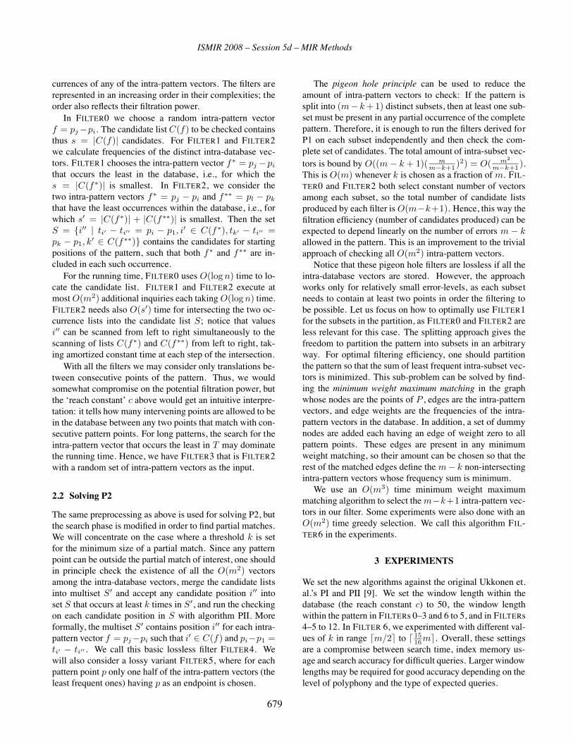
ISMIR 2008 – Session 5d – MIR Methods
currences of any of the intra-pattern vectors. The filters arerepresented in an increasing order in their complexities; theorder also reflects their filtration power.In FILTER0 we choose a random intra-pattern vector
f = pj−pi. The candidate list C(f) to be checked containsthus s = |C(f)| candidates. For FILTER1 and FILTER2we calculate frequencies of the distinct intra-database vec-tors. FILTER1 chooses the intra-pattern vector f∗ = pj −pi
that occurs the least in the database, i.e., for which thes = |C(f∗)| is smallest. In FILTER2, we consider thetwo intra-pattern vectors f∗ = pj − pi and f∗∗ = pl − pk
that have the least occurrences within the database, i.e., forwhich s′ = |C(f∗)| + |C(f∗∗)| is smallest. Then the setS = {i′′ | ti′ − ti′′ = pi − p1, i
′ ∈ C(f∗), tk′ − ti′′ =pk − p1, k
′ ∈ C(f∗∗)} contains the candidates for startingpositions of the pattern, such that both f∗ and f∗∗ are in-cluded in each such occurrence.For the running time, FILTER0 uses O(log n) time to lo-
cate the candidate list. FILTER1 and FILTER2 execute atmostO(m2) additional inquiries each taking O(log n) time.FILTER2 needs also O(s′) time for intersecting the two oc-currence lists into the candidate list S; notice that valuesi′′ can be scanned from left to right simultaneously to thescanning of lists C(f∗) and C(f∗∗) from left to right, tak-ing amortized constant time at each step of the intersection.With all the filters we may consider only translations be-
tween consecutive points of the pattern. Thus, we wouldsomewhat compromise on the potential filtration power, butthe ‘reach constant’ c above would get an intuitive interpre-tation: it tells howmany intervening points are allowed to bein the database between any two points that match with con-secutive pattern points. For long patterns, the search for theintra-pattern vector that occurs the least in T may dominatethe running time. Hence, we have FILTER3 that is FILTER2with a random set of intra-pattern vectors as the input.
2.2 Solving P2
The same preprocessing as above is used for solving P2, butthe search phase is modified in order to find partial matches.We will concentrate on the case where a threshold k is setfor the minimum size of a partial match. Since any patternpoint can be outside the partial match of interest, one shouldin principle check the existence of all the O(m2) vectorsamong the intra-database vectors, merge the candidate listsinto multiset S′ and accept any candidate position i′′ intoset S that occurs at least k times in S′, and run the checkingon each candidate position in S with algorithm PII. Moreformally, the multiset S′ contains position i′′ for each intra-pattern vector f = pj−pi such that i′ ∈ C(f) and pi−p1 =ti′ − ti′′ . We call this basic lossless filter FILTER4. Wewill also consider a lossy variant FILTER5, where for eachpattern point p only one half of the intra-pattern vectors (theleast frequent ones) having p as an endpoint is chosen.
The pigeon hole principle can be used to reduce theamount of intra-pattern vectors to check: If the pattern issplit into (m− k + 1) distinct subsets, then at least one sub-set must be present in any partial occurrence of the completepattern. Therefore, it is enough to run the filters derived forP1 on each subset independently and then check the com-plete set of candidates. The total amount of intra-subset vec-tors is bound by O((m− k + 1)( m
m−k+1 )2) = O( m2
m−k+1 ).This is O(m) whenever k is chosen as a fraction ofm. FIL-TER0 and FILTER2 both select constant number of vectorsamong each subset, so the total number of candidate listsproduced by each filter is O(m−k+1). Hence, this way thefiltration efficiency (number of candidates produced) can beexpected to depend linearly on the number of errors m − kallowed in the pattern. This is an improvement to the trivialapproach of checking all O(m2) intra-pattern vectors.Notice that these pigeon hole filters are lossless if all the
intra-database vectors are stored. However, the approachworks only for relatively small error-levels, as each subsetneeds to contain at least two points in order the filtering tobe possible. Let us focus on how to optimally use FILTER1for the subsets in the partition, as FILTER0 and FILTER2 areless relevant for this case. The splitting approach gives thefreedom to partition the pattern into subsets in an arbitraryway. For optimal filtering efficiency, one should partitionthe pattern so that the sum of least frequent intra-subset vec-tors is minimized. This sub-problem can be solved by find-ing the minimum weight maximum matching in the graphwhose nodes are the points of P , edges are the intra-patternvectors, and edge weights are the frequencies of the intra-pattern vectors in the database. In addition, a set of dummynodes are added each having an edge of weight zero to allpattern points. These edges are present in any minimumweight matching, so their amount can be chosen so that therest of the matched edges define them− k non-intersectingintra-pattern vectors whose frequency sum is minimum.We use an O(m3) time minimum weight maximum
matching algorithm to select them−k+1 intra-pattern vec-tors in our filter. Some experiments were also done with anO(m2) time greedy selection. We call this algorithm FIL-TER6 in the experiments.
3 EXPERIMENTS
We set the new algorithms against the original Ukkonen et.al.’s PI and PII [9]. We set the window length within thedatabase (the reach constant c) to 50, the window lengthwithin the pattern in FILTERs 0–3 and 6 to 5, and in FILTERs4–5 to 12. In FILTER 6, we experimented with different val-ues of k in range (m/2) to ( 15
16m). Overall, these settingsare a compromise between search time, index memory us-age and search accuracy for difficult queries. Larger windowlengths may be required for good accuracy depending on thelevel of polyphony and the type of expected queries.
679

ISMIR 2008 – Session 5d – MIR Methods
0.001
0.01
0.1
1
10
100
1000
10000
8 16 32 64 128 256 512 1024
Tim
e (m
s)
Pattern size (notes)
(a) Effect of pattern size on P1 algorithms
0.001
0.01
0.1
1
10
100
1000
10000
8 16 32 64 128 256 512 1024
Tim
e (m
s)
Database size (thousands of notes)
(b) Effect of database size on P1 algorithms
P1P1/F0P1/F1P1/F2P1/F3 (50 samples)FG6Index construction
Figure 3. Solving P1. Search time as function of pattern and database sizes in the MUTOPIA collection of 1.9 million notes.Database size experiments were done with a pattern size of 64 notes. Note the log scales.
We also compare with Clifford et. al.’s MSM [2] andFredriksson and Grabowski’s FG6 algorithm [3, Alg. 6.].The latter solves a slightly different problem; the time infor-mation is ignored, and the pitch values can differ by δ ≥ 0after transposition. We set δ = 0 to make the setting as closeto ours as possible. We tested also other algorithms in [3]but Alg. 6 was constantly fastest among them on our setting.To measure running times we experimented both on the
length of the pattern and the database. Reported times aremedian values of more than 20 trials using randomly pickedpatterns. As substantial variations in the running times arecharacteristic to the filtering methods, we have depicted thisphenomenon by using box-whiskers: The whisker below abox represents the first quartile, while the second begins atthe lower edge and ends at the median; the borders of thirdand fourth quartiles are given by the median, the upper edgeof the box and the upper whisker, respectively.We also measured how robust the PII-based methods
(FILTERs 4-6) are against noise, and calculated a precision-against-recall plot. Here we reported the mean value of a100-trial experiment in which the set of occurrences foundby PII was considered as the ground truth. All the experi-ments were carried out with the MUTOPIA database; at thetime it consisted of 1.9 million notes in 2270 MIDI files.
3.1 Experimenting on P1
In experimenting on the pattern size, the variations in therunning times of the PI-based filters are clearly depicted inFig. 3a. Out of the four filters, FILTER2 performed moststably while FILTER0 had the greatest variation. The figureshows also that all our filtering methods constantly outper-form both the original PI and the FG6 algorithm. With pat-tern sizes |P | � 400, FILTERs 1 and 2 are the fastest ones,but after that FILTER3 starts to dominate the results.The evident variation in our filters is caused by difficult
patterns that only contain relatively frequently appearingvectors. In our experiments, FILTERs 1–3 had search times
of at most 2 ms. It is possible to generate patterns that havemuch longer search times, especially if the database is verymonotonic or short windows are used. However, in practicethese filters are at least 10 times faster than PI and 200 timesfaster than FG6 for every pattern of less than 1000 notes.When experimenting on the size of the database as shown
in Fig. 3b, execution times of online algorithms PI andFG6 increases linearly in the database size. Also FILTER0’ssearch time increases at the same rate due to the poor filter-ing efficiency. FILTERS 1–3 have much lower slope becauseonly few potential matches need to be verified after filter-ing. Fig. 3b also depicts the construction time of the indexstructure for the filters. Remember that this costly operationneeds to be executed only once for any database.
3.2 Experimenting on P2
Fig. 4 shows the experimentally measured search times forP2 filters, PII and MSM. When varying the size of the pat-tern, our PII-based filters clearly outperformed MSM in allpractical cases (Fig. 4a): MSM becomes faster than PII onlywhen |P | > 400 and faster than FILTER4 when |P | > 1000.In this experiment FILTER6 dominates over FILTER5 until|P | � 250 after which FILTER5 starts to dominate. How-ever, a greedy version of FILTER6 outperforms them bothby an order of magnitude.Results of the experiments on the length of the database
are rather similar (Fig. 4b), exceptions being that MSM isconstantly outperformed by the others and that FILTER6 per-forms the best throughout the experiment. Again, the greedyFILTER6 is the fastest: it is nearly 100 times faster than FIL-TER6 and over million times faster than MSM.
3.2.1 Comparing whole musical works.
In [2], Clifford et al. carried out experiments for partial mu-sic matching and concluded that their algorithm is fasterthan PII when two whole documents are to be matched
680
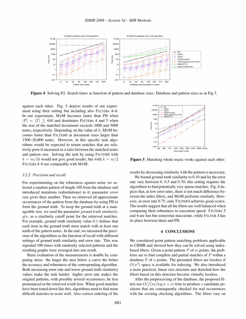
ISMIR 2008 – Session 5d – MIR Methods
0.01
0.1
1
10
100
1000
10000
100000
1e+06
8 16 32 64 128 256 512 1024
Tim
e (m
s)
Pattern size (notes)
(a) Effect of pattern size on P2 algorithms
0.01
0.1
1
10
100
1000
10000
100000
1e+06
8 16 32 64 128 256 512 1024
Tim
e (m
s)
Database size (thousands of notes)
(b) Effect of database size on P2 algorithms
P2P2/F4P2/F5P2/F6 (k=m/2)P2/F6 greedy (k=m*15/16)MSM (FFT)Index construction
Figure 4. Solving P2. Search times as function of pattern and database sizes. Database and pattern sizes as in Fig 3.
against each other. Fig. 5 depicts results of our experi-ment using their setting but including also FILTERs 4–6.In our experiment, MSM becomes faster than PII when|P | = |T | � 600 and dominates FILTERs 4 and 5 whenthe size of the matched documents exceeds 1000 and 5000notes, respectively. Depending on the value of k, MSM be-comes faster than FILTER6 at document sizes larger than1500–20,000 notes. However, in this specific task algo-rithms would be expected to return matches that are rela-tively poor if measured as a ratio between the matched notesand pattern size. Solving the task by using FILTER6 withk = m/16 would not give good results, but with k = m/2FILTERs 4–6 are comparable with MSM.
3.2.2 Precision and recall.
For experimenting on the robustness against noise we se-lected a random pattern of length 100 from the database andintroduced mutations (substitutions) to it; parameter errorrate gives their number. Then we retrieved all approximateoccurrences of the pattern from the database by using PII toform the ground truth. To keep the ground truth at a man-ageable size, we used the parameter ground truth similarity,gts, as a similarity cutoff point for the retrieved matches.For example, ground truth similarity value 0.1 defines thateach item in the ground truth must match with at least onetenth of the pattern notes. In the end, we measured the preci-sion of the algorithms as the function of recall with differentsettings of ground truth similarity and error rate. This wasrepeated 100 times with randomly selected patterns and theresulting graphs were averaged into one result.Basic evaluation of the measurements is doable by com-
paring areas: the larger the area below a curve the betterthe accuracy and robustness of the corresponding algorithm.Both increasing error rate and lower ground truth similarityvalues make the task harder: higher error rate makes theoriginal patterns, with possibly several occurrences, be lesspronounced in the retrieved result lists. When good matcheshave been toned down like this, algorithms need to find moredifficult matches to score well. Also correct ordering of the
0.001
0.01
0.1
1
10
100
1000
10000
100000
1e+06
128 256 512 1024 2048 4096 8192 16384 32768
Tim
e (m
s)Song length (notes)
P2P2/F4P2/F5P2/F6 (k=m/2)P2/F6 greedy (k=m/16)MSM (FFT)
Figure 5. Matching whole music works against each other.
results by decreasing similarity with the pattern is necessary.We bound ground truth similarity to 0.10 and let the error
rate vary between 0, 0.5 and 0.70; this setting requires thealgorithms to find potentially very sparse matches. Fig. 6 de-picts that, at low error rates, there is not much difference be-tween the index filters, and MSM performs similarly. How-ever, at error rate 0.75, only FILTER4 achieves good scores.The results suggest that all the filters are well balanced whencomparing their robustness to execution speed: FILTERs 5and 6 are fast but somewhat inaccurate, while FILTER 4 hasits place between them and PII.
4 CONCLUSIONS
We considered point pattern matching problems applicableto CBMR and showed how they can be solved using index-based filters. Given a point pattern P ofm points, the prob-lems are to find complete and partial matches of P within adatabase T of n points. The presented filters are lossless ifO(n2) space is available for indexing. We also introduceda more practical, linear size structure and sketched how thefilters based on this structure become virtually lossless.After the preprocessing of the database, the proposed fil-
ters use O(f(m) log n + s) time to produce s candidate po-sitions that are consequently checked for real occurrenceswith the existing checking algorithms. The filters vary on
681

ISMIR 2008 – Session 5d – MIR Methods
0
0.2
0.4
0.6
0.8
1
1.2
0 0.2 0.4 0.6 0.8 1
Pre
cisi
on
Recall
P2P2/F4
P2/F5P2/F6
MSM
0
0.2
0.4
0.6
0.8
1
1.2
0 0.2 0.4 0.6 0.8 1
Pre
cisi
on
Recall
P2P2/F4
P2/F5P2/F6
MSM
0
0.2
0.4
0.6
0.8
1
1.2
0 0.2 0.4 0.6 0.8 1
Pre
cisi
on
Recall
P2P2/F4
P2/F5P2/F6
MSM
Figure 6. Precision-Recall at error rates 0, 0.5 and 0.75 (left to right), with gts = 0.1.
the complexity of f(m) and on the output size s. Since thefiltering power of the proposed filters is hard to characterizetheoretically, we ran several experiments to study the prac-tical performance on typical inputs.The experiments showed that our filters perform much
faster than the existing algorithms on typical applicationscenarios. Only when comparing large musical works intheir entirety, MSM [2] outperforms our new filters.Since the guarantee of losslessness in the filters is only
valid on limited search settings (number of mismatches al-lowed, constants limiting maximal reach, etc.), it was impor-tant to study also the precision and recall. This comparisonwas especially fruitful against MSM, that is an approxima-tion algorithm, and can hence be considered as a lossy filteras well. The experiments showed that our filters typicallyperforms at the same level that MSM in this respect.As a future work, we plan to study the extensions of the
filters to approximate point pattern matching; in addition toallowing partial matching, we could allow matching a pointto some ε-distance from its target. Such setting gives a morerobust way to model the query-by-humming application.Although it is straightforward to extend the filters to con-sider the candidate lists of all intra-database vectors withinthe given ε-threshold from any intra-pattern vector, the over-all amount of candidate positions to check grows fast as thethreshold is loosen. Therefore, finding better strategies forfiltering in this scenario is an important future challenge.
5 ACKNOWLEDGEMENTS
We thank MSc Ben Sach from University of Bristol andDr. Kimmo Fredriksson from University of Kuopio for theirimplementations of the MSM and FG6 algorithms.
6 REFERENCES
[1] M. Clausen, R. Engelbrecht, D. Meyer, and J. Schmitz.Proms: A web-based tool for searching in polyphonic
music. In Proc. ISMIR’00, Plymouth, 2000.
[2] R. Clifford, M. Christodoulakis, T. Crawford, D. Mered-ith, and G. Wiggins. A fast, randomised, maximal subsetmatching algorithm for document-level music retrieval.In Proc. ISMIR’06, pages 150–155, Victoria, 2006.
[3] K. Fredriksson and Sz. Grabowski. Efficient algorithmsfor pattern matching with general gaps, character classesand transposition invariance. In Proc. SPIRE’2006,pages 267–278, Berlin, 2006.
[4] A. Ghias, J. Logan, D. Chamberlin, and B. Smith. Queryby humming - musical information retrieval in an audiodatabase. In PROC. ACM Multimedia, pages 231–236,San Francisco, 1995.
[5] A. Lubiw and L. Tanur. Pattern matching in polyphonicmusic as a weighted geometric translation problem. InProc. ISMIR’04, pages 289–296, Barcelona, 2004.
[6] M. Mongeau and D. Sankoff. Comparison of musical se-quences. Comp. and the Humanities, 24:161–175, 1990.
[7] R. Typke. Music Retrieval based on Melodic Similarity.PhD thesis, Utrecht University, 2007.
[8] A. Uitdenbogerd and J. Zobel. Manipulation of musicfor melody matching. In Proc. ACM Multimedia, pages235–240, Bristol, 1998.
[9] E. Ukkonen, K. Lemström, and V. Mäkinen. GeometricAlgorithms for Transposition Invariant Content-BasedMusic Retrieval. In Proc. ISMIR’03, pages 193–199,Baltimore, 2003.
[10] G. Wiggins, K. Lemström, and D. Meredith.SIA(M)ESE: An algorithm for transposition in-variant, polyphonic content-based music retrieval. InProc. ISMIR’02, pages 283–284, Paris, 2002.
682

ISMIR 2008 – Session 5d – MIR Methods
A TUNNELING-VANTAGE INDEXING METHOD FOR NON-METRICSR. Typke1
Austrian Research Institute
for Artificial Intelligence (OFAI), Vienna
A. C. Walczak-TypkeKurt Gödel Research Center for Mathematical Logic
University of Vienna
ABSTRACT
We consider an instance of the Earth Mover’s Distance
(EMD) useful for comparing rhythmical patterns. To make
searches for r-near neighbours efficient, we decompose our
search space into disjoint metric subspaces, in each of which
the EMD reduces to the l1 norm. We then use a combined
approach of two methods, one for searching within the sub-
spaces, the other for searching between them. For the for-
mer, we show how one can use vantage indexing without
false positives nor false negatives for solving the exact r-
near neighbour problem, and find an optimum number and
placement of vantage objects for this result. For searching
between subspaces, where the EMD is not a metric, we show
how one can guarantee that still no false negatives occur, and
the percentage of false positives is reduced as the search ra-
dius is increased.
1 INTRODUCTION
Searching a database for a melody or rhythm is often equiv-
alent to a special version of the nearest neighbour problem:
one wants to find items which are similar, but not necessar-
ily identical to a given query, and be sure to retrieve all such
items up to a certain level of dissimilarity. With a distance
measure which adequately captures similarity, this amounts
to retrieving all items which lie inside a ball around the
query, where the radius of the ball is the dissimilarity thresh-
old up to which retrieval results are considered relevant. We
will call this search radius r, and items whose distance from
a query is at most r will be called r-near neighbours.
If the database is large, one needs a data structure which
makes it possible to retrieve the r-near neighbours without
comparing the query to each point in the database. For high
numbers of dimensions, where exact methods such as kd-
trees do not offer much improvement over a linear search, a
number of approximate methods have been suggested. An-
doni and Indyk [2] point to many approximate methods and
describe one of the most popular among them, locality sen-sitive hashing (LSH), in detail. With LSH, one applies a
hash function to every data point. The hash function must be
chosen so that there is a high probability for points which are
close to each other to be hashed into the same bin. To search
for nearest neighbours, one then applies the hash function
1R. Typke gratefully acknowledges support by the Austrian Research
Fund (FWF), Project Number M1027-N15.
to the query and searches the bin into which the query was
hashed. However, LSH relies on the distance measure being
a metric.
We describe a method which combines vantage indexingwith tunneling, an approach applicable to certain non-metric
distance measures. Our specific distance measure is non-
metric; however, we can decompose our search space into
disjoint metric subspaces. Within the metric subspaces, the
non-metric reduces to the l1 norm. We use a new variant of
the vantage indexing method which can be used for solving
the exact r-near neighbour problem (i. e., without resort-
ing to approximation) for the l1 norm in moderately high
dimensional spaces (no more than about 9 dimensions). It
guarantees to retrieve exactly the items within the ball of in-
terest, without any false positives or false negatives, with a
time complexity of essentially O(log n) (n=number of data
points), but at the cost of using O(n2j−1) storage space
(j=number of dimensions). It is possible to use less stor-
age space, but at a cost: false positives can occur.
For certain locality sensitive hash functions, LSH is sim-
ilar to vantage indexing. Andoni and Indyk propose hash
functions for the l1 and l2 norms which involve calculat-
ing the distances to an arbitrary number of randomly chosen
vantage objects and then putting all data points into the same
bin whose distances to the vantage objects lie in a certain
range. We, on the other hand, use exactly as many vantage
objects as needed, placed in the space so that we are guar-
anteed to retrieve all data points we should retrieve, and no
others. Also, we avoid the need to pick a bin size which
might not fit very well with the actual search radius.
While our method for vantage indexing is specific to in-
stances where the EMD reduces to metric subspaces with
regular ball shapes, the second part of our combined method
is more generally applicable to prametric spaces that can be
decomposed into metric subspaces. By “tunneling”, we can
efficiently search between metric subspaces, still without in-
troducing false negatives. False positives can occur, but their
percentage among the retrieved items shrinks as the search
radius grows, making them tolerable.
2 MEASURING MELODIC OR RHYTHMICSIMILARITY WITH THE EMD
2.1 The Earth Mover’s Distance
The distance measure discussed in this paper measures the
distance between weighted point sets. Intuitively speaking,
683
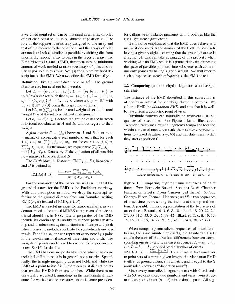
ISMIR 2008 – Session 5d – MIR Methods
a weighted point set ai can be imagined as an array of piles
of dirt each equal to wi units, situated at position xi. The
role of the supplier is arbitrarily assigned to one array and
that of the receiver to the other one, and the arrays of piles
are made to look as similar as possible by shifting dirt from
piles in the supplier array to piles in the receiver array. The
Earth Mover’s Distance (EMD) then measures the minimum
amount of work needed to make two arrays of piles as sim-
ilar as possible in this way. See [3] for a more detailed de-
scription of the EMD. We now define the EMD formally:
Definition. Fix a ground distance d on Rk. The ground
distance can, but need not be, a metric.
Let A = {a1, a2, . . . , am}, B = {b1, b2, . . . , bn} be
weighted point sets such that ai = {(xi, wi)}, i = 1, . . . , m,
bj = {(yj , vj)}, j = 1, . . . , n, where xi, yj ∈ Rk with
wi, vj ∈ R+ ∪ {0} being the respective weights.
Let WA =∑n
j=1 wi be the total weight of set A; the total
weight WB of the set B is defined analogously.
Let dij = d(xi, yj) denote the ground distance between
individual coordinates in A and B, without regard to their
weight.
A flow matrix F = (fij) between A and B is an m ×n matrix of non-negative real numbers, such that for each
1 � i � m,∑n
j=1 fij � wi, and for each 1 � j � n,∑mi=1 fij � vj . Furthermore, we require that
∑i
∑j fij =
min(WA, WB). Denote by F the collection of all possible
flow matrices between A and B.
The Earth Mover’s Distance, EMDd(A, B), between Aand B is defined as
EMDd(A, B) =minF∈F
∑mi=1
∑nj=1 fijdij
min(WA, WB).
For the remainder of this paper, we will assume that the
ground distance for the EMD is the Euclidean metric l2.
With this assumption in mind, we drop the subscript re-
ferring to the ground distance from our formulas, writing
EMD(A, B) instead of EMDl2(A, B).The EMD is a useful measure for music similarity, as was
demonstrated at the annual MIREX comparison of music re-
trieval algorithms in 2006. Useful properties of the EMD
include its continuity, its ability to support partial match-
ing, and its robustness against distortions of tempo and pitch
when measuring melodic similarity for symbolically encoded
music. For doing so, one can represent every note by a point
in the two-dimensional space of onset time and pitch. The
weights of points can be used to encode the importance of
notes. See [6] for details.
The EMD has one major disadvantage which can cause
technical difficulties: it is in general not a metric. Specif-
ically, the triangle inequality does not hold, and while the
EMD of a point to itself is 0, there can exist distinct points
that are also EMD 0 from one another. While there is no
universally accepted terminology in the mathematical liter-
ature for weak distance measures, there is some precedent
for calling weak distance measures with properties like the
EMD symmetric prametrics.
It should be emphasized that the EMD does behave as a
metric if one restricts the domain of the EMD to point sets
having a given weight, assuming that the ground distance is
a metric [3]. One can take advantage of this property when
working with an EMD which is a prametric by decomposing
the space of possible point sets into subspaces each contain-
ing only point sets having a given weight. We will refer to
such subspaces as metric subspaces of the EMD space.
2.2 Comparing symbolic rhythmic patterns: a nice spe-cial case
The instance of the EMD described in this subsection is
of particular interest for searching rhythmic patterns. We
call this EMD the Manhattan EMD, and note that it is well-
behaved from a geometric point of view.
Rhythmic patterns can naturally be represented as se-
quences of onset times. See Figure 1 for an illustration.
To render irrelevant a musical segment’s tempo and location
within a piece of music, we scale their numeric representa-
tions to a fixed duration (say, 60) and translate them so that
they start at position 0.
Figure 1. Comparing rhythms using sequences of onset
times. Top: Ferruccio Busoni: Sonatina No.6: Chamber
Fantasia on Bizet’s Opera Carmen (3rd theme); bottom:Georges Bizet: Carmen: Habanera; middle: two sequences
of onset times representing the incipits at the top and bot-
tom. A possible numeric representation of the two series of
onset times: Busoni: (0, 3, 6, 8, 10, 12, 15, 18, 20, 22, 24,
27, 30, 31.5, 33, 34.5, 36, 39, 42); Bizet: (0, 3, 6, 8, 10, 12,
15, 18, 21, 22.5, 24, 27, 30, 31, 32, 33, 34.5, 36, 39, 42).
When comparing normalized sequences of onsets con-
taining the same number of onsets, the Manhattan EMD
equals the sum of the absolute differences between corre-
sponding onsets ai and bi in onset sequences A = a1 . . . an
and B = b1 . . . bn, divided by the number of onsets:
EMD(A, B) =Pn
i=1 |ai−bi|n . Thus, if we restrict ourselves
to point sets of a certain given length, the Manhattan EMD
(with l2 as ground distance) is a metric and is equal to the l1norm (also known as “Manhattan norm”).
Since every normalized segment starts with 0 and ends
with 60, we omit these two numbers and view n-onset seg-
ments as points in an (n − 2)-dimensional space. All seg-
684

ISMIR 2008 – Session 5d – MIR Methods
ments lie in the subset of Rn−2 where the coordinates are
strictly increasing.
3 VANTAGE INDEXING FOR MANHATTAN EMD
Vantage indexing (introduced by Vleugels and Veltkamp [7])
is an approach to the retrieval of objects from a large database
which are similar to a given query. The search is restricted
to items whose pre-calculated distances to a small set of pre-
chosen vantage objects are similar to the query’s distances
to the same vantage objects.
3.1 Ball shapes
If one works with the l1 norm, a ball (the set of all points
whose distance lies within a certain radius around a point of
interest) has the shape of a cross-polytope. A one-dimensio-
nal cross-polytope is a line segment, a two-dimensional cross-
polytope is a square, for three dimentions, an octahedron,
and so forth.
3.2 Creating a ball by intersecting “onion layers”
V1
V2
Figure 2. In this two-dimensional example, only the light
gray area is inhabited by database objects since only there
the second coordinate is greater than the first. The dark
gray ball around Q with a given radius can be created by
intersecting onion layers around V1 and V2 whose thickness
equals the radius.
We call the area between the surfaces of two balls of dif-
fering radii around a vantage object an “onion layer”. 1 An
onion layer contains all items in the database whose distance
from the vantage object lies within a certain range. Search-
ing an onion layer can be done efficiently if one has built
an index (for example, a range tree) for the database column
that contains the distance to a vantage object. By building an
index for multiple columns containing distances to different
vantage objects (for example, a nested range tree), one can
also search intersections of onion layers efficiently.
If one can cover the ball around the query object whose
radius equals the search radius by using intersections of on-
ion layers in a way that the intersection of onion layers equals
exactly the ball of interest, neither false negatives nor false
positives will occur. Since the intersection of onion layers
can be searched efficiently, the ball of interest can as well.
See Figure 2 for an illustration.
Certain metric spaces have the property that there exists a
finite number of points x1, . . . , xn such that⋂
i(B(xi, R +
1 Inspiration has many sources, and onions have other good uses [5].
r) \B(xi, R)) = B(y, r) for some point y (here we denote
the ball with radius r around a point x with B(x, r)). In
other terms, some spaces have the property that one needs
only finitely many vantage objects so that the intersection of
onion layers is exactly that of a ball. The l1 space has this
property, as do other spaces whose balls are regular objects
with finitely many faces. An example of a metric space that
does not have this property is Euclidean space.
3.3 Optimum placement and number of vantage objectsnecessary for optimum indexing
In the case of one dimension, one vantage object is enough
to always achieve the desired effect of perfectly covering
only the interesting ball with onion layers. However, one
has to place the vantage object correctly. See Figure 3 for
good and bad examples.
0 60
V Q
0 15 60
V Q
0 60
Q
0 15 60
Q V1
Figure 3. Of interest is the ball around Q (at 15) with radius
10, shown as a grey bar. Left: This ball is identical to the
intersection of an onion layer around V with distance range
of 5 to 25 and the inhabited part of the space. Right: If
the vantage object is not put either to the left or to the right
of inhabited space, corresponding onion layers can intersect
with the inhabited space in two disjoint places (shown as
dotted lines) – one would need to use another vantage object
for the intersection of onion layers to be identical to the ball
of interest.
For two dimensions, two vantage objects are necessary,
and they are sufficient if they are placed, for example, like
in Figure 2. Here, the onion layers intersect in two square-
shaped regions, but only one of them (the one in the gray
area) can ever contain data points. Therefore, no false posi-
tives can occur.
One can cover exactly the ball of interest and no other
region (except for regions outside the inhabited space) by
using 2j−1 vantage objects (j is the number of dimensions
of the space) and placing them as follows:
• Let m be some number which is larger than any co-
ordinate that can ever occur in the inhabited subspace
(in the Bizet and Busoni example from Section 2.2,
we could let m = 60).
• For one dimension, place one vantage object at the
coordinate (0) (as illustrated in Fig. 3, left).
• For j dimensions, use twice as many vantage objects
as for j − 1 dimensions. The coordinates of the van-
tage objects for j dimensions are based on those for
j − 1 dimensions: for each vantage object position in
j − 1 dimensions, create two new lists of coordinates
for j dimensions by appending 0 or m, respectively,
685

ISMIR 2008 – Session 5d – MIR Methods
to the list of coordinates for j − 1 dimensions.
We need at least 2j−1 vantage objects because a cross-
polytope has 2j facets (a facet is a (j−1)-dimensional struc-
ture). For the intersection of onion layers to equal the ball
of interest, every facet of the ball needs to coincide with
the surface of an onion layer. One can use as few vantage
objects as possible if one covers opposite facets of the cross-
polytope with the surfaces of an onion layer around the same
vantage object. This is exactly what happens if one uses
2j−1 vantage objects and places them as above.
4 PARTIAL MATCHING BY TUNNELINGBETWEEN METRIC SUBSPACES
When searching sequences of onsets that were detected in
audio files, there are two problems: the detection is not
always completely reliable, producing both false negatives
and false positives, and often there will be multiple voices
with onsets, while a user might want to search for rhythmic
patterns which occur only in one voice. Therefore, for suc-
cessfully searching sequences of onsets from audio data, one
should be able to ignore a certain number of onsets and still
find matching subsequences or supersequences. In this sec-
tion, we will show how one can use tunnels between metric
subspaces to achieve partial matching while still benefiting
from the optimum vantage indexing within the subspaces of
sequences with equal numbers of onsets.
The EMD provides partial matching as described above
for point sets whose weight sums are unequal. Unfortu-
nately, the EMD does not obey the triangle inequality in
such a case. This makes it impractical to directly apply van-
tage indexing since there would be no way of controlling
the number of false negatives. Also, the locality sensitive
hashing method, which also relies on the triangle inequality,
becomes unusable.
Our approach is inspired by the case of the Manhattan
EMD, which is rather easy to visualize. In particular, one
can precisely visualize the neighbourhood, or “ball” of r-
near neighbours in the n-dimensional metric subspace for an
m-dimensional query point: assume that (q1, q2, . . . , qm) is
a query, where the initial 0 and final 60 are dropped, so that
the query is an m-dimensional object.
First, we visualize the neighbourhoods in higher-dimen-
sional metric subspaces, say of dimension m+i. In this case,
the set of points which are of distance 0 from the query com-
prise(m+i
i
)many i-dimensional hyperplanes which are par-
allel to axes, and pass through the points that are the various
possible completions of the query vector to m + i dimen-
sional space using i-many zeros. Then, the r-near neigh-
bours of the query are found in the union of the r-balls, as
calculated in the m+i-dimensional metric subspace, around
each of the points of distance 0. The shape of these neigh-
bourhoods is rather awkward, and is no longer a ball, but
rather the cartesian product of a ball and a hyperplane. This
shape is difficult to search efficiently. The reader may wish
to think about the case of m = 2 and i = 1.
The neighbourhoods in lower-dimensional metric sub-
spaces are a easier to describe. The points of distance 0from the query in the m − i-dimensional metric subspace
are simply the(mi
)many points obtained by reducing the
query to an m− i-dimensional point. The neighbourhood is
then the union of the r-balls around these points.
Our intuition is that a given point can be somehow con-
nected with “tunnels” to the points in other metric subspaces
which are of distance 0, and then take advantage of the
triangle inequality in the metric subspaces to use vantage
indexing. However, the points in the database can possi-
bly not include any such points of distance 0, so we have
to modify this simplistic idea of a tunnel by instead link-
ing to nearest neighbours. We precalculate, for every point
set in all spaces except for that with the lowest dimension-
ality, links to its nearest neighbours in lower-dimensional
spaces. If such links exist, one can efficiently retrieve not
only the nearest neighbours in the same space as the query
(e.g. as described in Section 3), but also the nearest neigh-
bours in higher-dimensional and lower-dimensional spaces
which are linked to the retrieved items from the space with
the same dimensionality as the query. This yields almost the
same result as an exhaustive linear search, but requires only
logarithmic complexity.
One needs, however, to limit the number of connections
per high-dimensional object by limiting the range of dimen-
sionalities across which one wants to search. By introducing
such a constant bound, one ensures that the number of con-
nections grows only linearly with the number of items in the
database. For the application of searching for rhythmic and
melodic patterns, this means that one should limit the par-
tial matching to a certain maximum number of missing or
extra notes which may be ignored when the dissimilarity is
calculated. Such a limit is probably desirable: without it, a
short (low-dimensional) pattern could become very similar
to very different long (high-dimensional) patterns.
4.1 Efficiently building tunnels
By projecting high-dimensional objects onto lower-dimen-
sional subspaces and then using vantage indexing as de-
scribed in Section 3 for finding the nearest neighbour of the
projection, one can benefit from the logarithmic search com-
plexity of vantage indexing for the purpose of building con-
nections between nearest neighbours in metric subspaces of
differing dimensionality.
Algorithm 1 can be used for building connections be-
tween objects of different dimensionality. Note that its run-
time lies in O(n log n) since we limit the number of dimen-
sionalities to cross (the number of notes to ignore) to a con-
stant t. The outermost loop is executed O(n) times. The
686

ISMIR 2008 – Session 5d – MIR Methods
Algorithm 1 Build connections between nearest neighbours
in subspaces of different dimensionality.
for all point sets p dofor i := 1 to max. number of dimensions to cross do
for all subspaces s with i dimensions less than p doproject point set p onto subspace suse the vantage index of subspace s for finding p’s
nearest neighbours in screate a connection between p and its nearest
neighbour in s (or all of them if they have equal
distances).
end forend for
end for
two inner loops each are executed only a constant number of
times. Each point set p with j dimensions can be projected
onto (j − i)-dimensional space in(ji
)many ways, and this
is bounded by a constant as long as the maximum possible
number of dimensions and the number of subspaces to cross
are bounded. Using the vantage index within the subspace
onto which p is projected takes O(log n) steps, which leads
to an overall runtime of O(n log n).The space complexity can be expected to lie in O(n)
since the number of connections to create should be bounded
by(ji
). There is one exception: if there are many nearest
neighbours in the subspace which all have the same distance
from the projected point, we might store more than(ji
)con-
nections for one projected point.
4.2 Using tunnels for retrieving items from higher di-mensions than the query
To find rhythmic patterns which are similar to a given query,
but contain up to t additional notes (which should be ignored
when calculating dissimilarity), one can tunnel into higher
dimensions by using the connections previously described.
Given a query Q, search radius r, and a database with a
vantage index for each metric subspace and connections be-
tween items and the nearest neighbours of their projections
in subspaces with up to t fewer dimensions, one can retrieve
Q’s r-near neighbours with the same dimensionality as Q or
up to t dimensions higher as follows:
Retrieve Q’s nearest neighbours n within radius r with as
many dimensions as Q, using the vantage index for this
subspace.
for all r-near neighbours n doRetrieve every item which is connected to n and has a
dimensionality higher than that of Q.
end forThis will retrieve exactly the desired objects from the
subspace where the query Q resides, but for the higher-
dimensional objects, both false positives and false negatives
may occur.
P1
P2
P3
P4 P5 Q P6
r
Figure 4. False negatives and false positives resulting from
tunneling, and how to avoid them.
The database shown in Figure 4 contains 6 point sets
P1, . . . , P6. Three, P1, . . . , P3, are two-dimensional, the
others, one-dimensional. The query Q is one-dimensional.
The area of interest within the search radius r around Q is
marked grey.
False positives: It is conceivable that the projection of a
higher-dimensional object onto Q’s subspace lies just out-
side the search radius, but its nearest neighbour in Q’s sub-
space happens to lie within the search radius. An example is
P1, whose projection onto the subspace (shown as a circle)
has a nearest neighbour beyond the border of the grey area.
False negatives: It is also possible that while the pro-
jection of a higher-dimensional object onto Q’s subspace
lies inside the search radius, the closest object in Q’s sub-
space lies outside the search radius. In this case, illustrated
with P3 and P6, the higher-dimensional object will not be
retrieved. In the extreme case that there is no single ob-
ject inside the search radius in Q’s subspace, no higher-
dimensional objects whatsoever will be retrieved.
Controlling false negatives and false positives. To avoid
all false negatives and limit the badness of false positives
to a threshold e, one can add the projections as additional
“ghost points” to the database if their nearest neighbour in
the subspace is further away than e/2, and extend the search
radius by e/2.
The distance of false positives to the query will be at most
e higher than desired because in the worst case, the nearest
neighbour of the projection will lie on the line connecting
the projection with the query. The nearest neighbour can be
up to r + e/2 away from the query, while the projection can
be another e/2 away from the nearest neighbour, leading to
a total maximum distance of r + e for false positives.
Such additional ghost points would be added as part of
the task of building the index, and so would not slow down
the search process. It would also not increase the compu-
tational complexity of building the index – the only price
is some extra space for storing ghost points wherever some
point from higher dimensions gets projected into a sparsely
populated area in a subspace. There is a tradeoff between
the required additional space and the maximum possible dis-
tance error for false positives.
687

ISMIR 2008 – Session 5d – MIR Methods
4.3 Using tunnels for retrieving items from lower dimen-sions than the query
As we have seen in Algorithm 1, subspaces can be searched
efficiently for a query even without using the pre-computed
connections. Since these connections are already there, they
can be used instead of projecting the query onto each pos-
sible subspace. To avoid false negatives, one still needs to
search the area around the nearest neighbour in the subspace
with the search radius r + a, using the vantage index of the
subspace, where a is the distance between the projection of
Q onto the subspace and its nearest neighbour in that sub-
space. Whenever a is greater than zero, the possibility of
false positives gets introduced. If such false positives can-
not be tolerated, one can resort to not using the connections
but instead projecting the query onto all possible subspaces.
5 EXPERIMENTAL EVALUATION OF VANTAGEINDEXING WITH TUNNELING
For an experimental evaluation, we used Dixon’s onset de-
tector from his “BeatRoot” system [4] for extracting onsets
from various recordings with piano music (piano concertos
and solo works by Beethoven, Liszt, and Schumann). We
used piano music because piano onsets are relatively easy
to detect correctly. The detected onsets were grouped into
overlapping sequences of 5 to 8 onsets. 40, 000 of these se-
quences were put into a database and indexed for optimum
retrieval within subspaces as described in Section 3. We also
added connections between subspaces as described in Sec-
tion 4, with connections spanning up to 3 dimensionalities,
thus allowing for ignoring up to 3 extra or missing notes.
Figure 5. Recall �, precision � (left scale), ratio of re-
trieved items , and ratio of true positives (right scale)
for the tunneling method and different search radii, averaged
over 20 queries.
For every search radius in a range from 0 to 2, we ran-
domly picked 20 items from the database as queries and
used the index to retrieve the most similar items according
to the EMD. To calculate precision and recall, we also did
exhaustive searches for each of these queries (by calculating
the EMD between the query and each of the 40, 000 items
in the database) and counted false positives and false nega-
tives.
With this experiment, we verified that it is indeed possi-
ble to reduce the number of false negatives to zero and limit
the distance error of false positives to e by adding the pro-
jections of high-dimensional points to the database in cases
where their nearest lower-dimensional neighbour is further
away than e/2, and by increasing the search radius by e/2.
Figure 5 shows that our index works well: for example, with
a search radius of 1.9, we need to retrieve 1.3% of the whole
database (curve: ), but we actually retrieve 1.95% ( Ex-
amined = 0.0195), which still relieves us from looking at
98.05% of the database. For this experiment, the value of
e was 1, i.e., we inserted ghost points only if the projection
and its nearest neighbour were more than 0.5 apart. With
this threshold, we needed about as many ghost points as real
points. The nested range tree we used for the vantage table
[1] has a space complexity of O(n log n).The larger our search radius, and thus the more important
it is that we do not get swamped with false positives, the
lower their percentage in the search results. This is probably
due to the fact that false positives can only occur near the
surfaces of searched balls, and when the search radius is
increased, one expects an ever larger percentage of objects
inside the ball rather than near its surface. Although the
precision is not very good for very low search radii, this
does not matter much since for low search radii, very few
items are retrieved at all from the database. As the number
of retrieved database items grows with the search radius, the
pain resulting from false positives is relieved by the fact that
at the same time, the percentage of false positives among the
retrieved items shrinks.
References[1] CGAL, Computational Geometry Algorithms Library.
http://www.cgal.org.
[2] A. Andoni and P. Indyk. Near-optimal hashing algo-
rithms for approximate nearest neighbor in high dimen-
sions. CACM, 51(1):117–122, 2008.
[3] S. Cohen. Finding Color and Shape Patterns in Images.
Stanford University, 1999. Ph.D. thesis.
[4] S. Dixon. Onset detection revisited. In Proc. of the 9thInt. Conf. on Digital Audio Effects (DAFx06), 2006.
[5] T. Keller. The importance of onion soup. In Bouchon,
pages 47–50. Artisan, 2004.
[6] R. Typke. Music Retrieval based on MelodicSimilarity. Doctoral Thesis, Universiteit Utrecht,
http://rainer.typke.org/books.html, 2007.
[7] J. Vleugels and R. C. Veltkamp. Efficient image re-
trieval through vantage objects. Pattern Recognition,
35(1):69–80, 2002.
688
Author IndexAnglade, Amèlie, 63
Arcos, Josep Lluı́s, 495
Baccigalupo, Claudio, 275
Bamberger, Jeanne, 21
Barrington, Luke, 225, 614
Bay, Mert, 462, 468
Benetos, Emmanouil, 583
Bergeron, Mathieu, 69
Bertin-Mahieux, Thierry, 603
Blech, Martin, 255
Blei, David, 349
Buhmann, Joachim, 167
Burgoyne, John Ashley, 407, 419
Burred, Juan José, 427
Cai, Lianhong, 319
Camacho, Arturo, 533
Cambouropoulos, Emilios, 83
Casey, Michael, 559
Cella, Carmine-Emanuele, 427
Celma, Òscar, 255
Chew, Elaine, 57
Chordia, Parag, 307, 571
Chua, Bee Yong, 565
Chuan, Ching-Hua, 57
Clausen, Michael, 413
Conklin, Darrell, 69
Cook, Perry, 23, 153, 349
Corthaut, Nik, 249
Cremer, Markus, 395
Cunningham, Pádraig, 401
Cunningham, Sally Jo, 185
D’haes, Wim, 433
Daniel, Adrien, 550
Daudet, Laurent, 527
David, Bertrand, 550
Deliege, François, 565
Demachi, Hazuki, 193
Devaney, Johanna, 407
Dixon, Simon, 45, 63
Doll, Travis, 445
Donaldson, Justin, 275
Dopler, Markus, 179
Doraisamy, Shyamala, 331
Downie, J. Stephen, 462, 468
Duan, Zhiyao, 237
Dubnov, Shlomo, 23
Duggan, Bryan, 401
Duval, Erik, 249
Eck, Douglas, 603
Eerola, Tuomas, 521
Ehmann, Andreas F., 462, 468
Eigenfeldt, Arne, 75
Ellis, Daniel, 577
Emelle, Lloyd, 231
Emiya, Valentin, 550
Ewert, Sebastian, 389
Fenech, David, 243
Feng, Ling, 121
Fiebrink, Rebecca, 23, 153
Fields, Ben, 269
Fields, Benjamin, 559
Flanagan, Patrick, 635
Flexer, Arthur, 173, 205
Fornari, Jose, 521
Fremerey, Christian, 413
Fujihara, Hiromasa, 281
Fujinaga, Ichiro, 407, 419, 597
Gainza, Mikel, 401
Ganseman, Joachim, 433
Garbers, Jörg, 101, 381
Gasser, Martin, 173, 205
Gerhard, David, 33
Ghosh, Joydeep, 295
Godfrey, Mark, 307, 571
Golzari, Shahram, 331
Gomez, Emilia, 495
Goto, Masataka, 133, 211, 281
Govaerts, Sten, 249
Grijp, Louis P., 101
Guaus, Enric, 255
Haas, Bas de, 51
689

ISMIR 2008 – Author Index
Hamanaka, Masatoshi, 107
Han, Jinyu, 95
Hansen, Lars Kai, 121
Hasegawa, Yuji, 199
Hashida, Mitsuyo, 489
Heinen, Eric, 295
Hirata, Keiji, 107
Hockman, Jason, 419
Hoffman, Matthew, 349
Holzapfel, Andre, 653
Hu, Xiao, 462
Inskip, Charlie, 477
Itoyama, Katsutoshi, 39, 133
Izumitani, Tomonori, 609
Jacobson, Kurt, 269, 559
Jones, M. Cameron, 468
Kaestner, Celso A. A., 451
Kalliris, George, 325
Kameoka, Hirokazu, 139
Kashino, Kunio, 609
Katayose, Haruhiro, 489, 620
Kersten, Stefan, 483
Kim, Youngmoo, 231, 445
Kirlin, Phillip, 363
Kitahara, Tetsuro, 620
Klapuri, Anssi, 369
Kleedorfer, Florian, 287
Knees, Peter, 179, 287
Knopke, Ian, 147
Koerich, Alessandro L., 451
Komatani, Kazunori, 39, 133
Kotropoulos, Constantine, 583
Krehbiel, Dwight, 343
Kurth, Frank, 413
Lai, Catherine, 115
Lamere, Paul, 24
Lanckriet, Gert, 225, 614
Lartillot, Olivier, 521
Laurier, Cyril, 462
Lee, Kyogu, 395
Lemström, Kjell, 677
Li, Tao, 671
Li, Wen, 659
Li, Yipeng, 538
Liao, Shih-Jie, 115
Lima, Ernesto Trajano de, 641
Little, David, 127
Liu, Yuxiang, 319
Lu, Lie, 237
Lukashevich, Hanna, 375
Mäkinen, Veli, 677
MacFarlane, Andy, 477
Magno, Terence, 161
Manaris, Bill, 343
Mandel, Michael, 577
Manolopoulos, Yannis, 83, 219
Manzagol, Pierre-Antoine, 603
Matsui, Toshie, 489
Mauch, Matthias, 45
Maxwell, James, 75
Mayer, Rudolf, 337
McKay, Cory, 597
Meintanis, Konstantinos, 507
Migneco, Raymond, 445
Mikkilä, Niko, 677
Miotto, Riccardo, 301
Miyamoto, Kenichi, 139
Moh, Yvonne, 167
Molina-Solana, Miguel, 495
Müllensiefen, Daniel, 89
Müller, Meinard, 389, 413
Murata, Kazumasa, 199
Nakadai, Kazuhiro, 199
Nanopoulos, Alexandros, 83, 219
Neumayer, Robert, 337
Niedermayer, Bernhard, 544
Nielsen, Andreas Brinch, 121
Niitsuma, Masahiro, 193
Norowi, Noris Mohd., 331
Ogata, Jun, 281
Ogata, Tetsuya, 39, 133
Ogihara, Mitsunori, 671
Okuno, Hiroshi G., 39, 133, 199
Ono, Nobutaka, 139
Oono, Masaki, 193
Orio, Nicola, 301
690

ISMIR 2008 – Author Index
Pachet, François, 355, 589
Pampalk, Elias, 24
Panagakis, Ioannis, 583
Pardo, Bryan, 95, 127
Paulus, Jouni, 369
Pearce, Marcus, 89
Pedersen, Torben Bach, 565
Peeters, Geoffroy, 243, 427
Perez, Alfonso, 483
Plaza, Enric, 275
Pohle, Tim, 179, 287
Pugin, Laurent, 407, 419
Röbel, Axel, 427
Rabbat, Patrick, 589
Rae, Alex, 571
Rafailidis, Dimitris, 83
Rafferty, Pauline, 477
Raimond, Yves, 263
Ramalho, Geber, 27, 641
Ramirez, Rafael, 483
Rauber, Andreas, 337
Ravelli, Emmanuel, 527
Rhodes, Christophe, 559
Richard, Gaël, 527
Riley, Jenn, 439
Riley, Matthew, 295
Rodet, Xavier, 243
Roos, Patrick, 343
Roy, Pierre, 355
Ruxanda, Maria, 219
Sable, Carl, 161
Sagayama, Shigeki, 139
Saito, Hiroaki, 193
Sandler, Mark, 263, 269
Sapp, Craig, 501
Sapp, Craig, 24
Scaringella, Nicolas, 626
Schedl, Markus, 179
Scheunders, Paul, 433
Schloss, W. Andrew, 647
Schmidt, Erik, 231
Schnitzer, Dominik, 173
Scholz, Ricardo, 27
Schwarz, Diemo, 427
Selfridge-Field, Eleanor, 24
Shea, Brendan O’, 401
Shenoy, Arun, 319
Shipman, Frank, 507
Silla, Carlos N. Jr., 451
Skalak, Michael, 95
Slaney, Malcolm, 313
Sordo, Mohamed, 255
Stylianou, Yannis, 653
Sulaiman, Nasir, 331
Sumi, Kouhei, 39
Symeonidis, Panagiotis, 219
Takaesu, Hiroshi, 193
Takeda, Ryu, 199
Thul, Eric, 663
Tian, Aibo, 659
Toh, Chee-Chuan, 515
Toiviainen, Petri, 521
Tojo, Satoshi, 107
Torii, Toyotaka, 199
Toussaint, Godfried, 663
Trohidis, Konstantinos, 325
Tsai, Wei-Ho, 115, 319
Tsoumakas, Grigorios, 325
Tsuchihashi, Yusuke, 620
Tsujino, Hiroshi, 199
Turnbull, Douglas, 225, 614
Tymoczko, Dmitri, 22
Typke, Rainer, 683
Tzanetakis, George, 647
Udzir, Nur Izura, 331
Utgoff, Paul, 363
Van Kranenburg, Peter, 101
Veltkamp, Remco, 51
Veltkamp, Remco C., 101
Verbert, Katrien, 249
Vlahavas, Ioannis, 325
Volk, Anja, 101
Walczak-Typke, Agatha, 683
Wang, DeLiang, 538
Wang, Ge, 23, 153
Wang, Ye, 319, 515
Weinberger, Kilian, 313
691

ISMIR 2008 – Author Index
White, William, 313
Widmer, Gerhard, 173, 205
Wiering, Frans, 51, 101, 381
Wiggins, Geraint, 89
Winget, Megan, 457
Woodruff, John, 538
Wright, Matthew, 647
Xiao, Linxing, 659
Yazdani, Mehrdad, 614
Yoshii, Kazuyoshi, 39, 199, 211
Zalonis, Thomas, 343
Zhang, Bingjun, 515
Zhang, Changshui, 237
Zhang, Edmond, 185
Zhang, Xinglin, 33
Zhou, Jie, 659
692