i

ECO 204 Introductory Mathematics for Economists II

ii

iii

Ibadan Distance Learning Centre Series

ECO 204 Introductory Mathematics for Economists II

By

Musbau Adetunji Babatunde, Ph.D Department of Economics

University of Ibadan

Published by

Distance Learning Centre

University of Ibadan

iv

© Distance Learning Centre

University of Ibadan

Ibadan.

All rights reserved. No part of this publication may be reproduced, stored in a retrieval system, or transmitted in any form or by any means, electronic, mechanical, photocopying, recording, or otherwise, without the prior permission of the copyright owner.

First Published 2009

ISBN 978-021-375-9

General Editor: Prof. F. O. Egbokhare

Series Editor: Olubunmi, I. Adeyemo

Typeset @ Distance Learning Centre, University of Ibadan

v

Table of Contents Page Vice-Chancellor's Message… … … … … … vi

Foreword… … … … … … … … vii

Course Introduction … … … … … … viii

Lecture One: Linear Functions… … … … 1

Lecture Two: The Firm’s Behaviour: Revenue, Cost and

Profit Functions … ... … … 8

Lecture Three: Curvilinear Demand and Supply

Functions … … … … … 12

Lecture Four: The IS – LM Model… … … … 15

Lecture Five: Differential Calculus… … … … 20

Lecture Six: Some Economic Applications of the

Rules… … … … … … 31

Lecture Seven: Optimization: Maxima and Minima… … 37

Lecture Eight: Profit Maximization/Loss Minimization … 47

Lecture Nine: Multivariate Differential Calculus… … 54

Lecture Ten: Constrained Optimization: The Lagrange

Multiplier Method… … … … 62

Lecture Eleven: Constrained Optimization of Cobb-Douglas

Functions… … … … … 69

Lecture Twelve: Integral Calculus … … … … 73

Lecture Thirteen: Economic Application of Integration… … 80

vi

Vice-Chancellor’s Message

I congratulate you on being part of the historic evolution of our Centre for External Studies into a Distance Learning Centre. The reinvigorated Centre, is building on a solid tradition of nearly twenty years of service to the Nigerian community in providing higher education to those who had hitherto been unable to benefit from it.

Distance Learning requires an environment in which learners themselves actively participate in constructing their own knowledge. They need to be able to access and interpret existing knowledge and in the process, become autonomous learners.

Consequently, our major goal is to provide full multi media mode of teaching/learning in which you will use not only print but also video, audio and electronic learning materials.

To this end, we have run two intensive workshops to produce a fresh batch of course materials in order to increase substantially the number of texts available to you. The authors made great efforts to include the latest information, knowledge and skills in the different disciplines and ensure that the materials are user-friendly. It is our hope that you will put them to the best use.

Professor Olufemi A. Bamiro, FNSE Vice-Chancellor

vii

Foreword

The University of Ibadan Distance Learning Programme has a vision of providing lifelong education for Nigerian citizens who for a variety of reasons have opted for the Distance Learning mode. In this way, it aims at democratizing education by ensuring access and equity. The U.I. experience in Distance Learning dates back to 1988 when the Centre for External Studies was established to cater mainly for upgrading the knowledge and skills of NCE teachers to a Bachelors degree in Education. Since then, it has gathered considerable experience in preparing and producing course materials for its programmes. The recent expansion of the programme to cover Agriculture and the need to review the existing materials have necessitated an accelerated process of course materials production. To this end, one major workshop was held in December 2006 which have resulted in a substantial increase in the number of course materials. The writing of the courses by a team of experts and rigorous peer review have ensured the maintenance of the University’s high standards. The approach is not only to emphasize cognitive knowledge but also skills and humane values which are at the core of education, even in an ICT age. The materials have had the input of experienced editors and illustrators who have ensured that they are accurate, current and learner friendly. They are specially written with distance learners in mind, since such people can often feel isolated from the community of learners. Adequate supplementary reading materials as well as other information sources are suggested in the course materials. The Distance Learning Centre also envisages that regular students of tertiary institutions in Nigeria who are faced with a dearth of high quality textbooks will find these books very useful. We are therefore delighted to present these new titles to both our Distance Learning students and the University’s regular students. We are confident that the books will be an invaluable resource to them. We would like to thank all our authors, reviewers and production staff for the high quality of work.

Best wishes.

Professor Francis O. Egbokhare Director

viii

Course Introduction

This course builds on the basic mathematical foundation set out in ECO 104 as well as delving into detailed economic application of those topics.

It also provides the basic requirements for microeconomics, macroeconomics and mathematical economics at the higher levels.

1

LECTURE ONE

Linear Functions Linear functions are functions whose graphs are straight line. An example of such can be Q = 123 – 3P

The two variables present in the function above are Q (quantity) and P (price) are respectively dependent and independent variables. It should be noted that the graph of the above equation slopes downward from left to right because of the negative sign on the slope.

The above equation can be written general form;

Q = A + BP + CY + Dπ + ET

Where A, B, C, D and E are constants and also for the certainty of its linearity, all the variables except Q and P must be held constant. However any variation in those other variables will lead to a shift in the curve.

2

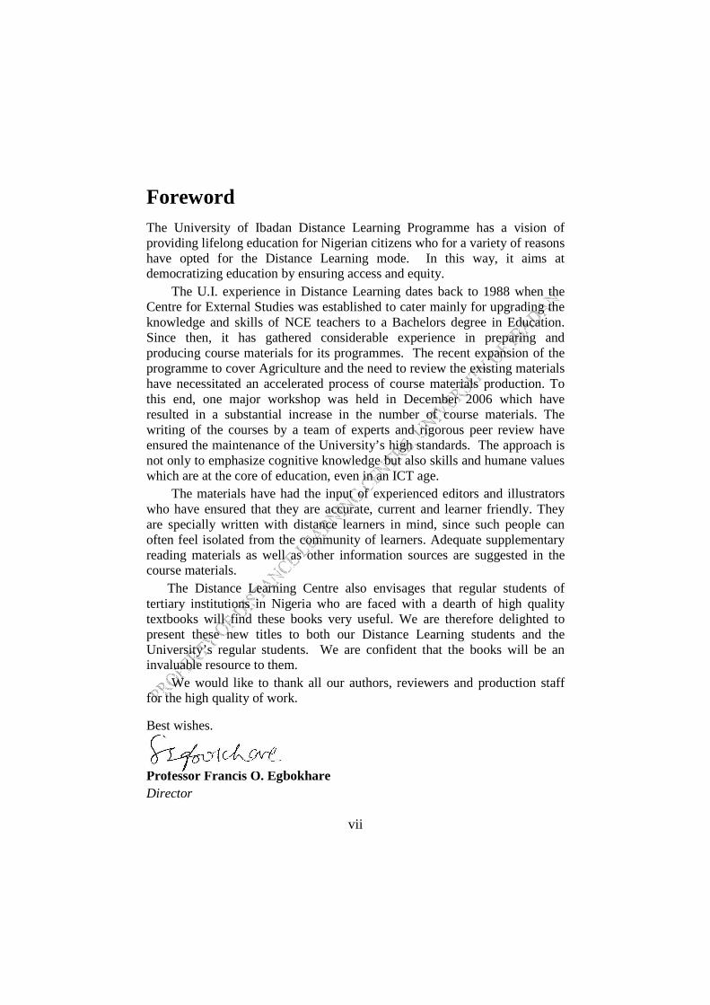
Economics makes use of certain linear functions and these can be shown as in the following:

1. Tax laws: Income tax is a fixed proportion of pre-tax income. This can be written in algebra as; D = Y – tY

Where D = disposable income

Y = Income

t = fixed tax proportion/rate 0< t < 1

then D = (1 – t) Y

D = aY where a = (1-t)

Note that the function is a positively sloped straight line function because the disposable income increases as income increases. Hence a positive relationship.

3

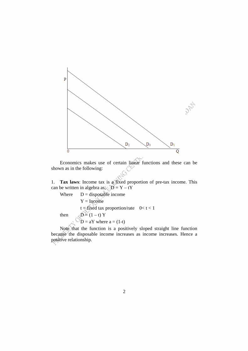
2. Consumption function: The consumption function relates consumption expenditure to the disposable income.

C = a + bD where a and b are constant

a = autonomous consumption

b = marginal propensity to consume

C = consumption expenditure (Explained variable)

D = disposable income

Derived relations: C = a + bD ……….. i

D = (1 – t) Y …………ii

Substituting equation (ii) into (i), we have;

C = a + b[(1 – t) Y]

= a + (b – bt) Y

If b – bt = d, then

C = a + dY

Now, the above shows consumption as directly related to income before tax.

4

3. Simultaneous linear functions: A very good example of this type of function is the demand and supply functions.

e.g. consider the demand and supply functions given below

Qd = 30 – 2P

Qs = -10 + 3P

Find the equilibrium price and quantity.

Solution At equilibrium, the consumer and the producer are expected to have reached an agreement on the quantity that will be bought and sold as well as the price that will be paid and received. Therefore, equating the demand function to the supply function will help solve the problem.

i.e Qd = Qs

30 – 2P = -10 + 3P

30 + 10 = 3P + 2P

40 = 5P

P = 40/5

P = 8

Substitute P = 8 into any of demand or supply function to get the equilibrium quantity;

Qd = 30 – 2(8) = 30 -16 =14 OR

Qs = -10 + 3(8) = -10 + 24 = 14

Q = 14 and P = 8

4. Cases in Economics where some arguments lead to linear equations and some statements leading to simultaneous linear equations.

Example: suppose commodities m and n are related in linear form and as shown in the following functions

Qm = K1 – a11Pm + a12Pn

Qn = K2 + a21Pm – a22Pn

If we take the specific form

Qm = 60 – 6Pm + 4Pn

5

Qn = 25 + 2Pm – 5Pn

Suppose that Qm = 24 and Qn = 15, then

24 = 60 – 6Pm + 4Pn …………i

15 = 25 + 2Pm – 5Pn ………….ii

From equation (i) we have

6Pm – 4Pn = 60 – 24

6Pm – 4Pn = 36 ……………iii

From equation (ii) we have

2Pm – 5Pn = 15 – 25

2Pm – 5Pn = -10 …………….iv

Equations (i) and (ii) have formed a simultaneous linear equation in which two variables are related to each other. The prices of the two commodities can now be obtained by solving those equations.

Multiply equation (iv) by 3

6Pm – 15Pn = -30 ……………..v

Subtract equation (v) from (iii)

6Pm – 4Pn – 6Pm + 15Pn = 36 + 30

11Pn = 66

Pn = 6 Substitute Pn = 6 into equation (iii)

6Pm – 4(6) = 36

6Pm – 24 = 36

6Pm = 36 + 24

6Pm = 60

Pm = 60/6

Pm = 10

Example 2: The quantity demanded of rice is given by the equation

Q = 60 – 1/3P

6

a. Find the quantity demanded of rice at prices of 0, 15, and 105

b. Express the inverse of the equation

c. Plot your answer on a graph. What type of graph did you derive?

Solution:

Q = 60 – 1/3P

a. when price = 0

Q = 60 – 1/3(0)

Q = 60 – 0

Q = 60

when price = 15

Q = 60 – 1/3(15)

Q = 60 – 5

Q = 55

When price = 105

Q = 60 – 1/3(105)

Q = 60 – 35

Q = 25

b. Expressing the inverse of the function means make P the subject of the formula

Q = 60 – 1/3P

1/3P = 60 – Q

Multiply through by 3

3 × 1/3 P = (60 – Q) × 3 = 60 × 3 – Q × 3

P = 180 – 3Q

7

Post-Test

1. The market for Sugar is characterized by the following demand and supply functions

Qd + 2P = 16 and Qs + 4 = 3P

Determine the equilibrium price and quantity.

2. Determine the equilibrium prices and quantities for the following markets

a. Qs = 3P – 20 and P = 44 – 0.2Qd

b. P = 0.125Qs – 45 and Qd = 125 – 2P

c. Qs + 32 = 7P and Qd – 128 + 9P = 0

d. 13P = Qs – 27 and Qd + 4P – 24 = 0

3. A consumer’s demand function for petrol is represented as Q = 30 – 1/3P where Q is quantity demanded and P is price per litre.

a. find the quantity demanded when price is N11 and N 22 per litre.

b. Suppose the function changes to take the form Q = 20 – 1/3P, find the quantity demanded at the same prices given in a.

8

LECTURE TWO

The Firm’s Behaviour: Revenue, Cost and Profit Functions

Total Revenue Function If a demand function assumes P = K – aQ being a relationship between price and quantity demanded, then

Total Revenue (TR) = P x Q = (K – aQ) Q

TR = KQ – aQ2

The TR function here is a second degree polynomial and the curve is curvilinear. In general, linear demand functions give rise to curvilinear TR functions.

Profit Function If the firm’s Total Cost (TC) function takes the form

TC = F + bQ (where F = Fixed Cost and b = Variable cost per unit)

Then TR – TC gives a profit function in terms of Q i.e f(Q)

If we denote profit by π, we can have

π = TR – TC = KQ – aQ2 – (F + bQ)

π = KQ – aQ2 – F – bQ

Which we can further express as

π = -aQ2 + (K – b)Q – F

The profit function is also a curvilinear function i.e a second degree polynomial.

9

Given this background, it is possible to find the quantity of goods that should be produced to satisfy the level of profit that the producer may want to attain at any point in time.

Assume that the parameters K, F, a and b take the values 18, 50, 1 and 3 respectively i.e the demand function is P = 18 – Q and the total cost function is TC = 50 + 3Q

TR = P x Q = 18Q – Q2; TC = 50 + 3Q

π = - Q2 + (18 – 3)Q – 50

π = - Q2 + 15Q – 50

Let us now solve for Q at different profit levels

e.g.

At what level of output will the firm breakeven (i.e. a point when profit = 0)

If π = 0, then

-Q2 + 15Q – 50 = 0

Q2 – 15Q + 50 = 0

Factorize to solve for Q

(Q – 5) (Q – 10) = 0

Q – 5 = 0; Q = 5

OR Q – 10 = 0; Q = 10

It is also possible to find the level of out put (Q) at which profit is equal to say 6.

If π = 6, then

-Q2 + 15Q – 50 = 6

Q2 – 15Q + 50 = - 6

Q2 – 15Q + 50 + 6 = 0

Q2 – 15Q + 56 = 0

10

Factorizing the equation, we have

(Q – 7) (Q – 8) = 0

Q = 7 or Q = 8

Example 2: Suppose the demand function of a firm is given by Q + P – 20 = 0 and its cost TC – 48 – 4Q = 0. Find the largest Q it can produce consistently with

a. breaking even

b. making a profit of N12

c. making a loss of N20

Solution:

P = 20 – Q

Thus, TR = P x Q = 20Q – Q2

TC = 4Q + 48

Profit function π = TR – TC = 20Q – Q2 – 4Q – 48

П = -Q2 + 16Q – 48

a. π = 0

-Q2 + 16Q – 48 = 0

Q2 – 16Q + 48 = 0

(Q – 4) (Q – 12) = 0

The largest quantity for breaking even is Q = 12

b. π = 12

-Q2 + 16Q – 48 = 12

Q2 – 16Q + 48 = -12

Q2 – 16Q + 48 + 12 = 0

Q2 – 16Q + 60 = 0

(Q – 6) (Q – 10) = 0

Q = 6 or Q = 10

The largest quantity for making a profit of N12 is Q = 10

11

c. π = - 20

- Q2 + 16Q – 48 = -20

Q2 – 16Q + 48 = 20

Q2 – 16Q + 48 – 20 = 0

Q2 – 16Q + 28 = 0

(Q – 2) (Q – 14) = 0

Q = 2 or Q = 14

The largest level of output consistent with making a loss of N20 is Q = 14

12

LECTURE THREE

Curvilinear Demand and Supply Functions Example 1: Suppose the market supply function is Ps = Q2 + 4Q + 1 and the market demand function takes the form Pd = -Q2 + Q + 4, find the equilibrium price and quantity

Solution:

At equilibrium, demand must be equal to supply

Q2 + 4Q + 1 = -Q2 – Q + 4

2Q2 + 5Q – 3 = 0

(2Q – 1) (Q + 3) = 0

Q = ½ or Q = - 3

Negative quantity does not make economic sense, therefore the quantity is Q = ½.

Substitute Q = ½ into any of supply or demand function to get the price

P = Q2 + 4Q + 1

(1/2) 2 + 4(1/2) + 1

¼ + 2 + 1

P = 3.25

13

Example 2: Given the market demand function P + Q2 + Q = 11 and the market supply function

2P – 2Q2 + Q – 4 = 0 Calculate the equilibrium price and quantity in the market.

Solution: From the demand function,

P = 11 – Q – Q2

And from the supply function,

P = Q2 – 0.5Q + 2

At equilibrium, demand = supply

11 – Q – Q2 = Q2 – 0.5Q + 2

-2Q2 – 0.5Q + 9 = 0

Multiply through by -2

4Q2 + Q – 9 = 0

(Q – 2) (4Q + 9) = 0

Q – 2 = 0 0r 4Q + 9 = 0

Q = 2 The other quantity is negative and it is therefore neglected.

Average Cost Functions Average costs are costs per unit of output. To obtain average cost, total cost is divided by quantity produced.

i.e. AC = TC/Q

since TC = F + bQ, then

AC = F bQ

Q

+

=F

Q+ b

If the Fixed cost (F) is 40 and b = 3,

14

Then TC = 40 + 3b

And AC = 40

Q + 3

GRAPH 5

A hyperbola always has two branches. The function above 40

Q + 3

represents a type of hyperbola called equilateral or rectangular hyperbola. A rectangular hyperbola is one whose asymptotes are perpendicular to each other and parallel to the coordinate axis. This type of hyperbola takes the form (x – u) (y – m) = r

Where u, m and r are constant and x and y are the variables.

x = u and y = m are the asymptotes of the rectangular hyperbolic function.

To see whether we can reduce the Average cost function to this standard form

40Z

Q= + 3

ZQ = 40 + 3Q

ZQ – 3Q = 40

(Q – 0) (Z – 3) = 40

Here, Q = 0 and Z = 3 are the asymptotes of the hyperbolic function, and Q and Z form the variables.

Exercise: Suppose a firm producing cassava chips has the following cost and revenue functions

TC = 500 + 2Q; TR = 8Q

i. identify the fixed cost and the variable cost from the equations

ii. what proportion of the total revenue is the variable cost

iii. at what quantity is profit equal to zero

iv. would you say the firm is in perfect competition or an imperfect competition (Hint: use the nature of the TR)

15

LECTURE FOUR

The IS – LM Model

The IS – LM model describes the overall equilibrium position in an economy. It is described as overall because both the goods/commodity and money markets are in equilibrium at the same time. The goods market equilibrium requires that the demand for goods be equal to the supply of goods. For a closed economy, the IS equation is represented by Y = C + I + G Where Y = equilibrium income C = consumption expenditure I = investment G = government spending Further defined, C = a + bY Where a = autonomous consumption b = marginal propensity to consume and I = α β− i

where α = autonomous investment β = part of investment that depends on interest rate

i = interest rate G* = autonomous government spending. Similarly, equilibrium in the money market requires that the demand for money be equal to its supply. Thus; Md = Ms

16

At any point in time, the money supply in an economy is constant (fixed) as it is determined by the monetary authority (Central Bank).

However, money demand is a function of income and interest rate. It is positively related to income (transaction balance) and negatively related to interest rate (speculative balance).

Md = qY + K - λ i

With the two equilibrium positions, it is possible to examine the overall equilibrium income and interest rate in the economy.

Example 1: Assume a two sector economy where C = 48 + 0.8Y, I = 98 – 75i, Ms = 250 and Md = 0.3Y + 52 – 150i

a. solve for the equilibrium Y and i

b. at the equilibrium, what is the level of consumption and investment

Solution a. Commodity market equilibrium exists when Y = C + I

Y = 48 + 0.8Y + 98 – 75i

Y – 0.8Y = 146 – 75i

0.2Y + 75i – 146 = 0 …………………..i

Monetary equilibrium exists when Ms = Md

250 = 0.3Y + 52 – 150i

0.3Y = 250 – 52 + 150i

0.3Y = 198 + 150i

0.3Y – 150i – 198 = 0 ……………………ii

Solve equations (i) and (ii) simultaneously

0.2Y + 75i – 146 = 0 ………………….i

0.3Y – 150i – 198 = 0 …………………ii

Multiply equation (i) by 2

0.4Y + 150i – 292 = 0 …………………iii

Add equations (ii) and (iii) together to eliminate i

0.7Y – 490 = 0

0.7Y = 490

Y = 700

17

Substitute Y = 700 into either equation (i) or (ii) to find i

0.2Y + 75i – 146 = 0

0.2(700) + 75i – 146 = 0

140 + 75i -146 = 0

75i – 6 = 0

75i = 6

i = 0.08 both commodity and money markets are in equilibrium when Y = 700 and i = 0.08

b. to obtain equilibrium C, substitute Y = 700 into consumption function

C = 48 + 0.8Y

48 + 0.8(700)

48 + 560

C = 608 For I, I = 98 – 75i

98 – 75(0.08)

98 – 6

I = 92

Example 2: Given C = 102 + 0.7Y; I = 150 – 100i; Ms = 300 and

Md = 0.25Y + 124 – 200i. Find

a. the equilibrium level of income and the equilibrium rate of interest

b. the level of C and I when the economy is in equilibrium c. if government spending G is introduced into the model, how is the

equilibrium Y and I affected.

Solution:

Commodity market equilibrium (IS) exists when

Y = C + I

Y = 102 + 0.7Y + 150 – 100i

Y – 0.7Y = 252 – 100i

18

0.3Y = 252 – 100i

0.3Y + 100i – 252 = 0 ………………i

Monetary equilibrium (LM) exists when

Ms = Md

300 = 0.25Y + 124 – 200i

0.25Y – 200i – 176 = 0 …………….ii

Then solve eqns (i) and (ii) simultaneously

0.3Y + 100i -252 = 0 …………………i

0.25Y – 200i – 176 = 0 ……………….ii

Multiply equation (i) by 2 to eliminate i

0.6Y + 200i – 504 = 0 …………………iii

Add equations (ii) and (iii) together

0.85Y – 680 = 0

0.85Y = 680

Y = 800 Substitute Y = 800 into eqn (i) or (ii)

0.25Y – 200i – 176 = 0

0.25(800) – 200i – 176 = 0

200 – 200i – 176 = 0

-200i + 24 = 0

200i = 24

i = 0.12

b. at Y = 800 and i = 0.12

C = 102 + 0.7Y

102 + 0.7(800)

102 + 560

C = 662 I = 150 – 100i

150 – 100(0.12)

150 – 12

I = 138

19

c. the introduction of government spending will affect the IS equation, thus

Y = C + I + G

Y = 102 + 0.7Y + 150 – 100i + 100

Y – 0.7Y = 352 – 100i

0.3Y = 352 – 100i

0.3Y + 100i – 352 = 0 ………………….iv

The monetary equilibrium is not affected, so we retain eqn (ii) and have

0.3Y + 100i – 352 = 0 ………………….iv

0.25Y – 200i – 176 = 0 …………………ii

Multiply eqn (iv) by 2 to eliminate i

0.6Y + 200i -704 = 0 ……………………..v

Add equations (v) and (ii) together

0.85Y – 880 = 0

0.85Y = 880

=880/0.085

Y = 1035.3 Substitute Y = 1035.3 into eqn (iv) or (ii) to find i

0.25Y – 200i – 176 = 0

0.25(1035.3) – 200i – 176 = 0

258.83 – 200i – 176 = 0

82.83 – 200i = 0

200i = 82.83

i = 0.4

Exercise: Find (a) the equilibrium income level and interest rate at the levels of C and I in equilibrium when

C = 89 + 0.6Y; I = 120 – 150i; Ms = 275 and Md = 0.1Y + 240 – 250i

20

LECTURE FIVE

Differentiation

Introduction The process of finding derivative is known as differentiation. A set of rules of differentiation exist for finding the derivatives of many common functions. Although there are many functions for which the derivative does not exist, our concern will be with functions which are differentiable.

Differentiation in calculus, denoted by dy

dx is equivalent to the slope

of a curve in geometry.

dy

dx explains how an infinitesimal change in x brings about a change

in y. An alternative to the dy

dx notation is the 'f (x) (read “f prime of x”).

Rules of Differentiation The rules presented in this section have been developed using the limit approach. For our purpose it will suffice to present the rules without proof. The rules of differentiation apply to functions which have specific structural characteristics/forms.

Rule 1: Constant function Rule. The derivative of a constant function y = f(x) = k is equal to zero for all values of x.

i.e dy

dx = 'f (x) given that x is a constant

21

As we pointed out earlier, the derivative of a function has its Geometric counterpart in the slope of the curve. The graph of the constant function is a horizontal straight line with a zero slope. i.e. its rate of change is zero.

This can be applied to fixed cost (FC) in Economics.

Given that y = FC = f(Q) = 2000

dy

dQ =

(2000)d

dQ = 0

GRAPH 6

The implication is that fixed cost, or any other constant function, does not change in response to changes in quantity.

Rule 2: Power function Rule The derivative of a power function y = f(x) = xn is equal to nxn-1

To carry out this operation, you use the power of x to multiply the function and then subtract 1 (one) from the original power of x in the given function to get the power of your derivative.

e.g Find the derivative of y = x5

dy

dx = 5x5-1 = 5x4

e.g y = f(x) = x8

dy

dx = 8x8-1 = 8x7

Note that such function as above may also be given with a constant known as the coefficient of x. for example, y = f(x) = Cxn and the derivative becomes

dy

dx = Cnxn-1

e.g y = f(x) = 4x

22

dy

dx = 4(1)x1-1

4x0

Since x0 = 1

Then dy

dx = 4

Given that y = 6x-2 find the derivative of y with respect to x

dy

dx = 6(-2)x-2-1

= -12x-3

If y = -3x2, find dy

dx

dy

dx = -3(2)x2-1

= -6x

e.g y = 2x1/2

dy

dx = 2(1/2) x1/2 – 1

= x-1/2

e.g Given that y = 3/x2, find dy

dx

Note that the above function can be rewritten as 3x-2, now differentiating becomes a simple task

dy

dx = 3(-2)x-2-1

= -6x-3

23

Rule 3: Sum or Difference Rule This rule implies that the derivative of a function formed by the sum (difference) of two or more component functions is the sum (difference) of the derivatives of the component functions.

[ ( ) ( )] ( ) ( )d f x g x df x dg x

dx dx dx

± = +

Example 1: Consider the function y = f(x) = 5x4 – 8x3 + 3x2 – x + 50. The derivative is found by differentiating each term in the function. Thus,

=

4 1 3 1 2 1 1 1

3 2 0

3 2

5(4 ) 8(3 ) 3(2 ) 0

5(4 ) 8(3 ) 3(2 )

20 24 6 1

dyx x x x

dx

x x x x

dyx x x

dx

− − − −= − + − +

− + −

= − + −

Example 2: Find dy

dx if

3 2

3 1 2 1 1 1

2 0

2

( ) 8 4 3 10

8(3 ) 4(2 ) 3( ) 0

8(3 ) 4(2 ) 3( )

24 8 3

f x x x x

dyx x x

dx

x x x

dyx x

dx

− − −

= − + −

= − + −

− +

= − +

Rule 4: Product Rule The derivative of the product of two functions is equal to the first function times the derivative of the second function plus the second function times the derivative of the first function.

[ ( ). ( )] ( ) ( ) ( ) ( )d d d

f x g x f x g x g x f xdx dx dx

= +

= ( ) '( ) ( ) '( )f x g x g x f x+

It is conventional to have it written as dy dv du

U Vdx dx dx

= +

24

In which case the function to be differentiated is written as

f(x) = U(x) . V(x)

Example 1: find dx

dy 32 ()5()( xxxxfif −−=

Solution:

U(x) = x2 – 5

V(x) = x – x3

Applying the formula dy dv du

U Vdx dx dx

= + , we have

2 2 3

2 4 2 2 4

4 2

( 5)(1 3 ) ( )2

3 5 15 2 2

15 18 5

x x x x x

x x x x x

dyx x

dx

− − + −− − + + −

= − + −

Example 2: find dy

dx if f(x) = 3 5 4 2( 2 )( 3 10)x x x x− − +

Solution: 3 5

4 2

2 4

3

( ) 2

( ) 3 10

3 10

4 6

U x x x

V x x x

dux x

dxdv

x xdxdy dv du

U Vdx dx dx

= −= − +

= −

= −

= +

3 5 3 4 2 2 4( 2 )(4 6 ) 3 10)(3 10 )x x x x x x x x− − + − + −

Expand the brackets 6 4 8 6 6 8 4 6 2 44 6 8 12 3 10 9 30 30 100x x x x x x x x x x− − + + − − + + −

25

Collect like terms 8 8 6 6 6 6 4 4 4 2

8 6 4 2

8 10 4 12 3 30 6 9 100 30

18 49 115 30

x x x x x x x x x x

x x x x

− − + + + + − − − += − + − +

Rule 5: Quotient Rule

If ( )

( )( )

U xf x

V x= where U and V are differentiable and( ) 0V x ≠ , then

2

( ). '( ) ( ). '( )'( )

V x U x U x V xf x

V

−=

OR

2

du dvV Udy dx dx

dx V

−=

Note: unlike in the product rule where we have a sum of two products, the quotient rule involves the difference between them. The implication of this is that while the arrangement does not matter in product rule (addition is commutative), it matters in quotient rule.

i.e. for product rule, dv du du dv

U V V Udx dx dx dx

+ = +

but for quotient rule, 2 2

du dv dv duV U U V

dx dx dx dxV V

− −≠ the one on the right is

wrong

Example 1: Consider f(x) = 2

3

(3 5)

(1 )

x

x

−−

applying quotient rule with

26

2

3 2

3 2 2

3 2

4 4 2

3 2

4 2

3 2

( ) 3 5, 6

( ) 1 , 3

(1 )6 (3 5)( 3 )'( )

(1 )

6 6 9 15

(1 )

3 15 6

(1 )

duU x x x

dxdv

V x x xdx

dy x x x xf x

dx x

x x x x

x

x x x

x

= − =

= − = −

− − − −= =−

− + −−

− +=−

Example 2: If 3

5

( 1)( ) ,

( 20)

xf x

x

− +=−

find '( )f x

Solution:

'( )f x = 2

du dvV Udy dx dx

dx V

−=

Wheredx

dy

3 2

5 4

5 2 3 4

5 2

7 2 3 4

5 2

7 4 3 2

5 2

( ) 1, 3

( ) 20, 5

( 20)( 3 ) ( 1)(5 )

( 20)

3 60 1 5

( 20)

3 5 60 1

( 20)

duU x x x

dxdv

V x x xdx

x x x x

x

x x x x

x

x x x x

x

= − + = −

= − =

− − − − +−

− + + − −−

− − + + −=−

27

Rule 6: Power of a Function

If ( ) [ ( )]nf x U x= where U is a differentiable function and n is a real number, then

1'( ) .[ ( )] . '( )nf x n U x U x−=

Example 1: consider )(,957)( 4 xffindxxxf −−=

Solution: Note that the function can be rewritten as

1/ 24( ) (7 5 9)f x x x= − −

We can apply rule 6, where 4( ) 7 5 9U x x x= − −

=

1

4 1/ 2 1 3

4 1/ 2 3

3 4 1/ 2

3 4 1/ 2

'( ) [ ( )] . '( )

1 (7 5 9) (28 5)21 (7 5 9) (28 5)21 (28 5)(7 5 9)2

5'( ) (14 )(7 5 9)2

nf x n U x U x

x x x

x x x

x x x

f x x x x

−

−

−

−

−

=

− − −

− −

− − −

= − − −

Example 2: Find the derivative of 5

2

3

1

x

x −

This function has the form stated in rule 6, where U is the rational function

2

3

(1 )

x

x−

[note that apart from applying rule 6, you must also apply quotient rule to find '( )u x ]

=

=

28

1

4 2

2 2 2

4 2 2

2 2 2

4 2

2 2 2

'( ) [ ( )] . '( )

3 (1 )(3) (3 )( 2 )5

1 (1 )

3 3 3 65

1 (1 )

3 3 35

1 (1 )

nf x n U x U x

x x x x

x x

x x x

x x

x x

x x

−=

− − − = − −

− + = − −

+ = − −

Rule 7: Chain Rule If we have a function y = f(u), where u is in turn a function of another variable x, say U = g(x), then the derivative of y with respect to x is equal to the derivative of y with respect to u, times the derivative of u with respect to x.

Expressed as .dy dy du

dx du dx=

Example 1: Given that 2( ) 2 1y f u u u= = − + and 2( ) 1u g x x= = −

Then, .dy dy du

dx du dx=

(2 2)(2 )dy

u xdx

= −

We then need to substitute 2( 1)x − for u so that dy

dx strictly becomes a

function of x.

2

2

2

3

[2( 1) 2](2 )

(2 2 2)(2 )

(2 4)(2 )

4 8

dyx x

dx

x x

x x

dyx x

dx

= − −

= − −= −

= −

29

Example 2: Given 3( ) 5y f u u u= = − where 4( ) 3u g x x x= = +

Solution:

.dy dy du

dx du dx=

2 3(3 5)(4 3)u x− +

Substitute 4 3x x+ for u

4 2 3

8 5 2 3

8 5 2 3

11 8 8 5 5 2 3

11 8 5 3 2

[3( 3 ) 5](4 3)

[3( 6 9 ) 5](4 3)

(3 18 27 5)(4 3)

12 9 72 54 108 81 20 15

12 81 162 20 81 15

dyx x x

dx

x x x x

x x x x

x x x x x x x

x x x x x

= + − +

+ + − ++ + − ++ + + + + − −+ + − + −

Practice Exercise Find the derivative of each of the following

1a. y = 63

b. 14y x=

c. 43y x=

2a. 3 4y x x= −

b. 6

23

xy x= −

c. 04y x=

3a. 3 5 2( 2 )( 6 )y x x x x= − +

b. 4 3(2 3 )(10 4 )y x x x x= − − + −

c. 2

3 210 ( 2 1)2

xy x x

= − − +

30

4a. 3 4(5 1)y x= +

b. 31 5y x= −

c. 2 1/3( 2 5)y x x= − +

In the following exercises, find dy

dx

5. 3( )y f u u= = and 2( ) 3 1u g x x x= = + +

6. 4 2( ) 1y f u u u= = + + and 2( ) 4u g x x= = −

7. ( )y f u u= = and 2

( )2

xu g x= =

31

LECTURE SIX

Some Economic Applications of the Rules

Marginal Cost and Marginal Revenue In general, the derivative of any total function gives its marginal function. For example, marginal cost is the derivative of total cost. i.e.

( )( )

dTC qMC q

dq=

And ( )

( )dTR q

MR qdq

=

e.g Given a short run total cost (TC) function 3 24 10 75TC Q Q Q= − + +

the marginal cost function is the derivative of the TC function

2( ) 3 8 10dTC

MC Q Q QdQ

= = − +

We would observe that the constant, which represents the fixed cost, does not affect the derivative because the derivative of a constant is zero. This fact provides the mathematical explanation of the well-known economic principle that the fixed cost of a firm does not affect its marginal cost.

Finding Marginal Revenue Function from Average Revenue Function Consider an average revenue (AR) function in the form AR = 15 – Q, we can find the marginal revenue function only after we have obtained the total revenue function.

32

2

( ) ( )

( ) (15 )

( ) 15

TR Q AR Q

TR Q Q Q

TR Q Q Q

== −= −

We can then take the derivative of TR (Q) with respect to Q to get the MR function.

( )( ) 15 2

dTR QMR Q Q

dQ= = −

The same procedure applies to deriving the marginal cost function from the average cost function. First, obtain the Total-Cost (TC) by multiplying the Average Cost (AC) by Q i.e TC = AC × Q, then take the derivative of the TC to get MC.

dTCMC

dQ=

Observe the similarities and differences between the Average Revenue function and the Marginal Revenue function derived from it.

The two functions have the same vertical intercept (15) but the slope of the MR function is twice that of the AR function. This is a general result whenever we have a linear Average Revenue function (i.e. Total Revenue is a quadratic function)

GRAPH 7: Relationship between AR and MR in an imperfect market arrangement

For a firm in a perfectly competitive market arrangement, the Total Revenue function is linear; hence, the Marginal Revenue and the Average Revenue functions coincide at a constant.

Example: Consider a perfectly competitive firm with a Total Revenue function of the form TR(Q) = 32Q, find the AR and MR.

33

Solution:

3232

32

TRAR

Q

QAR

Q

dTRMR

dQ

=

= =

= =

Therefore, for a firm in the perfect market arrangement, MR = AR = P

GRAPH 8 Relationship between Marginal cost and Average cost functions As an economic application of the quotient rule, let us consider the rate of change of average cost when output varies.

Given a Total Cost function TC = C(Q), the average cost (AC) function will be a quotient of two functions of Q, since

( )TC C QAC

Q Q= = as long as Q > 0

Therefore, the rate of change of AC with respect to Q can be found by differentiating AC.

2

( )[ '( ). ( ).1]

C QddAC C Q Q C QQ

dQ dQ Q

−= =

We can split the fraction and have

2 2

2

[ '( ). ] [ ( ).1]

'( ) ( )

C Q Q C Q

Q Q

C Q C Q

Q Q

−

−

Factorize;

1 ( )

'( )C Q

C QQ Q

−

34

Where '( )C Q MC=

And ( )C Q

ACQ

=

It then follows that

0dAC

dQ

>=<

if ( )

'( )C Q

C QQ

>=<

What this means is that;

The slope of AC is positive (i.e AC curve is upward sloping) when MC > AC

The slope of AC is zero when MC = AC; and

The slope of AC is negative when MC < AC

GRAPH 9

Observe that up to point Q* AC is downward sloping and the MC lies below it. At point Q*, the slope of AC = zero and MC = AC. At all points after Q*, AC is upward sloping and MC lies above it.

Example 1: Given the total cost function 3 28 15 30TC Q Q Q= − + + , write out a variable cost (VC) function. Find the derivative of the VC function, and give the economic meaning of that derivative.

Solution:

TC = VC + FC

3 2

2

8 15

3 16 15

VC Q Q Q

dVCQ Q

dQ

= − +

= − +

The economic meaning of the derivative above is the marginal cost (MC)

35

Remember we said that the fixed cost (FC) does not affect the MC. Therefore, the derivatives of both TC and VC give MC.

Example 2:

Given the average cost function 22 4 214AC Q Q= − + , find the MC function. Is the given function more appropriate as a long-run or short-run function? Why?

Solution:

TC = AC × Q 2

3 2

2

(2 4 214)

2 4 214

6 8 214

TC Q Q Q

TC Q Q Q

dTCMC Q Q

dQ

= − += − +

= = − +

The function is more appropriate as a long-run function because the total cost (TC) function does not have any fixed component which is characteristic of the long-run.

Note: In the long-run, all factors of production are variable as well as the associated cost. Therefore, in the long-run, fixed cost = 0 and variable cost is equal to the total cost.

Example 3: Given AR = 60 – 5Q,

a. find the total revenue function and the marginal revenue function.

b. Comparing the AR and the MR functions, what can you say about their relative slopes?

36

Solution:

a.

2

(60 5 )

60 5

60 10

TR AR Q

TR Q Q

TR Q Q

dTRMR Q

dQ

= ×= −= −

= = −

b. The slope of the MR function (10) is twice the slope of the AR function.

37

LECTURE SEVEN

Optimization: Maxima and Minima

An introduction to higher order derivatives:

So far we have dealt with first-order derivatives, now we turn to higher-order derivatives.

Given a function f(x), there are other derivatives which can be defined. This section discusses these higher order derivatives.

The second derivative The derivative '( )f x of the function f(x) is often referred to as the first derivative of the function. The adjective first is used to distinguish this derivative from other derivatives associated with the function.

The second derivative ''( )f x or 2

2

d y

dx of a function is the derivative of

the first derivative. This is done by applying the same rules of differentiation as were used in finding the first derivative.

Here are some examples. Table 1 Function f(x) First derivative '( )f x Second derivative ''( )f x

1 5x 45x 320x

2 3 22 5x x x− + 23 4 5x x− + 6 4x−

3 3 2x 1 23

2x 1 23

4x−

4 3(2 10)x− 26(2 10)x− 48 240x−

38

Let us solve the 4th example in Table 1 for clarity.

3(2 10)y x= − remember this is a power function.

[ ][ ] 1

3 1

2

( ) ( )

'( ) ( ) . '( )

'( ) 3(2 10) .2

'( ) 6(2 10)

n

n

f x u x

f x n u x u x

f x x

f x x

−

−

=

=

= −= −

To find ''( )f x , differentiate the result in '( )f x

[ ]''( ) 6(2) 2 10 .2

''( ) 12(2 10).2

''( ) 24(2 10)

''( ) 48 240

f x x

f x x

f x x

f x x

= −= −= −= −

Exercise: Find the first four derivatives of the function 1

x

x+ where

1x ≠ −

Optimization This involves maximizing or minimizing a function depending on the economic purpose it serves.

i. First-order condition for optimization (Necessary condition) For any function to reach its optimum point, the first derivative must be equal to zero i.e.

2

2''( ) 0

d yf x

dx= > [ ]'( ) 0 max min

dyf x or

dx= =

However, with the first order condition, we do not know the nature of the optimum point (either maximum or minimum). The second order condition helps to do this.

39

ii. Second order condition for optimization (Sufficient condition) The nature of the optimum point is determined by taking the second derivative, if the second derivative is negative, we have a maximum point.

i.e 2

2''( ) 0

d yf x

dx= < (maximum)

However if the second derivative is positive, then we have a minimum point. Thus

2

2''( ) 0

d yf x

dx= > (minimum)

Example 1: Find the relative extremum of the function 2( ) 4y f x x x= = − and determine its nature.

Solution:

0dy

dx= (first order condition/necessary condition)

8 1 0

8 1

18

dyx

dxx

x

= − =

=

=

For the nature of the point, we differentiate again 2

28

d y

dx= since the second derivative (8) is positive, we conclude that it is a

minimum point.

Example 2: Find the relative extrema of the function 3 2( ) 3 2y g x x x= = − + and determine the nature of those points.

Solution:

2

'( ) 0

3 6 0

dyg x

dxdy

x xdx

= =

= − =

40

solving the quadratic equation, we have

3 ( 2) 0x x− =

3 0x = or 2 0x− =

0x = or 2x =

The extrema occur at x = 0 and x = 2.

For their nature, we take the second derivative

2

26 6

d yx

dx= −

when 0x =

2

2

6(0) 6

6d y

dx

= −

= −

- 6 < 0 (maximum) when x = 2,

2

2

6(2) 6

12 6

6 0d y

dx

= −= −

= >

Application to Revenue, Cost and Profit Revenue maximization: The money which flows into an organization either from selling products or providing services is referred to as revenue. The most fundamental way of computing total revenue from selling a product (or service) is

TR = Price per unit × Quantity sold. Example: The demand for the product of a firm varies with the price that the firm charges for the product. The firm estimates that annual total revenue is a function of price.

2( ) 50 500R f p p p= = − +

41

a. Determine the price which should be charged in order to maximize total revenue

b. What is the maximum value of annual total revenue?

Solution:

a.

'( ) 100 500dR

f p pdp

= = − +

if we set )(Pf = 0

100 500 0

100 500

5

p

p

p

− + =− = −

=

the sufficient condition should be tested, thus

2

2''( ) 100 0

d Rf p

dp= = − <

b. the maximum value of R is found by substituting P = 5 into the function [f(p)]

2(5) 50(5 ) 500(5)

50(25) 2500

1250 2500

1250m

f

R

= − += − += − +

=

where mR means maximum revenue.

Cost minimization: Producers attempt to be efficient by minimizing cost.

Example 1: A retailer of motorized bicycles has examined cost data and has determined a cost function which expresses the annual cost of purchasing, owning, and maintaining inventory as a function of the size (number of units) of each order it places for the bicycles. The cost function is

4860( ) 15 750000C f q q

q= = + +

42

a. Determine the order size which minimizes annual inventory cost

b. What is the minimum annual inventory cost expected to be?

Solution:

We may rewrite the function as

1

2

( ) 4860 15 750000

'( ) 4860 15

f q q q

dCf q q

dq

−

−

= + +

= = − +

if we equate '( ) 0f q = , we have 2

2

2

4860 15 0

4860 15

486015

q

q

q

−

−

− + =− = −− = −

multiply both sided by 2q 24860 15q− = −

divide both sides by -15 2324 q=

take the square root of both sides

29324=

18q = ±

the value q = - 18 is meaningless in this application (it is not possible to have a negative quantity of goods). We can check the nature of the critical (extremum) point at q = 18.

23

2

3

''( ) 9720

9720

d Cf q q

dq

q

−= =

=

substitute q = 18

43

3

97201.667 0(min)

18= >

b. to get the minimum inventory cost, we substitute 18 for q in the original cost function.

4860(18) 15(18) 750000

18270 270 750000

750540

f = + +

= + +=

Example 2: The total cost of producing q units of a certain product is described by the function 2100000 1500 0.2C q q= + +

a. Determine the number of units of q that should be produced in order to minimize average cost per unit.

b. Show that MC = AC at the minimum point of AC. Solution:

a. we are asked to minimize average cost, not total cost. So we need to find the AC function from the TC function given.

1

2

2

2

1000001500 0.2

100000 1500 0.2

100000 0.2

0

1000000.2 0

1000000.2

TCAC

Q

AC qq

AC q q

dACq

dq

dAC

dq

q

q

−

−

=

= + +

= + +

= − +

=

− + =

− = −

44

Multiply both sides by 2q 2100000 0.2q− = −

Divide both sides by – 0.2

2 100000500000

0.2

500000

707.11

q

q

q

−= =−

== ±

take the square root of both sides

Negative quantity is not attainable, so we take q = 707.11 as the number of units required to minimize AC.

The nature of this critical point can be tested, thus 2

32

2

3

200000

200000

200000

(707.11)

0.00056 0(min)

d ACq

dq

q

−=

=

=

= >

b.

1500 0.4

1000001500 0.2

dTCMC q

dq

AC qq

= = +

= + +

Substitute the value of q at which AC is minimum i.e. 707.11 into both MC and AC functions and solve

1500 0.4(707.11) 1782.84

1000001500 0.2(707.11) 1782.84

707.11

MC

AC

= + =

= + + =

It is shown that MC = AC = 1782.84 at the point where AC is minimum.

45

GRAPH 10

Practice Exercise 1. A firm has determined that total revenue is a function of the price charged for its product. Specifically, the total revenue function is

2( ) 10 1750R f p p p= = − +

a. Determine the price which results in the maximum total revenue

b. What is the maximum value of total revenue?

2. A community which is located in a resort area is trying to decide on the parking fee to charge at the town-owned beach. There are other beaches in the area, and there is competition for bathers among the different beaches. The town has determined the following function which expresses the average number of cars per day ‘q’ as a function of the parking fee ‘p’

Q = 600 – 12P

a. Determine the fee which should be charged to maximize daily beach revenue.

b. What is the maximum beach revenue expected to be?

c. How many cars are expected on an average day?

The example below will be helpful in solving question 2.

The demand function for a firm’s product is q = 150000 – 75p

a. Determine the fee which should be charged to maximize daily beach revenue.

b. What is the maximum beach revenue expected to be?

c. How many cars are expected on an average day?

Solution:

a.

2

(150000 75 )

150000 75

TR P Q

TR p p

TR p

= ×= −= −

46

To maximize, 0dTR

dp=

150000 150 0

150000 150

150000

1501000

dTRp

dp

p

p

p

= − =

=

=

=

b. the maximum value of TR is obtained by substituting 1000 for p in the TR function.

TR = P × Q 2150000(1000) 75(1000)

150000000 75000000

75000000

TR

TR

TR

= −= −=

c. Substitute 1000 for p in the demand function.

150000 75(1000)

150000 75000

75000

q

q

q

= −= −=

47

LECTURE EIGHT

Profit Maximization/Loss Minimization

Let us employ the general form of total revenue R = R (Q) and total cost C = C(Q). we know that profit is equal to revenue minus cost

i.e.

( ) ( ) ( )

R C

Q R Q C Q

= −

= −∏∏

To maximize profit, we need to satisfy the necessary condition for a maximum

0d

dQ

π =

'( ) '( )

'( ) '( ) 0

'( ) '( )

dR Q C Q

dQ

R Q C Q

R Q C Q

π = −

− ==

Where '( )R Q = Marginal Revenue (derivative of Total Revenue),

and '( )C Q = Marginal Cost (derivative of Total Cost)

therefore, for profit to be maximized,

MR = MC However, the first order condition may lead to a minimum rather than a maximum; thus, we must check the second order condition;

2

2''( ) ''( ) ''( )

dQ R Q C Q

dQ

π = = −∏

48

For this to be less than zero (<0),

''( ) ''( )R Q C Q<

This implies that the slope of MR must be less than the slope of MC as the sufficient condition for profit maximization.

Example 1: A manufacturer has developed a new design for solar collection panels. Marketing studies have indicated that annual demand for the panels depend on the price charged. The demand function for the panels has been estimated as q = 100000-200p the total cost of producing ‘q’ panels is estimated by the function 2150000 100 0.003C q q= + + .

a. Write out the profit function for the manufacturer

b. Determine the units of output that should be produced to maximize profit

c. Determine the price that should be charged per unit

d. What is the maximum annual profit?

Solution:

a. ( ) ( ) ( )q TR q TC q= −∏

TR p q= ×

Because we want our total revenue to be expressed in terms of q, we make p the subject of the formula in the demand function.

2

2 2

2 2

2

200 100000

500 0.005

(500 0.005 )

500 0.005

500 0.005 (150000 100 0.003 )

500 0.005 150000 100 0.003

0.008 400 150000

p q

p q

TR p q q q

TR q q

q q q q

q q q q

q q

= −= −= × = −= −= − − + +

= − − − −

= − + −

∏∏∏

Divide both sides by 200

49

b. 0d

dq

π =

0.016 400 0

0.016 400

400

0.01625,000

dq

dq

q

q

q

π = − + =

=

=

=

c. substitute 25,000 for q in the p function.

500 0.005

500 0.005(25000)

500 125

375

p q

p

p

p

= −= −= −=

e. The maximum profit (substitute for q in the profit function)

2

2

0.008 400 150000

0.008(25000) 400(25000) 150000

4,850,000

q q= − + −

= − + −=

∏

∏

Exercise: 1. A firm has the following total cost and demand functions

3 21 7 111 503

100

Q Q Q

Q p

− + +

= −

a. Write out the total revenue function in terms of Q

b. Formulate the total profit function in terms of Q

c. Find the profit maximizing level of output

d. What is the maximum profit?

2. A company estimates that demand for its product fluctuates with the price it charges. The demand function is q = 280000 – 400p. The total

50

cost of producing q units of the product is estimated by the function 2350000 300 0.0015C q q= + +

a. Determine how many units of q should be produced in order to maximize profit

b. What price should be charged?

c. What is the maximum profit expected?

Effects of Taxes and Subsidies on the Profit maximizing behaviour There are basically two forms of taxes that can be imposed on a firm.

1. Lump-sum tax

2. Quantity/per unit tax

Taxes generally reduce the total revenue accruing to the firm.

Effects of Lump-sum tax Suppose a lump-sum tax of 100,000 is imposed on the manufacturer in the example above:

a. how will it affect his profit maximizing behaviour (i.e. quantity and price)

b. what will his maximum profit be?

Solution:

Before tax, 2500 0.005TR q q= −

After tax, 2500 0.005 100,000TR q q= − −

The total cost function remains unchanged

2 2

2 2

2

500 0.005 100000 (150000 100 0.003 )

500 0.005 100000 150000 100 0.003

400 0.008 250000

0;400 0.016 0

TR TC

q q q q

q q q q

q q

dq

dq

π

= −

= − − − + +

= − − − − −

= − −

= − =

∏∏∏∏

51

0.016 400q =

25,000q =

500 0.005

500 0.005(25000)

500 125

375

p q

p

p

p

= −= −= −=

The lump-sum tax does not affect the profit maximizing level of output and the price charged.

b. 2400 0.008 250000q q= − −∏

2400(25000) 0.008(25000) 250000

10,000,000 5,000,000 250,000

4,750,000

= − −= − −=

Effects of Quantity/Unit tax Suppose a per unit tax of 10 is imposed on the producer above,

a. Examine the effect on profit maximizing level of output

b. What price will be charged? c. What is the new profit?

Solution:

Before tax, 2500 0.005TR q q= −

After tax, 2500 0.005 10TR q q q= − −

2490 0.005TR q q= −

Total cost is not affected

2 2490 0.005 (150000 100 0.003 )q q q q= − − + +∏

2 2490 0.005 150000 100 0.003q q q q= − − − −

2390 0.008 150000q q= − −∏

52

0;390 0.016 0d

qdq

π = − =

0.016 390

24,375

q

q

==

500 0.005

500 0.005(24,375)

500 121.875

378.125

p q

p

p

p

= −= −= −=

Substituting q = 24,375 in the equation

2390 0.008 150000q q= − −∏

2390(24375) 0.008(24375) 150000

4,603,125

= − −=

The quantity tax reduces the profit maximizing level of output, increases the price and reduces the maximum profit.

“The effect of subsidies is the direct opposite of the observation above. This is because subsidy is a negative tax.” Differentiation and point elasticity Consider a demand function Q = f(P), Elasticity is defined as

%

%

Q p Q

Q p p

∆ ∆ ∆÷ =∆

For infinitesimal change,

;Q dQ p dp∆ = ∆ =

dQ dp

Q p

dQ p

dp Q

∈= ÷

∈= ×

Example: Find the price elasticity of demand for Q = 100 – 2P when P = 10.

53

Solution:

2; 10

100 2(10) 80

102

800.25

dQ p

dp Q

dQp

dp

Q

∈= ×

= − =

= − =

∈= − ×

∈= −

For the interpretation, we only take the absolute value 0.25 1( )inelastic∈ = <

Elastic

UnitElastic

Inelastic

when ∈ 1

> = <

54

LECTURE NINE

Multivariate Differential Calculus

Introduction When a function has more than one variable, there are two types of differentiation that can be considered – partial and total. The total derivative allows all variables to change simultaneously while partial derivative allows only one variable to change, holding others constant.

Partial derivative assumes that the variables of the function are independent of one another and so other variables are treated as constant when considering a particular variable. ( , )y f u v= ; the partial derivatives

are given by 0

limu

dy y

du u→

∆ = ∆ �

. E.g.

23 3

6 ; 3

y u v

y yu

u v

= −∂ ∂= = −∂ ∂

Observe the difference in notation compared with what we had in single variable functions.

Single variable function Multi-variate function

( )y f u= ( , ,...)y f u v=

dy

du or '( )f u

y

u

∂∂

or uf ; y

v

∂∂

or vf

2

2

d y

du or ''( )f u

2

2

y

u

∂∂

or uuf ; 2

2

y

v

∂∂

or vvf

55

Example 1

Find all the partial derivatives of the function 2 2( 2 )y u v w= + + .

Solution:

To find u

yf

u

∂ =∂

treat 22v w+ as a constant

2

2

( )

2( )

2( )

y u c

yu c

uy

u v wu

= +∂ = +∂∂ = + +∂

For y

v

∂∂

, treat 2u w+ as a constant

2(2 )y v c= +

2

2(2 ).2

4(2 )

yv c

vy

v u wv

∂ = +∂∂ = + +∂

Lastly, for y

w

∂∂

, treat u + 2v as a constant

2( )y c w= +

2

2

2( ).2

4 ( 2 )

yc w w

w

w u v w

∂ = +∂= + +

Example 2

Find xf and yf if 3( , ) 10f x y xy= −

Solution: To find xf , y must be assumed to be constant. This function can

then be mentally rearranged as 3( , ) ( 10 )f x y y x= −

Where 310y− is the constant coefficient of x.

56

Therefore, 310xf y= −

For yf , the function can be assumed as having the form 3( , ) ( 10 )f x y x y= −

Where 10x− is the constant coefficient of3y

Therefore, 23( 10 )yf x y= −

230yf xy= −

Second-order partial derivatives 1. Pure second-order partial derivative; and

2. Cross/mixed partial derivative

Example 1: Given that a firm’s costs are related to output of two goods x and y in the form 2 20.5 2TC x xy y= − + ……………………………(i)

It is possible to find the first-order partial derivatives xf and yf which

translate to the additional cost of a slight increment in x and y respectively.

2 0.5xf x y= − ……………………………………….. (ii)

0.5 4yf y y= − + ……………………………………… (iii)

It is possible to find three different second-order partial derivatives. i.e.

xx

yy

f

f} pure second-order partial derivatives

xy yxf f= Cross partial derivative

Note: The cross partial xyf is always equal toyxf . This proposition is

known as the Young’s theorem

To obtain xxf , differentiate equation (ii) with respect to x

2xxf =

For yyf , differentiate equation (iii) with respect to y

4yyf =

57

Lastly, for xyf differentiate equation (ii) with respect to y

0.5xyf = − the same result is obtained if we differentiate equation (iii)

with respect to x

Optimization of Multi-variate functions in Economics Many producers or sellers deal in more than one product item and in order to maximize profit, or minimize cost, they need an optimal mix of the products in which they deal. Optimization of multivariate functions helps to achieve this.

Conditions for optimality:

Condition Maxima Minima 1st order 0, 0x yf f= = 0, 0x yf f= =

2nd order 0, 0xx yyf f< < 0, 0xx yyf f> >

3rd order 2( )( ) ( )xx yy xyf f f> 2( )( ) ( )xx yy xyf f f>

Example 1: A firm producing two goods x and y has the profit function 2 264 2 4 4 32 14x x xy y y= − + − + −∏ . To find the profit maximizing level

of output for each of the two goods, and test to be sure that profits are maximized,

1. Take the first-order partial derivatives, set them equal to zero and solve for x and y simultaneously.

64 4 4 0

4 8 32 0

x

y

x y

x y

= − + =

= − + =∏∏

4 4 64x y− + = − …………………………(i)

4 8 32x y− = − ……………………………(ii)

Add equations (i) and (ii)

4 96

9624

4

y

y

− = −−= =−

To get x,

58

4 8(24) 32

4 192 32

4 32 192

4 160

40

x

x

x

x

x

− = −− = −= − +=

=

2. Take the second order direct partial derivatives and make sure both are negative, as required for a relative maximum.

4 0

8 0

xx

yy

= − <

= − <∏∏

3. Take the cross partials to make sure that 2( )xx yy xy>∏ ∏ ∏

2( 4)( 8) (4)− − >

32 16>

We have now confirmed that profit is indeed maximized.

We can also find the profit at that point.

2 264 2 4 4x x xy y= − + −∏

2 264(40) 2(40) 4(40)(24) 4(24) 32(24) 14

2560 3200 3840 2304 768 14

1650

= − + − + −= − + − + −

=∏

Example 2: In monopolistic competition, producers must determine the price that will maximize their profit. Assume that a producer offers two different brands of a product, for which the demand functions are

1 1

2 2

14 0.25

24 0.5

Q P

Q P

= −= −

And the joint cost function is 2 21 1 2 25TC Q Q Q Q= + +

Find the profit maximizing level of output, the price that should be charged for each brand, and the maximum profit.

Solution: First establish the profit function in terms of 1Q and 2Q

59

Since TR TC= −∏ , we need to find the firm’s TR

1 1 2 2TR PQ P Q= +

Make 1P and 2P the subject in the demand functions.

1 1

2 2

56 4

48 2

P Q

P Q

= −= −

1 1 2 2

2 21 1 2 2

(56 4 ) (48 2 )

56 4 48 2

TR Q Q Q Q

TR Q Q Q Q

= − + −

= − + −

2 2 2 2

1 1 2 2 1 1 2 2

2 21 1 2 2 1 2

56 4 48 2 5

56 5 48 3 5

Q Q Q Q Q Q Q Q

Q Q Q Q Q Q

= − + − − − −

= − + − −∏∏

We can now maximize the profit function

1 2

1

2 12

56 10 5

48 6 5

Q QQ

Q QQ

π

π

∂ = − −∂∂ = − −∂

1 210 5 56 0Q Q+ − = ………………….(i)

1 25 6 48 0Q Q+ − = …………………...(ii)

Multiply equation ii by 2 to eliminate 1Q

1 210 12 96 0Q Q+ − = ………………….(iii)

Subtract equation (i) from (iii)

2

2

2

7 40 0

7 40

5.7

Q

Q

Q

− ==

=

Substitute 2 5.7Q = into equation (i) or (ii)

60

1 2

1

1

1

1

10 5 56 0

10 5(5.7) 56 0

10 28.5 56 0

10 27.5

2.75

Q Q

Q

Q

Q

Q

+ − =+ − =+ − ==

=

Take the second derivatives to be sure profit is maximized

1 1

10 0Q Q = − <∏ ; 2 2

10 0Q Q = − <∏ ; 1 2

5Q Q = −∏

Therefore, 1 1 2 2 1 2

2( )Q Q Q Q Q Q<∏ ∏ ∏

To find the profit maximizing prices

1 1

1

2 2

2

56 4

56 4(5.7)

45

48 2

48 2(5.7)

36.6

P Q

P

P Q

P

= −= −

== −

= −=

Lastly, the maximum profit

2 2

1 1 2 2 1 2

2 2

56 5 48 3 5

56(2.75) 5(2.75) 48(5.7) 3(5.7) 5(2.75)(5.7)

Q Q Q Q Q Q= − + − −

= − + − −∏

213.94=∏

Exercise:

1. Given the profit function 2 2160 3 2 2 120 18x x xy y y= − − − + −∏

for a firm producing two goods x and y, a. Find the levels of output x and y at which profit is maximized b. Test the second order conditions c. What is the maximum profit?

2. A monopolist sells two products x and y for which the demand functions are

25 0.5

30x

y

x P

y P

= −= −

61

And the combined cost function is 2 22 20C x xy y= + + + . Find,

a. The profit maximizing levels of output

b. The profit maximizing prices

c. The maximum profit.

3. Find:

a. profit maximizing levels of output

b. Prices and

c. maximum profit when 1 1520Q P= −

2 2820 2Q P= −

And 2 21 2 20.1 0.1 0.2 325C Q Q Q Q= + + +

62

LECTURE TEN

Constrained Optimization: The Lagrange Multiplier Method

Solutions to economic problems usually have to be found under constraints (e.g. maximizing utility subject to budget constraint or minimizing cost subject to minimal requirement of output). The use of Lagrangian function helps to solve this.

The constraints represent restrictions that can influence the degree to which an objective function is optimized. Constraints may reflect such restrictions as limited resources (e.g. labour, materials or capital), limited demand for products, sales goals etc. problems having this structure are considered to be constrained optimization problems.

Generally, we can optimize 1 2( )y f x x= subject to 1 2( )g x x K=

Where 1 2( )f x x is the objective function, and

1 2( )g x x is the constraint.

To solve, we set up a composite function known as the Lagrangian function. Thus

[ ]1 2 1 2 1 2( ) ( ) ( )L x x f x x g x x Kλ λ= − −

The variable λ (lambda) is known as the lagrangian multiplier.

Notice in the lagrangian function that λ can equal any value and the term [ ]1 2( )g x x Kλ − will equal zero, provided that 1 2( )x x are values

which satisfy the constraint.

Then we take the partial derivatives of 1 2( )L x x λ with respect to

1x , 2x and λ and set them equal to 0. i.e.

63

10xL = ;

20xL = ; and 0Lλ =

We then solve the equations simultaneously.

Example1: Maximize 2 21 2 1 2( ) 25f x x x x= − − subject to 1 22 4x x+ =

Solution: The lagrangian function yields the following transformation

2 21 2 1 2 1 2( ) 25 (2 4)L x x x x x xλ λ= − − − + −

Taking the partial derivatives, we have

1

2

1

2

1 2

2 2

2

2 4

x

x

L x

L x

L x xλ

λλ

= − −

= − −

= − − +

Critical values are found by setting the three partial derivatives equal to zero.

12 2 0x λ− − = …………………..(i)

22 0x λ− − = ……………………(ii)

1 22 4 0x x− − + = ………………..(iii)

Multiply equation ii by 2

24 2 0x λ− − = ……………………(iv)

Subtract equation (iv) from (i).

1 2

1 2

1 2

2 4 0

2 4

2

x x

x x

x x

− + ==

=

Substitute 1 22x x= into equation (iii)

2 2

2 2

2

2

2(2 ) 4 0

4 4 0

5 4

0.8

x x

x x

x

x

− − + =− − + =− = −

=

Since 1 22x x= ,

1

1

2(0.8)

1.6

x

x

==

64

To findλ , substitute into either equation (i) or (ii)

2

2

2 0

2

2(0.8)

1.6

x

x

λλλλ

− − == −= −= −

The maximum value of the objective function can also be found.

2 21 2 1 2( ) 25f x x x x= − −

2 225 1.6 0.8

25 2.56 0.64

21.8

= − −= − −=

What does λ (the lagrangian multiplier) mean?

λ shows the extent (and direction) to which the objective function changes when the constant part of the constraint changes by 1 unit. From the example above, if the constant in the constraint increases by 1 (changes from 4 to 5), the objective function will reduce by 1.6 (i.e. 21.8 – 1.6 = 20.2)

Example 2: a. What combination of goods x and y should a firm produce to

minimize cost when the joint cost function is 2 26 10 30C x y xy= + − + and the firm has a production quota

of 34x y+ = .

b. Estimate the effect on cost if the production quota is reduced by 1 unit.

Solution: 2 26 10 30 ( 34)L x y xy x yλ= + − + − + −

12

20

34

x

y

L x y

L y x

L x yλ

λλ

= − −= − −

= − − +

65

Equate to zero and solve simultaneously

12 0x y λ− − = …………………… (i)

20 0y x λ− − = ……………………. (ii)

34 0x y− − + = ……………………. (iii)

Subtract equation (i) from (ii).

13 21 0

13 21

21

13

x y

x y

x y

− + ==

=

Substitute 21

13x y= into equation (iii)

34 0

2134

1321 13

3413

34 442

13

x y

y y

y y

y

y

− − + =

− − = −

− − = −

− = −=

21 21; (13)

13 13x y x= =

21x =

Solve forλ in equation (i)

12 0

12(21) 13 0

252 13

239

x y λλ

λλ

− − =− − =

− ==

The minimum value of cost

2 2

2 2

6 10 30

6(21) 10(13) 21(13) 30

C x y xy

C

= + − += + − +

4093C =

66

b. with 239λ = , a unit decrease in the constant of the constraint (the production quota) will lead to a cost reduction of approximately 239.

Example 3: A monopolistic firm has the following demand functions for each of its products x and y;

72 0.5

120x

y

x P

y P

= −= −

The combined cost function is 2 2 35C x xy y= + + + and maximum joint production is 40, thus x + y = 40. Find the profit maximizing level of:

a. output b. prices and c. the maximum profit.

Solution:

144 2

120x

y

P x

P y

= −= −

(144 2 )xTR x x= − ; (120 )yTR y y= −

(144 2 ) (120 )x yTR TR TR x x y y= + = − + −

2 2 2 2

2 2 2 2

2 2

144 2 120 ( 35)

144 2 120 35

144 3 2 120 35

x x y y x xy y

x x y y x xy y

x x xy y y

= − + − − + + +

= − + − − − − −

= − − − + −

∏∏∏

With the constraint, 2 2144 3 2 120 35 ( 40)L x x xy y y x yλ= − − − + − − + −

144 6

4 120

40

x

y

L x

L x y

L x yλ

λλ

= − −= − − + −

= − − +

Equate to zero and solve simultaneously 144 6 0x λ− − = …………………….(i) 4 120 0x y λ− − + − = ………………..(ii)

40 0x y− − + = ………………………(iii)

67

Subtract equation i from ii

5 3 24 0x y− − = ……………………….(iv)

Multiply equation (iii) by 3

3 3 120 0x y− − + =

Subtract equation (iv) from (v)

8 144 0

8 144

18

x

x

x

− + ==

=

Substitute x = 18 into equation (iii)

40 0

18 40 0

22 0

22

x y

y

y

y

− − + =− − + =− + =

=

Substitute x = 18 and y = 22 into equation (i)

144 6(18) 22 0

144 108 22 0

14 0

14

λλ

λλ

− − − =− − − =

− ==

b. 144 2xP x= −

144 2(18)

108

= −=

120yP y= −

120 22

98

= −=

c. 2 2144 3 2 120 35x x xy y y= − − − + −∏

2 2144(18) 3(18) 18(22) 2(22) 120(22) 35= − − − + −∏

2861=∏

68

Exercise: 1a. Minimize costs for a firm with the cost function

2 25 2 3 800C x xy y= + + + subject to the production quota 39x y+ = .

b. Estimate additional costs if the production quota is increased to 40

2a. Maximize utility 1 2 1 22U Q Q Q Q= + + subject to 1 22 5 51Q Q+ = .

b. What happens to the consumer’s utility if his budget changes from 51 to 56

69

LECTURE ELEVEN

Constrained Optimization of Cobb-Douglas Functions

Economic analysis frequently employs the Cobb-Douglas production function ( 0;0 , 1)q AK L Aα β α β= > < < , where q is the quantity of output in physical units, K is quantity of capital and L is the quantity of labour. Here α measures the percentage change in q for a 1 percent change in K while L is held constant. β does the exact opposite. A is an efficiency parameter reflecting the level of technology.

A strict Cobb-Douglas function, in which 1α β+ = , exhibits constant returns to scale. For a Cobb-Douglas function, in which 1α β+ ≠ , there is increasing returns to scale if 1α β+ > ; and decreasing returns to scale if

1α β+ < .

Example 1: Given a budget constraint of N108 when 3kP = and 4LP = ,

the generalized Cobb-Douglas production function 0.4 0.5q K L= is optimized as follows Solution:

The constraint 3 4 108K L+ =

Set up the Lagrangian function 0.4 0.5 (3 4 108)q K L K Lλ= − + −

Take the first-order partial derivatives

70

0.6 0.5

0.4 0.5

0.4 3

0.5 4

3 4 108

qK L

Kq

K LLq

K L

λ

λ

λ

−

−

∂ = −∂∂ = −∂∂ = − − +∂

Equate the derivatives to zero and solve simultaneously

0.6 0.50.4 0K L− = …………………………i

0.4 0.50.5 0K L− = ………………………….ii

3 4 108K L+ = …………………………..iii

Divide equation (i) by (ii) to eliminateλ 0.6

0.4 0.5

0.6 0.4 0.5 ( 0.5)

1 1

1 1

0.4 0.5 3

0.5 43

0.84

0.8 0.75

0.75

0.8

0.9375

0.9375

K L

K L

K L

K L

K L

L

KL K

λλ

−

−

− − − −

−

−

=

=

=

=

=

=

Substitute 0.9375L K= into equation iii

3K + 4(0.9375K) = 108

3K + 3.75K = 108

6.75K = 108

K = 16

Substitute K = 16 into L = 0.9375K

0.9375(16)

15

L

L

==

0.5

71

Example 2: Optimize 0.3 0.5q K L= subject to 6 2 384K L+ =

Solution:

0.3 0.5 (6 2 384)q K L K Lλ= − + −

0.7 0.50.3 6 0q

K LK

λ−∂ = − =∂

…………………….(i)

0.3 0.50.5 2 0q

K LL

λ−∂ = − =∂

…………………….(ii)

6 2 384 0q

K Lλ

∂ = − − + =∂

6 2 384K L+ = …………………………(iii)

Divide equation (i) by (ii)

0.7 0..5

0.3 0.5

1 1

1 1

0.3 6

0.5 2

0.6 3

3

0.6

K L

K L

K L

K L

λλ

−

−

−

−

=

=

=

5

5

L

KL K

=

=

Substitute L = 5K into equation (iii)

6 2(5 ) 384

6 10 384

16 384

24

K K

K K

K

K

+ =+ ==

=

5

5(24)

120

L K

L

L

===

72

Exercise: Maximize the following utility functions subject to the given budget constraints.

a. 0.6 0.25U X Y= given that 8xP = ; 5yP = and 680B =

b. 0.8 0.2U X Y= given that 5xP = ; 3yP = and 75B =

73

LECTURE TWELVE

Integral Calculus Introduction Integration, also known as anti-derivative, is the reverse of differentiation. The function to be integrated is known as the integrand while the result is referred to as the integral. There are two major categories of integral calculus, these are; indefinite and definite integral. Rules of Integral Calculus 1. Constant function Rule: The integral of any constant K is given by

Kdx Kx C= +∫ where C is a constant

Example 1: 2 2dx x C= +∫

Example 2: 35 35dx x C= +∫

Example 3: 1dx x C= +∫

2. The Power Rule: If y is a function of x, and x is a power function, as in ( ) ny f x x= = , then

1

( )1

nn x

f x dx x dx Cn

+

= = ++∫ ∫

Example 1: 4( )f x x=

4 1 5

4( )4 1 5

x xf x dx x dx C C

+

= = + = ++∫ ∫

Example 2: Find the integral of4

1( )f x

x= .

74

Solution: The function can be rewritten as 4( )f x x−=

4 1 3

4( )4 1 3

x xf x dx x dx C C

− + −−= = + = +

− + −∫ ∫

3. Logarithmic Rule: '( )

ln ( )( )

f xdx f x C

f x= +∫

Example 1: 1

lndx x Cx

= +∫

Example 2: Cxx

dxx

+== ∫∫ ln1

33

Example 3: Cxdxx

)3(ln3

3 22

++∫

Example 4: 2 2

6 23 3ln

12 12

x xdx dx x C

x x= = +

+ +∫ ∫

4. Composite function Rule: If [ ]( ) ( )n

y f x g x=

where g(x) is related to '( )f x before or after factorization,

[ ] [ ] 1( ) ( )

( ) ( ) .1 '( )

nn f x g x

ydx f x g x Cn f x

+

= = ++∫

Example 1: 3 2 3 2( 3 1) ( 2 )x x x x dx+ + +∫

Since 3 2 2

2 2

( ) 3 1; ( ) 2

'( ) 3 6 3( 2 )

f x x x g x x x

f x x x x x

= + + = += + = +

3 2 3 1 2

3 2 3 22

( 3 1) ( 2 )( 3 1) ( 2 ) .

3 1 3( 2 )

x x x xx x x x dx

x x

++ + ++ + + =+ +∫

3 2 4

3 2 4

( 3 1) 1.

4 31

( 3 1)12

x x

x x

+ +

+ +

75

Example 2: 2 2( 6 ) ( 3)x x x dx+ +∫

Solution: 2

32

2 2

32

( ) ( 6 ); ( ) ( 3)

'( ) 2 6 2( 3)

6 ( 3)( 6 ) ( 3) .

3 2( 3)

16

6

f x x x g x x

f x x x

x x xx x x dx

x

x x C

= + = += + = +

+ + + + =+

= + +

∫

The type of relationship that must exist between the two functions in this case must be that the derivative of the higher polynomial function is perfectly divisible by the lower polynomial function. It may in some cases involve differentiating the higher polynomial first to know if it gives the multiple of what we refer to as the lower polynomial.

Integral of a sum and multiple For an integral which has the function as a sum of separate parts in the explanatory variable, the whole integration is separable into individual units.

If ( ) ( ) ( )f x g x h x= + ,

then [ ]( ) ( ) ( ) ( ) ( )f x dx g x h x dx g x dx h x dx C= + = + +∫ ∫ ∫ ∫

Example 1: 3( ) 3 4 5f x x x= + + , Find ( )f x dx∫

3( ) 3 4 5f x dx x x dx = + + ∫ ∫

3

42

3 4 5

32 5

4

x dx xdx dx C

xx x C

= + + +

= + + +

∫ ∫ ∫

76

Example 2: If 3 2( ) 2 5 5f x x x x= + + + , Find ( )f x dx∫

Solution 3 2( ) (2 5 5)f x dx x x x= + + +∫ ∫

3 2

4 3 2

2 5 5

1 5 15

2 3 2

x dx x dx xdx dx

x x x x C

= + + +

= + + + +

∫ ∫ ∫ ∫

The integral of a multiple may either be solved by using integration by substitution method or solving through the use of integration by part – this is particularly useful if none of the functions is the derivative of the other.

Integration by Substitution

Example 1: Solve 2 312 ( 2)x x dx+∫

Solution:

Assume 3 2u x= + , such that we have 212x udx+∫

Take the derivative of u.

23du

xdx

= ; make dx the subject of the formula

23

dudx

x= ; then

2 22

12 12 .3

dux udx x u

x+ =∫ ∫

2

244 2

2

uudu C u C= + = +∫

Then, substitute 3 2u x= + back into the answer

Cxxf ++= 23 )2(2)(

77

Example 2: 3 44 (2 10)x x dx+∫

Let 42 10u x= +

38du

xdx

=

Make dx the subject of the formula

38

dudx

x=

3 4 34 (2 10) 4 ( )x x dx x u dx+ =∫ ∫

Substitute 38

dudx

x=

33

2

2

4 .8

1.

21 1

. .2 2 2

4

dux u

x

u du

uu du C

uC

= = +

= +

∫

∫ ∫

Substitute 42 10u x= + back into the answer

4 21(2 10)

4x C+ +

Example 3: 2 3 89 ( 2)x x dx+∫

Let 3 2u x= + ; and 23du

xdx

=

Make dx the subject of the formula; 23

dudx

x=

2 3 8 2 89 ( 2) 9 .x x dx x u dx+ =∫ ∫

78

2 82

8

9 .3

3

dux u

x

u du

=

=

∫

∫

9

93 1

9 3

uC u C= + = +

Substituting 3 2u x= +

3 91( 2)

3x C+ +

In all the above examples, it can be seen that integration by substitution can be approached through the use of the following steps.

If ( ) ( )y f x g x=

[ ( ) ( )].ydx f x g x dx=∫ ∫

Assuming that the polynomial g(x) is of a higher degree relating to f(x), then the steps to be taken are:

a. let the function with the higher order be expressed as another function say ( )u g x=

b. take the derivative of u with respect to x. i.e. du

dx

c. solve algebraically for dx

d. substitute u for g(x) and substitute the value of dx for it.

( ).'( )

duydx f x u

g x=∫ ∫ such that ( )f x and '( )g x can divide each

other.

e. Integrate with respect to u

f. Substitute g(x) in place of u in the final answer; such that the final answer reflects a function of x as the solution.

79

Integration by Part Integration by part is derived through the corresponding integral rule for product rule. That is, this is derived as the converse of the product rule in differentiation.

[ ]( ). ( ) ( ) ( )d dv du

u x v x u x v xdx dx dx

= +

Integrating both sides with respect to dx we have

[ ]( ). ( ) ( ) ( )d dv du

u x v x dx u x v xdx dx dx

= +∫ ∫ ∫

( ). ( ) ( ) ( )dv du

u x v x u x v xdx dx

= +∫ ∫

Thus, the formula for the integration by part is

( ) ( ). ( ) ( )dv du

u x u x v x v xdx dx

= −∫ ∫

OR

( ) ( ). ( ) ( )du dv

v x u x v x u xdx dx

= −∫ ∫

80

LECTURE THIRTEEN

Economic Application of Integration

The usefulness of integral calculus in economics cannot be overemphasized. Some of its applications are presented in this section.

Recall that the derivative of a total function gives its marginal function. For example, the derivative of the total revenue function yields

the marginal revenue function dTR

MRdq

= . You can reverse the operation

by taking the integral of the marginal function to obtain the total function.

For example, .dTR

MRdq dq Kdq

= +∫ ∫

Example 1: For a marginal cost function ( ) 2 1MC q q= + . Find the total cost function at q = 10, assuming that the fixed cost is equal to 10.

Solution:

22( ) 2 1

2TC q MCdq q q q C= = + = + +∫ ∫

TC = 2q q C+ +

When q = 0, TC = FC

2(0) 0 10C+ + =

10C =

Therefore, the total cost function is 2( ) 10TC q q q= + +

Specifically, total cost when q = 10 is obtained as follows.

81

210 10 10

100 10 10 120

TC = + += + + =

Example 2: If 135LMP L= is a firm’s marginal product, given that labour is

the only factor of production, find the firm’s production function.

Solution:

1 3 3 435 .5

4

LQ MP dq

Q L dl L C

=

= = +

∫

∫

3 415

4Q L C= +

Q = 0 when L = 0 Then ;

3 415

0 (0)40

C

C

= +

=

Therefore, 3 415

4Q L=

Definite Integral Definite integrals are integrals with limit/boundary. The introduction of boundary helps to eliminate the arbitrary constant.

Example 1: 2

0(5 3)x dx+∫

22

0

2 2

53

2

5(2) 5(0)3(2) 3(0)

2 2

[10 6] 0

16

xx

= +

= + − +

= + −=

82

Example 2: For a firm with the marginal revenue 85 5MR Q= − , what is the change in total revenue if it expands its output from 2 to 6?

Solution: 626

22

5(85 5 ) 85

2

qq dq q

− = −

∫

2 25(6) 5(2)85(6) 85(2)

2 2

420 160

260

= − − −

= −=

The solution of definite integral may sometimes involve sketching the graph of the integral. This is only possible where a full polynomial is given.

Measuring changes in capital stock also requires the use of definite integral.

Example 3: The rate of net investment is 3 540I t= and capital stock at t = 0 is 75. Find the capital function.

Solution:

3 5 8 5540 40

8K Idt t dt t C

= = = +

∫ ∫

8 525K t C= +

When t = 0, K = 75.

Then 8 525(0) 75C+ =

75C =

Therefore, 8 525K t C= + ; and

8 525 75K t= +

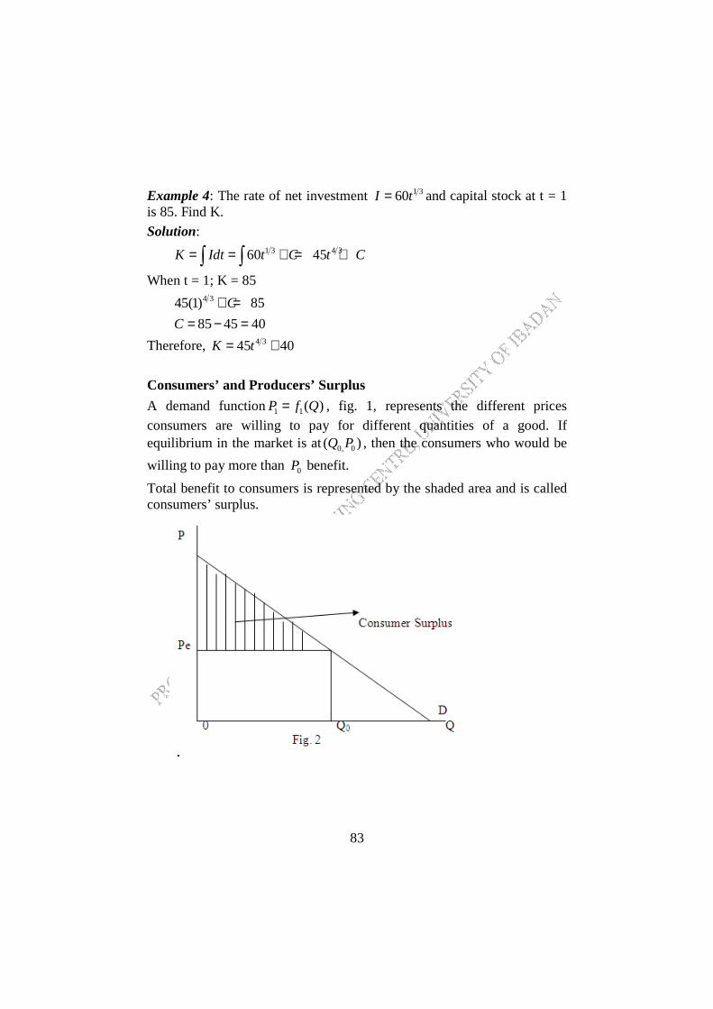
83

Example 4: The rate of net investment 1 360I t= and capital stock at t = 1 is 85. Find K. Solution:

1 3 4 360 45K Idt t C t C= = + = +∫ ∫

When t = 1; K = 85

4 345(1) 85

85 45 40

C

C

+ == − =

Therefore, 4 345 40K t= +

Consumers’ and Producers’ Surplus

A demand function1 1( )P f Q= , fig. 1, represents the different prices

consumers are willing to pay for different quantities of a good. If equilibrium in the market is at 0, 0( )Q P , then the consumers who would be

willing to pay more than 0P benefit.

Total benefit to consumers is represented by the shaded area and is called consumers’ surplus.

84

Mathematically,

Consumers’ surplus0

1 0 00( )

Qf Q dQ Q P= −∫

A supply function 2 2( )P f Q= , fig, 2, represents the different prices at

which quantities of a good will be supplied. If market equilibrium occurs at 0, 0( )Q P , the producers who would supply at a lower price than 0P

benefit.

Total gain to producers is called producers’ surplus and is designated by the shaded area.

Mathematically,

Producers’ surplus0

0 0 20( )

QQ P f Q dQ= − ∫

Example: Given the demand function 242 5P Q Q= − − , assuming that the equilibrium price is 6. What is the consumer surplus?

85

Solution:

At 0 6P = , the demand function becomes

2

2

42 5 6

36 5 0

( 9)( 4) 0

9, 4

Q Q

Q Q

Q Q

Q Q

− − =− − =+ − + =

= − =

Negative quantity is not feasible, so we neglect – 9.

So 0 4Q =

Consumer surplus4 2

0(42 5 ) 4(6)Q Q dQ= − − −∫

42 3

0

542 24

2 3

282 3

Q QQ

− − −

=

Practice Exercise 1. Solve the following

a. 23 5x x dx+∫

b. 2

1

2 5

xdx

x x

++ +∫

c. 5 4 3 4 4 3 2(6 4 2 5) (15 8 3 )x x x x x x dx+ + + + +∫

d. 2

3

3 2

2 1

xdx

x x

+ + + ∫

2. Find an expression for total cost (TC) if the fixed cost (FC) and marginal cost (MC) are 92 and 23 28 84Q Q− + respectively.

3. If the marginal revenue is given by 120 8MR Q= − , find an expression for total revenue.

4. Integrate the following functions for x varying between 0 and 2

a. 1 36x

b. 318 3 4x x− +

86

5. Determine the total cost function given that fixed cost is 125 and the marginal cost 25 22 56MC Q Q= − +

6. Given 1 2( ) 9I t t= , find the level of capital formation

a. in 8 years [0,8]

b. from fourth year through eight year [4,8]

7. A polynomial which can be written as ( 1)( 1)( 2) 3Q Q Q P+ + − − = is given as the demand function. Calculate the consumer supply if the equilibrium price 0 3P =

8. If the marginal propensity to consume (MPS) is given as 1 2'( ) 0.3 0.1S Y Y−= − and if the aggregate savings is nil when 81Y = . Find the savings function S(Y).

9. Suppose that the net investment flow is described by the equation 1 2( ) 3I t t= and that the initial capital stock at time t = 0 is K (0), what

is the time path of capital K.