IAEA-TECDOC-261

IAEA SAFEGUARDSTECHNICAL MANUAL

PART FSTATISTICAL CONCEPTS AND TECHNIQUES

VOLUME 3

A TECHNICAL DOCUMENT ISSUED BY THEINTERNATIONAL ATOMIC ENERGY AGENCY, VIENNA, 1982

The IAEA does not normally maintain stocks of reports in this series.However, microfiche copies of these reports can be obtained from

INIS ClearinghouseInternational Atomic Energy AgencyWagramerstrasse 5P.O. Box 100A-1400 Vienna, Austria

Orders should be accompanied by prepayment of Austrian Schillings 100,in the form of a cheque or in the form of IAEA microfiche service couponswhich may be ordered separately from the INIS Clearinghouse.

ACKNOWLEDGEMENT

Appreciation is extended to J. L. Jaech, Exxon Nuclear, USA, andR. Avenhaus, Hochschule der Bundeswehr München, Neubiberg, FRG, for theirextensive efforts and collaboration to produce this improved volume ofPart F, Statistical Concepts and Techniques.

Appreciation is also extended to Erlinda Go and Jere Bracey, IAEA, fortheir efforts in editing and correcting the draft and to Virgilio Castillo,IAEA, and Charlotte Jennings, Exxon Nuclear, USA, for the very difficulttask of typing and correcting the manuscript.

IAEA SAFEGUARDS TECHNICAL MANUALPART F: STATISTICAL CONCEPTS AND TECHNIQUES, VOLUME 3

IAEA, VIENNA, 1982

Printed by the IAEA in AustriaMarch 1982

CONTENTS

Chapter

1. INTRODUCTION2. MEASUREMENT ERRORS

2.1 Definition of Errors2.2 Sources of Error

2.2.1 Statistical Sampling Error2.2.2 Bulk Measurement Error2.2.3 Material Sampling Error2.2.4 Analytical Measurement Error2.2.5 Other Errors2.2.6 Statistical Sampling Distributions

2.3 Error Models2.3.1 Additive Model2.3.2 Other Models

2.4 Kinds of Errors2.4.1 Random Errors2.4.2 Systematic Errors; Biases2.4.3 Short-term Systematic Errors

2.5 Effects of Errors2.5.1 Effect on Facility MUF2.5.2 Effect on Inspector-Operator Comparisons

2.6 Error Estimation2.6.1 Measurement of Standards

2.6.1.1 Single Standard2.6.1.2 Several Standards2.6.1.3 Measurement at Different Times

2.6.2 Calibration of Measurement Systems2 . 6 . 2 ,2 .6 .2 ,2 .6 .2 ,

. 6 .2 ,

.6 .2 ,2 . 6 . 2 ,2 .6 .2 ,

2.2.

2 . 6 . 2 ,2.6.2,

1 Linear Cal ibra t ion ; Constant Var iance2 Linear Cal ibra t ion; Non-Constant Variance3 Single Point Calibration4 SAM-2 Calibration for Percent U-2355 Several Calibration Data Sets; Linear Model6 Linear Calibration; Cumulative Model7 Several Calibration Data Sets;

Cumulative Model8 Nonlinear Calibration9 Nonlinear Calibration; Several Data

Calibration Data Sets

Page

1-23-10233-744-555-666-77-98-99

10-1410-1111-1212-1414-1614-1515-1616-100

1717-1920-2425-28

29-57

29-3535-3939-4141-4444-4747-50

50-5252-55

56-57

2.6.3 Measurements of Non-Standard Materials 57-782.6.3.1 Replicate Measurements; Analysis of Variance 58-592.6.3.2 Duplicate Measurements; Paired Differences 59-612.6.3.3 Grubbs' Analysis; Two Measurement Methods 61-672.6.3.4 Grubbs' Analysis; More than Two Measurement

Methods with Constant Relative Bias 67-722.6.3.5 More than Two Measurement Methods with

Non-Constant Relative Bias 72-752.6.3.6 Combining Parameter Estimates from

Different Experiments 75-782.6.4 Error Estimation in the Presence of Rounding Errors 78-792.6.5 Inter!aboratory Test Data 79-100

2.6.5.1 Single Standard Reference Material 79-862.6.5.2 Several Samples; Non-Standard Materials 86-902.6.5.3 Laboratory-Dependent Random Error 902.6.5.4 Distribution of Inspection Samples toSeveral Laboratories 91-100

2.7 References 101-102

3. ERROR PROPAGATION 103-1783.1 Definition of Error Propagation 1033.2 Error Propagation; Additive Model 104-1063.3 General Error Propagation; Taylor's Series 106-1093.4 Calculation of Variance of MUF

3.4.1 Definition of MUF 109-1103.4.2 Direct Application of Error Propagation Formulas 110-1123.4.3 Variance of Element MUF by General Approach 112-130

112-114114-115115-119119-128128130

130-138

131-134134-138

3.4.6 Effects of Other Factors on MUF and its Variance 138-1393.5 Calculation of Variance of D. the Difference Statistic 139-168

3.5.1 Definition of, D 140-1413.5.2 Variance of D by Direct Application of

Error Propagation Formulas 141-1453.5.3 Variance of D by General Approach 145-160

3.4.43.4.5

3.4.3.13.4.3.23.4.3.33.4.3.43.4.3.5VarianceVariance3.4.5.13.4.5.2

AssumptionsNotationRandom Error Variance of MUFSystematic Error Variance of MUFCase of Constant Absolute Errorsof Cumulative MUFof Isotope MUF by General ApproachVariance of Isotope MUF Due to MeasurementErrors in Bulk and Element Measurements

Variance of Isotope MUF Due to Errors inIsotope Measurements

3.5.3.1 Assumptions 1453.5.3.2 Notation , 1463.5.3.3 Random Error Variance of D A 146-1503.5.3.4 Systematic Error Variance of D 150-160

3.5.4 Variance of D for Isotope 160-1683.6 The (MUF-D) Statistic 168-175

3.6.1 Application of (MUF-D) 168-1693.6.2 Variance of (MUF-D) 169-174

3.7 References 175-176Annex 3.1 177-178

4. DESIGN INSPECTION PLANS 179-2524.1 Purpose of Inspection 179-1824.2 Inspection Activities 182-184

4.2.1 Attributes Inspection Activities 182-1844.2.2 Variables Inspection Activities 184-185

4.3. Criteria for Inspection Plan Design 184-1894.3.1 Attributes Inspection Criteria 185-1864.3.2 Variables Inspection Criteria 186

4.3.2.1 Criteria for Variables Inspectionin Attributes Mode 186-187

4.3.2.2 Criteria for Variables Inspectionin Variables Mode, Using D~ 187-188

4.3.2.3 Criteria for Variables Inspectionin Variables Mode, Using (MUF-D) 188-189

4.4. Selection of Inspection Sample Sizes 189-2124.4.1 Attributes of Inspection Sample Sizes 189-196

4.4.1.1 Attributes Inspection Sample Sizein Given Stratum 189-191

4.4.1.2 Attributes Inspection Sample SizesOver All Strata 192-193

4.4.1.3 Game Theoretic Results 194-1864.4.2 Var iables Inspection Sample Size 196-198

4.4.2.1 Variables Inspection Sample Size --Attributes Mode 196-198

4.4 .2 .2 Variables Inspection Sample Size--Variables Mode 198-213

4.5 Evaluat ion of Inspection P l a n — I n d i v i d u a l Tests 213-228

4.5.1 Dist inct ion Between Pr inc ipa l and Supplemental Tests 213-2144.5.2 Attributes.Inspection Tests 214-216

4.5.3 Tests on J3,, and Shipper/Receiver Difference Tests 216-2194.5.4 Test on D ^ 219-2224.5.5 Test on MUF A 222-2244.5.6 Test on (MUF-D) 224-228

4.6 Overall Probability of Detection of Goal Amount 228-2314.6.1 Attributes and (MUF-D) Tests 228-2314.6.2 Attributes, tf, and MUF Tests 231-240

4.7 References 241Annex 4.1 (a) 1/0 versus M/a 242Annex 4.1 (b) " " " 243Annex 4.2 (a) A Function For Computing Bivariate Normal 244ProbabilitiesAnnex 4.2 (b) " " " " " 245Annex 4.2 (c) " " " " " 246Annex 4.2 (d) " " " " " 247Annex 4.3 (a) " " " " " 248Annex 4.3 (b) " " " " " 249Annex 4.3 c) " " " " " 250Annex 4.3 (d) " " " " " 251Annex 4.4 Qptional Values for Significance Levels in

D and MUF Tests 252

5. IMPLEMENTING INSPECTION PLANS 253-3085.1 Cn-Site Activities 253-271

5.1.1 Drawing a Random Sample 2535.1.1.1 Random Number Table 253-2555.1.1.2 Pocket Calculator 255-2575.1.1.3 Computer 257-258

5.1.2 Attributes Inspection Defect Criteria 258-268

5.1.2.1 Effects of Mistakes (Defects) on MUF 258-2625.1.2.2 Large Defects--Attributes Tester 263-2655.1.2.3 Medium Defects—Variables Tester 265-268

5.1.3 Confidence Interval for Defects 268-2715.1.3.1 Numbers of Defects 268-271

5.2 Post-Inspection Activit ies 272-294

5.2.1 Supplemental Tests of Hypotheses 272-285

5.2.1.1 Normality Tests 272-2765.2.1.2 Randomness Tests 276-2815.2.1.3 Variance Tests 281-2835.2.1.4 Tests on D, and on Shipper/Receiver

Differences 283-2855.2.1.5 International Standards of Accountancy 285-286

5.2.2 Principal Tests of hypotheses 286-2905.2.2.1 Test on D 286-2885.2.2.2 Test on MUF 288-2895.2.2.3 Tests on (MUF-D) 289-290

5.2.3 Confidence Intervals on Material Unaccounted For 290-2945.2.3.1 Confidence Interval Based on MUF A 291-2925.2.3.2 Confidence Interval Based on (MUF-D) 293-294

5.3 References 295

Annex 5.1 (a) Random Normal Numbers 296Annex 5.1 (b) " " " 297Annex 5.1 (c) " " " 298Annex 5.1 (d) " " " 299Annex 5.1 (e) " " " 300Annex 5.2 A

n_i+l Coefficients 301Annex 5.3 Critical Values for the W-Test 302Annex 5.4 Percentage Points of the Distribution of

the D1 Test Statistic 303Annex 5.5 (a) Percentiles of the F Distribution 304Annex 5.5 (b) " " " " " 305Annex 5.5 (c) " " " " " 306Annex 5.6 Percentiles of the x2 Distribution 307Annex 5.7 Critical Values for Tests on 0. , D,

MUF and (MUF-D) 308Annex 5.8 Values of t , for Confidence Intervals

on MUF a/ 308

6. CURRENT DEVELOPMENT IN ACCOUNTING FOR NUCLEAR MATERIALS 309-3166.1 Introduction Ä 3096.2 Alternative to D, MUF Test 309-3106.3 Random Error Variance Inflation Factor 310-3116.4 Analysis of Successive MUF'S 311-3126.5 Overall Effectiveness of Agency Safeguards^Containment, Surveillance, and Materials Accountancy 312-3136.6 Statistical Methods for Analysis of Interlaboratory

Test Data 313-3146.7 Calibration Models 3146.8 Effects of Mistakes (Defects) on MUF 3146.9 Error Estimation-Paired Differences 314-3156.10 References 316-317

- l -Chapter 1

INTRODUCTION

Part F of the Safeguards Technical Manual is being issued in three volumes.Volume 1 was published in 1977 and revised slightly in 1979. Volume 1 discussesbasic probability concepts, statistical inference, models and measurement errors,estimation of measurement variances, and calibration. These topics of generalinterest in a number of application areas, are presented with examples drawn fromnuclear materials safeguards. The final two chapters in Volume 1 deal with problemareas unique to safeguards: calculating the variance of MUF and of D respectively.

Volume 2 continues where Volume 1 left off with a presentation of topicsof specific interest to Agency safeguards. These topics include inspectionplanning from a design and effectiveness evaluation viewpoint, on-facility siteinspection activities, variables data analysis as applied to inspection data,preparation of inspection reports with respect to statistical aspects of theinspection, and the distribution of inspection samples to more than one analyticallaboratory.

Volumes 1 and 2 are written in a simplified mode with little provided in theway of statistical bases for the computational procedures set forth in somewhatof a cookbook manner. The volumes indicate how to deal with specific problemswith step-by-step computational procedures, but create little understanding of theprocedures themselves, their attendant assumptions and possible limitations inapplications. Further, the volumes are characterized by a lack of cohesivenessor unity of purpose, consisting of a number of rather isolated procedures withlittle in the way of a unified development of the statistical applications toAgency safeguards.

Because of these shortcomings in Volumes 1 and 2, the need for preparationof a Volume 3 was identified. Volume 3 covers generally the same material asVolumes 1 and 2 but with much greater unity and cohesiveness. Further, the cook-book style of the previous two volumes has been replaced by one that makes use ofequations and formulas as opposed to computational steps, and that also providesthe bases for the statistical procedures discussed. Hopefully, this will helpminimize the frequency of misapplications of the techniques.

Volume 3 stands alone in the sense that Volumes 1 and 2 need not be readbefore Volume 3; many examples are common to the volumes but are worked from a dif-ferent perspective. Having studied Volumes 1 and 2 prior to Volume 3, however,may be helpful in reaching a quicker understanding of the Volume 3 material. Further,a greater appreciation for the material in the first two volumes should follow fromstudying Volume 3 which is intended to provide the motivation for the statisticalprocedures covered in the two volumes. Volume 3, of course, also contains morerecently developed statistical techniques not present in the earlier volumes.

The 13 chapters of Volumes 1 and 2 have been rearranged and replaced byfour chapters in this Volume, identified as Chapters 2-5., Chapter 2 discusses

1-1

- 2 -

measurement errors in considerable detail {the table of contents is given at thestart of each chapter). Chapter 3 is concerned with all aspects of error propaga-tion as it relates to safeguards. Chapters 4 and 5 deal with Agency inspections,first from the design viewpoint, and then with respect to their implementation.The final chapter, Chapter 6, identifies and discusses current developments inthe statistical aspects of safeguards, in anticipation of the need to reviseVolume 3 periodically to keep the material contained therein current.

Volumes 1 and 2 each contain a glossary of terms. This glossary is omittedin Volume 3 because of the rather exhaustive discussion of measurement errors inChapter 2. This lengthy discussion effectively replaces the glossary which mustbe viewed as a limited attempt to summarize a lot of ideas about measurement errorswith a few definitions; which is difficult to do effectively. Hence, the need forthe full discussion of these ideas in Chapter 2.

Volumes 1 and 2 are somewhat deficient in the completeness of their biblio-graphies. In Volume 3, a more complete bibliography is included. However, onlythose works actually cited in Volume 3 are listed in the bibliography. Thisshould not detract from ones ability to perform additional background researchin a given topic, however, since the cited articles themselves often contain crossreferences to other relevant work. Further, in safeguards applications, one canlocate most articles of interest in a limited number of places. These include pri-marily the Institute of Nuclear Materials Management (INMM) Journals and AnnualMeeting Proceedings, IAEA Conference Proceedings and related Agency reports, andProceedings of the recently instituted meetings of the European Safeguards Researchand Development Association (ESARDA). Further, in the INMM journals, complete list-ings are often given of available publications issued at a given facility. Thus,it is a simple matter to locate most articles pertinent to a given topic.

1-2

- 3 -

Chapter 2

MEASUREMENT ERRORS

2.1 DEFINITION OF ERRORSMaterial balance accounting is an integral part of Agency safeguards.

It relies heavily on measured data, which are subject to error. The inferencesthat are drawn on the basis of accounting data are, as a result, drawn in thepresence of errors, and are hence stated in the language of statistics.

This chapter, Chapter 2 of Volume 3, Part F, is concerned with measure-ment errors, including error sources, error models, kinds of errors, effectsof errors, and estimation of errors. Later chapters deal with the effects oferrors in drawing inferences on facility performance, based both on the facility'saccounting data, and also on the inspection data.

As a starting point in the discussion, it is important to define whatis meant by the word, error.

ANSI Standard N15.5[2.l] provides the following definition:Error of a Measurement—The magnitude and the sign of the difference

between the measured value and the true value.This definition is an attractive one in the context of this Volume since

it speaks of a measured value as opposed to a reported or recorded value. Theimportant distinction is that the measured value is the value that would applyto the measurement in question were there no mistakes in recording or reportingthe value. The basic assumption behind drawing inferences on the basis ofaccounting data is that the data are free of mistakes, or defects as they willbe called in later chapters. Steps are taken to provide some degree of assur-ance that this is, in fact, a reasonable assumption. However, whatever may bethe concern on the presence of such defects in the data, it is important tokeep in mind that the inferences to be drawn on the basis of the measured, quan-titative data are based on the definition of an error of measurement given here.

By a simple extension of the definition, a mistake may be said to haveoccurred if a reported value differs by any amount from a measured value. Asynonym for a measured value is an observed value, and these two expressionswill be used interchangeably throughout this volume.

2.2 SOURCES OF ERRORThe definition of error given in Section 2.1 is a bit simplistic in that

it implies a very simple error structure. In fact, most errors of measurementare not simply structured, and a given error of measurement often represents thecombined net effect of many errors.

l-l

- 4 -

In this section, a discussion is given of the various sources of errorthat might affect a given measurement. The narrative discussion of this sectionis followed by a parallel mathematical model presentation in later sections.

2.2.1 Statistical Sampling ErrorConsider a population of individual items, each of which has a true value

of some specified characteristic associated with it. If one of these items isselected in some random fashion, then the true value associated with that itemwill differ from some nominal or base true value (e.g., the average of all truevalues over all population items) by some amount. Define a statistical samplingerror as the difference: true value for randomly selected item minus base truevalue.

In many Agency safeguards applications, statistical sampling error neednot be included when making inferences. This is because: (1) the facility it-self will measure 100% of the items involved in the material balance; and (2) theinspection data are analyzed as by-difference data in which the operator's valueis compared with the inspector's value for each item in question, the true valueof the item in question thus not affecting this difference. That is, the statis-tical sampling error for the difference is zero.

The following points must, however, be kept in mind. (1) Each item maynot have a unique measured value of the characteristic in question associatedwith it, although it will surely have a unique true value of that characteris-tic. The effect of this is discussed in 2.2.3.

(2) Suppose the facility does not have measured values for its items sothat there is no item by item comparison of the operator's data with that of theinspector. In this event, it is necessary to make inferences about the operator'smaterial balance solely on the basis of the inspector's data for the sampleditems. Statistical sampling error must then be included, for the result foundin inspection clearly depends on which sub-group of items are selected andmeasured. This could prove to be a major source of error in some situations.

(3) In the event of attributes inspection of the go, no-go type, the truevalue associated with each item is conventionally either 1, corresponding to adefect, or 0, corresponding to a non-defect. The nominal or base value for thepopulation in question is a fraction or proportion, equal to the true total num-ber of defects divided by the total number of items. Thus, there is a statis-tical sampling error committed as each item is selected. The effect of thiserror on the inferences drawn about the population will disappear only if allitems in the population are included in the sample.

2.2.2 Bulk Measurement ErrorMaterial accountancy is based on three measurement operations: (1) deter-mination of the net weight or volume of an item (bulk measurement); (2) sampling

of the material; (3) analysis of the sampled material for element and/or isotopeconcentration. In the event of NDA measurement, the bulk measurement and the

2-2

- 5 -

sampling of the material are not performed ('unless a density correction is appliedon the basis of the weight or unless the NDA measurement is made on a sample ofmaterial rather than on the whole item).

It is convenient to divide the total error of a measurement into componentparts, the parts corresponding to these three basic measurement operations. Thebulk measurement error is defined as the magnitude and sign of the differencebetween an item true weight (or volume) and its measured or observed weight. Withthis definition, it is implied that the error is a single quantity, and as far asits effect is concerned, it is possible to regard it as such. However, in actuality,the bulk measurement error may be, and quite likely will be, the net effect of manyerrors associated with the bulk measurement, some of which may tend to cancel oneanother in their effect. See the further discussion in 2.2.5 and 2.4.

2.2.3 Material Sampling ErrorMaterial sampling error is defined with respect to the characteristic be-

ing measured. This may be uranium concentration, U-235 concentration, plutoniumconcentration, etc.

Material sampling error is the magnitude and sign of the difference betweenthe true value of the characteristic in question for the sampled material andthe corresponding true value for the totality of material represented by thesample. It is important to keep in mind just what is this totality of material.To illustrate, if the characteristic in question is uranium concentration, and ifthe concentration is to be uniquely determined for a given container, then thesampling error is the difference between the uranium concentration for the (pre-sumably) small sample drawn from the container, and the average concentration inthat container. This may be called the "within-container sampling error." On theother hand, if a sample is drawn from a given container with the concentrationto be applied to other nominally like containers, then the variability in concen-tration from one container to another is included in the sampling error, alongwith the variability within containers.

In this latter context, it is noted that material sampling error is closelyrelated to statistical sampling error for that part of the error that occursbecause of differences in concentration from item to item. Some prefer to notmake a distinction between statistical and material sampling errors. Others findit convenient to do so; it is largely a matter of personal preference, but itseems convenient in the context of material accountancy to make that distinction.This is because when concentrations are uniquely determined for different con-tainers (or groups of containers), and the value in question is the differencebetween the inspector's and the operator's measured concentrations, the statis-tical sampling error, as defined here, has no effect. On the other hand, therewill still be a material sampling error, assuming that both parties did notanalyze the same sample of material.

2.2.4 Analytical Measurement ErrorAs with material sampling error, analytical error is defined with respect

to a specified characteristic. Analytical error is the magnitude and sign of the

2-3

- 6 -

difference between the true value of the characteristic for the sampled materialand the corresponding measured or observed value. Note that this error isdefined with respect to the material sampled, and not to the totality of materialto be characterized by that sample. It is, of course, the combined effects ofsampling and analytical that is important.

In the event of measurement by NDA rather than by the bulk measurement-sampling-analytical route, then the error in the NDA measurement may for conven-ience be labeled an analytical error (although, as pointed out in Section 2.2.2,sampling error will also be introduced if the NDA measurement is performed on asample of material rather than on the entire item).

2.2.5 Other ErrorsAs was indicated in 2.2.2, a given identified error is actually the net

effect of potentially many errors. For example, in the weighing operation, theerror in weighing could be the combined effect of how the item was positionedon the scale, the scale type, the particular scale of that type, the operator,and the environment (temperature, humidity) to name a few obvious potentialsources of error. The extent to which specific error sources are identifiedand studied individually depends on the circumstances. For example, if theweighing error for the operation in question has little impact on the qualityof the accountancy data, then there is little need to identify each sourcethat contributes to the error. On the other hand, if the observed weights atthe measurement point in question are judged to have larger than desirableerrors of measurement, studies might well be initiated to ascertain why. Inconducting these studies, at least some of the potential individual measurementerror sources would be identified and evaluated as to their individual effects.

Regardless of the degree to which the error structure is decomposed intoindividual sources, in the accountancy applications to be discussed in thisvolume, the principal breakdown of errors will be limited to bulk measurement,material sampling, and analytical errors, always keeping in mind the more complexunderlying error structure.

2.2.6 Statistical Sampling DistributionsEach time a measurement of some kind is made, there is a corresponding

measurement error associated with the observed or measured value. Obviously,one does not know the value of the error; if it were known, then the observedvalue could be "corrected" for the known error, leaving the true value.

Although one may not know the particular error involved in a givenmeasurement, one must know something about the possible magnitude of the errorso that some statement can be made about the true value in question. The infor-mation about the error is conveyed through its known (or estimated) probabilitydistribution. Specifically, one might have knowledge that an error, say e, isdistributed according to the normal distribution with zero mean and variance*i-

As has been indicated before, a given measured value is affected by manyerrors of measurement. By appropriately propagating errors (this topic to be

2-4

- 7 -

covered in Chapter 3), and by applying results from mathematical statisticstheory, one can describe in some defined way the effect of the combined errorson the measured value. Carrying this one step further, one can find similarresults for specified functions of a number of measured values. The specifiedfunctions of interest in safeguards applications are, for example, MUF, totalinventory, operator minus inspector value, etc.

Given any measured value or any specified function of measured values(called a statistic) a goal in statistical inference is to make probabilitystatements about some parameter on the basis of the observed or measured data.To do this, one must know the probability density function of the statistic inquestion. The probability density function enables one to compute a probabilityof occurrence for each possible set of outcomes of the statistic. The functionin question can be derived from statistical theory given a set of input assump-tions. The resulting function is often referred to as a sampling distribution.(In statistical theory, there is a distinction between a density function anda distribution function, the latter being the integral of the former. Morecorrectly, the statistical function in question should be called a samplingdensity function.)

The foregoing discussion is pertinent to the discussion on errors becausea sampling distribution provides for probability statements about the size ofthe error that might have been committed in a given application. For example,an important statistic in safeguards applications is the material unaccountedfor (MUF). Each time a MUF is calculated, an error is made because the calculatedMUF will differ from the true MUF by some amount due to all the errors of mea-surement that were unavoidably committed when calculating the MUF. Thus, giventhe sampling distribution of the MUF statistic, one can make inferences aboutthe true MUF on the basis of the calculated MUF, for even though the size andsign of the error is not known, one does have knowledge of how it behaves ina probabilistic sense. Precisely how this knowledge is derived is the subjectof the next chapter.

2.3 ERROR MODELSIn the foregoing discussion, it is indicated that there are many potential

sources of error that might affect an observed result. In Section 2.4 to follow,it will be shown that these errors do not all behave in the same way. Althoughone is interested ultimately in the net effect of all errors of different kindsas they jointly affect a result, it is often helpful, and sometimes essential,to write down an appropriate mathematical model to identify the errors and howthey relate to one another. There are several reasons for doing this:

(1) Writing the model aids in propagating the errors, i.e., in findingthe net effect of the errors acting jointly.(2) It identifies which are the important sources of error so that cor-

rective steps can be taken if necessary and possible.(3) It helps to insure that potentially important errors are not over-looked.

2-5

- 8 -

(4) It leads one "to question the assumptions inherent in the model, andthus leads to more realistic models.

On this latter point, it should be understood that a model is a mathematicaldescription of reality. When faced with the choice, one of course prefers simplemodels, even if they may depart a bit from reality. The model builder has animportant task: to write the model that provides an adequate description of reality;and, at the same time to derive a model that is not too difficult to use. Properattention must be devoted to model-building because the model may impact heavilyon the results of the analysis. This very important point is sometimes overlooked.

In the next two sections, two kinds of models are considered: the additivemodel and non-additive model.

2.3.1 Additive ModelThe additive model is the simplest model with which to work, and is also

one which often provides a close approximation to reality. It is the basis formany common statistical techniques, such as the analysis of variance, and iswidely employed in practice.

A very simple additive model isx = y + e (eq. 2.3.1)

where, for example,x = observed gross weight of can of U0? powder, in gramsu = true gross weight of cane = the error

The additive nature of the model is clear. The error, e, selected insome as yet unspecified way, is simply added to the true weight to give theobserved weight. Of course, one only has knowledge of x, and not y or e. Onthe basis of the observed x and some knowledge about the probability distributionfor e, one can make inferences about the size of y (i.e., assign a value to ualong with some probability statement.) In another context, one might know y (e.g.,assigned value of a standard) and observe x, and use this information to makeinferences about e.

This simple additive model can be extended to include additional terms.For example, suppose that a difference between scales exists. Then, letting

0. = error for scale ithe previous model might be written

X1 = y + 91 + e (eq. 2.3.2)As this model is written, if e. were, say, 3 grams, then the model would

indicate that items weighed on this scale would consistently read high by 3 grams,not counting the additional error, e, associated with any given reading.

2-6

- 9 -

The additive model is considered further in Section 2.4.

2.3.2 Other ModelsAlthough the additive model provides an adequate description of reality in

many instances, this is not always the case. As a very simple example, even thoughindividual errors may be described by additive models, it does not follow that astatistic of interest will have an additive model. To illustrate, keeping in mind(eq. 2.3.1,)(but letting the weights be net weights rather than gross weights), let

y = a + n (eq. 2.3.3)where y = observed ratio of uranium to UCL

a = true ration = the error

Suppose now that one is interested in the observed net weight of uranium,and not U02- The model for this is found by multiplying each side of (eq. 2.3.1)by each siae of (eq. 2.3.3)

xy = ya + yn + ae + er\ (eq. 2.3.4)which is no longer a simple additive model.

As an extension of this, suppose that the model for the uranium to UO^ ratiois not additive as in (eq. 2.3.3), but is rather of the multiplicative form:

y = an (eq. 2.3.5)as would be the case if the error, n, were expressed as a multiplier, e.g., n =1.01 would represent a 1% relative error. Then, the model for the net weight ofuranium is, from (eq. 2.3.1) and (eq. 2.3.5),

xy = yan + ean (eq. 2.3.6)which is another non-additive model that might apply.

To summarize, although additive models are often adequate, it does notfollow that they apply in all situations. One must be aware of the model beforeerrors can be appropriately propagated and inferences drawn.

As a final comment, non-additive models may at times be appropriatelytransformed to result in additive models. For example, upon using logarithms,(eq. 2.3.5) may be written

Iny = Ina + lnr\ (ecl- 2.3.7)which is now additive in the logarithms.

When errors are propagated in Chapter 3, the model will be kept in mind, ifnot explicitly written in each instance.

2-7

- 10 -

2.4 KINDS OF ERRORSIt has already been noted that there are potentially many sources of error

that might affect a given measured value. It is also important to note that notall error sources will behave the same way in their effects. This fact is especiallyimportant in safeguards applications, as will be noted time and time again in futurechapters.

There are three broad categories or kinds of errors that will be identified.These are random errors, systematic errors or biases, and errors that fall inneither category, which are usually called short-term systematic errors in safe-guards applications. The different kinds of errors are perhaps best understoodin the context of an example. The example will be developed further in each ofthe next three sections until the three basic kinds of errors will have been dis-cussed, along with variations on them.

2.4. 1 Random ErrorsThe example to be developed is as follows. Six sintered U0? pellets of

nominally the same composition are to be analyzed for percent uranium. Letx-j = measured percent uranium for pellet ip = nominal (or true) percent uranium

p- = deviation from the nominal value for pellet iEJ = deviation due to analytical for measurement j

For simplicity in exposition, an additive model is assumed. (The dis-tinction to be made among the kinds of errors is independent of this assumption.)The model representing the six measured values may be written:

= y

P6 + £6

(eq. 2.4.1)

Consider pj. Since this differs for each of the six observations in thedata set, pi is called a random error. Further, with reference to the discussionin Section 2.2.1, pi is a statistical sampling random error. If pj is regarded asa random variable with zero mean and with variance a^,theno^ is called the statis-tical sampling random error variance. Note the important distinction between pjand 02; p-j is an error while a^ is an error variance.

Consider ej. Since this also differs for each of the observations in thedata set, ej is also a random error. More specifically, with reference to Section2.2.4, ej is an analytical random error and, analagous with c^, the quantity a|is called the analytical random error variance.

2-8

- 11 -It is noted from (eq. 2.4.1) that since p and e have the same subscripts

for all six observations, it is not possible to distinguish between the samplingand analytical errors. One might wish to combine them in the model, replacing(p + e1) by mlS etc. The quantity m might then be called the measurementrandom error, and a^ the measurement random error variance.

With respect to this last point, it is recognized by modelers that thereare many potential sources of error that affect a given result, some identifiedand others not. It is common practice to group effects in a model especially whenthe effects cannot be distinguished, as in this model. If, say, duplicate analyseswere performed on each pellet, then p-j and EJ would not be combined; their effectsare then distinguishable.

The characteristic feature of a random error in a model is that its sub-script changes for each observation in the data set. The safeguards significanceof random errors is that their effect on measurement uncertainty can be reducedin a relative sense by making additional measurements. A random error is saidto propagate to zero in a relative sense with an increasing number of measurements.For this reason, random errors are controllable and, given sufficient resources,can be made to have little importance in many safeguards applications.

2.4.2 Systematic Errors; BiasesThe model (eq. 2.4.1) is extended. Let

A = deviation from the nominal due to the analytical method, forall measurements in the data set

Then write

X = y + A + p + e1 1 1

X = y + A + p + e2 2 2

X = y + A + p +e3 3 3

(eq. 2.4.2)

X = y + A + p + s4 4 k

X = y + A + p + eb 5 5

X = y + A + p + eG 6 6

2-9

- 12 -

Note that A differs from p-j and ej in that there is no subscript (or,equivalent!,/, the subscript may be the same for all members of the data set).The quantity A is called a systematic error or a bias, terms which are oftenused interchangeably. Some users make a distinction between these two termsin the situation where the quantity A is estimated in some way. The distinctionmade is that if observations in the data set are corrected on the basis of theestimate of A, then A is called a bias. However, since one cannot know A pre-cisely, but can only estimate it, it is clear that the observations cannot becompletely corrected for the bias A. There is a residual bias, consisting ofthe difference between A and its estimate, and this residual bias is then calleda systematic error. This distinction between bias and systematic error is notmade by all modelers. The important idea to keep in mind is that whatever theA quantity is called, the assumptions concerning A must be stated or implied sothat errors can be properly propagated corresponding to the assumed model.

In modeling, the distinction between the systematic error and the randomerror is that the subscript on the systematic error is the same for all membersof the data set (or, equivalently, there is no subscript). If A is a randomvariable with zero mean and variance a|, then a^ is called a systematic errorvariance. As a random variable, A is selected at random from some populationjust as was the random error, pi or z-\, the distinction being that, once selected,A is the same for all members of the data set.

In many safeguards applications, the effect of the systematic error is ofdominant importance when compared with that of the random error. This is because,unlike the random error, the effect or impact of the systematic error cannot bereduced by taking additional measurements. The systematic error, as will be seenin later chapters, limits the effectiveness of safeguards from the material account-ing point of view, unless steps can be taken to reduce its effect in some way.Merely making more measurements will not help.

2.4.3 Short-term Systematic ErrorsThe model (eq. 2.4.2) is further extended. Suppose that the six pellets

are not all distributed to the same laboratory for analysis. LetA, = deviation from the nominal due to the analysis being performed

in laboratory kAlso suppose that within laboratory k, conditions change from one time-frame

(day, shift, week, etc.) to the next so thatt /.\ = deviation from the nominal due to the analysis being performed in

( ' time frame m within laboratory kNote that in the case of O^, the subscript is written to indicate that

the "time" effect is peculiar to a given laboratory. That is, time frame 1 inlaboratory 1 does not correspond to time frame 1 in laboratory 2, say.

With £|< and tm(|<) defined, suppose that the model now becomes

2-10

- 13 -

X = y + A + A + t / % + p + e1 1 l ( l ) 1 1

X = y + A + £ + t + p +e2 1 l ( l ) 2 2

X = y + A + £ + t , ^ + p + e3 1 id) 3 3

(eq. 2 .4.3)X = y + A + £ + t , + p +e

4 2 1(2) 4 it

X =y + A + J l + t . + p + £5 2 2 (2 ) 5 5

X = y + A + £ + t + p + e6 2 3 (2) 6 6

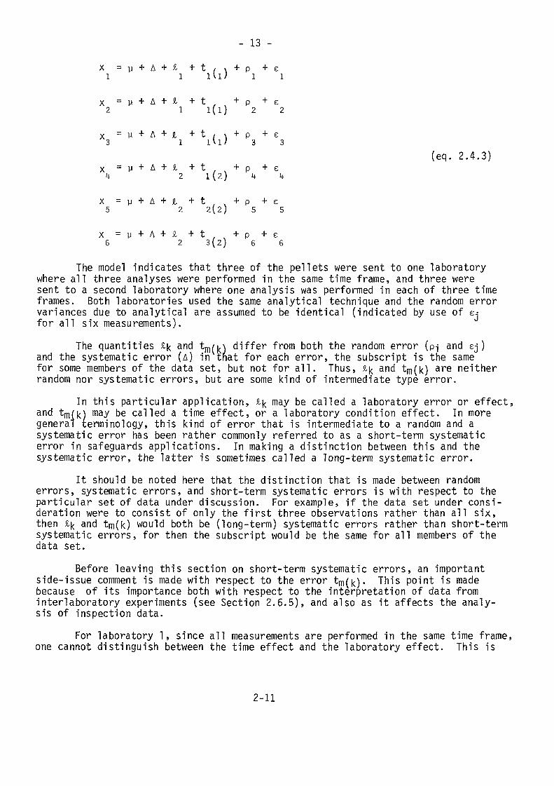
The model Indicates that three of the pellets were sent to one laboratorywhere all three analyses were performed in the same time frame, and three weresent to a second laboratory where one analysis was performed in each of three timeframes. Both laboratories used the same analytical technique and the random errorvariances due to analytical are assumed to be identical (indicated by use of e,-for all six measurements).

The quantities % and tm/^\ differ from both the random error (p-j and ej )and the systematic error (A) in that for each error, the subscript is the samefor some members of the data set, but not for all. Thus, % and tm(|<) are neitherrandom nor systematic errors, but are some kind of intermediate type error.

In this particular application, % may be called a laboratory error or effect,and tm(|<) may be called a time effect, or a laboratory condition effect. In moregeneral terminology, this kind of error that is intermediate to a random and asystematic error has been rather commonly referred to as a short-term systematicerror in safeguards applications. In making a distinction between this and thesystematic error, the latter is sometimes called a long-term systematic error.

It should be noted here that the distinction that is made between randomerrors, systematic errors, and short-term systematic errors is with respect to theparticular set of data under discussion. For example, if the data set under consi-deration were to consist of only the first three observations rather than all six,then % and tm(k) would both be (long-term) systematic errors rather than short-termsystematic errors, for then the subscript would be the same for all members of thedata set.

Before leaving this section on short-term systematic errors, an importantside-issue comment is made with respect to the error tm(|<). This point is madebecause of its importance both with respect to the interpretation of data frominterlaboratory experiments (see Section 2.6.5), and also as it affects the analy-sis of inspection data.

For laboratory 1, since all measurements are performed in the same time frame,one cannot distinguish between the time effect and the laboratory effect. This is

2-11

- 14 -

an important point because one professed aim of inter!aboratory experiments is toremove the effects of differences between laboratories by correcting all resultsto some base value, that is, by obtaining estimates of the %'s and correcting forthe laboratory effects. However, this approach does not recognize the importanceof the time effect, tm(k) which is usually confounded with or indistinguishablefrom the laboratory effect &L,. Thus, when one attempts to remove laboratorybiases in this way, the results are only applicable to the given time frame thatexisted at the time of the interlaboratory experiment. The between-time variance,cr£, may well be a dominant effect when compared with o|, in which case it would bemisleading to conclude that one can correct for differences between laboratories.Rather, in most instances, one would use interlaboratory data to obtain the com-bined estimate, a| + a|, which becomes a systematic error variance, long term,when applied only to a given laboratory, and short term otherwise. In this instance,one usually calls this simply a between laboratory variance, it being understoodthat the time effect is implicitly included in that variance component. Notethat for laboratory 2, the measurements are made at three different times, but thismay not be the usual mode in inter-laboratory experiments.

2.5 EFFECTS OF ERRORSMuch of this Volume deals with the effects of errors on quantities of safe-

guards importance in a very detailed way. The discussion in this section antici-pates the more detailed presentations to follow in later chapters, and is intendedto provide an overview of the role played by errors of measurement. First, theeffect of errors on facility MUF is discussed, and then the effect on operatorand inspector comparisons is considered.

2.5.1 Effect on Facility MUFA given facility reports a MUF at the end of each material balance period,

i.e., upon completion of a physical inventory. The MUF is affected by errors ofmeasurement. It is also affected by unmeasured inventories, unmeasured loss streams,and mistakes in the recording, transmittal, and reporting of data. It wouldalso be affected, of course, by any thefts or diversions. As a first step in theevaluation of the facility MUF, only the effect of measurement errors is takeninto account. That is, one wants to make probability statements about the trueMUF on the basis of the observed MUF and its calculated standard deviation due toerrors of measurement. The true MUF, which includes the effects of all factorsother than the errors of measurement, may then be further evaluated, but thisfurther evaluation may be largely non-statistical in nature.

Associated with each MUF is an actual standard deviation describing itsuncertainty. There is also a calculated or reported standard deviation. It ishighly unlikely that these agree exactly, although the extent to which they dis-agree may be difficult to characterize. The disagreement comes about because ofone or more of a number of reasons:

(1) The actual input measurement error variances will not be the same astheir estimated values used in the error propagation.

2-12

- 15 -

(2) There are approximations used in the error propagation.(3) The errors may be improperly propagated, even though the approximate

nature of the propagation may not lead to a serious discrepancy. Im-proper propagation could occur because of a large number of reasons.Some common ones being:(a) Treating constant element or isotope factors as having no

associated error(b) Failing to account for items that are identically a part of

two cancelling components of the MUF calculation (e.g., inreceipts and ending inventories)

(c) Making arithmetic mistakesWhile keeping in mind that the calculated standard deviation of MUF is not

the actual standard deviation (a quantity that will not be known), neverthelessthe calculated standard deviation is used in making judgements about the signi-ficance of the MUF. The inspector need not proceed on blind faith and acceptthe facility's calculated MUF. Experience with similar plants provides guide-lines as to what is a reasonable value for the standard deviation. Any largedifferences between calculated and guideline values can be investigated as tocause, and the calculated value appropriately corrected if found to be in error.

Assuming that the calculated standard deviation of MUF is a reasonablycorrect value, a diagnostic look at the calculations will reveal what are themajor sources of error. An identification can then be made of possible steps thatmight be taken to reduce its size. On the other hand, study may also reveal thatexcessive measurement effort is being made in some instances; measurement effortmay well be better directed elsewhere. In short, it is worthwhile to go beyondthe simple calculation of the standard deviation of MUF, and use the calculationsto redirect measurement effort as judged desirable.

This diagnostic look may well reveal that the standard deviation of MUFis limited in size by systematic errors. Unfortunately, it is not a simplematter to obtain estimates of systematic error variances in all cases, nor is itpossible to reduce their effects without extensive effort, if at all. (It isfaulty reasoning to suppose that extensive system recalibrations will eliminatesystematic errors, although it is a step in the right direction.) One conclusionthat might follow is that too much effort in the facility measurement controlprogram is being directed at obtaining current estimates of random error varianceswhose effects on the standard deviation of MUF may be negligible in a relativesense. This information, if put to use, may be quite important to a facility bur-dened by measurements made solely for safeguards purposes. The facility and theinspectorate can jointly benefit by careful study of the calculations affectingthe standard deviation of MUF.

2.5.2 Effect on Inspector-Operator ComparisonsOne principal aim of an Agency inspection is to make a quantitative verifi-

cation of the facility MUF. This verification makes use of the ß statistic, treated

2-13

- 16 -

in detail in the next chapter, but which for present purposes is defined as simplythe estimate of the difference between the facility MUF and the inspector's esti-mate of this quantity. It is based on paired comparisons between the operator'sand inspector's measured values on an item-by-item basis.

As with MUF, the quantity D is affected by errors of measurement. ^UnlikeMUF, which is affected only by facility measurements, the uncertainty in D is alsoaffected by uncertainties in inspector measurements. Also, whereas the standarddeviation of MUF is often limited in size by systematic errors, this may notnecessarily be the case with D because much fewer measurements are made by theinspector than by the facility. Further, only those facility measurements thatare involved in the inspector comparisons affect the standard deviation of D, sothat the contribution to the random error variance of D due to the facility mea-surements will be relatively much larger than their contribution to the varianceof MUF.

As will be seen in Chapter 4, the random error variances will determine howmany measurements the inspector will make and how he will allocate these amongthe various flow and inventory items. Thus, for purposes of inspection, it j_s_necessary to have good estimates of the inspector's and the facility's randomerror variances.

It may be true in some applications that systematic error variances forthe operator and/or the inspector are of such a size that the inspection samplesizes are limited in the sense that further measurements beyond a minimum numberwill have negligible effect on the variance of D. In this limiting case, if thesystematic error variances for the facility and for the inspector are roughlyequivalent in size, then the variance of D is twice the variance of MUF.

Another statistic of importance in Agency inspections is the so-called(MUF-Ô) statistic, which is interpreted as the facility MUF adjusted for biaseson the basis of the inspection data. An attractive property of (MUF-Ô) is thatit is unaffected by the operator's systematic errors. In a sense, it is thefacility MUF with the operator's systematic errors replaced by the inspector's.The advantage is obvious: the inspector should be better able to evaluate andcontrol his systematic errors than he can the operator's. This (MUF-D) statisticwill also be studied in detail in later chapters.

2.6 ERROR ESTIMATIONIt should be apparent from the preceding sections that it is important to

have valid information about measurement error variances. This information cancome from a potentially large number of sources. In the balance of this chapter,methods will be given for obtaining estimates of the various measurement parameters,The techniques given are not intended to include all possible means of estimatingmeasurement error variances, but do include those most often applied.

There are five main sub-topics: Measurements of Standards, Calibration ofMeasurement Systems, Measurements of Non-standard Materials, Error Estimation inthe Presence of Rounding Errors, and Inter!aboratory Test Data.

2-14

- 17 -

2.6.1 Measurements of StandardsA physical standard is an item having an assigned value associated with

it for the characteristic in question. The value may be known without error, orit may have an error associated with it. In Section 2.6.1.1, the case of a singlestandard is considered. In 2.6.1.2, several physical standards are involved. In2.6.1.3, measurements are made on a standard distributed over time.

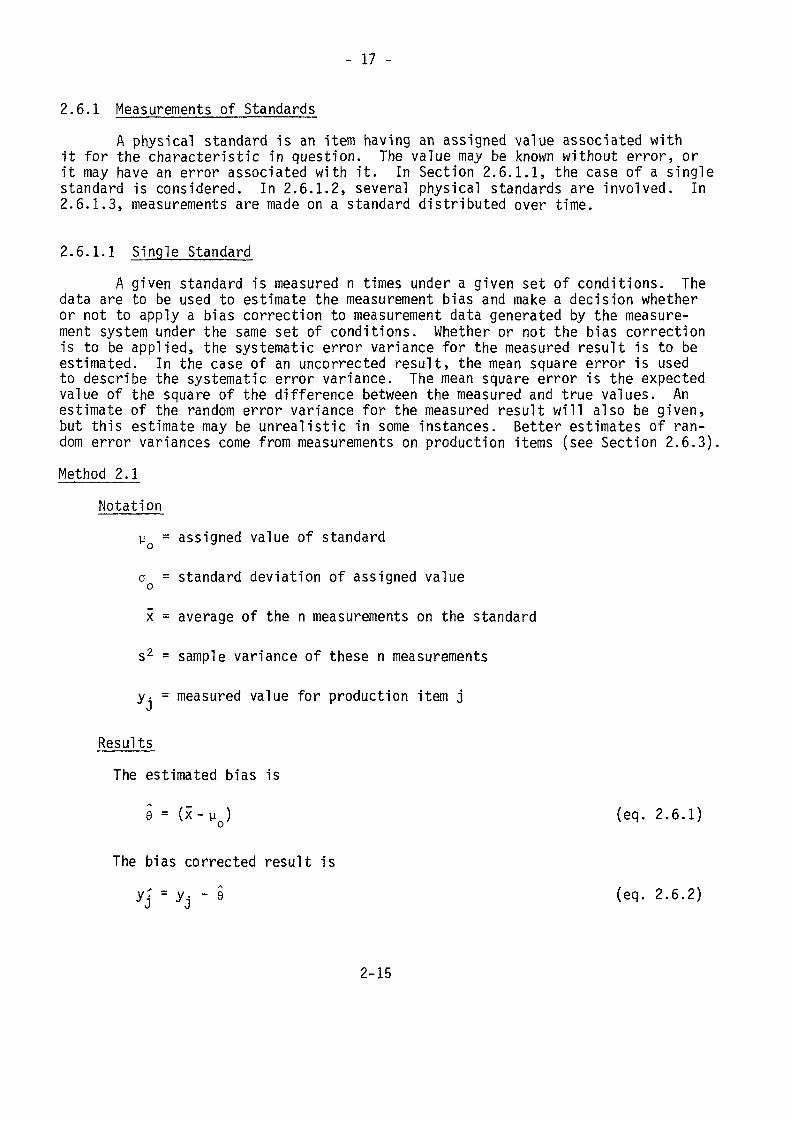
2.6.1.1 Single StandardA given standard is measured n times under a given set of conditions. The

data are to be used to estimate the measurement bias and make a decision whetheror not to apply a bias correction to measurement data generated by the measure-ment system under the same set of conditions. Whether or not the bias correctionis to be applied, the systematic error variance for the measured result is to beestimated. In the case of an uncorrected result, the mean square error is usedto describe the systematic error variance. The mean square error is the expectedvalue of the square of the difference between the measured and true values. Anestimate of the random error variance for the measured result will also be given,but this estimate may be unrealistic in some instances. Better estimates of ran-dom error variances come from measurements on production items (see Section 2.6.3).Method 2.1

Notationuo = assigned value of standard

o = standard deviation of assigned value

x = average of the n measurements on the standard

s2 = sample variance of these n measurements

y. = measured value for production item jU

ResultsThe estimated bias is

8 = (x- y ) (eq. 2.6.1)

The bias corrected result isy- = y. - ê (eq. 2.6.2)

2-15

- 18 -

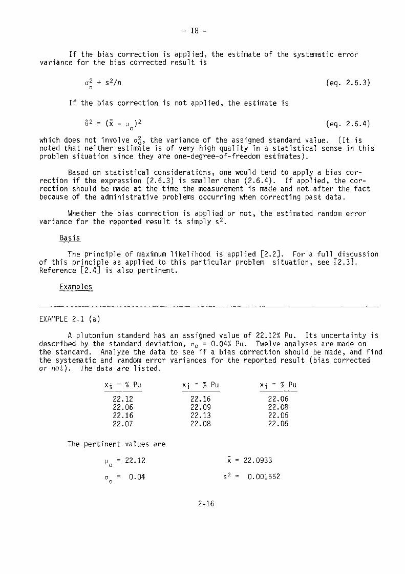
If the bias correction is applied, the estimate of the systematic errorvariance for the bias corrected result is

a2 + s2/n (eq. 2.6.3)

If the bias correction is not applied, the estimate is

e2 = (x - y )2 (eq. 2.6.4)which does not involve a2, the variance of the assigned standard value.noted that neither estimate is of very high quality in a statisticalproblem situation since they are one-degree-of-freedom estimates).

(It issense in this

Based on statistical considerations, one would tend to apply a bias cor-rection if the expression (2.6.3) is smaller than (2.6.4). If applied, the cor-rection should be made at the time the measurement is made and not after the factbecause of the administrative problems occurring when correcting past data.

Whether the bias correction is applied or not, the estimated random errorvariance for the reported result is simply s2.

BasisThe principle of maximum likelihood is applied [2.2]. For a full discussion

of this principle as applied to this particular problem situation, see [2.3].Reference [2.4] is also pertinent.

Examples

EXAMPLE 2.1 (a)A plutonium standard has an assigned value of 22.12% Pu. Its uncertainty is

described by the standard deviation, o0 = 0.04% Pu. Twelve analyses are made onthe standard. Analyze the data to see if a bias correction should be made, and findthe systematic and random error variances for the reported result (bias correctedor not). The data are listed.

Pu22.1222.0622.1622.07

x-j = % Pu22.1622.0922.1322.08

Pu22.0622.0822.0522.06

The pertinent values areyo = 22.12a = 0.04o

x = 22.0933s2 = 0.001552

2-16

- 19 -

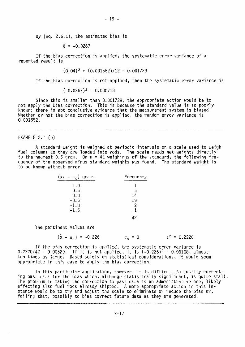
By (eq. 2.6.1), the estimated bias isê = -0.0267

If the bias correction is applied, the systematic error variance of areported result is

(0.04)2 + (0.001552)/12 = 0.001729If the bias correction is not applied, then the systematic error variance is

(-0.0267)2 = 0.000713Since this is smaller than 0.001729, the appropriate action would be to

not apply the bias correction. This is because the standard value is so poorlyknown; there is not conclusive evidence that the measurement system is biased.Whether or not the bias correction is applied, the random error variance is0.001552.

EXAMPLE 2.1 (b)A standard weight is weighed at periodic intervals on a scale used to weigh

fuel columns as they are loaded into rods. The scale reads net weights directlyto the nearest 0.5 gram. On n = 42 weighings of the standard, the following fre-quency of the observed minus standard weights was found. The standard weight isto be known without error.

grams1.00.50.00.51.01.5

The pertinent values are(x - y0) = -0.226

Frequency1514192

42

a0 = 0 s2 = 0.2220If the bias correction is applied, the systematic error variance is

0.2220/42 = 0.00529. If it is not applied, it is (-0.226)2 = 0.05108, almostten times as large. Based solely on statistical considerations, it would seemappropriate in this case to apply the bias correction.

In this particular application, however, it is difficult to justify correct-ing past data for the bias which, although statistically significant, is quite smallThe problem in making the correction to past data is an administrative one, likelyaffecting also fuel rods already shipped. A more appropriate action in this in-stance would be to try and adjust the scale to eliminate or reduce the bias or,failing that, possibly to bias correct future data as they are generated.

2-17

- 20 -

2.6.1.2 Several StandardsThere are two general types of situations in which more than one standard

may be measured. In the first type of application, a given scale is to be usedto measure gross and tare weights to determine the net weight for an item. Thebias in the scale is to be evaluated at both the gross and tare weight ranges inorder to estimate the bias for a reported net weight. In the second situation,more than one physical standard is measured but it is assumed that any bias isconstant over the range covered by the standards. The standards may have dif-ferent associated uncertainties, and they may be measured different numbers oftimes. The problem is to estimate the overall bias and to find the random andsystematic error variances of the reported result on a production item, whetheror not it is corrected for bias.

In what follows, Method 2.2 applies to the first situation and Method 2.3to the second.Method 2.2

Notationyq = assigned value of gross weight standardyj. = assigned value of tare weight standardeu = standard deviation of assigned gross weight standard valuea, = standard deviation of assigned tare weight standard valuex = average of n measurements on gross weight standardx. = average of n, measurements on tare weight standards2 = sample variance of the n measurementsy Ds2 = sample variance of the n. measurementsy. = measured net weight for item jÜ

ResultsThe estimated bias in the net weight is

ê = (x - v ) - (xt - ut) (eq. 2.6.5)The bias- corrected result is

y' = y. - ê (eq. 2.6.6)J ü

If the bias correction is applied, the estimate of the systematic errorvariance for the bias corrected result is

2-18

- 21 -

ag + öt + sg/ng + st/nt (eq' 2'6'7)

If the bias correction is not applied, the estimate is simply e2, from(eq. 2.6.5).

Based on statistical considerations, one would tend to apply a bias cor-rection if the expression (2.6.7) is smaller than e2. If applied, the correctionshould be made at the time the measurement is made, and not after the fact.

Whether the bias correction is applied or not, the random error variancefor the reported result is

s2 + s2 (eq. 2.6.8)

BasisThe basis is the same as for Method 2.1 with a simple extension to include

both the gross and tare weight standards.Examples

EXAMPLE 2.2 (a)A case history dealing with the estimation of scale accuracy and precision

is given in reference [2.5]. Suppose that standards S and P in that reference andweighed in combination correspond to a typical gross weight while standard B isthe tare weight standard. From the reference, the following information is derived,

yg = 8878.0 g ; ut = 1591.7 g ; °g = at = °'97 g

Assume that weighings of these standards yield the following data:n =30 nt = 20

x = 8881.3 g xt = 1589.9 g

sg = 6.2 g st = 4.9 g

The estimated bias in the net weight is§ = 3.3 + 1.8 = 5.1 g

If the bias correction is applied, the systematic error variance of the biascorrected result is2(0.97)2 + (6.2)2/30 + (4.9)2/20 = 4.36 g2

2-19

_ 22 -

If the bias correction is not applied, this variance is(5.I)2 = 26.01 g2

In this example, since 4.36 <26.01, one would apply the bias correction onthe basis of statistical considerations alone, assuming that scale adjustmentscould not reduce the bias to a more acceptable lower value.

Method 2.3Notation

m = number of standardsn. = number of measurements on standard ky. = assigned value for standard kak = standard deviation of assigned value, standard kx, = average of the measurements on standard ks2. = sample variance of these measurements

ResultsThe estimated bias is the weighted average

m , mê = Z w

k(xk-yk)/£ wk (eq. 2.6.9)k=l / k=l

whereW|< = (a2 + s2/nk)'1 (eq. 2.6.10)

and where s2 is the estimated random error variance,m

s2 = S (nk - 1) s2/(n-m) (eq. 2.6.11)k=l

n being the total number of observations,m

n - 5] nk (eq. 2.6.12)k=l

2-20

- 23 -

If the bias correction is applied, the estimate of the systematic errorvariance for the bias corrected result is

m -iI Y. w.\ (eq. 2.6.13)\ /\k=l /

If the bias correction is not applied, the estimate is simply e2, from(eq. 2.6.9).

As with Methods 2.1 and^2.2, one would tend to correct for bias if expres-sion (2.6.13) is smaller than e2.

BasisThe estimate of the bias is a weighted estimate where the weights are the

inverses of the variances of the estimated biases for each condition. This is astandard weighting procedure and leads to the result that the variance of theweighted average is the reciprocal of the summed weights [2.6].Examples

EXAMPLE 2.3 (a)Three standards are used in controlling the measurement quality of a mass

spectrometer. The standard values in percent U-235 are 2.013, 3.009, and 4.949respectively. The observations on these standards are as follows:

Standard 1 Standard 2 Standard 32.013 3.009 4.9532.018 3.013 4.9572.015 3.010 4.9492.015 3.017 4.9462.013 3.0092.010 3.008

3.0133.0103.0113.006

Assume that errors are constant on a relative basis. From Section 2.3.2,then, it is appropriate to transform the data to natural logarithms. The standardvalues in this transformed scale become:

y = In 2.013 = 0.69963 ; y - 1.10161 ; y = 1.59919l 2 3The errors in the standards are each 0.05% relative at one standard deviation.

a = a = a = 0.0005i 2 3

2-21

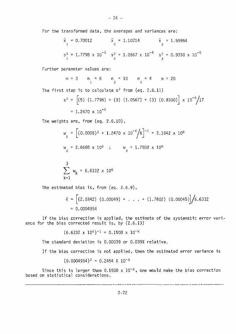
- 24 -

For the transformed data, the averages and variances are:x = 0.70012 x = 1.10214 x = 1.599641 2 3

s2 = 1.7798 x 10"5 s2 = 1.0567 x 10~6 s2 = 0.9330 x 10~6

Further parameter values are:m = 3 n = 6 n = 10 n = 4 n = 20

1 2 3

The first step is to calculate s2 from (eq. 2.6.11)s2 = [(5) (1.7798) + (9) (1.0567) + (3) (0.9300)1 x 10~6/17

- 1.2470 x 10"6

The weights are, from (eq. 2.6.10),

w = [(0.0005)2 + 1.2470 x IQ~&/6\~1 = 2.1842 x 1061 L / J

w = 2.6688 x 106 ; w = 1.7802 x 1052 3

wk = 6.6332 x 106k=l

The estimated bias is, from (eq. 2.6.9),

0 = [(2.1842) (0.00049) + . . . + (1.7802) (0.00045)1/6.6332= 0.0004954

If the bias correction is app l i ed , the estimate of the systematic error va r i -ance for the bias corrected result is, by (2.6.13)

(6.6332 x 105)-1 = 0.1508 x 10~6

The standard deviation is 0.00039 or 0.039% relative.If the bias correction is not applied, then the estimated error variance is

(0.0004954)2 = 0.2454 X 10~6

Since this is larger than 0.1508 x 10~6, one would make the bias correctionbased on statistical considerations.

2-22

- 25 -

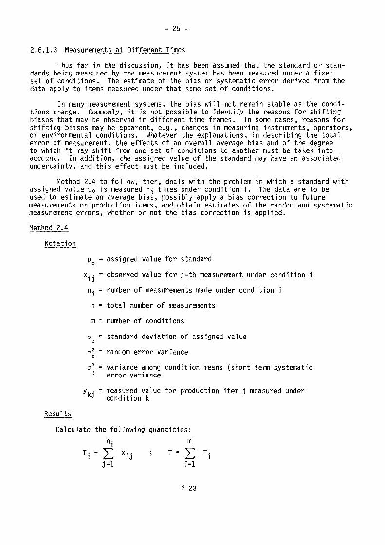
2.6.1.3 Measurements at Different TimesThus far in the discussion, it has been assumed that the standard or stan-

dards being measured by the measurement system has been measured under a fixedset of conditions. The estimate of the bias or systematic error derived from thedata apply to items measured under that same set of conditions.

In many measurement systems, the bias will not remain stable as the condi-tions change. Commonly, it is not possible to identify the reasons for shiftingbiases that may be observed in different time frames. In some cases, reasons forshifting biases may be apparent, e.g., changes in measuring instruments, operators,or environmental conditions. Whatever the explanations, in describing the totalerror of measurement, the effects of an overall average bias and of the degreeto which it may shift from one set of conditions to another must be taken intoaccount. In addition, the assigned value of the standard may have an associateduncertainty, and this effect must be included.

Method 2.4 to follow, then, deals with the problem in which a standard withassigned value y0 is measured n-j times under condition i. The data are to beused to estimate an average bias, possibly apply a bias correction to futuremeasurements on production items, and obtain estimates of the random and systematicmeasurement errors, whether or not the bias correction is applied.Method 2.4

Notationy = assigned value for standard0

x.. = observed value for j-th measurement under condition i' J

n. = number of measurements made under condition in = total number of measurementsm = number of conditionsa = standard deviation of assigned valuea2 = random error varianceeo2 = variance among condition means (short term systematic6 error variance

y. . = measured value for production item j measured underJ condition kResults

Calculate the following quantities:m

T, = • Z Ti1=12-23

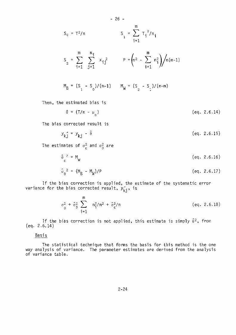
- 26 -m

So = T2/n Si = X V/ni1=1

m n - / m

V Xi/ P = K -1=1 j=l V 1=1

MB = (Si - S

Then, the estimated bias is§ = (T/n - y ) (eq. 2.6.14)

The bias corrected result isykj = ykj - § (eq. 2.6.15)

The estimates of a2 and a2 aree ö

5 2 = M (eq. 2.6.16)e w

oe2 = (MB - MW)/P (eq. 2.6.17)

If the bias correction is applied, the estimate of the systematic errorvariance for the bias corrected result, y^., is

mni/n2 + Se/n (ec)- 2.6.18)

1=1If the bias correction is not applied, this estimate is simply e2, from

(eq. 2.6.14)Basis

The statistical technique that forms the basis for this method is the oneway analysis of variance. The parameter estimates are derived from the analysisof variance table.

2-24

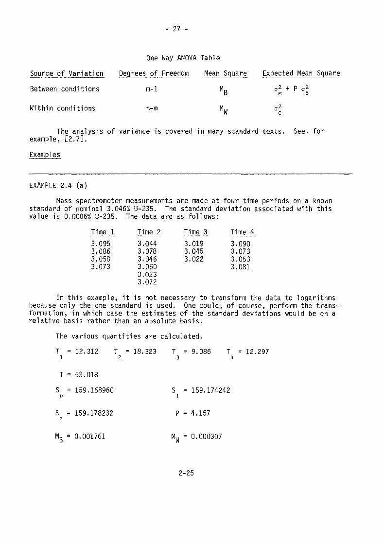
- 27 -

One Way ANOVA TableSource of Variation Degrees of Freedom Mean Square Expected Mean SquareBetween conditions m-1 MD a2 + P a2D e ö

W i t h i n conditions n-m MW a2

The analysis of variance is covered in many standard texts. See, forexample, [2.7].Examples

EXAMPLE 2.4 (a)Mass spectrometer measurements are made at four time periods on a known

standard of nominal 3.046% U-235. The standard deviation associated with thisvalue is 0.0006% U-235. The data are as follows:

Time 1 Time 2 Time 3 Time 43.0953.0863.0583.073

3.0443.0783.0463.0603.0233.072

3.0193.0453.022

3.0903.0733.0533.081

In this example, it is not necessary to transform the data to logarithmsbecause only the one standard is used. One could, of course, perform the trans-formation, in which case the estimates of the standard deviations would be on arelative basis rather than an absolute basis.

The various quantities are calculated.T = 12.312 T = 18.323 T = 9.086 T = 12.2971 2 3 U

T = 52.018S = 159.168960 S = 159.174242o iS = 159.178232 P = 4.1572

MB = 0.001761 Mw = 0.000307

2-25

- 28 -

Then, by (eq. 2.6.14),ê = 0.0139

By (eq. 2.6.16) and (eq. 2.6.17),a 2 = 0.000307 (random error)

a2 = 0.000350 (short term systematic error)uIf the bias correction is applied, the systematic error variance for the

bias corrected result is, by (eq. 2.6.18),(0.0006)2 + (0.000350) (77)/289 + (0.000307)/17 = 0.000112

If the bias correction is not applied, this variance becomes(0.0139)2 = 0.000193

Since 0.000193 exceeds 0.000112, one would tend to correct for bias inthis instance.

EXAMPLE 2.4 (b)In the example just concluded, suppose that the time grouping were ignored.

The data would then be analyzed by Method 2.1. The bias estimate, e is still0.0139. However, the estimate of the systematic error variance would be different.For these data:

s2 = 0.0005795n = 17

Thus, from (eq. 2.6.3), if the bias correction is applied, the estimateof the systematic error variance is

(0.0006)2 + (0.0005795)717 = 0.00003445, compared with 0.000112when the time grouping is taken into account as it should be. If the bias correctionwere not applied, the estimate of the systematic error variance would be the sameas in the preceding example.

This example illustrates the importance of correctly specifying the modelfor the statistical analysis. The existence of the short-term systematic errorin this set of data must be accounted for in the analysis.

2-26

- 29 -

2.6.2 Calibration of Measurement SystemsThe problem of calibration is closely related to that of measuring standards

(Section 2.6.1) in that physical standards are also used in the calibration problem.In calibration, the measured response (Y) is related to the standard value (X) insome functional way, depicted by Y = f(X). The quantities Y and X may not be inthe same units, e.g., X may be in grams U-235 and Y may be in count rates for anNDA counter. The calibration problem involves estimating the parameters for thefunction f(X) so that the relationship may be used to relate an observed responsefor a production item, observed on the Y scale, to an estimated value on the Xscale for that item. Various statements about error variances are also made onthe basis of the calibration data.

Various calibration problems are treated. First the case in which thefunctional relationship is linear and the variance of the measured response isconstant over the range of calibration is covered.

2.6.2.1 Linear Calibration; Constant VarianceThe measured response, Y, is related to the assigned value, X, by a linear

relationship. At any fixed value of X, Y is normally distributed with mean valuegiven by the linear relationship and with unknown but constant variance. Thecalibration data consist of n pairs of observations.

The calibration process leads to obtaining estimates of the parameters(slope, intercept, variance). The estimated calibration equation is then usedfor measuring production items, and random and systematic error variances arederived for the production item characteristic value corresponding to this response.

Two cases are considered. In Method 2.5, it is assumed that the interceptparameter is known. When this known value is zero, a special case, then the cali-bration curve passes through the origin. Method 2.6 covers the case when thevalue for the intercept parameter is not known.Method 2.5

Notation(y-> x.) = i-th data point; i = 1, 2, ..., na = intercept parameter (known)3 = slope parameter (unknown)

y. = a + ß x. , calibration equationa2 = variance of y. at given x^

2-27

- 30 -

ResultsCalculate the following quantities:

s =1

s =it

ny x1=1 "*n

i = l "*

n

ns = E

5 i = 1

Vi

^

nS3 = ,?!

X 2

The parameter estimates are

ß = (S - aS )/S (eq. 2.6.19)2 1 3

(n-1) Ô2 = (S - 2aS + na2) - (S - aS )2/S (eq. 2.6.20)5 k 2 1 3

For a production item, the measured response is yo- The correspondingcharacteristic value for the item is x0, estimated by

x = (y -a)/ß (eq. 2.6.21)o oThe quantity ß, once calculated, behaves as a constant. Thus, the uncertainty

in ß affects xo as a systematic error. Denoting the systematic error variance ofx0 by Vs(x0), it is given by

VS(X0) = (yQ - a)2 V(i)/e"

= xo2V{ß)/ß2 (eq. 2.6.22)

where V(ß) is the variance of ß, given by

V(ß) = S2/S (eq. 2.6.23)

The random error variance of x is denoted by V (x )o r oVjx ) = 52/ß2 (eq. 2.6.24)r o

2-28

- 31 -

Consider k measured responses: y01, y^-, . ...^yg^ and the correspondingvalues calculated byA(eq. 2.6.21) and denoted by xoi, Xo2> . • • • , XQ^. Letting x0tbe the sum of these x0j values, consider the random and systematic error variancesof x0t. These are

Vr(xot) = k aVß2 (eq. 2.6.25)

and vs(^ot) = *ot v )/ 2 (ecl- 2-

Equivalently, if x0 denotes the average value, i.e., xot divided by k,then

Vs(xot) = k2x2 V(ß)/ß2 (eq. 2.6.27)

Equation 2.6.22 may be considered a special case of (eq. 2.6.27) with k=l.

BasisThe estimate given by (eq. 2.6.19) and (eq. 2.6.20) are maximum likelihood

estimates [2.2]. Equivalently, ß is derived from the principle of least squares,i.e., it is the value of ß that minimizes the sum of squares:

Q = E (Y, - a - ßX.)2 (eq. 2.6.28)1 = 1 n n

The expressions for the variances of the quantities of interest are basedon error propagation methods to be discussed in Chapter 3.

Examples

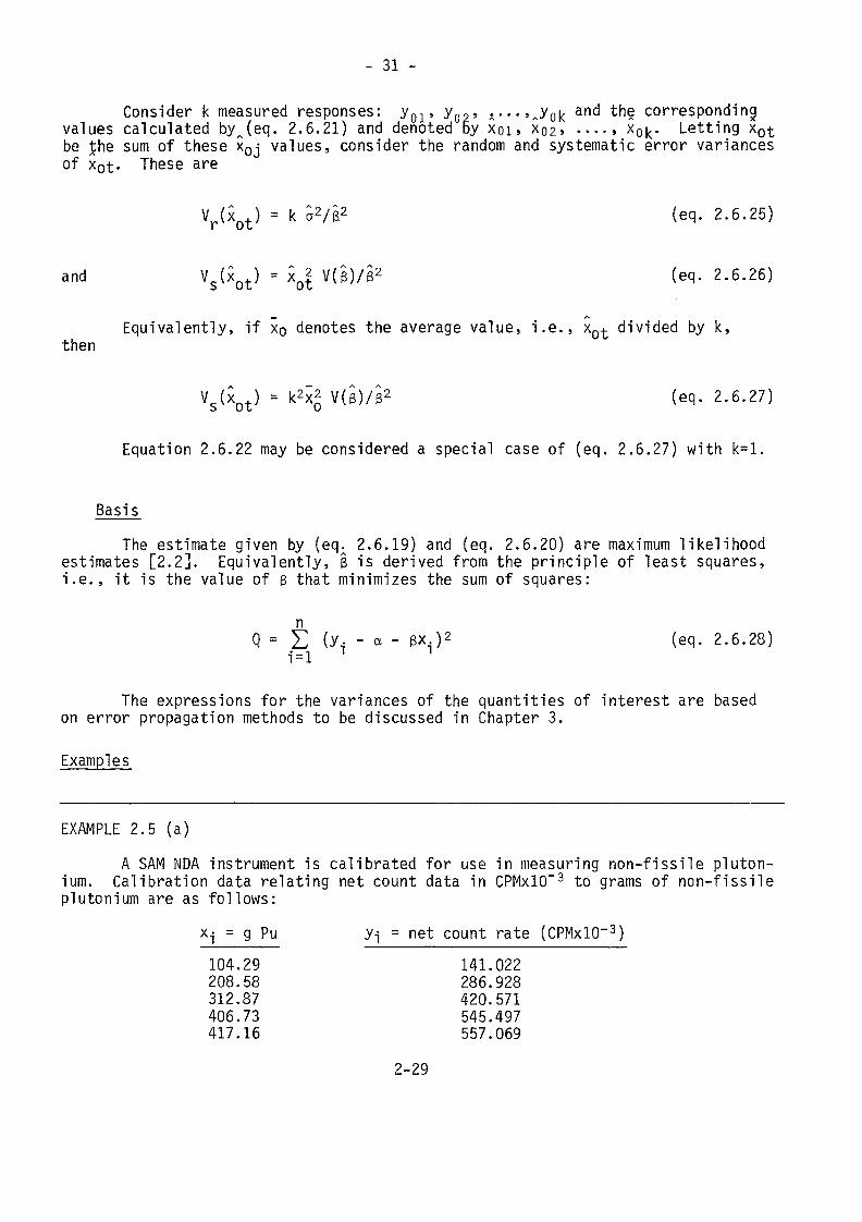
EXAMPLE 2.5 (a)A SAM NDA instrument is calibrated for use in measuring non-fissile pluton-

ium. Calibration data relating net count data in CPMxlO"3 to grams of non-fissileplutonium are as follows:

x.j = g Pu y i = net count rate (CPMxlO'3)104.29 141.022208.58 286.928312.87 420.571406.73 545.497417.16 557.069

2-29

- 32 -

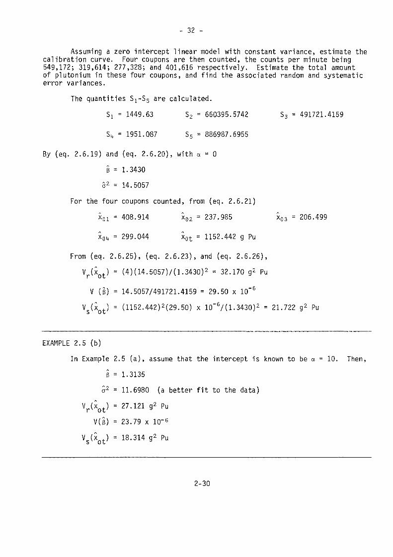
Assuming a zero intercept linear model with constant variance, estimate thecalibration curve. Four coupons are then counted, the counts per minute being549,172; 319,614; 277,328; and 401,616 respectively. Estimate the total amountof plutonium in these four coupons, and find the associated random and systematicerror variances.

The quantities Sj-Ss are calculated.S} = 1449.63 S2 = 660395.5742 S3 = 491721.4159

Su = 1951.087 S5 = 886987.6955

By (eq. 2.6.19) and (eq. 2.6.20), with a = 0§ = 1.3430

Ô2 = 14.5057For the four coupons counted, from (eq. 2.6.21)

X01 = 408.914 X02 = 237.985 X03 = 206.499

xott = 299.044 xot = 1152.442 g Pu

From (eq. 2.6.25), (eq. 2.6.23), and (eq. 2.6.26),Vr(xot) = (4)(14.5057)/(1.3430)2 = 32.170 g2 Pu

V (ß) = 14.5057/491721.4159 = 29.50 x 10"6

V (xn,) = (1152.442)2(29.50) x 10"6/(1.3430)2 = 21.722 g2 PuS U U

EXAMPLE 2.5 (b)In Example 2.5 (a), assume that the intercept is known to be a = 10. Then,

ß = 1.3135a2 = 11.6980 (a better fit to the data)

Vr(xQt) = 27.121 g2 PuV(ß) - 23.79 x 10'6

Vs(xot) = 18.314 g2 Pu

2-30

- 33 -

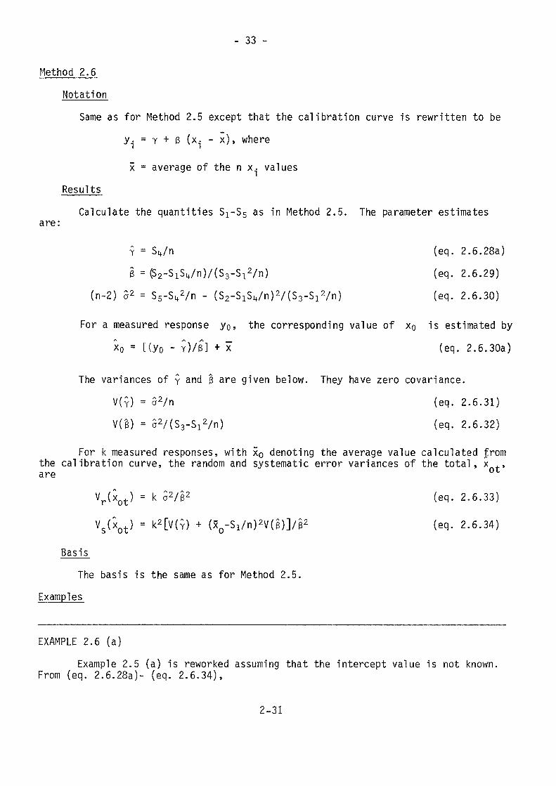
Method 2.6Notation

Same as for Method 2.5 except that the calibration curve is rewritten to bey.,- = Y + 3 (x. - x), wherex = average of the n x. values

ResultsCalculate the quantities S^Ss as in Method 2.5. The parameter estimatesare:

Y = S^/n (eq. 2.6.28a)ß = (S2-S1S4/n)/(S3-S12/n) (eq. 2.6.29)

(n-2) S2 = Sg-S^/n - (S2-S1Slf/n)2/(S3-S12/n) (eq. 2.6.30)

For a measured response YQ, the corresponding value of XQ is estimated byXo = [(YO - Y)/P] + x" (eq. 2.6.30a)

The variances of y and 3 are given below. They have zero covariance.V(Y) = 52/n (eq. 2.6.31)V(|) = 02/(S3-S12/n) (eq. 2.6.32)

For k measured responses, with x0 denoting the average value calculated fromthe calibration curve, the random and systematic error variances of the total, x ,,are OT:

Vr(xot) = k 52/ß2 (eq. 2.6.33)

Vs(xQt) = k2[V(Y) + (xo-S1/n)2V(ß)]/ß2 (eq. 2.6.34)

BasisThe basis is the same as for Method 2.5.

Examples

EXAMPLE 2.6 (a)Example 2.5 (a) is reworked assuming that the intercept value is not known.

From (eq. 2.6.28a)- (eq. 2.6.34),

2-31

- 34 -

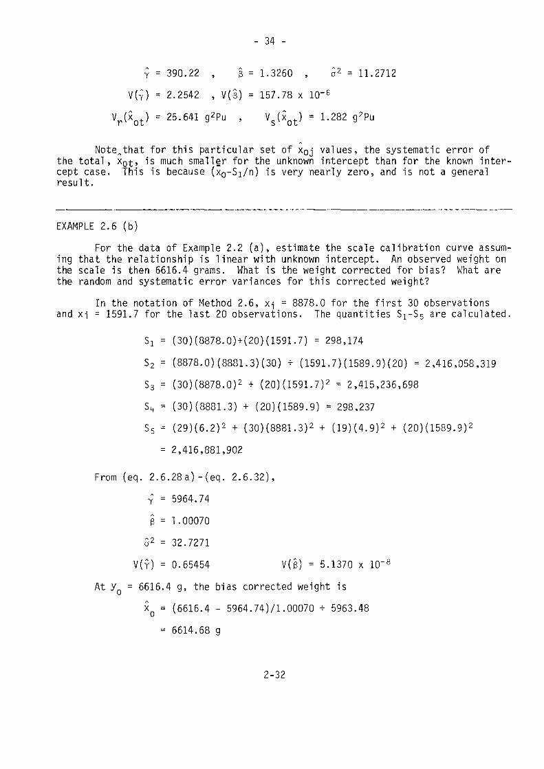
Ç = 390.22 , 3 = 1.3260 , à2 = U. 2712V(Y) = 2.2542 , V(s) = 157.78 x 10~6

(x) = 25.641 g2Pu , V(} = l'282

ANote^that for this particular set of x0j values, the systematic error ofthe total, x0£, is much smaller for the unknown intercept than for the known inter-cept case. This is because (x0-S!/n) is very nearly zero, and is not a generalresult.

EXAMPLE 2.6 (b)For the data of Example 2.2 (a), estimate the scale calibration curve assum-

ing that the relationship is linear with unknown intercept. An observed weight onthe scale is then 6616.4 grams. What is the weight corrected for bias? What arethe random and systematic error variances for this corrected weight?

In the notation of Method 2.6, x-j = 8878.0 for the first 30 observationsand xi = 1591.7 for the last 20 observations. The quantities S!-S5 are calculated.

Sj = (30)(8878.0)+(20)(1591.7) = 298,17452 = (8878.0)(8881.3)(30) + (1591.7)(1589.9)(20) = 2,416,058,31953 = (30)(8878.0)2 + (20)(1591.7)2 - 2,415,236,69854 - (30}(8881.3) + (20)(1589.9) = 298,23755 - (29)(6.2)2 + (30M8881.3)2 + (19)(4.9)2 + (20) (1589.9)2

= 2,416,881,902

From (eq. 2.6.28 a) -(eq. 2.6.32),Y = 5964.74ß = 1.00070

a2 = 32.7271V(Y) = 0.65454 V(ß) = 5.1370 x 10'8

At y = 6616.4 g, the bias corrected weight isXQ = (6616.4 - 5964.74)71.00070 + 5963.48

= 6614.68 g

2-32

- 35 -

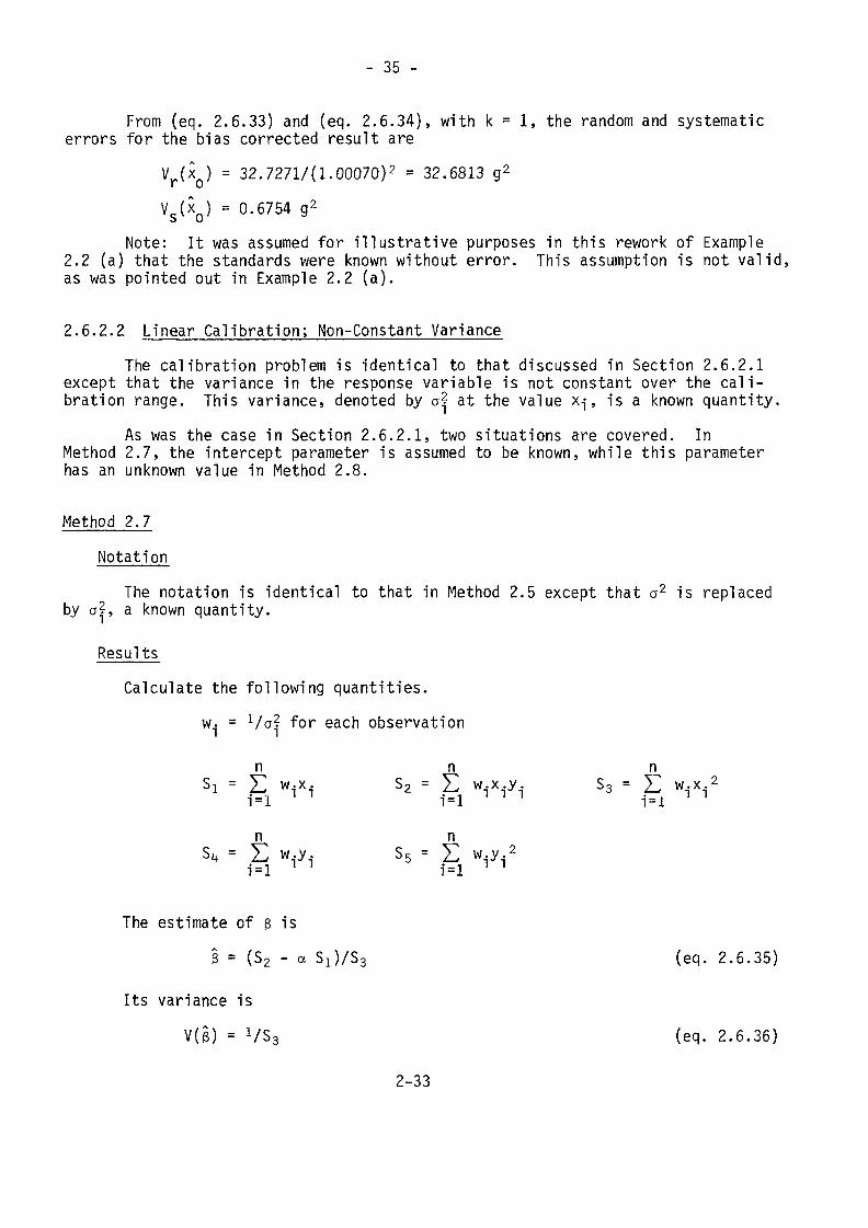
From (eq. 2.6.33) and (eq. 2.6.34), with k = 1, the random and systematicerrors for the bias corrected result are

Vr(x ) = 32.7271/(1.00070)2 = 32.6813 g2

Vs(xQ) = 0.6754 g2

Note: It was assumed for illustrative purposes in this rework of Example2.2 (a) that the standards were known without error. This assumption is not valid,as was pointed out in Example 2.2 (a).

2.6.2.2 Linear Calibration; Non-Constant VarianceThe calibration problem is identical to that discussed in Section 2.6.2.1

except that the variance in the response variable is not constant over the cali-bration range. This variance, denoted by a? at the value x-j, is a known quantity.

As was the case in Section 2.6.2.1, two situations are covered. InMethod 2.7, the intercept parameter is assumed to be known, while this parameterhas an unknown value in Method 2.8.

Method 2.7Notation

The notation is identical to that in Method 2.5 except that a2 is replacedby a?, a known quantity.

ResultsCalculate the following quantities.

w. = VCT? for each observation

n n nS - V w.x. s2 = Ü w-x.y . S3 = Y\ w.x.2

n nS, = V w y Sc = V w v 2°4 L-i wi-M °5 L-i w •,••/•;

i=l 1 1 1=1 1 1

The estimate of ß is

0 = (S2 - a Sj/Sa (eq. 2.6.35)

Its variance is

V ( ß ) = VS3 (eq. 2.6.36)

2-33

- 36 -

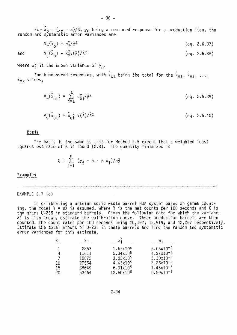
For x0 = {y0 - a)/ß, y0 being a measured response for a production item, therandom and systematic error variances are

Vr(xo) =and VS(XQ) = xSv(ê)/ê

(eq. 2.6.37)(eq. 2.6.38)

where a2 is the known variance of y .For k measured responses, with xot being the total for the x01, x02, ...,values,

Vr(xot) = (eq. 2.6.39)

Vs(xot) = X (eq. 2.6.40)

BasisThe basis is the same as that for Method 2.5 except that a weighted least

squares estimate of ß is found (2.8). The quantity minimized isnQ = IL1=1 - « - x,)/a2

Examples

EXAMPLE 2.7 (a)In calibrating a uranium solid waste barrel NDA system based on gamma count-

ing, the model Y = ßX is assumed, where Y is the net counts per 100 seconds and X isthe grams U-235 in standard barrels. Given the following data for which the variancea? is also known, estimate the calibration curve. Three production barrels are thencounted, the count rates per 100 seconds being 20,192; 13,919; and 42,267 respectively.Estimate the total amount of U-235 in these barrels and find the random and systematicerror variances for this estimate.

47101520

28531161118072275543864953464

65xl05.34xl05.03X105

4.43xl056.91xl0512.50xl05

12.3.

6.06xlO-&4.27xlO-63.30xlQ-62.26xlQ-61.45xlQ-6O-SOxlO'5

2-34

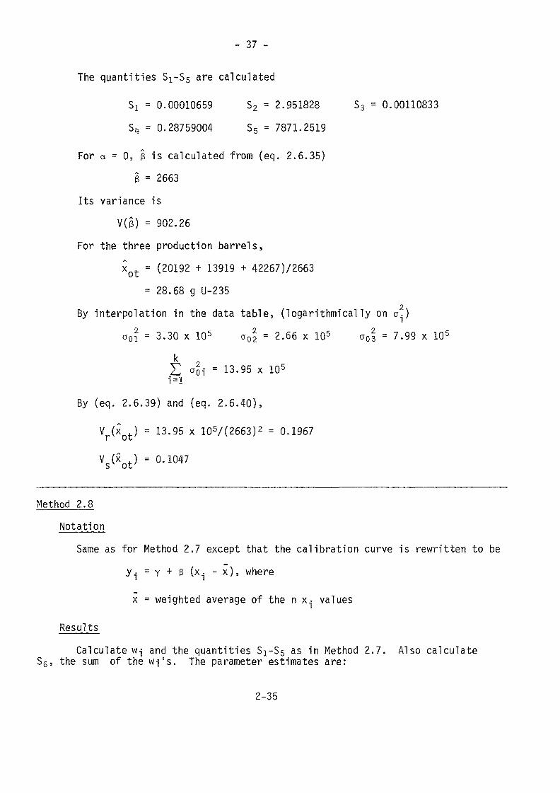
The quantities S^Ss are calculated

Si = 0.00010659 S2 = 2.951828 S3 = 0.00110833S^ = 0.28759004 S5 = 7871.2519

For a = 0, ß is calculated from (eq. 2.6.35)ß = 2663

Its variance isV(ß) = 902.26

For the three production barrels,x t = (20192 + 13919 + 42267)72663

= 28.68 g U-2352By interpolation in the data table, (logarithmically on a.)

= 3.30 x 105 a0| = 2.66 x 105 a03 = 7.99 x 105(

= 13.95 x 105

By (eq. 2.6.39) and (eq. 2.6.40),

Vr(xot) = 13.95 x 105/(2663)2 = 0.1967

Vs(xot) = 0.1047

Method 2.8Notation

Same as for Method 2.7 except that the calibration curve is rewritten to beyi = y + ß (xi - x), wherex = weighted average of the n x. values

ResultsCalculate w-j and the quantities 81-85 as in Method 2.7. Also calculateS6, the sum of the w-j's. The parameter estimates are:

2-35

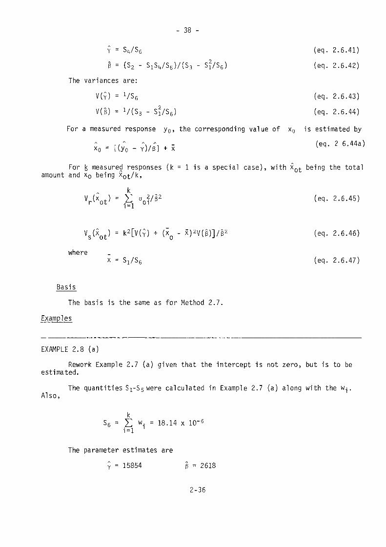
- 38 -

Y = S^/Sg (eq . 2.6.41)

ß = (S2 - S1S t t /S6) /(S3 - S?/S6) (eq. 2 .6 .42 )

The variances are:

V ( Ç ) = VS6 (eq. 2.6.43)

V ( ß ) = V(S 3 - S?/S6) (eq. 2 .6 .44)

For a measured response y0, the corresponding value of x0 is estimated byr," -\ ,-\ - (eq. 2 6.44a)x0 = [(YO - r)/ß] + x v M /

For k measured responses (k = 1 is a special case), with xot being the totalamount and x0 being -

Vr(xot) = Ç ao|/ß2 (eq. 2.6.45)

Vs(xQt) - k2[V(C) + (XQ - x)2V(ß)]/ß2 (eq. 2.6.46)

wherex = Si/Se (eq. 2.6.47)

BasisThe basis is the same as for Method 2.7.

Examples

EXAMPLE 2.8 (a)Rework Example 2.7 (a) given that the intercept is not zero, but is to beestimated.The quantities 81-85 were calculated in Example 2.7 (a) along with the w^.

Also,

S6 = Z wi = 18.14 x 1CT6

i = l

The parameter estimates areÇ = 15854 ß = 2618

2-36

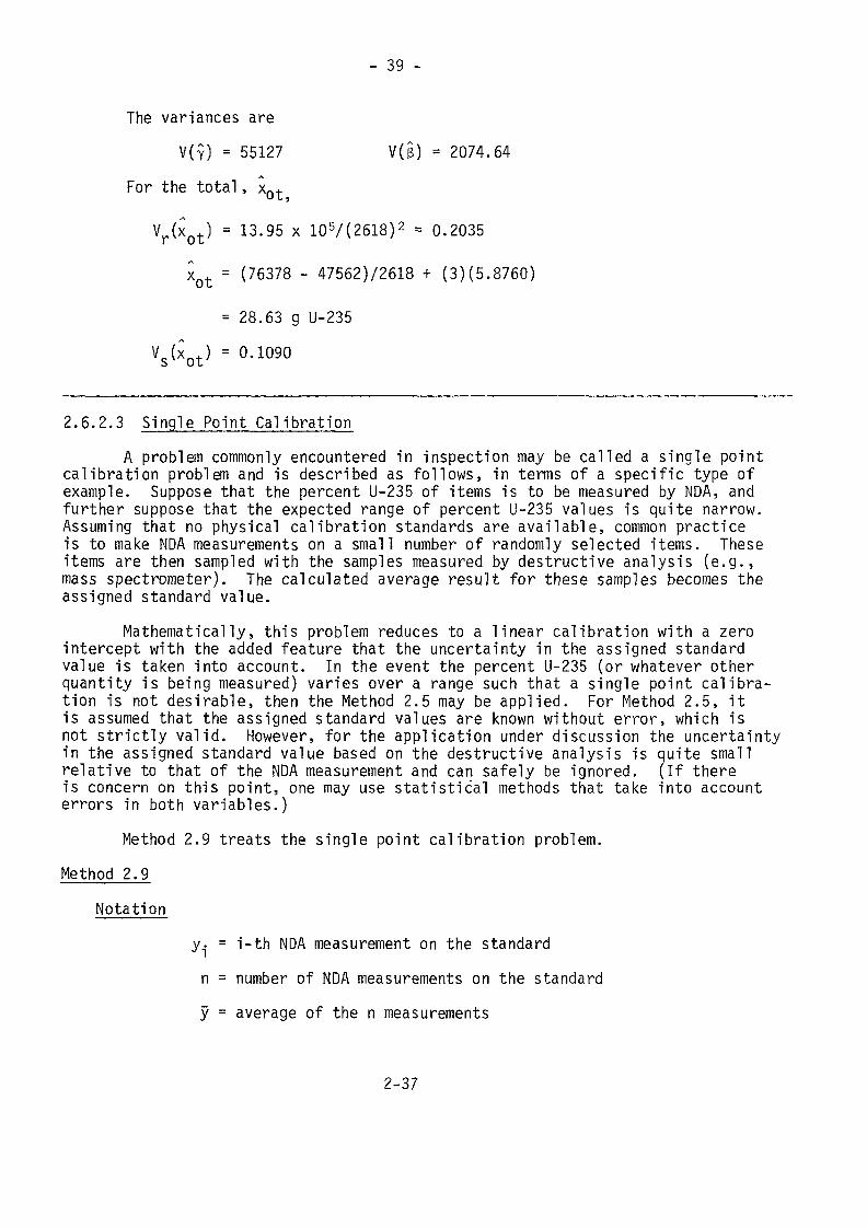
The variances areV(y) = 55127

AFor the total , X

- 39 -

V(3) = 2074.64

Vr(xQt) = 13.95 x 105/(2618)2 = 0.2035

xQt = (76378 - 47562)72618 + (3) (5. 8760)

= 28.63 g U-235Vs(xot) = 0.1090

2.6.2.3 Single Point CalibrationA problem commonly encountered in inspection may be called a single point

calibration problem and is described as follows, in terms of a specific type ofexample. Suppose that the percent U-235 of items is to be measured by NDA, andfurther suppose that the expected range of percent U-235 values is quite narrow.Assuming that no physical calibration standards are available, common practiceis to make NDA measurements on a small number of randomly selected items. Theseitems are then sampled with the samples measured by destructive analysis (e.g.,mass spectrometer). The calculated average result for these samples becomes theassigned standard value.

Mathematically, this problem reduces to a linear calibration with a zerointercept with the added feature that the uncertainty in the assigned standardvalue is taken into account. In the event the percent U-235 (or whatever otherquantity is being measured) varies over a range such that a single point calibra-tion is not desirable, then the Method 2.5 may be applied. For Method 2.5, itis assumed that the assigned standard values are known without error, which isnot strictly valid. However, for the application under discussion the uncertaintyin the assigned standard value based on the destructive analysis is quite smallrelative to that of the NDA measurement and can safely be ignored. (If thereis concern on this point, one may use statistical methods that take into accounterrors in both variables.)

Method 2.9 treats the single point calibration problem.Method 2.9

Notation/.j = i-th NDA measurement on the standardn = number of NDA measurements on the standardy = average of the n measurements

2-37

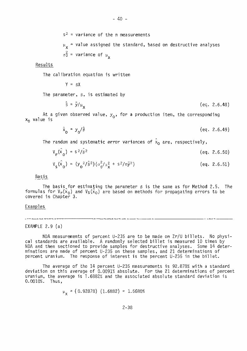
- 40 -

s2 = variance of the n measurementsy = value assigned the standard, based on destructive analysesA2ao - variance of y

X

Results

The calibration equation is writtenY = ßX

The parameter, ß, is estimated byß = y/yv (eq. 2.6.48)/\

At a given observed value, y , for a production item, the correspondingx0 value is

XQ = yo/§ (eq. 2.6.49)

The random and systematic error variances of x0 are, respectively,V r (x Q ) = s2 /ß2 (eq. 2.6.50)

Vs(*o} = (yo2/ 2)(aX + s2/ny2) (eq> 2'6-51)

BasisThe basis^for estimating the parameter ß is the same as for Method 2.5. The

formulas for Vr(x0) and VS(XQ) are based on methods for propagating errors to becovered in Chapter 3.Examples

EXAMPLE 2.9 (a)NDA measurements of percent U-235 are to be made on Zr/U billets. No physi-

cal standards are available. A randomly selected billet is measured 10 times byNDA and then sectioned to provide samples for destructive analyses. Some 14 deter-minations are made of percent U-235 on these samples, and 21 determinations ofpercent uranium. The response of interest is the percent U-235 in the billet.

The average of the 14 percent U-235 measurements is 92.878% with a standarddeviation on this average of 0.0091% absolute. For the 21 determinations of percenturanium, the average is 1.6882% and the associated absolute standard deviation is0.0010%. Thus,

yv - (0.92878) (1.6882) = 1.5680%A

2-38

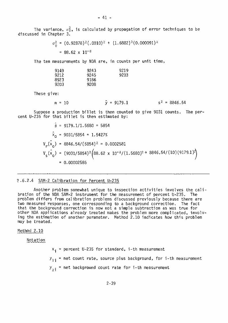
- 41 -

The variance, OQ» is calculated by propagation of error techniques to bediscussed in Chapter 3.

a2 = (0.92878)2(.0010)2 + (1.6882)2(0.000091)2

= 88.62 x 1CT8

The ten measurements by NDA are, in counts per unit time,

9149 9243 92199212 9245 92038923 91869203 9208

These give:n = 10 y = 9179.1 s2 = 8846.54

Suppose a production billet is then counted to give 9031 counts. The per-cent U-235 for that billet is then estimated by:

ß = 9179.1/1.5680 = 5854x0 = 9031/5854 = 1.5427%

Vr{xQ) = 8846.54/(5854)2 = 0.0002581Vs(xQ) = (9031/5854)2(88.62 x 10-8/(1.5680)2+ 8846.54/( 10) (9179.1)

= 0.00002585

2.6.2.4 SAM-2 Calibration for Percent U-235Another problem somewhat unique to inspection activities involves the cali-

bration of the NDA SAM-2 instrument for the measurement of percent U-235. Theproblem differs from calibration problems discussed previously because there aretwo measured responses, one corresponding to a background correction. The factthat the background correction is now not a simple subtraction as was true forother NDA applications already treated makes the problem more complicated, involv-ing the estimation of another parameter. Method 2.10 indicates how this problemmay be treated.Method 2.10

Notationx.j = percent U-235 for standard, i-th measurement

yx . = net count rate, source plus background, for i-th measurementy = net background count rate for i-th measurement

2-39

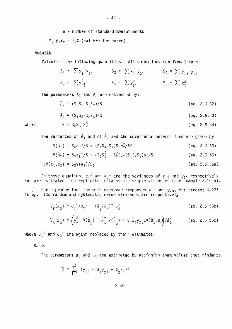
- 42 -

n = number of standard measurementsY1-ß1Y2 = ß2X (calibration curve)

ResultsCalculate the following quantities. All summations run from 1 to n.

Si = Exi yn. s2 = £Xi y2i s3 = £y i1 yz1

s, = Ey2i s5 = Ey22i s0 = E xf

The parameters ßj and ß2 are estimated by:ß! = (S0S3-S1S2)/S (eq. 2.6.52)

62 = (S1S5-S2S3)/S (eq. 2.6.53)where S = S0S5-S2 (eq. 2.6.54)

The variances of &1 and of 02 and tne covariance between them are given byV(M = S0a!2/S + (505^-5^)5001/52 (eq. 2.6.55)V(02) = S5ai2/S + (S0S3 + s|sIt-2S1S2S3)a2/S2 (eq. 2.6.56)

CV(ßl5ß2) = S2V(0i)/S0 (eq. 2.6.56a)

In these equation, a^2 and c?22 are the variances of y^ and y21- respectivelyand are estimated from replicated data as the sample variances (see example 2.10 a).For a production item with measured responses y^o and y2o> the percent U-235

is x0- Its random and systematic error variances are respectively

Vr(x0) = o^/ßj,2 + ( ß ß ) 2 a2 (eq. 2.6.56b)

ß2 (eq. 2.6.56c)

where c^2 and a22 are again replaced by their estimates.

BasisThe parameters 3i and 32 are estimated by assigning them values that minimize

nQ V^ / \ 9= E (y,.,- - ß y ,• - ß x,-)2i=i n 1 21 2 n

2-40

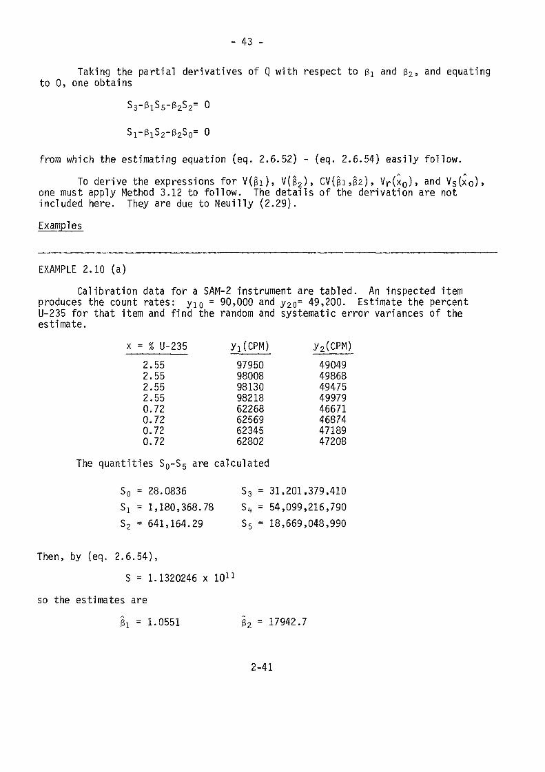
- 43 -

Taking the partial derivatives of Q with respect to ^ and ß2, anc' equatingto 0, one obtains

from which the estimating equation (eq. 2.6.52) - (eq. 2.6.54) easily fol low.

To derive the expressions for V ( f h ) , V ( § 2 ) , C V ( ß i , ß 2 ) , V r (x 0 ) , and V s ( x o ) ,one must apply Method 3.12 to fol low. The details of the derivation are notincluded here. They are due to Neu i l l y (2 .29) .

Examples

EXAMPLE 2.10 (a)Calibration data for a SAM-2 instrument are tabled. An inspected item

produces the count rates: y10 = 90,000 and y2o= 49,200. Estimate the percentU-235 for that item and find the random and systematic error variances of theestimate.

x = % U-235 yi(CPM) y2(CPM)2.552.552.552.550.720.720.720.72

The quanti t ies S0-S5 are calculated

S0 = 28.0836 S3 = 31,201,379,410Sx = 1,180,368.78 S4 = 54,099,216,790S2 = 641,164.29 S5 = 18,669,048,990

Then, by (eq. 2 .6.54) ,

S = 1.1320246 x 1011

so the estimates are

§1 = 1.0551 ß2 = 17942.7

2-41

9795098008981309821862268625696234562802

4904949868494754997946671468744718947208

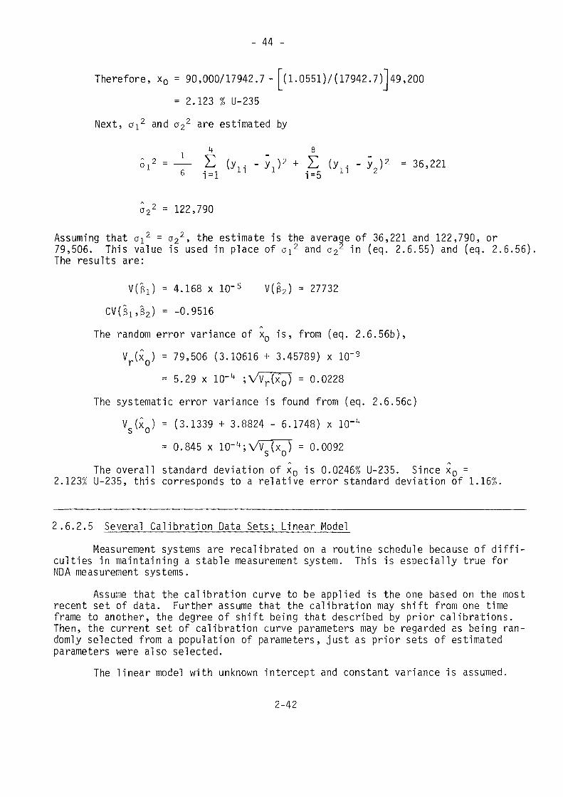
- 44 -

Therefore, x0 - 90,000/17942.7 - l"(l. 0551)7(17942. 7)149,200= 2.123 % U-235

Next, ai2 and a22 are estimated by

52 = i= —— £ (y - y )2 + E (y. - yj2 - 36,221s i=1 n i 1=5 n 2

Ô22 = 122,790

Assuming that ai2 - a22, the estimate is the average of 36,221 and 122,790, or79,506. This value is used in place of c^2 and a2 in (eq. 2.6.55) and (eq. 2.6.56)The results are:

V(3i) = 4.168 x IQ'5 V(02) = 27732CV(3i,ß2) = -0.9516

The random error variance of XQ is, from (eq. 2.6.565),Vr(xQ) = 79,506 (3.10616 + 3.45789) x 10'9

= 5.29 x I0~k ;Vvr(x"0) = 0.0228The systematic error variance is found from (eq. 2.6.56c)

VS(XQ) = (3.1339 + 3.8824 - 6.1748) x 10'^= 0.845 x 10-4;VvJfx^) = 0.0092

The overall standard deviation of x0 is 0.0246% U-235. Since x0 =2.123% U-235, this corresponds to a relative error standard deviation of 1.16%.

2.6.2.5 Several Calibration Data Sets; Linear ModelMeasurement systems are recalibrated on a routine schedule because of diffi-

culties in maintaining a stable measurement system. This is especially true forNDA measurement systems.

Assume that the calibration curve to be applied is the one based on the mostrecent set of data. Further assume that the calibration may shift from one timeframe to another, the degree of shift being that described by prior calibrations.Then, the current set of calibration curve parameters may be regarded as being ran-domly selected from a population of parameters, just as prior sets of estimatedparameters were also selected.

The linear model with unknown intercept and constant variance is assumed.

2-42

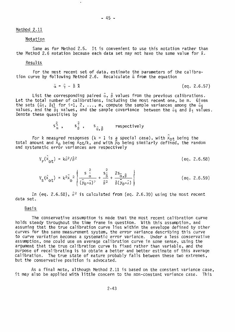
- 45 -

Method 2.11Notation

Same as for Method 2.5. It is convenient to use this notation rather thanthe Method 2.6 notation because each data set may not have the same value for x.

ResultsFor the most recent set of data, estimate the parameters of the cal ibra-

tion curve by fo l lowing Method 2.6. Recalculate 5. from the equation

a = y - (eq. 2 .6 .57)

List the corresponding paired a, § values from the previous calibrations.Let the total number of calibrations, including the most recent one, be m. Giventhe sets (ai, ßj) for i=l, 2, ..., m, compute the sample variances among the âjvalues, and the ßj values, and the sample covariance between the âj and ßj values,Denote these quantities by

2 2sa , S3 » s- g respectivelyA

For k measured responses (k = 1 is a special case), wi th x0t being thetotal amount and x0 being x0t/k, and with yo being s imi lar ly defined, the randomand systematic error variances are respectively

Vxot> =

- k2v2 2

S /\ c * 0 c^ ^, C- J A

a +

(eq. 2.6.58)

(eq. 2.6.59)

In (eq. 2.6.58), a2 is calculated from (eq. 2.6.30) using the most recentdata set.

BasisThe conservative assumption is made that the most recent calibration curve

holds steady throughout the time frame in question. With this assumption, andassuming that the true calibration curve lies within the envelope defined by othercurves for the same measurement system, the error variance describing this curveto curve variation becomes a systematic error variance. Under a less conservativeassumption, one could use an average calibration curve in some sense, using theargument that the true calibration curve is fixed rather than variable, and thepurpose of recalibrating is to obtain a better and better estimate of this averagecalibration. The true state of nature probably falls between these two extremes,but the conservative position is advocated.

As a final note, although Method 2.11 is based on the constant variance case,it may also be applied with little concern to the non-constant variance case. This

2-43

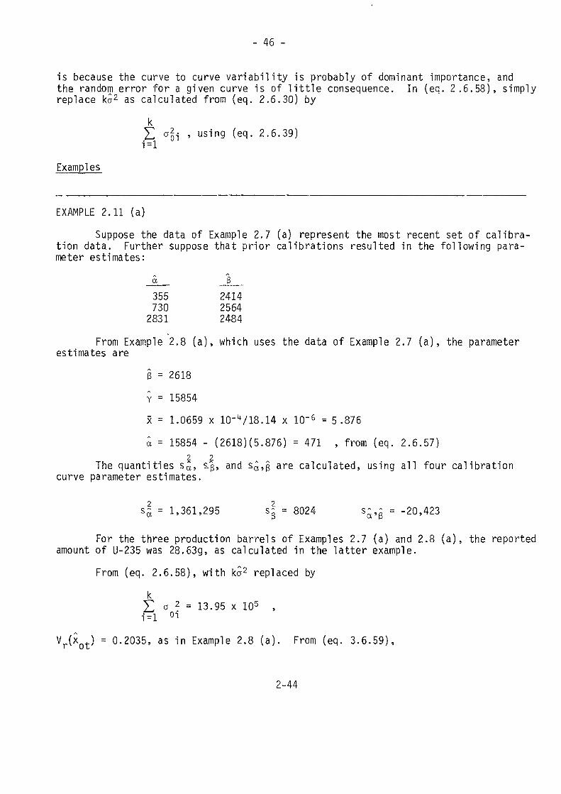
- 46 -

is because the curve to curve variability is probably of dominant importance, andthe random error for a given curve is of little consequence. In (eq. 2.6.58), simplyreplace ka2 as calculated from (eq. 2.6.30) by

k£ o^i , using (eq. 2.6.39)

Examples

EXAMPLE 2.11 (a)Suppose the data of Example 2.7 (a) represent the most recent set of calibra-

tion data. Further suppose that prior calibrations resulted in the following para-meter estimates:

355 2414730 2564

2831 2484From Example 2.8 (a), which uses the data of Example 2.7 (a), the parameter

estimates areß = 2618Y = 15854x = 1.0659 x 10-V18.14 x IQ-6 = 5.876a = 15854 - (2618)(5.876) = 471 , from (eq. 2.6.57)

2 2The quantities sa, sg, and s^,§ are calculated, using all four calibrationcurve parameter estimates.

si = 1,361,295 s~ = 8024 s£,g = -20,423

For the three production barrels of Examples 2.7 (a) and 2.8 (a) , the reportedamount of U-235 was 28.63g, as calculated in the latter example.

From (eq. 2.6.58), with ka2 replaced by

kY) a 2 = 13.95 x 105 ,iXL oi

Vr(xQt) = 0.2035, as in Example 2.8 (a). From (eq. 3.6.59),

2-44

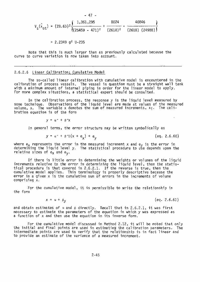
- 47 -( 1,361,295 8024 40846 )

Vc(x , ) = (28.63)2{————————— + ————— - —————————>s ot ((25459 - 471)2 (2618)2 (2618) (24988))

= 2.2349 g2 U-235

Note that this is much larger than as previously calculated because thecurve to curve variation is now taken into account.

2.6.2.6 Linear Calibration; Cumulative ModelThe so-called linear calibration with cumulative model is encountered in thecalibration of process vessels. The vessel in question must be a straight wall tank

with a minimum amount of internal piping in order for the linear model to apply.For more complex situations, a statistical expert should be consulted.

In the calibration process, the response y is the liquid level measured bysome technique. Observations of the liquid level are made at values of the measuredvolume, x. The variable x denotes the sum of measured increments, x-j. The cali-bration equation is of the form

y = a' + 3'xIn general terms, the error structure may be written symbolically as

y = a' + ß'z(x + ex) + e (eq. 2.6.60)where ex represents the error in the measured increment x and ey is the error indetermining the liquid level y. The statistical procedure to use depends upon therelative sizes of ex and ey.

If there is little error in determining the weights or volumes of the liquidincrements relative to the error in determining the liquid level, then the statis-tical procedure is that covered in 2.6.2.1. If the reverse is true, then thecumulative model applies. This terminology is properly descriptive because theerror in a given x is the cumulative sum of errors in the increments of volumecomprising x.

For the cumulative model, it is permissible to write the relationship inthe formX = a + ßy (eq. 2.6.61)

and obtain estimates of a and ß directly. Recall that in 2.6.2.1, it was firstnecessary to estimate the parameters of the equation in which y was expressed asa function of x and then use the equation in its inverse form.

For the cumulative model discussed in Method 2.12, it will be noted that onlythe initial and final points are used in estimating the calibration parameters. Theintermediate points are used to verify that the relationship is in fact linear andto provide an estimate of the variance of a measured increment.

2-45

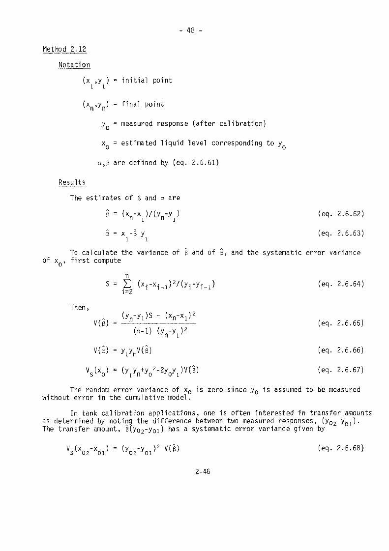
- 48 -

Method 2.12Notation

(x ,y ) = initial pointi i(xn,yn) = final point

y = measured response (after calibration)

x = estimated liquid level corresponding to y

a, 3 are defined by (eq. 2.6.61)

ResultsThe estimates of 3 and a are

(eq-a = x -3 y (eq. 2.6.63)i i

To calculate the variance of 3 and of a, and the systematic error varianceof x , first compute

nS = .E (X1-x1_l)2/(y1-y1_l) (eq. 2.6.64)

Then,V(3) = — —— - ————— —— —— (eq. 2.6.65)(n-i) (y )2V(o) = yiynV(3) (eq. 2.6.66)

Vs(xo} = (Vn+yo2'2Vi)v(e) (eq- 2>6-67)

The random error variance of x0 is zero since y0 is assumed to be measuredwithout error in the cumulative model.

In tank calibration applications, one is often interested in transfer amountsas determined by noting the difference between two measured responses, (yoz'^oi^'The transfer amount, 3(yo2~yoi) nas a systematic error variance given by

- 2-6-68)2-46

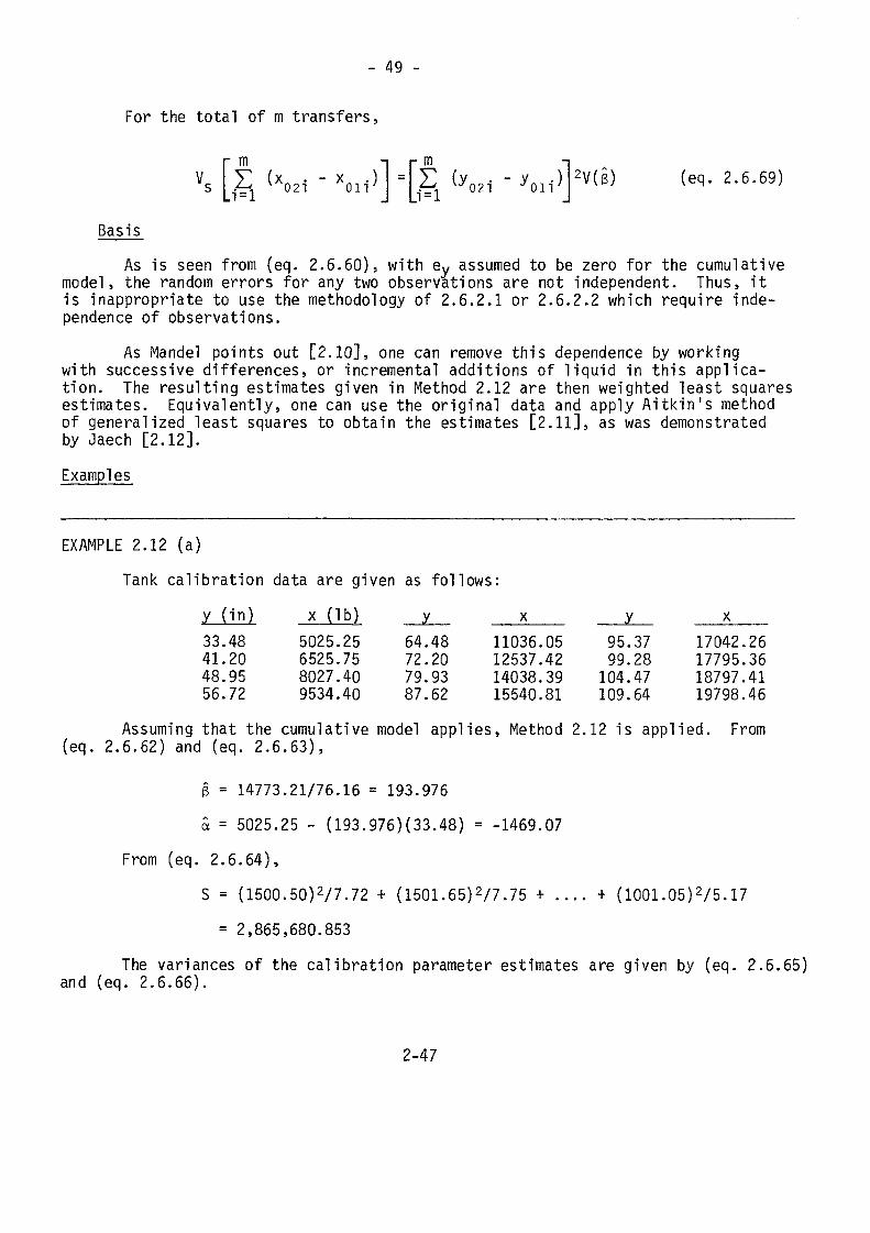
- 49 -

For the total of m transfers,

0212V(3) (eq. 2.6.69)

BasisAs is seen from (eq. 2.6.60), with 6y assumed to be zero for the cumulativemodel, the random errors for any two observations are not independent. Thus, it

is inappropriate to use the methodology of 2.6.2.1 or 2.6.2.2 which require inde-pendence of observations.

As Mandel points out [2.10], one can remove this dependence by workingwith successive differences, or incremental additions of liquid in this applica-tion. The resulting estimates given in Method 2.12 are then weighted least squaresestimates. Equivalently, one can use the original data and apply Aitkin's methodof generalized least squares to obtain the estimates [2.11], as was demonstratedby Jaech [2.12].Examples

EXAMPLE 2.12 (a)Tank calibration data are given as follows:

y (in) x Çlb) y x x33.4841.2048.9556.72

5025.256525.758027.409534.40

64.4872.2079.9387.62

11036.0512537.4214038.3915540.81

95.3799.28104.47109.64

17042.2617795.3618797.4119798.46

Assuming that the cumulative model applies, Method 2.12 is applied. From(eq. 2.6.62) and (eq. 2.6.63),

ß = 14773.21/76.16 = 193.976S = 5025.25 - (193.976)(33.48) = -1469.07

From (eq. 2.6.64),S = (1500.50)2/7.72 + (1501.65)2/7.75 + .... + (1001.05)2/5.17

= 2,865,680.853The variances of the calibration parameter estimates are given by (eq. 2.6.65)

and (eq. 2.6.66).

2-47

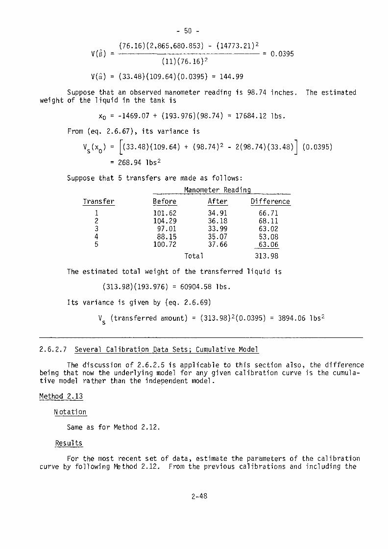
- 50 -(76.16)(2,865,680.853) - (14773.2l)2

V(ß) = —————————————————————————— = 0.0395

Before101.62104.2997.0188.15100.72

After34.9136.1833.9935.0737.66

Difference66.7168.1163.0253.0863.06

V(â) = (33.48)(109.64)(0.0395) = 144.99Suppose that an observed manometer reading is 98.74 inches. The estimated

weight of the liquid in the tank isX0 = -1469.07 + (193.976)(98.74) = 17684.12 Ibs.

From (eq. 2.6.67), its variance isVS(XQ) = |~(33.48)(109.64) + (98.74)2 - 2(98.74)(33.48)1 (0.0395)

= 268.94 Ibs2

Suppose that 5 transfers are made as follows:_____Manometer Reading

Transfer12345

Total 313.98

The estimated total weight of the transferred liquid is

(313.98)(193.976) = 60904.58 Ibs.

Its variance is given by (eq. 2.6.69)

Vs (transferred amount) = (313.98)2(0.0395) - 3894.06 Ibs2

2.6.2 .7 Several Calibration Data Sets; Cumulative Model

The discussion of 2.6.2.5 is applicable to this section also, the differencebeing that now the underlying model for any given calibration curve is the cumula-tive model rather than the independent model.

Method 2.13

Notation

Same as for Method 2.12.Results

For the most recent set of data, estimate the parameters of the calibrationcurve by following Method 2.12. From the previous calibrations and including the

2-48

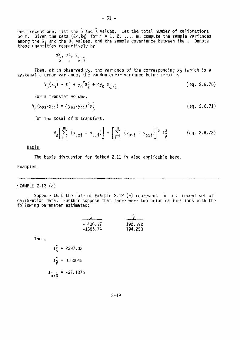
- 51 -

most recent one, list the a and ß values. Let the total number of calibrationsbe m. Given the sets (ai,ß-j) for i = 1, 2, ..., m, compute the sample variancesamong the â-j and the 0j values, and the sample covariance between them. Denotethese quantities respectively by

s2 s 2 s

Then, at an observed y0, the variance of the corresponding x0 (which is asystematic error variance, the random error variance being zero) is

W = S l + y 02 s l + 2 y o 5 ^ Ceq. 2.6.70)

For a transfer volume,

V ( x 0 2 - X o i ) = (yo2-yoi)2 s (eq. 2.6.71)s

For the total of m transfers,

P m "I - m ~jVS[:C (X021 - x011)J = E (y02i - yo l i)J2 si (eq. 2.6.72)

Basis

The basis discussion for Method 2.11 is also applicable here.Examples

EXAMPLE 2.13 (a)Suppose that the data of Example 2.12 (a) represent the most recent set of

calibration data. Further suppose that there were two prior calibrations with thefollowing parameter estimates:

-1408.77 192.792-1505.74 194.250

Then,_ 2 = 2397.33a

sf = 0.60045

= -37.1376

2-49

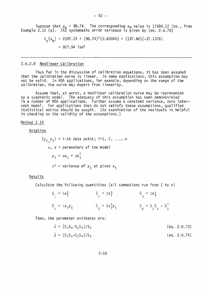
- 52 -

Suppose that yQ = 98.74. The corresponding x0 value is 17684.12 Ibs., fromExample 2.12 (a). Its systematic error variance is given by (eq. 2.6.70)V S (X Q ) = 2397.33 + (98.74)2(0.60045) + (197.48)(-37.1376)

= 917.54 Ibs2

2.6.2.8 Nonlinear CalibrationThus far in the discussion of calibration equations, it has been assumed

that the calibration curve is linear. In some applications, this assumption maynot be valid. In NDA applications, for example, depending on the range of thecalibration, the curve may depart from linearity.

Assume that, at worst, a nonlinear calibration curve may be representedby a quadratic model. The adequacy of this assumption has been demonstratedin a number of NDA applications. Further assume a constant variance, zero inter-cept model. For applications that do not satisfy these assumptions, qualifiedstatistical advice should be sought. (An examination of the residuals is helpfulin checking on the validity of the assumptions.)Method 2.14

Notation{y,- x.) = i-th data point; i=l, 2, ..., ni » i

a, ß = parameters of the modelyi = «xi + 3x?a2 = variance of y. at given x.

ResultsCalculate the following quantities (all summations run from 1 to n)

S = zx? S = EX? S = Dd1 1 2 1 3 1

S = EX.y. S = Ex?y. S = S S - S2

k l l 5 T 1 6 1 3 2

Then, the parameter estimates are:

a = (S 3S 4 -S 2S 5 ) /S 6 (eq. 2.6.73)

3 = (S1S5-S2S i f)/S6 (eq. 2.6.74)

2-50

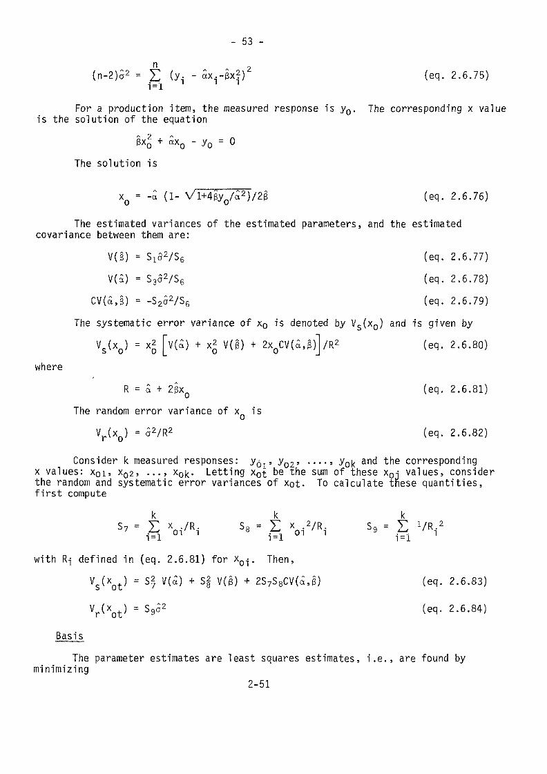
- 53 -

E1=1

(n-2)S2 = E (y, - âx,-§x2)2 (eq. 2.6.75)

For a production item, the measured response is y0. The corresponding x valueis the solution of the equation

§XQ + axQ - y0 = 0The solution is

XQ = -0 (l- Vl+4ßy0/a2}/2ß (eq. 2.6.76)

The estimated variances of the estimated parameters, and the estimatedcovariance between them are:

where

V(e) = S^/Sg (eq. 2.6.77)V(a) = S302/S6 (eq. 2.6.78)

CV(S,§) = -S2o2/S6 (eq. 2.6.79)The systematic error variance of x0 is denoted by Vs(x0) and is given by

Vs(xo) = x2 [v(a) + x2 V(e) + 2xoCV(a,e)]/R2 (eq. 2.6.80)

R = a + 2ßxQ (eq. 2.6.81)The random error variance of x is

Vr(xQ) = S2/R2 (eq. 2.6.82)

Consider k measured responses: y^, yo2, ...., y0^ and the correspondingx values: x0i, x02, ...» x^. Letting x0t be the sum of these x0j values, considerthe random and systematic error variances of xot- To calculate these quantities,first compute

S7 - Z xo./R. Se - xo1VR, S9 -

with Ri defined in (eq. 2.6.81) for xoi. Then,V s ( X ) = $2 V(0) + S§ V(ß) + 2S7S8CV(a,3) (eq. 2.6.83)

BasisVxot) = S952 (eq- 2.6.84)

The parameter estimates are least squares estimates, i.e., are found byminimizing

2-51

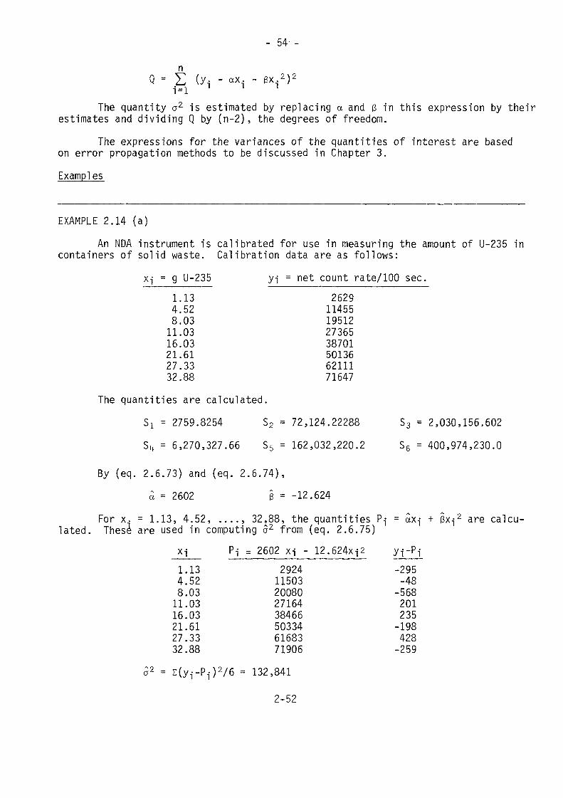
- 54- -

Q = E (y, - ax - ex 2)2i=lThe quantity a2 is estimated by replacing a and 3 in this expression by their

estimates and dividing Q by (n-2), the degrees of freedom.The expressions for the variances of the quantities of interest are based

on error propagation methods to be discussed in Chapter 3.Examples

EXAMPLE 2.14 (a)An NDA instrument is calibrated for use in measuring the amount of U-235 in

containers of solid waste. Calibration data are as follows:x-j = g U-235 yi = net count rate/100 sec.

1.13 26294.52 114558.03 1951211.03 2736516.03 3870121.61 5013627.33 6211132.88 71647

The quantities are calculated.Si = 2759.8254 S2 = 72,124.22288 S3 = 2,030,156.602S4 = 6,270,327.66 S5 - 162,032,220.2 S6 = 400,974,230.0

By {eq. 2.6.73) and (eq. 2.6.74),a = 2602 ß = -12.624

For x. = 1.13, 4.52, ...., 32.88, the quantities Pj - ax-j + ßx-j2 are calcu-lated. These are used in computing 52 from (eq. 2.6.75)Xi PÎ = 2602 xi - 12.624xj2 yj-Pj1.134.528.0311.0316.0321.6127.3332.88

292411503200802716438466503346168371906

-295-48-568201235-198428-259

= E(yi-Pi)2/6 = 132,841

2-52

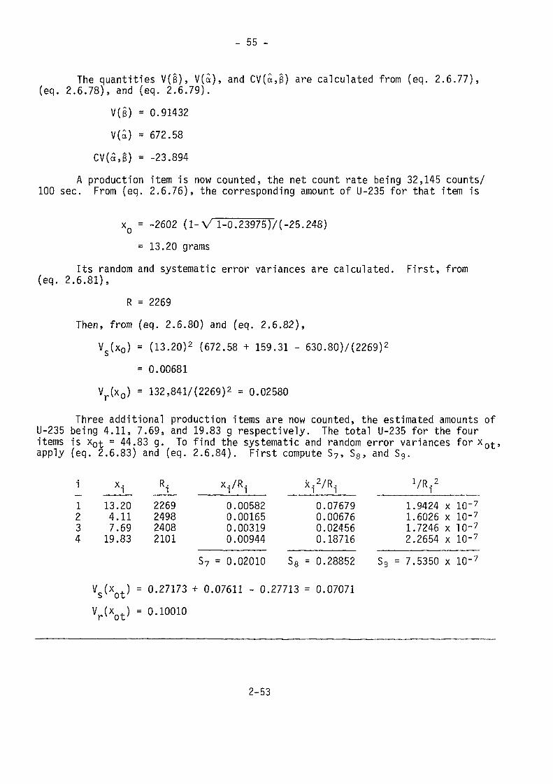
- 55 -

The quantities V(ß), V(S), and CV(S,g) are calculated from (eq. 2.6.77),(eq. 2.6.78), and (eq. 2.6.79).

V(s) = 0.91432V(S) = 672.58

CV(a,e) = -23.894A production item is now counted, the net count rate being 32,145 counts/

100 sec. From (eq. 2.6.76), the corresponding amount of U-235 for that item is

XQ = -2602 (1-V l-0.23975)/(-25.248)= 13.20 grams

Its random and systematic error variances are calculated. First, from(eq. 2.6.81),

R = 2269Then, from (eq. 2.6.80) and (eq. 2.6.82),

Vs(x0) = (13.20)2 (672.58 + 159.31 - 630.80)/(2269)2

= 0.00681Vr(x0) = 132,841/(2269)2 = 0.02580

Three additional production items are now counted, the estimated amounts ofU-235 being 4.11, 7.69, and 19.83 g respectively. The total U-235 for the fouritems is x0t = 44.83 g. To find the systematic and random error variances for *0t,apply (eq. 2.6.83) and (eq. 2.6.84). First compute S7, S8, and S9.

i1234

xi13.204.117.6919.83

Ri2269249824082101

VRi0.005820.001650.003190.00944

xi2/R10.076790.006760.024560.18716

VR.J2

1.9424 x IQ'71.6026 x 10-71.7246 x 10-72.2654 x 10-7

S7 = 0.02010 S8 = 0.28852 S9 = 7.5350 x lO"7

Vs(XQt) = 0.27173 + 0.07611 - 0.27713 = 0.07071vr(xot) = o.iooio

2-53

- 56 -

2.6.2.9 Nonlinear Calibration; Several Calibration Data SetsThe decision of 2.6.2.5 is applicable to this section also, the difference

being that now the underlying model for any given calibration curve is the quadra-tic model with zero intercept, discussed in 2.6.2.8.Method 2.15

NotationSame as for Method 2.14.

ResultsFor the most recent set of data, estimate the parameters of the calibration

curve by following Method 2.14. From the previous calibrations, and including themost recent one, list the a and § values. Compute the sample variances of the mex's and g's, and the sample cov.ariance between them, calling the results s~, sg,and sâ,ê respectively. Then, at an observed y0, the systematic error variance ofthe corresponding x0 is given by (eq. 2.6.80) with:

p

V(â) replaced by s-

V ( ß ) replaced by s àP

CV(a,ß) replaced by s ~ , su> p

The random error variance of x0 is given by (eq. 2.6.82), using the valuefor a2 from the most recent calibration.For k measured responses, x0t has systematic error variance given by(eq. 2.6.83), making the same replacements for V(a), V(e), and CV(a,ß) as just

indicated. For the random error variance of xot> use (eq. 2.6.84) with the valueof a2 based on the most recent calibration.

BasisThe basis discussion for Method 2.11 is also applicable here.

Examples

EXAMPLE 2.15 (a)Suppose that the data of Example 2.14 (a) represent the most recent set of

calibration data. Further suppose that there were four prior calibrations withthe following parameter estimates:

2-54

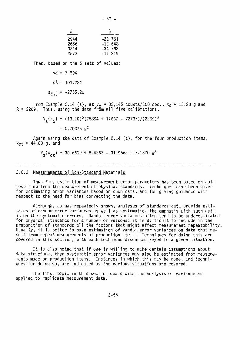
- 57 -

2944 -22.7612656 -12.6483214 -34.7922573 -11.219

Then, based on the 5 sets of values:sa = 7 894s§ = 101.224

SÄ.S = -2755-20From Example 2.14 (a), at yQ = 32,145 counts/100 sec., x0 = 13.20 g andR = 2269. Thus, using the data from all five calibrations,

VS(XQ) = (13.20)2(75894 + 17637 - 72737)/(2269)2

= 0.70375 g2

Again using the data of Example 2.14 (a), for the four production items,xot = 44.83 g, andvc(xnt) = 30.6619 + 8.4263 - 31.9562 = 7.1320 g2

2.6.3 Measurements of Non-Standard Materials,Thus far, estimation of measurement error parameters has been based on data

resulting from the measurement of physical standards. Techniques have been givenfor estimating error variances based on such data, and for giving guidance withrespect to the need for bias correcting the data.

Although, as was repeatedly shown, analyses of standards data provide esti-mates of random error variances as well as systematic, the emphasis with such datais on the systematic errors. Random error variances often tend to be underestimatedfor physical standards for a number of reasons; it is difficult to include in the .preparation of standards all the factors that might affect measurement repeatability.Usually, it is better to base estimation of random error variances on data that re-sult from repeat measurements of production items. Techniques for doing this arecovered in this section, with each technique discussed keyed to a given situation.

It is also noted that if one is willing to make certain assumptions aboutdata structure, then systematic error variances may also be estimated from measure-ments made on production items. Instances in which this may be done, and techni-ques for doing so, are indicated as the various situations are covered.

The first topic in this section deals with the analysis of variance asapplied to replicate measurement data.

2-55

- 58 -

2.6.3.1 Repli ça te_ Measurements; Analysis of VarianceReplicate or repeat measurements are made on the same or similar production

items. The scatter in the repeat measurements is used to estimate the randomerror variance using a statistical technique known as the one way analysis ofvariance.

It is important to keep in mind just which measurement error parameter isbeing estimated in a given case. Depending on how the measurements are performed,for example, the random error variance being estimated may be the sum of samplingand analytical error variances, say, or it may be just the analytical error variance.This will be pointed out in the examples.

In Method 2.16, the one way analysis of variance as applied to this problemsituation is discussed.Method 2.16

Notationx.. = observed value for j-th measurement on production item i' J

n. = number of measurements made on production item in = total number of measurements (sum of n. values)m = number of production items measureda2 = random error variance

ResultsFollowing Method 2.4, a2 is estimated by (eq. 2.6.16). That is, a2 is the

same calculated quantity as was of in Method 2.4.Basj\s

The basis is the same as for Method 2.4.Examples

EXAMPLE 2.16 (a)Five cans of UCL powder are weighed at random and at routine intervals on a

given scale. Assume that the actual contents do not change in weight, and estimatea2 from the following data (weights in kg).

2-56

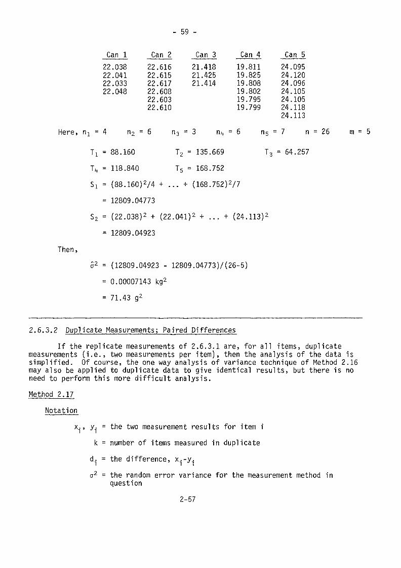
- 59 -

Here,

Then,

Can 122.03822.04122.03322.048

= 4 n2 =

Can 222.61622.61522.61722.60822.60322.610

6 n3 =

T2 =

T5 =

Can 321.41821.42521.414

3 nit =

135.669168.752

Can 419.81119.82519.80819.80219.79519.799

6 n5T

Can 524.09524.12024.09624.10524.10524.11824.113

= 7 n

3 = 64.257

/4 + ... + (168.752)2/7

T! = 88.160T4 = 118.84051 = (88.160)2/4

= 12809.0477352 = (22.038)2 + (22.041)2 + ... + (24.113)2

= 12809.04923

à2 = (12809.04923 - 12809.04773)/(26-5)= 0.00007143 kg2

= 71.43 g2

= 26 m = 5

2.6.3.2 Duplicate Measurements; PairedJMfferencesIf the replicate measurements of 2.6.3.1 are, for all items, duplicate

measurements (i.e., two measurements per item), then the analysis of the data issimplified. Of course, the one way analysis of variance technique of Method 2.16may also be applied to duplicate data to give identical results, but there is noneed to perform this more difficult analysis.Method 2.17

Notation

k =

a2 =

the two measurement results for item inumber of items measured in duplicatethe difference, x.-y.the random error variance for the measurement method inquestion

2-57

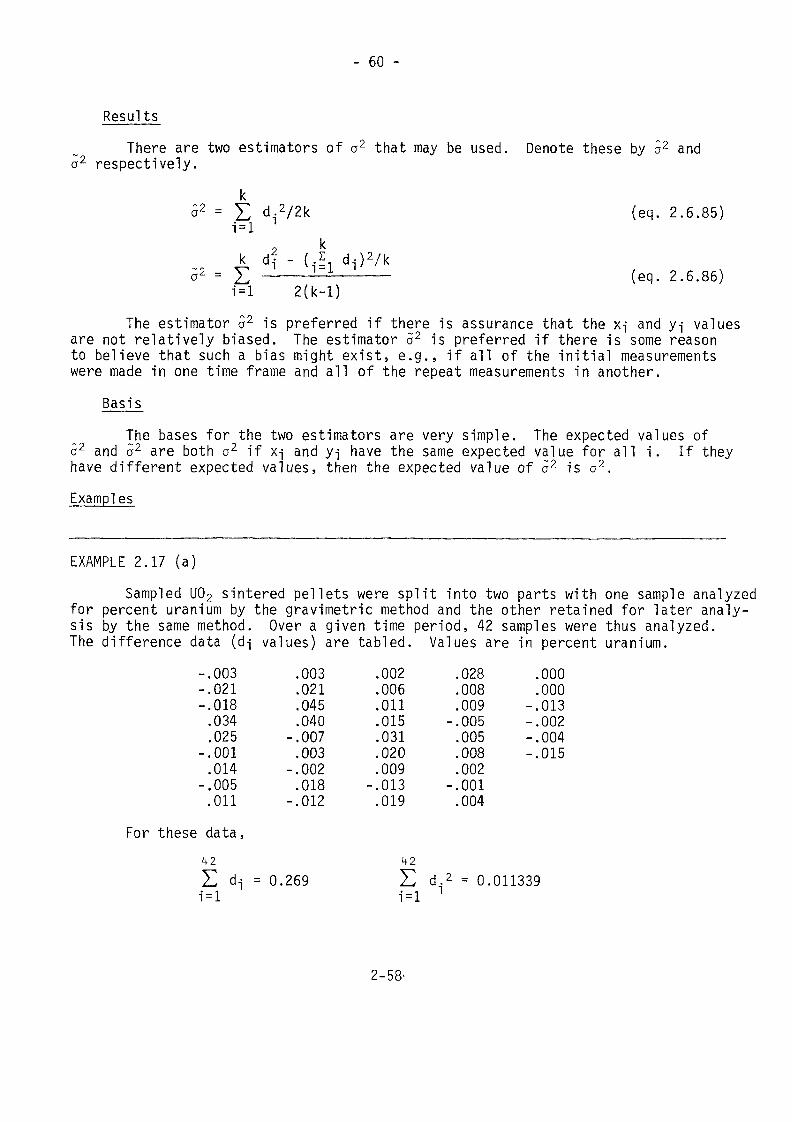
- 60 -

Results

There are two estimators of o2 that may be used. Denote these by a2 anda2 respectively.

a2 =

cf- =

g d12/2ki = 1

A di)2/k1=1 2(k-l)

(eq. 2.6.85)

(eq. 2.6.86)

The estimator a2 is preferred if there is assurance that the Xj and y-j valuesare not relatively biased. The estimator 52 is preferred if there is some reasonto believe that such a bias might exist, e.g., if all of the initial measurementswere made in one time frame and all of the repeat measurements in another.

BasisThe bases for the two estimators are very simple. The expected values of

a2 and 52 are both a2 if x-j and y-j have the same expected value for all i. If theyhave different expected values, then the expected value of a2 is o2.

Examples

EXAMPLE 2.17 (a)Sampled U02 sintered pellets were split into two parts with one sample analyzed

for percent uranium by the gravimetric method and the other retained for later analy-sis by the same method. Over a given time period, 42 samples were thus analyzed.The difference data (d-j values) are tabled. Values are in percent uranium.

-.003-.021-.018.034.025

-.001.014

-.005.011

For these data,42

E d-j1 = 1

.003

.021

.045

.040

.007

.003

.002

.018

.012

.002

.006

.011

.015

.031

.020

.009

.013

.019

42

.028

.008

.009

.005

.005

.008

.002

.001

.004

.000

.000-.013-.002-.004-.015

= 0.269 E d.2 = 0.011339

2-58'

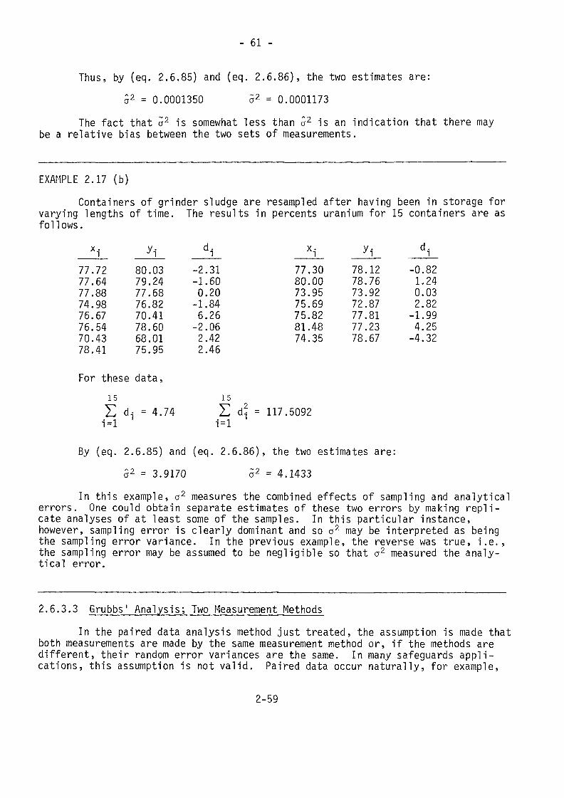
- 61 -

Thus, by (eq. 2.6.85) and (eq. 2.6.86), the two estimates are:o2 = 0.0001350 52 = 0.0001173

The fact that a2 is somewhat less than a2 is an indication that there maybe a relative bias between the two sets of measurements.

EXAMPLE 2.17 (b)Containers of grinder sludge are resampled after having been in storage for

varying lengths of time. The results in percents uranium for 15 containers are asfollows.

xi77.7277.6477.8874.9876.6776.5470.4378.41

80.0379.2477.6876.8270.4178.6068.0175.95

di-2.-1.

.31

.600.20

-1.84.26.06.42

6.-2.2.2.46

xi77.3080.0073.9575.6975.8281.4874.35

'i78.1278.7673.9272.8777.8177.2378.67

di-0.821.240.032.

-1,4.829925

-4.32

For these data,15 15Z di = 4.74 E d* = 117.5092

By (eq. 2.6.85) and (eq. 2.6.86), the two estimates are:a2 = 3.9170 52 = 4.1433

In this example, a2 measures the combined effects of sampling and analyticalerrors. One could obtain separate estimates of these two errors by making repli-cate analyses of at least some of the samples. In this particular instance,however, sampling error is clearly dominant and so a2 may be interpreted as beingthe sampling error variance. In the previous example, the reverse was true, i.e.,the sampling error may be assumed to be negligible so that a2 measured the analy-tical error.

2.6.3.3 Grubbs' Analysis; Two Measurement^ MethodsIn the paired data analysis method just treated, the assumption is made that

both measurements are made by the same measurement method or, if the methods aredifferent, their random error variances are the same. In many safeguards appli-cations, this assumption is not valid. Paired data occur naturally, for example,

2-59

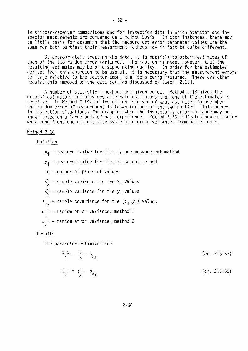
- 62 -

in shipper-receiver comparisons and for inspection data in which operator and in-spector measurements are compared on a paired basis. In both instances, there maybe little basis for assuming that the measurement error parameter values are thesame for both parties; their measurement methods may in fact be quite different.

By appropriately treating the data, it is possible to obtain estimates ofeach of the two random error variances. The caution is made, however, that theresulting estimates may be of disappointing quality. In order for the estimatesderived from this approach to be useful, it is necessary that the measurement errorsbe large relative to the scatter among the items being measured. There are otherrequirements imposed on the data set, as discussed by Jaech [2.13].

A number of statistical methods are given below. Method 2.18 gives theGrubbs ' estimators and provides alternate estimators when one of the estimates isnegative. In Method 2.19, an indication is given of what estimates to use whenthe random error of measurement is known for one of the two parties. This occursin inspection situations, for example, when the inspector's error variance may beknown based on a large body of past experience. Method 2.20 indicates how and underwhat conditions one can estimate systematic error variances from paired data.Method 2.18

Notationx. = measured value for item i, one measurement methody. = measured value for item i, second methodn - number of pairs of valuess2 = sample variance for the x. valuesX »s2 = sample variance for the y. valuess = sample covariance for the (x.,y.) values2 _

2 -

random error variance, method 1a ^ = random error variance, method 22

ResultsThe parameter estimates are

a 2 = S2 - Si x xy (eq. 2.6.87)

2 = s2 - sxy (eq. 2.6.88}

2-60

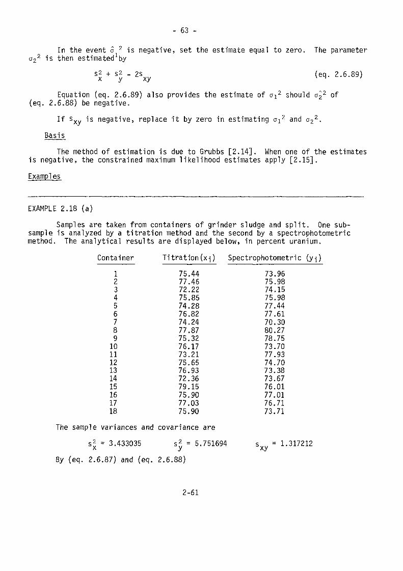
- 63 -

In the event 5 2 is negative, set the estimate equal to zero. The parametera22 is then estimated^

s2 + 52 - 2sx y xy (eq. 2.6.89)

Equation (eq. 2.6.89) also provides the estimate of aj2 should a^2 of(eq. 2.6.88) be negative.

If s is negative, replace it by zero in estimating a!2 and a22.xyBasis

The method of estimation is due to Grubbs [2.14]. When one of the estimatesis negative, the constrained maximum likelihood estimates apply [2.15].Examples

EXAMPLE 2.18 (a)Samples are taken from containers of grinder sludge and split. One sub-

sample is analyzed by a titration method and the second by a spectrophotometricmethod. The analytical results are displayed below, in percent uranium.

Container123456789101112131415161718

Titration (x-j) Spectrophotometric (y-j)75.4477.4672.2275.8574.2876.8274.2477.8775.3276.1773.2175.6576.9372.3679.1575.9077.0375.90

73.9675.9874.1575.9877.4477.6170.3080.2778.7573.7077.9374.7073.3873.6776.0177.0176.7173.71

The sample variances and covariance ares2 = 3.433035A

s2 = 5.751694By (eq. 2.6.87) and (eq. 2.6.88)

sxy = 1.317212

2-61

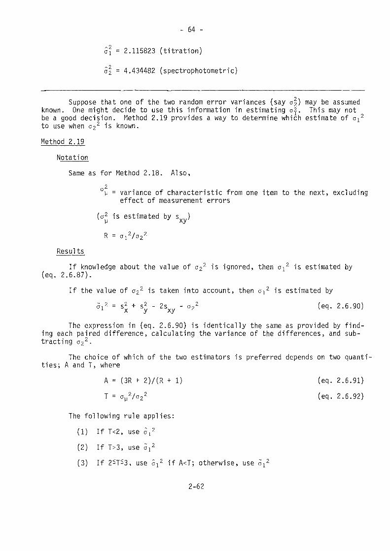
- 64 -

= 2.115823 (titration)

= 4.434482 (spectrophotometric)

Suppose that one of the two random error variances (say a|) may be assumedknown. One might decide to use this information in estimating a£. This may notbe a good decision. Method 2.19 provides a way to determine which estimate of c^2to use when a22 is known.Method 2.19

NotationSame as for Method 2.18. Also,

2°y = variance of characteristic from one item to the next, excludingeffect of measurement errors

(a2 is estimated by s }

R = QResults

If knowledge about the value of a22 is ignored, then o^2 is estimated by(eq. 2.6.87).

If the value of a22 is taken into account, then c^2 is estimated byÔ!2 = s2 + s2 - 2sxy - a22 (eq. 2.6.90)

The expression in (eq. 2.6.90) is identically the same as provided by find-ing each paired difference, calculating the variance of the differences, and sub-tracting cr22.

The choice of which of the two estimators is preferred depends on two quanti-ties; A and T, where

A = (3R + 2)/(R + 1) (eq. 2.6.91)T = a//a22 (eq. 2.6.92)

The following rule applies:(1) If T<2, use a!2

(2) If T>3, use ai2

(3) If 2*1*3, use 5}2 if A<T; otherwise, use aL2

2-62

- 65 -

BasisThe criterion for selecting one estimator over the other is the sampling

variance of each estimator. The estimator with the smaller variance is regardedas the better one. For details, see [2.16].Examples

EXAMPLE 2.19 (a)In Exa

tity a2, is no(eq. 2.6.92),

In Example 2.18 (a), suppose that a22 = 4.00 is a known quantity. The quan-xytity a2, is not known, but is replaced by its estimate, sxy = 1.317. Then, by

T = 1.317/4.00 = 0.33Since this is less than 2, use the estimator a]_2, i.e., ignore the know-

ledge about the value of a22.

Normally, one obtains information about systematic errors by measuring stan-dards, and not production items. However, by making certain assumptions, it ispossible to obtain estimates of systematic error variances from paired data also.In a sense, such estimates may be more realistic than those based on standardsdata.

Two key assumptions are made:(1) Both measurement methods are indeed applied to the same items, i.e.,

the item being measured in no way changes in true value after thefirst measurement is made.

(2) The systematic error or bias associated with each of the two mea-surement methods is a random variable with zero mean and variancethat is called the systematic error variance for that method.

With these assumptions kept in mind, Method 2.20 is now considered.Method 2.20

NotationSame as for Method 2.18. Also

x, y = average of the x.. and y. measurements respectivelyasi = systematic error variance for method I

== systematic error variance for method 2

2-63

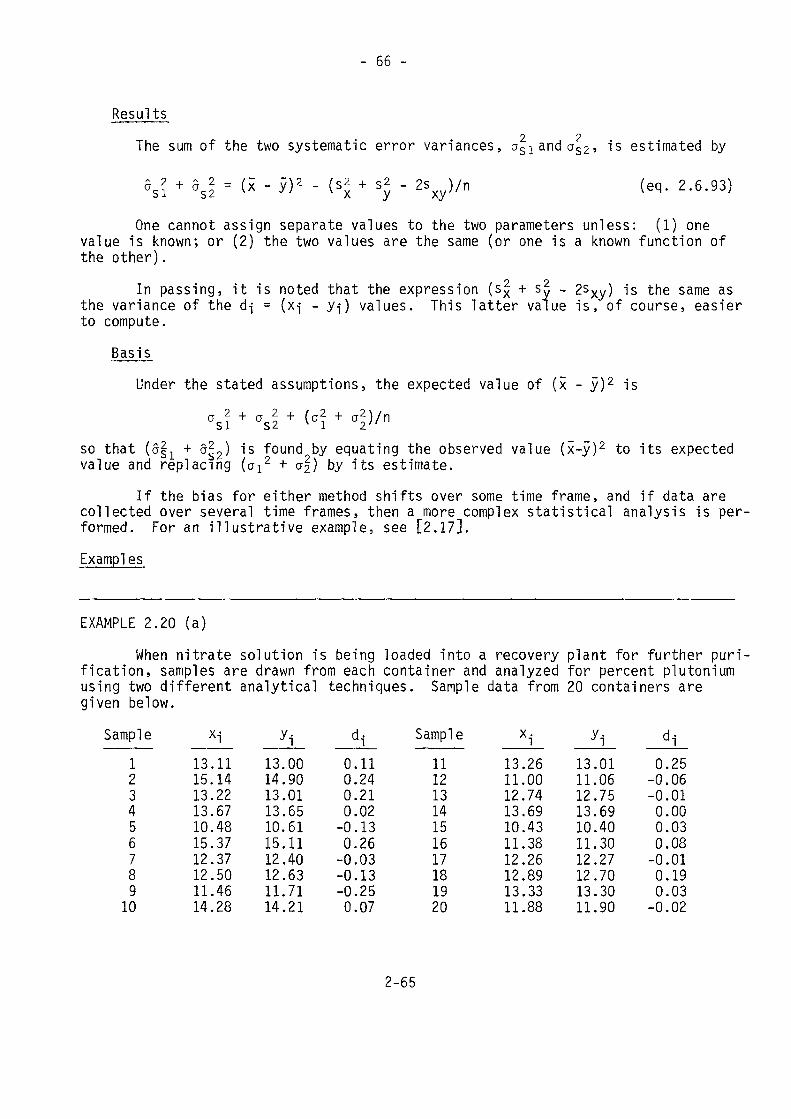
- 66 -

Results2 2The sum of the two systematic error variances, oslandas2, is estimated by

5s? + ÔS2 = (* ~ W ~ (sx + Sy " 2Sxy)/n (eq< 2'6-93)One cannot assign separate values to the two parameters unless: (1) one

value is known; or (2) the two values are the same (or one is a known function ofthe other).

In passing, it is noted that the expression (s2- + s| - 2sxy) is the same asthe variance of the d-j = (x^ - y-j) values. This latter value is, of course, easierto compute.

BasisUnder the stated assumptions, the expected value of (x - y)2 is

0S? + °S2 + K + CT2)/n

so that (o2 + 522) is found by equating the observed value (x-y)2 to its expectedvalue and replacing (ai2 + erf.) by its estimate.If the bias for either method shifts over some time frame, and if data are

collected over several time frames, then a more complex statistical analysis is per-formed. For an illustrative example, see [2.17].Examples

EXAMPLE 2.20 (a)When nitrate solution is being loaded into a recovery plant for further puri-fication, samples are drawn from each container and analyzed for percent plutonium

using two different analytical techniques. Sample data from 20 containers aregiven below.

Sample x-j yi di Sample xi yi d^1 13.11 13.00 0.11 11 13.26 13.01 0.252 15.14 14.90 0.24 12 11.00 11.06 -0.063 13.22 13.01 0.21 13 12.74 12.75 -0.014 13.67 13.65 0.02 14 13.69 13.69 0.005 10.48 10.61 -0.13 15 10.43 10.40 0.036 15.37 15.11 0.26 16 11.38 11.30 0.087 12.37 12.40 -0.03 17 12.26 12.27 -0.018 12.50 12.63 -0.13 18 12.89 12.70 0.199 11.46 11.71 -0.25 19 13.33 13.30 0.0310 14.28 14.21 0.07 20 11.88 11.90 -0.02

2-65

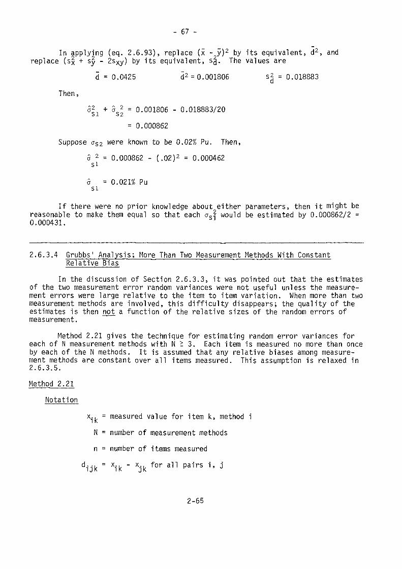
- 67 -

In applying (eq. 2.6.93), replace (x - y)2 by its equivalent, d2, andreplace (sx + Sy - 2sxy) by its equivalent, s|. The values are

d = 0.0425 d2 = 0.001806 s2 = 0.018883Then,

£2 + S.2 = 0.001806 - 0.018883/20o J, o 2-

= 0.000862Suppose aS2 were known to be 0.02% Pu. Then,

5 2 = 0.000862 - (,02)2 = 0.000462si0 = 0.021% Pusi

If there were no prior knowledge about either parameters, then it might bereasonable to make them equal so that each as2 would be estimated by 0.000862/2 =0.000431.

2.6.3.4 Grubbs' Analysis; More Than Two Measurement Methods With ConstantRelative Bias

In the discussion of Section 2.6.3.3, it was pointed out that the estimatesof the two measurement error random variances were not useful unless the measure-ment errors were large relative to the item to item variation. When more than twomeasurement methods are involved, this difficulty disappears; the quality of theestimates is then not, a function of the relative sizes of the random errors ofmeasurement.

Method 2.21 gives the technique for estimating random error variances foreach of N measurement methods with N > 3. Each item is measured no more than onceby each of the N methods. It is assumed that any relative biases among measure-ment methods are constant over all items measured. This assumption is relaxed in2.6.3.5.Method 2.21

Notationx., = measured value for item k, method iN = number of measurement methodsn = number of items measured

dijk= Xik - Xjk for a11 pairs *' J

2-65

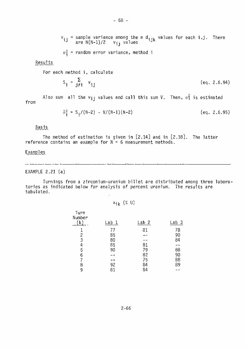
- 68 -

v.. = sample variance among the n d... values for each i,j. There1J are N(N-l)/2 v-j values 1JK

a? = random error variance, method iResults

For each method i, calculateS. = J. v... (eq. 2.6.94)

Also sum all the v-jj values and call this sum V. Then, v\ is estimatedfrom

5? = S^N-2) - V/(N-l)(N-2) (eq. 2.6.95)

BasisThe method of estimation is given in [2.14] and in [2.18]. The latter

reference contains an example for N = 6 measurement methods.Examples

EXAMPLE 2.21 (a)Turnings from a zirconium-uranium billet are distributed among three labora-

tories as indicated below for analysis of percent uranium. The results aretabulated.XT k (% U)

Lab 2 Lab 3Turn

Number(k)123456789

Lab 17785808590

9281

81----817982758484

789084--88908889--

2-66

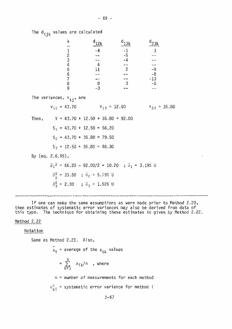
- 69 -

d!2k-4-_-_4

11_-_ _8

-3

d!3k-1-5-4--

2----3

--

d23k3

----_--9-8

-13-5__

The d.,, values are calculated

123456789

The variances, v.., are' J

v12 = 43.70 v13 = 12.50 v23 = 35.80

Then, V = 43.70 + 12.50 + 35.80 = 92.0051 = 43.70 + 12.50 = 56.2052 = 43.70 + 35.80 = 79.5053 = 12.50 + 35.80 = 48.30

By (eq. 2.6.95),Ô!2 = 56.20 - 92.00/2 = 10.20 ; al = 3.19% U$2 = 33.50 ; Ô2 = 5.79% Ual = 2.30 ; 53 = 1.52% U

If one can make the same assumptions as were made prior to Method 2.20,then estimates of systematic error variances may also be derived from data ofthis type. The technique for obtaining these estimates is given by Method 2.22.Method 2.22

NotationSame as Method 2.21. Also,

x- = average of the x-,. valuesl 1K

n= Z xik/n ' where

k=ln = number of measurements for each method

G2. - systematic error variance for method i2-67

- 70 -

Results

First, perform the calculations of Method 2.21 to obtain estimates of therandom error variances, o^. Then, the sum of the systematic error variances,is estimated by

S1

N£ 02Jr\ (eq. 2 .6 .96)

where s^- is the sample variance among the N x-j values.One cannot obtain separate estimates of the systematic error variances with-

out additional information. For example, one might be willing to assume that allsystematic error variances are the same, or are related to one another in some knownway.

Basis2 The result in (eq. 2.6.96) is based on the fact that the expected value of

Nsxi isN Ny 02. + f a2/n

(_. f c "1 f—^t i '

so thatNy^ ~2

i=l si

2is found by equating the expected value of Ns^-j to its observed value and replacingo? by its estimate for all i.Examples

EXAMPLE 2.22 (a)One cannot perform this analysis on the data of Example 2.21 (a) because it

is necessary that all measurement methods measure all items in order to obtain esti-mates of the systematic error variance. This assumption was not necessary when usingGrubbs' method to estimate random error variances.

EXAMPLE 2.22 (b)Percent plutonium analyses on sintered pellet samples are reported for 13

samples by four laboratories. Analyze the following data to find estimates of therandom error variances. Assume that all four laboratories have the same systematicerror variance and obtain its estimate.

2-68

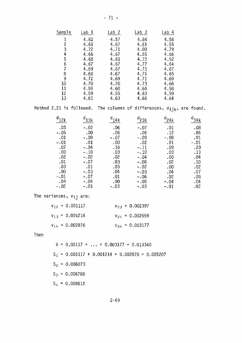
- 71 -

Sample Lab 112345678910111213

Method 2.21 isd!2k.05

-.06.01

-.01.07.00.02.01.03.00

-.01.04

-.02

4.624.614.724.664.684.674.694.684.724.704.594.594.61

followed.d!3k-.02.00

-.08.01

-.04-.10-.02-.07.01

-.03-.07-.04-.05

Lab 24.574.674.714.674.614.674.674.674.694.704.604.554.63

The columnsd!4k.06.06

-.07.00.16.03.02.03.03.04.01.00

-.03

Lab 3 Lab 44.644.614.804.654.724.774.714.754.714.734.664.634.66

of differences;d23k-.07.06

-.09.02

-.11-.10-.04-.08-.02-.03-.06-.08-.03

4.564.554.794.664.524.644.674.654.694.664.584.594.64' dijkd24k.01.12

-.08.01.09.03.00.02.00.04.02

-.04-.01

The variances, v- j j are:

Vi2 = 0.001117

v13 = 0.001214

v l t t = 0.002876

Then

V23 = 0.002397= 0.002559= 0.003177

V5152

= 0.00117 + ... + 0.003177 = 0.013340= 0.001117 + 0.001214 + 0.002876 = 0.005207= 0.006073= 0.006788= 0.008612

are found,J34k.08.06.01-.01.20.13.04.10.02.07.08.04.02

2-69

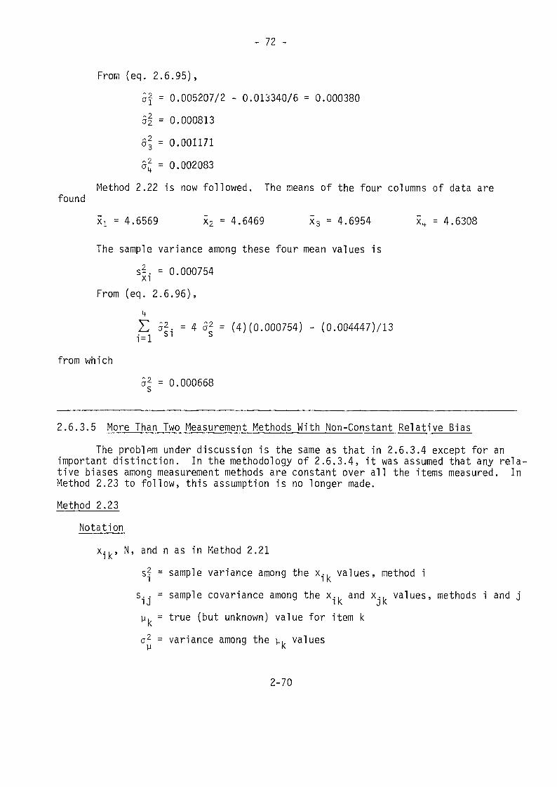
- 72 -

From (eq. 2.6.95),Ôf = 0.005207/2 - 0.013340/6 = 0.000380ai = 0.00081303 = 0.001171S2. = 0.002083

Method 2.22 is now followed. The means of the four columns of data arefound

x1 = 4.6569 x2 = 4.6469 x3 = 4.6954 xk = 4.6308

The sample variance among these four mean values iss|. = 0.000754

From (eq. 2.6.96),

E 52. = 4 S2 = (4)(0.000754) - (0.004447)/13• _ -i o I o

from which02 = 0.000668

2.6.3.5 More Than Two Measurement Methods_With Non-Constant Relative BiasThe problem under discussion is the same as that in 2.6.3.4 except for an

important distinction. In the methodology of 2.6.3.4, it was assumed that any rela-tive biases among measurement methods are constant over all the items measured. InMethod 2.23 to follow, this assumption is no longer made.Method 2.23

Notationx.. , N, and n as in Method 2.21l K

s? = sample variance among the x., values, method i1 IK

s.. = sample covariance among the x., and x., values, methods i and j1J l K J Ky. = true (but unknown) value for item k,2 =a2 = variance among the y, valuesu K

2-70

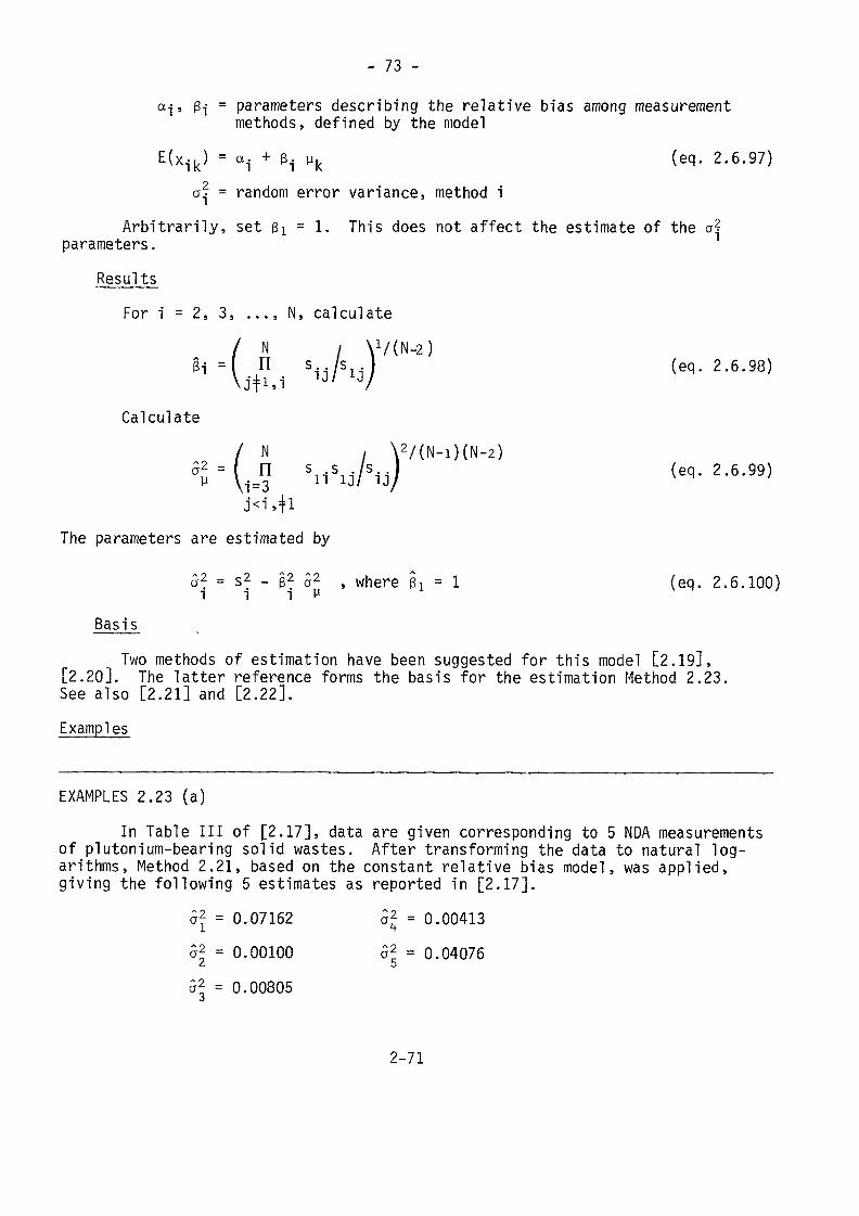
- 73 -

a-j , 3-j = parameters describing the relative bias among measurementmethods, defined by the model

E(xik) = a,. + ei yk (eq. 2.6.97)a2 = random error variance, method i

Arbitrarily, set ßL = 1. This does not affect the estimate of the a|parameters.

ResultsFor i = 2, 3, ..., N, calculate

/(N-2)(eq. 2.6.98)

Calculate

The parameters are estimated by2 - §2 52

Basis

/(N-i)(N-2) (eq- 2-6-99)

(eq> 2.6.100)

Two methods of estimation have been suggested for this model [2.19],[2.20]. The latter reference forms the basis for the estimation Method 2.23.See also [2.21] and [2.22].Examples

EXAMPLES 2.23 (a)In Table III of [2.17], data are given corresponding to 5 NDA measurementsof plutonium-bearing solid wastes. After transforming the data to natural log-

arithms, Method 2.21, based on the constant relative bias model, was applied,giving the following 5 estimates as reported in [2.17].52 = 0.07162£2 = 0.0010052 = 0.00805

= 0.00413= 0.04076

2-71

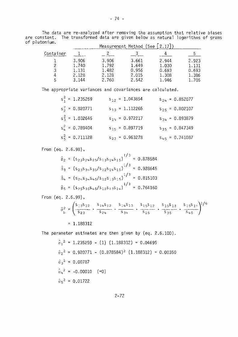
- 74 -

The data are re-analyzed after removing the assumption that relative biasesare constant. The transformed data are given below as natural logarithms of gramsof plutonium. Measurement Method (See [2.17])

Container12345

13.9061.7401.1312.1283.144

23.9061.7921.4822.1282.760

33.6611.6490.9562.0152.542

42.9441.0300.6931.3081.946

52.9231.1310.6931.3861.705

The appropriate variances and covariances are calculated.si = 1.235259 S12 = 1.043854 s2u = 0.852077s2 = 0.920771 s13 = 1.112266 s25 = 0.80210753 - 1.032645 su, = 0.972217 s34 = 0.893879s2 = 0.789404 s15 = 0.897719 S35 = 0.847349si = 0.711128 S23 = 0.963278 Sk5 = 0.741087

From (eq. 2 .6 .98) ,1/3

32 = (s23S2tS2 5 /s1 3s l l ts1 5) = 0.8785841/3

33 = ( S 2 3 S 3 4 S 3 5 / S l 2 S l ^ S 1 5 ) = 0.9286451/3

= (s2i ts3 i +s l t5/s12S1 3s15) = 0.8151031/3

= 0.764160

From (eq. 2 . 6 . 9 9 ) ,15S12 S15S13 S15S1M'

25 35

= 1.188312The parameter estimates are then given by (eq. 2.6.100).

Si2 = 1.235259 - (1) (1.188312) = 0.04695S22 = 0.920771 - (0.8785S4)2 (1.188312) = 0.00350532 = 0.00787V = -0.00010 (=0)552 = 0.01722

2-72

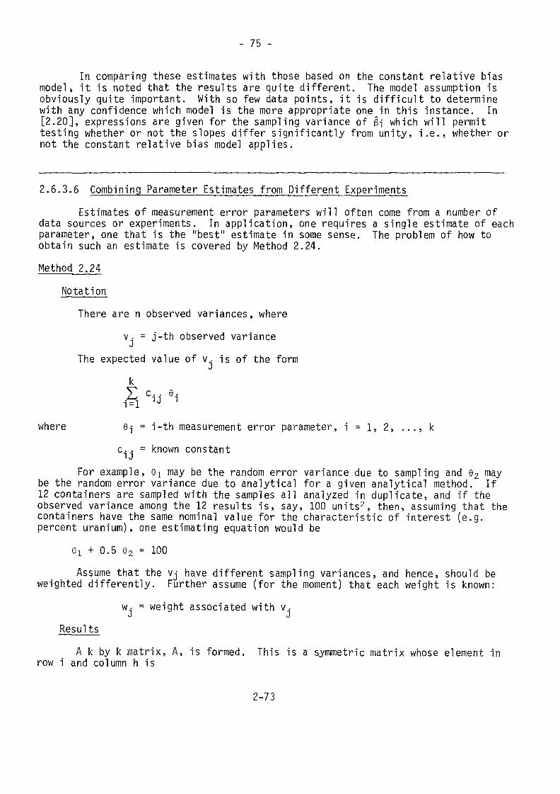
- 75 -

In comparing these estimates with those based on the constant relative biasmodel, it is noted that the results are quite different. The model assumption isobviously quite important. With so few data points, it is difficult to determinewith any confidence which model is the more appropriate one in this instance. In[2.20], expressions are given for the sampling variance of ßi which will permittesting whether or not the slopes differ significantly from unity, i.e., whether ornot the constant relative bias model applies.

2.6.3.6 Combining Parameter Estimates from Different ExperimentsEstimates of measurement error parameters will often come from a number of

data sources or experiments. In application, one requires a single estimate of eachparameter, one that is the "best" estimate in some sense. The problem of how toobtain such an estimate is covered by Method 2.24.Method 2.24

NotationThere are n observed variances, where

v. = j-th observed varianceJ

The expected value of v. is of the formJ

kE C. . 6.11 i1=1 1J 1

where e-j = i-th measurement error parameter, i = 1, 2, ..., kc.. = known constant

* \J

For example, QI may be the random error variance due to sampling and e2 maybe the random error variance due to analytical for a given analytical method. If12 containers are sampled with the samples all analyzed in duplicate, and if theobserved variance among the 12 results is, say, 100 units2, then, assuming that thecontainers have the same nominal value for the characteristic of interest (e.g.percent uranium), one estimating equation would be

0! + 0.5 e2 = 100Assume that the Vj have different sampling variances, and hence, should be

weighted differently. Further assume (for the moment) that each weight is known:w. = weight associated with v.j j

ResultsA k by k matrix, A, is formed. This is a symmetric matrix whose element inrow i and column h is

2-73

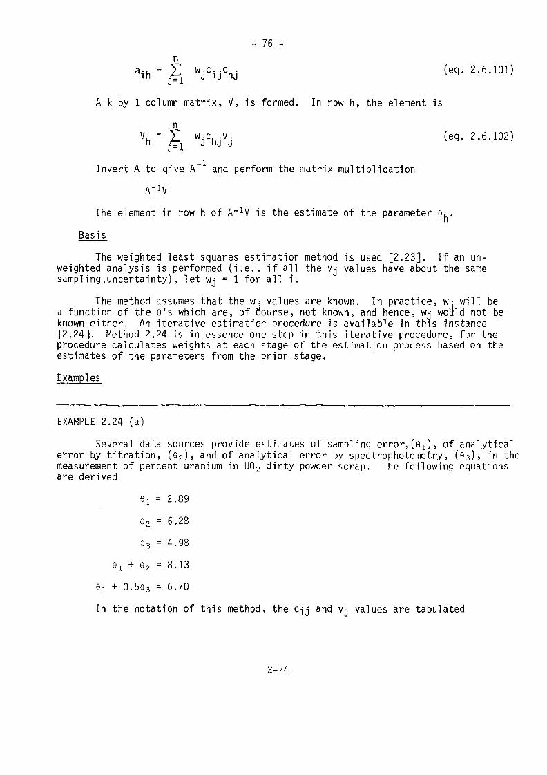
- 76 -

aih = Ç w j C i jch j (eq. 2.6.101)J -L

A k by 1 column matrix, V, is formed. In row h, the element is

V£ WJChjVj (eq. 2.6.102)j -^iInvert A to give A and perform the matrix multiplication

A"!VThe element in row h of A-1V is the estimate of the parameter e, .

BasisThe weighted least squares estimation method is used [2.23]. If an un-

weighted analysis is performed (i.e., if all the Vj values have about the samesampling .uncertainty), let Wj = 1 for all i.

The method assumes that the Wj values are known. In practice, W; will bea function of the e's which are, of course, not known, and hence, Wj would not beknown either. An iterative estimation procedure is available in this instance[2.24], Method 2.24 is in essence one step in this iterative procedure, for theprocedure calculates weights at each stage of the estimation process based on theestimates of the parameters from the prior stage.Examples

EXAMPLE 2.24 (a)Several data sources provide estimates of sampling error,(GJ), of analytical

error by titration, (e2), and of analytical error by spectrophotometry, (e3), in themeasurement of percent uranium in U02 dirty powder scrap. The following equationsare derived

Q! = 2.8902 = 6.2863 = 4.98

Ql + 02 = 8.13

0! + 0.563 = 6.70

In the notation of this method, the c-j j and Vj values are tabulated

2-74

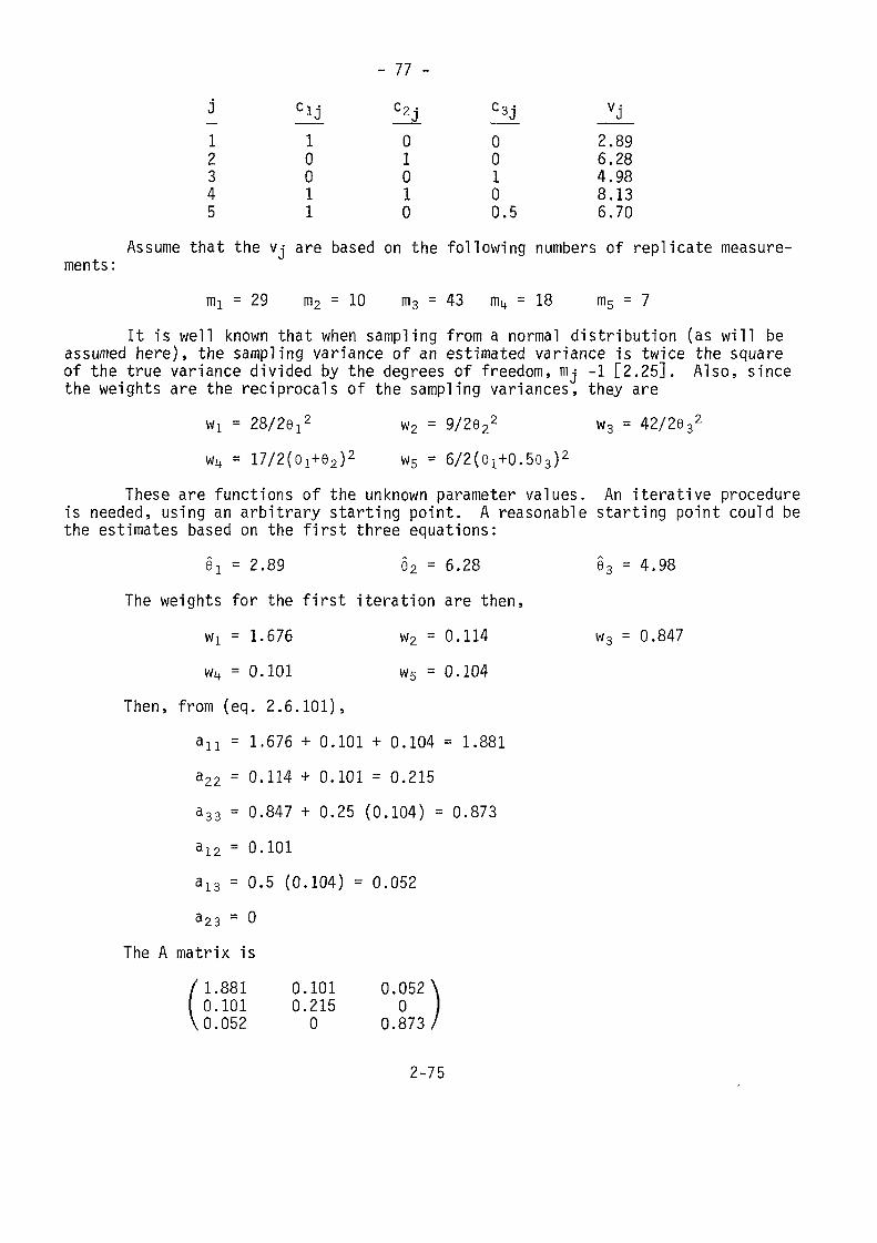
- 77 -c2j c3j Vj

12345

10011

01010

00100.5

2.896.284.988.136.70

Assume that the Vj are based on the following numbers of replicate measure-ments:mi =29 m2 = 10 m3 =43 mk = 18 m5 = 7

It is well known that when sampling from a normal distribution (as will beassumed here), the sampling variance of an estimated variance is twice the squareof the true variance divided by the degrees of freedom, mj -1 [2.25]. Also, sincethe weights are the reciprocals of the sampling variances, they are

W! = 28/2S!2 w2 = 9/2622 W3 = 42/2632

w4 = 17/2(e1+e2)2 w5 = 6/2(e1+o.5e3)2These are functions of the unknown parameter values. An iterative procedure

is needed, using an arbitrary starting point. A reasonable starting point could bethe estimates based on the first three equations:BI = 2.89 92 = 6.28 63 = 4.98

The weights for the first iteration are then,Wi = 1.676 w2 = 0.114 w3 = 0.847w^ = 0.101 ws = 0.104

Then, from (eq. 2.6.101),an = 1.676 + 0.101 + 0.104 = 1.881a22 = 0.114 + 0.101 = 0.215a33 = 0.847 + 0.25 (0.104) = 0.873a12 = 0.101a13 = 0.5 (0.104) = 0.052a23 = 0

The A matrix is/1.881 0.1010.101 0.215

X0.052 0

2-75

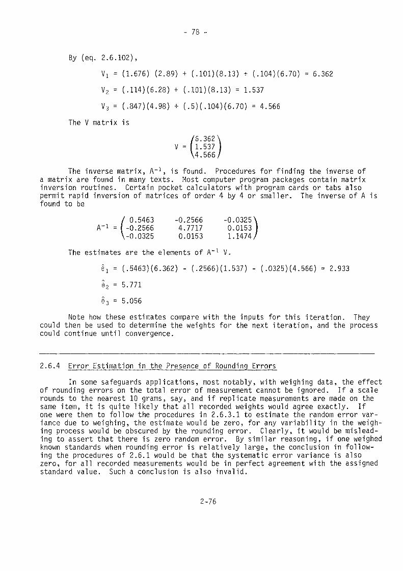
- 78 -

By (eq. 2.6.102),Vi - (1.676) (2.89) + (.101M8.13) + (.104)(6.70) - 6.362V2 - (.114)(6.28) + (.101)(8.13) = 1.537V3 = (.847)(4.98) + (.5)(.104)(6.70) = 4.566

The V matrix is/6.362\

V - 1.537\4.566/

The inverse matrix, A"1, is found. Procedures for finding the inverse ofa matrix are found in many texts. Most computer program packages contain matrixinversion routines. Certain pocket calculators with program cards or tabs alsopermit rapid inversion of matrices of order 4 by 4 or smaller. The inverse of A isfound to be

/ 0.5463A'1 - -0.2566

V-0.0325-0.25664.77170.0153

-0.0325X0.01531.1474/

The estimates are the elements of A"1 V.ej = (.5463)(6.362) - (.2566)(1.537) - ( .0325)(4.566) = 2.933Qz = 5.771§3 = 5.056

Note how these estimates compare with the inputs for this iteration. Theycould then be used to determine the weights for the next iteration, and the processcould continue until convergence.

2.6.4 Error Estimation jn the Presence of Rounding ErrorsIn some safeguards applications, most notably, with weighing data, the effect

of rounding errors on the total error of measurement cannot be ignored. If a scalerounds to the nearest 10 grams, say, and if replicate measurements are made on thesame item, it is quite likely that all recorded weights would agree exactly. Ifone were then to follow the procedures in 2.6.3.1 to estimate the random error var-iance due to weighing, the estimate would be zero, for any variability in the weigh-ing process would be obscured by the rounding error. Clearly, it would be mislead-ing to assert that there is zero random error. By similar reasoning, if one weighedknown standards when rounding error is relatively large, the conclusion in follow-ing the procedures of 2.6.1 would be that the systematic error variance is alsozero, for all recorded measurements would be in perfect agreement with the assignedstandard value. Such a conclusion is also invalid.

2-76

- 79 -

By statistical theory based on the uniform or rectangular distribution,for a measurement process in which data are rounded to the nearest u units, thesystematic error standard deviation can be no smaller than u/Via units. The sameis true of the random error standard deviation for a single weighing [2.26].

If rounding error is not the sole error, but is nevertheless too large tobe ignored, e.g., if the measurement data fall into 2 or 3 groups, then an itera-tive method of obtaining the estimates of the parameters has been developed. Themethodology is beyond the scope of this Volume, but the model and estimation pro-cedure are referenced [2.27]. The computer program based on this estimation methodis in the Agency library. It is recommended that the method be used whenever mea-surement data are grouped in 2 or 3 cells because of rounding.

2.6.5 Inter!aboratory Test DataIn many Agency safeguards applications, more than one analytical laboratory

is involved in some way. Most notably, this occurs whenever inter!aboratory sam-ple exchange or "round robin" programs are instigated in order to obtain informationon measurement error parameters. Another instance in which such data are generatedis whenever inspection samples are sent to more than one laboratory for analysis.

In the sections to follow, the analyses of inter!aboratory data are consi-dered. In 2.6.5.1, samples of a single standard reference material are sent toa number of laboratories in a round robin exercise. In 2.6.5.2, non-standardmaterials are distributed to a number of laboratories for analysis. Section 2.6.5.3considers the same problem, but it is now assumed that random errors of measure-ment may be laboratory dependent. The distribution of inspection samples to anumber of laboratories with different specified patterns of distribution is dis-cussed in 2.6.5.4.2.6.5.1 Single Standard Reference Material

The purpose of an exercise in which samples of single standard referencematerial are sent to participating laboratories is to identify factors that contri-bute to the uncertainty of a measured value, and assess their importance. To ac-complish this, it is necessary that detailed instructions be sent the laboratoriesrelative to how the samples should be measured. That is, one might be interestedin obtaining estimates of differences due to replicate measurements of aliquots,differences among aliquots, etc. To obtain such estimates, it is necessary thatthe analyses be performed according to some plan.

The statistical analysis of the data resulting from such an exercise iscalled a nested or hierarchal analysis of variance with the plan or experimentaldesign called a genera! unbalanced nested design. To permit a simpler presentationof the analysis, it will be assumed in Method 2.25 that there are 4 identifiedvariance components to be estimated, and the example will specify the 4 componentsin question. It should be readily apparent from the analysis of Method 2.25 howthe procedures should be altered to account for fewer or more than 4 components.Further, the 4 variance components identified in the example can, of course, bereplaced by other components.

2-77

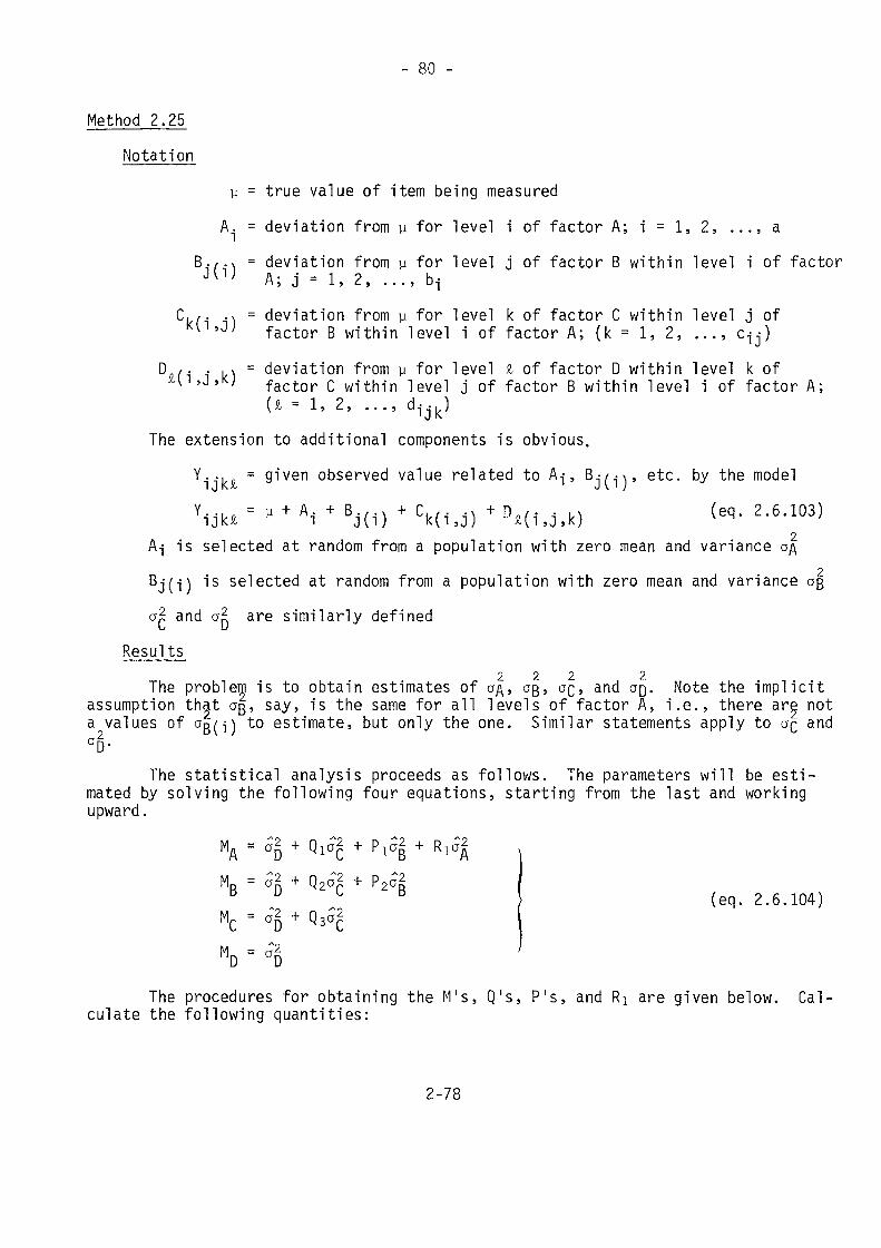
- 80 -

Method 2.25Notation

u = true value of item being measuredA. = deviation from u for level i of factor A; i = 1, 2, ..., a/.\ = deviation from p for level j of factor B within level i of factorv'/ A • 1=1 ? h •M , j - i, c. , . . . , D

. ,. .U'J= deviation from y for level k of factor C within level j offactor B within level i of factor A; (k = 1, 2, ..., c-)

D /. . ,v = deviation from y for level £ of factor D within level k ofMI,J,K; factor C within level j of factor B within level i of factor A;U = 1 , 2 , ...,d1jk)

The extension to additional components is obvious.Y.., = given observed value related to A-j, BJ(J)> etc. by the model

A-j is selected at random from a population with zero mean and variance a/\2Bj(-j) is selected at random from a population with zero mean and variance ag

a2 and a^ are similarly definedResults

2 2 2 2The problem is to obtain estimates of o/\, aß, OQ, and OQ. Note the implicitassumption that ag, say, is the same for all levels of factor A, i.e., there are nota values of og/j) to estimate, but only the one. Similar statements apply to OQ anda§.

The statistical analysis proceeds as follows. The parameters will be esti-mated by solving the following four equations, starting from the last and workingupward.

(eq. 2.6.104)

The procedures for obtaining the M's, Q's, P's, andculate the following quantities:

are given below. Cal-

2-78

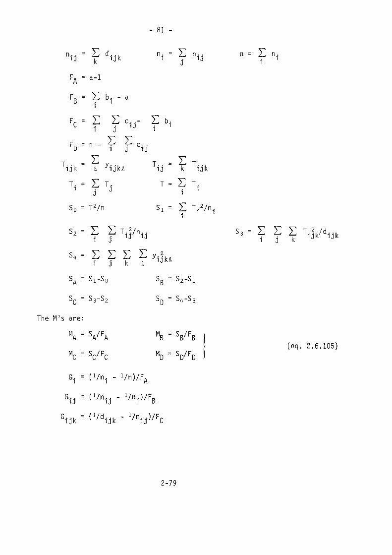
- 81 -

= E d,.ijk "i • n = E n

F = a-1

F =

F - E E Clj E b

T i j k ijk£ - - C T . .ij k ij..,ijk

So = T2/n

S2 = E

Si = E T1Vn1

= E E E y *

SR - S2-Si

- 83-82

s3 - E E E Mk/di j k 1Jk 1Jk

The M's are:

MA = SA/FA

MC = VFC

= SB/FB(eq. 2.6.105)

Gi = (Vn i - Vn)/FA

Gij -

2-79

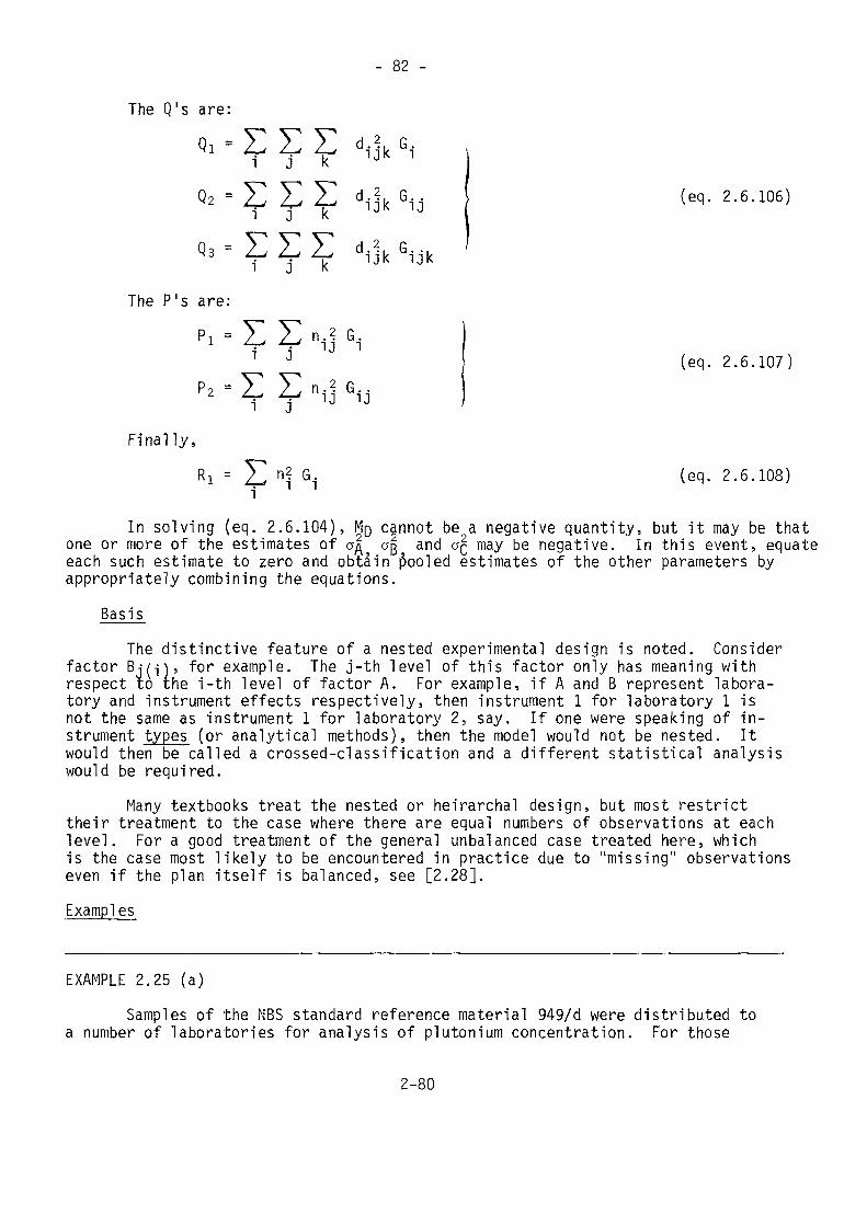
- 82 -

The Q's are:

QI = E E Z d,2i j k

Z v~^2^ EkQs = E E ZJ

The P's are:PI = L Ei jP2 - E E

ijk Gi

Finally,Ri = V n? G.4 - ^ - i i

«m'ijk Gijk

(eq. 2.6.106)

* G1J(eq. 2.6.107)

(eq. 2.6.108)

In solving (eq. 2.6.104), MD cannot be a negative quantity, but it may be thatone or more of the estimates of a^ a§9 and OQ may be negative. In this event, equateeach such estimate to zero and obtain pooled estimates of the other parameters byappropriately combining the equations.

BasisThe distinctive feature of a nested experimental design is noted. Consider

factor Bj(-j), for example. The j-th level of this factor only has meaning withrespect to the i-th level of factor A. For example, if A and B represent labora-tory and instrument effects respectively, then instrument 1 for laboratory 1 isnot the same as instrument 1 for laboratory 2, say. If one were speaking of in-strument types (or analytical methods), then the model would not be nested. Itwould then be called a crossed-classification and a different statistical analysiswould be required.

Many textbooks treat the nested or heirarchal design, but most restricttheir treatment to the case where there are equal numbers of observations at eachlevel. For a good treatment of the general unbalanced case treated here, whichis the case most likely to be encountered in practice due to "missing" observationseven if the plan itself is balanced, see [2.28].Examples

EXAMPLE 2.25 (a)Samples of the NBS standard reference material 949/d were distributed to

a number of laboratories for analysis of plutonium concentration. For those

2-80

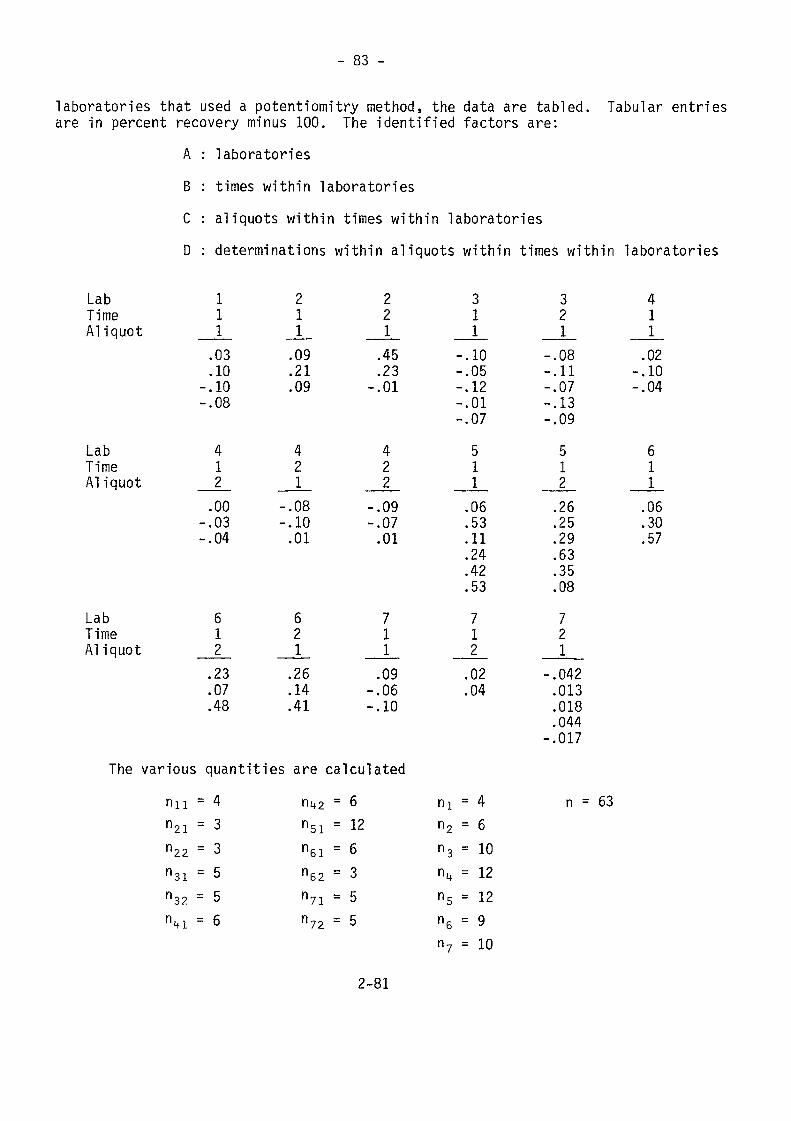
- 83 -

laboratories that used a potentiomitry method, the data are tabled. Tabular entriesare in percent recovery minus 100. The identified factors are:

A : laboratoriesB : times within laboratoriesC : aliquots within times within laboratoriesD : determinations within aliquots within times within laboratories

LabTimeAliquot

LabTimeAliquot

LabTimeAliquot

111.03.10

-.10-.08

412.00

-.03-.04

612.23.07.48

211.09.21.09

421

-.08-.10.01

621.26.14.41

221.45.23

-.01

422

-.09-.07.01

711.09

-.06-.10

311

-.10-.05-.12-.01-.07511.06.53.11.24.42.53712.02.04

321

-.08-.11-.07-.13-.09512.26.25.29.63.35.08721

-.042.013.018.044

-.017

411.02

-.10-.04

611.06.30.57

The various quantities are calculatednu = 4 n if 2 = 6 ni = 4 n = 63n21 =3 n51 = 12 n2 = 6r>22 = 3 n61 = 6 "3 = 10n31 =5 n62 = 3 n^ = 12n32 =5 n71 = 5 n5 = 12nkl =6 n?2 = 5 n6 = 9

n7 = 10

2-81

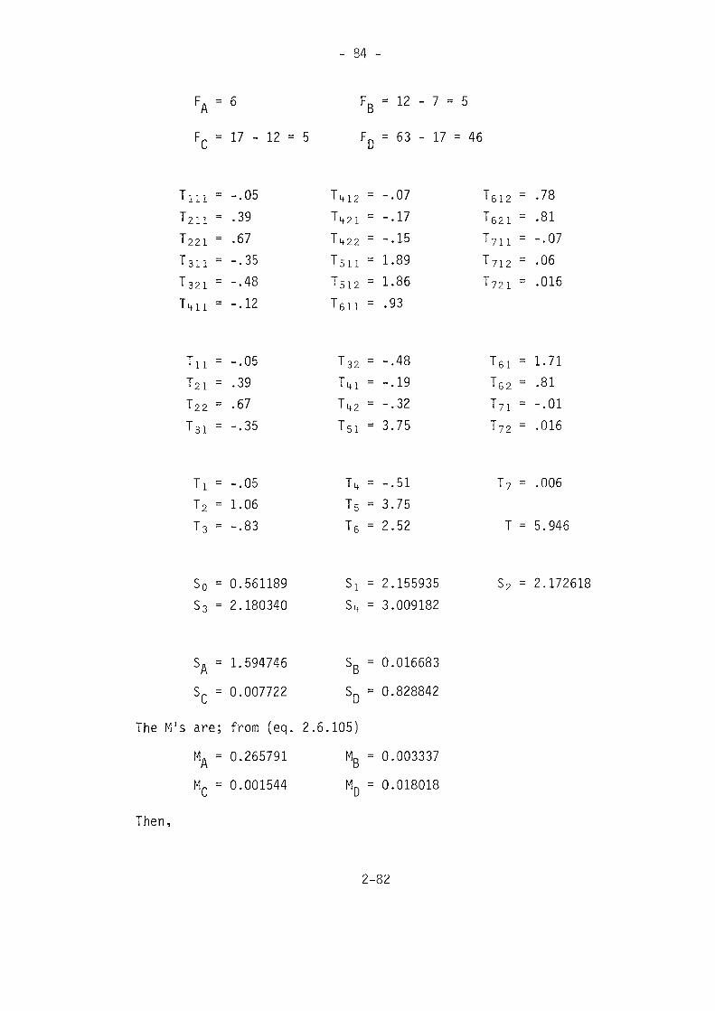
- 84 -

Fn = 12 - 7 = 5

FC = 17 - 12 = 5 FD = 63 - 17 = 46

Tin =T211 =

T221 =

T311 =

Ts2 i ~T 4 11 ~

TII =T21 =T22 =

T3i =

TI -T2 =T3 =

-.05.39.67-.35-.48-.12

-.05.39.67-.35

-.051.06-.83

T412 = -.07T421 = -.17Tit22 = --15TSU = 1.89T512 = 1.86T 6 i i = .93

T32 = -.48Tm = -.19T42 = -.32TSI = 3.75

T^ = -.51T5 = 3.75T6 = 2.52

T 6 1 2 - .78T6 2 1 - .81T711 = -.07T7 1 2 = .06T7 2 1 - .016

T6i - 1.71T62 = .81T71 - -.01T72 - .016

T7 - .006

T = 5.946

S0 = 0.561189S3 = 2.180340

Si = 2.155935= 3.009182

S2 = 2.172618

SA - 1.594746Sc = 0.007722 SD =

The M's are; from (eq. 2.6.105)MA = 0.265791MC = 0.001544

Then,

'B^D

0.0166830.828842

0.0033370.018018

2-82

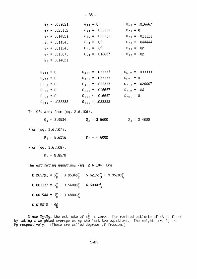
- 85 -

GI =G2 =G3 =G4 =G5 =G6 =G7 =

GUI ~6211 =6221 =

Gall =

6321 =

Git u =

.039021

.025132

.014021

.011243

.011243

.015873

.014021

00000.033333

Gil =G2i =G22 =

GSI =G 32 =

Giti =

Git 12 ~Git21 =

Git22 =G511 =

G512 =

Geil =

0.033333.033333.02.02.016667

.033333

.033333

.033333

.016667

.016667

.033333

Git 2GSIG6iG62G71

G72

Gei2G621GyiiG?12G721

= .016667= 0= .011111= .044444= .02= .02

= .033333- 0= .026667= .06= 0

The Q's are; from (eq. 2.6.106),Q! = 3.9534 Q2 = 3.5600

P2 = 4.6000

Q3 = 3.4800

From (eq. 2.6.107),P! = 5.6216

From (eq. 2.6.108),RI = 8.8570

The estimating equations (eq. 2.6.104) are

0.265791 = ôg + 3.9534$2 + 5.6216ô| + 8.85700

0.003337 = 4.6000ag

0.001544 =

0.018018 = ag

2 2Since MQ<MD, the estimate of QQ is zero. The revised estimate of OQ is foundby taking a weighted average using the last two equations. The weights are FC andFD respectively. (These are called degrees of freedom.)

2-83

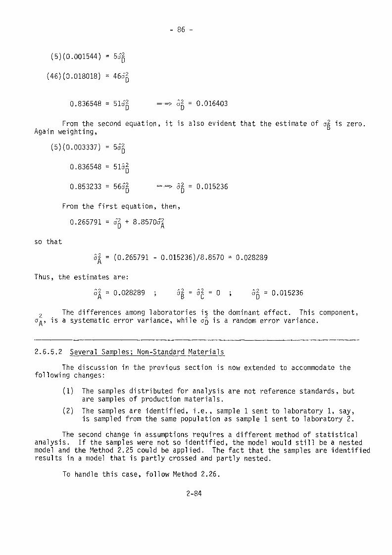
(5)(0.001544) =

(46)(0.018018) = 46ô2

0.836548 = 5 lag ——> ag - 0.016403

From the second equation, it is also evident that the estimate of a2, is zero,Again weighting,

(5)(0.003337) = Sag

0.836548 = 5152

0.853233 = 56o2 =^> 52 = 0.015236

From the first equation, then,0.265791 = a2, + 8.8570a2

so that02 = (0.265791 - 0.015236)78.8570 = 0.028289

Thus, the estimates are:a| - 0.028289 ; a2. - 5£ = Q . -2 = Q.015236

2 The differences among laboratories i| the dominant effect. This component,a, is a systematic error variance, while ap is a random error variance.

2.6 .5 .2 Several Samples; Non-Standard Mater ia ls

The discussion in the previous section is now extended to accommodate thefollowing changes:

(1) The samples distributed for analysis are not reference standards, butare samples of production materials.

(2) The samples are identified, i.e., sample 1 sent to laboratory 1, say,is sampled from the same population as sample 1 sent to laboratory 2.

The second change in assumptions requires a different method of statisticalanalysis. If the samples were not so identified, the model would still be a nestedmodel and the Method 2.25 could be applied. The fact that the samples are identifiedresults in a model that is partly crossed and partly nested.

To handle this case, follow Method 2.26.

2-84

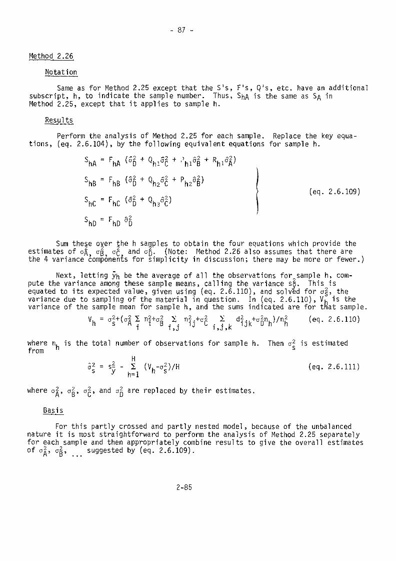
- 87 -

Method 2.26Notation

Same as for Method 2.25 except that the S's, F's, Q's, etc. have an additionalsubscript, h, to indicate the sample number. Thus, SnA is the same as S/\ inMethod 2.25, except that it applies to sample h.

ResultsPerform the analysis of Method 2.25 for each sample. Replace the key equa-

tions, (eq. 2.6.104), by the following equivalent equations for sample h.ShA = FhA <*g + V? + Vï + Rhi^ShB = FhBShC = FhC (5

ShD = FhD aD

(eq. 2.6.109)

Sum these over the h samples to obtain the four equations which provide theestimates of a/\, OB, °C an^ °D- (Note: Method 2.26 also assumes that there arethe 4 variance components for simplicity in discussion; there may be more or fewer.)

Next, letting yn be the average of all the observations for sample h, com-pute the variance among these sample means, calling the variance s|. This isequated to its expected value, given using (eq. 2.6.110), and solved for a|, thevariance due to sampling of the material in question. In (eq. 2.6.110), Vu is thevariance of the sample mean for sample h, and the sums indicated are for that sample,

)/n2 (eq. 2.6.110)II 3 n . l D . • IJ ^ ,• -j I, IJ I ^ u l' NI I ,J I ,J »K

where n, is the total number of observations for sample h. Then a2 is estimatedfrom h s

HS2 = s| - I (V.-a2)/H (eq. 2.6.111)s Y n=1 n s

where a?, a2,, ai, and a2 are replaced by their estimates.M D L » uBasis

For this partly crossed and partly nested model, because of the unbalancednature it is most straightforward to perform the analysis of Method 2.25 separatelyfor each sample and then appropriately combine results to give the overall estimatesof a|, a2,, suggested by (eq. 2.6.109).

2-85

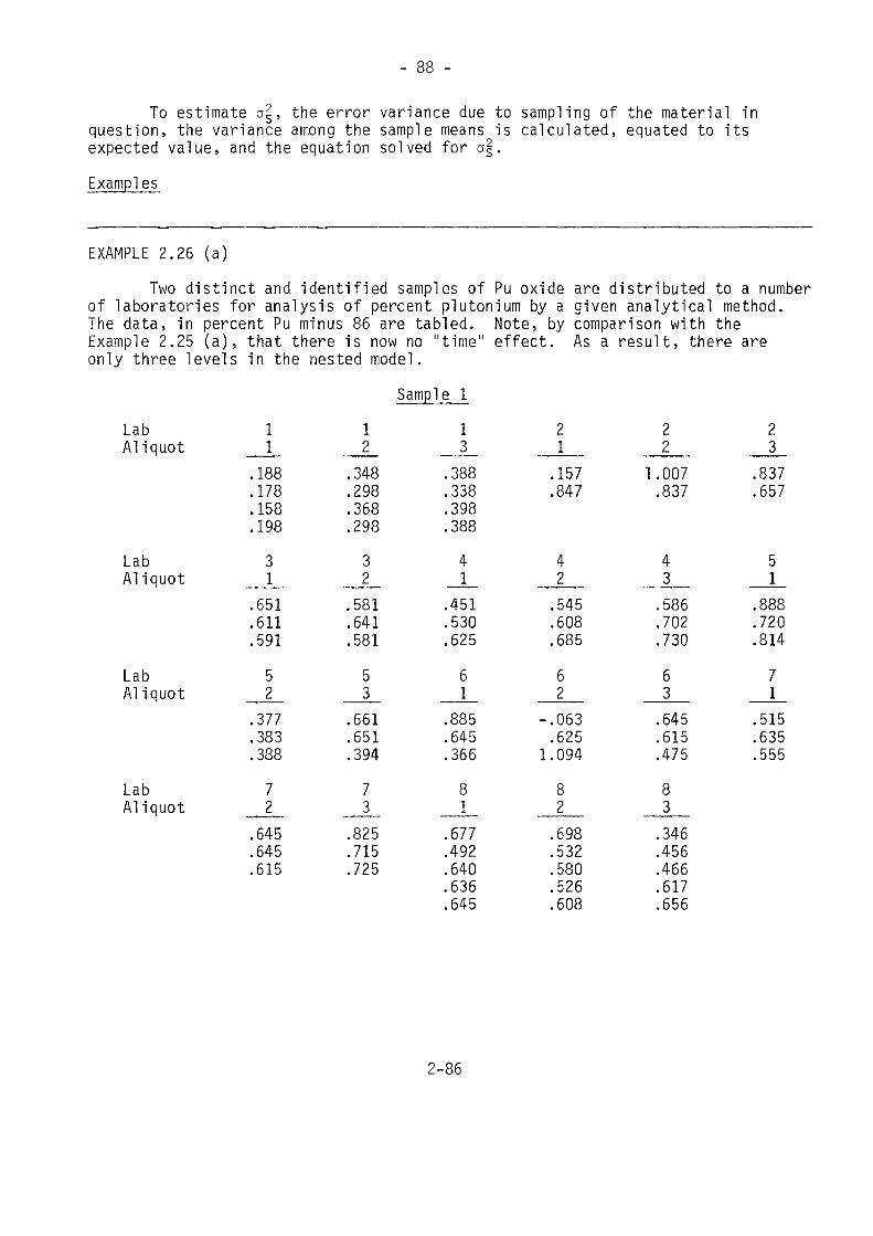
To estimate a|, the error variance due to sampling of the material inquestion, the variance among the sample means is calculated, equated to itsexpected value, and the equation solved for a|.Examples

EXAMPLE 2.26 (a)Two distinct and identified samples of Pu oxide are distributed to a number

of laboratories for analysis of percent plutonium by a given analytical method.The data, in percent Pu minus 86 are tabled. Note, by comparison with theExample 2.25 (a), that there is now no "time" effect. As a result, there areonly three levels in the nested model.

LabAliquot

LabAliquot

LabAliquot

LabAliquot

188178158198

.651

.611

.59152

.377

.383

.38872

.645

.645

.615

12

.348

.298

.368

.29832

.581

.641

.58153

.661

.651

.39473

.825

.715

.725

Sample 113

.388

.338

.398

.38841

.451

.530

.625

.885

.645

.36681

.677

.492

.640

.636

.645

21.157.847

42.545.608.68562

-.063.625

1.094

.698

.532

.580

.526

.608

22

1.007.837

43.586.702.7306J_.645.615.47583.346.456.466.617.656

23

.837

.657

51

.888

.720

.814

.515

.635

.555

2-86

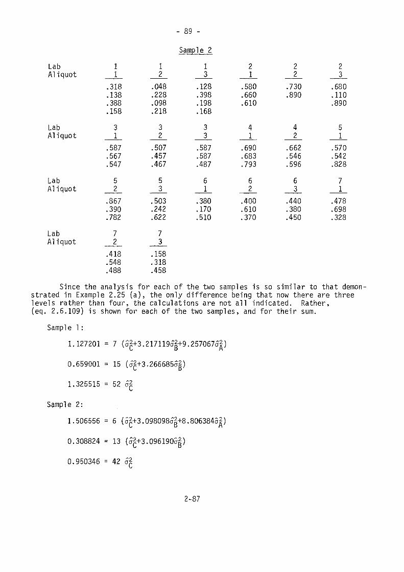
- 89 -

LabAliquot

12

Sample 2l3

2l

22

23

LabAliquot

LabAI iquot

LabAIiquot

.318

.138388158

.587

.567

.54752

.867

.390

.782

.418

.548

.488

.048

.228

.098

.21832

.507

.457

.46753

.503

.242

.62273

.158

.318

.458

.128

.398

.198

.16833

.587

.587

.487

.380

.170

.510

.580

.660

.610

4l

.690

.683

.79362

.400

.610

.370

.730

.890

42

.662

.546

.59663

.440

.380

.450

.680

.110

.890

5l

.570

.542

.828

.478

.698

.328

Since the analysis for each of the two samples is so similar to that demon-strated in Example 2.25 (a), the only difference being that now there are threelevels rather than four, the calculations are not all indicated. Rather,(eq. 2.6.109) is shown for each of the two samples, and for their sum.

Sample 1 :1.127201 = 7 ($2+3.217119a2+9.257067a2)

0.659001 = 15 (52+3.26668552)

1.325515 = 52 6*

Sample 2:1.506556

0.308824

0.950346

6 (02+3.09809802+8.80638452)

13 (52+3.09619052,)

42 5

2-87

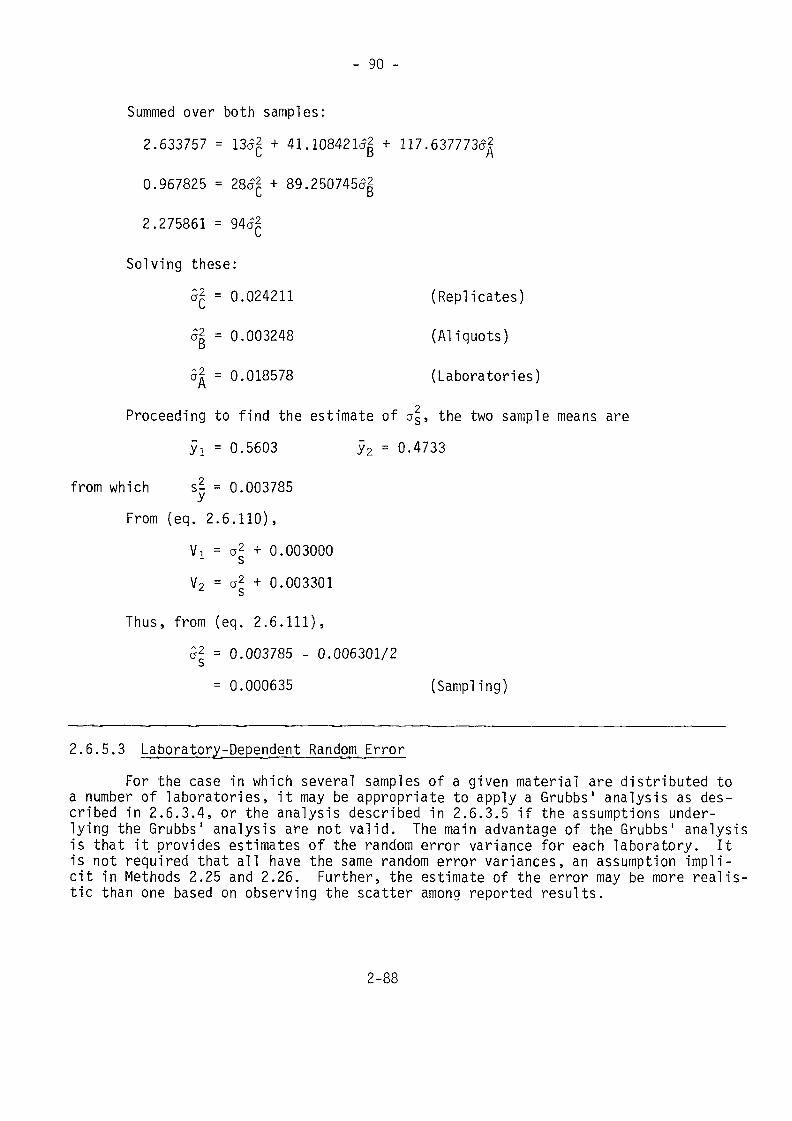
- 90 -

Summed over both samples:2.633757 = 13Ô2. + 41.108421ÔJ* + 117.637773a|

0.967825 = 28<j2 + 89.25074552

2.275861 = 94e?2,

Solving these:

5£ = 0.024211 (Repl ica tes )

Ô2, = 0.003248 (A l iquo t s )

ojj = 0.018578 (Laboratories)

Proceeding to find the estimate of 05, the two sample means areyi = 0.5603 y2 = 0.4733

from which s- = 0.003785From (eq. 2.6.110),

Vi = a2 + 0.003000V2 = a2 + 0.003301

Thus, from (eq. 2.6.111),a* - 0.003785 - 0.006301/2

= 0.000635 (Sampling)

2.6.5.3 Lgboratory^-Dependent Random ErrorFor the case in which several samples of a given material are distributed to

a number of laboratories, it may be appropriate to apply a Grubbs1 analysis as des-cribed in 2.6.3.4, or the analysis described in 2.6.3.5 if the assumptions under-lying the Grubbs1 analysis are not valid. The main advantage of the Grubbs1 analysisis that it provides estimates of the random error variance for each laboratory. Itis not required that all have the same random error variances, an assumption impli-cit in Methods 2.25 and 2.26. Further, the estimate of the error may be more realis-tic than one based on observing the scatter among reported results.

2-88

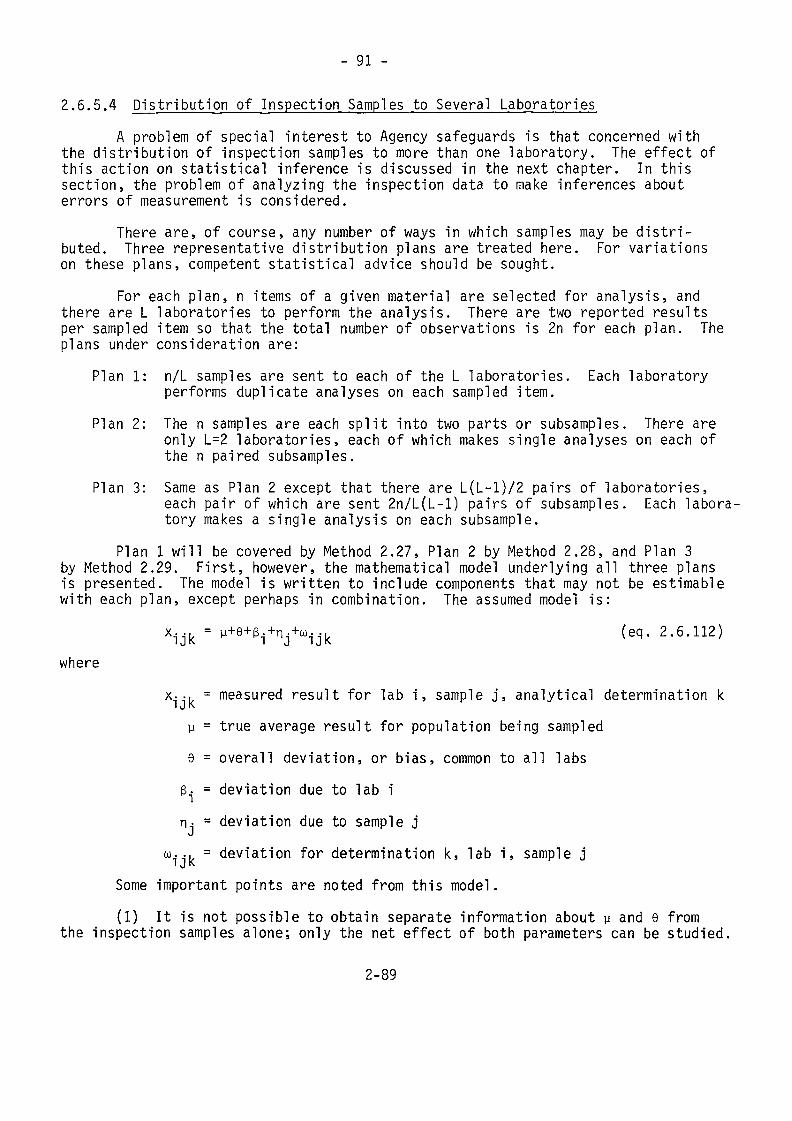
- 91 -

2.6.5.4 Distribution of Inspection Samples to Several LaboratoriesA problem of special interest to Agency safeguards is that concerned with

the distribution of inspection samples to more than one laboratory. The effect ofthis action on statistical inference is discussed in the next chapter. In thissection, the problem of analyzing the inspection data to make inferences abouterrors of measurement is considered.

There are, of course, any number of ways in which samples may be distri-buted. Three representative distribution plans are treated here. For variationson these plans, competent statistical advice should be sought.

For each plan, n items of a given material are selected for analysis, andthere are L laboratories to perform the analysis. There are two reported resultsper sampled item so that the total number of observations is 2n for each plan. Theplans under consideration are:

Plan 1: n/L samples are sent to each of the L laboratories. Each laboratoryperforms duplicate analyses on each sampled item.

Plan 2: The n samples are each split into two parts or subsamples. There areonly L=2 laboratories, each of which makes single analyses on each ofthe n paired subsamples.

Plan 3: Same as Plan 2 except that there are L(L-l)/2 pairs of laboratories,each pair of which are sent 2n/L(L-l) pairs of subsamples. Each labora-tory makes a single analysis on each subsample.

Plan 1 will be covered by Method 2.27, Plan 2 by Method 2.28, and Plan 3by Method 2.29. First, however, the mathematical model underlying all three plansis presented. The model is written to include components that may not be estimablewith each plan, except perhaps in combination. The assumed model is:

wherex... = measured result for lab i, sample j, analytical determination kl J K

y = true average result for population being samplede = overall deviation, or bias, common to all labs

ß. = deviation due to lab in.: = deviation due to sample jJ

wiik = devi'atl'ori f°r determination k, lab i, sample jSome important points are noted from this model.(1) It is not possible to obtain separate information about y and e fromthe inspection samples alone; only the net effect of both parameters can be studied.

2-89

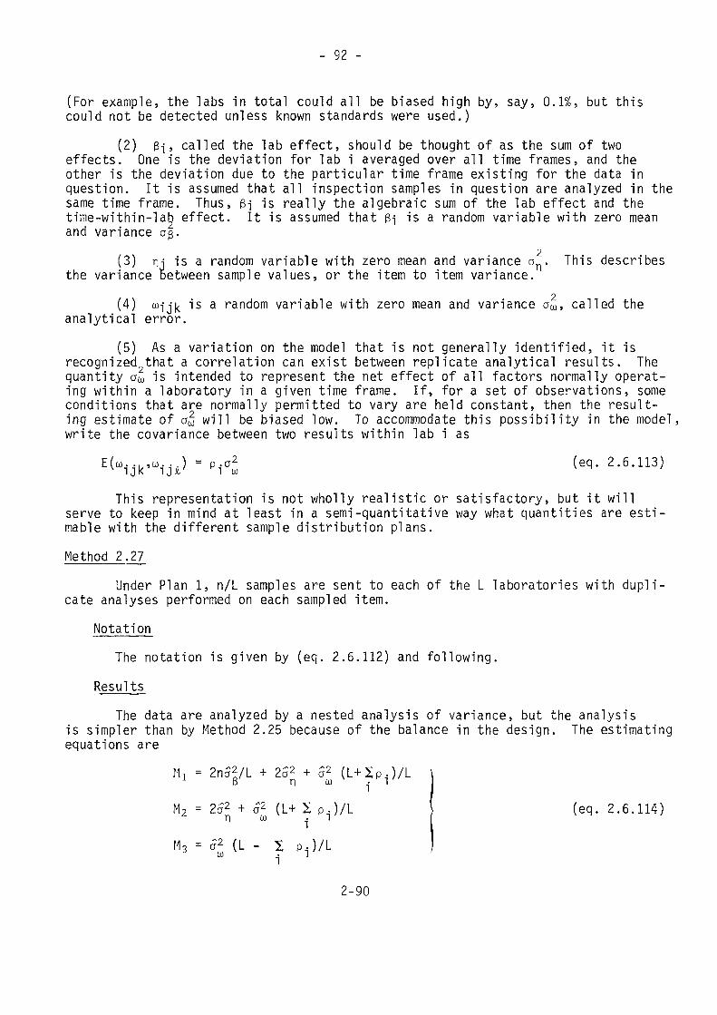
- 92 -

(For example, the labs in total could all be biased high by, say, 0.1%, but thiscould not be detected unless known standards were used.)

(2) 3-j, called the lab effect, should be thought of as the sum of twoeffects. One is the deviation for lab i averaged over all time frames, and theother is the deviation due to the particular time frame existing for the data inquestion. It is assumed that all inspection samples in question are analyzed in thesame time frame. Thus, ßj is really the algebraic sum of the lab effect and thetime-within-lab effect. It is assumed that ß-j is a random variable with zero meanand variance og.

2(3) nj is a random variable with zero mean and variance on- This describesthe variance between sample values, or the item to item variance.

(4) cojjk is a random variable with zero mean and variance a^, called theanalytical error.

(5) As a variation on the model that is not generally identified, it isrecognized that a correlation can exist between replicate analytical results. Thequantity aw is intended to represent the net effect of all factors normally operat-ing within a laboratory in a given time frame. If, for a set of observations, someconditions that are normally permitted to vary are held constant, then the result-ing estimate of a^ will be biased low. To accommodate this possibility in the model,write the covariance between two results within lab i as

- 2'6-113'This representation is not wholly realistic or satisfactory, but it will

serve to keep in mind at least in a semi-quantitative way what quantities are esti-mable with the different sample distribution plans.Method 2.27

Under Plan 1, n/L samples are sent to each of the L laboratories with dupli-cate analyses performed on each sampled item.

NotationThe notation is given by (eq. 2.6.112) and following.

ResultsThe data are analyzed by a nested analysis of variance, but the analysis

is simpler than by Method 2.25 because of the balance in the design. The estimatingequations are

M! = 2na2/L + 252 + S2 (L+2P.)/Lp ri u • i

M2 = 2a2 + a2 (L+ 2 p.}/l

(L - 2 P^/L

(eq. 2.6.114)

2-90

- 93 -

The M1 s are calculated from the data as follows. Calculate

S0 = T2/2n Sj = L 2 T?/2n

S2 = 2 2 Q . 2 / 2 S3 = 2 2 2x2i j 1J i j k 1JK

The M's of (eq. 2. 6. 114) are calculated fromMI = (Si-SoVU-l)M2 = (S2-Si)/(n-L)M3 = (S3-S2)/n

From the first two equations of (eq. 2.6.114), it is evident that a2 isestimated by

52 = (M1-M2)L/2n (eq. 2.6.115)P

oFrom the equations for M2 and M3, it is also evident that a^ and a2 can onlybe estimated if n

If

is positive, MS will tend to overestimate a^, while a will tend to be underestimated. However, no matter what the size of

the sum of a2 and c2 is estimated by (M2+M3)/2.2On the other2hand, if the sampling error, an, were known to be negligiblysmall relative to a^, then

52 = (M2+Ms)/2 (eq. 2.6.116)Ü)

and zp. = L(M2-M3)/(M2+M3) (eq. 2.6.117)

2-91

- 94 -

If p-j is to be estimated separately for each laboratory, then the data maybe analyzed separately for each laboratory, as the example will illustrate.

The (eq. 2.6.114) are very instructive in pointing out just what combina-tions of parameters are being estimated by each statistic.

BasisGiven the model of (eq. 2.6.112) and the expressions for Mls M2, and M3,the estimating equations (eq. 2.6.114) are found by equating the expected values

of M!, M2, and M3 to their respective observed values.Examples

EXAMPLE 2.27 (a)In an inspection, 24 sintered U02 pellets are sampled. Eight pellets are

sent to each of labs 1, 2, and 3, and each lab performs duplicate analyses. Thedata, in percent U minus 80, are given below.

Lab 1 Lab 2 Lab 3Pellet %U-80 Pellet %U-80 Pellet %U-80

1 8.056, 7.992 9 7.939, 8.107 17 8.144, 8.1222 8.088, 7.999 10 7.883, 7.970 18 8.240, 8.2793 8.044, 8.026 11 8.005, 7.923 19 8.132, 8.0544 8.015, 8.117 12 8.064, 8.119 20 8.233, 8.2665 7.897, 7.825 13 8.001, 7.922 21 8.079, 8.1276 8.039, 8.099 14 7.977, 7.982 22 8.102, 8.1307 7.950, 7.881 15 7.881, 7.921 23 7 .977, 7.8378 8.113, 8.068 16 7.946, 8.023 24 8.105, 8.048

The design parameter values are

n - 24 L = 3

The calculated quantities are:

Qn = 16.048 Q29 = 16.046 Q 3 , 1 7 = 16.266Qi2 - 16.087 0.2,10 = 15.853 Q 3 , 1 8 = 16.519Qi3 = 16.070 0,2,11 = 15.928 Q 3 , 1 9 = 16.186Qm = 16.132 Q 2 , 1 2 = 16.183 Q 3 , 2 0 = 16.499Qis = 15.722 Q 2 , i 3 = 15.923 Q 3 , 2 1 = 16.206Q15 - 16.138 02,14 = 15.959 Q 3 , 2 2 = 16.232Q17 = 15.831 Q 2 , 1 5 = 15.802 Q 3 , 2 3 = 15.814Q18 = 16.181 Q 2 , 1 6 = 15.969 Q 3 , 2 i + = 16.153

2-92

become :

- 95 -

T! = 128.209 T2 = 127.663 T3 = 129.875

T = 385.747

S0 = 3100.015583 Si = 3100.181554S2 = 3100.491001 S3 = 3100.557383

The M's are calculated from these S values, and the estimating equations

0.082986 = 16a2 + 2a2 + a2 (1+p)P f| U

0.014736 = 2a2 + a2 (1+p)n to

0.002766 = a2 (1-p)u

where p = (p1+p2+p3)/3

From the first two equations,52 = (.082986 - .014736)716 - 0.004266P

If one can assume that p = 0, thenÔ2 = 0.002766toÔ2 = (.014736 - .002766)/2 = 0.005985

Regardless of the value of p, the sum of the two variance components is52+52 = (.014736 + .002766)/2 = 0.008751w n

The sampling error for percent U in uranium pellets should be very small.If an = 0, then from the last two of the estimating equations,

.014736 = <^(l+p)

.002766 = o2(l-p)

which gives p = 0.684 (large positive correlation)a2 = 0.008751

2-93

- 96 -

The correlation coefficient is not likely to be the same for all three labora-tories. The parameters pl5 p2, and p3 can be estimated separately for each lab bysetting L=l in Method 2.27 and using only the last two of the estimating equations(eq. 2.6.114). The summary results are, again assuming af=0:

Lab 1 .013171 = a2(l+Pl) 0^ = 0.007783.002395 = a2(l-Pl) ^ = 0.692

Lab 2 .006856 = a^(l+p2) 5* = 0.005282.003708 = a2(l-p2) p2 = 0.298

Lab 3 52 = 0.013188 ; p3 = 0.834

Method 2.28Under Plan 2, the n samples are each split into two subsamples. L=2, and

each lot makes a single analysis on each of the n subsamples.Notation

The notation is given by (eq. 2.6.112) and following.Results

The data are analyzed by the method of Grubbs (see 2.6.3.3). In order toapply this, it is necessary that the sampling error variance, a^, be small relativeto the analytical error variance, a£. However, for large a^, the estimate of a£ ismeaningful if, in fact, a§ is the same for both laboratories. The correlationcoefficient, pj, does not enter into the analysis since replicate measurements arenot made.

Compute Vj. and V2, the sample variances among the n values for labs 1 and 2respectively. Also compute V12, the sample covariance for the n pairs of values.Then, the estimating equations are:

^ = V12 (eq. 2.6.118)

wl (eq. 2.6.119)0 „ = Vo —V1 oC^Z ^ 1 *-

(Eq. 2.6.119) provides separate estimates of a^ for each lab. If both labshave the same value of o^, then this is estimated by

^ =(Vi+V2-2V12)/2 (eq. 2.6.120)

2-94

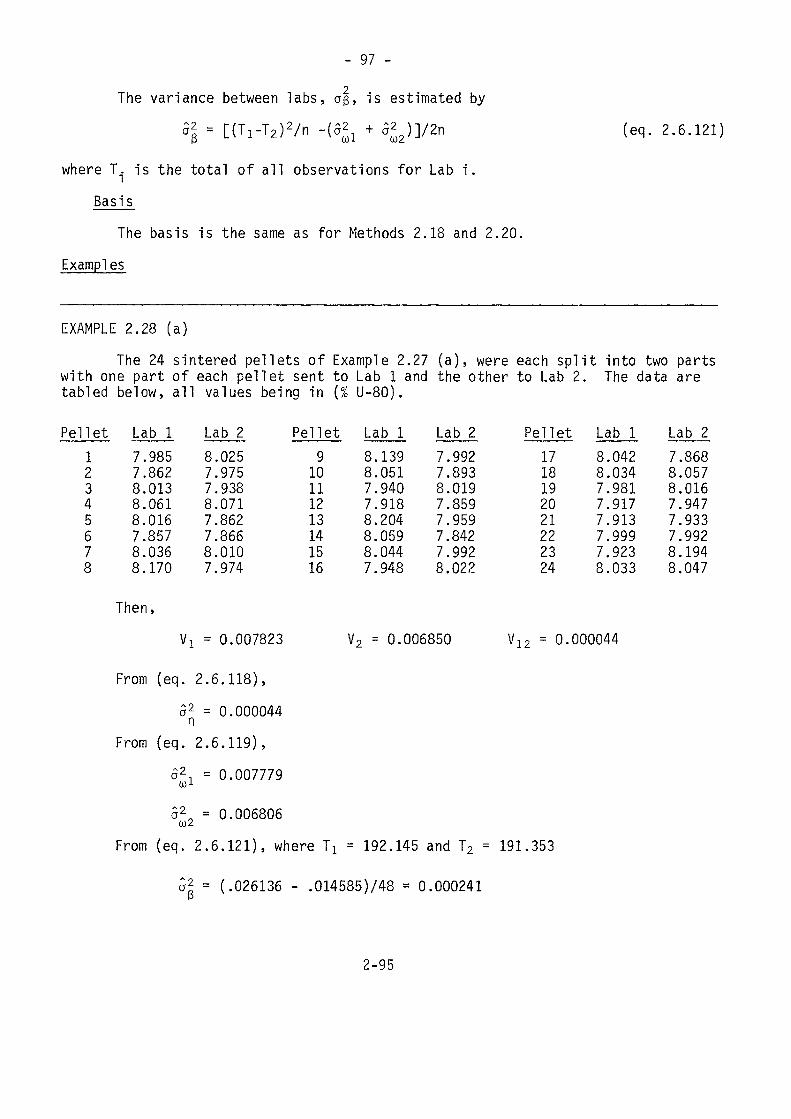
- 97 -2The variance between labs, a$, is estimated by

°l = [(Ti-T2)2/n -(3 + 5J2)]/2n (eq. 2.6.121)

where T. is the total of all observations for Lab i.Basis

The basis is the same as for Methods 2.18 and 2.20.Examples

EXAMPLE 2.28 (a)The 24 sintered pellets of Example 2.27 (a), were each split into two parts

with one part of each pellet sent to Lab 1 and the other to Lab 2. The data aretabled below, all values being in (% U-80).

Pellet Lab 1 Lab 2 Pellet Lab 1 Lab 2 Pellet Lab 1 Lab 2123456

7.9857.8628.0138.0618.0167.857

8.0257.9757.9388.0717.8627.866

91011121314

8.1398.0517.9407.9188.2048.059

7.9927.8938.0197.8597.9597.842

171819202122

8.0428.0347.9817.9177.9137.999

7.8688.0578.0167.9477.9337.992

8.036 8.010 15 8.044 7.992 23 7.923 8.1948.170 7.974 16 7.948 8.022 24 8.033 8.047

Then,Vj = 0.007823 V2 = 0.006850 V12 = 0.000044

From (eq. 2.6.118),a2 = 0.000044n

From (eq. 2.6.119),Ô2, = 0.007779w1

Ô2 = 0.0068060)2From (eq. 2.6.121), where T! = 192.145 and T2 = 191.353

ol = (.026136 - .014585)748 = 0.000241

2-95

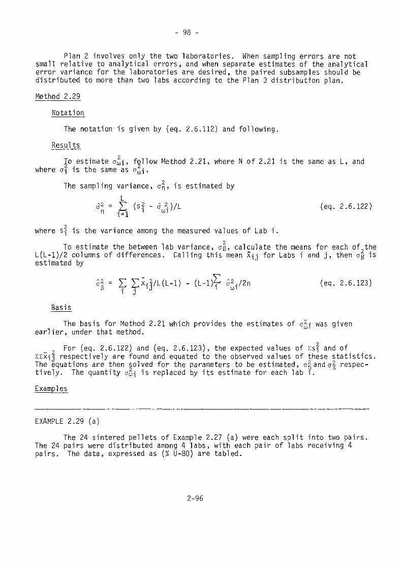
- 98 -

Plan 2 involves only the two laboratories. When sampling errors are notsmall relative to analytical errors, and when separate estimates of the analyticalerror variance for the laboratories are desired, the paired subsamples should bedistributed to more than two labs according to the Plan 3 distribution plan.Method 2.29

NotationThe notation is given by (eq. 2.6.112) and following.

ResultsTo estimate aw-j, follow Method 2.21, where N of 2.21 is the same as L, and

where a-j is the same as aw1-.The sampling variance, o^, is estimated by

L^ = .£ (si - .)/L (eq. 2.6.122)

where s-j is the variance among the measured values of Lab i.2To estimate the between lab variance, ag, calculate the means for each of the

L(L-l)/2 columns of differences. Calling this mean x-jj for Labs i and j, then aB isestimated by

a2. = Z EM/L(L-1) - (L-D? ^V2ri (ecl- 2.6.123)3 . .j iJ i ui

BasisThe basis for Method 2.21 which provides the estimates of o^-j was given

earlier, under that method.For (eq. 2.6.122) and (eq. 2.6.123), the expected values of zsf and of

*• respectively are found and equated to the observed values of these statistics.The equations are then solved for the parameters to be estimated, o^anda| respec-tively. The quantity a^-j is replaced by its estimate for each lab i.Examples

EXAMPLE 2.29 (a)The 24 sintered pellets of Example 2.27 (a) were each split into two pairs

The 24 pairs were distributed among 4 labs, with each pair of labs receiving 4pairs. The data, expressed as (% U-80) are tabled.

2-96

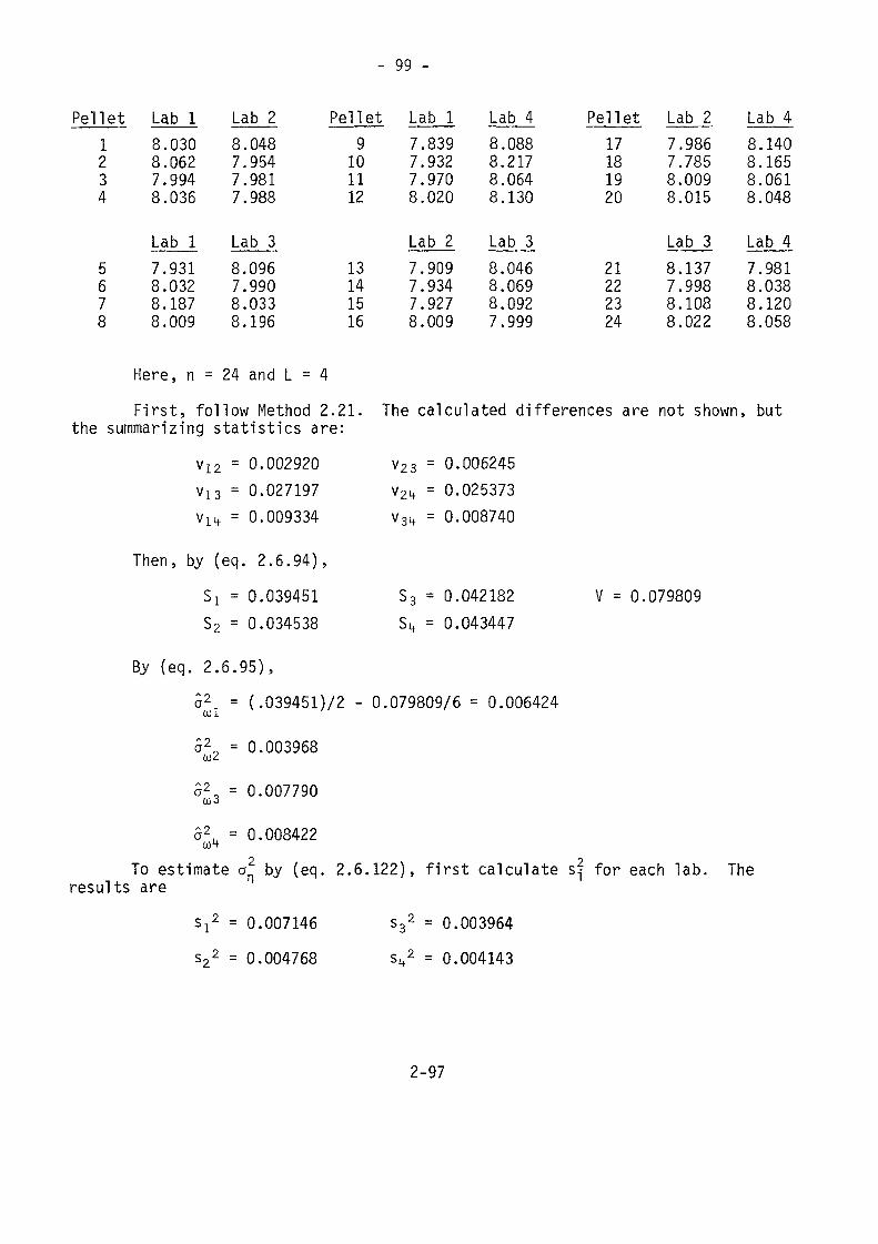
- 99 -

Pellet1234

5678

Lab 18.0308.0627.9948.036

Lab 17.9318.0328.1878.009

Here, n

Lab 28777

.048

.954

.981

.988

Pell9101112

Lab 38788

= 24

.096

.990

.033

.196

and L = 4

13141516

First, follow Method 2.21.the summarizing statistics are:

V 12 =

Vl3 =V

Then, by1 U =

(eqSi =S2 =

0.0029200.0271970.009334

. 2.6.94),0.0394510.034538

et Lab 17778

.839

.932

.970

.020

Lab 27778

The

V23

V2tfV34

S3Sit

.909

.934

.927

.009

Lab 48.0888.2178.0648.130

Lab 38.0468.0698.0927.999

Pell17181920

et Lab 27.7.8.8.

986785009015

Lab 321222324

calculated differences

= 0.= 0.= 0.

= 0.= 0.

006245025373008740

042182043447

V =

8.7.8.8.

are not

137998108022

shown

Lab 48.1408.1658.0618.048

Lab 47.9818.0388.1208.058

, but

0.079809

By (eq. 2.6.95),a2 = (.039451)72 - 0.079809/6 = 0.006424col

a2 = 0.0039680)2

a2, = 0.007790wo

a2, = 0.008422To estimate a by (eq. 2.6.122), first calculate s^ for each lab.

results are The

Si2 = 0.007146s22 = 0.004768

S32 = 0.003964s,2 = 0.004143

2-97

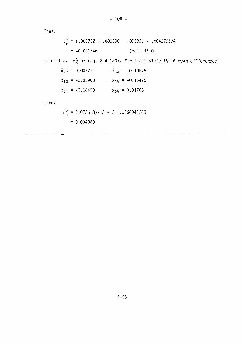
- 100 -

Thus,a2 = (.000722 + .000800 - .003826 - .004279)74

= -0.001646 (call it 0)To estimate a| by (eq. 2.6.123), first calculate the 6 mean differences,

Xi2 = 0.03775 X23 = -0.10675

X13 = -0.03900 X2u = -0.15475

x l l t = -0.18450 x34 = 0.01700

Then,5§ = (.073618)712 - 3 (.026604)748p

= 0.004389

2-98

- 101 -

2.7 REFERENCES[2.1] "Statistical Terminology and Notation for Nuclear Materials Manage-ment," American National Standards Institute, Inc., ANSI N15.5-1972,New York.

[2.2] Bennett, C. A. and Franklin, N. L., "Statistical Analysis in Chemis-try and the Chemical Industry", John Wiley and Sons, Inc., New York,Appendix 5A, (1954).

[2.3] Oaech, J. L., "Accounting for the Uncertainty in a Standard Value",Nuclear Materials Management Journal, Vol. VI, No. 2, 50-53, (1977).

[2.4] Jaech, J. L., "Some Thoughts on Bias Corrections," Nuclear MaterialsManagement Journal, Vol. IV, No. 2, 40-44, (1975).

[2.5] Jaech, J. L., "Estimation of Scale Accuracy and Precision: A CaseHistory", Nuclear Materials Management Journal, Vol. VII, No. 3, 81-84,(1978).

[2.6] Brownlee, K. A., "Statistical Theory and Methodology in Science andEngineering", John Wiley and Sons, Inc., New York, 72 ff, (1960).

[2.7] Bennett, C. A. and Franklin, N. L., Op Cit., 319-349.[2.8] Bennett, C. A. and Franklin, N. L., Op Cit., 243-245.[2.9] Bennett, C. A. and Franklin, N. L., Op Cit., 245-255.[2.10] Mandel, John, "Fitting a Straight Line to Certain Types of Cumula-

tive Data", J. of the Amer. Stat. Assoc., Vol 52., 552-66 (1957).[2.11] Aitken, A. D., "On Least Squares and Linear Combinations of Observa-tions", Proc. Royal Soc. of Edinburgh. Vol. 55, 42-48, (1935).

[2.12] Jaech, J. L., "A Note on the Equivalence of Two Methods of Fitting aStraight Line Through Cumulative Data", J. of the Amer. Stat. Assoc.,Vol. 59, 863-66 (1964).

[2.13] Jaech, J. L., "Pitfalls in the Analysis of Paired Data", NuclearMaterials Management Journal, Vol. II, No. 2, 32-39 (1973).

[2.14] Grubbs, F. E., "On Estimating Precision of Measuring Instrumentsand Product Variability", J. of the Amer. Stat. Assoc., Vol. 43, 243-264 (1948).

[2.15] Thompson, W. A. Jr., "Precision of Simultaneous Measurement Proce-dures", J. of the Amer. Stat. Assoc., Vol. 58, 474-479 (1963).

[2.16] Jaech, J. L., "Making Inferences About the Shipper's Variance in aShipper-Receiver Difference Situation", Nuclear Materials ManagementJournal, Vol. IV, No. 1, 36-38, (1975).

2-99

- 102 -

[2.17] Jaech, J. L., "Case Studies on the Statistical Analysis of Safe-guards Data", IAEA-SM-201/14, Safeguarding Nuclear Materials, Vol. 1,545-559, (1976).

[2.18] Jaech, J. L., "Errors of Measurement With More Than Two MeasurementMethods", Nuclear Materials Management Journal, Vol. IV, No. 4, 38-41 {1976}

[2.19] Mandel, J. and Lashof, T. W., "The Interlaboratory Evaluation ofTesting Methods", ASTM Bull. 239. TP 133, 53-61 (1959).

[2.20] Jaech, J. L., "A Program to Estimate Measurement Error in Nondes-tructive Evaluation of Fuel Element Quality", Technometrics, Vol. 6,293-300 (1964).

[2.21] Jaech, J. L., "Extension of Grubbs1 Method When Relative Biases AreNot Constant", Nuclear Materials Management Journal, Vol. VIII, No. 1,76-80, (1979).

[2.22] Jaech, J. L., "Estimating Within Laboratory Variability from Inter-laboratory Test Data", Journal of Quajity Technology, Vol. 11, No. 4,185-191 (1979).

[2.23] Bennett, C. A. and Franklin, N. L., Op Cit., 243-45.[2.24] Jaech, J. L. and Kraft, A. "Combining Estimates of Measurement Pre-

cisions from Different Experiments", Nuclear Materials Management Journal,Vol. VI, No. 1, 37-43 (1977).

[2.25] Anderson, R. L. and Bancroft, T. A., "Statistical Theory in Research"McGraw-Hill, Inc., New York, (Problem 8.6 with yif - 3a^) (1952).

[2.26] Jaech, J. L., "Statistical Methods in Nuclear Material Control",TID-26298, U.S. Gov't Printing Office, 40-41 (1973).

[2.27] Jaech, J. L., "Rounding Errors in Weighing", Nuclear MaterialsManagement Journal , Vol. V, No. 2, 54-57 (1976).

[2.28] Tingey, F. H. et al, "SALE Report 1. First Report on Error Compo-nents in the Analysis of Uranium and Plutonium Product Materials', April1972 (1972).

[2.29] Neuilly, M., "Commentaires Sur Le Document", AIEA-174 (1979)(private correspondence).

2-100

- 103 -

Chapter 3

ERROR PROPAGATION

3.1 DEFINITION OF ERROR PROPAGATIONIn the Safeguards Dictionary [3.1] prepared by the Brookhaven National Labora-

tory for the then United States Atomic Energy Commission, error propagation isdefined as follows: "The determination of the value to be assigned as the uncer-tainty of a given quantity using mathematical formulae for the combination ofmeasurement errors. Error propagation involves many considerations and the choiceof formulae for computing the uncertainty depends upon the functional relations ofthe measurement parameters involved."

This definition is made with respect to safeguards applications since itspeaks of combining measurement errors. Nevertheless, the definition accuratelyidentifies error propagation as a procedure based on using mathematical formulae.It is consistent with another quote taken from an expository paper on error propaga-tion by Birge [3.2], "The subject of the propagation of errors . . . is a purelymathematical matter, with very definite and easily ascertained conclusions."Although the practitioner might quarrel with the words "easily ascertained" therecan be no quarrel with the principal point in both quotations, namely, error propa-gation is a mathematical exercise and hence leads to precise and well-definedprocedures.

Although the error propagation procedures may be exact, this does not meanthat the net effect of the propagated errors is exactly determined. The errorpropagation formulas draw a mathematically precise line from some model to theconclusions; any inexactness in an answer derived from error propagation comes notfrom drawing this mathematically precise line, (assuming that this line is drawncorrectly), but rather from the starting point, that is, from the mathematicalmodel. This underscores the importance of the model insofar as it corresponds toa valid description of reality.

The general error propagation problem may be formulated as follows. Let arandom variable of interest (such as the MUF or material unaccounted for) be writtenas a specific function of a number of other random variables as in (eq. 3.1.1).

y = f(xi,x2, ..., XR) (eq. 3.1.1)The precise form of this function is known in the error propagation problem,

that is, the problem is not to estimate the parameters of the function (which is astatistical problem), but is rather to find the uncertainty in y as a function ofthe uncertainties in the x's (a mathematical problem) given that the function iswell defined. In the section to follow, error propagation is considered when f isa linear function, and the more general case for the nonlinear function is treatedin Section 3.3.

3-1

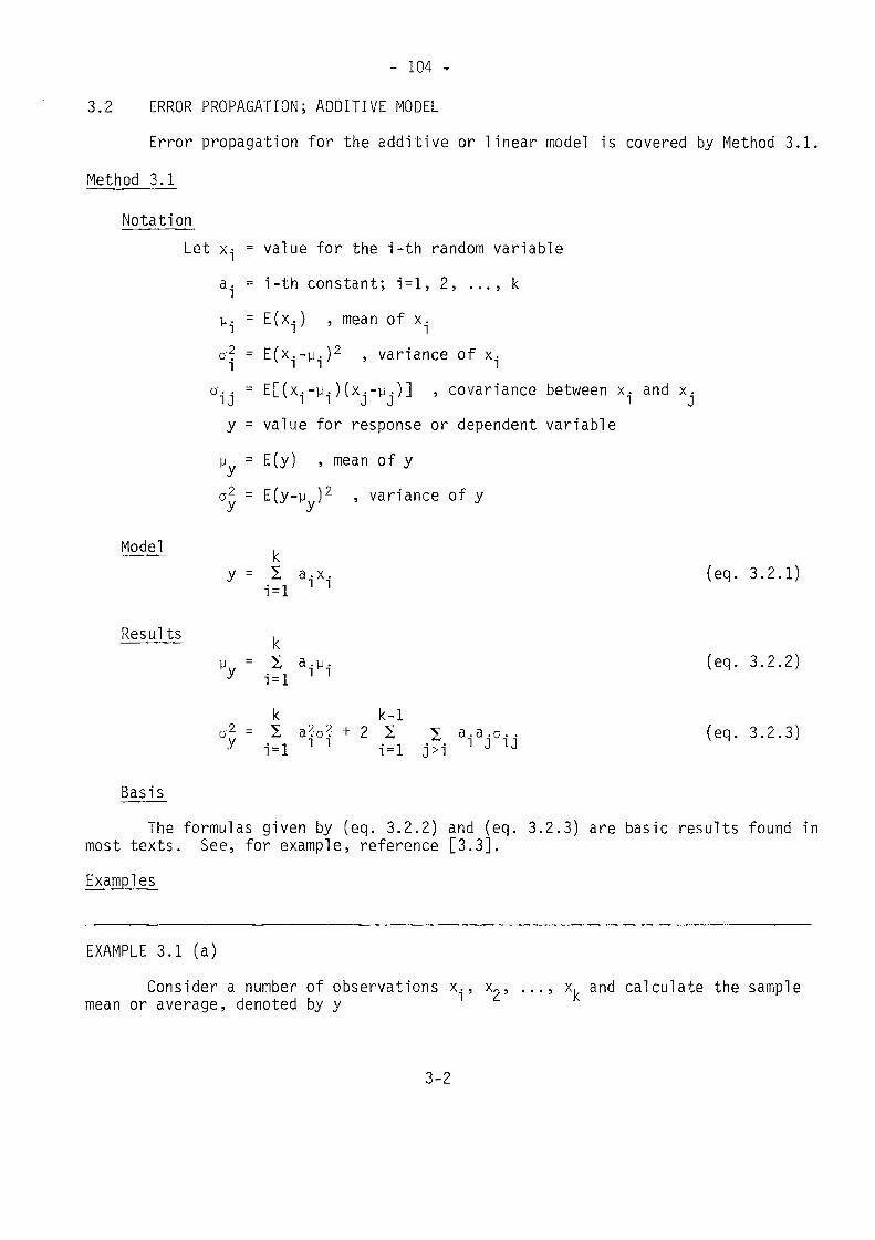
- 104 -

3.2 ERROR PROPAGATION; ADDITIVE MODELError propagation for the additive or linear model is covered by Method 3.1.

Method 3.1Notation

Let xiai

Model

Results

value for the i-th random variablei-th constant; i=l, 2, . .., kE(x..) , mean of x.

- - > variance of x.

y ="y =Jy =

E[(x.-y . ) (x.-vi .)] 5 covariance between x. and x.' ' J U ' J

value for response or dependent variableE(y) , mean of yE(y-y )2 , variance of y

ky = Si = lk

1 = 1k

a.u-

k-1a.a.a. .i J U

(eq. 3.2.1)

(eq. 3.2.2)

(eq. 3.2.3)

Bas i sThe formulas given by (eq. 3.2.2) and (eq. 3.2.3) are basic results found in

most texts. See, for example, reference [3.3].Examples

EXAMPLE 3.1 (a)Consider a number of observations x., x„, ..., x, and calculate the sample

mean or average, denoted by y

3-2

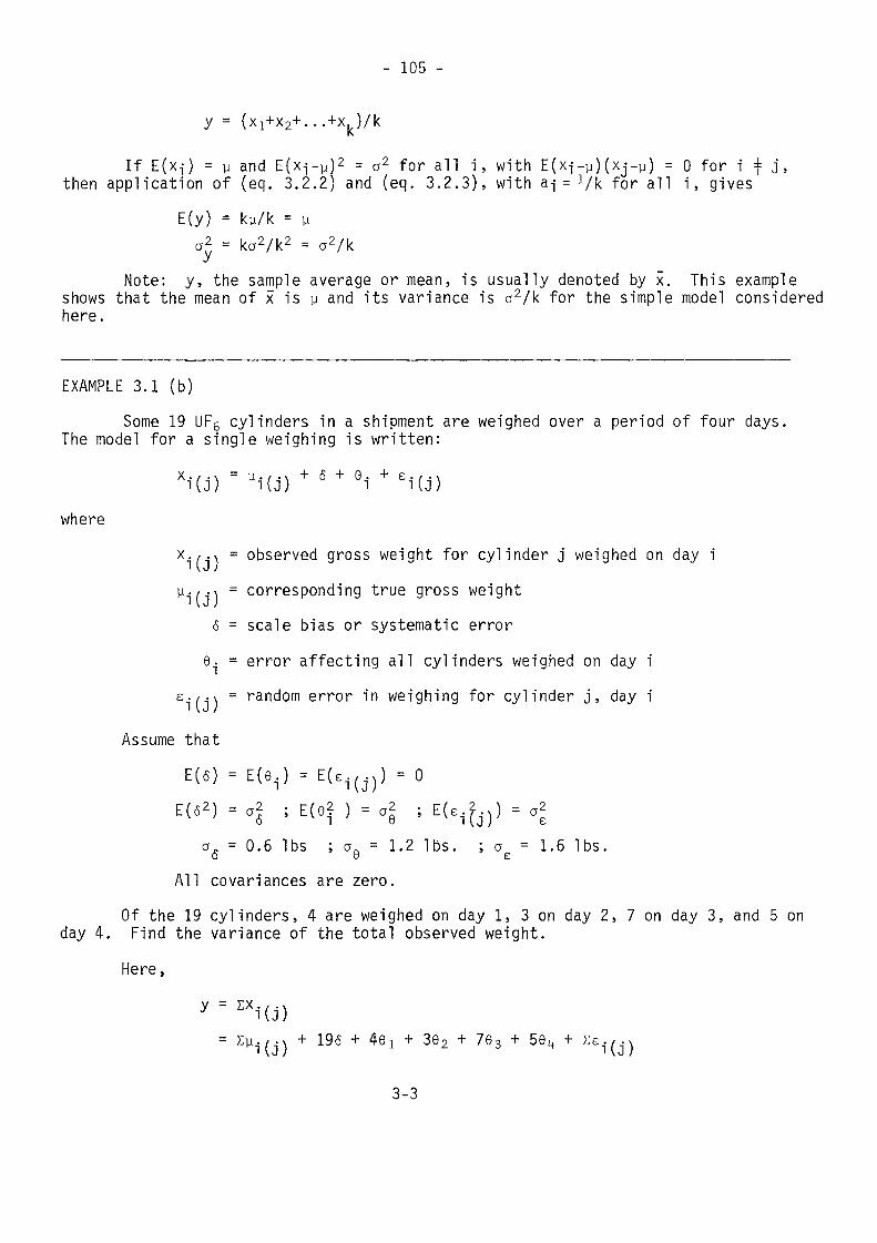
- 105 -

y = (x1+x2+...+xk)/k

If E(XJ) = y and E(xj-y)2 = a2 for all i, with E(x1--y)(xJ--y) = 0 for i =j= j,then application of (eq. 3.2.2} and (eq. 3.2.3), with a-j = Vk for all i, gives

E(y) = ky/k = ya2 = ka2/k2 = a2/k

Note: y, the sample average or mean, is usually denoted by x. This exampleshows that the mean of x is y and its variance is a2/k for the simple model consideredhere.

EXAMPLE 3.1 (b)Some 19 UF6 cylinders in a shipment are weighed over a period of four days.The model for a single weighing is written:

Xi(J)where

x-(,-\ = observed gross weight for cylinder j weighed on day iy./.i, = corresponding true gross weight

6 = scale bias or systematic error9. = error affecting all cylinders weighed on day i

£./.\ = random error in weighing for cylinder j, day i

Assume thatE(6) = E(0.) = E(e.(j)) = 0E(62)=a2 ; E ( e 2 ) = a 2 ; E(e

ax = 0.6 Ibs ; a. = 1.2 Ibs. ; a =1.6 1 bs .o ö eAll covariances are zero.

Of the 19 cylinders, 4 are weighed on day 1, 3 on day 2, 7 on day 3, and 5 onday 4. Find the variance of the total observed weight.

Here,y = zx1(j)

+ 196 + 40! + 362 + 763 + 50^ + Ze^jj

3-3

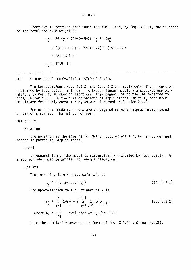
- 106 -

There are 19 terms in each indicated sum. Then, by (eq. 3.2.3), the varianceof the total observed weight is

a2 = 361a2 + (16+9+49+25)a2 + 19a2Y o ö e

= (361H0.36) + (99)(1 .44) + (19) (2 .56)

= 321.16 Ibs2

a - 17.9 IbsJ

3.3 GENERAL ERROR PROPAGATION; TAYLOR'S SERIESThe key equations, (eq. 3.2.2) and (eq. 3.2.3), apply only if the function

indicated by (eq. 3.1.1) is linear. Although linear models are adequate approxi-mations to reality in many applications, they cannot, of course, be expected toapply universally. In the area of safeguards applications, in fact, nonlinearmodels are frequently encountered, as was discussed in Section 2.3.2.

For nonlinear models, errors are propagated using an approximation basedon Taylor's series. The method follows.Method 3.2

NotationThe notation is the same as for Method 3.1, except that a-j is not defined,

except in particular applications.Mode]_

In general terms, the model is schematically indicated by (eq. 3.1.1). Aspecific model must be written for each application.

ResultsThe mean of y is given approximately by

Uy ~ f(ui>U2>" • » y^) (ecl- 3.3.1)The approximation to the variance of y is

k k-1a2, = 2 b?a? + 2 2 X b.b.a. . (eq. 3.3.2)

r, L

where b. = ~~ , evaluated at y. for all i1 à X • I

Note the similarity between the forms of (eq. 3.3.2) and (eq. 3.2.3).

3-4

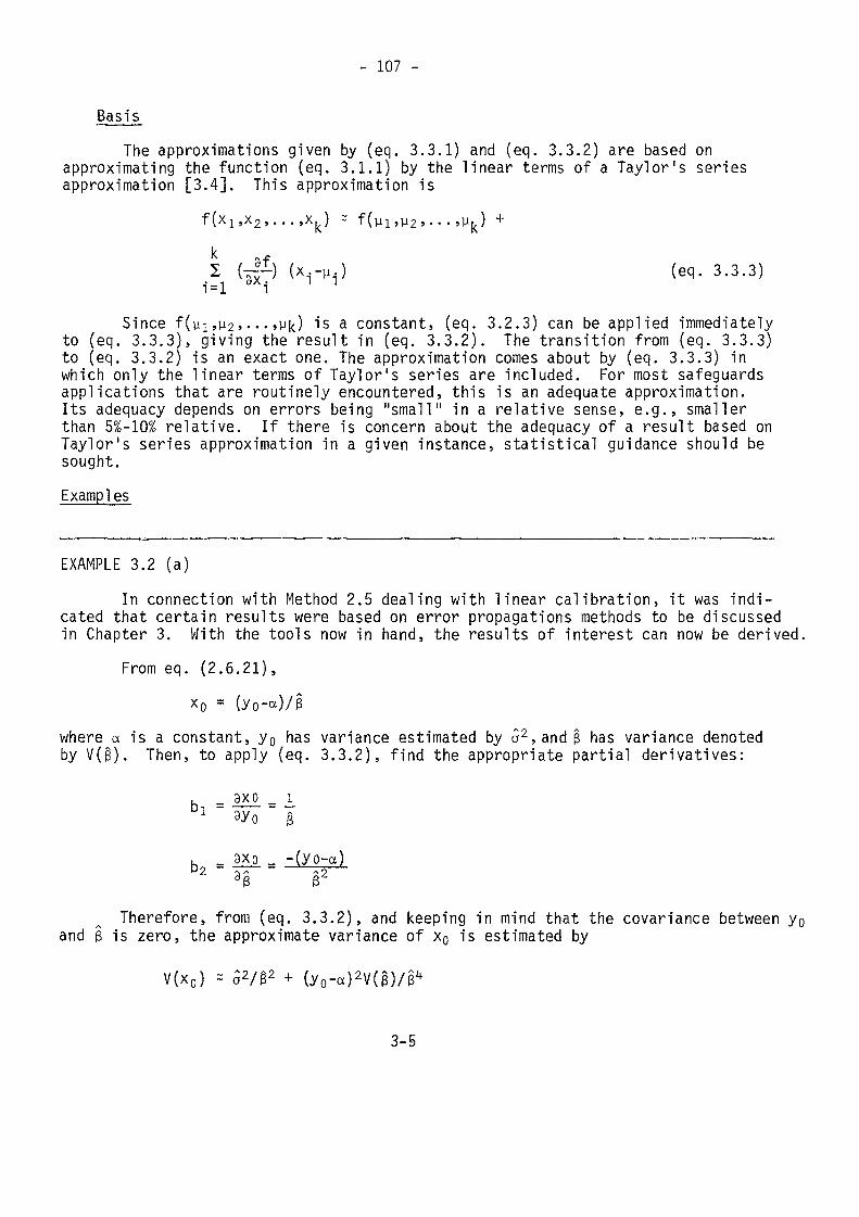
- 107 -

BasisThe approximations given by (eq. 3.3.1) and (eq. 3.3.2) are based on

approximating the function (eq. 3.1.1) by the linear terms of a Taylor's seriesapproximation [3.4]. This approximation is

f(x1,x2,...,xk) =k afZ ( l1) (X4-H.)i=l 3xi n n (eq. 3.3.3)

Since f (m ,u2> • • • >vk) is a constant, (eq. 3.2.3) can be applied immediatelyto (eq. 3.3.3), giving the result in (eq. 3.3.2). The transition from (eq. 3.3.3)to (eq. 3.3.2) is an exact one. The approximation comes about by (eq. 3.3.3) inwhich only the linear terms of Taylor's series are included. For most safeguardsapplications that are routinely encountered, this is an adequate approximation.Its adequacy depends on errors being "small" in a relative sense, e.g., smallerthan 5%-10% relative. If there is concern about the adequacy of a result based onTaylor's series approximation in a given instance, statistical guidance should besought.Exampl es

EXAMPLE 3.2 (a)In connection with Method 2.5 dealing with linear calibration, it was indi-

cated that certain results were based on error propagations methods to be discussedin Chapter 3. With the tools now in hand, the results of interest can now be derived.

From eq. (2.6.21),

where a is a constant, y0 has variance estimated by <j2,and§ has variance denotedby V(ß). Then, to apply (eq. 3.3.2), find the appropriate partial derivatives:

, _b =_ 3X0 _ 1=

_ 3x0 _ -(yo-cQ~ ~ —

Therefore, from (eq. 3.3.2), and keeping in mind that the covariance betweenand is is zero, the approximate variance of x0 is estimated by

V(x0) = 52/02 + (y0-

3-§

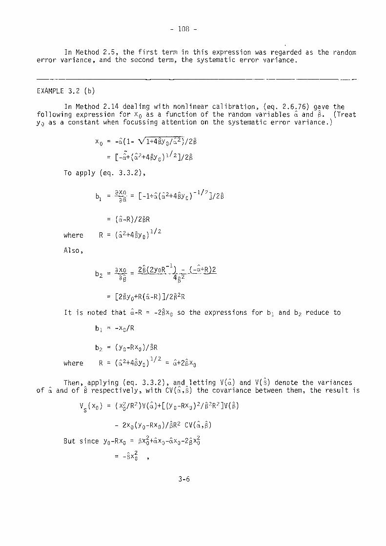
- 108 -

In Method 2.5, the first term in this expression was regarded as the randomerror variance, and the second term, the systematic error variance.

EXAMPLE 3.2 (b)In Method 2.14 dealing with nonlinear calibration, (eq. 2.6.76) gave the

following expression for x0 as a function of the random variables a and §. (TreatYo as a constant when focussing attention on the systematic error variance.)

x0 = -a(l- Vl+4§y0/a2)/23

= [-â~+(â2+4êy0)1/2]/2êTo apply (eq. 3.3.2) ,

where R = (a2+4ßy0)1 / 2

A l s o ,

"1b2 == MO. = 2g(2yoR" ) - (-g+R)2K 4a2

= [2ßy0+R(a-R)]/2ß2RIt is noted that a-R = -2§x0 so the expressions for bi and b2 reduce to

where R = (a2+4ßy0)1/2 = a+2ßxQThen, applying (eq. 3.3.2), andjetting V(a) and V(ß) denote the variances

of a and of 3 respectively, with CV(â,ê) the covariance between them, the result isV(x0) = (x2/R2)V(a)+[(y0-Rx0)2/§2R2]V(ß)

But since y0-Rx0 =

- 2x 0 (y 0 -Rx 0 ) /§R 2 C V ( 0 , ß )

3-6

- 109 -

the expression for the systematic error variance of x0, v (x0) reduces to

Vs(x0) = (x02/R2)[V(a)+x02V(e) + 2x0CV(S,§)]which is the result, (eq. 2.6.80).

Other applications of error propagation will be encountered later in thisvolume.

3.4 CALCULATION OF VARIANCE OF MUF3.4.1 Definition of MUF

The word, MUF, is an acronym for material unaccounted for. It is definedas the difference between the book inventory and the physical inventory. Thisdefinition may be with respect to either the element or isotope weight.

The facility MUF for a given material balance (or accounting) period is ameasure of the performance of the facility with respect to its control of thenuclear materials involved. The MUF, as verified by inspection, or alternately,as adjusted on the basis of inspection results, is the key index of performanceused by the Agency in its quantitative assessment of facility performance.

The MUF calculation is represented schematically by the following equation:MUF = I - 0 + B - E (eq. 3.4.1)

where J_ designates inputs, 0_ designates outputs (which are sometimes subdividedinto product and waste streams), B_ refers to beginning inventory, and £_ to endinginventory. The three terms in (eq. 3.4.1), I, 0, and B, collectively representthe book inventory, while E represents the physical inventory. Note that thephysical inventory for one accounting period becomes a part of the book inventoryfor the subsequent period.

The definition of MUF implicity assumes that the material balance is basedcompletely on measured data. The use of by-difference accounting results in ameaningless MUF. For example, if the contents of waste streams are calculated asthe differences between the measured amounts entering a process step and thoseexiting the step, it is clear that the calculated MUF would be zero over thatparticular material balance area, i.e., it would be meaningless as a performanceindex.

In order to judge the significance of a given MUF, either as verified or asadjusted by the inspection results, it is necessary to calculate its variance. AMUF is affected by many factors. For example, in taking inventory, if a measuredvalue is improperly recorded, i.e., if a mistake is made in recording the value inquestion, this will affect the MUF. Such a mistake will not, however, affect thevariance of MUF as will be defined here, for the variance of MUF is calculated toinclude only the uncertainties arising from the measurement process under theassumption that this process is functioning properly.

3-7

- 110 -

In this connection, it may be helpful to make a distinction between anobserved MUF and a true MUF. The true MUF is the actual amount of material un-accounted for, excluding the effects of errors of measurement. It includes theeffects of unmeasured inventories, process losses, recording mistakes, plus anydiverted material. The observed MUF is a random variable whose expected value isthe true MUF. In the absence of any errors of measurement, the observed MUF isidentical to the true MUF. Equivalently stated, the variance of the (observed)MUF is zero in this case.

Clearly, an observed MUF together with its calculated variance are notsufficient information on which to make a judgement as to whether or not materialhas been diverted. Other information must be brought to bear to make such a judge-ment. However, it should also be clear that if the calculated variance of MUF isexcessively large due to a poor measurement system, then one can never hope to carrythe MUF evaluation beyond this first stage; any possible diversion would be quiteobscurred by large errors of measurement and no reasonable judgement about divertedmaterial could be made.

In the next section, it will be indicated how the variance of a given MUFcan be calculated exactly by application of the error propagation formulas alreadygiven. Following that, a general approach to calculating the variance of MUF underspecified rather non-restrictive assumptions will be considered.3.4.2 Direct Application of Error Propagation Formulas

If a given calculated MUF is based on a simple model, then either Method 3.1or Method 3.2 already given may be applied directly to calculate its variance. Thisis illustrated by the following example in which the variance of MUF is calculatedby application of Method 3.1.

EXAMPLE 3.1 (c)Consider the plutonium MUF in a somewhat simplified chemical reprocessing

facility. The components of the material balance are identified as follows:Inputs : A batch consists of a volume of material in the input account-

ability tank. Each volume contains nominally 10 kg Pu. Over the material balanceperiod, there are 40 batches. The model for batch i is

where x,. = measured plutonium in batch iTj. = true plutonium in batch i

ô - systematic error for batch ie. = random error for batch i

All quantities are expressed in kilograms. The model has been simplifiedin that <5 and e-j each represent the combined effects of several measurement errors

3-8

- Ill -(volume, sampling, analytical). Assume that 6 and e^ (and other measurement errorsidentified in what follows) have zero means with:

afi = 0.044 kg a£ = 0.109 kgProduct : Product is outputted as plutonium nitrate. Each batch contains

nominally 22 kg Pu, and there are 18 batches over the material balance period. Forbatch i, the model is

xpi = Tpi + A + "1where Xp-j, Tpi, A, and ^-j are defined in a manner analagous to Xj-f, TIJ, 6, and e-j.Assume

aA = 0.082 kg a = 0.191 kgA 3 nWaste : Waste is batched with a nominal batch size of 0.25 kg Pu. There

are 16 batches over the material balance period. The model isxwi = TwT + a + wi ' Wlth

a = 0.030 kg a = 0.052 kga 3 w 3

Inventory: There are 10 batches (process vessels) in inventory. The inven-tory level is very low because physical inventories are taken after clean out. Forbeginning inventory:

xBi - TBi + 3 + 9land for ending inventory,

xEi = TE1 + 3 + Y.

Note that 3 appears in the model for both beginning and ending inventoriesand therefore will cancel in the MUF equation. The value of aß is hence immaterial.For 8j and yi> assume

aQ = a = 0.002 kg

The model for MUF can then be written and Method 3.1 applied since the MUFequation is of the form (eq. 3.2.1).

40 40 18 18MUF = $ T + 406 + X £.,• - X T , -ISA - j ni = l n 1=1 n i = l P1 1=1 1

16 16 10 10" + T + 10ß +

3-9

- 112 -10 10S T -10ß - S y.-

Then, assuming all covariances are zero, (eq. 3.2.3) is applied,Var (MUF) = 1600 (.044)2 + 40(.109)2 + 324(.082)2 + 18(.191)2

+256(.030)2 + 16(.052)2 + 10(.002)2 + 10(.002)2

= 6.6818 kg2 PuStandard deviation (MUF) = 2.585 kg Pu

In this example, the standard deviations were expressed on an absolute basis,i.e., in kilograms plutonium. If they were expressed on a relative basis, multi-plicative rather than additive models would have been written, and Method 3.2 applied.The answer, of course, would be the same.

3.4.3 Variance of Element MUF by General ApproachAlthough conceptually one can apply Method 3.1 or Method 3.2 in calculating

the variance of any MUF, in practice it will often be difficult to write explicitlythe model that is required to apply these methods. Even when it is possible to doso with moderate effort, as was done in the example just concluded, it may be muchsimpler to apply a general solution to the problem based on some simplifying assump-tions set forth in the section to follow. The assumptions will rarely be 100%satisfied in practice, but (1) moderate departures from them will often have neg-ligible effect; and (2) one can make slight alterations in the calculations toaccount for departures in assumptions if deemed necessary. This will be illus-trated in the examples to follow.

The general approach to calculating the variance of element (and of isotope)MUF is an extension of methods documented in [3.5] and later expanded upon [3.6].A computerized version of the calculations has been developed and is described in[3.7]. The computer code, identified as NUMSAS, is available. The program orderform is reproduced as Annex 3.1.

3.4.3.1 AssumptionsThe variance of element MUF is considered first. Isotope MUF will be treated

in a later section.In calculating the variance of element MUF, it is convenient to develop a

hierarchy of classifications consisting of items, batches, strata, and components.An item is a primary unit which has a weight, volume and destructive analysis or

NDA measurement associated with it. A number of item collectively form a batch, where abatch consists of all items that are related because they have a common element concen-tration factor. In the event the element factor is uniquely determined for each item,

3-10

- 113 -then an item and a batch are identical, i.e., there is one item in that batch. Notethat this definition of batch may be different than used in accounting reports tothe Agency. A number of batches collectively form a stratum, which consists of allbatches of like material. As will be illustrated in the examples, one has a certainamount of freedom in defining a stratum in a given application; strata of similarmaterials may be combined into a single stratum in order to reduce the amount ofcalculation at the expense of bending the assumptions somewhat. Finally, strata arecombined to form a component of the MUF equation. There are four MUF components,identified in the schematic (eq. 3.4.1).

With the classifications in mind, the following assumptions are made:(1) All random, short-term systematic, and long-term systematic error stan-

dard deviations are known and are expressed on a relative basis. For example, a0.4% relative standard deviation is expressed as 0.004. (However, see Section 3.4.3.5.)

(2) Within a given batch, the number of samples drawn and the number ofanalyses per sample are both constants.

(3) Within a given stratum, the number of items per batch is constant.(4) No more than one scale or analytical method is used in a given stratum.(5) A given element concentration factor cannot apply to more than onestratum.Some comments on these assumptions are helpful. First, with respect to

the distinction between short-term and long-term systematic errors, it is not alwaysevident just how a given error should be classified. Whenever a given measurementsystem is recalibrated, this signals a change in the error structure and introducesa new short-term systematic error. However, such error shifts may also occur in ameasurement system even when the system is not recalibrated. Each error sourceshould be evaluated using the methods of Chapter 2 to properly characterize itfrom point of view of how often the error may shift in value. When calculatingthe variance of MUF, whether an error is a short-term or long-term systematic errorcan have significant impact on the calculated variance of MUF, and hence, it is worththe effort to properly characterize each error.

With respect to assumption (4), this assumption can be relaxed if the mea-surement methods in question are of the same design (e.g., same type scale). Inthis event, the use of several scales, say, is equivalent to the use of one scalewith several shifts in the systematic error (i.e., with a short-term systematicerror). See examples 3.3 (a) and 3.4 (a).

As regards assumption (5), this assumption is not generally satisfied whendealing with isotope MUF as opposed to element MUF. Should the assumption beviolated for element MUF, then the methods of Section 3.4.5 for isotope MUF maybe applied.

Before continuing with the general methodology, the notation to be usedin the following sections is summarized.

3-11

- 114 -

3.4.3.2 NotationThe following notation is used.

x. = total element weight in stratum k, where the element weight isqp found using bulk measurement method q, sampling is from materialtype p, and analytical technique t is used. If measurement isby NDA, regard the NDA instrument as an analytical method."Dummy" methods can be used for the bulk and sampling measure-ments.

Note : It may be that within a stratum, the same systematic error does notaffect all items, i.e., there is a short-term systematic error. Use parenthesesto indicate the total element weight associated with "condition i" for a givenmeasurement. For example:

- total element weight identified with condition 3 for analyticalmethod t in stratum k= total element weight identified with condition 2 for bulk method(e.g., scale) q in stratum k.

To continue,6 = a relative standard deviation; subscripts identify a specific

one.s,g,r = first subscript on ô: s refers to a long term systematic error;

g to a short term systematic error; r to a random error.q,p,t = second, third, and fourth subscripts on 6; defined as for the

subscripts on x; if the measurement method in question is abulk method, replace p and t by dots; for example

6r = random error standard deviation in sampling of material type p.n. = number of items per batch in stratum k.tn. - number of batches in stratum k.r. = number of samples drawn per batch in stratum k to estimate the batch

element concentration factor.c, = number of analyses per sample in stratum kk = total number of strata

V(-..) = variance of quantity within parentheses, for example,V(x. .) = variance of element weight in stratum k;V(MUF) = variance of MUF

3-12

- 115 -Note: s, g, and r subscripted on V is defined as when subscripted on 6; if

V has no subscript, this refers to a total variance.With this notation in mind, Method 3.3 will now provide formulas needed to

compute the random error variance of MUF.

3.4.3.3 Random Error Variance of MUFMethod 3.3

NotationThe notation is given in 3.4.3.2.

ModelThe schematic model for MUF is given by (eq. 3.4.1). For the individual

measurements, the multiplicative model is used. This is discussed in 2.3.2.Results

For stratum k, the random error variance of the total element weight isV (x. J = x2 (52 /n m+ô 2 /r.m.+o2 «./c.r.m.) (eq. 3.4.2)rv kqpt' kqptv rq«'' k k r-p« k k r--r k k k' v H '

To find V (MUF), V (x,„n.J is summed over all the strata.r » KCjpUK

Vr(MUF) = 2 Vr(xkqpt) (eq. 3.4.3)K. x

If, in a given situation, a nominal (historical average, stoichiometric) elementfactor is used, then 6 and 6 . are both zero for that stratum. To avoiddivision by zero in (eq.<p'3.4.2), " rR may be set equal to one.

BasisThe formula for Vr(MUF) is derived by application of Method 3.2.

Examples

EXAMPLE 3.3 (a)In this first example, consider a simplified material balance for a fuel

fabrication facility. There are seven strata identified. There are 4 bulk mea-surement methods (q=l-4), 5 material types (p=l-5), and 4 analytical methods (t=l-4)

The error standard deviations are tabled.6ri>> = 0.000658 or.1< = 0.000531 <S r < > 1 = 0.000433

&r2tt = 0.000877 <Sr.2> = 0 <5r<>2 = 0.000568

cSrq =0* 6r , = 0* <5„ 0.0577• s • • r«o» r a*s3-13

- 115 -

= 0.00250 &rtltt = 0.0181

6r.s. - 0.0418*"dummy" methods

Stratum 1 is an input stratum consisting of containers of U02 powder. Stra-tum 2 is an output product stratum consisting of containers of sintered U02 pellets.Stratum 3 is an output waste stream stratum consisting of containers of solid wastemeasured by NDA. Stratum 4 is a beginning inventory stratum consisting of containersof dirty scrap. Stratum 5 is a beginning inventory stratum consisting of containersof grinder sludge. Stratum 6 is an ending inventory stratum containing the samekinds of material as Stratum 4. Stratum 7 is an ending inventory stratum contain-ing the same kinds of material as Stratum 5.

Before continuing with this example, it is important to emphasize an impor-tant point. Before any calculations of the variance of MUF are performed, datafor any items that are identical in both a plus and minus component of the MUFequation must be deleted. For example, if an item in beginning inventory wereremeasured in ending inventory, then depending as the use made of the remeasuredvalue, this item may or may not be included in the MUF variance calculation. Ifthe remeasured value were booked, then the item would be included; if it were notbooked, but were only used for verification of the previously booked value, thenit would not be included—it would neither affect the MUF nor its variance.

To continue with the example, it is convenient to organize the parametervalues in tabular form before performing the calculations of (eq. 3.4.2). This isdone below.

Stratum ( k )

1 2 3 4 5 6 7

m,

qPt

1508051111

240,000

47,7601

2401222

238,800

12770

11333

1200

3006101444

7200

2004121454

4000

3006101444

7200

2004121454

4000

(i) entries are in kg uranium

3-14

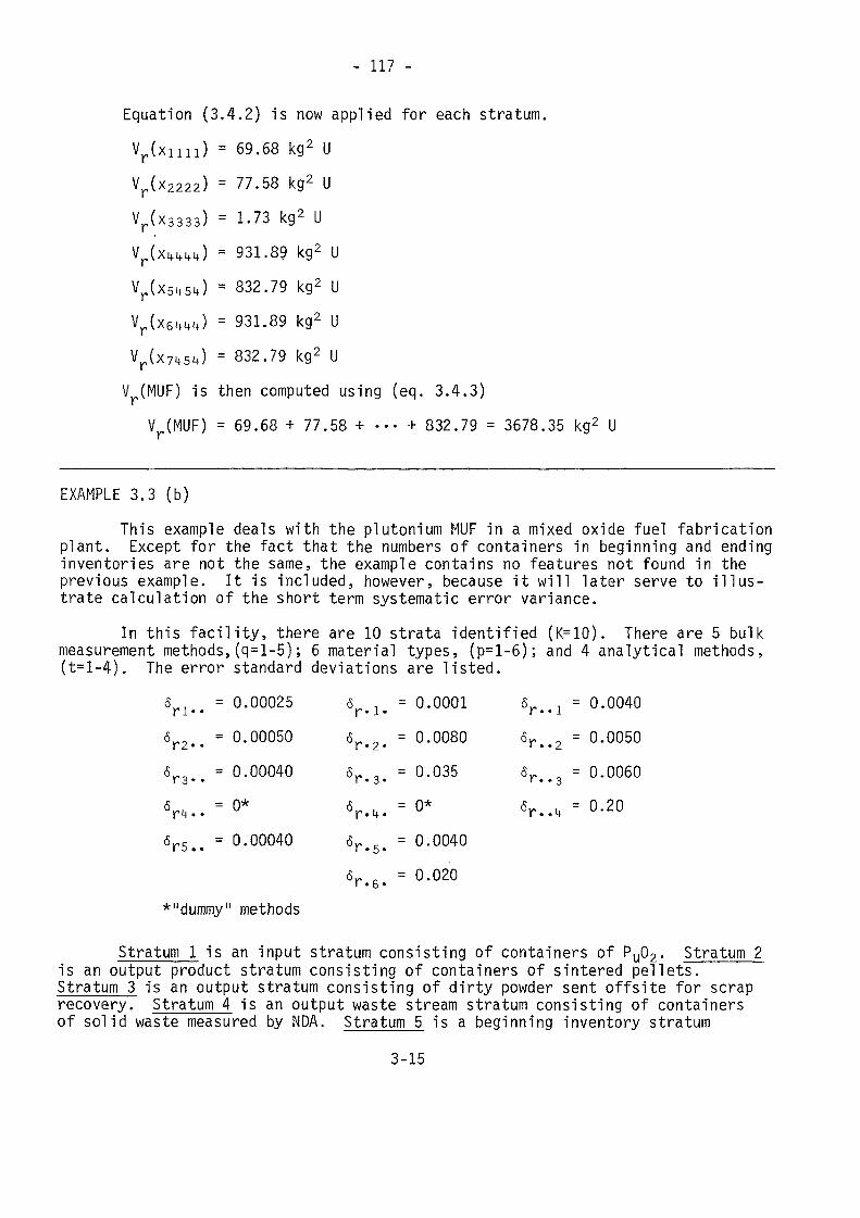
- 117 -

Equation (3.4.2) is now applied for each stratum.Vr(xim) = 69.68 kg2 UVr(x2222) = 77.58 kg2 UVr(x3333) = 1.73 kg2 U

= 931.89 kg2 U= 832.79 kg2 U= 931.89 kg2 U= 832.79 kg2 U

V (MUF) is then computed using (eq. 3.4.3)Vr(MUF) = 69.68 + 77.58 + ••• + 832.79 = 3678.35 kg2 U

EXAMPLE 3.3 (b)This example deals with the plutonium MUF in a mixed oxide fuel fabrication

plant. Except for the fact that the numbers of containers in beginning and endinginventories are not the same, the example contains no features not found in theprevious example. It is included, however, because it will later serve to illus-trate calculation of the short term systematic error variance.

In this facility, there are 10 strata identified (K=10). There are 5 bulkmeasurement methods,(q=l-5); 6 material types, (p=l-6); and 4 analytical methods,(t=l-4). The error standard deviations are listed.

orl_ = 0.00025 o r < 1 > = 0.0001 o r < > 1 - 0.00406r2>. = 0.00050 <Sr<2. = 0.0080 6r><2 = 0.00506ra = 0.00040 Sr , = 0.035 &r o = 0.0060T O * * J * o * O

K = n* rt = n* K = n ?nr if. . r.it. r»«4 u.tu

6r5>> = 0.00040 Srt5t = 0.00406r c = 0.020r «6•

*"dummy" methods

Stratum 1 is an input stratum consisting of containers of Pu02. Stratum 2is an output product stratum consisting of containers of sintered pellets.Stratum 3 is an output stratum consisting of dirty powder sent offsite for scraprecovery. Stratum 4 is an output waste stream stratum consisting of containersof solid waste measured by NDA. Stratum 5 is a beginning inventory stratum

3-15

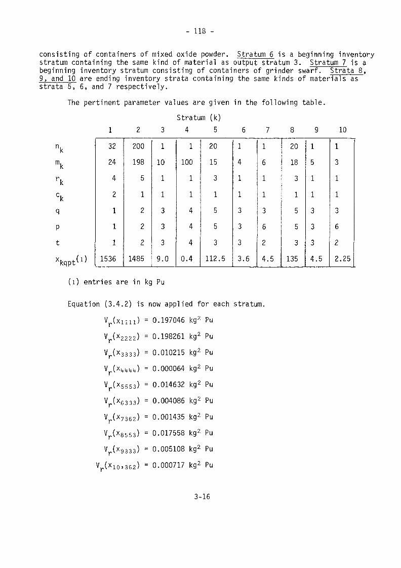
- 118 -

consisting of containers of mixed oxide powder. Stratum 6 is a beginning inventorystratum containing the same kind of material as output stratum 3. Stratum 7 is abeginning inventory stratum consisting of containers of grinder swarf. Strata 8,9, and 10 are ending inventory strata containing the same kinds of materials asstrata 5, 6, and 7 respectively.

The pertinent parameter values are given in the following table.Stratum (k)

1 2 3 4 5 6 7 8 9 1 0

m,

kqpt(i)

322442111

1536

20019851222

1485

110113339.0

110011444

0.4

201531553

112.5

14113333.6

16113624.5

201831553

135

15113334.5

13113622.25

(i) entries are in kg Pu

Equation (3.4.2) is now applied for each stratum.Vr(xim) = 0.197046 kg2 PuVr(><2222) = 0.198261 kg2 PuVr(x3333) = 0.010215 kg2 PuV (x J = 0.000064 kg2 PuVr(x5553) = 0.014632 kg2 PuVr(x6333) = 0.004086 kg2 PuVr(x7362) = 0.001435 kg2 PuVr(x8553) = 0.017558 kg2 PuVr(x9333) = 0.005108 kg2 Pu

Vr(x10,362) = 0.000717 kg2 Pu

3-16

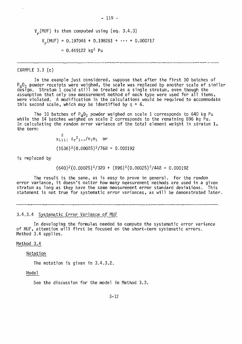
- 119 -

V (MUF) is then computed using (eq. 3.4.3)Vr(MUF) = 0.197046 + 0.198261 + ••• + 0.000717

= 0.449122 kg2 Pu

EXAMPLE 3.3 (c)In the example just considered, suppose that after the first 10 batches of

PU02 powder receipts were weighed, the scale was replaced by another scale of similardesign. Stratum 1 could still be treated as a single stratum, even though theassumption that only one measurement method of each type were used for all items,were violated. A modification in the calculations would be required to accommodatethis second scale, which may be identified by q = 6.

The 10 batches of PU02 powder weighed on scale 1 corresponds to 640 kg Puwhile the 14 batches weighed on scale 2 corresponds to the remaining 896 kg Pu.In calculating the random error variance of the total element weight in stratum 1,the term:

2 9xim <Sr i-Mmi or(1536)2(0.00025)2/768 = 0.000192

is replaced by(640)2(0.00025)2/320 + (896)2(0.00025)2/448 = 0.000192

The result is the same, as is easy to prove in general. For the randomerror variance, it doesn't matter how many measurement methods are used in a givenstratum as long as they have the same measurement error standard deviations. Thisstatement is not true for systematic error variances, as will be demonstrated later.

3.4.3.4 Systematic Error Variance of MUFIn developing the formulas needed to compute the systematic error variance

of MUF, attention will first be focused on the short-term systematic errors.Method 3.4 applies.Method 3.4

Ngt_a_tipn_The notation is given in 3.4.3.2.

ModelSee the discussion for the model in Method 3.3.

3-17

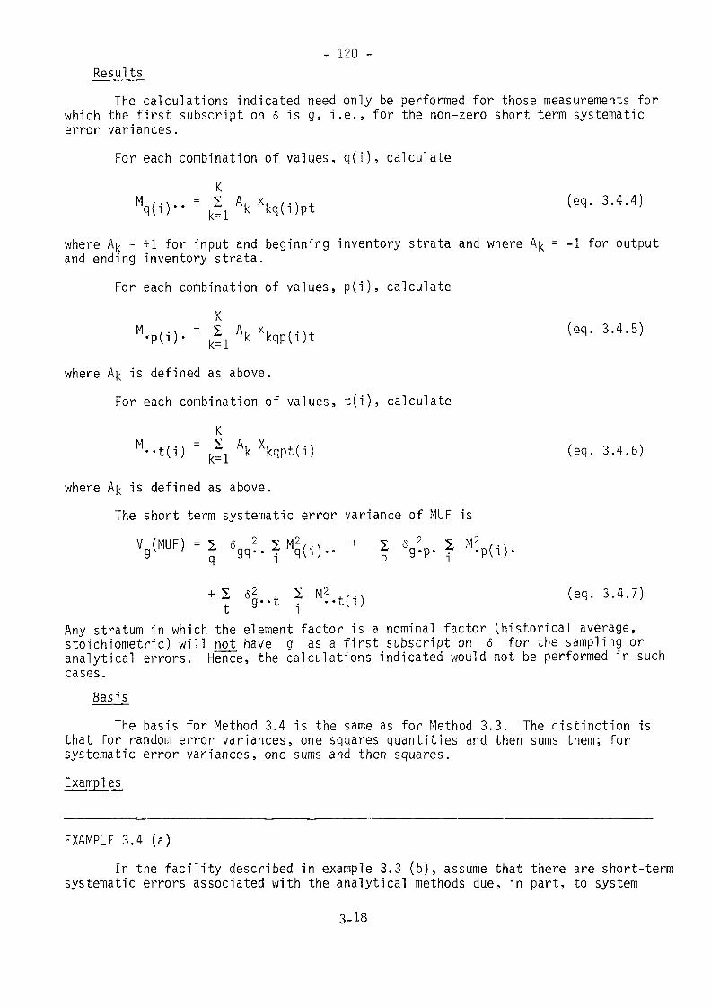
- 120 -Results

The calculations indicated need only be performed for those measurements forwhich the first subscript on ô is g, i.e., for the non-zero short term systematicerror variances.

For each combination of values, q(i), calculate

(eq-3-4-4'where A|< = +1 for input and beginning inventory strata and where A^ = -1 for outputand ending inventory strata.

For each combination of values, p(i), calculate

where A|< is defined as above.

For each combinat ion of va lues , t ( i ) , ca lcu la te

KM - - t ( i ) = ^ Ak X k q p t ( i ) (eq. 3 .4 .6)

where A|< is defined as above.

The short term systematic error variance of MUF isVg(MUF)=S «„„?•? "qd)" + S «gîp. S "îp(,).

Any stratum in which the element factor is a nominal factor (historical average,stoichiometric) will not have g as a first subscript on 6 for the sampling oranalytical errors. Hence, the calculations indicated would not be performed in suchcases.

BasilThe basis for Method 3.4 is the same as for Method 3.3. The distinction is

that for random error variances, one squares quantities and then sums them; forsystematic error variances, one sums and then squares.Examples

EXAMPLE 3.4 (a)In the facility described in example 3.3 (b), assume that there are short-term

systematic errors associated with the analytical methods due, in part, to system

3-18

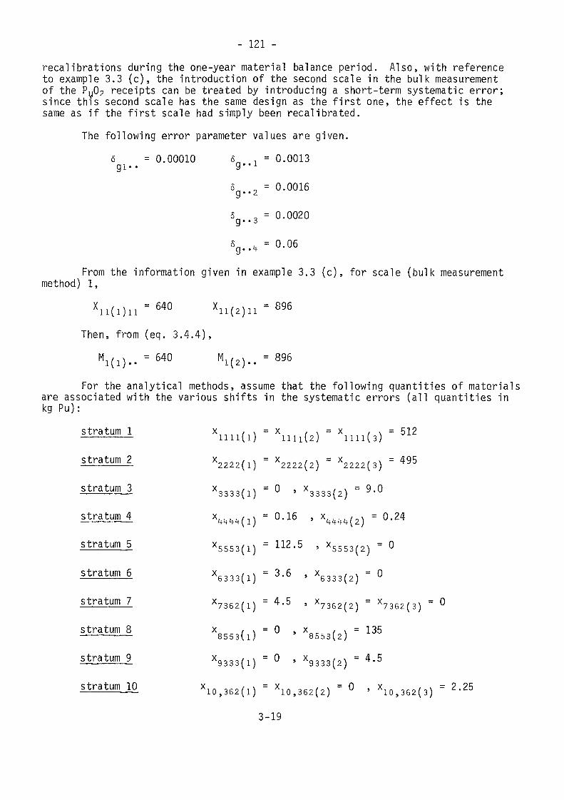
- 121 -

recalibrations during the one-year material balance period. Also, with referenceto example 3.3 (c), the introduction of the second scale in the bulk measurementof the PU02 receipts can be treated by introducing a short-term systematic error;since this second scale has the same design as the first one, the effect is thesame as if the first scale had simply been recalibrated.

The following error parameter values are given.6 = 0.00010 6 T = 0.0013g i - - 9"1

<5 , = 0.0016g • • 2

6 , = 0.0020g • • 3

fi„ u = 0.06q. . M-

From the information given in example 3.3 (c), for scale (bulk measurementmethod) 1,

Then, from (eq. 3.4.4),M,/.x = 640 M,/,x = 8961(1).. H2)"

For the analytical methods, assume that the following quantities of materialsare associated with the various shifts in the systematic errors (all quantities inkg Pu):

stratum 1 x , ,. = x = x / \ = 512—————— 1111(1) 1111(2) 1111(3)StratUÏÏ1 2 X 2 2 2 2 ( l ) = X 2 2 2 2 ( 2 ) = X 2 2 2 2 ( 3 ) = 495

X 3 3 3 3 ( l ) = ° ' X 3 3 3 3 ( 2 ) = 9'°

= °'24

X5553(l) = 112'5 ' X5553(2) = 0

X6333(l) = 3'6 ' X6333(2) = °

Stratum 7 X7362(l) = 4>5 ' X7362(2) = X7362(3)

X8553(l) = ° ' X8553(2) =

X9333(l) = ° » X9333(2) = 4'

10 X10)362(1) = X10, 362(2) = ° ' Xl 0 , 362( 3 )

3-19

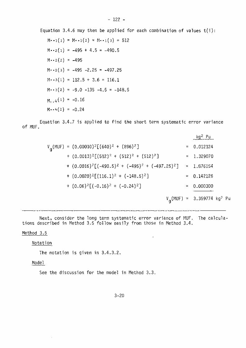
- 122 -Equation 3.4.6 may then be applied for each combination of values t(i):

M--i(i) = M-.l(2) = M"i(3) = 512M--2(i) = -495 + 4.5 = -490.5M.-2(2) = -495M-.a(3) = -495 -2.25 = -497.25M--3(i) = 112.5 + 3.6 - 116.1M--3(2) = -9.0 -135 -4.5 = -148.5M..4(0 = -O-16M--t(2) = -0.24

Equation 3.4.7 is applied to find the short term systematic error varianceof MUF.

kg2 PuV (MUF) = (0.00010)2[(640)2 + (896)2] = 0.012124

+ (0.0013)2[(512)2 + (512)2 + (512)2] = 1.329070+ (0.0016)2[(-490.5)2 + (-495)2 + (-497.25)2] = 1.876154+ (0.0020)2[(116.1)2 + (-148.5)2] = 0.142126+ (0.06)2[(-0.16)2 + (-0.24)2] = 0.000300

V (MUF) = 3.359774 kg2 Pu

Next, consider the long term systematic error variance of MUF. The calcula-tions described in Method 3.5 follow easily from those in Method 3.4.Method 3.5

NotationThe notation is given in 3.4.3.2.

ModelSee the discussion for the model in Method 3.3.

3-20

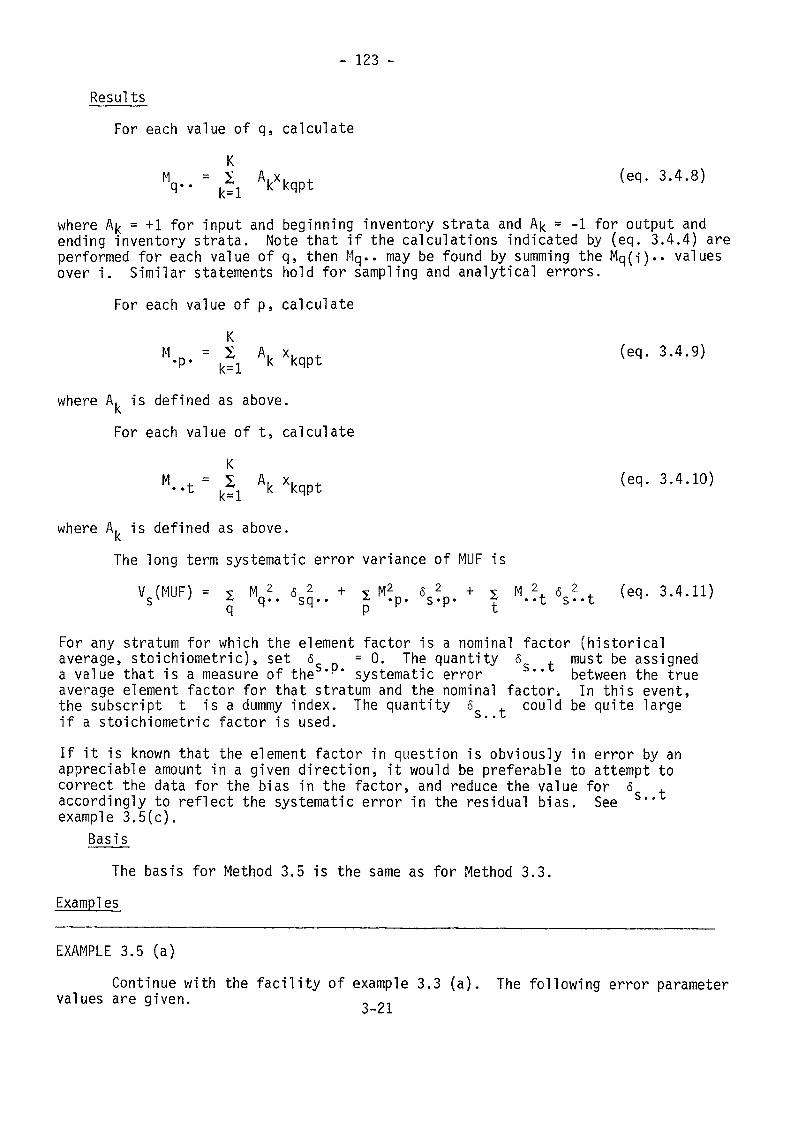
- 123 -

Results

For each value of q, calculate

V - k| Vkqpt

where A^ = +1 for input and beginning inventory strata and A|< = -1 for output andending inventory strata. Note that if the calculations indicated by (eq. 3.4.4) areperformed for each value of q, then Mq.. may be found by summing the Mq(-j).. valuesover i. Similar statements hold for sampling and analytical errors.

For each value of p, calculate

V = k| Ak Xkqpt

where A. is defined as above.For each value of t, calculate

M"t= k| AkXkqpt

where A. is defined as above.The long term systematic error variance of MUF is

V (MUF) = £ Mn2 6 2 + £ M2n oc2 + 2 M 2 6 2 (eq. 3.4.11)sv ' z q*- sq*- ~ *p- s-p- -r «-t S"tq P <-For any stratum for which the element factor is a nominal factor (historicalaverage, stoichiometric), set <5 =0. The quantity 6 . must be assigneda value that is a measure of the "• ' systematic error *' between the trueaverage element factor for that stratum and the nominal factor. In this event,the subscript t is a dummy index. The quantity 6 . could be quite largeif a stoichiometric factor is used.If it is known that the element factor in question is obviously in error by anappreciable amount in a given direction, it would be preferable to attempt tocorrect the data for the bias in the factor, and reduce the value for 6 .accordingly to reflect the systematic error in the residual bias. See sexample 3.5(c).

BasjjsThe basis for Method 3.5 is the same as for Method 3.3.

Exampl es^

EXAMPLE 3.5 (a)Continue with the facility of example 3.3 (a). The following error parametervalues are given.

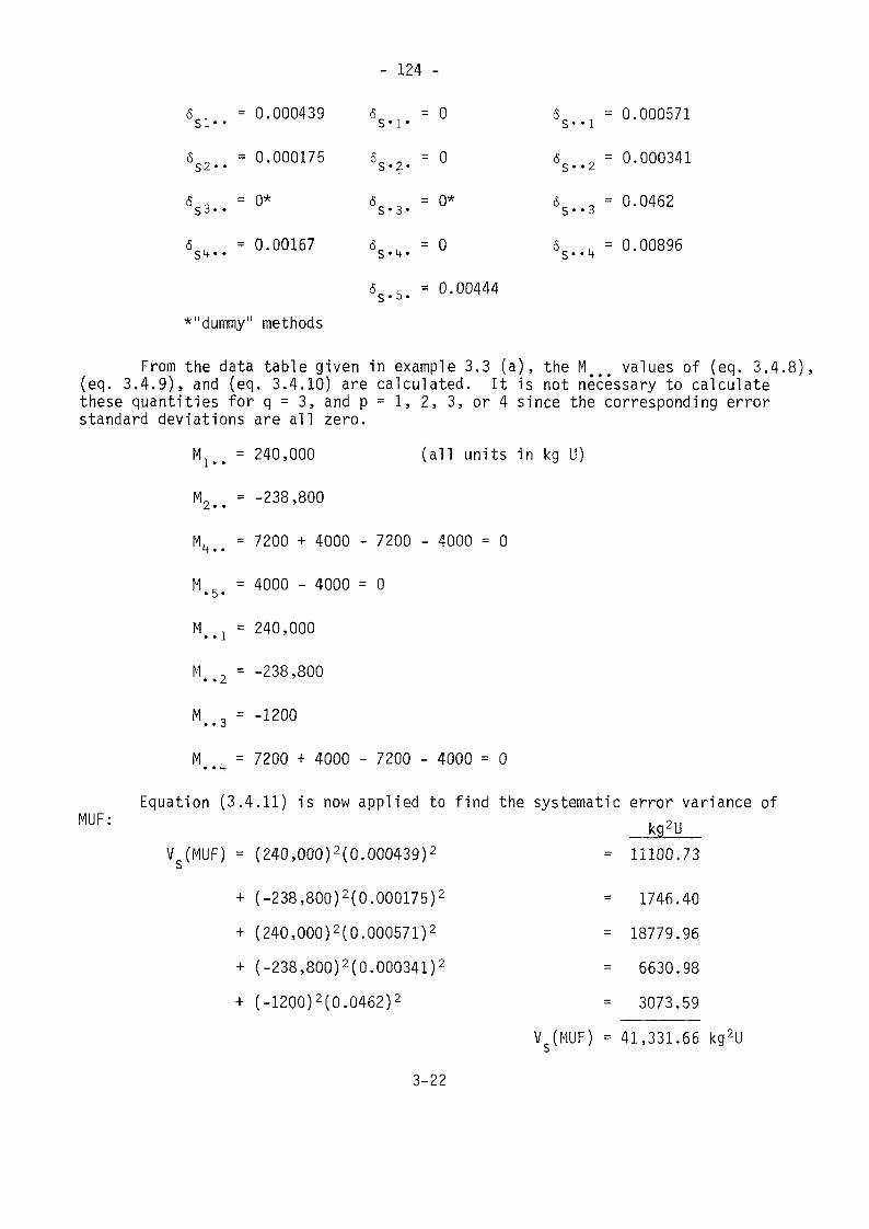
- 124 -

Se. = 0.000439 Ô n = 0 6 - 0.000571SI" 5' l- S' 'l

S = 0.000175 6S>2< = 0 ô 2 = 0.000341

= 0.0462

= 0.00896

S , =0*S3- •

ô , = 0.00167S 4 * *

6 S - 3 . = °*

&c , = oS « 4 «

ôs

f-6s

6S.5. = 0.00444

*"dummy" methods

From the data table given in example 3.3 (a), the M 4 > > values of (eq. 3.4.8),(eq. 3.4.9), and (eq. 3.4.10) are calculated. It is not necessary to calculatethese quantities for q = 3, and p = 1, 2, 3, or 4 since the corresponding errorstandard deviations are all zero.

Mle. = 240,000 (all units in kg U)

M2.. = -238,800

M. = 7200 + 4000 - 7200 - 4000 = 04 • •

M . = 4000 - 4000 = 0• 5«

M..J = 240,000

M.. 2 = -238,800

M , = -1200• • 6

M . = 7200 + 4000 - 7200 - 4000 = 0• • kEquation (3.4.11) is now applied to find the systematic error variance of

Vs(MUF) = (240,000)2(0.000439)2 = 11100.73

+ (-238,800)2(0.000175)2 = 1746.40+ (240, 000)2(0. 000571)2 = 18779.96+ (-238,800)2(0.000341)2 - 6630.98+ (-1200)2(0.0462)2 = 3073.59

VS(MUF) - 41,331.66 kg2U

3-22

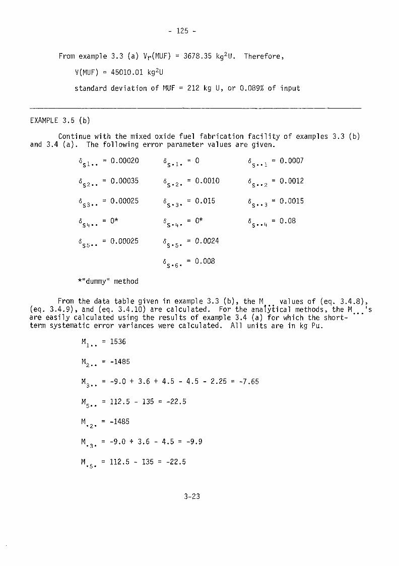
- 125 -

From example 3.3 (a) Vr{MUF) = 3678.35 kg2U. Therefore,V(MUF) = 45010.01 kg2Ustandard deviation of MUF = 212 kg U, or 0.089% of input

EXAMPLE 3.5 (b)Continue with the mixed oxide fuel fabrication facility of examples 3.3 (b)

and 3.4 (a). The following error parameter values are given.6 , = 0.00020 Sp , = 0 6 . = 0.0007si • • s-1 • s • • i<S , = 0.00035 6 „ = 0.0010 oe , = 0.0012S2« • S* 2« S • • 2

6 , = 0.00025 Sf , = 0.015 5 , = 0.0015S3« • S' 3* S* • 3

S . = 0.08<SS if •

6

= 0*

= 0.00025

ô s - <

6„ ,

+ . = °*

. = 0.0024

6 c = 0.008S «6*

*"dummy" method

From the data table given in example 3.3 (b), the M 4> values of (eq. 3.4.8),(eq. 3.4.9), and (eq. 3.4.10) are calculated. For the analytical methods, the M < < e ' sare easily calculated using the results of example 3.4 (a) for which the short-term systematic error variances were calculated. All units are in kg Pu.

M. = 1536i • •M2>. = -1485

M, = -9.0 + 3.6 + 4.5 - 4.5 - 2.25 = -7.653 • •

Mr = 112.5 - 135 = -22.55« •

M = -1485•2«

M 0 = -9.0 + 3.6 - 4.5 = -9.9• 3 •

M c = 112.5 - 135 = -22.5• 5*

3-23

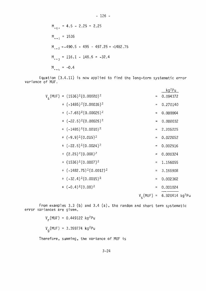
- 126 -

M = 4.5 - 2.25 - 2.25•6«

M . - 1536• • iM , =-490.5 - 495 - 497.25 = -1482.75• » z

M = 116.1 - 148.5 = -32.4• -3

M = -0.4• • 4

Equation (3.4.11) is now applied to find the long-term systematic errorvariance of MUF.

kg2PuVs(MUF) = (1536)2(0.00020)2 = 0.094372

+ (-1485)2(0.00035)2 = 0.270140+ (-7.65)2(0.00025)2 = 0.000004+ (-22.5)2(0.00025)2 = 0.000032+ (-1485)2(0.0010)2 = 2.205225+ (-9.9)2(0.015)2 - 0.022052+ (-22.5)2(0.0024)2 = 0.002916+ (2.25)2(0.008)2 = 0.000324+ (1536)2(0.0007)2 = 1.156055+ (-1482.75)2(0.0012)2 = 3.165908+ (-32.4)2(0.0015)2 - 0.002362+ (-0.4)2(0.08)2 = 0.001024

VS(MUF) = 6.920414 kg2Pu

From examples 3.3 (b) and 3.4 (a), the random and short term systematicerror variances are given.

Vr(MUF) = 0.449122 kg2Pu

V (MUF) = 3.359774 kg2Pu

Therefore, summing, the variance of MUF is

3-24

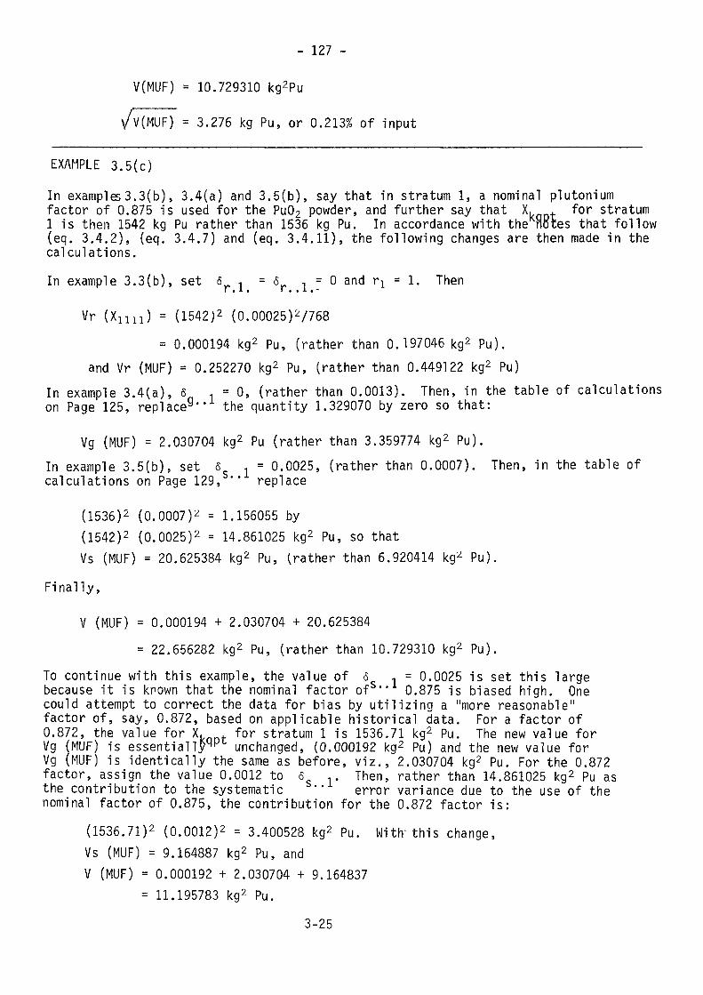
- 127 -

V(MUF) = 10.729310 kg2Pu

/ V(MUF) = 3.276 kg Pu, or 0.213% of input

EXAMPLE 3.5(c)In examples 3.3(b), 3.4(a) and 3.5(b), say that in stratum 1, a nominal plutoniumfactor of 0.875 is used for the Pu02 powder, and further say that X. . for stratum1 is then 1542 kg Pu rather than 1536 kg Pu. In accordance with the notes that follow(eq. 3.4.2), (eq. 3.4.7) and (eq. 3.4.11), the following changes are then made in thecalculations.In example 3.3(b), set <S , =6 n = 0 and rj = 1. Theni » .L • f * » t ~

Vr (Xmi) = (1542)2 (0.00025)2/768= 0.000194 kg2 Pu, (rather than 0.197046 kg2 Pu),

and Vr (MUF) = 0.252270 kg2 Pu, (rather than 0.449122 kg2 Pu)In example 3.4(a), s , = 0, (rather than 0.0013). Then, in the table of calculationson Page 125, replace9' the quantity 1.329070 by zero so that:

Vg (MUF) = 2.030704 kg2 Pu (rather than 3.359774 kg2 Pu).In example 3.5(b), set 5 . = 0.0025, (rather than 0.0007). Then, in the table ofcalculations on Page 129,s'' replace

(1536)2 (0.0007)2 = 1.156055 by(1542)2 (0.0025)2 = 14.861025 kg2 Pu, so thatVs (MUF) = 20.625384 kg2 Pu, (rather than 6.920414 kg2 Pu).

Finally,V (MUF) = 0.000194 + 2.030704 + 20.625384

= 22.656282 kg2 Pu, (rather than 10.729310 kg2 Pu).To continue with this example, the value of 6 , = 0.0025 is set this largebecause it is known that the nominal factor of 0.875 is biased high. Onecould attempt to correct the data for bias by utilizing a "more reasonable"factor of, say, 0.872, based on applicable historical data. For a factor of0.872, the value for X. . for stratum 1 is 1536.71 kg2 Pu. The new value forVg (MUF) is essential ljrpl unchanged, (0.000192 kg2 Pu) and the new value forVg (MUF) is identically the same as before, viz., 2.030704 kg2 Pu. For the 0.872factor, assign the value 0.0012 to 6 .. Then, rather than 14.861025 kg2 Pu asthe contribution to the systematic error variance due to the use of thenominal factor of 0.875, the contribution for the 0.872 factor is:

(1536.7l)2 (0.0012)2 = 3.400528 kg2 Pu. With'this change,Vs (MUF) = 9.164887 kg2 Pu, andV (MUF) = 0.000192 + 2.030704 + 9.164837

= 11.195783 kg2 Pu.3-25

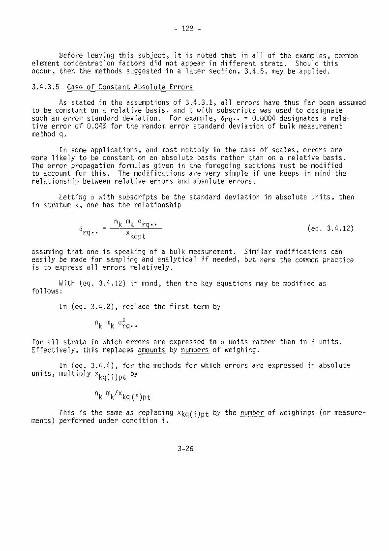
- 128 -

Before leaving this subject, it is noted that in all of the examples, commonelement concentration factors did not appear in different strata. Should thisoccur, then the methods suggested in a later section, 3.4.5, may be applied.3.4.3.5 Case of_ Constant Absolute^ Errors

As stated in the assumptions of 3.4.3.1, all errors have thus far been assumedto be constant on a relative basis, and s with subscripts was used to designatesuch an error standard deviation. For example, 6rq.. = 0.0004 designates a rela-tive error of 0.04% for the random error standard deviation of bulk measurementmethod q.

In some applications, and most notably in the case of scales, errors aremore likely to be constant on an absolute basis rather than on a relative basis.The error propagation formulas given in the foregoing sections must be modifiedto account for this. The modifications are very simple if one keeps in mind therelationship between relative errors and absolute errors.

Letting 0 with subscripts be the standard deviation in absolute units, thenin stratum k, one has the relationship

- ' ^ -assuming that one is speaking of a bulk measurement. Similar modifications caneasily be made for sampling and analytical if needed, but here the common practiceis to express all errors relatively.

With (eq. 3.4.12) in mind, then the key equations may be modified asfollows:

In (eq. 3.4.2), replace the first term bynk mk a?q.-

for all strata in which errors are expressed in a units rather than in 6 units.Effectively, this replaces amounts^ by numbers of weighing.

In (eq. 3.4.4), for the methods for which errors are expressed in absoluteunits, multiply xkq(-j)pt by

nkVXkq(i)ptThis is the same as replacing *kq(i)pt b^ tne nurober of weighings (or measure

ments) performed under condition i.

3-26

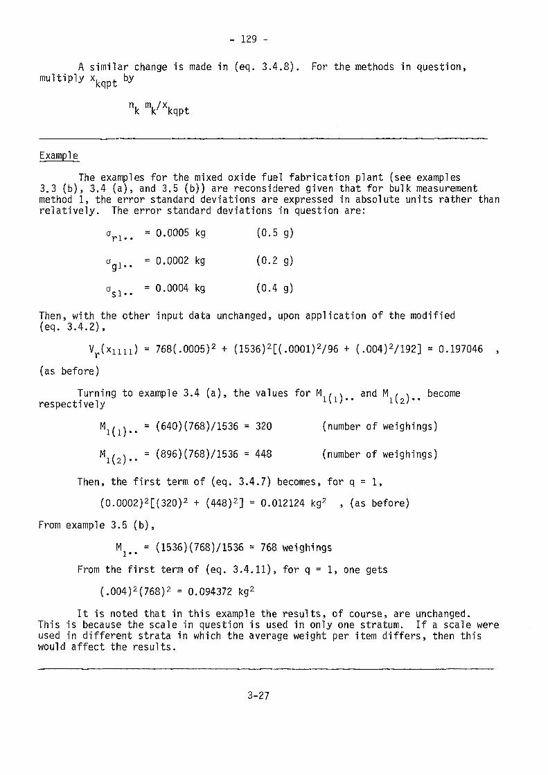
- 129 -

A similar change is made in (eq. 3.4.8). For the methods in question,multiply xkqpt by

n. m./x. .k k' kqpt

Example^The examples for the mixed oxide fuel fabrication plant (see examples

3.3 (b), 3.4 (a), and 3.5 (b)) are reconsidered given that for bulk measurementmethod 1, the error standard deviations are expressed in absolute units rather thanrelatively. The error standard deviations in question are:

arl.. = 0.0005 kg (0.5 g)

agl.. = 0.0002 kg (0.2 g)

asl_ = 0.0004 kg (0.4 g)

Then, with the other input data unchanged, upon application of the modified(eq. 3.4.2),

Vr(xmi) = 768(.0005)2 + (1536)2[(.0001)2/96 + (.004)2/192] = 0.197046 ,(as before)

Turning to example 3.4 (a), the values for M,/,).. and M / \ becomerespectively { )" i\2)"Mi(i)-- = (640)(768)/1536 = 320 (number of weighings)Mi(2)-- = (89ß)(768)/1536 = 448 (number of weighings)

Then, the first term of (eq. 3.4.7) becomes, for q = 1,(0.0002)2[(320)2 + (448)2] = 0.012124 kg2 , (as before)

From example 3.5 (b),Mle. = (1536)(768)71536 = 768 weighings

From the first term of (eq. 3.4.11), for q = 1, one gets(.004)2(768)2 = 0.094372 kg2

It is noted that in this example the results, of course, are unchanged.This is because the scale in question is used in only one stratum. If a scale wereused in different strata in which the average weight per item differs, then thiswould affect the results.

3-27

- 130 -

3.4.4 Variance of Cumulative_ MUFThe cumulative MUF is the sum of individual MUF's over a number of material

balance periods. The cumulative MUF has the same model structure as the MUF fora given material balance period, i.e., the MUF components are still the inputs,outputs, beginning and ending inventories. Therefore, the variance of the cumula-tive MUF is calculated using the same methods as are used for the MUF over a singlebalance period. In this connection, note that if one were interested in calculat-ing the variance of the cumulative MUF over, say, a three year period, then onlythe inventories at the beginning and end of this three year period affect theMUF, and hence its variance. It doesn't matter how many physical inventories thereare during this period of time; the three year MUF is completely independent ofsuch intermediate inventories.

In a parallel situation, if one were interested in calculating the MUF andits variance over a number of combined material balance areas (or facilities),then the remarks in the foregoing paragraph still apply. The summation is nowover space rather than over time. Thus, if the MUF for a state were to be calcu-lated, this quantity, and hence its variance, is affected only by inputs to andoutputs from the state, and the beginning and ending inventories in that state.Clearly, transfers among facilities within the state do not affect the MUF, justas transfers among locations within a facility do not affect the facility MUF.The problem is not one of calculating a state MUF or its variance; in conceptthis is a simple exercise, or at least, no more complicated than that of calculat-ing similar quantities for a facility. The problem is rather one of implementation,since all facilities within the state would have to be inventoried simultaneously.One could back off from this requirement by maintaining records of facility trans-fers between inventory times, but to be effective, inventories would have to bereasonably close to being simultaneous in time.

The foregoing discussion suggests the related questions as to how frequentlyone should take inventory to close a material balance and compute a MUF, and howfinely one should divide a material balance area into sub-areas. Here is an in-stance in which one's intuition is perhaps challenged by the facts, for it hasbeen proven that from point of view of maximizing the probability of detectingthe removal of material from a given material balance area over a fixed time inter-val , one should neither subdivide the material balance area into smaller sub-areas,nor should one subdivide the time interval to close the material balance morefrequently [3.8]. There are, of course, criteria to consider other than the detec-tion probability. It is clear that the role of more frequent material balanceclosings (more frequent inventories) is to detect removals of material more quickly.Correspondingly, subdivision of material balance areas into sub-areas will serveto localize the removals. It is unfortunate that these two important kinds ofcriteria, detection probability and identification of removals in time and spacework at cross-purposes; clearly, some balance is needed. See also references[3.9]- [3.11].

3.4.5 Variance of Isotope MUF by General ApproachIn the foregoing sections, the variance of element MUF was treated. The

isotope MUF for a facility may also be calculated, and so it is necessary to pro-vide methods for calculating its variance.

3-28

- 131 -

Before providing such methods, it is worthwhile to note that for facilitiesother than enrichment plants, primary emphasis should logically be devoted to con-trolling the element MUF. If adequate control is maintained on the element MUF,then, except for mistakes in booking isotope values, there is no way the isotopeMUF could be out of control. Since, on a percentage of throughput basis, theuncertainty in the isotope MUF cannot be smaller than the uncertainty in the ele-ment MUF, it follows that the element MUF is the quantity of primary concern.This fact was pointed out, and quantified results were found for a light waterreactor fuel fabrication facility in a paper by Nilson, Schneider, and Jaech[3.12]. The authors pointed out that the variance of isotope MUF can easily betwice that of the variance of element MUF on a percentage of throughput basis.In the type of facility they treated, from a materials control viewpoint, the iso-tope MUF provides no information beyond that provided by the element MUF. (Theauthors do point out, however, that to guard against substitution diversion stra-tegies, isotope measurements must, of course, be made. The question is not whetheror not such measurements need be made, but rather, how the resulting data are tobe factored into the decision framework.)

The variance of the isotope MUF is, as implied in the preceding paragraphs,made up of two types of sources of variance. First, any uncertainties in measur-ing bulks and element concentrations will also result in an uncertainty in theisotope value since the isotope is normally calculated as the product of bulk,element concentration, and isotope concentration. The exception is with NDA mea-surements in which the isotope is measured directly and the element is calculatedfrom that measurement. Such items normally comprise a small part of the materialbalance. That part of the variance of the isotope MUF that is due to errors inthe measurements of bulk and element concentration is covered in Section 3.4.5.1.

Secondly, errors occur in the measurement of isotope concentration. Here,booking practices play an important role. If a block of material is inputted to afacility at a given measured isotope concentration value, and if nothing in theprocess changes that concentration, then the output would be at the same concentra-tion as the input. To assure that the concentration remains unchanged, measurementsare also made of the output. But in the situation just described, these measure-ments should be treated as verification measurements and should not be booked unlessthey provide evidence that the isotope concentration had indeed changed. If suchverification type measurements are booked, then they introduce an artifical MUFin the isotope value and also affect the variance of the isotope MUF. This willbe illustrated in the example of Section 3.4.5.2 in which section the method isprovided for calculating that contribution to the variance of isotope MUF due touncertainties in the measurements of isotope concentrations.

3.4.5.1 Variance of Isotope MUF Due to Measuretne_irt_Errprs_ in Bu1j< and ElementMeasurements

Method 3.6Notation

The notation is given in 3.4.3.2 except that x now refers to an isotopeweight rather than an element weight.

3-29

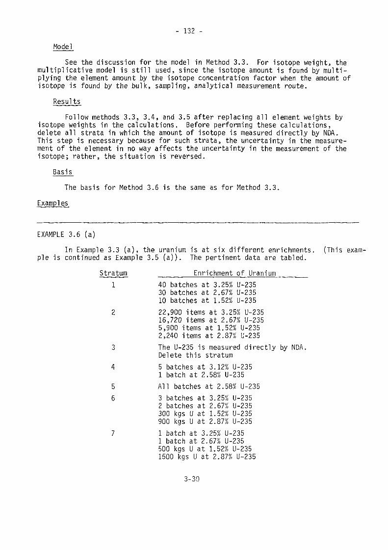
- 132 -Mode]

See the discussion for the model in Method 3.3. For isotope weight, themultiplicative model is still used, since the isotope amount is found by multi-plying the element amount by the isotope concentration factor when the amount ofisotope is found by the bulk, sampling, analytical measurement route.

ResultsFollow methods 3.3, 3.4, and 3.5 after replacing all element weights by

isotope weights in the calculations. Before performing these calculations,delete all strata in which the amount of isotope is measured directly by NDA.This step is necessary because for such strata, the uncertainty in the measure-ment of the element in no way affects the uncertainty in the measurement of theisotope; rather, the situation is reversed.

BasisThe basis for Method 3.6 is the same as for Method 3.3.

Examples

EXAMPLE 3.6 (a)In Example 3.3 (a), the uranium is at six different enrichments. (This exam-

ple is continued as Example 3.5 (a)). The pertinent data are tabled.Stratum Enrichment of Uranium

1 40 batches at 3.25% U-23530 batches at 2.67% U-23510 batches at 1.52% U-235

2 22,900 items at 3.25% U-23516,720 items at 2.67% U-2355,900 items at 1.52% U-2352,240 items at 2.87% U-235

3 The U-235 is measured directly by NDA.Delete this stratum

4 5 batches at 3.12% U-2351 batch at 2.58% U-235

5 All batches at 2.58% U-2356 3 batches at 3.25% U-235

2 batches at 2.67% U-235300 kgs U at 1.52% U-235900 kgs U at 2.87% U-235

7 1 batch at 3.25% U-2351 batch at 2.67% U-235500 kgs U at 1.52% U-2351500 kgs U at 2.87% U-235

3-30

- 133 -

Using the notation of the two cited examples, these data are converted tokgs U-235. From Example 3.3 (a):

Xmi = (120,000)(0.0325) + (90,000) (0.0267) + (30,000)(0.0152)= 6759.00

x2222 = 6723.21 x6l(im = 211.47

x^i^ = 218.16 x7V51t = 109.85

X51t51t = 103.20

From Example 3.5 (a):

M = 6759.00 M n = 6759.00i • • • • iM0 = -6723.21 M „ = -6723.212* • • • 2

M, = 0.04 M , = 0.04If • • * • H-

M , = -6.65• 5 «

From Example 3.3 (a), to find Vr(MUF):Vr(xim) = 0.0553 kg2 U-235Vr(x2222) = 0.0615 kg2 U-235

= 0.8556 kg2 U-235= 0.5543 kg2 U-235

Vr(x61tlf i t) = 0.8039 kg2 U-235

V r(x7 l454) = 0.6280 kg2 U-235

Then,

Vr(MUF) = 2.9586 kg2 U-235

From Example 3.5 (a), to find V (MUF):kg2U-235

(6759.00)2(0.000439)2 = 8.8043+ (-6723.21)2(0.000175)2 = 1.3843+ (0.04)2(0.00167)2 = 0.0000+ (-6.65)2(0.00444)2 = 0.0009+ (6759.00)2(0.000571)2 = 14.8949

3-31.

- 134 -

+ (-6723.21)2(0.00034l)2 = 5.2561+ (0.04)2(0.00896)2 = 0.0000

VS(MUF) = 30.3405 kg2U-235

The variance in the U-235 isotope MUF due to errors of measurement for bulkand uranium concentrations is the sum,

2.9586 + 30.3405 = 33.2991 kg2U-235To this must now be added the uncertainties due to the measurement of U-235

concentrations in strata 1, 2, and 4-7, and due tu the measurement of the amountof U-235 in stratum 3. The procedure for incorporating these uncertainties is inMethod 3.7.

3.4.5.2 Variance of Isotope MUF Due to Measurement Errors in Isotope MeasurementsMethod 3.7

NotationS. = algebraic sum of isotope weights for isotope factor i. In the

algebraic sum, amounts in input and beginning inventory stratahave a plus sign while those in output and ending inventorystrata have a minus sign.

G = total number of isotope factorsr.* = number of samples drawn to establish isotope factor ic-* = number of isotopic analyses per sampleo*, with subscripts = a relative standard deviation associated with

an isotopic measurement. The subscripts are defined as inSection 3.4.3.2. The only errors assumed to be non-zero are:

<5* = random error in sampling for isotope

6* t = random error in isotopic analysisI * L*

<5* t = long term systematic error in isotopic analysiso * * U

T. = sum of S. values based on analytical method t\f t

V*{MUF) = random error variance in MUF due to random errors in isotopemeasurements

V*(MUF) = systematic error variance in MUF due to systematic errors ins isotope measurements3-32

- 135 -Model

See the discussion for the model in Method 3.6.Results

GV*(MUF) = £ S2(S*2.pyr* + 6£2.t/r*c*) (eq. 3.4.13}

VJ(MUF) = £ T2 ôj.2t (eq. 3.4.14)\f

Basrs_The basis for this method is the same as for Method 3.3.

Examples

EXAMPLE 3.7 (a)Example 3.6 (a) is continued. The following values are given for the para-

meters. (The nominal factor applies to the NDA measurements in stratum 3.)Factor (i)0.03250.02670.01520.02870.03120.0258Nominal

ri5321454

2770

£i2221221

£111211_

t1112113

6* . = 0.0005 6* 0 = 0.0005r•i• r-2-6* . = 0.0015 a* . = 0.0008r« • i s« «i

= 0.0022 6* = 0.0010

6* _ = 0.07 6* , = 0.04r • • s s • • 3Equations ( eq. 3.4.13) and (eq. 3.4.14) may now be applied, but first, the

S-j and Tt values must be calculated. The data are from Example 3.6 (a).

3-33

- 136 -

51 = 0.0325 (120,000 - 114,500 - 3600 - 1000} - 29.25

52 = 80.10 S5 = 187.20

53 = -4.56 S6 = 134.16

54 = -390.32 S7 = -36.00

T! = 29.25 + 80.10 - 4.56 + 187.20 + 134.16 = 426.15

T2 = -390.32

T3 = -36.00

From (eq. 3.4.13.),V*(MUF) = (29.25)2[(0.0005)2/5 + (0.0015)2/10] + •••

= 0.0766 kg2U-235From (eq. 3.4.14),

V*(MUF) - (426.15)2(0.0008)2 + •••

= 2.3422 kg2U-235Using the results from Examples 3.6 (a) and the above, the total variance

of the isotope MUF is V*(MUF):V*(MUF) = 33.2991 + 0.0766 + 2.3422 = 35.7179 kg2U-235

standard deviation = 5.976 kg U-235To continue with this example, suppose now that booking practices are changed

such that measurements of outputs are not regarded as verification measurementsbut are actually booked. Redefine the factors as follows:

Stratum Factors ____Description1

2

0.032500.026700.015200.032570.026680.015210.02870

Measurement of input; theshipper's values arebookedMeasurement of output,based on facility mea-surements

3-34

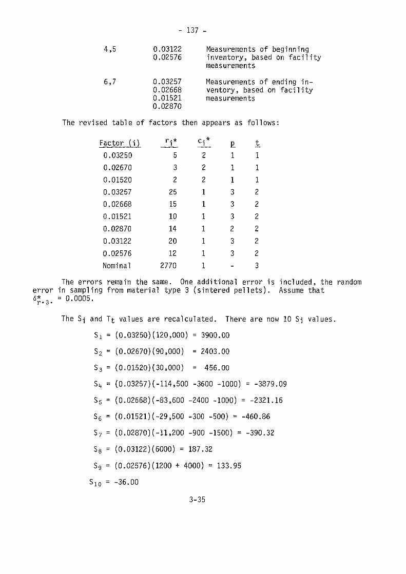
- 137 -4,5 0.03122 Measurements of beginning

0.02576 inventory, based on facilitymeasurements

6,7 0.03257 Measurements of ending in-0.02668 ventory, based on facility0.01521 measurements0.02870

The revised table of factors then appears as follows:

Factor (i)0.032500.026700.015200.032570.026680.015210.028700.031220.02576Nominal

r.j*532251510142012

2770

p . ft

2221l11111

R111333233_

t1112222223

The errors remain the same. One additional error is included, the randomerror in sampling from material type 3 (sintered pellets). Assume that<5* , = 0.0005.r • s •

The S-j and T^ values are recalculated. There are now 10 S-j values.51 = (0.03250)(120,000) = 3900.0052 = (0.02670)(90,000) = 2403.0053 = (0.01520)(30,000) = 456.0054 = (0.03257)(-114,500 -3600 -1000) = -3879.0955 = (0.02668)(-83,600 -2400 -1000) = -2321.1656 = (0.01521)(-29,500 -300 -500) = -460.8657 = (0.02870)(-11,200 -900 -1500) = -390.3258 = (0.03122)(6000) = 187.3259 = (0.02576)(1200 + 4000) = 133.95S10 = -36.00

3-35

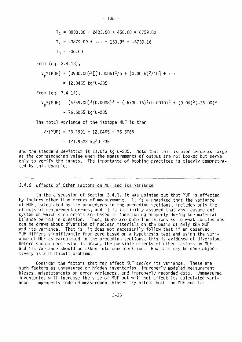
- 138 -

T! = 3900.00 + 2403.00 + 456.00 - 6759.00T2 = -3879.09 + ... + 133.95 = -6730.16T3 = -36.00

From (eq. 3.4.13),Vr*(MUF) = (3900.00)2[(0.0005)2/5 + (0.0015)2/10] + •••

= 12.0465 kg2U-235From (eq. 3.4.14),VS*(MUF) = (6759.00)2(0.0008)2 + (-6730.16)2(0.0010)2 + (0.04)2(-36.00)2

= 76.6065 kg2U-235The total variance of the isotope MUF is then

V*(MUF) = 33.2991 + 12.0465 + 76.6065= 121.9522 kg2U-235

and the standard deviation is 11.043 kg U-235. Note that this is over twice as largeas the corresponding value when the measurements of output are not booked but serveonly to verify the inputs. The importance of booking practices is clearly demonstra-ted by this example.

3.4.6 Effects of Other Factors on MUF and its VarianceIn the discussion of Section 3.4.1, it was pointed out that MUF is affected

by factors other than errors of measurement. It is emphasized that the varianceof MUF, calculated by the procedures in the preceding sections, includes only theeffects of measurement errors, and it is implicitly assumed that any measurementsystem on which such errors are based is functioning properly during the materialbalance period in question. Thus, there are some limitations as to what conclusionscan be drawn about diversion of nuclear materials on the basis of only the MUFand its variance. That is, it does not necessarily follow that if an observedMUF differs significantly from zero based on a hypothesis test and using the vari-ance of MUF as calculated in the preceding sections, this is evidence of diversion.Before such a conclusion is drawn, the possible effects of other factors on MUFand its variance should be taken into consideration. How this may be done objec-tively is a difficult problem.

Consider the factors that may affect MUF and/or its variance. These aresuch factors as unmeasured or hidden inventories, improperly modeled measurementbiases, misstatements on error variances, and improperly recorded data. Unmeasuredinventories will increase the size of MUF but will not affect its calculated vari-ance. Improperly modeled measurement biases may affect both the MUF and its

3-36

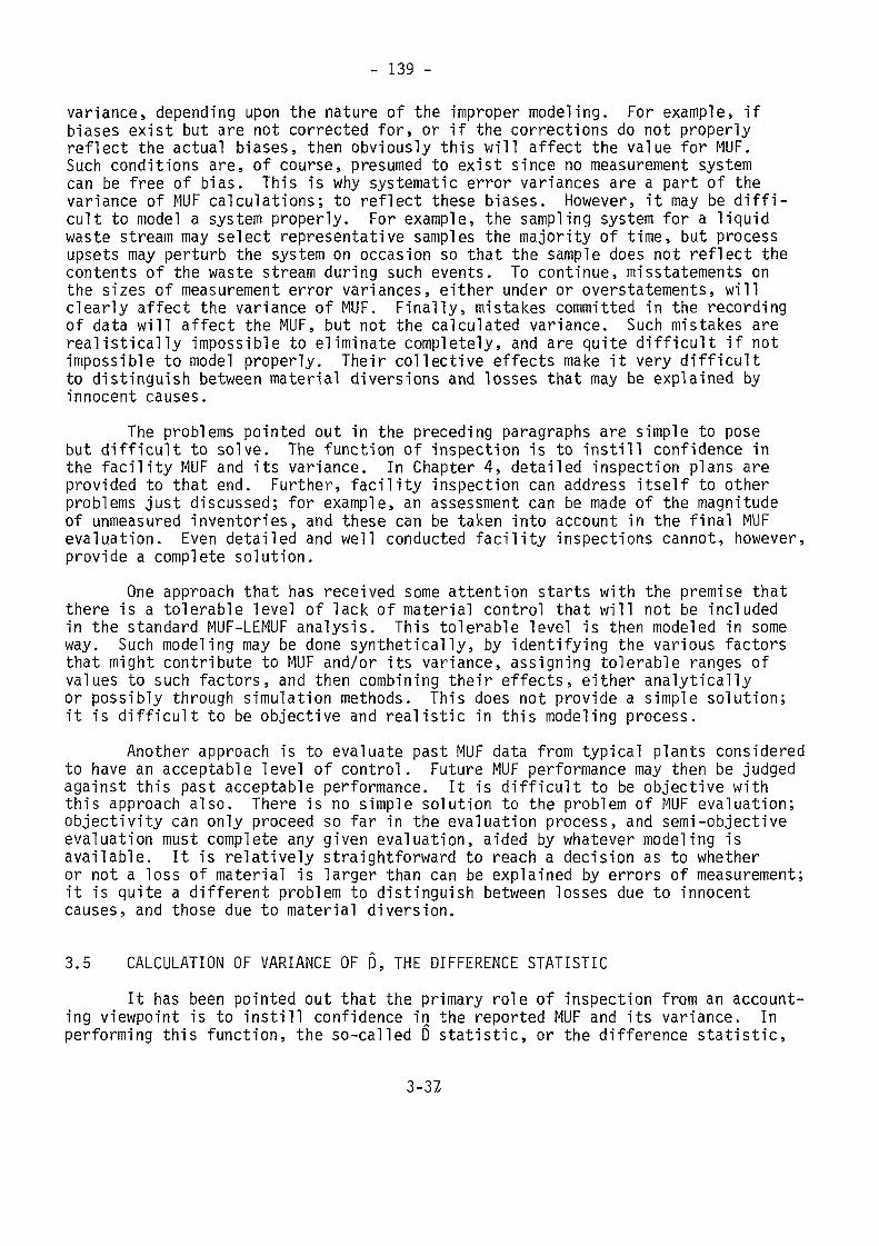
- 139 -

variance, depending upon the nature of the improper modeling. For example, ifbiases exist but are not corrected for, or if the corrections do not properlyreflect the actual biases, then obviously this will affect the value for MUF.Such conditions are, of course, presumed to exist since no measurement systemcan be free of bias. This is why systematic error variances are a part of thevariance of MUF calculations; to reflect these biases. However, it may be diffi-cult to model a system properly. For example, the sampling system for a liquidwaste stream may select representative samples the majority of time, but processupsets may perturb the system on occasion so that the sample does not reflect thecontents of the waste stream during such events. To continue, misstatements onthe sizes of measurement error variances, either under or overstatements, willclearly affect the variance of MUF. Finally, mistakes committed in the recordingof data will affect the MUF, but not the calculated variance. Such mistakes arerealistically impossible to eliminate completely, and are quite difficult if notimpossible to model properly. Their collective effects make it very difficultto distinguish between material diversions and losses that may be explained byinnocent causes.

The problems pointed out in the preceding paragraphs are simple to posebut difficult to solve. The function of inspection is to instill confidence inthe facility MUF and its variance. In Chapter 4, detailed inspection plans areprovided to that end. Further, facility inspection can address itself to otherproblems just discussed; for example, an assessment can be made of the magnitudeof unmeasured inventories, and these can be taken into account in the final MUFevaluation. Even detailed and well conducted facility inspections cannot, however,provide a complete solution.

One approach that has received some attention starts with the premise thatthere is a tolerable level of lack of material control that will not be includedin the standard MUF-LEMUF analysis. This tolerable level is then modeled in someway. Such modeling may be done synthetically, by identifying the various factorsthat might contribute to MUF and/or its variance, assigning tolerable ranges ofvalues to such factors, and then combining their effects, either analyticallyor possibly through simulation methods. This does not provide a simple solution;it is difficult to be objective and realistic in this modeling process.

Another approach is to evaluate past MUF data from typical plants consideredto have an acceptable level of control. Future MUF performance may then be judgedagainst this past acceptable performance. It is difficult to be objective withthis approach also. There is no simple solution to the problem of MUF evaluation;objectivity can only proceed so far in the evaluation process, and semi-objectiveevaluation must complete any given evaluation, aided by whatever modeling isavailable. It is relatively straightforward to reach a decision as to whetheror not a loss of material is larger than can be explained by errors of measurement;it is quite a different problem to distinguish between losses due to innocentcauses, and those due to material diversion.

3.5 CALCULATION OF VARIANCE OF D, THE DIFFERENCE STATISTICIt has been pointed out that the primary role of inspection from an account-

ing viewpoint is to instill confidence in the reported MUF and its variance. Inperforming this function, the so-called D statistic, or the difference statistic,

3-3Z

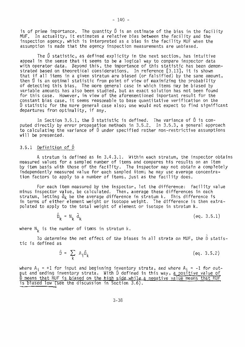
- 140 -

is of prime importance. The quantity D is an estimate of the bias in the facilityMUF. In actuality, it estimates a relative bias between the facility and theinspection agency, which is interpreted as a bias in the facility MUF when theassumption is made that the agency inspection measurements are unbiased.

The D statistic, as defined explicity in the next section, has intuitiveappeal in the sense that it seems to be a logical way to compare inspector datawith operator data. Beyond this, the importance of this statistic has been demon-strated based on theoretical considerations. In reference [3.13], it is shownthat if all items in a given stratum are biased (or falsified) by the same amount,then D is an optimal statistic from point of view of maximizing the probabilityof detecting this bias. The more general case in which items may be biased byvariable amounts has also been studied, but an exact solution has not been foundfor this case. However, in view of the aforementioned important result for theconstant bias case, it seems reasonable to base quantitative verification on theD statistic for the more general case also; one would not expect to find significantdepartures from optimal ity, if any.

In Section 3.5.1, the D statistic is defined. The variance of D is com-puted directly by error propagation methods in 3.5.2. In 3.5.3, a general approachto calculating the variance of D under specified rather non-restrictive assumptionswill be presented.

3.5.1 Definition of DA stratum is defined as in 3.4.3.1. Within each stratum, the inspector obtains

measured values for a sampled number of items and compares his results on an itemby item basis with those of the facility. The inspector may not obtain a completelyindependently measured value for each sampled item; he may use average concentra-tion factors to apply to a number of items, just as the facility does.

For each item measured by the inspector, let the difference: facility valueminus inspector value, be calculated. Then, average these differences in eachstratum, letting d|< be the average difference in stratum k. This difference isin terms of either element weight or isotope weight. The difference is then extra-polated to apply to the total weight of element or isotope in stratum k.

(eq. 3.5.1)

where N, is the number of items in stratum k.To determine the net effect of the biases in all strata on MUF, the D statis

tic is defined asD = E A.D. (eq. 3.5.2)

k 1 k

where A-,- = +1 for input and beginning inventory strata, and where A^ = -1 for out-gut and ending inventory strata. With D defined in this way, expositive value qf_D means that MUF is biased on the high side while a negative value means that MUFis biased low T/see the discussion in Section 3.6).

3-38

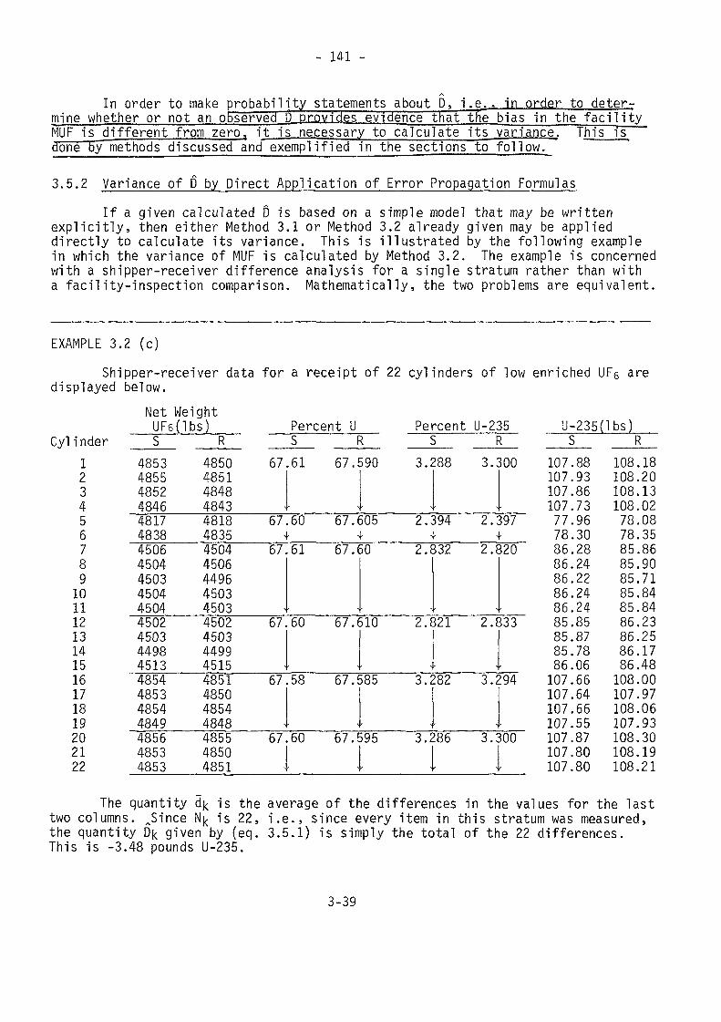
- 141 -

In order to make probability statements about D, i.e., in order to deter-Itrine whether or not an observed D provides evidence that the bias In the facilityMUF is different from zero, ij is necessary to calculate its variance. This isdone by methods discussed and exemplified in the sections to follow.

3.5.2 Variance of D by Direct Application of Error Propagation FormulasIf a given calculated D is based on a simple model that may be written

explicitly, then either Method 3.1 or Method 3.2 already given may be applieddirectly to calculate its variance. This is illustrated by the following examplein which the variance of MUF is calculated by Method 3.2. The example is concernedwith a shipper-receiver difference analysis for a single stratum rather than witha facility-inspection comparison. Mathematically, the two problems are equivalent.

EXAMPLE 3.2 (c)Shipper-receiver data for a receipt of 22 cylinders of low enriched UFg are

displayed below.

Cylinder12345678910111213141516171819202122

NetUFsS

4853485548524846481748384506450445034504450445024503449845134854485348544849485648534853

Weightilbsj____ Percent U Percent U-235

R S R S R4850 67485148484843

.61 67. î590 3.2188 3.;300

4818 67.60 67.605 2.394 2.3974835 4 * 4- 4-4504 674506449645034503 \4502 674503449945154851 67485048544848

61 67. «

60 67. e

58 67. E

50 2. t

510 2.Ï

585 3.Î

332 2. i

321 2.Î

182 3. i

320

333

?94

4855 67.60 67.595 3.286 3.3004850 I I I !4851 4 - 4 - 4 - 1

U-235(1bs)S

107.88107.93107.86107.7377.9678.3086.2886.2486.2286.2486.2485.8585.8785.7886.06107.66107.64107.66107.55107.87107.80107.80

R108.18108.20108.13108.0278.0878.3585.8685.9085.7185.8485.8486.2386.2586.1786.48108.00107.97108.06107.93108.30108.19108.21

The quantity dj< is the average of the differences in the values for the lasttwo columns. J5ince N|< is 22, i.e., since every item in this stratum was measured,the quantity Dk given by (eq. 3.5.1) is simply the total of the 22 differences.This is -3.48 pounds U-235.

3-39

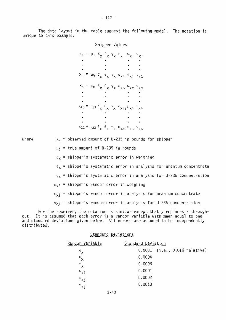
- 142 -

The data layout in the table suggest the following model. The notation isunique to this example.

Shipper ValuesXi = Ui 8 Y e o, v

vxi= U5

Xi3=

where x. = observed amount of U-235 in pounds for shippery-j - true amount of U-235 in poundsox = shipper's systematic error in weighingex = shipper's systematic error in analysis for uranium concentrateYX = shipper's systematic error in analysis for U-235 concentrationexj = shipper's random error in weighingu)x.j = shipper's random error in analysis for uranium concentratev^j = shipper's random error in analysis for U-235 concentration

For the receiver, the notation is similar except that y replaces x through-out. It is assumed that each error is a random variable with mean equal to oneand standard deviations given below. All errors are assumed to be independentlydistributed.

Standard DeviationsRandom Variable Standard Deviation

6X 0.0001 {i.e., 0.01% relative)6X 0.0004Yx 0.0006ex1 0.0001u . 0.0002v. 0.0010xj

3-40

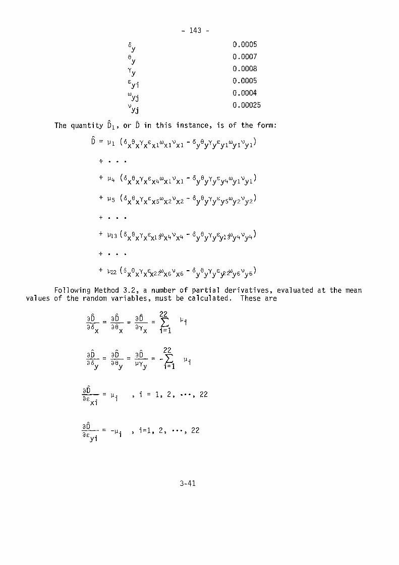
- 143 -6 0.00059 0.0007y 0.0008e 1 0.0005u 0.0004yjv 0.00025

•J J

The quantity DI, or D in this instance, is of the form:n - l K \

vis

Following Method 3.2, a number of partial derivatives, evaluated at the meanvalues of the random variables, must be calculated. These are

3D_ _ 3D = 3D _ y p.90x " "x " x " 1 = 1

la-. = il_ = 3-P - V30y " "y " y " 'fa "1y\

"ae — = ui 5 i = 1» 2, •••, 22

3-41

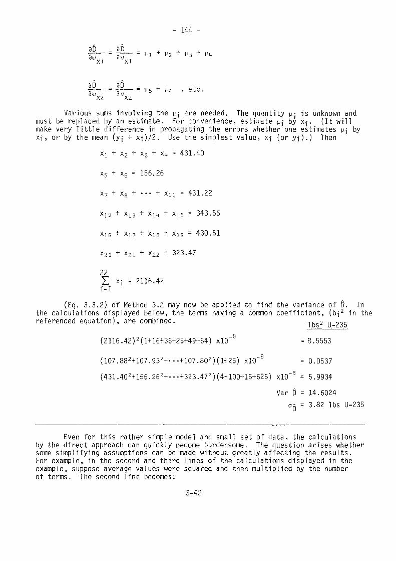
- 144 -

3D 3D -

_ . _ . M5 + P6 ,etc.

Various sums involving the y-j are needed. The quantity u^ is unknown andmust be replaced by an estimate. For convenience, estimate uj by x-j . (It willmake very little difference in propagating the errors whether one estimates P-J byXT, or by the mean (y-, + xi)/2. Use the simplest value, xj (or yi).) Then

Xj + x2 + x3 + x4 = 431.40

x5 + x6 = 156.26

X7 + x8 + ••• + xn = 431.22X12 + *i3 + Xi4 + xis = 343.56

x16 + x17 + x18 + xig = 430.51

X20 + x2i + x22 = 323.47

22£ x-j = 2116.42i=l

(Eq. 3.3.2} of Method 3.2 may now be applied to find the variance of D. Inthe calculations displayed below, the terms having a common coefficient, (bj2 in thereferenced equation), are combined. ,, 2 y 035

(2116.42)2(l+16+36+25+49+64) xlO"8 = 8.5553

(107.882+107.932+-..+107.802)(l+25) xlO"8 = 0.0537(431.402+156.262+---+323.472)(4+100+16+625) xlO"8 - 5.9934

Var D = 14.6024a = 3.82 Ibs U-235

Even for this rather simple model and small set of data, the calculationsby the direct approach can quickly become burdensome. The question arises whethersome simplifying assumptions can be made without greatly affecting the results.For example, in the second and third lines of the calculations displayed in theexample, suppose average values were squared and then multiplied by the numberof terms. The second line becomes:

3-42

- 145 -

22(96.20)2(l+25) xlO"8 = 0.0529 (compared with 0.0539)This third line becomes

6(352.74)2(4+100+16+625) xlO"8 = 5.5618 (compared with 5.9934)With these simplifying assumptions, up would be 3.76 Ibs U-235 rather than

3.82 Ibs U-235, which is not a difference of major impact.This example, and others of a similar nature, suggests that, as for the

variance of MUF, a general approach for calculating the variance of 5 based onsimplifying assumptions can also be developed. This is the subject of the nextsection.3.5.3 Variance of D by General Approach

General formulas will be developed to permit simple calculation of the vari-ance of D. These formulas will be based on assumptions set forth in Section 3.5.3.1As was true for the calculation of the variance of MUF by general formulas, theassumptions will rarely if ever be completely valid in given applications. However,experience has shown that this is not a great difficulty, since in many cases, evenmoderate departures from the assumptions have very little effect (as was illustratedby the example just presented). Further, if one has concern about the validity ofthe general formulas in a given instance, they can readily be altered as appropriateto accommodate a different set of circumstances.

3.5.3.1 AssumptionsThe assumptions about the facility data were set forth in Section 3.4.3.1.

(Again, the variance of D for element weight is considered here; see Section 3.5.4for isotope weight.) The additional assumptions relative to the inspection are asfollows:

(1) For samples of items within a stratum, the inspector also makes mea-surements. He need not necessarily make the same type of measurement as thefacility, e.g., he may use nondestructive assay methods to a much greater extentthan does the facility operator.

(2) The inspector and the facility use the same material sampling proce-dures, and hence, systematic errors in sampling will cancel. The effect ofchanging this assumption on the calculations should be quite obvious.

(3) When there are batches within a stratum, the inspector may firstsample batches at random and then measure the same number of items in each batchsampled.

(4) The inspector may utilize a number of laboratories to analyze thesamples, but for a given stratum, all use the same analytical method. This ideais carried further in the next section.

3-43

- 146 -

3.5.3.2 NotationThe notation is an extension to that given earlier in Section 3.4.3.2. The

quantity Y|<qpt "is defined as was x^qp^, except that y refers to an inspector value.The measurement methods q, p, t refer to his methods .

Note: As was the case with the facility operator, it may be that withina stratum, the same systematic error does not affect all items, i.e., there is ashort term systematic error. Use parentheses to indicate the total element weightassociated with "condition i" for a given measurement.

Since, under assumption (3) of the previous paragraph, the inspector mayutilize a number of laboratories, this concept is extended to accommodate thispossibility. Specifically,

y, 4-/-Î/")) ~ total element weight in stratum k as determined by the inspec-qp ( (3 i ) using the indicated measurement methods, and for thoseitems measured under condition j within laboratory i.If need be, this idea can be extended further using additional classifica-

tions that may be either crossed or nested. However, the extension just indicatedshould be adequate to cover the great majority of applications.

To continue with the notation, 8 with subscripts still denotes a relativestandard deviation. The first subscript of r, s, or g is defined as in 3.4.3.2.If the first subscript is h, this refers to a short term systematic error withinanother such error, i.e., to a condition or time effect within a laboratory. Sub-scripts 2, 3, and 4 are defined as in 3.4.3.2. A fifth subscript is either x torefer to an operator standard deviation or y to refer to one for the inspector.Further, let u^, w^, v^, and a^ denote inspector parameters associated withstratum k:

u, = number of batches sampled by the inspector

w, = number of items per sampled batch for which the inspectormakes bulk measurements

v. = number of samples drawn by the inspector per sampled batchto determine the element factor

a, = number of analyses performed by the inspector per sampleWith this notation in mind, Method 3.8 will now provide formulas needed to

compute the random error variance of 0.

3.5.3.3 Random Error Variance of DMethod 3.8

NotationThe notation is given in Sections 3.4.3.2 and 3.5.3.2.

3-44

- 147 -Model

The statistic D is defined in (eq. 3.5.2). The model for a given term inthe indicated sum is exemplified by the model discussed in example 3.2 (c).

ResultsFor stratum k, the random error variance of D^ due to measurement errors

committed by the facility isVrx(0k} = x

That due to the inspector isVry(0k] = *Kqpt[6rWUkWk + 6r-p.y/ukvk + ôr- -ty/akukvk] (eq. 3.5.4)

The variance of D, is

VV = VÔk) + VVThe variance of 0 is then found by summing Vr(ß|<) over the strata.

KVJD) = £ V (D.) (eq. 3.5.6)r k=l r k

Basj_sThe formula for Vr(D) is found by application of Methods 3.1 and 3.2. The

key equations, (eq. 3.5.3) and (eq. 3.5.4) are simple to remember if it is keptin mind that the divisor for each variance component is the number of measurementoperations affecting that component. For example, in (eq. 3.5.3), the divisor on5rq..x is tne number of batches sampled by the inspector, u^, times the number ofitems weighed per sampled batch by the inspector. Since these items are comparedon a one by one basis with the corresponding facility measurements, only those itemsweighed (i.e., bulk measured) by the inspector affect DJJ. All other items in thatstratum that are weighed by the facility do not affect D|<, and hence, the numberof such weighings is not in the divisor. Similar reasoning holds for^the secondterm. Only the numbers of samples drawn by the facility that affect D|< are in-cluded. This is the number of batches sampled by the inspector times the numberof items sampled by the facility per such sampled batch.Examples

EXAMPLE 3.8 (a)The facility of examples 3.3 (a) and 3.5 (a) is inspected. The matrix below

sets forth the pertinent parameter values for the inspector. The facility data aregiven in example 3.3 (a). For purposes of error propagation, assume that xUnn4. =v Kqptykqpf

3-45

- 148 -

Stratum

qPtukwkvka.,

1111

12322

21221

10024

2

3233

10111

k

41446322

51544432

61446322

71544432

The error standard deviations for the inspector are as follows:Vi..y = 0.000658 6r.1>y = 0.000531 6r..iy = 0.000433

5r2..y=0 ôr.2.y=0 6r.,2y = 0.000822

Vs.y = ° 6r..3y = °-0923

V,.y = °-°181 V"»y = °'0198

ôr.5.y = °'0418

Equation 3.5.3 is now applied for each stratumVrx(ßi) = 1143 kg2UVrx(D2) = 515 kg2UVrx(D3) - 479 kg2UVrx(D4) = Vrx(D6) = 950 kg2UVrx(D5) = Vrx(D7) = 839 kg2U

Equation 3.5.4 is now applied for each stratumVry(ßi) = 1594 kg2UVry(02) = 1050 kg2UVry(D3) = 1227 kg2Uvry(^) = v

ry(Ôe) = 2263 kg2UVry(D5) = Vry(D7) - 2591 kg2U

3-46

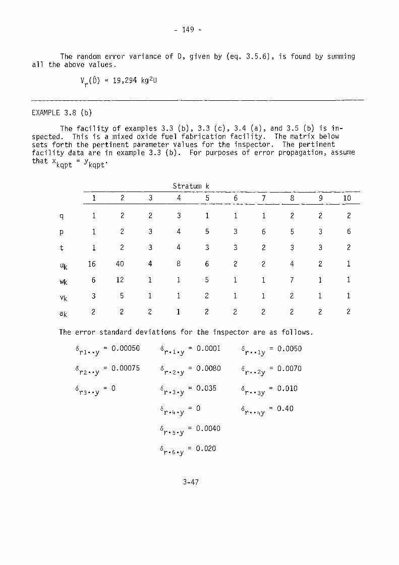
- 149 -

The random error variance of D, given by (eq. 3.5.6), is found by summingall the above values.

Vr(D) = 19,294 kg2U

EXAMPLE 3.8 (b)The facility of examples 3.3 (b), 3.3 (c), 3.4 (a), and 3.5 (b) is in-

spected. This is a mixed oxide fuel fabrication facility. The matrix belowsets forth the pertinent parameter values for the inspector. The pertinentfacility data are in example 3.3 (b). For purposes of error propagation, assumethat Xkqpt =

Stratum k1

1

1

1

16

6

3

2

2

2

2

2

40

12

5

2

3

2

3

3

4

1

1

2

4

3

4

4

8

1

1

1

5

1

5

3

6

5

2

2

6

1

3

3

2

1

1

2

7

1

6

2

2

1

1

2

8

2

5

3

4

7

2

2

9

2

3

3

2

1

1

2

10

2

6

2

1

1

1

2

qptukwk

akThe error standard deviations for the inspector are as follows.

ôri..y = 0.00050 6r.1<y = 0.0001 6r..ly = 0.0050

Ô = °-00075 = °-0080 = °-0070

y = 0 ôr..4y=0-40

= 0.0040

= 0.020

3-47

- 150 -

Equation 3.5.3 is now applied for each stratum, as is (eq. 3.5.4) for theinspector. All quantities are in ko2 plutonium.

Vrx(Ô!) = 0.296817 Vy(Ôl) = 0.621036

Vrx(D2) = 0.982474 Vry(D2) = 0.978395

Vrx(D3) = 0.025538 Vfy{D3) = 0.025830

V (D\) - 0.000800 V™(Û4) = 0.003200i x r y

Vrx(D5) = 0.036630 Vry(D5) = 0.069715

Vrx(D6) = 0.008172 Vry(06) = 0.008264

Vrx(D7) = 0.004305 vry(Ô7) = 0.004301

Vrx(D8) = 0.079079 Vry(D8) = 0.150722

Vrx(D9) = 0.012769 Vry(D9) = 0.012915

Vrx(D10) = 0.002152 Vry(D10) - 0.002152

The random error variance of D, given by (eq. 3.5.6), is found by summingall the above values.

V (6) = 3.325266 kg2 plutonium

3.5.3.4 Systematic Error Variance of DIn developing the formulas needed to compute the systematic error variance

of D, attention will first be directed at the short term systematic error.Method 3.9 applies.Method 3.9

NotationThe notation is given in Sections 3.4.3.2 and 3.5.3.2.

ModelSee the discussion for the model in Method 3.8.

3-48

- 151 -

ResultsThe calculations indicated need only be performed for those measurements

for which the first subscript on 6 is g or h, i.e., for the non-zero short termsystematic error variances.

For each combination of values q(i), calculate

" \ l < 1 ) - - x - JiVkqdJpt (eq. 3.5.7}

where A|< = +1 for input and beginning inventory strata and where A^ - -1 for out-put and ending inventory strata.

For each combination of values t(i), calculate

where the A|< are defined as for (eq. 3.5.7).The contribution to the short term systematic error variance of D due to

facility measurements is

Vgx(D) = E 6|q..x E M*(1)..x

+ E ..tx E M*..t(i)x (eq. 3.5.9)

For the inspector, for each combination of values q(i), calculate

Hq(1,..y • kE Akykq(1)pt (eq. 3.5.10)

with the A |< defined as for (eq. 3.5.7).For each combination of values t(i(j)), calculate

KkÇ1 Vkqptd(j))

with Ab defined as above. Finally, for each combination t(i), calculate from(eq. 3.5.11),

M"t(i)y= p..t(i(j))y (eq. 3.5.12)

3-49

- 152 -

The contribution to the short term systematic error variance of D due toinspector measurements is

Mz,., +U l 3

g-'ty .t(i)y (*<*• 3.5.13)

The total short term systematic error variance of D isVg(D) = Vgx(D) + Vgy(D) (eq. 3.5.14)

BasisThe basis for Method 3.9 is the same as for Method 3.8. The distinction is

that for random error variances, one first squares quantities and then sums them;for systematic error variances, one sums and then squares.

It is implicitly assumed in this method that both the inspector and thefacility apply the same material sampling procedures and hence commit the same sys-tematic errors. For the D statistic, these errors would then cancel. This is why,in the method, there are no expressions for M.p/-j).x and M.p(-j).y Should thisassumption not be valid, the equations used to compute these two quantities areessentially the same as (eq. 3.5.7) and (eq. 3.5.10), with obvious modifications.The equations (eq. 3.5.9) and (eq. 3.5.13} would each contain the additional setof terms.Examples

EXAMPLE 3.9 (a)The low enriched uranium fuel fabrication facility of example 3.8 (a) is

continued. Say that there are no short term systematic errors for either thefacility or the inspector except for those occurring because the inspector dis-tributes the inspection samples to four laboratories. The values for the errorparameters are:

& ,.. = 0.000544

ô . = 0.00711g..i+y

The allocation of samples to the various laboratories is given by thefollowing table. The tabular entries are the amounts of uranium, in kilograms,represented by the samples sent to the laboratories, i.e., they arevalues.

3-50

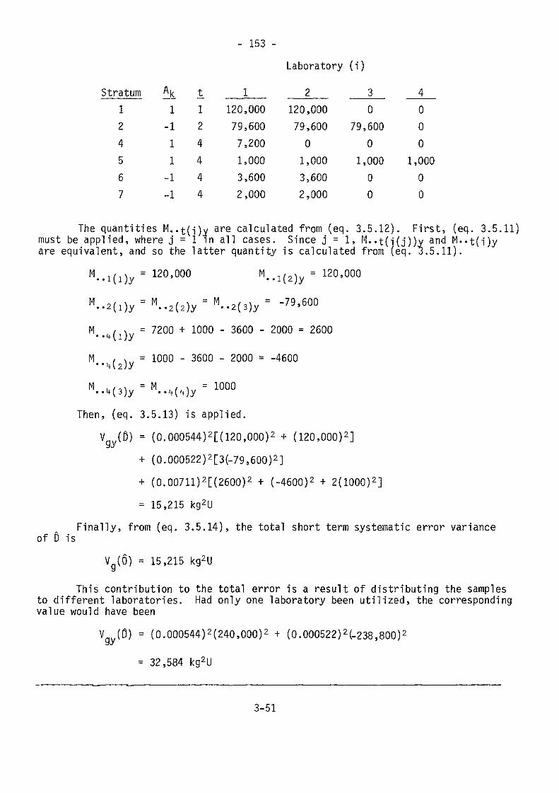
- 153 -

Laboratory ( i )

stratum124567

Ak1

-111

-1-1

t124444

1120,00079,6007,2001,0003,6002,000

2120,00079,60001,0003,6002,000

30

79,6000

1,00000

4000

1,00000

must beare equi

The quantities M..t(i)y are calculated from (eq. 3.5.12). First, (eq. 3.5.11)i applied, where j = 1 in all cases. Since j = 1, M..t(i(j))y and M.-t(i)yn'valent, and so the latter quantity is calculated from (eq. J.5.11).

M..i(i)y = 120>000 M--i(2)y = 120'000M..2(l)y =M..2(2)y = M-2(3)y = -79'600

M { \ = 7200 + 1000 - 3600 - 2000 = 2600. .it(i)yM , x = 1000 - 3600 - 2000 = -4600

of D is

"..„(,),-"..„(„„ -1000

Then, (eq. 3.5.13) is appl ied .

V (D) = (0.000544)2[(120,000)2 + (120,000)2]C3%/

+ (0.000522)2[3(-79S600)2]+ (0.00711)2[(2600)2 + (-4600)2 + 2(1000)2]= 15,215 kg2U

Finally, from (eq. 3.5.14), the total short term systematic error variance

Vg(D) = 15,215 kg2U

This contribution to the total error is a result of distributing the samplesto different laboratories. Had only one laboratory been utilized, the correspondingvalue would have been

V (0) = (0.000544)2(240,000)2 + (0.000522)2(-238,800)2jtJ

= 32,584 kg2U

3-51

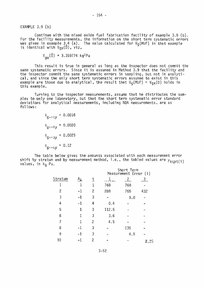
- 154 -

EXAMPLE 3.9 (b)Continue with the mixed oxide fuel fabrication facility of example 3.8 (b).

For the facility measurements, the information on the short term systematic errorswas given in example 3.4 (a). The value calculated for Vg(MUF) in that exampleis identical with Vgx(ß), viz,

V (D) = 3.359774 kg2Pu

This result is true in general as long as the inspector does not commit thesame systematic errors. Since it is assumed in Method 3.9 that the facility andthe inspector commit the same systematic errors in sampling, but not in analyti-cal, and since the only short term systematic errors assumed to exist in thisexample are those due to analytical, the result that Vg(MUF) = VgX(D) holds inthis example.

Turning to the inspector measurements, assume that he distributes the sam-ples to only one laboratory, but that the short term systematic error standarddeviations for analytical measurements, including NDA measurements, are asfollows:

6 1% = 0.0016g.-iy

The table below gives the amounts associated with each measurement errorshift by stratum and by measurement method, i.e., the tabled values are yk t/.pvalues, in kg Pu. ^ '

Short TermMeasurement Error (i)Stratum Aj^ t_ 1 2 3

1 1 1 768 7682 - 1 2 2 8 8 7 6 5 4 3 23 -1 3 9.0 -4 -1 4 0.45 1 3 112.56 1 3 3.67 1 2 4.58 -1 3 135 -9 -1 3 - 4.5 -

10 -1 2 - o. 9r.C , t_ J

3-52

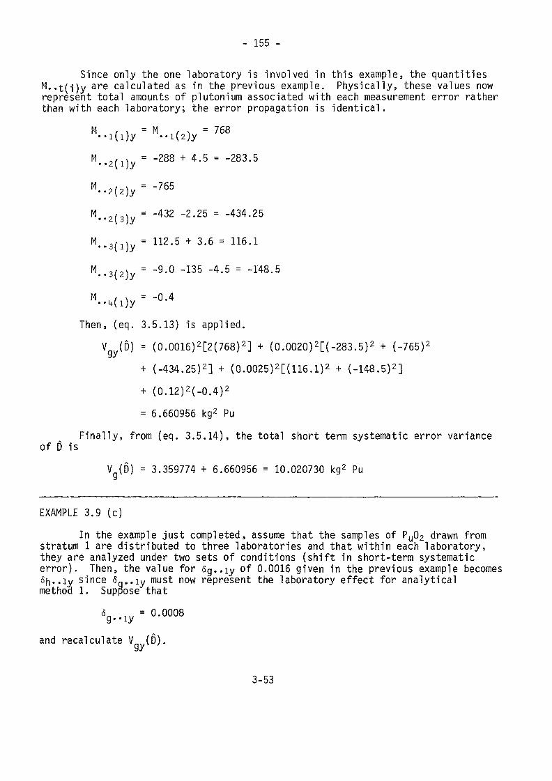
- 155 -

Since only the one laboratory is involved in this example, the quantitiesM..t(i)y are calculated as in the previous example. Physically, these values nowrepresent total amounts of plutonium associated with each measurement error ratherthan with each laboratory; the error propagation is identical.

M / N = M f •, = 768••i(i)y '-i(2)yM..2(l)y = -288+4.5 = -283.5

M..2(2)y--765

M..2(3)y = -432 -2.25 = -434.25

M..3(l)y = 112.5 + 3.6= 116.1

M..3(2)y = ~9'° "135 ~4'5 = -148-5

"..„<0y '-O'*Then, (eq. 3.5.13) is applied.

V (D) = (0.0016)2[2(768)2] + (0.0020)2[(-283.5)2 + (-765)2y*7

+ (-434.25)2] + (0.0025)2[(116.1)2 + (-148.5)2]+ (0.12)2(-0.4)2

= 6.660956 kg2 PuFinally, from (eq. 3.5.14), the total short term systematic error variance

of ß isV (D) = 3.359774 + 6.660956 = 10.020730 kg2 Pu

EXAMPLE 3.9 (c)In the example just completed, assume that the samples of PU02 drawn fromstratum 1 are distributed to three laboratories and that within each laboratory,

they are analyzed under two sets of conditions (shift in short-term systematicerror). Then, the value for <5g..iy of 0.0016 given in the previous example becomesSh"iy since <5g..iy must now represent the laboratory effect for analyticalmethod 1. Suppose that

V.ly = °-0008and recalculate V (D).

3-53

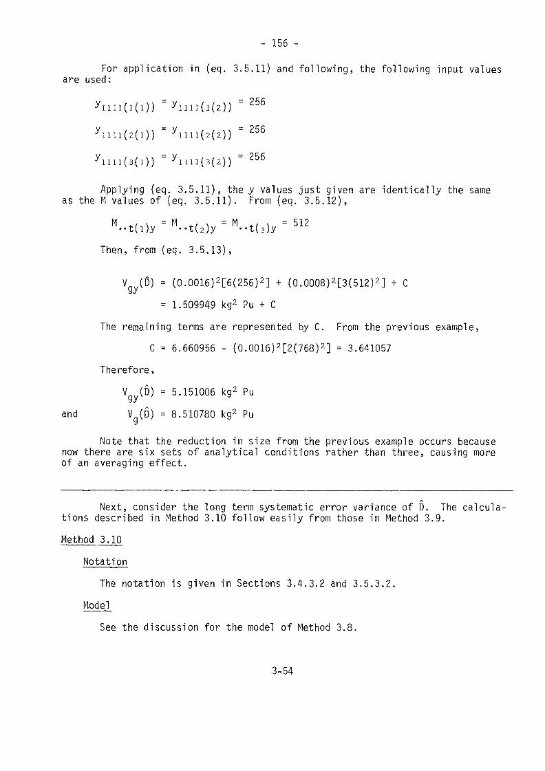
- 156 -

For application in {eq. 3.5.11) and following, the following input valuesare used:

= = 256

= 256

Applying {eq. 3.5.11), the y values just given are identically the sameas the M values of (eq. 3.5.11). From (eq. 3.5.12),

Then, from (eq. 3.5.13),

V (D) = (0.0016)2[6(256)2] + (0.0008)2[3(512)2] + CÏ3»/

- 1.509949 kg2 Pu + CThe remaining terms are represented by C. From the previous example,

C = 6.660956 - (0.0016)2[2(768)2] = 3.641057Therefore,

V (D) - 5.151006 kg2 Pu*3%7

and V (D) = 8.510780 kg2 Pu

Note that the reduction in size from the previous example occurs becausenow there are six sets of analytical conditions rather than three, causing moreof an averaging effect.

Next, consider the long term systematic error variance of D. The calcula-tions described in Method 3.10 follow easily from those in Method 3.9.Method 3.10

NotationThe notation is given in Sections 3.4.3.2 and 3.5.3.2.

ModelSee the discussion for the model of Method 3.8.

3-54

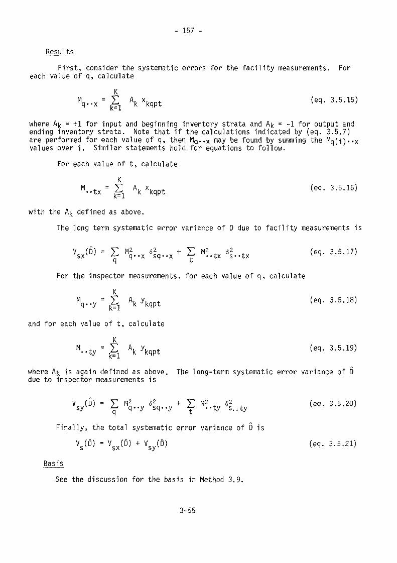
- 157 -

ResultsFirst, consider the systematic errors for the facility measurements. For

each value of q, calculate

Vx • £ \ "kqpt t6«- 3'5-15'

where Ak = +1 for input and beginning inventory strata and A|< = -1 for output andending inventory strata. Note that if the calculations indicated by (eq. 3.5.7)are performed for each value of q, then Mq..x may be found by summing the Mq(i)..xvalues over i. Similar statements hold for equations to follow.

For each value of t, calculate

M..tx= I, Akxkqpt (eq. 3.5.16)

with the A),, defined as above.The long term systematic error variance of D due to facility measurements is

VSX(D) - E "q2..x <fq..x + E «î.tx «|..tx <eq. 3.5.17)

For the inspector measurements, for each value of q, calculate

and for each value of t, calculate

M = y^ A y (ea 3 5 ig). . -H/ / > n\f •'bnnt V CH- o.J.iay**./ I 1 ^ ix M M v1X~" X

where A^ is again defined as above. The long-term systematic error variance of Ddue to inspector measurements is

V (D) = V M2 62 + T^ M2 <S2 (ea 3 5 20)vsyv ' ^ q--y sq--y ^ --ty s..ty ^ q' <5-°"::u

Finally, the total systematic error variance of D isVS(D) = VsX(D) + Vsy(D) (eq. 3.5.21)

BasisSee the discussion for the basis in Method 3.9.

3-55

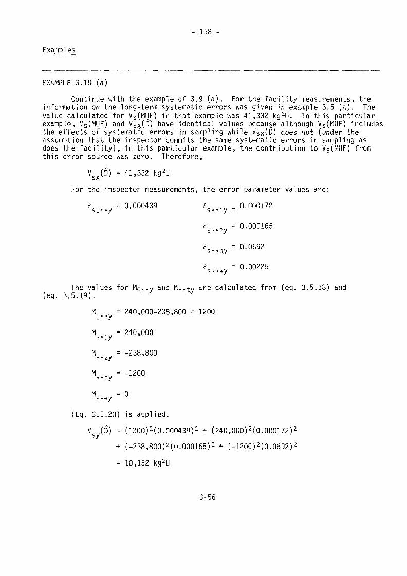
- 158 -

Examples

EXAMPLE 3.10 (a)Continue with the example of 3.9 (a). For the facility measurements, the

information on the long-term systematic errors was given in example 3.5 (a). Thevalue calculated for VS(MUF) in that example was 41,332 kg2U. In this particularexample, VS(MUF) and VSx(D) have identical values because although VS(MUF) includesthe effects of systematic errors in sampling while Vsx(D) does not (under theassumption that the inspector commits the same systematic errors in sampling asdoes the facility), in this particular example, the contribution to VS(MUF) fromthis error source was zero. Therefore,

Vsx(D) = 41,332 kg2UFor the inspector measurements, the error parameter values are:

ôsi-.y = °-000439 fis.-iy = °-000172

6. „ = 0.000165

S = 0.0692s* *ay6p , = 0.00225s • • 'ty

The values for Mn..y and M.. v are calculated from (eq. 3.5.18) and(eq. 3.5.19).

M = 240,000-238,800 = 1200

M..iy = 240,000

M_2 = -238,800

M = -1200• *ay

M . = 0• <lfy

(Eq. 3.5.20) is applied.

Vs (D) = (1200)2(0.000439)2 + (240,000)2(0.000172)2

+ (-238,800)2(0.000165)2 + (-1200)2(0.0692)2

= 10,152 kg2U

3-56

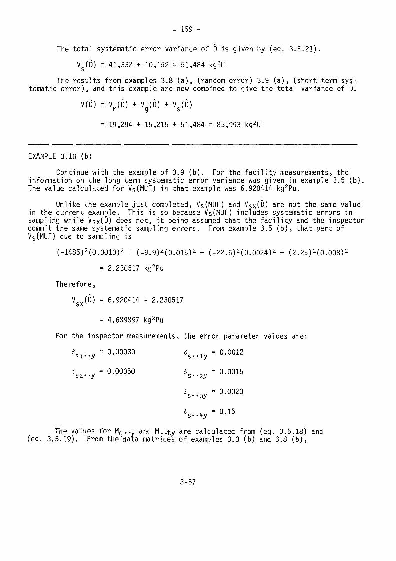
- 159 -

The total systematic error variance of D is given by (eq. 3.5.21).VS(D) = 41,332 + 10,152 = 51,484 kg2U

The results from examples 3.8 (a), (random error) 3.9 (a), (short term sy§-tematic error), and this example are now combined to give the total variance of D.

V(D) = Vr(D) + Vg(D) + VS(D)

= 19,294 + 15,215 + 51,484 = 85,993 kg2U

EXAMPLE 3.10 (b)Continue with the example of 3.9 (b). For the facility measurements, theinformation on the long term systematic error variance was given in example 3.5 (b).

The value calculated for VS(MUF) in that example was 6.920414 kg2Pu.Unlike the example just completed, VS(MUF) and VSX(D) are not the same valuein the current example. This is so because Vs(MUF) includes systematic errors in

sampling while Vsx(O) does not, it being assumed that the facility and the inspectorcommit the same systematic sampling errors. From example 3.5 (b), that part ofVS(MUF) due to sampling is

(-1485)2(0. 0010)2 + (-9.9)2(0.015)2 + (-22.5)2(0.0024)2 + (2.25)2(0.008)2

= 2.230517 kg2PuTherefore,

VCV(D) = 6.920414 - 2.230517SX

= 4.689897 kg2PuFor the inspector measurements, the error parameter values are:

6si..y = °-00030 V.iy = °-0012

6s2-.y = °-00050 ôs..2y = °'0015

6 = 0.0020

The values for Mq..y and M..ty are calculated from (eq. 3.5.18) and(eq. 3.5.19). From the data matrices of examples 3.3 (b) and 3.8 (b),

3-57

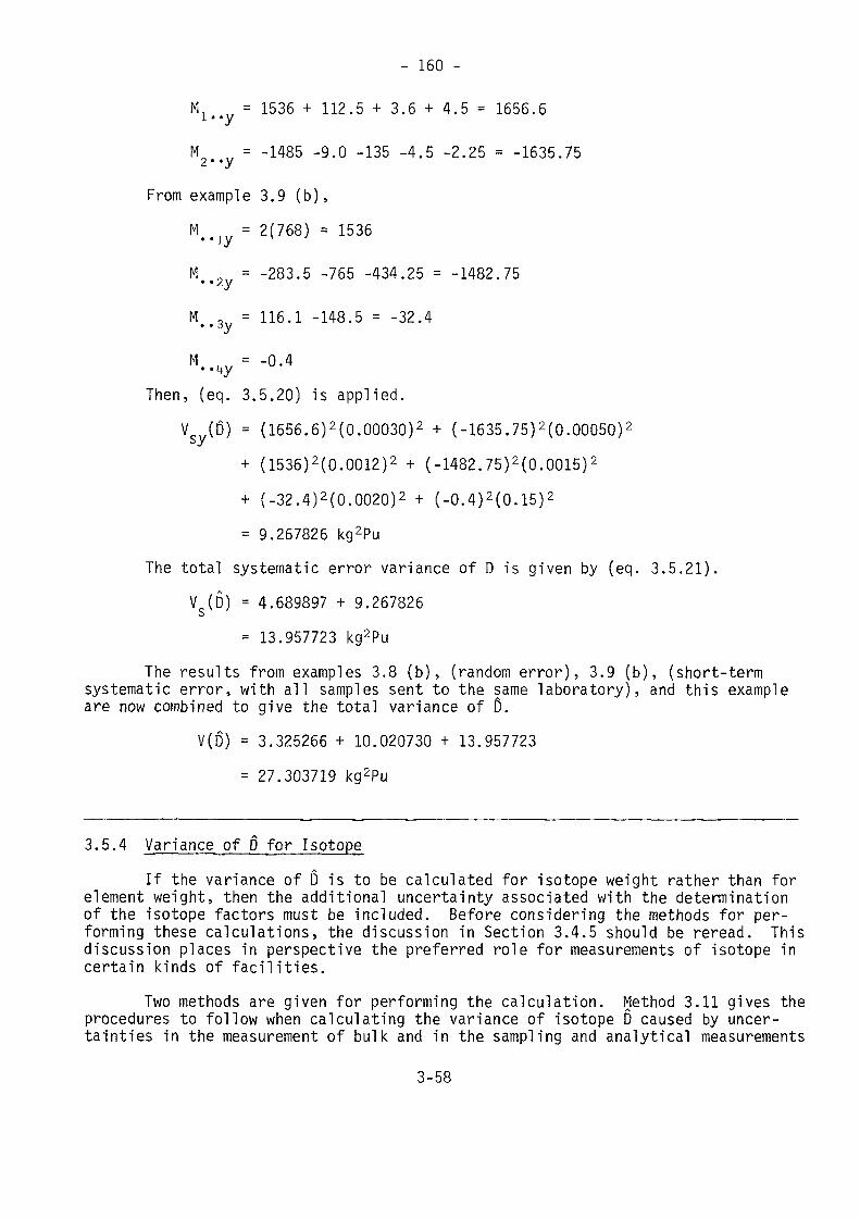
- 160 -

M = 1536 + 112.5 + 3.6 + 4.5 = 1656.6

M2--y = ~1485 ~9'° "135 ~4'5 ~2'25 = ~1635-75

From example 3.9 (b)5M.. l y = 2(768) = 1536

M_2 = -283.5 -765 -434.25 = -1482.75•J

M = 116.1 -148.5 = -32.4

M Jw = -0.4• '^yThen, (eq. 3.5.20) is app l ied .

V (D) = {1656.6)2(0.00030)2 + (-1635.75)2(0.00050)2~*y+ (1536)2(0.0012)2 + (-1482.75)2(0.0015)2

+ (-32.4)2(0.0020)2 + (-0.4)2(0.15)2

= 9.267826 kg2PuThe total systematic error variance of D is given by (eq. 3.5.21).

V (D) = 4.689897 + 9.267826= 13.957723 kg2Pu

The results from examples 3.8 (b), (random error), 3.9 (b), (short-termsystematic error, with all samples sent to the same laboratory), and this exampleare now combined to give the total variance of 0.

V(D) = 3.325266 + 10.020730 + 13.957723= 27.303719 kg2Pu

3.5.4 Variancejrf D for IsotopeIf the variance of D is to be calculated for isotope weight rather than for

element weight, then the additional uncertainty associated with the determinationof the isotope factors must be included. Before considering the methods for per-forming these calculations, the discussion in Section 3.4.5 should be reread. Thisdiscussion places in perspective the preferred role for measurements of isotope incertain kinds of facilities.

Two methods are given for performing the calculation. Method 3.11 gives theprocedures to follow when calculating the variance of isotope D caused by uncer-tainties in the measurement of bulk and in the sampling and analytical measurements

3-58

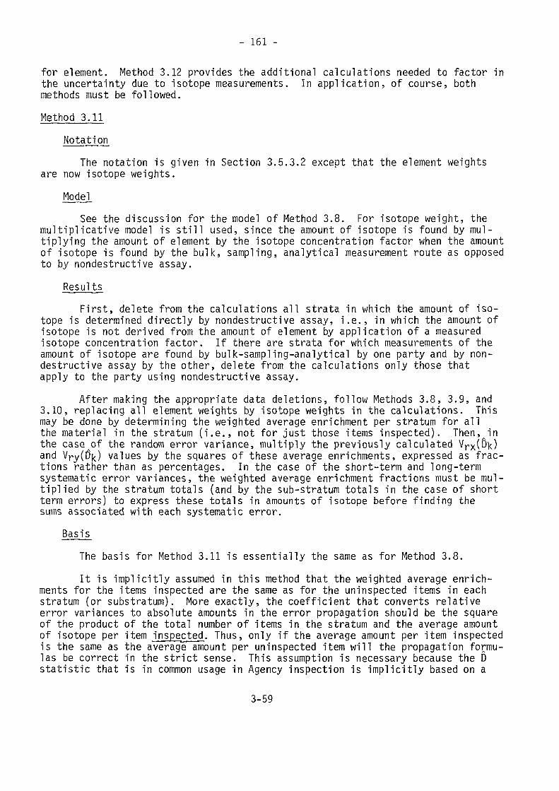
- 161 -

for element. Method 3.12 provides the additional calculations needed to factor inthe uncertainty due to isotope measurements. In application, of course, bothmethods must be followed.Method 3.11

NotationThe notation is given in Section 3.5.3.2 except that the element weights

are now isotope weights.Model

See the discussion for the model of Method 3.8. For isotope weight, themultiplicative model is still used, since the amount of isotope is found by mul-tiplying the amount of element by the isotope concentration factor when the amountof isotope is found by the bulk, sampling, analytical measurement route as opposedto by nondestructive assay.

ResultsFirst, delete from the calculations all strata in which the amount of iso-

tope is determined directly by nondestructive assay, i.e., in which the amount ofisotope is not derived from the amount of element by application of a measuredisotope concentration factor. If there are strata for which measurements of theamount of isotope are found by bulk-sampling-analytical by one party and by non-destructive assay by the other, delete from the calculations only those thatapply to the party using nondestructive assay.

After making the appropriate data deletions, follow Methods 3.8, 3.9, and3.10, replacing all element weights by isotope weights in the calculations. Thismay be done by determining the weighted average enrichment per stratum for allthe material in the stratum (i.e., not for just those items inspected). Then,^inthe case of the random error variance, multiply the previously calculated Vrx(D|<)and Vry(ß|<) values by the squares of these average enrichments, expressed as frac-tions rather than as percentages. In the case of the short-term and long-termsystematic error variances, the weighted average enrichment fractions must be mul-tiplied by the stratum totals (and by the sub-stratum totals in the case of shortterm errors) to express these totals in amounts of isotope before finding thesums associated with each systematic error.

BasisThe basis for Method 3.11 is essentially the same as for Method 3.8.It is implicitly assumed in this method that the weighted average enrich-

ments for the items inspected are the same as for the uninspected items in eachstratum (or substratum). More exactly, the coefficient that converts relativeerror variances to absolute amounts in the error propagation should be the squareof the product of the total number of items in the stratum and the average amountof isotope per item inspected. Thus, only if the average amount per item inspectedis the same as the average amount per uninspected item will the propagation formu-las be correct in the strict sense. This assumption is necessary because the Dstatistic that is in common usage in Agency inspection is implicitly based on a

3-59

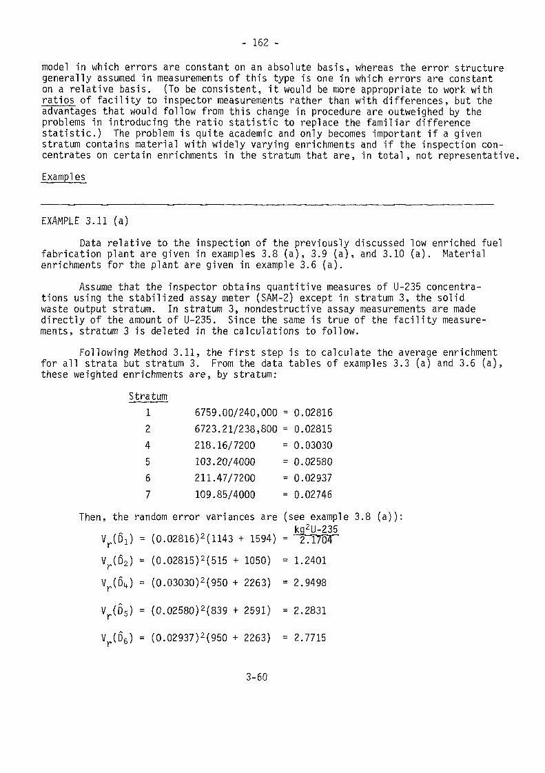
- 162 -

model in which errors are constant on an absolute basis, whereas the error structuregenerally assumed in measurements of this type is one in which errors are constanton a relative basis. (To be consistent, it would be more appropriate to work withratios of facility to inspector measurements rather than with differences, but theadvantages that would follow from this change in procedure are outweighed by theproblems in introducing the ratio statistic to replace the familiar differencestatistic.) The problem is quite academic and only becomes important if a givenstratum contains material with widely varying enrichments and if the inspection con-centrates on certain enrichments in the stratum that are, in total, not representative.Examples

EXAMPLE 3.11 (a)Data relative to the inspection of the previously discussed low enriched fuel

fabrication plant are given in examples 3.8 (a), 3.9 (a), and 3.10 (a). Materialenrichments for the plant are given in example 3.6 (a).

Assume that the inspector obtains quantitive measures of U-235 concentra-tions using the stabilized assay meter (SAM-2) except in stratum 3, the solidwaste output stratum. In stratum 3, nondestructive assay measurements are madedirectly of the amount of U-235. Since the same is true of the facility measure-ments, stratum 3 is deleted in the calculations to follow.

Following Method 3.11, the first step is to calculate the average enrichmentfor all strata but stratum 3. From the data tables of examples 3.3 (a) and 3.6 (a),these weighted enrichments are, by stratum:

Stratum1 6759.00/240,000 = 0.028162 6723.21/238,800 = 0.028154 218.16/7200 = 0.030305 103.20/4000 = 0.025806 211.47/7200 = 0.029377 109.85/4000 = 0.02746

Then, the random error variances are (see example 3.8 (a)):kg2U-235V(D}) = ( 0 . 02816)2(1143 + 1594) = " "

Vr(D2) = (0.02815)2(515 + 1050) = 1.2401Vr(D\) = (0.03030)2(950 + 2263) = 2.9498

Vr(D5) = (0.02580)2(839 + 2591) = 2.2831

V (D6) = (0.02937)2(950 + 2263) = 2.7715

3-60

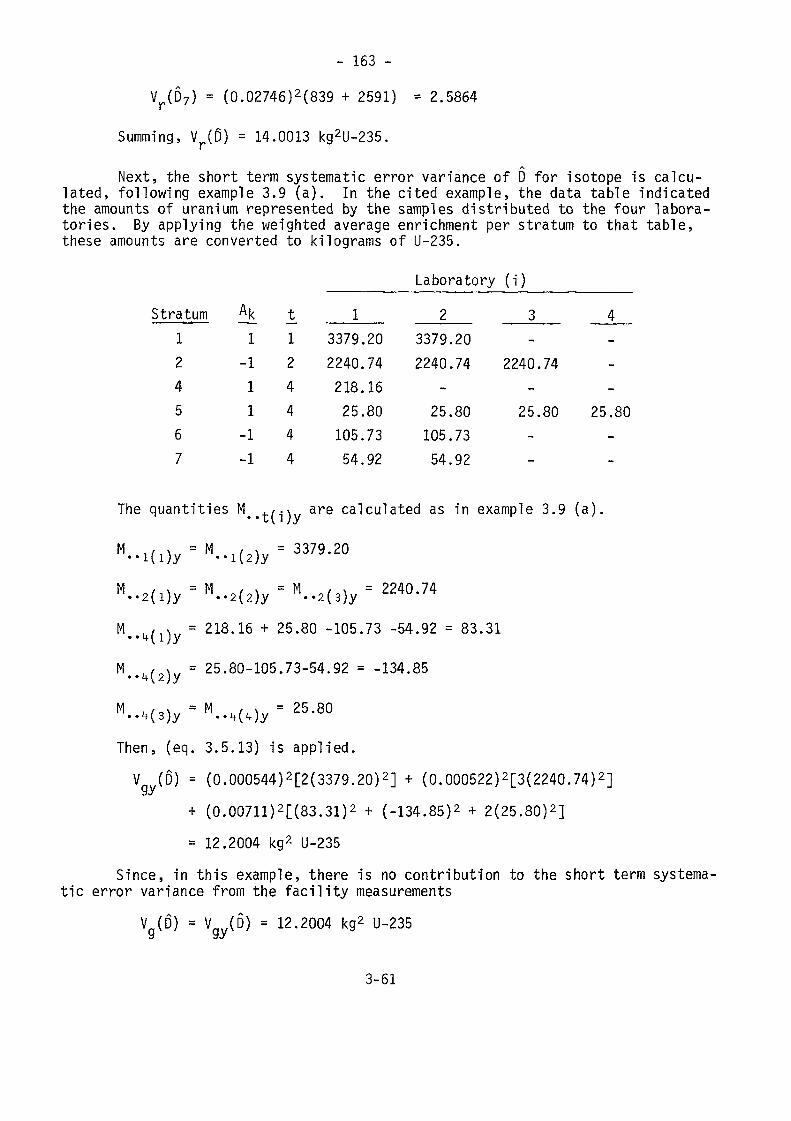
- 163 -Vr(D7) = (0.02746)2(839 + 2591) = 2.5864

Summing, V (ß) = 14.0013 kg2U-235.

Next, the short term systematic error variance of D for isotope is calcu-lated, following example 3.9 (a). In the cited example, the data table indicatedthe amounts of uranium represented by the samples distributed to the four labora-tories. By applying the weighted average enrichment per stratum to that table,these amounts are converted to kilograms of U-235.

Laboratory (i)Stratum

124567

Ak1

-111

-1-1

t124444

13379.202240.74218.1625.80105.7354.92

23379.202240.74

-25.80105.7354.92

3-

2240.74-25.80-_

4---

25.80-_

The quantities M ..4/-\v are calculated as in example 3.9 (a).

M--Ki)y = M-i(2)y -

M , ,,, = 218.16 + 25.80 -105.73 -54.92 = 83.31..if(l)y

M ,, x = 25.80-105.73-54.92 = -134.85..i+(2)y

"..»OJy-N..^^-25-80

Then, (eq. 3.5.13) is applied.V (D) = (0.000544)2[2(3379.20)2] + (0.000522)2[3(2240.74)2]y*/

+ (0.00711)2[(83.31)2 + (-134. 85)2 + 2(25. 80)2]= 12.2004 kg2 U-235

Since, in this example, there is no contribution to the short term systema-tic error variance from the facility measurements

V (D) = V (D) = 12.2004 kg2 U-235y y*y

3-61

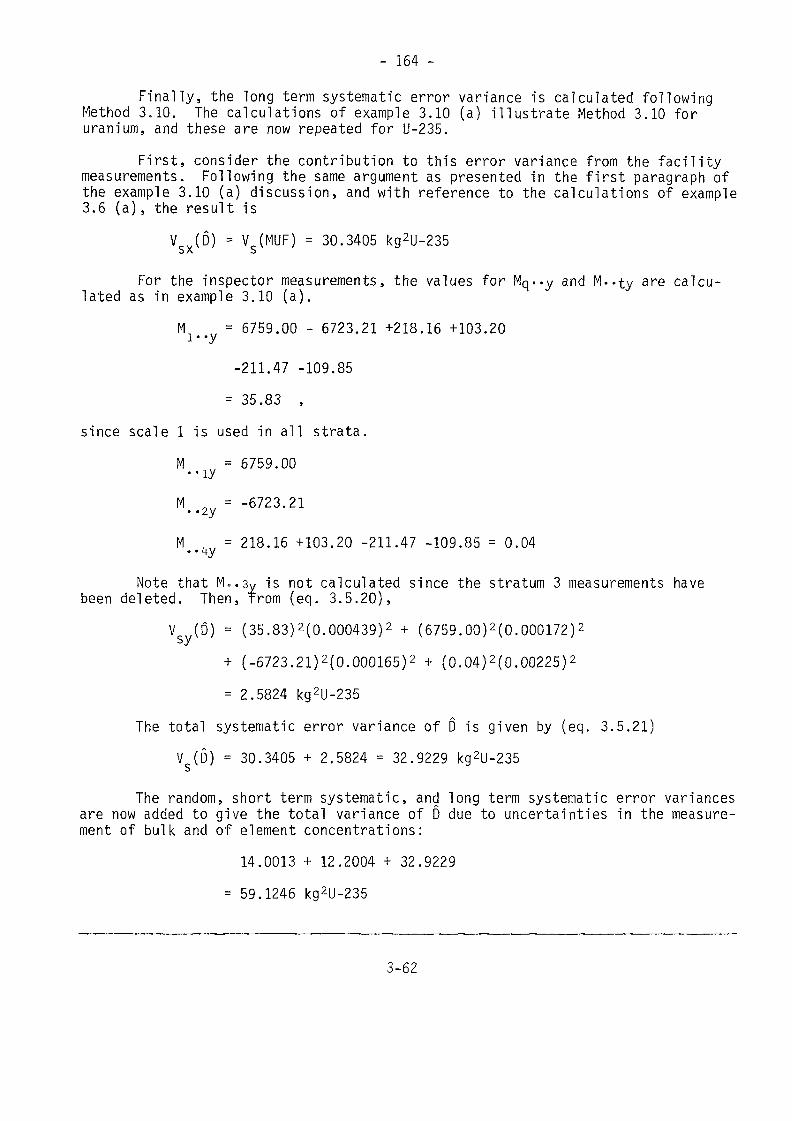
- 164 -Finally, the long term systematic error variance is calculated following

Method 3.10. The calculations of example 3.10 (a) illustrate Method 3.10 foruranium, and these are now repeated for U-235.

First, consider the contribution to this error variance from the facilitymeasurements. Following the same argument as presented in the first paragraph ofthe example 3.10 (a) discussion, and with reference to the calculations of example3.6 (a) , the result is

CV - VC(MUF) = 30.3405 kg2U-235SX S

For the inspector measurements, the values for Mq..y and M.«ty are calcu-lated as in example 3.10 (a).

M = 6759.00 - 6723.21 +218.16 +103.20l..y

-211.47 -109.85= 35.83 ,

since scale 1 is used in all strata.M - 6759.00••iyM..2y = -6723-21

M , = 218.16 +103.20 -211.47 -109.85 = 0.04. . i|y

Note that M..3y is not calculated since the stratum 3 measurements havebeen deleted. Then, from (eq. 3.5.20),

V (D) = (35. 83)2(0. 000439)2 + (6759.00)2(0.000172)2

+ (-6723. 21)2(0. 000165)2 + (0.04)2(0.00225)2

= 2.5824 kg2U-235The total systematic error variance of D is given by (eq. 3.5.21)

V (D) = 30.3405 + 2.5824 = 32.9229 kg2U-235

The random, short term systematic, and long term systematic error variancesare now added to give the total variance of D due to uncertainties in the measure-ment of bulk and of element concentrations:

14.0013 + 12.2004 + 32.9229= 59.1246 kg2U-235

3-62

- 165 -Method 3.11, as exemplified in example 3.11 (a) just completed, gives the

variance of 0 in isotope weight that is caused by uncertainties in the measurementof bulk and in the sampling and analytical measurement for element. Thus, theresult in example 3.11 (a), viz, V-t(D) = 59.1246 kg U-235, does not include theeffects of errors in measuring the isotope that are committed by either the facil-ity or the inspector. Procedures for including these errors are detailed inMethod 3.12Methoid 3.12

NotationThe notation is an extension to that given earlier in Method 3.7. For the

error standard deviations, a slight change is made in the notation to distinguishbetween facility and inspector errors. Specifically, the following errors aredefined.6* = random error standard deviation in sampling for isotope,*p' assumed to be the same for the facility and the inspectors* i = random error standard deviation in isotopic analysix the facility's analytical method t

s for

6* . = systematic error standard deviation in isotopic analysisfor the facility's analytical method t<5* . = random error standard deviation in isotopic analysis for

y the inspector's analytical method t5t..tv = systematic error standard deviation in isotopic analysisy for the inspector's analytical method t

Additional parameters relating to the inspector's measurement are defined:v.* = number of samples drawn by the inspector to verify thefacility's isotopic concentration factor ia.* = number of isotopic analyses per sample performed by the1 inspector

ModelSee the discussion for the model in Method 3.11.

ResuUsFor facility^measurements, the random and systematic error contributions

to the variance ofAD due to measurements of isotopic concentrations are denotedby Vrx(D) and Vsx(O) respectively. They are calculated by:G

V*x (D) = Ç Sf (5*2p./r* + 6*2.tx/r|c|) {eq. 3.5.22)

3-63

- 166 -

These equations are identical to those for V*(MUF) and Vs(MUF) given by(|q. 3.4.13) and (eq. 3.4.14) respectively. An additional subscript is added to<$r..-t, 65.. t, and Tt in the cited equations to designate that these parametersrelate to facility measurements, but the numerical calculations are identical.

For the inspector, the random error is

V*y (0) =.£ Sf (6 p./vif + o*^ty/v* a*) (eq. 3.5.24)

To compute the systematic error, first calculateT - sum of S-j values based on the inspector's isotopic analy-Iy tical method t

ET2y 6*2. (eq> 3.5>.

The total variance of D due to isotopic measurements is

V (Ô) = Vrx(Ö) + Vsx(Ô) + Vry() + Vsy() (eq* 3-5-26)To compute the total variance of the isotope D due to all sources of error,

the results of Methods 3.11 and 3.12 are combined. That is, find the sumV*(D) = V (D) + Vt* (D) (eq. 3.5.27)

BasisThe basis for this method is essentially the same as for Method 3.8.Some important assumptions on which the computational equations are based

should be emphasized. First, since <5*.p.has no x or y subscript, it is implicitlyassumed that both parties use the same sampling equipment. Further, it is assumedthat systematic errors in sampling for isotope are zero. Finally, no provisionis made for calculating a short term systematic error variance for isotope measure-ments; such errors are assumed to be zero.

If any of these assumptions should be invalid in a given application, theadditional calculations required should be apparent from similar applications de-tailed by the methods of this chapter.Examples

3-64

- 167 -EXAMPLE 3.12 (a)

Continue with example 3.11 (a). Additional information relative to theinspector's measurements is required.

In stratum 1, of the 12 batches inspected, 6 have 3.25% enrichment, 4 have2.67%, and 2 have 1.52%. To measure the enrichment, the inspector uses the sta-bilized assay meter (SAM-2) on 5 items per sampled batch.

In stratum 2, SAM-2 measurements are made on 50 items. Twenty of these areat 3.25% U-235, 15 at 2.67%, 5 at 1.52%, and 10 at 2.87%.

In stratum 3, the inspector measures the amount of U-235 directly on the10 items. In stratum 4, all 6 batches are measured with SAM-2 measurements madeon 3 items per batch. In stratum 5, all batches are again measured with SAM-2measurements made on 4 items per batch. No measurements are made of enrichmentin strata 6 and 7.

The inspector's error standard deviations are

«J..ly = °-004 S*s..2y = °-06

where the subscript 1 refers to the SAM-2 and the subscript 2 to the nondestructiveassay instrument used in measuring the solid waste in stratum 3.

The pertinent data for the facility are given in example 3.7 (a), and useis made of some of the results calculated in that example.

In applying (eq. 3.5.22) to calculate V*x (D) and (eq. 3.5.23) to calculateVsx (0)> it was noted that these equal V*(MUF) and Vs(MUF) respectively, quantitieswhich were already calculated for this facility in example 3.7 (a).

V * (D) = 0.0766 kg2 U-235PA

Vs* (ß) = 2.3422 kg2 U-235

For the inspector measurements, a-f of (eq. 3.5.23) equals one for all i,while values for v* are derived from the information given about the inspector'smeasurements per stratum

i Factor vi*1 0.0325 30 + 20 = 502 0.0267 20 + 15 = 353 0.0152 10 + 5 = 154 0.0287 105 0.0312 156 0.0258 3 + 16 = 197 Nominal 10

3-65

- 168 -From (eq. 3.5.24),

Vr* (D) = (29.25)2[(0.0005)2 + (0.01)2]/50

+ (80.10)2[(0.0005)2 + (0.01)2]/35+ (-4.56)2[(0.0005)2 + (0.01)2]/15 + (-390.32)2[(0.0005)2 + (0.01)2]/10+ (187.20)2[(0.0005)2 + (0.01)2]/15 + (134.16)2[(0.0005)2 + (0.01)2]/19+ (-36.00)2(0.10)2/10

= 3.1727 kg2U-235To calculate VSy (D) from (eq. 3.5.25), it is first necessary to computeTty for t = 1 (SAM-2) and t - 2 (NDA for solid waste).

T = 29.25 + 80.10 -4.56 +187.20 +134.16 - 390.32 = 35.83

T2y = -36.00

V* (D) - (35.83)2(0.004)2 + (-36.00)2(0.06)2

= 4.6861 kg2U-235From (eq. 3.4.15),

V* (D) = 0.0766 + 2.3422 + 3.1727 + 4.6861

= 10.2776 kg2U-235The total variance of the isotope D is found using (eq. 3.5.27) and the

results from this current example and from example 3.12 (a).V*(D) = 59.1246 + 10.2776 - 69.4022 kg2U-235

3.6 THE (MUF-D) STATISTIC

3.6.1 Application of_(MUF-D)There are two statistics, or quantities, that are used to evaluate the mater-

ial balance data for a given facility. The first is the facility MUF, the amountof material that is unaccounted for based on the facility's measurements of inputs,outputs, and inventories. Methods for calculating the variance of MUF are givenin Section 3.4. The second statistic is the so-called difference statistic, or Dstatistic, which measures the relative bias between the facility and inspection

3-66

- 169 -

measurements, or better stated, between the values recorded by the facility andthe corresponding values based on measurements made by the inspector. Methods forcalculating the variance of D are given in Section 3.5.

In making inferences based on the observed or reported values for MUF and D,one is faced with a choice as to how to proceed. On the one hand, a significancetest can be made of the bias between the facility and inspector values by using theD statistic. If the test outcome is that there is no evidence of bias, then onemay accept the facility's stated MUF and test it for significance, making no fur-ther^use of D. The other approach is to correct the facility MUF for bias usingthe D statistic. The quantity,ß, is defined in such a way that if D is positive,the MUF is^overstated while if D is negative, MUF is understated. This suggeststhat (MUF-D) is the statistic which may be regarded as the inspector's estimateof the facility MUF.

In the next chapter, in Section 4.6, comparisons are made of the two evalua-tion approaches: (1) first test for the significance of D and, if not significant,then test for the significance of MUF; (2) test for the significance of (MUF-D).These comparisons are made for^specific examples, and on the basis of these exam-ples it is inferred that (MUF-D) is the preferred statistic if, in fact, the cri-terion for selection of a statistic is based on the probability of detection.

The fact that the probability of detection is larger for (MUF-Ô) than for theD and MUF tests applied separately, to be illustrated in the examples of Section 4.6,has, in fact, been shown to be true in general [3.14]. This fact is consistent byanalogy with the earlier reported finding discussed in Section 3.4.4 in which thestatistical advantages of making a single test of diversion without making sub-divisions by time or by space was pointed out. Thus, the (MUF-D) statistic, beinga global statistic in the same sense that the overall MUF is (i.e., the MUF overthe total finite time period and over the total material balance area) would beexpected to have the same advantage as the MUF global statistic.

For other studies in which comparisons are made of (MUF-D) with D and MUFapplied separately, see [3.15] and [3.16].

Consider now the calculation of the variance of (MUF-D), a quantity neededin the chapter to follow.3.6.2 Variance^ of (MUF-D)

Having calculated the variance of MUF and of D separately by the methodsof Sections 3.4 and 3.5, it is a simple matter to calculate the variance of(MUF-D). This calculation is given by Method 3.13.Method 3.13

NotationThe notation is consistent with that in previous sections. Specifically,

V(MUF) = variance of element MUFV*(MUF) = variance of isotope MUF

3-67

- 170 -V(D) = variance of element 0V*(D) = variance of isotope D

Additional notation includes:V(MUF-D) = variance of element (MUF-D)

V*(MUF-D) = variance of isotope (MUF-D)V0 = that part of the variance of element MUF due to systematicerrors that are common to both the facility and the inspector

V0* = defined as V0, but for isotope MUFOne additional quantity is needed. This is the covariance between MUF and

Dj denoted bycov (MUF, 0) for elementcov* (MUF, D) for isotope

ModelA simple additive model will be used to provide the bases for the results.

In this model, all errors of a given type, (i.e., random or systematic) are com-bined and represented by a single error. In this exposition, short-term systema-tic errors are not included, for simplicity. For the same reason, a very simplematerial balance involving only two strata (an input and an output stratum) isconsidered. Further, the items within a stratum are presumed to be so orderedsuch that the first nn- items out of the total of N-j items are the ones inspected.None of these simplifying assumptions affect the validity of the results.

The model is written as follows. For inputs, the facility measurement ofitem i is

xn- = xii + ei + Ai + eiiand for outputs it is

X2i = X2i + 92 + A2 + £2i

In stratum 1, i runs from 1 to Nj and in stratum 2, i runs from 1 to N2.The small x's represent observed values and the large X's represent true values.The quantities els Al5 02, and A2 are systematic errors, while en" and e21- arerandom errors. All errors are presumed to be distributed with zero means andvariances denoted by a^i, a&1, •••, ae2 respectively.

The corresponding inspector values areyii = Xii + 6i + <h + m-j (eq. 3.6.3)

and y2. = X2i + 02 + ip2 + n2i (eq. 3.6.4)

3-68

- 171 -Note that QI and 02 are the same as for the facility measurements, i.e.,they represent those systematic errors that are committed by both parties. In

(eq. 3.6.3), i runs from 1 to HI while in (eq. 3.6.4), i runs from 1 to n2. Thesmall y's represent inspector measurements.

ResultsFor element,V(MUF-D) = V(D) - V(MUF) + 2 V0 (eq. 3.6.5)

cov(MUF,D) = V(MUF) - V0 (eq. 3.6.6)For isotope,

V*(MUF-D) = V*(0) - V*(MUF) + 2 V* (eq. 3.6.7)cov*(MUF,0) = V*(MUF) - V* (eq. 3.6.8)

BasisEquations (eq. 3.6.1) - (eq. 3.6.4) form the basis for the results. They

are written in general terms to apply to either element or isotope so that byderiving (eq. 3.6.5) and (eq. 3.6.6) for element, the corresponding equations forisotope will follow.

The approach is to write the model for MUF, for D, and for (MUF-D) using themodel equations, find the variance of these quantities by error propagation, anddemonstrate that the variances are related as indicated by (eq. 3.6.5). If(eq. 3.6.5) is shown to be true, (eq. 3.6.6) will follow easily, as will be shown.

First, consider MUF.NI N2"UF=E x^-^x,,

N, NI= Ç1 Xn. + M! + NlAl + Ç EI.

N2 N2- E X2, -Mz-Mz - E e2. (eq. 3.6.9)1=1 n 1=1 1

The variance of MUF isV(MUF) = N^a^+N^a^+Nja^+Nla^+Nfa^+Nza^ (eq. 3.6.10)

Consider D = N!d!-N2d2 where

3-69

- 172 -nl nlH! = E X ./n +91+A1+ E e -/ni

i = l n l i = l n

v1 v1i=l in i=l n

"i J,i= A}-^! + V e,,-/ni - 2_, n „-/n i (eq. 3.6.11)i=l n 1=1 nSimilarly,

n2 n2d2 = A2-4J2 + E e

2i/n2 - E ri2j/n2 (eq- 3.6.12)

The variance of D follows immediately:V(D) = Ni2a2 + Ni2a2 + Ni2o2 /ni + Ni2a2 /ni1 A! 1 ij/i ^ ei -1 x ni x

+ N22a2 + N22a2 + N22a2 /n2 + N22a2 /n2 (eq. 3.6.13)z A2 ^ 1(J2 z £2 T12

From (eq. 3.6.9), (eq. 3.6.11), and (eq. 3.6.12), and including only theerror terms,

(MUF-D) = - 22

tf(MUF-D) = N^c^ + N^ojj + N22o22 + N22c,22+ N,( -1)« + N2( -D, + ïli «2nl + „22 (eq. 3.6.15}

Finally, from (eq. 3.6.10), (eq. 3.6.13), and (eq. 3.6.15), and noting thatvo = \2a1l + N22a02' tnat the truth of (eq. 3.6.5) is demonstrated. That is

V(D) - V(MUF) + 2V0 = N^a + N22a2 + N^a + N22a2

which is the expression for V(MUF-D), completing the proof.

3-70

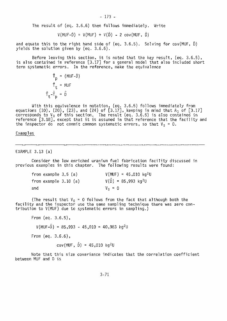
- 173 -The result of (eq. 3.6.6) then follows immediately. Write

V(MUF-Ô) = V(MUF) + V(D) - 2 cov(MUF, D)and equate this to the right hand side of (eq. 3.6.5). Solving for cov(MUF, D)yields the solution given by (eq. 3.6.6).

Before leaving this section, it is noted that the key result, (eq. 3.6.5),is also contained in reference [3.17] for a general model that also included shortterm systematic errors. In the reference, make the equivalence

fp = (MUF-Ô)ft = MUF

s*. '"' *

TfTp = D

With this equivalence in notation, (eq. 3.6.5) follows immediately fromequations (10), (20), (23), and (24) of [3.17], keeping in mind that A! of [3.17]corresponds to VQ of this section. The result (eq. 3.6.5) is also contained inreference [3.18], except that it is assumed in that reference that the facility andthe inspector do not commit common systematic errors, so that V0 = 0.Examples^

EXAMPLE 3.13 (a)Consider the low enriched uranium fuel fabrication facility discussed in

previous examples in this chapter. The following results were found:from example 3.5 (a) V(MUF) = 45,010 kg2Ufrom example 3.10 (a) V(D) = 85,993 kg2Uand V0 = 0

(The result that V0 = 0 follows from the fact that although both thefacility and the inspector use the same sampling technique there was zero con-tribution to V(MUF) due to systematic errors in sampling.)

From (eq. 3.6.5),V(MUF-D) = 85,993 - 45,010 = 40,983 kg2U

From (eq. 3.6.6),cov(MUF, D) = 45,010 kg2U

Note that this size covariance indicates that the correlation coefficientbetween MUF and D is

3-71

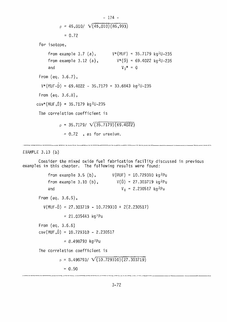
- 174 -P = 45,010/ V(45,010)(85,993)- 0.72

For isotope,from example 3.7 (a), V*(MUF) = 35.7179 kg2U-235from example 3.12 (a), V*(D) = 69.4022 kg2U-235and V0* = 0

From (eq. 3.6.7),V*(MUF-D) = 69.4022 - 35.7179 = 33.6843 kg2U-235From (eq. 3.6.8),

cov*(MUF,D) = 35.7179 kg2U-235The correlation coefficient is

p = 35.7179/ V(35.7179)(69.4022)= 0.72 , as for uranium.

EXAMPLE 3.13 (b)Consider the mixed oxide fuel fabrication facility discussed in previous

examples in this chapter. The following results were found:from example 3.5 (b), V(MUF) = 10.729310 kg2Pufrom example 3.10 (b), V(D) = 27.303719 kg2Puand V0 = 2.230517 kg2Pu

From (eq. 3.6.5),V(MUF-D) = 27.303719 - 10.729310 + 2(2.230517)

= 21.035443 kg2PuFrom (eq. 3.6.6)cov(MUF,D) = 10.729310 - 2.230517

= 8.498793 kg2PuThe correlation coefficient is

p = 8.4987937 V(10.729310)(27.303719)= 0.50

3-72

- 175 -

3.7 REFERENCES[3.1] Technical Support Organization, Bookhaven National Laboratory,"Safeguards Dictionary:, WASH-1173, p. 14 (1971).

[3.2] Birge, Raymond T., "The Propagation of Errors", The American PhysicsTeacher, 7_, No. 6 (1939).

[3.3] Bennett, C. A., and Franklin, N. L., "Statistical Analysis in Chemis-try and the Chemical Industry", John Wiley and Sons, Inc., New York,p. 49-50, (1954).

[3.4] Sokolnikoff, Ivan S., "Advanced Calculus", McGraw-Hill Book Co.,Inc., New York, p. 319 (1939).

[3.5] Jaech, J. L., "A New Approach to Calculating LE-MUF", NuclearMaterials Management Journal, Vol. 1, No. 2, 14-17, (1972)

[3.6] Jaech, J. L., "Statistical Methods in Nuclear Material Control",TID-26298, U.S. Gov't Printing Office, Chpt. 6, (1973).

[3.7] Argentesi, F.; Casilli, T.; and Franklin, M. "Nuclear MaterialStatistical Accountancy System", EUR6471-EN, (1979).

[3.8] Avenhaus, R., "Material Accountability—Theory, Verification, Appli-cations", John Wiley and Sons, 1978.

[3.9] Avenhaus, R. and Heil, J., "Safeguards Systems Parameters",IAEA-SM-231/7, Nuclear Safeguards Technology 1978, Vol. 1, 1979.

[3.10] Avenhaus, R. and Frick, H., "Vergleich Zweier Verfahren derMaterialbilanzierung", Oper. Res. Conf., Aachen, Sept. 1977.

[3.11] Frick, H., "Game Theoretical Treatment of Material AccountabilityProblems, Part II", Int. J. Game Theory 6, Issue 1, 1977.

[3.12] Nilson, R., Schneider, R. A., and Jaech, J. L., "Safeguards Assur-ance in LWR Fuel Fabrication Plants", First Annual Symposium on Safe-guards and Nuclear Materials Management (ESARDA), Brussels, 1979.

[3.13] Avenhaus, R., "Data Verification", submitted to Management Service,1980.

[3.14] Avenhaus, R. and Frick, H., "Statistical Analysis of AlternativeData Evaluation Schemes (The MUF-D Evaluation Problem)", First AnnualSymposium on Safeguards and Nuclear Materials Management (ESARDA),Brussels, 1979.

[3.15] Jaech, J. L., "Effects of Inspection Design Variables on InspectionSample Sizes and on Detection Probabilities", Second Annual Symposiumas Safeguards and Nuclear Materials Management (ESARDA), Edinburgh, 1980.

3-73

- 176 -

[3.16] Beedgen, R. and Neu, H., "Statistical Analysis of Alternative DataEvaluation Schemes Part III: Numerical Example with MUF-D and Bivariate(D,MUF) Tests", Second Annual Symposium on Safeguards and Nuclear MaterialsManagement (ESARDA), Edinburgh, 1980.

[3.17] Jaech, J. L.3 "Inventory Verification Based on Variables Data",prepared for IAEA Working Group on Accuracy of Nuclear Materials Account-ancy and Technical Effectiveness of Safeguards, Vienna, August 28-Sep-tember 1, 1972.

[3.18] Hough, C. G., Schneider, R. A., Stewart, K. B., Jaech, J. L., andBennett, C. A., "Example of Verification and Acceptance of Operator Data-Low Enriched Uranium Fabrication", BNWL-1852, August, 1974.

3-74

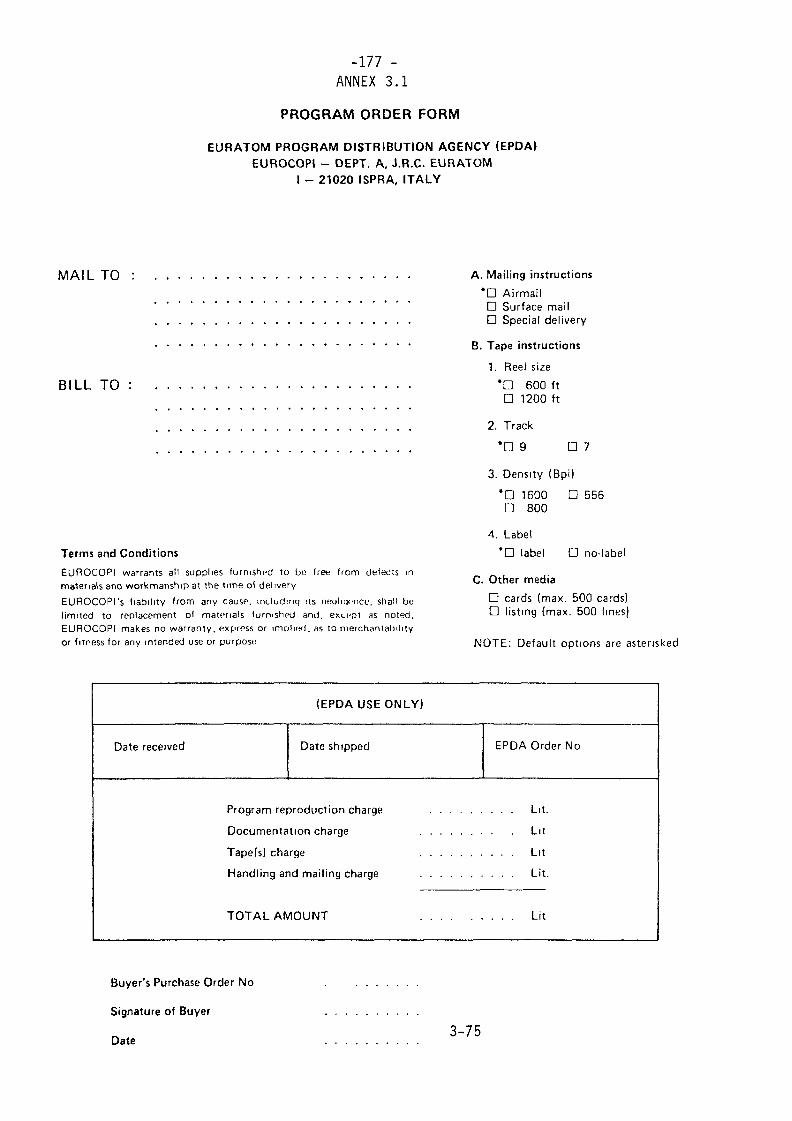
-177 -ANNEX 3.1

PROGRAM ORDER FORM

EURATOM PROGRAM DISTRIBUTION AGENCY (EPDAlEUROCOPI - DEPT. A, J.R.C. EURATOM

I - 21020 ISPRA, ITALY

MAIL TO

BILL TO

Terms and ConditionsEUROCOPI warrants all supplies furnished 10 bo free f rom defects inmaterials and workmanship at the time ol deliveryEUROCOPI's liability from any causf, including its neolnjcnCL', shall belimited to replacement of materials furmshpd and. except as noted.EUROCOPI makes no warranty, express or implied, as to merchantabilityor fitness for any intended use or purpose

A. Mailing instructions*D AirmailD Surface mailD Special delivery

B. Tape instructions

1. Reel size

*D 600 ftD 1200 ft

2. Track

*D 9 D 7

3. Density (Bpi)

*D 1600 D 556D 800

4. Label

*D label D no-label

C. Other mediaD cards (max. 500 cards)D listing (max. 500 lines)

NOTE: Default options are asterisked

(EPDA USE ONLY»

Date received Date shipped EPDA Order No

Program reproduction charge

Documentation charge

Tape(s) charge

Handling and mailing charge

TOTAL AMOUNT

Lit.

Lu

Lit

Lit.

Lit

Buyer's Purchase Order No

Signature of Buyer

Date 3-75

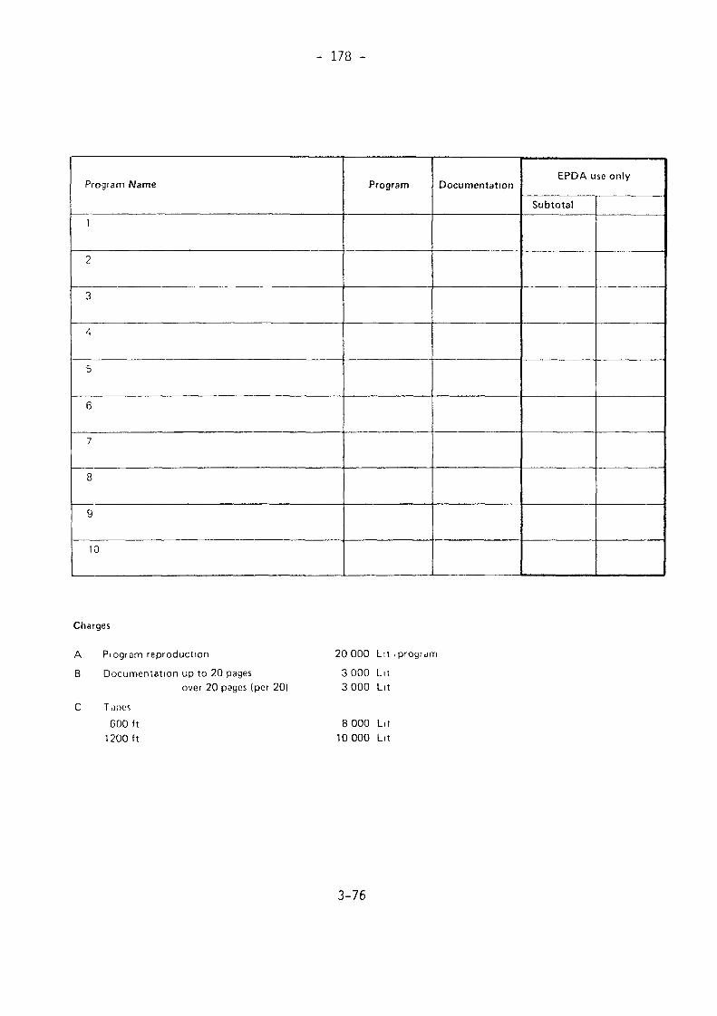
- 178 -

Progiam Name

1

2

3

4

5

6

7

8

9

10

Program DocumentationEPDA use only

Subtotal

Charges

A Program reproduction

B Documentation up to 20 pagesover 20 pages (per 20)

C T .][>(.'<600f t

1200 ft

20 000 Lit /program

3000 Lit3000 Lit

8000 Lit10000 Lit

3-76

- 179 -Chapter 4

DESIGN OF INSPECTION PLANS

4.1 PURPOSE OF INSPECTIONStated very simply and in somewhat general terms, the purpose of Agency

inspection is to provide assurance that the material balance data for a facilityproperly reflect the state of material control that exists in that facility, andfurther, that the state of control is satisfactory, i.e., it provides no indica-tion of unaccounted for losses of material. In order to provide objectivity,quantitative criteria are established, and statements about the inspection activi-ties are framed in terms of these criteria.

Inspection plans are to be derived to apply to a given facility and for agiven material balance period. The inspection plan is not restricted to includeonly those activities that take place to verify amounts of material in inventoryat a given time; the plan must also include provisions for monitoring flow streams,i.e., inputs to and outputs from the facility.

This discussion ori inspection activities is limited to those activities thatbear on material accountancy. There are other activities that take place duringan inspection, e.g., checking on containment and surveillance devices, but suchactivities, while certainly of importance in helping to provide assurance that thematerial balance data are acceptable when evaluated against the criteria, are notconsidered to be a part of those activities aimed directly at providing this assur-ance in quantitative terms.

In planning for inspection, it is assumed that the facility accounting datamay misrepresent the actual amounts of material in discrete items. Although suchdata misrepresentations may clearly occur because of innocent reasons, e.g.,because of mistakes in recording the measured data, it is assumed for planningpurposes that data misrepresentations occur intentionally in order to mask diver-sion. This assumption is made in order to provide assurance that the inspection iseffective and credible against all possible combinations of understatements and over-statements of material. To be effective and credible, the inspection must guardagainst the worst possible set of circumstances; this worst possible set corres-ponds to actions that would be taken by a diverter attempting to conceal diversionthrough data falsification. More is said to this point in later sections.

It is noted here that the assumed existence of an adversary, the diverter,is the basis for game-theoretic developments of inspector strategies. Throughoutthis chapter, reference will be made to results derived from game-theoretic consi-derations, and they will be compared with results found using other approaches,which also assume the existence of an adversary. Generally speaking, there isclose agreement in results among the different approaches to the inspection problem.This is a comfortable result, and permits some freedom for inspection planners tochoose among the various approaches to inspection planning that are proposed. Fora rather complete treatment of the game theoretic approach to safeguards problems,see Avenhaus [4.1].4.1.1 Response of Accountancy Statistics to Diversion Scenarios

Before proceeding further, it is worthwhile to discuss different diversionscenarios^and how the accountancy measures available to the inspector: MUF, D,and (MUF-D) react to these scenarios. It is perhaps most enlightening to consider

4-1

- 180 -

this problem in the context of a specific example. In this example, errors ofmeasurement are ignored, total inspection and a perfect material balance areassumed, i.e., in the absence of diversion, the MUF would be zero. (In thepresence of measurement errors and random sampling corresponding to less thantotal inspection, the results of the following discussion are interpreted for theexpectations of the statistics.)

For the example facility material balance, assume the following:BI = 1000 units (beginning inventory)R = 500 units (receipts)S = 800 units (shipments plus waste streams)

El = 700 units (ending inventory)MUF = BI + R - S - EI = 0 units

Some representative diversion scenarios are now constructed, and the re-sponses of the test statistics to these scenarios are noted.Scenario 1

100 units are moved from BI aftejr having been verified by the inspector.The facility is therefore short 100 units at the end of the balance period, i.e.,there are actually only 600 units in El.

Strategy 1Do not falsify El, i.e., book the true 600 unit value for ending inventory.

Then, the MUF being the booked amount gives MUF = 1000 + 500 - 800 - 600 = 100.The Öfc statistics for k = 1, 2, 3, and 4 are all zero since the actual amountsagree with the book amounts. Thus

5 = 0MUF-D - 100 units, reflecting 100 units diverted into MUF and 0 units

diverted through data falsification.Strategy 2

Falsify the El, i.e., book the El as 700 units even though there are only600 units present. Then,

MUF = 1000 + 500 - 800 - 700 = 0DI = D2 = D3 = 0D4 = 700 - 600 = 100D = -64. = -100 (The minus sign occurs because this represents a

data falsification in a negative component ofthe MUF equation.)

MUF-D = 0 -(-100) = 100 units, reflecting 0 units diverted into MUFand 100 units diverted through data falsification,i.e., through overstating the ending inventory.

4-2

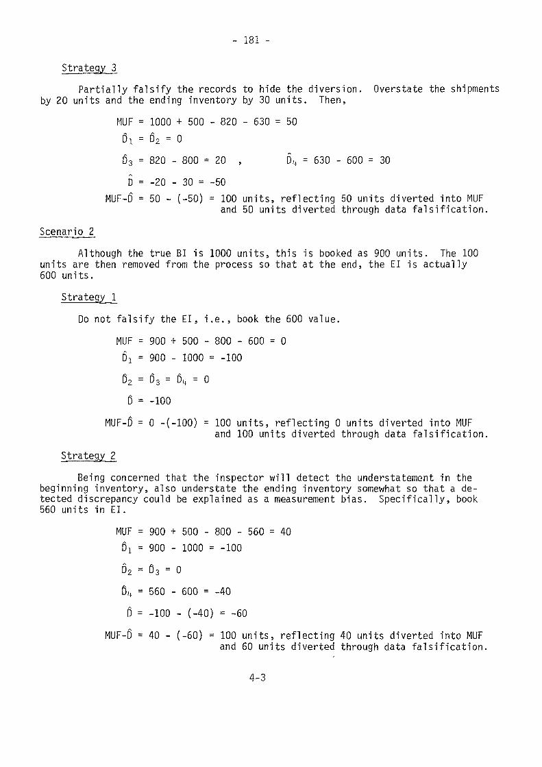
- 181 -

Strategy 3Partially falsify the records to hide the diversion. Overstate the shipments

by 20 units and the ending inventory by 30 units. Then,MUF = 1000 + 500 - 820 - 630 = 50D! = D2 = 0D3 = 820 - 800 = 20 , D^ = 630 - 600 = 30D = -20 - 30 = -50

MUF-D = 50 - (-50) = 100 units, reflecting 50 units diverted into MUFand 50 units diverted through data falsification.

Scenario 2Although the true BI is 1000 units, this is booked as 900 units. The 100

units are then removed from the process so that at the end, the El is actually600 units.

Strategy^ _!_Do not falsify the El, i.e., book the 600 value.

MUF = 900 + 500 - 800 - 600 = 0D! = 900 - 1000 = -100D2 = D3 = D\ = 0D = -100

MUF-D = 0 -(-100) = 100 units, reflecting 0 units diverted into MUFand 100 units diverted through data falsification.

Strategy 2Being concerned that the inspector will detect the understatement in the

beginning inventory, also understate the ending inventory somewhat so that a de-tected discrepancy could be explained as a measurement bias. Specifically, book560 units in El.

MUF = 900 + 500 - 800 - 560 = 40D! - 900 - 1000 = -100D2 = D3 = 0D\ = 560 - 600 = -40D - -100 - (-40) = -60

MUF-D = 40 - (-60) = 100 units, reflecting 40 units diverted into MUFand 60 units diverted through data falsification.

4-3

- 182 -These examples should make it clear that the (MUF-D) statistic reacts to thetotal amount diverted, no matter what diversion strategy is employed. This is al-

ways true, no matter which diversion scenarios may be constructed. In this connec-tion, data_fa1sification canjje said to occur only if the material in question isinspectable, i.e., available to the inspector for verification. Thus, with scen-ario 1, for example, it is not an admissible strategy to remove the 100 units frombeginning inventory before_ it is offered for inspection. Clearly, such a diversionwould not be detected within the closed loop of the facility material balance inquestion. Material not made available for inspection is clearly not safeguarded.Also, if material is diverted into MUF, i.e., simply removed from the process andthen shipped to a clandestine facility, such a shipment is not a declared shipmentand hence, the fact that there is a discrepancy between the amount shipped and theamount booked as shipment does not constitute a data falsification. This is becausethe amount booked is in perfect agreement with the amount presented for inspection.

Since the diverter may not restrict his strategies to the "admissible" onesas defined here, for complete protection other statistics would also need to beincluded, such as shipper-receiver differences. For a complete discussion, seeReference [4.2].4.2 INSPECTION ACTIVITIES

Inspection activities, while perhaps quite varied in a number of respects,e.g., measurement complexity, cost, accuracy, etc. may be broadly classified asfalling into one of two categories—attributes or variables inspection. In attri-butes inspection, the item inspected is classified as being either acceptable ornot acceptable {i.e., a defect) on the basis of the measurement. Attributes in-spection has nothing to do with the quality of the measurement, but rather, withthe end use to which the measurement is put. Variables inspection, on the otherhand, assigns a measured value to each item inspected, and the measured values fora group of items are combined in some way to provide a statistic, or a function ofthe observations, used in the evaluation in some predetermined way. As was thecase with attributes inspection, the quality of the measurement in question is notthe feature that determines that an inspection measurement is variable in nature,but rather, it is the end use to which the measurement is put.

The definitions of attributes and variables inspection in the widely refer-enced U.S.Military Standards are quoted here to close out this discussion.

From [4.3]: "Inspection by attributes is inspection whereby eitherthe unit of product is classified simply as defective or nondefec-tive, or the number of defects in the unit of product is counted,with respect to a given requirement or set of requirements."

From [4.4]: "Inspection by variables is inspection wherein a speci-fied quality characteristic on a unit of product is measured on acontinuous scale, such as pounds, inches, feet per second, etc.,and a measurement is recorded."

A more detailed discussion of inspection activities as they relate to thisfield of application follows.4.2.1 Attributes Inspection Activities

The specific attributes inspection activities that may be performed in agiven inspection depend on the circumstances of that inspection. Some activities,

4-4

- 183 -

although attributes in nature, are performed on 100% of the items and hence are nota part of the statistical planning or evaluation function. They are included inthe discussion to follow for completeness.

In broad terms, the inspection activities discussed in this chapter fall inone of two categories. One category consists of records examination and the otherrelates to inspection of measurements data. Within each category there is a fur-ther subdivision of possible inspections. Those that might be a part of attributesinspection are discussed below.

In connection with the records examination, consider the following activities:1) Inspection to detect recording and/or calculational mistakes in the

stratum subtotals and in combining stratum subtotals to calculate the MUF. Thiswould normally be a 100% inspection effort.

2) Reconciliation of data for receipts, shipments, and inventories asstated in the records with those submitted in reports to the Agency. This is apost-inspection activity and should be a 100% inspection with discrepancies notedand corrected.

3) Inspection to detect recording and/or calculational mistakes for indi-vidual items, including checking for proper application of the source data. Thiswill normally be done on a sampling basis, and is part of the statistical attri-butes inspection.

Activities of types 1-3 are a part of the records examination. In addition,two activities related to the verification of amounts of nuclear material are apart of attributes inspection.

4) Counting of items to verify that the numbers of items located agreewith the number listed on the facility records. This could be a 100% inspection,or it could be a part of the statistical attributes inspection, combined withactivities 3 and 5.

5) Inspection with an attributes tester to detect discrepancies, or defects,that are larger than can be explained by the combined errors of measurement forthe facility and for the inspector's attributes tester.

Some further discussion of this activity is helpful. Consider the attri-butes tester. This is a measurement device of some sort that will classify aninspected item as being either a defect or not a defect. The definition of an itemdefect is different from a planning viewpoint than it is from an implementationviewpoint. For planning purposes, a defect is defined in Section 4.3.1. From animplementation viewpoint, a defect is defined in Chapter 5, The fact that differ-ent criteria for defining a defect are used should not really be a bothersomepoint; in planning, it is important to establish criteria such that the amountof inspection performed is sufficient to provide protection against the best diver-sion strategies that might be used by a diverter. (This point was made previouslyin Section 4.1).

Measurement devices used as the attributes tester may not even be testers inthe true sense of the word. For example, the attributes test may consist of tipping

4-5

- 184 -

a container to verify that the actual weight does not differ greatly from thatlisted by the facility. The stabilized assay meter (SAM) may also be regardedas an attributes tester since it verifies that the item contains uranium ofroughly the proper enrichment.

In summary, statistical attributes inspection might consist of randomlyselecting items from the facility listing, locating those items, checking the cal-culations from the source data for those items, and performing attributes measure-ments such as tipping the containers and/or measuring with an NDA instrument suchas the SAM. In any particular inspection, and for a given stratum in that inspec-tion, the definition of an attributes test will, of course, have to be explicitlyset forth in implementation. This is not necessary in planning, however. It isonly required that some type of attributes inspection be anticipated.4.2.2 Variables Inspection Activicies

Variables inspection presupposes the existence of a variables measuringinstrument, or a variables tester. Unlike attributes inspection, it is necessaryto have in mind the specific tester to be used in each stratum at the planningstage, because the measurement error variances affect the planning. A variablestester may actually consist of a number of distinct measurement operations suchas weighing, material sampling, and chemical analysis, or possibly, NDA analysisof the sample.

For planning purposes, variables inspection consists of two types of acti-vities, both of which are related to the inspection of measurement data (as opposedto records examination). To continue with the list of inspection activities begunin the previous section, activities 6 and 7 defined below comprise the variableinspection.

6) Inspection to detect defects that are sufficiently small so as to es-cape detection with the attributes tester. This inspection activity is referredto as variables inspection in the attributes mode. As was the case with attributesinspection, the definition of a defect used in planning, given in Section 4.3.2.1,differs from that used in implementation, given in Chapter 5, and for the samereason. Interestingly enough, for planning purposes, it will be seen that thedefinition of a defect is related to the measurement error of the attributes tester.This means that, as stated above, although it is not necessary to specify theattributes tester when planning for attributes inspection, it is at least neces-sary to have some idea of its measurement error in order to plan for the variablesinspection in the attributes mode.

7) Inspection to detect small defects or biases that may exist in all orsome items in the given strata. This inspection activity is aimed at developingdata for the difference statistic, D, discussed in detail in Chapter 3.

For a discussion of how activities 6 and 7, both relating to variables in-spection, are united in the planning stage, see Section 4.3.2.

4.3 CRITERIA FOR INSPECTION PLAN DESIGNHaving outlined the types of inspection activities for both the attributes

and the variables inspection, the criteria used in planning the inspection are nowconsidered. First these criteria are discussed for attributes inspection.

4-6

- 185 -

4.3.1 Attributes Ins£ectior[ CriteriaIn determining the number of items to be inspected, attention is focussed

first on a single stratum. Essential to the inspection design is some quantity M.M = goal amount of element (or isotope) established by external

considerations and supplied as an input to the planning.The attributes inspection criterion is stated very simply. If an amount,

M, is missing from the stratum in question, this fact should be detected with (high)probability, (1-ß). The parameter ß is also an input parameter.

Several comments are relevant. First, the definition of "detected" is con-sidered. In order to minimize the amount of inspection that must be performed, azero-acceptance number plan is used. This means that if even a single defect isfound among the items inspected, this constitutes "detection". The action tofollow in the event of this detection is yet another matter that must be defined.One action might be to 100% inspect the stratum in question on an attributes basis,correcting all records for the defective items. This is generally not possible,and some other action might be required, such as giving the facility the opportunityto improve the data base prior to another inspection to follow soon. A third possi-bility, and, in fact, the action most likely to be taken is that the effects onMUF of the detected discrepancy will be evaluated in some way. Section 5.1.3describes a procedure to calculate the confidence interval for the number ofdefects in a stratum population. Section 5.1.2.1 describes a procedure to cal-culate the quantitative effect of defects on MUF. Whatever the follow-up action,detection is clearly and objectively defined here, and such a definition is all that isneeded in planning.

Next, consider the definition of a defect. It is clearly to a diverter'sbenefit to falsify the smallest number of items necessary in order to accumulatethe goal amount of M units. Thus, he would choose to falsify each item falsifiedby the maximum amount possible. Assume that this maximum amount corresponds tothe nominal or average amount of element (or isotope) per item, denoted by x|<, andexpressed in the same units as M. Thus, the number of items that would have to befalsified in order to accumulate M units (i.e., the number of "defects") is M/x^in stratum k. With this in mind, the criterion for attributes inspection statedabove may now be restated in its equivalent form, as follows:

If the number of gross or large defects in stratum k is M/x^, choose thesample size, na|<, large enough such that at least one of these defects will appearin the items inspected with probability (1-ß).

At this point in the discussion, a possibly worrisome point should be broughtup. The inspection is designed to detect M units if all M units are missing instratum k. In actual fact, the adversary would likely not attempt to remove all Munits by this mechanism, i.e., by large data falsifications restricted to a singlestratum. Clearly, if some amount less than M is diverted from stratum k in thisfashion, then the probability of detection in that stratum is some amount smallerthan the desired value, (1-ß). This is a valid point of concern and touches on thegeneral problem of how the diverter would choose to divert M units by various meansso as to escape detection. This general problem is treated in detail in latersections (see Sections 4.4.1.2 and 4.6). At this point in the discussion, oneneed only accept the fact that the inspection criterion as stated is appropriate;its appropriateness will be demonstrated later.

4-7

- 186 -

4.3.2 Vajnab1es_Iinspection Criteria

With variables inspection, there are two kinds of criteria. One set is rele-vant to variables inspection in the attributes mode and the other to variables in-spection in the variables mode. The inspection sample size for stratum k will bederived based on each set of criteria. In implementing the plan, the larger ofthe two sample sizes will be used in each stratum. This means that the actual pro-tection afforded by the plan, i.e., the plan's ability to detect the goal amount,M, will be least as large as that calculated based on the design criteria as appliedseparately in the attributes and variables mode. This point is discussed furtherin Section 4.6.

Before presenting inspection criteria for variables inspection in each ofits two modes, it is helpful to discuss briefly why the two separate sample sizesmust be calculated. The reason is that an inspection plan must counter the beststrategy of a diverter. Specifically, it may well happen that if variables inspec-tion in a variables mode is all that's planned for, then the sample size in a givenstratum may be too small to counter the strategy in which a diverter falsifiesnot all items by a small amount, but rather, a selected smaller number of itemsby an amount just small enough to escape detection by attributes inspection withthe attributes tester. The argument used by the diverter is that if any suchdefected item is included among the items inspected by variables inspection, it issure to be labelled a defect; however, chances are that the item would not be in-cluded among the items to be inspected were variables inspection only planned todevelop data for the D statistic. To combat that argument, variables inspectionsample sizes must also be large enough to detect these medium sized defects, thosesufficiently small so as not to be detected by the attributes tester, but muchlarger than would be needed to accumulate M units by small defects were all itemsin the stratum to be falsified.

It is remarked that rather than defining these two categories of defects(medium and small), one could treat both categories of defects simultaneously ona continuous scale. This is done by defining two quantities for a given stratum,one being the number of items to be falsified by the diverter, and the other beingthe size of the falsification per item. In a game theoretical sense, then, thediverter chooses these two quantities in some optimum way while the inspectoralso chooses his best strategy to combat the diverter. Limited calculations in-dicate that the two different approaches to the problem lead to basically the sameresults from an inspection planning viewpoint [4.1].

Attention is now directed at presenting criteria for variables inspection,first in the attributes mode.4.3.2.1 Criteria^ for Variables Inspection in Attributes Mode

The discussion in Section 4.3.1 on attributes inspection criteria is rele-vant to variables inspection in the attributes mode also. The only differenceis in the definition of a defect. As with attributes inspection, it is in thebest interest of a diverter to falsify any item selected for falsification by thelargest amount feasible. In the case of attributes inspection, this amount wasX|<; in the case of variables inspection, it is Y^X^, where Yk is some number lessthan 1.

4-8

- 187 -

The parameter Y|< is an input design parameter. It describes the abilityof the attributes tester to detect a given degree of falsification. Specifically,Y^ may be defined by the following statement: if a discrepancy exceed Y^X^ insize, it will be labelled a gross defect in the attributes tester inspection withprobability one; if it is smaller than Y^, it will be detected with probabilityzero.

In defining Y|< in this fashion, there is no need to define a measurementerror as such associated with the attributes tester. For example, if the attri-butes test involves tipping a container to see if it contains about the recordedamount of gross weight, it is difficult to assign a measurement error to thisoperation. However, the argument can be made that if the item contains say lessthan half its recorded amount, then this would be detected by the tipping opera-tion. In this event, Y|< would be assigned the value 0.5.

In the event the attributes tester produces a quantitative response orreading, the/i Y|< may be defined in terms of the measurement error standard devia-tion of the difference between the facility and the inspection measurements. Often,this reduces to the measurement error standard deviation for the inspector measure-ment, which will likely be the dominant error in attributes inspection. If the errorstandard deviation of this difference is denoted by <$(< on a relative basis, thenY|< might be defined to be, say, 46 . For example, a 5% relative error standarddeviation results in a value for Y^ of 0.20.

When there is some doubt as to the value of Y^ in a given application, itis always preferable to err on the high side. By erring in this direction, theresulting inspection sample size will be larger than needed, i.e., the error willbe on the conservative side. This is one reason that the definition Y^ = 4o|<is used; even though it is quite likely that a discrepancy smaller than Y^x^ wouldbe detected by the attributes tester, the probability of this event is implicitlyassumed to be zero in order to be sure that the sample size for variables inspectionin the attributes mode is conservatively large.

With these thoughts in mind, the criterion for variables inspection in theattributes mode may now be stated as follows:

If the number of medium defects in stratum k is M/Y^X^, choose the samplesize, nyifc, large enough such that at least one of these defects will appear in theitems inspected with probability (1-3).4.3.2.2 Criteria for Variables Inspection in Variables Mode, Using D

It was mentioned earlier that the data collected from the variables inspectionare used to calculate D, the difference statistic defined explicitly in Section3.5.1. This fact implies that the criteria for the variables inspection samplesizes, when variables inspection is in the variables mode, is related in some wayto this D statistic.

The design criteria in this application are again related to the goal amount,M. In general terms, a sufficient number of items must be inspected such thatif the mean value of D is -M, this fact is detected using the D statistic withprobability (1-ß). (Note: The mean of D carries the minus sign, -M, because anegative value for ß benefits the diverter, as D has been defined.)

4-9

- 188 -

A number of comments must be made on this general criterion. First, theprecise definition of "detected" must be given. This is related to the probabilityof a "false alarm", i.e., of claiming detection when in fact the true mean of D iszero. This probability should be small. It is an input value in planning, and islabelled a.

Secondly, it is noted that, unlike attributes inspection, the sample sizefor variables inspection in the variables mode is calculated over all strata, andnot for a particular stratum. In finding this total sample size, it is implicitlyassumed that the items to be inspected are allocated among the strata in some opti-mum fashion. Specifically, in this discussion, they are allocated to result ina minimum variance for D for a fixed total sample size. Other bases for optimumallocation could be factored in, such as the cost of analysis and the attractivenessof the material from a diversion standpoint, but this is not done formally here [4.5],

As a third comment, it is noted that it may not be possible to meet the cri-terion as stated because the variance of ßjs limited by the systematic error vari-ance. The random part of the variance of D will continue to decrease with increasedinspection sample sizes; the systematic part will not. Further, even in the casethat the design criterion can be met, the effect on (1-3) of measuring additionalitems beyond a certain point may not be worth the effort. Therefore, the emphasisin this chapter will not be so much on determining a specific variables inspectionsample size, but rather, in examining the relationship between sample size and(1-ß) as an aid in choosing the sample size.

Fourthly, it is recognized that the variance of ß under the hypothesis thatthere is no diversion through small data falsifications may be smaller than thatunder the alternative hypothesis that some material may be thus diverted. This isbecause under the alternative hypothesis, the diverter will likely choose to notfalsify all items by the same amount. Thus a statistical sampling error will beintroduced because the variance of D will depend on which items were selected to beinspected. (See eq. (3.38) of [4.1] for an exact expression for this varianceunder a specified model.) The parameter CQ is introduced to relate the varianceof ß under the null hypothesis to its variance under the alternative hypothesisduring the planning stage. Specifically, for planning purposes, it is assumed thatthe random error variance of D under the alternative hypothesis is C^ times thecorresponding variance under the null hypothesis.

As a final comment, it has been noted previously that measurements made witha variables tester may well consist of a number of measurement operations, e.g., aweighing, a sampling, and an analytical measurement. For simplicity, it is assumedin this chapter that the sample size in question is taken to be the number of itemssampled to determine the element concentration factor. In calculating the randomerror variance of ß in planning, the number of items to be weighed is set equal tothe number of items to be sampled. The number of analytical determinations to bemade per sampled item may be arbitrarily inputted.4.3.2.3 Criteria for_Variab1es Inspection in Variables Mode, Using (MUF-D)

In Section 3.6, the (MUF-D) statistic was introduced. It was pointed outthat (MUF-D) may be regarded as the inspector's estimate of the facility MUF. Fur-ther it was suggested that the separate tests on ß and MUF could be combined intoone test using (MUF-D).

4-10

- 189 -

Clearly, the variance of MUF is independent of inspection sample sizes.In the Section 4.3.2.2 just preceding this one, criteria for determining the vari-able inspection sample sizes using the D statistic were given. The aim here wasto detect M units through use of D. If the (preferred) test statistic, (MUF-D),is used in the evaluation phase, then it might be logical that (MUF-D) also bethe statistic used in inspection planning, rather than D. This latter statisticis aimed only at detection of diverted amounts through small data falsifications;the (MUF-D) statistic responds to the combination of two strategies of diversion,one through small data falsifications, and the other through diversion into MUF.Diversion into MUF means that material is simply removed from the process with noattempts made to alter any records.

When planning is with respect to (MUF-D) rather than to ß, then the cri-teria discussed in the preceding Section 4.3.2.2 still apply, the only differencebeing that (MUF-D) replaces D as the test statistic.

4.4 SELECTION OF INSPECTION SAMPLE SIZESThe methods for deriving the inspection sample sizes may now be given. First,

the attributes inspection sample sizes are considered.4.4.1 Attributes Inspection Sample Sizes

In Section 4.4.1.1, the method for determining the attributes inspectionsample size in stratum k is given. In Section 4.4.1.2, it is demonstrated thatthis procedure provides protection against all diverter strategies in which M unitsare diverted through large data falsifications but allocated among the variousstrata.4.4.1.1 Attributes Inspection _Sampl e_S_i ze in Given StratumMethod 4.1

NotationThe notation is given in Section 4.3.1 in part. It is repeated here for

convenience, and some additional notation is included.M = goal amount of element (or isotope)N^ = number of items in stratum k

nak = nuniker °f items to be inspected in stratum kß = probability of failing to detect the amount M, if this

amount is missing from the stratumx, = average amount of element (or isotope) per item in stratum kexpressed in the same units as M

4-11

- 190 -

ModelThe random variable Is the number of defects found in a sample of na|< itemsselected at random from a population of % items containing a given number of defects,

It is well known that this random variable follows a hypergeometric density func-tion [4.6].

ResultsThe required sample size, n . , is given by

nak = Nk(l-ßXk/M)

The result should always be rounded up_ to the next integer.

(eq. 4.4.1)

A zero acceptance plan is used to minimize the amount of inspection required.The sample size, n^, is the solution of the equation:

Prob (0 defects | M/xk defects in the population) = ß

Using the hypergeometric model, this equation is written/M/xk\ /Nk - M/xk\\ 0 / V nak / „ (eq. 4.4.2)

It is shown in [4.7] that an approximate solution to (eq. 4.4.2) is

na|< = 0.5 (lV</M) (2Nk - M/xk + 1) (eq. 4.4.3)

When (M/xV - 7) is small relative to N. , it may be deleted from{eq. 4.4.3), and yeq. 4.4.1) follows immediately. When (M/x. - 1) is not in-significant relative to l\, the use of (eq. 4.4.1) will result in a conserva-tively large sample size.V

However, it follows from (eq. 4.4.2) that detection is certain (ß = 0) ifn , > Nk - M/x. - i.e., if the sample size is greater than the number of non-dlrectij/e items in the population so that the sample size never need exceedNk - M/x\ + 1. Also if cost of sampling is an important factor more preciseapproximation in (eq. 4.4.3) may be warranted.Note: When computing ß for given N. , M, x. , and n . the approximation of(eq. 4.4.1) may seriously overestimate 3 unless the condition that (M/xY - 1)is small compared to Nk is satisfied, thus indicating a lower probabilité ofdetection than that actually achieved. If the condition is not clearly met theuse of (eq. 4.4.3) is to be preferred for calculating ß when n . < N. - M/x, .T-P ^ ^ M _ M/3 o 4o •; ^11-1+• •; /•*-.! 11/ n a K K KIf nak 'k - M/xk' is identically 0.

4-12

- 191 -

Examples

EXAMPLE 4.1 (a)Let the stratum to be inspected be the feed stratum in the low enriched

uranium fabrication plant of Example 3.3 (a). From the data of that example,

N! = 12000xi = 20 kg U

Say that the input design parameter values areM = 1500 kg Uß = 0.05

Then, using (eq. 4.4.1),ri = 12000(1- 0.051/?5)ai

= 469.87 = 470 items

EXAMPLE 4.1 (b)Let the stratum to be inspected be stratum 8 of the mixed oxide fuel fabri-

cation facility of Example 3.3 (b). This is the ending inventory stratum of mixedoxide powder items. From the cited example,

N8 = 360x8 = 0.375 kg Pu

Say that the input design parameter values areM = 8 kg Puß = 0.05

Then, from (eq. 4.4.1),nafl = 360 (l-0.05°-375/8)as

= 47.16 = 48 items

4-13

- 192 -4.4.1.2 Attributes jjispectjon Sample Sizes Over All Strata

As was mentioned in Section 4.3.1, a diverter would likely not divert all Munits from a given stratum and, as a result, the probability of detecting an amountless than M diverted from a given stratum will be less than (1-ß). Assume, initially,that the diverter diverts the goal amount M through gross data falsifications only,but that he diverts an amount M|< from stratum k so that the sum of M|< over the kstrata is M. (This assumption is relaxed later to permit the accumulation of thegoal amount through a combination of strategies in which not all of it need be di-verted through gross data falsifications.) What is then the probability of detect-ing this diversion?

To answer this question, "detection" must be defined. In the case of a sin-gle stratum, the diversion was detected if one or more defects appeared in thesampled items. To extend this definition over all the strata, detection will besaid to occur if at least one such defect is found in one or more strata.

Let ßk = probability of finding 0 defects in the sample of na|<items in stratum kThe overall probability of nondetection is simply the product of the ß|<

values over all the strata. The nak in this definition of ß|< is given by (eq. 4.4.1)The expression for 3k is found. The solution to (eq. 4.4.1) with ß|<replacing 3 and l\ replacing M provides this expression.

Mk/xk0k = (1 - nak/Nk) (eq. 4.4.4)

But with na|< given by (eq. 4.4.1), the expression (1 - na|</%) may be re-placed by kRx /MP 5

so (eq. 4.4.4) becomesfM (eq. 4.4.5)

IN

The product of the ßk values is thenEMiYM

O ßk = Bk = 0 (eq. 4.4.6)kThis gives the probability of nondetection, which is exactly the design

value for a given stratum. Thus, even though the probability of detection is not(1-ß) in any given stratum (unless M^ = M for that stratum), the overall probabilityof detection will be (1-ß), given that detection consists of finding at least onedefect in at least one stratum.

4-14

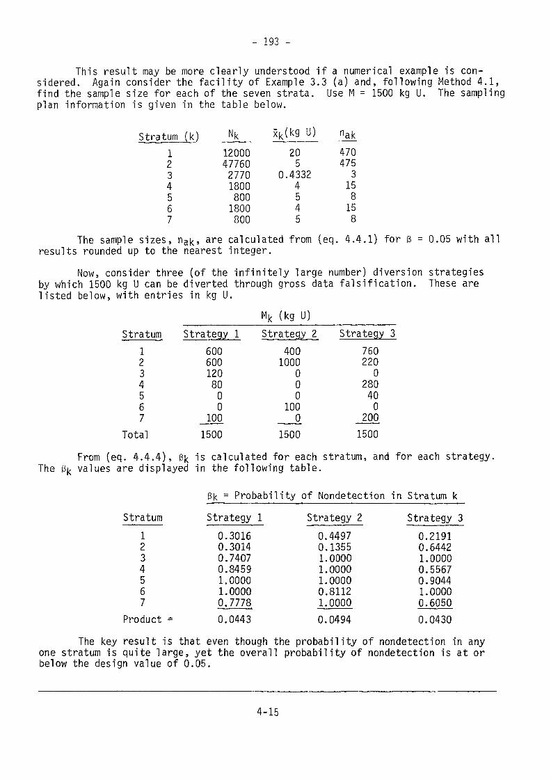
- 193 -

This result may be more clearly understood if a numerical example is con-sidered. Again consider the facility of Example 3.3 (a) and, following Method 4.1,find the sample size for each of the seven strata. Use M = 1500 kg U. The samplingplan information is given in the table below.

Stratum (k)123

Nk x

567

1200047760277018008001800800

J<U<9_U)_205

0.43324545

nak4704753158158

The sample sizes, nak, are calculated from (eq. 4.4.1) for ß = 0.05 with allresults rounded up to the nearest integer.Now, consider three (of the infinitely large number) diversion strategies

by which 1500 kg U can be diverted through gross data falsification. These arelisted below, with entries in kg U.

Stratum1234567

Total

Mk (kg U)Strategy 1

6006001208000

1001500

Strategy_24001000

000

1000

1500

Strategy 37602200

280400

2001500

TheFrom (eq. 4.4.4), ß|< is calculated for each stratum, and for each strategy.values are displayed in the following table.

Bk = Probability of Nondetection in Stratum kStratum

1234567

Product =

Strategy 10.30160.30140.74070.84591.00001.00000 77780.0443

Strategy 20.44970.13551.00001.00001.00000.81121.00000.0494

Strategy 30.21910.64421.00000.55670.90441.00000.60500.0430

The key result is that even though the probability of nondetection in anyone stratum is quite large, yet the overall probability of nondetection is at orbelow the design value of 0.05.

4-15

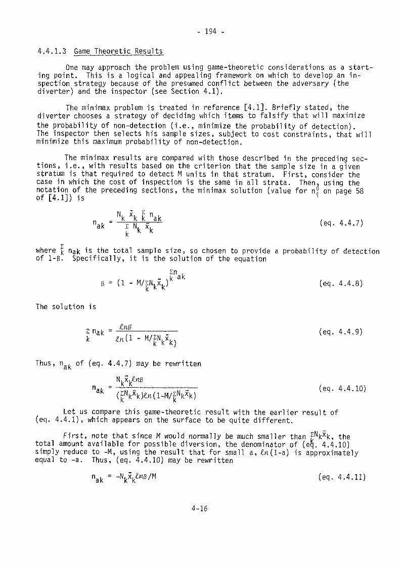
- 194 -

4.4.1.3 Game Theoretic ResultsOne may approach the problem using game-theoretic considerations as a start-

ing point. This is a logical and appealing framework on which to develop an in-spection strategy because of the presumed conflict between the adversary (thediverter) and the inspector (see Section 4.1).

The minimax problem is treated in reference [4.1]. Briefly stated, thediverter chooses a strategy of deciding which items to falsify that will maximizethe probability of non-detection (i.e., minimize the probability of detection).The inspector then selects his sample sizes, subject to cost constraints, that willminimize this maximum probability of non -detection.

The minimax results are compared with those described in the preceding sec-tions, i.e., with results based on the criterion that the sample size in a givenstratum is that required to detect M units in that stratum. First, consider thecase in which the cost of inspection is the same in all strata. Then, using thenotation of the preceding sections, the minimax solution (value for n. on page 58of [4.1]) is 1

M ^ ni« — K K K a Knak ' z N. x,

k K K

£where ^ na|< is the total sample size, so chosen to provide a probability of detectionof 1-ß. Specifically, it is the solution of the equationzn ,

3 = (1 - M/|Nkxk)k a (eq. 4.4.8)

The solution is

2 nak = 7; —— TT-r- (eq. 4.4.9)k In (l -

Thus, nak of (eq. 4.4.7) may be rewritten

Let us compare this game-theoretic result with the earlier result of(eq. 4.4.1), which appears on the surface to be quite different.

First, note that since M would normally be much smaller than ?Nk^k, thetotal amount available for possible diversion, the denominator of (eq. 4.4.10)simply reduce to -M, using the result that for small a, In (I -a) is approximatelyequal to -a. Thus, (eq. 4.4.10) may be rewritten

nak = -NI I S/M to- 4.4.11)

4-16

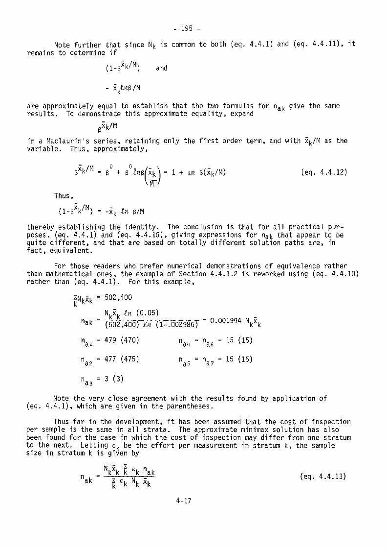
- 195 -Note further that since Nk is common to both (eq. 4.4.1) and (eq. 4.4.11), it

remains to determine if(l-ß*k/M) and

are approximately equal to establish that the two formulas for nak give the sameresults. To demonstrate this approximate equality, expand

exk/Min a Maclaurin's series, retaining only the first order term, and with xk/M as thevariable. Thus, approximately,

e(xk/M) (eq. 4.4.12)~M~

Thus,(l-ßVM) = -xk In ß/M

thereby establishing the identity. The conclusion is that for all practical pur-poses, (eq. 4.4.1) and (eq. 4.4.10), giving expressions for nak that appear to bequite different, and that are based on totally different solution paths are, infact, equivalent.

For those readers who prefer numerical demonstrations of equivalence ratherthan mathematical ones, the example of Section 4.4.1.2 is reworked using (eq. 4.4.10)rather than (eq. 4.4.1). For this example,

= 502,400Nkxk In (0.05)

"ak = (502,400) In (1-.002986) = °-001994 \xknal = 479 (470) n^ = na6 = 15 (15)

na2 = 477 (475) n^ = r\a? = 15 (15)

na3 = 3 (3)

Note the very close agreement with the results found by application of(eq. 4.4.1), which are given in the parentheses.Thus far in the development, it has been assumed that the cost of inspection

per sample is the same in all strata. The approximate minimax solution has alsobeen found for the case in which the cost of inspection may differ from one stratumto the next. Letting sk be the effort per measurement in stratum k, the samplesize in stratum k is given by

MY ^ c- nn - k k k Ek nak - . .nak " V e ' N" ;"" (eq> 4-4-aK l k k k

4-17

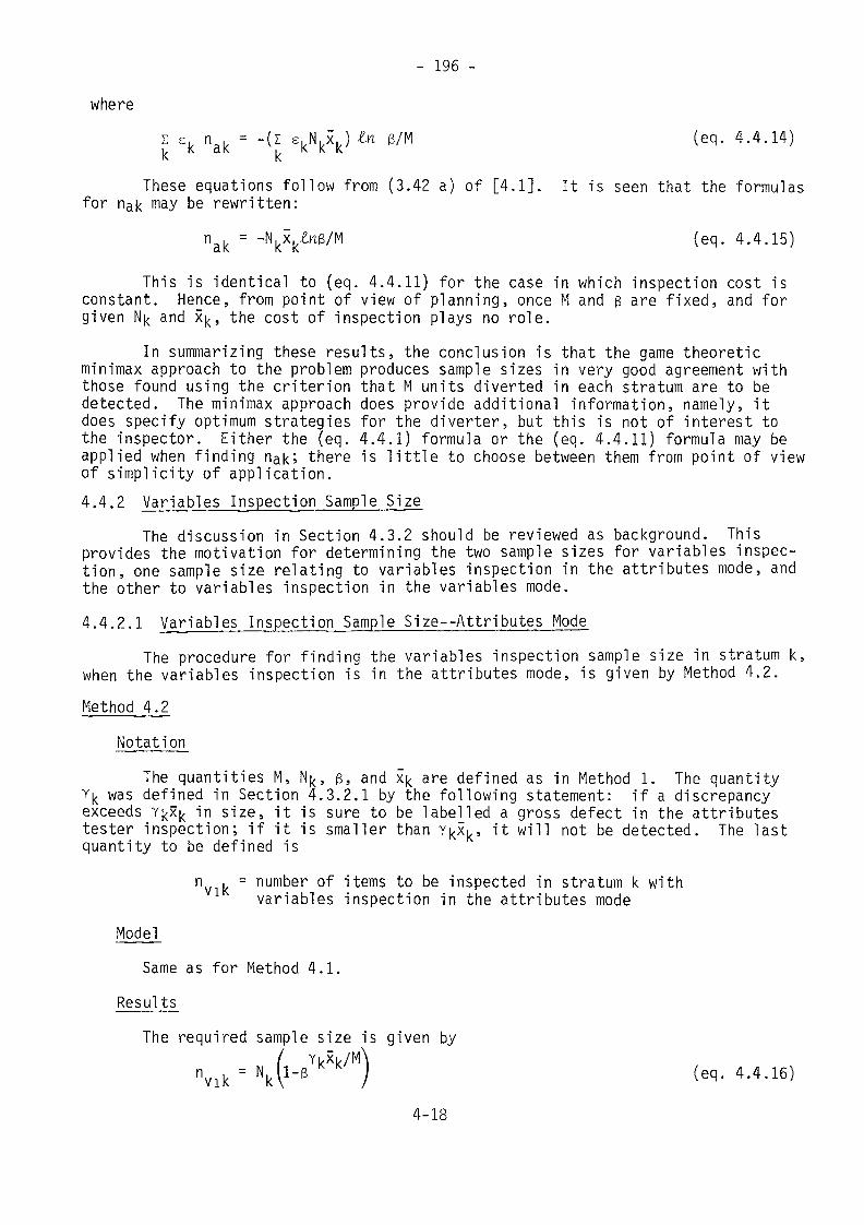
- 196 -

where

l Bk na[< = -(E e k N k x k ) In g/M (eq. 4.4.14)K- K

These equations follow from (3.42 a) of [4.1]. It is seen that the formulasfor nak may be rewritten:

nak = -Vk£nß/M (eq' 4-4-15)This is identical to (eq. 4.4.11) for the case in which inspection cost is

constant. Hence, from point of view of planning, once M and ß are fixed, and forgiven Nk and %, the cost of inspection plays no role.

In summarizing these results, the conclusion is that the game theoreticminimax approach to the problem produces sample sizes in very good agreement withthose found using the criterion that M units diverted in each stratum are to bedetected. The minimax approach does provide additional information, namely, itdoes specify optimum strategies for the diverter, but this is not of interest tothe inspector. Either the (eq. 4.4.1) formula or the (eq. 4.4.11) formula may beapplied when finding nak; there is little to choose between them from point of viewof simplicity of application.4.4.2 Variables Inspection Sample Size

The discussion in Section 4.3.2 should be reviewed as background. Thisprovides the motivation for determining the two sample sizes for variables inspec-tion, one sample size relating to variables inspection in the attributes mode, andthe other to variables inspection in the variables mode.4.4.2.1 Variables Inspection Sample Si ze--Attri butes Mode

The procedure for finding the variables inspection sample size in stratum k,when the variables inspection is in the attributes mode, is given by Method 4.2.Method 4.2

Notation^The quantities M, N^, ß, and xk are defined as in Method 1. The quantity

Y|< was defined in Section 4.3.2.1 by the following statement: if a discrepancyexceeds Y^X^ in size, it is sure to be labelled a gross defect in the attributestester inspection; if it is smaller than Y|<xk, it will not be detected. The lastquantity to be defined is

n . = number of items to be inspected in stratum k withvariables inspection in the attributes mode

ModelSame as for Method 4.1.

ResultsThe required sample size is given by

( yk*kMVk = MI-B I ( e q" 4 '4-16)

4-18

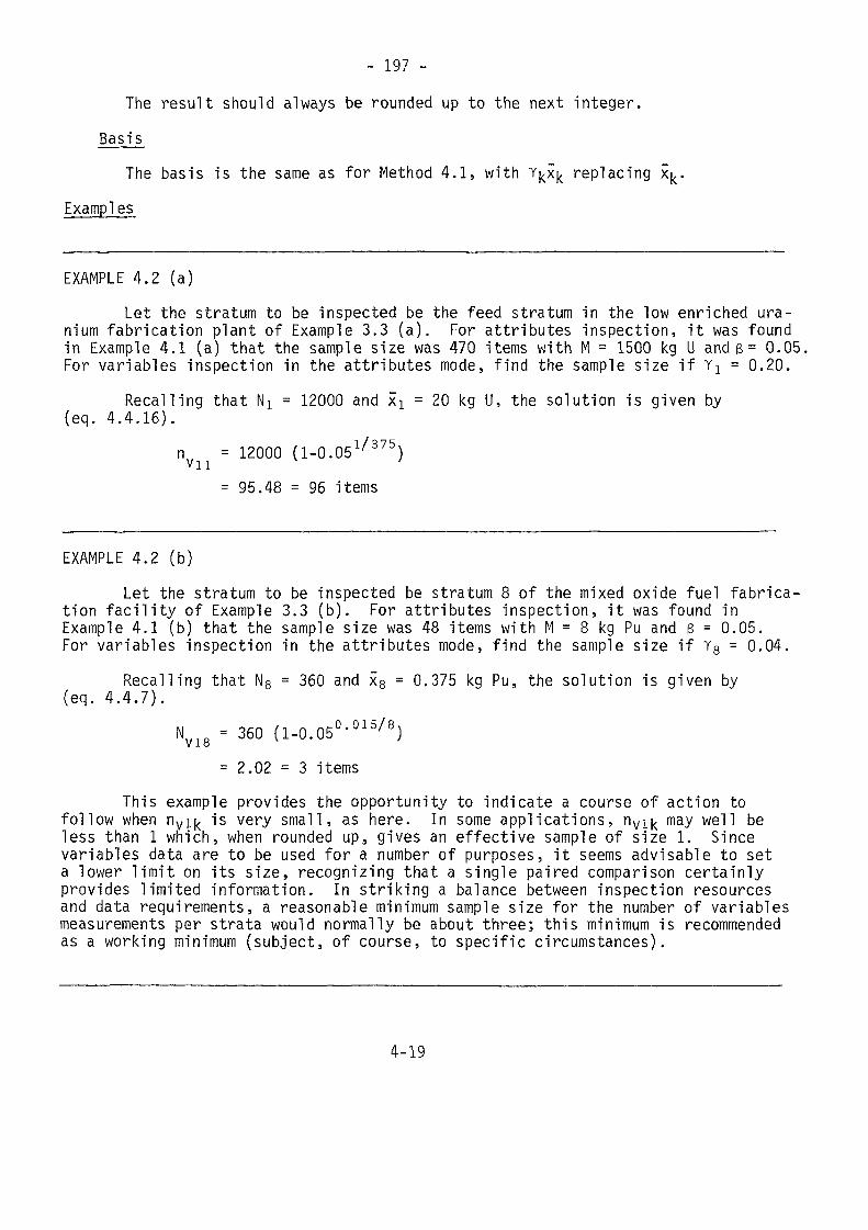
- 197 -The result should always be rounded up to the next integer.

BasisThe basis is the same as for Method 4.1, with Y^X^ replacing

Examples

EXAMPLE 4.2 (a)Let the stratum to be inspected be the feed stratum in the low enriched ura-

nium fabrication plant of Example 3.3 (a). For attributes inspection, it was foundin Example 4.1 (a) that the sample size was 470 items with M = 1500 kg U and 3 = 0.05.For variables inspection in the attributes mode, find the sample size if YJ = 0.20.

Recalling that N: = 12000 and KI = 20 kg U, the solution is given by(eq. 4.4.16).n = 12000 (1-0.051/375)

= 95.48 = 96 items

EXAMPLE 4.2 (b)Let the stratum to be inspected be stratum 8 of the mixed oxide fuel fabrica

tion facility of Example 3.3 (b). For attributes inspection, it was found inExample 4.1 (b) that the sample size was 48 items with M = 8 kg Pu and ß = 0.05.For variables inspection in the attributes mode, find the sample size if Y8 = 0.04.

Recalling that NQ = 360 and x8 = 0.375 kg Pu, the solution is given by(eq. 4.4.7).

V18 = 360 (1-0.05°'°15/8)= 2.02 = 3 items

This example provides the opportunity to indicate a course of action tofollow when nvi^ is very small, as here. In some applications, nvl|<. may well beless than 1 which, when rounded up, gives an effective sample of size 1. Sincevariables data are to be used for a number of purposes, it seems advisable to seta lower limit on its size, recognizing that a single paired comparison certainlyprovides limited information. In striking a balance between inspection resourcesand data requirements, a reasonable minimum sample size for the number of variablesmeasurements per strata would normally be about three; this minimum is recommendedas a working minimum (subject, of course, to specific circumstances).

4-19

- 198 -

As was the case with attributes inspection, the sample size for variablesinspection in the attributes mode in stratum k will detect an amount M withprobability (1-3). If an amount smaller than M units were diverted throughmedium falsification in stratum k, then the detection probability will clearlybe less than (1-3) in that particular stratum. However, by an argument verysimilar to that given in Section 4.4.1.2, if detection involves finding at leastone defect in at least one stratum, then no matter how the M units are allocatedamong the strata, the overall probability of detection will be (1-3).

An extension to this result will be given in Section 4.5.2 where the proba-bility of finding at least one gross or medium defect in at least one stratumfor attributes and/or variables inspection in the attributes mode is calculated.The goal quantity M, or more generally, the amount diverted through gross andmedium data falsifications, which may be less than M, may be allocated arbitrarilyamong the strata, and into either gross or medium falsifications.4.4.2.2 Variables Inspection Sample Size--Varj_ab1es Mode

Sections 4.3.2.2 and 4.3.2.3 should be reviewed. The sample size for vari-ables „inspection in the variables mode will utilize either the D statistic or the(MUF-D) statistic for planning purposes. Method 4.3 provides the equations neededto compute the sample size.Method 4.3

NotationMuch of the notation needed for this method has been defined in prior sections.

It is repeated here to facilitate application of the method.V (D) = short term systematic error variance of D defined9 by (eq. 3.5.14)V (D) = long term systematic error variance of D defineds by (eq. 3.5.21)

A /vV (D, ) = random error variance of D|< due to the facility samplings and analytical errors, computed for those strata in whichthe number of items measured by the inspector exceeds thenumber of batches. In this event, the error, although ran-dom in origin, behaves like a systematic error.

Vrl(D, ) = random error variance of D|< per item due to facilitysampling and analytical errors, computed for those stratafor which V^D^} is not computed.

V (D. ) = random error variance of D^ per item due to the facility2 bulk measurementV (D.) = random error variance of D^ per item due to the inspector'sr3 sampling and analytical errors.

4-20

- 199 -

a2 = The sum of the components of the variance of D whose values do nots decrease with additional inspector measurements (i.e., systematicerrors)

s? = random error variance of D^ per item measured by the inspectorV (D)'JHo = random error variance of D under the hypothesis that nothing hasbeen diverted and obscured by small data falsificationsVr(D)ÎHi = random error variance of D under the alternative that small datafalsifications have been introduced to mask diversion

C02 = variance inflation factor relating V (D)] to V (D)|Hv» » 'oratio of Vr(D)|H0 to a2(Note: e is inversely proportional to the total sample size)

V(MUF) = variance of element MUFV0 = that part of the variance of element MUF due to systematic errorsthat are common to both the facility and the inspector

STAT = test statistic, either D or (MUF-D)a = significance level of test3 = probability of failing to detect an amount M diverted and masked by

small data falsificationsM = goal quantity in amount of elementt = defined such that the area under the standardized normal curve tCC _i • 0*to °° IS a

t = defined such that the area under the standardized normal curvep from t. to « is 3Pu. = number of batches sampled by the inspectorw. = number of items per sampled batch for which the inspector makesbulk measurementsv, = number of samples drawn by the inspector per sampled batch to

determine the element factora, = number of analyses performed by the inspector per sample instratum km. = number of batches in stratum kr. = number of sample drawn by the facility per batch to determinethe element factorC|^ = number of analyses performed by the facility per sample in stratum k

4-21

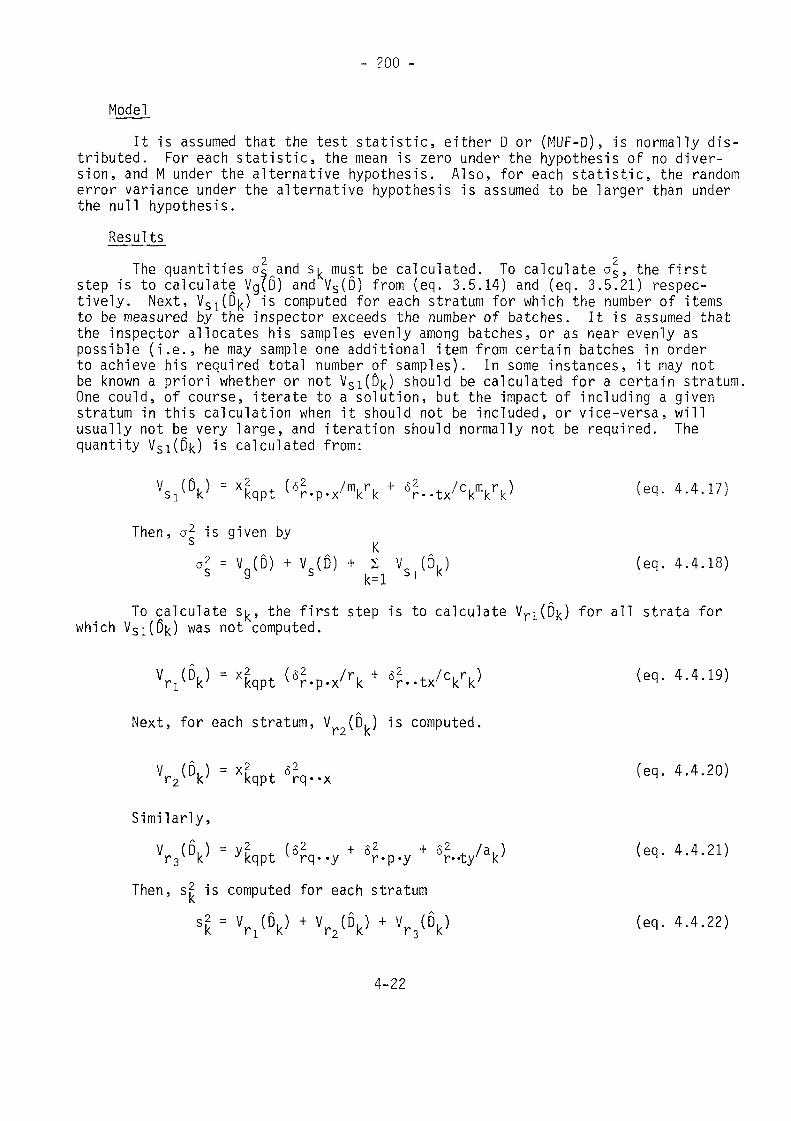
- 200 -

ModeJL

It is assumed that the test statistic, either D or (MUF-D), is normally dis-tributed. For each statistic, the mean is zero under the hypothesis of no diver-sion, and M under the alternative hypothesis. Also, for each statistic, the randomerror variance under the alternative hypothesis is assumed to be larger than underthe null hypothesis.

Results2 2The quantities a^ and s^ must be calculated. To calculate as, the firststep is to calculate Vg(D) and VS(D) from (eq. 3.5.14) and (eq. 3.5.21) respec-

tively. Next, VS^D^) is computed for each stratum for which the number of itemsto be measured by the inspector exceeds the number of batches. It is assumed thatthe inspector allocates his samples evenly among batches, or as near evenly aspossible (i.e., he may sample one additional item from certain batches in orderto achieve his required total number of samples). In some instances, it may notbe known a priori whether or not Vsi(o|J should be calculated for a certain stratum.One could, of course, iterate to a solution, but the impact of including a givenstratum in this calculation when it should not be included, or vice-versa, willusually not be very large, and iteration should normally not be required. Thequantity Vsi(D|<) is calculated from:

= kqpt (eq. 4.4.17)

Then, a2 is given bya2 = V (D) + V (D) + 2 V (D. )s g s k=1 Sl k

To calculate s^, the first step is to calculatewhich Vsl(ß|<) was not computed.

(eq. 4.4.18)

for all strata for

= X kqpt (eq. 4.4.19)

Next, for each stratum, V (D, ) is computedr 2. K

V (D, ) = x2 . <52r2 k ' kqpt r q * - x (eq. 4.4.20)

Similarly,

V (D, ) = 2r ^ k ' (<52 + o2 + o2 /a, )v rq*-y r -p -y V-ty' k'

Then, s? is computed for each stratum=

(eq. 4 .4.21)

(eq. 4 .4 .22)

4-22

- 201 -

The quantities V(MUF) and V0 are computed using Methods 3.3, 3.4, and 3.5,keeping in mind the systematic errors that are common to both the facility and theinspector when computing V0. Then calculate k2

kz = V(MUF) -JVo. (eq. 4.4.23)as

With M known, computem = M/as (eq. 4.4.24)

2The quantities a and ß (and hence, ta and tß) are chosen, as is Co, thevariance inflation factor. Finally, a decision is made as to the choice of thetest statistic to be used in planning, i.e., either 0 or (MUF-D). Define

a = 1 if STAT is D(eq. 4.4.25)

= 1-k if STAT is (MUF-D)The quantity e, which is inversely proportional to the sample size, is then

calculated.6 = (A-B)/C (eq. 4.4.26)

whereA = [(C§+l)atJt| + m2t2 + C5m2t|

- Cjat] (eq. 4.4.27)

B = 2mt t a(Co-l)(C-tJ)+Com2 (eq. 4.4.28)ut p p et

C = U t2,)2 (eq. 4.4.29)

Two special cases are considered. First, if Cg = 1, thene = m2/(t +tj2 - a (eq. 4.4.30)a p

If C = 0, i .e . , if C2 = (t / tj2 , then0 a Pa2(t2 - t2)2 - 2am2(t2 + t2) + mk0 - —— —— A.—— _-.._« —— Ê ———— (eq. 4.4.31)

4m2t2aHaving computed e, the total sample size, nv , is found by

Kn^ = ( 2 sk)2/ea2 (eq. 4.4.32)

K -L

4-23

- 202 -In stratum k, the sample size is

Knv2k = nv2 V sk {eq. 4.4.33)

Note 1: The quantity e as computed by (eq. 4.4.26), (eq. 4.4.30), or(eq. 4.4.31T may be negative. This means that the input value for ß is unattain-able because of the limitations due to the systematic error. A larger value ofß must then be selected and e recomputed.

Note 2: The number of items inspected in stratum k, nv2|<, is interpretedto be the total number of weighings or, equivalently, the total number of samplesdrawn to estimate element concentration factors. That is,

V2k = Vk = Vk (eq. 4.4.34)

It is quite unlikely that V|< and w.. will be integers, unless 1%, the numberof batches, is either equal to one or to the total number of items in the stratum.Thus, for some strata, it is more correct to write

mk.= kiki wkiki (eq. 4.4.35)

where v|q is the number of samples drawn by the inspector in batch i of stratum k,and Wkj is similarly defined for bulk measurements. For any two such batches, i andj, the quantities Vki and v^j would not normally differ by more than one, nor wouldw[<i and

Note 3: The results given by this method are quite general in nature. Ifcertain parameter values are fixed, then simpler graphical solutions for 6 areobtained. Specifically, commonly used values are

= 0.05 c?- a = 1 (i.e., use D statistic)For these values of the parameters, the figures in Annexes 4.1 (a) and

4.1 (b) show the relationship between e (or more exactly, Ve), and ß (or, moreexactly, 1-3). Having selected a value for 8 corresponding to the desired, orfeasibly attainable value for ß, the corresponding sample sizes are again givenby (eq. 4.4.32) and (eq. 4.4.33).

2 2A comment is in order on the value assigned Co. Commonly, the value Co = 4has been used in planning. This means that the random error variance of D underthe alternative hypothesis of diversion is four times that under the null hypothesisof no diversion. The variance is inflated when not all items are falsified, orwhen the items that are falsified (which may be all the items) are falsified byvarying amounts. For the first case, an expression for the variance of ß under His given by equation (3.38) in [4.1], and a similar expression, modified to reflectthe different amounts by which items are falsified, would describe the seconddiversion strategy. Examination of the cited equation (3.38) would indicate thatC0 = 4 is a reasonable upper bound; this corresponds to falsifying items by an

4-24

- 203 -amount equal to about 3.5 times the random error standard deviation for each itemelement weight. Since the value of 4 represents an upper bound, it is conserva-tive for planning purposes in that the sample sizes determined for this value ofC2, will tend to err on the high side. (Also see Section 6.3 of this Manual.)

BasisThe sample size is selected using amount of element^as the variable rather

than amount of isotope. First, let the test statistic be D rather than (MUF-D).The variance of D under the hypothesis of no diversion is

whereV(D)|H0 = a2 + Vr(D)|H0 (eq. 4.4.36)

Vr(D)|H0 = 6a2 (eq. 4.4.37)

defines the quantity 6Under the alternative hypothesis, HI} the variance of D is

V(D)|H]. = a2 + C20a2 (eq. 4.4.38)

The quantity Vr(D) [HQ is a function of the total sample size and also of theallocation of this total sample size among the K strata. From (eq. 3.5.6), andrecognizing that Vr(D) [HO is the same as Vr(D),

KVr(D)|H0 = 2 Vr(D.) (eq. 4.4.39)r k=1 r k

where Vr(D.) may be written in the form:

VA> = xkqpt (Ôrq..x/nv2k + 6r.p.x/DIV

+ ykqptwhere

DIV = min (nv2R, m^) (eq. 4.4.41)

and where a^ is a known input value (i.e., the number of analyses per sample per-formed by the inspector is known)From (eq. 4.4.19) - (eq. 4.4.23), it is seen that Vr(D)[H0 may be writtenin the form

KVr(D)|H0 = 2 S2/n (eq. 4.4.42)r k=1 K V2k

4-25

- 204 -

keeping in mind that Vri(D)<) is included in the definition ofstrata where DIV of (eq. 4.4.41) is nV2|<.only for those

In allocating the samples among the strata, this allocation should be per-formed so as to minimize Vr(D)|H0. This is seen from (eq. 4.4.48) to follow inwhich the aim is to maximize tg. In this equation, e is directly proportionalto Vr(D)|Ho. When all items are falsified by the same amount, the variance infla-tion factor, Cjj, is one, and tg is clearly maximized as e is minimized. At valuesof C^ greater than one, tß is maximized as e is minimized as long as ß<0.50, whichis the region of interest. For values of ß>0.50, it would benefit the inspectorto have a large variance of 0, but this region of ß is of little practicalimportance.

Minimization of Vr(D)|H0 is a standard minimization problem, and it iseasily shown that the nV2|< should be chosen by the equation:

'V2k = nV2 v k=l(This result is derived in [4.8]

for optimization may be included.)

(eq. 4.4.43)

where it is also shown how other criteria

From (eq. 4.4.42) and (eq. 4.4.43), along with (eq. 4.4.37), the key rela-tionship between nya Qnd e, given by (eq. 4.4.32), follows easily. If some otheroptimization criterion were imposed, then the relationship between e and nv2 wouldhave to be altered accordingly, but the equations to follow, which lead to thesolution for e, would remain unchanged.

The value for e is selected such that the goal amount, M, is detected withprobability (1-ß) under the alternative. Further, the significance level of thetest is set at a. Before writing down the equations that lead to the^solution for9, it should be noted that as D is defined, large negative values of D are evidencesof diversion, and not large positive values. It is convenient to replace D by itsnegative counterpart, D," such that large positive values of 0" lead to rejectionof the null hypothesis of no diversion. Thus, define

0- = -0 (eq. 4.4.44)It is^obvious that the variance of D will, of course, be the same as the

variance of D. The two equations to solve for e and the critical value, D0, are

andProb {Û'>DO E(D') = 0) = o

Prob (D->D0|E(ir) = M) = 1-ßFrom (eq. 4.4.45), (eq. 4.4.36), and (eq. 4.4.37),

(eq. 4.4.45)

(eq. 4.4.46)

(eq. 4.4.47)

4-26

- 205 -

where ta is defined in the Notation section. From (eq. 4.4.46), (eq. 4.4.38),and (eq. 4.4.47),

t a VÏ+0 -M= -t (eq. 4.4.48)

or, replacing M/as by m, solve the following equation for e.

(eq. 4.4.49)

Before indicating the solution to this equation, note the effect of replacingthe test statistic 0 by (MUF-Ô) while keeping all other parameters f^xed. Inthis event, from (eq. 3.6.5), the variance of the test statistic, (MUF-D), underthe null hypothesis is

V(MUF-D)|H0 = a2(l+e-k2)

while its variance under the alternative hypothesis is

(eq. 4.4.50)

V(MUF-D)|H! = (eq. 4.4.51)

with k2 defined by (eq. 4.4.53). It follows immediately that for (MUF-D) as thetest statistic, (eq. 4.4.49) becomes

(eq. 4.4.52)

where a = l-k (eq. 4.4.53)

Thus, in general terms, (eq. 4.4.52) may be solved for e- where a = 1 ifthe sample size is based on detecting M units with the D statistic, and a = l-k2if the (MUF-ß) statistic is used. It is shown in [4.9] that the solution to(eq. 4.4.52) is given by the key results: (eq. 4.4.26), (eq. 4.4.30), and(eq. 4.4.31).Exampl es

EXAMPLE 4.3 (a)Consider the low enriched uranium facility of Examples 3.3 (a) and 3.5 (a).

Follow Method 4.3 to determine the variables inspection sample size when inspectionis in the variables mode. Set M = 1500 kg U, and assume that duplicate analysesare performed in all strata but stratum 3. The inspection samples are distributedto a single laboratory as indicated in Example 3.9 (a). From that example, andfrom Example 3.10 (a) ,

4-27

- 206 -

V (D) = 32,584 kg2U

Vs(D) = 51,484 kg2U

The quantities Vsi(Dk) are then computed using (eq. 4.4.17) for those stratafor which the numbers of items to be measured by the inspector exceed the numbersof batches. These strata include strata 2, 4, 5, 6, and 7.

Vsl(D2) = (238,800)2[(0.000568)2/240] = 77Vsl(DiJ = VS1(D6)

= (7200)2[(0.0181)2/60 + (0.0274)2/60] = 932VS1(D5) = VSi(07)

- = (4000)2[(0.0418)2/48 + (0.0274)2/48] = 833From (eq. 4.4.18),

a2 = 32,584+51,484+77+2(932)+2(833) = 87,675 kg2UNext, Vpl(D1) and Vr (D3) are calculated from (eq. 4.4.19).

vrl(Di) = (240,000)2[(0.000531)2/5 + (0.000433)2/5] = 5408Vrl(D3) = (1200)2(0.0577)2 = 4794

For each stratum, Vr2(D|<) and Vr3(D|<) are found using (eq. 4.4.20) and(eq. 4.4.21), and assuming that x|<qpt = Ykqpt for a11 k-Vr2(Di) = (240,000)2(0.000658)2 = 24,939Vr2(D2) = (238.800)2(0.000877)2 = 43,860

Vr2(D3) = 0Vr2(D4) = Vr2(D6) = (7200)2(0.00250)2 = 324Vr2(D5) = Vr2(D7) = (4000)2(0.00250)2 = 100Vr,(Di) = (240,000)2[(0.000658)2+(.000531)2+(0.000433)2/2] = 46,579> 3

V (D2) = (238,800)2[(0.000658)2+(0.000822)2/2] = 43,956i 3

Vrs(D3) = (1200)2(0.0923)2 - 12,268Vr3(D4) = Vr3(D6) = (7200)2[(0.000658)2+(0.0181)2

+ (0.0198)2/2] = 27,167Vr3(D5) = Vr (67) = (4000)2[(0.000658)2+ (0.0418)2

+ (0.0198)2/2] = 31,099

4-28

- 207 -

The quantity s. is now computed for each stratum using (eq. 4.4.22).s2 = 5,408 + 24,939 + 46,579 = 76,926 ; sx = 277s2 = 43,860 + 43,956 = 87,816 ; s2 = 296s2 = 4,794 + 12,268 = 17,062 ; s3 = 1313

s2 = s2 = 324 + 27,167 = 27,491 ; St. = S6 = 1664 6s§ = s2 = 100 + 31,099 = 31,199 ; S5 = S7 = 177

72 s, = 1390

k=l K

Suppose that the following criteria are set:a = 0.05 (significance level)c2 = 4 (variance inflation factor)a = 1 (D statistic used in planning)

Then, following Note 3, the graphical solution for e is found. Here,M/as = 1500/296 = 5.07

Set 3 = 0.05, or 1-ß = 0.95. From Annex 4.1 (b),Ve ~ 1.75

The total sample size is then given by (eq. 4.4.32).n, = (1390)2(1.75)/(87,675)V2

= 39In each stratum, the sample size is given by (eq. 4.4.33).

nv2i = (39)(277)/1390 = 8nv22 = (39)(296)/1390 = 8nv23 = 4

Total = 40

4-29

- 208 -

To^illustrate application of the more general methodology suppose now thatthe (MUF-D) statistic is to be used in planning, and that ß = 0.025 with all otherparameters the same. It is necessary to calculate k2 from (eq. 4.4.23) to obtainthe value for a from (eq. 4.4.25). From Example 3.5 (a),

V(MUF) = 45,010 kg2UFrom Example 3.10 (a), V0 = 0 since, although both the facility and theinspector commit the same systematic errors in sampling, the contribution to the

variance of MUF due to these sources of error was zero in this example. Thus,k2 = 45,010/87,675 = 0.5134a = l-k2 = 0.4866

The quantity e is now calculated from (eq. 4.4.26), but first, A, B, and Care found using (eq. 4.4.27), (eq. 4.4.28), and (eq. 4.4.29).

A = [(5)(0.4866)(1.645)2(1.960)2+(5.07)2(1.645}2+(4)(5.07)2(1.960)2-(0.4866}(1.645)'f-(4)(0.4866)(1.960)'t] = 457.5541

B = (2)(5.07)(1.645)(1.960) V(0.4866)(3)[(4)(1.960)2-(1.645)2]+(4)(5.07)2 = 360.0746C = [(1.645)2 - (4K1.960)2]2 = 160.2851

. _ 457.5541 - 360.0746 _ n ,nR?9 ' ———Ï6O851———— ~ °'6082

The total sample size in this instance isnv2 = (1390)2/(0.6082)(87,675) = 37

2Finally, suppose that the variance inflation factor, Co, were set equal to 1rather than 4. Then, 9 is given directly by (eq. 4.4.30).

8 = (5.07)2/(1.645+1.960)2 - 0.4866= 1.4913

and the sample size is 15 rather than 37.

EXAMPLE 4.3 (b)Consider the mixed oxide fuel fabrication facility first introduced in

Example 3.3 (b) and considered in a number of examples following that one. SetM = 8 kg Pu, and assume that duplicate analyses are performed in all strata butstratum 4. Further assume that the inspection samples are distributed to only onelaboratory, and that the short term systematic error structure is as indicated inExample 3.9 (b). Find the inspection sample size for two cases:

4-30

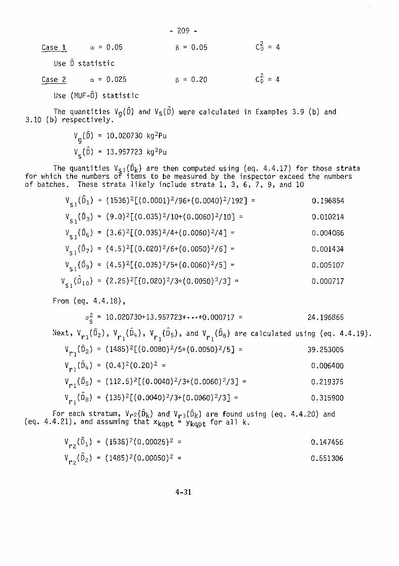
- 209 -Case 1^ a = 0.05 ß = 0.05 Co = 4

Use D statisticCase 2 a = 0.025 3 = 0.20 Co = 4

Use (MUF-D) statisticThe quantities Vg(D) and VS(D) were calculated in Examples 3.9 (b) and3.10 (b) respectively.

V (D) = 10.020730 kg2Pu3

V (D) = 13.957723 kg2Puo

The quantities Vsi(D|<) are then computed using (eq. 4.4.17) for those stratafor which the numbers of items to be measured by the inspector exceed the numbersof batches. These strata likely include strata 1, 3, 6, 7, 9, and 10

VSI(D!) = (1536)2[(0.0001)2/96+(0. 0040)2/192] = 0.196854V (03) = (9.0)2[(0.035)2/10+(0.0060)2/10] = 0.010214Vsl(ß6) = (3.6)2[(0.035)2/4+(0.0060)2/4] = 0.004086Vsl(D7) = (4.5)2[(0.020)2/6+(0.0050)2/6] = 0.001434VC1(D9) = (4.5)2[(0.035)2/5+(0.0060)2/5] = 0.005107o J-

VS1(D10) = (2.25)2[(0.020)2/3+(0.0050)2/3] = 0.000717

From (eq. 4.4.18),a2 = 10. 020730+13. 957723+. -.+0.000717 = 24.196865

Next, Vri(D2), Vri(Dit), Vri(D5), and Vp (D8) are calculated using (eq. 4.4.19)Vri(D2) = (1485)2[(0.0080)2/5+(0. 0050)2/5] - 39.253005Vri(Du) = (0.4)2(0.20)2 = 0.006400Vrl(D5) = (112. 5)2[(0.0040)2/3+(0. 0060)2/3] = 0.219375Vri(D8) = (135)2[(0.0040)2/3+(0. 0060)2/3] = 0.315900

For each stratum, Vr2(D|<) and Vr3(Dk) are found using (eq. 4.4.20) and(eq. 4.4.21), and assuming that x^qpt = ykqpt for a11 k-

Vr2(0!) = (1536)2(0.00025)2 = 0.147456Vr2(D2) = (1485)2(0.00050)2 = 0.551306

4-31

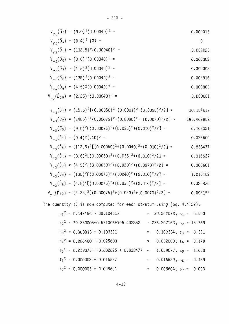
- 210 -

Vr2(D5)Vr2(D6)Vr2(D7)Vr2(D8)

Vr2(Dio)

= (9.0)2(0.00040)2 == (0.4)2 (0) == (112.5)2(0.00040)2

= (3.6)2(0.00040)2 == (4.5)2(0.00040)2 == (135)2(0.00040)2 == (4.5)2(0.00040)2 == (2.25)2(0.00040)2 =

Vr3(Di) = (1536)2[(0.00050)2+(0.0001)2+(0.0050)2/2] == (1485)2[(0.00075)2+(0.0080)2+ (0.0070)2/2] =- (9.0)2[(0.00075)2+(0.035)2+(0.010)2/2] == (0.4)2(.40)2 =

i ^

V„,(D5) = (112.5)2[(0.00050)2+(0.0040)2+(0.010)2/2] =i «j

^„(De ) = (3.6)2[(0.00050)2+(0.035)2+(0.010)2/2] =i 3

V _(D7) = (4.5)2[(0.00050)2+(0.020)2+(0.0070)2/2] =I J

Vr3(D8) = (135)2[(0.00075)2+(.0040)2+(0.010)2/2] =V JD9) = (4.5)2[(0.00075)2+(0.035)2+(0.010)2/2] =Y1 JVr3(Dio) = (2.25)2[(0.00075)2+(0.020)2+(0.0070)2/2] =

2The quantity s^ is now computed for each stratum using (eq,si2 = 0.147456 + 30.104617s22 = 39.253005+0.551306+196.402852s32 = 0.000013 + 0.103321s 2 = 0.006400 + 0.025600S52 - 0.219375 + 0.002025 + 0.838477s52 = 0.000002 + 0.016527S72 = 0.000003 + 0.008601

= 30.252073;= 236.207163;= 0.103334;= 0.032000;= 1.059877;= 0.016529;= 0.008604;

0.0000130

0.0020250.0000020.0000030.0029160.0000030.000001

30.104617196.4028520.1033210.0256000.8384770.0165270.0086011.2131020.0258300.002152

4.4.22).si - 5.50052 = 15.36953 = 0.321s4 = 0.179S5 = 1.030s6 = 0.129S7 = 0.093

4-32

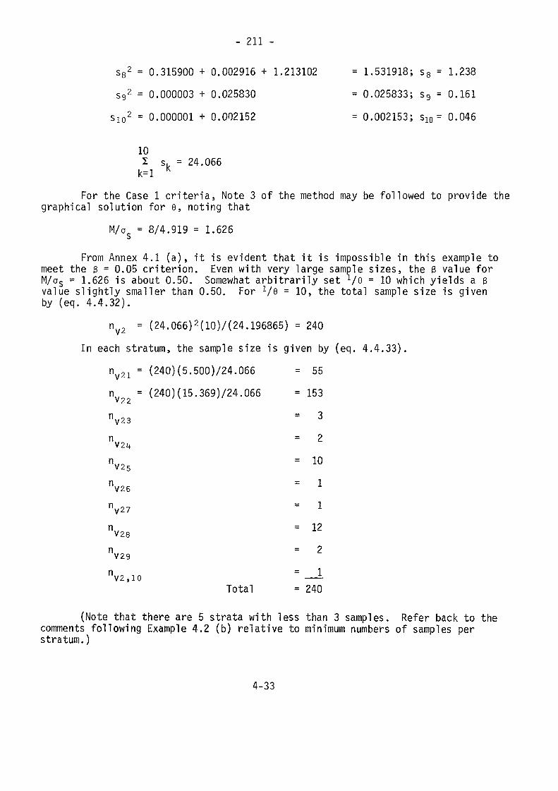
- 211 -

s82 = 0.315900 + 0.002916 + 1.213102 = 1.531918; S8 = 1.238s92 = 0.000003 + 0.025830 = 0.025833; S9 = 0.161

s102 = 0.000001 + 0.002152 = 0.002153; S10 = 0.046

10X s. = 24.066k=l K

For the Case 1 criteria, Note 3 of the method may be followed to provide thegraphical solution for e, noting that

M/as = 8/4.919 = 1.626

From Annex 4.1 (a), it is evident that it is impossible in this example tomeet the ß = 0.05 criterion. Even with very large sample sizes, the 3 value forM/as = 1.626 is about 0.50. Somewhat arbitrarily set Ve = 10 which yields a 3value slightly smaller than 0.50. For 1/Q = 10, the total sample size is givenby (eq. 4.4.32).

nv2 = (24. 066)2(10)/(24. 196865) = 240In each stratum, the sample size is given by (eq. 4.4.33).

= 55= (240)(15. 369)724.066 = 153

= 3

= 2

= 10

nv26 = 1

nV27 = !

= 12

= 2

Total = 240

(Note that there are 5 strata with less than 3 samples. Refer back to thecomments following Example 4.2 (b) relative to minimum numbers of samples perstratum.)

4-33

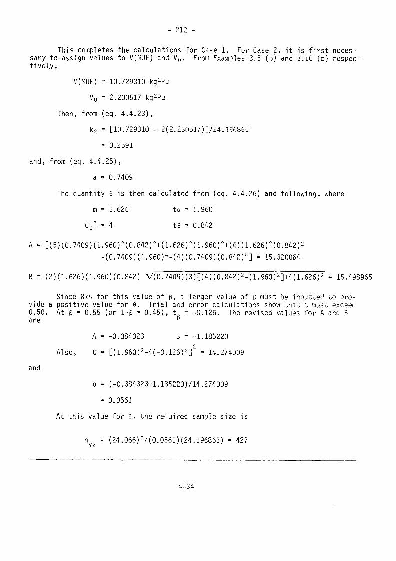
- 212 -

This completes the calculations for Case 1. For Case 2, it is first neces-sary to assign values to V(MUF) and V0. From Examples 3.5 (b) and 3.10 (b) respec-tively,

V(MUF) = 10.729310 kg2PuV0 = 2.230517 kg2Pu

Then, from (eq. 4.4.23),k2 = [10.729310 - 2(2.230517)1/24.196865

= 0.2591and, from (eq. 4.4.25),

a = 0.7409The quantity 6 is then calculated from (eq. 4.4.26) and following, where

m = 1.626 ta = 1.960C02 =4 tß = 0.842

A = [(5)(0.7409)(1.960)2(0.842)2+(1.626)2(1.960)2+(4)(1.626)2(0.842)2-(0.7409)(1.960)1+-(4)(0.7409)(0.842)4] = 15.320064

B = (2)(1.626)(1.960)(0.842) V(0.7409)(3)[(4)(0.842)2-(1.960)2]+4(1.626)2 = 15.498965

Since B<A for this value of ß, a larger value of 3 must be inputted to pro-vide a positive value for e. Trial and error calculations show that ß must exceed0.50. At 3 = 0.55 (or 1-3 = 0.45), t = -0.126. The revised values for A and Bare ß

A - -0.384323 B = -1.185220Also, C = [(1.960)2-4(-0.126)2]2 = 14.274009

and6 = (-0.384323+1.185220)714.274009

= 0.0561At this value for e, the required sample size is

ny2 = (24.066)2/(0.0561)(24.196865) = 427

4-34

- 213 -

4.5 EVALUATION OF INSPECTION PLAN —INDIVIDUAL TESTSIn this section and in Section 4.6 to follow, methods are given for evaluat-

ing the inspection plan along with the accountability measures taken by the facility.Evaluation is measured by the probability that the statistical test in questionwill return a significant result as a function of the amount of material unaccountedfor by the mechanism to which the test is designed to be responsive.

In applying the statistical tests in question, a distinction is made be-tween principal and supplemental tests, as discussed in the next section.

4.5.1 Distinction Between Principal and Supplemental TestsAs will be discussed in Section 4.6, of chief concern or interest to the

inspection planner is the overall probability of detection of a specified goalamount. Detection occurs if at least one of the statistical tests in questionreturns a positive response. The statistical tests that are applied collectivelyin calculating this overall probability of detection are called principal tests.One important characteristic of the principal tests is that, taken as a group,there is control over the value for a, the significance level (false alarm proba-tility) associated with the collection of statistical tests to be applied.

There are two combinations of tests that are identified as principal tests.These are as follows.

Combination 1:1) The tests for gross defects performed with the attributes tester. There

are K such tests.2) The tests for medium defects performed with the variables tester used

in the attributes made. There are K such tests.3} The test for the significance of (MUF-D), the facility MUF adjusted for

the bias (small defects) that is estimated by the D statistic.

Combination 2:1) Same as above.2) Same as above.3) The test for the significance of D, the measure of facility bias as it

affects the MUF.4) The test for the significance of the facility MUF.

These principal tests are discussed separately in Sections 4.5.2, 4.5.4,4.5.5, and 4.5.6. The tests that comprise Combination 1 are then considered col-lectively in Section 4.6.1 while those that comprise Combination 2 are treated inSection 4.6.2.

4-35

- 214 -

In addition to these principal tests, the data analyst (inspector) wouldwant to perform other statistical tests when analyzing the data for a givenfacility over a given material balance period (see Section 4.1.1). These othertests are referred to as supplemental tests to distinguish them from the principaltests. Examples of supplemental tests that may be applied include:

1) Tests for the significance of D^, the measure of facility bias instratum k.2) Tests for the significance of shipper-receiver differences.3) Miscellaneous tests on distributional properties, such as outlier tests

and tests for normality.4) Tests for randomness of small calculational mistakes.5) Tests for randomness of data over time and other data groupings, includ-

ing CUSUM plots and analyses of variance.This listing is not intended to be all inclusive, but rather to portray the

kinds of supplemental tests that the data analyst may apply. The statistical testsare described in Chapter 5. In this chapter, Chapter 4, the emphasis is not onthe test itself, but rather on its ability to detect a specified missing amountof material. Not all of the supplemental tests identified above may be evaluatedin this fashion because for some tests, it is difficult to specify an alternativehypothesis that relates directly and in^a meaningful way to a missing amount ofmaterial. Tests 1 and 2, the tests on D^ and on the shipper-receiver differencecan be so evaluated, and are discussed in Section 4.5.3.

As the above listing suggests, and as will become more evident in Chapter 5,a large number of statistical tests might be performed in the course of evaluatinginspection and material balance data for a given facility. With so many tests, itwould be expected that a few would give positive signals due to chance alone, andone should not become unduly concerned when this occurs. The important emphasisshould be placed on the principal tests, using either Combination of tests 1 or 2identified above. For these principal tests, the false alarm rate, a, can be con-trolled as mentioned earlier. The functions of the supplemental tests are essen-tially twofold: to provide some degree of assurance that the assumptions under-lying the application of the primary tests are valid; and to isolate causes ofsignificant results returned by the primary tests.4.5.2 Attributes Inspection Tests

Two attributes inspection tests are performed in each stratum, one using theattributes tester to check for gross defects, and one using the variables testerin the attributes mode to check for medium defects. For the K strata, there area total of 2K attributes tests. There is no problem in performing each test sincethe existence of one or more defects in any stratum corresponds to detection, i.e.,to rejection of the null hypothesis that no defects (gross on medium in size asthe case may be) exist. Further, there is no concern with controlling the falsealarm rate either since a is zero for each attributes test (clearly, if there areno defects in the population there is zero probability that any will be found inthe sample.)

4-36

- 215 -

Consider the power of the attributes test taken as a whole, i.e., considerthe probability that one or more of the tests will lead to rejection of the hypo-thesis through observing one or more defects. This is called the probability ofdetection. In calculating the probability of detection, it is simpler to find itscomplement, the probability of nondetection. Nondetection implies that no defectsare found in any of the strata. To calculate the nondetection probability, define

h. = amount of element falsified as gross defects in stratum kg, = amount of element falsified as medium defects in stratum k

Summed over all strata, the total amount falsified (i.e., diverted andobscured through data falsification) is

K*k=l (h + gk) =K a2M (eq. 4.5.1)

where 0 * a2The sample sizes for attributes inspection using the attributes tester and

the variables tester in the attributes mode, na|< and n^^ respectively, are givenby (eq. 4.4.1) and (eq. 4.4.16). Let pa|< be the probability of not finding a defectin stratum k with the attributes tester, and let pvk be similarly defined for thevariables tester. Then, letting ß^ = ß for all strata and for both testers, from(eq. 4.4.5),

Pakak

Pvk(eq. 4.5.2)

Since the tests are independent, over all strata, the probability of non-detection, denoted by Q2 ispakpvk

(eq. 4.5.3),32

where the last step is a consequence of (eq. 4.5.1).This result indicates that no matter how the aaM units of element are dis-tributed among the strata and between gross and medium defects, the overall proba-

bility of nondetection is ß32, where the sample size in each stratum and for eachtester is based on the same value for ß.It is important to note that if ß is not the same for all strata-tester

combinations, then the largest value for ß must be used in (eq. 4.5.3). This isso because the optimum strategy of the diverter is to falsify the data in thestrata with the largest ß values. To illustrate the importance of this point,suppose that a2 = 0.6 (60% of the goal amount M is diverted and obscured through

4-37

- 216 -

gross and/or medium defects) and that ß = 0.05 for all strata-tester combinations.Then, by (eq. 4.5.3), the non-detection probability is

0.2 = (0.05)0'6 = 0.1657 , (detection probability = 0.8343).Suppose, however, that constraints on the inspection require that 3 = 0.50,

say, for the attributes tester in a given stratum. Then, assuming that the stratumin question is sufficiently large to permit diversion of the entire amount, a2M,from this stratum, the nondetection probability is

Q? = (0.50)0'6 = 0.6598, (detection probability = 0.3402).This small detection probability occurs in spite of the fact that 3 = 0.05

for all other strata-tester combinations. The example illustrates the need to coverall strata with comparable intensity of inspection (i.e., to achieve the same valuefor ß).

4.5.3 Tests on D|< and Shipper/Receiver Difference TestsFrom a mathematical viewpoint, there is no distinction between a test on D^

(defined by (eq. 3.5.1)), and a shipper/receiver difference test. In both cases,measurements for one party are compared^with measurements for the second party.Thus, it is permissible to discuss the Dj< test and have this discussion apply tothe shipper/receiver test as well.

Before giving the method for finding the probability that the D^ test willdetect a given amount of material diverted from stratum k through small data falsi-fications, two points must be made. First, in Section 4.4.2.2, the concept of thevariance inflation factor, C02, was introduced. That is, the random error varianceof ß under the alternative hypothesis was assumed to be C02 times the correspondingvariance under the null hypothesis. A similar inflation factor would apply to D|<,the 0 statistic for an individual stratum. For planning purposes, it is reasonableto assign a conservatively large value to C02 in order to assure that the correspond-ing sample size is conservative on the high side. From an evaluation viewpoint,however, it is more reasonable that the inflation factor be a function of the amountdiverted. An assumed empirical relationship between the variance inflation factorand the amount diverted under the alternative model is used in the method to follow.

As a second point, the facility value minus the inspector value is the basisfor the Dk statistic. If the stratum in question is either an input or a beginninginventory stratum, then it is to the diverter's advantage to introduce falsificationsthat will result in a negative^ value for Ek, i.e., the mean of D^ under the alterna-tive would be a negative vaTue". On the other hand, if the stratum in question iseither an output or an ending inventory stratum, then a positive value of D^ wouldbenefit the diverter. To avoid repetition, and to provide consistency with thedevelopment in Section 4.5.4 to follow^ assume that the stratum in question isan output stratum so that the mean of D^ under the alternative is positive. (Itwould be a simple matter to apply Method 4.4 to an input or a beginning inventorystratum; simply change the sign of D|<, or, equivalently, redefine 0|< to be basedon inspector minus facility values for such a stratum).

Method 4.4 is now given. This provides the equations needed to calculate theprobability of nondetection and its complement, the probability of detection, for aspecified alternative.

4-38

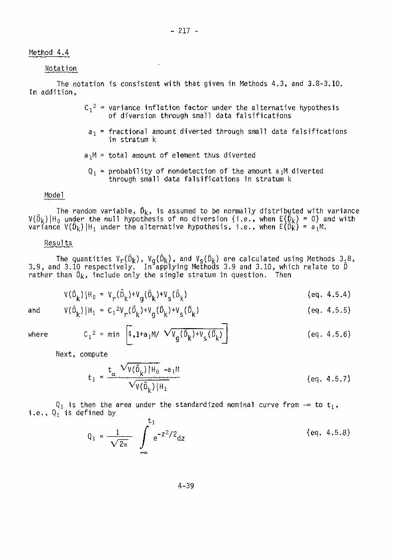
- 217 -

Method 4.4Notation

The notation is consistent with that given in Methods 4.3, and 3.8-3.10.In addition,

Ci2 = variance inflation factor under the alternative hypothesisof diversion through small data falsifications

aj = fractional amount diverted through small data falsificationsin stratum k

axM = total amount of element thus divertedQ! = probability of nondetection of the amount aiM diverted

through small data falsifications in stratum kModel

The random variable, ß|<, is assumed to be normally distributed with varianceV(D|<)|Ho under the null hypothesis of no diversion (i.e., when £(0 ) = 0) and withvariance V(D|<)|H1 under the alternative hypothesis, i.e., when E(D|<) = a^.

ResultsThe quantities Vr(D|<), VgCDk), and Vs(0|<) are calculated using Methods 3.ß,3.9, and 3.10 respectively. In applying Methods 3.9 and 3.10, which relate to D

rather than 0|<, include only the single stratum in question. Then

V(6k)|H0 = Vr(Dk)+Vg(Dk)+Vs(Dk) (eq. 4.5.4)and V(Dk)|H1 = C12Vr(Dk)+Vg(D|<)+Vs(Dk} (eq. 4.5.5)

where CL2 = min

Next, compute

VVg(Dk)+Vs(Dk)J (eq. 4.5.6)

t VV(D )|H0 -aiMt l=-2 —— -V; ———— (eq. 4.5.7)

VV(Dk)|H1Qi is then the area under the standardized nominal curve from -» to tl5i.e., Q! is defined by

fJ

4.5.8)

4-39

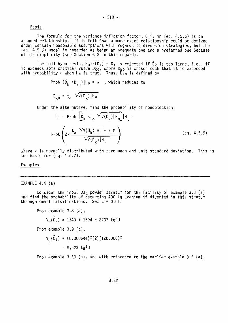
- 218 -Basis

The formula for the variance inflation factor, Ci2, in (eq. 4.5.6) is anassumed relationship. It is felt that a more exact relationship could be derivedunder certain reasonable assumptions with regards to diversion strategies, but the(eq. 4.5.6) model is regarded as being an adequate one and a preferred one becauseof its simplicity (see Section 6.3 in this regard).

AThe null hypothesis, H0:E(D[<) = 0, is rejected if D|< is too large, i.e., ifit exceeds some critical value D|<0, where Dko is chosen such that it is exceededwith probability a when H0 is true. Thus, D|<o is defined by

Prob (Dk >D. )(HO = a , which reduces to

Dko = ta V v ( D k ) | H 0

Under the al ternat ive, f i nd the probabi l i ty of nondetection:

Qi = Prob

P r o b f z < ° V V V | n o -°i': (eq. 4.5.9)

where z is normally distributed with zero mean and unit standard deviation. This isthe basis for (eq. 4.5.7).Examples

EXAMPLE 4.4 (a)Consider the input U02 powder stratum for the facility of example 3.8 (a)and find the probability of detecting 400 kg uranium if diverted in this stratum

through small falsifications. Set a = 0.01.From example 3.8 (a),

Vr(0!) = 1143 + 1594 = 2737 kg2UFrom example 3.9 (a),

Va(Di) = (0.000544)2(2)(120,000)2y= 8,523 kg2U

From example 3.10 (a), and with reference to the earlier example 3.5 (a),

4-40

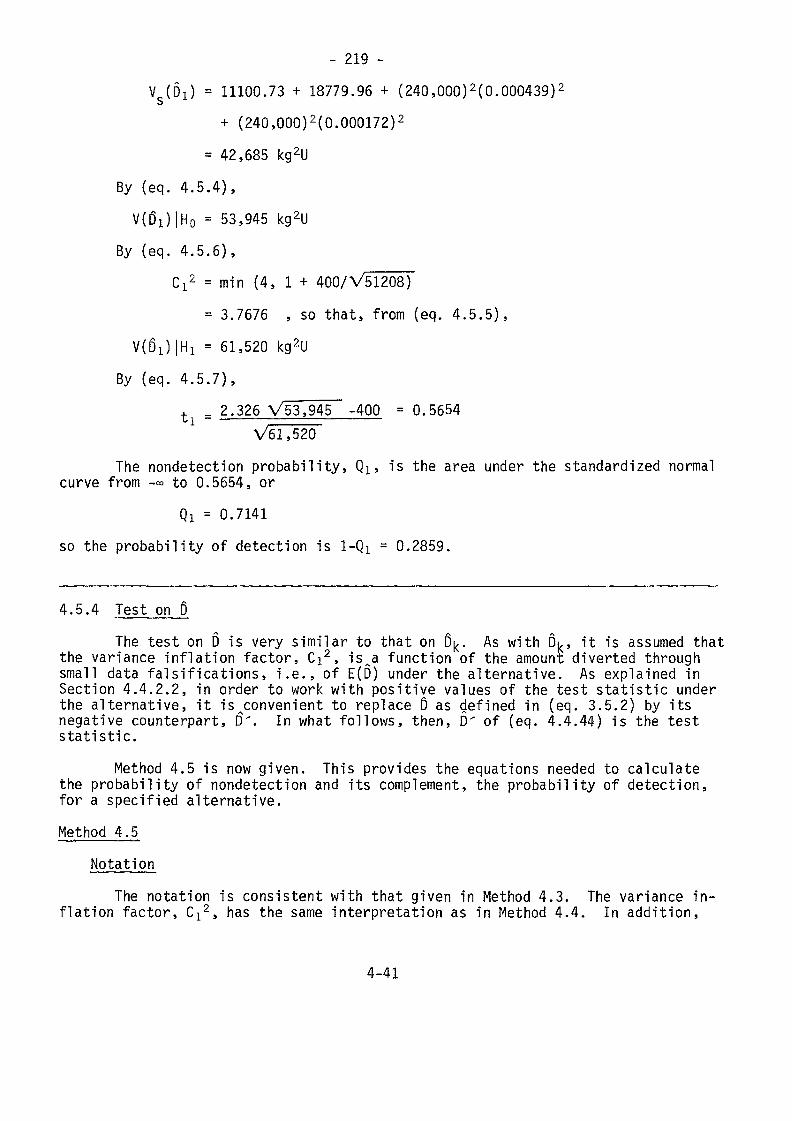
- 219 -V (DO = 11100.73 + 18779.96 + (240,000)2(0.000439)2

+ (240,000)2(0.000172)2

= 42,685 kg2UBy (eq. 4.5.4),V(ßi)|H„ = 53,945 kg2U

By (eq. 4.5.6),Ci2 = min (4, l + 400/V51208)

= 3.7676 , so that, from (eq. 4.5.5),V(D1)|H1 = 61,520 kg2U

By (eq. 4.5.7),t ^ 2.326 V53,945 -400 =0.5654

V61.520The nondetection probability, Qls is the area under the standardized normalcurve from -« to 0.5654, or

Qi = 0.7141so the probability of detection is 1-Qi = 0.2859.

4.5.4 Test on DThe test on D is very similar to that on D^. As with D^, it is assumed that

the variance inflation factor, Ci2, is^a function of the amount diverted throughsmall data falsifications, i.e., of E(D) under the alternative. As explained inSection 4.4.2.2, in order to work with positive values of the test statistic underthe alternative, it is^convenient to replace Û as Refined in (eq. 3.5.2) by itsnegative counterpart, D". In what follows, then, D' of (eq. 4.4.44) is the teststatistic.

Method 4.5 is now given. This provides the equations needed to calculatethe probability of nondetection and its complement, the probability of detection,for a specified alternative.Method 4.5

NotationThe notation is consistent with that given in Method 4.3. The variance in-

flation factor, Ci2, has the same interpretation as in Method 4.4. In addition,

4-41

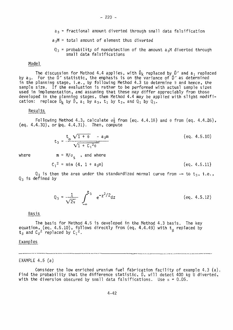
- 220 -

as - fractional amount diverted through small data falsificationa3M = total amount of element thus divertedQ3 = probability of nondetection of the amount a3M diverted throughsmall data falsifications

ModelThe discussion for Method 4.4 applies, with D^ replaced by^D' and a^ replaced

by a3. For the D' statistic, the emphasis is on the variance of D" as determinedin the planning stage, i.e., by following Method 4.3 to determine e and hence, thesample size. If the evaluation is rather to be performed with actual sample sizesused in implementation, and assuming that these may differ appreciably from thosedeveloped in the pjanning stages, then Method 4.4 may be applied with slight modifi-cation: replace D^ by D, ax by a3, ti by t3, and Qj. by Q3.

ResultsFollowing Method 4.3, calculate o| from (eq. 4.4.18) and e from (eq. 4.4.26),

(eq. 4.4.30), or (eq. 4.4.31). Then, compute

t Vl + 9 - a3m (eq. 4.5.10)t3 " Vl + Ci2/

where m = M/a , and whereC}2 = min (4, 1 + a3m) (eq. 4.5.11)

Q3 is then the area under the standardized normal curve from -°° to t3, i.e.,Q3 is defined by

(eq. 4.5.12)

BasisThe basis for Method 4.5 is developed in the Method 4.3 basis. The key

equation, (eq. 4.5.10), follows directly from (eq. 4.4.49) with t replaced byt3 and C02 replaced by C^. ß

Examples

EXAMPLE 4.5 (a)Consider the low enriched uranium fuel fabrication facility of example 4.3 (a)

Find the probability that the difference statistic, D, will detect 400 kg U diverted,with the diversion obscured by small data falsifications. Use a - 0.05.

4-42

- 221 -

From the cited example,

ag = V87,675 = 296 kg U

e = (1.75)"1 = 0.571

a3m = 400/296 = 1.351

Then, from (eq. 4.5.10), since C^ = 2.351 from (eq. 4.5.11),

_ 1.645 Vl.571 -1.351 = 0.464- ——— - .V27342

and Qs = 0.679 , nondetection probability1-Q3 =0.321 , probability of detection

EXAMPLE 4.5 (b)

Consider the mixed oxide fuel fabrication facility of example 4.3 (b). Usingthe Case 2 criteria in that example, find the probability that the 0 statistic willdetect 5 kg Pu diverted, with the diversion obscured by small data falsifications.From the cited example,

as = 4.919 kg Pu ; e = 0.0561 ; a3m = 5/4.919 = 1.016From (eq. 4.5.11), C:2 = 2.106, so, applying (eq. 4.5.10),

1.960 Vl.0561 - 1.016 = 0.946- -Vl.1131

Q3 = 0.828 , nondetection probability1-0.3 = 0.172 , probability of detection

EXAMPLE 4.5 (c)For the same mixed oxide fuel fabrication facility in the previous example,

suppose the inspection plan is as indicated in example 3.8 (b), and rework theexample 4.5 (b).

In applying Method 4.5 to solve this problem, the development of Method 4.4is followed, with ß|< replaced by D, al by a3, ti by t3, and Ql by Q3. Fromexample 3.8 (b),

4-43

- 222 -Vr(D) = 3.325266 kg2Pu

From example 3.9 (b),V (D) = 10.020730 kg2Pu

From example 3.10 (b),V (Ö) = 13.957723 kg2Pu

By (eq. 4.5.4), appropriately modified,V{D')|H0 = 27.303719 kg2Pu

By (eq. 4.5.6), appropriately modified,C2 = min(4, 1 + 5/ V23.978453)

= 2.021so that, from the modified (eq. 4.5,5),

V(D')|H! = 30.698816Then,

t = 1.960 V27.303719 - 5 = 0.946V30.698816

Q3 = 0.8281-0,3 = 0.172

Note that the answers are precisely the same (to three decimals) as in theprevious example. In the previous example, the total sample size was 427; inexample 3.8 (b), the number of samples was 287 and the number of weighings was653. The fact that the detection probabilities agree to within 3 decimals is abit fortuitous, but close agreement would be expected because of the dominanceof systematic errors in this example.

4.5.5 Test on MUFAlthough the inspector has no direct control over the size of the variance

of MUF, this quantity has an impact^on the ability to detect diversion, especiallyas it affects the variance of (MUF-D) as considered in the next section. Thetest on MUF is considered in Method 4.6.

4-44

- 223 -

Method 4.6Notation

The notation is given in section 3.4.3.2. In addition,ait = fractional amount of element diverted into MUF

a4M = total amount of element thus divertedQit = probability of nondetection of the amount a^M diverted into MUF

ModelThe quantity MUF is assumed to be a random variable which is normally dis-

tributed with variance V(MUF). Under the null hypothesis, the mean of MUF is zero,while it is a^M under the alternative.

ResultsCompute t4 = t - a^M/ Vv(MUF) (eq. 4.5.13)Qit is the area under the standardized normal curve from -°° to t4, i.e.,is defined by

V27Basis

/

2e"z /2dz (eq. 4.5.14)

The null hypothesis that E(MUF) = 0 is rejected if MUF exceeds some criticalvalue MO, where M0 is chosen such that it is exceeded with probability a when H0 istrue. Thus, M0 is defined by

Prob (MUF>M0)|(E(MUF) = O) = a , which reduces toMO = ta VV(MUF)

Under the alternative, E(MUF) = a^M. Find the probability of nondetection:Q4 = Prob (MUF<t W(MUF) | (E(MUF) =a

= Prob (z<t - a4M/ W(MUF) (eq. 4.5.15)where z is normally distributed with zero mean and unit standard deviation. This isthe basis for (eq. 4.5.15).Exampl es

4-45

- 224 -

EXAMPLE 4.6 (a)

Consider the mixed oxide fuel fabrication facility of examples 3.3 (b),3.4 (a), and 3.5 (b), find the probability that the MUF test would detect a divertedamount of 3 kg Pu if a = 0.05.

From example 3.5 (b) ,V(MUF) - 10.729310 kg2Pu

Therefore, by (eq. 4.5.13),

t4 = 1-645 - 3/VlO.729310

- 0.729

Qit = 0.767 , nondetection probability1-0,4 ~ 0.233 , probability of detection

4.5.6 Test on (MUF-Ö)Consider the (MUF-D) statistic introduced in Section 3.6 and discussed fur-

ther in Sections 4.3.2.3 and 4.4.2.2. The detection probability employing (MUF-D)as the test statistic is covered by Method 4.7. This statistic is responsive tothe combination of diversions employing two strategies: diversion into MUF anddiversion obscured by small data falsifications.Method 4.7

NotationThe notation is given in Method 3.13. In addition,

Q5 = probability of nondetection of the amount (a3+ai+)M divertedinto MUF and small data falsifications (a3 and a^ are definedin Methods 4.5 and 4.6 respectively)Model

The random variable, {MUF-D), is assumed to be normally distributed withmean zero and variance V(MUF-D)|H0 under the null hypothesis, and with mean(a3+a4)M and variance V(MUF-ß) H: under the alternative.

Two approaches to finding the detection probability for the (MUF-D) statis-tic are used. First, it is assumed that the inspection sample sizes are thosedeveloped in the planning stage, i.e., following Method 4.3. In the second approach,actual sample sizes used in the inspection are utilized, the assumption being thatthey may differ appreciably from the planned sample sizes.

4-46

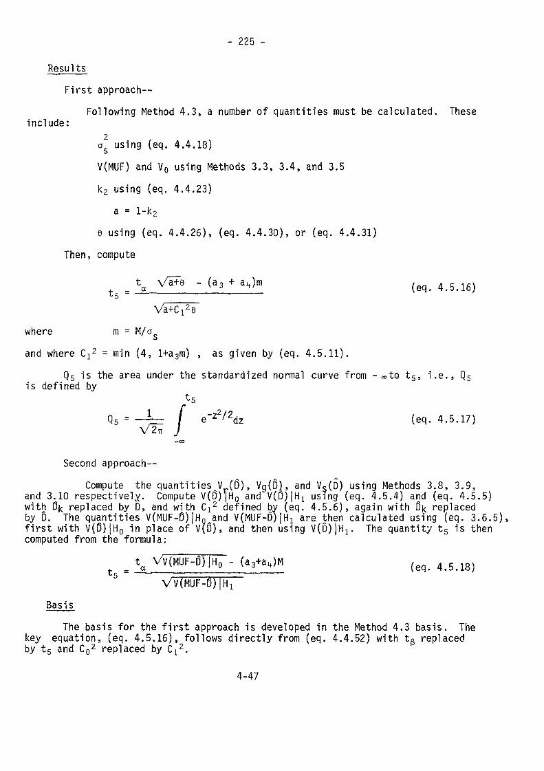
- 225 -

ResultsFirst approach--

Following Method 4.3, a number of quantities must be calculated. Theseinclude:

2as using (eq. 4.4.18)V(MUF) and V0 using Methods 3.3, 3.4, and 3.5k2 using (eq. 4.4.23)

a = l-k2e using (eq. 4.4.26), (eq. 4.4.30), or (eq. 4.4.31)

Then, compute

- (a3 * ajm (eq> 4^

where m = M/aand where C:2 = min (4, l+a3m) , as given by (eq. 4.5.11).

Q5 is the area under the standardized normal curve from - «to t5, i.e., Q5is defined byt5

Qs = -~= I e'z2/2dz (eq. 4.5.17}V2^ J

Second approach —Comp

and 3.10 respecCompute the quantitiesJr(D), Vg(D]|, and V§(D) using Methods 3.8, 3.9,anu o.iu respectively. Compute V(D)|H0 and (6)1 using (eq. 4.5.4) and (eq. 4.5.5)

with 0k replaced by D, and with Ci2 defined by (eq. 4.5.6), again with ß|< replacedby D. The quantities V(MUF-Ô)[Hg^and V(MUF-0)|Hi are then calculated using (eq. 3.6.5),first with V(ß)|H0 in place of V(ß), and then using V(D)|H1. The quantity ts is thencomputed from the formula:

o"" (a3+aJM (eq. 4.5.18)_

BasisThe basis for the first approach is developed in the Method 4.3 basis. The

key equation, (eq. 4.5.16), follows directly from (eq. 4.4.52) with tg replaced,by ts and C02 replaced by Cj2.

4-47

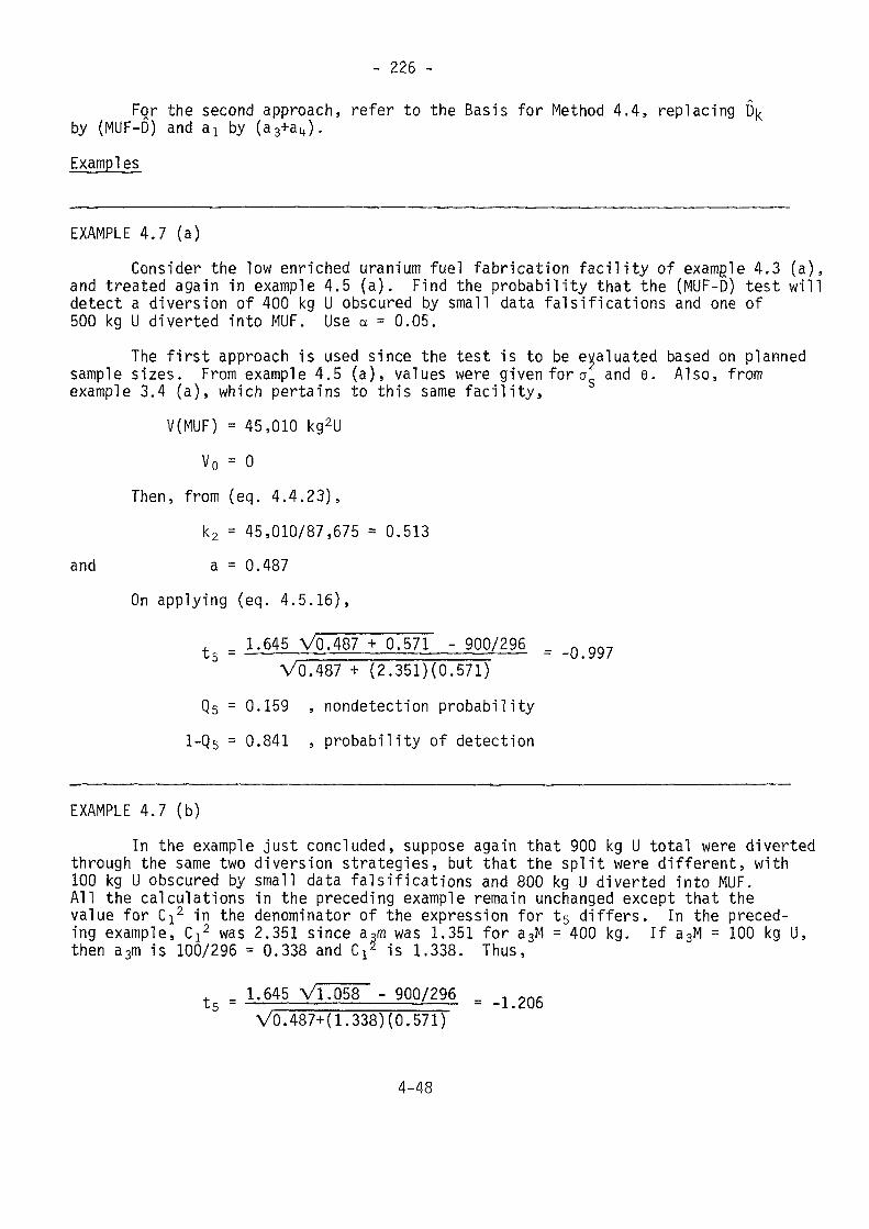
- 226 -

For the second approach, refer to the Basis for Method 4.4, replacingby (MUF-D) and ax by (a3+ajj.Examples

EXAMPLE 4.7 (a)Consider the low enriched uranium fuel fabrication facility of example 4.3 (a),

and treated again in example 4.5 (a). Find the probability that the (MUF-D) test willdetect a diversion of 400 kg U obscured by small data falsifications and one of500 kg U diverted into MUF. Use a = 0.05.

The first approach is used since the test is to be evaluated based on plannedsample sizes. From example 4.5 (a), values were given for a and e. Also, fromexample 3.4 (a), which pertains to this same facility,

V(MUF) = 45,010 kg2UV0 = 0

Then, from (eq. 4.4.23),k2 = 45,010/87,675 = 0.513

and a = 0.487On applying (eq. 4.5.16),

t = j.645 VQT487 + 0.571 - 900/296 = _Q

VO.487 + (2.351)(0.571)

Qs = 0.159 , nondetection probabilityl-Qs = 0.841 , probability of detection

EXAMPLE 4.7 (b)In the example just concluded, suppose again that 900 kg U total were diverted

through the same two diversion strategies, but that the split were different, with100 kg U obscured by small data falsifications and 800 kg U diverted into MUF.All the calculations in the preceding example remain unchanged except that thevalue for Ci2 in the denominator of the expression for ts differs. In the preced-ing example, Ci2 was 2.351 since a^m was 1,351 for a3M = 400 kg. If a3M = 100 kg U,then a3m is 100/296 = 0.338 and C^ is 1.338. Thus,

- 1.645 VT.058 - 900/296 _- ———————————————————————— -

V0.487+(1.338)(0.571)

4-48

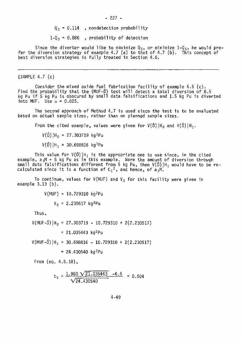
- 227 -

Qs = 0.114 , nondetection probability

1-Q5 = 0.886 , probability of detection

Since the diverter would like to maximize Q5, or minimize l-Qs, he would pre-fer the diversion strategy of example 4.7 (a) to that of 4.7 (b). This concept ofbest diversion strategies is fully treated in Section 4.6.

EXAMPLE 4.7 (c)Consider the mixed oxide fuel fabrication facility of example 4.5 (c).

Find the probability that the (MUF-Ö) test will detect a total diversion of 6.5kg Pu if 5 kg Pu is obscured by small data falsifications and 1.5 kg Pu is divertedinto MUF. Use a = 0.025.

The second approach of Method 4.7 is used since the test is to be evaluatedbased on actual sample sizes, rather than on planned sample sizes.

From the cited example, values were given for V(D)|Ho and 7(0)1 .V(D)|H0 = 27.303719 kg2PuV(D)|H! = 30.698816 kg2Pu

This value for V(ß)|H]. is the appropriate one to use since, in the citedexample, a3M = 5 kg Pu as in this example. Were the amount of diversion throughsmall data falsifications different from 5 kg Pu, then V^D)!^ would have to be re-calculated since it is a function of C^, and hence, of a3M.

To continue, values for V(MUF) and V0 for this facility were given inexample 3.13 (b).V(MUF) = 10.729310 kg2Pu

V0 = 2.230517 kg2PuThus,V(MUF-D)|H0 = 27.303719 - 10.729310 + 2(2.230517)

= 21.035443 kg2PuV(MUF-D)|H]. = 30.698816 - 10.729310 + 2(2.230517)

= 24.430540 kg2PuFrom (eq. 4.5.18),

+ 1.960 V21.035443 -6.5 _ n ...u5 - ———• ————— - U.ÖU4

V24.430540

4-49

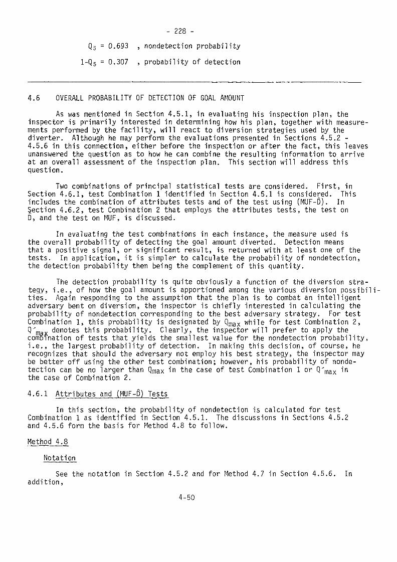
- 228 -Q5 = 0.693 , nondetection probability

1-Q5 = 0.307 , probability of detection

4.6 OVERALL PROBABILITY OF DETECTION OF GOAL AMOUNTAs was mentioned in Section 4.5.1, in evaluating his inspection plan, the

inspector is primarily interested in determining how his plan, together with measure-ments performed by the facility, will react to diversion strategies used by thediverter. Although he may perform the evaluations presented in Sections 4.5.2 -4.5.6 in this connection, either before the inspection or after the fact, this leavesunanswered the question as to how he can combine the resulting information to arriveat an overall assessment of the inspection plan. This section will address thisquestion.

Two combinations of principal statistical tests are considered. First, inSection 4.6.1, test Combination 1 identified in Section 4.5.1 is considered. Thisincludes the combination of attributes tests and of the test using (MUF-D). InSection 4.6.2, test Combination 2 that employs the attributes tests, the test onD, and the test on MUF, is discussed.

In evaluating the test combinations in each instance, the measure used isthe overall probability of detecting the goal amount diverted. Detection meansthat a positive signal, or significant result, is returned with at least one of thetests. In application, it is simpler to calculate the probability of nondetection,the detection probability then being the complement of this quantity.

The detection probability is quite obviously a function of the diversion stra-tegy, i.e., of how the goal amount is apportioned among the various diversion possibili-ties. Again responding to the assumption that the plan is to combat an intelligentadversary bent on diversion, the inspector is chiefly interested in calculating theprobability of nondetection corresponding to the best adversary strategy. For testCombination 1, this probability is designated by Qmax while for test Combination 2,Q"x denotes this probability. Clearly, the inspector will prefer to apply thecombination of tests that yields the smallest value for the nondetection probability,i.e., the largest probability of detection. In making this decision, of course, herecognizes that should the adversary not employ his best strategy, the inspector maybe better off using the other test combination; however, his probability of nonde-tection can be no larger than Qmax in the case of test Combination 1 or Q'niax 1>nthe case of Combination 2.4.6.1 Attributes and (MUF-D) Tests

In this section, the probability of nondetection is calculated for testCombination 1 as identified in Section 4.5.1. The discussions in Sections 4.5.2and 4.5.6 form the basis for Method 4.8 to follow.Method 4.8

NotationSee the notation in Section 4.5.2 and for Method 4.7 in Section 4.5.6. In

addition,4-50

- 229 -Q = probability of nondetection for test Combination 1

Qmax = maximum value for Q; that value of Q corresponding to thebest strategy of the diverterModel

See the discussion in Section 4.5.2 and the model discussion for Method 4.7,Results

The joint probability of nondetection is

Q = ß92 Q5 (eq. 4.6.1)Q5 is a function of a3 and a^. The quantities a2, 83, and a^ sum to 1. Q5is given by (eq. 4.5.17) and (eq. 4.5.16) or (eq. 4.5.18) for given a3 and a4.Use a trial and error approach to find Qmax- Var-V aa in increments from0 to 1 (steps of 0.1 are adequate). At a given value of a2, calculate Q5, where(a3+atj is equal to (l-a2).In calculating Ci2, use the following rule to select the value for a3:

If t5 is negative, choose a3 = l-a2If t5 is positive, choose a3 = 0

(rule 4.6.1)

Qmax is easily determined, either from the table of Q versus a2 values,with a2 rounded to the nearest tenth, or from a plot of the tabled data, which per-mits choosing a value of a2 between tabled values.Bas i s

Equation 4.6.1 follows from the fact that the tests on the attributes andthe (MUF-D) test are independent. Rule 4.6.1 applies because that value of a3should be chosen to give the largest value to 0,5. If t5 is negative, Q5 is maxi-mized when t5 is as close to zero as possible, i.e., when the denominator of t5is made as large as possible. This occurs when a3=l-a2. If t5 is positive, 0.5is maximized when t5 is made as large as possible, i.e., when the denominator ismade as small as possible. This occurs when a3=0.lExampl es

EXAMPLE 4.8 (a)In following up on the low enriched uranium fuel fabrication facility of

example 4.7 (a), set M = 1500 kg U and find the value of Qmax- Assume that3 = 0.05 for the attributes tests and that a = 0.05 for the (MUF-D) test.

4-51

- 230 -From example 4.7 (a),

1.6920 - 1500(33+3 )7296t5 = ————————————————VO.487+0.571C!2

1.6920 - 5.0676(a3+a4)

VO.487+0.571C!2

The table below gives the value for Q as a function of a2. The column headed"MUM" is the sign of the numerator in the expression for t5, which dictates thevalue for a3.

00.10.20.30.40.50.60.70.80.91.0

,32

1.00000.74110.54930.40710.30170.22360.16570.12280.09100.06750.0500

NUMNEGNEGNEGNEGNEGNEGNEGPOSPOSPOSPOS

10.90.80.0.0,0.4

0000

.7

.6

.5

-2.028-1.723-1.419-1.115-0.810-0.532-0.2250.1670.6601.1521.645

0.02130.04240.07790.13240.20900.29740.41100.56630.74540.87530.9500

0.02130.03140.04280.05390.06310.06650.06810.06950.06780.05910.0475

For a2 rounded to the nearest tenth, Qmax is 0.0695. Thus, the maximum proba-bility of nondetection, 0.0695, occurs at a2 = 0.7, 33 = 0, 3*4 = 0.3, or when 1050kg U is diverted into large and medium data falsifications, and 450 kg U is divertedinto MUF.

EXAMPLE 4.8 (b)In following up on the mixed oxide fuel fabrication facility of example

4.7 (c), set M = 8 kg Pu snd find the value of Qmax. „Assume that ß = 0.20 forthe attributes tests and that a = 0.025 for the (MUF-D) test. (Note: ThisUrge vslue for ß is reasonable becsuse of the insbility of the variables measure-ments to detect the gosl amount of M = 8 kg Pu. The value for Qmax will be inde-pendent of the ß value for the attributes testing up to fairly Urge values of ß.)

For example 4.7 (c) and the earlier example 4.5 (c),1.960 V21.035443 -8(a3+au)V23.978453 - 10.729310 + 2(2.230517) + 3.32526608.9894 - 8(33+3it)V17.7102 + 3.325266C!2

4-52

- 231 -The table below gives Q values as a function of a .

az00.10.20.30.40.50.60.70.80.91.0

1.00000.85130.72480.61700.52530.44720.38070.32410.27590.23490.200

MUMPOSPOSPOSPOSPOSPOSPOSPOSPOSPOSPOS

M00000000000

t 50.2160.3900.5650.7300.9131.0881.262437611786

1.960

0.58550.65170.71400.76730.81940.86170.89650.92460.94640.96300.9750

Q0.58550.55480.51750.47340.43040.38540.34130.29970.26110.22620.1950

Qmax is 0.5855, occurring at a^ = 0, i.e., when all 8 kg Pu is diverted intoMUF(atf=l). Clearly, the adversary would be unwise were he to divert into large andmedium data falsifications in this example since the inspector can control his3 error in the attributes inspection. The ability of the inspector to detect thegoal amount is limited by systematic errors of measurement that affect the D andMUF statistics, and hence, the (MUF-D) statistic.Note that at a2 = 0.1, Q would be larger than the value at a2 - 0 if

0.6517 l> 0.5855This inequality holds if ß > 0.343, which means that the ß value for attri-

butes inspection could be increased to 0.343, with the attendent reduced inspectionsample sizes, before the intelligent adversary would choose to divert even a por-tion of the goal amount into large and/or medium data falsifications. Stated froma different perspective, Qmax will be 0.5855 for all values of the attributes in-spection, ß, less than 0.343.

4.6.2 Attributes, 6, and MUF TestsIn this section, the probability of nondetection is calculated for the test

Combination 2 as identified in Section 4.5.1. With reference to Sections 4.5.2,4.5.4, and 4.5.5, the probability of nondetection for the attributes, D, and MUFtests is not ßa QsQ^ as might be expected because ß and MUF are correlated. Thiscorrelation must be taken into account when performing the calculations. This isnot simply an academic point; failure to take into account the correlation may lendto totally erroneous conclusions.

The procedures for calculating the probability of nondetection using testCombination 2 are now given by Method 4.9.Method 4.9

See the notation in Section 4.5.2 and for Methods 4.5, 4.6, and 4.7. Inaddition,

4-53

- 232 -Q' = probability of nondetection for test Combination 2

Q" = maximum value for Q'; that value of Q' corresponding to thebest strategy of the diverterp = correlation coefficient between D' and MUF

ModelSee the discussion in Section 4X5.2 and the model discussions for Methods 4.5and 4.6. Further, it is assumed that D' and MUF are jointly distributed as the

bivariate normal with correlation coefficient p.Results

The probability of nondetection isQ' = ßa2 L(t3, tu, p) (eq. 4.6.2)

where-(k2 + k3)P = —;—— (eq. 4.6.3)V(l+C120)(k2+2k3)

2where k3 = VO/CTS (eq. 4.6.4)and where k2 is given by (eq. 4.4.23)

The expression for p given by (eq. 4.6.3) applies if the evaluation is beingperformed based on sample sizes developed during the planning stage. If implemen-tation sample sizes are used, then the more general expression for p applies.

= -V(MUF)j^Vo __ (eq. 4.6.5)V[V(0)|H1][V(MUF)]

To continue with (eq. 4.6.2), L(t3,tit,p) is the probability that two randomvariables, distributed as a bivariate normal distribution, are jointly less thant3 and tit respectively, where p is the correlation coefficient. This probabilitymay be found by table look-up or by computer calculations. Both approaches areconsidered.

Before proceeding further, it is necessary to remark on the choices forta used in the equations for t3, (eq. 4.5.10]) and for t^, (eq. 4.5.13). If onewere to assume independence between MUF and D, and if a were the overall signifi-cance level, then a3 and c^ would satisfy the relationship

1-ct = (l-a3)(l-a4) (eq. 4.6.6)Further, if a3 = a^, = a0, then a0 is the solution of the equation

(l-a0)2 = 1-a ,

4-54

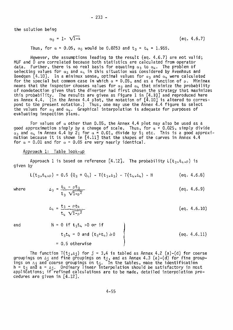
- 233 -

the solution being(eq. 4.6.7)

Thus, for a = 0.05, a0 would be 0.0253 and t3 = ti, = 1.955.However, the assumptions leading to the result (eq. 4.6.7) are not valid;

MUF and D are correlated because both statistics are calculated from operatordata. Further, there is no real basis for equating a3 to a4. The problem ofselecting values for »3 and a^ in this situation was considered by Avenhaus andBeedgen [4.10]. In a minimax sense, optimal values for a3 and a^ were calculatedfor the special but common case in which a = 0.05, and as a function of p. Minimaxmeans that the inspector chooses values for a3 and a^ that minimize the probabilityof nondetection given that the diverter had first chosen the strategy that maximizesthis probability. The results are given as Figure 1 in [4.10] and reproduced hereas Annex 4.4. (In the Annex 4.4 plot, the notation of [4.10] is altered to corres-pond to the present notation.) Thus, one may use the Annex 4.4 figure to selectthe values for a3 and c^. Graphical interpolation is adequate for purposes ofevaluating inspection plans.

For values of a other than 0.05, the Annex 4.4 plot may also be used as agood approximation simply by a change of scale. Thus, for a = 0.025, simply dividea3 and CX1+ in Annex 4.4 by 2; for a = 0.01, divide by 5; etc. This is a good approxi-mation because it is shown in [4.11] that the shapes of the curves in Annex 4.4for a = 0.01 and for a = 0.05 are very nearly identical.

Approach 1: Table look-upApproach 1 is based on reference [4.12]. The probability L(t3,ti+,p) isgiven byL(t3,t£t,p) = 0.5 (Q3 + QJ - T(t3,A3) - T(U,Alt) - H (eq. 4.6.8)

where (eq. 4.6.9)

(eq. 4.6.10)

and H = 0 if t3t4 >0 or iftgt^ = 0 and (t3+tij

=0.5 otherwise(eq. 4.6.11)

The function T(tj,Aj) for j = 3,4 is tabled as Annex 4.2 (a)-(d) for coarsegroupings on AJ and fine groupings on tj, and as Annex 4.3 (a)-(d) for fine group-ings on AJ and coarse groupings on tj. In the tables, make the identificationh = tj and a = AJ. Ordinary linear interpolation should be satisfactory in mostapplications; if refined calculations are to be made, detailed interpolation pro-cedures are given in [4.12].

4-55

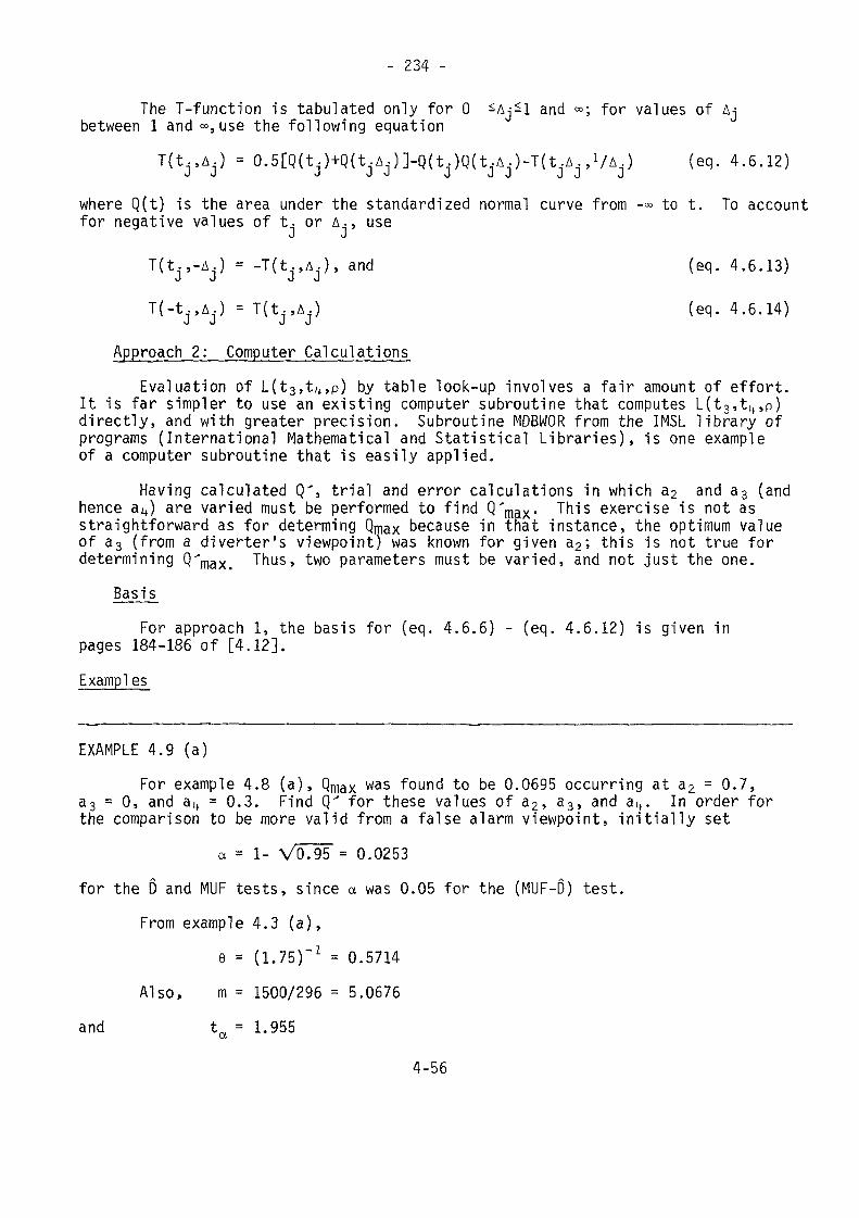
- 234 -

The T-function is tabulated only for 0 -Aj-1 and »; for values of Ajbetween 1 and «,use the following equation

T(tj,Aj) = 0.5[Q(tj)+Q(tjAj)]-Q(tj)Q(tjA.).)-T(t.).Ar1/Aj) (eq. 4.6.12)

where Q(t) is the area under the standardized normal curve from -°° to t. To accountfor negative values of t. or A., use

J J

T(t.,-A.) - -T(t.,A,), and (eq. 4.6.13)J J J J

TC-t^Aj) = T(trA..) (eq. 4.6.14)

Approach 2: Computer CalculationsEvaluation of L(t3,ti+,p) by table look-up involves a fair amount of effort.It is far simpler to use an existing computer subroutine that computes L(t3,ti+,p)directly, and with greater precision. Subroutine MDBWOR from the IMSL library of

programs (International Mathematical and Statistical Libraries), is one exampleof a computer subroutine that is easily applied.Having calculated Q', trial and error calculations in which a2 and a3 (and

hence a^) are varied must be performed to find Q'max- Tpis exercise is not asstraightforward as for determing Qmax because in that instance, the optimum valueof a3 (from a diverter's viewpoint) was known for given a2; this is not true fordetermining Q'max> Thus, two parameters must be varied, and not just the one.

Basis^For approach 1, the basis for (eq. 4.6.6) - (eq. 4.6.12) is given in

pages 184-186 of [4.12].Examples^

EXAMPLE 4.9 (a)For example 4.8 (a), Qmax was found to be 0.0695 occurring at a2 = 0.7,a3 = 0, and a4 = 0.3. Find Q" for these values of a2, a3, and ai+. In order for

the comparison to be more valid from a false alarm viewpoint, initially seta = l - VO.95 = 0.0253

for the D and MUF tests, since a was 0.05 for the (MUF-D) test.From example 4.3 (a),

9 = (1.75)"1 = 0.5714Also, m = 1500/296 = 5.0676

and t = 1.955Ot

4-56

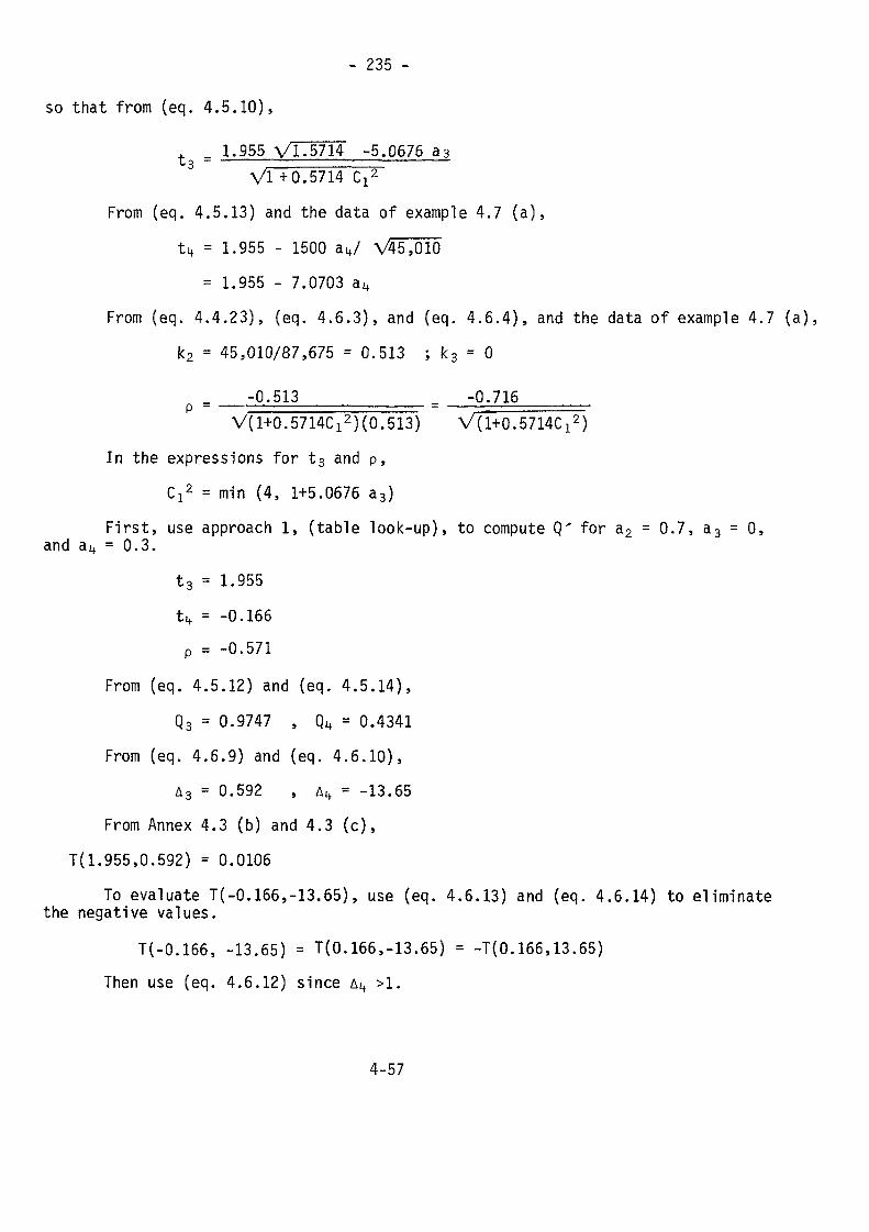
- 235 -

so that from (eq. 4.5.10),

t = 1.955 VT75714 -5.0676 a3

Vl +0.5714 Ci2

From (eq. 4.5.13) and the data of example 4.7 ( a ) ,

tit = 1-955 - 1500 ait/ V45.010

= 1.955 - 7.0703 a4

From (eq. 4.4.23), (eq. 4.6.3), and (eq. 4.6.4), and the data of example 4.7 (a),k2 = 45,010/87,675 = 0.513 ; k3 = 0

-0.513 -0.716p - VU+0.5714C!2) (0.513) VU+0.5714C!2)In the expressions for t3 and p,

Cj2 = min (4, 1+5.0676 a3)First, use approach 1, (table look-up), to compute Q' for a2 = 0.7, a3 = 0,and a4 = 0.3.

t3 = 1.955tu = -0.166p = -0.571

From (eq. 4.5.12) and (eq. 4.5.14),Q3 = 0.9747 , Q4 = 0.4341

From (eq. 4.6.9) and (eq. 4.6.10),A3 - 0.592 , A^ - -13.65

From Annex 4.3 (b) and 4.3 (c),1(1.955,0.592) = 0.0106

To evaluate T(-0.166,-13.65), use (eq. 4.6.13) and (eq. 4.6.14) to eliminatethe negative values.T(-0.166, -13.65) = T(0.166,-13.65) = -1(0.166,13.65)

Then use (eq. 4.6.12) since A^ >1.

4-57

- 236 -

T(0.166, 13.65) = 0.5 (0.5659 + 0.9883) - (0.5659)(0.9883) - 0.0009= 0.2169

Finally, H of (eq. 4.6.8) is 0.5 so that, from (eq. 4.6.8)L(1.955, -0.166, -0.571) = 0.5 (0.9747 + 0.4341) - 0.0106 + 0.2169 - 0.5

= 0.4107Then, from (eq. 4.6.2),

CT = (0.05)°'7(0.4107) = 0.0504Using the MDBNOR subroutine, L(t3,tit,p) is calculated to be 0.4109, in goodagreement with the table look-up value.Note that at this combination of values of a2> a3, and a^, Q' is smallerthan Q; this does not mean, however, that Q" max is smaller than Qmax since Q andQ" may not reach their respective maximum values at the same combination of values

for a2, a3, and a^. Further calculations are needed to determine Q' max.Before proceeding with these additional calculations, the optimal choices

for «3 and c^ are used in place of a3 = a4 = 0.0253, where these optimal choicesare given by Annex 4.4. In using Annex 4.4, the value of p is, of course, thatcalculated under the null hypothesis, i.e., corresponding to Cx2 = 1. This is

p = -0.716/VI.5714 = -0.571Thus, from Annex 4.4, by graphical interpolation, chose

a3 = 0.035 a^ = 0.021t = 1.811 t , = 2.03403 a4

The example calculation is now performed with these values used instead of1.955 in the expressions for t3 and t^. At a2 = 0.7, a3 = 0, and a^ - 0.3,

t3 = 1.811 tu = -0.087 p - -0.571From (eq. 4.5.12) and (eq. 4.5.14),

Q3 = 0.965 Q4 = 0.465From (eq. 4.6.9) and (eq. 4.6.10),

A3 = 0.637 A4 = -24.66From Annex 4.3 (c),

T(1.811, 0.637) = 0.0148To evaluate T(-0.087, -24.66), use (eq. 4.6.13) and (eq. 4.6.14) to eliminate

the negative values.

4-58

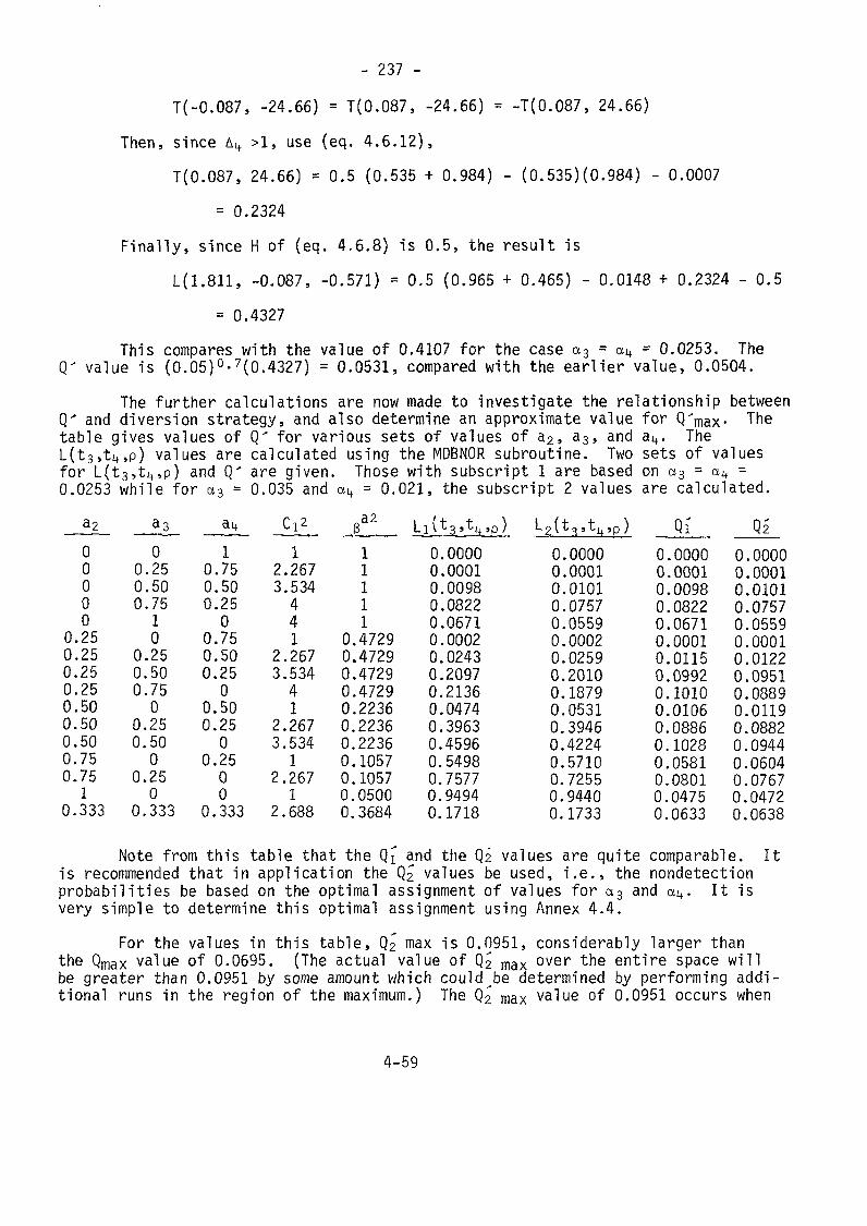
- 237 -K-0.087, -24.66) = T(0.087, -24.66) = -T(0.087, 24.66)

Then, since >l, use (eq. 4.6.12),T(0.087, 24.66) = 0.5 (0.535 + 0.984) - (0.535)(0.984) - 0.0007

= 0.2324

Fina l ly , since H of (eq. 4,6.8) is 0.5, the result is

L(1.811, -0.087, -0.571) = 0.5 (0.965 + 0.465) - 0.0148 + 0.2324 - 0.5= 0.4327

This compares with the value of 0.4107 for the case a3 = a.^ = 0.0253. TheQ" value is (0.05)°-7(0.4327) = 0.0531, compared with the earlier value, 0.0504.

The further calculations are now made to investigate the relationship betweenQ" and diversion strategy, and also determine an approximate value for Q'rnax- Thetable gives values of Q' for various sets of values of a2, a3, and a^. TheL(t3,tit,p) values are calculated using the MDBNOR subroutine. Two sets of valuesfor L(t3,ti+,p) and Q" are given. Those with subscript 1 are based on a3 = au =0.0253 while for a3 = 0.035 and 04. = 0.021, the subscript 2 values are calculated.

a200000

0.250.250.250.250.500.500.500.750.751

0.333

00.250.500.75

10

0.250.500.750

0.250.500

0.250

0.333

10.750.500.250

0.750.500.250

0.500.250

0.2500

0.333

12.2673.534441

2.2673.53441

2.2673.534

12.2671

2.688

11111

0.47290.47290.47290.47290.22360.22360.22360.10570.10570.05000.3684

Qï 0,20.00000.00010.00980.08220.06710.00020.02430.20970.21360.04740.39630.45960.54980.75770.94940.1718

0.00000.00010.01010.07570.05590.00020.02590.20100.18790.05310.39460.42240.57100.72550.94400.1733

0.00000.00010.00980.08220.06710.00010.01150.09920.10100.01060.08860.10280.05810.08010.04750.0633

0.00000.00010.01010.07570.05590.00010.01220.09510.08890.01190.08820.09440.06040.07670.04720.0638

Note from this table that the Qi and the Q2 values are quite comparable. Itis recommended that in application the Q2 values be used, i.e., the nondetectionprobabilities be based on the optimal assignment of values for a3 and a^. It isvery simple to determine this optimal assignment using Annex 4.4.

For the values in this table, Q2 max is 0.0951, considerably larger thanthe Qmax value of 0.0695. (The actual value of Q2 max over the entire space willbe greater than 0.0951 by some amount which could^be determined by performing addi-tional runs in the region of the maximum.) The Q2 max value of 0.0951 occurs when

4-59

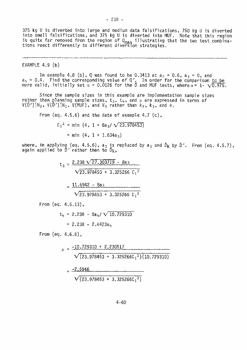
- 238 -

375 kg U is diverted into large and medium data falsifications, 750 kg U is divertedinto small falsifications, and 375 kg U is diverted into MUF. Note that this regionis quite far removed from the region of Qma„ illustrating that the two test combina-tions react differently to different diversion strategies.

EXAMPLE 4.9 (b)In example 4.8 (b), Q was found to be 0.3413 at a2 = 0.6, a3 = 0, anda^ = 0.4. Find the corresponding value of Q". In order for the comparison to be

more valid, initially set a = 0.0126 for the 0 and MUF tests, where a= l- V0.975.Since the sample sizes in this example are implementation sample sizesrather than planning sample sizes, t3, t^, and p are expressed in terms ofV(6')|H0, V(D')|H15 V(MUF), and V0 rather than k2, k3, and 9.From (eq. 4.5.6) and the data of example 4.7 (c),

Ci2 = min (4, 1 + 8a3/ V23.978453)= min {4, 1 + 1.634a3)

where, in applying (eq. 4.5.6), aï is replaced by a3 and D^ by fr. From (eq. 4.5.7),again applied to 0' rather than to 0|<,

+. _ 2.238 V27.303719 - 8as3 ~ —— 'V23.978453 + 3.325266 C^

= 11.6942 - 8as__________V23.978453 + 3.325266 Cz2

From (eq. 4.5.13),^ = 2.238 - 8a4/V 10.729310

= 2.238 - 2.4423akFrom (eq. 4.6.5),

- -10.729310 + 2.230517p _ ———————————————V(23.978453 + 3.325266C!2)(10.729310)

_ -2.5946_____________V{23.978453 + 3.325266Ci2)

4-60

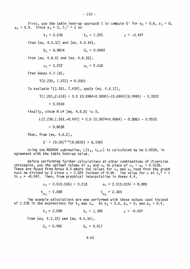
- 239 -

First, use the table look-up approach 1 to compute Q/ for a2 = 0.6, a3 = 0,a^ = 0.4. Since a3 = 0, C^ = 1 so

t3 = 2.238 tit = 1.261 p = -0.497

From (eq. 4.5.12) and (eq. 4.5.14),

Q3 = 0.9874 Qz, = 0.8964

From (eq. 4.6.9) and (eq. 4.6.10),

A3 = 1.222 A4 = 2.618

From Annex 4.3 ( d ) ,

T(2.230, 1.222) = 0.0063

To evaluate T(1.261, 2.618), apply (eq. 4.6.12),

1(1.261,2.618) = 0.5 (0.8964+0.9995)-(0.8964)(0.9995) - 0.0002

= 0.0518

Fina l ly , since H of (eq. 4.6.8) is 0,

1(2.238,1.261,-0.497) = 0.5 (0.9874+0.8964) - 0.0063 - 0.0518

= 0.8838Then, from (eq. 4.6.2),

Q- = (0.20)°-6(0.8838) = 0.3365Using the MDBNOR subroutine, L(t3, t^,p) is calculated to be 0.8838, inagreement with the table look-up value.Before performing further calculations at other combinations of diversionstrategies, use the optimal values of a3 and a4 in place of a3 = a4 = 0.0126.These are found from Annex 4.4 where the values for a3 and a^ read from the graphmust be divided by 2 since a = 0.025 instead of 0.05. The value for p at C^2 = 1

is p = -0.497. Then, from graphical interpolation in Annex 4.4,a3 = 0.5(0.036) = 0.018 on, = 0.5(0.018) = 0.009t = 2.098 t =2.365«3 a4

The example calculations are now performed with these values used insteadof 2.238 in the expressions for t3 and t^. At a2 = 0.6, a3 = 0, and a 4. = 0.4,

t3 = 2.098 tj, = 1.388 p = -0.497From (eq. 4.5.12) and (eq. 4.5.14),

Q3 = 0.982 0,4 = 0.917

4-61

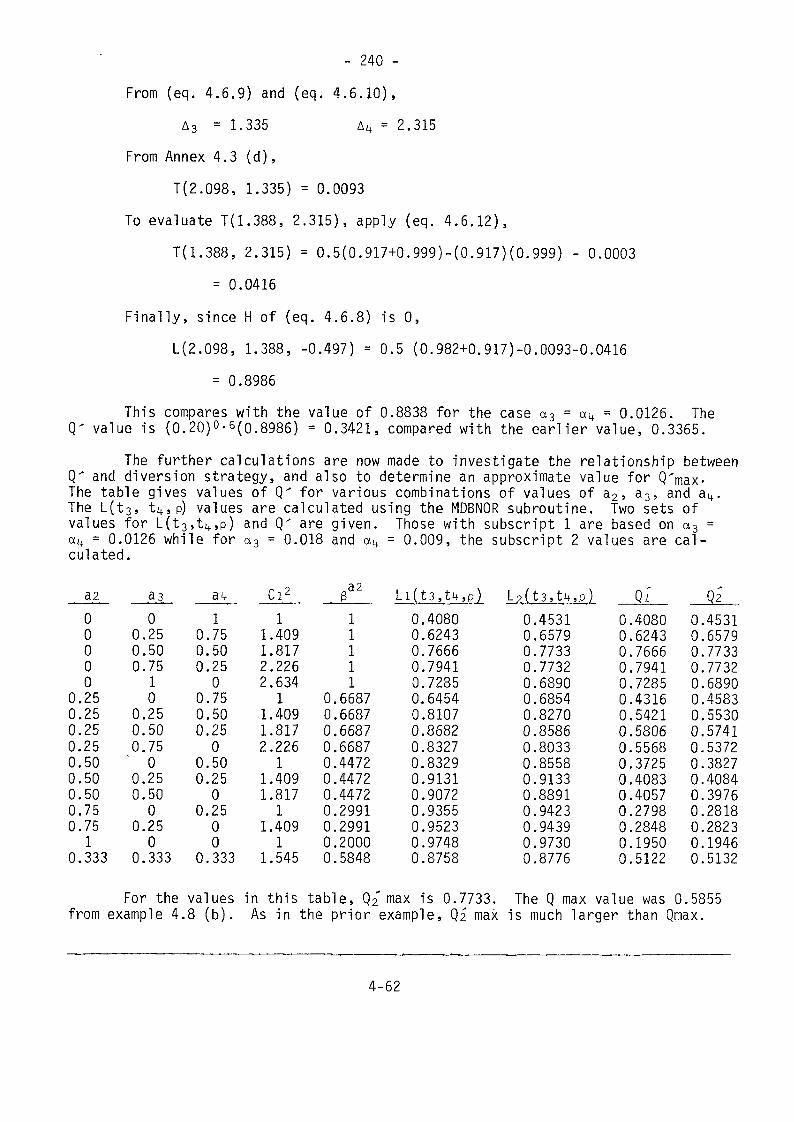
- 240 -From (eq. 4.6.9) and (eq. 4.6.10),

A3 = 1.335 A4 = 2.315From Annex 4.3 (d),

T(2.098, 1.335) = 0.0093To evaluate T(1.388, 2.315), apply (eq. 4.6.12),

1(1.388, 2.315) = 0.5(0.917+0.999)-(0.917)(0.999) - 0.0003- 0.0416

Finally, since H of (eq. 4.6.8) is 0,L(2.098, 1.388, -0.497) = 0.5 (0.982+0.917)-0.0093-0.0416

- 0.8986This compares with the value of 0.8838 for the case a3 = a^ = 0.0126. The

Q' value is (0.20)°-6(0.8986) = 0.3421, compared with the earlier value, 0.3365.The further calculations are now made to investigate the relationship between

Q" and diversion strategy, and also to determine an approximate value for Q'rnax-The table gives values of Q' for various combinations of values of a2, a3, and a^.The L(t3, tin?) values are calculated using the MDBNOR subroutine. Two sets ofvalues for [.(tittup) and Q" are given. Those with subscript 1 are based on a3 =014 = 0.0126 while for a3 = 0.018 and a4 = 0.009, the subscript 2 values are cal-culated.

Cr ,32

00000

0.250.250.250.250.500.500.500.750.75

10.333

00.250.500.75

10

0.250.500.75

00.250.50

00.25

00.333

10.750.500.25

00.750.500.25

00.500.25

00.25

00

0.333

11.4091.8172.2262.634

11.4091.8172.226

11.4091.817

11.409

11.545

11111

0.66870.66870.66870.66870.44720.44720.44720.29910.29910.20000.5848

Li(t3,;U,p) L2(t3.tit,p) Qi0.40800.62430.76660.79410.72850.64540.81070.86820.83270.83290.91310.90720.93550.95230.97480.8758

0.45310.65790.77330.77320.68900.68540.82700.85860.80330.85580.91330.88910.94230.94390.97300.8776

0.40800.62430.76660.79410.72850.43160.54210.58060.55680.37250.40830.40570.27980.28480.19500.5122

0.45310.65790.77330.77320.68900.45830.55300.57410.53720.38270.40840.39760.28180.28230.19460.5132

For the values in this table, Q2* max is 0.7733. The Q max value was 0.5855from example 4.8 (b). As in the prior example, 0,2 max is much larger than Qmax.

4-62

- 241 -

4.7 REFERENCES[4.1] Avenhaus, R., "Material Accountability—Theory, Verification, Appli-cations", John Wiley and Sons, 1978.

[4.2] Beetle, T.M., "Quantifying Scenarios to Check Statistical Procedures",Nuclear Materials Management Meeting Proceedings, Vol. V, No. Ill, 612-621, (1976).

[4.3] Mil-Std-105 D, "Sampling Procedures and Tables for Inspection byAttributes", 1963.

[4.4] Mil-Std.414, "Sampling Procedures and Tables for Inspection byVariables for Percent Defective", 1957.

[4.5] Jaech, J.L., "Statistical Methods in Nuclear Material Control",TID-26298, U.S. Gov't Printing Office, 350 ff., (1973).

[4.6] Brownlee, K.A., "Statistical Theory and Methodology in Science andEngineering", John Wiley and Sons, Inc., Chapter 4, 1960.

[4.7] Jaech, J.L., op cit, p. 327.[4.8] Jaech, J.L., op cit, p. 361-365.[4.9] Jaech, J.L., "Effects of Inspection Design Variables on InspectionSample Sizes and on Detection Probabilities", Second ESARDA Symposium,Edinburgh, March 1980.

[4.10] Avenhaus, R. and Beedgen, R., "Statistical Analysis of AlternativeData Evaluation Schemes Part II: Extended Theoretical Consideration",Second ESARDA Symposium, Edinburgh, March 1980.

[4.11] Avenhaus, R., "Significance Thresholds of One-Sided Tests for Meansof Bivariate Normally Distributed Variables", Commun, Statist.-Theor.Meth., A8(3), 223-230 (1979).

[4.12] Owen, D., "Handbook of Statistical Tables", Addison-Wesley Publish-ing Co., Reading, Mass. 1962.

4-63

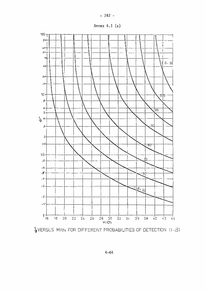
- 242 -

Annex 4.1 (a)

16 18 20 22 24 2.5 28 30 3.2 34 36 3.8 40 42 44

^VERSUS M/CTS FOR DIFFERENT PROBABILITIES OF DETECTION (I -Q)

4-64

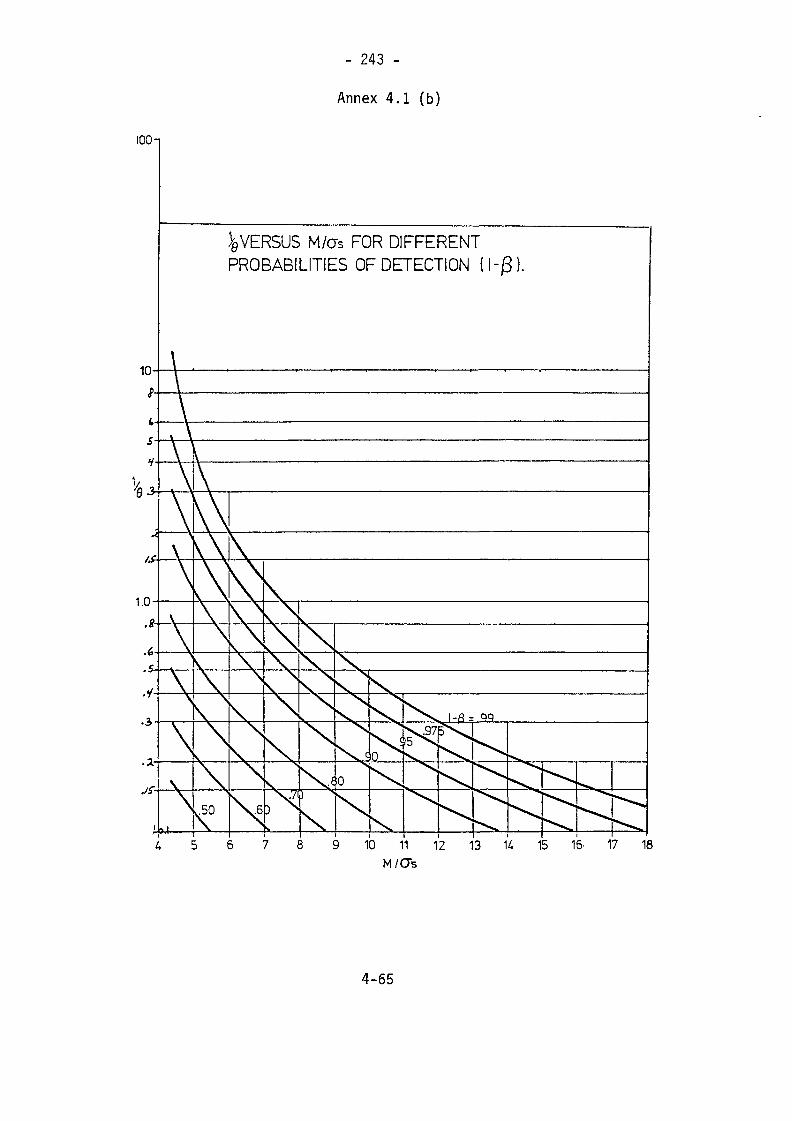
- 243 -

Annex 4.1 (b)

ICO-i

VERSUS M/CTS FOR DIFFERENTPROBABILITIES OF DETECTION (

10 11 12 13 M,M/Os

15 1S 17 18

4-65

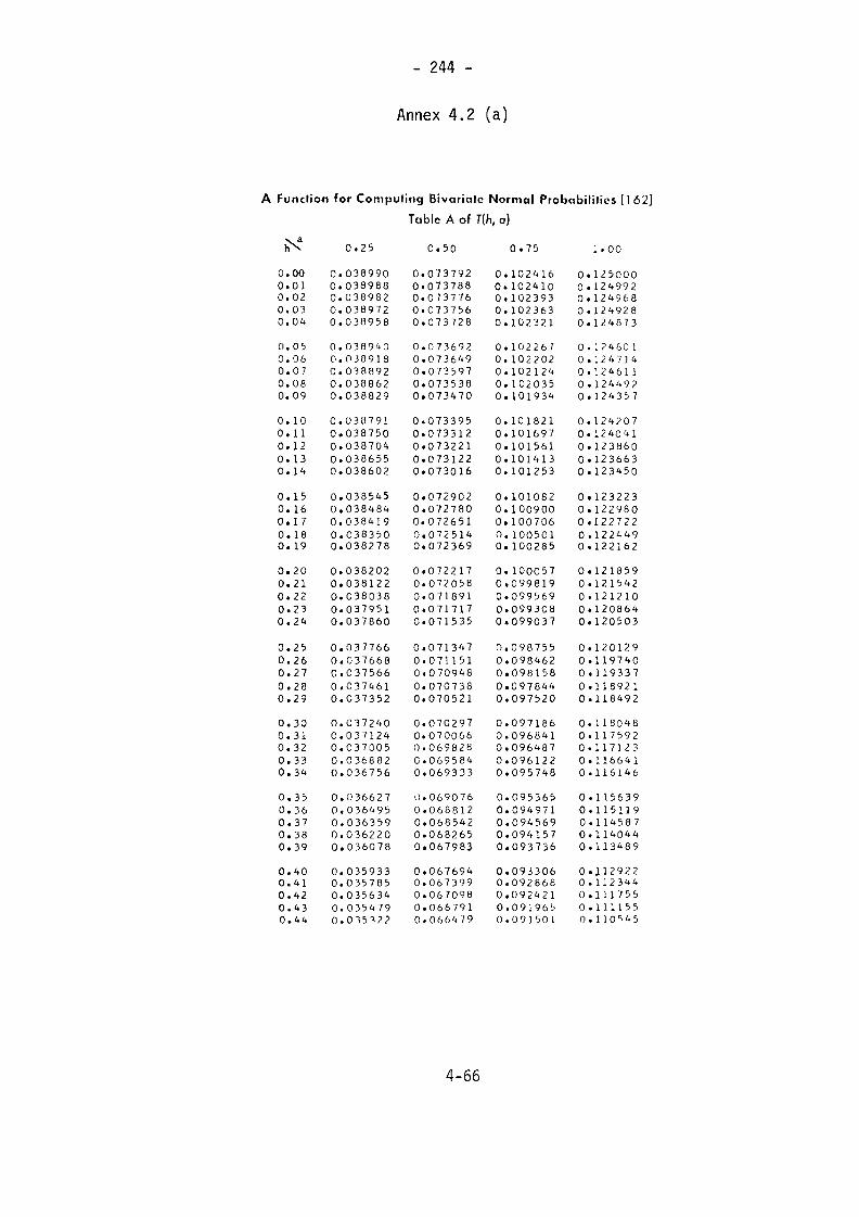
- 244 -

Annex 4.2 (a)

A Functio-n for Computing Divariatc Normal Probabilities [162]

Table A of r(fi, a)

0 .25 0.50 0.75 1.00

0.000.010.020.030.040.050.060.070.080.09

0.100.110. 120.130. 14

0.150.160.170. 180. 19

0.200.210.220.230.24

0.250.260.270.280.290.300.310.320.330.340.350.360.370.380.390.400.410.420.430.44

0.0389900.0389880.0389820. 0389720.0389580. 0389400.0389180.0388920.0388620.0388290.0387910.0387500.0387040.0386550.0386020.0385450.0384840.0384190.0383500.038278

0.0382020.0381220.0380380.0379510.037860

0.0377660.037668C. 0375660.0374610.0373520.0372400.0371240.0370050.0368820.036756

0.0366270.0364950.0363590.0362200.0360780.0359330.0357850.0356340.035479O.OT51??

0.0737920.0737880.0737760.0737560.073728

0.0736920.0736490.0735970.0735380.073470

0.0733950.0733120.0732210.0731220.073016

0.0729020.0727800.0726510.0725140.0723690.0722170.0720580.0718910.0717170.071535

0.0713470.0711510.0709480.0707380.0705210.0702970.0700660.0698280.0695840.069333

0.0690760.0688120.0685420.0682650.0679830.0676940.0673990.0670980.0667910.066479

0. 1024160« 1024100.1023930. 1023630. 1023210. 10226 10. 1022020.1021240. 1020350. 101934

0. 1018210. 1016970.1015610.1014130. 101253

0. 1010820. 1009000. 1007060. 1005010. 1002850. 1000570.0998190.0995690.0993080.099037

0. 0987550.0984620.0981580.0978440.0975200.0971860.096Ü410.0964870.0961220.095748

0.0953650.0949710.0945690.0941570.0937360.0933060.0928680.0924210.0919650.091501

0.1250000« 1249920. 1249680 . 1 249280.124873

0. 1P40010.1247)40.12461 10.12449?0. 124357

0.1242070. 124Q410.1238600.1236630.123450

0.1232230.1229800.1227220 .1224490.122162

0.1218590.1215420.1212100. 1208640.120503

0.1201290.1197400 . 1193370.1189210.1184920. 1 180480.1175920.1171230 . 1166410.116146

0. 1156390.1151190.1 145870. 1140440.113489

0 .)129220.1123440.11 17550.1111550. 1 10^45

4-66

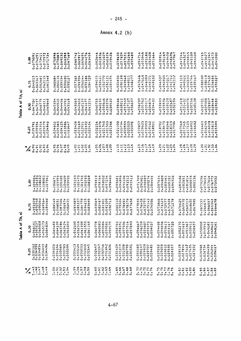
- 245 -

Annex 4.2 (b)

"2

•-.

§ 0<n

- oo

m

•n 0r* ^t

o oo

o0

O f-»A r~°so

*-*0>

. rM0 0

o

^o-

•-* * rg <»

fM -$ iri r~^ en CM f-t

o o o o0 0 0 0

>J €O ^H 4rn xO o mfO .-M fM ^H

O O O O

o o o o

i in —< oo

0 0 O 0

o o o o

-J *O ON O

in m o oorv rM e\j CMo o o oo o o o

o o o o

co m oOO O fNiO O ON

OOO

O O O

«o *-« inO o mo o i>O O O

O O O

J O NO

co (NJ tn

000

O O O

CM en mo o e\iNO en — <

fNJ (M CMO O O

O O O

O O O

000>

en j\co r-

00

oo

or~ON CNJ•O O00 CO

00

O O

CNJ COON ,M

en m00

o o

CO -ÎCO NÛ

CNJ CM0 0

O O

00

fM r- rf% NÛ o-

r- o- o »^ -*NO in in ^ en

o o o o oo o o o o

*O O 4 CO CM

o o o o oo o o o o

lA fM (T> Is" sOO O en I*- *-*O O F-^ \O CMen fM (M •—* r~l

o o o o oo o o o o

CO O* r— < fM -4*o NO en 0s iA

r\i CM CM CM CMo o o o oo o o o o

•O CO O fM -*CM •-*•-* O O>

o o o o oo o o o o

tA r-« O •-* -4r- rg r- CM r-o -J r^ *~* -J"^ m <M CM »-HO O O O O

o o o o o

r*- CM co en o\O o ON o* co

o o o o oo o o o o

\o co o en \ot~4 r- »}• o ^oCM O r- lA fM

o o o o oo o o o o

O 0s f~t 00 &>

co r— f*- »o iA

oooooo o o o o

o co co *-« r-en ro <r *-* r-oo •-* IA o r\iO O ON CO CO

O O O O O

o o o o o

*o CM o r^ r*-•o *-* in o in.j o in *-« *oco to r- r— o

o o o o oo o o o o

O -3" ON lA •-•cn CT^ in CM 0^o r*- in tn o^-t O O O O

o o o o oo o o o o

•j" *n o o -4

S S m r t S

o o o o oo o o o o

NO 03 Cn •—< CM•j t-* ON r — *n»O O en r r-«r r~ NO in in

o o o o oo o o o o

ON CNJ ÎN- - CM

f\j r~ m co NO in in ^ ^

o o o o oo o o o o

r- in en rg t~t

o o o o oo o o o o

•* » 0 -01^

o o ON co r~oooooo o o o o

r in r e\i CMen CM r-« t— « i~<in o* en r *—i-3 m en CM eM

O O O O O

o o o o o

ON in CNJ co inON in *— i NÛ CM

o o o o oo o o o o

o r- N* t-i or- NÏ CM o r-OO OO OO CO f"-

o o o o oo o o o o

CNI in

00

0 0

in -NId l>•— oo oo o

CO CM

CO J-

o oo o

in enf^ r~o oo o

CO ~* <fin in -j

000

O O O

cn -O r*~en <j NÛin r^ *— tO ON ON

O O O

O O O

CO -O COr~-iTN.cnON m ^HO O O

O O O

O O O

en CM (MCM O CO

f — NO NÛ

O O O

ooo

in f^ in o o

o o o o oo o o o o

o co o NO r--in o -* co enCO 00 f~ NÛ N/>

o o o o oo o o o o

r-* oo r*- co cnCM O If CO OOr- m 01 ^ oON ON CO OO OD

O O O O O

o o o o o

cn in co m cj*

-j CM o oo in

o o o o oo o o o o

•4" tn fNi *"H *-t «-H tn in ON iA **^ en in o oo ON *.f CM -4" o •—* «o >u <M CM o* i—t ON ^ ^ ^ o^ r\i rvj o NO •—< ••? in %o *o in •$ en CM,fviOiA o *ï r*- ON o o o o i*- <f «-« %o »-i o o en NÛ co o* o «-< »-H o o c o r ^ i A rnoco iA rM oo in r-< r-- m ON in r-« r*- m

O O* M O O m >O ON ;n *O ON •""* -J" r** O CM -XV r— O CM -tf" sO <X> «-H tn lA r— 0s O CM -J" «O CO ON r-* tn - O CO O1* *"H r-j »J *O P— O**o o* ON co co r*- vu iA iA^en cn rsj .-i •-« o o c o c o r - ^ u IA NJ- -4- m PJ r - *ooooo r- ^o in IA ^ en CM .-( o o ON co r^ -o iA_î O O O O O O O O O O O O O O O CT* ON O*" ON ON ON O* ON ON ON ON ON 0s CO CO CO CO CO QO CO CO OO CO CO CO f*- r-- t~- f"- Is"

_i ,-4 .-< —< ,-H _< ,-, .-4 .-< *-i •-C'-i.-i.-irH O O O O O O O O O O O O O Q O O O O O O O O O O O O O O O O

ooooo ooooo ooooo ooooo ooooo ooooo ooooo ooooo ooooo

tnr*.O

tcco o -t o<M-^ »O vÛ NÛOiA O in ot-H O O ON 0**

OOO 0 0

-3- en O r- entA O -^ ON- <f

O O O O O

o^ r— o> in inco en t*~ r~t •&oo en r*- CM *u»A m -4- <t en.

o o o o o

<T\ r*~ f-t o^ fNivO CO O O rH

o >T ON cn r*-cn CM *-»•-< oo o o o o

o <r*H O

O ON

O O

en œ coo\ r- inco co r-o o o

en o f*- t oO ^ r- r-4 lAr-- vu »A m ^i

o o o o o

vu rsj r* rg r*-co CM in O1* r\(m en CM r-« r-i

o o o o o

in o en in mCM r- *-t in o*u O> en *Q ONO ON O1 CO f"—

O O O O O

m r^r- 43

0 0

r- m coo -4- r^O en «o*O iA •*

O O O

ooooo ooooo ooooo ooooo ooooo ooooo ooooo ooooo ooooo

-Oo

o»no

•-«r- co en -t^u en o r*» en«-<cu in i— i co\o in in in ^•O^*O vO •-OOO OOO

OO OOO

O ON -* -t !>ce en co CM inj- •-< r- <r o^ *T en en m*û -O *O NU *ûO O O O O

o o o o o

O %O CO lA COON i— i m in «uvu m o in r-<CM fM rH -H rHO vO %O O Oo o o o oo o o o o

co m <r r-n inr*- co co co h~t— en ON in t~tO O ON ON ON>u o in in ino o o o oo o o o o

in «M «o *o en\o in rn «—< ONr- m o in oco co r*- h- r-iA m iA iA iAo o o o oo o o o o

r*~ ON r- en r*-\o en O h* en\û CM CD en ON\u *O A lA -^tA iA »A iA iAO O O O O

o o o o o

co vu en r*- oO lA r-* \O CM^ O vu r-l |—

iTi m iA lA m-o o o o oo o o o o

o oCM CDCM •-«lA lAO O

0 0

r- CM r*-\o •— • *nen ON <r*H O OlA lA iA000

O O O

O eMo <rO iAO ONlA ^4"0 0

o o

en r\i •-»CO CM vOo »o -<ON CO CO<»• >T sfO O O

O O O

^o^coo^- tn-MO^r- in ^ - r j o c o - o ^ ra o co »o -3-cs jor^ in mr-^o^r-^r cMOcoincn r - < c o o < f C M o r * - - r c M O«n<r~t^^- < t< rmcn tn mmcn rs j r s j cM<MCMr-c r - i ,_^H^- IOO ooo>-o^^ o o ^ c o c o c o cor- r - r - r * - o o ^ u o ^ )cnmrncnrn m m m c n m mmmmrn , m c n c n m c n m t n m c n m c n m f M c M C M C M C N J C M C M C M r M C M c \ j c M ( M r \ j r y r M C M ( Mooooo o o o o o o o o o o o o o o o o o o o o o o o o o o o o o o o o o o o o o o o oooooo ooooo ooooo ooooo ooooo ooooo ooooo ooooo ooooo

* > *sO «£> o •Jï ->u * x > < o « A O > < o r - f^-r^r- r^ r- f - t^h-f«- co co co co oo co to co co to• • * * • • * * • • • « • • • • * • • • • • • • • • • » * •

O O O O t j O O O O O O O O O C J O O O O O O O O O O O O O O O

4-67

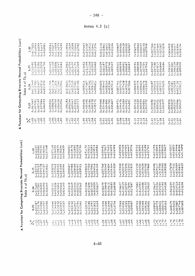
- 246 -

Annex 4.2 (c)

c_^JI/I

al P

roba

bi

Eo2o;"oa>to

r C

ompu

ting

o**-c0

oo•-4

u-ir*O

O-£T

< za; o

0

rg Aen a>r- -a

o oO 0

o -o-h O

O O

0 O

o ,-,<t oa r-

o o

.00

74

67

0.0

07

33

1 C

0 0

a* -j o.0 O in

o o oo o o

rg o — »in r«i en<-i o r-

0 0 O

o o o

r- -o <i)

t rg C7-

O O O

.00

71

97

0

.00

70

64

0

.00

69

33

0

O O 0

, ,-, ,-,

o eg CT* r~ vnin eg co in rg

O O O O O

O O O O O

iu O vO r- ro

-T r-t CO in rg~j -f m m en

o o o o oo o o o o

~t ^t g> eg r-i

0 O C) 0 0

.00

68

04

0

.00

66

76

0

.00

65

50

0

.00

64

26

0

.C0

63

04

0

o o o o o

CO O5 CO CO CO

,_,<«,...-.

-j tn en - IAi> -o tn o r-

o o o o oo o o o o

tx> o en r- org rg rg .M r-*

o o o o oo o o o o

J Ü IT . 1 .f>eg > i i i> io

0 0 O 0- IM

o o o o o

.00

61

83

0.0

06

06

4

0.0

05

94

7

00

05

83

1

00

05

71

7 0

o o o o o

„_.-,_,-,

vO CO '-I

O O 0

o o o

eg o O

•£} in r— •

o o oo o o

in r- egiO CO Oin en r-<r> u (^o o oO O 0

00

56

05

00

05

49

5 0

00

53

86

0

O 0 O

-1 _ rt

-ï" r-o eni — i , — io oo o

IA mO *uO -0o oo oO 0

0 r-t

o .-<O CO

o oo o

00

52

78

00

05

17

2 0

O 0

rt r-l

•— i *o r-\ *u egr— 1 CO vO en r— 1

•-1 O O O O

o o o o oo o o o o

eg ON r- <t eg

O O (7* (7* O^

O O O O O

O O O O O

O -1 eM o o

o o o o oo o o o o

00

50

68

00

04

96

6 0

00

48

65

00

04

76

5 0

,00

46

67

0o o o o o

o o o o oegej rgegr^

CO lACO *OO"> O^o o0 0

o o

r-t ON

en Oy\ ON

0 O

0 O

<r r-r- r-o o0 0

00

45

71

0

00

44

76

0

o o

0 O

eg eg

eg o co-ï eg o*

O O Oo o oO 0 0

O CO COCO \o ^CO CO CO

O 0 O

O 0 o

CO lA \oO -t co-T eg Or- r- r-o o oO 0 0

00

43

83

00

04

29

1 0

00

42

01

0«

o o o

o o oeg eg eg

r~ iA en < — i oco co co co r~o o o o oo o o o oo o o o o

rH CO OS <f rgON ON O eg -J-eg o ON r- inco co r- r- r-

o o o o oo o o o o

o* in -t >û oe\j r— eg r- tn

iO •£> -O ^ «Oo o o o oo o o o o

00

41

12

0

00

40

25

00

03

93

9

00

03

85

4 0

00

37

71

0

o o o o o

eg eg rg eg rg

*o r- cor- in enr- r- r-o o oo o o0 0 O

en co r-g3 CO r-t

en r-H O

r- r- r-o o oo o o

CO 3 Or-l O O

o o o0 0 O

00

36

90

00

03

61

0 0

.0

03

53

1 0

.

o o o

eg eg eg

o e\ieg o

O OO O

0 0

O -4-J- COCO -Û

0 0

0 O

r- <n

o oO 0

00

34

53

C.

00

33

77 0

.

o o

eg rg

in co r-i in ON

o o o o oo o o o oo o o o o

m - ON CO ONrg xu o in O

o o o o o

o o o o o

e i r— i in rg I-HO co in en r-<in en ej r-t o

o o o o oo o o o o

00

33

03 0

.0

03

22

9 0

.0

03

15

7 0

.0

03

08

6 0

.0

03

01

7 0

.

o o o o o

e! eg r^ eg ej

-QaJ3o

dû"5Ê13

DI oc »-3aEou

co

oo ooo o

en en COr- eNj f~

r~ iniA -T• en en en

0 00 0

OO O

o r-< -rco co '-O

o -ueg COin r~ r- o

• eg eg eg0 OO O

OO O

cor- -o

° oo o00 0

0

03

41

37

0.

o

o

oo

r—in

oo

0

03

36

01

0.

0260

99 0

.

o

olA

<f

O

0

O O O O O

03

30

70

0.

03

25

43

0.

03

20

22

0.

03

15

05

0.

03

09

94

0.

02

57

11

0.

0253

26 0

.0

24

94

4 0

.0

24

56

6 0

.0

24

19

0 0

.

o o o o o

in o co r- r--f <r en en enen r-< e> t— lA

•3 <r en tn m

O t > O O O

o o o o o

o o o o o

03

04

87

0.

02

99

85

0.

02

94

89

0.

02

89

97

0.

02

85

11

0.

0238

18 0

.02

3449

0.

0230

84 0

.0

22

72

1 0

.02

2362

0.

o o o o o

ON rg r- -t rgen r-< o r- <ntn en eg eg <NJo o o o oo o o o o

o o o o o

02

80

29

Oi

02

75

53

0.

02

70

82

0.

02

66

16

00

26

15

5 0

0220

06 0

.02

1654

0.

0213

05 0

.02

0959

0

0206

17

0

o o o o o

eg -t r-- eg cor- co ON r-i rgeg eg r-t r-i r-»O O O O O

o o o o o

o o o o

02

57

00

00

25

24

9 0

02

48

04

0.0

24

36

4 0

02

02

79

0.

0199

43 0

..0

19

61

1 0

.01

92

83

0

o o o o

-j. \0 CO r-i*j rg o C7*r-t r* rl O

o o o oo o o o

o

,02

39

29

0.0

18

95

8 0

o

ooo

o o o o o

,02

35

00

0,0

23

07

5 0

.02

26

56

0.0

22

24

2 0

,02

18

33

0

,01

86

37

0.0

18

31

9 0

,01

80

05

0.0

17

69

4 0

.017

387

0

o o o o o

\o e> eg in coin m eg o coo o o o ONo o o o oo o o o o

o o o o o

02

14

30

00

21

03

2 0

02

06

38

00

20

25

0 0

,01

98

68

0

.01

70

83

0.0

16

78

3 0

0164

86

0,0

16

19

3 0

.01

59

03

0

o o o o o

en o o** O egrg go o o- COr- in en r\j oc?* o* o* ON c^o o o o oo o o o o

o o o o o,0

19

49

0 0

.01

91

17

0

,01

87

50

0.0

18

38

8 0

.01

80

30

0

.01

56

17

0.0

15

33

4 0

.01

50

55

0.0

14

78

0 0

.01

45

08

0

o o o o o

r- <n t-i o rveg r- eg r- rgCO CO CO CO CO

o o o o oo o o o o

o* oo co oo r—o o o o o

.01

76

78

0.0

17

33

1 0

.01

69

89

0.0

16

65

1 0

.01

63

19

0

.01

42

39

0.0

13

97

4 0

.01

37

13

0.0

13

45

4 0

.01

32

00

0

o o o o o

m o r- >A *Ar- en co -* or-< o co r- -o

o o o o oo o o o o

4-68

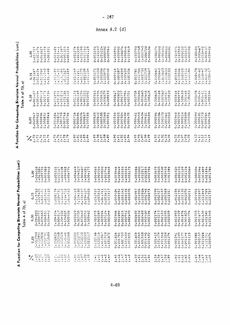
- 247

Annex .4.2 (d)

r*- -o r^ co f-Hrv r~ tv r- fo,r~ o ^ 'f^ O O 0 O Oo o o o o

oj ï f> -n •-<t -4 tO <n rn

0 0 O O Oo o o o o

r— ro o \o c\irg CM .-« ^ ,-«»-* r-» r- 1 r-* .-«

o o o o oo o o o o

o in rv o soo o o o ot~t r* r-4 O O

o o o o oO 0 O O O

m o r-- t .-HO« o co CD coo o o o oo o o o oO O 0 O 0

(f\ >O -3" fV O>r- r- r^ r- vuo o o o oo o o o oo o o o o

r~~ in ro <— « (j*o o o o oo o o o oo o o o o

r— in m »-» oin in in in in0 O O O OO 0 O O O0 0 O 0 0

CO -jO >n in CM

o o o o oo o o o oo o o o o

r- x»to m^) 0

O t >O 0

0 0

O en «>

ui in -j00 O

O 0 O

0 O O

m o-J j*-« r i

O < 1O 0

i. ) i >

io r*- tog? rv, ou•«i i«> CM

t •-< r-t

o •> ol 0 O

* ) 0 O

o r+ in o 4-^ -•« r- m oCV CV •-« • — — « . - <

r 1 .-< •- « .-1 , -1

o o o o oO 0 0 0 0

o o o o o

t-i co *o in inr- m o r- <i-O O O O O,-H --I -H O O

o o o o o0 0 0 O O

O 0 C) 0 O

•o Is- o en \oT-I oo u~\ m ou> to co oo unO O 0 O 00 O O O OO O 0 O 0

o o o o o

r— i >jO (M O* l ~co iT» en O COr-- r- r - r~- so0 O O 0 O0 O O 0 O0 O O O O

o o o o o

in en•4D -41

\O -OO 00 O0 0

0 0

CO (A <nrg o co-u »4Ö ino o o> 0 0o o oO O f 5

j- -o co --t -j-vO -41 fV i-i Oin in in . n tC) O O O (Jo c> o o > >o o o o o

o o o o o

co CM Is- rv r~-t*- O xf <n i-H

t J 4 J 4O O O O OO O , ) v > O0 0 0 0 0

o o o o o

co

* r t O O O O O O O O O O O O O O O O O O O O O O O O O O O O O O O O O O O O O O O O O O O O Oo

JQoa."àE _o o

•z. £t> t~

o <.- tlCO -Q

O ) O o o o o o o o o o o o o o o o o o o o o o o o o o o o o o o o o o o o o o o o o o o o o o

•£

aEo«J

ooooo ooooo ooooo ooooo ooooo ooooo ooooo ooooo oooooo

CO CO CO CO CO CO CO CO CO CO O O O 0^ O O O1 O O O O O OOO O O O O O

r- Jf J0 0o o

, i r

O 0o o

CM

OO

in u> IM ^o rgo a» c j i/> in

o O o o oo o o o o

(t> in -4 r\j eg.-i IG in IM cr%r-l O O O (7-

-< -* i-l r< Oo o o o oo o o o o

M -4" ^"J O f°lvu m C^ r— inO C7^ O il) (O0 O O O Oo o o o oo o o o o

r- rv r- >t .-<rg o ï*- *n mto co h- h- r-O O 0 O OO O O O 0o o o o o

o> j) IA in inO CO J3 -4- rvr- xfl *o -jD >oo o o o oo o o o oo o o o o

.00

06

05

.00

05

86

.00

05

65 ( ) r<ï

in rO

0 0O C5o o

vu O^ ft CO (*1•-H O co »Û inm <r <j jo p o o oo o o o oo o o o o

«> -t >. » (*- J-r*l f\j r-< ij^ ii~>-J J 4 c*l cr\O O O O OO O O O Oo o o o o

XICMo

r-J-oooo

rgINIo-ooo

SÛ CM COo r- -»CO CO COo o o0 0 0o o o

*J e\j o co *org i*) r- in enco co r~- r- r-o o o o oo o o o oo o o o o

gj gD gD h- cor-i o r— iA enf*- \O <f) *U *uo o o o oo o o o oo o o o o

o rg IA oo rHrg c~> CO O iA\U ^3 IA u~) (AO O O O OO O O O OO O O O O

lA O -t O IAm rg o cr* r-tA lA iA <f -J-o o o o oo o o o oo o o o o

.-1 00 t r-l O\gD <r en rg oj- j- -r .j j-o o o o oo o o o oo o o o o

g3 <r m <-i oe> co r-- g3 inen en m en eno o o o oo o o o oo o o o o

o o o o o<f rg r-i o o<n <n m en mo o O o oO o O o oo o o o o

o r-i en *r soo co r- g3 IArg rg rg rg rgO O o O OO O O O OO 0 O O O

pgtNrs j fN j rg r v r v c \ j r v c » j r g r v r g r g c M rgcv rg rg rv r o c o c ^ t ^ o " * mmf^ in ro m co m m [^

DJla

o oco r- in ^to -jO ijT» in in in

• oo o o o*""' 000 0 0

Ov> 0 O O

o *u <n o r*-

o o o o oo o o o o0 O 0 0 O

,4- eg o o r^^o tn -j PJ f— *

o o o o oo o o o oo o o o o

in -o o vO ino in vn <r <fo ^ co r- NO*t rn co en coo o o o oo o o o oo o o o o

«o O* u> ro en- -4- in -o r*-

tn <f fO rvj I-Hro en <n ro mo o o o oo o o o oo o o o o

CO O «-t fO lAo o o aï r-cn co CM INI rgo o o o oo o o o oo o o o o

o m o co cor*- o m. in co^ >u in -j- rnrv fM rg rv rvO O O O OO O O O O

O O O O O

O rO O> «O »Trv in co CM *om rv I-H «-H orv rg rv rv CMO O O O Oo o o o oO O O O 0

^ o a- -*• oo <r co rn coo o co co r-rg r-i i— i r-* i-»0 O O O Oo o o o oo o o o o

o

o "o

•O(\l Ü.I t f~4

lJ^ in in in i/iJO 0 0 0OO O O 0

r- inLJ UlA to oo o

c J OO f-J JO 0o o

IIJuvJ>o

in o /*•* r* ov(> iA m r\j (M3 IM rv <-t o

^J <t <f ^ J-O O O O OO O O O O

i/ rv *-* en r-r-« r—l ^H *-H r-H

o io r- -o inm m n m coo o O O oo o o o o

J- AJ fO tA Orv ro -* iA r-<T co rv r-i oen en m en eoO O O O Oo o o o o

.00

29

67

.00

29

05

.00

28

26

.00

27

48

.00

26

73 <?. r- r- co rH

e> rv in co eviin in %}• tn mcv rg CM rv CMO o o o oo o o o o

O rv O O <-*in o m f— *~4rv --i --H O Oev »M rv (v CMO O O O OO O O O O

m r- m QV P-iA e> --j co ro,r> co co r^ r-r-H r-« r-H ^H I-H

O O O O Oo o o o o

Z o o o o <.j o<^ooo ooooo ooooo ooooo ooooo ooooo ooooo-c"D «+- cnr - torM-M ^ -o -û iAo o in rv rHrv inr>vo<j -< t O O I A C M O o<MinoxO - rmcnino e o O v O i A - * I A T ^ O I A O

*C O or-Oin^j to v CM rv rv rgcn<r in \o r -coor \ j j - soo^'-'-J'i^- o e o v û o c o f— «—c m o^ en co rv r ^ - r v r * - cs i r ^ - t nco -4 1

O ^ o co r— vO in <r cne \ j - - - *oo% o o r " - v o m - 3 h encMr \ j '~ -<o o ^ c o c O j t — ^ *û iA - ^ ^m rs i rv ' -^oo o o c o c o r ^ h ^ v û v O i A i n> ^ "^ i^ ' -d ' - j j ' x r < r < t < r < î m m f n m m r n c n c n c o m e n r v r v r v r v r v r ve^ j r v r v fM c M r M C - g r v r v r - i i -Hi—I^H^H *-« r-* rn »-» *—t* — 4 ) « O O O O O O O O O O O O O O O O O O O O O O O O O O O O O O O O O O O O O O O O O O O O O— °ooooo ooooo ooooo ooooo ooooo ooooo ooooo ooooo ooooo?O ooooo ooooo ooooo ooooo ooooo ooooo ooooo ooooo ooooo3f*»^ in r~t o r-* co LA *f\ VA %o co (\i r- <\j o* r~ ^o •O f*~ o*- rv \o •—* r^ <n r—* ej> o^ cj^ o rv u> CT* en co -4~ •—« o** r~- \o u~\ o r*~ co <—< ^g 4 10 r-i ir\ a') (xj o ( j a> m f- r v gj r-t vO <—« M"> ^-H r— CM co m t> in o ^> ^^ o*- iA *-* r- ^j- o r*- *}• o r— j- •—i co iA CM o t"A tn u c o t O 1 ^ x u ^ u - i j i < i o ' i (vc j r - ' i -» - . j o o ^ o ^ ù o u> r^ r * - sug } ^ûin-n^ j^ j < fcnmo' i ' \ j rvrv ' -H ' -HrH o o o o o

f» C\J r ' f x J r g f > 1 ' r M CM CM AJ IM (M i M t v r j f M f M C M r V ' - ^ r - < » - ^ ,-t,-t.-!.-Hr-« ^-»^r-t^-ir-H ^H^^rH^,, ^H^,.,^^,^ ,-,^-,^^0*•* • OLJ o <.> o ooo > o t ) o o o o o o *-> o o ooooo ooooo ooooo ooooo ooooo* . " O o O O O O O O O O O O C ^ O O O O O O O O O O O O O O O O O O O O O O O O O O O O O O O Oo ..... * . « . . . * . . « . . * * . * * . . . . * * . « * « « « , • * . . « « * * . «

* * " O o O i ^ * > C J t 5 < > O O ( > i i < J C ' C > O O O O O O O O O O O O O O O O O O O O O O O O O O O O o Oco\ t « • y l i * ' J t ' f l ) ( ) * i i M O i j . i i i i f - u > o > ^ ) « - « r v t n 4 inor-uio o<-nrvc | i - j i no r^coo O * - * < M c n ^ l A v o r - i u oc / <vi\ j ( i . g rv n. o t IM m »M »n IM n o^ m ^ t t 4- 4 <t -* J -J -ï m iA m u\ iA m ^ irn a^ m >u g> •*> o ^j ^ o ^) ^ ^D /c . * . . . . . . . . . . . . . ..... ..... ..... ..... ..... . . . . .

1^ - J i ; i l i j ' J . .j . g . ; . -j • j i j i ^ . j . j j i J i V < V 4 V I V I V I V * J ' V ( V ( V i g i V i V i V f V f V I V I J i V J J I V I V ' V P J I V t j i - j i j i V

4-69

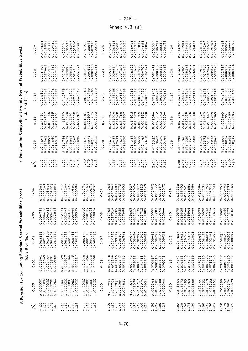
- 248 -

Annex 4.3 (a)

_ _"£oo

0).t:rzi_QOnO

<£"5E2 'o

"5 ^= o

£ u

?l*^Q.

OU

0*^

—_

*J^W

DU_

<

to fi ro rg CQ in to r~ o coto LA to co <— - in r- 4- in o

i> a) o ro 4 ^ m in .0 »r« m

• IM ^j eg r\t ,-« -HO o o oo o o o o o o o o o o

o o o o o o o o o o

4- ro o r-« o t> rg rH in in41 *O *i? p"i O g) (?> rn in O»

co ro 4- c/> co --» oo o o r- •-«rH aj r™ T r« r~- eg o ,u <o fg. i^j fsi Oj f\l »-t » - « O O O O

O O O C) O O O O O O O

O O O O O 0 0 O 0 0

O u3 <^ -0 aj o t« (XI rg

r— n) <^ aD . * - ^ »-< -o r~ i/\ or-* >& u\ IM Cj v() f J n) in i*-| rg

O O O O O O O O O O O

o o ooo o o o o o

*-«r-o iA.-H ino--«or^-

g> S 5 S o S ? ^ S S S

. INI INj CNJ •— * *— « •— ' O O O Oo o o o o o o o o o o

o o o o o o o o o o

£ S £ S 2 c o S S S SlA O o ^ c o c û c ^ l f ^ ~ ^ Û O »— < COr-n c^ ( \ iOh-<r or - inm--*• rgrgr\ j ' -*r-< f - i O O ^ O

O 0 0 0 O 0 O O O O O

o o o o o o o o o o

0 in i > .n 0 ^ ( , .n o >ni) y O r 1 it* t-- *"> (-J in r ("5 oj

-^ t J t J ' - - l < - J . - < ^-l t r - < < N J C X J

vO rvj in-O in •-*rvj ^o c~i

O O OO O O

O O O

J\ -H OO rsj Or\j ^u («ï^H O OO O OO O O

000

m 0 m

»-* in fM. < o oO O OO 00

O O O

-H 00 O

0 £ £

O O OO O O

O O O

rt !N Ino in r j^i O Oo • > oO O O

O O O

o in oin r- org <M m

en^••«Ooo

^omoooo

0tnoooI. )

ï<^

rt0oo

rtrH

Oooo

mrg

.<•,

•*.

O

rorg•

O

rg

c )

rH

4

O

0rg•

o

00 f)00 r-l

-r mn mo oo o

o -ra> inO 03in -jo\ mo o0 O

m aio m

ni f"i0 0

0 û

-t vO

S2t (<\O O

O 0

2 m-J 4"^-t OCO CO0 0

o o

o xno CM

o o

in co inO 4- rgO rH lA

co rg (MO O O

O O O

co r- inJO rg ro-0 O -0•-» r- «- *to rg rgO O O

O O O

in o- o^ a> coo m Oft CNI r\jO O O

o o o

0 su T-

0 J«

'NJ pg r-*O O O

O O O

? £g °vQ vO CT*r- ro coCNJ rg r-iO O O

O O O

o ^ om r- o

0 O -H

CO F~~i-H r~4

C7* tï*

r-* rH

O O

O O

CN< -Oin inCM 4"O rHr-4 »~4

O O

O O

m c\jco i>

i/\ O

O O

o o

CO COrH (N(

•-H r-t

O O

0 0

to Sf\l 0^ orH rH

0 O

O O

m oCN" iA

rH ,-,

O CO -Or-- co -4CO CO CO

O O OO O O

O O O

ON lA rH

r- o -r«A r~- r -t~~ 41 CNtO O OO O O

O O O

^> o in(V if\ *O

O O OO O O

O O O

a* rg co£ £ £

O O OO O O

O O O

!n ? 2>O r-H -

go -f rgo o oO O O

o o o

.r» o mr- r-j rg

*-< r\i rg

in r~-in (7>in r~-•--• o0 Oo o0 O

<> oO^ «Û^t r-r-< O0 OO 0

o o

rg .-.

-J r*-

0 00 0

0 O

j- rgS r^

0 oO O

o o

rg co(T^ >O

r-( 0

O O

O O

o o

o inin r-rg rg

*tCO

oooo

_r-r*^OO0

O

^_

enoooo

m

Sooo

rg(*ïoooo

oom

c*\r-^H CT*O rgO •O 0

0

1—o^ COO rg0 •0 O

o

rg

*-« r~o rgO •O O

o

-0

s so •0 0

o

Jtr~i in

o rg3 •o oo

inIN

ro,

m o"itN OO \n

? To o0 O

r-. 0in co<f o(A rj-J ^t0 o

0 O

^ ^

O^ gD<-i O

O O

0 O

^ -

5 rg

<J ro0 0

O O

° g?

C^ r~co r~r"\ n~iO O

O O

0 O rj

O 0

o* oo in,n -o

t r".O O

0 0

cn -rg gDrg inco rg<n m0 0

O o

cr> 0rg f-

Ï ^

O O

0 O

00 O

2gm eno o0 0

S 2m c\j-J om rgo o

0 0

o mm r-

O 0

aor~CO

rgoO

,_,rgOgDrgO

O

~a>r\£

oo

gD

rg

rgO

O

O^t*1rgO

O

0

0

^

in r-tn -T

o grrg --iO O

O 0

rg o0 ,-H

in r-O ro•-* r-t

0 O

O 0

-J 0

a) c"i

0 O

0 O

ON t<-l

sisr-i --<o oo o

s ?in enr- rgt— i ^-*0 O

o o

^ 0rg in

rt r-.

rg rg rg *o -^en r- <n

O O OO O O

O O O

r-i <n mt o •*

o in rge> tn enO O Oo o oO O O

0 .1 00-n rg 4

a> in enO O OO O O

O O O

r- .0 ON

ICNOO O OO O O

O O O

£ 5 5r— < O 0s«co in INIO O Oo o oO O O

xA 0 lAr- o fNil fN, CNl

r- r- 41 o^rH C\J 4 <?x

rH O O OO O O Oo o o oo o o o

r- (NI CN) 4*^ O *O ff1P~ O 41 «—*rH O O Oo o o oo o o oo o o o

M3 r- rH 0

-H r~ CNI co» - « O O Oo o o oo o o oo o o o

ro rH (y\ ~f

UD CO ? rH

O O O OO O O O

0 3 0 0

0 rî ?gD 03 m »-H^-i O O OO O O Oo o o oo o o o

o in o inin r- 0 rg

rg rg en <--,

. __ , 4" i<\ r-4 -JJ fjij at O O m o O i T ï INI »-* O O O ( N l C O - O f ^ ^ O in \OOt> 'H ^ O r ^ « - l O -t « H J - i A - O f O O r H f ^ O r - - C ^ - J f M ' " **,• o -i j^in-tr^ t\j CM . < o o o o o o o - j -o i tN ioco o^n^Hr - i o o o o --* c N j ^ c ^ - o m o r ~ - - j c N » - i < ^ o o oC • O O O O O O O O O O O O O O • f - n * - * ^ H ^ O O O O O O O O O O « <N| fNI r- t , - ! «-1 r ^ O O O O O O O Oo o ooooo ooooo oooo o ooooo ooooo oooo o ooooo ooooo oooo

" ' ooooo ooooo oooo ooooo ooooo oooo ooooo ooooo oooo

f*- rg »HI o o*> co -ï" co <j" r** *—* o in (NI o "H o co o^> o <~H fo r-* o IA co -^ *u f - co -^ o »^ r^~ ro «~H iA «-« co IA INJ o4" 4" 4" c1 eg rg «—> «—t oo oooo o CNI eg *—* o* i*- IA j* rg rH r-t oooo *—* o o^ co IA rg o^ «o *d~ eg. •—* o o o oOOOOO O O O O O OOOO • »-H rH ,-< O O O O O O O OOOO * rgr-i.-i«-«'-« O O O O O OOOO

£ o ooooo ooooo oooo o ooooo ooooo oooo o ooooo ooooo ooooooooo ooooo oooo ooooo ooooo oooo ooooo ooooo oooo

o§ - co LA O rg o

^0 oo co o o co in co co co in -3~f"-tn r—* rg co >-* o^ <i~ co o 0s O co coin rg; iA o eg gD eg o r~~ co co 4" 0s eg eg o t7*

c£. O (O (M fN) CNJ rH .—* »-H O O O O O O O O r-i O O co O in ro eg «-H O O O O O rH o CO "-Û *3" ""H CO -O -t eg t-H O O O O.£* *"- • O O O O O O O O O O O O O O • rH rH O O O O O O O O O O O O • r-H r-t rH rH rH O O O O O O O O On H~ o ooooo ooooo oooo o ooooo ooooo oooo o ooooo ooooo ooooB jY^ ooooo ooooo oooo ooooo ooooo oooo ooooo ooooo oooo

.> Vco "7;-U i—i io -j «—i in o^ r*™ -4 u~i r^- o g3 CQ co co 4" ^o r*~ eg co eg, o\ co r*~ h- gj «A oo r*~ co o r*~ in co in co rH t*\ F— r—i o f*~

^: o r-^^r-4»-to ooooo OCDOO o oo^cor^m -tcni\i.-«o oooo »-* r--o*nroo r-mc^rgr-H oooo;j # O O O O O O O O O O O O O O « O O O O O O O O O O O O O O * r-t^H^H^-t^H O O O O O O O O OQ_ O O O O O O O O O O O O O O O o O O O O O O O O O O O O O O O O O O O O O O O O O O O O OC O O O O O O O O O O 0 } 0 > O O O O O O O O O O O O O O O O O O O O O O O O O O O Oo

O O O O O O O O O O O O O O O *-» *o go o •-« coor - - * " -« c O r - 4 0 o o (^ fvcoc* i in ^-i-ir^tni-^ o r ^ - r C T »»*. O O C) O O Ou OOO O O O O ino^otNi tnr - - r -4r -c^ - t c o c o s t g o r - c > g D O ^-n-Hcnin ovnr- r -_ O O O O O O O O O O O O O O O * r> C h r - O O C O v O i A r - O ^ O c ^ ^ - * O O O o o r a a - C > J D (N(^Hj-r-*tNI v O r ^ ^ O~ O O O O O O O O O O O O O O O o r ^ r - r - x o j - c n o g ^ r n o o o o o «- t ^n incn-- to r ^ tn tncMf -» o o o o° • O O O O O C ) O O O O O O O O * O O O O O O O O O O O O O O • r-t.-«.-«^-«O O O O O O O O O O— O O O O O O O O O ï J O O O O O O O O O O O O O O O O O O O O O O O O O O O O O O O O O O Oc Ooooo o o o o o o o o t i ooooo ooooo oooo ooooo ooooo oooo

y.

4-70

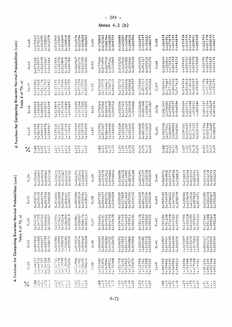
- 249 -

Annex 4.3 (b)

• — ;•

^0u

-.t:7nO

J3O01

"5EoZoo0

iäDlC*^

DQ.EOUL.o

*»-couCD

LJL

<

0-T*

O

CO-4

O

"n"w r--_-- **"* 0

*OCÜ

^5° gD

' — -J'^o

in"o

n) yfjG

cn r- in*r\ rH rorg o cnr- r- -oo o oO C") O

in r* oCM r- oCM co rgrH co rgr- g,) -oO O O

O o o

^ a) -DCM r\j r-o -o • <v/- r- ' •<g;) g;> -oO v i o

O O O

co co rg•-H gD insO CO Oa) gD O

o o o0 vJ 0

C_TV LU eno o -HCM O Or- LA cogD vO 'n0 O O

0 O 0

O iA C)o *"* -no o o

f— Oo f—iA enm rg

0 O

0 0

r- -tco corg rHLA JO o

O O

f- o•i) U>r- cf\•-* o• A .4D O

o o

r- coeo gDco rg0 0

0 0

O 0

CO f-Ch -tCO iAO^ 0s

•t COO O

O CD

iA Or-~ o

o rH

iA »H Qv•4- o -reo gD oen r\i *HO O O

O 0 O

41 O iAiA r~~ «Aco in coo -HI cn01 (M r-*

C) 0 O

o o CD

.n to gDi J i(li o g)y , i cn1 (.J r-C

J ( ) O

O O O

O- O co-4 rH lA

a> r- -4"O C) (O{-, i ( g ,HO 0 0

o o o

•i) .H lA

to r- <rm (n CMo* o eoCM rg rHo ; ï oO O O

.n < * mrg if> l*-

QS COrH COvA COCÜ -*O OO O

O 0

O rg.-4 co•4 r-CO -4o oo oo o

01 t«-.O IMrg r-lo j-C) 0C > 0

O 0

co cnco gD

(O -tO o0 0

O o

lA rH

gj OC) vOco -j."> Oo o

C) O

o mO C\J

-4- -t o mr- oo o gjiA rg gD CM<M rH O O

O 0 O O0 O O O

O O CD O

r^ rg iA rgst r— Q~> OtA rg iA CMrg r-« c > oO 0 0 o0 O O 0

O O O 0

0 ON C. ON*-< lit O% .A

U-, ig iA (MC J r 4 t > O

<> o o oo c» to

0 O 0 O

§ <r 5 ÎAst rg iA rgrg «-t t ) OO O '.-> v)O O O O

O O J O

O« rg O iniA O1 P- iAst rg u~\ rgrg rH O Oc > O 0 OCD O O O

O O O O

"C> »n t » <t\«n r— > rg

r,j m <n

»in*o

enin

O

*M>«O

,_<in

0

oin

o

m mo o00 .-<

r- r-0 0

o o

-o J-«u p-in or— >jr- r-0 0

0 0

to iArH --fC\ —

? ?

O D

O O

o gDNÛ gDO m

r~- r-o oo o

rg r-r- cn

r- r-o oo o

O 'n0 ™

0 O

>f fO Og3 O rgr- o r*-OO CO lAgD iA -4*O O O

O O O

O rH O«— < -4" gDr- .-» or- r- ingD iA sto o oo o o

f- o osj r - •-*gD rg .j•O vf) »T-fl iA J-O vJ O

o o o

en Ch rgr- co -41

LA eo r^iA lA COO iA ^4O O O

O O O

O CO lACO CJS vO-4 -J O

gD iA <fO O C">

O O O

O iA C>in r- f>

O 0 r-t

if\ r-ao ogD rgm mft\ f\jo oo o

rg vOcn -<rg ChcO rgco rgO 0

o o

rg chf- t-tf"- gjrg rgen rgc> o

O 0

<f in0 .-«en enrg rgm CMO 0

0 O

co gDrg Oco o

eo rgO c,)

0 0

in oCM iA

rH

gD O ^J\ CM Of> O 0st c« in^-•00o o oo o o

en gD *Qco rg -41

r~- er* o4 co IA^00o o oo o o

vu co r~o rg og] ul Ovj ui -ro o oo o o

iA CO *Org rg -4"4 r— o^ co <t^00o o oo o o

Ch iA COen rg o«rg gD co

r-H O O

0 0 0

O O 0

in o (nr- o rg

r* rM rg

in r-0s r*\•o cnesi «-HO O0 0

O O

co r-r^ rgg> cnCM r-*

o o0 O

o o

O T-in •-«•u nirg r-tO 0CD O

o o

fM OgD mrg rH0 OO O

0 0

o ino ovO <N

0 00 0

o o

O J~\LA r-rg rg

rg f-«CM r-vO rgO OO Oo oo o

co Or-H f*-

gD rgO Oo oo o0 0

4" CO-4 vu^O r\jf j OO OO O

O O

o r-g3 rgO ^>O Oo o^> o

iA iAo gDgD rgo o'} OC) O

o o

O (A« ; rg

CO CO

tfS i-4 O^ iA O

^in•

O

co»A*

O

r-tA

O

gDlA«

O

iAin•

o

ro *A »*"co o co^f i— i mco co r-o o oo o o

o ^ gD.t f-* r-«o co cocn o CMco 03 r~o o oo o o

cn r- -jin gr> o-J vß ajrg er •-«CD r- r-0 C J O

O O O

^ O -tfM iA COr-1 CO Oco r- r-o o o000

o — r-ro <r oO cn coO f*~ 0s-co r~~ gDo o oo o o

O »A OO rg in

O 0 O

gD c*\,-t coCM co-O -T0 0

0 0

(*> cOlA COf ï CMt-t COvO -I

o o0 0

O com r-<«A gDO r-

CD O

O 0

0 v>

gD oo gilA <J"o oo o

lA .-Hin gDco coco gDiA ^4"o oo o

tn or- oO -H

09 ^ gD r-H ÖDm r^ .A iA oco in r- -ï rotft vT in O VAf\ rg i~t o OO O O O O

O O O O O

rg rg -41 O COrg f-t o r*- go-4" co gD co rgiA ^J iA O inm CM •-* o oo o o o oo o o o o

r> .n co r- r-O -4 -t 0) rgO^ O -4 f^J *N4 ^ iA O if>rn rg •-* O Oo o o o oO O O O O

gD r- co o coin r- CM CM •-*j- en LA o inc*i rg ^H O OO O O O O

O O O i O

r~i rg -j CM oco 0s CM *—• ^J

-4" CO iA C> iAco rg rH ,j oo o o o oO O O O O

UV O iA O iArg iA r*- "> rg

^H r-i r-* rg rg

fl 00 CO f""o> r- r*i r-i - m vQ rgrg <-. O OO 0 O OO O O O

0 0 0 0

lA O iA -Of*- r- rO r-f- co g> rgCM '-< O OO 0 O OO O O O

O 0 0 O

gD cn rg ^iA gD ro r-p~ (O gD c 4

o o 6 o0 CD 0 0

0 C) O C)

cn iA rg r-r- m vu rgrg •— * C5 OO -D i OO O O O

C? O .J O

gD vO IA m— « 4- fM f-r— m o rgrg ^ O Oo O ') OO 0 0 O

O O O O

o >A o g^iA r- c j» r>4

rg r-j m cn

. — ."coot/l01

""

1Hooa.~5E0 0Z ^^* P "

3 ^*-"C O0 tu>CÛ —

O) oE ^""5aE0U

o<•*>

coucu.<

-teo•0

cnm•o

CMCO*

O

rH

CO*o

of)

0

*/

*— » r— u)gj t/1 rHr-i <t ajrg O iA«A in -4-0 O O

O O 0

O LA cnm rH r-t- rH lA

o r> -4-LA -4 41

0 0 0

000

rH LA O

O eg rHrj r- m«.T» r- en-4 J -4"O 0 O

O O O

cn -u r-<r rg iACO CO Or- vu rgvT -T -4O O O

o o o

r- au f-a) ^ 4 <oc*\ y r--O 4 O-J- -4 -4

000

O "V DO ' J 'A

en ogD LAO OUJ r-t

10 cnO 0

0 O

gD iArH CO

O rgr- oen eno O

O o

CM r-vO O•o -t-o o-tn rgO O

O 0

0 r-<t> r—r- LAiA COro rgO O

O O

co CQrg r-jr- r-•4" r^>n eg

O O

.n i »"( • 0

r-i fM ^() ü"\ r~m .-o o ^) coCM rH ^^ 0 O

o o o o oo o o o o

r-i O -O r-t COO m O r-4 OsO co st -4- r-rg LA o vu cnrM rH r-H O O

O O O O O

O O O O O

•t -t CM co inO 4" *-H rg *or-< in o -o <ofNj •— l rH O O

O O O O O

o o o o o

r~4 co e1"! rg gDco O r-- er« rgCO O CO O iAr-4 lA O> vQ COOJ rH O O OO O O O O

O O O o O

r * CÜ O^ O' -4

-O f-- O r-j (Of a\ I/T (j* jC* <J O> iA cOCj •-* > ) O

0 < 1 O 0 O

K » • 1 il i t J ii-i

i i m t - < j

O O lA rHiA t O rgO Oi -t rgCM. *-< O O0 O 0 OO O O O

O 0 0 O

gD O" -u r~O rH CO rHO o -4 rgrg r-i o oO O O OO O O O

O O O O

rH r- vD eovu o> r^ *-HON {J« J CMrn O O Oo o o oo o o oO 0 0 0

<f <t iA Orn r~ o oO O -t rgrH O 0 Oo O 0 OO O O O

0 O O O

gD r-t in ^vO iA iA OCO a- -t rgrH 0 O O

0 0 0 0

o o o o

r > KI ) .Ain r- o ( j

co•o

coco*0

r-cn•'o

vOco4

o

iAro

«

(*1 lA CM ÖD O

rH rg ch O OON f~- rH st VA

iA iA lA -t CO,o o o o oO O O O O

f~- Is- rH lA fj*

0s eo r-t g3 iAr- o r- o rgr~ in o co stm m in <t coO O O O O

O O O O O

rH rH rH rg Oo t> o iA r—st in IA o -4"v(j st O rg coiA if i t -4" eno o o o oo o o o o

r in CM «H cov> ro co eo r*Ch rg rg o gD<t co co rH rgiA iA st st cnO O O O O

o o o o o

Cn <— « ^ rH COco r IA o gDLA CO O O U5m rH r- O rH

iA iA <f st rO

o o o o o

O i^ O iA CDo ' i "•> r- • .

co o IA m coO^ rH O CJ^ CO

O rg t> rg «-tvO to rH r— 4"rg rH r-H o OO O O O O

o o o o o

en Ch vO <f rgcn rg gD iA *•"<iA CO vQ r-l *-Hin r- rH i - -tCM rH rH O OO O O O O

o o o o o

rH CO CO rH -JrgD J- CM rH CO

O 4" -T O O

CM rH rH O OO O O O O

O O O O O

rH O lA vO -4"

co IA r*- gD incn o -H co ost r- t-t gD eofM rH rH O O

O O O O O

O O O O O

IA rg co r- CMo LA rg rH r—r^ sU o r- cotn gD O gD rorg rH rH .D O

0 0 CD O 0

rg ni r- o rg

-t r- co t>IA cn cn eo

rg rH o OO O O Oo o o oo o o o

iA G"- O gDrH rH eO COrg rH IA rgrg rH O OO O O OO O O O

O O O O

r- o rg en*H rH LA rgrg rH o OO O O OO O O O

O O O O

lA rH CO- OCO CO rH CMfH o IA rgrg rH o oO O CD OO O O O

O 0 O O

tO rH IA lAO sO O rgO o in rgrg rH O 00 0 O 0

O C) O O

CD U". CD U-i*n r- o rg

1*

O

en,j-•o

rg•4"

O

rH

<J-^

O

o-

*

r-l CO lA O f^

o co r^ cn coIA to r- co covO vO IA •& enO O O O O

o o o o o

co o* «~H CM o**cn rg rg o r-•O iA vO C7^ O<}• rg vO p*- cogD gD iA j- eoo o o o oo o o o o

-4" O co iA rgco co iA rg eorg rg <j o coco '-* LA r- f-gD ^O J\ -4" cOO O O O O

O O O O O

r- rH IA co gDCM rg co ^ r-O* O* rg O iArH Ch -4" gD gDvO »A lA •& COo o o o oo o o o o

O rg eo (O rgiA O O gD •—<IA gD r-< o coO ro eo iA iAgD iA iA f cO

O O O O O

o *n I'D >A oo ''g m r- o

r-< CM c'l -4 roCO O O Ch iAco o m r- ^j-CM rg r-i o oo o o o oo o o o o

gD iA -O O *Hco f*- i— « rg f^rg vu co co -4-co o~> rg r~ -4~rg r-< r-C O Oo o o o oo o o o o

O co LA co cOin r-t o- o or- co iA vO ~jr- o rg r- <jrg r-* — « O OO O O 0 O

o o o o o

r- -j o ro coO in p- vO eor\j O co LA cnr— co CM f^- *4:M — i *-« o oO O O O O

O 0 O 0 0

vO lA O O r— <iA co -4" cO vOgD in — • ^J rMO co rg r~ 41

O O . ) O >

O O O O O

LA t. j if > C J a~irg «A r~ • ) rg

co oo cn cnrg rH r- inJ CM tA rgCM r4 O Oo o o oo o o oo o o o

iA eo r^ OO O gD iAcn rg LA rgrg '-* O oo o o o0 0 0 0

O O O O

rg co O oo•-O co gD •4>

eo rH ! \ rgrj rH. o O0 O 0 OO O O O

O O O O

r ^H to iArg r- in -4-m —H in CMrg rH o OO O CD OO O O O

O O O O

•—t iA gD rgO iA -41 •&rg rH iA rgrj -H O OO O O OO O O O

o o c; o

, 1 iA > >l\u\ r- ï rg

4-71

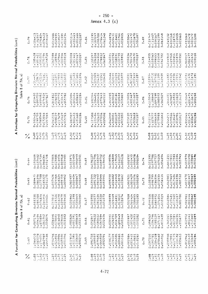
- 250 -Annex 4.3 (c)

"™T f-

I ö

VIv

•% *s0 0a.

~äE _

Z -c P

"5 v- °

1 -cu —O) O.E •- £Q. °Eouo

*• iAC f~o •— oc3u.4 v

"I? ^c •0 0

roba

bilit

ies

{

0.6

3

a."äE _o aZ - ^-C vu

"a M- °•= o

2 1O) O

1 ^Eouo

**" oC 4>o

'£ c>

c3u.

o o o- r^ iA-H r-, O O O

o o o o o

CO r-H O .J COIM CM r-J C> fM-T o O r-- r--iA • — i f i iA CD

r"* r-l O Ci O

O O J O O

J in JJ . i IM

Î 'U l' t r-( I-J

10

34

30

C0

99

72

0 0

.03

93

82

C0

74

51

6 :

05

78

27

:

10

24

16

C

09

87

55

00

88

54

9 C

07

36

66

00

57

36

5 0

o o o o o

o in o iA oo IM IA r-- o

Û9

06

09

û0

67

48

2 0

07

87

39

C0

66

06

^ 0

05

17

38

1

08

94

75

00

86

39

6 0

07

77

88

00

65

32

0 0

.0

51

17

5 0

OB

33

3G

0

.0

35

30

0 0

07

66

26

0Û

64

54

6 0

.0

50

60

** 0

.

o o o o o

go -t -J CM <fr- O iA go rvj

f- -4" LA en Oco co r- \o \r\O O O O O

o o o o o

O CO , — i 0"% O•—* r- r- go enO O CO o ^f

CO CO r- gD -4o co o o o0 0 0 O C)

O 'f O LA OO r-j IA r- O

0 „» 0 0 . -.

rg CO CC O j"\^ rvj rH -H OO O O O O

O O O O O

CO -O -J ^Û CO

en iA o IA cor-j co r~ o »A

O C ) O O O

0 O «. J O O

«'. . «> u C)

r-i n co u (O

O i > •• > ( j O

04

)81

2 7

02

82

03

:0

17

77

0

;0

1C

47

3 :

OC

57

82

C

O -. J O 0 O

IA (?"• co o <nrH CM r- CM go»A co ^o -4 r-r--« co r- o «A

o o o o o

O O C) O O

lA O iA O *ACM LA F-- o rg

03

78

05

10

15

80

0 1

01

64

56

10

09

81

8

20

05

48

5 2

03

74

26

0.

02

55

66

00

16

32

4 0

00

97

50

0,

00

54

52

0.

o o o o o

O O CO O co~ï f\J CO f— r-*O <• 1 rt -û <f

m r\j r-i o OO O O O O

o o o o o

*û • — 1 CO *O f*%<f co 4" O co

m CM ^ O OO O O O O

03

62

46

00

24

83

1 0

..0

15

90

4

C0

09

53

0 C

.0

05

34

6 0

,

i ) 0 0 O O

in o IA o IAIM IA r~ r > IM

. 1 r l r-l IS) IX,

•—i *û O CO

m r-« o oO O O Oo o o o

0 0 0 O

co »-, r- h-O <û O coo >r *o c\jm r-t o o

O O O O

o o o o

r 1 II) J) . )

o r o rgin r 1 0 0O 0 0 l>

CC

29

94

C0

01

45

6 :

00

06

65

:0

00

28

6 C

.

00

29

87

C0

01

45

3 C

C0

06

65

00

02

86

C

o o o o

o IA o ,AIA r~ o CM

00

28

71

2

00

14

09

20

00

64

9 3

00

02

81

3

00

28

57

00

01

40

4 o

00

06

47

0

00

02

80

0

00

28

42

0.

00

13

98

0

00

06

45

00

00

28

0 0

,

o o o o

\Û ,-1 cn OIM o -J r-f\J .-, 0 Oo o o oO O 0 O

0 0 0 0

O lA O COr-i co <r r-CO tn *JD CMfM r-i O OC) 0 0 OO O 0 O

o o o o

o in o inin r- j IM

co

o

meu

O

fMa>

O

r-«CO.

O

oCO«

o

o

o

00•ao

r-•oo

oo

in-oo

in r— co <T coo a- o ~i ~»

•-H O O* p— ><3r-1 ~> o o o0 O O O O

r-- CO O IM r~

CM CM O CO COO *O -f co O

— ' ri O O O

0 O 0 O O

tn m .-i CM vT

10

S3

54

C.1

04

40

1

00

93

40

6 C

07

76

43

C0

60

02

2 C

10

73

88

03

03

48

4 C

09

26

20

00

77

03

6 C

05

95

98

C

o o o o o

O f* o in oo c\j m r- o

09

61

27

00

92

75

6 0

06

33

47

0.0

69

76

2 0

05

44

21

1

09

50

44

00

91

72

2 0

08

24

45

00

69

04

6

00

53

90

1

0

09

39

50

00

90

67

7 0

.0

81

53

4 0

06

33

20

0.

05

33

73

0

o o o o o

f~- CM IM -T *O<}• rsj r-t co en

c*j o o r~ njo« co co vO ino o o o o

.09

17

33 0

.0

88

55

7 0

.0

79

68

1 0

06

68

39

0.

05

22

91

0.

il O 0 O O

o IA o in oo rvj in r- ot > l ) O O rH

r- m o -û om o* co o in

o o o o o0 O O O 0

^1 <\J r-H in CM

(M O rn r^ Cr*r- i j m **- com CN co o in

o o o o oo u o o o

i^ (>v a) O in

t> 1 1 c ) O O

04

32

05

C.0

29

00

2 C

.01

81

84

C

01

06

68

00

05

86

5 C

.

04

29

39

C0

28

85

1 0

01

81

07

00

10

63

2 0

00

58

50

0

o o o o o

iTi O lA O iT\r\j m r~ o IM

03

95

94

10

26

88

9 1

01

70

63

10

10

12

7 2

00

56

28

2.

03

92

50

00

26

68

2 0

01

69

48

00

10

07

0 0

00

56

02

0

03

88

99

00

26

46

9 0

01

68

31

0

01

00

10 0

.0

05

57

4 0

.

o o o o o

nH 1-1 O <7* O

-ï in o <t <r

m IM f-* o oo o o o o

03

81

77

0.

C2

6C

28

0.

01

65

85

0,

00

98

85

0,

00

55

16

0,

0 0 Ci 0 O

lA O ,n O lAIM in h- ci r\j

ri .-, ,-< (M IM

r-H Cvj O r—-ï c*- ^ co

f" -i O 0o o o oo o o oo o o o

•O O O f^<*°i r r*~ coO \J *Û IMm 1-4 o o0 O O O

< > o o o

O *J -û fMfn '-i O O

o o o o

.00

30

26

00

14

67

00

06

69

00

02

87

,

00

30

20

O0

01

46

5 C

00

06

68

C0

00

28

7

o o o o

O IA O lAtn [— o rg

00

29

32

20

01

43

3 2

00

06

58

30

00

28

4 3

00

29

21

00

01

42

9 0

00

06

56

00

00

28

3 0

00

29

09

00

01

42

4 0

00

06

55

00

00

28

3 0

.

o o o o

r^ o co rgf> IM in cofM ri 0 O

o o o oo o o o

00

28

84

00

14

15

C.

0^

06

51

0,

0 J

0 2

8 2

C

o o o o

O lA O lAlA r~ i 1 fM

IM IM 01 m

CO«0

toCO

O

r~CO

o

CO

o

lACO

o

-Jr-o

oni -

o

r\ir-

o

r-•o

or-.0

iA *-i CJi IM rn

r< r-l O O O

O O O O O

lA tO ,A lA CO

*T O CO *~* fM

— •-< O O O

O O O O O

• ; c> o a, oo r- i> r-i <r

r< : 1 0 O 1 >

11

30

43

C1

08

84

8 C

09

71

98

0.

08

05

53

C.

06

20

29

C.

11

21

24

0

10

79

77

C0

96

45

8 0

.0

79

98

8 0

.0

61

64

2 0

o o o o o

O *A O lA Oo CM IA r~- o

10

13

93

0,

09

77

80

00

87

70

7 0

.07

32

05

0.0

56

89

4 1

.

10

03

60

00

96

79

5 0

08

68

54

00

72

53

5 0

05

64

16

0

09

93

16

0.

09

58

00

0.

08

59

92

00

71

85

6 0

05

59

29

0

O O O O 0

en o o r- unSU O^ fM O f*°\

CO ~t IA r-l lAfji CT* co r~- ino o o o o

C9

72

00

C.

09

37

81

0.

08

42

39

0.

07

04

69

00

54

93

2 C

O O 0 O O

o IA o in oO IM lA f~— O

l> 0 0 0 rH

IM CO lA *T\ Om J} r-H O SÛ

lA O CO O lA-I Cl -H r-< OO O O O O

o o o o o

O co -0 O Or-i ,4- i.-* r- in

J O 03 O lA

0 0 C) O O

o o o o o

I'l lA ^) (•> O.

^ IU l/l U C7>-f o> ai l. ,M

i> < ) 0 . l)

0444

51 :

.0

29

69

7 t.

01

85

33

:.0

10

82

50

05

^2

9 C

.

cn gD o o r~-

vt O CO O LAJ- CM —— rH OO O 0 O O

o o o o o

lA O LA O "AINI lA r- O rg

.04

12

11

1.

.02

78

51

1.

.01

75

83

1.

.01

03

84

2.

.00

57

43

2

04

09

01

00

27

66

9 0

01

74

86

00

10

33

6

00

05

72

2 0

04

05

84

0.0

27

48

1 0

.01

73

85

0.

'J 1

0 2

8 7

0

00

57

00

0

0 0 O O O

vO co co m r^o r- r- o in-J fM r-l r-« O

o o o o o

03

99

30

C0

27

09

1 0

01

71

73

001

U 1

82

C0

05

65

3

C) O O O O

lA O in o IAfM iA r^ Cl IM

r-i t H . 1 (N IM

O 00 CM CO»O r— r— co

m '-• o Oo o o oo o o oo o o o

r- r~- (M colA f- Is- CUO -J -O IMm r-* o o

o o o oO t) O Ö

in *j r* a>

1<1 r- . O < )

*. ) O O l J

00

30

49

:.0

01

47

5 C

.O

C0

67

1 1

.0

00

28

8 :.

00

30

45

00

01

47

3 0

.0

00

67

1 0

.0

00

28

8 0

o o o o

O iA O iAiA r — O fM

.00

29

79

2.

.00

14

50

2.

.00

06

64

3.

.00

02

86

3.

00

29

70

00

01

44

7

00

00

66

3

00

00

28

5 0

00

29

61

00

01

44

4

0.0

00

66

2

0.0

00

28

5 0

0 O O O

f\J r-l O IT>

r-l r-l O O

O O O OO 0 CI O

OC

29

42

00

01

43

7 C

00

06

59

C0

00

28

4 C

O 0 0 O

O , A ("J iTiUN l— , IM

IsJ W IM in

4-72

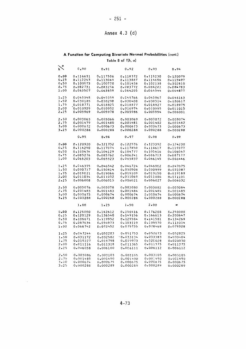
- 251 -

Annex 4.3 (d)

A Function for Computing Bivariate Normal Probabilities (conf.)

Table B of J{h, a)

0.90 0.91 0.92 0.93 0.94

0.000.250.500.751.00

1.251.501.752.002.252.502.753.003.25

0.000.250.500.751.00

1.251.501.752.002.252.502.753.003.25

0.000.250.500.751.001.251.501.752.002.252.502.753.003.25

0.1166310.1122430.1000730.0827310.0635070.0453480.0301850.018771"0.0109290.005969

0.0030630.0014790.0006720.000288

0.95

0.1209200.1162900.1034740.0852760.065203

0.0463550.0307170.0190210.0110340.006008

0.0030760.0014830.0006730.000288

1.000.1250000.1201290.1066710 .0876340.0667420.0472440.0311720.0192270.011116O.OU60380.0030860.0014850.0006740.000288

0.1175060.1130690. 1007700.0832560.0638590.0455590.0302980.0188250.0109520.0059780.0030660.0014800.0006730.000288

0.96

0.1217520.1170740.1041290.0857620.065523

0.0465420.0308140.0190660.0110520.006015

0.0030780.0014830.0006740.000288

1.250.1426120.1365400.1199520.0969730.0724520.0502830.0325820.0197980.0113180.006100

0.0031030.001490Ü. 0006750.000289

0.1183720.1138870.1014580.0837720.0642050.0457660.0304080.0188770.0109740.005986

0.0030690.0014810.0006730.0002880.97

0.1225760.1178500. 1047770.0862410.065837

0.0467240.0309080.0191090.0110690.0060210.0030800.0014840.0006740.000288

1.500.1564160.1491560.1295840.1031190.075735

0.051753• 0.0331340.0199730.0113650.00611 1

0.0031050.001 4900.0006750.000289

0.1192300. 1146960. 1021380.0842810.0645440.0459670.0305140.0189270.0109950.005994

0.0030720.0014820.0006730.000288

0.98

0.1233920.1186170.1054160.0867130.066145

0.0469020.0309990.0191500.0110860.0060270.0030820.0014850.0006740.000288

2.000.1762080. 1666130.1415810. 1095700.078468

0.0526730.0333830.0200280.0113750.0061120.0031050.0014900.0006/50.000289

0. 1200790.1154970.1028100.0847830.064877

0.0461630. 0306170.0189750.0110150.0060010.0030740.0014820.0006730.000288

0.99

0. 1242000. 1193770. 1060470.0871770.066446

0.0470750.0310870.0191890.0111010.0060320.0030840.0014850.0006740.000288

00

0.2500000.2006470« 1542690. 1133140.079328

0.0528250.0334040.0200300.0113750.0061120.0031050.0014900.0006750.000289

4-73

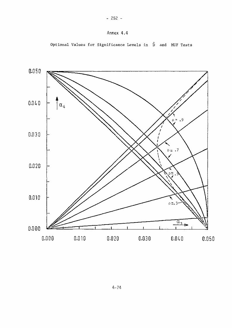
- 252 -

Annex 4.4

Optional Values for Significance Levels in D and MUF Tests

0.050

0.0 t

0.030

0.020 -

0.010

0.000

0.000 0.010 0.020 0.030 0.0/.O 0.050

4-74

- 253 -

Chapter 5

IMPLEMENTING INSPECTION PLANS

5.1 ON-SITE ACTIVITIESThe activities that are statistical in nature and that are performed on site,

i.e., at the facility, are those activities that relate to attributes inspection,using both the attributes and variables tester, and to variables inspection. Adetailed description of the kinds of activities involved is given in Section 4.2.The discussion in Section 4.2 does not address specific problems in implementationhowever. Such problems include the procedure for drawing a random sample, and themeans of establishing defect criteria. These topics are now addressed in Sections5.1.1 and 5.1.2 respectively. A third topic dealing with on-site inspection activi-ties is the construction of confidence intervals based on data derived from theattributes inspection. This topic is covered in Section 5.1.3.5.1.1 Drawing a Random Sample

It is important that items selected for measurement during an inspectionbe selected in a random fashion. Clearly, it is unacceptable to select only thoseitems that are easily accessible, for then the diverter would falsify only theitems that are not readily accessible. Nor should one rely on his own ability toselect a random sample; this is difficult to do without introducing some non-random features into the selection process. In order to combat the possibilitythat the diverter might anticipate which items are likely to be inspected, thesample should be selected by some random process. Some means for doing this areset forth in the next three sections. In each case, it is necessary that the itemsin the population be numbered serially from 1 to N, and the problem is to randomlyselect n from these N items.

5.1.1.1 Random Number Table^Random number tables may be used to supply random numbers. Annex 5.1 (a)-(e)

gives 5,000 four digit random numbers taken from [5.1]. More extensive tables areavailable [5.2].

Random number tables are simple to use. The procedure for using theAnnex 5.1 tables is given as Method 5.1. Clearly, Method 5.1 may be applied toany set of such random numbers.Method 5.1

NotationN = number of items in population to be sampledn = number of sampled items, with n<N

5-1

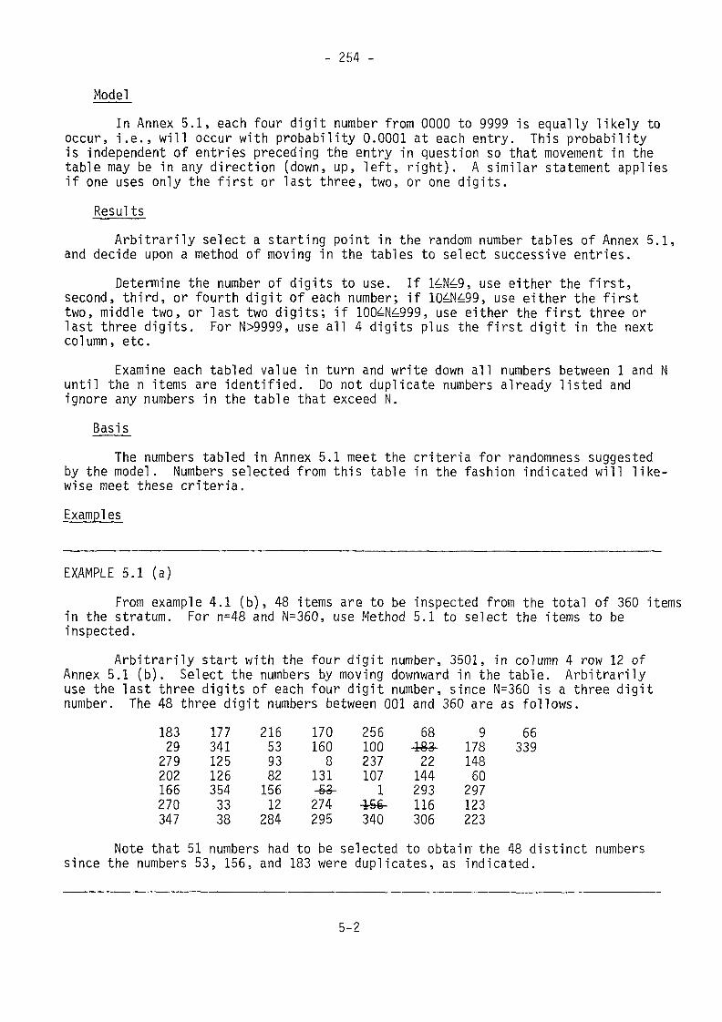
- 254 -

ModelIn Annex 5.1, each four digit number from 0000 to 9999 is equally likely to

occur, i.e., will occur with probability 0.0001 at each entry. This probabilityis independent of entries preceding the entry in question so that movement in thetable may be in any direction (down, up, left, right). A similar statement appliesif one uses only the first or last three, two, or one digits.

ResultsArbitrarily select a starting point in the random number tables of Annex 5.1,

and decide upon a method of moving in the tables to select successive entries.Determine the number of digits to use. If 1 N 9, use either the first,

second, third, or fourth digit of each number; if 104N499, use either the firsttwo, middle two, or last two digits; if 100 N 999, use either the first three orlast three digits. For N>9999, use all 4 digits plus the first digit in the nextcolumn, etc.

Examine each tabled value in turn and write down all numbers between 1 and Nuntil the n items are identified. Do not duplicate numbers already listed andignore any numbers in the table that exceed N.

BasisThe numbers tabled in Annex 5.1 meet the criteria for randomness suggested

by the model. Numbers selected from this table in the fashion indicated will like-wise meet these criteria.Examples

EXAMPLE 5.1 (a)From example 4.1 (b), 48 items are to be inspected from the total of 360 items

in the stratum. For n=48 and N=360, use Method 5.1 to select the items to beinspected.Arbitrarily start with the four digit number, 3501, in column 4 row 12 of

Annex 5.1 (b). Select the numbers by moving downward in the table. Arbitrarilyuse the last three digits of each four digit number, since N=360 is a three digitnumber. The 48 three digit numbers between 001 and 360 are as follows.

18329279202166270347

1773411251263543338

21653938215612284

1701608

131-£3-274295

256100237107

1-ie€-340

681Q9TUJ

22144293116306

917814860297123223

66339

Note that 51 numbers had to be selected to obtain' the 48 distinct numberssince the numbers 53, 156, and 183 were duplicates, as indicated.

5-2

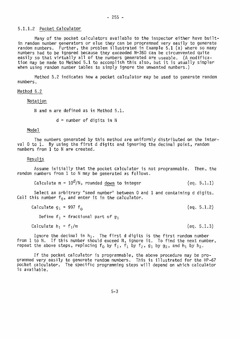
- 255 -

5.1.1.2 Pocket CalculatorMany of the pocket calculators available to the inspector either have built-

in random number generators or else they can be programmed very easily to generaterandom numbers. Further, the problem illustrated in Example 5.1 (a) where so manynumbers had to be ignored because they exceeded N=360 can be circumvented quiteeasily so that virtually all of the numbers generated are useable. (A modifica-tion may be made to Method 5.1 to accomplish this also, but it is usually simplerwhen using random number tables to simply ignore the unwanted numbers.)

Method 5.2 indicates how a pocket calculator may be used to generate randomnumbers .Method 5.2

NotationN and n are defined as in Method 5.1.

d = number of digits in NModel

The numbers generated by this method are uniformly distributed on the inter-val 0 to 1. By using the first d digits and ignoring the decimal point, randomnumbers from 1 to N are created.

ResultsAssume initially that the pocket calculator is not programmable. Then, therandom numbers from 1 to N may be generated as follows.Calculate m = 10 /N, rounded down to integer (eq. 5,1.1)Select an arbitrary "seed number" between 0 and 1 and containing d digits.

Call this number f0, and enter it in the calculator.Calculate gl = 997 f0 (eq. 5.1.2)

Define fl = fractional part of glCalculate h} = f^m (eq. 5.1.3)Ignore the decimal in h^. The first d digits is the first random number

from 1 to N. If this number should exceed N, ignore it. To find the next number,repeat the above steps, replacing f0 by fl5 fj by f2, Qi by g2, and hi by h2.

If the pocket calculator is programmable, the above procedure may be pro-grammed very easily to generate random numbers. This is illustrated for the HP-67pocket calculator. The specific programming steps will depend on which calculatoris available.

5-3

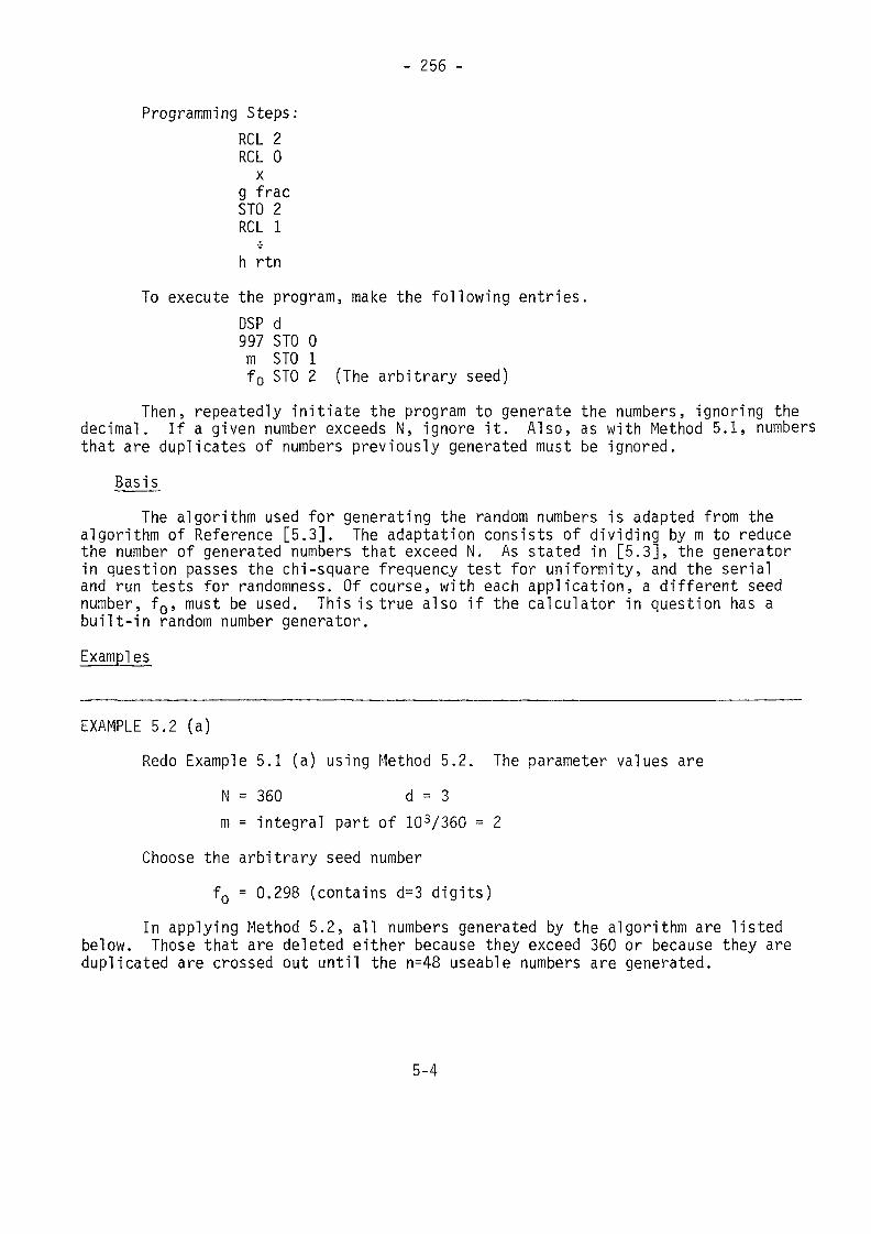
- 256 -

Programming Steps:RCL 2RCL 0x

g fracSTO 2RCL 1h rtn

To execute the program, make the following entries.DSP d997 STO 0m STO 1f0 STO 2 (The arbitrary seed)

Then, repeatedly initiate the program to generate the numbers, ignoring thedecimal. If a given number exceeds N, ignore it. Also, as with Method 5.1, numbersthat are duplicates of numbers previously generated must be ignored.

BasisThe algorithm used for generating the random numbers is adapted from the

algorithm of Reference [5.3]. The adaptation consists of dividing by m to reducethe number of generated numbers that exceed N. As stated in [5.3], the generatorin question passes the chi-square frequency test for uniformity, and the serialand run tests for randomness. Of course, with each application, a different seednumber, f0, must be used. This is true also if the calculator in question has abuilt-in random number generator.Examples

EXAMPLE 5.2 (a)Redo Example 5.1 (a) using Method 5.2. The parameter values are

N = 360 d = 3m = integral part of 103/360 = 2

Choose the arbitrary seed numberf0 = 0.298 (contains d=3 digits)

In applying Method 5.2, all numbers generated by the algorithm are listedbelow. Those that are deleted either because they exceed 360 or because they areduplicated are crossed out until the n=48 useable numbers are generated.

5-4

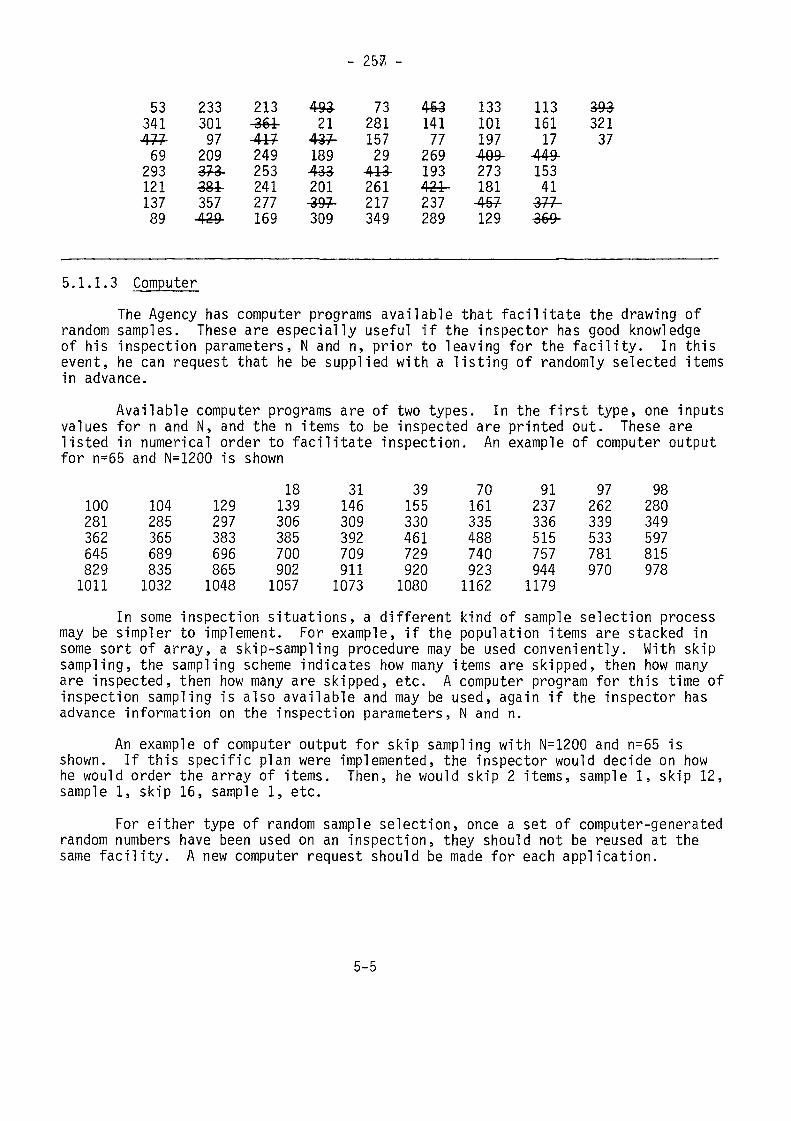
- 257, -

533414776929312113789

23330197209*5 r* O™OQl^OT '

357429-

213O ö T447249253241277169

493-21

437-1894-30I \J ±j201-397-309

7328115729

443-261217349

44314177269193237289

133101197409-273181457129

11316117

449-15341377-OgQou y

ono&y -j32137

5.1.1.3 ComputerThe Agency has computer programs available that facilitate the drawing of

random samples. These are especially useful if the inspector has good knowledgeof his inspection parameters, N and n, prior to leaving for the facility. In thisevent, he can request that he be supplied with a listing of randomly selected itemsin advance.

Available computer programs are of two types. In the first type, one inputsvalues for n and N, and the n items to be inspected are printed out. These arelisted in numerical order to facilitate inspection. An example of computer outputfor n=65 and N=1200 is shown

100281362645829

1011

104285365689835

1032

129297383696865

1048

18139306385700902

1057

31146309392709911

1073

39155330461729920

1080

70161335488740923

1162

91237336515757944

1179

97262339533781970

98280349597815978

In some inspection situations, a different kind of sample selection processmay be simpler to implement. For example, if the population items are stacked insome sort of array, a skip-sampling procedure may be used conveniently. With skipsampling, the sampling scheme indicates how many items are skipped, then how manyare inspected, then how many are skipped, etc. A computer program for this time ofinspection sampling is also available and may be used, again if the inspector hasadvance information on the inspection parameters, N and n.

An example of computer output for skip sampling with N=1200 and n-65 isshown. If this specific plan were implemented, the inspector would decide on howhe would order the array of items. Then, he would skip 2 items, sample 1, skip 12,sample 1, skip 16, sample 1, etc.

For either type of random sample selection, once a set of computer-generatedrandom numbers have been used on an inspection, they should not be reused at thesame facility. A new computer request should be made for each application.

5-5

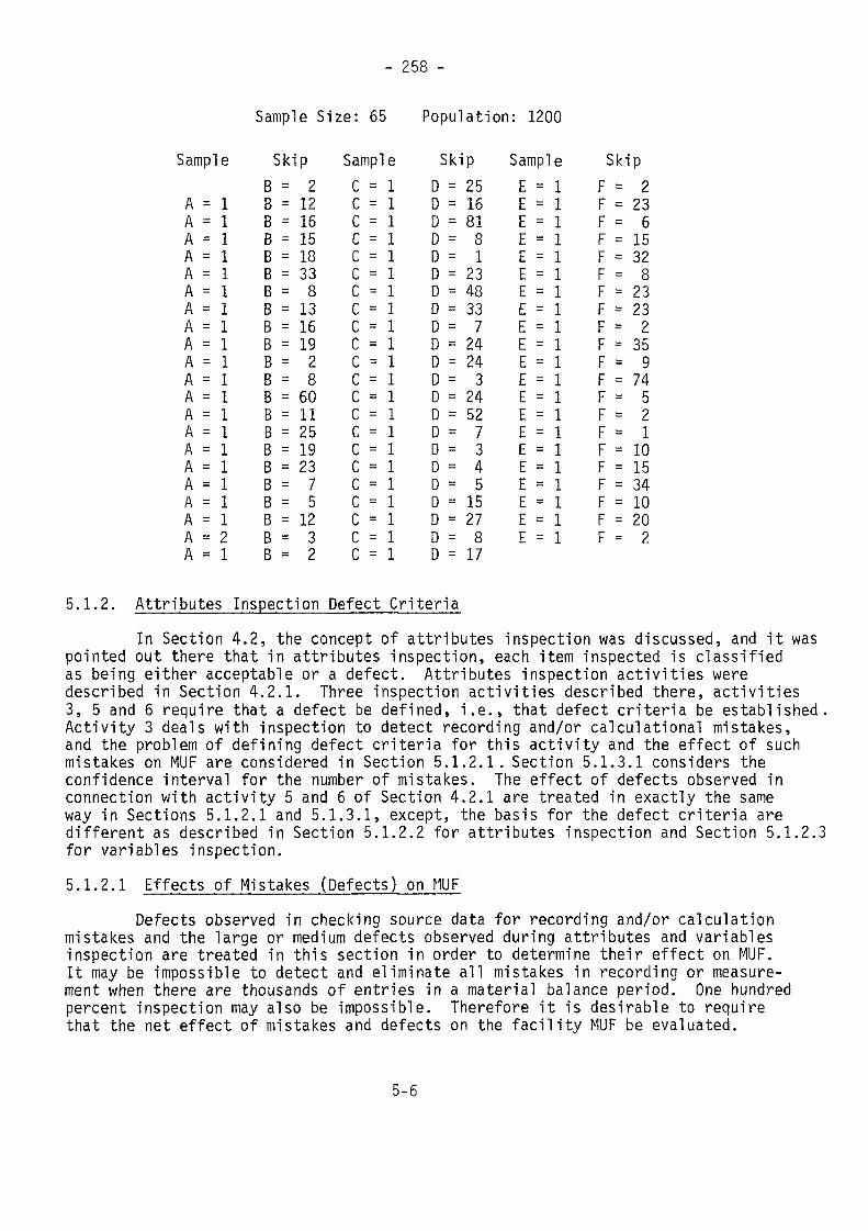
- 258 -

Sample Size: 65 Population: 1200

Sample Skip Sample Skip Sample SkipB = 2 C = l D = 25 E = l F = 2

A = l B = 12 C = l D = 16 E = l F = 23A = l B = 16 C = l D = 81 E = l F = 6A = l B = 15 C = l D = 8 E = 1 F = 15A = l B = 18 C = l D = l E = l F = 32A = l B = 33 C = l D = 23 E = l F = 8A = l B = 8 C = l D = 48 E = l F = 23A = l B = 13 C = l D = 33 E = l F = 23A = l B- 16 C = l D = 7 E = l F=2A = l B = 19 C = l D = 24 E = l F = 35A = l B = 2 C = l D = 24 E = l F = 9A = l B = 8 C = l D = 3 E = l F = 74A = l B = 60 C = l D = 24 E = l F = 5A = l B = 11 C = l D = 52 E = l F = 2A = l B = 25 C = l 0=7 E = l F = lA = l B = 19 C = l D=3 E = l F = 10A = l B = 2 3 C = l D=4 E = l F = 15A = l B=7 C = l D-5 E = l F = 3 4A = l B=5 C = l D = 15 E = l F = 10A = l B = 12 C = l D = 2 7 E = l F = 2 0A = 2 B=3 C = l D=8 E = l F=2A = l B=2 C = l D- 17

5.1.2. Attributes Inspection Defect CriteriaIn Section 4.2, the concept of attributes inspection was discussed, and it was

pointed out there that in attributes inspection, each item inspected is classifiedas being either acceptable or a defect. Attributes inspection activities weredescribed in Section 4.2.1. Three inspection activities described there, activities3, 5 and 6 require that a defect be defined, i.e., that defect criteria be established.Activity 3 deals with inspection to detect recording and/or calculational mistakes,and the problem of defining defect criteria for this activity and the effect of suchmistakes on MUF are considered in Section 5.1.2.1. Section 5.1.3.1 considers theconfidence interval for the number of mistakes. The effect of defects observed inconnection with activity 5 and 6 of Section 4.2.1 are treated in exactly the sameway in Sections 5.1.2.1 and 5.1.3.1, except, the basis for the defect criteria aredifferent as described in Section 5.1.2.2 for attributes inspection and Section 5.1.2.3for variables inspection.5.1.2.1 Effects of Mistakes (Defects) on MUF

Defects observed in checking source data for recording and/or calculationmistakes and the large or medium defects observed during attributes and variablesinspection are treated in this section in order to determine their effect on MUF.It may be impossible to detect and eliminate all mistakes in recording or measure-ment when there are thousands of entries in a material balance period. One hundredpercent inspection may also be impossible. Therefore it is desirable to requirethat the net effect of mistakes and defects on the facility MUF be evaluated.

5-6

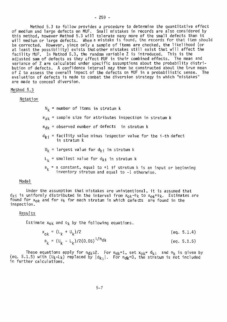
- 259 -Method 5.3 to follow provides a procedure to determine the quantitative effect

of medium and large defects on MUF. Small mistakes in records are also considered bythis method, however Method 5.3 will tolerate many more of the small defects than itwill medium or large defects. When a mistake is found, the records for that item shouldbe corrected. However, since only a sample of items are checked, the likelihood (orat least the possibility) exists that other mistakes still exist that will affect thefacility MUF. In Method 5.3, the random variable Z is introduced. This is theadjusted sum of defects as they affect MUF in their combined effects. The mean andvariance of Z are calculated under specific assumptions about the probability distri-bution of defects. A confidence interval may then be constructed about the true meanof Z to assess the overall impact of the defects on MUF in a probabilistic sense. Theevaluation of defects is made to combat the diversion strategy in which "mistakes"are made to conceal diversion.Method 5.3.

NotationNI,, = number of items in stratum k

nak = sample size for attributes inspection in stratum k= observed number of defects in stratum k= facility value minus inspector value for the i-th defectin stratum k= largest value for dki in stratum k= smallest value for dki in stratum k

Model

= a constant, equal to +1 if stratum k is an input or beginninginventory stratum and equal to -1 otherwise.

Under the assumption that mistakes are unintentional, it is assumed thati is uniformly distributed in the interval from x0k-6k to x0k+6k- Estimates are

found for x0k and for 6k for each stratum in which defects are found in theinspection.Results

Estimate x0k and 6k by the following equations.xok = (Lk + Uk)/2 ^- 5'1-4)U Is. Is. Is.

6, = (U. - L,)/2(0.05)1/ndk (eq. 5.1.5)

These equations apply for n^k^. For n<jk=l> set x0k= dkl and 6k is given by(eq. 5.1.5) with (U|<-Lk) replaced by [d^J. For ndk=0, the stratum is not includedin further calculations.

5-7

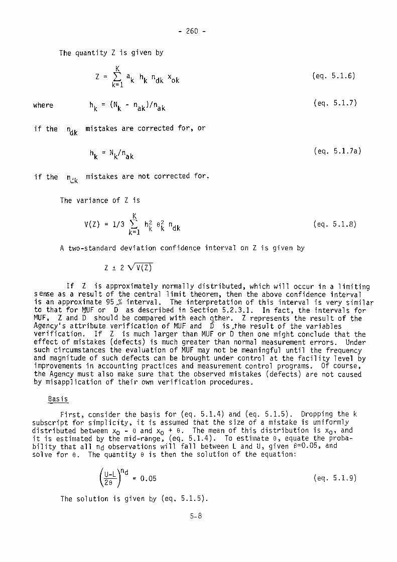
- 260 -

The quantity Z is given byK« ^

k * K K Q K OK=1where hk = (Nk - nak)/nak ^ec1- 5-1-7)

if the n,, mistakes are corrected for, ordk(eq. 5.1.7a)

if the n,k mistakes are not corrected for.

The variance of Z isK

V ( Z ) = 1/3 Y hj 02 nd|< (eq. 5.1.8)K~~ J.

A two-standard deviation confidence interval on Z is given by

Z ±

If I is approximately normally distributed, which will occur in a limitingsense as a result of the central limit theorem, then the above confidence intervalis an approximate 95 J, interval. The interpretation of this interval is very similarto that for MUF or D as described in Section 5.2.3.1. In fact, the intervals forMUF, Z and D should be compared with each ather. Z represents the result of theAgency's attribute verification of MUF and D is „the result of the variablesverification. If Z is much larger than MUF or D then one might conclude that theeffect of mistakes (defects) is much greater than normal measurement errors. Undersuch circumstances the evaluation of MUF may not be meaningful until the frequencyand magnitude of such defects can be brought under control at the facility level byimprovements in accounting practices and measurement control programs. Of course,the Agency must also make sure that the observed mistakes (defects) are not causedby misapplication of their own verification procedures.

Bas isFirst, consider the basis for (eq. 5.1.4) and (eq. 5.1.5). Dropping the k

subscript for simplicity, it is assumed that the size of a mistake is uniformlydistributed between x0 - e and x0 + e. The mean of this distribution is x0, andit is estimated by the mid-range, (eq. 5.1.4). To estimate e, equate the proba-bility that all nd observations will fall between L and U, given 3=0.05, andsolve for e. The quantity e is then the solution of the equation:

= 0.05 (eq. 5.1.9)

The solution is given by (eq. 5.1.5).5-8

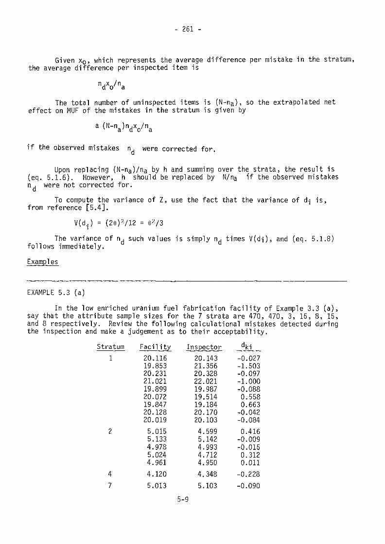
- 261 -

Given x0, which represents the average difference per mistake in the stratum,the average difference per inspected item is

Vo/naThe total number of uninspected items is (N-na), so the extrapolated neteffect on MUF of the mistakes in the stratum is given by

a (N-na)ndxQ/na

if the observed mistakes n , were corrected for.

Upon replacing (N-na)/na by h and summing over the strata, the result is(eq. 5.1.6). However, h should be replaced by N/na if the observed mistakesn . were not corrected for.dTo compute the variance of Z, use the fact that the variance of dj is,

from reference [5.4]..) = (2e)2/12 = 62/3

The variance of n, such values is simply n , times V(di), and (eq. 5.1.8)follows immediately.Examples

EXAMPLE 5.3 (a)In the low enriched uranium fuel fabrication facility of Example 3.3 (a),

say that the attribute sample sizes for the 7 strata are 470, 470, 3, 15, 8, 15,and 8 respectively. Review the following calculational mistakes detected duringthe inspection and make a judgement as to their acceptability.

Stratum Facility j n_sj3ector1 20.116

19.85320.23121.02119.89920.07219.84720.12820.019

5.0155.1334.9785.0244.9614.1205.013

20.14321.35620.32822.02119.98719.51419.18420.17020.1034.5995.1424.9934.7124.9504.3485.103

-0.027-1.503-0.097-1.000-0.0880.5580.663

-0.042-0.084

0.416-0.009-0.015

0.3120.011

-0.228-0.090

47

5-9

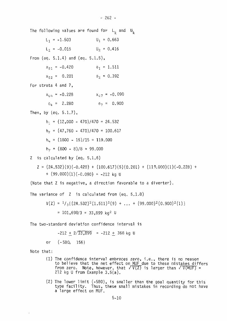
- 262 -

The following values are found for L. and U,L! = -1.503 Ui = 0.663L2 - -0.015 U2 = 0.416

From (eq. 5.1.4) and (eq. 5.1.5),x01 = -0.420 0! = 1.511X02 = 0.201 92 = 0.392

For strata 4 and 7,xolt = -0.228 XU7 = -0.09064 = 2.280 e7 = 0.900

Then, by (eq. 5.1.7),hx = (12,000 - 470)/470 = 24.532h2 = (47,760 - 470)/470 = 100.617h„ = (1800 - 15)715 •-= 119.000h7 = (800 - 8)/8 = 99.000

Z is calculated by (eq. 5.1.6)

Z = (24 .532 ) (9 ) ( -0 .420 ) + (100.617)(5)(0 .201) + (119.000)(1)(-0 .228) ++ (99 .000)(1) ( -0 .090) = -212 kg U

(Note that Z is negative, a direction favorable to a diverter).

The variance of Z is calculated from (eq. 5.1.8)V(Z) = V3[(24.532)2(l.511)2(9) + ... + (99.000)2(0.900)2(D]

= 101,698/3 = 33,899 kg2 U

The two-standard deviation confidence interval is-212 + 2v/33,899 = -212 +_ 368 kg U

or (-580, 156)Note that:

(1) The confidence interval embraces zero, i.e., there is no reasonto believe that the net effect on MUF due to these mistakes differsfrom zero. Note, however, that / V(Z) is larger than / V^UF) =212 kg U from Example 3.5(a).

(2) The lower limit (-580), is smaller than the goal quantity for thistype facility. Thus, these small mistakes in recording do not havea large effect on MUF.

5-10

- 263 -

5.1.2.2 Large Defects --Attributes TesterFor planning purposes, a gross or large defect was defined in Section 4.3.1

to be of size equal to the average element weight in the stratum, this weight beingdenoted by x|<. However, for many attributes testers, a discrepancy need not beas large as x^ to be detected, since detection simply implies that the tester hasdetermined that the facility value associated with the item in question is incor-rect, with high probability. As an illustration, if the attributes test involvestipping a container to see if it has the listed amount of material in it, thenquite clearly the defect need not be of size x|< (i.e., empty container) to bedetected. Quite likely, if the weight were off by, say, 50% or more, this wouldbe detected as a significant discrepancy, i.e., it would be classified as a defect.

The foregoing discussion leads to the following definition of a large defect.Definition: In attributes inspection with the attributes tester, a defectis a discrepancy between the facility and the inspector values that is larger than

Y |< x|< in absolute value.To further explain this definition, if the tester in question has an asso-

ciated error of measurement, then Y^ may be a multiple of the measurement errorstandard deviation. On a relative basis, let $^ be the standard deviation of theattributes tester. Then, Yk=4<5 would be a reasonable value for j since anydiscrepancy larger than 4 measurement error standard deviations is almost certainlya real discrepancy, one that cannot be explained as beinq due to measurement errors.This relationship between S, and yk assumes that the facility error of measure-ment is negligible in size compared with the inspector measurement error for theattributes tester. If this is not the case, then 8^ would be the standard deviationof the difference between the facility and the inspector value, i.e., would be thesquare root of the sum of the squared standard deviations for both parties.

This discussion may be summarized as Method 5.4, the procedure for defininga defect in attributes inspection with the attributes tester.Method 54

Notationx, = average element weight for an item in stratum kYk = a fractional value which, when multiplied by xY, defines a dis-pancy that is larger in absolute value than can be explained by

errors of measurement6|<1 = relative random error standard deviation for facility measurementÔk2 = re^atl've random error standard deviation for inspector measurement

Note: The definition for x^ implies that the characteristic being measuredis the element weight. More generally, x"|< relates to any measured characteristicbeing checked by the inspector, e.g., the enrichment being verified by a stabilizedassay meter (SAM).

5-11

- 264 -

ModelWhen relating Y|< to <skl and 6^, it is implicitly assumed that a discrepancy

due to measurement errors is normally distributed.However, this is not an important assumption since the factor of 4 used in

(eq. 5.1.10) has significance for distribution functions other than the normaldistribution, i.e., it is quite unlikely that an observation will differ from themean by more than 4 standard deviations even for non-normal populations that mightoccur.

ResultsAssuming that the attributes tester in question has an associated measure-

ment error, calculateY i = 4(62 + 62j (eq. 5.1.10)

Calculate the product Y|<xk- If a discrepancy exceeds this product inabsolute value, it is labeled a defect. If a zero-acceptance sampling plan isbeing utilized, then discovery of at least one defect leads to "rejection" ofthe stratum in question, and whatever action such rejection implies (seeSection 4.3.1). Procedures for evaluation of the effect of discrepancies on thematerial balance are given in Section 5.1.3, Confidence Interval for Defects andSection 5.1.2.1, Effect of Mistakes (Defects) on MUF.

If the particular attributes tester cannot be characterized as having anerror of measurement in the strict sense of the word, assign a value to Yk such thatthere is little question but that a discrepancy larger in absolute value thanis unexplai nable as being due to errors in measurement.

BasisFor Y,, defined by (eq. 5.1.10), and assuming measurement errors to be nor-

mally distributed, a discrepancy as large as Y^ would occur due to chance aloneless than 7 times out of 100,000. Thus, a discrepancy larger in absolute valueis correctly labeled a defect with very high probability.Examples

EXAMPLE 5.4 (a)With reference to example 4.1 (a), a total of 470 items (containers of U02powder) are to be inspected. Suppose that the attributes inspection consists of

verifying the enrichment with a stabilized assay meter (SAM), which has a relativeerror standard deviation of 0.025 (2.5% relative). The problem is to define adefect.

In applying (eq. 5.1.10), &^2 = 0.025. The value for <5kl is negligiblysmall and may be ignored since the facility value is based on a mass spectrometermeasurement. Therefore,

Y|< = (4)(0.025) = 0.10

5-12

- 265 -

To assign a value to xk, note from Example 3.6 (a) that the UÛ2 powder isat 3 enrichments: 3.25%, 2.67%, and 1.52%. Therefore, 3 different defect criteriaare established.For the 3.25% containers, Y),xk = 0.325% U-235For the 2.67% containers, Ykxk = 0.267% U-235For the 1.52% containers, Yxk = 0.152% U-235

5.1.2.3 Medium Dejfects--Variab1es TesterThe discussion in this section perhaps more logically belongs in Section 5.2

dealing with post-inspection activities as opposed to on-site activities becausethe final data analysis will probably have to depend on awaiting the results fromthe laboratory. However, the statistical aspects of this problem are closely relatedto those discussed in Section 5.1.2.2, and on that basis, it is reasonable to con-sider the subject at this time. Further, variables measurements may, in fact,be performed nondestructively so that in some cases, the evaluation discussed herecould be performed on site.

As was the case with gross defects, there is a distinction between a mediumdefect as defined for inspection planning purposes and a medium defect defined inimplementation. In planning, the inspector wants assurance that his sample sizeis large enough to combat the diverter's best strategy, that of falsifying givencontainers as much as feasible to escape detection with the attributes tester.From this viewpoint, defect size was related to the measurement error of the attri-butes tester. On the other hand, in implementation, any discrepancy that cannot beexplained as being due to the measurement errors of the variables tester, and of thefacility measurement, is labeled a defect.

Previous results may be used in defining a defect specifically for a givenstratum. The computational formulas given by Methods 3.8, 3.9, and 3.10 are adaptedto apply to a single item. Method 5.5 gives the procedure for defining a defectwhen the variables tester is used in the attributes mode.Method 5.5

NotationThe notation is given in Sections 3.4.3.2 and 3.5.3.2. Further notation

is as follows:d.. = facility value minus inspector value for element weight of

item i in stratum kx-ikqpt = facility value for element weight of item i in stratum k based

on facility measurement method q for the bulk measurement,p for sampling, and t for analytical

y.. . = defined as X-jkQDt> except it is an inspector value

5-13

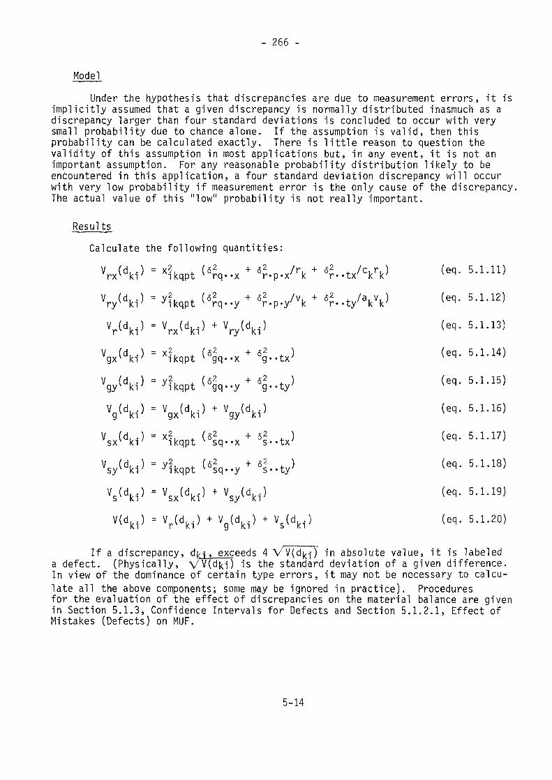
- 266 -

ModelUnder the hypothesis that discrepancies are due to measurement errors, it is

implicitly assumed that a given discrepancy is normally distributed inasmuch as adiscrepancy larger than four standard deviations is concluded to occur with verysmall probability due to chance alone. If the assumption is valid, then thisprobability can be calculated exactly. There is little reason to question thevalidity of this assumption in most applications but, in any event, it is not animportant assumption. For any reasonable probability distribution likely to beencountered in this application, a four standard deviation discrepancy will occurwith very low probability if measurement error is the only cause of the discrepancy.The actual value of this "low" probability is not really important.

ResultsCalculate the following quantities:

Vrx<dk1> ' x?kqpt < srq-.x + «?.p.x/rk + «?..tx/Vk>

Vdk1> = y!kqpt <6rq..y + 6rWvk + '?• Wk>

Vdk1> - Vrx<dki> + Vdki'

. .x+ 5g 2 . . tx> (eq. 5.1.14)

. + 5 > (eq. 5.1.15)

<52:,..x+5s2..tx> (eq. 5.1.17)

Vdki'=yfkqpt(ssq..y+Ss..ty' (eq. 5.1.18)

V«ki> - Vsx<dki> + Vsy<dki'VUM) = Vr(dk,) * Vdki> * Vs(dkl'

If a discrepancy, dn , exceeds 4 Wc'djc-,-) in absolute value, it is labeleda defect. (Physically, V V(d|<i) is the standard deviation of a given difference.In view of the dominance of certain type errors, it may not be necessary to calcu-late all the above components; some may be ignored in practice). Proceduresfor the evaluation of the effect of discrepancies on the material balance are givenin Section 5.1.3, Confidence Intervals for Defects and Section 5.1.2.1, Effect ofMistakes (Defects) on MUF.

5-14

- 267 -

BasjsIf the assumption of normality is valid, then a discrepancy as large as

4 VrV(dk|) would occur due to chance alone less than 7 times out of 100,000. Thus,a discrepancy larger in absolute value is correctly labeled a defect with veryhigh probability.

It is noted that the results were given on the basis that the item charac-teristic in question is the element weight. It is simple to modify the key equationsshould another characteristic be under investigation. Only those measurementoperations that affect the difference statistic are, of course, included in thecalculations. It may be that additional terms would be required, e.g., if theitem characteristic is isotope weight rather than element weight. The results inSection 3.5.4, appropriately modified to apply to the single item, are pertinentin this event.

and y-i|<qpt are essentially identical so that various pairs ofcombined; (2) some error variances are zero and will hence not

The calculations indicated by the equations seem quite involved. However,they may be applied quite easily by noting that: (1) for error propagationpurposes, x-j^qptequations may beappear in the equations; and (3) the calculations for Vr(dk-j), Vg(dki), and Vs(dkl-)need not actually be performed; they are intermediate values leading up to thefinal (5.1.20).Examples

EXAMPLE 5.5 (a)The low enriched uranium fuel fabrication facility of example 3.3 (a) is

inspected. In the U02 powder stratum, 36 measurements are made of item elementweight, using the data of example 3.8 (a) (12 batches sampled with 3 items weighedper batch). Determine the defect criterion for the variables tester in the attri-butes mode. Use the nominal value of 20 kg U for xjkqpt and y-j|<qpt for a^ items.

The following parameter values are given in prior example. From example3.3 (a), for the facility:

q = l p = 1r-! = 5 ci = l

«ri..x- 0.000658 Vrx

From example 3.5 (a)= 0.000439 6„ ...

t = l

= 0.000531

= 0.000571

k = l

6r..lx = 0.000433

Sl"X

From example 3.8 (a), for the inspectorq = l p = 1

vi = 2 ai = 2<$ , ,. = 0.000658 0„ , ., = 0.000531

t = 1

= 0.000433

5-15

- 268 -

From example 3.9 (a),& = 0.000544g--iy

From example 3.10 (a),6 = 0.000439 S . = 0.000172si'-y s-'iy

The equations, (eq. 5.1.11) - (eq. 5.1.20) are now applied to give the following results.

V^dj.) = 0.000211 vry

(dii} = °-000248 V0!!') = °-000459

Vgx^-j) = 0 V^i^ = °-000118 V0!!') = °-000118vcv(din) = 0-000208 V_w(d..) = 0.000089 V_(d..) = 0.000297

SX -*• I ^,7 -I- * oil

.) = 0.000874

4 VV(dzi) = 0.118 kg U, defect criterion

5.1.3 Confidence Intervals for Defects

5.1.3.1 Numbers of DefectsUpon completion of the attributes inspection, a confidence interval may be

calculated for the number of defects in the population, (or, in the case of mistakes,the number of mistakes). This interval may be helpful in reaching a decision as tothe need for further inspection in a given stratum. A procedure for estimatingthe effect of the defects on MUF 1s given in Section 5.1.2.1.

The methods for constructing a confidence interval are given. Method 5.6applies when zero defects are observed. Method 5.7 is applicable for M observeddefects.

Method 5.6Notation

N = number of items in populationn = sample size

1-ß = confidence coefficientU = upper limit of confidence interval

5-16

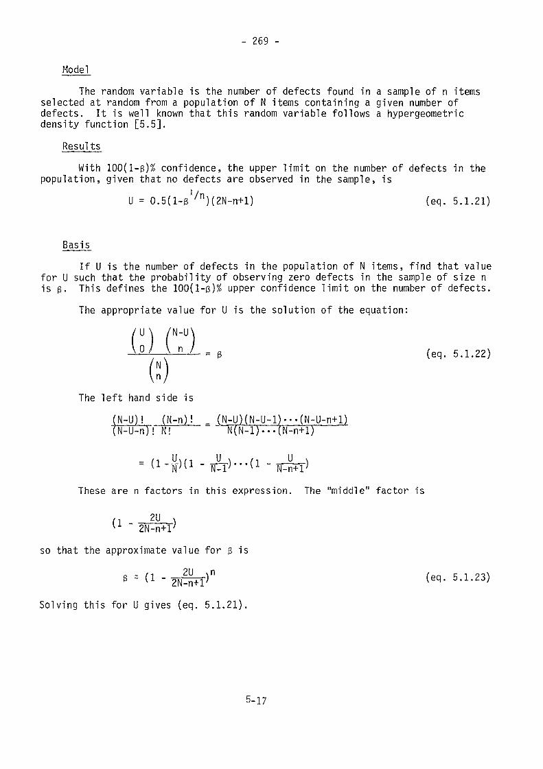
- 269 -

ModelThe random variable is the number of defects found in a sample of n items

selected at random from a population of N items containing a given number ofdefects. It is well known that this random variable follows a hypergeometricdensity function [5.5].

ResultsWith 100(l-ß)% confidence, the upper limit on the number of defects in the

population, given that no defects are observed in the sample, isU = 0.5(l-ß /n)(2N-n+l) (eq. 5.1.21)

Basj_sIf U is the number of defects in the population of N items, find that value

for U such that the probability of observing zero defects in the sample of size nis ß. This defines the 100(l-ß)% upper confidence limit on the number of defects.

The appropriate value for U is the solution of the equation:U\ /N-UO/ ( n (eq. 5.1.22)

The left hand side is(N-n)! _

J-U-n)! N! ~N(N-l).-.(N-n+l)

These are n factors in this expression. The "middle" factor is

_ _2N-n+l'so that the approximate value for ß is

(eq'Solving this for U gives (eq. 5.1.21).

5-17

- 270 -

Examples^

EXAMPLE 5.6 (a)With reference to example 4.1 (b), in the mixed oxide powder stratum of the

mixed oxide fuel fabrication facility, 48 items out of the 360 total items were in-spected in attributes sampling. No defects were found. What is the 95% upper con-fidence limit on the number of defects in the remaining 312 items?

The parameter values are:N = 360 n - 48 ß = 0.05

By (eq. 5.1.21), the limit isU = 0.5 (l-0.051/48)(720-48+l)

= 20.4, or 21 items

Method 5.7 is applicable when el defects are observed in the sample.

Method 5.7Notation

N, n, (1-3), and U as in Method 5.6d = number of defects observed in the sample

ModelSee Method 5.6

ResultsDefine t by3

tfJ

1-3 2e"Z dz = 1-3 (eq. 5.1.24)

That is, the area under the standardized normal curve from -» to t 0 isI~P

5-18

- 271 -

Calculate the quantities z, x, A, B, C, and p using the following equations,z = d+0.5 (eq. 5.1.25)x = 1- (n-l)/(N-l) (eq. 5.1.26)A = n2 + t2_ nx (eq. 5.1.27)

B = nz + 0.5t2 nx (eq. 5.1.28)i-pC = z2 (eq. 5.1.29)

p = (B + VB2-AC)/A (eq. 5.1.30)

Then, the upper limit, U, is given byU = [pN + 0.5]-1 (eq. 5.1.31)

where the brackets indicate that the largest integer contained in (pN+0.5) shouldbe used. Note that since U is the limit on the number of defects in the lot, then(U-d) is the limit for the (N-n) uninspected items.

BasisThe normal approximation to the hypergeometric distribution forms the basis

for this result. See reference [5.6].Examples

EXAMPLE 5.7 (a)With reference to example 5.6 (a), suppose that 2 defects were found in the

sample of 48 items. What is the 95% upper limit on the number of defects in theremaining 312 items?

N = 360 n = 48 ß = 0.05 d = 2t = 1.645 z = 2.5 x = 0.8691i-ß

A = 2416.8867B = 176.4434C = 6.25p = 0.1254U = 45.14 -l = 44 defects, including those found in the sample.

U-d = 42, required limit

5-19

- 272 -

5.2 POST-INSPECTION ACTIVITIESGenerally speaking, the statistical activities discussed in Section 5.1 are

those that would be performed on-site during the course of an inspection. InSection 5.2, further statistical analyses are described, those that would normallybe performed after the physical inspection has been completed and the appropriateinspection data accumulated.

Not all of the statistical techniques described need be performed on anygiven inspection. The collection of techniques are those available to the inspec-tor for his use in evaluating the data, and include those techniques most likelyto be utilized, if not in connection with each phase of each inspection, certainlyfrequently enough to warrant inclusion here.

In Section 5.2.1, supplemental statistical tests of hypotheses are described(see Section 4.5.1 for the distinction between supplemental and primary tests).These tests include the test for normality, tests for randomness, variance tests,and the test for the significance of D^, the difference statistic in stratum k.The principal statistical tests are described in Section 5.2.2. These includethe test on D, the test on MUF, and the test on (MUF-D). Finally, the construc-tion of confidence intervals for the facility MUF and for the inspector's estimateof the facility MUF, (MUF-D), are treated in Section 5.2.3.

5.2.1 Supplemental Tests of Hypotheses

5.2.1.1 Normality TestsVarious statistical procedures to be applied in the analyses of variables

data are based on the assumption of normality. The effect of a failure in thisassumption on the validity of the procedure depends on the nature and degree of non-normality and on the specific statistical procedure involved. Tests for normalityare given in Methods 5.8 and 5.9. One of these tests may be applied whenever thereis a question on the validity of this assumption. If the test results indicatethat the assumption is of questionable validity, then guidance should be soughtfrom a statistical expert to determine the effects of the non-normality on thestatistical procedures to be applied. Guidance can also be given on the need tomodify the procedures to account for the non-normality. Further, non-normalityof the data in question may be indicative of unindentified variables affectingthe results, and may therefore provide valuable insight into the structure of thedata. For example, data falsifications introduced by a diverter, if not carefullyand thoughtfully introduced, could perhaps be detected by a test of normality. Ofcourse, it doesn't necessarily follow that detection of non-normality in the datasignals diversion; it merely signals the need to perform a more careful investiga-tion of the data in order to uncover the reasons for the departure from normality.

There are a number of statistical tests of normality that have been suggested.Some require large sample sizes and are therefore generally inappropriate for mostsituations likely to be encountered by the inspector. In the absence of knowledgeabout the alternative hypothesis, i.e., about the particular type of non-normalitylikely to exist, it is advisable to apply a statistical test that is generally sensi-tive to all kinds of non-normality. The so called W-test for normality is such atest. It is applicable for sample sizes up to 50, and is described in Method 5.8.For sample sizes larger than 50, a related test referred to as the D" test may beapplied. Method 5.9 describes this test.

5-20

- 273 -

Method 5.8Notation

Xi,x2,---,x = sample values for some random variable, ordered such thatX1<X2<"*<Xn

ModelUnder the null hypothesis, the data are normally distributed. The distribu-

tion under the alternative hypothesis is not specified.Results

Using the coefficients an_i+1 given in Annex 5.2, calculateb = an(xn-x1)+an_1(xn_1-x2)+...+an_k+1(xn_k+1-xk) (eq. 5.2.1)

where k = n/2 for even n

= (n-l)/2 for odd n

Calculate

S2 = Ç x/- (g x^2/n (eq. 5.2.2)

(Note that S2 is simply (n-1) times the calculated variance of the x-jvalues.)

Calculatew = b2/S2 (eq. 5.2.3)

A small value for W is indicative of non-normality. If W is less than thecritical value given in Annex 5.3 for a given significance level, a, conclude thatthe data are not normally distributed.

Basis.The W-test for normality is covered in [5.7].

Examples

EXAMPLE 5.8 (a)In the low enriched uranium fuel fabrication plant treated in previous exam-ples, 19 U02 powder cans in stratum 1 are measured for total uranium by the inspector.His results are compared item by item with the facility values by noting the differ-

ence in uranium weights. These facility-minus-inspector values are given in grams

5-21

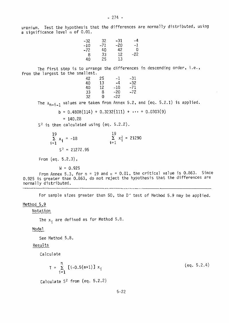
- 274 -uranium. Test the hypothesis that the differences are normally distributed, usinga significance level a of 0.01.

-32-10-72

840

32-71403325

-31-20421213

-4-10

-22

The first step is to arrange the differences in descending order, i.e.,from the largest to the smallest.

42 25 -1 -3140 13 -4 -3240 12 -10 -7133 8 -20 -7232 0 -22

The an ,- -, values are taken from Annex 5.2, and (eq. 5.2.1) is applied,n— i — ib = 0.4808(114) + 0.3232(111) + ••• + 0.0303(9)

= 140.28S2 is then calculated using (eq. 5.2.2).

19 19Z x. - -18 Z x? = 21290

1=1 ' 1=1S2 = 21272.95

From (eq. 5.2.3),W = 0.925

From Annex 5.3, for n - 19 and a = 0.01, the critical value is 0.863. Since0.925 is greater than 0.863, do not reject the hypothesis that the differences arenormally distributed.

For sample sizes greater than 50, the D" test of Method 5.9 may be applied.Method 5.9

NotationThe x. are defined as for Method 5.8.

Model,See Method 5.8.

ResultsCalculate

T = 2 [i-0.5(n+l)] x. («I- 5-2-4)i=l

Calculate S2 from (eq. 5.2.2)5-22

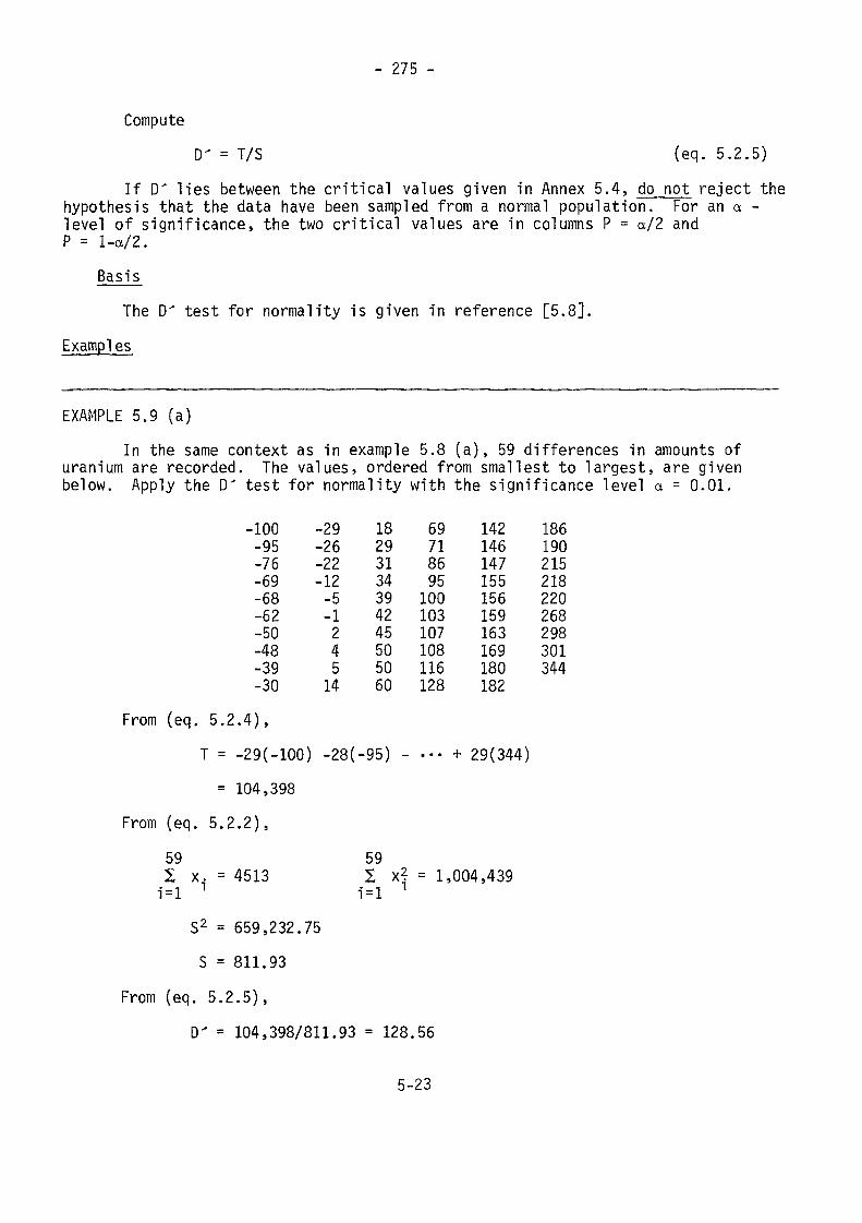
- 275 -

ComputeD' = T/S (eq. 5.2.5)

If D' lies between the critical values given in Annex 5.4, do not reject thehypothesis that the data have been sampled from a normal population. For an a -level of significance, the two critical values are in columns P = a/2 andP = l-a/2.

BasisThe D' test for normality is given in reference [5.8].

Examples

EXAMPLE 5.9 (a)In the same context as in example 5.8 (a), 59 differences in amounts of

uranium are recorded. The values, ordered from smallest to largest, are givenbelow. Apply the D' test for normality with the significance level a = 0.01.

-100-95-76-69-68-62-50-48-39-30

-29-26-22-12-5-124514

18293134394245505060

69718695100103107108116128

142146147155156159163169180182

186190215218220268298301344

From (eq. 5.2.4),T = -29(-100) -28(-95) - ••• + 29(344)

= 104,398From (eq. 5.2.2),

59 592 x. = 4513 Z x? = 1,004,439i=l 1 1=1 1

S2 = 659,232.75S = 811.93

From (eq. 5.2.5),D' = 104,398/811.93 = 128.56

5-23

- 276 -

For a = 0.01, and n = 59, the lower critical value in the P = 0.005 columnis 121.0 by interpolation. In the P = 0.995 column, the upper critical value is130.1. Since D' falls between these two critical values, do not reject the hypo-thesis that the data have been sampled from a normal population.

5.2.1.2 Randomness TestsTesting for randomness of a set of data is difficult because randomness is a

characteristic that is difficult to define. It is simpler to approach the problemfrom the alternative viewpoint, i.e., to consider different types of non-randomnessthat may characterize the data. In the context of inspection, certain kinds ofdiversion strategies that include data falsification could create some types ofnon-randomness, e.g., the creation of sub-populations of falsified and non-falsifieditems. Further, tests for randomness could uncover assignable causes in the data,i.e., could lead to a better understanding of the data structure that would aidthe statistical analysis.

The tests for normality discussed in Section 5.2.1.1 may be regarded astests of randomness in the specific instance in which randomness is equated to nor-mality. This equivalence between randomness and normality is often present withmeasurements data, and so the normality tests could have wide application here.

As another special case especially relevant to inspection, inspection of aflow stratum may take place over a period of time. Bias shifts in either the facil-ity's or inspector's data could create non-randomness in the data. A similar state-ment applies to shipper-receiver data. Thus, a particular type of non-randomnessthat the inspector should be aware of is shifts in the population parameter valueswhen data are ordered in time. This is the particular type of non-randomnessaddressed in this section.

Two methods are given to address this type of non-randomness. The firstmethod is simple to apply and is very effective in providing a good visual impres-sion of the data. It detects bias shifts very effectively but is partly subjectivein that a quantitative measure of non-randomness is not produced. Often, thisfirst method, involving a CUSUM (cumulative sjjm) plot is sufficient in detectingnon-randomness due to bias shifts. If a more objective measure of non-randomnessis needed, then the second method, involving an analysis of variance, may be applied.Collectively, these two methods plus the test for normality provide the tests neededto test for the most important types of non-randomness likely to characterizeinspection data.Method 5.10

Notationx. = observed value for the random variable, ordered in time or1 with respect to some other factor

ModelFor the CUSUM plot as presented here, the inferences are made on the basis

of a visual impression from the plot. This impression is generally adequate in

5-24

- 277 -

making conclusions about the presence of parameter shifts. There are objectivemeans for making inferences from CUSUM plots. These involve the use of V-masksand are not considered further here [5.9]. Such decision-making tools assume acertain structure in the data, commonly, that the observations are drawn at randomfrom a normal distribution. When the plot is made just to create a visual impres-sion, this assumption about the data structure is not required.

ResultsFrom an inspection of the data, as based on some other considerations,

select some central value for the data. In the case of difference data, this cen-tral value would be zero. The purpose of this central value selection is to forcethe plot to be nearly horizontal in the absence of shifts in the parameter value.Call the central value y.

Calculate the difference values:d. = (X..-M) (eq. 5.2.6)

Calculate the CUSUM valuessi = s^+d. (eq. 5.2.7)

where SQ = 0. Thus,si = d!S2 = Si + 02

s3 = s2 + d3 , etc.Using an equal spacing along the abscissa, plot the s-j values. Observe

the plot to determine if more than one line segment is needed to connect the plottedpoints. If so, conclude that there is non-randomness exhibited by the data in thesense that the parameter describing central tendency is not constant (bias shift).

BasisAs long as the mean of the x-j values remains constant, all the plotted

points may be connected visually by a straight line segment. If there is a shiftin the mean, then this straight line will change direction, or, stated alternately,more than one line segment will be needed. If the central value, y, is wiselychosen, and if there are no shifts in the parameter value (i.e., in the mean ofthe x-j values), the slope will be zero.Examples

5-25

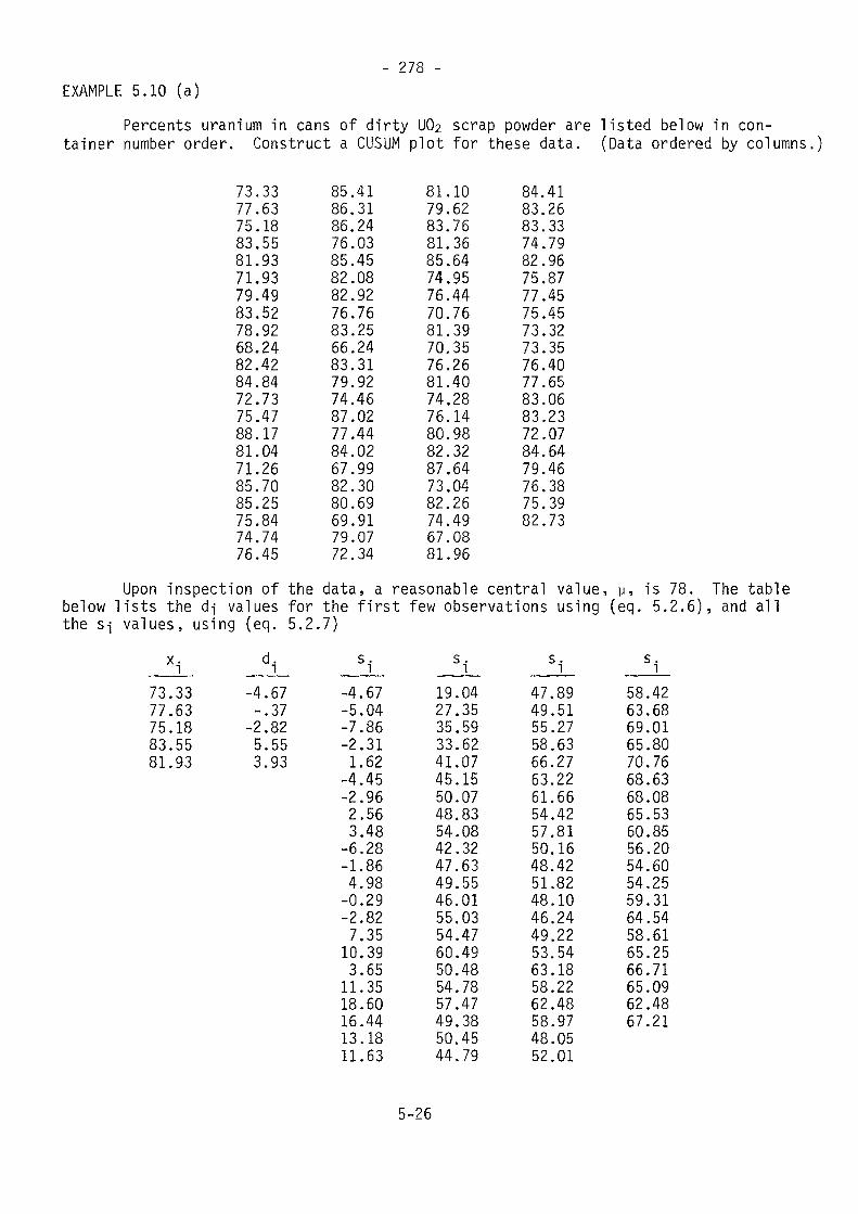
EXAMPLE 5.10 (a)

Percents uranium in cans of dirty UÛ2 scrap powder are 1tainer number order. Construct a CUSUM

73.3377.6375.1883.5581.9371.9379.4983.5278.9268.2482.4284.8472.7375.4788.1781.0471.2685.7085.2575.8474.7476.45

Upon inspection of thebelow lists the dj values forthe s-j values, using {eq. 5.2

x. d.i i73.33 -4.6777.63 -.3775.18 -2.8283.55 5.5581.93 3.93

85.4186.3186.2476.0385.4582.0882.9276.7683.2566.2483.3179.9274.4687.0277.4484.0267.9982.3080.6969.9179.0772.34

plot for

81.1079.6283.7681.3685.6474.9576.4470.7681.3970.3576.2681.4074.2876.1480.9882.3287.6473.0482.2674.4967.0881.96

data, a reasonablethe first.7)

si-4.67-5.04-7.86-2.311.62

-4.45-2.962.563.48

-6.28-1.864.98

-0.29-2.827.35

10.393.65

11.3518.6016.4413.1811.63

listed below in con-these data. (Data ordered by columns.)

84.4183.2683.3374.7982.9675.8777.4575.4573.3273.3576.4077.6583.0683.2372.0784.6479.4676.3875.3982.73

central value:few observations using

s .i19.0427.3535.5933.6241.0745.1550.0748.8354.0842.3247.6349.5546.0155.0354.4760.4950.4854.7857.4749.3850.4544.79

si47.8949.5155.2758.6366.2763.2261.6654.4257.8150.1648.4251.8248.1046.2449.2253.5463.1858.2262.4858.9748.0552.01

, u, is 78. The table(eq. 5.2.6), and all

s.i58.4263.6869.0165.8070.7668.6368.0865.5360.8556.2054.6054.2559.3164.5458.6165.2566.7165.0962.4867.21

5-26

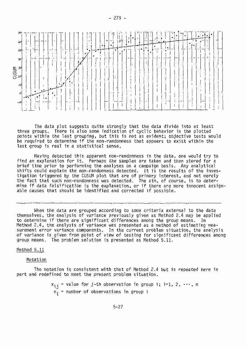
- 279 -

r nr

The data plot suggests quite strongly that the data divide into at leastthree groups. There is also some indication of cyclic behavior in the plottedpoints within the last grouping, but this is not as evident; objective tests wouldbe required to determine if the non-randomness that appears to exist within thelast group is real in a statistical sense.

Having detected this apparent non-randomness in the data, one would try tofind an explanation for it. Perhaps the samples are taken and then stored for abrief time prior to performing the analyses on a campaign basis. Any analyticalshifts could explain the non-randomness detected. It is the results of the inves-tigation triggered by the CUSUM plot that are of primary interest, and not merelythe fact that such non-randomness was detected. The aim, of course, is to deter-mine if data falsification is the explanation, or if there are more innocent assign-able causes that should be identified and corrected if possible.

When the data are grouped according to some criteria external to the datathemselves, the analysis of variance previously given as Method 2.4 may be appliedto determine if there are significant differences among the group means. InMethod 2.4, the analysis of variance was presented as a method of estimating mea-surement error variance components. In the current problem situation, the analysisof variance is given from point of view of testing for significant differences amonggroup means. The problem solution is presented as Method 5.11.Method 5.11

NotationThe notation is consistent with that of Method 2.4 but is repeated here inpart and redefined to meet the present problem situation.

X-. = value for j-th observation in group i; 1=1, 2,' Jn. = number of observations in group i

m

5-27

- 280 -

Modelx-jj is normally distributed about u-j, the mean for group i, and with variance

a2, constant for all groups. Under the hypothesis, y-j is the same for all i.Results

Following Method 2.4, calculate the quantities:Ti, T, S0, Sl9 S2, Mß, and MW

Form the F ratio:F = MB/MW (eq. 5.2.8)

Select a value for a, the significance level of the test. For a = 0.05,0.025, and 0.01, enter the table in Annex 5.5 (a), 5.5 (b), or 5.5 (c) respectively.If F exceeds the tabled value for degrees of freedom for the numerator, (m-1),and degrees of freedom for the denominator, (n-m), conclude that y-j ^ y for alli, i.e., reject the hypothesis that the group means are the same.

BasisThe statistical technique that forms the basis for this method is the one

way analysis of variance which is described in many texts. See, for example, [5.10],Examples

EXAMPLE 5.11 (a)In Example 5.10 (a), say that the percent uranium values were determined in

four analytical compaigns, i.e., during four distinct periods of operation in thelaboratory. The data are divided into groups as follows:

Group 1: 73.33 - 71.26 (m = 17)Group 2: 85.70 - 83.25 (n2 = 14)Group 3: 66.24 - 81.96 (n3 = 35)Group 4: 84.41 - 82.73 (n4 = 20)Following Method 2.4:

T! - 1329.65 S0 = 533761.2853T2 - 1142.43 Si = 533902.8742T3 = 2727.93 S2 = 536132.4325T4 = 1575.20 MB = 47.1963T - 6775.21 Mw = 27.1897

5-28

- 281 -From (eq. 5.2.8),

F = 47.1963/27.1897 = 1.736Choose a = 0.05 and enter the table of Annex 5.5 (a). The tabled value

for 3 degrees of freedom in the numerator and 82 degrees of freedom in the denomina-tor is 2.74, by interpolation. Since the F value of 1.736 does not exceed thistabled value, do not reject the hypothesis that the group means are equal.

Some further comments are in order because this conclusion seems to conflictwith that reached in Example 5.10 (a) on the basis of the CUSUM plot. First, itwas pointed out that the CUSUM plot provide a visual impression of the data, andin this particular example, is quite suggestive of a real difference in group means.However, the statistical significance of that conclusion is not stated. On thebasis of this current example, it appears that the conclusion of a significantdifference is not warranted at the a = 0.05 significance level; the actual valuefor a, it turns out, would be slightly larger than a = 0.10. The up-and-down patternof the data plot is an indication of a large random error variance or in this case,of a rapidly shifting bias, which tends to obscure the differences in the groupmeans.

Further, from the data plot, in observing the slopes of the line segments,it is apparent' that group means 1, 3, and 4 are nearly equal whereas group mean 2is relatively high. The analysis of variance tests the global hypothesis that allgroup means are equal; if three are in fact equal while one differs somewhat, theanalysis of variance may not detect this fact so readily. In fact, had groups 1,3, and 4 been combined and tested against group 2, then MB and Mw would have been

MB = 133.0415 Mw = 26.6441and F with 1 and 84 degrees of freedom is 4.993, a significant result at a = 0.05.Here is an example in which the CUSUM plot was perhaps more sensitive in detectingthe particular alternative hypothesis that apparently exists; with the analysisof variance, the alternative hypothesis is not specified.

By way of summary, the four group means arexi = 78.21 x3 = 77.94X2 = 81.60 x\ = 78.76

5.2.1.3 Variance TestsIn advance of an inspection, the facility provides values for its random

and systematic error variances. These values are used in planning the inspectionand also in the data analysis if, in fact, the inspection data substantiate thestated values. This section addresses the problem of verifying that the facility'sstated values for the random error variances are valid. The method makes use ofthe facility minus inspection data.

5-29

- 282 -

Method 5.12Notation

d. = difference between facility and inspector values for specifiedcharacteristic and stratum

n = number of d. valuesa2 = facility's stated random error variance for given characteristic

and stratuma2 = corresponding inspector's value

ModelThe quantity dj is normally distributed with arbitrary mean and variance

equal to (o2+a2) under the null hypothesis that a2 and a2 are correctly stated.

ResultsCalculate

n / n \/n (eq. 5.2.9)

Calculate the chi-square statistic

x2 = S^/(a? + a2) (eq. 5.2A n_1 d/ \ o i' ^ ^

Select a value for a, the significance lev£l of the test. Enter the tablein Annex 5.6 under the columns headed xa/2 and xi-a/2 , and for degrees of freedom(df) equal to (n-1). If x^-1 of (eq. 5.2.10)falls between the two tabled values,do not_ reject the hypothesis, i.e., conclude that the sum, (o2+a2), is correct.

In the event the hypothesis is rejected, conclude that a§ misrepresentsthe actual variance for the facility. This conclusion assumes that the inspectorcan properly assign the a2 value.

Bas i sThe statistical technique that forms the basis for this method is the chi-

square test on the variance which is described in many texts (see, for example,[5.11]).

Of underlying importance to this test is the validity of the assumption thatthe inspector's value, a2, is correct. This should pose no problem because of thewide base of experience upon which the a2 value will generally be based. However,the problem can be circumvented under some circumstances, i.e., it is possible totest the hypothesis about the validity of a? irrespective of the value for a?.

5-30

- 283 -

The procedure for making this test, and the conditions under which the alternatetest is preferred, are given in reference [5.12].Example

EXAMPLE 5.12 (a)Consider the data of Example 5.8 (a). These data represent differences

between facility and inspector measurements of total uranium in containers of lowenriched U02 powder.

From example 3.3 (a),a2, = [(.000950)(20000)]2 = 361.00 g2U

From example 3.8 (a),a2 = 361.00 g2U

Then, again from example 5.8 (a),s2, = 21272.95

From (eq. 5.2.10), the chi-square value isXl28 = 21272.95/722.00 = 29.46

At a = 0.05, from Annex 5.6, the tabled critical values are 8.23 and 31.53.Since 29.46 lies between these two numbers, do not reject the hypothesis that(02+a2) = 722.00.

5.2.1.4 Test on Dk and on Shipper/Receiver Differences^The final supplemental test to be considered is the test on D|<, the difference

statistic in stratum k. Although primary emphasis in the analysis of the variableinspection data is on the difference statistic appropriately summed overfall strata,there are occasions when one might wish to test for the significance of D^ in a givenstratum. As a prime example of this, it was pointed out in Section 4.5.3 that ashipper-receiver difference test is formally equivalent to a test on 0^, and one isinterested in routinely performing such tests on shipper-receiver differences.

The D^ test was considered in Section 4.5.3 from point of view of its proba-bility of detection. In this current section, emphasis is on how the significancetest is performed.Method 5.13

NotationThe notation is consistent with that given in Methods 3.8 - 3.10.

5-31

- 284 -

ModelThe random variable, D^, is assumed to be normally distributed with variance

V(Dk) and with mean zero under the null hypothesis.Results

Calculate V(D|<) as the sum of three variance componentsV(Dk) = Vr(Dk) + Vg(Dk) + Vs(Dk) (eq. 5.2.11)

where Vr(Dj<) is given by (eq. 3.5.5), and where Vg(ß|<) and V^D^) are given res-pectively by (eq. 3.5.14) and (eq. 3.5.21), in each case the calculations being per-formed for only the single stratum.

A.Having observed D^, compute the statistic

(eq. 5.2.12)Select a value for a, the significance level of the test, and find the cor-

responding critical value, ta, from Annex 5.7. Then,(a) if stratum k is an input or beginning inventory stratum, reject the

hypothesis that the mean of 0^ is zero if t<-ta;(b) if stratum k is an output or ending inventory stratum, reject the

hypothesis if t>ta.Basis

This is the standard test on the mean of a normally distributed randomvariable with known variance [5.13]. The test is constructed as a one-sided testbecause from a diversion viewpoint, only those values of Dk that differ from zeroin one direction favor the diverter. Of course, a large value of D^ in the oppositedirection would also be called to the attention of the facility as evidence of amalfunctioning measurement system.Examples

EXAMPLE 5.13 (a)In example 3.8 (b), the inspection sample sizes are given for the mixed

oxide fuel fabrication facility. In the Pu02 powder stratum, 16 of the 24 strataare randomly selected with 6 items weighed per batch and with 3 samples drawn perbatch to determine percent plutonium. Duplicate analytical determinations aremade. For the resulting 96 paired differences, say that

al = -0.00468 kg Pu, so that, from (eq. 3.5.1)DI - -(768)(0.00468) = -3.594

5-32

- 285 -

At a significance level, a= 0.010, does this represent a significantdifference?

From the cited example,V (Di) = 0.296817 + 0.621036 = 0.917853 kg2Pu

From example 3.9 (b), the calculations for the short term systematic errorvariance are performed for stratum 1. Example 3.9 (b) made use of earlier calcula-tions performed in Example 3.4 (a). In the expression for Vg^) given below, thefirst two terms come from example 3.4 (a) and the last term from example 3.9 (b).

V (ßx) = 0.012124 + 1.329070 + (0.0016)2[2(768)2]y= 4.361093 kg2Pu

From example 3.10 (b), the calculations for the long term systematic errorvariance are performed for stratum 1. Example 3..10 (b) made use of earlier resultsfrom example 3.5 (b). In the expression for VS(DI) given below, the first two termscome from example 3.5 (b) and the last two from example 3.10 (b).

V (Dj) = 0.094372 + 1.156055 + (1656.6)2(0.00030)2+(1536)2(0.0012)2

= 4.894802 kg2PuThe (eq. 5.2.11) may now be applied

V(D!) = 0.917853+4.361093+4.894802 = 10.173748 kg2PuFrom (eq. 5.2.12),

t - -3.5947V 10.173748 = -1.127At a = 0.010, ta = 3.090. Since -1.127 is not less than -3.090, conclude

that the facility measurements of plutonium are not significantly smaller than theinspector measurements for this input stratum, i.e., there is no reason to concludethat the input values are understated.

5.2.1.5 International Standards of Accountancy [5.15]

In Section 3.4 the variance of MUT, V (MUF), is used to test the hypothesisthat the true MUF is equal to some stated value (e.g., zero). V (MUF) may becalculated from the operator's design information data on his random and systematicrandom error variances. The inspector may verify these error estimates usinginspection results, estimation methods described in Chapter 2 and the Chi-square testof Section 5.2.1.3. Depending on the outcome of these many possible tests theinspector may calculate his own estimate of V (MUF) in order to determine whether theoperator's system of measurements conform to international standards or be equivalentin quality to such standards.

5-33

- 286 -

Standards do not exist for each measurement method and material combination.Instead the Agency has defined such standards for V (MUF) which are consideredachievable in practice at bulk facilities of each identified type. For example,at uranium fabrication facilities the international standard of accountancy fora.,||p is 0.3 %, expressed as a percentage of the larger of inventory or throughput.This represents a maximum expected value for oMUp that is easily achievable by themajority of facilities using well known measurement methods that are widely used inthe industry.

EXAMPLE 5.13(a)From example 3.3(a) we see that the outputs of 238800 + 1200 = 240000 kg U

are much larger than beginning or ending inventory. In this case, the standard ofaccountancy would be

= (0.003) (240000) - 720 kg U

and the calculated value of / V (MUF) from Example 3.5(a) is

v V (MUF) - / 45010 = 212 kg U.

Since 212 < 719 kg U we conclude that the operator's system of measurements is wellwithin this international standard. In the event that / V (MUF) is greater thanthe standard the test of MUF in Section 11.9 should be based on the standard valuerather than the calculated value and the state should be informed that the systemof measurements does not meet the maximum expected values for

A similar approach can be used for testing the quality of the inspector'ssystem of measurements as represented by V (D). In fact this may be more importantthan checking V (MUF) since V (D) is the primary measure of the Agency's verificationaccuracy. Safeguards effectiveness based on nuclear material accountancy will belimited by this verification accuracy as the size and throughput of bulk handlingfacilities increase.

5.2.2 Principal Tests of HypothesesIn assessing the safeguards performance of a facility, the key measures are

D, MUF, and MUF-D. The observed values of these quantities and their calculatedvariances form the basis for both the principal tests of hypotheses discussed inSection 4.5.1 and the estimation of the true MUF. This section describes theperformance of significance tests, and the next section describes the constructionof confidence intervals estimates.5.2.2.1 Test on D

The D test was considered in Section 4.5.4 from point of view of itsdetection probability. In this current section, emphasis is on how the significanttest is performed.

5-34

- 287 -Method 5.14

NotationThe notation is that used in Methods 3.8 to 3.10.

ModelThe random variable, D, is assumed to be normally distributed with zero meanand with variance V(D) under the null hypothesis.

ResultsCalculate V(D) as the sum of three variance components:

V(0) = Vr(D) + Vg(D) + Vs(D) (eq. 5.2.13)

where V^D), Vg(D), and VS(D) are given in (eq. 3.5.6), (eq. 3.5.14), and (eq. 3.5.21)respectively.Compute

t = D/ VV(D] (eq. 5.2.14)Select a value for a, the significance level of the test. If t<-t , conclude

that there is a significant difference between the facility and inspector°Vesults.The value for ta comes from Annex 5.7.Basis

The basis is the same as for the D^ test of Method 5.13. For D, a largenegative value favors the diverter and so the test is a one-sided test against thatalternative.Examples

EXAMPLE 5.14 (a)Continue with the mixed oxide facility of example 5.13 (a). This relates to

the inspection described in example 3.8 (b). At a = 0.025, how large must ß be ina negative direction in order to reject the hypothesis that its mean is zero?

From (eq. 5.2.14) and Annex 5.7, the hypothesis in question is rejected if

D<-1.960 Vv(D)s*.The quantity V(D) for this example was calculated in example 3.10 (b).

V(D) = 27.303719 kg2Pu

5-35

- 288 -Therefore, the hypothesis will be rejected if

D<-1.960 V27.303719 , or if

D<-10.242 kg Pu

5.2.2.2 Test on MUFThe test on MUF was considered in Section 4.5.5 from point of view of its

detection probability. In this current section, emphasis is on how the significancetest is performed.Method 5.15

NotationThe notation is given in Section 3.4.3.2.

ModelThe random variable, MUF, is assumed to be normally distributed with zero

mean and with variance V(MUF) under the null hypothesis.Results

Calculate V(MUF) as the sum of three variance components.V(MUF) - V (MUF) + V (MUF) + V (MUF) (eq. 5.2.15)

Î?

where Vr(MUF), Vg(MUF), and VS(MUF) are given in (eq. 3.4.3), (eq. 3.4.7), and(eq. 3.4.11) respectively.

Computet = MUF/ V V(MUF) (eq. 5.2.16)

Select a value for a, the significance level of the test. If t exceeds tafrom Annex 5.7, reject the hypothesis that the mean of MUF is zero.Bas/is

The basis is the same as for the D^ test of Method 5.13. For MUF, a largepositive value is an indication of diversion and so the test is one-sided againstthat alternative.Examples

EXAMPLE 5.15 (a)Consider the MUF for the mixed oxide fuel fabrication facility. Values for

Vr(MUF), Vg(MUF), and VS(MUF) were calculated in Examples 3.3 (b), 3.4 (a), and5-36

- 289 -3.5 (b) respectively. At a = 0.050, how large must MUF be in order to reject thehypothesis that its mean is zero?

From the cited examples, as summarized in example 3.5 (b),/V(MUF) = 3.276 kg Pu

For a = 0.050, ta = 1.645 so that the hypothesis is rejected if MUF exceeds(1.645)(3.276) = 5.389 kg Pu

5.2.2.3 Test on (MUF-D)The test on (MUF-Û) was considered in Section 4.5.6 from point of view of its

probability of detection. In this current section, emphasis is on how the signifi-cance test is performed.Method 5.16

NotationThe notation is that of Method 3.13.

ModelThe random variable, (MUF-D), is assumed to be normally distributed with zero

mean and with variance V(MUF-D) under the null hypothesis.Results

Calculate V(MUF-D) from (eq. 3.6.5). Computet = (MUF-D)/V V(MUF-D) (eq. 5.2.17)

Select a value for a, the significance level of the test. If t exceeds tafrom Annex 5.7, reject the hypothesis that the mean of (MUF-D) is zero.Basis

The basis is the same as for the ß|< test of Method 5.13. For (MUF-Ô), alarge positive value is an indication of diversion and so the test is one-sidedagainst that alternative.Examples

EXAMPLE 5.16 (a)Consider the low enriched uranium fuel fabrication facility of example 3.13 (a)

At a = 0.050, how large must (MUF-D) be in order to reject the hypothesis that itsmean is zero?5-37

exceeds

- 290 -From the cited example,V(MUF-D) = 40,983 kg2U

For a = 0.050, ta = 1.645 so that the hypothesis is rejected if (MUF-D)

(1.645) V40,983 = 333 kg U

EXAMPLE 5.16 (b)Suppose that in the previous example, (MUF-D) were calculated for U-235

rather than for uranium. Then, sinceV*(MUF-D) = 33.6843 kg2U-235

from Example 3.13 (a), the critical value is1.645 V 33.6843 = 9.547 kg U-235

This example illustrates how Methods 5.13-5.16, written in terms of elementweights, may easily be adapted to relate to isotope weights. The changes in cal-culations are obvious.

EXAMPLE 5.16 (c)Consider the mixed oxide^fuel fabrication facility of example 3.13 (b). At

a = 0.050, how large must (MUF-D) be in order to reject the hypothesis that itsmean is zero?

From the cited example,V(MUF-D) = 21.035443 kg2Pu

For a = 0.050, ta = 1.645 so that the hypothesis is rejected if (MUF-D)exceeds1.645 V21.035443 = 7.545 kg Pu

This completes the discussion on tests of hypothesis for the various statis-tics derived from the inspection data. The final topic on the analysis of inspectiondata is the construction of confidence intervals.5.2.3 Confidence Intervals on Material Unaccounted For

jNThe values of MUF and MUF-D are estimates of the true material unaccounted forcalculated from facility data and facility data plus inspection data, respectively.These observed values and their calculated variances contain all the information about

5-38

- 291 -

the magnitude of the true MUF available to the inspector. In addition to the specifictests of the hypothesis of no diversion (true MUF equal to zero) described in thepreceding section,it is revealing to display the total information about material un-accounted for upon completion of the analysis of facility and inspection data. Inparticular, the estimated magnitude of a significant diversion relative to the goalquantity M used as a basis for inspection planning may be of interest.

A convenient way to convey this information is through the determination ofa confidence interval estimate of the true MUF and a graphical presentation of thisinterval as it relates to both the absence of any diversion (true MUF equal 0) andthe diversion of a significant quantity (true MUF equal M). In Section 5.2.3.1 thefacility MUF forms the basis for construction of the confidence interval while inSection 5.2.3.2 the basis is the adjusted estimate MUF-D based on inspection data.5.2.3.1 Confjidence Interval Based on MUFMethod 5.17

NotationThe notation is given in Section 3.4.3.2. Further, M is the goal amount.

ModelThe random variable, MUF, is assumed to be normally distributed with variance

V(MUF). The observed MUF is assumed to be the estimate of the true unknown MUF inthe sense that its expected value is the true MUF. (No small biases or data fal-sifications.)

ResultsCalculate V(MUF) by (eq. 5.2.15). Choose a value for the confidence coeffi-

cient (1-a) and computeL = MUF - t1-a/ VV(MUF)

and U = MUF + t1_a/2VV(MUF)

(eq. 5.2.18)

(eq. 5.2.19)

where t / is read from Annex 5.8 for given (1-a).l-a/2To display the results graphically, draw a horizontal line scaled in amounts

of element. Let the smallest value on the left be min (0,L) and the largest valueon the right be max (M,U). Indicate the values for 0, L, U, and M on this lineby appropriately marking the line, and connect the L and U marks.

There are six possible ways in which the 0, L, U, and M marks may beordered. (Note that L must be less than U and 0 is less than M.) These possi-bilities are listed below along with a narrative description of their interpreta-tions. In the first three cases the test of the hypothesis of a true MUF less thanor equal to zero would be rejected.

5-39

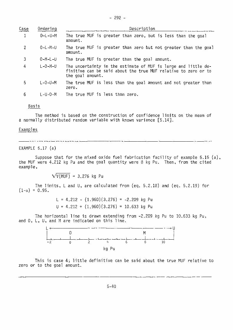
- 292 -

Case Ordering __________________Description______________________1 0-L-U-M The true MUF is greater than zero, but is less than the goal

amount.2 0-L-M-U The true MUF is greater than zero but not greater than the goal

amount.3 0-M-L-U The true MUF is greater than the goal amount.4 L-O-M-U The uncertainty in the estimate of MUF is large and little de-

finitive can be said about the true MUF relative to zero or tothe goal amount.

5 L-O-U-M The true MUF is less than the goal amount and not greater thanzero.

6 L-U-O-M The true MUF is less than zero.

BasisThe method is based on the construction of confidence limits on the mean of

a normally distributed random variable with known variance [5.14].Examples

EXAMPLE 5.17 (a)Suppose that for the mixed oxide fuel fabrication facility of example 5.15 (a),

the MUF were 4.212 kg Pu and the goal quantity were 8 kg Pu. Then, from the citedexample,

VV(MUF) = 3.276 kg PuThe limits, L and U, are calculated from (eq. 5.2.18) and (eq. 5.2.19) for

(1-a) = 0.95.L = 4.212 - (1.960)(3.276) = -2.209 kg PuU = 4.212 + (1.960)(3.276) = 10.633 kg Pu

The horizontal line is drawn extending from -2.209 kg Pu to 10.633 kg Pu,and 0, L, U, and M are indicated on this line.

-2

0

1 , . , ,0

1 12

M... , , ,„. f., , 1.

4 6 8

——— . ...—f. L

i i10

kg Pu

This is case 4; little definitive can be said about the true MUF relative tozero or to the goal amount.

5-40

- 293 -5.2.3.2 Confidence Interval Based on (MUF-D)Method 5.18

NotationThe notation is that of Method 3.13. M is the goal amount.

ModelThe random variable (MUF-ß)js assumed to be normally distributed with vari-

ance V(MUF-D). The observed (MUF-D) is assumed to be the estimate of the true un-known MUF in the sense that its expected value is the true MUF (facility MUF cor-rected for biases or data falsifications).

ResultsCalculate V(MUF-D) from (eq. 3.6.5). Choose a value for the confidence

coefficient (1-a) and compute the lower and upper confidence limits:L = (MUF-D) - t , Vv(MUF-D) (eq. 5.2.20)l-a/2U = (MUF-D) + t _ , VV(MUF-D) (eq. 5.2.21)

where t /is read from Annex 5.8 for given (1-a).l-a/2

Proceed as in Method 5.17 to display the results graphically.Basis

The basis is the same as for Method 5.17.Examples

EXAMPLE 5.18 (a)Suppose that for the mixed oxide fuel fabrication facility of example 5.17 (a),

D = -3.617 kg Pu. Then,(MUF-D) = 4.212 + 3.617 = 7.829 kg Pu

For this facility, from example 5.16 (c),V(MUF-D) = 21.035443 kg2Pu

From (eq. 5.2.20) and (eq. 5.2.21), for (1-a) = 0.90,L = 7.829 - 1.645 V21.035443 = 0.284 kg PuU = 7.829 + 1.645 V21.035443 = 15.374 kg Pu

5-41

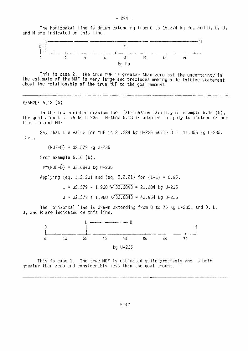
- 294 -The horizontal line is drawn extending from 0 to 15.374 kg Pu, and 0, L, U,

and M are indicated on this line.U

) M( i t i t i | 1 1 * 1 t l ( 1

10 12kg Pu

This is case 2. The true MUF is greater than zero but the uncertainty inthe estimate of the MUF is very large and precludes making a definitive statementabout the relationship of the true MUF to the goal amount.

EXAMPLE 5.18 (b)In the low enriched uranium fuel fabrication facility of example 5.16 (b),

the goal amount is 75 kg U-235. Method 5.18 is adapted to apply to isotope ratherthan element MUF.

Then;Say that the value for MUF is 21.224 kg U-235 while D = -11.355 kg U-235.

(MUF-D) = 32.579 kg U-235From example 5.16 (b),V*(MUF-D) - 33.6843 kg U-235

Applying (eq. 5.2.20) and (eq. 5.2.21) for (1-a) = 0.95,L - 32.579 - 1.960 V33.6843 = 21.204 kg U-235U = 32.579 + 1.960 V33.6843 = 43.954 kg U-235

The horizontal line is drawn extending from 0 to 75 kg U-235, and 0, L,U, and M are indicated on this line.

0

0l

10

L

1 1 i i

20 30

i {

i i

jN

.L 1 1 1 1 1

40 50 60 70

kg U-235

This is case 1. The true MUF is estimated quite precisely and is bothgreater than zero and considerably less than the goal amount.

5-42

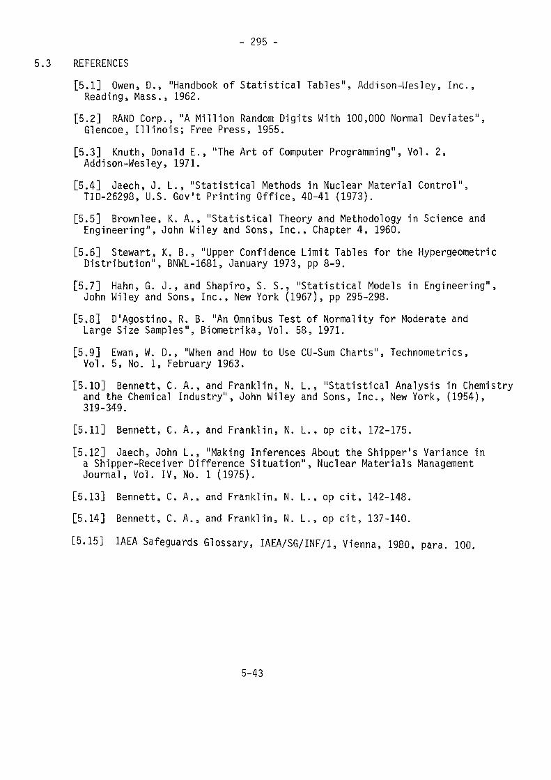
- 295 -5.3 REFERENCES

[5.1] Owen, D., "Handbook of Statistical Tables", Addison-Uesley, Inc.,Reading, Mass., 1962.

[5.2] RAND Corp., "A Million Random Digits With 100,000 Normal Deviates",Glencoe, Illinois; Free Press, 1955.

[5.3] Knuth, Donald E., "The Art of Computer Programming", Vol. 2,Addison-Wesley, 1971.

[5.4] Oaech, J. L., "Statistical Methods in Nuclear Material Control",TID-26298, U.S. Gov't Printing Office, 40-41 (1973).

[5.5] Brownlee, K. A., "Statistical Theory and Methodology in Science andEngineering", John Wiley and Sons, Inc., Chapter 4, 1960.

[5.6] Stewart, K. B., "Upper Confidence Limit Tables for the HypergeometricDistribution", BNWL-1681, January 1973, pp 8-9.

[5.7] Hahn, G. J., and Shapiro, S. S., "Statistical Models in Engineering",John Wiley and Sons, Inc., New York (1967), pp 295-298.

[5.8] D'Agostino, R. B. "An Omnibus Test of Normality for Moderate andLarge Size Samples", Biometrika, Vol. 58, 1971.

[5.9] Ewan, W. D., "When and How to Use CU-Sum Charts", Technometrics,Vol. 5, No. 1, February 1963.

[5.10] Bennett, C. A., and Franklin, N. L., "Statistical Analysis in Chemistryand the Chemical Industry", John Wiley and Sons, Inc., New York, (1954),319-349.

[5.11] Bennett, C. A., and Franklin, N. L., op cit, 172-175.[5.12] Jaech, John L., "Making Inferences About the Shipper's Variance ina Shipper-Receiver Difference Situation", Nuclear Materials ManagementJournal, Vol. IV, No. 1 (1975).

[5.13] Bennett, C. A., and Franklin, N. L., op cit, 142-148.[5.14] Bennett, C. A., and Franklin, N. L., op cit, 137-140.[5.15] IAEA Safeguards Glossary, IAEA/SG/INF/1, Vienna, 1980, para. 100.

5-43

- 296 -

Annex 5.1 (a)

5-44

- 297 -Annex 5.1 (b)

- 298 -Annex 5.1 (c)

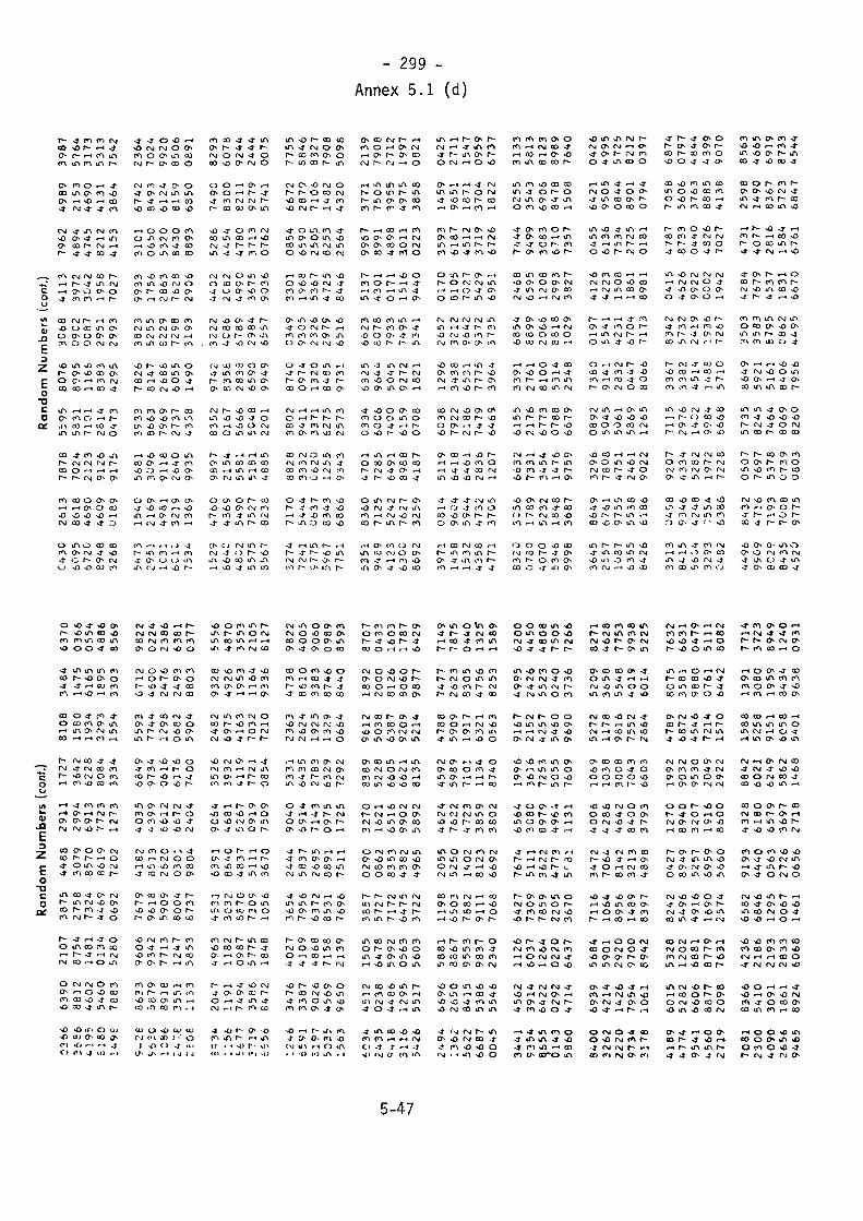
- 299 -Annex 5.1 (d)

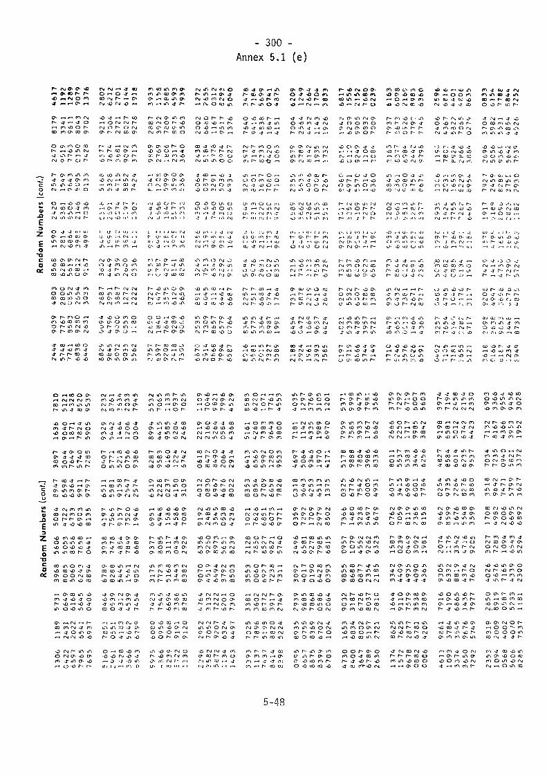
- 300 -Annex 5.1 (e)

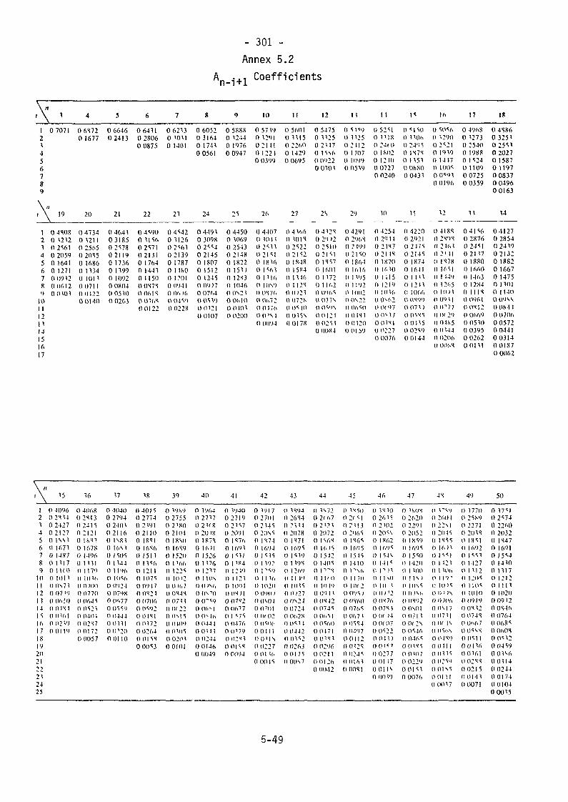
- 301 -

Annex 5.2A -+1 Coefficients

\"

121456789

,\

~2145fi789

101 112|l14151617

1

07071

19\ ____

0 4 SOS0 12120 21610 20590 16410 1271009120061200101

4

0 6S720 1677

20

0 47340 12110 25650 20S50 16860 11340 10110 0 7 1 10012200140

5

0 664602413

21

0 46410318502178021190 17360 1 1990 10920 OR04005100 0263

6

064110 28060 0875

22

0 41900 1 1 160217 10 21310 17640 14410 1150OOS7X0 06 1 S0016S00122

7

0 62130 10H0 1401

21

041420 11260 2161021390 17870 1 ISO0 1201009410 1)6160 04190 02 2 X

It

0 6052031640 174100561

24

044910 309X0211402 I450 1 8070 15I20 1245009)70 0764001190012100107

0

0 5SS80 12440 197600947

25

044500 10690 25430 21480 18220 151)0 12X30 10460 0X210 Oh 1 01)01010 0200

10

0 57190 12910 21 110 12210 0399

26

044070 10110 211102IH0 1 8 160 |1610 11160 10X900X760 067200176IMPXI0 0094