i THESIS CONVERSION OF LOW BMEP 4-CYLINDER TO ...
146
i THESIS CONVERSION OF LOW BMEP 4-CYLINDER TO HIGH BMEP 2-CYLINDER LARGE BORE NATURAL GAS ENGINE Submitted by John Ladd Department of Mechanical Engineering In partial fulfillment of the requirements For the degree of Master of Science Colorado State University Fort Collins, Colorado Summer 2016 Master’s Committee: Advisor: Daniel B. Olsen John Petro Borgusz Bienkiewicz
-
Upload
khangminh22 -
Category
Documents
-
view
3 -
download
0
Transcript of i THESIS CONVERSION OF LOW BMEP 4-CYLINDER TO ...
i
THESIS
CONVERSION OF LOW BMEP 4-CYLINDER TO HIGH BMEP 2-CYLINDER LARGE
BORE NATURAL GAS ENGINE
Submitted by
John Ladd
Department of Mechanical Engineering
In partial fulfillment of the requirements
For the degree of Master of Science
Colorado State University
Fort Collins, Colorado
Summer 2016
Master’s Committee:
Advisor: Daniel B. Olsen
John Petro Borgusz Bienkiewicz

ii
Copyright by John Warner Ladd 2016
All Rights Reserved
ii
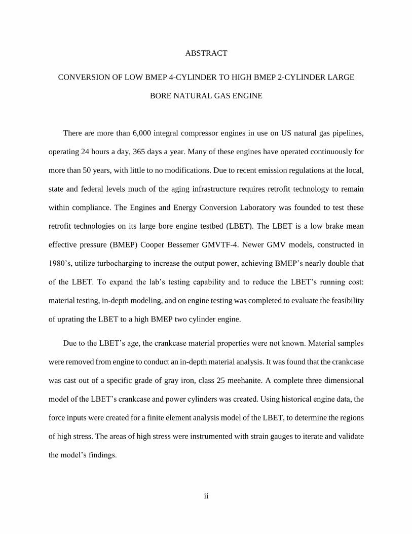
ABSTRACT
CONVERSION OF LOW BMEP 4-CYLINDER TO HIGH BMEP 2-CYLINDER LARGE
BORE NATURAL GAS ENGINE
There are more than 6,000 integral compressor engines in use on US natural gas pipelines,
operating 24 hours a day, 365 days a year. Many of these engines have operated continuously for
more than 50 years, with little to no modifications. Due to recent emission regulations at the local,
state and federal levels much of the aging infrastructure requires retrofit technology to remain
within compliance. The Engines and Energy Conversion Laboratory was founded to test these
retrofit technologies on its large bore engine testbed (LBET). The LBET is a low brake mean
effective pressure (BMEP) Cooper Bessemer GMVTF-4. Newer GMV models, constructed in
1980’s, utilize turbocharging to increase the output power, achieving BMEP’s nearly double that
of the LBET. To expand the lab’s testing capability and to reduce the LBET’s running cost:
material testing, in-depth modeling, and on engine testing was completed to evaluate the feasibility
of uprating the LBET to a high BMEP two cylinder engine.
Due to the LBET’s age, the crankcase material properties were not known. Material samples
were removed from engine to conduct an in-depth material analysis. It was found that the crankcase
was cast out of a specific grade of gray iron, class 25 meehanite. A complete three dimensional
model of the LBET’s crankcase and power cylinders was created. Using historical engine data, the
force inputs were created for a finite element analysis model of the LBET, to determine the regions
of high stress. The areas of high stress were instrumented with strain gauges to iterate and validate
the model’s findings.

iii
Several test cases were run at the high and intermediate BMEP engine conditions. The model
found, at high BMEP conditions the LBET would operate at the fatigue limit of the class 25
meehanite, operating with no factor of safety but the intermediate case were deemed acceptable.

iv
ACKNOLEDGEMENTS
The author would like to recognize individual contributors to this work. There were numerous
students and staff that played key roles with the research, analysis, testing, and modeling for this
project. First and foremost, the author would like to recognize Dr. Daniel Olsen for his countless
hours spent on this project and his selfless mentoring. The author would also like to recognize the
committee members for their greatly appreciated contributions to the project, Dr. John Petro and
Dr. Borgusz Bienkiewicz.
Kirk Evan, director of engineering at the EECL, was an amazing resource for analyzing and
managing the vast amounts of data accumulated on this project. Joe Wilmetti, Smash Lab manager,
for taking time out of his busy schedule to aid with tensile and hardness testing. Trevor Aguirre,
AMPT researcher, for his assistance with imaging the material samples and demonstrating
Archimedes’ method for density calculation. Steve Johnson, Mechanical Engineering lab manger,
for his assistance machining the material sample to desired size and shape. And last but not least,
Dr. Christian Puttlitz for his tireless editing and meetings to improve the presentation of results
seen in this report.

v
1 Introduction ............................................................................................................................. 1
1.1 Goal and Purpose ............................................................................................................. 2
1.2 Literature Review ............................................................................................................. 3
1.2.1 Engine Background ................................................................................................... 3
1.2.2 Cylinder Deactivation ............................................................................................... 5
1.2.3 Engine Uprate ......................................................................................................... 14
1.2.4 Finite Element Analysis Background ..................................................................... 20
2 Crankcase Material Determination ........................................................................................ 24
2.1 Overview ........................................................................................................................ 24
2.2 Material Analysis Methods ............................................................................................ 24
2.3 Material Testing ............................................................................................................. 28
2.3.1 Non-Destructive Testing ......................................................................................... 29
2.3.2 Destructive Testing ................................................................................................. 39
2.4 Material Analysis Conclusion ........................................................................................ 45
3 Crankcase Model Development and FEA Testing ................................................................ 46
3.1 Overview ........................................................................................................................ 46
3.2 Model Improvement ....................................................................................................... 46
3.3 FEA Set Up and Results ................................................................................................. 48
3.3.1 Pre-Processing......................................................................................................... 48
TABLE OF CONTENTS

vi
3.3.2 Analysis................................................................................................................... 60
3.3.3 Post-Processing, FEA Results ................................................................................. 61
4 On-Engine Measurements ..................................................................................................... 65
4.1 Overview ........................................................................................................................ 65
4.2 Engine Operation and Data Acquisition......................................................................... 65
4.3 Strain Gauge Theory, Calibration, and Engine Mounting ............................................. 67
4.3.1 Strain Gauge Theory ............................................................................................... 67
4.3.2 Strain Gauge Instrumentation and Calibration ....................................................... 70
4.3.3 Strain Gauge Engine Mounting .............................................................................. 75
4.4 On Engine Strain Gauge Measurements ........................................................................ 78
4.4.1 Nominal Condition.................................................................................................. 79
4.4.2 Single Cylinder Deactivation .................................................................................. 87
4.4.3 Double Cylinder Deactivation ................................................................................ 90
5 GMVH-2 Operation – Model Extrapolation ......................................................................... 94
5.1 Intermediate Test Cases ................................................................................................. 97
6 Conclusions ........................................................................................................................... 99
6.1 Key Findings ................................................................................................................ 100
6.1.1 Material Testing .................................................................................................... 100
6.1.2 Model Construction and Validation ...................................................................... 101
6.1.3 Uprated Operation ................................................................................................. 101

vii
6.2 Short Comings .............................................................................................................. 103
6.2.1 Limited Model Validity ........................................................................................ 103
6.2.2 Consistent Strain Gauge Failure ........................................................................... 103
6.2.3 Poor Load Control during Cylinder Deactivation Experiments ........................... 103
6.3 Direction for Future Research ...................................................................................... 104
6.3.1 Permanent Cylinder Deactivation ......................................................................... 104
6.3.2 In-depth Crankcase Inspection .............................................................................. 104
7 References ........................................................................................................................... 105
8 Appendix ............................................................................................................................. 109
8.1 Appendix A Meehanite Metal Selection Guide ........................................................... 109
8.2 Appendix B Reynold French Repair Brochure ............................................................ 115
8.3 Appendix C Working Model Simulation ..................................................................... 121
8.4 Appendix D Strain Gauge Instrumentation Manual ..................................................... 123
8.5 Appendix E Strain gauge Mounting Instructions ......................................................... 126
viii
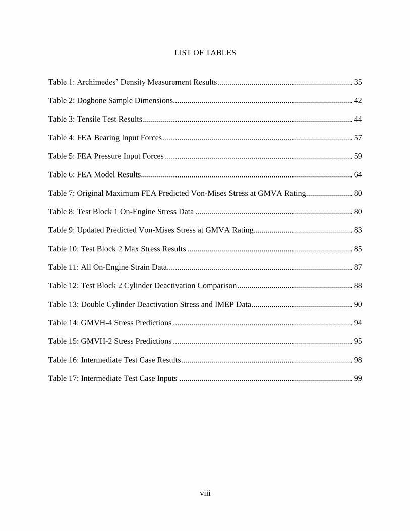
LIST OF TABLES
Table 1: Archimedes’ Density Measurement Results ................................................................... 35
Table 2: Dogbone Sample Dimensions......................................................................................... 42
Table 3: Tensile Test Results ........................................................................................................ 44
Table 4: FEA Bearing Input Forces .............................................................................................. 57
Table 5: FEA Pressure Input Forces ............................................................................................. 59
Table 6: FEA Model Results ......................................................................................................... 64
Table 7: Original Maximum FEA Predicted Von-Mises Stress at GMVA Rating....................... 80
Table 8: Test Block 1 On-Engine Stress Data .............................................................................. 80
Table 9: Updated Predicted Von-Mises Stress at GMVA Rating................................................. 83
Table 10: Test Block 2 Max Stress Results .................................................................................. 85
Table 11: All On-Engine Strain Data............................................................................................ 87
Table 12: Test Block 2 Cylinder Deactivation Comparison ......................................................... 88
Table 13: Double Cylinder Deactivation Stress and IMEP Data .................................................. 90
Table 14: GMVH-4 Stress Predictions ......................................................................................... 94
Table 15: GMVH-2 Stress Predictions ......................................................................................... 95
Table 16: Intermediate Test Case Results ..................................................................................... 98
Table 17: Intermediate Test Case Inputs ...................................................................................... 99

ix
LIST OF FIGURES
Figure 1: GMV Articulated Connecting Rod Assembly ................................................................ 1
Figure 2: GMV Air Flow Schematic and Cross Section................................................................. 4
Figure 3: EECL Supercharger Flow Curves [9] ............................................................................. 6
Figure 4: Average Misfires vs BSFC [11] ...................................................................................... 8
Figure 5: Average Misfires per 100 cycles vs Trapped Air Fuel Ratio [11] .................................. 8
Figure 6: GMVTF-4 Orientation at the EECL ................................................................................ 9
Figure 7: U.S. Yearly Natural Gas Production [1] ........................................................................ 15
Figure 8: Common Crankcase Failure Noted by Reynolds French [35] ...................................... 18
Figure 9: GMV Crankcase Crack Identification and Repair [35] ................................................. 19
Figure 10: High Stress FEA Results [21] ..................................................................................... 20
Figure 11: FEA Solution Approximation [27] .............................................................................. 21
Figure 12: Two Dimensional Geometry Discretized into Finite Elements [26] ........................... 22
Figure 13: FEA Validation Process Map [24] .............................................................................. 23
Figure 14: ASTM E8 Dogbone for Tensile Test [30] ................................................................... 26
Figure 15: Engineering vs True Stress-Strain Curve [31] ............................................................ 27
Figure 16: Sample Location .......................................................................................................... 28
Figure 17: Cross Section Slice from Sample ................................................................................ 28
Figure 18: Flake vs Nodular Graphite in Meehanite [19] ............................................................. 29
Figure 19: Platen Tool .................................................................................................................. 30
Figure 20: Grinding and Polishing Wheel .................................................................................... 30
Figure 21: Counter Rotation Technique ....................................................................................... 30
Figure 22: Etched Sample ............................................................................................................. 31
x
Figure 23: 20x Sample Image ....................................................................................................... 32
Figure 24: 10x Sample Image ....................................................................................................... 32
Figure 25: 40x Sample Image ....................................................................................................... 33
Figure 26: Archimedes’ Principle Diagram .................................................................................. 34
Figure 27: Measuring Sample Mass ............................................................................................. 35
Figure 28: MERC Archimedes’ Scale .......................................................................................... 36
Figure 29: CSU Hardness Test Apparatus .................................................................................... 38
Figure 30: Rockwell Hardness Test Procedure ............................................................................. 38
Figure 31: Milling Sample into Rectangular Cross Section ......................................................... 39
Figure 32: Micro Dogbone Sample and Jaw Adaptors ................................................................. 40
Figure 33: MTS Tensile Testing Apparatus with Extensometer .................................................. 41
Figure 34: Fractured Sample 3 ...................................................................................................... 43
Figure 35: Stress Strain Curve from Sample 3 ............................................................................. 43
Figure 36: Improved GMVTF Crankcase Model with Power Cylinders ..................................... 47
Figure 37: Working Model Force Outputs [21] ............................................................................ 50
Figure 38: Eureqa Model Definition Functions ............................................................................ 52
Figure 39: Force x for Bearing Group 1 Prediction ...................................................................... 53
Figure 40: Eureqa Model Extrapolation ....................................................................................... 54
Figure 41: Final Eureqa Output Equations ................................................................................... 55
Figure 42: Bearing Load Force Input for Bearings 3 and 4 .......................................................... 56
Figure 43: Pressure Force Load Constraint on Cylinder Head 2 .................................................. 58
Figure 44: Ansys Workbench Solution Status Window ............................................................... 61

xi
Figure 45: Areas of Maximum Stress above Bearings 3 and 4 at PP for Cylinder 3 at GMVH Rating
....................................................................................................................................................... 62
Figure 46: LBET LabVIEW Control Panel Controller ................................................................. 66
Figure 47: Illustration of Strain [39] ............................................................................................. 67
Figure 48: Wheatstone Bridge [39]............................................................................................... 68
Figure 49: Omega Strain Gauge Signal Conditioners................................................................... 70
Figure 50: KFH-6 Three Foil Strain Gauge .................................................................................. 71
Figure 51: Torsional Cantilever Beam Apparatus ........................................................................ 71
Figure 52: Ansys FEA Model of Test Apparatus ......................................................................... 72
Figure 53: Governing Equations and Calculations for Cantilever Beam ..................................... 74
Figure 54: Strain Gauge 1 and 3 Mounting Locations Above Bearing 4 ..................................... 75
Figure 55: Strain Gauge 2, 4 and 5 Mounting Locations above Bearing 3 .................................. 76
Figure 56: Tarp Placement in the Crankcase ................................................................................ 77
Figure 57: Final Strain Gauge Mounts.......................................................................................... 78
Figure 58: Foil 2A Electrical Short ............................................................................................... 81
Figure 59: Test Block 1 data comparison ..................................................................................... 82
Figure 60: Strain Gauge Mounting Discrepancy .......................................................................... 83
Figure 61: Test Block 2 Data Comparison ................................................................................... 85
Figure 62: Average Pressure and Voltage Traces from Test Block 2........................................... 85
Figure 63: Over Extruded "Airbox" .............................................................................................. 86
Figure 64: Final Nominal Data Comparison ................................................................................. 87
Figure 65: Voltage Trace Comparison between Nominal and Single Cylinder Deactivation ...... 89
Figure 66: Stress vs Cylinder 4 IMEP .......................................................................................... 89

xii
Figure 67: Deactivated Cylinder Traces ....................................................................................... 91
Figure 68: Nominal Cylinder Traces ............................................................................................ 91
Figure 69: IMEP Comparison between Nominal and Deactivated Conditions with COV as error
metric ............................................................................................................................................ 92
Figure 70: Frequency of Measured Stress at Strain Gauge 2 ........................................................ 93
Figure 71: FEA Model Shortfall ................................................................................................... 95
Figure 72: Approximate s-n curve for Class 25 Meehanite .......................................................... 96

xiii
ABREVIATIONS AND SYMBOLS
Term Abbreviation Advanced Materials Processing and Testing Lab AMPT After Top Dead Center ATDC American Society for Metals ASM American Society of Mechanical Engineers ASME Brake horsepower bhp Brake mean effective pressure BMEP Brake Specific Fuel Consumption BSFC Computer Numerically Controlled CNC Electronic Gas Admission Valve EGAV Engines and Energy Conversion Laboratory EECL Finite Element Analysis FEA Gauge Factor GF Large Bore Engine Test Bed LBET Mechanical Gas Admission Valve MGAV Motor Sport Research Center MERC Pipeline Gas Admission Valve PLGAV Revolutions per Minute rpm Top Dead Center TDC Unburned Hydrocarbon Emissions UHC

1
1 INTRODUCTION
In 2014, nearly 27 trillion cubic feet of natural gas was consumed in the United States [1].
Natural gas is primarily transported from drilling site to the end user via a vast network of pipelines
spanning over 1.5 million miles [2]. To move the natural gas, the pipeline needs to maintain a
constant pressure gradient, created by compressor stations spaced every 50 to 100 miles [3]. Many
of these compressor stations have been in continuous operation for more than 50 years utilizing
the power and reliability of integral compressors.
There are more than 6,000 integral compressors in use on US pipelines, operating 24 hours a
day 365 days a year [3]. Integral compressors typically operate at slow speeds with the compressor
cylinder directly attached to the combustion cylinder via an articulated connecting rod, Figure 1.
Many of these engines have operated continuously for more than 50 years with little to no
modifications [4]. Due to recent emissions regulations at the local, state and federal levels much
of the aging infrastructure requires retrofit technology to remain within compliance or risks
replacement. Retrofit technologies can improve efficiency and decrease emissions at a fraction of
the cost of replacement. A large integral compressor operator can save over $4 million by uprating
an old engine rather than installing a modern centrifugal compressor [5]. The large bore engine
Figure 1: GMV Articulated Connecting Rod Assembly

2
testbed (LBET) at the Engines and Energy Conversion Laboratory (EECL) provides industry with
means to test new technology without sacrificing compressor station throughput.
The EECL utilizes a Cooper Bessemer GMVTF-4 as the LBET. The engine is a slow speed,
low brake mean effective pressure (BMEP), large bore integral compressor. Operating as a lean
burn, two-stroke cycle engine, producing 440 brake horse power (bhp) at 300 revolutions per
minute (rpm), with a 14” (36cm) bore and 14” (36cm) stroke and a total displacement of 140 liters.
The engine is outfitted with over 100 independent sensors, allowing the measurement and analysis
of pertinent parameters. The engine is loaded with a water-brake dynamometer to simulate
compression work. The engine is controlled with a LabVIEW virtual Interface with the ability to
attain a wide range of operational parameters to accurately simulate field engine conditions.
1.1 GOAL AND PURPOSE
The goal is to convert and uprate the current GMVTF-4 to a GMVH-2. The motivation for
the uprate project is to expand the testing capabilities of the EECL as well as reducing the running
and prototyping cost of the engine.
The GMVTF-4 was the second generation model produced by Cooper Bessemer, from 1948
to 1963, operating as a low BMEP (~67psi) model [6]. There were eight new models designed
after the GMVTF that were more powerful and more efficient leading up to the high BMEP
(~125psi) GMVH model. Uprating the engine to a GMVH would allow the EECL to conduct
experiments at conditions that simulate the operation of every GMV model, as well as establishing
an uprating practice. Deactivating two of the cylinders will reduce the research and development
cost for engine retrofit companies, making the LBET more attractive to industry sponsors.

3
1.2 LITERATURE REVIEW
A comprehensive literature review was completed to establish the theoretical framework for
the proposed work and identify the potential risks.
1.2.1 Engine Background
The EECL was started at Colorado State University with the installation of the GMVTF-
4, to provide an independent, unbiased test facility for large-bore, industrial, natural gas engines.
The LBET is equipped with over 100 state of the art measuring devices and controls for producing
accurate emissions and performance data.
The Cooper Bessemer GMV was known for its excellent performance and ruggedness. In
its 55 years of production 4616 models were produced at the Cooper Bessemer plant in Mount
Vernon, Ohio [7]. The GMV integral compressor was recognized by the American Society of
Mechanical Engineers (ASME) as a Heritage Landmark. The GMV was credited as a major
contributor to the world’s economy for more than a half century, providing compression energy
for the natural gas transmission, gas treatment, petrochemical, refinery and power industries in the
United States and forty-four countries around the world [7].
The Cooper Bessemer GMV design was an advancement over the traditional gas driven
horizontal compressors. The GMV is a V-angle integral compressor, meaning the compression
cylinders are directly attached to the power cylinders. The 60 degree V-angle design reduced the
floor space requirements of the engine by up to one half of its horizontal compressor counterparts.
The compactness of the engine allowed it to be shipped completely assembled, keeping the original
factory alignments, reducing the complexity of installation.

4
The GMV is a two cycle engine, meaning every other stroke of the engine is a power stroke,
having greater power density relative to its four cycle counterparts. On the downward stroke, the
power piston first uncovers the exhaust ports allowing the some of the burned gases to exit the
cylinder. Further movement of the piston then uncovers the air intake ports and the scavenging air
in the receiver rushes into the cylinder sweeping the remaining exhaust gases out and filling the
cylinder fresh air, seen on the right cylinder in Figure 2.The stock GMV utilized a trunk style
piston with the power pistons controlling the opening and closing of the intake and exhaust ports.
Scavenging air was provided by horizontal pistons attached to the cross heads. The stock savaging
airflow can be seen in Figure 2 denoted by the white arrows. The LBET utilizes an external
supercharger system in place of the scavenging pistons but the cross heads are still in place. At the
time of port closure, the mechanically operated injector valve at the top of the cylinder opens and
pressurized natural gas is admitted into the cylinder regulated by the governor in accordance with
Figure 2: GMV Air Flow Schematic and Cross Section

5
the load requirements. Shortly before top dead center is reached, ignition takes place, combustion
occurs and the cycle is then repeated.
1.2.2 Cylinder Deactivation
To be competitive, the lab needed the capability to simulate a wide range of atmospheric
conditions. The requirement was fulfilled by using a supercharger, driven by an electric motor,
and a variable back pressure valve. This combination allows the lab to emulate the pressures of a
turbocharged engine at the desired altitude of an industry sponsor.
The current supercharger assembly consists of a 300hp Magnetek electric motor connected
to Gardener CycloBlower via a V-belt and jackshaft. The current configuration is able to provide
enough boost to run the LBET on all four cylinders at GMVA levels, a BMEP of ~72 psi. As
configured the system would not be able to provide enough air flow to run the LBET at GMVH
levels on four cylinders, but by deactivating two cylinders the system would meet the air
throughput demands to run LBET as a GMVH-2 without modification. The need for cylinder
deactivation was dictated by the limitation of the supercharger but will reduced associated costs
on the LBET. A GMVH typically operates with over 20 inHg of boost and as can be seen in
compressor flow curves of Figure 3, the SCFM exponentially decreases as boost level increases
[8] [9].
The most common reason for field engine cylinder deactivation is due to reduced power
requirements, often associated with depleting gas fields [10]. Large bore two-stroke compression
engines are designed to run within a finite range of output power requirements with optimal

6
efficiency at constant 100% load. Reduced load results in an increased propensity to misfire,
increased brake specific fuel consumption (BSFC), decreased thermal efficiency, as well as
increased emissions [11][12][13][10]. A misfire is considered to be any combustion cycle resulting
in an IMEP of less than 10psi [11]. When a cylinder misfires there is incomplete combustion
*Data obtained with inlet at 14.7 PSIA and 68 F with no recorded losses.
**Data obtained 110 ft downstream from blower, losses not accounted for.
Figure 3: EECL Supercharger Flow Curves [9]

7
resulting in high unburned hydrocarbon emissions (UHC’s). UHC’s represent wasted chemical
energy being exhausted to the environment as well as having high warming potential. Old large
bore engines, like the GMV, have a fixed air supply, also known as an uncontrolled engine. As
load decreases in uncontrolled engines, the fuel governor reduces the fuel to the cylinder, making
the in-cylinder mixture leaner [14]. With enough load decrease the engine will approach its lean
limit and begin to misfire with increasing frequency, shown in Figure 5. Figure 4 and Figure 5
includes results for three different fuel injection technologies, mechanical gas admission valve
(MGAV), electronic gas admission valve (EGAV), and pipeline gas admission valve (PLGAV).
As the trapped air/fuel ratio increases the number of misfires increases. PLGAV improves the
mixing process and reduces the number of misfires at a given air/fuel ratio.
The increased frequency of misfires also means more fuel is required, Figure 4, to attain
the same power output, increasing BSFC [11][12]. The goal of field engine cylinder deactivation
is to avoid these negative consequences associated with low load by having each cylinder run as
close to 100% load as possible.
There are two different approaches to cylinder deactivation, which are to block the fuel
supply to the desired cylinders or remove the cylinder head and connecting rod. Fuel supply
regulation can either be done by shutting the fuel admission valves to the cylinder or by utilizing
skip-fire technology to rotate which cylinders are deactivated by dynamically regulating the fuel
valves. Removing the cylinder head and connecting rods is a time intensive process but does reduce
frictional losses.

8
Evaluation of different high pressure fuel injection techniques
Figure 4: Average Misfires per 100 cycles vs Trapped Air Fuel Ratio [11]
Evaluation of different high pressure fuel injection techniques
Figure 5: Average Misfires vs BSFC [11]

9
Smalley et al., through Southwest Research Institute, conducted a study to investigate the
effects of cylinder deactivation on two-cycle engine performance [12]. The objectives were to
identify any major problems with cylinder deactivation, to quantify likely benefits and any
potential increases in load or stress, and to generate guidelines on the basis of project results. They
conducted an industry survey to identify common problems associated with cylinder deactivation.
The survey yielded that there was a decrease in BSFC between 5% and 23% under part load and a
decreased propensity to misfire but there was increased incidence of spark plug fouling as well as
minor accumulation of oil in exhaust manifolds. At the conclusion of the industry survey
mechanical tests and analysis were conducted on a GMV-10 to create recommendations for engine
operators.
A GMV-10 is a pump scavenged engine at 100% load, producing 110 bhp per cylinder at
a rated speed of 300rpm, the same operating conditions of the GMVTF-4 at the EECL. Smalley
evaluated 23 potential cylinder deactivation patterns on their output torque, combustion stability,
and fuel consumption. The scope of the research at EECL is only concerned with the cylinder
“bank” deactivation, deactivating one side of the engine. Figure 6 is a schematic of the orientation
of the GMVTF-4 at the EECL, the south facing cylinders are where the cross heads are housed
Figure 6: GMVTF-4 Orientation at the EECL

10
that would drive compressor cylinders if this was a field engine. A GMV-10, the engine Smalley
tested, would look very similar but would have 10 power cylinders, 5 crosshead housings, and no
dynamometer attached. The EECL engine banks will be referred to, hereafter, as the north
(cylinders 1 and 3) or south bank (cylinder 2 and 4). Bank deactivation was the chosen method
due to the cylinder firing order. All the firing cylinders are relative to cylinder 1 top dead center
(TDC) at 0 degrees, cylinder 2 TDC is at 62 degrees, cylinder 3 TDC is at 180 degrees, and cylinder
4 TDC is at 242 degrees. The bank cylinders are 180 degrees out of phase, which will minimize
torque and speed variations compared with other two cylinder deactivation patterns.
Smalley’s evaluation of bank deactivation on the GMV-10 completed a mechanical
evaluation of parameters that would cause crankshaft distress. A loading and torsional vibration
model were completed to determine an annual dollar cost of risk for each arrangement. The greatest
concern for cylinder deactivation was increased stresses on the crankshaft and crankcase due
excitation of the crankshaft’s fundamental frequencies. The GMV-10 crankshaft speeds of concern
were when the natural frequency of the crankshaft intersected with the torsional frequency. The
speeds of concern were 244 rpm and 279 rpm corresponding to when 8th fundamental frequency
intersected with the second torsional and 7th fundamental frequency intersected with the first
torsional, respectively. The concern was the engine speed may vary enough to excite its
fundamental frequencies, increasing stresses. Smalley found that the engine running on all ten
cylinders had an average speed variation of 6 rpm keeping the engine away from speeds that excite
its fundamental frequencies. Smalley then conducted tests to determine the speed variation while
deactivating one of the cylinder banks. The tests found both banks also had a speed variation of 6
rpm. Smalley conducted subsequent tests on bank deactivating with relaxed speed control,
allowing the engine to enter its excitation frequencies. The south bank was determined to impart
11
a slightly greater torsional stress on the engine at 279 rpm, while at 244 rpm neither bank had an
advantage. The conclusion of the bank deactivation analysis was either bank would be adequate
given proper speed control was utilized.
The south bank on the GMVTF-4 has shown greater combustion stability, compared to the
north bank, making it the preferred test bank to run the engine. The improved combustion stability
of the south bank can be attributed to the cylinders running richer relative to the north bank,
decreasing the propensity of misfires. Due to the firing order and manifold design, the north bank
receives a plugging pulse before the exhaust ports close, making the in-cylinder mixture leaner
[15]. The LBET is fitted with adequate speed control to ensure the engine remains close to its
operational speed of 300 rpm.
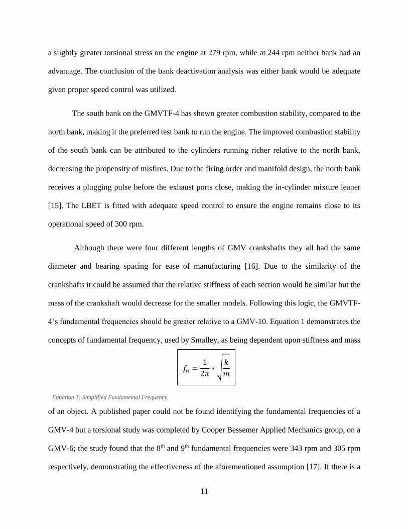
Although there were four different lengths of GMV crankshafts they all had the same
diameter and bearing spacing for ease of manufacturing [16]. Due to the similarity of the
crankshafts it could be assumed that the relative stiffness of each section would be similar but the
mass of the crankshaft would decrease for the smaller models. Following this logic, the GMVTF-
4’s fundamental frequencies should be greater relative to a GMV-10. Equation 1 demonstrates the
concepts of fundamental frequency, used by Smalley, as being dependent upon stiffness and mass
of an object. A published paper could not be found identifying the fundamental frequencies of a
GMV-4 but a torsional study was completed by Cooper Bessemer Applied Mechanics group, on a
GMV-6; the study found that the 8th and 9th fundamental frequencies were 343 rpm and 305 rpm
respectively, demonstrating the effectiveness of the aforementioned assumption [17]. If there is a
Equation 1: Simplified Fundamental Frequency
= ∗

12
fundamental frequency within a 10 rpm range of the nominal operating speed of 300 rpm the
frequencies would be of the 9th or 10th order, having minimal increase on crankshaft torsional
stresses.
On the LBET, the north bank cylinders can either be left in the engine or removed to reduce
frictional losses. Smalley’s experiments found that leaving the cylinder “dead” cylinders in the
engine reduced the total output of the engine to 40% of maximum load, but removing the “dead”
cylinder, would theoretically allow the engine to operate at 50% of maximum load. At the current
rating the GMVTF-4, BMEP ~67 psi, operating on two cylinder would produce ~180 bhp but at a
GMVH-2 rating, BMEP ~125 psi, the engine could produce ~330 bhp, Equation 2. If the
deactivated cylinders were removed the frictional losses would reduce, increasing the power output
to ~220 bhp and ~410 bhp for GMVTF-2 and GMVH-2 configurations, respectively.
Either option would be viable at the EECL but there are concerns to both methods.
Smalley’s survey polled industry users of large bore two stroke compressor engines like the
GMVTF on their experience with cylinder deactivation. The users polled in the survey did not
remove the power cylinders, like Smalley’s experiments. The only problems reported with cylinder
deactivation was spark plug fouling in the deactivated power cylinders and oil accumulation in the
exhaust manifold. Smalley classifies these concerns as minor but noted they should not be
neglected to ensure the safe operation of the engine. Typically the LBET runs less than 15 days a
year allowing for the regular inspection of the engine without effecting operational deadlines.
= = . = ሶ∗
Equation 2: BMEP Ratio and Calculation

13
Jackson et al. completed a similar investigation as Smalley but on a 4-stroke White
Superior V-16 engine [10]. The engine’s load requirements dropped below 50% of its rated power
and was running inefficiently. Jackson’s investigation determined the engine as an ideal candidate
for cylinder deactivation to improve combustion stability. The cylinder deactivation was
completed in two phases. First, eight of the engine’s cylinders were deactivated by removing the
push rods to an entire bank. This prevented the intake and exhaust valves from opening and was
thought to have less frictional losses than to have the valves remain open [10]. The engine ran for
three months in this configuration to determine if running “dead” cylinders was detrimental to
engine performance. Other than the expected frictional losses the “dead” cylinders did not affect
the engine performance; the cylinders had normal wear patterns on the liners, pistons, rings, valves,
and cylinder heads without any excessive oxidation. The engine could be run in this configuration
indefinitely but the frictional losses were detrimental to the total brake specific fuel consumption.
Jackson moved forward with the deactivation experiment to reduce the frictional losses by
removing the “dead” cylinders. To complete this task, the pistons, cylinder heads, connecting rods,
and valve push rods were removed, the oil admission holes were plugged to maintain engine oil
pressure, and the exhaust manifold openings were sealed with a steal plate. Jackson then completed
an in depth torsional analysis of the now modified crankshaft. By removing the cylinder heads and
connecting rods the concentrated inertia of each of the eight crank assemblies was reduced by
22.5%. The reduction in inertia resulted in the node one fundamental frequency to increase by
7.5%. It was noted that the multiple node frequencies also increased but had very limited effect on
the stresses measured on the crank case and bearings. The bank deactivation BSFC savings
increased from 12% to 25% when the power cylinders were removed, reducing the frictional
losses. In addition to the improved BSFC the engine was also noted to have less misfire events as

14
well as reduced spark plug fouling associated with the improved combustion stability of running
the engine near 100% load per cylinder.
Cylinder bank deactivation will be viable for the GMVTF-4 at the EECL. The north
cylinders will be the ideal bank to deactivate due to the increased combustion stability of the south
bank. The engine will be able to run with “dead” cylinders or conduct a similar cylinder removal
project as Jackson. If the cylinders are not removed regular engine inspection should be completed
to ensure that oil is not accumulating in the manifold or in the “dead” cylinders. To address the
speed and torque variation concern identified by Smalley, a tight speed control should be
implemented to keep speed fluctuations within 10 rpm of 300 rpm. This method will allow the lab
to move between two and four cylinder operation with ease, which will depend upon the industry
sponsor’s desire. Removing the cylinders from the north bank would be a time intensive project
and would require additional analysis. An in depth torsional analysis would be beneficial to
determine if a significant fundamental frequency would be within the operational range of the
engine. Additional investigation would also have to be considered on how to manage the airflow
through the engine, because a two stroke engine like the GMV does not utilize valves like a 4-
stroke.
1.2.3 Engine Uprate
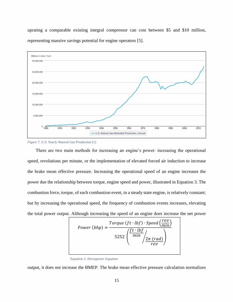
The domestic natural gas supply is estimated to have over 348 trillion cubic feet of natural gas
[18]. The collection and distribution of this vast supply has steadily increased over the past century,
as shown in Figure 7. To meet the ever increasing market demand the U.S. pipeline network has
continued to expand, installing new high speed compressor engines as well as uprating the old
slow speed integral compressors. The purchase and installation of new high speed compressor
engines to meet the increased demands can cost upwards of $16 million per engine [5]. In contrast,
15
uprating a comparable existing integral compressor can cost between $5 and $10 million,
representing massive savings potential for engine operators [5].
There are two main methods for increasing an engine’s power: increasing the operational
speed, revolutions per minute, or the implementation of elevated forced air induction to increase
the brake mean effective pressure. Increasing the operational speed of an engine increases the
power due the relationship between torque, engine speed and power, illustrated in Equation 3. The
combustion force, torque, of each combustion event, in a steady state engine, is relatively constant;
but by increasing the operational speed, the frequency of combustion events increases, elevating
the total power output. Although increasing the speed of an engine does increase the net power
output, it does not increase the BMEP. The brake mean effective pressure calculation normalizes
Figure 7: U.S. Yearly Natural Gas Production [1]
ℎ = ∙ ∙ ∙ ൙
Equation 3: Horsepower Equation

16
an engine’s power by its displacement and operational speed, allowing for a one to one comparison
of single combustion events between engines. To increase the BMEP, the power of each
combustion event must be increased. Increasing the amount of in-cylinder air, increases the amount
of available oxygen. The additional in-cylinder oxygen means more fuel can be combusted while
maintaining a constant air to fuel ratio. The elevated fuel density increases the amount of potential
chemical energy for the cylinder to use per combustion event. This corresponds to higher in-
cylinder pressures, increasing the work per combustion event.
A standard GMVTF was a pump scavenged engine running at 300 rpm with a peak
combustion pressure of ~500psi; while a GMVH was turbocharged, running at 330 rpm with a
peak combustion pressure of ~900 psi [8]. The concern with uprating the GMVTF is that the
increased operational stresses may cause premature failure of the crankshaft or the crankcase. To
address these concerns analyses of engine materials and stresses associated with combustion and
engine speed were performed.
The GMVTF-4 at the EECL was constructed at the Cooper foundry in the Mount Vernon
foundry. The GMV ran using a high strength steel crankshaft. During Smalley’s cylinder
deactivation investigation an in depth strength analysis was conducted on the GMV’s crank shaft.
The crank shafts were mass produced at the Mount Vernon facility with a “generous diameter to
length ratio” giving the crankshaft extreme ruggedness and resistance to torsional stresses [16].
The crank shaft is supported by two main bearings between each crank throw and an end bearing
on each end resulting in comparatively low bearing pressures. Despite its 12 inch diameter Smalley
suggested to avoid premature failure the torsional stresses should remain below 8 ksi on the
crankshaft [12].

17
Unlike many engines of its time period, the GMV crankcase was cast out of a meehanite iron
rather than typical gray iron [16]. Meehanite is a trademark for an engineering process for making
a range of cast irons produced under carefully controlled and precise conditions [19]. Exceptional
strength and wear resistance of meehanite can be attributed to its close grained, uniform matrix
[16][19]. The literature did not specify the grade of meehanite the crankcase was cast out of but
there are three broad types: high duty flake iron (gray iron), high duty nodular iron (ductile iron),
and a specialized group designed for heat, wear, and corrosion resistance. As the meehanite process
is trademarked the grade names are consistent regardless of manufacturer. Courtesy of Meehanite
Metal Corporation in Mequon Wisconsin a metal selection guide was acquired, Appendix A. Upon
investigation of the selection guide the possible crankcase materials were narrowed down to “G”
and “S” series meehanite. The “G” series is a flake graphite iron known for good impact strength,
shock resistance, and machinability as well as responding well to heat treatment. The “G” series
iron have fatigue strengths ranging from 11 to 30 ksi; compared to standard gray iron with fatigue
strengths between 8 and 10 ksi [19][20]. The “S” series is a nodular graphite iron with primarily a
pearlitic matrix known for its high strength and machinability, resulting in fatigue strengths
between 30 and 53 ksi [19]. The engineering department at Colorado State University has
technology to measure the hardness and tensile strength of material samples as well as the ability
to polish, etch and image samples to determine material properties.
Reynolds French is a service company specializing in repair of cracked and damaged engine
casting. Many GMV castings were repaired by Reynolds French, and they outline the most
common repairs in their GMV repair brochure, Appendix B. Many of their GMV repairs were
replacing worn pieces of the engines and re-alignment projects but they have completed several
crankcase repair projects. GMV series engines have a common crankcase design and Reynolds

18
French has noted that as the horsepower was increased through the use of turbochargers, the
breakage was consistently found along the upper web of the engine, depicted in Figure 8. The
crankcase failures begin as small cracks but if not repaired the crack can propagate through the
web resulting in catastrophic engine failure. Figure 9 shows an extensive repair of a propagating
crack in a GMV crankcase. To avoid costly repairs and failure, Reynolds French suggests
conducting annual crankcase inspection to insure the integrity of the engine.
Figure 8: Common Crankcase Failure Noted by Reynolds French [35]

19
Dennis Schmitt conducted an investigation on the uprate technology development for pipeline
compressor engines. The majority of his research was focused on the Clark TLA-6 but he also
conducted a crankcase strength analysis on the GMVTF-4 at the EECL. Schmitt used a
combination of modelling techniques to predict the forces and responses associated with the
GMV’s operation. He later evaluated his findings by taking on-engine measurements.
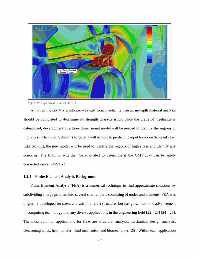
S chmitt created a simplified three dimensional model of the GMV crankcase and determined
the areas of greatest stress were above and below the main bearing in the GMV [21]. The areas of
high stress were determined as the points of interest where strain gauges would be mounted inside
the crankcase, Figure 10. Schmitt’s model did not identify the upper webs as an area of concern,
as noted by Reynolds French. Moving forward, the bearing and upper web stress should be
monitored to ensure the safe operation of the GMVTF under uprated operation. An in depth
material analysis should also be completed to determine the true strength characteristics of the
crankcase to accurately predict its behavior.
Figure 9: GMV Crankcase Crack Identification and Repair [35]
20
Although the GMV’s crankcase was cast from meehanite iron an in-depth material analysis
should be completed to determine its strength characteristics. Once the grade of meehanite is
determined, development of a three dimensional model will be needed to identify the regions of
high stress. The use of Schmitt’s force data will be used to predict the input forces on the crankcase.
Like Schmitt, the new model will be used to identify the regions of high stress and identify any
concerns. The findings will then be evaluated to determine if the GMVTF-4 can be safely
converted into a GMVH-2.
1.2.4 Finite Element Analysis Background
Finite Element Analysis (FEA) is a numerical technique to find approximate solutions by
subdividing a large problem into several smaller parts consisting of nodes and elements. FEA was
originally developed for stress analysis of aircraft structures but has grown with the advancement
in computing technology to many diverse applications in the engineering field [22] [23] [24] [25].
The most common applications for FEA are structural analysis, mechanical design analysis,
electromagnetics, heat transfer, fluid mechanics, and biomechanics [25]. Within each application
Figure 10: High Stress FEA Results [21]

21
there are different types of analysis but equilibrium is the most common when analyzing structural
mechanics [25].
FEA is a very powerful engineering tool but the user must understand it is not an exact
solution. This method uses numerical approximations and is not composed of closed form
analytical equations [22]. Conducting stress analysis, the FEA numerical methods will discretize
the three dimensional model into many “finite elements” and solve for an equilibrium, determined
by the spatial distribution of the forces, shown in Figure 12. The numerical methods approximation
are defined at the boundaries of each element, or nodes. Once the boundary nodes are determined,
the internal nodes are approximated using interpolation equations.
Figure 11: FEA Solution Approximation [27]

22
Although FEA is an approximate numerical solution the accuracy of the model can often
be improved by increasing the number of finite elements representing the geometry. By increasing
the number of finite the elements the accuracy of the model does increase. But the cost of the
greater accuracy has a point of diminishing return where the significantly more computing power
does not warrant the additional elements, illustrated in Figure 11.
FEA allows the user to predict the behavior of very complex geometries. Complex geometries
cannot be analyzed using closed form solutions and using numerical methods would lead to drastic
simplification of the part. FEA allows a user to analyze these geometries but the user must
determine the validity of the generated results. One key process for FEA, the user must conduct a
“reality check” do determine if the results are reasonable. To determine whether the results are
reasonable the user can evaluate a closed form solution to verify the model findings [22] [26] [26]
[27]. Closed form solutions and on sample measurement allows the user to calibrate the FEA
Figure 12: Two Dimensional Geometry Discretized into Finite Elements [26]

23
models. Once the model is calibrated the user can extrapolate and explore theoretical test cases. A
process map for validating the FEA measurements is outlined in Figure 13.
The improvement of solid modelling is an iterative process that leads to many revisions of the
model to obtain an accurate representation of the specimen.
Figure 13: FEA Validation Process Map [24]

24
2 CRANKCASE MATERIAL DETERMINATION
2.1 OVERVIEW
There are two main categories of material testing, non-destructive and destructive. Due to
the engine’s size and location the techniques to evaluate the crankcase properties would have to
be brought to EECL or samples would need to be removed and evaluated. Removing small samples
from the engine was chosen due to cost constraints and the increased flexibility to take the samples
to multiple labs. Non-destructive tests were favorable because it allowed each sample to be tested
for multiple properties but unfortunately some properties could only be determined using
destructive means.
2.2 MATERIAL ANALYSIS METHODS
To determine the specific grade of meehanite, the metal selection guide in Appendix A
provided a guideline for the material properties to be analyzed. The material properties of interest
were the graphitic microstructures, hardness, density, tensile/fatigue strength, and modulus. The
literature review narrowed down the potential material candidates to “G” and “S” grades of
meehanite with flake and nodular graphite microstructures, respectively. A common
metallographic technique for determination of a sample’s microstructure is the process of grinding,
polishing, etching and imaging using an optical microscope. The grinding process roughly shapes
the sample to a manageable size and to a flat and uniform finish. The polishing phase is a precise
form of grinding, smoothing the surface to a mirror finish, often a smoothness of one micron [28]
[29]. The use of etchants helps expose grain boundaries, highlights the metallic phase, and exposes
the general microstructure. Varder Voort suggests using a nital solution with a concentration

25
between a 2% to 6%, to etch the sample[29]. Nital is a mixture of nitric acid and alcohol. The
etchant works because nitric acid has a strong oxidation response to ferritic metals, enhancing the
imaging of the material microstructure. The polished and etched sample must be handled with care
to ensure no surface contamination or damage before imaging. An optical microscope is adequate
for the determination of the type of graphic structure present on the meehanite samples. The
Advanced Materials Processing and Testing Lab (AMPT) at the Motor Sport Research Center
(MERC) run by Dr. Troy Holland has the ability to process the material samples to determine the
microstructure. The AMPT also has the capability to conduct precise density calculations using
Archimedes’ method.
Once the microstructure and density is determined, hardness testing can further narrow
potential candidates. The Smash Lab at CSU, managed by Joe Wilmetti, has the ability to conduct
Rockwell B hardness testing using a 1/16 inch ball indenter. The lab has the ability to take multiple
hardness samples and then to average the data to ensure an accurate hardness was determined. The
determination of the microstructure, hardness, and density are non-destructive tests allowing a
single sample to be used multiple times to determine the properties.
The determination of tensile strength and modulus of a sample requires stressing the sample
until failure, which is destructive testing. A common method to determine the ultimate tensile
strength of a material is to machine it into a dogbone, as specified in ASTM E8 [30]. The dogbone
sample can either be cylindrical or rectangular. The CSU Smash lab has various sizes of tensile
testing machines able to accommodate the “standard” sizes of ASTM dogbone samples. The
tensile testing machines in the Smash Lab are equipped with hydraulic wedge style grips that are
only capable of holding rectangular dogbone samples. To test “sub-sized” dogbone samples the

26
construction of a specialized jaw adapter would be required to ensure the material does not slip
out of the jaw assembly.
Dogbone samples are designed to be easily held and manipulated by tensile testing machines
with the “reduced section” as the designed point of failure, seen in Figure 14. To ensure the failure
occurs in the reduced section the radius between the shoulder and the reduced section are designed
to minimize stress concentration and have the failure occur in the known area of the reduced
section [30]. The surface of the sample should also be smooth to further reduce stress
concentrations.
The MTS tensile testing machines are interfaced with a data acquisition and control system
to measure and regulate the jaw speed and applied force. The system has the ability to record the
applied force and relative displacement of the jaws once the test has commenced. In conjunction
with the MTS software, an extensometer should be used to accurately measure the change in length
of the gauge area. The extensometer is used to accurately measure the strain of the sample. The
software is capable to measure the total displacement of the machine sample but this method is
inadequate to determine the sample strain. ASTM E8 strongly advised against using the total
sample displacement for modulus calculation [30].
Figure 14: ASTM E8 Dogbone for Tensile Test [30]

27
Prior to pulling the test piece the dimensions of the dogbone must be measured and recorded
to properly calculate the stress and strain. The important characteristics to measure are the gauge
length and the cross sectional area of the gauge length.
To calculate the modulus the stress and the strain of the sample must be determined [31].
The force, for the stress calculation, is measured from the MTS load cells in conjunction with
displacement of the system and the extensometer at a rate of ~2.5kHz. The gauge length and area
is measured before the test using precise engineering calipers to determine the cross section area
(Agauge) and the original length (Lo-gauge), Equation 6a and Equation 6b. The data is then used to
create an engineering stress-strain curve, like the curve shown in Figure 15. An engineering stress
strain curve does not take into account the necking, shrinking area of the gauge section of the iron
but is the curve used to determine engineering material properties [31]. The linear elastic region
Equation 6a: Stress Calculation [31]
=
Equation 6b: Strain Calculation [31]
= − − −
Equation 6c: Modulus Calculation [31]
=
Figure 15: Engineering vs True Stress-Strain Curve [31]
1. Ultimate Tensile Strength 2. Yield Strength (Yield Point) 3. Rupture (Failure) 4. Strain Hardening Region 5. Necking Region A. Engineering Stress-Strain B. True Stress-Strain

28
of the curves, from the start of collection to the yield point, is where the modulus of elasticity is
calculated. Modulus is the measure of an object’s resistance to elastic deformation when force is
applied. In the elastic region, the material can be deformed under load but once the load is removed
the material will return to its original shape. However, past the yield point the part will be
permanently or plastically deformed.
All the techniques described above were used to narrow down the likely grade of meehanite
iron of which the GMV crankcase was cast.
2.3 MATERIAL TESTING
Two samples were removed from the north side of the engine under the crankcase doors,
shown in Figure 16. The samples were roughly 14 inches long with a rough triangular-like cross
section (Figure 17). Several non-destructive and destructive tests were conducted to determine the
material properties of the meehanite crankcase. The material testing was conducted at the CSU
Smash Lab and the AMPT.
Figure 16: Sample Location
Figure 17: Cross Section Slice from Sample

29
2.3.1 Non-Destructive Testing
Two cross sectional slices were used to determine the graphitic structure, density, and
hardness of the samples. There were two possible classes of meehanite the crankcase could be cast
out of, “G” series or “S” series with flake and nodular graphite structures respectively (Figure 18).
2.3.1.1 Imaging to Determine Graphitic Structure
To determine the graphitic structure of the iron a combination of grinding, polishing,
etching, and imaging techniques were used at the AMPT laboratory.
The first step in the process, grinding, was crucial to have the surface of the slices as flat
as possible. The process required the use of successively finer sandpaper to flatten and smooth the
surface. Once the sample was relatively flat, it was mounted to the platen. The platen was a precise
smoothing tool used in conjunction with a sanding wheel to give a precise flat finish seen in Figure
19 and Figure 20. The platen’s carbide feet resist wear themselves while the operator was able to
provide steady, even pressure on the sample. The process to flatten and smooth the sample was to
move the platen along the outer circle in the clockwise direction while the sanding wheel is
spinning in the counter-clockwise direction, shown in Figure 21. The counter rotation technique
gave the sample a smooth, even finish. The process was repeated using finer sandpaper until 800
grit sandpaper was used.
Figure 18: Flake vs Nodular Graphite in Meehanite [19]

30
The polishing of the sample was completed in three steps: 6-micron finish followed by 3-
micron finish, and finally a 1-micron finish. All the polishing steps used a specific polishing pad
and a polishing media applied to the pad. The pad and media combination was essentially very
fine sandpaper and the same counter rotation technique was used to attain the finishes. Once the
1-micron finish was achieved the sample had a mirror finish and was ready to be removed from
the platen and subsequently etched in nital.
Figure 21: Counter Rotation Technique
Figure 19: Platen Tool
Figure 20: Grinding and Polishing Wheel

31
Before the etching process, the sample was cleaned using a fine brush and non-abrasive
soap to remove the polishing media. The sample was then immediately rinsed with ethanol to
prevent the water from causing surface oxidation. The cleaned sample was etched by submerging
it in a 4% nital solution. When the sample was removed it no longer had a mirror finish but a
smooth, “grainy” appearance, seen in Figure 22. The sample was handled with care to ensure no
surface blemishes were introduced so that clear images could be obtained.
The sample was imaged using an optical microscope at three magnifications: 10x, 20x, and
40x. Several images were taken of the sample at the three magnification levels. Figure 24, Figure
23, and Figure 25 were chosen as representative images to show the microstructure. Comparing
the images to images from Meehanite Metal, the crankcase appears to be cast from a flake iron, or
“G” grade.
Figure 22: Etched Sample

32
Figure 24: 10x Sample Image
Figure 23: 20x Sample Image

33
2.3.1.2 Density Calculation
Density is defined as the mass per unit volume and is an important measurement for
determining material properties. One particular method for determining density is to use
Archimedes’ principle. The basis of the Archimedes’ principle is the buoyant force on a submerged
object is equal to the weight of the fluid displaced. If the weight of the fluid displaced can be
measured, the fluid volume displaced can be calculated and in-turn the density of the sample can
be determined. Figure 26 shows a visual representation of Archimedes’ principle. In the example,
the sample has a weight of 7 kg when not submerged and weight of 4 kg when submerged, meaning
3 kg of water is displaced. At room temperature, water roughly has a density of 1 g/cm3, meaning
that 3,000 cm3 of water was displaced. This would give the sample a density of 2.33 g/cm3. This
procedure was repeated to calculate the density of the GMV sample, using the equipment at the
MERC.
The scale at the MERC was a RADWAG XA 110/2x capable of 7 significant figures of
accuracy. Figure 27 corresponds to the left drawing in Figure 26 and Figure 28 to the right
Figure 25: 40x Sample Image

34
drawing. In Figure 28 the basket support system, that sample was held in, was directly connected
to the load cell of the scale and the beaker was supported over the load cell. The apparatus was set
up and allowed to stabilize before “zeroing” the scale, to take into account the weight and
buoyancy of the basket assembly. Table 1 shows the measurements and results from the
Archimedes’ method.
The imaging results determined the sample was a flake graphite, limiting the grade
possibilities to “G” type. Archimedes’ method determined the sample’s density was 7.02 g/cm3.
The determined density was close to the density of GE-30 from Meehanite metal at 7.06 g/cm3 and
the ASTM class 25 iron at 7.15 g/cm3 [19][20][32].
Figure 26: Archimedes’ Principle Diagram

35
Figure 27: Measuring Sample Mass
Table 1: Archimedes’ Density Measurement Results
Object Measurement
Water Temperature 21° C
Water Density 0.9968 g/cm3
Sample Mass 27.58253 g
Submerged Mass 23.66623 g
Mass of Water Displaced 3.92 g
Volume of Water Displaced 3.93 g
Density of Sample 7.02 g/cm3

36
1. Basket Support 2. Beaker of Water 3. Sample 4. Sample Basket 5. Load Measurement 6. Beaker Support
Figure 28: MERC Archimedes’ Scale

37
2.3.1.3 Hardness Testing
The ASM Handbook defines hardness as resistance of a metal to plastic deformation [33].
Hardness is a homogenous property for meehanite. To determine the hardness of a material there
are various methods, but the Smash Lab at CSU has the capability to conduct Rockwell B hardness
testing. The procedure for conducting Rockwell B hardness testing is defined in ASTM-E-18.
The Rockwell hardness is determined by measuring the plastic deformation of a part
relative to a “zero” point [34]. The penetration depth of the indenter and the hardness are inversely
proportional, shown in Equation 7. To calculate the hardness, a uniform sample is placed in the
apparatus and preliminary load is applied to establish the “zero” point. The test force is then
applied, for the Rockwell B test the test force in 100 kg. The force is then relaxed to the preliminary
load and the depth measurement is determined, denoted as “h”. The described process can be seen
in Figure 30.
The Antonik Tester Service Rockwell hardness tester, in the CSU Smash Lab, was used to
conduct multiple hardness tests on the material samples, shown in Figure 29. The average
Rockwell B hardness was determined to be 92 with a standard deviation of 6. This corresponds to
a Brinell hardness range of 160 to 180. This harness reported hardness from Meehanite Metal of
the GC-40 grade and the GE-30 grade were hardness measurements of 180 and 160, respectively,
and the ASTM class 25 iron had a reported hardness of 174 [19][20][32]. This result aligned with
the density determination from the previous section.
= − ℎ.
Equation 7: Rockwell Hardness Equation [34]

38
Figure 30: Rockwell Hardness Test Procedure
Figure 29: CSU Hardness Test Apparatus

39
2.3.2 Destructive Testing
The original large samples were cut into four smaller samples to collect more data to confirm
the material properties. Recall from Figure 22 the original samples were long bars with a rough
triangular cross section. To shape the sample bars into a rectangular cross section a vertical mill
was used to remove one of the triangular corners as well as flatten the sample, seen in Figure 31.
The large rectangular bars were subsequently cut into four smaller bars. The four smaller bars had
dimensions of 3” x 1” x 0.5”. To machine the samples into dogbone samples the ASTM tensile
testing was consulted to determine the proper dimensions for the specimens [30].
The code specified the samples would have a 1/8” round to neck the grip section down to the
gauge length. The designed specimens had a gauge length of 1.5” with a cross sectional area of
roughly 0.1875 square inches. The specified dimensions were then used to generate a tool path for
a computer numerically controlled (CNC) milling machine producing four identical pieces like
Figure 31: Milling Sample into Rectangular Cross Section
40
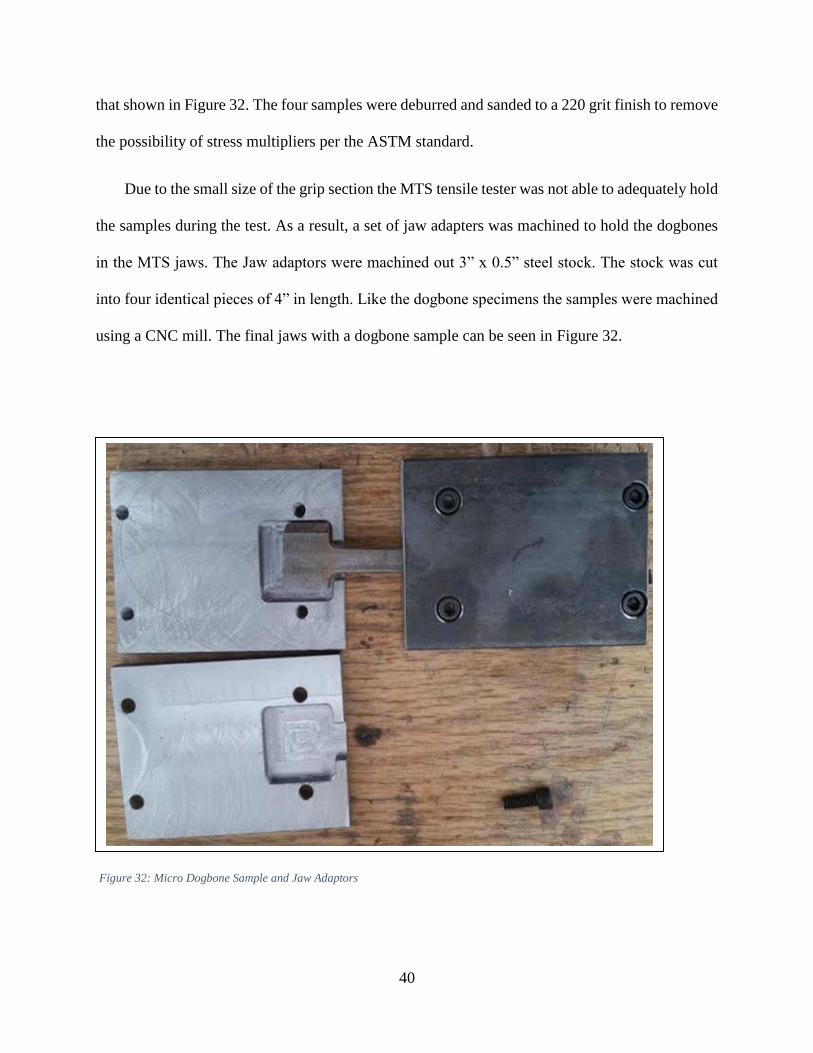
that shown in Figure 32. The four samples were deburred and sanded to a 220 grit finish to remove
the possibility of stress multipliers per the ASTM standard.
Due to the small size of the grip section the MTS tensile tester was not able to adequately hold
the samples during the test. As a result, a set of jaw adapters was machined to hold the dogbones
in the MTS jaws. The Jaw adaptors were machined out 3” x 0.5” steel stock. The stock was cut
into four identical pieces of 4” in length. Like the dogbone specimens the samples were machined
using a CNC mill. The final jaws with a dogbone sample can be seen in Figure 32.
Figure 32: Micro Dogbone Sample and Jaw Adaptors

41
To complete the tensile testing the Smash Lab’s MTS 647 apparatus was used with hydraulic
wedge grips. The MTS machine was used in conjunction with an extensometer externally attached
to measure the strain of the gauge section of the tensile specimens. The complete setup of the
tensile testing machine can be seen in Figure 33 with extensometer seen between the grips. The
entire machine is controlled by the MTS software that actuates the jaws in conjunction with
collecting the force and strain data.
Figure 33: MTS Tensile Testing Apparatus with Extensometer

42
Prior to conducting the tensile testing each of the four sample’s dimensions were measured
and recorded to calculate the stress within the gauged section, shown in Table 2. The MTS
software was also used to define the “pull rate” of the samples. The “pull rate” is how much
displacement the machine will put on the sample per given time interval. The standard “pull rate”
for iron samples of this size is 0.04 in/min and was implemented on the system [30].
The sample was monitored by watching the real time stress strain graph generated by the MTS
software. The user watches the graph to find when the sample enters the “necking” or strain
hardening regime of the stress strain curve. This was when the sample was no longer behaving
elastically and would be expected to fail shortly. Once the necking regime was entered the tensile
test was halted. Material fracture is a very traumatic event and can damage extensometers. To
protect the integrity of the instrument it was removed at this point. The test was then continued to
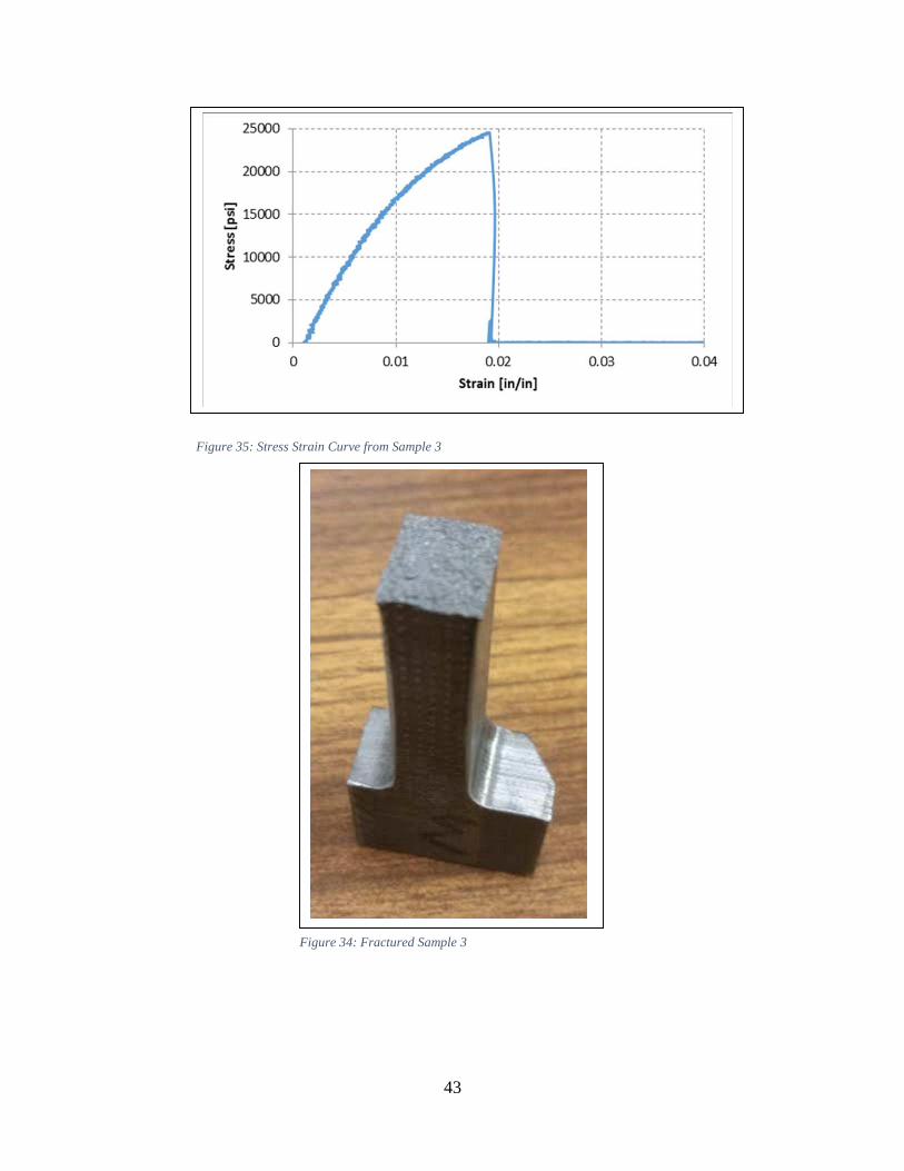
ultimate failure. Figure 35 shows the stress strain graph from sample 3 and Figure 34 showing the
fractured sample 3. Unfortunately due to the small gauge length the extensometer was not able to
be directly fastened to the sample and produced inconclusive strain results. Consequently, an
accurate modulus could not be determined for the tensile tests. The same technique was used for
the remaining three samples with the results seen in Table 3.
Sample Height [in] Width [in] Cross Sectional Area [in2] Gauge Length [in] 1 0.481 0.383 0.184 1.498 2 0.503 0.385 0.194 1.497 3 0.503 0.383 0.193 1.500 4 0.486 0.385 0.187 1.496
Table 2: Dogbone Sample Dimensions
43
Figure 35: Stress Strain Curve from Sample 3
Figure 34: Fractured Sample 3

44
The average failure stress of the samples was determined to be ~24 ksi while GE-30 has an
ultimate tensile strength of 30 ksi and ASTM grade 25 iron has an ultimate tensile strength of 26
ksi [19][20]. As can be seen in Figure 34, the sample exhibits a grey fracture surface, consistent
with gray iron [32]. A fatigued sample would show beach marking in this grade of iron but the
fracture surface was a brittle fracture with no cyclic loading concerns. Based on this, the engine
crankcase is likely cast out of a Class 25 grade of Meehanite.
Sample Ultimate Failure Strength [ksi]
1 24.49 2 24.89 3 24.04 4 22.55 Average 23.99
Table 3: Tensile Test Results

45
2.4 MATERIAL ANALYSIS CONCLUSION
The most likely grade of meehanite the crankcase was cast out of a class 25 meehanite.
Although Meehanite metal does not currently produce a class 25 the selection guide can still
provide an approximation for iron properties. ASTM cites that class 25 iron is often used for
cylinder heads, as well engine blocks and housings [20].
Class 25 irons are flake graphite iron with a pearlitic matrix. This result is consistent with the
findings from section 2.3.1.1. Class 25 grade had a densities of 7.15 g/cc, compared to the
measured sample density of 7.02 g/cc from section 2.3.1.2, corresponding to a percent difference
1.8% [20]. The class 25 grade had a reported hardness of 174 on the Brinell hardness scale
compared to the measured sample hardness range from section 2.3.1.3 of 160 to 180,
encompassing the reported value. The class 25 iron had an ultimate tensile strength 26 ksi and the
average failure stress of the samples was ~24 ksi corresponding to percent difference of 7%. After
speaking with Joe Wilmetti, the Smash Lab manager, the MTS machine has not had a factory
calibration for over 5 years, and citing Dr. John Petro’s experience in material testing this could
result in a 5% measured load error. This likely error could explain the discrepancy between the
reported ultimate tensile strength and the measured.
The FEA software had a gray cast iron already in its material toolbox with properties between
the GE-30 Meehanite and ASTM class 25 grade. This material was assumed to adequately predict
the engine material properties for conducting FEA.
To determine the exact grade of iron a spectrographic analysis would be required to determine
the elemental composition within the metal.

46
3 CRANKCASE MODEL DEVELOPMENT AND FEA TESTING
3.1 OVERVIEW
The goal of creating a three dimensional model and FEA was to identify the regions of high
stress in the engine, where failure was likely to occur. A combination of past models, engineering
drawings, and on engine measurements were used to develop an improved representation of the
LBET. The previous FEA conducted by Schmitt only considered the force inputs at the main
bearings. The enhanced computing ability of the engineering compute servers allowed for more
input forces and a finer mesh analysis to be conducted, improving the model accuracy.
3.2 MODEL IMPROVEMENT
The three dimensional model of the LBET was constructed in Creo Parametric. Creo is a
suite of design software supporting product design by PTC. The suite consists of several apps,
each delivering a distinct set of capabilities for product development. The direct modeling and
model assembly features, within Creo, were used to create a virtual three dimensional
representation of the engine.
The model was constructed using a combination of past models, engineering drawings, and
on engine measurements. Schmitt’s simplified model provided the groundwork for the
development of an accurate representation of the GMV crankcase. Schmitt constructed the
simplified model of the crankcase due to computing power limitations. He noted that more
complex geometries needed for a more accurate model would produce meshing errors in the FEA
program [22].

47
The new GMV crankcase model was focused on improving the accuracy of the bearing caps,
the web design, and removing artificial stress concentrations. Particular interest was given to
improving the upper web accuracy, because of common premature failures noted in field engines
[35]. The model improvement was an iterative process and was constantly improved after each
FEA simulation to remove artificial stress concentrators due to the meshing method. Particular
care was placed in the assembly and modeling of the combustion cylinders to account for the
reactionary forces placed on the upper webs due to in-cylinder pressures. The improved model of
the GMV can be seen in Figure 36.
Figure 36: Improved GMVTF Crankcase Model with Power Cylinders

48
The model was then imported into a FEA program, Ansys Workbench, to compete an in
depth structural analysis of the engine.
3.3 FEA SET UP AND RESULTS
Ansys Workbench was the software used to conduct the FEA investigation. Ansys has a
wide range of capabilities but only the Mechanical toolbox was used. Ansys Mechanical toolbox
is a finite element analysis tool for structural analysis. The generated model can be manipulated
and improved to provide the most accurate representation of the LBET.
The findings from the material testing determined the engine crankcase was cast out of
class 25 grade of meehanite. The material properties for class 25 meehanite were very similar to
the existing gray cast iron already available in the Ansys toolbox but some of the values were
modified to better reflect the class 25 iron. The crankcase and cylinder geometries were designated
as the modified gray cast iron for all the simulation cases.
FEA modeling was conducted in three steps, pre-processing, analysis and post-processing
or result interpretations.
3.3.1 Pre-Processing
The pre-processing step was where the FEA model was constructed using the three
dimensional Creo model. Ansys divided the imported three dimensional geometry into a finite
number of discrete sub-regions, “elements”, connected at discrete points called, “nodes” [36]. Each
of the nodes will either have defined loads or a set displacement dependent upon the model
assumptions. The final model consisted of 662,686 nodes and 407,582 elements. Once the mesh
was generated the input forces were implemented on the model.

49
3.3.1.1 Bearing Forces
The articulated crank assembly of the GMV, has a complex motion that would make
predicting the bearing forces very complicated using simple analytical methods. Schmitt used the
software Working Model to predict the how combustion forces would be translated to the bearings.
MSC Working Model was an engineering simulation software product by Design Simulation
Technologies, utilizing virtual mechanical components to simulate an objects response in a two
dimensional work space.
The model was constructed using test data collected from the LBET running at nominal
conditions, standard mechanical gas admission valve fuel injection, and sea level manifold
conditions with a boost of 7.5 inHg gauge [22]. The in cylinder pressure data were converted into
the input force for the Working Model simulation with the peak pressure maintained at 18° after
top dead center (ATDC) [22]. The working model simulation took into account the weights and
inertial loading of the components that move and rotate, but the geometries were simplified for
two dimensional representation [22]. Each of the two simulated banks consisted of the crankshaft,
master connecting rod, two power piston connecting rods, two power pistons, and one cross head.
The simulation also took into account the frictional losses of the entire mechanism
It was assumed the journal bearings were under normal operating conditions. The main
journal bearings are fluid film bearings, where under normal conditions they were in a full
hydrodynamic regime with minimal frictional losses [16]. Schmitt assumed the bearing friction
was 0.01 [22]. The assumed frictional value of 0.01 was within the known friction coefficients for
standard journal bears in the hydrodynamic regime [37]. The wrist bearing’s coefficient of friction
was assumed to be 0.05 which is within the typical range of oil lubricated iron on iron joints [37].

50
Schmitt also accounted for the frictional losses due to the piston rings. The GMV has dynamically
lubricated steel rings and cast iron sleeves and assumed the friction between them were 0.1 [22].
Due to the limitations of the two dimensional simulation the bearing reactant forces were
assumed to have zero out of plane force and were only vertical and lateral components. Appendix
C has partial input and results data as well as how the Working Model simulation was organized.
Figure 37 was the output results from the working model simulation used as bearing input forces
in Schmitt’s FEA model.
The university no longer holds a license for Working Model and resources were unavailable
to purchasing software licenses for this project. The output from Schmitt’s models could be used
to predict the engine’s stress response while running at nominal GMVTF conditions but could not
be directly modified to predict the bearing forces at uprated conditions.
Figure 37: Working Model Force Outputs [21]

51
To predict how the bearing load would change at uprated conditions, a relationship from the
original model was determined. The Working Model simulation used a number of equations to
predict how the load would be transferred from the power pistons to the main crank bearings. The
load on the bearings is directly related to the in-cylinder pressure and the speed of rotation. As the
engine’s operational speed would remain at 300 rpm at the uprated conditions, it was assumed the
inertial loading on the crank bearings would relatively remain constant. To account for the greater
in-cylinder pressures, GMVA and GMVH pressure data was obtained. The EECL had conducted
testing on the LBET at GMVTF and GMVA conditions with peak pressures of ~500 psi and ~600
psi respectively. To determine the average peak pressure of a GMVH, data from Southwest
Research Institute from their GMVH-6 research engine was obtained. The GMVH had a typical
peak pressure of ~900 psi [38]. The pressure ratios were 6:5 for the GMVA condition and 9:5 for
the GMVH condition. To determine the how the in-cylinder pressures related to the bearing force
a correlation was created using Eureqa. Eureqa is a mathematical software tool originally created
by Cornell's Creative Machines Lab and distributed by Nutonian, Inc. The software utilizes
symbolic regression to determine the simplest mathematical equations to describe a given data set.
Four models were developed to predict the x and y forces on the bearings.
Nine variables were input into the Eureqa’s data set: crank angle [rad], cylinder 1 force [lbf],
cylinder 2 force [lbf], cylinder 3 force [lbf], cylinder 4 force [lbf], force x for bearings group 1,
force y for bearings group 1, force x for bearings group 2, and force y for bearings group 2. The
cylinder force bearing group and crank angle data were designated as the input and the bearing
force data were designated as the output. Four models were created to predict the force magnitude
for each of the output variables, defined by the function in Figure 38. Notice that “crank” was
defined as function of sine or cosine and bearing group 1 was only dependent upon cylinders 1 and

52
2, like bearing group 2 was only dependent upon cylinder 3 and four. These parameters were
chosen because the crank had cyclic pattern that can be approximated by a combination of
trigonometric functions. And the original Working Model simulation had the same input force
arrangement for the two bearing groups.
The Eureqa software was left to run for 84 hours to develop a correlation for the four
components of the bearing forces. A comparison between the original case and the predicted case
can be seen in Figure 39 for x force of bearing group 1. All four Eureqa models matched the
original prediction just as well. Figure 40 shows the extrapolation of the Eureqa model predicting
the force outputs for the GMVA and GMVH conditions. As expected, at the peak pressure events
of cylinders 1 and 2 the model predicts greater bearing load but at all other part of the cycle the
model does not predict much change in the predicted bearing force. It was noted that the Eureqa
model may have over predicted the bearing forces at cylinder peak pressures. In Figure 40, the
GMVH bearing force was predicted to be 4.5 times greater than the GMVTF condition when the
peak pressure was only 1.8 times greater. Based on this observation all predictions from the Eureqa
model were used except for the peak pressure cases. At the peak pressure cases a force ratio was
determined based upon the peak pressures to multiply the GMVTF case by. The ratio between
GMVA and GMVTF was 6:5 and between GMVH and GMVTF was 6:5.
Fx1 = f((Cylinder 1)*sin(Crank), (Cylinder 1)*cos(Crank), (Cylinder 2)*sin(Crank), (Cylinder ______2)*cos(Crank), (Cylinder 1), (Cylinder 2))
Fy1 = f((Cylinder 1)*sin(Crank), (Cylinder 1)*cos(Crank), (Cylinder 2)*sin(Crank), (Cylinder ______2)*cos(Crank), (Cylinder 1), (Cylinder 2))
Fy2 = f((Cylinder 3)*sin(Crank), (Cylinder 3)*cos(Crank), (Cylinder 4)*sin(Crank), (Cylinder ______4)*cos(Crank), (Cylinder 3), (Cylinder 4))
Fx2 = f((Cylinder 3)*sin(Crank), (Cylinder 3)*cos(Crank), (Cylinder 4)*sin(Crank), (Cylinder ______4)*cos(Crank), (Cylinder 3), (Cylinder 4))
Figure 38: Eureqa Model Definition Functions

53
Eight points of interest were determined as likely points of high crankcase stress. The four
peak pressure events and four high magnitude points between the peak pressure points were
determined as the points of interest. These eight points were also extrapolated to the GMVA and
GMVTF cases. Table 4 has complete list of bearing input forces for the FEA simulation.
The four bearing force prediction equations can be seen in Figure 41.
Figure 39: Force x for Bearing Group 1 Prediction

54
Figure 40: Eureqa Model Extrapolation

55
= . ∗ cos + . ∗ ∗ sin + .∗ ∗ sin ∗ cos − . − . ∗ sin− . − ∗ − . ∗ ∗ sin− . − ∗ ∗ sin ∗ cos = . + . ∗ + − . + .∗ ∗ + − . ∗ ∗ − . ∗ ∗ − . − . ∗ ∗ − . ∗ ∗ = . + . ∗ + . ∗ + . ∗ + . ∗ + . −∗ ∗ ∗+ . ∗ ∗ − . = . ∗ + . ∗ ∗ + .∗ ∗ ∗ − . − . ∗ − . − ∗ − . ∗ ∗ − . − ∗ ∗ ∗
Figure 41: Final Eureqa Output Equations

56
Ansys Mechanical has the ability to simulate the characteristics of a bearing load, using the
“bearing load” load constraint. The constraint was assumed to be identical for bearings 1 and 2
using the F12x and the F12y forces, similarly the F34x and the F34x were used for bearing 3 and 4 on
the engine. The bearing surfaces were selected, seen in Figure 42, and twenty four load case were
analyzed, eight points from the three operating conditions.
Figure 42: Bearing Load Force Input for Bearings 3 and 4

57
GMV-TF
Crank Angle [deg] Fx1 [lbf] Fy1 [lbf] Fx2 [lbf] Fy2 [lbf]
Magnitude 1 [lbf]
Magnitude 2 [lbf]
18.00 1.48E+04 -3.30E+04 1.49E+04 -4.47E+04 3.61E+04 3.62E+04 50.50 8.57E+03 -1.72E+04 -1.36E+04 -5.18E+04 1.92E+04 2.19E+04 80.50 1.18E+04 -4.97E+04 -3.50E+04 -4.45E+04 5.10E+04 6.08E+04
127.25 5.19E+04 -2.41E+04 -4.63E+04 -1.90E+04 5.72E+04 5.22E+04 197.75 1.44E+04 -4.74E+04 1.17E+04 -3.28E+04 4.96E+04 4.88E+04 229.25 -1.32E+04 -5.19E+04 8.39E+03 -1.60E+04 5.36E+04 5.26E+04 260.50 -3.55E+04 -4.47E+04 1.04E+04 -5.21E+04 5.71E+04 4.58E+04 307.75 -4.70E+04 -1.71E+04 5.26E+04 -2.34E+04 5.00E+04 5.53E+04
GMV-A
Crank Angle [deg] Fx1 [lbf] Fy1 [lbf] Fx2 [lbf] Fy2 [lbf]
Magnitude 1 [lbf]
Magnitude 2 [lbf]
18.00 1.76E+04 -4.01E+04 1.49E+04 -4.54E+04 4.38E+04 4.28E+04 50.50 1.01E+04 -2.12E+04 -1.36E+04 -5.17E+04 2.35E+04 2.52E+04 80.50 1.42E+04 -6.03E+04 -3.49E+04 -4.44E+04 6.20E+04 6.97E+04
127.25 6.24E+04 -2.95E+04 -4.58E+04 -2.04E+04 6.90E+04 5.45E+04 197.75 1.44E+04 -4.83E+04 1.40E+04 -3.93E+04 5.04E+04 5.02E+04 229.25 -1.32E+04 -5.26E+04 1.01E+04 -1.92E+04 5.42E+04 5.36E+04 260.50 -3.54E+04 -4.56E+04 1.24E+04 -6.26E+04 5.77E+04 4.72E+04 307.75 -4.68E+04 -2.01E+04 6.32E+04 -2.80E+04 5.09E+04 6.63E+04
GMV-H
Crank Angle [deg] Fx1 [lbf] Fy1 [lbf] Fx2 [lbf] Fy2 [lbf]
Magnitude 1 [lbf]
Magnitude 2 [lbf]
18.00 2.63E+04 -6.01E+04 1.49E+04 -4.75E+04 6.57E+04 6.20E+04 50.50 1.51E+04 -3.18E+04 -1.34E+04 -5.24E+04 3.52E+04 3.46E+04 80.50 2.13E+04 -9.05E+04 -3.43E+04 -4.53E+04 9.29E+04 9.68E+04
127.25 9.37E+04 -4.42E+04 -4.42E+04 -2.54E+04 1.04E+05 6.25E+04 197.75 1.44E+04 -5.00E+04 2.10E+04 -5.90E+04 5.21E+04 5.42E+04 229.25 -1.31E+04 -5.42E+04 1.51E+04 -2.88E+04 5.57E+04 5.62E+04 260.50 -3.51E+04 -4.73E+04 1.86E+04 -9.38E+04 5.89E+04 5.09E+04 307.75 -4.60E+04 -2.66E+04 9.48E+04 -4.21E+04 5.31E+04 9.84E+04
Table 4: FEA Bearing Input Forces

58
3.3.1.2 Pressure Forces
Schmitt’s models assumed the forces exerted by pressure were mono-directional along the
connecting rods, into the crank bearings, when in reality the in-cylinder pressure exerts force in all
directions. Reynolds French noted failures were common along the upper web of the engine which
Schmitt did not find as an area of interest in his models. By including the cylinder heads in the
model, the reactionary forces of the combustion events can now be included. Three sources of
pressure data were used in conjunction with the predicted bearing forces to simulate the engine
running at GMVTF, GMVA, and GMVH conditions.
The pressure forces were inputted into the model using the “pressure” load constraint. The
top of cylinder heads were the selected surfaces where the forces of interest and cylinder walls
were neglected. It was assumed the hoop stress exerted on the cylinder walls would not
Figure 43: Pressure Force Load Constraint on Cylinder Head 2

59
substantially affect the forces transferred to the upper web of the crankcase. The pressure loads
were inputted to act normal to the surface of interest, seen in Figure 43, using the same tabular
method as the bearing loads at the same eight points for each engine condition, with values seen
in Table 5.
GMV-TF
Crank
Angle [deg]
Cylinder 1
[psi]
Cylinder 2
[psi] Cylinder 3 [psi] Cylinder 4 [psi] Significance
18.00 504.42 81.33 16.00 13.15 PP of Cyl 1
50.50 207.55 252.44 16.61 13.38 High Magnitude
Points 80.50 99.59 504.42 20.44 16.16 PP of Cyl 2
127.25 41.02 140.84 62.20 20.40 High Magnitude
Points 197.75 16.00 25.54 485.78 91.86 PP of Cyl 3
229.25 16.01 15.15 210.73 237.50 High Magnitude
Points 260.50 19.36 16.06 97.12 520.47 PP of Cyl 4
307.75 62.28 16.02 42.00 129.53 High Magnitude
Points GMV-A
Crank
Angle [deg]
Cylinder 1
[psi]
Cylinder 2
[psi] Cylinder 3 [psi] Cylinder 4 [psi] Significance
18.00 605.31 97.60 19.21 15.78 PP of Cyl 1
50.50 249.06 302.93 19.94 16.06 High Magnitude
Points 80.50 119.50 605.31 24.53 19.40 PP of Cyl 2
127.25 49.23 169.00 74.64 24.48 High Magnitude
Points 197.75 19.20 30.64 582.94 110.23 PP of Cyl 3
229.25 19.22 18.18 252.88 285.00 High Magnitude
Points 260.50 23.23 19.27 116.54 624.56 PP of Cyl 4
307.75 74.73 19.23 50.40 155.44 High Magnitude
Points GMV-H
Crank
Angle [deg]
Cylinder 1
[psi]
Cylinder 2
[psi] Cylinder 3 [psi] Cylinder 4 [psi] Significance
18.00 907.96 146.40 28.81 23.68 PP of Cyl 1
50.50 373.59 454.39 29.90 24.09 High Magnitude
Points 80.50 179.25 907.96 36.79 29.10 PP of Cyl 2
127.25 73.84 253.50 111.95 36.72 High Magnitude
Points 197.75 28.81 45.96 874.40 165.34 PP of Cyl 3
229.25 28.82 27.27 379.32 427.50 High Magnitude
Points 260.50 34.85 28.90 174.81 936.84 PP of Cyl 4
307.75 112.10 28.84 75.60 233.16 High Magnitude
Points
Table 5: FEA Pressure Input Forces

60
The FEA predicted stresses were ignored in the cylinder heads because the installed
cylinders are from a GMVH were assumed to be able to safely operate at the uprated condition.
3.3.1.3 Crankcase Constraints and Assumptions
Defining the constraints on an object when conducting FEA is equally as important as
properly defining the force inputs [24]. The GMV User’s Manual specifies the mounting system
for the LBET should be very stable and level [16]. The mounting system was designed to be long
lasting and maintain rigidity. To simulate the mounting system on the LBET, the base of the
modeled crankcase was defined as a fixed support in Ansys. The fixed support constraint prevents
movement in all six degrees of freedom, meaning the crankcase cannot translate or rotate.
Recall from Figure 36 the cover plates, above where the material specimens were removed,
were not modeled. The cover plates provided additional structural support to the engine and
constraints were needed to simulate them. The remote displacement tool was utilized to maintain
a rigid distance between the top of the opening and the bottom with properties consistent with the
assumed class 25 meehanite properties.
After the selection of the constraints and loads, the model was ready to move to in depth
analysis.
3.3.2 Analysis
The analysis step of FEA was where the model was interpreted by the Ansys Mechanical
Code. Ansys Mechanical discretized the elements and nodes constructing a system of linear and
non-linear equations to predict the model’s reaction to forces [36]. Equation 8 represents the matrix
=
Equation 8: FEA Node Reaction Matrix [36]

61
construction of the system of equations Ansys used to predict the results of each discrete point.
“Kij” was the constructed matrix dependent on the type of point and the method to numerically
solve for it, “fij” represents the input forces at the given point, and “uij” was the reaction of the
point. Ansys conducted thousands of calculations per second but user did not directly interact with
this aspect of the program. Ansys provides a status bar to let the user know where in the calculation
process the program was, Figure 44. Despite the modern computing power, the average run-time
for the fully constructed model was upwards of five hours.
3.3.3 Post-Processing, FEA Results
Ansys Mechanical can calculate deformation, strain, stress, energy, and damage each node
would sustain at the given condition. Meehanite metal gave the failure fatigue stress of the GE-30
grade of meehanite as 13.5 ksi and ASTM specifies the fatigue strength of class 25 irons as 12 ksi
so the predicted Von Mises stress at each node must be less than 12 ksi to avoid fatigue failure
[19][20][32]. The Von Mises stress was calculated because it allows for direct comparison to the
ultimate strength and endurance limit of a material [20].
Figure 44: Ansys Workbench Solution Status Window

62
Figure 45 displays the regions of high stress above main crank bearings three and four at peak
pressure for cylinder 3 at GMVH rating. As can be seen in Figure 45, the maximum stress for the
entire engine is 16,734 psi but this was measured in head of cylinder 3 while the max stress in the
crankcase at this test point was 9,621psi. Recall the predicted stress within the cylinder head will
be neglected as they are GMVH cylinders and are assumed to be able to operate at GMVH rating.
The high stress regions directly above the bearing are consistent with the findings of Schmitt, while
high stress region along the upper web is where Reynold French typically sees premature engine
failure in the field [21] [35]. The stresses below cylinders 1 and 2 were very similar as the stresses
below cylinders 3 and 4 at their relative peak pressures. Looking towards on engine testing,
mounting strain gauges below cylinders 3 and 4 is the most practical because there is already an
Figure 45: Areas of Maximum Stress above Bearings 3 and 4 at PP for Cylinder 3 at GMVH Rating

63
instrumentation port installed in the east crankcase door. Four points of interest were analyzed for
each of the test cases, directly above bearing 3 and 4 and the upper webs above bearings 3 and 4,
seen in Table 6. The max stress were often seen above the main crank, likely due to model
simplifications.
Recall, class 25 grade meehanite had a fatigue strength of 12 ksi. None of the points of interest
approached this level of stress but the some of the max stress values in the crankcase at GMVH
level were above this fatigue strength. The model’s max stress regions could not be practically
instrumented nor was visual confirmation available to determine whether the regions were
accurately modeled.
The results in Table 6 were the final FEA iteration of the LBET before strain gauge
measurements were taken. Based upon the on-engine measurement, outlined in chapter 4, the
model was progressively iterated and improved to create the most accurate representation of the
GMV crankcase. But by simply looking at the max stress values it is possible the LBET could be
operated at GMVH levels but at this operation point there would no factor of safety. However, this
is not advised as the identified regions of max stress could not be visually verified to determine if
they were an accurate representation of the crankcase.

64
GMV-TF
Crank
Angle
[deg]
Above
Bearing 4
[psi]
Upper Web
4 [psi]
Above Bearing
3 [psi]
Upper Web 3
[psi]
Max Crankcase
Stress [psi]
18.00 833 295 1024 586 6549
50.50 1022 710 1202 472 7427
80.50 1249 752 1530 428 7562
127.25 727 954 1205 422 2968
197.75 1750 1027 1670 1186 5228
229.25 967 665 922 647 6397
260.50 854 481 874 548 6711
307.75 1180 234 1524 961 3600
Max 1750 1027 1670 1186 7562
GMV-A
Crank
Angle
[deg]
Above
Bearing 4
[psi]
Upper Web
4 [psi]
Above Bearing
3 [psi]
Upper Web 3
[psi]
Max Crankcase
Stress [psi]
18.00 986 1205 345 703 7842
50.50 1239 1463 825 569 8935
80.50 1486 1817 879 511 9043
127.25 904 1447 1177 525 3533
197.75 2130 2019 1243 1589 6298
229.25 1194 1122 798 805 7692
260.50 997 1016 596 687 8039
307.75 1410 1813 255 1186 4320
Max 2130 2019 1243 1589 9043
GMV-H
Crank
Angle
[deg]
Above
Bearing 4
[psi]
Upper Web
4 [psi]
Above Bearing
3 [psi]
Upper Web 3
[psi]
Max Crankcase
Stress [psi]
18.00 1512 1845 515 1081 11784
50.50 1865 2194 1244 833 13358
80.50 2272 2768 1344 771 13607
127.25 1336 2140 1692 734 5341
197.75 3161 3018 1872 2130 9386
229.25 1711 1638 1226 1167 11526
260.50 1549 1583 867 955 12046
307.75 2145 2732 450 1704 6489
Max 3161 3018 1872 2130 13607
Table 6: FEA Model Results

65
4 ON-ENGINE MEASUREMENTS
4.1 OVERVIEW
Based on the findings from the modeling analysis and historical field data the regions of
concern were determined to be above the main crank bearings and along the upper webs of the
LBET crankcase. To determine the validity of the findings from chapter 3, on engine
measurements were completed using strain gauges. The strain gauges were calibrated on an
external test piece and were then mounted inside the crankcase.
4.2 ENGINE OPERATION AND DATA ACQUISITION
The LBET operates at 300 rpm, loaded with a computer-controlled, water brake
dynamometer to provide load control. The nominal rated load is 440 bhp, which corresponds to a
BMEP of 68 psi. For this testing the engine was to be operated at a GMVA rating of 500 bhp,
which corresponds to a BMEP of 77 psi.
The LBET is controlled and monitored using a LabVIEW data acquisition system. The
system monitors, records, and controls important engine operating parameters. These
measurements are taken at a speed of 2 Hz or once every half second. A snapshot of the front
panel of the LabVIEW program can be seen in Figure 46. The data acquisition system is also
interfaced with a high speed combustion analyzer.

66
The central component of the high speed system is an NI PXI-1002, interfaced with a high
resolution encoder. The NI system records the signal inputs at every step of the encoder, meaning
3,600 data point are taken per revolution. The signal inputs are four cylinder pressure transducers
and the six strain gauge signal conditioners. The data from the NI system is then written into files
containing 1,000 complete combustion cycles, roughly capturing three minutes of data. The data
files can then be post processed to determine the combustion and strain characteristics.
Figure 46: LBET LabVIEW Control Panel Controller

67
4.3 STRAIN GAUGE THEORY, CALIBRATION, AND ENGINE MOUNTING
4.3.1 Strain Gauge Theory
Engineering strain is the fractional relationship between amount of deformation and the
original “length” of the area illustrated in Equation 9 and Figure 47 [39]. Engineering strain is a
dimensionless parameter but is often expressed with units of in/in.
There are many methods to measure strain but the most common method is with a strain
gauge. A strain gauge works by relating the amount of electrical resistance to the amount of
deformation [39]. A strain gauge consists of a set of metallic foils arranged in a grid pattern. The
grid pattern is designed to maximize the amount of wire parallel to the active strain direction and
to minimize the cross sectional area. This arrangement enhances the strain signal in the active
direction while minimizing the effects of shear strain. All strain gauge foils have nominal
resistances with the most common being 120Ω, 350 Ω, and 1,000 Ω.
To determine the amount of measured strain the foil’s gauge factor (GF) must be known.
The gauge factor is the foil’s sensitivity to strain and is defined as the ratio of fractional change in
electrical resistance to the engineering strain, illustrated in Equation 11.
Equation 9: Engineering Strain
= ∆
Figure 47: Illustration of Strain [39]

68
Suppose the point of interest undergoes moderate strain of 500 x 10-6 in/in. A strain gage
with a gage factor of 2 and nominal resistance of 120 Ω will experience a change in electrical
resistance of 0.12 Ω, or a 1% change. To accurately measure such a small change in resistance,
strain gauges are configured with a voltage excitation source in a Wheatstone bridge, shown in
Figure 48. The bridge consists of four resistive arms with an excitation voltage, of Vex, applied
across the bridge with the output of the bridge Vo defined in Equation 10.
There are different bridge configuration to determine the placement of the strain gauges in
the circuit. The “quarter bridge” configuration replaces R4 with a strain gauge with nominal
resistance of RG while the other three resistors should equal the nominal resistance of the strain
gauge. When there is no strain on the system the bridge will be “balanced” because RG=R1=R2=R3
and the output voltage will be zero. Once a strain is applied to the system, the bridge will be
“unbalanced” because RG ≠ R1=R2=R3 and the output voltage will respond accordingly. The
relationship from Equation 11 is plugged into Equation 10 the response of voltage output is defined
in Equation 12 for the quarter bridge configuration.
Equation 11: Gauge Factor Relationship
= ∆ Τ∆ Τ = ∆ Τ
Figure 48: Wheatstone Bridge [39]
= + − + ൨ ∗
Equation 10: Output Voltage Equation

69
The circuitry for a quarter Wheatstone bridge, less the strain gauge, is often a part of an
integrated circuit called a signal conditioner. A signal conditioner will provide the excitation
voltage, the three reference resistors, and as well as calibration ability. The data acquisition system
can then store the output voltage and post processing can be used to determine the strain at the
point of interest.
Strain rarely occurs in a uniaxial direction. To get an accurate representation of the strain at
the points of interest, the transverse strain must also be accounted for. The most common method
to measure the multidirectional strain is to use multi-foil strain gauge rosettes. Rosettes have three
foils, known as the A, B, and C foils, with each foil oriented at 0°, 45°, and 90°, respectively. Each
foil connected to its own quarter bridge signal conditioner to calculate its local strain.
Once the strain of each foil is determined, the elastic modulus (E) and Poissons ratio (ν) are
used to calculate the two principle stresses outlined in Equation 13. The elastic modulus and
Poisons ratio for class 25 meehanite are ~14,000 ksi and 0.29 respectively [20]. The two principle
stresses are then used to calculate the two dimensional Von-Mises stress, Equation 14. The Von-
Mises stress is used to predict the equivalent stress at the point of interest as if the entire stress was
being loaded in a uniaxial tensile direction [20].
The calculated Von-Mises stress can then be compared to the modeled Von-Mises stresses
from chapter 3.
Equation 12: Quarter Bridge Vo response = − ∗ + ∗ ൗ

70
4.3.2 Strain Gauge Instrumentation and Calibration
Six Omega strain gauge signal conditioners were used for this project, seen in Figure 49.
To minimize project costs, the strain gauges were selected to be compatible with the signal
conditioner. The signal conditioners provided an excitation voltage of 10V and had nominal
resistance values of ~120Ω for the remaining three legs of the Wheatstone bridge. A complete
Equation 14: Principle Stress Calculation for Three Foil Rosette
= ∗ + − ± ඥ − + − −+
Equation 13: Two Dimensional Von-Mises Stress
= − +
Figure 49: Omega Strain Gauge Signal Conditioners

71
product description of the signal conditioners is available in Appendix D. To meet these
requirements Omega KFH-6 three foil strain gauge rosettes were selected, seen in Figure 50. Each
of the three foils had a nominal resistance of 120.4 Ω ± 0.35% and gauge factor of 2.04 ± 1.0%.
To evaluate the accuracy of the strain gauges and the signal conditioners a test apparatus
was constructed. The apparatus was designed to put a bending moment and a torsional load at a
point of interest.
A cantilever beam with a torsional offset was selected as the designed test apparatus, seen
in Figure 51. The apparatus was constructed out of 4” by 4” square steel tube with 0.25” thickness
as the base and a 24.5” steel tube with an outer diameter of 1.32” and a wall thickness of 0.24” and
Figure 50: KFH-6 Three Foil Strain Gauge
Figure 51: Torsional Cantilever Beam Apparatus

72
welded to the base. And finally a 7.5” x 2” angle stock was welded to the end with 0.18” thickness.
The apparatus was also modeled in Creo Parametric to conduct FEA on the bar. The Ansys model
of the apparatus can be seen in Figure 52. The load was applied to the end of the edge of the angle
stock and the square tube base was assumed to be rigidly mounted to the table. As expected, the
area of greatest stress was at the end of the steel pipe where the torsional and bending moments
were maximized. In conjunction with the FEA model, a closed form solution was also completed
as a third check to the FEA assumptions and the strain gauge measurements. Figure 53 is the
collection of governing equations used to calculate the closed form solution for a torsional
cantilever beam with a ~10 lb force applied [20].
For a ~10 lb load the closed form solution predicted a stress of 1623.4 psi and the FEA
model predicted a stress of 1617 psi, a 0.4% difference. The strain gauge was mounted onto the
test apparatus using the provided epoxy. It was mounted 20” from the end of bar where the weight
was attached. The strain gauge was interfaced with three of signal conditioners for each test. Three
Figure 52: Ansys FEA Model of Test Apparatus

73
loading and unloading events were measured with an average calculated stress of 1567 psi. This
corresponds to a 3% difference between the predicted stresses and the measured stresses.
Following this result, the signal conditioners and strain gauges were deemed acceptable to begin
mounting inside the LBET crankcase.

74
Figure 53: Governing Equations and Calculations for Cantilever Beam

75
4.3.3 Strain Gauge Engine Mounting
Recall from chapter 3, the predicted stresses were very similar above all the crank bearings
but the crankcase door in front of bearings three and four already had an instrumentation port to
allow for instrumentation wiring to pass through the crankcase. This led to the decision to only
mount the strain gauges behind this door to minimize engine modifications. Four locations were
selected to mount the Omega strain gauges, directly above main crank bearing 3 and 4 and along
the upper webs of the crank bearings, seen in Figure 54 and Figure 55. Originally only four strain
Figure 54: Strain Gauge 1 and 3 Mounting Locations Above Bearing 4

76
gauges were mounted, but after the first day of testing the original strain gauge number two failed.
It was replaced and the last strain gauge, number 5, was also placed inside the crankcase as a
redundancy measure.
Proper strain gauge mounting was crucial to obtain accurate strain measurements with the
instructions provided by Omega in Appendix E. Once the crankcase door was removed a tarp was
placed inside the crankcase to prevent the grinding contaminants from falling into the oil reservoir,
seen in Figure 56. After the tarp was placed in the engine the mountain locations were marked
inside the engine.
Figure 55: Strain Gauge 2, 4 and 5 Mounting Locations above Bearing 3

77
As specified by Omega, the strain gauge must be directly mounted to the contaminant free
surface. First the internal paint was ground off until the crankcase metal was exposed. It was then
ground to a smooth uniform finish, followed by hand sanding using 120 grade Emery paper. This
attained the desired surface finish to maximize adhesion and minimize the chance of air bubbles
forming in the epoxy.
Surface cleaning was crucial to remove all grease and other contaminants. As specified by
Omega, gauze pads were soaked in acetone to clean the mounting surface. Several rounds of
cleaning were completed to ensure no contaminants were left on the surface. The same technique
was used to clean the strain gauges before the mounting process.
The Omega strain gauge adhesive had a setting time of 60 to 120 seconds and required the
user to very quickly secure the strain gauge after application. The adhesive was directly spread
onto the strain gauge surface and then the gauge was quickly pressed to the location of interest in
Figure 56: Tarp Placement in the Crankcase

78
the crankcase. The top of the strain gauge was held in place with a Teflon film for 2 to 3 minutes
to ensure proper adhesion. These steps were repeated for all mounted strain gauges and were left
to cure for 24 hours. After the curing process a nonconductive gasket material was placed over the
strain gauges to mitigate oil contamination of the instruments. The final strain gauge mount
locations can be seen in Figure 57.
4.4 ON ENGINE STRAIN GAUGE MEASUREMENTS
There were 3 testing blocks with measured strain data. The first testing block was conducted
between January 5th and 9th of 2015, the second testing block was completed June 28th and 29th of
2015, and the third testing block was completed between September 29th and October 2nd of 2015.
The LBET was operated at GMVA rating to establish the baseline point of operation to
determine the validity of the FEA modeling. The six strain gauge signal conditioners allowed for
two of the five rosettes to be collected simultaneously. And were directly interfaced with the high
speed combustion analyzer. Before any data points were taken the engine was allowed to reach
temperature equilibrium. The selected Omega strain gauges were selected to have minimal
Figure 57: Final Strain Gauge Mounts

79
dependence on temperature when bonded to ferritic metals. The strain foils were designed to a
have a thermal expansion coefficient very close to that of ferritic metals and as a result the output
voltage was expected to vary by 1.63 x 10⁻⁸ volts per Rankine. The engine crankcase temperature
was determined by measuring the lube oil and jacket water temperatures which were 160° F and
150° F, respectively. This corresponds to a measured voltage increase of 1.023 x 10⁻⁵ Volts, which
was 3 orders of magnitude smaller than the average peak to peak voltage measurement.
Peak to peak voltage was determined as the best method to determine the dynamic strain at
the points of interest. The peak to peak voltage value encompasses both the tension and
compression aspects of the complete combustion cycle, but it was assumed the loading would
primarily be in tension.
Two cylinder deactivation attempts were conducted on the LBET. To conduct the cylinder
deactivation attempts no modification were made to the engine. The only changes from nominal
operation was reducing the load on the dynamometer and shutting off the fuel to deactivated
cylinders. The first attempt was successful at running the LBET with only cylinder 1 deactivated
and the second attempt was able to deactivate both cylinders 1 and 3 and attain relatively stable
operation.
4.4.1 Nominal Condition
Nominal condition data was taken during all three test blocks to establish a baseline for
engine operation at the GMVA power rating. The engine was operated at constant speed of 300
rpm and loaded at 500 bhp with an average IMEP of ~150 psi and a BMEP of ~77 psi. Based on
the FEA models the expected Von-Mises stress for strain gauges are outlined in Table 7.

80
During the first block of testing the strain data was unable to be interfaced with the LBET’s
encoder, as a result the strain data could only be analyzed against time. This error was corrected
by the second block of testing and continued to work through the third block. In the second half of
the first block of testing it was noted that strain gauge number two began to fail and was replaced
before the second block of testing with addition of strain gauge 5 as redundancy. During the second
block of testing strain gauge number one failed and was no longer valid for collecting strain data.
Unfortunately, there were no spare strain gauges to correct this issue.
4.4.1.1 Test Block 1
The high speed combustion analyzer did not calculate the stress and strain during the time
of collection. The raw voltage signals were post processed to determine the Von-Mises stresses.
The first test block was primarily focused on collecting data from the upper webs of the crankcase,
strain gauges 3 and 4. But data were also taken from strain gauges 1 and 2, the results seen in Table
8. The data from strain gauge two was inconclusive because of an electrical short on its “A” foil.
Original Maximum Predicted VM stress at each Strain Gauge Location Strain Gauge 1
[psi] Strain Gauge 2
[psi] Strain Gauge 3
[psi] Strain Gauge 4
[psi] Strain Gauge 5
[psi]
2130 2019 1243 1589 2019
Table 7: Original Maximum FEA Predicted Von-Mises Stress at GMVA Rating
Table 8: Test Block 1 On-Engine Stress Data
On-Engine Strain Data Test Block 1 Strain Gauge 1
[psi] Strain Gauge 2
[psi] Strain Gauge 3
[psi] Strain Gauge 4
[psi]
Max Stress 2164 4709 988 1507 Stress Std Dev 77 84 58 104

81
The short was noticed during the post processing the strain data. The voltage traces for all
other foils had a very smooth and regular curve. The voltage trace from the 2A foil was very jagged
and did not follow a regular trend, shown in Figure 58. Note that all voltage traces but 2A are on
the secondary y-axis. After disregarding strain gauge number two all the remaining data was
analyzed and compared to the predicted FEA stress, shown in Figure 59.
The on-engine stress data was averaged together and the standard deviation was used to
determine the error bars on the bar graph. The measured data from strain gauge 1 and 4 are very
similar to the FEA prediction but the range for strain gauge number 3 did not align with the
predicted stress from the FEA modeling. The original FEA model was analyzed to determine the
discrepancy cause.
Figure 58: Foil 2A Electrical Short

82
The strain gauge mounting process was very difficult. There was limited space and mobility
to mount the strain gauges at the desired locations. When comparing the actual strain gauge
location to the point of interest in the FEA models there was a discrepancy. The upper part of the
web, above bearing number four, could not be reached as desired. This shortfall is illustrated in
Figure 60. The new location’s max stress was determined by FEA to be 1150 psi, which was still
outside the experimental range. A likely cause of high predicted stresses in FEA models is often
due to sharp corners acting as stress concentrators [26]. Seen in Figure 60, the model does not have
rounded corner like the actual engine and was identified as a likely cause of the elevated predicted
stress inside the crankcase. The original crankcase model was modified to address this concern
and reanalyzed in Ansys Workbench. The updated max stress values at the points of interest are
given in Table 9.
Figure 59: Test Block 1 data comparison

83
The updated model did not predict much change at the strain gauge 1, 2, and 5 locations, as
they were not close to a sharp corner. But the addition of the rounding along the webs reduced the
stresses at strain gauge location 3 and 4. The new predicted stresses for strain gauge 3 fell within
the experimental range.
4.4.1.2 Test Block 2
Prior to test block 2, the strain gauge number 2 was replaced and the redundant strain gauge
number 5 was installed. The encoder signal was also corrected to have the voltage data relative to
crank angle. The encoder’s reset coincided with the TDC of cylinder 1. The TDC’s of the cylinder
2 was 62°, cylinder 3 was 180°, and cylinder 4 was 242°. During the first day of block two, strain
Figure 60: Strain Gauge Mounting Discrepancy
Table 9: Updated Predicted Von-Mises Stress at GMVA Rating
Updated Maximum Predicted VM stress at each Strain Gauge Location Strain Gauge 1
[psi] Strain Gauge 2
[psi] Strain Gauge 3
[psi] Strain Gauge 4
[psi] Strain Gauge 5
[psi]
2134 2017 1016 1543 2134

84
gauge number 1 had a short similar to the failure from test block 1. There were no additional strain
gauges available to replace the broken strain gauge so for the second day of block two testing strain
gauges 2 and 3 were sampled.
Figure 62 displays the average pressure and strain gauge voltage traces for one of the data
collections from test block 2. Note the graph does not show the calculate stress but the raw voltage
data from data acquisition system but recall, from strain gauge theory, a high voltage change
corresponds to a high stress. The greatest voltage changes for “B” and “C” foil of strain gauge two
were observed at the peak pressure event for cylinder 3 and the max voltage change for “A” was
at peak pressure of cylinder 4. This observation was consistent with the other voltage traces from
the test block.
Only data from strain gauges 2 and 3 were analyzed and the results can be seen in Table 10
with a comparison to the updated model in Figure 61. The measured stress from strain gauges 1,
3, and 4 align with the updated FEA model but strain gauge 2 did not. Further model investigation
was conducted to identify the cause for this discrepancy.
Upon comparing the FEA model to the LBET it was identified the “airbox” was extruded
through the webbing. This caused there to be extra material at the stain gauge 2 location, shown in
Figure 63. The “airbox” extrude error was corrected and the FEA model was run again. The
updated FEA value for strain gauge was 2268 psi, which was inside the experimental data range.
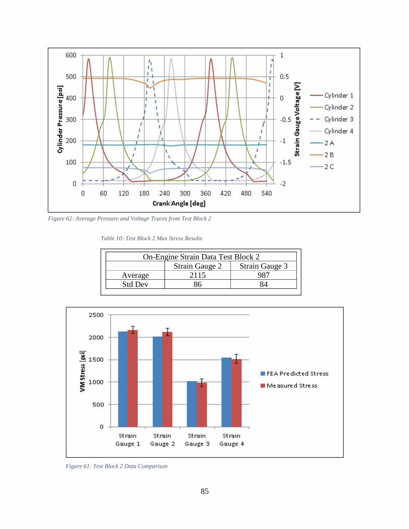
85
Figure 62: Average Pressure and Voltage Traces from Test Block 2
Table 10: Test Block 2 Max Stress Results
On-Engine Strain Data Test Block 2 Strain Gauge 2 Strain Gauge 3
Average 2115 987 Std Dev 86 84
Figure 61: Test Block 2 Data Comparison

86
4.4.1.3 Test Block 3
The intent of collecting nominal data during test block 3 was to confirm the strain gauges
2 and 3 were operating as intended for the cylinder double cylinder deactivation attempt. Strain
gauges were operating as expected and were ready for cylinder deactivation data.
The additional collected data was added to the averages for strain gauge 2 and 3. The
averages of all the strain data can be seen in Table 11with a comparison to the FEA models in
Figure 64. The improved FEA model appears to be an accurate representation of the LBET at the
designated points of interest.
Figure 63: Over Extruded "Airbox"

87
4.4.2 Single Cylinder Deactivation
The first cylinder deactivation attempt was completed during test block 2, at the conclusion
of another project’s test day. Recall, deactivating an entire bank of a large bore engine will reduce
the output power by 60% [12]. To complete the cylinder deactivation testing the engine was
unloaded to ~180 bhp, 40% of 440 bhp. Once the engine stabilized at this operating condition the,
fuel to cylinder 1 was cut. The engine had several knock and misfire events in the remaining three
cylinders as they began to compensate for cylinder 1 no longer firing. Once the engine combustion
Table 11: All On-Engine Strain Data
All On-Engine Strain Data Strain Gauge 1
[psi] Strain Gauge 2
[psi] Strain Gauge 3
[psi] Strain Gauge 4
[psi]
Max Stress 2164 2226 968 1517 Stress Std 77 109 103 104
Figure 64: Final Nominal Data Comparison

88
stabilized it was noted that load on the dynamometer was slowly increasing. The LabVIEW code
controlling the engine was unable to halt the load increase of the dynamometer. When the fuel was
cut to cylinder 3 the engine load at 220 bhp (50%). The load was too great for the LBET to run on
only two cylinders and following several misfire and knock events in the active cylinders the LBET
shut down.
The water break dynamometer only has inlet flow controls, greatly limiting its ability to
regulate loads less than 60%. This was identified as the cause of the steady rise of the load until
the engine shut down. Despite the sudden shut down very interesting results were noted.
The magnitude of the stress data at strain gauge location 2 was significantly smaller than
the average nominal data collected earlier that day, seen in Table 12. Recall, the high change in
voltage measured on the strain gauges was often seen at or near the combustion events of cylinders
3 and 4. The average peak pressure for cylinders 3 and 4 were only ~400 psi compared to the ~600
psi peak pressure from the testing at GMVA rating. A comparison of the voltage traces from 2A
for both test cases can be seen in Figure 65. Note how the GMVA voltage trace has a much larger
change magnitude than the deactivated case but the rest of the voltage trace was very similar.
The lower peak pressure also lowered the IMEPs of cylinder 3 and 4 from 150 psi and 140
psi to 106 psi and 104 psi, respectively This phenomenon prompted the investigation to determine
if there was a correlation between IMEP and measured stress. As the load was steadily increasing
Table 12: Test Block 2 Cylinder Deactivation Comparison
On-Engine Strain Data Test Block 2 Strain Gauge 2 Nominal
[psi] Strain Gauge 2 Cylinder 1
Deactivation [psi]
Average 2226 930 Std 109 190

89
during the cylinder deactivation the IMEP was also increasing. Figure 66 shows the relationship
between IMEP and the measured stress at strain gauge 2. The stress data has substantial scatter but
there is a bulk upward trend in the data that suggests the IMEP is a major contributing factor the
measured stress.
Figure 65: Voltage Trace Comparison between Nominal and Single Cylinder Deactivation
Figure 66: Stress vs Cylinder 4 IMEP

90
4.4.3 Double Cylinder Deactivation
The double cylinder deactivation attempt was completed during the third test block. Unlike
the previous attempt, the engine was started only on cylinders 2 and 4, with the fuel cut to cylinders
1 and 3. This technique was devised to collect as much data as possible before the dynamometer
overloaded the engine, ultimately leading to shut down.
When the LBET is started it runs at idle speed, 250 rpm, and the dyno is completely
unloaded. Once the LBET was running the load on the dynamometer was slowly increased. The
dynamometer load steadily increased until ~50% where the engine shut down like the previous
test. Three complete data points were collected on strain gauges 2 and 3. Unfortunately during post
processing it was noted strain gauge 3 had a short, despite being in working order the previous
day. Each data point had 1,000 combustion cycles for a total of 3,000 points. As expected with
increasing load the IMEP of the active cylinders steadily rose. In the first collection the average
IMEP of cylinders 2 and 4 were 60 psi and 70 psi, respectively. In the final collection before
shutdown the average IMEP of cylinders 2 and 4 were 137 psi and 134 psi, respectively. The
average stress also rose with the elevated IMEP measurements. The results can be seen in Table
13. When the LBET shut down due to overload the dynamometer provided 190 bhp of resistance.
Meaning if the engine was running on all four cylinders the engine would have provided ~475 bhp,
a GMVA rating. As a point of comparison, Figure 67, Figure 68, and Figure 69 illustrate the
difference between the GMVA-4 and the GMVA-2 operational conditions.
Collection 1 Collection 2 Collection 3 Strain Gauge 2 Avg Stress [psi] 730 744 885 Strain Gauge 2 std [psi] 18 30 68 Cylinder 2 IMEP [psi] 60 90 137 Cylinder 4 IMEP [psi] 70 93 134
Table 13: Double Cylinder Deactivation Stress and IMEP Data

91
Figure 67: Deactivated Cylinder Traces
Figure 68: Nominal Cylinder Traces

92
As can be seen, the deactivated case had a lower average voltage change as compared to the
four cylinder case. Consistent with previous testing the greatest voltage change was seen at peak
pressure of cylinder 3. Therefor the reduced measured stress for the cylinder deactivation case
matches the previous data trends. The frequency of the stresses are outlined in Figure 70. In the
frequency histogram, the bulk of the stress events are concentrated near their averages but there is
overlap in the high stress events for the deactivated case. Some of the max stress events are at
~92% of the average stress for the nominal case. The cause of the high stress events is not known
but cannot be ignored. The high stress events are ~3% of the recorded stresses during the cylinder
deactivated case but do not follow a regular pattern of occurrence.
Figure 69: IMEP Comparison between Nominal and Deactivated Conditions with COV as error metric

93
Figure 70: Frequency of Measured Stress at Strain Gauge 2

94
5 GMVH-2 OPERATION – MODEL EXTRAPOLATION
The FEA model was iterated and validated at the four points of interest for the GMVA
operating condition. GMVH-4 operating conditions were inputted in the model to predict the
crankcase’s response. The GMVH-4 condition was chosen to determine the max expected stress
because the experimental data found that the two cylinder operation had high stress events at ~92%
of nominal stress. The model predicted the stresses at the points of interest were between 1.6 and
1.9 times greater than the predicted stresses for the GMVA condition, shown in Table 14. This
was greater than expected because the peak pressure difference between the two conditions was a
ratio of 9:6, or 1.5 times greater and the IMEP’s had a ratio of 23:15, or 1.53 time greater. The
generated results when then used to determine the worst case scenario stresses during GMVH-2
operation, seen in Table 15, by multiplying the Table 14 results by 0.92.
Recall the fatigue limit of class 25 meehanite was 12 ksi. At the four points of interest, the
extrapolated model predicted they would be below the fatigue limit but there were several high
stress points that were at or above the limit. The validity of these points cannot be confirmed but
GMVH-4
Crank
Angle
[deg]
Strain Gauge
1 [psi]
Strain
Gauge 2
[psi]
Strain Gauge
3 [psi]
Strain Gauge
4 [psi]
Max Crankcase
Stress [psi]
18.00 1725 2012 631 1202 11729
50.50 2082 2751 1444 996 13412
80.50 2452 3071 1513 899 13542
127.25 1510 2662 2165 909 5306
197.75 3855 3331 2300 2876 9424
229.25 2042 1863 1412 1393 11523
260.50 1784 1828 1031 1160 12031
307.75 2397 3444 464 2183 6461
Max 3855 3444 2300 2876 13542
Table 14: GMVH-4 Stress Predictions

95
should still be considered. Several of the max stress points were in non-accessible parts of the
crankcase to install instrumentation or to visually confirm the modeled geometry was correct, an
example illustrated in Figure 71. The max stress region was predicted directly above the main
crank bearing but there was additional housing on the LBET around the crankcase webbing. The
housing around the bearing provided minimal structural support but was needed for proper bearing
operation.
GMVH-2
Crank
Angle
[deg]
Strain Gauge
1 [psi]
Strain Gauge
2 [psi]
Strain Gauge 3
[psi]
Strain Gauge 4
[psi]
Max Crankcase
Stress [psi]
18.00 1587 1851 581 1106 10790
50.50 1916 2531 1328 917 12339
80.50 2255 2825 1392 827 12459
127.25 1390 2449 1992 836 4881
197.75 3547 3065 2116 2646 8670
229.25 1879 1714 1299 1282 10601
260.50 1642 1682 949 1068 11068
307.75 2205 3169 427 2008 5944
Max 3547 3169 2116 2646 12459
Table 15: GMVH-2 Stress Predictions
Figure 71: FEA Model Shortfall

96
Juvinall specifies a method to predict the s-n curve of a material given the fatigue strength and
the ultimate tensile strength, seen in Equation 16. S is defined as the failure stress, N is the number
of cycles, A and B are unknown constants. The ultimate tensile strength, 26 ksi, is assumed to hold
true to 103 cycle and the fatigue strength, 12 ksi, is assumed to be at 106 cycles. The two conditions
are used to create two equations and two unknowns leading to A = -0.119 and B = 4.751. The
completed equation, seen in Equation 15, is then used to create the approximate s-n curve seen in
Figure 72.
log = ∗ log +
Equation 16: s-n Curve Prediction [20]
log = − . ∗ log + .
Equation 15: Class 25 Meehanite Approximate s-n curve
Figure 72: Approximate s-n curve for Class 25 Meehanite

97
The GMVH-2 model predicted a max frame stress of 12.459 ksi which would lead to a
predicted failure at ~7 x 10⁵ cycles. Using the experimental finding that high stress events will
only be ~3% of cycle, would mean the LBET could operate for 1300 hours before a likely failure.
There are several problems with this assumption: first, this assumes the FEA model accurately
predicted the high stress regions despite no on-engine validation at those locations, second, the
LBET operational history is unknown prior to installation at the EECL, and third, the LBET has
not recently been examined for material flaws. Given these concerns, intermediate cases were
evaluated between GMVA and GMVH rating.
5.1 INTERMEDIATE TEST CASES
The intermediate cases had peak pressures of 700 psi and 800 psi and used the same bearing
force prediction as the previous models. The FEA input conditions can be seen in Table 17 with
the results in Table 16.
After examining the intermediate cases it was determined the 800psi peak pressure case would
exceed the fatigue limit of class 25 meehanite. But the 700 psi peak pressure case was deemed
acceptable. The max stress regions were located in similar locations as the previous models but at
lower magnitudes. The LBET would be able to operate with a peak pressure of 700 psi with a two
or four active power cylinders, but the two cylinder case would provide an additional safety margin
from the fatigue limit. The predicted output powers for the two and four cylinder cases are ~240
bhp and ~600 bhp respectively, slightly below a GMVE rating [6]. The two cylinder predicted
output power is still below the lower limit of operation of the dynamometer. To correct this, either
outlet flow control will need to be installed or the replacement of the system with an AC
motor/generator with a variable frequency drive to regulate load.

98
Table 16: Intermediate Test Case Results
700 psi Peak Pressure
Crank
Angle
[deg]
Strain Gauge
1 [psi]
Strain Gauge
2 [psi]
Strain Gauge 3
[psi]
Strain Gauge 4
[psi]
Max Crankcase
Stress [psi]
18.00 1291 1659 478 867 10085
50.50 1717 2055 1221 826 11289
80.50 1849 2479 1173 702 11192
127.25 1098 2109 1488 701 4422
197.75 2835 2789 1623 1803 8103
229.25 1702 1494 1057 1055 9596
260.50 1392 1416 803 937 10201
307.75 1947 2484 398 1422 5616
Max 2835 2789 1623 1803 11289
800 psi Peak Pressure
Crank
Angle
[deg]
Strain Gauge
1 [psi]
Strain Gauge
2 [psi]
Strain Gauge 3
[psi]
Strain Gauge 4
[psi]
Max Crankcase
Stress [psi]
18.00 1449 1997 522 1131 11395
50.50 1952 2392 1221 826 12849
80.50 2298 2632 1512 856 13058
127.25 1359 2181 1717 726 5075
197.75 3133 3240 1992 2028 8992
229.25 1953 1779 1157 1113 11387
260.50 1495 1582 909 964 11543
307.75 2065 2652 414 1739 6444
Max 3133 3240 1992 2028 13058

99
Table 17: Intermediate Test Case Inputs
700 psi Peak Pressure
Crank Angle
[deg]
Cylinder 1
[psi]
Cylinder 2
[psi]
Cylinder 3
[psi]
Cylinder 4
[psi] Fx1 [lbf] Fy1 [lbf]
18.00 7.06E+02 1.14E+02 2.24E+01 1.84E+01 1.71E+04 -3.90E+04
50.50 2.91E+02 3.53E+02 2.33E+01 1.87E+01 9.78E+03 -2.06E+04
80.50 1.39E+02 7.06E+02 2.86E+01 2.26E+01 1.38E+04 -5.86E+04
127.25 5.74E+01 1.97E+02 8.71E+01 2.86E+01 6.07E+04 -2.86E+04
197.75 2.24E+01 3.58E+01 6.80E+02 1.29E+02 1.44E+04 -4.89E+04
229.25 2.24E+01 2.12E+01 2.95E+02 3.32E+02 -1.31E+04 -5.32E+04
260.50 2.71E+01 2.25E+01 1.36E+02 7.29E+02 -3.53E+04 -4.63E+04
307.75 8.72E+01 2.24E+01 5.88E+01 1.81E+02 -4.66E+04 -2.26E+04
800 psi Peak Pressure
Crank Angle
[deg]
Cylinder 1
[psi]
Cylinder 2
[psi]
Cylinder 3
[psi]
Cylinder 4
[psi] Fx1 [lbf] Fy1 [lbf]
18.00 8.07E+02 1.30E+02 2.56E+01 2.10E+01 1.95E+04 -4.45E+04
50.50 3.32E+02 4.04E+02 2.66E+01 2.14E+01 1.12E+04 -2.36E+04
80.50 1.59E+02 8.07E+02 3.27E+01 2.59E+01 1.58E+04 -6.70E+04
127.25 6.56E+01 2.25E+02 9.95E+01 3.26E+01 6.94E+04 -3.27E+04
197.75 2.56E+01 4.09E+01 7.77E+02 1.47E+02 1.44E+04 -4.95E+04
229.25 2.56E+01 2.42E+01 3.37E+02 3.80E+02 -1.31E+04 -5.37E+04
260.50 3.10E+01 2.57E+01 1.55E+02 8.33E+02 -3.52E+04 -4.68E+04
307.75 9.96E+01 2.56E+01 6.72E+01 2.07E+02 -4.63E+04 -2.47E+04

100
6 CONCLUSIONS
There are more than 6,000 integral compressor engines in use on US natural gas pipelines,
operating 24 hours a day, 365 days a year. Many of these engines have operated continuously for
more than 50 years, with little to no modifications. Due to recent emission regulations at the local,
state and federal levels much of the aging infrastructure requires retrofit technology to remain
within compliance. The Engines and Energy Conversion Laboratory was founded to test these
retrofit technologies on its large bore engine testbed. The LBET is a low BMEP Cooper Bessemer
GMVTF-4. Newer GMV models, constructed in 1980’s, utilize turbocharging to increase the
output power, achieving BMEP’s nearly double that of the LBET. To expand the lab’s testing
capability and to reduce the LBET’s running cost: material testing, in-depth modeling, and on
engine testing was completed to evaluate the feasibility of uprating the LBET to a high BMEP two
cylinder engine.
6.1 KEY FINDINGS
6.1.1 Material Testing
Two material samples were removed from the LBET’s crankcase and were analyzed for
microstructure, density, hardness, and ultimate tensile strength. The literature review specified that
Cooper Bessemer GMV’s were cast out a meehanite, a specific grade of gray iron, but did not
specify the specific grade. The material properties were necessary to accurately model the LBET
using FEA.
The crankcase was determined to be cast out of a flake graphite, consistent with common
meehanite grades from that era. The density of the material sample was determined using

101
Archimedes’ method finding it had a density of 7.02 g/cc. This density was consistent with the
lower strength grades of meehanite. The hardness tests determined the crankcase likely had a
hardness between 160 and 180 on the Brinell scale, also consistent with the lower strength grades.
Four dogbone samples were machined to determine the ultimate tensile strength of the crankcase
material. The samples failed at an average stress of ~24ksi, with no evidence of fatigue failure.
Based on the material test results it was determined the LBET crankcase was cast out of a class 25
grade of meehanite, very common for crankcase construction.
6.1.2 Model Construction and Validation
An in-depth three dimensional model of the LBET’s crankcase and power cylinders was
constructed using a combination of past models, engineering drawings, and on engine
measurements. The model was analyzed using FEA to identify potential regions of high stress.
The areas of concern were noted to be above the main crank bearing and along the upper engine
webbing. These points of interest were instrumented with 3-foil strain gauges to determine if the
model findings were valid. The on-engine stress measurements prompted many iterations of the
FEA model to be completed. At the conclusion of the modeling iterations, the points of interest
were determined to be accurately modeled in the FEA. However, the validity of other high stress
region in the crankcase cannot be addressed.
6.1.3 Uprated Operation
The FEA model was extrapolated from a moderate BMEP GMVA conditions to high BMEP
GMVH conditions. The model predicted the 4 original points of interest were below the fatigue
limit of class 25 meehanite but there were high stress regions above the fatigue limit that were not
validated. Suggesting the LBET could not be run as a GMVH-4.

102
The cylinder deactivated cases measured a lower stress at strain gauge 2 compared to
nominal four cylinder operation. The test data noted the greatest change in strain gauge voltage
was at the cylinder 3 peak pressure event. When deactivated, cylinder 3’s peak pressure dropped
from ~600 psi to ~300 psi the average measured stresses dropped by ~50% as well. However, there
were several high stress events recorded during cylinder deactivation at ~92% of the nominal
average stress condition. The cause of the high stress events was not determined. The high stress
events were ~3% of the recorded stresses during the cylinder deactivated case but did not follow
a regular pattern of occurrence. Using a general equation to approximate the class 25 meehanite s-
n curve, the LBET theoretically could be operated at GMVH-2 conditions for ~1,300 hours before
failure but this is not advised because the FEA model was not validated at all locations, the
operational history of LBET was not known prior to installation at the EECL, and the crankcase
has not had an in-depth inspection.
To avoid premature failure of the LBET, two intermediate uprate conditions were run in the
FEA. The intermediate cases assumed a peak pressure of 800 psi and 700 psi. The 800 psi case
was determined to have high stress regions above the fatigue limit and deemed unacceptable. The
700 psi predicted the high stress regions to be below the fatigue limit for both four cylinder and
two cylinder operation. The 700 psi case equates to roughly a GMVE.
Although the models suggest the LBET could operate as a GMVE-2 an in-depth crankcase
examination is suggested to ensure the integrity of the crankcase.

103
6.2 SHORT COMINGS
6.2.1 Limited Model Validity
The model was validated at four locations in the crankcase, taking several iterations. There
were several regions of high stress in the crankcase that could not be practically instrumented or
visually inspected, limiting the confirmed validity of the FEA model to the original four points of
interest. To address this concern significant strain gauge instrumentation would be required in
conjunction with continuous model iteration.
6.2.2 Consistent Strain Gauge Failure
Strain gauge failure was a consistent problem throughout the on-engine testing phase. The
likely cause was determined to be insufficient sealant. The sealant material degraded over time in
the crankcase, allowing lubrication oil to directly interact with the strain gauge foils, likely leading
to shorts. To address this concern a better sealant material would be required as well as additional
strain gauges mounted in the crankcase to be redundant.
6.2.3 Poor Load Control during Cylinder Deactivation Experiments
The current water brake dynamometer only has inlet flow control to regulate load. This
current method of load control cannot maintain a constant set point below 60% load. This shortfall
led to the premature engine shutdown during both cylinder deactivation attempts due to overload.
To address this low load concern the addition of outlet flow control is needed to maintain set points
below 60% load or the replacement of the system with an AC motor/generator with a variable
frequency drive to regulate load.

104
6.3 DIRECTION FOR FUTURE RESEARCH
6.3.1 Permanent Cylinder Deactivation
Although the LBET cannot safely operate as a GMVH-2 it could still operate as a two
cylinder test engine at a GMVE rating. The intent of this research would be to install improved
load control at low loads and evaluate the cylinder deactivation techniques. The improved load
control could be accomplished either with installing an outlet flow control on the current water
brake dynamometer or replacing the system with an AC motor/generator with a variable frequency
drive to regulate load.
There are two cylinder deactivation techniques available, remove cylinder 1 and 3 or leave
them inside LBET without fuel flow. If the cylinders are removed lube oil system as well the intake
and exhaust manifolds would need modification. If the cylinder are left in the crankcase the
frictional losses would need to be determined to accurately measure the performance
characteristics. At the conclusion of the proposed project, the modified LBET would have to be
benchmarked against field engines to determine its ability to test new industry technology.
6.3.2 In-depth Crankcase Inspection
Recall, the LBET could operate at GMVH-2 conditions for 1,300 hours before 7 x 10⁵ high
stress cycles occurred, but there were several concerns advising against this. One of the main
concerns were the crankcase has not recently been examined for material flaws. Three non-
destructive techniques could be used on the LBET to evaluate its current state, liquid penetrant
inspection for surface defect detection, and either electromagnetic testing or ultrasonic testing to
determine internal flaws outlined by ASM [40]. If there are no signs of fatigue cracks the LBET
could operate at elevated conditions above GMVE rating for limited periods.

105
7 REFERENCES
[1] “U.S. Natural Gas Statisics,” 2014. [Online]. Available:
http://www.eia.gov/dnav/ng/ng_sum_lsum_dcu_nus_a.htm.
[2] “1985-2013: U.S. Department of Transportation, Pipeline and Hazardous Materials Safety
Administration, Office of Pipeline Safety, Annual Report Mileage Summary Statistics.” U.S.
Department of Transportation, 2014.
[3] N. G. Annual, “Natural Gas Compressor Stations on the Interstate Pipeline Network :,” no.
November, pp. 1–12, 2007.
[4] U. S. EPA, “AP-42, Compilation of Air Pollutant Emission Factors: Chapter 3.2, Natural Gas-fired
Reciprocating Engines,” pp. 1–18, 2014.
[5] R. Potter, “Don ’ t Retire … ReHire ! The use of Integral Slow Speed Engines As Horsepower
Expansion By,” no. October, pp. 1–16, 2005.
[6] M. Vernon, “Cooper Bessemer Type GMV Intergral Angle Natural Gas Compressor History,” pp.
1–12, 2006.
[7] “Cooper Bessemer GMV Heritage Landmark Award,” ASME Journal of Mechanical Engineering,
2006. [Online]. Available: https://www.asme.org/getmedia/9e28281d-2403-4337-9ec3-
df2251a26ede/240-Cooper-Bessemer-Type-GMV-Integral-Angle-Gas-E.aspx.
[8] G. D. Bourn, F. A. Phillips, and R. E. Harris, “Technologies to Enhance the Operation of Existing
Natural Gas Compression Infrastructure,” 2005.
[9] K. Evan, “Supercharger Installation.” Colorado State University, Fort Collins, CO.
[10] P. Jackson, M. D. and Jones, “Deactivating Compressor Engine Cylinders Saves Fuel.” The Oil and
Gas Journal, 1976.

106
[11] B. W. and G. Hutcherson, “Relative Performance of High-Pressure Fuel Gas Delivery - 1997
GMC.pdf.” .
[12] B. F. Smalley, A. J., and Vinyard, S., and Evans, “Power Cylinder Deactivation for Reduced Fuel
Consumption Under Part Load,” San Antonio, Texas, 1986.
[13] M. Wilcutts, J. Switkes, M. Shost, and A. Tripathi, “Design and Benefits of Dynamic Skip Fire
Strategies for Cylinder Deactivated Engines,” Apr. 2013.
[14] G. Hutcherson, R. Potter, R. Schoonover, and B. Willson, “Evaluation of Low Emission
Technologies for Large Bore Natural Gas Engines Prepared for Tenneco Gas Testing conducted
by :,” no. July 1995.
[15] J. Adair, D. Olsen, and A. Kirkpatrick, “Exhaust tuning of large-bore, multiculinder, two-stroke,
natural gas enigines.pdf,” Int. J. Engine Res., vol. 131, no. 7, 2006.
[16] “GMV-TF Natural Gas Pipeline Compressor User’s Manual,” Mt. Vernon, Ohio.
[17] R. W. Harvey, “GMV-6 Torsional Study,” Maysville, OK, 1989.
[18] “U.S. Crude Oil and Natural Gas Proved Reserves,” 2014. [Online]. Available:
http://www.eia.gov/naturalgas/crudeoilreserves/.
[19] F. G. Engineering and C. Applications, “Meehanite® metal selection guide.”
[20] R. C. Juvinall and K. M. Marshek, Fundamentals of Machine Component Design, 5th ed. Danvers,
MA: John Wiley and Sons, 2012.
[21] D. Schmitt and R. Baker, “Systematic Engine Uprate Technology Development and Deployment
for Pipeline Compressor Engines through Increased Torque ( November 2004 - October 2005 )
Prepared by :,” Colorado State University, 2005.
[22] D. Schmitt, “Frame Stress and Crankshaft Modal Analysis on Large Bore Natural Gas Engines,”

107
Colorado State University, 2005.
[23] K. Gupta and J. Meek, Finite Element Multidisciplinary Analysis, 2nd ed. USA: American Institute
of Aeronautics and Astronautics, 2003.
[24] R. Cook, Finite Element Modeling for Stress Analysis, 1st ed. New York: John Wiley and Sons,
1995.
[25] K. H. Huebner, D. Dewhirst, L., D. E. Smith, and T. G. Byrom, The Finite Element Method for
Engineers, 4th ed. New York: John Wiley and Sons, 2001.
[26] R. Cook, D. Malkus, M. Plesha, and R. Witt, Concepts and Applications of Finite Element Analysis,
4th Edition, 4th ed. New York: John Wiley and Sons, 2001.
[27] A. Becker, Introductory Guide to Finite Element Analysis. New York: ASME, 2004.
[28] K. Geels, “Metallographic and Materialographic Specimen Preparation, Light Microscopy, Image
Analysis and Hardness Testing".” ASTM International, West Conshohocken, PA, 2007.
[29] G. Vander Voort, Metallography: Principles and Practice. Materials Park, Ohio: ASM
International, 1984.
[30] ASTM Int., “Standard Test Methods for Tension Testing of Metallic Materials 1,” Astm, no. C, pp.
1–27, 2009.
[31] R. W. Hertzberg, Deformation and Fracture Mechanics of Engineering Materials, 4th ed. Danvers,
MA: John Wiley and Sons, 1996.
[32] L. Fisher, Selection of Engineering Materials and Adhesives, 1st ed. Danves, MA: Taylor Francis
Group, 2005.
[33] G. Aggen, “ASM Handbook Online,” ASM, Mar-1995. [Online]. Available:
http://products.asminternational.org/hbk/index.jsp.

108
[34] ASTM E18-15, “Standard Test Methods for Rockwell Hardness of Metallic Materials,” ASTM Int.,
pp. 1–38, 2015.
[35] “Reynold French Cooper Bessemer GMV Repairs,” Reynolds French and Company, Tulsa, OK,
2010.
[36] B. A. Szabo and I. Babuška, “Finite Element Analysis,” p. 368, 1991.
[37] R. Norton, Machine Design: An Integraed Approach, 2nd ed. River, NJ: Prentice-Hall, 2000.
[38] G. D. Bourn, F. A. Phillips, and R. E. Harris, “Technologies to Enhance the Operation of Existing
Natural Gas Compression Infrastructure,” Morgantown, WV.
[39] “Measuring Strain with Strain Gages,” National Instruments, 2016. [Online]. Available:
http://www.ni.com/white-paper/3642/en/. [Accessed: 20-Jun-2003].
[40] C. G. Goetzel, Nondestructive Inspection and Quality Control, 11th ed. Metals Park, Ohio:
American Society for Metals, 1976.

109
8 APPENDIX
8.1 APPENDIX A MEEHANITE METAL SELECTION GUIDE

110

111

112

113

114

115
8.2 APPENDIX B REYNOLD FRENCH REPAIR BROCHURE

116

117

118

119

120

121
8.3 APPENDIX C WORKING MODEL SIMULATION

122
Bearing Force [lbf] Pressure Input Forces [lbf] Crank Angle [deg] Fx Fy Fx Fy Cylinder 1 Cylinder 2 Cylinder 3 Cylinder 4
0 -18820 47330 1430 12450 46410.00 6977.55 2340.012 7203.531 0.25 15010 13730 -29320 41170 46410.00 6977.55 2340.012 7203.531 0.5 14760 13760 -29120 41260 46590.00 7020.96 2339.858 7157.041
0.75 14520 13800 -28920 41350 46760.00 7077.301 2335.394 7108.397 1 14270 13830 -28730 41430 46930.00 7125.946 2330.93 7057.29
1.25 14020 13870 -28530 41520 47110.00 7181.979 2330.16 7008.645 1.5 13760 13940 -28330 41610 47310.00 7239.86 2328.775 6957.845
1.75 13490 14000 -28140 41690 47520.00 7286.195 2325.388 6900.734 2 13220 14090 -27940 41770 47750.00 7342.537 2321.694 6843.931
2.25 12940 14170 -27750 41850 47970.00 7397.954 2323.541 6786.666 2.5 12660 14260 -27550 41920 48200.00 7452.448 2317.691 6728.478
2.75 12370 14360 -27360 42000 48450.00 7511.099 2320.924 6664.747 3 12070 14480 -27160 42080 48720.00 7567.748 2318.461 6609.33
3.25 11760 14620 -26970 42150 49010.00 7621.934 2319.538 6547.293 3.5 11440 14760 -26770 42220 49300.00 7679.815 2317.691 6480.638
3.75 11120 14910 -26580 42290 49600.00 7737.85 2318.307 6412.597 4 10800 15080 -26380 42360 49920.00 7800.81 2316.46 6345.942
4.25 10450 15260 -26190 42430 50260.00 7862.078 2314.612 6281.288 4.5 10100 15460 -26000 42490 50630.00 7919.496 2316.46 6210.168
4.75 9730 15680 -25800 42560 51010.00 7980.764 2315.844 6144.899 5 9360 15910 -25610 42620 51400.00 8043.109 2316.614 6071.008
5.25 8979 16140 -25410 42680 51810.00 8101.451 2315.69 5998.966 5.5 8588 16400 -25220 42740 52240.00 8165.643 2313.997 5925.537

123
8.4 APPENDIX D STRAIN GAUGE INSTRUMENTATION MANUAL
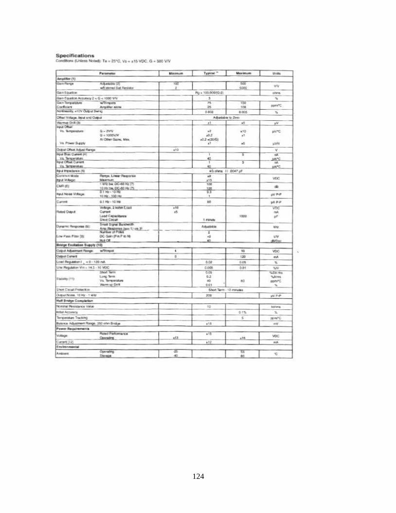
124

125

126
8.5 APPENDIX E STRAIN GAUGE MOUNTING INSTRUCTIONS

127

128

129

130

131
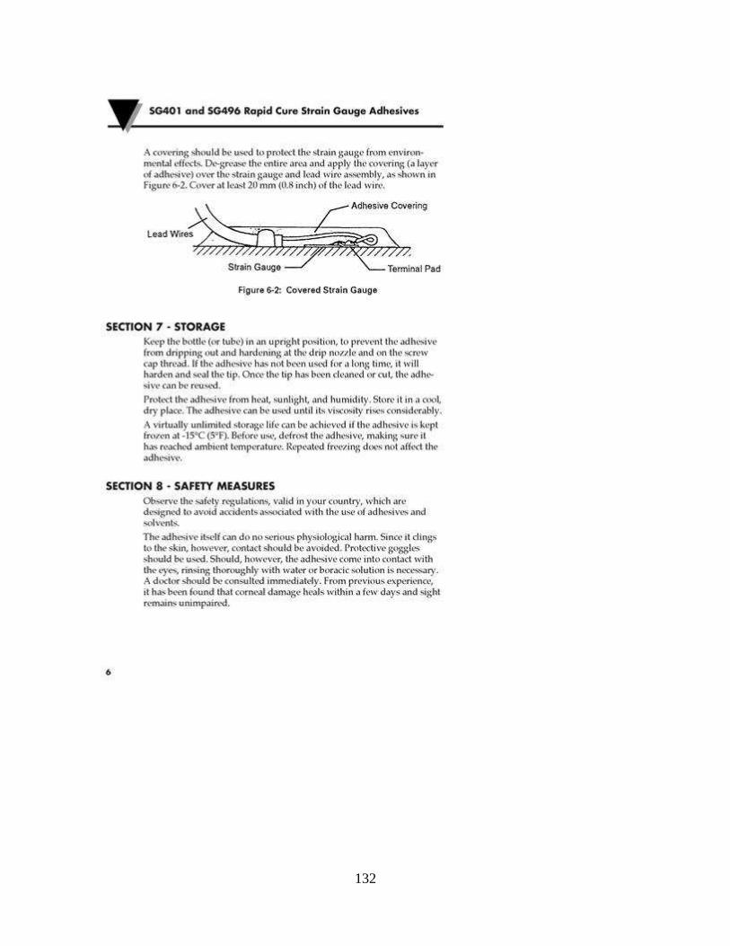
132