Husrev Taha Sencar Luisa Verdoliva Nasir Memon Editors

Advances in Computer Vision and Pattern Recognition

Husrev Taha SencarLuisa VerdolivaNasir Memon Editors

Multimedia Forensics

Advances in Computer Vision and PatternRecognitionFounding Editor

Sameer Singh

Series Editor

Sing Bing Kang, Zillow, Inc., Seattle, WA, USA

Advisory Editors

Horst Bischof, Graz University of Technology, Graz, Austria

Richard Bowden, University of Surrey, Guildford, Surrey, UK

Sven Dickinson, University of Toronto, Toronto, ON, Canada

Jiaya Jia, The Chinese University of Hong Kong, Shatin, New Territories, HongKong

Kyoung Mu Lee, Seoul National University, Seoul, Korea (Republic of)

Zhouchen Lin , Peking University, Beijing, Beijing, China

Yoichi Sato, University of Tokyo, Tokyo, Japan

Bernt Schiele, Max Planck Institute for Informatics, Saarbrücken, Saarland,Germany

Stan Sclaroff, Boston University, Boston, MA, USA

https://orcid.org/0000-0003-1493-7569

More information about this series at https://link.springer.com/bookseries/4205

https://link.springer.com/bookseries/4205

Husrev Taha Sencar · Luisa Verdoliva ·Nasir MemonEditors

Multimedia Forensics

EditorsHusrev Taha SencarResearch Complex, HBKU, Education CityQatar Computing Research InstituteDoha, Qatar

Nasir MemonCenter for Cyber SecurityNew York UniversityBrooklyn, NY, USA

Luisa VerdolivaUniversity of Naples Federico IINapoli, Italy

ISSN 2191-6586 ISSN 2191-6594 (electronic)Advances in Computer Vision and Pattern RecognitionISBN 978-981-16-7620-8 ISBN 978-981-16-7621-5 (eBook)https://doi.org/10.1007/978-981-16-7621-5

© The Editor(s) (if applicable) and The Author(s) 2022. This book is an open access publication.Open Access This book is licensed under the terms of the Creative Commons Attribution 4.0 InternationalLicense (http://creativecommons.org/licenses/by/4.0/), which permits use, sharing, adaptation, distribu-tion and reproduction in any medium or format, as long as you give appropriate credit to the originalauthor(s) and the source, provide a link to the Creative Commons license and indicate if changes weremade.The images or other third party material in this book are included in the book’s Creative Commons license,unless indicated otherwise in a credit line to the material. If material is not included in the book’s CreativeCommons license and your intended use is not permitted by statutory regulation or exceeds the permitteduse, you will need to obtain permission directly from the copyright holder.The use of general descriptive names, registered names, trademarks, service marks, etc. in this publicationdoes not imply, even in the absence of a specific statement, that such names are exempt from the relevantprotective laws and regulations and therefore free for general use.The publisher, the authors and the editors are safe to assume that the advice and information in this bookare believed to be true and accurate at the date of publication. Neither the publisher nor the authors orthe editors give a warranty, expressed or implied, with respect to the material contained herein or for anyerrors or omissions that may have been made. The publisher remains neutral with regard to jurisdictionalclaims in published maps and institutional affiliations.

This Springer imprint is published by the registered company Springer Nature Singapore Pte Ltd.The registered company address is: 152 Beach Road, #21-01/04 Gateway East, Singapore 189721,Singapore

https://doi.org/10.1007/978-981-16-7621-5

http://creativecommons.org/licenses/by/4.0/

Preface

In 2013, we edited the first edition of this book to provide an overview of chal-lenges and developments in digital image forensics. This was the first book on thetopic providing a comprehensive review of prominent research themes as well asthe perspectives of legal professionals and forensic practitioners. Since then, theresearch in this field has expanded dramatically. On one hand, the volume of multi-media content generated and exchanged over the Internet increased hugely. Imagesand videos represent an ever-increasing share of the data traveling on the net and thepreferred communications means for most users, especially of the younger genera-tions. Therefore, they are also the preferred target of malicious attacks. On the otherhand, with the advent of deep learning, attacking multimedia is becoming easier andeasier. Ten years ago, manipulating an image in a credible way required uncommontechnical skills and significant efforts. Manipulating a video, beyond trivial frame-level operations, was possible only formovie productions. This scenario has radicallychanged now, and multimedia manipulation is at anyone’s reach. Sophisticated toolsbased on autoencoders or generative adversarial networks are freely available, aswell as huge datasets to train them at will. Deepfakes have become commonplaceand represent a real and growing menace for the integrity of information, with reper-cussions on various sectors of society, from the economy to journalism to politics.And these problems can only worsen as new and increasingly sophisticated forms ofmanipulation are taking shape.

Unsurprisingly, multimedia manipulation and forensics are becoming hot topics,not just for the research community but for society at large. Several no-profit orga-nizations have been created to investigate these phenomena. Major IT companies,like Google and Facebook, published online large datasets of manipulated videosto foster research on these topics. Funding agencies are promoting large researchprojects. Especially remarkable is the Media Forensic initiative (MediFor) launchedby DARPA in 2016 to support leading research groups on media integrity all overthe world, which generated important outcomes in terms of methods and referencedatasets. This was followed in 2020 by the Semantics Forensics initiative (SemaFor)aiming at semantic-level detectors of fake media, working jointly on text, audio,images, and video to counter next-generation attacks.

v

vi Preface

The greatly increased focus onmultimedia integrity has caused an intense researcheffort in latest years, which involves not only the multimedia forensics communitybut the much larger field of computer vision. Indeed, deep learning takes the lion’sshare not only on the attacker’s side but also on the defender’s side. It provides theanalyst with new powerful forensic tools for detection. Given a suitably large trainingset, deep learning architectures ensure a significant performance gain with respect toconventional methods and much higher robustness to post-processing and evasionstechniques. In addition, deep learning can be used to address other fundamentalproblems, such as source identification. In fact, being able to track the provenanceof a multimedia asset helps establishing its integrity and, as sensors become moresophisticated and software-oriented, source identification tools must follow suit.Likewise, neural networks, especially generative adversarial networks, are naturalcandidates to perform precious counter-forensics tasks. In synthesis, deep learningis part of the problem but also part of the solution, and the research activity going onin this cat-and-mouse game seems to be continuously growing.

All this said, we felt this was the right time to create an updated version of thatbook, with largely renovated content, to cover the rapid advancements in multimediaforensics and provide an updated review of the most promising methods and state-of-the-art techniques.

We organized the book into three main parts following a brief introduction ofdevelopment in imaging technologies. The first part will provide an overview ofkey findings related to the attribution problem. The work pertaining to the integrityof images and videos is collated in the second part. The last part features work oncombatting adversarial techniques that rise as a significant challenge to forensicsmethods.

Doha, QatarNapoli, ItalyBrooklyn, USA

Husrev Taha SencarLuisa VerdolivaNasir Memon

Contents

Part I Present and Challenges

1 What’s in This Book and Why? . . . . . . . . . . . . . . . . . . . . . . . . . . . . . . . . . 3Husrev Taha Sencar, Luisa Verdoliva, and Nasir Memon

2 Media Forensics in the Age of Disinformation . . . . . . . . . . . . . . . . . . . . 7Justin Hendrix and Dan Morozoff

3 Computational Imaging . . . . . . . . . . . . . . . . . . . . . . . . . . . . . . . . . . . . . . . . 41Scott McCloskey

Part II Attribution

4 Sensor Fingerprints: Camera Identification and Beyond . . . . . . . . . . 65Matthias Kirchner

5 Source Camera Attribution from Videos . . . . . . . . . . . . . . . . . . . . . . . . . 89Husrev Taha Sencar

6 Camera Identification at Large Scale . . . . . . . . . . . . . . . . . . . . . . . . . . . . 117Samet Taspinar and Nasir Memon

7 Source Camera Model Identification . . . . . . . . . . . . . . . . . . . . . . . . . . . . 133Sara Mandelli, Nicolò Bonettini, and Paolo Bestagini

8 GAN Fingerprints in Face Image Synthesis . . . . . . . . . . . . . . . . . . . . . . 175João C. Neves, Ruben Tolosana, Ruben Vera-Rodriguez,Vasco Lopes, Hugo Proença, and Julian Fierrez

Part III Integrity and Authenticity

9 Physical Integrity . . . . . . . . . . . . . . . . . . . . . . . . . . . . . . . . . . . . . . . . . . . . . 207Christian Riess

10 Power Signature for Multimedia Forensics . . . . . . . . . . . . . . . . . . . . . . . 235Adi Hajj-Ahmad, Chau-Wai Wong, Jisoo Choi, and Min Wu

vii

viii Contents

11 Data-Driven Digital Integrity Verification . . . . . . . . . . . . . . . . . . . . . . . 281Davide Cozzolino, Giovanni Poggi, and Luisa Verdoliva

12 DeepFake Detection . . . . . . . . . . . . . . . . . . . . . . . . . . . . . . . . . . . . . . . . . . . 313Siwei Lyu

13 Video Frame Deletion and Duplication . . . . . . . . . . . . . . . . . . . . . . . . . . 333Chengjiang Long, Arslan Basharat, and Anthony Hoogs

14 Integrity Verification Through File Container Analysis . . . . . . . . . . . 363Alessandro Piva and Massimo Iuliani

15 Image Provenance Analysis . . . . . . . . . . . . . . . . . . . . . . . . . . . . . . . . . . . . 389Daniel Moreira, William Theisen, Walter Scheirer,Aparna Bharati, Joel Brogan, and Anderson Rocha

Part IV Counter-Forensics

16 Adversarial Examples in Image Forensics . . . . . . . . . . . . . . . . . . . . . . . 435Mauro Barni, Wenjie Li, Benedetta Tondi, and Bowen Zhang

17 Anti-Forensic Attacks Using Generative Adversarial Networks . . . . 467Matthew C. Stamm and Xinwei Zhao

Symbols

iid Independent and identically distributedPCE Peak to Correlation EnergyPRNU Photo-Response Non-Uniformityr.v. Random variableCov(., .) Covariance of two r.v.sE(.) Expected value of a r.v.ρ Linear correlation valuefX (x) Probability density function of a r.v. XFX (x) Cumulative distribution function of a r.v. XμX ,σ 2

X Mean and variance of a r.v. XDCT Discrete cosine transformDFT Discrete Fourier transformI A multidimensional array that may represent an image or a videoI (m, n) The value of the (m, n)-th entry of image II (m, n, t) The value of the (m, n)-th entry of t-th frame of video IH0 Null hypothesisH1 Alternative hypothesisPD Probability of DetectionPFA Probability of False AlarmPM Probability of MissPCR Probability of Correct RejectionPE Probability of ErrorTPR True Positive RateFPR False Positive RateFNR False Negative RateTro Read-out time of a rolling shutter cameraDNN Deep Neural NetworksR@k Recall at top-k objects retrieved in a rankV O Vertex OverlapEO Edge OverlapV EO Graph overlap, a.k.a. vertex-edge overlap

ix

x Symbols

PSNR Peak Signal to Noise RatioMSE Mean Squared ErrorASR Attack Success RateCNN Convolutional Neural NetworkDNN Deep Neural networkDL Deep LearningML Machine Learning

Notation

We use the following notational conventions.

• Concerning random variables:

– Random variables by uppercase roman letters, e.g., X , Y .– Particular realizations of a randomvariable by corresponding lowercase letters,

e.g., x , y.– A sequence of n r.v.s and its particular realizationswill be, respectively, denoted

by Xn and xn .– Predicted random variables by the hat sign, e.g., X .– The alphabet of a random variable will be indicated by the capital calligraphic

letter corresponding to the r.v. X .

• Concerning matrices and vectors:

– Matrices by boldface capital letters, e.g., A.– The entry in the i-th row and j-th column of a matrix A by A(i, j).– Column vectors by boldface lowercase letters, e.g., x.– < v,w >: scalar product between vectors v and w.– Operators are set in normal font, for example, the transpose AT.

• Concerning sets:

– Set names by uppercase calligraphic letters, i.e., A-Z .– Sets will be specified by listing their objects within curly brackets, i.e., {. . . }.– Standard number sets by Blackboard bold typeface, e.g., N,Z,R, etc.

• Concerning functions:

– Functions are typeset as a single lowercase letter, in math font, e.g., f (A).– Multi-letter functions, and in particularly commonly known functions, are set

in lowercase normal font, e.g., cos(x), corr(x, y), or j∗ = argminj

∑Ni=1 A(i, j).

xi

xii Notation

– To deal with specific functions from a field of functions (e.g., sphericalharmonics basis functions that are indexed by two parameters), we could usecomma-separated subscripts, e.g., hi, j (x).

– Non-math annotations are set in normal font, e.g., fspecial(A). The purpose isto disambiguate names from variables, like in the example f speciali (A).

• Concerning images and videos:

– I will be exclusively used to refer to an image or a sequence of images, and Inwith n ∈ N for multiple images/videos.

– I (i, j) will be used as a row-major pixel-wise image reference denoting thepixel value at row i , column j of I.

– Similarly, I (i, j, t) denotes the value of the (i, j)-th pixel of t-th frame ofvideo I.

– Image pair-wise adjacency matrices will be denoted by M for single matrixand Mn with n ∈ N for multiple matrices.

– Row-major adjacency matrix element reference M(i, j) ∈ M for the elementexpressing the relation between the i-th and the j-th images of interest.

• Concerning graphs:

– A generic graph by G for single and Gn with n ∈ N for multiple graphs.– G = (V, E) to express a graph’s set of vertices V and set of edges E .– Vertex names by vn ∈ V , with n ∈ N.– Edge names by en ∈ E , with n ∈ N; E = (vi , v j ) to detail an edge’s pair of

vertices; if the edge is directed, vi precedes v j in such relation.

• In the context of machine learning and deep learning:

– A generic dataset by D.– Training, validation, and test datasets, respectively, by Dtr ,Dv,Dts .– i−th sample at the input of a DNN and its corresponding label (if indicated)

by (xi , yi ).– Loss function used for DNN training by L.– Sigmoid activation function σ().– Output of a DNN by φ(x) when the input is equal to x .– Gradient of function φ by ∇φ .– The Jacobian matrix of a multivalued function φ by Jφ .– The logit value (output of a CNN prior to the final softmax layer) at node i by

zi .– Mathematical calligraphic capital letters in function form M(·) represent a

model function (i.e., a Neural Network).

• Concerning norms:

– L1, L2, squared L2, and L-infinity norms, respectively, by L1, L2, L22, L∞.

– p norm by P.Pp.

Part IPresent and Challenges

Chapter 1What’s in This Book and Why?

Husrev Taha Sencar, Luisa Verdoliva, and Nasir Memon

1.1 Introduction

Multimedia forensics is a societally important and technically challenging researcharea that will need significant effort for the foreseeable future. While the researchcommunity is growing and work like that in this book demonstrates significantprogress, many challenges remain. We expect that forensically tackling ever-improving media acquisition and generation methods and countering the pace ofchange in media manipulation will continue to require significant technical break-throughs in defensive technologies.

Whether performed at the individual level or class level attribution is at the heartof multimedia forensics. This form of passive forensic analysis exploits traces intro-duced by the acquisition or generation pipeline and subsequent editing. These tracesare often subtle and invisible to humans but can be detected currently by analysisalgorithms and provide mechanisms by which generation or manipulation can beautomatically detected. Despite significant achievements in this area of research,advances in imaging technologies and newly introduced approaches to media syn-thesis have a strong potential to render existing forensic capabilities ineffective.

More critically, media manipulation has now become a pressing problem withbroad implications. In the past, it required significant skill to create compellingmanipulations because editing tools, such asAdobe Photoshop, required experiencedusers to alter images convincingly. Over the last several years, the rise of machinelearning-based technologies has dramatically lowered the skill necessary to create

H. T. Sencar (B)Qatar Computing Research Institute, HBKU, Ar-Rayyan, Qatare-mail: [email protected]

L. VerdolivaUniversity Federico II of Naples, Naples, Italy

N. MemonNew York University Tandon School of Engineering, New York, NY, USA

© The Author(s) 2022H. T. Sencar et al. (eds.),Multimedia Forensics, Advances in Computer Vision and PatternRecognition, https://doi.org/10.1007/978-981-16-7621-5_1

3

http://crossmark.crossref.org/dialog/?doi=10.1007/978-981-16-7621-5_1&domain=pdf

mailto:[email protected]

https://doi.org/10.1007/978-981-16-7621-5_1

4 H. T. Sencar et al.

compelling manipulations. For example, Generative Adversarial Networks (GANs)can create photo-realistic faces with no skill by an end-user other than the ability torefresh a web page. Deepfake algorithms, such as autoencoders to swap faces in avideo, can create manipulations much more easily than previous generation videotools. While these machine learning techniques have many positive uses, they havealso been misused for darker purposes such as to perpetrate fraud, to create falsepersonas, and to attack personal reputations.

The asymmetry in the operational setting of digital forensics where attackers haveaccess to details and inner workings of the involved methods and tools and therebyhave the freedom to tailor their actions makes the task even more difficult. It won’tbe surprising to see these advanced capabilities being deployed to counter forensicmethods. Clearly, these are all pressing and important problems for which technicalsolutions must play a role.

There are a number of significant challenges that must be addressed by forensicscommunity. Imaging technologies are constantly being improved bymanufacturers atboth hardware and software levels with little public information about their specifics.This implies a black-box access to these technologies and involves a significantreverse engineering effort on the part of researchers. With rapid advancements incomputational imaging, this task will only get more strenuous.

Further, new manipulation techniques are becoming available at a rapid paceand each generation improves on the previous. As a result, defenders must developways to limit the a priori knowledge and training samples required from an attackalgorithm and should assume an open world scenario where they might not haveknowledge of all the attack algorithms. Meta-learning approaches for developingdetection algorithms more quickly would also be highly beneficial. Manipulationsin the wild are propagated via noisy channels, like social media, and so there is aneed for robust detection technologies that are not fooled by launderings such assimple compression or more sophisticated replay attacks. Finally, part of the taskof forensics is unwinding how the media was manipulated and who manipulated it.Consequently, approaches to understanding the provenance of manipulated mediaare necessary.

All of these challenges motivated us to prepare this book on multimedia foren-sics. Our main objective was to discuss new research directions and also presentsome possible solutions to existing problems. In this regard, this book provides atimely vehicle for showcasing important research that has emerged in the last yearsaddressing media attribution, authenticity verification, and counter-forensics. Wehope our content also sparks new research efforts in the fight against forgeries andmisinformation.

1.2 Overviews

Our book begins with an overview of the challenges posed by media manipulationas seen from today. In their chapter, Hendrix and Morozoff provide a comprehen-sive view of all aspects of the problem to better emphasize the increasing need for

1 What’s in This Book and Why? 5

advanced media forensics capabilities. This is followed by an examination of foren-sics challenges that arise from the increased adoption of computational imaging. Thechapter by McCloskey assesses the ability to detect automated focus manipulationsperformed by computational cameras. For this, it looks at cues that can be used todistinguish optical blur from synthetic blur. The chapter also covers computationalimaging research with potential future implications on forensics.

This chapter is followed by a series of chapters focusing on different dimensionsof the attribution problem. Undoubtedly, one of the breakthrough discoveries inmultimedia forensics is that Photo-Response Non-Uniformity (PRNU) of an imagingsensor, which manifests as a unique and permanent pattern introduced to all mediacaptured by the sensor, can be used for identification and verification of the source ofdigital media. Our book has three chapters covering different aspects PRNU-basedsource camera attribution. The first chapter by Kirchner reviews the rich body ofliterature on camera identification from sensor noise fingerprints with an emphasison still images from digital cameras and the evolving challenges in this domain. Thesecond chapter by Sencar examines extension of these capabilities to video domainand outlines recently developed methods for estimating the sensor’s PRNU fromvideos. The third chapter on this topic by Taspinar et al. provides an overview oftechniques proposed to perform source matching efficiently in the presence of a largecollection of media.

Another vertical in attribution domain is the source camera model identificationproblem. Assuming that a picture or video has been digitally acquired with a camera,the goal of this research direction is to identify the brand and model of the deviceused at acquisition time without relying on metadata. The chapter by Mandelli et al.investigates source camera model identification through pixel analysis and discusseswide series of methodologies proposed to solve this problem.

The remarkable progress of deep learning, in particular Generative AdversarialNetworks (GANs), has led to the generation of extremely realistic fake facial content.The potential for misuse of such capabilities opens up new problem in forensics thatfocuses on identification of GAN fingerprints used in face image synthesis. Neveset al. provide an in-depth literature analysis of state-of-the-art detection approachesfor face synthesis and manipulation as well as spoofing those detectors.

The next part of our book involves several chapters focusing on integrity andauthenticity of multimedia. This part starts with a review of physics-based methodsthatmainly analyzes the interaction of light and objects and the geometricmapping oflight and objects onto the image sensor. In his chapter, Reese reviews the major linesof research on physics-based methods and discusses their strengths and limitations.

The following chapter investigates forensic applications of the Electric NetworkFrequency (ENF) signal. Since ENF serves as an environmental signature capturedby audio and video recordings made in locations where there is electrical activity, itprovides an additional dimension for time–location authentication and for inferringthe grid in which a recording was made. The chapter by Hajj-Ahmad et al. providesan overview of the increasing amount of research work that has been done in thisfield.

6 H. T. Sencar et al.

The long-lasting problem of image and video manipulation is revisited in the sub-sequent four chapters. However, distinct from conventional manipulation detectionmethods, Cozzolino et al. focus on the data-driven deep learning-based methods pro-posed in recent years. This chapter discusses in detail forensics traces these methodsrely on, and describes architectural solutions used for detection and localization,together with the associated training strategies. The next chapter features the newclass of forgery known as DeepFakes that involve impersonating audios and videosgenerated by deep neural networks. In this chapter, Lyu surveys the state-of-the-artDeepFake detection methods and evaluates solutions proposed to tackle this problemalong with their pros and cons. In the third chapter of the topic, Long et al. provide anoverview of the work related to video frame deletion and duplication and introducedeep learning-based approaches to tackle these two types of manipulations.

A complementary integrity verification approach is presented next. Several workdemonstrated that media manipulation not only leaves forensic traces in the audio-visual content but also in the file structure. The chapter authored by Piva coversproposed forensic methods devoted to the analysis of image and video file formatsto validate multimedia integrity.

The last chapter on authenticity verification introduces the problem of provenanceanalysis. By jointly examining multiple multimedia files, instead of making individ-ual assessments, and evaluating pairwise relationships between them, the prove-nance of multimedia files is more reliably determined. The chapter by Moreira et al.addresses this problem by covering state-of-the-art analysis techniques.

The last part of our book includes two chapters on counter-forensics comple-menting the advances brought by deep learning to forensics. The advances broughtby deep learning have also significantly expanded the capabilities of anti-forensicattackers. The first chapter by Barni et al. focuses on adversarial examples in imageforensics and how they can be used in creation of attacks. It also describes possiblecountermeasures against them, and discusses their effectiveness. The other chapter byStamm et al. focuses on emerging threat posed by GAN-based anti-forensic attacksin creating realistic, but completely synthetic forensic traces.

Open Access This chapter is licensed under the terms of the Creative Commons Attribution 4.0International License (http://creativecommons.org/licenses/by/4.0/), which permits use, sharing,adaptation, distribution and reproduction in any medium or format, as long as you give appropriatecredit to the original author(s) and the source, provide a link to the Creative Commons license andindicate if changes were made.

The images or other third party material in this chapter are included in the chapter’s CreativeCommons license, unless indicated otherwise in a credit line to the material. If material is notincluded in the chapter’s Creative Commons license and your intended use is not permitted bystatutory regulation or exceeds the permitted use, you will need to obtain permission directly fromthe copyright holder.


Chapter 2Media Forensics in the Ageof Disinformation

Justin Hendrix and Dan Morozoff

2.1 Media and the Human Experience

Empiricism is the notion that knowledge originates from sensory experience. Implicitin this statement is the idea that we can trust our senses. But in today’s world,much of the human experience is mediated through digital technologies. Our sensoryexperiences can no longer be trusted a priori. The evidence before us—what we seeand hear and read—is, more often than not, manipulated.

This presents a profound challenge to a species that for most of its existencehas relied almost entirely on sensory experience to make decisions. A group ofresearchers from multiple universities and multiple disciplines that study collectivebehavior recently assessed that the study of the impact of digital communicationstechnologies on humanity should be understood as a “crisis discipline,” alongside thestudy of matters such as climate change and medicine (Bak-Coleman et al. 2021).Noting that since “our societies are increasingly instantiated in digital form,” theyargue the potential of digital media to perturb the ways in which we organize our-selves, deal with conflict, and solve problems is profound:

Our social adaptations evolved in the context of small hunter-gatherer groups solving localproblems through vocalizations and gestures. Now we face complex global challenges frompandemics to climate change—and we communicate on dispersed networks connected bydigital technologies such as smartphones and social media.

The evidence, they say, is clear: in this new information environment, misinforma-tion, disinformation, and media manipulation pose grave threats—from the spread ofconspiracy theories (Narayanan et al. 2018), rejection of recommended public healthinterventions (Koltai 2020), subversion of democratic processes (Atlantic Council2020), and even genocide (Łubinski 2020).

Media manipulation is only one of a series of problems in the digital informationecosystem—but it is a profound one. For most of modern history, trust and verifiabil-ity of media—whether printed material, audio and more recently images, video, and

J. Hendrix (B) · D. MorozoffNew York University, Vidrovr Inc., New York, NY, USAe-mail: [email protected]


7



https://doi.org/10.1007/978-981-16-7621-5_2

8 J. Hendrix and D. Morozoff

other modalities—have been linked to one’s ability to access and coordinate infor-mation to previously gathered facts and beliefs. Consequently, in order to deceivesomeone, the deceiver had to rely on the obfuscation of a media object’s salient fea-tures and hope that the consumer’s time and ability to perceive these differences wasnot sufficient. This generalization extends from boasts and lies told in the school-yard, to false narratives circulated by media outlets, to large-scale disinformationcampaigns pursued by nations during military conflicts.

A consistent property and limitation of deceptive practices is that their successis linked to two conditions. The first condition is that the ability to detect falseinformation is linked to the amount of time we have to process and verify it beforetaking action on it. For instance, showing someone a brief picture of a photoshoppedface is more likely to be taken as true if the viewer is given less time to examineit. The second condition is linked to the amount of time and effort required by thedeceiver to create the manipulation. Hence, the impact and reach of a manipulationis limited by the resources and effort involved. A kid in school can deceive theirfriends with a photoshopped image, but it required Napoleon and the French Empireto flood the United Kingdom with fake pound notes during the Napoleonic wars andcause a currency crisis.

A set of technological advancements over the last 30years has led to a tectonicshift in this dynamic. With the adoption of Internet and social media in the 1990s and2000s, respectively, the marginal costs required to deceive a victim have plummeted.Any person on the planet with a modicum of financial capital is able to reach billionsof people with their message, effectively breaking the resource dependence of adeceiver. This condition is an unprecedented one in the history of the world.

Furthermore, thematuration and spread ofmachine learning-poweredmedia tech-nologies has provided the ability to generate diverse media at scale, lowering thebarriers to entry for all content creators. Today, the amount of work required todeliver mass content at Internet scale is exponentially decreasing. This is inevitablycompounding the problem of trust online.

As a result, our society is approaching a precipice of far-reaching consequences.Media manipulation is easy for anyone, even if they are without significant resourcesor technical skills. While conversely the amount of media available to people contin-ues to explode, the amount of time dedicated to verifying a single piece of content isalso falling. As such, if we are to have any hope of adapting our human sensemakingto this digital age, we will need media forensics incorporated into our digital infor-mation environment in multiple layers. We will require automated tools to augmentour human abilities to make sense of what we read, hear, and see.

2.2 The Threat to Democracy

One of themost pressing consequences of mediamanipulation is the threat to democ-racy. Concern over issues of trust and the role of information in democracies is severe.Globally, democracy has run into a difficult patch, with 2020 perhaps among its worst

2 Media Forensics in the Age of Disinformation 9

years in decades. The Economist Intelligence Unit’s Democracy Index found that asof 2020 only “8.4% of the world’s population live in a full democracy while morethan a third live under authoritarian rule” (The Economist 2021). In theUnited States,the twin challenges of election disinformation and the fraught public discourse onthe COVID-19 pandemic exposed weaknesses in the information ecosystem.

Technology—once regarded as a boon to democracy—is now regarded by someas a threat to it. For instance, a 2019 survey of 1000 experts 2 by the Pew ResearchCenter and Elon University’s Imagining the Internet Center found that, when pressedon the impact of the use of technology by citizens, civil society groups, and gov-ernments on core aspects of democracy and democratic representation, 49% of the“technology innovators, developers, business and policy leaders, researchers, andactivists” surveyed said technology would “mostly weaken core aspects of democ-racy and democratic representation in the next decade,” while 33% said technologywould mostly strengthen democracies.

Perhaps the reason for such pessimism is that current interventions tomanage trustin the information ecosystem are not taking place against a static backdrop. Socialmedia has accompanied a decline of trust in institutions and the media generally,exacerbating a seemingly intractable set of social problems that create ripe conditionsfor the proliferation of disinformation and media manipulation.

Yet, the decade aheadwill see evenmore profounddisruptions to theways inwhichinformation is produced, distributed, sought, and consumed. A number of techno-logical developments are driving the disruption, including the installation of 5Gwireless networks, which will enable richer media experiences, such as AR/VR andhaving more devices trading information more frequently. The increasing advanceof various computational techniques to generate, manipulate, and target content isalso problematic. The pace of technological developments suggest that, by the endof the decade, synthetic media may radically change the information ecosystem anddemand new architectures and systems to aid sensemaking.

Consider a handful of recent developments:

• Natural text to speech enables technologies like Google Assistant, but is also beingused for voice phishing scams.

• Fully generated realistic images from StyleGAN2—a neural network model—arebeing leveraged to make fake profiles in order to deceive on social media.

• Deep Fake face swapping videos are now capable of fooling many people who donot pay close attention to the video.

It is natural, in this environment, that the study of the threat itself is a thrivingarea of inquiry. Experts are busy compiling threats, theorizing threat models, study-ing the susceptibility of people to different types of manipulations, exploring whatinterventions build resilience to deception, helping to inform the debate about whatlaws and rules need to be in place, and offering input on the policies technologyplatforms should have in place to protect users from media manipulation.

In this chapter, we will focus on the emerging threat landscape, in order to give thereader a sense of the importance ofmedia forensics as a discipline.While the technical


work of discerning text, images, video, and audio and their myriad combinationsmaynot seem to qualify as a “crisis discipline,” we believe that it is indeed.

2.3 New Technologies, New Threats

In this section, we describe selected research trends with high potential impact on thethreat landscape of syntheticmedia generation.Wehope to ground the reader in the artof the possible at the cutting edge of research and provide some intuition to where thefield is headed. We briefly explain the key contributions and why we believe they aresignificant for students andpractitioners ofmedia forensics. This list is not exhaustive.

These computational techniques will underpin synthetic media applications in thefuture.

2.3.1 End-to-End Trainable Speech Synthesis

Most speech generation systems include several processing steps that are customarilytrained in isolation (e.g., text-to-spectrogram generators, vocoders). Moreover, whilegenerative adversarial networks (GANs) have made tremendous progress on visualdata, their application to human speech still remains limited.A recent paper addressesboth of these issues with an end-to-end adversarial training protocol (Donahue et al.2021). The paper describes a fully differentiable feedforward architecture for text-to-speech synthesis, which further reduces the amount of the necessary training-timesupervision by eliminating the need for linguistic feature alignment. This furtherlowers the barrier for engineering novel speech synthesis systems, simplifying theneed for data pre-processing to generate speech from textual inputs.

Another attack vector that has been undergoing rapid progress is voice cloning(Hao 2021). Voice cloning can synthetically convert a short audio recording ofone person’s voice to produce a very similar voice applied in various inauthenticcapacities. A recent paper proposes a novel speech synthesis system, NAUTILUS,which brings text-to-speech and voice cloning under the same framework (Luongand Yamagishi 2020). This demonstrates the possibility that a single end-to-endmodel could be used for multiple speech synthesis tasks and could lead to unifica-tion recently seen in natural language models (e.g., BERT Devlin et al. 2019 wherea single architecture beats state of the art in multiple benchmark problems).

2.3.2 GAN-Based Codecs for Still and Moving Pictures

Generative adversarial networks (GANs) have revolutionized image synthesis as theyrapidly evolved from small-scale toy datasets to high-resolution photorealistic con-


tent. They exploit the capacity of deep neural networks to learn complex manifoldsand enable generative sampling of novel content. While the research started fromunconditional, domain-specific generators (e.g., human faces), recent work focuseson conditional generation. This regime is of particular importance for students andpractitioners of media forensics as it enables control of the generation process.

One area where this technology is underappreciated with regard to its misusepotential is lossy codecs for still and moving pictures. Visual content abounds withinconsequential background content or abstract textures (e.g., grass, water, clouds)which canbe synthesized in highquality insteadof explicit coding.This is particularlyimportant in limited bandwidth regimes that typically occur in mobile applications,social media, or video conferencing. Examples of recent techniques in this areainclude GAN-based videoconferencing compression from Nvidia (Nvidia Inc 2020)and thefirst high-fidelityGAN-based image codec fromGoogle (Mentzer et al. 2020).

Thismayhave far-reaching consequences. Firstly, effortlessmanipulation of videoconference streams may lead to novel man-in-the-middle attacks and further blur theboundary between acceptable and malicious alterations (e.g., while replaced back-grounds are often acceptable, the faces or expressions are probably not). Secondly,the ability to synthesize an infinite number of content variations (e.g., decode thesame image with different looking trees) poses a threat to reverse image search—oneof the very few reliable techniques for fact checkers today.

2.3.3 Improvements in Image Manipulation

Progress in machine learning, computer vision, and graphics has been constantlylowering the barrier (i.e., skill, time, compute) for convincing image manipulation.This threat iswell recognized, hencewe simply report a novelmanipulation techniquerecently developed by University ofWashington and Adobe (Zhang et al. 2020). Theauthors propose a method for object removal from photographs that automaticallydetects and removes the object’s shadow. This may be another blow to image forensictechniques that look for (in)consistency of physical traces in the photographs.

2.3.4 Trillion-Param Models

The historical trend of throwing more compute at a problem to see where theperformance ceiling is continuous with large-scale language models (Radford andNarasimhan 2018; Kaplan et al. 2020). Following on the heels of the much popular-ized GPT-3 (Brown et al. 2020), Google Brain recently published their new SwitchTransformer model (Fedus et al. 2021)—a × 10 parameter increase over GPT-3.Interestingly, research trends related to increasing efficiency and reducing costs areparalleling the development of these large models.


With large sparsemodels, it is becoming apparent that lower precision (e.g., 16-bit)can be effectively used, combined with new chip architecture improvements target-ing these lower bit precisions (Wang et al. 2018; Park and Yoo 2020). Furthermore,because of the scales of data needed to train these enormous models, sparsificationtechniques are further being explored (Jacobs et al. 1991; Jordan and Jacobs 1993).New frameworks are also emerging that facilitate distribution of ML models acrossmanymachines (e.g., TensorflowMesh that was used in Google’s Switch Transform-ers) (Shazeer et al. 2018). Finally, an important trend that is also stemming from thisdevelopment is improvements in compression and distillation of models, a conceptthat was explored in our first symposium as a potential attack vector.

2.3.5 Lottery Tickets and Compression in Generative Models

Following in the steps of a landmark 2018 paper proposing the neural lottery hypoth-esis (Frankle and Carbin 2019), work continues in ways of discovering intelligentcompression and distillation techniques to prune large models without losing accu-racy. A recent paper being presented at ICLR 21 has applied this hypothesis toGANs (Chen et al. 2021). There have also been interesting approaches investigat-ing improvements in the training dynamics of subnetworks by leveraging differentialsolvers to stabilize GANs (Qin et al. 2020). The Holy Grail around predicting subnet-works or initialization weights still remains elusive, and so the trend of training everlarger parameter models, and then attempting to compress/distill them, will continueuntil the next ceiling is reached.

2.4 New Developments in the Private Sector

To understand how the generative threat landscape is evolving, it is important totrack developments from industry that could be used in media manipulation. Here,we include research papers, libraries for developers, APIs for the general public,as well as polished products. The key players include research and developmentdivisions of large corporations, such as Google, Nvidia, and Adobe, but we also seerelevant activities from the startup sector.

2.4.1 Image and Video

Nvidia Maxine (Nvidia Inc 2020)—Nvidia released a fully accelerated platformsoftware development kit for developers of video conferencing services to build anddeploy AI-powered features that use state-of-the-art models in their cloud. A notablefeature includes GAN-based video compression, where human faces are synthesizedbased on facial landmarks and a single reference image. While this significantly


improves user experience, particularly for low-bandwidth connections, it opens uppotential for abuse.

Smart Portraits and Neural Filters in Photoshop (Nvidia Inc 2021)—Adobe intro-duced neural filters into their flagship photo editor, Photoshop. The addition includessmart portraits, a machine-learning-based face editing feature which brings the latestface synthesis capabilities to the masses. This development continues the trend ofbringing advanced ML-power image editing to mainstream products. Other notableexamples of commercially available advanced AI editing tools include Anthropic’sPortraitPro (Anthropics Inc 2021) and Skylum’s Luminar (Skylum Inc 2021).

ImageGPT (Chen et al. 2020) and DALL-E (Ramesh et al. 2021)—Open AI isexperimenting with extending their GPT-3 language model to other data modalities.ImageGPT is an autoregressive image synthesis model capable of convincing com-

Fig. 2.1 Synthesized images generated byDALL-E based on a prompt requesting “snail-like tanks”


pletion of image prompts. DALL-E is an extension of this idea that combines visualand language tokens. It allows for image synthesis based on textual prompts. Themodel shows a remarkable capability in generating plausible novel content based onabstract concepts, e.g., “avocado chairs” or “snail tanks,” see Fig. 2.1.

Runway ML (RunwayML Inc 2021)—Runway ML is a Brooklyn-based startupthat provides an AI-powered tool for artists/creatives. Their software brings mostrecent open-source ML models to the masses and allows for their adoption inimage/video editing workflows.

Imaginaire (Nvidia Inc 2021)—Nvidia released a PyTorch library that containsoptimized implementation of several image and video synthesis methods. This tool isintended for developers and provides variousmodels for supervised and unsupervisedimage-to-image and video-to-video translation.

2.4.2 Language Models

GPT-3 (Brown et al. 2020)—OpenAI developed a language model with 175-billionparameters. It performs well in few-shot learning scenarios, producing nuanced textand functioning code. Shortly after, the model has been released via a Web API forgeneral-purpose text-to-text mapping.

Switch Transformers (Fedus et al. 2021)—Six months after the GPT-3 release,Google announced their record-breaking language model featuring over a trillionparameters. The model has been described in a detailed technical manuscript, andhas been published along with a Tensorflow Mesh implementation.

CLIP (Radford et al. 2021)—Released in early January 2021 by OpenAI, CLIP isan impressive zero-shot image classifier. It pre-trained on 400 million text-to-imagepairs. Given a list of descriptions, CLIP will make a prediction for which descriptor,or caption, a given image should be paired.

2.5 Threats in the Wild

In this section, we wish to provide a summary of observed disinformation campaignsand scenarios that are relevant to students and practitioners of media forensics. Wewould like to underscore new tactics and evolving resources and capabilities ofadversaries.

2.5.1 User-Generated Manipulations

Thus far, user-generated media, aimed at manipulating public opinion, by and large,have not made use of sophisticated media manipulation capabilities beyond image,video, and sound editing software available to the general public. Multiple politically


chargedmanipulated videos emerged and gainedmillions of views during the secondhalf of 2020. Documented cases related to the US elections include manipulation ofthe visual background of a speaker (Reuters Staff 2021c), adding manipulated audio(Weigel 2021), cropping of a footage (Reuters Staff 2021a), manipulated editing ofa video, and an attempt to spread false claim that an original video is a “deep fake”production (Reuters Staff 2021b).

In all of the cases mentioned, the videos gained millions of views within hourson Twitter, YouTube, Facebook, Instagram, TikTok, and other platforms, before theywere taken down or flagged to emphasize they were manipulated. Often the videosemerged from an anonymous account on social media, but were shared widely, inpart by prominent politicians and campaign accounts on Twitter, Facebook, andother platforms. Similar incidents emerged in India (e.g., an edited version of avideo documenting police brutality) (Times of India Anam Ajmal 2021).

Today, any user can employ AI-generated images for creating a fake person. Asrecently reported in the New York Times (Hill and White 2021), Generated Photos(Generated Photos Inc 2021) can create “unique, worry-free” fake persons for “$2.99or 1,000 people for $1000.” Similarly, there’s open advertising onTwitter byRosebudAI for creating human animation (Rosebud AI Inc 2021).

Takedowns of far-right extremists and conspiracy-related accounts by severalplatforms, including Twitter, Facebook, Instagram, andWhatsApp announcement ofchanges to its privacy policies resulted in reports ofmigration to alternative platformsand chat services. Though it is still too early to assess the long-term impact of thischange, it has the potential of impacting consumption and distribution of media,particularly among audiences that are already keen to proliferate conspiracy theoriesand disinformation.

2.5.2 Corporate Manipulation Services

In recent years, investigations by journalists, researchers, and social media platformshave documented several information operations that were conducted by state actorsvia marketing and communications firms around the world. States involved included,amongothers, SaudiArabia,UAE, andRussia (CNNClarissaWard et al. 2021). Someresearchers claim outsourcing information operations has become “the new normal,”and so far the operations that were exposed did not spread original synthetic media(Grossman and Ramali 2021).

For those countries seeking the benefits of employing inauthentic content butunable to internally develop such a capability, there are plenty of manipulation com-panies available for hire. Regimes incapable of building a manipulation capability,deprived of the technological resources, and no longer need to worry as an entirelynew industry of Advanced Persistent Manipulators (APM) (GMFUS Clint Watts2021) have emerged in the private sector tomeet the demand.Many advertising agen-cies, able tomakemanipulated content with ease, are hired by governments for publicrelations purposes and blur the lines between authentic and inauthentic contents.


The use of a third party by state actors tends to be limited to a targeted campaign.In 2019, reports by Twitter-linked campaigns run by the Saudi firm Smaat to theSaudi government (Twitter Inc 2021). The firm used automated tools to amplify pro-Saudi messages, using networks of thousands of accounts. The FBI has accused thefirm’s CEO for being the Saudi government agent in an espionage case involvingtwo Saudi former Twitter employees (Paul 2021).

In 2020, a CNN investigation exposed an outsourced effort by Russia, throughGhana and Nigeria to impact U.S. politics. The operation targeted African Americandemographics in the United States using accounts on Facebook, Twitter, and Insta-gram. It was mainly manually executed by a dozen troll farm employees in WestAfrica (CNN Clarissa Ward et al. 2021).

2.5.3 Nation State Manipulation Examples

For governments seeking to utilize, acquire, or develop synthetic media tools, theresources and technology capability needed to create and harness these tools aresignificant, hence the rise of third-party actors is described in Sect. 2.5.2. Below is asampling of recent confirmed or presumed nation state manipulations.

People’s Republic of ChinaOver the last 2 years, Western social media platforms have encountered a size-able amount of inauthentic images and video attributed or believed to be stemmingfrom China (The Associated Press ERIKA KINETZ 2021; Hatmaker 2021). Towhat degree these attributions are directly connected to the Chinese government isunknown, but the incentives align to suggest the Chinese Communist Party (CCP)controlling the state, and the country’s information environment creates or condonesthe deployment of these malign media manipulations.

Australia has made the most public stand against Chinese manipulations. InNovember 2020, Chinese foreign minister and leading CCP Twitter provocateurposted a fake image showing an Australian soldier with a bloody knife next to achild (BBC Staff 2021). The image sought to inflame tensions in Afghanistan whereAustralian soldiers have recently been found to have killed Afghan prisoners duringthe 2009 to 2013 time period.

Aside from this highly public incident and Australian condemnation, signs ofChinese employment of inauthentic media continue to mount. Throughout the fallof 2019 and 2020, Chinese language YouTube news channels proliferated. Thesenew programs, created in high volume and distributed on a vast scale, periodicallymix real information and real people with selectively sprinkled inauthentic content,much of which is difficult to assess as an intended manipulation or a form of narratedrecreation of actual or perceived events. Graphika has reported on these “politicalspam networks” that distribute pro-Chinese propaganda, first targeting Hong Kongprotests in 2019 (Nimmo et al. 2021), and the more recent addition of English lan-guage YouTube videos focusing on US policy in 2020 (Nimmo et al. 2021). Reports


Fig. 2.2 Screenshots of posts from Facebook and Twitter

showed the use of inauthentic ormisattributed content in both visual and audio forms.Accounts used AI-generated account profile images and dubbed voice overs.

A similar network of inauthentic accountswere spotted immediately following the2021 US presidential inauguration. Users with Deep Fake profile photos, which beara notable similarity to AI-generated photos on thispersondoesnotexist.com, tweetedverbatim excerpts lifted from the Chinese Ministry of Foreign Affairs, see Fig. 2.2.These alleged Chinese accounts were also enmeshed in a publicly discussed cam-paign reported by The Guardian as amplifying a debunked ballot video surfacingamong voter fraud allegations surrounding the U.S. presidential election.

The accounts’ employment of inauthentic faces, Fig. 2.3, while somewhat sloppy,does offer a way to avoid detection as has been seen repeatedly when stolen realphotos dropped into image or facial recognition software are easily detected.

Fig. 2.3 Three examples of Deep Fake profile photos from a network of 13 pro-China inauthenticaccounts on Twitter. Screengrabs of photos directly from Twitter

FranceIndividuals associated with the French military have been linked to a 2020 infor-mation operation, aimed at discrediting a similar Russian IO employing trolls to


spread disinformation in the Central African Republic and other African countries(Graphika and The Stanford Internet Observatory 2021). The French operation usedfake media to create Facebook accounts. This is an interesting example of tacticalstrategy that employs a fake campaign to fight disinformation.

Russia/IRAThe Russian-sponsored Internet Research Agency was found to have created a smallnumber of fake Facebook, Twitter, and LinkedIn accounts that were amplifying awebsite posing as an independent news outlet, peacedata.net (Nimmo et al. 2021).While IRA troll accounts have beenprolific for years, this is thefirst observed instanceof their use of AI-generated images. Fake profiles were created to give credibility topeacedata.net, who hired unwitting freelance writers to provide left-leaning contentfor audiences, mostly in the US and UK, as part of a calculated, albeit ineffective,disruption campaign.

2.5.4 Use of AI Techniques for Deception 2019–2020

During the year 2019–2020, at the height of the COVID-19 pandemic, nefariousgenerative AI techniques gained popularity. The following are examples of variousmodalities employed for the purposes of deception and information operations (IO).

Ultimately, we also observe that commercial developments are rapidly advanc-ing the capability for video and image manipulation. While resources required totrain GANs and other models will remain a prohibitive factor in the near future,improvements in image codecs, larger training parameters, lowering precision, andcompression/distillation create additional threat opportunities. The threat landscapewill change rapidly in the next 3 to 5 years, requiring media forensics capabilities toadvance quickly to keep up with the capabilities of adversaries.

GAN-Generated ImagesThemost prevalent documented use so far ofAI capabilities in IOhas been in utilizingavailable free tools to create fake personas online. Over the past year, the use of GANtechnology has become increasingly common, in operations linked to state actors, ororganizations driven by political motivation, see Fig. 2.3. The technology wasmostlyapplied in generating profile pictures for inauthentic users on social media, relying onopen-source available tools such as thispersondoesntexist.com andGenerated Photos(Generated Photos Inc 2021).

Several operations used GANs to create hundreds to thousands of accounts thatspammed platforms with content and comments, in an attempt to amplify messages.Some of these operations were attributed to Chinese actors and to PR firms.

Other operations limited the use of GAN-generated images to create a handfulof more “believable” “fake personas” that appeared as creators of content. At leastone of those efforts was attributed to Russia’s IRA. In at least one case, a LinkedInaccount with a GAN-generated image was used as part of a suspected espionage


effort to contact US national security experts (Associated Press 2021).

Synthetic AudioIn recent years, there were at least three attempts documented, one of which wassuccessful, to defraud companies and individuals using synthetic audio. Two casesincluded use of synthetic audio to impersonate the company CEO in a phone call.In 2019, a British energy company transferred over $200,000 following a fraudulentphone call, generated with synthetic audio to impersonate the parent company’ CEO,requesting the money transfer (Wall Street Journal Catherine Stupp 2021). A similarattempt to defraud a US-based company failed in 2020 (Nisos 2021). Symantec hasreported at least three cases in 2019 of synthetic audio being deployed to defraudprivate companies (The Washington Post Drew Harwell 2021).

Deception Using GPT-3While user-generatedmanipulations aiming at impactingpublic opinionhave avoidedadvanced technology so far, there was at least one attempt to use GPT-3 in gen-erating automated text, by an anonymous user/bot on Reddit (The Next WebThomas Macaulay 2021). The effort seemed to abuse a third-party app access toOpenAI API and to give hundreds of comments. In some cases, the bot publishedconspiracy theories and made false statements.

Additionally, recent reports notedGPT-3has an “anti-Muslim”bias (TheNextWebTristan Greene 2021). This conclusion points to the potential damage that could becaused by apps that are using the technology, even with no malicious intentions.

IO and Fraud Using AI TechniquesOver a dozen cases of use of synthetic media for information operations and othercriminal activities were recorded during the past couple of years. In December 2019,social media platforms noted the first use of AI techniques in a case of “coordinatedinauthentic behavior” which was attributed to The BL, a company with ties to thepublisher of The Epoch Times, according to Facebook. The company created hun-dreds of fake Facebook accounts using GAN techniques to create synthetic profilepictures. The use of GAN to create false portrait pictures of non-existent personasrepeated itself in more than a handful of IO that were discovered during 2020, includ-ing in operations that were attributed by social media platforms to Russian IRA, toChina, and to a US-based PR firm.

2.6 Threat Models

Just as the state of the art in technologies for media manipulation has advanced, sohas theorizing around threat models. Conceptual models and frameworks used tounderstand and analyze threats and describe adversary behavior are evolving along-side what is known of the threat landscape. It is useful for students of media forensicsto understand these frameworks generally, as they are used in the field by analysts,


Fig. 2.4 BEND framework

technologists, and others whowork to understand andmitigate against manipulationsand deception.

It is useful to apply different types of frameworks and threat models for differentkinds of threats. There is a continuum between the sub-disciplines and sub-concernsthat form media and information manipulation. At times it is possible to seek toput too much under the same umbrella. For instance, when analyzing COVID-19 misinformation analysis, the processes and models that are used to tackle thatare extremely different than the processes and models that we use to tackle covertinfluence operations that tend to be state-sponsored, or to understand attacks thatare primarily financially motivated and conducted by criminal groups. It’s impor-tant to think about what models apply in what circumstances, and specifically whatdisciplines can contribute to which models.

The below examples do not represent a comprehensive selection of threat modelsand frameworks, but serve as examples.


2.6.1 Carnegie Mellon BEND Framework

Developed by Dr. Kathleen Carley, the BEND framework is a conceptual system thatseeks to make sense of influence campaigns, and their strategies and tactics. Carleynotes that the “BEND framework is the product of years of research on disinformationand other forms of communication based influence campaigns, and communicationobjectives of Russia and other adversarial communities, including terror groups suchas ISIS that began in late December of 2013.”1 The letters that are represented in theacronym BEND refer to elements of the framework, such as “B” which references“Back, Build, Bridge, and Boost” influence maneuvers.

2.6.2 The ABC Framework

Initially developed by Camille Francois, then Chief Innovation Officer at Graphika,the ABC framework offers a mechanism to understand “three key vectors character-istic of viral deception” in order to guide potential remedies (François 2020). In thisframework:

• A is forManipulativeActors. In Francois’s framework,manipulative actors engageknowingly and with clear intent in their deceptions.

• B is for Deceptive Behavior. Behavior encompasses all of the techniques and toolsamanipulative actormay use, from engaging a troll farmor a bot army to producingmanipulated media.

• C is forHarmfulContent.Ultimately, it is themessage itself that defines a campaignand often its efficacy.

Fig. 2.5 ABCDE framework

1 https://link.springer.com/article/10.1007/s10588-020-09322-9.

https://link.springer.com/article/10.1007/s10588-020-09322-9


Later, AlexandreAlaphilippe, ExecutiveDirector of the EUDisinfoLab, proposedadding a D for Distribution, to describe the importance of the means of distributionto the overall manipulation strategy (Brookings Inst Alexandre Alaphilippe 2021).And yet another letter joined the acronym courtesy of James Pamment in the fallof 2020-Pamment proposed E to evaluate the Effect of the manipulation campaign(Fig. 2.5).

2.6.3 The AMITT Framework

The Misinfosec and Credibility Coalition communities, led by Sara-Jayne Terp,ChristopherWalker, JohnGray, andDr. Pablo Breuer, developed the AMITT (Adver-sarial Misinformation and Influence Tactics and Techniques) frameworks to codifythe behaviours (tactics and techniques) of disinformation threats and responders, toenable rapid alerts, risk assessment, and analysis. AMITT proposes diagrammingand treating equally both threat actor behaviors and response behaviors by the target(Gray and Terp 2019). The AMITT TTPs application of tactics, techniques, proce-dures, and frameworks is the disinformation version of the ATT&K model, whichis an information security standard threat model. The AMITT STIX model is thedisinformation version of the STIX model, which is an information security datasharing standard.

2.6.4 The SCOTCH Framework

In order to enable analysts “to comprehensively and rapidly characterize an adver-sarial operation or campaign,” Dr. Sam Blazek developed the SCOTCH framework(Blazek 2021) (Fig. 2.6).

• S—Source—the actor who is responsible for the campaign.• C—Channel—the platform and its affordances and features that deliver the cam-paign.

• O—Objective—the objective of the actor.• T—Target—the intended audience for the campaign.• C—Composition—the language, content, or message of the campaign.• H—Hook—the psychological phenomena being exploited by the campaign.

Blazek offers this example of how SCOTCH might describe a campaign:

At the campaign level, a hypothetical example of a SCOTCH characterization is: Non-StateActors used Facebook, Twitter, and Low-Quality Media Outlets in an attempt to Underminethe Integrity of the 2020 Presidential Election among Conservative American Audiencesusing Fake Images and Videos and capturing attention by Hashtag Hijacking and Posting inShared-Interest Facebook Groups via Cutouts (Fig. 2.7).


Fig. 2.6 AMITT framework

Fig. 2.7 Deception model effects


2.6.5 Deception Model Effects

Still other frameworks are used to explain how disinformation diffuses in a popula-tion.Mathematicians have employed game theory to look at information as quantitiesthat diffuse according to certain dynamics over networks. For instance, Carlo Kopp,Kevin Korb, and Bruce Mills model cooperation and diffusion in populations (Koppet al. 2018) exposed to “fake news”:

This model “depicts the relationships between the deception models and the com-ponents of system they are employed to compromise.”

2.6.6 4Ds

Some frameworks focus on the goals manipulators. Ben Nimmo, then at the Cen-tral European Policy Institute and now at Facebook, where he leads global threatintelligence and strategy against influence operations, developed the 4Ds to describethe tactics of Russian disinformation campaigns (StopFake.org 2021). “They can besummed up in fourwords: dismiss, distort, distract, dismay,”wroteNimmo (Fig. 2.8).

• Dismiss may involve denying allegations made against Russia or a Russian actor.• Distortion includes outright lies, fabrications, or obfuscations of reality.• Distract includes methods of turning attention away from one phenomenon toanother.

• Dismay is a method to get others to regard Russia as too significant a threat toconfront.

2.6.7 Advanced Persistent Manipulators

Clint Watts, a former FBI Counterterrorism official, similarly thinks about the goalsof threat actors and describes, in particular, nation states and other well-resourcedmanipulators as Advanced Persistent Manipulators.

They use combinations of influence techniques and operate across the full spectrum ofsocial media platforms, using the unique attributes of each to achieve their objectives. Theyhave sufficient resources and talent to sustain their campaigns, and the most sophisticatedand troublesome ones can create or acquire the most sophisticated technology. APMs canharness, aggregate, and nimbly parse user data and can recon new adaptive techniques toskirt account and content controls. Finally, they know and operate within terms of service,and they take advantage of free-speech provisions. Adaptive APM behavior will thereforecontinue to challenge the ability of social media platforms to thwart corrosive manipulationwithout harming their own business model (Fig. 2.8).


Fig. 2.8 Advanced persistent manipulators framework

2.6.8 Scenarios for Financial Harm

Jon Bateman, a fellow in the Cyber Policy Initiative of the Technology and Interna-tional Affairs Program at the Carnegie Endowment for International Peace, showshow assessments of threats can be applied to specific industry areas or targets in hiswork on the threats of media manipulation to the financial system (Carnegie Endow-ment John Batemant 2020).

In the absence of hard data, a close analysis of potential scenarios can help to better gaugethe problem. In this paper, ten scenarios illustrate how criminals and other bad actors couldabuse synthetic media technology to inflict financial harm on a broad swath of targets. Basedon today’s synthetic media technology and the realities of financial crime, the scenariosexplore whether and how synthetic media could alter the threat landscape.

2.7 Investments in Countering False Media

Just as there is substantial effort at theorizing and implementing threat models tounderstandmediamanipulation, there is a growing effort in civil society, government,and the private sector to contend with disinformation. There is a large volume ofwork in multiple disciplines to categorize both the threats and many key indicatorsof population susceptibility to disinformation, including new work on resilience,dynamics of exploitative activities, and case studies on incidents and actors, includingthose who are not primarily motivated by malicious intent. This literature combines


Fig. 2.9 Synthetic media scenarios and financial harm (Carnegie Endowment for Interna-tional Peace JON BATEMAN 2020)

with a growing list of government, civil society and media and industry interventionsaimed at mitigating the harms of disinformation.

There are now hundreds of groups and organizations in the United States andaround the world working on various approaches and problem sets to monitor and


counter disinformation in democracies, see Fig. 2.10. This emerging infrastructurepresents an opportunity to create connective tissue between these efforts, and toprovide common tools and platforms that enable theirwork.Consider three examples:

1. The Disinfo Defense League: A project of the Media Democracy Fund, the DDLis a consortium of more than 200 grassroots organizations across the U.S. thathelps to mobilize minority communities to counter disinformation campaigns(ABC News Fergal Gallagher 2021).

2. The Beacon Project: Established by the nonprofit IRI combats state-sponsoredinfluence operations, in particular, ones from Russia. The project identifies andexposes disinformation and works with local partners to facilitate a response(Beacon Project 2021).

3. CogSec Collab: The Cognitive Security Collaborative that maps and bringstogether information security researchers, data scientists, and other subject-matterexperts to create and improve resources for the protection and defense of the cog-nitive domain (Cogsec Collab 2021).

At the same time, there are significant efforts underway to contend with the impli-cations of these developments in synthetic media and the threat vectors they create.

Fig. 2.10 There are nowhundreds of civil society, government, and private sector groups addressingdisinformation across the globe. (Cogsec Collab 2021)


2.7.1 DARPA SEMAFOR

The Semantic Forensics (SemaFor) program under the Defense Advanced ResearchProjects Agency (DARPA) represents a substantial research and development effortto create forensic tools and techniques to develop semantic understanding of contentand identify synthetic media across multiple modalities (DARPA 2021).

2.7.2 The Partnership on AI Steering Committee on MediaIntegrity Working Group

The Partnership on AI has hosted an industry led effort to create similar detectors(Humprecht et al. 2020). Technology platforms and universities continue to developnew tools and techniques to determine provenance and identify synthetic media andother forms of digital media of questionable veracity. The Working Group bringstogether organizations spanning civil society, technology companies, media organi-zations, and academic institutions will be focused on a specific set of activities andprojects directed at strengthening the research landscape related to new technicalcapabilities in media production and detection, and increasing coordination acrossorganizations implicated by these developments.

2.7.3 JPEG Committee

In October 2020, the JPEG committee released a draft document initiating a discus-sion to explore “if a JPEG standard can facilitate a secure and reliable annotation ofmediamodifications, both in good faith andmalicious usage scenarios” (Joint Bi levelImage Experts Group and Joint Photographic Experts Group 2021). The committeenoted the need to consider revision of standardization practices to address pressingchallenges, including use ofAI techniques (“DeepFakes”) and use of authenticmediaout of context for the purposes of spreading misinformation and forgeries. The papernotes two areas of focus: (1) having a record of modifications of a file within its meta-data and (2) proving the record is secured and accessible so provenance is traceable.

2.7.4 Content Authenticity Initiative (CAI)

The CAI was founded in 2019 and led by Adobe, Twitter, and The New York Times,with the goal of establishing standards that will allow better evaluation of content. InAugust 2020, the forum published its white paper “Setting the Standard for DigitalContent Attribution” highlighting the importance of transparency around provenanceof content (Adobe, New York Times, Twitter, The Content Authenticity Initiative2021). CAI will “provide a layer of robust, tamper-evident attribution and history


data built upon XMP, Schema.org, and other metadata standards that goes far beyondcommon uses today.”

2.7.5 Media Review

Media Review is an initiative led by the Duke Reporters Lab to provide the factchecker community a schema that would allow evaluation of videos and images,through tagging of different types ofmanipulation (Schema.org 2021).MediaReviewis based on the ClaimReview project, and is currently a pending schema.

2.8 Excerpts on Susceptibility and Resilience to MediaManipulation

Like other topics in forensics, media manipulation is directly tied to psychology.Though a thorough treatment of this topic is outside the scope of this chapter, wewould like to expose the reader to some foundational work in these areas of research.

The following section is a collection of critical ideas from different areas of psy-chological mis/disinformation research. The purpose of these is to convey powerfulideas in the authors’ own words. We hope that readers will select those of interestand investigate those works further.

2.8.1 Susceptibility and Resilience

Below is a sample of recent studies on various aspects of exploitation via disinforma-tion which are summarized and quoted. We categorize these papers by overarchingtopics, but note that many bear relevant findings across multiple topics.

Resilience to online disinformation: A framework for cross-national compara-tive research (Humprecht et al. 2020)This paper seeks to develop a cross-country framework for analyzing disinformationeffects and population susceptibility and resilience. Three country clusters are iden-tified: media-supportive; politically consensus-driven (e.g., Canada, many WesternEuropean democracies); polarized (e.g., Italy, Spain, Greece); and low-trust, politi-cized, and fragmented (e.g., United States). Media-supportive countries in the firstcluster are identified as most resilient to disinformation, and the United States isidentified as most vulnerable to disinformation owing to its “high levels of populistcommunication, polarization, and low levels of trust in the news media.”

Who falls for fake news? The roles of bullshit receptivity, overclaiming, famil-iarity, and analytic thinking (Pennycook and Rand 2020)The tendency to ascribe profundity to randomly generated sentences – pseudo-profound bullshit receptivity – correlates positively with perceptions of fake news


accuracy, and negatively with the ability to differentiate between fake and real news(media truth discernment). Relatedly, individualswho overclaim their level of knowl-edge also judge fake news to be more accurate. We also extend previous researchindicating that analytic thinking correlates negatively with perceived accuracy byshowing that this relationship is not moderated by the presence/absence of the head-line’s source (which has no effect on accuracy), or by familiarity with the headlines(which correlates positively with perceived accuracy of fake and real news).

Fake news, fast and slow: Deliberation reduces belief in false (but not true) newsheadlines (Bago et al. 2020)The Motivated System 2 Reasoning (MS2R) account posits that deliberation causespeople to fall for fake news, because reasoning facilitates identity-protective cogni-tion and is therefore used to rationalize content that is consistent with one’s politicalideology. The classical account of reasoning instead posits that people ineffectivelydiscern between true and false newsheadlineswhen they fail to deliberate (and insteadrely on intuition)... Our data suggest that, in the context of fake news, deliberationfacilitates accurate belief formation and not partisan bias.

Political psychology in the digital (mis) information age: A model of news beliefand sharing (Van Bavel et al. 2020)This paper reviews complex psychological risk factors associated with belief in mis-information such as partisan bias, polarization, political ideology, cognitive style,memory, morality, and emotion. The research analyzes the implications and risksof various solutions, such as fact-checking, “pre-bunking,” reflective thinking, de-platforming of bad actors, and media literacy.

Misinformation and morality: encountering fake news headlines makes themseem less unethical to publish and share (Effron and Raj 2020)Experimental results and a pilot study indicate that “repeatedly encountering mis-information makes it seem less unethical to spread—-regardless of whether onebelieves it. Seeing a fake-news headline one or four times reduced how unethicalparticipants thought it was to publish and share that headline when they saw it again– evenwhen it was clearly labelled false and participants disbelieved it, and even afterstatistically accounting for judgments of how likeable and popular it was. In turn,perceiving it as less unethical predicted stronger inclinations to express approval ofit online. People were also more likely to actually share repeated (vs. new) headlinesin an experimental setting. We speculate that repeating blatant misinformation mayreduce the moral condemnation it receives by making it feel intuitively true, and wediscuss other potential mechanisms.”

When is Disinformation (In) Credible? Experimental Findings on MessageCharacteristics and Individual Differences. (Schaewitz et al. 2020)“...we conducted an experiment (N = 294) to investigate effects of message factorsand individual differences on individuals’ credibility and accuracy perceptions ofdisinformation as well as on their likelihood of sharing them. Results suggest thatmessage factors, such as the source, inconsistencies, subjectivity, sensationalism, or


manipulated images, seem less important for users’ evaluations of disinformationarticles than individual differences. While need for cognition seems most relevantfor accuracy perceptions, the opinion toward the news topic seems most crucial forwhether people believe in the news and share it online.”

Long-term effectiveness of inoculation against misinformation: Three longitu-dinal experiments. (Maertens et al. 2020)“In 3 experiments (N = 151, N = 194, N = 170), participants played either BadNews (inoculation group) or Tetris (gamified control group) and rated the reliabilityof news headlines that either used a misinformation technique or not. We foundthat participants rate fake news as significantly less reliable after the intervention. InExperiment 1, we assessed participants at regular intervals to explore the longevity ofthis effect and found that the inoculation effect remains stable for at least 3months. InExperiment 2, we sought to replicate these findings without regular testing and foundsignificant decay over a 2-month time period so that the long-term inoculation effectwas no longer significant. In Experiment 3, we replicated the inoculation effect andinvestigated whether long-term effects could be due to item-response memorizationor the fake-to-real ratio of items presented, but found that this is not the case.”

2.8.2 Case Studies: Threats and Actors

Below one may find a collection of exposed current threats and actors utilizingmanipulations of varying sophistication.The QAnon Conspiracy Theory: A Security Threat in the Making? (CombatingTerrorism Center Amarnath Amarasingam, Marc-André Argentino 2021)Analysis of QAnon shows that, while disorganized, it is a significant public secu-rity threat due to historical violent events associated with the group, ease of accessfor recruitment, and a “crowdsourcing” effect wherein followers “take interpreta-tion and action into their own hands.” The origins and development of the groupare analyzed, including review of adjacent organizations such as Omega KingdomMinistries. Followers’ behavior is analyzed and five criminal cases are reviewed.

Political Deepfake Videos Misinform the Public, But No More than Other FakeMedia (Barari et al. 2021)“We demonstrate that political misinformation in the form of videos synthesized bydeep learning (“deepfakes”) can convince the American public of scandals that neveroccurred at alarming rates – nearly 50% of a representative sample – but no more sothan equivalent misinformation conveyed through existing news formats like textualheadlines or audio recordings. Similarly, we confirm that motivated reasoning aboutthe deepfake target’s identity (e.g., partisanship or gender) plays a key role in facili-tating persuasion, but, again, no more so than via existing news formats. ...Finally, aseries of randomized interventions reveal that brief but specific informational treat-ments about deepfakes only sometimes attenuate deepfakes’ effects and in relatively


small scale. Above all else, broad literacy in politics and digital technology moststrongly increases discernment between deepfakes and authentic videos of politicalelites.”

Deepfakes and disinformation: exploring the impact of synthetic political videoon deception, uncertainty, and trust in news (Vaccari and Chadwick 2020)An experiment using deepfakes tomeasure its value as a deception tool and its impacton public trust: “While we do not find evidence that deceptive political deepfakesmisled our participants, they left many of them uncertain about the truthfulness oftheir content. And, in turn, we show that uncertainty of this kind results in lowerlevels of trust in news on social media.”

Coordinating a Multi-Platform Disinformation Campaign: Internet ResearchAgency Activity on Three US Social Media Platforms, 2015–2017 (Lukito 2020)An analysis of the use of multiple modes as a technique to develop and deployinformation attacks: [Abstract] “The following study explores IRA activity on threesocial media platforms, Facebook, Twitter, and Reddit, to understand how activitieson these sites were temporally coordinated. Using a VAR analysis with GrangerCausality tests, results show that IRA Reddit activity granger caused IRA Twitteractivity within a one-week lag. One explanation may be that the Internet ResearchAgency is trial ballooning on one platform (i.e., Reddit) to figure out whichmessagesare optimal to distribute on other social media (i.e., Twitter).”

The disconcerting potential of online disinformation: Persuasive effects of astro-turfing comments and three strategies for inoculation against them (Zerback et al.2021)This paper examines online astroturfing as part of Russian electoral disinformationefforts, finding that online astroturfing was able to change opinions and increaseuncertainty even when the audience was “inoculated” against disinformation priorto exposure.

2.8.3 Dynamics of Exploitative Activities

Below are some excerpts from literature covering the dynamics and kinetics of IOactivities and their relationships to disinformation.

Cultural Convergence: Insights into the behavior of misinformation networkson Twitter (McQuillan et al. 2020)“We use network mapping to detect accounts creating content surrounding COVID-19, then Latent Dirichlet Allocation to extract topics, and bridging centrality to iden-tify topical and non-topical bridges, before examining the distribution of each topicand bridge over time and applying Jensen-Shannon divergence of topic distributionsto show communities that are converging in their topical narratives.” The primarytopic under discussion within the data was COVID-19, and this report includes a


detailed analysis of “cultural bridging” activities among/between communities withconspiratorial views of the pandemic.

An automated pipeline for the discovery of conspiracy and conspiracy the-ory narrative frameworks: Bridgegate, Pizzagate and storytelling on the web(Tangherlini et al. 2020)“Predicating our work on narrative theory, we present an automated pipeline forthe discovery and description of the generative narrative frameworks of conspiracytheories that circulate on social media, and actual conspiracies reported in the newsmedia. We base this work on two separate comprehensive repositories of blog postsand news articles describing the well-known conspiracy theory Pizzagate from 2016,and the New Jersey political conspiracy Bridgegate from 2013. ...We show how thePizzagate framework relies on the conspiracy theorists’ interpretation of “hiddenknowledge” to link otherwise unlinked domains of human interaction, and hypothe-size that this multi-domain focus is an important feature of conspiracy theories. Wecontrast this to the single domain focus of an actual conspiracy. While Pizzagaterelies on the alignment of multiple domains, Bridgegate remains firmly rooted in thesingle domain of New Jersey politics. We hypothesize that the narrative frameworkof a conspiracy theory might stabilize quickly in contrast to the narrative frameworkof an actual conspiracy, which might develop more slowly as revelations come tolight.”Fake news early detection: A theory-driven model (Zhou et al. 2020)“The method investigates news content at various levels: lexicon-level, syntax-level,semantic-level, and discourse-level.We represent news at each level, relying onwell-established theories in social and forensic psychology. Fake news detection is thenconducted within a supervised machine learning framework. As an interdisciplinaryresearch, ourwork explores potential fake news patterns, enhances the interpretabilityin fake news feature engineering, and studies the relationships among fake news,deception/disinformation, and clickbaits. Experiments conducted on two real-worlddatasets indicate the proposed method can outperform the state-of-the-art and enablefake news early detection when there is limited content information”“...Among content-based models, we observe that (3) the proposed model performscomparatively well in predicting fake news with limited prior knowledge. We alsoobserve that (4) similar to deception, fake news differs in content style, quality, andsentiment from the truth, while it carries similar levels of cognitive and percep-tual information compared to the truth. (5) Similar to clickbaits, fake news headlinespresent higher sensationalism and lower newsworthiness while their readability char-acteristics are complex and difficult to be directly concluded. In addition, fake news(6) is often matched with shorter words and longer sentences.”

A survey of fake news: Fundamental theories, detection methods, and opportu-nities (Zhou and Zafarani 2020)“By involving dissemination information (i.e., social context) in fake news detection,propagation-based methods are more robust against writing style manipulation bymalicious entities. However, propagation-based fake news detection is inefficient forfake news early detection ... as it is difficult for propagation-based models to detect


fake news before it has been disseminated, or to perform well when limited newsdissemination information is available. Furthermore, mining news propagation andnews writing style allow one to assess news intention. As discussed, the intuitionis that (1) news created with a malicious intent, that is, to mislead and deceive thepublic, aims to be “more persuasive” compared to those not having such aims, and(2) malicious users often play a part in the propagation of fake news to enhance itssocial influence.” This paper also emphasizes the need for explainable detection asa matter of public interest.

A Signal Detection Approach to Understanding the Identification of Fake News(Batailler et al. 2020)“The current article discusses the value of Signal Detection Theory (SDT) in disen-tangling twodistinct aspects in the identification of fake news: (1) ability to accuratelydistinguish between real news and fake news and (2) response biases to judge newsas real versus fake regardless of news veracity. The value of SDT for understandingthe determinants of fake news beliefs is illustrated with reanalyses of existing datasets, providing more nuanced insights into how partisan bias, cognitive reflection,and prior exposure influence the identification of fake news.”Sharing of fake news on social media: Application of the honeycomb frameworkand the third-person effect hypothesis (Talwar et al. 2020)This publication uses the “honeycomb framework” of Kietzmann, Hermkens,McCarthy, and Silvestre (Kietzmann et al. 2011) to explain sharing behaviors relatedto fake news. Qualitative evaluation supports the explanatory value of the honeycombframework, and the authors are able to identify a number of quantitative associationsbetween demographics and sharing characteristics.

Modeling echo chambers and polarization dynamics in social networks(Baumann et al. 2020)“We propose a model that introduces the dynamics of radicalization, as a reinforcingmechanism driving the evolution to extreme opinions from moderate initial condi-tions. Inspired by empirical findings on social interaction dynamics, we consideragents characterized by heterogeneous activities and homophily. We show that thetransition between a global consensus and emerging radicalized states is mostlygoverned by social influence and by the controversialness of the topic discussed.Compared with empirical data of polarized debates on Twitter, the model qualita-tively reproduces the observed relation between users’ engagement and opinions, aswell as opinion segregation in the interaction network. Our findings shed light onthe mechanisms that may lie at the core of the emergence of echo chambers andpolarization in social media.”

(Mis)representing Ideology on Twitter: How Social Influence Shapes OnlinePolitical Expression (Guess 2021)In comparing users’ tweets as well as those of the accounts that they follow, alongsideself-reported political affiliations from surveys, a distinction between self-reportedpolitical slant and those views expressed in tweets. This raises the notion that public


political expression may be distinct from individual affiliations, and that an indi-vidual’s tweets may not be an accurate proxy for their beliefs. The authors callfor a re-examination of potential social causes of/influences upon public politicalexpression: [from Abstract] “we find evidence consistent with the hypothesis thatusers’ public expression is powerfully shaped by their followers, independent of thepolitical ideology they report identifying with in attitudinal surveys. Finally, we findthat users’ ideological expression is more extreme when they perceive their Twitternetworks to be relatively like-minded.”

2.8.4 Meta-Review

A modern review on the literature surrounding disinformation may be found below.

A systematic literature review on disinformation: Toward a unified taxonomicalframework (Kapantai et al. 2021)“Our online information landscape is characterized by a variety of different types offalse information. There is no commonly agreed typology framework, specific cate-gorization criteria, and explicit definitions as a basis to assist the further investigationof the area. Our work is focused on filling this need. Our contribution is twofold.First, we collect the various implicit and explicit disinformation typologies proposedby scholars.We consolidate the findings following certain design principles to articu-late an all-inclusive disinformation typology. Second, we propose three independentdimensions with controlled values per dimension as categorization criteria for alltypes of disinformation. The taxonomy can promote and support further multidisci-plinary research to analyze the special characteristics of the identified disinformationtypes.”

2.9 Conclusion

While media forensics as a field is generally occupied by engineers and computerscientists, it intersects with a variety of other disciplines, and its importance is crucialto the ability for people to form consensus and collaboratively solve problems, fromclimate change to global health.

John Locke, an English philosopher and influential thinker on empiricism and theEnlightenment, once wrote that “the improvement of understanding is for two ends:first, our own increase of knowledge; secondly, to enable us to deliver that knowledgeto others.” Indeed, your study of media forensics takes Locke’s formulation a stepfurther. The effort you put in to understanding this field will not only increase yourown knowledge, it will allow you to build an information ecosystem that deliversthat knowledge to others—the knowledge necessary to fuel human discourse.

The work is urgent.


Acknowledgements This chapter relies on contributions fromSamBlazek, Adi Cohen, Stef Daley,Pawel Korus, and Clint Watts.

References

ABC News Fergal Gallagher. Minority communities fighting back against disinformation aheadof election. https://www.goodmorningamerica.com/news/story/minority-communities-fighting-back-disinformation-ahead-election-73794172

Adobe, New York Times, Twitter, The Content Authenticity Initiative. The content authen-ticity initiative. https://documentcloud.adobe.com/link/track?uri=urn:aaid:scds:US:2c6361d5-b8da-4aca-89bd-1ed66cd22d19

Anthropics Inc. PortraitPro. https://www.anthropics.com/portraitpro/Associated Press, Experts: spy used AI-generated face to connect with targets. https://apnews.com/article/bc2f19097a4c4fffaa00de6770b8a60d

Atlantic Council (2020) The long fuse: Misinformation and the 2020 election. https://www.atlanticcouncil.org/event/the-long-fuse-eip-report/

Bago B, Rand DG, Pennycook G (2020) Fake news, fast and slow: deliberation reduces belief infalse (but not true) news headlines. J Exp Psychol Gen 149(8):1608–1613

Bak-Coleman JB, Alfano M, Barfuss W, Bergstrom CT, Centeno MA, Couzin ID, Donges JF,Galesic M, Gersick AS, Jacquet J, Kao AB, Moran RE, Romanczuk P, Rubenstein DI, TombakKJ, Van Bavel JJ, Weber EU (2021) Stewardship of global collective behavior. Proc Natl AcadSci 118(27)

Barari S, Lucas C, Munger K (2021) Political deepfakes are as credible as other fake media and(sometimes) real media

Batailler C, Brannon S, Teas P, Gawronski B (2020) A signal detection approach to understandingthe identification of fake news. Perspect Psychol Sci 10

Baumann F, Lorenz-Spreen P, Sokolov IM, Starnini M (2020) Modeling echo chambers and polar-ization dynamics in social networks. Phys Rev Lett 124:048301

BBC Staff. Australia demands China apologise for posting ‘repugnant’ fake image. https://www.bbc.com/news/world-australia-55126569

Beacon Project. The Beacon Project. https://www.iribeaconproject.org/who-we-are/missionBlazek S, SCOTCH: a framework for rapidly assessing influence operations. https://www.atlanticcouncil.org/blogs/geotech-cues/scotch-a-framework-for-rapidly-assessing-influence-operations/

Brookings Inst AlexandreAlaphilippe. Adding a ‘D’ to theABCdisinformation framework . https://www.brookings.edu/techstream/adding-a-d-to-the-abc-disinformation-framework/

Brown TB, Mann B, Ryder N, Subbiah M, Kaplan J, Dhariwal P, Neelakantan A, Shyam P, SastryG, Askell A, Agarwal S, Herbert-Voss A, Krueger G, Henighan T, Child R, Ramesh A, ZieglerDM, Wu J, Winter C, Hesse C, Chen M, Sigler E, Litwin M, Gray S, Chess B, Clark J, Berner C,McCandlish S, Radford A, Sutskever I, Amodei D (2020) Language models are few-shot learners

Carnegie Endowment for International Peace JON BATEMAN. Deepfakes and synthetic mediain the financial system: assessing threat scenarios. https://carnegieendowment.org/2020/07/08/deepfakes-and-synthetic-media-in-financial-system-assessing-threat-scenarios-pub-82237

Carnegie Endowment John Batemant (2020) Deepfakes and synthetic media in the financialsystem: assessing threat scenarios. https://carnegieendowment.org/2020/07/08/deepfakes-and-synthetic-media-in-financial-system-assessing-threat-scenarios-pub-82237

Chen M, Radford A, Child R, Wu J, Jun H, Luan D, Sutskever I (2020) Generative pretrainingfrom pixels. In: Daumé III H, Singh A (eds) Proceedings of the 37th international conferenceon machine learning, vol 119. Proceedings of machine learning research, pp 1691–1703. PMLR,13–18

Chen X, Zhang Z, Sui Y, Chen T (2021) Gans can play lottery tickets too

https://www.goodmorningamerica.com/news/story/minority-communities-fighting-back-disinformation-ahead-election-73794172

https://www.goodmorningamerica.com/news/story/minority-communities-fighting-back-disinformation-ahead-election-73794172

https://documentcloud.adobe.com/link/track?uri=urn:aaid:scds:US:2c6361d5-b8da-4aca-89bd-1ed66cd22d19

https://documentcloud.adobe.com/link/track?uri=urn:aaid:scds:US:2c6361d5-b8da-4aca-89bd-1ed66cd22d19

https://www.anthropics.com/portraitpro/

https://apnews.com/article/bc2f19097a4c4fffaa00de6770b8a60d

https://apnews.com/article/bc2f19097a4c4fffaa00de6770b8a60d

https://www.atlanticcouncil.org/event/the-long-fuse-eip-report/

https://www.atlanticcouncil.org/event/the-long-fuse-eip-report/

https://www.bbc.com/news/world-australia-55126569

https://www.bbc.com/news/world-australia-55126569

https://www.iribeaconproject.org/who-we-are/mission

https://www.atlanticcouncil.org/blogs/geotech-cues/scotch-a-framework-for-rapidly-assessing-influence-operations/



https://www.brookings.edu/techstream/adding-a-d-to-the-abc-disinformation-framework/

https://www.brookings.edu/techstream/adding-a-d-to-the-abc-disinformation-framework/

https://carnegieendowment.org/2020/07/08/deepfakes-and-synthetic-media-in-financial-system-assessing-threat-scenarios-pub-82237





CNN Clarissa Ward et al (2020) Russian election meddling is back – via Ghana and Nigeria– and in your feeds. https://www.cnn.com/2020/03/12/world/russia-ghana-troll-farms-2020-ward/index.html

Cogsec Collab, Global disinformation groups. https://datastudio.google.com/u/0/reporting/a8491164-6aa8-45d0-b609-c70339689127/page/ierzB

Cogsec Collab. Cogsec Collab. https://cogsec-collab.org/CombatingTerrorismCenterAmarnathAmarasingam,Marc-AndréArgentino.TheQAnonconspir-acy theory: a security threat in the making? https://ctc.usma.edu/the-qanon-conspiracy-theory-a-security-threat-in-the-making/

DARPA. DARPA SEMAFOR. https://www.darpa.mil/news-events/2021-03-02Devlin J, Chang M-W, Lee K, Toutanova K (2019) Bert: pre-training of deep bidirectional trans-formers for language understanding

Donahue J, Dieleman S, Binkowski M, Elsen E, Simonyan K (2021) End-to-end adversarial text-to-speech

Effron DA, Raj M (2020) Misinformation and morality: encountering fake-news headlines makesthem seem less unethical to publish and share. Psychol Sci 31(1):75–87 PMID: 31751517

Fedus W, Zoph B, Shazeer N (2021) Switch transformers: scaling to trillion parameter models withsimple and efficient sparsity

François C (2020) Actors, behaviors, content: a disinformation abc. AlgorithmsFrankle J, Carbin M (2019) The lottery ticket hypothesis: finding sparse, trainable neural networksGenerated Photos Inc. Generated photos. https://generated.photos/GMFUS Clint Watts. Advanced persistent manipulators, part one: the threat to the social mediaindustry. https://securingdemocracy.gmfus.org/advanced-persistent-manipulators-part-one-the-threat-to-the-social-media-industry/

Graphika and The Stanford Internet Observatory.More-troll kombat. https://public-assets.graphika.com/reports/graphika_stanford_report_more_troll_kombat.pdf

Gray JF, Terp S-J (2019) Misinformation: We’re Four Steps Behind Its Creators. https://cyber.harvard.edu/sites/default/files/2019-11/Comparative%20Approaches%20to%20Disinformation%20-%20John%20Gray%20Abstract.pdf

Grossman S, Ramali LK, Outsourcing disinformation. https://www.lawfareblog.com/outsourcing-disinformation

Guess AM, (Mis)representing ideology on Twitter: how social influence shapeson-line political expression. https://www.uzh.ch/cmsssl/ikmz/dam/jcr:995dbede-c863-4931-9ba8-bc0722b6cb59/20201116_guess.pdf

Hao K (2021) AI voice actors sound more human than ever—and they’re ready to hire. https://www.technologyreview.com/2021/07/09/1028140/ai-voice-actors-sound-human/

Hill K, White NYTMJ (2020) Designed to deceive: do these people look real to you? https://www.nytimes.com/interactive/2020/11/21/science/artificial-intelligence-fake-people-faces.html

Humprecht E, Esser F, Van Aelst P (2020) Resilience to online disinformation: a framework forcross-national comparative research. Int J Press/Polit 25(3):493–516

Humprecht E, Esser F, Van Aelst P (2020) Resilience to online disinformation: a framework forcross-national comparative research. Int J Press/Polit 25(3):493–516

Jacobs RA, Jordan MI, Nowlan SJ, Hinton GE (1991) Adaptive mixtures of local experts. NeuralComput 3(1):79–87

Joint Bi level Image Experts Group and Joint Photographic Experts Group. JPEG fake media: con-text use cases and requirements. http://ds.jpeg.org/documents/wg1n89043-REQ-JPEG_Fake_Media_Context_Use_Cases_and_Requirements_v0_1.pdf

JordanMI, JacobsRA (1993)Hierarchicalmixtures of experts and the emalgorithm. In: Proceedingsof 1993 international conference on neural networks (IJCNN-93-Nagoya, Japan), vol 2, pp 1339–1344

Kapantai E, Christopoulou A, Berberidis C, Peristeras V (2021) A systematic literature review ondisinformation: toward a unified taxonomical framework. New Media Soc 23(5):1301–1326

https://www.cnn.com/2020/03/12/world/russia-ghana-troll-farms-2020-ward/index.html

https://www.cnn.com/2020/03/12/world/russia-ghana-troll-farms-2020-ward/index.html

https://datastudio.google.com/u/0/reporting/a8491164-6aa8-45d0-b609-c70339689127/page/ierzB

https://datastudio.google.com/u/0/reporting/a8491164-6aa8-45d0-b609-c70339689127/page/ierzB

https://cogsec-collab.org/

https://ctc.usma.edu/the-qanon-conspiracy-theory-a-security-threat-in-the-making/

https://ctc.usma.edu/the-qanon-conspiracy-theory-a-security-threat-in-the-making/

https://www.darpa.mil/news-events/2021-03-02

https://generated.photos/

https://securingdemocracy.gmfus.org/advanced-persistent-manipulators-part-one-the-threat-to-the-social-media-industry/

https://securingdemocracy.gmfus.org/advanced-persistent-manipulators-part-one-the-threat-to-the-social-media-industry/

https://public-assets.graphika.com/reports/graphika_stanford_report_more_troll_kombat.pdf

https://public-assets.graphika.com/reports/graphika_stanford_report_more_troll_kombat.pdf

https://cyber.harvard.edu/sites/default/files/2019-11/Comparative%20Approaches%20to%20Disinformation%20-%20John%20Gray%20Abstract.pdf



https://www.lawfareblog.com/outsourcing-disinformation

https://www.lawfareblog.com/outsourcing-disinformation

https://www.uzh.ch/cmsssl/ikmz/dam/jcr:995dbede-c863-4931-9ba8-bc0722b6cb59/20201116_guess.pdf

https://www.uzh.ch/cmsssl/ikmz/dam/jcr:995dbede-c863-4931-9ba8-bc0722b6cb59/20201116_guess.pdf

https://www.technologyreview.com/2021/07/09/1028140/ai-voice-actors-sound-human/

https://www.technologyreview.com/2021/07/09/1028140/ai-voice-actors-sound-human/

https://www.nytimes.com/interactive/2020/11/21/science/artificial-intelligence-fake-people-faces.html

https://www.nytimes.com/interactive/2020/11/21/science/artificial-intelligence-fake-people-faces.html

http://ds.jpeg.org/documents/wg1n89043-REQ-JPEG_Fake_Media_Context_Use_Cases_and_Requirements_v0_1.pdf

http://ds.jpeg.org/documents/wg1n89043-REQ-JPEG_Fake_Media_Context_Use_Cases_and_Requirements_v0_1.pdf


Kaplan J, McCandlish S, Henighan T, Brown TB, Chess B, Child R, Gray S, Radford A, Wu J,Amodei D (2020) Scaling laws for neural language models

Kietzmann JH, Hermkens K, McCarthy IP, Silvestre BS (2011) Social media? get serious! under-standing the functional building blocks of social media. Bus Horiz 54(3):241–251. SPECIALISSUE: SOCIAL MEDIA

Koltai K (2020) Vaccine information seeking and sharing: how private facebook groups contributedto the anti-vaccine movement online. IN: AoIR selected papers of internet research, 2020, Oct

Kopp C, Korb KB, Mills BI (2018) Information-theoretic models of deception: modelling cooper-ation and diffusion in populations exposed to “fake news”. PLOS ONE 13(11):1–35

Łubinski P (2020) Social media incitement to genocide (in:) the concept of genocide in internationalcriminal law developments after Lemkin, p 306

Lukito J (2020) Coordinating a multi-platform disinformation campaign: internet research agencyactivity on three u.s. social media platforms, 2015 to 2017. Polit Commun 37(2):238–255

Luong H-T, Yamagishi J (2020) Nautilus: a versatile voice cloning systemMaertensR,Roozenbeek J,BasolM, vanderLindenS (2020)Long-termeffectiveness of inoculationagainst misinformation: three longitudinal experiments. J Exp Psychol Appl 27:10

McQuillan L,McAweeney E, Bargar A, RuchA (2020) Insights into the behavior of misinformationnetworks on twitter, Cultural convergence

Mentzer F, Toderici G, TschannenM, Agustsson E (2020) High-fidelity generative image compres-sion

Narayanan V, Barash V, Kelly J, Kollanyi B, Neudert L-M, Howard PN (2018) Polarization, parti-sanship and junk news consumption over social media in the us

Nimmo B, François C, Shawn Eib C, Ronzaud L, Graphika, IRA again: unlucky thirteen. https://public-assets.graphika.com/reports/graphika_report_ira_again_unlucky_thirteen.pdf

Nimmo B, Shawn Eib C, Tamora L, Graphika, Cross-Platform SpamNetwork Targeted Hong KongProtests. https://public-assets.graphika.com/reports/graphika_report_spamouflage.pdf

Nimmo B, Shawn Eib C, Tamora L, Graphika, Spamouflage goes to America. https://public-assets.graphika.com/reports/graphika_report_spamouflage_goes_to_america.pdf

Nisos, The rise of synthetic audio deepfakes. https://www.nisos.com/technical-blogs/rise_synthetic_audio_deepfakes

Nvidia Inc (2020) Taking it to the MAX: adobe photoshop gets new NVIDIA AI-powered neuralfilters. https://blogs.nvidia.com/blog/2020/10/20/adobe-max-ai/

Nvidia Inc. Imaginaire. https://github.com/NVlabs/imaginaireNvidia Inc. Nvidia Maxine. https://developer.nvidia.com/MAXINEPark E, Yoo S (2020) Profit: a novel training method for sub-4-bit mobilenet modelsPaul RK, Twitter suspends accounts linked to Saudi spying case. https://www.reuters.com/article/us-twitter-saudi-idUSKBN1YO1JT

Pennycook G, Rand DG (2020)Who falls for fake news? the roles of bullshit receptivity, overclaim-ing, familiarity, and analytic thinking. J Personal 88(2):185–200

QinC,WuY, Springenberg JT, BrockA,Donahue J, LillicrapTP,Kohli P (2020) Training generativeadversarial networks by solving ordinary differential equations

Radford A, Kim JW, Hallacy C, Ramesh A, Goh G, Agarwal S, Sastry G, Askell A, Mishkin P,Clark J, Krueger G, Sutskever I (2021) Learning transferable visual models from natural languagesupervision

Radford A, Narasimhan K (2018) Improving language understanding by generative pre-trainingRamesh A, Pavlov M, Goh G, Gray S, Voss C, Radford A, Chen M, Sutskever I (2021) Zero-shottext-to-image generation

Reuters Staff. Fact check: Clip of Biden taken out of context to portray him as plotting a voterfraud scheme. https://www.reuters.com/article/uk-fact-check-biden-voter-protection-not/fact-check-clip-of-biden-taken-out-of-context-to-portray-him-as-plotting-a-voter-fraud-scheme-idUSKBN27E2VH

https://public-assets.graphika.com/reports/graphika_report_ira_again_unlucky_thirteen.pdf

https://public-assets.graphika.com/reports/graphika_report_ira_again_unlucky_thirteen.pdf

https://public-assets.graphika.com/reports/graphika_report_spamouflage.pdf

https://public-assets.graphika.com/reports/graphika_report_spamouflage_goes_to_america.pdf

https://public-assets.graphika.com/reports/graphika_report_spamouflage_goes_to_america.pdf

https://www.nisos.com/technical-blogs/rise_synthetic_audio_deepfakes

https://www.nisos.com/technical-blogs/rise_synthetic_audio_deepfakes

https://blogs.nvidia.com/blog/2020/10/20/adobe-max-ai/

https://github.com/NVlabs/imaginaire

https://developer.nvidia.com/MAXINE

https://www.reuters.com/article/us-twitter-saudi-idUSKBN1YO1JT

https://www.reuters.com/article/us-twitter-saudi-idUSKBN1YO1JT

https://www.reuters.com/article/uk-fact-check-biden-voter-protection-not/fact-check-clip-of-biden-taken-out-of-context-to-portray-him-as-plotting-a-voter-fraud-scheme-idUSKBN27E2VH




Reuters Staff. Fact check: Donald Trump concession video not a ‘confirmed deep-fake’. https://www.reuters.com/article/uk-factcheck-trump-consession-video-deep/fact-check-donald-trump-concession-video-not-a-confirmed-deepfake-idUSKBN29G2NL

Reuters Staff. Fact check: Video does not show Biden saying ‘Hello Minnesota’ inFlorida rally. https://www.reuters.com/article/uk-factcheck-altered-sign-biden-mn/fact-check-video-does-not-show-biden-saying-hello-minnesota-in-florida-rally-idUSKBN27H1RZ

Rosebud AI Inc. Rosebud AI. https://www.rosebud.ai/RunwayML Inc. RunwayML. https://runwayml.com/Schaewitz L, Kluck JP, Klösters L, Krämer NC (2020) When is disinformation (in)credible?experimental findings on message characteristics and individual differences. Mass Commun Soc23(4):484–509

Schema.org. Media review. https://schema.org/MediaReviewShazeer N, Cheng Y, Parmar N, Tran D, Vaswani A, Koanantakool P, Hawkins P, Lee H, Hong M,Young C, Sepassi R, Hechtman B (2018) Mesh-tensorflow: deep learning for supercomputers

Skylum Inc. Luminar. https://skylum.com/luminarStopFake.org. Anatomy of an info-war: how Russia’s propaganda machine works, and howto counter it. https://www.stopfake.org/en/anatomy-of-an-info-war-how-russia-s-propaganda-machine-works-and-how-to-counter-it/

Talwar S,DhirA, SinghD,VirkGS, Salo J (2020) Sharing of fake news on socialmedia: Applicationof the honeycomb framework and the third-person effect hypothesis. J Retail Consum Serv57:102197

Tangherlini TR, Shahsavari S, ShahbaziB,EbrahimzadehE,RoychowdhuryV (2020)An automatedpipeline for the discovery of conspiracy and conspiracy theory narrative frameworks: bridgegate,pizzagate and storytelling on the web. PLOS ONE 15(6):1–39

Techcrunch Taylor Hatmaker. Chinese propaganda network on Facebook used AI-generated faces.https://techcrunch.com/2020/09/22/facebook-gans-takes-down-networks-of-fake-accounts-originating-in-china-and-the-philippines/

The Associated Press ERIKA KINETZ. Army of fake fans boosts China’s messagingon Twitter. https://apnews.com/article/asia-pacific-china-europe-middle-east-government-and-politics-62b13895aa6665ae4d887dcc8d196dfc

The Economist. Global democracy has a very bad year. https://www.economist.com/graphic-detail/2021/02/02/global-democracy-has-a-very-bad-year

The Next Web Thomas Macaulay. Someone let a GPT-3 bot loose on Reddit – it didn’tend well. https://thenextweb.com/neural/2020/10/07/someone-let-a-gpt-3-bot-loose-on-reddit-it-didnt-end-well/

The Next Web Tristan Greene. GPT-3 is the world’s most powerful bigotry generator. What shouldwe do about it? https://thenextweb.com/neural/2021/01/19/gpt-3-is-the-worlds-most-powerful-bigotry-generator-what-should-we-do-about-it/

The Washington Post Drew Harwell, An artificial-intelligence first: voice-mimicking softwarereportedly used in a major theft. https://www.washingtonpost.com/technology/2019/09/04/an-artificial-intelligence-first-voice-mimicking-software-reportedly-used-major-theft/

Times of India Anam Ajmal. 1st in India: Twitter tags BJP IT cell chief’s tweet as‘manipulated media’. https://timesofindia.indiatimes.com/india/1st-in-india-twitter-tags-bjp-it-cell-chiefs-tweet-as-manipulated-media/articleshow/79538441.cms

Twitter Inc. New disclosures to our archive of state-backed information operations. https://blog.twitter.com/en_us/topics/company/2019/new-disclosures-to-our-archive-of-state-backed-information-operations.html

Vaccari C, Chadwick A (2020) Deepfakes and disinformation: exploring the impact of syn-thetic political video on deception, uncertainty, and trust in news. Soc Media + Soc6(1):2056305120903408

Van Bavel JJ, Harris EA, Pärnamets P, Rathje S, Doell K, Tucker JA (2020) Political psychologyin the digital (mis)information age: a model of news belief and sharing

https://www.reuters.com/article/uk-factcheck-trump-consession-video-deep/fact-check-donald-trump-concession-video-not-a-confirmed-deepfake-idUSKBN29G2NL

https://www.reuters.com/article/uk-factcheck-trump-consession-video-deep/fact-check-donald-trump-concession-video-not-a-confirmed-deepfake-idUSKBN29G2NL

https://www.reuters.com/article/uk-factcheck-altered-sign-biden-mn/fact-check-video-does-not-show-biden-saying-hello-minnesota-in-florida-rally-idUSKBN27H1RZ

https://www.reuters.com/article/uk-factcheck-altered-sign-biden-mn/fact-check-video-does-not-show-biden-saying-hello-minnesota-in-florida-rally-idUSKBN27H1RZ

https://www.rosebud.ai/

https://runwayml.com/

https://schema.org/MediaReview

https://skylum.com/luminar

https://www.stopfake.org/en/anatomy-of-an-info-war-how-russia-s-propaganda-machine-works-and-how-to-counter-it/

https://www.stopfake.org/en/anatomy-of-an-info-war-how-russia-s-propaganda-machine-works-and-how-to-counter-it/

https://techcrunch.com/2020/09/22/facebook-gans-takes-down-networks-of-fake-accounts-originating-in-china-and-the-philippines/

https://techcrunch.com/2020/09/22/facebook-gans-takes-down-networks-of-fake-accounts-originating-in-china-and-the-philippines/

https://apnews.com/article/asia-pacific-china-europe-middle-east-government-and-politics-62b13895aa6665ae4d887dcc8d196dfc

https://apnews.com/article/asia-pacific-china-europe-middle-east-government-and-politics-62b13895aa6665ae4d887dcc8d196dfc

https://www.economist.com/graphic-detail/2021/02/02/global-democracy-has-a-very-bad-year

https://www.economist.com/graphic-detail/2021/02/02/global-democracy-has-a-very-bad-year

https://thenextweb.com/neural/2020/10/07/someone-let-a-gpt-3-bot-loose-on-reddit-it-didnt-end-well/

https://thenextweb.com/neural/2020/10/07/someone-let-a-gpt-3-bot-loose-on-reddit-it-didnt-end-well/

https://thenextweb.com/neural/2021/01/19/gpt-3-is-the-worlds-most-powerful-bigotry-generator-what-should-we-do-about-it/

https://thenextweb.com/neural/2021/01/19/gpt-3-is-the-worlds-most-powerful-bigotry-generator-what-should-we-do-about-it/

https://www.washingtonpost.com/technology/2019/09/04/an-artificial-intelligence-first-voice-mimicking-software-reportedly-used-major-theft/

https://www.washingtonpost.com/technology/2019/09/04/an-artificial-intelligence-first-voice-mimicking-software-reportedly-used-major-theft/

https://timesofindia.indiatimes.com/india/1st-in-india-twitter-tags-bjp-it-cell-chiefs-tweet-as-manipulated-media/articleshow/79538441.cms

https://timesofindia.indiatimes.com/india/1st-in-india-twitter-tags-bjp-it-cell-chiefs-tweet-as-manipulated-media/articleshow/79538441.cms

https://blog.twitter.com/en_us/topics/company/2019/new-disclosures-to-our-archive-of-state-backed-information-operations.html




Wall Street Journal Catherine Stupp. Fraudsters used AI to mimic CEO’s voice in unusual cyber-crime case. https://www.wsj.com/articles/fraudsters-use-ai-to-mimic-ceos-voice-in-unusual-cybercrime-case-11567157402

Wang N, Choi J, Brand D, Chen C-Y, Gopalakrishnan K (2018) Training deep neural networks with8-bit floating point numbers

Washington Post David Weigel. Twitter flags GOP video after activist’s computerized voicewas manipulated. https://www.washingtonpost.com/politics/2020/08/30/ady-barkan-scalise-twitter-video/

Zerback T, Töpfl F, Knöpfle M (2021) The disconcerting potential of online disinformation: per-suasive effects of astroturfing comments and three strategies for inoculation against them. NewMedia Soc 23(5):1080–1098

ZhangE,Martin-Brualla R,Kontkanen J, Curless B (2020)No shadow left behind: removing objectsand their shadows using approximate lighting and geometry

Zhou X, Jain A, Phoha VV, Zafarani R (2020) Fake news early detection: a theory-driven model.Digit Threat Res Pract 1(2)

Zhou X, Zafarani R (2020) A survey of fake news: fundamental theories, detection methods, andopportunities. ACM Comput Surv 53(5)



https://www.wsj.com/articles/fraudsters-use-ai-to-mimic-ceos-voice-in-unusual-cybercrime-case-11567157402

https://www.wsj.com/articles/fraudsters-use-ai-to-mimic-ceos-voice-in-unusual-cybercrime-case-11567157402

https://www.washingtonpost.com/politics/2020/08/30/ady-barkan-scalise-twitter-video/

https://www.washingtonpost.com/politics/2020/08/30/ady-barkan-scalise-twitter-video/


Chapter 3Computational Imaging

Scott McCloskey

Since the advent of smartphones, photography is increasingly being done with small,portable, multi-function devices. Relative to the purpose-built cameras that domi-nated previous eras, smartphone cameras must overcome challenges related to theirsmall form factor. Smartphone cameras have small apertures that produce a widedepth of field, small sensors with rolling shutters that lead to motion artifacts, andsmall form factors which lead to more camera shake during exposure. Along withthese challenges, smartphone cameras have the advantage of tight integration withadditional sensors and the availability of significant computational resources. Forthese reasons, the field of computational imaging has advanced significantly in recentyears,with academic groups and researchers from smartphonemanufacturers helpingthese devices become more capable replacements for purpose-built cameras.

3.1 Introduction to Computational Imaging

Computational imaging (or computational photographic) approaches are character-ized by the co-optimization of what and how the sensor captures light and howthat signal is processed in software. Computational imaging approaches now com-monly available on most smartphones include panoramic stitching, multi-frame highdynamic range (HDR) imaging, ‘portrait mode’ for low depth of field, and multi-frame low-light imaging (‘night sight’ or ‘night mode’).

As image quality is viewed as a differentiating feature between competing smart-phone brands, there has been tremendous progress improving subjective image qual-ity, accompanied by a lack of transparency due to the proprietary nature of the work.

S. McCloskey (B)Kitware, Inc., New York, NY, USAe-mail: [email protected]


41



https://doi.org/10.1007/978-981-16-7621-5_3

42 S. McCloskey

Like the smartphonemarketmore generally, computational imaging approaches usedtherein change very quickly from one generation of the phone to the next. This com-bination of different modes, and the proprietary and rapid nature of changes, all posechallenges for forensics practitioners.

This chapter investigates some of the forensics challenges that arise from theincreased adoption of computational imaging and assesses our ability to detect auto-mated focusmanipulations performed by computational cameras.We then lookmoregenerally at a cue to help distinguish optical blur from synthetic blur. The chapterconcludes with a look at some early computational imaging research that may impactforensics in the near future.

This chapter will not focus on the definitional and policy issues related to compu-tational imagery, believing that these issues are best addressed within the context ofa specific forensic application. The use of an automated, aesthetically driven compu-tational imaging mode does not necessarily imply nefarious intent on the part of thephotographer in all cases, but may in some. This suggests that broad-scale screeningfor manipulated imagery (e.g., on social media platforms) might not target portraitmode images for detection and further scrutiny, but in the context of an insuranceclaim or a court proceeding, higher scrutiny may be necessary.

As with the increase in the number, complexity, and ease of use of software pack-ages for image manipulation, a key forensic challenge presented by computationalimaging is the degree to which they democratize the creation of manipulated media.Prior to these developments, the creation of a convincing manipulation required aknowledgeable user dedicating a significant amount of time and effort with onlypartially automated tools. Much like Kodak cameras greatly simplified consumerphotography with the motto “You Press the Button, We Do the Rest,” computationalcameras allow users to create—with the push of a button—imagery that’s inconsis-tent with the classically understood physical limitations of the camera. Realizing thatmost people won’t carry around a heavy camera with a large lens, a common goalof computational photography is to replicate the aesthetics of Digital Single LensReflex (DSLR) imagery using the much smaller and lighter sensors and optics usedin mobile phones. From this, one of the significant achievements of computationalimaging is the ability to replicate the shallow depth of field of a large aperture DSLRlens on a smartphone with a tiny aperture.

3.2 Automation of Geometrically Correct Synthetic Blur

Optical blur is a perceptual cue to depth (Pentland 1987), a limiting factor in theperformance of computer vision systems (Bourlai 2016), and an aesthetic tool thatphotographers use to separate foreground and background parts of a scene. Becausesmartphone sensors and apertures are so small, images taken by mobile phonesoften appear to be in focus everywhere, including background elements that distracta viewer’s attention. To draw viewers’ perceptual attention to a particular objectand avoid distractions from background objects, smartphones now include ‘portrait

3 Computational Imaging 43

Fig. 3.1 (Left) For a close-in scene captured by a smartphone with a small aperture, all parts ofthe image will appear in focus. (Right) In order to mimic the aesthetically pleasing properties ofa DSLR with a wide aperture, computational cameras now include a ‘portrait mode’ that blurs thebackground so the foreground stands out better

mode’ which automatically manipulates the sensor image via the application of spa-tially varying blur. Figure3.1 shows an example of the all-in-focus natively capturedby the sensor and the resulting portrait mode image. Because there is a geometricrelationship between optical blur and depth in the scene, the creation of geometricallycorrect synthetic blur requires knowledge of the 3D scene structure. Consistent withthe spirit of computational cameras, portrait modes enable this with a combinationof hardware and software. Hardware acquires the scene in 3D using either stereocameras or sensors with the angular sensitivity of a light field camera (Ng 2006).Image processing software uses this 3D information to infer and apply the correctamount of blur for each part of the scene. The result is automated, geometricallycorrect optical blur that looks very convincing. A natural question, then, is whetheror not we can accurately differentiate ‘portrait mode’-based imagery from genuineoptical blur.

3.2.1 Primary Cue: Image Noise

Regardless of how the local blurring is implemented, the key difference betweenoptical blur and portrait mode-type processing can be found in image noise. Whenblur happens optically, before photons reach the sensor, only small signal-dependentnoise impacts are observed. When blur is applied algorithmically to an already digi-tized image, however, the smoothing or filtering operation also implicitly de-noisesthe image. Since the amount of de-noising is proportional to the amount of localsmoothing or blurring, differences in the amount of algorithmic local blur can bedetected via inconsistencies between the local intensity and noise level. Two regionsof the image having approximately the same intensity should also have approxi-mately the same level of noise. If one region is blurred more than the other, or one is

44 S. McCloskey

blurred while the other is not, an inconsistency is introduced between the intensitiesand local noise levels.

For our noise analysis, we extend the combined noise models of Tsin et al. (2001)and Liu et al. (2006). Ideally, a pixel produces a number of electrons Enum propor-tional to the average irradiance from the object being imaged. However, shot noiseNS is a result of the quantum nature of light and captures the uncertainty in thenumber of electrons stored at a collection site; NS can be modeled as the Poissonnoise. Additionally, site-to-site non-uniformities called fixed pattern noise K are amultiplicative factor impacting the number of electrons; K can be characterized ashaving mean 1 and a small spatial variance σ2

K over all of the collection sites. Ther-mal energy in silicon generates free electrons which contribute dark current to theimage; this is modeled as an additive factor NDC , modeled as the Gaussian noise.The on-chip output amplifier sequentially transforms the charge collected at eachsite into a measurable voltage with a scale A, and the amplifier generates zero meanread-out noise NR with variance σ2

R . Demosaicing is applied in color cameras tointerpolate two of the three colors at each pixel, and it introduces an error that issometimes modeled as noise. After this, the camera response function (CRF) f (·)maps this voltage via a non-linear transform to improve perceptual image quality.Lastly, the analog-to-digital converter (ADC) approximates the analog voltage as aninteger multiple of a quantization step q. The quantization noise can be modeled asthe addition of a noise source NQ .

With these noise sources inmind, we can describe a digitized 2D image as follows:

D(x, y) = f((K (x, y)Enum(x, y) + NDC(x, y) + NS(x, y) + NR(x, y))A

)

+ NQ(x, y) (3.1)

The variance of the noise is given by

σ2N (x, y) = f ′2

(A2

(K (x, y)Enum(x, y) + E[NDC(x, y)] + σ2

R

)) + q2

12(3.2)

where E[·] is the expectation function. This equation tells us two things which aretypically overlooked in the more simplistic model of noise as an additive Gaussiansource:

1. The noise variance’s relationship with intensity reveals the shape of the CRF’sderivative f ′.

2. Noise has a signal-dependent aspect to it, as evidenced by the Enum term.

An important corollary to this is that different levels of noise in regions of an imagehaving different intensities is not per se an indicator of manipulation, though it hasbeen taken as one in past work (Mahdian and Saic 2009).We show in our experimentsthat, while the noise inconsistency cue fromMahdian and Saic (2009) has some pre-dictive power in detecting manipulations, a proper accounting for signal-dependentnoise via its relationship with image intensity significantly improves accuracy.


Measuring noise in an image is, of course, ill-posed and is equivalent to thelong-standing image de-noising problem. For this reason, we leverage three dif-ferent approximations of local noise, measured over approximately uniform imageregions: intensity variance, intensity gradient magnitude, and the noise feature ofMahdian and Saic (2009) (abbreviated NOI). Each of these is related to the imageintensity of the corresponding region via a 2D histogram. This step translates subtlestatistical relationships in the image to shape features in the 2D histograms whichcan be classified by a neural network. As we show in the experiments, our detec-tion performance on histogram features significantly improves on that of popularapproaches applied directly to the pixels of the image.

3.2.2 Additional Photo Forensic Cues

One of the key challenges in forensic analysis of images ‘in the wild’ is that compres-sion and other post-processing may overwhelm subtle forgery cues. Indeed, noisefeatures are inherently sensitive to compression which, like blur, smooths the image.In order to improve detection performance in such challenging cases, we incorpo-rate additional forensic cues which improve our method’s robustness. Some portraitmode implementations appear to operate on a JPEG image as input, meaning that theoutputs exhibit cues related to double JPEG compression. As such, there is a rangeof different cues that can reveal manipulations in a subset of the data.

3.2.2.1 Demosaicing Artifacts

Forensic researchers have shown that the differences between the demosaicing algo-rithm and the differences between the physical color filter array bonded to the sensorcan be detected from the image. Since focus manipulations are applied on the demo-saiced images, the local smoothing operations will alter these subtle Color FilterArray (CFA) demosaicing artifacts. In particular, the lack of CFA artifacts or thedetection of weak, spatially varying CFA artifacts indicates the presence of globalor local tampering, respectively.

Following the method of Dirik and Memon (2009), we consider the demosaicingscheme fd being a bilinear interpolation. We divide the image into W × W sub-blocks and only compute the demosaicing feature at the non-smooth blocks of pixels.Denote each non-smooth block as Bi , where i = 1, . . . ,mB , and mB is the numberof non-smooth blocks in the image. The re-interpolation error of i-th sub-block forthe k-th CFA pattern θk is defined as Bi,k = fd(Bi , θk) and k = 1, . . . , 4. The MSEerror matrix E (2)

i (k, c), c ∈ R,G, B between the blocks B and B is computed innon-smooth regions all over the image. Therefore, we define the metric to estimatethe uniformity of normalized green channel column vector as

46 S. McCloskey

F = median

( 4∑l=1

|100 × E (2)i (k, 2)∑3

l=1 E(2)i (l, 2)

− 25|)

E (2)i (k, c) = 100 × Ei (k, 2)∑3

l=1 Ei (l, 2)

Ei (k, c) = 1

W × W

W∑x=1

W∑y=1

(Bi (x, y, c) − Bi,k(x, y, c)

)2(3.3)

3.2.2.2 JPEG Artifact

In some portrait mode implementations, such as the iPhone, the option to save bothan original and a portrait mode image of the same scene suggests that post-processingis applied after JPEG compression. Importantly, both the original JPEG image andthe processed version are saved in the JPEG formatwithout resizing. Hence, DiscreteCosine Transform (DCT) coefficients representing un-modified areas will undergotwo consecutive JPEG compressions and exhibit double quantization (DQ) artifacts,used extensively in the forensics literature. DCT coefficients of locally blurred areas,on the other hand, will result from non-consecutive compressions and will presentweaker artifacts.

We follow the work of Bianchi et al. (2011) and use the Bayesian inference toassign to eachDCT coefficient a probability of being doubly quantized. Accumulatedover each 8 × 8 block of pixels, the DQ probability map allows us to distinguishoriginal areas (having high DQ probability) from tampered areas (having low DQprobability). The probability of a block being tampered can be estimated as

p = 1/

( ∏i |mi �=0

(R(mi ) − L(mi )

) ∗ kg(mi ) + 1

)

R(m) = Q1

(⌈Q2

Q1

(m − b

Q2− 1

2

)⌉− 1

2

)

L(m) = Q1

(⌊Q2

Q1

(m − b

Q2+ 1

2

)⌋+ 1

2

)(3.4)

wherem is the value of the DCT coefficient; kg(·) is a Gaussian kernel with standarddeviation σe/Q2; Q1 and Q2 are the quantization steps used in the first and secondcompression, respectively; b is the bias; and u is the unquantized DC coefficient.


3.2.3 Focus Manipulation Detection

To summarize the analysis above, we adopt five types of features: color variance(VAR), image gradient (GRAD), double quantization (ADQ) (Bianchi et al. 2011),color filter artifacts (CFA) (Dirik andMemon 2009), and noise inconsistencies (NOI)(Mahdian and Saic 2009) for refocusing detection. Each of these features is computeddensely at each location in the image, and Fig. 3.2 illustrates the magnitude of thesefeatures in a feature map for an authentic image (top row) and a portrait mode image(middle row). Though there are notable differences between the featuremaps in thesetwo rows, there is no clear indication of a manipulation except, perhaps, the ADQfeature. And, as mentioned above, the ADQ cue is fragile because it depends onwhether blurring is applied after an initial compression.

As mentioned in Sect. 3.2.1, the noise cues are signal-dependent in the sense thatblurring introduces an inconsistency between intensity and noise levels. To illustratethis, Fig. 3.2’s third row shows scatter plots of the relationship between intensity (onthe horizontal axis) and the various features (on the vertical axis). In these plots, par-ticularly the columns related to noise (Variance, Gradient, and NOI), the distinctionbetween the statistics of the authentic image (blue symbols) and the manipulatedimage (red symbols) becomes quite clear. Noise is reduced in most of the images,though the un-modified foreground region (the red bowl) maintains relatively highernoise because it is not blurred. Note also that the noise levels across the manipulatedimage are actuallymore consistent than in the authentic image, showing that previousnoise-based forensics (Mahdian and Saic 2009) are ineffective.

Fig. 3.2 Feature maps and histogram for authentic andmanipulated images. On the first row are theauthentic image feature maps; the second row shows the corresponding maps for the manipulatedimage. We show scatter plots relating the features to intensity in the third row, where blue samplepoints correspond to the authentic image, and red corresponds to a manipulated DoF image (whichwas taken with an iPhone)

48 S. McCloskey

Fig. 3.3 Manipulated refocusing image detection pipeline. The example shown is an iPhone7plusportrait mode image

Figure3.3 shows our portrait mode detection pipeline, which incorporates thesefive features. In order to capture the relationship between individual features andthe underlying image intensity, we employ an intensity versus feature bivariatehistogram—which we call the focus manipulation inconsistency histogram (FMIH).We use FMIH for all five features for defocus forgery image detection, each of whichis analyzed by a neural network called FMIHNet. These five classification resultsare combined by a majority voting scheme to determine a final classification label.

After densely computing the VAR, GRAD, ADQ, CFA, and NOI features foreach input image (shown in the first five columns of the second row of Fig. 3.3), wepartition the input image into superpixels and, for each superpixel isp, we computethe mean F(isp) of each feature measure and its mean intensity. Finally, we generatethe FMIH for each of the five figures, shown in the five columns of the third row ofFig. 3.3. Note that the FMIH are flipped vertically with respect to the scatter plotsshown in Fig. 3.2. A comparison of the FMIH extracted features from the same scenecaptured with different cameras is shown in Fig. 3.4.


Fig. 3.4 Extracted FMIHs for the five feature measures with images captured using Canon60D,iPhone7Plus, and HuaweiMate9 cameras

3.2.3.1 Network Architectures

We have designed a FMIHNet, illustrated in Fig. 3.5, for the five histogram features.Our network is a VGG (Simonyan and Zisserman 2014) style network consisting ofconvolutional (CONV) layers with small receptive fields (3 × 3). During training,the input to our FMIHNet is a fixed-size 101 × 202 FMIH. The FMIHNet is a fusionof two relatively deep sub-networks: FMIHNet1 with 20 CONV layers for VARand CFA features, and FMIHNet2 with 30 CONV layers for GRAD, ADQ, andNOI features. The CONV stride is fixed to 1 pixel; the spatial padding of the input

Fig. 3.5 Network architecture: FMIHNet1 for Var and CFA features; FMIHNet2 for Grad, ADQ,and NOI features

50 S. McCloskey

features is set to 24 pixels to preserve the spatial resolution. Spatial pooling is carriedout by five max-pooling layers, performed over a 2 × 2 pixel window, with stride2. A stack of CONV layers followed by one Fully Connected (FC) layer performstwo-way classification. The final layer is the soft-max layer. All hidden layers haverectification (ReLU) non-linearity.

There are two reasons for the small 3 × 3 receptive fields: first, incorporatingmultiple non-linear rectification layers instead of a single one makes the decisionfunction more discriminative; secondly, this reduces the number of parameters. Thiscan be seen as imposing a regularization on a later CONV layer by forcing it to havea decomposition through the 3 × 3 filters.

Because most of the values in our FMIH are zeros (i.e., most cells in the 2Dhistogram are empty) and because we only have two output classes (authentic andportrait mode), more FC layers seem to degrade the training performance.

3.2.4 Portrait Mode Detection Experiments

Having introduced a newmethod to detect focus manipulations, we first demonstratethat our method can accurately identify manipulated images even if they are geomet-rically correct. Here, we also show that our method is more accurate than both pastforensic methods (Bianchi et al. 2011; Dirik and Memon 2009; Mahdian and Saic2009) and the modern vision baseline of CNN classification applied directly to theimage pixels. Second, having claimed that the photometric relationship of noise cueswith the image intensity is important, we will show that our FMIH histograms are amore useful representation of these cues.

To demonstrate our performance on the hard cases of geometrically correct focusmanipulations, we have built a focusmanipulation dataset (FMD) of images capturedwith a Canon 60D DSLR and two smartphones having dual lens camera-enabledportrait modes: the iPhone7Plus and the Huawei Mate9. Images from the DSLRrepresent real shallow DoF images, having been taken with focal lengths in the range17–70 and f numbers in the range F/2.8-F/5.6. The iPhonewas used to capture alignedpairs of authentic and manipulated images using portrait mode. The Mate9 was alsoused to capture authentic/manipulated image pairs, but these are only approximatelyaligned due to its inability to save the image both before and after portrait modeediting.

We use 1320 such images for training and 840 images for testing. The trainingset consists of 660 authentic images (220 from each of the three cameras) and 660manipulated images (330 from each of iPhone7Plus and Huawei Mate9). The testset consists of 420 authentic images (140 from each of the three cameras) and 420manipulated images (140 from each of iPhone7Plus and HuaweiMate9).

Figure3.4 shows five sample images fromFMDand illustrates the perceptual real-ism of the manipulated images. The first row of Table 3.1 quantifies this performanceand shows that a range of CNN models (AlexNet, CaffeNet, VGG16, and VGG19)have classification accuracies in the range of 76–78%. Since our method uses five


Table 3.1 Image classification accuracy on FMD

Data AlexNet CaffeNet VGG16 VGG19

Image 0.760 0.782 0.771 0.784

VAR map 0.688 0.725 0.714 0.726

GRAD map 0.733 0.767 0.740 0.769

ADQ map 0.735 0.759 0.736 0.740

CFA map 0.761 0.788 0.777 0.785

NOI map 0.707 0.765 0.745 0.760

Table 3.2 FMIH classification accuracy on FMD

Data SVM AlexNet CaffeNet VGG16 VGG19 LeNet FMIHNet

VAR 0.829 0.480 0.480 0.475 0.512 0.635 0.850

GRAD 0.909 0.503 0.500 0.481 0.486 0.846 0.954

ADQ 0.909 0.496 0.520 0.503 0.511 0.844 0.946

CFA 0.882 0.510 0.520 0.481 0.510 0.871 0.919

NOI 0.858 0.497 0.506 0.520 0.530 0.779 0.967

Vote 0.942 -– -– -– -– 0.888 0.982

different feature maps which can easily be interpreted as images, the remaining rowsof Table 3.1 show the classification accuracies of the same CNN models appliedto these feature maps. The accuracies are slightly lower than for the image-basedclassification.

In Sect. 3.2.1, we claimed that a proper accounting for signal-dependent noise viaour FMIH histograms improves upon the performance of the underlying features.This is demonstrated by comparing the image- and feature map-based classificationperformance of Table 3.1 with the FMIH-based classification performance shown inTable 3.2. Using FMIH, even the relatively simple SVMs and LeNet CNNs deliverclassification accuracies in the 80–90% range. Our FMIHNet architecture producessignificantly better results than these, with our method’s voting output having aclassification accuracy of 98%.

3.2.5 Conclusions on Detecting Geometrically CorrectSynthetic Blur

Wehave presented a novel framework to detect focusmanipulations, which representan increasingly difficult and important forensics challenge in light of the availabil-ity of new camera hardware. Our approach exploits photometric histogram features,with a particular emphasis on noise, whose shapes are altered by the manipula-tion process. We have adopted a deep learning approach that classifies these 2D

52 S. McCloskey

histograms separately and then votes for a final classification. To evaluate this, wehave produced a new focus manipulation dataset with images from a Canon60DDSLR, iPhone7Plus, and HuaweiMate9. This dataset includes manipulations, par-ticularly from the iPhone portrait mode, that are geometrically correct due to theuse of dual lens capture devices. Despite the challenge of detecting manipulationsthat are geometrically correct, our method’s accuracy is 98%, significantly betterthan image-based detection with a range of CNNs, and better than prior forensicsmethods.

While these experiments make it clear that the detection of imagery generated byfirst-generation portrait modes is reliable, it’s less clear that this detection capabilitywill hold up as algorithmic and hardware improvements are made to mobile phones.This raises the question of how detectable digital blurring (i.e., blurring performedin software) is compared to optical blur.

3.3 Differences Between Optical and Digital Blur

As mentioned in the noise analysis earlier in this chapter, the shape of the CameraResponse Function (CRF) shows up in image statistics. The non-linearity of the CRFimpacts more than just noise and, in particular, its effect is now well-understood onmotion deblurring (Chen et al. 2012; Tai et al. 2013). While that work showed howan unknown CRF is a noise source in blur estimation, we will demonstrate that it isa key signal helping to distinguish authentic edges from software-blurred gradients,particularly at splicing boundaries. This allows us to identify forgeries that involveartificially blurred edges, in addition to ones with artificially sharp transitions.

We first consider blurred edges: for images captured by a real camera, the bluris applied to scene irradiance as the sensor is exposed, and it is then mapped toimage intensity via the CRF. There are two operations involved, CRF mapping andoptical/manual blur convolution. By contrast, in a forged image, the irradiance ofa sharp edge is mapped to intensity first and then blurred by the manual blur pointspread function (PSF). The key to distinguishing these is that the CRF is a non-linearoperator, so it is not commutative, i.e., applying the PSF before the CRF leads to adifferent result than applying the CRF first, even if the underlying signal is the same.

The key difference is that the profile of an authentic blurred edge (CRF beforePSF) is asymmetric w.r.t the center location of an edge, whereas an artificially blurrededge is symmetric, as illustrated in Fig. 3.6. This is because, due to its non-linearity,the slope of the CRF is different across the range of intensities. CRFs typically have alarger gradient in low intensities, small gradient in high intensities, and approximatelyconstant slope in themid-tones. In order to capture this, we use the statistical bivariatehistogram of pixel intensity versus gradient magnitude, which we call the intensitygradient histogram (IGH), and use it as the feature for synthetic blur detection aroundedges in an image. The IGH captures key information about the CRF without havingto explicitly estimate it and, as we show later, its shape differs between natural andartificial edge profiles in a way that can be detected with existing CNN architectures.


Gradient IGHEdge Profile

Fig. 3.6 Authentic blur (blue), authentic sharp (cyan), forgery blur (red) and forgery sharp(magenta) edge profiles (left), gradients (center), and IGHs (right)

Before starting the theoretical analysis, we clarify our notation. For simplicity, westudy the role of the operations ordering on a 1D edge. We denote the CRF, which isassumed to be a non-linear monotonically increasing function, as f (r), normalizedto satisfy f (0) = 0, f (1) = 1. And the inverse CRF is denoted as g(R) = f −1(R),satisfyingg(0) = 0, f (g(1)) = 1. r represents irradiance, and R intensity.Weassumethat the optical blur PSF is a Gaussian function, having confirmed that the blur toolsin popular image manipulation software packages use a Gaussian kernel,

Kg(x) = 1

σ√2π

ex2

−2σ2 (3.5)

When the edge in irradiance space r is a step edge, like the one shown in green inFig. 3.6,

Hstep(x) ={a x < c

b x � c(3.6)

where x is the pixel location. If we use a unit step function,

u(x) ={0 x < 0

1 x � 0(3.7)

The step edge can be represented by

Hstep(x) = (b − a)u(x − c) + a (3.8)

3.3.1 Authentically Blurred Edges

An authentically blurred (ab) edge is

Iab = f (Kg(x) ∗ Hstep(x)) (3.9)

54 S. McCloskey

where ∗ represents convolution. The gradient of this

∇ Iab = f ′(Kg(x) ∗ Hstep(x)) · d[Kg(x) ∗ Hstep(x)]dx

= f ′(Kg(x) ∗ Hstep(x)) · Kg(x) ∗ dHstep(x)

dx

Because the differential of the step edge is a delta function,

dHstep(x)

dx= (b − a)δ(x − c) (3.10)

We have

∇ Iab = f ′(Kg(x) ∗ Hstep(x)) · Kg(x) ∗ (b − a)δ(x − c)

= (b − a) f ′(Kg(x) ∗ Hstep(x)) · Kg(x − c)

Substituting (3.9) into above equation, we have the relationship between Iab andgradient ∇ Iab

∇ Iab = (b − a) f ′( f −1(Iab)) · Kg(x − c) (3.11)

And Kg(x − c) is just shifting the blur kernel to the location of the step. Because fis non-linear and its gradient is large at lower irradiance and small at higher irradiance,f ′ is asymmetric. Therefore, IGH of authentically blurred edge is asymmetric, asshown in blue in Fig. 3.6.

3.3.2 Authentic Sharp Edge

In real images, the assumption that a sharp edge is a step function does not hold.Some (Ng et al. 2007) assume a sigmoid function, for simplicity, whereas we choosea small Gaussian kernel to approximate the authentic sharp (as) edge.

Ias = f (Ks(x) ∗ Hstep(x)) (3.12)

The IGH is the same as that of an authentic blur edge (3.11), with the size and σof the kernel being smaller. Because the blur extent is very small, there is a smalltransition edge region, and the effect of CRF will not be very obvious. The IGHremains symmetric shown as cyan in Fig. 3.6.


3.3.3 Forged Blurred Edge

The model for a forged blurred (fb) edge is

I f b = Kg(x) ∗ f (Hstep(x))

The gradient of this is

∇ I f b = d[Kg(x) ∗ f (Hstep(x))]dx

= Kg(x) ∗ [ f ′(Hstep(x)) · H ′step(x)]

Because

f ′(Hstep(x)) = ( f ′(b) − f ′(a))u(x − c) + f ′(a) (3.13)

and

f (x) · δ(x) = f (0) · δ(x), (3.14)

we have

∇ I f b = Kg(x) ∗ [ f ′(b)δ(x − c)]= (b − a) f ′(b)Kg(x) ∗ δ(x − c)

= (b − a) f ′(b)Kg(x − c).

Clearly, ∇ I f b has the shape the same as the PSF kernel, which is symmetric w.r.t.the location of the step c, shown as red in Fig. 3.6.

3.3.4 Forged Sharp Edge

A forged sharp (fs) edge appears as an abrupt jump in intensity as

I f s = f (Hstep(x)) (3.15)

The gradient of the spliced sharp boundary image is

∇ I f s = d I f sdx

= d[ f (Hstep(x))]dx

= f ′(Hstep(x)) · (b − a)δ(x − c)

= f ′(b) · δ(x − c)

56 S. McCloskey

There are only two intensities a and b, both having the same (large) gradient. TheIGH of a forged sharp edge will only have all pixels fall in only two bins shown asmagenta in Fig. 3.6.

3.3.5 Distinguishing IGHs of the Edge Types

To validate the theoretical analysis, we show IGHs of the four types of edges inFig. 3.7. An authentically blurred edge is blurred first, inducing intensity valuesbetween the low and high values in irradiance. This symmetric blur profile then ismapped through the CRF, becoming asymmetric.

In the forged blur edge case, by contrast, the irradiance step edge is mapped byCRF first to a step edge in intensity space. Then the artificial blur (via PhotoShop,etc.) induces values between the two intensity extrema, and the profile reflects thesymmetric shape of PSF.

The forged sharp edge (from, for instance, a splicing operation) is an ideal stepedge, whose nominal IGH has only two bins with non-zero counts. However, dueto the existence of noise in images captured by cameras, shading, etc., the IGH offorgery sharp edge appears a rectangular shape as shown in Fig. 3.7. The horizontalline shows that the pixels fall into bins of different intensities with the same gradient,which is caused by the pixel intensity varying along the sharp edge. The two verticallines show that the pixels fall into bins of different gradients with similar intensityvalues, which is caused by the pixels intensity varying on the constant color regions.

As for the authentic sharp edge, the IGH is easily confused with a forged blurrededge, in that both are symmetric. If we only consider the shape of IGH, this wouldlead to a large number of false alarms. To disambiguate the two, we add an additionalfeature: the absolute value of the center intensity and gradient for each bin. This valuehelps due to the fact that at the same intensity value, the gradient of the blurred edge

Authentic Sharp Authentic Blur Forgery BlurForgery Sharp

Fig. 3.7 The figure shows the four different edge classes and their IGH


is always smaller than the sharp edge. With our IGH feature, we are able to detectsplicing boundaries that are hard for prior methods, such as spliced regions havingconstant color or those captured by the same camera.

3.3.6 Classifying IGHs

Having described the IGH and how these features differ between the four categoriesof edges, we now consider mechanisms to solve the inverse problem of inferring theedge category from an image patch containing an edge. Since our IGH is similarto a bag of words-type features used extensively in computer vision, SVMs are anatural classificationmechanism to consider. In light of the recent success of powerfulConvolutional Neural Networks (CNNs) applied directly to pixel arrays, we considerthis approach, but find a limited performance that may be due to relatively sparsetraining data over all combinations of edge step height, blur extent, etc. To addressthis, we map the classification problem from the data-starved patch domain to acharacter shape recognition in the IGH domain, for which we leverage existing CNNarchitectures and training data.

3.3.6.1 SVM Classification

As in other vision applications, SVMs with the histogram intersection kernel (Majiet al. 2008) perform best for IGH classification. We unwrap our 2D IGH into avector and append the center intensity and gradient value of each bin. Following theexample of SVM-based classification on the bag of words features, we use a multi-classification scheme by training four one-vs-all models: authentic versus others,authentic sharp versus others, forged sharp versus others, and forged blur versusothers. Then we combine the scores of all four models to classify the IGH as eitherauthentic or a forgery.

3.3.6.2 CNN on Edge Patches

We evaluate whether a CNN applied directly to edge patches can out-perform meth-ods involving our IGH.Weuse the very popularCaffe (Jia et al. 2014) implementationfor the classification task.

We first train a CNN model on edge patches. In order to examine the differencebetween authentic and forged patches, we synthesized the authentic and forged blurprocesses on white, gray, and black edges as shown in Fig. 3.8. Given the sameirradiancemap,we apply the sameGaussian blur andCRFmapping in both orderings.The white region in the authentically blurred image always appears to be larger thanin the forgery blur image, because the CRF has a higher slope in the low-intensityregion. That means all intensities of an authentically blurred edge are brought to the

58 S. McCloskey

Real ImagesAuthentic

Forgery

Synthesized Irradiance

Authentic

Forgery

Fig. 3.8 Authentic versus forgery images and edge profiles. The synthesized images are using thesame CRF and Gaussian kernel. The real images are captured by Canon 70D. The forgery image isgenerated by blurring a sharp image the same amount to match the authentic image

white point faster than a forgery. This effect can also be observed in real images, suchas the Skype logo in Fig. 3.8, where the white letters in the real image are bolder thanin the forgery. Another reason for this effect is that cameras have limited dynamicrange. A forged sharp edge will appear like the irradiance map with step edges, whilean authentically sharp edge would be easily confused with forgery blur since thisCRF effect is only distinguishable with a relatively large amount of blur. Thus, thetransition region around the edge potentially contains a cue for splicing detection ina CNN framework.

3.3.6.3 CNN on IGHs

Our final approachmarries our IGH feature with the power of CNNs. Usually, peoplewouldn’t use a histogram with CNN classification because spatial arrangements areimportant for other tasks, e.g., object recognition. But, as our analysis has shown,the cues relevant to our problem are found at the pixel level, and our IGH can beused to eliminate various nuisance factors: the orientation of the edge, the height ofthe step, etc. This has an advantage of reducing the training data dimensionality and,thus, the large number of training data needed to produce accurate models. Lackingan ImageNet-scale training set for forgeriesis a key advantage of our method.

In the sense that a quantized IGH looks like various U-shaped characters, ourapproach reduces the problem of edge classification into a handwritten characterrecognition problem, which has been well studied (LeCun et al. 1998). Since we areonly interested in the shape of the IGH, the LeNet model (LeCun et al. 1998) is veryuseful for the IGH recognition task.


3.3.7 Splicing Logo Dataset

To validate our IGH-based classification approach, we built our own Splicing LogoDataset (SpLogo) containing 1533 authentic images and 1277 forged blur images oflogos with different colors and different amounts of blur. All the images are taken bya Canon70D. Optical blur is controlled via two different settings: one is by changingthe focal plane (lens moving) and the other is by changing the aperture with thefocal plane slightly off the logo plane. The logos are printed on a sheet of paper,and the focal plane is set to be parallel to the logo plane to eliminate the effect ofdepth-related defocus. Next, the digitally blurred images are generated to match theamount of optical blur through a optimization routine.

3.3.8 Experiments Differentiating Optical and Digital Blur

We use a histogram intersection kernel (Maji et al. 2008) for our SVM and LeNet(LeCun et al. 1998) forCNNwith a 1e−6 base learning rate and 1e6 maximumnumberof iterations. The training set contains 1000 authentic and 1000 forged patches.

Table3.3 compares the accuracy of the different approaches described inSect. 3.3.6. Somewhat surprisingly, the CNN applied directly to patches does theworst job of classification. Among the classification methods employing our hand-crafted feature, CNN classifiers obtain better results than SVM, and adding the abso-lute value of intensity and gradient to IGH increases classification accuracy.

3.3.9 Conclusions: Differentiating Optical and Digital Blur

These experiments show that, at a patch level, the IGH is an effective tool to detectdigital blur around edge regions. How these patch-level detections relate to a higher-level forensics application will differ based on the objectives. For instance, to detectimage splicing (with or without subsequent edge blurring), it would suffice to findstrong evidence of one object with a digitally blurred edge. To detect globally blurredimages, on the other hand, it would require evidence that all of the edges in the imageare digitally blurred. In either case, the key to our detection method is that a non-linear CRF leads to differences in pixel-level image statistics depending on whether

Table 3.3 Patch classification accuracy for SpLogo data and different classification approaches

Classifier Image IGHnoV IGH

SVM – 0.972 0.972

CNN 0.896 0.972 0.99

60 S. McCloskey

it is applied before or after blurring. Our IGH feature captures these statistics andprovides a way to eliminate nuisance variables such as edge orientation and stepheight so that CNN methods can be applied despite a lack of a large training set.

3.4 Additional Forensic Challenges from ComputationalCameras

Our experiments with blurred edges show that it’s possible to differentiate blur cre-ated optically from blur added post-capture via signal processing. The key to doingso is understanding that the non-linearities of the CRF are not commutative withblur, which is modeled as a linear convolution. But what about the CRF itself? Ourexperiments involved imagery from a small number of devices, and past work (Hsuand Chang 2010) has shown that different devices have different CRF shapes. Doesthat mean that we need a training set of imagery from all different cameras, in orderto be invariant to different CRFs? In subsequent work (Chen et al. 2019), we showedthat CRFs from nearly 200 modern digital cameras had very similar shapes. Whilethe CRFs between camera models differed enough to recognize the source camerawhen a calibration target (a color checker chart) was present, we later found that thesmall differences did not support reliable source camera recognition on ‘in the wild’imagery. For forensic practitioners, the convergence of CRFs represents amixed bag:their similarity makes IGH-like approaches more robust to different camera types,but reduces the value of CRFs as a cue to source camera model identification.

Looking forward, computational cameras present additional challenges to foren-sics practitioners. As described elsewhere in this book, the development of deepneural networks that generate synthetic imagery is an important tool in the fightagainst misinformation.While Generative Adversarial Network (GAN)-based imagedetectors are quite effective at this point, they may become less so as computationalcameras increasingly incorporateU-Net enhancements (Ronneberger et al. 2015) thatare architecturally similar to GANs. It remains to be seen whether U-Net enhancedimagery will lead to increased false alarms from GAN-based image detectors, sincethe current generation of evaluation datasets don’t explicitly include such imagery.

To the extent that PRNUandCFA-based forensics are important tools, newcompu-tational imaging approaches challenge their effectiveness. Recent work fromGoogle(Wronski et al. 2019), for instance, uses a tight coupling betweenmulti-frame captureand image processing to remove the need for demosaicing and breaks the sensor-to-image pixel mapping that’s needed for PRNU to work. As these improvements maketheir way into mass market smartphone cameras, assumptions about the efficacy ofclassical forensic techniques will need to be re-assessed.


References

Bianchi T, De Rosa A, Piva A (2011) Improved dct coefficient analysis for forgery localization injpeg images. In: 2011 IEEE international conference on acoustics, speech and signal processing(ICASSP). IEEE, pp 2444–2447

Bourlai T (ed) (2016) Face recognition across the imaging spectrum. SpringerChen X, Li F, Yang J, Yu J (2012) A theoretical analysis of camera response functions in imagedeblurring. In: European conference on computer vision. Springer, pp 333–346

Chen C, McCloskey S, Yu J (2019) Analyzing modern camera response functions. In: IEEE winterconference on applications of computer vision,WACV2019,WaikoloaVillage, HI, USA, January7-11, 2019. IEEE, pp 1961–1969

Dirik AE, Memon N (2009) Image tamper detection based on demosaicing artifacts. In: 2009 16thIEEE international conference on image processing (ICIP). IEEE, pp 1497–1500

Hsu Y-F, Chang S-F (2010) Camera response functions for image forensics: an automatic algorithmfor splicing detection. IEEE Trans Inf Forensics Secur 5(4):816–825

Jia Y, Shelhamer E, Donahue J, Karayev S, Long J, Girshick R, Guadarrama S, Darrell T (2014)Caffe: convolutional architecture for fast feature embedding. arXiv:1408.5093

LeCun Y, Bottou L, Bengio Y, Haffner P (1998) Gradient-based learning applied to documentrecognition. Proc IEEE 86(11):2278–2324

Liu C, FreemanWT, Szeliski R, Bing Kang S (2006) Noise estimation from a single image. In: 2006IEEE computer society conference on computer vision and pattern recognition, vol 1. IEEE, pp901–908

Mahdian B, Saic S (2009) Using noise inconsistencies for blind image forensics. Image Vis Comput27(10):1497–1503

Maji S, Berg AC, Malik J (2008) Classification using intersection kernel support vector machinesis efficient. In: IEEE conference on computer vision and pattern recognition, 2008. CVPR 2008.IEEE, pp 1–8

Ng R (2006) Digital light field photography. PhD thesis, Stanford, CA, USA. AAI3219345Ng T-T, Chang S-F, Tsui M-P (2007) Using geometry invariants for camera response functionestimation. In: 2007 IEEE conference on computer vision and pattern recognition. IEEE, pp 1–8

Pentland AP (1987) A new sense for depth of field. IEEE Trans Pattern Anal Mach Intell PAMI–9(4):523–531

Ronneberger O, Fischer P, Brox T (2015) U-net: convolutional networks for biomedical imagesegmentation. In: Medical image computing and computer-assisted intervention (MICCAI), vol9351. LNCS. Springer, pp 234–241. arXiv:1505.04597 [cs.CV]

Simonyan K, Zisserman A (2014) Very deep convolutional networks for large-scale image recog-nition. arXiv:1409.1556

Tai Y-W, Chen X, Kim S, Joo Kim S, Li F, Yang J, Yu J, Matsushita Y, BrownMS (2013) Nonlinearcamera response functions and image deblurring: theoretical analysis and practice. IEEE TransPattern Anal Mach Intell 35(10):2498–2512

Tsin Y, Ramesh V, Kanade T (2001) Statistical calibration of ccd imaging process. In: Eighth IEEEinternational conference on computer vision, 2001. ICCV 2001. Proceedings, vol 1. IEEE, pp480–487

Wronski B, Garcia-Dorado I, ErnstM, Kelly D, KraininM, Liang C-K, LevoyM,Milanfar P (2019)Handheld multi-frame super-resolution. ACM Trans Graph 38(4)

http://arxiv.org/abs/1408.5093



62 S. McCloskey




Part IIAttribution

Chapter 4Sensor Fingerprints: CameraIdentification and Beyond

Matthias Kirchner

Every imaging sensor introduces a certain amount of noise to the images it captures—slight fluctuations in the intensity of individual pixels even when the sensor planewas lit absolutely homogeneously. One of the breakthrough discoveries in multime-dia forensics is that photo-response non-uniformity (PRNU), a multiplicative noisecomponent caused by inevitable variations in the manufacturing process of sensorelements, is essentially a sensor fingerprint that can be estimated from and detectedin arbitrary images. This chapter reviews the rich body of literature on camera identi-fication from sensor noise fingerprints with an emphasis on still images from digitalcameras and the evolving challenges in this domain.

4.1 Introduction

Sensor noise fingerprints have been a cornerstone ofmedia forensics ever since Lukášet al. (2005) observed that digital images can be traced back to their sensor basedon unique noise characteristics. Minute manufacturing imperfections are believed tomake every sensor physically unique, leading to the presence of a weak yet deter-ministic sensor pattern noise in images captured by the camera (Fridrich 2013). Thisfingerprint, commonly referred to as photo-response non-uniformity (PRNU), can beestimated from images captured by a specific camera for the purpose of source cam-era identification. As illustrated in Fig. 4.1, a noise signal is extracted in this processat test time from a probe image of unknown provenance, which can then be comparedagainst pre-computed fingerprint estimates from a set of candidate cameras.

M. Kirchner (B)Kitware, Inc., Clifton Park, NY, USAe-mail: [email protected]


65



https://doi.org/10.1007/978-981-16-7621-5_4

66 M. Kirchner

Fig. 4.1 Basic camera identification from PRNU-based sensor noise fingerprints (Fridrich 2013).(1) A camera fingerprint K is estimated from a number flatfield images taken by the camera ofinterest. (2) At test time, a noise residualW is extracted from a probe image of unknown provenance.(3) A detector decides whether or not the probe image originates from the camera of interest byevaluating a suitable similarity score, ρ

Because PRNU emerges from physical noise-like properties of individual sensorelements, it has a number of attractive characteristics for source device attribution(Fridrich 2013). The fingerprint signal appears random and is of high dimensionality,which makes the probability of two sensors having the same fingerprint extremelylow (Goljan et al. 2009). At the same time, it can be assumed that all common imagingsensor types exhibit PRNU, that each sensor output contains a PRNU component,except for completely dark or saturated images, and that PRNUfingerprints are stableover time (Lukás et al. 2006). Finally, various independent studies have found thatthe fingerprint is highly robust to common forms of post-processing, including lossycompression and filtering.

The goal of this chapter is not to regurgitate the theoretical foundations of thesubject at length, as these have been discussed coherently before, including in adedicated chapter in the first edition of this book (Fridrich 2013). Instead, we hopeto give readers an overview of the ongoing research and the evolving challenges inthe domain while keeping the focus on conveying the important concepts.

So why is it that there is still an abundance of active research when extensiveempirical evidence (Goljan et al. 2009) has already established the feasibility ofhighly reliable PRNU-based consumer camera identification at scale? The simpleanswer is technological progress. Modern cameras, particularly those installed insmartphones, go to great lengths to produce visually appealing imagery. Imagingpipelines are ever evolving, and computational photography challenges our under-standing of what a “camera-original” image looks like. On the flip side, many ofthese new processing steps interfere with the underlying assumptions at the coreof PRNU-based camera identification, which requires strictly that the probe imageand the camera fingerprint are spatially aligned with respect to the camera sensorelements. Techniques such as lens distortion correction (Goljan and Fridrich 2012),

4 Sensor Fingerprints: Camera Identification and Beyond 67

electronic image stabilization (Taspinar et al. 2016), or high dynamic range imag-ing (Shaya et al. 2018) have all been found to impede camera identification if notaccounted for through spatial resynchronization. Robustness to low resolution andstrong compression is another concern (van Houten and Geradts 2009; Chuang et al.2011; Goljan et al. 2016; Altinisik et al. 2020, i. a.) that has been gaining moreand more practical relevance due the widespread sharing of visual media throughonline social networks (Amerini et al. 2017; Meij and Geradts 2018). At the sametime, the remarkable success of PRNU-based camera identification has also surfacedconcerns for the anonymity of photographers, who may become identifiable throughthe analysis and combination of information derived from one or multiple images.As a result, the desire to protect anonymous image communication, e.g., in the caseof journalism, activism, or legitimate whistle-blowing, has brought counter-forensictechniques (Böhme and Kirchner 2013) to suppress traces of origin in digital imagesto the forefront.

We discuss these and related topics with a specific focus on still camera images inmore detail below. Our treatment of the subject here is complemented by dedicatedchapters on video source attribution (Chap. 5) and large scale camera identifica-tion (Chap. 6). An overview of computational photography is given in Chap. 3.Sections4.2 and 4.3 start with the basics of sensor noise fingerprint estimation andcamera identification, before Sect. 4.4 delves into the challenges related to spatialsensor misalignment. Section4.5 focuses on recent advances in image manipulationlocalization based on PRNU fingerprints. Counter-forensic techniques for finger-print removal and copying are discussed in Sect. 4.6, while Sect. 4.7 highlights earlyattempts to apply tools from the field of deep learning to domain-specific problems.A brief overview of relevant public datasets in Sect. 4.8 follows, before Sect. 4.9concludes the chapter.

4.2 Sensor Noise Fingerprints

State-of-the-art sensor noise forensics assumes a simplified imagingmodel for single-channel images I(m, n), 0 ≤ m < M , 0 ≤ n < N ,

I = I(o)(1 + K) + θ , (4.1)

in which the multiplicative PRNU factor K modulates the noise-free image I(o),while θ comprises a variety of additive noise components (Fridrich 2013). Ampleempirical evidence suggests that signal K is a unique and robust camera fingerprint(Goljan et al. 2009). It can be estimated from a set of L images taken with the specificsensor of interest. The standard procedure relies on a denoising filter F(·) to obtaina noise residual,

Wl = Il − F(Il) , (4.2)

http://dx.doi.org/https://doi.org/10.1007/978-981-16-7621-5_5



68 M. Kirchner

from the l-th image Il , 0 ≤ l < L . The filter acts mainly as a means to increase thesignal-to-noise ratio between the signal of interest (the fingerprint) and the observedimage. To date, most works still resort to the wavelet-based filter as adopted by Lukášet al. (2006) for its efficiency andgenerally favorable performance, although anumberof studies have found that alternative denoising algorithms can lead to moderateimprovements (Amerini et al. 2009; Cortiana et al. 2011; Al-Ani and Khelifi 2017;Chierchia et al. 2014, i. a.). In general, it is accepted that noise residuals obtainedfrom off-the-shelf filters are imperfect by nature and that they are contaminated non-trivially by remnants of image content. Salient textures or quantization noise mayexacerbate the issue. For practical applications, a simplified modeling assumption

Wl = KIl + ηl (4.3)

with i. i. d. Gaussian noise ηl leads to a maximum likelihood estimate (MLE) K ofthe PRNU fingerprint of the form (Fridrich 2013)

K =∑

l WlIl∑

l I2l

. (4.4)

In this procedure, it is assumed that all images Il are spatially aligned so that the pixel-wise operations are effectively carried out over the same physical sensor elements.

If available, it is beneficial to use flatfield images for fingerprint estimation tominimize contamination from image content. The quality of the estimate in Eq. (4.4)generally improves with L , but a handful of homogeneously lit images typicallysuffices in practice. Uncompressed or raw sensor output is preferable over com-pressed images, as it will naturally reduce the strength of unwanted nuisance signalsin Eq. (4.1). When working with raw output from a sensor with a color filter array(CFA), it is advisable to subsample the images based on the CFA layout (Simon et al.2009).

Practical applications warrant a post-processing step to clean the fingerprint esti-mate from non-unique artifacts, which may otherwise increase the likelihood of falsefingerprint matches. Such artifacts originate from common signal characteristics thatoccur consistently across various devices, for instance, due to the distinctively struc-tured layout of the CFA or block-based JPEG compression. It is thus strongly rec-ommended to subject K to zero-meaning and frequency-domain Wiener filtering,as detailed in Fridrich (2013). Additional post-processing operations have been dis-cussed in the literature (Li 2010; Kang et al. 2012; Lin and Li 2016, i. a.), althoughtheir overall merit is often marginal (Al-Ani and Khelifi 2017). Other non-trivialnon-unique artifacts have been documented as well. Cases of false source attributionlinked to lens distortion correction have been reported when images from a differentcamera were captured at a focal length that was prominently featured during finger-print estimation (Goljan and Fridrich 2012; Gloe et al. 2012). Non-unique artifactsintroduced by advanced image enhancement algorithms in modern devices are asubject of ongoing research (Baracchi et al. 2020; Iuliani et al. 2021).


For multi-channel images, the above procedures can be applied to each colorchannel individually before averaging the obtained signals into a single-channelfingerprint estimate (Fridrich 2013).

4.3 Camera Identification

For a given probe image I of unknown provenance, camera identification can beformulated as a hypothesis testing problem:

H0 : W = I − F(I) does not contain the fingerprint of interest, K

H1 : W does contain the fingerprint K ;

i. e., the probe is attributed to the tested camera if H1 holds. In practice, the test canbe decided by evaluating a similarity measure ρ,

ρ = sim(W, KI)≷H1H0

τ . (4.5)

for a suitable threshold τ . Under the modeling assumptions adopted in the literature(Fridrich 2013), the basic building block for this is the normalized cross-correlation(NCC), which is computed over a grid of shifts s = (s1, s2), 0 ≤ s1 < M , 0 ≤ s2 <N , for two matrices A,B as

NCCA,B(s1, s2) =∑

m,n

(A(m, n) − A

) (B(m + s1, n + s2) − B

)

∥∥A − A

∥∥

∥∥B − B

∥∥

. (4.6)

We assume implicitly that matrices A and B are of equal dimension and that zero-padding has been applied to assert this where necessary. In practice, the above expres-sion is evaluated efficiently in the frequency domain. It is common in the field toapproximate Eq. (4.6) by working with the circular cross-correlation, i. e., by oper-ating on the FFTs of matrices A, B without additional zero-padding. Taking themaximum NCC over a set S of admissible shifts as similarity,

ρ(S)ncc = max

s∈SNCCW,KY(s) , (4.7)

can conveniently account for potential sensor misalignment between the tested fin-gerprint and the probe as they would result from different sensor resolutions and /orcropping. Peak-to-correlation energy (PCE) has been proposed as an alternative thatmitigates the need for sensor-specific thresholds

ρ(S)pce = (MN − |N |) · (

ρ(S)ncc

)2

∑s/∈N NCC2

W,KY(s)

. (4.8)

70 M. Kirchner

In the equation above, N denotes a small neighborhood around the peak NCC.It is commonly set to a size of 11 × 11 (Goljan et al. 2009). In practice, cameraidentification must account for the possibility of mismatching sensor orientations inthe probe image and in the fingerprint estimate, so the test for the presence of thefingerprint should be repeated with one of the signals rotated by 180◦ if the initialtest stays below the threshold.

The choice of set S crucially impacts the characteristics of the detector, as a largersearchgridwill naturally increase the varianceof detector responses on true negatives.If it can be ruled out a priori that the probe image underwent cropping, the “search”can be confined to S = {(0, 0)} to reduce the probability of false alarms. Interestedreaders will find a detailed error analysis for this scenario in Goljan et al. (2009),where the authors determined a false alarm rate of 2.4 × 10−5 while attributing97.62% of probes to their correct source in experiments with more than one millionimages from several thousand devices. The PCE threshold for this operating point is60, which is now used widely in the field as a result.

A number of variants of the core camera identification formulation can beaddressed with only a little modification (Fridrich 2013). For instance, it can be ofinterest to determine whether two arbitrary images originate from the same device,without knowledge or assumptions about associated camera fingerprints (Goljan et al.2007). In a related scenario, the goal is to compare and match a number of finger-print estimates, which becomes particularly relevant in setups with the objective ofclustering a large set of images by their source device (Bloy 2008; Li 2010; Ameriniet al. 2014; Marra et al. 2017, i.a.).

Specific adaptations also exist for testing against large databases of camera finger-prints, where computational performance becomes a relevant dimension to monitorin practice. This includes efforts to reduce the dimensionality of camera fingerprints(Goljan et al. 2010; Bayram et al. 2012; Valsesia et al. 2015, i.a.) and protocols forefficient fingerprint search and matching (Bayram et al. 2015; Valsesia et al. 2015;Taspinar et al. 2020, i.a.). We refer the reader to Chap. 6 in this book which discussesthese techniques in detail.

4.4 Sensor Misalignment

Camera identification from PRNU-based sensor fingerprints can only succeed if theprobe image and the tested fingerprint are spatially aligned. While cross-correlationcan readily account for translation and cropping, additional steps become inevitableif more general geometric transformations have to be considered. This includes,for instance, combinations of scaling and cropping when dealing with the variety ofimage resolutions and aspect ratios supported bymodern devices (Goljan andFridrich2008; Tandogan et al. 2019). Specifically, assuming that a probe image I underwenta geometric transform Tu∗(·) with parameters u∗, we want to carry out the abovebasic procedures on I ← T−1

u∗ (I). If the parameters of the transform are unknown,the problem essentially translates into a search over a set U of admissible candidate



transforms u. In practice, the maximum similarity over all candidate transforms willdetermine whether or not an image contains the tested fingerprint,

ρ = maxu∈U

sim(T−1u (I) − F

(T−1u (I)

), KT−1

u (I))

≷H1H0

τ , (4.9)

and the detector threshold should be adjusted accordingly compared to the simplercase above to maintain a prescribed false alarm rate. Unfortunately, this search canquickly become computationally expensive. A number of approximations have beenproposed to speed up the search (Goljan and Fridrich 2008), including applyingthe inverse transform to a precomputed noise residual W instead of recomputingthe noise residual for each candidate transform, and evaluating sim(T−1

u (WI), K)

instead of sim(T−1u (W), KT−1

u (I)).1 As for the search itself, a coarse-to-fine gridsearch is recommended by Goljan and Fridrich (2008) for potentially scaled andcropped images, while Mandelli et al. (2020) adopt a particle swarm optimizationtechnique. Gradient-based search methods generally do typically not apply to theproblem due to the noise-like characteristics of detector responses outside of a verysharp peak around the correct candidate transform (Fridrich 2013).

Sensormisalignmentmaynot only be caused by “conventional” image processing.With camera manufacturers constantly striving to improve the visual image qualitythat their devices deliver to the customer, advanced in-camera processing and therise of computational photography in modern imaging pipelines can pose significantchallenges in that regard. One of the earliest realizations along those lines was thatcomputational lens distortion correction can introduce non-linear spatial misalign-ment that needs to be accounted for (Goljan and Fridrich 2012; Gloe et al. 2012).Of particular interest is lens radial distortion, which lets straight lines in a sceneappear curved in the captured image. This type of distortion is especially prominentfor zoom lenses as they are commonly available for a wide variety of consumercameras. For a good trade-off between lens size, cost and visual quality, camerascorrect for lens radial distortion through warping the captured image according toa suitable compensation model that effectively inverts the nuisance warping intro-duced by the lens. This kind of post-processing will displace image content relativeto the sensor elements. It impairs camera identification because the strength of lensradial distortion depends on the focal length, i.e., images taken by the same camera atdifferent focal lengths will undergo different warping in the process of lens distortioncorrection. As a result, a probe image captured at a certain focal length that was not(well) represented in the estimation of the camera fingerprint K in Eq. (4.4) may notbe associated with its source device inadvertently.

A simple first-order parametric model to describe and invert radially symmet-ric barrel/pincushion distortion facilitates camera identification via a coarse-to-finesearch over a single parameter (Goljan and Fridrich 2012), similar to the handlingof general geometric transformations in Eq. (4.9) above. The model makes a number

1 The two expressions are equivalent when used in combination with the PCE whenever it can beassumed that T−1

u (W) · T−1u (I) ≈ T−1

u (WI).

72 M. Kirchner

of simplifying assumptions that may not always hold in practice to avoid a higherdimensional search space, including the assumed concurrence of the optical centerand the image center. Crucially, the practical applicability of such an approach firstand foremost depends on the validity of the assumed distortion correction model inreal cameras. In most circumstances, it is ultimately not fully known which designchoices camera manufacturers make, and we are not aware of published large-scaleevaluations that span a significant number of different devices/lenses. There are inci-dental observations of missed detections that suggest deviations from a purely radialdistortion correction model (Gloe et al. 2012; Goljan and Fridrich 2014), however.

One of the reasons why interest in the effects of lens distortion correction andtheir remedies seems to have waned over the past years may be the enormous gain inthe popularity of smartphones and similar camera-equipped mobile devices. Thesedevices operate under very different optical and computational constraints than “con-ventional” consumer cameras and have introduced their own set of challenges to thefield of PRNU-based camera identification. The source attribution of video data,and in particular the effects of electronic image stabilization (EIS), have arguablybeen the heavyweight in this research domain, and we direct readers to Chap. 5of this book for a dedicated exposition. In the context of this chapter, it sufficesto say that EIS effectively introduces gradually varying spatial misalignment tosequences of video frames, which calls for especially efficient computational cor-rection approaches (Taspinar et al. 2016; Iuliani et al. 2019; Mandelli et al. 2020;Altinisik and Sencar 2021, i.a.).

Other types of in-camera processing are more and more moving into the focusas well. For instance, high dynamic range (HDR) imaging (Artusi et al. 2017) isroutinely supported on many devices today and promises enhanced visual quality,especially also under challenging light conditions. In smartphones, it is usually real-ized by fusing a sequence of images of a scene, each taken at a different exposuresetting in rapid succession. This requires registration of the images to mitigate globalmisalignment due to camera motion and local misalignment due to moving objects inthe scene. In practice, the HDR image will be a content-dependent weighted mixtureof the individual exposures, and different regions in the image may have undergonedifferent geometric transformations.Without additional precautions, camera identifi-cation may fail under these conditions (Shaya et al. 2018). While it seems infeasibleto express such complex locally varying geometric transformations in a paramet-ric model, it is possible to conduct a search over candidate transformation on localregions of the image. Empirical evidence from a handful of smartphones suggeststhat the contributions of the individual exposures can be locally synchronized viacross-correlation, after correcting for a global, possibly anisotropic rescaling oper-ation (Hosseini and Goljan 2019). Future research will have to determine whethersuch approach generalizes.

Sensor misalignment can be expected to remain a practical challenge, and it islikely to take on new forms and shapes as imaging pipelines continue to evolve. Wesurmise that the nature of misalignments will broaden beyond purely geometricalcharacteristics with the continued rise of computational photography and cameramanufacturers allowing app developers access to raw sensor measurements. Empir-



ical reports of impaired camera identification across mismatching imaging pipelinesmay be taken as first cautionary writing on the wall (Joshi et al. 2020).

4.5 Image Manipulation Localization

When a region of an image is replaced with content from elsewhere, the new contentwill lack the characteristic camera PRNU fingerprint one would expect to find other-wise. This is true irrespective of whether the inserted content has been copied fromwithin the same image, or from a different image. Recasting camera identification asa local test for the presence of an expected fingerprint thus allows for the detectionand localization of image manipulations (Chen et al. 2008; Fridrich 2013).

A straightforward approach is to examine the probe image I by sliding an analysiswindow of size B × B over the probe image, and to assign a binary label Y(m, n) ∈{−1, 1},

Y(m, n) = sgn (ρ(m, n) − τ ) , (4.10)

to the window centered around location (m, n), with ρ(m, n) obtained by evaluat-ing Eq. (4.5) for the corresponding analysis window. The resulting binary map Ywill then be indicative of local manipulations, with Y(m, n) = −1 corresponding tothe absence of the fingerprint in the respective neighborhood. The literature mostlyresorts to the normalized correlation for this purpose, ρ = ρ({0})ncc . It can be computedefficiently in one sweep for all sliding windows by implementing the necessary sum-mations as linear filtering operations on the whole image.

The localization of small manipulated regions warrants sufficiently small analysiswindows, which impacts the ability to reliably establish whether or not the expectedfingerprint is present negatively. The literature often finds a window size of B = 64as a reasonable trade-off between resolution and accuracy (Chierchia et al. 2014;Chakraborty andKirchner 2017;Korus andHuang2017).Acore problem for analysiswindows that small is that themeasured local correlation under H1 depends greatly onlocal image characteristics. One possible remedy is to formulate a camera-specificcorrelation predictor ρ(m, n) that uses local image characteristics to predict howstrongly the noise residual in a particular analysis window is expected to correlatewith the purported camera fingerprint under H1 (Chen et al. 2008). The decisionwhether to declare the absence of the tested fingerprint can then be conditioned onthe expected correlation.

Adopting the rationale that more conservative decisions should be in place whenthe local correlation cannot be expected to take on large values per se, an adjustedbinary labeling rule decidesY(m, n) = −1 iff ρ(m, n) ≤ τ and ρ(m, n) > λ, wherethreshold λ effectively bounds the probability of missed fingerprint detection underH1 (Chen et al. 2008). To ensure that the binary localization map mostly containsconnected regions of a minimum achievable size, a pruning and post-processing stepwith morphological filters is recommended.

74 M. Kirchner

(a) pristine image (b) manipulated image

(c) local correlation ρ (d) binary localization map

Fig. 4.2 Imagemanipulation localization. The local correlation between the camera fingerprint andthe noise residual extracted from themanipulated image is lowest (darker) in themanipulated region.It was computed from sliding windows of size 64 × 64. The binary localization map (overlayed ontop of the manipulated image) was obtained with a conditional random field approach that evaluatesthe difference betweenmeasured and predicted correlation,ρ − ρ (Chakraborty andKirchner 2017).Images taken from the Realistic Tampering Dataset (Korus and Huang 2017)

Significant improvements have been reported when explicitly accounting for theobservation that local decisions from neighboring sliding windows are interdepen-dent. A natural formulation follows from approaching the problem in a global opti-mization framework with the objective of finding the optimal mapping

Y∗ = argmaxY

p(Y|ρ, ρ)

. (4.11)

This sets the stage for rewarding piecewise constant label maps via a variety ofprobabilistic graphicalmodeling techniques such asMarkov randomfields (Chierchiaet al. 2014) and conditional random fields (Chakraborty and Kirchner 2017; Korusand Huang 2017). Figure4.2 gives an example result.

A general downside of working with fixed-sized sliding windows is that ρ(m, n)will naturally change only very gradually, which makes the detection of very smallmanipulated regions challenging (Chierchia et al. 2011). Multi-scale reasoning overvarious analysis window sizes can mitigate this to some extent (Korus and Huang2017). Favorable results have also been reported for approaches that incorporateimage segmentation (Korus and Huang 2017; Zhang et al. 2019; Lin and Li 2020) orguided filtering (Chierchia et al. 2014) to adaptively adjust analysis windows basedon image characteristics.


Surprisingly, very few notable updates to the seminal linear correlation predictorρ from simple intensity, flatness, and texture features by Chen et al. (2008) havesurfaced in the literature, despite its paramount role across virtually all PRNU-basedlocalization approaches and a generally rather mixed performance (Quan and Li2021). We highlight here the replacement of the original linear regression modelwith a feed-forward neural network by Korus and Huang (2017), and the observationthat amore accurate prediction can be achievedwhen the camera’s ISO speed is takeninto account (Quan and Li 2021). Attempts to leverage a deep learning approach toobtain potentially more expressive features Chakraborty (2020) are commendablebut require a more thorough evaluation for authoritative conclusions.

Overall, image manipulation localization based on camera sensor noise has itsplace in the broader universe of digital media forensics when there is a strong priorbelief that the probe image indeed originates from a specific camera. If the manipu-lated region is sufficiently small, this can be established through conventional full-frame camera identification.Non-trivial sensormisalignment as discussed inSect. 4.4can be expected to complicate matters significantly for localization, but we are notaware of a principled examination of this aspect to date.

4.6 Counter-Forensics

The reliability and the robustness of camera identification based on sensor noisehave been under scrutiny ever since seminal works on sensor noise forensics sur-faced over 15years ago. As a result, it is widely accepted that PRNU fingerprintssurvive a variety of common post-processing operations, including JPEG compres-sion and resizing. Counter-forensics focuses on more deliberate attempts to impairsuccessful camera identification by acknowledging that there are scenarios whereintelligent actors make targeted efforts to induce a certain outcome of forensic anal-yses (Böhme and Kirchner 2013). In this context, it is instructive to distinguishbetween two major goals of countermeasures, fingerprint removal and fingerprintcopying (Lukás et al. 2006; Gloe et al. 2007). The objective of fingerprint removalis the suppression of a camera’s fingerprint to render source identification impossi-ble. This can be desirable in efforts of protecting the anonymity of photographers,journalists, or legitimate whistleblowers in threatening environments (Nagaraja et al.2011). Fingerprint copying attempts to make an image plausibly appear as if it wascaptured by a different camera, which is typically associated with nefarious motives.It strictly implies the suppression of the original fingerprint and it is thus generally aharder problem. The success of such counter-forensic techniques is to a large degreebound by the admissible visual quality of the resulting image. If an image purports tobe camera-original but has suffered from noticeable degradation, it will likely raisesuspicion. If anonymity is of utmost priority, strong measures that go along with asevere loss of image resolution are more likely acceptable.

Existing fingerprint removal methods can be categorized under two generalapproaches (Lukás et al. 2006). Methods of the first category are side-informed

76 M. Kirchner

(a) original image (b) modified image (c) close-up

Fig. 4.3 Fingerprint removal with PatchMatch replaces local image content with visually similarcontent from elsewhere in the image (Entrieri and Kirchner 2016). The PCE, computed consideringall possible cross-correlation shifts, decreases from 5,617 for the original image to 32 after themodification. The “anonymized” image has a PSNR of 38.3dB. Original image size: 2,000×2,000pixels

in the sense that they use an estimate of the sensor noise fingerprint to ensure adetector output below the identification threshold. Flatfielding—a denoising tech-nique that targets the general imaging model in Eq. (4.1)—is known to remove themultiplicative noise termK effectively, but it ideally requires access to the raw sensormeasurements (Lukás et al. 2006; Gloe et al. 2007). Adaptive fingerprint removaltechniques explicitly attempt to minimize Eq. (4.5) by finding a noise sequence thatcancels out the multiplicative fingerprint term in Eq. (4.3) (Karaküçük and Dirik2015; Zeng et al. 2015). This works best when exact knowledge of the detector (andthus the images used to estimate K) is available.

Uninformed techniques make less assumptions and directly address the robust-ness of the sensor noise fingerprint. Methods of this category apply post-processingto the image until the noise pattern is too corrupted to correlate with the finger-print. No specific knowledge of the camera, the camera’s fingerprint, or the detectoris assumed in this process. However, the high robustness of the sensor fingerprintmakes this a non-trivial problem (Rosenfeld and Sencar 2009), and solutions mayoften come with a more immediate loss of image quality compared to side-informedmethods. One promising direction is to induce irreversible sensor misalignment.Seam-carving—a form of content-adaptive resizing that shrinks images by remov-ing low-energy “seams” (Avidan and Shamir 2007)—is an effective candidate oper-ation in this regard (Bayram et al. 2013), although a considerable amount of seamsmust be removed to successfully desynchronize the sensor fingerprint (Dirik et al.2014). This bears a high potential for the removal of “important” seams, degradingimage quality and resolution. In many ways, recomposing the image entirely insteadof removing a large number of seams is thus a more content-preserving alterna-tive. The idea here is to replace local content with content from elsewhere in theimage with the objective of finding replacements that are as similar to the originalcontent as possible while lacking the telltale portion of the fingerprint. A modifiedversion of the PatchMatch algorithm (Barnes et al. 2009) has been demonstrated to


produce viable results (Entrieri and Kirchner 2016), while a later variant employedinpainting for this purpose (Mandelli et al. 2017). Figure4.3 showcases an exampleof successful fingerprint removal with the PatchMatch algorithm. All three strate-gies, seam-carving, PatchMatch, and inpainting, can reliably prevent PRNU-basedcamera identification from a single image. An aggregation of fingerprint traces frommultiple “anonymized” images from the same camera can reestablish the link to thecommon source device to some extent, however (Taspinar et al. 2017; Karaküçükand Dirik 2019).

In a fingerprint copy attack, a nefarious actor Eve operates with the goal of makingan arbitrary image J look as if it was captured by an innocent user Alice’s camera.Eve may obtain an estimate K E of Alice’s camera fingerprint from a set of publiclyavailable images and leverage themultiplicative nature of the PRNU to obtain (Lukáset al. 2006)

J′ = J(1 + αK E ) , (4.12)

where the scalar factorα > 0 determines the fingerprint strength. Attacks of this typehave been demonstrated to be effective, in the sense that they can successfully mis-lead a camera identification algorithm in the form of Eq. (4.5). The attack’s successgenerally depends on a good choice of α: too low values mean that the bogus imageJ′ may not be assigned to Alice’s camera; a too strong embedding will make theimage appear suspicious (Goljan et al. 2011; Marra et al. 2014). In practical scenar-ios, Eve may have to apply further processing to make her forgery more compelling,e.g., removing the genuine camera fingerprint, synthesizing color filter interpola-tion artifacts (Kirchner and Böhme 2009), and removing or adding traces of JPEGcompression (Stamm and Liu 2011).

Under realistic assumptions, it is virtually impossible to preventEve from forcing ahigh similarity score in Eq. (4.5). All is not lost, however. Alice can utilize that noiseresiduals computed with practical denoising filters are prone to contain remnantsof image content. The key observation here is that the similarity between a noiseresidual WI from an image I taken with Alice’s camera and the noise residual WJ′

due to a common attack-induced PRNU term will be further increased by someshared residual image content, if I contributed to Eve’s fingerprint estimate KE .The so-called triangle test (Goljan et al. 2011) picks up on this observation by alsoconsidering the correlation between Alice’s own fingerprint and bothWI andWJ′ todeterminewhether the similarity betweenWIwithWJ′ is suspiciously large.Apooledversion of the test establishes whether any images in a given set of Alice’s imageshave contributed to KE (Barni et al. 2018), without determining which. Observe thatin either case Alice may have to examine the entirety of images ever made publicby her. On Eve’s side, efforts to create a fingerprint estimate KE in a procedure thatdeliberately suppresses telltale remnants of image content can thwart the triangletest’s success (Caldelli et al. 2011; Rao et al. 2013; Barni et al. 2018), thereby onlysetting the stage for the next iteration in the cat-and-mouse game between attacksand defenses.

The potentially high computational (and logistical) burden and the security con-cerns around the triangle test can be evaded in a more constrained scenario. Specif-

78 M. Kirchner

ically, assume that Eve targets the forgery of an uncompressed image but only hasaccess to images shared in a lossy compression format when estimating KE . Here, itcan be sufficient to test for the portion of the camera fingerprint that is fragile to lossycompression to establish that Eve’s image J′ does not contain a complete fingerprint(Quiring andKirchner 2015). Thisworks because the PRNU in uncompressed imagesis relatively uniform across the full frequency spectrum, whereas lossy compressionmainly removes high-frequency information from images. As long as Alice’s publicimages underwent moderately strong compression, such as JPEG at a quality factorof about 85, no practicable remedies for Eve to recover the critically missing portionof her fingerprint estimate are known at the time of this writing (Quiring et al. 2019).

4.7 Camera Fingerprints and Deep Learning

The previous sections have hopefully given the reader the impression that researcharound PRNU-based camera fingerprints is very much alive and thriving, and thatnew (and old) challenges continue to spark the imagination of academics and prac-titioners alike. Different from the broader domain of media forensics, which is nowroutinely drawing on deep learning solutions, only a handful of works have madeattempts to apply ideas from this rapidly evolving field to the set of problems typicallydiscussed in the context of device-specific (PRNU-based) camera fingerprints. Wecan only surmise that this in part due to the robust theoretical foundations that havedefined the field and that have ultimately led to the wide acceptance of PRNU-basedcamera fingerprints in practical forensic casework, law enforcement, and beyond.Data-driven “black-box” solutions may thus appear superfluous to many.

However, one of the strengths that deep learning techniques can bring to the rigidframework of PRNU-based camera identification is in fact their very nature: theyare data-driven. The detector in Sect. 4.3 was originally derived under a specificset of assumptions with respect to the imaging model in Eq. (4.1) and the noiseresiduals in Eq. (4.3). There is good reason to assume that real images will deviatefrom these simplified models to some degree. First and foremost, noise residualsfrom a single image will always suffer from significant and non-trivial distortion, ifwe accept that content suppression is an ill-posed problem in the absence of viableimage models (and possibly even of the noise characteristics itself (Masciopinto andPérez-González 2018)). This opens the door to potential improvements from data-driven approaches, which ultimately do not care about modeling assumptions butrather learn (hopefully) relevant insights from the training data directly.

One such approach specifically focuses on the extraction of a camera signaturefrom a single image I at test time (Kirchner and Johnson 2019). Instead of relyingon a “blind” denoising procedure as it is conventionally the case, a convolutionalneural network (CNN) can serve as a flexible non-linear optimization tool that learnshow to obtain a better approximation of K. Specifically, the network is trained toextract a noise pattern K to minimize ‖K − K‖22, as the pre-computed estimate K isthe best available approximation of the actual PRNU signal under the given imaging


Fig. 4.4 Camera identification from noise signals computed with a deep-learning based fingerprintextractor (coined “SPN-CNN”) (Kirchner and Johnson 2019). The ROC curves were obtained bythresholding the normalized correlation, ρ

(0)ncc, between the extracted SPN-CNN noise patterns,

K, and “conventional” camera fingerprints, K, for patches of size 100 × 100 (blue) and 50 × 50(orange). Device labels correspond to devices in theVISION (Shullani et al. 2017) (top) andDresdenImage Databases (Gloe and Böhme 2010) (bottom). Curves for the standard Wavelet denoiser andan off-the-shelf DnCNN denoiser (Zhang et al. 2017) are included for comparison

model. The trained network replaces the denoiser F(·) at test time, and the fingerprintsimilarity is evaluated directly for K instead of KI in Eq. (4.5). Notably, this breakswith the tradition of employing the very same denoiser for both fingerprint estimationand detection. Empirical results suggest that the resulting noise signals have clearbenefits over conventional noise residuals when used for camera identification, asshowcased in Fig. 4.4. A drawback of this approach is that it calls for extractionCNNs trained separately for each relevant camera (Kirchner and Johnson 2019).

The similarity function employed by the detector in Eq. (4.5) is another targetfor potential improvement. If model assumptions do not hold, the normalized cross-correlation may no longer be a good approximation of the optimal detector (Fridrich2013), and a data-driven approach may be able to reach more conclusive decisions.Along those lines, a Siamese network structure trained to compare spatially alignedpatches from a fingerprint estimate K and the noise residualW from a probe image Iwas reported to greatly outperform a conventional PCE-based detector across a rangeof image sizes (Mandelli et al. 2020). Different from the noise extraction approachbyKirchner and Johnson (2019), experimental results suggest that no device-specifictraining is necessary. Both approaches have not yet been subjected to more realisticsettings that include sensor misalignment.

While the two works discussed above focus on specific building blocks in theestablished camera identification pipeline, we are not currently aware of an end-to-end deep learning solution that achieves source attribution at the level of individualdevices at scale. There is early evidence, however, to suggest that camera modeltraces derived from a deep model can be a beneficial addition to conventional camerafingerprints, especiallywhen the size of the analyzed images is small (Cozzolino et al.2020).

80 M. Kirchner

CNNs have also been utilized in the context of counter-forensics, where the two-fold objective of minimizing fingerprint similarity while maximizing image qualityalmost naturally invite data-driven optimization solutions to the problem of side-informed fingerprint removal. An early proposal trains an auto-encoder inspiredanonymization operator by encoding the stated objectives in a two-part cost function(Bonettini et al. 2018). The solution, which has to be retrained for each new image,relies on a learnable denoising filter as part of the network, which is used to extractnoise residuals from the “anonymized” images during training. The trained network ishighly effective at test time as long as the detector uses the same denoising function,but performance dwindles when a different denoising filter, such as the standardWavelet-based approach, is used instead. This limits the practical applicability of thefingerprint removal technique for the time being.

Overall, it seems almost inevitable that deep learning will take on a more promi-nent role across a wide range of problems in the field of (PRNU-based) deviceidentification. We have included these first early works here mainly to highlight thetrend, and we invite the reader to view them as important stepping stones for futuredevelopments to come.

4.8 Public Datasets

Various publicly available datasets have been compiled over time to advance researchon sensor-based device identification, see Table4.1. Not surprisingly, the evolutionof datasets since the release of the trailblazing Dresden Image Database (Gloe andBöhme 2010) mirrors the general consumer shift from dedicated digital camerasto mobile devices. There are now also several diverse video datasets with a goodcoverage across different devices available. In general, a defining quality of a gooddataset for source device identification is not only the number of available imagesper unique device, but also whether multiple instances of the same device modelare represented. This is crucial for studying the effects of model-specific artifactson false alarms, which may remain unidentified when only one device per cameramodel is present. Other factors worth considering may be whether the image/videocapturing protocol controlled for certain exposure parameters, or whether all deviceswere used to capture the same set (or type) of scenes.

Although it has become ever more easy to gather suitably large amounts of datastraight from some of the popular online media sharing platforms, dedicated custom-made research datasets offer the benefit of a well-documented provenance while fos-tering the reproducibility of research and mitigating copyright concerns. In addition,many of these datasets include, by design, a set of flatfield images to facilitate thecomputation of high-quality sensor fingerprints. However, as we have seen through-out this chapter, a common challenge in this domain is to keep pace with the latesttechnological developments on the side of camera manufacturers. This translatesinto a continued need for updated datasets to maintain practical relevance and time-liness. Results obtained on an older dataset may not hold up well on data from newer


Table 4.1 Public datasets with a special focus on source device identification. The table lists thenumber of available images and videos per dataset, the number of unique devices and cameramodelscovered, as well as the types of cameras included (C: consumer, D: DSLR, M: mobile device)

Dataset Year Images Videos Devices Models Cameras

DresdenGloe and Böhme (2010)*

2010 14k+ 73 25 CD

RAISEDang-Nguyen et al. (2015)

2015 8k+ 3 3 D

VISIONShullani et al. (2017)**

2017 11k+ 0.6k 35 30 M

HDRShaya et al. (2018)

2018 5k+ 23 22 M

SOCRatESGaldi et al. (2019)

2019 9k+ 1k 103 60 M

video-ACIDHosler et al. (2019)

2019 12k+ 46 36 CDM

NYUAD-MMDTaspinar et al. (2020)

2020 6k+ 0.3k 78 62 M

DaxingTian et al. (2019)

2020 43k+ 1k+ 90 22 M

WarwickQuan et al. (2020)*

2020 58k+ 14 11 CD

ForchheimHadwiger and Riess (2020)**

2020 3k+ 27 25 M

*Includes multiple images of the same scene with varying exposure settings**Provides auxiliary data from sharing the base data on various social network sites

devices due to novel sensor features or acquisition pipelines. A good example isthe recent release of datasets with a specific focus on high dynamic range (HDR)imaging (Shaya et al. 2018; Quan et al. 2020), or the provision of annotations forvideos that underwent electronic image stabilization (Shullani et al. 2017). With thevast majority of media now shared in significantly reduced resolution through onlinesocial network platforms or messaging apps, some of the more recent datasets alsoconsider such common modern-day post-processing operations explicitly (Shullaniet al. 2017; Hadwiger and Riess 2020).

4.9 Concluding Remarks

Camera-specific sensor noise fingerprints are a pillar of media forensics, and they areunrivaled when it comes to establishing source device attribution. While our focusin this chapter has been on still camera images (video data is covered in Chap.5 ofthis book), virtually all imaging sensors introduce the same kind of noise fingerprintsas we discussed here. For example, line sensors in flatbed scanners received earlyattention (Gloe et al. 2007; Khanna et al. 2007), and recent years have also seen


82 M. Kirchner

biometric sensors move into the focus (Bartlow et al. 2009; Kauba et al. 2017;Ivanov and Baras 2017, 2019, i. a.).

Although keeping track of advances by device manufacturers and novel imagingpipelines is crucial for maintaining this status, an active research community hasso far always been able to adapt to new challenges. The field has come a long wayover the past 15years, and new developments such as the cautious cross-over intothe world of deep learning promise a continued potential for fruitful exploration.New perspectives and insights may also arise from applications outside the realm ofmedia forensics. For example, with smartphones as ubiquitous companions in oureveryday life, proposals to utilize camera fingerprints as building blocks to multi-factor authentication let users actively provide their device’s sensor fingerprint via acaptured image to be granted access to a web server (Valsesia et al. 2017; Quiringet al. 2019; Maier et al. 2020, i. a.). This poses a whole range of interesting practicalchallenges on its own, but it also invites a broader discussion about what camerafingerprintsmean to an image-saturatedworld.At theminimum, concerns over imageanonymity must be taken seriously in situations that call for it, and so we also seecounter-forensics as part of the bigger picture unequivocally.

Acknowledgements Parts of this work were supported by AFRL and DARPA under ContractNo. FA8750-16-C-0166. Any findings and conclusions or recommendations expressed in this mate-rial are solely the responsibility of the authors and do not necessarily represent the official views ofAFRL, DARPA, or the U.S. Government.

References

Al-Ani M, Khelifi F (2017) On the SPN estimation in image forensics: a systematic empiricalevaluation. IEEE Trans Inf Forensics Secur 12(5):1067–1081

Altinisik E, Sencar HT (2021) Source camera verification for strongly stabilized videos. IEEE TransInf Forensics Secur 16:643–657

Altinisik E, Tasdemir K, Sencar HT (2020) Mitigation of H.264 and H.265 video compression forreliable PRNU estimation. IEEE Trans Inf Forensics Secur 15:1557–1571

Amerini I, Caldelli R, Cappellini V, Picchioni F, PivaA (2009)Analysis of denoising filters for photoresponse non uniformity noise extraction in source camera identification. In: 16th internationalconference on digital signal processing, DSP 2009, Santorini, Greece, July 5-7, 2009. IEEE, pp1–7

Amerini I, Caldelli R, Crescenzi P, del Mastio A, Marino A (2014) Blind image clustering based onthe normalized cuts criterion for camera identification. Signal Process ImageCommun29(8):831–843

Amerini I, Caldelli R, Del Mastio A, Di Fuccia A, Molinari C, Rizzo AP (2017) Dealing with videosource identification in social networks. Signal Process Image Commun 57:1–7

Artusi A, Richter T, Ebrahimi T, Mantiuk RK (2017) High dynamic range imaging technology[lecture notes]. IEEE Signal Process Mag 34(5):165–172

Avidan S, Shamir A (2007) Seam carving for content-aware image resizing. ACM Trans Graph26(3):10


Baracchi D, Iuliani M, Nencini AG, Piva A (2020) Facing image source attribution on iphone X. In:Zhao X, Shi Y-Q, Piva A, Kim HJ (eds) Digital forensics and watermarking - 19th internationalworkshop, IWDW 2020, Melbourne, VIC, Australia, November 25–27, 2020, Revised SelectedPapers, vol 12617. Lecture notes in computer science. Springer, pp 196–207

Barni M, Nakano-Miyatake M, Santoyo-Garcia H, Tondi B (2018) Countering the pooled triangletest for prnu-based camera identification. In: 2018 IEEE international workshop on informationforensics and security, WIFS 2018, Hong Kong, China, December 11-13, 2018. IEEE, pp 1–8

BarniM, Santoyo-GarciaH, Tondi B (2018)An improved statistic for the pooled triangle test againstprnu-copy attack. IEEE Signal Process Lett 25(10):1435–1439

Bartlow N, Kalka ND, Cukic B, Ross A (2009) Identifying sensors from fingerprint images. In:IEEE conference on computer vision and pattern recognition, CVPR workshops 2009, Miami,FL, USA, 20–25 June 2009. IEEE Computer Society, pp 78–84

Bayram S, Sencar HT, Memon ND (2013) Seam-carving based anonymization against image &video source attribution. In: 15th IEEE international workshop on multimedia signal processing,MMSP 2013, Pula, Sardinia, Italy, September 30 - Oct. 2, 2013. IEEE, pp 272–277

Bayram S, Sencar HT, Memon ND (2012) Efficient sensor fingerprint matching through fingerprintbinarization. IEEE Trans Inf Forensics Secur 7(4):1404–1413

Bayram S, Sencar HT, Memon ND (2015) Sensor fingerprint identification through compositefingerprints and group testing. IEEE Trans Inf Forensics Secur 10(3):597–612

Bloy Greg J (2008) Blind camera fingerprinting and image clustering. IEEE Trans Pattern AnalMach Intell 30(3):532–534

Böhme R, Kirchner M (2013) Counter-forensics: attacking image forensics. In: Sencar HT, MemonN (eds) Digital image forensics: there is more to a picture than meets the eye. Springer, pp327–366

Bonettini N, Bondi L, Mandelli S, Bestagini P, Tubaro S, Guera D (2018) Fooling PRNU-baseddetectors through convolutional neural networks. In: 26th European signal processing conference,EUSIPCO 2018, Roma, Italy, September 3-7, 2018. IEEE, pp 957–961

Caldelli R, Amerini I, Novi A (2011) An analysis on attacker actions in fingerprint-copy attack insource camera identification. In: 2011 ieee international workshop on information forensics andsecurity, WIFS 2011, Iguacu Falls, Brazil, November 29 - December 2, 2011. IEEE ComputerSociety, pp 1–6

Chakraborty S (2020) ACNN-based correlation predictor for prnu-based imagemanipulation local-ization. In: Alattar AM,MemonND, SharmaG (eds)Mediawatermarking, security, and forensics2020, Burlingame, CA, USA, 27-29 January 2020

Chakraborty S, Kirchner M (2017) PRNU-based image manipulation localization with discrim-inative random fields. In: Alattar AM, Memon ND (eds) Media Watermarking, Security, andForensics 2017, Burlingame, CA, USA, 29 January 2017 - 2 February 2017, pages 113–120.Ingenta, 2017

ChenM, Fridrich JJ, GoljanM, Lukáš J (2008) Determining image origin and integrity using sensornoise. IEEE Trans Inf Forensics Secur 3(1):74–90

Chierchia G, Cozzolino D, Poggi G, Sansone C, Verdoliva L (2014) Guided filtering for PRNU-based localization of small-size image forgeries. In: IEEE international conference on acoustics,speech and signal processing, ICASSP 2014, Florence, Italy,May 4-9, 2014. IEEE, pp 6231–6235

Chierchia G, Parrilli S, Poggi G, Verdoliva L, Sansone C (2011) PRNU-based detection of small-size image forgeries. In: 17th international conference on digital signal processing, DSP 2011,Corfu, Greece, July 6-8, 2011. IEEE, pp 1–6

Chierchia G, Poggi G, Sansone C, Verdoliva L (2014) A Bayesian-MRF approach for PRNU-basedimage forgery detection. IEEE Trans Inf Forensics Secur 9(4):554–567

Chuang W-H, Su H, Wu M (2011) Exploring compression effects for improved source cameraidentification using strongly compressed video. In: Macq B, Schelkens P (eds) 18th IEEE inter-national conference on image processing, ICIP 2011, Brussels, Belgium, September 11-14, 2011.IEEE, pp 1953–1956

84 M. Kirchner

Connelly B, Eli S, Adam F, Goldman Dan B (2009) Patchmatch: a randomized correspondencealgorithm for structural image editing. ACM Trans Graph 28(3):24

Cortiana A, Conotter V, Boato G, De Natale FGB (2011) Performance comparison of denoisingfilters for source camera identification. In: Memon ND, Dittmann J, Alattar AM, Delp EJ III(eds) Media forensics and security III, San Francisco Airport, CA, USA, January 24-26, 2011,Proceedings, SPIE Proceedings, vol 7880. SPIE, p 788007

Cozzolino D, Marra F, Gragnaniello D, Poggi G, Verdoliva L (2020) Combining PRNU andnoiseprint for robust and efficient device source identification. EURASIP J Inf Secur 2020:1

Dang-Nguyen D-T, Pasquini C, Conotter V, Boato G (2015) RAISE: a raw images dataset for digitalimage forensics. In: Ooi WT, Feng W-c, Liu F (eds), Proceedings of the 6th ACM multimediasystems conference, MMSys 2015, Portland, OR, USA, March 18-20, 2015. ACM, pp 219–224

Dirik AE, Sencar HT,MemonND (2014) Analysis of seam-carving-based anonymization of imagesagainst PRNUnoise pattern-based source attribution. IEEETrans Inf Forensics Secur 9(12):2277–2290

Entrieri J, Kirchner M (2016) Patch-based desynchronization of digital camera sensor fingerprints.In: Alattar AM, Memon ND (eds) Media watermarking, security, and forensics 2016, San Fran-cisco, California, USA, February 14-18, 2016. Ingenta, pp 1–9

Fridrich J (2013) Sensor defects in digital image forensic. In: Sencar HT, Memon N (eds) DigitalImage forensics: there is more to a picture than meets the eye. Springer, Berlin, pp 179–218

Galdi C, Hartung F, Dugelay J-L (2019) SOCRatES: A database of realistic data for source camerarecognition on smartphones. In: De Marsico M, di Baja GS, Fred ALN (eds) Proceedings of the8th international conference on pattern recognition applications and methods, ICPRAM 2019,Prague, Czech Republic, February 19-21, 2019. SciTePress, pp 648–655

Gloe T, Böhme R (2010) The Dresden image database for benchmarking digital image forensics. JDigit Forensic Pract 3(2–4):150–159

Gloe T, Franz E, Winkler A (2007) Forensics for flatbed scanners. In: Delp EJ III, Wong PW (eds.)Security, steganography, and watermarking of multimedia contents IX, San Jose, CA, USA,January 28, 2007, SPIE Proceedings, vol 6505. SPIE, p. 65051I

Gloe T, Kirchner M,Winkler A, Böhme R (2007) Can we trust digital image forensics? In: LienhartR, Prasad AR, Hanjalic A, Choi S, Bailey BP, Sebe N (eds) Proceedings of the 15th internationalconference on multimedia 2007, Augsburg, Germany, September 24-29, 2007. ACM, pp 78–86

Gloe T, Pfennig S, Kirchner M (2012) Unexpected artefacts in PRNU-based camera identification:a ’Dresden image database’ case-study. In: Li C-T, Dittmann J, Katzenbeisser S, Craver S (eds)Multimedia and security workshop, MM&Sec 2012, Coventry, United Kingdom, September 6-7,2012. ACM, pp 109–114

Goljan M, Chen M, Comesaña P, Fridrich JJ (2016) Effect of compression on sensor-fingerprintbased camera identification. In: Alattar AM, Memon ND (eds) Media watermarking, security,and forensics 2016, San Francisco, California, USA, February 14-18, 2016. Ingenta, pp 1–10

GoljanM, ChenM, Fridrich JJ (2007) Identifying common source digital camera from image pairs.In: Proceedings of the international conference on image processing, ICIP 2007, September16-19, 2007, San Antonio, Texas, USA. IEEE, pp 125–128

Goljan M, Fridrich JJ, Filler T (2009) Large scale test of sensor fingerprint camera identification.In: Delp EJ, Dittmann J, Memon ND, Wong PW (eds) Media forensics and security I, partof the IS&T-SPIE electronic imaging symposium, San Jose, CA, USA, January 19-21, 2009,Proceedings, SPIE Proceedings, vol 7254. SPIE, p. 72540I

GoljanM, Fridrich JJ, Filler T (2010)Managing a large database of camera fingerprints. In: MemonND, Dittmann J, Alattar AM, Delp EJ (eds) Media forensics and security II, part of the IS&T-SPIE electronic imaging symposium, San Jose, CA, USA, January 18-20, 2010, Proceedings,SPIE Proceedings, vol 7541. SPIE, pp 754108

GoljanM, Fridrich JJ (2008) Camera identification from cropped and scaled images. In: Delp EJ III,Wong PW, Dittmann J, Memon ND (eds) Security, forensics, steganography, and watermarkingof multimedia contents X, San Jose, CA, USA, January 27, 2008, SPIE Proceedings, vol 6819.SPIE, pp 68190E


Goljan M, Fridrich JJ (2012) Sensor-fingerprint based identification of images corrected for lensdistortion. In: Memon ND, Alattar AM, Delp EJ III (eds) Media watermarking, security, andforensics 2012, Burlingame, CA, USA, January 22, 2012, Proceedings, SPIE Proceedings, vol8303. SPIE, p 83030H

Goljan M, Fridrich JJ (2014) Estimation of lens distortion correction from single images. In: Alat-tar AM, Memon ND, Heitzenrater C (eds) Media watermarking, security, and forensics 2014,San Francisco, CA, USA, February 2, 2014, Proceedings, SPIE Proceedings, vol 9028. SPIE, p90280N

Goljan M, Fridrich JJ, Chen M (2011) Defending against fingerprint-copy attack in sensor-basedcamera identification. IEEE Trans Inf Forensics Secur 6(1):227–236

Hadwiger B, Riess C (2021) The Forchheim image database for camera identification in the wild.In: Del BimboA, Cucchiara R, Sclaroff S, Farinella GM,Mei T, BertiniM, Escalante HJ, VezzaniR (eds) Pattern recognition. ICPR international workshops and challenges - virtual event, January10-15, 2021, Proceedings, Part VI, Lecture Notes in Computer Science, vol 12666. Springer, pp500–515

Hosler BC, ZhaoX,Mayer O, Chen C, Shackleford JA, StammMC (2019) The video authenticationand camera identification database: a new database for video forensics. IEEE Access 7:76937–76948

Hosseini MDM, Goljan M (2019) Camera identification from HDR images. In: Cogranne R, Ver-doliva L, Lyu S, Troncoso-Pastoriza JR, Zhang X (eds) Proceedings of the ACM workshop oninformation hiding and multimedia security, IH&MMSec 2019, Paris, France, July 3-5, 2019.ACM, pp 69–76

Iuliani M, Fontani M, Piva A (2019) Hybrid reference-based video source identification. Sensors19(3):649

Iuliani M, Fontani M, Piva A (2021) A leak in PRNU based source identification - questioningfingerprint uniqueness. IEEE Access 9:52455–52463

Ivanov VI, Baras JS (2017) Authentication of swipe fingerprint scanners. IEEE Trans Inf ForensicsSecur 12(9):2212–2226

Ivanov VI, Baras JS (2019) Authentication of area fingerprint scanners. Pattern Recognit 94:230–249

Joshi S, Korus P, Khanna N,MemonND (2020) Empirical evaluation of PRNUfingerprint variationformismatched imaging pipelines. In: 12th IEEE internationalworkshop on information forensicsand security, WIFS 2020, New York City, NY, USA, December 6-11, 2020. IEEE, pp 1–6

Kang X, Li Y, Qu Z, Huang J (2012) Enhancing source camera identification performance with acamera reference phase sensor pattern noise. IEEE Trans Inf Forensics Secur 7(2):393–402

Karaküçük A, Dirik AE (2015) Adaptive photo-response non-uniformity noise removal againstimage source attribution. Digit Investigat 12:66–76

Karaküçük A, Dirik AE (2019) PRNU based source camera attribution for image sets anonymizedwith patch-match algorithm. Digit Investig 30:43–51

Kauba C, Debiasi L, Uhl A (2017) Identifying the origin of iris images based on fusion of localimage descriptors and PRNU based techniques. In: 2017 IEEE international joint conference onbiometrics, IJCB 2017, Denver, CO, USA, October 1-4, 2017. IEEE, pp 294–301

Khanna N, Mikkilineni AK, Chiu GT-C, Allebach JP, Delp EJ (2007) Scanner identification usingsensor pattern noise. In: Delp EJ III, Wong PW (eds) Security, steganography, and watermarkingof multimedia contents IX, San Jose, CA, USA, January 28, 2007. SPIE Proceedings, vol 6505,p 65051K. SPIE

Kirchner M, Böhme R (2009) Synthesis of color filter array pattern in digital images. In: Delp EJ,Dittmann J, Memon ND, Wong PW (eds) Media forensics and security I, part of the IS&T-SPIEelectronic imaging symposium, San Jose, CA, USA, January 19-21, 2009, Proceedings, SPIEProceedings, vol 7254. SPIE, p 72540K

Kirchner M, Johnson C (2019) SPN-CNN: boosting sensor-based source camera attribution withdeep learning. In: IEEE international workshop on information forensics and security, WIFS2019, Delft, The Netherlands, December 9-12, 2019. IEEE, pp 1–6

86 M. Kirchner

Knight S, Moschou S, Sorell M (2009) Analysis of sensor photo response non-uniformity in RAWimages. In: Sorell M (ed) Forensics in telecommunications, information and multimedia, secondinternational conference, e-forensics 2009, Adelaide, Australia, January 19–21, 2009, RevisedSelected Papers, vol 8. Lecture Notes of the Institute for Computer Sciences. Springer, SocialInformatics and Telecommunications Engineering, pp 130–141

Korus P, Huang J (2017) Multi-scale analysis strategies in prnu-based tampering localization. IEEETrans Inf Forensics Secur 12(4):809–824

Li C-T (2010) Source camera identification using enhanced sensor pattern noise. IEEE Trans InfForensics Secur 5(2):280–287

Li C-T (2010) Unsupervised classification of digital images using enhanced sensor pattern noise.International symposium on circuits and systems (ISCAS 2010), May 30 - June 2, 2010. France.IEEE, Paris, pp 3429–3432

Lin X, Li C-T (2016) Preprocessing reference sensor pattern noise via spectrum equalization. IEEETrans Inf Forensics Secur 11(1):126–140

Lin X, Li C-T (2020) PRNU-based content forgery localization augmented with image segmenta-tion. IEEE Access 8:222645–222659

Lukás J, Fridrich JJ, Goljan M (2005) Determining digital image origin using sensor imperfections.In: Said A, Apostolopoulos JG (eds) Electronic Imaging: Image and Video Communications andProcessing 2005, San Jose, California, USA, 16–20 January 2005, SPIE Proceedings, vol 5685.SPIE

Lukáš J, Fridrich JJ, Goljan M (2006) Digital camera identification from sensor pattern noise. IEEETrans Inf Forensics Secur 1(2):205–214

Maier D, Erb H, Mullan P, Haupert V (2020) Camera fingerprinting authentication revisited. In:23rd international symposium on research in attacks, intrusions and defenses ({RAID} 2020), pp31–46

Mandelli S, Bestagini P, Verdoliva L, Tubaro S (2020) Facing device attribution problem for stabi-lized video sequences. IEEE Trans Inf Forensics Secur 15:14–27

Mandelli S, Bondi L, Lameri S, Lipari V, Bestagini P, Tubaro S (2017) Inpainting-based cameraanonymization. In: 2017 IEEE international conference on image processing, ICIP 2017, Beijing,China, September 17-20, 2017. IEEE, pp 1522–1526

Mandelli S, Cozzolino D, Bestagini P, Verdoliva L, Tubaro S (2020) CNN-based fast source deviceidentification. IEEE Signal Process Lett 27:1285–1289

Marra F, Poggi G, Sansone C, Verdoliva L (2017) Blind PRNU-based image clustering for sourceidentification. IEEE Trans Inf Forensics Secur 12(9):2197–2211

Marra F, Roli F, Cozzolino D, Sansone C, Verdoliva L (2014) Attacking the triangle test in sensor-based camera identification. In: 2014 IEEE international conference on image processing, ICIP2014, Paris, France, October 27-30, 2014. IEEE, pp 5307–5311

Masciopinto M, Pérez-González F (2018) Putting the PRNU model in reverse gear: findings withsynthetic signals. In: 26th European signal processing conference, EUSIPCO 2018, Roma, Italy,September 3-7, 2018. IEEE, pp 1352–1356

Meij C, Geradts Z (2018) Source camera identification using photo response non-uniformity onWhatsApp. Digit Investig 24:142–154

Nagaraja S, Schaffer P, Aouada D (2011) Who clicks there!: anonymising the photographer ina camera saturated society. In: Chen Y, Vaidya J (eds) Proceedings of the 10th annual ACMworkshop on Privacy in the electronic society, WPES 2011, Chicago, IL, USA, October 17,2011. ACM, pp 13–22

Quan Y, Li C-T, Zhou Y, Li L (2020) Warwick image forensics dataset for device fingerprinting inmultimedia forensics. In: IEEE international conference on multimedia and expo, ICME 2020,London, UK, July 6-10, 2020. IEEE, pp 1–6

Quan Y, Li C-T (2021) On addressing the impact of ISO speed upon PRNU and forgery detection.IEEE Trans Inf Forensics Secur 16:190–202


Quiring E, Kirchner M (2015) Fragile sensor fingerprint camera identification. In: 2015 IEEEinternationalworkshop on information forensics and security,WIFS2015,Roma, Italy,November16-19, 2015. IEEE, pp 1–6

Quiring E, Kirchner M, Rieck K (2019) On the security and applicability of fragile camera finger-prints. In: Sako K, Schneider SA, Ryan PYA (eds) Computer security - ESORICS 2019–24thEuropean symposium on research in computer security, Luxembourg, September 23–27, 2019,Proceedings, Part I, vol 11735. Lecture notes in computer science. Springer, pp 450–470

Rao Q, Li H, Luo W, Huang J (2013) Anti-forensics of the triangle test by random fingerprint-copyattack. In: Computational visual media conference

Rosenfeld K, Sencar HT (2009) A study of the robustness of PRNU-based camera identification.In: Delp EJ, Dittmann J, Memon ND, Wong PW (eds), Media forensics and security I, partof the IS&T-SPIE electronic imaging symposium, San Jose, CA, USA, January 19-21, 2009,Proceedings, SPIE Proceedings, vol 7254. SPIE, p 72540M

Shaya OA, Yang P, Ni R, Zhao Y, Piva A (2018) A new dataset for source identification of highdynamic range images. Sensors 18(11):3801

Shullani D, Fontani M, Iuliani M, Shaya OA, Piva A (2017) VISION: a video and image datasetfor source identification. EURASIP J Inf Secur 2017:15

StammMC, Liu KJR (2011) Anti-forensics of digital image compression. IEEE Trans Inf ForensicsSecur 6(3–2):1050–1065

Tandogan SE, Altinisik E, Sarimurat S, Sencar HT (2019) Tackling in-camera downsizing forreliable camera IDverification. In:AlattarAM,MemonND,SharmaG(eds)Mediawatermarking,security, and forensics 2019, Burlingame, CA, USA, 13–17 January 2019. Ingenta

Taspinar S, Mohanty M, Memon ND (2016) Source camera attribution using stabilized video. In:IEEE international workshop on information forensics and security, WIFS 2016, Abu Dhabi,United Arab Emirates, December 4-7, 2016. IEEE, pp 1–6

Taspinar S, Mohanty M, Memon ND (2017) PRNU-based camera attribution from multiple seam-carved images. IEEE Trans Inf Forensics Secur 12(12):3065–3080

Taspinar S, Mohanty M, Memon ND (2020) Camera fingerprint extraction via spatial domainaveraged frames. IEEE Trans Inf Forensics Secur 15:3270–3282

Taspinar S, Mohanty M, Memon ND (2020) Camera identification of multi-format devices. PatternRecognit Lett 140:288–294

Tian H, Xiao Y, Cao G, Zhang Y, Xu Z, Zhao Y (2019) Daxing smartphone identification dataset.IEEE. Access 7:101046–101053

Valsesia D, Coluccia G, Bianchi T, Magli E (2015) Compressed fingerprint matching and cameraidentification via random projections. IEEE Trans Inf Forensics Secur 10(7):1472–1485

Valsesia D, Coluccia G, Bianchi T,Magli E (2015) Large-scale image retrieval based on compressedcamera identification. IEEE Trans Multim 17(9):1439–1449

Valsesia D, Coluccia G, Bianchi T, Magli E (2017) User authentication via PRNU-based physicalunclonable functions. IEEE Trans Inf Forensics Secur 12(8):1941–1956

van Houten W, Geradts ZJMH (2009) Source video camera identification for multiply compressedvideos originating from youtube. Digit Investig 6(1–2):48–60

Zeng H, Chen J, Kang X, Zeng W (2015) Removing camera fingerprint to disguise photographsource. In: 2015 IEEE international conference on image processing, ICIP 2015, Quebec City,QC, Canada, September 27-30, 2015. IEEE, pp 1687–1691

ZhangW, Tang X, Yang Z, Niu S (2019) Multi-scale segmentation strategies in PRNU-based imagetampering localization. Multim Tools Appl 78(14):20113–20132

Zhang K, Zuo W, Chen Y, Meng D, Zhang L (2017) Beyond a Gaussian denoiser: residual learningof deep CNN for image denoising. IEEE Trans Image Process 26(7):3142–3155

88 M. Kirchner




Chapter 5Source Camera Attribution from Videos

Husrev Taha Sencar

Photo-response non-uniformity (PRNU) is an intrinsic characteristic of a digitalimaging sensor, which manifests as a unique and permanent pattern introduced toall media captured by the sensor. The PRNU of a sensor has been proven to be aviable identifier for source attribution and has been successfully utilized for identi-fication and verification of the source of digital media. In the past decade, variousapproaches have been proposed for the reliable estimation, compact representation,and faster matching of PRNU patterns. These studies, however, mainly featured pho-tographic images, and the extension of source camera attribution capabilities to thevideo domain remains a problem. This is primarily because the steps involved inthe generation of a video are much more disruptive to the PRNU pattern, and there-fore, its estimation from videos involves several additional challenges. This chapterexamines these challenges and outlines recently developed methods for estimatingthe sensor’s PRNU from videos.

5.1 Introduction

The PRNU is caused by variations in size and material properties of the photosen-sitive elements that comprise a sensor. These essentially affect the response of eachpicture element under the same amount of illumination. Therefore, the process ofidentification boils down to quantifying the sensitivity of each picture element. Thisis realized through an estimation procedure using a set of pictures acquired by thesensor (Chen et al. 2008). To determinewhether amedia is captured by a given sensor,

H. T. Sencar (B)Qatar Computing Research Institute, HBKU, Ar-Rayyan, Qatare-mail: [email protected]


89



https://doi.org/10.1007/978-981-16-7621-5_5

90 H. T. Sencar

the estimated sensitivity profile, i.e., the PRNU pattern, from the media in questionis compared to a reference PRNU pattern obtained in advance using a correlation-based measure, most typically using the peak-to-correlation energy (PCE) (VijayaKumar 1990).1 In essence, the reliability and accuracy of a source attribution deci-sion strongly depend on the fact that the PRNU-bearing raw signal at the sensoroutput has to pass through several steps of in-camera processing before the mediais generated. These processing steps have a disruptive effect on the inherent PRNUpattern.

The imaging sub-systems used by digital cameras largely remain proprietary to themanufacturer; therefore, it is quite difficult to access their details. At a higher level,however, the imaging pipeline in a camera includes various stages, such as acquisi-tion, pre-processing, color-processing, post-processing, and image and video coding.Figure5.1 shows the basic processing steps involved in capturing a video, most ofwhich are also utilized during the acquisition of a photograph. When generating avideo, an indispensable processing step is the downsizing of the full-frame sensoroutput to reduce the amount of data that needs processing. This may be realized atacquisition by sub-sampling pixel readout data (trough binning Zhang et al. 2018 orskippingGuo et al. 2018 pixels), aswell as during color-processing by downsamplingcolor interpolated image data. Another key processing step employed bymodern daycameras at the post-processing stage is image stabilization. Since many videos arenot captured while the camera is in a fixed position, all modern cameras performimage stabilization to correct perspective distortions caused by handheld shooting orother vibrations. Stabilization can be followed by other post-processing steps, suchas noise reduction and dynamic range adjustment, which may also include transfor-mations, resulting in further weakening of the PRNUpattern. Finally, the sequence ofpost-processed pictures is encoded into a standard video format for effective storageand transfer.

Video generation involves at least three additional steps compared to the gener-ation of photos, including downsizing, stabilization, and video coding. When com-bined together, these operations have a significant adverse impact on PRNU esti-mation in two main respects. The first relates to geometric transformations appliedduring downsizing and stabilization, and the second concerns information loss largelycaused by resolution reduction and compression. These detrimental effects could befurther compounded by out-of-camera processing. Video editing tools today pro-vide a wide variety of sophisticated processing options over cameras as they are lessbounded by computational resources and real-time constraints. Hence, the estimationof sensor PRNU from videos requires a thorough understanding of the implicationsof these operations and the development of effective mitigations against them.

1 Details on the estimation of the PRNU pattern from photographic images can be found in theprevious two chapters of this book.

5 Source Camera Attribution from Videos 91

Fig. 5.1 The processing steps involved in the imaging pipeline of a camera when generating avideo. The highlighted boxes are specific to video capture

5.2 Challenges in Attributing Videos

The now well-established PRNU estimation approach was devised considering in-camera processing relevant to the generation of photographic images. There are,however, several obstacles that prevent its direct application to the sequence of pic-tures that comprise a video. These difficulties can be summarized as follows.

Video frames have lower resolution than the full-sensor resolution typically usedfor acquiring photos. Therefore, a reference PRNU pattern estimated from photosprovides a more comprehensive characteristic of the sensor. Hence, the use of aphoto-based reference pattern for attribution requires the mismatch with the dimen-sions of video frames to be taken into account. Alternatively, one might considercreating a separate reference PRNU pattern at all frame sizes. This, however, maynot always be possible as videos can be captured at many resolutions (Tandoganet al. 2019). Moreover, in the case of smartphones, this may vary from one cameraapp to another based on the preference of developers among a set of supported reso-lutions. Overall, the downsizing operation in a camera involves various proprietaryhardware and software mechanisms that involve both cropping and resizing opera-tions. Therefore, source attribution from videos requires the determination of thosedevice-dependent downsizing parameters. When these parameters are not known apriori, PRNU estimation also has to incorporate the search for these parameters.

The other challenge concerns the fact that observed PCE values in matchingPRNU patterns are much lower in videos compared to photos. This decrease in PCEvalues is primarily caused by the downsizing operation and video compression.Morecritically, low PCE values are encountered even when the PRNU pattern is estimatedfrom multiple frames of the video whose source is in question, i.e., reference-to-reference matching. When performing reference-to-reference matching, downsizingcan be ignored as a factor as long as the resizing factor is higher than 1

6 (Tandoganet al. 2019), and the compression is the main concern. In this setting, at medium-

92 H. T. Sencar

to-low compression levels (2 Mbps to 600 Kbps coding bit rates), the average PCEvalue drops significantly as compression becomes more severe (where PCE valuesdrop from around 2000 to 40) (Altinisik et al. 2020). Alternatively, when PRNUpatterns from video frames are individually matched with the reference pattern (i.e.,frame-to-referencematching), even downsizing by a factor of two causes a significantreduction in measured PCE values (Bondi et al. 2019). Frame-to-reference matchingat HD-sized frames has been found to yield PCE values mostly around 20 (Altinisikand Sencar 2021).

Correspondingly, a further issue concerns the difficulty of setting adecision thresh-old for matching. Large-scale tests performed on photographic images show that set-ting the PCE value to 60 as a threshold yields extremely low false matches when thecorrect-match rate is quite high. In contrast, as demonstrated in the results of earlierworks, where decision thresholds of 40–100 (Iuliani et al. 2019) and 60 (Mandelliet al. 2020) are utilized when performing frame-to-reference matching, such thresh-old values on video frames yield much lower attribution rates.

Another major challenge to video source attribution is posed by image stabiliza-tion. When performed electronically, stabilization requires determining and counter-acting undesired camera motion. This involves the application of frame or sub-framelevel geometric transformations to align the content in successive pictures of a video.From the PRNU estimation standpoint, this requires registration of PRNU patternsby inverting stabilization transformations in a blind manner. This both increasesthe computational complexity of PRNU estimation and reduces accuracy due to anincrease in false-positive matches generated during the search for unknown transfor-mation parameters.

Although in-camera processing steps introduce artifacts that obstruct correct attri-bution, they can also be utilized to perform more reliable matching. For example,biases introduced to the PRNUestimate by the demosaicing operation and blockinesscaused by compression are known to introduce periodic structures onto the estimatedPRNUpattern. These artifacts can essentially be treated as pilot signals to detect cluesabout the processing history of a media after the acquisition. In the case of photos,the linear pattern associated with the demosaicing operation has been shown to beeffective in determining the amount of shift, rotation, and translation, with weakerpresence in newer cameras (Goljan 2018). In the case of videos, however, the linearpattern is observed to be even weaker, most likely due to the application of in-cameradownsizing and more aggressive compression of video frames compared to photos.Therefore, it cannot be reliably utilized in identifying global or local transformations.In a similar manner, since video coding uses variable block sizes determined adap-tively during encoding, as opposed to a fixed block size used by still image coding,blockiness artifact is also not useful in reducing the computational complexity ofdetermining the subsequent processing.

Obviously, themost important factor that underlies these challenges is the inabilityto access details of the in-camera processing steps due to strong competition betweenmanufacturers. In the lack of such knowledge and with continued advances in cam-era technology, research in this area has to treat in-camera processing largely as a


black-box and propose PRNU estimation methods that can cope with this ambigu-ity. As a result, the estimation of the PRNU from videos is likely to incur highercomputational complexity and yield lower attribution accuracy.

5.3 Attribution of Downsized Media

Cameras capture images and videos at a variety of resolutions. This is typicallyperformed to accommodate different viewing options and support different displayand print qualities. However, downsizing becomes necessary when taking a burst ofshots or capturing a video in order to reduce the amount of data that needs processing.Furthermore, to perform complex operations like image stabilization, typically, thesensor is cropped and only the center portion is converted into an image.

The downsizing operation can be realized through different mechanisms. In themost common case, cameras capture data at full-sensor resolution which is convertedinto an image and then resampled in software to the target resolution. An alternativeor precursor to sub-sampling is on-sensor binning or averaging which effectivelyobtains larger pixels. This may be performed either at the hardware level during theacquisition by electrically connecting neighboring pixels or by averaging pixel valuesdigitally immediately after analog-to-digital conversion. Therefore, as a result ofperforming resizing, pixel binning, and sensor cropping, photos and videos capturedat different resolutions are likely to yield non-matching PRNUs.

The algorithm for how a camera performs downsizing of full-frame sensor outputwhen capturing a photo or video is implemented as part of the in-camera processingpipeline and is proprietary to every camera maker. Therefore, the viable approachto understand downsizing behavior is to acquire media at different resolutions andcompare the resulting PRNUs to determine the best method for matching PRNUpatterns at different resolutions.

Given that smartphones and tablets have become the defacto camera today, animportant concern is whether the use of the default camera interface, i.e., the nativecamera app, to capture photos and videos only exposes certain default settings anddoes not reveal all possible options that may potentially be selected by other cameraapps that utilize the built-in camera hardware in a device.

To address this limitation, Tandogan et al. (2019) used a custom camera appto discover the features of 21 Android-based smartphone cameras. This approachalso allowed direct control over various camera settings, such as the application ofelectronic zoom, deployment of video stabilization, compression, and use of highdynamic range (HDR) imaging,whichmay interferewith the sought after downsizingbehavior. Most notably, it was determined that cameras can capture photos at 15–30 resolutions and videos at 10–20 resolutions, with newer cameras offering moreoptions. A great majority of these resolutions were in 4:3 and 16:9 aspect ratios.To determine the active sensor pixels used during video acquisition, videos werecaptured at all supported frame resolutions and a photo was taken while recording

94 H. T. Sencar

continued. This setting led to the finding that each photo is taken at the highest reso-lution of the same aspect ratio, which possibly indicates that frames are downscaledby a fixed factor before being encoded into a video.

The maximum resolution of a video is typically much smaller than the full-sensorsize. Therefore, a larger amount of cropping and scaling has to be performed on videoframes. Hence, the twomost important questions that relate to in-camera downsizingare about its impact on the reliability of PRNU matching and how matching shouldbe performed when two PRNU patterns are of different sizes.

5.3.1 The Effect of In-Camera Downsizing on PRNU

Investigating the effects of downsizing on camera ID verification, (Tandogan et al.2019) determined that an important consideration is knowledge of the specifics ofthe downsizing operation. When downscaling is performed using the well-knownbilinear, bicubic, and Lanczos interpolation filters, the resulting PCE values for allresizing factors higher than 1

12 (which reduces the number of pixels in the originalimage by a factor of 122) is found to yield PCE values higher than the commonlyused decision threshold of 60. However, when there is a mismatch between themethodused for downscaling the referencePRNUpattern and the downsizingmethoddeployed by a camera, the matching performance dropped very fast. In this setting,even at the scaling factor of 1

4 , estimated PRNUs could not be matched. Hence, it canbe deduced that when the underlying method is known, downsizing does not pose asignificant obstacle to source attribution despite significant data loss. When it is notknown, however, in-camera downsizing is disruptive to successful attribution evenat relatively low downsizing factors.

5.3.2 Media with Mismatching Resolutions

The ability to reliablymatch PRNUpatterns extracted frommedia at different resolu-tions depends on knowledge of howdownsizing is performed. In essence, this reducesto determining the amount of cropping and scaling applied to media at lower reso-lution. Although implementation details of these operations may remain unknown,the area and position of cropping and an approximate scaling factor can be identi-fied through a search. An important concern is whether the search for downsizingparameters should be performed in the spatial domain or the PRNU domain.

Since downsizing is performed in the spatial domain, the search has to be ideallyperformed in the spatial domain where identified parameters are validated based onthe match of the estimated PRNU with the reference PRNU. In this search setting,each trial for the parameters in the spatial domain has to be followed by PRNUestimation. As downsizing parameters are determined through a brute-force searchand the search space for the parameters can be large, this may be computationally


expensive. This is indeed a greater concern when it comes to inverting stabilizationtransformations because the search has to be performed for each frame individuallyrather than once for the camera model. Hence, an alternative approach is to performthe search directly using the PRNU patterns, removing the need for repetitive PRNUestimation. However, since the PRNU estimation process is not linear in nature, thischange in the search domain is likely to introduce a degradation in performance.To determine this, Altinisik et al. (2021) applied random transformations to a set ofvideo frames, estimated PRNU patterns, inverted the transformation, and evaluatedthe match with the corresponding reference patterns. The resulting PCE values whencompared to performing transformation and inversion in the spatial domain (to alsotake into account the effect of transformation-related interpolation) showed that thesearch of parameters in the PRNU domain yielded mostly acceptable results.

Source attribution under geometric transformations has been previously studied.Considering scaled and cropped photographic images, Goljan et al. (2008) demon-strated that through a search of transformation parameters, the alignment betweenPRNU patterns can be re-established. For this, the PRNU pattern obtained from theimage in question is upsampled in discrete steps and matched with the referencePRNU at all shifts. The parameter values that yield the highest PCE are identifiedas the correct scaling factor and the cropping position. In a similar manner, a PRNUpattern extracted from a higher resolution video can be compared with PRNU pat-terns extracted from low-resolution videos. With this goal, Refs. Tandogan et al.(2019), Iuliani et al. (2019), and Taspinar et al. (2020) examined in-camera downsiz-ing behavior to enable reliable matching of PRNU patterns at different resolutions.Essentially to determine how scaling and cropping are performed, the high-resolutionPRNUpattern is downscaled and a search is performed to determine cropping bound-aries by computing the normalized cross-correlation (NCC) between the twopatterns.This process is repeated by downsizing the high-resolution pattern in decrements andperforming the search until the alignment is established. Alternatively, Bellavia et al.(2021) proposed a content alignment approach. That is, instead of aligning PRNUpatterns extracted from photos and pictures of a video captured independently, theyused pictures and videos of a static scene and estimated the scaling and croppingparameters through keypoint registration.

The presence of electronic stabilization poses two complications to this process.First, since stabilization transformations vary from frame to frame, the above searchmay at best (i.e., onlywhen stabilization transformation is in the form of a frame levelaffine transformation) identify the combined effect, and downsizing-related croppingand scaling can only be approximately determined. Second, the search has to beperformed at the frame level (frame-to-reference matching) where PRNU strengthwill be significantly weaker as opposed to using a reference pattern obtained frommultiple frames (reference-to-reference matching). Therefore, the process will bemore error prone. Ultimately, since downsizing-related parameters (i.e., scaling ratioand cropping boundaries) vary at the camera model level, the above approach can beused to generate a dictionary of parameters that specify how in-camera downsizing isperformed using videos acquired under controlled conditions to prevent interferencefrom stabilization.

96 H. T. Sencar

5.4 Mitigation of Video Coding Artifacts

As a raw video is a sequence of images, its size is impractically large to store ortransfer. Video compression exploits the fact that frames in a video sequence arehighly correlated in time and aims to reduce the spatial and temporal redundancyso that as few bits as possible are used to represent the video sequence. Conse-quently, compression-related information loss causes much more severe artifacts invideos compared to those in photos. Currently, the most prevalent and popular videocompression standards are H.264/AVC and its recent descendent H.265/HEVC.

The ability to cope with video coding artifacts crucially requires addressing twoproblems. The first relates to the disruptive effects of a filtering operation, i.e., theloop filtering, deployed by video codecs to suppress artifacts arising due to block-based operation of video coding standards. Proposed solutions to cope with thishave either tried to compensate for such effects in post-processing or to eliminateits effects by intervening in the decoding process. The second problem concernscompression-related information loss. Several approaches have been proposed tocombat the adverse effects of compression by incorporating frame and block levelencoding information to the PRNU estimation.

5.4.1 Video Coding from Attribution Perspective

The widely used PRNU estimation method tailored for photographic images in facttakes into account compression artifacts. To combat this, the Fourier domain rep-resentation of the PRNU pattern is Wiener filtered to remove all structural patternssuch as those caused by blockiness. However, video coding has several important dif-ferences from still image coding (Richardson 2011; Sze et al. 2014), and the PRNUestimation approach for videos should take these differences into account.

Block-basedoperation:BothH.264 andH.265video compression standards oper-ate by dividing a picture into smaller blocks. Each coding standard has differentnaming and size limits for those blocks. In H.264, the largest blocks are called mac-roblocks and they are 16 × 16 pixels in size. A macroblock can be further dividedinto smaller sub-macroblock regions that are as small as 4 × 4 pixels. H.265 formatis an improved version of H.264, and it is designed with parallel processing in mind.The sizes of container blocks in H.265 can vary from 64 × 64 to 16 × 16 pixels.These container blocks can be recursively divided into smaller blocks (down to thesize of 8 × 8 pixels) which may be further divided into sub-blocks of 4 × 4 pixelsduring prediction. For the sake of brevity, we refer to all block types as macroblockseven though the term macroblock no longer exists in the H.265 standard.

Frame types: A frame in an H.264 or H.265 video can have three types: I, P, andB. An I frame is self-contained and temporally independent. It can be likened to aJPEG image in this sense. However, they are quite different inmany aspects includingvariable block sizes, use of prediction, integer transformation derived from a form


of discrete sine transform (DST), variable quantization, and deployment of a loopfilter. The macroblocks in P frame can use previous I or P frame macroblocks to findthe best prediction. Encoding of a B frame provides the same flexibility. Moreover,future I and P frames can be utilized when predicting B frame macroblocks. A videois composed of a sequence of frames that may exhibit a fixed or varying pattern of I,P, and B frames.

Block types: Similar to frames, macroblocks can be categorized into three types,namely, I, P, and B. An I macroblock is intra-coded with no dependence on future orprevious frames, and I frames only contain this type of block. A P macroblock canbe predicted from a previous P or I frame, and P frames can contain both types ofblocks. Finally, a B macroblock can be predicted using one or two frames of I or Ptypes. A B frame can contain all three types of blocks. If a block happens to havethe same motion vectors as its preceding block and few or no residuals, this blockis skipped since it can be constructed at the decoder side using the preceding blockinformation. This type of block has the inherent properties of its preceding blocksand they are called skipped blocks. Skipped blocks might appear in P and B framesonly.

Rate-Distortion optimization: During encoding, each picture block is predictedeither from the neighboring blocks of the same frame (intra-prediction) or from theblocks of the past or future frames (inter-prediction). Therefore, each coded blockcontains the position information of the reference picture block (motion vector) andthe difference between the current block and the reference block (residual). Thisresidual matrix is first transformed to the frequency domain and then quantized. Thisis also the stage where information loss takes place.

There is ultimately a trade-off between the amount of data used for representing apicture (data rate) and the quality of the reconstructed picture. Finding an optimumbalance has been a research topic for a long time in video coding. The approach takenby the H.264 standard is based on rate-distortion optimization (RDO). According tothe RDO algorithm, the relationship between the rate and distortion is defined as

J = D + λR, (5.1)

where D is the distortion introduced to a picture block, R is the number of bitsrequired for its coding, λ is a Lagrangian multiplier computed as a function of thequantization parameter QP , and J is the rate-distortion (RD) value to be minimized.The value of J obviously depends on several coding parameters such as block type (I,P or B), intra-prediction mode (samples used for extrapolation), the number of pairof motion vectors, sub-block size (4× 4, 8× 4, etc.), and the QP . Each parametercombination is called coding mode of the block, and the encoder picks the mode mthat yields the minimum J as given in

m = argmin Jii

, (5.2)

98 H. T. Sencar

where the index i ranges over all possible coding modes. It must be noted that theselection for the optimum mode in Eq. (5.2) is performed on the encoder side. Thatis, the encoder knows all variables involved in the computation of Eq. (5.1). Thedecoder, in contrast, has only the knowledge of the block type, the rate (R), and theλ value and is oblivious to D and J values.

Overall due to the RDO, at one end of the distortion spectrum are the intra-codedblocks which undergo light distortion and yield the highest number of bits, and at theother end are the skipped blocks which have the samemotion vectors and parameters(i.e., the quantization parameter and the quantized transform coefficients) as theirspatially preceding blocks, thereby requiring only a few bits to encode at the expenseof a higher distortion.

Quantization: In video coding, the transformation and quantization steps aredesigned to minimize computational complexity so that they can be performed usinglimited-precision integer arithmetic. Therefore, an integer transform is used, which isthen merged with quantization in a single step so that it can be realized efficiently onhardware. As a result of this optimization, the actual quantization step size cannot beselected by the user but is controlled indirectly as a function of the above-stated quan-tization parameter, QP . In practice, the user mostly decides on the bitrate of codedvideo and the encoder varies the quantization parameter so that the intended rate canbe achieved. Thus, the quantization parameters might change several times whencoding a video. Moreover, a uniform quantizer step is applied to every coefficient ina 4 × 4 or 8 × 8 block by default. However, frequency-dependent quantization canalso be performed depending on the selected compression profile.

Loop filtering: Block-wise quantization performed during encoding yields ablockiness effect on the output pictures. Both coding standards deploy an in-loopfiltering operation to suppress this artifact by applying a spatially variant low passfilter to smooth the block boundaries. The strength of the filter and the number ofpixels affected by filtering depend on several constraints such as being at the bound-ary of a macroblock, the amount of quantization applied, and the gradient of imagesamples across the boundary. It must be noted that the loop filter is also deployedduring encoding to ensure synchronization between encoder and decoder. In essence,the decoder reconstructs each macroblock by adding a residual signal to a referenceblock identified by the encoder during prediction. In the decoder, however, all thepreviously reconstructed blocks would have been filtered. To not create such a dis-crepancy, the encoder also performs prediction assuming filtered block data ratherthan using the original macroblocks. The only exception to this is the intra-frameprediction where extrapolated neighboring pixels are taken from an unfiltered block.

Overall, the reliability of an estimated PRNU pattern from a picture of a videodepends on the amount of distortion introduced during coding. This distortion ismainly induced by the RDO algorithm at the block level and by the loop filtering atblock boundaries depending on the strength of compression. Therefore, the disruptiveeffects of these operations must be countered.


5.4.2 Compensation of Loop Filtering

The strength of the blocking effect at the blockboundaries of a video frame is cruciallydetermined by the level of compression. In high-quality videos, such an artifact willbe less apparent, so from a PRNU estimation point of view, the presence of loopfiltering will be of less concern. However, for low-quality videos, the application ofloop filtering will result in the removal of a significant portion of the PRNU pattern,thereby making source attribution less reliable (Tan et al. 2016).

Earlier research explored this problem by focusing on the removal of blockingand ringing noise (Chen et al. 2007). Assuming most codecs use fixed 16 × 16sized macroblocks, a frequency domain method was proposed to remove PRNUcomponents that exhibit periodicity. To better suppress compression artifacts, Hyunet al. (2012) proposed an alternative approach utilizing a minimum average cor-relation energy (MACE) filter which essentially minimizes the average correlationplane energy, thereby yielding higher PCE values. By applying a MACE filter to theestimated pattern, a 10% improvement in identification accuracy is compared to theresults of Chen et al. (2007). Later, Altinisik et al. (2018) took a proactive approachthat involves intervention in the decoding process as opposed to performing post-estimation processing.

A simplified decoding schema for H.264 and H.265 codecs is given in Fig. 5.2.In this model, the coded bit sequence is run through entropy decoding, dequantiza-tion, and inverse transformation steps before the residual block and motion vectorsare obtained. Finally, video frames are reconstructed through the recursive motioncompensation loop. The loop filtering is the last processing step before the visualpresentation of a frame. Despite the fact that the loop filter is primarily related tothe decoder side, it is also deployed on the encoder side to be compatible with thedecoder. On the encoder side, a decoded picture buffer is used for storing referenceframes and those pictures are all loop filtered. Inter-prediction is carried out on loopfiltered pictures.

It can be seen in Fig. 5.2 that for intra-prediction, unfiltered blocks are used. SinceI type macroblocks that appear in all frames are coded using intra-frame prediction,bypassing the loop filter during decoding will not introduce any complications. How-ever, for P and B type macroblocks since the encoder performs prediction assumingfiltered blocks, simply removing the loop filter at the decoder will not yield a cor-rect reconstruction. To compensate for this behavior that affects P and B frames,the decoding process must be modified to reconstruct both filtered and non-filteredversions of each macroblock. Filtered macroblocks must be used for reconstructingfuture macroblocks, and non-filtered ones need to be used for PRNU estimation.2

It must be noted that due to this modification, video frames will now exhibitblocking artifacts. However, since (sub-)macroblock sizes are not deterministic andpartitioning of macroblocks into smaller blocks is mainly decided by the RDO algo-

2 An implementation of loop filter compensation capability for H.264 and H.265 decodingmodules in the FFMPEG libraries can be obtained at https://github.com/VideoPRNUExtractor/LoopFilterCompensation.

https://github.com/VideoPRNUExtractor/LoopFilterCompensation

https://github.com/VideoPRNUExtractor/LoopFilterCompensation

100 H. T. Sencar

Fig. 5.2 Simplified schema of decoding for H.264 and H.265 codecs. In the block diagram, forH.264, the filtering block represents the deblocking loop filter and for H.265, it involves a similardeblocking filter cascaded with the sample adaptive offset filter

rithm, PRNU estimates containing blocking artifacts are very unlikely to exhibit astructure that is persistent across many consecutive frames. Hence, estimation ofa reference PRNU pattern from several video frames will suppress these blockingartifacts through averaging.

5.4.3 Coping with Quantization-Related Weakening of PRNU

The quantization operation applied to prediction error for picture blocks is the keycontributing factor to theweakening of the underlying PRNUpattern. A relative com-parison between the effects of video and still image compression onPRNUestimationis provided in Altinisik et al. (2020) in terms of the change in the mean squared error(MSE) and PCE values computed between a set of original and compressed images.Table5.1 shows the compression parameter pairs, i.e., QP for H.264 and QF forthe JPEG, which yield similar MSE and PCE values. It can be seen that H.264 cod-ing, in comparison to JPEG coding, maintains a relatively high image quality, despiterapidlyweakening the inherent PRNUpattern. Essentially, thesemeasurements showthat what would be considered medium level in video compression is equivalent toheavy JPEG compression. This essentially indicates why the conventional methodof PRNU estimation is not very effective on videos.

Several studies have proposed ways to tackle this problem. In van Houten andGeradts (2009), the authors studied the effectiveness of the PRNU estimation anddetection process on singly andmultiply compressed videos. For this purpose, videoscaptured by webcams were compressed using a variety of codecs at varying reso-lutions and matched with the reference PRNU patterns estimated from raw videos.The results of that study highlight the dependence on the knowledge of encodingsettings for successful attribution and the non-linear relationship between qualityand the detection statistic.

Chuang et al. (2011) explored the use of different types of frames in PRNU esti-mation and found that I frames yield more reliable PRNU patterns than predicted Pand B frames and suggested giving a higher weight to the contribution of I frames


Table 5.1 A comparative evaluation of JPEG and H.264 encoding in terms of MSE and PCE

Equalized MSE Equalized PCE

QFJ PEG QPH.264 QFJ PEG QPH.264

92 5 92 5

92 10 90 10

91 15 84 15

90 18 77 18

89 21 66 21

87 24 50 24

82 27 33 27

77 30 22 30

67 35 10 35

61 40 3 40

57 45 1 45

57 50 1 50

during estimation. In Altinisik et al. (2018), macroblock level compression informa-tion is incorporated into estimation by masking out heavily compressed blocks. Asimilar masking approach was proposed by Kouokam et al. (2019) in which blocksthat lack high-frequency content in the prediction error are eliminated from PRNUestimation. Later, Altinisik et al. (2020) examined the relationship between the quan-tization parameter of a block and the reliability of the PRNU pattern to introduce ablock level weighting scheme that adjusts the contribution of each block accordingly.To better utilize block level parameters, the same authors in Altinisik et al. (2021)considered different PRNU weighting schemes based on encoding block type andcoding rate of a block to provide a more reliable estimation of the PRNU pattern.

Since encoding is performed at the block level, its weakening effect on the PRNUpattern must also be compensated at the block level by essentially weighting thecontribution of each block in accordance with the level of distortion it has under-gone. It must be emphasized here that the block-based PRNU weighting approachdisregards the picture content and only utilizes decoding parameters. Hence, otherapproaches proposed to enhance the strength of PRNU by suppressing content inter-ference (Li 2010; Kang et al. 2012; Lin and Li 2016) and improving the denoisingperformance (Al-Ani et al. 2015; Zeng and Kang 2016; Kirchner and Johnson 2019)are complementary to it. The PRNU weighting approach can be incorporated intothe conventional PRNU estimation method (Chen et al. 2008) by simply introducinga block-wise mask for each picture. When obtaining a reference pattern from anunstabilized (or very lightly stabilized) video, this can be formulated as

K =∑N

i=1 Ii × Wi × Mi∑N

i=1(Ii )2 × Mi

, (5.3)

102 H. T. Sencar

where K is the sensor-specific PRNU factor computed using a set of video picturesI1, . . . , IN ; Wi represents the noise residue obtained after denoising picture Ii ; andMi is a mask to appropriately weigh the contribution of each block based on differentblock level parameters. It must be noted that the weights that comprise the mask cantake values higher than one; therefore, to prevent a blow-up, the mask term is alsoincluded in the denominator as a normalization factor. When the video is stabilized,however, Eq. (5.3) cannot be used since each picture would have been subjected to adifferent stabilization transformation. Therefore, each frame needs to be first inversetransformed and Eq. (5.3) must be evaluated only after applying the identified inversetransformation to both Ii and the mask Mi .

Ultimately, the distortion induced to a block as a result of the RDO serves asthe best estimator for the strength of the PRNU. This distortion term, however, isunknown at the decoder. Therefore, when devising a PRNUweighting scheme, avail-able block level coding parameters must be used. This essentially leads to severalweighting schemes based on masking out skipped blocks, the quantization strength,and the coding bitrate of a block. Developing a formulation that relates these blocklevel parameters directly to the strength of the PRNU is in general analyticallyintractable. Therefore, one needs to rely on measurements obtained by changingcoding parameters in a controlled manner and determine how the estimated PRNUpattern affects the accuracy of the attribution.

Eliminating Skipped Blocks: Skip blocks do not transmit any block residualinformation. Hence, they provide larger bitrate savings at the expense of a higherdistortion when compared to other block types. As a consequence, the PRNU patternextracted from skipped blocks will be the least reliable. Nevertheless, the distortionintroduced by substituting a skip block with a reference block cannot be arbitrarilyhigh as it is bounded by the RDO algorithm, Eq. (5.1). This weighting scheme,therefore, deploys a binary mask M where all pixel locations corresponding to askipped block are set to zero and those corresponding to coded blocks are assigneda value of one. A major concern with the use of this scheme is that at lower bitrates,skip blocks are expected to be much more frequently encountered than other typesof blocks, thereby potentially leaving very few blocks to reliably estimate a PRNUpattern. The rate of the skipped blocks in a video, i.e., the ratio of the number ofskipped blocks to the total number of blocks, depending on the coding bitrate isinvestigated in Altinisik et al. (2021). Accordingly, it is determined that for videoswith a bitrate lower than 1 Mbps, more than 70% of the blocks are skipped duringcoding. This finding overall indicates that unless the video is extremely short induration or encoded at a very low bitrate, elimination of skipped blocks will notsignificantly impair the PRNU estimation.

Quantization-Based PRNU Weighting: Quantization of the prediction residueassociated with a block is the main reason behind the weakening of the PRNU pat-tern during compression. To exploit this, Altinisik et al. (2020) used the strength ofquantization as the basis of the weighting scheme and empirically obtained a relationbetween the quantization parameter QP and the PCE, which reflects the reliability ofthe estimated PRNU pattern. The underlying relationship is obtained by re-encodinga set of high-quality videos at all possible, i.e., 51, QP levels. Then, average PCE


Fig. 5.3 Quantization-basedweighting functions forPRNU blocks depending onQP values when skippedblocks are included (redcurve) and eliminated (bluecurve)

values between video pictures coded at different QP values and the camera referencepattern are computed separately for each video. To suppress the camera-dependentvariation in PCEvalues, the obtained average PCEvalues are normalizedwith respectto the PCE value obtained for a fixed QP value. The resulting normalized averagePCE values are further averaged across all videos to obtain a camera-independentrelationship between PCE and QP values. Finally, the obtained QP-PCE relation-ship is converted into a weighting function by taking into account the formulationof the PCE metric as shown in Fig. 5.3 (red curve). Correspondingly, the frame levelmask M in Eq. (5.3) is obtained by filling all pixel locations corresponding to a blockwith a particular QP value with the respective values on this curve.

Quantization-BasedPRNUWeightingWithoutSkippedBlocks:Anotherweight-ing scheme that follows the previous two schemes is the quantization-basedweightingof non-skipped blocks. Repeating the same evaluation process for quantization-basedPRNU weighting while excluding skipped blocks, the weighting function given inFig. 5.3 (blue curve) is obtained (Altinisik et al. 2021). As can be seen, both curvesexhibit similar characteristics, although in this case, the weights vary over a smallerrange. This indicates that the variation in the strength of the PRNU estimated acrossall coded blocks is less variable. This is mainly because eliminating skipped blocksresult in higher PCE values at higher QP values where compression is more severeand skipped blocks aremore frequent. Therefore, when the resulting QP-PCE valuesare normalized with respect to a fixed PCE value, it yields a more compact weightfunction. This new weight function is used in a similar way when creating a maskfor each video picture with one difference that for skipped blocks the correspondingmask values are set to zero regardless of the QP value of the block.

Coding Rate (λR)-Based PRNU Weighting: Although the distortion introducedto a block can be inferred from its type or through the strength of quantization it hasundergone (QP), the correct evaluation of the reliability of the PRNU ultimatelyrequires incorporating the RDO algorithm. Since the terms D and J , in Eq. (5.1), areunknown at the decoder, Altinisik et al. (2021) considered using λR which can bedetermined using the number of bits spent for coding a block and the block’s QP .Similar to previous schemes, the relationship between λR and PCE is empiricallydetermined by re-encoding the raw-quality videos at 42 different bitrates varying

104 H. T. Sencar

Fig. 5.4 The weightingfunction based on λRobtained using pictures of 20re-encoded videos at 42different bitrates

Fig. 5.5 Average PCEvalues for 47 high-qualityvideos encoded at 11different bitrates rangingfrom a 600 kbps to 1200kbps and b 1500 kbps to4000 kbps

between 200 Kbps and 32 Mbps and obtaining a camera-independent weightingfunction as displayed in Fig. 5.4 to create a mask for weighting PRNU blocks.

Comparison:Tests performed on a set of videos coded at different bitrates showedthat block-based PRNUweighting schemes yield a better estimate of the PRNU bothin terms of the average improvement in PCE values and in the number of videosthat yield a PCE value above 60 when compared to the conventional method, evenafter performing loop filter compensation (Altinisik et al. 2021). It can be observedthat the improvement in PCE values due to PRNU weighting becomes more visibleat bitrates higher than 900 Kbps as shown in Fig. 5.5. Overall, at all bitrates, therate associated with a block is determined to be a more reliable estimator for the


Fig. 5.6 ROC curvesobtained by matching PRNUpatterns obtained from eachtest video using differentestimation methods withmatching and non-matchingreference PRNU patterns

strength of extracted PRNU pattern. Similarly, the performance of the QP-basedweighting scheme consistently improves when skipped blocks are eliminated fromthe estimation process.

It was also found that at very high compression rates (at coding rates less than0.024 bits per pixel per frame), elimination of skipped blocks performs comparablyto a coding rate-based weighting scheme. This finding essentially indicates that athigh compression rates, PRNU patterns extracted from coded blocks are all equallyweakened, and a block-based weighting approach does not provide an additionalgain. Tests also showed that the improvement in the performance due to block-based PRNU weighting does not come at the expense of an increased number offalse-positive matches as demonstrated by the resulting ROC curves presented inFig. 5.6. The gap between the two curves that correspond to the conventional method(tailored for photographic images) and the use of rate-based PRNUweighting schemealso reveals the importance of incorporating video coding parameters into PRNUestimation.

5.5 Tackling Digital Stabilization

Most cameras deploy digital stabilization while recording a video. With digital sta-bilization, frames captured by the sensor are moved and warped to align with oneanother through in-camera processing. Stabilization can also be applied externallywith greater freedom in processing on a computer using one of several video edit-ing tools or in the cloud, such as performed by YouTube. In all cases, however, theapplication of such frame level processing introduces asynchronicity among PRNUpatterns of consecutive frames of a video.

Attribution of digitally stabilized videos, thus, requires an understanding of thespecifics of how stabilization is performed. This, however, is a challenging task asthe inner workings and technical details of processing steps of camera pipelines areusually not revealed. Nevertheless, at a high level, the three main steps of digitalstabilization involve camera motion estimation, motion smoothing, and alignmentof video frames according to the corrected camera motion. Motion estimation is per-

106 H. T. Sencar

formed either by describing the geometric relationship between consecutive framesthrough a parametric model or through tracking key feature points across frames toobtain feature trajectories (Xu et al. 2012; Grundmann et al. 2011). With sensor-richdevices such as smartphones and tablets, data from motion sensors are also utilizedto improve the estimation accuracy (Thivent et al. 2018). This is followed by theapplication of a smoothing operation to estimate camera motion or the obtained fea-ture trajectories to eliminate the unwanted motion. Finally, each frame is warpedaccording to the smoothed motion parameters to generate the stabilized video.

The most critical factor in stabilization depends on whether the camera motionis represented by a two-dimensional (2D) or three-dimensional (3D) model. Earlymethods mainly relied on the 2D motion model that involves application of full-frame 2D transformations, such as affine or projective models, to each frame duringstabilization. Although this motion model is effective for scenes far away from thecamera where parallax is not a concern, it cannot be generalized to more complicatedscenes captured under spatially variant camera motion. To overcome 2D modelinglimitations, more sophisticated methods have considered 3D motion models. How-ever, due to difficulties in 3D reconstruction, which requires depth information, thesemethods introduce simplifications to 3D structure and rely heavily on the accuracyof feature tracking (Liu et al. 2009, 2014; Kopf 2016; Wang et al. 2018). Most crit-ically, these methods involve the application of spatially variant warping to videoframes in a way that preserves the content from distortions introduced by such localtransformations.

In essence, digital image stabilization tries to align content in successive picturesthrough geometric registration, and the details of how this is performed depend on thecomplexity of cameramotion during capture. This may vary from the application of asimple Euclidean transformation (scale, rotation, and shift applied individually or incombination) to spatially varying warping transformation in order to compensate forany type of perspective distortion.As these transformations are applied on aper-framebasis and the variance of camera motion is high enough to easily remove pixel-to-pixel correspondences among frames, alignment or averaging of frame level PRNUpatterns will not be very effective in estimating a reference PRNU pattern. Therefore,performing source attribution in a stabilized video requires blindly determining andinverting those transformations applied to each frame.

At the simplest level, an affine motion model can be assumed. However, thedeficiency of affine transformation-based stabilization solutions have long been amotivation for research in the field of image stabilization. Furthermore, real-timeimplementation of stabilization methods has always been a concern. With the con-tinuous development of smartphones and each year’s models packing more comput-ing power, it is hard to make an authoritative statement on the state of stabilizationalgorithms. In order to develop a better understanding, we performed a test using theApple iMovie video editing tool that runs on Mac OS computers and iOS mobiledevices. With this objective, we shot a video by panning the camera around a stillindoors scene while stabilization and electronic zoom were turned off. The videowas then stabilized by iMovie at 10% stabilization setting which determines themaximum amount of cropping that can be applied to each frame during alignment.


Fig. 5.7 KLT feature point displacements in two sample frames in a video stabilized using theiMovie editing tool at 0.1 stabilization setting. Displacements aremeasured in reference to stabilizedframes

To evaluate the nature of warping applied to video frames, we extracted Kanade–Lucas–Tomasi (KLT) reference feature points, which are frequently used to estimatethe motion of key points (Tomasi and Kanade 1991). Then, displacements of KLTpoints in pre- and post-stabilized video frames were measured. Figure5.7 shows theoptical flows estimated using KLT points for two sample frames. It can be seen thatKLT points in a given locality move similarly, mostly inwards due to cropping andscaling. However, a single global transformation that will cover the movement of allpoints seems unlikely. In fact, our attempts to determine a single warp transforma-tion to map key points in successive frames failed with only 4–5, out of the typical50, points resulting in a match. This finding overall supports the assumption thatdigital image stabilization solutions available in today’s cameras may be deployingsophisticated methods that go beyond frame level affine transformations.

To take into account more complex stabilization transformations, projective trans-formations can be utilized. A projective transformation can be represented by a 3 × 3matrix with 8 free parameters that specify the amount of rotation, scaling, translation,and projection applied to a point in a two-dimensional space. In this sense, affinetransformations form a subset of all such transformations without the two-parameterprojection vector. Since a transformation is performed by multiplying the coordinatevector of a point with the transformation matrix, its inversion requires determinationof all these parameters. This problem is further exacerbated when transformationsare applied in a spatially variant manner. Since in that case different parts of a pic-ture will have undergone different transformations, transform inversion needs to beperformed at the block level where encountered PCE values will be much lower.

5.5.1 Inverting Frame Level Stabilization Transformations

Attribution for images subjected to geometric transformations has been previouslystudied earlier in a broader context. Considering scaled and cropped photographic

108 H. T. Sencar

images, Goljan et al. (2008) proposed a brute-force search for the geometric trans-form parameters to re-establish alignment between PRNU patterns. To be able toachieve this, the PRNU pattern obtained from the image in question is upsampledin discrete steps and matched with the reference PRNU at all shifts. The values thatyield the highest PCE are identified as the correct scaling factor and the croppingposition.More relevantly, by focusing on panoramic images, Karakucuk et al. (2015)investigated source attribution undermore complex geometric transformations. Theirwork showed the feasibility of estimating inverse transform parameters consideringprojective transformations.

In the case of stabilized videos, Taspinar et al. (2016) proposed determining thepresence of stabilization in a video by extracting reference PRNU patterns from thebeginning and end of a video and by testing thematch of the two patterns. If stabiliza-tion is detected, one of the I frames is designated as a reference and it is attempted toalign other I frames to it through a search of inverse affine transformations to correctfor the applied shift and rotation. The pattern obtained from the aligned I frames isthen matched with a reference PRNU pattern obtained from a non-stabilized videoby performing another search.

Iuliani et al. (2019) introduced another source verification method similar toTaspinar et al. (2016) by also considering mismatches in resolution, thereby effec-tively identifying stabilization and downsizing transformations in a combined man-ner. To perform source verification, 5–10 I frames are extracted and correspondingPRNU patterns are aligned with the reference PRNU pattern by searching for thecorrect amount of scale, shift, and cropping applied to each frame. Those framesthat yield a matching statistic above some predetermined PCE value are combinedtogether to create an aligned PRNU pattern. Tests performed on videos captured by 8cameras in the VISION dataset using the first fiveframes of each video revealed that86% of videos captured by cameras that support stabilization in the reduced datasetcan be correctly attributed to their source with no false positives. This method wasalso shown to be effective on a subset of videos downloaded from YouTube with anoverall accuracy of 87.3%.

To extract a reference PRNUpattern from a stabilized video,Mandelli et al. (2020)presented a method considering stabilization transformations in the form of affinetransformations. In this approach, PRNU estimates obtained from each frame arematched with other frames in a pair-wise manner to identify those translated withrespect to each other. Then the largest group of frames that yield a sufficientmatch arecombined together to obtain an interim reference PRNU pattern, and the remainingframes are aligned with respect to this pattern. Alternatively, when the referencePRNU pattern at a different resolution is already known, then it is used as a referenceand PRNU patterns of all other frames are matched by searching for transformationparameters. For verification, five I frames extracted from the stabilized video arematched to this reference PRNU pattern. If the resulting PCE values for at least oneof the frames is observed to be higher than the threshold, a match is assumed tobe achieved. The results obtained on the VISION dataset show that the method iseffective in successfully attributing 71% and 77% of videos captured by camerasthat support stabilization with 1% false-positive rate, respectively, when 5 and 10


I frames are used. Alternatively, if the reference PRNU pattern is extracted fromphotos, rather than flat videos, under the same conditions, attribution rates are foundto increase to 87% for 5 frames and to 91% for 10 frames.

Anote concerning the use of videos in theVISIONdataset is the lackof labeling forvideos. The above-mentioned studies (i.e., Iuliani et al. 2019 andMandelli et al. 2020)considered all videos captured by cameras that support stabilization as stabilizedand reported performance results accordingly. However, the number of weakly andstrongly stabilized videos in the VISION dataset is smaller than the overall numberof 257 videos captured by such cameras. In fact, it is demonstrated in Altinisik andSencar (2021) that 105 of those videos are not stabilized or very lightly stabilized(as they can be attributed using the conventional method after compensation of theloop filtering), 108 are stabilized using frame level affine transformations, and theremaining 44 aremore strongly stabilized.Hence, by including the 105 videos in theirevaluation, these approaches inadvertently yielded higher attribution performance forstabilized videos.

5.5.2 Inverting Spatially Variant StabilizationTransformations

This form of stabilization may cause different parts of a frame to undergo differentwarpings. Therefore, tackling it requires inverting the stabilization transformationwhile being restricted to operate at sub-frame level. To address this problem,Altinisiket al. (2021) proposed a source verificationmethod that allows an efficient search of alarge range of projective transformations by operating at the block level. Consideringdifferent block sizes, they determined that blocks of size less than 500 × 500 pixelsyield extremely lowPCEvalues and cannot be used to reliably identify transformationparameters. Therefore, in their search, a block of a video frame is inverse transformedrepetitively and the transformation that yields the highest PCE between the inversetransformed block and the reference PRNU pattern is identified.

During the search, rather than changing transformation parameters blindly, whichmay lead to unlikely transformations and necessitate interpolation to convert non-integer coordinates to integer values, only transformations that move corner verticesof the block within a search window are considered. It is assumed that coordinatesof each corner of a selected block may move independently within a window of15 × 15 pixels, i.e., spanning a range of ±7 pixels in both coordinates in respect ofthe original position. Considering the possibility that a block might have also beensubjected to a translation (e.g., introduced by a cropping) not contained within thesearched space of transformations, each inverse transformed block is also searchedwithin a shift range of ±50 pixels in all directions in the reference pattern.

To accelerate the search, instead of performing a pure random search over alltransformation space, the method adopts a three-level hierarchical grid search. Withthis approach, the search space over rotation, scale, and projection is coarsely sam-

110 H. T. Sencar

pled. In the first level, each corner coordinate ismoved by±4 pixels (in all directions)over a coarse grid to identify five transformations (out of 94 possibilities) that yieldthe highest PCE values. A higher resolution search is then performed by the sameprocess over neighboring areas of the identified transformations on a finer grid bychanging the corner coordinates of transformed blocks±2 and, again, retaining onlythe five transformations producing the five highest values. Finally, in the third level,coarse transformations determined in the previous level are further refined by consid-ering all neighboring pixel coordinates (around a±1 range) to identify themost likelytransformations needed for inverting the warping transformation due to stabilization.This overall reduced the number of transformations from 158 to 11 × 94 possibilities.A pictorial depiction of the grid partitioning of the transformation space is shownin Fig. 5.8. The search complexity is further lowered by introducing a two-level gridsearch approach that provides an order of magnitude decrease in computation, from11 × 94 to 11 × 93 transformations, without a significant change in the matchingperformance.

Themajor concernwith increasing the degree of freedomwhen inverting stabiliza-tion transformation is the large number of transformations that must be considered tocorrectly identify each transformation. Essentially, this causes an increase in false-positive matches, as multiple inverse transformed versions of a PRNU block (orframe) are generated and matched with the reference pattern. Therefore, there is aneed for measures to eliminate spurious matches arising due to incorrect transfor-mations. With this objective, (Altinisik and Sencar 2021) also imposed block andsub-block level constraints to validate the correctness of identified inverse transfor-mations and demonstrated their effectiveness.

The results of this approach are used to verify the source of stabilized videos inthree datasets. Results showed that the introducedmethod is able to correctly attribute23–30% of the stabilized videos in the three datasets that cannot be attributed using

Fig. 5.8 Three-levelhierarchical grid partitioningof transformation space.Coarse grid points that yieldhigh PCE values are morefinely partitioned forsubsequent search. Thearrows show a sample traceof search steps to identify alikely transformation pointfor one of the corner verticesof a selected block


Table 5.2 Characteristics of datasets to study stabilization

Dataset # of Cameras # of unstabilizedvideos

# of weaklystabilized videos

# of stronglystabilized videos

VISION 14 105 108 44

iPhone SE-XR 8 0 19 22

APS 7 0 8 15

earlier proposed approaches (that assume an affine motion model for stabilization),without any false attributions while utilizing only 10 frames from each video.

5.6 Datasets

There is a lack of large-scale datasets to enable test and development of video sourceattribution methods. This is mainly because there are very few resources on theInternet that provide original videos compared to photographic images. In almostall public video sharing sites, video data are re-encoded to reduce the storage andtransmission requirements. Furthermore, video metadata typically exclude sourcecamera information, adding another layer of complication to data collection fromopen sources.

The largest available dataset is the VISION dataset, which includes a collectionof photos and videos captured by 35 different camera models (Shullani et al. 2017).However, this dataset is, however, not comprehensive enough to cover the diver-sity of compression and stabilization behavior of available cameras. To tackle thecompression problem, (Altinisik et al. 2021; Tandogan et al. 2019) utilized a setof raw-quality videos captured by 20 smartphone cameras through a custom cam-era app under controlled conditions. These videos were then externally compressedunder different settings.3 To study the effects of stabilization, (Altinisik and Sencar2021) introduced two other datasets in addition to the VISION dataset. One of theseincludes media captured by two iPhone camera models (the iPhone SE-XR dataset)and the other includes a set of externally stabilized videos using the Adobe PremierePro video processing tool (the APS dataset).4 Table5.2 provides the stabilizationcharacteristics of the videos in those datasets.

3 These videos are available at https://github.com/VideoPRNUExtractor.4 The iPhone SE-XR and the APS datasets are also available at the above link.

https://github.com/VideoPRNUExtractor

112 H. T. Sencar

5.7 Conclusions and Outlook

The generation of a video involves several processing steps that are growing in bothsophistication and number. These processing steps are known to be very disruptiveto PRNU estimation, and there is little public information about their specifics.Therefore, developing a PRNU estimation method for videos that is as accurateand efficient as it is for photographic images is an extremely challenging task.

Current research focusing on this problem hasmainly attempted tomitigate down-sizing, stabilization, and video coding operations. Overall, the reported results ofthese studies have shown that it is difficult to generate a reference PRNU patternfrom a video, specifically for stabilized and low-to-medium compressed videos.Therefore, almost all approaches to attribution of stabilized videos assume a sourceverification setting where a given video is matched against a known camera. That is,a reference PRNU pattern of the sensor is assumed to be available.

In a source verification setting, with the increase in the number of frames in avideo, the likelihood of correctly attributing a video also increases. However, thisdoes not remove the need to devise a PRNU estimation method. To emphasize this,we tested how the conventional PRNU estimation method (developed for photos,without the Wiener filtering component) performs when the source of all framescomprising strongly stabilized videos in the three public datasets mentioned aboveis verified using the corresponding camera reference PRNU patterns. These resultsshowed that out ofmore than 80K frames tested, only two frames yielded a PCE valueabove the commonly accepted threshold of 60 (78 and 491) while a great majorityyielded PCE values less than 10.

Ultimately, the reliable attribution of videos depends on the severity of informationlossmainly causedbyvideo coding and the ability to invert geometric transformationsmostly stemming from stabilization. For highly compressed videos, with bitrateslower than 900 kbps, the PRNU is significantly weakened. Similarly, the use ofsmaller blocks or low-resolution frames, with sizes below 500 × 500 pixels, do notyield reliable PRNU patterns. Thus, PCE values corresponding to true and falsematching cases largely overlap.

Nonetheless, the most challenging aspect of source attribution remains stabiliza-tion. Since most modern smartphone cameras activate stabilization when the camerais set to video mode, before video recording starts, its disruptive effects should beconsidered to be always present. Overall, coping with stabilization induces a signif-icant computational overhead to PRNU estimation which is mainly determined bythe assumed degree of freedom in the search for applied transformation parameters.More critically, this warping inversion step amplifies the number of false attributions,which forces the use of higher threshold values for correct matching, thereby furtherreducing the accuracy. This underscores the need to develop methods for an effectivesearch of transformation space to determine the correct transformation and trans-formation validation mechanisms to eliminate false-positive matches as a researchpriority.


Overall, the PRNU-based source attribution of photos and videos is an importantcapability in the arsenal of media forensics tools. Despite significant work in thisfield, reliable attribution of a video to its source camera remains a clear problem.Therefore, further research is needed to increase the applicability of this capabilityinto practice.

References

Al-Ani M, Khelifi F, Lawgaly A, Bouridane A (2015) A novel image filtering approach for sensorfingerprint estimation in source camera identification. In: 12th IEEE international conference onadvanced video and signal based surveillance, AVSS 2015, Karlsruhe, Germany, August 25–28,2015. IEEE Computer Society, pp 1–5

Altinisik E, Sencar HT (2021) Source camera verification for strongly stabilized videos. IEEE TransInf Forensics Secur 16:643–657

Altinisik E, Tasdemir K, Sencar HT (2018) Extracting PRNU noise from H.264 coded videos. In:26th european signal processing conference, EUSIPCO 2018, Roma, Italy, September 3-7, 2018.IEEE, pp 1367–1371

Altinisik E, Tasdemir K, Sencar HT (2020) Mitigation of H.264 and H.265 video compression forreliable PRNU estimation. IEEE Trans Inf Forensics Secur 15:1557–1571

Altinisik E, Tasdemir K, Sencar HT (2021) Prnu estimation from encoded videos using block-basedweighting. In: Media watermarking, security, and forensics. Society for Imaging Scienceand Technology

Bellavia F, Fanfani M, Colombo C, Piva A (2021) Experiencing with electronic image stabilizationand PRNU through scene content image registration. Pattern Recognit Lett 145:8–15

Bondi L, Bestagini P, Pérez-González F, Tubaro S (2019) Improving PRNU compression throughpreprocessing, quantization, and coding. IEEE Trans Inf Forensics Secur 14(3):608–620

ChenM, Fridrich JJ, GoljanM, Lukás J (2008) Determining image origin and integrity using sensornoise. IEEE Trans Inf Forensics Secur 3(1):74–90

Chen M, Fridrich JJ, Goljan M, Lukás J (2007) Source digital camcorder identification usingsensor photo response non-uniformity. In: Delp III EJ, Wong PW (eds) Security, steganography,and watermarking of multimedia contents IX, San Jose, CA, USA, January 28, 2007, SPIEproceedings, vol 6505. SPIE, p 65051G

ChuangW-H, Su H,WuM (2011) Exploring compression effects for improved source camera iden-tification using strongly compressed video. In:MacqB, Schelkens P (eds) 18th IEEE internationalconference on image processing, ICIP 2011, Brussels, Belgium, September 11–14, 2011. IEEE,pp 1953–1956

Goljan M (2018) Blind detection of image rotation and angle estimation. In: Alattar AM, MemonND, Sharma G (eds) Media watermarking, security, and forensics 2018, Burlingame, CA, USA,28 January 2018–1 February 2018. Ingenta

GoljanM, Fridrich JJ (2008) Camera identification from cropped and scaled images. In: Delp III EJ,Wong PW, Dittmann J, Memon ND (eds) Security, forensics, steganography, and watermarkingof multimedia contents X, San Jose, CA, USA, January 27, 2008, SPIE proceedings, vol 6819.SPIE, pp 68190E

Grundmann M, Kwatra V, Essa IA (2011) Auto-directed video stabilization with robust L1 optimalcamera paths. In: The 24th IEEE conference on computer vision and pattern recognition, CVPR2011, Colorado Springs, CO, USA, 20–25 June 2011. IEEE Computer Society, pp 225–232

Guo J, Gu H, Potkonjak M (2018) Efficient image sensor subsampling for dnn-based image clas-sification. In: Proceedings of the international symposium on low power electronics and design,ISLPED 2018, Seattle, WA, USA, July 23-25, 2018. ACM, pp 40:1–40:6

114 H. T. Sencar

Hyun D-K, Choi C-H, Lee H-K (2012) Camcorder identification for heavily compressed low reso-lution videos. In: Computer science and convergence. Springer, pp 695–701

IulianiM, FontaniM, Shullani D, Piva A (2019) Hybrid reference-based video source identification.Sensors 19(3):649

Kang X, Li Y, Zhenhua Q, Huang J (2012) Enhancing source camera identification performancewith a camera reference phase sensor pattern noise. IEEE Trans Inf Forensics Secur 7(2):393–402

Karaküçük A, Emir Dirik A, Sencar HT, Memon ND (2015) Recent advances in counter PRNUbased source attribution and beyond. In: Alattar AM, Memon ND, Heitzenrater C (eds) Mediawatermarking, security, and forensics 2015, San Francisco, CA, USA, February 9–11, 2015,Proceedings, SPIE proceedings, vol 9409. SPIE, p 94090N

Kirchner M, Johnson C (2019) SPN-CNN: boosting sensor-based source camera attribution withdeep learning. In: IEEE international workshop on information forensics and security, WIFS2019, Delft, The Netherlands, December 9–12, 2019. IEEE, pp 1–6

Kopf J (2016) 360◦ video stabilization. ACM Trans Graph 35(6):195:1–195:9Kouokam EK, Dirik AE (2019) Prnu-based source device attribution for youtube videos. DigitInvestig 29:91–100

Li C-T (2010) Source camera identification using enhanced sensor pattern noise. IEEE Trans InfForensics Secur 5(2):280–287

Lin X, Li C-T (2016) Enhancing sensor pattern noise via filtering distortion removal. IEEE SignalProcess Lett 23(3):381–385

Liu F, Gleicher M, Jin H, Agarwala A (2009) Content-preserving warps for 3d video stabilization.ACM Trans Graph 28(3):44

Liu S, Yuan L, Tan P, Sun J (2014) Steadyflow: spatially smooth optical flow for video stabilization.In: 2014 IEEE conference on computer vision and pattern recognition, CVPR 2014, Columbus,OH, USA, June 23–28, 2014. IEEE Computer Society, pp 4209–4216

Mandelli S, Bestagini P, Verdoliva L, Tubaro S (2020) Facing device attribution problem for stabi-lized video sequences. IEEE Trans Inf Forensics Secur 15:14–27

Richardson IE (2011) The H. 264 advanced video compression standard. WileyShullani D, Fontani M, Iuliani M, Al Shaya O, Piva A (2017) VISION: a video and image datasetfor source identification. EURASIP J Inf Secur 2017:15

Sze V, Budagavi M, Sullivan GJ (2014) High efficiency video coding (hevc). In: Integrated circuitand systems, algorithms and architectures, vol 39. Springer, p 40

Tan TK, Weerakkody R, Mrak M, Ramzan N, Baroncini V, Ohm J-R, Sullivan GJ (2016) Videoquality evaluation methodology and verification testing of HEVC compression performance.IEEE Trans Circuits Syst Video Technol 26(1):76–90

Tandogan SE, Altinisik E, Sarimurat S, Sencar HT (2019) Tackling in-camera downsizing forreliable camera IDverification. In:AlattarAM,MemonND,SharmaG(eds)Mediawatermarking,security, and forensics 2019, Burlingame, CA, USA, 13-17 January 2019. Ingenta

Taspinar S, Mohanty M, Memon ND (2020) Camera identification of multi-format devices. PatternRecognit Lett 140:288–294

Taspinar S, Mohanty M, Memon ND (2016) Source camera attribution using stabilized video. In:IEEE international workshop on information forensics and security, WIFS 2016, Abu Dhabi,United Arab Emirates, December 4–7, 2016. IEEE, pp 1–6

Thivent DJ, Williams GE, Zhou J, Baer RL, Toft R, Beysserie SX (2018) Combined optical andelectronic image stabilization, May 22. US Patent 9,979,889

Tomasi C, Kanade T (1991) Detection and tracking of point. Technical report, features. TechnicalReport CMU-CS-91-132, Carnegie, Mellon University

van Houten W, Geradts ZJMH (2009) Source video camera identification for multiply compressedvideos originating from youtube. Digit Investig 6(1–2):48–60

Vijaya Kumar BVK, Laurence Hassebrook (1990) Performance measures for correlation filters.Appl Opt 29(20):2997–3006

Wang Z, Zhang L, Huang H (2018) High-quality real-time video stabilization using trajectorysmoothing and mesh-based warping. IEEE Access 6:25157–25166


Xu J, ChangH, Yang S,WangM (2012) Fast feature-based video stabilizationwithout accumulativeglobal motion estimation. IEEE Trans Consumer Electron 58(3):993–999

Zeng H, Kang X (2016) Fast source camera identification using content adaptive guided imagefilter. J Forensic Sci 61(2):520–526

Zhang J, Jia J, Sheng A, Hirakawa K (2018) Pixel binning for high dynamic range color imagesensor using square sampling lattice. IEEE Trans Image Process 27(5):2229–2241




Chapter 6Camera Identification at Large Scale

Samet Taspinar and Nasir Memon

Chapters 3 and 4 have shown that PRNU is a very effective solution for sourcecamera verification, i.e., linking a visual object to its source camera (Lukas et al.2006). However, in order to determine the source camera, there has to be a suspectcamera in the possession of a forensics analyst which is often not the case. On theother hand, in the source camera identification problem, the goal is to match a PRNUfingerprint to a large database. This capability is needed when one needs to attributeone or more images from an unknown camera to a large number of images in alarge image repository to find other images that may have been taken from the samecamera. For example, consider that a legal entity acquires some illegal visual objects(such as child pornography) without any suspect camera available. Consider also thatthe owner of the camera shares images or videos on social media such as Facebook,Flickr, or YouTube. In such a scenario, it becomes crucial to find a way to link theillegal content to those social media accounts. Given that these social media containsbillions of accounts, camera identification at large scale becomes a very challengingtask.

This chapter will focus on how databases that support camera identification canbe created and the methodologies to search query images on those databases. Alongwith that, the time complexities, strengths, and drawbacks of different methods willalso be presented in this chapter.

S. TaspinarOverjet, Boston, MA, USAe-mail: [email protected]

N. Memon (B)New York University Tandon School of Engineering, New York, NY, USAe-mail: [email protected]


117


http://dx.doi.org/10.1007/978-981-16-7621-5_3

http://dx.doi.org/10.1007/978-981-16-7621-5_4



https://doi.org/10.1007/978-981-16-7621-5_6

118 S. Taspinar and N. Memon

6.1 Introduction

As established in Chaps. 3 and 4, once a fingerprint, K , is obtained from a camera,the PRNU noise obtained from other query visual objects can be tested against thefingerprint to determine if they are captured by the same camera. Each of thesecomparisons is a verification task (i.e., 1-to-1).

On the other hand, in the identification task, the source of a query image or video issearchedwithin a fingerprint collection. The collection could be compiled from socialmedia such as Facebook, Flickr, and YouTube. Visual objects from each camera insuch a collection can be clustered together, and their fingerprints extracted to createa known camera fingerprint database. This chapter will discuss identification on alarge scale which can be seen as a sequence of multiple verification tasks (i.e., 1-to-many). Specifically, we will focus on structuring large databases of images or camerafingerprints and the search efficiency of different methods using such databases.

Notice that search can mainly be done in two ways: querying one or more imagesfrom a camera against a database of camera fingerprints or querying a fingerprintagainst a database of images. This chapter will focus on the first case where we willassume there is only a single query image whose source camera is under question.However, the workflow is the same for the latter case as well.

Over the past decade, various approaches have been proposed to speed up cameraidentification using large databases of camera fingerprints. These methods can begrouped under two categories: (i) techniques for decreasing the cost of pairwisecomparisons and (ii) decreasing number of comparisons made. Along with these athird category aims at combining the strengths of two approaches to create a superiormethod.

We will assume that neither query images nor the images used for computingthe fingerprint are geometrically transformed unless otherwise stated. As describedin Chap.3, some techniques can be used to reverse the geometric transformationsperformed before searching the database. However, not all algorithms proposed inthis chapter will work, and geometric transformations may cause a failure in themethodology. We will also assume that there is no camera brand/model informationavailable as metadata typically easy to forge and often does not exist when visualobjects are obtained from socialmedia. However, when reliablemetadata is available,it can speed up search further by restricting to the relevant models in the obviousmanner.

6.2 Naive Methods

This section will present the most basic methods for source camera identification.Consider that images or videos from N known cameras are obtained. Their fin-gerprints are extracted as a one-time operation and stored in a fingerprint dataset,

http://dx.doi.org/10.1007/978-981-16-7621-5_3

http://dx.doi.org/10.1007/978-981-16-7621-5_4

http://dx.doi.org/10.1007/978-981-16-7621-5_3

6 Camera Identification at Large Scale 119

D = K1, K2, . . . KN to form a fingerprint dataset. This step is common for all themethods presented in this and other camera identification methods.

6.2.1 Linear Search

The most straightforward search method for source camera identification is linearsearch (brute force). A query visual object with n pixels, whose fingerprint estimateis Kq , is then compared with all the fingerprints until (i) it matches with one of them(i.e., at least one H1 case) (ii) no more fingerprints left (i.e., all comparisons are H0

cases)

H0 : Ki �= Kq (non-matching fingerprints)H1 : Ki = Kq (matching fingerprints)

(6.1)

So the complexity of the linear search is O(nN ) for a single query image. Sincemodern cameras typically have more than 10M pixels, and the number of camerasin a comprehensive database could be many millions, the computational cost of thismethod becomes exceedingly large.

6.2.2 Sequential Trimming

Another simple method is to trim all images to a fixed length such that all fingerprintsbecome the same length k where k ≤ n (Goljan et al. 2010). The main benefits ofthis method are it would speed up the search by n/k times, and the memory and diskusage drop by the same ratio.

Given a camera fingerprint, Ki , and a fingerprint of a query object, Kq , their cor-relation cq is independent of the number of remaining pixels after trimming (i.e., k).However, as k drops, the probability of false alarm, PFA increases, and the proba-bility of detection, PD decreases for a fixed decision threshold (Fridrich and Goljan2010). Therefore, the sequential trimming method may have only limited speed upif the goal is to retain performance.

Moreover, this method still requires the query fingerprint to be correlated with Nfingerprints in the database (i.e., linear with the number of cameras in the database).However, the time the computation complexity drops to O(kN ) as fingerprint istrimmed from n to k elements.


6.3 Efficient Pairwise Correlation

As presented in Chap.3, the complexity of a single correlation is proportional tothe number of pixels in a fingerprint pair. Since modern cameras contain millionsof pixels and a large database can contain billions of images, using naive searchmethods is prohibitively expensive for source camera identification.

The previous section shows that the time complexity of a brute-force search isproportional to the number of fingerprints and number of pixels in each fingerprint(i.e., O(n × N )). Similarly, sequential trimming can only speed up the search a fewtimes. Hence, further improvements for identification are required.

This section presents the first approach mentioned in Sect. 6.1 that decreases thetime complexity of a pairwise correlation.

6.3.1 Search over Fingerprint Digests

Thefirstmethod that addresses the aboveproblem is searchingoverfingerprint digests(Goljan et al. 2010). This method reduces the dimensionality of each fingerprint byselecting the k largest (in terms of magnitude) fingerprint elements along with theirspatial location from a fingerprint F .

Fingerprint Digest

Given a fingerprint, F , with n fingerprint elements, the proposedmethod picks the topk largest of them as well as their indices. Suppose that the values of these k elementsare VF = {v1, v2, . . . vk} and their locations are LF = {l1, l2, . . . lk} for 1 ≤ li ≤ nwhere VF = F[LF ].

The digest of each fingerprint can be extracted and stored along with the originalfingerprint. An important aspect is determining the number of pixels, k, in a digest.Picking a large number of pixels will not yield a high speedup, whereas a low numberwill result in many false positives.

Search step

Suppose that the fingerprint of the query image is X and it is correlated with one ofthe digests in the database VF whose indices are LF . In the first step, the digest of Xis estimated as

VX = X [LF ] (6.2)

Then, corr(VF , VX ) is obtained. If the correlation is lower than a preset thresh-old, τ , then X and F are said to be from different sources. Otherwise, the originalfingerprint X and F are correlated to decide if they originate from the same sourcecamera. Overall, this method speeds up approx. k/n times where k << n. Therefore,a significant speedup can be achieved.

http://dx.doi.org/10.1007/978-981-16-7621-5_3


6.3.2 Pixel Quantization

The previous section presented that search in large databases is proportional to thenumber of images in a database, N and the number of elements each fingerprinthas, n. To be more precise, together with these variables, the number of bits ofeach fingerprint element also plays a role in the time complexity of the search.Taking the number of bits into account, the time complexity of a brute-force searchbecomes O(b × n × N ) where b is the number of bits of each element. Therefore,another avenue for speeding up pairwise fingerprint comparison is by quantizing thefingerprint elements.

Bayram et al. (2012) proposed a fingerprint binarization method where each fin-gerprint element is represented only by its sign, and the magnitude is discarded.Hence, each element is represented by either 0 or 1. Given a camera fingerprint, X ,with n elements, its binary form, XB , can be represented as

XBi =

{0, Xi < 0

1, Xi >= 0(6.3)

where XBi is the i th element in binary form for i ∈ {1, . . . n}.

This way, the efficiency of pairwise fingerprint matching can be improved by afactor of b. The original work (Lukas et al. 2006) uses 64-bit double precision foreach fingerprint element. Therefore, the binary quantization method can save storageusage and computation efficiency by a factor 64 as compared to Lukas et al. (2006).However, binary quantization comes with an expense of a decrease in the correctdetection.

Alternatively, one can use the quantization approach but with more bits insteadof a single bit. This way, the metrics can be preserved. When the bit depth of twofingerprints is reduced from 64-bit to 8-bit format, the pairwise correlation changesmarginally (i.e., less than 10−4) but nearly 8 times speed up can be achieved as thecomplexity of Pearson correlation is proportional to the number of bits.

6.3.3 Downsizing

Another simple yet effective method is creating multiple downsized versions of afingerprint where along with the original fingerprint L other copies of the fingerprintare stored (Yaqub et al. 2018; Tandogan et al. 2019). In these methods, a camerafingerprint whose resolution is r × c, is downsized by a scaling factor s in the firstlevel. Then, in the next level, the scaled fingerprint is further resized by s, and so on.Hence, the resolution of a fingerprint in Lth level the resolution becomes r

sL × csL .

Since, multiple copies of a fingerprint is stored in this method, the storage usageincreases by r×c

s2+s4+...s2L . The authors show that the optimal value for s is 2 as it causesthe least interpolation artefact, and L is 3 level. Moreover, Lanczos−3 interpolation


results in best accuracy as it best approximates the Sinc kernel (Lehman et al. 1999).In these settings, the storage requirement increases by ≈33%.

Matching

Given a query fingerprint and a dataset of N fingerprints (for each one of them 3other resized versions are stored), a pairwise comparison can be done as follows:

The query fingerprint is resized to L3 size (i.e., by 1/8) and compared by L3version of i th fingerprint. If the comparison of L3 query and reference fingerprintpair is below a preset threshold, the query image is not captured by the i th camera, andthe query fingerprint is then compared by (i + 1)th reference fingerprint. Otherwise,L2 fingerprint are compared. The same process is continued for other levels as well.The preset PCE threshold is set to 60, as presented in Goljan et al. (2009).

The results show that when cropping is not involved, this method can achieveup to 53 times speed up with a small drop in the true positive rate.

6.3.4 Dimension Reduction Using PCA and LDA

It is known that sensor noise is high-dimensional data (i.e., more thanmillions of pix-els). This data contains redundant and interfering components such as demosaicing,JPEG compression, and other in-camera image processing operations. Because ofthese artifacts are the probability of matchmay decrease, and a significant slow downhappens. Therefore, removing those redundant or interfering signals helps improvethe matching accuracy and the efficiency of pairwise comparison.

Li et al. propose to use Principal Component Analysis (PCA) and Linear Discrim-inant Analysis (LDA) to compress camera fingerprints (Li et al. 2018). The proposedmethod first uses PCA-based denoising (Zhang et al. 2009) to create a better repre-sentation of camera fingerprints. Then LDA is utilized to decrease the dimensionalityfurther as well as further improve matching accuracy.

Fingerprint Extraction

Suppose that there are n images, {I1, . . . In}, captured by a camera. These images arecropped from their centers such that each becomes N × N resolution. First, PRNUnoise, xi , extracted from these images using one of extraction methods (Lukas et al.2006; Dabov et al. 2009). In this step, the noise signals are flattened to create columnvectors. Hence, the size of xi becomes N 2 × 1. They are then horizontally stackedto created the training matrix, X as follows:

X = [x1, x2, . . . xn] (6.4)


Feature extraction via PCA

The mean of X , μ, becomes

μ = 1

n

n∑i=1

xi

The training set is normalized by subtracting the mean from each image by xi =xi − μ. Hence, the normalized training set X becomes

X = [x1, x2, . . . xn] (6.5)

The covariance matrix, � of X can be calculated as � = E[X X T ] ≈ 1n X X T .

PCA is performed for finding orthonormal vectors, uk and their eigenvalues, λk .The dimensionality of X is very high (i.e., N 2 × n). Hence the computational com-plexity of PCA is prohibitively high. Instead of direct computation, singular valuedecomposition (SVD) is applied, which is a close approximation of PCA. SVD canbe written as

� = ��T (6.6)

where � = [φ1,φ2 . . . φm] is the m × m orthonormal eigenvector matrix and � =diag{λ1,λ2 . . . λn} are eigenvalues.

Alongwith creating decorrelated eigenvectors, PCA allow to reduce dimensional-ity. Using the first d ofm eigenvectors, transformationmatrixMpca = {φ1,φ2 . . . φd}for d < m. Then the transformed dataset, Y becomes Y = MT

pca X whose size isd × n. Generally speaking, most of the discriminative information of the SPN signalwill concentrate on the first few eigenvectors. In this research, the authors kept onlyd eigenvalues to preserve 99% of the variance, which is used to create a compactversion of the PRNU noise. Moreover, thanks to this dimension reduction, the “con-tamination” caused by other in-camera operations can be decreased. The authors callthis a “PCA feature”.

Feature extraction via LDA

LDA is used for two purposes: (i) dimension reduction (ii) increasing the distancebetween different classes. Since the training set is already labeled, LDA can be usedto reduce dimension and increase separability of different classes. This can be doneby finding a transformation matrix, Mlda that maximizes the ratio of the determinantof between-class scatter matrix, Sb to within-classes scatter matrix Sw:

Mlda = argmaxJ

=∣∣∣ J T Sb JJ T Sw J

∣∣∣ (6.7)

where Sw = ∑cj=1

∑Li=1(yi − μ j )(yi − μ j )

T . There are c distinct classes and j thclass has L j samples, yi is the i th sample of the class j and μ j is the mean of the


class j . On the other hand Sb is defined as Sb = 1c

∑cj=1

∑Li=1(μ j − μ)(μ j − μ)T

where μ is the average of all samples.Using the “LDA feature” extractor, Mlda , a c − 1 dimensional vector can be

obtained as

z = MTlda[(Md

pca)T X ]

= ((Mdpca)

T (MTlda)X

(6.8)

So, PCA and LDA operations can be combined using only a single operation,i.e., Me = ((Md

pca)T (MT

lda). Typically (c − 1) is lower than d, which can furthercompress the training data.

Reference Fingerprint Estimation

Consider that j th camera, c j , which has captured image I1, I2, . . . IL j and their PRNUnoise patterns are x1, x2, . . . xL j , respectively.

The reference fingerprint for c j can be obtained using (6.8). So, using (6.8), LDAfeatures are extracted (i.e., z j = MT

e X ).

Source Matching

The authors present two different methodologies: Algorithm 1 and 2. These algo-rithms make use of yd (PCA-SPN) and z (LDA-SPN), respectively. Both of thesecompressed fingerprints have much lower dimensionality compared to the originalfingerprint, x .

The source camera identification process is straightforward for both algorithms.“One-time”fingerprint compression step is used to set up the databases, thePCA-SPNof queryfingerprint, ydq , is correlated by eachfingerprint in the database. Similarly, forLDA-SPN, zq is correlated with fingerprint in themore compressed dataset. Decisionthresholds τy and τz can be setup based on desired false acceptance rate (Fridrichand Goljan 2010).

6.3.5 PRNU Compression via Random Projection

Valsesia et al. (2015a, b) utilized the idea of applying random projections (RP) fol-lowed by binary quantization to reduce fingerprint dimension for camera identifica-tion on large databases.

Dimension Reduction

Given a dataset, Dwhich contains N n-dimensional fingerprints, the goal is to reduceeach fingerprint to m-dimensions with slight or no information loss where m << n.RP is a method to reduce original fingerprints using a random matrix � ∈ Rm×n

so that the original dataset, D ∈ Rn×N , can be compressed to a lower dimensionalsubspace, A ∈ Rm×N , as follows:


A = �D (6.9)

Johnson et al. present that given an n dimensional data, there exists an m dimen-sional Euclidean space via a transformation that retains all pairwise distances withina factor of 1 + ε (Lindenstrauss 1984).

A linear mapping, f , can be represented by a random matrix � ∈ Rm×n . The ele-ments of � can be drawn from certain probability distributions such as Gaussian orRademacher (Achlioptas 2003). However, one of the main drawbacks of generatingm × n random numbers. Given that n is on the order of several million, generat-ing and storing such a random matrix is not feasible as it would require too muchmemory. Moreover, full matrix multiplication is carried out for the dimension reduc-tion of each fingerprint. This problem can be overcome by using circulant matrices.Instead of generating an entirem × n matrix, only the first row is generated in Gaus-sian distribution, and the rest of the matrix can be obtained by circular shift. Themultiplication after generating � can be done using Fast Fourier Transform (FFT).Thanks to FFT, the dimension reduction can be efficiently done with a complexityof O(N × n × logn) as opposed to O(N × m × n).

Further improvement can be achieved by binarization. Instead of a floating value,each element can be represented by a single bit as

A = sign(�D) (6.10)

The compressed dataset A is now a matrix consisting of N vectors, each of whichis a separate fingerprint, Ki as

A = {yi : yi = sign(�Ki )}, i = {1, . . . , N } (6.11)

Search

Now that database of N fingerprints is set up, the authors present two methods toidentify the source of a query fingerprint: linear search and hierarchical search. Inthese search methods, a query fingerprint, K ∈ Rn is first transformed in similarmanner as the database (i.e., random projection followed by binary quantization) asfollows:

y = sign(�K ) (6.12)

Since the query fingerprint and the N fingerprints in the dataset are compressed totheir binary form, pairwise correlation can be done using Hamming distance insteadof Pearson correlation coefficient.

Linear Search

The most straightforward approach for search is by brute-force approach. In thismethod, the compressed query fingerprint, y is compared against each fingerprintin A, yi . Therefore, similar to the search over fingerprint digests (Sect. 6.3.1), the


computational complexity of themethod is proportional to the number of fingerprints,N (i.e., O(N )). Moreover, this method also provides the benefit achieved by thebinary quantization (Sect. 6.3.2). However, it is crucial to note that the number ofpixels used for a fingerprint digest is significantly lower than the random projection.While fingerprint digests typically require up to a few 10K pixels, this methodtypically requires 0.5M pixels.

Hierarchical Search

A first step improvement for linear search is creating a hierarchical search schemawhere two different sets of compressed datasets are created. In the first step a coarseversion of the compressed fingerprints m1 elements (m1 << m) correlated with aquery fingerprint. This step works as a pre-filter that each coarse query fingerprintis correlated with the coarse versions of the N fingerprints. This step reduces thesearch space to N ′ (N ′ << N ). In the second step, the m random projections of theN ′ fingerprint are loaded into memory and correlated with them random projectionsof the query fingerprint. This way, as opposed to loading m × N bits into memory,m1 × N + m × N ′ bits are loaded.

One way to do this is to pick m1 random indices such as the first m1 of them.However, this method is not robust enough to achieve any improvement over thelinear search presented above. An alternative method is to pick indices with thelargest magnitude similar to fingerprint digests (Goljan et al. 2010).

6.3.6 Preprocessing, Quantization, Coding

Another method that is proposed to compress PRNU fingerprints is through prepro-cessing, quantization, and finally entropy coding (Bondi et al. 2018). The prepro-cessing step consists of decimation and random projection. In this step, the numberof fingerprint elements is reduced. The quantization step aims to reduce the num-ber of bits per fingerprint element. Finally, entropy coding is another step to furtherdecrease the number of elements, which is similar to Huffman coding.

Preprocessing Step

The first step in this method is decimation. Given a fingerprint K with r rows, andc columns, this step decimates the fingerprint over d times. The columns are groupedby d elements to create � c

d �. Then the same operation is done along the rows. Thus,the resolution of the output fingerprint becomes � r

d � × � cd �.

For decimation, the authors propose to use a 1 × 5 bicubical interpolation as

Kd =

⎧⎪⎨⎪⎩1.5|x |3 − 2.5|x |2 + 1, if |x | ≤ 1

−0.5|x |3 + 2.5|x |2 − 4|x | + 2, if 1 < |x | ≤ 2

0, otherwise

(6.13)


Kd is flattened to create a column vector. Then, RandomProjection (RP) is appliedto Kd to produce r∗

P which contains P elements.

Dead-Zone Quantization

Although binary quantization is shown to be an effective method to reduce bitrate,the authors present a slightly different approach to divide to quantize r∗

P . Instead ofchecking the sign of a fingerprint element, the authors divide the value range into3 ranges, and depending on where an element lies, its value is assigned as one of{0, 1,−1} as follows:

r δ(i) =

⎧⎪⎨⎪⎩

+1, if r ∗ (i) > σδ

0, if − σδ ≤ r ∗ (i) ≤ σδ

−1, if r ∗ (i) < −σδ

(6.14)

where σ is the standard deviation of r∗P and δ is a factor for determining sparsity of

the vector. Then +1’s are assigned to 10 and −1’s to 11 to create a bit-stream, r δP

from r∗P .

Entropy Coding

The last step of this pipeline is to apply an arithmetic entropy coding to the bit-stream r δ

P . Here δ is a tunable variable that by increasing it, more sparse vector canbe created.

6.4 Decreasing the Number of Comparisons

The methodologies presented in the previous section aim to speed up pairwise com-parisons. Although they can significantly decrease the cost of a fingerprint search,this improvement is not sufficient given the sheer number of cameras available.Often,a large database can contain many millions of cameras, and alternative methods maybe required to carry over search in large datasets. This section presents an alterna-tive methodology that improves searching in large databases by reducing pairwisecomparisons.

6.4.1 Clustering by Cameras

An obvious way to reduce the search space is by clustering camera fingerprints bytheir brands or models. A query fingerprint can be compared with only the camerafingerprints from the same brand/model.

As presented in Chapter 4, a fingerprint dataset, D = {K1, K2, . . . KN } can bedivided into smaller groups as D = {D1, D2, . . . Dm} where Di is a set that consistsof a single camera model.



Fig. 6.1 a Composite Fingerprint-based Search Tree (CFST): query is matched against the tree ofcomposite fingerprints with fingerprints at the leaves

This way, a query fingerprint from the same camera model as Di can be searchedwithin that group and a speedup of |D|

|Di | can be achieved where |d| is the length ofthe list d.

One of the main strengths of this approach is that it can be combined with anyother search methodology presented in this chapter.

6.4.2 Composite Fingerprints

Bayram et al. (2012) proposed a group testing approach to organize large databasesand utilize it to decrease the number of comparisons when searching for the sourceof a camera fingerprint (or an image). In group testing methods, multiple objects arecombined to create a composite object. When a composite object is compared witha query object, a negative decision indicates that none of the objects in the groupmatches with the query object. On the other hand, a positive decision indicates oneor more objects in the composite may match with the query object.

Building a Composite Tree

The proposed method is proposed to generate composite fingerprints, which createsunordered binary trees. A leaf node on these trees is a single fingerprint, whereas theinternal nodes are the composition of their descendant nodes.

Suppose that there are N fingerprints, {F1, F2 . . . FN } which will be used to gen-erate a composite tree as in Fig. 6.1. The composite tree in the figure is formed of 4fingerprints (i.e., {F1, F2, F3, F4}), and the composite fingerprints are defined as

C1:N = 1√N

N∑j=1

Fj (6.15)


The reason for normalizing the composite fingerprint by 1√N

is to ensure thecomposite has unit variance.

Notice that one of the main drawbacks of this approach is that it doubles thestorage usage (i.e., for N fingerprints, a composite tree contains 2 ∗ N − 1).

Source Identification

Suppose that a database D consists of N fingerprints of length n, i.e., D ={F1, F2 . . . FN }. Now consider a query fingerprint, Fq whose source is under ques-tioning. To determine whether Fq is captured by any camera in the composite treeformed of {F1, F2 . . . FN }, Fq and C1:N are correlated.

Given a preset threshold, τ , the correlation of Fq and C1:N can result in thefollowing:

• Hc0 : corr(Fq ,C1:N ) < τ : none of the fingerprints in C1:N match with Fq

• Hc1 : corr(Fq ,C1:N ) ≥ τ , one or more fingerprints in C1:N may match with Fq .

The decision of the preset threshold, τ depends on the number of fingerprints ina composite (i.e., N in this case).

If the decision of the correlation with C1:N is positive, Fq is correlated with itschildren (i.e., C1:N/2 and CN/2+1:N ). This process is recursively done until a matchis found or all pairwise comparisons are found to be negative.

6.5 Hybrid Methods

In this section, other methodologies combining multiple of the previous methods.These methods improve …

6.5.1 Search over Composite-Digest Search Tree

In this work, Taspinar et al. (2017) leverages the individual strengths of the searchover fingerprint digest (Sect. 6.3.1) and composite fingerprint (Sect. 6.4) to make thesearch on large databases more efficient.

In this method, two-level composite-digest search trees are created as in Fig. 6.2.Each root node is a composite fingerprintwhich is themeanof the original fingerprintsin the tree, and each leaf node is a digested version of individual fingerprints.

Similar to Sect. 6.4, as the number of fingerprints increases in a composite finger-print, the share of each fingerprint will decrease, which will result in a less reliabledecision. Therefore, creating a composite from so many fingerprints will not be aviable option. Because this will lead to more incorrect decisions (i.e., lower true pos-itive and higher false positive rates). Therefore, a more viable approach is to dividethe large dataset into smaller subgroups.


Fig. 6.2 Composite-Digest Search Tree (CDST): one-level CFST with fingerprint digests at theleaves instead of fingerprints

Fig. 6.3 Full Digest Search Tree (FDST): one-level CFST comprised of composite digests andfingerprint digests

The search stage for this approach is performed in two steps. In the first stage, aquery fingerprint is compared with composite fingerprints. If the decision is negative,it indicates that the entire subset doesn’t contain the source camera of the query image.Otherwise, a linear search is done over the fingerprint digests (leaf nodes) as opposedto the linear full-length versions of the fingerprints.

6.5.2 Search over Full Digest Search Tree

To further improve the efficiency of the previous method, Taspinar et al. present thesearch over a full digest search tree where the tree structure and search method arethe same except that composite fingerprint are also digested as in Fig. 6.3 (Taspinaret al. 2017).

In this method, composite fingerprints contain more fingerprint elements thanindividual fingerprint digests. The reason for this is a composite fingerprint obtainedfrom n fingerprints is contaminated by n − 1 other fingerprints when it is correlated


by a fingerprint obtained from one of its child cameras. Hence, typically a highernumber of fingerprint elements are used for composite fingerprint digests.

6.6 Conclusion

This chapter presented source camera identification on large databases, which is acrucial task when a crime image or video such as child pornography is found, andthere is no suspect camera available. To tackle this problem, visual objects can becollected from social media, and a fingerprint estimate can be extracted from eachcamera in the set.

Assuming that there is no geometric transformation on visual objects, or thetransformations are reverted through a registration step, this chapter focused ondetermining if one of the cameras in the dataset has captured the query visual objects.

The methods are grouped under three main categories: reducing the complexityof pairwise fingerprint correlation, decreasing the number of correlations, and hybridmethods that use two methods to achieve both of the ways of speeding up.

Various techniques have been presented in this chapter that can help speed up thesearch.

References

Achlioptas D (2003) Database-friendly random projections: johnson-lindenstrauss with binarycoins. J Comput Syst Sci 66(4):671–687

Bayram S, Sencar HT, Memon N (2012) Efficient sensor fingerprint matching through fingerprintbinarization. IEEE Trans Inf Forensics Secur 7(4):1404–1413

Bondi L, Bestagini P, Perez-Gonzalez F, Tubaro S (2018) Improving prnu compression throughpreprocessing, quantization, and coding. IEEE Trans Inf Forensics Secur 14(3):608–620

Dabov K, Foi A, Katkovnik V, Egiazarian K (2009) Bm3d image denoising with shape-adaptiveprincipal component analysis. In: SPARS’09-signal processing with adaptive sparse structuredrepresentations

Fridrich J, Goljan M (2010) Derivation of rocs for composite fingerprints and sequential trimming.Technical Report, Department of Electrical and Computer Engineering, Binghamton University,Binghamton, NY, USA

Goljan M, Fridrich J, Filler T (2009) Large scale test of sensor fingerprint camera identification. In:Media forensics and security, vol 7254. International Society for Optics and Photonics, p 72540I

Goljan M, Fridrich J, Filler T (2010) Managing a large database of camera fingerprints. In: Mediaforensics and security II, vol 7541. International Society for Optics and Photonics, p 754108

Lehmann TM, Gonner C, Spitzer K (1999) Survey: interpolation methods in medical image pro-cessing. IEEE Trans Med Imaging 18(11):1049–1075

Li R, Li C-T, Guan Yu (2018) Inference of a compact representation of sensor fingerprint for sourcecamera identification. Pattern Recogn 74:556–567

LindenstraussWJJ (1984) Extensions of lipschitz maps into a hilbert space. ContempMath 26:189–206

Lukas J, Fridrich J, Goljan M (2006) Digital camera identification from sensor pattern noise. IEEETrans Inf Forensics Secur 1(2):205–214


Tandogan SE, Altınısık E, Sarimurat S (2019) Sencar HT (2019) Tackling in-camera downsizingfor reliable camera id verification. Electron Imag 5:545–1

Taspinar S, Sencar HT, Bayram S, Memon N (2017) Fast camera fingerprint matching in verylarge databases. In: 2017 IEEE international conference on image processing (ICIP). IEEE, pp4088–4092

Valsesia D, Coluccia G, Bianchi T, Magli E (2015a) Compressed fingerprint matching and cameraidentification via random projections. IEEE Trans Inf Forensics Secur 10(7):1472–1485

Valsesia D, Coluccia G, Bianchi T, Magli E (2015b) Large-scale image retrieval based on com-pressed camera identification. IEEE Trans Multimedia 17(9):1439–1449

YaqubW,MohantyM,MemonN (2018) Towards camera identification from cropped query images.In: 25th ICIP. IEEE, pp 3798–3802

Zhang L, Lukac R, XiaolinW, Zhang D (2009) Pca-based spatially adaptive denoising of cfa imagesfor single-sensor digital cameras. IEEE Trans Image Process 18(4):797–812




Chapter 7Source Camera Model Identification

Sara Mandelli, Nicolò Bonettini, and Paolo Bestagini

Every camera model acquires images in a slightly different way. This may be dueto differences in lenses and sensors. Alternatively, it may be due to the way eachvendor applies characteristic image processing operations, from white balancing tocompression. For this reason, images captured with the same camera model presenta common series of artifacts that enable to distinguish them from other images. Inthis chapter, we focus on source camera model identification through pixel analysis.Solving the source cameramodel identification problem consists in identifyingwhichcamera model has been used to shoot the picture under analysis. More specifically,assuming that the picture has been digitally acquired with a camera, the goal is toidentify the brand and model of the device used at acquisition time without the needto rely on metadata. Being able to attribute an image to the generating camera modelmay help forensic investigators to pinpoint the original creator of images distributedonline, as well as to solve copyright infringement cases. For this reason, the forensicscommunity has developed a wide series of methodologies to solve this problem.

7.1 Introduction

Given a digital image under analysis, we may ask ourselves a wide series of differentquestions about its origin. We may be interested in knowing whether the picture hasbeen downloaded from a certain website. We may want to know which technology isused to digitalize the image (e.g., if it comes from a camera equipped with a rollingshutter or a scanner relying on a linear sensor).Wemay be curious about themodel ofcamera used to shot the picture.Alternatively,wemay need very specific details aboutthe precise device instance that was used at image inception time. Despite all of thesequestions are related to source image attribution, they are very different in nature.

S. Mandelli · N. Bonettini · P. Bestagini (B)Politecnico di Milano, Milan, Italye-mail: [email protected]


133



https://doi.org/10.1007/978-981-16-7621-5_7

134 S. Mandelli et al.

Therefore, answering all of them is far from being an easy task. For this reason, themultimedia forensics community typically tackles one of these problems at a time.

In this chapter, we are interested in detecting the camera model that is used toacquire an image under analysis. Identifying the camera model which is used toacquire a photograph is possible thanks to the many peculiar traces left on the imageat shooting time. To better understand which are the traces we are referring to, inthis section we provide the reader with some background on the standard imageacquisition pipeline. Finally, we provide the formal definition of the camera modelidentification problem considered in this chapter.

7.1.1 Image Acquisition Pipeline

We are used to shoot photographs everyday with our smartphones and cameras in aglimpse of an eye. Fractions of seconds pass from the moment we trigger the shutterto the moment we visualize the shot that we took. However, in this tiny amount oftime, the camera performs a huge amount of operations.

The digital image acquisition pipeline is not unique, and may differ depending onthe vendor, the device model and the available on-board technologies. However, itis reasonable to assume that a typical digital image acquisition pipeline is composedof a series of common steps (Ramanath et al. 2005), as shown in Fig. 7.1.

Light rays pass through a lens that focus themon the sensor. The sensor is typicallya Charge-Coupled Device (CCD) or Complementary Metal-Oxide Semiconductor(CMOS), and can be imagined as a matrix of small elements geometrically organizedon a plane. Each element represents a pixel, and returns a different voltage dependingon the intensity of the light that hits it. Therefore, the higher the amount of capturedlight, the higher the output voltage, and the brighter the pixel value.

As these sensors react to light intensity, different strategies to capture color infor-mation may be applied. If multiple CCD or CMOS sensors are available, prisms canbe used to split the light into different color components (typically red, green, andblue) that are directed to the different sensors. In this way, each sensor captures theintensity of a given color component, thus a color image can be readily obtained com-bining the output of each sensor. However, multiple sensors are typically availableonly on high-end devices, making this pipeline quite uncommon.

A more customary way of capturing color images consists in making use of aColor Filter Array (CFA) (or Bayer filter). This is a thin array of color filters placed

Fig. 7.1 Typical steps of a common image acquisition pipeline

7 Source Camera Model Identification 135

on top of the sensor. Due to these filters, each sensor’s element is hit only by lightin a narrow wavelength band corresponding to a specific color (typically red, greenor blue). This means that the sensor returns the intensity of green light for certainpixels, the intensity of blue light for other pixels, and the intensity of red light forthe remaining pixels. Which pixels capture which color depends on the shape ofthe CFA, which is a vendor choice. At this point, the output of the sensor consistsof three partially sampled color layers in which only one color value is recordedat each pixel location. Missing color information, like the blue and red compo-nents for pixels that only acquired green light, are retrieved via interpolation fromneighboring cells with the available color components. This procedure is known asdebayering or demosaicing, and can be implemented using proprietary interpolationtechniques.

After this raw version of a color image is obtained, a list of additional operationsare in order. For instance, as lenses may introduce some kinds of optical distortion,most notably barrel distortion, pincushion distortion or combinations of them, it iscommon to apply some digital correction that may introduce forensic traces. Addi-tionally, white balancing and color correction are other operations that are oftenapplied and may be vendor-specific. Finally, lossy image compression is typicallyapplied by means of JPEG standard, which again may vary with respect to compres-sion quality and vendor-specific implementation choices.

Since a few years ago, these processing steps were the main sources of cameramodel artifacts. However, with the rapid proliferation of computational photographytechniques, modern devices implement additional custom functionalities. This is thecase of bokeh images (also known as portrait images) synthetically obtained throughprocessing. These are pictures in which the background is digitally blurred withrespect to the foreground object to obtain an artistic effect. Moreover, many devicesimplement the possibility of shooting High Dynamic Range (HDR) images, whichare obtained by combiningmultiple exposures into a single one. Additionally, severalsmartphones are equipped with multiple cameras and produce pictures by mixingtheir outputs. Finally,manyvendors introduce the possibility of shooting photographswith special filter effects that may enhance the picture in different artistic ways. Allof these operations are custom and add traces to the pool of artifacts that can beexploited as a powerful asset for forensic analysis.

7.1.2 Problem Formulation

The problem of source camera model identification consists in detecting the modelof the device used to capture an image. Although the definition of this problemseems pretty straightforward, depending on the working hypothesis and constraints,the problem may be cast in different ways. For instance, the analyst may only haveaccess to a finite set of possible camera models. Alternatively, the forensic investiga-tor may want to avoid using metadata. In the following, we provide the two cameramodel identification problem formulations that we consider in the rest of the chapter.


Fig. 7.2 Representation of closed-set (a) and open-set (b) camera model identification problem

In both formulations, we only focus on pixel-based analysis, i.e., we do not considerthe possibility of relying on metadata information.

Closed-set IdentificationClosed-set camera model identification refers to the problem of detecting which isthe camera model used to shoot a picture within a set of known devices, as shown inFig. 7.2a. In this scenario, the investigator assumes that the image under analysis hasbeen taken with a device within a family of devices she/he is aware of. If the imagedoes not come from any of those devices, the investigator will wrongly attribute theimage to one of those known devices, no matter what.

Formally, let us define the set of labels of known camera models as Tk . Moreover,let us define I as a color image acquired by the device characterized with label t ∈ Tk .The goal of closed-set camera model identification is to provide an estimate t of tgiven the image I and the set Tk . Notice that t ∈ Tk by construction. Therefore, if thehypothesis that t ∈ Tk does not hold in practice, this approach is not applicable, asthe condition t ∈ Tk would imply that t �= t .

Open-set IdentificationIn many scenarios, it is not realistic to assume that the analyst has full control overthe complete set of devices that may have been used to acquire the digital imageunder analysis. In this case, it is better to resort to the open-set problem formulation.The goal of open-set camera model identification is twofold, as shown in Fig. 7.2b.Given an image under analysis, the analyst aims

• To detect if the image comes from the set of known camera models or not.• To detect the specific camera model, if the image comes from a known model.

This is basically a generalization of the closed-set formulation that accommodatesfor the analysis of images coming from unknown devices.

Formally, let us define the set of labels of knownmodels as Tk , and the set of labelsof unknownmodels (i.e., all the other existing cameramodels) as Tu . Moreover, let usdefine I as a color image acquired by the device characterized with label t ∈ Tk

⋃Tu .

The goal of open-set camera model identification is


• To estimate whether t ∈ Tk or t ∈ Tu .• To provide an estimate t of t in case t ∈ Tk . In this case also t ∈ Tk .Despite this problem formulation looks more realistic than its closed-set counterpart,the vast majority of camera model literature only copes with the closed-set problem.This is mainly due to the difficulty in well modeling the unknown set of models.

7.2 Model-Based Approaches

Asmentioned in Sect. 7.1.1, multiple operations performed during image acquisitionmay be characteristic of a specific camera brand and model. This section provides anoverviewof cameramodel identificationmethods thatwork by specifically leveragingthose traces. These methods are known as model-based methods, as they assume thateach artifact can be modeled, and this model can be exploited to reverse engineer theused device. Methods that model each step of the acquisition chain are historicallythe first ones being developed in the literature (Swaminathan et al. 2009).

7.2.1 Color Filter Array (CFA)

As CCD/CMOS sensor elements of digital cameras are sensitive to the received lightintensity and not to specific colors, the CFA is usually introduced in order to split theincoming light into three corresponding color components. Then, a three-channelcolor image can be obtained by interpolating the pixel information associated withthe color components filtered by the CFA. There are several works in the literaturethat exploit specific characteristics associated with the CFA configuration, i.e., thespecific arrangement of color filters in the sensor plane and the CFA interpolationalgorithm to retrieve information about the source camera model.

CFA ConfigurationEven without investigating the artifacts introduced by demosaicing, we can exploitinformation from the Bayer configuration to infer some model-specific features. Forexample, Takamatsu et al. (2010) developed a method to automatically identify CFApatterns from the distribution of image noise variances. In Kirchner (2010), the Bayerconfiguration was estimated by restoring the raw image (i.e., prior to demosaicing)from the output interpolated image. Authors of Cho et al. (2011) showed how toestimate the CFA pattern from a single image by extracting pixel statistics on 2 × 2image blocks.

CFA InterpolationIn an image acquisition pipeline, the demosaicing step inevitably injects some inter-pixel correlations into the interpolated image. Existing demosaicing algorithms differ


in the size of their support region, in the way they select the pixel neighborhood, andin their assumptions about the image content and adaptability to this Gunturk et al.(2005), Menon and Calvagno (2011). Over the years, the forensics community haslargely exploited these interpolation traces to discriminate among different cameramodels.

The first solution dates back to 2005 (Popescu and Farid 2005). The authors esti-mated the inter-pixel correlation weights from a small neighborhood around a givenpixel, treating each color channel independently. They also observed that differentinterpolation algorithms present different correlation weights. Similarly, authors ofBayram et al. (2005) exploited the correlationweights estimated as shown in Popescuand Farid (2005) and combined them with frequency domain features. In Bayramet al. (2006), the authors improved upon their previous results by treating smoothand textured image regions differently. Their choice was motivated by the differenttreatment of distinct demosaicing implementations on high-contrast regions.

In 2007, Swaminathan et al. (2007) estimated the demosaicing weights only oninterpolated pixels, i.e., without accounting for pixelswhich are relatively invariant tothe CFA interpolation process. Authors found the CFA pattern by fitting linear filter-ing models and selecting the one which minimized the interpolation error. As done inBayram et al. (2006), they considered three diverse estimations according to the localtexture of the images. Interestingly, the authors’ results pointed out some similarityin interpolation patterns among camera models from the same manufacturer.

For the first time, Cao and Kot (2009) did not explore each color channel indepen-dently, but instead exposed cross-channel pixel correlations caused by demosaicing.Authors reported that many state-of-the-art algorithms often employ color differenceor hue domains for demosaicing, and this inevitably injects a strong correlation acrossimage channels. In this vein, authors extended thework by Swaminathan et al. (2007)by estimating the CFA interpolation algorithm using a partial second-order derivativemodel to detect both intra-channel and cross-channel demosaicing correlations. Theyestimated these correlations by grouping pixels into 16 categories based on their CFApositions. In 2010, the same authors tackled the camera model identification problemon mobile phone devices, showing how CFA interpolation artifacts enable to achieveexcellent classification results on dissimilar models, while confusing cameras of thesame or very similar models (Cao and Kot 2010).

In line with Cao and Kot (2009), also Ho et al. (2010) exploited cross-channelinterpolation traces. The authors measured the inter-channel differences of red andblue colors with respect to the green channel, and converted these into the frequencydomain to estimate pixel correlations. They were motivated by the fact that manydemosaicing algorithms interpolate color differences instead of color channels (Gun-turk et al. 2005). Similarly, Gao et al. (2011) worked with variances of cross-channeldifferences.

Differently from previous solutions, in 2015, Chen and Stamm (2015) proposed anew framework to deal with camera model identification, inspired to the rich modelsproposed by Fridrich and Kodovský (2012) for steganalysis. Authors pointed outthat previous solutions were limited by their essential use of linear or local linearparametric models, while modern demosaicing algorithms are both non-linear and


adaptive (Chen and Stamm 2015). The authors proposed to build a rich model ofdemosaicing by grouping together a set of non-parametric submodels, each capturingspecific partial information on the interpolation algorithm. The resulting rich modelcould return a much more comprehensive representation of demosaicing comparedto previous strategies.

Authors of Zhao and Stamm (2016) focused on controlling the computation costassociated with the solution proposed in Swaminathan et al. (2007), which relied onleast squares estimation and could become impractical when a consistent numberof pixels was employed. The authors proposed an algorithm to find the pixel setthat yields the best estimate of the parametric model, still keeping the computationalcomplexity feasible. Results showed that the proposed method could achieve highercamera model classification accuracy than Swaminathan et al. (2007), at a fixedcomputational cost.

7.2.2 Lens Effects

Every digital camera includes a sophisticated optical system to project the acquiredlight intensity on small CCD or CMOS sensors. Projection from the lens on to thesensor inevitably injects some distortions in the acquired image, usually known asoptical aberrations. Among them, the most common optical aberrations are radiallens distortion, chromatic aberration, and vignetting. The interesting point from aforensics perspective is that different camera models use different optical systems,thus they reasonably introduce different distortions during image acquisition. For thisreason, the forensics literature has widely exploited optical aberration as a model-based trace.

Radial Lens DistortionRadial lens distortion is due to the fact that lenses in consumer cameras usuallycannot magnify all the acquired regions with a constant magnification factor. Thus,different focal lengths and magnifications appear in different areas. This lens imper-fection causes radial lens distortion which is a non-linear optical aberration thatrenders straight lines in the real image as curved lines on the sensor. Barrel distortionand pincushion distortion are the two main distortion forms we usually find in digitalimages. In San Choi et al. (2006), the authors measured the level of distortion of animage and used the distortion parameters as a feature to discriminate among differentsource camera models. Additionally, they investigated the impact of optical zoom onthe reliability of the method, noticing that a classification beyond mid-range focallengths can be problematic, due to the vanishing of distortion artifacts.

Chromatic AberrationChromatic aberration stems from wavelength-dependent variations of the refractiveindex of a lens. This phenomenon causes a spread of the color components over thesensor plane. The consequence of chromatic aberration is that color fringes appear


in high-contrast regions. We can identify axial chromatic aberration and lateral chro-matic aberration. The former accounts for the variations of the focal point along theoptical axis; the latter indicates the relative displacement of different light compo-nents along the sensor plane.

In 2007,Lanh et al. (2007) applied themodel proposed in Johnson andFarid (2006)to estimate the lateral chromatic aberration using small patches extracted from theimage center. Then, they fed the estimated parameters to a Support Vector Machine(SVM) classifier for identifying the source camera model. Later, Gloe et al. (2010)proposed to reduce the computational cost of the previous solution by locally estimat-ing the chromatic aberration. The authors also pointed out some issues due to non-linear phenomena occurring in modern lenses. Other studies were carried on in Yuet al. (2011), where authors pointed out a previously overlooked interaction betweenchromatic aberration and focal distance of lenses. Authors were able to obtain astable chromatic aberration pattern distinguishing different copies of the same lens.

VignettingVignetting is the phenomenon of light intensity fall-off around the corners of animage with respect to the image center. Usually, wide-aperture lenses are more proneto vignetting, because fewer light rays reach the sensor’s edges.

The authors of Lyu (2010) estimated the vignetting pattern from images adopt-ing a generalization of the vignetting model proposed in Kang and Weiss (2000).They exploited statistical properties of natural images in the derivative domain toperform a maximum likelihood estimation. The proposed method was tested amongsynthetically generated and real vignetting, showing far better results for lens modelidentification on synthetic data. The lower accuracy on real scenarios can be due todifficulties in correctly estimating the vignetting pattern whenever highly texturedimages are considered.

7.2.3 Other Processing and Defects

The traces left by the CFA configuration, the demosaicing algorithm, and the opticalaberrations due to lens defects are only a few of the footprints that forensic ana-lysts can exploit to infer camera model-related features. We report here some othermodel-based processing operations and defects that carry information about the cam-era model.

Sensor DustIn 2008, Dirik et al. (2008) exploited the traces left by dust particles on the sensorof digital single-lens reflex cameras to perform source camera identification. Theauthors estimated the dust pattern (i.e., its location and shape) from the camera orfrom a number of images shot by the camera. The proposed methodology was robust


to both JPEG compression and downsizing operations. However, the authors pointedout some issues in correctly estimating the dust pattern for complex and non-smoothimages, especially for low focal length values.

Noise ModelModeling the noise pattern of acquired images can represent a valuable feature todistinguish among cameras of the same or different models.

Here, Photo Response Non Uniformity (PRNU) is arguably one of the most influ-ential contributions to multimedia forensics. PRNU is a multiplicative noise patternthat occurs in any sensor-recorded digital image, due to imperfections in the sensormanufacturing process. In Lukás et al. (2006), Chen et al. (2008) the authors pro-vided a complete modeling of the digital image at the sensor output as a functionof the incoming light intensity and noise components. They discovered the PRNUnoise to represent a powerful and robust device-related fingerprint, able to uniquelyidentify different devices of the same model. Since this chapter deals with model-level identification granularity, we do not further analyze the potential of PRNU fordevice identification.

Contrarily to PRNU-based methods, which model only the multiplicative noiseterm due to sensor imperfections, other methods focused on modeling the entirenoise corrupting the digital image and exploited this noise to tackle the cameramodelidentification task. For instance, Thai et al. (2014) worked with raw images at thesensor output. The authors modeled the complete noise contribution of natural rawimages (known as the heteroscedastic noise Foi et al. 2009)with only two parameters,and used it as a fingerprint to discriminate cameramodels. Contrarily to PRNUnoise,heteroscedastic noise could not separate different devices of the same camera model,thus it is more appropriate for model-level identification granularity.

The heteroscedastic noise consists of a Poisson-distributed component whichaccounts for the photon shot noise and dark current, and a Gaussian-distributed termwhich addresses other stationary noise sources like read-out noise (Foi et al. 2009).The proposed approach in Thai et al. (2014) involved the estimation of the twocharacteristic noise parameters per camera model considering 50 images shot bythe same model. However, the method presented some limitations: first, it requiresraw image format without post-processing or compression operations; second, non-linear processes like gamma correction modify the heteroscedastic noise model;finally, changes in ISO sensitivity and demosaicing operations worsen the detectorperformances.

In 2016, the authors improved upon their previous solution, solving the cam-era model identification from TIFF and JPEG compressed images and taking intoaccount the non-linear effect of gamma correction (Thai et al. 2016). They proposed ageneralized noise model starting from the previously exploited heteroscedastic noisebut including also the effects of subsequent processing and compression steps. Thisway, each camera model could be described by three parameters. The authors testedtheir methodology over 18 camera models.


7.3 Data-Driven Approaches

Contrarily to model-based methods presented in Sect. 7.2, in the last few years wehave seen the widespread adoption of data-driven approaches to camera model iden-tification. All solutions that extract knowledge and insights from data without explic-itly modeling the data behavior using statistical models fall into this category. Thesedata-driven approaches have greatly outperformed multiple model-based solutionsproposed in the past. While model-based solutions usually focus on a specific com-ponent of the image acquisition pipeline, data-driven approaches can capture modeltraces left by the interplay among multiple components. For instance, image noisecharacteristics do not only originate from sensor properties and imperfections, butare the result of CFA interpolation and other internal processing operations (Kirchnerand Gloe 2015).

We can further divide data-driven approaches into two broad categories:

1. Methods based on hand-crafted features, which derive properties of data byextracting suitable data descriptors like repeated image patterns, texture, and gra-dient orientations.

2. Methods based on learned features, which directly exploit raw data, i.e., withoutextracting any descriptor, to learn distinguishable data properties and to solve thespecific task.

7.3.1 Hand-Crafted Features

Over the years, the multimedia forensics community has often imported imagedescriptors from other research domains to solve the camera model identificationproblem. For instance, descriptors developed for steganalysis and image classifica-tion have been widely used to infer forensic traces on images. The reason behindtheir application in the forensics field is that, in general, these descriptors enable aneffective representation of images and contain relevant information to distinguishamong different image sources.

Surprisingly, the very first proposed solution to solve the cameramodel identifica-tion problem in a blind setup exploited hand-crafted features (Kharrazi et al. 2004).The authors extracted descriptors about color channel distributions, wavelet statisticsand image quality metrics, then they fed these to an SVM classifier to distinguishamong few camera models.

In the following, we illustrate the existing solutions based on hand-crafted featureextraction.

Local Binary PatternsLocal binary patterns (Ojala et al. 2002) represent a good example of a generalimage descriptor that can capture various image characteristics. In a nutshell, localbinary patterns can be computed as the difference between a central pixel and its


local neighborhood, binary quantized and coded to produce an histogram carryinginformation about the local inter-pixel relations.

In 2012, the authors of Xu and Shi (2012) were inspired by the idea that the entireimage acquisition pipeline could generate localized artifacts in the final image, andthese characteristics could be captured by the uniformgrayscale invariant local binarypatterns (Ojala et al. 2002). The authors extracted features for red and green colorchannel in the spatial and wavelet domains, resulting in a 354-dimension feature perimage. As commonly done in the majority of works previous to the wide adoptionof neural networks, the authors fed these features to an SVM classifier to classifyimage sources among 18 camera models.

DCT Domain FeaturesSince the vast majority of cameras automatically stores the acquired images in JPEGformat, many forensics works approach camera model identification by exploitingsome JPEG-related features. In particular, many researches focused on extractingmodel-related features in the Discrete Cosine Transform (DCT) domain.

In 2009, Xu et al. (2009) extracted the absolute value of the quantized 8 × 8DCT coefficient blocks, then computed the difference between the element blocksalong four directions to look for inter-coefficient correlations. They fed these toMarkov transitionprobabilitymatrices to identify statistical differences inside imagesof distinct camera models. The elements of transition probability matrices werethresholded and fed as hand-crafted features to an SVM classifier.

DCT domain features have been exploited also in Wahab et al. (2012), wherethe authors extracted some conditional probability features from the absolute valuesof three 8 × 8 DCT coefficient blocks. From these blocks, they only used the 4 ×4 upper left frequencies which demonstrated to be most significant for the modelidentification task. The authors fed an SVM classifier to distinguish among 4 cameramodels.

More recently, the authors of Bonettini et al. (2018) have shown that JPEG eigen-algorithm features can be used for cameramodel identification aswell. These featurescapture the differences among DCT coefficients obtained after multiple JPEG com-pression steps. A standard random forest classifier is used for the task.

Color FeaturesCamera model identification can be faced also by looking at some model-specificimage color features. Such artifacts can be found according to the specific propertiesof the used CFA and color correction algorithms.

As previously reported, in 2004, Kharrazi et al. (2004) assumed that certain traitsand patterns should exist between the RGB bands of an image, regardless of thescene content depicted. Therefore, they extracted 21 image features which aimed atcapturing cross-channel correlations and energy ratios together with intra-channelaverage value, pixel neighbor distributions and Wavelet statistics. In 2009, this setof features was enlarged with 6 additional color features by Gloe et al. (2009),which included the dependencies between the average values of the color channels.


Specifically, the authors extended the feature set by computing the norms of the dif-ference between the original and the white-point corrected image.

Image Quality Metrics FeaturesIn 2002, Avcibas et al. (2002) proposed to extract some image quality metrics to inferstatistical properties from images. This feature set included measures based on pixeldifferences, correlations, edges, spectral content, context, and human visual system.The authors proposed to exploit these features for steganalysis applications.

In 2004, Kharrazi et al. (2004) employed a subset of these metrics to deal with thecamera model identification task. The authors motivated their choice by noticing thatdifferent cameras produce images of different quality, in terms of sharpness, lightintensity and color quality. They computed 13 image quality metrics, dividing theminto three main categories: those based on pixel differences, those based on correla-tions and those based on spectral distances. While Kharrazi et al. (2004) averagedthese metrics over the three color channels, Çeliktutan et al. (2008) evaluated eachcolor band separately resulting in 40 features.

Wavelet Domain FeaturesWavelet-domain features are known to be effective to analyze the information contentof images and noise components, enabling to capture interesting insights on theirstatistical properties for what concerns different resolutions, orientations, and spatialpositions (Mallat 1989).

These features have been exploited as well to solve the camera model identi-fication task. For instance, Kharrazi et al. (2004) exploited 9 Wavelet-based colorfeatures. Later on, Çeliktutan et al. (2008) added 72 more features by evaluating thefour moments of theWavelet coefficients over multiple sub-bands, and by predictingsub-band coefficients from their neighborhood.

Binary Similarity FeaturesLike image quality metrics, also binary similarity features were first proposed totackle steganalysis problems and then adopted in forensics applications. For instance,Avcibas et al. (2005) investigated statistical features extracted from different bitplanes of digital images, measuring their correlations and their binary texture char-acteristics.

Binary similarities were exploited in 2008 by Çeliktutan et al. (2008), which con-sidered the characteristics of the neighborhood bit patterns among the less significantbit planes. The authors investigated histograms of local binary patterns by account-ing for occurrences within a single bit plane, across different bit planes and acrossdifferent color channels. They resulted in a feature vector of 480 elements.

Co-occurrence Based Local FeaturesTogether with binary similarity features and image quality metrics, also rich models,or co-occurrence-based local features (Fridrich and Kodovský 2012), were importedfrom steganalysis to forensics. Three main steps compose the extraction of co-occurrences of local features (Fridrich and Kodovský 2012): (i) the computation


of image residuals via high-pass filtering operations; (ii) the quantization and trun-cation of residuals; (iii) the computation of the histogram of co-occurrences.

In this vein, Chen and Stamm (2015) built a rich model of a camera demosaicingalgorithm inspired by Fridrich and Kodovský (2012) to perform camera model iden-tification. The authors generated a set of diverse submodels so that every submodelconveyed different aspects of the demosaicing information. Every submodelwas builtusing a particular baseline demosaicing algorithm and computing co-occurrencesover a particular geometric structure. By merging all submodels together, the authorsobtained a feature vector of 1,372 elements to feed an ensemble classifier.

In 2017, Marra et al. (2017) extracted a feature vector of 625 co-occurrencesfrom each color channel and concatenated the three color bands, resulting in 1,875elements. The authors investigated a wide range of scenarios that might occur inreal-world forensic applications, considering both the closed-set and the open-setcamera model identification problems.

Methods with Several FeaturesIn many state-of-the-art works, several different kinds of features were extractedfrom images instead of just one. The motivation lied in the fact that merging multiplefeatures could better help finding model-related characteristics, thus improving thesource identification performance.

For example, (as already reported) Kharrazi et al. (2004) combined color-relatedfeatures with Wavelet statistics and image quality metrics, ending with 34-elementfeatures. Similarly, Gloe (2012) used the same kinds of features but extended theset up to 82 elements. On the other hand, Çeliktutan et al. (2008) exploited imagequality metrics, Wavelet statistics, and binary similarity measures, resulting in a totalof 592 features.

Later on, in 2018, Sameer and Naskar (2018) investigated the dependency ofsource classification performance with respect to illumination conditions. To infermodel-specific traces, they extracted image quality metrics and Wavelet featuresfrom images.

Hand-crafted Features in Open-set ProblemsThe open-set identification problem started to be investigated in 2012 byGloe (2012),which proposed two preliminary solutions based on the extraction of 82-elementhand-crafted features from images. The first approach was based on a one-classSVM, trained for each available camera model. The second proposal trained a binarySVM in one-versus-one fashion, for all pairs of known camera models. However,the achieved results were unconvincing and revealed practical difficulties to han-dle unknown models. Nonetheless, this represented a very first attempt to handleunknown source models and highlighted the need of further investigations on thetopic.

Later in 2017, Marra et al. (2017) explored the open-set scenario consideringtwo case studies: (i) the limited knowledge situation, in which only images from onecamera model were available; (ii) the zero knowledge situation, in which authors hadno clue on the model used to collect images. In the former case, the authors aimed at


detecting whether images came from the known model or from an unknown one; inthe latter case, the goal was to retrieve a similarity among images shot by the samemodel.

To solve the first issue, the authors followed a similar approach to Gloe (2012) bytraining a one-class SVM on the co-occurrence based local features extracted fromknown images. They solve the second task by looking for K nearest neighbor featuresin the testing image dataset using a kd-tree-based search algorithm. The performedexperiments reported acceptable results but definitively underlined the urgency ofnew strategies to handle realistic open-set scenarios.

7.3.2 Learned Features

We have recently assisted in the rapid rise of solutions based on learned forensicfeatures which have quickly replaced hand-crafted forensic feature extraction. Forinstance, considering the camera model identification task, we can directly feeddigital images to a deep learning paradigm in order to learn model-related features toassociate images with their original source. Actually, we can differentiate betweentwo kinds of learning frameworks:

1. Two-step sequential learning frameworks, which first learn significant featuresfrom data and successively learn how to classify data according to the extractedfeatures.

2. End-to-end learning frameworks, which directly classify data by learning somefeatures in the process.

Among deep learning frameworks, Convolutional Neural Networks (CNNs) arenow the widespread solution to face several multimedia forensics tasks. In the fol-lowing, we report state-of-the-art solutions based on learned features which tacklethe camera model identification task.

Two-step Sequential Learning FrameworksOne of the first contributions to camera model identification with learned featureswas proposed in 2017 by Bondi et al. (2017a). The authors proposed a data-drivenapproachbasedonCNNs to learnmodel-specificdata features. Theproposedmethod-ology was based on two steps: first, training a CNN with image color patches of64 × 64 pixels to learn a feature vector of 128 elements per patch; second, trainingan SVM classifier to distinguish among 18 camera models from the Dresden ImageDatabase (Gloe and Böhme 2010). In their experimental setup, the authors outper-formed state-of-the-art methods based on hand-crafted features (Marra et al. 2017;Chen and Stamm 2015).

In the same year, Bayar and Stamm (2017) proposed a CNN-based approachrobust to resampling and recompression artifacts. In their paper, the authors proposedan end-to-end learning approach (completely based on CNNs) as well as a two-step learning approach. In the latter scenario, they extracted a set of deep features


from the penultimate CNN layer and fed an Extremely Randomized Trees (ET)classifier, purposely trained for camera model identification. The method was testedon 256 × 256 image patches (retaining only the green color channel) from 26 cameramodels of the Dresden Image Database (Gloe and Böhme 2010). To mimic realisticscenarios, JPEG compression and resampling were applied to the images. The two-step approach returned slightly better performances than the end-to-end approach.

The same authors also started to investigate open-set camera model identificationusing deep learning (Bayar and Stamm 2018). They compared different two-stepapproaches based on diverse classifiers, showing that the ET classifier outperformedthe other options.

Meanwhile, Ferreira et al. (2018) proposed a two-step sequential learning approachin which the feature extraction phase was composed of two parallel CNNs, anInception-ResNet (Szegedy et al. 2017) and an Xception (Chollet 2017) architecture.First, the authors selected 32 patches of 229 × 229 pixels per image according to aninterest criterion. Then, they separately trained the two CNNs returning 256-elementfeatures each. Theymerged these features and passed them through a secondary shal-low CNN for classification. The proposed method was tested over the IEEE SignalProcessing Cup 2018 dataset (Stamm et al. 2018; IEEE Signal Processing Cup 2018Database 2021). The authors considered data augmentations as well, including JPEGcompression, resizing, and gamma correction.

In 2019, Rafi et al. (2019) proposed another two-step pipeline. The authors firsttrained a 201-layer DenseNet CNN (Huang et al. 2017) with image patches of256 × 256 pixels. They proposed the DenseNet architecture since dense connec-tions could help in detecting minute statistical features related to the source cameramodel. Moreover, the authors augmented the training set by applying JPEG com-pression, gamma correction, random rotation, and empirical mode decomposition(Huang et al. 1998). The trained CNN was used to extract features from imagepatches of different sizes; these features were concatenated and employed to train asecond network for classification. The proposed method was trained over the IEEESignal Processing Cup 2018 dataset (Stamm et al. 2018; IEEE Signal ProcessingCup 2018 Database 2021) but tested on the Dresden Image Database as well (Gloeand Böhme 2010).

Following the preliminary analysis performed byBayar and Stamm (2018), Júnioret al. (2019) proposed an in-depth study on open-set cameramodel identification. Theauthors pursued a two-steps learning approach, comparing several feature extractionalgorithms and classifiers. Together with hand-crafted feature extraction methodolo-gies, the CNN-based approach proposed in Bondi et al. (2017a) was investigated.Not much surprisingly, this last approach revealed to be the best effective for featureextraction.

An interesting two-step learning framework was proposed by Guera et al. (2018).The authors explored a CNN-based solution to estimate the reliability of a givenimage patch, i.e., its likelihood to be used for model identification. Indeed, saturatedor dark regions might not contain sufficient information on the source model, thuscould be discarded to improve the attribution accuracy. The authors borrowed theCNNarchitecture fromBondi et al. (2017a) as feature extractor and built amulti-layer


network for reliability estimation. They compared an end-to-end learning approachwith two different sequential learning strategies, showing that two-step approacheslargely outperformed the end-to-end solution. The authors suggested the lower per-formance of the end-to-end approach could be due to the limited amount of trainingdata, probably not enough to learn all the CNN parameters in end-to-end fashion.The proposed method was tested on the same Dresden’s models employed in Bondiet al. (2017a). By discarding unreliable patches from the process, an improvementon 8% was measured on the identification accuracy.

End-to-end Learning FrameworksThe very first approach to camera model identification with learned features wasproposed in 2016 byTuama et al. (2016).Differently from the above presentedworks,the authors developed a complete end-to-end learning framework, where featureextraction and classification were performed in a unified framework exploiting asingleCNN.The proposedmethodwas quite innovative considering that the literaturewas based on feature extraction and classification steps. In their work, the authorsproposed to extract 256 × 256 color patches from images, to compute a residualthrough high-pass filtering, and then to feed a shallow CNN architecture whichreturned a classification score for each camera model. The method was tested on26 models from the Dresden Image Database (Gloe and Böhme 2010) and 6 furthercamera models from a personal collection.

In 2018, Yao et al. (2018) proposed a similar approach to Bondi et al. (2017a), butthe authors trained a CNN using an end-to-end framework. 64 × 64 color patcheswere extracted from images, fed to a CNN and then passed through majority votingto classify the source camera model. The authors evaluated their methodology on 25models from theDresden ImageDatabase (Gloe andBöhme 2010), investigating alsothe effects of JPEG compression, noise addition, and image re-scaling on a reducedset of 5 devices.

Another end-to-end approach was proposed in 2020 by Rafi et al. (2021), whichput particular emphasis on the use of CNNs as pre-processing block prior to a classi-fication network. The pre-processing CNN was composed of a series of “RemNant”blocks, i.e., 3-layer convolutional blocks followed by batch normalization. The out-put to the pre-processing step contained residual information about the input imageand preserved model-related traces from a wide range of spatial frequencies. Thewhole network, named “RemNet”, included the pre-processing CNN and a shal-low CNN for classification. The authors tested their methodology on 64 × 64 imagepatches, considering 18 models from the Dresden Image Database (Gloe and Böhme2010) and the IEEE Signal Processing Cup 2018 dataset (Stamm et al. 2018; IEEESignal Processing Cup 2018 Database 2021).

A very straightforward end-to-end learning approach was deployed in Mandelliet al. (2020), where the authors did not aim at exploring novel strategies to boost theachieved identification accuracy, but investigated how JPEG compression artifactscan affect the results. The authors compared four state-of-the-art CNN architecturesin different training and testing scenarios related to JPEG compression. Experimentswere computed on 512 × 512 image patches from 28 camera models of the Vision


Image Dataset (Shullani et al. 2017). Results showed that being careful to the JPEGgrid alignment and to the compression quality factor of training/testing images is ofparamount importance, independently on the chosen network architecture.

Learned Features in Open-set ProblemsThe majority of the methods presented in previous sections tackled closed-set cam-era model identification, leaving open-set challenges to future investigations. Indeed,the open-set literature still counts very few works and lacks proper algorithm com-parisons with respect to closed-set investigations. Among learned feature method-ologies, only Bayar and Stamm (2018) and Júnior et al. (2019) tackled open-setclassification. Here, we illustrate the proposed methodologies in greater more detail.

In 2018, Bayar and Stamm (2018) proposed two different learning frameworksfor open-set model identification. The common paradigm behind the approacheswas two-step sequential learning, where the feature extraction block included allthe layers of a CNN that precede the classification layer. Following their prior work(Bayar and Stamm 2017), the authors trained a CNN for camera model identificationand selected the resulting deep features associated with the second-to-last layer totrain a classifier. The authors investigated 4 classifiers: (i) one fully connected layerfollowed by the softmax function, which is the standard choice in end-to-end learningframeworks; (ii) an ET classifier; (iii) an SVM-based classifier; (iv) a classifier basedon the cosine similarity distance.

In the first approach, the authors trained the classifier in closed-set fashion over theset of known camera models. In the testing phase, they thresholded the maximumscore returned by the classifier. If that score exceeded a predefined threshold, theimage was associated with a known camera model, otherwise it was declared to beof unknown provenance.

In the second approach, known camera models were divided in two disjoint sets:“known-known” models and “known-unknown” models. A closed-set classifier wastrained over the reduced set of “known-known” models, while a binary classifier wastrained to distinguish “known-known” models from “known-unknown” models. Inthe testing phase, if the binary classifier returned the “known-unknown” class, theimage was linked to an unknown source model, otherwise, the image was associatedwith a known model.

In any case, when the image was determined to belong to a known model, theauthors estimated the actual source model as in a standard closed-set framework.

Experimental results were evaluated on 256 × 256 grayscale image patchesselected from 10 models of the Dresden Image Database (Gloe and Böhme 2010)and other 15 personal devices. The authors showed that the softmax-based classifierperformed worst among the 4 proposals. The ET classifier achieved the best perfor-mance for both approaches both in identifying the source model in closed-set fashionand in known-vs-unknown model detection.

An in-depth study on the open-set problem has been pursued by Júnior et al.(2019). The authors thoroughly investigated this issue by comparing 5 feature extrac-tion methodologies, 3 training protocols and 12 open-set classifiers. Among featureextractors, they selected hand-crafted based frameworks (Chen and Stamm 2015;


Marra et al. 2017) together with learned features (Bondi et al. 2017a). As for trainingprotocols, they considered the two strategies presented by Bayar and Stamm (2018)and one additional strategy which included more “known-unknown” camera mod-els. Several open-set classifiers were explored, ranging from different SVM-basedapproaches to one classifier proposed in the past by the same authors and to thosepreviously investigated by Bayar and Stamm (2018).

The training dataset included 18 cameramodels from theDresden ImageDatabase(Gloe and Böhme 2010), i.e., the samemodels used by Bondi et al. (2017a) in closed-set scenario, as known models, and the remaining Dresden’s models as “known-unknown” to be used for the additional proposed training protocol. Furthermore,35 models from the Image Source Attribution UniCamp Dataset (Image SourceAttribution UniCamp Dataset 2021) and 250 models from the Flickr image hostingservice were used to simulate unknown models.

As performed by Bondi et al. (2017a), the authors extracted 32 non-overlapping64 × 64 patches from images. Results demonstrated the highest effectiveness ofCNN-based learned features over hand-crafted features. Many open-set classifiersreturned high performances and, as reported in Bayar and Stamm (2018), ET clas-sifier was one of the best performing. Interestingly, the authors noticed that thethird additional training protocol that required more “known-unknown” models wasoutperformed by a simpler solution, corresponding to the second training approachproposed by Bayar and Stamm (2018).

Learned Forensics SimilarityAn interesting research work which parallels camera model identification was pro-posed in 2018 by Mayer and Stamm (2018). In their paper, the authors proposed atwo-step learning framework that did not aim at identifying the source camera modelof an image, but aimed at determining whether two images (or image patches) wereshot by the same camera model.

The main novelty did not lie in the feature extraction step, which was CNN-based as many other contemporaneous works, but in the second step developing alearned forensics similarity measure between the two compared patches. This wasimplemented by training a multi-layer neural network that mapped the features frompatches into a single similarity score. If the score overcame a predefined threshold,the two patches were said to come from the same model.

The authors did not limit the comparison over known camera models, but alsodemonstrated the effectiveness of the method on unknown models. In particular,they trained the two networks over disjoint camera model sets, exploiting grayscaleimage patches with size 256 × 256, selected from 20 models of the Dresden ImageDatabase (Gloe andBöhme 2010) and 45 furthermodels. Results showed that authorscould accurately detect a model similarity even if both the two images came fromunknown sources.


7.4 Datasets and Benchmarks

This section provides a template with the fundamental characteristics an imagedataset should have in order to explore camera model identification. Then, it showsan overview of available datasets in the literature. It also explains how to properlydeal with these datasets for a fair evaluation.

7.4.1 Template Dataset

The task of camera model identification assumes that we are not interested in retriev-ing information on the specific device used for capturing a photograph neither on thescene content depicted. Given these premises, we can define some “good” featuresa template dataset should include (Kirchner and Gloe 2015):

• Images of similar scenes taken with different camera models.• Multiple devices per camera model.

Collecting several images with similar scenes shot by different models avoids anypossible bias on the results due to the depicted scene content. Moreover, capturingimages from multiple devices of the same camera model accounts for realistic sce-narios. Indeed, we should expect to investigate query images shot by devices neverseen at algorithm development phase, even though their camera models were known.

A common danger that needs to be avoided is to confuse model identificationwith device identification. Hence, as we want to solve the source identification taskat model-based granularity, we must not confuse device-related traces with model-related ones. In other words, query images coming from an unknown device of aknown model should not be confused as coming from an unknown source. In thisvein, a dataset should consist of multiple devices from the same model. This enablesto evaluate a feature set or a classifier for its ability to detect models independentlyfrom individual devices. Including more devices per model in the image datasetallows to check for this requirement and helps keeping the problem at bay.

7.4.2 State-of-the-art Datasets

The following datasets are frequently used or have been specifically designed forcamera model identification:

• Dresden Image Database (Gloe and Böhme 2010).• Vision Image Dataset (Shullani et al. 2017).• Forchheim Image Database (Hadwiger and Riess 2020).• Dataset for Camera Identification on HDR images (Shaya et al. 2018).• Raise Image Dataset (Nguyen et al. 2015).


Table 7.1 Main datasets’ characteristics

Dataset No. of models No. of images Image formats

Dresden (Gloe and Böhme 2010) 26 18,456 JPEG,Uncompressed-Raw

Vision (Shullani et al. 2017) 28 34,427 JPEG

Forchheim (Hadwiger and Riess2020)

25 23,106 JPEG

HDR (Shaya et al. 2018) 21 5,415 JPEG

Raise (Nguyen et al. 2015) 3 8,156 Uncompressed-Raw

Socrates (Galdi et al. 2019) 60 9,700 JPEG

IEEE Cup (Stamm et al. 2018;IEEE Signal Processing Cup 2018Database 2021)

10 2,750 JPEG

• Socrates Dataset (Galdi et al. 2019);• the dataset for the IEEE Signal Processing Cup 2018: Forensic Camera ModelIdentification Challenge (Stamm et al. 2018; IEEE Signal Processing Cup 2018Database 2021).

To highlight the differences among the datasets in terms of camera models andimages involved, Table7.1 summarizes the main datasets’ characteristics. In the fol-lowing, we illustrate in detail the main features of each dataset.

Dresden Image DatabaseThe Dresden Image Database (Gloe and Böhme 2010) has been designed with thespecific purpose of investigating the camera model identification problem. This isa publicly available dataset, including approximately 17,000 full-resolution natu-ral images stored in the JPEG format with the highest available JPEG quality and1,500 uncompressed raw images. The image acquisition process has been carefullydesigned in order to provide image forensics analysts a dataset which satisfies the twoproperties reported in Sect. 7.4.1. Images were captured under controlled conditionsfrom 26 different camera models considering up to 5 different instances per model.For each motif, at least 3 scenes were captured by varying the focal length.

Thanks to the careful design process and to the considerable amount of imagesincluded, theDresden ImageDatabase has becomeover the years one of themost usedimage datasets for tackling image forensics investigations. The use of this dataset asa benchmark has favored the spreading of research works on the topic, easing thecomparison between different methodologies and their reproducibility. Focusing onthe research on the camera model identification task, the Dresden Image Databasehas been used several times by state-of-the-art works (Bondi et al. 2017b; Marraet al. 2017; Tuama et al. 2016).

Vision Image DatasetThe Vision dataset (Shullani et al. 2017) is a recent image and video dataset, pur-posely designed for multimedia forensics investigations. Specifically, Vision dataset


has been designed to follow the trend on image and video acquisition and socialsharing. In the last few years, photo-amateurs have rapidly transitioned to hand-helddevices as preferred mean to capture images and videos. Then, the acquired contentis typically shared on social media platforms like WhatsApp or Facebook. In thisvein, Vision dataset collects almost 12,000 native images captured by 35 modernsmartphones/tablets, including also their related social media version.

TheVision datasetwell satisfies the first requirement presented in Sect. 7.4.1 aboutcapturing images of similar scenes taken with different camera models. Moreover,it represents a substantial improvement with respect to Dresden Image Database,since it collects images from modern devices and social media platforms. However,a minor limitation regards the second requirement provided in Sect. 7.4.1: there areonly few camera models with two or more instances. Indeed, over the 35 availablemodern devices, we have 28 different camera models.

In the literature, Vision dataset has been used many times for investigations onthe camera model identification problem. Among them, we can cite (Cozzolino andVerdoliva 2020; Mandelli et al. 2020).

Forchheim Image DatabaseThe Forchheim Image Database (Hadwiger and Riess 2020) consists of more than23,000 images of 143 scenes shot by 27 smartphone cameras of 25 models and 9brands. It has been proposed to cleanly separate scene content and forensic traces,and to support realistic post-processing like social media recompression. Indeed, sixdifferent qualities are provided per image, collecting different copies of the sameoriginal image passed through social networks.

Dataset for Camera Identification on HDR ImagesThe proposed dataset collects standard dynamic range and HDR images captured indifferent conditions, including various capturingmotions, scenes, and devices (Shayaet al. 2018). It has been proposed to investigate the source identification problem onHDR images, which usually introduce some difficulties due to their complexity andwider dynamic range. 23 mobile devices were used for capturing 5,415 images indifferent scenarios.

Raise Image DatasetThe Raise Image Dataset (Nguyen et al. 2015) concerns 8,156 high-resolution rawimages, depicting various subjects and scenarios. 3 different camera of diverse mod-els were employed.

Socrates DatasetThe Socrates Dataset (Galdi et al. 2019) has been built to investigate the source cam-era identification problem on images and videos coming from smartphones. Imagesand videos have been collected directly by smartphone owners, ending up with about9,700 images and 1000 videos captured with 104 different smartphones of 15 differ-ent makes and about 60 different models.


Dataset for the IEEE Signal Processing Cup 2018: Forensic Camera ModelIdentification ChallengeThe IEEE Signal Processing Cup (SP Cup) is a student competition in which under-graduate students form teams to work on real-life challenges. In 2018, the cameramodel identification goal was selected as the topic for the SP Cup (Stamm et al.2018). Participants were provided with a dataset consisting of JPEG images from 10different camera models (including point-and-shoot cameras, cell phone cameras,and digital single-lens reflex cameras), with 200 images captured using each cameramodel. In addition, also post-processed operations (e.g., JPEG recompression, crop-ping, contrast enhancement) were applied to the images. The complete dataset canbe downloaded from IEEE DataPort (IEEE Signal Processing Cup 2018 Database2021).

7.4.3 Benchmark Protocol

The benchmark protocol commonly followed by forensics researchers is to dividethe available images into three disjoint image datasets: the training dataset It , thevalidation dataset Iv and the evaluation dataset Ie. This split ensures that imagesseen during the training process (i.e., images belonging to either It or Iv) are neverused in testing phase, thus they do not introduce any bias in the results.

Moreover, it is reasonable to assume that query images under analysis might notbe acquired with the same devices seen in training phase. Therefore, what is usuallydone is to pick a selection of devices to be used for the training process, namely thetraining device set Dt . Then, the proposed method can be evaluated over the totalamount of available devices. A realistic and challenging scenario is to include onlyone device per known camera model in the training set Dt .

7.5 Case Studies

This section is devoted to numerical analysis of some selected methods in order toshowcase the capabilities of modern camera model identification algorithms. Specif-ically, we consider a set of baseline CNNs and co-occurrences of image residuals(Fridrich and Kodovský 2012) analyzing both closed-set and open-set scenarios. Theimpact of JPEG compression is also investigated.

7.5.1 Experimental Setup

To perform our experiments, we select natural JPEG compressed images from theDresden Image Database (Gloe and Böhme 2010) and the Vision Image Dataset


(Shullani et al. 2017). Regarding the Dresden Image Database, we consider imagesfrom “Nikon_D70” and “Nikon_D70s” camera models as coming from the samemodel, as the differences between these two models are negligible due to a minorversion update (Gloe and Böhme 2010; Kirchner and Gloe 2015). We pick the samenumber of images per device, and use as reference the device with the lowest imagecardinality. We end up with almost 15,000 images from 54 different camera models,including 108 diverse devices.

We work in a patch-wise fashion, extracting N patches with size P × P pixelsfrom each image. We investigate four different networks. Two networks are selectedfrom the recently proposed EfficientNet family of models (Tan and Le 2019), whichachieves very good results both in computer vision and multimedia forensics tasks.Specifically, we select EfficientNetB0 and EfficientNetB4 models. The other net-works are known in literature as ResNet50 (He et al. 2016) and XceptionNet (Chollet2017). Following a common procedure in CNN training, we initialize the networkweights using those trained on ImageNet database (Deng et al. 2009). All CNNs aretrained using cross-entropy loss and Adam optimizer with default parameters. Thelearning rate is initialized to 0.001 and is decreased by a factor 10 whenever thevalidation loss does not improve for 10 epochs. The minimum accepted learning rateis set to 10−8. We train the networks for at most 500 epochs, and training is stoppedif loss does not decrease for more than 50 epochs. The model providing the bestvalidation loss is selected.

At test time, classification scores are always fed to the softmax function. In theclosed-set scenario, we assign the query image to the camera model associated withthe highest softmax score. We use the average accuracy of correct predictions asevaluation metrics. In the open-set scenario, we evaluate results as a function ofthe detection accuracy of “known” versus “unknown” models. Furthermore, we alsoprovide the average accuracy of correct predictions over the set of known cameramodels. In other words, given that a query image was taken with one camera modelbelonging to the known class, we evaluate the classification accuracy as in a closed-set problem reduced to the “known” categories.

Concerning the dataset split policy, we always keep 80%of the images for trainingphase, further divided in 85%/15% for training set It and validation set Iv , respec-tively. The remaining 20% of the images are used in the evaluation set Ie. All testshave been run on a workstation equipped with one Intel® Xeon Gold 6246 (48 [email protected]), RAM 252 GB, one TITAN RTX (4608 CUDA Cores @1350MHz),24 GB, running Ubuntu 18.04.2. We resort to Albumentation (Buslaev et al. 2020)as data augmentation library for applying JPEG compression to images, and we usePytorch (Paszke et al. 2019) as Deep Learning framework.

7.5.2 Comparison of Closed-Set Methods

In this section, we compare closed-set camera model identification methodologies.We do not consider model-based approaches, since data-driven methodologies have


extensively outperformed them in the last few years (Bondi et al. 2017a; Marraet al. 2017). In particular, we compare 4 different CNN architectures with a well-known state-of-the-art method based on hand-crafted feature extraction. Specifically,we extracted the co-occurrences of image residuals as suggested in Fridrich andKodovský (2012). Indeed, it has been shown that exploiting these local featuresprovides valuable insights on the camera model identification task (Marra et al.2017).

Since data-drivenmethods need to be trained on a specific set of images (or image-patches), we consider different scenarios in which the characteristics of the trainingdataset change.

Training with Variable Patch-sizes, Proportional Number of Patches per ImageIn this setup, we work with images from both the Dresden Image Database and theVision Image Dataset. We randomly extract N patches per image with size P × Ppixels.We consider patch-sizes P ∈ {256, 512, 1024}. As first experiment, wewouldlike to maintain a constant number of image pixels seen in training phase. In doingso, we can compare the methods’ performance under the same number of inputpixels. Hence, the smaller the patch-size, the more image patches are provided. Incase of P = 256, we randomly extract N = 40 patches per image; for P = 512, werandomly extract N = 10 patches per image; when P = 1024, we randomly extractN = 3 patches per image. The number of input image pixels remains constant in thefirst two situations, while the last scenario includes few pixels more.

Co-occurrence Based Local Features. We extract co-occurrences features of 625elements (Fridrich and Kodovský 2012) from each analyzed patch independent ofthe input patch-size P . More precisely, we extract features based on the third orderfilter named “s3-spam14hv”, as suggested in Marra et al. (2017). We apply this filterto the luminance component of the input patches.

Then, to associate the co-occurrences features with one camera model, we traina 54-classes classifier composed of a shallow neural network. The classifier isdefined as

• a fully connected layer with 625 input channels, i.e., the dimension of co-occurrences, and 256 output channels;

• a dropout layer with 0.5 as dropout ratio;• a fully connected layer with 256 input channels and 54 output channels.

We train this elementary network using Adam optimization with initial learning rateof 0.1, following the same paradigm described in Sect. 7.5.1. Results on evaluationimages are shown in Table7.2.

Table 7.2 Accuracy of camera model identification in closed-set scenario using co-occurrencesfeatures

Patch-size P 256 512 1024

Accuracy (%) 68.77 78.81 82.77


Fig. 7.3 Confusion matrix achieved in closed-set classification by co-occurrences extraction, P =1024

Notice that the larger the patch-size, the higher the achieved accuracy. Even thoughthe number of image pixels seen by the classifier in training phase is essentiallyconstant, the features extracted from the patches become more significant as thepixel region fed to the co-occurrence extraction grows. Figure7.3 shows the achievedconfusion matrix for P = 1024.

CNNs. CNN results are shown in Table7.3. Differently from co-occurrences,CNNs seem tobe considerably less dependent on the specific patch-size, as long as thenumber of image pixels fed to the network remains the same. All the network modelsperform slightly worse on larger patches (i.e., P = 1024). This lower performancemay originate from a higher difficulty of the networks in converging during thetrainingprocess. Larger patches inevitably require reducedbatch-size during training.Less samples in the batch means less results’ average in one training epoch andreduced CNN capabilities in converging to the best parameters.


Table 7.3 Accuracy of closed-set camera model identification using 4 different CNN architecturesas a function of the patch-size. The number of extracted patches per image varies such that theoverall image pixels seen by CNNs is almost constant

Patch-size P 256 512 1024

EfficientNetB0 (%) 94.68 94.60 94.28

EfficientNetB4 (%) 94.29 94.57 93.20

ResNet50 (%) 93.71 92.48 91.70

XceptionNet (%) 93.74 94.21 91.23

Fig. 7.4 Confusion matrix achieved in closed-set classification by EfficientNetB0, P = 512,N = 10

Overall, results on CNNs strongly outperform co-occurrences. Fixing a patch-size, all the CNNs return very similar results. The EfficientNet family of modelsslightly outperforms the other CNN architectures, as it has been shown several timesin the literature (Tan and Le 2019).

To provide an example of the results, Fig. 7.4 shows the achieved confusionmatrixby EfficientNetB0 architecture for P = 512, N = 10.


Fig. 7.5 Closed-setclassification accuracyachieved by CNNs as afunction of the number ofextracted patches per image,patch-size P = 256

Training with Fixed Patch-sizes, Variable Number of Patches per ImageIn this setup, we work again with images from both the Dresden Image Database andthe Vision Image Dataset. Differently from the previous setup, we do not evaluateresults of co-occurrences since they are significantly outperformed by the CNN-based framework. Instead of exploring diverse patch-sizes, we now fix the patch-sizeP = 256. We aim at investigating how CNN performance changes by varying thenumber of extracted patches per image. N can vary among {1, 5, 10, 25, 40}.

Figure7.5 depicts the closed-set classification accuracy results. For small valuesof N (i.e., N < 10), all the 4 networks enhance their performance as the number ofextracted patches increases.When N further increases, CNNs achieve a performanceplateau and accuracy does not change too much across N ∈ {10, 25, 40}.

Training with Variable Patch-size, Fixed Number of Patches per ImageWe now fix the number of extracted patches per image to N = 10. Then, we varythe patch-size P among {64, 128, 256, 512}. The goal is to explore whether resultschange as a function of the patch-size.

Figure7.6 depicts the results. All the CNNs achieve accuracies beyond 90%whenpatch-size is larger or equal to 256. When the data fed to the network are too small,CNNs are not able to estimate well the classification parameters.

Investigations on the Influence of JPEG Grid AlignmentWhen editing a photograph or uploading a picture over a socialmedia platform, itmaybe cropped with respect to its original size. After the cropping, a JPEG compressionis usually applied to the image. These operations may de-synchronize the 8 × 8characteristic pixel grid of the original JPEG compression. Usually, a new 8 × 8 grid


Fig. 7.6 Closed-setclassification accuracyachieved by CNNs as afunction of the patch-size P ,the number of extractedpatches per image is fixed toN = 10

non-aligned with the original one is generated. When training a CNN to solve animage classification problem, the presence of JPEG grid misalignment on imagescan strongly impact the performance. In this section, we summarize the experimentsperformed in Mandelli et al. (2020) to investigate on the influence of JPEG gridalignment on the closed-set camera model identification task.

During training and evaluation steps, we investigate two scenarios:

1. working with JPEG compressed images whose JPEG grid is aligned to the 8 × 8pixel grid starting from upper-left corner;

2. working with JPEG compressed images whose JPEG grid starts in random pixelposition.

To simulate these scenarios, we first compress all the images with the maximumJPEGQuality Factor (QF), i.e., QF = 100. This process generates images with JPEGlattice and does not impair the image visual quality. The first scenario includes imagescropped such that the extracted image patches are always aligned to the 8 × 8 pixelgrid. In the latter scenario, we extract patches in random positions. Differently fromprevious sections, here we are considering a reduced image dataset, the same used inMandelli et al. (2020) from which we are reporting the results. Images are selectedonly from the Vision dataset and N = 10 squared patches of 512 × 512 pixels areextracted from the images.

Figure7.7 shows the closed-set classification accuracy for all CNNs as a func-tion of the considered scenarios. In particular, Fig. 7.7a depicts results in case wetrain and test on randomly cropped patches; Fig. 7.7b shows what happens whentraining on JPEG-aligned images and testing on randomly cropped images; Fig. 7.7cexplores training on randomly cropped images and testing on JPEG-aligned images;Fig. 7.7d draws results in case we train and test on JPEG-aligned images. It is worth


(a) (b)

(c) (d)

Fig. 7.7 Closed-set classification accuracy achieved by CNNs as a function of JPEG grid align-ment in training and/or evaluation phases. The bars represent, respectively, from left to right:EfficientNetB0; EfficientNetB4; ResNet50; XceptionNet. In a, we train and test on ran-domly cropped patches; in b, we train on JPEG-aligned and test on randomly cropped patches;in c, we train on randomly cropped and test on JPEG-aligned patches; in d, we train and test onJPEG-aligned patches

noticing that being careful to the JPEG grid alignment is paramount for achievinggood accuracy. When training a detector on JPEG-aligned patches and testing onJPEG-misaligned ones, results drop consistently as shown in Fig. 7.7b.

Investigations on the Influence of JPEG Quality FactorIn this section, we aim at investigating how the QF of JPEG compression affectsCNN performance in closed-set cameramodel identification. As done in the previoussection, we illustrate the experimental setup provided in Mandelli et al. (2020),where the effect of JPEG compression quality is studied for images belonging tothe Vision dataset. We JPEG-compress the images with diverse QFs, namely QF ∈{50, 60, 70, 80, 90, 99}. Then, we extract N = 10 squared patches of 512 × 512pixels from images. Following previous considerations, we randomly extract thepatches both for the training and evaluation datasets.

To explore the influence of JPEG QF on CNN results, we train the network in twoways:

1. we use only images of the original Vision Image dataset;2. we perform some training data augmentation. Half of the training images are

taken from the original Vision Image dataset; the remaining part is compressedwith a JPEG QF picked from the reported list.

Notice that the second scenario assumes some knowledge on the JPEG QF of theevaluation images, and can thus improve the achieved classification results.

Closed-set classification accuracy achieved by the CNNs is reported in Fig. 7.8.In particular, we show results as a function of the QF of the evaluation images.


Fig. 7.8 Accuracy as a function of test QF for a EfficientNetB0, b EfficientNetB4, c ResNet50, dXceptionNet. The curves are drawn in accordance to the following legend: train on QF = 50;

train on QF = 60; train on QF = 70; train on QF = 80; train on QF = 90; train on QF =99; No augmentation

The gray curve represents the first training scenario, i.e., in absence of training dataaugmentation. Note that this setup always draws the worst results. Also training ondata augmented with QF = 99 almost corresponds to absence of augmentation andachieves acceptable results only when the test QF matches the training one. On thecontrary, training on data augmentedwith low JPEGQFs (i.e., QF ∈ {50, 60}) returnsacceptable results for all the possible test QFs. For instance, by training on data com-pressed with QF = 50, evaluation accuracy can improve from 0.2 to more than 0.85.


7.5.3 Comparison of Open-Set Methods

In the open-set scenario some camera models are unknown, so we cannot train CNNson the complete device set as information can be extracted only from the knowndevices. Let us represent the original camera model set with T : known models aredenoted as Tk , unknown models are denoted as Tu .

To perform open-set classification, two main training strategies can be pursued(Bayar and Stamm 2018; Júnior et al. 2019):

1. Consider all the available set Tk as “known” camera models. Train one closed-setclassifier over Tk camera models.

2. Divide the set of Tk camera models into two disjoint sets: the “known-known” setTkk , and the “known-unknown” set Tku . Train one binary classifier to identify Tkkcamera models from Tku camera models.

Results are evaluated accordingly to two metrics (Bayar and Stamm 2018):

1. the accuracy of detection between known camera models and unknown cameramodels;

2. the accuracy of closed-set classification among the set of known camera models.This metric is validated only for images belonging to camera models in set Tk .Our experimental setup considers only EfficientNetB0 as network architecture,

sinceEfficientNet family ofmodels (bothEfficientNetB0 andEfficientNetB4) alwaysreports higher or comparable accuracies with respect to other architectures. Wechoose EfficientNetB0 which is lighter than EfficientNetB4 to reduce training andtesting time.We exploit images fromboth theDresden ImageDatabase and theVisionImage Dataset. Among the pool of 54 camera models, we randomly extract 36 cam-era models for the “known” set Tk and leave the remaining 18 to the “unknown”set Tu . Following considerations, we randomly extract N = 10 squared patches perimage with patch-size P = 512.

Training One Closed-set Classifier over “Known” Camera ModelsWe train one closed-set classifier over models belonging to Tk set by following thesame training protocol previously seen for closed-set camera model identification.In testing phase, we proceed with two consequential steps:

1. detect if the query image is taken by a “known” camera model or an “unknown”model;

2. if the query image comes from a “known” camera model, identify the sourcemodel.

Regarding the first step, we follow the approach suggested in Bayar and Stamm(2018). Given a query image, if themaximumscore returned by the classifier exceedsa predefined threshold, we assign the image to the category of “known” cameramodels. Otherwise, the image is associated with an “unknown” model. Followingthis procedure, the closed-set classification accuracy across models in Tk is 95%.Figure7.9 shows the confusion matrix achieved by closed-set classification.


Fig. 7.9 Confusionmatrix achieved in closed-set classification by training one classifier (in closed-set fashion) over the 36 camera models in Tk . The average closed-set accuracy is 95%

The detection accuracy varies with the threshold used to classify “known” ver-sus “unknown” camera models. Figure7.10 depicts the ROC curve achieved by theproposed method. Specifically, we see the behavior of True Positive Rate (TPR) asa function of the False Positive Rate (FPR). Themaximum accuracy value is 86.19%.

Divide the Set of Known Camera Models into “Known-known” and “Known-unknown”In this experiment, we divide the set of known camera models into two disjoint sets:the set of “known-known” models Tkk and the set of “known-unknown” models Tku .Then, we train a binary classifier which discriminates between the two classes. Intesting phase, all the images assigned to the “known-unknown” classwill be classifiedas unknown. Notice that by training one binary classifier we are able to recognizeas “known” category only images taken from camera models in Tkk . Therefore, evenif camera models belonging to Tku are known, their images will be classified asunknown in testing phase.


Fig. 7.10 ROC curveachieved by training oneclassifier (in closed-setfashion) over camera modelsin Tk

0.0 0.2 0.4 0.6 0.8 1.0FPR

0.0

0.2

0.4

0.6

0.8

1.0

TPR

Fig. 7.11 Training datasetsplit policy applied to set Tkin case C = 2 and C = 3

To overcome this limitation, we explore the possibility of training a binary classi-fier in different setups. In practice, we divide the known camera models’ set Tk intoC disjoint subsets containing images of |Tk |/C models, where | · | is the cardinalityof the set. We define every disjoint set as Tkc , c ∈ [1,C]. Then, for each disjoint setTkc , we train one binary classifier telling known models and unknown models apart.Set Tkc represents the “known-known” class, while the remaining sets are joined andform the “known-unknown” class. Figure7.11 depicts the split policy applied to Tkfor C = 2 and C = 3. For instance, when C = 3, we end up with 3 different trainingsetups: the first considers Tk1 as known class and models in {Tk2 , Tk3} as unknowns;


Fig. 7.12 Maximumdetection accuracy achievedin the ROC curve by trainingC classifiers over cameramodels in Tk

2 3 4 6 9 12 18 36C

0.82

0.84

0.86

0.88

Accuracy

C = 1

the second considers Tk2 as known class and models in {Tk1 , Tk3} as unknowns; thethird considers Tk3 as known class and models in {Tk1 , Tk2} as unknowns.

In testing phase, we assign a query image to the “known-known” class only if atleast one classifier returned a score associated with the “known-known” class whichis sufficiently confident. In practice, we threshold the maximum score associatedto the “known-known” class returned by the C classifiers. Whenever the maximumscore overcomes the threshold, we assign the query image to a known camera model;otherwise we associate it with an unknown model.

Notice that the number of classifiers can vary from C = 2 to C = 36 (i.e., thetotal number of available known camera models). In our experiments, we considerCequal to all the possible divisors of 36, i.e., C ∈ {2, 3, 4, 6, 9, 12, 18, 36}. In orderto work with balanced training datasets, we always fix the number of images for eachclass to be equal to the image cardinality of the known set Tkk .

The maximum detection accuracy achieved as a function of the number of clas-sifiers used is shown in Fig. 7.12. The case C = 1 corresponds to training only oneclassifier in closed-set fashion. Notice that when the number of classifiers starts toincrease (i.e., whenC > 9), the proposedmethodology can outperform the closed-setclassifier.

We also evaluate the accuracy achieved in closed classification for images belong-ing to knownmodels in Tk . For each disjoint set Tkc , we can train a |Tk |/C-class clas-sifier in closed-set fashion. If one of the C binary classifiers assigns the query imageto the Tkc set, we can identify the source camera model by exploiting the relatedclosed-set classifier. This procedure is not needed in case C = |Tk |, i.e., C = 36.In this case, we can exploit the maximum score returned by the C binary classi-fiers. If the maximum score is related to the “known-known” class, the estimatedsource camera model is associated with the binary classifier providing the highestscore. If the maximum score is related to the “known-unknown” class, the estimatedsource cameramodel is unknown. For example, Fig. 7.13 shows the confusionmatrixachieved in closed-set classification by training 36 classifiers. The average closed-setaccuracy is 99.56%.

ExploitingC = 36 binary classifiers outperforms the previously presented closed-set classifier, both in known-vs-unknown detection and closed-set classification. This


Fig. 7.13 Confusion matrix achieved in closed-set classification by training 36 classifier, consid-ering the 36 camera models in Tk . The average closed-set accuracy is 99.56%

comes at the expense of training 36 binary classifiers instead of oneC-class classifier.However, each binary classifier is trained over a reduced amount of images, i.e., twicethe number of images of the “known-known” class. On the contrary, the C-classclassifier is trained over the total amount of known images. Therefore, the requiredcomputation time by training 36 classifiers does not significantly increase and it isstill acceptable.


In this chapter, we have reported multiple examples of camera model identificationalgorithms developed in the literature. From this report and the showcased exper-imental results, it is possible to understand that the camera model identificationproblem can be well solved in some situations, but not always.


For instance, good solutions exist for solving the camera model identification taskin a closed-set scenario, when images have not been further post-processed or edited.Given a set of known camera models and a pool of training images, standard CNNscan solve the task in a reasonable amount of time with high accuracy.

However, this setup is too optimistic. In practical situations, it is unlikely thatimages never undergo any processing step after acquisition. Moreover, it is not real-istic to assume that an analyst has access to all possible camera models needed for aninvestigation. In this situation, further research is needed. As an example, compres-sion artifacts and other processing operations like cropping or resizing can stronglyimpact on the achieved performance. For this reason, a deeper analysis on imagesshared through social media networks is worthy of investigations.

Moreover, open-set scenarios are still challenging even considering original (i.e.,not post-processed) images. The proposed methods in the literature are not able toapproach closed-set accuracy yet. As the open-set scenario is more realistic than itsclosed-set counterpart, further work in this direction should be done.

Furthermore, the newest smartphone technologies based on HDR images, multi-ple cameras, super-dense sensors and advanced internal processing (e.g., “beautify”filters, AI-guided enhancements, etc.) can further complicate the source identifica-tion problem, due to an increased image complexity (Shaya et al. 2018; Iuliani et al.2021). For instance, it has been already shown that sensor-based methodologies tosolve the camera attribution problem may suffer for the portrait mode employed insmartphones of some particular brands (Iuliani et al. 2021). When portrait modalityis selected to capture a human subject in foreground and blur the remaining back-ground, sensor traces risk to be hindered (Iuliani et al. 2021).

Finally, we have not considered scenarios involving attackers. On one hand,antiforensic techniques could be applied to images in order to hide camera modeltraces. Alternatively, workingwith data-driven approaches, it is important to considerpossible adversarial attacks to the used classifiers. In the light of these considerations,forensic approaches for camera model identification in modern scenarios still haveto be developed. Such future algorithmic innovations can be further fostered withnovel datasets that include these most recent challenges.

References

Avcibas I, Sankur B, Sayood K (2002) Statistical evaluation of image quality measures. J ElectronImaging 11(2):206–223

Avcibas I, Kharrazi M, Memon ND, Sankur B (2005) Image steganalysis with binary similaritymeasures. EURASIP J Adv Signal Process 17:2749–2757

Bayar B, Stamm MC (2017) Augmented convolutional feature maps for robust cnn-based cameramodel identification. In:2017 IEEE international conference on image processing, ICIP 2017,Beijing, China, September 17–20, 2017. IEEE, pp 4098–4102


Bayar B, Stamm MC (2018) Towards open set camera model identification using a deep learningframework. In: 2018 IEEE international conference on acoustics, speech and signal processing,ICASSP 2018, Calgary, AB, Canada, April 15–20, 2018. IEEE, pp 2007–2011

Bayram S, Sencar HT, Memon ND, Avcibas I (2005) Source camera identification based on CFAinterpolation. In: Proceedings of the 2005 international conference on image processing, ICIP2005, Genoa, Italy, September 11–14, 2005. IEEE, pp 69–72

Bayram S, Sencar HT, Memon N, Avcibas I (2006) Improvements on source camera-model iden-tification based on cfa interpolation. Proc WG 11(9)

Bondi L, Baroffio L, Guera D, Bestagini P, Delp EJ, Tubaro S (2017a) First steps toward cameramodel identificationwith convolutional neural networks. IEEESignal ProcessLett 24(3):259–263

Bondi L, Lameri S, Guera D, Bestagini P, Delp EJ, Tubaro S (2017b) Tampering detection andlocalization through clustering of camera-based CNN features. In: 2017 IEEE conference oncomputer vision and pattern recognitionworkshops, CVPRworkshops 2017, Honolulu, HI, USA,July 21–26, 2017. IEEE Computer Society, pp 1855–1864

Bonettini N, Bondi L, Bestagini P, Tubaro S (2018) JPEG implementation forensics based on eigen-algorithms. In: 2018 IEEE international workshop on information forensics and security, WIFS2018, Hong Kong, China, December 11–13, 2018. IEEE, pp 1–7

Buslaev A, Iglovikov VI, Khvedchenya E, Parinov A, Druzhinin M, Kalinin AA (2020) Albumen-tations: fast and flexible image augmentations. Information 11(2):125

Cao H, Kot AC (2009) Accurate detection of demosaicing regularity for digital image forensics.IEEE Trans Inf Forensics Secur 4(4):899–910

Cao H, Kot AC (2010) Mobile camera identification using demosaicing features. In: Internationalsymposium on circuits and systems (ISCAS 2010), May 30–June 2, 2010, Paris, France. IEEE,pp 1683–1686

Çeliktutan O, Sankur B, Avcibas I (2008) Blind identification of source cell-phone model. IEEETrans Inf Forensics Secur 3(3):553–566

ChenM, Fridrich JJ, GoljanM, Lukás J (2008) Determining image origin and integrity using sensornoise. IEEE Trans Inf Forensics Secur 3(1):74–90

Chen C, Stamm MC (2015) Camera model identification framework using an ensemble of demo-saicing features. In: 2015 IEEE international workshop on information forensics and security,WIFS 2015, Roma, Italy, November 16–19, 2015. IEEE, pp 1–6

Choi C-H, Choi J-H, LeeH-K (2011) Cfa pattern identification of digital cameras using intermediatevalue counting. In: Proceedings of the thirteenth ACMmultimedia workshop on Multimedia andsecurity, pp 21–26

Chollet F (2017) Xception: deep learning with depthwise separable convolutions. In: 2017 IEEEconference on computer vision and pattern recognition, CVPR 2017, Honolulu, HI, USA, July21–26, 2017. IEEE Computer Society, pp 1800–1807

Cozzolino D, Verdoliva L (2020) Noiseprint: a cnn-based camera model fingerprint. IEEE TransInf Forensics Secur 15:144–159

Deng J, Dong W, Socher R, Li L-J, Li K, Li F-F (2009) Imagenet: a large-scale hierarchical imagedatabase. In: 2009 IEEE computer society conference on computer vision and pattern recognition(CVPR 2009), 20–25 June 2009, Miami, Florida, USA. IEEE Computer Society, pp 248–255

Dirik AE, Sencar HT,MemonND (2008) Digital single lens reflex camera identification from tracesof sensor dust. IEEE Trans Inf Forensics Secur 3(3):539–552

Ferreira A, Chen H, Li B, Huang J (2018) An inception-based data-driven ensemble approach tocamera model identification. In: 2018 IEEE international workshop on information forensics andsecurity, WIFS 2018, Hong Kong, China, December 11–13, 2018. IEEE, pp 1–7

Foi A (2009) Clipped noisy images: heteroskedastic modeling and practical denoising. Signal Proc89(12):2609–2629

Fridrich JJ, Kodovský J (2012) Rich models for steganalysis of digital images. IEEE Trans InfForensics Secur 7(3):868–882


Galdi C, Hartung F, Dugelay J-L (2019) SOCRatES: a database of realistic data for source camerarecognition on smartphones. In: De Marsico M, di Baja GS, Fred ALN (eds) Proceedings of the8th international conference on pattern recognition applications and methods, ICPRAM 2019,Prague, Czech Republic, February 19–21, 2019. SciTePress, pp 648–655

Gao S, Xu G, Hu RM (2011) Camera model identification based on the characteristic of CFA andinterpolation. In: Shi Y-Q, KimH-J, Pérez-González F (eds) Digital forensics and watermarking -10th internationalworkshop, IWDW2011,Atlantic City, NJ,USA,October 23–26, 2011, RevisedSelected Papers, vol 7128 of Lecture Notes in computer science. Springer, pp 268–280

Gloe T (2012) Feature-based forensic cameramodel identification. TransDataHidingMultim Secur8:42–62

Gloe T, Böhme R (2010) The Dresden image database for benchmarking digital image forensics. JDigit Forensic Pract 3(2–4):150–159

Gloe T, BorowkaK,Winkler A (2009) Feature-based cameramodel identificationworks in practice.In:Katzenbeisser S, SadeghiA-R (eds) Information hiding, 11th internationalworkshop, IH 2009,Darmstadt, Germany, June 8–10, 2009, Revised Selected Papers, vol 5806 of Lecture notes incomputer science. Springer, pp 262–276

Gloe T, Borowka K, Winkler A (2010) Efficient estimation and large-scale evaluation of lateralchromatic aberration for digital image forensics. In: Memon ND, Dittmann J, Alattar AM, DelpEJ (eds) Media forensics and security II, part of the IS&T-SPIE electronic imaging symposium,San Jose, CA, USA, January 18–20, 2010, Proceedings, vol 7541 of SPIE Proceedings. SPIE, p754107

Guera D, Zhu F, Yarlagadda K, Tubaro S, Bestagini P, Delp EJ (2018) Reliability map estimationfor cnn-based camera model attribution. In: 2018 IEEE winter conference on applications ofcomputer vision, WACV 2018, Lake Tahoe, NV, USA, March 12–15, 2018. IEEE ComputerSociety, pp 964–973

Gunturk BK, Glotzbach JW, Altunbasak Y, Schafer RW, Mersereau RM (2005) Demosaicking:color filter array interpolation. IEEE Signal Proc Mag 22(1):44–54

Hadwiger B, Riess C (2020) The forchheim image database for camera identification in the wild.arXiv:abs/2011.02241

He K, Zhang X, Ren S, Sun J (2016) Deep residual learning for image recognition. In: 2016 IEEEconference on computer vision and pattern recognition, CVPR 2016, Las Vegas, NV, USA, June27–30, 2016. IEEE Computer Society, pp 770–778

Ho JS, AuOC, Zhou J, Guo Y (2010) Inter-channel demosaicking traces for digital image forensics.In: Proceedings of the 2010 IEEE international conference on multimedia and Expo, ICME 2010,19–23 July 2010, Singapore. IEEE Computer Society, pp 1475–1480

Huang NE, Shen Z, Long SR, WuMC, Shih HH, Zheng Q, Yen N-C, Tung CC, Liu HH (1998) Theempirical mode decomposition and the hilbert spectrum for nonlinear and non-stationary timeseries analysis. Proc R Soc Lond Ser A: Math Phys Eng Sci 454(1971):903–995

Huang G, Liu Z, van der Maaten L, Weinberger KQ (2017) Densely connected convolutionalnetworks. In: 2017 IEEE conference on computer vision and pattern recognition, CVPR 2017,Honolulu, HI, USA, July 21–26, 2017. IEEE Computer Society, pp 2261–2269

IEEE Signal Processing Cup 2018 Database - Forensic Camera Model Identification. https://cutt.ly/acK1lg2. Accessed 06 April 2021

Image Source Attribution UniCamp Dataset. http://www.recod.ic.unicamp.br/~filipe/dataset.Accessed 09 April 2021

Iuliani M, Fontani M, Piva A (2021) A leak in PRNU based source identification. Questioningfingerprint uniqueness. IEEE Access 9:52455–52463

Johnson MK, Farid H (2006) Exposing digital forgeries through chromatic aberration. In:Voloshynovskiy S, Dittmann J, Fridrich JJ (eds) Proceedings of the 8th workshop on multimedia& security, MM&Sec 2006, Geneva, Switzerland, September 26–27, 2006. ACM, pp 48–55

Júnior PRM, Bondi L, Bestagini P, Tubaro S, Rocha A (2019) An in-depth study on open-set cameramodel identification. IEEE Access 7:180713–180726


https://cutt.ly/acK1lg2

https://cutt.ly/acK1lg2

http://www.recod.ic.unicamp.br/~filipe/dataset


Kang SB,Weiss RS (2000) Canwe calibrate a camera using an image of a flat, textureless lambertiansurface? In: Vernon D (ed) Computer vision - ECCV 2000, 6th European conference on computervision, Dublin, Ireland, June 26–July 1, 2000, Proceedings, Part II, vol 1843 of Lecture notes incomputer science. Springer, pp 640–653

Kharrazi M, Sencar HT, Memon ND (2004) Blind source camera identification. In: Proceedings ofthe 2004 international conference on image processing, ICIP 2004, Singapore, October 24–27,2004. IEEE, pp 709–712

Kirchner M (2010) Efficient estimation of CFA pattern configuration in digital camera images.In: Memon ND, Dittmann J, Alattar AM, Delp EJ (eds) Media forensics and security II, partof the IS&T-SPIE electronic imaging symposium, San Jose, CA, USA, January 18–20, 2010,Proceedings, vol 7541 of SPIE Proceedings. SPIE, p 754111

Kirchner M, Gloe T (2015) Forensic camera model identification. In: Handbook of digital forensicsof multimedia data and devices. Wiley-IEEE Press, pp 329-374

Lanh TV, Emmanuel S, Kankanhalli MS (2007) Identifying source cell phone using chromaticaberration. In: Proceedings of the 2007 IEEE international conference on multimedia and Expo,ICME 2007, July 2–5, 2007, Beijing, China. IEEE Computer Society, pp 883–886

Lukás J, Fridrich JJ, Goljan M (2006) Digital camera identification from sensor pattern noise. IEEETrans Inf Forensics Secur 1(2):205–214

Lyu S (2010) Estimating vignetting function from a single image for image authentication. In:Campisi P, Dittmann J, Craver S (eds) Multimedia and security workshop, MM&Sec 2010,Roma, Italy, September 9–10, 2010. ACM, pp 3–12

Mallat S (1989) A theory for multiresolution signal decomposition: the wavelet representation.IEEE Trans Pattern Anal Mach Intell 11(7):674–693

Mandelli S, Bonettini N, Bestagini P, Tubaro S (2020) Training cnns in presence of JPEG com-pression: multimedia forensics vs computer vision. In: 12th IEEE international workshop oninformation forensics and security, WIFS 2020, New York City, NY, USA, December 6–11,2020. IEEE, pp 1–6

Marra F, Poggi G, Sansone C, Verdoliva L (2017) A study of co-occurrence based local features forcamera model identification. Multim Tools Appl 76(4):4765–4781

Mayer O, Stamm MC (2018) Learned forensic source similarity for unknown camera models. In:2018 IEEE international conference on acoustics, speech and signal processing, ICASSP 2018,calgary, AB, Canada, April 15–20, 2018. IEEE, pp 2012–2016

MenonD, CalvagnoG (2011) Color image demosaicking: an overview. Signal Proc ImageCommun26(8–9):518–533

Nguyen DTD, Pasquini C, Conotter V, Boato G (2015) RAISE: a raw images dataset for digitalimage forensics. In: Ooi WT, Feng W-C, Liu F (eds) Proceedings of the 6th ACM multimediasystems conference, MMSys 2015, Portland, OR, USA, March 18–20, 2015. ACM, pp 219–224

Ojala T, Pietikäinen M, Mäenpää T (2002) Multiresolution gray-scale and rotation invariant textureclassification with local binary patterns. IEEE Trans Pattern Anal Mach Intell 24(7):971–987

PaszkeA, Gross S,Massa F, Lerer A, Bradbury J, ChananG, Killeen T, Lin Z, Gimelshein N, AntigaL, Desmaison A, Köpf A, Yang E, DeVito Z, Raison M, Tejani A, Chilamkurthy S, Steiner B,Fang L, Bai J, Chintala S (2019) Pytorch: an imperative style, high-performance deep learninglibrary. In: Wallach HM, Larochelle H, Beygelzimer A, d’Alché-Buc F, Fox EB, Garnett R (eds)Advances in neural information processing systems 32: annual conference on neural informationprocessing systems 2019, NeurIPS 2019, December 8–14, 2019, Vancouver, BC, Canada, pp8024–8035

Popescu AC, Farid H (2005) Exposing digital forgeries in color filter array interpolated images.IEEE Trans Signal Proc 53(10):3948–3959

RafiAM,Kamal U, Hoque R, Abrar A, Das S, Laganière R, HasanK (2019) Application of densenetin camera model identification and post-processing detection. In: IEEE conference on computervision and pattern recognition workshops, CVPR workshops 2019, Long Beach, CA, USA, June16–20, 2019. Computer Vision Foundation/IEEE, pp 19–28


Rafi AM, Tonmoy TI, Kamal U, Wu QMJ, Hasan K (2021) Remnet: remnant convolutional neuralnetwork for camera model identification. Neural Comput Appl 33(8):3655–3670

Ramanath R, Snyder WE, Yoo Y, Drew MS (2005) Color image processing pipeline. IEEE SignalProcess Mag 22(1):34–43

Sameer VU, Naskar R (2018) Eliminating the effects of illumination condition in feature basedcamera model identification. J Vis Commun Image Represent 52:24–32

San Choi K, Lam EY,Wong KKY (2006) Automatic source camera identification using the intrinsiclens radial distortion. Optics Express 14(24):11551–11565

Shaya OA, Yang P, Ni R, Zhao Y, Piva A (2018) A new dataset for source identification of highdynamic range images. Sensors 18(11):3801

Shullani D, Fontani M, Iuliani M, Shaya OA, Piva A (2017) VISION: a video and image datasetfor source identification. EURASIP J Inf Secur 2017:15

Stamm MC, Bestagini P, Marcenaro L, Campisi P (2018) Forensic camera model identification:Highlights from the IEEE signal processing cup 2018 student competition [SP competitions].IEEE Signal Process Mag 35(5):168–174

Swaminathan A, WuM, Liu KJR (2007) Nonintrusive component forensics of visual sensors usingoutput images. IEEE Trans Inf Forensics Secur 2(1):91–106

Swaminathan A,WuM, Liu KJR (2009) Component forensics. IEEE Signal ProcMag 26(2):38–48Szegedy C, Ioffe S, Vanhoucke V, Alemi AA (2017) Inception-v4, inception-resnet and the impactof residual connections on learning. In: Singh SP, Markovitch S (eds) Proceedings of the thirty-first AAAI conference on artificial intelligence, February 4–9, 2017, San Francisco, California,USA. AAAI Press, pp 4278–4284

Takamatsu J, Matsushita Y, Ogasawara T, Ikeuchi K (2010) Estimating demosaicing algorithmsusing image noise variance. In: The twenty-third IEEE conference on computer vision and patternrecognition, CVPR 2010, San Francisco, CA, USA, 13–18 June 2010. IEEE Computer Society,pp 279–286

Tan M, Le QV (2019) Efficientnet: rethinking model scaling for convolutional neural networks. In:Chaudhuri K, Salakhutdinov R (eds) Proceedings of the 36th international conference onmachinelearning, ICML 2019, 9–15 June 2019, Long Beach, California, USA, vol 97 of Proceedings ofmachine learning research. PMLR, pp 6105–6114

Thai TH, Cogranne R, Retraint F (2014) Camera model identification based on the heteroscedasticnoise model. IEEE Trans Image Proc 23(1):250–263

Thai TH, Retraint F, Cogranne R (2016) Camera model identification based on the generalizednoise model in natural images. Digit Signal Proc 48:285–297

Tuama A, Comby F, Chaumont M (2016) Camera model identification with the use of deep convo-lutional neural networks. In: IEEE international workshop on information forensics and security,WIFS 2016, Abu Dhabi, United Arab Emirates, December 4–7, 2016. IEEE, pp 1–6

Wahab AWA, Ho ATS, Li S (2012) Inter-camera model image source identification with condi-tional probability features. In: Proceedings of IIEEJ 3rd image electronics and visual computingworkshop (IEVC 2012)

XuG,GaoS, ShiY-Q,HuRM,SuW(2009)Camera-model identificationusingmarkovian transitionprobability matrix. In: Ho ATS, Shi YQ, Kim HJ, Barni M (eds) Digital watermarking, 8thinternational workshop, IWDW 2009, Guildford, UK, August 24–26, 2009. Proceedings, vol5703 of Lecture notes in computer science. Springer, pp 294–307

Xu G, Shi YQ (2012) Camera model identification using local binary patterns. In: Proceedingsof the 2012 IEEE international conference on multimedia and Expo, ICME 2012, Melbourne,Australia, July 9–13, 2012. IEEE Computer Society, pp 392–397

Yao H, Qiao T, Ming X, Zheng N (2018) Robust multi-classifier for camera model identificationbased on convolution neural network. IEEE Access 6:24973–24982


Yu J, Craver S, Li E (2011) Toward the identification of DSLR lenses by chromatic aberration. In:Memon ND, Dittmann J, Alattar AM, Delp III EJ (eds) Media forensics and security III, SanFrancisco Airport, CA, USA, January 24–26, 2011, Proceedings, vol 7880 of SPIE Proceedings.SPIE, p 788010

Zhao X, Stamm MC (2016) Computationally efficient demosaicing filter estimation for forensiccamera model identification. In: 2016 IEEE international conference on image processing, ICIP2016, Phoenix, AZ, USA, September 25–28, 2016. IEEE, pp 151–155




Chapter 8GAN Fingerprints in Face ImageSynthesis

João C. Neves, Ruben Tolosana, Ruben Vera-Rodriguez, Vasco Lopes,Hugo Proença, and Julian Fierrez

The availability of large-scale facial databases, together with the remarkable pro-gresses of deep learning technologies, in particular Generative Adversarial Networks(GANs), have led to the generation of extremely realistic fake facial content, raisingobvious concerns about the potential for misuse. Such concerns have fostered theresearch on manipulation detection methods that, contrary to humans, have alreadyachieved astonishing results in various scenarios. This chapter is focused on the anal-ysis of GAN fingerprints in face image synthesis. In particular, it covers an in-depthliterature analysis of state-of-the-art detection approaches for the entire face synthe-

1The present chapter is an adaptation from the following article: Neves et al. (2020). DOI: http://dx.doi.org/10.1109/JSTSP.2020.3007250.

J. C. NevesNOVA LINCS, Universidade da Beira Interior, Covilha, Portugale-mail: [email protected]

R. Tolosana · R. Vera-Rodriguez · J. Fierrez (B)Biometrics and Data Pattern Analytics - BiDA Lab, Universidad Autonoma de Madrid, 28045Madrid, Spaine-mail: [email protected]

R. Tolosanae-mail: [email protected]

R. Vera-Rodrigueze-mail: [email protected]

V. LopesUniversity of Beira Interior, 6201-001 Covilhã, Portugale-mail: [email protected]

H. ProençaIT - Instituto de Telecomunicações, 3810-193 Aveiro, Portugale-mail: [email protected]


175


http://dx.doi.org/10.1109/JSTSP.2020.3007250

http://dx.doi.org/10.1109/JSTSP.2020.3007250







https://doi.org/10.1007/978-981-16-7621-5_8

176 J. C. Neves et al.

sis manipulation. It also describes a recent approach to spoof fake detectors basedon a GAN-fingerprint Removal autoencoder (GANprintR). A thorough experimentalframework is included in the chapter, highlighting (i) the potential of GANprintRto spoof fake detectors, and (ii) the poor generalisation capability of current fakedetectors.

8.1 Introduction

Images1 and videos containing fake facial information obtained by digital manipula-tion have recently become a great public concern (Cellan-Jones 2019). Up until theadvent of DeepFakes a few years ago, the number and realism of digitally manip-ulated fake facial contents were very limited by the lack of sophisticated editingtools, the high domain of expertise required, and the complex and time-consumingprocess involved to generate realistic fakes. The scientific communities of biometricsand security in the past decade paid some attention in understanding and protectingagainst those limited threats around face biometrics (Hadid et al. 2015), with specialattention to presentation attacks conducted physically against the face sensor (cam-era) using various kinds of face spoofs (e.g. 2D or 3D printed, displayed,mask-based,etc.) (Hernandez-Ortega et al. 2019; Galbally et al. 2014).

However, nowadays it is becoming increasingly easy to automatically synthesisenon-existent faces or even to manipulate the face of a real person in an image/video,thanks to the free access to large public databases and also to the advances on deeplearning techniques that eliminate the requirements of manual editing. As a result,accessible open software and mobile applications such as ZAO and FaceApp haveled to large amounts of synthetically generated fake content (ZAO 2019; FaceApp2017).

The current methods to generate digital fake face content can be categorised intofour different groups, regarding the level of manipulation (Tolosana et al. 2020c;Verdoliva 2020): (i) entire face synthesis, (ii) face identity swap, (iii) facial attributemanipulation and (iv) facial expression manipulation.

In this chapter, we focus on the entire face synthesis manipulation, wherea machine learning model, typically based on Generative Adversarial Networks(GANs) (Goodfellow et al. 2014), learns the distribution of the human face data,allowing to generate non-existent faces by sampling this distribution. This type offacial manipulation provides astonishing results and is able to generate extremelyrealistic fakes. Nevertheless, contrary to humans, most state-of-the-art detection sys-tems provide very good results against this type of facial manipulation, remarkinghow easy it is to detect the GAN “fingerprints” present in the synthetic images.

This chapter covers the following aspects in the topic of GAN Fingerprints:

• An in-depth literature analysis of the state-of-the-art detection approaches forthe entire face synthesis manipulation, including the key aspects of the detection

8 GAN Fingerprints in Face Image Synthesis 177

Real Face

Synthe c Face

Face Manipula on

Detector

Face Manipula on

Detector

Real

Synthe c

Face Manipula on

Detector Real

Fake Image a er GANprintR

GAN-Fingerprint Removal (GANprintR)

Method

DET Curve

FRR

(%)

FAR (%)

10

60

0 10 600

DET Curve

FRR

(%)

FAR (%)

10

60

0 10 600

Low EER

High EER

Fig. 8.1 Architecture of the GAN-fingerprint removal approach. In general, the state-of-the-art face manipulation detectors can easily distinguish between real and synthetic fake images. Thisusually happens due to the existence and exploitation by those detectors of GAN “fingerprints”produced during the generation of synthetic images. The GANprintR approach proposed in (Neveset al. 2020) aims to remove the GAN fingerprints from the synthetic images and spoof the facialmanipulation detection systems, while keeping the visual quality of the resulting images

systems, the databases used for developing and evaluating these systems, and themain results achieved by them.

• An approach to spoof state-of-the-art facial manipulation detection systems, whilekeeping the visual quality of the resulting images. Figure8.1 graphically sum-marises the approach presented in Neves et al. (2020) based on a GAN-fingerprintRemoval autoencoder (GANprintR).

• A thorough experimental assessment of this type of facial manipulation consider-ing fake detection (based on holistic deep networks, steganalysis, and local arti-facts) and realistic GAN-generated fakes (with and without the proposed GAN-printR) over different experimental conditions, i.e. controlled and in-the-wild sce-narios.

• A recent database named iFakeFaceDB,2 resulting from the application of theGANprintR approach to already very realistic synthetic images.

2 https://github.com/socialabubi/iFakeFaceDB.

https://github.com/socialabubi/iFakeFaceDB


The remainder of the chapter is organised as follows. Section8.2 summarisesthe state of the art on the exploitation of GAN fingerprints for the detection ofentire face synthesismanipulation. Section8.3 explains theGAN-fingerprint removalapproach (GANprintR) presented in Neves et al. (2020). Section8.4 summarises thekey features of the real and fake databases considered in the experimental assessmentof this type of facial manipulation. Sections8.5 and 8.6 describe the experimentalsetup and results achieved, respectively. Finally, Sect. 8.7 draws the final conclusionsand points out some lines for future work.

8.2 Related Work

Contrary to popular belief, image manipulation dates back to the dawn of photog-raphy. Nevertheless, image manipulation only became particularly important afterthe rise of digital photography, due to the use of image processing techniques orlow-cost image editing software. As a consequence, in the last decades the researchcommunity devised several strategies for assuring authenticity of digital data. Inaddition, digital image tampering still required some level of expertise to deceive thehumans’ eye, and both factors helped reducing significantly the use of manipulatedcontent for malicious purposes. However, after the proposal of Generative Adversar-ial Networks (Goodfellow et al. 2014), the possibility of synthesising realistic digitalcontent became possible. Among the four possible levels of face manipulation, thischapter focuses on the entire face synthesismanipulation, particularly on the problemof distinguishing between real and fake facial images.

Typically, synthetic face detection methods rely on the “fingerprints” caused bythe generation process. According to the type of fingerprints used, each approachcan be broadly divided into three categories: (i) methods based on visual artifacts;(ii) methods based on frequency analysis; and (iii) learning-based approaches forautomatic fingerprint estimation. Table8.1 provides a comparison of the state-of-the-art synthetic face detection methods.

The following sections describe the state-of-the-art techniques for synthetic datageneration and review the state-of-the-art methods capable of detecting syntheticface imagery according to the taxonomy described above.

8.2.1 Generative Adversarial Networks

Proposed by Goodfellow et al. (2014), GANs are a novel generative concept, com-posed of two neural networks contesting each other in the form of a competition. Agenerator learns to generate instances that resemble the training data, while a dis-criminator learns to distinguish between the real and the generated images, whileserving the goal of penalising the generator. The goal is to have a generator thatcan learn how to generate plausible images that can fool the discriminator. While

8 GAN Fingerprints in Face Image Synthesis 179Ta

ble

8.1

Com

parisonof

thestate-of-the-artsynthetic

face

detectionmetho

ds

Study

Features

Classifiers

Bestp

erform

ance

Databases

Vis

uala

rtif

acts

McC

loskey

andAlbright

(2018)

ColourHistogram

SVM

AUC

=70%

NISTMFC

2018

Maternetal.(2019)

Eye

Colour

K-N

NAUC

=85.2%

Real:CelebA

Fake:O

wnDatabase(PGGAN)

Yangetal.(2019)

HeadPo

seSV

MAUC

=89%

Real:UADFV

/DARPA

MediFor

Fake:

UADFV

/DARPA

MediFor

Heetal.(2019)

Colou

r-related

Random

Forest

Acc.=

99%

Real:CelebA

Fake:O

wnDatabase(PGGAN)

Lietal.(2020)

Correlatio

nBetween

AdjacentP

ixelsin

Multip

leColourChannels

–Acc.=

91.87

Real:FF

HQ/LFW

/LSU

N/FFH

QFake:O

wnDatabase(ProGAN,S

tyGAN,B

igGAN,

CocoG

AN,D

CGANandWGAN-G

P)

Huetal.(2020)

DifferenceBetweentheTw

oCornealSp

ecular

Highlights

Rule-based

AUC

=94%

Real:FF

HQ

Fake:O

wnDatabase(StyleGan2)

Hig

h-fr

eque

ncy

info

rmat

ion

Yuetal.(2018)

GANFingerprint

Rule-based

Acc.=

99.50%

Real:CelebA

Fake:O

wnDatabase

Wangetal.(2020b)

CNNNeuronBehaviour

SVM

Acc.=

84.78%

Real:CelebA-H

Q/FFH

QFake:O

wnDatabase

Stehou

wer

etal.(2020)

Image-related

CNN+Atte

ntion

EER

=0.05%

Real:CelebA/FFH

Q/FaceForensics++

Fake:O

wnDatabase

Marra

etal.(2019a)

GANFingerprint

Rule-based

AUC

=99.9%

Real:RAISE

Fake:O

wnDatabase(Cycle-G

AN,P

roGAN,and

Star-G

AN)

Albrightetal.(2019)

GANFingerprint

Rule-based

Acc.=

98.33%

Real:MNIST/CelebA

Fake:O

wnDatabase(ProGAN,S

AGAN,S

NGAN)

Guarneraetal.(2020)

LocalPixelC

orrelatio

nsK-N

NAcc.=

99.81%

Real:CelebA

Fake:O

wnDatabase(StarG

AN,S

tyleGAN,

StyleG

AN2,

GDWCT,

AttG

AN)


Tabl

e8.

1(contin

ued)

Study

Features

Classifiers

Bestp

erform

ance

Databases

Hig

h-fr

eque

ncy

info

rmat

ion

Zhang

etal.(2019)

ImageSp

ectrum

CNN

Acc.=

97.2%

CycleGAN/AutoG

AN

Duralletal.(2020)

Frequencyfeatures

extracted

from

DFT

SVM

Acc.=

90%

Real:OwnDatabase(CelebA,F

FHQ)

Fake:O

wnDatabase(100

K,S

tyleGan)

Franketal.(2020)

Frequencyfeatures

extracted

from

DCT

Ridge-regression

Acc.=

100%

Real:FF

HQ

Fake:O

wnDatabase(StyleGAN)

Bon

ettin

ietal.(2020)

Distributionof

thequ

antiz

edcoeffic

ientsof

theDCT

Random

Forest

Acc.=

99.83%

GAN-generated

(Marra

etal.2019b)(CycleGAN,

ProG

AN)

Lea

rnin

g-ba

sed

Marra

etal.(2018)

Image-related

CNN

Acc.=

95.07%

Real:OwnDatabase(CycleGAN)

Fake:O

wnDatabase(CycleGAN)

Hsu

etal.(2020)

Raw

Image

CNN

Precision

=88

Recall=

87.32

Real:CelebA

Fake:O

wnDatabase(D

CGAN,W

GAP,WGAN-G

P,LSG

AN,P

GGAN)

Marra

etal.(2019c)

Raw

ImageUsing

Increm

entalL

earning

Strategy

CNN

Acc.=

99.37%

Real:CelebA-H

QFake:D

oGANS(CycleGAN,P

roGAN,G

low,

StarGAN)

Xuanetal.(2019)

Pre-processedIm

ageUsing

Bluror

Noise

inTraining

CNN

Acc.=

95.45%

Real:CelebA-H

QFake:O

wnDatabase(D

C-G

AN,W

GAN-G

P,PG

GAN)

Wangetal.(2020a)

Raw

Image

CNN

mAP

=93

OwnDatabase(using

11synthesismodels)

Hsu

etal.(2020)

Raw

Image

CNN

Precision

=96.76Recall=

90.56

Real:CelebA

Fake:O

wnDatabase(D

CGAN,W

GAP,WGAN-G

P,LSG

AN,P

GGAN)

Natarajetal.(2020)

Co-occurrence

matrixof

each

colour

channel(RGB)

CNN

Acc.=

87.96%

OwnDatabase(ProGAN,S

tarG

AN,G

lowGAN,

StyleG

AN2)


Tabl

e8.

1(contin

ued)

Study

Features

Classifiers

Bestp

erform

ance

Databases

Lea

rnin

g-ba

sed

Goebeletal.(2020)

Co-occurrence

matrixof

each

colour

channel(RGB)

CNN

Acc.=

98.17%

OwnDatabase(StarG

AN,C

ycleGAN,P

roGAN,

Spade,StyleG

AN)

Banietal.(2020)

Co-occurrence

matrixof

each

colour

channel(RGB)andfor

each

colour

channelspairs

CNN

Acc.=

99.70%

Real:FF

HQ

Fake:O

wnDatabase(StyleGAN2)

Hulzebo

schetal.(2020)

Pre-processedIm

ageUsing

ColourTransform

ations,

Co-occurrence

Matricesor

High-pass

Filte

rs

CNN

Acc.=

99.9%

Real:CelebA-H

Q/FFH

QFake:O

wnDatabase(StarG

AN,G

LOW,P

roGAN,

StyleG

AN)

Liu

etal.(2020)

GlobalT

exture

Features

captured

by“G

ram-Block”

(extra

layer)

CNN

Acc.=

95.51%

Real:CelebA-H

Q/FFH

QFake:O

wnDatabase(StyleGAN,P

GGAN,

DCGAN,D

RAGAN,S

tarG

AN)

Yuetal.(2020a)

ChannelDifferences,Image

Spectrum

CNN

Acc.=

99.41%

Real:FF

HQ

Fake:O

wnDatabase(StyleGAN,S

tyleGAN2)


at the beginning, GANs were only capable of producing low-resolution images offaces with some notorious visual artifacts, in the last years several techniques haveemerged for synthesising highly realistic content (including BigGAN Brock et al.2019, CycleGAN Zhu et al. 2017, GauGAN Park et al. 2019, ProGAN Karras et al.2018, StarGAN Choi et al. 2018, StyleGAN Karras et al. 2019, and StyleGAN2Karras et al. 2020) that even humans cannot distinguish from the real ones. Next, wereview the state-of-the-art approaches specifically devised for detecting a entire facesynthesis manipulation.

8.2.2 GAN Detection Techniques

As denoted before, the images generated by the initial versions of GANs exhibitedseveral visual artifacts, including distinct eye colour, holes in the face, deformedteeth, among others. For this reason, several approaches attempted to leverage thesetraits for detecting face manipulations (Matern et al. 2019; Yang et al. 2019; Hu et al.2020). Matern et al. (2019) extracted several geometric facial features which werethen fed to a Support Vector Machine (SVM) classifier to distinguish between realand synthetic face images. Yang et al. (2019) exploited the weakness of GANs ingenerating consistent head poses and trained a SVM to distinguish between real andsynthetic faces based on the estimation of the 3Dhead pose.As the remaining artifactsbecame less noticeable, researchers focused on more subtle features of the face, asin Hu et al. (2020), where synthetic face detection was performed by analysing thedifference between the two corneal specular highlights. Other visual artifact typicallyexploited is the probability distribution of colour channels. McCloskey and Albright(McCloskey and Albright 2018) hypothesised that the colour is markedly differentbetween real camera images and fake synthesis images, and proposed a detectionsystem based on the colour histogram and a linear SVM. He et al. (2019) exploiteddifferent colour channels (YCbCr, HSV and Lab) to extract from a CNN differentdeep representations, which were subsequently fed to a Random Forest classifierfor distinguishing between real and synthetic data. Li et al. (2020) observed that itis easier to spot the differences between real and GAN-generated data in non-RGBcolour spaces, since GANs are trained for producing content in RGB channels.

As the quality and realism of synthetic data improved, visual artifacts started tobecome ineffectual, which in turn fostered researchers to explore digital forensictechniques for the problem of synthetic data detection. Each camera sensor leavesa unique and stable mark on each acquired photo, denoted as the photo-responsenon-uniformity (PRNU) pattern (Lukás et al. 2006). This mark is usually denoted asthe camera fingerprint, which inspired researchers to detect the presence of similarpatterns in images synthesised by GANs. These approaches usually define the GANfingerprint as a high-frequency signal available in the image. Marra et al. (2019a)defined GANfingerprint as the high-level image information obtained by subtractingthe image from its corresponding denoised version. Yu et al. (2018) improved (Marraet al. 2019a) by subtracting from the original image the corresponding reconstructed


version obtained from an autoencoder, whichwas tuned based on the discriminabilityof the fingerprints inferred by this process. They learned a model fingerprint for eachsource (each GAN instance plus the real world), such that the correlation indexbetween one image fingerprint and each model fingerprint gives the probability ofthe image being produced by a specific model. Their proposed approach was testedusing real faces from CelebA database (Liu et al. 2015) and synthetic faces createdthrough different GAN approaches (PGGAN Karras et al. 2018, SNGAN Miyatoet al. 2018, CramerGAN Bellemare et al. 2017, and MMDGAN Binkowski et al.2018), achieving a final accuracy of 99.50% for the best performance. Later, theyextended their approach (Yu et al. 2020b) by proposing a novel strategy for thetraining of the generative model such that the fingerprints can be controlled by theuser, and easily decoded from a synthetic image, allowing to solve the problem ofsource attribution, i.e. identifying the model that generated the image. In (Albrightand McCloskey 2019), the authors proposed an alternative to (Yu et al. 2018) byreplacing the autoencoder by an inverted GAN capable of reconstructing an imagebased on the attributes inferred from the original image. Zhang et al. (2019) proposedthe use of the up-sampling artifact in the frequency domain as a discriminative featurefor distinguishing veridical and synthetic data. Frank et al. (2020) reported similarconclusions regarding the discriminability of the frequency space of GAN-generatedimages. They relied on the Discrete Cosine Transform (DCT) for extracting featuresfromeither real and fake images, in order to train a linear classifier.Durall et al. (2020)found out that upconvolution or transposed convolution layers of GAN architecturesare not capable of reproducing the spectral distribution of natural images. Basedon this finding, they showed that generated face images can be easily identifiedby training a SVM with the features extracted with the Discrete Fourier Transform(DFT). Guarnera et al. (2020) used pixel correlation as a GAN fingerprint, since theynoticed that the correlation of pixels in synthetic images are exclusively dependenton the operations performed by all the layers present in the GAN which generate it.Their proposed approach was tested using fake images generated by several GANarchitectures (AttGAN, GDWCT, StarGAN, StyleGAN and StyleGAN2).

A distinct family of methods adopts a data-driven strategy for the problem ofdetecting GAN-generated imagery. In this strategy, a standard image classifier, typ-ically a Convolutional Neural Network (CNN), is trained directly with raw imagesor through a modified version of them (Barni et al. 2020; Hsu et al. 2020). Marraet al. (2018) carried out a study about the classification accuracy of different CNNarchitectureswhen fedwith raw images. Itwas observed that, in spite almost ideal per-formance was obtained, the performance decreased significantly when compressedimages were used in the test set. Later, the authors proposed a strategy based onincremental learning for addressing this problem and the generalisation to unseendatasets (Marra et al. 2019c). Inspired by the forensic analysis of imagemanipulation(Cozzolino et al. 2014), Nataraj et al. (2019a) proposed a detection system based ona combination of pixel co-occurrence matrices and CNNs. Their proposed approachwas initially tested in a database of various objects and scenes created through Cycle-GAN (Zhu et al. 2017). Besides, the authors performed an interesting analysis to seethe robustness of the proposed approach against fake images created through differ-


ent GAN architectures (CycleGAN vs. StarGAN), with good generalisation results.This idea was later improved in (Goebel et al. 2020) and (Barni et al. 2020).

The above studies show that a simple CNN is able to easily distinguish betweenreal and synthetic data generated from specific GAN architectures, but is not capableof maintaining the same performance in data originated from GAN architectures notseen during training or even in data altered by image filtering operations. For thisreason, Xuan et al. (2019) used an image pre-processing step in the training stageto remove artifacts of a specific GAN architecture. The same idea was exploitedin (Hulzebosch et al. 2020) to improve the accuracy in real-world scenarios, wherethe particularities of the data (e.g. image compression) and the generator architectureare not known. Liu et al. (2020) observed that the texture of fake faces is substantiallydifferent from the real ones. Based on this observation, the authors devised a novelblock to be added to the backbone of a CNN, the Gram-Block, which is capable ofextracting global image texture features and improve the generalisation of the modelagainst data generated by GAN architectures not used during training. Similarly,Yu et al. (2020a) introduced a novel convolution operator intended for separatelyprocessing the low- and high-frequency information of the image, improving thecapability to detect the patterns of synthetic data available in the high-frequencyband of the images. Finally, Wang et al. (2020a) studied the topic of generalisation tounseen datasets. For this, they collected a dataset consisting of fake images generatedby 11 different CNN-based image generator models and concluded that the correctcombination of pre-processing and data augmentation techniques allows a standardimage classifier to generalise to unseen dataset even when trained with data obtainedfrom a single GAN architecture.

To summarise this section, we conclude that state-of-the-art automatic detectionsystems against face synthesis manipulation have excellent performance, mostlybecause they are able to learn the GAN fingerprints present in the images. However,it is also clear that the dependence on the model fingerprint affects the generabilityand the reliability of the model, e.g. when presented with adversarial attacks (Gandhiand Jain 2020).

8.3 GAN Fingerprint Removal: GANprintR

GANprintR was originally presented in (Neves et al. 2020) and aims at transform-ing synthetic face images, such that their visual appearance is unaltered but theGAN fingerprints (the discriminative information that permits the distinction fromreal imagery) are removed. Considering that the fingerprints are high-frequency sig-nals (Marra et al. 2019a), we hypothesised that their removal could be performed byan autoencoder, which acts as a non-linear low-pass filter. We claimed that by usingthis strategy, the detection capability of state-of-the-art facial manipulation detectionmethods significantly decreases, while at the same time humans still are not capableof perceiving that images were transformed.


Fig. 8.2 GAN-fingerprint Removal module (GANprintR) based on a convolutional AutoEn-coder (AE). The AE is trained using only real face images from the development dataset. In theevaluation stage, once the autoencoder is trained, we can pass synthetic face images through it toprovide them with additional naturalness, in this way removing the GAN-fingerprint informationthat may be present in the initial fakes

In general, an autoencoder comprises two distinct networks, encoder ψ anddecoder γ :

ψ : X �→ l

γ : l �→ X ′,(8.1)

where X denotes the input image to the network, l is the latent feature representationof the input image after passing through the encoder ψ , and X ′ is the reconstructedimage generated from l, after passing through the decoder γ . The networks ψ andγ can be learned by minimising the reconstruction loss Lψ,γ (X, X ′) = ||X − X ′||2over a development dataset following an iterative learning strategy.

As result, when L is nearly 0, ψ is able to discard all redundant informationfrom X and code it properly into l. However, for a reduced size of the latent featurerepresentation vector, L will increase and ψ will be forced to encode in l only themost representative information of X . We claimed that this kind of autoencoder actsas a GAN-fingerprint removal system.

Figure8.2 describes theGANprintRarchitecture basedona convolutionalAutoEn-coder (AE) composed of a sequence of 3×3 convolutional filters, coupledwith ReLUactivation functions. After each convolutional layer, a 2×2max-pooling layer is usedto progressively decrease the size of the activation map to 28×28×8, which repre-sents the bottleneck of the reconstruction model.

The AE is trained with images from a public dataset that comprises face imageryfrom real persons. In the evaluation phase, the AE is used to generate improved fakesfrom input fake faces where GAN “fingerprints”, if present in the initial fakes, willbe reduced. The main rationale of this strategy is that by training with real imagesthe AE can learn the core structure of this type of natural data, which can then beexploited to improve existing fakes.


CASIA-WebFace (Real)

VGGFace2 (Real)

TPDNE (Synthetic)

100K-Faces (Synthetic)

PGGAN (Synthetic)

Fig. 8.3 Examples of the databases considered in the experiments of this chapter after applyingthe pre-processing stage described in Sect. 8.5.1


8.4 Databases

Four different public databases and one generated are considered in the experimentalframework of this chapter. Figure8.3 shows some examples of each database. Wenow summarise the most important features.

8.4.1 Real Face Images

• CASIA-WebFace: this database contains 494,414 face images from 10,575 actorsand actresses of IMDb. Face images comprise random pose variations, illumina-tion, facial expression and resolution.

• VGGFace2: this database contains 3,31 million images from 9,131 different sub-jects, with an average of 363 images per subject. Images were downloaded fromthe Internet and contain large variations in pose, age, illumination, ethnicity andprofession (e.g. actors, athletes, and politicians).

8.4.2 Synthetic Face Images

• TPDNE: this database comprises 150,000 unique faces, collected from the web-site.3 Synthetic images are based on the recent StyleGAN approach (Karras et al.2019) trained with FFHQ database (Flickr-Faces-HQ 2019).

• 100K-Faces: this database contains 100,000 synthetic images generated usingStyleGAN (Karras et al. 2019). In this database the StyleGANnetworkwas trainedusing around 29,000 photos of 69 different models, producing face images with aflat background.

• PGGAN: this database comprises 80,000 synthetic face images generated using thePGGAN network. In particular, we consider the publicly available model trainedusing the CelebA-HQ database.

8.5 Experimental Setup

This section describes the details of the experimental setup followed in the experi-mental framework of this chapter.

3 https://thispersondoesnotexist.com.

https://thispersondoesnotexist.com


8.5.1 Pre-processing

In order to ensure fairness in our experimental validation,we created a curated versionof all the datasets where the confounding variables were removed. Two differentfactors were considered in this chapter:

• Background: this is a clearly distinctive aspect among real and synthetic faceimages as different acquisition conditions are considered in each database.

• Head pose: images generated by GANs hardly ever produce high variation fromthe frontal pose (Dang et al. 2020), contrasting with most popular real facedatabases such as CASIA-WebFace and VGGFace2. Therefore, this factor mayfalsely improve the performance of the detection systems since non-frontal imagesare more likely to be real faces.

To remove these factors from both the real and synthetic images, we extracted 68face landmarks, using the method described in (Kazemi and Sullivan 2014). Giventhe landmarks of the eyes, an affine transformation was determined such that thelocation of the eyes appears in all images at the same distance from the borders. Thisstep allowed to remove all the background information of the images while keepingthemaximum amount of the facial regions. Regarding the head pose, landmarks wereused to estimate the pose (frontal vs. non-frontal). In the experimental framework ofthis chapter, we kept only the frontal face images, in order to avoid biased results.After this pre-processing stage, we were able to provide images of constant size(224×224 pixels) as input to the systems. Figure8.3 shows examples of the crop-out faces of each database after applying the pre-processing steps. The syntheticimages obtained by this pre-processing stage are the ones used to create the databaseiFakeFaceDB after being processed by the GANprintR approach.

8.5.2 Facial Manipulation Detection Systems

Three different state-of-the-art manipulation detection approaches are considered inthis chapter.

(1) XceptionNet (Chollet 2017): this network was selected, essentially because itprovides the best detection results in the most recently published studies (Dang et al.2020; Rössler et al. 2019; Dolhansky et al. 2019). We followed the same trainingapproach considered in (Rössler et al. 2019): (i) the model was initialised with theweights obtained after training with the ImageNet dataset (Deng et al. 2009), (ii) wechanged the last fully-connected layer of the ImageNet model by a new one (twoclasses, real or synthetic image), (iii) we fixed all weights up to the final layers andpre-trained the network for few epochs, and finally (iv) we trained the network for20 more epochs and chose the best performing model based on validation accuracy.

(2) Steganalysis (Nataraj et al. 2019b): the method by Nataraj et al. was selectedfor providing an approach based on steganalysis, rather than directly extracting fea-tures from the images, as in the XceptionNet approach. In particular, this approach


calculates the co-occurrence matrices directly from the image pixels on each chan-nel (red, green and blue), and passes this information through a custom CNN, whichallows the network to extract non-linear robust features. Considering that the sourcecode is not available from the authors, we replicated this technique to perform ourexperiments.

(3) Local Artifacts (Matern et al. 2019): we have chosen the method of Matern etal., because it provides an approach based on the direct analysis of the visual facialartifacts, in opposition to the remaining approaches that follow holistic strategies. Inparticular, the authors of that work claim that some parts of the face (e.g. eyes, teeth,facial contours) provide useful information about the authenticity of the image, andthus train a classifier to distinguish between real and synthetic face images usingfeatures extracted from these facial regions.

All our experiments were implemented under a PyTorch framework, with aNVIDIA Titan X GPU. The training of the Xception network was performed usingthe Adam optimiser with a learning rate of 10−3, dropout for model regularisationwith a rate of 0.5, and a binary cross-entropy loss function. Regarding the steganal-ysis approach, we reused the parameters adopted for Xception network, since theauthors of (Nataraj et al. 2019b) did not detail the training strategy adopted. Regard-ing the local artifacts approach, we adopted the strategy for detecting “generatedfaces”, where a k-nearest neighbour classifier was used to distinguish between realand synthetic face images based on eye colour features.

8.5.3 Protocol

The experimental protocol designed in this chapter aims at performing an exhaus-tive analysis of the state-of-the-art facial manipulation detection systems. As such,three different experiments were considered: (i) controlled scenarios, (ii) in-the-wildscenarios, and (iii) GAN-fingerprint removal.

Each database was divided into two disjoint datasets, one for the development ofthe systems (70%) and the other one for evaluation purposes (30%). Additionally,the development dataset was divided into two disjoint subsets, training (75%) andvalidation (25%). The same number of real and synthetic images were consideredin the experimental framework. In addition, for real face images, different userswere considered in the development and evaluation datasets, in order to avoid biasedresults.

The GANprintR approach was trained during 100 epochs, using the Adam opti-mizer with a learning rate of 10−3, and a mean square error (MSE) to obtain thereconstruction loss. To ensure an unbiased evaluation, GANprintR was trained withimages from the MS-Celeb dataset (Guo et al. 2016), since it is disjoint from thedatasets used in the development and evaluation of all the fake detection systemsused in our experiments.


8.6 Experimental Results

This section describes the results achieved in the experimental framework of thischapter.

8.6.1 Controlled Scenarios

In this section, we report the results of the detection of entire face synthesis incontrolled scenarios, i.e. when samples from the same databases were considered forboth development and final evaluation of the detection systems. This is the strategycommonly used in most studies, typically resulting in very good performance (seeSect. 8.2).

A total of six experiments were carried out: A.1 to A.6. Table8.2 describes thedevelopment and evaluation databases considered in each experiment together withthe corresponding final evaluation results in terms of EER.Additionally, we representin Fig. 8.4 the evolution of the loss/accuracy of the XceptionNet and Steganalysisdetection systems for Exp. A.1.

The analysis of Fig. 8.4 shows that both XceptionNet and Steganalysis approacheswere able to learn discriminative features to detect between real and synthetic faceimages. The training process was faster for the XceptionNet detection system com-pared with Steganalysis, converging to a lower loss value in fewer epochs (closeto zero after 20 epochs). The best validation accuracy achieved in Exp. A.1 for theXceptionNet and Steganalysis approaches were 99% and 95%, respectively. Similartrends were observed for the other experiments.

We now analyse the results included in Table8.2 for experiments A.1 to A.6.Analysing the results obtained by the XceptionNet system, almost ideal performance

(a) XceptionNet [203] (b) Steganalysis [684]

Fig. 8.4 Exp. A.1: Evolution of the loss/accuracy with the number of epochs


Tabl

e8.

2C

ontr

olle

dan

din

-the

-wild

scen

ario

s:manipulationdetectionperformance

interm

sof

EER(%

)fordifferentd

evelop

mentand

evaluatio

nsetups.

RrealandR

fakedenotetheRecallofthe

realandfake

classes,respectiv

ely.Controlled(Exp.A

.1–A

.6).In-the-w

ild(Exp.B

.1–B

.24).V

F2=VGGFace2.CASIA

=CASIA-W

ebFace.A

llmetrics

aregivenin

(%)

Experim

ent

Development

Evaluation

XceptionN

et(C

holle

t2017)

Steganalysis

(Natarajetal.2019b)

Localartifacts

(Maternetal.2019)

Real

Synthetic

Real

Synthetic

EER

Rreal

Rfa

keEER

Rreal

Rfa

keEER

Rreal

Rfa

ke

A.1

VF

2T

PD

NE

VF

2T

PD

NE

0.22

99.7

799

.80

10.9

289

.07

89.1

038

.53

60.7

262

.20

B.1

VF2

TPD

NE

VF2

100F

0.45

99.30

99.80

23.07

71.66

85.59

35.86

64.13

64.16

B.2

VF2

TPD

NE

VF2

PGGAN

13.82

78.44

99.73

27.12

67.28

83.87

40.10

59.05

60.80

B.3

VF2

TPD

NE

CASIA

100F

0.35

99.30

100.00

24.00

71.23

83.53

35.61

64.05

64.69

B.4

VF2

TPD

NE

CASIA

PGGAN

13.72

78.47

100.00

28.05

66.81

81.61

39.87

59.0

61.4

A.2

VF

210

0FV

F2

100F

0.28

99.7

099

.73

12.2

887

.70

87.7

331

.45

67.8

369

.26

B.5

VF2

100F

VF2

TPD

NE

21.18

70.32

99.54

28.02

66.72

82.09

42.89

55.17

60.16

B.6

VF2

100F

VF2

PGGAN

44.43

52.96

97.71

32.62

62.35

79.31

48.70

50.53

52.87

B.7

VF2

100F

CASIA

TPD

NE

21.07

70.37

99.94

28.85

66.29

80.14

46.04

52.50

55.98

B.8

VF2

100F

CASIA

PGGAN

44.32

53.01

99.71

33.45

61.90

77.15

51.89

47.8

48.6

A.3

VF

2P

GG

AN

VF

2P

GG

AN

0.02

99.9

710

0.00

3.32

96.6

796

.70

35.1

364

.33

65.4

1

B.9

VF2

PGGAN

VF2

TPD

NE

16.85

74.79

100.00

33.32

60.42

91.74

40.84

57.55

61.17

B.10

VF2

PGGAN

VF2

100F

5.85

89.53

100.00

25.60

66.87

94.04

44.47

53.99

57.77

B.11

VF2

PGGAN

CASIA

TPD

NE

16.85

74.79

100.00

35.73

59.19

81.85

39.89

58.02

62.82

B.12

VF2

PGGAN

CASIA

100F

5.85

89.53

100.00

28.02

65.73

86.50

43.53

54.5

59.5

A.4

CA

SIA

TP

DN

EC

ASI

AT

PD

NE

0.02

99.9

710

0.00

12.0

887

.90

87.9

339

.36

59.6

261

.65

B.13

CASIA

TPD

NE

VF2

100F

1.75

99.35

97.20

36.68

59.58

71.82

39.03

60.67

61.25

B.14

CASIA

TPD

NE

VF2

PGGAN

4.42

94.21

97.04

30.77

65.13

76.40

38.94

61.02

61.10

B.15

CASIA

TPD

NE

CASIA

100F

0.32

99.37

100.00

34.12

61.02

78.41

38.05

61.20

62.67

(contin

ued)


Tabl

e8.

2(contin

ued)

Experim

ent

Development

Evaluation

XceptionN

et(C

holle

t2017)

Steganalysis

(Natarajetal.2019b)

Localartifacts

(Maternetal.2019)

Real

Synthetic

Real

Synthetic

EER

Rreal

Rfa

keEER

Rreal

Rfa

keEER

Rreal

Rfa

ke

B.16

CASIA

TPD

NE

CASIA

PGGAN

2.98

94.37

100.00

28.20

66.48

82.19

37.96

61.5

62.5

A.5

CA

SIA

100F

CA

SIA

100F

0.08

99.9

099

.93

16.0

583

.94

83.9

633

.96

65.0

467

.03

B.17

CASIA

100F

VF2

TPD

NE

5.93

97.69

90.95

34.00

62.64

71.80

43.11

55.00

59.83

B.18

CASIA

100F

VF2

PGGAN

10.08

89.64

90.20

45.63

52.91

58.71

46.36

52.37

55.92

B.19

CASIA

100F

CASIA

TPD

NE

1.10

97.91

99.93

31.67

63.97

76.67

44.22

53.94

58.54

B.20

CASIA

100F

CASIA

PGGAN

5.25

90.55

99.93

43.30

54.34

64.74

47.49

51.3

54.6

A.6

CA

SIA

PG

GA

NC

ASI

AP

GG

AN

0.05

99.9

399

.97

4.62

95.3

795

.40

34.7

964

.42

66.0

0

B.21

CASIA

PGGAN

VF2

TPD

NE

4.90

99.96

91.10

31.73

61.93

88.92

43.52

55.25

57.94

B.22

CASIA

PGGAN

VF2

100F

4.88

100.00

91.10

41.97

54.63

80.35

44.69

54.05

56.89

B.23

CASIA

PGGAN

CASIA

TPD

NE

0.03

99.97

99.97

31.43

62.08

90.07

41.46

56.64

61.00

B.24

CASIA

PGGAN

CASIA

100F

0.02

100.00

99.97

41.67

54.79

82.22

42.63

55.5

60.0


is achievedwithEERvalues less than0.5%.These results are in agreement to previousstudies in the topic (see Sect. 8.2), pointing for the potential of theXceptionNetmodelin controlled scenarios. Regarding the Steganalysis approach, a higher degradation ofthe systemperformance is observed,when comparedwith theXceptionNet approach,especially for the 100K-Face database, e.g. a 16% EER is obtained in Exp. A.5.Finally, it can be observed that the approach based on local artifacts was the leastefficient to spot the differences between real and synthetic data, with an average35.5% EER over all experiments.

In summary, for controlled scenarios XceptionNet has excellent manipulationdetection accuracies, then Steganalysis provides good accuracies, and finally LocalArtifacts have poor accuracy. In the next section we will see the limitations of thesetechniques in-the-wild.

8.6.2 In-the-Wild Scenarios

This section evaluates the performance of the facial manipulation detection systemsin more realistic scenarios, i.e. in-the-wild. The following aspects are considered:(i) different development and evaluation databases, and (ii) different image reso-lution/blur among the development and evaluation of the models. This last point isparticularly important, as the quality of raw images/videos is usually modified when,e.g. they are uploaded to social media. The effect of image resolution has been pre-liminary analysed in previous studies (Rössler et al. 2019; Korshunov and Marcel2018), but for different facial manipulation groups, i.e. face swapping/identity swapand facial expression manipulation. The main goal of this section is to analyse thegeneralisation capability of state-of-the-art entire face synthesis detection in uncon-strained scenarios.

First, we focus on the scenario of considering the same real but different syn-thetic databases in development and evaluation (Exp. B.1, B.2, B.5, B.6, and so on,provided in Table8.2). In general, the results achieved in the experiments evidencea high degradation of the detection performance regardless of the facial manipula-tion detection approach. For the XceptionNet, the average EER is 11.2%, i.e. over20 times higher than the results achieved in Exp. A.1–A.6 (<0.5% average EER).Regarding the Steganalysis approach, the average EER is 32.5%, i.e. more than 3times higher than the results achieved in Exp. A.1–A.6 (9.8% average EER). ForLocal Artifacts, the observed average EER was 42.4%, with an average worseningof 19%. The large degradation of the first two detectors suggests that they mightrely heavily on the GAN fingerprints of the training data. This result confirms thehypothesis that different GAN models produce different fingerprints, as also men-tioned in previous studies (Yu et al. 2018). Moreover, these results suggest that theseGAN fingerprints are the information used by the detectors to distinguish betweenreal and synthetic data.

Table8.2 also considers the case of using different real and synthetic databasesfor both development and evaluation (Exp. B.3, B.4, B.7, B.8, etc.). In this scenario,


an average EERs of 9.3%, 32.3% and 42.3% in fake detection were obtained forXceptionNet, Steganalysis and Local Artifacts, respectively. When comparing theseresults with the EERs of the previous experiments (where only the synthetic evalua-tion set was changed), no significant gap in performancewas found, which points thatthe change of synthetic data might be the main cause for performance degradation.

Finally, we also analyse how different image transformations affect facial manip-ulation detection systems. In this analysis, we focus only on the XceptionNet modelas it provides much better results when compared with the remaining detection sys-tems. For each baseline experiment (A.1 to A.6), the evaluation set (both real andfake images) was transformed by: (i) resolution downsizing (1/3 of the original res-olution), (ii) a low-pass filter (9× 9 Gaussian kernel, σ = 1.7), and (iii) jpeg imagecompression using a quality level of 60. The resulting EER together with the Recall,PSRN and SSIM values are provided in Table8.3, together with the performance ofthe original images. The results suggest a high performance degradation in all exper-iments, proving the vulnerability of the fake detection system to unseen conditions,even if they result from simple image transformations.

To further understand the impact of these transformations, we evaluated anincreasing downsize ratio in the performance of the fake detection system. Figure8.5depicts the detection performance results in terms of EER (%), from lower to highermodifications of the image resolution. In general, we can observe increasingly higherdegradation of the fake detection performance for decreasing resolution. For exam-ple, when the image resolution is reduced by 1/4, the average EER increases 6%when compared with the raw image resolution (raw equals to 1/1). This performancedegradation is even higher when we further reduce the image resolution, with EERs(%) higher than 15%. These results support the conclusion about a poor generali-sation capacity of state-of-the-art facial manipulation detection systems to unseenconditions.

8.6.3 GAN-Fingerprint Removal

This section analyses the results of the strategy for GAN-fingerprint Removal (GAN-printR). We evaluated to what extent our method is capable of spoofing state-of-the-art facial manipulation detection systems by improving fake images already obtainedwith some of the best and most realistic known methods for entire face synthesis.For this, the experiments A.1 to A.6 were repeated for the XceptionNet detectionsystem, but the fake images of the evaluation set were transformed after passingthrough GANprintR.

Table8.3 provides the results achieved for both the original fake data and afterGANprintR. The analysis of the results shows that GANprintR obtains higher fakedetection error than the remaining attacks, while maintaining a similar or even bettervisual quality. In all the experiments, the EERof themanipulation detection increaseswhen using GANprintR to transform the synthetic face images. Also, the detectiondegradation is higher than other types of attacks for similar PSNR values and slightly


Table 8.3 Comparison between the GANprintR approach and typical image manipulations.The detection performance is provided in terms of EER (%) for experiments A.1 to A.6, when usingdifferent versions of the evaluation set. TDE stands for transformation of the evaluation data anddetails the technique used to modify the test set before fake detection. Rreal and R f ake denote theRecall of the real and fake classes, respectively,

Experiment TDE EER (%) Rreal (%) XceptionNet

R f ake (%) PSNR(db)

SSIM

A.1 Original 0.22 99.77 99.80 – –Downsize 1.17 98.83 98.87 35.55 0.93

Low-pass filter 0.83 99.17 99.20 34.63 0.92

jpeg compression 1.53 98.47 98.50 36.02 0.96

GANprintR 10.63 89.37 89.40 35.01 0.96


Low-pass filter 2.87 97.10 97.13 35.22 0.93


GANprintR 6.37 93.64 93.66 35.59 0.96


Low-pass filter 1.53 98.43 98.47 34.10 0.90


GANprintR 17.27 82.71 82.73 34.82 0.95


Low-pass filter 0.07 99.90 99.93 34.63 0.92


GANprintR 4.47 95.50 95.53 35.01 0.96


Low-pass filter 11.53 88.44 88.46 35.22 0.93


GANprintR 11.47 88.50 88.53 35.59 0.96


Low-pass filter 2.10 97.90 97.93 34.10 0.90


GANprintR 8.37 91.64 91.66 34.82 0.95


Fig. 8.5 Robustness of the fake detection system regarding the image resolution. The Xcep-tionNet model is trained with the raw image resolution and evaluated with lower image resolutions.Note how the EER increases significantly while reducing the image resolution

higher values of SSIM. In particular, the average EERwhen considering GANprintRis 9.8%, i.e. over 20 times higher than the results achieved when using the originalfakes (<0.5% average EER). This suggests that our method is not simply removinghigh-frequency information (evidenced by the comparison with the low-pass filterand downsize) but it is also removing the GAN fingerprints from the fakes improvingtheir naturalness. It is important to remark that different real face databases wereconsidered for training the face manipulation detectors and our GANprintR module.

In addition, we provide in Fig. 8.6 an analysis of the impact of the latent featurerepresentation of the autoencoder in terms of EER and PSNR. In particular, we followthe experimental protocol considered in Exp. A.3, and calculate the EER of Xcep-tionNet for detecting fakes improved with various configurations of GANprintR.Moreover, the PSNR for each set of transformed images is also included in Fig. 8.6together with a face example of each configuration to visualise the image quality.The face examples included in Fig. 8.6 show no substantial differences between theoriginal fake and the resulting fakes after GANprintR for the different latent fea-ture representation size of the GANprintR, which is confirmed by the tight range ofPSNR values obtained along the different latent feature representations. The EERvalues of fake detection significantly increase as the size of latent feature represen-tations diminish, evidencing that GANprintR is capable of spoofing state-of-the-artdetectors without significantly degrading the visual aspect of the image.


Fig. 8.6 Robustness of the fake detection system after GAN-fingerprint Removal (GAN-printR). The latent feature representation size of the AE is varied to analyse the impact on bothsystem performance and visual aspect of the reconstructed images. Note how the EER increases sig-nificantly when considering GANprintR spoof approach, while maintaining a high visual similaritywith the original image

Finally, to confirm that GANprintR is actually removing the GAN-fingerprintinformation and not just reducing the image resolution of the images, we performeda final experiment where we trained the XceptionNet for fake detection consideringdifferent levels of image resolution, and then tested it using fakes improved withGANprintR. Figure8.7 shows the fake detection performance in terms of EER fordifferent sizes of the latent feature representation ofGANprintR. Five differentGAN-printR configurations are tested per image resolution. The obtained results point forthe stability of EER values with respect to downsized synthetic images in training,concluding that GANprintR is actually removing the GAN-fingerprint information.

8.6.4 Impact of GANprintR on Other Fake Detectors

For completeness, we provide in this section a comparative analysis between theimpact of the GANprintR approach on the three state-of-the-art manipulation detec-tion approaches considered in this chapter. Table8.4 reports the EER and Recallobserved when using the original images and when using the modified version of thesame images.

InSect. 8.6.1 it has been concluded thatXceptionNet stands out as themost reliableapproach at recognising synthetic faces. The analysis of Table8.4 evidences that thisconclusion also holds when using images transformed by GANprintR. Nevertheless,it is also interesting to analyse the performance degradation caused by theGANprintR


Fig. 8.7 Robustness of the fake detection system trained with different resolutions and thentested with fakes improved with GANprintR under various configurations (representationsizes). Five different GANprintR configurations are tested per image resolution level. The resultsobserved point for the stability of EER values with respect to using downsized synthetic images intraining. This observation supports the conclusion that GANprintR is actually removing the GANfingerprints.

approach. The average number of percentage points that the EER has increased forXceptionNet, Steganalysis and Local Artifacts is 9.65, 14.68 and 4.91, respectively.Even though, in this case, the work of Matern et al. (2019) stands out for havingthe lowest performance degradation, we believe that this is primarily due to the highEER achieved in the original set of images.


This chapter has covered the topic of GAN fingerprints in face image synthesis. Wehave first provided an in-depth literature analysis of the most popular GAN synthesisarchitectures and fake detection techniques, highlighting the good fake detectionresults achieved by most approaches due to the “fingerprints” inserted in the GANgeneration process.

In addition, we have reviewed a recent approach to improve the naturalnessof facial fake images and spoof state-of-the-art fake detectors: GAN-fingerprintRemoval (GANprintR). GANprintR was originally presented in Neves et al. (2020)and is based on a convolutional autoencoder. The autoencoder is trained using onlyreal face images from the development dataset. In the evaluation stage, once theautoencoder is trained, we can pass synthetic face images through it to provide themwith additional naturalness, in this way removing the GAN-fingerprint informationthat may be present in the initial fakes.

A thorough experimental assessment of this type of facial manipulation has beencarried out considering fake detection (based on holistic deep networks, steganalysis,


Tabl

e8.

4Im

pact

ofth

eG

AN

prin

tRap

proa

chon

thre

est

ate-

of-t

he-a

rtm

anip

ulat

ion

dete

ctio

nap

proa

ches

.Asignificant

performance

degradationis

observed

inallm

anipulationdetectionapproaches

whenexpo

sedtoim

ages

transformed

byGANprintR.T

hedetectionperformance

isprovided

interm

sof

EER

(%),while

RrealandR

fake

deno

tetheRecallo

ftherealandfake

classes,respectiv

ely

Experim

ent

Data

XceptionN

etSteganalysis(N

atarajetal.2019b)

Localartifacts(M

aternetal.2

019)

EER(%

)Rreal(%

)R

fake

(%)

EER(%

)Rreal(%

)R

fake

(%)

EER(%

)Rreal(%

)R

fake

(%)

A.1

Original

0.22

99.77

99.80

10.92

89.07

89.10

38.53

60.72

62.20

GANprintR

10.63

89.37

89.40

22.37

77.61

77.63

44.06

55.16

56.67

A.2

Original

0.28

99.70

99.73

12.28

87.70

87.73

31.45

67.83

69.26

GANprintR

6.37

93.64

93.66

17.30

82.71

82.73

36.35

62.93

64.41

A.3

Original

0.02

99.97

100.00

3.32

96.67

96.70

35.13

64.33

65.41

GANprintR

17.27

82.71

82.73

35.13

64.85

64.85

42.24

57.28

58.29

A.4

Original

0.02

99.97

100.00

12.08

87.90

87.93

39.36

59.62

61.65

GANprintR

4.47

95.50

95.53

24.97

75.04

75.06

42.75

56.16

58.37

A.5

Original

0.08

99.90

99.93

16.05

83.94

83.96

33.96

65.04

67.03

GANprintR

11.47

98.50

98.53

19.80

80.17

80.19

38.14

60.77

62.97

A.6

Original

0.05

99.93

99.97

4.62

95.37

95.40

34.79

64.42

66.00

GANprintR

8.37

93.64

93.66

27.77

72.21

72.22

39.15

60.02

61.70


and local artifacts) and realisticGAN-generated fakes (with andwithoutGANprintR)over different experimental conditions, i.e. controlled and in-the-wild scenarios. Wehighlight three major conclusions about the performance of the state-of-the-art fakedetection methods: (i) the existing fake systems attain almost perfect performancewhen the evaluation data is derived from the same source used in the training phase,which suggests that these systems have actually learned the GAN “fingerprints” fromthe training fakes generated with GANs; (ii) the observed fake detection performancedecreases substantially (over one order of magnitude) when the fake detection isexposed to data from unseen databases, and over seven times in case of substantiallyreduced image resolution; and (iii) the accuracyof the existing fake detectionmethodsalso drops significantly when analysing synthetic data manipulated by GANprintR.

In summary, our experiments suggest that the existing facial fake detection meth-ods still have a poor generalisation capability and are highly susceptible to—evensimple—image transformation manipulations, such as downsizing, image compres-sion or others similar to the one proposed in this work. While loss of resolutionmay not be particularly concerning in terms of the potential misuse of the data, itis important to note that approaches such as GANprintR are capable of confound-ing detection methods, while maintaining a high visual similarity with the originalimage.

Having shown some of the limitations of the state-of-the-art in face manipulationdetection, future work should research about strategies to harden such face manipu-lation detectors by exploiting databases such as iFakeFaceDBiFakeFaceDB.4 Addi-tionally, further works should study: (i) how improved fakes obtained in similar waysas GANprintR can jeopardise other kinds of sensitive data (e.g. other popular bio-metrics like fingerprint (Tolosana et al. 2020a), iris (Proença and Neves 2019), orbehavioural traits (Tolosana et al. 2020b)), (ii) how to improve the security of systemsdealing with other kinds of sensitive data (Hernandez-Ortega et al. 2021), and finally(iii) best ways to combine multiple manipulation detectors (Tolosana et al. 2021) ina proper way (Fiérrez et al. 2018) to deal with the growing sophistication of fakes.

Acknowledgements This work has been supported by projects: PRIMA (H2020-MSCA-ITN-2019-860315),TRESPASS-ETN(H2020-MSCA-ITN-2019-860813),BIBECA(RTI2018-101248-B-I00 MINECO/FEDER), Bio-Guard (Ayudas Fundación BBVA a Equipos de Investigación Cien-tífica 2017), by NOVA LINCS (UIDB/04516/2020) with the financial support of FCT—Fundaçãopara a Ciência e a Tecnologia, through national funds, by FCT/MCTES through national fundsand co-funded by EU under the project UIDB/EEA/50008/2020, and by FCT—Fundação para aCiência e a Tecnologia through the research grant ‘2020.04588.BD’. We gratefully acknowledgethe donation of the NVIDIA Titan X GPU used for this research made by NVIDIA Corporation.Ruben Tolosana is supported by Consejería de Educación, Juventud y Deporte de la Comunidad deMadrid y Fondo Social Europeo.

4 https://github.com/socialabubi/iFakeFaceDB.

https://github.com/socialabubi/iFakeFaceDB


References

Albright M, McCloskey S (2019) Source generator attribution via inversion. In: IEEE Conferenceon computer vision and pattern recognition workshops, CVPR workshops 2019, Long Beach,CA, USA, June 16–20, 2019. Computer Vision Foundation/IEEE, pp 96–103

Barni M, Kallas K, Nowroozi E, Tondi B (2020) CNN detection of GAN-generated face imagesbased on cross-band co-occurrences analysis. arXiv:abs/2007.12909

Bellemare MG, Danihelka I, Dabney W, Mohamed S, Lakshminarayanan B, Hoyer S, Munos R(2017) The cramer distance as a solution to biased wasserstein gradients. arXiv:abs/1705.10743

Binkowski M, Sutherland DJ, Arbel M, Gretton A (2018) Demystifying MMD GANs. In: 6thinternational conference on learning representations, ICLR 2018, Vancouver, BC, Canada, April30 - May 3, 2018, conference track proceedings. OpenReview.net

Bonettini N, Bestagini P, Milani S, Tubaro S (2020) On the use of benford’s law to detect GAN-generated images. arXiv:abs/2004.07682

Brock A, Donahue J, Simonyan K (2019) Large scale GAN training for high fidelity natural imagesynthesis. In: 7th international conference on learning representations, ICLR 2019, NewOrleans,LA, USA, May 6–9, 2019. OpenReview.net

Cellan-Jones R (2019) Deepfake videos double in nine months. https://www.bbc.com/news/technology-49961089

Choi Y, Choi M-J, KimM, Ha J-W, Kim S, Choo J (2018) StarGAN: unified generative adversarialnetworks for multi-domain image-to-image translation. In: 2018 IEEE conference on computervision and pattern recognition, CVPR 2018, Salt Lake City, UT, USA, June 18–22, 2018. IEEEComputer Society, pp 8789–8797

Chollet F (2017) Xception: deep learning with depthwise separable convolutions. In: 2017 IEEEconference on computer vision and pattern recognition, CVPR 2017, Honolulu, HI, USA, July21–26, 2017. IEEE Computer Society, pp 1800–1807

Cozzolino D, Gragnaniello D, Verdoliva L (2014) Image forgery detection through residual-basedlocal descriptors and block-matching. In: 2014 IEEE international conference on image process-ing, ICIP 2014, Paris, France, October 27–30, 2014. IEEE, pp 5297–5301

Dang H, Liu F, Stehouwer J, Liu X, Jain AK (2020) On the detection of digital face manipulation.In: 2020 IEEE/CVF conference on computer vision and pattern recognition, CVPR 2020, Seattle,WA, USA, June 13–19, 2020. IEEE, pp 5780–5789

Deng J, Dong W, Socher R, Li L-J, Li K, Li F-F (2009) Imagenet: a large-scale hierarchical imagedatabase. In: 2009 IEEE computer society conference on computer vision and pattern recognition(CVPR 2009), 20–25 June 2009, Miami, Florida, USA. IEEE Computer Society, pp 248–255

Dolhansky B, Howes R, Pflaum B, Baram N, Canton-Ferrer C (2019) The deepfake detectionchallenge (DFDC) preview dataset. arXiv:abs/1910.08854

Durall R, Keuper M, Keuper J (2020) Watch your up-convolution: CNN based generative deepneural networks are failing to reproduce spectral distributions. In: 2020 IEEE/CVF conferenceon computer vision and pattern recognition, CVPR 2020, Seattle, WA, USA, June 13–19, 2020.IEEE, pp 7887–7896

FaceApp (2017) https://apps.apple.com/gb/app/faceapp-ai-face-editor/id1180884341Fiérrez J, Morales A, Vera-Rodríguez R, Camacho D (2018) Multiple classifiers in biometrics. Part2: trends and challenges. Inf Fusion 44:103–112

Flickr-Faces-HQ Dataset (FFHQ) (2019)Frank J, Eisenhofer T, Schönherr L, Fischer A, Kolossa D, Holz T (2020) Leveraging frequencyanalysis for deep fake image recognition. In: Proceedings of the 37th international conference onmachine learning, ICML 2020, 13–18 July 2020, Virtual Event, volume 119 of Proceedings ofmachine learning research. PMLR, pp 3247–3258

Galbally J,Marcel S, Fierrez J (2014) Biometric anti-spoofingmethods: a survey in face recognition.IEEE Access 2:1530–1552




https://www.bbc.com/news/technology-49961089

https://www.bbc.com/news/technology-49961089


https://apps.apple.com/gb/app/faceapp-ai-face-editor/id1180884341


Gandhi A, Jain S (2020) Adversarial perturbations fool deepfake detectors. In: 2020 internationaljoint conference on neural networks, IJCNN 2020, Glasgow, United Kingdom, July 19–24, 2020.IEEE, pp 1–8

GoebelM,Nataraj L,NanjundaswamyT,MohammedTM,ChandrasekaranS,ManjunathBS (2020)Detection, attribution and localization of GAN generated images. arXiv:abs/2007.10466

Goodfellow IJ, Pouget-Abadie J, Mirza M, Xu B, Warde-Farley D, Ozair S, Courville AC, BengioY (2014) Generative adversarial nets. In: Ghahramani Z, Welling M, Cortes C, Lawrence ND,Weinberger KQ (eds) Advances in neural information processing systems 27: annual confer-ence on neural information processing systems 2014, December 8–13 2014, Montreal, Quebec,Canada, pp 2672–2680

Guarnera L, Giudice O, Battiato S (2020) Deepfake detection by analyzing convolutional traces.In: 2020 IEEE/CVF conference on computer vision and pattern recognition, CVPR workshops2020, Seattle, WA, USA, June 14–19, 2020. IEEE, pp 2841–2850

Guo Y, Zhang L, Hu Y, He X, Gao J (2016) MS-Celeb-1M: a dataset and benchmark for large-scaleface recognition. In: Leibe B, Matas J, Sebe N, Welling M (eds) Computer vision - ECCV 2016- 14th European conference, Amsterdam, The Netherlands, October 11–14, 2016, proceedings,Part III, vol 9907 of Lecture notes in computer science. Springer, pp 87–102

Hadid A, Evans NWD, Marcel S, Fiérrez J (2015) Biometrics systems under spoofing attack: anevaluation methodology and lessons learned. IEEE Signal Process Mag 32(5):20–30

He P, Li H, Wang H (2019) Detection of fake images via the ensemble of deep representations frommulti color spaces. In: 2019 IEEE international conference on image processing, ICIP 2019,Taipei, Taiwan, September 22–25, 2019. IEEE, pp 2299–2303

Hernandez-Ortega J, Fiérrez J,Morales A, Galbally J (2019) Introduction to face presentation attackdetection. In: Marcel S, Nixon MS, Fiérrez J, Evans NWD (eds) Handbook of biometric anti-spoofing - presentation attack detection, Second Edition, advances in computer vision and patternrecognition. Springer, pp 187–206

Hernandez-Ortega J, TolosanaR, Fierrez J,MoralesA (2021)DeepFakesON-Phys: deepfakes detec-tion based on heart rate estimation. In: Proceedings of the 35th AAAI conference on artificialintelligence workshops

Hsu C-C, Zhuang Y-X, Lee C-Y (2020) Deep fake image detection based on pairwise learning.Appl Sci 10(1):370

Hu S, Li Y, Lyu S (2020) Exposing GAN-generated faces using inconsistent corneal specularhighlights. arXiv:abs/2009.11924

Hulzebosch N, Ibrahimi S,WorringM (2020) Detecting CNN-generated facial images in real-worldscenarios. In: 2020 IEEE/CVF conference on computer vision and pattern recognition, CVPRworkshops 2020, Seattle, WA, USA, June 14–19, 2020. IEEE, pp 2729–2738

Karras T, Aila T, Laine S, Lehtinen J (2018) Progressive growing of GANs for improved quality,stability, and variation. In: 6th international conference on learning representations, ICLR 2018,Vancouver, BC, Canada, April 30–May 3, 2018, conference track proceedings. OpenReview.net

Karras T, Laine S, Aila T (2019) A style-based generator architecture for generative adversarialnetworks. In: IEEE conference on computer vision and pattern recognition, CVPR 2019, LongBeach, CA, USA, June 16–20, 2019. Computer Vision Foundation/IEEE, pp 4401–4410

Karras T, Laine S, Aittala M, Hellsten J, Lehtinen J, Aila T (2020) Analyzing and improving theimage quality of StyleGAN. In: 2020 IEEE/CVF conference on computer vision and patternrecognition, CVPR 2020, Seattle, WA, USA, June 13–19, 2020. IEEE, pp 8107–8116

Kazemi V, Sullivan J (2014) One millisecond face alignment with an ensemble of regression trees.In: 2014 IEEE conference on computer vision and pattern recognition, CVPR 2014, Columbus,OH, USA, June 23–28, 2014. IEEE Computer Society, pp 1867–1874

Korshunov P, Marcel S (2018) Deepfakes: a new threat to face recognition? Assessment and detec-tion. arXiv:abs/1812.08685

Li H, Li B, Tan S, Huang J (2020) Identification of deep network generated images using disparitiesin color components. Signal Process 174:107616





Liu Z, Luo P, Wang X, Tang X (2015) Deep learning face attributes in the wild. In: 2015 IEEEinternational conference on computer vision, ICCV 2015, Santiago, Chile, December 7–13, 2015.IEEE Computer Society, pp 3730–3738

Liu Z, Qi X, Torr PHS (2020) Global texture enhancement for fake face detection in the wild. In:2020 IEEE/CVF conference on computer vision and pattern recognition, CVPR 2020, Seattle,WA, USA, June 13–19, 2020. IEEE, pp 8057–8066

Lukás J, Fridrich J, Goljan M (2006) Digital camera identification from sensor pattern noise. IEEETrans Inf Forensics Secur 1(2):205–214

Marra F, Gragnaniello D, Cozzolino D, Verdoliva L (2018) Detection of GAN-generated fakeimages over social networks. In: IEEE 1st conference on multimedia information processing andretrieval, MIPR 2018, Miami, FL, USA, April 10–12, 2018. IEEE, pp 384–389

Marra F, Gragnaniello D, Verdoliva L, Poggi G (2019a) Do GANs leave artificial fingerprints? In:2nd IEEE conference on multimedia information processing and retrieval, MIPR 2019, San Jose,CA, USA, March 28–30, 2019. IEEE, pp 506–511

Marra F, Saltori C, Boato G, Verdoliva L (2019b) Incremental learning for the detection and classifi-cation of GAN-generated images. In: 2019 IEEE international workshop on information forensicsand security (WIFS). IEEE, pp 1–6

Marra F, Saltori C, Boato G, Verdoliva L (2019c) Incremental learning for the detection and clas-sification of GAN-generated images. In: IEEE international workshop on information forensicsand security, WIFS 2019, Delft, The Netherlands, December 9–12, 2019. IEEE, pp 1–6

Matern F, Riess C, Stamminger M (2019) Exploiting visual artifacts to expose deepfakes and facemanipulations. In: Proceedings of the IEEE winter applications of computer vision workshops

McCloskey S, Albright M (2018) Detecting GAN-generated imagery using color cues.arXiv:abs/1812.08247

Miyato T, Kataoka T, KoyamaM, Yoshida Y (2018) Spectral normalization for generative adversar-ial networks. In: 6th international conference on learning representations, ICLR 2018, Vancouver,BC, Canada, April 30–May 3, 2018, conference track proceedings. OpenReview.net

Nataraj L, Mohammed TM, Manjunath BS, Chandrasekaran S, Flenner A, Bappy JH, Roy-Chowdhury AK (2019a) Detecting gan generated fake images using co-occurrence matrices.Electr Imag 2019(5):532–1

Nataraj L, Mohammed TM, Manjunath BS, Chandrasekaran S, Flenner A, Bappy JH, Roy-Chowdhury AK (2019b) Detecting GAN generated fake images using co-occurrence matrices.In: Alattar AM, Memon ND, Sharma G (eds) Media watermarking, security, and forensics 2019,Burlingame, CA, USA, 13–17 January 2019. Ingenta

Neves JC, Tolosana R, Vera-Rodriguez R, Lopes V, Proença H, Fierrez J (2020) GANprintR:improved fakes and evaluation of the state of the art in face manipulation detection. IEEE J SelTop Signal Process 14(5):1038–1048

Park T, Liu M-Y, Wang T-C, Zhu J-Y (2019) Semantic image synthesis with spatially-adaptivenormalization. In: IEEE conference on computer vision and pattern recognition, CVPR 2019,Long Beach, CA, USA, June 16–20, 2019. Computer Vision Foundation/IEEE, pp 2337–2346

Proença H, Neves JC (2019) Segmentation-less and non-holistic deep-learning frameworks for irisrecognition. In: IEEE conference on computer vision and pattern recognition workshops, CVPRworkshops 2019, Long Beach, CA, USA, June 16–20, 2019. Computer Vision Foundation/IEEE,pp 2296–2305

Rössler A, Cozzolino D, Verdoliva L, Riess C, Thies J, NießnerM (2019) Faceforensics++: learningto detect manipulated facial images. In: 2019 IEEE/CVF international conference on computervision, ICCV 2019, Seoul, Korea (South), October 27–November 2, 2019. IEEE, pp 1–11

Tolosana R, Gomez-Barrero M, Busch C, Ortega-Garcia J (2020a) Biometric presentation attackdetection: beyond the visible spectrum. IEEE Trans Inf Forensics Secur 15:1261–1275

Tolosana R, Vera-Rodriguez R, Fierrez J, Ortega-Garcia J (2020b) BioTouchPass2: touchscreenpassword biometrics using time-aligned recurrent neural networks. IEEE Trans Inf ForensicsSecur 15:2616–2628



Tolosana R, Vera-Rodriguez R, Fierrez J, Morales A, Ortega-Garcia J (2020c) DeepFakes andbeyond: a survey of face manipulation and fake detection. Inf Fusion 64:131–148

Tolosana R, Romero-Tapiador S, Fierrez J, Vera-Rodriguez R (2021) DeepFakes evolution: analysisof facial regions and fake detection performance. In: Proceedings of the international conferenceon pattern recognition workshops

Verdoliva L (2020) Media forensics and deepfakes: an overview. IEEE J Sel Top Signal Process14(5):910–932

Wang S-Y,Wang O, Zhang R, Owens A, Efros AA (2020a) CNN-generated images are surprisinglyeasy to spot... for now. In: 2020 IEEE/CVFconference on computer vision and pattern recognition,CVPR 2020, Seattle, WA, USA, June 13–19, 2020. IEEE, pp 8692–8701

Wang R, Juefei-Xu F, Ma L, Xie X, Huang Y, Wang J, Liu Y (2020b) Fakespotter: a simple yetrobust baseline for spotting ai-synthesized fake faces. In: Bessiere C (ed) Proceedings of thetwenty-ninth international joint conference on artificial intelligence, IJCAI 2020. ijcai.org, pp3444–3451

Xuan X, Peng B, Wang W, Dong J (2019) On the generalization of GAN image forensics. In:Sun Z, He R, Feng J, Shan S, Guo Z (eds) Biometric recognition - 14th Chinese conference,CCBR 2019, Zhuzhou, China, October 12–13, 2019, Proceedings, vol 11818 of Lecture notes incomputer science. Springer, pp 134–141

Yang X, Li Y, Lyu S (2019) Exposing deep fakes using inconsistent head poses. In: IEEE interna-tional conference on acoustics, speech and signal processing, ICASSP 2019, Brighton, UnitedKingdom, May 12–17, 2019. IEEE, pp 8261–8265

YuN, Davis L, FritzM (2018) Attributing fake images to GANs: analyzing fingerprints in generatedimages. arXiv:abs/1811.08180

Yu Y, Ni R, Zhao Y (2020a) Mining generalized features for detecting ai-manipulated fake faces.arXiv:abs/2010.14129

Yu N, Skripniuk V, Abdelnabi S, Fritz M (2020b) Artificial GAN fingerprints: rooting deepfakeattribution in training data, pp arXiv–2007

ZAO (2019) https://apps.apple.com/cn/app/id1465199127Zhang X, Karaman S, Chang S-F (2019) Detecting and simulating artifacts in GAN fake images.In: IEEE international workshop on information forensics and security, WIFS 2019, Delft, TheNetherlands, December 9–12, 2019. IEEE, pp 1–6

Zhu J-Y, Park T, Isola P, Efros AA (2017) Unpaired image-to-image translation using cycle-consistent adversarial networks. In: IEEE international conference on computer vision, ICCV2017, Venice, Italy, October 22–29, 2017. IEEE Computer Society, pp 2242–2251





https://apps.apple.com/cn/app/id1465199127


Part IIIIntegrity and Authenticity

Chapter 9Physical Integrity

Christian Riess

Physics-based methods anchor the forensic analysis in the physical laws of imageand video formation. The analysis is typically based on simplifying assumptions tomake the forensic analysis tractable. In scenes that satisfy such assumptions, differenttypes of forensic analysis can be performed. The two most widely used applicationsare the detection of content repurposing and content splicing. Physics-basedmethodsexpose such cases with assumptions about the interaction of light and objects, andabout the geometric mapping of light and objects onto the image sensor.

In this chapter, we review the major lines of research on physics-based methods.The approaches are categorized as geometric and photometric, and combinations ofboth. We also discuss the strengths and limitations of these methods, including aninteresting unique property: most physics-based methods are quite robust to low-quality material, and can even be applied to analog photographs. The chapter closeswith an outlook and with links to related forensic techniques such as the analysis ofphysiological signals.

9.1 Introduction

Consider a story that is on the internet. Let us also assume that an important part ofthat story is a picture or video to document the story. If this story goes viral, it becomespotentially relevant also to classical journalists. Relevance may either inherently begiven, because the story reports a controversial event of public interest, or relevancemay emerge from the sole fact that a significant number of people are discussing a

C. Riess (B)IT Security Infrastructures Lab, Friedrich-Alexander University Erlangen-Nürnberg,Erlangen, Germanye-mail: [email protected]


207



https://doi.org/10.1007/978-981-16-7621-5_9

208 C. Riess

particular topic. Additionally, quality journalism also requires confidence in the truthvalue that is associated with a news story. Hence, classical journalistic work involvesthe work of eye witnesses and other trusted sources of documentation. However,stories that emerge from internet sources are oftentimes considerably more difficultto verify for a number of reasons. One reason may be because the origin of thestory is difficult to determine. Another reason may be that reports are difficult toverify because involved locations and people are inaccessible, as it is oftentimesthe case for reports from civil war zones. In these cases, a new specialization ofjournalistic research formed in the past years, namely journalistic fact checking. Thetechniques of fact checkers will be introduced in Sect. 9.1.1. We will note that theclass of physics-based methods in multimedia forensics is closely related to thesetechniques. More precisely, physics-based approaches can be seen as computationalsupport tools that smoothly integrate into the journalistic fact checking toolbox, ashighlighted in Sect. 9.1.2. We close this section with an outline for the remainingchapter in Sect. 9.1.3.

9.1.1 Journalistic Fact Checking

Classical journalistic research about a potential news story aims to answer the so-called “Five W” questions who, what, why, when, and where about an event, i.e.,who participated in the event, what happened, why, and at what time and place ithappened. The answers to these questions are typically derived and verified fromcontextual information, witnesses, and supporting documents. Investigative journal-ists foster a broad network of contacts and sources to verify such events. However,for stories that emerge on the internet, this classical approach can be of limited effec-tivity, particularly if the sources are anonymized or covered by social media filters.Journalistic fact checkers still heavily rely on classical techniques, and, for exam-ple, investigate the surroundings in social networks to learn about possible politicalalignments and actors from where a message may have originated. For images orvideos, context is also helpful.

One common issue with such multimedia content is repurposing. This means thatthe content itself is authentic, but it has been acquired at a different time or a differentplace than what is claimed in the associated story. To find cases of repurposing, thefirst step is a reverse image search as it is possible with specialized search engineslike tineye.com or images.google.com.

Furthermore, a number of open-source intelligence tools are available for a furtherin-depth verification of the image content. Depending on the shown scene and thecontext of the news story, photogrammetric methods allow to validate time and placefrom the position of the sun and known or estimated shadow lengths of buildings,vehicles, or other known objects. Any landmarks in the scene, written text, or signscan be further used to constrain the possible location of acquisition, combined with,e.g., regionally annotated satellite maps. Another type of open-source informationis monitoring tools for flights and shipping lines. Such investigations require a high

9 Physical Integrity 209

manual work effort to collect and organize different pieces of evidence and to assesstheir individual credibility. In journalistic practice, however, these approaches arecurrently the gold standard to verify multimedia content from sources with verylimited contextual information. Unfortunately, this manual effort also implies that aninvestigation may take several days or weeks. While it would oftentimes be desirableto quell wrong viral stories early on, this is in many cases not possible with currentinvestigative tools and techniques.

9.1.2 Physics-Based Methods in Multimedia Forensics

In multimedia forensics, the group of physics-based methods follows the same spiritas journalistic fact checking. Like the journalistic methods, they operate on the con-tent of the scene. They also use properties of known objects, and some amount ofoutside knowledge, such as the presence of a single dominant light source. However,there are two main differences. First, physics-based methods in multimedia foren-sics operate almost exclusively on the scene content. They use much less contextualknowledge, since this contextual information is strongly dependent on the actualcase, which makes it difficult to address in general-purpose algorithms. Second,journalistic methods focus on validating time, place, and actors, while physics-basedmethods in multimedia forensics aim to verify that the image is authentic, i.e., thatthe scene content is consistent with the laws of physics.

The second difference makes physics-based forensic algorithms complementaryto journalistic methods. They can add specific evidence whether an image is a com-posite from multiple sources. For example, if an image shows two persons on a freefield who are only illuminated by the sun, then one can expect that both people areilluminated from the same direction. More subtle cues can be derived from the lawsof perspective projection. This applies to all common acquisition devices, since it isthe foundation of imaging with a pinhole camera. The way how light is geometri-cally mapped onto the sensor is tied to the camera and to the location of objects inthe scene. In several cases, the parameters for this mapping can be calculated fromspecific objects. Two objects in an image with inconsistent parameters can indicatean image composition. Similarly, it is possible to compare the color of incident lighton different objects, or the color of ambient light in shadow areas.

To achieve this type of analysis, physics-based algorithms use methods fromrelated research fields, most notably from computer vision and photometry. Typi-cally, the analysis analytically solves an assumed physical model for a quantity ofinterest. This has several important consequences, which distinguish physics-basedapproaches from statistical approaches in multimedia forensics. First, physics-basedmethods typically require an analyst to validate the model assumptions, and to per-form a limited amount of annotations in the scene to access the known variables. Incontrast, statistical approaches can in most cases work fully automatically, and arehencemuch better suitable for batch processing. Second, the applied physical modelsand analysis methods can be explicitly checked for their approximation error. This

210 C. Riess

makes physics-based methods inherently explainable, which is an excellent propertyfor defending a decision based on a physics-based analysis. The majority of physics-based approaches do not use advanced machine learning methods, since this wouldmake the explainability of the results much more complicated. Third, physics-basedalgorithms require specific scene constellations in order to be applicable. For exam-ple, an analysis that assumes that the sun is the only light source in the scene is notapplicable to indoor photographs or night time pictures. Conversely, the focus onscene content in conjunction with manual annotations by analysts makes physics-based methods by design extremely robust to the quality or processing history of animage. This is a clear benefit over statistical forensic algorithms, since their perfor-mance quickly deteriorates on images of reduced quality or complex post-processing.Some physics-based methods can even be applied to printouts, which is also not pos-sible for statistical methods.

With these three properties, physics-based forensic algorithms can be seen ascomplementary to statistical approaches. Their applicability is limited to specificscenes and manual interactions, but they are inherently explainable and very robustto the processing history of an image.

Closely related to physics-based methods are behavioral cues of persons andphysiological features as discussed in Chap. 11 of this book. These methods are notphysics-based in the strict sense, as they do not use physical models. However, thesemethods share with physics-based methods the property that they operate on thescene content, and offer as such in many cases also resilience to various processinghistories.

9.1.3 Outline of This Chapter

A defining property of physics-based methods is the underlying analytic models andtheir assumptions. The most widely used models will be introduced in Sect. 9.2. Themodels are divided into two parts: geometric and optical models are introduced inSect. 9.2.1, and photometric and reflectance models are introduced in Sect. 9.2.2.Applications of these models in forensic algorithms are presented in Sect. 9.3. Thispart is subdivided into geometric methods, photometric methods, and combinationsthereof. This chapter concludes with a discussion on the strength and weaknesses ofphysics-based methods and an outlook on emerging challenges in Sect. 9.4.

9.2 Physics-Based Models for Forensic Analysis

Consider a photograph of a building, for example, the Hagia Sophia in Fig. 9.1. Theway how this physical object is converted to a digital image is called image formation.Three aspects of the image formation are particularly relevant for physics-basedalgorithms. These three aspects are illustrated below.

http://dx.doi.org/10.1007/978-981-16-7621-5_11


Fig. 9.1 Example photograph “Turkey-3019—Hagia Sophia” (full picture credits at the end ofchapter)

First, landmark points like the tips of the towers are projected onto the camera.For all conventional cameras that operate with a lens, the laws of perspective projec-tion determine the locations to which these landmarks are projected onto the sensor.Second, the dome of the building is bright where the sun is reflected into the cam-era, and darker at other locations. Brightness and color variations across pixels arerepresented with photometric models. Third, the vivid colors and, overall, the finalrepresentation of the image are obtained from the several camera-internal processingfunctions, which computationally perform linear and non-linear operations on theimage.

The first two components of the image formation are typically used for a physics-based analysis. We introduce the foundation for the analysis of geometric propertiesof the scene in Sect. 9.2.1, andwe introduce foundations for the analysis of reflectanceproperties of the scene in Sect. 9.2.2.

9.2.1 Geometry and Optics

The use of geometric laws in image analysis is a classical topic from the field ofcomputer vision. Geometric algorithms typically examine the relation between thelocation of 3-D points in the scene and their 2-D projection onto the image. Incomputer vision, the goal is usually to infer a consistent 3-D structure from one ormore 2-D images. One example is the stereo vision to calculate depth maps for anobject or scene from two laterally shifted input images. In multimedia forensics, the

212 C. Riess

Fig. 9.2 The mapping between world- and camera coordinates is performed with the extrinsiccamera parameters (left). The mapping from the 3-D scene onto the 2-D image plane is performedwith the intrinsic camera parameters (right)

underlying assumption of a geometric analysis is that the geometric consistency ofthe scene is violated by an inserted object or by certain types of object editing.

For brevity of notation, let us denote a point in the image I at coordinate (y, x) asx = I (y, x). This point corresponds to a 3-D point in the world at the time when theimage was taken. In the computer vision literature, this point is typically denoted asX, but here it is denoted as x to avoid notational confusion with matrices. Vectors thatare used in projective geometry are typically written in homogeneous coordinates.This also allows to conveniently express points at infinity. Homogeneous vectorshave one extra dimension with an entry zh , such that the usual Cartesian coordinatesare obtained by dividing each other entry by zh . Assume that we convert Cartesiancoordinates to homogeneous coordinates, and choose zh = 1. Then, the remainingvector elements xi are identical to their corresponding Cartesian coordinates, sincexi/1 = xi .

When taking a picture, the camera maps the 3-D point x from the 3-D world ontothe 2-D image point x. Mathematically, this is a perspective projection, which canbe very generally expressed as

x = K[R|t]x , (9.1)

where x and x are written in homogeneous coordinates. This projection consists oftwo matrices: the matrix [R|t] ∈ R

3×4 contains the so-called extrinsic parameters. Ittransforms the point x from an arbitrary world coordinate system to the 3-D coordi-nates of the camera. Thematrix K ∈ R

3×3 contains the so-called intrinsic parameters.It maps these 3-D coordinates onto the 2-D image plane of the camera.

Bothmapping steps are illustrated inFig. 9.2. Themapping of theworld coordinatesystem to the camera coordinate system via the extrinsic camera parameters is shownon the left. The mapping of the 3-D scene onto the 2-D image plane is shown on theright.

Both matrices have a special form. The matrix of extrinsic parameters [R|t] is a3 × 4 matrix. It consists of a 3 × 3 rotation matrix in the first three columns and a3 × 1 translation vector in the fourth column. The matrix of intrinsic parameters K


is an upper triangular 3 × 3 matrix

K =⎛⎝

fx s cx0 fy cy0 0 1

⎞⎠ , (9.2)

where fx and fy are the focal length in pixels along x- and y-direction, (cx , cy) isthe camera principal point, and s denotes pixel skewness. The camera principal point(oftentimes also called camera center) is particularly important for forensic applica-tions, as it marks the center of projection. The focal length is also of importance, as itchanges the size of the projection cone fromworld coordinates to image coordinates.This is illustrated in the right part of Fig. 9.2 with two example focal lengths: thesmaller focal length f1 maps the whole person onto the image plane, whereas thelarger focal length f2 only maps the torso around the center of projection (green)onto the image plane.

Forensic algorithms that build on top of these equations typically do not use thefull projection model. If only a single image is available, and no further externalknowledge on the scene geometry, then the world coordinate system can be alignedwith the camera coordinate system. In this case, the x- and y-axes of the worldcoordinate system correspond to the x- and y-axes of the camera coordinate system,and the z-axis points with the camera direction into the scene. In this case, the matrix[R|t] can be omitted. Additionally, it is a common assumption to assume that thepixels are square, the lens is sufficiently homogeneous, and that the camera skew isnegligible. These assumptions simplify the projection model to only three unknownintrinsic parameters, namely

x =⎛⎝

f 0 cx0 f cy0 0 1

⎞⎠ x . (9.3)

These parameters are the focal length f and the center of projection (cx , cy), whichare used in several forensic algorithms.

One interesting property of the perspective projection is the so-called vanishingpoints: in the projected image, lines that are parallel in the 3-D world converge toa vanishing point on the image. Vanishing points are not necessarily visible withinthe shown scene but can also be outside of the scene. For example, a 3-D buildingtypically consists of parallel lines in three mutually orthogonal directions. In thisspecial case, the three vanishing points span an orthogonal coordinate system withthe camera principal point at the center.

One standard operation in projective geometry is homography. It maps pointsfrom one plane onto another. One example application is shown in Fig. 9.3. On theleft, a perspectively distorted package of printer paper is shown. The paper is in A4format, and has hence a known ratio between height and width. After annotationof the corner points (red squares in the left picture), the package can be rectified toobtain a virtual frontal view (right picture). In forensic applications, we usually use

214 C. Riess

Fig. 9.3 Example homography. Left: rectification of an object with known aspect ratio (the A4paper) using four annotated corners (red dots). Right: rectified object after calculation of the homog-raphy from the distorted paper plane onto the world coordinate plane

a mapping from a plane in the 3-D scene onto the camera image plane or vice versaas presented in Sect. 9.3.1. For this reason, we review the homography calculationin the following paragraphs in greater detail.

All points on a plane lie on a 2-D manifold. Hence, the mapping of a 2-D planeonto another 2-D plane is actually a transform of 2-D points onto 2-D points. Wedenote by x a point on a plane in homogeneous 2-D world coordinates, and a pointin homogeneous 2-D image coordinates as x. Then, the homography is performedby multiplication with a 3 × 3 projection matrix H,

x = Hx . (9.4)

Here, the equality sign holds only up to the scale of the projection matrix. This scaleambiguity does not affect the equation, but it implies that the homography matrixH has only 8 degrees of freedom instead of 9. Hence, to estimate the homographymatrix, a total of 8 constraints are required. These constraints are obtained frompoint correspondences. A point correspondence is a pair of two matching points,where one point lies on one plane and the second point on the other plane, and bothpoints mark the same location on the object. The x-coordinates and the y-coordinatesof a correspondence, each contribute one constraint, such that a total of four pointcorrespondences suffices to estimate the homography matrix.

The actual estimation is performed by solving Eq.9.4 for the elements h =(h11, . . . , h33)T ofH. This estimation is known as Direct Linear Transformation, andcan be found in computer vision textbooks, e.g., by Hartley and Zisserman (2013,Chap. 4.1). The solution has the form

Ah = 0 , (9.5)

where A is a 2 · N × 9 matrix. Each of the N available point correspondences con-tributes two rows to A of the form


Fig. 9.4 Distortions and aberrations from the camera optics. From left to right: image of a rectangu-lar grid, and its image under barrel distortion and pincushion distortion, axial chromatic aberrationand lateral chromatic aberration

a2k = (−x1,−y1,−1, 0, 0, 0, x2 x1, x2 x2, x2) (9.6)

anda2k+1 = (0, 0, 0,−x1,−y1,−1, y2 x1, y2 x2, y2) . (9.7)

Equation9.5 can be solved via singular value decomposition (SVD). After the fac-torization into A = U�V T, the unit singular vector that corresponds to the smallestsingular value is the solution for h.

The homography matrix implicitly contains the intrinsic and extrinsic cameraparameters. More specifically, the RQ-decomposition factorizes a matrix into a prod-uct of an upper triangular matrix and an orthogonal matrix (Hartley and Zisserman2013, Appendix 4.1). Applied to the 3 × 3 matrix H, the 3 × 3 upper triangularmatrix corresponds then to the intrinsic camera parameter matrixK. The orthogonalmatrix corresponds to a 3 × 3 matrix [r1r2t], where the missing third rotation vectorof the extrinsic parameters is calculated as the cross-product r3 = r1 × r2.

The equations above implicitly assume a perfect mapping from points in the sceneto pixels in the image. However, in reality, the camera lens is not perfect, which canslightly alter the pixel representation. We briefly state notable deviations from a per-fect mapping without going further into detail. Figure9.4 illustrates these deviations.The three grids on the left illustrate geometric lens distortions,which change themap-ping of lines from the scene onto the image. Probably, the most well-known types arebarrel distortion and pincushion distortion. Both types of distortions either stretch orshrink the projection radially around a center point. Straight lines appear then eitherstretched away from the center (barrel distortion) or contracted toward the center(pincushion distortion). While lens distortions affect the mapping of macroscopicscene elements, another form of lens imperfection is chromatic aberration, which isillustrated on the right of Fig. 9.4. Here, the mapping of a world point between thelens and image plane is shown. However, different wavelengths (and hence colors)are not mapped onto the same location on the sensor. The first illustration showsaxial chromatic aberration, where individual color channels focus at different dis-tances. In the picture, only the green color channel converges at the image plane andis in focus; the other two color channels are slightly defocused. The second illus-tration shows lateral chromatic aberration, which displaces different wavelengths.In extreme cases, this effect can also be seen when zooming into a high-resolutionphotograph as a slight color seam at object boundaries that are far from the imagecenter.

216 C. Riess

9.2.2 Photometry and Reflectance

The use of photometric and reflectance models in image analysis is also a classicaltopic from the field of computer vision. These models operate on brightness orcolor distributions of pixels. If a pixel records the reflectance from the surface of asolid object, its brightness and color are a function of the object material, and therelative orientation of the surface patch, the light sources, and the camera in thescene. In computer vision, classical applications are, for example, intrinsic imagedecomposition for factorizing an object into geometry and material color (calledalbedo), photometric stereo and shape from shading for reconstructing the geometryof an object from the brightness distribution of its pixels, and color constancy forobtaining a canonical color representation that is independent of the color of theillumination. In multimedia forensics, the underlying assumption is that the lightsource and the camera induce global consistency constraints that are violated whenan object is inserted or otherwise edited.

The color and brightness of a single pixel I (y, x) are oftentimes modeled asirradiance of light that is reflected from a surface patch onto the camera lens. To thisend, the surface patch itself must be illuminated by one or more light sources. Eachlight source is assumed to emit photons with a particular energy distribution, whichis the spectrum of the light source. In human vision, the visible spectrum of a lightsource is perceived as the color of the light. The surface patch may reflect this lightas diffuse or specular reflectance, or a combination of both.

Diffuse reflectance, also called Lambertian reflectance, is by far the most com-monly assumed model. The light-object interaction is illustrated in the left part ofFig. 9.5. Here, photons entering the object surface are scattered within the object,and then emitted in a random direction. Photons are much more likely to enter anobject when they perpendicularly hit the surface than when they hit at a flatter angle.This is mathematically expressed as a cosine between the angle of incidence and thesurface normal. The scattering within the object changes the spectrum toward thealbedo of the object, such that the spectrum after leaving the object corresponds tothe object color given the color of the light source. Since the photons are emitted inrandom directions, the perceived brightness is identical from all viewing directions.

Specular reflectance occurs when photons do not enter the object, but instead arereflected at the surface. The light-object interaction is illustrated in the right part

Fig. 9.5 Light-object interaction for diffuse (Lambertian) and specular reflectance


of Fig. 9.5. Specular reflectance has two additional properties. First, the spectrumof the light is barely affected by this minimal interaction with the surface. Second,specular reflectance is not scattered in all directions, but only in a very narrow angleof exitance that is opposite to the angle of incidence. This can be best observed onmirrors, which exhibit almost perfect specular reflectance.

The photometric formation of a pixel can be described by a physical model. Leti = I (y, x) be the usual RGB color representation at pixel I (y, x). We assume thatthis pixel shows an opaque surface object. Then, the irradiance of that pixel into thecamera is quite generally described as

i(θ e, ν) = fcam

⎛⎝

∫

θ i

∫

λ

r(θ i, θ e, ν, λ) · e(θ i, λ) · crgb(λ) d θ i d λ

⎞⎠ . (9.8)

Here, θ i and θ e denote the 3-D angles under which a ray of light falls onto the surfaceand exits the surface, λ denotes the wavelength of light, ν is the normal vector ofthe surface point, e(θ i, λ) denotes the amount of light coming from angle θ i withwavelength λ, r(θ i, θ e, ν, λ) is the reflectance function indicating the fraction oflight that is reflected in direction θ e after it arrived with wavelength λ from angleθ i, and crgb(λ) models the camera’s color sensitivity in the three RGB channels towavelength λ. The inner expression integrates over all angles of incidence and allwavelengths tomodel all light that potentially leaves this surface patch in the directionof the camera. The function fcam captures all further processing in the camera. Forexample, consumer cameras always apply a non-linear scaling called gamma factorto each individual color channel to make the colors appear more vivid. Theoretically,fcam could also include additional processing that involves multiple pixels, such asdemosaicking, white balancing, and lens distortion correction, although this is ofminor concern for the algorithms in this chapter.

The individual terms of Eq.9.8 are illustrated in Fig. 9.6. Rays of light are emittedby the light source and arrive at a surface with term e(θ i, λ). Reflections from thesurface with function r(θ i, θ e, ν, λ) are filtered for their colors on the camera sensorwith crgb, and further processed in the camera with fcam.

For algorithm development, Eq. 9.8 is in most cases too detailed to be useful.Hence, most components are typically neutralized by additional assumptions. Forexample, algorithms that focus on geometric arguments, such as the analysis oflighting environments, typically assume to operate on a grayscale image (or just asingle-color channel), and hence remove all influences from the wavelength λ andthe color sensitivity crgb from the model. Conversely, algorithms that focus on colortypically ignore the integral over θ i and all other influences of θ i and θ e, and alsoassume a greatly simplified color sensitivity function crgb. Both types of algorithmsoftentimes assume that the camera response function fcam is linear. In this case, itis particularly important to invert the gamma factor as a pre-processing step whenanalyzing pictures from consumer cameras. The exact inversion formula depends on

218 C. Riess

Fig. 9.6 Photometric image formation. Light sources emit light rays, which arrive as e(θ i, λ) withwavelength λ at an angle of incidence θ i on a surface. The surface reflectance r(θ i, θe, ν, λ)modelsthe reflection. Several of these rays may mix and eventually reach the camera sensor with colorfilters crgb. Further in-camera processing is denoted by fcam

the color space. For the widely used sRGB color space, the inversion formula for asingle RGB-color channel isRGB of a pixel is

ilinearRGB ={

25isRGB323 if isRGB < 0.04045( 200isRGB+11

211

) 125 otherwise

(9.9)

where we assume that the intensities are in a range from 0 to 1.The reflectance r(θ i, θ e, λ) is oftentimes assumed to be purely diffuse, i.e.,without

any specular highlights. This reflectance model is called Lambertian reflectance. Inthis simple model, the angle of exitance θ e is ignored. The amount of light that isreflected from an object only depends on the angle of incidence θ i and the surfacenormal ν. More specifically, the amount of reflected light is the cosine between theangle of incidence and the surface normal ν of the object at that point. The fullreflectance function also encodes the color of the object, written here as sd(λ), whichyields a product of the cosine due to the ray geometry and the color,

rLambertian(θ i, ν, λ) = cos(θ i, ν)sd(λ) . (9.10)

In many use cases of this equation, it is common to pull sd(λ) out of the equation(or to set it to unity, thereby ignoring the impact of color) and to only consider thegeometric term cos(θ i, ν).

The dichromatic reflectance model is a linear combination of purely diffuse andspecular reflectance, i.e.,

rdichromatic(θ i, θ e, ν, λ) = cos(θ i, ν)sd(λ) + ws(θ i, ν, θ e)ss(λ) . (9.11)

Here, the purely diffuse term is identical to the Lambertian reflectance Eq.9.10. Thespecular term again decomposes into a geometric part ws and a color part ss . Bothare to my knowledge not explicitly used in forensics, and can hence be superficially


treated. However, the geometric partws essentially contains the mirror equation, i.e.,the angle of incidence θ i and the angle of exitance θ e have to be mirrored aroundthe surface normal. The object color ss is typically set to unity with an additionalassumption, which is called the neutral interface reflectance function. This has theeffect that the color of specular highlights is equal to the color of the light sourcewheninserting the dichromatic reflectance function rdichromatic into the full photometricmodel in Eq.9.8.

9.3 Algorithms for Physics-Based Forensic Analysis

This section reviews several forensic approaches that exploit the introduced physicalmodels. We introduce in Sect. 9.3.1 geometric methods that directly operate on thephysical models from Sect. 9.2.1. We introduce in Sect. 9.3.2 photometric methodsthat exploit the physicalmodels fromSect. 9.2.2. Then,wepresent inSect. 9.3.3meth-ods that slightly relax assumptions from both geometric and photometric approaches.

9.3.1 Principal Points and Homographies

We start with a method that extracts relatively strong constraints from the scene.Consider a picture that contains written text, for example, signs with political mes-sages during a rally. If a picture of that sign is not taken exactly frontally, but at anangle, then the letters are distorted according to the laws of perspective projection.Conotter et al. proposed a direct application of homographies to validate a properperspective mapping of the text (Conotter et al. 2010): An attacker who aims tomanipulate the text on the sign must also distort the text. However, if the attacker fitsthe text only in a way that is visually plausible, the laws of perspective projectionare still likely to be violated.

To calculate the homography, it is necessary to obtain a minimum of four pointcorrespondences between the image coordinates and a reference picture in worldcoordinates. However, if only a single picture is available, there is no outside ref-erence for the point correspondences. Alternatively, if the text is printed with acommonly used font, the reference can be synthetically created by rendering thetext in that font. From this reference and the text in the image are SIFT keypointsextracted to obtain point correspondences for homography calculation. The matrixA from Eq.9.5 is composed with at least four corresponding keypoints points andsolved. To avoid degenerate solutions, the corresponding points must be selectedsuch that there are always at least two corresponding points that do not lie on a linewith other corresponding points. The homography matrix H can then be used toperform the inverse homography, i.e., from image coordinates to world coordinates,and to calculate the root mean square error (RMSE) between the reference and thetransformed image.

220 C. Riess

Fig. 9.7 Example scene for height measurements (“berlin square” by zoetnet; full picture creditsat the end of the chapter). Lines that converge to the three vanishing points are shown in red, green,and blue. With an object or person with known height, the heights of other objects or persons canbe calculated

This method benefits from its relatively strong scene constraints. If it is plausibleto assume that the written text is indeed on a planar surface, and if a sufficientlysimilar font is available (or even the original font), then it suffices to calculate thereprojection error of a homography onto the reference. A similar idea can be used iftwo images show the same scene, and one of the images has been edited (Zhang et al.2009a). In this case, the second image serves as a reference for the mapping of thefirst image. However, many scenes do not provide an exact reference like the exactshape of the written text or a second picture. Nevertheless, if there is other knowledgeabout the scene, slightly more complex variations of this idea can be used.

For example, Yao et al. show that the vanishing line of a ground plane perpen-dicular to the optical axis can be used to calculate the height ratio of two personsor objects at an identical distance to the camera (Yao et al. 2012). This height ratiomay be sufficient when additional prior knowledge is available like the actual bodyheight of the persons. Iuliani et al. generalize this approach to ground planes withnon-zero tilt angles (Iuliani et al. 2015). This is illustrated in Fig. 9.7. The left sideshows in red, green, and blue reference lines from the rectangular pattern on thefloor and vertical building structures to estimate the vanishing points. The right sideshows that the height of the persons on the reference plane can then be geometricallyrelated. Note two potential pitfalls in this scene: first, when the height of persons isrelated, it may still be challenging to compensate for different body poses (Thakkarand Farid 2021). Second, the roadblock on the left could in principle provide therequired reference height. However, it is not exactly on the same reference plane, asthe shown public square is not entirely even. Hence, measurements with that blockmay be wrong.

Another example is to assume some prior information about the geometry ofobjects in the scene. Then, a simplified form of camera calibration can be performedon each object. In a second step, all objects can be checked for their agreement onthe calibration parameters. If two objects disagree, it is assumed that one of theseobjects has been inserted from another picture with different calibration parameters.


For example, Johnson and Farid proposed to use the eyes of persons for cameracalibration (Johnson and Farid 2007a). The underlying assumption is that a specificpart, namely the eyes’ limbi lie on a plane in 3-D space. The limbus is the boundarybetween the iris and the white of the eye. The limbi are assumed to be perfect circleswhen facing the camera directly. When viewed at an angle, the appearance of thelimbi is elliptical. Johnson and Farid estimate the homography from these circlesinstead of isolated points. Since the homography also contains information aboutthe camera intrinsic parameters, the authors calculate the principal point under theadditional assumptions that the pixel skew is zero, and that the focal length is knownfrom metadata or contextual knowledge of the analyst. In authentic photographs, theprincipal point can be assumed to be near the center of the image. If the principal pointlargely deviates from the image center, it can be plausibly concluded that the imageis cropped (Xianzhe et al. 2013; Fanfani et al. 2020). Moreover, if there are multiplepersons in the scene with largely different principal points, it can be concluded thatthe image is spliced from two sources. In this case, it is likely that the relativeposition of one person was changed from the source image to the target image, e.g.,by copying that person from the left side of the image to the right side. Another usefultype of additional knowledge can be structures with orthogonal lines like man-madebuildings. These orthogonal lines can be used to estimate their associated vanishingpoints, which also provides the camera principal point (Iuliani et al. 2017).

An inventive variation of these ideas has been used by Conotter et al. (2012).They investigate ballistic motions in videos, as it occurs, e.g., for a video of a thrownbasketball. Here, the required geometric constraint does not come from an object perse, but instead from the motion pattern of an object. The assumption of a ballisticmotion pattern includes a linear parabolic motion without external forces except forinitial acceleration and gravity. This also excludes drift from wind. Additionally,the object is assumed to be rigid and compact with a well-defined center of mass.Under these assumptions, the authors show that the consistency of the motion can bedetermined by inserting the analytic motion equation into the perspective projectionEq.9.1. This model holds not only for a still camera, but also for a moving camera ifthe camera motion can be derived from additional static objects in the surrounding.The validation of true physical motion is additionally supported by the cue that theprojection of the object size becomes smaller when the object moves away from thecamera and vice versa.

Kee and Farid (2009) and Peng et al. (2017a) use the additional assumption that3-D models are known for the heads of persons in a scene. This is a relatively strongassumption, but such a 3-D model could, for example, be calculated for people ofpublic interest from which multiple photographs from different perspectives exist,or a 3-D head model could be captured as part of a court case. With this assumption,Kee and Farid show that approximately co-planar landmarks from such a head modelcan also be used to estimate a homography when the focal length can be retrievedfrom the metadata (Kee and Farid 2009). Peng et al. use the full 3-D set of faciallandmarks and additional face contours to jointly estimate the principal point andthe focal length (Peng et al. 2017a). Their main contribution is to show that spliced

222 C. Riess

images of faces can be exposed when the original faces have been captured withdifferent focal length settings.

9.3.2 Photometric Methods

Pixel colors and brightness offer several cues to physics-based forensic analysis. Incontrast to the approaches of the previous section, the photometric methods do notmodel perspective projections, but instead argue about local intensity distributions ofobjects. We distinguish two main directions of investigation, namely the distributionof the amount of light that illuminates an object from various directions and the colorof light.

9.3.2.1 Lighting Environments

Johnson and Farid proposed the first method to calculate the distribution of incidentlight on an object or person (Johnson and Farid 2005, 2007b). We discuss thismethod in greater detail due to its importance in the field of physics-based methods.The method operates on a simplified form of the generalized irradiance model fromEq.9.8. One simplifying assumption is that the camera function is linear, or thata non-linear camera response has been inverted in a pre-processing step. Anothersimplifying assumption is that the algorithm is only used on objects of a single color,hence all dependencies of Eq.9.8 on wavelength λ can be ignored. Additionally,Lambertian reflectance is assumed, which removes the dependency on θ e. Theseassumptions lead to the irradiance model

i(ν) =∫

θ i

cos(θ i, ν) · e(θ i) d θ i (9.12)

for a single image pixel showing object surface normal ν. Here, we directly insertedEq.9.10 for the Lambertian reflectance model without the wavelength λ, i.e., thecolor term in sd(λ) in Eq.9.10 is set to unity.

Johnson andFarid present twocoupled ideas to estimate the distributionof incidentlight: First, the integral over the angles of incident rays can be summarized by only9 parameters in the orthonormal spherical harmonics basis. Second, these nine basiscoefficients can be easily regressed when aminimum of 9 surface points are availablewhere both the intensity i and their associated surface normal vectors ν are known.

Spherical harmonics are a frequency representation of intensities on a sphere. Inour case, they are used to model the half dome of directions from which light mightfall onto a surface point of an opaque object. We denote the spherical harmonicsbasis functions as hi, j (x, y, z) where j ≤ 2i − 1 and the parameters x , y, and zare points on a unit sphere, i.e., ‖(x, y, z)T‖22 = 1. Analogous to other frequency


transforms like the Fourier transform or the DCT, the zeroth basis function h0,0is the DC component that contains the overall offset of the values. Higher orders,i.e., where i > 0, contain increasingly higher frequencies. However, it suffices toconsider only the basis functions up to second order (i.e., i ≤ 2), tomodel all possibleintensity distributions that can be observed under Lambertian reflectance. Theseorders i = {0, 1, 2} consist of a total of 9 basis functions. For these 9 basis functions,the coefficients are estimated in the proposed algorithm.

The solution for the lighting environment requires knowledge about the surfacenormals from image locations where the brightness is measured. Obtaining suchsurface normals from only a 2-D image can be difficult. Johnson and Farid proposetwo options to address this challenge. First, if the 3-D structure of an object is known,a 3-D model can be created and fitted to the 2-D image. Then, the normals from thefitted 3-Dmodel can be used. This approach has been demonstrated by Kee and Faridfor faces, for which reliable 3-D model fitting methods are available (Kee and Farid2010). Second, if no explicit knowledge about the 3-D structure of an object exists,then it is possible to estimate surface normals from occluding contours of an object.At an occluding contour, the surface normal is approximately coplanarwith the imageplane.Hence, the z-component is zero, and the x- and y-components can be estimatedas lines that are orthogonal to the curvature of the contour. However, without thez-component, also the estimated lighting environment can only be estimated as aprojection onto the 2-D image plane. On the other hand, the spherical harmonicsmodel also becomes simpler. By setting all coefficients that contain z-componentsto zero, only 5 unknown coefficients remain (Johnson and Farid 2005, 2007b).

The required intensities can be directly read from the pixel grid. Johnson andFarid use the green color channel, since this color channel is usually most denselysampled by the Bayer pattern, and it has a high sensitivity to brightness differences.When 2-D normals from occluding contours are used, the intensities in the actualpixel location at the edge of an object might be inaccurate due to sampling errorsand in-camera processing. Hence, in this case the intensity is extrapolated from thenearest pixels within the object along the line of the normal vector.

The normals and intensities from several object locations are the known factorsin a linear system of equations

Al = i , (9.13)

where i ∈ RN×1 are the observed intensities at N pixel locations on an object. For

these N locations, matching surface normals must be available and all constraintsmust be satisfied. In particular, the N locationsmust be selected from the same surfacematerial, and they must be directly illuminated. A is the matrix of the sphericalharmonics basis functions. In the 3-D case, its shape is RN×9, and in the 2-D caseit is RN×5. Each of the N rows in this matrix evaluates the basis functions for thesurface normal of the associated pixel. The vectors l are the unknown coefficients ofthe basis functions, with dimension R

9×1 in the 3-D case and R5×1 in the 2-D case.

An additional Tikhonov regularizer dampens higher frequency spherical harmonicscoefficients, which yields the objective function

224 C. Riess

E(l) = ‖Al − i‖22 + μ‖Rl‖22 , (9.14)

with the Tikhonov regularizer R = diag(1 2 2 2 3 3 3 3 3) for the 3-D case, andR = diag(1 2 2 3 3) for the 2-D case. A minimum is found after differentiationwith respect to l and solving for l, i.e.,

l = (ATA + μRTR)−1ATi . (9.15)

The lighting environments of two objects can be directly compared via correlation.A simple approach is to render two spheres from the coefficients of each object, andto correlate the rendered intensities in the 3-D case, or just the intensities along theboundary of the sphere in the 2-D case. Alternatively, the coefficients can also bedirectly compared after a suitable transform (Johnson and Farid 2005, 2007b).

This first work on the analysis of lighting environments inspired many follow-upworks to relax the relatively restrictive assumptions of the method. Fan et al. (2012)explored shape-from-shading as an intermediate step to estimate 3-D surface normalswhen an explicit 3-D object model is not available. Riess et al. added a reflectanceterm to the 2-D variant of the algorithm, such that also contours from different mate-rials can be used (Riess et al. 2017). Carvalho et al. investigate human annotationsof 3-D surface normals on objects other than faces (Carvalho et al. 2015). Peng etal. automate the 3-D variant by Kee and Farid (2010) via automated landmark detec-tion (Peng et al. 2016). Seuffert et al. show that high-quality 3-D lighting estimationrequires a good-fitting geometric model (Seuffert et al. 2018). Peng et al. furtherinclude a texture term for 3-D lighting estimation on faces (Peng et al. 2015, 2017b).

Some methods also provide alternatives to the presented models. The assumptionof an orthographic projection has also been relaxed, and will be separately discussedin Sect. 9.3.3. Matern et al. integrate over the 2-D image gradients, which providesa slightly less accurate, but very robust 2-D lighting estimation (Matern et al. 2020).Huang et al. propose to calculate 3-D lighting environments from general objectsusing surface normals from shape-from shading algorithms (Huang andSmith 2011).However, this classic computer vision approach requires relatively simple objectssuch as umbrellas to be robustly applicable. Zhou et al. train a neural network tolearn the lighting estimation from faces in a fully data-driven manner (Zhou et al.2018).

An example 2-D lighting estimation is shown on top of Fig. 9.8. The person iswearing a T-shirt, which makes it difficult to find surface normals that are of thesame material and at the same time point in a representative number of directions.Contours for the T-shirt and the skin are annotated in green and red, together withtheir calculated normals. The x-axes of the scatterplots contain the possible angles ofthe surface normals between −π and +π . The y-axes contain the image intensities.The left scatterplot naively combines the intensities of the black T-shirt (green) andthe light skin (red). Naively fitting the spherical harmonics to the distribution of bothmaterials leads to a failure case: the light skin dominates the estimation, such thatthe dominant light source (maximum of the red line) appears to be located below theperson. On the other hand, using only the skin pixels or only the T-shirt pixels leads to


Fig. 9.8 2-D lighting estimation on objects with multiple materials. Top: Example 2-D lightingestimation according to Johnson and Farid (2005, 2007b). From left to right: contour annotationsand estimated normals for twomaterials (green and red lines) on a person. The scatterplots show theangle of the normal along the x-axis with the associated pixel intensities along the y-axis. The leftscatterplot mixes both materials, which leads to a wrong solution. The right scatterplot performsan additional reflectance normalization (Riess et al. 2017), such that both materials can be usedsimultaneously. Bottom: 2-D lighting environments can also be estimated from image gradients,which are overall less accurate, but considerably more robust to material transitions and wrong orincomplete segmentations

a very narrow range of surface normals, which also makes the estimation unreliable.The right plot shows the same distribution, but with the reflectance normalizationby Riess et al. (2017), which correctly estimates the location of the dominant lightsource above the person. The three spheres on the bottom illustrate the estimationof the light source from image gradients according to Matern et al. (2020). Thismethod only assumes that objects are mostly convex, and that the majority of localneighborhoods for gradient computation consists of the same material. With thesemodest assumptions, the method can oftentimes still operate on objects with largealbedo differences, and on object masks with major errors in the segmentation.

9.3.2.2 Color of Illumination

The spectral distribution of light determines the color formation in an image. Forexample, the spectrum of sunlight is impacted by the light path through the atmo-sphere, such that sunlight in the morning and in the evening is more reddish than atnoon.As another example, cameraflashlight oftentimes exhibits a strongblue compo-nent. Digital cameras typically normalize the colors in an imagewith amanufacturer-specific white-balancing function that oftentimes uses relatively simple heuristics.Post-processing software such as Adobe Lightroom provides more sophisticatedfunctions for color adjustment.

These many influencing factors on the colors of an image make their forensicanalysis interesting. It is a reasonable assumption that spliced images exhibit differ-

226 C. Riess

ences in the color distribution if the spliced image components had different lightingconditions upon acquisition or if they had undergone different post-processing.

Forensics analysis methods assume that the camera white-balancing is a globalimage transformation that does not introduce local color inconsistencies in an originalimage. Hence, local inconsistencies in the color formation are attributed to potentialsplicing manipulations.

There are several possibilities to locally analyze the consistency of the lightingcolor. One key requirement is the need to estimate the illuminant color locally onindividual objects to expose inconsistencies. Particularly well-suited for local illumi-nation color estimation is the dichromatic reflectance model from Eq.9.11 in com-bination with the neutral interface reflectance function. This model includes diffuseand specular reflectance, with the additional assumption that the specular portionexhibits the color of the light source.

To our knowledge, the earliest method that analyzes reflectance has been pre-sented by Gholap and Bora (2008). This work proposes to calculate the intersectionof so-called dichromatic lines of multiple objects to expose splicing, using a classicalresult by Tominaga and Wandell (1989): on a monochromatic object, the distribu-tion of diffuse and specular pixels forms a 2-D plane in the 3-D RGB space. Thisplane becomes a line when projecting it onto the 2-D r -g chromaticity space, wherer = iR/(iR + iG + iB) and g = iG/(iR + iG + iB) denote the red and green colorchannels, normalized via division by the sum of all color channels of a pixel. If thescene is illuminated by a single, global illuminant, the dichromatic lines of differ-ently colored objects all intersect at one point. Hence, Gholap and Bora propose tocheck for three or more scene objects whether their dichromatic lines intersect in asingle point. This approach has the advantage that it is very simple. However, to ourknowledge it barely provides possibilities to validate the model assumptions, i.e.,ways to check whether the assumption of dichromatic reflectance and a single globalilluminant holds for the objects under investigation.

Riess and Angelopoulou (2010) propose the inverse-intensity chromaticity (IIC)spacebyTan et al. (2004) to directly estimate the color of the illuminant. The IIC spaceis simple to calculate, but provides very convenient properties for forensic analysis.It also operates on surfaces of dichromatic reflectance, and requires only a few pixelsof identical material that exhibit a mixture of specular and diffuse reflectance. Foreach color channel, the IIC space is calculated as a 2-D chart for related pixels. Eachpixel is transformed to a tuple

iR,G,B →(

1

iR,G,B,

iR,G,B

iR + iG + iB

), (9.16)

where again iR , iG , and iB denote the red, green, and blue color channels. On pixelswith different portions of specular and diffuse reflectance, the distribution forms atriangle or a line that indicates the chromaticity of the light source at the y-axisintercept. This is illustrated in Fig. 9.9. For persons, the nose region is oftentimesa well-suited location to observe partially specular pixels. Close-ups of the manualannotations are shown together with the distributions in IIC space. In this original


Fig. 9.9 Example application of illuminant color estimation via IIC color charts. For each personin the scene, a few pixels are selected that are of the same material, and that exhibit a mixture ofspecular and diffuse reflectance. The associated IIC diagrams are shown on the right. The pixeldistributions (blue) point toward the estimated color of the light source at the y-axis intercept (redlines)

image, the pixel distributions for the red, green, and blue IIC diagrams point to almostidentical illuminant chromaticities. In real scenes, the illuminant colors are oftentimesachromatic. However, the IIC diagrams are very sensitive to post-processing. Thus,if an image is spliced from sources with different post-processing, major differencesin the IIC diagrams may be observed.

A convenient property of IIC diagrams is their interpretability. Pixel distributionsthat do not match the assumptions do not form a straight line. For example, purelydiffuse pixels tend to cluster in circular shapes, and pixels of different materials formseveral clusters, which indicates to an analyst the need to revise the segmentation.

One disadvantage of the proposed method is the need for manual annotations,since the automated detection of specularities is a severely underconstrained prob-lem, and hence not reliable. To mitigate this issue, Riess and Angelopoulou proposeto estimate the color of the illuminant on small, automatically segmented imagepatches of approximately uniform chromaticity. They introduce the notion of “illu-minant map” for a picture where each image patch is colored with the estimatedilluminant chromaticity. An analyst can then consider only those regions that matchthe assumptions of the approach, i.e., that exhibit partially specular and partially dif-fuse reflectance on dichromatic materials. These regions can be considered reliable,and their estimated illuminant colors can be compared to expose spliced images.However, for practical use, we consider illuminant maps oftentimes inferior to acareful, fully manual analysis.

228 C. Riess

Another analytic approach based on the dichromatic reflectance model has beenproposed by Francis et al. (2014). It is conceptually similar, but separates specularand diffuse pixels directly in RGB space. Several works use machine learning toautomate the processing and to increase the robustness of illuminant descriptors. Forexample, Carvalho et al. use illuminant maps that are calculated from the IIC space,and also from the statistical gray edge illuminant estimator, to train a classifier for theauthenticity assessment of human faces (de Carvalho et al. 2013). By constrainingthe application of the illuminant descriptors only to faces, the variety of possiblesurface materials is greatly restricted, which can increase the robustness of the esti-mator. However, this approach also performs further processing on the illuminantmaps, which slightly leaves the ground of purely physics-based methods and entersthe domain of statistical feature engineering. Hadwiger et al. investigate a machinelearning approach to learn the color formation of digital cameras (Hadwiger et al.2019). They use images with Macbeth color charts to learn the relationship betweenground truth colors and their representations of different color camera pipelines. Indifferent lines of work on image colors, Guo et al. investigate fake colorized imagedetection via hue and saturation statistics (Guo et al. 2018). Liu et al. investigatemethods to assess the ambient illumination in shadow regions for their consistencyby estimating the shadow matte (Liu et al. 2011).

9.3.3 Point Light Sources and Line Constraints in theProjective Space

Outdoor scenes that are only illuminated by the sun provide a special set of con-straints. The sun can be approximated as a point light source, i.e., a source where alllight is emitted from a single point in 3-D space. Also, indoor scenes may in specialcases contain light sources that can be approximated as a single point, like a singlecandle that illuminates the scene (Stork and Johnson 2006).

Such a single-point light source makes the modeling of shadows particularlysimple: the line that connects the tip of an object with the tip of its cast shadow alsointersects the light source.Multiple such lines can be used to constrain the position ofthe light source. Conversely, shadows that have been artificially inserted may violatethese laws of projection.

Several works make use of this relationship. Zhang et al. (2009b) and Wu etal. (2012) show that cast shadows of an object can be measured and validated againstthe length relationships of the persons or objects that cast the shadow.One assumptionof theseworks is that the shadow is cast on a groundplane, such that themeasurementsare well comparable. Conversely, Stork and Johnson use cast shadows to verify thata scene is illuminated by a specific light source, by connecting occluding contoursthat likely stem from that light source (Stork and Johnson 2006).


However, these approaches require a clear correspondence between the locationon the object that casts the shadow and the location where the shadow is cast to. Thisis not an issue for poles and other thin cylindrical objects, as the tip of the object canbe easily identified. However, it is oftentimes difficult to find such correspondenceson objects of more complex shapes.

O’Brien and Farid hence propose a geometric approach with much more relaxedrequirements tomark specific locations for object-shadow correspondences (O’Brienand Farid 2012). The method is applicable not only to cast shadows, but also to amixture of cast shadows and attached shadows as they occur on smooth surfaces.The idea is that if the 2-D image plane would be infinitely large, there would be alocation onto which the light source is projected, even if it is outside of the actualimage. Object-shadow correspondences can constrain the projected location of thelight source. The more accurate an object-shadow correspondence can be identified,the stronger is the constraint. However, it is also possible to incorporate very weakconstraints like attached shadows. If the image has been edited, and, for example, anobject has been inserted with incorrect illumination, then the constraints from thatinserted object are likely to violate the remaining constraints in the image.

The constraints are formed from half-planes in the 2-D image plane. An attachedshadow separates the 3-D space into two parts, namely one side that is illuminated andone side that is in shadows. The projection of the illuminated side onto the 2-D imageplane corresponds to one half-plane with a boundary normal that corresponds to theattached shadow edge. An object-shadow correspondence with some uncertaintyabout the exact location at the object and the shadow separates the 3-D space into a3-Dwedge of possible light source locations.Mapping thiswedge onto the 2-D imageplane leads to a 2-D wedge. Such a wedge can be constructed from two opposinghalf-planes.

An application of this approach is illustrated in Fig. 9.10. Here, the pen and thespoon exhibit two different difficulties for analyzing the shadows, which is shownin the close-ups on the top right: the shadow of the pen is very unsharp, such that itis difficult to locate its tip. Conversely, the shadow of the spoon is very sharp, butthe round shape of the spoon makes it difficult to determine from which locationon the spoon surface the shadow tip originates. However, both uncertainties can bemodeled as half-plane constraints shown at the bottom. These constraints have acommon intersection in the image plane outside of the image, shown in pink. Hence,the shadows of both objects are consistent. Further objects could now be included inthe analysis, and their half-plane constraints have to analogously intersect the pinkarea.

In follow-up work, this approach has been extended by Kee et al. to also includeconstraints from object shading (Kee et al. 2013). This approach is conceptuallyhighly similar to the estimation of lighting environments as discussed in Sect. 9.3.2.1.However, instead of assuming an orthographic projection, the lighting environmentsare formulated here within the framework of perspective projection to smoothlyintegrate with the shadow constraints.

230 C. Riess

Fig. 9.10 Example scene for forensics from cast shadows. The close-ups show the uncertain areasof shadow formation. Left: the shadow of the tip of the pen is very unsharp. Right: the round shapeof the spoon makes it difficult to exactly localize the location that casts the tip of the shadow.Perspective constraints according to O’Brien and Farid allow to nevertheless use these uncertaintyregions for forensic analysis (O’Brien and Farid 2012): the areas of the line constraints overlapin the pink region of the image plane (although outside of the actual image), indicating that theshadows of both objects are consistent

9.4 Discussion and Outlook

Physics-based methods for forensic analysis are based on simplified physical modelsto validate the authenticity of a scene. Journalistic verification uses physics-basedmethods mostly to answer questions about the time and place of an acquisition,the academic literature mostly focuses on the detection of inconsistencies within animage or video.

Conceptually, physics-based methods are quite different from statisticalapproaches. Each physics-based approach requires certain scene elements to per-form an analysis, while statistical methods can operate on almost arbitrary scenes.Also, most physics-based methods require the manual interaction of an analyst toprovide “world knowledge”, for example, to annotate occluding contours, or to selectpartially specular pixels. On the other hand, physics-based methods are mostly inde-pendent of the image or video quality, which makes them particularly attractive foranalyzing low-quality content or even analog content. Also, physics-based methodsare inherently explainable by verification of their underlying models. This would inprinciple also make it well possible to perform a rigorous analysis of the impact ofestimation errors from various error sources, which is muchmore difficult for statisti-cal approaches. Surprisingly, such robustness investigations have until now only been


performed to a limited extent, e.g., for the estimation of vanishing points (Iuliani et al.2017), perspective distortions (Peng et al. 2017a), or height measurements (Thakkarand Farid 2021).

The future of physics-basedmethods is challenged by the technical progress in twodirections: First, the advent of computational images in modern smartphones. Sec-ond, physically plausible computer-generated scene elements from modern methodsin computer graphics and computer vision.

Computational images compensate for the limited camera optics in smartphones,which are due to space constraints not competitive with high-quality cameras. Hence,when a modern smartphone captures “an image”, it actually captures a short video,and calculates a high-quality single image from that frame sequence. However, if theimage itself is not the result of a physical image formation process, the validity ofphysics-based models for forensic analysis is inherently questioned. It is currently anopen question to which extent these computations affect the presented physics-basedalgorithms.

Recent computer-generated scene elements are created with an increasing con-tribution of learned physics-based models for realistically looking virtual reality oraugmented reality (VR/AR) applications. These approaches are a direct competitionto physics-based forensic algorithms, as they use very similar models to minimizetheir representation error. This emphasizes the need for multiple complementaryforensic tools to expose manipulations from cues that are not relevant for the specifictasks of suchVR/AR applications, and are hence not considered in their optimization.

9.5 Picture Credits

• Figure9.1 is published byDennis Jarvis (archer10, https://www.flickr.com/photos/archer10/ with an Attribution-ShareAlike 2.0 Generic (CC BY-SA 2.0) License.Full text to the license is available at https://creativecommons.org/licenses/by-sa/2.0/; link to the original picture is https://www.flickr.com/photos/archer10/2216460729/. The original image is downsampled for reproduction.

• Figure9.7 is published by zoetnet, https://flickr.com/photos/zoetnet/ with anAttributed 2.0 Generic (CC BY 2.0) License. Full text to the license is available athttps://creativecommons.org/licenses/by/2.0/; link to the original picture is https://flickr.com/photos/zoetnet/9527389096/. The original image is downsampled forreproduction, and annotations of perspective lines are added.

https://www.flickr.com/photos/archer10/

https://www.flickr.com/photos/archer10/

https://creativecommons.org/licenses/by-sa/2.0/

https://creativecommons.org/licenses/by-sa/2.0/

https://www.flickr.com/photos/archer10/2216460729/

https://www.flickr.com/photos/archer10/2216460729/

https://flickr.com/photos/zoetnet/

https://creativecommons.org/licenses/by/2.0/

https://flickr.com/photos/zoetnet/9527389096/

https://flickr.com/photos/zoetnet/9527389096/

232 C. Riess

References

Carvalho T, Farid H, Kee E (2015) Exposing photo manipulation from user-guided 3d lightinganalysis. In: Alattar AM, Memon ND, Heitzenrater C (eds) Media watermarking, security, andforensics 2015, San Francisco, CA, USA, February 9–11, 2015, Proceedings, vol 9409 of SPIEProceedings. SPIE, p 940902

Conotter V, O’Brien James F, Farid H (2012) Exposing digital forgeries in ballistic motion. IEEETrans Inf Forensics Secur 7(1):283–296

Conotter V, Boato G, Farid H (2010) Detecting photo manipulation on signs and billboards. In:Proceedings of the international conference on image processing, ICIP 2010, September 26–29,Hong Kong, China. IEEE, pp 1741–1744

de Carvalho TJ, Riess C, Angelopoulou E, Pedrini H, de Rezende Rocha A (2013) Exposing digitalimage forgeries by illumination color classification. IEEE Trans Inf Forensics Secur 8(7):1182–1194

Fanfani M, Iuliani M, Bellavia F, Colombo C, Piva A (2020) A vision-based fully automatedapproach to robust image cropping detection. Signal Proc Image Commun 80

Fan W, Wang K, Cayre F, Xiong Z (2012) 3d lighting-based image forgery detection using shape-from-shading. In: Proceedings of the 20th European signal processing conference, EUSIPCO2012, Bucharest, Romania, August 27–31, 2012. IEEE, pp 1777–1781

Francis K, Gholap S, Bora PK (2014) Illuminant colour based image forensics using mismatchin human skin highlights. In: Twentieth national conference on communications, NCC 2014,Kanpur, India, February 28–March 2, 2014. IEEE, pp 1–6

Gholap S, Bora PK (2008) Illuminant colour based image forensics. In: IEEE region 10 conference,TENCON 2008, Hyderabad, India, November 19–21 2008

Guo Y, Cao X, ZhangW,Wang R (2018) Fake colorized image detection. IEEE Trans Inf ForensicsSecur 13(8):1932–1944

Hadwiger B, Baracchi D, Piva A, Riess C (2019) Towards learned color representations for imagesplicing detection. In: IEEE international conference on acoustics, speech and signal processing,ICASSP 2019, Brighton, United Kingdom, May 12–17, 2019. IEEE, pp 8281–8285

Hartley R, Zisserman A (2004) Multiple view geometry in computer vision. Cambridge UniversityPress, Cambridge

Huang R, SmithWAP (2011) Shape-from-shading under complex natural illumination. In: Macq B,Schelkens P (eds) 18th IEEE international conference on image processing, ICIP 2011, Brussels,Belgium, September 11–14, 2011. IEEE, pp 13–16

Iuliani M, Fanfani M, Colombo C, Piva A (2017) Reliability assessment of principal point estimatesfor forensic applications. J Vis Commun Image Represent 42:65–77

IulianiM,FabbriG, PivaA (2015) Image splicing detection based ongeneral perspective constraints.In: 2015 IEEE international workshop on information forensics and security, WIFS 2015, Roma,Italy, November 16–19, 2015. IEEE, pp 1–6

Johnson MK, Farid H (2006) Exposing digital forgeries by detecting inconsistencies in lighting. In:Eskicioglu AM, Fridrich JJ, Dittmann J (eds) Proceedings of the 7th workshop on Multimedia &Security, MM&Sec 2005, New York, NY, USA, August 1–2, 2005. ACM, pp 1–10

Johnson MK, Farid H (2007a) Detecting photographic composites of people. In: Shi YQ, KimH-J, Katzenbeisser S (eds) Digital watermarking, 6th international workshop, IWDW 2007,Guangzhou, China, December 3–5, 2007, Proceedings, vol 5041 of Lecture notes in computerscience. Springer, pp 19–33

Johnson MK, Farid H (2007b) Exposing digital forgeries in complex lighting environments. IEEETrans Inf Forensics Secur 2(3–1):450–461

Kee E, Farid H (2009) Detecting photographic composites of famous people. Technical ReportComputer Science Technical Report TR2009-656, Department of Computer Science, DartmouthCollege


Kee E, Farid H (2010) Exposing digital forgeries from 3-d lighting environments. In: 2010 IEEEinternational workshop on information forensics and security, WIFS 2010, Seattle, WA, USA,December 12–15, 2010. IEEE, pp 1–6

Kee E, O’Brien JF, Farid H (2013) Exposing photo manipulation with inconsistent shadows. ACMTrans Graph 32(3):28:1–28:12

Liu Q, Cao X, Deng C, Guo X (2011) Identifying image composites through shadow matte consis-tency. IEEE Trans Inf Forensics Secur 6(3–2):1111–1122

Matern F, Riess C, StammingerM (2020) Gradient-based illumination description for image forgerydetection. IEEE Trans Inf Forensics Secur 15:1303–1317

O’Brien JF, Farid H (2012) Exposing photo manipulation with inconsistent reflections. ACM TransGraph 31(1):4:1–4:11

Peng B, Wang W, Dong J, Tan T (2015) Improved 3d lighting environment estimation for imageforgery detection. In: 2015 IEEE international workshop on information forensics and security,WIFS 2015, Roma, Italy, November 16–19, 2015. IEEE, pp 1–6

Peng B, Wang W, Dong J, Tan T (2016) Automatic detection of 3d lighting inconsistencies viaa facial landmark based morphable model. In: 2016 IEEE international conference on imageprocessing, ICIP 2016, Phoenix, AZ, USA, September 25–28, 2016. IEEE, pp 3932–3936

Peng B, WangW, Dong J, Tan T (2017a) Position determines perspective: investigating perspectivedistortion for image forensics of faces. In: 2017 IEEE conference on computer vision and patternrecognition workshops, CVPR workshops 2017, Honolulu, HI, USA, July 21–26, 2017. IEEEComputer Society, pp 1813–1821

Peng B, Wang W, Dong J, Tan T (2017b) Optimized 3d lighting environment estimation for imageforgery detection. IEEE Trans Inf Forensics Secur 12(2):479–494

Riess C, Angelopoulou E (2010) Scene illumination as an indicator of image manipulation. In:Böhme R, Fong PWL, Safavi-Naini R (eds) Information hiding - 12th international conference,IH 2010, Calgary, AB, Canada, June 28–30, 2010, Revised Selected Papers, vol 6387 of Lecturenotes in computer science. Springer, pp 66–80

RiessC,UnberathM,Naderi F, Pfaller S, StammingerM,AngelopoulouE (2017)Handlingmultiplematerials for exposure of digital forgeries using 2-d lighting environments. Multim Tools Appl76(4):4747–4764

Seuffert J, Stamminger M, Riess C (2018) Towards forensic exploitation of 3-d lighting environ-ments in practice. In: LangwegH,MeierM,Witt BC, Reinhardt D (eds) Sicherheit 2018, Beiträgeder 9. Jahrestagung des Fachbereichs Sicherheit der Gesellschaft für Informatik e.V. (GI), 25.–27.4.2018, Konstanz, volume P-281 of LNI. Gesellschaft für Informatik e.V., pp 159–169

Stork DG, Johnson MK (2006) Estimating the location of illuminants in realist master paintingscomputer image analysis addresses a debate in art history of the baroque. In: 18th internationalconference on pattern recognition (ICPR 2006), 20–24 August 2006, Hong Kong, China. IEEEComputer Society, pp 255–258

Tan RT, Nishino K, Ikeuchi K (2004) Color constancy through inverse-intensity chromaticity space.J Opt Soc Amer A 21(3):321–334

Thakkar N, Farid H (2021) On the feasibility of 3D model-based forensic height and weight esti-mation. In: Workshop on media forensics (in conjunction with CVPR)

Tominaga S,Wandell BrianA (1989) Standard surface-reflectancemodel and illuminant estimation.J Opt Soc Am A 6(4):576–584

Wu L, Cao X, Zhang W, Wang Y (2012) Detecting image forgeries using metrology. Mach VisAppl 23(2):363–373

Xianzhe M, Ru SN, Yan Li Y (2013) Detecting photographic cropping based on vanishing points.Chinese J Electron 22(2):369–372

Yao H, Wang S, Zhao Y, Zhang X (2012) Detecting image forgery using perspective constraints.IEEE Signal Proc Lett 19(3):123–126

234 C. Riess

Zhang W, Cao X, Feng Z, Zhang J, Wang P (2009a) Detecting photographic composites usingtwo-view geometrical constraints. In: Proceedings of the 2009 IEEE international conference onmultimedia and Expo, ICME 2009, June 28–July 2, 2009, New York City, NY, USA. IEEE, pp1078–1081

Zhang W, Cao X, Zhang J, Zhu J, Wang P (2009b) Detecting photographic composites usingshadows. In: Proceedings of the 2009 IEEE international conference on multimedia and Expo,ICME 2009, June 28–July 2, 2009, New York City, NY, USA. IEEE, pp 1042–1045

Zhou H, Sun J, Yacoob Y, Jacobs DW (2018) Label denoising adversarial network (LDAN) forinverse lighting of faces. In: 2018 IEEE conference on computer vision and pattern recognition,CVPR 2018, Salt Lake City, UT, USA, June 18–22, 2018. IEEEComputer Society, pp 6238–6247




Chapter 10Power Signature for MultimediaForensics

Adi Hajj-Ahmad, Chau-Wai Wong, Jisoo Choi, and Min Wu

There has been an increasing amount of work surrounding the Electric NetworkFrequency (ENF) signal, an environmental signature captured by audio and videorecordings made in locations where there is electrical activity. ENF is the frequencyof power distribution networks, 60Hz in most of the Americas and 50Hz in mostother parts of the world. The ubiquity of this power signature and the appearance ofits traces in media recordings motivated its early application toward time–locationauthentication of audio recordings. Since then, more work has been done towardutilizing this signature for other forensic applications, such as inferring the gridin which a recording was made, as well as applications beyond forensics, such astemporally synchronizing media pieces. The goal of this chapter is to provide anoverview of the research work that has been done on the ENF signal and to providean outlook for the future.

A. Hajj-AhmadAmazon, Inc, Seattle, WA, USA

C.-W. Wong · J. ChoiElectrical and Computer Engineering and Forensic Sciences Cluster, North Carolina StateUniversity, Raleigh, NC, USA

M. Wu (B)Electrical and Computer Engineering and Institute for Advanced Computer Studies,University of Maryland, College Park, MD, USAe-mail: [email protected]


235



https://doi.org/10.1007/978-981-16-7621-5_10

236 A. Hajj-Ahmad et al.

10.1 Electric Network Frequency (ENF): AnEnvironmental Signature for Multimedia Recordings

In this chapter, we discuss the Electric Network Frequency (ENF) signal, an environ-mental signature that has been under increased study since 2005 and has been shownto be a useful tool for a number of information forensics and security applications.The ENF signal is such a versatile tool that later work has also shown that it can haveapplications beyond security, such as for digital archiving purposes and multimediasynchronization.

The ENF signal is a signal influenced by the electric power grid. Most of thepower provided by the power grid comes from turbines that work as generators ofalternating current. The rotational velocity of these turbines determines the ENF,which usually has a nominal value 60Hz in most of the Americas and 50Hz in mostother parts of the world. The ENF fluctuates around its nominal value as a result ofpower-frequency control systems that maintain the balance between the generationand consumption of electric energy across the grid (Bollen and Gu 2006). Thesefluctuations can be seen as random, unique in time, and typically very similar in alllocations of the same power grid. The changing instantaneous value of the ENF overtime is what we define as the ENF signal.

What makes the ENF particularly relevant to multimedia forensics is that theENF can be embedded in audio or video recordings made in areas where there iselectrical activity. It is in this way that the ENF serves as an environmental signaturethat is intrinsically embedded in media recordings. Once we can extract this invisiblesignature well, we can answer many questions about the recording it was embeddedin. For example: When was the recording made? Where was it made? Has it beentampered with? A recent study has shown that ENF traces can even be extracted fromimages captured by digital cameras with rolling shutters, which can allow researchersto determine the nominal frequency of the area in which an image was captured.

Government agencies and research institutes of many countries have conductedENF-related research and developmental work. This includes academia and govern-ment in Romania (Grigoras 2005, 2007, 2009), Poland (Kajstura et al. 2005), Den-mark (Brixen 2007a, b, 2008), the United Kingdom (Cooper 2008, 2009a, b, 2011),the United States (Richard and Peter 2008; Sanders 2008; Liu et al. 2011, 2012;Ojowu et al. 2012; Garg et al. 2012, 2013; Hajj-Ahmad et al. 2013), the Netherlands(Huijbregtse and Geradts 2009), Brazil (Nicolalde and Apolinario 2009; Rodríguezet al. 2010; Rodriguez 2013; Esquef et al. 2014, Egypt (Eissa et al. 2012; Elme-salawy and Eissa 2014), Israel (Bykhovsky and Cohen 2013), Germany (Fechnerand Kirchner 2014), Singapore (Hua 2014), Korea (Kim et al. 2017; Jeon et al.2018), and Turkey (Vatansever et al. 2017, 2019). Among the work studied, we cansee two major groups of study. The first group addresses challenges in accuratelyestimating an ENF signal from media signals. The second group focuses on possibleapplications of the ENF signal once it is extracted properly. In this chapter, we con-duct a comprehensive literature study on the work done so far and outline avenuesfor future work.

10 Power Signature for Multimedia Forensics 237

The rest of this chapter is organized as follows. Section10.2 describes the meth-ods for ENF signal extraction. Section10.3 discusses the findings of works study-ing the presence of ENF traces and providing statistical models for ENF behav-ior. Section10.4 explains how ENF traces are embedded in videos and images andhow they can be extracted. Section10.5 delves into the main forensic and securityENF applications proposed in the literature. Section10.6 describes an anti-forensicsframework for understanding the interplay between an attacker and an ENF ana-lyst. Section10.7 extends the conversation toward ENF applications beyond security.Section10.8 summarizes the chapter and provides an outlook for the future.

10.2 Technical Foundations of ENF-Based Forensics

As will be discussed in this chapter, the ENF signal can have a number of usefulreal-world applications, both in multimedia forensics-related fields and beyond. Amajor first step to these applications, however, is to properly extract and estimate theENF signal from an ENF-containing media signal. But, how can we check that whatwe have extracted is indeed the ENF signal? For this purpose, we introduce the notionof power reference signals in Sect. 10.2.1. Afterward, we discuss various proposedmethods to estimate the ENF signal from a media signal. We focus here on ENFextraction from digital one-dimensional (1-D) signals, typically audio signals, anddelay the explanation of extracting ENF from video and image signals to Sect. 10.4.

10.2.1 Reference Signal Acquisition

Power reference recordings can be very useful to ENF analysis. The ENF tracesfound in the power recordings are typically much stronger than the ENF traces foundin audio recordings. This is why they can be used as a reference and a guide for ENFsignals extracted from audio recordings, especially in cases where one has accessto a pair of simultaneously recorded signals, one a power signal and one an audiosignal; the ENF in both should be very similar at the same instants of time. In thissection, we describe different methods used in the ENF literature to acquire powerreference recordings.

The Power Information Technology Laboratory at the University of Tennessee,Knoxville (UTK), operates the North American Power Grid Frequency MonitoringNetwork System (FNET), or GridEye. The FNET/GridEye is a power grid situationalawareness tool that collects real-time, Global Position System (GPS) timestampedmeasurements of grid reference data at the distribution level (Liu et al. 2012). Aframework for FNET/GridEye is shown in Fig. 10.1. The FNET/GridEye systemconsists of two major components, which are the frequency disturbance recorders(FDRs) and the information management system (IMS). The FDRs are the sensorsof the system; each FDR is an embedded microprocessor system that performs local


Fig. 10.1 Framework of the FNET/GridEye system (Zhang et al. 2010)

GPS-synchronized measurements, such as computing the instantaneous ENF valuesover time. In this setup, the FDR estimates the power frequency values at a rate of10 records/s using phasor techniques (Phadke et al. 1983). The measured data is sentto the server through the Internet, where the IMS collects the data, stores it, andprovides a platform for the visualization and analysis of power system phenomena.More information on the FNET/GridEye system can be found in FNET Server WebDisplay (2021), Zhong et al. (2005), Tsai et al. (2007), and Zhang et al. (2010).

A system similar to the FNET/GridEye system, named the wide area managementsystems (WAMS), has been set up in Egypt, where the center providing the informa-tion management functions is at Helwan University (Eissa et al. 2012; Elmesalawyand Eissa 2014). The researchers operating this system have noted that during systemdisturbances, the instantaneous ENF value is not the same across all points of thegrid. It follows that in such cases, the ENF value from a single point in the grid maynot be a reliable reference. For this purpose, in Elmesalawy and Eissa (2014), theypropose a method for establishing ENF references from a number of FDRs deployedin multiple locations of the grid, rather than from a single location.

Recently, the authors ofKimet al. (2017) presented anENFmap that takes a differ-ent route: Instead of relying on installing specialized hardware, they built their ENFmap by extracting ENF signals from the audio tracks of open-source online streamingmultimedia data obtained from such sources as “Ustream”, “Earthcam”, and “Skyline


Fig. 10.2 Sample generic schematic of sensoring hardware (Top et al. 2012)

webcams”. Most microphones used in such streaming services are mains-powered,whichmakes the ENF traces captured in the recordings stronger than those thatwouldbe captured in recordings made using battery-powered recorders. Kim et al. (2017)addressed in detail the challenges that come with the proposed approach, includingaccounting for packet loss, aligning different ENF signals temporally, and interpo-lating ENF signals geographically to account for locations that are not covered bythe streaming services.

Systems such as the ones discussed offer tremendous benefits in power frequencymonitoring and coverage, yet one does not need access to them in order to acquireENF references locally. An inexpensive hardware circuit can be built to record apower signal or measure ENF variations, given access to an electric wall outlet. Typ-ically, a transformer is used to convert the voltage from the wall outlet voltage levelsdown to a level that an analog-to-digital converter can capture. Figure10.2 showsa sample generic circuit that can be built to record the power reference signal (Topet al. 2012).

There is more than one design to build the sensor hardware. In the example ofFig. 10.2, an anti-aliasing filter is placed in the circuit along with a fuse for safetypurposes. In some implementations, such as in Hajj-Ahmad et al. (2013), a step-down circuit is connected to a digital audio recorder that records the raw powersignal, whereas in other implementations, such as in Fechner and Kirchner (2014),the step-down circuit is connected to a BeagleBone Black board, via a Schmitt triggerthat computes an estimate of the ENF signal spontaneously. In the former case, therecorded digital signal is processed later using ENF estimation techniques, whichwill be discussed in the next section, to extract the reference ENF signal while in thelatter case, the ENF signal is ready to be used as a reference for the analysis.

As can be seen, there are several ways to acquire ENF references depending on theresources one has access to. An ENF signal extracted through these measurementstypically has a high signal-to-noise ratio (SNR) and can be used as a reference inENF research and applications.


10.2.2 ENF Signal Estimation

In this section,we discuss several approaches that have been proposed in the literatureto extract the ENF signal embedded in audio signals.

A necessary stage before estimating the changing instantaneous ENF value overtime is preprocessing the audio signal. Typically, since the ENF component is in alow-frequency band, a lowpass filter with proper anti-aliasing can be applied to theENF-containing audio signal to make the computations of the estimation algorithmseasier. For some estimation approaches, it also helps to bandpass the ENF-containingaudio signal around the frequency band of interest, i.e., frequency band surroundingthe nominal ENF value. Besides that, the ENF-containing signal is then divided intoconsecutive overlapping or nonoverlapping frames. The aim of the ENF extractionprocess would be to apply a frequency estimation approach on each frame to estimateits most dominant frequency around the nominal ENF value. This frequency estimatewould be the estimated instantaneous ENF value for the frame. Concatenating thefrequency estimates of all the frames together would form the extracted ENF signal.The length of the frame, typically on the order of seconds, determines the resolutionof the extracted ENF signal. Typically, a trade-off exists here. Smaller frame sizewould better capture the ENF variations but may result in poorer performance of thefrequency estimation approach, and vice versa.

Generally speaking, an ENF estimation approach can be one of three types: (1) atime-domain approach, (2) a nonparametric frequency-domain approach, and (3) aparametric frequency-domain approach.

10.2.2.1 Time-Domain Approach

The time-domain zero-crossing approach is fairly straightforward, and it is one ofthe few ENF estimation approaches that is not preceded by dividing the record-ing into consecutive frames for individual processing. As described in Grigoras(2009), a bandpass filter with 49–51 Hz or 59–61Hz cutoff is first applied to theENF-containing signal without downsampling initially. This is done to separate theENF waveform from the rest of the recording. Afterward, the zero-crossings of theremaining ENF signal are computed, and the time differences between consecutivezero values are computed and used to obtain the instantaneous ENF estimates.

10.2.2.2 Nonparametric Frequency-Domain Approach

Nonparametric approaches do not assume any explicit model for the data. Most ofthese approaches are based on the Fourier analysis of the signal.

Most nonparametric frequency-domain approaches are based on the periodogram-based or spectrogram-based approach utilizing the short-time Fourier transform(STFT). STFT is often used for signals with a time-varying spectrum, such as speech


signals. After the signal is segmented into overlapping frames, each frame undergoesFourier analysis to determine the frequencies present. A spectrogram is then definedas the squared magnitude of the STFT and is usually displayed as a two-dimensional(2-D) intensity plot, with the two axes being time and frequency, respectively (Hajj-Ahmad et al. 2012).

Because of the slowly varying nature of the ENF signal, it is reasonable to considerthe instantaneous frequencywithin the duration of a frame approximately constant foranalysis. Given a sinusoid of a fixed frequency embedded in noise, the power spectraldensity (PSD) estimated by the STFT should ideally exhibit a peak at the frequencyof the sinusoidal signal. Estimating this frequency well gives a good estimate for theENF value of this frame.

A straightforward approach to estimating this frequency would be finding thefrequency that has the maximum power spectral component. Directly choosing thisfrequency as the ENF value, however, typically leads to a loss in accuracy, becausethe spectrum is computed for discretized frequency values and the actual frequency ofthemaximum energymay not be alignedwith these discretized frequency values. Forthis reason, typically, the STFT-based ENF estimation approach carries out furthercomputations to obtain a more refined estimate. Examples of such operations arequadratic or spline interpolations being done about the detected spectral peak, ora weighted approach where the ENF estimate is found by weighing the frequencybins around the nominal value based on their spectrum intensities (Hajj-Ahmad et al.2012; Cooper 2008, 2009b; Grigoras 2009; Liu et al. 2012).

In addition to the STFT-based approach that is most commonly used, the authorsin Ojowu et al. (2012) advocate the use of a nonparametric, adaptive, and high-resolution technique known as the time-recursive iterative adaptive approach (TR-IAA). This algorithm reaches the spectral estimates of a given frame by minimizinga quadratic cost function using a weighted least squares formulation. It is an iterativetechnique that takes 10–15 iterations to converge, where the spectral estimate isinitialized to be either the spectrogram or the final spectral estimate of the precedingframe (Glentis and Jakobsson 2011). As compared to STFT-based techniques, thisapproach is more computationally extensive. In Ojowu et al. (2012), the authorsreport that the STFT-based approach gives slightly better estimates of the networkfrequency when the SNR is high, yet the adaptive TR-IAA approach achieves ahigher ENF estimation accuracy in the presence of interference from other signals.

To enhance the ENF estimation accuracy, Ojowu et al. (2012) propose a frequencytracking method based on dynamic programming that finds a minimum cost path.For each frame, the method generates a set of candidate frequency peak locationsfrom which the minimum cost path is generated. The cost function selected in thisproposed extension takes into account the slowly varying nature of the ENF andpenalizes significant jumps in frequency from frame to frame. The minimum pathfound is the estimated ENF signal.

In low SNR scenarios, the sets of candidate peak frequency locations used byOjowu et al. (2012) may not be precisely estimated. To avoid using imprecise peaklocations, the Zhu et al. (2018, 2020) apply dynamic programming directly to a 2-Dtime–frequency representation such as the spectrogram. The authors also propose to


extract multiple ENF traces of unequal strengths by iteratively estimating and erasingthe strongest one. A near-real-time variant of the multiple ENF extraction algorithmwas proposed in Zhu et al. (2020) to facilitate efficient online frequency tracking.

There have been other proposed modifications to nonparametric approaches inthe literature to improve the final ENF signal estimate. In Ling Fu et al. (2013), theauthors propose a discrete Fourier transform (DFT)-based binary search algorithm tolower the computational complexity. Instead of calculating the full Fourier spectrum,the proposed method uses the DFT to calculate a spectral line at the midpoint ofa frequency interval at each iteration. At the end of the iteration, the frequencyinterval will be replaced by its left or right half based on the relative strength of thecalculated spectral line and that of the two ends of the interval. The search stops oncethe frequency interval is narrow enough, and the estimated frequency of the currentframe will be used to initialize the candidate frequency interval of the next frame.

In Dosiek (2015), the author considers the ENF estimation problem as a fre-quency demodulation problem. By considering the captured power signal to be acarrier sinusoid of nominal ENF value modulated by a weak stochastic signal, a0-Hz intermediate frequency signal can be created and analyzed instead of using thehigher frequency modulated signal. This allows the ENF to be estimated through theuse of FM algorithms.

In Georgios Karantaidis and Constantine Kotropoulos (2018), the authors sug-gested using refined periodograms as the basis for the nonparametric frequencyestimation approach, including Welch, Blackman–Tukey, and Daniel, as well as theCapon method, which is a filter bank approach based on a data-dependent filter.

In Xiaodan Lin and Xiangui Kang (2018), the authors propose to improve theextraction of ENF estimates in cases of low SNR by exploiting the low-rank structureof the ENF signal in an approach that uses robust principal component analysis toremove interference from speech content and background noise. Weighted linearprediction is then involved in extracting the ENF estimates.

10.2.2.3 Parametric Frequency-Domain Approach

Parametric frequency-domain ENF estimation approaches assume an explicit modelfor the signal and the underlying noise. Due to such an explicit assumption aboutthe model, the estimates obtained using parametric approaches are expected to bemore accurate than those obtained using nonparametric approaches if the model-ing assumption is correct (Manolakis et al. 2000). Two of the most widely usedparametric frequency estimation methods are based on the subspace analysis of asignal–noise model, namely the MUltiple SIgnal Classification (MUSIC) (Schmidt1986) and Estimation of Signal Parameters via Rotational Invariance Techniques(ESPRIT) (Roy and Kailath 1989). These methods can be used to estimate the fre-quency of a signal composed of P complex frequency sinusoids embedded in whitenoise. As ENF signals consist of a real sinusoid, the value of P for ENF signals is 2when no harmonic signals exist.


The MUSIC algorithm is a subspace-based approach to frequency estimationthat relies on eigendecomposition and the properties between the signal and noisesubspaces for sinusoidal signals with additive white noise. MUSIC makes use of theorthogonality between the signal and noise subspaces to compute a pseudo-spectrumfor a signal. This pseudo-spectrum should have P frequency peaks corresponding tothe dominant frequency components in the signal, i.e., the ENF estimates.

The ESPRIT algorithm makes use of the rotational property between staggeredsubspaces that are invoked to produce the frequency estimates. In our case, thisproperty relies on observations of the signal over two intervals of the same lengthstaggered in time. ESPRIT is similar to MUSIC in the sense that they are bothsubspace-based approaches, but it is different in that it workswith the signal subspacerather than the noise subspace.

10.2.3 Higher Order Harmonics for ENF Estimation

The electric power signal is subject to waveform distortion due to the presence ofnonlinear elements in the power system. A nonlinear element takes a non-sinusoidalcurrent for a sinusoidal voltage. Thus, even for a nondistorted voltage waveform, thecurrent through a nonlinear element is distorted. This distorted current waveform,in turn, leads to a distorted voltage waveform. Though most elements of the powernetwork are linear, transformers are not, especially during sustained over-voltagesand power electronic components. Besides that, a main reason behind the distortionis due to nonlinear load, mainly power-electronic converters (Bollen and Gu 2006).

A significant way in which the waveform distortion of the power signal manifestsitself is in harmonic distortion, where the power signal waveform can be decomposedinto a sum of harmonic components with the fundamental frequency being close tothe 50/60 Hz nominal ENF value. It follows that scaled versions of almost the samevariations appear in many of the harmonic bands, although the strength of the tracesmay differ at different harmonics with varying recording environments and devicesused. An example of this can be seen in Fig. 10.3. In extracting the ENF signal,we can take advantage of the presence of ENF traces at multiple harmonics of thenominal frequency in order to make our ENF signal estimate more robust.

In Bykhovsky andCohen (2013), the authors extend the ENFmodel from a single-tone signal to amulti-tone harmonic one. Under this model, they use the Cramer–Raobound for the estimation model that shows that the harmonic model can lead to atheoretical O

(M3

)factor improvement in the ENF estimation accuracy, with M

being the number of harmonics. The authors then derive a maximum likelihoodestimator for the ENF signal, and their results show a significant gain as comparedwith the results on the single-tone model.

In Hajj-Ahmad et al. (2013), the authors propose a spectrum combining approachto ENF signal estimation, which exploits the different ENF components appearing ina signal and strategically combines thembased on the local SNRvalues. A hypothesis


(a) Power recording - residential (b) Audio recording - residential

(c) Power recording - workplace (d) Audio recording - workplace

Fig. 10.3 Spectrogram strips about the harmonics 60Hz for two sets of simultaneously recordedpower and audio measurements (Hajj-Ahmad et al. 2013)

testing performance of anENF-based timestampverification application is examined,which validates that the proposed approach achieves a more robust and accurateestimate than conventional ENF approaches that rely solely on a single tone.

10.3 ENF Characteristics and Embedding Conditions

Despite that there has been an increasing amount of work recently geared towardextracting the ENF signal from media recordings and then using it for innovativeapplications, there has been relatively less work done toward understanding the con-ditions that promote or hinder the embedding of ENF in media recordings. Furtherwork also can be done toward understanding theway theENFbehaves. In this section,


we will first go over the existing literature on the conditions that affect ENF captureand then discuss recent statistical modeling efforts on the ENF signal.

10.3.1 Establishing Presence of ENF Traces

Understanding the conditions that promote or hinder the capture of ENF traces inmedia recordings would go a long way in helping us benefit from the ENF signal inour applications. It would also help us understand better the situations in which ENFanalysis is applicable.

If a recording is made with a recorder connected to the electric mains power, it isgenerally accepted that ENF traces will be present in the resultant recording (FechnerandKirchner 2014;Kajstura et al. 2005;Brixen2007a;Huijbregtse andGeradts 2009;Cooper 2009b, 2011; Garg et al. 2012). The strength and presence of the ENF tracesdepend on the recording device’s internal circuitry and electromagnetic compatibilitycharacteristics (Brixen 2008).

If the recording is made with a battery-powered recorder, the question of whetheror not the ENF will be captured in the recording becomes more complex. Broadlyspeaking, ENF capturing can be affected by several factors that can be divided intotwo groups: factors related to the environment in which the recording was madeand factors related to the recording device used to make the recording. Interactionsbetween different factors may as well lead to different results. For instance, elec-tromagnetic fields in the place of recording promote ENF capturing if the recordingmicrophone is dynamic but not in the case where the recording microphone is elec-tret. Table10.1 shows a sample of factors that have been studied in the literature fortheir effect on ENF capture in audio recordings (Fechner and Kirchner 2014; Brixen2007a; Jidong Chai et al. 2013).

Overall, themost commoncause ofENFcapture in audio recordings is the acousticmains hum, which can be produced by mains-powered equipment in the place ofrecording. The hypothesis that this background noise is a carrier of ENF traces wasconfirmed in Fechner and Kirchner (2014). Experiments carried out in an indoorsetting suggested high robustness of ENF traces where the ENF traces were presentin a recording made 10m away from a noise source located in a different room.Future work will still need to conduct large-scale empirical studies to infer howlikely real-world audio recordings will contain distinctive ENF traces.

Hajj-Ahmad et al. (2019) conducted studies exploring factors that affect the cap-ture of ENF traces. They demonstrated thatmoving a recorderwhilemaking a record-ing will likely compromise the quality of the ENF being captured, due to the Dopplereffect, possibly in conjunction with other factors such as air pressure and other vibra-tions. They also showed that using different recorders in the same recording settingcan lead to different strengths of ENF traces captured and at different harmonics.Further studies along this line will help understand better the applicability of ENFresearch and inform the design of scalable ENF-based applications.


Table 10.1 Sample of factors affecting ENF capture in audio recordings made by battery-poweredrecorders (Hajj-Ahmad et al. 2019)

Factors Effect

Environmental Electromagnetic (EM) fields Promote ENF capture inrecordings made by dynamicmicrophones but not in thosemade by electret microphones

Acoustic mains hum Promotes ENF capture;sources include fans, poweradaptors, lights, and fridges

Electric cables in vicinity Not sufficient for ENF capture

Device-related Type of microphone Different types have differentreactions to the same sources,e.g., to EM fields

Frequency band of recorders Recorders may be incapable ofrecording low frequencies,e.g., around 50/60Hz

Internal compression byrecorder

Strong compression, e.g.,Adaptive Multi-Rate, can limitENF capturing

In Zhu et al. (2018), Zhu et al. (2020), the authors propose an ENF traces presencetest for 1-D signals. The presence of the ENF is first tested for each frame usinga test statistic quantifying the relative energy within a small neighborhood of thefrequency of the spectral peak. A frame can be classified as “voiced” or “unvoiced”by thresholding the test statistic. The algorithm merges frames of the same decisiontype into a segment while allowing frames of the other type to be sparsely presentedin a long segment. This refinement produces a final decision result containing twotypes of segments that are sparsely interleaved over time.

In Vatansever et al. (2017), the authors address the issue of the presence of ENFtraces in videos. In particular, the problem they address is that ENF analysis onvideos can be computationally expensive, and typically, there is no guarantee thata video would contain ENF traces prior to analysis. In their paper, they propose anapproach to assess a video before further analysis to understand whether it containsENF traces. Their ENF detection approach is based on using superpixels, whichare steady object regions having very close reflectance properties, in a representativevideo frame. They show that their algorithm can work on video clips as short as 2minand can operate independently of the camera image sensor type, i.e., complementarymetal-oxide semiconductor (CMOS) or charge-coupled device (CCD).


10.3.2 Modeling ENF Behavior

Understanding how the ENF behaves over time can be important toward understand-ing if a detected frequency component corresponds to the ENF or not. Several studieshave carried out statistical modeling on the ENF variations. In Fig. 10.4, we can seethat ENF values collected from the UK grid over one month follow a Gaussian-likedistribution (Cooper 2009b).

Other studies have been carried out on the North American grids, where there arefour interconnections, namely Eastern Interconnection (EI), Western Interconnec-tion (WECC), Texas Interconnection (ERCOT), and a Quebec Interconnection. Thestudies show that the ENF generally follows Gaussian distributions in the Easterninterconnection, the Western interconnection, and the Quebec interconnection, yetthe mean and standard deviation values are different across interconnections. Forinstance, the Western interconnection shows a smaller standard deviation than theEastern interconnection indicating that it maintains a slightly tighter control overthe ENF variations. The differences in density are reflective of the control strategiesemployed on the grids and the size of the grids (Liu et al. 2011, 2012; Garg et al.2012; Top et al. 2012). A further indication of the varying behaviors of ENF varia-tions across different grids is that a study has shown that the ENF data collected inSingapore do not strictly follow a Gaussian distribution (Hua 2014).

In Garg et al. (2012), the authors have shown that the ENF signal in the NorthAmerican Eastern interconnection can be modeled as a piecewise wide sense sta-tionary (WSS) signal. Following that, they model the ENF signal as a piecewiseautoregressive (AR) process, and show how this added understanding of the ENFsignal behavior can be an asset toward improving performance in ENF applications,such as with time–location authentication, which will be discussed in Sect. 10.5.1.

Fig. 10.4 Histogram of ENFdata collected from the UKfor November 2006, with aGaussian distributionoverlaid forreference Cooper (2009b)


10.4 ENF Traces in the Visual Track

In Garg et al. (2011), the authors showed for the first time that the ENF signal canbe sensed and extracted from the light illumination using a customized photodiodecircuit. In this section, we explain how the ENF signal can be extracted from videoand image signals captured by digital cameras. First, we describe each stage of thepipeline that an ENF signal goes through and is processed. Different types of imagingsensors, namely CCD and CMOS, will be discussed. Second, we explain the stepsto extract the ENF signal. We start from simple videos with white-wall scenes andthen move to more complex videos with camera motion, foreground motion, andbrightness change.

10.4.1 Mechanism of ENF Embedding in Videos and Images

The intensity fluctuation in visual recordings is caused by the alternating pattern of thesupply current/voltage. We define ENF embedding as the process of adding intensityfluctuations caused by the ENF to visual recordings. The steps of the ENF embeddingare illustrated in Fig. 10.5. The process starts by converting the AC voltage/currentinto a slightly flickering light signal. The light then travels through the air with itsenergy attenuated. When it arrives at an object, the flickering light interacts with thesurface of the object, producing a reflected light that flickers at the same speed. Thelight continues to travel through the air and the lens and goes through another roundof attenuation before it arrives at the imaging sensor of a camera or the retina of ahuman. Through a short temporal accumulation process that is lowpass in nature,a final sensed signal will contain the flickering component in addition to the purevisual signal. We describe each stage of ENF embedding in Sect. 10.4.1.1.

Depending on whether a camera’s image sensor type is CCD or CMOS, the flick-ering due to the ENFwill be captured at the frame level or the row level, respectively.The latter scenario has an equivalent sampling rate that is hundreds or thousands oftimes that of the former scenario. We provide more details about CCD and CMOSin Sect. 10.4.1.2.

10.4.1.1 Physical Embedding Processes

Given the supply voltage

v(t) = A(t) cos

(2π

∫ t

−∞f (τ )dτ + φ0

)(10.1)


Voltage to power

conversion

Power to illumina�on conversion

exposure �me

0

( )

Supply voltage with frequency ( )

Supply power with frequency 2 ( )

0

0

Flickering visual light

0

Sampled and quan�zed visual signal

Scene geometry

Lightsource

( )( )

0

Scene modulated reflec�on light

Photons accumula�on(modeled by convolu�on with a

rectangular window)

∗

0

P( )

Exposure �me

Fig. 10.5 Illustration of the ENF embedding process for visual signals. The supply voltage v(t)with frequency f (t) is first converted into the visual light signal, which has a DC component andan AC component flickering at 2 f (t) Hz. The visual light then reaches an object and interactswith the object’s surface. The reflected light emitted from the object arrives at a camera’s imagingsensor at which photons are collected for a duration of the exposure time, resulting in a sampledand quantized temporal visual signal whose intensity fluctuates at 2 f (t) Hz

with a time-varying voltage amplitude A(t), a time-varying frequency f (t) Hz, anda random initial phase φ0, it follows from the power law that the frequency of supplypower is double that the supply voltage,1 namely

P(t) = v2(t)/R = A2(t) cos2(2π

∫ t

−∞f (τ )dτ + φ0

)/R (10.2a)

= A2(t)

2R

{cos

(2π

∫ t

−∞[2 f (τ )]dτ + 2φ0

)+ 1

}. (10.2b)

Note that for the nonnegative supply power P(t), the ratio of the amplitude of the ACcomponent to the strength of the DC is equal to one. The voltage to power conversionis illustrated by the first block of Fig. 10.5.

Next, the supply power in the electrical form is converted into the electromagneticwavebya lightingdevice.The conversionprocess equivalently applies a lowpassfilterto attenuate the relative strength of the AC component based on the optoelectronicprinciples of the fluorescent or incandescent light. The resulting visual light containsa stable DC component and a relatively smaller flickering AC component with a

1 We simplify the above analysis by assuming that the load is purely resistive but the result appliesto inductive and capacitive loads as well.


time-varying frequency 2 f (t). The power to light conversion is illustrated by thesecond block of Fig. 10.5.

A ray of the visual light then travels to an object and interacts with the object’ssurface to produce reflected or reemitted light that can be picked up by the eyes ofan observer or a camera’s imaging system. The overall effect is a linear scaling tothe magnitude of the visual light signal, which preserves its flickering componentfor the light arriving at the lens. The third block of Fig. 10.5 illustrates a geometricsetup where a light source shines on an object, and a camera acquires the reflectedlight. Given a point p on the object, the intensity of reflected light arriving at thecamera is dependent on the light–objective distance d(p) and the camera–objectdistance d ′(p) per the inverse-square law that light intensity is inversely proportionalto the squared distance. The intensity of the reflected light is also determined by thereflection characteristics of the object at p. The reflection characteristics can bebroadly summarized into the diffuse reflection and the specular reflection, whichare widely adopted in computer vision and computer graphics for understandingand modeling everyday vision tasks (Szeliski 2010). The impact of reflection on theintensity of the reflected light is a combined effect of albedo, the direction of theincident light, the orientation of the object’s surface, and the direction of the camera.From the camera’s perspective, the light intensities at different locations of the objectform an image of the object (Szeliski 2010). Adding a time dimension, the intensitiesof all locations fluctuate synchronously at the speed of 2 f (t)Hz due to the changingappearance caused by the flickering light.

The incoming light is further sampled and quantized by the camera’s sensing unitto create digital images or videos. Through the imaging sensor, the photons of theincoming light reflected from the scene are converted into electrons and subsequentlyinto voltage levels that represent the intensity levels of pixels of a digital image.Photons are collected for a duration of the exposure time to accumulate a sizablemassto clearly depict the scene. Hajj-Ahmad et al. (2016) show that the accumulation ofphotons can be viewed as convolving a rectangular window to the perceived lightsignal arriving at the lens as illustrated in the last block of Fig. 10.5. This is a secondlowpass filtering process that further reduces the strength of the AC componentrelative to the DC.

10.4.1.2 Rolling Versus Global Shutter

When images and videos are digitized by cameras, depending on whether the cam-era uses a global-shutter or rolling-shutter sensing mechanism, the ENF signal willbe embedded into the visual data in different ways. CCD cameras usually captureimages using global shutters. It exposes and reads out all pixels of an image/framesimultaneously, hence the ENF is embedded by capturing the global intensity ofthe image. In contrast, CMOS cameras usually capture images using rolling shut-ters (Jinwei Gu et al. 2010). A rolling shutter exposes and reads out only one row ofpixels at a time, hence the ENF is embedded by sequentially capturing the intensity ofevery row of an image/frame. The rolling shutter digitizes rows of each image/frame


Fig. 10.6 (Left) Rolling-shutter sampling time diagram of a CMOS camera: Rows of each frameare sequentially exposed and read out, followed by an idle period before proceeding to the nextframe (Su et al. 2014a). (Right) The row signal of a white-wall video generated by averaging thepixel intensities of each row and concatenating the averaged values for all frames (Su et al. 2014b).The discontinuities are caused by idle periods

sequentially, making it possible to sense the ENF signal much faster than using theglobal shutter—the effective sampling rate is scaled up by a multiplicative factorthat equals the number of rows of sensed images, which is usually on the order ofhundreds or thousands. The left half of Fig. 10.6 shows a timing diagram of wheneach row and each frame are acquired using a rolling shutter. Rows of each frame aresampled uniformly in time, followed by an idle period before proceeding to the nextframe (Su et al. 2014a). The right half of Fig. 10.6 shows a row signal of a white-wallvideo (Su et al. 2014b), which can be used for frequency estimation/tracking. Therow signal is generated by averaging the pixel intensities of each row and concatenat-ing the averaged values for all frames (Su et al. 2014b). Note that the discontinuitiesare caused by the missing values during the idle periods.

10.4.2 ENF Extraction from the Visual Track

ENF signals can be embedded in both global-shutter and rolling-shutter videos asexplained in Sect. 10.4.1.2. However, being able to successfully extract anENF signalfrom a global-shutter video needs a careful selection of a camera’s frame rate. Thisis because global-shutter videos may suffer from frequency contamination due toaliasing caused by an insufficient sampling rate normally ranging from 24 to 30 fps.Two typical failure examples are using a 25-fps camera in an environment with lightflickering 100Hz or using a 30-fps camera with 120Hz light. We will detail thischallenge in Sect. 10.4.2.1.

The rolling shutter, traditionally considered to be detrimental to image qualities(Jinwei Gu et al. 2010), can sample the flickering of the light signal hundreds orthousands of times faster than the global shutter. A faster sampling rate eliminatesthe need to worry about the ENF’s potential contamination due to aliasing.


Wewill explain the steps to extract theENF signal starting fromsimple videoswithno visual content in Sect. 10.4.2.2 to complex videoswith cameramotion, foregroundmotion, and brightness change in Sect. 10.4.2.3.

10.4.2.1 Challenges of Using Global-Shutter Videos

In Garg et al. (2013), the authors used a CCD camera to capture white-wall videosunder indoor lighting to demonstrate the feasibility of extracting ENF signals fromthe visual track. The white-wall scene can be considered to contain no visual contentexcept for an intensity bias, hence it can be used to demonstrate the essential stepsto extract ENF from videos. The authors took the average of the pixel values in eachH -by-W frame of the video and obtained a 1-D sinusoid-like time signal sframe(t)for frequency estimation, namely

sframe(t) = 1

HW

H−1∑

x=0

W−1∑

y=0

I (x, y, t), t = 0, 1, 2, . . . , (10.3)

where H is the number of rows,W is the number of columns, I is the video intensity,and x , y, and t are its row, column, and time indices, respectively. Here, the subscript“frame” of the signal symbol implies that its sampling is conducted at the frame level.Figure10.7(a) and (b) shows the spectrograms calculated from the power signal andthe time signal sframe(t) of frame averaged intensity. It is revealed that the ENFestimated from the video has the same trend as that from the power mains and hasdoubled dynamic range, confirming the feasibility of ENF extraction from videos.

One major challenge in using a global-shutter-based CCD camera for ENF esti-mation is the aliasing effect caused by the insufficient sampling rate. Most consumerdigital cameras adopt a frame rate of around 30 fps, while the ENF signal and its har-monics appear at integer multiples of 100 120Hz. The ENF signal, therefore, suffersfrom a severe aliasing effect due to an insufficient sampling rate. InGarg et al. (2013),

Fig. 10.7 Spectrograms of fluctuating ENF measured from a power mains, and b frames of awhite-wall video recording (Garg et al. 2013)


Fig. 10.8 Issue of mixed frequency components caused by aliasing when global-shutter CCDcameras are used. (Left) Time-frequency representation of the original signal containing substantialsignal contents around ±120 Hz and DC (0 Hz); (Right) Mixed/aliased frequency componentsaround DC after being sampled at 30 fps. Twomirrored components, in general, cannot be separatedonce mixed. Their overlap with the DC component further hinders the estimation of the desiredfrequency component

the illumination was 100Hz and the camera’s sampling rate was at 30 fps, resultingin an aliased component centered 10Hz as illustrated in Fig. 10.7(b). Such a combi-nation of ENF nominal frequency and the CCD camera’s frame rate does not affectthe ENF extraction. However, the 30-fps sampling rate can cause major difficultiesin ENF estimation for global-shutter videos captured in 120-Hz ENF countries suchas the US. We point out two issues using the illustrations in Fig. 10.8. First, two mir-rored frequency components cannot be easily separated once they are mixed. Sincethe power signal is real-valued, a minored −120 Hz component also exists in itsfrequency domain as illustrated in the left half of Fig. 10.8. When the frame rate is30Hz, both ±120 Hz components will be aliased to 0Hz upon sampling, creatinga symmetrically overlapping pattern at 0Hz as shown in the right half of Fig. 10.8.Once the two desired frequency components are mixed, they cannot, in general, beseparated without ambiguity hence making the ENF extraction impossible in mostcases. Second, to make the matter worse, the native DC content around 0 Hz mayfurther distort the mirrored and aliased ENF components (Garg et al. 2013), whichmay further hinder the estimation of the desired frequency component.

10.4.2.2 Rolling-Shutter Videos with No Visual Content

To address the challenge of insufficient sampling rate, Garg et al. (2013); Su et al.(2014a); Choi andWong (2019) exploited the fact that a rolling shutter acquires rowsof each frame in a sequential manner, which effectively upscales the sampling rateby a multiplicative factor of the number of rows in a frame. In the rolling-shutterscenario, the authors again use a white-wall video to demonstrate the essential stepsof extracting ENF traces. As discussed in Sect. 1.4.1.2, the ENF is embedded bysequentially affecting the row intensities. To extract the ENF traces, it is intuitive to


average the similarly affected intensity values within each row to produce one valueindicating the impact of ENF at the timestamp at which the row is exposed. Moreprecisely, after averaging, the resulting “video” data is indexed only by row x andtime t :

Irow(x, t) = 1

W

W−1∑

y=0

I (x, y, t), x = 0, . . . , H − 1, t = 0, 1, . . . . (10.4)

Su et al. (2014a) define a 1-D row signal by concatenating Irow(x, t) along time,namely

srow(n) = Irow(n mod H, floor(n/H)), n = 0, 1, . . . (10.5)

Using a similar naming convention as in (10.3), the subscript in srow(n) implies that itssampling is equivalently conducted at the row level, which is hundreds or thousandsof times faster than the frame rate. This allows the frequency estimation of ENF tobe conducted on a signal of a much higher rate without suffering from potentiallymixed signals due to aliasing.

The multi-rate signal analysis (Parishwad 2006) is used in Su et al. (2014a) toanalyze the concatenated signal (10.5) and shows that such direct concatenation byignoring a frame’s idle period can result in slight distortion to the estimated ENFtraces. To avoid such distortion, Choi and Wong (2019) show that the signal mustbe concatenated as if it were sampled uniformly in time. That is, the missing samplepoints due to the idle period need to be filled in with zeros before the concatenation.This zero-padding approach can produce undistorted ENF traces but requires theknowledge of the duration of the idle period ahead of time. The idle period is relatedto a camera-model specific parameter named read-out time (Hajj-Ahmad et al. 2016),whichwill be discussed in Sect. 10.5.4. The authors inVatansever et al. (2019) furtherillustrate how the frequency of the main ENF harmonic is replaced with new ENFcomponents depending on the length of the idle period. Their model reveals that thepower of the captured ENF signal is inversely proportional to the idle period length.

10.4.2.3 Rolling-Shutter Videos with Complex Visual Content

In practical scenarios, an ENF signal in the form of light intensity variation coexistswith the nontrivial video content reflecting camera motion, foreground motion, andbrightness change. To be able to extract an ENF signal from such videos, the generalprinciple is to construct a reasonable estimator for the video content V (x, y, t) andthen subtract it from the original video I (x, y, t) in order to single out the lightintensity variation due to ENF (Su et al. 2014a, b). The resulting ENF-only residualvideo E(x, y, t) = I (x, y, t) − V (x, y, t) can then be used for ENF extraction byfollowing the procedure laid out in Sect. 10.4.2.2. A conceptual diagram is shown inFig. 10.9. Below, we formalize the procedure to generate an ENF-only residual videousing a static-scene example. The procedure is also applicable to videos with more


Fig. 10.9 A schematic of how ENF can be extracted from rolling-shutter videos

complex scenes once motion estimation and compensation are conducted to estimatethe visual content V (x, y, t). We will also explain how camera motion, foregroundmotion, and brightness change can be addressed.

ENF-Only Residual Video GenerationBased on the ENF embedding mechanism discussed in Sect. 10.4.1.2, we formulatean additive ENF embedding model2 for rolling-shutter captured video as follows:

I (x, y, t) = V (x, y, t) + E(x, t), (10.6)

where V (x, y, t) is the visual content and E(x, t) is the ENF component that dependson row index x and time index t . For a fixed t , the ENF component E(x, t) is asinusoid-like signal.

Our goal is to estimate E(x, t) given a rolling-shutter captured video I (x, y, t)modeled by (10.6). Once we obtain the estimate E(x, t), one can choose to use thedirect concatenation (Su et al. 2014a) or the periodic zero padding (Choi and Wong2019) to generate a 1-D time signal for frequency estimation.

Dangling modifier. An intuitive approach to estimate E(x, t), is to first obtaina reasonable estimate V (x, y, t) of the visual content and subtract it from the rawvideo I (x, y, t), namely

E(x, y, t) = I (x, y, t) − V (x, y, t). (10.7)

2 Although a multiplicative model may better describe the optophysical process of how ENF ismodulated into the reflected light, the multiplicative model is not very analytically tractable forENF analysis. The additive model is also more correct when the AC component in the digitizedimage is relatively weaker than the DC component as pointed out in Sect. 10.4.1.1.


For a static scene video, since the visual contents of every frame are identical, itis intuitive to obtain an estimator by taking the average of a random subset T ⊂{0, 1, 2, . . . } of video frames

V (x, y, t) = 1

|T |∑

t∈TI (x, y, t). (10.8)

Such a random average can help cancel out the ENF component in (10.6). OnceE(x, y, t) is obtained, the same procedure of averaging over the column index (Suet al. 2014a) as in (10.4) is conducted to estimate E(x, t), as the pixels of the samerow in E(x, y, t) are perturbed by the ENF in the same way:

E(x, t) = 1

W

W−1∑

y=0

E(x, y, t) (10.9a)

= E(x, t) + 1

W

W−1∑

y=0

[V (x, y, t) − V (x, y, t)]. (10.9b)

When∑W−1

y=0 V (x, y, t) is a good estimator for∑W−1

y=0 V (x, y, t) for all (x, t), the

second term is close to zero, making E(x, t) a good estimator for E(x, t). To extractthe ENF signal, E(x, t) is then vectorized into a 1-D time signal as in (10.5), namely

srow(n) = E(n mod H, floor(n/H)), n = 0, 1, . . . (10.10)

Camera Motion

For videos with more complex scenes, appropriate video processing tools need to beused to generate the estimated visual content V (x, y, t). We first consider the classof videos containing merely camera motions such as panning, rotation, zooming, andshaking. Two frames that are not far apart in time can be regarded as being generatedby almost identical scenes projected to the image plane with some offset in the imagecoordinates. The relationship of the two frames can be established by finding eachpixel of the frame of interest at t0 and its new location in a frame at t1, namely

I(x + dx(x, y, t1) , y + dy(x, y, t1) , t0

) ≈ I (x, y, t1), (10.11)

where (dx, dy) is the motion vector associated with the frame of interest pointingto the new location in the frame at t1. Motion estimation and compensation arecarried out in Su et al. (2014a), Su et al. (2014b) using optical flow to obtain a set ofestimated frames Ii (x, y, t0) for the frame of interest I (x, y, t0). As the ENF signalhas a relatively small magnitude compared to the visual content and the motioncompensation procedure often introduces noise, an average over all these motion-compensated frames, namely


V (x, y, t) = 1

n

n∑

i=1

Ii (x, y, t), (10.12)

should lead to a good estimation of the visual content per the law of large numbers.

Foreground MotionWe now consider the class of videos with foreground motions only. In this case,the authors in Su et al. (2014a), Su et al. (2014b) use a video’s static regions toestimate the ENF signal. Given two image frames, the regions that are not affectedby foreground motion in both frames are detected by thresholding the pixel-wisedifferences. The row averages of the static regions are then calculated to generate a1-D time signal for ENF estimation.

Brightness CompensationMany cameras are equipped with an automatic brightness control unit that wouldadjust a camera’s sensitivity in response to the changes of the global or local lightillumination. For example, as a person in a bright background moves closer to thecamera, the background part of the image can appear brighter when the control unitrelies on the overall intensity of the frame to adjust the sensitivity (Su et al. 2014b).Such a brightness change can bias the estimated visual content and lead to a failurein the content elimination process.

Su et al. (2014b) found that the intensity values of two consecutive frames roughlyfollow the linear relationship

I (x, y, t) ≈ β1(t)I (x, y, t + 1) + β0(t), ∀(x, y), (10.13)

where β1(t) is a slope and β0(t) is an intercept for the frame pair(I (x, y, t), I (x, y,

t + 1)). By estimating the parameters, background intensity values of different

frames can be matched to the same level, which allows a precise visual contentestimation and elimination.

10.4.3 ENF Extraction from a Single Image

In an extension to ENF extraction from videos, Wong et al. (2018) showed thatENF can even be extracted from a single image taken by a camera with a rollingshutter. As with rolling-shutter videos, each row of an image is sequentially acquiredand contains the temporal flickering component due to the ENF. The acquisition ofall rows within an image happens during the frame period that is usually 1/30 or1/25 s based on the common frame rates, which is too short to extract a meaningfultemporal ENF signal for most ENF-based analysis tasks. However, an easier binaryclassification problem can be answered (Wong et al. 2018): Is it possible to tellwhether the capturing geographic region of an image has 50 Hz or 60 Hz supplyfrequency?


There are several unsolved research challenges in ENF from images. For example,the proposed ENF classifier in Wong et al. (2018) works well for images with syn-thetically added ENF, but its performance on real imagesmay be further improved byincorporating a more sophisticated physical embedding model. Moreover, instead ofmaking a binary decision, one may construct a ternary classifier to test whether ENFis present in a given image. Lastly, one may take advantage of a few frames capturedin a continuous shooting mode to estimate the rough shape of the ENF signal forauthentication purposes.

10.5 Key Applications in Forensics and Security

The ENF signal has been shown to be a useful tool in solving several problems thatare faced in digital forensics and security. In this section, we highlight major ENF-based forensic applications discussed in the ENF literature in recent years. We startwith joint time–location authentication, and proceed to discuss ENF-based tamperingdetection, ENF-based localization of media signals, and ENF-based approaches forcamera forensics.

10.5.1 Joint Time–Location Authentication

The earliest works on ENF-based forensic applications have focused on ENF-basedtime-of-recording authentication of audio signals (Grigoras 2005, 2007; Cooper2008; Kajstura et al. 2005; Brixen 2007a; Sanders 2008). The ENF pattern extractedfrom an audio signal should be very similar to the ENF pattern extracted from a powerreference recording simultaneously recorded. So, if a power reference recording isavailable from a claimed time-of-recording of an audio signal, the ENF pattern canbe extracted from the audio signal and compared against the ENF pattern from thepower recording. If the extracted audio ENFpattern is similar to the reference pattern,then the audio recording’s claimed timestamp is deemed authentic.

To discern the measure of similarity between the two ENF patterns, the minimummean squared error (MMSE) or Pearson’s correlation coefficient can be used. Certainmodifications to these matching criteria have been proposed in the literature.

One such modification to the matching criteria was proposed in Garg et al. (2012)where the authors exploit their findings that the US ENF signal can be modeledas a piecewise linear AR process to achieve better matching in ENF-based time-of-recording estimation. In thiswork, the authors extract the innovation signals resultingfrom the AR modeling of the ENF signals, and use these innovation signals formatching instead of the original ENF signals. Experiments done under a hypothesisdetection framework show that this approach provides higher confidence in time-of-recording estimation and verification.


Other matching approaches have been proposed as well. For instance, in Hua(2014), the authors proposed a new threshold-based dynamic matching algorithm,termed the error correction matching algorithm (ECM), to carry out the matching.Their approach accounts for noise affecting ENF estimates due to limited frequencyresolution. In their paper, they illustrate the advantages of their proposed approachusing both synthetic and real signals. The performance of this ECM approach,along with a simplified version of it termed the bitwise similarity matching (BSM)approach, is compared against the conventional MMSE matching criterion in Hua(2018). The authors find that due to the complexity of practical situations, the per-formance of the ECM and BSM approaches over the benchmark MMSE approachmay not be guaranteed. However, in the situations examined in the paper, the find-ing is that ECM results in the most accurate matching results while BSM sacrificesmatching accuracy for processing speed.

In Vatansever et al. (2019), the authors propose a time-of-recording authenticationapproach tailored to ENF signals extracted from videos taken with cameras usingrolling shutters. As mentioned in Sect. 10.4.1.2, such cameras typically have an idleperiod between each frame, thus resulting in missed ENF samples in the resultantvideo. In Vatansever et al. (2019), and based on multiple idle period assumptions,missing illumination periods in each frame are interpolated to compensate for themissing samples. Each interpolated time series then yields an ENF signal that can bematched to the ground-truth ENF reference through correlation coefficients to findor verify the time-of-recording.

An example of a real-life case where ENF-based time-of-recording authenticationwas used was described in Kajstura et al. (2005). In 2003, the Institute of ForensicResearch in Cracow, Poland, was asked to investigate a 55-min long recording of aconversation between two businessmen made using a Sony portable digital recorder(model: ICD-MS515). The time of the creation of the recording indicated by theevidential recorder differed by close to 196 days from the time reported by witnessesof the conversation. Analysis of the audio recording revealed the presence of ENFtraces. The ENF signal extracted from the audio recording was compared againstreference ENF signals provided by the power grid operator, and it was revealed thatthe true time of the creation of the recording was the one reported by the witnesses.In this case, the date/time setting on the evidential recorder at the time of recordingwas incorrect.

A broader way to look at this particular ENF forensics application is not justas a time-of-recording authentication but as a joint time–location authentication.Consider the case where a forensic analyst is asked to verify, or discover, the correcttime-of-recording and the location-of-recording of a media recording. In additionto authenticating the time-of-recording, the analyst may as well be able to identifythe location-of-recording on a power grid level. Provided the analyst has access toENF reference data from candidate times-of-recording and candidate grids-of-origin,comparing the ENF pattern extracted from the media recording to the reference ENFpatterns extracted from candidate time/location ENF patterns should point to thecorrect time-of-recording and grid-of-origin of the media recording.


This application was the first that piqued the interest of the forensics commu-nity in the ENF signal. Yet, wide application in practical settings still faces severalchallenges.

First, the previous discussion has assumed that the signal has not been tamperedwith. If it had been tampered with, the previously described approach may not besuccessful. Section10.5.2 describes approaches to verify the integrity of a mediarecording using its embedded ENF.

Second, depending on the initial information available about the recording,exhaustively matching the extracted media ENF pattern against all possible ENF pat-terns may be too expensive. An example of a recent work addressing this challenge isPop et al. (2017), where the authors proposed computing a bit sequence encoding thetrend of an ENF signal when it is added into the ENF database. When presented witha query ENF signal to be timestamped, its trend bit sequence is computed and com-pared to the reference trend bit sequences as a way to prune its candidate timestamps,and reduce the final number of reference ENF signals it would need to be comparedagainst using conventional approaches such as MMSE and correlation coefficient.

Third, this application assumes the availability of reference ENF data from thetime and location of the media recording under study. In the case where referencedata is incomplete or unavailable, a forensic analyst will need to resort to othermeasures to carry out the analysis. In Sect. 10.5.3, one such approach is described,which infers the grid-of-origin of a media recording without the need for concurrentreference ENF data.

10.5.2 Integrity Authentication

Audio forgery techniques can be used to conduct piracy over the Internet, falsifycourt evidence, or modify security device recordings or recordings of events takingplace in different parts of the world (Gupta et al. 2012). This is especially relevanttoday with the prevalent use of social media by people who add on to news coverageof global events by sharing their own videos and recordings ofwhat they experienced.

In some cases, it is instrumental to be able to ascertain whether recordings areauthentic or not. Transactions involving large sums of money, for example, can takeplace over the phone. In such cases, it is possible to change the numbers spoken ina previously recorded conversation and then replay the message. If the transactionis later challenged in court, the forged phone conversation can be used as an alibiby the accused to argue that the account owner did authorize the transaction (Guptaet al. 2012). This would be a case where methods to detect manipulation in audiorecordings are necessary. In this section, we discuss the efforts made to use thecaptured ENF signal in audio recordings for integrity authentication.

The basic idea of ENF-based authentication is that if an ENF-containing record-ing has been tampered with, the changes made will affect the extracted ENF signalas well. Examples of tampering include removing parts of the recording and insert-ing parts that do not belong. Examining the ENF of a tampered signal would reveal


Fig. 10.10 ENF matching result demonstrating video tampering detection based on ENFtraces (Cooper 2009b)

Fig. 10.11 Audio signals from Brazil bandpassed around the 60Hz value, a filtered original signal,and b filtered edited signal (Nicolalde and Apolinario 2009)

discontinuities in the extracted ENF signal that raise the question of tampering. Theeasiest scenario in which to check for tampering would be the case where we havereference ENF available. In such a case, the ENF signal can be compared to the ref-erence ENF signal from the recording’s claimed time and location. This comparisonwould either support or question the integrity of the recording. Figure10.10 showsan example where comparing an ENF signal extracted from a video recording withits reference ENF signal reveals the insertion of a foreign video piece.


The case of identifying tampering in ENF-containing recordingswith no referenceENF data becomes more complicated. The approaches studied in the literature havefocused on detecting ENF tampering based on ENF phase and/ormagnitude changes.Generally speaking, when an ENF-containing recording has been tampered with, itis highly likely to find discontinuities in the phase of the ENF at regions where thetampering took place.

In Nicolalde and Apolinario (2009), the authors noticed that phase changes in theembedded ENF signal result in a modulation effect when the recording containingthe ENF traces is bandpassed about the nominal ENF band. An example of this isshown in Fig. 10.11, where there are visible differences in the relative amplitude inan edited signal versus in its original version. Here, the decrease in amplitude occursat locations where the authors had introduced edits into the audio signal.

Plotting the phase of an ENF recording will also reveal changes indicating tam-pering. In Rodríguez et al. (2010), the authors describe their approach to compute thephase that goes as follows. First, a signal is downsampled and then passed througha bandpass filter centered around the nominal ENF value. If no ENF traces arefound at the nominal ENF, due to attacks aimed at avoiding forensics analysis, forinstance (Chuang et al. 2012; Chuang 2013), bands around the higher harmonics ofthe nominal ENF can be used instead (Rodriguez 2013). Afterward, the filtered signalis divided into overlapping frames of NC cycles of the nominal ENF, and the phaseof each segmented frame is computed using DFT or using a high-precision Fourieranalysis method called DFT1 (Desainte-Catherine and Marchand 2000). When thephase of the signal is plotted, one can not only visually inspect for tampering but canalso glean insights as to whether the editing was the result of a fragment deletion orof a fragment insertion, as can be seen in Fig. 10.12.

Rodríguez et al. (2010) also proposed an automatic approach for discriminat-ing between an edited signal and an unedited one, which follows from the phaseestimation just described. The approach depends on a statistic F defined as

F = 100 log

(1

N − 1

N∑

n=2

[φ(n) − mφ

]2)

, (10.14)

where N is the number of frames used for phase estimation, φ(n) denotes the esti-mate phase of frame n, and mφ is the average of the computed phases. The processof determining whether or not an ENF-containing recording is authentic is formu-lated under a detection framework with the null hypothesis H0 and the alternativehypothesis H1 denoting an original signal and an edited signal, respectively. If F isgreater than a threshold γ , then the alternative hypothesis H1 is favored; otherwise,the null hypothesis H0 is favored.

For optimal detection, the goal is to obtain a value for the threshold γ that max-imizes the value of the probability of detection PD = Pr (F > γ | H1). To do so,the authors in Rodríguez et al. (2010) prepare a corpus of audio signals, includingoriginal and edited signals, and evaluate the database with the proposed automaticapproach with a range of γ values. The value chosen for γ is the one it takes at the


Fig. 10.12 Phase estimated using DFT from edited Spanish audio signals where the edits were afragment deletion and b fragment insertion (Rodríguez et al. 2010)

equal error rate (EER) point where the probability of miss PM = 1 − PD is equalto the probability of false alarm PFA = Pr (F > γ | H0). Experiments carried outon the Spanish databases AHUMADA and GAUDI resulted in an EER of 6%, andexperiments carried out on Brazilian databases Carioca 1 and Carioca 2 resulted inan EER of 7%.

Esquef et al. (2014), the authors proposed a novel edit detection method forforensic audio analysis that includes modification on their approach in Rodríguezet al. (2010). In this version of the approach, the detection criterion is based onunlikely variations of the ENF magnitude. A data-driven magnitude threshold ischosen in a hypothesis framework similar to the one in Rodríguez et al. (2010). Theauthors conduct a qualitative evaluation of the influences of the edit duration andlocation as well as noise contamination on the detection ability. This new approachachieved a 4% EER on the Carioca 1 database versus 7% EER on the same databasefor the previous approach of Rodríguez et al. (2010). The authors report that theirresults indicate that amplitude clipping and additive broadband noise severely affectthe performance of the proposed method, and further research is needed to improvethe detection performance in more challenging scenarios.

The authors further extended their work in Esquef et al. (2015). Here, they modi-fied the detection criteria by taking advantage of the typical pattern of ENF variationselicited by audio edits. In addition to the threshold-based detection strategy of Esquefet al. (2014), a verification of the pattern of the anomalous ENF variations is carried


Fig. 10.13 Flowchart of the proposed ENF-based authentication system in Hua et al. (2016)

out, making the edit detector less prone to false positives. The authors confrontedthis newly proposed approach with that of Esquef et al. (2014) and demonstratedexperimentally that the new approach is more reliable as it tends to yield lower EERssuch as a reduction from 4% EER to 2% EER on the Carioca 1 database. Experi-ments carried out on speech databases degraded with broadband noise also supportthe claim that the modified approach can achieve better results than the original one.

Other groups have also addressed and extended the explorations into ENF-basedintegrity authentication and tampering detection. We mention some highlights inwhat follows.

In Fuentes et al. (2016), the authors proposed a phase locked loop (PLL)-basedmethod for determining audio authenticity. They use a voltage-controlled oscillator(VCO) in a PLL configuration that produces a synthetic signal similar to that of apreprocessed ENF-containing signal. Some corrections are made to the VCO signalto make it closer to the ENF, but if the ENF has strong phase variations, there willremain large differences between the ENF signal and the VCO signal, signifyingtampering. An automatic threshold-based decision on the audio authenticity is madeby quantifying the frequency variations of the VCO signal. The experimental resultsshown in this work show that the performance of the proposed approach is on parwith that of previous works (Rodríguez et al. 2010; Esquef et al. 2014), achieving,for instance, 2% EER on the Carioca 1 database.


In Hua et al. (2016), the authors present a solution to the ENF-based audio authen-tication system that jointly performs timestamp verification (if tampering is notdetected) and detection of tampering type and tampering region (if tampering isdetected). A high-level description of this system is shown in Fig. 10.13. The authen-tication tool here is an absolute error map (AEM) between the ENF signal understudy and reference ENF signals from a database. TheAEM is quantitatively amatrixcontaining all the raw information of absolute errors where the extracted ENF signalis matched to each possible shift of a reference signal. The AEM-based solutionsrely coherently on the authentic and trustworthy portions of the ENF signal understudy to make their decisions on authenticity. If the signal is deemed authentic, thesystem returns the timestamp at which a match is found. Otherwise, the authors pro-pose two variant approaches that analyze the AEM to find the tampering regions andcharacterize the tampering type (insertion, deletion, or splicing). The authors frametheir work here as a proof-of-concept study, demonstrating the effectiveness of theirproposal by synthetic performance analysis and experimental results.

In Reis et al. (2016), Reis et al. (2017), the authors propose their ESPRIT-Hilbert-based tampering detection scheme with SVM classifier (SPHINS) framework fortampering detection, which uses an ESPRIT-Hilbert ENF estimator in conjunctionwith an outlier detector based on the sample kurtosis of the estimated ENF. Thecomputed kurtosis values are vectorized and applied to an SVM classifier to indicatethe presence of tampering. They report a 4%EERperformance on the cleanCarioca 1database and that their proposed approach gives improved results, as compared tothose in Rodríguez et al. (2010); Esquef et al. (2014), for low SNR regimes and inscenarios with nonlinear digital saturation, when applied to the Carioca 1 database.

In Lin and Kang (2017), the authors propose an approach where they apply awavelet filter to an extracted ENF signal to reveal the detailed ENF fluctuationsand then carry out autoregressive (AR) modeling on the resulting signal. The ARcoefficients are used as input features for an SVM system for tampering detection.They report that, as compared to Esquef et al. (2015), their approach can achieveimproved performance in noisy conditions and can provide robustness against MP3compression.

In the same vein as ENF-based integrity authentication, Su et al. (2013); Lin et al.(2016) address the issue of recaptured audio signals. The authors in Su et al. (2013)demonstrate that recaptured recordingsmay contain two sets of ENF traces, one fromthe original time of the recording and the other due to the recapturing process. Theytackle the more challenging scenario that the two traces overlap in frequency byproposing a decorrelation-based algorithm to extract the ENF traces with the help ofthe power reference signal. Lin et al. (2016) employ a convolutional neural network(CNN) to decide if a certain recording is recaptured or original. Their deep neuralnetwork relies on spectral features based on the nominal ENF and its harmonics.Their paper goes into further depth, examining the effect of the analysis window onthe approach’s performance and visualizing the intermediate feature maps to gaininsight on what the CNN learns and how it makes its decisions.


10.5.3 ENF-Based Localization

The ENF traces captured by audio and video signals can be used to infer informationabout the location in which themedia recording was taken. In this section, we discussapproaches to use the ENF to do inter-grid localization, which entails inferring thegrid in which the media recording was made, and intra-grid localization, whichentails pinpointing the location-of-recording of the media signal within a grid.

10.5.3.1 Inter-Grid Localization

This section describes a system that seeks to identify the grid in which an ENF-containing recordingwasmade, without the use of concurrent power references Hajj-Ahmad et al. (2013), Hajj-Ahmad et al. (2015). Such a system can be very importantfor multimedia forensics and security. It can pave the way to identify the origins ofvideos such as those of terrorist attacks, ransom demands, and child exploitation.It can also reduce the computational complexity and facilitate other ENF-basedforensics applications, such as the time-of-recording authentication application ofSect. 10.5.1. For instance, if a forensic analyst is given amedia recording of unknowntime and location information, inferring the grid-of-origin of the recording wouldhelp in narrowing down the set of power reference recordings that need to be usedto compare the media ENF pattern.

Upon examining ENF signals from different power grids, it can be noticed thatthere are differences between them in the nature and the manner of the ENF vari-ations (Hajj-Ahmad et al. 2015). These differences are generally attributed to thecontrol mechanisms used to regulate the frequency around the nominal value and thesize of the power grid. Generally speaking, the larger the power grid is, the smallerthe frequency variations are. Figure10.14 shows the 1-min average frequency duringa 48-hour period from five different locations in five different grids. As can be seen inthis figure, Spain, which is part of the large continental European grid, shows a smallrange of frequency values as well as fast variations. The smallest grids of Singaporeand Great Britain show relatively large variations in the frequency values (Bollenand Gu 2006).

Given an ENF-containing media recording, a forensic analyst can process thecaptured ENF signal to extract its statistical features to facilitate the identificationof the grid in which the media recording was made. A machine learning system canbe built that learns the characteristics of ENF signals from different grids and usesit to classify ENF signals in terms of their grids-of-origin. Hajj-Ahmad et al. (2015)have developed such a machine learning system. In that implementation, ENF signalsegments are extracted from recordings 8min long each. Statistical, wavelet-based,and linear-predictive-related features are extracted from these segments and used totrain an SVM multiclass system.

The authors make a distinction between “clean” ENF data extracted from powerrecordings and “noisy” ENF data extracted from audio recordings, and various com-


Fig. 10.14 Frequencyvariationsmeasured inSweden (top left), in Spain (top center), on theChineseeast coast (top right), in Singapore (bottom left), and in Great Britain (bottom right) (Bollen andGu 2006)

binations of these two sets of data are used in different training scenarios. Overall, theauthorswere able to achieve an average accuracy of 88.4%on identifyingENFsignalsextracted from power recordings from eleven candidate power grids, and an averageaccuracy of 84.3% on identifying ENF signals extracted from audio recordings fromeight candidate grids. In addition, the authors explored using multi-conditional sys-tems that can adapt to cases where the noise conditions of the training and testingdata are different. This approach was able to improve the identification accuracy ofnoisy ENF signals extracted from audio recordings by 28%when the training datasetis limited to clean ENF signals extracted from power recordings.

This ENF-based application was the focus of the 2016 Signal Processing Cup(SP Cup), an international undergraduate competition overseen by the IEEE SignalProcessing Society. The competition engaged participants from nearly 30 countries.334 students formed 52 teams that registered for the competition; among them,more than 200 students in 33 teams turned in the required submissions by the opencompetition deadline in January 2016. The top three teams from the open competitionattended the final stage of the competition at ICASSP 2016 in Shanghai, China, topresent their final work (Wu et al. 2016).

Most student participants from the SP Cup have uploaded their final reports toSigPort (Signal Processing 2021).Anumber of themhave also further developed theirworks and published them externally. A common improvement on the SVMapproachoriginally proposed inHajj-Ahmad et al. (2015)was tomake the classification systemamulti-stage one, with earlier stages distinguishing between 50Hz grid versus 60Hzgrid, or an audio signal versus a power signal. An example of such a system isproposed in Suresha et al. (2017).


In Šaric et al. (2016), a team from Serbia examined different machine learningalgorithms that can be used to achieve inter-grid localization, including K -nearestneighbors, random forests, SVM, linear perceptron, and neural networks. In theirsetup, the classifier that achieved the highest accuracy overall was random forest.They also explored adding additional features to those of Hajj-Ahmad et al. (2015),related to the extrema and rising edges in the ENF signal, which showed performanceimprovements between 3% and 19%.

Aside fromSP-Cup-relatedworks, Jeon et al. (2018) demonstrated how their ENFmap proposed in Jeon et al. (2018) can be utilized for inter-grid location identificationas part of their LISTEN framework. Their experimental setup included identifyinggrid-of-origin of audio streams extracted from Skype and Torfan from seven powergrids, achieving classification accuracies in the 85–90% range for audio segments oflength 10–40mins. Their proposed system also tackled intra-grid localization, whichwe will discuss next.

10.5.3.2 Intra-Grid Localization

Though the ENF variations at different points in the same grid are very similar,research has shown that there can be discernible differences between these variations.The differences can be due to the local load characteristics of a given city and thetime needed to propagate a response to demand and supply in the load to otherparts of the grid (Bollen and Gu 2006). System disturbances, such as short circuits,line switching, and generator disconnections, can be contributing causes to thesedifferent ENF values (Elmesalawy and Eissa 2014). When a significant change inthe load occurs somewhere in the grid, it has a localized effect on the ENF in thegiven area. This change in the ENF then propagates across the grid at, typically, aspeed of approximately 500ms (Tsai et al. 2007).

In Hajj-Ahmad et al. (2012), the authors conjecture that small and large changes inthe load may cause location-specific signatures in local ENF patterns. Following thisconjecture, such differences may be exploited to pinpoint the location-of-recordingof a media signal within a grid. Due to the finite propagation speed of frequencydisturbances across the grid, the ENF signal is anticipated to be more similar forlocations close to each other as compared to locations that are farther apart. As anexperiment, concurrent recordings of power signals were done in three cities in theEastern North American grid shown in Fig. 10.15a.

Examining the ENF signals extracted from the different power recordings, theauthors found that they have a similar general trend but possible microscopic dif-ferences. To better capture these differences, the extracted ENF signals are passedthrough a highpass filter, and the correlation coefficient between the highpassed ENFsignals is used as a metric to examine the location similarity between recordings.Figure10.15b shows the correlation coefficients between various 500s ENF seg-ments from different locations at the same time. We can see that the closer the twocity-of-origins are, the more similar their ENF signals are, and the farther they areapart, the less similar their ENF signals are. From here, one can start to think about


Fig. 10.15 a Locations of power recordings. b Pairwise correlation coefficients between 500slong, highpass-filtered ENF segments extracted from power recordings made in the locations shownin a (Hajj-Ahmad et al. 2012)

using the ENF signal as a location stamp and exploiting the relation between pairwiseENF similarity and distance between locations of recording. A highpass-filtered ENFquery can be compared to highpass-filtered ENF signals from known city anchors ina grid as a means toward pinpointing the location-of-recording of an ENF query.

The authors further examined the use of the ENF signal as an intra-grid locationstamp in Garg et al. (2013), where they proposed a half-plane intersection method toestimate the location of ENF-containing recordings and found that the localizationaccuracy can be improved with the increase in the number of locations used asanchor nodes. This study conducted experiments on power ENF signals. With audioand video signals, the situation is more challenging because of the noisy nature ofthe embedded ENF traces. The location-specific signatures are best captured usinginstantaneous frequencies estimated at 1 s temporal resolution, and reliable ENFsignal extraction at such a high temporal resolution is an ongoing research problem.Nevertheless, there is a potential of being able to use ENF signals as a location stamp.

Jeon et al. (2018) have included intra-grid localization as part of the capabilities oftheir LISTEN framework for inferring the location-of-recording of a target recording,which relies on an ENF map built using ENF traces collected from online streamingsources. After narrowing down the power grid to which a recording belongs throughinter-grid localization, their intra-grid localization approach relies on calculatingthe Euclidean distance between a time-series sequence of interpolated signals in thechosen power grid and the target recording’s ENF signal. The approach then narrowsdown the location of recording to a specific region within the grid.

In Chai et al. (2016); Yao et al. (2017); Cui et al. (2018), the authors rely on theFNET/GridEye system, described in Sect. 10.2.1, to achieve intra-grid localization.In these works, the authors work on ENF-based intra-grid localization for ENFsignals extracted from clean power signals without using concurrent ENF power


references. Such intra-grid localization is made possible by exploiting geolocation-specific temporal variations induced by electromechanical propagation, nonlinearload, and recurrent local disturbance (Yao et al. 2017).

In Cui et al. (2018), the authors apply features similar to those proposed in intra-grid localization approaches and rely on a random forest classifier for training. InYao et al. (2017), the authors apply wavelet analysis to ENF signals and feed detailsignals into a neural network for training. The results show that the system worksbetter at larger geographical scales andwhen the training and testing ENF-containingrecordings were recorded closer together in time.

10.5.4 ENF-Based Camera Forensics

An additional ENF-based application that has been proposed uses the ENF tracescaptured in a video recording to characterize the camera that was used to producethe video (Hajj-Ahmad et al. 2016). This is done within a nonintrusive frameworkthat only analyzes the video at hand to extract a characterizing inner parameter of thecamera used. The focus was on CMOS cameras equipped with rolling shutters, andthe parameter estimated was the read-out time Tro, which is the time it takes for thecamera to acquire the rows of a single frame. Tro is typically not listed in a camera’suser manual and is usually less than the frame period equal to the reciprocal of avideo’s frame rate.

This work was inspired by prior work on flicker-based video forensics thataddresses issues in the entertainment industry pertaining to movie piracy-relatedinvestigations (Baudry et al. 2014; Hajj-Ahmad 2015). The focus of that work wason pirated videos that are produced by camcording video content displayed on anLCD screen. Such pirated videos commonly exhibit an artifact called the flicker sig-nal, which results from the interplay between the backlight of the LCD screen andthe recording mechanism of the video camera. In Hajj-Ahmad (2015), this flickersignal is exploited to characterize the LCD screen and camera producing the piratedvideo by estimating the frequency of the screen’s backlight signal and the camera’sread-out time Tro value.

Both the flicker signal and the ENF signal are signatures that can be intrinsicallyembedded in a video due to the camera’s recording mechanism and the presenceof a signal in the recording environment. For the flicker signal, the environmentalsignal is the backight signal of the LCD screen, while for the ENF signal, it is theelectric lighting signal in the recording environment. In Hajj-Ahmad et al. (2016), theauthors leverage the similarities between the two signals to adapt the flicker-basedapproach to an ENF-based approach targeted at characterizing the camera producingthe ENF-containing video. The authors carried out an experiment involving ENF-containing videos produced using five different cameras, and the results showed thatthe proposed approach achieves high accuracy in estimating the discriminating Troparameter with a relative estimation error within 1.5%.


Vatansever et al. (2019) further extend thework on the application by proposing anapproach that can operate on videos that the approach in Hajj-Ahmad et al. (2016)cannot address, which are cases where the main ENF component is aliased 0Hzwhen the nominal ENF is a multiple of the video camera’s frame rate, e.g., a videocamera with 25 fps capturing 100Hz ENF. The approach examines the two strongestfrequency components at which the ENF component appears, following a modelproposed in the same paper, and deduces the read-out time Tro based on the ratio ofstrength between these two components.

10.6 Anti-Forensics and Countermeasures

ENF signal-based forensic investigations such as time–location authentication,integrity authentication, and recording localization discussed in Sect. 10.5 rely onthe assumption that the ENF signal buried in a hosting signal is not maliciouslyaltered. However, there may exist adversaries performing anti-forensic operations tomislead forensic investigations. In this section, we examine the interplay betweenforensic analysts and adversaries to better understand the strengths and limitationsof ENF-based forensics.

10.6.1 Anti-Forensics and Detection of Anti-Forensics

Anti-forensic operations by adversaries aim at altering the ENF traces to invalidateor mislead the ENF analysis. One intuitive approach is to superimpose an alternativeENF signal without removing the native ENF signal. This approach can confusethe forensic analyst when the two ENF traces are overlapping and have comparablestrengths, underwhich it is impossible to separate the nativeENF signalwithout usingside information (Su et al. 2013; Zhu et al. 2020). A more sophisticated approach isto remove the ENF traces either in the frequency domain by using a bandstop filteraround the nominal frequency (Chuang et al. 2012; Chuang 2013) or in the timedomain by subtracting a time signal synthesized via frequency modulation based onsome accurate estimates of the ENF signal such as those from the power mains (Suet al. 2013). The most malicious approach is to mislead the forensic analyst byreplacing the native ENF signal with some alternative ENF signal (Chuang et al.2012; Chuang 2013). This can be done by first removing the native signal and thenadding an alternative ENF signal.

Forensic analysts are motivated to devise ways to detect the use of anti-forensicoperations (Chuang et al. 2012; Chuang 2013), so that the forged signal can berejected or be recovered to allow forensic analysis. In case an anti-forensic operationfor ENF is carried out merely around the fundamental frequency, the consistency ofthe ENF components from multiple harmonic frequency bands can be used to detectsuch operation. The abrupt discontinuity in a spectrogram may be another indicator


for an anti-forensic operation. In Su et al. (2013), the authors formulated a compositehypothesis testing problem to detect the operation of superimposing an alternativeENF signal.

Adversaries may respond to forensic analysts by improving their anti-forensicoperations (Chuang et al. 2012; Chuang 2013). Instead of replacing the ENF com-ponent at the fundamental frequency, adversaries can attack all harmonic bands aswell. The abrupt discontinuity check for spectrogram can be addressed by envelopeadjustment via the Hilbert transform. Such dynamic interplay continues by evolvingtheir actions in response to each other’s actions (Chuang et al. 2012; Chuang 2013),and actions tend to become more complex as the interplay goes on.

10.6.2 Game-Theoretic Analysis on ENF-Based Forensics

Chuang et al. (2012), Chuang (2013) quantitatively analyzed the dynamic interplaybetween forensic analysts and adversaries using the game-theoretic framework. Arepresentative but simplified scenario that involves different actions was quantita-tively evaluated. The optimal strategies in terms of Nash equilibrium, namely thestatus in which no player can increase his/her own benefit (or formally, the utility)via unilateral strategy changes, were derived. The optimal strategies and the resultingforensic and anti-forensic performances at the equilibrium can lead to a comprehen-sive understanding of the capability of ENF-based forensics in a specific scenario.

10.7 Applications Beyond Forensics and Security

The ENF signal as an intrinsic signature of multimedia recordings gives rise toapplications beyond forensics and security. For example, an ENF signal’s uniquefluctuations can be used as a time–location signature to allow the synchronization ofmultiple pieces of media signals that overlap in time. This allows the synchronizedsignal pieces to jointly reveal more information than the individual pieces (Su et al.2014c, b; Douglas et al. 2014). In another example, the slowly varying trend of theENF signal can serve as an anchor for the detection of abnormally recorded segmentswithin a recording (Chang and Huang 2010; Feng-Cheng Chang and Hsiang-ChehHuang 2011) and can thus allow for the restoration of tape recordings suffering fromirregular motor speed (Su 2014).

10.7.1 Multimedia Synchronization

Conventional multimedia synchronization approaches rely on passive/active calibra-tion of the timestamps or identifying common contextual information from two or


more recordings. Voice and music are the contextual information that can be usedfor audio synchronization. Overlapping visual scenes, even recorded from differentviewing angles, can be exploited for video synchronization. ENF signals naturallyembedded in the audio and visual tracks of recordings can complement conventionalsynchronization approaches as they would not rely on common contextual informa-tion.

ENF-based synchronization can be categorized into two major scenarios, onewhere multiple recordings for synchronization overlap in time, and one where theydo not. If multiple recordings from the same power grid are recorded with timeoverlap, then they can be readily synchronized by the ENF without using otherinformation. In Su et al. (2014c), Douglas et al. (2014), Su et al. (2014b), the authorsuse the ENF signals extracted from audio tracks for synchronization. For videoscontaining both the visual and audio tracks, it is possible to use either modality asthe source of ENF traces for synchronization. Su et al. (2014b) demonstrate usingthe ENF signals from the visual track for synchronization. Using the visual trackfor multimedia synchronization is important for such scenarios as video surveillancecases where an audio track may not be available.

In Golokolenko and Schuller (2017), the authors show that the idea can beextended to synchronizing the audio streams from wireless/low-cost USB soundcards in a microphone array. Sound cards have their own respective sample buffers,which fill up at different rates, thus leading to synchronizationmismatches of streamsby different sound cards. Conventional approaches to address the synchronizationrequire specialized hardware, which is not a requirement for a synchronizationapproach based on using the captured ENF traces.

If recordings were not captured with time overlap, then reference ENF databasesare needed to help determine the absolute recording time of each piece. This fallsback to the time-of-recording authentication scenario discussed in Sect. 10.5.1—Each recording will need to determine its timestamp by matching against one ormultiple reference databases, depending onwhether the source location of the record-ing is known.

10.7.2 Time-Stamping Historical Recordings

ENF traces can help archivists by providing a time-synchronized exhibit of multime-dia files. Many twentieth century recordings are important cultural heritage records,but some may lack necessary metadata, such as the date and the exact time of record-ing. Su et al. (2013), Su et al. (2014c), Douglas et al. (2014) found ENF traces in the1960s phone conversation recordings of President Kennedy in the White House, andin the multi-channel recordings of the 1970 NASA Apollo 13 mission. In Su et al.(2014c), the ENF was used to align two recordings of around 4 hours in length fromthe Apollo 13 mission, and the result was confirmed by the audio contents of the tworecordings.


A set of time-synchronized exhibits of multimedia files with reliable metadataof recording time and high-SNR ENF traces can be used to reconstruct a referenceENF database for various purposes (Douglas et al. 2014). Such a reconstructed ENFdatabase froma set of recordings can be valuable for applyingENFanalysis to sensingdata collected in the past before power signals recorded for reference purposes isavailable.

10.7.3 Audio Restoration

Audio signal digitized from an analog tape has its content frequency “drifted” offthe original value due to the inconsistent rolling speed between the recorder andthe digitizer. The ENF signal, although varying along time, has a general trendthat remains around the nominal frequency. When ENF traces are embedded ina tape recording, this consistent trend can serve as the anchor for correcting theabnormal speed of the recording (Su 2014). Figure10.16a shows the drift of thegeneral trend of the ENF followed by an abrupt jump in a recording from the NASAApollo 11 Mission. The abnormal speed can be corrected by temporally stretchingor compressing the frame segments of an audio signal using techniques such asmulti-rate conversion and interpolation (Su 2014). The spectrogram of the resultingcorrected signal is shown in Fig. 10.16b in which the trend of the ENF is constantwithout an abrupt jump.


This chapter has provided an overview of the ENF signal, an environment signaturethat can be captured by multimedia recordings made in locations where there is elec-

Fig. 10.16 The spectrogram of an Apollo mission control recording a before and b after speedcorrection on the digitized signal (Su 2014)


trical activity. We first examined the embedding mechanism of ENF traces, followedby how ENF signals, can be extracted from audio and video recordings. We notedthat in order to reliably extract ENF signals from visual recordings, it is often helpfulto exploit the rolling-shutter mechanism commonly used by cameras with CMOSimage sensor arrays. We then systematically reviewed how the ENF signature canbe used for media recordings’ time and/or location authentication, integrity authen-tication, and localization. We also touched on anti-forensics in which adversaries tryto mislead forensic analysts and discussed countermeasures. Applications beyondforensics, including multimedia synchronization and audio restoration, were alsodiscussed.

Looking into the future, we notice many new problems have naturally arisen astechnology continues to evolve. For example, given the popularity of short video clipsthat last for less than 30s, ENF analysis tools need to accommodate short recordings.The technical challenge lies in how to efficiently make use of the ENF informationthan traditional ENF analysis tools that focus on recordings of minutes or even hourslong.

Another technical direction is to push forward the limit of ENF extraction algo-rithms from working on videos to images. Is it possible to extract enough ENFinformation from a sequence of fewer than ten images captured over a few sec-onds/minutes to infer the time and/or location? For the case of ENF extraction froma single rolling-shutter image, is it possible to know more beyond whether the imageis captured at a 50 or 60Hz location?

Exploring new use cases of ENF analysis based on its intrinsic ENF embeddingmechanism is also a natural extension. For example, deepfake video detection maybe a potential avenue for ENF analysis. ENF can be naturally embedded throughthe flickering of indoor lighting into the facial region and the background of a videorecording. A consistency test may be designed to complement detection algorithmsbased on other visual/statistical cues.

References

Baudry S, Chupeau B, Vito MD, Doërr G (2014) Modeling the flicker effect in camcorded videosto improve watermark robustness. In: IEEE international workshop on information forensics andsecurity (WIFS), pp 42–47

Bollen M, Gu I (2006) Signal processing of power quality disturbances. Wiley-IEEE PressBrixen EB (2007a) Techniques for the authentication of digital audio recordings. In: Audio engi-neering society convention 122

Brixen EB (2007b) Further investigation into the ENF criterion for forensic authentication. In:Audio engineering society convention 123

Brixen EB (2008) ENF; quantification of the magnetic field. In: AES international conference:audio forensics-theory and practice

BykhovskyD,CohenA (2013)Electrical network frequency (ENF)maximum-likelihood estimationvia a multitone harmonic model. IEEE Trans Inf Forensics Secur 8(5):744–753

Catalin G (2009) Applications of ENF analysis in forensic authentication of digital audio and videorecordings. J Audio Eng Soc 57(9):643–661


Chai J, Liu F, Yuan Z, Conners RW, Liu Y (2013) Source of ENF in battery-powered digitalrecordings. In: Audio engineering society convention 135

Chai J, Zhao J, Guo J, Liu Y (2016) Application of wide area power systemmeasurement for digitalauthentication. In: IEEE/PES transmission and distribution conference and exposition, pp 1–5

ChangF-C,HuangH-C (2010)Electrical network frequency as a tool for audio concealment process.In: International conference on intelligent information hiding and multimedia signal processing,IIH-MSP ’10, Washington, DC, USA. IEEE Computer Society, pp 175–178

Chang F-C, HuangH-C (2011) A study on ENF discontinuity detection techniques. In: Internationalconference on intelligent information hiding and multimedia signal processing, IIH-MSP ’11,Washington, DC, USA. IEEE Computer Society, pp 9–12

Choi J, Wong C-W (2019) ENF signal extraction for rolling-shutter videos using periodic zero-padding. In: IEEE international conference on acoustics, speech and signal processing (ICASSP),pp 2667–2671

Chuang W-H, Garg R, Wu M (2012) How secure are power network signature based time stamps?In: ACM conference on computer and communications security, CCS ’12, New York, NY, USA,2012. ACM, pp 428–438

Chuang W-H, Garg R, Wu M (2013) Anti-forensics and countermeasures of electrical networkfrequency analysis. IEEE Trans Inf Forensics Sec 8(12):2073–2088

Cooper AJ (2008) The electric network frequency (ENF) as an aid to authenticating forensic digitalaudio recordings an automated approach. In: AES international conference: audio forensics-theory and practice

Cooper Alan J (2011) Further considerations for the analysis of ENF data for forensic audio andvideo applications. Int J Speech Lang Law 18(1):99–120

Cooper AJ (2009a) Digital audio recordings analysis: the electric network frequency (ENF) crite-rion. Int J Speech Lang Law 16(2):193–218

Cooper AJ (2009b) An automated approach to the electric network frequency (ENF) criterion:theory and practice. Int J Speech Lang Law 16(2):193–218

CuiY,LiuY, Fuhr P,Morales-RodriguezM(2018)Exploiting spatial signatures of powerENF signalfor measurement source authentication. In: IEEE international symposium on technologies forhomeland security (HST), pp 1–6

Dosiek L (2015) Extracting electrical network frequency from digital recordings using frequencydemodulation. IEEE Signal Process Lett 22(6):691–695

Eissa MM, Elmesalawy MM, Liu Y, Gabbar H (2012) Wide area synchronized frequency measure-ment system architecture with secure communication for 500kV/220kV Egyptian grid. In: IEEEinternational conference on smart grid engineering (SGE), p 1

Elmesalawy MM, Eissa MM (2014) New forensic ENF reference database for media recordingauthentication based on harmony search technique using GIS and wide area frequency measure-ments. IEEE Trans Inf Forensics Secur 9(4):633–644

Esquef PA, Apolinario JA, Biscainho LWP (2014) Edit detection in speech recordings via instanta-neous electric network frequency variations. IEEE Trans Inf Forensics Secur 9(12):2314–2326

Esquef PAA, Apolinário JA, Biscainho LWP (2015) Improved edit detection in speech via ENFpatterns. In: IEEE international workshop on information forensics and security (WIFS), pp 1–6

Fechner N, Kirchner M (2014) The humming hum: Background noise as a carrier of ENF artifactsin mobile device audio recordings. In: Eighth international conference on IT security incidentmanagement IT forensics (IMF), pp 3–13

FNET Server Web Display (2021) http://fnetpublic.utk.edu, Accessed Jun. 2021Fuentes M, Zinemanas P, Cancela P, Apolinário JA (2016) Detection of ENF discontinuities usingPLL for audio authenticity. In: IEEE latin American symposium on circuits systems (LASCAS),pp 79–82

Fu L, Markham PN, Conners RW, Liu Y (2013) An improved discrete Fourier transform-basedalgorithm for electric network frequency extraction. IEEE Trans Inf Forensics Secur 8(7):1173–1181

http://fnetpublic.utk.edu


Garg R, Hajj-Ahmad A, Wu M (2013) Geo-location estimation from electrical network frequencysignals. In: IEEE international conference on acoustics, speech and signal processing (ICASSP),pp 2862–2866

Garg R, Varna AL, Hajj-Ahmad A, WuM (2013) ‘Seeing’ ENF: Power-signature-based timestampfor digital multimedia via optical sensing and signal processing. IEEE Trans Inf Forensics Secur8(9):1417–1432

Garg R, Varna AL, Wu M (2011) ‘Seeing’ ENF: Natural time stamp for digital video via opticalsensing and signal processing. In: ACM international conference on multimedia, MM ’11, NewYork, NY, USA. ACM, pp 23–32

Garg R, Varna AL, Wu M (2012) Modeling and analysis of electric network frequency signal fortimestamp verification. In: IEEE international workshop on information forensics and security(WIFS), pp 67–72

Glentis GO, Jakobsson A (2011) Time-recursive IAA spectral estimation. IEEE Signal Process Lett18(2):111–114

Golokolenko O, Schuller G (2017) Investigation of electric network frequency for synchronizationof low cost and wireless sound cards. In: European signal processing conference (EUSIPCO), pp693–697

Grigoras C (2005)Digital audio recordings analysis: the electric network frequency (ENF) criterion.Int J Speech Lang Law 12(1):63–76

Grigoras C (2007) Applications of ENF criterion in forensic audio, video, computer and telecom-munication analysis. Forensic Sci Int 167(2–3):136–145

Gu J, Hitomi Y, Mitsunaga T, Nayar S (2010) Coded rolling shutter photography: Flexible space-time sampling. In: IEEE international conference on computational photography (ICCP), pp 1–8,Cambridge, MA

Gupta S, Cho S, Kuo JCC (2012) Current developments and future trends in audio authentication.IEEE MultiMed 19(1):50–59

Hajj-AhmadA, Berkovich A,WuM (2016) Exploiting power signatures for camera forensics. IEEESignal Process Lett 23(5):713–717

Hajj-Ahmad A,Wong C-W, Gambino S, Zhu Q, YuM,WuM (2019) Factors affecting ENF capturein audio. IEEE Trans Inf Forensics Secur 14(2):277–288

Hajj-Ahmad A, Baudry S, Chupeau B, Doërr G (2015) Flicker forensics for pirate device identi-fication. In: ACM workshop on information hiding and multimedia security, IH&MMSec ’15,New York, NY, USA. ACM, pp 75–84

Hajj-Ahmad A, Garg R,WuM (2012) Instantaneous frequency estimation and localization for ENFsignals. In: APSIPA annual summit and conference, pp 1–10

Hajj-Ahmad A, Garg R, Wu M (2013) ENF based location classification of sensor recordings. In:IEEE international workshop on information forensics and security (WIFS), pp 138–143

Hajj-Ahmad A, Garg R,WuM (2013) Spectrum combining for ENF signal estimation. IEEE SignalProcess Lett 20(9):885–888

Hajj-Ahmad A, Garg R, Wu M (2015) ENF-based region-of-recording identification for mediasignals. IEEE Trans Inf Forensics Secur 10(6):1125–1136

Hua G (2018) Error analysis of forensic ENF matching. In: IEEE international workshop on infor-mation forensics and security (WIFS), pp 1–7

Hua G, Zhang Y, Goh J, Thing VLL (2016) Audio authentication by exploring the absolute-error-map of ENF signals. IEEE Trans Inf Forensics Secur 11(5):1003–1016

HuaG, Goh J, Thing VLL (2014) A dynamicmatching algorithm for audio timestamp identificationusing the ENF criterion. IEEE Trans Inf Forensics Secur 9(7):1045–1055

Huijbregtse M, Geradts Z (2009) Using the ENF criterion for determining the time of recording ofshort digital audio recordings. In: Geradts ZJMH, Franke KY, Veenman CJ (eds) ComputationalForensics, Lecture Notes in Computer Science, vol 5718. Springer Berlin Heidelberg, pp 116–124

Huijbregtse M, Geradts Z (2009) Using the ENF criterion for determining the time of recording ofshort digital audio recordings. In: International workshop on computational forensics (IWCF),pp 116–124


Jeon Y, Kim M, Kim H, Kim H, Huh JH, Yoon JW (2018) I’m listening to your location! inferringuser locationwith acoustic side channels. In:WorldWideWeb conference,WWW’18, pages 339–348, Republic and Canton of Geneva, Switzerland. International World Wide Web ConferencesSteering Committee

KajsturaM, Trawinska A, Hebenstreit J (2005) Application of the electric network frequency (ENF)criterion: a case of a digital recording. Forensic Sci Int 155(2–3):165–171

Karantaidis G, Kotropoulos C (2018) Assessing spectral estimation methods for electric networkfrequency extraction. In: Pan-Hellenic conference on informatics, PCI ’18, New York, NY, USA.ACM, pp 202–207

KimH, Jeon Y, Yoon JW (2017) Construction of a national scale ENFmap using online multimediadata. In: ACM on conference on information and knowledge management, CIKM ’17, NewYork,NY, USA. ACM, pp 19–28

Lin X, Liu J, Kang X (2016) Audio recapture detection with convolutional neural networks. IEEETrans Multimed 18(8):1480–1487

Lin X, Kang X (2017) Supervised audio tampering detection using an autoregressive model. In:IEEE international conference on acoustics, speech and signal processing (ICASSP), pp 2142–2146

Lin X, Kang X (2018) Robust electric network frequency estimation with rank reduction and linearprediction. ACM Trans Multimed Comput Commun Appl 14(4):84:1–84:13

Liu Y, Yuan Z, Markham PN, Conners RW, Liu Y (2011) Wide-area frequency as a criterion fordigital audio recording authentication. In: Power and energy society general meeting, pp 1–7

Liu Y, Yuan Z, Markham PN, Conners RW, Liu Y (2012) Application of power system frequencyfor digital audio authentication. IEEE Trans Power Deliv 27(4):1820–1828

Manolakis DG, Ingle VK, Kogon SM(2000) Statistical and adaptive signal processing. McGraw-Hill, Inc

Myriam D-C, Sylvain M (2000) High-precision fourier analysis of sounds using signal derivatives.J Audio Eng Soc 48(7/8):654–667

Nicolalde DP, Apolinario J (2009) Evaluating digital audio authenticity with spectral distances andENF phase change. In: IEEE international conference on acoustics, speech and signal processing(ICASSP), Washington, DC, USA. IEEE Computer Society, pp 1417–1420

OardDW,WuM,KrausK, Hajj-AhmadA, SuH, Garg R (2014) It’s about time: Projecting temporalmetadata for historically significant recordings. In: iConference, Berlin, Germany, pp 635–642

Ojowu O, Karlsson J, Li J, Liu Y (2012) ENF extraction from digital recordings using adaptivetechniques and frequency tracking. IEEE Trans Inf Forensics Secur 7(4):1330–1338

Phadke AG, Thorp JS, Adamiak MG (1983) A new measurement technique for tracking voltagephasors, local system frequency, and rate of change of frequency. IEEE Trans Power Appar SystPAS-102(5):1025–1038

Pop G, Draghicescu D, Burileanu D, Cucu H, Burileanu C (2017) Fast method for ENF databasebuild and search. In: International conference on speech technology and human-computer dia-logue (SpeD), pp 1–6

Ralph S (1986) Multiple emitter location and signal parameter estimation. IEEE Trans AntennasPropag 34(3):276–280

Reis PMGI, da Costa JPCL, Miranda RK, Del Galdo G (2016) Audio authentication using thekurtosis of ESPRIT based ENF estimates. In: International conference on signal processing andcommunication systems (ICSPCS), pp 1–6

Reis PMGI, da Costa JPCL, Miranda RK, Del Galdo G (2017) ESPRIT-Hilbert-based audio tam-pering detection with SVM classifier for forensic analysis via electrical network frequency. IEEETrans Inf Forensics Secur 12(4):853–864

Rodríguez DPN, Antonio Apolinário J, Wagner Pereira Biscainho L (2010) Audio authenticity:Detecting ENF discontinuity with high precision phase analysis. IEEE Trans Inf Forensics andSecur 5(3):534–543

Rodriguez DP, Apolinario JA, Biscainho LWP (2013) Audio authenticity based on the discontinuityof ENF higher harmonics. In: Signal processing conference (EUSIPCO), pp 1–5


Roy R, Kailath T (1989) ESPRIT-estimation of signal parameters via rotational invariance tech-niques. IEEE Trans Acoust Speech Signal Process 37(7):984–995

Sanders RW (2008) Digital audio authenticity using the electric network frequency. In: AES inter-national conference: audio forensics-theory and practice

Sanders R, Popolo PS (2008) Extraction of electric network frequency signals from recordingsmade in a controlled magnetic field. In: Audio engineering society convention 125

Šaric Z, Žunic A, Zrniéc T,KneževicM,Despotovic D,Delic T (2016) Improving location of record-ing classification using electric network frequency (ENF) analysis. In: International symposiumon intelligent systems and informatics (SISY), pp 51–56

Signal Processing (SP) Cup Project Reports (2021) https://sigport.org/events/sp-cup-project-reports, Accessed Jun. 2021

Su H (2014) Temporal and spatial alignment of multimedia signals. PhD thesis, University ofMaryland, College Park

Su H, Garg R, Hajj-Ahmad A,WuM (2013) ENF analysis on recaptured audio recordings. In: IEEEinternational conference on acoustics, speech and signal processing (ICASSP), pp 3018–3022

Su H, Hajj-Ahmad A, Garg R, Wu M (2014a) Exploiting rolling shutter for ENF signal extractionfrom video. In: IEEE international conference on image processing (ICIP), pp 5367–5371

Su H, Hajj-Ahmad A, Wong C-W, Garg R, Wu M (2014b) ENF signal induced by power grid: Anew modality for video synchronization. In: ACM international workshop on immersive mediaexperiences, ImmersiveMe ’14, New York, NY, USA, 2014. ACM, pp 13–18

Su H, Hajj-Ahmad A, WuM, Oard DW (2014c) Exploring the use of ENF for multimedia synchro-nization. In: IEEE international conference on acoustics, speech and signal processing (ICASSP),pp 4613–4617

Suresha PB, Nagesh S, Roshan PS, Gaonkar PA, Meenakshi GN, Ghosh PK (2017) A high reso-lution ENF based multi-stage classifier for location forensics of media recordings. In: Nationalconference on communications (NCC), pp 1–6

Szeliski R (2010)Computer vision: algorithms and applications, chapter 2.2. SpringerTop P, Bell MR, Coyle E, Wasynczuk O (2012) Observing the power grid: Working toward a moreintelligent, efficient, and reliable smart grid with increasing user visibility. IEEE Signal ProcessMag 29(5):24–32

Tsai S-J, Zhang L, Phadke AG, Liu Y, Ingram MR, Bell SC, Grant IS, Bradshaw DT, LubkemanD, Tang L (2007) Frequency sensitivity and electromechanical propagation simulation study inlarge power systems. IEEE Trans Circuits Syst I: Regular Papers 54(8):1819–1828

Vaidyanathan PP (2006) Multirate systems and filter banks. Pearson Education IndiaVatansever S, Dirik AE, Memon N (2017) Detecting the presence of ENF signal in digital videos:a superpixel-based approach. IEEE Signal Process Lett 24(10):1463–1467

Vatansever S, Dirik AE, Memon N (2019) Analysis of rolling shutter effect on ENF based videoforensics. IEEE Trans Inf Forensics Secur 1

Wong C-W, Hajj-Ahmad A, Wu M (2018) Invisible geo-location signature in a single image. In:IEEE international conference on acoustics, speech and signal processing (ICASSP), pp 1987–1991

Wu M, Hajj-Ahmad A, Kirchner M, Ren Y, Zhang C, Campisi P (2016) Location signatures thatyou don’t see: highlights from the IEEE Signal Processing Cup 2016 student competition [SPEducation]. IEEE Signal Process Mag 33(5):149–156

Yao W, Zhao J, Till MJ, You S, Liu Y, Cui Y, Liu Y (2017) Source location identification ofdistribution-level electric network frequency signals at multiple geographic scales. IEEE Access5:11166–11175

Zhang Y, Markham P, Xia T, Chen L, Ye Y,Wu Z, Yuan Z, Wang L, Bank J, Burgett J, Conners RW,Liu Y (2010) Wide-area frequency monitoring network (FNET) architecture and applications.IEEE Trans Smart Grid 1(2):159–167

Zhong Z, Xu C, Billian BJ, Zhang L, Tsai SS, Conners RW, Centeno VA, Phadke AG, Liu Y (2005)Power system frequency monitoring network (FNET) implementation. IEEE Trans Power Syst20(4):1914–1921

https://sigport.org/events/sp-cup-project-reports

https://sigport.org/events/sp-cup-project-reports


Zhu Q, Chen M, Wong C-W, Wu M (2018) Adaptive multi-trace carving based on dynamic pro-gramming. In: Asilomar conference on signals, systems, and computers, pp 1716–1720

Zhu Q, Chen M, Wong C-W, Wu M (2020) Adaptive multi-trace carving for robust frequencytracking in forensic applications. IEEE Trans Inf Forensics Secur 16:1174–1189




Chapter 11Data-Driven Digital Integrity Verification

Davide Cozzolino, Giovanni Poggi, and Luisa Verdoliva

Images and videos are by now a dominant part of the information flowing on theInternet and the preferred communication means for younger generations. Besidesproviding information, they elicit emotional responses, much stronger than text does.It is probably for these reasons that the advent of AI-powered deepfakes, realisticand relatively easy to generate, has raised great concern among governments andordinary people alike. Yet, the art of image and video manipulation is much olderthan that. Armed with conventional media editing tools, a skilled attacker can createhighly realistic fake images and videos, so-called “cheapfakes”. However, despitethe nickname, there is nothing cheap in cheapfakes. They require significant domainknowledge to be crafted and their detection, can be much more challenging than thedetectionofAI-generatedmaterial. In this chapter,we focus on the detectionof cheap-fakes, that is, image and video manipulations carried out with conventional means.However, we skip conventional detection methods, already thoroughly described inmany reviews, and focus on the data-driven deep learning-basedmethods proposed inrecent years. We look at manipulation detection methods under various perspectives.First, we analyze in detail the forensics traces they rely on, and then themain architec-tural solutions proposed for detection and localization, together with the associatedtraining strategies. Finally, major challenges and future directions are highlighted.

11.1 Introduction

In the last few years, multimedia forensics has been drawing ever-increasing atten-tion in the scientific community and beyond. Indeed, with the editing software tools

D. Cozzolino (B) · G. Poggi · L. VerdolivaUniversity Federico II of Naples, Naples, Italye-mail: [email protected]


281



https://doi.org/10.1007/978-981-16-7621-5_11

282 D. Cozzolino et al.

available nowadays, modifying images or videos has become extremely easy. In thewrong hands, and used for the wrong purposes, this capability may represent majorthreats for both individuals and the society as a whole. In this chapter, we focus onconventional manipulations, also known as cheapfakes, in contrast to deepfakes thatare based on the use of deep learning tools for their generation (Paris and Donovan2019). Generating a cheapfake does not require artificial-intelligence-based technol-ogy, however a skilled attacker can carry out very realistic fakes, which can havedisruptive consequences. In Fig. 11.1, we show some examples of very commonmanipulations: inserting an object copied from a different image (splicing), replicat-ing an object coming from the same image (copy-move), or removing an object byextending the background (inpainting). Usually, to better fit the object in the scene,some suitable post-processing operations are also applied, like resizing, rotation,boundary smoothing, or color adjustment.

A large number of methods have been proposed for forgery detection and local-ization, both for images and videos (Farid 2016; Korus 2017; Verdoliva 2020). Here,we focus on methods that verify the digital (as opposed to physical or semantic)integrity of the media asset, namely, discover the occurrence of a manipulation bydetecting the pixel-level inconsistencies it caused. It is worth emphasizing that evenwell-crafted manipulations, which do not leave visible artifacts on the image, alwaysmodify its statistics, leaving traces that can be exploited by pixel-level analysis tools.In fact, the image formation process inside a camera comprises a certain number ofoperations, both hardware and software, specific of each camera, which leave dis-tinctive marks on each acquired image (Fig. 11.2). For example, camera models usewidely different demosaicing algorithms, as well as different quantization tables

Fig. 11.1 Examples of image manipulations carried out using conventional media editing tools.From left to right: splicing (alien material inserted in the image), copy-move (an object has beencloned), inpainting (objects removed using background patches)

11 Data-Driven Digital Integrity Verification 283

Fig. 11.2 In-camera processing pipeline. An image is captured using a complex acquisition sys-tem. The optical filter reduces undesired light components and the lenses focus the light on thesensor, where the red-green-blue (RGB) components are extracted by means of a color filter array(CFA). Then, a sequence of internal processing steps follow, including lens distortion correction,enhancement, demosaicing, and finally compression

for JPEG compression. Their traces allow one to identify the camera model thatacquired a given image. So, when parts of different images are spliced together, aspatial anomaly in these traces can be detected, revealing the manipulation. Like-wise, the post-camera editing process may introduce some specific artifacts, as wellas disrupt camera-specific patterns. Therefore, by emphasizing possible deviationswith respect to the expected behavior, one can establish with good confidence if thedigital integrity has been violated.

In the multimedia forensics literature, there has been intense work on detectingany possible type of manipulation, global or local, irrespective of its purpose. Sev-eral methods detect a large array of image manipulations, like resampling, medianfiltering, and contrast enhancement. However, these operations can also be carriedout only to improve the image appearance or for other legitimate purposes, with nomalicious intent. For this reason, in this chapter, we will focus on detecting local(semantically) relevant manipulations, like copy-moves, inpainting, and composi-tions, that can modify the meaning of the image.

Early digital integrity method followed a model-based approach, relying on somemathematical or statistical models of data and attacks. More recent methods, instead,are for the most part data-driven, based on deep learning: they exploit the availabilityof large amounts of data to learn how to detect specific or generic forensic clues.These can be further classified based on whether they give as output an image-leveldetection score that indicates the probability that the image has been manipulated ornot, or a pixel-level localizationmask that provides a score for each pixel. In addition,we will distinguish methods based on the training strategy they apply:

• two-class learning, where training is carried out on datasets of labeled pristine andmanipulated data;

• one-class learning, where only real data are used during training andmanipulationsare regarded as anomalies.

In the rest of the chapter, we first analyze in detail the forensics clues exploitedin the various approaches, then review the main architectural solutions proposedfor detection and localization, together with their training strategies and the most


popular datasets proposed in this field. Finally, we draw conclusions and highlightmajor challenges and future directions.

11.2 Forensics Clues

Learning-based detection methods are typically designed on the basis of the specificforensic artifacts they look for. For example, some proposed convolutional neuralnetworks (CNNs) base their decision on low-level features (e.g., camera-based),while others focus on higher level features (e.g., edge boundaries in a composition),and still others on features of both types. Therefore, this section will review the mostinteresting clues that can be used for digital integrity verification.

11.2.1 Camera-Based Artifacts

One powerful approach is to exploit the many artifacts that are introduced duringthe image acquisition process (Fig. 11.2). Such artifacts are specific of the individualcamera (the device) or the camera model, and therefore represent some form ofsignature superimposed on the image, which can be exploited for forensic purposes.As an example, if part of the image is replaced with content taken from anothersource, this added material will lack the original camera artifacts, allowing detectionof the attack. Some of the most relevant artifacts are related to the sensor, the lens,the color filter array, the demosaicing algorithm, and the JPEG quantization tables.In all cases, with the aim of analyzing weak artifacts, the image content (the scene)represents an undesired strong disturbance. Therefore, it is customary to work on theso-called noise residuals, obtained by suppressing the high-level content. To this end,one can estimate the “true” image by means of a denoising algorithm, and subtract itfrom the original image, or use some high-pass filters in the spatial or in the transformdomain (Lyu and Farid 2005; He et al. 2012).

A powerful camera-related artifact is the photo-response non-uniformity noise(PRNU), successfully used not only for forgery detection but also for source identi-fication (Chen et al. 2008). The PRNU pattern is due to unavoidable imperfectionsin the sensor manufacturing process. It is unique for each individual camera, stablein time, and present in all acquired images, therefore it can be considered as a devicefingerprint. Using such a fingerprint, manipulations of any type can be detected. Infact, whenever the image is modified, the PRNU pattern is corrupted or even fullyremoved, a strong clue of a possible manipulation (Lukàš et al. 2006). The maindrawbacks of PRNU-based methods are

(i) the need of images taken from the same camera under test to obtain a goodestimate of the reference pattern and

(ii) the need to have a PRNU pattern spatially aligned with the image under test.


Fig. 11.3 Training a noiseprint extraction network. Pairs of patches feed the two branches of theSiamese network that extract the corresponding noiseprint patches. The output distance must beminimized for patches coming from the same camera and spatial location, maximized for the others

In Cozzolino and Verdoliva (2020), a learning-based strategy is proposed toextract a stronger camera fingerprint, the image noiseprint. Like the PRNU pattern, itbehaves as a fingerprint embedded in all acquired images. Contrary to it, it dependson all camera-model artifacts which contribute to the digital history of an image.Noiseprints are extracted by means of a CNN, trained to capture, and emphasize allcamera-model artifacts, while suppressing the high-level semantic content. To thisend, the CNN is trained in a Siamese configuration, with two replicas of the network,identical for architecture and weights, on two parallel branches. The network is fedwith pairs of patches drawn from a large number of pristine images of various cameramodels. When the patches on the two branches are aligned (same camera model andsame spatial position, see Fig. 11.3) they can be expected to contain much the sameartifacts. Therefore, the output of each branch can be used as reference for the inputof the other one, by-passing the need for clean examples. Eventually, the networklearns to extract the desired noiseprint, and can be used with no further supervisionon images captured by any camera model, both inside and outside the training set.

Of course, the extracted noiseprints will always contain traces of the imperfectlyrejected high-level image, acting as noise for the forensic purposes. However, byexploiting all sorts of camera-related artifacts, noiseprints enable more powerful andreliable forgery detection procedures than PRNU patterns. On the down side, thenoiseprint does not allow one to distinguish between two devices of the same cameramodel. Therefore, it should not be regarded as a substitute of the PRNU, but ratheras a complementary tool.

In Fig. 11.4, we show some examples of noiseprints extracted from different fakeimages, with the corresponding heat maps obtained by feature clustering. In the firstcase, the noiseprint clearly shows the 8×8 grid of the JPEG format. Sometimes,traces left by image manipulations on the extracted noiseprint are so strong to alloweasy localization even by direct inspection. The approach can be also easily extendedto videos (Cozzolino et al. 2019), but larger datasets are necessary to make up for thereduced quality of the sources, due to heavy compression. Interestingly, noiseprintscan be also used in a supervised setting (Cozzolino and Verdoliva 2018). Given a


Fig. 11.4 Examples of manipulated images (top) with their corresponding noiseprints (middle)and heat maps obtained by a proper clustering (bottom)

Fig. 11.5 Noiseprint in supervised modality. The localization procedure is the classic pipeline usedwith PRNU-based methods: the noiseprint is extracted from a set of pristine images taken by thesame camera of the image under analysis, their average represents a clean reference, namely, areliable estimate of the camera noiseprint that can be used for image forgery localization

suitable training set of images, a reliable estimate of the noiseprint is built, wherehigh-level scene leakages are mostly removed, and used in a PRNU-like fashion todiscover anomalies in the image under analysis (see Fig. 11.5).

Aswementionedbefore,manydifferent artifacts arise from the in-camera process-ing pipeline, related to sensor, lens, and especially the internal processing algorithms.Of course, one can also focus on just one of these artifacts to develop a manipulationdetector. Indeed, this has been the dominant approach in the past, with many model-based methods proposed to exploit very specific features, leveraging a deep domainknowledge. In particular, there has been intense research on the CFA-demosaicingcombination. Most digital cameras use a periodic color filter array, so that each indi-vidual sensor element records light only in a certain range of wavelengths (i.e., red,


Fig. 11.6 Histograms of the DCT coefficients clearly show the statistical differences betweenimages subject to a single or double JPEG compression

green, blue). The missing color information is then interpolated from surroundingpixels in the demosaicing process, which introduces a subtle periodic correlationpattern in all acquired images. Both CFA configuration and demosaicing algorithmsare specific of each camera model, leading to different correlation patterns whichcan be exploited for forensic means. For example, when a region is spliced in a phototaken by another camera model, its periodic pattern will appear anomalous. Most ofthe methods proposed in this context are model-based (Popescu and Farid 2005; Caoand Kot 2009; Ferrara et al. 2012), however recently a convolutional neural networkspecifically tailored to the detection of mosaic artifacts has been proposed (Bammeyet al. 2020). The network is trained only on authentic images and includes 3 × 3convolutions with a dilation of 2, so as to examine pixels that all belong to the samecolor channel and detect possible inconsistencies. In fact, a change of the mosaic canlead to forged blocks being detected at incorrect positions modulo (2, 2).

11.2.2 JPEG Artifacts

Many algorithms in image forensics exploit traces left by the compression process.Some methods look for anomalies in the statistical distribution of original DCTsamples, assumed to comply with the Benford law (Fu et al. 2007). However, themost popular approach is to detect double compression traces (Bianchi and Piva2012). In fact, when a JPEG-compressed image undergoes a local manipulationand then is compressed again, double compression (or double quantization, DQ)artifacts appear all over the image (with very high probability) in the forged area.This phenomenon is exploited also in the well-known Error Level Analysis (ELA),widespread among practitioners for its simplicity.

The effects of double compression are especially visible in the distributions of theDCT coefficients which, after the second compression, show characteristic periodicpeaks and valleys (Fig. 11.6). Based on this observation, Wang and Zhang (2016)performs splicing detection by means of a CNN trained with histograms of DCTcoefficients. The histograms are computed either from single-compressed patches(forged areas) or double-compressed ones (pristine areas), with quality factors in


the range 60–95. To reduce the dimensionality of the feature vector, only a smallinterval near the peak of each histogram is chosen to represent the whole histogram.Following this seminal paper, also Amerini et al. (2017) and Park et al. (2018)use histograms of DCT coefficients as input, while (Kwon et al. 2021) uses one-hot coded DCT coefficients as already proposed in Yousfi and Fridrich (2020) forsteganalysis. Also the quantization tables can bring useful information, and are usedas additional input in Park et al. (2018); Kwon et al. (2021). Leveraging domain-specific prior knowledge, the approach proposed in Barni et al. (2017) works on noiseresiduals rather than on image pixels, and uses the first layers of the CNN to extracthistogram-related features. In Park et al. (2018), instead, the quantization tables fromthe JPEG header are used as input together with the histogram features. It is worthobserving that methods based on deep learning provide good results also in caseswhere conventional methods largely fail, such as when test images are compressedwith a quality factor (QF) never seen in training or when the second QF is larger thanthe first one. Double compression detectors have been also proposed for H.264 videoanalysis, with a two-stream neural network that analyzes separately intra-coded andpredictive frames (Nam et al. 2019).

11.2.3 Editing Artifacts

The editing process often generates a trail of precious traces, besides artifacts relatedto re-compression. Indeed, when a new object is inserted in an image, it typicallyrequires several post-processing steps to fit the new context smoothly. These includegeometric transformations, like rotation and scaling, contrast adjustment, and blur-ring, to smooth the object-background boundaries. Both rotation and resampling,for example, require some forms of interpolation, which in turn generates periodicartifacts. Therefore, some methods (Kirchner 2008) look for traces of resamplingas a proxy for possible forgeries. In this section, we describe the most used anddiscriminative editing-based traces exploited in forensics algorithms.

Copy-moves

A very commonmanipulation consists in replicating or hiding objects. Of course, thepresence of identical regions is a strong hint of forgery, but clones are often modifiedto disguise traces, and near-identical natural objects also exist, which complicatesthe forensic analysis. Studies on copy-move detection date back to 2003, with theseminal work of Fridrich (2003). Since then, a large literature has grown on thistopic proposing solutions that allow for copy-move detection even in the presence ofrotation, resizing, and other geometric distortions (Christlein et al. 2012). Methodsbased on keypoints are very efficient, while block-based dense methods (Cozzolinoet al. 2015) are more accurate and deal also with removals.


Fig. 11.7 Examples of additive copy-moves. From left to right: manipulated images and corre-sponding ground truths, binary localization maps obtained using a dense approach (Cozzolino et al.2015) and those obtained by means of a deep-learning-based one (Chen et al. 2020). The lattermethod allows telling apart the source and copied areas

A first solution that relies on deep learning has been proposed inWu et al. (2018),where an end-to-end CNN-based solution is able to jointly optimize the three mainsteps of a classic copy-move solution, that is, feature extraction, matching, and post-processing. To improve performance across different scenarios, multiscale featureanalysis and hierarchical feature mapping are employed in Zhong and Pun (2019).Overall, deep-learning-based methods appear to outperform conventional methodson low-resolution images (i.e., small-size images) and can be designed to distinguishthe copy from the original region. In fact, typically, copy-move detection methodsgenerate amapwhere both the original object and its clone are highlighted, but do notestablish which is which. The problem of source-target disambiguation is consideredin Wu et al. (2018); Barni et al. (2019); Chen et al. (2020). The main idea originallyproposed in Wu et al. (2018) is to use a CNN for manipulation detection and anotherone for similarity computation. Then a suitable fusion of these two outputs helps todistinguish the source region from its copies (Fig. 11.7).

Inpainting

Inpainting is a very effective image manipulation approach that can be used tohide objects/people. The main classic approaches for their detection rely on meth-ods inspired by copy-move detection, given that in the widespread exemplar-basedinpainting, multiple small regions are copied from all over the image and combinedtogether to cover the object. Patch-based inpainting is addressed in Zhu et al. (2018)with an encoder/decoder architecture which provides a localization map as output.In Li and Huang (2019), instead, a fully convolutional network is used to localize theinpainted area in the residual domain. The CNN does not look any specific editingartifact caused by inpainting, but only trained on a large number of examples ofreal and manipulated images, making the detection very effective for the analyzedmethods.


Splicings

Other approaches focus on anomalies which appear at the boundaries of objectswhen a composition is performed, due to the inconsistencies between regions drawnfrom different sources. For example, Salloum et al. (2018) uses a multi-task fullyconvolutional network comprising a specific branch for detecting boundaries betweeninserted regions and background and another one for analyzing the surface of themanipulation. Both in this work and in Chen et al. (2021), training is carried outalso using the edge map extracted from the ground truth. In other papers (Liu et al.2018; Shi et al. 2018; Zhang et al. 2018; Phan-Xuan et al. 2019), instead, trainingis performed on patches that are either authentic or composed of pixels belongingto the two classes. Therefore, the CNN is forced to look for the boundaries of themanipulation.

Face Warping

InWang et al. (2019), a CNN-based solution is proposed to detect artifacts introducedby a specific Photoshop tool, Face-Aware Liquify, which performs image warpingof human faces. The approach is very successful for this task because the networkis trained on manipulated images automatically generated by the very same tool. Todeal with more challenging situations and increase robustness, data augmentation isapplied by including resizing, JPEG compression, and various types of histogramediting.

11.3 Localization Versus Detection

Integrity verification can be carried out at two different levels: image-level (detec-tion) or pixel-level (localization). In the first case, a global integrity score is provided,which indicates the likelihood that a manipulation occurred anywhere in the image.The score can be a real number, typically an estimate of the probability of manipula-tion, or a binary decision (yes/no). Localization instead builds upon the hypothesisthat a detector has already decided on the presence of a manipulation and tries toestablish for each individual pixel if it has been manipulated. Therefore, the outputhas the same size of the image and, again, can be real valued, corresponding to aprobability map or more in general a heat map, or binary, corresponding to a decisionmap (see Fig. 11.8). It is worth noting that most localization methods in practice alsotry to detect the presence of a manipulation and do not make any assumptions onthe fake/pristine nature of the image. Many methods focus on localization, otherson detection or on both tasks. A brief summary of the main characteristics of theseapproaches is presented in Table11.1. In this section, we analyze the major direc-tions adopted in the literature to address these problems by using deep-learning-basedsolutions.


Fig. 11.8 The output of a method for digital integrity verification can be either a (binary or con-tinuous) global score related to the probability that the image has been tampered or a localizationmap, where the score is computed at pixel level

11.3.1 Patch-Based Localization

The images to analyze are usuallymuch larger than the input layer of neural networks.To avoid resizing the input image, which may destroy precious evidence, severalapproaches propose to work on small patches, with size typically spanning from64×64 to 256×256 pixels, and analyze the whole image patch by patch. Localizationcan be performed in different ways based on the learning strategy, as described inthe following.

Two-class Learning

Supervised learning relies on the availability of a large dataset of both real andmanip-ulated patches. Once the patch is classified at test time, localization is carried out byperforming a sliding-window analysis of the whole image.Most of the early methodsare designed in this way. For example, to detect traces of double compression, in Parket al. (2018) a dataset of single-compressed and double-compressed JPEGblockswasgenerated using a very large number of quantization tables. Clearly, the more diverseand varied the dataset is, themore effective the trainingwill be, with strong impact onthe final performance. Beyond double compression, one can be interested in detect-ing traces of other types of processing, like blurring or resampling. In this case, onehas only to generate a large number of patches of such kind. The main issue is thevariety of parameters one can consider and that does not allow to easily cover thewhole space. Patch-based learning is also used to detect object insertion in an image,based on the presence of boundary artifacts. In this case, manipulated patches includepixels coming from two different sources (the host image and the alien object), witha simple edge separating the two regions (Zhang et al. 2018; Liu et al. 2018).


Table11.1

Anoverview

ofthemainapproaches

prop

osed

intheliteraturetogether

with

theirmainfeatures:the

type

ofartifacttheyaim

todetect,the

training

andtestinpu

t,i.e.,patches,resizedim

ages

ororiginalim

ages.Inadditio

n,wealso

indicateifthey

have

been

design

edforlocalization(L),detection(D

),or

both

Acronym

[ref]

Artifact

Training

Testing

LD

(1)Localization,

Patch-based,T

wo-class

WangandZhang

(2016),B

arni

etal.(2017),Amerinietal.(2017),P

arketal.

(2018)

JPEG

Patchat64-256

Patchat64-256

�

Liuetal.(2018),Sh

ietal.(2018),Z

hang

etal.(2018),Ph

an-X

uanetal.(2019)Sp

licing

Patchat32-64

Patchat32-64

�(2)Localization,

Patch-based,O

ne-class

Cozzolin

oandVerdoliv

a(2016)

Cam

era-based

None

Originalsize

�Bondi

etal.(2017)

Cam

era-based

Patchat64

Originalsize

��

Self-con

sistency

Huh

etal.(2018)

Cam

era-based

Patchat128

Originalsize

��

RFM

Yao

etal.(2020)

Cam

era-based

Patchat64

Originalsize

��

Adaptive-CFA

Bam

mey

etal.(2020)

Dem

osaicing

Patchat648

Originalsize

��

ForensicgraphMayer

andStam

m(2019)

Cam

era-based

Patchat128-256

Originalsize

��

NoiseprintC

ozzolin

oandVerdoliv

a(2020)

Cam

era-based

Patchat48

Originalsize

�Niu

etal.(2021)

JPEG

Patchat64

Originalsize

��

(3)Localization,

Image-ba

sed,

Segm

entation

-like

Wuetal.(2018)

Copy-move

Resized

to25

6Resized

to25

6�

�MFC

NSa

lloum

etal.(2018)

Splic

ing

Patch

Originalsize

�BusterN

etWuetal.(2018)

Copy-move

Patchat256

Originalsize

��

Zhu

etal.(2018)

Inpaintin

gPatchat256

Patchat256

�Liand

Huang

(2019)

Inpaintin

gOriginalsize

Originalsize

�ManTra-N

etWuetal.(2019)

Editin

gPatchat256

Originalsize

��

RRU-N

etBietal.(2019)

Splic

ing

Resized

to38

4Originalsize

��

D-U

netB

ietal.(2020)

Splic

ing

Resized

to51

2Resized

to51

2�

�(contin

ued)


Table11.1

(contin

ued)

Acronym

[ref]

Artifact

Training

Testing

LD

H-LST

MBappy

etal.(2019)

Splic

ing

Resized

to25

6Resized

to25

6�

LST

M-SkipMazaherietal.(2019)

Splic

ing

Resized

to25

6Resized

to25

6�

MAGritte

Kniaz

etal.(2019)

Splic

ing

Resized

to51

2Resized

to51

2�

CMSD

/STRDChenetal.(2020)

Copy-move

Resized

to25

6Resized

to25

6�

�SP

ANHuetal.(2020)

Editin

gResized

to52

1Resized

to51

2�

GSC

NetSh

ietal.(2020)

Editin

gResized

to25

6Resized

to25

6�

DU-D

C-ECNetZhang

andNi(2020)

Splic

ing

Patchat128

Originalsize

��

DOA-G

ANIslam

etal.(2020)

Copy-move

Resized

to32

0Resized

to32

0�

�CAT-NetKwon

etal.(2021)

JPEG

Patchat512

Originalsize

�MVSS

-NetChenetal.(2021)

Splic

ing

Resized

to51

2Originalsize

��

PSCC-N

etLiu

etal.(2021)

Editin

gPatchat256

Originalsize

��

MS-CRF-AttRao

etal.(2021)

Splic

ing

Patchat256

Originalsize

��

(4)Localization,

Image-ba

sed,

Obj.Detection

-like

RGB-N

Zho

uetal.(2018)

Editin

gResized

to60

0Resized

to60

0�

�Con

st.R

-CNNYangetal.(2020)

Editin

gResized

to60

0Resized

to60

0�

�(5)Detection

SRM-CNNRao

andNi(2016)

Splic

ing

Patchat128

Patchat128

�E2E

Marra

etal.(2019)

Editin

gOriginalsize

Originalsize

�


One-class learning

Several methods in forensics look at the problem using an anomaly detection per-spective, developing a model of the pristine data and looking for anomalies withrespect to this model, which can suggest the presence of a manipulation. The ideais to extract a specific type of forensic feature during training, whose distributiondepends strongly on the source image or class of images. Then, at test time, thesefeatures are extracted from all patches of the image (with suitable stride) and clus-tered based on their statistics. If two distinct clusters emerge, the smallest one isregarded as anomalous, likely due to a local manipulation, and the correspondingpatches provide a map of the tampered area. The most successful features used forthis task are low level, like those related to the CFA pattern (Bammey et al. 2020),compression traces (Niu et al. 2021), or all the in-camera processing operations(Cozzolino and Verdoliva 2016; Bondi et al. 2017; Cozzolino and Verdoliva 2020).For example, some features allow one to classify different camera models with highreliability. In the presence of a splicing, the features observed in the pristine and theforged regions will be markedly different, indicating that different image parts wereacquired by different camera models (Bondi et al. 2017; Yao et al. 2020).

Autoencoders can be very useful to implement a one-class approach. In fact, anetwork trained on a large number of patches extracted from untampered imageseventually learns to reproduce pristine images with good accuracy. On the contrary,anomalies will give rise to large reconstruction errors, pointing to a possible manipu-lation. Noise inconsistencies are used in Cozzolino and Verdoliva (2016) to localizesplicings without requiring a training step. At test time, handcrafted features areextracted from the patches of the image and an iterative algorithm based on featurelabeling is used to detect the anomaly region. The same approach has been extendedto videos in D’Avino et al. (2017), using an LSTM recurrent network to account fortemporal dependencies.

In Bammey et al. (2020), instead, the idea is to learn locally the possible configu-rations of a CFA mosaic. Whenever such pattern is not found in the sliding-windowanalysis at test time, an anomaly is identified, and then a possible manipulation. Asimilar approach can be followed with reference to the JPEG quality factor: in thiscase, if an inconsistency is found in the image, this means that the anomalous regionwas compressedwith a different compression level than the rest of the image, a strongevidence of local modifications (Niu et al. 2021).

11.3.2 Image-Based Localization

Majority of approaches that carry out localization rely on fully convolutional net-works and leverage architectures developed originally for image segmentation,regarding the problem itself as a special form of segmentation between pristine andmanipulated regions. A few methods, instead, take inspiration from object detection


and make decisions on regions extracted from a preliminary region proposal phase.In the following, we review the main ideas.

Segmentation-like approach

These methods take as input the whole image and produce a localization map ofthe same size. Therefore, they avoid the problem of post-processing a large numberof patch-level results in some sensible way. On the down side, they need a largecollection of fake and real images for training, as well as their associated pixel-levelground truth, two rather challenging requirements. Actually, many methods keepbeing trained on patches and keep working on patches at testing time, but all thepieces of information are processed jointly in the network to provide an image-leveloutput, just as it happens with denoising networks. Therefore, for these methods,training can be performed at patch level by considering many different types of localmanipulations (Wu et al. 2019; Liu et al. 2021) or including boundaries between thepristine and forged area (Salloum et al. 2018; Rao et al. 2021; Zhang and Ni 2020).Many other solutions, instead, use the information from the whole image by resizingit to a fixed dimension (Wu et al. 2018; Bappy et al. 2019; Mazaheri et al. 2019; Biet al. 2019, 2020; Kniaz et al. 2019; Shi et al. 2020; Chen et al. 2020; Hu et al. 2020;Islam et al. 2020; Chen et al. 2021). The image is reduced to the size of the net-work input, and therefore fine-grained pixel-level dependencies typical of in-cameraand out-camera artifacts are destroyed. Moreover, local manipulations may becomeextremely small after resizing and easily neglected in the overall loss. This approachis conceptually simple but causes a significant loss of information. To increase thenumber of training samples and generalize across a large variety of possible manip-ulations, in Zhou et al. (2019) an adversarial strategy is also adopted. Even the lossfunctions used in these works are typically inspired by semantic segmentation, suchas pixel-wise cross-entropy (Bi et al. 2019, 2020; Hu et al. 2020), weighted cross-entropy (Bappy et al. 2019; Rao et al. 2021; Salloum et al. 2018; Zhang andNi 2020),and dice (Chen et al. 2021). Since often the manipulation region is much smaller thanthe whole image in Li and Huang (2019), it is proposed to adopt the focal loss, whichassigns a modulating factor to the cross-entropy term and then can address the classimbalance problem.

Object Detection-Like Approach

A different strategy is to identify only the region box that includes the manipulationadopting approaches that are applied for the object detection task. This path is firstfollowed in Zhou et al. (2018) relying on the Region Proposal Network (RPN) (Renet al. 2017) very popular for object detection. This is adapted to provide regions withpotential manipulations, by using features extracted both from the RGB channels andfrom the noise residual as input. The approach proposed inYang et al. (2020), instead,


adopts Mask R-CNN (He et al. 2020) and includes an attention region proposalnetwork to identify the manipulated region.

11.3.3 Detection

Despite the obvious importance of detection, which should take place before local-ization is attempted, in the literature there has been limited attention to this specificproblem.A large number of localizationmethods have been used to performdetectionthrough a suitable post-processing of the localization heatmap aimed at extracting aglobal score. In some cases, the average or themaximum value of the heatmap is usedas decision statistics (Huh et al. 2018; Wu et al. 2019; Rao et al. 2021). However,localization methods often perform clustering or segmentation in the target imageand therefore they tend to find a forged area also in pristine images, generating alarge number of false alarms.

Other methods propose ad hoc information fusion strategies. Specifically, in Raoand Ni (2016); Boroumand and Fridrich (2018), training is carried out on a patch-level analysis then statistics-based information is aggregated for the whole image toform a feature vector as the input of a classifier, either a support vector machine ora neural network. Unfortunately, a patch-level analysis does not allow taking intoaccount both local information (through textural analyses) and global informationover the whole image (through contextual analyses) at the same time. That is, byfocusing on a local analysis, the big picture may go lost.

Based on these considerations, a different direction is followed in Marra et al.(2019). The network takes as input the whole image without any resizing, so as notto lose precious traces of manipulation hidden in its fine-grain structure. All patchesare analyzed jointly, through a suitable aggregation, to make the final image-leveldecision on the presence of amanipulation.More important, also in the trainingphase,only image-level labels are used to update the network weights, and only image-levelinformation back-propagates until the early patch-level feature extraction layers. Tothis end, a gradient checkpointing technique is used, which allows to keep inmemoryall relevant variables at the cost of a limited increase in computation. This approachallows for the joint optimization of patch-level feature extraction and image-leveldecision. The first layers extract features that are instrumental to carry out a globalanalysis and the last layers exploit this information to highlight local anomalies that


Image ROI-based localiza�onAc�va�on map

Fig. 11.9 Example of localization analysis based on the detection approach proposed inMarra et al.(2019). From left to right: test image, corresponding activation map, and ROI-based localizationresult with ground-truth box (green) and automatic ones (magenta). Detection scores are shown onthe corner of each box

would not appear at the patch level. In Marra et al. (2019), this end-to-end approachis shown to also allow a good interpretation of results by means of activation mapsand a good localization of forgeries (see Fig. 11.9).

11.4 Architectural Solutions

In this section, we describe the most popular and interesting deep-learning-basedarchitectural solutions proposed in digital forensics.

11.4.1 Constrained Networks

To exploit low-level features related to camera-based artifacts, one needs to suppressthe scene content. This can be done by pre-processing the input image, through apreliminary denoising step, or by means of suitable high-pass filters, like the popularspatial rich models (SRM) initially proposed in the context of steganalysis (Fridrichand Kodovsky 2012) and applied successfully in image forensics (Cozzolino et al.2014). Several CNN architectures try to include this pre-processing in their archi-tecture by means of a constrained first layer which performs the desired high-passfiltering. For example, in Rao and Ni (2016), a set of fixed high-pass filters inspiredto the spatial rich model are used to compute residuals of the input patches, whilein Bayar and Stamm (2016) the high-pass filters of the first convolutional layer arelearnt using the following constraints:

wk (0, 0) = −1∑

i, j

wk (i, j) = 0 (11.1)


where wk (i, j) is the weight of k-th filter at the (i, j) position and (0, 0) indicatesthe central position. This solution is pursued also in other works, such as (Wu et al.2019; Yang et al. 2020; Chen et al. 2021), while many others use a fixed filtering(Li and Huang 2019; Barni et al. 2017; Zhou et al. 2018) or adopt a combination offixed high-pass filters and trainable ones (Wu et al. 2019; Zhou et al. 2018; Bi et al.2020; Zhang and Ni 2020).

A slightly different perspective is considered in Cozzolino et al. (2017) where aCNN architecture is built to replicate exactly the co-occurrence-based methods ofFridrich and Kodovsky (2012). All the phases of this procedure, i.e., extraction ofnoise residuals, scalar quantization, computation of co-occurrences, and histogramare implemented using standard convolutional or pooling layers. Once establishedthe equivalence, the network is modified to enable its fine-tuning and further improveperformance. Since the resulting network has a lightweight structure, fine-tuning canbe carried out using a small training set, limiting computation time.

11.4.2 Two-Branch Networks

In order to exploit different types of clues at the same time, it is possible to adopta CNN architecture that accepts multiple inputs (Zhou et al., 2018; Shi et al., 2018;Bi et al., 2020; Kwon et al., 2021). For example, a two-branch approach is proposedin Zhou et al. (2018) in order to take into account both low-level features extractedfrom noise residuals and high-level features extracted from RGB images. In Ameriniet al. (2017); Kwon et al. (2021), instead, information extracted from the spatialand DCT domain is analyzed so as to take explicitly into account also compressionartifacts. Two-branch solutions can also be used to produce multiple outputs, asdone in Salloum et al. (2018), where the fully convolutional network has two outputbranches: one provides the localization map of splicing while the other provides amap containing only the edges of the forged region. In the context of copy-movedetection, the two-branch structure is used to address separately the problems ofdetecting duplicates and disambiguating between the original object an its clones(Wu et al. 2018; Barni et al. 2019).

11.4.3 Fully Convolutional Networks

Fully convolution networks (FCNs) can be extremely useful since they preservespatial dependencies and generate an output of the same size of the input image.Therefore, the network can be trained to output a heat map which allows to performtampering localization. Various architectures have shown to be particularly usefulfor forensics applications.

Some methods (Bi et al. 2019; Shi et al. 2020; Zhang and Ni 2020) rely ona plain U-Net architecture (Ronneberger et al. 2015), one of the most successful


network for semantic segmentation, initially proposed for biomedical applications.A more innovative variation of FCNs is proposed in Bappy et al. (2019); Mazaheriet al. (2019) where the architecture includes a long short-term memory (LSTM)module. The blocks of the image are sequentially processed by theLSTM. In thisway,the network can model the spatial relationships between neighboring blocks, whichfacilitates detecting manipulated blocks as those that break the natural statistics ofauthentic ones.Other papers include spatial pyramidmechanisms in the architectures,in order to capture relationships at different scales of the image (Bi et al. 2020; Wuet al. 2019; Hu et al. 2020; Liu et al. 2021; Chen et al. 2021).

Both LSTM modules and spatial pyramids aim at overcoming the intrinsic limitsof networks based only on convolutions where, due to the limited overall receptivefield, the decision on a pixel depends only on the information in a small region aroundthe pixel. With the same aim, it is also possible to use attention mechanisms (Chenet al. 2008, 2021; Liu et al. 2021; Rao et al. 2021), as in Shi et al. (2020), wherechannel attention is used in the Gram matrix to measure the correlation between anytwo feature maps.

11.4.4 Siamese Networks

Siamese networks can be extremely useful for several forensic purposes. In fact,by leveraging the Siamese configuration, with two identical networks working inparallel, one can focus on the similarity and differences among patches, making upfor the absence of ground-truth data.

This approach is applied inMayer andStamm(2018),where a constrainednetworkis used to extract camera-model features, while another network is trained to learn thesimilarity between pairs of such features. This strategy is further developed inMayerand Stamm (2019)where a graph-based representation is introduced to better identifythe forensic relationships among all patches within an image. A Siamese networkis also used in Huh et al. (2018) to establish if image patches were captured withdifferent imaging pipelines. The proposed approach is self-supervised and localizesimage splicings by predicting the consistency of EXIF attributes between pairs ofpatches in order to establish whether they came from a single coherent image. Oncetrained on pristine images, featured by their EXIF header, the network can be used onany new image without further supervision. As already seen in Sect. 1.2.1, a Siameseapproach can help to extract a camera-model fingerprint, where artifacts related tocameramodel are emphasized (Cozzolino andVerdoliva 2020, 2018; Cozzolino et al.2019).


11.5 Datasets

For two-class learning-based approaches, having good data for training is ofparamount importance. By “good”, we mean abundant (for data-hungry modernCNNs), representative (of the many possible manipulations encountered in the wild)and well curated (e.g., balanced, free from biases). Moreover, to assess the perfor-mance of new proposals, it is important to compare results on multiple datasets withdifferent features. The research community has made considerable efforts throughthe years to release a number of datasets with a wide array of image manipulations.However, not all of them possess the right properties to support, by themselves, thedevelopment of learning-based methods. In fact, a way too popular approach is tosplit a single dataset in training, validation, and test set, carrying out training andexperiments on this single source, a practice that may easily induce some forms ofpolarization or overfitting, if the dataset is not built with great care.

In Fig. 11.10, we show a list of the most widespread datasets that have been pro-posed since 2011. During this short time lapse, the size of the datasets has rapidlyincreased, by roughly two orders of magnitude, together with the variety of manip-ulations (see Table11.2). although the capacity to fool an observer has not grown ata similar pace. In this section, the most widespread datasets are described, and theirfeatures are briefly discussed.

The Columbia dataset (Hsu and Chang 2006) is one of the first dataset proposedin the literature. It has been extensively used, however it includes only unrealisticforgeries without any semantic meaning. A more realistic dataset with splicings isDSO-1 (Carvalho et al. 2013) that in turn has the limitation that all images have the

Real

Fake

2012 2013 2015 2016 2017 2018 2019 2020

Fig. 11.10 An overview of the most used datasets in the current literature for image manipulationdetection and localization. We can observe that more recent ones are much larger, while the levelof realism has not really improved upon time. Note that the size of the circles corresponds to thenumber of samples in the dataset


Table 11.2 List of datasets including generic image manipulations. Some of them are targeted forspecific manipulations, while others are more various and contain different types of forgeries

Dataset Refs. manipulations # prist. # forged

Columbia gray Ng and Chang (2004) Splicing (unrealistic) 933 912

Columbia color Hsu and Chang (2006) Splicing (unrealistic) 182 180

CASIA v1 Dong et al. (2013) Splicing, copy-move 800 921

CASIA v2 Dong et al. (2013) Splicing, copy-move 7,200 5,123

MICC F220 Amerini et al. (2011) Copy-move 110 110

MICC F2000 Amerini et al. (2011) Copy-move 1,300 700

VIPP Bianchi and Piva(2012)

Splicing 68 69

FAU Christlein et al. (2012) Copy-move 48 48

DSO-1 Carvalho et al. (2013) Splicing 100 100

CoMoFoD Tralic et al. (2013) Copy-move 260 260

Wild Web Zampoglou et al.(2015)

Real-world cases 90 9,657

GRIP Cozzolino et al.(2015)

Copy-move 80 80

RTD (Korus) Korus and Huang(2016)

Various 220 220

COVERAGE Wen et al. (2016) Copy-move 100 100

NC2016 Guan et al. (2019) Various 560 564

NC2017 Guan et al. (2019) Various 2,667 1,410

FaceSwap Zhou et al. (2017) Face swapping 1,758 1,927

MFC2018 Guan et al. (2019) Various 14,156 3,265

PS-Battles Heller et al. (2018) Various 11,142 102,028

MFC2019 MFC (2019) Various 10,279 5,750

DEFACTO Mahfoudi et al. (2019) Various – 229,000

FantasticReality Kniaz et al. (2019) Splicing 16,592 19,423

SMIFD-500 Rahman et al. (2019) Various 250 250

IMD2020 Novozámský et al.(2020)

Various 414 2,010

same resolution, they are in uncompressed format and there is no information on howmany cameras were used. A very large dataset of face swapping has been introducedin Zhou et al. (2017), which contains around 4,000 real andmanipulated images usingtwo different algorithms. Several datasets have been designed for copy-move forgerydetection (Christlein et al. 2012; Amerini et al. 2011; Tralic et al. 2013; Cozzolinoet al. 2015; Wen et al. 2016), one of the most studied forms of manipulation. Someof them modify the copied object in multiple ways, including rotation, resizing, andchange of illumination, to stress the capabilities of copy-move methods.


Many other datasets include various types ofmanipulations so as to present amorerealistic scenario. The CASIA dataset (Dong et al. 2013) includes both splicings andcopy-moves and inserted objects are post-processed to better fit the scene. Nonethe-less, it exhibits a strong polarization, as highlighted in Cattaneo and G. Roscigno(2014): authentic images can be easily separated from tampered ones since they werecompressedwith different quality factors. Forgeries of various nature are present alsoin the Realistic Tampering Dataset proposed in Korus and Huang (2016) that com-prises all uncompressed, but very realistic manipulations. The Wild Web Dataset isinstead a collection of cases from the Internet (Zampoglou et al. 2017).

The U.S. National Institute of Standards and Technology (NIST) has releasedseveral large datasets (Guan et al. 2019) aimed at testing forensic algorithms inincreasingly realistic and challenging conditions. The first one, NC2016, is quitelimited and present some redundancies, such as same images repeated multiple timesin different conditions. While this can be of interest to study the behavior of somealgorithms, it prevents the dataset to be split for training, validation, and test toavoid overfitting. Much more challenging and large datasets have been proposed byNIST in subsequent years: NC2017, MFC2018, and MFC2019. These datasets arevery large and present very different types of manipulations, resolutions, formats,compression levels, and acquisition devices.

Some very large datasets have been released recently. DEFACTO (Mahfoudi et al.2019) comprises over 200,000 images with a wide variety of realistic manipulations,both conventional, like splicings, copy-moves, and removals, and more advanced,like facemorphing. The PS-Battles Dataset, instead, provides for each original imagea varying number of manipulated versions (Heller et al. 2018), for a grand total of102,028 images. However, it does not provide ground truths and the original them-selves are not always pristine. SMIFD-500 (Social Media Image Forgery DetectionDatabase) Rahman et al. (2019) is a set of 500 images collected from popular socialmedia, while FantasticReality (Kniaz et al. 2019) is a dataset of splicing manipula-tions split into two parts: “Rough” and “Realistic”. The “Rough” part contains 8ksplicings with obvious artifacts while the “Realistic” part provides 8k splicings thatwere retouched manually to obtain a realistic output.

A dataset of manipulated images has been also built in Novozámský et al. (2020).It features 35,000 images collected from 2,322 different camera models, and manip-ulated in various ways, e.g., copy-paste, splicing, retouching, and inpainting. More-over, it also includes a set of 2,000 realistic fake images downloaded from the Internetalong with the corresponding real images.

Since some methods work on anomaly detection and are trained only on pristinedata, well-curated datasets comprising a large number of real images are also ofinterest. The Dresden image database (Gloe and Böhme 2010) contains over 14,000JPEG images from 73 digital cameras of 25 different models. To allow studyingthe peculiarities of different models and devices, the same scene is captured by alarge number of cameras. Raw images can be found both in Dresden and in theRAISE dataset (Dang-Nguyen et al. 2015), composed of 8,156 images taken by 3different camera models. A dataset comprising both SDR (standard dynamic range)and HDR (high dynamic range) images has been presented in Shaya et al. (2018).


A total of 5,415 images were captured by 23 mobile devices in different scenariosunder controlled acquisition conditions. The VISION dataset, instead, Shullani et al.(2017) includes 34,427 images and 1,914 videos from 35 devices of 11major brands.They appear both in their original format and after uploading/downloading on variousplatforms (Facebook, YouTube, WhatsApp) so as to allow studies on data retrievedfrom social networks. Anothermixed dataset, SOCRATES, is proposed inGaldi et al.(2017). It contains 6,200 images and 680 videos captured using 67 smartphones of14 brands and 42 models.

11.6 Major Challenges

In this section, we want to highlight somemajor challenges of current deep-learning-based approaches.

• Localization versus Detection. To limit computational complexity and memorystorage, deep networks work on relatively small input patches. Therefore, to pro-cess large images, one must either resize them or analyze them patch-wise. Thefirst solution does not fit forensic needs, as it destroys precious statistical evi-dence related to local textures. On the other hand, a patch-wise analysis may missimage-level phenomena. A feature extractor trained on patches can only learn goodfeatures for local decisions, which are not necessarily good to make image-leveldecisions. Most deep-learning-based methods sweep under the rug the detectionproblem and focus on localization. Then, detection is addressed as an afterthoughtthrough some forms of processing of the localization map. Not surprisingly, theresulting detection performance is often very poor.Table11.3 compares the localization and detection performances of some patch-wise methods. We present results in terms of Area Under the Curve (AUC) fordetection and the Matthews Correlation Coefficient (MCC) for localization. MCCis robust to unbalanced classes (the forgery is often small compared to the wholeimage) its absolute value belongs to the range [0, 1]. It represents the cross-correlation coefficient between the decision map and the ground truth, computedas

MCC = T P × T N − FP × FN√(T P + FP)(T P + FN )(T N + FP)(T N + FN )

where

– TP (true positive): # positive pixels declared positive;– TN (true negative): # negative pixels declared negative;– FP (false positive): # negative pixels declared positive;– FN (false negative): # positive pixels declared negative;

We can note that, while the localization results are relatively good, detection resultsare much worse and often no better than coin flipping. A more intense effort onthe detection problem seems necessary.


Table 11.3 Localization bymeans ofMCCanddetection bymeans ofAUCperformance compared.With a few exceptions, the detection performance is very poor (AUC= 0.5 amounts to coin flipping)MCC/AUC DS0-1 VIPP RTD PS-Battles

100/100 62/62 220/220 80/80

RRU-Net Bi et al. (2019) 0.250/0.522 0.288/0.538 0.240/0.524 0.303/0.583

Const. R-CNN Yang et al. (2020) 0.355/0.575 0.382/0.480 0.370/0.522 0.423/0.517

EXIF-SC Huh et al. (2018) 0.529/0.763 0.402/0.633 0.278/0.541 0.345/0.567

SPAN Hu et al. (2020) 0.318/0.697 0.336/0.556 0.260/0.564 0.320/0.583

Adaptive-CFA Bammey et al. (2020) 0.121/0.380 0.130/0.498 0.127/0.472 0.094/0.526

Noiseprint Cozzolino and Verdoliva (2020) 0.758/0.865 0.532/0.568 0.345/0.531 0.476/0.495

• Robustness. Forensic analyses rely typically on the weak traces associated withthe digital history of the target image/video. Such traces are further weakened andtend to disappear altogether in the presence of other quality-impairing processingsteps. As an example, consider the image of Fig. 11.11, with a large splicing,localized with high accuracy. After compression or resizing, the localization mapbecomesmore fuzzy, and decision unreliable. Likewise, in the images of Fig. 11.12with copy-moves, the attribution of the two copies becomes incorrect after heavyresizing. On the other hand, most images and videos of interest are found onsocial networks, where they are routinely heavily resized and recompressed forstorage efficiency, with non-deterministic parameters. Therefore, robustness is acentral problem that all multimedia forensic methods should confront with fromthe beginning.

• Generalization. Carrying out a meaningful training is a hard task in image foren-sics, in fact, it is very easy to introduce some sort of bias. For example, one maytrain and test the network on images acquired only by a limited number of devices,identifying the provenance source instead of the artifact trace, or may use differ-ent JPEG compression pipelines for real and fake images, giving rise to differentdigital histories. A network will no doubt learn all these features if they help dis-criminating between pristine and tampered images, and may neglect more generalbut weaker traces of manipulation. This will lead to a very good performance ona training-aligned test set, and very bad performance on independent tests. There-fore, it is important to avoid biases to the extent possible, and even more importantto test the trained networks on multiple and independent test sets.

• Semantic Detection. Developing further on detection, a major problem is tellingapart innocent manipulations frommalicious ones. An image may be manipulatedfor many reasons, very frequently only for improving its appearance or to betterfit it in the context of interest. These images should not be detected, as they arenot really of interest and their number would easily overwhelm any subsequentanalysis system. A good forensic algorithm should be able to single out onlymalicious attacks, based on the type of manipulation, often concerning only asmall part of the image, and especially based on the context, including all otherrelated media and textual information.


Image

Result

JPEG 90 JPEG 80 JPEG 70 JPEG 60

Resizing 40%Resizing 50%Resizing 75%Resizing 90%

Fig. 11.11 Results of splicing localization in the presence of different levels of compression andresizing. MCC is 0.998, it decreases to 0.985, 0.679, 0.412, and 0.419 by varying the compressionlevel: JPEG quality equal to 90, 80, 70, and 60, respectively. MCC decreases to 0.994, 0.991, 0.948,and 0.517 by varying the resizing factor: 0.90, 0.75, 0.50, and 0.40, respectively

Resizing 50%Resizing 75%Resizing 90%Ground truthForged Image

Fig. 11.12 Results of copy-move detection and attribution in the presence of resizing

11.7 Conclusions and Future Directions

Manipulating images and videos is becoming simpler and simpler, and fakemedia arebecoming widespread, with the well-known associated risks. Therefore, the develop-ment of reliablemultimedia forensic tools ismore urgent than ever. In recent years, themain focus of research has been on deepfakes, images, and videos (often of persons)fully generated by means of AI tools. Yet, detecting computer-generated materialseems to be relatively simple, for the time being. These images and videos lack somecharacteristic features of real media assets (think of device and model fingerprints)and exhibit instead traces of their own generation process (e.g., GAN fingerprints).Moreover, they can be generated in large number, providing for a virtually unlimitedtraining set for deep learning methods to learn from.

Cheapfakes, instead, though crafted with conventional methods, keep evadingmore easily the scrutiny of forensic tools. Also for them, detectors based on deeplearning can be expected to provide improved performance. However, creating largeunbiased datasets with manipulated images representative of the wide variety ofattacks is not simple. In addition, the manipulations themselves rely on real (asopposed to generated) data, hardly detected as anomalous. Finally, manipulatedimages are often resized and recompressed, further weakening the feeble forensic


Orig

inal

Imag

eSplicing Inpain ngCopy-Move

Forg

edIm

age

Fig. 11.13 Examples of conventional manipulations carried out using deep learning methods:splicing (Tan et al. 2018), copy-move (Thies et al. 2019), inpainting (Zhu et al. 2021)

traces a detector can rely on. All this said, the current state of deep-learning-basedmethods for cheapfake detection can be considered promising, and further improve-ments will certainly come.

However, new challenges loom on the horizon. The acquisition and processingtechnology evolves rapidly, deleting or weakening well-known forensic traces, justthink of the effects of video stabilization and new shooting modes on PRNU-basedmethods (Mandelli et al. 2020; Baracchi et al. 2020). Of course, new traces willappear, but research may struggle keeping this fast pace. Likewise, also manipula-tion methods evolve, see Fig. 11.13. For example, the inpainting process has beensignificantly improved thanks to deep learning, with recent methods which fill imageregions using newly generated semantically consistent content. In addition, methodshave been already proposed to conceal the traces left by various types of attacks.Along this line, another peculiar problem of deep-learning-based methods is theirvulnerability to adversarial attacks. The class (pristine/fake) of an asset can be easilychanged by means of a number of simple methods, without significantly impairingits visual quality.

As a final remark, we underline the need for interpretable tools. Deep learningmethods, despite their excellent performance, act as black boxes, providing little orno hints on why certain decisions are made. Of course, such decisions may be easilyquestioned and may hardly stand in a court of justice. Improving explainability,though largely unexplored, is therefore a major topic for current and future work inthis field.

Acknowledgements This material is based on research sponsored by the Defense AdvancedResearch Projects Agency (DARPA) and the Air Force Research Laboratory (AFRL) under agree-ment number FA8750-20-2-1004. The U.S. Government is authorized to reproduce and distributereprints for Governmental purposes notwithstanding any copyright notation thereon. The views andconclusions contained herein are those of the authors and should not be interpreted as necessar-ily representing the official policies or endorsements, either expressed or implied, of DARPA andAFRL or the U.S. Government. This work is also supported by the PREMIER project, funded by


the Italian Ministry of Education, University, and Research within the PRIN 2017 program and bya Google gift.

References

Al Shaya O, Yang P, Ni R, Zhao Y, Piva A (2018) A new dataset for source identification of highdynamic range images. Sensors 18

Amerini I, Ballan L, Caldelli R, Del Bimbo A, Serra G (2011) A SIFT-Based forensic methodfor copy-move attack detection and transformation recovery. IEEE Trans Inf Forensics Secur6(3):1099–1110

Amerini I,UricchioT,BallanL,CaldelliR (2017)Localizationof JPEGdouble compression throughmulti-domain convolutional neural networks. In: IEEE computer vision and pattern recognition(CVPR) workshops

Bammey Q, von Gioi R, Morel J-M (2020) An adaptive neural network for unsupervised mosaicconsistency analysis in image forensics. In: IEEE conference on computer vision and patternrecognition (CVPR), pp 14182–14192

Bappy JH, Simons C, Nataraj L, Manjunath BS, Roy-Chowdhury AK (2019) Hybrid LSTMand encoder-decoder architecture for detection of image forgeries. IEEE Trans Image Process28(7):3286–3300

Baracchi D, Iuliani M, Nencini A, Piva A (2020) Facing image source attribution on iPhone X. In:International workshop on digital forensics and watermarking (IWDW)

Barni M, Bondi L, Bonettini N, Bestagini P, Costanzo A, Maggini M, Tondi B, Tubaro S (2017)Aligned and non-aligned double JPEG detection using convolutional neural networks. J VisCommun Image Represent 49:153–163

Barni M, Phan Q-T, Tondi B (2021) Copy move source-target disambiguation through multi-branchCNNS. IEEE Trans Inf Forensics Secur 16:1825–1840

Bayar B, Stamm MC (2016) A deep learning approach to universal image manipulation detectionusing a new convolutional layer. In: ACM workshop on information hiding and multimediasecurity

Bianchi T, Piva A (2012) Image forgery localization via block-grained analysis of JPEG artifacts.IEEE Trans. Inf. Forensics Secur 7(3):1003–1017

Bi X, Wei Y, Xiao B, Li W (2019) RRU-Net: the ringed residual U-Net for image splicing forgerydetection. In: IEEE computer vision and pattern recognition (CVPR) workshops

Bi X, Liu Y, Xiao B, Li W, Pun C-M, Wang G, Gao X (2020) D-Unet: a dual-encoder u-net forimage splicing forgery detection and localization. arXiv:2012.01821

Bondi L, Lameri S, Güera D, Bestagini P, Delp EJ, Tubaro S (2017) Tampering detection andlocalization through clustering of camera-based CNN features. In: IEEE computer vision andpattern recognition (CVPR) workshops

BoroumandM, Fridrich J (2018) Deep learning for detecting processing history of images. In: IS&Telectronic imaging: media watermarking, security, and forensics

Cao H, Kot AC (2009) Accurate detection of demosaicing regularity for digital image forensics.IEEE Trans Inf Forensics Secur 5:899–910

CattaneoG,RoscignoG (2014)Apossible pitfall in the experimental analysis of tampering detectionalgorithms. In: International conference on network-based information systems, pp 279–286

Chen M, Fridrich J, Goljan M, Lukàš J (2008) Determining image origin and integrity using sensornoise. IEEE Trans Inf Forensics Secury 3(4):74–90

Chen X, Dong C, Ji J, Cao J, Li X (2021) Image manipulation detection by multi-view multi-scalesupervision. arXiv:2104.06832

ChenB,TanW,CoatrieuxG,ZhengY, ShiYQ (2020)A serial image copy-move forgery localizationscheme with source/target distinguishment. IEEE Trans. Multimed




ChristleinV, Riess C, Jordan J, Angelopoulou E (2012) An evaluation of popular copy-move forgerydetection approaches. IEEE Trans Inf Forensics Secur 7(6):1841–1854

Cozzolino D, Verdoliva L (2020) Noiseprint: a CNN-based camera model fingerprint. IEEE TransInf Forensics Secur 15(1):14–27

Cozzolino D, Poggi G, Verdoliva L (2015) Efficient dense-field copy-move forgery detection. IEEETrans Inf Forensics Secur 10(11):2284–2297

Cozzolino D, Gragnaniello D, Verdoliva L (2014) Image forgery detection through residual-basedlocal descriptors and block-matching. In: IEEE International Conference on Image Processing(ICIP), pp 5297–5301

Cozzolino D, Poggi G, Verdoliva L (2017) Recasting residual-based local descriptors as convolu-tional neural networks: an application to image forgery detection. In: ACM workshop on infor-mation hiding and multimedia security, pp 1–6

Cozzolino D, Poggi G, Verdoliva L (2019) Extracting camera-based fingerprints for video forensics.In: IEEE computer vision and pattern recognition (CVPR) workshops, pp 130–137

Cozzolino D, Verdoliva L (2016) Single-image splicing localization through autoencoder-basedanomaly detection. In: IEEE workshop on information forensics and security (WIFS), pp 1–6

Cozzolino D, Verdoliva L (2018) Camera-based image forgery localization using convolutionalneural networks. In: European signal processing conference (EUSIPCO), Sep 2018

Dang-Nguyen DT, Pasquini C, Conotter V, Boato G (2015) RAISE: a raw images dataset for digitalimage forensics. In: 6th ACM multimedia systems conference, pp 219–1224

D’Avino D, Cozzolino D, Poggi G, Verdoliva L (2017) Autoencoder with recurrent neural networksfor video forgery detection. In: IS&T international symposium on electronic imaging: mediawatermarking, security, and forensics

de Carvalho T, Riess C, Angelopoulou E, Pedrini H, Rocha A (2013) Exposing digital imageforgeries by illumination color classification. IEEE Trans Inf Forensics Secur 8(7):1182–1194

Dong J, Wang W, Tan T (2013) CASIA image tampering detection evaluation database. In: IEEEChina summit and international conference on signal and information processing, pp 422–426

Farid H (2016) Photo forensics. The MIT PressFerrara P, Bianchi T, De Rosa A, Piva A (2012) Image forgery localization via fine-grained analysisof CFA artifacts. IEEE Trans Inf Forensics Secur 7(5):1566–1577

Fridrich J, Kodovsky J (2012) Rich models for steganalysis of digital images. IEEE Trans InfForensics Secur 7:868–882

Fridrich J, Soukal D, Lukáš J (2003) Detection of copy-move forgery in digital images. In: Pro-ceedings of the 3rd digital forensic research workshop

Fu D, Shi YQ, Su W (2007) A generalized Benford’s law for JPEG coefficients and its applicationsin image forensics. In: Proceedings of the SPIE, Security, Steganography, and Watermarking ofMultimedia Contents IX

Galdi C, Hartung F, Dugelay J-L (2017) Videos versus still images: asymmetric sensor pattern noisecomparison on mobile phones. Media watermarking, security and forensics. In: IS&T EI

Gloe T, Böhme R (2010) The ‘Dresden Image Database’ for benchmarking digital image forensics.In: Proceedings of the 25th annual ACM symposium on applied computing, vol 2, pp 1585–1591,Mar 2010

Grgic S, Tralic D, Zupancic I, Grgic M (2013) CoMoFoD-New database for copy-move forgerydetection. In: Proceedings of the 55th international symposium ELMAR, pp 49–54

GuanH,KozakM,RobertsonE, LeeY,YatesAN,DelgadoA, ZhouD,KheyrkhahT, Smith J, FiscusJ (2019) MFC datasets: large-scale benchmark datasets for media forensic challenge evaluation.In: IEEE winter conference on applications of computer vision (WACV) workshops, pp 63–72

He Z, Lu W, Sun W, Huang J (2012) Digital image splicing detection based on Markov features inDCT and DWT domain. Pattern Recogn 45:4292–4299

He K, Gkioxari G, Dollár P, Girshick R (2020) Mask R-CNN. IEEE Trans Pattern Anal Mach Intell42(2):386–397

Heller S, Rossetto L, Schuldt H (2018) The ps-battles dataset-an image collection for image manip-ulation detection. arXiv:1804.04866



Hsu Y-F, Chang S-F (2006) Detecting image splicing using geometry invariants and camera char-acteristics consistency. In: IEEE international conference on multimedia and expo (ICME), pp549–552

Huh M, Liu A, Owens A, Efros AA (2018) Fighting fake news: image splice detection via learnedself-consistency. In: European conference on computer vision (ECCV)

Hu X, Zhang Z, Jiang Z, Chaudhuri S, Yang Z, Nevatia R (2020) SPAN: spatial pyramid atten-tion network for image manipulation localization. In: European conference on computer vision(ECCV), pp 312–328

Islam A, Long C, Basharat A, Hoogs A (2020) DOA-GAN: dual-order attentive generative adver-sarial network for image copy-move forgery detection and localization. In: IEEE conference oncomputer vision and pattern recognition (CVPR), pp 4675–4684

Kirchner M (2008) Fast and reliable resampling detection by spectral analysis of fixed linear pre-dictor residue. In: 10th ACM workshop on multimedia and security, pp 11–20

Kniaz VV, Knyaz V, Remondino F (2019) The point where reality meets fantasy: Mixed adversarialgenerators for image splice detection. Adv Neural Inf Process Syst (NIPS) 32:215–226

Korus P (2017) Digital image integrity—a survey of protection and verification techniques. DigitSignal Process 71:1–26

Korus P, Huang J (2016) Evaluation of random field models in multi-modal unsupervised tamperinglocalization. In: IEEE international workshop on information forensics and security, pp 1–6, Dec2016

Kwon M-J, Yu I-J, Nam S-H, Lee H-K (2021) CAT-Net: compression artifact tracing networkfor detection and localization of image splicing. In: IEEE winter conference on applications ofcomputer vision (WACV), pp 375–384, Jan 2021

Li H, Huang J (2019) Localization of deep inpainting using high-pass fully convolutional network.In: IEEE international conference on computer Vision (ICCV), pp 8301–8310

LiuY,GuanQ, ZhaoX, CaoY (2018) Image forgery localization based onmulti-scale convolutionalneural networks. In: ACM workshop on information hiding and multimedia security

Liu X, Liu Y, Chen J, Liu X (2021) PSCC-Net: progressive spatio-channel correlation network forimage manipulation detection and localization. arXiv:2103.10596

Lukàš J, Fridrich J, Goljan M (2006) Detecting digital image forgeries using sensor pattern noise.In: Proceedings of the SPIE, pp 362–372

Lyu S, Farid H (2005) How realistic is photorealistic? IEEE Trans Signal Process 53(2):845–850Mahfoudi G, Tajini B, Retraint F, Morain-Nicolier F, Dugelay JL, France B, Pic M (2019)DEFACTO: image and face manipulation dataset. In: European signal processing conference

Mandelli S, Bestagini P, Verdoliva L, Tubaro S (2020) Facing device attribution problem for stabi-lized video sequences. IEEE Trans Inf Forensics Secur 15(1):14–27

Marra F, Gragnaniello D, Verdoliva L, Poggi G (2020) A full-image full-resolution end-to-end-trainable CNN framework for image forgery detection. IEEE Access 8:133488–133502

Mayer O, StammMC (2020) Exposing fake images with forensic similarity graphs. IEEE J Sel TopSignal Process 14(5):1049–1064

Mayer O, Stamm MC (2018) Learned forensic source similarity for unknown camera models. In:IEEE international conference on acoustics, speech and signal processing (ICASSP), pp 2012–2016, Apr 2018

MazaheriG,ChowdhuryMithunN,Bappy JH,Roy-ChowdhuryAK(2019)A skip connection archi-tecture for localization of imagemanipulations. In: IEEE computer vision and pattern recognition(CVPR) workshops

MFC2019. https://www.nist.gov/itl/iad/mig/media-forensics-challenge-2019-0Nam S-H, Park J, Kim D, Yu I-J, Kim T-Y, Lee H-K (2019) Two-Stream network for detectingdouble compression of H.264 videos. In: IEEE international conference on image processing(ICCV)

Ng T-T, Chang S-F (2004) A data set of authentic and spliced image blocks. Tech. Rep. TR203-2004-3, Columbia University


https://www.nist.gov/itl/iad/mig/media-forensics-challenge-2019-0


Niu Y, Tondi B, Zhao Y, Ni R, Barni M (2021) Image splicing detection, localization and attributionvia JPEG primary quantization matrix estimation and clustering. arXiv:2102.01439

Novozámský A, Mahdian B, Saic S (2020) IMD2020: a large-scale annotated dataset tailored fordetecting manipulated images. In: IEEE winter conference on applications of computer vision(WACV) workshops

Paris B, Donovan J (2019) Deepfakes and cheap fakes. Data & Society, USAPark J, Cho D, Ahn W, Lee H-K (2018) Double JPEG detection in mixed JPEG quality factorsusing deep convolutional neural network. In: European conference on computer vision (ECCV)

Phan-Xuan H, Le-Tien T, Nguyen-Chinh T, Do-Tieu T, Nguyen-Van Q, Nguyen-Thanh T (2019)Preserving spatial information to enhance performance of image forgery classification. In: Inter-national conference on advanced technologies for communications (ATC), pp 50–55

Popescu AC, Farid H (2005) Exposing digital forgeries in color filter array interpolated images.IEEE Trans Signal Process 53(10):3948–3959

RahmanM, Tajrin J, Hasnat A, Uzzaman N, Atiqur Rahaman R (2019) SMIFD: novel social mediaimage forgery detection database. In: International conference on computer and informationtechnology (ICCIT), pp 1–6

Rao Y, Ni J (2016) A deep learning approach to detection of splicing and copy-move forgeries inimages. In: IEEE international workshop on information forensics and security (WIFS), pp 1–6

Rao Y, Ni J, Xie H (2021) Multi-semantic CRF-based attention model for image forgery detectionand localization. Signal Process 183:108051

Ren S, He K, Girshick R, Sun J (2017) Faster R-CNN: towards real-time object detection withregion proposal networks. IEEE Trans Pattern Anal Mach Intell 39(6):1137–1149

Ronneberger O, Fischer P, Brox T (2015) U-net: Convolutional networks for biomedical imagesegmentation. In: Medical image computing and computer-assisted intervention (MICCAI), pp234–241

Salloum R, Ren Y, Jay Kuo CC (2018) Image splicing localization using a multi-task fully convo-lutional network (MFCN). J Vis Commun Image Represent 201–209

Shi Z, Shen X, Kang H, Lv Y (2018) Image manipulation detection and localization based on thedual-domain convolutional neural networks. IEEE Access 6:76437–76453

Shi Z, Shen X, Chen H, Lyu Y (2020) Global semantic consistency network for image manipulationdetection. IEEE Signal Process Lett 27:1755–1759

Shullani D, Fontani M, Iuliani M, Al Shaya O, Piva A (2017) VISION: a video and image datasetfor source identification. EURASIP J Inf Secur 1–16

TanF,Bernier C, CohenB,OrdonezV,BarnesC (2018)Where andwho?Automatic semantic-awareperson composition. In: IEEE winter conference on applications of computer vision (WACV), pp1519–1528

Thies J, Zollhöfer M, Nießner M (2019) Deferred neural rendering: image synthesis using neuraltextures. ACM Trans Grap (TOG) 38(4):1–12

Verdoliva L (2020) Media forensics and DeepFakes: an overview. IEEE J Sel Top Signal Process14(5):910–932

WangS-Y,WangO,OwensA,ZhangR,EfrosAA (2019)Detecting photoshopped faces by scriptingphotoshop. In: International conference on computer vision (ICCV)

Wang Q, Zhang R (2016) Double JPEG compression forensics based on a convolutional neuralnetwork. EURASIP J Inf Secur 1–12

Wen B, Zhu Y, Subramanian R, Ng T-T, Shen X,Winkler S (2016) COVERAGE—a novel databasefor copy-move forgery detection. In: IEEE international conference on image processing (ICIP),pp 161–165

Wu Y, Abd-Almageed W, Natarajan P (2018) BusterNet: detecting copy-move image forgery withsource/target localization. In: European conference on computer vision (ECCV), pp 170–186

WuY, Abd-AlmageedW, Natarajan P (2018) Image copy-move forgery detection via an end-to-enddeep neural network. In: IEEE winter conference on applications of computer vision (WACV)



Wu Y, AbdAlmageed W, Natarajan P (2019) ManTra-Net: manipulation tracing network for detec-tion and localization of image forgeries with anomalous features. In: IEEE Conference on Com-puter Vision and Pattern Recognition (CVPR)

Yang C, Li H, Lin F, Jiang B, Zhao H (2020) Constrained R-CNN: a general image manipulationdetection model. In: IEEE international conference on multimedia and expo (ICME), pp 1–6

Yao H, Xu M, Qiao T, Wu Y, Zheng N (2020) Image forgery detection and localization via areliability fusion map. Sensors 20(22):6668

Yousfi Y, Fridrich J (2020) An intriguing struggle of CNNs in JPEG Steganalysis and the OneHotsolution. IEEE Signal Process. Lett. 27:830–834

Zampoglou M, Papadopoulos S, Kompatsiaris Y (2017) Large-scale evaluation of splicing local-ization algorithms for web images. Multimed Tools Appl 76(4):4801–4834

ZampoglouM, Papadopoulos S, Kompatsiaris Y (2015) Detecting image splicing in the wild (web).In: IEEE international conference on multimedia and expo (ICME) workshops

Zhang R, Ni J (2020) A dense u-net with cross-layer intersection for detection and localization ofimage forgery. In: IEEE conference on acoustics, speech and signal processing (ICASSP), pp2982–2986

Zhang Z, ZhangY, Zhou Z, Luo J (2018) Boundary-based Image Forgery Detection by Fast ShallowCNN. In: IEEE international conference on pattern recognition (ICPR)

Zhong J-L, Pun C-M (2019) An end-to-end dense-inceptionnet for image copy-move forgery detec-tion. IEEE Trans Inf Forensics Secur 15:2134–2146

Zhou P, Chen B-C, Han X, Najibi M, Shrivastava A, Lim S-N, Davis L (2020) Generate, segment,and refine: towards generic manipulation segmentation 34:13058–13065, Apr 2020

Zhou P, HanX,Morariu V, Davis L (2017) Two-stream neural networks for tampered face detection.In: IEEE computer vision and pattern recognition (CVPR) workshops, pp 1831–1839

Zhou P, Han X,Morariu V, Davis L (2018) Learning rich features for image manipulation detection.In: IEEE conference on computer vision and pattern recognition (CVPR)

Zhu X, Qian Y, Zhao X, Sun B, Sun Y (2018) A deep learning approach to patch-based imageinpainting forensics. Signal Process: Image Commun 67:90–99

Zhu M, He D, Li X, Li C, Li F, Liu X, Ding E, Zhang Z (2021) Image inpainting by end-to-endcascaded refinement with mask awareness. IEEE Trans Image Process 30:4855–4866




Chapter 12DeepFake Detection

Siwei Lyu

One particular disconcerting form of disinformation are the impersonating audios/videos backed by advanced AI technologies, in particular, deep neural networks(DNNs). These media forgeries are commonly known as the DeepFakes. The AI-based tools are making it easier and faster than ever to create compelling fakes thatare challenging to spot. While there are interesting and creative applications of thistechnology, it can be weaponized to cause negative consequences. In this chapter, wesurvey the state-of-the-art DeepFake detection methods. We introduce the technicalchallenges in DeepFake detection and how researchers formulate solutions to tacklethis problem. We discuss the pros and cons, as well as the potential pitfalls anddrawbacks of each types of the solutions. Notwithstanding this progress, there area number of critical problems that are yet to be resolved for existing DeepFakedetection methods. We will also highlight a few of these challenges and discuss theresearch opportunities in this direction.

12.1 Introduction

Falsified images and videos created by AI algorithms, more commonly known asDeepFakes, are a recent twist to the disconcerting problem of online disinformation.Although fabrication and manipulation of digital images and videos are not new(Farid 2012), the rapid developments of deep neural networks (DNNs) in recent yearshave made the process of creating convincing fake images/videos increasingly easierand faster. DeepFake videos first caught the public’s attention in late 2017, when

S. Lyu (B)Department of Computer Science and Engineering, University at Buffalo,State University of New York, Buffalo, NY 14260, USAe-mail: [email protected]


313



https://doi.org/10.1007/978-981-16-7621-5_12

314 S. Lyu

Fig. 12.1 Examples of DeepFake videos: (top) Head puppetry, (middle) face swapping, and (bot-tom) lip syncing

a Reddit account with the same name began posting synthetic pornographic videosgenerated using a DNN-based face-swapping algorithm. Subsequently, technologiesthat make DeepFakes have been mainstreamed through readily available softwarefreely available on GitHub.1 There are also emerging online services2 and start-upcompanies also commercialized tools that that can generate DeepFake videos ondemand.3

Currently, there are three major types of DeepFake videos.

• Head puppetry entails synthesizing a video of a target person’s whole head andupper shoulder using a video of a source person’s head, so the synthesized targetappears to behave the same way as the source.

• Face swapping involves generating a video of the target with the faces replacedby synthesized faces of the source while keeping the same facial expressions.

• Lip syncing is to create a falsified video by only manipulating the lip region sothat the target appears to speak something that s/he does not speak in reality.

Figure12.1 shows some example frames of each type of DeepFake videos aforemen-tioned.

While there are interesting and creative applications of DeepFake videos, dueto the strong association of faces to the identity of an individual, they can also be

1 E.g., FakeApp (FakeApp 2020), DFaker (DFaker github 2019), faceswap-GAN (faceswap-GANgithub2019),faceswap (faceswapgithub2019), andDeepFaceLab (DeepFaceLabgithub2020).2 E.g., https://deepfakesweb.com.3 E.g., Synthesia (https://www.synthesia.io/) and Canny AI https://www.cannyai.com/.

https://deepfakesweb.com

https://www.synthesia.io/

https://www.cannyai.com/

12 DeepFake Detection 315

weaponized. Well-crafted DeepFake videos can create illusions of a person’s pres-ence and activities that do not occur in reality, which can lead to serious political,social, financial, and legal consequences (Chesney and Citron 2019). The potentialthreats range from revenge pornographic videos of a victim whose face is synthe-sized and spliced in, to realistically looking videos of state leaders seeming to makeinflammatory comments they never actually made, a high-level executive comment-ing about her company’s performance to influence the global stock market, or anonline sex predator masquerades visually as a family member or a friend in a videochat.

Since the first known case of DeepFake videos were reported in December 2017,4

the mounting concerns over the negative impacts of DeepFakes have spawned anincreasing interest in DeepFake detection in theMultimedia Forensics research com-munity, and the first dedicated DeepFake detection algorithm was developed by mygroup in June 2018 (Li et al. 2018). Subsequently, there are avid developmentswith many DeepFake detection methods developed in the past few years, e.g., Liet al. (2018, 2019a, b), Li and Lyu (2019) Yang et al. (2019), Matern et al. (2019),Ciftci et al. (2020), Afchar et al. (2018), Güera and Delp (2018a, b), McCloskey andAlbright (2018), Sabir et al. (2019), Rössler et al. (2019), Nguyen et al. (2019a, b, c),Nataraj et al. (2019), Xuan et al. (2019), Jeon et al. (2020), Mo et al. (2018), Liu et al.(2020), Fernando et al. (2019), Shruti et al. (2020), Koopman et al. (2018), Ameriniet al. (2019), Chen and Yang (2020), Wang et al. (2019a), Guarnera et al. (2020),Durall et al. (2020), Frank et al. (2020), Ciftci and Demir (2019), Chen and Yang(2020), Stehouwer et al. (2019), Bonettini et al. (2020), Khalid andWoo (2020). Cor-respondingly, there have also been several large-scale benchmark datasets to evaluateDeepFake detection performance (Yang et al. 2019; Korshunov and Marcel 2018;Rössler et al. 2019; Dufour et al. 2019; Dolhansky et al. 2019; Ciftci and Demir2019; Jiang et al. 2020; Wang et al. 2019b; Khodabakhsh et al. 2018; Stehouweret al. 2019). DeepFake detection has also been supported by government fundingagencies and private companies alike.5

A climax of these efforts is the first DeepFake Detection Challenge from late 2019to early 2020 (Deepfake detection challenge 2021). Overall, the DeepFake DetectionChallenge corresponds to the state-of-the-art, with the winning solutions being a tourde force of advanced DNNs (an average precision of 82.56% by the top performer).These provide us effective tools to expose DeepFakes that are automated and massproduced by AI algorithms. However, we need to be cautious in reading these results.Although the organizers have made their best effort to simulate situations that Deep-Fake videos are deployed in real life, there is still a significant discrepancy betweenthe performance on the evaluation dataset and a more real dataset—when tested onunseen videos, the top performer’s accuracy reduced to 65.18%. In addition, all solu-

4 https://www.vice.com/en/article/gydydm/gal-gadot-fake-ai-porn.5 Detection of DeepFakes is one of the goals of the DARPAMediFor (2016–2020), which also spon-sored the NIST MFC 2018 and 2020 Synthetic Data Detection Challenge (NIST MFC 2018), andSemaFor (2020–2024) programs. The Global DeepFake Detection Challenge (Deepfake detectionchallenge 2021) in 2020 was sponsored by leading tech companies including Facebook, Amazon,and Microsoft.

https://www.vice.com/en/article/gydydm/gal-gadot-fake-ai-porn

316 S. Lyu

tions are based on clever designs of DNNs and data augmentations, but provide littleinsight beyond the “black box”-type classification algorithms. Furthermore, thesedetection results may not completely reflect the actual detection performance of thealgorithm on a single DeepFake video, especially ones that have been manually pro-cessed and perfected after being generated from the AI algorithms. Such “crafted”DeepFake videos are more likely to cause real damages, and careful manual postprocessing can reduce or remove artifacts that the detection algorithms predicate on.

In this chapter, we survey the state-of-the-art DeepFake detection methods. Weintroduce the technical challenges in DeepFake detection and how researchers for-mulate solutions to tackle this problem. We discuss the pros and cons, as well as thepotential pitfalls and drawbacks of each types of the solutions. We also provide anoverview of research efforts for DeepFake detection and a systematic comparison ofexisting datasets, methods, and performances. Notwithstanding this progress, thereare a number of critical problems that are yet to be resolved for existing DeepFakedetection methods. We will also highlight a few of these challenges and discuss theresearch opportunities in this direction.

12.2 DeepFake Video Generation

Although in recent years there have been many sophisticated algorithms for generat-ing realistic synthetic face videos (Bitouk et al. 2008; Dale et al. 2011; Suwajanakornet al. 2015, 2017; Thies et al. 2016; Korshunova et al. 2017; Pham et al. 2018; Karraset al. 2018a, 2019; Kim et al. 2018; Chan et al. 2019), most of these have not beenin mainstream as open-source software tools that anyone can use. It is a much sim-pler method based on the work of neural image style transfer (Liu et al. 2017) thatbecomes the tool of choice to create DeepFake videos in scale, with several indepen-dent open-source implementations. We refer to this method as the basic DeepFakemaker, and it is underneath many DeepFake videos circulated on the Internet or inthe existing datasets.

The overall pipeline of the basic DeepFake maker is shown in Fig. 12.2 (left).From an input video, faces of the target are detected, fromwhich facial landmarks arefurther extracted. The landmarks are used to align the faces to a standard configuration(Kazemi and Sullivan 2014). The aligned faces are then cropped and fed to an auto-encoder (Kingma and Welling 2014) to synthesize faces of the donor with the samefacial expressions as the original target’s faces.

The auto-encoder is usually formed by two convoluntional neural networks(CNNs), i.e., the encoder and the decoder. The encoder E converts the input tar-get’s face to a vector known as the code. To ensure the encoder capture identity-independent attributes such as facial expressions, there is one single encoder regard-less the identities of the subjects. On the other hand, each identity has a dedicateddecoder Di , which generates a face of the corresponding subject from the code. Theencoder and decoder are trained in tandem using uncorresponded face sets of mul-tiple subjects in an unsupervised manner, Fig. 12.2 (right). Specifically, an encoder-


Fig. 12.2 Synthesis (left) and training (right) of the basic DeepFake maker algorithm. See texts formore details

decoder pair is formed alternatively using E and Di for input face of each subject,and optimize their parameters to minimize the reconstruction errors (�1 differencebetween the input and reconstructed faces). The parameter update is performed withthe back-propagation until convergence.

The synthesized faces are then warped back to the configuration of the originaltarget’s faces and trimmed with a mask from the facial landmarks. The last stepinvolves smoothing the boundaries between the synthesized regions and the originalvideo frames.Thewhole process is automatic and runswith littlemanual intervention.

12.3 Current DeepFake Detection Methods

In this section, we provide a brief overview of current DeepFake detection meth-ods. As this is an actively researched area with the literature growing rapidly, wecannot promise comprehensive coverage of all existing methods. Furthermore, asthe focus here is on DeepFake videos, we exclude detection methods for GAN-generated images. Our objective is to summarize the existing detection methods at amore abstract level, pointing out some common characteristics and challenges thatcan benefit future developments of more effective detection methods.

12.3.1 General Principles

As detection of DeepFakes is a problem in Digital Media Forensics, it complies withthree general principles of Digital Media Forensics.

• Principle 1: Manipulation operations leave traces in the falsified media.

318 S. Lyu

Digitally manipulated or synthesized media (including DeepFakes) are createdby a process other than a capturing device recording an event actually occursin the physical world. This fundamental difference in the creation process willbe reflected in the resulting falsified media, albeit revealed with different scalesdepending on the amount of changes to the original media. Based on this principle,we can conclude that DeepFakes are detectable.

• Principle 2: A single forensic measure can be circumvented.Any forensic detection method is based on differentiating the real and falsifiedmedia on certain characteristics in the media signals. However, the same charac-teristics can be exploited to evade the very forensic detections, either by hiding thetraces or disrupting them. This principle is the premise for anti-forensic measuresfor DeepFake detections.

• Principle 3: There is an intention behind every falsified media.A falsified media in the wild is made for a reason. It could be a satire or a prank butalso amalicious attack to the victim’s reputation and credibility. Understanding themotivation behind the DeepFake can provide richer information to the detectionof DeepFakes, as well as to prevent and mitigate the damages.

12.3.2 Categorization Based on Methodology

We categorize existing DeepFake detection methods into three types. The first twowork by seeking specific artifacts in DeepFake videos that differ them from the realvideos (Principle 1 of Sect. 12.3.1).

12.3.2.1 Signal Feature-Based Methods

The signal feature-based methods (e.g., Afchar et al. 2018; Güera and Delp 2018b;McCloskey and Albright 2018; Li and Lyu 2019) look for abnormalities at the signallevel, treating the videos as a sequence of frames f (x, y, t), and a synchronizedaudio signal a(t) if the audio track exists. Such abnormalities are often caused byvarious steps in the processing pipeline of DeepFake generation.

For instance, our recent work (Li and Lyu 2019) exploits the signal artifactsintroduced by the resizing and interpolation operations during the post-processing ofDeepFake generation. Similarly, thework in Li et al. (2019a) focuses on the boundarywhen the synthesized face regions are blended into the original frame. In Frank et al.(2020), the authors observe that synthesized faces often exhibit abnormalities in highfrequencies, due to the up-sampling operation. Based on this observation, a simpledetection method in the frequency domain is proposed. In Durall et al. (2020), thedetection method uses a classical frequency domain analysis followed by an SVMclassifier. The work in Guarnera et al. (2020) uses the EM algorithm to extract aset of local features in the frequency domain that are used to distinguish frames ofDeepFakes from those of the real videos.


The main advantage of signal feature-based methods is that the abnormalitiesare usually fundamental to generation process, and fixing them may require signif-icant changes to the underlying DNN model or post-processing steps. On the otherhand, the reliance on signal features also means that signal feature-based DeepFakedetection methods are susceptible to disturbance to the signals, such as interpola-tion (rotation, up-sizing), down-sampling (down-sizing), additive noise, blurring,and compression.

12.3.2.2 Physical/Physiological-Based Methods

The physical/physiological-based methods (e.g., Li et al. 2018; Yang et al. 2019;Matern et al. 2019; Ciftci et al. 2020; Hu et al. 2020) expose DeepFake videos basedon their violations to the fundamental laws of physics or human physiology. TheDNN model synthesizing human faces do not have direct knowledge about physio-logical traits of human faces or the physical laws of the surrounding environment,such information may be incorporated into the model indirectly (and inefficiently)through training data. This lack of knowledge can lead to detectable traits that arealso intuitive to humans. For instance, the first dedicated DeepFake detection method(Li et al. 2018) works by detecting the inconsistency or lack of realistic eye blinkingin DeepFake videos. This is due to the training data for the DeepFake generationmodel, which are often obtained from the Internet as the portrait images of a subject.As the portrait images are dominantly those with the subject’s eyes open, the DNNgeneration models trained using them cannot reproduce closed eyes for a realisticeye blinking. The work of Yang et al. (2019) use the physical inconsistencies in thehead poses of the DeepFake videos due to splicing the synthesized face region intothe original frames. The work of Matern et al. (2019) summarizes various appear-ance artifacts that can be observed in DeepFake videos, such as the inconsistent eyecolors, missing reflections, and fuzzy details in the eye and teeth areas. The authorsthen propose a set of simple features for for DeepFake detection. The work in Ciftciet al. (2020) introduces a DeepFake detection method based on biological signalsextracted from facial regions that are invisible to human eyes in portrait videos,such as the slight color changes due to the blood flow caused by heart beats. Thesebiological signals are used to reveal the spatial coherence and temporal consistency.

The main advantage of physical/physiological-based methods is its superiorintuitiveness and explainability. This is especially important when the detectionresults are used by practitioners such as journalists. On the other hand, physical/physiological-based detection methods are limited by the effectiveness and robust-ness of the underlying Computer Vision algorithms, and their strong reliance on thesemantic cues also limits their applicability.

320 S. Lyu

12.3.2.3 Data-Driven Methods

The third category of detection methods are data-driven methods (e.g., Sabir et al.2019; Rössler et al. 2019; Nguyen et al. 2019a, b, c; Nataraj et al. 2019; Xuan et al.2019; Wang et al. 2019b; Jeon et al. 2020; Mo et al. 2018; Liu et al. 2020; Li et al.2019a, b; Güera and Delp 2018a; Fernando et al. 2019; Shruti et al. 2020; Koopmanet al. 2018; Amerini et al. 2019; Chen and Yang 2020; Wang et al. 2019a; Guarneraet al. 2020; Durall et al. 2020; Frank et al. 2020; Ciftci and Demir 2019; Chen andYang 2020; Stehouwer et al. 2019; Bonettini et al. 2020; Khalid and Woo 2020),which do not target at specific features, but use videos labeled as real or DeepFaketo train ML models (oftentimes DNNs) that can differentiate DeepFake videos fromthe real ones. Note that feature-based methods can also use DNN classifiers, so whatmakes the data-driven methods different is that the cues for classifying the two typesof videos are implicit and found by the ML models. As such, the success of data-driven methods largely depends on the quality and diversity of training data, as wellas the design of the ML models.

Early data-driven DeepFake detection methods reuse standard DNNmodels (e.g.,VGG-Net Do et al. 2018, XceptionNet Rössler et al. 2019) designed for other Com-puter Vision tasks such as object detection and recognition. There also exist methodsthat use more specific or novel network architectures. MesoNet (Afchar et al. 2018)is an early detectionmethod that uses a customizedDNNmodel to detect DeepFakes,and interprets the detection results by correlating them with some mesoscopic levelimage features. The DeepFake detection method of Liu et al. (2020) uses the Gram-Net to capture differences in global image texture, which has the additional “Gramblocks” in the conventional CNNmodels that can calculate the Grammatrices at dif-ferent levels of the network. The detection methods in Nguyen et al. (2019c, b) usecapsule networks and show that it can achieve similar performance but with fewerparameters than the CNN models.

It should be mentioned that, to date, the state-of-the-art performance in DeepFakedetection is obtained with the data-drive methods based on large-scale DeepFakedatasets and innovative model design and training procedures. For instance, the topperformer of the DeepFake Detection Challenge6 is based on the use of an ensembleDNN models that entails seven different EfficientNet models Tan and Le (2019).The runner-up method7 also uses ensemble models that includes EfficientNet andXceptionNet models but also introduce a new data augmentationmethods (WSDAN)to anticipate the different configurations of faces.

6 https://github.com/selimsef/dfdc_deepfake_challenge.7 https://github.com/cuihaoleo/kaggle-dfdc.

https://github.com/selimsef/dfdc_deepfake_challenge

https://github.com/cuihaoleo/kaggle-dfdc


12.3.3 Categorization Based on Input Types

Another way to categorize existing DeepFake detection methods can be obtainedby the type of the inputs. Most existing DeepFake detection methods are based onbinary classification at the frame level, i.e., determining the likelihoodof an individualframe as real or of DeepFake. Although simple and easy to implement, there are twoissues relatedwith the frame-baseddetectionmethods. First, the temporal consistencyamong frames are not explicitly considered, as (i) many DeepFake videos exhibittemporal artifacts and (ii) real or DeepFake frames tend to appear in continuousintervals. Second, it necessitates an extra step when video-level integrity score isneeded: we have to aggregate the scores over individual frames to compute such ascore using certain types of aggregation rules, common choices of which includethe average, the maximum, or the average of top range. Temporal methods (e.g.,Sabir et al. 2019; Amerini et al. 2019; Koopman et al. 2018), on the other hand, takethe whole frame sequences as input, and use the temporal correlation between theframes as an intrinsic feature. Temporal methods often uses sequential models suchas RNNs as basic model structure, and directly output the videos level prediction.The audio-visual detection methods also use the audio track as an input, and detectDeepFakes based on the asynchrony between the audios and frames.

12.3.4 Categorization Based on Output Types

Regardless of the underlying methodology or types of input, the majority of existingDeepFake detection methods formulate the problem as binary classification, whichreturns a label for each input video that signifies if the input is a real or a DeepFake.Often, the predicted labels are accompanied with a confidence score, a real valuein [0, 1], which may be interpreted as the probability of the input to belong to oneof the classes (i.e., real or DeepFake). A few methods extend this to a multi-classclassification problem, where the labels also reflect different types of DeepFakegeneration models. There are also methods that solve the location problem (e.g., Liet al. 2019b; Huang et al. 2020), which further identifies the spatial area (in the formof bounding boxes or masked out region) and time interval of DeepFake treatments.

12.3.5 The DeepFake-o-Meter Platform

Unfortunately, the plethora of DeepFake detection algorithms were not taken fulladvantage of. On the one hand, differences in training datasets, hardware, and learn-ing architectures across research publications make rigorous comparisons of differ-ent detection algorithms challenging. On the other hand, the cumbersome processof downloading, configuring, and installing of individual detection algorithms deny

322 S. Lyu

Fig. 12.3 Detection results on DeepFake-o-meter of a state-of-the-art DeepFake detection method(Li and Lyu 2019) over a fake video on youtube.com. The lower integrity score (range in [0, 1])suggests a video frame more likely to be generated using DeepFake algorithms

the access of the state-of-the-art DeepFake detection methods to most users. To thisend, we have developed DeepFake-o-meter http://zinc.cse.buffalo.edu/ubmdfl/deepfake-o-meter/, an open platform for DeepFake detections. For developers ofDeepFake detection algorithms, it provides an API architecture to wrap individualalgorithms and run on a third-party remote server. For researchers, it is an eval-uation/benchmarking platform to compare multiple algorithms on the same input.For users, it provides a convenient portal to use multiple state-of-the-art detectionalgorithms. Currently, we have incorporated 11 state-of-the-art DeepFake image andvideo detection methods. A sample analysis result is shown in Fig. 12.3.

12.3.6 Datasets

The availability of large-scale datasets of DeepFake videos is an enabling factorto the development of DeepFake detection methods. The first DeepFake datasetUADFV (Yang et al. 2019) only has 49 DeepFake videos with visible artifacts whenit was released in June 2018. Subsequently, more DeepFake datasets are proposedwith increasing quantities and qualities. Several examples of synthesized DeepFakevideo frames are shown in Fig. 12.4.

• UADFV (Yang et al. 2019): This dataset contains 49 real videos downloaded fromYoutube, which were used to create 49 DeepFake videos.

• DeepfakeTIMIT (KorshunovandMarcel 2018):Theoriginal videos in this datasetis from the VidTIMIT database, from which a total of 640 DeepFake videos weregenerated.

• FaceForensics++ (Rössler et al. 2019): FaceForensics++ is a forensics datasetconsisting of 1,000 original video sequences that have been manipulated withfour automated face manipulation methods: DeepFakes, Face2Face, FaceSwapand NeuralTextures.

https://www.youtube.com

http://zinc.cse.buffalo.edu/ubmdfl/deepfake-o-meter/

http://zinc.cse.buffalo.edu/ubmdfl/deepfake-o-meter/


Fig. 12.4 Example frames of DeepFake videos from the Celeb-DF dataset (Li et al. 2020). Theleft most column corresponds to frames from the original videos, and the other columns are framefrom DeepFake videos swapped with synthesized faces

324 S. Lyu

• DFD: The Google/Jigsaw DeepFake detection dataset has 3,068 DeepFake videosgenerated based on 363 original videos of 28 consented individuals of variousgenders, ages, and ethnic groups.

• DFDC (Dolhansky et al. 2019): The Facebook DeepFake Detection Challenge(DFDC) Dataset is part of the DeepFake detection challenge, which has 4,113DeepFake videos created based on 1,131 original videos of 66 consented individ-uals of various genders, ages and ethnic groups.

• Celeb-DF (Li et al. 2020): The Celeb-DF dataset contains real and DeepFakesynthesizedvideos having similar visual quality onparwith those circulatedonline.It includes 590 original videos collected from YouTube with subjects of differentages, ethic groups and genders, and 5,639 corresponding DeepFake videos.

• DeeperForensics-1.0 (Jiang et al. 2020): DeeperForensics-1.0 consists of 10,000DeepFake videos generated by a new DNN-based face swapping framework.

• DFFD (Stehouwer et al. 2019): The DFFD dataset contains 3,000 videos of fourtypes of digital manipulations as identity swap, expression, swap, attribute manip-ulation, and entire synthesized faces.

12.3.7 Challenges

Albeit impressive progress has been made in the performance of detection of Deep-Fake videos, there are several concerns over the current detection methods that sug-gest caution.Performance Evaluation. Currently, the problem of detecting DeepFake videosis commonly formulated, solved, and evaluated as a binary classification problem,where each video is categorized as real or a DeepFake. Such dichotomy is easy toset up in controlled experiments, where we develop and test DeepFake detectionalgorithms using videos that are either pristine or made with DeepFake generationalgorithms. However, the picture is murkier when the detection method is deployedin real world. For instance, videos can be fabricated or manipulated in ways otherthan DeepFakes, so not being detected as a DeepFake video does not necessarilysuggest the video is a real one. Also, a DeepFake video may be subject to othertypes of manipulations and a single label may not comprehensively reflect such.Furthermore, in a video with multiple subjects’ faces only one or a few are generatedwith DeepFake for a fraction of the frames. So the binary classification scheme needsto be extended to multi-class, multi-label, and local classification/detection to fullyhandle the complexities of real-world media forgeries.Explainability of Detection Results. Current DeepFake detection methods aremostly designed to perform batch analysis over a large collection videos. However,when the detection methods are used in the field by journalists or law enforcement,we usually need only to analyze a small number of videos. Numerical score corre-sponding to the likelihood of a video being generated using a synthesis algorithm isnot as useful to the practitioners if it is not corroborated with proper reasoning of thescore. In such scenarios, it is very typical to request a justification for the numerical


score for the analysis to be acceptable for publishing or used in court. However, manydata-driven Deepfake detection methods, especially those based on the use of deepneural networks, usually lack explainability due to the black box nature of the DNNmodels.Generalization Across Datasets. As a DNN-based DeepFake detection methodneeds to be trained on a specific training dataset, a lack of generalization has beenobserved for DeepFake videos created using models not represented in the trainingdataset. This is different from overfitting, as the learned model may perform wellon testing videos that are created with the same model but not used in training. Theproblem is caused by “domain shifting” when the trained detectionmethod is appliedto DeepFake videos generated using different generation models. A simple solutionis to enlarge the training set to represent more diverse generation models, but a moreflexible approach is needed to scale up to previously unseen models.SocialMedia Laundering. A large fraction of online videos are now spread throughsocial networks, e.g., FaceBook, Instagram, and Twitter. To save network bandwidthand also to protect the users’ privacy, these videos are usually striped off meta-data, down-sized, and then heavy compressed before they are uploaded to the socialplatforms. These operations, commonly known as social media laundering, are detri-mental to recover traces of underlying manipulation, and at the same time increasethe false positive detections, i.e., classifying a real video as a DeepFake. So far, mostdata-driven DeepFake detection methods that use signal-level features are muchaffected by social media laundering. A practical measure to improve the robustnessof DeepFake detection methods to social media laundering is to actively incorporatesimulations of such effects in training data, and also enhance evaluation datasets toinclude performance on social media laundered videos, both real and synthesized.Anti-forensics. With the increasing effectiveness of DeepFake detection methods,we also anticipate developments of corresponding anti-forensicmeasures, which takeadvantage of the vulnerabilities of current DeepFake detection methods to concealrevealing traces of DeepFake videos. The data-driven DNN-based DeepFake detec-tion methods are particularly susceptible to anti-forensic attacks due to the knownvulnerability of general deep neural network classification models (see Principle 2of Sect. 12.3.1). Indeed, recent years have witnessed a rapid development of anti-forensic methods based on adversarial attacks to DNN models targeting DeepFakedetectors (Huang et al. 2020;Carlini andFarid 2020;Gandhi and Jain 2020;Neekhara2020). Anti-forensic measures can also be developed in the other aspect, to disguise areal video as a DeepFake video by adding simulated signal level features used by cur-rent detection algorithms, a situation we term as fake DeepFake. Further, DeepFakedetection methods must improve to handle such intentional and adversarial attacks.

326 S. Lyu

12.4 Future Directions

Besides continuing improving to solve the aforementioned limitations, we also envi-sion a few important directions of DeepFake detection methods that will receivemore attention in the coming years.Other Forms of DeepFake Videos. Although face swapping is currently the mostwidely known form of DeepFake videos, it is by no means the most effective. In par-ticular, for the purpose of impersonating someone, face swapping DeepFake videoshave several limitations. Psychological studies (Sinha et al. 2009) show that humanface recognition largely relied on information gleaned from face shape and hairstyle.As such, to create convincing impersonating effect, the person whose face is to bereplaced (the target) has to have similar face shape and hairstyle to the person whoseface is used for swapping (the donor). Second, as the synthesized faces need to bespliced into the original video frame, the inconsistencies between the synthesizedregion and the rest of the original frame can be severe and difficult to conceal. In theserespects, other forms ofDeepFake videos, namely, head puppetry and lip-syncing, aremore effective and thus should become the focus of subsequent research in DeepFakedetection. Methods studying whole face synthesis or reenactment have experiencedfast development in recent years. Although there have not been as many easy-to-useand free open-source software tools generating these types of DeepFake videos asfor the face-swapping videos, the continuing sophistication of the generation algo-rithms will change the situation in the near future. Because the synthesized regionis different from face swapping DeepFake videos (the whole face in the former andlip area in the latter), detection methods designed based on artifacts specific to faceswapping are unlikely to be effective for these videos. Correspondingly, we shoulddevelop detection methods that are effective to these types of DeepFake videos.Audio DeepFakes. AI-based impersonation are not limited to imagery, recentAI-synthesized content-generation are leading to the creation of highly realisticaudios (Ping et al. 2017;Gu andKang 2018;AlBadawy andLyu 2020). Using synthe-sized audios of the impersonating target can significantly make the DeepFake videosmore convincing and compounds its negative impact. As audio signals are 1D signalsand have very different nature from images and videos, different methods need tobe developed to specifically target such forgeries. This problem has drawn attentionin the speech processing community recently with part of the most recent GlobalASVspoofing Challenge (https://www.asvspoof.org/). Dedicated to AI-driven voiceconversion detection, and a few dedicated methods for audio DeepFake detection,e.g., AlBadawy et al. (2019), have also shown up recently. In the coming years, weexpect more developments in these areas, in particular, those can leverage featuresin both visual and audio features of the fake videos.Intent Inference. Even though the potential negative impacts of DeepFake videosare tremendous, in reality, the majority of DeepFake videos are not created not witha malicious intent. Many DeepFake videos currently circulated online are of a prank-some, humorous, or satirical nature. As such, it is important to expose the underlyingintent of a DeepFake in the context of legal or journalistic investigation (Principle 3

https://www.asvspoof.org/


in Sect. 12.3.1). Inferring intention may require more semantic and contextual under-standing of the content, few forensic methods are designed to answer this question,but this is certainly a direction that future forensic methods will focus on.Human Performance. Although the potential negative impacts of online DeepFakevideos are widely recognized, currently there is a lack of formal and quantitativestudy of the perceptual and psychological factors underlying their deceptiveness.Interesting questions such as if there exist an uncanny valley8 for DeepFake videos,what is the just noticeable difference between high-quality DeepFake videos and realvideos to human eyes, or what type/aspects of DeepFake videos are more effective indeceiving the viewers, have yet to be answered. To pursue these questions, it calls forclose collaboration among researchers in digital media forensics and in perceptualand social psychology. There is no doubt that such studies are invaluable to researchin detection techniques as well as a better understanding of the social impact thatDeepFake videos can cause.Protection measures. However, given the speed and reach of the propagation ofonline media, even the currently best forensic techniques will largely operate ina postmortem fashion, applicable only after AI synthesized fake face images orvideos emerge. We aim to develop proactive approaches to protect individuals frombecoming the victims of such attacks, which complement to the forensic tools.

One such method we have recently studied (Li et al. 2019c; Sun et al. 2020) isto add specially designed patterns known as the adversarial perturbations that areimperceptible to human eyes but can result in detection failures. The rationale isas follows. High-quality AI face synthesis models need large number of, typicallyin the range of thousands, sometimes even millions, training face images collectedusing automatic face detection methods, i.e., the face sets. Adversarial perturbations“pollute” a face set to have few actual faces andmany non-faces with low or no utilityas training data for AI face synthesis models. The proposed adversarial perturbationgeneration method can be implemented as a service of photo/video sharing platformsbefore a user’s personal images/videos are uploaded or as a standalone tool that theuser can use, to process the images and videos before they are uploaded online.

12.5 Conclusion and Outlook

We predict that several future technological developments will further improve thevisual quality and generation efficiency of the fake videos. Firstly, one critical dis-advantage of the current DeepFake generation methods are that they cannot producegood details such as skin and facial hairs. This is due to the loss of information in theencoding step of generation. However, this can be improved by incorporating GANmodels (Goodfellow et al. 2014) which have demonstrated performance in recov-

8 The uncanny valley in this context refers to the phenomenon whereby a DeepFake generated facebearing a near-identical resemblance to a human being arouses a sense of unease or revulsion in theviewers.

328 S. Lyu

ering facial details in recent works (Karras et al. 2018b, 2019, 2020). Secondly,the synthesized videos can be more realistic if they are accompanied with realisticvoices, which combines video and audio synthesis together in one tool.

In the face of this, the overall running efficiency, detection accuracy, and moreimportantly, false positive rate, have to be improved for wide practical adoption.The detection methods also need to be more robust to real-life post-processing steps,social media laundering, and counter-forensic technologies. There is a perpetualcompetition of technology, know-hows, and skills between the forgery makers anddigital media forensic researchers. The future will reckon the predictions we makein this work.

References

Afchar D, Nozick V, Yamagishi J, Echizen I (2018) Mesonet: a compact facial video forgerydetection network. In: WIFS

AlBadawy E, Lyu S (2020) Voice conversion using speech-to-speech neuro-style transfer. In: Inter-speech, Shanghai, China

AlBadawy E, Lyu S, Farid H (2019) Detecting ai-synthesized speech using bispectral analysis. In:Workshop on media forensics (in conjunction with CVPR), Long Beach, CA, United States

Amerini I, Galteri L, Caldelli R, Del BimboA (2019) Deepfake video detection through optical flowbased cnn. In: Proceedings of the IEEE international conference on computer vision workshops,pp 0-0

Bitouk D, Kumar N, Dhillon S, Belhumeur P, Nayar SK (2008) Face swapping: automaticallyreplacing faces in photographs. ACM Trans Graph (TOG)

BonettiniN,Cannas ED,Mandelli S, Bondi L, Bestagini P, Tubaro S (2020)Video facemanipulationdetection through ensemble of cnns. arXiv:2004.07676

Carlini N, Farid H (2020) Evading deepfake-image detectors with white- and black-box attacks.arXiv:2004.00622

Chan C, Ginosar S, Zhou T, Efros AA (2019) Everybody dance now. In: ICCVChen Z, Yang H (2020) Manipulated face detector: joint spatial and frequency domain attentionnetwork. arXiv:2005.02958

ChesneyR, CitronDK (2019)Deep Fakes: a looming challenge for privacy, democracy, and nationalsecurity. In: 107 California Law Review (2019, Forthcoming); U of Texas Law, Public LawResearch Paper No. 692; U of Maryland Legal Studies Research Paper No. 2018-21

Ciftci UA, Demir I (2019) Fakecatcher: detection of synthetic portrait videos using biologicalsignals. arXiv:1901.02212

Ciftci UA, Demir I, Yin L (2020) How do the hearts of deep fakes beat? Deep fake source detectionvia interpreting residuals with biological signals. In: IEEE/IAPR international joint conferenceon biometrics (IJCB)

Dale K, Sunkavalli K, JohnsonMK, Vlasic D, MatusikW, Pfister H (2011) Video face replacement.ACM Trans Graph (TOG)

DeepFaceLab github. https://github.com/iperov/DeepFaceLab. Accessed 4 July 2020Deepfake detection challenge. https://deepfakedetectionchallenge.aiDFaker github. https://github.com/dfaker/df. Accessed 4 Nov 2019Do N-T, Na I-S, Kim S-H (2018) Forensics face detection from gans using convolutional neuralnetwork

Dolhansky B, Howes R, Pflaum B, Baram N, Ferrer CC (2019) The deepfake detection challenge(DFDC) preview dataset. arXiv:1910.08854





https://github.com/iperov/DeepFaceLab

https://deepfakedetectionchallenge.ai

https://github.com/dfaker/df



Dufour N, Gully A, Karlsson P, Vorbyov AV, Leung T, Childs J, Bregler C (2019) Deepfakesdetection dataset by google & jigsaw

Durall R, KeuperM, Keuper J (2020)Watch your up-convolution: Cnn based generative deep neuralnetworks are failing to reproduce spectral distributions. arXiv:2003.01826

faceswap github. https://github.com/deepfakes/faceswap. Accessed 4 Nov 2019faceswap-GAN github. https://github.com/shaoanlu/faceswap-GAN. Accessed 4 Nov 2019FakeApp. https://www.malavida.com/en/soft/fakeapp/. Accessed 4 July 2020Farid H (2012) Digital image forensics. MIT Press, CambridgeFernando T, Fookes C, Denman S, Sridharan S (2019) Exploiting human social cognition forthe detection of fake and fraudulent faces via memory networks. Computer vision and patternrecognition. arXiv:1911.07844

Frank J, Eisenhofer T, Schönherr L, Fischer A, Kolossa D, Holz T (2020) Leveraging frequencyanalysis for deep fake image recognition. arXiv:2003.08685

Gandhi A, Jain S (2020) Adversarial perturbations fool deepfake detectors. arXiv:2003.10596Goodfellow I, Pouget-Abadie J, Mirza M, Xu B, Warde-Farley D, Ozair S, Courville A, Bengio Y(2014) Generative adversarial nets. In: NeurIPS

Guarnera L, Battiato S, Giudice O (2020) Deepfake detection by analyzing convolutional traces.In: Proceedings of the IEEE conference on computer vision and pattern recognition workshops

Güera D, Delp EJ (2018a) Deepfake video detection using recurrent neural networks. In: 2018 15thIEEE international conference on advanced video and signal based surveillance (AVSS). IEEE,pp 1–6

Güera D, Delp EJ (2018b) Deepfake video detection using recurrent neural networks. In: AVSSGu Y, Yongguo K (2018) Multi-task WaveNet: a multi-task generative model for statistical para-metric speech synthesis without fundamental frequency conditions. In: Interspeech, Hyderabad,India

Huang Y, Juefeixu F, Wang R, Xie X, Ma L, Li J, Miao W, Liu Y, Pu G (2020) Fakelocator: robustlocalization of gan-based face manipulations via semantic segmentation networks with bells andwhistles. Computer vision and pattern recognition. arXiv:2001.09598

Hu S, Li Y, Lyu S (2009) Exposing GAN-generated faces using inconsistent corneal specularhighlights. arXiv:11924:2020

Jeon H, Bang Y, Woo SS (2020) Fdftnet: facing off fake images using fake detection fine-tuningnetwork. Computer vision and pattern recognition. arXiv:2001.01265

Jiang L, Wu W, Li R, Qian C, Loy CC (2020) Deeperforensics-1.0: a large-scale dataset for real-world face forgery detection. arXiv:2001.03024

Karras T, Aila T, Laine S, Lehtinen J (2018a) Progressive growing of GANs for improved quality,stability, and variation. In: ICLR

Karras T, Aila T, Laine S, Lehtinen J (2018b) Progressive growing of GANs for improved quality,stability, and variation. In: International conference on learning representations (ICLR)

Karras T, Laine S, Aila T (2019) A style-based generator architecture for generative adversarialnetworks. In: CVPR

Karras T, Laine S, Aittala M, Hellsten J, Lehtinen J, Aila T (2020) Analyzing and improving theimage quality of stylegan. In: Proceedings of the IEEE/CVF conference on computer vision andpattern recognition, pp 8110–8119

Kazemi V, Sullivan J (2014) One millisecond face alignment with an ensemble of regression trees.In: CVPR

Khalid H, Woo SS (2020) Oc-fakedect: classifying deepfakes using one-class variational autoen-coder. In: Proceedings of the IEEE/CVF conference on computer vision and pattern recognition(CVPR) workshops

KhodabakhshA, Ramachandra R, RajaKB,Wasnik P, BuschC (2018) Fake face detectionmethods:can they be generalized?, pp 1–6

Kim H, Garrido P, Tewari A, XuW, Thies J, Nießner N, Pérez P, Richardt C, Zollhöfer M, TheobaltC (2018) Deep video portraits. ACM Trans Graph (TOG)

Kingma DP, Welling M (2014) Auto-encoding variational bayes. In: ICLR


https://github.com/deepfakes/faceswap

https://github.com/shaoanlu/faceswap-GAN

https://www.malavida.com/en/soft/fakeapp/





http://arxiv.org/abs/11924:2020



330 S. Lyu

Koopman M, Rodriguez AM, Geradts Z (2018) Detection of deepfake video manipulation. In: The20th Irish machine vision and image processing conference (IMVIP), pp 133–136

Korshunova I, ShiW,Dambre J, Theis L (2017) Fast face-swap using convolutional neural networks.In: ICCV

Korshunov P, Marcel S (2018) Deepfakes: a new threat to face recognition? Assessment and detec-tion. arXiv:1812.08685

Li Y, Lyu S (2019) Exposing deepfake videos by detecting face warping artifacts. In: IEEE confer-ence on computer vision and pattern recognition workshops (CVPRW)

Li Y, Chang M-C, Lyu S (2018) In Ictu Oculi: exposing AI generated fake face videos by detectingeye blinking. In: IEEE international workshop on information forensics and security (WIFS)

Li L, Bao J, Zhang T, Yang H, Chen D, Wen F, Guo B (2019a) Face x-ray for more general faceforgery detection. arXiv:1912.13458

Li J, Shen T, Zhang W, Ren H, Zeng D, Mei T (2019b) Zooming into face forensics: a pixel-levelanalysis. Computer vision and pattern recognition. arXiv:1912.05790

Li Y, Yang X, Wu B, Lyu S (2019c) Hiding faces in plain sight: disrupting ai face synthesis withadversarial perturbations. arXiv:1906.09288

LiY, Sun P,QiH, Lyu S (2020) Celeb-DF: a Large-scale challenging dataset forDeepFake forensics.In: IEEE conference on computer vision and patten recognition (CVPR), Seattle, WA, UnitedStates

LiuM-Y, Breuel T, Kautz J (2017) Unsupervised image-to-image translation networks. In: NeurIPSLiu Z, Qi X, Jia J, Torr P (2020) Global texture enhancement for fake face detection in the wild.arXiv:2002.00133

Matern F, Riess C, Stamminger M (2019) Exploiting visual artifacts to expose deepfakes and facemanipulations. In: IEEE winter applications of computer vision workshops (WACVW)

McCloskey S, Albright M (2018) Detecting gan-generated imagery using color cues.arXiv:1812.08247

Mo H, Chen B, Luo W (2018) Fake faces identification via convolutional neural network. In:Proceedings of the 6th ACMworkshop on information hiding and multimedia security, pp 43–47

Nataraj L, Mohammed TM, Manjunath BS, Chandrasekaran S, Flenner A, Bappy JH, Roy-Chowdhury AK (2019) Detecting gan generated fake images using co-occurrence matrices. Elec-tron Imag (2019)5:532–1

Neekhara P (2020) Adversarial deepfakes: evaluating vulnerability of deepfake detectors to adver-sarial examples. arXiv:2002.12749

Nguyen HH, Fang F, Yamagishi J, Echizen I (2019a) Multi-task learning for detecting and seg-menting manipulated facial images and videos. In: IEEE international conference on biometrics:theory, applications and systems (BTAS)

Nguyen HH, Yamagishi J, Echizen I (2019b) Capsule-forensics: using capsule networks to detectforged images and videos. In: ICASSP 2019-2019 IEEE international conference on acoustics,speech and signal processing (ICASSP). IEEE, pp 2307–2311

Nguyen HH, Yamagishi J, Echizen I (2019c) Use of a capsule network to detect fake images andvideos. arXiv:1910.12467

NIST MFC 2018 Synthetic Data Detection Challenge. https://www.nist.gov/itl/iad/mig/media-forensics-challenge-2019-0

Pham HX, Wang Y, Pavlovic V (2018) Generative adversarial talking head: bringing portraits tolife with a weakly supervised neural network. arXiv:1803.07716

Ping W, Peng K, Gibiansky A, Arik SO, Kannan A, Narang S, Raiman J, Miller J (2017) Deepvoice 3: 2000-speaker neural text-to-speech. arXiv:1710.07654

Rössler A, CozzolinoD,Verdoliva L, Riess C, Thies J, NießnerM (2019) FaceForensics++: learningto detect manipulated facial images. In: ICCV

Sabir E, Cheng J, Jaiswal A, AbdAlmageed W, Masi I, Natarajan P (2019) Recurrent convolutionalstrategies for face manipulation detection in videos. Interfaces (GUI) 3:1

Shruti Agarwal HF, El-Gaaly T, Lim S-N (2020) Detecting deep-fake videos from appearance andbehavior shruti. arXiv:2004.14491















Sinha P, Balas B, Ostrovsky Y, Russell R (2009) Face recognition by humans: 20 results all com-puter vision researchers should know about. https://www.cs.utexas.edu/users/grauman/courses/spring2007/395T/papers/sinha_20results.pdf

Stehouwer J, Dang H, Liu F, Liu X, Jain AK (2019) On the detection of digital face manipulation.Computer vision and pattern recognition. arXiv:1910.01717

Sun P, Li Y, Qi H, Lyu S (2020) Landmark breaker: obstructing deepfake by disturbing landmarkextraction. In: IEEE workshop on information forensics and security (WIFS), New York, NY,United States

Suwajanakorn S, Seitz SM, Kemelmacher-Shlizerman I (2015) What makes tom hanks look liketom hanks. In: ICCV

Suwajanakorn S, Seitz SM, Kemelmachershlizerman I (2017) Synthesizing obama: learning lipsync from audio. ACM Trans Graph 36(4):95

Tan M, Le Q (2019) EfficientNet: rethinking model scaling for convolutional neural networks.In: Chaudhuri K, Salakhutdinov R (eds) Proceedings of the 36th international conference onmachine learning, vol 97 of Proceedings of machine learning research, Long Beach, California,USA, 09–15 Jun 2019. PMLR, pp 6105–6114

Thies J, Zollhofer M, Stamminger M, Theobalt C, Niessner M (2016) Face2Face: real-time facecapture and reenactment of rgb videos. In: IEEE conference on computer vision and patternrecognition (CVPR)

Wang R, Juefeixu F, Ma L, Xie X, Huang Y, Wang J, Liu Y (2019a) Fakespotter: a simple yetrobust baseline for spotting ai-synthesized fake faces. Cryptography cryptography and security.arXiv:1909.06122

Wang S, Wang O, Zhang R, Owens A, Efros AA (2019b) Cnn-generated images are surprisinglyeasy to spot... for now. Computer vision and pattern recognition. arXiv:1912.11035

Xuan X, Peng B,WangW, Dong J (2019) On the generalization of gan image forensics. In: Chineseconference on biometric recognition. Springer, pp 134–141

Yang X, Li Y, Lyu S (2019) Exposing deep fakes using inconsistent head poses. In: ICASSP



https://www.cs.utexas.edu/users/grauman/courses/spring2007/395T/papers/sinha_20results.pdf

https://www.cs.utexas.edu/users/grauman/courses/spring2007/395T/papers/sinha_20results.pdf





Chapter 13Video Frame Deletion and Duplication

Chengjiang Long, Arslan Basharat, and Anthony Hoogs

Videos can be manipulated in a number of different ways, including object additionor removal, deep fake videos, temporal removal or duplication of parts of the video,etc. In this chapter, we provide an overview of the previous work related to videoframe deletion and duplication and dive into the details of two deep-learning-basedapproaches for detecting and localizing frame deletion (Chengjiang et al. 2017) andduplication (Chengjiang et al. 2019) manipulations. This should provide the reader abrief overview of the related research and details of a couple of deep-learning-basedforensics methods to defend against temporal video manipulations.

13.1 Introduction

Digital video forgery (Sowmya and Chennamma 2015) is referred to as intentionalmodification of the digital video for fabrication. A common digital video forgerytechnique is temporal manipulation, which includes frame sequence manipulationssuch as dropping, insertion, reordering and looping. By altering only the temporalaspect of the video the manipulation is not detectable by single-image forensic tech-niques; therefore, there is need for digital forensics methods that perform temporalanalysis of videos to detect such manipulations.

In this chapter, wewill first focus on the problem of video frame deletion detectionin a given, possibly manipulated, video without the original video. As illustrated inFig. 13.1, we define a frame drop to be a removal of any number of consecutive

C. LongMeta Reality Labs, Burlingame, CA, USA

A. Basharat (B) · A. HoogsKitware, Inc., Clifton Park, NY, USAe-mail: [email protected]


333



https://doi.org/10.1007/978-981-16-7621-5_13

334 C. Long et al.

Fig. 13.1 The illustration of frame dropping detection challenge. Assuming that there are threeconsecutive frame sequences (marked in red, green and blue, respectively) in an original video, themanipulated video is obtained after removing the green frame sequence. Our goal is to identify thelocation of the frame drop at the end of the red frame sequence and the beginning of the blue framesequence

frames within a video shot.1 In our work (Chengjiang et al. 2017) to address thisproblem, we only consider videos with a single shot to avoid the confusion betweenframe drops and shot breaks. Single-shot videos are prevalent from various sources,like mobile phones, car dashboard cameras or body-worn cameras.

To the best of our knowledge, only a small amount of recent work (Thakuret al. 2016) has explored automatically detecting dropped frames without a refer-ence video. In digital forgery detection, we cannot assume a reference video, unlikerelated techniques that detect frame drops for quality assurance. Wolf (2009) pro-posed a frame-by-frame motion energy cue defined based on the temporal infor-mation difference sequence for finding dropped/repeated frames, among which thechanges are slight. Unlike Wolf’s work, we detect the locations where frames aredropped in a manipulated video without being compared with the original video.Recently, Thakur et al. (2016) proposed an SVM-based method to classify tamperedor non-tampered videos. In this work, we explore the authentication (Valentina et al.2012; Wang and Farid 2007) of the scene or camera to determine if a video has oneor more frame drops without a reference or original video. We expect such authen-tication is able to explore underlying spatio-temporal relationships across the videoso that it is robust to digital-level attacks and conveys a consistency indicator acrossthe frame sequences.

We believe that we can still use similar assumption that consecutive frames areconsistent with each other and the consistency will be destroyed if there exists tem-poral manipulation. To authenticate a video, two-frame techniques such as colorhistogram, motion energy (Stephen 2009) and optical flow (Chao et al. 2012; Wanget al. 2014) have been used. By only using two frames these techniques cannot gen-eralize to work on both videos with rapid scene changes (often from fast camera

1 A shot is a consecutive sequence of frames captured between the start and stop operations of asingle video camera.

13 Video Frame Deletion and Duplication 335

Fig. 13.2 An illustration of frame duplication manipulation in a video. Assume an original videohas three sets of frames indicated here by red, green and blue rectangles. A manipulated video canbe generated by inserting a second copy of the red set in the middle of the green and the blue sets.Our goal is to detect both instances of the red set as duplicated and also determine that the secondinstance is the one that’s forged

motion) and videos with subtle scene changes such as static camera surveillancevideos.

In the past few years, deep learning algorithms have made significant break-throughs, especially in the image domain (Krizhevsky et al. 2012). The features com-puted by these algorithms have been used for image matching/classification (Zhanget al. 2014; Zhou et al. 2014). In this chapter, we evaluate approaches using thesefeatures for dropped frame detection using two to three frames. However, theseimage-based deep features still lack modeling the motion effectively.

Inspired by Tran et al.’s C3D network (Tran et al. 2015), which is able to extractpowerful spatio-temporal features for action recognition, we propose a C3D-basednetwork for detecting frame drops, as illustrated in Fig. 13.3. As we can observe,there are three aspects to distinguish our C3D-based network approach (Chengjianget al. 2017) from Tran et al.’s work. (1) Our task is to check whether there existframes dropped between the 8th and the 9th frame, which makes the center partmore informative than the two ends of the 16-frame video clips; (2) the output of thenetwork has two branches, which correspond to “frame drop” and “no frame drop”,between the 8th and the 9th frame; (3) unlike most approaches, we use the outputscores from the network as confidence score directly and define confidence scorewith a peak detection step and a scale term based on the output score curves; and (4)such a network is able to not only predict whether the video has frame dropping butalso detect the exact location where the frame dropping occurs.

To summarize, the contributions of our work (Chengjiang et al. 2017) are:

• Proposed a 3D convolutional network for frame dropping detection, and the con-fidence score is defined with a peak detection step and a scale term based on theoutput score curves. It is able to identify whether there exists frame dropping andeven determine the exact location of frame dropping without any information ofthe reference/original video.

• For performance comparison, we also compared a series of baselines, includ-ing cue-based algorithms (color histogram, motion energy and optical flow) andlearning-based algorithms (an SVM algorithm and convolutional neural networks(CNNs) using two or three frames as input).

336 C. Long et al.

• The experimental results on both the Yahoo Flickr Creative Commons 100Million(YFCC100m) dataset and the Nimble Challenge 2017 dataset clearly demonstratethe efficacy of the proposed C3D-based network.

An increasingly large volume of digital video content is becoming available in ourdaily lives through the internet due to the rapid growth of increasingly sophisticated,mobile and low-cost video recorders. These videos are often edited and altered forvarious purposes using image and video editing tools that have become more readilyavailable. Manipulations or forgeries can be done for nefarious purposes to eitherhide or duplicate an event or content in the original video. Frame duplication refers toa video manipulation where a copy of a sequence of frames is inserted into the samevideo either replacing previous frames or as additional frames. Figure13.2 providesan example of frame duplication where in the manipulated video the red framesequence from the original video is inserted between the green and the blue framesequences. As a real-world example, frame duplication forgery could be done to hidean individual leaving a building in a surveillance video. If such a manipulated videowas part of a criminal investigation, without effective forensics tools the investigatorscould be misled.

Videos can also be manipulated by duplicating a sequence of consecutive frameswith the goal of concealing or imitating specific content in the same video. Inthis chapter, we also describe a coarse-to-fine framework based on deep convo-lutional neural networks to automatically detect and localize such frame duplica-tion (Chengjiang et al. 2019). First, an I3D network finds coarse-level matchesbetween candidate duplicated frame sequences and the corresponding selected origi-nal frame sequences. Then a Siamese network based onResNet architecture identifiesfine-level correspondences between an individual duplicated frame and the corre-sponding selected frame. We also propose a robust statistical approach to compute avideo-level score indicating the likelihood of manipulation or forgery. Additionally,for providing manipulation localization information we develop an inconsistencydetector based on the I3D network to distinguish the duplicated frames from theselected original frames. Quantified evaluation on two challenging video forgerydatasets clearly demonstrates that this approach performs significantly better thanfour state-of-the-art methods.

It is very important to develop robust video forensic techniques, to catch videoswith increasing sophisticated forgeries. Video forensics techniques (Milani et al.2012; Wang and Farid 2007) aim to extract and exploit features from videos that candistinguish forgeries from original, authentic videos. Like other areas in informationsecurity, the sophistication of attacks and forgeries continue to increase for imagesand videos, requiring a continued improvement in forensic techniques. Robust detec-tion and localization of duplicated parts of a video can be a very useful forensic toolfor those tasked with authenticating large volumes of video content.

In recent years, multiple digital video forgery detection approaches have beenemployed to solve this challenging problem.Wang andFarid (2007) proposed a frameduplicationdetection algorithmwhich takes the correlation coefficient as ameasure ofsimilarity. However, such an algorithm results in a heavy computational load due to a


large number of correlation calculations. Lin et al. (2012) proposed to use histogramdifference (HD) instead of correlation coefficients as the detection features. Thedrawback is that the HD features do not show strong robustness against commonvideo operations or attacks. Hu et al. (2012) propose to detect duplicated framesusing video sub-sequence fingerprints extracted from the DCT coefficients. Yang etal. (2016) propose an effective similarity-analysis-based method that is implementedin two stages, where the features are obtained via SVD. Ulutas et al. propose to usea BoW model (Ulutas et al. 2018) and binary features (Ulutas et al. 2017) for frameduplication detection. Although deep learning solutions, especially those based onconvolution neural networks, have demonstrated promising performance in solvingmany challenging vision problems such as large-scale image recognition (Kaiminget al. 2016; Stock and Cisse 2018), object detection (Shaoqing et al. 2015; Yuhuaet al. 2018; Tang et al. 2018) and visual captioning (Venugopalan et al. 2015; Anejaet al. 2018; Huanyu et al. 2018), no deep learning solutions were developed for thisspecific task at the time, which motivated us to fill this gap.

In Chengjiang et al. (2019) we describe a coarse-to-fine deep learning framework,called C2F-DCNN, for frame duplication detection and localization in forged videos.As illustrated in Fig. 13.4, we first utilize an I3D network (Carreira and Zisserman2017) to obtain the candidate duplicate sequences at a coarse level; this helps narrowthe search faster through longer videos. Next, at a finer level, we apply a Siamesenetwork composed of two ResNet networks (Kaiming et al. 2016) to further confirmduplication at the frame level to obtain accurate corresponding pairs of duplicatedand selected original frames. Finally, the duplicated frame range can be distinguishedfrom the corresponding selected original frame range by our inconsistency detectorthat is designed as an I3D network with 16-frames as an input video clip.

Unlike other methods, we consider the consistency between two consecutiveframes from a 16-frame video clip in which these two consecutive frames are atthe center, i.e., 8th and 9th frame. This is aimed at capturing the temporal contextfor matching a range of frames for duplication. Inspired by Long et al. (2017), wedesign an inconsistency detector based on the I3D network to cover three categories,i.e., “none”, “frame drop” and “shot break”, which represent that between the 8thand 9th frame there are no manipulations, frames removal within one shot, and a shotboundary transition, respectively. Therefore, we are able to use output scores from thelearned I3D network to formulate a confidence score of inconsistency between anytwo consecutive frames to distinguish the duplicated frame range from the selectedoriginal frame range, even in videos with multiple shots.

We also proposed a heuristic strategy to produce a video-level frame duplicationlikelihood score. This is built upon the measures like the number of possible framesduplicated, the minimum distance between duplicated frames and selected frames,and the temporal gap between the duplicated frames and the selected original frames.

To summarize, the contributions of this approach (Chengjiang et al. 2019) are asfollows:

• A novel coarse-to-fine deep learning framework for frame duplication detectionand localization in forgedvideos. This framework features fine-tuned I3Dnetworks

338 C. Long et al.

and the ResNet Siamese network, providing a robust yet efficient approach toprocess large volumes of video data.

• Designed an inconsistency detector based on a fine-tuned I3D network that coversthree categories to distinguish duplicated frame range from the selected originalframe range.

• A heuristic formulation for video-level detection score, which leads to significantimprovement in detection benchmark performance.

• Evaluated performance on two video forgery datasets and the experimental resultsstrongly demonstrate the effectiveness of the proposed method.

13.2 Related Work

13.2.1 Frame Deletion Detection

The most related prior work can be roughly split into two categories: video inter-frame forgery identification and shot boundary detection.

Video inter-frame forgery identification. Video inter-frame forgery involvesframe insertion and frame deletion. Wang et al. proposed an SVM method (Wanget al. 2014) based on the assumption that the optical flows are consistent in anoriginal video, while in forgeries the consistency will be destroyed. Chao’s opticalflow method (Chao et al. 2012) provides different detection schemes for inter-frameforgery based on the observation that the subtle difference between frame insertionand deletion. Besides optic flow, Wang et al. (2014) also extracted the consistency ofcorrelation coefficients of gray values as distinguishing features to classify originalvideos and forgeries. Zheng et al. (2014) proposed a novel feature called block-wisebrightness variance descriptor (BBVD) for fast detection of video inter-frame forgery.Different from this inter-frame forgery identification, our proposed C3D-based net-work (Chengjiang et al. 2017) is able to explore the powerful spatio-temporal rela-tionships as the authentication of the scene or camera in a video for frame droppingdetection.

Shot Boundary Detection. There is a large amount of work to solve the shotboundary detection problem (Smeaton et al. 2010). The task of shot boundary detec-tion (Smeaton et al. 2010) is to detect the boundaries to separate multiple shotswithin a video. The TREC video retrieval evaluation (TRECVID) is an importantbenchmark dataset for automatic shot boundary detection challenge. And differentresearch groups from across the world have worked to determine the best approachesto shot boundary detection using a common dataset and common scoring metrics.Instead of detecting where two shots are concatenated, we are focused on detectinga frame drop within a single shot.


Fig. 13.3 The pipeline of the C3D-based method. At the training stage, the C3D-based networktakes 16-frame video clips extracted from the video dataset as input, and produces two outputs, i.e.,“frame drop” (indicated with “+”) or “no frame drop” (indicated with “–”). At the testing stage,we decompose a testing video into a sequence of continuous 16-frame clips and then fit them intothe learned C3D-based network to obtain the output scores. Based on the score curves, we use apeak detection step and introduce a scale term to define the confidence scores to detect/identifywhether there exist dropped frames for per frame clip or per video. The network model consistedof 66 million parameters with 3× 3× 3 filter size at all convolutional layers

13.2.2 Frame Duplication Detection

The research related to frame duplication can be broadly divided into inter-frameforgery, copy-move forgery and convolutional neural networks.

Inter-frame forgery refers to frame deletion and frame duplication. For featuresused for inter-frame forgery, either spatially or temporally, keypoints are extractedfrom nearby patches recognized over distinctive scales. Keypoint-based methodolo-gies can be further subdivided into direction-based (Douze et al. 2008; Le et al. 2010),keyframe-based coordinating (Law-To et al. 2006) and visual-words-based (Sowmyaand Chennamma 2015). In particular, keyframe-based feature has been shown to per-form well for close video picture/feature identification (Law-To et al. 2006).

In addition to keypoint-based features, Wu et al. (2014) propose a velocity fieldconsistency-based approach to detect inter-frame forgery. This method is able todistinguish the forgery types, identify the tampered video and locate the manipulatedpositions in forged videos as well. Wang et al. (2014) propose to make full use ofthe consistency of the correlation coefficients of gray values to classify originalvideos and inter-frame forgeries. They also propose an optical flow method (Wanget al. 2014) based on the assumption that the optical flows are consistent in anoriginal video, while in forgeries the consistency will be destroyed. The optical flowis extracted as a distinguishing feature to identify inter-frame forgeries through asupport vector machine (SVM) classifier to recognize frame insertion and framedeletion forgeries.

340 C. Long et al.

Fig. 13.4 The C2F-DCNN framework for frame duplication detection and localization. Given atesting video, we first run the I3D network (Carreira and Zisserman 2017) to extract deep spatial-temporal features and build the coarse sequence-to-sequence distance to determine the possibleframe sequences that are likely to have frame duplication. For the likely duplicated sequences, aResNet-based Siamese network further confirms a frame duplication at the frame level. For thevideos with duplication detected, temporal localization is determined with an I3D-based inconsis-tency detector to distinguish the duplicated frames from the selected frames

Huang et al. (2018) proposed a fusion of audio forensics detection methods forvideo inter-frame forgery. Zhao et al. (2018) developed a similarity analysis-basedmethod to detect inter-frame forgery in a video shot. In this method, the HSV colorhistogram is calculated to detect and locate tampered frames in the shot, and thenthe SURF feature extraction and FLANN (Fast Library for Approximate NearestNeighbors) matching are used for further confirmation.

Copy-move forgery is created by copying and pasting content within the sameframe, and potentially post-processing it (Christlein et al. 2012; D’Amiano et al.2019).Wang et al. (2009) propose a dimensionality reduction approach through prin-cipal component analysis (PCA) on the different pieces. Mohamadian et al. (2013)develop a singular value decomposition (SVD) based method in which the imageis isolated into numerous little covering squares and after that SVD is requested toremove the copied frames. Yang et al. (2018) proposed a copy-move forgery detec-tion based on a modified SIFT-based detector. Wang et al. (2018) presented a novelblock-based robust copy-move forgery detection approach using invariant quater-nion exponent moments. D‘Amiano et al. (2019) proposed a dense-field methodwith a video-oriented version of PatchMatch for the detection and localization ofcopy-move video forgeries.

Convolutional neural networks (CNNs) have been demonstrated to learn rich,robust and powerful features for large-scale video classification (Karpathy et al.2014). Various 3D CNN architectures (Tran et al. 2015; Carreira and Zisserman2017;Hara et al. 2018;Xie et al. 2018) have been proposed to explore spatio-temporalcontextual relations between consecutive frames for representation learning. Unlikethe existing methods for inter-frame forgery and copy-move forgery which mainlyuse hand-crafted features or bag-of-words, we take advantage of convolutional neuralnetworks to extract spatial and temporal features for frame duplication detection andlocalization.


13.3 Frame Deletion Detection

There is limited work exploring frame deletion or dropping detection problem with-out reference or original video. Therefore, we first introduce a series of baselines,including cue-based and learning-based methods, and then introduce our proposedC3D-based CNN.

13.3.1 Baseline Approaches

We studied three different cue-based baseline algorithms from the literature, i.e., (1)color histogram, (2) optical flow (Wang et al. 2014; Chao et al. 2012) and (3) motionenergy (Stephen 2009) as follows:

• Color histogram. We calculate the histograms on all R, G and B three chan-nels. Whether there are frames dropped between the two consecutive frames isdetected by thresholding the score calculated by the L2 distances based on thecolor histograms of the two adjacent frames.

• Optical flow. We calculate the optical flow (Wang et al. 2014; Chao et al. 2012)from the two adjacent frames by the Lucas-Kanade method. Whether there existframes dropped between the current frame and the next frame is detected bythresholding the L2 distance between the average moving direction between theprevious frame and the current frame, and the average moving direction betweenthe current frame and the next frame.

• Motion energy. Motion energy is the temporal information (TI) differencesequence (Stephen 2009), i.e., the difference of Y channel in the YCrCb colorspace. Whether there exist frames dropped between the current frame and the nextframe is detected by thresholding the motion energy between the current frameand the next frame.

Note that each algorithm mentioned above compares two consecutive frames andestimates whether there are missing frames between them. We also developed fourlearning-based baseline algorithms as follows:

• SVM. We train an SVM model to predict whether there are frames droppedbetween two adjacent frames. The feature vector is the concatenation of the abso-lute difference of color histograms and the two-dimensional absolute difference ofthe optical flow directions. The optical flow dimensionality is much smaller thanthe color histogram, and therefore we give it a higher weight.

• Pairwise Siamese Network. We train a Siamese CNN that determines if the twoinput frames are consecutive or if there is frame dropping between them. EachCNN consists of two convolutional layers and three fully connected layers. Theloss used is contrastive loss.

• Triplet Siamese Network. We extend the pairwise Siamese network to use threeconsecutive frames. Unlike the pairwise Siamese network, the triplet Siamese

342 C. Long et al.

Table 13.1 A list of related algorithms for temporal video manipulation detection. The first threealgorithms are cue-basedwithout any trainingwork.The rest are learned-based algorithms, includingthe traditional SVM, the popular CNNs and the method we proposed in Chengjiang et al. (2019)

Method Brief description Learning?

Color histogram RGB 3 channel histograms +L2 distance

No

Optical flow The optic flow (Wang et al.2014; Chao et al. 2012) withLucas-Kanade method + L2distance

No

Motion energy Based on temporal informationdifference (Stephen 2009)sequence

No

SVM 770-D feature vector(3× 256-D RGB histogram +2-D optic flow)

Yes

Pairwise Siamese Network Siamese network architecture(2 conv layers + 3 fc layers +contrastive loss)

Yes

Triplet Siamese Network Siamese network architecture(Alexnet-variant +Euclidean&contrastive loss)

Yes

Alexnet (Krizhevsky et al.2012) Network

Alexnet-variant networkarchitecture

Yes

C3D-basedNetwork (Chengjiang et al.2019)

C3D-variant networkarchitecture + confidence score

Yes

network consisted of three Alexnets (Krizhevsky et al. 2012) merging their outputwith Euclidean loss between the previous frame and the current frame, and withcontrastive loss between the current frame and the next frame.

• Alexnet-variant Network. The input frames are converted to gray-scale and putinto the RGB channels.

To facilitate the comparison of the competing algorithms,we summarize the abovedescriptions in Table 13.1.

13.3.2 C3D Network for Frame Deletion Detection

The baseline CNN algorithms we investigated lacked a strong temporal feature suit-able to capture the signature of frame drops. These algorithms only used features fromtwo to three frames that were computed independently. C3D network was originallydesigned for action recognition, however, we found that spatio-temporal signature


produced by the 3D convolution is also very effective in capturing the frame dropsignatures.

The pipeline of our proposed method is as shown in Fig. 13.3. As we can observe,there are three modifications from the original C3D network. First, the C3D networktakes clips of 16 frames, therefore we check the center of the clip (between frames 8and 9) for frame drops to give equal context on both sides of the drop. This is done byformulating our training data so that frame drops only occur in the center. Secondly,we have a binary output associated with “frames dropped” and “no frames dropped”between the 8th and 9th frame. Lastly, we further refine the per-frame network outputscores into a confidence score using peak detection and temporal scaling to furthersuppress the noisy detections. With the refined confidence scores we are not onlyable to identify whether the video has frame drops but also localize them by applyingthe network to the video in a sliding window fashion.

13.3.2.1 Data Preparation

To obtain the training data, we used 2,394 iPhone 4 consumer videos from theWorld Dataset made available on the DARPA Media Forensics (MediFor) programfor research. We pruned the videos such that all videos were of length 1–3min.We get ended up with 314 videos, of which we randomly selected 264 videos fortraining, and the rest 50 videos for validation. We developed a tool that randomlydrops fixed-length frame sequences from videos. It picks a random number of framedrops and random frame offsets in the video for each removal. The frame drops donot overlap, and it forces 20 frames to be kept around each drop. In our experiments,we manipulate each video many different times to create more data. We vary thefixed frame drop length to see how it affects detection we used 0.5 s, 1 s, 2 s, 5 sand 10 s as five different frame drop durations. We used the videos with these dropdurations to train a general C3D-based network for frame drop detection.

13.3.2.2 Training

We usemomentumμ = 0.9, γ = 0.0001 and set power to be 0.075.We start trainingat a base learning rate of α = 0.001 and the “inv” as the learning rate policy. Weset the batch size to be 15 and use the 206000th iteration as the learned model fortesting, which achieves about 98.2% validation accuracy.

13.3.2.3 Testing

The proposed C3D-based network is able to identify the temporal removal manipu-lation due to dropped frames in a video and also localize one or more frame dropswithin the video. We observe that some videos captured by moving digital cam-eras may have multiple changes due to quickly camera motion, zooming in/out, etc.,

344 C. Long et al.

which can be deceiving to the C3D-based network and can result in false frame drop-ping detections. In order to reduce such false alarms and increase the generalizationability of our proposed network, we propose an approach to refine the raw networkoutput scores to the confidence scores using peak detection and introduction of ascale term based on the output score variation, i.e.,

1. We first detect the peaks on the output score curve obtained from the proposedC3D-based network per video. Among all the peaks, we only pick the top 2%peaks and ignore the rest of the peaks. Then we shift the time window to checkthe number of peaks (denoted as np) appearing in the time windowwith i th frameas the center (denoted as W (i)). If the number is more than one, i.e., other peaksin the neighborhood, the output score f (i) will be penalized. The value will bepenalized more if there are a lot of high peaks detected. The intuition behind isthat we want to reduce the false alarms when there are multiple peaks occurringclose just because the camera is moving or even zooming in/out.

2. We also introduce a scale term �(i) defined as the difference of the median scoreand the minimum score within the time window W (i) to control the influence ofthe camera motion.

Based on the above statement, we can obtain the confidence score for the i th frameas

fcon f (i) ={

f (i) − λ�(i) when np < 2f (i)np

− λ�(i) otherwise , (13.1)

whereW (i) = {i − w

2, . . . , i + w

2}. (13.2)

Note that λ in Eq.13.1 is a parameter to control how much the scale term affects theconfidence score, and w in Eq.13.2 indicates the width of the time window.

For testing per frame, say i th frame, we first form a 16-frame video clip and setthe i th frame to be the 8th frame in the video clip, and then we can get the outputscore fcon f (i). If fcon f (i) > Threshold, then we predict there are dropped framesbetween the i th frame and the (i + 1)th frame. For testing per video, we take itas a binary classification and confidence measure per video. To simplify, we use asimple confidence measure, i.e., max

ifcon f (i) across all frames. If max

ifcon f (i) >

Threshold, then there are temporal removal within the video. Otherwise, the videois predicted without any temporal removal. The results reported in this work arewithout any Threshold as we are reporting the ROC curves.

13.3.3 Experimental Result

We conducted the experiments on a Linux machine with Intel(R) Xeon(R) CPU E5-2687 0 @ 3.10GHz, 32GB system memory and graphical card NVIDIA GTX 1080


(a) (b) (c)

(d) (e) (f)

Fig. 13.5 Performance comparison on the YFCC100m dataset against seven baseline approaches,using per-frame ROCs for five different drop durations (a–e), and (f) is frame-level ROC for all thefive drop durations combined

(Pascal). We report our results as the ROC curves based on the output score fcon f (i)and accuracy as metrics. We present the ROC curves with false positive rate as wellas false alarm rate per minute to provide and demonstrate the level of usefulness fora user that might have to adjudicate each detection reported by the algorithm. Wepresent the ROC curves for both per-frame analysis where the ground truth data isavailable and per-video analysis otherwise.

To demonstrate the effectiveness of the proposed approach, we ran experimentson the YFCC100m dataset2 and the Nimble Challenge 2017 (Development 2 Beta1) dataset.3

13.3.3.1 YFCC100m Dataset

We download 53 videos tagged with iPhone from Yahoo Flickr Creative Commons100 Million (YFCC100m) dataset and manually verified that they are single-shotvideos. To create ground truth we used our automatic randomized frame droppingtool to generate the manipulated videos. For each video we generated manipulated

2 YFCC100m dataset: http://www.yfcc100m.org.3 Nimble Challenge 2017 dataset: https://www.nist.gov/itl/iad/mig/nimble-challenge-2017-evaluation.

http://www.yfcc100m.org

https://www.nist.gov/itl/iad/mig/nimble-challenge-2017-evaluation

https://www.nist.gov/itl/iad/mig/nimble-challenge-2017-evaluation

346 C. Long et al.

Table 13.2 The detailed results of our proposed C3D-based network. #pos and #neg are the numberinstances for the positive and the negative testing 16-frame video clips, respectively. The Accposand Accneg are the corresponding accuracy. Acc is the total accuracy. All the accuracies use theunit %

Duration (s) #pos : #neg Accpos Accneg Acc

0.5 2816:416633 98.40 98.15 98.16

1 2333:390019 99.49 98.18 98.18

2 2816:416633 99.57 98.11 98.12

5 1225:282355 99.70 98.17 98.18

10 770:239210 100.00 98.12 98.13

videos with frame drops of 0.5, 1, 2, 5 or 10 s intervals at random locations. For eachvideo and each drop duration, we randomly generate 10 manipulated videos. In thisway we collect 53 × 5 × 10 = 2650 manipulated videos as testing dataset.

For each drop duration, we run all the competing algorithms in Table13.1 on the530 videos with the parameter setting w = 16, λ = 0.22. The experimental resultsare summarized in the ROC curves for all these five different drop durations inFig. 13.5.

One can note that (1) the traditional SVM outperforms the three simple cue-basedalgorithms; (2) the four convolution neural networks algorithms performmuch betterthan the traditional SVM and all the cue-based algorithms; (3) among all the CNN-based networks, both the triplet Siamese network and the Alexnet-variant networkperform similar and better than the pairwise Siamese network; and (4) our proposedC3D-based network performs the best. This provides some empirical support to thehypothesis that the proposed C3D-based method is able to take advantage of thetemporal and spatial correlations, while the other CNN-based networks only explorethe spatial information in the individual frames.

To better understand the C3D-based network, we provide more experimentaldetails in Table13.2. With the drop duration increase, both the number of positiveand negative testing instances decrease and the positive accuracy keeps increasing.As one might expect, the shorter the frame drop duration, the more difficult it is todetect.

We also merge the results of the C3D-based network with five different dropdurations in Fig. 13.5 together to plot a unified ROC curve. For comparison, we alsoplot another ROC curve that uses the output scores to detect whether there exist framedropswithin a testing video. Aswe can see in Fig. 13.5(f), using output score from theC3D-based network, we can still achieve very good performance to 0.9983854 AUC.This observation can be explained by the fact that the raw phone videos from theYFCC100m dataset have less quick motion, no zooming in/out occurring and evenno video manipulations. Also, the manipulated videos are generated in the same wayas the generation of training manipulated videos with the same five drop durations.Since there are no overlaps on the video contents between training videos and testingvideos, such a good performance demonstrates the power and the generalization


(a) (b)

(c) (d)

Fig. 13.6 The visualization of two successful examples (one true positive and the other one is truenegative) and two failure examples (one false positive and the other one is false negative) from theYFCC100m dataset. The red dashed line indicates the location between the 8th frame and the 9thframe where we test for a frame drop. The red arrows point to the frame on the confidence scoreplots

ability of the trained network. Although using output score directly achieves a verygood AUC, using the confidence score defined in Eq.13.1 can still improve the AUCfrom 0.9983854 to 0.9992465. This demonstrates the effectiveness of our confidencescore defined with such a peak detection step and a scale term.

We visualize both success and failure cases in our proposed C3D-based network,as shown in Fig. 13.6. Looking at the successful cases in Fig. 13.6(a), “frame drops”is identified correctly in the 16-frame video clip because a man stands at one side inthe 8th frame and move to another side suddenly in the 9th frame, and the video clipin Fig. 13.6(b) is predicted as “no frame drops” correctly since a child follows hisfather in all 16 frames and the 8th frame and the 9th frame are consistent with eachother.

Regarding the failures cases, as shown in Fig. 13.6(c), there is no frame drop but itis still identified as “frame drop” between the 8th frame and the 9th frame due to thecamera shakes during the video capture of such a street scene. Also, “frame drop”in the top clip cannot be detected correctly between the 8th frame and the 9th framein the video clip, as shown in Fig. 13.6(d), since the scene inside the bus has almostno visible changes between these two frames.

348 C. Long et al.

Fig. 13.7 The ROC curve of our proposed C3D-based network on the Nimble Challenge 2017dataset

Note that our training stage is carried out off-line. Here we only offer the runtimefor the testing stage under our experimental environment. For each testing video clipwith a 16-frame length, it takes about 2 s. For a one-minute short video with 30 FPS,it requires about 50min to complete the testing throughout all the frame sequence.

13.3.3.2 Nimble Challenge 2017 Dataset

In order to check whether our proposed C3D-based network is able to identify atesting video with unknown arbitrary drop duration, we also conducted experimentson the Nimble Challenge 2017 dataset, specifically the NC2017-Dev2Beta1 version,in which there are 209 probe videos with various video manipulations. Among thesevideos, there are six videos manipulated with “TemporalRemove”, which is regardedas “frame dropping”. Therefore, we run our proposed C3D-based network as a binaryclassifier to classify all these 209 videos into two groups, i.e., “frame dropping” and“no frame dropping”, at the video level. In this experiment, the parameters are set asw = 500, λ = 1.25.

We first plot the output scores from the C3D-based network and the confidencescore of each of the six videos is labeled with “TemporalRemove” in Fig. 13.9. Itis clear that the video named “d3c6bf5f224070f1df74a63c232e360b.mp4” has thelowest confidence score smaller than zero.

To explain such a case, we further check the content of the video, as shown inFig. 13.8. As we can observe, this video is even really hard for us to identify it as“TemporalRemoval” since it is taken by a static camera and only the lady’s mouthand head are taking very slight changes across the whole video from the beginningto the end. As we trained purely on iPhone videos, our training network was biased


Fig. 13.8 The entire frame sequence of the 34-second video“d3c6bf5f224070f1df74a63c232e360b.mp4”, which has 1047 frames and was captured by astatic camera. We observe that only the lady’s mouth and head are taking very slight change acrossthe video from the beginning to the end

Fig. 13.9 The illustration of output scores from the C3D-based network and their confidence scoresfor six videos labeled with “TemporalRemove” from the Nimble Challenge 2017 dataset. The bluecurve is the output score, the red “+” marks the detected peaks, and the red confidence score is usedto determine whether the video can be predicted as a video with “frame drops”

toward videos with camera motion. With a larger dataset of static camera videos, wecan train different networks for static and dynamic cameras to address this problem.

We plot the ROC curve in Fig. 13.7. As we can see, the AUC of the C3D-basednetwork with confidence scores is high to 0.96, while the AUC of the C3D-basednetwork with the output scores directly is only 0.86. The insight behind such asignificant improvement is that there are testing videos with camera quick-moving,zooming in and out, as well as other types of videomanipulations, and our confidencescores defined with the peak detection step and the scale term to penalize multiplepeaks occurring too close and large scales is able to significantly reduces the falsealarms. Such a significant improvement by 0.11 AUC strongly demonstrates theeffectiveness of our proposed method.

350 C. Long et al.

13.4 Frame Duplication Detection

As shown in Fig. 13.4, given a probe video, our proposed C2F-DCNN framework isdesigned to detect and localize frame duplication manipulation. An I3D network isused to produce a sequence-to-sequence matrix and determine the candidate framesequences at the coarse-search stage. A Siamese network is then applied for a fine-level search to verify whether frame duplications exist. After this, an inconsistencydetector is applied to further distinguish duplicated frames from selected frames. Allof these steps are described below in detail.

13.4.1 Coarse-Level Search for Duplicated Frame Sequences

In order to efficiently narrow the search space, we start by finding possible duplicatesets of frames throughout the video using a robust CNN representation. We split avideo into overlapping frame sequences, where each sequence has 64 frames and thenumber of overlapped frames is 16.We choose I3DNetwork (Carreira and Zisserman2017), instead of using C3D network (Tran et al. 2015) due to these reasons: (1) Itinflates 2D ConvNets into 3D and makes filters from typically N × N square toN×N×N cubic; (2) it bootstraps 3D filters from 2D filters to bootstrap parametersfrom the pre-trained ImageNet models; and (3) it paces receptive field growth inspace, time and network depth.

In this work, we apply the pre-trained off-the-shell I3D network to extract the1024-dimensional feature vector for k = 64 frame sequences since the input for thestandard I3D network is 64 rgb-data and 64 flow-data. We observed that a lot oftime was being spent on the pre-processing. To reduce the testing runtime, we onlycompute thefirst k rgb-data and k flow-data items. For the subsequent frame sequence,we can copy (k − 1) rgb-data and (k − 1) flow-data from the previous video clip,and only calculate the last rgb-data and flow-data. This significantly improved thetesting efficiency.

Based on the sequence features, we calculate the sequence-to-sequence distancematrix over the whole video using L2 distance. If the distance is smaller than thethreshold T1, then this indicates that these two frame sequences are likely duplicatedand we take them as two candidate frame sequences for further confirmation duringthe next fine-level search.

13.4.2 Fine-Level Search for Duplicated Frames

For the candidate frame sequences, detected by the previous stage described inSect. 13.4.1, we evaluate the distance between all pairs of frames across the twosequences, i.e., a duplicated frame and the corresponding selected original frame.


Fig. 13.10 A sample distance matrix based on the frame-to-frame distances computed by theSiamese network between a pair of frame sequences. The symbols shown on the line segment withlow distance are used to compute the video-level confidence score for frame duplication detection

For this purpose we propose a Siamese neural network architecture, which learnsto differentiate between two frames in the provided pair. It consists of two identicalnetworks by sharing exactly the same parameters, each taking one of the two inputframes. A contrastive loss function is applied to the last layers to calculate the dis-tance between the pair. In principle, we can choose any neural network to extractfeatures for each frame.

In this work, we choose the ResNet network (Kaiming et al. 2016) with 152layers given its demonstrated robustness. We connect two ResNets in the Siamesearchitecture with a contrastive loss function, and each loss value associated with thedistance between a pair of frames is formulated into the frame-to-frame distancematrix, in which the distance is normalized to the range [0, 1]. A distance smallerthan the threshold T2 indicates that these two frames are likely duplicated. For videosthat have multiple consecutive frames duplicated we expect to see a line with lowvalues parallel to the diagonal in the visualization of the distance matrix, as plottedin Fig. 13.10.

It is worth mentioning that we provide both frame-level and video-level scores toevaluate the likelihood of frame duplication. For the frame-level score, we can use thevalue in the frame-to-frame distance directly. For the video-level score, we propose aheuristic strategy to formulate the confidence value.Wefirst find theminimal value ofdistance dmin = d(imin, jmin) where imin, jmin = argmin0≤i< j≤n d(i, j) is the frame-to-frame distance matrix. Then a search is performed in two directions to find thenumber of consecutive duplicated frames:

k1 = argmaxk:k≤imin

|d(imin − k, jmin − k) − dmin| ≤ ε (13.3)

andk2 = argmax

k:k≤n− jmin

|d(imin + k, jmin + k) − dmin| ≤ ε (13.4)

where ε = 0.01 and the length of the interval with duplicated frames can be definedas

352 C. Long et al.

l = k1 + k2 + 1. (13.5)

Finally, we can formulate the video-level confidence score as follows:

Fvideo = − dmin

l × ( jmin − imin). (13.6)

The intuition here is that a more likely frame duplication is indicated by a smallervalue of dmin, a longer interval of duplicated frames and a larger temporal gap betweenthe selected original frames and the duplicated frames.

13.4.3 Inconsistency Detector for Duplication Localization

We observe that the duplicated frames inserted into the source video usually yieldartifacts due to temporal inconsistency at both the beginning frames and the endframes in a manipulated video. To automatically distinguish the duplicated framesfrom selected frames, we make use of both spatial and temporal information bytraining an inconsistency detector to locate this temporal discrepancy. For this pur-pose, we build upon our work discussed above, Long et al. (2017), which proposed aC3D-based network for frame-drop detection and only works for single-shot videos.Instead of using only one RGB stream data as input, we replace the C3D networkwith an I3D network to also incorporate the optical flow data stream. It is also worthmentioning that unlike the I3D network used in Sect. 13.4.1, input to the I3D networkhere is a 16-frame temporal interval, every frame in a sliding window, with RGBand optical flow data. The temporal classification provides insight into the tempo-ral consistency between the 8th and the 9th frame within the 16-frame interval. Inorder to handle multiple shots in a video with hard cuts, we extend the binary clas-sifier to three classes: “none”—no temporal inconsistency indicating manipulation;“frame drop”—there are frames removed within one-shot video; and “shot break” or“break”—there is a temporal boundary or transition between two video shots. Notethat the training data with shot-break videos are obtained from TRECVID 2007dataset (Kawai et al. 2007), and we only use the hard-cut shot-breaks since soft-cutchanges gradually and has strong consistency between any two consecutive frames.The confusion matrix in Fig. 13.11 illustrates the high effectiveness of the proposedI3D network-based inconsistency detector.

Based on the output scores for the three categories from the I3D network, i.e.,SnoneI3D (i), SdropI3D (i) and SbreakI3D (i), we formulate the confidence score of inconsistencyas the following function:

S(i) = SdropI3D (i) + SbreakI3D (i) − λSnoneI3D (i), (13.7)

where λ is the weight parameter, and for the results presented here, we use λ = 0.1.We assume the selected original frames have a higher temporal consistency with


Fig. 13.11 The confusion matrix for three classes of temporal inconsistency within a video, usedwith the I3D-based inconsistency. We expect a high likelihood of “drop” class at the two ends of theduplicated frame sequence and a high “none” likelihood at the ends of the selected original framesequence

Fig. 13.12 Illustration of distinguishing duplicated frames from the selected frames. The indexranges for the red frame sequence and the green sequence are [72, 191] and [290, 409], respectively.s1 and s2 are the corresponding inconsistency scores for the red sequence and green sequence,respectively. Obviously, s1 > s2, which indicates that the red sequence is duplicated frames asexpected

frames before and after such frames than the duplicated frames because the insertionof duplicated frames usually causes a sharp inconsistency at the beginning and theend of the duplicated interval, as illustrated in Fig. 13.12. Given a pair of framesequences that are potentially duplicated, [i, i + l] and [ j, j + l], we compare twoscores,

s1 =wind∑

k=−wind

S(i − 1 + k) + S(i + l + k) (13.8)

and

s2 =wind∑

k=−wind

S( j − 1 + k) + S( j + l + k), (13.9)

where wind is the window size. We check the inconsistency at both the beginningand the end of the sequence. In this work, we set wind = 3 to avoid the failurecases where a few start or end frames were detected incorrectly. If s1 > s2, then theduplicated frame segment is [i, i + l]. Otherwise, the duplicated frame segmentation

354 C. Long et al.

Fig. 13.13 Illustration of frame-to-frame distance between duplicated frames and the selectedframes

is [ j, j + l]. As shown in Fig. 13.12, our modified I3D network is able to measurethe consistency between consecutive frames.

13.4.4 Experimental Results

We evaluate our proposed C2F-DCNN method on a self-collected video dataset andthe Media Forensics Challenge 2018 (MFC18)4 dataset (Guan et al. 2019).

Our self-collected video dataset is obtained through automatically adding frameduplicationmanipulation on the 12 raw static camera videos fromVIRATdataset (Ohet al. 2011) and 17 dynamic iPhone 4 videos. The duration of each video is in therange from 47seconds to 3minutes. In order to generate test videos with frameduplication, we randomly select frame sequences with the duration 0.5, 1, 2, 5 and10s, and then re-insert them into the same source videos. We use the X264 videocodec and a frame rate of 30 fps to generate these manipulated videos. Note that weavoid any temporal overlap between the selected original frames and the duplicatedframes in all generated videos. Since we have the frame-level ground truth, we canuse it for frame-level performance evaluation.

The MFC18 dataset consists of two subsets, Dev dataset and Eval dataset, whichwe denote as the MFC18-Dev dataset and the MFC18-Eval dataset, respectively.There are 231 videos in the MFC18-Dev dataset and 1036 videos in the MFC18-Eval dataset. The duration of each video is in the range from 2seconds to 3minutes.The frame rate for most of the videos is 29–30 fps, while a smaller number of videosare 10 or 60 fps and only five videos in the MFC18-Eval dataset are larger than240 fps. We opt out these five videos and another two videos which have less than 17

4 https://www.nist.gov/itl/iad/mig/media-forensics-challenge-2018.

https://www.nist.gov/itl/iad/mig/media-forensics-challenge-2018


frames from the MFC18-Eval dataset because the input for the I3D network shouldhave at least 17 frames.We use the remaining 1029 videos in theMFC18-Eval datasetto conduct the video-level performance evaluation.

The detection task is to detect whether or not a video has been manipulated withframe duplication manipulation, while the localization task to localize the duplicatedframes index. For themeasurementmetrics, we use the performancemeasures of areaunder the ROC curve (AUC) for the detection task, and use the Matthews correlationcoefficient

MCC = TP × TN − FP × FN√(TP + FP)(TP + FN)(TN + FP)(TN + FN)

for localization evaluation, where TP, FP, TN and FN refer to frames which representtrue positive, false positive, true negative and false negative, respectively. See Guanet al. (2019) for further details on the metrics.

13.4.4.1 Frame-Level Analysis on Self-collected Dataset

To better verify the effectiveness of deep learning solution in frame-duplicationdetection on the self-collected dataset, we consider four baselines: Lin et al.’smethod (Guo-Shiang and Jie-Fan 2012) that uses histogram difference as the detec-tion features, Yang et al.’s method (Yang et al. 2016) that is an effective similarity-analysis-based method with SVD features, Ulutas et al.’s method (Ulutas et al. 2017)based on binary features and another method by them (Ulutas et al. 2018) that usesbag-of-words with 130-dimensional SIFT descriptors. Different from our proposedC2F-DCNN method, all of these methods use traditional feature extraction withoutdeep learning.

Note that the manipulated videos are generated by us, hence both selected originalframes and duplicated frames are accessible to us. We treat these experiments as awhite-box attack and evaluate the performance of frame-to-frame distance measure-ments.

We run the proposed C2F-DCNN approach and the above-mentioned four state-of-the-art approaches on our self-collected dataset and the results are summarizedin Table13.3. As we can see, due to the X264 codec, the contents of the duplicatedframes have been affected so that the detection of a duplicated frame and its corre-sponding selected frame is very challenging. In this case, our C2F-DCNN methodstill outperforms the four previous methods.

To help the reader better understand the comparison, we provide a visualizationof the normalized distances between the selected frames and the duplicated framesin Fig. 13.13. We can see our C2F-DCNN performs the best for both sample videos,especially with respect to the ability to distinguish the temporal boundary betweenduplicated frames andnon-duplicated frames.All these observations strongly demon-strate the effectiveness of this deep learning approach for frame duplication detection.

356 C. Long et al.

Table 13.3 TheAUC performance of frame-to-frame distancemeasurements for frame duplicationdetection on our self-collected video dataset.(unit: %)

Method iPhone 4 videos VIRAT videos

Lin 2012 (Guo-Shiang andJie-Fan 2012)

80.81 80.75

Yang 2016 (Yang et al. 2016) 73.79 82.13

Ulutas 2017 (Ulutas et al.2017)

70.46 81.32


73.25 69.10

C2F-DCNN 81.46 84.05

Fig. 13.14 The ROC curvesfor video-level frameduplication detection on theMFC18-Dev dataset

Fig. 13.15 The ROC curvesfor video-level frameduplication detection on theMFC18-Eval dataset

13.4.4.2 Video-Level Analysis on the MFC18 Dataset

It is worth mentioning that the duplicated videos in the MFC18 dataset usuallyinclude multiple manipulations, and this makes the content between the selectedoriginal frames and duplicated frames different at times. Therefore, the testing videoin both theMFC18-Dev and theMFC18-Eval datasets are very challenging. Sinceweare not aware of the details about the generation of all the testing videos, we take thisdataset as a black-box attack and evaluate its video-level detection and localizationperformance.


Table 13.4 The MCC metric in [–1.0, 1.0] range for video temporal localization on the MFC18dataset. Our approach generates the best MCC score, where 1.0 is perfect

Method MFC18-Dev MFC18-Eval

Lin 2012 (Guo-Shiang andJie-Fan 2012)

0.2277 0.1681

Yang 2016 (Yang et al. 2016) 0.1449 0.1548


0.2810 0.3147


0.0115 0.0391

C2F-DCNN w/ ResNet 0.4618 0.3234

C2F-DCNN w/ C3D 0.6028 0.3488

C2F-DCNN w/ I3D 0.6612 0.3606

Table 13.5 The video temporal localization performance on the MFC18 dataset. Note√, × and

⊗ indicate correct cases, incorrect cases and ambiguously incorrect cases, respectively. And #(.)indicates the number of a kind of specific cases

Dataset #(√

) #(×) #(⊗)

MFC18-Dev 14 6 1

MFC18-Eval 33 38 15

We compare the proposed C2F-DCNN method and the above-mentioned fourstate-of-the-art methods, i.e., Lin 2012 (Guo-Shiang and Jie-Fan 2012), Yang2016 (Yang et al. 2016),Ulutas 2017 (Ulutas et al. 2017) andUlutas 2018 (Ulutas et al.2018) on these two datasets. We use the negative minimum distance (i.e.,−dmin) as adefault video-level scoring method to generate a video-level score for each compet-ingmethod, including ours. “C2F-DCNN+confscore” denotes our best configurationwith C2F-DCNN along with the proposed video-level confidence score defined inEq.13.6. In contrast, “C2F-DCNNa” uses only −dmin as the confidence score. Thecomparative manipulated video detection results are summarized in Figs. 13.14 and13.15.

A few observations that we would like to point out: (1) C2F-DCNN always out-performs the four previous methods for the video-level frame duplication, with thevideo-level score as negative minimum distance; (2) with “+conf score”, our “C2F-DCNN+confscore” method generates a significant boost in AUC as compared tothe baseline score of −dmin and achieves a high correct detection rate at a low falsealarm rate; and (3) the proposed “C2F-DCNN+confscore”method achieves very highAUC scores on the two benchmark datasets: 99.66% on MFC18-Dev, and 98.02%on MFC18-Eval.

We also performed a quantified analysis of the temporal localization within amanipulated video with frame duplication. For comparison with the four previ-ous methods, we use the feature distance between any two consecutive frames.

358 C. Long et al.

Fig. 13.16 The visualization of confusion bars in video temporal localization. For each subfigure,the top (purple) bar is ground truth indicating duplication, the middle bar (pink) is the system outputfrom the proposed method and the bottom bar is the confusion calculated based on the above thetruth and the system output. Note TN, FN, FP, TP and “OptOut” in the confusion are marked inwhite, blue, red, green and yellow/black, respectively. a and b–d are correct results, which includecompletely correct cases and partially correct cases. e and f show the failure cases

For the proposed C2F-DCNN approach, the best configuration “C2F-DCNN w/I3D” includes the I3D network as the inconsistency detector. We also provide twobaseline variants by replacing the I3D inconsistency detector with a ResNet net-work feature distance SRes(i) only (“C2F-DCNNw/ ResNet”) or the C3D network’sscores SdropC3D (i) − λSnoneC3D (i) from (Chengjiang et al. 2017) (“C2F-DCNN w/ C3D”).The temporal localization results are summarized in Table13.4, from which we canobserve that (1) our deep learning solutions, “C2F-DCNNw/ ResNet”, “C2F-DCNNw/ C3D” or “C2F-DCNN w/ I3D” work better than the four previous methods and“C2F-DCNN w/ I3D” performs the best. These observations suggest that 3D convo-lutional kernel is able to measure the inconsistency between the consecutive frames,and both RGB data stream and optical flow data stream are complementary to furtherimprove the performance.

To better understand the video temporal localization measurement, we plot theconfusion bars on the video timeline based on the truth and the corresponding systemoutput under different scenarios, as shown in Fig. 13.16. We would like to emphasizethat no algorithm is able to distinguish duplicated frames from selected frames forthe ambiguously incorrect cases indicated as ⊗ in Table13.5, because such videos


often break the assumption of temporal consistency and in many cases the duplicatedframes are difficult to identify by the naked eye.

13.5 Conclusions and Discussion

We presented a C3D-based network with a confidence score defined with a peakdetection step and a scale term for frame dropping detection. The method we pro-posed in Chengjiang et al. (2017) flexibly explores the underlying spatio-temporalrelationship across the one-shot videos. Empirically, it is not only able to identifymanipulation of temporal removal type robustly but also to detect the exact locationwhere the frame dropping occurred.

Our future work includes revising frame dropping strategy to be more realistic fortraining video collection, evaluating an LSTM-based network for quicker runtime,and working on other types of video manipulation detection such as addressing shotboundaries and duplication in looping cases.

Multiple factors cause frame duplication detection and localization becomingmore andmore challenging in video forgeries. These factors include high frame rates,multiple manipulations (e.g., “SelectCutFrames”, “TimeAlterationWarp”,“AntiForensicCopyExif”, “RemoveCamFingerprintPRNU”5) involved before andafter, and gaps between the selected frames and the duplicated frames. In partic-ular, zero gap between the selected frames and the duplicated frames renders themanipulation undetectable because the inconsistency which should exist at the endof the duplicated frames does not appear in the video temporal context.

Regarding the runtime, the I3D network for inconsistency detection is the mostexpensive component in our framework but we only apply it on the candidate framesthat are likely to have frame duplication manipulations detected in the coarse-searchstage. For each testing video clip with a 16-frame length, it takes about 2 s with ourlearned I3D network. For a one-minute short video with 30 FPS, it requires less than5min to complete the testing throughout all the frame sequences.

The coarse-to-fine deep learning approach is designed for frame duplication detec-tion at both frame-level and video-level, as well as for video temporal localization.This work also included a heuristic strategy to formulate the video-level confidencescore, as well as an I3D network-based inconsistency detector to distinguish theduplicated frames from the selected frames. The experimental results have demon-strated the robustness and effectiveness of the method.

Our future work includes continuing to extend multi-stream 3D neural networksfor both frame drop, frame duplication and other video manipulation tasks like loop-ing detection, working on frame-rate variations and train on multiple manipulations,investigating the effects of various video codecs on algorithm accuracy.

5 These manipulation operation are defined in the MFC18 dataset.

360 C. Long et al.

Acknowledgements This work was supported by DARPA under Contract No. FA875016-C-0166.Any findings and conclusions or recommendations expressed in this material are solely the respon-sibility of the authors and does not necessarily represent the official views of DARPA of the U.S.Government. Approved for Public Release, Distribution Unlimited.

References

Aneja J, Deshpande A, Schwing AG (2018) Convolutional image captioning. In: The IEEE confer-ence on computer vision and pattern recognition (CVPR)

Awad G, Le DD, Ngo CW, Nguyen VT, Quénot G, Snoek C, Satoh SI (2010) National institute ofinformatics, Japan at trecvid 2010. In: TRECVID

Carreira J, Zisserman A (2017) Quo vadis, action recognition? a newmodel and the kinetics dataset.In: 2017 IEEE conference on computer vision and pattern recognition (CVPR). IEEE, pp 4724–4733

Chao J, Jiang X, Sun T (2012) A novel video inter-frame forgery model detection scheme based onoptical flow consistency. In: International workshop on digital watermarking, pp 267–281

Chen Y, Li W, Sakaridis C, Dai D, Van Gool L (2018) Domain adaptive faster r-cnn for objectdetection in thewild. In: The IEEEconference on computer vision andpattern recognition (CVPR)

Christlein V, Riess C, Jordan J, Riess C, Angelopoulou E (2012) An evaluation of popular copy-move forgery detection approaches. arXiv:1208.3665

Conotter V, O’Brien JF, Farid H (2013) Exposing digital forgeries in ballistic motion. IEEE TransInf Forensics Secur 7(1):283–296

D’Amiano L, Cozzolino D, Poggi G, Verdoliva L (2019) A patchmatch-based dense-field algo-rithm for video copy-move detection and localization. IEEE Trans Circuits Syst Video Technol29(3):669–682

Douze M, Gaidon A, Jegou H, Marszalek M, Schmid C (2008) Inria-lear’s video copy detectionsystem. In: TRECVID 2008 workshop participants notebook papers. MD, USA, Gaithersburg

GuanH,KozakM,RobertsonE, LeeY,YatesAN,DelgadoA, ZhouD,KheyrkhahT, Smith J, FiscusJ (2019) MFC datasets: large-scale benchmark datasets for media forensic challenge evaluation.In: 2019 IEEE winter applications of computer vision workshops (WACVW). IEEE, pp 63–72

Hara K, Kataoka H, Satoh Y (2018) Can spatiotemporal 3D CNNs retrace the history of 2D CNNsand imagenet? In: The IEEE conference on computer vision and pattern recognition (CVPR)

He K, Zhang X, Ren S, Sun J (2016) Deep residual learning for image recognition. In: The IEEEconference on computer vision and pattern recognition (CVPR)

Huang T, Zhang X, Huang W, Lin L, Weifeng S (2018) A multi-channel approach through fusionof audio for detecting video inter-frame forgery. Comput Secur 77:412–426

Karpathy A, Toderici G, Shetty S, Leung T, Sukthankar R, Fei-Fei L (2014) Large-scale videoclassification with convolutional neural networks. In: Proceedings of the IEEE conference oncomputer vision and pattern recognition, pp 1725–1732

Kawai Y, Sumiyoshi H, Yagi N (2007) Shot boundary detection at TRECVID 2007. In: TRECVID2007 workshop participants notebook papers. MD, USA, Gaithersburg

Krizhevsky A, Sutskever I, Hinton GE (2012) Imagenet classification with deep convolutionalneural networks. In: Advances in neural information processing systems, vol 25, pp 1097–1105

Law-To J, Buisson O, Gouet-Brunet V, Boujemaa N (2006) Robust voting algorithm based on labelsof behavior for video copy detection. In: Proceedings of the 14th ACM international conferenceon multimedia. ACM, pp 835–844

Lin G-S, Chang J-F (2012) Detection of frame duplication forgery in videos based on spatial andtemporal analysis. Int J Pattern Recognit Artif Intell 26(07):1250017



Long C, Basharat A, Hoogs A (2019) A coarse-to-fine deep convolutional neural network frame-work for frame duplication detection and localization in forged videos. In: IEEE internationalconference on computer vision and pattern recognition workshop (CVPR-W) on media forensics

Long C, Smith E, Basharat A, Hoogs A (2017) A C3D-based convolutional neural network forframe dropping detection in a single video shot. In: IEEE international conference on computervision and pattern recognition workshop (CVPR-W) on media forensics

Milani S, Fontani M, Bestagini P, Barni M, Piva A, Tagliasacchi M, Tubaro S (2012) An overviewon video forensics. APSIPA Trans Signal Inf Process 1

Mohamadian Z, Pouyan AA (2013) Detection of duplication forgery in digital images in uniformand non-uniform regions. In: 2013 UKSim 15th international conference on computer modellingand simulation (UKSim). IEEE, pp 455–460

Oh S, Hoogs A, Perera A, Cuntoor N, Chen CC, Lee JT, Mukherjee S, Aggarwal JK, Lee H, DavisL, et al (2011) A large-scale benchmark dataset for event recognition in surveillance video. In:2011 IEEE conference on computer vision and pattern recognition (CVPR). IEEE, pp 3153–3160

Ren S, He K, Girshick R, Sun J (2015) Faster r-cnn: towards real-time object detection with regionproposal networks. In Cortes C, Lawrence ND, Lee DD, Sugiyama M, Garnett R (eds) Advancesin neural information processing systems (NIPS), pp 91–99

Smeaton AF, Over P, Doherty AR (2010) Video shot boundary detection: seven years of trecvidactivity. CVIU 114(4):411–418

Sowmya KN, Chennamma HR (2015) A survey on video forgery detection. Int J Comput Eng Appl9(2):17–27

Stock P, Cisse M (2018) Convnets and imagenet beyond accuracy: understanding mistakes anduncovering biases. In: The European conference on computer vision (ECCV)

TangP,WangX,WangA,YanY,LiuW,Huang J,YuilleA (2018)Weakly supervised region proposalnetwork and object detection. In: The European conference on computer vision (ECCV)

Thakur MK, Saxena V, Gupta JP (2016) Learning based no reference algorithm for dropped frameidentification in uncompressed video, pp 451–459

Thakur MK, Saxena V, Gupta JP (2016) Learning based no reference algorithm for dropped frameidentification in uncompressed video. In: Information systems design and intelligent applications:proceedings of third international conference INDIA 2016, vol 3, pp 451–459

Tran D, Bourdev L, Fergus R, Torresani L, Paluri M (2015) Learning spatiotemporal features with3d convolutional networks. In: 2015 IEEE international conference on computer vision (ICCV).IEEE, pp 4489–4497

UlutasG,UstubiogluB,UlutasM,NabiyevV (2017) Frame duplication/mirroring detectionmethodwith binary features. IET Image Process 11(5):333–342

Ulutas G, Ustubioglu B, Ulutas M, Nabiyev VV (2018) Frame duplication detection based on bowmodel. Multimed Syst 1–19

Venugopalan S, Xu H, Donahue J, Rohrbach M, Mooney R, Saenko K (2015) Translating videosto natural language using deep recurrent neural networks. In: North American chapter of theassociation for computational linguistics—human language technologies (NAACL-HLT)

Wang J,LiuG,ZhangZ,DaiY,WangZ (2009)Fast and robust forensics for image region-duplicationforgery. Acta Autom Sin 35(12):1488–1495

Wang Q, Li Z, Zhang Z, Ma Q (2014) Video inter-frame forgery identification based on optical flowconsistency. Sens Transducers 166(3):229

Wang Q, Li Z, Zhang Z, Ma Q (2014) Video inter-frame forgery identification based on consistencyof correlation coefficients of gray values. J Comput Commun 2(04):51

Wang X, Liu Y, Huan X, Wang P, Yang H (2018) Robust copy-move forgery detection usingquaternion exponent moments. Pattern Anal Appl 21(2):451–467

WangW,FaridH (2007)Exposingdigital forgeries in videobydetectingduplication. In: Proceedingsof the 9th workshop on multimedia & security. ACM, pp 35–42

Wolf S (2009) A no reference (NR) and reduced reference (RR) metric for detecting dropped videoframes. In: National telecommunications and information administration (NTIA)

362 C. Long et al.

Wu Y, Jiang X, Sun T, Wang W (2014) Exposing video inter-frame forgery based on velocity fieldconsistency. In: 2014 IEEE International Conference on acoustics, speech and signal processing(ICASSP). IEEE, pp 2674–2678

Xie S, Sun C, Huang J, Tu Z, Murphy K (2018) Rethinking spatiotemporal feature learning: speed-accuracy trade-offs in video classification. In: The European conference on computer vision(ECCV)

Yang J, Huang T, Lichao S (2016) Using similarity analysis to detect frame duplication forgery invideos. Multimed Tools Appl 75(4):1793–1811

Yang B, Sun X, Guo H, Xia Z, Chen X (2018) A copy-move forgery detection method based onCMFD-SIFT. Multimed Tools Appl 77(1):837–855

Yongjian H, Li C-T, Wang Y, Liu B (2012) An improved fingerprinting algorithm for detection ofvideo frame duplication forgery. Int J Digit Crime Forensics (IJDCF) 4(3):20–32

Yu H, Cheng S, Ni B, Wang M, Zhang J, Yang X (2018) Fine-grained video captioning for sportsnarrative. In: The IEEE conference on computer vision and pattern recognition (CVPR)

Zhang N, Paluri M, Ranzato MA, Darrell T, Bourdev L (2014) Pose aligned networks for deepattribute modeling. In: CVPR. Panda

ZhaoDN,WangRK, Lu ZM (2018) Inter-frame passive-blind forgery detection for video shot basedon similarity analysis. Multimed Tools Appl 1–20

Zheng L, Sun T, Shi YQ (2014) Inter-frame video forgery detection based on block-wise brightnessvariance descriptor. In: International workshop on digital watermarking, pp 18–30

Zhou B, Lapedriza A, Xiao J, Torralba A, Oliva A (2014) Learning deep features for scene recog-nition using places database. In: NIPS




Chapter 14Integrity Verification Through FileContainer Analysis

Alessandro Piva and Massimo Iuliani

In the previous chapters, multimedia forensics techniques based on the analysisof the data stream, i.e., the audio-visual signal, aimed at detecting artifacts andinconsistencies in the (statistics of the) content were presented. Recent researchhighlighted that useful forensic traces are also left in the file structure, thus offeringthe opportunity to understand a file’s life-cycle without looking at the content itself.This Chapter is then devoted to the description of the main forensic methods for theanalysis of image and video file formats.

14.1 Introduction

Most forensic techniques look for traces within the content itself that are, however,mostly ineffective in some scenarios, for example, when dealing with strongly com-pressed or low resolution images and videos. Recently, it has been shown that also theimage or video file containermaintain some traces of the content history. The analysisof the file format and metadata allows to determine their compatibility, complete-ness, and consistency based on the expected media’s history. This analysis proved tobe strongly promising since the image and video compression standards leave somefreedom in the file container’s generation. This fact allows forensic practitioners toidentify media’s container signatures related to a specific brand, model, social mediaplatform, etc. Furthermore, the cost for analyzing a file header is usually negligible.This is even more relevant when dealing with digital videos where the stream analy-

A. Piva (B) · M. IulianiDepartment of Information Engineering, University of Florence, Via di S. Marta, 3, 50139Florence, Italye-mail: [email protected]


363



https://doi.org/10.1007/978-981-16-7621-5_14

364 A. Piva and M. Iuliani

sis can quickly become unfeasible. Indeed, recent methods highlight that video canbe analyzed in seconds, independently of their length and resolution.

It is worth also mentioning that most of the achieved results highlighted that mostinteresting containers’ signatures usually have a low intra-variability, thus suggestingthat this analysis can be promising even when only a few training data are available.On the other side, these techniques’ main drawback is that they only allow forgerydetection while localization is usually beyond its capabilities.

Furthermore, the design of practical media containers’ parsers is not to be under-estimated since it requires a deep comprehension of image and video formats, and theparser should be updated when newmodels are introduced in the market or unknownelements are added to the media header. Finally, we are currently not aware of anypublicly available software that would allow users to consistently forge such infor-mation without advanced programming skills. This makes the creation of plausibleforgeries undoubtedly a highly non-trivial task and thereby reemphasizes that filecharacteristics and metadata must not be dismissed as unreliable source of evidencefor the purpose of file authentication per se. The Chapter is organised as follows:in Sects. 14.1.1 and 14.1.2 the main image and video file format specifications aresummarized. Then, in Sect. 14.2 and 14.3 the main methods for the analysis of imageand video file formats are described. Finally, in Sect. 14.4 the main findings of thisresearch area are provided, along with some possible future works.

14.1.1 Main Image File Format Specifications

Multimedia technologies allow digital image generation based on several image for-mats. DSLR cameras and proficient acquisition devices can store images in uncom-pressed formats (e.g., DNG, CR2, BMP). When necessary, lossless compressionschemes (e.g., PNG) can be applied to reduce the image size without impacting itsquality. Furthermore, lossy compression schemes (e.g., JPEG, HEIF) are availableto strongly reduce image size with minimal impact on visual quality.

Nowadays, most of the devices on the market and social media platforms generateand store JPEG images. For this reason, most of the forensic literature focuses on thisimage type. The JPEG standard itself JPEG (1992) defines the pixel data encodingand decoding, while the full-featured file format implementation is defined in theJPEG Interchange Format (JIF) ISO/IEC (1992). This format is quite complicated,and some simpler alternatives are generally preferred for handling and encapsulatingJPEG-encoded images: the JPEG File Interchange Format (JFIF) Eric Hamilton(2004) and the Exchangeable Image File Format (Exif) JEITA (2002), both built onJIF.

Each of the formats defines the basic structure of JPEG files as a set of markersegments, either mandatory or optional. An identifier of the marker id indicatesthe beginning of each marker segment. Abbreviations for marker ids are denotedby 16 bit short values starting with 0xFF. Marker segments can encapsulate eitherdata compression parameters (e.g., in DQT, DHT, or SOF) or application-specific

14 Integrity Verification Through File Container Analysis 365

metadata, like thumbnails or EXIF metadata (e.g., in APP0(JFIF) or APP1(EXIF)).Additionally, somemarkers consist of themarker id only and indicate state transitionsnecessary to parse the file format. For example, SOI andEOI indicate the start and endof a JPEG file, requiring all other markers to be placed between these two mandatorymarkers.

The JIF standard also allows application markers (APPn), populated with entriesin the form of key-value pairs. The values can vary from human-readable strings tocomplex structures like binary data. The APP0 segment defines pixel densities andpixel ratios, and an optional thumbnail of the actual image can be placed here. InAPP1, theEXIF standard enables cameras to save a vast range of optional information(EXIF-Tags) related to the camera’s photographic settingswhen andwhere the imagewas taken. The information are split into five main image file directories (IFDs): (i)Primary; (ii) Exif; (iii) Interoperability; (iv) Thumbnail; and (v) GPS. However, thecontent of each IFD is customizable by cameramanufacturers, and the EXIF standardalso allows for the creation of additional IFDs. Other metadata are customizablewithin the file header, such as XMP and IPTC that provide additional informationlike copyright or the image’s editing history. Furthermore, image processing softwarecan introduce a wide variety of marker segment sequences.

These differences in the file formats and the not strictly standardization of severalsequences may expose forensic traces within the image file container Thomas Gloe(2012). Indeed, not all segments are mandatory and different combinations thereofcan occur. Some segments can appear multiple times (e.g., quantization tables canbe either encapsulated in one single or multiple separate DQT segments). Further-more, the sequence of segments is generally not fixed (with some exceptions) andcustomizable. For example, JPEG thumbnails exist in different segments and employtheir own complete sequence ofmarker segments. Eventually, arbitrary data can existafter EOI.

In the next sections, we report the main technologies and the results achievedbased on the technical analysis of these formats.

14.1.2 Main Video File Format Specifications

When a camera acquires a digital video, image sequence processing and audiosequence processing are performed in parallel. After compression and synchro-nization, the streams are encapsulated in a multimedia container, simply called avideo container from now on. There are several compression standards; however,H264/AVC or MPEG-4 Part 10 International Telecommunication Union (2016), andH265/HEVC or MPEG-H Part 2 International Telecommunication Union (2018) arethemost relevant sincemostmobile devices implement them.Video and audio tracks,plus additional information (such as metadata and sync information), are then encap-sulated in the video container based on specific format standards. In the following,we describe the two most adopted formats.


MP4-like videos

Most smartphones and compact cameras output videos in mp4, mov, or 3gp format.This video packaging refers to the same standard, ISO/IEC 14496 Part 12 ISO/IEC(2008), that defines the main features ofMP4 File Format ISO/IEC (2003) andMOVFile Format Apple Computer, Inc (2001). The ISO Base format is characterized bya sequence of atoms or boxes. A unique 4-byte code identifies each node (atom)and each atom consists of a header and a data box, and possibly nested atoms. Asan example, we report in Fig. 14.1 a typical structure of an MP4-like container. Thefile type box, ftyp, is a four-letter code that is used to identify the type of encod-ing, the compatibility, or the intended usage of a media file. According to the latestISO standards, it is considered a semi-mandatory atom, i.e., the ISO expects it to bepresent and explicit as soon as possible in the file container. In the example given inFig. 14.1 (a), the fields of the ftyp descriptor explain that the video file is MP4-likeand it is compliant to the MP4 Base Media v1 [IS0 14496-12:2003] (here isom)and the 3GPP Media (.3GP) Release 4 (here 3gp4) specifications.1 The movie box,moov, is a nested atom containing the metadata needed to decode the data stream,which is embedded in the following mdat atom. It is important to note that moov

Fig. 14.1 Representation ofa fragment of an MP4-likevideo container, of anoriginal video acquired by aSamsung Galaxy S3

1 The reader can refer to http://www.ftyps.com/ for further details.

http://www.ftyps.com/


may contain multiple trak box instances, as shown in Fig. 14.1. The trak atom ismandatory, and its numerosity depends on the number of streams included in the file;for example, if the video contains a visual-stream and an audio-stream, there will betwo independent trak atoms. A more detailed description of these structures canbe found in Carlos Quinto Huamán et al. (2020).

AVI videos

Audio video interleave (AVI) is a container format developedbyMicrosoft in 1992 forWindows software Microsoft. Avi riff file (1992). AVI files are based on the RIFF(resource interchange file format) document format consisting of a RIFF headerfollowed by zero or more lists and chunks.

A chunk is defined as ckID, ckSize, and ckData, where ckID identifies the datacontained in the chunk, ckSize is a 4-byte value giving the size of the data in ckData,and ckData is zero or more bytes of data.

A list consists of LIST, listSize, listType, and listData, where LIST is the literalcode LIST, listSize is a 4-byte value giving the size of the list, listType is a 32-bitunsigned integer, and listData consists of chunks or lists, in any order.

An AVI file might also include an index chunk, which gives the location of thedata chunks within the file. All AVI files must keep these three components in theproper sequence: the hdrl list defining the format of the data and is the first requiredLIST chunk; the movi list containing the data for the AVI sequence; the idx1 listcontaining the index.

Depending on the specific camera or phone model, additional lists and JUNKchunks may exist between the hdrl and movi lists. These optional data segments areeither used for padding or to store metadata. The idx1 chunk indexes the data chunksand their location in the file.

14.2 Analysis of Image File Formats

The first studies in the image domain considered JPEG quantization tables and imageresolution values Hany Farid (2006); Jesse D. Kornblum (2008); H. Farid (2008).Just with these few features, the authors demonstrated that it is possible to linka probe image to a set of devices or editing software. Then, in Kee Eric (2011),the authors increased the set of features by also considering JPEG coding data andExif metadata. These studies provided better results in terms of integrity verificationand device identification. The main drawback of such approaches is that a user caneasily edit the metadata’s information, limiting these methods’ reliability. Followingstudies demonstrated that the file structure also contains a lot of traces of the content’shistory. These data are also more reliable, being much more challenging to extractand modify for a user than metadata. Furthermore, available editing software andmetadata editors do not allow themodification of such low-level information ThomasGloe (2012). However, like the previous ones, this method is based on a manual


analysis of the extracted features, to be compared with a set of collected signatures.In Mullan Patrick et al. (2019), the authors present the first automatic method forcharacterizing the source device, based on the analysis of features extracted fromthe JPEG header information. Finally, another branch of research demonstrated thatthe JPEG file format can be exploited to understand whether a probe image hasbeen exchanged through a social network service. In the following, we describe theprimary studies of this domain.

14.2.1 Analysis of JPEG Tables and Image Resolution

InHany Farid (2006), the author shows, for the first time, thatmanufacturers typicallyconfigure the compression of devices differently according to their own needs andpreferences. This difference, primarily manifested in the JPEG quantization table,can be used to identify the device that acquired a probe image.

To carry out this analysis, the authors collect a single image, at the highest quality,from each of 204 digital cameras. Then, they extract the JPEG quantization table,noticing that 62 cameras show a unique table.

The remaining cameras fall into equivalence classes of sizes between 2 and 28(i.e., between 2 and 28 devices share the same quantization tables). Usually, camerasthat share the same tables belong to the same manufacturer. Conversely, differentmakes and models usually share the same table. These results highlight that JPEGquantization tables can partially characterize the source device. Thus, they effectivelynarrow the source of an image, if not to a single camera make and model, at least toa small set of possible cameras (on average, this set size is 1.43).

This study was performed by also saving the images with five Photoshop versions(at that time, version CS2, CS, 7, 4, and 3) at each of the 13 available levels ofcompression available. As expected, quantization tables at each compression levelwere different fromone another.Moreover, at each compression level, the tableswerethe same for all five versions of Photoshop. More importantly, no one of these tablescan be found in the images belonging to the 204 digital cameras. These findingsallow arguing the possibility to link an image to specific editing software, or at leastto a set of possible editing tools.

Similar results have been presented in Jesse D. Kornblum (2008). The authorsexamined images from devices (a Motorola KRZR K1m, a Canon PowerShot 540, aFujiFilm Finepix A200, a Konica Minolta Dimage Xg, and a Nikon Coolpix 7900)and images edited by several software programs such as libjpeg, Microsoft Paint,the Gimp, Adobe Photoshop, and Irfanview. The analysis carried out on this datasetshows that, although some cameras always use the same quantization tables, most ofthem use a different set of quantization tables in each image. Moreover, these tablesusually differ according to the source or editing software.

In H. Farid (2008), the author expands the earlier work by considering a muchlarger dataset of images and adding the image resolution to the quantization table asdiscriminating features for source identification.


The author analyzes over 330 thousand Flickr images from 859 different cameramodels from 48manufacturers. Quantization tables and resolutions allowed to obtain10153 different image classes.

The resolution and quantization table were then combined to narrow the searchcriteria to identify the source camera. The analysis revealed that 2704 out of 10153entries (26.6%) have a unique paired resolution and quantization table. In these cases,the features can correctly discriminate the source device. Moreover, 37.2% of theclasses have at most two matches, and 44.1% have at most three matches. Theseresults show that the combination of JPEG quantization table and image resolutionallows matching the source of an image to a single camera make and model or atleast to a small set of possible devices.

14.2.2 Analysis of Exif Metadata Parameters

InKeeEric (2011), the authors expand theprevious analysis by creating a larger imagesignature for identifying the source camera with greater accuracy than only usingquantization tables and resolution. This approach considers a set of features of theJPEG format, namely properties of the run-length encoding employed by the JPEGstandard and some Exif header format characteristics. In particular, the signatureis composed of three kinds of features: image parameters, thumbnail parameters,and Exif metadata parameters. The image parameters consist of the image size,quantization tables, and the Huffman codes; the Y, Cb, and Cr 8 × 8 quantizationtables are represented as a vector of 192 values; the Huffman codes are specifiedas six vectors (one for the dc DCT coefficients and one for the ac DCT coefficientsof each of the three channels Y, Cb, and Cr) storing the number of codes of lengthfrom 1 to 15. This part of the signature is then composed of 284 values: 2 imagedimensions, 192 quantization values, and 90 Huffman codes.

The same components are extracted from the image thumbnail, usually embeddedin the JPEGheader. Thus, the thumbnail parameters are other 284 values: 2 thumbnaildimensions, 192 quantization values, and 90 Huffman codes.

A compact representation of EXIF Metadata is finally obtained by counting thenumber of entries in each of the five image file directories (IFDs) that compose theEXIF metadata, as well as the total number of any additional IFDs, and the totalnumber of entries in each of these. It worth noticing that some manufacturers adoptmetadata representation that does not conform to the EXIF standard, yielding errorswhen parsing the metadata. The authors also consider these errors as discriminatingfeatures, so the total number of parser errors, as specified by the EXIF standard, isalso stored. Thus, they consider 8 values from the metadata: 5 entry values from thestandard IFDs, 1 for the number of additional IFDs, 1 for the number of entries inthese additional IFDs, 1 for the number of parser errors.

The image signature is then composed of 284 header features extracted from thefull resolution image, 284 header features from the thumbnail image, and another 8from the EXIF metadata, for a total of 576 features. These signatures are extracted


Table 14.1 The percentage of camera configurations with an equivalence class size from 1 to 5.Each row corresponds to different subsets of the complete signature

Equivalence class size

1 2 3 4 5

Image 12.9% 7.9% 6.2% 6.6% 3.4%

Thumbnail 1.1% 1.1% 1.0% 1.1% 0.7%

EXIF 8.8% 5.4% 4.2% 3.2% 2.6%

Image+thumbnail 24.9% 15.3% 11.3% 7.9% 3.7%

All 69.1% 12.8% 5.7% 4.0% 2.9%

from the image files and analyzed to verify if they can assign the image to a givencamera make and model.

Tests are carried out on over 1.3 million Flickr images, acquired by 773 cameraand cell phone models, belonging to 33 different manufacturers.

These images span 9, 163 different distinct pairings of the camera make, model,and signature, referred to as a camera configuration. It is worth noting that eachcamera model can produce different signatures based on the acquisition resolutionsand quality settings. Indeed, in the collected dataset, wefind an average of 12 differentsignatures for each camera make and model.

The camera signature analysis on the above collection shows that the image,thumbnail, and EXIF parameters are not distinctive individually. However, whencombined, they provide a highly discriminative signature. This result indicates thatthe three classes of parameters are not highly correlated, and hence their combinationimproves overall distinctiveness, as show in Table14.1.

Eventually, the signature was tested on images edited by Adobe Photoshop (ver-sions 3, 4, 7, CS, CS2, CS3, CS4, CS5 at all qualities), by exploiting, in this case,image and thumbnail quantization tables and Huffman codes only. No overlaps werefound between any Photoshop version/quality and camera manufacturer. The Photo-shop signatures, each residing in an equivalence class of size 1, are unique.Thismeansthat any photo-editing with Photoshop can be easily and unambiguously detected.

14.2.3 Analysis of the JPEG File Format

In Thomas Gloe (2012), the author makes a step forward with respect to the previousstudies. They analyze the JPEG file format structure to identify new characteristicsthat are more discriminating than JPEG metadata only. In this study, a subset ofimages extracted from the Dresden Dataset (Thomas Gloe and Rainer Bähme 2014)was used. In particular, 4, 666 images belonging to the JPEG scenes (a part of thedataset built to specifically study model-specific JPEG compression algorithms) and16, 956 images of natural scenes were considered. Images were captured with one


device of each available camera model while iterating over all combinations of com-pression, image size, and flash settings) Overall, they considered images acquired by73 devices from 26 camera models of 14 different brands. A part of these authenticimages was re-saved with each of the eight investigated image processing software(ExifTool, Gimp, IrfanView, Jhead, cjpeg, Paint.NET, PaintShop, and Photoshop),with all available combinations of JPEG compression settings. Finally, they obtainedand analyzed more than 32, 000 images.

The study focuses firstly on analyzing the sequence and occurrence of markersegments in the JPEG data structures. The main findings of the author are that:

1. some optional segments can occur with different combinations;2. segments can appear multiple times;3. the sequence of segments is generally not fixed, with the exception of some

required combinations;4. JPEG thumbnails exist in different segments and employ their complete sequence

of marker segments;5. arbitrary data can exist after the marker end of image (EOI) of the main image.

The markers’ analysis allows to distinguish between pristine and edited images cor-rectly. Furthermore, none of the investigated software allows to recreate the sequenceof markers consistently.

The author also considered the sequence of EXIF data structures that store cam-era properties and image acquisition settings. Interestingly, they found differencesbetween digital cameras, image processing software, and metadata editors. In par-ticular, the following four characteristics appear to be relevant:

1. the byte order is different between camera models (and the default settingemployed by ExifTool);

2. sequences of image file directories (IFDs) and corresponding entries (includingtag, data type and often also offsets) appear constant in images acquired with thesame model and differ between different sources;

3. some manufacturers use different data types for the same entry;4. raw values of rational types differ between different models while resulting in the

same interpreted values (e.g., 200/10 or 20/1).

These findings allow to conclude that the analysis of EXIF data structures can beuseful to discriminate between authentic and edited images.

14.2.4 Automatic Analysis of JPEG Header Information

All previousworks analyzed images acquired bydigital cameras,whereas today,mostof the visual content is generated by smartphones. These two classes of devices aresomewhat different.While traditional digital cameras typically have a fixed firmware,modern smartphones keep updating their acquisition software and operating system,


making it harder to achieve a unique characterization of device models based on theimage file format.

InMullan Patrick et al. (2019), the authors performed a large-scale study onApplesmartphones to characterize the source device based on JPEG header information.The results confirm that identifying the hardware is much harder for smartphonesthan for traditional cameras, while we can identify the operating system version andselected apps.

The authors exploit Flickr images following the rules adopted in Kee Eric (2011).Starting from a crawling of one million images, they filtered the downloaded mediato remove edited images, obtaining at the end a dataset of 432, 305 images. Allimages belong to Apple devices, including all models comprised between iPhone 4and iPhone X, between iPad Air and iPad Air 2, with operating system versions fromiOS 5 to iOS 12.

They consider two families of features: the number of entries in the imagefile directories (IFDs) and the quantization tables. The selected directories includethe standard IFDs “ExifIFD”, “IFD0”, “IFD1”, “GPS”, and the special directories“ICC_Profile” and “MakerNotes”. The Y and Cb quantization tables are concate-nated, and their hash is computed, obtaining one alphanumeric number, called QC-Table. Differently from Kee Eric (2011), the Huffman tables were not consideredsince, in the collected database, they are identical in the vast majority of cases. Forsimilar reasons, they also discarded the sequence of JPEG syntax elements studiedby Thomas Gloe (2012).

First, the authors verified the modification of the header information for Applesmartphones over time. They showed that image metadata change more often thancompression matrices, and that different hardware platforms with same operatingsystem exhibit very similar metadata information. These findings highlight that it ismore complicated to analyse smartphones than digital cameras.

After that, the authors design an algorithm for determining the smartphone hard-ware model from the header information in an automatic way. This is the first algo-rithm designed to perform an automatic source identification on images through fileformat information. The classification is performed with a random forest, that usesnumbers of entries per directory and quantization tables, as described before, asfeatures.

Firstly, a random forest classifier was trained to identify seven different iPhonemodels marketed in 2017. Secondly, the same algorithm was trained to verify itsability to identify the operating system from header information, considering allversions from iOS 4 to iOS 11. In all the two cases, experiments were performedby considering as input features: (i) the Exif directories only, (ii) the quantizationtables only, (iii) metadata and quantization features together. We report the achievedresults in Table14.2. It worth noticing that using only the quantization tables givesthe lowest results, whereas the highest accuracy is reached with all the consideredfeatures. Moreover, it is easier to discriminate among operating systems than amonghardware models.


Table 14.2 Overall accuracy of models and iOS version classification when using EXIF directories(EXIF-D), quantization matrices (QT), or both

EXIF-D QT Both

iPhone Modelsclassification

61.9% 35.4% 65.6%

iOS versionClassification

80.4% 33.7% 81.7%

14.2.5 Methods for the Identification of Social Networks

Several works investigated how JPEG file format modifications can be exploited tounderstand whether a probe image has been exchanged through a social networkservice. Indeed, a social network usually recompresses, resizes, and alters imagemetadata.

Castiglione et al. Castiglione et al. (2011) made the first study on image resizing,compression, renaming, andmetadatamodifications introduced byFacebook,Badoo,and Google+.

Giudice et al. Oliver Giudice et al. (2017) built a dataset of images from differentdevices, including digital cameras and smartphones with Android and iOS operatingsystems. Then, they exchanged all the images through ten different social networks.

The considered features are a 44-dimensional vector composed of pixel width andheight, an array containing the Exif metadata, the number of JPEG markers, the first32 coefficients of the luminance quantization table, and the first 8 coefficients of thechrominance quantization table. These features are fed to an automatic detector basedon two K-NN classifiers and a decision tree fitted on the built dataset. The methodcan predict the social network the image belongs to and the client application withan accuracy of 96% and 97.69% respectively.

Summarizing, the authors noticed that modifications left by the process in theJPEG file depend on both the platform (server-side) and the application used for theupload (client-side).

In Phan et al. (2019), the previous method was extended by merging JPEG meta-data information (including quantization tables, Huffman coding tables, image size)with content-related features, namely the histograms of DCT coefficients. A CNN istrained on these features to detect an image’s multiple exchanges through Facebook,Flickr, and Twitter.

The adopted dataset consists of two parts: R-SMUD (RAISE Social Multiple Up-Download), generated by the RAISE dataset Duc-Tien Dang-Nguyen et al. (2015),containing images shared over the three Social Networks; V-SMUD (VISION SocialMultiple Up-Download), obtained from a part of theVISIONdataset Dasara Shullaniet al. (2017), shared three times via the three social networks, following differenttesting configurations.

The experiments demonstrated that JPEG metadata’s information improves theperformancewith respect to using content-based information only.When considering


single-shared contents, the accuracy improves from 85.63% to 99.87% on R-SMUDand is in both cases 100.00% on V-SMUD. When considering images shared bothonce and twice, the accuracy improves from 43.24% to 65.91% on R-SMUD andfrom 58.82% to 77.12% on V-SMUD.When dealing with three times shared imagesalso, they achieve an accuracy of 36.18% on R-SMUD and 49.72% on V-SMUD.

14.3 Analysis of Video File Formats

Gloe et al. proposed the first more in-depth analysis of video file containers GloeThomas et al. (2014). The authors observe that videos from different cameras andphone models expose different container formats and compression. This allows aforensic practitioner to extract this informationmanually and, based on a comparisonwith a reference, expose forensic findings. In Jieun Song et al. (2016) the authorsstudied 296 video files in AVI format acquired with 43 video event data recorders(VEDRs), and theirmanipulated versionwith 5 different video editing software tools.All videos were classified according to a sequence of field data structure types. Thisstudy showed that the field data structure represents a valid feature set to determinewhether video editing software was used to process a probe video. However, thesemethods require themanual analysis of the video container information, thus needinghigh effort and high programming skills. Some attempts were proposed to identifythe containers’ signature of the most relevant brands and social media platformsCarlos Quinto Huamán et al. (2020). Another path tried to automatize the forensicanalysis of video file structures by verifying their multimedia stream descriptorswith simple binary classifiers through a supervised approach David Güera et al.(2019). However, in Iuliani Massimo (2019), the authors propose a way to formalizethe MP4-like (.mp4, .mov, .3gp) video file structure. A probe video is convertedin an XML tree-based structure; then, the comparison between the parsed data anda reference dataset addresses both integrity verification and brand classification. Asimilar approach has been also proposed in Erik Gelbing (2021), but the experimentshave been applied only to the scenario of brand classification.

Both Iuliani Massimo (2019) and David Güera et al. (2019) allow the integrityassessment of a digital video with negligible computational costs. A further improve-ment was finally proposed in Yang Pengpeng et al. (2020), where decision trees wereemployed to reduce further the computational effort required to a fixed amount oftime, independently of the reference dataset’s size. These latest works also introducedan open-world scenario where the tested device was not available in the training set.The issue is also addressed in Raquel Ramos López et al. (2020), where informationextracted from the video container was used to cluster sets of videos by data source,consisting in brand, model, or social media. In the next sections, we briefly summa-rize the main works: (i) the first relevant paper on video container Gloe Thomas et al.(2014), (ii) the first video container formalization and usage Iuliani Massimo (2019),(iii) the most recent work for efficient video file format analysis Yang Pengpeng et al.(2020).


14.3.1 Analysis of the Video File Structure

In Gloe Thomas et al. (2014), the authors identify the manufacturer and model-specific video file format characteristics and show how processing software furthermodifies those features. In particular, they consider 19 digital cameras and 14 mobilephones belonging to different models, and they consider from 3 to 14 videos perdevice, with all available video quality settings (e.g., frame size and frame rate).In Table14.3, we report the list of these devices. Most of these digital cameras

Table 14.3 The list of devices analyzed in the study

Make Model Container

Digital camera models

Agfa DC-504, DC-733s, DC-830i,Sensor530s

AVI

Agfa Sensor505-X AVI

Canon S45,S70, A640, Ixus IIs AVI

Canon EOS-7D MOV

Casio EX-M2 AVI

Kodak M1063 MOV

Minolta DiMAGE Z1 MOV

Nikon CoolPix S3300 AVI

Pentax Optio A40 AVI

Pentax Optio W60 AVI

Praktica DC2070 MOV

Ricoh GX100 AVI

Samsung NV15 AVI

Mobile phone models

Apple IPhone 4 MOV

Benq Siemens S88 3GP

BlackBerry 8310 3GP

Google Nexus 7 3GP

LG KU990 3GP, AVI

Motorola MileStone 3GP

Nokia 6710 3GP, MP4

Nokia E61i 3GP, MP4

Nokia E65 3GP, MP4

Nokia X3-00 3GP

Palm Pre MP4

Samsung GT-5500i MP4

Samsung SGH-D600 MP4

Sony Ericsson K800i 3GP


store videos in AVI format, and some use Apple Quicktime MOV containers andcompress video data using motion JPEG (MJPEG), and only three use more efficientcodecs (DivX,Xvid, orH.264). All themobile phones store video data inMOV-basedcontainer formats (MOV, 3GP,MP4), except for the LGKU990 camera phone, whichsupports AVI. On the contrary, the mobile phones adopt H.263, H.264, MPEG-4 orDivX, and not MJPEG compression.

A subset of the camera models has also been used to generate cut short videos,10 seconds long, through video editing tools (FFmpeg, Avidemux, FreeVideoDub,VirtualDub, Yamb, and Adobe Premiere. Except for Adobe Premiere, all of themhave allowed lossless video editing, i.e., the edited files have been saved without re-compressing the original stream. After that, they have analyzed the extracted data.This analysis reveals considerable differences between device models and softwarevendors, and some general findings are summarized here.

The authors carry out the first analysis by grouping the devices according to the filestructure, i.e., AVI or MP4. Original AVI videos do not share the same components.Both the content and the format of specific chunks may vary, depending on theparticular Camera model. Their edited versions, with all software tools, even whenlossless processing is applied, leave distinct traces in the file structure, which donot match any of the camera’s features in the dataset. It is then possible to usethese differences to spot if a video file was edited with these tools by comparing aquestioned file’s file structure with a device’s reference container.

Original MP4 videos, due to the by far more complex file format, exhibit an evenmore considerable degree of source-dependent internal variations than AVI files.However, none of the cut videos produced through the editing tools is compati-ble with any source device considered in the study. Dealing with original MJPEG-compressed video frames, different camera models adopt different JPEG markersegment sequences when building MJPEG-compressed video frames. Moreover,content-adaptive quantization tables are generally used in a video sequence, suchthat 2914 unique JPEG luminance quantization tables in this small dataset have beenfound. On these contents, lossless video editing leaves compression settings unal-tered, but they introduce very distinctive artifacts in container files’ structure. Thesefindings stated that videos from different digital cameras and mobile phones appearto employ different container formats and compression. It worth noticing that thisstudy is not straightforward since the authors had to write customized file parsersto extract the file format information from the videos. On the other side, this diffi-culty is also advantageous since we are currently unaware of any publicly availablesoftware that consistently allows users to forge such information without advancedprogramming skills. This fact makes the creation of realistic forgeries undoubtedlya highly non-trivial undertaking and thereby reemphasizes that file characteristicsand metadata must not be dismissed as unreliable sources of evidence to address fileauthentication.


14.3.2 Automated Analysis of mp4-like Videos

The previous method is subjected to two main limitations: Firstly, being manualis time demanding. Secondly, it is prone to error since the forensic practitionerhave to subjectively assess the finding’s value. In Iuliani Massimo (2019), an auto-mated method for unsupervised analysis of video file containers to assess videointegrity and classify the source device brand. The authors developed an MP4 ParserlibraryApache (2021) that automatically extracted a video container and store it in anXMLfile. The video container is represented as a labeled treewhere internal nodes arelabeled by atoms names (e.g.,moov-2), and leaves are labeled by field-value attributes(e.g.,@stuff:MovieBox[]). To take into account the order of the atoms, each XML-node is identified by a 4-byte code of the corresponding atom along with an indexthat represents the relative position with respect to the other siblings at a certain level.

Technical Description

A video file container, extracted from a video X , can be represented as an orderedcollection of atoms a1, . . . , an , possibly nested.

We can describe each atom in terms of a set of field-value attributes, as ai =(ω1(ai ), . . . , ωmi (ai )

).

By combining the two previous descriptions, the video container can be charac-terized by the set of field-value attributes X = (

ω1, . . . , ωm), each with its associated

path pX (ω), that is the ordered list of atoms to be crossed to reach ω in X startingfrom the root. As an example, consider the video X , whose fragments are reported inFig. 14.1.Thepath to reach thefield-valueω =@timescale: 1000 in X is the sequenceof atoms (ftyp-1, moov-2, mvhd-1). In this sense, we state that pX (ω) = pX ′ (ω

′) if

the same ordered list of atoms is crossed to reach the field-values in the two trees,respectively, which is not the case in the previous example.

In summary, the video container structure is completely described by a list of mfield-value attributes X = (

ω1, . . . , ωm), and their corresponding paths pX (ω1), . . . ,

pX (ωm).From now on, we will denote with X = {X1, . . . , XN } the world set of digital

videos, and with C = {C1, . . . ,Cs} the set of disjoint possible origins, e.g., deviceHuawei P9, iPhone 6s, and so on.

When a video is processed in anyway (with respect to its native form), its integrityis compromised SWGDE-SWGIT (2017).

More generally, given a query video X and a native reference video X′coming

from the same supposed device model, their container structure dissimilarities canbe exploited to expose integrity violation evidence, as follows.

Given two containers X = (ω1, . . . , ωm), X′ = (ω

′1, . . . , ω

′m) with the same car-

dinality2 m, we define a similarity core function between two field-values as

2 If the two containers have a different cardinality, we pad the smaller one with empty field-valuesto obtain the same value m.


S(ωi , ω′j ) =

{1 if ωi = ω

′j and pX (ωi ) = pX ′ (ω

′j )

0 otherwise(14.1)

We can easily extend the measure to the comparison between a single field-valueωi ∈ X and the whole X

′as

1X ′ (ωi ) ={1 if ∃ ω

′j ∈ X

′ : S(ωi , ω′j ) = 1

0 otherwise(14.2)

Then, the dissimilarity between X and X′can be computed as the mismatching

percentage of all field-values, i.e.,

mm(X, X′) = 1 −

m∑

i=11X ′ (ωi )

m(14.3)

and, to preserve symmetry, the degree of dissimilarity between X and X′can be

computed as

D(X, X′) = mm(X, X

′) + mm(X

′, X)

2. (14.4)

Based on its definition, D(X, X′) ∈ [0, 1], D(X, X

′) = 1 when X = X

′, and D(X,

X′) = 0, when they have no elements in common.

Experiments

The method is tested on 31 portable devices from VISION dataset Dasara Shullaniet al. (2017) that leads to an available collection of 578 videos in the native formatplus their corresponding social versions (YouTube and WhatsApp are considered).

The metric in Eq. (14.4) is applied to determine whether a video’s integrity ispreserved or violated. The authors consider four different scenarios of integrity vio-lation3:

• exchange through WhatsApp;• exchange through YouTube;• cut without re-encoding through FFmpeg;• date editing through ExifTool.

For each of the four cases, we consider the set of videos X1, . . . , XNCi, avail-

able for each device Ci , and we compute the intra-class dissimilarities between twonative videos Xi , X j belonging to the same model Di, j = D(Xi , X j ),∀i �= j basedon Eq. (14.4). For simplicity, we denote with Doo this set of dissimilarities. Then,we consider the corresponding inter-class dissimilarities Dt

i, j = D(Xi , Xtj ), ∀i �= j ,

3 See the paper for the implementation details.


Table 14.4 AUC values computed for all devices for each of the four attacks, and when the nativevideo is compared to videos from other devices. In the case of ExifTool and Other Devices, theachieved min and max AUC values are represented. For all other cases, an AUC equal to 1 is alwaysobtained

Case WhatsApp YouTube FFmpeg ExifTool

AUC 1.00 1.00 1.00 [0.64 1.00]

between a native video Xi and its corrupted version Xtj obtained with the tool-t

(WhatsApp, YouTube, ffmpeg, or Exiftool). We denote with Dtoa this set of dissimi-

larities. By applying this procedure to all the considered devices, we collected 2890samples for both Doo and any of the four Dt

oa .In most of the performed tests the maximum value achieved for Doo is lower than

the minimum value of Dtoa , thus indicating that the two classes can be separated.

In Table14.4 we report the AUCs for each of the considered cases. Noticeably,the integrity violation through ffmpeg, YouTube, and WhatsApp, the AUC is 1 forall devices. These values clearly show that the exchange through WhatsApp andYouTube strongly compromises the container structure, and thus it is easily possibleto detect the corresponding integrity violation. Interestingly, cutting the video usingffmpeg, without any re-encoding, also results in a substantial container modificationthat we can detect. On the contrary, the date change with Exiftoolinduced on somecontainers a modification that is comparable with the observed intra-variability ofnative videos; in these cases, the method can not detect it. Fourteen devices stillachieve unitary AUC, eight more devices yield an AUC greater than 0.8, and theremaining nine devices yield AUC below 0.8, with the lowest value of 0.64 obtainedfor D02 and D20 (Apple iPhone 4s and iPad mini).

To summarize, for the video integrity verification tests, the method obtains perfectdiscrimination for videos altered by social networks or ffmpeg, while for Exiftoolitachieves an AUC greater than 0.82 on 70% of the considered devices. It worth alsonoticing that analyzing a video query requires less than a second.

More detailed results are reported in the corresponding paper. The authors alsoshow that this container description can be immersed in a likelihood ratio frameworkto determine which atoms and field-values are highly discriminative for specificclasses. In this way, they also show how to classify the brand of the originatingdevice Iuliani Massimo (2019).

14.3.3 Efficient Video Analysis

The method described in Iuliani Massimo (2019), although effective, has a linearcomputational cost since it requires checking the dissimilarity of the probe videowith all available reference containers. As a consequence, increasing the referencedataset size leads to a higher computational effort.


In this section, we summarize themethod proposed inYang Pengpeng et al. (2020)that provides an efficient way to analyze video file containers independently on thereference dataset’s size.

The method, called EVA from now on, is based on Decision Trees Ross Quinlan(1986), a non-parametric learning method used for classification problems in manysignal processing fields.

Their key feature is breaking down a complex decision-making process into acollection of more straightforward decisions.

The process is extremely efficient since a decision can be taken by checking asmall number of features.

Furthermore, EVA allows both to characterize the identified manipulations and toprovide an explanation for the outcome.

The method is also enriched with a likelihood ratio framework designed toautomatically clean up the container elements that only contribute to source intra-variability (for the sake of brevity, we do not report these details here).

In short, EVA can identify the manipulating software (e.g., Adobe Premiere, ffm-peg, …) and provide additional information related to the original content historysuch as the source device operating system.

Technical Description

Similarly to the previous case, we consider a video container X as a labeled treewhere internal nodes and leaves correspond to, respectively, atoms and field-valueattributes. It can be characterised by the set of symbols {s1, . . . sm}, where si can be:(i) the path from the root to any field (value excluded), also called field-symbols; (ii)the path from the root to any field-value (value included), also called value-symbols.An example of this representation can be4:

s1 = [ftyp/@majorBrand]s2 = [ftyp/@majorBrand/isom]…si= [moov/mvhd/@duration]si+1= [moov/mvhd/@duration/73432]…

Overall, we denote with � the set of all unique symbols s1, . . . , sM availablein the world set of digital video containers X = {X1, . . . , XN }. Similarly, C ={C1, . . . ,Cs} denotes a set of possible origins (e.g., Huawei P9, Apple iPhone 6s).Let a container X , the different structure of its symbols {s1, . . . , sm} can be exploitedto assign the video to a specific class Cu .

For this purpose, binary decision trees Rasoul Safavian and Landgrebe (1991) areemployed to build a set of hierarchical decisions. In each internal tree node the inputdata is tested against a specific condition; the test outcome is used to select a childas the next step in the decision process. Leaf nodes represent decisions taken by the

4 Note that @ is used to identify atom parameters, and root is used for visualization purposes.Still, it is not part of the container data.


algorithm. More specifically, EVA adopts the growing-pruning-based ClassificationAnd Regression Trees (CART) Leo Breiman (2017).

Given the size of unique symbols |�| = M , a video container X is convertedinto a vector of integers X �→ (x1 . . . xM) where xi is the number of times that sioccurs into X . This approach is inspired by the bag-of-words representation HinrichSchütze et al. (2008) which is used to reduce variable-length documents to a fixed-length vectorial representation.

For the sake of example, we consider two classes:

Cu : iOS devices, native videos;Cv: iOS devices, dates modified through Exiftool (see Sect. 14.3.3 for details).

With these settings, the decision tree highlights that the usage of Exiftool can besimply decided by looking, for instance, at the presence of moov/udta/XMP_/@stuff.

Experiments

Testswere performed on 34 smartphones of 10 different brands.Over a thousand tam-pered videos were tested, considering both automated (ffmpeg, Exiftool) and manualediting operations (Kdenlive, Avidemux and Adobe Premiere). The manipulationsmainly include cut with and without re-encoding, speed up, and slow motion.

Achieved videos (both native and manipulated) were also exchanged throughYouTube, Facebook, Weibo, and TikTok.

All testswere performed by adopting an exhaustive leave-one-out cross-validationstrategy: the dataset is partitioned in 34 subsets, each one of them containing pristine,manipulated, and social-exchanged videos belonging to a specific device. In thisway, test accuracy collected after each iteration is computed on videos belongingto an unseen device. When compared to state of the art, EVA exposes competitiveeffectiveness at the lowest computational effort (see 14.5).

In comparison with David Güera et al. (2019), it achieves higher accuracy.We canreasonably attribute this performance to their use of a smaller feature space; indeed,only a subset of the available pieces of information are extracted without consideringtheir position within the video container. On the contrary, EVA features also includethe path from the root to the value, thus providing a higher discriminating power.Indeed, this approach distinguishes between two videos where the same information

Table 14.5 Comparison of our method with the state of the art. Values of accuracy and time areaveraged over the 34 folds

Balanced accuracy Training time Test time

Guera et al. DavidGüera et al. (2019)

0.67 347s < 1s

Iuliani et al. IulianiMassimo (2019)

0.85 N/A 8s

EVA 0.98 31s < 1s


is stored in different atoms. When compared with Iuliani Massimo (2019), EVA iscapable of obtaining better classification performance with a lower computationalcost. In Iuliani Massimo (2019), O(N ) comparisons are required since all the Nreference-set examples must be compared with a tested video; on the contrary, thecost for a decision tree analysis is O(1) since the output is reached in a constantnumber of steps. Furthermore, EVA allows a simple explanation for the outcome.For the sake of example, we report in Fig. 14.2a a sample tree from the integrityverification experiments: the decision is taken by up to four checks, just based onthe presence of the symbols ftyp/@minorVersion = 0,uuid/@userType,moov/udta/XMP_ and moov/udta/auth. Then, a single decision tree can han-dle both easy- and hard-to-classify cases at the same time.

Manipulation CharacterizationEVA is also capable of identifying themanipulating software and the operating systemof the originating device. More specifically, three main questions were posed:

A Software identification: Is the proposed method capable of identifying the soft-ware used to manipulate a video? If yes, is it possible to identify the operatingsystem of the original video?

B Integrity Verification on Social Media: Given a video from a social mediaplatform (YouTube, Facebook, TikTok or WeiBo), can we determine whetherthe original video was pristine or tampered?

C Blind scenario:Given a video that may or may not has been exchanged througha social media platform, is it possible to retrieve some information on the videoorigin?

In the Software Identification, the experiment comprises the following classes:“native” (136 videos), “Avidemux” (136 videos), “Exiftool” (136 videos), “ffmpeg”(680 videos), “Kdenlive” (136 videos), and “Premiere” (136 videos). As shown inTable14.6, EVA obtains a balanced global accuracy of 97.6% with slightly loweraccuracy in identifying ffmpeg with respect to the other tools. These wrong classifi-cations are reasonable because ffmpeg library is used byother software and, internally,by Android devices.

The algorithmmaintains a high discriminative power evenwhen trained to identifythe originating operating system (Android vs. iOS).

In a few cases, EVA wrongly classifies only the source’s operating system. Thismistake happens explicitly in the case of Kdenlive and Adobe Premiere. At the sametime, these programs are always correctly identified. This result indicates that thecontainer’s structure of videos saved by Kdenlive and Adobe Premiere is probablyreconstructed in a software-specific way. More detailed performance is reported inthe related paper.

With regard to Integrity Verification on Social Media, EVA was also testedon YouTube, Facebook, TikTok, and Weibo videos to determine whether they werepristine or manipulated before the upload (Table14.7).

Results highlight poor performance due to the social media transcoding processthat flattens the containers almost independently on the video origin. For example,


Fig. 14.2 Pictorial representation of some of the generated decision trees


Table 14.6 Confusion matrix under the software identification scenario for native contents (Na),Avidemux (Av), Exiftool (Ex), ffmpeg (Ff), Kdenlive (Kd), Premiere (Pr)

Na Av Ex Ff Kd Pr

Na 0.97 – 0.03 – – –

Av – 1.00 – – – –

Ex 0.01 – 0.99 – – –

Ff – 0.01 – 0.90 0.09 –

Kd - – – – 1.00 –

Pr – – – – – 1.00

Table 14.7 Performance achieved for integrity verification on social media contents. We report foreach social network the obtained accuracy, true positive rate (TPR), and true negative rate (TNR).All these performance measures are balanced

Accuracy TNR TPR

Facebook 0.76 0.40 0.86

TikTok 0.80 0.51 0.75

Weibo 0.79 0.45 0.82

YouTube 0.60 0.36 0.74

after YouTube transcoding, videos produced by Avidemux and by Exiftool are showntohave exactly the samecontainer representation.Wedonot knowhow the consideredplatforms process the videos due to the lack of public documentation, but we canassume that uploaded videos undergo custom/multiple processing. Indeed, socialmedia videos need to be viewable on a great range of platforms and thus need to betranscoded to multiple video codecs and adapted for various resolutions and bitrates.Thus, it seems plausible that those operations could discard most of the originalcontainer structure.

Eventually, in the Blind Scenario, the authors show that we can remove the priorinformation (whether the video belongs to social media or not) without degradingdetection performances.

In summary, EVA can be considered an efficient forensic method for checkingvideo integrity. If manipulation is detected,EVA can also identify the editing softwareand, in most cases, the video source device’s operating system.

14.4 Concluding Remarks

In this chapter, we described how features extracted from image and video file con-tainers can be exploited for integrity verification. In some cases, these features alsoprovide insights into the probe’s previous history. In several cases, they allow the


characterization of the source device’s brand or model. Similarly, they allow derivingthat the content was exchanged through a particular social network.

This kind of information shows several advantages with respect to content-basedtraces. Firstly, it is usually much faster to be extracted and analyzed than content-based ones. It also requires an almost fixed computational effort, independently on themedia size and resolution (this characteristic is particularly relevant for videos). Sec-ondly, it is also much more challenging to perform anti-forensics operations on thesefeatures since the structure of an image, or video file is overly complicated. Thus, itis not straightforward to mimic a native file container. There are, however, severaldrawbacks to be taken into account. First of all, current editing tools and metadataeditors cannot access such low-level information. It is required to design a properparser to extract the information stored in the file container.Moreover, these features’effectiveness strongly depends on the availability of updated reference datasets ofnative and manipulated contents. Eventually, these features cannot discriminate thefull history of a media since some processing operations, like uploading to a socialnetwork, tend to remove the traces left by previous steps. It is also worth mentioningthat the forensic analysis of social media content is fragile since the providers’ set-tings keep changing. This fact makes collected data and achieved results outdated ina short time. Furthermore, collecting large datasets can be challenging depending onthe social media provider’s upload and download protocol. Future work should bedevoted to the fusion of content-based and format-based features since it is expectedthat the exploitation of these two domains can provide a better performance, as wit-nessed in Phan et al. (2019), where images exchanged on multiple social networkswere studied.

References

Apache. Java mp4 parser. http://www.github.com/sannies/mp4parserApple Computer, Inc. Quicktime file format. 2001Carlos Quinto Huamán, Ana Lucila Sandoval Orozco, and Luis Javier García Villalba. Authentica-tion and integrity of smartphone videos through multimedia container structure analysis. FutureGeneration Computer Systems, 108:15–33, 2020

A. Castiglione, G. Cattaneo, and A. De Santis. A forensic analysis of images on online socialnetworks. In 2011 Third International Conference on Intelligent Networking and CollaborativeSystems, pages 679–684, 2011

Dasara Shullani, Marco Fontani, Massimo Iuliani, Omar Al Shaya, and Alessandro Piva. VISION:a video and image dataset for source identification. EURASIP Journal on Information Security,2017(1):15, 2017

David Güera, Sriram Baireddy, Paolo Bestagini, Stefano Tubaro, and Edward J Delp. We need nopixels: Video manipulation detection using stream descriptors. In International Conference onMachine Learning (ICML), Synthetic Realities: Deep Learning for Detecting AudioVisual FakesWorkshop, 2019

Duc-Tien Dang-Nguyen, Cecilia Pasquini, Valentina Conotter, and Giulia Boato. Raise: A rawimages dataset for digital image forensics. In Proceedings of the 6th ACM multimedia systemsconference, pages 219–224, 2015

Eric Hamilton. Jpeg file interchange format. 2004


Eric Kee, Johnson Micah K, Hany Farid (2011) Digital image authentication from JPEG headers.IEEE Trans. Inf. Forensics Secur. 6(3–2):1066–1075

Erik Gelbing, Leon Würsching, Sascha Zmudzinski, and Martin Steinebach. Video source iden-tification from mp4 data based on field values in atom/box attributes. In Proceedings of MediaWatermarking, Security, and Forensics 2021, 2021

H. Farid. Digital image ballistics from jpeg quantization: a followup study. [Technical ReportTR2008-638] Department of Computer Science, Dartmouth College, Hanover, NH, USA, 2008

HanyFarid.Digital image ballistics from jpeg quantization. [Technical Report TR9-1-2006]Depart-ment of Computer Science, Dartmouth College, Hanover, NH, USA, 2006

Hinrich Schütze, Christopher D Manning, and Prabhakar Raghavan. Introduction to informationretrieval, volume 39. Cambridge University Press Cambridge, 2008

International Telecommunication Union. Advanced video coding for generic audiovisual servicesh.264. https://www.itu.int/rec/T-REC-H.264/, 2016

International Telecommunication Union. High efficiency video coding. https://www.itu.int/rec/T-REC-H.265, 2018

ISO/IEC 10918-1. Information technology. digital compression and coding of continuous-tone stillimages. ITU-T Recommendation T.81, 1992

ISO/IEC 14496. Information technology. coding of audio-visual objects, part 12: Iso base mediafile format, 3rd ed. 2008

ISO/IEC 14496. Information technology. coding of audio-visual objects, part 14: Mp4 file format.2003

JEITA CP-3451. Exchangeable image file format for digital still cameras: Exif version 2.2. 2002Jesse D. Kornblum. Using jpeg quantization tables to identify imagery processed by software.Dig-ital Investigation, 5:S21–S25, 2008. The Proceedings of the Eighth Annual DFRWS Conference

Jieun Song, Kiryong Lee, Wan Yeon Lee, and Heejo Lee. Integrity verification of the ordered datastructures in manipulated video content. Digital Investigation, 18:1–7, 2016

JPEG: Still image data compression standard. Springer Science & Business Media, 1992Leo Breiman. Classification and regression trees. Routledge, 2017Massimo Iuliani, Dasara Shullani, Marco Fontani, Saverio Meucci, Alessandro Piva (2019) Avideo forensic framework for the unsupervised analysis of mp4-like file container. IEEE Trans.Inf. Forensics Secur. 14(3):635–645

Microsoft. Avi riff file. https://docs.microsoft.com/en-us/windows/win32/directshow/avi-riff-file-reference, 1992

Oliver Giudice, Antonino Paratore, Marco Moltisanti, and Sebastiano Battiato. A classificationengine for image ballistics of social data. In Sebastiano Battiato, Giovanni Gallo, RaimondoSchettini, and Filippo Stanco, editors, Image Analysis and Processing - ICIAP 2017, pages 625–636, Cham, 2017. Springer International Publishing

Patrick Mullan, Christian Riess, Felix Freiling (2019) Forensic source identification using jpegimage headers: The case of smartphones. Digital Investigation 28:S68–S76

Q. Phan, G. Boato, R. Caldelli, and I. Amerini, Tracking multiple image sharing on social networks.In: 2019 IEEE International Conference on Acoustics, Speech and Signal Processing (ICASSP2019), pages 8266–8270, 2019

Pengpeng Yang, Daniele Baracchi, Massimo Iuliani, Dasara Shullani, Rongrong Ni, Yao Zhao,Alessandro Piva (2020) Efficient video integrity analysis through container characterization.IEEE J. Sel. Top. Signal Process. 14(5):947–954

Raquel RamosLópez, ElenaAlmaraz Luengo,AnaLucila SandovalOrozco, andLuis JavierGarcía-Villalba. Digital video source identification based on container’s structure analysis. IEEE Access,8:36363–36375, 2020

J. Ross Quinlan. Induction of decision trees.Machine learning, 1(1):81–106, 1986S Rasoul Safavian and David Landgrebe. A survey of decision tree classifier methodology. IEEEtransactions on systems, man, and cybernetics, 21(3):660–674, 1991

SWGDE-SWGIT. SWGDE best practices for maintaining the integrity of imagery, Version: 1.0,July 2017

https://www.itu.int/rec/T-REC-H.264/

https://www.itu.int/rec/T-REC-H.265

https://www.itu.int/rec/T-REC-H.265

https://docs.microsoft.com/en-us/windows/win32/directshow/avi-riff-file-reference

https://docs.microsoft.com/en-us/windows/win32/directshow/avi-riff-file-reference


Thomas Gloe. Forensic analysis of ordered data structures on the example of JPEG files. In 2012IEEE International Workshop on Information Forensics and Security, WIFS 2012, Costa Adeje,Tenerife, Spain, December 2-5, 2012, pages 139–144. IEEE, 2012

Thomas Gloe, and Rainer Bähme (2010) The Dresden image database for benchmarking digitalimage forensics. J Digit Forensic Pract 3(2–4):150–159

Thomas Gloe, André Fischer, Matthias Kirchner (2014) Forensic analysis of video file formats.Digit. Investig. 11(1):S68–S76




Chapter 15Image Provenance Analysis

Daniel Moreira, William Theisen, Walter Scheirer, Aparna Bharati,Joel Brogan, and Anderson Rocha

The literature of multimedia forensics is mainly dedicated to the analysis of sin-gle assets (such as sole image or video files), aiming at individually assessing theirauthenticity. Different from this, image provenance analysis is devoted to the jointexamination of multiple assets, intending to ascertain their history of edits, by eval-uating pairwise relationships. Each relationship, thus, expresses the probability ofone asset giving rise to the other, through either global or local operations, such asdata compression, resizing, color-space modifications, content blurring, and contentsplicing. The principled combination of these relationships unveils the provenanceof the assets, also constituting an important forensic tool for authenticity verification.This chapter introduces the problem of provenance analysis, discussing its impor-tance and delving into the state-of-the-art techniques to solve it.

15.1 The Problem

Consider a questioned media asset, namely a query (such as a digital image whoseauthenticity is suspect), and a large corpus of media assets (such as the Internet).Provenance analysis comprises the problemof (i) finding,within the available corpus,

D. Moreira · W. Theisen · W. Scheirer (B)University of Notre Dame, Notre Dame, IN, USAe-mail: [email protected]

A. BharatiLehigh University, Bethlehem, PA, USA

J. BroganOak Ridge National Laboratory, Oak Ridge, TN, USA

A. RochaUniversity of Campinas, Campinas, Brazil


389



https://doi.org/10.1007/978-981-16-7621-5_15

390 D. Moreira et al.

Fig. 15.1 Images that became viral on the web in the last decade, all with unknown sources.In a, the claimed world’s first dab, supposedly captured during WWII. The dabbing soldier washighlighted, to make himmore noticeable. In b, the claimed proof of an unlikely friendship betweenthe Notorious B.I.G., on the left, and Kurt Cobain, on the right. In c, a photo of a supposed NATOmeeting aimed at supporting a particular political narrative

Fig. 15.2 A reverse image search of Fig. 15.1a leads to the retrieval of these two images, amongothers. Figure15.1a is probably the result of cropping (a), which in turn is a color transformationof (b). The dabbing soldier was highlighted in a, to make him more noticeable. Image (b) is, thus,the source, comprising a behind-the-scenes picture from Dunkirk (2017)

the assets that directly and transitively share content with the query, as well as of (ii)establishing the derivation and content-donation processes that explain the existenceof the query. Take, for example, the three queries depicted in Fig. 15.1, which becameviral images in the last decade. Reasons for their virality range from the popularity ofharmless pop-culture jokes and historical oddities (such as in the case of Fig. 15.1a,b) to interest in more critical political narratives and agendas (such as in Fig. 15.1c).Provenance analysis offers a principled and automated framework to debunk suchmedia types by retrieving and associating other assets that help to elucidate theirauthenticity.

To get a glimpse of the expected outcome of performing provenance analysis,one could manually submit each one of the three queries depicted in Fig. 15.1 to areverse image search engine, such asTinEye (2021), and try to select and associate theretrieved images to the queries by hand. This process is illustrated through Figs. 15.2,15.3, and 15.4. Based on Fig. 15.2, for instance, one can figure out that the claimedworld’s first dab, supposedly captured during WWII, is a crop of Fig. 15.2a, which

15 Image Provenance Analysis 391

Fig. 15.3 A reverse image search of Fig. 15.1b leads to the retrieval of these two images, amongothers. Figure15.1b is probably a composition of (a) and (b), where a donates the background,while b donates the Notorious B.I.G. on his car’s seat. Cropping and color corrections are alsoperformed to complete the forgery

Fig. 15.4 A typical reverse image search of Fig. 15.1c leads to the retrieval of a but not b. Imageb was obtained through one of the content retrieval techniques presented in Sect. 15.2 (contextincorporation). Figure15.1c is, thus, a composition of a and b, where a donates the backgroundand b donates Vladimir Putin. Cropping and color corrections are also performed to complete theforgery

in turn is a color modified version of Fig. 15.2b, a well-known picture of the cast ofthe Hollywood movie Dunkirk (2017).

Figure15.3, in turn, helps to reveal that Fig. 15.1b is actually a forgery (com-position), where Fig. 15.3a probably serves as the background for the splicing ofthe Notorious B.I.G. on his car’s seat, taken from Fig. 15.3a. In a similar fashion,Fig. 15.4 points out that Fig. 15.1c is also a composition, this time using Fig. 15.4aas background, and Fig. 15.4b as the donor of the portrayed individual. In this par-ticular case, Fig. 15.4b is not easily found by a typical reverse image search. To doso, we had to perform context incorporation, a content retrieval strategy adapted toprovenance analysis that is explained in Sect. 15.2.

In the era of misinformation and “fake news”, there is a symptomatic crisis of trustin the media assets shared online. People are aware of editing software, with whicheven unskilled users can quickly fabricate andmanipulate content. Althoughmany ofthese manipulations have benign purposes (no, there is nothing wrong with the sillymemes you share), some content is generated with malicious intent (general publicdeception and propaganda), and some modifications may undermine the ownership


of the media assets. Under this scenario, provenance analysis reveals itself as aconvenient tool to expose the provenance of the assets, aiding in the verification oftheir authenticity, protecting their ownership, and restoring credibility.

In the face of the massive amount of data produced and shared online, though,there is no space for performing provenance analysis manually, such as formerlydescribed. Besides the need for particular adaptations such as context incorporation(see Sect. 15.2), provenance analysis must also be performed at scale automati-cally and efficiently. By combining ideas from image processing, computer vision,graph theory, and multimedia forensics, provenance analysis constitutes an interest-ing interdisciplinary endeavor, into which we delve into in detail in the followingsections.

15.1.1 The Provenance Framework

Provenance analysis can be executed at scale and fully automated by following a basicframework that involves two stages. Such a framework is depicted in Fig. 15.5. Asone might observe, the first stage is always related to the activity of content retrieval,which incorporates a questioned media asset (a.k.a. the query) and a corpus of mediaassets to retrieve a selection of assets of interest that are related to the query.

Figure15.6 depicts the expected outcome of content retrieval for Fig. 15.1b as thequery. In the case of provenance analysis, the content retrieval activity must retrievenot only the objects that directly share content with the query but also transitively.Take, for example, images 1, 2, and 3 within Fig. 15.6, which all share some visual

Fig. 15.5 The provenance framework. Provenance analysis is usually executed in two stages.Starting from a given query and a corpus of media assets, the first stage is always related to thecontent retrieval activity, which is herein explained in Sect. 15.2. The first stage’s output is a listof assets of interest (content list), which is fed to the second stage. The second stage, in turn, mayeither comprise the activity of graph construction (discussed within Sect. 15.3) or the activity ofcontent clustering (discussed within Sect. 15.4). While the former activity aims at organizing theretrieved assets in a provenance graph, the latter focuses on establishing meaningful asset clusters


Fig. 15.6 Content retrieval example for a given query. The desired output of content retrieval forprovenance analysis is a list of media assets that share content with the query, either directly (such asobjects 1, 2, and 3) or transitively (object 4, through object 1). Methods to perform content retrievalare discussed in Sect. 15.2

elements with the query. Image 4, however, has nothing in common with the query.But its retrieval is still desirable because it shares visual content with image 1 (thehead of Tupac Shakur, on the right), hence it is related to the query transitively.Techniques to perform content retrieval for the provenance analysis of images arepresented and discussed in Sect. 15.2.

Once a list of relatedmedia assets is available, the provenance framework’s typicalexecution moves forward to the second stage, which has two alternate modes. Thefirst, provenance graph construction, aims at computing the directed acyclic graphwhose nodes individually represent the query and the related media assets and whoseedges express the edit and content-donation story (e.g., cropping, blurring, splicing,etc.) between pairs of assets, linking seminal to derived elements. It, thus, embodiesthe provenance of the objects it contains. Figure15.7 provides an example of prove-nance graph, constructed for the media assets depicted in Fig. 15.6. As shown, thequery is probably a crop of image 1, which is a composition. It uses image 2 as back-ground and splicing objects from images 3 and 4 to complete the forgery. Methodsto construct provenance graphs from sets of images are presented in Sect. 15.3.

The provenance framework may be changed by replacing the second stage ofgraph construction with a content clustering approach. This setup is sound in thestudy of contemporary communication on the Internet, such as exchanging memesand the reproduction of viral movements. Dabbing (see Fig. 15.1a), for instance, is anexample of this phenomenon. In these cases, the users’ intent is not limited to retriev-ing near-duplicate variants or compositions that make use of a given query. They arealso interested in the retrieval and grouping of semantically similar objects, whichmay greatly vary in appearance to elucidate the provenance of a trend. This situationis represented in Fig. 15.8. Since graph construction may not be the best approach toorganize semantically similar media assets obtained during content retrieval, contentclustering reveals itself as an interesting option, as we discuss in Sect. 15.4.


Fig. 15.7 Provenance graph example. This graph is constructed using the media assets retrievedin the example given through Fig. 15.6. In a nutshell, it expresses that the query is probably a cropof image 1, which in turn is a composition forged by combining the contents of images 2, 3, and 4.Methods to perform provenance graph construction are presented in Sect. 15.3

Fig. 15.8 Content retrieval of semantically similar assets. Some applications might aim at identify-ing particular behaviors or gestures that are depicted in a meme-style viral query. That might be thecase for someone trying to understand the trend of dabbing, which is reproduced in all of the imagesabove. In such a case, provenance content retrieval might still be helpful to fetch related objects.Graph construction, however, may be rendered useless due to the dominant presence of semanticallysimilar objects rather than near-duplicates or compositions. In such a situation, we propose usingcontent clustering as the second stage of the provenance framework, which we discuss in Sect. 15.4

15.1.2 Previous Work

Early Work: De Rosa et al. (2010) have mentioned the importance of consideringgroups of images instead of single images while performing media forensics. Start-ing with a set of images of interest, they have proposed to express pairwise imagedependencies through the analysis of the mutual information between every pair ofimages. By combining these dependencies into a single correlation adjacency matrixfor the entire image set, they have suggested the generation of a dependency graph,


whose edges should be individually evaluated as being in accordance with a partic-ular set of image transformation assumptions. These assumptions should presumea known set of operations, such as rotation, scaling, and JPEG compression. Edgesunfit to these assumptions should be removed.

Similarly, Kennedy and Chang (2008) have explored solutions to uncover theprocesses through which near-duplicate images have been copied or manipulated.By relying on the detection of a closed set of image manipulation operations (suchas cropping, text overlaying, and color changing), they have proposed a systemto construct visual migration maps: graph data structures devised to express theparent-child derivation operations between pairs of images, being equivalent to thedependency graphs proposed in De Rosa et al. (2010).

Image Phylogeny Trees: Rather than modeling an exhaustive set of possible oper-ations between near-duplicate images, Dias et al. (2012) designed and adopted arobust image similarity function to compute a pairwise image similarity matrix M.For that, they have introduced an image similarity calculation protocol to generateM, which is widely used across the literature, including provenance analysis. Thismethod is detailed in Sect. 15.3. To obtain a meaningful image phylogeny tree fromM, to represent the evolution of the near-duplicate images of interest, they have intro-duced oriented Kruskal, a variation of Kruskal’s algorithm that extracts an orientedoptimum spanning tree from M. As expected, phylogeny trees are analogous to theaforementioned dependency graphs and visual migration maps.

In subsequentwork,Dias et al. (2013) have reported a large set of experimentswiththeir methodology in the face of a family of six possible image operations, namelyscaling, warping, cropping, brightness and contrast changes, and lossy compression.Moreover, Dias et al. (2013) have also explored the replacement of oriented Kruskalwith other phylogeny tree-building methods, such as oriented Prim and Edmond’soptimum branching.

Melloni et al. (2014) have contributed to the topic of image phylogeny treereconstruction by investigating ways to combine different image similarity metrics.Bestagini et al. (2016) have focused on the clues left by local image operations (suchas object splicing, object removal, and logo insertion) to reconstruct the phylogenytrees of near-duplicates. More recently, Zhu and Shen (2019) have proposed heuris-tics to improve phylogeny trees by correcting local image inheritance relationshipedges. Castelletto et al. (2020), in turn, have advanced the state of the art by training adenoising convolutional autoencoder that takes an image similarity adjacency matrixas input and returns an optimum spanning tree as the desired output.

Image Phylogeny Forests: All the techniques mentioned so far were conceived tohandle near-duplicates. Aiming at providing a solution to deal with semanticallysimilar images, Dias et al. (2013) have extended the oriented Kruskal method pro-posed in Dias et al. (2012) to what they named the automatic oriented Kruskal. Thistechnique is an algorithm to compute a family of disjoint phylogeny trees (hence aphylogeny forest) from a given set of near-duplicate and semantically similar images,such that each disjoint tree describes the relationships of a particular group of near-duplicates.


In the same direction, Costa et al. (2014) have provided two extensions to theoptimum branching algorithm proposed in Dias et al. (2013), namely automaticoptimum branching and extended automatic optimum branching. Both solutions arebased on the automatic calculation of branching cut-off execution points. Alter-natively, Oikawa et al. (2015) have proposed the use of clustering techniques forfinding the various disjoint phylogeny trees. Images coming from the same source(near-duplicates) should be placed in the same cluster, while semantically similarimages should be placed in different clusters.

Milani et al. (2016), in turn, have suggested relying on the estimation of thegeometric localization of captured viewpoints within the images as a manner to dis-tinguish between near-duplicates (which should share viewpoints) from semanticallysimilar objects (which should present different viewpoints). Lastly, Costa et al. (2017)have introduced solutions to improve the creation of the pairwise image similaritymatrices, even in the presence of semantically similar images and regardless of thegraph algorithm used to construct the phylogeny trees.

Multiple Parenting: Previously mentioned phylogeny work did not address the crit-ical scenario of image compositions, in which objects from one image are splicedinto another. Aiming at dealing with these cases, de Oliveira et al. (2015) havemodeled every composition as the outcome of two parents (one donor, which pro-vides the spliced object, and one host, which provides the composition background).Extended automatic optimum branching, proposed in Costa et al. (2014), shouldthen be applied for the reconstruction of ideally three phylogeny trees: one for thenear-duplicates of the donor, one for the near-duplicates of the host, and one for thenear-duplicates of the composite.

Other Types ofMedia:Besides processing still images, someworks in the literaturehave addressed the phylogeny reconstruction of assets belonging to other types ofmedia, such as video (seeDias et al. 2011; Lameri et al. 2014; Costa et al. 2015, 2016;Milani et al. 2017) and even audio (see Verde et al. 2017). In particular, Oikawa etal. (2016) have investigated the role of similarity computation between digital objects(such as images, video, and audio) in multimedia phylogeny.

Provenance Analysis: The herein-mentioned literature of media phylogeny hasmade use of diverse metrics, individually focused on retrieving either the root, theleaves, or the ancestors of a node within a reconstructed phylogeny tree, evaluatingthe tree as a whole. Moreover, the datasets used in the experiments presented dif-ferent types of limitations, such as either containing only images in JPEG format orlacking compositions with more than two sources (cf. object 1 depicted in Fig. 15.7).

Aware of these limitations and aiming to foster more research in the topic ofmulti-asset forensic analysis, the American Defense Advanced Research ProjectsAgency (DARPA) and the National Institute of Standards and Technology (NIST)have joined forces to introduce new terminology, metrics, and datasets (all hereinpresented, in the following sections), within the context of the Media Forensics(MediFor) project (see Turek 2021). Therefore, they coined the term ProvenanceAnalysis to express a broader notion of phylogeny reconstruction, in the sense of


including not only the task of reconstructing the derivation stories of the assets ofinterest but also the fundamental step of retrieving these assets (as we discuss inSect. 15.2). Furthermore, DARPA and NIST have suggested the use of directedacyclic graphs (a.k.a. provenance graphs), instead of groups of trees, to representthe derivation story of the assets better.

15.2 Content Retrieval

With the amount of content on the Internet being so vast, performing almost anytype of computationally expensive analysis across the web’s entirety or even smallersubsets for that matter is simply intractable. Therefore, when setting out to tackle thetask of provenance analysis, a solution must start with an algorithm for retrieving areasonably-sized subset of relevant data from a larger corpus of media. With this inmind, effective strategies for content retrieval become an integral module within theprovenance analysis framework.

This section will focus specifically on image retrieval algorithms that provideresults contingent on one or multiple images as queries into the system. This imageretrieval is commonly known as reverse image search or more technically Content-Based Image Retrieval (CBIR). For provenance analysis, an appropriate CBIR algo-rithm should produce a corpus subset that contains a rich collection of images withrelationships relevant to the provenance of the query image.

15.2.1 Approaches

Typical CBIR: Typical CBIR solutions employ multi-level representations of theprocessed images to reduce the semantic gap between the image pixel values (inthe low level) and the system user’s retrieval intent (in the highlevel, see Liu et al.2007). Having provenance analysis inmind, the primary intent is to trace connectionsbetween images that mutually share visual content. For instance, when performingthe query from Fig. 15.6, one would want a system to retrieve images that containidentical or near-identical structural elements (such as the corresponding images,respectively, depicting the Notorious B.I.G. and Kurt Cobain, both used to generatethe composite query, but not other images of unrelated people sitting in cars). Con-sidering that, we can describe an initial concrete example of a CBIR system that isnot entirely suited to provenance analysis and further gradually provide methods tomake it more suitable to the problem at hand.

A typical and moderately useful CBIR system for provenance analysis may relyon local features (a.k.a. keypoints) to obtain a low-level representation of the imagecontent. Hence, it may consist of four steps, namely: (1) feature extraction, (2)feature compression, (3) feature retrieval, and (4) result ranking. Feature extractioncomprises the task of computing thousands of n-dimensional representations for


Fig. 15.9 SURF keypoints extracted from a given image. Each yellow circle represents a keypointlocation, whose pixel values generate an n-dimensional feature vector. In a, a regular extractionof SURF keypoints, as defined by Bay et al. (2008). In b, a modified keypoint extraction dubbeddistributed keypoints, proposed byMoreira et al. (2018), whose intention is also to describe homoge-neous regions, such as the wrist skin and clapboard in the background. Images adapted from DanielMoreira et al. (2018)

each image, ranging from classical handcrafted technologies, such as Scale InvariantFeature Transform (SIFT, see Lowe 2004) and Speeded-up Robust Features (SURF,see Bay et al. 2008), to neural network learned methods, such as Learned InvariantFeature Transform (LIFT, see Yi et al. 2016) and Deep Local Features (DELF, seeNoh et al. 2017). Figure15.9a depicts an example of SURF keypoints extracted froma target image.

Although the feature-based representation of images drastically reduces theamount of space needed to store their content, there is still a necessity for reduc-ing their size, a task performed during the second CBIR step of feature compression.Take, for example, a CBIR system that extracts 1,000 64-dimensional floating-pointSURF features from each image. Using 4 bytes for each dimension, each imageoccupies a total of 4 × 64 × 1000 = 256,000 bytes (or 256kB) of memory space.While that may seem relatively low from a single-image standpoint, consider animage database containing ten million images (which is far from being an unrealis-tic number, considering the scale of the Internet). This would mean the need for animage index on the order of 25 terabytes. Instead, we recommend utilizingOptimizedProduct Quantization (OPQ, see Ge et al. 2013) to reduce the size of each featurevector. In summary, OPQ learns grids of bins arranged along different axes within thefeature vector space. These bin grids are rotated and scaled within the feature vectorspace to distribute optimally feature vectors extracted from an example training set.This provides a significant reduction in the number of bits required to describe avector while keeping relatively high fidelity. For the sake of illustration, a simplifiedtwo-dimensional example of OPQ bins is provided in Fig. 15.10.

The third CBIR step (feature retrieval) aims at using the local features to indexand compare, within the optimized n-dimensional space they constitute, and throughEuclidean distance or similar method, pairs of image localities. Inverted File Indices(IVF, see Baeza-Yates and Ribeiro-Neto 1999) are the index structure commonlyused in the feature retrieval step. Utilizing a feature vector binning scheme, such


Fig. 15.10 A simplified 2D representation of OPQ. A set of points in the feature space a is re-described by rotating and translating grids of m bins to high-density areas (b), in red. The gridintervals and axis are learned separately for each dimension. Each dimension of a feature point canthen be described using only m bits

as that of OPQ, an index is generated such that it stores a list of features containedwithin each bin. Each stored feature, in turn, points back to the image it was extractedfrom (hence the inverted terminology). The only calculation required is to determinethe query feature’s respective bin within the IVF to retrieve the nearest neighbors toa given query feature. Once this bin is known, the IVF can return the feature vectors’list in that bin and the nearest surrounding neighbor bins. Given that each featurevector points back to its source image, one can trace back the database images thatare similar to the query. This simple yet powerful method provides easy scalabilityand distributability to index search. This is the main storage and retrieval structureused within powerful state-of-the-art search frameworks, such as the open-sourceFacebook Artificial Intelligence Similarity Search (FAISS) library introduced byJeff Johnson et al. (2019).

Lastly, the result ranking step takes care of polling the feature-wise most similardatabase images to the query. The simplest metric with which one can rank therelatedness of the query image with the other images is feature voting (see Pinto etal. 2017). To perform it, one must iterate through each query feature and its retrievednearest neighbor features. Then, by checking which database image each returnedfeature belongs to, one must accumulate a tally of how many features are matchedto the query for each image. This final tally is then utilized as the votes for eachdatabase image, and these images are ranked (or ordered) accordingly. An exampleof this method can be seen in Fig. 15.11.

With these four steps implemented, one already has access to a rudimentary imagesearch system capable of retrieving both near-duplicates and semantically similarimages. While operational, this system is not particularly powerful when taskedwith finding images with nuanced inter-image relationships relevant to provenanceanalysis. In particular, images that share only small amounts of contentwith the queryimage will not receive many votes in the matching process and may not be retrievedas a relevant result. Instead, this system can be utilized as a foundation for a retrievalsystem more fine-tuned to the task of image provenance analysis. In this regard, fourmethods to improve a typical CBIR solution are discussed in the following.


Fig. 15.11 A 2D simplified representation of IVF and feature voting. Local features are extractedfrom three images, representing a small gallery. The feature vector space is partitioned into agrid, and gallery features are indexed within this grid. Local features are then extracted from thequery image of Reddit Superman (whose chest symbol and underwear are modified versions of theyawning cat’s mouth depicted within the first item of the gallery). Each local query feature is fedto the index, and nearest neighbors are retrieved. Colored lines represent how each local featurematches the IVF features and subsequently map back to individual gallery features. We see howthese feature matches can be used in a voting scheme to rank image similarities in the bottom left

Distributed Keypoints: To take the best advantage of these concepts, we mustensure that the extracted keypoints for the local features used within the indexing andretrieval pipeline do a good job describing the entire image. Most keypoint detectorsreturn points that lie on corners, edges, or other high-entropy patches containingvisual information. This, unfortunately, means that some areas within an image maybe given too many vital points and may be over-described, while other areas may beentirely left out, receiving no keypoints at all. An area with no keypoints and, thus,no representation within the database image index has no chance of being correctlyretrieved if a query with similar features comes along.

To mitigate over-description and under-description of image areas, Moreira etal. (2018) proposed an additional step in the keypoint detection process, which isthe avoidance and removal of keypoints that present too much overlap with others.Such elements are then replaced with keypoints coming from weaker-entropy imageregions, allowing for a more distributed content description. Figure15.9b depicts anexample of applying this strategy, in comparison with the regular SURF extractionapproach.

Context Incorporation: One of the main reasons a typical CBIR solution performspoorly in an image provenance scenario is the nature behind many image manip-ulations within provenance cases. These manipulations often consist of compositeimages with small objects coming from donor images. An example of these types ofrelationships is shown in Fig. 15.12.


Fig. 15.12 An example of composite from the r/photoshopbattles subreddit. The relations of thecomposite with the images donating small objects, such as the hummingbird and the squirrel,challenge the retrieval capabilities of a typical CBIR solution. Context incorporation comes inhandy in these situations. Image adapted from Joel Brogan et al. (2021)

These types of image relationships do not lend themselves to a naive feature votingstrategy, as the size of the donated objects is often too small to garner enough localfeature matches to impart a high vote score with the query image. We can augmentthe typical CBIR pipeline with an additional step, namely context incorporation,to solve this problem. Context incorporation takes into consideration the top Nretrieved images for a given query, to accurately localize areas within the query andthe retrieved images that differ from each other (most likely due to a composite ormanipulation), to generate attention masks, and to re-extract features over only thedistinct regions of the query, for a second retrieval execution. By using only thesefeatures, the idea is that the additional retrieval and voting stepswill be driven towardsfinding the images that have donated small regions to the query due to the absenceof distractors.

Figure15.13 depicts an example where context incorporation is crucial to obtainthe image that has donated Vladimir Putin (Fig. 15.13d) to a questioned query(Fig. 15.13a), in the first positions of the result rank. Different approaches for per-forming context incorporation, including attention mask generation, were proposedand benchmarked by Brogan et al. (2017), while an end-to-end CBIR pipelineemploying such a strategy was discussed by Pinto et al. (2017).

IterativeFiltering:Another requirement of content retrievalwithin provenance anal-ysis is the recovery of images directly related to the query and transitively related toit. That is the case of image 4 depicted within Fig. 15.6, which does not share content


Fig. 15.13 Context incorporation example. In a, the query image. In b, the most similar retrievednear-duplicate (top 1 image) through a typical CBIR solution. In c, the attention mask highlightingthe different areas between a and b, after proper content registration. In d, the top 1 retrieved imageafter using c as a newquery (a.k.a., context incorporation). Thefinal result rankmaybe a combinationof the two ranks after using a and c as a query, respectively. Image d is only properly retrieved,from the standpoint of provenance analysis, thanks to the execution of context incorporation

directly with the query, but is related to it through image 1. Indeed, any other near-duplicates of image 4 should ideally be retrieved by a flawless provenance-awareCBIR solution. Aiming at also retrieving transitively related content to the query,Moreira et al. (2018) introduced iterative filtering. After retrieving the first rank ofimages, the results are iteratively refined by suppressing near-duplicates of the queryand promoting non-near-duplicates as new queries to the next retrieval iteration.This process is executed a number of times, leading to a set of image ranks for eachiteration, which are then combined into a single one, at the end of the process.

Object-Level Retrieval: Despite the modifications above to improve typical CBIRsolutions towards provenance analysis, local-feature-based retrieval systems do notinherently incorporate structural aspects into the description and matching process.For instance, any retrieved image with a high match vote score could still, in fact,be completely dissimilar to the query image. That happens because the matchingprocess does not take into account the position of local features with respect to eachother within an image. As a consequence, unwanted database images that containfeatures individually similar to the query’s features, but in a different pattern, maystill be ranked highly.


Fig. 15.14 An example of howOS2OSmatching is accomplished. In a, a query image has the localfeature keypoints mapped relative to a computed centroid location. In b, matching features from adatabase image are projected to an estimated centroid location using the vectors shown in a. In c,the subsequent vote accumulation matrix is created. In d, the accumulation matrix is overlayed onthe database image. The red area containing many votes shows that the query and database imagesmost likely share an object in that location

To avoid this behavior, Brogan et al. (2021) modified the retrieval pipeline toaccount for the structural layout of local features. To do so, they proposed a methodto leverage the scale and orientation components calculated as part of the SURF key-point extraction mechanism and to perform a transform estimation similar to the gen-eralized Hough voting (see Ballard 1981), relative to a computed centroid. Becauseeach feature’s scale and orientation are known, for both the query’s and databaseimages’ features, database features can be projected to the query keypoint layoutspace. Areas that contain similar structures accumulate votes in a given location ona Hough accumulator matrix. By clustering highly active accumulation areas, oneis able to quickly determine local areas shared between images that have structuralconsistency with each other. A novel ranking algorithm then leverages these areaswithin the accumulator to subsequently score the relationship between images. Thisentire process is called “objects in scenes to objects in scenes” (OS2OS) matching.An example of how the voting accumulation works is depicted in Fig. 15.14.


15.2.2 Datasets and Evaluation

The literature for provenance analysis has reported results of content retrieval overtwo major datasets, namely the Nimble Challenge (NC17, 2017) and the MediaForensics Challenge (MFC18, 2018) datasets.

NC17 (2017): On the occasion of promoting the Nimble Challenge 2017, NISTreleased an image dataset containing a development partition (Dev1-Beta4) specifi-cally curated to support both research tasks for provenance analysis. Namely, prove-nance content retrieval (named provenance filtering by the agency) and provenancegraph construction. This partition contains 65 image queries and 11,040 images eitherrelated to the queries through provenance graphs, or completely unrelated material(named distractors). The provenance graphs were manually created by image editionexperts and include operations such as splicing, removal, cropping, scaling, blurring,and color transformations. As a consequence, the partition offers content retrievalground truth composed of 65 expected image ranks. Aiming to increase the chal-lenge offered by this partition, Moreira et al. (2018) extended the set of distractorsby adding one million unrelated images, which were randomly sampled from Eval-Ver1, another partition released by NIST as part of the 2017 challenge. We rely onthis configuration to provide some results of content retrieval and explain how thedifferent provenance CBIR add-ons explained in Sect. 15.2.1 contribute to solve theproblem at hand.

MFC18 (2018): Similar to the 2017 challenge, NIST released another imagedataset in 2018, with a partition (Eval-Ver1-Part1) also useful for provenance contentretrieval. Used to officially evaluate the participants of the MediFor program (seeTurek 2021), this set contains 3,300 query images and over one million images,including content related to the queries and distractors. Many of these queries arecomposites, with the expected content retrieval image ranks provided as ground truth.Moreover, this dataset also provides ground-truth annotations as to whether a relatedimage contributes only a particular small object to the query (such as in the case ofimage 4 donating Tupac Shakur’s head to image 1, within Fig. 15.7), instead of anentire large background. These cases are particularly helpful to assess the advantagesof using the object-level retrieval approach presented in Sect. 15.2.1 in comparisonto the other methods.

As suggested in the protocol introduced by NIST (2017), the metric used toevaluate the performance of a provenance content retrieval solution is the CBIRrecall of the images belonging to the ground truth rank, at three specific cut-offpoints. Namely, (i) R@50 (i.e., the percentage of ground-truth expected images thatare retrieved among the top 50 assets returned by the content retrieval solution), (ii)R@100 (i.e., the percentage of ground truth images retrieved among the top 100assets returned by the solution), and (iii) R@200 (i.e., the percentage of ground truthimages retrieved among the top 200 assets returned by the solution). Since the recallexpresses the percentage of relevant images being effectively retrieved, the methoddelivering higher recall is considered better.


In the following section, results in terms of a recall are reported for the differentsolutions presented in Sect. 15.2.1, over the aforementioned datasets.

15.2.3 Results

Table15.1 summarizes the results of provenance content retrieval reportedbyMoreiraet al. (2018) over the NC17 dataset. It helps to put into perspective some of thetechniques detailed in Sect. 15.2.1. As one might observe, by comparing rows 1 and2 of Table15.1, the simplemodification of usingmore keypoints (from 2,000 to 5,000features) to describe the images within the CBIR base module already provides asignificant improvement on the system recall. DistributedKeypoints, in turn, improvethe recall of larger ranks (for R@100 and R@200), while Iterative Filtering aloneallows the system to reach an impressive recall of 90% of the expected images amongthe top 50 retrieved ones. At the time of their publication, Moreira et al. (2018) foundthat a combination of Distributed Keypoints and Iterative Filtering led to the bestcontent retrieval solution, represented by the last row of Table15.1.

More recently, Brogan et al. (2021) performed new experiments on the MFC18dataset, this time aiming at evaluating the performance of their proposed OS2OSapproach. Table15.2 compares the results of the best solution previously identifiedby Moreira et al. (2018), in row 1, with the addition of OS2OS, in row 2, and

Table 15.1 Results of provenance content retrieval over the NC17 dataset. Reported here are theaverage recall values of 65 queries at the top 50 (R@50), top 100 (R@100), and top 200 (R@200)retrieved images. Provenance add-ons on top of theCBIRbasemodulewere presented in Sect. 15.2.1

CBIR Base ProvenanceAdd-ons

R@50 R@100 R@200 Source

2,000 SURF features,OPQ

ContextIncorpora-tion

71% 72% 74% DanielMoreiraet al. (2018)


ContextIncorpora-tion



DistributedKeypoints



IterativeFiltering



Distrib. Key-points,IterativeFiltering



Table 15.2 Results of provenance content retrieval over the MFC18 dataset. Reported here arethe average recall values of 3,300 queries at the top 50 (R@50), top 100 (R@100), and top 200(R@200) retrieved images. Provenance add-ons on top of the CBIR base module were presentedin Sect. 15.2.1. OS2OS stands for “objects in scene to objects in scene”, previously presented asobject-level retrieval


R@50 R@100 R@200 Source



77% 81% 82% Joel Broganet al. (2021)


Distrib. Key-points,OS2OS

83% 83% 84% Joel Broganet al. (2021)

1,000 DELF features,OPQ

IterativeFiltering

87% 90% 91% Joel Broganet al. (2021)


OS2OS 91% 93% 95% Joel Broganet al. (2021)

replacement of the SURF features with DELF (see Noh et al. 2017) features, in rows3 and 4, over theMFC18 dataset. OS2OS alone (compare rows 1 and 2) improves thesystem recall for all the three rank cut-off points. Also, the usage of only 1,000 DELFfeatures (a data-driven image description approach that relies on learned attentionmodels, in contrast to the 5,000 handcrafted SURF features) significantly improvesthe system recall (compare rows 1 and 3). In the end, the combination of a DELF-based CBIR system and OS2OS leads to the best content retrieval approach, whoserecall values are shown in the last row of Table15.2.

Lastly, as explained before, the MFC18 dataset offers a unique opportunity tounderstand how the content retrieval solutionswork for the recovery of dataset imagesthat eventually donated small objects to the queries at hand since it contains specificannotations in this regard. Table15.3 summarizes the results obtained by Brogan etal. (2021) when evaluating this aspect. As expected, the usage of OS2OS greatlyimproves the recall of small-content donors, as it can be seen through rows 2 and 4of Table15.3. Overall, the best content retrieval approach (a combination of DELFfeatures and OS2OS) is able to retrieve only 55% of the expected small-contentdonors among the top 200 retrieved assets (see the last row of Table15.3). This resultindicates that more work still needs to be done in this specific aspect: improving theprovenance content retrieval of small-content donor images.


Table 15.3 Results of provenance content retrieval over the MFC18 dataset, with focus on theretrieval of images that donated small objects to the queries. Reported here are the average recallvalues of 3,300 queries at the top 50 (R@50), top 100 (R@100), and top 200 (R@200) retrievedimages. Provenance add-ons on top of the CBIR basemodulewere presented in Sect. 15.2.1. OS2OSstands for “objects in scene to objects in scene”, previously presented as object-level retrieval


R@50 R@100 R@200 Source



28% 34% 42% Joel Broganet al. (2021)


Distrib. Key-points,OS2OS

45% 48% 52% Joel Broganet al. (2021)


IterativeFiltering

41% 45% 49% Joel Broganet al. (2021)


OS2OS 51% 54% 55% Joel Broganet al. (2021)

15.3 Graph Construction

A provenance graph depicts the story of edits and manipulations underwent by amedia asset. This section focuses on the provenance graph of images, whose verticesindividually represent the image variants and whose edges represent the direct pair-wise image relationships. Depending on the transformations applied to one imageto obtain another, the two connected images can share partial to full visual content.In the case of partial content sharing, the source images of the shared content arecalled the donor images (or simply donors), while the resultant manipulated image iscalled the composite image. In full-content sharing, we have near-duplicate variantswhen one image is created from another through a series of transformations such ascropping, blurring, and color changes. Once a set of related images is collected fromthe first stage of content retrieval (see Sect. 15.2), a fine-grained analysis of pairwiserelationships is required to obtain the full provenance graph. This analysis involvestwo major steps, namely (1) image similarity computation and (2) graph building.

Similarity computation involves understanding the degree of similarity betweentwo images. It is a fundamental task for any visual recognition problem. Imagematching methods are at the core of vision-based applications, ranging from hand-crafted approaches to modern deep-learning-based solutions. A matching method isa similarity (or dissimilarity) score that can be used for further decision-making andclassification. For provenance analysis, computing pairwise image similarity helpsdistinguish between direct versus indirect relationships. A selection of a feasible setof pairwise relationships creates a provenance graph. To analyze the closest prove-nance match to an image in the provenance graph, pairwise matching is performedfor all possible image pairs in the set of k retrieved images. The similarity scores are


then recorded in a matrixM of size k × k where each cell indexedM(i, j) representsthe similarity between image Ii and image I j .

Graph building, in turn, comprises the task of constructing the provenance graphafter similarity computation. The matrix containing the similarity scores for all pairsof images involved in the provenance analysis for each case can be interpreted as anadjacency matrix. This implies that each similarity score in this matrix is the weightof an edge in a complete graph of k vertices. Extracting a provenance graph requiresselecting a minimal set of edges that span the entire set of relevant images or vertices(this can be different from k). If the similarity measure used for the previous stage issymmetric, the final graph will be undirected, whereas an asymmetric measure of thesimilarity will lead to a directed provenance graph. The provenance cases consideredin the literature, so far, are spanning trees. This implies that there are no cycles withingraphs, and there is at most one path to get from one vertex to another.

15.3.1 Approaches

There are multiple aspects of a provenance graph. Vertices represent the differentvariants of an image or visual subject, pairwise relationships between images (i.e.,undirected edges) represent atomic manipulations that led to the evolution of themanipulated image, and directions for these relationships providemore precise infor-mation about the change. Finally, the last details are the specific operations performedon one image to create the other. The fundamental task for an image-based prove-nance analysis is, thus, performing image comparison. This stage requires describingan image using a global or a set of local descriptors. Depending on the methods usedfor image description and matching, the similarity computation stage can create dif-ferent types of adjacencyweightmatrices. The edge selection algorithm then dependson the nature of the computed image similarity. In the rest of this section, we presenta series of six graph construction techniques that have been proposed in the literatureand represent the current state of the art in image provenance analysis.

Undirected Graphs: A simple and yet-effective graph construction solution wasproposed by Bharati et al. (2017). It takes the top k retrieved images for the givenquery and computes the similarity between the two elements of every image pair,including the query, through keypoint extraction, description, and matching. Key-point extractors and descriptors, such as SIFT (see Lowe 2004) or SURF (see Bay etal. 2008), offer a manner to highlight the important regions within the images (suchas corners and edges), and to describe their content in a way that is robust to severalof the transformations manipulated images might have been through (such as scal-ing, rotating, and blurring.). The quantity of keypoint matches that are geometricallyconsistent with the others in the match set can act as an image similarity score foreach image pair.

As depicted in Fig. 15.15, two images that share visual content will present morekeypoint matches (see Fig. 15.15a) than the ones that have nothing in common (see


Fig. 15.15 Examples of geometrically consistent keypoint matching. In a, the matching of key-points over two images that share visual content. In b, the absence of matches between images thatdo not look alike. The number of matching keypoint pairs can be used to express the similaritybetween two images

Fig. 15.15b). Consequently, a symmetric pairwise image adjacency matrix can bebuilt by simply using the number of keypoint matches between every image pair.Ultimately, a maximum spanning tree algorithm, such as Kruskal’s (1956) or Prim’s(1957), can be used to generate the final undirected image provenance graph.

Directed Graphs: The previously described method has the limitation of generatingonly symmetric adjacency matrices, therefore, not providing enough information tocompute the direction of the provenance graphs’ edges. As explained in Sect. 15.1,within the problem of provenance analysis, the direction of an edge within a prove-nance graph expresses the important information of which asset gives rise to theother.

Aiming to mitigate this limitation and inspired by the early work of Dias etal. (2012), Moreira et al. (2018) proposed an extension to the keypoint-based imagesimilarity computation alternative. After finding the geometrically consistent key-point matches for each pair of images (Ii , I j ), the obtained keypoints can be used forestimating the homography Hi j that guides the registration of image Ii onto imageI j , as well as the homography Hji that analogously guides the registration of imageI j onto image Ii .

In the particular case of Hi j , after obtaining the transformation Tj (Ii ) of imageIi towards I j , Tj (Ii ) and I j are properly registered, with Tj (Ii ) presenting the samesize of I j and the matched keypoints relying on the same position. One can, thus,compute the bounding boxes that enclose all the matched keypoints within eachimage, obtaining two correspondent patches R1, within Tj (Ii ), and R2, within I j .With the two aligned patches at hand, the distribution of the pixel values of R1 can bematched to the distribution of R2, before calculating the similarity (or dissimilarity)between them.

Considering that patches R1 and R2 have the same width W and height H aftercontent registration, one possible method of patch dissimilarity computation is thepixel-wise mean squared error (M SE):

M SE(R1, R2) =∑W

w

∑Hh (R1(w, h) − R2(w, h))2

H × W, (15.1)


where R1(w, h) ∈ [0, 255] and R2(w, h) ∈ [0, 255] are the pixel values of R1 andR2 at position (w, h), respectively.

Alternatively to M SE , one can express the similarity between R1 and R2 as themutual information (M I ) between them. From the perspective of information theory,M I is the amount of information that one random variable contains about another.From the point of view of probability theory, it measures the statistical dependenceof two random variables. In practical terms, assuming each random variable as,respectively, the aligned and color-corrected patches R1 and R2, the value of M I canbe given by the entropy of discrete random variables:

M I (R1, R2) =∑

x∈R1

∑

y∈R2

p(x, y) log

(p(x, y)

∑x p(x, y)

∑y p(x, y)

)

, (15.2)

where x ∈ [0, 255] refers to the pixel values of R1, and y ∈ [0, 255] refers to the pixelvalues of R2. The p(x, y) value regards the joint probability distribution function ofR1 and R2. As explained by Costa et al. (2017), it can be satisfactorily approximatedby

p(x, y) = h(x, y)∑

x,y h(x, y), (15.3)

where h(x, y) is the joint histogram that counts the number of occurrences for eachpossible value of the pair (x, y), evaluated on the corresponding pixels for bothpatches R1 and R2.

As a consequence of their respective natures, while M SE is inversely proportionalto the two patches’ similarity, M I is directly proportional. Aware of this, one caneither use (i) the inverse of the M SE scores or (ii) the M I scores directly as thesimilarity elements si j within the pairwise image adjacency matrix M, to representthe similarity between image I j and the transformed version of image Ii towards I j ,namely Tj (Ii ).

The homography Hji is calculated in an analogous way to Hi j with the differencethat Ti (I j ) is manipulated by transforming I j towards Ii . Due to this, the size ofthe registered images, the format of the matched patches, and the matched colordistributions will be different, leading to unique M SE (or M I ) values for setting s ji .Since si j �= s ji , the resulting similarity matrix M will be asymmetric. Figure15.16depicts this process.

Upon computing the full matrix, the assumption introduced by Dias et al. (2012)is that, in the case of si j > s ji , it would be easier to transform image Ii towardsimage I j , than the contrary (i.e., I j towards Ii ). Analogously, si j < s ji would meanthe opposite. This information can, thus, be used for edge selection. The orientedKruskal (2012) solution (with a preference for higher adjacency weights) would helpconstruct the final provenance graph.


Fig. 15.16 Generationof an asymmetric pairwise image adjacencymatrix.Basedon the comparisonof two distinct content transformations for each image pair (Ii , I j ), namely Ii towards I j and vice-versa, this method allows the generation of an asymmetric pairwise image similarity matrix, whichis useful for computing provenance graphs with directed edges

Clustered Graph Construction: As an alternative to the oriented Kruskal, Moreiraet al. (2018) introduced a method of directed provenance graph building, whichleverages both symmetric keypoint-based and asymmetricmutual-information-basedimage similarity matrices.

Inspired by Oikawa et al. (2015) and dubbed clustered graph construction, theidea behind such a solution is to group the available retrieved images in a way thatonly near-duplicates of a common image are added to the same cluster. Starting fromthe image query Iq as the initial expansion point, the remaining images are sortedaccording to the number of geometrically consistent matches shared with Iq , fromthe largest to the smallest. The solution then clusters probable near-duplicates aroundIq , as long as they share enough content, which is decided based upon the numberof keypoint matches (see Daniel Moreira et al. 2018). Once the query’s cluster isfinished (i.e., the remaining images do not share enough keypoint matches with thequery), a new cluster is computed over the remaining unclustered images, takinganother image of the query’s cluster as the new expansion point. This process isrepeated iteratively by trying different images as the expansion point until everyimage belongs to a near-duplicate cluster.

Once all images are clustered, it is time to establish the graph edges. Imagesbelonging to the same cluster are sequentially connected into a single path withoutbranches. This makes sense in scenarios containing sequential image edits whereone near-duplicate is obtained on top of the other. As a consequence of the iterativeexecution and selection of different images as expansion points, the successful ones(i.e., the images that were helpful in the generation of new image clusters) fatallybelong to more than one cluster, hence serving as graph bifurcation points. Orthogo-nal edges are established in such cases, allowing every near-duplicate image branchto be connected to the final provenance graph through an expansion point image as a


Fig. 15.17 Usage of metadata information to refine the direction of pairwise image provenancerelationships. For the presented images, the executed manipulation operation could be either thesplicing or the removal of the male lion. According to the image generation date metadata, theoperation is revealed to be a splice since the image on the left is older. Adapted from AparnaBharati et al. (2019)

joint. To determine the direction of every single edge,Moreira et al. (2018) suggestedusing the mutual information similarity asymmetry in the same way as depicted inFig. 15.16.

Leveraging Metadata: Image comparison techniques may be limited dependingupon the transformations involved in any given image’s provenance analysis. In caseswhere the transformations are reversible or collapsible, the visual content analysismay not suffice for edge selection during graph building. Specifically, the homogra-phy estimation and color mapping steps involved in asymmetric matrix computationfor edge direction inference could be noisy. To make this process more robust, itis pertinent to utilize other evidence sources to determine connections. As can beseen from the example in Fig. 15.17, it is difficult to point out the plausible directionof manipulation with visual correspondence, but auxiliary information related to theimage, mostly accessible within the image files (a.k.a. image metadata), can increaseconfidence in predicting the directions.

Image metadata, when available, can provide additional evidence for directededge inference. Bharati et al. (2019) identify highly relevant tags for the task. Spe-cific tags that provide the time of image acquisition and editing, location, editingoperation, etc. can be used for metadata analysis that corroborates visual evidencefor provenance analysis. An asymmetric heuristic-based metadata comparison par-allel to a symmetric visual comparison is proposed. The metadata comparison sim-ilarity scores are higher for image pairs (ordered) with consistency from more setsof metadata tags. The resulting visual adjacency matrix is used for edge selection,while the metadata-based comparison scores are used for edge direction inference.As explained in clustered graph construction, there are three parts of the graph build-ing method, namely node cluster expansion, edge selection, and assigning directionsto edges. The metadata information can supplement the last two depending on thespecific stage at which it is incorporated. As metadata tags can be volatile in theworld of intelligent forgeries, a conservative approach is to use them to improve the


confidence of the provenance graph obtained through visual analysis. The proposeddesign enables the usage of metadata when available and consistent.

Transformation-Aware Embeddings: While metadata analysis can improve thefidelity of edge directions in provenance graphs when available and not tamperedwith, local keypoint matching for visual correspondence faces challenges in imageordering for provenance analysis. Local matching is efficient and robust to findingshared regions between related images. This works well for connecting donors withcomposite images but can be insufficient in capturing subtle differences betweennear-duplicate images, which affect the ordering of long chains of operations. Estab-lishing sequences of images that vary slightly based on the transformations requiresdifferentiating between slightly modified versions of the same content.

Towards improving the reconstructions of globally-related image chains in prove-nance graphs, Bharati et al. (2021) proposed encoding awareness of the transforma-tion sequence in the image comparison stage. Specifically, the devised method learnstransformation-aware embeddings to better order related images in an edit sequenceor provenance chain. The framework uses a patch-based siamese structure trainedwith an Edit Sequence Loss (E SL) using sets of four image patches. Each set isexpressed as quadruplets or edit sequences, namely (i) the anchor patch, which rep-resents the original content, (ii) the positive patch, a near-duplicate of the anchorafter M image processing transformations, (iii) the weak positive patch, the positivepatch after N transformations, and (iv) the negative patch, a patch that is unrelatedto the others. The quadruplets of patches are obtained for training using a specific setof image transformations that are of interest to image forensics, particularly imagephylogeny and provenance analysis, as suggested in Dias et al. (2012). For eachanchor patch, random unit transformations are sequentially applied, one on top ofthe other’s result, allowing to generate positive and weak positive patches from theanchor, after M and M + N transformations, respectively. The framework aims atproviding distance scores to pairs of patches, where the output score between theanchor and the positive patch is smaller than the one between the anchor and theweak positive, which, in turn, is smaller than the score between the anchor and thenegative patch (as shown in Fig. 15.18).

Given a feature vector for an anchor image patch a, two transformed derivativesof the anchor patch p (positive) and p′ (weak positive) where p = TM(a) and p′ =TN (TM(a)), and an unrelated image patch from a different image n, E SL is a pairwisemargin ranking loss computed as follows:

SL(a, p, p′, n) =max(0,−y × (d(a, p′) − d(a, n)) + µ1)+max(0,−y × (d(p, p′) − d(p, n)) + µ2)+max(0,−y × (d(a, p) − d(a, p′)) + µ3)

(15.4)

Here, y is the truth function which determines the rank order (see Rudin andSchapire 2009) and µ1, µ2, and µ3 are margins corresponding to each pairwisedistance term and are treated as hyperparameters. Both terms having the same sign


Fig. 15.18 Framework to learn transformation-aware embeddings in the context of ordering imagesequences for provenance. Specifically, to satisfy an edit-based similarity precision constraint, i.e.,d(a, p) < d(a, p′) < d(a, n). Adapted from Aparna Bharati et al. (2021)

implies ordering is correct, and the loss is zero. A positive loss is accumulated whenthe ordering is wrong, and they are of opposite signs.

The above loss is optimized, and the model corresponding to the best measure forvalidation is used for feature extraction from patches of test images. Features learnedwith the proposed technique are used to provide pairwise image similarity scores.The value di j between images Ii and I j is computed by matching the set of features(extracted from patches) from one image to the other using an iterative greedy brute-force matching strategy. At each iteration, the best match is selected as the pairof patches between image Ii and image I j whose l2-distance is the smallest andwhose patches did not participate in a match on previous iterations. This guaranteesa deterministic behavior regardless of the order of the images, meaning that eithercomparing the patches of Ii against I j or vice-versawill lead to the same consistent setof patch pairs. Once all patch pairs are selected, the average l2-distance is calculatedand finally set as di j . The inverse of di j is then used to set both si j and s ji within thepairwise image similarity matrix M, which in this case is a symmetric one. Uponcomputing all values withinM for all possible image pairs, a greedy algorithm (suchasKruskal’s 1956) is employed to order these pairwise values and create an optimallyconnected undirected graph of images.

Leveraging Manipulation Detectors: A challenging aspect of image provenanceanalysis is establishing high-confidence direct relationships between images thatshare a small portion of content. Keypoint-based approaches may not suffice as theremay not be enough keypoints in the shared regions, and global matching approachesmay not appropriately capture thematching region’s importance. To improve analysisof composite images where source images have only contributed a small region anddetermine the source image among a group of image variants, Zhang et al. (2020) pro-posed to combine a pairwise ancestor-offspring classifierwithmanipulation detection


approaches. They build the graph by combining edges based on both local featurematching and pixel similarity.

Their proposed algorithm attempts to balance global and local features andmatch-ing scores to boost performance. They start by using a weighted combination ofthe matched SIFT keypoints and the matched pixel values for image pairs that canbe aligned, and null for the ones that cannot be aligned. A hierarchical cluster-ing approach is used to group images coming from the same source together. Forgraph building within each determined cluster, the authors combine the likelihoodof images being manipulated or extracted from a holistic image manipulation detec-tor (see Zhang et al. 2020) and the pairwise ancestor score extracted by an L2-Net(see Tian et al. 2017). The image manipulation detector uses a patch-based con-volutional neural network (CNN) to predict manipulations from a median-filteredresidual image. For ambiguous cases where the integrity score may not be assignedaccurately, a lightweight CNN-based ancestor-offspring network takes patch pairsas input and predicts one’s scores to be derived from the other. The similarity scoresused as edge weights are the average of the integrity and the ancestor scores fromthe two used networks. The image with the highest score among the smaller set ofimages is considered as the source. All incoming links to this vertex are removed toreduce confusion in directions. This one is then treated as the root of the arborescencebuilt by applying Chu-Liu/Edmonds’ algorithm (see Chu 1965; Edmonds 1967) onpairwise image similarities.

The different arborescences are connected by finding the best-matched imagepair among the image clusters. If the matched keypoints are above a threshold,these images are connected, indicating a splicing or composition possibility. Asreported in the following section, this method obtains state-of-the-art results on theNIST challenges (MFC18 2018 and MFC19 2019), and it significantly improvesthe computation of the edges of the provenance graphs over the Reddit PhotoshopBattles dataset (see Brogan 2021).


With respect to the step of provenance graph construction, four datasets stand outas publicly available and helpful benchmarks, namely NC17 (2017), MFC18 (2018)(both discussed in Sect. 15.2.2), MFC19 (2019), and the Reddit Photoshop Battlesdataset (2021).

NC17 (2017): As mentioned in Sect. 15.2.2, this dataset contains an interestingdevelopment partition (Dev1-Beta4), which presents 65 image queries, each onebelonging to a particular manually curated provenance graph. As expected, theseprovenance graphs are provided within the partition as ground truth. The number ofimages per provenance graph ranges from two to 81, with the average graph orderbeing equal to 13.6 images.

MFC18 (2018): Besides providing images and ground truth for content retrieval(as explained in Sect. 15.2.2), the Eval-Ver1-Part1 partition of this dataset also pro-


(a) (b)

Fig. 15.19 A representation of how provenance graphs were obtained from the users’ interactionswithin the Reddit r/photoshopbattles subreddit. In a, the parent-child posting structure of comments,which are used to generate the provenance graph depicted in b. Equivalent edges across the twoimages have the same color (either green, purple, blue, or red). Adapted from Daniel Moreira et al.(2018)

vides provenance graphs and 897 queries aiming at evaluating graph construction.For this dataset, the average graph order is 14.3 images, and the resolution of itsimages is larger, on an average, when compared to NC17. Moreover, its provenancecases encompass a larger set of applied image manipulations.

MFC19 (2019): A more recent edition of the NIST challenge released a larger setof provenance graphs. The Eval-Part1 partition within theMFC19 (2019) dataset has1,027 image queries, and the average order of the provided ground truth provenancegraphs is equal to 12.7 image vertices. In this group, the number of types of imagemanipulations used to generate the edges of the graphs was almost twice the numberof MFC18.

Reddit Photoshop Battles (2021): Aiming at testing the image provenance anal-ysis solutions over more realistic scenarios, Moreira et al. (2018) introduced theReddit Photoshop Battles dataset. This dataset was collected from images posted tothe Reddit community known as r/photoshopbattles (2012), where professional andamateur imagemanipulators share doctored images. Each “battle” starts with a teaserimage posted by a user. Subsequent users post modifications of either the teaser orpreviously submitted manipulations in comments to the related posts. By using theunderlying tree comment structure, Moreira et al. (2018) were able to infer and col-lect 184 provenance graphs, which together contain 10,421 original and compositeimages. Figure15.19 illustrates this provenance graph inference process.


To evaluate the available graph construction solutions, two configurations areproposed by the NIST challenge (2017). In the first one, named the “oracle” scenario,there is a strong focus on the graph construction task. It assumes that a flawlesscontent retrieval solution is available, thus, starting from the ground-truth contentretrieval image ranks to build the provenance graphs, with neithermissing images nordistractors. In the second one, named “end-to-end” scenario, content retrievalmust beperformed before graph construction, thus, delivering imperfect image ranks (withmissing images or distractors) to the step of graph construction. We rely on bothconfigurations and on the aforementioned datasets to report results of provenancegraph construction, in the following section.

Metrics: As suggested byNIST (2017), given a provenance graph G(V, E) gener-ated by a solutionwhose performancewewant to assess,we compute the F1-measure(i.e., the harmonic mean of precision and recall) of the (i) retrieved image verticesV and of the (ii) established edges E , when compared to the ground truth graphG ′(V ′, E ′), with its V ′ and E ′ homologous components. The first metric is namedvertex overlap (V O) and the second one is named edge overlap (E O), respectively:

V O(G ′,G) = 2 × |V ′ ∩ V ||V ′| + |V | , (15.5)

E O(G ′,G) = 2 × |E ′ ∩ E ||E ′| + |E | . (15.6)

Moreover, we compute the vertex and edge overlap (V E O), which is the F1-measureof retrieving both vertices and edges simultaneously:

V E O(G ′,G) = 2 × |V ′ ∩ V | + |E ′ ∩ E ||V ′| + |V | + |E ′| + |E | . (15.7)

In a nutshell, these metrics aim at assessing the overlap between G and G ′. Thehigher the values of V O , E O , and V E O , the better the performance of the solution.Finally, in the particular case of E O and V E O , when they are both assessed foran approach that does not generate directed graphs (such as Undirected Graphs andTransformation-Aware Embeddings, presented in Sect. 15.3.1), an edge within E isconsidered a hit (i.e., a correct edge) when there is a homologous edge within E ′ thatconnects equivalent image vertices, regardless of the edges’ directions.

15.3.3 Results

Table15.4 puts in perspective the different provenance graph construction approachesexplained in Sect. 15.3.1, when executed over the NC17 dataset. The provided results


were all collected in oracle mode, hence the high values of V O (above 0.9), sincethere are neither distractors nor missing images in the rank lists used to build theprovenance graphs. A comparison between rows 1 and 2 within this table showsthe efficacy of leveraging image metadata as additional information to compute theedges of the provenance graphs. The values of E O (and V E O , consequently) havea significant increase (from 0.12 to 0.45, and from 0.55 to 0.70, respectively), whenmetadata is available. In addition, by comparing rows 3 and 4, one can observe thecontribution of the data-driven Transformation-Aware Embeddings approach, in thescenario where only undirected graphs are being generated. In both cases, the gener-ated edges have no direction by design, making their edge overlap conditions easierto be achieved (since the order of the vertices within the edges become irrelevant forthe computation of E O and V E O , justifying their higher values when comparedto rows 1 and 2). Nevertheless, contrary to the first two approaches, these solutionsare not able to define which image gives rise to the other within the establishedprovenance edges.

Table15.5 compares the current state-of-the-art solution (Leveraging Manipula-tionDetectors byXuZhang et al. 2020)with the official NIST challenge participationresults of the Purdue-NotreDame team (2018), for bothMFC18 andMFC19 datasets.In both cases, the reported results refer to the more realistic end-to-end scenario,where performers must execute content retrieval prior to building the provenancegraphs. As a consequence, the image ranks fed to the graph construction step arenoisy, since they contain both missing images and distractors. For all the reportedcases, the image ranks had 50 images and presented an average R@50 of around90% (i.e., nearly 10% of the needed images are missing). Moreover, nearly 35% ofthe images within the 50 available ones in a rank are distractors, on average. The

Table 15.4 Results of provenance graph construction over the NC17 dataset. Reported here arethe average vertex overlap (V O), edge overlap (E O), and vertex and edge overlap (V E O) valuesof 65 queries. These experiments were executed in the “oracle” scenario, where the image ranksfed to the graph construction step are perfect (i.e., with neither distractors nor missing images)

Graphconstructionapproach

VO EO VEO Source

Clustered graphconstruction

0.93 0.12 0.55 Daniel Moreiraet al. (2018)

Clust. GraphConst.,LeveragingMetadata

0.93 0.45 0.70 Aparna Bharatiet al. (2019)

UndirectedGraphs

0.90 †0.65 †0.78 Aparna Bharatiet al. (2021)

Transformation-AwareEmbeddings

1.00 †0.68 †0.85 Aparna Bharatiet al. (2021)

†Values collected over undirected edges


Table 15.5 Results of provenance graph construction over the MFC18 and MFC19 datasets.Reported here are the average vertex overlap (V O), edge overlap (E O), and vertex and edgeoverlap (V E O) values of 897 queries, in the case of MFC18, and of 1,027 queries, in the case ofMFC19. These experiments were executed in the “end-to-end” scenario, thus, building graphs uponimperfect image ranks (i.e., with distractors or missing images)

Dataset GraphConst. approach

VO EO VEO Source

MFC18 Clustered GraphConstruction

0.80 0.27 0.54 MFC19(2019)

LeveragingManipulationDetectors

0.82 0.40 0.61 Xu Zhanget al. (2020)

MFC19 Clustered GraphConstruction

0.70 0.30 0.52 MFC19(2019)


0.85 0.42 0.65 Xu Zhanget al. (2020)

Table 15.6 Results of provenance graph construction over the Reddit Photoshop Battles dataset.Reported here are the average vertex overlap (V O), edge overlap (E O), and vertex and edge overlap(V E O) values of 184 queries. These experiments were executed in the “oracle” scenario, where theimage ranks fed to the graph construction step are perfect. “N.R.” stands for not-reported values

Graphconstructionapproach

VO EO VEO Source

Clustered GraphConstruction

0.76 0.04 0.40 Daniel Moreiraet al. (2018)

Clust. GraphConst.,LeveragingMetadata

0.76 0.09 0.42 Aparna Bharatiet al. (2019)


N.R. 0.21 N.R. Xu Zhang et al.(2020)

best solution (contained in rows 2 and 4 within Table15.5) still delivers low valuesof E O when compared to V O , revealing an important limitation of the availableapproaches.

Table15.6, in turn, reports results on the Reddit Photoshop Battles dataset. As onemight observe, especially in terms of E O , this set is a more challenging one for thegraph construction approaches, except for the state-of-the-art solution (LeveragingManipulation Detectors by Xu Zhang et al. (2020). While methods that have workedfairly well on the NC17, MFC18, and MFC19 datasets drastically fail in the caseof the Reddit dataset (see E O values below 0.10 in the case of rows 1 and 2), thestate-of-the-art approach (in the last row of the table) more than doubles the results


of E O . Again, even with this improvement, increasing the values of E O withingraph construction solutions is still an open problem that deserves attention fromresearchers.

15.4 Content Clustering

In the study of human communication on the Internet and the understanding of theprovenance of trending assets, such as memes and other forms of viral content,the users’ intent is mainly focused on the retrieval, selection, and organization ofsemantically similar objects, rather than the gathering of near-duplicate variants orcompositions that are related to a query. Under this scenario, although the step ofcontent retrieval may be useful, the step of graph construction loses its purpose,since the available content is preferably related through semantics (e.g., differentpeople on diverse scenes doing the same action, such as the “dabbing” trend depictedon Fig. 15.8), greatly varying in appearance, making the techniques presented onSect. 15.3 less suitable.

Humans can only process somuch data at once—if toomuch is present, they beginto be overwhelmed. In order to help facilitate the human processing and perceptionof the retrieved content, Theisen et al. (2020) proposed a new stage to the provenancepipeline focused on image clustering.Clustering the images based on shared elementshelps triage themassive amounts of data that the pipeline has grown to accommodate.Nobody can reasonably review several million images to find emerging trends andsimilarities, especiallywithout ordering in the image collection.However,when theseimages are grouped based on shared elements using the provenance pipeline, thenumber of items a reviewer would have to look at can decrease by several magnitudeorders.

15.4.1 Approach

Object-Level Content Indexing: From the content retrieval techniques discussedin Sect. 15.2, Theisen et al. (2020) recommended the use of OS2OS matching (seeBrogan et al. 2021) to index the millions of images eventually available, due to twomajor reasons. Firstly, to obtain a fast and scalable content retrieval engine. Secondly,to benefit from the OS2OS capability of comparing images through either large andglobal content matching or through many small object-wise local matches.

Affinity Matrix Creation: In the task of analyzing a large corpus of assets sharedon the web to understand the provenance of a trend, the definition of a query (i.e.,a questioned asset) is not always as straightforward as it is in the image provenanceanalysis case. For example, the memes shared during the 2019 Indonesian electionsand discussed inWilliamTheisen et al. (2020). In such cases, a natural question to ask


would be which memes in the dataset one should use as the queries, for performingthe first step of content retrieval.

Inspired by a simplification of iterative filtering (see Sect. 15.2.1), Theisen etal. (2020) identified the cheapest option as being randomly sampling images fromthe dataset and iteratively using them as queries, for executing content retrieval untilall the dataset images (or a sufficient number of them) are “touched” (i.e., they areretrieved by the content retrieval engine). There are several advantages to this, otherthan being easy to implement. Randomly sampling means that end-users would needto have no prior knowledge of the dataset and potential trends they are looking for.The cluster created at the end of the process would show “emergent” trends, whichcould even surprise the reviewer.

On the other hand, from a more forensics-driven perspective, it is straightforwardto imagine a system in which “informed queries” are used. If the users alreadysuspect that several specific trends may exist in the data, cropped images of theobjects pertaining to a trend may be used as a query, thus, prioritizing the contentthat the reviewers are looking for. This might be a demanding process because theuser must already have some sort of idea of the landscape of the data and mustproduce the query images themselves.

Following the suit in the solution proposed in William Theisen et al. (2020),prior to performing clustering, a particular type of image pairwise adjacency matrix(dubbed affinity matrix) must first be generated. By leveraging the provenancepipeline’s pre-existing steps, this matrix can be constructed based on the retrieval ofthemany selected queries. To prepare for the clustering step, a number of queries needto be run through the content retrieval system, the number of queries, and the recallof them depending on what type of graph the user wants to model for the analyzeddataset. Using the retrieval step’s output, a number of query-wise “hub” nodes arenaturally generated, each of them having many connections. Consider, for example,that the user has decided to have a recall of the top 100 best matches for any selectedquery. This means that for every query submitted, there are 100 connections to otherassets. These connections link the query image to each of the 100 matches, thus,imposing a “hubness” onto the query image. For the sake of illustration, Fig. 15.20shows an example of this process, for the case of memes shared during the 2019Indonesian elections.

By varying the recall and number of queries, the affinity matrix can be generated,and an order can be imposed. Lowering the recall will result in a decrease in hub-like nodes in the structure but will require more queries to be run to connect all theavailable images. The converse is also true. Once enough queries have been run, thefinal step of clustering can be executed.

Spectral Clustering: After the affinity matrix has been generated, Theisen etal. (2020) suggested the use of multiclass spectral clustering (see Stella and Shi2003) to organize the available images. In the case of memes, this step has the effectof assigning each image to a hypothesized meme genre, similar to the definition pre-sented by Shifman (2014). The most important and perhaps trickiest part is decidingon a number of clusters to create. While more clusters may allow for a more targeted


Fig. 15.20 A demonstration of the type of structure that may be inferred from the output of contentretrieval, with many selected image queries. According to global and object-level local similarity,images with similar sub-components should be clustered together, presenting connections to theirrespective queries. Image adapted from William Theisen et al. (2020)

look into the dataset, it increases processing time for both the computer generatingthe clusters and the human reviewing them at the end. In their studies, Theisen etal. (2020) pointed out that 150 clusters appeared sufficient when the number of totaldataset available images was on the order of millions of samples. This allowed for amaximum amount of images per cluster that a human could briefly review, but notso few images that trends could not be noticed.


Indonesian Elections Dataset: The alternative content clustering stage inside theframework of provenance analysis aims to unveil emerging trends in large imagedatasets collected around a topic or an event of interest. To evaluate the capabilityof the proposed solutions, Theisen et al. (2020) collected over two million imagesfrom social media, concentrated around the 2019 Indonesian presidential elections.Harvested from Twitter (2021) and Instagram (2021) over 13months (from March31, 2018, to April 30, 2019), this dataset spans an extensive range of emotion and


Fig. 15.21 Imposter-host test to measure the quality of the computed image clusters. Five imagesare presented at a time to a human subject, four of which belong to the same host cluster. Theremaining one belongs to an unrelated cluster, therefore, being named imposter. The human subjectis always asked to identify the imposter, which in this example is the last image. A high numberof correct answers given by humans indicate that the clustering solution was successful. Imageadapted from William Theisen et al. (2020)

thought surrounding the elections. The images are publicly available at https://bit.ly/2Rj0odI.

Human Understanding Assessments: Keeping the objective of aiding the humanunderstanding of large image datasets in mind, a metric is needed to measure howmeaningful an image cluster is for a human. Inspired by the work of Weninger etal. (2012), Theisen et al. (2020) proposed an imposter-host test, which is performedby showing a person a collection of N images, all but one of which are from acommon “host” cluster, which was previously computed by the proposed solution,whose quality needs to be measured. The other item, the “imposter”, is randomlyselected from one of the other established clusters. The idea is that the more relatedthe images in a single cluster are, the easier it should be for a human to pick outthe imposter image. Figure15.21 depicts an example of this configuration. To testthe results of their studies, Theisen et al. (2020) hired Amazon Mechanical Turkworkers (2021) to perform 25 of these imposter-host tasks each subject, with Nequal to 5 images, in order to measure the ease with which a human can pick out animposter from the clusters that were generated.

https://bit.ly/2Rj0odI

https://bit.ly/2Rj0odI


Fig. 15.22 Accuracy of the imposter-host tasks given toAmazonMechanical Turkworkers, relativeto cluster size. The larger the point on the accuracy axis, the more images were in the cluster. Thelargest cluster is indicated as having 15.89% of all the dataset images. Image adapted fromWilliamTheisen et al. (2020)

15.4.3 Results

TheAmazonMechanical Turk experiments reported by Theisen et al. (2020) demon-strated that the provenance pipeline’s clustering step can produce human interpretableclusters while minimizing the average cluster size. The average accuracy for theimposter-host test was 62.42%. If the worker is shown five images, the chance ofcorrectly guessing would be 1/5 (20%). Therefore, the reported average is far abovethe baseline, thus, demonstrating the salience of the trends discovered in the clus-ters to human reviewers. The median cluster size was only 132 images per cluster.A spread of the cluster sizes as related to the worker accuracy for a cluster can beseen in Fig. 15.22. Surprisingly even the largest cluster, containing 15.89% of all theimages, has an accuracy still higher than random chance. Three examples of whatan individual cluster could look like can be seen in Fig. 15.23.

15.5 Open Issues and Research Directions

State of the Art: Based on the results presented and discussed in the previoussections within this chapter, one can safely conclude that, in the current state of theart of provenance analysis, the available solutions are indeed proven to be effectivefor at least two tasks, namely (1) authenticity verification of images and (2) theunderstanding of image-sharing trends online.

As for the verification of the authenticity of a questioned image (i.e. the query),this is done through the principled inspection of a given corpus of potentially relatedimages to the query. In this case, whenever a non-empty set of related images isretrieved and a non-empty provenance graph (either directed or undirected) is gen-erated and presented, one might infer the edit history of the query and take it asevidence of potential conflicts that might attest against its authenticity, such as inad-vertent manipulations or source misattributions.

Regarding the understanding of trending content online, this can be done duringthe unfolding of a target event, such as national elections or international sportscompetitions. In this case, the quick retrieval of related images and subsequentcontent-based clustering have the potential to unveil emergent trends and surface


Fig. 15.23 Three examples of what the obtained clusters may look like. In a and b, it is very easyto see the similarity shared among all the images. In c, it is not quite as clear, but if one were to looka little more closely, they might notice the stylized “01” logo in each of the images. This smaller,shared component is what makes object-level matching and local feature analysis a compelling tool.Image adapted from William Theisen et al. (2020)


their provenance, allowing for a better comprehension of the event itself, as wellas its relevance. A summary of what the public is thinking about an event and whothe actors are trying to steer public opinion is only a couple of the possibilities thatprovenance content clustering may allow one to do.

While results have been very promising, no solution is without flaws, and muchwork is left to be done. In particular, imageprovenance analysis still hasmany caveats,which are briefly described below. Similarly, multimodal provenance analysis is anunexplored field, which deserves a great deal of attention from researchers shortly.

Image Provenance Analysis Caveats: There are open problems in image prove-nance analysis that still need attention from the scientific community. For instance,the solutions proposed to compute the directions of the edges of the provenancegraphs still deliver values of edge overlap that are inferior to the results for vertexrecall and vertex overlap. This aspect indicates that the proposed solutions are betterat determining which images must be added to the provenance graphs as vertices, butthere is still plenty of room to improve the computation of how these vertices must beconnected. In this regard, novel techniques of learning which image might have beenacquired or generated first and leveraging the output of single-image manipulationdetectors (tackled throughout this book) are desired.

Moreover, an unexplored aspect of image provenance analysis is understanding,representing, and detecting the space of image transformations used to generateone image from the other. By doing so, one will determine what transformationsmight have been performed during the establishment of an edge, a problem thatcurrently still lacks solutions. Thankfully, through the recent joint efforts of DARPAand NIST within the MediFor program (2021), a viable regime for data generationand annotation at the level of registering the precisely applied image transformationsthat have been performed from one asset to the other has emerged. This regime’soutcome is available to the scientific community as a useful benchmark (see Guanet al. 2019) for further research.

Multimodal Provenance Analysis:As explained in Sect. 15.3, we have already wit-nessed that additional information such as image metadata helps to improve prove-nance analysis. Moving forward, another important research direction that requiresprogress is the identification and principled usage of information coming from otherasset modalities (such as the text of image captions, in the case of questionableassets that are rich documents), as well as the development of provenance analysisfor media types other than images (e.g., the provenance of text documents, videos,audios, etc.).

When one considers the multimodal aspect, many questions appear and are openfor research. One of them is how to analyze complex assets, such as the texts comingfrom different suspect documents (looking for cases of plagiarism and attributionto the original author), or the images extracted from scientific papers (which maybe inadvertently reused to fabricate scientific findings, such as what was recentlydescribed inPubPeerFoundation (2020)).Another question is how to leverage imagesand captions in a document, or the video frames and their respective audio subtitles,within a movie.


Video provenance analysis, in particular, is a topic that deserves a great dealof attention. While one might assume image-based methods could be extended tovideo by being run over multiple frames, such a solution would fail to glean videos’inherent temporal dimension. Sometimes videos shared on social media such asInstagram (2021) or TikTok (2021) are composites of one or more pieces of viralfootage. Tracking the provenance of videos is as important as tracking the provenanceof still images.

Document provenance analysis, in turn, has also gained attention lately due tothe recent pandemic of bad science (see Scheirer 2020). The COVID-19 crisis hascaused a subsequent explosion in scientific publications surrounding the pandemic,not all of which might be considered highly rigorous. Using a provenance pipelineto aid in document analysis could allow reviewers to find repeated figures acrossmany publications. It would be the reviewers’ decision, though, to determine if therepetition is something as simple as citing the previous work or something morenefarious like trying to claim pre-existing work as one’s own.

Towards an End-user Provenance Analysis System: Finally, for the solutionsdiscussed in this chapter to be truly useful, they require front-end development andback-end integration, which are currently missing. Such a system would allow usersto perform tasks similar to reverse image search, with the explicit intent of findingthe origins of all related content within the query asset in question. If a front-endrequiring minimal user skill to use could be designed, provenance analysis could beconsolidated as a powerful tool for fighting fake news and misinformation.

Table 15.7 List of datasets useful for provenance analysis


15.6 Summary

The current state of the art of provenance analysis is mature enough for aidingimage authenticity verification by processing a corpus of images rather than theprocessing of a single and isolated asset. However, more work needs to be done toimprove the quality of the generated provenance graphs concerning the direction andidentification of image transformations associated with the graphs’ edges. Besides,provenance analysis still needs to be extended tomedia types other than images, suchas video, audio, and text. In this regard, both the development of algorithms and thecollection of datasets are yet to be done, revealing a unique research opportunity.

Provenance Analysis Datasets: Table15.7 enlists the currently available and usefuldatasets for image provenance analysis.

Table 15.8 List of implementations of provenance analysis solutions


Provenance Analysis Source Code: Table15.8 summarizes the currently availablesource code for image provenance analysis.

Acknowledgements AndersonRocha thanks the financial support of the São PauloResearch Foun-dation (FAPESP, Grant #2017/12646-3).

References

Advance Publications, Inc (2012) Reddit PhotoshopBattles. https://bit.ly/3ty7pJr. Accessed on 19Apr 2021

Amazon Mechanical Turk, Inc (2021) Amazon Mechanical Turk. https://www.mturk.com/.Accessed 11 Apr 2021

Baeza-Yates R, Ribeiro-Neto B (1999) Modern information retrieval, vol 463, Chap 8. ACM Press,New York, pp 191–227

Ballard D (1981) Generalizing the Hough transform to detect arbitrary shapes. Elsevier PatternRecognit 13(2):111–122

Bay H, Ess A, Tuytelaars T, Van Gool L (2008) Speeded-up robust features (SURF). ElsevierComput Vis Image Understand 110(3):346–359

Bestagini P, Tagliasacchi M, Tubaro S (2016) Image phylogeny tree reconstruction based on regionselection. In: IEEE international conference on acoustics, speech and signal processing, pp 2059–2063

Bharati A, Moreira D, Flynn P, Rocha A, Bowyer K, Scheirer W (2021) Transformation-awareembeddings for image provenance. IEEE Trans Inf Forensics Secur 16:2493–2507

Bharati A, Moreira D, Brogan J, Hale P, Bowyer K, Flynn P, Rocha A, Scheirer W (2019) Beyondpixels: Image provenance analysis leveraging metadata. In: IEEE winter conference on applica-tions of computer vision, pp 1692–1702

Bharati A, Moreira D, Pinto A, Brogan J, Bowyer K, Flynn P, Scheirer W, Rocha A (2017) U-phylogeny: Undirected provenance graph construction in the wild. In: IEEE international confer-ence on image processing, pp 1517–1521

Brogan J (2019) Reddit Photoshop Battles Image Provenance. https://bit.ly/3jfrLSJ. Accessed on16 Apr 2021

Brogan J, Bestagini P, Bharati A, Pinto A, Moreira D, Bowyer K, Flynn P, Rocha A, Scheirer W(2017) Spotting the difference: Context retrieval and analysis for improved forgery detection andlocalization. In: IEEE international conference on image processing, pp 4078–4082

Brogan J, Bharati A, Moreira D, Rocha A, Bowyer K, Flynn P, Scheirer W (2021) Fast localspatial verification for feature-agnostic large-scale image retrieval. IEEE Trans Image Process30:6892–6905

ByteDance Ltd (2021) About TikTok. https://www.tiktok.com/about?lang=en. Accessed 11 Apr2021

Castelletto R, Milani S, Bestagini P (2020) Phylogenetic minimum spanning tree reconstructionusing autoencoders. In: IEEE international conference on acoustics, speech and signal processing,pp 2817–2821

Chu Y-J (1965) On the shortest arborescence of a directed graph. Sci Sini 14:1396–1400Costa F, OikawaM,Dias Z, Goldenstein S, RochaA (2014) Image phylogeny forests reconstruction.IEEE Trans Inf Forensics Secur 9(10):1533–1546

Costa F,DeOliveiraA, Ferrara P,DiasZ,GoldensteinS,RochaA (2017)Newdissimilaritymeasuresfor image phylogeny reconstruction. Springer Pattern Anal Appl 20(4):1289–1305

Costa F, Lameri S, Bestagini P, Dias Z, Rocha A, Tagliasacchi M, Tubaro S (2015) Phylogenyreconstruction formisaligned and compressed video sequences. In: IEEE international conferenceon image processing, pp 301–305

https://bit.ly/3ty7pJr

https://www.mturk.com/

https://bit.ly/3jfrLSJ

https://www.tiktok.com/about?lang=en


Costa F, Lameri S, Bestagini P, Dias Z, Tubaro S, Rocha A (2016) Hash-based frame selection forvideo phylogeny. In: IEEE international workshop on information forensics and security, pp 1–6

De Oliveira A, Ferrara P, De Rosa A, Piva A, Barni M, Goldenstein S, Dias Z, Rocha A (2015)Multiple parenting phylogeny relationships in digital images. IEEE Trans Inf Forensics Secur11(2):328–343

De Rosa A, Uccheddu F, Costanzo A, Piva A, BarniM (2010) Exploring image dependencies: a newchallenge in image forensics. In: IS&T/SPIE electronic imaging, SPIE vol 7541, Media forensicsand security II, pp 1–12

Dias Z, Rocha A, Goldenstein S (2012) Image phylogeny by minimal spanning trees. IEEE TransInf Forensics Secur 7(2):774–788

Dias Z, Goldenstein S, Rocha A (2013) Toward image phylogeny forests: automatically recoveringsemantically similar image relationships. Elsevier Forensic Sci Int 231(1–3):178–189

Dias Z, Goldenstein S, Rocha A (2013) Large-scale image phylogeny: tracing image ancestralrelationships. IEEE Multimed 20(3):58–70

Dias Z, Goldenstein S, Rocha A (2013) Exploring heuristic and optimum branching algorithms forimage phylogeny. Elsevier J Vis Commun Image Represent 24(7):1124–1134

Dias Z, Rocha A, Goldenstein S (2011) Video phylogeny: Recovering near-duplicate video rela-tionships. In: IEEE international workshop on information forensics and security, pp 1–6

Edmonds J (1967) Optimum branchings. J Res Natl Bure Stand B 71(4):233–240Facebook, Inc (2021) About Instagram. https://about.instagram.com/about-us. Accessed 11 Apr2021

Ge T, He K, Ke Q, Sun J (2013) Optimized product quantization for approximate nearest neighborsearch. In: IEEE conference on computer vision and pattern recognition, pp 2946–2953

GuanH,KozakM,RobertsonE, LeeY,YatesAN,DelgadoA, ZhouD,KheyrkhahT, Smith J, FiscusJ (2019) Mfc datasets: Large-scale benchmark datasets for media forensic challenge evaluation.In: 2019 IEEE winter applications of computer vision workshops (WACVW). IEEE, pp 63–72

Idée, Inc. TinEye (2020) Reverse image search. https://tineye.com/. Accessed on 17 Jan 2021Johnson J, Douze M, Jégou H (2019) Billion-scale similarity search with gpus. IEEE Trans BigData 1–12

Kennedy L, Chang S-F (2008) Internet image archaeology: Automatically tracing the manipulationhistory of photographs on the web. In: ACM international conference on multimedia, pp 349–358

Kruskal J (1956) On the shortest spanning subtree of a graph and the traveling salesman problem.Proc Am Math Soc 7(1):48–50

Lameri S, Bestagini P, Melloni A, Milani S, Rocha A, Tagliasacchi M, Tubaro S (2014) Who ismy parent? reconstructing video sequences from partially matching shots. In: IEEE internationalconference on image processing, pp 5342–5346

Liu Y, Zhang D, Guojun L, Ma W-Y (2007) A survey of content-based image retrieval with high-level semantics. Elsevier Pattern Recognit 40(1):262–282

Lowe D (2004) Distinctive image features from scale-invariant keypoints. Springer Int J ComputVis 60(2):91–110

Melloni A, Bestagini P, Milani S, Tagliasacchi M, Rocha A, Tubaro S (2014) Image phylogenythrough dissimilarity metrics fusion. In: IEEE European workshop on visual information pro-cessing, pp 1–6

Milani S, Bestagini P, Tubaro S (2016) Phylogenetic analysis of near-duplicate and semantically-similar images using viewpoint localization. In IEEE international workshop on informationforensics and security, pp 1–6

Milani S, Bestagini P, Tubaro S (2017) Video phylogeny tree reconstruction using aging measures.In: IEEE European signal processing conference, pp 2181–2185

Moreira D, Bharati A, Brogan J, Pinto A, Parowski M, Bowyer K, Flynn P, Rocha A, Scheirer W(2018) Image provenance analysis at scale. IEEE Trans Image Process 27(12):6109–6123

National Institute of Standards and Technology (2017) Nimble Challenge 2017 Evaluation. https://bit.ly/3e8GeOP. Accessed on 16 Apr 2021

https://about.instagram.com/about-us

https://tineye.com/

https://bit.ly/3e8GeOP

https://bit.ly/3e8GeOP


National Institute of Standards and Technology (2018) Nimble Challenge 2018 Evaluation. https://bit.ly/3mY2sHA. Accessed on 16 Apr 2021

National Institute of Standards and Technology (2019) Media Forensics Challenge 2019. https://bit.ly/3susnrw. Accessed on 19 Apr 2021

Noh H, Araujo A, Sim J, Weyand T, Han B (2017) Large-scale image retrieval with attentive deeplocal features. In: IEEE international conference on computer vision, pp 3456–3465

Oikawa M, Dias Z, Rocha A, Goldenstein S (2015) Manifold learning and spectral clustering forimage phylogeny forests. IEEE Trans Inf Forensics Secur 11(1):5–18

Oikawa M, Dias Z, Rocha A, Goldenstein S (2016) Distances in multimedia phylogeny. Int TransOper Res 23(5):921–946

Pinto A, Moreira D, Bharati A, Brogan J, Bowyer K, Flynn P, Scheirer W, Rocha A (2017) Prove-nance filtering for multimedia phylogeny. In: IEEE international conference on image processing,pp 1502–1506

PrimR (1957) Shortest connection networks and some generalizations. Bell Syst Tech J 36(6):1389–1401

PubPeer Foundation (2020) Traditional Chinese medicine for COVID-19 treatment. https://bit.ly/2Su3g8U. Accessed on 11 Apr 2021

Rudin C, Schapire R (2009) Margin-based ranking and an equivalence between adaboost and rank-boost. J Mach Learn Res 10(10):2193–2232

Scheirer W (2020) A pandemic of bad science. Bull Atom Sci 76(4):175–184Shifman L (2014) Memes in digital culture. MIT PressStella Y, Shi J (2003) Multiclass spectral clustering. In: IEEE international conference on computervision, pp 313–319

Theisen W, Brogan J, Thomas PB, Moreira D, Phoa P, Weninger T, Scheirer W (2021) Automaticdiscovery of political meme genres with diverse appearances. In: AAAI International Conferenceon Web and Social Media, pp 714–726

Tian Y, Fan B, Wu F (2017) L2-net: Deep learning of discriminative patch descriptor in Euclideanspace. In: IEEE conference on computer vision and pattern recognition, pp 661–669

Turek M (2020) Media Forensics (MediFor). https://www.darpa.mil/program/media-forensics.Accessed on 24 Feb 2021

Twitter, Inc (2021) About Twitter. https://about.twitter.com/. Accessed 11 Apr 2021University of Notre Dame, Computer Vision Research Laboratory (2018) MediFor (Media Foren-sics). https://bit.ly/3txaZU7. Accessed on 16 Apr 2021

Verde S, Milani S, Bestagini P, Tubaro S (2017) Audio phylogenetic analysis using geometrictransforms. In: IEEE workshop on information forensics and security, pp 1–6

Weninger T, Bisk Y, Han J (2012) Document-topic hierarchies from document graphs. In: ACMinternational conference on information and knowledge management, pp 635–644

Yi KM, Trulls E, Lepetit V, Fua P (2016) LIFT: learned invariant feature transform. In: SpringerEuropean conference on computer vision, pp 467–483

Zhang X, Sun ZH, Karaman S, Chang S-F (2020) Discovering image manipulation history bypairwise relation and forensics tools. IEEE J Sel Top Signal Process 1012–1023

Zhu N, Shen J (2019) Image phylogeny tree construction based on local inheritance relationshipcorrection. Springer Multimed Tools Appl 78(5):6119–6138

https://bit.ly/3mY2sHA

https://bit.ly/3mY2sHA

https://bit.ly/3susnrw

https://bit.ly/3susnrw

https://bit.ly/2Su3g8U

https://bit.ly/2Su3g8U

https://www.darpa.mil/program/media-forensics

https://about.twitter.com/

https://bit.ly/3txaZU7

Part IVCounter-Forensics

Chapter 16Adversarial Examples in Image Forensics

Mauro Barni, Wenjie Li, Benedetta Tondi, and Bowen Zhang

Abstract Wedescribe the threats posedby adversarial examples in an image forensiccontext, highlighting the differences and similarities with respect to other applica-tion domains. Particular attention is paid to study the transferability of adversarialexamples from a source to a target network and to the creation of attacks suitableto be applied in the physical domain. We also describe some possible countermea-sures against adversarial examples and discuss their effectiveness. All the conceptsdescribed in the chapter are exemplified with results obtained in some selected imageforensics scenarios.

16.1 Introduction

Deep neural networks, most noticeably Convolutional Neural Networks (CNNs),are increasingly used in image forensic applications due to their superior accuracyin detecting a wide number of image manipulations, including double and multipleJPEG compression (Wang andZhang 2016; Barni et al. 2017),median filtering (Chenet al. 2015), resizing (Bayar and Stamm 2018), contrast manipulation (Barni et al.2018), splicing (Ahmed and Gulliver 2020). Good performance of CNNs have alsobeen reported for image source attribution, i.e., to identify the model of the camerawhich acquired a certain image (Bondi et al. 2017; Freire-Obregon et al. 2018; Bayarand Stamm 2018), and deepfake detection (Rossler et al. 2019). Despite the goodperformance they achieve, the use of CNNs in security-oriented applications, likeimage forensics, is put at risk by the easiness with which adversarial examples canbe built (Szegedy et al. 2014; Carlini and Wagner 2017; Papernot et al. 2016). As a

M. Barni (B) · B. TondiDepartment of Information Engineering and Mathematics, University of Siena, Siena, Italye-mail: [email protected]

W. LiInstitute of Information Science, Beijing Jiaotong University, Beijing, China

B. ZhangSchool of Cyber Engineering, Xidian University, Xi’an, China


435



https://doi.org/10.1007/978-981-16-7621-5_16

436 M. Barni et al.

matter of fact, an attacker who has access to the internal details of the CNN used fora certain image recognition task can easily build an attacked image which is visuallyindistinguishable from the original one but is misclassified by the CNN. Such aproblem is currently the subject of an intense research activity, yet no satisfactorysolution has been found yet (see Akhtar and Ajmal (2018) for a survey on thistopic). The problem is worsened by the observation that adversarial attacks are oftentransferable from the target network to other networks designed for the same task(Papernot et al. 2016). This means that even in a Limited Knowledge (LK) scenario,wherein the attacker has only partial information about the to-be-attacked network,he can attack a surrogate network mimicking the target one and the attack will beeffective also on the target network with good probability. Such a property opens theway toward very powerful attacks that can be used in real applications wherein theattacker does not have full access to the attacked system (Papernot et al. 2016).

While some recent works have shown that CNN-based image forensics tools arealso susceptible to adversarial examples (Guera et al. 2017; Marra et al. 2018), somedifferences exist between the generation of adversarial examples targeting computervision networks and networks trained to solve image forensic problems. For instance,in Barni et al. (2019), it is shown that adversarial examples aiming at deceiving imageforensic networks are less transferable than those addressing computer vision tasks.A possible explanation for such a different behavior could be the different kindsof features image forensic networks rely on with respect to those used in computervision applications, however a definitive answer to this question is not known yet.

With the above ideas in mind, the goal of this chapter is to give a brief introductionto adversarial examples and illustrate their applicability to image forensics networks.Particular attention is given to the transferability of the examples, since it is mainlythanks to this property that adversarial examples can be exploited to develop practicalattacks against image forensic detectors. We also describe some possible defensesagainst adversarial examples, even if, up to date, a definitive strategy to make thecreation of adversarial examples impossible, or at least impractical, is not available.

16.2 Adversarial Examples in a Nutshell

In this section we briefly review the various approaches proposed so far to generateadversarial examples, without referring specifically to a multimedia forensics sce-nario. After a rigorous formalization of the problem, we review the main approachesproposed so far, then we consider the generation of adversarial examples in the phys-ical domain. Eventually, we discuss the problems associated with the generation ofadversarial attacks in a black-box setting. Throughout the rest of this chapter we willalways refer to the case of deep neural networks aiming at classifying an input imageinto a number of possible classes, since this is by far the most relevant setting in amultimedia forensic context.

16 Adversarial Examples in Image Forensics 437

16.2.1 Problem Definition and Review of the Most PopularAttacks

Let x ∈ [0, 1]n denote a clean image1 whose true label is y and let φ be a CNN-based image classifier providing a correct classification of x , namely, φ(x) = y.An adversarial example is a perturbed image x ′ = x + δ for which φ(x ′) �= y. Morespecifically, an untargeted attack aims at generating an adversarial example for whichφ(x ′) = y′ for any y′ �= y, while for a targeted attack the wrong label y′ must corre-spond to a specific target class yt .

In practice, we require that δ is a very small quantity, so that the perturbed imagex ′ is perceptually identical to x . Such a goal is usually achieved by constraining theL p norm of δ to be lower than a small positive quantity, that is ‖δ‖p ≤ ε, where ε isa very small value.

Starting from the seminal work by Szegedy, many approaches to generate theadversarial perturbation δ have been proposed, leading to a wide variety of differentalgorithms an attacker can rely on. The proposed approaches include gradient-basedattacks (Szegedy et al. 2014; Goodfellow et al. 2015; Kurakin et al. 2017; Madryet al. 2018; Carlini and Wagner 2017), transfer-based attacks (Dong et al. 2018,2019), decision-based attacks (Chen et al. 2017; Ilyas et al. 2018; Li et al. 2019),and so on. Most methods assume that the attacker has a full knowledge of the to-be-attacked model φ a situation usually referred to as a white-box attack scenario. Itgoes without saying that this may not be the case in practical applications for whichmore flexible black-box or gray-box attacks are needed. We will discuss the maindifficulties associated with black-box attacks in Sect. 16.2.2.

In the following we review some of the most popular gradient-based white-boxattacks.

• L-BFGSAttack. In Szegedy et al. (2014), Szegedy et al. first proposed to generateadversarial examples aiming at fooling a CNN-based classifier andminimizing theperturbation of the image at the same time. The problem is formulated as

minimize ‖δ‖22subject to φ(x + δ) = yt

x + δ ∈ [0, 1]n. (16.1)

Here, the perturbation introduced by the attack is limited by using the squaredL2 norm. Solving the above minimization is not an easy task, so the adversarialexamples are looked for by solving more manageable problem:

minimizeδ

λ · ‖δ‖22 + L(x + δ, yt )

subject to x + δ ∈ [0, 1]n (16.2)

1 Hereafter, we assume that image pixels assume values in [0, 1]. For gray-level images n is equalto the number of pixels, while for color images n accounts for all the color channels.

438 M. Barni et al.

where L(x + δ, yt ) is a loss term forcing the CNN to assign the target label ytto x + δ and λ is a parameter balancing the importance of two terms. In Szegedyet al. (2014), the usual cross-entropy loss is adopted as L(x + δ, yt ). The latteroptimization problem is solved by the box-constraint L-BFGS method. Moreover,the optimal value of λ is determined by conducting a binary search within a pre-defined range of values.

• Fast Gradient Sign Method (FGSM). A drawback of the L-BFGS method is itscomputational complexity. For this reason, Goodfellow et al. (2015) proposed afaster attack. The new method starts from the observation that, for small valuesof the perturbation, the output of the CNN can be computed by using a linearapproximation, and that, due to the large dimensionality of x , a small perturbationof the input in the direction of gradient can result in a large modification of theoutput. Accordingly, the adversarial examples are generated by adding a smallperturbation to the clean image as follows:

x ′ = x + ε · sign(∇xL(x, y)) (16.3)

where ∇xL is the gradient of L with respect to x , and the adversarial perturba-tion is constrained by ‖δ‖∞ ≤ ε. Using the sign of the gradient, ensures that theperturbation is within the allowed limits. Since the adversarial examples are gen-erated based on the gradient of the loss function with respect to the input image x ,they can be efficiently calculated by using the back-propagation algorithm, thusresulting in a very efficient attack.

• Iterative FGSM (I-FGSM). The FGSM attack is a one-step attack whose strengthcan be modulated only by increasing the value of ε, with the risk that the linearityapproximation the method relies on is no more valid. In Kurakin et al. (2017), theone-step FGSM is extended to an iterative, multi-step, method by applying FGSMmultiple times with a small step size, each time by recomputing the gradient. Theperturbed pixels are then clipped in an ε−neighborhood of the original input, toensure that the distortion constraint is satisfied. The N -th step of the resultingmethod, referred to as I-FGSM (or sometimes BIM—Basic Iterative Method), isdefined by

x ′0 = x, x ′

N = x ′N−1 + clipε{α · sign(∇xL(x ′

N−1, y))} (16.4)

whereα is a small step size used to update the attack at each iteration. Similarly to I-FGSM, a universal first-order adversary, called projected gradient descent (PGD),has been proposed in Madry et al. (2018). Compared with I-FGSM, in which thestarting point of the iterations is exactly the input image, the starting point of PGDis obtained by randomly projecting the input image within an allowed perturbationball, which can be done by adding small random perturbations to the input image.Then, the following iterations are conducted in the same way as I-FGSM.

• Jacobian-based Saliency Map Attack (JSMA). According to the JSMA algo-rithm proposed by Papernot et al. in (2016), the adversarial examples are generatedon the basis of an adversarial saliency map, which indicates the contribution of the


image pixels to the classification result. In particular, the saliencymap is computedbased on the forward propagation of the pixel values to the output of the to-be-attacked network. According to the saliency map, at each iteration, a pair of pixelswhose modification leads to a significant increase of the output values assignedto the target class and/or a decrease of the values assigned to the other classes areperturbed by an amount θ. The iterations stop when the perturbed image is classi-fied as belonging to the target class or a maximum distortion level is reached. Tokeep the perturbation imperceptible, each pixel can be modified up to a maximumof T times.

• Carlini & Wagner Attack (C&W). In Carlini and Wagner (2017), Carlini andWagner proposed to solve the optimization problem in (16.2) in a more efficientway. Specifically, two modifications of the basic optimization algorithm are pro-posed. On one hand, the loss term is replaced by a properly designed functiondirectly related to the maximum difference between the logit of the target classand those of the other classes. On the other hand, the box-constraint used tokeep the perturbed pixels in a valid range is automatically satisfied by lettingδ = 1

2 (tanh(ω) + 1) − x , where ω is a new variable used for the transformationof δ. In this way, the box-constraint optimization problem in (16.2) is transformedinto the following unconstrained problem:

minimizeω

∥∥ 12 (tanh(ω) + 1) − x

∥∥2

2 + λ · g( 12 (tanh(ω) + 1)) (16.5)

where the function g is defined as

g(x ′) = max(maxi �=t

zi (x′) − zt (x

′),−κ), (16.6)

and where zi is the logit corresponding to the i−th class, and the parameter κ > 0is used to encourage the attack to generate adversarial examples classified withhigh confidence. Finally, the adversarial examples are generated by solving themodified optimization problem using the Adam optimizer.

16.2.2 Adversarial Examples in the Physical Domain

The algorithms described in the previous sections work in the digital domain, sincethey directly modify the digital images fed to the CNN. In many applications, how-ever, it is required that the adversarial examples are generated in the physical domain,producing real-world objects that, when sensed by the sensors of the attacked systemand fed to the CNN, cause a misclassification error. In this setting, and by focusingon the case of still images, which is the most relevant case for multimedia foren-sics applications, the images with the adversarial examples must first be printed ordisplayed on a screen and then shown to a camera, which will digitize them againbefore feeding them to the CNN classifier. This process, sometimes referred to as

440 M. Barni et al.

Fig. 16.1 Physical domain and digital domain attacks

image rebroadcast, involves a digital-to-analog and an analog-to-digital conversionsthat may degrade the adversarial perturbation thus making the attack ineffective. Therebroadcast process involved by a physical domain attack is exemplified in Fig. 16.1.

As shown in the figure, during the rebroadcast process, the image is affected byseveral forms of degradation including noise addition, light changes and geometrictransformations. If no countermeasure is taken, it is very likely that the invisibleperturbations introduce to generate the adversarial examples are damaged up to apoint to make the attack ineffective.

Recognizing the above difficulties, several methods have been proposed to gener-ate physical domain adversarial examples. Kurakin et al. first brought up this conceptin Kurakin et al. (2017). In this paper, the new images taken after rebroadcasting aregeometrically calibrated before being fed to the classifier. In this way, the adversar-ial perturbation is not affected by any geometric distortion, hence easing the attack.More realistic scenarios are considered in later works. In the seminal paper by Atha-lye et al. (2018) a method is proposed to generate physical adversarial examplesthat are robust to various distortions, including changes of the viewing angle anddistance. Specifically, a procedure, named Expectation Over Transformation (EOT),is applied to generate the adversarial examples by ensuring that they are effectiveacross a number of possible transformations.

Let x be the to-be-attacked image, with ground truth label y, and let yt be targetclass of the attack. Without loss of generality, let the output of the classifier be


obtained by computing the probability P(yi |x) that the input image x belongs toclass yi and then choosing for the class resulting in the maximum probability,2

namely,φ(x) = argmax

iP(yi |x). (16.7)

The generation of adversarial examples is formalized as an optimization problemthat maximizes the likelihood of the target class yt over an ε-radius ball around theoriginal image x , i.e.,

argmaxδ

log P(yt |x + δ) (16.8)

subject to ||δ||p ≤ ε. (16.9)

To ensure robustness of the attack, EOT considers a set T of transformations(usually consisting of geometric transformations) and a probability distribution PTover T , and maximizes the likelihood of the target class averaged over a transformedversion of the input images, generated according to PT . A similar strategy is appliedto the constraint, i.e., EOT constrains the expected distance between the transformedversions of the adversarial example and the original image. As a result, with EOTthe optimization problem is reformulated as

argmaxδ

EPT [log P(yt |t (x + δ))] (16.10)

subject to EPT [||t (x + δ) − t (x)||p] (16.11)

where t is a transformation in T and EPT denotes expectation over T . The basicEOT approach has been extended in many ways, including a wider variety of trans-formations and by optimizing the perturbation over more than a single image. Forinstance, Sharif et al. (2016) have proposed a way to generate adversarial examplesin the physical domain for face recognition systems. They restrict the perturbationwithin a small area around the eye-glass frame and increase the robustness of theperturbations by optimizing them over a set of properly chosen images. Eykholtet al. (2018) have proposed an attack capable of generating adversarial examplesunder even more realistic conditions. The attack targets a road sign classificationsystem possibly deployed on board of autonomous vehicles. In addition, to samplethe images from synthetic transformations as done by the basic EOT attack, they alsogenerated experimental data containing actual physical condition variability. Theirexperiments show that the generated adversarial examples are so effective that canbe printed on stickers and applied to road signs, and fool a vehicular traffic signrecognition system in driving-by tests.

Zhang et al. (2020) further enlarged the set of transformations to implement a phys-ical domain attack against a face authentication system equipped with a spoofing-

2 This is the common case of CNN classifiers adopting one-hot-encoding to represent the result ofthe classification.

442 M. Barni et al.

detection module, whose aim is to distinguish real faces and rebroadcast face photos.This situation presents an additional challenge, as explained in the following. Toattack the face authentication system in the physical world, the attacker must presentthe perturbed images in front of the system by printing them or showing them ona screen. The rebroadcasting procedure, then, introduces new physical traces intothe image fed to the classifier, which, having been trained to recognize rebroadcasttraces, can recognize them and classify the images correctly despite the presence ofthe adversarial perturbation. To exit this apparent deadlock, the authors propose toutilize the EOT framework to design an attack that pre-emptively takes into accountthe new traces introduced by the rebroadcast procedure. The experiments shown inZhang et al. (2020) demonstrate that EOT effectively allows to carry out an adver-sarial attack even in such difficult conditions.

16.2.3 White Versus Black-Box Attacks

An adversarymay have different levels of knowledge about the algorithm used by theforensic analyst. From this point of view, adversarial examples in DL are commonlyclassified as white-box and black-box attacks (Yuan et al. 2019). In a white-boxscenario, the attacker knows everything about the target forensic classifier, that is,he knows all the details of φ(·). In a black-box scenario, instead, the attacker knowsnothing about it, or, has only a very limited knowledge. In some works, following thetaxonomy in Zheng andHong (2018), the class of gray-box attacks is also considered,referring to a situation wherein the attacker has a partial knowledge of the classifier,for instance, he knows the architecture of the classifier, but has no knowledge of itsinternal parameters (e.g., he does not know some of the hyper-parameters or, morein general, he does not know the training data Dtr used to train the classifier).

In thewhite-box scenario, the attacker is also assumed toknow thedefence strategyadopted by the forensic analyst φ(·), hence he can take into account the presenceof such a defence during the attack. Having full access to φ(·), the most commonwhite-box attacks rely on some form of gradient-descent (Goodfellow et al. 2015;Kurakin et al. 2017; Dong et al. 2018), or directly solve the optimization problemunderlying the attack as in Carlini and Wagner (2017); Chen et al. (2018).

When the attacker has a partial knowledge of the algorithm (gray-box setting),he can build its own version of the classifier φ′(·), usually referred to as substituteor surrogate classifier, providing a hopefully good approximation of φ(·), and thenuse φ′(·) to carry out the attack. Hence, the attacker implements a white-box attackagainst φ′(·), hoping that the attack will also work against φ(·) (attack transferability,see Sect. (16.3.1)). Mathematically speaking, the difference between white-box andblack-box attacks is the loss function that the adversary seeks to maximize, namelyL(φ(·), ·) in the white-box case and L(φ′(·), ·) in the black-box case. As long as anattack thought to work against φ(·) can be transferred to φ′(·), adversarial samplescrafted forφ′(·)will also bemisclassified byφ(·) (Papernot et al. 2016). The substitute


classifierφ′(·) is built by exploiting the available information andmaking an educatedguess about the unknown parameters.

Black-box attacks often assume that the target network can be queried as anoracle, for a limited number of times, to get useful information to build the substituteclassifier (Liu et al. 2016). When the score values or the logit values zi can beobtained by querying the target model (score-based black-box attacks), the gradientcan be estimated by drawing some random samples and acquiring the correspondingloss values (Ilyas et al. 2018). A more challenging scenario is when only hard-labelpredictions, i.e., the predicted classes, are returned by the queried model (Brendelet al. 2017).

In the DL literature, several approaches have been proposed to craft adversarialexamples against substitute models, in such a way to maximize the probability thatthey can be transferred to the originalmodel.One approach is the translation-invariant(Dong et al. 2019) attack method, that, instead of optimizing the objective functiondirectly on the perturbed image, optimizes it over a set of shifted versions of theimage. Another closely related approach improves the transferability of adversarialexamples by creating diverse input patterns (Xie et al. 2019). Instead of only usingthe original images to generate adversarial examples, themethod applies image sometransformations to the inputs with a given probability at each iteration of the gradient-based attack. The transformations include resizing and padding.

A general and simple method to increase the transferability of adversarial exam-ples is described in Sect. 16.3.2.

16.3 Adversarial Examples in Multimedia Forensics

Given the recent trend toward the use of deep learning architectures in MultimediaForensics, several Counter-Forensic (CF) attacks against deep learning models havebeen developed in the last years. In this case, one of the main advantages of CNN-based classifiers and detectors, namely, their ability to learn forensic features directlyfrom the input data (be their images, videos, or audio tracks), turns into a weakness.An informed attacker can in fact generate his attacks directly in the sample domainwithout the need to map them from the feature domain to the sample domain, as ithappens with conventional methods based on hand-crafted features.

The vulnerability of multimedia forensics tools based on deep learning has beenaddressed by many works as summarized in Marra et al. (2018). The underlyingmotivations for the vulnerability of CNNs used in multimedia forensics are basicallythe same characterizing image recognition applications, with a prominent role playedby the huge dimension of the space of possible inputs, which is substantially largerthan the set of images used to train themodel. As a result, in a white-box scenario, theattacker can easily create slightly modified images that fall into an ‘unseen’ regionof the image space thus forcing a misclassification error. Such a weakness of deeplearning-based approaches represents a serious threat in multimedia forensics wherethe tools are designed to work under intrinsically adversarial conditions.

444 M. Barni et al.

Adversarial examples that have been developed against CNNs in multimediaforensics are reviewed in the following.

The first targeted attack based on adversarial examples was proposed in Gueraet al. (2017) to fool a CNN-based camera model identification system. By relyingon adversarial examples, the authors propose a counter-forensic method for slightlyaltering an image in such a way to change the estimated camera model. A state-of-the-art CNN-based camera model detector based on the DenseNet architecture(Huang et al. 2017) is considered in the analysis. The counter-forensic method usesboth the FGSM attack and the JSMA attack to craft adversarial images obtaininggood performance in both cases.

Adversarial attacks against CNN-based image forensics methods have beenderived in Gragnaniello et al. (2018) for several common manipulation detectiontasks. The following common processing has been considered: image blurring,applied with different variance of the Gaussian filter; image resizing, both down-scaling and upscaling; JPEG compression, with different qualities; and median fil-tering detection, with window sizes 3 × 3 and 7 × 7. Several CNNmodels have beensuccessfully attacked by means of adversarial perturbations obtained via the FGSMalgorithm applied with different strengths ε.

Adversarial perturbations have been shown to offer poor robustness to imageprocessing operations, e.g., image compression (Marra et al. 2018). In particular,rounding to integers is sometimes sufficient to wash out the perturbation andmake anadversarial example ineffective. A gradient-inspired pixel domain attack to generateadversarial examples against CNN-based forensic detectors in the integer domainhas been proposed in Tondi (2018). In contrast to standard gradient-based attacks,which perturb the attacked image based on the gradient of the loss function w.r.t.the input, in the attack proposed in Tondi (2018), the gradient of the output scorefunction is approximatedwith respect to the pixel values, incorporating the constraintthat the input is an integer in the optimization. The performance of the integer-basedattack has been assessed against three image manipulation detectors, for medianfiltering, resizing, and contrast adjustment. Moreover, while common gradient-basedadversarial attacks, like FGSM, I-FGSM, C&W, etc.…, work in a white-box setting,the attack proposed in Tondi (2018) is a black-box one, since it does not need anyknowledge of the internal parameters of the model, requiring only that the networkcan be queried as an oracle and the output observed.

All the above attacks are targeted to a specific CNN classifier. Carrying out aneffective attack in a completely black-box or no-knowledge scenario, that is, gen-erating an attack that can be effectively transferred to the (unknown) model usedby the analyst, turns out to be a difficult task, that is exacerbated by the complex-ity of the decision functions learnt by neural networks. For this reason, and giventhat white-box attacks can be hardly applied in practical applications, studying thetransferability of adversarial examples plays a major role to assess the security ofDL-based multimedia forensics tools.


16.3.1 Transferability of Adversarial Examples inMultimedia Forensics

It has been demonstrated in several studies concerning computer vision applications(Tramèr et al. 2017; Papernot et al. 2016) that, in a gray-box or black-box scenario,adversarial examples crafted to attack a given CNN model are also effective againstother models designed for the same task. In this section, we focus on the transfer-ability of adversarial examples in an image forensics context and review the mainresults reported so far regarding the transferability of adversarial examples in imageforensics.

Several works have investigated the transferability of adversarial examples in anetwork mismatch scenario (Marra et al. 2018; Gragnaniello et al. 2018). Focusingon camera model identification, in Marra et al. (2018), Marra et al. analyzed thetransferability of adversarial examples generated by means of FGSM among differ-ent networks. Four different network architectures for camera model identificationtrained on the VISION dataset (Shullani et al. 2017) are utilized for experiments, i.e.,Shallow CNN (Bondi et al. 2017), DenseNet-40 (Huang et al. 2017), DenseNet-121(Huang et al. 2017), and XceptionNet (Chollet 2017). The classification accuracyachieved by these models is 80.77% for Shallow CNN, 87.96% for DenseNet-40,93.88% for DenseNet-121, and 95.15% for XceptionNet. The transferability perfor-mance for the case of cross-network mismatch is shown in Table16.1. As it can beseen, the classification accuracy on attacked images remains pretty high when thenetwork used to build the adversarial examples is not the same targeted by the attack,thus proving a poor transferability of the attacks.

Amore comprehensive investigation of the transferability of adversarial examplesin differentmismatch scenarios has been carried out in Barni et al. (2019). As in Barniet al. (2019), in the following we report the transferability of adversarial examplesin various settings, according to the kind of attack used to create the examples andthe mismatch existing between the source and the target models.

Table 16.1 Classification accuracy (%) for cross-networkmismatch in the context of cameramodelidentification. The FGSM attack is used

Source network

Shallow CNN DenseNet-40 DenseNet-121 XceptionNet

TN Shallow CNN 2.19 40.87 42.13 42.51

DenseNet-40 37.23 3.88 37.13 53.42

DenseNet-121 62.81 60.60 4.67 44.35

XceptionNet 68.19 79.80 57.21 2.63

446 M. Barni et al.

Type of attacks

We consider the transferability of attacks generated according to two of themost pop-ular general attacks proposed so far, namely I-FGSM and JSMA (see Sect. 16.2.1 fora detailed description of such attacks). The attacks were implemented by relying onthe Foolbox package (Rauber et al. 2017).

Source/target model mismatch

To carry out a comprehensive evaluation of the transferability of adversarial exam-ples, three differentmismatch situations between the networkused to create the adver-sarial examples (hereafter referred to as source network—SN) and the network theadversarial examples should be transferred to (hereafter named target network—TN)are considered. Specifically, we consider the following situations: (i) cross-networkmismatch, wherein different network architectures are trained on the same dataset;(ii) cross-training-set mismatch, according to which the same network architectureis trained on different datasets; and (iii) cross-network-and-training-set mismatch,wherein different architectures are trained on different datasets.

Network architectures

For cross-network mismatch, we consider BSnet (Bayar and Stamm 2016), designedfor the detection of a number ofwidely used imagemanipulations, andBC+net (Barniet al. 2018) proposed to detect generic contrast adjustment operations. In particular,BSnet consists of 3 convolutional layers, 3max-pooling layers, and 3 fully-connectedlayers, and the filters used in the first convolutional layer are constrained to extractresidual-based features from images. As for BC+net, it has 9 convolutional layers,and no constraint is applied to the filters used in the network. The results reported inthe following refer to two common image manipulations, namely, median filtering(with window size 5 × 5) and image resizing (by a factor of 0.8).

Datasets

For cross-training-set mismatch, we consider two datasets: the RAISE (R) dataset(Dang-Nguyen et al. 2021) and the VISION (V) dataset (Shullani et al. 2017). Morein details, RAISE consists of 8156 high-resolution uncompressed images with size4288 × 2848 in RAISE, 2000 of which were used for the experiments. With regardto the VISION dataset, it contains 11,732 JPEG images, with 2000 images usedfor experiments, with a minimum resolution equal to 2336 × 4160 and a maximumone of 3480 × 4640. Results refer to JPEG images compressed with a quality factorlarger than 97. The images were split into training, validation, and test sets withoutoverlap. All color images were first converted to gray-scale.


Table 16.2 Detection accuracy (%) of the models in the absence of attacks

Model Median filtering Image resizing

φRBSnet φV

BSnet φRBC+net φR

BSnet φVBSnet φR

BC+net

Accuracy 98.1 99.5 98.4 97.5 96.6 98.5

Experimental methodology

Before evaluating the transferability of adversarial examples, the detection modelswere first trained. The input patch size was set to 128 × 128. To train the BSnetmodels, 200,000 patches per class were considered while 10,000 patches were usedfor testing. As to BC+net models, 106 patches were used for training, 105 for vali-dation, and 5 × 104 for testing. The Adam optimizer was used with a learning rateof 10−4 for both networks, and the training batch size was set to 32 patches. BSnetwas trained for 30 epochs and BC+net for 3 epochs. The detection accuracies ofthe models are given in Table16.2. For sake of clarity, the symbol φDB

net is used todenote the trained models, where net ∈ {BSnet, BC+net} corresponds to the networkarchitecture, and DB ∈ {R, V} is the dataset used for training.

In counter-forensic applications, it is reasonable to assume that the attacker isinterested only in passing off the manipulated images as original ones to hide thetraces of manipulations. Therefore, for all the experiments, 500 manipulated imageswere attacked to generate the adversarial examples.

For I-FGSM, the number of iterationswas set to 10, and the optimal attack strengthused in each iteration was determined by spanning the range [0 : εs : 0.1], where εswas set to 0.01 and 0.001 in different cases. As for JSMA, the perturbation strengthθ was set to 0.01 and 0.1. For each attack, two different attack strengths were con-sidered. The average PSNR of the adversarial examples is always larger than 40 dB.

Transferability results

For each setting, we show the average PSNR of the adversarial examples, and theattack success rate on the target network, ASRTN, which corresponds to the trans-ferability degree (the attack success rate on the source network—ASRSN—is alwaysclose to 100%, hence it is not reported in the tables).

Table16.3 reports the results regarding cross-network transferability. All modelswere trained on the RAISE dataset. In most of the cases, the adversarial examplesare not transferable, indicating a likely failure of the attacks in a black-box scenario.The only exception is median filtering when the attack is carried out by I-FGSM, forwhich we have ASRTN = 82.5% with an average PSNR of 40 dB.

With regard to cross-training-set transferability, the BSnet network was trainedon the RAISE and the VISION datasets, obtaining the results shown in Table16.4.For the cases of median filtering, the values of ASRTN are relatively high for I-FGSMwith εs = 0.01, while the transferability is poor with the other attacks. With regard

448 M. Barni et al.

Table 16.3 Attack transferability for cross-network mismatch

SN = φRBSnet, TN = φR

BC+net

Attack Parameter Median filtering Image resizing

ASRTN % PSNR (dB) ASRTN % PSNR (dB)

I-FGSM εs = 0.01 82.5 40.0 0.2 40.0

εs = 0.001 18.1 59.7 0.2 58.5

JSMA θ = 0.1 1.0 49.6 1.6 46.1

θ = 0.01 1.6 58.5 0.6 55.0

Table 16.4 Transferability of adversarial examples for cross-training-set mismatch

SN = φRBSnet, TN = φV

BSnet



I-FGSM εs = 0.01 84.5 40.0 69.2 40.0

εs = 0.001 4.5 59.7 4.9 58.5

JSMA θ = 0.1 1.2 49.6 78.2 46.0

θ = 0.01 0.2 58.5 11.5 55.0

SN = φVBSnet, TN = φR

BSnet



I-FGSM εs = 0.01 94.1 40.0 0.2 40.0

εs = 0.001 7.7 59.9 0.0 59.6

JSMA θ = 0.1 1.0 49.6 0.0 50.6

θ = 0.01 0.8 58.1 0.0 57.8

to image resizing, when the source network is trained on RAISE, the ASRTN reachesa high level when the stronger attacks are employed (IFGSM with εs = 0.01, andJSMAwith θ = 0.1). However, the adversarial examples are never transferable whenthe SN is trained onVISION, showing that the transferability betweenmodels trainedon different datasets is not symmetric.

The results for the case of strongest mismatch (cross-network-and-training-set)are illustrated in Table16.5. Only the case of median filtering attacked by I-FGSMwith εs = 0.01 achieves a large transferability, while for all the other cases the trans-ferability is nearly null.

In summary, in contrast to computer vision applications, adversarial examplestargeting image forensics networks are generally non-transferable.Accordingly, fromthe attacker’s side, it is important to investigate if the attack transferability can beimproved by increasing the attack strength used to generate adversarial exampleslying deeper inside the target region of the attack.


Table 16.5 Attacks transferability for cross-network-and-training-set mismatch

SN = φVBSnet, TN = φR

BC+net



I-FGSM εs = 0.01 79.6 40.0 0.4 40.0

εs = 0.001 0.8 59.9 0.2 59.6

JSMA θ = 0.1 0.8 49.6 0.0 50.2

θ = 0.01 1.2 58.1 0.0 57.4

16.3.2 Increased-Confidence Adversarial Examples withImproved Transferability

The lack of transferability of adversarial examples in image forensic applications ispartly due to the fact that, in most implementations, the attacks aim at generatingadversarial examples with minimum distortion. Consequently, the resulting adver-sarial examples are close to the decision boundary and a small difference betweenthe decision boundaries of the source and target networks can lead to the failure ofthe attack on the TN. To overcome this problem, the attacker may want to generateadversarial examples lying deeper into the target region of the attack. However, giventhe complexity of the decision boundary learned by CNNs, it is hard to control thedistance of the adversarial examples from the boundary. In addition, increasing theattack strength by simply going on with the attack iterations until a limit value ofPSNR is reached may not be effective, since a lower PSNR does not necessarilyresult in a stronger attack with higher transferability (see Table16.3).

In order to generate adversarial examples with higher transferability that can beused for counter-forensics applications, a general strategy consists in increasing theconfidence of the misclassification, where the confidence is defined as the maximumdifference between the logit of the target class and those of the classes (Li et al.2020). Specifically, by focusing on the binary case, for a clean image x with labely = i (i = 0, 1), a perturbed image x ′ is looked for which z1−i − zi > c, wherec > 0 is the desired confidence value. By implementing the above stop condition,the most popular attacks (such as I-FGSM and PGD) can be modified to generateadversarial examples with increased confidence.

In the following, we evaluate the transferability of increased-confidence adver-sarial examples by adopting a methodology similar to that used in Sect. 16.3.1.

Attacks

We report the results obtained by applying the increased-confidence strategy to fourpopular attacks, namely, I-FGSM, Momentum-based I-FGSM (MI-FGSM) (Donget al. 2018), PGD, andC&Wattack. In particular, theMI-FGSM is amethod proposedexplicitly to improve the transferability of the attacks by mitigating the momentum

450 M. Barni et al.

term in each iteration of the I-FGSM with a decay factor μ.

Networks

Three network architectures are considered in the cross-network experiments, that is:BSnet (Bayar and Stamm 2016), BC+net (Barni et al. 2018), and VGG-16 network(VGGnet) commonly used in computer vision applications (VGGnet consists of 13convolutional layers and 3 fully connected layers, more information can be foundin Simonyan and Zisserman (2015)). With regard to the image manipulation tasks,we report results referring to median filtering, image resizing, and addition of whiteGaussian noise (AWGN) with zero mean and unitary standard deviation.

Datasets

The experiments on cross-training-setmismatch are basedon theRAISEandVISIONdatasets.

Experimental setup

BSnet and BC+net were trained by using the same setting described in Sect. 16.3.1.With regard to VGGnet, 105 patches were used for training and validation, and 104

patches were used for testing. The models were trained for 50 epochs by using theAdam optimizer with a learning rate of 10−5. The range of detection accuracies inthe absence of attacks are [98.1, 99.5%] for median filtering detection, [96.6, 99.0%]for image resizing, and [98.3, 99.9%] for AWGN detection.

The attacks were applied to 500 manipulated images for each task. The Fool-box toolbox (Rauber et al. 2017) was employed to generate increased-confidenceadversarial examples with the new stop condition. Specifically, for C&W attack,all the parameters were set to their default values. For PGD, the binary search wasconducted with initial values of ε = 0.3 and α = 0.005, for 100 iterations. For I-FGSM, we also applied 100 steps, with the optimal stepsize determined in the range[0.001 : 0.001 : 0.1]. Eventually, for MI-FGSM, all the parameters were set to thesame values of I-FGSM except the decay factor, for which we let μ = 0.2.

Transferability results

In the following we show some results demonstrating the improved transferabilityof adversarial examples with increased confidence. For each attack, we report theASRTN and the average PSNR. The ASRSN is always close to 100% and hence it isomitted in the tables. For the confidence value c that depends on the logits of the SN,different values were chosen for different networks.

Table16.6 reports the results for cross-network mismatch, showing the transfer-ability when (SN,TN) = (φR

VGGnet,φRBSnet) for three different image manipulations.

As expected, by using an increased confidence, the transferability of the adversarialexamples improves significantly in all these cases. Specifically, the ASRTN reaches a


Table 16.6 Attacks transferability for cross-network mismatch (SN = φRVGGnet, TN = φR

BSnet). TheASRTN (%) and average PSNR (dB) of adversarial examples is reported

Median filtering

c I-FGSM MI-FGSM PGD C&W

ASRTN PSNR ASRTN PSNR ASRTN PSNR ASRTN PSNR

0 27.2 58.1 27.2 58.1 5.4 67.5 8.4 69.1

12 71.0 47.9 71.6 47.8 55.0 52.0 50.6 54.6

12.5 88.2 45.3 88.6 45.3 79.0 48.9 70.1 51.5

13 96.4 42.5 96.6 42.7 94.6 45.4 91.2 48.1

Image resizing



0 0.4 59.3 0.4 59.2 1.8 75.4 1.2 71.5

17 25.0 33.3 24.8 33.3 22.0 33.4 40.4 36.8

18 39.6 30.9 37.4 30.9 39.8 30.9 53.6 34.3

19 51.6 28.9 52.6 28.9 52.0 28.9 64.4 32.2

AWGN



0 10.6 56.2 10.8 56.0 5.8 60.6 1.2 64.2

10 40.4 52.1 41.4 51.9 20.6 54.8 19.2 57.8

15 79.4 49.4 77.8 49.2 50.8 51.4 52.0 53.8

20 91.0 45.4 92.2 45.4 82.8 46.8 79.9 49.5

maximum of 96.6, 64.4, and 92.2% for median filtering, image resizing, and AWGN,respectively. Moreover, a larger confidence always results in adversarial exampleswith higher transferability and larger image distortion, and different degrees of trans-ferability are obtained on different attacks. Among the four attacks, the C&W attackalways achieves the highest PSNR for similar values ofASRTN.Anoticeable observa-tion regards the MI-FGSM attack. While (Dong et al. 2018) reports that MI-FGSMattack improves the transferability of attacks against computer vision networks, asimilar improvement of ASRTN is not observed in Table16.6 (w.r.t. I-FGSM). Thereason could be that the gradients between subsequent iterations are highly correlatedin image forensics models, and thus the advantage of gradient stabilization soughtfor by MI-FGSM is reduced.

Considering cross-training-set transferability, the results for the cases of medianfiltering, image resizing, and AWGN addition are shown in Table16.7. The transfer-ability of adversarial examples from BSnet trained on RAISE to the same architec-ture trained on VISION is reported. According to the table, increasing the confidencealways helps to improve the transferability of the adversarial examples. Moreover,although the transferability is improved in all the cases, transferring adversarial exam-ples for the case of image resizing detection still tends to be more difficult, as a larger

452 M. Barni et al.

Table 16.7 Attacks transferability for cross-training-set mismatch (SN: φRBSnet, TN: φV

BSnet). TheASRTN (%) and the average PSNR (dB) of adversarial examples is reported

Median filtering



0 4.8 59.7 4.8 59.7 0.2 74.5 0.2 72.0

50 65.0 48.9 65.4 48.8 61.2 50.3 60.0 52.2

80 88.0 45.1 88.0 44.8 84.4 45.8 82.0 47.8

100 97.4 42.9 97.4 42.7 96.6 43.5 95.0 45.2

Image resizing



0 12.8 58.7 12.8 58.6 9.8 66.9 9.8 68.3

30 53.0 48.0 48.6 47.8 38.6 49.6 23.8 52.5

40 64.0 44.7 60.2 44.6 54.2 45.7 32.8 48.9

50 67.2 41.7 64.2 41.7 59.8 42.3 39.2 45.9

AWGN



0 0.6 57.7 0.6 57.6 0.2 62.4 0.2 65.0

20 13.8 49.7 15.0 49.6 11.0 52.2 12.2 54.4

30 54.4 44.8 72.8 45.1 77.2 47.3 78.0 49.4

40 88.2 41.0 93.0 41.3 94.0 43.0 95.4 45.5

Table 16.8 Attacks transferability for cross-network-and-training-set mismatch (SN = φVBSnet, TN

= φRBC+net), including ASRTN (%) and average PSNR (dB) of adversarial samples

Median filtering



0 2.6 60.0 2.6 60.0 0.0 71.9 0.0 70.5

100 84.6 42.4 85.6 42.4 83.0 43.1 78.0 45.1

Image resizing



0 2.0 59.8 2.0 59.7 0.8 74.7 0.8 73.3

400 37.4 31.2 33.4 31.1 40.0 31.2 17.0 33.6

image distortion is needed to achieve a transferability comparable to that obtainedfor median filtering and AWGN addition.


Finallywe consider the strongestmismatch case, i.e., cross-network-and-training-set mismatch, in the case of median filtering and image resizing detection. Onlythe attack transferability with c = 0 and that with largest confidences are reportedin Table16.8. A higher transferability is achieved (with a good image quality) forthe case of median filtering, while adversarial examples targeting image resizingdetection are less transferable.

To summarize, in contrast to computer vision applications, using adversarialexamples for counter-forensics in a black-box or gray-box scenario, requires thatproper measures are taken to ensure the transferability of the attacks (Li et al. 2020).As we have shown by referring to the method proposed in Li et al. (2020), however,attack transferability can be ensured in a wide variety of settings, the price to paybeing a slight increase of the distortion introduced by the attack, thus calling for thedevelopment of suitable defences.

16.4 Defenses

As a response to the threats posed by the existence of adversarial examples andby the ease with which they can be crafted, many defence mechanisms have beenproposed to develop CNN-based forensic methods that can work in adversarial con-ditions. Generally speaking, defences can work in a reactive or proactive manner.In the first case, the defence mechanisms are designed to work in conjunction withthe original CNN algorithm φ, e.g., by revealing whether an adversarial example isbeing fed to the CNN by means of a dedicated detector, or by mitigating the (pos-sibly present) adversarial perturbation applying some input transformations beforefeeding the CNN (this latter approach has been tested in the general DL literature—e.g., Xu et al. (2017)—but has not been adopted as a defence strategy in forensicapplications). The second branch of defences aims at building more secure CNNmodels from scratch or by properly modifying the original models. The large major-ity of the methods developed in the ML and DL-based forensic literature belongs tothis category. Among the most popular approaches, we mention adversarial training,multiple classification, and detector randomization. With regard to detector random-ization, we refer to methods wherein the detector is built by including within it somerandom elements, thus qualifying this approach as a proactive one. This contrastswith randomization techniques commonly adopted inDL literature, like, for instance,stochastic activation pruning (Dhillon et al. 2018), that randomly drops some neuronsof the CNN during the forward pass.

In the following, we review some of the methods developed in the forensic liter-ature to defend against adversarial examples.

454 M. Barni et al.

16.4.1 Detect Then Defend

The most common defence approach in early anti-counter-forensics works consistedin performing adversarial examples detection to rule out adversarial images, followedby the application of standard (unaware) detectors for the analysis of the samplesdeemed to be benign.

The analyst, aware of the counter-forensic method the system may be subject to,develops a new detector φA capable to expose the attacked images by looking forthe traces left by the counter-forensic algorithm. This goal is achieved by resort-ing to new, tailored, features. The new algorithm φA is explicitly designed to revealwhether the image underwent a certain attack or not. If this is the case, the analystmay refuse the image or try to clean it to remove the effect of the attack. In this kindof approaches, the algorithm φA is used in conjunction with the original, unaware,algorithm φ. Such a view is adopted in Valenzise et al. (2013); Zeng et al. (2014), toaddress the adversarial detection of JPEG compression and median filtering, whenthe attacker tries to hinder the detection by removing the traces of JPEG compressionand median filtering. Among the examples for the case of model-based analysis, wemention the algorithm in Costanzo et al. (2014) against the keypoint removal andinjection attack against copy-move detectors. The “detect then defend” approach hasalso been adopted recently in the case of CNN-based forensic detectors, to defendagainst adversarial examples. For instance, Carrara et al. (2018) proposes to tell apartadversarial examples from benign images by looking at their behavior in the featurespace. The method focuses on the analysis of the trajectory of the internal repre-sentations of the network (i.e., the activation of the neurons of the hidden layers),arguing that, for adversarial inputs, the representations follow a different evolutionwith respect to the case of genuine (non-adversarial) inputs. Detection is achieved bydefining a feature distance to encode these trajectories into a fixed length sequence,used to train an Long Short TermMemory (LSTM) neural network to discern adver-sarial inputs from genuine ones.

Modeling normal data distributions for the activations has also been considered inthe general DL literature to reveal abnormal behavior of adversarial examples (Taoet al. 2018).

It goes without saying that, this kind of defences can be easily circumvented ifthe attacker has some information about the method used by the analyst to exposethe attack, thus entering a never-ending loop where attacks and forensic algorithmsare iteratively developed.

16.4.2 Adversarial Training

A simple, yet effective, approach to improve the robustness of machine learningclassifiers against adversarial attacks is adversarial training. Adversarial trainingconsists in augmenting the training dataset with examples of adversarial images.


Such an approach implicitly assumes that the attack algorithm is known to the analystand that the attack is not carried out on the retrained version of the detector. Thisidentifies adversarial training as a white-box defense carried out against a gray-boxattack.

Let DA be the set of attacked images used for training. The adversarial trainedclassifier isφ(·, T ;Dtr ∪ DA), whereT = {t1, t2, . . .} denotes the set of all the hyper-parameters (i.e., the non-trainable parameters) of the network, including, for instance,the type of algorithm, its structure, the loss function, the internal parameters, the train-ing procedure, etc.…Adversarial training has been widely adopted in the general DLliterature to improve the robustness of DL classifiers against adversarial examples(Goodfellow et al. 2015;Madry et al. 2018). DL-based forensics is no exception, withthe proposal of several approaches that resort to adversarial training to defend againstadversarial examples (see, for instance, (Schöttle et al. 2018; Zhao et al. 2018)). Inmachine-learning-based forensic literature, JPEG-aware training is often consideredto achieve robustness against JPEG compression. The interest in JPEG compressionis motivated by the fact that JPEG compression is a common post-processing oper-ation applied to images, either innocently (e.g., when uploading images on a socialnetwork), or maliciously (in some cases, in fact, JPEG compression can be consid-ered as a simple and effective laundering attack (Barni et al. 2019)). The algorithmsin Barni et al. (2017, 2016), for double JPEG detection, and in Boroumand andFridrich (2017) for a variety of manipulation detection problems, based on SupportVector Machines (SVM), are examples of this approach. Several examples have alsobeen proposed more recently in CNN-based forensics, e.g., for camera model iden-tification (Marra et al. 2018), contrast adjustment detection (Barni et al. 2018), andGAN detection (Barni et al. 2020; Nataraj et al. 2019).

Resizing is another common processing operator applied to images, either inno-cently or maliciously. In a splicing scenario, for instance, image resizing can beapplied to delete the traces of the splicing operation. Accordingly, a resizing-awaredetector can be trained to detect splicing in the presence of resizing. From a differentperspective, resizing can also be used as a defence against adversarial perturbations.Like other geometric transformations, resizing can be applied to the input imagesbefore testing, so to disable the effectiveness of the adversarial perturbations (Heet al. 2017).

16.4.3 Detector Randomization

Detector randomization is another defense strategy that has been proposed to makelife difficult for the attacker. With regard to computer vision applications, manyrandomization-based approaches have been proposed to hinder the transferabilityof adversarial examples in gray-box or black-box scenarios, and hence improve thesecurity of the applications (Xie et al. 2018; Dhillon et al. 2018; Taran et al. 2019;Liu et al. 2018).

456 M. Barni et al.

A similar approach can also be employed for securing image forensics detectors.Themethod proposed in Chen et al. (2019) applies randomization in the feature spaceby randomly selecting a subset of features to be used by the subsequent forensicdetector. Randomization is based on a secret key, unknown to the attacker, who,then, cannot gain full knowledge of the to-be-attacked system (thus being forcedto operate in a gray-box attack scenario). In Chen et al. (2019), the effectivenessof random feature selection (RFS) is proven theoretically, under some simplifyingassumptions, and verified experimentally for two detectors based on support vectormachines.

The approach proposed in Chen et al. (2019) has been extended to detectors basedon deep learning by means of a techniques called Random Deep Feature Selection(RDFS) (Barni et al. 2020). In detail, a CNN-based forensic detector is first dividedinto two parts, i.e., the convolutional layers, playing the role of feature extractor,and the fully connected layers, to be regarded as the final detector. Let N denote thenumber of features extracted by the convolutional layers. To train a secure detector,a subset of K features is randomly selected according to a secret key. The fullyconnected layers are then retrained based on the selected K features. To maintaina good classification accuracy, the same model with the same secret key is appliedduring the training and the testing phases. In this case, the convolutional layers areonly used for feature extraction and are frozen in the retraining phase to keep thefeature space unchanged.

Assuming that the attacker has no knowledge of the RDFS strategy, he will tar-get the original CNN-based model during his attack and the effectiveness of therandomized network will ultimately depend on the transferability of the attack.

The effectiveness of RDFS has been evaluated in Barni et al. (2020). Specifically,the experiments were conducted based on the RAISE dataset (Dang-Nguyen et al.2021). Two different network architectures (BSnet (Bayar and Stamm 2016) andBC+net (Barni et al. 2018)) are utilized to detect three different imagemanipulations,namely, median filtering, image resizing, and adaptive histogram equalization (CL-AHE).

To build the original models based on BSnet, for each class, a number of 100,000patches was considered for training, and 3000 and 10,000 patches were consideredfor validation and testing, respectively. As to the models based on BC+net, 500,000patches per class were used for training, 5000 for validation, and 10,000 for testing.For both networks, the input patch size was set to 64 × 64, and the batch size wasset to 32. The Adam optimizer with learning rate of 10−4 was used for training.The BSnet models were trained for 40 epochs and the BC+net models for 4 epochs.For BSnet, the classification accuracy of the models are 98.83, 91.30, and 90.45%for median filtering, image resizing, and CL-AHE, respectively. The correspondingaccuracy values are 99.73, 95.05, and 98.30% for BC+net.

To build the RDFS-based detectors, first, a subset of the original training set with20,000 patches (per class) was randomly selected. Then, for each model, the FClayers were retrained based on K features randomly selected from the full featureset. TheAdamoptimizerwith learning rate of 10−5 is utilized.An early stop conditionwas adopted with a maximum number of 50 epochs, and the training process will


stop when the validation loss changes less than 10−3 within 5 epochs. The numberof K considered in the experiments are K = {5, 10, 30, 50, 200, 400} as well as thefull feature with K = N . For each K , 50 models trained on randomly selected Kfeatures were utilized in the experiments.

Three popular attacks were applied to generate adversarial examples, namely L-BFGS, I-FGSM and PGD. All the attacks were conducted based on Foolbox (Rauberet al. 2017). The detailed parameters of the attacks are given below. For L-BFGS,the parameters were set as default. I-FGSM was conducted with 10 iterations, andthe best strength was found by spanning the range [0 : 0001 : 0.1]. For PGD, abinary search was conducted with initial values of ε = 0.3 and α = 0.05, to find theoptimal parameters. An exception for PGD is that the parameters used for attackingthe models for the detection of CL-AHEwere set as ε = 0.01 andα = 0.025 withoutusing binary search.

In the absence of attacks, the classification performance of the models trained onK features was evaluated on 4000 patches per class, while the defense performancewas evaluated based on 500 manipulated images.

Tables16.9 and 16.10 show the classification accuracy for the cases of BSnetand BC+net on three different manipulations. The RDFS strategy is helpful to hin-der the transferability of adversarial examples on both networks at the expense of aslight decrease of the classification accuracy on clean images (in absence of attacks).Considering the BSnet, with the decrease of K , the detection accuracy of adversar-ial examples increases. For instance, the gain of the accuracy reaches 20–30% forK = 30 and 30–50% for K = 10, while the classification accuracy on clean imagesdecreases by only 2–4% in these two cases. A similar behavior can be observedin the cases of BC+net in Table16.10. In some cases, the detection accuracy forK = N is already pretty high, which means that the adversarial examples built onthe original CNN cannot transfer to the new detector trained on the full feature set.This phenomenon confirms the conclusion that adversarial examples have a poortransferability in the context of image forensics.

Further research has been carried out to evaluate the effectiveness of RDFS againstincreased-confidence adversarial examples (Li et al. 2020). Both the original CNNsand the RDFS detectors utilized in Barni et al. (2020) were tested. Two differentattacks were conducted, namely, C&W attack and PGD, to generate adversarialexamples with confidence value c. Similarly to Li et al. (2020), different confidencevalues are chosen for different SN.The detection accuracies of theRDFSdetectors forthe median filtering and image resizing task in the presence of increased-confidenceadversarial examples are shown in Tables16.11 and 16.12. It can be observed thatdecreasing K also helps improving the defense performance of the RDFS detectorsagainst increased-confidence adversarial examples. For example, considering thecase of BSnet for median filtering detection, for adversarial examples with c = 10generated based on C&W attack, by decreasing K from N to 10, the detectionaccuracy is improved by 34.5%. However, with the increase of the confidence, theattack tends to be stronger, and the detection accuracy tends to be very low, even forsmall value of K .

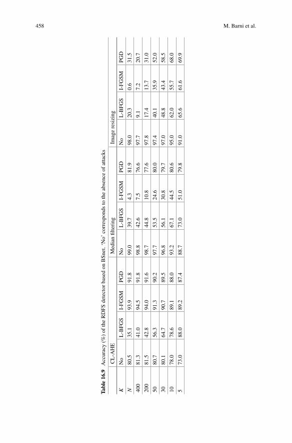
458 M. Barni et al.

Table16.9

Accuracy(%

)of

theRDFS

detector

basedon

BSn

et.‘No’

correspondsto

theabsenceof

attacks

CL-A

HE

Medianfiltering

Imageresizing

KNo

L-BFG

SI-FG

SMPG

DNo

L-BFG

SI-FG

SMPG

DNo

L-BFG

SI-FG

SMPG

D

N80.5

35.1

93.9

91.8

99.0

39.7

4.3

81.9

98.0

20.3

0.6

31.5

400

81.3

41.0

94.5

91.8

98.8

42.6

7.5

76.6

97.7

9.1

7.2

20.7

200

81.5

42.8

94.0

91.6

98.7

44.8

10.8

77.6

97.8

17.4

13.7

31.0

5080.7

56.3

91.3

90.2

97.7

53.5

24.6

80.0

97.4

40.1

35.9

52.0

3080.1

64.7

90.7

89.5

96.8

56.1

30.8

79.7

97.0

48.8

43.4

58.5

1078.0

78.6

89.1

88.0

93.2

67.1

44.5

80.6

95.0

62.0

55.7

68.0

573.0

88.0

89.2

87.4

88.7

73.0

51.0

79.8

91.0

65.6

61.6

69.9


Table16.10

Accuracy(%

)of

theRDFS

detector

basedon

BC+net.‘N

o’correspondsto

theabsenceof

attacks

CL-A

HE

Medianfiltering

Imageresizing

KNo

L-BFG

SI-FG

SMPG

DNo

L-BFG

SI-FG

SMPG

DNo

L-BFG

SI-FG

SMPG

D

N98.2

26.2

34.0

33.5

99.7

71.3

13.7

85.2

100

81.2

75.2

89.8

400

97.1

21.0

83.6

30.1

99.6

75.6

15.6

88.1

99.8

80.0

71.8

89.3

200

96.9

26.0

83.0

48.5

99.6

76.2

17.0

88.6

99.7

77.9

69.6

88.0

5095.1

35.3

80.0

50.6

99.6

76.6

21.9

87.4

96.8

73.0

66.8

85.2

3094.3

39.8

76.3

56.7

99.4

79.6

30.0

88.5

92.7

70.7

65.5

81.8

1091.1

48.3

68.8

55.6

98.8

79.2

44.3

86.1

78.6

63.0

59.9

71.9

587.4

47.0

63.7

47.2

97.2

77.1

48.3

83.3

74.4

60.7

58.7

67.7

460 M. Barni et al.

Table 16.11 Detection accuracy (%) of the RDFS detector (based on BSnet) on increased-confidence adversarial examples

Median filtering Image resizing

C&W PGD C&W PGD

c 0 10 20 0 10 20 0 5 10 0 5 10

K = N 62.9 0.2 0.2 84.7 0.2 0.2 32.1 1.0 0.0 30.1 0.7 0.0

K = 400 53.6 0.2 0.2 75.2 0.2 0.2 18.4 0.7 0.0 20.5 0.7 0.0

K = 200 56.7 0.4 0.2 74.7 0.4 0.2 26.7 3.9 0.1 29.0 4.0 0.1

K = 50 62.1 6.7 0.5 80.1 9.2 0.5 48.0 17.5 2.9 52.0 20.2 3.4

K = 30 64.5 14.9 2.2 79.1 19.4 2.7 57.5 29.9 9.1 59.8 30.6 9.5

K = 10 72.0 34.7 15.5 81.1 38.2 16.4 66.9 47.1 29.2 69.0 48.8 30.0

K = 5 75.5 46.2 29.2 80.0 53.7 33.0 64.0 51.6 39.9 65.1 52.7 40.6

Table 16.12 Detection accuracy (%) of the RDFS detector (based on the BC+net) on increased-confidence adversarial examples

Median filtering Image resizing

C&W PGD C&W PGD

c 0 30 60 0 30 60 0 10 20 0 10 20

K = N 46.1 1.4 0.0 84.3 0.7 0.0 89.3 33.1 5.4 89.8 23.7 3.3

K = 400 52.6 3.1 0.0 87.3 2.7 0.0 88.3 35.4 5.4 89.4 28.1 3.2

K = 200 56.0 4.9 0.4 87.7 4.9 0.0 86.2 35.2 6.4 88.4 31.0 4.5

K = 50 61.9 10.5 0.7 86.8 13.8 0.5 80.1 37.1 11.0 85.0 37.3 8.7

K = 30 68.2 18.1 2.5 87.9 24.8 2.5 76.7 39.4 14.4 80.4 39.7 13.5

K = 10 71.7 36.0 14.8 85.8 42.5 14.2 72.0 46.3 26.2 75.4 47.3 25.2

K = 5 71.1 39.8 20.9 82.8 46.9 20.1 61.1 38.8 23.4 63.1 39.9 23.0

16.4.4 Multiple-Classifier Architectures

Another possibility to combat counter-forensics attacks is to resort to intrinsicallymore secure architectures. This approach has been widely considered in the generalliterature of ML security and in ML-based forensics, however there are only fewmethods resorting to such an approach in the case of CNNs.

Among the approaches developed for general ML applications we mention(Biggio et al. 2015), where a multiple classifier architecture is proposed, referredto as a one-and-a-half classifier. The one-and-a-half class architecture consists oftwo-class classifiers and two one-class classifiers run in parallel followed by a finalone-class classifiers. It has been shown that, when properly trained, this architecturecan effectively limit the damage of an attacker with perfect knowledge. The one-and-a-half architecture has also been considered in forensic applications, to improve thesecurity of SVM-based detectors (Barni et al. 2020). In particular, considering sev-


eral manipulation detection tasks, the authors of Barni et al. (2020) showed that theone-and-a-half class architecture can outperform two-class architectures in terms ofsecurity against white-box attacks, for a fixed level of robustness. The effectivenessof such an approach for CNN-based classifiers has not been investigated yet.

Another simple possibility to design a more secure classifier consists in buildingan ensemble of individual algorithms using some convenient ensemble strategies, asproposed in Strauss et al. (2017) in the general DL literature. A similar approachhas been consider in Fontani et al. (2014) for ML-based forensics, where the authorspropose to improve the robustness of the decision by fusing the outputs of severalforensic algorithms looking for different traces. The method has been assessed forthe representative forensic task of splicing detection in JPEG images. Even in thiscase, the effectiveness of such an approach for CNN-based forensic applications hasstill to be investigated.

Other approaches that have been proposed in security-oriented applications forgeneral ML-based classification consist in using multiple classifiers in conjunctionwith randomization. Randomness can pertain to the selection of the training samplesof the individual classifiers, like in Breiman (1996), or it can be associated with theselection of the features used by the classifiers, as in Ho (1998). Another strategyresorting to multiple classification and randomization has been proposed in Biggioet al. (2008) for spam-filtering applications, where the source of randomness is in thechoice of the weights assigned to the filtering modules of the individual classifiers.

Regarding the DL literature, an approach that goes in this direction is modelswitching (Wang et al. 2020), according to which a certain number of trained sub-models are randomly selected at test time.

All considered, combining multiple classification with randomization in theattempt to improve the security of DL-based forensic classifiers is something thathas not been studied much and is worth of further investigation.

16.5 Final Remarks

Deep learning architectures provide new powerful tools enriching the toolbox avail-able to image forensics designers. At the same time, they introduce new vulnera-bilities due to some inherent security weaknesses of DL techniques. In this chapter,we have reviewed the threats posed by adversarial examples and their possible usefor counter-forensics purposes. Even if adversarial examples targeting image foren-sics networks tend to be less transferable than those created for computer visionapplications, we have shown that, by properly increasing the strength of the attacks,a transferability level which is sufficient for practical applications can be reached.We have also presented some possible remedies against attacks based on adversar-ial examples, even if a definitive solution capable to prevent such attacks in themost challenging white-box scenario has not been found yet. We are convinced that,together with the necessity of developing image forensics techniques suitable to beapplied outside controlled laboratory settings, robustness against intentional attacks

462 M. Barni et al.

is one of the most pressing needs, if we want that image forensics is finally used inreal-life applications contributing to restore the credibility of digital media.

References

Ahmed B, Gulliver TA (2020) Image splicing detection using mask-RCNN. Signal, Image VideoProcess

Akhtar N, Ajmal M (2018) Threat of adversarial attacks on deep learning in computer vision: asurvey. IEEE Access 2018(6):14410–14430

Athalye A, Engstrom L, Ilyas A, Kwok K (2018) Synthesizing robust adversarial examples. In:International conference on machine learning, pp 284–293

Barni M, Bondi L, Bonettini N, Bestagini P, Costanzo A, Maggini M, Tondi B, Tubaro S (2017)Aligned and non-aligned double JPEG detection using convolutional neural networks. J VisCommun Image Represent 49:153–163

Barni M, Nowroozi E, Tondi B (2020) Improving the security of image manipulation detectionthrough one-and-a-half-class multiple classification. Multimed Tools Appl 79(3):2383–2408

Barni M, Chen Z, Tondi B (2016) Adversary-aware, data-driven detection of double jpeg compres-sion: how tomake counter-forensics harder. In: 2016 IEEE international workshop on informationforensics and security (WIFS). IEEE, pp 1–6

BarniM, Costanzo A, Nowroozi E, Tondi B (2018) CNN-based detection of generic contrast adjust-ment with jpeg post-processing. In: 2018 IEEE international conference on image processing,ICIP 2018, Athens, Greece, Oct 7–10, 2018. IEEE, pp 3803–3807

Barni M, Huang D, Li B, Tondi B (2019) Adversarial CNN training under jpeg laundering attacks:a game-theoretic approach. In: 2019 IEEE international workshop on information forensics andsecurity (WIFS), pp 1–6

Barni M, Kallas K, Nowroozi E, Tondi B (2019) On the transferability of adversarial examplesagainst CNN-based image forensics. In: IEEE international conference on acoustics, speech andsignal processing, ICASSP 2019, Brighton, United Kingdom, 12–17 May 2019. IEEE, pp 8286–8290

Barni M, Kallas K, Nowroozi E, Tondi B (2020) CNN detection of gan-generated face imagesbased on cross-band co-occurrences analysis. In: IEEE international workshop on informationforensics and security

Barni M, Nowroozi E, Tondi B (2017) Higher-order, adversary-aware, double jpeg-detection viaselected training on attacked samples. In: 2017 25th European signal processing conference(EUSIPCO), pp 281–285

Barni M, Nowroozi E, Tondi B, Zhang B (2020) Effectiveness of random deep feature selection forsecuring image manipulation detectors against adversarial examples. In: 2020 IEEE internationalconference on acoustics, speech and signal processing, ICASSP 2020, Barcelona, Spain, 4–8May 2020. IEEE, pp 2977–2981

Bayar B, Stamm M (2018) Constrained convolutional neural networks: a new approach towardsgeneral purpose image manipulation detection. IEEE Trans Inf Forensics Secur 13(11):2691–2706

Bayar B, Stamm MC (2016) A deep learning approach to universal image manipulation detectionusing a new convolutional layer. In: Pérez-González F, Bas P, Ignatenko T, Cayre F (eds) Pro-ceedings of the 4th ACMworkshop on information hiding and multimedia security, IH&MMSec2016, Vigo, Galicia, Spain, 20–22 June 2016. ACM, pp 5–10

Bayar B, Stamm MC (2018) Towards open set camera model identification using a deep learningframework. In: 2018 IEEE international conference on acoustics, speech and signal processing(ICASSP), pp 2007–2011


Biggio B, Corona I, He ZM, Chan PP, Giacinto G, Yeung DS, Roli F (2015) One-and-a-half-classmultiple classifier systems for secure learning against evasion attacks at test time. In: Internationalworkshop on multiple classifier systems. Springer, pp 168–180

Biggio B, Fumera G, Roli F (2008) Adversarial pattern classification using multiple classifiersand randomisation. In: Joint IAPR international workshops on statistical techniques in patternrecognition (SPR) and structural and syntactic pattern recognition (SSPR). Springer, pp 500–509

Bondi L, Baroffio L, Guera D, Bestagini P, Delp EJ, Tubaro S (2017) First steps toward cameraidentification with convolutional neural networks. IEEE Signal Process Lett 24(3):259–263

Boroumand M, Fridrich J (2017) Scalable processing history detector for jpeg images. ElectronImaging 2017(7):128–137

Breiman L (1996) Bagging predictors. Mach Learn 24(2):123–140Brendel W, Rauber J, Bethge M (2017) Decision-based adversarial attacks: reliable attacks againstblack-box machine learning models. arXiv:abs/1712.04248

Carlini N, Wagner DA (2017) Towards evaluating the robustness of neural networks. In: 2017 IEEEsymposium on security and privacy, SP 2017, San Jose, CA, USA, 22–26 May 2017. IEEE,Computer Society, pp 39–57

Carrara F, Becarelli R, Caldelli R, Falchi F, Amato G (2018) Adversarial examples detection infeatures distance spaces. In: Proceedings of the European conference on computer vision (ECCV)workshops

Chen PY, SharmaY, ZhangH, Yi J, Hsieh CJ (2018) Ead: elastic-net attacks to deep neural networksvia adversarial examples. In: Proceedings of the AAAI conference on artificial intelligence, vol32

Chen PY, Zhang H, Sharma Y, Yi J, Hsieh CJ (2017) ZOO: zeroth order optimization based black-box attacks to deep neural networks without training substitute models. In: Thuraisingham BM,Biggio B, Freeman DM, Miller B, Sinha A (eds) Proceedings of the 10th ACM workshop onartificial intelligence and security, AISec@CCS 2017, Dallas, TX, USA, 3 Nov 2017. ACM, pp15–26

Chen J, Kang X, Liu Y, Wang ZJ (2015) Median filtering forensics based on convolutional neuralnetworks. IEEE Signal Process Lett 22(11):1849–1853 Nov

Chen Z, Tondi B, Li X, Ni R, Zhao Y, Barni M (2019) Secure detection of image manipulation bymeans of random feature selection. IEEE Trans Inf Forensics Secur 14(9):2454–2469

Chollet F (2017) Xception: deep learning with depthwise separable convolutions. In: 2017 IEEEconference on computer vision and pattern recognition, CVPR 2017, Honolulu, HI, USA, 21–26July 2017. IEEE Computer Society, pp 1800–1807

Costanzo A, Amerini I, Caldelli R, Barni M (2014) Forensic analysis of sift keypoint removal andinjection. IEEE Trans Inf Forensics Secur 9(9):1450–1464

Dang-Nguyen DT, Pasquini C, Conotter V, Boato G (2021) RAISE: a raw images dataset for digitalimage forensics. In: Proceedings of the 6th ACM multimedia systems conference, MMSys ’15,New York, NY, USA, 2015. ACM, pp 219–224

Dhillon GS, Azizzadenesheli K, Lipton ZC, Bernstein J, Kossaifi J, Khanna A, Anandkumar A(2018) Stochastic activation pruning for robust adversarial defense. In: Conference track pro-ceedings 6th international conference on learning representations, ICLR 2018, Vancouver, BC,Canada, April 30–May 3, 2018. OpenReview.net

DongY, Liao F, PangT, SuH, Zhu J,HuX, Li J (2018)Boosting adversarial attackswithmomentum.In: 2018 IEEE conference on computer vision and pattern recognition, CVPR 2018, Salt LakeCity, UT, USA, 18–22 June 2018. IEEE Computer Society, pp 9185–9193

Dong Y, Pang T, Su H, Zhu J (2019) Evading defenses to transferable adversarial examples bytranslation-invariant attacks. In: IEEE conference on computer vision and pattern recognition,CVPR 2019, Long Beach, CA, USA, 16–20 June 2019. Computer Vision Foundation/IEEE, pp4312–4321

Fontani M, Bonchi A, Piva A, Barni M (2014) Countering anti-forensics by means of data fusion.In: Media watermarking, security, and forensics 2014, vol 9028. International Society for Opticsand Photonics, p 90280Z


464 M. Barni et al.

Freire-Obregon D, Narducci F, Barra S, Castrillon-Santana M (2018) Deep learning for sourcecamera identification on mobile devices. Pattern Recognit Lett

Goodfellow IJ, Shlens J, Szegedy C (2015) Explaining and harnessing adversarial examples. In:Bengio Y, LeCun Y (eds) Conference track proceedings 3rd international conference on learningrepresentations, ICLR 2015, San Diego, CA, USA, 7–9 May 2015

Gragnaniello D,Marra F, Poggi G, Verdoliva L (2018) Analysis of adversarial attacks against CNN-based image forgery detectors. In: 26th European signal processing conference, EUSIPCO 2018,Roma, Italy, 3–7 Sept 2018. IEEE, pp 967–971

Guera D, Wang Y, Bondi L, Bestagini P, Tubaro S, Delp EJ (2017) A counter-forensic methodfor CNN-based camera model identification. In: IEEE computer vision and pattern recognitionworkshops, pp 1840–1847

He W, Wei J, Chen X, Carlini N, Song D (2017) Adversarial example defense: ensembles of weakdefenses are not strong. In: 11th {USENIX} workshop on offensive technologies ({WOOT} 17)

Ho TK (1998) The random subspace method for constructing decision forests. IEEE Trans PatternAnal Mach Intell 20(8):832–844

Huang G, Liu Z, Van Der Maaten L, Weinberger KQ (2017) Densely connected convolutionalnetworks. In 2017 IEEE conference on computer vision and pattern recognition, CVPR 2017,Honolulu, HI, USA, 21–26 July 2017. IEEE Computer Society, pp 2261–2269

Ilyas A, Engstrom L, Athalye A, Lin J (2018) Black-box adversarial attacks with limited queriesand information. In: Dy JG, Krause A (eds) Proceedings of the 35th international conferenceon machine learning, ICML 2018, Stockholmsmässan, Stockholm, Sweden, 10–15 July 2018,vol 80 of Proceedings of machine learning research. PMLR, pp 2142–2151

Kevin Eykholt K, Evtimov I, Fernandes E, Li B, Rahmati A, Xiao C, Prakash A, Kohno T, Song D(2018) Robust physical-world attacks on deep learning visual classification. In: Proceedings ofthe IEEE conference on computer vision and pattern recognition, pp 1625–1634

KurakinA,Goodfellow I,BengioS (2017)Adversarial examples in the physicalworld. In:Workshoptrack proceedings 5th international conference on learning representations, ICLR 2017, Toulon,France, 24–26 April 2017. OpenReview.net

Li Y, Li L, Wang L, Zhang T, Gong B (2019) NATTACK: learning the distributions of adver-sarial examples for an improved black-box attack on deep neural networks. In: Chaudhuri K,Salakhutdinov R (eds) Proceedings of the 36th international conference on machine learning,ICML 2019, 9–15 June 2019, Long beach, California, USA, vol 97 of Proceedings of machinelearning research. PMLR, pp 3866–3876

Li W, Tondi B, Ni R, Barni M (2020) Increased-confidence adversarial examples for deep learningcounter-forensics. In: Del Bimbo A, Cucchiara R, Sclaroff S, Farinella GM, Mei T, BertiniM, Escalante HJ, Vezzani R (eds) Pattern recognition. ICPR international workshops andchallenges—virtual event, 10–15 Jan 2021, Proceedings, Part VI, vol 12666 of Lecture notesin computer science. Springer, pp 411–424

Liu X, Cheng M, Zhang H, Hsieh CJ (2018) Towards robust neural networks via random self-ensemble. In: Ferrari V, Hebert M, Sminchisescu C, Weiss Y (eds) Computer vision—ECCV2018—15th European conference, Munich, Germany, 8–14 Sept 2018, Proceedings, Part VII,vol 11211 of Lecture notes in computer science. Springer, pp 381–397

Liu Y, Chen X, Liu C, Song D (2016) Delving into transferable adversarial examples and black-boxattacks. arXiv:1611.02770

MadryA,MakelovA, Schmidt L, TsiprasD,VladuA (2018)Towards deep learningmodels resistantto adversarial attacks. In: Conference track proceedings 6th international conference on learningrepresentations, ICLR 2018, Vancouver, BC, Canada, April 30–May 3, 2018. OpenReview.net

Marra F, Gragnaniello D, Verdoliva L (2018) On the vulnerability of deep learning to adversarialattacks for camera model identification. Signal Process Image Commun 65:240–248

Nataraj L, Mohammed TM, Manjunath BS, Chandrasekaran S, Flenner A, Bappy JH, Roy-Chowdhury AK (2019) Detecting gan generated fake images using co-occurrence matrices. Elec-tron Imaging 2019(5):532–1



Papernot N, McDaniel P, Goodfellow IJ (2016) Transferability in machine learning: from phenom-ena to black-box attacks using adversarial samples. CoRR. arXiv:abs/1605.07277

Papernot N, McDaniel P, Jha S, Fredrikson M, Celik ZB, Swami A (2016) The limitations of deeplearning in adversarial settings. In: IEEE European symposium on security and privacy, EuroS&P2016, Saarbrücken, Germany, 21–24 Mar 2016. IEEE, pp 372–387

Rauber J, Brendel W, Bethge M (2017) Foolbox v0. 8.0: a python toolbox to benchmark the robust-ness of machine learning models. arXiv:1707.04131

RosslerA, CozzolinoD,Verdoliva L, Riess C, Thies J, NiessnerM (2019) Faceforensics++: learningto detect manipulated facial images. In: IEEE/CVF international conference on computer vision

Schöttle P, Schlögl A, Pasquini C, Böhme R (2018) Detecting adversarial examples-a lesson frommultimedia security. In: 2018 26th European signal processing conference (EUSIPCO). IEEE,pp 947–951

Sharif M, Bhagavatula S, Bauer L, Reiter MK (2016) Accessorize to a crime: real and stealthyattacks on state-of-the-art face recognition. In: ACM conference on computer and communica-tions security, p 1528–1540

Shullani D, Fontani M, Iuliani M, Shaya OA, Piva A (2017) VISION: a video and image datasetfor source identification. EURASIP J Inf Secur 1–16

Simonyan K, Zisserman A (2015) Very deep convolutional networks for large-scale image recog-nition. In: Bengio Y, LeCun Y (eds) Conference track proceedings 3rd international conferenceon learning representations, ICLR 2015, San Diego, CA, USA, 7–9 May 2015

Strauss T, Hanselmann M, Junginger A, Ulmer H (2017) Ensemble methods as a defense to adver-sarial perturbations against deep neural networks. arXiv:1709.03423

Szegedy C, Zaremba W, Sutskever I, Bruna J, Erhan D, Goodfellow I, Fergus R (2014) Intriguingproperties of neural networks. In: Bengio Y, LeCun Y (eds) Conference track proceedings 2ndinternational conference on learning representations, ICLR 2014, Banff, AB, Canada, 14–16April 14–16 2014

Tao G, Ma S, Liu Y, Zhang X (2018) Attacks meet interpretability: attribute-steered detection ofadversarial samples. arXiv:1810.11580

Taran O, Rezaeifar S, Holotyak T, Voloshynovskiy S (2019) Defending against adversarial attacksby randomized diversification. In: Proceedings of the IEEE conference on computer vision andpattern recognition, pp 11226–11233

Tondi B (2018) Pixel-domain adversarial examples against CNN-based manipulation detectors.Electron Lett

Tramèr F, Papernot N, Goodfellow I, Boneh D, McDaniel P (2017) The space of transferableadversarial examples. CoRR. arXiv:abs/1704.03453

Valenzise G, Tagliasacchi M, Tubaro S (2013) Revealing the traces of JPEG compression anti-forensics. IEEE Trans Inf Forensics Secur 8(2):335–349

Wang Q, Zhang R (2016) Double JPEG compression forensics based on a convolutional neuralnetwork. EURASIP J Inf Secur 1:2016

Wang X, Wang S, Chen PY, Lin X, Chin P (2020) Block switching: a stochastic approach for deeplearning security. arXiv:2002.07920

Xie C, Wang J, Zhang Z, Ren Z, Yuille A (2018) Mitigating adversarial effects through randomiza-tion. In: Conference track proceedings 6th international conference on learning representations,ICLR 2018, Vancouver, BC, Canada, April 30–May 3, 2018. OpenReview.net

Xie C, Zhang Z, Zhou Y, Bai S, Wang J, Ren Z, Yuille AL (2019) Improving transferability ofadversarial examples with input diversity. In: Proceedings of the IEEE conference on computervision and pattern recognition, pp 2730–2739

Xu W, Evans D, Qi Y (2017) Feature squeezing: detecting adversarial examples in deep neuralnetworks. arXiv:1704.01155

Yuan X, He P, Zhu Q, Li X (2019) Adversarial examples: attacks and defenses for deep learning.IEEE Trans Neural Netw Learn Syst 30(9):2805–2824

Zeng H, Qin T, Kang X, Liu L (2014) Countering anti-forensics of median filtering. In: IEEEinternational conference acoustics, speech and signal processing. IEEE, pp 2704–2708








466 M. Barni et al.

Zhang B, Tondi B, Barni M (2020) Adversarial examples for replay attacks against CNN-basedface recognition with anti-spoofing capability. Comput Vis Image Underst 102988:197–198

Zhao W, Yang P, Ni R, Zhao Y, Wu H (2018) Security consideration for deep learning-based imageforensics. CoRR arXiv:abs/1803.11157

Zheng Z, Hong P (2018) Robust detection of adversarial attacks by modeling the intrinsic prop-erties of deep neural networks. In: Proceedings of the 32nd international conference on neuralinformation processing systems, NIPS’18, USA, 2018. Curran Associates Inc., pp 7924–7933





Chapter 17Anti-Forensic Attacks Using GenerativeAdversarial Networks

Matthew C. Stamm and Xinwei Zhao

17.1 Introduction

The rise of deep learning has led to rapid advances in multimedia forensics. Algo-rithms based on deep neural networks are able to automatically learn forensic traces,detect complex forgeries, and localize falsified content with increasingly greateraccuracy. At the same time, deep learning has expanded the capabilities of anti-forensic attackers.Newanti-forensic attacks have emerged, including those discussedin Chap.14 based on adversarial examples, and those based on generative adversarialnetworks (GANs).

In this chapter, we discuss the emerging threat posed by GAN-based anti-forensicattacks. GANs are a powerful machine learning framework that can be used to createrealistic, but completely synthetic data. Researchers have recently shown that anti-forensic attacks can be built by using GANs to create synthetic forensic traces.Whileonly a small number of GAN-based anti-forensic attacks currently exist, results showthese early attacks are both effective at fooling forensic algorithms and introduce verylittle distortion into attacked images. Furthermore, by using the GAN framework tocreate new anti-forensic attacks, attackers can dramatically reduce the time requiredto create a new attack.

For simplicity,wewill assume in this chapter thatGAN-based anti-forensic attackswill be launched against images. This also aligns with the current state of research,since all existing attacks are targeted at images. However, the ideas and methodolo-gies presented in this chapter can be generalized to a variety of media modalitiesincluding video and audio. We expect new GAN-based anti-forensic attacks targetedon these modalities will likely arise in the near future.

This chapter begins with Sect. 17.2, which provides a brief background on GANs.Section17.3 provides background on anti-forensic attacks, including how they are

M. C. Stamm (B) · X. ZhaoDepartment of Electrical and Computer Engineering, Drexel University, Philadelphia, PA, USAe-mail: [email protected]


467


http://dx.doi.org/10.1007/978-981-16-7621-5_14


https://doi.org/10.1007/978-981-16-7621-5_17

468 M. C. Stamm and X. Zhao

traditionally designed as well as their shortcomings. In Sect. 17.4, we discuss howGANs are used to create anti-forensic attacks. This gives a high-level overviewof the components of an anti-forensic GAN, differences between attacks based onGANs and adversarial examples, as well as an overview of existing GAN-basedanti-forensic attacks. Section17.5 provides more details about how these attacks aretrained, including different techniques that can be employed based on the attacker’sknowledge of and access to the forensic algorithm under attack. We discuss knownshortcomings of anti-forensic GANs and future research directions in Sect. 17.6.

17.2 Background on GANs

Generative adversarial networks (GANs) are a machine learning framework thatis used to train generative models (Goodfellow et al. 2014). In their standard form,GANsconsist of twocomponents: a generatorG and adiscriminator D. Thegeneratorand the discriminator can be viewed as competitors in a two-player game. The goalof the generator is to learn to produce deceptively synthetic data that can mimicthe real data, while the goal of the discriminator aims to learn to distinguish thesynthetic data from the real data. The two parties are trained alternatively and eachparty attempts to improve its performance to defeat the other until the synthetic datais indistinguishable from the real data.

The generator is a generativemodel that creates synthetic data x′ bymapping someinput z in a latent space to an output as a set of real data x. Ideally, the generatorproduces synthetic data x′ with the same distribution as real data x such that the twocannot be differentiated. The discriminator is a discriminative model that will assigna scalar to each input data. The discriminator can output any scalar between 0 and 1,with 1 representing the real data and 0 representing the synthetic data. During trainingphase, the discriminator aims to maximize the probability of assigning correct labelto both real data x and synthetic data x′, while the generator aims to reduce thedifference between the discriminator’s decision on the synthetic data and 1 (i.e.,it must be real data). Training a GAN is equivalent to finding the solution of themin-max function

minG

maxD

Ex∼ fX (x)[log D(x)] + Ez∼ fZ (z)[log(1 − D(G(z)))] (17.1)

where fX (x) represents the distribution of real data, fZ (z) represents the distributionof input noise, E represents the operation of calculating expected value.

17 Anti-Forensic Attacks Using Generative Adversarial Networks 469

17.2.1 GANs for Image Synthesis

While GANs can be used to synthesize many types of data, one of their most com-mon uses is to synthesize images or modify images. The development of severalspecific GANs has provided important insights and guidelines into the design ofGANs for images. For example, while the GAN framework does not specify thespecific form of the generator or discriminator, the development of DCGAN showedthat deep convolutional generators and discriminators yield substantial benefits whenperforming image synthesis (Radford et al. 2015). Additionally, this work suggestedconstraints on the architectures of the generator and discriminator that can result instable training. The creation of Conditional GANs (CGANs) showed the benefit ofusing information such as labels as auxiliary inputs to both the generator and thediscriminator (Mehdi Mirza and Simon Osindero 2014). This can help can improvethe visual quality and control the appearance of synthetic images generated by aGAN. InfoGAN showed that the latent space can be structured to both select andcontrol generation of images (Chen et al. 2016). Pix2Pix (Isola et al. 2018) showedthat GANs can learn to translate from one image space to another (Isola et al. 2018),while StackGANdemonstrated that text can be used to guide the generation of imagesvia a series of CGANs (Zhang et al. 2017).

Since their first appearance in literature, the development of GANS for imagesynthesis has proceeded at an increasingly rapid pace. Research has been performedto improve the architectures of the generator and discriminator (Zhang et al. 2019;Brock et al. 2018; Karras et al. 2017; Zhu et al. 2017; Karras et al. 2020; Choiet al. 2020), improve the training procedure (Arjovsky et al. 2017; Mao et al. 2017),and build publicly available datasets to aid the research community (Yu et al. 2016;Liu et al. 2015; Karras et al. 2019; Caesar et al. 2018). Because of these efforts,GANs have been used to achieve state-of-the-art performance on various computervision tasks, such as super-resolution (Ledig et al. 2017), photo inpainting (Pathaket al. 2016), photo blending (Wu et al. 2019), image-to-image translation (Isola et al.2018; Zhu et al. 2017; Jin et al. 2017), text-to image-translation (Zhang et al. 2017),semantic-image-to-photo translations (Park et al. 2019), face aging (Antipov et al.2017), generating human faces (Karras et al. 2017; Choi et al. 2018, 2020; Karraset al. 2019, 2020), generating 2-D (Jin et al. 2017; Karras et al. 2017; Brock et al.2018) and 3-D objects (Wu et al. 2016), video prediction (Vondrick et al. 2016), andmany more applications.

17.3 Brief Overview of Relevant Anti-Forensic Attacks

In this section, we provide a brief discussion of what anti-forensic attacks are andhow they are designed.


17.3.1 What Are Anti-Forensic Attacks

Anti-forensic attacks are countermeasures that amedia forger can use to fool forensicalgorithms. They operate by falsifying the traces that forensic algorithms rely uponto make classification or detection decisions. A forensic classifier that is targeted byan anti-forensic attack is referred to as a victim classifier.

Just as there are many different forensic algorithms, there are similarly a widevariety of anti-forensic attacks (Stammet al. 2013; Böhme andKirchner 2013).Manyof them, however, can be broadly grouped into two categories:

• Attacks designed to disguise evidence of manipulation and editing. Attackshave been developed to fool forensic algorithms designed to detect a variety ofmanipulations such as resampling (Kirchner and Bohme 2008; Gloe et al. 2007),JPEGcompression (StammandLiu 2011; Stammet al. 2010; Fan et al. 2013, 2014;Comesana-Alfaro and Pérez-González 2013; Pasquini and Boato 2013; Chu et al.2015), median filtering (Fontani and Barni 2012; Wu et al. 2013; Dang-Nguyenet al. 2013; Fan et al. 2015), contrast enhancement (Cao et al. 2010), and unsharpmasking (Laijie et al. 2013), as well as algorithms detect forgeries by identifyinginconsistencies in lateral chromatic aberration (Mayer and Stamm 2015), identifycopy-move forgeries (Amerini et al. 2013; Costanzo et al. 2014), and detect videoframe deletion (Stamm et al. 2012a, b; Kang et al. 2016).

• Attacks designed to falsify the source of a multimedia file. Attacks have beendeveloped to falsify demosaicing traces associated with an image’s source cameramodel (Kirchner and Böhme 2009; Chen et al. 2017)??, as well as PRNU tracesthat can be linked to a specific device (Lukas et al. 2005; Gloe et al. 2007; Goljanet al. 2010; Barni and Tondi 2013; Dirik et al. 2014; Karaküçük and Dirik 2015)

To understand how anti-forensic attacks operate, it is helpful to first considera simple model of how forensic algorithms operate. Forensic algorithms extractforensic traces from an image, then associate those traces with a particular forensicclass. That class can be associated with editing operation or manipulation that animagehas undergone, the image’s source (i.e., it’s cameramodel, its source device, it’sdistribution channel, etc.,) or some other property that a forensic investigator wishesto ascertain. It is important to note thatwhen performingmanipulation detection, evenunaltered images contain forensic traces. While they do not contain traces associatedwith editing, splicing, or falsification, they do contain traces associatedwith an imagebeing generated by a digital camera and not undergoing subsequent processing.

Anti-forensic attacks create synthetic forensic traces within an image that aredesigned to fool a forensic classifier. This holds true even for attacks designed toremove evidence of editing. These attacks synthesize traces in manipulated imagesthat are associated with unaltered images. Most anti-forensic attacks are targeted,i.e., they are designed to trick the forensic classifier into associating an image with aparticular target forensic class. For example, attacks against manipulation detectorstypically specify the class of ‘unaltered’ images as the target class. Attacks designedto fool source identification algorithms synthesize traces associated with a target


source that the image did not truly originate from. Additionally, a small number ofanti-forensic attacks are untargeted. This means that the attack does not care whichclass the forensic algorithmassociates the imagewith, so long as it is not the true class.Untargeted attacks are more commonly used to fool source identification algorithms,since an untargeted attack still tricks the forensic algorithm into believing that animage can form an untrue source. They are typically not used against manipulationdetectors, since a forensic investigator will still decide that image is inauthentic evenif their algorithm mistakes manipulation A for manipulation B.

17.3.2 Anti-Forensic Attack Objectives and Requirements

When creating an anti-forensic attack, an attackermust consider several design objec-tives. For an attack to be successful, it must satisfy the following design requirements;

• Requirement 1: Fool the victim forensic algorithmAn anti-forensic attack should cause the victim algorithm to classify an imageas belonging to the attacker’s target class. If the attack is designed to disguisemanipulation or content falsification, then the target class is the class of unalteredimages. If the attack is designed to falsify an image’s source, then the target class isthe desired fake source chosen by the attacker such as a particular source camera.

• Requirement 2: Introduce no visually perceptible artifacts.An attack should not introduce visually distinct telltale signs that a human caneasily identify. If this occurs, a human will quickly disregard an attacked imageas fake even if it fools a forensic algorithm. This is particularly important if theimage is to be used as part of a misinformation campaign, since images that arenot plausibly real will be quickly flagged.

• Requirement 3: Maintain high visual quality of the attacked image.Similar to Requirement 2, if an attack fools a detector but significantly distortsan image, it is not useful to an information attacker. Some distortion is allowable,since ideally no one other than the attacker will be able to compare the attackedimage to its unattacked counterpart. Additionally, this requirement is put in placeto ensure that an attack does not undo desired manipulations that an attacker haspreviously performed to an image. For example, localized color corrections andcontrast adjustments may be required to make a falsified image appear visuallyplausible. If an anti-forensic attack reverses these intentional manipulations, thenthe attack is no longer successful.

In addition to these requirements, there are several other highly desirable proper-ties for an attack to possess. These include


• Desired Goal 1: Be rapidly deployable in practical scenarios.Ideally, an attack should be able to be launched quickly and efficiently, thusenabling rapid attacks or attacks at scale. It is flexible enough to attack images ofany arbitrary size, not only images of a fixed predetermined size. Additionally, itshould not require prior knowledge of which region of an image will be analyzed,such as a specific image block or block grid (it is typically unrealistic to assumethat an investigator will only examine certain fixed image locations).

• Desired Goal 2: Achieve attack transferability.An attack achieves transferability if it is able to fool other victim classifiers thatit has not been explicitly designed or trained to fool. This is important because aninvestigator can typically utilize multiple different forensic algorithms to performa particular task. For example, several different algorithms exist for identifying animage’s source camera model. An attack designed to fool camera model identifi-cation algorithm A is maximally effective if it also transfers to fool camera modelidentification algorithms B and C.

While it is not necessary that an attack satisfy these additional goals, attacks thatdo are significantly more effective in realistic scenarios.

17.3.3 Traditional Anti-Forensic Attack Design Procedureand Shortcomings

While anti-forensic attacks target different forensic algorithms, at a high level themajority of them operate in a similar manner. First, an attack builds or estimates amodel of the forensic trace that it wishes to falsify. This could be associated withthe class of unaltered images in the case that the attack is designed to disguiseevidence of manipulation or falsification, or it could be associated with a particularimage source. Next, this model is used to guide a technique that synthesizes forensictraces associated with this target class. For example, anti-forensic attacks to falsifyan image’s source camera model synthesize demosaicing traces or other forensictraces associated with a target camera model. Alternatively, techniques designed toremove evidence of editing such as multiple JPEG compression or median filteringsynthesize traces that manipulation detectors associate with unaltered images.

Traditionally, creating a new anti-forensic attack has required a human expert tofirst design an explicit model of the target trace that the attack wishes to falsify. Next,the expertmust create an algorithmcapable of synthesizing this target trace such that itmatches their model.While this approach has led to the creation of several successfulanti-forensic attacks, it is likely not scalable enough to keep pace with the rapiddevelopment of new forensic algorithms. It is very difficult and time consuming forhumans to construct explicit models of forensic traces that are accurate enough to foran attack to be successful. Furthermore, the forensic community has widely adoptedthe usemachine learning and deep learning approaches to learn sophisticated implicitmodels directly from data. In this case, it may be intractable for human experts to


explicitly model a target trace. Even if a model can be successfully constructed, anew algorithm must be designed to synthesize each trace under attack. Again, this isalso a challenging and time-consuming process.

In order to respond to the rapid advancement of forensic technologies, adversarieswould like to develop some automated means of creating new anti-forensic attacks.Tools from deep learning such as convolutional neural networks have allowed foren-sics researchers to successfully automate how forensic traces are learned. Similarly,intelligent adversaries have begun to look to deep learning for approaches to auto-mate the creation of new attacks. As a result, new attacks based upon GANs havebegun to emerge.

17.3.4 Anti-Forensic Attacks on Parametric Forensic Models

WIth the advances of software and apps, it is very easy for people to manipulateimages the way they want. To make an image deceptively convincing to human eyes,post-processing operations such as resampling, blending, denoising are often appliedto the falsified images. Recent years, deep learning-based algorithms are also used tocreate innovation contents. In the hand of an attacker, these techniques can be usedformalicious purposes. Previous research shows thatmanipulations and attacks leavetraces that can bemodeled or characterized by forensic algorithms.While these tracesmay be invisible to human eyes, through forensic algorithms forged images can bedetected or distinguished from the real images.

Anti-forensic attacks are countermeasures attempting to fool target forensic algo-rithms. Some anti-forensic attacks aim to remove forensic traces left bymanipulationoperations or attacks that the forensic algorithms analysis. Some anti-forensic attackssynthesize fake traces to make the forensic algorithms make a wrong decision. Forexample, anti-forensic attacks can remove traces left by resampling and make theforensic algorithms designed for characterizing resampling traces to believe the anti-forensically attacked images as “unaltered”. Anti-forensic attacks can also synthe-size fake forensic traces associated with a particular target camera model B into animages, and make a camera model identification algorithm to believe an image wascaptured by the camera model B, while the image was actually captured by cam-era model A. Anti-forensic attacks can also hide forensic traces to obfuscate theirtrue origins. Anti-forensic attacks are expected to leave invisible distortion, since anvisible distortion often flag “fake” for investigators. However, anti-forensic attacksdo not consider countermeasures of itself, and only examine fooling target forensicalgorithms.

Additionally, anti-forensic attacks are often designed to falsify particular foren-sic traces. A common methodology is typically used to create anti-forensic attackssimilar to those described in the previous section. First, a human expert designs aparametricmodel of the target forensic trace that theywish to falsify during the attack.Next, an algorithm is created to introduce a synthetic trace into the attacked imageso that it matches this model. Often this is accomplished by creating a generative


noise model which is used to introduce specially designed noise either directly intothe image or into some transform of the image. Many anti-forensic attacks have beendeveloped following this methodology, such as removing traces left by median fil-tering, JPEG compression, or resampling, or synthesizing demosaicing informationof camera models.

This approach to creating attacks has several important drawbacks. First, it is bothchallenging and time consuming for human experts to create accurate parametricmodels of forensic traces. In some cases it is extremely difficult or even infeasible tocreatemodels accurate enough to fool state-of-the-art detectors. Furthermore,modelsof one forensic cannot typically be reused to attack a different forensic trace. Thiscreates an important scalability challenge for the attacker.

17.3.5 Anti-Forensic Attacks on Deep Neural Networks

An even greater challenge arises from the widespread adoption of deep-learning-based forensic algorithms such as convolutional neural networks (CNNs). Theapproach described above cannot be used to attack forensic CNNs since they don’tutilize an explicit feature set or model of a forensic trace. Anti-forensic attacks tar-geting on deep-learning-based forensic algorithms now draw an increasing amountof attentions both from academia and industries.

While deep learning has achieved many state-of-the-art performances on manymachine learning tasks, including computer vision and multimedia forensics,researchers found that non-ideal properties of neural networks can be exploited andcausemisclassifications of an input image. Several explanations have been posited forthe non-ideal properties of neural networks that adversarial examples exploit, suchas imperfections caused by the locally-linear nature of neural networks (Goodfellowet al. 2014) or that there is misalignment between the features used by humans andthose learned by neural networks when performing the same classification task (Ilyaset al. 2019). These findings facilitate the development of adversarial example gener-ation algorithms.

Adversarial example generation algorithms operate by adding adversarial pertur-bations to an input image. The adversarial perturbations are some noises producedby optimizing a certain distance metric, usually L p norm (Goodfellow et al. 2014;Madry et al. 2017; Kurakin et al. 2016; Carlini and Wagner 2017). The adversarialperturbations aim to push the representation in latent feature space just across thedecision boundary of the desired class (i.e., targeted attack) or push the data awayfrom its true class (i.e., untargeted attack). Forensic researchers found that adversarialexample generation algorithms can be used as anti-forensic attacks on forensic algo-rithms. In 2017, Güera et al. showed that camera model identification CNNs (Güeraet al. 2017) can be fooled by Fast Gradient Sign method (FGSM) (Goodfellow et al.2014) and Jacobian-based Saliency Map (JSMA) (Papernot et al. 2016).


There are several drawbacks for using adversarial example generation algorithmsas anti-forensic attacks. To ensure theCNNcanbe successfully fooled, the adversarialperturbations added to the imagemay be strong and result in fuzzy or distorted outputimages. While using some tricks, researchers could control the visual quality of anti-forensic attacked images to a certain level, maintaining high visual quality is still achallenge for further study.Another drawback is that adversarial perturbations have tobe optimized for particular given input image. As a result, it could be time-consumingfor producing large volume of anti-forensically attacked images. Additionally, theadversarial perturbations are not invariant to detection block alignment.

17.4 Using GANs to Make Anti-Forensic Attacks

Recently, researchers have begun adapting the GAN framework to create a new classof anti-forensic attacks. Though research into these new GAN-based attacks is stillin its early stages, recent results have shown that these attacks can overcome manyof the problems associated with both traditional anti-forensic attacks and attacksbased on adversarial examples. In this section, we will describe at a high level howGAN-based anti-forensic attacks are constructed. Additionally, we will discuss theadvantages of utilizing these types of attacks.

17.4.1 How GANs Are Used to Construct Anti-ForensicAttacks

GAN-based anti-forensic attacks are designed to fool forensic algorithms built uponneural networks. At a high level, they operate by using an adversarially trainedgenerator to synthesize a target set of forensic traces in an image. Training occursfirst, before the attack is launched. Once the anti-forensic generator has been trained,an image can be attacked simply by passing it through the generator. The generatordoes not need to be re-trained for each image, however, it must be re-trained if a newtarget class is selected for the attack.

Researchers have shown that GANs can be adapted to both automate and gen-eralize the anti-forensic attack design methodology described in Sect. 17.5 of thischapter. The first step in the traditional approach to creating an anti-forensic attackinvolves the creation of a model of the target forensic trace. While it is difficult orpotentially impossible to build an explicit model of the traces learned by forensicneural networks, GANs can exploit the model that has already been learned by theforensic neural network. This is done by adversarially training the generator againsta pre-trained version of the victim classifier C . The victim classifier can either takethe place of the discriminator in the traditional GAN formulation, or it can be usedin conjunction with a traditional discriminator. Currently, there is not a clear consen-


sus on whether a discriminator is necessary or beneficial when creating GAN-basedanti-forensic attacks. Additionally, in some scenarios the attackermay not have directaccess to the victim classifier. If this occurs, the victim classifier cannot be directlyintegrated into the adversarial training process. Instead, alternate means of trainingthe generator must be used. These are discussed in Sect. 17.5.

When the generator is adversarially trained against the victim classifier, it learnsthe model of the target forensic trace implicitly used by the victim classifier. Becauseof this, the attacker does not need to explicitly design a model of the target trace, aswould typically be done in the traditional approach to creating an anti-forensic attack.This dramatically reduces the time required to construct an attack. Furthermore, itincreases the accuracy of the trace model used by the attack, since it is directlymatched to the victim classifier.

Additionally, GAN-based attacks significantly reduce the effort required for thesecond step of the traditional approach to creating an anti-forensic attack, i.e., creatinga technique to synthesize the target trace. This is because the generator automaticallylearns to synthesize the target trace through adversarial training.While existingGAN-based anti-forensic attacks utilize different generator architectures, the generator stillremains somewhat generic in that it is a deep convolutional neural network. CNNscan be quickly and easily implemented using deep learning frameworks such asTensorFlow or Pytorch, making it easy for an attacker to experimentally optimizethe design of their generator.

Currently, there are no well-established guidelines for designing anti-forensicgenerators. However, research by Zhang et al. has shown that when an upsamplingcomponent is utilized in aGAN’s generator, it leaves behind “checkerboard” artifactsin the synthesized image. Zhang et al. (2019). As a result, it is likely important toavoid the use of upsampling in the generator so that visual or statistically detectableartifacts that may act as giveaways are not introduced to an attacked image. This isreinforced by the fact thatmany existing attacks utilize fully convolutional generatorsthat do not include any pooling or upsampling layers.

Convolutional generators also possess the useful property that once they aretrained, they can be used to attack an image of any size. Fully convolutional CNNsare able to accept images of any size as an input and produce output images of thesame size. As a result, these generators can be deployed in realistic scenarios inwhich the size of the image under attack may not be known a prior, or may vary inthe case of attacking multiple images. They also provide an advantage in that synthe-sized forensic traces are distributed throughout the attacked image and do not dependon a blocking grid. As a result, the attacker does not require advanced knowledgeof which image region or block that an investigator will analyze. This is a distinctadvantage over anti-forensic attacks based upon adversarial examples.

Research also suggests that a well-constructed generator can be re-trained tosynthesize different forensic traces than the ones which it was initially designed for.For example, theMISLGAN attack was initially designed to falsify an image’s originby synthesizing source camera model traces linked with a different camera model.


Recent work has also used this generator architecture to construct a GAN-basedattack that removes evidence of multiple editing operations.

17.4.2 Overview of Existing GAN-Based Attacks

Recently, several GAN-based anti-forensic attacks have been developed to falsifyinformation about an image’s source and authenticity. Here we provide a briefoverview of existing GAN-based attacks.

In 2018, Kim et al. proposed a GAN-based attack to remove median filteringtraces from an image (Kim et al. 2017). This GAN was built using a generator anda discriminator. The generator was trained to remove the median filtering traces,and the discriminator was trained to distinguish between the restored images andthe unaltered images. The author introduced loss computed from a pre-trained VGGnetwork to improve the visual quality of attacked images. This attack was able toremove media filtering traces from gray-scale images, and fool many traditionalforensic algorithms using hand-designed features, and CNN detectors.

Chen et al. proposed a GAN-based attack in 2018 named MISLGAN to falsify animage’s source camera model (Chen et al. 2018). In this work, the authors assumedthat the attacker has access to the forensic CNN that the investigator will use toidentify an image’s source camera model. Their attack attempts to modify the tracesin images associated with a target camera model such that the forensic CNN mis-classifies an attacked image as having been captured by the target camera model.MISLGAN is consists of three major components: a generator, a discriminator, andthe pre-trained forensic camera model CNN. The generator was adversarially trainedagainst both the discriminator and the camera model CNN for each target cameramodel. The trained generator was shown to be able to falsify fake camera modelsfor any color images with high success attack rate (i.e., the percentage of an imagebeing classified as the target camera model after being attacked). This attack wasdemonstrated to be effective even when images under attack were captured by cam-era models not used during training. Additionally, the attacked images also maintainhigh visual qualities even comparing with the original unaltered image side by side.

In 2019, the authors of MISLGAN extended this work to create a black boxattack against forensic source camera model identification CNNs (Chen et al. 2019).To accomplish this, the authors integrated a substitute network to approximate thecamera model identification CNNs under attack. By training MISLGAN against asubstitute network, this attack can successfully fool state-of-the-art camera modelCNNs even in black-box scenarios, and outperformed adversarial example generationalgorithms such as FGSM (Goodfellow et al. 2014). This GAN-based attack hasbeen adapted to remove traces left by editing operations and to create transferableanti-forensic attacks (Zhao et al. 2021). Additionally, by improving the generator’sarchitecture, Zhao et al. were able to falsify traces left in synthetic images by theGAN generation process (Xinwei Zhao and Matthew C. Stamm 2021). This attack


was shown to fool existing synthetic image detectors targeted at detecting both GAN-generated faces and objects.

In 2021, Cozzolino et al. proposed a GAN-based attack, SpoC (Cozzolino et al.2021), to falsify camera model information of a GAN-synthesized image. SpoC isconsisted of a generator, a discriminator, and a pre-trained embedder. The embedderis used to learn the reference vectors of real images or the images of the target cam-era models in the latent spaces. This attack can successfully fool GAN-synthesizedimage detectors or the camera model identification CNNs, and outperformed adver-sarial example generation algorithm such as FGSM (Goodfellow et al. 2014) andPGD (Madry et al. 2017). The authors also showed that the attack is robust to JPEGcompression of a certain level.

In 2021, Wu et al. proposed a GAN-based attack, JRA-GAN, to restore JPEGcompressed images (Wu et al. 2021). The authors used a GAN to restore the highfrequency information in the DCT domain, and remove the blocking effect causedby JPEG compression to fool JPEG compression detection algorithms. The authorsshowed that the attack can successfully restore gray-scale JPEG compressed imagesand fool traditional JPEG detection algorithms using hand-designed features, andCNN detectors.

17.4.3 Differences Between GAN-Based Anti-ForensicAttacks and Adversarial Examples

While attacks built fromGANs and from adversarial examples both use deep learningto create anti-forensic countermeasures, it is important to note that the GAN-basedattacks described in this chapter are fundamentally different from adversarial exam-ples

As discussed in Chap. 16, adversarial examples operate by exploiting non-idealproperties of a victim classifier. There are several explanations that have been con-sidered by the research community as to why adversarial examples exist and aresuccessful. These include “blind spots” caused by non-ideal training or overfitting,a mismatch between features used by humans and those learned by neural networkswhen performing classification (Ilyas et al. 2019), and inadvertent effects caused bythe locally-linear nature of neural networks (Goodfellow et al. 2014). In all of theseexplanations, adversarial examples cause a classifier tomisclassify due to unintendedbehavior.

By contrast, GAN-based anti-forensic attacks do not try to trick the victim clas-sifier into misclassifying an image by exploiting its non-ideal properties. Instead,they replace the forensic traces present in an image with a synthetic set of traces thataccurately match the victim classifier’s model of the target trace. In this sense, theyattempt to synthesize traces that the victim classifier correctly uses to perform taskssuch as manipulation detection and source identification. This is possible becauseforensic traces, such as those linked to editing operations or an image’s source cam-



era, are typically not visible to the human eye. As a result, GANs are able to createnew forensic traces in an image without altering its content or visual appearance.

Additionally, adversarial example attacks are customized to each image underattack. Often, this is done through an iterative training or search process that mustbe repeated each time a new image is attacked. It is worth noting that GAN-basedtechniques for generating adversarial examples that have recently been proposed inthe computer vision and machine learning literature (Poursaeed et al. 2018; Xiaoet al. 2018). These attacks are distinct from the GAN-based attacks discussed in thischapter, specifically because they generate adversarial examples and not syntheticversions of features that should accurately be associated with the target class. Forthese attacks, the GAN framework is instead adapted to search for an adversarialexample that can be made from a particular image in the same manner that iterativesearch algorithms are used.

17.4.4 Advantages of GAN-Based Anti-Forensic Attacks

There are several advantages to using GAN-based anti-forensic attacks over bothtraditional human-designed approaches and those based on adversarial examples.We briefly summarize these below. Open problems and weaknesses of GAN-basedadversarial attacks are further discussed in Sect. 17.6.

• Rapid and automatic attack creation: As discussed earlier, GANs both automateand generalized the traditional approach to designing anti-forensic attacks. As aresult, it is much easier and quicker to create newGAN-based attacks than throughtraditional human-designed approaches.

• Low visual distortion: In practice, existing GAN-based attacks tend to introducelittle-to-no visually detectable distortion. While this condition is not guaranteed,visual distortion can be effectively controlled during training by carefully balanc-ing the weight placed on the generator’s loss term controlling visual quality. Thisis discussed in more detail in Sect. 17.5. By contrast, several adversarial exampleattacks can leave behind visually detectable noise-like artifacts (Güera et al. 2017).

• Attack only requires training once: After training, GAN-based attack can belaunched on any image as long as the target class remains constant. This differsfrom attacks based on adversarial examples, which need to create a custom set ofmodifications for each image, often involving an iterative algorithm. Additionally,no image-specific parameters need to be learned, unlike for several traditionalanti-forensic attacks.

• Scalable deployment in realistic scenarios: Attack requires only to pass theimage through a pre-trained convolutional generator. It launches very rapidly andcan be deployed at scale. Additionally, since the attack is launched

• Ability to attack images of arbitrary size: Because the attack is launched viaa convolutional generator, the attack can be applied to images of any size. Bycontrast, attacks based on adversarial examples only produce attacked images of


the same size as the input to the victim CNN, which is typically a small patch andnot a full sized image.

• Does not require advanced knowledge of the analysis region: One way to adaptadversarial attacks to larger images is to break the image into blocks, then attackeach block separately. This however requires advanced knowledge of the particularblocking grid that will be used during forensic analysis. If the blocking grid usedby the attacker and the detector do not align, or if the investigator analyzes animage multiple times with different blocking grids, adversarial example attacksare unlikely to be successful.

17.5 Training Anti-Forensic GANs

In this section, we give an overview of how to train an anti-forensic generator. Webegin by discussing the different terms of the loss function used during training. Weshown how each term of the loss function is formulated in the perfect knowledgescenario (i.e., when a white box attack is launched). After this, we show how tomodify the loss function to train the attack to create black box attacks in limitedknowledge scenarios, as well transferable attacks in the zero knowledge scenario.

17.5.1 Overview of Adversarial Training

During adversarial training, the generator G used in GAN-based attack should beincentivized to produce visually convincing anti-forensic attacked images that canfool the victim forensic classifier C , as well as a discriminator D if it is used. Thesegoals are achieved byproperly formulating the generator’s loss functionLG . A typicalloss function for adversarially training an anti-forensic generator consists of threemajor loss terms: the classification lossLC , the adversarial lossLA (if a discriminatoris used), and perceptual loss LP ,

LG = αLP + βLC + γLA, (17.2)

where α, β, γ are weights to balance the performance of the attack and the visualquality of the attacked images.

Like all anti-forensic attacks, the generator’s primary goal is to produce outputimages that fool a particular forensic algorithm. This is done by introducing a terminto the generator’s loss function that we describe as the forensic classification loss,or classification loss for short. Classification loss is the key element to guide thegenerator to learn the forensic traces of the target class. Depending on the attacker’saccess to and knowledge level of the forensic classifier, particular strategiesmay needto be adopted during trainingWewill elaborate on this later in this section. Typically,the classification loss is defined as 0 if the output of the generator is classified by the


forensic classifier as belonging to the target class t and 1 if the output is classified asany other class.

If the generator is trained to fool a discriminator as well, then the adversarialloss provided by the feedback of the discriminator is consolidated into the total lossfunction. Typically, the adversarial loss is 0 if the generated anti-forensically attackedimages fools the discriminator and 1 if not.

At the same time, the anti-forensic generator should introduce minimal distor-tion into the attacked image. Some amount of distortion is acceptable, since in ananti-forensic setting, the unattacked image will not be presented to the investigator.However these distortions should not undo or significantly alter any modificationsthat were introduced by the attacker before the image is passed through the anti-forensic generator. To control the visual quality of anti-forensically attack images,the perceptual loss measures the pixel-wise difference between the image underattack and the anti-forensically attacked image produced by the generator. Minimiz-ing the perceptual loss during the adversarial training process helps to ensure thatattacked images produced by the generator contain minimal, visually imperceptibledistortions.

When constructing an anti-forensic attack, it is typically advantageous to exploit asmuch knowledge of the algorithm under attack as possible. This holds especially truewith GAN-based attacks, which directly integrates a forensic classifier into trainingthe attack. Since gradient information from a victim forensic classifier is neededto compute the classification loss, different strategies must be adopted to train theanti-forensic generator depending on the attacker’s knowledge about the forensicclassifier under attack. As a result, it is necessary to provide more detail about thedifferent knowledge levels that an attacker may have of the victim classifier beforewe are able to completely formulate the loss function. We note that the knowledgelevel typically only has an influence on the classification loss. The perceptual lossand discriminator loss remain unchanged for all knowledge levels.

17.5.2 Knowledge Levels of the Victim Classifier

Asmentioned previously, we refer to the forensic classifier under attack as the victimclassifier C . Depending on the attacker’s knowledge level of the victim classifier, itis common to categorize the knowledge scenarios into the perfect knowledge (i.e.,white box) scenario, the limited knowledge (i.e., black box) scenario, and the zeroknowledge scenario.

In the perfect knowledge scenario, the attacker has full access to the victim clas-sifier or an exact identical copy of the victim classifier. This is an ideal situation forthe attacker. The attacker can launch a white box attack in which they train directlyagainst the victim classifier that they wish to fool.

In many other situations, however, the attacker has only partial knowledge or evenzero knowledge of the victim classifier. Partial knowledge scenarios may include avariety of specific settings in real life. A common aspect is that the attacker does not


have full access or control over the victim classifier. However, the attacker is allowedto probe the victim classifier as a black box. For example, they can query the victimclassifier using an input, then observe the value of its output. Because of this, thepartial knowledge scenario is also referred to as the black box scenario. This scenariois a more challenging, but potentially more realistic situation for the attacker. Forexample, a piece of forensic software may or online service may be encrypted toreduce the risk of attack. As a result, its users would only be able to provide inputimages and observe the results that the system output.

An even more challenging situation is when the attacker has zero knowledge ofthe victim classifier. Specifically, the attacker not only has no access to the victimclassifier, but also the attacker is not allowed to observe the victim classifier by anymeans. This is also a realistic situation for the attacker. For example, an investigatormay develop private forensic algorithms and keep this information classified forsecurity purposes. In this case, we assume that the attacker knows what the victimclassifier’s goal is (i.e., manipulation detection, source camera model identification,etc.). A broader concept of zero knowledge may include the attacker not knowing ifa victim classifier exists, or what the specific goals of the victim classifier are (i.e.,the attacker will not know anything about an image will be analyzed). Currently,however, this is beyond the scope of existing antiforensics research.

In both the black box and the zero knowledge scenarios, the attacker cannot usethe victim classifier C to directly train the attack. The attacker needs to modify theclassification loss in (17.2) such that a new classification loss is provided by otherclassifiers that can accessed during attack training. We note that the perceptual lossand the adversarial loss usually remain the same for all knowledge scenarios, or mayneed trivial adjustment based on specific cases. The main change, however, is theformulation of the classification loss.

17.5.3 White Box Attacks

We start by discussing the formulation of each loss term in the perfect knowledgescenario, i.e., when creating a white box attack. Each term in the generator’s loss isdefined below. The perceptual loss and the adversarial loss will remain the same forall subsequent knowledge scenarios.

• Perceptual Loss: The perceptual loss LP can be formulated in many differentways. The mean squared error (L2 loss) or mean absolute difference (L1 loss)between an image before and after attack are the most commonly used formula-tions, i.e.,

LP = 1N ‖I − G(I )‖p, (17.3)

where N is the number of pixels in the reference image I and anti-forensicallyattacked image G(I ), ‖ · ‖p denotes the p norm and p equals to 1 or 2. Empiri-cally, the L1 loss usually yields better visual quality for GAN-based anti-forensic


attacks. This is potentially because the L1 loss penalizes small pixel differencescomparatively more than the L2 loss, which puts greater emphasis on penalizinglarge pixel differences.

• Adversarial Loss: The adversarial loss LA is used to ensure the anti-forensicallyattacked image can fool the discriminator D. Ideally, the discriminator’s outputof the anti-forensically attacked images is 1 when the attacked images fool thediscriminator, 0 otherwise. Therefore, the adversarial loss is typically formulatedas the sigmoid cross-entropy between the discriminator’s output of the generatedanti-forensically attacked image and 1.

LA = log(1 − D(G(I ))), (17.4)

Asmentioned previously, a separate discriminator is not always usedwhen creatinga GAN-based anti-forensic attack. If this is the case, then the adversarial loss termcan be discarded.

• Classification Loss: In the perfect knowledge scenario, since the victim classifierC is fully accessible by the attacker, the victim classifier can be directly used tocalculate the forensic classification loss LC . Typically this is done by computingthe softmax cross-entropy between the classifier’s output and the target class t ,i.e.,

LC = − log(C(G(I ))t ) (17.5)

where C(G(I ))t is the softmax output of victim classifier at location t .

17.5.4 Black Box Scenario

The perfect knowledge scenario is often used to evaluate the baseline performance ofan anti-forensic attack. However, it is frequently unrealistic to assume that an attackerwould have full access to the victim classifier. More commonly, the victim classifiermay be presented as a black box to the attacker. Specifically, the attacker does nothave full control over the victim classifier, nor do they have enough knowledge ofits architecture to construct a perfect replica. As a result, the victim classifier cannot be used to produce the classification loss as formulated in the perfect knowledgescenario. The victim classifier can, however, be probed by the attacker as a blackbox, then the output can be observed. This is done by providing it input images, thenrecording how the victim classifier classifies those images. The attacker can use thisinformation and modify the classification loss to exploit it.

One approach is to build a substitute network Cs to mimic the behavior of thevictim classifier C . The substitute network is a forensic classifier built and fullycontrolled by the attacker. Ideally, if the substitute network is trained properly, itperfectly mimics the decisions made by the victim classifier. The substitute network


can then be used to adversarially train the generator instead of the victim classifierby reformulating the classification loss as

LC = − log(Cs(G(I ))t ) (17.6)

where Cs(G(I ))t the softmax output of the substitute network Cs at location t .When training a substitute network, it is important that it is trained to reproduce

the forensic decisions produced by the victim classifier even if these decisions areincorrect. By doing this, the substitute network can approximate the latent space inwhich the victim classifier encodes forensic traces. For an attack to be successful,it is important to match this space as accurately as possible. Additionally, there areno strict rules guiding the design of the substitute network’s architecture. Researchsuggests that as long as the substitute network is deep and expressive enough to repro-duce the victim classifier’s output, a successful black box attack can be launched.For example, Chen et al. demonstrated that successful black box attacks againstsource camera model identification algorithms can be trained using different substi-tute networks can built primarily from residual blocks and dense blocks (Chen et al.2019).

17.5.5 Zero Knowledge

In the zero knowledge scenario, the attacker has no access to the victim classifier C .Furthermore, the attacker cannot observe or probe the victim classifier like in blackbox scenario. As a result, the substitute network approach described in the black boxscenario does not translate to the zero knowledge scenario. In this circumstance, thesynthetic forensic traces created by the attack must be transferable enough to foolthe victim classifier.

Creating transferable attacks is challenging and remains an open research area.One recently proposed method of achieving attack transferability is to adversariallytrain the anti-forensic generator against an ensemble of forensic classifiers. Eachforensic classifier Cm in the ensemble is built and pre-trained for a forensic classifi-cation by the attacker and acts as a surrogate for the victim classifier. For example, ifthe attacker’s goal is to fool a manipulation detection CNN, then each surrogate clas-sifier in the ensemble should be trained to perform manipulation detection as well.These surrogate classifiers, however, should be as diverse as possible. Diversity canbe achieved by varying the architecture of the surrogate classifiers, the classes thatthey distinguish between, or other factors.

Together, these surrogate classifiers can be used to replace the victim classifierand compute a single classification loss in the similar fashion as in the white boxscenario. The final classification loss is formulated as a weighted sum of individualclassification losses pertaining to each surrogate classifier in the ensemble, such that


LC =M∑

m=1

βmLCm (17.7)

where M is the number of surrogate classifiers in the ensemble, LCm corresponds toindividual classification loss of the mth surrogate classifier, βm corresponds to theweight of mth individual classification loss.

While there exists no strict mathematical justification for why this approach canachieve robustness, the intuition is that each surrogate classifier in the ensemble learnsto partition the forensic feature space into separate regions for the target and otherclasses. By defining the classification loss in this fashion, the generator is trained tosynthesize forensic features that lie in the intersection of these regions. If a diverseset of classifiers are used to form the ensemble, this intersection will likely lie insidethe decision region that other classifiers (such as the victim classifier) associate withthe target class.

17.6 Known Problems with GAN-Based Attacks & FutureDirections

While GAN-based anti-forensic attacks pose a serious threat to forensic algorithms,this research is still in its very early stages. There are several known shortcomingsof these new attacks, as well as open research questions.

One important issue facing GAN-based anti-forensic attacks is transferability.While these attacks are strongest in the white box scenario where the attacker hasfull access to the victim classifier, this scenario is the least realistic. More likely, theattacker knows only the general goal of the victim classifier (i.e., manipulation detec-tion, source identification, etc.) and possibly the set of classes this classifier is trainedto differentiate between. This corresponds to the zero knowledge scenario describedin Sect. 17.5.5. In this case, the attacker must rely entirely on attack transferabilityto launch a successful attack.

Recent research has shown, however, that achieving attack transferability againstforensic classifiers is a difficult task (Barni et al. 2019; Zhao and Stamm 2020). Forexample, small implementation differences between two forensic CNNs with thesame architecture can prevent a GAN-based white box attack trained against oneCNN from transferring to the other nearly identical CNN (Zhao and Stamm 2020).These differences can include the data used to train each CNN or how each CNN’sclasses are defined, i.e., distinguish unmanipulated versus manipulated (binary) orunmanipulated versus each possible manipulation (multi-class). For GAN-basedattacks to work in realistic scenarios, new techniques must be created for achiev-ing transferrable attacks. While the ensemble-based strategy training discussed inSect. 17.5.5 is a new way to create transferrable attacks, there is still much work tobe done. Additionally, it is possible that there are theoretical limits on attack trans-


ferability. As of yet, these limits are unknown, but future research on this topic mayhelp reveal them.

Another important topic that research has not yet addressed is the types of foren-sic algorithms that GAN-based attacks are able to attack. Currently, anti-forensicattacks based on both GANs and adversarial examples are targeted against forensicclassifiers. However, many forensic problems are more sophisticated than simpleclassification. For example, state-of-the-art techniques to detect locally falsified orspliced content are use sophisticated approaches built upon Siamese networks, notsimple classifiers (Huh et al. 2018; Mayer and Stamm 2020, ?). Siamese networksare able to compare forensic traces in two local regions of an image and produce ameasure of how similar or different these traces are, rather than simply providing aclass decision. Similarly, state-of-the-art algorithms built to localize fake or manipu-lated content also utilize Siamese networks during training or localization (Huh et al.2018; Mayer and Stamm 2020, ?; Cozzolino and Verdoliva 2018). Attacking theseforensic algorithms is much more challenging than attacking comparatively simpleCNN-based classifiers. It remains to be seen if and how GAN-based anti-forensicattacks can be constructed to fool these algorithms.

At the other end of the spectrum, little-to-no work currently exists aimed specifi-cally at detecting or defending againstGAN-based anti-forensic attacks. Past researchhas shown that traditional anti-forensic attacks often leave behind their own forensi-cally detectable traces (Stamm et al. 2013; Piva 2013; Milani et al. 2012; Barni et al.2018). Currently, it is unknown if these new GAN-based attacks leave behind theirown traces, or what these traces may be. Research into adversarial robustness maypotentially provide some protection against GAN-based anti-forensic attacks (Wanget al. 2020; Hinton et al. 2015). However, because GAN-based attacks operate differ-ently than adversarial examples, it is unclear if these techniques will be successful.New techniques may need to be constructed to allow forensic algorithms to correctlyoperate in the presence of a GAN-based anti-forensic attack. Clearly, much moreresearch is needed to provide protection against these emerging threats.

Acknowledgements Research was sponsored by the Army Research Office and was accomplishedunder Cooperative Agreement Number W911NF-20-2-0111, the Defense Advanced ResearchProjects Agency (DARPA) and the Air Force Research Laboratory (AFRL) under agreement num-bers and HR001120C0126, and by the National Science Foundation under Grant No. 1553610.The U.S. Government is authorized to reproduce and distribute reprints for Governmental purposesnotwithstanding any copyright notation thereon. The views and conclusions contained herein arethose of the authors and should not be interpreted as necessarily representing the official policies orendorsements, either expressed or implied, of DARPA and AFRL, the Army Research Office, theNational Science Foundation, or the U.S. Government.


References

Amerini I, Barni M, Caldelli R, Costanzo A (2013) Counter-forensics of sift-based copy-movedetection by means of keypoint classification. EURASIP J Image Video Process 1:1–17

Antipov G, Baccouche M, Dugelay JL (2017) Face aging with conditional generative adversarialnetworks. In: 2017 IEEE international conference on image processing (ICIP), pp 2089–2093

Arjovsky M, Chintala S, Bottou L (2017) Wasserstein GANBarni M, Kallas K, Nowroozi E, Tondi B (2019) On the transferability of adversarial examplesagainst CNN-based image forensics. In: ICASSP 2019-2019 IEEE international conference onacoustics, speech and signal processing (ICASSP). IEEE, pp 8286–8290

Barni M, Stamm MC, Tondi B (2018) Adversarial multimedia forensics: Overview and challengesahead. In: 2018 26th European signal processing conference (EUSIPCO). IEEE, pp 962–966

Barni M, Tondi B (2013) The source identification game: an information-theoretic perspective.IEEE Trans Inf Forensics Secur 8(3):450–463

Böhme R, Kirchner M (2013) Counter-forensics: attacking image forensics. In: Sencar HT, MemonN (eds) Digital image forensics: there is more to a picture than meets the eye. Springer, pp327–366

Brock A, Donahue J, Simonyan K (2018) Large scale GAN training for high fidelity natural imagesynthesis. arXiv:1809.11096

Caesar H, Uijlings J, Ferrari V (2018) Coco-stuff: thing and stuff classes in context. In: 2018 IEEEconference on computer vision and pattern recognition (CVPR). IEEE

Cao G, Zhao Y, Ni R, Tian H (2010) Anti-forensics of contrast enhancement in digital images. In:Proceedings of the 12th ACM workshop on multimedia and security, pp 25–34

Carlini N, Wagner D (2017) Towards evaluating the robustness of neural networks. In: 2017 IEEEsymposium on security and privacy, pp 39–57

ChenX,DuanY,HouthooftR, Schulman J, Sutskever I,Abbeel P (2016) Interpretable representationlearning by information maximizing generative adversarial nets, Infogan

Chen C, Zhao X, StammMC (2017) Detecting anti-forensic attacks on demosaicing-based cameramodel identification. In: 2017 IEEE international conference on image processing (ICIP), pp1512–1516

ChenC, ZhaoX, StammMC(2018)Mislgan: an anti-forensic cameramodel falsification frameworkusing a generative adversarial network. In: 2018 25th IEEE international conference on imageprocessing (ICIP). IEEE, pp 535–539

Chen C, Zhao X, Stamm MC (2019) Generative adversarial attacks against deep-learning-basedcamera model identification. IEEE Trans Inf Forensics Secur 1

Chen C, Zhao X, Stamm MC (2019) Generative adversarial attacks against deep-learning-basedcamera model identification. IEEE Trans Inf Forensics Secur 1

Choi Y, Choi M, Kim M, Ha JW, Kim S, Choo J (2018) Stargan: unified generative adversarialnetworks for multi-domain image-to-image translation. In: Proceedings of the IEEE conferenceon computer vision and pattern recognition

Choi Y, Uh Y, Yoo J, Ha JW (2020) Stargan v2: diverse image synthesis for multiple domains. In:Proceedings of the IEEE conference on computer vision and pattern recognition

Chu X, Stamm MC, Chen Y, Liu KR (2015) On antiforensic concealability with rate-distortiontradeoff. IEEE Trans Image Process 24(3):1087–1100

Comesana-Alfaro P, Pérez-González F (2013) Optimal counterforensics for histogram-based foren-sics. In: 2013 IEEE international conference on acoustics, speech and signal processing. IEEE,pp 3048–3052

Costanzo A, Amerini I, Caldelli R, Barni M (2014) Forensic analysis of sift keypoint removal andinjection. IEEE Trans Inf Forensics Secur 9(9):1450–1464

Cozzolino D, Thies J, Rossler A, Nießner M, Verdoliva L (2021) Spoofing camera fingerprints,Spoc

Cozzolino D, Verdoliva L (2018) Noiseprint: a CNN-based camera model fingerprint.arXiv:1808.08396




Dang-Nguyen DT, Gebru ID, Conotter V, Boato G, De Natale FG (2013) Counter-forensics ofmedian filtering. In: 2013 IEEE 15th international workshop on multimedia signal processing(MMSP). IEEE, pp 260–265

Dirik AE, Sencar HT, Memon N (2014) Analysis of seam-carving-based anonymization of imagesagainst PRNUnoise pattern-based source attribution. IEEETrans Inf Forensics Secur 9(12):2277–2290

Fan W, Wang K, Cayre F, Xiong Z (2013) A variational approach to jpeg anti-forensics. In: 2013IEEE international conference on acoustics, speech and signal processing. IEEE, pp 3058–3062

Fan W, Wang K, Cayre F, Xiong Z (2014) JPEG anti-forensics with improved tradeoff betweenforensic undetectability and image quality. IEEE Trans Inf Forensics Secur 9(8):1211–1226

Fan W, Wang K, Cayre F, Xiong Z (2015) Median filtered image quality enhancement and anti-forensics via variational deconvolution. IEEE Trans Inf Forensics Secur 10(5):1076–1091

Fontani M, Barni M (2012) Hiding traces of median filtering in digital images. In: Proceedings ofthe 20th European signal processing conference (EUSIPCO). IEEE, pp 1239–1243

Gloe T, Kirchner M, Winkler A, Böhme R (2007) Can we trust digital image forensics? In: Pro-ceedings of the 15th ACM international conference on Multimedia, pp 78–86

Goodfellow IJ, Shlens J, Szegedy C (2014) Explaining and harnessing adversarial examples.arXiv:1412.6572

Güera D, Wang Y, Bondi L, Bestagini P, Tubaro S, Delp EJ (2017) A counter-forensic method forCNN-based camera model identification. In: Computer vision and pattern recognition workshops(CVPRW). IEEE, pp 1840–1847

Hinton G, Vinyals O, Dean J (2015) Distilling the knowledge in a neural networkHuh M, Liu A, Owens A, Efros AA (2018) Fighting fake news: image splice detection via learnedself-consistency. In: Proceedings of the European conference on computer vision (ECCV), pp101–117

Ian Goodfellow I, Pouget-Abadie J, Mirza M, Xu B, Warde-Farley D, Ozair S, Courville A, BengioY (2014) Generative adversarial nets. In: Advances in neural information processing systems, pp2672–2680

Ilyas A, Santurkar S, Tsipras D, Engstrom L, Tran B, Madry A (2019) Adversarial examples arenot bugs, they are features

Isola P, Zhu JY, Zhou T, Efros AA (2018) Image-to-image translation with conditional adversarialnetworks

Jin Y, Zhang J, LiM, TianY, ZhuH, Fang Z (2017) Towards the automatic anime characters creationwith generative adversarial networks

Kang X, Liu J, Liu H, Wang ZJ (2016) Forensics and counter anti-forensics of video inter-frameforgery. Multimed Tools Appl 75(21):13833–13853

Karaküçük A, Dirik AE (2015) Adaptive photo-response non-uniformity noise removal againstimage source attribution. Digit Investig 12:66–76

Karras T, Aila T, Laine S, Lehtinen J (2017) Progressive growing of gans for improved quality,stability, and variation. arXiv:1710.10196

Kim D, Jang HU, Mun SM, Choi S, Lee HK (2017) Median filtered image restoration and anti-forensics using adversarial networks. IEEE Signal Process Lett 25(2):278–282

Kirchner M, Bohme R (2008) Hiding traces of resampling in digital images. IEEE Trans Inf Foren-sics Secur 3(4):582–592

Kirchner M, Böhme R (2009) Synthesis of color filter array pattern in digital images. In: Mediaforensics and security, vol 7254. International Society for Optics and Photonics, p 72540K

Kurakin A, Goodfellow I, Bengio S, et al (2016) Adversarial examples in the physical worldLaijie L, Gaobo Y,Ming X (2013) Anti-forensics for unsharp masking sharpening in digital images.Int J Digit Crime Forensics (IJDCF) 5(3):53–65

Ledig C, Theis L, Huszar F, Caballero J, Cunningham A, Acosta A, Aitken A, Tejani A, Totz J,WangZ, ShiW (2017) Photo-realistic single image super-resolution using a generative adversarialnetwork




Liu Z, Luo P, Wang X, Tang X (2015) Deep learning face attributes in the wild. In: Proceedings ofinternational conference on computer vision (ICCV)

Lukas J, Fridrich J, Goljan M (2005) Determining digital image origin using sensor imperfections.In: Image and video communications and processing 2005, vol 5685. International Society forOptics and Photonics, pp 249–260

MadryA,MakelovA, Schmidt L, TsiprasD,VladuA (2017)Towards deep learningmodels resistantto adversarial attacks. arXiv:1706.06083

Mao X, Li Q, Xie H, Lau RY, Wang Z, Paul Smolley S (2017) Least squares generative adversarialnetworks. In: Proceedings of the IEEE international conference on computer vision, pp 2794–2802

Mayer O, Stamm MC (2015) Anti-forensics of chromatic aberration. In: Media watermarking,security, and forensics 2015, vol 9409. International Society for Optics and Photonics, p 94090M

Mayer O, StammMC (2020) Exposing fake images with forensic similarity graphs. IEEE J Sel TopSignal Process 14(5):1049–1064

Mayer O, StammMC (2020) Forensic similarity for digital images. IEEE Trans Inf Forensics Secur15:1331–1346

Milani S, Fontani M, Bestagini P, Barni M, Piva A, Tagliasacchi M, Tubaro S (2012) An overviewon video forensics. APSIPA Trans Signal Inf Process 1

Miroslav Goljan, Jessica Fridrich, and Mo Chen. Sensor noise camera identification: Counteringcounter-forensics. InMedia Forensics and Security II, volume 7541, page 75410S. InternationalSociety for Optics and Photonics, 2010

Mirza M, Osindero S (2014) Conditional generative adversarial netsPapernot N, McDaniel P, Jha S, Fredrikson M, Celik ZB, Swami A (2016) The limitations of deeplearning in adversarial settings. In 2016 IEEE European symposium on security and privacy(EuroS&P). IEEE, pp 372–387

Park T, LiuMY,Wang TC, Zhu JY (2019) Gaugan: semantic image synthesis with spatially adaptivenormalization. In: ACM SIGGRAPH 2019 Real-Time Live!, p 1

Pasquini C, Boato G (2013) JPEG compression anti-forensics based on first significant digit dis-tribution. In: 2013 IEEE 15th international workshop on multimedia signal processing (MMSP).IEEE, pp 500–505

Pathak D, Krahenbuhl P, Donahue J, Darrell T, Efros AA (2016) Context encoders: feature learningby inpainting

Piva A (2013) An overview on image forensics. ISRN Signal Process 2013Poursaeed O, Katsman I, Gao B, Belongie S (2018) Generative adversarial perturbations. In: Pro-ceedings of the IEEE conference on computer vision and pattern recognition, pp 4422–4431

RadfordA,MetzL,Chintala S (2015)Unsupervised representation learningwith deep convolutionalgenerative adversarial networks. arXiv:1511.06434

StammMC,LinWS,LiuKR (2012a)Temporal forensics and anti-forensics formotion compensatedvideo. IEEE Trans Inf Forensics Secur 7(4):1315–1329

StammMC, LinWS, Liu KR (2012b) Forensics versus anti-forensics: a decision and game theoreticframework. In: 2012 IEEE international conference on acoustics, speech and signal processing(ICASSP). IEEE, pp 1749–1752

StammMC, Liu KR (2011) Anti-forensics of digital image compression. IEEE Trans Inf ForensicsSecur 6(3):1050–1065

Stamm MC, Tjoa SK, Lin WS, Liu KR (2010) Anti-forensics of jpeg compression. In: 2010 IEEEinternational conference on acoustics, speech and signal processing. IEEE, pp 1694–1697

Stamm MC, Wu M, Liu KR (2013) Information forensics: an overview of the first decade. IEEEAccess 1:167–200

Tero Karras T, Laine S, Aila T (2019) A style-based generator architecture for generative adver-sarial networks. In: Proceedings of the IEEE/CVF conference on computer vision and patternrecognition, pp 4401–4410

Tero K, Samuli L, Miika A, Janne H, Jaakko L, Timo A (2020) Analyzing and improving the imagequality of style GAN. In: Proceedings of the CVPR




Vondrick C, Pirsiavash H, Torralba A (2016) Generating videos with scene dynamicsWang SY, Wang O, Zhang R, Owens A, Efros AA (2020) CNN-generated images are surprisinglyeasy to spot... for now. In: Proceedings of the IEEE conference on computer vision and patternrecognition, vol 7

Wu ZH, StammMC, Liu KR (2013) Anti-forensics of median filtering. In: 2013 IEEE internationalconference on acoustics, speech and signal processing. IEEE, pp 3043–3047

Wu J, Kang X, Yang J, Sun W (2021) A framework of generative adversarial networks with novelloss for jpeg restoration and anti-forensics. Multimed Syst, pp 1–15

Wu J, Zhang C, Xue T, Freeman WT, Tenenbaum JB (2016) Learning a probabilistic latent spaceof object shapes via 3d generative-adversarial modeling. arXiv:1610.07584

WuH, Zheng S, Zhang J, HuangK (2019) Towards realistic high-resolution image blending, Gp-ganXiaoC, LiB, Zhu JY,HeW,LiuM, SongD (2018)Generating adversarial exampleswith adversarialnetworks. arXiv:1801.02610

Yu F, Seff A, Zhang Y, Song S, Funkhouser T, Xiao J (2016) Lsun: construction of a large-scaleimage dataset using deep learning with humans in the loop

ZhangH, Goodfellow I,Metaxas D, OdenaA (2019) Self-attention generative adversarial networks.In: International conference on machine learning. PMLR, pp 7354–7363

Zhang X, Karaman S, Chang SF (2019) Detecting and simulating artifacts in GAN fake images. In:2019 IEEE international workshop on information forensics and security (WIFS), pp 1–6

Zhang H, Xu T, Li H, Zhang S, Wang X, Huang X, Metaxas DN (2017) Stackgan: text to photo-realistic image synthesis with stacked generative adversarial networks. In: Proceedings of theIEEE international conference on computer vision, pp 5907–5915

Zhao X, Chen C, Stamm MC (2021) A transferable anti-forensic attack on forensic CNNs using agenerative adversarial network

Zhao X, Stamm MC (2020) The effect of class definitions on the transferability of adversarialattacks against forensic CNNs. Electron Imaging 2020(4):119–1

Zhao X, Stamm MC (2021) Making GAN-generated images difficult to spot: a new attack againstsynthetic image detectors

Zhu JY, ParkT, Isola P, EfrosAA (2017)Unpaired image-to-image translation using cycle-consistentadversarial networks. In: Proceedings of the IEEE international conference on computer vision,pp 2223–2232






Husrev Taha Sencar Luisa Verdoliva Nasir Memon Editors

Documents

Transcript of Husrev Taha Sencar Luisa Verdoliva Nasir Memon Editors