Machine Vision and Applications (2007) 18:139–149DOI 10.1007/s00138-006-0061-z

SPECIAL ISSUE PAPER

Human appearance modeling for matching across video sequences

Yang Yu · David Harwood ·Kyongil Yoon · Larry S. Davis

Received: 20 March 2006 / Accepted: 27 October 2006 / Published online: 25 April 2007© Springer-Verlag 2007

Abstract We present an appearance model for estab-lishing correspondence between tracks of people whichmay be taken at different places, at different times oracross different cameras. The appearance model is con-structed by kernel density estimation. To incorporatestructural information and to achieve invariance tomotion and pose, besides color features, an additionalfeature of path-length is used. To achieve illuminationinvariance, two types of illumination insensitive colorfeatures are discussed: brightness color feature and RGBrank feature. The similarity between a test image and anappearance model is measured by the information gainor Kullback–Leibler distance. To thoroughly representthe information contained in a video sequence with aslittle data as possible, a key frame selection and match-ing scheme is proposed. Experimental results demon-strate the important role of the path-length feature inthe appearance model and the effectiveness of the pro-posed appearance model and matching method.

Y. Yu · D. Harwood · L. S. Davis (B)Institute for Advanced Computer Studies (UMIACS),University of Maryland, College Park, MD 20742, USAe-mail: lsd@umiacs.umd.edu; lsd@cs.umd.edu

Y. Yue-mail: yyu@umiacs.umd.edu

D. Harwoode-mail: harwood@umiacs.umd.edu

K. YoonDepartment of Mathematics and Computer Science,McDaniel College, Westminster, MD 21157, USAe-mail: kyoon@mcdaniel.edu

Keywords Visual surveillance · Appearancemodeling and matching · Color path-length profile ·Kullback–Leibler distance · Key frame selection

1 Introduction

In video surveillance of public facilities, such as a subway,a set of cameras are used to observe human activi-ties separated in time and space. One of the importantsub-problems in understanding human activities is toestablish correspondence between observations of peo-ple who might appear, disappear and reappear withindifferent scenes, at different times or across differentcameras. Here, we assume that in spite of the temporaland spatial separation between observations from pos-sibly different cameras, the appearance of a person doesnot change very much. This is often true in practice. Forexample, people may first enter a building, then aftera short time they may exit wearing the same clothing;or people may walk toward a camera at one end of ahallway, then toward another camera at the other endof the hallway with little appearance change.

Since the appearance of people does not change verymuch between observations, appearance features canbe utilized to solve the matching problem. However,there are still large variations induced by various factors,including the illumination conditions being differentfrom cameras in different places, appearance variationscaused by changing body postures and views, etc. Thus,a successful matching approach must have effective rep-resentations of appearance to accommodate the varia-tions caused by illumination, pose and view changes, and

140 Y. Yu et al.

the matching criterion should reflect the real differencesbetween observations.

We present an appearance model based on spatial/color statistical features. The color and path-length fea-tures of the pixels inside the silhouette of a person areused to construct an appearance model. Path-length, thelength of the shortest path from a distinguished point,which is the top of the head here, to a point constrainedto lie entirely within the body, captures the structuralinformation of appearance. It has the property of aninner-distance [13], so is invariant to 2D-articulations.This makes it less sensitive to human motion than thespatial positions of the features. To cope with illumina-tion change, color features robust to illumination changeare combined with path-length to build the appearancemodel. We consider the illumination insensitive colorfeatures and path-length to be probabilistic random vari-ables and estimate the color path-length distributionusing kernel density estimation. Once the appearancemodel is built, correspondence between observationsare found by minimizing the Kullback–Leibler distance,which measures the information gain between observa-tions. We will show how the Kullback–Leibler distanceis obtained when the probability density is approxi-mated with kernel density estimation. To completelyrepresent the information in a video sequence in whichpeople’s pose and view may change and new featuresmay come into view, key frames with large informationgain are chosen to represent the sequence. The similar-ity between sequences are measured by the distancesbetween the key frames.

The paper is organized as follows. In the next section,related work is discussed. In Sect. 3 the color path-lengthappearance model is described. Section 4 describesappearance modeling and matching from snapshotsusing kernel density estimation and the Kullback–Leibler distance. Section 5 describes construction ofappearance models from video sequences and acorresponding matching method. Section 6 containsexperimental results. Finally Sect. 7 concludes the paper.

2 Related work

The most common appearance model is the color histo-gram [1,5]. Although histogram-based approaches arevery flexible and robust to non-rigid deformations, theydo not contain any geometric appearance information.So, they cannot discriminate appearances that are thesame in color distribution, but different in color struc-ture. For example, these approaches cannot differentiatea person wearing a brown shirt and blue pants from aperson wearing a blue shirt and brown pants. To achieve

illumination invariance, [8] proposed to learn the bright-ness transfer functions across cameras through a trainingsequence and match appearances according to the prob-ability of the color and the space and time relationshipamong the cameras.

To incorporate structure information, [3] proposedto use a joint feature-spatial space, where both the fea-ture values and the spatial position of the features aretaken as probabilistic random variables. Although thisapproach can discriminate differences due to structure,it is very sensitive to pose. For example, a walking personwith left foot down and right foot up will be differentfrom the same walking person with right foot down andleft foot up. So appearance features that are invariantto human pose are preferable. Reference [12] proposedapplying functionals over appropriate geometric sets forappearance modeling, which they refer to as geomet-ric transforms. If a geometric transform is applied todifferent parts of the human body, then a pose invari-ant appearance model can be obtained. Their approachrequires automatically decomposing a human body intonatural parts, which is itself a very difficult problem.

Other appearance models have been proposed forface recognition and vehicle matching applications. Ref-erence [16] measured the similarity between facesequences by the principal angle between the subspacespanned by the sequences. However, the linear sub-space assumption does not apply to human appearancesince the local deformations resulting from motion arequite complicated. Reference [14] proposed to first alignthe edges of vehicles and use the alignment features tomatch vehicles. It would be challenging to apply thisto human appearance since wrinkles of clothing willresult in many edges. Reference [15] use shapeme his-tograms to construct and match vehicle representationfrom image sequences.

3 Color path-length profile

We assume that silhouettes of moving people areobtained by motion segmentation techniques such asbackground subtraction [4] and assume that the tracksof each person have been generated. The backgroundsubtraction results have local errors (typically at thetrue boundaries of silhouettes) and occasional “cata-strophic” failures, short subsequences of highly errone-ous segmentation. As we have mentioned, we assumethat the actual appearance of a person does not changevery much between observations.

The ideal appearance feature should both easily dis-criminate different appearances and tolerate changesdue to factors such as motion and illumination. The

Human appearance modeling for matching across video sequences 141

features we choose here are color and path-length ofthe pixels inside the silhouette of a person. The path-length of the pixel inside the silhouette is the length ofthe shortest path from a distinguished point, which wechoose as the top of the head, to the pixel. A similar con-cept to path-length is inner-distance [13] which is definedas the shortest path between landmark points within thesilhouette. In [13] it is shown that the inner-distancefeature captures shape information and is insensitive toarticulation. The path-length feature has a similar prop-erty. It not only reflects structure information, but isalso insensitive to human motion which can be approx-imated as articulation. Due to the fact that the humanbody and clothing are typically bilaterally symmetric, thepath-length is also invariant to poses that are bilaterallysymmetric. For example, the color path-length feature ofthe front view of a walking person with left foot up andright foot down is very close to that of the same walkingperson with right foot up and left foot down. The colorpath-length feature of the side view of a person walkingfrom left to right is close to the side view of the sameperson walking from right to left. Instead of using thecentroid of the silhouette as the distinguished point [9]we choose the top of the head as the base point. Thetop of the head is easy to detect and relatively stable tomovement. Compared with the centroid of silhouette, itcan discriminate the features of upper body and lowerbody because they have different path-lengths and donot produce mixed distributions. Finally, the top of thehead is less sensitive to noise than the foot point, whichcan be hard to detect due to shadows.

In the following section we will describe how to usethe color path-length feature to build appearance mod-els and perform matching. We will first present the con-struction and matching of the appearance model basedon one snapshot of a track. After that, appearance mod-eling and matching based on consecutive frames of atrack are discussed.

4 Matching from snapshots

4.1 Appearance model from snapshot

Suppose each pixel inside the silhouette of a snapshotis represented by the feature vector (x, l) where x is thefeature value or color of the pixel and l is the path-lengthof the pixel. To achieve invariance to the size of image,the path-length feature is normalized by the height ofthe silhouette. Given all the pixels of a snapshot of aperson, we estimate the distribution or p.d.f p (x, l), ofthe feature vector by kernel density estimation [2]:

p(x, l) = 1N

N∑

i=1

k

(∥∥∥∥x − xi

hx

∥∥∥∥2)

k

(∥∥∥∥l − liσl

∥∥∥∥2)

(1)

where k (·) is the kernel function, and hx and σl are band-widths of the feature value and path-length, respectively.One obvious feature is the R, G, B values of the pixelsinside the silhouette. In that case

p (x, l) = 1N

N∑

i=1

k

(∥∥∥∥r − ri

hr

∥∥∥∥2)

k

(∥∥∥∥g − gi

hg

∥∥∥∥2)

× k

(∥∥∥∥b − bi

hb

∥∥∥∥2)

k

(∥∥∥∥l − liσl

∥∥∥∥2)

(2)

However, pixel values in the RGB space are greatlyinfluenced by illumination changes. We describe twocolor feature sets designed to achieve illuminationinvariance. One choice of color features is based onthe observation [10] that as illumination level and colorchanges, the R, G, B values of a pixel are distributed ina cylinder whose axis goes toward the origin point ofthe RGB space. Illumination level change makes theR, G, B value move along the axis of the cylinder, andthe illumination color change makes the R, G, B valuemove radially away from the axis of the cylinder. Basedon this observation, we decompose the distance of thefeature value to a sample pixel value into a brightnesscomponent and a color component. In this case, theappearance model with kernel density estimation is

p (x, l) = 1N

N∑

i=1

k

(∥∥∥∥dB (x, xi)

σB

∥∥∥∥2)

× k

(∥∥∥∥dC (x, xi)

σC

∥∥∥∥2)

k

(∥∥∥∥l − liσl

∥∥∥∥2)

(3)

where dB (x, xi) and dC (x, xi) are, respectively, thebrightness and color distance between the feature valuex and the sample pixel value xi (as shown in Fig. 1), andσB and σC are their bandwidths. dB (x, xi) and dC (x, xi)

can be obtained by

d2B (x, xi) = (‖xi‖ − ‖x‖ cos θ)2

=(

‖xi‖ − 〈x, xi〉‖xi‖

)2

(4)

and

d2C (x, xi) = ‖x‖2 − ‖x‖2 cos2 θ

= ‖x‖2 −( 〈x, xi〉

‖xi‖)2

(5)

where ‖x‖2 = R2 + G2 + B2, ‖xi‖2 = R2i + G2

i + B2i and

〈x, xi〉 = R · Ri + G · Gi + B · Bi. By applying a large

142 Y. Yu et al.

xi

x

B

R

G

d B(x

,xi)

dC(x,xi)

θ

Fig. 1 Brightness distance and color distance between featurevalue x and the sample pixel value xi

bandwidth to the brightness component, the differencesresulting from illumination changes can be given lessweight and illumination invariance can be achieved.

The second set of color features is ranked R, G, Bvalues. In order to obtain the rank, the cumulative his-togram H of the snapshot is first obtained. The rankO (x) of feature value x is the percentage value of thecumulative histogram

O (x) = �H(x) · 100� (6)

where �x� is the largest integer that is less than x. Rankedcolor feature is based on the assumption that the shapeof the color distribution function does not change verymuch under different illumination, so the percentage ofimage points of object i with color value less than xi isequal to the percentage of image points of object i ina different illumination condition with color value lessthan xj [7]. Ranked color feature disregard the absolutevalues of the color features and reflect the relative val-ues instead. The ranked color features are invariant tomonotonic color transforms, so are unchanged under awide range of illumination changes.

4.2 Kullback–Leibler distance

Suppose in the database there are n appearance modelsbuilt from n snapshots S(J) (J = 1, 2, 3, . . . , n) of n differ-ent appearances, and that the distribution p(J) (x, l) of thefeature space (X, L)(J) of the snapshot of appearance Jis obtained as described in Sect. 4.1. Then the similarityof the model distribution p(J) (x, l) and the distributionp(K) (x, l) of a test image K can be measured by the Ku-llback–Leibler distance [11]:

D(

p(K)||p(J))

=∫

p(K) (x, l) logp(K) (x, l)p(J) (x, l)

dxdl (7)

Formulae (7) can be rewritten as follows:

D(

p(K)||p(J))

=−∫

p(K) (x, l) log p(J) (x, l)dxdl

−(−∫

p(K) (x, l) log p(K) (x, l)dxdl)

(8)

The first term in (8) measures how unexpected the fea-ture space (X, L)(K) of distribution p(K) (x, l) was fromthe model distribution p(J) (x, l), and the second termmeasures how unexpected (X, L)(K) is from the true dis-tribution. So (8) is also a measure of information gain [6].K is a true correspondence with J, or snapshot K andsnapshot J are of the same person, if the unexpected-ness of (X, L)(K) from model p(J) (x, l) is minimized orthe Kullback–Leibler distance is minimized, that is,

J = arg minJ∈S

D(

p(K)||p(J))

(9)

where S is the set S = {S(J), J = 1, 2, . . . , n

}of the snap-

shots in the database. Here, we should note that in (7) theintegral is over the entire feature space. We can rewrite(7) as

D(

p(K)||p(J))

= E(X,L)(K)

[log

p(K) (x, l)p(J) (x, l)

](10)

which reflects the fact that the Kullback–Leibler dis-tance is an average log-likelihood ratio over the featurespace (X, L)(K). In practice we have the sample featurevalues of the pixels inside the silhouette. From the weaklaw of large numbers

D(

p(K)||p(J))

= 1N(K)

N(K)∑

i=1

logp(K) (xi, li)p(J) (xi, li)

(11)

with probability 1, where (xi, li) are the sample featurevalues of the pixels from the snapshot of appearance K.Here, we should note that it is not necessary to use allthe pixels inside the silhouette to calculate (11). As longas the number of samples is large enough, (11) is truewith probability 1. So, we can sample the pixels insidethe silhouette and average the log-likelihood ratio, sav-ing significant computation. The samples should be cho-sen according to the distribution of path-length so thatthey are evenly distributed over the whole silhouette. Toachieve that, the pixels are first ranked in order of path-length, then the sampling is performed so that more sam-ples are taken at path-lengths with larger probabilities.

In (11) both p(J) (x, l) and p(K) (x, l) are derived bykernel density estimation using the sample pixel valuesof the image in the respective snapshot. They can be

Human appearance modeling for matching across video sequences 143

expressed as follows:

p(J)(x(K)i , l(K)

i )

= 1N(J)

N(J)∑

m=1

k

⎛

⎝∥∥∥∥∥

x(K)i − x(J)

m

hx

∥∥∥∥∥

2⎞

⎠ k

⎛

⎝∥∥∥∥∥

l(K)i − l(J)

m

σl

∥∥∥∥∥

2⎞

⎠

(12)

p(K)(x(K)i , l(K)

i )

= 1N(K)

N(K)∑

m=1

k

⎛

⎝∥∥∥∥∥

x(K)i − x(K)

m

hx

∥∥∥∥∥

2⎞

⎠ k

⎛

⎝∥∥∥∥∥

l(K)i − l(K)

m

σl

∥∥∥∥∥

2⎞

⎠

(13)

where the superscript indicates from which person thesample feature value is drawn. So formulae (12) pro-vides the probability of feature value (x(K)

i , l(K)i ) appear-

ing in the feature space of appearance J, and formulae(13) provides the probability of feature value (x(K)

i , l(K)i )

appearing in the feature space of appearance K.

5 Matching from video

When people walk, their hands may move and occludetheir torsos, which can change the color path-length fea-tures. Additionally, a person may turn around, and newfeatures may appear. So, one snapshot may not repre-sent all the appearance information in a track. A bruteforce solution would be to use all the frames in the tracksand an all-to-all matching framework. However, thiswould require significant storage and computation, andwould not take advantages of the redundancies betweenframes in video sequences. It is important to select keyframes that contain all the information in the sequence.To save matching time and storage space we want tochoose as few key frames as possible. Below we proposea simple scheme of choosing key frames from a videosequence.

Suppose for appearance J we have one track T(J) con-taining M consecutive images T(J) = {I(J)

1 , I(J)2 , . . . , I(J)

M }.The key frame selection process is as follows. The firstframe is selected as the first key frame; it becomes the“current key frame” Ki for the following steps. Then,we calculate the Kullback–Leibler distance of the sub-sequent frames to the current key frame. If the currentKullback–Leibler distance is greater than a threshold,the current frame becomes the “next current key frame”Ki+1. In this way, those frames with large informationgain or having new information are selected, and thosenot selected can be explained by the key frames.

Once the key frames are selected, the distance L oftwo sequences I, J is defined as

L(I,J) = MEDIANi∈K(I)

MINj∈K(J)D(p(I)

i ||p(J)j ) (14)

where K(I) is the set of key frames of sequence I. So, foreach key frame of sequence I the closest distance to thekey frames of sequence J is first retrieved; then, we takethe median of these closest distances to be the distanceof the two sequences. If a sequence contains some poorsegmentations that cannot be filtered out based on sim-ple shape constraints, then the key frame selection mayselect outliers in the sequence as some of the key frames.So, computing the median of the closest distances of thekey frames tends to eliminate the effect of these outliers.

6 Experimental results

We perform experiments on matching both from snap-shots and from tracks. Codebook-based background sub-traction [10] was used to segment the moving people.Then small noise is filtered and morphological opera-tions of closings and connected component analysis areused to obtain the silhouettes of people. The head pointis chosen as the middle point of the top row of the sil-houette. Since color path-length features are taken asrandom variables, the exact position of the head point isnot required. Some other techniques such as skin detec-tion can also be utilized to find the head point.

6.1 Snapshot matching

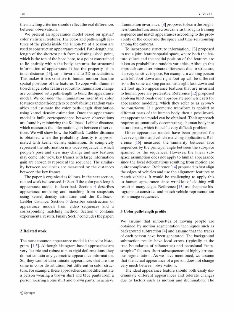
The first data set was collected by the Honeywell cor-poration. Two indoor cameras captured 30 appearances,each under different lighting conditions, from differentlocations and with people moving in different directionswith respect to the cameras. Figure 2a and b show exam-ple images of the 30 different appearances taken bythe two cameras. Although some appearances are actu-ally from the same person, they are clothed differentlyand are treated as different in our experiments. First, todemonstrate the effectiveness of the appearance modelbased on color path-length profile, we describe resultswhen snapshots are used for matching. The bandwidthsfor the different feature sets are shown in Table 1. Theywere determined by sampling a small training set andselecting the bandwidths which minimized the sum oftype I and II errors, the error of the same appearancetaken as different and the error of different appearancestaken as the same.

144 Y. Yu et al.

Fig. 2 Dataset 1: indoorimage sequences taken by twocameras collected by theHoneywell corporation

Table 1 Bandwidth selection of different features

Feature Bandwidth

RGB andpath-length hR = hG = hB = 3, σl = 0.02RGB rankand path-length hR = hG = hB = 3, σl = 0.02Brightness,colorand path-length σB = 50, σC = 1, σl = 0.01Normalized RGB hr = hg = 0.02, hb = 20

We first manually selected snapshots from the videosequences so that the appearances have similar poses in

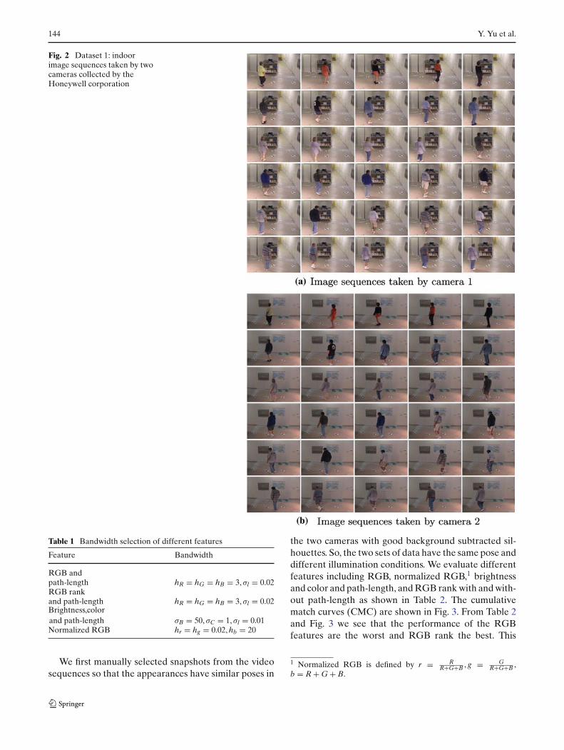
the two cameras with good background subtracted sil-houettes. So, the two sets of data have the same pose anddifferent illumination conditions. We evaluate differentfeatures including RGB, normalized RGB,1 brightnessand color and path-length, and RGB rank with and with-out path-length as shown in Table 2. The cumulativematch curves (CMC) are shown in Fig. 3. From Table 2and Fig. 3 we see that the performance of the RGBfeatures are the worst and RGB rank the best. This

1 Normalized RGB is defined by r = RR+G+B , g = G

R+G+B ,b = R + G + B.

Human appearance modeling for matching across video sequences 145

Table 2 Performances of different features when snapshots areused to build appearance models

Feature used Camera 1 Camera 2matches with matches withcamera 2 (%) camera 1 (%)

RGB andpath-length 13.33 23.33RGB rank andpath-length 86.67 100Brightness, colorand path-length 76.67 73.33Normalized RGBand path-length 20 40RGB rank only 66.67 63.33

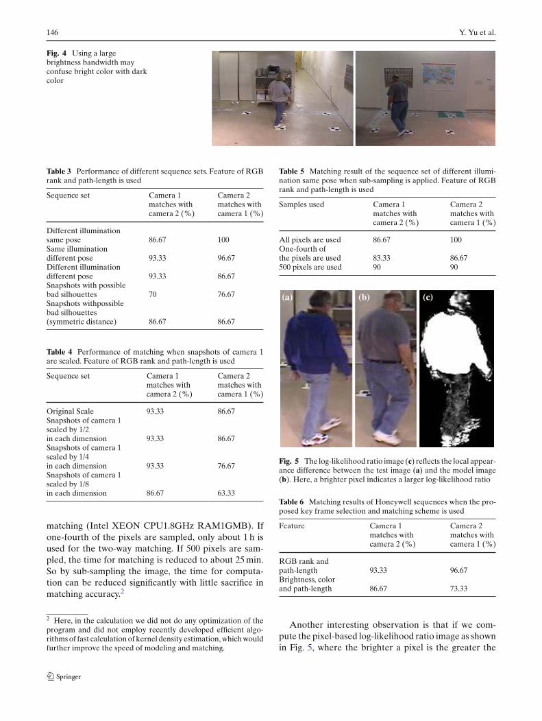
is because the sequences are taken indoors where theillumination varies significantly as people move relativeto an extended and proximal light source. This is alsoreflected in the optimal bandwidths for the brightnessand color features, which are determined to be σB =50, σC = 1. This means that the best classification per-formance used a large brightness bandwidth to ignorethe severe brightness changes between cameras. How-ever, large brightness bandwidths are problematic sincesometimes a bright color may be confused with a darkcolor. Figure 4 shows an example of mismatching whenbrightness, color and path-length features are used and abright color is confused with a dark color. As RGB ranktogether with path-length is the most invariant to illu-mination, in the following experiments we will usuallyonly show performance with the feature of RGB rankand path-length. Table 2 and Fig. 3 also show that if onlyRGB rank feature is used, the performance drops signifi-cantly compared with that with the path-length feature,illustrating the importance of path-length in discrimi-nating different appearances.

Next, we manually selected two snapshots of eachappearance from camera 1 so that the snapshots aretaken approximately at the same place but with different

poses. In this way, we have two sets of appearances thatare of the same illumination and different pose. Alsowe randomly picked snapshots from the sequences ofthe two cameras so that we have snapshots of differ-ent illumination and different pose. All the above snap-shots have good background subtraction results. Table 3shows the matching results of the three sets of snap-shots. From the results it is observed that when illumi-nation invariant color features are used, the influenceof pose on the matching result is marginal. This illus-trates the pose insensitivity of the path-length feature.In the above match, all the snapshots are selected man-ually with good background subtraction results. We alsoperform matching when the snapshots are randomlyselected from video sequences without knowing if thesilhouette is good or not. The matching results are alsoshown in Table 3. The matching rate drops to 70 and76.67% when the silhouettes of snapshots are not nec-essarily good. This is intended to serve as a baseline forthe experiments described in the next subsection, whichwill show that with our key frame selection and match-ing the effects of bad silhouettes can be significantlyreduced.

To study the performance when snapshots of differentsize are matched, we filtered the snapshots of camera 1and scaled each dimension to 1/2, 1/4, 1/8 of the originalsize, then matched them with the snapshots of camera2. Table 4 shows that only when the size is scaled to 1/8,does the matching rate drop significantly.

We also studied the influence of sampling as men-tioned in Sect. 4.2. Table 5 shows that when one-fourthof the pixels are used the performance slightly degrades.When only 500 pixels are selected, the performanceeven improves a little compared with using one-fourthof the pixels. This is partly because when fewer pixelsare sampled, the chance of selecting the noisy pixels dueto imperfect segmentation is reduced. When all pixelsare used, it takes about 2.5 h to conduct the two-way

Fig. 3 Cumulative matchcurves (CMC) of differentfeatures when snapshots ofthe two cameras are of similarpose

0 5 10 15 20 25 300.1

0.2

0.3

0.4

0.5

0.6

0.7

0.8

0.9

1

brightness color path−lengthnormalized RGB path−lengthRGB rank and path−lengthRGB rank onlyRGB and path−length

0 5 10 15 20 25 300.2

0.3

0.4

0.5

0.6

0.7

0.8

0.9

1

brightness color path−lengthnormalized RGB path−lengthRGB rank and path−lengthRGB rank onlyRGB and path−length

MC of different featureswhen camera 1 matches with camera 2

MC of different featureswhen camera 2 matches with camera 1

(a) (b)

146 Y. Yu et al.

Fig. 4 Using a largebrightness bandwidth mayconfuse bright color with darkcolor

Table 3 Performance of different sequence sets. Feature of RGBrank and path-length is used

Sequence set Camera 1 Camera 2matches with matches withcamera 2 (%) camera 1 (%)

Different illuminationsame pose 86.67 100Same illuminationdifferent pose 93.33 96.67Different illuminationdifferent pose 93.33 86.67Snapshots with possiblebad silhouettes 70 76.67Snapshots withpossiblebad silhouettes(symmetric distance) 86.67 86.67

Table 4 Performance of matching when snapshots of camera 1are scaled. Feature of RGB rank and path-length is used

Sequence set Camera 1 Camera 2matches with matches withcamera 2 (%) camera 1 (%)

Original Scale 93.33 86.67Snapshots of camera 1scaled by 1/2in each dimension 93.33 86.67Snapshots of camera 1scaled by 1/4in each dimension 93.33 76.67Snapshots of camera 1scaled by 1/8in each dimension 86.67 63.33

matching (Intel XEON CPU1.8GHz RAM1GMB). Ifone-fourth of the pixels are sampled, only about 1 h isused for the two-way matching. If 500 pixels are sam-pled, the time for matching is reduced to about 25 min.So by sub-sampling the image, the time for computa-tion can be reduced significantly with little sacrifice inmatching accuracy.2

2 Here, in the calculation we did not do any optimization of theprogram and did not employ recently developed efficient algo-rithms of fast calculation of kernel density estimation, which wouldfurther improve the speed of modeling and matching.

Table 5 Matching result of the sequence set of different illumi-nation same pose when sub-sampling is applied. Feature of RGBrank and path-length is used

Samples used Camera 1 Camera 2matches with matches withcamera 2 (%) camera 1 (%)

All pixels are used 86.67 100One-fourth ofthe pixels are used 83.33 86.67500 pixels are used 90 90

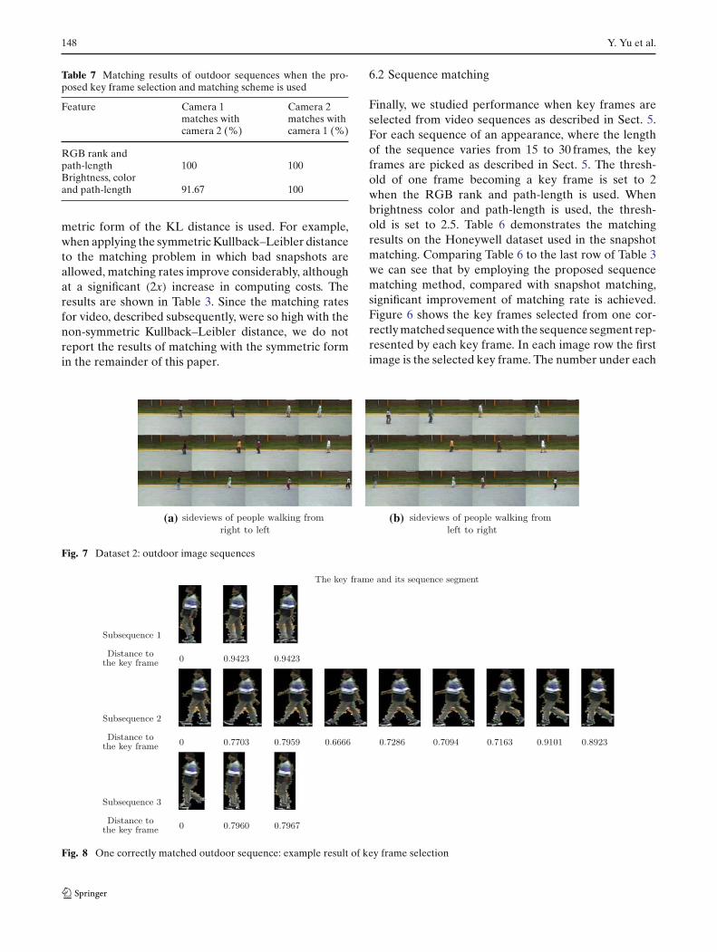
Fig. 5 The log-likelihood ratio image (c) reflects the local appear-ance difference between the test image (a) and the model image(b). Here, a brighter pixel indicates a larger log-likelihood ratio

Table 6 Matching results of Honeywell sequences when the pro-posed key frame selection and matching scheme is used

Feature Camera 1 Camera 2matches with matches withcamera 2 (%) camera 1 (%)

RGB rank andpath-length 93.33 96.67Brightness, colorand path-length 86.67 73.33

Another interesting observation is that if we com-pute the pixel-based log-likelihood ratio image as shownin Fig. 5, where the brighter a pixel is the greater the

Human appearance modeling for matching across video sequences 147

The key frame and its sequence segment

Subsequence 1

Distance tothe key frame 0 1.156693

Subsequence 2

Distance tothe key frame 0 1.022280 1.132054 1.345722 1.590653 1.432031 1.717502 1.743563 1.827377

Subsequence 3

Distance tothe key frame 0 1.050916 1.175069 1.942938 1.713872 1.914410

Subsequence 4

Distance tothe key frame 0 1.316717

Subsequence 5

Distance tothe key frame 0

Subsequence 6

Distance tothe key frame 0

Subsequence 7

Distance tothe key frame 0 0.980267 1.350398 1.445136 1.454350 1.855563 1.985814 1.989596

Subsequence 8

Distance tothe key frame 0

Fig. 6 One correctly matched indoor sequence: example result of key frame selection

log-likelihood ratio, we can observe that the image reflectsappearance differences. In Fig. 5 the two people weardifferent jackets but similar blue jeans, so the log-like-lihood ratio in the upper part of the body is very large,but very small in the lower part of the body. So, by ana-

lyzing the log-likelihood ratio image, we can detect localappearance differences.

We also studied performance of the symmetric formof Kullback–Leibler distance. Better matching resultsfor the snapshot matching can be obtained if the sym-

148 Y. Yu et al.

Table 7 Matching results of outdoor sequences when the pro-posed key frame selection and matching scheme is used

Feature Camera 1 Camera 2matches with matches withcamera 2 (%) camera 1 (%)

RGB rank andpath-length 100 100Brightness, colorand path-length 91.67 100

metric form of the KL distance is used. For example,when applying the symmetric Kullback–Leibler distanceto the matching problem in which bad snapshots areallowed, matching rates improve considerably, althoughat a significant (2x) increase in computing costs. Theresults are shown in Table 3. Since the matching ratesfor video, described subsequently, were so high with thenon-symmetric Kullback–Leibler distance, we do notreport the results of matching with the symmetric formin the remainder of this paper.

6.2 Sequence matching

Finally, we studied performance when key frames areselected from video sequences as described in Sect. 5.For each sequence of an appearance, where the lengthof the sequence varies from 15 to 30 frames, the keyframes are picked as described in Sect. 5. The thresh-old of one frame becoming a key frame is set to 2when the RGB rank and path-length is used. Whenbrightness color and path-length is used, the thresh-old is set to 2.5. Table 6 demonstrates the matchingresults on the Honeywell dataset used in the snapshotmatching. Comparing Table 6 to the last row of Table 3we can see that by employing the proposed sequencematching method, compared with snapshot matching,significant improvement of matching rate is achieved.Figure 6 shows the key frames selected from one cor-rectly matched sequence with the sequence segment rep-resented by each key frame. In each image row the firstimage is the selected key frame. The number under each

ideviews of people walking fromright to left

ideviews of people walking fromleft to right

(a) (b)

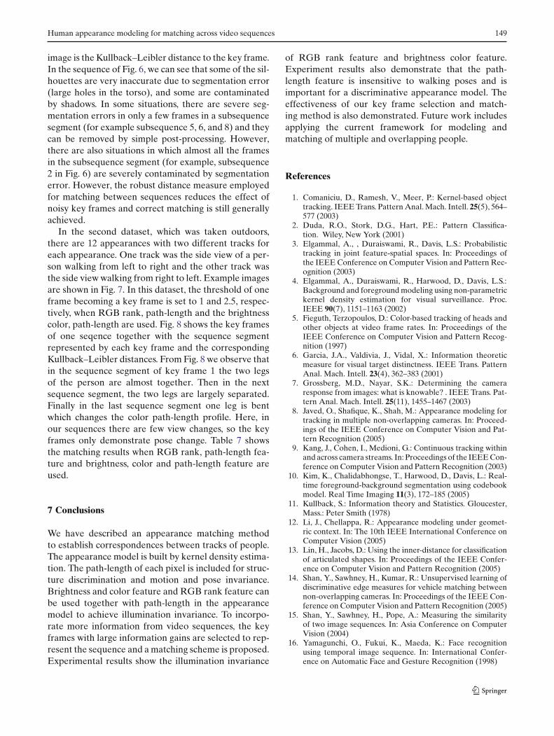
Fig. 7 Dataset 2: outdoor image sequences

The key frame and its sequence segment

Subsequence 1

Distance tothe key frame 0 0.9423 0.9423

Subsequence 2

Distance tothe key frame 0 0.7703 0.7959 0.6666 0.7286 0.7094 0.7163 0.9101 0.8923

Subsequence 3

Distance tothe key frame 0 0.7960 0.7967

Fig. 8 One correctly matched outdoor sequence: example result of key frame selection

Human appearance modeling for matching across video sequences 149

image is the Kullback–Leibler distance to the key frame.In the sequence of Fig. 6, we can see that some of the sil-houettes are very inaccurate due to segmentation error(large holes in the torso), and some are contaminatedby shadows. In some situations, there are severe seg-mentation errors in only a few frames in a subsequencesegment (for example subsequence 5, 6, and 8) and theycan be removed by simple post-processing. However,there are also situations in which almost all the framesin the subsequence segment (for example, subsequence2 in Fig. 6) are severely contaminated by segmentationerror. However, the robust distance measure employedfor matching between sequences reduces the effect ofnoisy key frames and correct matching is still generallyachieved.

In the second dataset, which was taken outdoors,there are 12 appearances with two different tracks foreach appearance. One track was the side view of a per-son walking from left to right and the other track wasthe side view walking from right to left. Example imagesare shown in Fig. 7. In this dataset, the threshold of oneframe becoming a key frame is set to 1 and 2.5, respec-tively, when RGB rank, path-length and the brightnesscolor, path-length are used. Fig. 8 shows the key framesof one seqence together with the sequence segmentrepresented by each key frame and the correspondingKullback–Leibler distances. From Fig. 8 we observe thatin the sequence segment of key frame 1 the two legsof the person are almost together. Then in the nextsequence segment, the two legs are largely separated.Finally in the last sequence segment one leg is bentwhich changes the color path-length profile. Here, inour sequences there are few view changes, so the keyframes only demonstrate pose change. Table 7 showsthe matching results when RGB rank, path-length fea-ture and brightness, color and path-length feature areused.

7 Conclusions

We have described an appearance matching methodto establish correspondences between tracks of people.The appearance model is built by kernel density estima-tion. The path-length of each pixel is included for struc-ture discrimination and motion and pose invariance.Brightness and color feature and RGB rank feature canbe used together with path-length in the appearancemodel to achieve illumination invariance. To incorpo-rate more information from video sequences, the keyframes with large information gains are selected to rep-resent the sequence and a matching scheme is proposed.Experimental results show the illumination invariance

of RGB rank feature and brightness color feature.Experiment results also demonstrate that the path-length feature is insensitive to walking poses and isimportant for a discriminative appearance model. Theeffectiveness of our key frame selection and match-ing method is also demonstrated. Future work includesapplying the current framework for modeling andmatching of multiple and overlapping people.

References

1. Comaniciu, D., Ramesh, V., Meer, P.: Kernel-based objecttracking. IEEE Trans. Pattern Anal. Mach. Intell. 25(5), 564–577 (2003)

2. Duda, R.O., Stork, D.G., Hart, P.E.: Pattern Classifica-tion. Wiley, New York (2001)

3. Elgammal, A., , Duraiswami, R., Davis, L.S.: Probabilistictracking in joint feature-spatial spaces. In: Proceedings ofthe IEEE Conference on Computer Vision and Pattern Rec-ognition (2003)

4. Elgammal, A., Duraiswami, R., Harwood, D., Davis, L.S.:Background and foreground modeling using non-parametrickernel density estimation for visual surveillance. Proc.IEEE 90(7), 1151–1163 (2002)

5. Fieguth, Terzopoulos, D.: Color-based tracking of heads andother objects at video frame rates. In: Proceedings of theIEEE Conference on Computer Vision and Pattern Recog-nition (1997)

6. Garcia, J.A., Valdivia, J., Vidal, X.: Information theoreticmeasure for visual target distinctness. IEEE Trans. PatternAnal. Mach. Intell. 23(4), 362–383 (2001)

7. Grossberg, M.D., Nayar, S.K.: Determining the cameraresponse from images: what is knowable? . IEEE Trans. Pat-tern Anal. Mach. Intell. 25(11), 1455–1467 (2003)

8. Javed, O., Shafique, K., Shah, M.: Appearance modeling fortracking in multiple non-overlapping cameras. In: Proceed-ings of the IEEE Conference on Computer Vision and Pat-tern Recognition (2005)

9. Kang, J., Cohen, I., Medioni, G.: Continuous tracking withinand across camera streams. In: Proceedings of the IEEE Con-ference on Computer Vision and Pattern Recognition (2003)

10. Kim, K., Chalidabhongse, T., Harwood, D., Davis, L.: Real-time foreground-background segmentation using codebookmodel. Real Time Imaging 11(3), 172–185 (2005)

11. Kullback, S.: Information theory and Statistics. Gloucester,Mass.: Peter Smith (1978)

12. Li, J., Chellappa, R.: Appearance modeling under geomet-ric context. In: The 10th IEEE International Conference onComputer Vision (2005)

13. Lin, H., Jacobs, D.: Using the inner-distance for classificationof articulated shapes. In: Proceedings of the IEEE Confer-ence on Computer Vision and Pattern Recognition (2005)

14. Shan, Y., Sawhney, H., Kumar, R.: Unsupervised learning ofdiscriminative edge measures for vehicle matching betweennon-overlapping cameras. In: Proceedings of the IEEE Con-ference on Computer Vision and Pattern Recognition (2005)

15. Shan, Y., Sawhney, H., Pope, A.: Measuring the similarityof two image sequences. In: Asia Conference on ComputerVision (2004)

16. Yamagunchi, O., Fukui, K., Maeda, K.: Face recognitionusing temporal image sequence. In: International Confer-ence on Automatic Face and Gesture Recognition (1998)