How to win at “Who wants to be a millionaire ... - Chance

How to win at “Who wants to be a millionaire?”

Robert C. Dalang1 and Violetta Bernyk2

Abstract

We propose a mathematical model for the TV game show “Who wants tobe a millionaire?” Using methods from probability theory and stochastic opti-mization, we compute the optimal strategy for a player who wishes to maximizehis expected payoff. The mathematical model contains some surprising intrica-cies, but it provides, in addition to the optimal strategy, quantitative answersto questions such as “how much can the player expect to win,” and “what arehis chances of actually winning a million dollars” at this game. The optimalstrategy is presented in a largely self-contained appendix and can easily be usedeven by non-mathematicians.

Copyright c© 2003 by R.C. Dalang and V. Bernyk

1Institut de Mathematiques, Ecole Polytechnique Federale, 1015 Lausanne, Switzerland. Email:[email protected] The research of this author is partially supported by the Swiss National Foun-dation for Scientific Research.

2Institut de Mathematiques, Ecole Polytechnique Federale, 1015 Lausanne, Switzerland. Email:[email protected]

R.C. Dalang and V. Bernyk 2

1 Introduction

The TV game show “Who wants to be a millionaire?” is shown in many countries.The objective of this paper is to provide a mathematical model for this game, andwithin this model, to compute the optimal strategy for the player. The techniquesare based on probability theory and stochastic optimization, and illustrate many ofthe issues that arise during mathematical modelling of a “real-world” phenomenon oractivity. The concepts from probability theory mainly rely on topics generally devel-oped in a first course in probability, such as a one semester course from [8], thoughsome context would be provided by better familiarity with Markov chains, such ascan be obtained from a one semester course based for instance on [4]. The issues ofstochastic optimization are treated informally but with care. While we develop themodel in detail, explaining the choices we have made and their justification, the opti-mal strategy that we provide in Section 9 can be used by any player, without studyingthe model itself. We conclude with a discussion of the strengths and weaknesses ofour model, and some possibilities for extensions.

Rules of the game

The rules of the game are as follows. A player is successively confronted with up tofifteen questions, and the goal of the game is to correctly answer all the questions andto win a million dollars (or units of local currency). Question number n has a facevalue fn, n = 1, . . . , 15, shown in Table 1 for the USA version of the game. For eachquestion, four possible answers a, b, c and d are proposed to the player. After seeingquestion n and the four possible answers, the player may choose to answer, to useone of three “lifelines” (described below) or to quit without replying and to receivethe payoff fn−1 (f0 is set to 0). There is no time limit for answering, and players areencouraged to share their thoughts on the correct answer with the audience.

If the player answers correctly, he moves to question n + 1. If the player answersincorrectly, the game is over and the player receives the amount wn, also shown inTable 1. The values of wn increase strictly at n = 5 and n = 10, which are called“milestones.” If the player is not sure of the correct answer, he may use one of thethree lifelines. He may use more than one lifeline for the same question, but eachlifeline can be used only once during the entire game.

The three lifelines

One lifeline is titled “50:50.” When the player asks to use this lifeline, a computereliminates two incorrect answers, so the player only has to select the correct answerfrom the two remaining answers.

A second lifeline is titled “Phone-a-friend.” When the player asks to use thislifeline, the host telephones a friend selected by the player, and the player has 30seconds to communicate the question, the four answers, and to obtain the reply from


Question Face value Payoff wn forn fn an incorrect answer1 100 02 200 03 300 04 500 05 1000 06 2000 10007 4000 10008 8000 10009 16000 100010 32000 100011 64000 3200012 125000 3200013 250000 3200014 500000 3200015 1000000 32000

Table 1: The face values and the payoffs for an incorrect answer (USA version).

his friend. He is then free to use the information supplied by the friend as he sees fit.The third lifeline is titled “Ask-the-audience.” When the player asks to use this

lifeline, the host asks all members of the audience to enter their answer into thecomputer. The computer tabulates the audience’s answers in a histogram, whichindicates the proportion of the audience that thinks that each of the four answersis correct. This histogram is shown to the player, and the player is free to use thisinformation as he sees fit.

The motivation for a mathematical model

The game just described combines randomness, embodied by the fact that theplayer is more or less likely to know the answers to the various questions, with de-cisions that he must make, such as use a particular lifeline, take the risk of replyingeven if he is not certain of the answer, or decide to quit the game.

There is a well-developped theory that addresses the issue of helping the playermake the right decisions, expounded in books such as [1], [2], [5] and [7]. This theoryis rather technical, and the reader who consults any of these references will find thatbefore any theory can be applied, a mathematical model for the game is needed.Unfortunately, most of the literature begins by assuming that such a model is given!

Therefore, the first step is to create a mathematical model for the game, withthe objective of helping the player make the various decisions that are part of the


game. No model can change the player’s knowledge of the answers to the questions,or influence the questions proposed to the player. But when the player hesitatesbetween answering and quitting, or between using one lifeline rather than another,the model and the strategy computed within the model will tell him which decisionis best.

Structure of this paper

In Section 2, we describe briefly the basic requirements of a mathematical model,and we set up the main ingredients and notation. We describe how we represent theplayer’s possible states of knowledge concerning the answers to the fifteen questions,we give an explicit description of the possible stages in the game, and we set up thebasic Markovian framework that describes the player’s progression in the game.

In Section 3, we explain the stochastic optimization technique that is used tocompute the optimal strategy. This general technique can only be applied after thevarious parameters of the model have been selected, which we proceed to do in thenext sections. In Section 4, we explain our choices for setting up the transitionprobabilities for a player who does not make use of the lifelines. In Section 5, weanalyse each of the lifelines in turn.

In Section 6, we turn our attention to the issue of the player’s risk tolerance: weuse utility functions to model the relative value the player attributes to an uncertainreward, versus a reward that he will receive with certainty.

In Section 7, we present and discuss the optimal strategy produced by our model.This strategy is summarized in self-contained manner accessible to non-mathematiciansin the Appendix (Section 9), and can be used without reference to the mathematicalmodel: the reader who is only interested in applying the strategy can go directly tothis appendix.

In Section 8, we conclude with various comments on our model and the optimalstrategy that it produces.

2 Setting up the model

We begin by specifying some key requirements of any mathematical model.

Requirements of a mathematical model

A model is a simplification of reality, which should however capture the mainfeatures of the game. The assumptions of the model should as far as possible comefrom the description of the game, and from observations of how the game is played.The model should be easy to use. The effort required to compute the optimal strategyshould be reasonable, and the optimal strategy that it produces should reflect reality,in the sense that in many cases, it should correspond to what an intelligent player


might want to do or would at least be comfortable doing. And it should provideguidance to the player in situations where he does not know what to do.

We shall see that many of these requirements can be respected. However, as wewill comment on in Section 8, there are several elements of information regarding thegame that are not available to us and that might lead us to modify the model if theywere. With these ideas in mind, we proceed to construct our model.

The player’s states of knowledge

We let n denote the number of the question that the player is contemplating,n = 1, . . . , 15, and n = 16 after the player has correctly answered all fifteen questions(a rather rare occurence, as we will see in Section 7).

The central unknowns in the game are the likelihoods that the player will be ableto answer question n, for each n. Since there are no time limits, the player generallychats a bit with the host, and indicates either that he knows the answer, or has noidea of the answer, or has some idea of the answer. It is standard to model sucha situation by representing the player’s degree or state of knowledge concerning theanswer as a prior probability vector π = (πa, πb, πc, πd), where the four componentsare non-negative and sum to one, and πa represents the probability that the playerassigns to the event “the correct answer is a,” with the analogous interpretation foreach of the other three components of π.

Of course, this would mean that there are an infinite number of possible statesof knowledge, which is not convenient for a computer implementation. In addition,most players will be able to say that they know the answer, or are confident, but notcertain, that they know the answer, or that they are hesitating between two answers,but they will not state their prior probabilities to the third decimal place! In fact,we have decided to limit ourselves to five basic states of knowledge, which are thefollowing.

State 0: the player definitely knows the answer (zero uncertainty).

State 1: the player is quite confident, but not certain, that he knows the correctanswer.

State 2: the player mainly hesitates between 2 answers, the other two are un-likely possibilities.

State 3: Two answers were just eliminated by the computer by using the 50:50lifeline, but the player still hesitates between the two remaining answers.

State 4: the player has no idea of the correct answer (he hesitates between all4 answers).

In terms of prior probability vectors, we shall associate to state k, k = 0, . . . , 4, apermutation of the probability vectors indicated in Table 2.


k Probability vector

0 (1, 0, 0, 0)

1(

45, 1

15, 1

15, 1

15

)2

(25, 2

5, 1

10, 1

10

)3

(12, 1

2, 0, 0

)4

(14, 1

4, 1

4, 1

4

)Table 2: For each state k of knowledge, the player’s prior probabilities are a permu-tation of those that are shown.

When the player gives an incorrect answer, he does not move to the next questionbut he has lost. Since his payoff is different depending on how many of the milestoneshe has passed, we shall need three “lost” states, which we denote L1, L2 and L3. Theplayer moves to state L1 if he gives an incorrect answer to one of questions 1 through5, he moves to state L2 if he gives an incorrect answer to one of questions 6 through10, and he moves to state L3 if he gives an incorrect answer to one of questions11 through 15. We consider that once state Lm, m = 1, 2, 3 has been reached, theplayer remains in that state while the computer runs through the remaining questions(though in reality without showing them to the player or the audience).

Finally, we let W be the state reached by the (fortunate) player who has correctlyanswered all fifteen questions.

We shall denote Kn the set of possible states of the player after answering n − 1questions. These are

K1 = {0, . . . , 4},Kn = {0, . . . , 4} ∪ {L1}, n = 2, . . . , 6,Kn = {0, . . . , 4} ∪ {L1, L2}, n = 7, . . . , 11,Kn = {0, . . . , 4} ∪ {L1, L2, L3}, n = 12, . . . , 15,K16 = {W, L1, L2, L3}.

We note that if the player gives an incorrect answer to question n, then he moves tostate (n + 1, Lm), with m = 1 if 1 ≤ n ≤ 5, m = 2 if 6 ≤ n ≤ 10, and m = 3 if11 ≤ n ≤ 15.

Stages in the game

In order to describe the progression of the player in the game, it is necessaryto keep track, not only of the number of the question that the player is currentlycontemplating, but also of the lifelines that remain available. Since each lifelinecan be used only once, there are eight possible configurations for the availablility of


lifelines, from “all three are available”, to “no more lifelines are available”. To keeptrack of this, let Lifeline 1 be the 50:50 lifeline; Lifeline 2 be the “Phone-a-friend”lifeline; and Lifeline 3 be the “Ask-the-audience” lifeline.

We set S = {0, 1}3, and for s = (s1, s2, s3) ∈ S, sm will denote the number oftimes lifeline m has been used, m = 1, 2, 3. The three lifelines are symbolized by `1,`2 and `3, where

`1 = (1, 0, 0), `2 = (0, 1, 0), `3 = (0, 0, 1).

Each element s ∈ S represents therefore the lifelines still available to the player: forinstance, s = (0, 0, 0) if all three lifelines are still available, s = (1, 1, 0) if only Lifeline3 is still available.

For s = (s1, s2, s3) and t = (t1, t2, t3) in S, define

s ∨ t = (max(s1, t1), max(s2, t2), max(s3, t3)), s− t = (s1 − t1, s2 − t2, s3 − t3),

and set D(s) = {s ∨ `1, s ∨ `2, s ∨ `3} \ {s}: this set has cardinality 0, 1, 2 or 3. Forinstance, it has cardinality 3 if s = (0, 0, 0) and cardinality 0 if s = (1, 1, 1).

For σ ∈ D(s), σ− s ∈ {`1, `2, `3} represents the lifeline that was used to pass froms to σ. For s 6= (1, 1, 1), the set D(s) represents the possible situations of lifelinesafter using one of the lifelines that are still available.

At any stage in the game, the progression of the player in the game is fully describedby the couple (n, s) ∈ {1, . . . , 16} × S. These are the stages in the game.

At the stage (n, s), the status of the player, with regard to his degree of knowledgeof the question he is currently contemplating, or whether he has given an incorrectanswer, is a random variable Xn,s with values in Kn. The event {Xn,s = k} occurs ifthe player’s state of knowledge concerning question n is k, and {Xn,s = Lm} occurs ifthe player previously gave an incorrect answer. The randomness arises from the factthat before question n is displayed, we do not know what the player’s status will beat that or future stages of the game.

Markovian nature of the game

At a given stage (n, s) in the game, once we know the status Xn,s, the previousstatuses, such as the degree of knowledge to previous questions, and for which previousquestion a particular (no longer available) lifeline was used, are no longer relevant:our decision on how to proceed at this stage will be based only on the value of Xn,s.

At a stage (n, s), the player can either choose to answer, in which case he moves toa new stage (n + 1, s), with a new status Xn+1,s, or he can choose to use a lifeline, inwhich case he moves to a new stage (n, σ), with σ ∈ D(s), and a new status Xn,σ. Thelifeline he just used was σ − s. The key elements in the description of the evolutionof the player’s status are the transition probabilites

pn(j, k) = P{Xn+1,s = k | Xn,s = j}, j ∈ Kn, k ∈ Kn+1,


and, for s ∈ S such that s ∨ `m ∈ D(s),

pn,`m(j, k) = P{Xn,s∨`m = k | Xn,s = j}, j, k ∈ Kn.

We assume in Section 3 that we know these transition probabilities. In Sections 4and 5, we shall explain how we determine them.

3 Optimization

For n = 1, . . . , 16, s ∈ S and k ∈ Kn, the payoff to the player if he quits the game atstage (n, s) does not depend on s, so we denote it f(n, k). Clearly, f(n, k) = fn−1, k =0, . . . , 4, since this is the payoff if the player is contemplating question n but choosesto quit the game without answering the question. For n = 2, . . . , 16, f(n, L1) = w1,for n = 7, . . . , 16, f(n, L2) = w6, and for n = 12, . . . , 16, f(n, L3) = w11, where w1,w6 and w11 are as in Table 1. Finally, f(16, W ) = f15 = 1000000.

Most players probably do not come to the game thinking that they will win onemillion dollars. However, most would like to win as much as possible, and a mathe-matical interpretation is that they seek to maximize their expected payoff. We shallbe slightly more general than this: for a given function u : RI + → RI , which we inter-pret as a utility function (see Section 6), we let g(n, k) = u(f(n, k)), and we postulatethat the player’s objective is to maximize the expected utility of his payoff, that is,the expected value of g(n, k). For the time being, the reader may simply think of thecase u(x) = x, so that g ≡ f .

For n = 1, . . . , 16, s ∈ S and k ∈ Kn, let u∗(n, s, k) be the expected utility ofa player currently at stage (n, s) and in status k, who proceeds optimally from thisstage on.

It is intuitively clear that u∗(·, ·, ·) should satisfy the equation

u∗(n, s, j) = max

(g(n, j), C(n, s, j), max

σ∈D(s)L(n, s, σ, j)

), (1)

where

C(n, s, j) =∑

k∈Kn+1

pn(j, k)u∗(n + 1, s, k), L(n, s, σ, j) =4∑

k=0

pn,σ−s(j, k)u∗(n, σ, k).

Indeed, either it is optimal to quit without answering, and the utility of the payoff isg(n, j), or it is optimal to answer without using any lifeline, and the expected futurepayoff is C(n, s, j), or it is optimal to use one of the available lifelines, say σ − s,and the expected future payoff is L(n, s, σ, j), which achieves the maximum in thethird quantity on the right-hand side of (1) (note that if s = (1, 1, 1), then D(s) = ∅and this third quantity is omitted from the equation). A rigorous justification of this


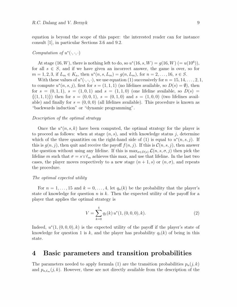
equation is beyond the scope of this paper: the interested reader can for instanceconsult [1], in particular Sections 3.6 and 9.2.

Computation of u∗(·, ·, ·)

At stage (16, W ), there is nothing left to do, so u∗(16, s, W ) = g(16, W ) (= u(106)),for all s ∈ S, and if we have given an incorrect answer, the game is over, so form = 1, 2, 3, if Lm ∈ Kn, then u∗(n, s, Lm) = g(n, Lm), for n = 2, . . . , 16, s ∈ S.

With these values of u∗(·, ·, ·), we use equation (1) successively for n = 15, 14, . . . , 2, 1,to compute u∗(n, s, j), first for s = (1, 1, 1) (no lifelines available, so D(s) = ∅), thenfor s = (0, 1, 1), s = (1, 0, 1) and s = (1, 1, 0) (one lifeline available, so D(s) ={(1, 1, 1)}) then for s = (0, 0, 1), s = (0, 1, 0) and s = (1, 0, 0) (two lifelines avail-able) and finally for s = (0, 0, 0) (all lifelines available). This procedure is known as“backwards induction” or “dynamic programming”.

Description of the optimal strategy

Once the u∗(n, s, k) have been computed, the optimal strategy for the player isto proceed as follows: when at stage (n, s), and with knowledge status j, determinewhich of the three quantities on the right-hand side of (1) is equal to u∗(n, s, j). Ifthis is g(n, j), then quit and receive the payoff f(n, j). If this is C(n, s, j), then answerthe question without using any lifeline. If this is maxσ∈D(s) L(n, s, σ, j) then pick thelifeline m such that σ = s∨`m achieves this max, and use that lifeline. In the last twocases, the player moves respectively to a new stage (n + 1, s) or (n, σ), and repeatsthe procedure.

The optimal expected utility

For n = 1, . . . , 15 and k = 0, . . . , 4, let qn(k) be the probability that the player’sstate of knowledge for question n is k. Then the expected utility of the payoff for aplayer that applies the optimal strategy is

V =4∑

k=0

q1(k) u∗(1, (0, 0, 0), k). (2)

Indeed, u∗(1, (0, 0, 0), k) is the expected utility of the payoff if the player’s state ofknowledge for question 1 is k, and the player has probability q1(k) of being in thisstate.

4 Basic parameters and transition probabilities

The parameters needed to apply formula (1) are the transition probabilities pn(j, k)and pn,`m(j, k). However, these are not directly available from the description of the


game, and will have to be determined from more basic quantities.The first set of parameters are the qn(k), which describe the likelihood that the

player will have a particular degree of knowledge for each question. These parametersshould reflect the fact that the questions become more and more difficult. Since thereare milestones after questions 5 and 10, it is natural to divide the fifteen questionsinto three groups and to set, for k ∈ {0, . . . , 4},

qn(k) =

ρ1(k), if 1 ≤ n ≤ 5,ρ2(k), if 6 ≤ n ≤ 10,ρ3(k), if 11 ≤ n ≤ 15.

A reasonable numerical choice for the ρm(k) is shown in Table 3. For n = 1, . . . , 5, wehave for instance assumed that the player definitely knows the answer with probability0.5, while for n = 11, . . . , 15, this probability is only 0.2. Since state k = 3 can onlybe reached by using the 50:50 lifeline, we have set ρm(3) = 0, m = 1, 2, 3. We havepreferred to let some of the probabilities be very small, i.e. 0.05, rather than set themto 0.

k = 0 k = 1 k = 2 k = 3 k = 4ρ1(k) 0.5 0.4 0.05 0 0.05ρ2(k) 0.2 0.3 0.2 0 0.3ρ3(k) 0.2 0.2 0.1 0 0.5

Table 3: Our choice for the probabilities that the player’s state of knowledge for aquestion is k, for the three groups of questions.

Likelihood of giving a correct answer when in a given state

Let rk be the probability that the player’s answer is correct if his state of knowledgeregarding the correct answer is k. According to our choice of states, r0, . . . , r4 shouldbe as shown in Table 4.

k = 0 k = 1 k = 2 k = 3 k = 4

rk 1 45

25

12

14

Table 4: The probability that the player gives the correct answer if his state ofknowledge is k.

Transition probabilities when no lifeline is used

The transition probabilites pn(j, k) can be easily expressed from the qn(k) and rk.Indeed, when in state j at stage (n, s), the player will be in state k at stage (n+ 1, s)


(no lifeline is used) if and only if the player’s answer to question n is correct and hisstate of knowledge regarding question n + 1 is k. We assume that giving a correctanswer to question n is independent of the player’s state of knowledge for questionn + 1, so for j ∈ {0, . . . , 4},

pn(j, k) = rj qn+1(k), k ∈ {0, . . . , 4}, 1 ≤ n ≤ 14,

pn(j, Lm) =

{1− rj if (n, m) ∈ Λ,0 otherwise,

p15(j, W ) = rj,

where Λ = ({1, . . . , 5} × {1}) ∪ ({6, . . . , 10} × {2}) ∪ ({11, . . . , 15} × {3}). Notethat if the player gives an incorrect answer when at stage (n, s), then he moves tostate Lm ∈ Kn+1 at stage (n + 1, s), where (n, m) ∈ Λ. For completeness, we setpn(Lm, Lm) = 1 if Lm ∈ Kn, n = 2, . . . , 15. The three different numerical values ofthe matrix (pn(j, k), j = 0, . . . , 4, k = 0, . . . , 4) are shown in Table 5.

n = 1, . . . , 4 : n = 5, . . . , 9 : n = 10, . . . , 14 :

12

25

120

0 120

25

825

125

0 125

15

425

150

0 150

14

15

140

0 140

18

110

180

0 180

15

310

15

0 310

425

625

425

0 625

225

325

225

0 325

110

320

110

0 320

120

340

120

0 340

15

15

110

0 12

425

425

225

0 25

225

225

125

0 15

110

110

120

0 14

120

120

140

0 18

Table 5: The numerical values of the matrix (pn(j, k), j = 0, . . . , 4, k = 0, . . . , 4) forthe three groups of questions. Notice that row j of each matrix sums to rj, since wehave not shown columns (or rows) that correspond to the states Lm.

5 Modelling the lifelines

We now turn to the transition probabilites pn,`m(j, k). Each lifeline has its ownspecificities. We begin with the 50:50 lifeline.

5.1 The 50:50 lifeline

If the player is in state 4, then the 50:50 lifeline eliminates two incorrect answers,and we see no reason to assume that this makes it easier to choose between the two


remaining answers. Therefore the player’s new state of knowledge is k = 3, and weset pn,`1(4, 3) = 1, and pn,`1(4, k) = 0, k 6= 3.

Player in state 3

When the player is in state 3, it means that he has just used the 50:50 lifeline, andcannot use it again. However, it does not affect the conclusions of our model if, forsimplicity, we set pn,`1(3, 3) = 1 and pn,`1(3, k) = 0 for k 6= 3.

Player in state 2

If the player is in state 2, assume that the player has assigned probabilities 25, 2

5,

110

, 110

to the events “a, respectively b, c, d, is the correct answer.” The computer willeliminate two incorrect answers. If we knew the correct answer, then any two otheranswers would have equal probability 1

3of being eliminated. For two answers such as

a and b, let Ea,b be the event “the computer eliminates answers a and b,” and let Ca

be the event “the correct answer is a.”If a and b are eliminated, which occurs with probability

P (Ea,b) = P (Ea,b | Cc) P (Cc) + P (Ea,b | Cd) P (Cd) =1

3· 1

10+

1

3· 1

10=

1

15,

then we consider that the player moves to state 3, hesitating now between c and d.If c and d are eliminated, which occurs with probability

P (Ec,d) = P (Ec,d | Ca) P (Ca) + P (Ec,d | Cb) P (Cb) =1

3· 2

5+

1

3· 2

5=

4

15,

then the player moves to state 3 (still hesitating between a and b). If one of {a, b}and one of {c, d} are eliminated, which occurs with probability 4P (Eb,d), where

P (Eb,d) = P (Eb,d | Ca) P (Ca) + P (Eb,d | Cc) P (Cc) =1

3· 2

5+

1

3· 1

10=

1

6,

then we consider that the player moves to state 1. Indeed, by Bayes’ formula,

P (Ca | Eb,d) =P (Eb,d | Ca) · P (Ca)

P (Eb,d)=

13· 2

516

=4

5,

which is best represented by state 1. Therefore,

pn,`1(2, 3) =1

15+

4

15=

1

3, pn,`1(2, 1) = 4 · 1

6=

2

3.

Player in state 1


If the player is in state 1, assume that the player has assigned probability 45

toanswer a and 1

15to each of answers b, c and d. As above, if we knew the correct answer,

then any two other answers would have equal probability 13

of being eliminated.Answer a is retained if two among b, c and d are eliminated. The probability that

any given one of these three pairs is eliminated is

P (Eb,c) = P (Eb,c | Ca) P (Ca) + P (Eb,c | Cd) P (Cd) =1

3· 4

5+

1

3· 1

15=

13

45.

Therefore, the probability that a is retained is 3 · 1345

= 1315

. Notice that

P (Ca | Eb,c) =P (Eb,c | Ca) · P (Ca)

P (Eb,c)=

13· 4

51345

=12

13' 0.92,

which is substantially higher than the probability 25

= 0.8 assigned to state 1. Wetherefore consider that the player’s new state of knowledge can be 0 or 1, with re-spective probabilities 6

15and 7

15. If a is eliminated, which occurs with probability

1− 1315

= 215

, then we assume that the player’s new state of knowledge is 3. Therefore,

pn,`1(1, 0) =6

15, pn,`1(1, 1) =

7

15and pn,`1(1, 3) =

2

15.

The transition probabilites associated with the 50:50 lifeline are summarized in Table6. Notice that they do not depend on n.

k = 0 k = 1 k = 2 k = 3 k = 4

pn,`1(0, k) 1 0 0 0 0

pn,`1(1, k) 615

715

0 215

0

pn,`1(2, k) 0 23

0 13

0

pn,`1(3, k) 0 0 0 1 0

pn,`1(4, k) 0 0 0 1 0

Table 6: Transition probabilites from each state of knowledge to state k when the50:50 lifeline is used.

5.2 The lifeline “Phone-a-friend”

Modelling this lifeline is more complex than the 50:50 lifeline, since there are twoclearly distinct issues: the friend’s state of knowledge of the answer, and how hisstate of knowledge influences our own state of knowledge. We address these twoissues in turn.


First of all, we assume that the possible states of knowledge for the friend arethe same as for the player. Let Fn(k) be the probability that the friend’s state ofknowledge for question n is k. On the one hand, we can assume that the friend hasbeen chosen because he is knowledgeable, and so we could consider that he is morelikely to know the correct answer than the player. On the other hand, only 30 secondsare allowed for the player to communicate the question and the four possible answers,and for the friend to reply. Rather often, the communication problem is significant.In the end, we have chosen simply to set Fn(k) = qn(k), that is, friend and playerhave the same probabilites of being in each state.

Consider now the issue of how the friend’s state of knowledge affects our own stateof knowledge. Let I(j, i, k) denote the probability, given that the player’s state ofknowledge is j and the friend’s state of knowledge is i, that after using the lifeline“Phone-a-Friend”, the player’s new state of knowledge is k. Clearly, the player’s newstate of knowlege could just as well be the friend’s new state of knowledge, so weshould have I(j, i, k) = I(i, j, k), and therefore we only consider the case j ≥ i.

If the player’s state of knowledge is j = 4, and the friend’s state of knowledgeis i, then the player’s new state k of knowledge is certainly k = i, so I(4, i, i) = 1,i = 0, . . . , 4.

Player in state 3

If the player’s state of knowledge is j = 3, meaning he has just used the 50:50lifeline, and the friend’s state of knowledge is also i = 3, then the player remains instate 3, so I(3, 3, 3) = 1 and I(3, 3, k) = 0 for k 6= 3. If the friend’s state of knowledgeis i = 2, then we assume that the interaction between friend and computer is thesame as between player and computer when the 50:50 lifeline was used, so we useTable 6 to set I(3, 2, 1) = 2

3and I(3, 2, 3) = 1

3. Similarly, if i = 1, we use Table 6

to set I(3, 1, 0) = 615

, I(3, 1, 1) = 715

and I(3, 1, 3) = 215

. Finally, if i = 0, the playermoves to state k = 0 and so I(3, 0, 0) = 1.

Dependence between player’s and the friend’s selections

In principle, bringing together two knowledgeable people should enhance each’sstate of knowledge. One can check that given the player’s and his friend’s states ofknowledge, if we assume that the answers they select are independent, then this isnot the case. Of course, since player and friend derive their knowledge from the samesources (school, books, TV documentaries, etc.), independence of selections is nota satisfactory assumption. We shall assume that the friend’s state of knowledge isindependent of the player’s state of knowledge, but given their states of knowledge,the answers they think correct are not independent.

Player in state 2


If the player’s state of knowledge is j = 2, assume that the player has assignedprobabilities 2

5, 2

5, 1

10and 1

10to answers a, b, c and d, respectively.

If the friend is in state 1, we assume that the friend selects his preferred answeraccording to the probabilities assigned by the player. If the friend selects a or b, whichoccurs with probability 4

5, we assume that the player’s new state of knowledge is 1. If

the friend selects c or d, which occurs with probability 15, we assume that this brings

some confusion to the player and so his new state is 4. Therefore, I(2, 1, 1) = 45

andI(2, 1, 4) = 1

5.

If the friend is in state 2, we assume that the friend selects his two preferredanswers by drawing without replacement tickets a, b, c, d from an urn, with respectiveprobabilites 2

5, 2

5, 1

10and 1

10. If a and b are selected, which occurs with probability

4

5·

25

25

+ 210

=24

45,

then the player remains in state 2. If one of {a, b} and one of {c, d} are selected,which occurs with probability

4

5·

210

25

+ 210

+2

10·

45

45

+ 110

=20

45,

then we assume that the player will give his preference to the one answer both he andhis friend consider likely, and so his new state of knowledge is 1. If both c and d areselected, which occurs with probability

2

10·

110

45

+ 110

=1

45,

then we assume that the player’s new state of knowledge is 4. Therefore,

I(2, 2, 1) =20

45, I(2, 2, 2) =

24

45, I(2, 2, 4) =

1

45.

Player in state 1

If j = 1 and i = 1, and if the answer the friend considers likely is the same as theone the player considers likely, then we assume that the player moves to state k = 0.Otherwise, we assume that he moves to state k = 2. We assume that the friend’schoice is obtained by selecting one of the four answers according to the probabilities45, 1

15, 1

15, 1

15, so the former occurs with probability 4

5and the latter with probability

15. Therefore I(1, 1, 0) = 4

5and I(1, 1, 2) = 1

5.

Finally, for all the triples (j, i, k) that have not been explicitely discussed above,we set I(j, i, k) = 0. The values of I(j, i, k) are summarized in Table 7.


i = 0 i = 1 i = 2 i = 3 i = 4

j = 0 0 (1) 0 (1) 0 (1) 0 (1)

j = 1 0 (1) 0(

45

); 2

(15

)1(

45

); 4

(15

)1 (1)

j = 2 0 (1) 1(

45

); 4

(15

)1(

2045

); 2

(2445

); 4

(145

)2 (1)

j = 3 0 (1) 0(

615

); 1

(715

); 3

(215

)1(

23

); 3

(13

)3 (1) 3 (1)

j = 4 0 (1) 1 (1) 2 (1) 4 (1)

Table 7: The box at row j, column i, contains the values of k for which I(j, i, k) > 0,and next to each k, the value of I(j, i, k) in parentheses.

The transition probabilites for the “Phone-a-friend” lifeline

When using the “Phone-a-friend” lifeline, the transition probabilities pn,`2(j, k),j, k = 0, . . . , 4, are now computed via the formula

pn,`2(j, k) =4∑

i=0

Fn(i) I(j, i, k).

The three different numerical values of the matrix (pn,`2(j, k), j = 0, . . . , 4, k =0, . . . , 4) are shown in Table 8.

n = 1, . . . , 5 : n = 6, . . . , 10 : n = 11, . . . , 15 :

1 0 0 0 0

4150

9100

225

0 1100

12

77225

23300

0 73900

3350

1150

0 325

0

12

25

120

0 120

1 0 0 0 0

1125

2350

350

0 125

15

74225

61150

0 29450

825

41150

0 61150

0

15

310

15

0 310

1 0 0 0 0

925

2950

125

0 150

15

46225

83150

0 19450

725

425

0 1425

0

15

15

110

0 12

Table 8: The numerical values of the matrix (pn,`2(j, k), j = 0, . . . , 4, k = 0, . . . , 4)for the three groups of questions. Notice that the rows of each matrix sum to 1.


5.3 The lifeline “Ask-the-audience”

When the player uses this lifeline, each member of the audience enters what he thinksto be the correct answer into an electronic device. The computer then summarizesthe replies in a histogram that is shown to the player.

Typical such histograms are shown in Figure 1. In Case 1, 70% of the audiencesays that a is the correct answer. In Case 2, the audience is split between a and b,and in Case 3, the audience is almost equally divided between the four answers.

Case 1 Case 2 Case 3

Figure 1: Three typical histograms of audience responses.

How does the player make use of the histogram of audience responses? First ofall, we assume that the audience aims to help the player (though according to ABC’swebsite, this seems not to be the case in at least one country, Russia). Second, weshall assume that from the histogram, the player determines that the audience’s stateof knowledge is one of the states 0, . . . , 4. In most cases, this should be clear, butin some borderline cases, it may not be so clear if the audience’s state is 2 or 4, forinstance.

With this assumption, we can treat this lifeline in the same way as the “Phone-a-Friend” lifeline. Let An(k) be the probability that the audience’s state of knowledgefor question n is k. Since members of the audience can talk to their neighbors, andsince they are not under the same stress as the player, they should be more likelyto know the correct answer, at least during the early stages of the game. It seemsreasonable to set

An(k) =

α1(k), if 1 ≤ n ≤ 5,α2(k), if 6 ≤ n ≤ 10,α3(k), if 11 ≤ n ≤ 15.

Our choice for the αn(k) is shown in Table 9. Comparing with Table 3, we haveassumed that the audience is more knowledgeable than the player for the first tenquestions.

The transition probabilites for the lifeline “Ask-the-audience”


k = 0 k = 1 k = 2 k = 3 k = 4

α1(k) 0.6 0.3 0.05 0 0.05

α2(k) 0.4 0.3 0.2 0 0.1

α3(k) 0.2 0.2 0.1 0 0.5

Table 9: Our choice for the probabilities that the audience’s state of knowledge for aquestion is k, for the three groups of questions.

If the player’s degree of knowledge is j and the audience’s state of knowledge isi, we shall assume that the player’s state of knowledge changes in the same way aswith the “Phone-a-friend” lifeline: with probability I(j, i, k), the player’s new stateof knowledge is k, where the I(j, i, k) are shown in Table 7. Therefore, the transitionprobabilities pn,`3(j, k) are computed via the formula

pn,`3(j, k) =4∑

i=0

An(i) I(j, i, k).

The three different numerical values of the matrix (pn,`3(j, k), j = 0, . . . , 4, k =0, . . . , 4) are shown in Table 10.

n = 1, . . . , 5 : n = 6, . . . , 10 : n = 11, . . . , 15 :

1 0 0 0 0

2125

9100

350

0 1100

35

59225

23300

0 11180

1825

1375

0 875

0

35

310

120

0 120

1 0 0 0 0

1625

1350

350

0 125

25

74225

31150

0 29450

1325

41150

0 31150

0

25

310

15

0 110

1 0 0 0 0

925

2950

125

0 150

15

46225

83150

0 19450

725

425

0 1425

0

15

15

110

0 12

Table 10: The numerical values of the matrix (pn,`3(j, k), j = 0, . . . , 4, k = 0, . . . , 4)for the three groups of questions. Notice that the rows of each matrix sum to 1.

6 Modelling the player’s risk tolerance

The issue that we address in this section is the following. Suppose that a person isoffered the alternative of receiving a fixed amount x or a random amount X with


expectation E(X) = x. Most people will prefer the fixed amount x. This is why“maximizing the expected reward” is generally not the most desirable optimizationcriterion, and is generally replaced by “maximizing the expected utility of the reward.”

A “utility function” is any function u : RI + → RI that is continuous, non-decreasingand concave, that is,

u(12(x1 + x2)) ≥ 1

2(u(x1) + u(x2)),

for all x1 and x2. Such functions are used in most standard economics textbooks [6].The idea is that the utility associated with an amount x is u(x). A standard class

of utility functions are the power functions u(x) = xp, where p < 1. The quantity1− p is known as the Arrow-Pratt risk-aversion index [6, p.20]. A value of 1− p near0 is to be used for a player who has a high risk tolerance, while a large value of 1− pshould be used for a cautious player.

What is a reasonable choice for the power p? Consider the rather extreme situationthat the player will be confronted with at questions 10 and 15: if the player leavesthe game without answering, he receives the payoff x = f9 (respectively x = f14). Ifhe does answer, and his answer is incorrect, his payoff is w6 (respectively w11), whichis approximately 15 times smaller than x. If he answers and the answer is correct,then his payoff will be at least w11 (respectively f15), which equals 2x. In short, if heis uncertain about the answer, he can quit the game with the payoff x, or answer andreceive either x/15 or 2x.

Consider the following alternative: (1) you are given x =$500000; or (2) a faircoin is tossed and you receive $32000 if it falls on heads, and $1000000 if it fallson tails. Which of these alternatives do you prefer? Even though the expectedreward is slightly higher in the second case, all the people we asked preferred the firstalternative. If the fixed amount is set to $400000, most people still prefer the firstalternative. When this fixed amount is set to $300000, then most people feel that thesecond alternative is more attractive. We can set the breakeven point, at which bothalternatives are equally attractive, at $350000 = 7

10x.

Based on these simple considerations, we can seek a utility function u(x) = xp

such that (7

10x

)p

= 12

( x

15

)p

+ 12(2x)p.

Dividing both sides of this equation by xp, one easily checks that this equality issatisfied to the third decimal place for p = 1

2, so that the utility function

u(x) =√

x (3)

does a satisfactory job of capturing our level of risk tolerance. We shall use thisparticular utility function to compute our optimal strategy.


7 The optimal stragegy

We now have in hand all the numerical quantities needed to compute the optimalstrategy according to the procedure described in Section 3. Since there are 15 ques-tions, 5 states of knowledge and 8 configurations for the availability of lifelines, thereare 15 × 5 × 8 = 600 values of u∗(n, s, j) to compute. While these could, at leastin principle, be computed by hand, we programmed a computer using the softwareMathematica, and double-checked the calculations on a second computer, using thesoftware Excel: both computers gave exactly the same results.

The optimal strategy that results is shown in the Appendix (Section 9). We havepresented the Appendix in such a way as to provide a self-contained description ofthe optimal stategy that can be used even by non-mathematicians. Some commentson this strategy are in order.

“Essential” uniqueness

First of all, the optimal strategy is not unique. Generally, this is for uninterestingreasons. For instance, if we are at stage (15, s), with s 6= (1, 1, 1) and X15,s = 0,meaning that we are at the last question, we know the answer, and one or morelifelines are available, then we can either answer immediately, or first use one or morelifelines. In all cases, we will win the million dollars. Additional non-uniquenesscomes from the fact that the lifelines `2 and `3 are equivalent for questions 11 to 15,so if both are available and it is optimal to use one, then it is also optimal to use theother (though for non-mathematical reasons, priority should be given to `3 in thiscase: see the relevant section in [3, Chapter 9]). At stage (15, (0, 1, 0), 4), it turnsout that it is optimal to use either lifeline `1 or `3, and at stage (15, (0, 0, 1), 4), it isoptimal to use either lifeline `1 or `2. Except for these cases, there is always exactlyone optimal action, which is indicated in Figure 2.

Relative values of the lifelines

The “most powerful” lifeline is Ask-the-audience, as is clear from Tables 6, 8and 10, since the the transition matrix (pn,`3(j, k)) gives more weight to the firstcolumns than do the other two matrices. This can also be seen from the inequalityu∗(1, (1, 1, 0), j) > u∗(1, s, j), for s ∈ {(1, 0, 1), (0, 1, 1)} and all j ∈ {0, . . . , 4}, whichcomes out of the computations and means that if at the outset of the game, we aregiven only one lifeline, then it is most advantageous for us if this lifeline is Ask-the-audience. It is interesting to notice that for n = 1, . . . , 5, if `2 and `3 are available, thenit is optimal to use the weaker lifeline Phone-a-friend, and to save Ask-the-audiencefor later use.

For n = 6, 7, 8, notice that if all three lifelines are available and we are in state 2,then it is preferable to use the 50:50 lifeline and save Ask-the-audience for later, butif we are in state 4, then the 50:50 lifeline is not powerful enough and we should use


Ask-the-audience.In state 1, it is worth taking the risk of answering without using a lifeline as long

as n ≤ 12. When n ≥ 13, then the situation depends on the availability of lifelines,as shown in Figure 2.

In states 2 or 4, it is almost always optimal to use a lifeline if one is available,though n = 6, s = (1, 0, 1) is an exception to this. In state 4, if no lifeline is available,then we should quit unless we have just passed a milestone (n = 1, 6, 7 and 11). Instate 2, if no lifelines is available, we can risk answering even if the milestones arefarther away (n = 1–4, 6–8 and 11–12).

Estimates of the expected reward

If we do use the optimal strategy described above, what will be our payoff R, onaverage? Equation (2) furnishes the expected utility V of our payoff if we use thisstrategy, that is, the expectation of the square root of our payoff. The numericalvalue that comes out of the calculations is V = 63.34. The square of this quantityhas the appropriate units, so an estimate of our expected payoff is V 2 ' 4012 dollars.However, Jensen’s inequality E(Y ) ≥ (E(

√Y ))2, valid for all non-negative random

variables Y , tells us that this is an underestimate, and in fact, it is a rather severeunderestimate.

One way of getting an upper bound on R is by setting to 1 the exponent p in ourutility function, which means that in (3), we set u(x) = x. With this new choiceof the utility function, we again go through the calculation of the u∗(n, s, j). Thiswill give us the strategy that maximizes the expected payoff (and not the expectedsquare root of the payoff), and the value V that comes out of this calculation isexactly the expected payoff under this new strategy. The numerical value that comesout is $19252.92. It turns out that the optimal strategy for this second optimizationcriterion is not so different from the previous one (though it sometimes recommendsthat the player answer when our more cautious strategy recommends that he quit),so this upper bound is probably relatively close to the expected payoff of the strategypresented in Figure 2.

When the player has correctly answered n − 1 questions and has not yet seenquestion n, we can use the quantity

4∑k=0

qn(k) u∗(n, s, k) (4)

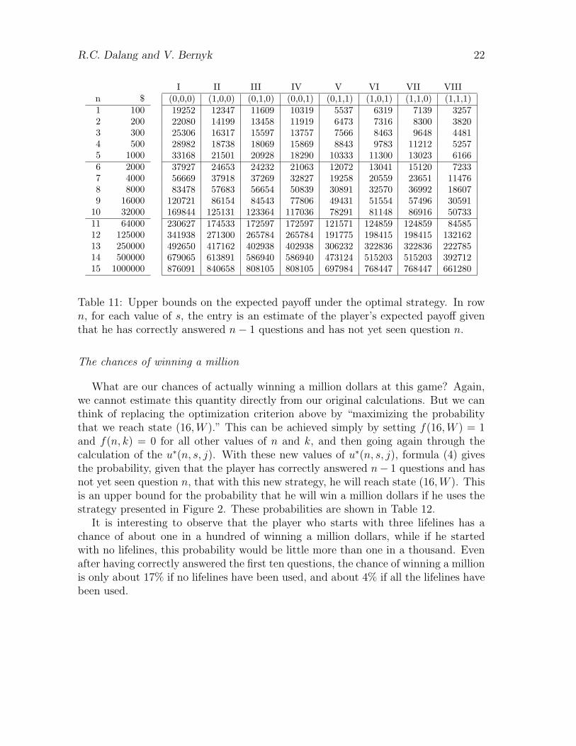
(computed with p = 1) to estimate the expected payoff if we proceed optimally fromthat stage on, and the availability of lifelines is described by s ∈ S. These quantities(rounded to the nearest integer) are shown in Table 11. It is interesting to note thateven after having correctly answered the first ten questions, the expected payoff isstill far below a million dollars ($230627 if all three lifelines are still available, and$84585 if all lifelines have been used).


I II III IV V VI VII VIIIn $1 1002 2003 3004 5005 10006 20007 40008 80009 16000

10 3200011 6400012 12500013 25000014 50000015 1000000

(0,0,0) (1,0,0) (0,1,0) (0,0,1) (0,1,1) (1,0,1) (1,1,0) (1,1,1)19252 12347 11609 10319 5537 6319 7139 325722080 14199 13458 11919 6473 7316 8300 382025306 16317 15597 13757 7566 8463 9648 448128982 18738 18069 15869 8843 9783 11212 525733168 21501 20928 18290 10333 11300 13023 616637927 24653 24232 21063 12072 13041 15120 723356669 37918 37269 32827 19258 20559 23651 1147683478 57683 56654 50839 30891 32570 36992 18607

120721 86154 84543 77806 49431 51554 57496 30591169844 125131 123364 117036 78291 81148 86916 50733230627 174533 172597 172597 121571 124859 124859 84585341938 271300 265784 265784 191775 198415 198415 132162492650 417162 402938 402938 306232 322836 322836 222785679065 613891 586940 586940 473124 515203 515203 392712876091 840658 808105 808105 697984 768447 768447 661280

Table 11: Upper bounds on the expected payoff under the optimal strategy. In rown, for each value of s, the entry is an estimate of the player’s expected payoff giventhat he has correctly answered n− 1 questions and has not yet seen question n.

The chances of winning a million

What are our chances of actually winning a million dollars at this game? Again,we cannot estimate this quantity directly from our original calculations. But we canthink of replacing the optimization criterion above by “maximizing the probabilitythat we reach state (16, W ).” This can be achieved simply by setting f(16, W ) = 1and f(n, k) = 0 for all other values of n and k, and then going again through thecalculation of the u∗(n, s, j). With these new values of u∗(n, s, j), formula (4) givesthe probability, given that the player has correctly answered n− 1 questions and hasnot yet seen question n, that with this new strategy, he will reach state (16, W ). Thisis an upper bound for the probability that he will win a million dollars if he uses thestrategy presented in Figure 2. These probabilities are shown in Table 12.

It is interesting to observe that the player who starts with three lifelines has achance of about one in a hundred of winning a million dollars, while if he startedwith no lifelines, this probability would be little more than one in a thousand. Evenafter having correctly answered the first ten questions, the chance of winning a millionis only about 17% if no lifelines have been used, and about 4% if all the lifelines havebeen used.


I II III IV V VI VII VIIIn $1 1002 2003 3004 5005 10006 20007 40008 80009 16000

10 3200011 6400012 12500013 25000014 50000015 1000000

(0,0,0) (1,0,0) (0,1,0) (0,0,1) (0,1,1) (1,0,1) (1,1,0) (1,1,1)0.0111 0.0065 0.0060 0.0053 0.0026 0.0029 0.0033 0.00130.0128 0.0075 0.0070 0.0062 0.0030 0.0034 0.0039 0.00160.0148 0.0086 0.0081 0.0071 0.0035 0.0040 0.0045 0.00180.0171 0.0100 0.0094 0.0083 0.0041 0.0046 0.0053 0.00220.0197 0.0116 0.0110 0.0096 0.0048 0.0054 0.0061 0.00250.0227 0.0134 0.0128 0.0112 0.0056 0.0063 0.0072 0.00300.0355 0.0212 0.0205 0.0182 0.0094 0.0103 0.0116 0.00500.0548 0.0335 0.0327 0.0295 0.0157 0.0170 0.0187 0.00840.0835 0.0522 0.0514 0.0476 0.0261 0.0278 0.0299 0.01410.1239 0.0798 0.0797 0.0759 0.0433 0.0453 0.0473 0.02370.1771 0.1180 0.1197 0.1197 0.0718 0.0735 0.0735 0.03990.2863 0.2032 0.2067 0.2067 0.1319 0.1338 0.1338 0.07600.4424 0.3387 0.3443 0.3443 0.2378 0.2395 0.2395 0.14470.6441 0.5387 0.5449 0.5449 0.4157 0.4178 0.4178 0.27560.8698 0.7948 0.8005 0.8005 0.6880 0.6910 0.6910 0.5250

Table 12: Upper bounds on the probability of winning a million dollars. In row n,for each value of s, the entry is an estimate of the conditional probability that theplayer will win a million dollars, given that he has correctly answered n− 1 questionsand has not yet seen question n.

8 Strengths and weaknesses of the model

It is quite satisfactory that the model provides an optimal strategy that is easilyapplied, as well as quantitative answers to questions concerning the expected rewardand the probability of winning a million dollars. In addition, these are obtained witha relatively limited computational effort.

The optimal strategy that comes out is quite reasonable. When we are confidentthat we know the answer, it recommends that we go ahead and answer, and whenwe are not, it provides guidance by telling us which lifeline to use or whether it ispreferable to quit the game. These were some of the main goals of the model.

On the other hand, the model does suffer from some weaknesses. For instance,there are several ingredients that are not given by the description of the game andthat we had to “invent.” The first such ingredient is our choice of the player’s possiblestates of knowledge. We could have decided to allow more (or fewer) such states.Our choice was based on the fact that after playing several times the commerciallyavailable version of the game, we found that we were always in one of these five states.For instance, we were never in the situation where we could definitely eliminate oneanswer, but were hesitating between the other three. This is probably due to the factthat the choice of answers is cleverly selected by the game’s designers. But in a morerefined model, additional states might be useful.

A second weakness is that we had to choose all the numbers that went into the prior


probabilities and likelihoods. On the one hand, no statistics for these are available,and we can consider that our model is suitable for a person who does not haveany statistical information on how often previous players found the correct answersto the various questions. The situation would be different if we did have statisticalinformation that allowed us to estimate the various prior probabilities and likelihoods.However, since neither the questions nor the answers are produced by a randomphysical mechanism, but by human beings, there is no guarantee that there is anystatistical consistency over long periods of time, so past statistics might not be veryuseful.

The analysis of the Phone-a-friend and Ask-the-audience lifelines forced us to makeassumptions on how the player’s knowledge interacts with the knowledge of the friendor audience. While we feel that we made reasonable choices, this portion of the modelmight warrant further thought.

Finally, the use of utility functions to model risk aversion is standard, but not fullysatisfactory, and other objectives might be preferable, though less tractable (such asmaximize the median reward, or maximize the probability of reaching at least question10, and if this occurs, then maximize the expected reward).

Overall, we consider that our model is satisfactory, practical, provides a nice illus-tration of existing theory on stochastic optimization, and can be used as a startingpoint for further analysis and study.

References

[1] Cairoli, R. & Dalang, R.C. Sequential Stochastic Optimization. John Wiley &Sons, New York, 1996.

[2] Dubins, L.E. & Savage, L.J. Inequalities for Stochastic Processes: How To Gam-ble If You Must. Dover Publ., New York, 1976.

[3] Haigh, J. Taking Chances (2nd ed.). Oxford University Press, New York, 2003.

[4] Hoel, P.G., Port, S.C. & Stone, C.J. Introduction to Stochastic Processes. Wave-land Press, Prospect Heights, Illinois, 1987.

[5] Maitra, A.P. & Sudderth, W.D. Discrete Gambling and Stochastic Systems.Springer Verlag, Berlin, 1996.

[6] Merton, R.C. Continuous-Time Finance. Blackwell Publ., Cambridge, Mas-sachusetts, 1992.

[7] Puterman, M.L. Markov Decision Processes. John Wiley & Sons, New York 1994.

[8] Ross, S.M. Introduction to Probability Models (fourth ed.). Academic Press,Boston, 1989.


9 Appendix. “Who wants to be a millionaire?”: the optimal strategy

The eight tables in Figure 2, numbered from I to VIII, indicate the optimal manner of usingthe lifelines and the best time to quit the game.

Explanation of the symbols

The symbols R, Q, PF, AA and 50 respectively correspond to the actions “Answer thequestion,” “Quit the game,” “use the lifeline Phone-a-Friend,” “use the lifeline Ask-the-Audience,” and “use the lifeline 50:50.”

The numbers 0, 1, 2, 3, and 4 on the second line of each of the eight tables representthe player’s degree of uncertainty about his knowledge of the correct answer. The number0 corresponds to the case where the player knows the correct answer (zero uncertainty), thenumber 1 to the case where the player is quite confident, but not certain, that he knowsthe correct answer, the number 2 to the case where the player hesitates between two ofthe answers and considers the other two as unlikely, the number 3 corresponds to the casewhere the player has just used the 50:50 lifeline and still does not know which of the tworemaining answers is correct, and the number 4 corresponds to the case where the playerhas no idea of the correct answer.

How to use the tables

At each stage in the game, the player selects the table that corresponds to the lifelinesthat are still available (the lifelines whose symbols are crossed out are those that are nolonger available). He then selects the column in that table which corresponds to his degreeof uncertainty about the answer. Finally, he selects the row in that table labelled with thenumber (and dollar value) of the question. Then he should accomplish the action indicatedin the table at the intersection of that column and row.

An example

If the player has not yet used any of the lifelines, is currently at question 6 and ishesitating between two answers, then table I tells him to use the 50:50 lifeline. Once he hasdone this and this lifeline is no longer available, he moves to table II. If he is now confidentthat he knows the answer, then column 1 of table II tells him to give the answer. On theother hand, if he is still hesitating between the two remaining answers, then column 3 oftable II tells him to use the lifeline Phone-a-friend. In this case, his only remaining lifelineis Ask-the-audience, so he moves to table VII, and so on.

A comment

The most important factor in the game is the player’s knowledge: a well-informed playerwill generally do better than one who is less-informed, and the strategy for using the lifelinesis at a second level of importance. The player should consider that the tables are designed tohelp him decide when to use each lifeline and when to quit. Since they have been computedfor an “average player,” it can be reasonable in some cases to do differently than indicatedin the tables.


I II III IV

n $1 1002 2003 3004 5005 10006 20007 40008 80009 1600010 3200011 6400012 12500013 25000014 50000015 1000000

50 PF AA0 1 2 3 4R R PF PFR R PF PFR R PF PFR R PF PFR R PF PFR R 50 AAR R 50 AAR R 50 AAR R AA AAR R AA AAR R 50 AAR R 50 AAR 50 50 AAR 50 50 AAR 50 50 50

50/\/\ PF AA0 1 2 3 4R R PF PF PFR R PF PF PFR R PF PF PFR R PF PF PFR R PF PF PFR R AA PF AAR R AA PF AAR R AA AA AAR R AA AA AAR R AA AA AAR R AA AA AAR R AA AA AAR R AA AA AAR AA AA AA AAR AA AA AA AA

50 PF/\ /\ AA0 1 2 3 4R R 50 AAR R AA AAR R AA AAR R AA AAR R AA AAR R 50 AAR R 50 AAR R 50 AAR R 50 AAR R AA AAR R 50 AAR R 50 AAR R 50 AAR 50 50 AAR 50 50 50

50 PF AA/\ /\0 1 2 3 4R R PF PFR R PF PFR R PF PFR R PF PFR R PF PFR R 50 PFR R 50 PFR R 50 PFR R 50 PFR R 50 PFR R 50 PFR R 50 PFR R 50 PFR 50 50 PFR 50 50 50

V VI VII VIII

n $1 1002 2003 3004 5005 10006 20007 40008 80009 1600010 3200011 6400012 12500013 25000014 50000015 1000000

50 PF/\ /\ AA/\ /\0 1 2 3 4R R 50 50R R 50 50R R 50 50R R 50 50R R 50 50R R 50 50R R 50 50R R 50 50R R 50 50R R 50 50R R 50 50R R 50 50R 50 50 50R 50 50 50R 50 50 50

50/\/\ PF AA/\ /\0 1 2 3 4R R PF PF PFR R PF PF PFR R PF PF PFR R PF PF PFR R PF PF PFR R R R PFR R PF R PFR R PF PF PFR R PF PF PFR R PF PF PFR R PF R PFR R PF PF PFR R PF PF PFR R PF PF PFR PF PF PF PF

50/\/\ PF/\ /\ AA0 1 2 3 4R R AA AA AAR R AA AA AAR R AA AA AAR R AA AA AAR R AA AA AAR R AA R AAR R AA R AAR R AA AA AAR R AA AA AAR R AA AA AAR R AA R AAR R AA AA AAR R AA AA AAR R AA AA AAR AA AA AA AA

50/\/\ PF/\ /\ AA/\ /\0 1 2 3 4R R R R RR R R R QR R R R QR R R R QR R Q R QR R R R RR R R R RR R R R QR R Q R QR R Q R QR R R R RR R R R QR R Q R QR R Q Q QR R Q Q Q

Figure 2: The optimal strategy. The symbols are explained at the beginning ofSection 9. Copyright c© 2003 R.C. Dalang and V. Bernyk. Commercial use prohibited withoutprior written authorization of the authors

How to win at “Who wants to be a millionaire ... - Chance

Documents

Transcript of How to win at “Who wants to be a millionaire ... - Chance