How tight should one’s hands be tied?

Fear of floating and credibility of

exchange rate regimes

Jesus Rodriguez Lopez∗

Universidad Pablo de Olavide de Sevilla and centrA

Hugo Rodriguez MendizabalUniversitat Autonoma de Barcelona and centrA

October 21, 2003

Abstract

This paper analyzes the linkages between the credibility of a targetzone regime, the volatility of the exchange rate, and the width of theband where the exchange rate is allowed to fluctuate. These three con-cepts should be related since the band width induces a trade-off betweencredibility and volatility. Narrower bands should give less scope for theexchange rate to fluctuate but may make agents perceive a larger proba-bility of realignment which by itself should increase the volatility of theexchange rate. We build a model where this trade-off is made explicit.The model is used to understand the reduction in volatility experiencedby most EMS countries after their target zones were widened on August1993. As a natural extension, the model also rationalizes the existence ofnon-official, implicit target zones (or fear of floating), suggested by someauthors.

Keywords: Fear of floating, target zones, exchange rate arrange-ments, rational expectations, credibility.

JEL classification: E52, E58, F31, F33.

∗Financial support from centrA is gratefully acknowledged. We have received very valuablecomments from Antonio Diez de los Rios, Gonzalo Fernandez de Cordoba, Chelo Gamez,Michael Goldberg, Amalia Morales, Jose Maria O’Kean, Javier Perez, Simon Sosvilla, JoseLuis Torres, participants at the II Workshop in International Economics at Malaga 2002,and participants at the XXVII Simposio de Analisis Economico at Salamanca 2002. Theirsuggestions and critiques have contributed to improve this paper. Of course, the remainingexisting errors are all authors’ entire responsibility. Corresponding author: Jesus Rodriguez,Dpto. de Economia y Empresa, Universidad Pablo de Olavide, Carretera de Utrera km.1,41013 Sevilla (Spain). jrodlop@dee.upo.es

1

CÆSAR: Cowards die many times before their deaths;The valiant never taste of death but once.Of all the wonders that I yet have heard,It seems to me most strange that men should fear,Seeing that death, a necessary end,Will come when it will come.W. Shakespeare. Julius Caesar, ACT2, scene 2.

1 Introduction

In the mid nineties, Obstfeld and Rogoff [26] predicted a world of widely float-ing exchange rates, given the removal of controls to the international capitalmobility. In contrast, recent analyses on exchange regimes have highlighteda common feature in exchange rate policies labeled as fear of floating : de jurefree floaters strongly intervene to soften the fluctuations of the nominal exchangerate (see Calvo and Reinhart [9], Reinhart [27], Fischer [16] and Levy-Yeyatiand Sturzenegger [24]). Intermediate regimes seem to be defining the currentworld so that completely fixed or fully flexible rates are rarely observed. Thegeneral aim of this paper is to provide an explanation as of why countries havefound it optimal to choose this intermediate alternative.For this purpose, we introduce a highly simplifying but useful analytical

starting point: any exchange regime is a particular case of a target zone. Onone extreme, fixed rates can be seen as target zones with band widths equalto zero. On the other extreme, pure floating rates are equivalent to fluctuationbands with a width tending to infinity. In between, dirty floats can be seen asimplicit target zones with finite bands while target zone regimes impose thosebands explicitly. Viewed in this manner, the choice of an exchange regimeconsists on deciding the width of a band of fluctuation.In particular, this paper analyzes the linkages between the credibility of a

regime, the volatility of the exchange rate and the width of the band wherethe exchange rate is allowed to fluctuate. It has been argued that differentexchange regimes, that is, different band widths, trade off price stability withmonetary independence. In this trade off, one of the most important ingredientsare the beliefs that market participants have about the incentives of the centralbank to defend the band, and these beliefs themselves affect the behavior ofthe exchange rate. More rigid systems, that is, narrower bands, impose ex-antelimits to the fluctuation of the exchange rate but also agents may perceive ahigher risk of realignment in the future. These expectations should feed intothe behavior of the exchange rate which itself determines the probability of achange in the system. Broader bands give more scope for the exchange rate tofluctuate but markets may consider the likelihood of a realignment low. In thispaper, we analyze the incentives central banks have to renege from announcedregimes and compute the endogenous relation between the width of the band,the volatility of the exchange rate and the probability of a change in the centralparity of a target zone.

2

As an example, consider the experience with the European Monetary System(EMS). This system was designed to foster stability of exchange rates amongEuropean currencies. In the language of Giavazzi and Pagano [17], by tyingthe hands of central banks, countries participating in the ERM could reach acertain degree of credibility for their monetary policies due to the disciplineeffect. Thus when, on August 3rd 1993, the EMS widened the band of fluctua-tion for the exchange rates, from ±2.25% to ±15%, some analysts predicted thedemise of the EMS, given that the wider band could motivate higher volatilityof exchange rates.1 The wider band appeared as a contradiction at the verymoment when the Treaty of Maastricht was imposing severe convergence cri-teria to EMU candidates. It seemed that the door was left open to access anenvironment with more scope for monetary discretion, exchange rates instabilityand larger inflation.However, market participants and researchers have documented two related

stylized facts after August 1993: a fall in exchange rate volatility (see Obst-feld [25]) and a substantial improvement in private beliefs about the long runsustainability of the EMS. Gomez-Puig and Garcia-Montalvo [18] estimate anEMS credibility indicator, based on the Markov switching methodology. For thepost 1993 period, they find that credibility increased for most of the currencies.Ledesma et alii [23], using a wide variety of credibility tests for the EMS, alsoconclude that credibility increased after the widening of the bands.2

As surveyed in Stockman [30], proponents of narrow band target zones sug-gest them as substitutes of a monetary commitment. Giavazzi and Pagano [17]argue that exchange arrangements like the ERM of the EMS contributed toimport credibility for domestic monetary policies, because differential inflationtranslates into real exchange rate appreciation, reducing the policy maker’s in-centive to inflate. Examples of these narrow bands are abundant. A quickglance into the recent regime classification of Reinhart and Rogoff [28] revealsthat most of the countries have at some point had an exchange arrangementinvolving a band (see their Appendix III). They sample market-determined ex-change rates for 153 countries from 1946 through 2001. Among these, the mostpopular exchange rate regime has been the crawling peg or narrow crawlingband, which account for over 26 percent of the observations. In the WesternHemisphere, explicit bands account for 42 percent of the observations.On the other hand, proponents of flexible rates argue that the central bank

may loose valuable short run monetary independence with a pegged exchangeregime (see, among others, Svensson [35], Obstfeld and Rogoff [26] and Stock-man [30]). A narrow target zone is simply one form of monetary policy rule and

1The Spanish Peseta and the Portuguese Escudo moved from a ±6% to a ±15% band.2This also seems to be the perception shared by the European Central Bank [15], as

asserted by President Wim Duisenberg: “[...] The second way in which ERM2 will contributeto a stable monetary environment within the EU is by limiting short-term exchange ratevolatility. As I have already mentioned, the widening of the fluctuation bands has reduced theincentive for market participants to test the sustainability of the narrow margins. A two-wayrisk arises as exchange rates move away from central rates, thereby discouraging speculativeattacks. The most recent experience is encouraging in this sense. In 1997, exchange ratevolatility among ERM currencies has been the lowest since 1992.”

3

some institutional reforms or other monetary policy rules could be used alter-natively. If an anti-inflation policy is not very credible inside the country then,instead, why should market participants appreciate that the discipline imposedby a narrow exchange regime will become a credible device outside?From a theoretical point of view, explicit modeling of band widening has

received little attention. Bartolini and Prati [3] develop a model where thecentral bank targets the exchange rate within a wide band in the short runbut attempts at keeping the exchange rate fluctuating in a narrow zone in thelong run. More recently, Chamley [10] has proposed a strategic game withspeculators and a central bank. Speculators learn about the possibility of asuccessful attack by looking at the position of the exchange rate within theband. The sustainability of a target zone regime increases by widening thebands of fluctuation. In both models, the idea of sustainability refers to theconcept of survival time rather than credibility.In the present paper, the concept of credibility is identified with the proba-

bility, perceived by the market, that the central bank will enforce defense mech-anisms to keep the currency within the committed zone. Rather than trying topredict the timing of the collapse of a target zone, as usual in the literature oncurrency crises, we suggest a rational expectations equilibrium that allows us toidentify the degree to which the central bank defends the currency at the marginsof the zone. Our model follows the cost-benefit analysis proposed by Obstfeld[25], where the central bank calibrates the opportunity costs from defendingrelative altering the regime. Rational expectations allows us to check whetherthe monetary authority has ex post incentives to defend the currency at a givenprobability of defense. Thereby, credibility is endogenous in our model. Since,in the absence of capital controls, sooner or later narrow band regimes suffercurrency crises, we will claim that the adoption of wide band target zones willpermit a substantial gain in credibility, enabling an environment for financialand monetary stability.Finally, the model is also used to further explore the idea of implicit bands

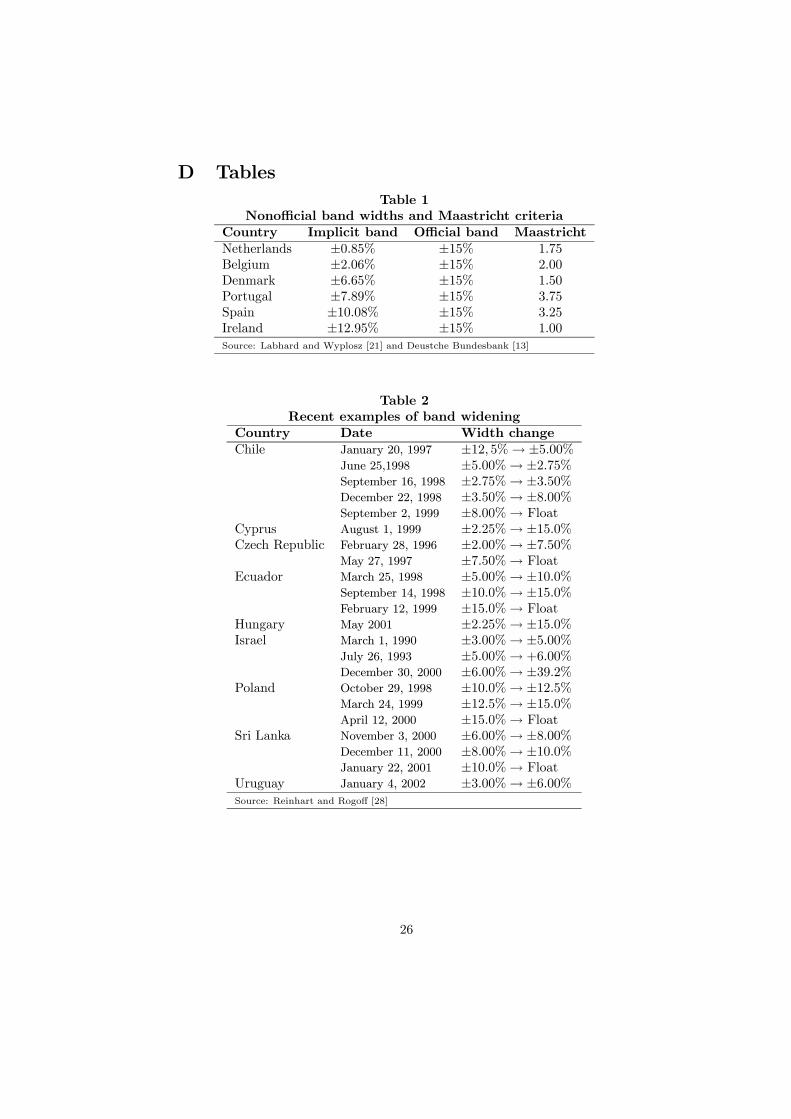
within official bands as estimated by Labhard and Wyplosz [21].3 These authorssuggest that European central banks were able to optimally fine tune theirdesired degree of monetary independence after the August 3rd 1993 reform.Their estimations of the implicit bands targeted by the monetary authorities arereproduced in Table 1, in the column “Implicit bands”. Some countries kept onholding a tighter band (Netherlands and Belgium), compatible with the former±2.25% system, but for most of the countries the narrow band system was nolonger optimal. Hence, the ±15% regime served as a benchmark reference underwhich all EMS countries were supposed to adjust the ranges of fluctuations fortheir currencies (see Table 1).4 Apart from the August 1993 ERM case, Table2 quotes some other examples of band widening from the mid nineties. Datahave been borrowed from Reinhart and Rogoff’s [28] Appendix III. It seems as

3In the words of Calvo and Reinhart [9], we attempt to provide a rationale to the fear offloating.

4Chung and Tauchen [12] and Chen and Giovannini [11] have also estimated implicit bandsfor the narrow band period.

4

though these countries were searching for an optimal width. Current exchangeagreements then go from ±2.25 for the Danish Krone (versus the Euro), up to±39.2% for the Israeli New Sheqel (versus a basket of currencies).

Tables 1 and 2 here

To capture this notion of implicit bands, we solve the model for a subgameperfect equilibrium where the central bank is given a menu of alternative bandwidths. Any of those bands produces an endogenous equilibrium credibility.Backward induction then reveals market traders the cheapest regime, which inturn signals the optimal band to be credibly committed by the central bank.The next section sets up a target zone model and the definition of a ra-

tional expectation equilibrium. A computation exercise is carried out in thethird section. The results show that there is a trade-off between credibility andvolatility as the band width increases. The optimal band is also determined inthis section. The last section summarizes the most relevant results.

2 The model

The model represents a highly stylized dynamic stochastic general equilibriumeconomy. It can be thought of as a reduced form version of more complicatedfully optimizing models. Time is discrete. First, consider an equation specifyingequilibrium in the money market:

mt − pt = ϕyt − γit + ξt, (1)

where mt is money supply, pt is the domestic price level of yt, a tradable good,it is the domestic interest rate of a one period of maturity bond, and ξt is someshock to money demand. They are all expressed in logs, with the exceptionof the interest rate. Parameters ϕ and γ are both positive: money demandincreases with output because of a transaction motive and there is an implicitliquidity preference behavior, meaning that money can be a substitute for abond that returns a nominal interest it.Let xt denote the log of the nominal exchange rate, expressing the price

of one unit of foreign currency in terms of domestic currency. The (log) realexchange rate is given by

qt = xt − pt + p∗t , (2)

where p∗t is the foreign price (variables with star will denote the foreign ana-logue).Call dt ≡ it − i∗, the interest rate differential, where i∗ is the foreign (con-

stant) rate, and assume perfect capital mobility, risk aversion and the uncoveredinterest rate parity condition (UIP)

dt = Et xt+1 − xt+ rt, (3)

5

where Et is the expectation operator conditional on information available attime t. The exogenous state variable rt represents the foreign risk premium,governed by a first order Markov process

rt = rt−1 + εt. (4)

The expected rate of depreciation must compensate for the interest rate differen-tial plus the foreign premium. The white noise εt is supposed to be Gaussian,εt ∼ N

¡0,σ2

¢, for convenience.5

Using (2), (3) and (1) one obtains

xt = ft + γEt xt+1 − xt , (5)

ft = mt + vt,

vt = θt + γrt,

θt = qt − p∗t − ϕyt + γi∗ − ξt.

Total fundamentals ft amount to an endogenous process, mt, plus an exogenousprocess, vt. We will assume that both the central bank and traders can observethe realization of vt.The monetary authority must choose the path for money mt so as to

maximize its preferences subject to the evolution of vt. The objective isto set up these preferences to capture the degree of monetary independencethat arises under alternative exchange rate regimes. As in Svensson [34], theconcept of monetary independence is associated with the interest rate variability.At one extreme, and in the absence of realignments, a fixed rate eliminatesmonetary independence. At the other extreme, a managed float regime providesthe highest degree of independence. In between, a target zone gives some scopeto focus the monetary policy on domestic problems. To capture this idea, thecentral bank (henceforth, CB) preferences are modeled to evaluate the trade-offbetween interest rate variability versus exchange rate variability

J =1

2E0

( ∞Xt=0

βth(dt − ρ0)

2+ λ (xt − c0)2

i). (6)

The long run desirable target for the interest rate differential is ρ0, that we willlater assume as zero, for convenience. The target for the exchange rate is thecentral parity c0 around which deviations are punished by the relative penaltyλ. The factor β ∈ (0, 1) is a time discount rate.

5The foreign risk premium plays a key role in the current paper. In general, UIP does nothold (see Ayuso and Restoy [1]). Conventional target zone models consider that deviationsfrom UIP are negligible in target zones (see Svensson [33]). A common practice in somecredibility tests of target zones relies in this idea (v.g. the simplest test, see Svensson [31],and the drift adjustment method of Bertola and Svensson [8]). However, Bekaert and Gray[6] find that the risk premia in a target zone are sizable and should not be ignored. Theyargue that this might be the reason of why the credibility tests run on EMS at the beginningof the nineties failed in anticipating the 1992-93 turbulences.

6

We think of a very short maturity term for the bond in the UIP, say a fewdays, a week or a month at most. The idea is that the CB controls some mone-tary aggregate mt to target dt, xt. Output realizations and real fluctuationsare observed with some delay, and not available by the time monetary policyis decided so, the only available information at any period is θt, rt. From (3)and (5) it is easy to show that mt will respond one to one to the shock θt andthe problem reduces to deciding how to split the shock rt between dt and xt.In what follows, the target zone regime will be characterized by the triple

λ ≥ 0, w ≥ 0,α ∈ [0, 1]. The first element is related to the preferences in (6).The number w is the band width. The last term α is the probability that the CBdefends the currency when it is outside the band and measures the credibilityof the exchange regime. We suppose that, within the bands, the CB defendsthe currency with probability 1. As stated in the introduction, the purpose ofthis paper is to construct a model able to generate a consistent target zonesolution, in the sense that the CB finds it optimal to defend the target zone atthe margins by probability α. There are not further incentives to renege fromthe target zone ex-post.The exchange rate is always determined as a function of the shock rt. At

any time t, the timing of the game is as follows:

1. The shock rt is realized.

2. If for that value of the shock the exchange rate should be outside a band[ct − w, ct + w], for instance, say it is above the upper limit ct + w, theCB can do any of two actions:

• It defends the currency with probability α. This means that theexchange rate is pegged at the edge of the band, xt = ct + w, andthe central parity is not altered, ct = ct−1.

• It realigns the currency with probability (1− α). In this case, thecentral bank devalues the central parity by µ, i.e. ct = ct−1+µ, andsituates the exchange rate at xt = ct−1 + max w, µ, that is, therate jumps to the new central parity if the realignment rate is higheror equal than the width, µ ≥ w. Otherwise, with overlapping zones,µ < w, the parity is altered by µ but the exchange rate remains atct−1 +w. This condition is necessary in order to avoid jumps to theinterior of the band, i.e. an appreciation under a devaluation.

3. If the realization of the shock makes the exchange rate be within the targetzone, the CB solves a minimization problem. The process is as follows:

• The central parity is left unaltered: ct = ct−1.• Forward looking agents form expectations Etxt+1.

• For given Etxt+1, rt, ρt, ct, the CB chooses xt, dt by minimizingthe loss (6) subject to the arbitrage condition (3), the relation in (4)and the additional restriction xt ∈ [ct − w, ct + w].

7

4. Finally, for given shock θt in the money demand equation (5), the CBsupplies the optimal quantity of money mt supporting the pair xt, dt.

In the loss function (6), the variable ρt has been defined as the long rundesirable target for the interest rate differential. The timing that has just beendescribed implies that the exchange rate is a function of the variable rt, theforeign risk premium, that must be fluctuating within a zone before an inter-vention is called for. Since rt is a return on an asset, it takes the form of aninterest rate. Therefore, the zone for this risk premium is an interval centeredat ρt. In fact, the rate of depreciation of xt uniquely depends on the differenceof rt from ρt. That is to say, when rt hits the upper limit of its zone, the ex-change rate hits also its upper limit, xt = ct+w. Let u(rt− ρt) be the functionlinking the exchange rate to the fundamental process rt within the band. Forthe exchange rate to belong to [ct − w, ct + w], the shock must be inside anotherband [ρt − r, ρt + r]. At rt = ρt ± r two level conditions must be satisfied

u (−r) = −w, (7)

and

u (r) = w. (8)

When a devaluation comes about (see step 2, bullet 2 in previous timing), thecentral parity is devalued by µ, and the new band for the fundamental is updated(see appendix A.1 for an explanation of how the process ρt∞t=0 is updated).In what follows, consider that the starting central parity is c0 = 0 and the

starting center is ρ0 = 0. The first order condition for values of rt ∈ [−r, r] is(1 + λ)x (rt) = rt +Et [x (rt+1)] . (9)

The function x (rt+1) satisfies

x (rt+1) = ct

+max w, µ if rt+1 > r with probability 1− α+w if rt+1 > r with probability α+u (rt+1) if rt+1 ∈ [−r, r]−w if rt+1 < −r with probability α−max w, µ if rt+1 < −r with probability 1− α.

(10)

The unknown continuous function u (rt) represents the CB’s best response whenthe risk premium lies within its band [−r, r]. Outside of it, condition (9) doesno longer hold and the trade-off is not optimal.6

6The assumption that the exchange rate can only jump when a realignment occurs simplifiesmatters. Bekaert and Gray [6] construct an empirical model where jumps can be taken atany point within the zone (“several within-the-band jumps are larger than several realignmentjumps”). There are other alternatives to model the realignment rate. For instance, the settingin Bertola and Caballero [7] is similar to ours, where agents perceive a constant size of therealignments, and the exchange rate takes a jump to the new central parity at realignments.Ball and Roma [2] and Svensson [33] assume that changes in the central parity follow a Poissonprocess.

8

In order to find out the particular form of the function u (rt), the band forthe fundamental [−r, r] must be computed, given the level conditions (7) and(8). This guarantees continuity of u (rt) from expression (10). Given that thefirst order conditions are only fulfilled in the interior of the bands, (9) can thenbe rewritten as

(1 + λ)u (rt) = rt +Et [x (rt+1)] . (11)

Forward recursion is used to solve for u (rt) with the first order condition (11)subject to (10). Appendix A.2 provides all the details for computation of thesolution.From condition (11) and (3), it is straightforward to see that the model

produces a positive relation between the exchange rate of depreciation withinthe band and the interest rate differential:

dt = λ [u (rt − ρt)− ct] + ρt, (12)

Outside the band, the trade-off is not optimal and expression (12) does not hold.As an illustration, consider the following particular case depicted in figure 1.

Further details of the properties of the function u (rt) can be found in Rodriguezand Rodriguez [29]. We consider a preference parameter λ = 0.5 and a standarddeviation σ = 0.002. As in the EMS case, we select a width w = ±2.25%, whoseexpected realignment rate is given by µ = ±4.5% (these values are convenientlyjustified in the following section). The exchange rate function is calculated forfive values of the probability of defense, α: 0, 14 ,

12 ,

34 and 1. These functions

are positively sloped for rt. The higher is α, the flattest the curve, that is, theexchange rate response to rt is smoother, the bigger is credibility. Hence, acredible band helps stabilize the exchange rate within the zone. For values of αclose to 0, the slope of that function increases, implying that the exchange rateis more sensible to variations in the risk premium. Then, volatility will increaseas long as α decreases.

Figure 1 here

2.1 The Concept of Equilibrium

The rational expectations equilibrium of this model amounts to finding a fixedpoint for the probability of defense, α. The idea is as follows. For a givenset of parameters (λ, σ, and w), and a prior about the probability α, marketparticipants may compute the ex-post incentives the central bank has to renegefrom the target zone regime. To estimate those incentives agents calculate thelosses for the central bank derived from defending the zone as compared to itslosses from realigning the band for any possible realization of the shock. Then,they compute the probability of the realizations for which losses from defendingare smaller than those of realigning. The rational expectations equilibriumimposes that this probability should be equal to α. If it is not equal, marketparticipants deduce that they were not estimating consistently the probabilityof defending and update it consequently.

9

To understand how this equilibrium is computed consider the following.Imagine that at some point in time t = τ the shock exceeds one of its bound-aries, say the upper one, rτ = er ≥ ρτ + r. The central bank has two options.If the currency is defended, neither the central parity cτ nor the center ρτ arealtered, so cτ = cτ−1 and ρτ = ρτ−1. Yet, for convenience, we assume that bothcτ and ρτ start at 0. Then, the current exchange rate is set at xτ = cτ +w, andthe interest rate differential is given by

d (er) = Eτ [xτ+1 − xτ ] + rτ = E [x (rτ+1) |rτ = er]− (cτ + w) + er. (13)

Hence, the CB pays a loss from then on of

LDτ (er) = 1

2

hd (er)2 + λw2

i+1

2EDτ

∞Xj=1

βt¡d2τ+j + λx2τ+j

¢ , (14)

where EDτ is the conditional expectation operator, given that the CB defendsat time t = τ .Instead, if the CB decides to devalue, the central parity and the exchange

rate are moved to xτ = cτ = cτ−1+µ, and the new center for the risk premiumis moved to ρτ = er. From (12), the interest rate differential will be given by

d (er) = er. (15)

Then, the CB receives a loss

LRτ (er) = 1

2

£er2 + λµ2¤+1

2ERτ

∞Xj=1

βt¡d2τ+j + λx2τ+j

¢ , (16)

where ERτ is the conditional expectation operator, given that the CB realignsat time t = τ .These two values lead us to define, for any value er, a cost function from

defending as

G (er) = LDτ (er)− LRτ (er) . (17)

If, for some r /∈ [−r, r], G (r) is negative, the costs from realigning will overcomethat from defending and the CB will keep the exchange rate at its primitivemargins. Otherwise, when G (r) > 0, realigning will be preferred to defendingfor that particular value of the shock. Indifference stands for the case G = 0.Since the objective function is quadratic, the function G (r) is an increasingfunction of the shock r, that is, the costs from defending relative to the costsfrom realigning increase as the value of the shock increases. Notice the relativecosts of defending are only conditional on the value of the shock; they do notdepend on previous costs. So, once the shock r has been reached, the functionG (r) determines whether it is preferable to defend or to realign. That is why wedo not write the subindex τ anymore. Given the monotonicity of the function

10

G (r), there must be a value of the risk premium, call it r∗, such that for allrt > r

∗ it is preferable to realign, that is, G (r) > 0 for all r > r∗. Then, marketparticipants can determine the probability of reaching such a value which will berelated to the probability of defending. With this information, they can evaluatewhether the assumed α, the subjective probability of defense, was correct or not.Furthermore, for given r0 = ρ0 = 0, denote by ζ (r∗) the probability that a

random walk stream, rt∞t=0, always wanders inside a moving corridor of width2r∗ ≥ 0, centered at ρt∞t=0, i.e.

ζ (r∗) = Pr£©rt − ρt−1 ∈ [−r∗, r∗]

ª∞t=1

|r0 = 0¤, (18)

and analogously define ζ (r) as

ζ (r) = Pr£©rt − ρt−1 ∈ [−r, r]

ª∞t=1

|r0 = 0¤,

such that r∗ ≥ r > 0, and where process ρt∞t=1 is updated as follows

• ρt = ρt−1, for −r∗ < rt − ρt−1 < r∗.

• ρt = rt, otherwise.7

Notice that the function ζ (r∗) is monotonically increasing. This implies that

limr∗→∞ ζ (r∗) = 1,

limr∗→0

ζ (r∗) = 0.

These concepts lead us to a rational expectation solution. Intuitively, agents ob-serve that there exists a shock making the CB indifferent between defending andrealigning. Equilibrium is found when the proportion of times that this shockis perceived to occur equals the proportion of times the currency is observed tobe defended. A more formal equilibrium concept follows:

Definition 1 : (Rational expectations equilibrium) A target zone systemdefined by the parameters (σ,λ, w,α) is said to be a rational expectation equi-librium, if there exists a risk premium |r∗| ≥ |r|, such that

G (r∗) = 0, (19)

and

ζ (r∗)− ζ (r)

1− ζ (r)= α, (20)

where r is the implied band width of the zone.

7Appendix A.1 reports further details on how the center ρt is updated under a more generalcase when the realignment rate is not necessarily higher than the band width.

11

Condition (19) makes agents perceive that the CB is indifferent betweenrealigning or defending. Condition (20) implies that market traders perceivethe CB is defending with a probability α whenever a marginal intervention iscalled for. On the one hand, the central bank will not realign as long as theshock is not larger than r∗ in absolute value which happens with probabilityζ (r∗). On the other hand, the market anticipates that realignment does notoccur if the risk premium stays with its band, which happens with probabilityζ (r), or if the shock leaves its band and the central bank defends the targetzone which happens with probability α [1− ζ (r)]. Obviously, in equilibriumthese two probabilities of defending should be equal, that is,

ζ (r∗) = ζ (r) + α [1− ζ (r)] ,

and solving for α gives condition (20).Imagine that condition (20) is matched, but condition (19) is not. For in-

stance, imagine there is a value for r, say er, such that G (er) < 0 and [ζ (er) −ζ (r)]/[1− ζ (r)] = α. Market participants perceive that the central bank wouldbe strictly better off from defending and letting the risk premium to deviatefurther from its center. Hence, there is still room for the risk premium to behigher, say er +∆ > er, before the central bank generates a devaluation. Sincethe function ζ (r) is monotonically increasing, this means that

ζ (er +∆)− ζ (r)

1− ζ (r)> α, (21)

that is, the perception by the market of the proportion of times the currency willbe observed to be defended, out of the margins of the zone, should be higherthan α. Agents will revise their estimation of the probability of defense byincreasing their subjective probability of defense, say to eα > α. With a largervalue of α, the function u(rt − ρt) becomes flatter and the limit of the bandfor the risk premium, r, larger. Given that ζ (er +∆) < 1, this movement of rreduces the left-hand side of (21). Notice, the response of the market increasingα moves the economy towards the equilibrium by closing the gap in (21).

3 Results

Since the model does not permit a closed form solution, numerical alternativesare given as tentative answers. This requires to rely results on some prespecifiedparameters. This section is organized in four parts. The first justifies theparameters for the numerical computations. The second part use the previousmodel to endogenize the credibility of the target zone, as represented by theprobability of defense α. Estimations of conditional volatilities are given in thethird subsection. The final subsection addresses to the question of determiningthe optimal band.

12

3.1 Parameters

The following values for the parameters are used in the numerical exercises ofthis section. We think of a month as the time frequency. As in Svensson [34],

the time discount factor is set to β = 0.90112 . We use this value to ease the

calculations but the main results of the paper do not hinge on it.Three bands are chosen, w = ±2.25%, ±6.00% and ±15%, the official widths

experienced in the ERM. For the last case, it is well known that EMS monetaryauthorities targeted implicit widths much narrower than the ±15% officiallyannounced, as estimated by Labhard and Wyplosz [21] (see also Bartolini andPrati [3]). In fact, when the Spanish Peseta and the Portuguese Escudo wererealigned on March 6th 1995, the edges of the zone had not been reached. Inboth cases, the realignment rate (µ = 7.5% and 3.5%, respectively) were smallerthan the official widths.Appendix B suggests some estimates for σ and µ. A VAR estimation lead to

conclude that σ = 0.01 can be a reasonable value for this variance. This valueparallels some other estimations for the risk premium standard deviation. Thevalue of the constant realignment rate µ is estimated depending on the bandwidth, w.8 Thus, we conclude that µ = ±4.5% and µ = ±6.3%, for widthsw = ±2.25 and w = ±6%, respectively, are consistent with the EMS history.For the wide band ±15% we use µ = ±7.5%, as the Spanish Peseta was sodevalued in March 6th 1995.Finally, regarding the preference parameter λ, we have used a grid ranging

from 10−8 to 1.

3.2 Credibility

The implementation of the rational expectation equilibrium goes as follows. Forparticular values for σ, λ and w, we guess the equilibrium probability of defenseα, and solve the model, that is, we find the function u, and the bounds forthe risk premium band, r. Second, we compute the value of er from expression(20). Third, we simulate N = 1000 runs of T = 500 observations for theshock starting at the value er. Fourth, the relative costs of defending versusrealigning are computed for each run in the simulation so the cost functionG (er) is approximated as the arithmetic mean over the N = 1000 simulatedruns. If the estimated G (er) is positive (negative), we scale down (up) the initialvalue of α and repeat the process until convergence is reached (see appendix Cfor the details of this iterative process).Table 3 collects the equilibrium values of α for different combinations of

the preference parameter λ, and the three widths considered. In our search ofvalues, we find that λ should be smaller or equal than 0.1 in order to produce

8Expected realignment rates are usually estimated through some measure of accumulatedcompetitiveness losses, v.g. the growth rates of the CPI, the Industrial Price Index or theUnit Labor Cost Index. In general, devaluations are not sufficient to dampen for the realappreciation (Giavazzi and Pagano [17]). By estimating different realignment rates for thedifferent band widths, we simply want to extract some figures that reasonably describe theERM history.

13

equilibrium values of α strictly in the [0, 1] interval. In complementary exercises(not reported here), when σ has been increased, this range for λ has increased:when the risk premium suffers a bigger volatility, a central bank needs a higherλ in order to preserve a certain degree of credibility.The main result to be highlighted from Table 3 is that the equilibrium proba-

bility of defense α increases as the band widens. The market perceives that thissituation might discourage the monetary authority to renege from the targetzone arrangement. Thus, credibility increases with the band width. Anotherinteresting result is that the system is more credible, the larger the preferenceweight attached to the variability of the exchange rate, λ. If the central bankexhibits in its preferences a strong targeting of the exchange rate around thecentral parity, the exchange rate variability will be lower. The preference pa-rameter λ punishes any deviation from the central parity. Then, the centralbank finds it consistent to commit the target zone arrangement with a higherprobability.Although the quantitative outcomes of this exercise are highly sensible to the

realignment rate µ, the qualitative results should remain the same independentlyof the particular value of µ or any other parameter. Here, we are assuming thatas the band gets wider, the realignment rate increases too which increases thecost of changing the central parity and makes the system more credible. Thechoice of making µ dependent of the width of the band has been made to matchwhat we observe in the data. However, if µ were constant the same effectswould appear. This is due to the fact that as the band widens, the probabilityof incurring in the fixed costs of realigning decrease.

Table 3 here

3.3 Volatility

Is the model consistent with the experience of the EMS? As pointed out inthe introduction, after the widening of the bands in 1993, researchers foundthat volatility of the exchange rate had decreased (see Gomez-Puig and Garcia-Montalvo [18], Ledesma et alii [23] and Ayuso et alii [1]). To see this, wecompute the standard deviation of the exchange rate, for t = 1, 2...36 periodsahead, conditional on information available at time 0

σx,t =

rE0

n[xt −E0 (xt)]2

o. (22)

If we consider that the starting conditional value for the risk premium is r0 = 0,it is easy to show that the conditional expectation is E0 (xt) = c0 = 0. Thestandard deviation for the interest rate differential has a similar form:

σd,t =

rE0

n[dt −E0 (dt)]2

o. (23)

Again, for r0 = 0, it is easy to show that the conditional expectation is E0 (dt) =ρ0 = 0.

14

Figure 2 shows the conditional standard deviation in (22) for the differenttime horizons and the three band widths used in the EMS. The value used forλ is 0.0001. We observe that the volatility of the exchange rate 19 periodsahead in the system with the width of ±15% is smaller than the one with thezone of ±2.25%. The reason for this result is in Table 3 where we find thatthe probability of a realignment in the first system is 85 percent while withthe narrow band is only 23 percent. We also observe that these reductions involatility from moving to the wide band increase as the time horizon is larger.With a larger probability of realignment future discrete jumps in the exchangerate are more likely.Figure 3 presents the same computations with λ = 0.1. With this value

for the central bank preferences wider bands present higher volatility. In thiscase, it is in the interest of the central bank to foster credibility and marketparticipants know that the monetary authority will be likely to defend the bandoften. In fact, Table 3 shows that all bands are equally credible. The onlydifference stands for the different reaction of the exchange rate to movements inthe shock. This response is given by the slope of the function u which is smallerfor narrower bands.Finally, Figure 4 presents the volatility of the interest rate differential for

λ = 0.0001. We observe this volatility decreases with the widening of the band.A broader band allows for more monetary independence, that is, the centralbank enjoys more degrees of freedom to adjust the nominal interest rate todomestic conditions. With a wider zone the exchange rate may now absorbmore variability from the risk premium shock. At the same time, a wider bandis also more credible, this helps stabilizing forward looking expectations and,through the UIP, the interest rate differential.

Figures 2-4 here

3.4 The optimal band width

This subsection explores the idea of Labhard andWyplosz [21] about non-officialbands inside official bands. Their estimates suggest that, while the widths ofthe target zones were widened on August 1993, most of EMS countries foundit optimal to target a tighter band than ±15% (see Table 1): The Netherlandskept on pursuing a close targeting to the DM, while Belgium enforced a bandsimilar to that of the previous period. The rest of countries preferred to gainmore degrees of freedom for their monetary policies, probably due to the needof meeting the convergence criteria imposed by the Maastricht Treaty.The exercise of this subsection rationalizes the choice of this nonofficial bands

by solving the model for a subgame perfect equilibrium. Given a value for theparameters λ, β, and σ, an equilibrium probability α can be found for anyband width w ≥ 0. This defines a continuum of equilibria within which onecan compute the ex-ante costs from such strategy as measured by (6). Any ofthose widths conforms the strategy set of the CB. A credible Nash equilibrium

15

is determined by choosing the strategy that returns the minimum ex-ante cost.This is the optimal band width.In order to perform this exercise, a word has to be said about the rate of

realignment. At the beginning of this section, we suggested a positive correlationbetween the band width and the realignment rate, on the basis of EMS history.We mapped the value of µ = 4.5% to w = ±2.25%, and µ = 6.3% to w = ±6%.In order to keep the same schedule in the parameters, we make the realignmentrate vary linearly with the band matching these previous points. This takes usto the function

µ = 0.0342 + 0.48w.

Denote J(w) the costs derived from the rational expectation equilibriumassociated with the width w, given the rest of parameters. The optimal bandwidth is found as

w∗ ≡ argminwJ (w) .

Let α∗ denote the equilibrium probability of defense associated with the optimalband w∗. These steps have been repeated for thirteen different values of λ fora grid ranging from 0.0008 to 0.01.Table 4 includes the equilibrium values for the optimal band and the associ-

ated probabilities of defense α∗ for each of the values of λ. As the central bankdislikes more the volatility of the exchange rate (for large values of λ), the op-timal band becomes smaller at the same time that more credible. In this sense,the August 3rd 1993 reform can be viewed as a benchmark regime within whichall the EMS countries could optimally adjust their targeted zones where theexchange rates were allowed to fluctuate. An important corollary of this resultis that, while this optimal fine-tuning of bands can be achieved when the officialband is ±15%, the official narrow width period of ±2.25% could only make feeluncomfortable those EMS currencies who wished to use a bigger optimal degreeof monetary independence. The column of Table 1 labelled “Maastricht” col-lects the average number of criteria not satisfied by the countries in the sampleof Labhard and Wyplosz [21] from 1993 until 1996. With the exception of Ire-land we see that countries that decided to let the exchange rate to fluctuate inwider bands were the ones that did not satisfy a larger number of criteria andtherefore needed to make more adjustments in their domestic economies.9

Table 4 here

9Ireland had held a long tradition (from 1826) of anchoring the Irish Pound versus thecurrency of the U.K., its main trading partner. As the U.K. left the EMS discipline onSeptember 1992, the economic gains from participating in the ERM could only come througha credible enough arrangement. The broad implicit band of Table 1 allowed for accommodationof the strong depreciation of the British Pound (BP) versus the Deustche Mark by the endof 1994 and early in 1995 (see Ledesma et alii [22]). In contrast, the sharp depreciation ofthe BP on September 1992, in combination with the tight ±2.25% official band, led the Irishauthorities to strongly realign on 1st February 1993 (+11%).

16

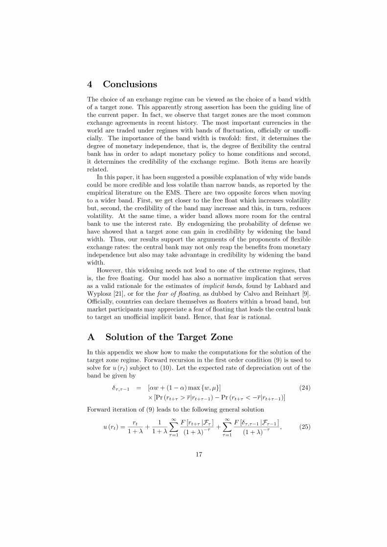
4 Conclusions

The choice of an exchange regime can be viewed as the choice of a band widthof a target zone. This apparently strong assertion has been the guiding line ofthe current paper. In fact, we observe that target zones are the most commonexchange agreements in recent history. The most important currencies in theworld are traded under regimes with bands of fluctuation, officially or unoffi-cially. The importance of the band width is twofold: first, it determines thedegree of monetary independence, that is, the degree of flexibility the centralbank has in order to adapt monetary policy to home conditions and second,it determines the credibility of the exchange regime. Both items are heavilyrelated.In this paper, it has been suggested a possible explanation of why wide bands

could be more credible and less volatile than narrow bands, as reported by theempirical literature on the EMS. There are two opposite forces when movingto a wider band. First, we get closer to the free float which increases volatilitybut, second, the credibility of the band may increase and this, in turn, reducesvolatility. At the same time, a wider band allows more room for the centralbank to use the interest rate. By endogenizing the probability of defense wehave showed that a target zone can gain in credibility by widening the bandwidth. Thus, our results support the arguments of the proponents of flexibleexchange rates: the central bank may not only reap the benefits from monetaryindependence but also may take advantage in credibility by widening the bandwidth.However, this widening needs not lead to one of the extreme regimes, that

is, the free floating. Our model has also a normative implication that servesas a valid rationale for the estimates of implicit bands, found by Labhard andWyplosz [21], or for the fear of floating, as dubbed by Calvo and Reinhart [9].Officially, countries can declare themselves as floaters within a broad band, butmarket participants may appreciate a fear of floating that leads the central bankto target an unofficial implicit band. Hence, that fear is rational.

A Solution of the Target Zone

In this appendix we show how to make the computations for the solution of thetarget zone regime. Forward recursion in the first order condition (9) is used tosolve for u (rt) subject to (10). Let the expected rate of depreciation out of theband be given by

δτ ,τ−1 = [αw + (1− α)max w, µ] (24)

× [Pr (rt+τ > r|rt+τ−1)− Pr (rt+τ < −r|rt+τ−1)]Forward iteration of (9) leads to the following general solution

u (rt) =rt1 + λ

+1

1 + λ

∞Xτ=1

F [rt+τ |Fτ ](1 + λ)−τ

+∞Xτ=1

F [δτ ,τ−1 |Fτ−1 ](1 + λ)−τ

, (25)

17

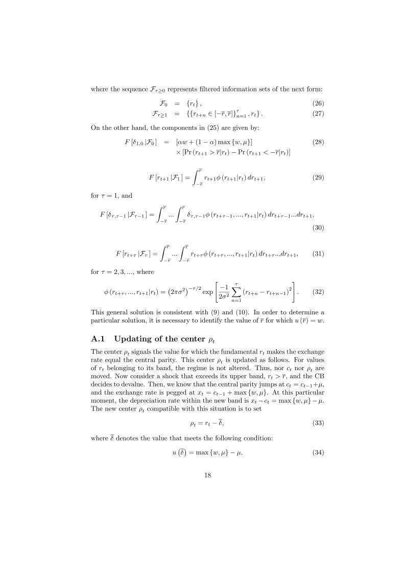
where the sequence Fτ≥0 represents filtered information sets of the next form:F0 = rt , (26)

Fτ≥1 = rt+n ∈ [−r, r]τn=1 , rt . (27)

On the other hand, the components in (25) are given by:

F [δ1,0 |F0 ] = [αw + (1− α)max w,µ] (28)

× [Pr (rt+1 > r|rt)− Pr (rt+1 < −r|rt)]

F [rt+1 |F1 ] =Z r

−rrt+1φ (rt+1|rt) drt+1, (29)

for τ = 1, and

F [δτ ,τ−1 |Fτ−1 ] =Z r

−r...

Z r

−rδτ ,τ−1φ (rt+τ−1, ..., rt+1|rt) drt+τ−1...drt+1,

(30)

F [rt+τ |Fτ ] =Z r

−r...

Z r

−rrt+τφ (rt+τ , ..., rt+1|rt) drt+τ ...drt+1, (31)

for τ = 2, 3, ..., where

φ (rt+τ , ..., rt+1|rt) =¡2πσ2

¢−τ/2exp

"−12σ2

τXn=1

(rt+n − rt+n−1)2#. (32)

This general solution is consistent with (9) and (10). In order to determine aparticular solution, it is necessary to identify the value of r for which u (r) = w.

A.1 Updating of the center ρt

The center ρt signals the value for which the fundamental rt makes the exchangerate equal the central parity. This center ρt is updated as follows. For valuesof rt belonging to its band, the regime is not altered. Thus, nor ct nor ρt aremoved. Now consider a shock that exceeds its upper band, rt > r, and the CBdecides to devalue. Then, we know that the central parity jumps at ct = ct−1+µ,and the exchange rate is pegged at xt = ct−1 +max w, µ. At this particularmoment, the depreciation rate within the new band is xt− ct = max w, µ−µ.The new center ρt compatible with this situation is to set

ρt = rt − δ, (33)

where δ denotes the value that meets the following condition:

u¡δ¢= max w, µ− µ. (34)

18

• If w ≤ µ, the exchange rate jumps and equals the new central parity, andthe depreciation within band is 0. Then, δ = 0 and the new center isρt = rt.

• If w > µ, the exchange rate equals its own previous upper limit, and thedepreciation is w − µ > 0. The new center is ρt = rt − δ.

When the shock exceeds the lower bound, rt < −r, the new center is peggedat

ρt = rt − δ. (35)

A similar condition arises to determine δ:

u (δ) = −max w, µ+ µ. (36)

Notice that u (δ) = −u ¡δ¢, then δ = −δ. Again, when −µ < −w, we have thatδ = −δ = 0.

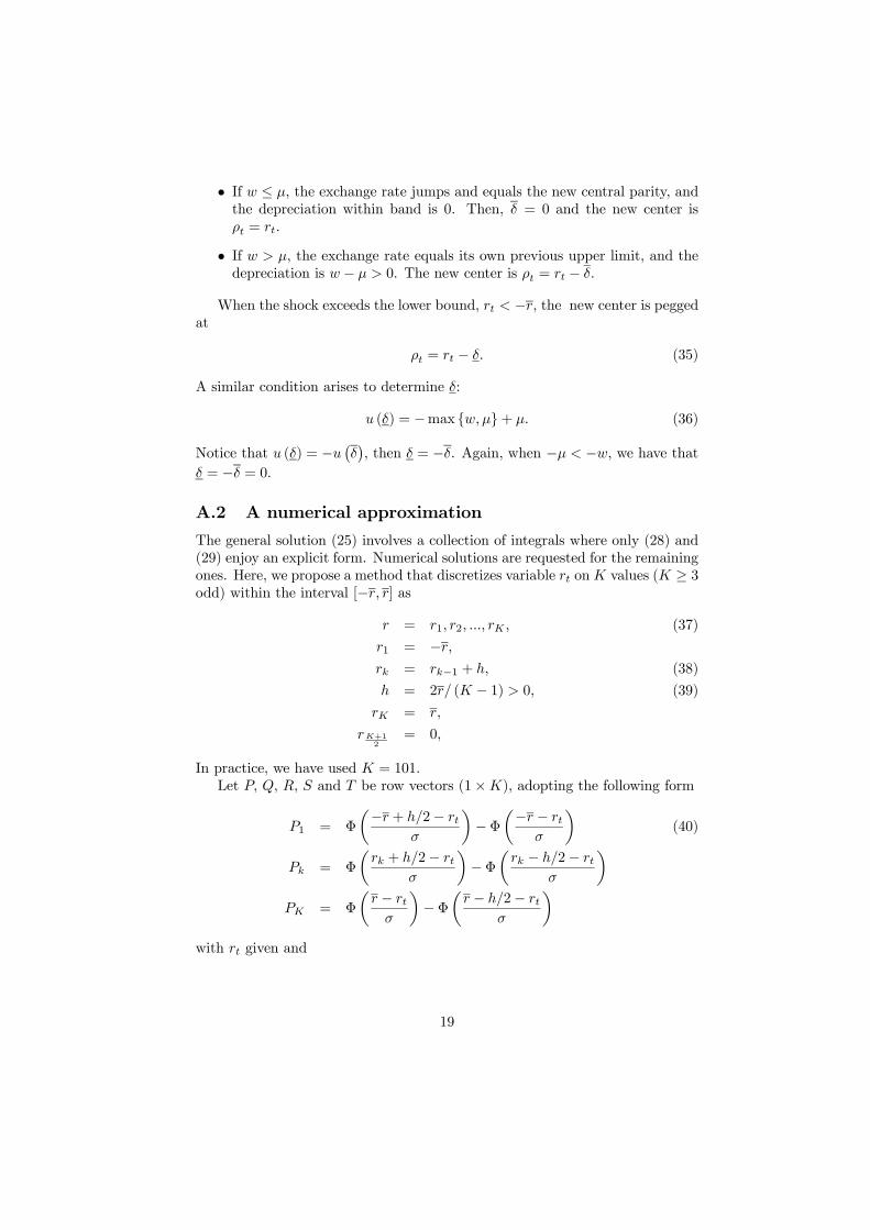
A.2 A numerical approximation

The general solution (25) involves a collection of integrals where only (28) and(29) enjoy an explicit form. Numerical solutions are requested for the remainingones. Here, we propose a method that discretizes variable rt onK values (K ≥ 3odd) within the interval [−r, r] as

r = r1, r2, ..., rK , (37)

r1 = −r,rk = rk−1 + h, (38)

h = 2r/ (K − 1) > 0, (39)

rK = r,

rK+12

= 0,

In practice, we have used K = 101.Let P, Q, R, S and T be row vectors (1×K), adopting the following form

P1 = Φ

µ−r + h/2− rtσ

¶− Φ

µ−r − rtσ

¶(40)

Pk = Φ

µrk + h/2− rt

σ

¶− Φ

µrk − h/2− rt

σ

¶PK = Φ

µr − rtσ

¶− Φ

µr − h/2− rt

σ

¶with rt given and

19

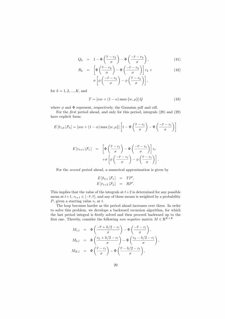
Qk = 1− Φµr − rkσ

¶− Φ

µ−r − rkσ

¶, (41)

Rk =

·Φ

µr − rkσ

¶− Φ

µ−r − rkσ

¶¸rk + (42)

σ

·φ

µ−r − rkσ

¶− φ

µr − rkσ

¶¸,

for k = 1, 2, ...,K, and

T = [αw + (1− α)max w, µ]Q (43)

where φ and Φ represent, respectively, the Gaussian pdf and cdf.For the first period ahead, and only for this period, integrals (28) and (29)

have explicit form:

E [δ1,0 |F0 ] = [αw + (1− α)max w, µ]·1− Φ

µr − rtσ

¶− Φ

µ−r − rtσ

¶¸

E [rt+1 |F1 ] =

·Φ

µr − rtσ

¶− Φ

µ−r − rtσ

¶¸rt

+σ

·φ

µ−r − rtσ

¶− φ

µr − rtσ

¶¸.

For the second period ahead, a numerical approximation is given by

E [δ2,1 |F1 ] = TP 0,E [rt+2 |F2 ] = RP 0.

This implies that the value of the integrals at t+2 is determined for any possiblemean at t+1, rt+1 ∈ [−r, r], and any of these means is weighted by a probabilityP , given a starting value rt at t.The loop becomes harder as the period ahead increases over three. In order

to solve this problem, we develope a backward recursion algorithm, for whichthe last period integral is firstly solved and then proceed backward up to thefirst one. Thereby, consider the following non negative matrix M ∈ RK×K

M1,l = Φ

µ−r + h/2− rlσ

¶− Φ

µ−r − rlσ

¶,

Mk,l = Φ

µrk + h/2− rl

σ

¶− Φ

µrk − h/2− rl

σ

¶,

MK,l = Φ

µr − rlσ

¶− Φ

µr − h/2− rl

σ

¶,

20

for k, l = 1, 2, ...K, with the following properties: the sum over each columngives a row vector mc ∈ R1×K , with all its components lying within the (0, 1)interval

mc (l) =KXk=1

Mkl =

Z r

−rφ (s|rl) ds ∈ (0, 1) (44)

for l = 1, 2, ...,K. The proof follows trivially. This property is sufficient toverify the Hawkins-Simon condition (Brauer-Solow Theorem).Matrix M contains the transition probabilities in the intermediate periods

from τ up to τ + 1, within the interval [−r, r] and for any conditional meanbelonging to [−r, r]. Thus, the solution for the third period is given by

E [δ3,2 |F2 ] = TMP 0,E [rt+3 |F3 ] = RMP 0.

Again, the value of the integrals are first determined at t + 3 for any possiblemean at t+ 2, rt+2 ∈ [−r, r], given by the columns of M . The vector P closesthe calculation for any possible mean at t+1, rt+1 ∈ [−r, r], for given a startingvalue rt.For τ = 2, 3, ..., further generalization gives a sequence:

E [δτ ,τ−1 |Fτ−1 ] = TMτ−2P 0,E [rt+τ |Fτ ] = RMτ−2P 0.

Plugging these values into (25), one obtains

u (rt) =rt1 + λ

+E [rt+1 |F1 ](1 + λ)2

+E [δ1,0 |F0 ]1 + λ

(45)

+1

1 + λ

∞Xτ=2

RMτ−2P 0

(1 + λ)τ+∞Xτ=2

TMτ−2P 0

(1 + λ)τ.

Let the vector of eigenvalues be given by η (M), and call η∗ (M) the Frobe-nius root, i.e. the maximum eigenvalue. From (44) we know thatmc (l) < 1, thisis a sufficient condition to verify the Hawkins-Simon condition (see Brauer-SolowTheorem). In turn, verification of the Hawkins-Simon condition implies that

η∗ (M) < 1, (see Hawkins and Simon [19] and [20]). Then, matrix (I −M)−1exists, it is non negative and can be written as

(I −M)−1 =∞Xj=0

M j

This gives rise to a convenient simplification

M =∞Xτ=2

(1 + λ)−τMτ−2 =

1

1 + λ[(1 + λ) I −M ]−1 .

21

The general solution becomes

u (rt) =Ω (rt)

1 + λ+∆ (rt) , (46)

with

Ω (rt) ≡ rt + E [rt+1 |F1 ]1 + λ

+RMP 0,

∆ (rt) ≡ E [δ1,0 |F0 ]1 + λ

+ TMP 0.

Application of level conditions (7) and (8) gives the particular solution

Ω (r)

1 + λ+∆ (r) = w.

Finally, the exchange rate expectation is

Etxt+1 =∞Xτ=1

F [rt+τ |Fτ ](1 + λ)τ

+ (1 + λ)∞Xτ=1

F [δτ ,τ−1 |Fτ−1 ](1 + λ)τ

,

or using the previous approximation

Etxt+1 = Ω (rt) + (1 + λ)∆ (rt)− rt. (47)

Once we know the expression for the exchange rate and the expectation, theinterest rates differential is obtained from the uncovered interest parity conditionas

dt = Ω (rt) + (1 + λ)∆ (rt)− xt (48)

B Estimation of σ and µ

Bekaert [4] reports an unconditional variance for a time invariant risk premiumof 10.6222, for the Dollar/Yen rate. This is equivalent to a monthly standarddeviation of σ = 0.008 basis points per month. Bekaert and Gray [6] estimatea mean for the foreign risk premium of 3.02% and standard deviation of 3.28%,in yearly terms, for the FF/DM exchange rate, with fluctuations between the[−3.30%,+31.45%] interval. For flexible rates, Bekaert [5] concludes that thisstandard deviation is about 10%.As a first approximation, we have used the ARCH-in-mean estimation by

Domowitz and Hakkio [14], for monthly observations 1973:6-1982:8, of StirlingPound, French Franc, German Marc, Japanese Yen and Swiss Franc, all againstthe USA Dollar. Table B.1 reports the results from a Montecarlo simulationwith calculations of the standard deviations for a first difference of rt. Valuesgoes from a minimum of 0% for the Swiss Franc (i.e. no variability in its riskpremium), to a maximum of 1% per month for the DM versus the dollar.

22

Table B.1 here

As a second approximation, we estimate a n-variate VAR

zt = a+kXi=1

Aizt−i + ηt (49)

with ηt ∼ N (0,Σ) for every t, serially uncorrelated, and Σ not diagonal, wherezt is a (n× 1) vector whose first element is given by ∆xt ≡ xt − xt−1. Threedifferent specifications are given:

Model 1 : zt = (∆xt,∆it,∆i∗t )0,

Model 2 : zt = (∆xt, it − i∗t )0 ,Model 3 : zt = (∆xt, it − i∗t ,πt − π∗t )

0,

with it and i∗t are the domestic and the German interest rates, respectively,

measured by 1-month interbank rates. Notice that ∆xt collects within bandjumps and realignments. In model 1, variables are first differenced to preservestationarity. In models 2 and 3, stationarity is also reached through the interestrate differential. On the other hand, πt and π∗t stand by domestic and Germaninflation rates, as measured by deseasonalized CPI’s. Both interest rates andinflation rates are natural candidates to forecast the exchange rate. Since norestrictions are imposed on the coefficients of matrices A0is, OLS can be appliedto estimate (49). We use monthly observations of these variables for Belgium,Denmark, France, Ireland, Italy, The Netherlands, Spain, Portugal and UnitedKingdom. All exchange rates are expressed in terms of one German Mark.Observations cover the final period of the EMS, from July 1989 to December1998 (114 observations).Thus, the one period ahead expectation is given by

eEt (zt+1) = ea+ kXi=1

eAizt+1−i. (50)

for which the first row of (50) yields an estimate for the expectation

eEt (∆xt+1) = eEt (xt+1 − xt) .This estimate is used to calculate deviations from UIP as

ert = it − i∗t − eEt (∆xt+1) .Finally, we compute the standard deviation eσ as

eσ = std (∆ert) .Results are collected in table B.2. A LR-test has been used to identify the

V AR (k) order. Countries are organized according to its σ-estimate in model

23

1, but this ordinality (and cardinality as well) is more or less preserved undermodels 2 and 3. At the first sight, countries who suffered the biggest speculativeattacks in September 1992 happen to have also the largest σ, regardless thepreference λ revealed by their respective central banks. Portugal is a borderlinecase, and perhaps should be a priori associated to the lowest half of the table.The mean value of these last four rows suggests a σ = 1% as representative ofthose currencies that experienced serious credibility losses by September 1992.This estimate coincides with the maximum given in the article of Domowitz andHakkio [14].

Table B.2 here

Table B.3 collects data of realignment rates for the different currencies par-ticipating in the ERM of the EMS, except the Dutch guilder. Columns representthe percentage of realignment. Pooling these data for each band, it seems thatµ = ±4.5% and µ = ±6.3%, for widths w = ±2.25 and w = ±6%, respectively,are consistent with the EMS history.

Table B.3 here

C Numerical search of equilibrium

Expressions (19) and (20) define a system of two equations on (α, er), that is, afunction f (α, er) : [0, 1]×R→ R2, with

f (α, er) = Ã ζ(er)−ζ(r)1−ζ(r) − α

G (er,α; λ,σ, µ)!,

now the function G (·) is expressed to mean that it is depending on (α, er), forgiven λ,σ, µ. Therefore, the problem to solve is to find a fixed point (α, er),such that f (α, er) = 0.The following procedure is a four step iterative numerical algorithm to solve

this fixed point problem.

• 1st step. This step generates two values, indexed withn = 1, 2.

Guess two starting values for α, say α(1) and α(2), such that

0 ≤ α(1) < α(2) < 1,

define the profiles P(1) =©λ, w,α(1)

ªand P(2) =

©λ, w,α(2)

ª, and calcu-

late the ranges£−r(1), r(1)¤ and £−r(2), r(2)¤, for which

x = u¡r(1)|P(1)

¢= w,

x = u¡r(2)|P(2)

¢= w.

24

Calculate the values er(1) and er(2) for whichα(1) =

ζ¡er(1)¢− ζ

¡r(1)

¢1− ζ

¡r(1)

¢ .

α(2) =ζ¡er(2)¢− ζ

¡r(2)

¢1− ζ

¡r(2)

¢ .

Compute the gain functions in both cases conditioned on their respec-tive values, er(1) and er(2). If G(1) = G

¡er(1);P(1)¢ is negative and G(1) =G¡er(2);P(2)¢ is positive, then proceed through step number 2. Otherwise,

find a duet of starting values,©0 ≤ α(1) < α(2) < 1

ªyielding©

G(1) < 0, G(2) > 0ª.

• 2nd step. This step generates values indexed withn = 3, 4, ...

Update α with a linear projection as

α(n) = αinf(n) −αsup(n) − αinf(n)

Gsup(n) −Ginf(n)Ginf(n),

where

Ginf(n) = max©G−ª ,

Gsup(n) = min©G+ª ,

with G− and G+ being the sets that collect the sequence of negative andpositive gains, respectively:

G− =nG¡er(i);P(i)¢i=1,...,n−1 / G ¡er(i);P(i)¢ ≤ 0o ,

G+ =nG¡er(i);P(i)¢i=1,...,n−1 / G ¡er(i);P(i)¢ > 0o ,

andnαinf(n),α

sup

(n)

ois the pair of probabilities associated to Gsup(n) and G

inf(n),

respectively. Calculate the range£−r(n), r(n)¤, for which

u¡r(n)|P(n)

¢= w.

Calculate the value er(n) that solvesα(n) =

ζ¡er(n)¢− ζ

¡r(n)

¢1− ζ

¡r(n)

¢ .

Calculate G(n) = G¡er(n);P(n)¢.

• 3rd step. If α(n+1) 6= α(n) go again to 2nd step. For practical purposes,

we give a numerical tolerance of 10−5 for the difference¯α(n+1) − α(n)

¯.

Otherwise, if such a tolerance level has been reached, the process is fin-ished.

25

D Tables

Table 1Nonofficial band widths and Maastricht criteria

Country Implicit band Official band MaastrichtNetherlands ±0.85% ±15% 1.75Belgium ±2.06% ±15% 2.00Denmark ±6.65% ±15% 1.50Portugal ±7.89% ±15% 3.75Spain ±10.08% ±15% 3.25Ireland ±12.95% ±15% 1.00Source: Labhard and Wyplosz [21] and Deustche Bundesbank [13]

Table 2Recent examples of band widening

Country Date Width changeChile January 20, 1997 ±12, 5%→ ±5.00%

June 25,1998 ±5.00%→ ±2.75%September 16, 1998 ±2.75%→ ±3.50%December 22, 1998 ±3.50%→ ±8.00%September 2, 1999 ±8.00%→ Float

Cyprus August 1, 1999 ±2.25%→ ±15.0%Czech Republic February 28, 1996 ±2.00%→ ±7.50%

May 27, 1997 ±7.50%→ FloatEcuador March 25, 1998 ±5.00%→ ±10.0%

September 14, 1998 ±10.0%→ ±15.0%February 12, 1999 ±15.0%→ Float

Hungary May 2001 ±2.25%→ ±15.0%Israel March 1, 1990 ±3.00%→ ±5.00%

July 26, 1993 ±5.00%→ +6.00%December 30, 2000 ±6.00%→ ±39.2%

Poland October 29, 1998 ±10.0%→ ±12.5%March 24, 1999 ±12.5%→ ±15.0%April 12, 2000 ±15.0%→ Float

Sri Lanka November 3, 2000 ±6.00%→ ±8.00%December 11, 2000 ±8.00%→ ±10.0%January 22, 2001 ±10.0%→ Float

Uruguay January 4, 2002 ±3.00%→ ±6.00%Source: Reinhart and Rogoff [28]

26

Table 3Equilibrium results for αw = ±2.25% w = ±6.0% w = ±15%

λ µ = ±4.50% µ = ±6.3% µ = ±7.5%1× 10−1 1.00 1.00 1.001× 10−2 0.98 0.99 0.981× 10−3 0.51 0.85 0.865× 10−4 0.39 0.76 0.851× 10−4 0.23 0.71 0.85

Table 4Optimal band widths

λ w (λ)∗ α (λ)∗

0.0008 15% 0.82230.0009 14% 0.81890.0010 11% 0.86940.0020 11% 0.99450.0030 8% 1.00000.0040 6% 1.00000.0050 5% 1.00000.0060 4% 1.00000.0070 3% 1.00000.0080 3% 1.00000.0090 2% 1.00000.0100 2% 1.00000.0500 1% 1.0000

27

Table B.1:Montecarlo simulation of σCountry std (∆rt) ' σUnited Kingdom 0.0022France 0.0044Germany 0.0101Japan 0.0046Switzerland 0

Table B.2:VAR estimation of σModel 1 Model 2 Model 3

Country k eσ k eσ k eσNetherlands 4 0.00055 2 0.00040 1 0.00026

Belgium 4 0.00321 4 0.00323 4 0.00325

France 4 0.00330 5 0.00305 5 0.00312

Portugal 12 0.00560 9 0.00499 10 0.00556

Denmark 6 0.00575 7 0.00566 7 0.00592

Spain 5 0.00628 7 0.00763 5 0.00574

Ireland 4 0.00898 2 0.00474 3 0.00746

United Kingdom 3 0.01301 5 0.01216 3 0.01337

Italy 3 0.01680 4 0.01704 4 0.01729

Table B.3:Realignment rates in the ERM10

Date FF IRP BF DK ITL SP ESC24-Sep-1979 2.00 2.00 2.00 5.00 2.00

30-Nov-1979 0.14 5.00

23-Mar-1981 -0.14 6.38

5-Oct-1981 8.76 5.50 5.50 5.50 8.76

22-Feb-1982 9.29 3.09

14-Jun-1982 10.61 4.25 4.25 4.25 7.20

21-Mar-1983 8.20 9.33 3.94 2.93 8.20

25-Jul-1985 8.51

6-Apr-1986 6.19 3.00 1.98 1.98 3.00

2-Aug-1986 8.70

12-Jan-1987 3.00 3.00 0.98 3.00 3.00

8-Jan-1990 3.82

14-Sep-1992 7.25

17-Sep-1992 5.26

23-Nov-1992 6.38 6.38

14-May-1993 8.70 6.95

Average 6.46 5.86 3.10 3.84 5.54 6.78 6.67

std 3.39 3.41 3.01 1.26 2.42 1.75 0.40

10FF stands for the French franc, IRP the Irish punt, BF the Belgium franc, DK the Danish

28

References

[1] Ayuso, Juan and Fernando Restoy: “Interest Rate Parity and Foreign Ex-change Risk Premia in the ERM”, Journal of International Economics, vol.15 n. 3 (June 1996), pp. 369-382.

[2] Ball, Clifford A. and Antonio Roma: “A Jump Diffusion Model for theEuropean Monetary System”, Journal of International Money and Finance,vol. 12 (1993), pp. 475-492.

[3] Bartolini, Leonardo and Alessandro Prati: “Soft Exchange Rate Bands andSpeculative Attacks: Theory and Evidence from the ERM since August1993”. Journal of International Economics, vol. 49 (1999), pp. 1-29.

[4] Bekaert, Geert: “Exchange Rate Volatility and Deviations from Unbiased-ness in a Cash-in-Advance Model”, Journal of International Economics,vol. 36 (1994), pp. 29-52.

[5] Bekaert, Geert: “The Time-Variation of Expected Returns and Volatility inForeign Exchange Markets”, Journal of Business and Economic Statistics,vol. 13 (October 1995), pp. 397-408.

[6] Bekaert, Geert and Stephen F. Gray: “Target zones and Exchange Rates:An Empirical Investigation”, Journal of International Economics, vol. 45(1999), pp. 1-35.

[7] Bertola, Giuseppe and Ricardo J. Caballero: “Target Zones and Realign-ments”, American Economic Review, vol. 82, No. 6 (June 1992), pp. 520-536.

[8] Bertola, Giuseppe and Lars E. O. Svensson: “Stochastic Devaluation Riskand the Empirical Fit of Target Zone Models”, Review of Economic Studiesvol. 60 (1993), pp. 689-712.

[9] Calvo, Guillermo and Carmen M. Reinhart: “Fear of Floating”. QuarterlyJournal of Economics, vol. CXVII (May 2002), pp. 379-408.

[10] Chamley, Christophe: “Dynamic Speculative Attack”. American EconomicReview, vol. 93 No.3 (June 2003), pp. 603-621.

[11] Chen, Zhaohui and Giovannini, Alberto: “Target zones and the distribu-tions of exchange rates”. Economic Letters, vol. 40 (1992), pp. 83-89.

[12] Chung, Chae-Shick and George Tauchen: “Testing target zone models usingefficient method of moments”. Journal of Business and Economic Statistics,vol. 19 No. 3 (July 2001), pp. 255-269.

Krona, ITL the Italian lira, SP the Spanish peseta and PESC the Portuguese escudo. TheItalian lira ITL participated in the narrow ±2.25% band from 12th-January-1987 until 14th-September-1992, when it left the ERM.

29

[13] Deustche Bundesbank (1994-1997): Annual Reports.

[14] Domowitz, Ian and Craig S. Hakkio: “Conditional Variance and the RiskPremium in the Foreign Exchange Market”, Journal of International Eco-nomics, vol. 19 (1985), pp. 47-66.

[15] European Central Bank: “A New European Monetary System”. Speech byWim Duisenberg, President of the European Monetary Institute, at theconference “The euro and the European innovative industry” in Toulouse,France, on 17th October 1997.

[16] Fischer, Stanley: “Exchange Rate Regimes: Is the Bipolar View Correct?”.Journal of Economic Perspectives vol. 15 (2) (Spring 2001), pp. 3-24.

[17] Giavazzi, Francesco and Marco Pagano: “The Advantage of Tying One’sHands. EMS Discipline and Central Bank Credibility”, European EconomicReview, vol. 32, (1988), pp. 1055-1082.

[18] Gomez Puig, Marta and Jose Garcia Montalvo: “A New Indicator to Assessthe Credibility of the EMS”. European Economic Review, vol. 41 (1997),pp. 1511-1535.

[19] Hawkins, David: “Some Conditions of Macroeconomic Stability”. Econo-metrica Vol. 16 (October 1948), pp. 309-322.

[20] Hawkins, David and Simon, Herbert A.: “Note: Some Conditions ofMacroeconomic Stability”, in Input-Output Analysis, Vol. 1, Elgar Refer-ence Collection, Kurz, Dietzenbacher and Lager (eds.) (1998), pp. 142-145,(previously published [1949]).

[21] Labhard, Vincent and Charles Wyplosz: “The New EMS: Narrow BandsInside Deep Bands”. American Economic Review Papers and Proceedingsvol. 86 No. 2 (1996), pp. 143-146.

[22] Ledesma-Rodriguez, Francisco, Manuel Navarro Ibanez, Jorge PerezRodriguez and Simon Sosvilla Rivero: “On the Credibility of the IrishPound in the EMS”, The Economic and Social Review, vol. 31, No. 2 (April2000), pp. 151-172.

[23] Ledesma-Rodriguez, Francisco, Manuel Navarro Ibanez, Jorge PerezRodriguez and Simon Sosvilla Rivero: “Assessing the credibility of a targetzone”. FEDEA Documento de Trabajo 2001-4.

[24] Levy-Yeyati, Eduardo and Federico Sturzenegger: “Deeds versus Words:Classifying Exchange Rate Regimes”. Mimeo, Universidad Torcuato DiTella, (2002).

[25] Obstfeld, Maurice: “Models of Currency Crises with Self-fulfilling Fea-tures”, European Economic Review, vol. 40 (3-5), (April 1996), pp. 1037-1047.

30

[26] Obstfeld, Maurice and Kenneth Rogoff: “The Mirage of Fixed ExchangeRates”. Journal of Economic Perspectives, vol. 9, no. 4 (Fall 1995), pp.73-96.

[27] Reinhart, Carmen M.: “The Mirage of Floating Exchange Rates”. Amer-ican Economic Review Papers and Proceedings, vol. 90 No. 2 (May 2000),pp. 65-70.

[28] Reinhart, Carmen M. and Kenneth Rogoff: “The Modern History of Ex-change Rate Arrangements: A Reinterpretation”. NBER working paper8963 (June 2002).

[29] Rodriguez Lopez, Jesus and Rodriguez Mendizabal, Hugo: “On the choiceof an exchange regime: target zones revisited”. Fundacion Centro de Estu-dios Andaluces, centrA, Documento de trabajo E2002/10.

[30] Stockman, Alan C.: “Choosing and Exchange-Rate System”. Journal ofBanking and Finance, vol. 23 No. 10 (1999), pp. 1483-1498.

[31] Svensson, Lars E. O.: “The simplest test of target zone credibility”, IMFStaff Papers, vol. 38 n. 3 (September 1991), pp. 655-665.

[32] Svensson, Lars E. O.: “An Interpretation of Recent Research on ExchangeRate Target Zones”, Journal of Economic Perspectives, vol. 6, No. 6 (Fall1992), pp. 119-144.

[33] Svensson, Lars E. O.: “The foreign exchange risk premium in a target zonemodel with devaluarion risk”, Journal of International Economics, vol. 33,(1992), pp. 21-40.

[34] Svensson, Lars E. O.: “Why Exchange Rate Bands?. Monetary Indepen-dence in Spite of Fixed Exchange Rates”. Journal of Monetary Economics,(1994), pp. 137-199.

[35] Svensson, Lars E. O.: “Fixed Exchange Rates as a Means to Price Stabil-ity: What Have We Learned?”, European Economic Review, vol. 38 (May,1994), pp. 447-468.

31

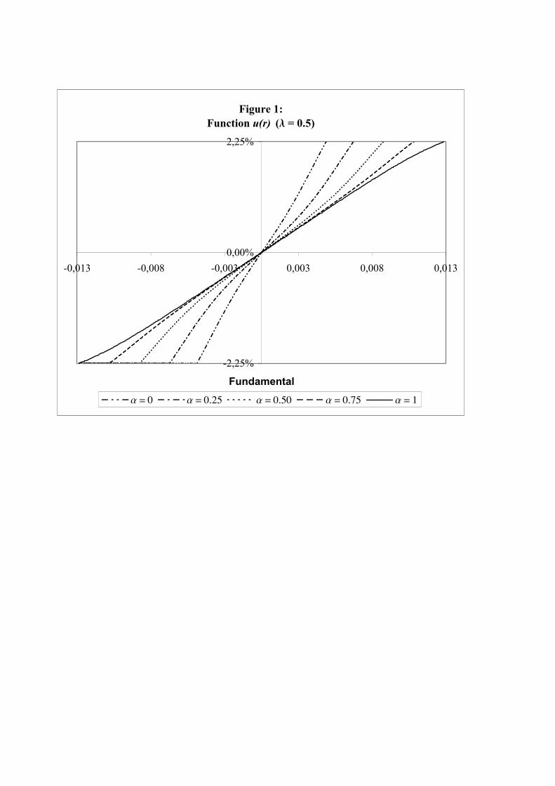
Figure 1:Function u(r) (l = 0.5)

-2,25%

0,00%

2,25%

-0,013 -0,008 -0,003 0,003 0,008 0,013

Fundamental

a = 0 a = 0.25 a = 0.50 a = 0.75 a = 1

Figure 3: λ = 10-1

Exchange rate standard deviation

0,0000,0200,0400,0600,0800,1000,1200,140

1 3 5 7 9 11 13 15 17 19 21 23 25 27 29 31 33 35

Time horizon

w = ±2.25%w = ±6%w = ±15%

Figure 2: λ = 10-4

Exchange rate standard deviation

0,00

0,05

0,10

0,15

0,20

1 3 5 7 9 11 13 15 17 19 21 23 25 27 29 31 33 35

Time horizon

w = ±2.25%w = ±6%w = ±15%

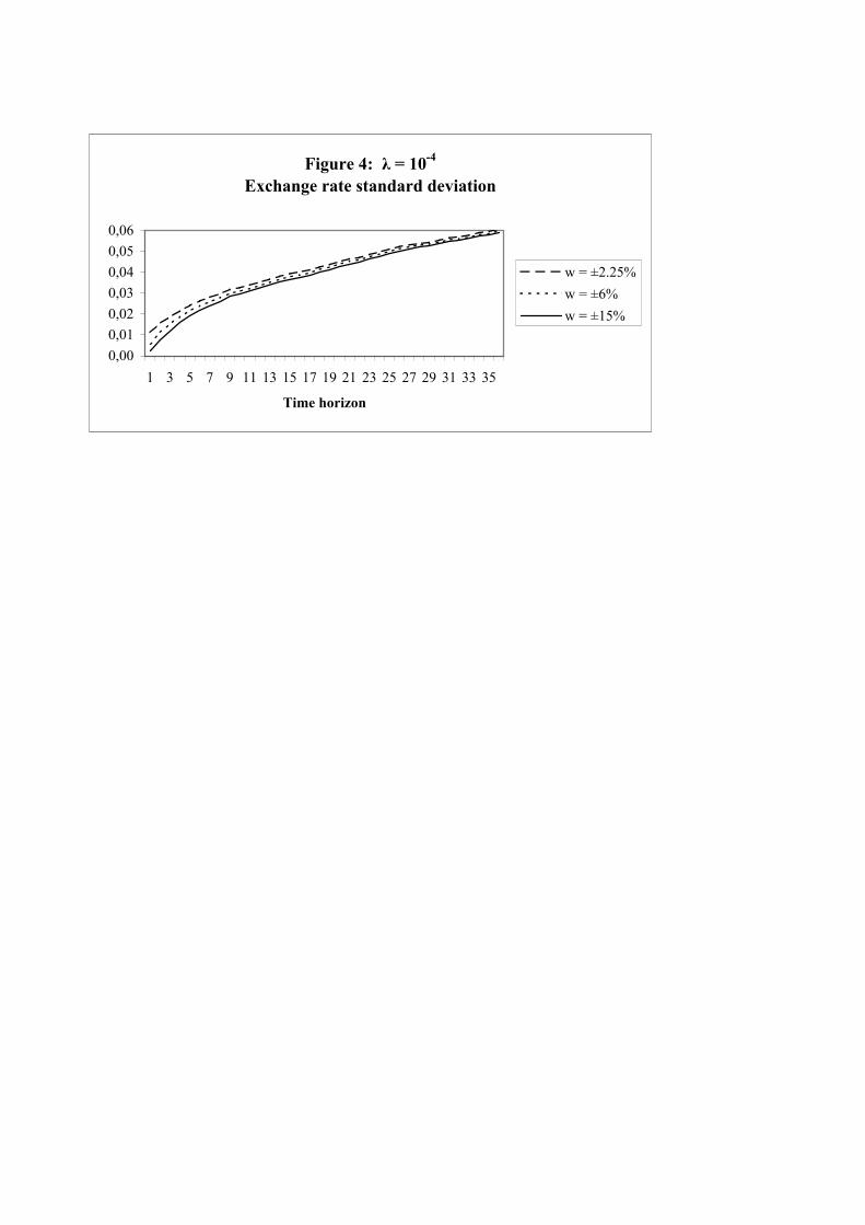
Figure 4: λ = 10-4

Exchange rate standard deviation

0,000,010,020,030,040,050,06

1 3 5 7 9 11 13 15 17 19 21 23 25 27 29 31 33 35

Time horizon

w = ±2.25%w = ±6%w = ±15%