How fast can you update your MST?(Dynamic algorithms for cluster computing)

Seth Gilbert

National University of Singapore

Singapore

seth.gilbert@comp.nus.edu.sg

Lawrence Li Er Lu

National University of Singapore

Singapore

lawrence.li@u.nus.edu

ABSTRACTImagine a large graph that is being processed by a cluster of com-

puters, e.g., described by the k-machine model or the Massively

Parallel Computation Model. The graph, however, is not static; in-

stead it is receiving a constant stream of updates. How fast can the

cluster process the stream of updates? The fundamental question

we want to ask in this paper is whether we can update the graph

fast enough to keep up with the stream.

We focus specifically on the problem of maintaining a minimum

spanning tree (MST), and we give an algorithm for the k-machine

model that can process O(k) graph updates per O(1) rounds withhigh probability. (And these results carry over to the Massively

Parallel Computation (MPC) model.) We also show a lower bound,

i.e., it is impossible to process k1+ϵ updates inO(1) rounds. Thus weprovide a nearly tight answer to the question of how fast a cluster

can respond to a stream of graph modifications while maintaining

an MST.

1 INTRODUCTIONThere are two different approaches for dealing with very large

graphs depending on whether the graph is static or dynamic.

If the graph is static, it can be distributed on a cluster of machines

that can then process the graph. In the distributed algorithms world,

this might be represented using the k-machine model [16], where

the graph is randomly distributed among k servers, each of which

can send logn bits to each of the other machines in each commu-

nication round. Alternatively, this might be represented using the

Massively Parallel Computation (MPC) model [15], which is de-

signed to capture the performance of Map-Reduce systems. In both

cases, you can efficiently find the minimum spanning tree (MST) of

a graph [6, 16].

If the graph is dynamic, a different approach is used. Most of

the research has focused on storing as little information about

the graph as possible, and treating the updates to the graph as a

stream of updates. In this case, graph sketches can be used to store

an approximate minimum spanning tree in O(n polylog(n)) space,processing updates to the edges as they arrive, one at a time [2].

The question we ask in this paper is whether these two ap-

proaches can be combined. How fast can a distributed cluster, e.g.,

a k-machine system, process a stream of updates to a minimum

spanning tree. Recently, Italiano et al. [13] gave a first answer to

this question: they showed how to maintain an approximate MST,

handling each individual update in O(1) rounds. This raised the

natural question: can we maintain an exact MST, and if so, what is

the fastest rate of updates that we can handle?

The main result of this paper, then, is an algorithm for maintain-

ing an exact MST, where the graph is distributed among k servers

and the cluster receives a stream of updates to the graph, adding

and deleting edges. Moreover, our algorithm can handle up to Θ(k)requests in O(1) rounds (with high probability), allowing for signif-

icant churn in the graph if k is large. The same basic approach can

be used in the MPC model.

To maintain the MST, we build on the nice idea proposed by

Italiano et al. [13] of using Euler tours to represent the MST. When

many edges are being added to a graph, the MST may change sig-

nificantly, and we develop a graph structural property that allows

us to quickly determine which edges need to be added and removed

from the MST. When many edges are deleted from a graph, a differ-

ent approach is needed. We reduce the problem to an MST in the

CONGESTED-CLIQUE model, carefully simulating the algorithm

by [14]. (A natural approach at simulation would take O(k) time,

and more care is needed in the reduction to achieve O(1) time.)

Thus we can handleO(k) edge insertions and deletions in onlyO(1)rounds with high probability.

A natural follow-up question is whether it is possible to do better.

We show a matching lower bound: it is impossible to handle k1+ϵ

requests in O(1) rounds. Thus, if the cluster needs to keep up with

the incoming stream, then it can only handle O(k) updates perround without falling behind the stream of updates.

2 BACKGROUND AND RELATEDWORKLarge scale graphs have recently become a topic of increasing in-

terest. Since these large scale graphs do not fit on a single machine,

the graph is stored in a distributed setting, and the algorithms are

distributed in nature. However, distributed graph algorithms of the

past, e.g., the CONGEST model [22], tend to treat each vertex as

a single machine, while these new graphs algorithms store many

vertices on a single machine, changing the nature of the distributed

graph algorithms. Two models that attempt to model these large

scale graphs are the k-machine model [16], and the popular Mas-

sively Parallel Computational(MPC) model [15]. These models have

been relatively well studied [7, 10, 17, 20, 21], and similar techniques

are involved in both models.

The connectivity and MST problems have been extensively stud-

ied in the MPC and k-machine models. More recently, building on

work in [8, 11], Jurdzinski and Nowicki [14] described an algorithm

that constructs an MST inO(1) rounds withO(n) space per machine

in the MPC model.1It is generally believed that no o(logn) round

connectivity algorithm exists in the MPC model for the sublinear

regime where each machine has O(n1−ϵ ) space. Assadi et al. [3]however, demonstrate how to obtain such round complexity when

the graphs involved are sparse.

1In fact, the algorithm is presented for the CONGESTED-CLIQUE, but it implies an

MPC algorithm.

1

arX

iv:2

002.

0676

2v1

[cs

.DC

] 1

7 Fe

b 20

20

Seth Gilbert and Lawrence Li Er Lu

Dynamic graph algorithms in this setting have recently come

up as a topic of interest. To the best of our knowledge, Italiano et

al. [13] was the first paper to look at dynamic updates in the MPC

model. They introduce the dynamic MPC model, several dynamic

problems in the MPC model, as well as their solutions to them. In

particular, they described how Euler tours can be used to solve the

dynamic connectivity and dynamic approximate MST problems in

O(1) communication rounds. The natural extension, batch dynamic

algorithms have also been very recently studied where more than

one update arrives per round. Dhulipala et al. [5] build on work on

the Euler Tour Tree data structure in the parallel setting [1, 23], and

demonstrate a batch-dynamic connectivity algorithm in the MPC

Model using sketching techniques. As of yet, we know of no existing

work on the dynamic exact MST problem or the batch-dynamic

MST problem.

Our work has more in common with the work by Italiano et

al. [13]: we generalise their results and demonstrate how Euler

tours can be used to solve the dynamic MST problem in O(1) com-

munication rounds. We also demonstrate how it is, in fact, possible

to resolve k queries in O(1) rounds with high probability, where kis the number of machines. Lastly, we show that it is not possible to

do much better than k queries in O(1) rounds, by proving a lower

bound. There can be no algorithm that can resolve k1+ϵ queries in

O(1) rounds.While they worked in the MPCmodel, we will primarily describe

our results for the k-machine model, while then describing how

our approach carries over to the MPC model.

3 MODELS AND PROBLEMSIn this section, we describe the main models for cluster computing,

and define the MST and Dynamic MST problems.

k-Machine ModelWe focus on the k-machine model described by Klauck et al. [16],

and highlight some of the differences between the k-machine model

and the MPC model. We are given a graph G = (E,V ), with nvertices andm edges.

Graph distribution: In the k-machine model, we assume that

the graph in question G is distributed across k machines in the

random vertex partition model. The n vertices of the graph are

distributed uniformly at random across these k machines, so that

each vertex has a 1/k chance of being on any one machine. If a

vertex is distributed onto a machine, so are all of the edges it is a

part of.

Communication: Communications occur in synchronous rounds.

The communication topology of these k machines is a clique, with

bidirectional links between any two machines that can only send

logn bits a round.

Space restrictions: Due to the large sizes of graphs involved, we

impose a space restraint on each machine. At any point in time,

each machine can only use an additional O(m/k) space, a con-

stant factor amount of additional space over the space required to

store the edges. Since each machine receives from up to k input

communication channels each round, we also assume that each

machine can also use O(k) space with no problems. Hence we use

O(maxm/k,k) space.

MPC ModelTheMPC model, described by Karloff et al. [15], is usually phrased

with the amount of space S being an input parameter instead of the

number of machines k . However, since these algorithms usually

only use a constant factor more space over the problem size, we can

in fact also think of the MPC model having the number of machines

k as an input parameter instead of the amount of space S .Space restrictions: The MPC model has k machines, each with up

to S space, with kS = Θ(m), where here Θ(m) hides additional logfactors.

Communication: Communications also occur in synchronous

rounds. Machines can communicate as much as they like with any

other machine, as long as for each machine, the total communi-

cations in each round is O(S). Contrast this with the k-machine

model, where machines can communicate up to a total of k lognsized messages each round, and notice that the two models scale in

opposite directions: for the k-machine model, more machines al-

lows for more inter-machine bandwidth; for the MPC model, more

machines means less inter-machine bandwidth.

Graph distribution: Since machines can exchange all of their data

in one round, the graph data can be distributed arbitrarily after a

single round at the beginning of the algorithm.

For both the k-machine model, as well as the MPC model, we

are primarily focused on minimizing the round complexity, while

respecting the space constraints.

We highlight the primary differences between the k-machine and

the MPC models here. As we will see, Lenzen’s routing lemma [18]

ensures that the methods of communication are not a real difference

between the two models, and that the primary difference is in the

scaling of the bandwidth with respect to the number of machines.

We will find that in general, algorithms in the k-machine model

tend to work on the premise that there are a small number of

machines, so that the vertex partitioning model makes more sense.

Algorithms in the MPC model tend to restrict the amount of space

on each machine, and we see most works focus on the amount of

space required on each machine for each algorithm to work. Most

work [3, 9] on the connectivity and MST problems generally work

in the regime where each machine has space that is O(n1−ϵ ).Here, we also highlight the CONGESTED CLIQUE [19] model.

While not a model intended for the study of large scale graphs, we

find that results in this model are particularly illuminating. The

CONGESTED CLIQUE model can be thought of as the special case

of the k-machine model where k = n. Instead of a random vertex

partition model, we instead have a bijection between machine and

vertex, and have eachmachine contain its vertex’s edge information.

The communication topology is a clique, with bidirectional links

between any two machines that can only send logn bits a round.

MST and Dynamic MSTTheMST problem is as follows. Given a weighted undirected graph

G, find a spanning tree such that the total sum of the weights of

the edges in this spanning tree is minimised. In the context of the

k-machine model, we ask only that the machines know if the edges

that live on their machines are in the MST or not, since storing the

actual MST itself on each machine requires too much space.

2

How fast can you update your MST?(Dynamic algorithms for cluster computing)

The dynamic MST problem introduces edge additions and edge

deletions. Whenever an edge is added or deleted, only the two

machines this edge lives on knows about the update. We ask that

the machines know if the edges that live on their machines are in

the MST or not, just as in the static case.

4 PRELIMINARIESIn this section, we discuss some of the basic communication primi-

tives in the k-machine and MPC models.

Lenzen RoutingWe begin by recalling Lenzen’s routing lemma [18].

Theorem 4.1. The following problems can be solved in O(1) com-munication rounds in a fully connected system of n nodes:

(1) Routing: Each node is the source or the destination of up to nmessages of size O(logn). Only the sources know the destina-tions of the messages and the contents.

(2) Sorting: Each node is given up to n comparable keys of sizeO(logn). Node i needs to learn the keys with indices from(i − 1)n + 1 to in.

Lenzen’s routing lemma tells us that the MPC communication

model and the k-machine communication models are only different

up to constant factors from each other, and that the only real re-

striction is the total bandwidth during each communication round.

In the k-machine model, this bandwidth scales with the number of

machines, while in the MPC model, this bandwidth scales inversely

with the number of machines.

Routing broadcastsAmachine performs a broadcast if it sends the same bits through all

of its communication links during that communication round. The

following lemma is in the spirit of the “Conversion Theorem” (The-

orem 4.1 of [16]). While they used a randomized routing approach

to obtain O(logn) bounds, we demonstrate that a deterministic

approach gives us O(1) bounds.

Lemma 4.2. Any algorithm in the k-machine model that performsa total of B broadcasts and/or max computations in R sets, with thebroadcasts and computations within each set having no dependencies,can be completed in a total of O(B/k + R) rounds.

This lemma is relatively straightforward, and its proof is available

in the appendix.

5 DYNAMIC MST: ONE AT A TIMEBefore going into the batch dynamic MST algorithm, we first de-

scribe the dynamic MST algorithm in this section that can handle

one update a time. In the following section, we show how to gen-

eralize this approach to k updates at a time. The main goal of this

section is to prove the following theorem:

Theorem 5.1. There is an algorithm that maintains a dynamicMST in O(1) communication rounds for each update. If the graph isinitially not empty, then initialization of the data structure after theMST instance has been solved takes O(n/k) rounds.

We split updates into edge additions and edge deletions, handled

separately. When an edge is added, we do cycle deletion to restore

the MST. When an edge is deleted, we add back the minimal edge

across the induced cut. As in Italiano et al. [13], where Euler tours

were used to solve the dynamic connectivity and dynamic approxi-

mate MST problems, we make use of the same basic approach. Euler

tours were first used in the dynamic MST problem by Henzinger et

al. [12]

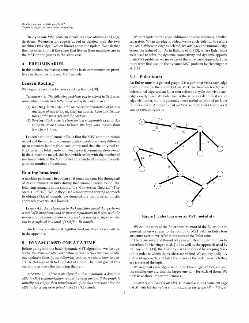
5.1 Euler toursAn Euler tour in a general graph G is a path that visits each edge

exactly once. In the context of an MST, we treat each edge as a

bidrectional edge, and an Euler tour refers to a cycle that visits each

edge exactly twice. An Euler tour is the same as a depth first search

edge visit order, but it is generally more useful to think of an Euler

tour as a cycle. An example of an MST with an Euler tour over it

can be seen in figure 1:

18

01

2345

6

7

8 9

10

12

2223

r

v

u

11

1314

15

16

1719

20

21

Figure 1: Euler tour over an MST, rooted at r

We call the start of the Euler tour the root of the Euler tour. Ingeneral, when we refer to the root of an MST with an Euler tour

structure over it, we refer to the start of the Euler tour.

There are several different ways in which an Euler tour can be

described. In Henzinger et al. [12] as well as the approach used by

Italiano et al. [13], the Euler tour was described by keeping track

of the order in which the vertices are visited. We employ a slightly

different approach, and label the edges in the order in which they

are traversed through.

We augment each edge e with these two integer values, and call

the smaller one ein , and the larger one eout for each of them. We

now have three important lemmas:

Lemma 5.2. Consider an MST M , rooted at r , and some cut edgec ∈ M with labeled values cin and cout . In the graphM ′ = M\c , an

3

Seth Gilbert and Lawrence Li Er Lu

edge e is not in the same component as the vertex s iff ein > cin andeout < cout .

Proof. LetM∗be the component separated from s . In the Euler-

ian cycle C , notice that cin denotes the time the Eulerian cycle

enters the component M∗, and cout is the time it leaves the com-

ponent M∗. As such, all the edges that are in the component M∗

will be visited between cin and cout , and will hence have values

between cin and cout .

Lemma 5.3. Consider anMSTM rooted at r . Consider any arbitraryvertex s that is not r . The edge with the highest labeling with oneendpoint touching s and the edge with the smallest labelling with oneendpoint touching s are the same edge e .

Proof. Let e be the first edge that the Euler tour crosses to enterv . This is the desired edge e , since it is the first and last time the

Euler tour visits the vertex s .

Let r be the root of the Euler cycle, and let s be any vertex, we

call the edge e as in lemma 5.3, the parent edge of s with respect

to r . In figure 1, the parent edge of v with respect to r is the edge(u,v).

Lemma 5.4. Consider an MSTM , and some Euler tour. Let r be theroot of this Euler tour. Consider any arbitrary vertex s that is not r .Let p be the parent edge of s with respect to r . An edge e is on the pathfrom r to s iff ein ≤ pin and eout ≥ pout .

Proof. Notice that an edge is on the path from r to s iff it is a

cut edge that when removed partitions r and s onto two separate

halves.

(⇐) Suppose ein < pin and eout > pout . Then, applying lemma

5.2 to the cut edge e tells us that the edge p is not in the same

partition as r with the cut edge e , so e is a cut edge that separates rand s and we are done. If ein = pin and eout = pout , then the edge

e is precisely the parent edge of s with respect to r , and is the first

time the component s is visited, and is hence also a cut edge.

(⇒) For the other direction, suppose e is a cut edge separatingr and s . If e does not touch s , then by lemma 5.2, the parent edge

p of s satisfies ein < pin and eout > pout . If e does indeed touch s ,then e must be the parent edge of s with respect to r , and we have

ein = pin and eout = pout .

Importantly, lemmas 5.2 and 5.4 give us a way to determine

where edges are in the MST, from just the two values ein and eoutof any edge.

5.2 Data structuresTo represent our Euler tour, we augment each edge in the MST

with:

(1) The two integer values from our Euler tour, and the direction.

(2) The size of the Euler tour this edge is in.

This additional edge information requires a constant factor more

space over the original edge information. For each machine, we

also store:

(1) For each neighbouring vertex, the Euler tour information of

a single arbitrary edge of that neighbour.

This requires an amount of space equal to the number of neighbours,

which is bounded by the number of edges on each machine, and

is hence again a constant factor more space over the original edge

information.

5.3 Maintaining the data structuresWe begin first by demonstrating several transformations that can

be made in the Euler tour structures, and the number of rounds of

communications required for each of them.

Lemma 5.5. Euler tours can be re-rooted after O(1) broadcasts.

Proof. Suppose we wish to reroot the Euler tour to some vertex

u. To do so, vertex u broadcasts the edge value of any outgoing

edge, say d . Each machine now subtracts d from all edge values on

its machines, taken modulo 2n − 1. This maintains the Euler tour

structure, since Euler tours are cycles.

Lemma 5.6. Consider an MST with an Euler tour structure over it.Given an edge e = (u,v) in the MST that disconnects the MST intotwo separate trees, we can delete it and maintain the two separateEuler tours after O(1) broadcasts.

Proof. The edge being deleted broadcasts its two values eminand emax . To restore the Euler tour property in both disconnected

trees, we simply apply the following function f to the weightswglobally:

f (w) =

w, forw < emin

w − emin , forw > emin andw < emax

w − (emax − emin + 1) forw > emax

Notice that this results in two Euler tours. The values in the com-

ponent connected to the root have to have their values connected

again, and have the large values shifted down by the number of

edges removed, emax −emin +1, while the values in the component

disconnected from the root have to have their values shifted down

to 0.

We also have that the sizes of the Euler tours have to be updated.

We apply the following function д to the edge with weightw and

size s globally:

д(w, s) =

s − (emax − emin + 1), forw < emin

emax − emin − 1, forw > emin andw < emax

s − (emax − emin + 1) forw > emax

The only remaining thing to maintain is the additional Euler

tour edge. In the event that machines used the edge (u,v) as theedge chosen edge, since the edge was deleted, a new replacement

edge is required. Here we just have both u and v broadcast a new

edge of theirs, and we are done.

Lemma 5.7. Consider two MSTs M1 and M2, both with an Eulertour structure over them. Given an edge (u,v) that connects the twoMSTs, we can combine the two MST and maintain the Euler tour afterO(1) broadcasts.

Proof. The machines hosting u and v both broadcast the size

of their individual Euler tours s1 and s2 respectively, as well as thevalue of an outgoing edge from u and v say a and b respectively.

The new size of the Euler tour is then s1 + s2 + 2, and the Euler tour

4

How fast can you update your MST?(Dynamic algorithms for cluster computing)

values are updated by the function fM1and fM2

for the two Euler

trees respectively:

fM1(w) =

w, forw < a

w + s2 + 2 forw >= a

fM2(w) = a + 1 + (w − b mod s2)

The new edge (u,v) has the values a and a+s2+1. This describesthe Euler tour starting from u, passing through (u,v) into M2 at

step a, and then passing back through to continue the Euler tour in

M1.

Notice that no additional work is required for the additional

Euler tour edge value chosen for each neighbour.

Lemmas 5.6 and 5.7 allow us to update the MST by deleting and

then adding edges into the MST as required. All that remains is

for us to demonstrate that the Euler tour structure allows us to

determine the edges to be deleted and added when an update in Goccurs.

5.4 UpdatesIn this section, we describe how the edges to be added/deleted

can be determined when an update arrives using the Euler tour

structure in O(1) communication rounds.

5.4.1 Edge additions. We perform edge additions as follows: We

see that in the event that any edge (u,v) is added, to maintain the

MST, we add that edge to the MST, find the unique cycle that is

created, and remove the largest weight edge from the MST. To do

so, we will on any input (u,v), have each machine determine if any

of their edges that is in the current MST is on the path from u to v ,then a leader node will find the global maximum from the largest

value from each machine. We see that each of the machines can

determine if the edge is on the path from u to v as follows:

(1) Reroot the tree to u using lemma 5.5.

(2) v determines its parent edge p and broadcasts pmin and

pmax .

(3) Edges e are on the path from u to v iff emin < pmin and

emax > pmax .

(4) A max query is run on edges in this set.

By lemma 5.4, the edges on the path from u to v are labeled

with values such that emin ≤ vmin and emax ≥ vmax . Now, each

machine can figure outwhich of their edges that are in theMST have

values that satisfy this property, and a leader node can figure out

the global maximum. The leader node compares the current largest

weight edge with the new edge, and makes the graph changes as

required.

5.4.2 Edge Deletions. To complete edge deletions, recall that to

maintain the MST after an edge e in the MST is deleted, we can

find the minimum weight edge across the cut and add it back into

the MST.

Lemma 5.2 states that given an edge c in theMST that bipartitions

the graph, edge e is not in the same component as the root r iff

ein > cin and eout < cout .Let Vi be the vertices that live on machine i , and let N (Vi ) be

the neighbouring vertices of Vi in the graph G. We determine the

minimum edge across the cut as follows:

(1) The edge being deleted broadcasts the values cin and cout .(2) For each vertex v ∈ Vi ∪ N (Vi ): Pick an arbitrary edge e

connected to v , with Euler tour value ein and eout .• If ein > cin and eout < cout or ein = cin and ein is

pointing away from v or eout = cout and eout is pointingtowards v , label vertex "with root"

• If ein < cin and eout > cout or ein = cin and ein is

pointing towards v or eout = cout and eout is pointingaway from v , label vertex "away from root

(3) A min query is run on the edges that have endpoints with

different labels.

This is the reason why we store an additional Euler tour edge

value for all neighbours, as it allows the machines to determine if

edges fall on different sides of the cut.

Since each step only requires O(1) broadcasts, we are done.

5.5 InitialisationIn the work by Klauck et al. [16], to demonstrate the power of

their conversion theorem, they described how a Boruvka style

component merging approach could allow us to construct an MST

in O(n/k) rounds. Using our Rerouting Lemma, the same approach

yields the following:

Theorem 5.8. We can construct an MST in the k-machine modelin O(n/k + logn) communication rounds.

The proof of this is a straightforward simulation of the Boruvka

style MST algorithm using our rerouting lemma. A full proof is

available in the appendix.

To complete the usage of Euler tours in our Dynamic MST prob-

lem, we demonstrate that the Euler tour structure can be initialised

in the same initial round complexity.

However, notice that a naive implementation, merging the Euler

tour data structures as the components are merged is not sufficient.

Our merge procedure only allows us to complete merges in pairs,

but the merges required after a phase of the component merging

algorithm could involve an arbitrary number of trees. The depen-

dencies that might result would not guarantee the round complexity

required. In a round where we would have to merge three com-

ponents c1, c2, c3 in a line, our previous approach would not allow

us to complete this in a single round, since we would have to first

merge the first two, then merge the resulting two components.2

We demonstrate that we are able to merge k Euler tours in O(1)communication rounds. Specifically, we prove the following lemma

about k-way merging:

Lemma 5.9. Consider any forest F with an Euler tour structureover each individual tree. Given a set of k MST edge additions or kMST edge deletions that do not create cycles, we can complete all saidupdates in O(1) communication rounds.

Proof. Suppose these updates are ordered. (If they are not or-

dered, order them lexicographically.) To complete k updates at once,

we do the following:

(1) For each edge being added and deleted, we broadcast:

2An alternate approach is to find a maximal matching of components to merge, but

this is, perhaps, simpler. And it is useful later to be able to updated multiple edges in

the MST at once.

5

Seth Gilbert and Lawrence Li Er Lu

• An outgoing edge’s Euler tour values from each endpoint.

• The size of the Euler tour of each endpoint.

• The Euler tour values of the edge if it is a deleted edge.

(2) Each machine performs the updates in order, updating the

above three values as necessary.

Notice that at any point in time, combining two Euler tours, or

separating two Euler tours only requires the above three values

to be broadcast. Each machine can keep track of these values, and

update them as necessary throughout the process to ensure that

they are still relevant after merges and separations. Notice that

outgoing edges are only involved in the edge addition case, and as

such will never be deleted.

Additional work to update the the Euler tour information of

neighbours only has to be completed if edges are deleted. Since at

most O(k) such vertices are affected, we can just broadcast them

all at the end of the process.

Since each step only requires O(k) broadcasts, by our rerouting

lemma A.2, this can be achieved inO(1) communication rounds.

This establishes the procedure for initialising the Euler tour trees,

and our entire algorithm is complete, and our algorithm is complete.

As a result, we have proven Theorem 5.1, the main result for this

section.

Notice that this k-way merging lemma allows us to initialise the

MST irregardless of how the MST is built. As such, independent

of how the MST is determined, this process always takes O(n/k)communication rounds.

We notice here that this problem seems to lend itself well to

batch updates. Updates to the tree, as well as broadcasts done to

determine which edges are to be deleted or added to restore the

MST only require O(1) broadcasts each. This seems to suggest the

possibility of resolvingO(k) updates inO(1) communication rounds

if dependencies could be avoided.

6 BATCH DYNAMIC MSTIn this section, we present ourmain contribution: the batch dynamic

minimum spanning tree algorithm. For the batch dynamic MST

problem, we have N updates arrive, with each update only arriving

at the two machines where the updated edge resides. The algorithm

is required to determine the MST after these N updates are resolved,

where each machine knows which of their edges is in the MST. The

main goal of this section is to prove the following theorem:

Theorem 6.1. There is a dynamic MST algorithm in thek-machinemodel that can satisfy k dynamic edge updates in O(1) communi-cation rounds, initialisation in O(n/k + logn) rounds (if the graphis initially non-empty), while using maxk,m/k + ∆ space, i.e., atmost a constant factor more space more than the original space neces-sary to store the graph G. The algorithm is deterministic worst caseO(1) in the edge addition case, and is a Las Vegas randomized algo-rithm for the edge deletion case, completing in O(1) rounds with highprobability for each attempt.

For both edge additions and deletions, our k-way updating algo-

rithm described in Section 5.5 allows us to reconstruct the trees as

necessary once we know which edges to add or remove. As such,

we only have to describe the procedure to determine which those

edges are.

6.1 Edge AdditionsWe now prove the following lemma:

Lemma 6.2. Given a set of k edge updates, we can determine thenew MST in O(1) communication rounds. Each machine will know ifeach of its edges are in the MST or not.

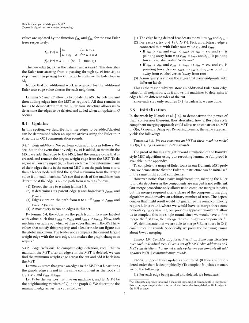
When k edges are added, it is not immediately clear how we can

simultaneously find a set of k edges to delete so that the remaining

graph is both cycle free and connected. For example, if we were

to pick the original k cycles induced by a single new edge, as well

as the existing MST edges, the maximal weight edges in all these

cycles might be the same edge. Here in figure 2, where the bold lines

represent edges in the original MST and the dotted lines represent

new edges being added, the edge labeled (2, 19) is in all three cycles,

and might be the only edge deleted, if it were the heaviest weight

edge in the graph.

It is also difficult to describe the cycles to run max queries on.

Cycles could be described through the series of added edges they

pass through, but such descriptions could be of length Θ(k).

0

1

23

4

56

7

8

910

11

12

13

141516

1718

19

20

21

Figure 2: Example 2: Bold edges are edges in the MST, solidedges are edges in the graph G, dotted edges are new edgesbeing added

The main insight is to notice that there are only essentiallyO(k)edges that matter. We first begin with some intuition as to what this

means. Consider again Figure 2. We first remove edges that are not

in any cycles, since they are irrelevant, and can never be considered

for removal. We look at the graph as if it were the original MST,

with k additional edges attached. In Figure 3, we can see this process

in action.

Crucially, we wish to decompose the original MST into O(k)non-intersecting paths such that at most one edge can be removed

from each of the paths. As an example, refer to the decomposition

of example 2 into the 5 paths described described by the third image

6

How fast can you update your MST?(Dynamic algorithms for cluster computing)

M M’ M’’

path 1

Figure 3: Example 2, removing irrelevant edges to obtain M ′, then contracting to obtain M ′′. The shaded vertex is the solevertex in B

in figure 3. Notice for example, that amongst the three edges in path

1, only one of the three edges can be deleted, if not the graph will

become disconnected. After which, we can consider the contracted

graph to the right, and solve the MST problem on that graph instead.

We now prove the key claim of this section:

Lemma 6.3. Given any MST, and any set of k edges to connectvertices in the MST, we can decompose the edges of the MST intoO(k)disjoint sets such that:

• At most one edge from each set can be removed while main-taining connectedness in the MST and the new edges.

• Each edge is in some set.

Proof. To perform this decomposition, we first remove all edges

that are not part of cycles, and place them all in one set. Call the

remaining forestM ′. We splitM ′

into paths by the following set of

vertices:

• Vertices that are one endpoint of the k edges being added,

call this set A.• Vertices that have degree more than 2 in M ′

, for example

the shaded vertex in example 2, call this set B.

M ′consists of all edges which are a part of a cycle, which are

edges that are on the shortest path from some two vertices in A.Any leaf in this forest must be some element in A, if not the edgeconnecting to that leaf cannot be on the shortest path from some

two vertices in A, and hence cannot be involved in a cycle.

Now, since A is maximally of size 2k , we have that the number

of leaves inM ′is at most 2k. Since B consists of the vertices that

have degree two in M ′, the number of elements in B is bounded

by the number of leafs in M ′by a degree double count. Hence,

|A| + |B | = O(k). Trivially the sets are disjoint.

We can now think of the induced tree T , with the vertices being

the elements in A and B, and the edges being the paths connecting

elements in A∪ B and A∪ B inM ′. Since this new graph is a forest,

the number of edges it can have is bounded by the number of

vertices, and is hence O(k). Hence the number of sets constructed

is O(k). In figure 3, the graphM ′′consists of the solid edges of T ,

and the dotted edges that are the newly added edges.

Next, notice that each of these sets is a path from some element

inA∪B to some element inA∪B. We wish to show that at most one

edge can be removed from any such set. Suppose otherwise, and

the two edges that can be removed are the edges (w,x) and (y, z)appearing in that order on the path. Since the remaining graph

is still connected, there must be some path inM from x tow , not

passing through y. Consider any such path, and let s be the lastvertex on the path from w to z that is visited on this path during

the first time it leaves the path. Consider the partitioning of the

MST induced by the edge (x ,w), and let t be the last vertex visitedin the component withw on this said path, at the first time it leaves

said component.

Now, t cuts across this partition, and the edge it crossed the

partition with is not part of the MST, so it is one endpoint of one of

the k edges, and is in A. As such, s is then either t , and is in A, andwe obtain a contradiction, or the path from s to t consists of edgesthat are part of cycles, and the degree of s is greater than 2, and s isin B, also a contradiction.

As such, each of these sets can have at most one edge removed,

whilst maintaining connectivity in the original MST edges and the

k new edges.

Lastly, since each edge that is part of some cycle is in theseO(k)sets, and all the other edges are in the first set, all edges are part of

some set and we are done.

Our strategy is to run a max-query on each of theseO(k) sets. Af-ter which, we only have to consider theseO(k) edges, as well as theoriginal new k edges that are being added, and solve a contracted

MST M ′′of size O(k) that can fit on a single machine. All these

edges, as well as their endpoints can then be sent to all machines,

and then each machine can resolve the MST on their own simul-

taneously. We reduce the problem to a problem on the contracted

graphM ′′with only O(k) edges.

The algorithm goes in rounds as follows:

7

Seth Gilbert and Lawrence Li Er Lu

(1) All the k new edges being added are broadcast to all ma-

chines, so that all machines know the set A.(2) Vertices in A broadcast the Euler tour values of one of its

edges.

(3) Vertices in A determine if their edges are part of shortest

paths between any elements in A, and broadcast all such

edges.

(4) All vertices determine if they are in B.(5) All vertices in A and B broadcast the Euler tour values of all

edges connected to them that are part of a shortest path.

(6) All machines build a picture of the tree induced, and conducts

O(k) max queries for the O(k) sets.(7) All of the maximums in the O(k) sets are broadcast, and

each machine determines the new MST, and the edges to be

deleted.

(8) Euler tours are updated.

We now describe how steps 3 and 4 work in detail. In step 3,

vertices in A determine if their edges are part of shortest paths

between any two vertices inA. Notice that all such edges are on the

shortest path from themselves to some other element in A. Hence,to determine if their edges are shortest path edges, they simulate the

rerooting process, rerooting the tree to each of the other possible

values in A, and checking to see if the edges they have are indeed

parent edges with respect to some other member of A. The edgesthat are parent edges after some reroot to some element in A are

the edges that are on shortest paths.

Notice too that there are only O(k) such edges, since there are

onlyO(k) paths inM ′. Hence broadcasting all these edges will take

O(1) communication rounds.

To determine if a vertex in B, it has to check that it has degree

larger than 2 in the graph induced only by shortest paths. To do so,

it has to check that it has at least 3 edges connecting to it that are

on shortest paths between elements in B.Recall Lemma 5.4, which states that if r is the root of the Euler

tour, then an edge e is on the path between r and s iff ein < pin and

eout > pout , where p is the parent edge of s . However, we cannotdirectly apply this result, since the values of cin and cout are onlyknown to the machine hosting s after rerooting the tree. To obtain

all the values cin and cout would require up to k broadcasts for

each of them, for each other possible value of r in A, for a total ofk2 broadcasts.

What is important is that the edge that is broadcast after the

rerooting process is always the parent edge. As such, to avoid

this problem, each machine simulates the rerooting process, and

determines what the values of cin and cout would be, since they

have been given all parent edges in step 3.

To complete step 4, for each vertex v , for each edge connected

to it, the machine checks for all the pairs of values in A\v, andsimulates the tree rerooting process, and checks to see if the edge

is indeed on the shortest path between the two vertices. Now, each

vertex will know its degree, and can determine if it’s in B.After the sets A and B are determined, all vertices broadcast

all the parent edges of any member of A ∪ B with respect to any

member of A ∪ B. Again, since there are only O(k) intervals, therecan only be O(k) such values.

In step 6, given the values of the Euler tour, each machine can

independently build a picture of the induced tree, by placing the

edges and vertices in the correct order. It then for each of the O(k)sets, determines membership of the set using lemma 5.4, since it has

all parent edges. It then finds the maximum weight edge in this set,

and sends it to somemachine for collation to find a global maximum

in each set. Notice here that we can assign which machine does

the collation deterministically, we simply order the paths based on

the order in which they appear in the Euler tour, and take mod

k . This results in O(k) max queries that can be completed in O(1)communication rounds.

After which, each machine knows precisely which edges are

relevant, and can obtain the new MST. We simply delete the correct

edges, with ties broken by lexicographical order, and maintain the

Euler tour structure.

6.2 Edge DeletionsWe now focus on edge deletions:

Lemma 6.4. Given a set of k edge deletions, after O(1) communi-cation rounds with high probability, we can determine the new MST.Each machine will know if each of its edges are in the MST or not.

Edge deletions only affect the MST if the deleted edges were

originally in the MST. After k edge deletions occur, our MST is

decomposed into k + 1 components defined by the deleted edges,

and we have to findminimum edges that reconnect our components.

This can be reduced to solving a new MST instance on k machines

and a graph with k + 1 vertices. This is the same as solving the MST

problem in the CONGESTED CLIQUE model(with the exception

that we allow for logn bits of communication, over logk bits of

communication). This problem has been solved very recently by

JurdziÅĎski and Nowicki in 2017 [14] using a randomized approach.

Their algorithm does not use more than O(k) space.To complete the reduction, we have to demonstrate how to con-

vert our setting to the CONGESTED CLIQUE setting, where each

machine has all the edges of its vertex. Notice here why this is not

trivial. From our Euler tour data structure, we can tell for each edge,

the two components it bridges. However, we cannot tell what the

minimum weight edge that bridges any two components i and jare, without first conducting a min query that takes a broadcast.

Doing k2 min queries to determine all the edges in our new graph

takes O(k) rounds.Here, we circumvent this problem by noticing the following fact.

On each machine, there can only be k edges that can possibly be

in the MST. If there are more than k edges that are candidates for

the MST, there must be a cycle, and the machine knows that the

largest weight edge on this cycle cannot be in the MST. Now, there

are at most k candidate edges on each machine, instead of k2, andwe can apply Lenzen’s routing theorem.

Notice also that we cannot apply Lenzen’s routing theorem di-

rectly, since there might be more than k edges that connect to

a component. Multiple machines may have candidate edges that

bridge some two components i and j. The algorithm is as follows:

(1) Broadcast all Euler tour values of k edges being deleted and

label disconnected components in Euler tour order.

(2) Determine which components each edge lies across.

8

How fast can you update your MST?(Dynamic algorithms for cluster computing)

0

1

23

4

56

7

8

910

11

12

13

141516

1718

19

20

21

1

2

3

( )192

(10

)130 21Euler Tour Values

BracketComponent 1 2 3 2 1

Figure 4: Example 3, Determining components using Euler Tour Values

(3) Each machine does cycle deletion to obtain up to k candidate

edges.

(4) Apply Lenzen’s routing theorem to sort the k candidate

lexicographically.

(5) Each machine keeps only the smallest weight edge across

any two components.

(6) Each machine communicates with its two neighbouring ma-

chines (by index), to ensure that there are no duplicates.

(7) Use Lenzen’s routing theorem to send all edges touching

component i to machine i .(8) Run JurdziÅĎski and Nowicki’s MST algorithm.

Steps 1 and 2 can be completed applying similar ideas to the

single edge deletion case described in Section 5.4.2. We construct

equivalence classes as follows. Each machine first receives the Euler

tour values of the k edges being deleted, and lists them out in order.

The smaller value of each pair of values is then represented with

an open bracket, and the larger value of each pair is represented

with a close bracket. All values that are contained in the same pair

of brackets, and are at the same nested depth are in the same equiv-

alence class. Each equivalence class then corresponds to the Euler

tour values of a connected component. Components are labeled in

order. Figure 3 illustrates this process.

Just as in Section 5.4.2, we can determine which components

each edge lies across with the neighbouring edge’s Euler tour values.

With the Euler tour values ein and eout , we can determine which

component the endpoint is in, by looking at where this value lies

in the set of brackets determined above. In the event that the edge

chosen is one of the boundary edge values(eg. 13 in figure 4), the

direction of the edge is used to determine the side of the component

it lies on.

Once all the edges are labeled with the components they cut

across, each machine can do cycle deletion on all of the edges EE(M) that they have on their machines, to determine at most kcandidate edges that could possibly be in the new MST.

7 LOWER BOUNDSFor a lower bound, we demonstrate that it is not possible to complete

much more than O(k) queries in O(1) rounds.

Theorem 7.1. For any constant δ , there is a sequence of 3k batchupdates, each of sizek1+δ , such that the total time required to completethese 3k batch updates is ω(k).

In [16], it was proven that the lower bound for the MST in-

stance problem in the k-machine model is O(n/k), and that the

class of graphs which requires this time complexity is the follow-

ing class of graphs Gb (X ,Y ), where X and Y are two b bit long

binary string. The graph Gb (X ,Y ) consists of b + 2 vertices, de-

noted by v1,v2, ...vb ,u,w . There is an edge from u to w , and for

each 1 ≤ i ≤ b, there is an edge from u to vi iff Xi = 1, and there is

an edge fromw to vi iff Yi = 1. There is also a guarantee that the

graph is connected, and that for each i , Xi ∨ Yi = 1.

Importantly, this class of graphs has a number of edges linear in

the number of vertices.

9

Seth Gilbert and Lawrence Li Er Lu

The series of 3k batch updates is then as follows. We pick k1+δ/2

vertices, and use the first k batch updates to delete all edges that

have both endpoints in this set of vertices, giving us an empty

clique of size k1+δ/2. The next 2k updates occur in pairs where

we add in a random instance of the above kind, then delete it.

When we add in the graph, we add it in with weights that are a

global minimum. Since these new edges are all globally minimum,

at the end of this batch of updates, this MST instance has to be

included in the global MST, and each of these batch updates has

to take Ω(kδ/2/logn) communication rounds, by the result in [16].

This series of k additions and deletions will then require at least

Ω(k1+δ/3/logn) communication rounds, which is ω(k).While for the proof in [16], k was treated as a constant, and

the result was with high probability in n, it is easy to verify that

the entire proof still holds with high probability in k when we set

n = k1+δ/2. We include a copy of the proof in the appendix.

8 MPC MODELThe above algorithm in the k-machine model maps over almost

exactly to the MPC model. The key issue to focus on is the space

usage: in the k-machine model, we need Θ(m/k + ∆) space on each

machine. In the sublinear regime for theMPCmodel, we are not able

to store all the edges of a high degree vertex on a single machine.

To adjust from the k-machine model to the MPC model, we have to

shift from a vertex partitioningmodel to an edge partitioningmodel,

which we can do since the MPC model allows for information to

be arbitrarily reorganized. The number of queries we can resolve

also scales differently, as the communication bandwidths for the

k-machine model and the MPC model scale differently.

Theorem 8.1. In the MPC model with k machines and S = Θ(nα )space on each machine for some constant α , such that kS = Θ(m),there is a dynamic MST algorithm that can satisfy S dynamic edgeupdates in O(1) communication rounds while using S space, at mostconstant factor more space over the original space necessary to storethe graphG . The algorithm is deterministic worst caseO(1) in the edgeaddition case, and a Las Vegas style algorithm for the edge deletioncase, with it being O(1) with high probability for a success in eachattempt. The data structure required can be initialised in O(logn)rounds.

We modify some parts of the k-machine algorithm to guarantee

that the space requirements are satisfied, and follow an edge parti-

tioning model. Each machine stores a set of edges of the graph. We

however do not completely disregard the vertex partitioning model.

To make it easier to complete certain vertex operations, we dupli-

cate all edges, and store the edges on themachines lexicographically,

so that any vertex is on a contiguous set of machines.

Some adjustments to the data structure have to be made to sat-

isfy the edge partitioning model. Instead of storing the Euler tour

information of a single arbitrary edge for each neighbour, we move

this information onto each edge instead. For any edge (u,v), weadditionally store an arbitrary Euler tour edge of u and an arbitrary

Euler tour edge of v .A crucial difference here is in the initialisation process. Applying

the initialisation argument in the k-machine model gives us an

initialisation time of O(n/S) rounds. However, MSTs in the MPC

model can be solved inO(logn) rounds in general, much faster than

this initialisation time.

To initialise the Euler tour data structure in O(logn) rounds, weuse a modified version of the BorÅŕvka style component merging al-

gorithm. The primary obstacle is to ensure that the edges we choose

to merge do not create dependencies. Merging two components is

the same as in the k-machine case, but in the MPC model, we can

also merge stars. For any component x , and an arbitrary number

of components connected to this component x we can merge them

in O(1) rounds. We describe this merging process later.

To determine the stars (these do not have to include all neigh-

bours of the central vertex) that are to be merged, we do the fol-

lowing. In one iteration of BorÅŕvka’s algorithm, we determine the

minimum outgoing edge from each component. This set of edges

forms a forest F . We orient the edges in this forest F by orienting

the edges along the minimum outgoing edge directions, with edges

pointing towards each other determined by vertex id. Then, we

apply the Cole-Vishkin coloring algorithm [4] on this oriented tree

to get a 3-coloring of the forest F .Now, WLOG, let a be the most frequently appearing color in this

coloring of F . Each component colored with a picks its minimum

outgoing edge, and merges through this edge.

The resulting set of chosen edges cannot have any paths of length

3, and is hence a collection of stars. There are Θ(n) such edges too,

resulting in O(logn) BorÅŕvka steps in total. What remains is to

demonstrate that each round of merging can be completed in O(1)rounds.

We sort the components lexicographically. For each component,

we call the first machine that holds that component the leader

machine for that component. From the previous step, we have

obtained some collection of stars Si , with the centre of each

star Si being the component si . Now, each si is unaware of the

components it is supposed to merge with, but its leader node can

obtain the vertices it is supposed to merge with through a converge-

cast.

Importantly here, what allows us to complete the converge-

cast successfully for an arbitrary number of components, despite

the leader node having only O(S) bandwidth, is the nature of theEuler tour values required. We illustrate this process. Suppose some

component wishes to merge with S1 through the edge (u,v), withu ∈ S1. Notice that to complete the merge, each component merging

with u only needs to know its displacement in the Euler tour. The

machine hosting the edge (u,v) on the v side sends the size of the

component on the v side to the machine hosting the edge (u,v) onthe u side. The machine hosting the edge (u,v) sums the sizes, for

the converge-cast towards the leader node. After receiving the total

sizes, the leader node can calculate the required displacements in

the Euler tour, and send back the correct values.

In the k-machine model algorithm, we extensively use broadcast

and converge-cast steps. In theMPCmodel, it is easy to see thatO(S)broadcasts and converge-casts can be completed in O(1) roundsusing broadcast and converge-cast trees[6]. This is because S = nα

for some constant α , and these trees grow by a factor of nα each

round, so these broadcasts take O(1/α) rounds.There are only two places in our algorithm where we make use

of the fact that a single machine holds all the information about a

vertex. We check that it is fine in both cases:

10

How fast can you update your MST?(Dynamic algorithms for cluster computing)

• For k-way merging, broadcasting an outgoing edge’s Euler

tour value from each endpoint of an added edge can be done

by the leader machine for that node.

• For the edge addition case, vertices verifying that they are

indeed in B is a simple degree check, which can be completed

in a single round by sending the leader machine for that

vertex the number of edges that are in B.

We highlight a section of interest. In the edge deletion case, we

reduce to solving an MST instance of size S . While solving the MST

instance in O(1) rounds in the sublinear regime is currently an

open problem, notice that our batch size scaling to our bandwidth

guarantees that we are always in the linear regime, which has been

solved.

9 CONCLUSIONIn this paper, we have explored how fast a cluster computing en-

vironment can maintain a minimum spanning tree subject to a

sequence of updates. Essentially, it comes down to the communica-

tion bandwidth. In the k-machine model, we can handle O(k) edgeupdates in O(1) rounds. In the MPC model where each machine

has space S , we can handle O(S) edge updates in O(1) rounds. (Ofnote, our contributions do not involve sketching techniques, as is

common in earlier approaches, although the MST subroutine we

use for the deletion case does.) We also demonstrate a lower bound

for the k-machine model, showing that it is not possible for an

algorithm to resolve k1+ϵ queries in O(1) communication rounds.

One observation is that the Euler tour data structure is especially

useful in the context of dynamic MST in this distributed setting.

Future directions include expanding the approach to the problem

of Steiner trees in the k-machine model, a structure very similar

to minimum spanning trees. Alternatively, under a different set of

restrictions [21], it is possible to construct an MST in the k-machine

model faster, in O(n/k2) communication rounds. We wonder if it

also possible to achieve this in the dynamic situation, obtaining

O(k2) updates in O(1) rounds. (In this case, only one endpoint

knows that an edge is in the MST. Surprisingly, this allows [21]

to beat the Ω(n/k) lower bound.) We also would like to explore

whether the approaches described here translate well into other

distributed models.

Acknowledgments. Thanks to Michael Bender and Martin Farach-

Colton for conversations about data stream processing. Thanks to

Faith Ellen for useful feedback.

REFERENCES[1] Umut A. Acar, Daniel Anderson, Guy E. Blelloch, and Laxman Dhulipala. 2019.

Parallel Batch-Dynamic Graph Connectivity. CoRR abs/1903.08794 (2019).

arXiv:1903.08794 http://arxiv.org/abs/1903.08794

[2] Kook Jin Ahn, Sudipto Guha, and Andrew McGregor. 2012. Graph Sketches:

Sparsification, Spanners, and Subgraphs (PODS âĂŹ12). Association for Comput-

ing Machinery, New York, NY, USA, 5âĂŞ14. https://doi.org/10.1145/2213556.

2213560

[3] Sepehr Assadi, Xiaorui Sun, and Omri Weinstein. 2019. Massively Parallel Al-

gorithms for Finding Well-Connected Components in Sparse Graphs (PODCâĂŹ19). Association for Computing Machinery, New York, NY, USA, 461âĂŞ470.

https://doi.org/10.1145/3293611.3331596

[4] Richard Cole and Uzi Vishkin. 1986. Deterministic Coin Tossingwith Applications

to Optimal Parallel List Ranking. Inf. Control 70, 1 (July 1986), 32âĂŞ53. https:

//doi.org/10.1016/S0019-9958(86)80023-7

[5] Laxman Dhulipala, David Durfee, Janardhan Kulkarni, Richard Peng, Saurabh

Sawlani, and Xiaorui Sun. [n.d.]. Parallel Batch-Dynamic Graphs: Algorithms

and Lower Bounds. 1300–1319. https://doi.org/10.1137/1.9781611975994.79

arXiv:https://epubs.siam.org/doi/pdf/10.1137/1.9781611975994.79

[6] Mohsen Ghaffari and Davin Choo. [n.d.]. Massively Parallel Algorithms. https:

//people.inf.ethz.ch/gmohsen/MPA19/Notes/MPA.pdf

[7] M. Ghaffari, F. Kuhn, and J. Uitto. 2019. Conditional Hardness Results for

Massively Parallel Computation from Distributed Lower Bounds. In 2019 IEEE60th Annual Symposium on Foundations of Computer Science (FOCS). 1650–1663.https://doi.org/10.1109/FOCS.2019.00097

[8] Mohsen Ghaffari and Merav Parter. 2016. MST in Log-Star Rounds of Congested

Clique (PODC âĂŹ16). Association for Computing Machinery, New York, NY,

USA, 19âĂŞ28. https://doi.org/10.1145/2933057.2933103

[9] Mohsen Ghaffari and Jara Uitto. 2018. Sparsifying Distributed Algorithms with

Ramifications in Massively Parallel Computation and Centralized Local Compu-

tation. CoRR abs/1807.06251 (2018). arXiv:1807.06251 http://arxiv.org/abs/1807.

06251

[10] Michael T. Goodrich, Nodari Sitchinava, and Qin Zhang. 2011. Sorting, Searching,

and Simulation in the MapReduce Framework. In Algorithms and Computation,Takao Asano, Shin-ichi Nakano, Yoshio Okamoto, and Osamu Watanabe (Eds.).

Springer Berlin Heidelberg, Berlin, Heidelberg, 374–383.

[11] James W. Hegeman, Gopal Pandurangan, Sriram V. Pemmaraju, Vivek B. Sardesh-

mukh, and Michele Scquizzato. 2015. Toward Optimal Bounds in the Congested

Clique: Graph Connectivity and MST (PODC âĂŹ15). Association for Computing

Machinery, New York, NY, USA, 91âĂŞ100. https://doi.org/10.1145/2767386.

2767434

[12] Monika Rauch Henzinger and Valerie King. 1995. Randomized Dynamic Graph

Algorithms with Polylogarithmic Time per Operation (STOC âĂŹ95). Associationfor Computing Machinery, New York, NY, USA, 519âĂŞ527. https://doi.org/10.

1145/225058.225269

[13] Giuseppe F. Italiano, Silvio Lattanzi, Vahab S. Mirrokni, and Nikos Parotsidis.

2019. Dynamic Algorithms for the Massively Parallel Computation Model. CoRRabs/1905.09175 (2019). arXiv:1905.09175 http://arxiv.org/abs/1905.09175

[14] Tomasz Jurdzinski and Krzysztof Nowicki. 2017. MST in O(1) Rounds of the

Congested Clique. CoRR abs/1707.08484 (2017). arXiv:1707.08484 http://arxiv.

org/abs/1707.08484

[15] Howard Karloff, Siddharth Suri, and Sergei Vassilvitskii. 2010. A Model of Com-

putation for MapReduce. 938–948. https://doi.org/10.1137/1.9781611973075.76

[16] Hartmut Klauck, Danupon Nanongkai, Gopal Pandurangan, and Peter Robinson.

2015. Distributed Computation of Large-Scale Graph Problems (SODA âĂŹ15).Society for Industrial and Applied Mathematics, USA, 391âĂŞ410.

[17] Silvio Lattanzi, Benjamin Moseley, Siddharth Suri, and Sergei Vassilvitskii. 2011.

Filtering: A Method for Solving Graph Problems in MapReduce (SPAA âĂŹ11).Association for Computing Machinery, New York, NY, USA, 85âĂŞ94. https:

//doi.org/10.1145/1989493.1989505

[18] Christoph Lenzen. 2013. Optimal deterministic routing and sorting on the con-

gested clique. Proceedings of the 2013 ACM symposium on Principles of distributedcomputing - PODC âĂŹ13 (2013). https://doi.org/10.1145/2484239.2501983

[19] Zvi Lotker, Elan Pavlov, Boaz Patt-Shamir, and David Peleg. 2003. MST Con-

struction in O(Log Log n) Communication Rounds (SPAA âĂŹ03). Associationfor Computing Machinery, New York, NY, USA, 94âĂŞ100. https://doi.org/10.

1145/777412.777428

[20] Gopal Pandurangan, Peter Robinson, and Michele Scquizzato. 2015. Al-

most Optimal Distributed Algorithms for Large-Scale Graph Problems. CoRRabs/1503.02353 (2015). arXiv:1503.02353 http://arxiv.org/abs/1503.02353

[21] Gopal Pandurangan, Peter Robinson, and Michele Scquizzato. 2018. Fast Dis-

tributed Algorithms for Connectivity and MST in Large Graphs. ACM Trans.Parallel Comput. 5, 1, Article Article 4 (June 2018), 22 pages. https://doi.org/10.

1145/3209689

[22] David Peleg. 2011. Distributed computing 25th international symposium, DISC2011, Rome, Italy, September 20-22, 2011: proceedings. Springer.

[23] Thomas Tseng, Laxman Dhulipala, and Guy Blelloch. [n.d.]. Batch-ParallelEuler Tour Trees. 92–106. https://doi.org/10.1137/1.9781611975499.8

arXiv:https://epubs.siam.org/doi/pdf/10.1137/1.9781611975499.8

A OMITTED PROOFSA.1 Rerouting Lemma

Lemma A.1. Any algorithm in the k-machine model that performsa total of B broadcasts in R sets, with the broadcasts within each sethaving no dependencies, can be completed in a total of O(B/k + R)rounds.

Proof. We can use a re-routing strategy to resolve this problem.

Suppose machine i has to complete Ci,r broadcasts during round r .

11

Seth Gilbert and Lawrence Li Er Lu

If we naively complete all the broadcasts, we will require a total of∑Rr=1maxi Ci,r communication rounds.

Notice that in the event where one machine i has to complete

significantly more broadcasts than the other machines, a rerouting

strategy is useful. Instead of machine i broadcasting information, it

instead sends k sets of different information to each of the other

machines, and those machines can broadcast the information in-

stead. If Br =∑ki=1Ci,r total broadcasts are to be completed in a

set, we show that this can in fact be achieved in O(Bi/k) rounds.The algorithm proceeds as follows:

(1) Each machine broadcasts the number of broadcasts it has to

do in this set to each other machine.

(2) The messages to be broadcast are globally ordered, by ma-

chine number, then bymessage number. Repeat the following

two round procedure Bi/k times. During iteration i:(a) Message ordered i ∗ k + j is sent to machine j from the

source machine.

(b) Each machine broadcasts the message it received.

Notice that step 1 is essential to the success of this algorithm,

since it guarantees that no two messages will be sent to the same

machine in step 2a). The ordering within each machine does not

need to be known by all machines, but the number of messages on

other machines that have priority over it does.

Importantly, this strategy also applies to converge-casts. In par-

ticular, this rerouting and re-balancing strategy also works for sub-

routines such as a max computation, where each machine produces

a value, and a global maximum is desired.

Suppose machine i needs to know the maximum of these values,

but is also caught up with doing several broadcasts of its own. It

can reroute this max computation to any other machine j , and haveall machines send j this information instead. The process occurs as

follows:

(1) Machine i tells machine j that it requires the max computa-

tion

(2) Machine j broadcasts to all other machines, requesting for

this information, using up the communication edges of j forO(1) rounds.

(3) All machines send this information to machine j, using upthe communication edges of J for another O(1) rounds.

(4) Machine j then sends this information back to machine i .

This completes the converge-cast. This gives us the stronger

lemma:

Lemma A.2. Any algorithm in the k-machine model that performsa total of B broadcasts and/or max computations in R sets, with thebroadcasts and computations within each set having no dependencies,can be completed in a total of O(B/k + R) rounds.

This lemma also implies that the MST construction problem can

be solved inO(n/k + logn) rounds by simulating the Boruvka style

component merging algorithm, instead of the O(n/k) rounds asdescribed in [16].

A.2 MST algorithmTheorem A.3. We can construct an MST in the k-machine model

in O(n/k + logn) communication rounds.

Proof. We begin with each vertex being its own component.

In each phase, we take each component and find the minimum

outgoing edge, and add it to the MST, merging the two components.

Finding the minimum outgoing edge is essentially a single min-

query, and the merging of two components can be done in a single

broadcast, to update the component names.

After each phase, the number of components decreases by at least

a factor of two, there are at most logn phases. The total number

of min-queries across these logn phases is O(n), since we have itbounded by

∑logni=0

n2i = O(n)minimum outgoing edge queries. The

total number of merges isn, so the algorithm requires a total ofO(n)broadcasts and min-queries, and can be completed inO(n/k+ logn)rounds applying our rerouting lemma A.2.

A.3 Lower bound theorem proofHere, we replicate the proof in [16] that at least Ω(k1+δ/3/logn)communication rounds are required to determine an MST of with

k1+δ/2 vertices.

Theorem A.4. Every public-coin ϵ-error randomized protocol ona k-machine network, sending logn bits per round, that computes aspanning tree of a k1+δ/2-node input graph has an expected roundcomplexity of Ω(kδ/2/logn)

Proof. Let b = k1+δ/2 − 2. The class of graphs is Gb (X ,Y ),whereX andY are two b bit long binary string. The graphGb (X ,Y )consists of b + 2 vertices, denoted by v1,v2, ...vb ,u,w . There is an

edge from u tow , and for each 1 ≤ i ≤ b, there is an edge from uto vi iff Xi = 1, and there is an edge fromw to vi iff Yi = 1. There

is also a guarantee that the graph is connected, so that for each i ,Xi ∨ Yi = 1. The total number of graphs in this class of graphs is

3b.

With probability 1 − 1/k , the vertices u andw are on different

machines., say p1 and p2. To guarantee that the output is a spanningtree, the machines hosting u andw have to figure out which of the

edges to use in the spanning tree. The proof will demonstrate that to

accomplish this, there has to be a large amount of information flow.

Specifically, the proof demonstrates that the conditional entropy

has to change by a large amount.

Before any communications occur, the conditional entropyH (Y |X )is 2b/3:

H (Y |X ) =∑x

Pr (X = x) · H (Y |X = x)

= 3−b

b∑l=0

(b

l

)2l · log 2l

= 3−bb

∑l = 0

b−1(b − 1

l

)2l+1

= 2b/3Since the k-machine model employs the random vertex partition

model, the machine hosting u, p1 knows not only X , but also some

vertices of vi and their edges, giving it some bits of Y . Let A be

the random variable denoting the amount of information that p1has. Employing a Chernoff bound, we can see that p1 knows at

most (1+ζ )b/k bits of Y for some small constant ζ with probability

1 − 2ζ 2b/3k ≥ 1 − 2

ζ 2kδ /2/3. This error probability is exponentially

12

How fast can you update your MST?(Dynamic algorithms for cluster computing)

small in k . In this error situation, at most b bits of entropy can be

lost, giving us a total reduction in entropy less than (1+ζ )b/k+o(1).Hence, we have that H (Y |A) ≥ 2b/3 − (1 + ζ )b/k − o(1).

We now calculate the entropy at the end of the algorithm. With

probability 1 − ϵ , the algorithm succeeds in producing a spanning

tree. One of p1 or p2 will output at most b/2 edges after the algo-rithm ends. WLOG, let this be p1. Let E be the random variable of

edges in the output of p1, and let T0 be the transcript of all mes-

sages to p1. Now, we have that H (Y |A,T0) ≤ H (Y |X ,E), since wecan simulate the algorithm and calculate both A andT0 from X and

E.We now estimateH (Y |X ,E). Again, we can use a Chernoff bound

to obtain that Y ≤ 2b/3 + ζb with error probability exponential in

k . Now, since p1 outputs at most b/2 edges, at least b/2 edges inY have to be known from E. This gives us l < 2b/3 + ζb − b/2 =b/6 + ζb edges that are free. These edges in Y that are unknown

have to correspond to edges in X that have been chosen to be in

the spanning tree, so there are at most b/2 such edges. This gives

us at most ∑l<b/6+ζ b

(b/2l

)≤ b ·

(b/2

b/6 + ζb

)possibilities for Y . This gives us the remaining entropy to be:

H (Y |X ,E) ≤ Pr (|Y | < 2b/3 + ζb)(log(

b/2b/6 + ζb

)+ logb) + o(1)

≤ H (1/3 + 2ζ )b/2 + o(b)Now, this gives us that H (T0 : Y |A) = H (Y |A) − H (Y |A,T0) ≥

2b/3− (1+ ζ )b/k −o(1) −H (1/3+ 2ζ )b/2 ≥ Ω(b) −o(b), and hencep1 has to have received messages of size Ω(b) = Ω(k1+δ/2). Giventhat there are k channels, with logn bits per channel, this gives us

the desired result.

u andw are on the same machine with probability 1 − 1/k , but(1 − 1/k)k1+δ/2 = Ω(k1+δ/3), and we are done.

13