How Do Vertical Contracts Affect Product Availability? An

Empirical Study of the Grocery Industry

Sylvia Hristakeva∗

UCLA Anderson School of Management

November 18, 2016

Abstract

Producers frequently provide financial incentives to retailers in order to gain distribution for

their products. These payments often take the form of vendor allowances: lump-sum transfers

to retailers that do not directly depend on volume. To quantify the size of vendor allowances and

their effects on product assortments and welfare, I develop a framework to identify lump-sum

transfers using only data on retail prices, sales, and assortments. Without making any assump-

tions about producer and retailer bargaining, set estimates of vendor allowances are recovered.

Additionally, by assuming that producers make take-it-or-leave-it offers, point estimates can be

obtained. Lower bounds from set estimates imply that, on average, vendor allowances amount

to at least 4.7% of retailer revenues. I apply model estimates to simulate how market outcomes

change in the absence of vendor allowances. Counterfactual simulations predict that retailers

fare worse, product variety is reduced as retailers replace “niche” products with “mainstream”

options, but consumers nevertheless are better off. Small producers, which offer high-velocity

products, increase market distribution and profits, but, absent marginal cost data, consequences

for large producers are uncertain.

∗I thank Julie Holland Mortimer and Michael Grubb for their guidance, advice, and continued support. I alsothank Arthur Lewbel, Drew Beauchamp, Alon Eizenberg, Paul Grieco, Wills Hickman, Mark Rysman for valuedcomments and suggestions. I am also grateful for feedback from seminar participants at Boston College, RochesterUniversity, Tilburg University, Yale SOM, UCLA Anderson. All estimates and analyses in this paper based onSymphonyIRI Group, Inc. data are by the author and not by SymphonyIRI Group, Inc. All remaining mistakes aremy own. Correspondence: sylvia.hristakeva@anderson.ucla.edu

1

1 Introduction

In many industries producers reach consumers only through the retail sector, which accounts for a

large fraction of the U.S. economy, totaling $5.0 trillion in 2013. Yet, due to limited shelf-space,

retailers carry only a subset of all available products. Therefore, retailers’ product assortment

choices have large consequences for consumer welfare and firm profits. In addition to consumer

preferences and retail competition, vertical contracts with producers are main determinants of re-

tailers’ product-assortment choices. Contracts between producers and retailers commonly consist

of wholesale prices and vendor allowances. I define vendor allowances as lump-sum transfers to

retailers that do not directly depend on volume. They can take the form of slotting fees, warehous-

ing allowances, vendor cash discounts, allowances for damaged goods, or operating support (e.g.

stocking personnel).1 Such financial incentives are extensively used by manufacturers to gain prod-

uct distribution, hence, vendor allowances likely have a direct impact on the product assortments

selected by retailers.

Given their potential impact on product availability and total welfare, it is not surprising that ven-

dor allowances have been the subject of policy discussion. Slotting fees were at the heart of Senate

hearings and Federal Trade Commission (FTC) workshops in 1990’s and the early 2000’s, with

repeated attempts from small business organizations to implement bans on slotting allowances.2

Nevertheless, there is little consensus about the equilibrium effects of vendor allowances on product

assortments or welfare of market participants. Theorists have presented models in which vendor

allowances are either anti-competitive or efficiency-enhancing. In fact, the FTC abstains from

providing clear guidelines on the use of slotting fees, citing unclear theoretical predictions and

scarce empirical evidence as a rationale. Unfortunately, the proprietary nature of vertical contracts

and firm costs has been an impediment to empirical analysis that could resolve these conflicting

narratives.

Taking into account these challenges, this paper addresses two main questions. First, how large

are unobserved vendor allowances? To answer this question, I develop a general framework to

identify vendor allowances when only limited data are available, including information on retailers’

prices, sales, and assortments. Importantly, the analysis does not require data on vertical contracts

or firm costs, which are typically unobserved. Instead, by exploiting the information from the

observed retailers’ assortment choices, vendor allowances are estimated using a revealed preference

approach. I apply the framework to the U.S. yogurt grocery market and find that, on average,

vendor allowances are at least 4.7% of retailers’ revenues, and that these transfers are larger for new

1The IRS broadly defines “vendor allowances” as payments “intended to offset retailer’s costs of selling the vendor’sproducts in its stores”. In practice, this could also include payments, such as promotional allowances, which arecalculated on a per-unit basis rather than a fixed lump-sum.

Initially, the term slotting fees was used to refer to one-time payments from producers to retailers to place a productin retailers’ stores. The term is now broadly used to refer to a variety of vertical arrangements, in which producersmake lump-sum payments to retailers (Federal Trade Commission (2014)).

2See Bloom et al. (2000), Federal Trade Commission (2001), Federal Trade Commission (2003).

2

products. The second question asks: what are the equilibrium consequences of vendor allowances

on product availability and welfare? I use model estimates to simulate U.S. grocery yogurt market

outcomes in a counterfactual scenario that eliminates vendor allowances. Results show that, in

the absence of vendor allowances, retailers’ profits decrease, whereas small producers increase the

number of products they supply in the market.

It is worth noting that, while vertical contracts and product availability have been examined in

the empirical industrial organization and marketing literatures, the two topics have largely been

considered separately. In contrast, a contribution of the empirical model is that it integrates both

vertical contracting and product assortment choices into the same framework. This proves essential

for quantifying vendor allowances and studying their effects on market outcomes.

The empirical framework integrates vertical negotiations with retailers’ product assortment choices

and retail price competition. The setup is static, taking the identities and characteristics of prod-

ucts, retailers, and markets as given. Interactions between producers, retailers, and consumers

are modeled as a four-stage game. First, producers and retailers negotiate over product-specific

wholesale prices and vendor allowances. In the second stage, retailers simultaneously choose prod-

uct assortments, which is followed by retail price competition modeled as a differentiated-product

Bertrand-Nash game.3 Last, consumers observe retail assortments and prices, and choose utility

maximizing product-retailer pairs. I develop two versions of the model that differ in the assump-

tions introduced at the negotiations stage only. The general version makes no assumptions about

producer and retailer bargaining power and delivers set estimates of vendor allowances. The second

version assumes that producers have all bargaining power and make take-it-or-leave-it wholesale

price and vendor allowance offers to retailers. The additional structure to the negotiations stage

allows me to recover point estimates of vendor allowances up to a normalization for one product.

I apply the framework to the U.S. grocery yogurt market between 2004 and 2010 using the IRI

academic dataset. The yogurt market presents a good setup for studying vendor allowances and

their consequences for product assortments for at least two reasons. First, the yogurt category is

characterized by a proliferation of differentiated product options, limited shelf space, and high costs

of holding inventories due to refrigeration. Thus, only a small fraction of all product options are

supplied by each individual retailer and retailer assortment choices substantially restrict consumer

choice and total welfare. Second, vendor allowances are known to play an important role for most

segments of the grocery industry, and especially for refrigerated categories.

The model is estimated in two steps. First, standard techniques, as in Berry et al. (1995), are applied

to consumer demand and retail pricing analyses: demand is estimated using the random-coefficients

logit model, while chain markups are recovered from the optimality conditions prescribed by the

Bertrand-Nash game. In the second step, the general and second versions of the model are taken

to the data. In both strategies vendor allowances are inferred as the transfers necessary to ratio-

3Interviews with industry representatives confirmed that grocery chains have final decision rights over the yogurtassortments supplied.

3

nalize observed assortments. The estimation exploits retailer incentive compatibility conditions: if

observed product choices are an equilibrium, then no chain can unilaterally increase its expected

profits by changing its product assortment.

A simple example illustrates how bounds on vendor allowances can be inferred from retailers’

product assortment choices. Suppose retailer 1 carries Yoplait Trix but it could switch to Breyers

Light, leaving the rest of its assortment unchanged. Retailer 1’s variable profit under its observed

product offerings is $20,500 per store and its variable profits under the alternative assortment would

have been $20,600. Then the estimation infers that the vendor allowance received for Yoplait Trix

must be at least $100 per store. The point-identification technique utilizes the same deviations.

However, the assumption that producers make take-it-or-leave-it offers necessitates that, under

equilibrium contracts, retailers’ incentive compatibility conditions are exactly satisfied.

The separation of retail assortment decisions and price competition allows me to separately identify

wholesale prices and vendor allowances. Conditional on product assortment choices, retail pricing

and demand analyses identify downstream variable profits. Then, using the observed retailer as-

sortment choices, I identify vendor allowances as the transfers needed to satisfy retail incentive

compatibility conditions. To ensure consistency of first-step parameter estimates, I assume that

retailers’ assortment choices are based on observables: retailers choose assortments before the re-

alization of structural shocks to demand and retailer marginal costs. The assumption is credible

because grocery chains alter assortments at only a few predetermined occasions due to high fixed

costs of these changes. In contrast, prices can be easily adjusted as market conditions change; thus,

structural shocks are allowed to affect retailers’ pricing decisions. I use cost-based instrumental

variables to address price endogeneity.

Model estimates suggest median consumer price elasticity of −3.5 and median retailer variable profit

margins on the order of 43%. The distribution of vendor allowances’ lower bounds implies that paid

transfers constitute at least 4.7% of retailer revenues. Under the assumption that producers make

take-it-or-leave-it offers, producers pay higher vendor allowances for new products. In addition,

estimates show substantial heterogeneity in the vendor allowances paid across products: retailers

receive higher vendor allowances as compensation for supplying low-velocity (“niche”) products,

such as soy yogurts.4

Next, I simulate a counterfactual scenario in which vendor allowances are eliminated. Keeping

retailer shelf space and wholesale prices fixed, I find new equilibrium assortments and prices.5

Results for five markets show that, absent vendor allowances, consumer surplus increases by 2.4%

on average. This benefit amounts to an average yearly increase of $3.3 million in consumer surplus

for the selected markets. Retail markups and prices decrease, as the new assortments consist of high-

velocity and low wholesale price products. In addition, competing chains carry more homogenous

4Product velocity refers to the sales of the product. For example, low-velocity products are slow-moving products,which record few sales in a time period.

5The estimation approach does not allow me to recover producer marginal costs. As a result, the counterfactualanalysis keeps wholesale prices fixed.

4

assortments, replacing “niche” products with “mainstream” options. These findings suggest that

producers employ vendor allowances to obtain distribution for “niche” products; consequently, these

financial incentives lead to increased product variety in a market.6 Retailers’ variable profits are,

on average, 3% higher; however, this increase is not sufficient to counteract the loss of vendor

allowances’ profits. Small producers, which primarily offer low wholesale price and high-velocity

products, expand their market distribution, leading to increased revenues (and profits). However,

without product-specific marginal cost estimates, I cannot determine the change in profitability for

large producers.

Two producers lose market coverage for some of their products in the counterfactual: Dean Foods

and Groupe Danone. The operational structure of Dean Foods implies that a large component of

the vendor allowances paid by the producer is in the form of cost savings from distributing other

product categories.7 Thus, it is optimal for Dean Foods to supply yogurt products because it is

able to exploit economies of scope in distribution. Groupe Danone may be using vendor allowances

to supply high-margin products, or to exclude products that compete with its “mainstream” of-

ferings. Assuming producers’ margins are the same across products implies that Groupe Danone

pays vendor allowances to exclude competitors. However, without marginal cost data, it is not

possible to rule out large differentials across products’ marginal costs, which would imply that the

observed assortment maximizes total vertical profits. Nevertheless, the paper provides a road map

for analyzing exclusionary incentives in future work if marginal cost data can be obtained.

The rest of the paper proceeds as follows. Section 2 describes related literature. Section 3 describes

the data. I outline both versions of the model in Section 4, and Section 5 discusses the details for

the empirical strategies. Section 6 reports results from demand and vendor allowances estimation.

Counterfactual experiments and implications are described in Section 7. Section 8 concludes.

2 Related Literature

Even though manufacturers rely extensively on financial incentives to gain product distribution,

theoretical predictions do not give clear guidance on the welfare effects of vendor allowances. On the

one hand, the use of vendor allowances may lead to anti-competitive practices. Shaffer (1991) shows

that lump-sum transfers from producers to retailers increase market prices. In addition, vendor

allowances may be used to foreclose a competitor (Shaffer (2005), Marx and Shaffer (2007), Asker

and Bar-Isaac (2014)), or may affect disproportionately smaller producers (Innes and Hamilton

(2006), Shaffer (2005)). Marx and Shaffer (2010) show that powerful retailers may find it optimal

to limit shelf space in order to extract higher rents from producers. On the other hand, vendor

6I refer to “product variety” as the number of unique products offered in a market.7Dean Foods distributes its products through a wide direct-store-delivery system, and this system was developed

to accommodate its core milk business.

5

allowances may arise as a mechanism for the efficient allocation of scarce shelf space (Sullivan

(1997)). Other welfare-enhancing mechanisms include the use of vendor allowances to signal product

quality (Lariviere and Padmanabhan (1997)), to increase product variety (Kuksov and Pazgal

(2007), Innes and Hamilton (2013)), to ensure that the assortment which maximizes vertical profits

is supplied (Aydin and Hausman (2009)), and to coordinate non-contractible manufacturer sales

effort (Foros et al. (2009)).

A few empirical studies have investigated some of these competitive effects in the context of new

product introductions. Sudhir and Rao (2006) use proprietary data on whether slotting fees were

offered to a single grocery chain and find that slotting fees arise due to retailer opportunity costs.

They also find support for the signaling efficiency hypothesis. Bloom et al. (2000) use a survey of

retailers and manufacturers and find that both upstream and downstream firms agree that slotting

fees influence assortments and that these payments are associated with the exercise of retailer

market power. However, the authors find that producers and retailers disagree on the effect of

lump-sum payments on producer profitability and on the differential impact across small and large

producers. I extend this literature by investigating the effect of lump-sum transfers on product

availability and by quantifying the welfare effects for market participants.

To that end, I connect two largely disparate empirical literatures, those on endogenous product

choice and vertical relationships. The endogenous product choice papers incorporate both product

assortment decisions and price competition in the analysis of differentiated product markets. Misra

(2008) investigates the assortment decisions across grocery stores within a chain. Draganska et al.

(2009b) focus on producer market distribution of ice-cream flavors and show that welfare impli-

cations can differ significantly once strategic product assortment choices are taken into account.

Eizenberg (2014) studies the personal computer market and investigates how innovation affects

producer choice of product assortment. Berry and Waldfogel (1999) and Berry et al. (2014) ana-

lyze optimal variety in the radio industry, while Thomas (2011) looks at optimal product variety

offered by multinational laundry detergent manufacturers. These works show that counterfactual

changes in the underlying demand, firm costs, or market conditions can affect both equilibrium

offerings and prices. However, this literature does not address the effects of vertical arrangements

on product availability.

Papers in the vertical relations literature investigate the effects of firm bargaining power on equi-

librium terms of trade, while taking the assortment decisions as exogenous to the model. Papers

examining vertical contracts in the grocery sector include Sudhir (2001), Villas-Boas (2007), Dra-

ganska et al. (2009a), Bonnet and Dubois (2010), Bonnet and Dubois (2015). When the assortment

decision is endogenized, producer profit functions become discontinuous in wholesale prices. Thus,

I cannot use the techniques developed in these vertical relations’ papers to back out vendor al-

lowances and producer marginal costs. As a result, this paper focuses on the assortment decision

and takes an agnostic stand on producer competition. Analyses of vertical contracts in other in-

dustries include video rentals (Mortimer (2008) and Ho et al. (2012)), cable television (Crawford

6

and Yurukoglu (2012)), and medical device market (Grennan (2013)).

A few papers investigate both endogenous product choice and vertical contracts. Ho (2009) analyzes

how hospital characteristics and bargaining ability may affect insurer-hospital networks using the

moment inequalities of Pakes et al. (2015). Conlon and Mortimer (2014) analyze product assortment

decisions in the context of a vertical rebate. Viswanathan (2012) analyzes the competitive effects of

another vertical arrangement: category captaincy. The author investigates how category captains

affect retail assortments when chains act as local monopolists. Israilevich (2004) uses observed

wholesale prices to infer slotting fees and analyzes the effect of slotting fees on the number of

products supplied in a chain. A strength of this paper is that the framework does not require data

on wholesale prices as they are rarely available to researchers, and, in contrast to Israilevich (2004),

the model endogenizes retailer price competition.

3 Industry and Data

The extensive use of vendor allowances in the grocery industry makes it a good context to study

the effects of these payments on welfare and product availability. The median vendor allowance

receipts, reported by public grocery chains, correspond to 7% of retailer revenues.8 In addition,

brick-and-mortar stores are faced with constrained shelf space, which highlights the importance of

assortment decisions for firm profits and consumer surplus. Within the grocery industry, I apply the

framework to yogurt products. The category offers several advantages as a context to study product

assortment decisions and vertical contracts. First, it is characterized by a proliferation of products,

while retailers carry only a small number of the product options available. For the analyzed sample

the average retailer offers 31 yogurt product lines selected from more than 100 non-private label

options. Second, two producers, Groupe Danone and General Mills, control the majority of market

sales. These producers capture, on average, 70% of yogurt sales during the sample period. At the

same time, the industry is populated with a number of small and regional producers who compete

to place their products on grocers’ shelves. As a result, I can investigate whether the use of

vendor allowances affects small producers disproportionately. Last, yogurts’ perishability alleviates

consumer-stockpiling considerations, which allows me to employ static demand techniques for the

consumer demand estimation.

The model is applied to the academic Information Resources Inc. (IRI) dataset, using data on

grocery chains’ quarterly sales and units sold in 42 geographical markets in the U.S. for the sample

period 2004-2010.9 I supplement the IRI dataset with information on grocery chains and market

8I collect data on reported vendor allowances from public U.S. grocery companies’ annual reports. Vendor in-centives reported in accounting statements include promotional allowances, product placement allowances, cash dis-counts, warehouse allowances, slotting allowances, swell allowances for damaged goods, vendor rebates and credits,wage reimbursements, long-term contract incentives.

9For more information on the IRI dataset see Bronnenberg et al. (2008) who provide a detailed description of the

7

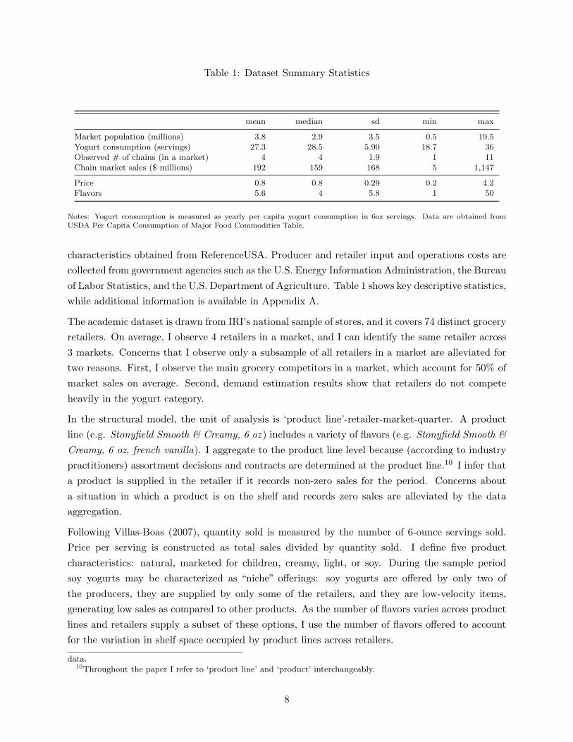
Table 1: Dataset Summary Statistics

mean median sd min max

Market population (millions) 3.8 2.9 3.5 0.5 19.5Yogurt consumption (servings) 27.3 28.5 5.90 18.7 36Observed # of chains (in a market) 4 4 1.9 1 11Chain market sales ($ millions) 192 159 168 5 1,147

Price 0.8 0.8 0.29 0.2 4.2Flavors 5.6 4 5.8 1 50

Notes: Yogurt consumption is measured as yearly per capita yogurt consumption in 6oz servings. Data are obtained fromUSDA Per Capita Consumption of Major Food Commodities Table.

characteristics obtained from ReferenceUSA. Producer and retailer input and operations costs are

collected from government agencies such as the U.S. Energy Information Administration, the Bureau

of Labor Statistics, and the U.S. Department of Agriculture. Table 1 shows key descriptive statistics,

while additional information is available in Appendix A.

The academic dataset is drawn from IRI’s national sample of stores, and it covers 74 distinct grocery

retailers. On average, I observe 4 retailers in a market, and I can identify the same retailer across

3 markets. Concerns that I observe only a subsample of all retailers in a market are alleviated for

two reasons. First, I observe the main grocery competitors in a market, which account for 50% of

market sales on average. Second, demand estimation results show that retailers do not compete

heavily in the yogurt category.

In the structural model, the unit of analysis is ‘product line’-retailer-market-quarter. A product

line (e.g. Stonyfield Smooth & Creamy, 6 oz ) includes a variety of flavors (e.g. Stonyfield Smooth &

Creamy, 6 oz, french vanilla). I aggregate to the product line level because (according to industry

practitioners) assortment decisions and contracts are determined at the product line.10 I infer that

a product is supplied in the retailer if it records non-zero sales for the period. Concerns about

a situation in which a product is on the shelf and records zero sales are alleviated by the data

aggregation.

Following Villas-Boas (2007), quantity sold is measured by the number of 6-ounce servings sold.

Price per serving is constructed as total sales divided by quantity sold. I define five product

characteristics: natural, marketed for children, creamy, light, or soy. During the sample period

soy yogurts may be characterized as “niche” offerings: soy yogurts are offered by only two of

the producers, they are supplied by only some of the retailers, and they are low-velocity items,

generating low sales as compared to other products. As the number of flavors varies across product

lines and retailers supply a subset of these options, I use the number of flavors offered to account

for the variation in shelf space occupied by product lines across retailers.

data.10Throughout the paper I refer to ‘product line’ and ‘product’ interchangeably.

8

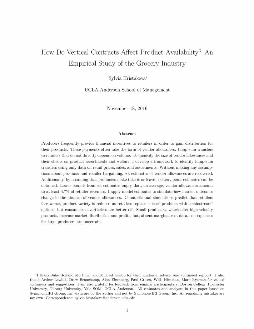
Figure 1: Assortment Snapshot: South census region 2010q1

r1

r9

r17

r25

r33

r41

r49

aCHOBANI aBREYERSSMART aSILK aYOPLAITLIGHT aDANNON aDANNONLGHTNFTCRBSUGRC aSTONYFIELDFARMYOKIDS aYOMILALA

Groupe DanoneGeneral MillsDeansBreyers LALAA

Dallas, TX

Products (sorted by producer)

Mar

ket-c

hain

obs

erva

tions

(sor

ted

by m

arke

t)

Notes: Assortment snapshot of markets in the South census region for 2010q1. Vertical axis goes over observed chains ineach market (sorted by market - e.g. Dallas, TX). Horizontal axis identifies products. Products separated by producers in thefollowing order: Agro Farma, Breyers, Dean Foods, General Mills, Groupe Danone, and LALA Foods. The remaining producersare not observed in the markets for the selected quarter. White blocks correspond to instances in which the product is notoffered in the retailer.

To identify vendor allowances, I exploit variation in observed assortments across grocery chains

and markets. In particular, if all retailers carry the same products, then these assortments will

provide no information about vendor allowances. To investigate the variation in product offerings,

Figure 1 shows a snapshot of market assortments for the first quarter of 2010 for the 12 markets

observed in the South census region. The vertical axis goes over the retailers in each market (e.g.

Dallas Texas), while the horizontal axis shows the product offerings, ordered by producer (Agro

Farma, Breyers, Dean Foods, General Mills, Groupe Danone, and LALA Foods). Each filled box

implies that the product-retailer pair is observed in the data, while white blocks correspond to

instances in which the product is not offered by the retailer. Figure 1 highlights that there is

substantial variation in the assortments selected by grocery chains both across markets and within

markets. Notice that some products are supplied in most retailers (Draganska et al. (2009b) refer

to these staple products), while the availability of other products varies markedly across retailers

and markets (Draganska et al. (2009b) define these as optional products). For example, only six

products gained universal distribution in the South census region for 2010q1: 4 of General Mills’

and 2 of Groupe Danone’s products.

The estimation methodology addresses retail price endogeneity by employing cost shifters as in-

strumental variables. Table 2 summarizes the cost data collected and their sources. Additional

to wage and energy costs, I create a “distance” measure to capture transportation costs from each

9

Table 2: Market and Input Costs Data

Variable source level of mean st. dev.variation

Retail Costs

Ave retail price of electricity U.S. Energy Information Quarter 10 2.47(cents per kilowatthour) Administration -Market

Ave weekly wage Bureau of Labor Statistics Quarter- 800.9 169.35Market

Gasoline ($ / barrel) U.S. Energy Information Quarter- 61.4 27.36Administration PAD

Distance from closest production facility to market : nautical milesDistance is calculated at the brand rather than producer level when only some plants produce the brand.

Agro Farma own calculation Market 828 631Anderson-Erickson own calculation Market 679 343Breyers own calculation Market 848 639Dean Foods own calculation Market 855 623Yoplait (General Mills) own calculation Market 379 200Colombo (General Mills) own calculation Market 965 670Danone (Groupe Danone) own calculation Market 354 160Stonyfield Farm (Groupe Danone) own calculation Market 960 668Brown Cow (Groupe Danone) own calculation Market 1485 630Crowley Foods own calculation Market 762 450LALA Foods own calculation Market 1010 452Johanna Foods own calculation Market 826 652Prairie Farms own calculation Market 508 333Springfield Creamery own calculation Market 1507 596Tillamook County Creamery own calculation Market 1539 591

Notes: PAD - Petroleum Administration for Defense District.

producer’s manufacturing facility to each market. I locate yogurt plants in the U.S. that were used

during the sample period. Then, using geographic distances and gas prices, I calculate a proxy for

transportation costs between plants and each market.

10

4 Model

Supply-side decisions and consumer behavior are modeled as the outcome of a four-stage, full-

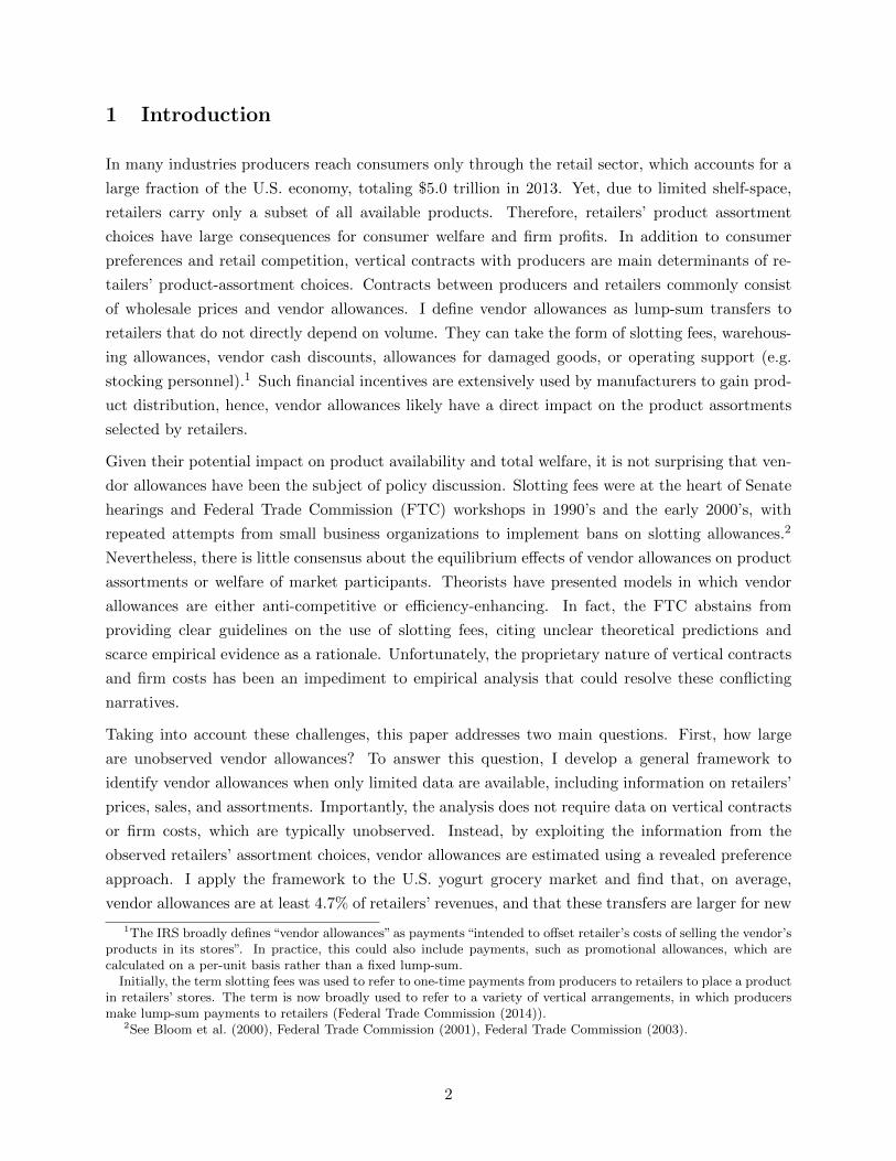
information game. Figure 2 presents the timeline for the game. First, producers and retailers

simultaneously negotiate over contract terms. Next, given wholesale prices and vendor allowances,

retailers simultaneously choose assortments. Structural shocks are realized and retailers take these

shocks into account in the price competition stage. Last, consumers choose the product-retailer

pair that gives them the highest utility level. Below I describe each stage in reverse order.

Figure 2: Timeline of the Game

t

Vertical contract

negotiations

Retail assortment decisions

Realize structural

shocks

Retail price

competition

Consumer utility

maximization

Stage 1 Stage 2 Stage 3 Stage4

Stage 4. Consumer Demand: Consumer demand is modeled using the random-coefficients

logit, which describes products as bundles of characteristics and consumers as utility maximizers.

In each market-quarter, {m, t}, consumers observe the full set of product offerings (Am,t) and select

the product-retailer pair that maximizes their utility. I define consumer i’s utility from choosing

product j in retailer r as:

ui,j,r = Xj,rβi − αipj,r + ξj,r + εi,j,r (1)

where market and time subscripts are omitted for ease of readability. The utility function depends

on prices (pj,r), observed product, retailer, and market characteristics (Xj,r), and a component

not observed by the researcher but considered by consumers when making their choices (ξj,r).

The model allows for two types of consumer heterogeneity: (αi, βi) are individual-specific taste

parameters, while εi,j,r are idiosyncratic shocks modeled as i.i.d. extreme value type I error terms.

The unobservable shocks to demand (ξj,r) create both a potential source of price endogeneity (Berry

(1994), Berry et al. (1995)) and a classic selection problem. The estimation section discusses the

methods and assumptions used to overcome these concerns.

To complete the demand model, the outside option is defined as the choice not to purchase yo-

gurt from the observed grocery chains in the market.11 The mean utility of the outside option is

normalized to 0 since it cannot be separately identified:

ui,0 = εi,011Without an outside option, a homogenous price increase (relative to all other sectors) of all products does not

change quantities purchased.

11

The static setup is justified by the perishability of the product, which alleviates most stockpiling

considerations. The logit model imposes that individuals can purchase one yogurt in a quarter, while

in reality consumers may buy multiple yogurts. I do not observe individual consumer purchases,

hence, I cannot allow for multi-unit shopping behavior as modeled by Hendel (1999) and Dube

(2004). The logit assumption implies that multi-unit purchases are either for different members of

the household or for independent consumption occasions.

The utility maximization assumption, along with the logit stochastic shock, implies that predicted

market shares for each product-retailer pair in the market ({j, r} ∈ A) are given by:

sj,r =

∫exp(Xj,rβi − αipj,r + ξj,r)

1 +∑

l,k∈A exp(Xl,kβi − αipl,k + ξl,k)dF (ν)dF (D) (2)

where A is the collection of products offered by all retailers in the market.

Stage 3. Retail Price Competition: Vendor allowances are defined as lump-sum transfers

that do not affect retailers’ sales. Thus, conditional on retail assortments, these payments are not

part of a retailer’s variable profit, which, in turn, renders vendor allowances irrelevant for third-

stage pricing analysis. Given market assortments (A), parameters that govern consumer utility

(θD = (αi, βi)), shocks to demand (ξ), and retailer marginal costs (w), retailer r’s variable profits

πr(A, θD, ξ, w) are calculated as:

πr(A, θD, ξ, w) =∑j∈Ar

(pj,r − wj,r)Msj,r(A, θD, ξ, p) (3)

where the summation goes over the products supplied by retailer r (Ar) and M stands for market

size.12 Notice that retailer r’s sales of product j (Msj,r(A, θD, ξ, w)) depend on its own assortment

and its competitors’ offerings. The main component of grocery chains’ marginal costs is wholesale

prices paid to producers. In the paper I refer to retailer marginal costs and wholesale prices inter-

changeably as the two cannot be separately identified given the data available and the distinction

does not affect the analysis.

Bertrand-Nash competition requires that equilibrium prices satisfy the first-order conditions:

sj,r(A, θD, ξ, w) +∑k∈Ar

(pk,r − wk,r)∂sk,r(A, θD, ξ, w)

∂pj,r= 0

As in Nevo (2001), I assume that, conditional on assortments, prices are uniquely determined in a

pure-strategy interior Bertrand-Nash equilibrium.

12Market and quarter subscripts are again omitted for readability.

12

Stage 2. Retail Assortment Decisions: Grocery chains have final decision rights over the

yogurt assortments supplied so the model implements this industry practice. Retail assortment

decisions are determined by consumer demand, wholesale prices, and vendor allowances. If a

market assortment is an equilibrium, then chain incentive compatibility conditions should hold. In

particular, let VAj,r be the vendor allowance that retailer r receives for supplying product j, then

retailer r’s expected profits equal:

E[Πr(A)] = E[πr(A) +∑j∈Ar

VAj,r − FCr] = E[πr(A)] +∑j∈Ar

VAj,r − FCr (4)

where FCr captures the cost of supplying Ar if the retailer incurs all expenses. I assume that

FCr can vary with assortment size but is invariant to the identities of the products supplied. As

a result, vendor distribution support, which decreases the cost borne by the retailer, is captured

by the vendor allowance transfers. Retail assortment decisions are made prior to the realization

of structural shocks to demand and retail marginal costs. However, the expectations operator

in equation (4) reflects the fact that retailers form expectations over these shocks when choosing

assortments.

Assuming that retailers are risk neutral, the following retailer incentive compatibility conditions

should be satisfied in equilibrium. If a market assortment (A) is an equilibrium outcome of the

game, then no retailer can increase its total profits by unilaterally altering its assortment:

E[Πr(A)] ≥ E[Πr(A′)] (5)

where A′ is any counterfactual assortment in which retailer r unilaterally deviates from the equilib-

rium assortment. These retailer incentive compatibility conditions are exploited for the estimation

of vendor allowances.

Stage 1. Vertical Negotiations: I pursue two approaches in modeling the negotiations stage.

The general version of the model does not impose assumptions on the bargaining protocol, while the

second approach assumes that producers simultaneously make take-it-or-leave-it offers to retailers.

For both strategies, a contract is defined as product-specific wholesale price and vendor allowance.

The contract structure does not allow for bundling because the practice is not common for the yogurt

category. The no-bundling assumption allows me to identify product-specific vendor allowances.

In line with industry practices, I assume that the parties cannot contract over chain prices at the

negotiations stage.

For the general strategy, equation (5) cannot be further simplified. These deviations imply upper

and lower bounds on vendor allowances. The second approach implies that, in equilibrium, producer

contract offers put retailers at their participation constraints. In particular, when A′ is retailer

r’s best outside option, then the assumption about producer take-it-or-leave-it offers implies that

13

condition (5) is exactly satisfied:

E[Πr(A)] = E[Πr(A′)] (6)

This paper focuses on retailer assortment decisions, hence, I do not attempt to model and analyze

dynamic decisions about product innovation or retailer long-term strategies. The above setup

assumes that manufacturers’ product introduction decisions and brand positioning, together with

retailers’ choice of location and characteristics, are exogenous to the model as they are made prior

to the negotiations stage.

5 Empirical Analysis

The model is estimated in two steps. First, standard techniques, as in Berry et al. (1995), are

applied to consumer demand and retail pricing analyses. Then, using demand and wholesale price

parameters, I estimate vendor allowances with a revealed preference approach. The separation of

the retail assortment and pricing decisions allows me to separately identify wholesale prices and

vendor allowances. The assumption is justified because assortment choices are “stickier” than retail

prices.

Step 1. Demand and Retailer Price Competition: In order to investigate retailer assortment

decisions, the empirical analysis requires a rich demand model, which allows for flexible variation in

consumer preferences. To that end, a flexible fixed-effects parameterization is used to characterize

consumer utility and wholesale prices. I include product-region-year intercepts, which capture

product mean valuations across census regions and the change in these valuations over time.13

Retailer-market-specific constants and quarter fixed effects account for differences in consumer

valuations across grocery chains and seasonal changes in yogurt preferences. In addition, the

demand specification includes interactions between product characteristics and retailer fixed effects.

The characteristics used are dummy variables indicating whether a product is natural, marketed

for children, creamy, light, or soy. These interactions capture the idea that a product characteristic

may be perceived differently across chains, that is, consumers may regard healthy products to be

of higher quality when bought in Whole Foods than at a discount grocery chain.

Due to data aggregation, weekly promotions lead to lower retail prices, which translate into lower

estimates of wholesale prices. Producers cover most promotional activities, and these discounts will

be captured by the wholesale price estimates. Product shelf location and number of facings can

also affect consumer demand. Unfortunately, I do not observe either variable. However, I include

the log of number of flavors supplied by the retailer as a proxy for the shelf space occupied by

each product line. The estimation includes random coefficients on price, flavors, and the constant

13The Census divides the U.S. in four regions: Northeast, Midwest, South, and West. These are the regions usedfor estimation.

14

term. Market size is constructed as market population multiplied by quarterly per capita yogurt

consumption, which is obtained from the USDA per capita consumption data.

Wholesale prices are described by observed characteristics Wj,r and an additive error term ωj,r:

log(wj,r) = Wj,rθw + ωj,r

The estimated parameters in Wj,r are product-region-year intercepts, retailer-market fixed effects,

as well as market energy costs and transportation costs interacted with retailer-specific constants.

By endogenizing retailers’ assortment decisions, I encounter a classic selection problem: firms supply

products with anticipated high profits. Specifically, retailers may choose assortments based on high

demand, low wholesale prices, or high vendor allowances. Selection on demand and wholesale prices

places a concern for demand and wholesale price parameter estimates and this issue is addressed

below. Selection on vendor allowances affects the estimates of these lump-sum payments only, so I

address the issue in the discussion of the vendor allowance estimation.

Selection on demand and wholesale prices implies that the observed sample is not a random sample

from the underlying distribution of product characteristics. To address this concern, the estimation

strategy assumes that product assortments and non-price characteristics are determined prior to

the realization of the demand and retail marginal cost shocks (ξ, ω). If assortment decisions are

based on observables only, then the selection considerations do not affect the consistency of the

demand and wholesale price parameter estimates. The assumption is credible for two reasons. First,

the estimation controls for product-region-year unobservables, retailer-specific intercepts, as well

as chain interactions with product characteristics. Thus, the unobservable shocks to demand and

retailer marginal costs do not capture systematic components that retailers are likely to know prior

to their assortment choices. Second, the assortment decisions are “sticky”. Changing an assortment

requires coordination across stores and involves large fixed costs; in consequence, grocery chains

typically adjust product selections at only a few predetermined occasions during the year.

Unlike assortment decisions, prices are easily adjusted as market conditions change, thus, I allow

retailers to select optimal prices once they observe demand and cost shocks. To the extent that re-

tailers observe these shocks and condition on them when setting prices, retail prices are endogenous.

For example, the unobservable demand shock may be decomposed as:

ξj,r,m,t = ξj,region,y + ξr,m + ∆ξj,r,m,t

The fixed effects included in the estimation capture both ξj,region,y - the product-region-specific

time-varying vertical component (varying over years); and ξr,m - the retailer-market unobservable.

The econometric error that remains in ∆ξj,r,m,t includes a time-varying deviation around the un-

observable mean for retailers’ valuations, as well as a product-retailer unobservable component.

Following Villas-Boas (2007), I employ cost-based instruments. The instruments capture direct

components of retailer market costs (energy and transportation costs) interacted with retailer fixed

15

effects. The intuition is that prices depend on retailers’ costs of operation, but these costs are not

correlated with unobservables.14

Demand parameters are estimated using a Mathematical Program with Equilibrium Constraints

(MPEC) algorithm. The MPEC computational algorithm is preferred to the nested fixed-point

(NFP) method as it avoids the numerical issues associated with nested inner loops (Dube et al.

(2012)). At the same time, the MPEC and NFP algorithms generate the same estimator (shown

by Su and Judd (2012)), hence, the statistical properties of the Berry et al. (1995) estimator apply

to both NFP and MPEC.

Step 2. Vendor Allowances: The estimation identifies vendor allowances as retailers’ opportu-

nity costs of shelf space. Without imposing additional structure on the bargaining game, I identify

bounds on vendor allowances. The second version of the model assumes that producers make take-

it-or-leave-it contract offers, which allows for point identification of paid product-specific vendor

allowances for the sample of selected products.

Both strategies are based on the assumption that observed assortments and prices constitute a Sub-

game Perfect Nash Equilibrium of the game described in Section 4. In particular, for each retailer

its observed assortment must yield weakly higher expected profits than any feasible alternative,

holding other retailers’ assortments fixed. I construct retailer unilateral deviations as counterfac-

tual scenarios in which a retailer switches one product at a time.15 If retailer r switches a product

it supplies j ∈ Ar with a product it does not supply l /∈ Ar, then retailer incentive compatibility

requires that:

E[Πr(A)] ≥ E[Πr(A′(l,−j,r))] for ∀j ∈ Ar and ∀l /∈ Ar (7)

where A′(l,−j,r) is the counterfactual assortment in which product j is replaced by l in retailer r.

Substituting the profit equation (4) in equation (7), yields that for all products j supplied in r and

all non-offered products l the following condition holds:

E[πr(A)] + (∑

k∈ArVAk,r)− FCr ≥ E[πr(A

′(l,−j,r))] + (

∑k∈A′

r,(l,−j,r)VAk,r)− FCr

The FCr term reflects the fixed cost associated with supplying an assortment if the retailer bears

all expenses. These costs can vary with assortment size but are assumed to be invariant to the

identities of the products offered. The counterfactual product assortment holds fixed the number

of products supplied by the retailer, hence these fixed costs remain unchanged across the two

assortments considered. Notice that the vendor incentives can take the form of both cash transfers

14Eizenberg (2014) presents an informal argument about the assumptions needed for point identification of demandparameters. The method requires that demand and marginal cost shocks are mean-independent for the set of allpotential products that may be offered in the market.

15Naturally, retailers have additional unilateral deviations. For example, the retailer can switch multiple productsat a time or it can add a new product by, instead, decreasing the shelf space of a different product category (e.g.cream cheese). I employ one-product deviations as these allow me to identify product-specific vendor allowances,while keeping yogurt shelf space constant.

16

and retailer cost savings. As a result, if a producer offers operations support (e.g. the producer

uses a direct-store-delivery system), then the resulting cost savings for the retailer are associated

with a vendor allowance transfer.

The vertical contract assumes that wholesale prices and vendor allowances are not conditional on

retail assortments, so the following holds:

(∑

k∈ArVAk,r)−VAj,r = (

∑k∈A′

r,(l,−j,r)VAk,r)−VAl,r

and the condition implies that:

E[πr(A)] + VAj,r ≥ E[πr(A′(l,−j,r))] + VAl,r for ∀j ∈ Ar and ∀l /∈ Ar (8)

Notice that vendor allowances affect retailer total profits but do not affect demand.16

Equation (8) is used for the estimation of both versions of the model. First, I discuss the assump-

tions for the bounds estimates. The second model allows me to recover point estimates of vendor

allowances for offered products up to a normalization of one product’s vendor allowance. The main

difference between the two strategies is the treatment of the vendor allowance of the counterfactu-

ally added product (VAl,r). In the general model, VAl,r is set to the edge of its support to derive the

most conservative bounds, while in the second model, VAl,r is differenced out. The latter option is

only possible when the bargaining power assumption implies that equation (8) is exactly satisfied.

(1) Bounds: To set-identify vendor allowances, I impose a bounded support assumption, which

implies that VAj,r ∈ [VALBj,r ,VAUB

j,r ], with VALBj,r > −∞ and VAUB

j,r < ∞. In the grocery industry,

lump-sum payments flow from producers to retailers, so industry practices provide a natural lower

bound on vendor allowances: VAj,r ≥ 0.17 For the upper bound I rely on producer individual

rationality, which imposes that a product’s vendor allowance cannot exceed the additional producer

profits generated by supplying the product in the chain. Unfortunately, I do not observe producer

marginal costs, thus, I use the change in producer revenues to construct the upper bound on the

support. The use of producer revenues instead of variable profits (or profits) to construct VAUBj,r

widens the estimated bounds.18

Bounds on vendor allowances are estimated by combining the bounded support assumption with the

retailer incentive compatibility conditions described in equation (8). In particular, for all products

16Vendor incentives, such as promotional allowances, which are paid per unit sold, are not captured by the vendorallowances’ estimate.

17Other forms of retailer efforts, which might differ across products and might be construed to be part of the vendorallowances, are assumed to be not material enough to violate the non-negativity assumption.

18Here the distinction between wholesale prices and chain marginal costs matters. However, as long as chainmarginal costs less wholesale prices are lower than producer marginal costs, the constructed producer revenues arehigher than the unobserved producer variable profits. Then, the constructed measure of producer individual rationalityis conservative.

17

offered in the market, the equilibrium conditions prescribe a lower bound on vendor allowances:

VAj,r ≥ −E[πr(A)− πr(A′(l,−j,r))] + VAl,r for ∀j ∈ Ar and ∀l /∈ Ar (9)

While, if product j is not supplied by the chain, I construct an upper bound on its vendor allowance:

VAj,r ≤ E[πr(A)− πr(A′(j,−k,r))] + VAk,r for ∀j /∈ Ar and ∀k ∈ Ar (10)

where product k is displaced by product j and the retailer loses any vendor allowances received

for product k: VAk,r. As described below, the estimation obtains the tightest bounds by using the

deviations that render the highest retailer variable profits.

Demand and wholesale price parameter estimates, along with the assumption of retailer price

competition, allow me to simulate expected retailer variable profits under the observed and coun-

terfactual scenarios. However, I do not have estimates for the vendor allowances on the right-hand

side of the inequalities (VAl,r and VAk,r). To circumvent this problem, I construct conservative

bounds employing the support of VAl,r and VAk,r. For all observed product-retailer pairs I obtain

the lowest lower bound for VAj,r by setting VAl,r = VALBl,r = 0. Then equation (9) becomes:

VAj,r ≥ max(−E[πr(A)− πr(A′(l,−j,r))] + 0,VALBj,r ) ≡ VAj,r, for ∀j ∈ Ar and ∀l /∈ Ar (11)

For all non-observed product-retailer pairs, the highest upper bound for VAj,r is constructed by

setting VAk,r to its upper bound, VAk,r = VAUBk,r :

VAj,r ≤ min(E[πr(A)− πr(A′(j,−k,r))] + VAUBk,r ,VAUB

j,r ) ≡ VAj,r, for ∀j /∈ Ar and ∀k ∈ Ar (12)

Notice that lower and upper bounds are constructed for different sets of products: for all offered

products I construct a lower bound, while upper bounds are created for all non-offered products.

This refers to the selection issue discussed, where retailers may choose to supply products with

higher vendor allowances. To account for this issue, I follow Eizenberg (2014) and use the support

of vendor allowances to fill in the “missing” bounds.

For example, the complete set of lower bound deviations combines the lower bound conditions

constructed for all offered products (VAj,r ∀j ∈ Ar) and the lower bounds from the support of

vendor allowances for all non-offered products (VALBj,r ∀j /∈ Ar). Analogously, the set of upper

bound deviations is constructed from the support for all offered products (VAUBj,r ∀j ∈ Ar) and

retailer incentive compatibility conditions for all non-offered products (VAj,r ∀j /∈ Ar).

Ljr =

VAj,r, if j ∈ Ar

VALBj,r , if j /∈ Ar

Ujr =

VAUBj,r , if j ∈ Ar

VAj,r, if j /∈ Ar

The approach further widens the bounds. The results section shows the product-specific empirical

distribution of the constructed bounds (Ljr, Ujr).

18

(2) Point identification: The second version of the model imposes that producers make take-it-

or-leave-it wholesale price and vendor allowance offers. This setup assumes that producers have all

bargaining power, while retailers have final decision rights over assortments. It is worth noting that

retailers’ ability to supply alternative assortments allows them to extract surplus from producers.

In equilibrium, contract offers are such that retailer incentive compatibility conditions are exactly

satisfied. As a result, vendor allowances reflect the shadow price of shelf space. I approximate the

shadow price of shelf space with the additional retailer variable profits generated by switching each

product with its best replacement. In particular, the point identification strategy assumes that

equation (8) holds with equality when product l is the best replacement product for product j in

retailer r:

VAj,r −VAl,r = E[πr(A′(l,−j,r))− πr(A)] for ∀j ∈ Ar (13)

Taking equation (13) to the data leads to selection issues, as the vendor allowance offer for product

j may be higher than the offer for product l. To circumvent this issue, I difference out VAl,r using

pairs of retailer deviations in which the same product l is the best replacement option. If retailer

r supplies both j and k, and for both products the best replacement option is l, then the following

two conditions hold:

VAj,r −VAl,r = E[πr(A′(l,−j,r))− πr(A)] (14)

VAk,r −VAl,r = E[πr(A′(l,−k,r))− πr(A)] (15)

Using conditions (14) and (15), VAl,r can be differenced out :

VAj,r −VAk,r = E[πr(A′(l,−j,r))]− E[πr(A

′(l,−k,r))] (16)

Now both products j and k are offered by retailer r. In order to take condition (16) to the data, I

define VAj,r = VAj + αNewj,m + vj,r, where VAj is a product specific constant and Newj,m tracks

if the product was introduced in the market in the given year. Substituting this parameterization

in equation (16) yields:

(VAj −VAk) + α(∆Newj,k,m) + ∆vj,k,r = E[πr(A′(l,−j,r))]− E[πr(A

′(l,−k,r))] (17)

where ∆Newj,k,m = Newj,m −Newk,m and ∆vj,k,r = vj,r − vk,r. The parameter estimates (VAj ’s,

α) are estimated for the sample of offered products. The error term (∆vj,k,r) is assumed to be

white noise as any product-, retailer-, and market-specific components are differenced out. Due

to the differencing nature of equation (17), I need to normalize the value of one product’s vendor

allowance.

19

Construction of deviations explained by example: To construct the deviations described

above, I define the set of potential product offerings for each grocery chain in a market as the

collection of products that are observed in the market combined with all products the retailer carries

in other markets during the quarter. These restrictions guarantee that producers actually distribute

the potential products at the time period and that the retailer can supply the counterfactual product

without incurring disproportionately large supply costs. In addition, I avoid deviations in which

regional brands are counterfactually supplied in other census regions, e.g. a deviation in which

Tillamook (a regional West coast producer) is offered in an East coast market. The resulting set

of potential products includes, on average, 14 replacement options for each retailer.

Two types of deviations are constructed: (i) drop each product from the observed assortment with

replacement, (ii) add a new product to a retailer’s portfolio with displacement. These unilateral

deviations keep fixed the shelf space occupied by the yogurt category, both in terms of number

of products and number of flavors offered. For drop deviations I replace the dropped product

with the counterfactual option that renders the highest variable retailer profits. By using the

best replacement product, the drop deviations lead to the tightest bound on (VAj,r − VAl,r), and

respectively on VAj,r. Analogously, the estimation strategy for the producer take-it-or-leave-it

offers’ model approximates the shadow price of shelf space with the additional retailer variable

profits generated by switching each product with its best replacement.

To present the method used to construct these deviations, consider the Boston market for the

2010q1 period and suppose that retailer 1 in Boston, {r1}, supplies Yoplait Trix, {trix}. First, I

construct retailer 1’s expected variable profits under the observed assortment, E[πr(A)] = 20, 500.

The next step is to construct retailer 1’s expected variable profits after removing Yoplait Trix and

replacing it with each product from its potential product deviations set. For simplicity, suppose

that there are three products in retailer 1’s potential offerings set: {Breyers Light, Stonyfield Farm

Yobaby, Weight Watchers}. The expected variable profits per store for each deviation equal:

E[πr(A′bl,−trix,r1)] = 20, 600, E[πr(A

′sfy,−trix,r1)] = 20, 540, and E[πr(A

′ww,−trix,r1)] = 20, 300;

These estimates imply that the best replacement for Yoplait Trix in retailer 1 is Breyers Light at

20, 600, so I use the drop Yoplait Trix, replace with Breyers Light deviation. This deviation is used

for both the general model and the second approach. The deviation allows me to construct a lower

bound on the vendor allowance for Yoplait Trix, VAtrix,r1. Note that the deviation yields that:

E[πr(A)] + VAtrix,r1 ≥ E[πr(A′bl,−trix,r1)] + VAbl,r1 =⇒ VAtrix,r1 ≥ 100 + VAbl,r1 (18)

I substitute VAbl,r1 = VALBbl,r1 = 0 to obtain that VAtrix,r1 ≥ VAtrix,r1 = 100.

The second strategy uses pairs of product deviations in which the same non-offered product is the

best replacement option. Suppose that retailer 1 also carries Stonyfield Farm, {sf}, and that its

best replacement product is again Breyers Light. Let the variable profits under the counterfactual

20

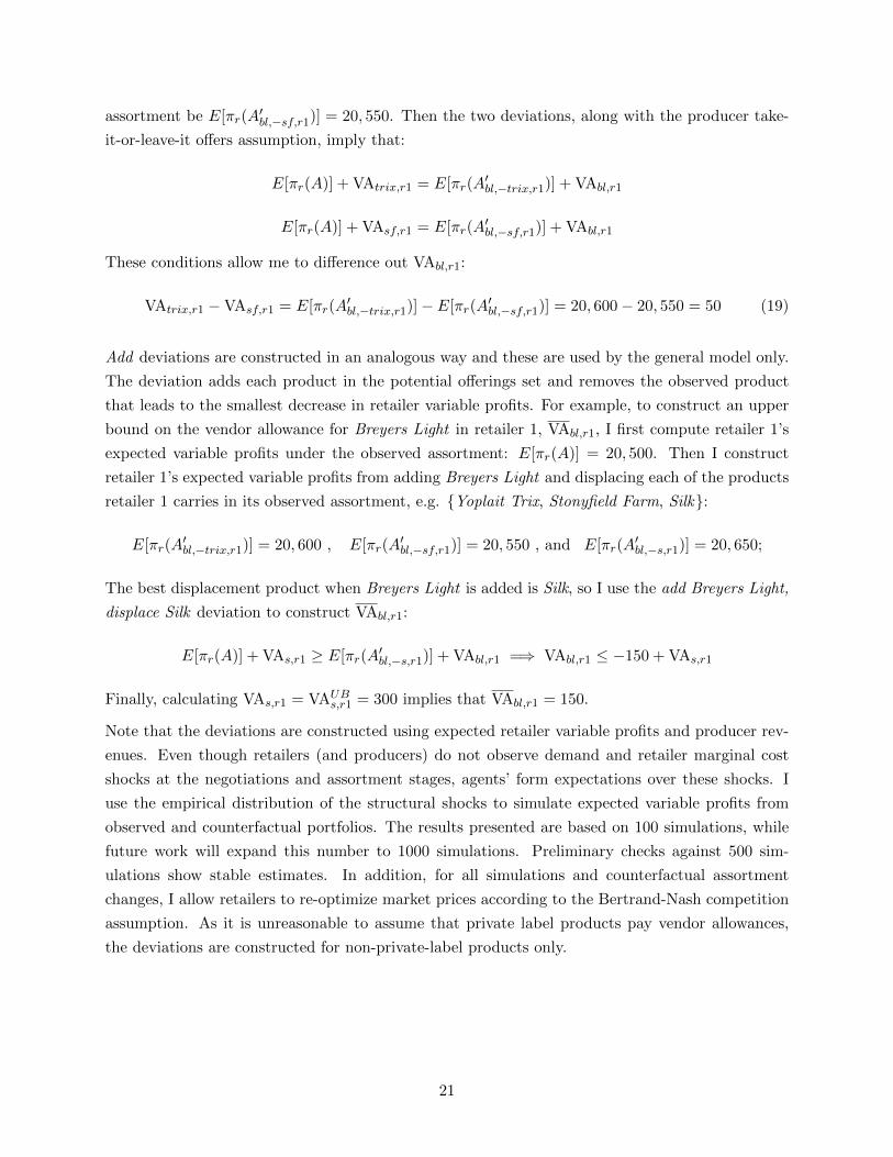
assortment be E[πr(A′bl,−sf,r1)] = 20, 550. Then the two deviations, along with the producer take-

it-or-leave-it offers assumption, imply that:

E[πr(A)] + VAtrix,r1 = E[πr(A′bl,−trix,r1)] + VAbl,r1

E[πr(A)] + VAsf,r1 = E[πr(A′bl,−sf,r1)] + VAbl,r1

These conditions allow me to difference out VAbl,r1:

VAtrix,r1 −VAsf,r1 = E[πr(A′bl,−trix,r1)]− E[πr(A

′bl,−sf,r1)] = 20, 600− 20, 550 = 50 (19)

Add deviations are constructed in an analogous way and these are used by the general model only.

The deviation adds each product in the potential offerings set and removes the observed product

that leads to the smallest decrease in retailer variable profits. For example, to construct an upper

bound on the vendor allowance for Breyers Light in retailer 1, VAbl,r1, I first compute retailer 1’s

expected variable profits under the observed assortment: E[πr(A)] = 20, 500. Then I construct

retailer 1’s expected variable profits from adding Breyers Light and displacing each of the products

retailer 1 carries in its observed assortment, e.g. {Yoplait Trix, Stonyfield Farm, Silk}:

E[πr(A′bl,−trix,r1)] = 20, 600 , E[πr(A

′bl,−sf,r1)] = 20, 550 , and E[πr(A

′bl,−s,r1)] = 20, 650;

The best displacement product when Breyers Light is added is Silk, so I use the add Breyers Light,

displace Silk deviation to construct VAbl,r1:

E[πr(A)] + VAs,r1 ≥ E[πr(A′bl,−s,r1)] + VAbl,r1 =⇒ VAbl,r1 ≤ −150 + VAs,r1

Finally, calculating VAs,r1 = VAUBs,r1 = 300 implies that VAbl,r1 = 150.

Note that the deviations are constructed using expected retailer variable profits and producer rev-

enues. Even though retailers (and producers) do not observe demand and retailer marginal cost

shocks at the negotiations and assortment stages, agents’ form expectations over these shocks. I

use the empirical distribution of the structural shocks to simulate expected variable profits from

observed and counterfactual portfolios. The results presented are based on 100 simulations, while

future work will expand this number to 1000 simulations. Preliminary checks against 500 sim-

ulations show stable estimates. In addition, for all simulations and counterfactual assortment

changes, I allow retailers to re-optimize market prices according to the Bertrand-Nash competition

assumption. As it is unreasonable to assume that private label products pay vendor allowances,

the deviations are constructed for non-private-label products only.

21

6 Results

Demand and Retailer Price Competition: Consumer demand is estimated with the random-

coefficients logit, which captures the effect of consumer heterogeneity in price sensitivity and pref-

erences for product characteristics. The individual-specific taste parameter on price is drawn from

the empirical income distribution, while the random coefficients on flavors (log(#flavors)) and the

constant term are estimated using draws from the i.i.d. standard normal distribution.

To investigate price endogeneity concerns, it is instructive to look at the estimates predicted by

a simple logit model, which imposes a value of 1 for the random coefficient parameters. Table 3

reports results from an OLS and an instrumental variables approach where estimates of product

characteristics are calculated as projections on the estimated product-region-year intercepts.19 The

2SLS estimation relies on instruments comprised of market energy prices and producer transporta-

tion costs interacted with retailer fixed effects. The results highlight the importance of accounting

for price endogeneity. Even though own-price elasticities are negative in both specifications, the

instrumental variables approach leads to larger (in absolute terms) price-sensitivity estimates and

to fewer own-price elasticities that are higher than -1 (1% of the observations with IV compared to

25% in the OLS setup).

The results from the full demand system parameterization are reported in Table 4. The estimates

align with expectations: demand is downward sloping, while the random coefficient on price implies

that consumer price sensitivity decreases with income. In addition, consumers prefer natural,

children’s, and light products, while they value less soy and creamy products. Consumers value

products with more flavor options offered in the chain; however, there is substantial heterogeneity

in individual preference for flavors. The last panel of Table 4 shows how consumer mean valuations

vary across producers. The excluded brand is retailer private labels, and the results show the

presence of substantial heterogeneity in consumer preferences across producers.

Projections of retailer wholesale price parameter estimates on product characteristics show that

products with each of the characteristics are more expensive than their counterparts. As expected,

the estimated wholesale prices for private labels’ are lower than the retailers’ costs of selling branded

products.

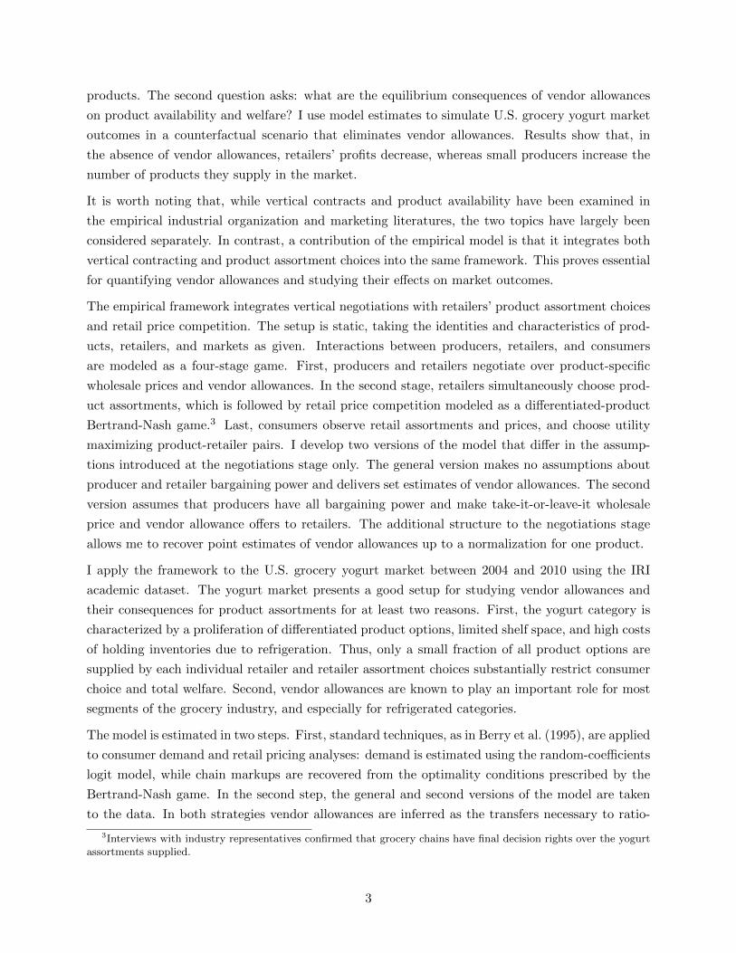
Demand estimates imply median consumer own-price elasticities of −3.45. The distribution of

estimated individual own-price elasticities is shown in Figure 3. Table 5 reports that none of the

calculated own-price elasticities are positive, and only 3.14% of the estimates suggest individuals on

the elastic part of their demands. The assumption about retail price competition leads to estimated

median retailer markups of 33 cents and median variable profit margins of 44%.20 To analyze how

well the model matches the observed margins in the grocery chain industry, I collect information

on variable profit margins reported by public grocery retailers in their accounting statements. I

19The procedure is described in Nevo (2001).20Margins are calculated as the ratio of variable profits to total sales.

22

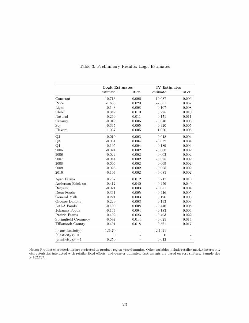
Table 3: Preliminary Results: Logit Estimates

Logit Estimates IV Estimatesestimate st.er. estimate st.er.

Constant -10.713 0.006 -10.087 0.006Price -1.635 0.020 -2.661 0.057Light 0.143 0.008 0.107 0.008Child 0.342 0.010 0.225 0.010Natural 0.269 0.011 0.171 0.011Creamy -0.019 0.006 -0.046 0.006Soy -0.335 0.005 -0.320 0.005Flavors 1.037 0.005 1.020 0.005

Q2 0.010 0.003 0.018 0.004Q3 -0.031 0.004 -0.032 0.004Q4 -0.195 0.004 -0.189 0.0042005 -0.024 0.002 -0.008 0.0022006 -0.022 0.002 -0.002 0.0022007 -0.044 0.002 -0.025 0.0022008 -0.006 0.002 0.009 0.0022009 -0.023 0.002 -0.005 0.0022010 -0.104 0.002 -0.085 0.002

Agro Farma 0.737 0.012 0.717 0.013Anderson-Erickson -0.412 0.040 -0.456 0.040Breyers -0.021 0.003 -0.051 0.004Dean Foods -0.361 0.005 -0.416 0.005General Mills 0.221 0.003 0.196 0.003Groupe Danone 0.229 0.003 0.193 0.003LALA Foods -0.400 0.008 -0.446 0.008Johanna Foods -0.144 0.004 -0.183 0.004Prairie Farms -0.402 0.023 -0.403 0.022Springfield Creamery -0.597 0.014 -0.625 0.014Tillamook County 0.491 0.018 0.561 0.017

mean(elasticity) -1.3470 - -2.1921 -(elasticity)> 0 0 - 0 -(elasticity)> −1 0.250 - 0.012 -

Notes: Product characteristics are projected on product-region-year dummies. Other variables include retailer-market intercepts,characteristics interacted with retailer fixed effects, and quarter dummies. Instruments are based on cost shifters. Sample sizeis 162,707.

23

Table 4: Demand and Wholesale Price Estimates

Demand Estimates Wholesale Priceestimate st.er. r.c. st.er. estimate st.er.

Constant -9.678 0.006 0.118 0.189 -0.842 0.000Price -6.205 0.164 2.636 0.085 - -Natural 0.136 0.010 - - 0.007 0.000Children 0.142 0.010 - - 0.188 0.000Creamy -0.100 0.006 - - 0.095 0.000Light 0.132 0.008 - - 0.104 0.000Soy -0.289 0.005 - - 0.253 0.001Flavors 0.813 0.017 0.527 0.022 - -

Q2 0.010 0.004 - - 0.010 0.001Q3 -0.057 0.004 - - -0.009 0.001Q4 -0.258 0.005 - - -0.003 0.0012005 -0.063 0.002 - - -0.067 0.0002006 -0.041 0.002 - - -0.091 0.0002007 -0.099 0.002 - - -0.093 0.0002008 -0.073 0.002 - - -0.092 0.0002009 -0.088 0.002 - - -0.023 0.0002010 -0.165 0.002 - - -0.096 0.000

Agro Farma 0.545 0.008 - - 0.840 0.002Anderson-Erickson -0.498 0.031 - - 0.463 0.002Breyers -0.140 0.003 - - 0.392 0.000Dean Foods -0.427 0.005 - - 0.586 0.001General Mills 0.108 0.003 - - 0.460 0.000Groupe Danone 0.131 0.003 - - 0.466 0.000LALA Foods -0.526 0.008 - - 0.296 0.001Johanna Foods -0.244 0.004 - - 0.452 0.001Prairie Farms -0.611 0.018 - - 0.305 0.002Springfield Creamery -0.768 0.010 - - 0.453 0.001Tillamook County 0.241 0.016 - - 0.736 0.002

Notes: Random coefficient estimates correspond to the choice probabilities described in Section 4. Results are obtainedusing the MPEC algorithm. The random coefficient on price is drawn from empirical income distribution, while the standardnormal distribution is used to estimated the random coefficients on flavors and the outside option. Product characteristics areprojected on product-region-year dummies. Other variables include retailer-market intercepts, characteristics interacted withretailer fixed effects, and quarter dummies. Sample size is 162,707.

24

Table 5: Implications from Demand and Retailer Price Competition Results

Median own-price elasticity -3.436% own-price elasticity > 0 0.000% own-price elasticity > −1 3.144

Median markup=(p-w) (in $) 0.332Median margin=(p-w)/p 0.437

Notes: Implications are derived for the full random-coefficients logit estimates presented in table 4. Markups are derived underthe assumption of retailer price competition. Variable profit margins are calculated as variable profits divided by total sales.

Figure 3: Estimated Own-Price Elasticities

Own-price elasticity -15 -10 -5 0 50

0.05

0.1

0.15

0.2

0.25

0.3

Notes: The graph shows the empirical density of the estimated individual own-price elasticities. Own-price elasticities arederived for the full random-coefficients logit estimates.

find that the median reported variable profit margins equals 27% for the sample period analyzed.

Grocery chains report margins as sales minus cost of sales. The cost of sales measure includes

inventory costs as well as warehousing and transportation costs. The difference between reported

and estimated retail margins may be driven by the inclusion of fixed costs in the reported variable

profit margins.

25

Vendor Allowances Using demand and wholesale price estimates, I construct counterfactual

unilateral deviations for each product. These deviations yield empirical distributions of constructed

upper and lower bounds for 141 non-private label products. Most products follow a similar pattern,

thus, Figure 4 shows the constructed distributions for a representative product Dannon Light ’n

Fit Carb & Sugar Control. An exception to these patterns is presented by Dean Foods’ products

due to the binding of the producer individual rationality constraints. I report some unique features

of Dean Foods and present a rationale that reconciles the pattern at the end of the section.

Figure 4 contains two graphs: the left panel shows the empirical cumulative distribution (EDF) of

upper and lower bounds using Lj,r and Uj,r, and the right panel shows the EDFs using the bounds

from constructed deviations only: VAj,r and VAj,r. Lower bounds’ EDFs are displayed with solid

lines while dashed lines trace upper bounds. As expected, the estimated distributions widen when

“missing” bounds are filled with estimates of the support of vendor allowances. Also because add

and drop deviations are constructed for different sets of retailers and markets, it is expected that

VAj,r and VAj,r may cross.

The EDFs show Dannon Light ’n Fit Carb & Sugar Control ’s vendor allowances per store and

quarter. For example, the cumulative distribution of the lower bounds (Lj,r) implies that 50% of

the constructed lower bounds are less than $33.21 The transfer of $33 per store translates into

0.1% of revenues for the median retailer. The distribution of the upper bounds establishes that

50% of these deviations are less than $162, which imply a payment equal to 0.5% of revenues for

the median retailer.

To gain perspective on the significance of vendor allowances for retailers’ profitability, I compare

the amount of received vendor allowances to retailer sales and variable profits. The constructed

drop deviations for observed products provide lower bounds on paid vendor allowances (VAj,r).

The estimates suggest that, on average, the vendor allowances received by grocery chains represent

at least 4.7% of retailers’ revenues and 10% of retailers’ variable profits. These payments are likely

important for retailer profitability, given that public grocery chains in the U.S. report profit margins

on the order of 2-4% of revenues.

The closest accounting statement metric is the vendor allowance payments reported in retailer

10-K filings. The median of these reported vendor allowance payments corresponds to 7% of their

revenues. The closeness between estimated and reported vendor allowances is reassuring, but should

be interpreted with caution, recognizing the distinction between the two measures. The estimated

vendor allowances are designed to reflect retailer opportunity costs. As a result, the estimates

capture vendor support in the form of distribution cost savings, a transfer that is not recorded

in accounting statements. Alternatively, reported vendor allowances from accounting statements

include payments, such as promotional allowances, which are paid on a per-unit basis rather than

21Lj,r is inflated with zeros for all add deviations constructed. In addition, as shown in the right panel, for 13%of the product’s drop deviations, I did not find any profitable unilateral deviations (when vendor allowances for thenon-offered products are constrained to zero).

26

Figure 4: Vendor Allowance Cumulative Empirical Distribution:Dannon Light ’n Fit Carb & Sugar Control

VAs ($/store)0 50 100 150 200 250 300

Prob

(VA

<x)

0

0.1

0.2

0.3

0.4

0.5

0.6

0.7

0.8

0.9

1

VAs ($/store)0 50 100 150 200 250 300

0

0.1

0.2

0.3

0.4

0.5

0.6

0.7

0.8

0.9

1

Lower BoundUpper Bound

Notes: The cumulative empirical distribution corresponds to the chain unilateral deviations described in Section 5. The leftpanel shows the empirical cumulative distribution of upper and lower bounds using Lj,r and Uj,r, and the right panel shows

the distributions obtained from constructed deviations only: V j,r and V j,r. The estimates reflect the vendor allowance offeredper store and per flavor for the product. Results are based on 100 simulations.

as a fixed lump sum. These vendor incentives would not be included in the vendor allowance

estimates, rather they would be captured by the wholesale price analysis.

To compare the vendor allowance payments across products, I rely on the point-identification tech-

nique described in Section 5. Figure 5 shows the relative differences in paid vendor allowances

for offered products. The excluded product is Dannon Light ’n Fit Carb & Sugar Control and its

vendor allowance is normalized to zero. The x-axis sorts the products by brand, while different

symbols identify product characteristics: natural products are marked by a star, a circle identifies

products marketed for children, etc. The results show that even within the same producer, there is

substantial heterogeneity in the vendor allowances paid across products. For example, the two ex-

treme vendor allowance estimates paid by Groupe Danone, indicate that each quarter the producer

pays $148 more per store and flavor for Stonyfield O’Soy than for Dannon All Natural. This result

aligns with industry narratives in which producers refuse to pay slotting fees for staple products,

and pay high lump-sum transfers for products that may be profitably replaced by the retailer.

The counterfactual simulations presented in the next section finds that soy and some natural-

children’s products are eliminated in the absence of vendor allowances. Figure 5 identifies soy

products with a diamond shape and natural-children’s products with a star surrounded by a circle.

27

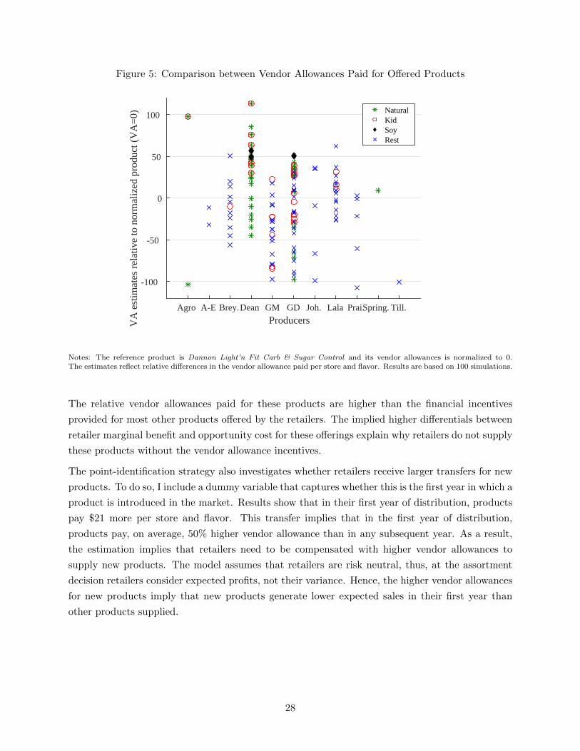
Figure 5: Comparison between Vendor Allowances Paid for Offered Products

ProducersAgro A-E Brey.Dean GM GD Joh. Lala Prai.Spring. Till.

VA

est

imat

es r

elat

ive

to n

orm

aliz

ed p

rodu

ct (

VA

=0)

-100

-50

0

50

100NaturalKidSoyRest

Notes: The reference product is Dannon Light’n Fit Carb & Sugar Control and its vendor allowances is normalized to 0.The estimates reflect relative differences in the vendor allowance paid per store and flavor. Results are based on 100 simulations.

The relative vendor allowances paid for these products are higher than the financial incentives

provided for most other products offered by the retailers. The implied higher differentials between

retailer marginal benefit and opportunity cost for these offerings explain why retailers do not supply

these products without the vendor allowance incentives.

The point-identification strategy also investigates whether retailers receive larger transfers for new

products. To do so, I include a dummy variable that captures whether this is the first year in which a

product is introduced in the market. Results show that in their first year of distribution, products

pay $21 more per store and flavor. This transfer implies that in the first year of distribution,

products pay, on average, 50% higher vendor allowance than in any subsequent year. As a result,

the estimation implies that retailers need to be compensated with higher vendor allowances to

supply new products. The model assumes that retailers are risk neutral, thus, at the assortment

decision retailers consider expected profits, not their variance. Hence, the higher vendor allowances

for new products imply that new products generate lower expected sales in their first year than

other products supplied.

28

The case of Dean Foods: A special case that requires further attention is Dean Foods. The

constructed producer individual rationality constraints bind for 80% of Dean Foods’ unilateral

deviations. Dean Foods is characterized by some unique features that distinguish the producer

from its competitors. Dean Foods is an international food manufacturer that specializes in dairy

products. During the sample period of 2004-2010, the firm produces a wide variety of local and

national brands such as Alta Dena, Land O’Lakes, Garelick, Silk, etc. Even though the company

distributes a number of yogurt products, its most popular dairy products are in the milk category.

Over the sample period milk products represent more than 70% of all offerings supplied by the

manufacturer. Moreover, Dean Foods completed the sale of all yogurt operations in 2011 in order

to “focus on core dairy products”. In addition, the manufacturer distributes its products through a

wide direct-store-delivery system, which is developed to accommodate its core milk business.22 As

a result, the milk category may affect the profitability of distributing yogurt products.

In particular, Dean Foods may choose to supply yogurt products because the producer is able

to “transfer vendor allowances” from its milk category. Vendor allowances capture any lump-sum

transfers from producers to retailers. Therefore, if a producer covers some of the distribution costs

typically incurred by the retailer, then these retailer cost savings will be reflected in higher vendor

allowances paid by the producer. In the model, vendor allowances capture economic transfers

from producers to retailers. Hence, the estimates for Dean Foods consist of both cash transfers

and provision of stocking service. In addition, Dean Foods’ operations convey that, because of

its economies of scope in distribution, the producer may be able to deliver yogurt products at

little or no additional costs. The estimated vendor allowances are derived from retailer incentive

compatibility conditions. These estimates capture retailers’ value of the transfer, which overstates

the cost of the vendor allowance to Dean Foods.

7 Counterfactual Analysis

The vendor allowance estimates indicate that these transfers represent a substantial component

of retailer revenues and variable profits. I investigate how vendor allowances affect market out-

comes with a counterfactual simulation that eliminates these lump-sum payments. In practice, the

elimination of vendor allowances may affect equilibrium product assortments, retail and wholesale

prices, and the number of products offered. The equilibrium analysis considers optimal retailer

product assortments and allows retailers to re-optimize prices to take into account new market as-

sortments. However, due to computational limitations, the analysis holds shelf space and wholesale

prices fixed.

The shelf-space assumption imposes that each retailer offers the same number of yogurts as in its ob-

served assortment, so that retailers’ fixed costs remain unchanged. In practice, if vendor allowances

22Direct-store-delivery is common practice in the milk category while I could not find evidence that other yogurtproducers have in place such a system.

29

were eliminated for yogurts, retailers could reallocate space across other product categories. How-

ever, in order to allow for such adjustments, I would need data on retailers’ category-specific fixed

costs, along with estimates of consumer preferences, wholesale prices, and vendor allowances for

other refrigerated categories. The assumption of fixed wholesale prices is necessary because the

estimation approach does not allow me to recover producer marginal costs.

It is worth highlighting that the implemented counterfactual eliminates vendor allowances so the

simulation does not require an assumption on where the vendor allowances lie between the estimated

lower and upper bound distributions. The vendor allowance estimates capture both cash payments

from producers and incentives in the form of retailer cost savings. As a result, the counterfactual

eliminates both channels. It would be instructive to analyze a scenario in which distribution cost

savigns are preserved, while only cash payments are eliminated. However, such an analysis requires

data on retailers’ distribution costs.

Finding the new equilibrium assortments in a market presents a combinatorial problem. The

typical grocery chain in the sample chooses 31 products from 45 options, which yields more than

100 billion possible assortments. In addition, the average-sized market contains data on 4 chains,

which raises the dimensionality of the problem to the fourth power. Consequently, I employ a

three-step approach to find the new equilibrium market assortments. The first step involves an

iterative algorithm that finds potential new equilibrium assortments. Each retailer’s assortment is

constructed by sequentially adding the most profitable product until the number of products equals

the observed assortment size. The function iterates over retailers in the market until no retailer

would find it profitable to alter its assortment. The second step takes the prescribed new assortment

and checks retailer unilateral deviations. For many of the retailers I am able to check all possible

deviations. However, for retailers with possible deviations exceeding 2 million, I use the fact that

some products are highly profitable in the market and all retailers supply these products (staple

products) in order to decrease the dimensionality of the problem. In particular, I fix staple products

and search over the remaining offerings. On average, there are 12 staple products in a market, so the

assortment problem reduces to the problem of choosing 19 products from 31 options. The last step

searches for other potential equilibria. For each market, one million potential assortments are picked

at random and the algorithm checks whether these assortments constitute an equilibrium. Even

though a unique equilibrium is not guaranteed, the brute-force search over assortments identifies a

single equilibrium in assortments and prices.

The analysis is conducted for a sample of 5 markets for the period from 2005q1 to 2008q4, resulting

in a total of 80 market-quarter pairs. Markets in which I observe a large number of retailers are

difficult to analyze due to the computational burden each retailer adds. Alternatively, very small

markets have less interesting effects on assortment changes. As a result, I choose medium-sized

markets with 3 to 6 grocery chains, in which the assortment and welfare implications of vendor

allowances may be readily explored. The selected markets are Birmingham, AL, Buffalo, NY,

Indianapolis, IN, Richmond, VA, and St. Louis, MO. The counterfactual experiment is conducted

30

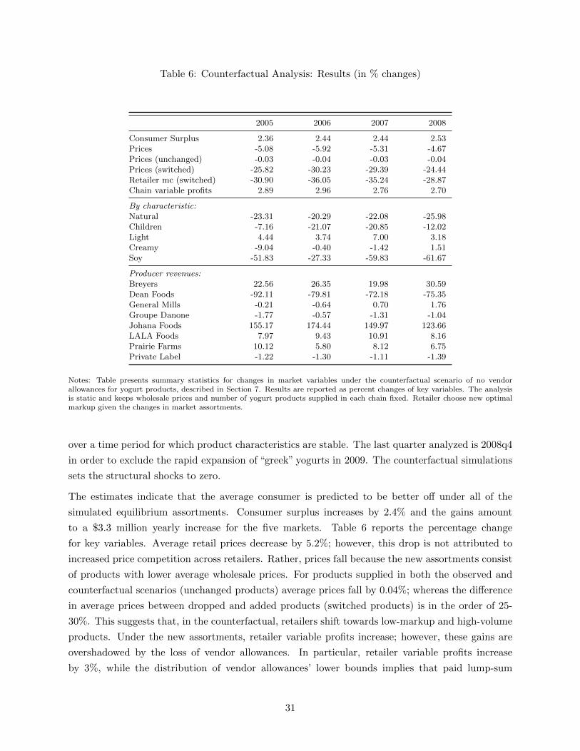
Table 6: Counterfactual Analysis: Results (in % changes)

2005 2006 2007 2008

Consumer Surplus 2.36 2.44 2.44 2.53Prices -5.08 -5.92 -5.31 -4.67Prices (unchanged) -0.03 -0.04 -0.03 -0.04Prices (switched) -25.82 -30.23 -29.39 -24.44Retailer mc (switched) -30.90 -36.05 -35.24 -28.87Chain variable profits 2.89 2.96 2.76 2.70

By characteristic:Natural -23.31 -20.29 -22.08 -25.98Children -7.16 -21.07 -20.85 -12.02Light 4.44 3.74 7.00 3.18Creamy -9.04 -0.40 -1.42 1.51Soy -51.83 -27.33 -59.83 -61.67

Producer revenues:Breyers 22.56 26.35 19.98 30.59Dean Foods -92.11 -79.81 -72.18 -75.35General Mills -0.21 -0.64 0.70 1.76Groupe Danone -1.77 -0.57 -1.31 -1.04Johana Foods 155.17 174.44 149.97 123.66LALA Foods 7.97 9.43 10.91 8.16Prairie Farms 10.12 5.80 8.12 6.75Private Label -1.22 -1.30 -1.11 -1.39

Notes: Table presents summary statistics for changes in market variables under the counterfactual scenario of no vendorallowances for yogurt products, described in Section 7. Results are reported as percent changes of key variables. The analysisis static and keeps wholesale prices and number of yogurt products supplied in each chain fixed. Retailer choose new optimalmarkup given the changes in market assortments.

over a time period for which product characteristics are stable. The last quarter analyzed is 2008q4

in order to exclude the rapid expansion of “greek” yogurts in 2009. The counterfactual simulations

sets the structural shocks to zero.

The estimates indicate that the average consumer is predicted to be better off under all of the

simulated equilibrium assortments. Consumer surplus increases by 2.4% and the gains amount

to a $3.3 million yearly increase for the five markets. Table 6 reports the percentage change

for key variables. Average retail prices decrease by 5.2%; however, this drop is not attributed to

increased price competition across retailers. Rather, prices fall because the new assortments consist

of products with lower average wholesale prices. For products supplied in both the observed and

counterfactual scenarios (unchanged products) average prices fall by 0.04%; whereas the difference

in average prices between dropped and added products (switched products) is in the order of 25-

30%. This suggests that, in the counterfactual, retailers shift towards low-markup and high-volume

products. Under the new assortments, retailer variable profits increase; however, these gains are

overshadowed by the loss of vendor allowances. In particular, retailer variable profits increase

by 3%, while the distribution of vendor allowances’ lower bounds implies that paid lump-sum

31

Figure 6: Change in Number of Unique Products by Characteristic

5 10 1510

20

30

natural

5 10 1510

20

30

children

5 10 1510

20

30

creamyA

vera

ge n

umbe

r of p

rodu

cts s

uppl

ied

in a

mar

ket

5 10 1510

20

30

light

5 10 150

2

4

6

soy

Observed assortmentsCounterfactual assortments

Notes: Each graph shows the average number of products under the observed and counterfactual assortments, separately foreach characteristic. If a product line is offered in two retailers in the market, I count it as two products. These graphs seekto highlight changes in market assortments. The counterfactual assortments correspond to new equilibrium assortments whenvendor allowances are eliminated.

transfers constitute at least 10% of retailer variable profits. Consequently, retailers fare worse in

the counterfactual.

The second panel of Table 6 reports how assortments adjust in the counterfactual, and Figure 6

shows these changes over time. Although natural and children’s products are predicted to lose 10-

20% of their market distribution, all retailers continue to offer at least one of these products; and,

on average, retailers supply 5 products with each characteristic. As a result, in the counterfactual

all retailers continue to offer consumers a variety of natural and children’s product options. In

contrast, soy products lose distribution in at least one retailer for 61% of the computed assortments.

Moreover, in the counterfactual soy yogurts are not supplied in Indianapolis, IN during 2005 and

2006, while in Richmond, VA the products disappear in 2008. Soy products may be characterized

as “niche” products in the yogurt industry, implying that retailers tailor their assortments towards

more “mainstream” products in the absence of vendor allowances.

Consequently, in the counterfactual, grocery chains position themselves closer to their competitors

in terms of assortments. To gain insight into assortment changes, one can examine results from a

representative market. Table 7 lists the products supplied under the observed and counterfactual

assortments in Buffalo, NY for the fourth quarter of 2007. The third column displays the number

of chains that carry the product line in the observed assortment, and the fourth column reports the

statistic for the counterfactual assortment. Under the observed market assortment, there are 43

32

Figure 7: Changes in Assortments for the Buffalo-2007q4 market

Groupe DanoneGeneral MillsDeansBreyers J

Observed Assortment

Counterfactual Assortment

L

Chain 1

Chain 3

Chain 2

Chain 1

Chain 3

Chain 2

Notes: The figure shows assortment snapshots for the Buffalo-2007q4 market. Vertical axis goes over observed chains in themarket. Horizontal axis identifies products. Products are ordered by brand: Breyers, Dean Foods, General Mills, GroupeDanone, Johanna Foods, and LALA Foods. Private label products are excluded from the graph as the counterfactual simulationkeeps private label assortments fixed. White blocks correspond to instances in which the product is not offered in the retailer-market pair. The counterfactual assortments correspond to new equilibrium assortments when vendor allowances are eliminated.

unique branded product lines supplied in the market, while in the simulated assortment, consumers

may choose from 39 product lines. In line with the characteristics’ changes described above, the

excluded products are: Horizon Organic Yogurt Tubes (Dean Foods’ natural and children’s prod-

uct), Silk Live (Dean Foods’ soy product), Brown cow (Groupe Danone’s natural product), and

Stonyfield Farm Squeezers (Groupe Danone’s natural and children’s product).

To analyze assortment changes across chains, Figure 7 shows a snapshot of the observed and

counterfactual assortments in Buffalo, NY for the fourth quarter of 2007. The first panel presents

the product offerings under the observed assortment and the second panel shows the counterfactual

choices. The vertical axis goes over the three retailers in the market and the horizontal axis identifies

products, sorted by producers. Figure 7 highlights that, absent vendor allowances, small producers,

who offer low-cost “mainstream” options, gain distribution in the market. In particular, Breyers,

Johanna Foods, and LALA Foods increase their total number of“shelf spots”by 3, 2, and 1 products

respectively.23 This increase is at the expense of Dean Foods, who loses 5 shelf spots in this market,

while Groupe Danone’s offerings decrease by 1. The total number of products supplied by General

Mills in the market does not change.

The increased market distribution for small producers results in higher total sales and revenues for

their products. This increase in market revenues, combined with the decrease in producer fixed

23Breyers yogurt producer should not be confused with the ice-cream maker. During the sample period the brandwas first owned by CoolBrands International and then by Healthy Food Holdings.

33

Table 7: Changes in Assortments for the Buffalo-2007q4 market

Producer Product Line # chains # chainsobserved counterfactual

Breyers

Breyers 2 3Breyers Creme Savers 2 3Breyers Light 2 3YoFarm YoCrunch 3 3

DeanFoods

Horizon Organic 2 1Horizon Organic Yogurt Tubes 1 -Silk 2 1Silk Live 2 -

GeneralMills

Yoplait Go Gurt 3 3Yoplait Go Gurt Fizzixx 3 2Yoplait Kids 3 3Yoplait Light 3 3Yoplait Light Thick and Creamy 2 3Yoplait Original 3 3Yoplait Thick and Creamy 3 3Yoplait Trix 3 3Yoplait Whips 3 3Yoplait Yo Plus 2 2

GroupeDanone

Brown Cow 2 -Dannon Activia 3 3Dannon Activia Light 3 3Dannon All Natural 3 3Dannon Creamy Fruit Blends 2 2Dannon Danimals 3 1Dannon Fat Free 3 3Dannon Fruit on the Bottom 3 3Dannon La Creme 3 3Dannon Light ’n Fit Carb & Sugar Control 3 3Dannon Light ’n Fit 3 3Dannon Light ’n Fit Creamy 2 2Dannon Natural 3 3Dannon Natural Flavors 3 3Dannon Premium 1 3Dannon Sprinklings 2 1Stonyfield Farm 2 3Stonyfield Farm Kids 1 2Stonyfield Farm O’Soy 1 1Stonyfield Farm Squeezers 1 -Stonyfield Farm Yobaby 2 3Stonyfield Farm Yokids 1 1

JohannaFoods

La Yogurt 2 3La Yogurt Custard Classics 2 3

LALAFoods

Weight Watchers 2 3

Private Labels 2 2

Notes: Table presents summary statistics for the assortment changes in Buffalo for the 4th quarter of 2007. The third columnshows the number of chains that supply the product in the observed assortment, and the 4th column shows the number in thecounterfactual assortment.

34

Figure 8: Change in Number of Unique Products by Producer

5 10 150

10

Breyers

5 10 150

10

Dean Foods

5 10 1520

40

General Mills

5 10 1520

40

Groupe Danone

5 10 150

10

Johanna Foods

Ave

rage

num

ber o

f pro

duct

s sup

plie

d in

a m

arke

t

5 10 150

10

LALA Foods

5 10 150

10

Prairie Farms

Observed assortmentsCounterfactual assortments

Notes: Each graph shows the average number of products under the observed and counterfactual assortments, separatelyfor each brand. If a product line is offered in two retailers in the market, I count it as two products. These graphs seek tohighlight changes in market assortments. The counterfactual assortments correspond to new equilibrium assortments whenvendor allowances are eliminated.

costs from the elimination of vendor allowance payments, implies that these producers are better

off in the absence of vendor allowances.24 In the counterfactual, General Mills’ assortments and

revenues change only slightly. The direction of the change vary by location: General Mills gains

distribution and revenues in Richmond, VA and Buffalo, NY; while the producer is worse off in

Birmingham, AL and St. Louis, MO. Groupe Danone’s revenues fall by 1.2% on average, and the

producer supplies fewer products in 70% of the counterfactual market-quarter pairs. Dean Foods

suffers a 80% decrease in revenues; moreover, the producer loses distribution for all of its products

in 40% of the analyzed market-quarter pairs. The patterns continue both across markets and over

time. Figure 8 shows the average number of product offerings across markets under the observed

and counterfactual assortments for each brand over time.

One may ask why Dean Foods and Groupe Danone pay vendor allowances to supply “niche” prod-

ucts. The discussion at the end of Section 6 shows that the vendor allowances paid by Dean Foods

24In order to contradict this implication, producer marginal costs of supplying to different retailers in the samemarket must vary drastically. The conclusion is also violated if small producers have increasing marginal costs ofproduction.

35

consist of both a cash transfer and provision of stocking service. Thus, economies of scope in dis-

tribution may rationalize Dean Foods’ supply decisions. The counterfactual analysis assumes that

all vendor allowance transfers are eliminated. However, if only cash transfers are eliminated, while

allowing for potential cost savings through the use of producer direct-store-delivery systems, then

Dean Foods’ product distribution and revenues might not change. To allow for such a counterfac-

tual, I would need data on retailers’ distribution costs.

Vendor allowances arise due to retailers’ opportunity costs of shelf space, hence, they may be used

as a means to allocate a scarce resource to its best available use.25 Thus, Groupe Danone may pay

vendor allowances for “niche” products because of high profit margins for these offerings. Under

this efficiency rationale, the observed assortment of Groupe Danone may maximize total vertical

profits, achieving the optimal assortment through the use of vendor allowances. Alternatively,

Groupe Danone may be using vendor allowances to protect its “mainstream” offerings. In that

case, Groupe Danone supplies “niche” products to the market in order to prevent the entry of

competitors’ products, which are close substitutes with its “mainstream” offerings.

These alternative strategies relate to the efficiency and exclusionary rationales discussed in the

debate about the effects of vendor allowances on product availability. Distinguishing between the

two rationales requires additional information about producers’ marginal costs. If one assumes that

producers’ margins are the same across all products, then the results support exclusion rather than

efficiency: total producer profits are higher under the observed assortment, but total vertical profits

are lower. However, if Groupe Danone’s cost function exhibits large discrepancies in costs across

products, or non-linearities, or gains in efficiency from producing some of the products together,

then the efficiency rationale may be supported. Hence, distinguishing between the two strategies

requires product-level data on producer marginal costs and remains a challenge for future work.

25Due to concerns about violations of the Robinson-Patman Act, wholesale prices differ across retailers only on thebasis of cost differences.

36

8 Conclusion

Despite the widespread use of vendor allowances in the retail sector, the Federal Trade Commission

does not have a conclusive position on the market effects of vendor allowances. This paper seeks to

further our understanding on the competitive implications of this vertical contract. Due to lack of

data on the size of vendor allowances received by retailers, I first quantify vendor allowances and

assess their importance for retailer profitability in the grocery industry using data on yogurt prod-

ucts. The framework incorporates both retail price competition and endogenous product assortment

decisions. Using a revealed preference approach, I identify the empirical distribution functions of

vendor allowances’ lower and upper bounds. Lower bound estimates for paid vendor allowances

imply that these transfers amount to 4.7% of estimated retailer revenues. When the negotiations

stage is modeled as producer take-it-or-leave-it offers, I find that paid vendor allowances are higher

for new products in the market. In addition, results show that there is substantial heterogeneity

in the paid vendor allowances across offered products and these transfers are larger for “niche”

products such as soy yogurts.

Next, I investigate the changes in market assortments, prices, and revenues in a counterfactual

scenario in which vendor allowances are eliminated. I find that vendor allowances benefit grocery

chains, while the effects on profitability of large producers are unclear. Without vendor allowances

consumer surplus increases as new assortment choices are tailored towards “mainstream” products

while eliminating “niche” products. In the counterfactual analysis, small producers increase both

their distribution and market sales. This expansion is primarily at the expense of Dean Foods and

Groupe Danone.

Dean Foods absorbs the distribution costs for its products by using its milk direct-store delivery

system to supply yogurts. The vendor allowance estimates capture lump-sum payments from pro-

ducers to retailer, which do not affect retailer sales. Hence, the counterfactual analysis eliminates

both cash payments from producers and incentives in the form of retailer cost savings. It would be

instructive to analyze a scenario in which distribution cost savigns are preserved, while only cash

payments are eliminated. However, such an analysis requires data on retailers’ distribution costs.

Groupe Danone’s strategy may be explained using both efficiency and anticompetitive rationales.

Under the assumption that producers’ margins are the same across product, the results imply vendor

allowances have an exclusionary effect. However, without marginal cost data, it is not possible to

rule out large variations in producer marginal costs across products that would imply Danone’s use

of vendor allowances promotes efficiency. Nevertheless, the paper shows how the framework can be

used to settle the debate in future work if marginal cost data can be obtained.

37

References

Asker, J. and H. Bar-Isaac (2014): “Raising retailers’ profits: On vertical practices and the

exclusion of rivals,” American Economic Review, 104, 672–86.

Aydin, G. and W. H. Hausman (2009): “The Role of Slotting Fees in the Coordination of

Assortment Decisions,” Production and Operations Management, 18, 635–652.

Berry, S. (1994): “Estimating discrete-choice models of product differentiation,” RAND Journal

of Economics, 25, 242–262.

Berry, S., A. Eizenberg, and J. Waldfogel (2014): “Optimal Product Variety in Radio

Markets,” Working paper.

Berry, S., J. Levinsohn, and A. Pakes (1995): “Automobile prices in market equilibrium,”

Econometrica, 63, 841–90.

Berry, S. and J. Waldfogel (1999): “Free entry and social inefficiency in radio broadcasting,”

RAND Journal of Economics, 30, 397–420.

Bloom, P. N., G. T. Gundlach, and J. P. Cannon (2000): “Slotting allowances and fees:

schools of thought and the views of practicing managers,” Journal of Marketing.

Bonnet, C. and P. Dubois (2010): “Inference on vertical contracts between manufacturers and

retailers allowing for nonlinear pricing and resale price maintenance,” The RAND Journal of

Economics, 41, 139–164.

——— (2015): “Identifying Two Part Tariff Contracts with Buyer Power: Empirical Estimation on

Food Retailing,” Tech. Rep. 1.

Bronnenberg, B. J., M. W. Kruger, and C. F. Mela (2008): “Database paper: The IRI

Marketing Data Set,” Marketing Science, 27, 745–748.

Conlon, C. and J. H. Mortimer (2014): “Efficiency and foreclosure effects of all-units discounts:

empirical evidence,” Working paper.

Crawford, G. and A. Yurukoglu (2012): “The welfare effects of bundling in multichannel

television markets,” The American Economic Review.

Draganska, M., D. Klapper, and S. B. Villas-Boas (2009a): “A larger slice or a larger pie?

An empirical investigation of bargaining power in the distribution channel,” Marketing Science,

29, 57–74.

Draganska, M., M. Mazzeo, and K. Seim (2009b): “Beyond plain vanilla: modeling joint

product assortment and pricing decisions,” Quantitative Marketing and Economics, 7, 105–146.

38

Dube, J., J. Fox, and C. Su (2012): “Improving the numerical performance of static and dynamic

aggregate discrete choice random coefficients demand estimation,” Econometrica, 80, 2231–2267.

Dube, J.-P. (2004): “Multiple discreteness and product differentiation: demand for carbonated

soft drinks,” Marketing Science, 23, 66–81.

Eizenberg, A. (2014): “Upstream innovation and product variety in the U.S. home PC market,”

The Review of Economic Studies, 81, 1003–1045.

Federal Trade Commission (2001): “Report on the Federal Trade Commission work-

shop on slotting allowances and other marketing practices in the grocery industry,”

http://www.ftc.gov/reports/report-federal-trade-commission-workshop-slotting-

allowances-other-marketing-practices, accessed Nov 2014.

——— (2003): “Slotting allowances in the retail grocery industry: selected case studies in five prod-

uct categories,” http://www.ftc.gov/reports/use-slotting-allowances-retail-grocery-

industry, accessed Nov 2014.

——— (2014): “Guides for Advertising Allowances and Other Merchandising Payments and Ser-

vices,” https://federalregister.gov/a/2014-23137.

Foros, O., H. J. Kind, and J. Y. Sand (2009): “Slotting allowances and manufacturers’ retail

sales effort,” Southern Economic Journal, 76, pp. 266–282.

Grennan, M. (2013): “Price discrimination and bargaining: empirical evidence from medical

devices,” American Economic Review, 103, 145–77.

Hendel, I. (1999): “Estimating multiple-discrete choice models: an application to computerization

returns,” Review of Economic Studies, 66, 423–46.

Ho, K. (2009): “InsurerpProvider networks in the medical care market,” American Economic

Review, 99, 393–430.

Ho, K., J. Ho, and J. H. Mortimer (2012): “The use of full-line forcing contracts in the video

rental industry,” American Economic Review, 102, 686–719.

Innes, R. and S. F. Hamilton (2006): “Naked slotting fees for vertical control of multi-product

retail markets,” International Journal of Industrial Organization, 24, 303–318.

——— (2013): “Slotting allowances under supermarket oligopoly,”American Journal of Agricultural

Economics, 95, 1216–1222.

Israilevich, G. (2004): “Assessing supermarket product-line decisions: the impact of slotting

fees,” Quantitative Marketing and Economics, 2, 141–167.

Kuksov, D. and A. Pazgal (2007): “Research note - The effects of costs and competition on

slotting allowances,” Marketing Science, 26, 259–267.

39

Lariviere, M. A. and V. Padmanabhan (1997): “Slotting allowances and new product intro-

ductions,” Marketing Science, 16, 112–128.

Marx, L. M. and G. Shaffer (2007): “Upfront payments and exclusion in downstream markets,”

RAND Journal of Economics, 38, 823–843.

——— (2010): “Slotting allowances and scarce shelf space,” Journal of Economics & Management

Strategy, 19, 575–603.

Misra, K. (2008): “Understanding retail assortments,” Working paper.

Mortimer, J. H. (2008): “Vertical contracts in the video rental industry,” Review of Economic

Studies, 75, 165–199.

Nevo, A. (2001): “Measuring market power in the ready-to-eat cereal industry,” Econometrica,

69, 307–342.

Pakes, A., J. Porter, K. Ho, and J. Ishii (2015): “Moment inequalities and their application,”

Econometrica, 215–334.

Shaffer, G. (1991): “Slotting allowances and resale price maintenance: a comparison of facilitating

practices,” RAND Journal of Economics, 22, 120–135.

——— (2005): “Slotting allowances and optimal product variety,” The B.E. Journal of Economic

Analysis & Policy, 5, 1–28.

Su, C. and K. L. Judd (2012): “Constrained optimization approaches to estimation of structural

models,” Econometrica, 80, 2213–2230.

Sudhir, K. (2001): “Structural Analysis of Manufacturer Pricing in the Presence of a Strategic

Retailer,” Marketing Science, 20, 244–264.

Sudhir, K. and V. R. Rao (2006): “Do slotting allowances enhance efficiency or hinder compe-

tition?” Journal of Marketing Research, 43, 137–155.

Sullivan, M. W. (1997): “Slotting allowances and the market for new products,” Journal of Law

and Economics, 40, 461–93.

Thomas, C. (2011): “Too Many Products: Decentralized Decision Making in Multinational Firms,”

American Economic Journal: Microeconomics, 3, 280–306.

Villas-Boas, S. B. (2007): “Vertical relationships between manufacturers and retailers: inference

with limited data,” Review of Economic Studies, 625–652.

Viswanathan, M. (2012): “Economic impact of category captaincy: An examination of assort-

ments and prices,” Working paper.

40

A Data Appendix

The data are obtained from the academic Information Resources Inc. (IRI) dataset that contains

information on grocery chains’ weekly sales and units sold in 47 distinct geographical markets in

the U.S. for the period of 2001-2011. Markets cover major metropolitan areas (e.g. Boston, MA)

or regions (e.g. New England). As shown in Figure A1, IRI market locations are scattered across

the U.S..

Figure A1: Locations of Markets and Producer Plants

Notes: Stars identify market locations, while red dots show the locations of producer manufacturing facilities.

The academic dataset is drawn from the IRI’s national sample of stores; IRI samples supermarkets

with annual sales of more than $2 million. The academic dataset includes information on a sample

of grocery and drug stores, hence, mass merchandisers, such as Walmart, are not included in the

sample. In the analysis I use data on grocery chains only. As a result, I observe between 4% and

16% of all stores in a geographic market, for a total of 74 grocery chains in the sample.26 For

each chain in the sample, the dataset contains information on an average of 25% of its stores. On

average, I observe 4 chains in a market, and each chain appears in the data in an average of 3

markets. Chains vary in size; their estimated market yearly sales range from $5 million to $1,147

million. Most of the chains in the IRI dataset are among the main competitors in their respective

markets. For each market I observe at least 2 and, on average, 3 to 4 of the 5 major grocery chains.

The five main competitors in a market account for 50-94% of sales in the grocery sector for the

analyzed markets.

In the analysis, I use 42 markets in which I observe information for at least two chains in the market

at any given quarter. The sample used covers seven years, 2004-2010, in order to match the data

26Information on all stores and their estimated yearly sales is gathered from ReferenceUSA data on U.S. Businesses.ReferenceUSA collects data on U.S. businesses and continuously updates the information. The data are assembledthrough public sources along with regular phone interviews with stores’ managers to verify the information and collectadditional data on businesses.

To calculate the reported measures, I use information on grocery stores with sales of more than $2 million a year.

41

collected from ReferenceUSA. The unit of analysis is ‘product line’-retailer-market-quarter. As a

result, a product is defined at the product line (e.g. Stonyfield Smooth & Creamy, 6 oz ), which

includes a variety of flavors (e.g. Stonyfield Smooth & Creamy, 6 oz, french vanilla). I aggregate

to the product line level because (according to industry practitioners) assortment decisions and

contracts are determined at the product line. I infer that a product line is supplied in a retailer if

it records non-zeros sales for the period. Concerns about a situation in which a product is on the

shelf and records zero sales are alleviated by the data aggregation at the quarter-retailer-market

level.

Following Villas-Boas (2007), quantity sold is measured by the number of 6-ounce servings sold.

Per-serving prices are constructed by dividing total sales by number of units sold. Prices are

converted to constant 2010 dollars using the Consumer Price Index by region. The average price

of a 6oz cup of yogurt is $0.80. Most of the price variation is across products and retailers. The

price variation over time due to temporary promotions is wiped out due to the aggregation at the

quarter level. Retail prices do not vary across flavors.

I define five product characteristics: natural, marketed for children, creamy, light, or soy. Over the

sample period the ingredients for most products change and a number of products are discontinued.

As a result, I rely on dummy variables to describe yogurts. These characteristics are neither

comprehensive nor exclusive, that is, a product can have none of the characteristics or it may

be defined as, for example, both natural and marketed for children. The natural characteristic

identifies organic products, or products which are marketed as using only natural ingredients.27 To

categorize products as creamy, light, or children’s, I inspect product line names and use key words.

The soy products in the dataset are Silk, Silk Live, and Stonyfield Farm O’Soy.

Markets offer a variety of natural, children’s, creamy, and light options: usually more than 20

product-retailer offerings with each of these characteristics are available. The only exception is

soy products as only 2-3 product-retailer options are offered in a market. Groupe Danone and

Dean Foods are the main producers of natural products and the only distributors of soy products.

Products marketed for children are offered by six of the producers analyzed. Price variation across

the product categories is shown in Table A1. The average price of natural and children’s products

are higher than their non-natural and non-children’s products. Natural, children’s, and creamy

products account for 8-11% of market sales each. Light products are responsible for, on average,

32% of market sales, while soy products are characterized by very low sales.

Following Draganska et al. (2009b), the estimation sample includes a producer if its market share

is at least 5% in at least 5 quarter-market pairs. As a result the sample consists of 12 national

and regional producers and 30 private label brands. Table A2 shows market shares and market

presence by producer. During the sample period the two main competitors are Groupe Danone and

27The products which are identified as natural are product lines under following brands: Brown Cow (GroupeDanone), Chiobani (Agro Farma), Danone Natural (Groupe Danone), Horizon Organic (Dean Foods), MountainHigh (Dean Foods), Nancy’s (Springfield Creamery), Silk (Dean Foods), Stonyfield Farm (Groupe Danone).

42

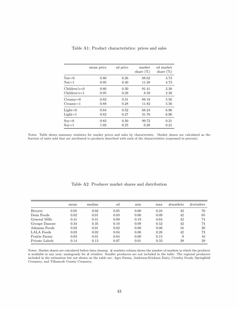
Table A1: Product characteristics: prices and sales

mean price sd price marketshare (%)

sd marketshare (%)

Nat=0 0.80 0.26 88.62 4.73Nat=1 0.95 0.40 11.38 4.73

Children’s=0 0.80 0.30 91.41 2.38Children’s=1 0.95 0.29 8.59 2.38

Creamy=0 0.82 0.31 88.18 5.56Creamy=1 0.88 0.28 11.82 5.56

Light=0 0.84 0.32 68.24 6.96Light=1 0.82 0.27 31.76 6.96

Soy=0 0.83 0.30 99.72 0.21Soy=1 1.02 0.25 0.28 0.21

Notes: Table shows summary statistics for market prices and sales by characteristic. Market shares are calculated as thefraction of units sold that are attributed to products described with each of the characteristics (expressed in percent).

Table A2: Producer market shares and distribution

mean median sd min max #markets #retailers

Breyers 0.05 0.02 0.05 0.00 0.24 42 70Dean Foods 0.02 0.01 0.03 0.00 0.09 42 65General Mills 0.41 0.41 0.09 0.19 0.64 42 74Groupe Danone 0.34 0.35 0.10 0.09 0.52 42 74Johanna Foods 0.02 0.01 0.02 0.00 0.08 16 20LALA Foods 0.03 0.02 0.04 0.00 0.28 42 73Prairie Farms 0.03 0.01 0.04 0.00 0.15 9 16Private Labels 0.14 0.13 0.07 0.01 0.33 39 29

Notes: Market shares are calculated before data cleanup. # markets column shows the number of markets in which the produceris available in any year; analogously for # retailers. Smaller producers are not included in the table. The regional producersincluded in the estimation but not shown on the table are: Agro Farma, Anderson-Erickson Dairy, Crowley Foods, SpringfieldCreamery, and Tillamook County Creamery.

43

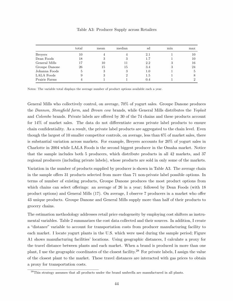
Table A3: Producer Supply across Retailers

total mean median sd min max

Breyers 10 4 4 2.1 1 10Dean Foods 18 3 3 1.7 1 10General Mills 17 10 11 2.2 3 16Groupe Danone 26 15 15 3.4 3 24Johanna Foods 5 3 3 1.0 1 5LALA Foods 9 3 2 1.5 1 8Prairie Farms 4 1 1 0.4 1 2

Notes: The variable total displays the average number of product options available each a year.

General Mills who collectively control, on average, 70% of yogurt sales. Groupe Danone produces

the Dannon, Stonyfield farm, and Brown cow brands, while General Mills distributes the Yoplait

and Colombo brands. Private labels are offered by 30 of the 74 chains and these products account

for 14% of market sales. The data do not differentiate across private label products to ensure

chain confidentiality. As a result, the private label products are aggregated to the chain level. Even

though the largest of 10 smaller competitor controls, on average, less than 6% of market sales, there

is substantial variation across markets. For example, Breyers accounts for 20% of yogurt sales in

Charlotte in 2004 while LALA Foods is the second biggest producer in the Omaha market. Notice

that the sample includes both 5 producers, which distribute products in all 42 markets, and 37

regional producers (including private labels), whose products are sold in only some of the markets.

Variation in the number of products supplied by producer is shown in Table A3. The average chain

in the sample offers 31 products selected from more than 71 non-private label possible options. In

terms of number of existing products, Groupe Danone produces the most product options from

which chains can select offerings: an average of 26 in a year; followed by Dean Foods (with 18

product options) and General Mills (17). On average, I observe 7 producers in a market who offer

43 unique products. Groupe Danone and General Mills supply more than half of their products to

grocery chains.

The estimation methodology addresses retail price endogeneity by employing cost shifters as instru-

mental variables. Table 2 summarizes the cost data collected and their sources. In addition, I create

a “distance” variable to account for transportation costs from producer manufacturing facility to

each market. I locate yogurt plants in the U.S. which were used during the sample period; Figure

A1 shows manufacturing facilities’ locations. Using geographic distances, I calculate a proxy for

the travel distance between plants and each market. When a brand is produced in more than one

plant, I use the geographic coordinates of the closest facility.28 For private labels, I assign the value

of the closest plant to the market. These travel distances are interacted with gas prices to obtain

a proxy for transportation costs.

28This strategy assumes that all products under the brand umbrella are manufactured in all plants.

44