Home mortgage risk: a case for insurance in India

Home Mortgage Risk: A Case for Insurance in India 57

INTERNATIONAL REAL ESTATE REVIEW2001 Vol. 4 No. 1: pp. 57 - 79

Home Mortgage Risk: A Case for Insurancein IndiaPiyush TiwariInstitute of Policy and Planning Sciences, University of Tsukuba, Tsukuba305-8573, Japan or [email protected]

Housing mortgage finance in India is constrained by the maximum loan-to-cost ratio and installment income ratio conditions imposed by housingfinance companies. The typical reason for this behaviour is that the marketfor the sharing of risk in mortgage lending is not yet fully developed.Mortgage insurance plays an important role in developing this market. Theobjective of this paper is to present a case for mortgage insurance market inIndia. This paper develops a mortgage premium structure framework inwhich mortgage insurers charge an insurance premium that equates lossesto revenue.

This paper also models mortgage termination due to prepayment anddefaults. We contend that the termination of mortgage in housing is not as`ruthless’ as OPM theory would suggest, primarily because households arenot financiers in the `stricter sense’. We have used the Cox proportionalhazard model to analyze prepayment and default of mortgage behaviour inIndia. The results indicate that financial concerns (like the option price, loanto value ratio, and monthly principal and interest to income ratio) areimportant determinants besides household characteristics. The cumulativeprepayment or default probabilities from these models are used in theestimation of the insurance premium structure.

Keywords

Default, Home mortgages, India, insurance, mortgage prepayment,proportional hazard

58 Tiwari

Introduction

The home mortgage market is growing rapidly in volume and importance.The outstanding volume of residential mortgage in India is currently over 200billion rupees and the volume has more than tripled during the last 15 years.The last decade has seen the emergence of many new housing financecompanies, and an increasing participation of banks in lending for housingfinance. Traditionally, the housing finance business in India has been limitedto primary markets. The nature of housing companies has been like a typicalsavings and loan corporation. The linkage with the secondary market hasbeen very weak. Housing finance companies have to raise resources from theprimary markets through various deposit schemes and lend to individualborrowers. These companies bear the risk associated with the housingmortgage. Unlike housing finance markets in the USA or the UK, the role ofsecondary markets has been meager in India. Only recently, NationalHousing Bank (NHB) permitted mortgage-backed securities with the role ofNHB as the ‘special purpose vehicle’. The first pool of mortgagessecuritized by NHB was fully subscribed by financial institutions. One of theconsequences of weak linkage with secondary market has been that the riskrelated to housing finance is solely borne by the housing finance institutions.This has restricted the availability of finance. The other implication of this isseen in the low loan-to-cost ratios of residential properties. The averageloan-to-cost ratio in India is around 55%. In the USA, the loan-to-cost ratiois around 95%, and in Japan it is around 80%. A low loan-to-cost ratioimplies that households have to amass a substantial amount of their ownequity before deciding to buy their own houses. High equity requirement forhousing has been a major constraint in home ownership.

In the absence of a secondary market, institutions and banks making housingloans bear various lending risks. These lending risks are (I) macro-economicrisk – due to changes in interest rates, which in turn are due to changes inmacroeconomic conditions, and (ii) liquidity risk – due to prepayment anddefault of loans. Housing finance institutions design instruments with anintention to offset these risks. The typical way is a penalty imposed forprepayments and high interest rates for lending to take into account macro-economic risk. The high interest payments by households restrict their abilityto borrow any further because the monthly payments towards their housingloans are restricted by their income. Housing finance institutions set the limitof monthly payments to about 30% of the monthly income of the borrower.

Wealth and income constraints restrict households from achieving the desiredstandard of housing. In more developed housing finance markets like theUSA or Hong Kong, mortgage insurance plays an active role where incomeand wealth are binding for households’ access to housing finance. Housing


mortgage insurance does not exist in India. In fact, the insurance market is inits infant stage in India, and has assumed great importance recently after theGovernment allowed private insurers to operate in the Indian insurancemarket. This paper is written with two purposes: (I) to empirically estimaterisks associated with housing mortgages, and (ii) to design a framework formortgage insurance in India.

The rest of the paper is organized as follows: Section 2 provides an overviewof the role of residential mortgage insurance in housing finance and homeownership. Section 3 reviews the literature in measuring the risk associatedwith the residential mortgages. Section 4 presents the results of theestimation of risk for residential mortgage market in India. In Section 5, aframework for residential mortgage insurance is presented. Section 6concludes the discussion.

The Role of Residential Mortgage Insurance

In developed economies, mortgage insurance has become an importantinstrument to cover some of the risks incurred by housing finance institutionsor investors in mortgage-based securities, and also to assist borrowers inmobilizing higher amounts of housing loans than would have been possibleotherwise, due to their wealth and income constraints.

For wealthier households, choice of loan-to-cost ratio depends on ahousehold’s portfolio diversification desires and its aversion to risk, as wellas the after-tax cost of mortgage financing relative to both the cost of otherdebt financing and after-tax returns on financial assets (Jones, 1993). Forless wealthy households facing binding mortgage qualification constraints,the choice is more straightforward: what loan-to-cost ratio maximizes theirwealth is the value of the house they can purchase.

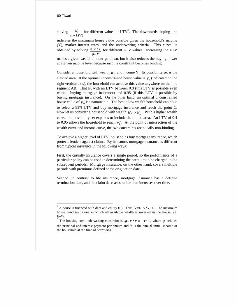
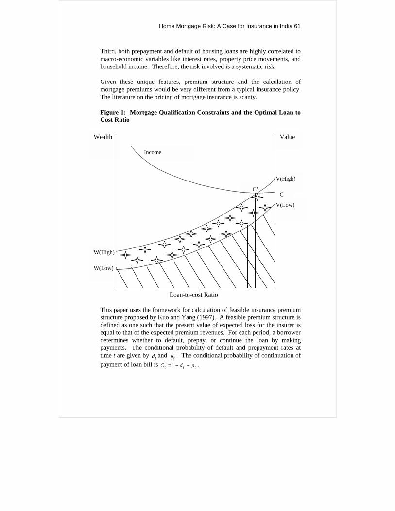
Figure 11 illustrates the maximum attainable housing value when wealth andincome constraints are binding separately, simultaneously, or not at allbinding. The right vertical axis is the house value and the left axis is wealth.The horizontal axis is the loan to cost ratio, ranging from 0 to 0.95. The twoupward sloping lines indicate the maximum house value possible given theinitial wealth of LW (low) or HW (high). These curves can be derived by

1 This example was taken from Hendershott and LaFayette (1995).

60 Tiwari

solving )1( LTV

Wi−

for different values of LTV2. The downwards-sloping line

indicates the maximum house value possible given the household’s income(Y), market interest rates, and the underwriting criteria. This curve3 isobtained by solving

LTVY

φ*30.0 for different LTV values. Increasing the LTV

makes a given wealth amount go down, but it also reduces the buying powerat a given income level because income constraint becomes binding.

Consider a household with wealth LW and income Y. Its possibility set is theslashed area. If the optimal unconstrained house value is *

LV (indicated on theright vertical axis), the household can achieve this value anywhere on the linesegment AB. That is, with an LTV between 0.8 (this LTV is possible evenwithout buying mortgage insurance) and 0.95 (if this LTV is possible bybuying mortgage insurance). On the other hand, an optimal unconstrainedhouse value of *

HV is unattainable. The best a low wealth household can do isto select a 95% LTV and buy mortgage insurance and reach the point C.Now let us consider a household with wealth LH WW > . With a higher wealthcurve, the possibility set expands to include the dotted area. An LTV of 0.4to 0.95 allows the household to reach *

LV . At the point of intersection of thewealth curve and income curve, the two constraints are equally non-binding.

To achieve a higher level of LTV, households buy mortgage insurance, whichprotects lenders against claims. By its nature, mortgage insurance is differentfrom typical insurance in the following ways:

First, the casualty insurance covers a single period, so the performance of aparticular policy can be used in determining the premium to be charged in thesubsequent periods. Mortgage insurance, on the other hand, covers multipleperiods with premiums defined at the origination date.

Second, in contrast to life insurance, mortgage insurance has a definitetermination date, and the claim decreases rather than increases over time.

2 A house is financed with debt and equity (E). Thus, V=LTV*V+E. The maximumhouse purchase is one in which all available wealth is invested in the house, i.e.E=W.3 The housing cost underwriting constraint is YVLTV *3.0* =φ , where φ includesthe principal and interest payment per annum and Y is the annual initial income ofthe household at the time of borrowing.


Wealth

W(High)

W(Low)

C’C

Value

V(High)

V(Low)

Third, both prepayment and default of housing loans are highly correlated tomacro-economic variables like interest rates, property price movements, andhousehold income. Therefore, the risk involved is a systematic risk.

Given these unique features, premium structure and the calculation ofmortgage premiums would be very different from a typical insurance policy.The literature on the pricing of mortgage insurance is scanty.

Figure 1: Mortgage Qualification Constraints and the Optimal Loan toCost Ratio

Loan-to-cost Ratio

This paper uses the framework for calculation of feasible insurance premiumstructure proposed by Kuo and Yang (1997). A feasible premium structure isdefined as one such that the present value of expected loss for the insurer isequal to that of the expected premium revenues. For each period, a borrowerdetermines whether to default, prepay, or continue the loan by ma ingpayments. The conditional probability of default and prepayment rattime t are given by td and tp . The conditional probability of continuatiopayment of loan bill is ttt pdC −−=1 .

Income

k
es atn of

62 Tiwari

For the insurer, the present value of accumulated loss from present to time t,denoted by tEAL is given by:

tt ELELELEAL +++= ...21 (1)

Alternatively, we can write Equation (1) as:

st

s

s

tsRstRt rBLdCrBLdEAL −

=

−

=

− ∑ ∏+=2

1

1

111 )( (2)

where tB is the unpaid balance at time t, RL is the ratio of the loss-to-unpaidbalance at time t, and r is the present value factor dependent on the discountrate used for calculating the present value of loss and revenue.

The present value of the expected revenue from present period to time t,tEAR , is given by:

tt EREREREAR +++= ...10 (3)

Alternatively, we may write:

ssss

t

s

s

ttt rBaCCBaCBaEAR −

=

−

=∑ ∏++= )(

2

1

111100

(4)

where ta refers to the ratio of time t insurance premium payment to tB . Theinsurers would charge premium so that:

tt EAREAL = (5)

The Residential Mortgage Risk Model

In the mortgage insurance premium framework, conditional probabilities ofdefault and prepayment have to be specified exogenously. In this section, wepresent a model for the estimation of these mortgage risks.

Mortgage insurers would like the loans they insure to continue until theirmaturity. However, at any point in time, borrowers have four options: (i) tocontinue paying their loans, (ii) to prepay their obligation before the maturityterm, (iii) to default, and (iv) to delay payment. The option to prepay ordefault is available to borrowers. It is widely accepted that mortgages can beviewed as ordinary debt instruments with various options attached to them.


Default is a put option: the borrower sells the house back to the lender inexchange for eliminating the mortgage obligation. Prepayment is a calloption: the borrower exchanges the unpaid balance on the debt instrument fora release of further obligation. By insuring the loan, the insurer bears the riskof terminating the loan due to prepayment and default. Prepayment stops thefuture stream of insurance premiums. Default stops future premiums and, inaddition, the insurers have to pay the insured amount to the housing financecompany. Probabilities of prepayment and default of mortgage loan enter intothe insurance premium calculations of the insurer, as discussed earlier. Wetherefore need to estimate prepayment and default probabilities at each pointin time.

Empirical estimation of mortgage termination has utilized logit or probitmodels to estimate the probability of termination or, more recently, utilizedhazard models to estimate the age of mortgages. Analyses of the probabilityof termination have utilized either data from mortgage pools (Cooperstein,Redburn, and Meyers, 1991; Foster and Van Order, 1985) or data fromindividual loans (Vandell and Thibodeau, 1985; Zorn and Lea, 1986; andCapone and Cunningham, 1992). Similarly, analyses of loan age have alsoused either data from mortgage pools (Follain, Scott, and Yang 1992; andSchwartz and Torous, 1993) or data from individual loans.

Earlier researchers (see for example Cox, Ingersoll, and Ross, 1985) haveused the option-pricing model proposed by Black and Scholes (1972) toestimate prepayment and default probabilities. Whenever the option is inmoney, the borrower terminates its obligation. Several explanations,however, can be offered to explain why the contingent claim option pricingmodels do not apply exactly to individual households’ housing mortgages.First, owner-occupants may not be as financially sophisticated as the pureoption pricing models (OPM) imply. Alternatively stated, these householdsmay face substantially high transaction costs in their refinancing decisionsbecause they require much time and effort to make correct decisions, giventheir lack of financial sophistication. Second, prepayments or defaults byhomeowners are influenced by many other decisions that make it difficult toidentify clearly the effects of OPM. For example, households often prepaybecause their job locations change, or there is a change in the composition ofhousehold, like divorce. Third, prepayment or default may occur as a part ofthe overall desire of households to readjust the composition of theirportfolios. For example, a person may choose to refinance in order toincrease his or her loan-to-value ratio and use the proceeds to make otherinvestments. Fourth, the data available to estimate prepayment or defaultstudies may constitute part of the problem. In particular, the interest ratepattern of the past fifteen years may not contain enough volatility to measure

64 Tiwari

with this precision their effects on prepayments. Similarly, housing pricesmay not have enough volatility to measure their effects on defaults.

Several recent empirical studies have applied the Cox Proportional HazardModel (Cox and Oakes, 1984) to estimate mortgage risk (e.g. Green andShoven, 1986; Schwartz and Torous, 1989; Quigley and Van Order, 1990,1995; Follain, Ondrich, and Sinha, 1996; Boyer, Follain, Ondrich, andPiccirillo, 1997). Instead of solving for the unique critical vales of the statevariables in the contingent claim model, the proportional hazard modelassumes that at each point of time during the mortgage contract period, themortgage has a certain probability of termination, conditional on survival ofthe mortgage. The hazard function in this model is defined as the product ofa baseline hazard and a set of time-varying covariates. These covariates neednot be limited to the option value itself. They may include other importantdeterminants of behaviour. The proportional hazard model can thusincorporate reasonable mortgage termination behaviour due to prepayment ordefault that would be considered sub-optimal under the contingent claimframework.

Results for the US market indicates that the hazard rate of prepayment isproportional to “lock-in,” which is the difference between the face value andthe market value of the mortgage as a proportion of the value of the property(Green and Shoven 1986). Other variables that affect the hazard rate besidesthe cash value of a mortgage are household income and characteristics of thehousehold head (Quigley 1987).

The proportional hazard model is used in the loan termination literature toanalyze mortgage termination behaviour.

In technical terms, on the basis of proportional hazard methodology, theprobability of mortgage termination due to prepayment or default (a), giventhe exogenous factors Z1,…,Zn at time t, can be divided into twomultiplicative factors:

Prob = h(a) * Π (Z1,…,Zn), (6)

where h(a) is the baseline hazard, which is the proportion of the populationthat would prepay or default under completely stationary or homogeneousconditions. The baseline hazard gives the normal time profile of theconditional prepayment or default rates (the probability of prepayment ordefault in year 1, year 2, etc., of a loan in a particular loan group). Inaddition, Π(Z1,…,Zn), are the exogenous factors that make prepayments ordefault more or less likely. The effect of these factors on prepayment ordefault is also assumed to be time separable. That is, past and future


attributes of the environment are assumed to have no effect on turnover in thepresent (Green and Shoven 1986; Quigley 1987; Van Order 1990)

The Cox Proportional Hazard model (Cox and Oates, 1984) is defined as:

H(ti, Z) = h0(ti) exp [Z(ti) β] (7)

where i is the month in observation, Z(ti) is a set of time-varying covariates,and h0 (.) is the baseline hazard reflecting the age-related amortization featureof mortgage. β s are the coefficients of covariates in Equation (7). The mostpopular estimation approach for proportional hazard model is the Cox partiallikelihood approach (CPL, see Cox and Oates, 1984).

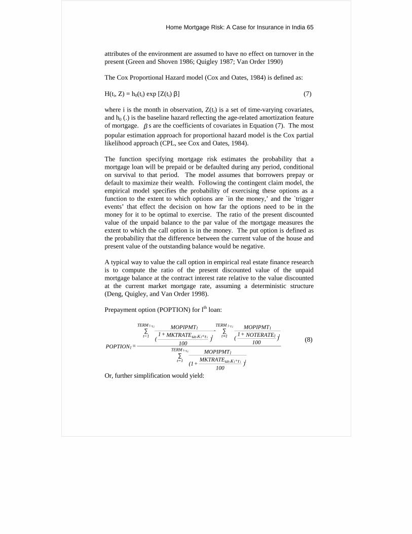
The function specifying mortgage risk estimates the probability that amortgage loan will be prepaid or be defaulted during any period, conditionalon survival to that period. The model assumes that borrowers prepay ordefault to maximize their wealth. Following the contingent claim model, theempirical model specifies the probability of exercising these options as afunction to the extent to which options are `in the money,’ and the `triggerevents’ that effect the decision on how far the options need to be in themoney for it to be optimal to exercise. The ratio of the present discountedvalue of the unpaid balance to the par value of the mortgage measures theextent to which the call option is in the money. The put option is defined asthe probability that the difference between the current value of the house andpresent value of the outstanding balance would be negative.

A typical way to value the call option in empirical real estate finance researchis to compute the ratio of the present discounted value of the unpaidmortgage balance at the contract interest rate relative to the value discountedat the current market mortgage rate, assuming a deterministic structure(Deng, Quigley, and Van Order 1998).

Prepayment option (POPTION) for lth loan:

)100

MKTRATE+(1

MOPIPMT

)100

NOTERATE+1(

MOPIPMT-)

100MKTRATE+1

(

MOPIPMT

= POPTION

l+K,

lTERM

1t=

ll

lTERM

1tl+K,

lTERM

1t=

l

ill

i-l

i1-

ill

i-l

τω

τω

τ

ττ

∑

∑∑= (8)

Or, further simplification would yield:

66 Tiwari

l

, K +l

TERM -

l,K +

TERM -POPTION = 1 -

MKTRATE [1 - (1

1+ NOTERATE100

) ]

NOTERATE [1 - (1

1+MKTRATE

100

) ]

l l il i

l l i

l i

ω ττ

ω τ

τ

(9)

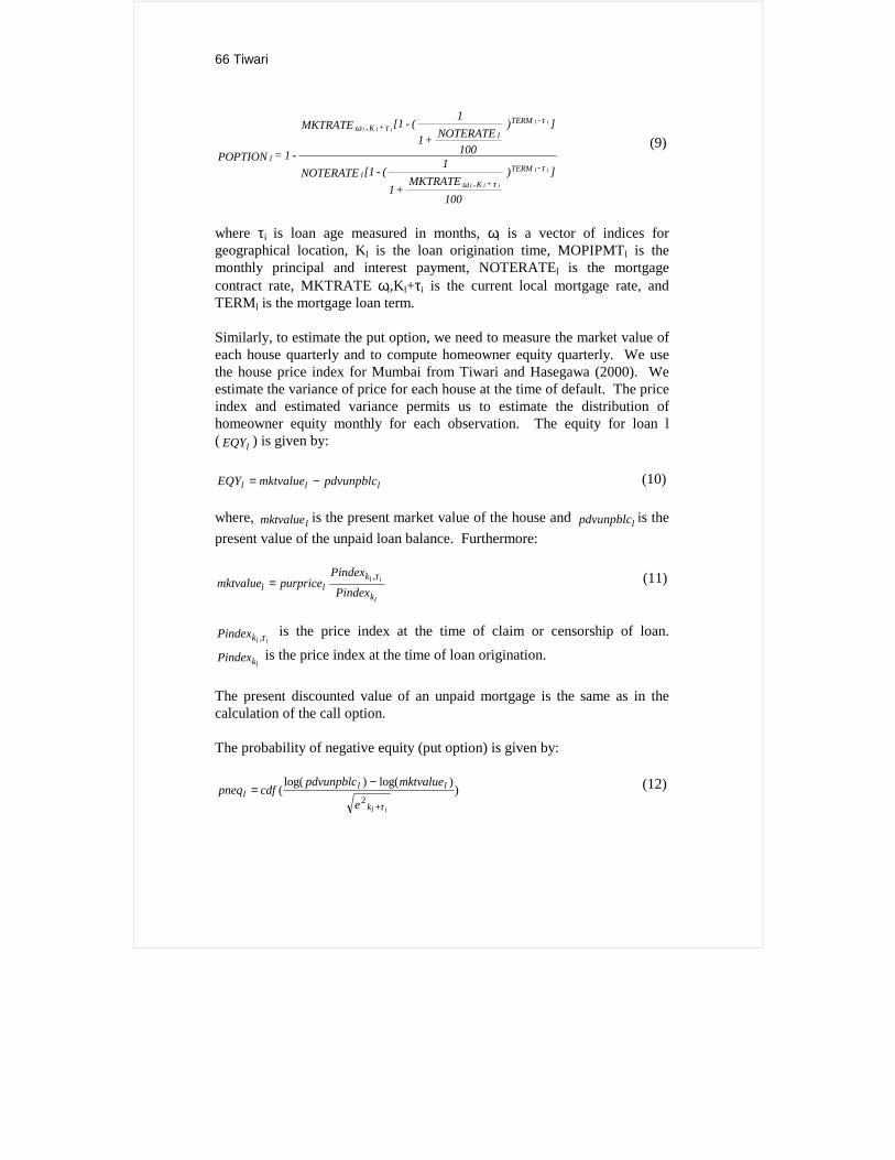
where τi is loan age measured in months, ωl is a vector of indices forgeographical location, Kl is the loan origination time, MOPIPMTl is themonthly principal and interest payment, NOTERATEl is the mortgagecontract rate, MKTRATE ωl,Kl+τi is the current local mortgage rate, andTERMl is the mortgage loan term.

Similarly, to estimate the put option, we need to measure the market value ofeach house quarterly and to compute homeowner equity quarterly. We usethe house price index for Mumbai from Tiwari and Hasegawa (2000). Weestimate the variance of price for each house at the time of default. The priceindex and estimated variance permits us to estimate the distribution ofhomeowner equity monthly for each observation. The equity for loan l( lEQY ) is given by:

lll pdvunpblcmktvalueEQY −= (10)

where, lmktvalue is the present market value of the house and lpdvunpblc is thepresent value of the unpaid loan balance. Furthermore:

l

il

k

kll Pindex

Pindexpurpricemktvalue τ,= (11)

ilkPindex τ, is the price index at the time of claim or censorship of loan.

lkPindex is the price index at the time of loan origination.

The present discounted value of an unpaid mortgage is the same as in thecalculation of the call option.

The probability of negative equity (put option) is given by:

))log()log(

(2

ilk

lll

e

mktvaluepdvunpblccdfpneq

τ+

−= (12)


where cdf(.) is the cumulative standard normal distribution function, andilke τ,

2 is the variance of price. pneq is the probability that equity is negative.That is, the probability that the put option is in money.

To estimate the model with CPL, we first calculate the call or put optioncovariates for each individual loan and construct the covariate matrix, whichconsists of the call option covariate (POPTION), put option covariate(PNEQ), the initial loan to value ratio, the monthly installment-to-incomeratio agreed to at the time of loan origination, and other household-relatedvariables explained in next section. Another factor that we consider is thatthe mortgage termination behaviour for home purchase loans and other loansrelated to housing (like home improvement etc.) is different. The incidencesof prepayment and default of other loans are much higher. We include adummy variable for other loans in our model to account for this difference.

Estimates of Mortgage Risks

Data

There are two databases that we have used for our analysis. The database forthe prepayment analysis is the administrative database of a housing financecompany for Mumbai, which contains 12,173 observations on single-familymortgage loans issued between January 1989 and March 1998. All are fixed-rate, level payment, and fully amortized. The term of loan in most cases is 15years, but other terms (5 and 10 years) also exist. The mortgage historyperiod ends in March 1998. The database for the default analysis contains3,497 loan observations for Mumbai. We define a loan delinquent for threeconsecutive months as defaulted4. The term of loan in most of the cases is 15years and the loans were issued during January 1990 to March 1996. Thesetwo databases are completely different but contain all segments ofhouseholds and properties in all locations of Mumbai. The typical way ofbuying properties in Mumbai is through real estate agents or developers.Most of the houses are of the apartment type. The share of independenthouses in total houses in Mumbai is negligible.

Developers require construction finance for their projects, and they borrowfrom housing finance companies. Housing finance companies lend todevelopers based on their credit worthiness and project viability. Pastexperience with developers plays an important role. In the process, housingfinance companies rate the developers and their projects. These ratings are 4 This is the typical way in which housing finance companies define defaults in Indiaon their balance sheets.

68 Tiwari

an important feature of developers’ marketing of their projects. Housingfinance companies also simplify the process for approving loans to borrowerswho buy properties in approved projects. The criterion to evaluateborrowers’ credit worthiness is based on their repayment abilities. Salariedborrowers have easy access to housing finance compared to self-employed orother types of borrowers. Income plays an important role in determining themaximum amount of a loan. The borrowers and the properties, which theyhave bought, are distributed all over Mumbai.

The data used in this paper is an administrative database, which accounts forthe flow of loan repayment for each of the loans during their term. Wheneverthe loan is prepaid or defaulted, the amount and date are also entered into thedatabase. In both databases, for each mortgage loan, the availableinformation includes the year and month of origination and termination (if ithas been closed), indicators of prepayment or default, the purchase price ofthe property, the original loan amount, the initial loan-to-value ratio, themortgage contract interest rate, the purpose of the loan (whether it is forhome ownership or home improvement), the monthly interest, and principalpayment.

Though we have referred to these databases as prepayment or defaultdatabases mainly due to the purpose for which they have been used, theprepayment databases include loan information for those which are eitherprepaid or still active. Similarly, the defaults database includes loans, whichare either delinquent or still active. These active loans may close normally atthe end of their terms or become prepaid or defaulted in the future. Thedatabases also reflect information about the borrowers, like the number of co-borrowers, if any, the monthly income of borrowers at the time of origination,the sex of the borrower, his or her employment status (self employed,unemployed, or in the service), education level, marital status (single,divorced, married), and the age of the borrower.

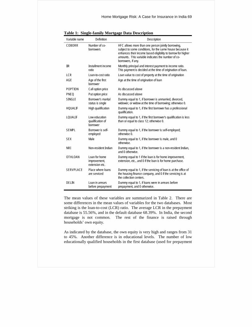
Databases used for prepayment analysis have information about whether aloan was in arrears before being prepaid. This information we have capturedin our analysis on prepayment. Housing finance companies in India lend forpurchase of houses and also for the extension, redevelopment, etc., ofexisting houses. We have referred to the loans for home extension, etc., asother loans (OTHLOAN), although they are part of the same database to helpus in identifying the role that different financial products play in theprepayment or default motives of households. Table 1 describes thevariables from the database used in this analysis.


Table 1: Single-family Mortgage Data DescriptionVariable name Definition Description

COBORR Number of co-borrowers

HFC allows more than one person jointly borrowing,subject to some conditions, for the same house because itenhances their income based eligibility to borrow for higheramounts. This variable indicates the number of co-borrowers, if any.

IIR Installment incomeratio

Monthly principal and interest payment to income ratio.This payment is decided at the time of origination of loan.

LCR Loan-to-cost ratio Loan value to cost of property at the time of originationAGE Age of the first

borrowerAge at the time of origination of loan

POPTION Call option price As discussed abovePNEQ Put option price As discussed aboveSINGLE Borrower’s marital

status is singleDummy equal to 1, if borrower is unmarried, divorced,widower, or widow at the time of borrowing; otherwise 0.

HQUALIF High qualification Dummy equal to 1, if the first borrower has a professionalqualification.

LQUALIF Low educationqualification ofborrower

Dummy equal to 1, if the first borrower’s qualification is lessthan or equal to class 12; otherwise 0.

SEMPL Borrower is self-employed

Dummy equal to 1, if the borrower is self-employed;otherwise 0.

SEX Male Dummy equal to 1, if the borrower is male, and 0otherwise.

NRI Non-resident Indian Dummy equal to 1, if the borrower is a non-resident Indian,and 0 otherwise.

OTHLOAN Loan for homeimprovement,extension etc.

Dummy equal to 1 if the loan is for home improvement,extension, etc., and 0 if the loan is for home purchase.

SERVPLACE Place where loansare serviced

Dummy equal to 1, if the servicing of loan is at the office ofthe housing finance company, and 0 if the servicing is atthe collection centers.

DELIN Loan in arrearsbefore prepayment

Dummy equal to 1, if loans were in arrears beforeprepayment, and 0 otherwise.

The mean values of these variables are summarized in Table 2. There aresome differences in the mean values of variables for the two databases. Moststriking is the loan-to-cost (LCR) ratio. The average LCR in the prepaymentdatabase is 55.56%, and in the default database 68.39%. In India, the secondmortgage is not common. The rest of the finance is raised throughhouseholds’ own equity.

As indicated by the database, the own equity is very high and ranges from 31to 45%. Another difference is in educational levels. The number of loweducationally qualified households in the first database (used for prepayment

70 Tiwari

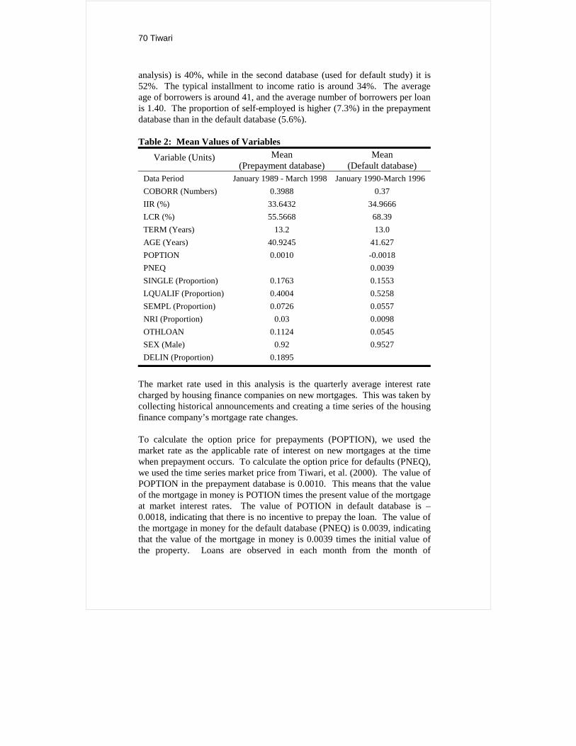
analysis) is 40%, while in the second database (used for default study) it is52%. The typical installment to income ratio is around 34%. The averageage of borrowers is around 41, and the average number of borrowers per loanis 1.40. The proportion of self-employed is higher (7.3%) in the prepaymentdatabase than in the default database (5.6%).

Table 2: Mean Values of Variables

Variable (Units) Mean(Prepayment database)

Mean(Default database)

Data Period January 1989 - March 1998 January 1990-March 1996COBORR (Numbers) 0.3988 0.37IIR (%) 33.6432 34.9666LCR (%) 55.5668 68.39TERM (Years) 13.2 13.0AGE (Years) 40.9245 41.627POPTION 0.0010 -0.0018PNEQ 0.0039SINGLE (Proportion) 0.1763 0.1553LQUALIF (Proportion) 0.4004 0.5258SEMPL (Proportion) 0.0726 0.0557NRI (Proportion) 0.03 0.0098OTHLOAN 0.1124 0.0545SEX (Male) 0.92 0.9527DELIN (Proportion) 0.1895

The market rate used in this analysis is the quarterly average interest ratecharged by housing finance companies on new mortgages. This was taken bycollecting historical announcements and creating a time series of the housingfinance company’s mortgage rate changes.

To calculate the option price for prepayments (POPTION), we used themarket rate as the applicable rate of interest on new mortgages at the timewhen prepayment occurs. To calculate the option price for defaults (PNEQ),we used the time series market price from Tiwari, et al. (2000). The value ofPOPTION in the prepayment database is 0.0010. This means that the valueof the mortgage in money is POTION times the present value of the mortgageat market interest rates. The value of POTION in default database is –0.0018, indicating that there is no incentive to prepay the loan. The value ofthe mortgage in money for the default database (PNEQ) is 0.0039, indicatingthat the value of the mortgage in money is 0.0039 times the initial value ofthe property. Loans are observed in each month from the month of


origination through the month of termination, maturation, or through March1998 for active loans.

Estimation Results

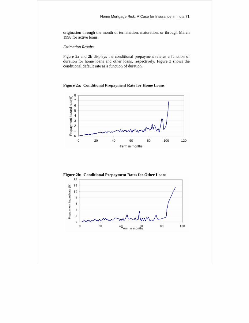
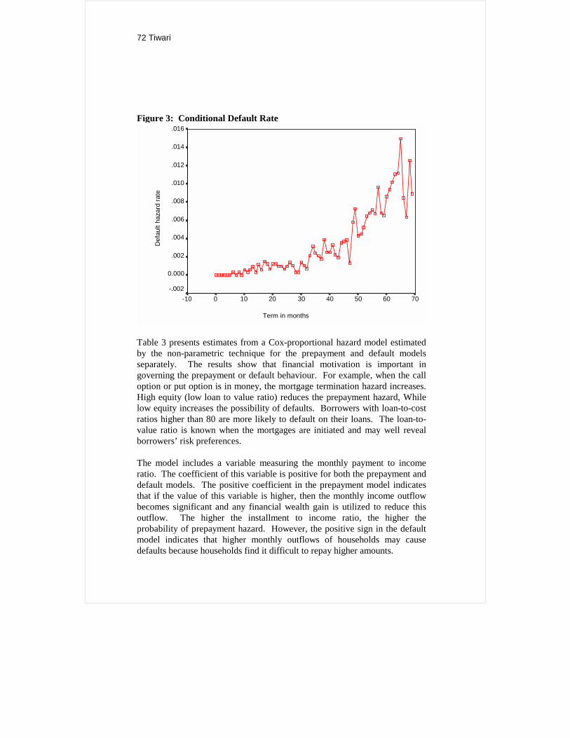
Figure 2a and 2b displays the conditional prepayment rate as a function ofduration for home loans and other loans, respectively. Figure 3 shows theconditional default rate as a function of duration.

Figure 2a: Conditional Prepayment Rate for Home Loans

012345678

0 20 40 60 80 100 120

Term in months

Prep

aym

ent h

azar

d ra

te(%

)

Figure 2b: Conditional Prepayment Rates for Other Loans

0

2

4

6

8

10

12

14

0 20 40 60 80 100Term in months

Prep

aym

ent h

azar

d ra

te (%

)

72 Tiwari

Figure 3: Conditional Default Rate

Term in months

70 60 50 40 30 20 10 0 -10

Def

ault

haza

rd ra

te

.016

.014

.012

.010

.008

.006

.004

.002

0.000 -.002

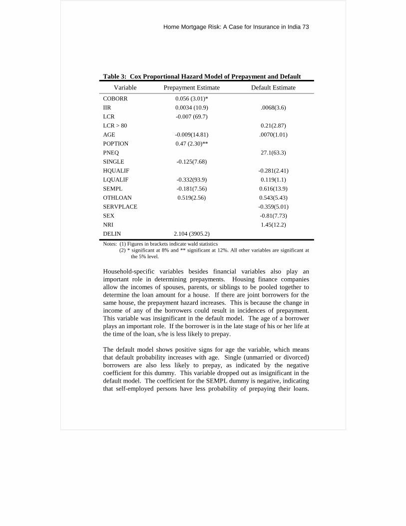
Table 3 presents estimates from a Cox-proportional hazard model estimatedby the non-parametric technique for the prepayment and default modelsseparately. The results show that financial motivation is important ingoverning the prepayment or default behaviour. For example, when the calloption or put option is in money, the mortgage termination hazard increases.High equity (low loan to value ratio) reduces the prepayment hazard, Whilelow equity increases the possibility of defaults. Borrowers with loan-to-costratios higher than 80 are more likely to default on their loans. The loan-to-value ratio is known when the mortgages are initiated and may well revealborrowers’ risk preferences.

The model includes a variable measuring the monthly payment to incomeratio. The coefficient of this variable is positive for both the prepayment anddefault models. The positive coefficient in the prepayment model indicatesthat if the value of this variable is higher, then the monthly income outflowbecomes significant and any financial wealth gain is utilized to reduce thisoutflow. The higher the installment to income ratio, the higher theprobability of prepayment hazard. However, the positive sign in the defaultmodel indicates that higher monthly outflows of households may causedefaults because households find it difficult to repay higher amounts.


Table 3: Cox Proportional Hazard Model of Prepayment and Default

Variable Prepayment Estimate Default EstimateCOBORR 0.056 (3.01)*IIR 0.0034 (10.9) .0068(3.6)LCR -0.007 (69.7)LCR > 80 0.21(2.87)AGE -0.009(14.81) .0070(1.01)POPTION 0.47 (2.30)**PNEQ 27.1(63.3)SINGLE -0.125(7.68)HQUALIF -0.281(2.41)LQUALIF -0.332(93.9) 0.119(1.1)SEMPL -0.181(7.56) 0.616(13.9)OTHLOAN 0.519(2.56) 0.543(5.43)SERVPLACE -0.359(5.01)SEX -0.81(7.73)NRI 1.45(12.2)DELIN 2.104 (3905.2)

Notes: (1) Figures in brackets indicate wald statistics (2) * significant at 8% and ** significant at 12%. All other variables are significant at

the 5% level.

Household-specific variables besides financial variables also play animportant role in determining prepayments. Housing finance companiesallow the incomes of spouses, parents, or siblings to be pooled together todetermine the loan amount for a house. If there are joint borrowers for thesame house, the prepayment hazard increases. This is because the change inincome of any of the borrowers could result in incidences of prepayment.This variable was insignificant in the default model. The age of a borrowerplays an important role. If the borrower is in the late stage of his or her life atthe time of the loan, s/he is less likely to prepay.

The default model shows positive signs for age the variable, which meansthat default probability increases with age. Single (unmarried or divorced)borrowers are also less likely to prepay, as indicated by the negativecoefficient for this dummy. This variable dropped out as insignificant in thedefault model. The coefficient for the SEMPL dummy is negative, indicatingthat self-employed persons have less probability of prepaying their loans.

74 Tiwari

The SEMPL dummy has a positive sign for the default model, indicating thatthe probability of default by self-employed borrowers is higher.

Borrowers who are less educationally-qualified (LQUALIF, 1-if borrowerhas studied only up to class 12, 0-otherwise) are less likely to prepay butmore likely to default. Highly-qualified borrowers are less likely to default.In the default model, the omitted borrowers are those who have attendeduniversity but have not acquired professional qualifications. A non-residentIndian borrower is more likely to default. This is primarily because her (his)intention of investing in residential properties in India is governed more bythe returns on the investment. Another likely reason can be that s/he finds itdifficult to pay because s/he lives abroad. Male borrowers are less likely todefault.

If a loan was in arrears, households can exercise their call option andterminate the loan. The variable, which captures this behaviour (DELIN),has a positive coefficient and is very highly significant. This variablecaptures some of the information, which cannot be captured otherwise. Forexample, if the borrower has infrequent income or difficulty in paying everymonth because of inaccessibility to payment location or lender’s recoverymechanism or arrears, the lender can induce the borrower to prepay andterminate his liability.

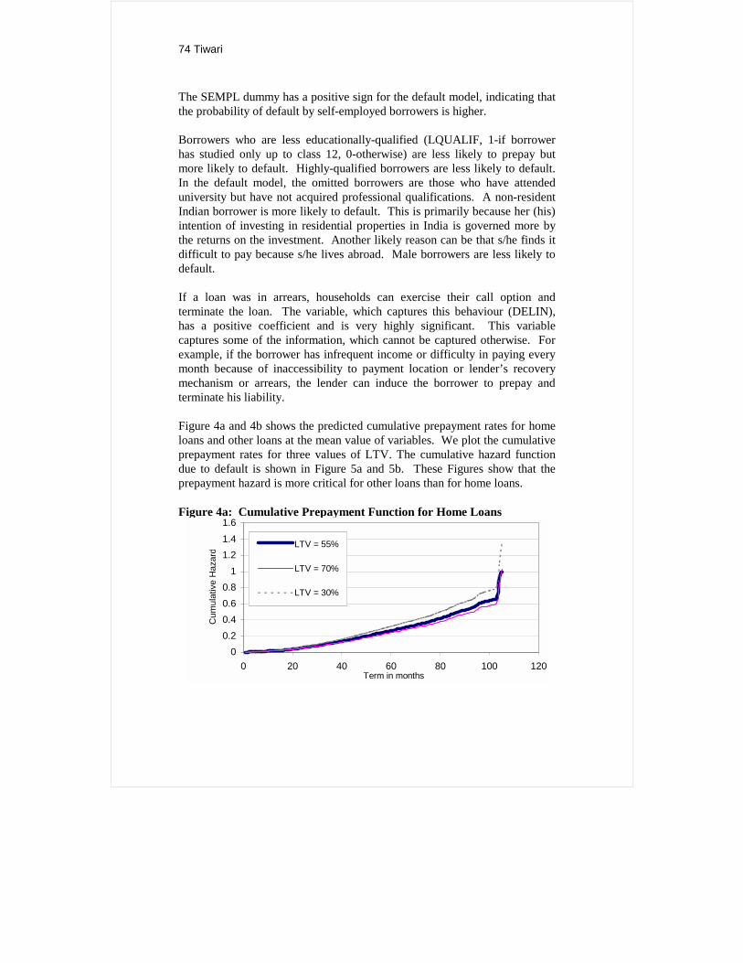
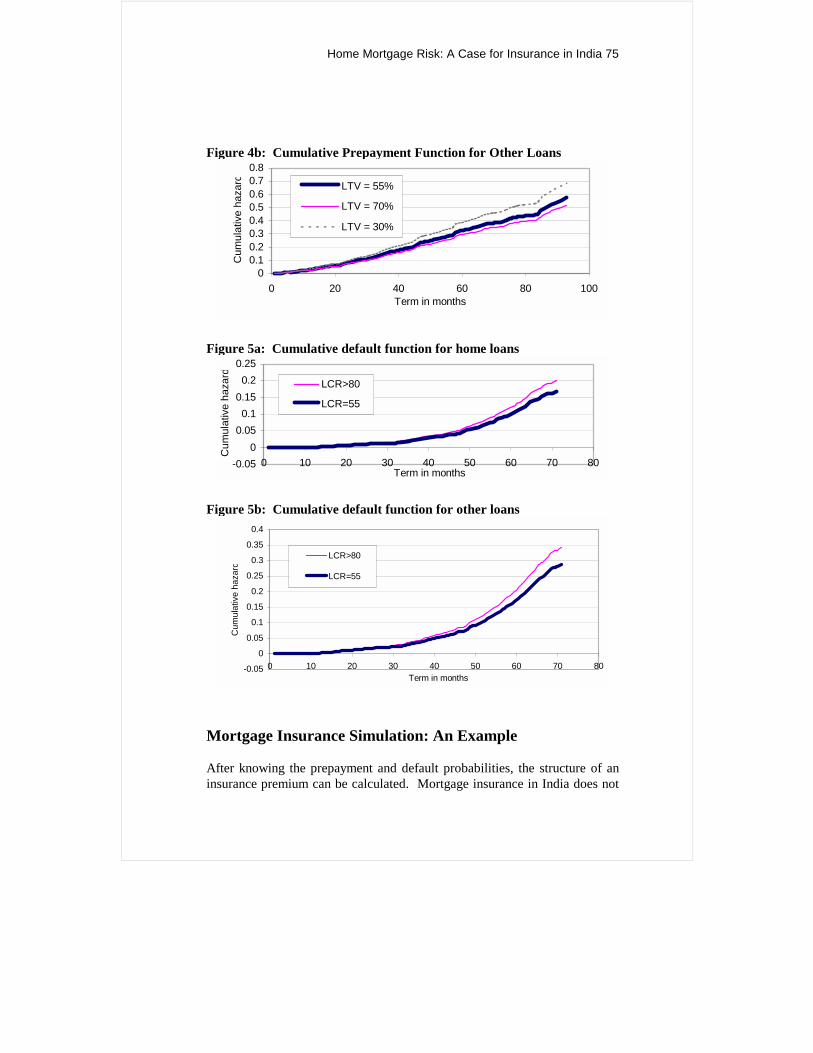
Figure 4a and 4b shows the predicted cumulative prepayment rates for homeloans and other loans at the mean value of variables. We plot the cumulativeprepayment rates for three values of LTV. The cumulative hazard functiondue to default is shown in Figure 5a and 5b. These Figures show that theprepayment hazard is more critical for other loans than for home loans.

Figure 4a: Cumulative Prepayment Function for Home Loans

00.20.40.60.8

11.21.41.6

0 20 40 60 80 100 120Term in months

Cum

ulat

ive

Haz

ard

LTV = 55%

LTV = 70%

LTV = 30%


Figure 4b: Cumulative Prepayment Function for Other Loans

00.10.20.30.40.50.60.70.8

0 20 40 60 80 100Term in months

Cum

ulat

ive

haza

rd LTV = 55%

LTV = 70%

LTV = 30%

Figure 5a: Cumulative default function for home loans

-0.050

0.050.1

0.150.2

0.25

0 10 20 30 40 50 60 70 80Term in months

Cum

ulat

ive

haza

rd

LCR>80

LCR=55

Figure 5b: Cumulative default function for other loans

-0.05

0

0.05

0.1

0.15

0.2

0.25

0.3

0.35

0.4

0 10 20 30 40 50 60 70 80Term in months

Cum

ulat

ive

haza

rd

LCR>80

LCR=55

Mortgage Insurance Simulation: An Example

After knowing the prepayment and default probabilities, the structure of aninsurance premium can be calculated. Mortgage insurance in India does not

76 Tiwari

exist. This paper computes the premium structure for a hypothetical case.The default and prepayment probabilities are estimated for the followingborrower category.

− Age: 40 years

− Sex: male

− Qualification: High

− Employment: Employed

− Monthly income: Rs.47500

− Cost of property: Rs.1428571

− Initial loan amount: Rs.1000000 (with LCR of 70)

− Loan amount with insurance: Rs.1357143 (with LCR of 95)

− Term of loan: 15 years

− Applicable interest rate: 15%

− Loan to cost ratio: Initial – 70, but after buying insurance – 95

− Installment to income ratio – 30 but with changed loan to value ratio - 41

We assumed the discount rate as 15% for the calculation of loss and revenuefor the mortgage insurance equation. We assumed an insurance structure thatrequires a uniform premium rate depending on outstanding unpaid balances.A calculation for the above borrower category indicates that a premium of0.05% of the outstanding balance would be able to cover the cost ofinsurance.

Conclusion

The objective of this paper is to evaluate the possibility of mortgageinsurance in India. The Indian housing market is constrained by theavailability of finance. The risk associated with the residential loan is borneby the lender. This makes the criteria of lending very stringent. The averageloan-to-cost ratio in India is around 0.55, and the installment-to-income ratiois 0.34. These constraints require a large initial equity from the home buyer.In developed markets like the US, borrowers buy mortgage insurance, whichenables them to borrow higher amounts. Mortgage insurers insure the loansagainst defaults for an insurance premium. We presented a framework toestimate the premium structure. To formulate the premium structure, aknowledge of the probability of prepayment and default was necessary. Thesecond objective of this paper was to estimate the probability of mortgagetermination due to either default or prepayment.


This paper has presented a model of mortgage termination throughprepayments or defaults for home mortgages in India using the Coxproportional hazard technique. This is the first analysis of housing mortgagetermination in India.

As a first step, we estimated the baseline hazard for mortgage termination.This baseline hazard was then modeled as a function of the price of calloptions and other financial and household variables.

The results of the analysis indicate that the financial value of a call option orput option plays an important role in the exercise of a prepayment or defaultoption. The results indicated that introducing volatility and uncertainty tofuture interest rates has an effect on mortgage prepayment behaviour. Theuncertainty and volatility of housing prices leads to default.

In addition, the results indicated that liquidity constraints also play animportant role in the exercise of options in the mortgage market. Those aremore likely to have low-levels of equity, and are less likely to exerciseprepayment options when it is in their financial interest to not do so. Theseresults are explicable, not by option theory, but rather by liquidity constraintsthat arise from qualification rules typically enforced by lenders.

Ceteris paribus, those who have chosen high initial LTV ratios are morelikely to exercise prepayment options in the mortgage market. This factor,known at the time mortgages are issued, also reflect investor preferences forrisk and investor sophistication in the market for mortgages on owner-occupied housing. A low level of equity has an impact on defaults. Thoughthe results did not find a very strong relation between the loan-to-cost ratiowith defaults.

Finally, borrowers’ household variables play an important role in determiningprepayment or default rates. All other variables remaining constant, a self-employed person is less likely to prepay, but more likely to default. Thesame goes for a single person, a less educated borrower, or a person in thelater stages of life at the time of the loan. However, joint borrowers have agreater likelihood of prepaying their loans. We used the conditionalprobabilities of default and prepayment in the insurance model, and ahypothetical simulation for the insurance premium structure has been carriedout. The overall results of the model are quite promising, and present a casefor developing a mortgage insurance market in India.

78 Tiwari

Acknowledgement

The author wishes to express his sincere gratitude to an anonymous referee for his/hervery useful comments. A research grant (No.(C) (2) 13630039) from the Ministry ofEducation, Science and Sports, Japan is gratefully acknowledged. The usualdisclaimer applies.

References

Black, F. and Scholes, M.S. (1972), The Pricing of Options and CorporateLiabilities, Journal of Political Economy, 81, 637-654.

Boyer, L.G., Follain, J.R., Ondrich, J., and Piccirillo, R.A. (1997), A HazardModel of Prepayment and Claim Rates for FHA Insured MultifamilyMortgages, Center for Policy Research, Syracuse University, New York.

Cox, J. C., Ingersoll, J.E., and Ross, S.A. (1985), A Theory of TermStructure of Interest Rates, Econometrica, 53, 385-467.

Cox, D.R. and Oakes, D.(1984), Analysis of Survival Data, Monographs onStatistics and Applied Probability, Chapman and Hall: London.

Deng, Y., Quigley, J.M., and Van Order, R. (1998), Mortgage Termination,Heterogeneity and the Exercise of Mortgage Options, Unpublished researchpaper.

Follain, J.R., Ondrich, J., and Sinha, G.P. (1996), Ruthless Prepayment?Evidence From Multifamily Mortgages, Center for Policy Research, SyracuseUniversity, New York.

Green, J., and Shoven, J.B., (1986), The Effect of Interest Rates on MortgagePrepayments, Journal of Money, Credit and Banking 18, 41-50.

Hendorshott, P.H., and LaFayette, W.C. (1995), Debt Usage and MortgageChoice: Sensitivity to Default Insurance Costs, NBER Working Paper Series:No. 5069.

Jones, L.D. (1993), The Demand for Home Mortgage Debt, Journal ofUrban Economics, 33, 10-28.

Kuo, C. and Tyler, T.Y. (1997), Rationale of Mortgage Insurance PremiumStructures, Mimeo.

Quigley, J.M. (1987), Interest Rate Variations, Mortgage Prepayments andHousehold Mobility, The Review of Economics and Statistics, 69(4), 636-643.


Quigley, J.M., and Van Order, R. (1990), Efficiency in the Mortgage Market:The Borrower’s Perspective, Journal of the American real Estate and UrbanEconomics Association, 18(3), 237-252.

Quigley, J.M., and Van Order, R. (1995), Explicit Tests of Contingent ClaimModels of Mortgage Defaults, Journal of Real Estate Finance andEconomics 11(2), 99-117.

Schwartz, E.S., and Torous, W.N. (1989), Prepayment and the Valuation ofMortgage-Based Securities, Journal of Finance 44(2), 375-392.

Tiwari, P., and Hasegawa, H. (2000), House Price Dynamics in Mumbai,1989-9, Review of Urban and Regional Development Studies, 12(2), 149-163.

Home mortgage risk: a case for insurance in India

Documents

Transcript of Home mortgage risk: a case for insurance in India