High-Performance Management Practices and Employee Outcomes in Denmark

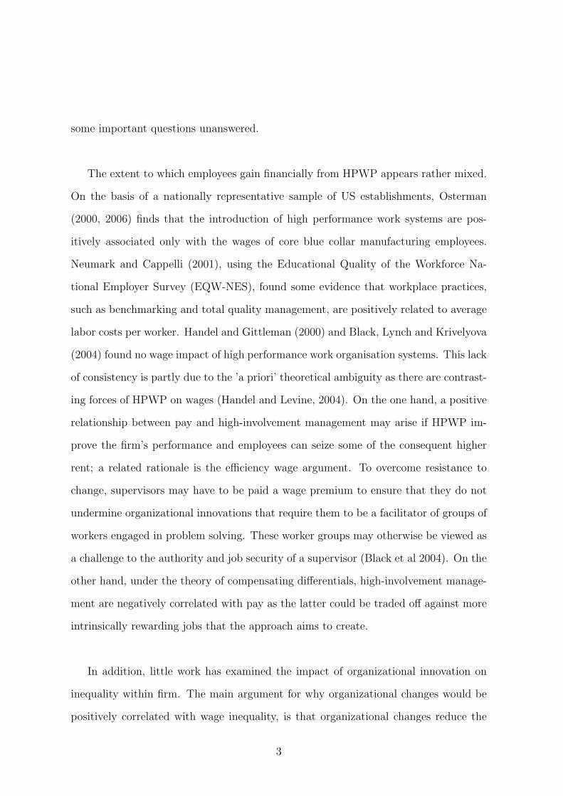
High-Performance Management Practices andEmployees’ Outcomes in Denmark

Annalisa Cristini ∗

University of BergamoTor Eriksson †

Aarhus School of Business

Dario Pozzoli‡

Aarhus School of Business

January 28, 2010

Abstract

High-involvement management practices have well-established benefits foremployers, but what do they do for employees? After showing that organiza-tional innovation is positively associated with firm performance, we investigatewhether high-involvement management is associated with higher wages, changesof wage inequality and the workforce composition, using data from a survey onDanish private sector firms with linked employer-employee data. We also ex-amine if the relationship between high-involvement management practices andemployee outcomes is affected by the industrial relations context.

JEL Classification: C33, J41, J53, L20Keywords: Workplace practices, pay, Denmark

∗Address: Department of Economics, University of Bergamo, Via dei Caniana 2, 24127 Bergamo,Italy. Email: [email protected]. Tel.: +39 035 2052 549; Fax: +39 035 2052549.†Corresponding Author. Aarhus School of Business, Department of Economics, Hermodsvej 22,

DK, 8230 Aabyhoj, Denmark. E-mail: [email protected]‡Aarhus School of Business, Department of Economics, Hermodsvej 22, DK, 8230 Aabyhoj, Den-

mark. E-mail: [email protected]

1

1 Introduction

In recent years, a growing body of literature has been concerned with the analysis

of the characteristics of high-involvement and high-performance work systems and of

their impacts on firm’s performance. This ”new organization of work” origins from

various intersecting managerial approaches which developed in the eighties and in the

nineties, the most important of which are the lean production model and Total Quality

Management (TQM). Centered on the concepts of employees’ involvement, empower-

ment and autonomy, a consensus set of innovative practices typically includes: self

managed teams, job rotation, formal arrangements aimed to openly discuss production

problems, like quality circles and more generally employer-employee meetings, systems

of rewarded suggestions, of performance related pay and information sharing.

According to a consistent number of empirical works these innovative work arrange-

ments are associated with levels of productivity higher than those usually observed

in more traditional systems (Ichniowski, Shaw and Prennushi 1997; Greenan and

Mairesse,1999; Eriksson, 2001; Bauer, 2003; Zwick and Kuckulenz, 2004; Cristini et

al, 2003); however, the channels through which these innovative practices give rise to

productivity improvements are not completely understood. Indeed, while some stud-

ies have failed to find support of HPWP as productivity enhancers (Freeman et al.

(2000), Cappelli and Neumark (2001), Godard (2004)), others have shown that the

mere presence of high-performance workplace practices (HPWPs, thereafter) may not

be sufficient to improve the firm’s performance and that factors like the lack of a coher-

ent bundle of practices, of complementary ICT investments, of adequate skills and of

unions’ support, may hamper a successful adoption of HPWP (Osterman 1995; Lynch

and Black 1998; Bresnahan, Brynjolfsson and Hitt 2002).

In particular, and this is our focus, the way employees’ outcomes contribute to the

productivity effects of HPWP has received relatively little attention, thereby leaving

2

some important questions unanswered.

The extent to which employees gain financially from HPWP appears rather mixed.

On the basis of a nationally representative sample of US establishments, Osterman

(2000, 2006) finds that the introduction of high performance work systems are pos-

itively associated only with the wages of core blue collar manufacturing employees.

Neumark and Cappelli (2001), using the Educational Quality of the Workforce Na-

tional Employer Survey (EQW-NES), found some evidence that workplace practices,

such as benchmarking and total quality management, are positively related to average

labor costs per worker. Handel and Gittleman (2000) and Black, Lynch and Krivelyova

(2004) found no wage impact of high performance work organisation systems. This lack

of consistency is partly due to the ’a priori’ theoretical ambiguity as there are contrast-

ing forces of HPWP on wages (Handel and Levine, 2004). On the one hand, a positive

relationship between pay and high-involvement management may arise if HPWP im-

prove the firm’s performance and employees can seize some of the consequent higher

rent; a related rationale is the efficiency wage argument. To overcome resistance to

change, supervisors may have to be paid a wage premium to ensure that they do not

undermine organizational innovations that require them to be a facilitator of groups of

workers engaged in problem solving. These worker groups may otherwise be viewed as

a challenge to the authority and job security of a supervisor (Black et al 2004). On the

other hand, under the theory of compensating differentials, high-involvement manage-

ment are negatively correlated with pay as the latter could be traded off against more

intrinsically rewarding jobs that the approach aims to create.

In addition, little work has examined the impact of organizational innovation on

inequality within firm. The main argument for why organizational changes would be

positively correlated with wage inequality, is that organizational changes reduce the

3

relative demand for unskilled production workers (Caroli and van Reenen 2001; Os-

terman 2000, Black, Lynch, and Krivelyova (2004)), as ”skill biased” HPWP could be

associated with higher layoff rates of unskilled production workers. On the other hand,

as long as organizational changes imply delegation of decision rights to lower layers is

the hierarchy, incentive considerations and skill upgrading through training may lead

to wage raises in the lower part of the occupational structure, thereby narrowing wage

inequality within firms. Again, the existing evidence on the impact of organizational

changes on wage inequality is ambiguous (Aghion, Caroli and Garcia-Penalosa, 1999).

Finally, the interaction between industrial relations setting and the new system of

work organization is also worthy of notice. In general, unions are expected to affect both

the probability of adoption and the cost of adopting HPWP. On the first issue, whether

unions and HPWPs coexist (Machin and Wood, 2005) depends on two factors: the

bargaining objects and the union’s bargaining power. If high involvement practices and

the conditions under which they are introduced enter the unions’ utility function and

unions sanction the usage of such practices, then one would expect HPWPs and unions

to coexist and unions to affect the decision to introduce high-involvement practices as

well as the specific practices to be adopted and the forms of their actual implementation.

As for the costs of introducing HPWPs, unions, if supportive of HPWP, are expected to

reduce employees’ resistance to change, hence the side payment on the part of the firm

that would have been necessary otherwise; on the contrary, if unions oppose HPWP the

’bribe’ to overcome resistance will rise hence increasing the cost of adoption. Moreover,

the cost will rise if unions seek quasi-rents in return for their approval of the practices

and in any case if the wage is bargained and the practices induce net productivity gains.

Finally, by offering an alternative to employee exit, unions’ voice helps employers retain

employees, which is a crucial argument for the success of high involvement practices

as those employees whose human capital is specific and valuable to the employer are

4

also those most productive (Freeman and Medoff, 1984). Thus, overall the presence of

unions has an ’a priori’ ambiguous effect both on the probability and on the cost of

HPWP’s adoption.

To the best of our knowledge, there are only few studies investigating the role of

unions in establishing the pay premium associated with high-involvement management.

Using a nationally representative survey of British private-sector workplaces, Forth and

Millward (2004) show that high-involvement management is associated with higher

pay and that the high-involvement management premium is higher where unions are

involved in effective pay bargaining. However, as the data used in this study are cross-

sectional, it is not possible to say whether a causal relationship exists. For the same

reason, the estimates in Godard (2007) suffer from a potential endogeneity bias; Godard

(2007) uses data collected in 2003 in national survey of Canadian and English workers

and finds that innovative work practices are associated with meaningful pay gains for

union workers in both Canada and England. Black, Lynch and Krivelyova (2004)

partly address the issue of endogeneity working with a small panel of approximately

180 manufacturing establishments drawn from two rounds of the EQW-NES; they

find a significant effect of HPWPs on wages and on wage inequality among unionized

employers only.

After showing that new workplace practices are associated with improved firm fi-

nancial performance, the purpose of this paper is to consider the following research

questions: 1) Is high-involvement management associated with higher or lower pay?;

2) Is organizational change correlated with within-firm wage inequality and with the

workforce composition, i.e. the proportion of managers, middle managers and hourly

paid workers as shares of all employees?; 3) Does the presence of trade unions help

employees to appropriate a greater share of the rents associated with high-involvement

practices?

We will address these issues by means of a unique data source, constructed by

5

merging information from two different sources: a detailed survey of Danish private

sector firms and an employer-employee linked data. The survey (see Eriksson 2000

for details) represents a unique source of information on Danish firms’ internal labor

markets and changes therein. The survey was administered by Statistics Denmark as

a mail questionnaire that was sent out in May and June 1999 to 3,150 private sector

firms with more than 20 employees. The response rate is 51 %, relatively high for a

long and detailed questionnaire, and there are 1,600 usable observations. The other

data source, the employer-employee linked panel, has been constructed by Statistics

Denmark by merging a number of register using the unique identification numbers of

individuals and firms. The panel contains detailed information about all employees

and their wage earnings in all Danish firms during the period 1990-1999. In addition,

the panel has economic information about firms with 20 or more full-time equivalent

employees, from 1992 to 1999. The longitudinal dimension of the register data enables

us to estimate the impact of workplace innovation on financial performance and on

employees outcomes in two steps: we use firm fixed effects estimation in the first stage,

and regress the average residuals on an index of organizational innovation in the second

stage (Black and Lynch 2001).

The structure of the paper is as follows. In Section II, we introduce our data.

Section III presents the estimation strategy. Section IV then discusses the findings

from our analysis and Section V concludes.

2 Data

The analysis uses a data set on Danish private sector firms with more than 20 em-

ployees, which has been constructed by merging information from two different main

sources.

The first source is a questionnaire directed at firms that contains information about

6

their work and compensation practices. A brief description of the questionnaire and

the main results are available in Eriksson (2001). The survey was administered by

Statistics Denmark as a mail questionnaire survey in May and June 1999, which was

sent out to 3,200 private sector firms with more than 20 employees. The firms were

chosen from a random sample, stratified according to size (as measured by the number

of full time employees) and industry. 1 The survey over-sampled large medium-sized

firms: all firms with 50 or more employees were included as wellas 35 per cent of firms

in the 20-49 employees range. The response rate was 51 per cent, which is relatively

high for the rather long and detailed questionnaire of the type that was used.

The second data source is the ”Integrated Database for Labor Market Research”

(IDA henceforth) provided by Denmark Statistics. IDA is a longitudinal employer-

employee register containing valuable information (age, demographic characteristics,

education, labor market experience, tenure and earnings) on each individual employed

in the recorded population of Danish firms during the period 1990-1999. Apart from

deaths and permanent migration, there is no attrition in the dataset. The labor market

status of each person is recorded at the 30th of November each year. The retrieved

information has been aggregated at firm level, such as proportion of certain employee

groups (i.e. proportion of men, skilled, managers, middle managers, hourly paid work-

ers, employees with different tenure and age) and the mean and variance wage in each

firm.2 The retrieved information has been consequentially merged to variables like

enterprises’ location (county), size and related industry. In addition, the panel has

financial information about firms with 20 or more full-time equivalent employees, for

the years 1992 to 1999; such information includes: intermediate goods or materials,

fixed assets, and value added. Given our two steps estimation procedure, we restrict

1In the final sample, 46% of firms belong to the manufacturing sector, 10% to the constructionsector, 32% to the wholesale trade sector, 4% to the transport sector and 8% to the financial sector.

2For the empirical specification where we use different time periods, we deflate wages with theconsumer price index using 2000 as base year.

7

our analysis to just those firms in the register data from 1997 to 1999. This choice

could be considered a reasonable compromise between having a sufficiently large num-

ber of years to identify the firm fixed effects and not too many to assume that most

of workplace practices don’t vary over this period.3 Table 1 reports the means and

standard deviations of the variables of interest for the period mentioned above. At the

bottom of the table, we also report the mean and standard deviation of the variables

drawn from the survey, such as the dummy variable for local wage agreement.

2.1 Variables

The definition of HPWPs is based on a set of questions included in the survey about

the involvement of the employees in self-managed teams, job rotation, quality circles,

total quality management, benchmarking, project organization, financial participation

schemes and training. For each practice, except for training programs and the different

financial participation schemes4, we also know when it was first adopted. Table 2 pro-

vides an overview of the diffusion of such practices. Training and financial participation

schemes are the most diffused practices, involving more than 50% of firms. Team work-

ing is also largely diffused among Danish firms (20 %), while project organization and

job rotation involves about 11% of the firms. Finally only 3-4% of Danish firms offer

some form of employee involvement through quality circles, total quality management

and benchmarking. The data on the years for which the firm has used the practices

are inversely correlated to the degree of diffusion of the practices. The most diffused

practices - self-managed teams and project organization - have been used for longer

than less diffused practices, such as benchmarking and total quality management. One

3Table 2 indicate that most of practices have been adopted for more than three years, whichsuggests that 1997-1999 is a likely period on which to expect HPWPs not to change much.

4The questionnaire only asked firms whether they made substantial changes in their paymentsystems in recent years, without being more specific as to when or to which payment system. Also,there is no information regarding the proportion of employees involved in a particular work design

8

interpretation is that firms introduce organizational innovation gradually and that a

sequential ordering of the practices may exist so that some practices form the basis to

others leading to the most advanced practices (Freeman, Kleiner and Ostroff, 2000).

It seems plausible to assume that the number of practices adopted can serve as a

proxy for the intensity of implementation. Hence our main measure of organizational

innovation is a single additive index of organizational innovation constructed as the

sum of all HPWPs adopted.

The four outcome variables are: 1. the log of firm value added; 2. the average firm

hourly wages both at the firm level and by three occupation groups (managers, middle

managers and hourly paid workers); 3. the wage inequality measured, alternatively,

as: i) the ratio of the average firm wage of managers to the average wage of hourly

paid workers, ii) the ratio of the 90th percentile to the 10th percentile, iii) the ratio

of the 90th percentile to the 50th percentile and iv) the ratio of the 50th percentile

to the 10th percentile of the wage distribution; 4. the workforce composition in terms

of proportion of managers, middle managers and hourly paid workers as shares of all

employees.

Table 3 reports the mean of the outcome variables by the number of HPWPs

adopted. First of all, firm financial performance is positively associated with the sum

of all HPWPs adopted. We can also notice that total average hourly wages increase

with the intensity of organizational innovation. Moreover this positive correlation is

mainly driven by the increase of the average wage of managers, as both the middle

managers’ and the hourly paid workers’ wages remain stable with the number of prac-

tices adopted. This implies that organizational innovation is positively associated with

wage inequality, measured by the ratio of the average firm wage of managers to the

average wage of hourly paid workers. Finally, also the workforce composition seems

9

to be correlated with organizational innovation, as the shares of managers and hourly

paid workers decrease with number of practices and the shares of middle managers

increases.

3 Empirical Strategy

3.1 Impact of organizational innovation on firm performance

In order to relate the firm’s total factor productivity to HPWPs, we use a two

step procedure (Black and Lynch 2001, Cristini et al 2003) according to which TFP

is first estimated using panel information and, in the second step, the estimated time

average TFP is related to the cross sectional measure of HPWP. The use of panel

information in the first step, coupled with a proper estimation technique, allows to

control of the unobservable firm characteristics and cope with some of the endogeneity

and with potential measurement errors. For comparison, we present both two-step

estimates and cross-section estimates. The empirical specification of the first stage

production function is then given by:

yit = β0 + βllit + βkkit + βzZit + uit, (1)

where the dependent variable is the log of the real value added5 , the covariates

are the log of labor (L), the log of capital stock (K), a number of other controls

(Z), including firm specific characteristics of employees and a full set of size, industry

and regional dummies. The panel data setting allows for the computation of within

estimators, which may remove the bias related to the omission of firm fixed effects.

5Value added and capital stock have been deflated by using GDP deflators drawn from World BankIndicators (base year 2000).

10

However, FE within estimators are inconsistent in case levels of inputs and output

are chosen simultaneously or explanatory variables are affected by measurement errors

(Griliches and Hausman 1986). Thus, it is important to compare FE within estimation

with the Levinsohn-Petrin estimation method (LP, thereafter) which corrects for the

simultaneity problem (see Levinsohn and Petrin (2003a) for more details).

Using the estimates of production function parameters, the firm i ’s TFP, at time

t, is defined as

tfpit = yit − βllit − βkkit − βzZit (2)

Next we average TFP over the period 1997 to 1999 and estimate the relationship

between these and the index of organizational innovation in the following equation:

tfpi = α + β1(Index) + β2(Unions) + γr + γj + ξ (3)

where β1 and β2 are respectively the productivity effect associated with the organi-

zational innovation and the presence of unions; γt, γr and γj are regional, and industry

controls.

3.2 Impact of organizational innovation on employee outcomes

In the second part of the paper we are interested in looking at the impact of organi-

zational innovation on employees’ outcomes: mean hourly wages, wage inequality and

workforce composition. These variables are obtained from the register data, averaging

over the employee outcomes in the firms. As in the previous subsection, we implement

11

two simple strategies using the log of the employees’ outcomes as dependent variables,

following the methodologies used to estimate the impact of workplace organization on

firm productivity. The first method is to use OLS in the cross-sectional 1999 sample,

while the second consists in exploiting the fact that we observe variables obtained from

the register data over time, and hence we can use that information to develop a two-step

estimation, where in the first step we recover a firm fixed component of the residual

and we use it as dependent variable in the second step, with the organizational index as

independent variable. The second strategy takes care of any unobserved time-invariant

firm heterogeneity that might be correlated with the firm specific characteristics. The

two-step empirical specification can be written as:

ln(Yit) = cons+ a(Xit) + uit, (stage1)

ln(Yit)− a(Xit) = cons+ β1(Index) + β2(Unions) + γr + γj + ξ, (stage2) (4)

where ln(Yit)− cons− a(Xit) is the average of the fixed component of the residual

over the period 1997-1999, the vector X collects the firm specific characteristics, Index

is our count measure of organizational innovation, Unions is the dummy variable related

to the presence of the unions.6

4 Results

Financial Performance. This section presents and discusses results obtained from the

empirical analysis. Firstly, the attention is devoted to the estimation of the TFP level

and how such estimates are associated with the index of organizational innovation.

6We capture the presence of the unions by looking at whether the firm has a local collectiveagreement concerning wages and working hours for all employees.

12

As outlined in section 4.1, three different approaches (1st-stage OLS , 2-stage FE and

2-stage LP) have been followed in order to estimate productivity at firm level. Table 4

reports the 1st-stage OLS results with table 8 the 2-stage results. While the OLS and

FE estimations lead to quite similar results, the labor (capital) coefficients are higher

(lower) with LP estimation method and closer to what has been found in previous

studies (Griffith et al. 2006, Cristini et al. 2003). This suggests that the other two

strategies may be affected by simultaneity and measurement errors. Consistent with

Black and Lynch (2001) we find that the proportion of employees with a tenure less

than two years, the proportion of employees with a secondary or a tertiary education,

the proportion of managers and middle managers and the proportion of men are sta-

tistically significant and carry the expected positive sign across estimation methods.

When we examine the impact of HPWPs on productivity, the results are also quite sim-

ilar across estimation methods. We find that our count index is positively associated

with total factor productivity, suggesting that organizational innovation contribute to

enhance firm performance. Consistent with Black and Lynch (2001) we also find that

unionized firms have lower productivity than an otherwise similar but non-unionized

firm. The last column of table 14 presents results of equation 3 when we interact union-

ization and our index of organizational innovation. When this interaction is included,

the effect of HPWPs remains positive and statistically significant, whereas the own

effect of unionization and the interaction effect are not statistically significant. Thus

unionized firms that have adopted some HPWPs do not have higher productivity than

other similar nonunion firms.

Wages. After showing that organizational innovation is associated with higher firm

performance, we next investigate whether innovative firms compensate employees for

their increased involvement in the production process and for incurring the risk as-

sociated with financial participation schemes. To answer this question, we estimate

13

equation 4 using the log of the average hourly wage both at firm level and by three

main occupation groups (managers, middle managers, hourly paid workers) as depen-

dent variable. Table 5 presents estimates from cross-sectional wage equation using data

for 1999 while table 9 reports results from the 2-stage approach. The relationships are

fairly similar to those we obtain when estimating the impact of organizational innova-

tion on productivity. Hence workplace practices that increase productivity also lead

to higher average wages. The results are quite similar across empirical specifications.

When we examine the average wage in each firm by occupation group, we find that

the results are relatively similar across occupations. However, it seems that the pay of

managers is more affected than the pay of middle managers and hourly paid workers.

This result is consistent with the notion that innovative practices increase the demands

on managers, as they are responsible for organizing the other workers and providing an

environment conducive to their participation in decision making (Black et al. 2004).

Consistent with what has been found in Buhai et al (2008), we find that higher firm

average education, higher proportion of male employees and of managers are associated

with higher average wage. The presence of unions does not affect the average hourly

wage both at firm level and by occupation groups and its interaction with our index of

organizational innovation is generally not statistically significant. All in all, these re-

sults suggest that a wage premium is paid to managers relative to hourly paid workers

to work in an HPWPs environment and that there is not a strong interaction between

the union representation and HPWPs (see table 12). In innovative workplaces, the

presence of a union does not provide meaningful gains for union members, as it has

been found for example in Black et al. (2004), Forth and Millward (2004) and Godard

(2007).

Wage inequality. To investigate whether organizational innovation increase wage

inequality at firm level, we look at: i) the ratio of the average wage of managers in a

14

firm to the average wage of hourly paid workers in a firm, ii) the ratio of the 90th per-

centile to the 10th or the 50th percentile and iii) the ratio of the 50th percentile to the

10th percentile of the wage distribution. Tables 6 and 10 present results respectively

from cross-sectional wage inequality equation and from the 2-stage approach. These

results suggest that a higher number of workplace practices increases within-firm wage

inequality. This is consistent with the wage results, according to which hourly paid

workers receive a lower wage premium to work in HPWP firms is compared to man-

agers. The presence of unions and its interaction with workplace practices are not

statistically significant (see table 13). The proportion of male workers and of workers

with a secondary/vocational education reduce wage inequality while the proportion of

managers and of workers with a tenure of at least 10 years have a positive impact on

wage inequality.

Workforce composition. The last employee outcome we investigate is whether HP-

WPs impact on the workforce composition of firms. To examine this question, we

estimate equation 4 using the firm level proportion of managers, middle managers and

hourly paid workers as dependent variable. Table 7 presents estimates from cross-

sectional analysis using data for 1999 while table 11 reports results from the 2-stage

approach. In terms of the relationship between organizational innovation and work-

force composition, the picture is mixed. Innovative workplaces have a lower share of

middle managers and a higher share of hourly paid workers. These results seem not to

support the idea that organizational change is skill biased, i.e. a variety of workplace

practices are associated with lower relative demand for unskilled production workers

(Caroli and van Reenen 2001; Osterman 2000). On the other hand, our results are

consistent with the hypothesis that organizational innovation is associated with the

loss of managerial jobs (Osterman 2000), i.e. HPWPs flatten the organizational hier-

archy and hence reduce the number of managerial employees. The impact of unions is

15

opposite and attenuates the main effect of organizational innovation (see table 14).

5 Sensitivity analysis: alternative indexes of orga-

nizational innovation

As we mentioned in subsection 3.1, a sequential ordering of the practices may exist so

that some practices form the basis to others leading to the most advanced practices, i.e.

workplace practices may be adopted along an ideally sequential path where the easiest

practices are the first ones to be introduced, gradually followed by the more difficult

ones (Freeman et al, 2000). In this case, the bundle of practices, at a point in time,

would be indicative of how far the firm has proceeded along the reorganization path.

To investigate whether the most widely adopted workplace practices are also the easiest

to adopt, we apply the Rasch analysis. This belongs to the class of ”unidimensional

latent trait models” widely applied in education to assess the ability of a person in

response to a set of questions. In this case, the latent variable we want to measure

is the reorganization process and we measure it along an ideal continuum; this means

that the more difficult the adoption of a given practice is, the further away this practice

will be placed along the reorganization path and the more its adoption will be retarded

in comparison to easier practices.

More formally, let yij be the binary response to whether the practice is adopted or not,

where i = 1, ...., n with n the number of the firms and j = 1, ....,m, with m the number

of practices. The Rasch model can be written as a logit-linear model:

logitPr (yij = 1| αi) = αi − θj (5)

where αi can be interpreted as an unobserved firm ability to innovate and θj as an

16

item-difficulty parameter. It is assumed that conditional on αi, the yi∗ are independent

(local independence). Actually Rasch (1960) gave an axiomatic derivation of the model

in which next to local independence, the main characterizing properties were that the

y∗j and yi∗ form a sufficient statistic for αi and θj. Andersen (1980) showed that

the conditional maximum likelihood estimator of θj, where conditioning occurs on the

subject’s score yi∗ , is efficient and is actually asymptotically normal distributed, with

all the nice properties of maximum likelihood estimators analogous to those of the

standard likelihood-ratio test.

We estimate Equation (5) using the conditional fixed effects estimator. Results are

given in Table . The order of the practices, from the most diffused to the least, is the

same order resulting from the estimated coefficients confirming that the most frequently

adopted practice, i.e. financial participation schemes in this case, is also the ”easiest”;

likewise, quality circles is the least frequently adopted practice and the most difficult to

adopt. Since the Rasch measure is unidimensional, the estimated coefficients indicate

the position of each practice along an ideal continuum (the reorganization process).

The position of the practices along such a ’reorganization-meter’ indicates that for

Danish firms the most difficult change is to go beyond the second practice (training),

in the sense that the increase in the difficulty is highest in this step. We then use

the estimated practice difficulty parameters of the Rasch analysis as weights of the

previous single additive index. With respect to the latter, which identifies the number of

practice adopted (”quantity”), the weighted measure, by accounting more weight to the

practices more advanced along the reorganization path should capture more properly

the progression of the reorganization. Overall the results using the new index confirm

the main analysis (see tables 16, 17 and 18). Organizational innovation is positively

associated with firm performance, average wage at firm level and wage inequality. As

in the previous section we find that organizational innovation affects more the pay

of managers than the pay of middle managers and hourly paid workers and reduces

17

the number of managerial employees. The main results are also confirmed when using

an index of workplace practices obtained from principal component analysis, denoted

PCA.7

6 Conclusions

Integrating existing research on firm organizational structure and performance, this pa-

per analyzes the impact of new workplace practices on workers. The analyzes presented

here offer several advantages over prior efforts to examine the relationship between

organizational innovation and organizational outcomes. Most important, the longitu-

dinal nature of our data and the ability it give us to measure employees’ outcomes

before these innovative practices were introduced offers an approach to controlling

for heterogeneity that improves on prior studies relying on cross-sectional data only.

We find evidence that employers do appear to reward their workers for engaging in

high-performance workplace practices. We also find a significant association between

organizational innovation and increased wage inequality. Finally we find that high-

performance management practices seems to be associated with the loss of managerial

jobs. We confirm the main results by computing alternative measures indicative of how

far how far has the firm proceed along the reorganization path. Finally we do not find

significant differences in the effects of HPWPs between unionized and not unionized

firms.

7The principal component analysis shows one principal component with an eigen vector greaterthan 1.

18

References

[1] Aghion, P., Caroli E. and Garcia-Penalosa C. (1999), ”Inequality and Economic

Growth: The Perspective of the New Growth Theories,” Journal of Economic Lit-

erature, American Economic Association, vol. 37(4), pages 1615-1660, December.

[2] Akerlof, G., 1984, ”Gift exchange and efficiency-wage theory: Four views” Amer-

ican Economic Review 74, 79-83.

[3] Andersen, E. B. (1980), ”Discrete statistical models with social science applica-

tions”, Amsterdam: North-Holland.

[4] Batt, R. (2004), ”Who Benefits from Teams? Comparing Workers, Supervisors,

and Managers”, Industrial Relations: A Journal of Economy and Society, Vol. 43,

No. 1, pp. 183-212.

[5] Bauer, T.K. (2003), ”Flexible Workplace Practices”, IZA Discussion Paper No.

700, Bonn.

[6] Lynch L. and Black S. (1998), ”Beyond the incidence of employer-provided train-

ing,” Industrial and Labor Relations Review, Cornell University, vol. 52(1), pages

64-81, October.

[7] Black, S. and Lynch L. (2001), “How to Compete: the Impact of Workplace Prac-

tices and Information Technology on Productivity”, The Review of Economics and

Statistics, 83(3), 434-445.

[8] Black, S., Lynch, L. and Krivelyova, A. (2004), ”How Workers Fare When Em-

ployers Innovate”, Industrial Relations: A Journal of Economy and Society, Vol.

43, No. 1, pp. 44-66.

[9] Bresnahan T., Brynjolfsson E. and Hitt L. (2002), ”Information Technology, Work-

place Organization, And The Demand For Skilled Labor: Firm-Level Evidence,”

19

The Quarterly Journal of Economics, MIT Press, vol. 117(1), pages 339-376,

February.

[10] Brown, C., (1980), ”Equalizing differences in the labour market”, Quarterly Jour-

nal of Economics 94, 113-134.

[11] Buhai S., Cottini E. Westergaard-Nielsen N. (2008), ”The Impact of Work-

place Conditions on Firm Performance,” Tinbergen Institute Discussion Papers

08-077/3, Tinbergen Institute.

[12] Cappelli P. and Neumark D. (2001), ”Do high performance work practices improve

establishment-level outcomes?”, Industrial and Labor Relations Review.

[13] Caroli E. and Van Reenen J. (2001), “Skills and organisational change: evidence

from British and French establishment in the 1980s and 1990s”, The Quarterly

Journal of Economics, Vol. 116, No. 4., pp. 1449-1492.

[14] Cristini A., Gaj A., Labory S. and Leoni R. (2003), ”Flat Hierarchical Structure,

Bundles of New Work Practices and Firm Performance”, Rivista Italiana Degli

Economisti, 2, 313-341.

[15] Eriksson, T. (2000), ”How common are the new compensation and work practices

and who adopts them?”, Working Paper 01-8, Aarhus School of Business.

[16] Forth J. and Millward N. (2004), ”High Involvement Management and Pay in

Britain”, Industrial Relations, 43 (1), 98-119.

[17] Freeman R. and Medoff J. (1984), What Do Unions Do?, New York: Basic Books.

293 pp.

[18] Freeman R., Kleiner M. and Ostroff C. (2000), ”The Anatomy of Employee In-

volvement and its Effects of Firms and Workers”, NBER Working Paper, n.8050.

20

[19] Godard, J. (2004), ”A Critical Assessment of the High-Performance Paradigm”,

British Journal of Industrial Relations, 42, 2, 349-378.

[20] Godard, J. (2007), ”Unions, Work Practices, and Wages under Different Institu-

tional Environments: The Case of Canada and England,” Industrial and Labor

Relations Review, Cornell University, vol. 60(4), pages 457-476, July.

[21] Griffith R., Harrison R. and J. Van Reenen (2006) ”How Special Is the Special

Relationship? Using the Impact of U.S. RD Spillovers on U.K. Firms as a Test of

Technology Sourcing”, American Economic Review 2006, December 1859-1875.

[22] Greenan N. and Mairesse J. (1999), “Organisational Change in French Manufac-

turing: what do we learn from firm representatives and from their employees?”,

NBER Working Paper n. 7287.

[23] Hamilton, B. H., Nickelson, J. A. and Owan, H., (2003), ”Team Incentives and

Worker Heterogeneity: An Empirical Analysis of the Impact of Teams on Produc-

tivity and Participation”, Journal of Political Economy 111, 465-497.

[24] Handel M. and Gittleman M. (2000), ”Is there a Wage Payoff to Innovative Work

Practices?,” Macroeconomics 0004032, EconWPA.

[25] Handel, M. and Levine D. (2004) ”Editors’ Introduction: The Effects of New Work

Practices on Workers”, Industrial Relations 43(1): 1-43.

[26] Ichniowski C., Shaw K., Prennushi G., (1997), “The Effects of HRM Systems on

Productivity: A Study of Steel Finishing Lines”, American Economic Review, 87,

291-313.

[27] Levinsohn J. and Petrin A. (2000), ”Estimating Production Functions Using In-

puts to Control for Unobservables”, Review of Economic Studies, vol. 70(2), pages

317-341, 04.

21

[28] Machin S. and Wood S. (2005), ”Human resource management as a substitute

for trade unions in British workplaces,” Industrial and Labor Relations Review,

Cornell University, vol. 58(2), pages 201-218, January.

[29] Osterman P., (1994), ”How common is workplace transformation and who adopts

it?,” Industrial and Labor Relations Review, Cornell University, vol. 47(2), pages

173-188, January.

[30] Osterman, P. (2000), ”Work reorganization in an era of restructuring: diffusion

and effects on employee welfare”, Industrial and Labor Relations Review, 53, 179-

96.

[31] Osterman, P. (2006), ”The Wage Effects of High Performance Work Organization

in Manufacturing”, Industrial and Labor Relations Review. January; 59(2): 187-

204.

[32] Salop, S. C., (1979), ”A model of the natural rate of unemployment”, American

Economic Review 69, 117-125.

[33] Smith, A., (1976), ”An inquiry into the nature and causes of the wealth of nations”,

New York, Oxford University Press.

[34] Yasar M., Raciborski R. and Poi B. (2008). Production function estimation in

Stata using the Olley and Pakes method. Stata Journal, StataCorp LP, vol. 8(2),

pages 221-231, June.

[35] Zwick T. and Kuckulenz A. (2004), ”Heterogeneous Returns to Training in Per-

sonal Services,” Working Papers of the Research Group Heterogenous Labor 04-10,

Research Group Heterogeneous Labor, University of Konstanz/ZEW Mannheim.

22

Tab

le1:

Des

crip

tive

stat

isti

cs

Vari

able

sD

efinit

ion

Mean

Sd

NID

AV

ari

able

s:m

enm

enas

ap

rop

orti

onof

all

emplo

yees

0.71

50.

204

4716

ten1

emplo

yees

wit

ha

tenure

less

than

two

year

sas

apro

por

tion

ofal

lem

plo

yees

0.34

70.

150

4716

ten2

emplo

yees

wit

ha

tenu

reb

etw

een

3an

d4

year

sas

apro

por

tion

ofal

lem

plo

yees

0.19

30.

094

4716

ten3

emplo

yees

wit

ha

tenu

reb

etw

een

5an

d8

year

sas

apro

por

tion

ofal

lem

plo

yees

0.20

40.

129

4716

pte

n4

emplo

yees

wit

ha

tenure

mor

eth

ante

nye

ars

asa

pro

por

tion

ofal

lem

plo

yees

0.25

50.

175

4716

age1

emplo

yees

aged

15-2

8as

apro

por

tion

ofal

lem

plo

yees

0.26

20.

155

4716

age2

emplo

yees

aged

29-3

6as

apro

por

tion

ofal

lem

plo

yees

0.24

80.

091

4716

age3

emplo

yees

aged

37-4

7as

apro

por

tion

ofal

lem

plo

yees

0.24

80.

091

4716

age4

emplo

yees

aged

47-6

5as

apro

por

tion

ofal

lem

plo

yees

0.24

00.

118

4716

psk

ill1

emplo

yees

wit

ha

tert

iary

educa

tion

asa

pro

por

tion

ofal

lem

plo

yees

0.04

30.

084

4716

psk

ill2

emplo

yees

wit

ha

seco

ndar

y/v

oca

tion

aled

uca

tion

asa

pro

por

tion

ofal

lem

plo

yees

0.56

40.

156

4716

man

man

ager

sas

apro

por

tion

ofal

lem

plo

yees

0.05

10.

053

4716

mid

dle

man

mid

dle

man

ager

sas

apro

por

tion

ofal

lem

plo

yees

0.21

00.

213

4716

blu

ecol

lblu

eco

llar

sas

apro

por

tion

ofal

lem

plo

yees

0.73

70.

224

4716

size

1to

tal

num

ber

ofem

plo

yees

(les

sth

an40

)0.

250

0.43

347

16si

ze2

tota

lnu

mb

erof

emp

loye

es(4

0-60

)0.

252

0.43

447

16si

ze3

tota

lnum

ber

ofem

plo

yees

(61-

120)

0.24

70.

431

4716

size

4to

tal

num

ber

ofem

plo

yees

(mor

eth

an12

0)0.

249

0.43

347

16w

age

mea

nre

alhou

rly

wag

e(t

otal

)17

4.28

349

.305

4716

wag

em

anm

ean

real

hou

rly

wag

e(m

anag

er)

341.

264

153.

394

4716

wag

em

iddle

man

mea

nre

alhou

rly

wag

e(m

iddle

man

ager

)20

6.97

357

.812

4716

wag

eblu

ecol

lm

ean

real

hou

rly

wag

e(b

lue

coll

ars)

151.

501

35.8

1147

16A

ccounti

ng

Vari

able

s:V

alue

added

(100

0kr.

)87

286.

9333

1463

.647

60M

ater

ials

(100

0kr.

)15

3125

5958

81.7

4760

Cap

ital

(100

0kr.

)73

224.

3450

3709

.947

60Surv

ey

vari

able

sC

ount

Index

num

ber

ofad

opte

dpra

ctic

es1.

844

1.36

914

11R

asch

Index

wei

ghte

dco

unt

mea

sure

(Ras

chp

aram

eter

sas

wei

ght)

0.10

10.

151

1411

PC

AIn

dex

pri

nci

pal

com

pon

ent

anal

yis

isin

dex

0.00

11.

451

1411

Unio

ns

whet

her

the

firm

has

alo

cal

coll

ecti

veag

reem

ent

conce

rnin

gw

ages

0.67

80.

467

1411

23

Table 2: Incidence and distribution of workplace practices.

Workplace practices % of Firms Years in Use1-2 3-6 ≥6

Project organization 12.77 3.16 3.22 6.38Benchmarking 3.54 1.20 1.33 1.01Self-managed team 18.90 5.56 5.44 7.90Quality circles 2.28 0.44 0.57 1.26Job rotation 11.06 2.53 3.67 4.87Total quality management 4.87 1.14 2.40 1.33Financial participation schemes 65.98 - - -Training 53.75 - - -

Table 3: Mean of employee outcomes and value added by number of practices adopted.

Outcomes Number of practices adopted0 1-2 3-4 ¿4

Wageslog(avg hourly wage), total 5.111 5.154 5.175 5.134log(avg hourly wage), managers 5.644 5.764 5.788 5.829log(avg hourly wage), middle managers 5.277 5.303 5.332 5.294log(avg hourly wage), blue collars 5.001 5.012 5.010 4.995Wage inequalitylog(avg wage manager)/log(avg wage blue collars) 0.644 0.751 0.777 0.836log(90th percentile)/log(50th percentile) 0.840 0.843 0.820 0.766log(90th percentile)/log(10th percentile) 0.382 0.440 0.450 0.432log(50th percentile)/log(10th percentile) 0.458 0.403 0.369 0.333Firm employment sharesmanagers as a proportion of all employees 0.055 0.058 0.056 0.049middle managers as a proportion of all employees 0.162 0.226 0.268 0.227blue collars as a proportion of all employees 0.782 0.714 0.726 0.675Financial performancelog(value added) 10.070 10.524 10.659 11.195N 194 858 289 70

Notes: All employee outcomes (wages, wage inequality, employment shares) and valueadded are expressed as time averages from 1997 to 1999.

24

Table 4: The effects of workplace practices on financial performance. Cross sectionresults.

Model1lnemp 0.153***

(0.031)lnk 0.750***

(0.028)men –0.183***

(0.045)ten1 0.213***

(0.056)ten2 0.107*

(0.063)ten3 0.049

(0.050)size1 –0.113***

(0.043)size2 –0.068*

(0.036)size3 –0.016

(0.030)age1 –0.123

(0.085)age2 0.248**

(0.099)age3 0.128

(0.106)pskill1 1.141***

(0.156)pskill2 0.740***

(0.058)middleman 0.173***

(0.047)man 0.707***

(0.150)Count Index 0.011*

(0.006)Unions -0.065

(0.025)N 1411

Notes: Estimations also include a constant term, regional and industry dummies. *Statisti-cally significant at the 0.10 level, **at the 0.05 level, ***at the 0.01 level. Model1: dependentvariable is the log of value added.

25

Table 5: The effects of workplace practices on average wages. Cross section results.

Model1 Model2 Model3 Model4men 0.152*** –0.142*** 0.110*** 0.179***

(0.013) (0.038) (0.022) (0.013)ten1 0.027 –0.198*** 0.016 0.050**

(0.020) (0.049) (0.033) (0.021)ten2 0.006 –0.179*** 0.006 0.015

(0.025) (0.059) (0.039) (0.026)ten3 –0.005 –0.083* 0.019 0.012

(0.017) (0.046) (0.026) (0.019)size1 –0.035*** –0.170*** –0.053*** –0.035***

(0.006) (0.020) (0.011) (0.007)size2 –0.024*** –0.116*** –0.038*** –0.028***

(0.006) (0.015) (0.009) (0.006)size3 –0.014*** –0.061*** –0.007 –0.017***

(0.005) (0.015) (0.008) (0.006)age1 –0.490*** –0.207*** –0.347*** –0.518***

(0.026) (0.066) (0.042) (0.029)age2 0.147*** 0.261*** 0.091* 0.205***

(0.034) (0.080) (0.048) (0.035)age3 –0.004 0.123 0.094 –0.020

(0.043) (0.097) (0.057) (0.043)pskill1 0.842*** 0.646*** 0.836*** 0.523***

(0.057) (0.108) (0.070) (0.064)pskill2 0.248*** 0.136*** 0.205*** 0.271***

(0.017) (0.049) (0.032) (0.019)middleman 0.222*** 0.362*** 0.009 –0.155***

(0.017) (0.040) (0.027) (0.021)man 0.580*** –0.491** –0.468*** –0.258***

(0.119) (0.223) (0.092) (0.061)Count Index 0.003*** 0.009** 0.003 0.001

(0.001) (0.003) (0.004) (0.002)Unions -0.018*** -0.037* -0.022 -0.012

(0.008) (0.021) (0.013) (0.008)N 1411 1411 1411 1411

Notes: Estimations also include a constant term, regional and industry dummies. For thefirst stage FE regression we also control for year dummies. *Statistically significant at the0.10 level, **at the 0.05 level, ***at the 0.01 level. Model1: the dependent variable is the logof hourly average wage of all employees; Model2: the dependent variable is the log of hourlyaverage wage of managers; Model2: the dependent variable is the log of hourly average wageof middle managers; Model3: the dependent variable is the log of hourly average wage ofhourly paid workers.

26

Table 6: The effects of workplace practices on wage inequality. Cross section results.

Model1 Model2 Model3 Model4men –0.297*** –0.038 –0.178*** 0.140***

(0.038) (0.025) (0.015) (0.018)ten1 –0.283*** 0.016 0.031 –0.015

(0.053) (0.039) (0.023) (0.031)ten2 –0.177*** 0.004 –0.007 0.011

(0.059) (0.047) (0.030) (0.039)ten3 –0.091** –0.052 –0.026 –0.027

(0.046) (0.033) (0.018) (0.026)size1 –0.133*** 0.107*** 0.007 0.100***

(0.018) (0.012) (0.007) (0.010)size2 –0.084*** 0.071*** 0.009 0.062***

(0.015) (0.010) (0.006) (0.008)size3 –0.039*** 0.045*** 0.018*** 0.027***

(0.014) (0.010) (0.005) (0.008)age1 0.253*** 1.038*** 0.083*** 0.956***

(0.069) (0.051) (0.029) (0.039)age2 0.122 –0.117* –0.022 –0.095**

(0.084) (0.065) (0.042) (0.047)age3 0.144 0.007 –0.038 0.045

(0.090) (0.074) (0.043) (0.053)pskill1 0.285** 0.546*** 0.189*** 0.356***

(0.115) (0.112) (0.073) (0.068)pskill2 –0.093* 0.272*** –0.046** 0.318***

(0.051) (0.036) (0.020) (0.029)middleman 0.456*** 0.287*** 0.176*** 0.112***

(0.043) (0.035) (0.021) (0.026)man –0.400*** 0.782*** 0.661*** 0.121

(0.143) (0.152) (0.104) (0.087)Count Index 0.008* –0.005 0.003 –0.008*

(0.005) (0.004) (0.002) (0.004)Unions -0.027 –0.038*** –0.021*** –0.018

(0.022) (0.015) (0.008) (0.012)N 1411 1411 1411 1411

Notes: Estimations also include a constant term, regional and industry dummies. For thefirst stage FE regression we also control for year dummies. *Statistically significant at the0.10 level, **at the 0.05 level, ***at the 0.01 level. Model1: the dependent variable is thelog of the ratio of the average wage of managers to the average wage of hourly paid workersin a firm; Model2: the dependent variable is the log of the ratio of of the 90th percentile tothe 10th percentile of the wage distribution; Model3: the dependent variable is the log ofthe ratio of of the 90th percentile to the 50th percentile of the wage distribution; Model4:the dependent variable is the log of the ratio of of the 50th percentile to the 10th percentileof the wage distribution.

.

27

Table 7: The effects of workplace practices on workforce composition. Cross sectionresults.

Model1 Model2 Model3men –0.017*** –0.135*** 0.152***

(0.004) (0.011) (0.012)ten1 –0.002 –0.003 0.005

(0.007) (0.018) (0.018)ten2 –0.005 –0.040* 0.045*

(0.008) (0.023) (0.023)ten3 0.002 0.005 –0.007

(0.006) (0.017) (0.017)age1 –0.105*** –0.173*** 0.278***

(0.008) (0.022) (0.023)age2 –0.052*** 0.098*** –0.046*

(0.010) (0.026) (0.027)age3 –0.069*** 0.130*** –0.061*

(0.012) (0.031) (0.032)pskill1 0.065*** 1.247*** –1.311***

(0.012) (0.031) (0.032)pskill2 0.034*** 0.396*** –0.431***

(0.006) (0.015) (0.016)Count Index -0.001 -0.007*** 0.007***

(0.001) (0.003) (0.003)Unions -0.013*** 0.033*** -0.019**

(0.003) (0.009) (0.009)N 1411 1411 1411

Notes: Estimations also include a constant term, regional and industry dummies. *Statis-tically significant at the 0.10 level, **at the 0.05 level, ***at the 0.01 level. Model1: thedependent variable is the share of managers; Model3: the dependent variable is the share ofmiddle managers; Model4: the dependent variable if the share of hourly paid workers.

28

Table 8: The effects of workplace practices on financial performance. Two step esti-mates.

Model1 Model2First Stage, LP First Stage, FE

lnemp 0.258*** 0.168***(0.028) (0.040)

lnk 0.410*** 0.818***(0.033) (0.008)

men –0.293*** –0.182(0.048) (0.147)

ten1 0.123** –0.034(0.058) (0.106)

ten2 0.019 –0.050(0.064) (0.102)

ten3 –0.005 –0.029(0.051) (0.085)

size1 –0.115** 0.128**(0.057) (0.064)

size2 –0.131*** 0.105**(0.045) (0.052)

size3 –0.096*** 0.073*(0.031) (0.041)

age1 –0.080 0.080(0.091) (0.165)

age2 0.058 0.127(0.103) (0.170)

age3 –0.008 0.325*(0.120) (0.177)

pskill1 1.000*** 0.465(0.174) (0.321)

pskill2 0.591*** –0.018(0.060) (0.132)

middleman 0.186*** 0.070(0.054) (0.056)

man 0.387** 0.163(0.153) (0.161)

N 4742 4760Count Index 0.040*** 0.015*

(0.010) (0.009)Unions 0.025 -0.097***

(0.034) (0.028)N 1411 1411

Notes: The dependent variable is the log of value added. Estimations also include a constantterm, regional and industry dummies. Model1: the first stage has been estimated using theLP method; Model2: the first stage has been estimated using the FE method. For the firststage regression we also control for year dummies. *Statistically significant at the 0.10 level,**at the 0.05 level, ***at the 0.01 level.

29

Table 9: The effects of workplace practices on average wages. Two step estimates.

Model1 Model2 Model3 Model4First Stage, FE

men 0.166*** 0.071 0.051 0.157***(0.036) (0.127) (0.080) (0.043)

ten1 –0.007 –0.008 –0.093* –0.074**(0.026) (0.077) (0.050) (0.031)

ten2 –0.009 –0.075 –0.072 –0.052(0.028) (0.080) (0.053) (0.033)

ten3 –0.010 0.089 0.009 –0.016(0.021) (0.059) (0.038) (0.025)

size1 0.032** 0.042 –0.012 –0.011(0.015) (0.043) (0.027) (0.017)

size2 0.028** 0.039 0.002 –0.010(0.013) (0.035) (0.022) (0.015)

size3 0.023** 0.028 0.010 –0.001(0.010) (0.029) (0.019) (0.012)

age1 –0.546*** –0.442*** –0.280*** –0.357***(0.043) (0.144) (0.089) (0.053)

age2 –0.403*** –0.483*** 0.000 –0.123**(0.041) (0.143) (0.088) (0.050)

age3 –0.291*** –0.328** 0.069 –0.061(0.044) (0.142) (0.087) (0.055)

pskill1 0.674*** 0.461* 0.927*** 0.484***(0.074) (0.263) (0.145) (0.103)

pskill2 0.334*** 0.094 0.168** 0.436***(0.035) (0.119) (0.075) (0.042)

middleman 0.099*** 0.215*** –0.278*** –0.259***(0.028) (0.083) (0.051) (0.033)

man 0.471*** –0.216 –1.145*** –0.530***(0.049) (0.149) (0.107) (0.064)

N 4716 4021 4449 4712Second Stage, OLS

Count Index 0.012*** 0.024*** 0.008** 0.007**(0.003) (0.006) (0.004) (0.003)

Unions -0.031*** -0.031 -0.044*** -0.027**(0.009) (0.023) (0.014) (0.009)

N 1411 1411 1411 1411

Notes: Estimations also include a constant term, regional and industry dummies. For thefirst stage FE regression we also control for year dummies. *Statistically significant at the0.10 level, **at the 0.05 level, ***at the 0.01 level. Model1: the dependent variable is the logof hourly average wage of all employees; Model2: the dependent variable is the log of hourlyaverage wage of managers; Model3: the dependent variable is the log of hourly average wageof middle managers; Model4: the dependent variable is the log of hourly average wage ofhourly paid workers.

30

Table 10: The effects of workplace practices on average wage inequality. Two stepestimates.

Model1 Model2 Model3 Model4First Stage, FE

men –0.107 –0.072 –0.137*** 0.065(0.130) (0.082) (0.048) (0.065)

ten1 –0.022 0.282*** 0.106*** 0.176***(0.078) (0.057) (0.033) (0.046)

ten2 –0.061 0.230*** 0.092*** 0.137***(0.082) (0.061) (0.036) (0.049)

ten3 0.100* 0.134*** 0.062** 0.072**(0.060) (0.046) (0.027) (0.036)

size1 0.034 0.076** 0.046** 0.030(0.044) (0.032) (0.019) (0.026)

size2 0.022 0.031 0.025 0.006(0.036) (0.027) (0.016) (0.022)

size3 0.013 0.007 0.019 –0.012(0.029) (0.023) (0.013) (0.018)

age1 –0.150 –0.052 –0.138** 0.086(0.150) (0.095) (0.055) (0.076)

age2 –0.321** –0.487*** –0.354*** –0.133*(0.149) (0.091) (0.053) (0.072)

age3 –0.167 –0.238** –0.110* –0.128*(0.150) (0.097) (0.056) (0.077)

pskill1 0.313 –0.295* 0.020 –0.315**(0.271) (0.161) (0.094) (0.129)

pskill2 –0.168 –0.326*** 0.014 –0.339***(0.122) (0.079) (0.046) (0.063)

middleman 0.422*** 0.007 0.009 –0.002(0.085) (0.061) (0.036) (0.049)

man –0.198 0.157 0.178*** –0.021(0.172) (0.107) (0.062) (0.085)

N 4008 4714 4714 4714First Stage, FE

Count Index 0.017*** –0.000 0.008*** –0.009**(0.006) (0.005) (0.003) (0.004)

Unions –0.003 –0.070*** –0.033*** –0.038***(0.022) (0.016) (0.009) (0.014)

N 1411 1410 1410 1410

Notes: Estimations also include a constant term, regional and industry dummies. For thefirst stage FE regression we also control for year dummies. *Statistically significant at the0.10 level, **at the 0.05 level, ***at the 0.01 level. Model1: the dependent variable is thelog of the ratio of the average wage of managers to the average wage of hourly paid workersin a firm; Model2: the dependent variable is the log of the ratio of of the 90th percentile tothe 10th percentile of the wage distribution; Model3: the dependent variable is the log ofthe ratio of of the 90th percentile to the 50th percentile of the wage distribution; Model4:the dependent variable is the log of the ratio of of the 50th percentile to the 10th percentileof the wage distribution. 31

Table 11: The effects of workplace practices on workforce composition. Two stepestimates.

Model1 Model2 Model3First Stage, FE

men 0.023* –0.004 –0.019(0.014) (0.024) (0.025)

ten1 –0.039*** –0.001 0.040**(0.010) (0.017) (0.018)

ten2 –0.032*** 0.004 0.028(0.011) (0.018) (0.019)

ten3 –0.019** 0.020 –0.000(0.008) (0.014) (0.014)

age1 –0.154*** –0.032 0.186***(0.016) (0.028) (0.029)

age2 –0.176*** 0.090*** 0.086***(0.015) (0.026) (0.027)

age3 –0.172*** 0.119*** 0.053*(0.016) (0.028) (0.030)

pskill1 0.121*** 0.198*** –0.319***(0.028) (0.048) (0.050)

pskill2 0.056*** 0.148*** –0.203***(0.013) (0.023) (0.024)

N 4716 4716 4716Count Index 0.001 -0.014*** 0.013***

(0.001) (0.003) (0.003)Unions -0.014*** 0.071*** -0.058***

(0.003) (0.011) (0.011)N 1411 1411 1411

Notes: Estimations also include a constant term, regional and industry dummies. For thefirst stage FE regression we also control for year dummies. *Statistically significant at the0.10 level, **at the 0.05 level, ***at the 0.01 level. Model1: the dependent variable is theshare of managers; Model3: the dependent variable is the share of middle managers; Model4:the dependent variable if the share of hourly paid workers.

32

Table 12: The interaction effects of workplace practices and unions on average wages.

Second Stage, OLSModel1 Model2 Model3 Model4

Count Index 0.018*** 0.025** 0.020** 0.012**(0.006) (0.013) (0.009) (0.006)

Unions –0.014 –0.029 –0.015 –0.013(0.015) (0.034) (0.023) (0.015)

Unions x Count Index –0.009 –0.001 –0.017* –0.008(0.007) (0.015) (0.010) (0.006)

N 1411 1411 1411 1411

Notes: Estimations also include a constant term, regional and industry dummies. For thefirst stage FE regression we also control for year dummies. *Statistically significant at the0.10 level, **at the 0.05 level, ***at the 0.01 level. Model1: dependent variable is the logof hourly average wage of all employees; Model2: dependent variable is the log of hourlyaverage wage of managers; Model3: dependent variable is the log of hourly average wage ofmiddle managers; Model4: dependent variable is the log of hourly average wage of hourlypaid workers.

Table 13: The interaction effects of workplace practices and unions on wage inequality.


Count Index 0.011** 0.006 0.008 –0.002(0.005) (0.008) (0.005) (0.007)

Unions –0.022 –0.055** –0.034** –0.020(0.033) (0.025) (0.014) (0.022)

Unions x Count Index 0.007 –0.009 0.001 –0.010(0.014) (0.010) (0.006) (0.009)

N 1410 1410 1410 1410


33

Table 14: The interaction effects of workplace practices and unions on workforce com-position and productivity.


Count Index 0.001 -0.029*** 0.029*** 0.014*(0.002) (0.007) (0.007) (0.008)

Unions -0.014*** 0.033** -0.019 -0.040(0.005) (0.016) (0.016) (0.050)

Unions x Count Index 0.000 0.022** -0.022** 0.037(0.003) (0.007) (0.008) (0.024)

N 1411 1411 1411 1411

Notes: Estimations also include a constant term, regional and industry dummies. For thefirst stage FE regression we also control for year dummies. *Statistically significant at the0.10 level, **at the 0.05 level, ***at the 0.01 level. Model1: the dependent variable is theshare of managers; Model3: the dependent variable is the share of middle managers; Model4:the dependent variable if the share of hourly paid workers.

Table 15: Rasch model results: conditional fixed effects estimates.

Fixed effectsCoeff P-value

Practice difficulty parameterTheta1 - -Theta2 1.040 0.000Theta3 2.647 0.000Theta4 3.289 0.000Theta5 3.493 0.000Theta6 4.532 0.000Theta7 4.824 0.000Theta8 5.381 0.000

Notes: Theta1 corresponds to financial participation, Theta2 to training, Theta3 toself-managed team, Theta4 to project organization, Theta5 to job rotation, Theta6to total quality management, Theta7 to benchmarking and Theta8 to quality circles.

34

Table 16: The effects of workplace practices and unions on average wages. Rasch andPCA indexes.


Rasch Index 0.046* 0.144** 0.008 0.012(0.025) (0.056) (0.046) (0.022)

Unions -0.029*** -0.028 -0.043*** -0.026***(0.009) (0.023) (0.014) (0.009)

PCA Index 0.007*** 0.017*** 0.003 0.003(0.001) (0.006) (0.005) (0.002)

Unions -0.013*** -0.029 -0.043*** -0.027***(0.003) (0.023) (0.014) (0.009)

N 1411 1411 1411 1411

Notes: Estimations also include a constant term, regional and industry dummies. For thefirst stage FE regression we also control for year dummies. *Statistically significant at the0.10 level, **at the 0.05 level, ***at the 0.01 level. Model1: dependent variable is the logof hourly average wage of all employees; Model2: dependent variable is the log of hourlyaverage wage of managers; Model3: dependent variable is the log of hourly average wage ofmiddle managers; Model4: dependent variable is the log of hourly average wage of hourlypaid workers.

Table 17: The effects of workplace practices and unions on wage inequality. Rasch andPCA indexes.


Rasch Index 0.094* –0.004 0.033 –0.037(0.056) -0.043 -0.023 -0.037

Unions –0.001 –0.070*** –0.032*** –0.039***(0.022) -0.016 -0.009 -0.013

PCA Index 0.013** 0.000 0.005** –0.005(0.006) (0.005) (0.002) (0.004)

Unions –0.002 –0.070*** –0.032*** –0.038***(0.022) (0.016) (0.009) (0.013)

N 1410 1410 1410 1410


35

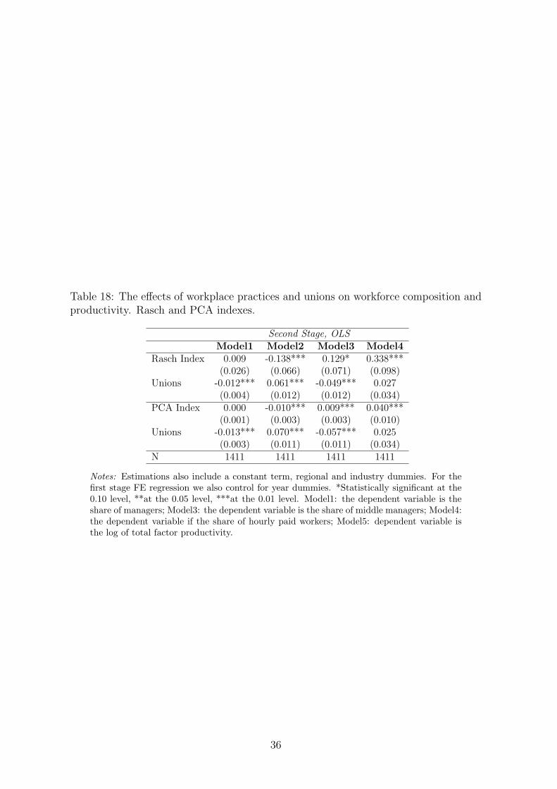
Table 18: The effects of workplace practices and unions on workforce composition andproductivity. Rasch and PCA indexes.


Rasch Index 0.009 -0.138*** 0.129* 0.338***(0.026) (0.066) (0.071) (0.098)

Unions -0.012*** 0.061*** -0.049*** 0.027(0.004) (0.012) (0.012) (0.034)

PCA Index 0.000 -0.010*** 0.009*** 0.040***(0.001) (0.003) (0.003) (0.010)

Unions -0.013*** 0.070*** -0.057*** 0.025(0.003) (0.011) (0.011) (0.034)

N 1411 1411 1411 1411

Notes: Estimations also include a constant term, regional and industry dummies. For thefirst stage FE regression we also control for year dummies. *Statistically significant at the0.10 level, **at the 0.05 level, ***at the 0.01 level. Model1: the dependent variable is theshare of managers; Model3: the dependent variable is the share of middle managers; Model4:the dependent variable if the share of hourly paid workers; Model5: dependent variable isthe log of total factor productivity.

36

High-Performance Management Practices and Employee Outcomes in Denmark

Documents

Transcript of High-Performance Management Practices and Employee Outcomes in Denmark