High-Order Non-Reflecting Boundary Scheme

for Time-Dependent Waves

Dan Givoli ∗ Beny Neta †

Department of Mathematics

Naval Postgraduate School

1141 Cunningham Road

Monterey, CA 93943, U.S.A.

May 1, 2002

∗Corresponding author. E-mail: dgivoli@nps.navy.mil , Tel.: +1-831-656-2758, Fax: +1-831-656-2355.

On leave (till Aug. 2002) from: Department of Aerospace Engineering and Asher Center for Space Research,

Technion — Israel Institute of Technology, Haifa 32000, Israel, E-mail: givolid@aerodyne.technion.ac.il ,

Tel.: +972-4-8293814, Fax: +972-4-8231848.†E-mail: bneta@nps.navy.mil , Tel.: +1-831-656-2235, Fax: +1-831-656-2355.

High-Order Non-Reflecting Boundaries 2

Abstract

A new non-reflecting boundary scheme is proposed for time-dependent wave problems in

unbounded domains. The linear time-dependent wave equation, with or without a disper-

sive term, is considered outside of an obstacle or in a semi-infinite wave guide. The infinite

domain is truncated via an artificial boundary B, and a high-order Non-Reflecting Boundary

Condition (NRBC) is imposed on B. Then the problem is solved numerically in the finite

domain bounded by B. The new boundary scheme is based on a reformulation of the se-

quence of NRBCs proposed by Higdon. In contrast to the original formulation of the Higdon

conditions, the scheme constructed here does not involve any high derivatives beyond second

order. This is made possible by introducing special auxiliary variables on B. As a result, the

new NRBCs can easily be used up to any desired order. They can be incorporated in a finite

element or a finite difference scheme; in the present paper the latter is used. The param-

eters appearing in the NRBC are chosen automatically via a special procedure. Numerical

examples concerning a semi-infinite wave guide are used to demonstrate the performance of

the new method.

Keywords: Waves, High-order, Artificial boundary, Non-reflecting boundary condition,

Higdon, Auxiliary variables, Finite difference.

High-Order Non-Reflecting Boundaries 3

1. Introduction

Methods for the numerical solution of wave problems in unbounded domains have been devel-

oped since the 70’s [1]. They have been considered in various fields of application involving

wave propagation, such as acoustics, electromagnetics, meteorology and solid geophysics.

The main four types of methods that have emerged are: boundary integral methods, infinite

element methods, absorbing layer methods and non-reflecting boundary condition (NRBC)

methods. The present paper concentrates on the latter.

In the method of NRBCs, the infinite domain is truncated via an artificial boundary B,

thus dividing the original domain into a finite computational domain Ω and a residual infinite

domainD. A special boundary condition is imposed on B, in order to complete the statement

of the problem in Ω (i.e., make the solution in Ω unique) and, most importantly, to ensure

that no (or little) spurious wave reflection occurs from B. This boundary condition is called

a NRBC, although a few other names are often used too [2]. The problem is then solved

numerically in Ω. The setup is illustrated in Fig. 1. Fig. 1(a) pertains to an exterior problem

outside of a scatterer or an obstacle. The artificial boundary B has a rectangular shape in

the figure, although sometimes a smooth shape (like a circle in two dimensions or a sphere

in three dimensions) is preferred. Fig. 1(b) describes a semi-infinite wave-guide problem. In

yΩ

D

Bx S

Γ

Γx

y

x=x

N

ΩB=

D

Γ

E

W bEΓ

(a) (b)

Figure 1. Setup for the NRBC method: (a) an exterior scattering problem; (b) a semi-infinite

wave-guide problem.

High-Order Non-Reflecting Boundaries 4

the example shown, B = ΓE is a cross section of the wave-guide which constitutes the east

side of Ω.

Naturally, the quality of the numerical solution strongly depends on the properties of

the NRBC employed. In the last 25 years or so, much research has been done to develop

NRBCs that after discretization lead to a scheme which is stable, accurate, efficient and easy

to implement. See [3]–[5] for recent reviews on the subject. Of course, it is difficult to find

a single NRBC which is ideal in all respects and all cases; this is why the quest for better

NRBCs and their associated discretization schemes continues.

The late 70’s and early 80’s produced some low-order local NRBCs that become well-

known, e.g., the Engquist-Majda NRBCs [6] and the Bayliss-Turkel NRBCs [7]. The late 80’s

and early and mid 90’s have been characterized by the emerging of exact nonlocal NRBCs like

those based on the Dirichlet-to-Neumann (DtN) map [8, 9] and on the Difference Potential

Method (DPM) [10, 11], and by the invention of the Perfectly Matched Layer (PML) [12].

More recently, high-order local NRBCs have been introduced. Sequences of increasing-order

NRBCs have been available before (e.g., the Bayliss-Turkel conditions [7] constitute such

a sequence), but they had been regarded as impractical beyond 2nd or 3rd order from the

implementation point of view. Only since the mid 90’s, practical high-order NRBCs have

been devised.

The first such high-order NRBC has apparently been proposed by Collino [13], for two-

dimensional time-dependent waves in rectangular domains. Its construction requires the

solution of the one-dimensional wave equation on B. Grote and Keller [14, 15] developed a

high-order converging NRBC for the three-dimensional time-dependent wave equation, based

on spherical harmonic transformations. They extended this NRBC for the case of elastic

waves in [16]. Sofronov [17] has independently published a similar scheme in the Russian

literature. Hagstrom and Hariharan [18, 19] constructed high-order NRBCs for the two- and

three-dimensional time-dependent wave equations based on the analytic series representation

for the outgoing solutions of these equations. It looks simpler than the previous two NRBCs.

For time-dependent waves in a two-dimensional wave guide, Guddati and Tassoulas [20] de-

vised a high-order NRBC by using rational approximations and recursive continued fractions.

Givoli [21] has shown how to derive high-order NRBCs for a general class of wave problems,

High-Order Non-Reflecting Boundaries 5

leading to a symmetric finite element formulation. In [22], this methodology was applied to

the particular case of time-harmonic waves, using optimally localized DtN NRBCs.

In the context of artificial boundary treatment, wave problems can roughly be divided

into four categories. These are, in order of difficulty:

(a) Linear time-harmonic wave problems.

(b) Linear time-dependent wave problems in non-dispersive homogeneous media.

(c) Linear time-dependent wave problems in dispersive and/or stratified media.

(d) Nonlinear time-dependent wave problems.

Linear time-harmonic waves have been treated extensively by NRBCs and absorbing layers,

including exact NRBCs of the DtN type [4], various PML formulations (see, e.g., [23, 24]),

and converging high-order NRBCs (see, e.g., [22]). Time-dependent waves are considerably

more difficult to handle from the artificial-boundary perspective. However, some exact and

high-order schemes have been devised in this case as well. These include the schemes pro-

posed in the references [13]–[21] mentioned above, as well as a scheme based on the Kirchhoff

formula for three-dimensional waves [25, 26], an iterative converging local NRBC [27], semi-

discrete DtN [28], time-dependent DtN [29], transform-based methods [30]–[32], and some

variations of the above [33]–[35].

The presence of wave dispersion and/or medium stratification makes the time-dependent

problem still more difficult as far as NRBC treatment is concerned. None of the high-order

and exact NRBCs mentioned above has been designed to deal with these effects. In fact, even

in one spatial dimension, an exact NRBC for the dispersive (Klein-Gordon) wave equation

is not available. Very recently, Navon et al. [36] developed a PML scheme for the dispersive

shallow water equations. Nonlinear waves (with the nonlinearity extending to infinity) are,

of course, the most difficult to handle. Some highly-accurate NRBCs have been proposed

for specific classes of nonlinear wave problems (see references in the review papers [3], [5]

and [37]).

In the present paper we develop a high-order NRBC scheme for both dispersive and non-

dispersive linear time-dependent waves. Wave dispersion appears in various applications.

High-Order Non-Reflecting Boundaries 6

One important example is that of meteorological models which take into account the earth

rotation [38]. Other examples include quantum-mechanics waves, the vibration of structures

with rotational rigidity such as beams, plates and shells, the vibration of strings and mem-

branes on an elastic foundation, acoustic wave propagation in a bubbly medium, and some

nonlinear wave problems after linearization.

Higdon [39] proposed a sequence of NRBCs for the dispersive wave equation. In fact, these

NRBCs were developed originally for non-dispersive waves [40]–[44], but Higdon showed in

[39] that they can be applied in the dispersive case too. The original implementation of the

Higdon NRBCs is limited to low orders. Recently, we have proposed a new implementation

method that allows the use of high-order discretized Higdon NRBCs [45]. However, this

method differs from the original Higdon formulation only on the discrete level, not on the

continuous level; thus, like the original Higdon scheme, it involves high normal and temporal

derivatives, of increasing order. This has several disadvantages which we allude to in the

next section. In addition, the computational effort required by the scheme devised in [45]

grows exponentially with the order of the NRBC.

In the present paper, we reformulate the Higdon NRBCs on the continuous level in a

completely new way. This formulation does not involve any high derivatives. This is made

possible by introducing special auxiliary variables on B. The new construction allows the

easy use of a Higdon-type NRBC of any desired order, and can be incorporated in a Finite

Element or a Finite Difference (FD) scheme. In the present paper we use FDs to discretize

both the partial differential equation in Ω and the NRBC on B. The computational effort

required by the scheme grows only linearly with the order.

Following is the outline of the rest of this paper. In Section 2 we state the problem under

investigation. We also present the Higdon NRBCs and recall their properties. In Section 3 we

reformulate the Higdon NRBCs, through the use of auxiliary variables, in a high-order way

which does not involve high derivatives. The FD discretization scheme for this formulation

is presented in Section 4. In Section 5 we discuss some computational issues, including the

automatic choice of the NRBC parameters and the “exactness” of the NRBC scheme. In

Section 6 we demonstrate the performance of the new method via some numerical examples

concerning a semi-infinite wave guide. We conclude with some remarks in Section 7.

High-Order Non-Reflecting Boundaries 7

2. Statement of the Problem and the Higdon NRBCs

We consider wave propagation in a two-dimensional channel or wave guide, as described in

Fig. 1(b). However, we emphasize that the same ideas can be applied with slight modifi-

cations to other configurations, such as that of exterior scattering shown in Fig. 1(a). A

Cartesian coordinate system (x, y) is introduced such that the wave-guide is parallel to the

x direction. The width of the wave-guide is denoted by b. In the wave guide we consider the

linear inhomogeneous Klein-Gordon equation,

∂2t u− C2

0∇2u+ f 2u = S . (1)

Here and elsewhere we use the following shorthand for partial derivatives:

∂ia =

∂i

∂ai. (2)

In (1), u is the unknown wave field, C0 is the given reference wave speed, f is the given

dispersion parameter, and S is a given wave source function. The C0 and f are allowed to

be functions of location; however, it is assumed that outside a finite region (typically located

near the west boundary ΓW ) they do not depend on x but only possibly on y. (Such y-

dependence corresponds to a stratified medium.) The wave source S is a function of location

and time, but it is assumed to have a local support.

Eq. (1) describes, for example, the lateral vibration of a membrane strip on an elas-

tic foundation, or the acoustic pressure in a dispersive medium (say, a linearized bubbly

medium). Also, it can be shown that the linearized shallow water equations, with a flat

bottom and zero initial conditions, reduce to (1), where u is the water elevation above the

reference level [38]. In the geophysical context, f is called the Coriolis parameter and is

related to the angular velocity of the earth.

On the south and north boundaries ΓS and ΓN we specify either the Dirichlet condition

u = 0 on ΓS & ΓN , (3)

or the Neumann condition

∂yu = 0 on ΓS & ΓN . (4)

High-Order Non-Reflecting Boundaries 8

In acoustics these correspond to “soft wall” and “hard wall” conditions, respectively. On the

west boundary ΓW we prescribe u using a Dirichlet condition, i.e.,

u(0, y, t) = uW (y, t) on ΓW , (5)

where uW (y, t) is a given function (incoming wave). At x → ∞ the solution is known to be

bounded and not to include any incoming waves. To complete the statement of the problem,

the initial conditions

u(x, y, 0) = u0 , ∂tu(x, y, 0) = v0 , (6)

are given at time t = 0 in the entire domain. We assume that the functions u0 and v0 have

a local support.

We now truncate the semi-infinite domain by introducing an artificial east boundary

B ≡ ΓE , located at x = xE ; see Fig. 1(b). This boundary divides the original semi-infinite

domain into two subdomains: an exterior domain D, and a finite computational domain Ω

which is bounded by ΓW , ΓN , ΓS and ΓE . We choose the location of ΓE such that the entire

support of S, u0 and v0 and the region of x-dependence of C0 and f are all contained inside

Ω. Thus, on ΓE and in D, the homogeneous counterpart of (1) holds, i.e.,

∂2t u− C2

0∇2u+ f 2u = 0 , (7)

with y-dependent (or, as a special case, constant) coefficients C20 and f 2, and the medium is

initially at rest.

To obtain a well-posed problem in the finite domain Ω we need to impose a boundary

condition on ΓE. This must be a NRBC so as to prevent spurious reflection of waves. We

shall use a NRBC which is a reformulation of the Higdon NRBC [39]. The Higdon conditions

were presented and analyzed in a sequence of papers [40]–[44] for non-dispersive acoustic and

elastic waves, and were extended in [39] for the dispersive case. The Higdon NRBC of order

J is

HJ :

J∏

j=1

(∂t + Cj∂x)

u = 0 on ΓE . (8)

Here, the Cj are parameters which have to be chosen and which signify phase speeds in the

x-direction. The main advantages of the Higdon conditions are as follows:

High-Order Non-Reflecting Boundaries 9

• The Higdon NRBCs are very general, namely they apply to a variety of wave problems,

in one, two and three dimensions and in various configurations. Moreover, they can be

used, without any difficulty, for wave problems in dispersive and stratified media. Most

other available NRBCs are either designed for non-dispersive homogeneous media (as

in acoustics and electromagnetics) or are inherently of low order (as in meteorology

and oceanography).

• The Higdon NRBCs constitute a sequence of conditions of increasing order. This, and

the fact that no asymptotic approximation is involved in their construction, enables one

in principle (leaving implementational issues aside for the moment) to obtain solutions

with unlimited accuracy. See the discussion in Section 5.3.

• The boundary condition (8) is exact for all waves that propagate with an x-direction

phase speed equal to either of C1, . . . , CJ . To see this, consider a wave which satisfies

the wave equation (7). Such a wave has the form

u = AYn(y) cos k(x− Cxt+ ψ) , (9)

where

Cx =ω

k, (10)

which is the x-direction phase velocity. In (9) and (10), A is the wave amplitude, ψ

is its phase, k is the x-component wave number, and ω is the wave frequency. The

function Yn(y) in (9) is determined from the dependency of C0 and f on y and from

the boundary conditions given on ΓS and ΓN . For example, if C0 and f are constant

then

Yn(y) =

sin nπyb, n = 1, 2, . . . ; if Dirichlet B.C. (3)

cos nπyb, n = 0, 1, 2, . . . ; if Neumann B.C. (4)

. (11)

It is common to refer to n as the “mode number.” The wave number k, the frequency

ω and the mode number n depend on each other through the dispersion relation. For

example, for C0 and f constant the dispersion relation is

ω2 = C20

(k2 +

n2π2

b2

)+ f 2 , n = 0, 1, 2, . . . (12)

High-Order Non-Reflecting Boundaries 10

where the mode n = 0 appears only in the case of Neumann conditions on ΓS and

ΓN . In general, solutions of (7) consist of an infinite number of waves of the form (9).

There are also solutions that decay exponentially in the x direction; however, they are

usually not of great concern, since the decaying modes are expected to be insignificant

at the time they reach ΓE . Now, it is easy to verify that if one of the Cj’s in (8) is

equal to Cx, then the wave (9) satisfies the boundary condition (8) exactly.

• Each wave of the form (9) is essentially characterized by two independent parameters,

say the wave number k and the mode number n. Other parameters, like the frequency

ω or the phase velocity Cx are determined from these two parameters through the

dispersion relation (see (10) and (12)). Despite this fact, the accuracy of the Higdon

NRBC is determined by only one parameter per wave, namely Cx. This significantly

facilitates accuracy control.

• For certain choices of the parameters, the Higdon NRBCs are equivalent to NRBCs

that are derived from rational approximation of the dispersion relation (the Engquist-

Majda conditions [6] being the most well-known example). This has been proved by

Higdon in [39, 40]. More precisely, Higdon’s theorem states that if a NRBC is based

on a symmetric rational approximation to the dispersion relation corresponding to

outgoing waves, then it is either (a) equivalent to (8) for a suitable choice of J and

the parameters Cj, or (b) unstable, or (c) not optimal. Lack of optimality means

here that the coefficients in the NRBC can be modified so as to reduce the amount of

the spurious reflection. Thus, the Higdon NRBCs can be viewed as generalization of

rational-approximation NRBCs.

• It is easy to show (see Higdon [39] for a similar setting) that when a wave of the

form (9) impinges on the boundary ΓE where the NRBC HJ is imposed, the resulting

reflection coefficient is

R =J∏

j=1

∣∣∣∣∣Cj − Cx

Cj + Cx

∣∣∣∣∣ . (13)

Again we see that if Cj = Cx for any one of the j’s then R = 0, namely there is no

reflection and the NRBC is exact. Moreover, we see that the reflection coefficient is a

High-Order Non-Reflecting Boundaries 11

product of J factors, each of which is smaller than 1. This implies that the reflection

coefficient becomes smaller as the order J increases regardless of the choice made for

the parameters Cj. Of course, a good choice for the Cj would lead to better accuracy

with a lower order J , but even if we miss the correct Cj’s considerably (say, if we

make the simplest choice Cj = C0 for j = 1, . . . , J), we are still guaranteed to reduce

the spurious reflection as we increase the order J . This is an important property of

Higdon’s NRBCs and is the reason for their robustness.

We note that the first-order condition H1 is a Sommerfeld-like boundary condition. If we

set C1 = C0 we get the classical Sommerfeld-like NRBC. A lot of work in the meteorological

literature is based on using H1 with a specially chosen C1. Pearson [46] used a special but

constant value of C1, while in the scheme devised by Orlanski [47] and in later improved

schemes [48]–[51] the C1 changes dynamically and locally in each time-step based on the

solution from the previous time-step. Some of the limited-area weather prediction codes

used today are based on such schemes, e.g., COAMPS [52]. See also the recent papers

[53]–[55] where several such adaptive H1 schemes are compared.

Difficulties associated with the original formulation of the Higdon NRBCs (see [39]) are

as follows:

• The discrete Higdon conditions were developed in the literature up to third order only,

because of their algebraic complexity which increases rapidly with the order.

• The original Jth-order Higdon NRBC involves high normal and temporal derivatives,

up to order J . In fact, it has the form

J∑j=0

γj ∂jx∂

J−jt u = 0 , (14)

which is obtained by expanding (8). The high derivatives pose obvious disadvantages.

High normal derivatives are problematic; when finite elements are used only the J = 1

condition is compatible with standard (low-order C0) elements, whereas when finite

differences are used, the discrete stencil must be a non-standard high-order one, pene-

trating deeply into the computational domain away from the artificial boundary. High

High-Order Non-Reflecting Boundaries 12

time derivatives are also disadvantageous in that they require the use of high-order

time discretization and the storage of the solution history.

• The Higdon NRBCs involve the parameters Cj which must be chosen. Higdon [39]

discusses some general guidelines for their manual a-priori choice by the user. No

procedure has been provided in the literature for the automatic choice of the Cj ’s.

The new scheme proposed in this paper overcomes all these difficulties. In the next

sections we shall reformulate the Higdon NRBCs such that they can easily be used up to an

arbitrarily high order. The scheme is coded once and for all for any order; the order of the

scheme is simply an input parameter. Moreover, it does not involve any high derivatives.

Later we shall also discuss the automatic choice of the parameters Cj.

3. High-Order Non-Reflecting Boundary Conditions

We first replace the Higdon condition (8) by the equivalent condition

HJ :

J∏

j=1

(∂x +

1

Cj∂t

)u = 0 on ΓE . (15)

Now we introduce the auxiliary functions φ1, . . . , φJ−1, which are defined on ΓE as well as in

the exterior domain D (see Fig. 1(b)). Eventually we shall use these functions only on ΓE ,

but the derivation requires that they be defined in D as well, or at least in a non-vanishing

region adjacent to ΓE . The functions φj are defined via the relations(∂x +

1

C1

∂t

)u = φ1 , (16)

(∂x +

1

C2∂t

)φ1 = φ2 , (17)

...(∂x +

1

CJ

∂t

)φJ−1 = 0 . (18)

By definition, these relations hold in D, and also on ΓE. It is easy to see that (16)–(18),

when imposed as boundary conditions on ΓE , are equivalent to the single boundary condition

(15). If we also define

φ0 ≡ u , φJ ≡ 0 , (19)

High-Order Non-Reflecting Boundaries 13

then we can write (16)–(18) concisely as(∂x +

1

Cj∂t

)φj−1 = φj , j = 1, . . . , J . (20)

This set of conditions involves only first-order derivatives. However, due to the appearance

of the x-derivative in (20), one cannot discretize the φj on the boundary ΓE alone. Therefore

we shall manipulate (20) in order to get rid of the x-derivative.

The function u satisfies the wave equation (7) in D. The function φ1 is obtained by

applying a linear operator to u, as in (16); hence it is clear that φ1 also satisfies the same

equation in D. Similarly, we deduce that each of the functions φj satisfies a wave equation

like (7), namely,

∂2xφj + ∂2

yφj − 1

C20

∂2t φj − f 2

C20

φj = 0 . (21)

Here we needed the assumption that C0 and f do not depend on x or on t. Now, we make

use of the following identity:

∂2xφj =

(∂x − 1

Cj+1

∂t

)(∂x +

1

Cj+1

∂t

)φj +

1

C2j+1

∂2t φj . (22)

Substituting (22) in (21) and replacing j with j − 1 everywhere yields, for j = 1, . . . , J ,(∂x − 1

Cj∂t

)(∂x +

1

Cj∂t

)φj−1 +

(1

C2j

− 1

C20

)∂2

t φj−1 + ∂2yφj−1 − f 2

C20

φj−1 = 0 . (23)

From this and (20) we get, for j = 1, . . . , J ,(∂x − 1

Cj∂t

)φj +

(1

C2j

− 1

C20

)∂2

t φj−1 + ∂2yφj−1 − f 2

C20

φj−1 = 0 . (24)

On the other hand, (20) can also be written as(∂x +

1

Cj+1∂t

)φj = φj+1 , j = 0, . . . , J − 1 . (25)

We subtract (24) from (25) to finally obtain, for j = 1, . . . , J − 1,(1

Cj+

1

Cj+1

)∂tφj = φj+1 +

(1

C2j

− 1

C20

)∂2

t φj−1 + ∂2yφj−1 − f 2

C20

φj−1 . (26)

As desired, the new boundary condition (26) does not involve x-derivatives. In addition,

there are no high y- and t-derivatives in (26) beyond second order.

Rewriting (16), (26) and (19), we can summarize the new formulation of the Jth-order

NRBC on ΓE as follows:

High-Order Non-Reflecting Boundaries 14

β0∂tu+ ∂xu = φ1 , (27)

βj∂tφj − αj∂2t φj−1 − ∂2

yφj−1 + λφj−1 = φj+1 , j = 1, . . . , J − 1 , (28)

αj =1

C2j

− 1

C20

, β0 =1

C1, βj =

1

Cj+

1

Cj+1, λ =

f 2

C20

, (29)

φ0 ≡ u , φJ ≡ 0 . (30)

4. Finite Difference Discretization

Now we consider the FD discretization of the NRBC (27)–(30). First we consider the bound-

ary condition for u, (27). We discretize ∂xu on ΓE by using the one-sided second-order

approximation [56]

(∂xu)nEq − −3un

Eq + 4unE−1,q − un

E−2,q

2∆x. (31)

Here and elsewhere, unpq (and also un

p,q) is the FD approximation of u(x, y, t) at grid point

(xp, yq) and at time tn, and the index E correspond to a grid point on the boundary ΓE .

From (27) we obtain a discrete formula for ∂tu, i.e.,

(∂tu)nEq

1

β0

((φ1)

nEq − (∂xu)

nEq

). (32)

Then we calculate the new u by the forward-in-time formula

un+1Eq = un

Eq + ∆t (∂tu)nEq . (33)

Next we consider the boundary condition for φj , (28). We use the following second-order

central difference approximations for the second temporal and tangential derivatives [56]:

(∂2t φj−1)

nEq

(φj−1)n+1Eq − 2(φj−1)

nEq + (φj−1)

n−1Eq

(∆t)2, (34)

(∂2yφj−1)

n+1Eq (φj−1)

n+1E,q+1 − 2(φj−1)

n+1Eq + (φj−1)

n+1E,q−1

(∆y)2. (35)

Note that (35) cannot be used at the two east corners (the two end points of ΓE). At these

corners, we do one of the following things. If the Dirichlet boundary conditions (3) are

applied on ΓS and ΓN , then it is easy to show from (16)–(18) that on these boundaries not

High-Order Non-Reflecting Boundaries 15

only u = 0 but also φj = 0 for j = 1, . . . , J . Thus, in the two east corners we simply take

u = 0 and φj = 0 for all the j’s. If the Neumann boundary conditions (4) are given on ΓS

and ΓN , we use at the two east corners a one-sided second-order approximation instead of

the central-difference formula (35). For example, at the south-east corner we use [56]

(∂2yφj−1)

n+1Eq 2(φj−1)

n+1Eq − 5(φj−1)

n+1E,q+1 + 4(φj−1)

n+1E,q+2 − (φj−1)

n+1E,q+3

(∆y)2. (36)

From (28) we obtain a discrete formula for ∂tφj , i.e.,

(∂tφj)nEq

1

βj

((φj+1)

nEq + αj(∂

2t φj−1)

nEq + (∂2

yφj−1)n+1Eq − λ(φj−1)

n+1Eq

). (37)

Then we calculate the new φj by the forward-in-time formula

(φj)n+1Eq = (φj)

nEq + ∆t (∂tφj)

nEq . (38)

The simplest solution procedure is the one based on the sequential solution of the equa-

tions for the φj’s. Namely, we first solve for u, then we solve for φ1, then for φ2, and so

on. At the stage when we update the values of φj, the quantities (φj−1)n+1E... appearing in

(34) and (35) are already known, having been derived in the previous stage for φj−1. On

the other hand, the quantity (φj+1)n+1Eq is not yet available; that is why we use (φj+1)

nEq in

(32) and (37) rather than (φj+1)n+1Eq . The latter fact may potentially lead to an unstable

solution. Indeed, when we have implemented the scheme based on the formulas (31)–(38)

with J ≥ 2, an instability developed in time. One remedy for this instability is to perform

a second iteration and update u and the φj’s again based on values obtained in the first

iteration. This two-cycle algorithm turns out to be stable. It is summarized in Box 1.

Note that the only algorithmic difference between the first and second iterations is in

the use of (φ1)nEq vs. (φ1)

n+1Eq in (32). All the other formulas remain unchanged in the two

iterations. We have tried to use also (φj+1)n+1Eq in (37) instead of (φj+1)

nEq in the second

iteration, but this led to instability.

As an alternative scheme, eqs. (31)–(38) may be solved simultaneously for all the j’s and

all the y-locations q, as one coupled system of linear equations on ΓE. The dimension of

this system is JNy, where Ny is the number of grid-points on ΓE. However, in the numerical

examples presented in Section 6 we have used the decoupled discretization scheme described

in Box 1.

High-Order Non-Reflecting Boundaries 16

• First iteration:

• Compute the (∂xu)n values on ΓE from (31).

• Compute the (∂tu)n values on ΓE from (32).

• Compute the un+1 values on ΓE from (33).

• If J = 1, stop.

• For j=1,. . . ,J-1:

– Compute the ∂2t (φj−1)

n values from (34).

– Compute the ∂2y(φj−1)

n+1 values from (35) and (in the two corners) from (36).

– Compute the ∂t(φj)n values from (37).

– Compute the (φj)n+1 values from (38).

• Next j

• Second iteration:

• Recompute the (∂tu)n values on ΓE from (32), but use (φ1)

n+1 instead of (φ1)n.

• Recompute the un+1 values on ΓE from (33).

• For j=1,. . . ,J-1:

– Recompute the ∂2t (φj−1)

n values from (34).

– Recompute the ∂2y(φj−1)

n+1 values from (35) and (in the two corners) from (36).

– Recompute the ∂t(φj)n values from (37).

– Recompute the (φj)n+1 values from (38).

• Next j

Box 1. Algorithm for the FD implementation of the Jth-order NRBC.

High-Order Non-Reflecting Boundaries 17

In the interior domain Ω, we use the standard second-order centered difference scheme

un+1pq = 2un

pq − un−1pq +

(C0∆t

∆x

)2 (un

p+1,q − 2unpq + un

p−1,q

)

+

(C0∆t

∆y

)2 (un

p,q+1 − 2unpq + un

p,q−1

)− (f∆t)2un

pq . (39)

Higdon [39] has proved that the discrete NRBCs (8) (in their original form) are stable if (39)

is used as the interior scheme. Since both (39) and the discretized NRBC are explicit, the

whole scheme is explicit.

5. Computational Issues

5.1. Complexity

From eqs. (31)–(38) and Box 1, it is easy to see that the number of operations related to the

Jth-order NRBC on ΓE is O(JNy) per time-step, where Ny is the number of grid-points on

ΓE . The associated computational effort is typically marginal with respect to the total effort

required by the entire solution process. In comparison, the scheme proposed in [45] which

directly uses the original Higdon NRBCs (but with a special high-order discretization scheme)

requires O(3JNy) operations per time-step, namely its complexity grows exponentially with

J .

5.2. Choosing the Parameters Cj

Now we discuss how to choose the J parameters Cj, appearing in the NRBC (27)–(30).

First, we note that some physical limitations may apply to the chosen values of the Cj’s.

For example, if C0 and f are constant then from (10) and (12) we get

Cx = C0

√1 +

n2π2/b2 + f 2

k2, n = 0, 1, 2, . . . (40)

and thus Cx ≥ C0. Hence in this case one should take Cj ≥ C0 for all the j’s.

Second, we recall that even the simple choice Cj = C0 for j = 1, . . . , J is guaranteed

to reduce the spurious reflection as J increases (see Section 2). Thus, this choice may be

High-Order Non-Reflecting Boundaries 18

successful in many cases provided that J is sufficiently large. What one gains from making

a specialized choice for the Cj is the ability to obtain the desired level of accuracy with

a smaller order J . However, one must bear in mind that since the NRBC-associated cost

increases only linearly with J , taking a large J may sometimes be preferable to spending a

considerable amount of computational effort on a sophisticated procedure to choose the Cj.

Three approaches for choosing the parameters Cj suggest themselves:

(a) The user chooses the Cj a-priori in a manual manner based on an “educated guess.”

(b) The Cj are chosen automatically by the computer code as a preprocess.

(c) The Cj are not constant, but are determined dynamically by the computer code.

Approach (a) is the one recommended in Higdon’s papers [39]–[44]. It is based on the

assumption that the user has some a priori knowledge on the character of the exact solution.

While this may be a good assumption in some applications, it is definitely desirable to have

at hand an automatic procedure that will not require the user’s intervention.

Approach (b) is attractive since it is automatic yet very inexpensive computationally.

We have adopted this approach in [45] as well as here, using an algorithm which is based

on the maximum resolvable wave numbers in the x and y directions, and on the minimax

formula [57] for choosing the x-component wave numbers. The algorithm consists of the

following steps (see [45] for further details): (1) Estimate the maximum resolvable wave

number k in the x direction. Assuming a maximum of 10 grid points per wave length, a

reasonable estimate is kmax = π/(5∆x), where ∆x is the grid spacing in the x direction. (2)

Similarly, estimate the maximum resolvable wave number k in the y direction. (3) Choose J

values of k from the interval (0, kmax]. The simplest choice is the uniform division, namely

kj = kmaxj/J . However, a better choice is to take the roots of the Chebyshev polynomial as

the kj. This choice is based on the symmetric minimax formula, proposed by Sommeijer et

al. [57]. In this case more of the kj are concentrated near the ends of the interval (0, kmax].

(4) For each kj, calculate the corresponding (and maximal in the y direction) frequency ωj

from the dispersion relation (cf. (12)). (5) Calculate Cj = ωj/kj (see (10)).

Approach (c) is the most sophisticated, and also the most expensive computationally. In

this approach, the values Cj are estimated for every grid point on the boundary at each time

High-Order Non-Reflecting Boundaries 19

step, from the solution in the previous time-steps. For the Sommerfeld-like NRBC (J = 1),

a procedure of this type is used a lot in meteorological applications [47]–[51]. Analogous

procedures may be employed with higher orders, although Higdon [39] reports bad results

with the Orlanski scheme [47] with J = 2 and J = 3. An adaptive scheme of a different

type, perhaps more suitable to high orders, is based on the Fast Fourier Transform (FFT);

see [58].

5.3. Exactness of the scheme

The proposed high-order NRBC scheme is converging, in the following sense. Consider the

exact solution of two problems: the first is the original problem in the infinite domain, and

the second is the problem in the truncated domain Ω, with the NRBC applied on B. Then

the distance δ, in some reasonable norm, between the two solutions in Ω may serve as an

error measure. Now, if a sequence of NRBCs satisfies the following two properties:

(1) for any given problem of the class under consideration the error measure δ of the NRBC

approaches zero as the order of the NRBC J goes to infinity while B is held fixed;

(2) the NRBC can be implemented once and for all for any order J , without limit;

then it is justified to call the sequence of NRBCs exact, or converging. In this sense the

Grote-Keller NRBC [15], the three-dimensional Hagstrom-Hariharan NRBC [19] and the

localized DtN condition [22] are all converging.

The NRBC scheme proposed in the present paper is also converging. The reason is that

by increasing J and choosing the parameters CJ in an appropriate way, one is assured to

reduce the spurious reflection down to any desired level. To demonstrate this we give two

arguments: a theoretical one and a practical one.

The theoretical argument is as follows. Consider the case of constant C0 and f . Any

solution of (7) may be written as a combination of plane waves, each one associated with

a certain phase velocity in the x direction, Cx ≥ C0 (see (9)–(12)). Each wave generates

the reflection coefficient R given by (13), which is a product of numbers smaller than one.

Thus, as J increases, the R generated by each wave must decrease. However, this does not

necessarily mean that R approaches zero as J → ∞. A sufficient condition for this to be

High-Order Non-Reflecting Boundaries 20

guaranteed is that the set of Cj’s is dense in the interval [C0,∞) as J → ∞, so that whatever

Cx is, it will be arbitrarily close to one of the Cj. This is indeed possible to achieve: the

sequence of Cj’s may be taken to be the sequence of all the rational numbers greater than

or equal to C0. The rational numbers form a countable set and thus can be ordered in a

sequence; moreover they are dense in the set of real positive numbers (a non-countable set).

This argument is “theoretical” because in practice the Cj will never be chosen in this fashion.

The practical argument is as follows. It is true that the phase velocity Cx of the waves

participating in the solution is not necessarily bounded, namely that for any number M

there may be waves for which Cx > M . However, those waves that have very high Cx

are not of practical interest, since they cannot be resolved by the discrete scheme anyway.

Moreover, such waves are expected to have small amplitudes and not to influence the solution

significantly compared to the resolved waves (otherwise the discretization is not satisfactory).

Thus, we can estimate a “practical bound” (Cx)max for the Cx (say, a multiple of ∆x/∆t).

Then we only have to consider the finite interval Cj ∈ [C0, (Cx)max]. The Cj may be chosen

by a uniform division of this interval into J values, or by using the algorithm outlined in

Section 5.2. Either way, as J → ∞, the set of the Cj ’s is dense in this interval.

5.4. Corners

In the wave-guide problem described in Section 2 the normal and tangential directions with

respect to ΓE are well defined and are fixed along ΓE . On the other hand, in the case of

an exterior scattering problem (see Fig. 1(a)), where the artificial boundary B is a rectangle

enclosing the scatterer or obstacle, these directions are not well-defined in the four corners.

However, this does not pose any difficulties. In a FD scheme, the corner grid-point can

arbitrarily be associated with one of the two straight edges that meet at this corner, and

can be treated just as any other grid point on this chosen edge. In a Finite Element scheme

the issue does not arise at all, since the NRBC is typically applied weakly. This is done

by integrating appropriate expressions along the element outer edges. Usually the Gauss

integration rule is employed, which involves evaluation of the integrand at some interior

points and not at the nodal points. In particular, there is no need to evaluate any derivative

at the nodal points located in the two east corners.

High-Order Non-Reflecting Boundaries 21

For the well-posedness of the exterior scattering problem in Ω when using the NRBC (27)–

(30) on all four sides of the rectangular artificial boundary, corner conditions which relate

the tangential and normal derivatives on two sides meeting at a corner must be applied.

However, discussion of these corner conditions is outside the scope of the present paper. We

also mention the possibility of adapting the new NRBCs to artificial boundaries with smooth

shapes (e.g., a circle in two dimensions or a sphere in three dimensions) by using variable

transformation; see e.g. [58].

5.5. Stability

Since the proposed method is explicit in time, one has to be concerned about numerical sta-

bility. For stability of the interior scheme (39), we must satisfy the well-known CFL condition

C0∆t/∆x ≤ 1. Since typically one would choose ∆t/∆x to be slightly below the stability

limit, we assume that ∆t and ∆x are chosen such that C0∆t/∆x = 1−ε. Now, it is expected

that the NRBC will also be associated with a stability condition. Indeed, the condition (27)

and its discrete counterpart (31)–(33) point to the CFL condition (1/β0)∆t/∆x ≤ 1. We

thus conclude that for stability,

β0 ≡ 1

C1≥ ∆t

∆x=

1 − ε

C0. (41)

A similar argument, as well as numerical experiments, lead also to the sufficient condition

for stability

βj ≡ 1

Cj+

1

Cj+1≥ 1

C0, (42)

for j = 1, . . . , J − 1. Satisfying (41) and (42) is usually easy if one arranges the parameters

Cj in an appropriate way. For example, for J = 4, the arrangement Cj/C0 = 1, 4, 4, 1 is

unstable (since β2 = 1/(2C0) < 1/C0) but Cj/C0 = 1, 4, 1, 4 is stable. If a general automatic

procedure is used to choose the Cj , then this procedure should take into account the stability

limitations. This can be done, for example, by sorting the Cj appropriately and by replacing

some of them by the reference phase speed C0. Of course, the issue of the NRBC stability

does not arise at all if equations (27)–(30) on ΓE are solved in an implicit manner.

High-Order Non-Reflecting Boundaries 22

6. Numerical examples

We apply the new scheme to a number of test problems in a wave guide, as described in

Section 2 and illustrated in Fig. 1(b). We set b = 5 and C0 = 1. The initial conditions are zero

throughout the domain. On the walls ΓS and ΓN we use the Dirichlet boundary condition

(3). We consider two cases: the non-dispersive case, namely f = 0, and the dispersive case,

with f = 0.5. On the boundary ΓW we take the Dirichlet boundary condition (5), with

uW (y, t) = sin(πy

b

)cos k(x− Cxt) , t > 0 . (43)

This has the form of a mode-1 wave (see (9)). In (43) we take k = 0.1, and compute from the

dispersion relation (12) the phase velocity Cx = 8.0966. Note that the sine-wave “loading”

(43) is activated at t = 0 in a step-like fashion, since for t < 0 the solution is zero.

We introduce the artificial boundary ΓE (see Fig. 1(b)) at xE = 5. Thus, the compu-

tational domain Ω is a 5 × 5 square. In Ω we use a uniform grid with 21 × 21 points. We

discretize the Klein-Gordon equation in Ω using the explicit central-difference FD interior

scheme (39). The time-step size is ∆t = 0.025, which is smaller than the CFL stability limit.

On ΓE we impose the new NRBC, while varying the order J . Initially we use Cj = 1 for all

the j’s.

A reference solution which is regarded as the “exact solution” uex is obtained by solving

the problem in a longer domain, with a refined grid and with a very high-order NRBC on

the artificial boundary. Fig. 2 shows the “exact solution” obtained for the case f = 0.5 by

performing 4000 time steps. The solution is shown at the point P (5, 2.75) (corresponding to

the grid point p = 21, q = 12) which is located on the artificial boundary ΓE , slightly above

the center of the waveguide. As the graph shows, the solution is initially zero, until the first

noticeable wave packet reaches this point. Then there is a strong dynamic response which

after a short time decays rapidly.

We define two error measures. The first one is the Eulerian norm of the error over ΓE ,

i.e.,

E(t) =

√√√√ 1

Ny

Ny∑m=1

(u(xE, ym, t) − uex(xE , ym, t))2 . (44)

High-Order Non-Reflecting Boundaries 23

-0.4

-0.3

-0.2

-0.1

0

0.1

0.2

0.3

0 20 40 60 80 100

Exa

ct u

t

Figure 2. “Exact solution” for the wave-guide test problem, in the dispersive case (f = 0.5).

The solution is shown at the point P (5, 2.75).

0

0.0005

0.001

0.0015

0.002

0.0025

0.003

0.0035

0 20 40 60 80 100

Err

or E

t

-0.005-0.004-0.003-0.002-0.001

00.0010.0020.0030.0040.0050.006

0 20 40 60 80 100

Err

or e

t

(a) (b)

Figure 3. Errors as a function of time, for the dispersive case (f = 0.5), generated by the

new NRBC of order J = 3: (a) the global error E defined by (44); (b) the pointwise error e

defined by (45), at the point P (5, 2.75).

High-Order Non-Reflecting Boundaries 24

The second measure is the pointwise error at a single point (xE , y0) on ΓE, i.e.,

e(t) = u(xE, y0, t) − uex(xE , y0, t) . (45)

Fig. 3 shows the errors generated by the new scheme with J = 3. In Fig. 3(a) the global error

E defined by (44) is plotted, while Fig. 3(b) corresponds to the pointwise error e defined by

(45), at the point P mentioned above. It is apparent that the errors are oscillatory. Their

amplitudes grow initially, reach a maximum, and then decay in time, albeit more slowly than

the solution itself.

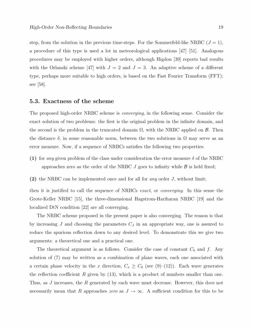
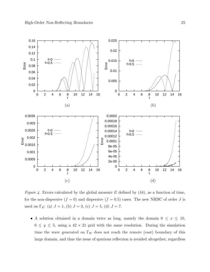
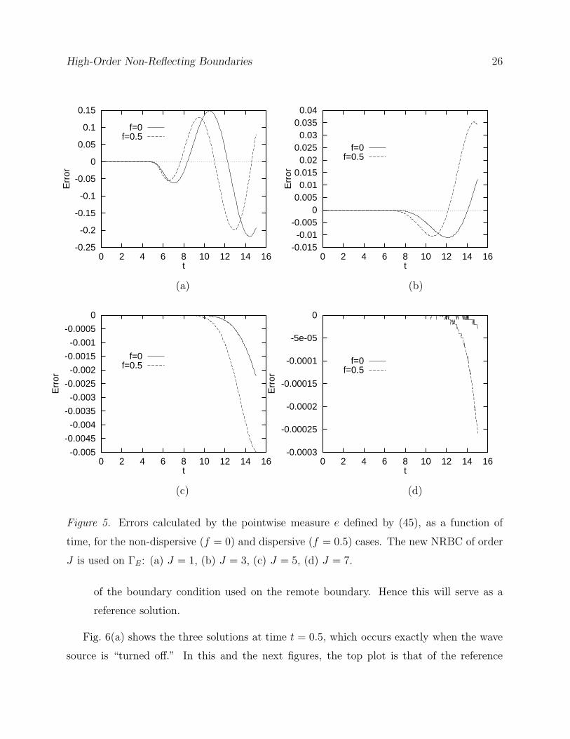
In Figs. 4 and 5 we compare the numerical errors for different orders J , calculated in the

first 600 time-steps. The figures show the global errors (Fig. 4) and pointwise errors (Fig.

5) as a function of time for the non-dispersive (f = 0) and dispersive (f = 0.5) cases. In

each case we show the error generated by the new NRBC of order J = 1, 3, 5 and 7. It is

apparent that the errors decrease as the order J increases. We also see that for J ≥ 2 the

error generated in the dispersive case is larger than that in the non-dispersive case. Note

that auxiliary variables appear in the formulation only for J ≥ 2, so the case J = 1 is special.

Now we consider the same wave guide as in the previous example, but with a different

loading. On the west boundary we replace (43) by the prescribed function

uW (y, t) =

cos[

π2rs

(y − ys)]

if |y − ys| ≤ rs & 0 < t ≤ ts

0 otherwise

(46)

Thus, the wave source on the west boundary is a cosine function in y with three parameters:

its center location ys, its width rs, and its time duration ts. We set ys = 1, rs = 1, and

ts = 0.5. We take f = 0.5 (the dispersive case). The computational parameters xE , ∆t and

the grid are the same as in the previous example. However, here we use the NRBC of order

J = 4 on ΓE, with the four Cj’s obtained automatically by employing the procedure outlined

in Section 5.2. These turn out to be Cj/C0 = 1, 3.7, 1 and 11.1.

We compare the solution obtained by the new scheme with two other solutions:

• A solution obtained in the same domain, but with the Higdon NRBC H1 on ΓE , using

C1 = 5, which in the middle of the range of the four Cj ’s mentioned above.

High-Order Non-Reflecting Boundaries 25

0

0.02

0.04

0.06

0.08

0.1

0.12

0.14

0.16

0 2 4 6 8 10 12 14 16

Err

or

t

f=0f=0.5

0

0.005

0.01

0.015

0.02

0.025

0 2 4 6 8 10 12 14 16

Err

or

t

f=0f=0.5

(a) (b)

0

0.0005

0.001

0.0015

0.002

0.0025

0.003

0.0035

0 2 4 6 8 10 12 14 16

Err

or

t

f=0f=0.5

0

2e-05

4e-05

6e-05

8e-05

0.0001

0.00012

0.00014

0.00016

0.00018

0.0002

0 2 4 6 8 10 12 14 16

Err

or

t

f=0f=0.5

(c) (d)

Figure 4. Errors calculated by the global measure E defined by (44), as a function of time,

for the non-dispersive (f = 0) and dispersive (f = 0.5) cases. The new NRBC of order J is

used on ΓE : (a) J = 1, (b) J = 3, (c) J = 5, (d) J = 7.

• A solution obtained in a domain twice as long, namely the domain 0 ≤ x ≤ 10,

0 ≤ y ≤ 5, using a 42 × 21 grid with the same resolution. During the simulation

time the wave generated on ΓW does not reach the remote (east) boundary of this

large domain, and thus the issue of spurious reflection is avoided altogether, regardless

High-Order Non-Reflecting Boundaries 26

-0.25

-0.2

-0.15

-0.1

-0.05

0

0.05

0.1

0.15

0 2 4 6 8 10 12 14 16

Err

or

t

f=0f=0.5

-0.015-0.01

-0.0050

0.0050.01

0.0150.02

0.0250.03

0.0350.04

0 2 4 6 8 10 12 14 16

Err

or

t

f=0f=0.5

(a) (b)

-0.005

-0.0045

-0.004

-0.0035

-0.003

-0.0025

-0.002

-0.0015

-0.001

-0.0005

0

0 2 4 6 8 10 12 14 16

Err

or

t

f=0f=0.5

-0.0003

-0.00025

-0.0002

-0.00015

-0.0001

-5e-05

0

0 2 4 6 8 10 12 14 16

Err

or

t

f=0f=0.5

(c) (d)

Figure 5. Errors calculated by the pointwise measure e defined by (45), as a function of

time, for the non-dispersive (f = 0) and dispersive (f = 0.5) cases. The new NRBC of order

J is used on ΓE : (a) J = 1, (b) J = 3, (c) J = 5, (d) J = 7.

of the boundary condition used on the remote boundary. Hence this will serve as a

reference solution.

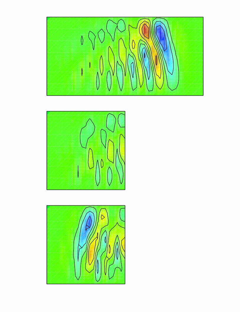
Fig. 6(a) shows the three solutions at time t = 0.5, which occurs exactly when the wave

source is “turned off.” In this and the next figures, the top plot is that of the reference

High-Order Non-Reflecting Boundaries 27

solution, the middle plot corresponds to the solution obtained by the new scheme with the

4th-order NRBC, and the lower plot describes the H1 solution. Both the colors and the

contour lines represent values of u. At time t = 0.5 all three solutions are identical, as

expected. The largest contour line shown represents a fast wave with a small amplitude

which is present due to the dispersion.

Fig. 6(b) corresponds to time t = 6. At this time the main bulk of the wave packet

generated on ΓW has just reached the boundary ΓE . The three plots are still similar, although

a slight spurious reflection near the boundary can be observed in the H1 solution.

Fig. 6(c) shows the three solutions at time t = 7.5. The main wave packet has already

passed the boundary ΓE. The 4th-order solution is almost indistinguishable from the refer-

ence solution, whereas in the H1 solution spurious reflection is evident. Figs. 6(d) and 6(e)

correspond to times t = 9.5 and t = 11, respectively. The reflected waves move backwards in

the H1 solution and pollute the entire computational domain. On the other hand, the 4th-

order solution exhibits, with a reasonable accuracy, the wave traces which are also present

in the reference solution.

7. Concluding Remarks

In this paper we have presented a new high-order sequence of NRBCs based on a reformula-

tion of the Higdon NRBCs, for time-dependent wave problems. The new NRBCs involve no

high derivatives, and are thus amenable for standard Finite Difference or Finite Element dis-

cretization. In this paper we considered the former; work on the latter is currently underway

and will be reported elsewhere.

The new NRBCs involve auxiliary variables defined on the artificial boundary B. On the

other hand, they do not involve high derivatives. This allows the easy use of a NRBC of

an arbitrarily high order. The scheme is coded once and for all for any order; the order of

the scheme is simply an input parameter. Moreover, we have shown that the sequence of

NRBCs is “converging” for a fixed B, namely that by increasing the order one can achieve

any desired level of accuracy. In addition, the computational effort associated with the new

boundary treatment increases only linearly with the order, as opposed to the exponential

High-Order Non-Reflecting Boundaries 28

growth in a previous scheme based on the original form of the Higdon NRBCs [45].

Due to the generality of the proposed NRBCs it is possible to use them for problems in

dispersive and stratified media. We have demonstrated the good performance of the scheme

for both non-dispersive and dispersive problems.

Related future work will include the adaptation of the proposed approach to more com-

plicated configurations, such as exterior problems with a rectangular artificial boundary B,

and three-dimensional problems. The new NRBCs will also be adapted to the case of curved

artificial boundaries by using variable transformation. In addition, the new NRBCs will be

applied to the Shallow Water Equations (SWEs). These serve as an important testbed for

more complicated models in meteorology [59].

Acknowledgments

This work was supported by the U.S. National Research Council (NRC), the Office of Naval

Research (ONR), and the Naval Postgraduate School (NPS).

References

[1] D. Givoli, Numerical Methods for Problems in Infinite Domains, Elsevier, Amsterdam,

1992.

[2] D. Givoli, “Non-Reflecting Boundary Conditions: A Review,” J. Comput. Phys., 94,

1–29, 1991.

[3] S.V. Tsynkov, “Numerical Solution of Problems on Unbounded Domains, A Review,”

Appl. Numer. Math., 27, 465–532, 1998.

[4] D. Givoli, “Exact Representations on Artificial Interfaces and Applications in Mechan-

ics,” Appl. Mech. Rev., 52, 333–349, 1999.

[5] T. Hagstrom, “Radiation Boundary Conditions for the Numerical Simulation of Waves,”

Acta Numerica, 8, 47–106, 1999.

High-Order Non-Reflecting Boundaries 29

[6] B. Engquist and A. Majda, “Radiation Boundary Conditions for Acoustic and Elastic

Calculations,” Comm. Pure Appl. Math., 32, 313–357, 1979.

[7] A. Bayliss and E. Turkel, “Radiation Boundary Conditions for Wave-Like Equations,”

Comm. Pure Appl. Math., 33, 707–725, 1980.

[8] J.B. Keller and D. Givoli, “Exact Non-Reflecting Boundary Conditions,” J. Comput.

Phys., 82, 172–192, 1989.

[9] D. Givoli and J.B. Keller, “Non-Reflecting Boundary Conditions for Elastic Waves,”

Wave Motion, 12, 261–279, 1990.

[10] V.S. Ryaben’kii and S.V. Tsynkov, “Artificial Boundary Conditions for the Numerical

Solution of External Viscous Flow Problems,” SIAM J. Numer. Anal., 32 1355–1389,

1995.

[11] S.V. Tsynkov, E. Turkel and S. Abarbanel, “External Flow Computations Using Global

Boundary Conditions,” AIAA J., 34, 700–706, 1996.

[12] J.P. Berenger, “A Perfectly Matched Layer for the Absorption of Electromagnetic

Waves,” J. Comput. Phys., 114, 185–200, 1994.

[13] F. Collino, “High Order Absorbing Boundary Conditions for Wave Propagation Models.

Straight Line Boundary and Corner Cases,” in Proc. 2nd Int. Conf. on Mathematical

& Numerical Aspects of Wave Propagation, R. Kleinman et al., Eds., SIAM, Delaware,

pp. 161-171, 1993.

[14] M.J. Grote and J.B. Keller, “Exact Nonreflecting Boundary Conditions for the Time

Dependent Wave Equation,” SIAM J. of Appl. Math., 55, 280–297, 1995.

[15] M.J. Grote and J.B. Keller, “Nonreflecting Boundary Conditions for Time Dependent

Scattering,” J. Comput. Phys., 127, 52–65, 1996.

[16] M.J. Grote and J.B. Keller, “Nonreflecting Boundary Conditions for Elastic Waves,”

SIAM J. Appl. Math., to appear.

High-Order Non-Reflecting Boundaries 30

[17] I.L. Sofronov, “Conditions for Complete Transparency on the Sphere for the Three-

Dimensional Wave Equation,” Russian Acad. Dci. Dokl. Math., 46, 397–401, 1993.

[18] T. Hagstrom and S.I. Hariharan, “Progressive Wave Expansions and Open Boundary

Problems,” in Computational Wave Propagation, B. Engquist and G.A. Kriegsmann,

Eds., IMA Volumes in Mathematics and Its Applications, Vol. 86, Springer, New York,

pp. 23–43, 1997.

[19] T. Hagstrom and S.I. Hariharan, “A Formulation of Asymptotic and Exact Boundary

Conditions Using Local Operators,” Appl. Numer. Math., 27, 403–416, 1998.

[20] M.N. Guddati and J.L. Tassoulas, “Continued-Fraction Absorbing Boundary Conditions

for the Wave Equation,” J. Comput. Acoust., 8, 139–156, 2000.

[21] D. Givoli, “High-Order Non-Reflecting Boundary Conditions Without High-Order

Derivatives,” J. Comput. Phys., 170, 849–870, 2001.

[22] D. Givoli and I. Patlashenko, “An Optimal High-Order Non-Reflecting Finite Element

Scheme for Wave Scattering Problems,” Int. J. Numer. Meth. Engng., 53, 2389–2411,

2002.

[23] E. Turkel and A. Yefet, “Absorbing PML Boundary Layers for Wave-Like Equations,”

Appl. Numer. Math., 27, 533–557, 1998.

[24] F. Collino and P. Monk, “The Perfectly Matched Layer in Curvilinear Coordinates,”

SIAM J. Sci. Comp., 19, 2061–2090, 1998.

[25] L. Ting and M.J. Miksis, “Exact Boundary Conditions for Scattering Problems,” J.

Acoust. Soc. Am., 80, 1825–1827, 1986.

[26] D. Givoli and D. Cohen, “Non-reflecting Boundary Conditions Based on Kirchhoff-type

Formulae,” J. of Comput. Phys., 117, 102–113. 1995.

[27] A.J. Safjan, “Highly Accurate Non-Reflecting Boundary Conditions for Finite Element

Simulations of Transient Acoustics Problems,” Comput. Meth. Appl. Mech. Engng.,

152, 175–193, 1998.

High-Order Non-Reflecting Boundaries 31

[28] D. Givoli, “A Spatially Exact Non-Reflecting Boundary Condition for Time Dependent

Problems,” Comput. Meth. Appl. Mech. Engng., 95, 97–113, 1992.

[29] I. Patlashenko, D. Givoli and P. Barbone, “Time-Stepping Schemes for Systems of

Volterra Integro-Differential Equations,” Comput. Meth. Appl. Mech. Engng., 190,

5691–5718, 2001.

[30] L.L. Thompson and P.M. Pinsky, “Space-Time Finite Element Method for Structural

Acoustics in Infinite Domains. Part 2: Exact Time-Dependent Non-Reflecting Boundary

Conditions,” Comput. Meth. Appl. Mech. Engng., 132, 229–258, 1996.

[31] B. Alpert, L. Greengard and T. Hagstrom, “Rapid Evaluation of Nonreflecting Bound-

ary Kernels for Time-Domain Wave Propagation,” SIAM J. Numer. Anal., 37, 1138–

1164, 2000.

[32] B. Alpert, L. Greengard and T. Hagstrom, “An Integral Evolution Formula for the Wave

Equation,” J. Comput. Phys., 162, 536–543, 2000.

[33] L.L. Thompson and R. Huan, “Finite Element Formulation of Exact Nonreflecting

Boundary Conditions for the Time-Dependent Wave Equation,” Int. J. Numer. Meth.

Engng., 45, 1607–1630, 1999.

[34] R. Huan and L.L. Thompson, “Accurate Radiation Boundary Conditions for the Time-

Dependent Wave Equation on Unbounded Domains,” Int. J. Numer. Meth. Engng., 47,

1569–1603, 2000.

[35] S. Krenk, “Unified Formulation of Radiation Conditions for the Wave Equation,” Int.

J. Numer. Meth. Engng., 53, 275–295, 2002.

[36] I.M. Navon, N. Neta and M.Y. Hussaini, “ A Perfectly Matched Layer Formulation

for the Nonlinear Shallow Water Equations Models: The Split Equation Approach,” to

appear.

[37] D. Givoli, “Recent Advances in the DtN Finite Element Method for Unbounded Do-

mains,” Archives of Comput. Meth. in Engng., 6, 71–116, 1999.

High-Order Non-Reflecting Boundaries 32

[38] J. Pedlosky, Geophysical Fluid Dynamics, Springer, New York, 1987.

[39] R.L. Higdon, “Radiation Boundary Conditions for Dispersive Waves,” SIAM J. Numer.

Anal., 31, 64–100, 1994.

[40] R.L. Higdon, “Absorbing Boundary Conditions for Difference Approximations to the

Multi-Dimensional Wave Equation, Math. Comput., 47, 437–459, 1986.

[41] R.L. Higdon, “Numerical Absorbing Boundary Conditions for the Wave Equation,”

Math. Comput., 49, 65–90, 1987.

[42] R.L. Higdon, “Radiation Boundary Conditions for Elastic Wave Propagation,” SIAM

J. Numer. Anal., 27, 831–870, 1990.

[43] R.L. Higdon, “Absorbing Boundary Conditions for Elastic Waves,” Geophysics, 56,

231–241, 1991.

[44] R.L. Higdon, “Absorbing Boundary Conditions for Acoustic and Elastic Waves in Strat-

ified Media,” J. Comput. Phys., 101, 386–418, 1992.

[45] D. Givoli and B. Neta, “High-Order Non-Reflecting Boundary Conditions for Dispersive

Waves,” Wave Motion, submitted.

[46] R.A. Pearson, “Consistent Boundary Conditions for the Numerical Models of Systems

That Admit Dispersive Waves,” J. Atmos. Sci., 31, 1418–1489, 1974.

[47] I. Orlanski, “A Simple Boundary Condition for Unbounded Hyperbolic Flows,” J.

Comp. Phys., 21, 251–269, 1976.

[48] W.H. Raymond and H.L. Kuo, “A Radiation Boundary Condition for Multi-Dimensional

Flows,” Q.J.R. Meteorol. Soc., 110, 535–551, 1984.

[49] M.J. Miller and A.J. Thorpe, “Radiation Conditions for the Lateral Boundaries of

Limited-Area Numerical Models,” Q.J.R. Meteorol. Soc., 107, 615–628, 1981.

[50] J.B. Klemp and D.K. Lilly, “Numerical Simulation of Hydrostatic Mountain Waves,” J.

Atmos. Sci., 35, 78–107, 1978.

High-Order Non-Reflecting Boundaries 33

[51] M. Wurtele, J. Paegle and A. Sielecki, “The Use of Open Boundary Conditions with

the Storm-Surge Equations,” Mon. Weather Rev., 99, 537–544, 1971.

[52] R.M. Hodur, “The Naval Research Laboratory’s Coupled Ocean/Atmosphere Mesoscale

Prediction System (COAMPS),” Mon. Wea. Rev., 125, 1414-1430, 1997.

[53] X. Ren, K.H. Wang and K.R. Jin, “Open Boundary Conditions for Obliquely Prop-

agating Nonlinear Shallow-Water Waves in a Wave Channel,” Comput. & Fluids, 26,

269–278, 1997.

[54] T.G. Jensen, “Open Boundary Conditions in Stratified Ocean Models,” J. Marine Sys-

tems, 16, 297–322, 1998.

[55] F.S.B.F. Oliveira, “Improvement on Open Boundaries on a Time Dependent Numerical

Model of Wave Propagation in the Nearshore Region,” Ocean Eng., 28, 95–115, 2000.

[56] J.C. Tannehill, D.A. Anderson and R.H. Pletcher, Computational Fluid Mechanics and

Heat Transfer, 2nd ed., Taylor & Francis, Washington DC, 1997.

[57] B.P. Sommeijer, P.J. van der Houwen and B. Neta, “Symmetric Linear Multistep Meth-

ods for Second Order Differential Equations with Periodic Solutions,” Applied Numerical

Mathematics, 2, 69–77, 1986.

[58] D. Givoli and B. Neta, “High-Order Higdon Non-Reflecting Boundary Conditions for

the Shallow Water Equations,” Rep. NPS-MA-02-001, Naval Postgraduate School, Mon-

terey, CA, 2002.

[59] D.R. Durran, Numerical Methods for Wave Equations in Geophysical Fluid Dynamics,

Springer, New York, 1999.

High-Order Non-Reflecting Boundaries 34

Captions for Figures

Fig. 1. Setup for the NRBC method: (a) an exterior scattering problem; (b) a semi-infinite

wave-guide problem.

Fig. 2. “Exact solution” for the wave-guide test problem, in the dispersive case (f = 0.5).

The solution is shown at the point P (5, 2.75).

Fig. 3. Errors as a function of time, for the dispersive case (f = 0.5), generated by the new

NRBC of order J = 3: (a) the global error E defined by (44); (b) the pointwise error

e defined by (45), at the point P (5, 2.75).

Fig. 4. Errors calculated by the global measure E defined by (44), as a function of time,

for the non-dispersive (f = 0) and dispersive (f = 0.5) cases. The new NRBC of order

J is used on ΓE: (a) J = 1, (b) J = 3, (c) J = 5, (d) J = 7.

Fig. 5. Errors calculated by the pointwise measure e defined by (45), as a function of time,

for the non-dispersive (f = 0) and dispersive (f = 0.5) cases. The new NRBC of order

J is used on ΓE: (a) J = 1, (b) J = 3, (c) J = 5, (d) J = 7.

Fig. 6. Solution of the cosine-source problem, dispersion parameter f = 0.5. Top plot —

reference solution in a long domain. Middle plot — solution obtained with the new

scheme, 4th-order NRBC. Lower plot — solution obtained with the Sommerfeld-like

NRBC H1. Solutions are shown at times: (a) t = 0.5, (b) t = 6, (c) t = 7.5, (d) t = 9.5,

(e) t = 11.