HIGH FIDELITY KINETIC MODEL FOR FLOTATION

Montana Tech LibraryDigital Commons @ Montana Tech

Graduate Theses & Non-Theses Student Scholarship

Spring 2018

HIGH FIDELITY KINETIC MODEL FORFLOTATION: APPLICATIONS TO RAREEARTH ELEMENTS AND COPPER/MOLYBDENUM SEPARATIONSRichard LaDouceurMontana Tech

Follow this and additional works at: https://digitalcommons.mtech.edu/grad_rsch

Part of the Materials Science and Engineering Commons

This Thesis is brought to you for free and open access by the Student Scholarship at Digital Commons @ Montana Tech. It has been accepted forinclusion in Graduate Theses & Non-Theses by an authorized administrator of Digital Commons @ Montana Tech. For more information, pleasecontact [email protected].

Recommended CitationLaDouceur, Richard, "HIGH FIDELITY KINETIC MODEL FOR FLOTATION: APPLICATIONS TO RARE EARTHELEMENTS AND COPPER/MOLYBDENUM SEPARATIONS" (2018). Graduate Theses & Non-Theses. 172.https://digitalcommons.mtech.edu/grad_rsch/172

https://digitalcommons.mtech.edu?utm_source=digitalcommons.mtech.edu%2Fgrad_rsch%2F172&utm_medium=PDF&utm_campaign=PDFCoverPages

https://digitalcommons.mtech.edu/grad_rsch?utm_source=digitalcommons.mtech.edu%2Fgrad_rsch%2F172&utm_medium=PDF&utm_campaign=PDFCoverPages

https://digitalcommons.mtech.edu/stdt_schr?utm_source=digitalcommons.mtech.edu%2Fgrad_rsch%2F172&utm_medium=PDF&utm_campaign=PDFCoverPages

https://digitalcommons.mtech.edu/grad_rsch?utm_source=digitalcommons.mtech.edu%2Fgrad_rsch%2F172&utm_medium=PDF&utm_campaign=PDFCoverPages

http://network.bepress.com/hgg/discipline/285?utm_source=digitalcommons.mtech.edu%2Fgrad_rsch%2F172&utm_medium=PDF&utm_campaign=PDFCoverPages

https://digitalcommons.mtech.edu/grad_rsch/172?utm_source=digitalcommons.mtech.edu%2Fgrad_rsch%2F172&utm_medium=PDF&utm_campaign=PDFCoverPages

mailto:[email protected]

HIGH FIDELITY KINETIC MODEL FOR FLOTATION: APPLICATIONS TO

RARE EARTH ELEMENTS AND COPPER/MOLYBDENUM

SEPARATIONS

by

Richard M. LaDouceur

A dissertation submitted in partial fulfillment of the

requirements for the degree of

Doctor of Philosophy:

Materials Science

Montana Tech

2018

i

HIGH FIDELITY KINETIC MODEL FOR FLOTATION: APPLICATIONS TO RARE EARTH ELEMENTS AND COPPER/MOLYBDENUM SEPARATIONS

By

RICHARD MICHAEL LADOUCEUR

B.S., Montana Tech of The University of Montana, Butte, MT, 2014

Dissertation presented in partial fulfillment of the requirements

for the degree of

Doctor of Philosophy in Materials Science

Montana Tech Butte, MT

2018

Approved by:

Beverly K.Hartline,Dean Montana Tech Graduate School

�� arbnentHead

gram Director , Montana Tech

.JaS*--,V...:��»:, Department Head p��;:eq·•ng, Montana Tech

--�� .......

Risser, Department Head Math, Montana Tech

�s:13--, Paul Gannon, Professor

Chemical Engineering, Montana State University

ii

© COPYRIGHT

by

Richard LaDouceur

2018

All Rights Reserved

iii

LaDouceur, Richard, Material Science Doctor of Philosophy, 2018

High-Fidelity Kinetic Model for Flotation: Applications to Rare Earth Element and Copper/Molybdenum Separations Chairperson or Co-Chairperson: Courtney A. Young

A high-fidelity kinetic model was developed to identify and elucidate the effects of varying principle froth flotation parameters on the sub-processes that occur within and between the flotation zones. Whereas traditional models fail to adequately address froth recovery and recovery by entrainment, the high-fidelity model defines these phenomena based on an improved understanding of the pulp/froth interface. Solution chemistry considerations that govern rare earth mineral separation by flotation were identified, characterized, and optimized. Application of novel surfactants such H205 and salicylhydroxamic acid (collectors) and dimethyl glycol monobutyl ether (depressant) was evaluated to define optimal flotation conditions. The effect of pressure on fine particle entrainment was also studied because, with certain rare earth mineral ores, sufficient mineral liberation is not achieved at nominal flotation particle sizes. Pressure can be applied to produce the small bubble sizes required for fine particle flotation. The correct solution chemistry for flotation (and not entrainment) can then be utilized for the selective recovery of rare earth minerals. The predictive high-fidelity kinetic model was developed using experimentally derived and statistically significant rate equations and was confirmed through application to copper/molybdenum sulfide and rare earth mineral ore samples. The parametric models identified ideal flotation conditions that optimized the recovery of rare earth minerals using the novel collectors; when the same experiments were modeled using the high-fidelity kinetic model, recovery by entrainment was found to be significant. The effects of pressure on gas dispersion mechanisms, such as gas holdup, and how those mechanisms effect bubble size and kinetic parameters were determined. Keywords: flotation, kinetic modeling, rare earths

iv

Dedication

To everyone that reads this and to my family who never will.

v

Acknowledgements

I would like to thank my family first and foremost. Without their inspiration, encouragement,

and support, the whole endeavor would have been impossible. I also need to thank my advisor

Dr. Courtney Young for giving me the opportunity and providing guidance, both technical and

for life. I also need to thank Dr. Jerry Downey for developing the MUS Materials Science

program and for serving on my committee. Dr. Jack Skinner, Dr. Hilary Risser, and Dr. Paul

Gannon deserve my gratitude also for serving on my Ph.D. committee and reviewing my

dissertation. And my unofficial sixth member of my committee, Peter Amelunxen of Aminpro

who without his expertise and near constant support I couldn’t have completed this work. Peter

provided the use of his model to begin and then trusted me to help develop the newest version

and I cannot thank him enough for everything.

I need to thank Ronda Coguill for giving me the initial invitation to come work for CAMP which

allowed me to first learn that I wanted to do research. I cannot thank Gary Wyss enough as he

has been invaluable in all aspects of my research, but especially understanding mineralogy and

mineral characterization. The undergraduate students that have worked for me also deserve my

thanks: Bryce Abstetar, Ethan Bailey, Jake Bentley, Katie Bozer, Molly Brockway, Steve

Broddy, Jared Clarke, Aimee Eubanks, John Hansen-Carlson, Mark Lavoie, Luke McCulloch,

Pat Rumley, and Jamie Young. I would especially like to thank two undergraduate students as

they have helped in most of my research and I am truly grateful for everything they have done,

Aleesha Aasved and Ben Suslavich.

The mechanical engineering senior design groups that I was lucky enough to advise also need

thanking. The first group consisting of Mike Kallas, Brady Sesselman, and Dylan Smith and the

second group of Lucas Reif, Kevin Tan, and Xiaotian Zhu completed excellent projects that

vi

aided me greatly. Several CAMP employees all deserve my thanks. Taylor Winsor, Cole

Carpenter, and Marshall Metcalf have assisted with the design and build of equipment needed for

the completion of my experiments and I could not have been successful without them.

Research was sponsored by the Army Research Laboratory and was accomplished under

Cooperative Agreement Number W911NF-15-2-0020. The views and conclusions contained in

this document are those of the authors and should not be interpreted as representing the official

policies, either expressed or implied, of the Army Research Laboratory or the U.S. Government.

The U.S. Government is authorized to reproduce and distribute reprints for Government purposes

notwithstanding any copyright notation herein. Research was also sponsored by Freeport-

McMoRan Inc. under a cooperative agreement between Montana Tech and Aminpro. I would

like to thank both funding agencies for their financial support.

vii

Table of Contents

DEDICATION ........................................................................................................................................... IV

ACKNOWLEDGEMENTS ............................................................................................................................ V

GLOSSARY OF TERMS ............................................................................................................................... X

LIST OF TABLES ..................................................................................................................................... XIV

LIST OF FIGURES .................................................................................................................................. XVIII

LIST OF EQUATIONS ........................................................................................................................... XXVII

1. INTRODUCTION ................................................................................................................................. 1

2. BACKGROUND ................................................................................................................................... 3

2.1. Kinetic Modeling ................................................................................................................ 3

Two-Compartment Kinetic Model ....................................................................................................... 5

Entrainment ........................................................................................................................................ 8

Bubble Surface Area Flux ................................................................................................................... 10

Bubble Particle Collision and Attachment ......................................................................................... 12

Froth Phase Recovery/Pulp-Froth Interface ...................................................................................... 14

Froth Selectivity ................................................................................................................................. 21

Drift Flux Analysis (DFA) .................................................................................................................... 24

2.2. Rare Earth Elements and Minerals ................................................................................... 26

2.3. Collectors .......................................................................................................................... 32

SHA .................................................................................................................................................... 32

H205 .................................................................................................................................................. 35

Other Novel Collectors ...................................................................................................................... 38

2.4. Depressants ...................................................................................................................... 40

2.5. Pressure and Fine Particle Flotation ................................................................................. 42

Electrical Resistance Tomography ..................................................................................................... 45

viii

3. KINETIC MODELING .......................................................................................................................... 47

3.1. Methods ........................................................................................................................... 47

Froth Recovery .................................................................................................................................. 47

Derivation of Entrainment, ENTi ........................................................................................................ 48

3.2. Results and Discussions .................................................................................................... 52

4. SYNTHESIS OF H205 ........................................................................................................................ 61

4.1. Methods ........................................................................................................................... 61


Notes on the Synthesis of H205 ........................................................................................................ 63

Comparison of H205 and SHA Spectra .............................................................................................. 63

Determination of Actives Sites on the Collector ............................................................................... 64

5. RARE EARTH FLOTATION – NOVEL COLLECTORS AND DEPRESSANTS ........................................................... 70

5.1. Methods ........................................................................................................................... 70

Rare Earth Flotation with SHA ........................................................................................................... 72

Rare Earth Flotation with Novel Collectors ....................................................................................... 73

Rare Earth Flotation with Depressants and SHA ............................................................................... 74


Rare Earth Flotation with SHA ........................................................................................................... 75

Rare Earth Flotation with Novel Collectors ....................................................................................... 84

Flotation Experiment Analysis ................................................................................................... 90

Discussion of Results ............................................................................................................... 113

Rare Earth Flotation with Depressants and SHA ............................................................................. 117

6. PRESSURE FLOTATION ..................................................................................................................... 128

6.1. Methods ......................................................................................................................... 128

Environmental Chamber for Rare Earth Flotation ........................................................................... 128

Environmental Chamber Design.............................................................................................. 128

Environmental Chamber Build ................................................................................................ 137

Auto Collection System Design ........................................................................................................ 141

ix

Electrical Resistance Tomography ................................................................................................... 146

6.2. Results and Discussions .................................................................................................. 148

7. CONCLUSIONS ............................................................................................................................... 158

7.1. Kinetic Modeling ............................................................................................................ 158

7.2. Rare Earth Collectors ...................................................................................................... 158

7.3. Pressure Flotation .......................................................................................................... 160

7.4. Future Work ................................................................................................................... 161

8 REFERENCES ...................................................................................................................................... 162

APPENDIX A: RARE EARTH COLLECTORS .................................................................................................... 179

APPENDIX B: RAW DATA ........................................................................................................................ 195

x

Glossary of Terms

AASAS alkyl aryl sulfonic acid salt (Nalco CoTILPS 712) ABS acrylonitrile butadiene styrene Ac cross-sectional area of cell Ai cross-sectional area of interface ANOVA analysis of variance using partial sum of squares AOX alternative oxidase enzyme CMC carboxymethyl cellulose d32 Sauter mean bubble size diameter DAQ data acquistion device DAS Data Acquistion System db bubble diameter DCM dichloromethane DFA drift flux analysis DGME diethylene glycol monobutyl ether DMSO dimethyl sulfoxide dp particle diameter Eb buoyancy efficiency Ec bubble-particle collision efficiency EDAX Electron Dispersive X-ray Analysis Ei inertia efficiency ENT degree of entrainment ERT Electrical Resistance Tomography Es interception mechanism efficiency ESR Electron Spin Resonance spectroscopy f(db) size distribution function of the bubbles FA fatty acid FAM fatty acid mixture (Nalco FA-2749 FCAW flux core arc welding FEA finite element analysis FKT full kinetics test FRT froth retention time FT-IR Fourier transform - infrared spectroscopy g acceleration due to gravity GMAW gas metal arc welding GTAW gas tungsten arc welding H flotation cell's hydrodynamics h flotation cell height HA hydroxamic acid or hydroxamate HREE heavy rare earth elements

xi

i size class Ib interfacial area of bubbles ITS Industrial Tomography Systems j component Jg superficial gas velocity Jl superficial liquid velocity k flotation rate constant LREE light rare earth elements m mass fraction of particles1 m Reynold's number flotation parameter2 MIBC methyl isobutyl carbinol MLA Mineral Liberation Analysis n Reynold's number adjustable flotation parameter3 n number of moles4 n total number of bubbles per unit volume5 Np number of floatable particles O flotation cell's operating conditions P pressure6 P floatability factor7 Pa probability of attachment Pc probability of collision Pd probability of detachment Pi probability of capture of particle class i PVC polyvinyl chloride Q volumetric gas flow rate 𝑄𝑄𝑐𝑐𝑤𝑤 water flux into the froth zone

𝑄𝑄𝑡𝑡𝑤𝑤 net volumetric flow rate of water

Qw water flux R universal gas constant R∞ maximum recovery

1 Equation 5 2 Equation 30 3 Equation 34 4 Equation 35 5 Equation 19 6 Equation 35 7 Equation 15

xii

Rc collection zone recovery 𝑅𝑅𝑐𝑐𝑤𝑤 collection zone recovery of water

REC rare earth element bearing carbonates REE rare earth element REH rare earth element bearing halides REM rare earth mineral REO rare earth element bearing oxides REP rare earth element bearing phosphates RER Rare Element Resources Res Reynold's number in a swarm RES rare earth element bearing silicates Rf froth zone recovery 𝑅𝑅𝑓𝑓𝑤𝑤 froth zone recovery of water

RMSE root mean square estimation or error Rpfi pulp/froth interface recovery Rs recovery of entrained particles to the concentrate Rw recovery of water to the concentrate Sb bubble surface area flux SDS sodium dodecyl sulfate SEM Scanning Electron Microscope SHA salicylhydroxamic acid SKT simple kinetics test SMAW shielded metal arc welding SSE residual sum of squares St Stokes number Stb bubble Stokes number T temperature U hindered settling velocity Ub velocity of bubble Up velocity of particle Usb slip velocity between bubbles and liquid Ut terminal rise velocity for a single bubble V volumetric gas flow rate Vc flotation cell volume vw net rise velocity of water XPS x-ray photoelectron spectroscopy

β rate of detachment of attached particles in the froth phase

εg fractional gas holdup

µf viscosity of fluid

xiii

ηl viscosity of liquid

ρf density of fluid

ρl density of liquid

ρp density of a particle

ρs density of the pulp

σl liquid phase conductivity

σm mean-mixture conductivity

τ mean residence time in the flotation cell φ fractional solids concentration ω rate of drainage of detached particles

xiv

List of Tables

Table I: Rare earth element requirements by application [1]. ..........................................26

Table II: REE bearing carbonate (REC) minerals. Adapted from [1] .............................29

Table III: REE bearing halide (REH) minerals. Adapted from [1]..................................29

Table IV: REE bearing oxide (REO) minerals. Adapted from [1] ..................................29

Table V: REE bearing phosphate (REP) minerals. Adapted from [1] .............................30

Table VI: REE bearing silicate (RES) minerals. Adapted from [1] ................................31

Table VII: Froth Recovery of Water .................................................................................52

Table VIII: Rise velocity of water for experimental collection times. .............................53

Table IX: Hindered Settling Velocity ...............................................................................54

Table X: Degree of Entrainment for gangue minerals for the experimental collection times

................................................................................................................................55

Table XI: Calculated Maximum Recovery and Flotation Rate Constant as a function of scraping

frequency, (Rf = 1 and Re = 0) ...............................................................................57

Table XII: Calculated Maximum Recovery and Flotation Rate Constant as a function of scraping

frequency with constant water recovery calculated at t=0, using new models for Rf and Re

................................................................................................................................57

Table XIII: Experimental FT_IR data of characteristic peaks of the collectors and their

complexes ..............................................................................................................66

Table XIV: Electrostatic potential values of the hydroxamic group elements in various levels of

deprotonation and tautomer forms based on Spartan molecular modeling calculations

................................................................................................................................68

xv

Table XV: Parametric design of experiments for flotation of rare earth minerals using SHA

................................................................................................................................73

Table XVI: Parametric design of experiments for flotation of rare earth minerals using novel

collectors ................................................................................................................74

Table XVII: Parametric design of experiments for flotation of rare earth minerals using

depressants .............................................................................................................75

Table XVIII: Select Flotation Experiment Feed Sample of Minerals of Interest (19 minute

milling time)...........................................................................................................77

Table XIX: Select Flotation Experiment Concentrate Sample of Minerals of Interest (19 minute

milling time)...........................................................................................................78

Table XX: Flotation Experiment SKT Rare Earth Mineral Concentrate Grade by Weight Percent

................................................................................................................................80

Table XXI: Point Prediction for Flotation of Rare Earth Minerals with Salicylhydroxamic Acid

with Design Variables at Upper Limits of the Design Space ................................83

Table XXII: Maximum Recovery Comparison between Parametric Experimental Design Model

and Two-Stage Compartmental Kinetics Model....................................................83

Table XXIII: Validation Assay of MLA Results as conducted by Hazen Research ........84

Table XXIV: Select Flotation Experiment Feed Sample of Minerals of Interest for Novel

Collectors Design of Experiments .........................................................................86

Table XXV: Select Flotation Experiment Concentrate Sample of Minerals of Interest for

Sarkosyl..................................................................................................................86

Table XXVI: Select Flotation Experiment Concentrate Sample of Minerals of Interest for

AASAS ..................................................................................................................87

xvi

Table XXVII: Select Flotation Experiment Concentrate Sample of Minerals of Interest for FAM

................................................................................................................................87

Table XXVIII: Select Flotation Experiment Concentrate Sample of Minerals of Interest for

H205 .......................................................................................................................87

Table XXIX: Design of Experiments Results for Novel Collector Rare Earth Mineral Flotation

................................................................................................................................89

Table XXX: Froth Recovery of Water for SKT (left: low pH, low dosage, FAM; right: high pH,

low dosage, FAM). Blue values are the true water flux values at time = 0 sec. ...92

Table XXXI: Recovery by Entrainment and Flotation per SKT Collection Stage (low pH, high

dosage, FAM) ........................................................................................................93

Table XXXII: Flotation First-order Rate Constant for SKT Experiments of Novel Collectors

using Kinetic Modeling..........................................................................................94

Table XXXIII: Modeled Maximum Recovery for SKT Experiments of Novel Collectors using

Kinetic Modeling ...................................................................................................95

Table XXXIV: ANOVA for Linear model of Rare Earth Recovery ................................99

Table XXXV: Constraints for Numerical Optimization for Recovery of Rare Earth Minerals by

Flotation ...............................................................................................................113

Table XXXVI: Numerical Optimization Constraints for Flotation Kinetics. .................115

Table XXXVII: Numerical Optimization for Parisite (Rare Earth Carbonate) Recovery and

Grade ....................................................................................................................116

Table XXXVIII: Select Flotation Experiment Feed Sample of Minerals of Interest for

Depressants Design of Experiments ....................................................................118

xvii

Table XXXIX: Select Flotation Experiment Concentrate Sample of Minerals of Interest for T10

..............................................................................................................................118

Table XL: Select Flotation Experiment Concentrate Sample of Minerals of Interest for T12

..............................................................................................................................119

Table XLI: Select Flotation Experiment Concentrate Sample of Minerals of Interest for K55

..............................................................................................................................119

Table XLII: Recovery of rare earth and gangue minerals using depressants .................121

Table XLIII: Increase in Grade for rare earth and gangue minerals using depressants ..121

Table XLIV: Flotation First-order Rate Constant for rare earth flotation using depressants.

..............................................................................................................................122

Table XLV: Altitude above sea level and air pressure ...................................................128

Table XLVI: Historical SKT experimental data .............................................................143

Table XLVII: Bubble Diameter, as calculated by Drift Flux Analysis, vs. Pressure for the four

flotation zones ......................................................................................................152

Table XLVIII: Goodness of fit for curve fitting of mean gas holdup and bubble surface flux for

flotation compartments ........................................................................................157

xviii

List of Figures

Figure 1: Schematic of the Flotation Process. The schematic shows the difference in the

collection zone and froth zone in a flotation cell .....................................................2

Figure 2: Process flow schematic for flotation showing typical phenomena. Schematic shows

the two methods for particles to report to the froth, collection and entrainment. ....4

Figure 3: Schematic diagram of the two-compartmental model [11]. The two-compartmental

model is a mass balance for the entire flotation process, a mass balance for the froth zone,

and a mass balance for the collection zone. .............................................................6

Figure 4: Schematic representation of the two-compartmental model, including water vectors

[16]. An overall mass balance is performed for the water portion. ........................9

Figure 5: Mechanisms for Particle Detachment [2]. The force of impact mechanism is dominant

in the froth phase. ...................................................................................................15

Figure 6: Froth recovery fitted to average rate constants calculated for 1 second scraping

frequency [3]. Froth recovery decreases as the scraping frequency increases. ....17

Figure 7: Froth recovery of chalcopyrite determined using two different measurement

techniques: CFD - changing froth depths and BLM - bubble load measurement, for two

different ore types in the Outokumpu 3 m3 flotation cell. (a) copper/lead/zinc rich ore

and (b) copper rich ore [25] ...................................................................................18

Figure 8: Pulp-froth interface recovery per mineral for the two different feed ore types. (a)

copper/lead/zinc ore and (b) copper rich ore [25] ..................................................19

xix

Figure 9: Schematic of the Pulp-Froth Interface Compartmental Model [25]. The pulp/froth

interface in the compartmental model includes drainage of particles from the froth.

................................................................................................................................19

Figure 10: Three zone model of a flotation cell showing the flow of attached and previously

attached material ....................................................................................................20

Figure 11: Cell by cell solids carry rate and copper and molybdenum production rate for a

cleaner/cleaner-scavenger bank [16] ......................................................................21

Figure 12: Effect of pressure on flotation recovery with airflow control at elevations of 3350 m

(11000 ft), 1735 m (5700 ft), and -760 m (-2500 ft) as well as in a glove box at simulated

elevations of 9144 m (30000 ft), 1735 m (5700 ft), and -610 m ( -2000 ft) [26]. The

trendline shows decreasing copper recovery as pressure is increased. ..................23

Figure 13: Effect of froth depth on relative cumulative grade and recovery [28] ............23

Figure 14: Lanthanide Contraction of Rare Earth Elements showing the decrease in ionic radii of

+3 cations as atomic number increases [1] ............................................................27

Figure 15: Crustal abundance of lanthanide elements [1] ................................................28

Figure 16: Ball and Stick Model for Salicylhydroxamic Acid (Black – Carbon, White –

Hydrogen, Red- Oxygen, Blue-Nitrogen) ..............................................................33

Figure 17: Equilibrium concentration of SHA in Ce Oxide (left) and Ce Carbonate (right) at 20

°C [57]. The concentration of SHA in Ce Oxide almost completely disappears from

solution at all pH values where for SHA in Ce Carbonate has very small changes in

concentration. .........................................................................................................34

Figure 18: Equilibrium concentration of SHA in Tb Oxide (left) and Tb Carbonate (right at 20

°C [57]. The concentration of SHA in Tb Carbonate almost completely disappears from

xx

solution at all pH values where for SHA in Ce Oxide has very small changes in

concentration. .........................................................................................................34

Figure 19: Ball and Stick Model for H205 (N,3-dihyroxynapthalene-2-caroxamide, Black –

Carbon, White – Hydrogen, Red- Oxygen, Blue-Nitrogen) ..................................35

Figure 20: Conformations and tautomers of hydroxamic acid .........................................37

Figure 21: 2D structure for sodium oleate (C18 fatty acid) [83] ......................................38

Figure 22: Ball and Stick Model for Sarkosyl (Sodium n-Lauroyl Sacrosine, Black – Carbon,

White – Hydrogen, Red- Oxygen, Blue-Nitrogen) ................................................39

Figure 23: Molecular structure of alkyl aryl sulfonate (left) and alkyl benzene sulfonate (right)

[92] .........................................................................................................................40

Figure 30: Concentration of small (10 µm) gangue particles in the plateau borders (kg/m3) with

froth height. At a given froth height, the concentration increases as the air rate increases.

(Lines are at progressively increasing air rates from left to right). Adapted from [121]

................................................................................................................................50

Figure 31: Water flux for simple kinetics test (SKT) .......................................................52

Figure 32: Normal distribution for the rise velocity of water for the experimental collection

times. ......................................................................................................................54

Figure 33: Degree of Entrainment as a function of particle size for the experimental collection

times .......................................................................................................................56

Figure 34: Rare Earth Mineral Recovery Model Reconciliation ......................................58

Figure 35: Rare Earth Mineral Grade Model Reconciliation............................................59

Figure 36: Flotation Kinetics for Rare Earth Minerals .....................................................60

xxi

Figure 24: Model of H205 (Top Left), Model of SHA (Top Right), FT-IR spectra of synthesized

H205 (Bottom Left), SHA (99%) (Bottom Right) .................................................64

Figure 25: A comparison of H205 Cu(II) complex (Top) with H205 (Bottom) FT-IR Spectrum

................................................................................................................................65

Figure 26: A comparison of SHA Cu(II) complex (Top) with SHA (Bottom) FT-IR Spectrum

................................................................................................................................66

Figure 27: The tautomerization of H205 (most electronegative atoms in red) .................67

Figure 28: H205 enol E tri-anion electrostatic potential map ...........................................68

Figure 29: SHA enol E tri-anion electrostatic potential map ............................................69

Figure 37: FLSmidth Flotation Cell ..................................................................................71

Figure 38: Zeta Potential vs. pH for Cerium (IV) Oxide with Salicylhydroxamic Acid. The plot

was generated using the Malvern Zetasizer and the line is for visual purposes only and is

not a trendline ........................................................................................................76

Figure 39: Particle Size Distribution for Flotation Experiment Rare Earth Concentrate Sample

(19 minute milling time) ........................................................................................79

Figure 40: 3D Surface Model Graph for the Recovery by Flotation of REMs by SHA...81

Figure 41: 3D Surface Model Graph for the Recovery by Flotation of Neodymium Parisite by

Salicylhydroxamic Acid.........................................................................................82

Figure 42: Zeta potential vs. pH for CoTILPS 712 on La2O3. The line is for visual purposes

only, it is not a trendline ........................................................................................85

Figure 43: Particle Size Distribution for Select Novel Collector Flotation Experiment Rare Earth

Concentrate Sample ...............................................................................................88

Figure 44: Kinetic Model Reconciliation - Recovery (low pH, low dosage, FAM) ........90

xxii

Figure 45: Kinetic Model Reconciliation - Grade (low pH, low dosage, FAM) ..............91

Figure 46: Degree of Entrainment for SKT Concentrate Collection Times as a Function of

Particle Size (left: low pH, low dosage, FAM; right: high pH, low dosage, FAM)92

Figure 47: Distribution of Rise Velocity based on Velocity of Water into Froth (left: low pH,

low dosage, FAM; right: high pH, low dosage, FAM) ..........................................93

Figure 48: Predicted Recovery of Rare Earth Minerals using Flotation Kinetic Modeling (low

pH, low dosage, FAM)...........................................................................................96

Figure 49: Predicted Recovery of Rare Earth Minerals using Flotation Kinetic Modeling (low

pH, high dosage, FAM) .........................................................................................97

Figure 50: Cook’s Distance for ANOVA of Rare Earth Recovery by Flotation ............100

Figure 51: Leverage for ANOVA of Rare Earth Recovery by Flotation ........................101

Figure 52: 3D Response Surface for Rare Earth Recovery by Flotation with Novel Collector

(FAM) ..................................................................................................................102

Figure 53: One Factor Analysis for Rare Earth Recovery (top left: low pH, low collector dosage;

top right: high pH, low collector dosage; bottom left: low pH, high collector dosage;

bottom right: high pH, high collector dosage) .....................................................103

Figure 54: Cook’s Distance for ANOVA of Monazite Recovery by Flotation ..............105

Figure 55: Leverage for ANOVA of Monazite Recovery by Flotation ..........................106

Figure 56: 3D Response Surface for Monazite Recovery by Flotation with Novel Collector

(Sarkosyl) .............................................................................................................107

Figure 57: 3D Response Surface for Monazite Recovery by Flotation with Novel Collector

(FAM) ..................................................................................................................107

xxiii

Figure 58: Interaction between Factors for Monazite Recovery by Novel Collectors (top left:

Sarkosyl; top right: FAM; bottom left: AASAS; bottom right: H205 .................109

Figure 59: Cook’s Distance for ANOVA of Calcite Recovery by Flotation ..................110

Figure 60: Leverage for ANOVA of Calcite Recovery by Flotation ..............................111

Figure 61: 3D Response Surface for Calcite Recovery by Flotation with Novel Collector (H205)

..............................................................................................................................112

Figure 62: 3D Response Surface for Calcite Recovery by Flotation with Novel Collector (FAM)

..............................................................................................................................112

Figure 63: Ramps for Numerical Optimization of Rare Earth Mineral Recovery. Ramps

describe the conditions and expected results to produce optimum values based upon

defined constraints. ..............................................................................................114

Figure 64: Ramps for Numerical Optimization of Monazite and Parisite First-order Rate

Constant. Ramps describe the conditions and expected results to produce optimum

values based upon defined constraints. ................................................................115

Figure 65: Ramps for Numerical Optimization of Parisite Recovery and Upgrading. Ramps

describe the conditions and expected results to produce optimum values based upon

defined constraints. ..............................................................................................117

Figure 66: Particle Size Distribution for Select Flotation Experiment with Depressant Rare Earth

Concentrate Sample .............................................................................................120

Figure 67: Cook’s Distance for Monazite Recovery using Depressants which identifies

experiment 7 as an outlier to the data ..................................................................123

xxiv

Figure 68: Predicted monazite recovery using novel depressants as determined by ANOVA (left:

minimum collector dosage, right: maximum collector dosage). The error bars identify

95% confidence interval. .....................................................................................124

Figure 69: Numerical Optimization ramps for maximized rare earth carbonate and phosphate

flotation and minimized gangue mineral flotation ...............................................125

Figure 70: Numerical Optimization ramp for maximized flotation rate constant of monazite and

minimized flotation rate constant of biotite and calcite .......................................126

Figure 71: Finite Element Analysis for the Design of the Environmental Chamber for Rare Earth

Mineral Flotation (Solidworks Simulation). Model was fixed on all outside faces and

load was applied iso-statically from inside the chamber. ....................................130

Figure 72: Updated Solidworks model for environmental chamber design ...................131

Figure 73: Outer door flange Solidworks model and measurements (in inches) ............132

Figure 74: Polycarbonate window Solidworks model and measurements (in inches) ...132

Figure 75: Baseplate Solidworks model and measurements (in inches) .........................132

Figure 76: Cross-sectional view of door and window for the environmental chamber ..133

Figure 77: Environmental chamber glove port spacing ..................................................134

Figure 78: Venturi Principles of Operation [131] ...........................................................135

Figure 79: Alicat Scientific Pressure Controller and operating schematic [132] ...........136

Figure 80: Environmental chamber air manifold process flow diagram. Regulated valves are

shown as valves with gauges, while unregulated valves are shown with handles.137

Figure 81: Environmental chamber final manifold build including electrical and data

feedthroughs .........................................................................................................139

Figure 82: Rare Earth Mineral Flotation Environmental Chamber ................................140

xxv

Figure 83: Sealable Plug for Environmental Chamber Glove Port.................................140

Figure 84: 3D Solidworks models of auto-scraper design for the flotation environmental

chamber ................................................................................................................141

Figure 85: Initial Auto-Scraper Stopper Design as modelled in Solidworks .................142

Figure 86: Initial Carousel Design as modelled in Solidworks ......................................144

Figure 87: Visual representation of carousel design and flotation cell within the environmental

chamber ................................................................................................................144

Figure 90: Auto-collection system bucket filling trough ................................................145

Figure 91: Braking system for auto-scraper....................................................................146

Figure 92: Final build Auto-collection system ...............................................................146

Figure 93: 3D Drawing of the ERT 6L cylindrical cell (top left), schematic of ERT 6L

cylindrical cell (top right), ERT electrodes on interior of FL Smidth laboratory flotation

cell (bottom left), ERT 6L cylindrical cell inside of the Montana Tech environmental

flotation chamber .................................................................................................148

Figure 94: Electrical Resistance Tomograms of Copper/Moly Concentrate at 16 psia. Froth

Zone (top left) Pulp/Froth Interface (top right) Dynamic Collection Zone (bottom left)

Turbulent Collection Zone (bottom right) ...........................................................150

Figure 95: Electrical Resistance Tomograms of Copper/Moly Concentrate at 16 psia. Froth

Zone (top left) Pulp/Froth Interface (top right) Dynamic Collection Zone (bottom left)

Turbulent Collection Zone (bottom right) ...........................................................151

Figure 96: Mean gas holdup vs. pressure as measured by ERT for a copper/moly concentrate

..............................................................................................................................152

xxvi

Figure 97: Bubble Surface Area Flux as a function of absolute pressure trends for all flotation

compartmental zones. ..........................................................................................153

Figure 98: Froth depth versus pressure for a copper/molybdenum concentrate .............155

Figure 99: MatLAB curve fitting for the turbulent compartmental zone (left: mean gas holdup,

right: bubble surface flux) ....................................................................................156

Figure 100: MatLAB curve fitting for the dynamic compartmental zone (left: mean gas holdup,


Figure 101: MatLAB curve fitting for the froth compartmental zone (left: mean gas holdup,


xxvii

List of Equations

(1) ..................................................................................................................................4

(2) ..................................................................................................................................5

(3) ..................................................................................................................................5

(4) ..................................................................................................................................5

(5) ..................................................................................................................................6

(6) ..................................................................................................................................6

(7) ..................................................................................................................................7

(8) ..................................................................................................................................7

(9) ..................................................................................................................................7

(10) ..................................................................................................................................8

(11) ..................................................................................................................................8

(12) ..................................................................................................................................9

(13) ................................................................................................................................10

(14) ................................................................................................................................10

(15) ................................................................................................................................10

(16) ................................................................................................................................11

(17) ................................................................................................................................11

(18) ................................................................................................................................11

(19) ................................................................................................................................12

(20) ................................................................................................................................12

(21) ................................................................................................................................13

(22) ................................................................................................................................13

xxviii

(23) ................................................................................................................................13

(24) ................................................................................................................................13

(25) ................................................................................................................................13

(26) ................................................................................................................................16

(27) ................................................................................................................................20

(28) ................................................................................................................................21

(29) ................................................................................................................................24

(30) ................................................................................................................................24

(31) ................................................................................................................................25

(32) ................................................................................................................................25

(33) ................................................................................................................................25

(34) ................................................................................................................................25

(35) ................................................................................................................................42

(36) ................................................................................................................................42

(37) ................................................................................................................................43

(38) ................................................................................................................................45

(39) ................................................................................................................................47

(40) ................................................................................................................................48

(41) ................................................................................................................................48

(42) ................................................................................................................................50

(43) ................................................................................................................................50

(44) ................................................................................................................................50

(45) ................................................................................................................................51

xxix

(46) ................................................................................................................................51

(47) ................................................................................................................................98

(48) ................................................................................................................................99

(49) ................................................................................................................................99

(50) ................................................................................................................................99

(51) ................................................................................................................................99

(52) ..............................................................................................................................105

(53) ..............................................................................................................................105

(54) ..............................................................................................................................105

(55) ..............................................................................................................................105

(56) ..............................................................................................................................129

(57) ..............................................................................................................................129

(58) ..............................................................................................................................156

(59) ..............................................................................................................................156

(60) ..............................................................................................................................156

(61) ..............................................................................................................................157

(62) ..............................................................................................................................157

(63) ..............................................................................................................................157

1

1. Introduction

Significant scientific challenges have hindered rare earth mineral separation [1]. To

address these challenges a high-fidelity flotation kinetic model was developed for copper-

molybdenum separation and validated using rare earth minerals. The kinetic model elucidated

flotation parameters throughout the volume of a laboratory flotation cell. Solution chemistry was

studied, and optimal conditions were determined for the efficient separation of rare earth

minerals by flotation. Bubble size and velocity can be controlled using pressure and its effect on

the separation of minerals was determined.

Rare earth minerals (REM) contain several lanthanide series elements which make cost-

effective mineral separation difficult. The molecular similarity of rare earth elements (REE)

results in minerals containing several or most REEs, such as bastnaesite [(Ce,La)CO3F], with

lanthanum and cerium usually represented in greater quantities than the other REEs. This

prevents efficient separation during concentration steps, for instance flotation, and has a direct

impact on successive metallurgical processes. Consequently, concentration during flotation is of

REMs as opposed to REEs.

Flotation is a beneficiation process that concentrates valuable minerals by physically

segregating and removing finely divided mineral particles contained in a slurry medium [2].

Flotation exploits differences in surface properties such as interfacial tension and surface charge.

Interfacial tension affects the wettability or hydrophobicity and surface charge determines

particle-chemical and particle-particle interactions. The hydrophobicity and surface charge can

be modified using surfactants known as collectors. To maximize recovery of REMs by flotation,

a kinetic model of the various collector-mineral systems was developed. A schematic of the

flotation process is shown in Figure 1.

2

Figure 1: Schematic of the Flotation Process. The schematic shows the difference in the collection zone and

froth zone in a flotation cell

REM flotation is difficult in industry due to the low degree of mineral liberation at

typical floatable particle sizes and their complex mineralogy. A high-fidelity flotation model for

their flotation is needed to address these problems. A selective collector and correct solution

chemistry, such as pH, are needed for efficient flotation. In addition, energy input conditions,

such as air input rate and impeller rotor speed, need to be elucidated to determine the kinetic

conditions inside of the flotation cell. Kinetic parameters, such as bubble surface area flux and

recovery by entrainment, have a fundamental role in mineral flotation and techniques and

empirical methods are needed to determine these parameters. To prevent entrainment of gangue

minerals in the rising water inside the flotation cell, the effect of pressure on bubble size and

velocity was studied.

3

2. Background

2.1. Kinetic Modeling

Empirical methods, such as the time multiplier method, are generally used to resolve the

differences in the residence time between laboratory testing and plant retention time to determine

plant recovery of floatable minerals. These empirical methods rely on experience as opposed to

a standard method for calculating the residence time requirements for the flotation cells in an

industrial plant from laboratory flotation kinetics tests. However, first-order kinetic models that

are analogous to chemical reaction kinetics are the most common model used to attempt to

determine this residence time. In addition, laboratory flotation experimentation is only valid if

the results can be used to successfully aid in the mineral processing industry. To be valid, the

laboratory results must be scalable into a full plant operation [3]. The hydrodynamic parameters

of the flotation cell (bubble generation, gas flow rate, and turbulence) [4], the chemical

parameters of the mineral complexation system (mineral dissolution, type and dosage of

reagents, and surface chemistry of the minerals) [5], and the mechanical aspects of the minerals

and flotation cell (particle size, particle-bubble interactions, and froth drainage) all affect the

dynamic response or the kinetics associated with the flotation process [6] [7]. Development of a

fundamental understanding of these phenomena is required. A process flow schematic for

flotation is shown in Figure 2.

4

Figure 2: Process flow schematic for flotation showing typical phenomena. Schematic shows the two

methods for particles to report to the froth, collection and entrainment.

Flotation can be described in three basic steps: (a) collision of a solid particle with a

bubble, (b) attachment of a particle to a bubble, and (c) detachment of a particle from a bubble.

Most flotation rate constant models can be described using Equation (1) [8]:

𝑘𝑘𝑖𝑖 = 𝑓𝑓(𝐻𝐻,𝑂𝑂,𝑃𝑃𝑖𝑖) (1)

where, ki is the flotation rate constant of particle class i, H is an expression for the flotation cell’s

hydrodynamics, O are the operating conditions, and Pi is the probability of capture of particle

BubblesPulp

Froth

Interface

solids water,reagents

tails

energy

gas

detachment

attachment

entrainment collection

drainage

concentratepressure

watergas

5

class i. Pi can be considered to consist of the probability of the three basic steps for flotation

using Equation (2):

𝑃𝑃 = 𝑃𝑃𝑐𝑐 ∗ 𝑃𝑃𝑎𝑎 ∗ (1 − 𝑃𝑃𝑑𝑑) (2)

where, the subscripts c, a, and d stand for collision, attachment, and detachment.

The two-compartmental model for flotation is the most common model and will be

discussed; however, limitations of the model in predicting the first-order rate constant for a

mineral are known. Furthermore, the true effect of froth recovery and entrainment, bubble

surface area flux and particle-bubble collisions need to be elucidated to develop a more accurate

rate constant. The two-compartmental model will therefore be expanded to investigate the

effects of the pulp-froth interface and the quiescent zone to develop a high-fidelity flotation

model.

Two-Compartment Kinetic Model

It is difficult to create a model that encompasses all possible operating variables. The

flotation process is a series of heterogeneous sub-processes as described above. However, a simple

example that is often employed is the first-order kinetic flotation model in Equation (3) for a plug

flow reactor and Equation (4) for a continuous stirred tank reactor [9] [10]:

𝑅𝑅(𝑡𝑡) = 𝑅𝑅∞[1 − 𝑒𝑒−𝑘𝑘𝑡𝑡] (3)

𝑅𝑅(𝑡𝑡) = 𝑅𝑅∞ �1 −1

(1 + 𝑘𝑘𝑡𝑡)� = 𝑅𝑅∞ �

𝑘𝑘𝑡𝑡1 + 𝑘𝑘𝑡𝑡

� (4)

where, R∞ is the ultimate or maximum recovery and k is the flotation rate constant. However,

because not all minerals have the same composition or particle size, a distribution of rate

constants exists. So, the rate constant is mineral specific. The distribution of rate constants will

6

account for the different composition classes and particle size classes. Equation (5) can be used

for the plug flow reactor and Equation (6) for the continuous stirred tank reactor [8]:

𝑅𝑅(𝑡𝑡) = ��𝑚𝑚𝑖𝑖𝑖𝑖 ∗ 𝑅𝑅∞𝑖𝑖𝑖𝑖[1 − exp�−𝑘𝑘𝑖𝑖𝑖𝑖𝑡𝑡�)𝑙𝑙

𝑖𝑖=1

𝑛𝑛

𝑖𝑖=1

(5)

𝑅𝑅(𝑡𝑡) = ��𝑚𝑚𝑖𝑖𝑖𝑖 ∗ 𝑅𝑅∞𝑖𝑖𝑖𝑖 ��𝑘𝑘𝑖𝑖𝑖𝑖𝑡𝑡�

1 + 𝑘𝑘𝑖𝑖𝑖𝑖𝑡𝑡�

𝑙𝑙

𝑖𝑖=1

𝑛𝑛

𝑖𝑖=1

(6)

where, mij is the mass fraction of particles of size class i and component j in the slurry and the

sum of the mass fractions is equal to 1, kij represent the flotation rate constant of particles of size

class i and component j, n is the number of size classes, and l is the number of components. The

equations show that once the cumulative recovery time profile is derived, which comes from

quantitative mineralogical and stoichiometric information, the kinetic first-order rate constant

can be calculated for each mineral. The calculation is performed using curve fitting techniques.

Flotation recovery is traditionally modelled as a two-compartmental model. A schematic

of the two-compartmental model is shown in Figure 3.

Figure 3: Schematic diagram of the two-compartmental model [11]. The two-compartmental model is a mass

balance for the entire flotation process, a mass balance for the froth zone, and a mass balance for the

collection zone.

7

The two-compartmental model accounts for different recovery in the froth and collection

zone. Collection zone is dynamic with short residence times per cross-sectional area while the

froth zone is close to static with longer residence times. Different recoveries are attributed to

various physical and chemical reactions occurring in the two compartmental zones. In addition,

dissimilarities in recovery are due to mineral liberation and locking effects that occur during

bubble-particle collisions. Equation (1) and (2) can be modified to account for the different

recoveries using Equation (7):

𝑅𝑅𝑓𝑓 =𝑘𝑘𝑘𝑘𝑐𝑐

(7)

where, Rf is the froth recovery and kc is the collection zone rate constant. By plugging Equation

(7) into Equation (1) and (2), Equation (8) for plug flow can be obtained:

𝑅𝑅 = 𝑅𝑅∞�1 − exp�−𝑘𝑘𝑐𝑐𝑅𝑅𝑓𝑓𝑡𝑡�� (8)

So, the overall flotation recovery for a continuously stirred tank reactor can be calculated using

Equation (9):

𝑅𝑅𝑓𝑓𝑙𝑙𝑓𝑓𝑡𝑡 =𝑅𝑅𝑐𝑐(𝑡𝑡)𝑅𝑅𝑓𝑓

𝑅𝑅𝑐𝑐(𝑡𝑡)𝑅𝑅𝑓𝑓 + 1 − 𝑅𝑅𝑐𝑐(𝑡𝑡) (9)

Although Equation (8) and (9) are generally accepted, there are still many difficulties in

accurately obtaining flotation kinetics data. It is challenging to study the response of the

collection zone recovery or the froth recovery to changing system parameters as the froth

recovery is always a product with either the collection zone rate constant or the collection zone

recovery. If it is assumed that the froth recovery is 100%, then the challenge associated with the

coupling can be resolved [3]. The collection zone rate constant is equal to the overall rate

constant because of this assumption.

8

Entrainment

Recovery of non-floatable particles occurs, or particles that report to the froth phase

without being attached to a bubble, is referred to as entrainment. Recovery by entrainment is a

function of particle size and water recovery of the flotation cell [12]. In addition, the effect of

hydraulic entrainment must be determined and accounted for in the model [13]. Entrainment is

a mass transport mechanism where mineral particles move upwards through the pulp/froth

interface and are transferred to the concentrate with the water rather than as froth. Entrainment

is affected by a variety of factors including water recovery, mass percent solids, particle size,

mineral specific gravity, impeller speed, air flow rate, bubble size, froth height, froth retention

time, froth structure, and rheology [14]. The effect of entrainment can be calculated for each

size class using Equation (10):

𝐸𝐸𝐸𝐸𝑇𝑇𝑖𝑖 = 𝑅𝑅𝑠𝑠𝑅𝑅𝑤𝑤

(10)

where, ENTi is the degree of entrainment of particle size class i, Rs is the recovery of entrained

particles to the concentrate, and Rw is the recovery of water to the concentrate. The total

recovery can then be calculated using Equation (11):

𝑅𝑅𝑡𝑡𝑓𝑓𝑡𝑡 =𝑘𝑘𝑘𝑘𝑅𝑅𝑓𝑓(1 − 𝑅𝑅𝑤𝑤) + 𝐸𝐸𝐸𝐸𝑇𝑇 ∗ 𝑅𝑅𝑤𝑤

�1 + 𝑘𝑘𝑘𝑘𝑅𝑅𝑓𝑓�(1 − 𝑅𝑅𝑤𝑤) + 𝐸𝐸𝐸𝐸𝑇𝑇 ∗ 𝑅𝑅𝑤𝑤 (11)

where, τ is the mean residence time in the flotation cell and is generally calculation by dividing

the cell volume by feed flowrate. Equation 11 considers the rate constant, froth recovery, water

recovery and entrainment when determining total recovery and is the current state of the art in

plant level flotation kinetic modeling [15].

9

Another way to calculate entrainment is by defining the recovery by entrainment for an

entire mineral class as the sum of entrainment for all size classes [16] as shown in Equation (12):

𝑅𝑅𝑒𝑒 = 𝑚𝑚�𝐸𝐸𝐸𝐸𝑇𝑇𝑖𝑖𝑚𝑚𝑖𝑖

𝑅𝑅𝑤𝑤

𝑛𝑛

𝑖𝑖=1

(12)

Entrainment, however, is often ignored when determining the flotation rate constant as the

relationship between particle size and a laboratory flotation test is unknown. So, the recovery

due to entrainment is assumed to be 0% and generates a bias in the laboratory rate constant

determination. The less hydrophobic particles that report to the concentrate due to entrainment

are calculated as a portion of the collected floatable particles, when they are not “floated.”

A water balance is needed to both describe the mass transfer of water and to understand

the effect of entrainment. The water balance is added to the two-compartmental model and

shown in Figure 4.

Figure 4: Schematic representation of the two-compartmental model, including water vectors [16]. An

overall mass balance is performed for the water portion.

Froth Phase

Pulp Phase [Collection Zone]

𝛽𝛽𝑒𝑒𝑒𝑒𝑑𝑑 = 1𝑇𝑇𝐺𝐺𝑖𝑖𝑆𝑆𝑆𝑆

𝐶𝐶𝐶𝐶𝑛𝑛𝑅𝑅𝑒𝑒𝑛𝑛𝑡𝑡𝐺𝐺𝐺𝐺𝑡𝑡𝑒𝑒

1− 𝑅𝑅𝑐𝑐 − 𝑅𝑅𝑒𝑒

𝑅𝑅𝑐𝑐𝑅𝑅𝑓𝑓

Fresh Feed1 − 𝑅𝑅𝑐𝑐+ 𝑅𝑅𝑐𝑐𝑅𝑅𝑓𝑓

𝑅𝑅𝑐𝑐𝑤𝑤𝑅𝑅𝑐𝑐

𝑅𝑅𝑐𝑐𝑤𝑤𝑅𝑅𝑓𝑓𝑤𝑤

𝑅𝑅𝑐𝑐𝑤𝑤 1− 𝑅𝑅𝑓𝑓𝑤𝑤

𝑅𝑅𝑐𝑐 1− 𝑅𝑅𝑓𝑓

1− 𝑅𝑅𝑐𝑐𝑤𝑤

10

And so, we can determine the recovery of water as a function of time using Equation

(13):

𝑅𝑅𝑤𝑤(𝑡𝑡) =𝑅𝑅𝑐𝑐𝑤𝑤(𝑡𝑡)𝑅𝑅𝑓𝑓𝑤𝑤

1 − 𝑅𝑅𝑐𝑐𝑤𝑤𝑅𝑅𝑓𝑓𝑤𝑤 (13)

where, 𝑅𝑅𝑐𝑐𝑤𝑤 is the collection recovery of water and 𝑅𝑅𝑓𝑓𝑤𝑤 is the froth recovery of water. And so,

using Equations (9), (12), and (13), the total recovery can be calculated as the sum of the

flotation and entrainment recoveries as shown in Equation (14) [16]:

𝑅𝑅(𝑡𝑡) =𝑅𝑅𝑐𝑐𝑤𝑤(𝑡𝑡)𝑅𝑅𝑓𝑓

1 − 𝑅𝑅𝑐𝑐(𝑡𝑡) + 𝑅𝑅𝑐𝑐(𝑡𝑡)𝑅𝑅𝑓𝑓+ 𝑚𝑚�

𝐸𝐸𝐸𝐸𝑇𝑇𝑖𝑖𝑚𝑚𝑖𝑖

𝑅𝑅𝑤𝑤(𝑡𝑡)𝑛𝑛

𝑖𝑖=1

(14)

Bubble Surface Area Flux

The reaction rate and the mass transport of water and particles are significantly affected

by hydrodynamic variables. Hydrodynamic variables increase the specific area of the dispersed

phase in the flotation cell. The rate constant decreases for coarse particles at high superficial gas

rates and fine particles are only effectively floated at much higher superficial gas velocities.

With the above assumption, it has been shown that the bubble surface area flux has a

linear relationship with the overall flotation rate constant (at shallow froth depths) as shown in

Equation (15):

𝑘𝑘 = 𝑘𝑘𝑐𝑐𝑅𝑅𝑓𝑓 = 𝑃𝑃𝑆𝑆𝑏𝑏𝑅𝑅𝑓𝑓 (15)

where, Sb is the bubble surface area flux and P is a curve fitting constant called the floatability

factor. Bubble surface area flux is useful as it can be directly related to flotation cell operating

parameters and drives collection rate [17]. Bubble surface area flux is the amount of bubble

surface area rising in a flotation cell per cross sectional area per unit time. The bubble surface

area flux is directly related to bubble size and the superficial gas velocity. Superficial gas

11

velocity is the bubble’s upward velocity relative to the cell cross-sectional area and is a function

air flow rates. The relationship for bubble surface area flux is shown in Equation (16):

𝑆𝑆𝑏𝑏 =6𝐽𝐽𝑔𝑔𝑑𝑑32

(16)

where, Jg is the superficial gas velocity and d32 is the Sauter mean bubble size diameter. The

Sauter mean bubble size diameter is calculated from the summation of bubble volume divided by

the summation of bubble surface area and is determined over the average bubble diameter since

it considers more of the large bubbles with large volumes and is therefore a better measure of

bubble size.

With these, the flotation rate constant can be related to the collision efficiency of bubbles

and particles. By solving the differential equation shown in Equation (17), the collision

efficiency can be obtained using Equation (18):

𝑑𝑑𝐸𝐸𝑝𝑝𝑑𝑑𝑡𝑡

= − �3𝑄𝑄𝐸𝐸𝑐𝑐ℎ2𝑑𝑑32𝑉𝑉𝑐𝑐

�𝐸𝐸𝑝𝑝 (17)

𝑘𝑘 =𝐸𝐸𝑐𝑐𝑆𝑆𝑏𝑏

4 (18)

where, Q is the air flow rate, Vc is the cell volume, h is the cell height, Np is the number of

floatable particles, and Ec is the bubble-particle collision efficiency.

However, an alternative method for understanding gas dispersion inside of the float cell is

the interfacial area of bubbles. The interfacial area of bubbles might be more accurate because it

considers the entire bubble size distribution as opposed to compacting it into the Sauter mean

bubble size diameter and is related to both the bubble surface area flux and gas holdup inside of

the float cell. Gas holdup and interfacial area of bubbles can be determined using Equations (19)

and (20):

12

𝐼𝐼𝑏𝑏 = 𝑛𝑛𝑛𝑛� 𝑑𝑑𝑏𝑏2𝑓𝑓(𝑑𝑑𝑏𝑏)𝑑𝑑𝑑𝑑𝑏𝑏𝑑𝑑𝑏𝑏,𝑚𝑚𝑚𝑚𝑚𝑚

𝑑𝑑𝑏𝑏,𝑚𝑚𝑚𝑚𝑚𝑚

(19)

𝜀𝜀𝑔𝑔 = 𝑛𝑛𝑛𝑛6� 𝑑𝑑𝑏𝑏3𝑓𝑓(𝑑𝑑𝑏𝑏)𝑑𝑑𝑑𝑑𝑏𝑏𝑑𝑑𝑏𝑏,𝑚𝑚𝑚𝑚𝑚𝑚

𝑑𝑑𝑏𝑏,𝑚𝑚𝑚𝑚𝑚𝑚

(20)

where, Ib is the interfacial area of bubbles, n is the total number of bubbles per unit volume, db is

the bubble diameter, f(db) is the size distribution function of the bubbles, and εg is gas hold up

which is the gas volumetric fraction inside of the flotation cell. Since the interfacial area of

bubbles examines the distribution of all bubble sizes, the Sauter mean bubble size is not needed.

Classical linear regression is not applicable without terms for interactions for the

determination of the gas dispersion variables as the variables are inter-correlated [18]. Linear

regression requires the predictor variables to be uncorrelated. A multivariable regression is

required. Projection to Latent Structures (PLS) can be utilized by taking advantage of the co-

linearity in the predictor variables. The flotation rate constant can be predicted by comparing the

relevance of the three gas dispersion variables. Using PLS shows that the flotation of fine

particles relies on surface area flux and coarse particle flotation is mainly a function of gas hold

up [18].

Bubble Particle Collision and Attachment

Collision between a bubble and a mineral particle is dictated by the zonal boundary

between long range hydrodynamic forces and short range interfacial interactions. Particle/bubble

trajectories determine whether a collision will happen. The collision encounter is controlled by

the relative motions of the bubble and particle and the liquid flow. Since the Reynold’s number

of the liquid flow is neither turbulent nor laminar, and a composite flow field must be considered

[19].

13

The collision efficiency of the bubble-particle system is a function of gravity (or

buoyancy), interception mechanism, and inertia. It can be calculated using Equation (21):

𝐸𝐸𝑐𝑐 = 1 − (1 − 𝐸𝐸𝑏𝑏)(1 − 𝐸𝐸𝑠𝑠)(1 − 𝐸𝐸𝑖𝑖) (21)

where, the subscripts for the efficiencies are c for collision, b for buoyancy, s for the interception

mechanism, and i for inertia. Eg can be replaced for Eb for small particle, large bubble

interactions. To determine the efficiency due to the buoyancy mechanism, Equation (22) can be

used:

𝐸𝐸𝑏𝑏 =𝑈𝑈𝑏𝑏

𝑈𝑈𝑏𝑏 + 𝑈𝑈𝑝𝑝 (22)

where, Ub is the bubble’s velocity and Up is the particle’s velocity. The interception mechanism

can be determined using Equation (23):

𝐸𝐸𝑠𝑠 = 1 −8𝑑𝑑𝑝𝑝3

(2𝑑𝑑 + 2𝑑𝑑𝑏𝑏)3 (23)

where, db and dp are the diameters of the bubble and particle, respectively. For the inertial

mechanism, Equation (24) and (25) are needed:

𝐸𝐸𝑖𝑖 = (𝑆𝑆𝑡𝑡𝑏𝑏

𝑆𝑆𝑡𝑡𝑏𝑏 + 0.5)2 (24)

𝑆𝑆𝑡𝑡𝑏𝑏 =49𝜌𝜌𝑙𝑙𝑑𝑑𝑏𝑏2𝑈𝑈𝑝𝑝𝜂𝜂𝑙𝑙𝑑𝑑𝑝𝑝

(25)

where, St is the Stokes number, ρl is the density of the liquid, and ηl is the viscosity of the liquid.

Once collision is possible, attachment should occur. Collision is governed by long range

forces while attachment is governed by short range (molecular and surface) forces. The energy

barrier between the bubble and particle must be overcome so that attachment can occur. Surface

14

forces to be considered are van der Waals, the electrostatic double layer, and hydrophobic forces.

Induction time is when the liquid film around the bubble must be thinned to a critical film

thickness which will cause a rupture of the liquid film and create the three-phase contact nuclei.

A stable wetting perimeter is established when the expansion of the three-phase contact nuclei

reaches the critical radius. Flotation kinetics shows that the induction time should be shorter

than the contact time between a bubble and particle [20]. Since the flotation rate constant is

directly related to flotation recovery, then flotation recovery is inversely proportional to bubble-

particle attachment time. Attachment time is a function of mineral type, amount of mineral

liberation, and solution chemistry. Attachment and detachment mechanisms are important when

considering froth phase recovery.

Froth Phase Recovery/Pulp-Froth Interface

Froth recovery is a premiere measure of metallurgical performance. The froth phase

separates bubble-particle aggregates from surrounding suspended material. Selective rejection of

less hydrophobic materials from the bubble surface results in the upgrading of the attached

material. An upgrade also occurs as more strongly hydrophobic particles selectively reattach

and/or displace less hydrophobic particles on the bubble surface. Froth recovery is defined as the

fraction of particles entering the pulp phase attached to air bubbles that are transferred to the

concentrate. Since a froth can be selective based upon factors like particle size and

hydrophobicity, such that the froth can selectively attach or detach particles, a difference can be

observed between the mineral content of aggregates entering the froth phase and those entering

the concentrate stream [21].

The attachment and detachment of particles from bubbles in the froth phase is governed

by four distinct sub-processes. Bubble coalescence is where bubbles come together in the froth

15

resulting in a reduction in available surface area. Particle detachment occurs when enough force

is applied to separate the particle from the aggregate, so the particles will detach from the bubble

surface. Particle drainage happens when particles detach in the froth phase and a portion of them

drain back into the pulp phase. Re-attachment in the froth occurs when particles that have

become detached may become re-attached lower in the froth phase.

During bubble coalescence, bubbles will burst freeing the attached fluid and mineral to

fall to the base of the new larger bubble. The fluid and particles can then do one of three things.

They can fall back into the pulp phase, report to the concentrate by staying entrained in the froth

phase, or the particles could re-attach to bubble surfaces. The coalescence, however, is not

selective of which particles are detached when the bubbles burst. It will initiate other

detachment mechanisms which will be selective.

It has been established that there are seven general mechanisms for particle detachment.

Six of the mechanisms are shown in Figure 5. Bubble oscillation is the seventh mechanism and

is not shown.

Figure 5: Mechanisms for Particle Detachment [2]. The force of impact mechanism is dominant in the froth

phase.

16

However, in the froth phase, only the force of impact mechanism in Figure 5 is

considered. The impact of the aggregate with the pulp-froth interface will cause detachment.

Bubble oscillation is the other mechanism that will cause detachment in the froth phase. Bubble

oscillation is when an aggregate strikes another object, the energy absorbed in the impact will

result in the oscillation of the bubble. The overall change in kinetic energy can be calculated by

considering the change in momentum of an aggregate as it decelerates upon reaching the pulp-

froth interface. The amount of energy that is dissipated as the aggregate is decelerated can take

several forms. Energy can be absorbed by bubble oscillation, it can be converted to heat, or it

can detach particles from the bubble surface by accelerating the attached particles. Energy that is

dissipated increases for larger bubble sizes and higher particle loading of bubbles. Detachment

is more likely to occur for particles that are less strongly attached to the bubbles. The

consequence of which means that selective particle detachment can occur at the pulp-froth

interface or due to bubble oscillations.

Particle drainage is selective based upon particle size and density. Froth recovery then

must also be selective based on these factors. The recovered froth will consist of greater

amounts of finer, less dense minerals than of coarser, denser minerals. The drainage of these

particles is proportional to their concentration in each size class i. An empirical model for the

froth recovery is shown in Equation (26):

𝑅𝑅𝑓𝑓(𝑖𝑖) = exp(−𝛽𝛽𝛽𝛽𝑅𝑅𝑇𝑇) + [1 − exp(−𝛽𝛽𝛽𝛽𝑅𝑅𝑇𝑇)] �1

1 + 𝜔𝜔𝑖𝑖𝛽𝛽𝑅𝑅𝑇𝑇� (26)

where, β is related to the rate of detachment of attached particles in the froth phase, FRT is the

froth retention time, and ωi is the rate of drainage of detached particles of size class i. From

Equation 26, it can be proved that longer froth retention time results in a lower froth recovery.

17

As froth retention time increases, the time bubbles must coalesce and the time available to drain

from the froth phase into the pulp both increase. Which is validated if the froth recovery is

assumed to be 100% due to the difficulties of separating the froth recovery from the collection

recovery. If it is assumed that the froth recovery is 100% then the challenge associated with the

coupling can be resolved. The collection zone rate constant is equal to the overall rate constant

because of this assumption. It has been shown, however, that this assumption is only valid at

high froth scraping rates [3]. Actual froth recovery is between 30% and 40% when the typical

laboratory scraping frequency of 10 to 15 seconds is performed as shown in Figure 6. This

results in additional bias if the froth recovery is assumed to be 100% and the rate constant will be

reduced as a result.

Figure 6: Froth recovery fitted to average rate constants calculated for 1 second scraping frequency [3].

Froth recovery decreases as the scraping frequency increases.

However, for fast scraping frequencies, the laboratory tests will result in higher water and

entrainment recoveries [22] and a bias will result in the recovery and rate constants for slower

floating minerals. If slower scraping frequencies are utilized, then the water and entrainment

recoveries will be more accurate but an under estimation of the rate constant for faster floating

0102030405060708090

100

0 5 10 15 20 25 30 35 40 45 50

Frot

h Re

cove

ry

Scraping Frequency [seconds]

18

minerals will result [16]. The consequence of this phenomena means that froth recovery and

entrainment recovery must be measured or inferred at the laboratory scale and not rationalized

within any flotation kinetic model.

The particles that have become detached through the different mechanisms can reattach

to bubbles lower in the froth phase. The detached particles either attach to uncovered bubble

surfaces or by displacing less strongly attached particles. A particle with higher hydrophobicity

have a greater probability of reporting to the concentrate because of reattachment. A bubble load

measurement device was used to study attachment and detachment rates in the froth zone of a

chromite flotation column ( [23], [24]). It was concluded that the pulp/froth interface must play

the dominant role in the upgrading action (i.e. the selective froth recovery) of the froth zone.

In addition, two methods for measuring froth recovery were reviewed; the bubble load

measurement approach, and the changing froth height approach [25]. The review shows that the

pulp-froth interface recovery of a given system can be estimated from the difference between the

two methods. The two methods based on data collected from an Outokumpu 3 m3 flotation cell

are compared in Figure 7.

Figure 7: Froth recovery of chalcopyrite determined using two different measurement techniques: CFD -

changing froth depths and BLM - bubble load measurement, for two different ore types in the Outokumpu 3

m3 flotation cell. (a) copper/lead/zinc rich ore and (b) copper rich ore [25]

19

Evidence shows that selective recovery occurs in systems that contain high

concentrations of a more hydrophobic species, such as chalcopyrite [25]. The effect is clearly

seen in Figure 8 by observing the difference in the pulp/froth interface recovery between

chalcopyrite and galena at deeper froth depth in a copper-rich ore.

Figure 8: Pulp-froth interface recovery per mineral for the two different feed ore types. (a) copper/lead/zinc

ore and (b) copper rich ore [25]

A three-zone compartmental model can be developed by this understanding of the froth

phase and pulp-froth interface based on the above discussion. A compartmental model is shown

in Figure 9.

Figure 9: Schematic of the Pulp-Froth Interface Compartmental Model [25]. The pulp/froth interface in the

compartmental model includes drainage of particles from the froth.

20

The overall flotation recovery can be determined using Equation (27):

𝑅𝑅 =𝑅𝑅𝑐𝑐𝑅𝑅𝑝𝑝𝑓𝑓𝑖𝑖𝑅𝑅𝑓𝑓

1 − 𝑅𝑅𝑐𝑐 + 𝑅𝑅𝑝𝑝𝑓𝑓𝑖𝑖(𝑅𝑅𝑓𝑓 + 𝑅𝑅𝑐𝑐 − 1) (27)

However, the model implies that the pulp/froth interface recovery, Rpfi, is the same for both the

bubble attached particles moving from the collection into the froth and for the particles that have

detached that are draining from the froth. So, as the pulp/froth interface recovery approaches

100%, the froth recovery must also approach 100%. It is experimentally determined that a

decrease in froth recovery is observed with an increase in particle size [25]. Also, pulp-froth

interface recovery of weaker hydrophobic minerals is lower than that for stronger hydrophobic

particles. The same decrease is observed with particle size at the pulp-froth interface as with

froth recovery and the pulp-froth interface recovery includes the drainage of particles out of the

froth.

If drainage from the froth zone is not subject to reattachment in the pulp/froth interface,

then a slightly simpler model can be used and is shown in Figure 10 and overall recovery can be

determined using Equation (28).

Figure 10: Three zone model of a flotation cell showing the flow of attached and previously attached material

Froth Phase

Pulp-Froth Interface

Pulp Phase [Collection Zone]

𝛽𝛽𝑒𝑒𝑒𝑒𝑑𝑑 = 1 𝑇𝑇𝐺𝐺𝑖𝑖𝑆𝑆𝑆𝑆

𝐶𝐶𝐶𝐶𝑛𝑛𝑅𝑅𝑒𝑒𝑛𝑛𝑡𝑡𝐺𝐺𝐺𝐺𝑡𝑡𝑒𝑒

1 −𝑅𝑅𝑐𝑐

𝑅𝑅𝑐𝑐

𝑅𝑅𝑐𝑐𝑅𝑅𝑝𝑝𝑓𝑓𝑖𝑖

𝑅𝑅𝑐𝑐𝑅𝑅𝑝𝑝𝑓𝑓𝑖𝑖𝑅𝑅𝑓𝑓

𝑅𝑅𝑐𝑐𝑅𝑅𝑝𝑝𝑓𝑓𝑖𝑖(1−𝑅𝑅𝑓𝑓)

𝑅𝑅𝑐𝑐(1−𝑅𝑅𝑝𝑝𝑓𝑓𝑖𝑖)

𝑅𝑅𝑅𝑅(1−𝑅𝑅𝑝𝑝𝑓𝑓𝑖𝑖𝑅𝑅𝑓𝑓)

Fresh Feed1 −𝑅𝑅𝑐𝑐(1−𝑅𝑅𝑝𝑝𝑓𝑓𝑖𝑖𝑅𝑅𝑓𝑓)

21

𝑅𝑅 =𝑅𝑅𝑐𝑐𝑅𝑅𝑝𝑝𝑓𝑓𝑖𝑖𝑅𝑅𝑓𝑓

1 − 𝑅𝑅𝑐𝑐 + 𝑅𝑅𝑝𝑝𝑓𝑓𝑖𝑖𝑅𝑅𝑓𝑓𝑅𝑅𝑐𝑐 (28)

Froth Selectivity

Selective froth recovery has also been observed in industrial settings. Figure 11 shows

the cell-by-cell solids, copper and molybdenum production of a cleaner/cleaner-scavenger

flotation bank. During the sampling period, the row was operating at a pH of 12.2 (with lime),

which is a relatively high pH that is known to reduce the rate constant of molybdenite. From this

data, copper recovery is shown to follow a classic exponential decay, typical of a first-order rate

equation (the air rate to the first cell of this row was throttled during the survey to avoid spillage

of concentrate, and the first cell is usually less productive than the second). Molybdenum,

however, shows a recovery profile that is quite distinctive from that of copper. The molybdenite

recovery only accelerates after the third or fourth cell, once the copper minerals have been

depleted and the carrying rate begins to decrease. The described behavior is not typical of a first-

order kinetic process and would seem to indicate that either the froth recovery or the interface

recovery is a function of the froth load.

Figure 11: Cell by cell solids carry rate and copper and molybdenum production rate for a

cleaner/cleaner-scavenger bank [16]

Aminpro conducted a series of laboratory-scale tests involving froth and interface

crowding [16]. For these tests, a series of acrylic froth crowders were constructed and fitted to

22

the standard Denver 5L flotation cell to simulate the effect of froth crowding on the flotation

kinetics of a copper/molybdenum cleaner stream. It was found that no froth selectivity occurred

when only the froth zone area was reduced, but selective crowding of molybdenite occurred

when both the interface and the froth zone was crowded. The results corroborate the findings of

Seaman [25], which suggest that selective froth recovery and froth crowding is primarily an

interface phenomenon.

Both Aminpro’s results and those of Seaman [25] show the selectivity of froth recovery is

more pronounced at deeper froth beds. One possible explanation involves the static pressure at

the interface. Deeper froth beds lead to higher differential pressure at the interface, reducing the

bubble diameter and bubble surface area flux should increase at the interface region. As the

bubble surface area flux is reduced, there is less available space for mass transfer of hydrophobic

particles into the froth, resulting in the selective detachment of those particles that are the least

hydrophobic.

This theory is supported by Young [26], who reports on standard flotation tests conducted

at different atmospheric pressures. The results in Figure 12 show that higher differential

pressure leads to quite significant reductions in the recovery of copper. Young’s tests were

conducted under standard flotation test conditions and with controlled (fixed) air rates. The

initial assumption is that reduced recovery is not related to changes in the collection zone

kinetics because, for fixed air flow, the bubble diameter in the collection zone is more closely

related to the slurry viscosity, surface tension, and the reactor Reynolds number (i.e. agitator tip

speed) than it is to the atmospheric pressure. As such, it is more likely Young’s results [26] show

a froth zone or interface phenomenon at work.

23

Figure 12: Effect of pressure on flotation recovery with airflow control at elevations of 3350 m (11000 ft),

1735 m (5700 ft), and -760 m (-2500 ft) as well as in a glove box at simulated elevations of 9144 m (30000 ft),

1735 m (5700 ft), and -610 m ( -2000 ft) [26]. The trendline shows decreasing copper recovery as pressure is

increased.

Froth stability has been shown to influence flotation performance and can be measured

using air recovery [27]. Factors such as froth depth and particle size have been shown to affect

froth stability ( [28], [29]). The effect of froth depth on flotation performance is shown in Figure

13.

Figure 13: Effect of froth depth on relative cumulative grade and recovery [28]

As froth depth is increased, the grade versus recovery curves shift to the right with

increased relative recoveries and relative grades having higher values for larger froth depths.

24

A truly representative phenomenological model of the flotation system—one that

encapsulates the observed effects of selective froth crowding—is not likely achievable unless the

pulp/froth interface is broken out and modeled separately [25]. Such a model would require

information not only of the grade of floatables in the collection and froth zones, but also the froth

height, gas holdup in both collection and froth zones, and atmospheric pressure acting on the

overall system.

Drift Flux Analysis (DFA)

Drift flux analysis (DFA) has been used to estimate bubble size in both bubble and

flotation columns ( [30], [31], [32], [33]). Two different methods have emerged for the

determination of bubble size, one by Dobby [31] and the other by Yianatos [33]. Given the

different methods, a simplified version was presented by Banisi [30]. Drift flux analysis says

that the slip velocity of a gas and liquid with uniform bubbles can be determined if gas holdup

and superficial gas velocity is known as shown in Equation (29):

𝑈𝑈𝑠𝑠𝑏𝑏 =𝐽𝐽𝑔𝑔𝜀𝜀𝑔𝑔

+𝐽𝐽𝑙𝑙

1 − 𝜀𝜀𝑔𝑔 (29)

where Usb is the slip velocity between bubbles and liquid, Jg is the superficial gas velocity, Jl is

the superficial liquid velocity, and εg is the fractional gas holdup. Slip velocity and a single

bubble’s terminal rise velocity in an infinite pool and gas holdup are related in Equation (30):

𝑈𝑈𝑠𝑠𝑏𝑏 = 𝑈𝑈𝑡𝑡(1 − 𝜀𝜀𝑔𝑔)𝑚𝑚−1 (30)

Ut is a single bubble’s terminal rise velocity and m is a flotation parameter and is a function of

the Reynold’s number. In his method, Banisi assumes a value of 3. By knowing the terminal

rise velocity of a single bubble and the Reynold’s number of the swarm of bubbles, the bubble

diameter can be determined as shown in Equations (31) and (32):

25

𝑅𝑅𝑒𝑒𝑠𝑠 =𝑑𝑑𝑏𝑏𝑈𝑈𝑡𝑡𝜌𝜌𝑓𝑓𝜇𝜇𝑓𝑓

(31)

𝑑𝑑𝑏𝑏 = [18𝜇𝜇𝑓𝑓𝑈𝑈𝑡𝑡𝑔𝑔𝑔𝑔𝜌𝜌

(1 + 0.15𝑅𝑅𝑒𝑒𝑠𝑠0.687)1 2� ] (32)

where Res is the Reynold’s number in a swarm, db is the bubble diameter, ρf is the fluid density,

µf is the fluid viscosity, and g is the acceleration due to gravity. So, to solve using Banisi’s

method, assume a value of db then calculate Usb, Ut, then Res, and finally iterate to the actual db.

The calculated bubble diameter can then be used to find bubble surface area flux as shown in

Equation (33):

𝑆𝑆𝑏𝑏 =6𝐽𝐽𝑔𝑔𝑑𝑑𝑏𝑏

(33)

where Sb is the bubble surface area flux and Jg is the superficial gas velocity.

However, drift flux analysis requires an infinite pool and breaks down when discussing

the froth zone or any time the mean gas hold up is greater than 70%. It has been shown that

differences exist in the characteristic flux curves for the pulp phase and the froth phase [34]. An

alternative method is proposed as shown in Equation (34):

𝑈𝑈𝑠𝑠𝑏𝑏 =𝜌𝜌𝑓𝑓𝑔𝑔(𝑑𝑑𝑏𝑏2 )2

𝜇𝜇𝑓𝑓𝑚𝑚(1 − 𝜀𝜀)𝑛𝑛−1

(34)

where m and n are adjustable parameters based on gas dispersion mechanisms such as surface

tension and viscosity. The difference in the slip velocity between the pulp phase and the froth

phase is due to an inter-bubble normal force for the froth causing the bubbles to rise as opposed

to a buoyancy force in the pulp phase causing the rise of the bubbles [35].

26

2.2. Rare Earth Elements and Minerals

Rare earth is a term used to categorize the lanthanide series of elements from atomic

number 57 to 71, as well as scandium and yttrium due to their chemical similarity [36]. Rare

earth elements (REEs) share similar physical and chemical properties, many of which are unique.

Because of their unique properties, REEs are major constituents of advanced materials. For

example, they are used to make high power magnets used in wind turbines and are utilized in

automotive catalytic converters. These and other applications and requirements of REEs are

shown in Table I.

Table I: Rare earth element requirements by application [1].

REE Applications La (%)

Ce (%)

Pr (%)

Nd (%)

Sm (%)

Eu (%)

Gd (%)

Tb (%)

Dy (%)

Y (%)

Other (%)

Magnets 23.4 69.4 2.0 0.2 5.0 Battery alloys 50.0 33.4 3.3 10.0 3.3 Metal alloys 26.0 52.0 5.5 16.5 Auto catalysts 5.0 90.0 2.0 3.0 Petroleum refining 90.0 10.0 Polishing compounds 31.5 65.0 3.5 Glass additives 24.0 66.0 1.0 3.0 2.0 4.0 Phosphors 8.5 11.0 4.9 1.8 4.6 69.2 Ceramics 17.0 12.0 6.0 12.0 53.0 Other 19.0 39.0 4.0 15.0 2.0 1.0 19.0

The DOE’s 2011 Critical Materials Strategy outlines the crucial role of rare earth metals

for a clean energy economy [37]. The DOD Strategic and Critical Materials 2013 Report on

Stockpile Requirements identified shortfalls in the required amounts of six REEs [38].

Increasing demand for systems and devices utilizing REEs and lack of a stockpile creates the

need for increasing the knowledge base for beneficiation of rare earth minerals (REMs). By

increasing the efficiency of REM separation will ease the critical supply burden and will lessen

dependence on foreign sources. Mining of REEs is currently dominated by China with estimates

of up to 97% of global production in 2007 [37]. Chinese manufacture of REEs is mainly a

27

byproduct of iron mining unique to the Bayan Obo ion-absorbed clay deposit. Mines in the

United States do not have the same advantage and require unique technologies to compete with

foreign mines.

Early separation technology was not advanced enough to produce commodity level

production of REEs and can be attributed to REE bearing ores containing many REMs, not just

one or two. The main reason for the diversity of REMs is the similarity in their ionic radii which

makes them substitutable in REMs and leads to their separation difficulties [36]. Additionally,

the REEs follow an opposite trend when it comes to ionic radii; as atomic number increases, the

ionic radii decrease. This reduction is known as the lanthanum contraction and is shown in

Figure 14.

Figure 14: Lanthanide Contraction of Rare Earth Elements showing the decrease in ionic radii of +3 cations

as atomic number increases [1]

28

Rare earths are commonly divided into light rare earths (LREE) and heavy rare earths

(HREE) [36]. The LREEs consist of lanthanum (La) to europium (Eu) and are commonly known

as the cerium (Ce) sub-group. While the HREEs consist of gadolinium (Gd) to lutetium (Lu) and

yttrium and are known as the yttrium (Y) sub-group. It is shown in Figure 14 why Y is classified

as a HREE with a similar ionic radius to erbium and not as a LREE as its atomic number would

suggest. REEs are generally abundant in the earth’s crust, where their abundance is higher than

the platinum group metals, silver, or gold [36] [39]. For example, cerium is available in similar

quantities in the earth’s crust as copper. Rare earth abundance is shown in Figure 15.

Figure 15: Crustal abundance of lanthanide elements [1]

Figure 14 shows that the even atomic number REEs have generally higher crustal

abundance which follows the Oddo-Harkins rule. The rule states that even atomic number

elements will have greater abundance in the cosmos than adjacent odd atomic number elements.

Even though the REEs are relatively abundant, REMs are usually not found in concentrations

29

that can be economically extracted and do not occur in equal distributions [36] [40]. Over 250

rare earth mineral forms have been identified including: silicates, oxides, carbonates, phosphates,

and halides [40], [41]. REMs are classified by mineral type in Tables II through VI. In this

regard, REE-bearing carbonates are referred to as RECs, halides as REHs, oxides as REOs,

phosphates as REPs and silicates as RESs.

Table II: REE bearing carbonate (REC) minerals. Adapted from [1]

Mineral name Chemical formula Density Magnetic properties Weight percent

Carbonates (g/cm3) Para/diamagnetic? REO ThO2 UO2 Ancylite (Ce) Sr(Ce,La)(CO3)2OH-H2O 3.82-4.30 n/a 46-53 0-0.4 0.10 Ancylite (La) Sr(La,Ce)(CO3)2OH-H2O 3.69 n/a 46-53 0-0.4 0.10 Bastnaesite (Ce) (Ce,La)(CO3)F 4.90-5.20 Paramagnetic 70-74 0-0.3 0.09 Bastnaesite (La) (La,Ce)(CO3)F n/a Paramagnetic 70-74 0-0.3 0.09 Bastnaesite (Y) Y(CO3)F 3.90-4.00 Paramagnetic 70-74 0-0.3 0.09 Calcio-ancylite (Ce) (Ca,Sr)Ce3(CO3)4(OH)3-H2O 3.95 n/a 60 - - Calcio-ancylite (Nd) Ca(Nd,Ce,Gd,Y)3(CO3)4(OH)3-H2O 4.02 n/a 60 - - Doverite YCaF(CO3)2 3.90 n/a - - - Parisite (Ce) Ca(Ce,La)2(CO3)3F2 4.33 Paramagnetic 59 0-0.5 0-0.3 Parisite (Nd) Ca(Nd,Ce)2(CO3)3F2 4.20-4.50 Paramagnetic - - - Synchysite (Ce) Ca(Ce,La)(CO3)2F 3.90 n/a 49-52 1.6 - Synchysite (Nd) Ca(Nd,La)(CO3)2F 4.14 (calc) n/a - - - Synchysite (Y) (Doverite) Ca(Y,Ce)(CO3)2F 3.90 n/a - - -

Table III: REE bearing halide (REH) minerals. Adapted from [1]


Halides (g/cm3) Para/diamagnetic? REO ThO2 UO2 Fluocerite (Ce) (Ce,La)F3 5.93 Paramagnetic - - - Fluocerite (La) (La,Ce)F3 5.93 Paramagnetic - - - Fluorite (Ca,REE)F2 3.18-3.56 Diamagnetic - - - Gagarnite (Y) NaCaY(F,Cl)6 4.11-4.29 n/a - - - Pyrochlore (Ca,Na,REE)2Nb2O6(OH,F) 4.45-4.90 Paramagnetic - - - Yttrofluorite (Ca,Y)F2 n/a n/a - - -

30

Table IV: REE bearing oxide (REO) minerals. Adapted from [1]


Oxides (g/cm3) Para/diamagnetic? REO ThO2 UO2 Anatase (Ti,REE)O2 3.79-3.97 Diamagnetic - - - Brannerite (U,Ca,Y,Ce)(Ti,Fe)2O6 4.20-5.43 Paramagnetic - - - Cerianite (Ce) (Ce4+,Th)O2 7.20 (syn) n/a - - - Euxenite (Y) (Y,Ca,Ce,U,Th)(Nb,Ta,Ti)2O6 5.90-5.90 Paramagnetic - - - Fergusonite (Ce) (Ce,La,Y)NbO4 5.45-5.48 Paramagnetic - - - Fergusonite (Nd) (Nd,Ce)(Nb,Ti)O4 n/a Paramagnetic - - - Fergusonite (Y) YNbO4 5.60-5.80 Paramagnetic - - - Loparite (Ce) (Ce,Na,Ca)(Ti,Nb)O3 4.60-4.89 n/a - - - Perovskite (Ca,REE)TiO3 3.98-4.26 Diamagnetic <37 0-2 0-0.05 Samarskite (REE,Fe2+,Fe3+,U,Th,Ca)(Nb,Ta,Ti)O4 5.00-5.69 Paramagnetic - - - Uraninite (U,Th,Ce)O2 10.63-10.95 Paramagnetic - - -

Table V: REE bearing phosphate (REP) minerals. Adapted from [1]


Phosphates (g/cm3) Para/diamagnetic? REO ThO2 UO2 Britholite (Ce) (Ce,Ca)5(SiO4PO4)3(OH,F) 4.20-4.69 Paramagnetic 56 1.5 - Britholite (Y) (Y,Ca)5(SiO4PO4)3(OH,F) 4.35 Paramagnetic 56 1.5 - Brockite (Ca,Th,Ce)(PO4)*H2O 3.90 n/a - - - Chevkinite (Ce) (Ce,Ce,Th)4(Fe2+,Mg)2(Ti,Fe3+)3Si4O22 4.53-4.67 Paramagnetic - - - Churchite (Y) YPO4*H2O 3.26 n/a - - - Crandallite CaAl3(PO4)2(OH)5*H2O 2.78-3.04 n/a - - - Florencite (Ce) CeAl3(PO4)2(OH)6 3.45-3.54 n/a - 1.4 - Florencite (La) (La,Ce)Al3(PO4)2(OH)6 3.52 n/a - 1.4 - Florencite (Nd) (Nd,Ce)Al3(PO4)2(OH)6 3.70 (calc) n/a - 1.4 - Fluorapatite (Ca,Ce)5(PO4)3F 3.10-3.25 n/a - - - Gorceixite (Ba,REE)Al3[(PO4)2(OH)5]*H2O 3.04-3.19 Diamagnetic - - - Goyazite SrAl3(PO4)2(OH)5*H2O 3.26 Diamagnetic - - - Monazite (Ce) (Ce,La,Nd,Th)PO4 4.98-5.43 Paramagnetic 35-71 0-20 0-16 Monazite (La) (La,Ce,Nd,Th)PO4 5.17-5.27 Paramagnetic 35-71 0-20 0-16 Monazite (Nd) (Nd,Ce,La,Th)PO4 5.43 (calc) Paramagnetic 35-71 0-20 0-16 Rhabdophane (Ce) (Ce,La)PO4*H2O 3.77-4.01 n/a - - - Rhabdophane (La) (La,Ce)PO4*H2O 4.40 n/a - - - Rhabdophane (Nd) (Nd,Ce,La)PO4*H2O 4.79 (calc) n/a - - - Vitusite (Ce) Na3(Ce,La,Nd)(PO4)2 3.60-3.70 n/a - - - Xenotime (Y) YPO4 4.40-5.10 Paramagnetic 52-67 - 0-5

31

Table VI: REE bearing silicate (RES) minerals. Adapted from [1]


Silicates (g/cm3) Para/diamagnetic? REO ThO2 UO2 Allanite (Ce) (Ce,Ca,Y)2(Al,Fe2+,Fe3+)3(SiO4)3(OH) 3.50-4.20 Paramagnetic 3-51 - - Allanite (Y) (Y,Ce,Ca)2(Al,Fe3+)3(SiO4)3(OH) n/a Paramagnetic 3-51 - - Cerite (Ce) Ce9Fe3+(SiO2)6[(SiO3)(OH)](OH)3 4.75 Paramagnetic - - - Cheralite (Ce) (Ca,Ce,Th)(P,Si)O4 5.28 n/a - - - Eudialyte Na4(Ca,Ce)2(Fe2+,Mn2+,Y)ZrSi8O22(OH,Cl)2 2.74-3.10 n/a 1-10 - - Gadolinite (Ce) (Ce,La,Nd,Y)2Fe2+Be2Si2O10 4.20 Paramagnetic - - - Gadolinite (Y) Y2Fe2+Be2Si2O10 4.36-4.77 Paramagnetic - - - Gerenite (Y) (Ca,Na)2(Y,REE)3Si6O18*2H2O n/a n/a - - - Hingganite (Ce) (Ce,Y)2Be2Si2O8(OH)2 4.82 (calc) n/a - - - Hingganite (Y) (Y,Yb,Er)2Be2Si2O8(OH)2 4.42-4.57 n/a - - - Hingganite (Yb) (Yb,Y)2Be2Si2O8(OH)2 4.83 (calc) n/a - - - Iimoriite (Y) Y2(SiO4)(CO3) 4.47 n/a - - - Kainosite (Y) Ca2(Y,Ce)2Si4O12(CO3)*H2O 3.52 n/a - - - Rinkite (rinkolite) (Ca,Ce)4Na(Na,Ca)2Ti(Si2O7)2F2(O,F)2 3.18-3.44 n/a - - - Sphene (titanite) (Ca,REE)TiSiO5 3.48-3.60 Paramagnetic <3 - - Steenstrupine (Ce) Na14Ce6Mn2Fe2(Zr,Th)(Si6O18)2(PO4)7*3H2O) 3.38-3.47 n/a - - - Thalenite (Y) Y3Si3O10(F,OH) 4.16-4.41 n/a - - - Thorite (Th,U)SiO4 6.63-7.20 Paramagnetic <3 - 10-16 Zircon (Zr,REE)SiO4 4.60-4.70 Diamagnetic - 0.1-0.8 -

The three most commonly exploited rare earth minerals are bastnaesite, monazite and

xenotime. Bastnaesite and monazite are cerium group minerals and have generally higher

amounts of cerium and lanthanum present than Figure 14 suggests. Xenotime is a yttrium group

mineral. Coordination number generally determines what sort of mineral the rare earth occurs

as. The LREEs have coordination numbers of 8 to 10 and the HREE have coordination numbers

of 6 to 8 corresponding to the lanthanide contraction in Figure 13. This coordination number

trend means that the HREE, or lower coordination number, are more likely to be present in oxide

and oxide-like minerals such as silicates, while the higher coordination number LREE’s appear

in greater concentrations in carbonates [42]. All these considerations must be considered when

beginning a study of rare earth flotation and will influence solution chemistry choices such as

collectors and depressants.

32

2.3. Collectors

For REM flotation, it is well established that hydroxamic acid (HA) is more selective

than fatty acid (FA) collectors [43], [44]. HAs, also known as hydroxamates, have been

identified as the most common collectors for REMs [45] because of their ability to chelate to

metal ions. The adsorption of oleic fatty acid and octyl hydroxamate have been studied on REM

surfaces [46]. Studies conducted on the interaction of octyl hydroxamate with various REMs

surfaces using various spectroscopic techniques such as X-Ray Photoelectron Spectroscopy

(XPS), Fourier Transform-Infrared Spectroscopy (FT-IR) and Raman spectroscopy along with

electron microscopy have been studied. It was concluded that such techniques offer ample

information to establish adsorption mechanisms [47]. Napthalenic hydroxamic acid was studied

as a unique collector for flotation of REMs from bastnaesite ore and indicated more selective

collectors were needed [48]. These studies have shown novel collectors are needed to improve

flotation and hence concentration performance.

SHA

Salicylhydroxamic acid (SHA) is of interest in REM flotation due to similarities with

current flotation methods utilizing octyl hydroxamate, notably the amine head group. SHA is

used in the medical industry to treat urinary tract infections by inhibiting plant and bacterial

urease [49] and as an inhibitor of the alternative oxidase enzyme (AOX) for the treatment of

malaria and similar parasites [50]. The SHA molecule is shown in Figure 16.

33

Figure 16: Ball and Stick Model for Salicylhydroxamic Acid (Black – Carbon, White – Hydrogen, Red-

Oxygen, Blue-Nitrogen)

The hydroxamate head group on the SHA molecule can form complexes with lanthanides

(or other trivalent metals and some divalent metals) and stability constants for these are known

[51] [52]. In addition, the chelates of SHA have an additional coordination site adjacent to the

hydroxamate group. The coordination of SHA can form a bidentate mono-anion, bidentate

mono-anionic or di-anionic ligands with bridging hydroxamate oxygen atoms [53]. The

thermodynamic properties of lanthanide complexes with SHA have also been studied [54].

Napthoyl, benzoyl, and salicylic hydroxamate collectors were studied using micro flotation tests

at room and elevated temperatures [55].

Adsorption studies of SHA on lanthanum and yttrium oxide showed a two-stage

adsorption mechanism. The first stage took place instantaneously with rapid adsorption on the

surface of the oxides followed by a slower second stage due to passivation of the oxide surface

with surface precipitates [56]. Many factors affect the adsorption of SHA onto REE surfaces

including pH, cationic size, bonding chemistry and the mineral type (whether oxide or carbonate)

[57]. Similar studies have shown that the kinetics and extent of adsorption on REOs is explained

in terms of the ionic size and electron configuration of the REE. The trend observed was that as

the ionic size of the REE decreased, the adsorption kinetics and amount of SHA adsorbed onto

the REO both decreased. So, SHA adsorbs to a greater extent, faster on larger REE cations, such

34

as lanthanum and cerium [57]. The adsorption behavior is opposite for RECs [57]. The

importance of this finding is that cerium and lanthanum are usually the most abundant REEs

present in the minerals of interest as shown in Figure 14. The equilibrium concentration of SHA

on cerium oxide and cerium carbonate (light rare earth) is shown in Figure 17 and terbium oxide

and terbium carbonate (heavy rare earth) is shown in Figure 18.

Figure 17: Equilibrium concentration of SHA in Ce Oxide (left) and Ce Carbonate (right) at 20 °C [57]. The

concentration of SHA in Ce Oxide almost completely disappears from solution at all pH values where for

SHA in Ce Carbonate has very small changes in concentration.

Figure 18: Equilibrium concentration of SHA in Tb Oxide (left) and Tb Carbonate (right at 20 °C [57]. The

concentration of SHA in Tb Carbonate almost completely disappears from solution at all pH values where for

SHA in Ce Oxide has very small changes in concentration.

35

H205

N,3-dihydroxy-2-naphthamide, also known simply as H205, was first synthesized by the

Baotou Research Institute of Rare Earths in China [58]. While the salicylhydroxamic acid (SHA)

analog of H205 is rather common due to its promise in medicine as an antimalarial drug, H205 is

more difficult to obtain. Currently, there is no information on its laboratory preparation.

However, because HAs garnered much interest from researchers over the past several years,

there are many well documented synthetic routes which can be explored. The H205 molecule is

shown in Figure 19.

Figure 19: Ball and Stick Model for H205 (N,3-dihyroxynapthalene-2-caroxamide, Black – Carbon, White –

Hydrogen, Red- Oxygen, Blue-Nitrogen)

It is well established that HAs can be formed from esters under alkaline conditions [59].

One of the qualitative tests for esters in a solution is the HA test which involves treating an ester

with an excess of hydroxylamine and strong base. The newly formed HA is treated with a ferric

chloride solution. HAs react with iron(III) salts to form vibrantly colored solutions. To increase

the effectiveness of the ester conversion to HA, the reaction can be irradiated using a microwave

reactor in alkaline conditions [60]. Because the target molecule does not contain any base-

sensitive functional groups, this synthetic method is preferable to other more complex methods

that preform the conversion via an anhydride or other routes.

36

The closest analog to the H205 collector that is currently being used is SHA, which is

N,2-dihydroxybenzamide and has been noted for its effectiveness in REM flotation [55], [61].

The only difference between the two collectors is the organic backbone. SHA contains benzyl

whereas H205 contains naphthyl and both have been studied on bastnaesite ores in which the

effect on zeta potential and micro-flotation was examined [48]. As occurs with HA s in general,

both SHA and H205 contain four primary active electronegative groups which can potentially

participate in coordination chemistry. Through a tautomerization mechanism, it is extremely

likely that they resonate between the amide and imidic forms [62]. For the imidic form, the

Pauling standardization of electronegativity was used to show that the most electronegative atom

in in the HA structure is the nitrogen with a value of 4.03; whereas, the oxygen in the N-OH

group calculated to be 3.69, the imidic OH group was determined at 3.85, and the phenolic OH

group was found to be 3.80. It was concluded that H205 coordinated via the imidic and

hydroxamic oxygen atoms [48]. By comparison, Electron Spin Resonance (ESR) spectroscopy

has been used and found that copper complexes of HAs form complexes with the carbonyl and

hydroxamine oxygens [63]. However, it is noted that their study focused on C-methyl-N-phenyl

HA which is a secondary hydroxamate. Secondary HAs, while not possessing the same metal ion

binding capability of primary HAs, can still form complexes [64]. Consequently, this study will

characterize the primary HAs of H205 and SHA copper complexes and whether they coordinate

via the route calculated by [48] to shed some light on its selectivity.

HAs could rotate across the single C-N bond to form Keto E and Z stereoisomers (see the

top of Figure 20). It was discovered that, with protic solvents such as water, the Keto Z

conformation was the most prevalent due to the stabilization of the intermolecular carbonyl and

hydroxyl bond [65]. In addition, HAs could tautomerize [66] and thereby form tautomers with

37

the uncharged version being the major species present (see bottom of Figure 20). The two

tautomers are also isomers; however, in this case, a double C=N bond prevails that restrains

rotation resulting in the Enol form. While HA could be considered an amide and thus would

tautomerize from the amide to the imidic form, most researchers on the subject use the keto-enol

nomenclature. Thus, from this point forward, the latter convention will be used.

Figure 20: Conformations and tautomers of hydroxamic acid

To achieve coordination, the hydroxamic group must tautomerize to its enol form [48].

The process of determining which form an amide or hydroxamic acid takes is complex because

small external effects can drastically change the absolute positions of characteristic bonds [67].

In this regard, external effects include but are not limited to the electronic environment, ionic

strength and hydrogen bonding; hence, the bonds which are used to characterize these

compounds must be chosen with care. However, by focusing on the carbonyl bond and the C=N

bond, the most prevalent tautomer can be determined [68], [69]. Furthermore, this information

might help discern the mechanism for HA adsorption at REM surfaces.

38

Other Novel Collectors

Non-hydroxamate based collectors are also of interest. FAs (usually sodium oleate or

C18 fatty acid), dicarboxylic acids and organic phosphoric acids are common alternative choices

for REC bastnaesite flotation and FAs being the alternative for REP monazite [46], [70], [71].

However, given the typical gangue minerals associated with monazite, a depressant is usually

needed when FAs are used [70], [71], [72]. FAs are usually the primary choice for investigation

of other REMs such as xenotime and apatite [70], [73], [74], [75], [76]. Tall oil FA, a mixture of

oleate and linoleate has been used in the flotation of REMs, specially xenotime and monazite,

from a silicate-hematite ore [77]. Based on zeta potential measurements and micro-flotation

tests, it was shown that quartz had poor floatability with sodium oleate but when sufficient HA

or sodium dodecyl sulfate (SDS) were added, significant recovery was obtained [78].

Due to the availability and their widespread use in flotation, FAs are traditionally the

collector of choice. FAs are carboxylic acids and serve as anionic collectors in flotation similar

to HAs. The main issue with FA use as a collector is that they have low selectivity for REM

flotation (as compared to HAs), require elevated temperatures, and require large depressant

volume dosages to be effective [79], [80], [81], [82]. Sodium oleate (C18 FA) is shown in

Figure 21.

Figure 21: 2D structure for sodium oleate (C18 fatty acid) [83]

39

Other novel collectors are not as well studied for REM flotation, or even in precious or

industrial minerals flotation. Sodium lauroyl sarcosinate, also referred to as sarkosyl, and

sulfonic acids are also of interest given their molecular structure. Sarkosyl has a 12-carbon chain

hydrophobic group (lauroyl) and a hydrophilic carboxylate group. The sarkosyl molecule is

shown in Figure 22.

Figure 22: Ball and Stick Model for Sarkosyl (Sodium n-Lauroyl Sacrosine, Black – Carbon, White –

Hydrogen, Red- Oxygen, Blue-Nitrogen)

Sarkosyl is a foaming agent in personal hygiene products such as shampoo or shaving

foam. Sarkosyl is also used to inhibit protein-protein binding interactions for vacuolar-type H+-

ATPase (V-ATPase), which affect the transfer of protons within a cell [84] or the initiation of

DNA transcription for E. coli [85]. Sarkosyl has also been studied as an anionic surfactant to

remove metal ions that contaminate soil and water by the formation of complexes with the metal

ions [86], [87] like SHA.

Sulfonic acids and sulfonates (sulfonic acid salts or esters), have been studied in a wide

range of applications but not as flotation collectors. Alkyl aryl sulfonates or benzene sulfonic

acid reduce the interfacial tension between oil and water and thereby provides a mechanism to

increase the recovery of oil in sandstone [88], [89]. Biphenylsulfonic acid has been shown to

serve as a catalyst to hydrolyze cellulose in water which could serve as an artificial enzyme to

40

convert cellulose into glucose [90]. The adsorption of metal ions (Cu2+, Fe2+ and Pb2+) from

cationic textile dyes using aminophenylsulfonic acid and phenylsulfonic acid has been shown to

be an effective treatment of wastewater [91]. The molecular structure of alkyl aryl sulfonate and

alkyl benzene sulfonate are shown in Figure 23.

Figure 23: Molecular structure of alkyl aryl sulfonate (left) and alkyl benzene sulfonate (right) [92]

2.4. Depressants

Depressants are a class of modifying reagents that control the interaction of collectors

between individual minerals [80]. In general, depressants are used to make an unwanted or

gangue mineral hydrophilic, so flotation will not occur for that mineral [93]. The depressing

action can occur in one of two ways: either the collector is prevented from adsorbing onto an

existing hydrophilic surface or adsorption of the depressant makes a hydrophobic surface,

hydrophilic [94]. Choice of depressant is generally a function of the gangue mineral present

within the ore body as opposed to the valuable mineral.

For REM flotation, barite (barium sulfate) and calcite (calcium carbonate) are common

gangue minerals associated with bastnaesite in hard rock ore and iron and silicate minerals in ion

absorbed clays. Zircon (zirconium silicate) and rutile (titanium oxide) are common gangue

minerals associated with monazite. Lignin sulfonate, sodium carbonate, sodium fluoride, and

41

sodium hexafluorosilicate have all been studied as depressants for barite and calcite at the

Mountain Pass, USA rare earth mine (hard rock ore) [44], [70], [79]. Sodium silicate at the

Bayan Obo, China (ion absorbed clay) mine is used to depress all the minerals and then HA is

added to float the REMs [95]. However, this solution chemistry requires a large dosage of

sodium silicate which has been shown can be offset using alum (KAl(SO4)2) or carboxymethyl

cellulose (CMC) [96]. When HAs are used as collectors, the more highly charged nature of rare

earth cations (RE+3) preferentially adsorb the collector as opposed to calcite or barite [47]. Even

though it has been shown that HAs form chelates with calcite and barite when REEs are not

present.

Other rare earth depressants are more likely activators for the REMs, mostly monazite. If a

sulfonate collector is used, sodium oxalate functions as an activator for monazite flotation [81]

[70]. Monazite is also activated using sodium sulfide [97]. REMs can also be separated from

each other using alum, with alum being shown to depress monazite at a pH of 5 [98].

Hydrolyzed aluminum ions preferentially adsorbed onto the surface of monazite compared to

bastnaesite. Other REMs are generally depressed using similar choices, usually some form of

sodium silicate, starch, alum or sodium sulfide. Any novel depressant needs to decrease the

flotation performance of the gangue mineral while not affecting the performance of the REM.

Most of these depressants function as the first class of depressant, one where the depressant

prevents the collector from adsorbing onto an existing hydrophilic surface.

Polymeric depressants are thought to depress using the second function by making a

hydrophobic surface, hydrophilic [94]. The polymeric depressant can either be an ionic or non-

ionic polymer. Ionic polymers such as CMC will ionize in solution and develop a negative

charge. When CMC adsorbs onto a gangue mineral surface and will repel other similarly

42

charged particles, such as anionic collectors. [99]. Non-ionic polymers depression mechanism is

not as well understood. Guar has been shown to strongly adsorb onto sulfides [100] or possibly

heterogeneous agglomeration which traps the sulfide minerals [101].

Dextran sodium sulfate is a polysaccharide with sodium sulfate groups attached to each

repeating unit and is used as an anticoagulant agent in blood by lowering the viscosity of blood

or as a food coating agent to determine the texture [102] among other uses. It has also been

studied as a depressant for calcite and fluorite in scheelite flotation [103]. Dextran sodium

sulfate created a decrease in the surface hydrophobicity of calcite and fluorite when added before

sodium oleate.

2.5. Pressure and Fine Particle Flotation

Since air is used in most flotation cells and the particles’ kinetic energy is significant, it is

expected that the system can follow the ideal gas law or at least be qualitatively similar as shown

in Equation (35):

𝑃𝑃𝑉𝑉 = 𝑛𝑛𝑅𝑅𝑇𝑇 (35)

where, P is pressure, V is volume, n is the number of moles, R is the universal gas constant, and

T is temperature. If the air flow rate into a flotation cell is constant, makeup water is not added,

and no collection occurs, then n should be a constant. Additionally, temperature should be

relatively constant during a laboratory flotation experiment. The stated assumptions reduce the

ideal gas law equation into the form shown in Equation (36):

𝑉𝑉 =𝐶𝐶𝑃𝑃

(36)

where, C is a constant consisting of n, R and T. Equation (36) shows that volume is inversely

proportional to pressure. In flotation, the transport mechanism is air bubbles and so the volume

43

of a bubble shall be considered. If the air bubble is assumed to be a sphere, then bubble diameter

is inversely proportional to pressure as shown in Equation (37):

𝑑𝑑𝑏𝑏 ∝1𝑃𝑃

(37)

where db is the bubble diameter.

At about 0.1 µm, diffusion and colloidal forces are the dominate flotation mechanisms at

typical flotation cell operating parameters. Whereas, at larger particle sizes, it is the bubble-

particle collision mechanism that dominates flotation. Two possible approaches for fine particle

flotation is to either decrease the bubble size or increase the apparent particle size [104]. One

possible means of increasing bubble-particle collisions for small particle sizes is to decrease the

bubble size which will increase the collision efficiency [105] and thus increase the flotation rate.

However, the decreased bubble size will result in a slower terminal rise velocity and lower

bubble surface flux, which results in higher residence times within the flotation cell. The higher

residence time can increase water recovery and thus entrainment usually of unwanted gangue

minerals [106].

The size of bubbles can be controlled mechanically by flotation cell design, such as gap

size in a stator or the bubble generation shape of the rotor. Hydrodynamic cavitation can also be

used to generate microbubbles which naturally attach to a particle that eliminates the need for

typical bubble-particle collision and attachment mechanisms [107]. Physiochemical methods

can also be used to generate smaller bubbles such as dissolved gas flotation or electroflotation.

Dissolved gas flotation relies on Henry’s Law which states that the amount of dissolved gas is

proportional to its partial pressure in the gas phase. If a solution is pressurized, gas molecules

become dissolved in the solution. When the pressure is removed, supersaturated gas molecules

precipitate as small bubbles [108]. Dissolved gas is subject to the same high recovery of water

44

as small bubble flotation. Electroflotation involves the electrolysis of water and the formation of

oxygen and hydrogen. Electrolytic oxygen has been shown to increase the recovery of sulfide

minerals [109].

By forming flocs or aggregates of fine particles, fine particle flotation performance can

be improved. Three different techniques are generally used: selective flocculation, coagulation

and hydrophobic aggregation. Selective flocculation uses long chain polymers to bridge between

adsorbed minerals and create the floc [110]; but, gangue can also become entrapped [111]. The

water purification technique of coagulation uses an electrolyte to decrease the electrostatic

repulsion between charged particles; however, no selectivity is achieved. A hydrophobized

surface can cause aggregation through hydrophobic forces if the surfaces are near [112].

Unfortunately, these floc flotation methods result in high entrainment/entrapment.

An alternative to using bubbles for fine particle flotation is liquid-liquid collection such

as using oil as the collection and transport medium [113]. In recent years, a process has been

developed for coal separation called hydrophobic hydrophilic separation (HHS) [114]. HHS has

shown better chalcopyrite recovery than two liquid flotation especially at finer particle sizes (15

µm). Promising results have been shown for HHS, but it hasn’t been shown to work on non-

liberated minerals. Interestingly, this technology is a reversion to bulk oil separation, the

precursor to froth flotation.

The effect of pressure on flotation has been studied to determine the availability of

oxygen for mass balance calculations or as a vacuum to generate bubbles. However, effect on

flotation cell performance is not well understood. Altitude and thus atmospheric pressure has

been shown to affect the recovery of copper with lower pressures resulting in higher recovery

[26]. Pressure as an operating parameter to control bubble size and velocity could not be found

45

in the literature. To determine the effectiveness of flotation under pressure, the gas dispersion

mechanisms need to be understood. Electrical resistance tomography can be utilized for this

purpose.

Electrical Resistance Tomography

Electrical Resistance Tomography (ERT) is used to visualize multiphase flow by

measuring the conductance of one phase versus the other phases present. In the case of flotation,

the ERT electrodes measure the conductive phase, which is water. The concentration of air or the

non-conductive phase can then be determined. The electrodes are placed around the outside of

the flotation vessel and in contact with the fluid, as such it is non-invasive.

The precision of the ERT results are limited by the geometry of the cell and resolution of

the electrodes. Using Maxwell’s equation, the mean gas holdup can be calculated by measuring

the conductivity of the liquid phase and the mean mixture conductivity of the two phases as

shown in Equation (38):

𝜀𝜀𝑔𝑔 =𝜎𝜎𝑙𝑙 − 𝜎𝜎𝑚𝑚

𝜎𝜎𝑙𝑙 + 0.5𝜎𝜎𝑚𝑚 (38)

where, σl is the conductivity of the liquid phase and σm is the mean mixture conductivity. The

gas phase is ignored as it is non-conductive.

Batch mixing processes have been studied by ERT to show the solid/fluid mixing [115].

Hydrocyclone separator imaging has been performed using ERT [116]. In recent years, ERT has

been shown to analyze the dispersed phase holdup in mechanically stirred vessel [117]. It has

been shown to characterize gas holdup in a bubble column bioreactor [118] and be responsive to

changing design and operating conditions for measuring gas distribution in a gas-liquid stirred

reactor [119]. Vadlakonda studied electrical resistance tomography ability to measure a wide

46

range of operating conditions for a column flotation and compared the results to pressure probe

and visual techniques [120].

47

3. Kinetic Modeling

3.1. Methods

The pseudo first-order flotation kinetics parameters (R∞ and k) for a given mineral and

size class can be measured by performing a laboratory flotation kinetics test and measuring the

cumulative recovery as a function of time. It is thought that froth recovery is not selective at the

batch scale because the fast scraping and resulting short froth residence times do not allow for

the accumulation of higher concentrations of floatable minerals in the froth, as was observed and

postulated by Seaman [25]. As such, it is reasonable to assume that the interface recovery in the

lab is 100%, and therefore Equation (39) reduces to the standard two-compartment model and is

shown below including the entrainment term [16]:

𝑅𝑅 =𝑅𝑅𝑐𝑐𝑅𝑅𝑓𝑓

1 − 𝑅𝑅𝑐𝑐 + 𝑅𝑅𝑐𝑐𝑅𝑅𝑓𝑓+ 𝑚𝑚�

𝐸𝐸𝐸𝐸𝑇𝑇𝑖𝑖𝑚𝑚𝑖𝑖 𝑖𝑖

𝑅𝑅𝑤𝑤

𝑛𝑛

𝑖𝑖=1

(39)

Equation (39) is mineral and size class specific, but it is difficult to apply at the laboratory scale

because of the unknown terms Rf and ENTi. The entrainment term includes a recovery of water

term that is required. Water should be treated the same as solids and so should have a collection

recovery component (𝑅𝑅𝑐𝑐𝑤𝑤) and a froth recovery component (𝑅𝑅𝑓𝑓𝑤𝑤).

Froth Recovery

The froth recovery is derived by calculating the water recovery as a function of time

during the kinetics test. Because the water recovery is the sum of the water flux into the froth

zone minus the drainage, it reasonable to assume that, at the beginning of the test (t = 0), the

volumetric water recovery to the concentrate is equal to the water flux into the froth zone

(because there is no froth zone at the beginning of the test; therefore, the drainage is zero).

Fitting a curve to the water recovery and extrapolating to t = 0 yields the water flux, which is

48

constant during the test. Assuming no reattachment in the froth zone, the froth recovery as a

function of time is derived and is therefore the ratio of total water recovered to water flux into

the froth. For more detailed discussion refer to Amelunxen [16].

Derivation of Entrainment, ENTi

For laboratory flotation, the net volumetric flow rate of water (𝑄𝑄𝑡𝑡𝑓𝑓𝑡𝑡𝑊𝑊 ) is independent of

froth height and defined by Equation (40):

𝑄𝑄𝑡𝑡𝑓𝑓𝑡𝑡𝑊𝑊 (𝑡𝑡) = 𝑅𝑅𝑓𝑓𝑊𝑊(𝑡𝑡) ∗ 𝑄𝑄𝐶𝐶𝑊𝑊 (40)

where, 𝑅𝑅𝑓𝑓𝑊𝑊 is the fractional froth recovery of water and 𝑄𝑄𝐶𝐶𝑊𝑊is water flux into the froth zone at t =

0. Equation (40) is valid for all points in the froth zone. The net rise velocity of water (vw) is

described as the volumetric flow rate divided by the cross-sectional area of bubble film available

for water conveyance. Due to coalescence, there should be less cross-sectional area at the top of

the froth zone than at the pulp/froth interface; thus, the lowest rise velocity should occur at the

interface and the highest rise velocity should occur near the top of the froth. The interface is

where the cross-sectional area (Ai) is maximum and defined by Equation (41):

𝐴𝐴𝑖𝑖 = 𝐴𝐴𝑐𝑐(1 − 𝜀𝜀𝑔𝑔) (41)

where, ɛg is the fractional volumetric gas holdup in the pulp zone and Ac is the cross-sectional

area of the cell. Since the net rise velocity of water is inversely proportional to cross-sectional

area and the interface is where the cross-sectional area is maximum, it will also be the point of

lowest net rise velocity. Since the net rise velocity increases through the height of the froth zone,

a particle that enters the interface through entrainment must be recovered in the concentrate.

Several consequences result from this concept for entrainment. For one, if the laboratory test is

not continuously scraped, the intermittent scraping frequency will result in a net rise velocity at

the top of the froth to be zero or negative between scrapes. So, particle drainage will be

49

increased, and entrainment recovery of solids will be reduced [3]. Similarly, at an industrial

scale, since the froth travels to a launder to be collected, the same phenomena will occur.

Another consequence is that, for continuously scraped tests, the concentration of entrained

particles must be constant with height above the interface.

The above discussion is supported by computer simulation studies [121]. A physics-based

froth simulation study was conducted over different air rates and froth heights, finding that, for

low air rates (low froth residence times), the solids concentration of entrained gangue particles is

variable with froth height. But, as the froth residence time is reduced, the concentration of

entrained gangue remains constant over most of the froth bed and only at the very top of the froth

bed, where the rise velocity is zero, does the concentration begin to drop as shown in Figure 29.

The curves can be extended to a laboratory test with constant and continuous scraping (red lines),

and the resulting curve offers some validation of the idea discussed above; namely that, in the

lab, hydraulic entrainment is primarily an interface phenomenon. The simulation is shown in

Figure 30 and modified to include continuous homogenous scraping.

50

Figure 24: Concentration of small (10 µm) gangue particles in the plateau borders (kg/m3) with froth height.

At a given froth height, the concentration increases as the air rate increases. (Lines are at progressively

increasing air rates from left to right). Adapted from [121]

The degree of hydraulic entrainment can be calculated directly for a continuously scraped

laboratory cell by applying hindered settling theory to particles at the interface as proposed by

Amelunxen and Rotham [122] using the method outlined by Concha and Almendra [123] and

modified by Lee [124] and Kim [125] as shown in Equation (42), (43), (44) and (45):

𝑈𝑈 =20.52µ𝑓𝑓𝑑𝑑𝜌𝜌𝑃𝑃

𝑓𝑓1(𝜙𝜙){1 + 0.0921[𝑑𝑑3|𝜌𝜌𝑠𝑠 − 𝜌𝜌𝑃𝑃|𝜌𝜌𝑃𝑃𝑔𝑔

0.75µ𝑓𝑓2]1 2� 𝑓𝑓2(𝜙𝜙)]1 2� − 1}2

(42)

𝑓𝑓1(𝜙𝜙) =(1 + 0.75𝜙𝜙1

3� )(1− 𝜙𝜙)(1− 1.47𝜙𝜙 + 2.67𝜙𝜙2)2

(1 − 1.45𝜙𝜙)1.83(1 + 2.25𝜙𝜙3.7)

(43)

𝑓𝑓2(𝜙𝜙) =(1 + 2.25𝜙𝜙3.7)(1− 1.45𝜙𝜙)1.83

(1 + 0.75𝜙𝜙13� )(1 − 𝜙𝜙)(1 − 1.47𝜙𝜙 + 2.67𝜙𝜙2)

(44)

51

𝜌𝜌𝑃𝑃 = 𝜌𝜌𝑓𝑓(1 − 𝜙𝜙) + �𝜌𝜌𝑠𝑠𝑘𝑘𝐶𝐶𝑘𝑘

𝑁𝑁

𝑘𝑘=1

(45)

where, the hindered settling velocity (U) is a function of the specific gravity of the fluid (ρf), the

diameter (d) and specific gravity of the particle (ρp), the pulp density (ρs), the fractional solids

concentration (Ф), the acceleration of gravity (g), and dynamic viscosity of the fluid (µf). The

functions f1 and f2 are empirical functions that account for the effects of solids concentration on

settling velocity of the particles. So, the recovery by entrainment is shown in Equation (46):

𝑅𝑅𝑒𝑒(𝑡𝑡) =1𝑚𝑚�𝑚𝑚𝑖𝑖[𝑣𝑣𝑟𝑟 > 𝑈𝑈𝑖𝑖]𝑛𝑛

𝑖𝑖=1

(46)

Spherical particles are assumed to simplify the calculations, and because of the

assumption of uniform rise velocity, the method yields an idealized entrainment; i.e. low specific

gravity or small-enough diameter particles with hindered settling velocities lower than the rise

velocity of water are recovered and all other particles are not recovered. Nevertheless, in the

actual laboratory test, the curve of degree of entrainment versus particle size isn’t vertical at

U=Vw (mainly due to interface turbulence, non-sphericity of particles, and heterogeneous

scraping rates and techniques). To correct for this behavior, a pulp/froth interface turbulence

parameter, S, is applied. The pulp/froth interface turbulence factor is the standard deviation of

the rise velocity of water. Thus, the curve of degree of entrainment versus particle size is

calculated assuming a normally distributed rise velocity with a mean of Vw and standard

deviation S. Copper/molybdenum flotation systems were used to validate the assumptions for

the model, as the separation of these elements is well understood compared to rare earth

elements. The flotation behavior is known for copper/molybdenum.

52

3.2. Results and Discussions

To determine the recovery of water, Rw, the wet mass for each collection time is weighed.

The water flux, Qw, is then calculated based on the time for each collection category. A plot of

water flux as a function of time is shown in Figure 31.

Figure 25: Water flux for simple kinetics test (SKT)

From Figure 31, the water flux at the start of the test can then be calculated. The value is

important as it will be used to calculate the froth recovery of water. Superficial water velocity

can also be calculated based on the water flux, the mean gas holdup in the cell, and the cell

cross-sectional area. Froth recovery of water is then calculated by dividing the water flux at each

collection time by the water flux at the start of the experiment. The froth recovery of water table

for a typical experiment is shown in Table VII.

Table VII: Froth Recovery of Water

Time Rw Qw Vw Rf water [min] [g] [g/sec] cm/sec %

0.05 51.66 0.173 100% 0.38 1877.70 41.73 0.140 81% 1.38 1948.00 25.97 0.087 50% 5.00 5810.20 16.14 0.054 31%

19.00 20431.50 15.48 0.052 30%

0

10

20

30

40

50

60

0 5 10 15 20 25

Water Recovery [g/sec]

Time [minutes]

Water Recovery

53

Now, to calculate the recovery by entrainment, the rise velocity and the hindered settling

velocity need to be determined. It is seen in Equation 46 that recovery by entrainment is a

function of either the rise velocity of water or hindered settling velocity, whichever is higher.

For the determination of the rise velocity, a normal distribution is assumed for the calculated

water velocity from Table VII. The mean for the normal distribution is the calculated superficial

water velocity and the standard deviation is a pulp/froth interface turbulence factor (S). A value

of 0.2 is chosen for S when the experiment is continuously scraped experiment and is based on

the work of Amelunxen [16]. The calculated rise velocity of water for the experimental

collection times is shown in Table VIII. A normal distribution for rise velocity is shown in

Figure 32.

Table VIII: Rise velocity of water for experimental collection times.

Rise Velocity and Dispersion Allowance Z P V(Con1) V(Con2) V(Con3) V(Con4)

-2.000 3% 0.094 0.051 0.038 0.032 -1.500 6% 0.110 0.060 0.044 0.037 -1.000 12% 0.126 0.068 0.050 0.042 -0.500 18% 0.141 0.077 0.056 0.047 0.000 20% 0.157 0.085 0.063 0.053

0.500 18% 0.173 0.094 0.069 0.058 1.000 12% 0.188 0.103 0.075 0.063 1.500 6% 0.204 0.111 0.082 0.068 2.000 3% 0.220 0.120 0.088 0.074

V mean µ 0.16 0.09 0.06 0.05 Stdev S 0.20 0.20 0.20 0.20

54

Figure 26: Normal distribution for the rise velocity of water for the experimental collection times.

Hindered settling velocity was calculated using Equation (42). Froth viscosity is needed

to calculate the hindered settling velocity so the temperature, percent solids, and specific gravity

of the minerals are needed. In addition, the solids and liquid density must be known. Hindered

settling velocity is calculated for each size fraction and is shown in Table IX.

Table IX: Hindered Settling Velocity

Solids

Density: 2620.00

Hindered Settling Velocity [Vs] Liquid

Density: 1000.00 Size Mean Size Con1 Con2 Con3 Con4

microns microns 0.12 0.06 0.02 0.01 300 212 256 6.26 7.36 8.58 9.26 150 181 3.16 3.72 4.35 4.70 106 128 1.59 1.87 2.19 2.37

75 91 0.80 0.94 1.10 1.19 53 64 0.40 0.47 0.55 0.60 38 45 0.20 0.24 0.28 0.30 27 32 0.10 0.12 0.14 0.15 19 23 0.05 0.06 0.07 0.07 13 16 0.03 0.03 0.03 0.04 9 11 0.01 0.01 0.02 0.02 7 8 0.01 0.01 0.01 0.01 0 3 0.00 0.00 0.00 0.00

0%

5%

10%

15%

20%

25%

0.000 0.050 0.100 0.150 0.200 0.250

Probability (%)

Rise Velocity [cm/s]

Distribution of Rise VelocityV[Con1)

V[Con2)

V[Con3)

V[Con4)

55

The hindered settling velocity is then compared to the rise velocity of water and

whichever is greater is used to determine the degree of entrainment. Degree of entrainment for

the gangue minerals and a function of particle size is shown in Table X and Figure 33.

Table X: Degree of Entrainment for gangue minerals for the experimental collection times

Degree of Entrainment Mean Size Con1 Con2 Con3 Con4

µm DE DE DE DE

256 0.00 0.00 0.00 0.00 181 0.00 0.00 0.00 0.00 128 0.00 0.00 0.00 0.00

91 0.00 0.00 0.00 0.00 64 0.00 0.00 0.00 0.00 45 0.00 0.00 0.00 0.00 32 0.89 0.03 0.00 0.00 23 0.98 0.95 0.09 0.00 16 0.98 0.98 0.95 0.89 11 0.98 0.98 0.98 0.98 8 0.98 0.98 0.98 0.98 3 0.98 0.98 0.98 0.98

Average 0.381 0.305 0.245 0.236

56

Figure 27: Degree of Entrainment as a function of particle size for the experimental collection times

To validate, the entrainment and froth recovery models described above, experimental

data from a scraping frequency test were analyzed. The experiments were all performed under

identical conditions so the volumetric flow rate of water from the collection zone should be

constant regardless of scraping frequency. To ensure, the same starting points for all scraping

frequencies, the water flux (𝑄𝑄𝑐𝑐𝑓𝑓𝑛𝑛𝑐𝑐𝑤𝑤 (t)) was extrapolated to a time of t=5 seconds for the fast

scraping frequency (2.5 sec) and then resulting value used in the kinetics model for the 10, 15

and 30 second scraping frequencies. The recovery and rate constants were then calculated and

compared for all scraping frequencies in Table XI and against traditionally calculated kinetics

parameters where the froth recovery is assumed to be 1 and entrainment recovery is 0 in Table

XII.

0.0

0.1

0.2

0.3

0.4

0.5

0.6

0.7

0.8

0.9

1.0

0 20 40 60 80 100

D.E. [Rs/Rw]

Particle Size [microns]

Degree of Entrainment

Con1

Con2

Con3

Con4

57

Table XI: Calculated Maximum Recovery and Flotation Rate Constant as a function of scraping frequency,

(Rf = 1 and Re = 0)

Scraping Frequency

CuFeS2 MoS2 FeS21 Fe-Oxides2 Gangue3

R∞ k R∞ k R∞ k R∞ k R∞ k sec % 1/min % 1/min % 1/min % 1/min % 1/min

2.5 96.6 1.4 81.1 1.1 91.7 1.3 24.9 0.1 15.5 0.2 10.0 95.7 0.7 70.9 0.6 88.9 0.7 15.5 0.3 5.5 0.3 15.0 95.7 0.7 72.5 0.6 93.2 0.7 9.4 0.1 5.5 0.3 30.0 95.1 0.6 71.8 0.5 89.9 0.6 15.1 0.4 5.0 0.3

1FeS2 calculated from residual sulfur assay 2Fe-oxides calculated from residual iron using the average stoichiometry of hematite and magnetite 3Gangue calculated from residual mass

Table XII: Calculated Maximum Recovery and Flotation Rate Constant as a function of scraping frequency

with constant water recovery calculated at t=0, using new models for Rf and Re

Scraping Frequency

CuFeS2 MoS2 FeS21 Fe-Oxides2 Gangue3

R∞ k R∞ k R∞ k R∞ k R∞ k sec % 1/min % 1/min % 1/min % 1/min % 1/min

2.5 95.7 1.8 79.1 1.5 90.9 1.8 20.2 0.3 5.1 0.5 10.0 95.7 1.7 72.6 1.6 89.2 1.7 18.6 0.1 5.5 0.3 15.0 95.5 1.9 70.7 1.8 92.9 1.9 12.2 0.2 6.0 0.3 30.0 95.0 1.4 70.7 1.3 89.7 1.4 14.9 0.3 7.5 0.3

1FeS2 calculated from residual sulfur assay 2Fe-oxides calculated from residual iron using the average stoichiometry of hematite and magnetite 3Gangue calculated from residual mass

From Table XII, the collection rate constants of the 2.5-sec, 10-sec, and 15-sec are all in

close agreement when derived using the phenomenological models for Rf and Re, demonstrating

that the new interpretation method yields similar rate constants regardless of the scraping

frequency. The 30-sec scraping frequency shows a slightly lower rate constant (indicating an

over-estimated froth recovery), since the first concentrate time interval had only two scrapes,

with the first after 30 seconds. If a third scrape was conducted (i.e. a scrape at 0 seconds, 30

58

seconds and 60 seconds), the rate constant for these tests would have been similar in value to

those of the other tests.

To reconcile the model for both recovery and grade, the predicted model values are

plotted as a function of the determined experimental recoveries as shown in Figures 34 and 35.

Figure 28: Rare Earth Mineral Recovery Model Reconciliation

0

10

20

30

40

50

60

70

80

90

100

0 10 20 30 40 50 60 70 80 90 100

Modeled Recovery [%]

Experimental Recovery [%]

Model Reconciliation - Recovery

Water Allanite Ancylite Cerianite

Monazite Parisite SiO2 Ideal

59

Figure 29: Rare Earth Mineral Grade Model Reconciliation

The closer the modeled values are to the experimental values as defined by the ideal line,

the better fit the model possesses and the more predictive the model becomes. Constraints are

placed on the model in terms of the allowable difference between the predicted modeled value

and the experimental value. Residuals are calculated, and an objective function determined as

well as standard error. The objective function must be minimized as it is the sum of the

residuals, or the difference between the observed value and the modeled value. Standard error is

calculated as the square root of the sum of squared differences divided by the sum of the squares

of the experimental values. With the constraints in place, maximum recovery and the first-order

rate constant can be calculated. An example of the maximum predicted recovery for REMs is

shown in Figure 36.

0.001

0.010

0.100

1.000

10.000

100.000

0.001 0.010 0.100 1.000 10.000 100.000

Modeled Assay [%]

Experimental Assay [%]

Model Reconciliation - Grade



60

Figure 30: Flotation Kinetics for Rare Earth Minerals

The modeled maximum recovery as calculated using Equation 39 for each mineral can

then be used to determine the first-order rate constant for each mineral using Equation 8. The

kinetic model can be utilized to predict plant scale-up performance using laboratory experiments.

0102030405060708090

100

0 5 10 15 20 25 30

Rec

over

y (%

)

Time (min)

Flotation Kinetics

Allanite Allanite Ancylite Ancylite Cerianite Cerianite

Monazite Monazite Parisite Parisite SiO2 SiO2

61

4. Synthesis of H205

4.1. Methods

The procedure for creating H205 is as follows. First, 2.5 mmole of 3-Hydroxy-2-

naphthoic acid (i.e., BON acid) was sourced from Alfa Aesar and added to roughly 10 mL of

methanol (MeOH). A catalytic amount of p-toluenesulfonic acid was then added. 3A molecular

sieves, which were previously dried in an oven overnight at 120oC, were added to the boiling

flask to help absorb water which is a byproduct of the esterification process. Water can lead to

unwanted hydrolysis of the product. The mixture was refluxed for 8-12 hrs. After refluxing, the

flask was vacuum filtered to remove the sieves and the solution was allowed to cool in the

freezer for 1-4 hours. The first crystals of the methyl ester were filtered off. Next, the solution

was placed under an air stream to evaporate off the MeOH to recover the rest of the ester

product.

The solids were then dissolved in dichloromethane, DCM and washed with copious

amounts of saturated sodium bicarbonate solution to remove as much of the remaining BON acid

as possible. The dichloromethane solution was then evaporated off. The product was

approximately 2 mmoles of methyl 3-hydroxy-2-naphthoate which represents an 80% yield. The

product took the form of thin needle-like crystals and had a slight minty smell like oil of

wintergreen. The melting point of the compound was 71.8-72.3oC, which corresponded to the

literature value of 73-75oC. Next, 2.5 mmols of the resulting methyl 3-hydroxy-2-naphthoate

was dissolved in 20 mL of MeOH.

In a separate beaker, 15 mmols of hydroxylammonium hydrochloride (NH2OH-HCl) was

dissolved in MeOH. To this solution, a stoichiometric excess of potassium hydroxide (KOH) was

added. A white precipitate of potassium chloride (KCl) immediately formed and was vacuum

62

filtered thereby yielding a hydroxylamine solution. The hydroxylamine solution was mixed in a

microwave reactor with the MeOH /methyl 3-hydroxy-2-naphthoate (C12H10O3) solution with 30

mmols of additional KOH. With a microwave set at 2450 MHz and 150 W, a reaction was

conducted for six minutes and cooled for five minutes. Excess KOH was then neutralized to pH

7 using a dilute hydrochloric acid (HCl) to prevent decomposition of the newly formed product.

Next, the precipitate was vacuum filtered, washed with cold water and cold DCM, and run

through a silica chromatography column so that the HA fraction could be collected. After the

eluent was evaporated, the dry product was recrystallized using ethanol and then further dried

under vacuum to remove residual ethanol.

SHA and copper sulfate, both of 99% purity, were obtained from Alfa Aesar. A saturated

solution of copper sulfate in 1:4 MeOH and water solvent was prepared and placed in a burette

for titration. Using separate beakers, both the SHA and synthesized H205 were dissolved in

MeOH. While stirring, the copper sulfate solution was added dropwise to each of the SHA and

H205 solutions. It is important to note that the MeOH in the copper sulfate solution prevented

SHA and H205 precipitates from crashing out in overly aqueous conditions. The solutions were

stirred for 30 minutes and then vacuum filtered. After washing the products with water and

MeOH, they were dried in an oven at 90oC resulting in fine, deep-green powders that were

soluble in dimethyl sulfoxide, DMSO.

Resulting H205 (i.e. N,3-dihydroxy-2-naphthamide) was, verified using H-NMR, FT-IR,

and Raman spectroscopies. FT-IR spectra were obtained using a Thermo-Scientific Nicolet iS5

ATR FT-IR spectrometer. Raman spectra were obtained using Renishaw inVia confocal Raman

microscope. Approximately 1 mmol of product was recovered after recrystallization. Based on

the starting material a ~40% molar yield was obtained. The following information was obtained:

63

M.P.= 166.8-170.1oC; 1H NMR (300MHZ, DMSO-d6 w/ 0.03% v/v TMS) δ 11.52 (2H,s), 9.41

(1H,s), 8.32 (1H, s), 7.85-7.83 (1H,d), 7.75-7.72 (1H,d), 7.51-7.46 (1H,m), 7.36-7.33 (1H,m),

7.31-7.28 (1H,m).


Notes on the Synthesis of H205

While the above method was successful in synthesizing N,3-dihydroxy-2-naphthamide

from BON acid, the product does contain a minor impurity. This side-product fluoresces heavily

using the Renishaw inVia confocal Raman microscope with an excitation frequency of 532 nm

and might be due to chromophore substitutions to the compound. It was found that these

substitutions became especially prominent after running the product through the silica column;

however, the impurity does not necessarily arise from this step. Furthermore, it appears the

impurity can crystallize with H205; hence, the H205 had purities between 80-90% with the first

stage and ~95% for the recrystallized product. Finally, because a near stoichiometric amount of

complex forms after chelation with the copper salt, the impurity does not seem to have a large

effect on the ability of the hydroxamic group to bind to the copper ions.

Comparison of H205 and SHA Spectra

FT-IR spectra were obtained using a thermo-scientific Nicolet iS5 ATR FT-IR

spectrometer. Because H205 and SHA have the same functional groups (see top of Figure 24), it

would be expected that they would have similar IR spectra (see bottom of Figure 24). Both H205

and SHA have strong carbonyl peaks with the characteristic secondary amide double peak

around 1530 cm-1. Looking at the higher wavenumbers, both compounds contain a broad peak

around the 3100 cm-1 region that likely contains degenerate peaks of the nitrogen and the alcohol

bonds. However, two peaks at 2687 and 2556 cm-1 appear prominently with SHA but are only

64

visible as shoulders with H205. This difference could be caused by intramolecular hydrogen

bonding which broadens the bands due to the multitude of bond strengths from the auto-

proteolysis reactions.

Figure 31: Model of H205 (Top Left), Model of SHA (Top Right), FT-IR spectra of synthesized H205

(Bottom Left), SHA (99%) (Bottom Right)

Determination of Actives Sites on the Collector

FT-IR spectra were also collected for the copper complexes as solids and compared to

their protonated forms. Spectral comparisons of H205-Cu(II) complex and SHA-Cu(II) complex

are shown in Figures 25 and 26, respectively. Table XIII highlights some of the characteristic

differences between the two collectors and their organometallic complexes. Specifically, five

bonds are examined because they strongly indicate if tautomerization occurs upon complexation:

65

C-H stretch, 2oAmide C-N, N-H stretch, C=O vibration and C=N stretch. The results indicate

that the C-H stretch changes very little after complexing with Cu(II). For example, with H205, it

decreases from 3055 to 3050 cm-1 but, in the SHA sample, there was an increase from 3049 to

3064 cm-1. Likewise, after complexing with Cu(II), the 2oAmide C-N vibration changes very

little in SHA (increasing from 1521 to 1525 cm-1); however, in H205, the change is significant

(decreasing from 1534 to 1497 cm-1). Most importantly, though, the N-H stretch and C=O

vibrations near 3280 cm-1 and 1615 cm-1, respectively, disappear when both collectors are

copper-complexed. Furthermore, for both collectors, the C=N stretch near 1580 cm-1 appears

when they are complexed.

Figure 32: A comparison of H205 Cu(II) complex (Top) with H205 (Bottom) FT-IR Spectrum

66

Figure 33: A comparison of SHA Cu(II) complex (Top) with SHA (Bottom) FT-IR Spectrum

Table XIII: Experimental FT_IR data of characteristic peaks of the collectors and their complexes

Compound C-H 2o Amide C-N N-H stretch C=O C=N stretch

H205 3055 1534 3272 1631 ̶

SHA 3049 1521 3285 1600 ̶

Cu(II)·H205 3050 1497 ̶ ̶ 1591

Cu(II)·SHA 3064 1525 ̶ ̶ 1567

All four of the compounds exhibit the characteristic secondary amine double peak

contour near 1515 cm-1. From the contour of the secondary amine peaks, it can be deduced that

these compounds likely take the Z form as shown earlier in Figure 20 [67]. Because the C=N

stretch is very prevalent and the C=O stretch is very repressed in both Cu-complexes, it is likely

that the enol tautomer takes precedence in the complex [68], [69]. It is therefore concluded that

H205 forms the two tautomers shown in Figure 27 with the Keto-Z form on the left and the Enol-

Z form on the right (see the left side of Figure 20). The likely dentate groups are designated in

red. The conclusion holds for SHA.

67

Figure 34: The tautomerization of H205 (most electronegative atoms in red)

The groups are inferred based on the Pauling electronegativity standardization performed

by Ren et al. [48] and through modeling via Spartan, a molecular modeling program. It is noted

that, in both forms, the two oxygen atoms nearest the amine group are the most likely to complex

with metal ions. HAs are particularly known for their chelation reactions and the result is

expected. Thus, with respect to REEs, H205 and SHA are likely to bond with REM surfaces by

reacting through these oxygens, leading to either chemisorbed or surface precipitated collector or

a combination of the two. A mechanism has been proposed [53] but is still being investigated to

confirm for all REM types [57], [126], [127].

In this regard, Spartan software was used to model H205 and SHA using Hartree-Fock 6-

31G* approximations in a simulated aqueous environment. Interestingly, resulting models

indicate that the two oxygen atoms on H205 are slightly more electronegative than those on SHA

suggesting H205 might be a better collector than SHA in such that it bonds more strongly; albeit,

this likely means that it becomes less selective too. The electrostatic potential data for the

tautomers of H205 and SHA are given in Table XIV for the individual atoms of the functional

group: hydroxamic oxygen, the nitrogen, the carbonyl oxygen, and the phenolic oxygen with

various levels of deprotonation. The most notable data point is the large jump of the potential of

the carbonyl oxygen in the Enol trianion form. Consequently, it is believed that this tautomer is

68

the form that coordinates the strongest with REEs; hence, the 3D grid maps for H205 and SHA

for Enol trianion tautomers are shown in Figures 28 and 29. These maps show the surface

potential around an isovalue of 0.002 with units being KJ/mol and spherical markers showing

inaccessibility along the surface.

Table XIV: Electrostatic potential values of the hydroxamic group elements in various levels of

deprotonation and tautomer forms based on Spartan molecular modeling calculations

H205 Keto Z anion

Enol E anion

Keto Z dianion

Enol E-3

O1 -hydroxamic -0.804 -0.671 -0.837 -0.856 N -0.244 -0.432 -0.206 -0.717 O2 - carbonyl -0.760 -0.773 -0.786 -1.041 O3- phenolic -0.723 -0.705 -0.863 0.827

SHA Keto Z anion

Enol E anion

Keto Z dianion

Enol E-3

O1 -hydroxamic -0.808 -0.507 -0.753 -0.797 N -0.237 -0.397 -0.055 -0.638 O2 - carbonyl -0.764 -0.628 -0.691 -0.905 O3- phenolic -0.727 -0.708 -0.753 0.776

Figure 35: H205 enol E tri-anion electrostatic potential map

69

Figure 36: SHA enol E tri-anion electrostatic potential map

70

5. Rare Earth Flotation – Novel Collectors and Depressants

5.1. Methods

A rare earth containing ore (~1.5 to 2% REE) was obtained from the Bear Lodge Project

operated by Rare Element Resources (RER) for this study [128]. The ore was chosen as it

contained only trace amounts of uranium and thorium (< 0.05%). The ore sample was

homogenized and split into approximately 1.2 kg samples which would be used for the flotation

experiments. A 60%-solids by mass slurry was prepared using deionized water and placed into a

rod mill under varying conditions depending upon the experiment matrix.

A cylindrical flotation cell designed by FLSmidth was used for the flotation testing.

The flotation experiments were performed using a six-liter flotation cell and varying the flotation

cell energy input parameters of volumetric air input flow rate and flotation cell rotor speed

depending upon the experiment matrix. Level in the flotation cell was maintained using a 20-

liter conditioning tank. Frother and pH modifiers were added into the conditioning tank. Methyl

isobutyl carbinol (MIBC) was used as the frother at a dosage of 125 grams per tonne.

Hydrochloric acid (1 M HCl) or sodium hydroxide (1 M NaOH) were used as pH modifiers

depending on the desired flotation pH. The flotation cell is shown in Figure 37.

71

Figure 37: FLSmidth Flotation Cell

Prior to the beginning of the experiment, an approximately 0.4 L feed sample of the

slurry was taken and wet sieved. Flotation experimentation for the REM tests was performed

based on the simple kinetics test (SKT) designed by Aminpro for all collectors and depressants.

SKT is performed for thirty minutes with samples collected at predetermined times. In the case

of these experiments, concentration samples were collected at forty-five seconds (Con 1), two

minutes (Con 2), eight minutes (Con 3), and thirty minutes (Con 4). The collection times allow

for the separation of fast floating and slow floating minerals.

The sized feed, timed concentrate, and tails samples were prepared and then analyzed

using a LEO 14.30VP scanning electron microscope (SEM) equipped with an Ametek Apollo 40

electron dispersive X-ray analysis (EDAX) detector for all collectors and depressants. SEM

imaging as well as spectroscopy was conducted at an electron beam accelerating potential of 25

kV. Samples were prepared for the SEM using a cross mount procedure. Cross mounting

procedure involves mixing the flotation samples with carbon and then epoxy resulting in a

sample block. The block is then cut in half through the thickness to ensure a sample face with

72

both light and heavy or small and large particles. A puck is formed by mounting the block face

side down in epoxy. The puck was then coarse polished from 180 micron to 400 micron and fine

polished from 15 micron to a 0.3 micron surface and carbon coated. EDAX spectra from the

SEM was analyzed using mineral liberation analysis (MLA) software by FEI to semi-

quantitatively determine the weight fraction of rare earth minerals present in feed, concentrate,

and tails samples as well as rare earth mineral liberation and association.

Rare Earth Flotation with SHA

The rod mill was operated for varying milling times (10.0, 14.5, and 19.0 minutes) at 60

rpm to obtain a range of particle sizes to be used in the parametric study using SHA as the

collector. The milled slurry was then added to the flotation cell and mixed with deionized water

until the cell volume was six liters. A six-liter volume resulted in 15 to 18% solids by mass

slurry in the flotation cell.

For SHA, varying dosages were added to the slurry once it was at the desired

experimental pH. The collector dosage amounts chosen were designed to test the selectivity of

SHA with the REMs and is not optimized for this study. Conditioning time for the slurry was 15

min before the flotation experiment was started for all collectors and depressants.

A design of experiments matrix was created using Design Expert 9 by Stat-Ease Inc.

based on the zeta potential measurements. The test matrix set pH to 7.5 and a collector dosage of

333 g/tonne (0.67 lb/ton) and varied flotation cell energy input parameters, impeller rotor speed

and air flow rate, as well as the milling time of the ore. A two-factorial design with three

variables and three midpoints for curvature was used to set the test matrix. Eleven tests with

eight tests varying impeller speed as either 1800 or 2200 rpm, ore milling time as either 10 or 19

73

min, and air flow rate as either 8 or 15 liters per minute were determined from the design. The

final three tests were midpoint tests with impeller speed set to 2000 rpm, ore milling time of 14

min 30 sec and an air flow rate of 11.5 liters per minute. The parametric design of experiments

is shown in Table XV.

Table XV: Parametric design of experiments for flotation of rare earth minerals using SHA

Experiment Air Flow Grind Time Rotor Speed (lpm) (min) (rpm)

1 8.0 10.0 1800 2 8.0 10.0 2200 3 8.0 19.0 1800 4 8.0 19.0 2200 5 15.0 10.0 1800 6 15.0 10.0 2200 7 15.0 19.0 1800 8 15.0 19.0 2200 9 11.5 14.5 2000

10 11.5 14.5 2000 11 11.5 14.5 2000

Rare Earth Flotation with Novel Collectors

A design of experiments matrix was created using Design Expert 10 by Stat-Ease Inc. for

novel REM collectors other than SHA. Four novel collectors would be tested: H205, sarkosyl, a

C18 and C20 fatty acid mixture (FAM), and an alkyl aryl sulfonic acid salt (AASAS). The fatty

acid mixture of C18 and C20 fatty acids is a proprietary collector made by Nalco called FA

2749. Alkyl aryl sulfonic acid salt is also a Nalco proprietary collector called CoTILPS 712.

The test matrix set flotation cell energy input parameters, impeller rotor speed and air flow rate,

to 2200 rpm and 20 lpm, respectively. Type of collector, pH and dosage were varied. The test

matrix was set using a two-factorial design with three variables and three midpoints for

curvature. The design resulted in twenty tests. Each novel collector (sarkosyl, fatty acid

mixture, alkyl aryl sulfonic acid salt, H205) would be tested at pH values of 6, 8.5, and 11 and

74

collector dosages of 250 g/tonne (0.5 lb/ton), 500 g/tonne (1.0 lb/ton), and 750 g/tonne (1.5

lb/ton). The test matrix for the design of experiments is shown in Table XVI.

Table XVI: Parametric design of experiments for flotation of rare earth minerals using novel collectors

Experiment Collector Dosage pH (g/tonne)

1 Sarkosyl 250 6.0 2 AASAS 250 6.0 3 Sarkosyl 250 11.0 4 AASAS 250 11.0 5 Sarkosyl 750 6.0 6 AASAS 750 6.0 7 Sarkosyl 750 11.0 8 AASAS 750 11.0 9 FAM 250 6.0

10 FAM 250 11.0 11 FAM 750 6.0 12 FAM 750 11.0 13 Sarkosyl 500 8.5 14 FAM 500 8.5 15 AASAS 500 8.5 16 H205 250 6.0 17 H205 250 11.0 18 H205 750 6.0 19 H205 750 11.0 20 H205 500 8.5

Rare Earth Flotation with Depressants and SHA

A design of experiments matrix was created using Design Expert 10 by Stat-Ease Inc. for

the depressants with SHA as the chosen collector. The matrix set flotation cell energy input

parameters, impeller rotor speed and air flow rate, to 2200 rpm and 20 lpm, respectively. Type

of depressant, collector dosage, and whether the depressant was added were varied. The matrix

was set using a two-factorial design with three variables and three midpoints for curvature,

which resulted in twelve tests. Each depressant (Huntsman Polymax T10, T12 and K55) would

be tested with a dosage of 417 g/tonne (0.83 lb/ton) and dosages of SHA at 417 g/tonne (0.83

75

lb/ton), 750 g/tonne (1.5 lb/ton), and 1083 g/tonne (2.17 lb/ton). Polymax T10 and T12 are

different concentrations of diethylene glycol monobutyl ether (DGME), a nonionic polymer and

Polymax K55 is a sodium sulfate based ionic comb-graft copolymer. The matrix for the design

of experiments is shown in Table XVII.

Table XVII: Parametric design of experiments for flotation of rare earth minerals using depressants

Experiment Collector Dosage Depressant (g/tonne)

1 417 None 2 417 K55 3 417 T10 4 1083 None 5 1083 K55 6 1083 T10 7 750 None 8 750 K55 9 750 T10

10 417 T12 11 750 T12 12 1083 T12


Rare Earth Flotation with SHA

To determine an effective pH for rare earth mineral flotation using salicylhydroxamic

acid, zeta potential versus pH measurements were performed. Zeta potential was determined

with a Malvern Zetasizer [56] for cerium oxide and salicylhydroxamic acid was plotted as a

function of pH and is shown in Figure 38.

76

Figure 38: Zeta Potential vs. pH for Cerium (IV) Oxide with Salicylhydroxamic Acid. The plot was

generated using the Malvern Zetasizer and the line is for visual purposes only and is not a trendline

The line on the graph drawn connecting the points is not intended as a trend line, but

merely to illustrate the zeta potential vs. pH behavior. The graph shows a decrease (zeta

potential is more negative) at a pH of 7.5. Zeta potential is approximately -22 mV at a pH of 7.7

and decreases to -29 mV at pH 7. The decrease can be attributed to the adsorption or surface

precipitation of salicylhydroxamic acid on the surface of the cerium oxide due to the anionic

nature of the collector.

Milling time was studied because of preliminary MLA data. Liberation of the REMs was

incomplete at shorter milling times. For a 15 min milling duration, a maximum of about 60%

liberation was achieved for parisite [Ca(Ce,La)2(CO3)3F2] at particle sizes smaller than 37 µm.

The REMs were mostly associated with potassium feldspar and calcite, which were the major

gangue minerals by weight. Less liberation was achieved for larger particle sizes. For example,

liberation was approximately 30% for parisite at particle sizes between 150 and 75 µm.

Monazite [(La,Ce)PO4] liberation was much lower; 45% for particle sizes smaller than 37 µm

and 5% for particle sizes between 150 and 75 µm. Greater liberation of the REMs was needed

-40

-35

-30

-25

-20

-15

-10

-5

04 4.5 5 5.5 6 6.5 7 7.5 8 8.5 9

Zeta

Pot

entia

l (m

V)

pH

CeO2 with SHA

77

but longer milling times would result in smaller particle sizes that are not desirable for flotation,

so a range of milling times was studied to balance the competing nature of mineral liberation

versus particle size.

The 11 flotation experiments were performed based on the design of experiments matrix

(Table 15) and the simple kinetics test parameters. The REMs present in the ore in major

quantities were monazite, parisite and neodymium parisite [Ca(Nd,Ce)2(CO3)3F2]. Ancylite

[Sr(Ce,La)(CO3)2(OH)*H2O] and allanite [(Ca,Ce)2(Al,Fe)3(SiO4)(Si2O7)O(OH)] were also

present but in minor quantities and would not be included in the analysis. A typical feed grade

for the rare earth minerals and select gangue minerals is shown in Table XVIII.

Table XVIII: Select Flotation Experiment Feed Sample of Minerals of Interest (19 minute milling time)

Mineral

Feed

+150 µm

(Wt%)

Feed

-150/+75 µm

(Wt%)

Feed

-75/+37 µm

(Wt%)

Feed

-38 µm

(Wt%)

Feed

Composite

(Wt%)

Monazite 0.21 0.33 0.78 1.81 1.10

Parisite 0.20 0.38 0.92 1.63 1.05

Parisite_Nd 0.03 0.09 0.20 0.60 0.35

RE Minerals 0.45 0.84 1.96 4.44 2.71

Calcite 4.46 8.07 12.21 10.93 9.89

K_Feldspar 85.05 77.96 65.94 53.81 64.96

The feed composite is a mass weighted average of the four feed particle size fractions.

Mineral grade or weight percent of REMs tends to the smaller particle sizes while the gangue

minerals have a higher weight percent in the larger particle sizes. A similar distribution is

observed for the shorter milling times. The simple kinetics test had four concentrate collection

times. Concentrate mineral grade typical for longer milling times as experimentally determined

are shown in Table XIX.

78

Table XIX: Select Flotation Experiment Concentrate Sample of Minerals of Interest (19 minute milling time)

Mineral

Con 1

(0s to 45s)

(Wt%)

Con 2

(45s to 2min)

(Wt%)

Con 3

(2min to 8min)

(Wt%)

Con 4

(8min to 30min)

(Wt%)

Con

Composite

(Wt%)

Monazite 1.65 1.98 1.63 1.53 1.67

Parisite 1.62 1.95 1.22 1.51 1.50

Parisite_Nd 0.47 0.48 0.44 0.55 0.48

RE Minerals 4.09 4.76 3.56 3.83 3.94

Calcite 10.11 8.47 10.10 11.10 10.07

K_Feldspar 54.05 52.03 58.29 59.59 56.54

The con composite is a mass weighted average of the four concentrate collection time

frames. The SKT concentrate grades show that the concentrate grade from the first-time period

(the first forty-five seconds of the test) is like the overall concentrate grade for the entire thirty-

minute test. However, a higher grade is observed during the second-time period (from forty-five

seconds to two minutes) for the REMs and lower grade for the gangue minerals; roughly sixteen

percent for both. A typical particle size distribution for the REM concentrate grade for longer

milling times is shown in Figure 39.

79

Figure 39: Particle Size Distribution for Flotation Experiment Rare Earth Concentrate Sample (19 minute

milling time)

Particle size distribution was calculated using MLA software. The 80% passing (P80)

particle size for the concentrate sample from the second sampling period is approximately twenty

μm, while the P80 particle size for the concentrate sample from the fourth sampling period is

approximately thirty μm. Similar concentrate particle size distributions were found for both

longer and shorter milling times. For shorter milling times, however, a greater selectivity for

REMs is observed in the first two sampling times as shown in Table XX.

80

Table XX: Flotation Experiment SKT Rare Earth Mineral Concentrate Grade by Weight Percent

Exp-

eriment

Con 1

(0s to 45s)

Con 2

(45s to 2min)

Con 3

(2min to 8min)

Con 4

(8min to 30min)

Con

Composite

Milling

Time

(Wt%) (Wt%) (Wt%) (Wt%) (Wt%) (min)

1 6.83 5.20 3.85 3.47 4.34 10.0

2 7.07 5.35 4.81 3.40 4.85 10.0

3 3.69 3.61 3.46 4.17 3.77 19.0

4 3.60 3.64 3.25 4.07 3.66 19.0

5 7.39 5.83 4.27 3.86 4.89 10.0

6 5.49 6.38 3.95 3.78 4.38 10.0

7 4.29 3.80 4.49 3.82 4.07 19.0

8 4.09 4.76 3.56 3.83 3.94 19.0

9 4.88 7.04 3.96 3.76 4.58 14.5

10 3.23 3.38 3.60 3.06 3.34 14.5

11 4.87 5.45 4.07 3.75 4.40 14.5

The experiments performed at milling times of ten minutes all have significantly higher

concentrate grades (45 to 55 percent greater) during the first two minutes of the experiment than

during the final twenty-eight minutes. Except for experiment 10, shorter milling times resulted

in a greater REM grade. Overall, upgrading of the ore for the flotation experiments ranged from

approximately 80% to 200%. When analyzing the concentrate grade using the design-of-

experiment test matrix only milling time is statistically significant. The energy input parameters

are not significant for concentrate grade; however, they become important when discussing

recovery.

A significant parametric model for overall REM recovery, as well as parisite, neodymium

parisite and monazite was determined based on energy input parameters and milling time. The

model shows that, as milling time is increased, recovery improves due to greater liberation of the

REMs at finer particle sizes. Impeller speed and air flow rate exhibit a similar response with an

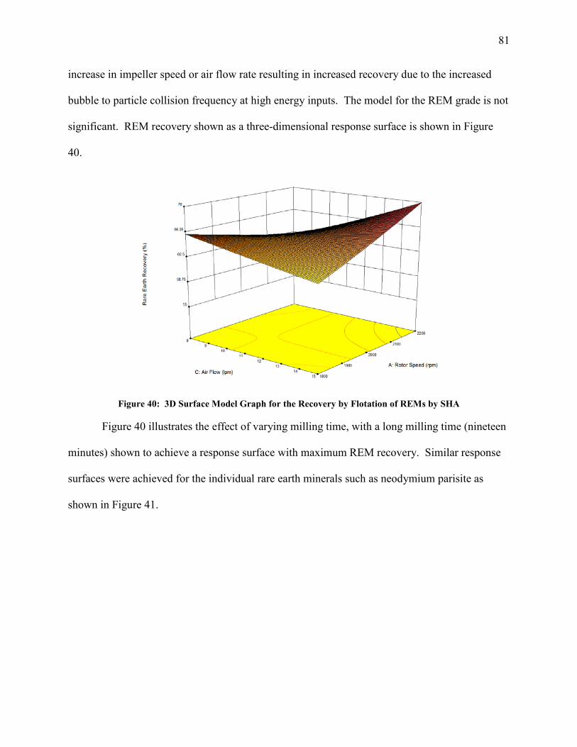
81

increase in impeller speed or air flow rate resulting in increased recovery due to the increased

bubble to particle collision frequency at high energy inputs. The model for the REM grade is not

significant. REM recovery shown as a three-dimensional response surface is shown in Figure

40.

Figure 40: 3D Surface Model Graph for the Recovery by Flotation of REMs by SHA

Figure 40 illustrates the effect of varying milling time, with a long milling time (nineteen

minutes) shown to achieve a response surface with maximum REM recovery. Similar response

surfaces were achieved for the individual rare earth minerals such as neodymium parisite as

shown in Figure 41.

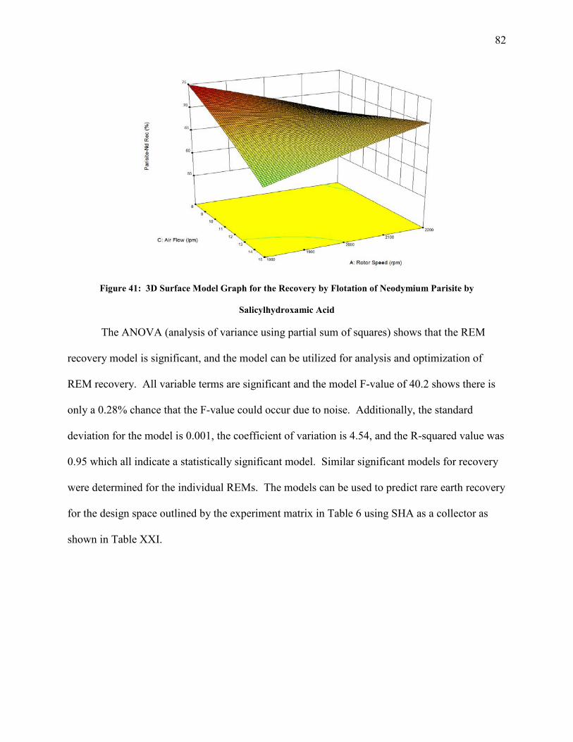
82

Figure 41: 3D Surface Model Graph for the Recovery by Flotation of Neodymium Parisite by

Salicylhydroxamic Acid

The ANOVA (analysis of variance using partial sum of squares) shows that the REM

recovery model is significant, and the model can be utilized for analysis and optimization of

REM recovery. All variable terms are significant and the model F-value of 40.2 shows there is

only a 0.28% chance that the F-value could occur due to noise. Additionally, the standard

deviation for the model is 0.001, the coefficient of variation is 4.54, and the R-squared value was

0.95 which all indicate a statistically significant model. Similar significant models for recovery

were determined for the individual REMs. The models can be used to predict rare earth recovery

for the design space outlined by the experiment matrix in Table 6 using SHA as a collector as

shown in Table XXI.

83

Table XXI: Point Prediction for Flotation of Rare Earth Minerals with Salicylhydroxamic Acid with Design

Variables at Upper Limits of the Design Space

Response

Predicted

Mean

Predicted

Median Std Dev

95%

CI low

95% CI

high

Parisite Recovery 62.63 60.40 3.16 51.71 100.00

Parisite-Nd Recovery 70.50 70.56 1.97 66.58 74.03

Monazite Recovery 70.99 70.93 3.75 64.15 78.27

Rare Earth Recovery 69.99 69.79 0.29 62.67 79.34

Rare Earth Grade 3.84 3.79 0.50 3.46 4.24

At the upper design limits for the experiments, maximum recovery is achieved for the

model. As expected, grade is not maximized with higher grades achieved at lower milling times

as shown in Table XXI. The model is showing a maximum rare earth recovery of 70% with

similar maximum recoveries for the individual REMs. Confirmatory experiments were

performed and REM recovery of 67% was achieved at the upper limits of the design space and

57% at the lower limits. Maximum recoveries are calculated based on Equation 3 using the two-

compartmental model as shown in Table XXII but differences are noted due to the degree of

entrainment calculated in the kinetics model.

Table XXII: Maximum Recovery Comparison between Parametric Experimental Design Model and Two-

Stage Compartmental Kinetics Model

Mineral Milling Time (10 min) Milling Time (19 min)

Parametric Kinetic Parametric Kinetic

Monazite 48.0% 35.4% 69.3% 74.3%

Parisite 46.2% 33.3% 64.4% 69.3%

Parisite_Nd 52.2% 40.5% 69.5% 74.5%

The compartmental kinetics model determines a maximum recovery approximately

thirteen percent lower than the parametric experimental design model for the shorter ore milling

time of ten minutes. An opposite relationship is determined at the longer ore milling time of

84

nineteen minutes with the kinetic model approximately five percent greater than the parametric

model.

Rare Earth Flotation with Novel Collectors

Samples from the design of experiments matrix for rare earth flotation using SHA were

analyzed at Hazen Research to verify the accuracy of the MLA analysis. The results of the

verification assay are shown in Table XXIII for select elements.

Table XXIII: Validation Assay of MLA Results as conducted by Hazen Research

Solids, wt% Ca Ce Fe Gd La Nd P Si Y

Con 1 5.10 0.96 7.97 0.023 0.550 0.342 0.42 18.7 0.011 Con 2 4.90 1.48 9.84 0.032 0.771 0.480 0.50 16.7 0.015 Con 3 5.33 1.10 7.20 0.027 0.643 0.399 0.44 18.8 0.012 Con 4 5.61 1.10 7.10 0.027 0.658 0.409 0.43 19.4 0.012 Tails 1 4.54 0.40 5.15 0.012 0.269 0.167 0.26 21.5 0.006 Tails 2 4.25 0.37 5.26 0.011 0.248 0.154 0.21 21.8 0.006 F +100 2.17 0.15 3.74 0.005 0.096 0.064 0.13 24.7 0.003

F 100x200 3.52 0.25 4.47 0.008 0.164 0.103 0.16 22.9 0.004 F 200x400 5.32 0.42 5.49 0.013 0.298 0.180 0.24 21.0 0.006

F -400 5.68 0.97 6.75 0.025 0.583 0.363 0.50 19.1 0.012

Based on this verification assay, the elemental ratios used for mineral determination in

MLA were modified. Cerium from the outside assay and MLA were roughly equivalent, 0.5%

different. Lanthanum was over-reporting by approximately 5% in MLA as opposed to the assay

obtained and conversely, neodymium was underreporting by approximately 5%.

Additionally, a second sample was obtained from RER and utilized for this design of

experiments. The new sample had a slightly different mineralogy and included some strictly

REO minerals. With new mineral ratios in MLA and the new sample, the minerals of interest

changed from monazite, parisite, and neodymium parisite to cerianite [CeO2], monazite, and

85

parisite. Allanite and ancylite were still present in minor quantities. The parisite minerals were

combined into a more accurate mineral given the determined assay.

To determine an effective pH for REM flotation, zeta potential versus pH measurements

were taken for all the novel collectors on lanthanum oxide. A plot of zeta potential versus pH of

the AASAS on lanthanum (III) oxide is shown in Figure 42.

Figure 42: Zeta potential vs. pH for CoTILPS 712 on La2O3. The line is for visual purposes only, it is not a

trendline

The plot of zeta potential versus pH shows that, approximately pH 11, the surface of the

lanthanum (III) oxide becomes negative with a large magnitude change when in the presence of

the collector, AASAS. The strong negative zeta potential (-920 mV) indicates that the collector

will adsorb best on the surface under basic conditions. Similar results were observed for

sarkosyl and FAM.

The twenty flotation experiments were performed based on the design of experiments

matrix (Table XVI) and the simple kinetics test parameters. The REMs present in the ore in

major quantities were monazite, parisite and cerianite [CeO2]. A typical feed grade for the rare

earth minerals and select gangue minerals is shown in Table XXIV.

-1000

-800

-600

-400

-200

0

2000 5 10 15

ζ(m

V)

pH

86

Table XXIV: Select Flotation Experiment Feed Sample of Minerals of Interest for Novel Collectors Design of

Experiments

Mineral

Feed

+150 µm

(Wt%)

Feed

-150/+75 µm

(Wt%)

Feed

-75/+37 µm

(Wt%)

Feed

-38 µm

(Wt%)

Feed

Composite

(Wt%)

Monazite 0.11 0.37 0.62 1.56 0.95

Parisite 0.25 0.44 1.32 1.81 1.21

Cerianite 0.04 0.07 0.20 0.38 0.23

RE Minerals 0.41 0.89 2.24 4.81 2.90

Calcite 4.73 7.93 12.09 11.61 10.17

K_Feldspar 82.87 76.24 63.85 51.50 63.10

The feed composite is a mass weighted average of the four feed particle size fractions.

Mineral grade or weight percent of REMs tends to the smaller particle sizes while the gangue

minerals have a higher weight percent in the larger particle sizes. Similar particle size

distributions are observed for all experiments, with the REMs reporting to the finer size fractions

in greater quantities than the coarse particle sizes. The simple kinetics test had four concentrate

collection times. Concentrate mineral grade for sarkosyl as determined from MLA is shown in

Table XXV, AASAS in Table XXVI, FAM in Table XXVII, and H205 in Table XXVIII.

Table XXV: Select Flotation Experiment Concentrate Sample of Minerals of Interest for Sarkosyl

Mineral

Con 1

(0s to 45s)

(Wt%)

Con 2

(45s to 2min)

(Wt%)

Con 3

(2min to 8min)

(Wt%)

Con 4

(8min to 30min)

(Wt%)

Con

Composite

(Wt%)

Monazite 1.29 1.51 0.96 1.00 1.22

Parisite 2.60 3.19 1.42 1.29 2.15

Cerianite 0.38 0.51 0.48 0.36 0.42

RE Minerals 4.95 5.91 3.49 1.54 4.23

Calcite 25.13 17.52 2.85 1.86 15.16

K_Feldspar 45.03 47.03 57.48 74.30 53.51

87

Table XXVI: Select Flotation Experiment Concentrate Sample of Minerals of Interest for AASAS

Mineral

Con 1

(0s to 45s)

(Wt%)

Con 2

(45s to 2min)

(Wt%)

Con 3

(2min to 8min)

(Wt%)

Con 4

(8min to 30min)

(Wt%)

Con

Composite

(Wt%)

Monazite 1.44 1.53 1.52 1.37 1.46

Parisite 2.35 3.03 1.69 1.28 2.06

Cerianite 0.42 0.68 0.49 0.31 0.46

RE Minerals 4.83 5.78 3.95 3.13 4.38

Calcite 16.32 14.06 6.57 4.24 10.72

K_Feldspar 48.65 49.58 59.38 66.35 55.54

Table XXVII: Select Flotation Experiment Concentrate Sample of Minerals of Interest for FAM

Mineral

Con 1

(0s to 45s)

(Wt%)

Con 2

(45s to 2min)

(Wt%)

Con 3

(2min to 8min)

(Wt%)

Con 4

(8min to 30min)

(Wt%)

Con

Composite

(Wt%)

Monazite 2.18 1.30 0.59 0.21 1.40

Parisite 3.88 1.65 0.63 0.19 2.23

Cerianite 0.48 0.61 0.34 0.08 0.43

RE Minerals 6.94 4.94 2.93 0.69 4.89

Calcite 31.28 8.43 3.16 0.75 16.40

K_Feldspar 29.41 51.89 62.00 78.34 47.47

Table XXVIII: Select Flotation Experiment Concentrate Sample of Minerals of Interest for H205

Mineral

Con 1

(0s to 45s)

(Wt%)

Con 2

(45s to 2min)

(Wt%)

Con 3

(2min to 8min)

(Wt%)

Con 4

(8min to 30min)

(Wt%)

Con

Composite

(Wt%)

Monazite 2.60 1.13 0.47 0.17 1.30

Parisite 4.01 1.37 0.42 0.19 1.84

Cerianite 0.94 0.74 0.24 0.10 0.57

RE Minerals 10.05 5.82 2.92 0.95 5.65

Calcite 20.10 11.60 6.10 3.81 11.74

K_Feldspar 32.83 45.54 57.49 71.78 49.20

88


frames. Representative gangue minerals, calcite and k-feldspar, are shown as they constitute

roughly 75% of the ore. The SKT concentrate grades show that the concentrate grade from the

first-time period (the first forty-five seconds of the test) is like the overall concentrate grade for

the entire thirty-minute test for three of the four collectors, the exception being the fatty acid

mixture. However, a higher grade is observed during the second-time period (from forty-five

seconds to two minutes) for the REMs again for three of the four collectors and the gangue

mineral potassium feldspar but a lower grade for the gangue mineral calcite. A typical particle

size distribution for the REM concentrate grade for longer milling times is shown in Figure 43.

Figure 43: Particle Size Distribution for Select Novel Collector Flotation Experiment Rare Earth

Concentrate Sample

89

Particle size distribution was calculated using MLA software. The P80 particle size for

the concentrate sample from the second and third sampling periods are approximately twenty

μm, while the P80 particle size for the concentrate sample from the first and fourth sampling

periods is approximately 30 μm. Similar particle size distributions are observed for all novel

collector flotation experiments. The results of the novel collector flotation experiments are

shown in Table XXIX.

Table XXIX: Design of Experiments Results for Novel Collector Rare Earth Mineral Flotation

Exp. Dose pH Collector RE

Recovery RE

Upgrade Parisite

Recovery Parisite Upgrade

Monazite Recovery

Monazite Upgrade

(g/tonne) (%) (%) (%) (%) (%) (%)

1 250 6 Sarkosyl 80 24 79 25 76 5 2 250 6 AASAS 72 61 67 50 75 77 3 250 11 Sarkosyl 73 68 66 60 74 40 4 250 11 AASAS 79 44 74 59 77 44 5 750 6 Sarkosyl 89 65 86 43 86 52 6 750 6 AASAS 79 56 73 60 78 41 7 750 11 Sarkosyl 90 73 88 88 88 63 8 750 11 AASAS 83 68 74 42 77 53 9 250 6 FAM 71 38 63 29 71 45

10 250 11 FAM 95 38 96 32 92 33 11 750 6 FAM 88 69 85 33 83 57 12 750 11 FAM 98 47 99 67 96 22 13 500 8.5 Sarkosyl 83 94 74 46 78 31 14 500 8.5 FAM 83 107 78 74 81 115 15 500 8.5 AASAS 76 26 67 3 75 14 16 750 11 H205 86 50 80 10 79 23 17 750 6 H205 76 74 65 36 73 38 18 250 11 H205 87 48 79 7 84 25 19 250 6 H205 73 58 64 50 73 73 20 500 8.5 H205 81 40 75 60 80 96

The maximum rare earth recovery (98%) is observed for experiment 12 with the largest

rare earth upgrading (107%) occurring for experiment 14. Both experiments used FAM to

collect REMs. Parisite recovery for experiment 12 is almost complete at 99% with FAM. The

highest observed monazite recovery was also on experiment 12 of 96%. Experiment 12 is the

90

high collector dosage and high pH condition, which indicates the optimal conditions are achieved

at these values. Additional analysis is needed, however, to verify the initial observed conclusion.

Flotation Experiment Analysis

5.2.2.1.1. Flotation Kinetics

Flotation experimental data were input into the SKT flotation kinetic model. Input data

included: flotation cell energy inputs, sized and weighed feed sample, concentrate and tailings

wet and dry masses, and mineral assays. Based on the data, a flotation kinetic model was

developed for each flotation experiment in the design of experiments. To ensure the accuracy of

the model, all five rare earth minerals were analyzed. Modeled recovery versus experimental

recovery was reconciled and shown in Figure 44. Modeled grade assay versus experimental

grade assay was reconciled and shown in Figure 45.

Figure 44: Kinetic Model Reconciliation - Recovery (low pH, low dosage, FAM)

0

10

20

30

40

50

60

70

80

90

100

0 10 20 30 40 50 60 70 80 90 100

Modeled Recovery [%]

Experimental Recovery [%]

Model Reconciliation - Recovery



91

Figure 45: Kinetic Model Reconciliation - Grade (low pH, low dosage, FAM)

The reconciled model shows that the monazite recovery correlates well with the

experimentally calculated recovery. Parisite modeled recovery does not deviate significantly

from the experimental recovery with a difference being 7.37 between modeled and experimental

for this experiment. The modeled parisite recovery for a typical experiment was 70.5 while the

experimental recovery was 62.9. For monazite, the modeled recovery was 70.3 while the

experimental recovery was 71.3 for the same experiment. The main difference between

experimental and modeled recovery can be related to the degree of entrainment of the

experiment. Typical degree of entrainment curves as calculated using Equation 46 are shown in

Figure 46.

0.001

0.010

0.100

1.000

10.000

100.000

0.001 0.010 0.100 1.000 10.000 100.000

Modeled Assay [%]

Experimental Assay [%]

Model Reconcilation - Grade



92

Figure 46: Degree of Entrainment for SKT Concentrate Collection Times as a Function of Particle Size (left:

low pH, low dosage, FAM; right: high pH, low dosage, FAM)

Degree of entrainment is calculated from water recovery and rise velocity of water as

outlined in hindered settling theory and Equation 42. The recovery of water to the froth is shown

in Table XXX and the distribution of the rise velocity of water is shown in Figure 47 for typical

flotation experiments.

Table XXX: Froth Recovery of Water for SKT (left: low pH, low dosage, FAM; right: high pH, low dosage,

FAM). Blue values are the true water flux values at time = 0 sec.

Time Rw Qw Vw Rf water (min) (g) (g/sec) (cm/sec) (%)

0.05 26.30 0.088 100% 0.38 878.30 19.52 0.065 74% 1.38 1602.30 21.36 0.072 81% 5.00 6252.40 17.37 0.058 66%

19.00 14556.40 11.03 0.037 42%

Time Rw Qw Vw Rf water (min) (g) (g/sec) (cm/sec) (%)

0.05 35.54 0.119 100% 0.38 1189.80 26.44 0.089 74% 1.38 2084.20 27.79 0.093 78% 5.00 7233.30 20.09 0.067 57%

19.00 18928.30 14.34 0.048 40%

0.00.10.20.30.40.50.60.70.80.91.0

0 50 100

D.E. [Rs/Rw]



Con1

Con2

Con3

Con4

0.00.10.20.30.40.50.60.70.80.91.0

0 50 100

D.E. [Rs/Rw]



Con1

Con2

Con3

Con4

93

Figure 47: Distribution of Rise Velocity based on Velocity of Water into Froth (left: low pH, low dosage,

FAM; right: high pH, low dosage, FAM)

Entrainment data can be utilized to differentiate between the recovery of the REMs by

flotation as opposed to entrainment. The differentiation is shown in Table XXXI by collection

stage from the SKT methodology for a typical flotation experiment.

Table XXXI: Recovery by Entrainment and Flotation per SKT Collection Stage (low pH, high dosage, FAM)

Allanite Ancylite Cerianite Monazite Parisite Recovery by Entrainment per Stage

Con 1 7.15 5.02 5.56 4.27 2.80 Con 2 7.53 4.68 5.72 4.59 3.35 Con 3 2.35 6.41 8.38 11.35 13.64 Con 4 6.60 22.72 22.70 22.79 22.79

Recovery by Flotation per Stage Con 1 23.91 46.59 40.84 54.58 70.19 Con 2 38.17 61.62 53.05 62.29 72.49 Con 3 87.05 64.64 53.82 37.45 24.83 Con 4 71.06 0.34 0.40 0.01 0.00

Total Recovery per Stage Con 1 31.06 51.61 46.40 58.85 72.99 Con 2 45.70 66.30 58.77 66.88 75.84 Con 3 89.40 71.06 62.20 48.80 38.46 Con 4 77.66 23.06 23.10 22.80 22.79

As expected, the recovery by entrainment increases with increasing residence time and

the recovery by flotation decreases with residence time. The most hydrophobic particles are

0%

5%

10%

15%

20%

25%

0.000 0.020 0.040 0.060 0.080 0.100 0.120

Probability


Distribution of Rise Velocity V[Con1)

V[Con2)

V[Con3)

V[Con4)

0%

5%

10%

15%

20%

25%

0.000 0.020 0.040 0.060 0.080 0.100 0.120

Probability


Distribution of Rise Velocity V[Con1)

V[Con2)

V[Con3)

V[Con4)

94

more likely to become attached to air bubbles and be recovered by flotation occurs early in the

test. As the more hydrophobic particles are removed, it becomes less likely that recovery by

flotation can occur. Relatively large entrainment recovery values are observed for most REMs,

especially in the later stages. In this example, all the parisite and almost all the monazite in the

fourth concentrate sample is recovered by entrainment. For REMs, recovery by entrainment is

large factor to be considered. Equation 29 accounts for the recovery by entrainment when

determine maximum recovery and the first-order rate constant. The calculated first-order rate

constant and modeled maximum recovery of REMs are shown in Table XXXII and XXXIII for

the novel collector design of experiments.

Table XXXII: Flotation First-order Rate Constant for SKT Experiments of Novel Collectors using Kinetic

Modeling

Flotation First-order Rate Constant, k Experiment Allanite Ancylite Cerianite Monazite Parisite

1 1.49 0.59 0.86 1.28 1.48 2 1.21 1.34 0.61 0.67 0.99 3 0.40 0.63 0.72 1.37 1.51 4 0.50 0.38 0.36 1.24 1.34 5 1.84 1.64 1.65 1.62 1.80 6 0.49 0.37 0.21 0.29 0.39 7 0.44 1.21 1.68 2.06 2.12 8 0.74 0.70 0.86 1.23 1.34 9 0.34 0.28 0.17 0.21 0.22

10 0.48 1.14 1.04 1.51 2.14 11 0.96 0.55 0.49 0.60 0.73 12 0.56 0.61 1.19 1.81 2.19 13 1.22 0.93 1.30 1.43 1.39 14 0.37 0.54 0.38 0.63 0.68 15 0.36 0.49 1.12 0.81 1.17 16 0.35 1.16 1.51 1.67 2.08 17 1.79 0.56 0.80 0.83 0.77 18 0.28 0.27 0.18 0.22 0.22 19 0.53 0.23 0.27 0.09 0.06 20 0.82 1.22 1.49 0.89 0.91

95

Table XXXIII: Modeled Maximum Recovery for SKT Experiments of Novel Collectors using Kinetic

Modeling

Modeled Maximum Recovery, Rmax Experiment Allanite Ancylite Cerianite Monazite Parisite

1 0.92 0.86 0.43 0.49 0.60 2 0.94 0.50 0.46 0.44 0.42 3 0.94 0.67 0.32 0.32 0.33 4 0.96 0.92 0.66 0.43 0.40 5 0.99 0.98 0.85 0.81 0.90 6 0.98 1.00 0.83 0.67 0.72 7 0.99 0.96 0.82 0.73 0.74 8 0.99 0.94 0.75 0.59 0.59 9 0.98 0.72 0.66 0.59 0.59

10 0.98 0.93 0.87 0.89 0.94 11 0.99 0.79 0.83 0.71 0.82 12 1.00 0.98 0.99 0.94 0.97 13 0.99 0.87 0.59 0.64 0.58 14 0.95 0.86 0.74 0.68 0.62 15 0.99 0.66 0.51 0.34 0.25 16 0.98 0.88 0.80 0.83 0.84 17 0.95 0.86 0.81 0.51 0.49 18 1.00 0.95 0.83 0.75 0.66 19 0.99 0.78 0.56 0.77 0.69 20 0.98 0.90 0.70 0.64 0.54

From Table XXXI, a wide range of flotation first-order rate constants can be observed for

the REMs. For the major component minerals, parisite and monazite, the first-order rate

constant ranges from 0.09 to 2.06 for monazite and 0.06 to 2.19 for parisite. The modeled

maximum recovery can then be plotted as a function of time, with data points corresponding to

collection times for the SKT experiments. Typical flotation kinetics curves are shown in Figure

48 and 49 for each of the 5 REMs.

96

Figure 48: Predicted Recovery of Rare Earth Minerals using Flotation Kinetic Modeling (low pH, low

dosage, FAM)

0102030405060708090

100

0 5 10 15 20 25 30

Rec

over

y (%

)

Time (min)

Flotation Kinetics



97

Figure 49: Predicted Recovery of Rare Earth Minerals using Flotation Kinetic Modeling (low pH, high

dosage, FAM)

Figure 47 shows allanite [(Ca,Ce)2(Al,Fe2)3(SiO4(Si2O7)O(OH)] has the fastest flotation

kinetics and the highest modeled maximum recovery, which corresponds to the flotation rate

constant for allanite for the experiment shown. Similarly, it can be observed that parisite

[Ca(Ce,La,Nd)2(CO3)3F2 has the fastest flotation kinetics, but recovery levels off after eight

minutes and allanite has the highest modeled maximum recovery, which corresponds to the

flotation rate constant for parisite for the experiment shown. The flotation rate constant and

calculated recoveries can then be used as responses for an analysis of variance for the design of

experiments of the novel collectors.

0102030405060708090

100

0 5 10 15 20 25 30

Rec

over

y (%

)

Time (min)

Flotation Kinetics



98

5.2.2.1.2. Analysis of Variance (ANOVA) for Novel Collectors

Since the feed grade for each mineral could vary between experiments, the grade was

normalized with an increase in grade value and then calculated and used for evaluation of the

results as opposed to the straight grade value from MLA. The increase in grade calculation is

shown in Equation 47:

Increase in grade = 100% ∗𝐶𝐶𝐶𝐶𝑛𝑛 𝐺𝐺𝐺𝐺𝐺𝐺𝑑𝑑𝑒𝑒 − 𝛽𝛽𝑒𝑒𝑒𝑒𝑑𝑑 𝐺𝐺𝐺𝐺𝐺𝐺𝑑𝑑𝑒𝑒

𝛽𝛽𝑒𝑒𝑒𝑒𝑑𝑑 𝐺𝐺𝐺𝐺𝐺𝐺𝑑𝑑𝑒𝑒 (47)

where the con and feed grade are in weight percent as measured by MLA. Increase in grade can

also be termed upgrading and the terms are interchangeable.

Responses chosen for the design of experiments were rare earth, monazite and parisite

recovery; rare earth, monazite, and parisite increase in grade; and monazite and parisite first-

order rate constant. Responses were analyzed using Historical data in Design-Expert 10 as

opposed to a two-factorial design. Given the nature of the experiments, a hierarchal design could

not be developed. However, each response could be examined based off the analysis of variance

results which, could result in either strictly a mean vs total, a linear model, or a two-factorial

model. All increase in grade models resulted in a mean vs total, meaning the predicted r-squared

value, or the ability of the regression model to predict response for new observations, was

negative for all possible transforms. The other models all resulted in linear models of the three

factors except for monazite recovery which would use a two-factorial model with the effect of

interactions between factors on the response variable (monazite recovery) analyzed.

Increase in grade response models could not predict the response of new observations and

so would not be analyzed. A power transform of -0.07 was chosen for the rare earth recovery

response based on Box-Cox transformation, which yields a data set that follows an approximate

99

normal distribution. The ANOVA for the linear model of rare earth recovery is shown in Table

XXXIV.

Table XXXIV: ANOVA for Linear model of Rare Earth Recovery

ANOVA for Response Surface Linear model Analysis of variance table [Classical sum of squares - Type II]

Source Sum of

Squares df Mean Square F

Value p- value Prob > F

Model 2.64E-04 5 5.29E-05 4.71 0.0099 significant A-Collector Dosage 8.90E-05 1 8.90E-05 7.92 0.0138 B-pH 9.53E-05 1 9.53E-05 8.48 0.0114 C-Type of Collector 8.02E-05 3 2.67E-05 2.38 0.1135 Residual 1.57E-04 14 1.12E-05 Cor Total 4.22E-04 19

The ANOVA shows a significant model with a p-value of 0.0099. Collector dosage and

pH are also significant with p-values < 0.05. The coefficient of variation for the model is 0.46%

and an adjusted r-squared of 0.49, which adjusts the r-squared value to the number of predictor

variables in the model. A post-hoc analysis was performed, and the results are shown in

Appendix A. The analysis however, did not result in a deeper understanding of the data.

Although the type of collector term is not significant, it was included in the model because it is a

categoric variable with four levels as opposed to a numeric variable and can be used as a

comparison tool between the various collectors without effecting the numeric variables as shown

in Equations 48 through 51, where A is the collector dosage and B is the pH.

𝑆𝑆𝐺𝐺𝐺𝐺𝑘𝑘𝐶𝐶𝑆𝑆𝑆𝑆𝑆𝑆: (𝑅𝑅𝐺𝐺𝐺𝐺𝑒𝑒 𝐸𝐸𝐺𝐺𝐺𝐺𝑡𝑡ℎ 𝑅𝑅𝑒𝑒𝑅𝑅𝐶𝐶𝑣𝑣𝑒𝑒𝐺𝐺𝑆𝑆)−0.07 = 0.747 − 9.43𝐸𝐸−6 ∗ 𝐴𝐴 − 9.76𝐸𝐸−4 ∗ 𝐵𝐵 (48)

𝛽𝛽𝐴𝐴𝐹𝐹: (𝑅𝑅𝐺𝐺𝐺𝐺𝑒𝑒 𝐸𝐸𝐺𝐺𝐺𝐺𝑡𝑡ℎ 𝑅𝑅𝑒𝑒𝑅𝑅𝐶𝐶𝑣𝑣𝑒𝑒𝐺𝐺𝑆𝑆)−0.07 = 0.745 − 9.43𝐸𝐸−6 ∗ 𝐴𝐴 − 9.76𝐸𝐸−4 ∗ 𝐵𝐵 (49)

𝐴𝐴𝐴𝐴𝑆𝑆𝐴𝐴𝑆𝑆: (𝑅𝑅𝐺𝐺𝐺𝐺𝑒𝑒 𝐸𝐸𝐺𝐺𝐺𝐺𝑡𝑡ℎ 𝑅𝑅𝑒𝑒𝑅𝑅𝐶𝐶𝑣𝑣𝑒𝑒𝐺𝐺𝑆𝑆)−0.07 = 0.750 − 9.43𝐸𝐸−6 ∗ 𝐴𝐴 − 9.76𝐸𝐸−4 ∗ 𝐵𝐵 (50)

𝐻𝐻205: (𝑅𝑅𝐺𝐺𝐺𝐺𝑒𝑒 𝐸𝐸𝐺𝐺𝐺𝐺𝑡𝑡ℎ 𝑅𝑅𝑒𝑒𝑅𝑅𝐶𝐶𝑣𝑣𝑒𝑒𝐺𝐺𝑆𝑆)−0.07 = 0.749 − 9.43𝐸𝐸−6 ∗ 𝐴𝐴 − 9.76𝐸𝐸−4 ∗ 𝐵𝐵 (51)

100

Note only a small change in the coefficient associated with each collector. Statistical

diagnostics were performed on the analysis of variance. The first diagnostic tool was Cook’s

Distance which identifies outliers in the observations and shows the influence of each

observation on the fitted response values. The Cook’s Distance for rare earth recovery ANOVA

is shown in Figure 50.

Figure 50: Cook’s Distance for ANOVA of Rare Earth Recovery by Flotation

An observation with a Cook’s Distance that is three times the mean Cook’s Distance

would be considered an outlier. The red line at 0.936 shows the recommended threshold value or

the value which defines an outlier to the observations. All observations are below the red line

and such the ANOVA passes this diagnostic. Leverage was also performed on the analysis of

variance model. Leverage is a diagnostic tool that measures how far away the independent

parameters of an observation are from those of the other observations and is shown in Figure 51.

Design-Expert® Software(Rare Earth Recovery) -̂0.07

Color points by value of(Rare Earth Recovery) -̂0.07:

0.725

0.742

Run Number

Coo

k's

Dis

tanc

eCook's Distance

0

0.2

0.4

0.6

0.8

1

1 4 7 10 13 16 19

0.935724

0

101

Figure 51: Leverage for ANOVA of Rare Earth Recovery by Flotation

A high leverage observation is an extreme predicator value, such as double of the mean

observation leverage value. The red line at 0.6 shows the high leverage value for this data set

and defines a high leverage observation. All observations are below the red line and so the

ANOVA passes this diagnostic. With the model being significant and passing both diagnostics,

a three-dimensional response surface was created. The 3-D response surface for rare earth

recovery using FAM is shown in Figure 52.

Design-Expert® Software(Rare Earth Recovery) -̂0.07

Color points by value of(Rare Earth Recovery) -̂0.07:

0.725

0.742

Run Number

Leve

rage

Leverage vs. Run

0.00

0.20

0.40

0.60

0.80

1.00

1 4 7 10 13 16 19

0.3

0.6

0

102

Figure 52: 3D Response Surface for Rare Earth Recovery by Flotation with Novel Collector (FAM)

The response surface shows that the highest predicted rare earth recovery using FAM is

95% at an experimental pH of 11 and collector dosage of 750 g/tonne, which is less than the

experimental result at those flotation conditions. Similar response surfaces for rare earth

recovery were created and are shown in Appendix A. The response of the predicted rare earth

recovery was also analyzed by studying the effect of changing the numeric variables on the

categoric variable due to the linear model. One factor analysis for rare earth recovery is shown

in Figure 53.

Design-Expert® SoftwareFactor Coding: ActualOriginal ScaleRare Earth Recovery (%)

Design points above predicted valueDesign points below predicted value98

71

X1 = A: Collector DosageX2 = B: pH

Actual FactorC: Type of Collector = FAM

6

7

8

9

10

11

250

350

450

550

650

750

70

75

80

85

90

95

100

Rar

e Ea

rth R

ecov

ery

(%)

A: Collector Dosage ((g/tonne))B: pH

103

Figure 53: One Factor Analysis for Rare Earth Recovery (top left: low pH, low collector dosage; top right:

high pH, low collector dosage; bottom left: low pH, high collector dosage; bottom right: high pH, high

collector dosage)

The trends for the rare earth recovery can be observed as a function of the type of

collector used at the varying experimental conditions. FAM has the highest predicted rare earth

recovery for all collector types and experimental conditions, while AASAS has the lowest

predicted rare earth recovery across all situations. Similar analysis was performed for the linear

C: Type of Collector

Sarkosyl FAM AASAS H205

Rar

e E

arth

Rec

over

y (%

)

60

70

80

90

100

One Factor



Rar

e E

arth

Rec

over

y (%

)

60

70

80

90

100

One Factor



Rar

e E

arth

Rec

over

y (%

)

60

70

80

90

100

One Factor



Rar

e E

arth

Rec

over

y (%

)

60

70

80

90

100

One Factor

104

models for Parisite Recovery, Monazite K and Parisite K. All tables and graphs are in Appendix

A. The parisite recovery model shows a maximum predicted recovery of 95% at a pH of 11 and

collector dosage of 750 g/tonne using FAM as the collector. One factor analysis shows that

FAM will have the highest predicted parisite recovery across all experimental conditions and

AASAS will have the lowest. Parisite first-order constant will be highest with a value of 2.4

using sarkosyl as the collector at a pH of 11 and a collector dosage of 750 g/tonne. It can be

observed from one factor analysis that sarkosyl will have the highest predicted monazite first-

order rate constant and H205 will have the lowest for the design space. The monazite first-order

rate constant linear model had the highest adjusted R-squared of 0.63 and was the only linear

model where the type of collector term was significant. Sarkosyl had the highest Monazite K

value of 2.1 at a pH of 11 and a collector dosage of 750 g/tonne and is also predicted to have the

highest k across all conditions based on one-factor analysis. Similar trends are observed across

all response surfaces with highest recovery or K values occurring at the high experimental

conditions and the lowest recovery or K values at the low experimental conditions.

For monazite recovery, a two-factorial model was suggested and a Box-Cox power

transformation of -3 was used and ANOVA performed. The analysis of variance resulted in a

significant model with a p-value of 0.0073 and all single factor terms being significant. In

addition, the effect of the factors on each other were analyzed and all interactions (A to B, A to

C, B to C) also being significant. The model resulted in a standard deviation of 2.02E-7, an

adjusted R-squared of 0.80 and a coefficient of variation of 9.9. Final equations for the model

based on each collector are shown in Equations 52 through 55, where A is collector dosage and

B is pH:

105

𝑆𝑆𝐺𝐺𝐺𝐺𝑘𝑘𝐶𝐶𝑆𝑆𝑆𝑆𝑆𝑆: (𝐹𝐹𝐶𝐶𝑛𝑛𝐺𝐺𝑀𝑀𝑖𝑖𝑡𝑡𝑒𝑒 𝑅𝑅𝑒𝑒𝑅𝑅𝐶𝐶𝑣𝑣𝑒𝑒𝐺𝐺𝑆𝑆)−3

= 3.27𝐸𝐸−6 − 2.73𝐸𝐸−9 ∗ 𝐴𝐴 − 5.15𝐸𝐸−8 ∗ 𝐵𝐵 + 1.20𝐸𝐸−10 ∗ 𝐴𝐴 ∗ 𝐵𝐵 (52)

𝛽𝛽𝐴𝐴𝐹𝐹: (𝐹𝐹𝐶𝐶𝑛𝑛𝐺𝐺𝑀𝑀𝑖𝑖𝑡𝑡𝑒𝑒 𝑅𝑅𝑒𝑒𝑅𝑅𝐶𝐶𝑣𝑣𝑒𝑒𝐺𝐺𝑆𝑆)−3

= 4.67𝐸𝐸−6 − 2.22𝐸𝐸−9 ∗ 𝐴𝐴 − 2.78𝐸𝐸−8 ∗ 𝐵𝐵 + 1.20𝐸𝐸−10 ∗ 𝐴𝐴 ∗ 𝐵𝐵

(53)

𝐴𝐴𝐴𝐴𝑆𝑆𝐴𝐴𝑆𝑆: (𝐹𝐹𝐶𝐶𝑛𝑛𝐺𝐺𝑀𝑀𝑖𝑖𝑡𝑡𝑒𝑒 𝑅𝑅𝑒𝑒𝑅𝑅𝐶𝐶𝑣𝑣𝑒𝑒𝐺𝐺𝑆𝑆)−3


(54)

𝐻𝐻205: (𝐹𝐹𝐶𝐶𝑛𝑛𝐺𝐺𝑀𝑀𝑖𝑖𝑡𝑡𝑒𝑒 𝑅𝑅𝑒𝑒𝑅𝑅𝐶𝐶𝑣𝑣𝑒𝑒𝐺𝐺𝑆𝑆)−3


(55)

The same statistical diagnostic tools were utilized as for the linear models; Cook’s

Distance and Leverage. The Cook’s Distance for monazite recovery is shown in Figure 54 and

Leverage is shown in Figure 55.

Figure 54: Cook’s Distance for ANOVA of Monazite Recovery by Flotation

Design-Expert® Software(Monazite Recovery)^-3

Color points by value of(Monazite Recovery)^-3:

0.000

0.000

Run Number

Coo

k's

Dis

tanc

e

Cook's Distance

0

0.2

0.4

0.6

0.8

1

1 4 7 10 13 16 19

1

0

106

Figure 55: Leverage for ANOVA of Monazite Recovery by Flotation

All values of Cook’s Distance fall below the red line at 1 and so the model passes the

diagnostic. The mean value of Leverage is 0.65 and so a high leverage observation would be

three times the mean or 1.95, which all values for the experiments fall well below and the

diagnostic is passed. 3D response surfaces were created for the novel collectors to sure predicted

behavior for the flotation variables. The 3D response surface for monazite recovery using

sarkosyl is shown in Figure 56 and using FAM in Figure 57.



0.000

0.000

Run Number

Leve

rage

Leverage vs. Run

0.00

0.20

0.40

0.60

0.80

1.00

1 4 7 10 13 16 19

0.65

0

107

Figure 56: 3D Response Surface for Monazite Recovery by Flotation with Novel Collector (Sarkosyl)

Figure 57: 3D Response Surface for Monazite Recovery by Flotation with Novel Collector (FAM)

The response surfaces for the other novel collectors can be seen in Appendix A. Figure

60 shows that maximum predicted monazite recovery will occur at a low pH and high collector

Design-Expert® SoftwareFactor Coding: ActualOriginal ScaleMonazite Recovery (%)


71


Actual FactorC: Type of Collector = Sarkosyl

6

7

8

9

10

11

250

350

450

550

650

750

70

77.5

85

92.5

100

Mon

azite

Rec

over

y (%

)




71



6

7

8

9

10

11

250

350

450

550

650

750

70

77.5

85

92.5

100

Mon

azite

Rec

over

y (%

)


Warning! Surface truncated by selected response (Y) range

108

dosage. A trend can also be observed of increasing recovery with the lowest recovery being

predicted at a high pH and low collector dosage and increasing across the surface in the negative

pH direction and positive collector dosage direction. The response surface for monazite recovery

using FAM as the novel collector shows a predicted 100% monazite recovery at high pH and

high collector dosage. An almost 30% in monazite recovery is predicted by the model between

the low recovery value at a low pH and low collector dosage to where the surface becomes

truncated at 100% recovery. AASAS follows the response surface for sarkosyl, Figure 60, with

the highest predicted recovery occurring at a low pH and high collector dosage value.

Interestingly, it also follows the response surface for FAM, Figure 56, with the lowest predicted

recovery occurring at a low pH and low collector dosage. The response surface for H205 has a

predicted maximum monazite recovery of almost 80% occurs at a high pH and low collector

dosage, while the minimum occurs at a low pH and high collector dosage. Monazite recovery

with H205 decreases with decreasing pH and decreases slightly with decreasing collector dosage.

Because the two-factorial model supported interactions between factors, interaction plots

were studied. The interaction plots are shown in Figure 58 with monazite recovery graphed as a

function of collector dosage and its effect on pH for each novel collector.


Design Points


Actual FactorC: Type of Collector = Sarkosyl

B- 6B+ 11

A: Collector Dosage ((g/tonne))

B: pH

250 350 450 550 650 750

Mon

azite

Rec

over

y (%

)

70

80

90

100

110

Interaction Design-Expert® SoftwareFactor Coding: ActualOriginal ScaleMonazite Recovery (%)

Design Points



B- 6B+ 11


B: pH

250 350 450 550 650 750

Mon

azite

Rec

over

y (%

)

70

80

90

100

110

Interaction

109

Figure 58: Interaction between Factors for Monazite Recovery by Novel Collectors (top left: Sarkosyl; top

right: FAM; bottom left: AASAS; bottom right: H205

The interaction plots show how the pH influences collector dosage for monazite

recovery. For sarkosyl, monazite recovery will increase as collector dosage increases, but will

increase at a faster rate for pH 6 than pH 11. A different trend is observed for monazite recovery

with FAM where monazite recovery increases with increasing collector dosage, but generally to

the same degree at pH 6 and 11. The monazite recovery starts out greater at a low collector

dosage for pH 11, however. Monazite recovery with AASAS is generally even but starts out

higher at pH 11. As collector dosage is increased, the monazite recovery becomes greater for pH

6 at a collector dosage of 575 g/tonne. For H205, collector dosage does not seem to affect

monazite recovery at pH 6, the change in recovery is less than 1%. But at pH 11, the monazite

recovery decreases as dosage is increased.

An analysis of variance was also conducted for the recovery of gangue minerals, calcite

and potassium feldspar. Minimization of the recovery of gangue minerals is desired. A two-

factorial design was suggested for calcite recovery while a mean versus total model was

suggested for feldspar recovery. The two-factorial model for calcite recovery is significant with

a p-value of 0.004. Two factors, pH and collector, were significant. However, collector dosage


Design Points


Actual FactorC: Type of Collector = AASAS

B- 6B+ 11


B: pH

250 350 450 550 650 750

Mon

azite

Rec

over

y (%

)

70

80

90

100

110

Interaction Design-Expert® SoftwareFactor Coding: ActualOriginal ScaleMonazite Recovery (%)

Design Points


Actual FactorC: Type of Collector = H205

B- 6B+ 11


B: pH

250 350 450 550 650 750

Mon

azite

Rec

over

y (%

)

70

80

90

100

110

Interaction

110

is not significant for calcite recovery and would not be included in the model. Adjusted R-

squared for the model is 0.64 with a coefficient of variation of 17%. The same statistical

diagnostic tools were utilized as for the rare earth models; Cook’s Distance and Leverage. The

Cook’s Distance for calcite recovery is shown in Figure 59 and Leverage is shown in Figure 60.

Figure 59: Cook’s Distance for ANOVA of Calcite Recovery by Flotation

Design-Expert® Software(Calcite Recovery)^1.55

Color points by value of(Calcite Recovery)^1.55:

1239.466

498.382

Run Number

Coo

k's

Dis

tanc

e

Cook's Distance

0

0.2

0.4

0.6

0.8

1

1 4 7 10 13 16 19

0.971515

0

111

Figure 60: Leverage for ANOVA of Calcite Recovery by Flotation

All values of Cook’s Distance fall below the red line at 0.97 and so the model passes the

diagnostic. The mean value of Leverage is 0.4 and so a high leverage observation would be

three times the mean or 0.8, which all values for the experiments fall below and the diagnostic is

passed. 3D response surfaces were created for the novel collectors to show predicted behavior

for the flotation variables. The 3D response surfaces for calcite recovery are shown in Figure 61

using H205 and in Figure 62 using FAM.

Design-Expert® Software(Calcite Recovery)^1.55

Color points by value of(Calcite Recovery)^1.55:

1239.466

498.382

Run Number

Leve

rage

Leverage vs. Run

0.00

0.20

0.40

0.60

0.80

1.00

1 4 7 10 13 16 19

0.4

0.8

0

112

Figure 61: 3D Response Surface for Calcite Recovery by Flotation with Novel Collector (H205)

Figure 62: 3D Response Surface for Calcite Recovery by Flotation with Novel Collector (FAM)

For a gangue mineral, a high recovery is undesirable. In Figure 60, H205 has a predicted

minimum calcite recovery of approximately 52% at a pH of 6 and a predicted maximum calcite

Design-Expert® SoftwareFactor Coding: ActualOriginal ScaleCalcite Recovery (%)


55


Actual FactorC: Type of Collector = H205

6

7

8

9

10

11

250

350

450

550

650

750

40

52

64

76

88

100

Cal

cite

Rec

over

y (%

)


Design-Expert® SoftwareFactor Coding: ActualOriginal ScaleCalcite Recovery (%)


55



6

7

8

9

10

11

250

350

450

550

650

750

40

52

64

76

88

100

Cal

cite

Rec

over

y (%

)


113

recovery of approximately 70% at a pH of 11. The minimum calcite recovery in Figure 61 for

FAM is approximately 67% at a pH of 6 and a maximum calcite recovery of 98% at a pH of 11.

Discussion of Results

Given the trends discussed, an understanding of the performance of the novel collectors for

REM flotation has been developed. A numerical optimization was conducted using Design Expert

10. Design Expert 10 uses a hill climbing iterative algorithm to determine if improvements to the

solution can be determined and continues to incrementally change single elements until the optimal

solution can be determined. The constraints for the numerical optimization are shown in Table

XXXV.

Table XXXV: Constraints for Numerical Optimization for Recovery of Rare Earth Minerals by Flotation

Constraints Lower Upper Lower Upper Name Goal Limit Limit Weight Weight Importance A: Collector Dosage is in range 250 750 1 1 3 B: pH is in range 6 11 1 1 3 C: Type of Collector is in range Sarkosyl H205 1 1 3 Rare Earth Recovery maximize 71 98 1 1 3 Parisite Recovery maximize 63 99 1 1 3 Monazite Recovery maximize 71 96 1 1 3 Calcite Recovery minimize 55 99 1 1 3 Feldspar Recovery minimize 39 66 1 1 3

Optimization of the factors associated with the design space is evaluated in the range as

outlined by the design of experiments. Rare earth, parisite and monazite recovery are maximized

while calcite and feldspar recovery are minimized. Given the above criteria, optimal conditions

114

were found based upon the design space for the flotation experiments. Ramps of the conditions

optimized are shown in Figure 63.

Figure 63: Ramps for Numerical Optimization of Rare Earth Mineral Recovery. Ramps describe the

conditions and expected results to produce optimum values based upon defined constraints.

The numerical optimization attempted to maximize the desirability function based on the

constraints shown in Table 34. A desirability function of 0.68 was obtained based upon those

constraints. With a collector dosage of 750 g/tonne at a pH of 11 and using sarkosyl, optimum

values for parisite, monazite and overall rare recovery can be achieved while minimizing the

recovery of gangue minerals. A 91% rare earth recovery is predicted, with monazite and parisite

recoveries being 85% and 89%, respectively. While gangue mineral recovery is limited to 68%

for calcite and 46% for potassium feldspar.

A numerical optimization was also taken to determine ideal rare earth kinetic conditions.

To limit entrainment, the residence time within the flotation cell should be minimized and thus

the first-order rate constant should be maximized. However, those conditions may not

necessarily result in optimal flotation performance with the possibility of increased kinetics

A:Collector Dosage = 750

250 750

B:pH = 11

6 11

C:Type of Collector = Sarkosyl

Treatments1 2 3 4

Rare Earth Recovery = 91.0789

71 98

Parisite Recovery = 88.1089

63 99

Monazite Recovery = 84.9401

71 96

Calcite Recovery = 68.4165

55 99

Feldspar Recovery = 45.9727

39 66

Desirability = 0.683

115

aiding gangue mineral recovery and so any optimization needs to consider the effect of increased

kinetic response of the valuable minerals versus the recovery of gangue minerals. The

constraints for the numerical optimization of flotation kinetics is shown in Table XXXVI.

Table XXXVI: Numerical Optimization Constraints for Flotation Kinetics.

Constraints

Lower Upper Lower Upper Name Goal Limit Limit Weight Weight Importance A: Collector Dosage is in range 250 750 1 1 3 B: pH is in range 6 11 1 1 3 C: Type of Collector is in range Sarkosyl H205 1 1 3 Monazite K maximize 0.09 2.06 1 1 3 Parisite K maximize 0.06 2.19 1 1 3 Calcite Recovery minimize 55 99 1 1 3 Feldspar Recovery minimize 39 66 1 1 3

The first-order rate constant should be maximized, but the recovery of gangue minerals

minimized while operating in the ranges of the factors for the design of experiments. Optimal

conditions were found for maximizing the kinetics of monazite and parisite and the ramps are

shown in Figure 64.

Figure 64: Ramps for Numerical Optimization of Monazite and Parisite First-order Rate Constant. Ramps

describe the conditions and expected results to produce optimum values based upon defined constraints.


250 750

B:pH = 11

6 11

C:Type of Collector = Sarkosyl

Treatments1 2 3 4

Monazite K = 2.10932

0.09 2.06

Parisite K = 2.40726

0.06 2.19


55 99


39 66


116

Optimal conditions for the rare earth kinetics are the same as what was determined for

rare earth recovery with sarkosyl at a high collector dosage and high pH. The desirability factor

of 0.847 matches the desired constraints significantly. Interestingly, the K value for parisite and

monazite are predicted to be higher than the experimental results found under these conditions.

Both optimizations show a high calcite recovery of approximately 68%. Calcite and parisite are

both calcium carbonates and so flotation behavior is expected to be similar. To be successful,

any collector will be more selective of REEs than for calcium or carbonate. A numerical

optimization of parisite recovery and increase in grade was performed and the constraints are

shown in Table XXXVII.

Table XXXVII: Numerical Optimization for Parisite (Rare Earth Carbonate) Recovery and Grade

Constraints

Lower Upper Lower Upper Name Goal Limit Limit Weight Weight Importance A: Collector Dosage is in range 250 750 1 1 3 B: pH is in range 6 11 1 1 3 C: Type of Collector is in range Sarkosyl H205 1 1 3 Parisite Recovery maximize 63 99 1 1 3 Parisite Upgrade maximize 3 88 1 1 3 Calcite Recovery minimize 55 99 1 1 3 Calcite Upgrade minimize 1 88 1 1 3 Feldspar Recovery minimize 39 66 1 1 3

For this optimization, parisite recovery and upgrading were maximized and calcite

recovery and upgrading as well as feldspar recovery were minimized. The upgrading models

were limited to mean vs. total type analysis as opposed to a linear or two-factorial model and so

the numerical optimization is limited, but interesting trends can be determined. Ramps for the

numerical optimization of REC flotation are shown in Figure 65.

117

Figure 65: Ramps for Numerical Optimization of Parisite Recovery and Upgrading. Ramps describe the

conditions and expected results to produce optimum values based upon defined constraints.

To maximize the recovery and grade of parisite and minimize the flotation performance

of gangue minerals, H205 should be used at a high collector dosage but a pH of 10.3. Calcite

recovery is still undesirable but an increase in grade, or upgrade, is only 8.3% while parisite

upgrading is 43.6%. The results imply that H205 has a higher selectivity of REEs than for

calcium or carbonates. H205 is a possible alternative to sarkosyl or FAM if the feed ore is

mostly a REC like bastnaesite or parisite. If simple rare earth recovery optimization is the

response of interest, then FAM at high collector dosage and pH of 11 should be chosen.

However, rare earth recovery is not independent, and all flotation conditions should be

considered. The use of sarkosyl as a REM collector achieves optimal results for maximum rare

earth recovery and kinetics and minimizes the recovery of gangue minerals.

Rare Earth Flotation with Depressants and SHA

Twelve flotation experiments were performed based on the design of experiments matrix

(Table 17) and the simple kinetics test parameters. The REMs present in the ore in major

quantities were monazite, parisite and cerianite. A typical feed grade for the rare earth minerals

and select gangue minerals is shown in Table XXXVIII.

A:Collector Dosage = 749.999

250 750

B:pH = 10.2939

6 11

C:Type of Collector = H205

Treatments1 2 3 4


63 99

Parisite Upgrade = 43.6394

3 88


55 99

Calcite Upgrade = 8.31934

1 88


39 66


118

Table XXXVIII: Select Flotation Experiment Feed Sample of Minerals of Interest for Depressants Design of

Experiments

Mineral

Feed

+150 µm

(Wt%)

Feed

-150/+75 µm

(Wt%)

Feed

-75/+37 µm

(Wt%)

Feed

-38 µm

(Wt%)

Feed

Composite

(Wt%)

Monazite 0.13 0.26 0.56 1.57 0.97

Parisite 0.36 0.74 1.37 2.36 1.66

Cerianite 0.06 0.15 0.21 0.76 0.46

RE Minerals 0.57 1.22 2.21 5.83 3.69

Calcite 4.02 8.03 11.09 10.97 10.04

K_Feldspar 82.01 72.89 63.99 48.55 59.21

Mineral grade or weight percent of REMs tends to the smaller particle sizes along with

calcite while potassium feldspar has a higher weight percent in the larger particle sizes. The

simple kinetics test had four concentrate collection times. Similar particle size distributions are

observed for all experiments, with the REMs reporting to the finer size fractions in greater

quantities than the coarse particle sizes. The simple kinetics test had four concentrate collection

times. An example of concentrate mineral grade for T10 as determined from MLA is shown in

Table XXXIX, T12 in Table XL, and K55 in Table XLI.

Table XXXIX: Select Flotation Experiment Concentrate Sample of Minerals of Interest for T10

Mineral

Con 1

(0s to 45s)

(Wt%)

Con 2

(45s to 2min)

(Wt%)

Con 3

(2min to 8min)

(Wt%)

Con 4

(8min to 30min)

(Wt%)

Con

Composite

(Wt%)

Monazite 1.33 2.03 1.29 0.60 1.28

Parisite 2.43 3.11 1.55 0.79 1.99

Cerianite 0.75 0.74 0.12 0.12 0.47

RE Minerals 5.38 6.69 3.54 1.72 4.40

Calcite 9.58 10.85 14.07 13.69 11.70

K_Feldspar 46.29 44.62 56.75 66.94 52.81

119

Table XL: Select Flotation Experiment Concentrate Sample of Minerals of Interest for T12

Mineral

Con 1

(0s to 45s)

(Wt%)

Con 2

(45s to 2min)

(Wt%)

Con 3

(2min to 8min)

(Wt%)

Con 4

(8min to 30min)

(Wt%)

Con

Composite

(Wt%)

Monazite 1.98 1.89 1.64 1.16 1.71

Parisite 3.48 2.84 1.89 1.64 2.54

Cerianite 1.02 0.82 0.36 0.13 0.62

RE Minerals 7.28 6.62 4.68 3.13 5.62

Calcite 10.92 11.46 12.78 13.37 12.01

K_Feldspar 39.44 43.45 53.15 62.23 48.44

Table XLI: Select Flotation Experiment Concentrate Sample of Minerals of Interest for K55

Mineral

Con 1

(0s to 45s)

(Wt%)

Con 2

(45s to 2min)

(Wt%)

Con 3

(2min to 8min)

(Wt%)

Con 4

(8min to 30min)

(Wt%)

Con

Composite

(Wt%)

Monazite 1.48 1.67 1.35 0.81 1.29

Parisite 2.32 2.41 1.70 1.18 1.83

Cerianite 0.60 0.66 0.52 0.28 0.50

RE Minerals 6.10 7.01 4.77 2.54 4.85

Calcite 15.91 17.57 12.38 7.94 12.87

K_Feldspar 46.87 39.94 50.51 63.41 51.46


frames. Representative gangue minerals, calcite and K-feldspar, are shown as they constitute

roughly 70% of the ore. A higher grade is observed during the second-time period (from forty-

five seconds to two minutes) for the rare earth minerals for two of the three depressants, T12 has

a higher grade in the first-time period. Gangue mineral grade increases as the experiment is

performed with lowest grades observed for the first-time period and highest grade for the fourth-

time period, except for calcite with K55 as a depressant. Calcite grade is significantly smaller,

121% higher, for the second concentrate sample compared to the fourth concentrate. A typical

particle size distribution for the rare earth mineral concentrate grade is shown in Figure 66.

120

Figure 66: Particle Size Distribution for Select Flotation Experiment with Depressant Rare Earth

Concentrate Sample

Particle size distribution was calculated using MLA software. The P80 particle size for

the concentrate sample from the second and third sampling periods are approximately twenty-

micron and the P80 particle size for the concentrate sample from the first and fourth sampling

periods is approximately thirty-micron. Similar particle size distributions are observed for all

depressant flotation experiments. The results of the depressant flotation experiments are shown

in Table XLII for recovery and Table XLIII for increase in grade. Since this was a depressant

study; calcite, iron oxide, potassium feldspar, and biotite are included.

121

Table XLII: Recovery of rare earth and gangue minerals using depressants

Recovery (%) Exp. Dosage Dep. RE Cerianite Monazite Parisite Calcite Feldspar Biotite FeO

1 417 None 70% 76% 69% 59% 54% 40% 73% 45% 2 417 K55 77% 84% 72% 69% 63% 45% 74% 50% 3 417 T10 71% 75% 72% 64% 51% 35% 67% 43% 4 1083 None 68% 76% 66% 60% 53% 39% 71% 44% 5 1083 K55 72% 80% 70% 65% 54% 38% 67% 47% 6 1083 T10 76% 87% 76% 71% 52% 36% 67% 54% 7 750 None 70% 78% 69% 62% 53% 40% 71% 46% 8 750 K55 64% 57% 71% 54% 51% 37% 67% 46% 9 750 T10 83% 88% 82% 80% 66% 51% 79% 64%

10 417 T12 80% 85% 78% 76% 57% 42% 74% 62% 11 750 T12 78% 79% 74% 77% 57% 41% 71% 56% 12 1083 T12 76% 82% 73% 70% 53% 38% 68% 55%

Table XLIII: Increase in Grade for rare earth and gangue minerals using depressants

Grade (%) Exp. Dosage Dep. RE Cerianite Monazite Parisite Calcite Feldspar Biotite FeO

1 417 None 35% 33% 18% 28% 11% -16% 44% 14% 2 417 K55 47% 38% 38% 25% 17% -15% 42% 3% 3 417 T10 57% 56% 51% 30% 26% -18% 63% -1% 4 1083 None 50% 84% 35% 31% 12% -15% 38% 6% 5 1083 K55 59% 60% 65% 53% 20% -18% 32% 28% 6 1083 T10 54% 49% 69% 40% 14% -17% 45% 34% 7 750 None 58% 53% 61% 32% 9% -16% 52% 8% 8 750 K55 46% 30% 64% 30% 15% -15% 44% 14% 9 750 T10 19% 1% 33% 20% 17% -11% 27% 8%

10 417 T12 24% 3% 24% 10% 12% -15% 35% 3% 11 750 T12 52% 62% 80% 38% 17% -18% 45% 27% 12 1083 T12 27% 62% 29% 23% 7% -13% 20% 29%

Calculated gangue recovery is a combination of gangue minerals recovered through

flotation and gangue minerals which are associated with rare earth minerals that are not fully

liberated. Experiment 9, which used the T10 or the lower concentration of DGME and a high

dosage of SHA, had the highest rare earth recovery of 83% and the highest gangue mineral

122

recovery for every mineral. The combination also resulted in the lowest increase in grade, only

1%, for rare earths and highest increase in grade for potassium feldspar.

Kinetic parameters were also determined for parisite and monazite and the gangue

minerals. Potassium feldspar had a calculated rate constant of 0 for all experiments and is not

shown. The flotation first-order rate constant for the design of experiments is shown in Table

XLIV.

Table XLIV: Flotation First-order Rate Constant for rare earth flotation using depressants.

Flotation First-order Rate Constant, k Exp. Dosage Dep. Calcite FeO Biotite Monazite Parisite

1 417 None 0.00 0.00 0.14 0.18 0.03 2 417 K55 0.73 0.33 0.04 0.37 0.53 3 417 T10 1.11 1.09 0.08 0.35 0.85 4 1083 None 0.00 0.98 0.18 0.42 0.48 5 1083 K55 0.81 0.28 0.04 0.50 0.05 6 1083 T10 0.06 0.00 0.31 0.73 0.70 7 750 None 0.00 0.35 0.07 0.04 0.14 8 750 K55 1.08 0.69 0.10 0.40 0.87 9 750 T10 0.12 1.49 0.38 0.82 1.13

10 417 T12 0.06 0.40 0.20 0.40 0.42 11 750 T12 0.41 1.43 0.09 0.84 1.13 12 1083 T12 0.00 1.72 0.07 0.88 0.79

Biotite has a low rate constant across all experiments, from 0.04 to 0.38. Interestingly, at

low collector dosage, 417 g/tonne, the lowest rate constant is when no depressant is present for

the gangue minerals and rare earths. However, this experiment resulted in a kinetic model with a

high degree of error (28%), especially compared to the other models, (<10%). Given the wide

range of results for the three depressants, an ANOVA for the design of experiments was

performed.

Responses chosen for the design of experiments were rare earth, monazite and parisite

recovery; rare earth, monazite and parisite increase in grade; and monazite and parisite first-order

123

rate constant. In addition, gangue mineral recovery, grade and first-order rate constant were also

analyzed. Responses were analyzed using Historical data in Design-Expert 10 as opposed to a

two-factorial design. Given the nature of the experiments, a hierarchal design could not be

developed. However, each response could be examined based off the analysis of variance results

which could result in either strictly a mean vs total, a linear model, or a two-factorial model. All

increase in grade models resulted in a mean vs total except for biotite. Monazite recovery was

analyzed first as it was the only model that resulted in two-factorial for the novel collector study.

When diagnostics were performed on the monazite recovery model, the Cook’s Distance was one

of the experiments was found to indicate an outlier. The Cook’s Distance for monazite recovery

is shown in Figure 67.

Figure 67: Cook’s Distance for Monazite Recovery using Depressants which identifies experiment 7 as an

outlier to the data

Cook’s Distance identified experiment 7 as being an outlier to the rest of the data with a

value equal to three times the mean Cook’s Distance. A similar leverage value was obtained and



1.834

3.554

Run Number

Coo

k's

Dis

tanc

e

Cook's Distance

0

0.2

0.4

0.6

0.8

1

1 3 5 7 9 11

0.96026

0

124

so experiment 7 was not used for the analysis of variance. Given the wide range of responses to

be analyzed, the factors of interest will be analyzed, and the numerical optimization studies will

be discussed. ANOVA results for the depressant design of experiments can be found in

Appendix A. The effect of the depressants on monazite recovery is shown in Figure 68, with the

minimum collector dosage used for the model on the left and maximum collector dosage on the

right.

Figure 68: Predicted monazite recovery using novel depressants as determined by ANOVA (left: minimum

collector dosage, right: maximum collector dosage). The error bars identify 95% confidence interval.

Maximum predicted monazite recovery is found using the T10 depressant at maximum

collector dosage. The lowest predicted monazite recovery was when no depressant was used

regardless of collector dosage. An increase in recovery for monazite with the depressant use

implies that the depressants are possibly preventing the adsorption of the collector onto the

surface of the gangue mineral. More of the collector is adsorbing onto the surface of monazite as

it cannot adsorb onto the gangue. The increase in recovery whether it is by collection of more

B: Depressant

None T10 T12 K55

Mon

azite

Rec

over

y ((

%))

0.6

0.65

0.7

0.75

0.8

0.85

0.9

One Factor

B: Depressant

None T10 T12 K55

Mon

azite

Rec

over

y ((

%))

0.6

0.65

0.7

0.75

0.8

0.85

0.9

One Factor

125

hydrophobic REMs or entrainment as the gangue minerals with depressant are too large to

transfer to the froth by water needed to be determined.

If monazite and parisite recovery are optimized and calcite, potassium feldspar and iron

oxide are minimized, optimal conditions for flotation involves maximizing SHA dosage and

using the depressant T10. The numerical optimization ramps for these conditions are shown in

Figure 69.

Figure 69: Numerical Optimization ramps for maximized rare earth carbonate and phosphate flotation and

minimized gangue mineral flotation

A desirability of 0.66 was obtained for these conditions. Feldspar and calcite recovery

are minimized with the values close to the minimum obtained values. However, iron oxide

recovery is not minimized as the optimized value is closer to the maximum experimental value.

Parisite and monazite recovery are both close to maximum experimental values given these

conditions. First-order rate constant analysis of variance only resulted in significant models for


417 1083

B:Depressant = T10

Treatments1 2 3 4

Monazite Recovery = 0.773933

0.655273 0.816959


0.538041 0.798221


0.510641 0.664151


0.358325 0.51317

FeO Recovery = 0.573609

0.442433 0.642824


126

monazite, calcite, and biotite. The numerical optimization ramps for significant models for the

flotation first-order rate constant are shown in Figure 70.

Figure 70: Numerical Optimization ramp for maximized flotation rate constant of monazite and minimized

flotation rate constant of biotite and calcite

At maximum collector dosage and using the T12 depressant resulted in optimal

conditions for the given constraints. Monazite K is optimized at the maximum experimental

value and calcite and biotite are close to the minimum experimental K value. A desirability of

0.86 was achieved and almost all conditions were optimized.

Diethylene glycol monobutyl ether results in higher recovery and faster flotation kinetics

of REMs than the ionic copolymer with sodium sulfate. It is difficult to determine the actual

mechanism for the observed behavior due to lack of information about the proprietary

depressants. One possible explanation however, is that the size and shape of the ionic copolymer

hinders the kinetic behavior. Optimal conditions for minimizing the flotation performance of

gangue minerals is also achieved with DGME over the ionic copolymer. A lower concentration


417 1083

B:Depressant = T12

Treatments1 2 3 4

Monazite K = 0.836241

0.0430133 0.875943

Calcite K = 0.158011

0.001 1.07703

Biotite K = 0.11641

0.0378539 0.38424


127

of DGME results in greater monazite recovery and minimal gangue mineral recovery over a

higher concentration of DGME. The implication of this trend is that DGME preferentially

interacts with silicates, possibly aluminum, over REEs. At a sufficient concentration of DGME,

this selectivity begins to disappear. When DGME concentration is increased, the number of

floatable particles decreases as the available sites for the collector decreases. The first-order rate

constant for particles that have been rendered hydrophobic should increase, which explains why

T12 results in a more optimal condition when considering the first-order rate constant.

128

6. Pressure Flotation

6.1. Methods

Environmental Chamber for Rare Earth Flotation

Environmental Chamber Design

An environmental chamber for REM flotation at varying absolute pressures has been

designed and constructed. The chamber operates at a maximum operating pressure of 111 kPa

(16.1 psia) to simulate mine locations at elevations of 760 m (2500 ft) below sea level such as

the Galena Mine in Wallace, Idaho, USA. Additionally, minimum operating pressure of 57.2

kPa (8.29 psia) to simulate mine locations at 4600 m (15,000 ft) above sea level such as Tintaya

Mine in Cusco, Peru was needed. The pressure values are based on Table XLV as shown with

the atmospheric pressure at an elevation close to where the experiments would take place at

Montana Tech in Butte, Montana, USA also shown.

Table XLV: Altitude above sea level and air pressure

Altitude Above Sea Level Absolute Barometer Absolute Atmospheric Pressure

(ft) (m) (in. Hg) (mm Hg) (psia) (kg/cm2) (kPa) -3000 -914 33.3 846 16.40 1.150 113.00 -2500 -762 32.7 831 16.10 1.130 111.00 -2000 -610 32.1 816 15.80 1.110 109.00

0 0 29.9 760 14.70 1.030 101.00 5000 1524 24.9 632 12.20 0.860 84.30 6000 1829 24.0 609 11.80 0.828 81.20 7000 2134 23.1 586 11.30 0.797 78.20

10000 3048 20.6 523 10.10 0.711 69.70 15000 4572 16.9 429 8.29 0.583 57.20 20000 6096 13.8 349 6.75 0.475 46.60

Since the chamber would be operating near people, an additional safety factor was

needed. Selection of a safety factor was based on “well-known materials under reasonably

constant environmental conditions, subjected to loads and stresses that can be determined readily

129

[129].” Based on this criterion, a range of safety factors from 1.5 to 2 was examined but

ultimately 2 was chosen and used to determine the required design pressures. The maximum and

minimum design pressures with the consideration of the safety factor are shown in Equations 56

and 57:

Max. Design Pressure = [2 ∗ (111 kPa − 81 kPa)] + 81 kPa = 141 kPa (56)

Min. Design Pressure = 81 kPa − [2 ∗ (81 kPa − 57 kPa)] = 33 kPa (57)

which correspond to gauge pressures of 59 and -48 kPa relative to the atmospheric pressure used

for Montana Tech where the experiments were conducted.

The environmental chamber would need to be of sufficient size to perform flotation

experiments with the FLSmidth flotation cell and all necessary experimental result collection

equipment. Based on these criteria, the inside dimensions of the chamber would need to be 1.5

m (5 ft) long by 0.8 m (2.5 ft) wide by 1.3 m (4.2 ft) high. The environmental chamber design

has a final volume of 1.47 m3 (52.08 ft3). Carbon steel type 1023 was chosen for material of

construction with 3/8” wall thickness. Because two operators would need to be working within

the glove box, two windows were designed each with a pair of 20 cm (8 in) diameter glove

portholes. Above the glove portholes, two 40 cm by 40 cm (16 in by 16 in) polycarbonate

windows would be used. A 60 cm by 60 cm (24 in by 24 in) 1023 carbon steel door was added

to allow for access to the chamber. A pressurized finite element analysis (FEA) using

Solidworks Simulation of the environmental chamber design was performed and is shown in

Figure 71 to determine the loads and stresses expected.

130

Figure 71: Finite Element Analysis for the Design of the Environmental Chamber for Rare Earth Mineral

Flotation (Solidworks Simulation). Model was fixed on all outside faces and load was applied iso-statically

from inside the chamber.

The finite element analysis of the chamber design shows a maximum stress in the

chamber to be 344 MPa (49,940 psi). Because the yield strength of 1023 carbon steel is 283

MPa (41,000 psi), a failure was foreseen in the FEA for the environmental chamber between the

windows. A proprietary A36 steel was obtained with a certified yield strength of 517 MPa

(75,000 psi) which provides an additional 50% to the factor of safety.

Given the location of the maximum stress determined by FEA, the design for the

environmental chamber was adapted. A single window was selected to minimize the stress

concentration seen in Figure 71. Since the single window would be roughly large enough to

function as an access for the chamber, it was decided the window would function as the access

door and that design choice was eliminated. The improved design is shown in Figure 72.

131

Figure 72: Updated Solidworks model for environmental chamber design

The window/door component would consist of a baseplate, polycarbonate window,

gasket material, and outer flange. A tight seal for the chamber would be provided by the gasket

material. The window flange design was based off accepted standards [130]. Using the

standard, Solidworks models were created for the outer door flange, polycarbonate window, and

baseplate components as shown in Figure 73, 74 and 75.

132

Figure 73: Outer door flange Solidworks model and measurements (in inches)

Figure 74: Polycarbonate window Solidworks model and measurements (in inches)

Figure 75: Baseplate Solidworks model and measurements (in inches)

133

A 1/8 in thick solid silicone rubber gasket was placed on either side of the polycarbonate

window to protect the window during bolting and to provide a pressure seal to prevent leaking.

The window/door components were combined into one piece using Momentive RTV-159

silicone adhesive except for the baseplate which would be welded to the environmental chamber.

Since the window/door would have to be opened and resealed regularly, it was mounted to the

environmental chamber using two gate hinges. To fasten the door/window to the baseplate, ½ in

– 2 ¼ in bolts were to be fastened into ½ in acorn nuts welded to the back of the baseplate. The

acorn nuts would prevent the bolt threads from becoming an air leak path. A drawing showing

the cross section of the door/window components is shown in Figure 76.

Figure 76: Cross-sectional view of door and window for the environmental chamber

To seal the door/window, a bolt pattern was needed. The Class 150 flange bolt pattern

[130] was adapted to a linear frame. Twenty-two bolts would be necessary to provide the proper

134

clamping force by converting the Class 150 pattern from 4 bolts per 7.5 in diameter flange to 1

bolt per 5.89 in of linear frame.

Placement of the glove ports relative to the window was made with human comfort and

ergonomics as considerations. The environmental chamber was placed on a 34 in high table

capable of supporting the weight of the chamber. Given the average male human height of 5 ft

10 in, the center of the glove ports was placed 8 in below the bottom edge of the baseplate. Two

operators would be needed for experiments inside the chamber, so two sets of glove ports were

planned. The glove port sets were placed with the right-hand glove for one operator being 12 in

from the left-hand glove for the other operator. A model showing glove port spacing is shown in

Figure 77.

Figure 77: Environmental chamber glove port spacing

A unique method was chosen to provide both negative and positive pressure to the

environmental chamber to meet the design needs of the system. An air compressor with a 159

liter per minute (5.6 cubic feet per minute) and maximum operating pressure of 1 MPa (135 psi)

135

and 2.2 kW (3 hp) power was installed to provide the positive pressure to the environmental

chamber.

The air compressor provided the negative pressure with the use of a venturi system with

an operating principle shown in Figure 78. Based on the venturi design, distinct advantages are

present over a vacuum pump based system. A venturi system has no moving parts, does not

require maintenance, does not require a power source, and is relatively compact. Since the air

compressor was already needed to provide positive pressure, the venturi system was chosen.

Figure 78: Venturi Principles of Operation [131]

The time to achieve vacuum can be calculated by regulating the air compressor to the

optimal operating pressure required by the venturi which is 0.6 MPa (90 psi). At this optimal

operating pressure, the venturi can evacuate the environmental chamber at the rate of 0.28 liters

per second (0.13 cubic feet per second). Given the design volume for the environmental

chamber of 1475 liters (52.08 cubic feet), it would take approximately seven minutes to

completely evacuate the chamber, assuming no additional air infiltrates the system.

Since both negative and positive pressure is supplied by the same source, a dual-purpose

pressure controller was needed. An Alicat Scientific Pressure Controller was chosen. The

controller and an operating schematic showing flow paths are shown in Figure 79.

136

Figure 79: Alicat Scientific Pressure Controller and operating schematic [132]

A common line connects a pressure sensor at the controller end to the closed volume, i.e.,

the environmental chamber. The sensed physical pressure is converted into an electric signal by a

transducer and then compared by the controller to the inputted set point. When positive pressure

is needed and until the set point is reached, the outlet exhaust valve is closed. When the positive

set point is reached, the inlet supply pressure is closed. The inlet supply pressure valve will open

and close based on the pressure sensor to maintain the set point. If negative pressure is needed,

the inlet supply valve closes, and outlet exhaust valve opens which is connected to the venturi.

The inlet and outlet valves are interlocked and cannot be opened at the same time.

Given the complex nature of the provided pressure system to the environmental chamber,

a pressure manifold was needed. The manifold system needed to control the air flow path from

the air compressor, through the pressure controller and venturi. Since the flotation cell requires

air flow to produce bubbles, the manifold was also designed to provide air to the flotation cell.

Flow path control, pressure regulation, and air filtering was also incorporated. The manifold

137

system design is shown in Figure 80. Because air flow to the flotation cell air flow controller

must be regulated to 15 psi and air flow rate to the pressure controller needed to be less than 14

lpm (30 scfh), the air supplied from the compressor was also regulated.

Figure 80: Environmental chamber air manifold process flow diagram. Regulated valves are shown as

valves with gauges, while unregulated valves are shown with handles.

Environmental Chamber Build

Since the environmental chamber would be constructed out of 1023 carbon steel, welding

procedures were developed based off AWS D1.1 [133] and modified to fit the chamber design.

Root pass welds joined the carbon steel chamber using gas metal arc welding (GMAW). Short

circuit transfer with a vertical down corner joint was utilized to complete the root pass weld. The

fill pass was performed using flux core arc welding (FCAW). Stringer beads were used to

138

perform these welds in the horizontal welding position. The stringer beads were staggered and

ground down after each stop to eliminate any chance of impurities. The filling of the weld joint

consisted of three stringer beads. FCAW was also used to perform the cap passes for the corner

weld joints. The cap pass was welded to a slight convex finish to the corner joint. Given that

issues may arise when joining three corners, the welds were staggered off the side of the

chamber to eliminate any problems with the starting and stopping of welds.

An oxyacetylene torch was used to cut the door baseplate hole and the glove ports into

the carbon steel plate. The door baseplate was joined to the environmental chamber using

FCAW. A single fillet weld was used on the outside and the inside of the chamber to join the

door baseplate to the chamber. Gas tungsten arc welding (GTAW) was utilized to weld the

acorn nuts onto the inside of the door baseplate. The door hinge was joined to the chamber using

shielded metal arc welding (SMAW). A single pass fillet weld was used to join the hinge to the

chamber. Lifting lugs would also be required to hoist and maneuver the environmental chamber

during the build. The lifting lugs were welded to the chamber using SMAW with two fillet pass

welds on both sides of the lug.

The environmental chamber would require power, data, and fluid feedthroughs for the

flotation experiments to be performed within the chamber. Carbon steel feedthroughs were

joined to the box using FCAW. An oxyacetylene torch was used to cut a through hold for the

feedthroughs just large enough for the feedthroughs to fit. A fillet weld was performed on the

inside of the chamber around the feedthrough to reduce the chance for leaks.

More advanced welding techniques were needed to weld the stainless-steel ports to the

carbon steel chamber. The welds were performed using GTAW and a “walking the cup”

technique utilized to perform the desired welds. The stainless-steel glove ports are relatively thin

139

and so much of the heat of the weld was concentrated on the carbon steel to prevent burn through

on the glove ports. A pre-flow of argon shielding gas was provided as well as a seven second

post-flow to allow the weld to fully solidify without any contaminates.

Supports for the manifold system were welded to the outside of the chamber using

GMAW. The manifold system was then constructed and is shown in Figure 81. The final design

of the manufactured rare earth mineral flotation environmental chamber is shown in Figure 82.

Figure 81: Environmental chamber final manifold build including electrical and data feedthroughs

140

Figure 82: Rare Earth Mineral Flotation Environmental Chamber

Given the applied positive and negative pressure in the environmental chamber during

operation, the ability to use the gloves to perform flotation experiments was determined to be

limited. The gloves were replaced with a plug designed to seal the opening in the environmental

chamber. The sealable plug in the glove port is shown in Figure 83. Because the gloves were

eventually removed, an auto collection system was needed to complete flotation experiments

within the environmental chamber.

Figure 83: Sealable Plug for Environmental Chamber Glove Port

141

Auto Collection System Design

The design of an automatic flotation experiment collection system was limited by the

spatial dimensions of the completed environmental chamber and the size of the FLSmidth

flotation cell. Half of the volume within the environmental chamber would be occupied by the

flotation cell and all process control equipment. The auto collection system scrapes the froth

from the cell and collect all samples from the flotation experiment using the SKT flotation

experimental design. Human intervention is limited, and the system operates for 30 minutes at

both pressure and vacuum.

A scraper design was proposed that would be driven by the flotation cell rotor. The rotor

driven scraper would minimize the power requirement within the environmental chamber as it

would not require a separate motor. Press-fit bearings would be set on the rotor shaft and a 3D

printed sleeve would slide over the bearings. A 3D printed scraper would be then clamped to the

sleeve. 3D printed parts would be made from acrylonitrile butadiene styrene (ABS) filament

using a UPrint 3D printer by Strasys. 3D models created using Solidworks for the scraper,

sleeve, and auto-scraper assembly are shown in Figure 84.

Figure 84: 3D Solidworks models of auto-scraper design for the flotation environmental chamber

142

The auto-scraper would be rotating at the same rpm as the impeller shaft which would

lead to an uncontrollable froth collection. A stopper was needed to slow the auto-scraper without

slowing the impeller shaft. Continuous rotation was not desirable and so the stopper was

designed to create a stop-and-go motion of the scraper. The initial stopper design is shown in

Figure 85 as modelled in Solidworks.

Figure 85: Initial Auto-Scraper Stopper Design as modelled in Solidworks

To collect the flotation experiment’s samples, a carousel design was proposed. The

carousel would place a bucket under the launder from the flotation cell. At predetermined times,

the carousel would turn using a stepper motor and place a new bucket under the launder to match

the concentrate collection times from the SKT flotation experiment. A signal would be sent from

a drive control program, in this case LabView, to the stepper motor driver that controls the

motion of the carousel. Given that the collection times are different, and the amount of floatable

material is a function of time, the size of the buckets that would be needed for each collection

time needed to be calculated. Historical SKT flotation experiment data was used to calculate the

necessary bucket size and is shown in Table XLVI.

143

Table XLVI: Historical SKT experimental data

Mass (g) Density (g/cm3) V (cm3) V (gal) C1 1482.5 1.029 1440.72 0.38 C2 2151.3 1.029 2090.67 0.55 C3 7112.9 1.029 6912.44 1.83 C4 18737.7 1.029 18209.62 4.81

C1 1975.4 1.029 1919.73 0.51 C2 2595.7 1.029 2522.55 0.67 C3 6671.5 1.029 6483.48 1.71 C4 16502.7 1.029 16037.61 4.24

C1 1534.2 1.029 1490.96 0.39 C2 1058.0 1.029 1028.18 0.27 C3 6386.6 1.029 6206.61 1.64 C4 NA 1.029 NA NA

The carousel would be circular given the limited space and constructed of polyvinyl

chloride (PVC) due to its satisfactory corrosion resistance to the environment within the

chamber, including most acids and sodium hydroxide [134]. Given that the SKT flotation

experiment operates for 30 minutes, it was determined that five collection buckets would be

needed with varying volume requirements. The carousel position is determined using a magnetic

sensor and magnets attached to the bottom of the buckets. A Solidworks model of the carousel

design is shown in Figure 86 and a visual representation of the flotation cell and carousel within

the environmental chamber is shown in Figure 87.

144

Figure 86: Initial Carousel Design as modelled in Solidworks

Figure 87: Visual representation of carousel design and flotation cell within the environmental chamber

A 1.5 hp stepper motor was chosen to rotate the carousel based on the expected weight of

collected samples requiring 0.6 horsepower to turn the carousel. Each step of the motor would

turn the carousel 1.5 degrees, meaning each signal from the drive controller turns the carousel

1.5 degrees. A National Instruments USB DAQ (Data Acquisition) with 8 solid state relays and

8 +/- 60V digital inputs was used to send input signals to the stepper motor controller. Input

145

signals were sent from a National Instruments LabView process control program. The control

program would start and stop the rotation of the carousel based upon predetermined times from

the SKT flotation experiment. As the carousel is turning, the magnet on the bottom of the

buckets would cross the magnetic sensor. The magnetic sensor sends a signal to the DAQ and

the control program then stops the stepper motor (and thus the carousel) and a timer starts within

the control program. When the timer completes, a signal is sent to the stepper motor until the

carousel crosses the next magnetic sensor.

Given that the stepper motor only turns the carousel 1.5° per signal from the control

program and the flotation collection process is continuous, a collection trough would be needed

to fill the collection buckets. A trough for the carousel was designed in Solidworks and is shown

in Figure 90.

Figure 88: Auto-collection system bucket filling trough

As the auto-collection system was being constructed, it was determined that the auto-

scraper stopper system was unreliable and would need to be redesigned. An adjustable brake pad

was designed and built and used to control the speed of the auto-scraper. Neoprene rubber with a

durometer hardness of 70A was chosen as the brake pad material. The final braking system

build is shown in Figure 91 and the as constructed auto-collection system is shown in Figure 92.

146

Figure 89: Braking system for auto-scraper

Figure 90: Final build Auto-collection system

Electrical Resistance Tomography

Electrical Resistance Tomography measurements were conducted in a specially

constructed 6L circular flotation cell designed by Industrial Tomography Systems (ITS) based on

an FL Schmidt cell design. The ERT flotation cell consisted of four planes of electrodes

147

consisting of sixteen electrodes per plane. The planes were chosen to capture measurements at

the three different compartments within the cell. Two planes were placed in the collection zone

to differentiate between the turbulent collection zone near the stator and the dynamic quiescent

zone before the pulp/froth interface. The interface plane was positioned such that the pulp/froth

interface was directly in the middle of the ERT electrodes.

Data from the ERT cell was collected using ITS’s Data Acquistion System (DAS) and

analyzed with ITS’s p2+ software. The DAS had two inputs and thus only two planes of data

could be collected at a time and all experiments were performed twice to capture all four planes

of data. Each set of tests was then run in triplicate. Figure 93 shows the ERT schematic and

photographs of the exterior and interior of the cell.

148

Figure 91: 3D Drawing of the ERT 6L cylindrical cell (top left), schematic of ERT 6L cylindrical cell (top

right), ERT electrodes on interior of FL Smidth laboratory flotation cell (bottom left), ERT 6L cylindrical cell

inside of the Montana Tech environmental flotation chamber

Flotation experiments were performed in the ERT cell using a copper/moly concentrate

from Freeport-McMoran’s Baghdad concentrator. A 20% solids copper/moly concentrate was

conditioned to 10 mS/cm to ensure proper resolution of the ERT results by the software. The

flotation cell was filled to approximately 5L to ensure the pulp/froth interface was in the middle

of the second plane of electrodes. Conditioning was performed using non-iodized salt. A

reference frame was required and taken with the copper/moly slurry in the ERT cell without

agitation or air addition at atmospheric pressure. The cell was operated at 2200 rpm impeller

speed and an air flow rate of 20 lpm (Jg=1.03 cm/sec).


The tomograms, shown in Figure 94 at 16 psia and in Figure 95 at 9 psia, show mean gas

holdup within the flotation cell as measured as the percentage of non-conductive material. At 16

psia, the tomograms show that the mean gas hold increases with height above the impeller zone.

A similar trend is observed for mean gas hold up at 9 psia. At the lower pressure, the mean gas

holdup is lower for all sections.

149

The tests were repeated for a range of increasing pressures and the results are plotted in

Figure 96 (the tomograms are not shown). From the plot, the mean gas holdup decreases with

decreasing pressure for the two collection zones. However, the interface and froth zone mean

gas holdup is relatively constant over the pressure range (within error).

150

Figure 92: Electrical Resistance Tomograms of Copper/Moly Concentrate at 16 psia. Froth Zone (top left)

Pulp/Froth Interface (top right) Dynamic Collection Zone (bottom left) Turbulent Collection Zone (bottom

right)

151

Figure 93: Electrical Resistance Tomograms of Copper/Moly Concentrate at 16 psia. Froth Zone (top left)

Pulp/Froth Interface (top right) Dynamic Collection Zone (bottom left) Turbulent Collection Zone (bottom

right)

152

Figure 94: Mean gas holdup vs. pressure as measured by ERT for a copper/moly concentrate

Bubble surface area flux was calculated from the ERT measured gas holdup using DFA

as described in Equations 31 and 32. The calculated bubble diameter from DFA is shown in

Table 47. A plot of bubble surface area flux versus pressure is shown in Figure XLVII.

Table XLVII: Bubble Diameter, as calculated by Drift Flux Analysis, vs. Pressure for the four flotation zones

Pressure Turbulent db

Dynamic db

Interface db

Froth db

(psia) (mm) (mm) (mm) (mm) 9.0 3.67 1.01 0.65 0.99 9.5 2.43 0.87 0.64 1.03

10.0 1.96 0.83 0.64 1.04 10.5 1.68 0.81 0.64 1.01 11.0 1.78 0.79 0.64 1.00 11.5 1.75 0.77 0.64 0.99 12.0 1.67 0.79 0.64 0.96 12.5 1.48 0.79 0.64 0.95 13.0 1.33 0.78 0.64 0.92 13.5 1.34 0.77 0.64 0.90 14.0 1.31 0.76 0.64 0.89 14.5 1.33 0.75 0.64 0.90 15.0 1.32 0.75 0.64 0.88 15.5 1.25 0.74 0.64 0.89 16.0 1.30 0.74 0.64 0.88

0

10

20

30

40

50

60

70

8.5 10.5 12.5 14.5 16.5

Mea

n Ga

s Hol

dup

(%)

Pressure (psia)

Mean Gas Holdup

Dynamic εg

Turbulent εg

Interface εg

Froth εg

153

Figure 95: Bubble Surface Area Flux as a function of absolute pressure trends for all flotation

compartmental zones.

The largest mean bubble diameter is found at low pressure in the turbulent collection

zone near the stator or as the bubbles leave the impeller just before they pass through the stator.

As the bubbles have not passed through the stator, they have been exposed to relatively little

shear; as such, there will be less fine bubbles, while the coarse bubbles will have a higher rise

velocity and the mean gas holdup will be less. The bubbles also have not had time to disperse

towards the walls of the flotation cell, indicated by the low gas holdup around the circumference

of the cell observed in the ERT for the turbulent and dynamic zones. They pass through the

stator, become smaller, and undergo dispersion as they rise towards the interface, at which time

they are almost fully dispersed. Mean gas holdup increases in the dynamic collection zone due to

the decrease in bubble size and the increased radial dispersion. It is understood that the method

used to calculate bubble diameter using DFA in the froth zone may not be completely accurate

due to the assumption of an infinite pool and is shown for comparison purposes.

When the bubbles reach the pulp/froth interface, the rise rate decreases significantly, and

the interface is the point of lowest net rise velocity and smallest bubble diameter. As bubbles

0

20

40

60

80

100

120

8.5 10.5 12.5 14.5 16.5

Bubb

le S

urfa

ce A

rea

Flux

(s-1

)

Absolute Pressure (psia)

Bubble Surface Area Flux vs. Pressure

Dynamic Sb

Turbulent Sb

Interface Sb

Froth Sb

154

coalesce in the froth zone, bubble diameter increases, gas hold up also increases, and rise

velocity increases through the height of the froth. Mean gas holdup in the pulp/froth interface

and the froth does not appear to be a function of pressure. One limitation of the ERT

measurement is the resolution achievable by the electrodes. The interface plane of electrodes is

measuring not just the interface, but parts of the froth zone and dynamic collection zone. By

measuring above and below the interface an interference may result, which could possibly

explain the linear behavior of the interface to changing pressures. As the froth zone was not

being collected throughout the tests and the sample used was a concentrate sample, it would be

expected that the bubbles would be extremely stable at the top of froth. Stability of the bubbles

could play a role in the linearity of the froth zone mean gas hold up measurements as a function

of pressure.

Bubble surface area flux is inversely related to bubble diameter. So, as bubble diameter

increases, the bubble surface area flux should decrease. Since bubble diameter is inversely

proportional to pressure as shown in Equation 37, then bubble surface area flux should be

proportional to pressure which is observed in Figure 96. Froth depth measurements were taken

as a function of pressure to verify the bubble surface area flux results and are shown in Figure

98.

155

Figure 96: Froth depth versus pressure for a copper/molybdenum concentrate

The froth depth decreases from approximately 1.5 inches at atmospheric pressure (12

psia) to about 1 inch at a pressure of 16 psia. So, as pressure is increased, the froth depth

decreases which can influence flotation performance due to the inability of floatable particles to

enter the froth phase. The available volume of froth is limited by pressure and so froth must be

removed at a faster scraping rate to allow for floated particles to transfer from the collection zone

to the froth zone. Limiting the transfer of floatable particles through the interface as froth depth

is decreased becomes the rate limiting step as pressure is increased, even though bubble surface

area flux is greater at higher pressures.

Curve fitting techniques using regression analysis were used to determine an empirical

equation for the effect of pressure on mean gas holdup and bubble surface flux for the

compartmental zones in a flotation cell. Matlab was used to perform the curve fitting. Fits were

determined for the dynamic zone, turbulent zone, and froth zone mean gas holdup and bubble

surface area flux. A goodness of fit could not be determined for the interface zone, due to the

resolution of the ERT sensors and the resulting scatter of the data. Turbulent zone curve fitting

is shown in Figure 99, dynamic zone in Figure 100, and froth zone in Figure 101.

y = -0.0964x + 2.5681R² = 0.7872

0.8

1

1.2

1.4

1.6

1.8

11.0 12.0 13.0 14.0 15.0 16.0 17.0

Frot

h De

pth

(in)

Absoute Pressure (psia)

Froth Depth for Copper/Moly Concentrate

156

Figure 97: MatLAB curve fitting for the turbulent compartmental zone (left: mean gas holdup, right: bubble

surface flux)

Figure 98: MatLAB curve fitting for the dynamic compartmental zone (left: mean gas holdup, right: bubble

surface flux)

Figure 99: MatLAB curve fitting for the froth compartmental zone (left: mean gas holdup, right: bubble

surface flux)

The equations to describe the relationship between mean gas holdup and pressure for the

three zones are shown in Equations 58-60:

𝑇𝑇𝑇𝑇𝐺𝐺𝑇𝑇𝑇𝑇𝑆𝑆𝑒𝑒𝑛𝑛𝑡𝑡 𝜀𝜀𝑔𝑔 = −2.5𝐸𝐸4 ∗ 𝑃𝑃−3.5 + 15.8 (58)

𝐷𝐷𝑆𝑆𝑛𝑛𝐺𝐺𝑚𝑚𝑖𝑖𝑅𝑅 𝜀𝜀𝑔𝑔 =0.46 ∗ 𝑃𝑃2 + 10.31 ∗ 𝑃𝑃 − 125.2

𝑃𝑃 − 8.62 (59)

𝛽𝛽𝐺𝐺𝐶𝐶𝑡𝑡ℎ 𝜀𝜀𝑔𝑔 = −0.94 ∗ 𝑃𝑃 + 76.8 (60)

157

whereas the equations to describe the relationship between bubble surface area flux and pressure

for the three zones are shown in Equations 61-63:

𝑇𝑇𝑇𝑇𝐺𝐺𝑇𝑇𝑇𝑇𝑆𝑆𝑒𝑒𝑛𝑛𝑡𝑡 𝑆𝑆𝑏𝑏 = −1.5𝐸𝐸6 ∗ 𝑃𝑃−4.7 + 68 (61)

𝐷𝐷𝑆𝑆𝑛𝑛𝐺𝐺𝑚𝑚𝑖𝑖𝑅𝑅 𝑆𝑆𝑏𝑏 =0.86 ∗ 𝑃𝑃2 + 62.8 ∗ 𝑃𝑃 − 613

𝑃𝑃 − 8.64 (62)

𝛽𝛽𝐺𝐺𝐶𝐶𝑡𝑡ℎ 𝑆𝑆𝑏𝑏 = 1.8 ∗ 𝑃𝑃 + 42.4 (63)

and the goodness of fit for the curve fits of the compartmental zones mean gas holdup and

bubble surface area flux are shown in Table XLVIII.

Table XLVIII: Goodness of fit for curve fitting of mean gas holdup and bubble surface flux for flotation

compartments

εg Sb Turbulent Dynamic Froth Turbulent Dynamic Froth

SSE 0.456 1.787 4.252 6.448 8.559 13.490 R-square 0.997 0.975 0.922 0.998 0.982 0.933

Adjusted R-square 0.996 0.968 0.915 0.997 0.977 0.928

RMSE 0.195 0.403 0.595 0.733 0.882 1.060 Model Power Rational Linear Power Rational Linear

SSE is the residual sum of squares which is the deviations predicted from actual

empirical data. RMSE is the root mean square estimation or error and measures the differences

between predicted sample values and actual observed values. Small values of SSE indicate a

tight fit for the model. Because RMSE uses the squared error, larger errors have an

exponentially larger effect on the RMSE and are sensitive to outliers. All the fitted curves

exhibit good prediction ability for new measurements using the equations determined.

158

7. Conclusions

7.1. Kinetic Modeling

Froth recovery and entrainment have been shown to be dependent upon pulp/froth

interface phenomena, and the high fidelity kinetic model calculates the phenomena using

empirical data. A compartmental model that includes the pulp/froth interface has been

developed and techniques have been determined to directly calculate the froth recovery and

recovery by entrainment. By including the pulp/froth interface in the high fidelity kinetic model,

an improvement in the accuracy of laboratory flotation experiments and are more valid than

traditional laboratory flotation experiments for determining the performance of plant scale-up.

7.2. Rare Earth Collectors

A significant parametric model for the recovery of REMs by flotation with SHA was

determined based on the experimental design parameters of flotation cell energy input

parameters, impeller speed and air flow rate, and ore milling time. At high energy inputs and

long milling times (nineteen minutes), the maximum REM recovery was achieved of

approximately 64 to 69% based on the parametric model and approximately 69 to 74% for the

compartmental kinetic model. Lower recoveries are observed with shorter milling times due to

insufficient liberation of the minerals of interest. It was found that REM grade is only affected

by ore milling time and not the flotation cell energy input parameters with an overall doubling of

the feed grade achieved under most parameters. A higher grade of REMs was concentrated by

flotation at short milling times (ten minutes) and during the first two minutes of the simple

kinetics test.

The flotation performance of SHA can be improved by depressing the gangue minerals

present in the ore. For an ore with potassium feldspar as the prominent non-valuable mineral, the

159

nonionic polymer diethylene glycol monobutyl ether can be utilized as a depressant. REM

recovery increases from a maximum of 69% with SHA alone to 83% with DGME. There is a

maximum concentration of DGME; however, where REM recovery decreases with increasing

DGME concentration. DGME will prevent the adsorption of an anionic collector onto a mineral

surface preferentially towards alumino-silicates like potassium feldspar over REEs. However,

maximum recovery of REMs by flotation is limited due to the high degree of entrainment

determined using the high fidelity kinetic model. Depressants can also reduce the flotation rate

constant for gangue minerals to essentially zero, limiting the ability to collect by solution

chemistry, and to a smaller extent by entrainment.

A wide range of responses for REM flotation using four novel collectors was studied.

Sarkosyl was identified as an ideal collector given the specific ore used for the flotation

experiments. The collector maximized the recovery of the REMs, both phosphates (REPs) and

carbonates (RECs), while minimizing the gangue minerals that were collected compared to the

other collectors. Flotation kinetics were also maximized using sarkosyl for REMs with the

lowest possible gangue mineral kinetics. The grade of the rare earths improved using H205

while also minimizing the grade of the gangue minerals, especially for RECs. H205 is more

selective of the cerium or lanthanum in parisite than for the calcium or carbonate present in both

parisite and calcite. However, recovery by entrainment as determined by the high fidelity kinetic

model is the limiting effect for efficient recovery by flotation of REMs. The maximum

calculated recoveries for the REMs by flotation is significantly lower when entrainment is

considered.

Solution chemistry has been determined to increase the selectivity of REMs using a

variety of novel collectors. However, entrainment is the limiting factor in transferring the

160

laboratory experiments to plant scale-up. Greater mineral liberation is needed, and the effect of

entrainment limited to allow for the flotation of smaller particle sizes.

7.3. Pressure Flotation

ERT has been shown to be effective at improving our understanding of gas distribution as

a function of pressure in laboratory flotation cells. The study has shown clear gradient bubble

sizes, gas holdup, and dispersion characteristics with increasing height and in the flotation cell.

The bubbles only become fully dispersed near the pulp/froth interface, where the rise velocity is

at a minimum and the bubble surface area flux is at a maximum. The results show that the

highest bubble surface area flux occurs at the pulp/froth interface, and the bubble surface area

flux in the froth zone is approximately half that of the interface, most likely due to drainage and

bubble coalescence. These results seem to validate the direct estimate of the entrainment

contribution as derived by applying hindered settling theory to particles at the interface [16].

Electrical resistance tomography measurements showed that the mean gas holdup in the

collection zone is a function of pressure, while the holdup in the interface zone is relatively

constant with pressure. The increased bubble surface area flux at higher pressures in the

collection zone is expected and consistent with the ideal gas law. Smaller bubble sizes allow for

the flotation of finer particles (like rare earths), but entrainment is still possible. However, froth

depth decreasing when pressure was increased becomes the dominant factor for flotation

performance and therefore appears that Young [52] was indeed correct. Higher bubble surface

flux should result in increased flotation performance if transport of floatable particles through the

interface from the collection zone to the froth zone approached 100%, which can only be

achieved if the froth can be collected (scraped) at a rate approaching the flotation rate constant

for the mineral.

161

7.4. Future Work

Additional validation experiments for the high fidelity kinetic model for flotation is

required. The model has been shown to be predictive for the flotation of copper/molybdenum

and rare earth minerals, however determination of the robustness of the model for other flotation

systems such as talc should also be considered. Copper/molybdenum mineral flotation has been

well-studied, and flotation is very effective for the separation of copper and molybdenum from

gangue minerals, while rare earth minerals are more difficult to separate by flotation. Both

systems have relatively low feed grades and enrichment by flotation is significant. The ability of

the model to predict flotation for mineral systems where the feed grade is significantly higher,

around 80% such as talc, would prove the model is truly predictive for flotation and not just

specific mineral flotation.

The high fidelity kinetic model identified the main limitation for the efficient separation

of rare earth minerals is fine particle entrainment. Greater mineral liberation is needed to allow

for the separation by flotation of rare earths, but at the liberation particle sizes needed, flotation

entrainment becomes the dominant collection mechanism. Advanced flotation techniques are

needed to allow for the flotation of liberated rare earth minerals. At high pressure, the bubble

surface area flux increases and thus recovery should increase but that is not the case. A means to

increase the froth depth at high pressures is needed to increase flotation recovery at high

pressures.

Kinetic modeling has only been proven for traditional laboratory flotation cells but can be

applied to alternate flotation cells such as column cells or Jameson cells. Additionally, it has not

been applied to non-mineral flotation such as the recycling of plastics. Kinetic models need to

be developed for these alternative flotation systems.

162

8 References

[1] A. Jordens, Y. P. Cheng and K. E. Waters, "A review of the beneficiation of rare earth

element bearing minerals," Minerals Engineering, vol. 41, pp. 97-114, 2013.

[2] V. Klassen and V. Mokrousov, An Introduction to the Theory of Flotation, London:

Butterworths, 1963.

[3] P. Amelunxen, G. Sandoval, D. Barriga and R. Amelunxen, "The implications of the froth

recovery at the laboratory scale," Minerals Engineering, pp. 54-61, 2014.

[4] K. Sutherland, "Physical chemistry of flotation XI: Kinetics of the flotation process,"

Journal of Physical Chemistry, pp. 394-425, 1948.

[5] R. Schuhmann, "Flotation Kinetics. I: Methods for stead-state study of flotation

problems," Journal of Physical Chemistry, pp. 891-902, 1942.

[6] A. M. Gaudin, R. Schuhmann Jr. and A. W. Schlechten, "Flotation kinetics. II: Eth effect

of size on the behavior of galena particles," Journal of Physical Chemistry, pp. 902-910,

1942.

[7] T. Morris, "Measurement and evaluation of the rate of flotation as a function of particle

size," T. AIME, vol. 193, p. 794, 1952.

[8] P. Ofori, G. O'Brien, P. Hapugoda and B. Firth, "Distributed flotation kinetics models - A

new implentation approach for coal flotation," Minerals Engineering, pp. 77-83, 2014.

[9] H. Garcia-Zuniga, "The efficiency obtained by flotation is an exponential function of

time," Soc. Nac. Minera, pp. 83-86, 1935.

163

[10] D. Kelsall, "Application of probability in the assessment of flotation systems,"

Transactions of the Institute of Mining and Metallurgy, pp. 191-204, 1961.

[11] J. Finch and G. Dobby, Column Flotation, Pergamon, 1990.

[12] N. Johnson, D. McKee and A. Lynch, "Flotation rates of non-sulphide minerals in

chalcopyrite flotatino processes," in Annual Meeting of the SME-AIME, San Francisco,

1972.

[13] O. Savassi, "A compartmental model for the mass transfer inside a conventional flotation

cell," International Journal of Mineral Processing, pp. 65-79, 2005.

[14] L. Wang, Y. Peng, K. Runge and D. Bradshaw, "A review of entrainment: Mechanisms,

contributing factors, and modelling in flotation," Minerals Engineering, pp. 77-91, 2015.

[15] A. V. Nguyen, P. George and G. J. Jameson, "Demonstration of a minimum in the

recovery of nanoparticles by flotation: Theory and experiment," Chemical Engineering

Sciencce, pp. 2494-2509, 2006.

[16] P. Amelunxen, R. Amelunxen, R. LaDouceur and C. Young, "A phenomenalogical model

of entrainment and froth recovery for laboratory flotation kinetics tests," in Flotation

2017, Cape Town, 2017.

[17] B. Gorain, T. Napier-Munn, J.-P. Franzidis and E. Manlapig, "Studies on impeller type,

impeller speed and air flow rate in an industrial scale flotation cell. Part 5: validation of k-

Sb relationship and effect of froth depth," Minerals Engineering, pp. 615-626, 1998.

[18] A. Vazirizadeh, J. Bouchard and R. del Villar, "On the relationship between

hydrodynamic characteristics and the kinetics of column flotation. Part 1: Modeling the

gas dispersion," Minerals Engineering, pp. 207-215, 2015.

164

[19] P. Basarova and M. Hubicka, "The collision efficiency of small bubbles with large

particles," Minerals Engineering, pp. 230-233, 2014.

[20] A. V. Nguyen, J. Ralston and H. J. Schulze, "On modelling of bubble-particle attachment

probability in flotation," International Journal of Mineral Processing, vol. 53, pp. 225-

249, 1998.

[21] D. Seaman, E. Manlapig and J.-P. Franzidis, "Selective transport of attached particles

across the pulp-froth interface," Minerals Engineering, pp. 841-851, 2006.

[22] G. Sandoval, R. Amelunxen, D. Barriga, P. Berrios and P. Amelunxen, "Review of

flotation batch test procedures and scale-up; implications for entrainment," in

International Mineral Processing congress (IMPC) 2014, Santiago, 2014.

[23] J. van Deventer, D. Feng and A. Burger, "The use of bubble loads to interpret transport

phenomenona at the pulp-froth interface in a flotation column," Chemical Engineering

Science, vol. 56, pp. 6313-6319, 2001.

[24] J. van Deventer, D. Feng and A. J. Burger, "Transport phenomena at the pulp-froth

interface in a flotation column (2)," International Journal of Mineral Processing, pp. 217-

231, 2004.

[25] D. R. Seaman, E. V. Manlapig and J.-. P. Franzidis, "Selective transport of attached

particles across the pulp-froth interface," Minerals Engineering, vol. 19, pp. 841-851,

2006.

[26] C. Young, "Preliminary investigation of the effect of pressure on flotation performance,"

JOM, Oct 2007.

165

[27] K. Hadler and J. Cilliers, "The relationship between the peak in air recovery and flotation

bank performance," Minerals Engineering, vol. 22, pp. 451-455, 2009.

[28] K. Hadler, M. Greyling, N. Plint and J. Cilliers, "The effect of froth depth on air recovery

and flotation performance," Minerals Engineering, Vols. 36-38, pp. 248-253, 2012.

[29] A. Norori-McCormac, P. Brito-Parada, K. Hadler, K. Cole and J. Cilliers, "The effect of

particle size distribution on froth stability in flotation," Separation and Purification

Technology, vol. 184, pp. 240-247, 2017.

[30] S. Banisi and J. Finch, "Technical Note: Reconciliation of Bubble Size Estimation

Methods Using Drift Flux Analysis," Minerals Engineering, pp. 1555-1559, 1994.

[31] G. Dobby, J. Yianatos and F. J. , "Estimation of Bubble Diameter in Flotation Columns

from Drift Flux Analysis," Canadian Metallurgical Quarterly, pp. 85-90, 1988.

[32] M. Xu and J. Finch, "Simplification of Bubble Size Estimation in a Bubble Swarm,"

Journal of Colloid and Interface Science, pp. 298-299, 1990.

[33] J. Yianatos, J. Finch, G. Dobby and M. Xu, "Bubble Size Estimation in a Bubble Swarm,"

Journal of Colloid Interface, pp. 37-44, 1988.

[34] P. Stevenson, P. Fennell and G. K. P., "On the drift-flux analysis of flotation and foam

fractionation processes," Canadian Journal of Chemical Engineering, pp. 635-642, 2008.

[35] X. Li, G. Evans and P. Stevenson, "Remarks on approaches that relate foam drainage rate

to bubble terminal velocity," International Journal of Multiphase Flow, vol. 42, pp. 24-

28, 2012.

[36] C. Gupta and N. Krishnamurthy, Extractive Metallurgy of Rare Earths, Boca Raton, FL,

USA: CRC Press, 2005.

166

[37] U.S. Department of Energy Office of Policy and International Affairs, "Critical Materials

Strategy," U.S. Department of Energy, Washington, D.C., USA, 2011.

[38] Office of the Under Secretary of Defense for Acquisition, Technology, and Logistics,

"Strategic and Critical Materials 2013 Report on Stockpile Requirements," U.S.

Department of Defense, Washington, D.C., USA, 2013.

[39] D. Trifonov, The Rare Earth Elements, Macmillan: New York, 1963.

[40] S. Vijayan, A. Melnyk, A. Singh, R. Singh and K. Nuttall, "Rare earths: their mining,

processing, and growing industrial usage," Mining Engineering, vol. 41, pp. 13-18, 1989.

[41] S. I. Levy, The Rare Earths: Their Occurrence, Chemistry, and Technology, 2nd Ed.,

London, UK: Edward Arnold & Co., 1924.

[42] Y. Kanazawa and M. Kamitani, "Rare earth minerals and resources in the world," Journal

of Alloys and Compounds, Vols. 408-412, pp. 1339-1343, 2006.

[43] Pradip and D. W. Fuerstenau, "The adsorption of hydroxamate on semi-soluble minerals.

Part I: Adsorption on barite, calcite and bastnaesite," Colloids and Surfaces, pp. 103-119,

1983.

[44] Pradip and D. W. Fuerstenau, "The role of inorganic and organic reagents in the flotation

separation of rare-earth ores," International Journal of Mineral Processing, pp. 1-22,

1991.

[45] W. Liu, B. Wang, S. Dai, A. Ma and D. Wei, "Current application and development

prospect of hydroxamate acid in flotation," Non-Ferrous Mining and Metallurgy, pp. 22,

25-27, 2006.

167

[46] O. Pavez, P. Brandao and A. Peres, "Adsorption of oleate and octyl-hyroxamate on to

rare-earth minerals," Minerals Engineering, pp. 357-366, 1996.

[47] J. Cui, G. A. Hope and A. N. Buckley, "Spectroscopic investigation of the interaction of

hydroxamate with bastnaesite (cerium) and rare earth oxides," Minerals Engineering, pp.

91-99, 2012.

[48] J. Ren, S. Lu, S. Song and J. Niu, "A new collector for rare earth mineral flotation,"

Minerals Engineering, pp. 1395-1404, 1997.

[49] W. N. Fishbein and P. P. Carbone, "Urease Catalysis II: Inhibition of the enzyme by

hydroxyurea, hydroxylamine, and acetohydroxamic acid," The Journal of Biological

Chemistry, pp. 2407-2414, 1965.

[50] A. D. Murphy and N. Lang-Unnasch, "Alternative oxidase inhibitors potentiate the

activity of atovaquone against Plasmodium falciparum," Antimicrobial Agents and

Chemotherapy, pp. 651-654, 1999.

[51] F. S. Rehmani, Z. T. Maqsood and S. A. Kazmi, "Comparative studies of stability

constants of trace metals salicylhydroxamic acid complexes," Journal of the Chemistry

Society of Pakistan, pp. 38-41, 1997.

[52] T. Seshadri, "Stability constants of lanthanide complexes with salicylhydroxamic acid,"

Talanta, pp. 168-170, 1970.

[53] V. Yilmaz and F. Ylimaz, "Thermal studies of transition metal complexes of

acetylsalicylhydroxamic acid," Thermochimica Acta, pp. 139-146, 2000.

168

[54] M. Lalia-Kantouri and C. Papadopoulos, "Thermal investigation by simultaneous

TG/DTG-DTA and IR spectroscopy of new lanthanide complexes with salicylhydroxamic

acid," Journal of Thermal Analysis and Calorimetry, pp. 375-380, 2005.

[55] L. Xia, B. Hart, S. Chelgani and K. Douglas, "Hydroxamate collectors for rare earth

minerals flotation," in Conference of Metallurgists Proceedings, Westmount, Quebec,

2014.

[56] W. Nicholas, R. LaDouceur, A. Das and C. A. Young, "Adsorption of Salicyl

Hydroxamic Acid on the Oxides of Selected Rare Earth Elements," in SME Annual

Meeting, Phoenix, AZ, 2016.

[57] G. Galt, Adsorption of salicylhydroxamic acid on selected rare earth oxides and

carbonates, Masters Thesis, Butte, MT: Montana Tech, 2017.

[58] Y. Zhang, "Froth Flotation of Xenotime," Diss. Colorado School of Mines, Boulder,

2016.

[59] A. Vogel, "Practical Organic Chemistry," Lowe and Brydon, 1948, p. 1062.

[60] A. Massaro, A. Mordini, G. Reginato, F. Russo and M. Taddei, "Microwave-Assisted

Transformation of Esters into Hydroxamic Acids," ChemInForm, p. 39(8), 2008.

[61] Y. Agrawal and H. Kapoor, "Stability constants of rare earths with hydroxamic acids,"

Journal of Inorganic and Nuclear Chemistry, vol. 8, no. 12, pp. 479-482, 1977.

[62] D. Fairlie, T. Woon, W. Wickramasinghe and A. Willis, "Amide-Iminol Tautomerism;

Effect of Metalation," Inoganic Chemistry, ACS publications, pp. 6424-6428, 1994.

[63] G. Larin, A. Rotov and V. Dzyuba, "Isomerism of copper(II) coordination compounds

with hydroxamic acids," Russian Chemical Bulletin, pp. 722-726, 1999.

169

[64] E. Nagy, I. Sovago, A. Ozsvath, D. Sanna and E. Farkas, "Metal ion binding capability of

secondary (N-methyl) versus primary (N-H) dipeptide hydroxamic acids," Polyhedron,

pp. 172-181, 2016.

[65] D. Brown, R. Googan, M. Fitzpatrick, W. Glass, D. Abukshima, L. Shiiels, M. Ahlgran,

K. Smolander, T. Pakkanen, T. Pakkanten and M. Perakyla, "Conformational behavior of

hydroxamic acids:Ab initio and structural studies," J. Chem. Soc, pp. 2673-2680, 1996.

[66] M. Remko, P. Mach, P. von RagueSchleyer and O. Exner, "Ab initio study of

formohydroxamic acid isomers, their anions and protonated forms," Journal of Molecular

Structure: THEOCHEM, vol. 279, pp. 139-150, 1993.

[67] G. Hope, R. Woods, A. Buckley, J. White and J. McLean, "Spectroscopic characterisation

of n-octanohydroxamic acid and potassium hydrogen n-octanohydrixmate," Inorganica

Chimica Acta, pp. 935-943, 2010.

[68] E. Adliguzel, F. Yilmaz, M. Emirik and M. Ozil, "Synthesis and characterization of two

new hydroxamic acids derivatives and thier metal complexes. An investigation of the

keto/enol, E/Z and hydroxamate/hydroximate forms," Journalof Molecular Structure, pp.

403-412, 2017.

[69] S. Shotor, K. Kassim, H. Bahron, A. Tajuddin, F. Yusof, C. Marmion and N. Rajab, "In-

Vitro Cytotoxicity studies of vanadyl complexes with hydroxamic acid series,"

International Conference on Science and Social Research, pp. 1283-1286, 2010.

[70] R. Houot, "Beneficiation of phosphatic ores through flotation: Review of industrial

applications and potential developments," International Journal of Mineral Processing,

vol. 9, pp. 353-384, 1982.

170

[71] O. Pavez and A. Peres, "Technical note bench scale flotation of a brazilian monazite ore,"

Minerals Engineering, vol. 7, no. 12, pp. 1561-1564, 1994.

[72] I. Plaksin, Flotation Properties of Rare Metal Minerals, New York, NY: Primary Sources,

1967.

[73] W. Cross and J. Miller, "Bubble attachment time measurements for selected rare-earth

phosphate minerals in oleate solutions," in Rare Earths: Extraction, Preparation, and

Applications, Las Vegas, NV, 1989.

[74] E. Jorjani and A. Bagherieh, "Determination of rare earth elements in products of

Chadormalu iron ore concentrator plant (Iran) from beneficiation point of view," Iran

Journal of Chemistry and Chemical Engineering, vol. 26, no. 4, pp. 11-18, 2007.

[75] Y. Lu, J. Drelich and J. D. Miller, "Oleate adsorption at an apatite surface studied by ex-

situ FTIR internal reflection spectroscopy," Journal of Colloid and Interface Science, vol.

202, pp. 462-476, 1998.

[76] E. Sorensen and T. Lundgaard, "Selective flotation of steenstrupine and monazite from

Kvanefjeld Lujavrite," Danish Atomic Energy Commission, Roskilde, DK, 1966.

[77] J. V. Satur, B. P. Calabia, M. Hoshino, S. Morita, Y. Seo, Y. Kon, T. Takagi, Y.

Watanabe, L. Mutele and S. Foya, "Flotation of rare earth minerals from silicate-hematite

ore using tall oil fatty acid collector," Minerals Engineering, vol. 89, pp. 52-62, 2016.

[78] G. B. Abaka-Wood, J. Addai-Mensah and W. Skinner, "A sudy of flotation characteristics

of monazite, hematite, and quartz using anionic collectors," International Journal of

Mineral Processing, vol. 158, pp. 55-62, 2017.

171

[79] Pradip, The surface properties and flotation of rare-earth minerals, Ph.D. Dissertation,

Berkeley, CA: Department of Materials Science and Minerals Engineering, University of

California, Berkeley, 1981.

[80] S. Bulatovic, "Flotation of Sulfide Ores," in Handbook of Flotation Regents: Chemistry,

Theory, and Practice, Amsterdam, NL, Elsevier, 2007, pp. 5-42.

[81] S. Bulatovic, "Flotation of REO Minerals," in Handbook of Flotation Reagents:

Chemistry, Theory, and Practice: Vol. 2 Flotation of Gold, PGM, and Oxide Minerals,

Amsterdam, NL, Elsevier, 2010, pp. 151-173.

[82] C. Jianzhong, H. Yunbing and C. Liping, "Flotation separation on rare earth minerals and

gangues," Journal of Rare Earths, vol. 25, no. 1, pp. 62-66, 2007.

[83] Pubchem, "Sodium Oleate," Pubchem, 5 2 2008. [Online]. Available:

https://pubchem.ncbi.nlm.nih.gov/compound/sodium_oleate#section=Top. [Accessed 20

1 2018].

[84] S. Rahman, S. Arai, S. Saijo, I. Yamato and T. Murata, "Sarkosyl is a good regeneration

reagent for studies on vacuolar-type ATPase subunit interactions in Biacore experiments,"

Analytical Biochemistry, vol. 418, pp. 301-303, 2011.

[85] H. Wang, C. O. Gill and X. Yang, "Use of sodium lauroyl sacrosinate (sarkosyl) in viable

real time PCR for enumeration of Escherichia coli," Journal of Microbiological Methods,

vol. 98, pp. 89-93, 2014.

[86] K. Hac-Wydro, I. Palasinska and P. Miskowiec, "The comparative studies on the ability

of anionic surfactants to bind lead (II) ions," Journal of Molecular Liquids, vol. 219, pp.

1071-1077, 2016.

172

[87] K. Hac-Wydro, A. O. Agnieszka Mateja and P. Miskowiec, "Influence of metal ions on

the aggregation of anionic surfactants. Studies on the interactions between environmental

pollutants in aqueous solutions," Journal of Molecular Liquids, vol. 240, pp. 514-521,

2017.

[88] J. Puig, E. Franses, H. Davis, W. Miller and L. Scriven, "On interfacial tenstions

measured with alkyl aryl sulfonate surfactants," Society of Petroleum Engineers Journal,

vol. 19, no. 2, 1979.

[89] J. Lawson and R. Dilgren, "Adsorption of sodium alkyl aryl sulfonates on sandstone,"

Society of Petroleum Engineers Journal, vol. 18, no. 1, 1978.

[90] B. W. Ananda S. Amarasekara, "Aryl sulfonic acid catalyzed hydrolysis of celluslose in

water," Applied Catalysts A: General, Vols. 417-418, pp. 259-262, 2012.

[91] A. P. C. A. M. H. G. M. Caldera Villalobos, "Removal of textile dyes and metallic ions

using polyelectrolytes and macroelectrolytes containing sulfonic acid groups," Journal of

Environmental Management, vol. 177, pp. 65-73, 2016.

[92] S. A. Q. X. Chegenizadeh Negin, "Most comman surfactants employed in chemical

enhanced oil recovery," Petroleum, vol. 3, pp. 197-211, 2017.

[93] B. Wills and T. Napier-Munn, Wills' Mineral Processing Technology, 7th Ed.,

Amsterdam: Elsevier, 2006.

[94] D. Bradshaw, B. Oostendorp and P. Harris, "Development of methodologies to improve

the assessment of reagent behaviour in flotation with particular reference to collectors and

depressants," Minerals Engineering, vol. 18, pp. 239-246, 2005.

173

[95] D. Taikang and H. Yingnan, "Studies on high grade rare earth flotation technology,"

Multipurpose Utilization of Mineral Resources, vol. 1, pp. 27-33, 1980.

[96] R. Jun, "Studies of synergistic effects of reagents for rare earth flotation," Nonferrous

Metals (Mineral Processing), vol. 3, pp. 6-9, 1992.

[97] A. Abeidu, "The separation of monazite from zircon by flotation," Journal of the Less-

Common Metals, vol. 29, no. 2, pp. 113-119, 1972.

[98] J. Ren, S. Song, A. Lopez-Valdivieso and S. Lu, "Selective flotation of bastnaesite from

monazite in rare earth concentrates using potassium alum as depressant," International

Journal of Mineral Processing, vol. 59, pp. 237-245, 2000.

[99] L. Parolis, G. Groenmeyer and P. Harris, "Equilibrium adsorption studies of

polysaccarides on talc: The effect of molecular weight, charge, and the influence of metal

cations," in SME Annual Meeting, Denver, CO, USA, 2004.

[100] P. Shortridge, P. Harris and D. Bradshaw, "The influence of ions on the effectiveness of

polysaccaride depressants in the flotation of talc," in Proceedings of the 3rd UBC-McGill

Bi-Annual International Symposium Fundamentals in Mineral Processing, Quebec City,

1999.

[101] P. Harris, K. Mapasa, A. Canham and D. Bradshaw, "The effect of power input on the

efficiency of guar depressants in flotation," in Proceedings of the 3rd UBC-McGill

International Symposium Fundamentals in Mineral Processing, Quebec City, 1999.

[102] S. Samant, R. Singhal, P. Kulkarni and D. Rege, "Protein-polysaccharide ineteractions: A

new approach in food formulations," International Journal of Food Science and

Technology, vol. 28, no. 6, pp. 547-562, 1993.

174

[103] W. Chen, Q. Feng, G. Zhang, Q. Yang, C. Zhang and F. Xu, "The flotation separation of

scheelite from calcite and fluorite using dextran sulfate sodium as depressant,"

International Journal of Mineral Processing, vol. 169, pp. 53-59, 2017.

[104] T. Miettinen, J. Ralson and D. Fornasiero, "The limits of fine particle flotation," Minerals

Engineering, pp. 420-437, 2010.

[105] R. Yoon, "Recent Advance in Fine Coal Flotation," in SME Annaul Meeting, Littleton

CO, 1989.

[106] Q. Liu and D. Wannas, "The role of polymeric-depressant-induced flocculation in fine

particle flotation," in Proceedings of the UBC-McGill Biennial International Symposium

on Fundamentals of Mineral Processing 5th, Hamilton, CA, 2004.

[107] Z. Zhou, Z. Xu and J. Finch, "On the role of cavitation in particle collection during

flotation - a critical review," Minerals Engineering, vol. 7, no. 9, pp. 1073-1084, 1994.

[108] K. Matis, G. Gallios and K. Kydros, "Separation of fines by flotation techniques,"

Separation Technology, vol. 3, no. 2, pp. 76-90, 1993.

[109] V. Glembotskii, A. Mamakov, A. Romanov and V. Nenno, "Selective separation of fine

mineral slimes using the method of electric flotation," in Proceedings 11th International

Mineral Processing Congress, 1975.

[110] J. Gregory, "Fundamentals of flocculation," Critical reviews in Environmental Control,

vol. 19, no. 3, pp. 185-230, 1989.

[111] J. Rubio, F. Capponi, E. Matiolo and G. Nunes, "Advances in flotation of mineral fines,"

in XXII International Mineral Processing Congress, 2003.

175

[112] P. Koh and L. Warren, "A pilot plant test of the shear-flocculation of ultrafine scheelite,"

in Chemeca 80: Process Industries: 80's; 8th Austrailan Chemical Engineering

Conference, 1980.

[113] R. Lai and D. Fuerstenau, "Liquid-liquid extraction of ultrafine particles," Transactions of

AIME, vol. 241, pp. 549-556, 1968.

[114] B. Li, K. Huang, N. Gupta, G. Luttrell and R.-H. Yoon, "Application of the Hydrophobic

Hydrophilic Separation (HHS) Process for the Recovery of Fine Particles," in Flotation

'17, Cape Town, SA, 2017.

[115] R. Williams, R. Mann, F. Dickin, O. Ilyas, P. Ying, R. Edwards and A. Ruston,

"Application of electrical impedance tomography to mixing in stirred vessels," in AIChE

Symposium Series, 1993.

[116] C. Xie, N. Reinecke, M. Beck, D. Mewes and R. Williams, "Electrical tomography

techniques for process engineering applications," The Chemical Engineering Journal, pp.

127-133, 1995.

[117] B. Abdullah, C. Dave, T. Nguyen, C. Cooper and A. Adesina, "Electrical resistance

tomography assisted analysis of dispersed phase hold-up in a gas-inducing mechanically

stirred vessel," Chemical Engineering Science, pp. 5648-5662, 2011.

[118] R. Babaei, B. Bonakdarpour and F. Ein-Mozaffari, "The use of electrical resistance

tomography for the characterization of gas holdup inside a bubble column bioreactor

containing activated sludge," Chemical Engineering Journal, pp. 260-269, 2015.

176

[119] M. Sardeshpande, S. Gupta and V. Ranade, "Electrical resistance tomography for gas

holdup in a gas-liquid stirred tank reactor," Chemical Engineering Science, pp. 479-490,

2017.

[120] B. Vadlakonda and N. Mangadoddy, "Hydrodynamic study of two phase flow of column

flotation using electrical resistance tomography and pressure probe techniques,"

Separation and Purification Technology, pp. 168-187, 2017.

[121] S. J. Neethling and J. J. Cilliers, "The entrainment of gangue into a flotation froth,"

International Journal of Mineral Processing, vol. 64, pp. 123-134, 2002.

[122] P. Amelunxen and P. Rothman, "The Online Determination of Bubble Surface Area Flux

using the CiDRA GH-100 Sonar Gas Holdup Meter," IFAC Proceedings Volumes, vol.

42, no. 23, pp. 156-160, 2009.

[123] F. Concha and E. R. Almendra, "Settling velocity of particulate systems, 1 - settling

velocity of individual spherical particles," International Journal of Mineral Processing,

vol. 5, pp. 349-369, 1979.

[124] C. Lee, "Modeling of Batch Hindered Settling, PhD Thesis," The Pennsylvania State

University, 1989.

[125] B. Kim, "Modeling of hindered settling column separations, PhD Thesis," The

Pennsylvania State University, 2003.

[126] M. Sime, Modeling and characterization of salicyl hydroxamate adsorption on various

rare earth minerals, Masters Thesis to be submitted, Butte, MT: Montana Tech, 2018.

[127] S. Trant, Comparison of salicyl hydroxamate adsorption on rare earth phosphates to

oxides and carbonates, Masters Thesis to be submitted, Butte, MT: Montana Tech, 2018.

177

[128] Rare Element Resources, "Rare Element Resources," [Online]. Available:

http://www.rareelementresources.com/.

[129] A. C. Ugural, Mechanical Design of Machine Components, 2nd Edition, CRC Press,

2015.

[130] E. Megyesy, Pressure Vessel Handbook, 14th Edition, ASME, 2008.

[131] Vaccon Vacuum Products, "Ultra-mini cylindrical venturi vacuum pumps," Vaccon,

2015. [Online]. Available: http://www.vaccon.com/detail.aspx?ID=35655. [Accessed

2016].

[132] Alicat Scientific, "Product Name: PCD Standard Closed Volume Series," Alicat

Scientific, 2016. [Online]. Available: http://www.alicat.com/products/pressure-

controllers/dual-valve-pressure-controllers/. [Accessed 2016].

[133] American Welding Society, AWS D1.1/D1.1M: 2015 Structural Welding Code Steel,

AWS, 2015.

[134] Vinidex, "Chemical Resistance of PVC Pipes," Vinidex, [Online]. Available:

http://www.vinidex.com.au/technical/chemical-resistance/chemical-resistance-of-pvc-

pipes/. [Accessed 20 04 2017].

[135] B. Gorain, M. Harris, J.-P. Franzidis and E. Manlapig, "The effect of froth residence time

on the kinetics of flotation," Minerals Engineering, pp. 627-638, 1998.

[136] O. Molerus, Principles of Flow in Disperse Systems, Chapman & Hall, 1993.

[137] K. Long, B. Van Gosen, N. Foley and D. Cordier, "The Principal Rare Earth Elements

Deposits of the United States - A Summary of Domestic Deposits and a Global

Perspective," US Geological Survey, Reston, Virginia, USA, 2010.

178

[138] J. R. D. F. Tatu Miettinen, "The limits of fine particle flotation," Minerals Engineering,

vol. 23, pp. 420-437, 2010.

[139] Y. Xia and F. Peng, "Selection of frothers from residual organic reagents for copper-

molybdenite sulfide flotation," International Journal of Mineral Processing, vol. 83, pp.

68-75, 2007.

179

Appendix A: Rare Earth Collectors

Sarkosyl, 78.6% AASAS,

67.5%FAM, 63.0%

H205, 64.3%

0.0%

20.0%

40.0%

60.0%

80.0%

100.0%

Novel Collectors

Reco

very

(%)

Parisite Recovery at pH 6, 250 g/tonne Collector


72.6%

FAM, 84.7% H205,

65.3%

0.0%

20.0%

40.0%

60.0%

80.0%

100.0%

Novel Collectors

Reco

very

(%)


Sarkosyl, 65.5%

AASAS, 73.9%

FAM, 95.5% H205,

78.9%

0.0%20.0%40.0%60.0%80.0%

100.0%120.0%

Novel Collectors

Reco

very

(%)



74.2%

FAM, 98.9% H205,

79.8%

0.0%20.0%40.0%60.0%80.0%

100.0%120.0%

Novel Collectors

Reco

very

(%)


Sarkosyl, 25%

AASAS, 50%

FAM, 29%

H205, 50%

0%10%20%30%40%50%60%

Novel Collectors

Grad

e (w

t%)

Parisite Increase in Grade at pH 6, 250 g/tonne Collector

Sarkosyl, 43%

AASAS, 60%

FAM, 33%

H205, 36%

0%

20%

40%

60%

80%

Novel Collectors

Grad

e (w

t%)


180

Sarkosyl, 60%

AASAS, 59%

FAM, 32%

H205, 7%

0%

20%

40%

60%

80%

Novel Collectors

Grad

e (w

t%)


Sarkosyl, 88%

AASAS, 42%

FAM, 67%

H205, 10%

0%

20%

40%

60%

80%

100%

Novel Collectors

Grad

e (w

t%)



78.9%FAM, 78.1%

H205, 71.0%

65.0%

70.0%

75.0%

80.0%

85.0%

Novel Collectors

Reco

very

(%)

Cerianite Recovery at pH 6, 250 g/tonne Collector Sarkosyl,

93.2%

AASAS, 84.5%

FAM, 89.4%

H205, 80.1%

70.0%

75.0%

80.0%

85.0%

90.0%

95.0%

Novel Collectors

Reco

very

(%)

Cerianite Recovery at pH 6, 750 g/tonne Collector

Sarkosyl, 79.8%

AASAS, 86.0%

FAM, 94.6% H205,

89.4%

70.0%75.0%80.0%85.0%90.0%95.0%

100.0%

Novel Collectors

Reco

very

(%)


Sarkosyl, 92.3%

AASAS, 83.6%

FAM, 98.2%

H205, 84.3%

75.0%

80.0%

85.0%

90.0%

95.0%

100.0%

Novel Collectors

Reco

very

(%)


181

Sarkosyl, 13%

AASAS, 91%

FAM, 59%H205, 52%

0%

20%

40%

60%

80%

100%

Novel Collectors

Grad

e (w

t%)

Cerianite Increase in Grade at pH 6, 250 g/tonne Collector

Sarkosyl, 35%

AASAS, 112%

FAM, 5%

H205, 72%

0%20%40%60%80%

100%120%

Novel Collectors

Grad

e (w

t%)


Sarkosyl, 64% AASAS,

57%

FAM, 13%

H205, 69%

0%

20%

40%

60%

80%

Novel Collectors

Grad

e (w

t%)


Sarkosyl, 70%

AASAS, 40%

FAM, 65%H205, 50%

0%

20%

40%

60%

80%

Novel Collectors

Grad

e (w

t%)



75.0%

FAM, 71.4%

H205, 72.8%

68.0%

70.0%

72.0%

74.0%

76.0%

Novel Collectors

Reco

very

(%)

Monazite Recovery at pH 6, 250 g/tonne Collector

Sarkosyl, 86.0%

AASAS, 77.7%

FAM, 83.0%

H205, 73.2%

65.0%

70.0%

75.0%

80.0%

85.0%

90.0%

Novel Collectors

Reco

very

(%)


182

Sarkosyl, 73.8%

AASAS, 76.8%

FAM, 91.9% H205,

84.0%

0.0%

20.0%

40.0%

60.0%

80.0%

100.0%

Novel Collectors

Reco

very

(%)



76.6%

FAM, 95.9% H205,

78.6%

0.0%20.0%40.0%60.0%80.0%

100.0%120.0%

Novel Collectors

Reco

very

(%)


Sarkosyl, 5%

AASAS, 77%

FAM, 45%

H205, 73%

0%20%40%60%80%

100%

Novel Collectors

Grad

e (w

t%)

Monazite Increase in Grade at pH 6, 250 g/tonne

CollectorSarkosyl,

52% AASAS, 41%

FAM, 57%H205, 38%

0%

20%

40%

60%

Novel Collectors

Grad

e (w

t%)


Collector

Sarkosyl, 40%

AASAS, 44%

FAM, 33%H205, 25%

0%10%20%30%40%50%

Novel Collectors

Grad

e (w

t%)


CollectorSarkosyl,

63% AASAS, 53%

FAM, 22%H205, 23%

0%

20%

40%

60%

80%

Novel Collectors

Grad

e (w

t%)


Collector

183

Sarkosyl, 47.8%

AASAS, 48.5% FAM,

38.7%

H205, 43.3%

0.0%10.0%20.0%30.0%40.0%50.0%60.0%

Novel Collectors

Reco

very

(%)

Feldspar Recovery at pH 6, 250 g/tonne Collector

Sarkosyl, 47.7%

AASAS, 43.9%

FAM, 47.7%

H205, 43.9%

40.0%

42.0%

44.0%

46.0%

48.0%

50.0%

Novel Collectors

Reco

very

(%)


Sarkosyl, 40.9%

AASAS, 45.9%

FAM, 44.8%

H205, 65.9%

0.0%

20.0%

40.0%

60.0%

80.0%

Novel Collectors

Reco

very

(%)


Sarkosyl, 42.0%

AASAS, 43.1%

FAM, 53.4% H205,

46.7%

0.0%10.0%20.0%30.0%40.0%50.0%60.0%

Novel Collectors

Reco

very

(%)


Sarkosyl, -17%

AASAS, -14%

FAM, -14%

H205, -13%

-20%

-15%

-10%

-5%

0%Novel Collectors

Grad

e (w

t%)

Feldspar Increase in Grade at pH 6, 250 g/tonne Collector

Sarkosyl, -16% AASAS, -

17%FAM, -

18%

H205, -16%

-19%

-18%

-17%

-16%

-15%

-14%Novel Collectors

Grad

e (w

t%)


184

Sarkosyl, -19%

AASAS, -25%

FAM, -21%

H205, -16%

-30%

-25%

-20%

-15%

-10%

-5%

0%Novel Collectors

Grad

e (w

t%)


Sarkosyl, -22% AASAS, -

26%

FAM, -20%

H205, -18%

-30%

-25%

-20%

-15%

-10%

-5%

0%Novel Collectors

Grad

e (w

t%)


Sarkosyl, 97.0%

AASAS, 97.0%

FAM, 98.2%

H205, 98.7%

96.0%96.5%97.0%97.5%98.0%98.5%99.0%

Novel Collectors

Reco

very

(%)

Allanite Recovery at pH 6, 250 g/tonne Collector

Sarkosyl, 99.6%

AASAS, 98.3%

FAM, 99.5%

H205, 98.3%

97.5%

98.0%

98.5%

99.0%

99.5%

100.0%

Novel Collectors

Reco

very

(%)


Sarkosyl, 97.8%

AASAS, 98.3%

FAM, 99.1%

H205, 99.5%

96.5%97.0%97.5%98.0%98.5%99.0%99.5%

100.0%

Novel Collectors

Reco

very

(%)


Sarkosyl, 99.4%

AASAS, 99.5%

FAM, 99.8%

H205, 99.3%

99.0%

99.2%

99.4%

99.6%

99.8%

100.0%

Novel Collectors

Reco

very

(%)


185

Sarkosyl, 795%

AASAS, 30%FAM, 33%

H205, 75%

0%

200%

400%

600%

800%

1000%

Novel Collectors

Grad

e (w

t%)

Allanite Increase in Grade at pH 6, 250 g/tonne Collector

Sarkosyl, 261%

AASAS, 34%

FAM, 615% H205,

462%

0%

200%

400%

600%

800%

Novel Collectors

Grad

e (w

t%)


Sarkosyl, 283%

AASAS, 7%

FAM, 115%

H205, 257%

0%50%

100%150%200%250%300%

Novel Collectors

Grad

e (w

t%)


Sarkosyl, 56%

AASAS, 147%

FAM, 36%

H205, 243%

0%50%

100%150%200%250%300%

Novel Collectors

Grad

e (w

t%)


0102030405060708090

100

0 5 10 15 20 25 30

Rec

over

y (%

)

Time (min)

FA-1 Kinetics Flotation Curves

Sr(Ce,La)(CO3)2(OH) . H2O Sr(Ce,La)(CO3)2(OH) . H2O (Ce,La)(CO3)F(Ce,La)(CO3)F (La,Ce)PO4 (La,Ce)PO4Ca(Ce,La)2(CO3)3F2 Ca(Ce,La)2(CO3)3F2 Ca(Nd,Ce)2(CO3)3F2Ca(Nd,Ce)2(CO3)3F2 SiO2 SiO2

186

0102030405060708090

100

0 5 10 15 20 25 30Rec

over

y (%

)

Time (min)

FA - 2 Kinetics Flotation Curves


0102030405060708090

100

0 5 10 15 20 25 30Rec

over

y (%

)

Time (min)



187

0102030405060708090

100

0 5 10 15 20 25 30Rec

over

y (%

)

Time (min)



0102030405060708090

100

0 5 10 15 20 25 30Rec

over

y (%

)

Time (min)



188

0102030405060708090

100

0 5 10 15 20 25 30

Rec

over

y (%

)

Time (min)



0102030405060708090

100

0 5 10 15 20 25 30Rec

over

y (%

)

Time (min)


Pb PbCuFeS2 CuFeS2Cu2S Cu2SCu5FeS4 Cu5FeS4CuS CuS

189

0102030405060708090

100

0 5 10 15 20 25 30

Rec

over

y (%

)

Time (min)

FD-6 Flotation Kinetics

(Ca,Ce)2(Al,Fe2)3(SiO4)(Si2O7)O(OH) (Ca,Ce)2(Al,Fe2)3(SiO4)(Si2O7)O(OH)Sr(Ce,La)(CO3)2(OH) . H2O Sr(Ce,La)(CO3)2(OH) . H2OCeO2 CeO2(Ce0.65La0.35)PO4 (Ce0.65La0.35)PO4

0102030405060708090

100

0 5 10 15 20 25 30

Rec

over

y (%

)

Time (min)



190

0102030405060708090

100

0 5 10 15 20 25 30

Rec

over

y (%

)

Time (min)



0102030405060708090

100

0 5 10 15 20 25 30

Rec

over

y (%

)

Time (min)



191

0102030405060708090

100

0 5 10 15 20 25 30

Rec

over

y (%

)

Time (min)



0102030405060708090

100

0 5 10 15 20 25 30

Rec

over

y (%

)

Time (min)



192

0102030405060708090

100

0 5 10 15 20 25 30

Rec

over

y (%

)

Time (min)



0102030405060708090

100

0 5 10 15 20 25 30

Rec

over

y (%

)

Time (min)



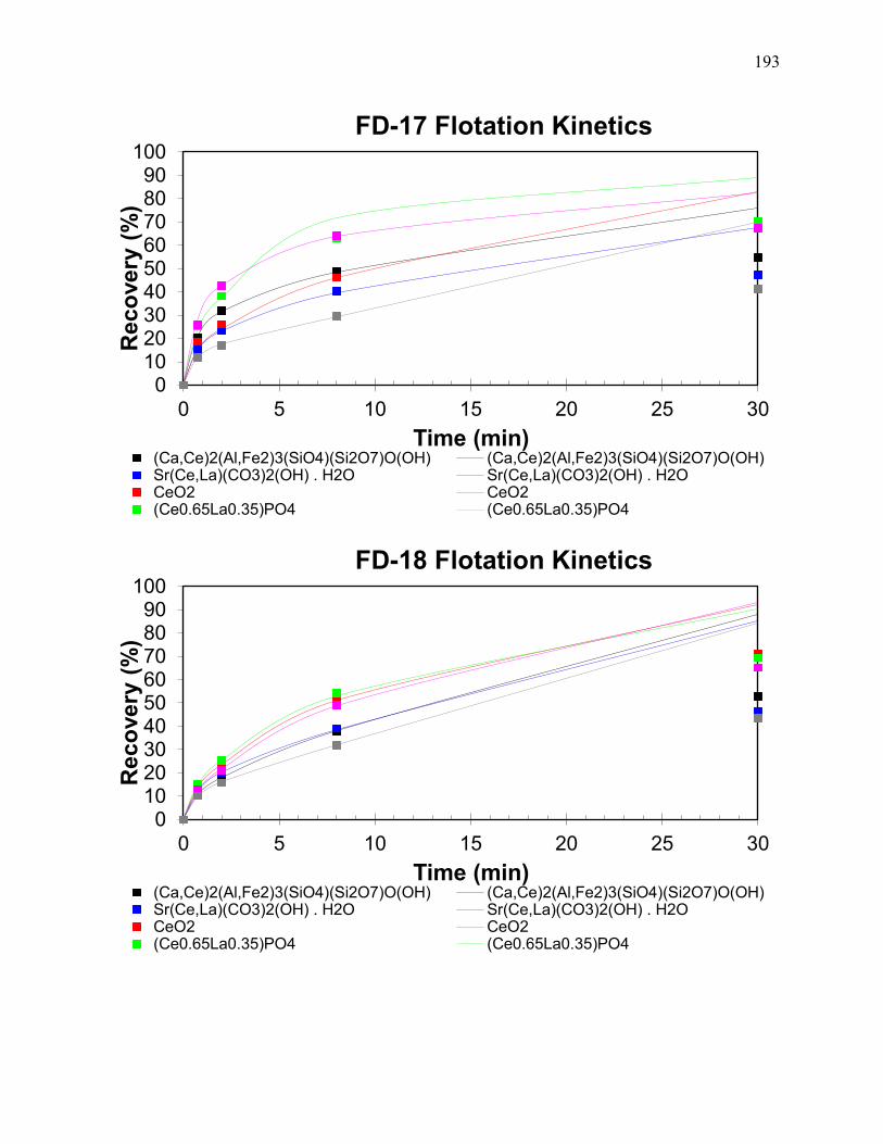
193

0102030405060708090

100

0 5 10 15 20 25 30

Rec

over

y (%

)

Time (min)



0102030405060708090

100

0 5 10 15 20 25 30

Rec

over

y (%

)

Time (min)



194

0102030405060708090

100

0 5 10 15 20 25 30

Rec

over

y (%

)

Time (min)



0102030405060708090

100

0 5 10 15 20 25 30

Rec

over

y (%

)

Time (min)



195

Appendix B: Raw Data

HIGH FIDELITY KINETIC MODEL FOR FLOTATION

Documents

Transcript of HIGH FIDELITY KINETIC MODEL FOR FLOTATION