
Hectospec, the MMT’s 300 Optical Fiber‐Fed Spectrograph
68
arXiv:astro-ph/0508554v1 25 Aug 2005 Hectospec, the MMT’s 300 Optical Fiber-Fed Spectrograph Daniel Fabricant, Robert Fata, John Roll, Edward Hertz, Nelson Caldwell, Thomas Gauron, John Geary, Brian McLeod, Andrew Szentgyorgyi, Joseph Zajac, Michael Kurtz, Jack Barberis, Henry Bergner, Warren Brown, Maureen Conroy, Roger Eng, Margaret Geller, Richard Goddard, Mike Honsa, Mark Mueller, Douglas Mink, Mark Ordway, Susan Tokarz, Deborah Woods, William Wyatt Smithsonian Astrophysical Observatory, a member of the Harvard-Smithsonian Center for Astrophysics, Cambridge, MA 02138 [email protected] Harland Epps Lick Observatory, UC Santa Cruz, Santa Cruz, CA 95064 and Ian Dell’Antonio Brown University, Box 1843, Providence, RI 02912 Received ; accepted
-
Upload
independent -
Category
Documents
-
view
0 -
download
0
Transcript of Hectospec, the MMT’s 300 Optical Fiber‐Fed Spectrograph

arX
iv:a
stro
-ph/
0508
554v
1 2
5 A
ug 2
005
Hectospec, the MMT’s 300 Optical Fiber-Fed Spectrograph
Daniel Fabricant, Robert Fata, John Roll, Edward Hertz, Nelson Caldwell, Thomas
Gauron, John Geary, Brian McLeod, Andrew Szentgyorgyi, Joseph Zajac, Michael Kurtz,
Jack Barberis, Henry Bergner, Warren Brown, Maureen Conroy, Roger Eng, Margaret
Geller, Richard Goddard, Mike Honsa, Mark Mueller, Douglas Mink, Mark Ordway, Susan
Tokarz, Deborah Woods, William Wyatt
Smithsonian Astrophysical Observatory, a member of the Harvard-Smithsonian Center for
Astrophysics, Cambridge, MA 02138
Harland Epps
Lick Observatory, UC Santa Cruz, Santa Cruz, CA 95064
and
Ian Dell’Antonio
Brown University, Box 1843, Providence, RI 02912
Received ; accepted

– 2 –
ABSTRACT
The Hectospec is a 300 optical fiber fed spectrograph commissioned at the
MMT in the spring of 2004. In the configuration pioneered by the Autofib instru-
ment at the AAT, Hectospec’s fiber probes are arranged in a radial, “fisherman
on the pond” geometry and held in position with small magnets. A pair of
high-speed six-axis robots move the 300 fiber buttons between observing config-
urations within ∼300 s and to an accuracy of ∼25 µm. The optical fibers run for
26 m between the MMT’s focal surface and the bench spectrograph operating at
R∼1000-2000. Another high dispersion bench spectrograph offering R∼35,000,
Hectochelle, is also available. The system throughput, including all losses in the
telescope optics, fibers, and spectrograph peaks at ∼10% at the grating blaze
in 1′′ FWHM seeing. Correcting for aperture losses at the 1.5′′ diameter fiber
entrance aperture, the system throughput peaks at ∼17%, close to our predic-
tion of 20%. Hectospec has proven to be a workhorse instrument at the MMT.
Hectospec and Hectochelle together were scheduled for 1/3 of the available nights
since its commissioning. Hectospec has returned ∼60,000 reduced spectra for 16
scientific programs during its first year of operation.
Subject headings: instrumentation: spectrographs, techniques: spectroscopic,
methods: data analysis
– 3 –
1. Introduction
1.1. Hectospec Overview
The Hectospec is a powerful fiber-fed spectrograph at the MMT Observatory in
routine operation since April 2004. During its first year of operation, Hectospec obtained
60,000 spectra during 79 scheduled nights, with 48 nights of clear weather. Hectochelle,
Hectospec’s high dispersion partner spectrograph, was scheduled for an additional 31 nights.
In total, Hectospec and Hectochelle were scheduled for 1/3 of the available MMT nights.
During Hectospec’s first year, it served 16 scientific programs.
Fabricant, Hertz & Szentgyorgyi (1994) and Fabricant et al. (1998b) outline the basic
design of the Hectospec fiber positioner, its bench spectrograph, and optical fiber probes.
Here, we emphasize: (1) the design refinements that occurred between 1998 and Hectospec’s
delivery to the telescope in August 2003 and (2) Hectospec’s performance at the telescope.
1.2. The Converted MMT and Its Optics
The MMT’s f/5 optical system is comprised of a 6.5 m primary mirror, a 1.7 m
secondary mirror, a series of large telescope baffles, a large refractive corrector, and a wave
front sensor used periodically to correct the figure of the primary mirror and the telescope
collimation. Fabricant et al. (2004) contains an overview of these components. Fata &
Fabricant (1994) and Callahan et al. (2004) describe the f/5 secondary and its support.
Fata & Fabricant (1993) and Fata, Kradinov & Fabricant (2004) discuss the f/5 wide field
corrector in more detail. Pickering, West & Fabricant (2004) describe the Shack-Hartmann
f/5 wave front sensor.
The wide field corrector has two modes of operation. For wide field spectroscopy with

– 4 –
optical fibers, the corrector provides a 1◦ diameter field of view on a curved but telecentric
focal surface 0.6 meters in diameter. The sag of the spectroscopic focal surface is 8 mm. In
the imaging mode, the corrector provides a field of view 0.58◦ in diameter on a flat focal
surface. The spectroscopic mode of the corrector includes counterrotating atmospheric
dispersion compensation prisms that are removed for the imaging mode.
The commissioning of Hectospec required the prior installation of the 1.7 meter f/5
secondary mirror at the MMT, which took place in April 2003. The wide field corrector
and the f/5 wave front sensor were commissioned during May and June 2003. The first
commissioning run with Hectospec took place in October 2003, and during this run we
obtained observations of nearby galaxy clusters. The second Hectospec commissioning
run was scheduled for April 2004. In mid April 2004 Hectospec was placed into routine
operation.
1.3. Hectochelle
Hectochelle uses Hectospec’s robotic fiber positioner and optical fibers to feed a high
dispersion bench spectrograph in place of Hectospec’s moderate dispersion spectrograph.
Single orders, or several overlapping orders, dispersed by Hectochelle’s echelle grating are
selected with bandpass filters. Szentgyorgyi et al. (1998) describe Hectochelle’s design.
2. Hectospec Fiber Positioner
2.1. Introduction
Hectospec’s robotic fiber positioner is unique for its high fiber placement speed while
retaining high positioning accuracy. The high speed robots meet their design goals reliably:
– 5 –
150 paired moves of the tandem robots in under 300 seconds, and with 25 µm fiber
positioning accuracy. The fiber robots attain this combination of high speed and accuracy
due to a very stiff mechanical system that settles rapidly, powerful servo motors that rapidly
accelerate the robots, and a sophisticated control system that incorporates many safety
features while minimizing communication overhead between system components.
Hectospec’s fiber geometry was first used by Autofib (Parry & Gray 1986), an early
robotic fiber-fed spectrograph for the Anglo-Australian Telescope with a single Cartesian
robot positioning 64 optical fibers. Hectospec’s 300 fiber buttons are held onto the (400
series stainless) steel focal surface with NdFeB magnets mounted in the bottom of the fiber
button. The magnets provide 200 g of holding force normal to the focal surface and >50 g
of holding force in the plane of the focal surface.
2.2. Fiber Buttons and Focal Surface Assembly
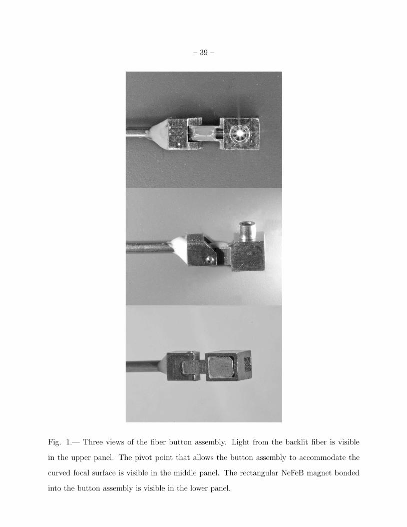
Figure 1 shows a fiber button assembly from three angles. The 1.27 mm diameter
stainless steel tube that protects the fiber after its exit from the fiber button is supported
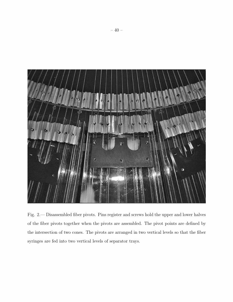
on its far end in brass pivot blocks. The fiber pivots are located 430 mm from the focal
plane’s center. The pivots are arranged in two vertical levels so that the fiber syringes are
fed into two vertical levels of separator trays. Using two levels provides more horizontal
space in the separator trays and protects the syringes from excessive bending as the fiber
button is moved tangentially on the focal surface. Figure 2 shows the (disassembled) fiber
pivots outside the edge of the focal surface.
– 6 –
2.3. Mechanical Design
The fiber positioner can be separated into two parts to allow servicing of the robots
and optical fibers. The upper unit (Figure 3) contains the two six axis robots and most
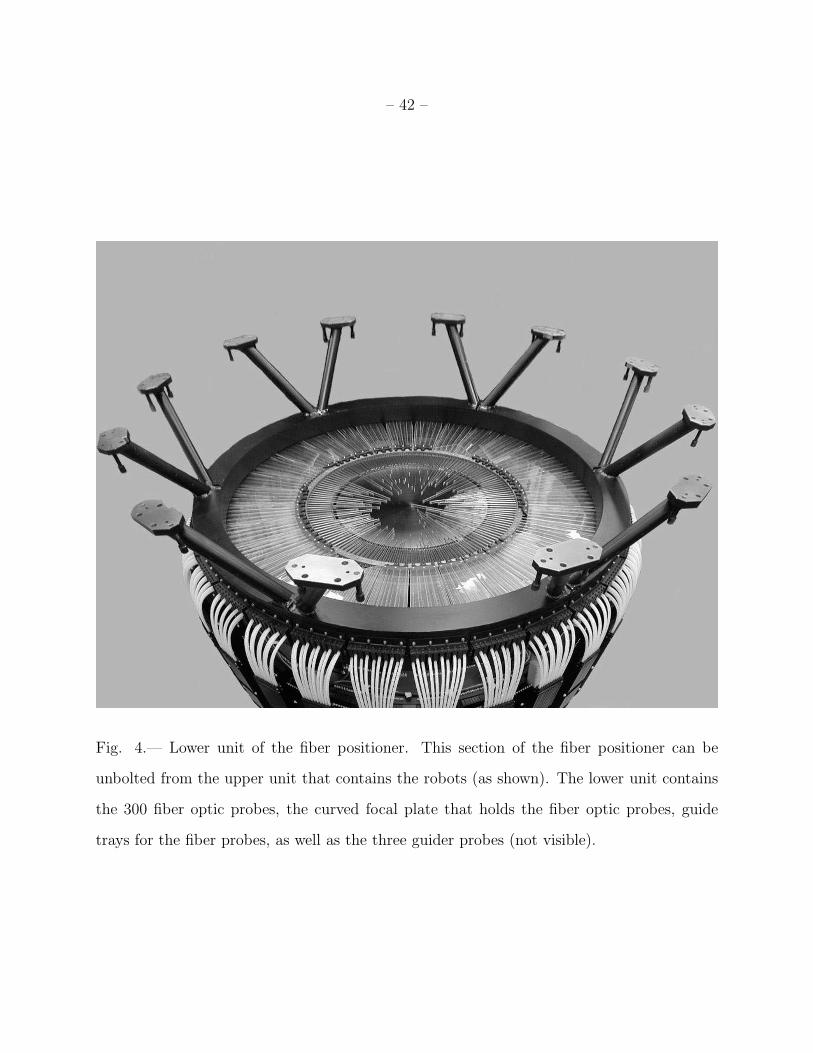
of the electronics. The lower unit (Figure 4) contains the fiber probes, the fiber shelves
(to prevent tangling of the optical fibers), the three guider probes and their track, the
intensified camera for the guider probes, and the fiber derotator assembly that allows the
fibers to follow instrument rotation. The two units are separated by removing protective
covers and then unbolting the upper end of the struts that connect the two assemblies.
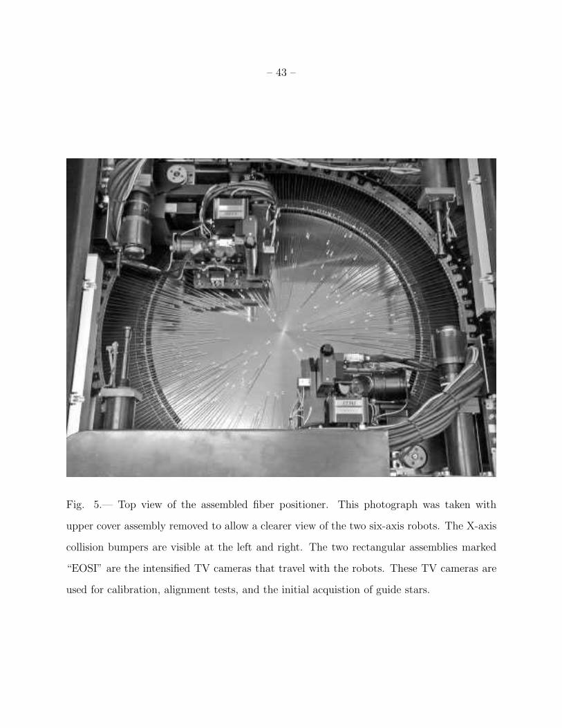
Figure 5 is a top view of the assembled upper and lower units.
A pair of high-speed six-axis robots operating in tandem position Hectospec’s 300
optical fibers. Each robot forms a three-axis Cartesian (XYZ) system that carries a
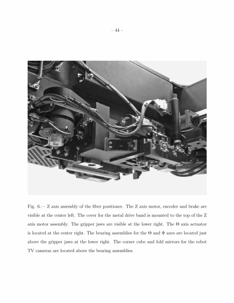
fiber gripper assembly. The Z-axis assembly (Figure 6) contains nested gimbals to allow
placement of the fiber buttons perpendicular to the curved focal surface, as well as
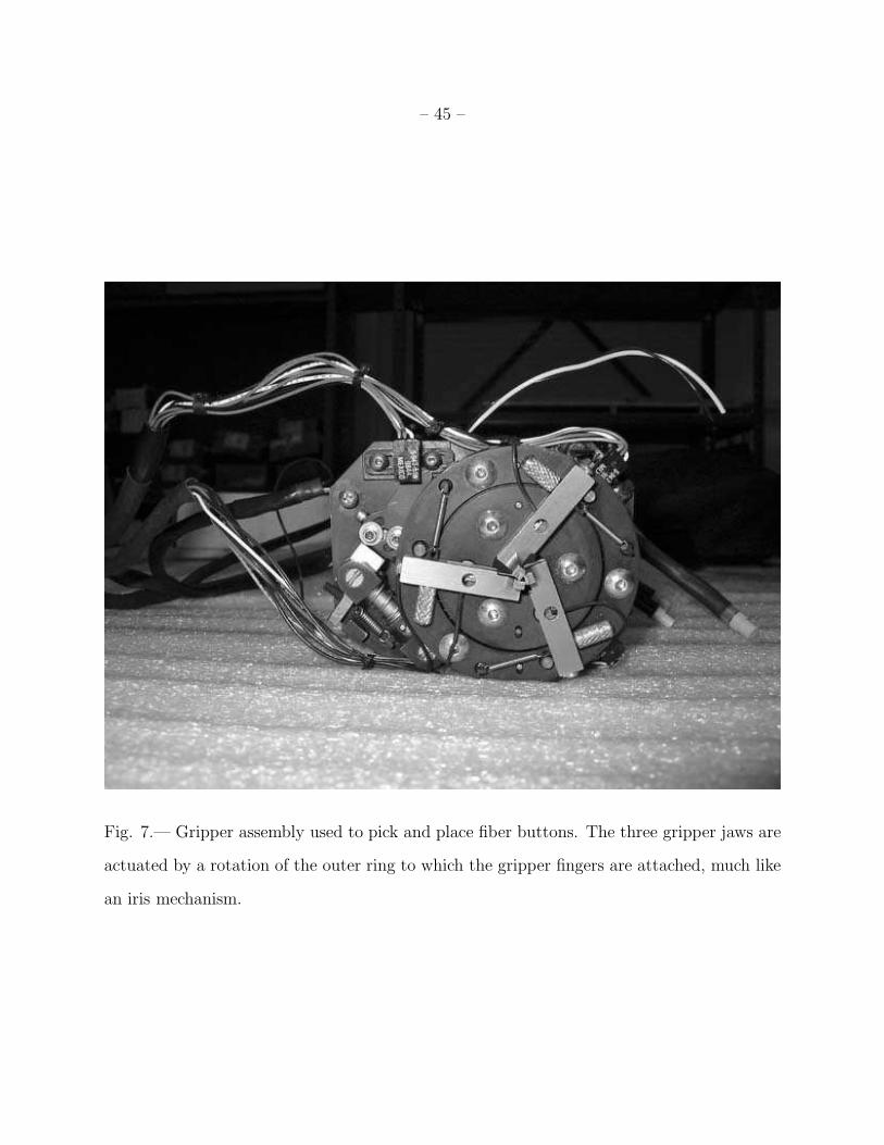
the gripper mechanism. Figure 7 shows the gripper assembly removed from the Z axis
assembly. The Hectospec gripper design is based on the earlier Hydra design (Barden et al.
1993). Many mechanical details including parts lists are found in the Hectospec Hardware
Reference Manual (http://cfa-www.harvard.edu/mmti/hectospec.html).
2.4. Speed and Accuracy
The timing budget for completing a Hectospec fiber repositioning consists of eight
steps: (1) coordinated XYΘΦ motion to the next button position, (2) Z axis down, (3)
gripper close, (4) Z axis up, (5) coordinated XYΘΦ motion to the new button position, (6)
Z axis down, (7) gripper open, and (8) Z axis up. In total each fiber repositioning requires
two coordinated XYΘΦ motions, four Z axis motions, and two gripper actuations. Table 1
– 7 –
gives approximate times for these motions; they total ∼1.8 s.
A combination of factors set Hectospec’s internal positioning accuracy: (1) the accuracy
of the servo loop closure, (2) the calibration of the axis encoders onto an orthogonal
Cartesian coordinate system (includes axis home reference repeatability), (3) button
movement as the gripper jaws are released, (4) the calibration of the fiber position within
the button body, (5) flexure of the focal surface from zenith to the observing position, and
(6) flexure in the guide probes over the course of an observation. Hectospec’s external
positioning accuracy also includes contributions from astrometric errors for the targets
and guide stars and instantaneous tracking errors. Table 2 summarizes the measured and
estimated magnitudes of the internal positioning error sources. We set a goal of 0.025 mm
for the total internal positioning error; Table 2 shows that the error contributions sum to
0.015 mm in quadrature and 0.036 mm in a worst case straight sum. The actual total
internal positioning error lies in between these estimates, or about 0.025 mm.
2.5. Robot Safety Features
The fiber positioning system has multiple levels of safety features built into the
hardware and the instrument control software. Our primary goal for these safety features
is to prevent collisions between the robots, collisions of the robots with the focal surface or
fibers on the focal surface, or high speed collisions of the robots into their mechanical limits
of travel. Additional safety features act to minimize the resulting damage if a collision
occurs. A large number of lower level safety checks stop robot motion on the detection of
an error condition that could result in damage to some part of the instrument.
– 8 –
2.5.1. Collision Prevention
The pair of robots start each move segment simultaneously and they wait until both
robots are finished before beginning the next move segment. (The eight move segments
are listed in Section 2.4.) Error conditions from either robot stop both robots. During the
paired moves the closest approach of the robots is 150 mm for the entire fiber pick and
place operation. Limit switches that detect approaches of the robots closer than 150 mm or
travel past the normal range of motion on all axes provide the next level of safety. Energy
absorbing bumpers on the X and Y axes produce a controlled deceleration of the robots
independent of the electronic and software systems once the limit switches are passed. The
most difficult limit to detect is a downward movement of the Z axis, because the appropriate
limit position varies over the focal surface due to its curvature. We built Z down limit
switches into each of Hectospec’s three gripper jaws; these switches are activated if the jaws
strike the focal surface or a fiber button. The entire gripper mechanism is spring loaded;
the gripper mechanism retracts if the spring preload is exceeded.
2.5.2. Lower Level Safety Features
A key safety feature built into most servo controllers, including the Delta Tau
Programmable Multi Axis Controllers (PMACs) used for Hectospec, is provided by the
following error monitor. The following error is defined as the instantaneous difference
between the commanded and actual positions read back from the encoder. The PMAC
servo controller can be programmed to begin a controlled deceleration when a preset
following error is exceeded. Each of Hectospec’s servo axes is protected by a following error
limit. The following error protects against servo runaway if an encoder signal is lost and
can provide safe shutdown if an obstruction is encountered. The following error provides
no protection for moves shorter than the preset following error. An additional level of
– 9 –
protection is provided for Hectospec’s powerful X and Y axes: the signals from rotary
encoders on the motor shaft and linear encoders on the axes are continously compared with
custom code in the PMACs and the system is shut down if a small error is exceeded.
Other safety features include over-temperature sensing, a PMAC CPU watchdog timer,
amplifier fault detection, move time out protection, and a dropped button sensor, all of
which terminate motion upon error detection. Many levels of error checking are also built
into Hectospec’s control software to prevent setting a fiber button down on top of another
button, to prevent striking a fiber button or part of the positioner structure with the robots,
or to move a fiber button beyond its safe travel limits.
2.6. Robot Calibration Techniques
The major portion of Hectospec’s calibration was carried out with a custom grid of
dots etched into an 0.61 m diameter Astrosital disk by Max Levy Corp. This calibration
disk is the same diameter as Hectospec’s focal surface and is pinned and screwed into three
support blocks in the guide probe tracks when in use. The grid is illuminated with high
frequency fluorescent lamps carried on the robots, and the dot positions are recorded by
the intensified cameras carried in the robot gripper assemblies. After averaging for 5 to 10
seconds, the noise in the dot position measurements is of order 2 µm. The dot positions
have an intrinsic positional accuracy better than 6 µm. The positions of the dots recorded
in the intensified robot cameras as the robots are commanded to move to the nominal
dot position allows us to transform the XY encoder positions to an orthogonal Cartesian
system. The largest errors prior to calibration are ∼40 µm, a testament to the accuracy
of Hectospec’s machining and to the quality of the axis rails. Most of this error is due to:
(1) small rotations of the robots as the gripper assembly moves along its rails and (2) the
position of the encoders at the guide rails, 150 mm above the position of the fiber button in
– 10 –
the gripper jaws (and the position of the grid dots during calibration). The spacing of the
guide blocks on the rails is also about 150 mm, so that deviations of the rail bed will map
∼1:1 to deviations of the gripper jaws. This type of position sensing error is commonly
termed Abbe error.
The gimbal axes were calibrated using the robot intensified cameras and a fine pattern
of dots etched into a smaller grid placed on the focal surface. The Z axis scale is accurately
determined by a rotary encoder and a precision ball screw driven through a 1:1 precision
pulley system. A displacement measuring laser interferometer was used to verify that this
scale is accurate to better than 1 µm RMS over the full range of travel. The ball screw
accuracy is so high that we removed an unnecessary LVDT intended for Z axis feedback. (A
small slip of ∼1 µm upon each downward movement of the Z-axis is removed by detecting a
home sensor each time the Z-axis is raised.) The position of the focal surface relative to the
robot axes was determined with a Kaman noncontact displacement probe mounted to the
gripper assembly. The robots were commanded to move across the focal surface in a grid
pattern, and the position of the focal surface was determined at each point.
2.7. Electronics
The main design challenge for Hectospec’s electronics was the distribution and routing
of cables associated with the 15 motor axes and their associated encoders and limit switches.
The weight and volume limits imposed by Hectospec’s Cassegrain mounting location
precluded mounting the majority of Hectospec’s electronics onboard. The relatively large
power supplies, servo amplifiers, stepper motor drivers, cable distribution boxes, and signal
and power conditioning components are located in remote racks. A total of 20 cables with
∼460 total conductors run between the fiber positioner and these racks, while 10 cables
with ∼110 total conductors run between the bench spectrograph and the electronics racks.
– 11 –
To maintain high reliablity in the signal path, heavy-duty Mil-C circular connectors are
used where cables must be disconnected to dismount the fiber positioner. The electronics
rack contains seven main electronics boxes: (1) an interface box that accepts the Mil-C
cables from the fiber positioner and distributes the signals to internal rack cables, (2) an
interface box that performs similar functions for the bench spectrograph cables, (3) a signal
conditioning and interface box for the Delta Tau PMAC servo controllers, (4) a pair of servo
electronics boxes that contain the X,Y,Z,Θ,Φ servo amplifiers as well as the gripper stepper
motor driver, (5) a stepper motor drive bay for the guider probe and spectrograph stepper
motors, (6) a power supply box, and (7) a power conditioning and distribution module.
On the fiber positioner there are four electronics boxes: (1) the main interface box that
accepts most of the Mil-C cables and distributes signals and power to internal cables, (2)
a smaller interface box that accepts the Mil-C cables for the X,Y,Z servo motors, (3) an
electronics box with a CPU and active circuits for on-board control functions, and (4) a
small auxiliary box with an over-illumination sensor to protect the intensified cameras as
well as power supplies for the fluorescent lamps used to illuminate the calibration grids.
Surge and over-voltage protection is provided in each of the main interface boxes
at the fiber positioner, bench spectrograph, at the rack, as well as in the rack-mounted
power conditioning box. Further details can be found in the Hectospec Hardware Reference
Manual (http://cfa-www.harvard.edu/mmti/hectospec.html).
2.8. Guider Probes
The guider probes each move one section of a trifurcated coherent fiber bundle along
an 86◦ arc just outside the focal surface plate that supports the fiber probes at the MMT
focus. Fabricant et al. (1998b) describe the basic geometry of the guider probes. The guider
– 12 –
probes are actuated along a curved rail by a stepper motor driving a pinion gear against a
large-diameter fixed gear. The guider probe has a brake mechanism, released by a solenoid,
to hold the probe in place after the guider probe is positioned with the telescope zenith
pointing. The largest challenge with this mechanism was designing a brake mechanism
that would grip firmly and that could be released with the limited force available from the
solenoid. Limited clearance from the structure precluded use of a large solenoid, and we
reworked this mechanism twice to reduce the friction in the brake release mechanism. In
future instruments pneumatic actuators might be a good replacement for solenoids because
the pneumatic actuators offer a better power to weight ratio and do not dissipate as much
heat.
2.9. Instrument Control Computers
The Hectospec fiber positioner is controlled by a Motorola 142 VME single board
computer running Linux. This computer is mounted in the same VME rack that houses the
two VME Delta Tau PMAC servo controllers. The hctserv server program running on the
Motorola 142 accepts high and low level commands from clients and issues the appropriate
motion control commands to the PMACs. Normally, the fiber positioner is operated by
sending a high level sequence command to move the fibers from one configuration to
another. The sequence begins when the client program reads the current fiber configuration
from the hctserv server which is stored in static memory. The client computes the sequence
of fiber pick and place operations required to go from the current to the new configuration,
and prepares a sequence table of paired pick and place moves for the two robots. The
sequence table is sent to the hctserv server, which checks that the sequence table can
execute without crossing fibers or colliding the robots. Each paired move is successively
loaded into the PMAC and executed.
– 13 –
A rack mounted Intel-based PC running Linux, “Snappy”, contains three Data
Translation DT3155 frame grabber boards that capture images from the two robot TV
guiders and the three guider probes. Snappy also communicates with the fiber positioner’s
internal electronic box through an RS-232 interface to control the gain of the intensified TV
guider cameras, to control internal lamps, and to monitor motor temperatures. A guider
server running on a remote computer acquires guide frames from Snappy and calculates
guide corrections for the telescope.
3. Hectospec Spectrograph
3.1. Mechanical Design
Fabricant et al. (1998b) describe the mechanical layout of Hectospec (see also Fabricant,
Hertz & Szentgyorgyi (1994)) and Fata & Fabricant (1998) describe the optics mounts.
Here we describe the dewar assembly and rotary shutter not previously discussed in the
literature.
3.1.1. Dewar Design
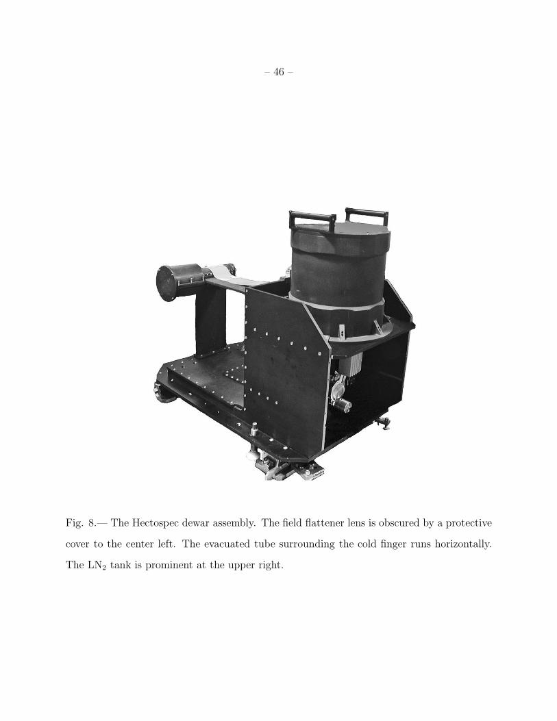
Hectospec uses an internal focus catadioptric camera (Fabricant, Hertz & Szentgyorgyi
(1994), Fabricant et al. (1998b)). Thus there is a premium upon mimimizing the footprint
of the CCD dewar support structure in the beam. The CCD dewar is an ∼100 mm diameter
cylinder supported on a thin vertical foot and by a thin-section horizontal evacuated tube
that surrounds the dewar’s cold strap. The cold strap runs between the dewar and a liquid
N2 cryostat mounted outside the optical beam running to and from the on-axis camera
mirror. The dewar window also serves as a field flattener lens for the camera. Figure 8
shows the dewar assembly. The dewar assembly is mounted on a focus stage.

– 14 –
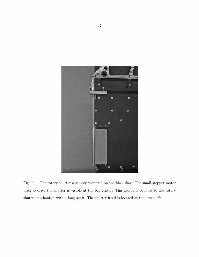
3.1.2. Rotary Shutter
At the spectrograph entrance “slit”, the optical fibers are arranged in two parallel
columns spaced ∼1.6 mm apart. The fibers in each column are spaced on 0.96 mm centers,
but the two columns are offset by 0.48 mm, giving a final effective fiber to fiber spacing
of 0.48 mm. The width of the structure holding the fibers, the “fiber shoe”, has been
minimized to reduce the obscuration of the beam returning past the fibers from the on-axis
collimator mirror. A narrow rotary shutter assembly is mounted on the fiber shoe in front
of the optical fibers. The rotating part of the shutter is an ∼150 mm long slotted cylinder.
The shutter is toggled between open and closed with 90◦ rotation actuated with a stepper
motor. The rotary shutter assembly mounted on the fiber shoe is shown in Figure 9.
3.2. CCDs and Array Electronics
Hectospec uses two E2V model 42-90 4608X2048 CCDs with 13.5 µm pixels, arranged
in a 4608X4096 array. The long axis of the CCDs are parallel to dispersion. Hectospec’s
CCDs have superb cosmetic quality, and the entire two CCD array has only a single bad
column. At a readout rate of 100,000 pixels s−1, the readout noise is 2.8 e− RMS. At the
operating temperature of -120 ◦C, the dark current is very low: 1 e− in 900 s of integration.
The electronics have a gain of 1 e− ADU−1, matching to a few percent between the four
amplifiers. The count rate due to background radiation is 1 event s−1 integrated over the
region occupied by the fiber spectra on the two CCD array.
Hectospec shares its array controller electronics design with the other MMT f/5 optical
and infrared instruments including Hectochelle, Megacam, and SWIRC. The design of these
electronics was driven by the requirements of the 72 channel Megacam version (Geary
2000). Hectospec’s two CCDs are read out through four amplifiers in 46 sec.
– 15 –
3.3. Optics
3.3.1. Image Quality
Fabricant et al. (1998b) and Fabricant, Hertz & Szentgyorgyi (1994) describe
Hectospec’s optics; here we describe the optical performance of the as-built spectrograph.
Hectospec’s optics have a reduction of 3.45, with an anamorphic demagnification (in the
spectral direction) of 1.06 with the 270 groove mm−1 grating. With perfect optics, the
image of the 250 µm fiber should be an ellipse 5.4 by 5.1 pixels across. The RMS image
diameters produced by the real optics, when illuminated by a point source emitting into
an f/5.3 cone, are 1.3 to 1.8 pixels. Optical ray traces with ZEMAX predict that the
azimuthally averaged two dimensional FWHM of the fiber image should be 4.8 to 5.0 pixels,
which agrees with the observed azimuthally averaged FWHM. The tails of the observed
images are broader than the ZEMAX prediction: the observed 95% encircled energy radius
is 4.2 pixels compared with the predicted 3.5 pixels. We attribute this difference to small
amounts of light emerging from the fibers at focal ratios faster than the modeled f/5.3;
this light is imaged in the wings of the fiber image. We have a pupil mask at the grating
to reject most of this focal ratio degraded light, but the mask is somewhat oversized to
account for pupil rotation that depends on field angle.
We discovered one general feature of the HIRES style of camera (Epps & Vogt 1993)
used in Hectospec: a ghost pupil is formed between the focal surface and the field flattener
element by light reflected from the CCD and then back again from the front surface of the
field flattener. The intensity of this ghost pupil is reduced by a factor of ∼10−3 relative
to the main image and the ghost pupil area is nearly as large as the detector area. We
noticed the ghost pupil because we operated the spectrograph briefly with a damaged
antireflection coating on the front surface of the field flattener. The reflectivity of the
damaged antireflection coating was about an order of magnitude larger than normal,

– 16 –
increasing the intensity of the ghost pupil by a corresponding factor. Once we replaced the
field flattener with a undamaged spare, the ghost pupil faded into obscurity, but it may be
wise to keep an eye on this issue in designs of this family of optics.
3.3.2. Optical Coatings
The initial optical coatings for the Hectospec spectrograph were developed for the FAST
spectrograph (Fabricant et al. 1998a) at Whipple Observatory’s 1.5 m Tillinghast Telescope.
FAST’s high throughput Sol-gel antireflection coatings and UV-enhanced overcoated silver
reflection coatings gave many years of service and we expected the same performance in
Hectospec. Hectospec’s Sol-gel antireflection coatings have been trouble free, but the first
protected silver coatings on the Hectospec mirrors were noticeably discolored by late 2002,
approximately three years after their coating. Reflectivity measurements indicated low
reflectivity between 5000 and 6000 A. We decided to strip the original coatings and to
recoat with the Lawrence Livermore National Laboratory (LLNL) durable silver reflective
coating (US Patent 6,078,425). The LLNL coating has slightly lower peak reflectivity than
the original (fresh) coating, but offers much better reflectivity below 4000 A.
3.4. Gratings
Hectospec’s 259 mm collimated beam diameter requires large custom ruled gratings.
Hectospec currently has two gratings: a 270 groove mm−1 grating blazed at 5000 A and
a 600 groove mm−1 grating blazed at 6000 A. In both cases we specified a 5000 A blaze,
but the blaze angle has proven to be the most difficult parameter to control in ruling
these large gratings. The 6000 A blaze for the 600 groove mm−1 grating was the closest to
specification achieved in four attempts. The 270 groove mm−1 grating provides a dispersion

– 17 –
of 1.2 A pixel−1 and a resolution of 6.2 A FWHM. The 600 groove mm−1 grating provides
a dispersion of 0.5 A pixel−1 and a resolution of 2.6 A FWHM. Both gratings have a
peak absolute efficiency of 72%. Higher ruling density gratings might be best provided by
assembling grating mosaics.
4. Hectospec Optical Fibers
4.1. Design of Fiber Run from Positioner to Spectrograph
The design of the optical fiber run between the fiber positioner and bench spectrograph
turned out to be a much larger challenge than we had imagined during the Hectospec’s
conceptual design phase. Optical fibers offer a unique means of mapping a spectrograph slit
efficiently onto a large number of objects distributed over a very large field of view. However,
fibers must be used carefully if they are not to severely compromise the sensitivity of the
spectrograph by degrading the focal ratio of the light incident on the fiber. Degradation
of the focal ratio in a fiber results in a loss of light in the spectrograph optics unless the
spectrograph optics are significantly oversized. Oversizing the optics is expensive in a
spectrograph as large as Hectospec’s, and forming good images from the light scattered into
faster focal ratios makes a difficult optical design problem harder. Focal ratio degradation
arises from mechanical stress of the fibers. Focal ratio degradation will typically cause time
variable throughput losses as the stress experienced by the fibers changes as the telescope
pointing direction changes. These throughput variations are doubly troublesome because
good sky subtraction relies on an accurate fiber to fiber throughput calibration.
We were aware from the time that we began work on Hectospec that the mounting
details of the fibers in the fiber probes at the fiber positioner end and in the fiber slit at the
spectrograph end of the fibers are important in controlling focal ratio degradation, but our
– 18 –
test program demonstrated the importance of what happens in between. We engineered
thermal breaks in the teflon tubing to address the thermal expansion mismatch between
the fused silica fiber and the teflon tubes that protect the fibers. Fabricant et al. (1998b)
describe the basic design elements that we used to control focal ratio degradation in the
fiber run. The other important design driver for the fiber run is that it must allow easy
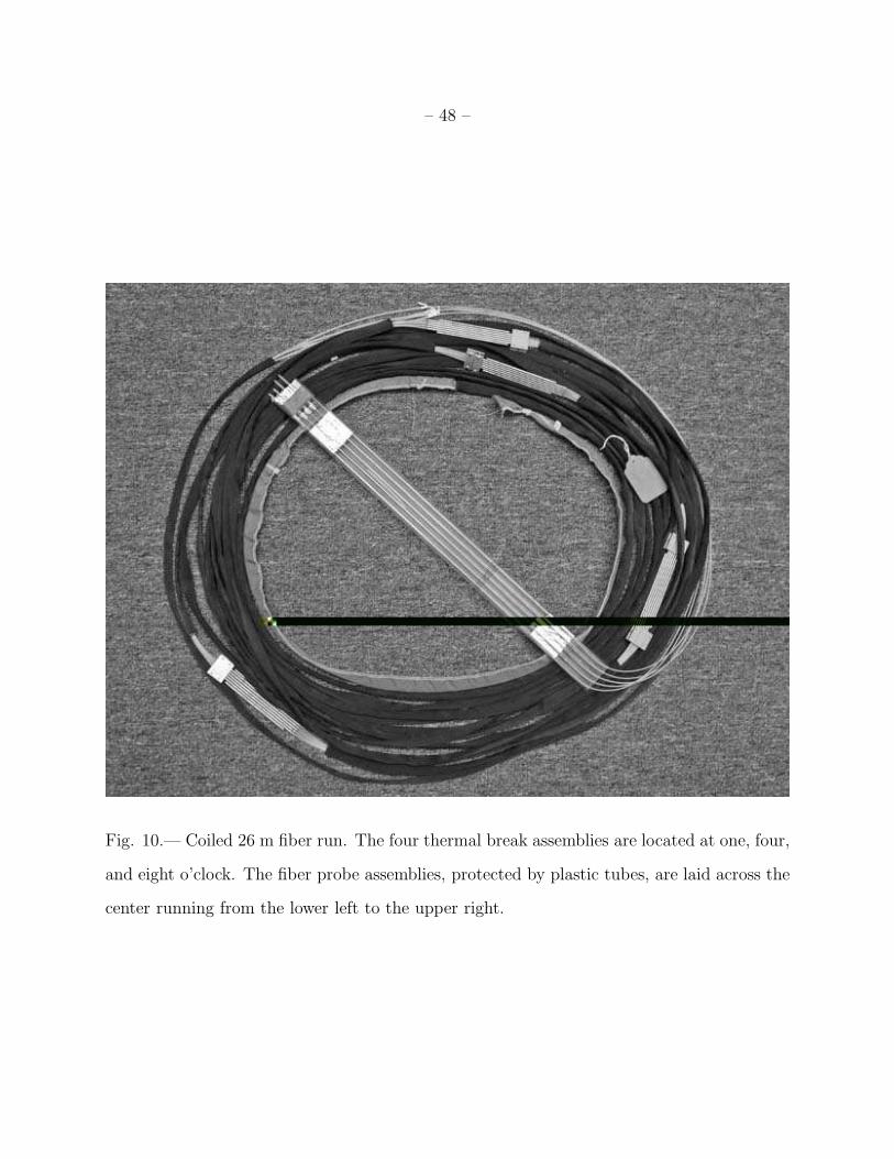
mounting and dismounting of the Hectospec on the telescope. Figure 10 shows the design of
the fiber run and the position of the thermal breaks that allow for the differential thermal
expansion of the fibers and their protective teflon tubes. Figure 11 is a closeup of one of the
four thermal breaks in the fiber run.
4.2. Laboratory Tests of the Optical Fibers
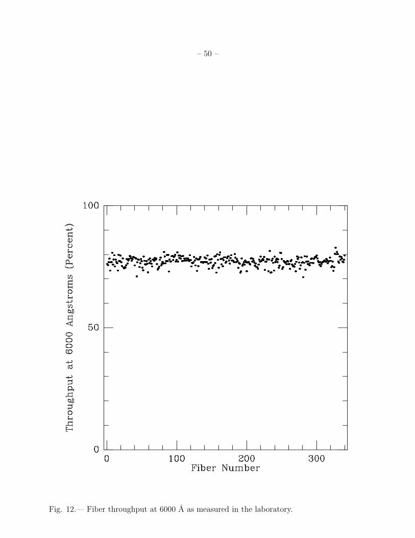
Our specifications called for a total fiber throughput of 75% at 6000 A into a focal
ratio of f/5.3, the final focal ratio of the spectroscopic wide field corrector and the design
focal ratio of the Hectospec bench spectrograph. At 6000 A the internal absorption of
Hectospec’s 26 m long fibers is 6%, the Fresnel reflection loss at the uncoated BSM51Y
prisms at the fiber input end is 5.3%, and the Fresnel loss at the bare fiber output end is
3.5%. The total throughput accounting for only these three fiber losses is 86%, requiring
that 87% of the light entering the fibers at f/5.3 exit within an f/5.3 cone if the total
throughput specification is to be met. As Figure 12 shows, we met our goal for total fiber
throughput with an average throughput of 77% and a standard deviation of 2%.
– 19 –
5. Observing with Hectospec
5.1. Observation Planning Software
Roll, Fabricant & McLeod (1998) describe the basic algorithms used in Hectospec
observation planning to match fiber probes to targets. Currently, each Hectospec observer
is responsible for planning the fiber configurations to be used at the telescope. The observer
begins by assembling a catalog containing the desired targets as well as potential guide
stars in the field. Observers may priority rank targets in the catalog and assign a minimum
and maximum number of fibers to each rank. The guide stars and the targets must have
excellent relative astrometry because the guide stars establish the field alignment. The
observer uses the xfitfibs program to create instrument configuration files from the input
catalog. xfitfibs combines the observation planning software with a graphical user interface
(GUI). The observer may use xfitfibs to plan multiple fiber configurations with multiple
field centers and to rank these centers in priority.
In addition to matching fibers to targets, xfitfibs selects guide stars, and assigns fibers
for the measurement of the sky background. The user can drag field centers with a mouse or
enter new field centers into a table and view the effects on a graphical display. The display
indicates guide stars within range of the guide probes as well as those accessible by changing
the instrument rotator angle. The xfitfibs software derives guide star magnitudes from
either the 2MASS or GSC2 catalogs, removes stars outside the specified magnitude range,
and aditionally removes non-stellar objects using GSC2 classifications or by SExtractor
classification from DSS images. Stars with close companions or brighter neighbors in the
field of the guide probes are also excluded. Selection of bright guide stars (R<16) minimizes
setup time with the intensified robot and guide cameras and allows operation in the full
moon.

– 20 –
5.2. Queue Operation
Hectospec is operated in queue mode to use valuable telescope time efficiently and
to distribute the time lost due to weather, telescope and instrument malfunctions evenly.
The goal of the queue scheduling is to distribute the available productive observing time
proportionally to the nights scheduled by the Time Allocation Committees. The MMT is
scheduled in trimesters, and the queue scheduling is for a single trimester at a time. The
queue schedule must be continually updated through an observing run in response to the
weather conditions and telescope/instrument performance. The observers provide the queue
manager with completed fiber configurations, which include the sequence of observations,
the fiber layout, and valid guide stars. These layouts are checked and then scheduled as
time permits. The fiber positioner is operated by experienced robot operators on behalf of
the queue. The robot operator also oversees the acquisition of calibration data in the late
afternoon and early evening including HeNeAr wavelength calibrations, incandescent lamps
for flatfielding, and typically twilight sky flatfield exposures. During the night, observers
assigned telescope time operate the spectrograph and evaluate the data quality on behalf
of the queue. Observers thereby gain firsthand experience with Hectospec’s operation and
capabilities, avoiding some of the communication difficulties that others have reported in
the operation of observing queues isolated from the scientist who will ultimately use the
data.
5.3. User Interfaces
5.3.1. Hobserve
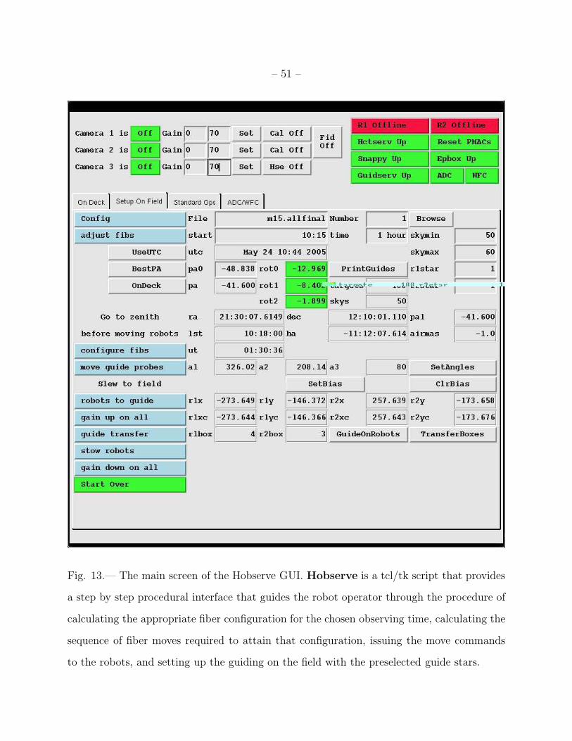
Hobserve (Figure 13) is a Tcl/Tk script that provides a step by step procedural
interface that guides the robot operator through the procedure of calculating the appropriate

– 21 –
fiber configuration for the chosen observing time, calculating the sequence of fiber moves
required to attain that configuration, issuing the move commands to the robots, and setting
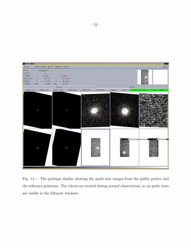
up the guiding on the field with the preselected guide stars. A separate graphical user
interface (GUI) (guidegui (Figure 14) displays the guide star images superposed on the
guider target positions. The Hobserve script coordinates the actions of several servers and
calls other high level shell scripts to accomplish its functions.
5.3.2. SPICE
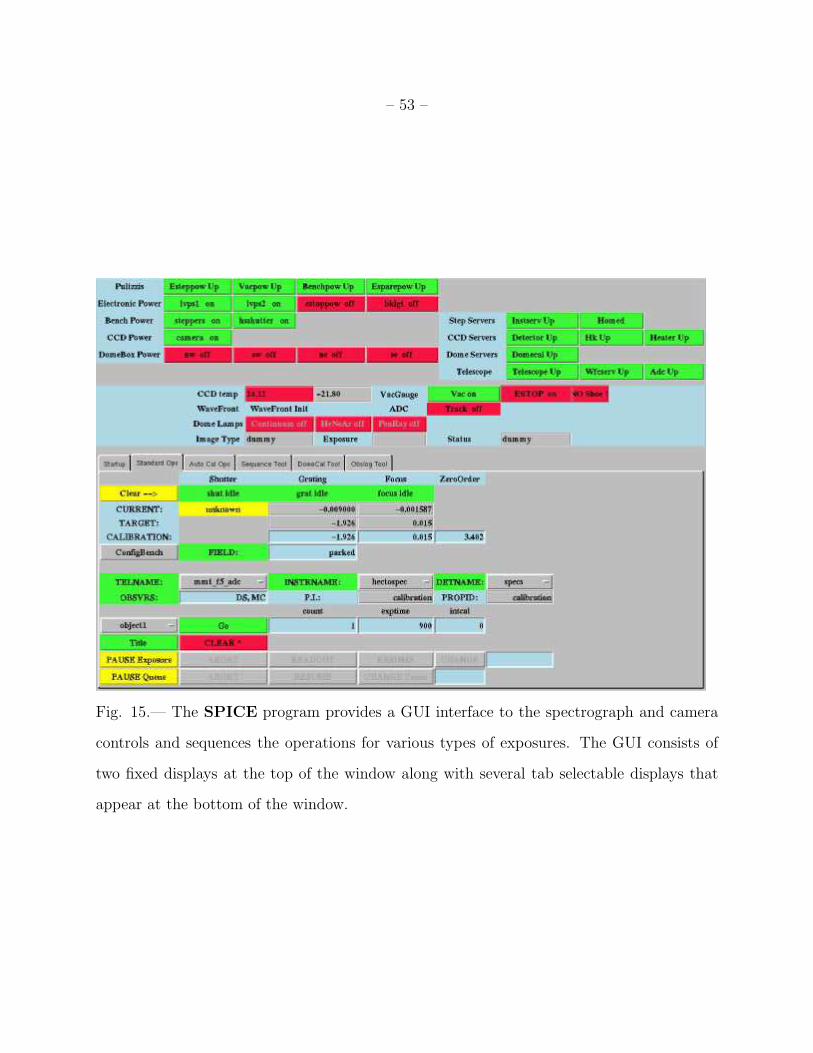
The SPICE Tcl/Tk program (Figure 15) provides a GUI interface to the spectrograph
and camera controls and sequences the operations for various types of exposures. The GUI
consists of two fixed displays at the top of the window along with several tab selectable
displays that appear at the bottom of the window. The upper fixed display indicates the
status of the system power controls and of the software servers that control hardware
components. The text message within the status buttons and the color of the status buttons
change together to indicate the instrument state. Toggling these buttons toggles the state of
the power or software server. The lower fixed display provides housekeeping information as
well as exposure status. The housekeeping items include the dewar temperature, the status
of the calibration lamps, the tracking status of the ADC prisms, and the position of the
wave front sensor carriage. The exposure status information includes the current exposure
count within the requested number of exposures, the current exposure type (skyflat, object,
bias, dark, etc.), and the current exposure state (exposing, reading out, etc.).
The observer can select one of four user-selectable tabbed displays: an initialization
tool, a standard operations tool, a calibration lamp tool, and an observing log tool. The
initialization tool controls the sequencing of powering up and homing the three spectrograph
axes (shutter, focus, and grating stage), as well as bringing up the required software servers.

– 22 –
The standard operations tool is the main tabbed display window that the observer uses
to acquire data and control the spectrograph. Within this window the grating rotation,
focus position, and shutter status are displayed and can be controlled. The current fiber
configuration file name is displayed, but the fiber configuration is controlled from the
Hobserve interface. The observer selects the desired exposure type from a pull-down
menu (object, dark, bias, domeflat, HeNeAr, focus, etc.) and specifies the desired exposure
time and number of exposures. Pressing “Go” initiates the exposure sequence. During
the initialization of the exposure, the software checks for possible problems including a
mismatch between the requested and encoded grating rotation and focus position, blocking
by the wavefront sensor, illumination of calibration lamps at inappropriate times, lack of
guiding signals, and ADC prism tracking turned off. The focus procedure automatically
moves the grating to the zero order position and takes a sequence of CCD charge-shifted
exposures at different focus settings. The grating is returned to its nominal position at the
end of the focus run. Focus changes during a run appear to be negligible.
The calibration lamp tool allows the observer to control the calibration lamps that
illuminate a screen mounted on the MMT building shutters. The calibration lamps are
mounted in four identical lamp boxes mounted in the MMT chamber. Lamp status, lamp
voltages, and lamps currents are displayed in a comprehensive color-coded table.
The observing log tool provides a summary of each of the exposures in the selected
night’s directory and a text box for the observer to annotate each exposure. A PostScript
formatted observing log of all the exposures (with observer comments) for the current night
is produced and archived.
– 23 –
5.4. Observing Sequence
At the beginning of the night or during an exposure on the previous field, the robot
operator loads in the next fiber configuration in the “on-deck” window of hobserve. The
expected start time and exposure duration of the observation are entered, and the fiber
positions are retweaked for the airmass and instrument rotator position at the expected
exposure midpoint. Depending on the nominal position angle entered during observation
planning, the rotator demand angles may exceed the ±90◦ soft limits. Therefore, the
position angle can be reset by the robot operator to minimize the rotator demand angles. If
guide stars are available in two of the three guide star probes, the “on-deck” configuration
is ready to go. If two guide stars are not available at this position angle, the position angle
can be manually adjusted to find minimum rotator demand angles consistent with obtaining
two guide stars. In the worst case, if two guide stars are not available at acceptable rotator
angles, another configuration can be chosen without loss of observing time.
We begin the reconfiguration process by slewing the telescope to the zenith. The robots
are capable of operating at any combination of zenith angle and rotator angle, but we
reconfigure the fibers with the telescope zenith pointing to minimize the power dissipation
and load on the drive components. After the robots reposition the fibers, the guide probes
are moved to correct guide star positions. The telescope is then slewed to a bright star
near the field position, and the wave front sensor is deployed to correct the primary
support forces and telescope collimation. While the wave front sensor probe is retracted,
the telescope is slewed to the field position and the instrument rotator is set to track the
desired position angle. The robot guide cameras are sent to the guide star positions and
the telescope pointing and the rotator angle are adjusted with autoguiding software until
the guide stars appear at the positions corresponding to a fiber held in the gripper jaws. A
pellicle beam splitter in the robot optical train allows 50% of the light to pass through to
– 24 –
the guide probes. The positions of the guide stars in the guide probes are captured and the
guiding is then transferred to the guide probes. This procedure directly ties the guiding to
the robot-defined coordinate system upon which the fibers are positioned. As soon as the
robots are parked an observation can begin.
6. Hectospec Performance at the MMT
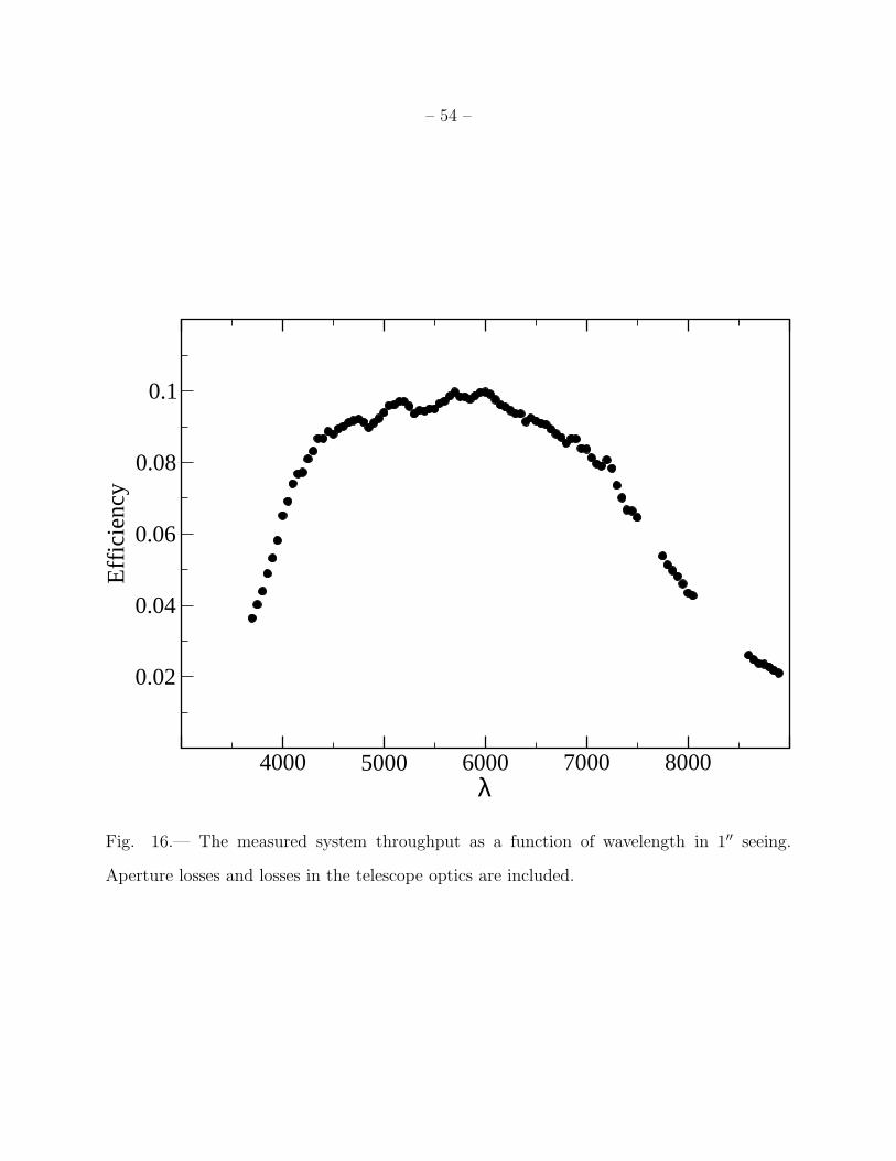
6.1. Throughput
We measured the throughput of Hectospec with the spectrophotometric standard star
BD+284211, stepping the star across one of Hectospec’s fibers to determine the point
of maximum throughput to eliminate light loss due to astrometric errors. With a direct
spectrograph, the entrance aperture is normally opened as wide as possible to separate the
measurement of spectrograph throughput from aperture losses. With fibers, the entrance
aperture is fixed and we measure total throughput including aperture losses. Figure 16
shows the derived throughput measurement for BD+284211 in 1′′ FWHM seeing. We have
separately calculated the aperture losses for Hectospec’s 1.5′′ diameter fibers as a function
of seeing using images obtained with Megacam; in 1′′ FWHM seeing we find that a 1.5′′
diameter contains 59% of the light, giving an aperture correction of 1.7. Referring to Figure
16 and applying this correction, the system throughput peaks at ∼17% between 5000
and 6000 A. Our prediction for the total system throughput peaked at 20% in the same
wavelength region, in reasonable agreement with the measurement.
6.2. Thermal Flexure of Bench Spectrograph
The room that encloses the Hectospec and Hectochelle bench spectrographs is one
level above the telescope chamber floor, and shares a common wall with the telescope
– 25 –
chamber. The spectrograph room is not well insulated from the telescope chamber due
to several doors and perforations. As a result, the temperature in the spectrograph room
fluctuates considerably more than we had planned. The nightly temperature swings
lead to temperature gradients in the optical bench and optical mounts that lead to
thermally-induced image motion with a maximum excursion of one pixel in both the spatial
and spectral directions during the course of a night. Larger shifts of a few pixels occur over
the course of an observing run. As discussed in Section 7.2, the shifts during a night are
easily corrected by tracing the positions of the fiber spectra and by tracking the positions
of night sky emission lines. During August 2005, we will replace the coated black cloth
currently enclosing the bench spectrographs to prevent light leaks with light-tight insulated
panels. This replacement will remove a potential fire hazard from the light-tight but
flammable cloth and improve the thermal insulation in the spectrograph room.
6.3. Gravitational and Rotator-Induced Flexure of Fiber Positioner
Our finite element models of Hectospec predicted that the Hectospec’s focal plane
assembly (onto which the fibers are attached) would shift by ∼50 µm relative to the robot’s
gripper assembly as the telescope pointing changes from zenith to an elevation angle of
30◦. This flexure is relevant because we use the robots to establish the correct position of
the guide stars in the guider probes. We took advantage of a cloudy night to measure this
flexure by placing the fibers on the focal surface at the zenith in the usual fashion, tipping
the telescope in elevation, and measuring the position of the backlit fibers. The average
deflections that we measured moving from an elevation angle of 90◦ to an elevation angle
of 30◦ are 40 µm in one robot and 42 µm in the other. We also noticed that rotating the
instrument rotator produces repeatable deflections of up to 25 µm if the elevation angle is
held constant. Rotator-induced deflections were anticipated, and set stringent requirements
– 26 –
on the accuracy of the rotator bearing.
6.4. Observing Overhead
The elapsed time between completing an exposure on one field and beginning another
is 1040 s. Table 3 lists the items that contribute to the observing overhead. The observing
overhead will drop slightly with increased automation of the wave front sensing procedure,
but is unlikely to drop much below 900 s.
6.5. Hectospec Reliability
Hectospec has proven to be reliable at the telescope despite its complexity. We have
lost ∼4 nights of observing time in Hectospec’s first year of operation due to instrument
malfunctions. The most serious incident occurred in July 2004. A backlash removal spring
in the gripper mechanism failed, and the gripper misplaced a button. During the diagnosis
and recovery process, a series of low level robot commands were issued and the robots were
inadvertantly parked with a fiber caught in the gripper jaws. This event resulted in the
spectacular destruction of the captured optical fiber. The damaged fiber was replaced with
a spare fiber from one of the five spare groups of fibers, and the antibacklash springs in
both grippers were replaced with longer springs of the same spring constant. Our analysis
revealed that the original spring was repeatedly overstressed in normal operation. We have
also revised our procedures to require visual inspection of the Hectospec focal plane and
fiber positions before executing low level robot commands.
Two of the other Hectospec malfunctions involved the guide probes. During the first
incident, the guider probe braking mechanism on one of the probes stuck open, causing
the guide probes to fall out of position as the telescope was slewed away from the zenith.
– 27 –
The problem was traced to excessive friction on the brake guide shafts which was removed
by polishing the shafts on all three guider probes. The second incident was caused by the
guider brake failing to release on one of the guider probes. This problem was traced to a
loose connector, which was possibly not fully seated following the brake shaft rework.
7. Hectospec Data Analysis Pipeline
7.1. Introduction
The ∼5000 spectra produced nightly by the Hectospec are reduced using a semi-
automated pipeline; typically this reduction is completed by the afternoon following the
observations. The reduction yields a catalog of redshifts, errors, signal to noise estimates
and crude spectral types in time to modify the next nights observing plans, if necessary.
Mink et al. (2005) give an overview of the entire data flow, from forming the observing
catalog to archiving and releasing the final reduced spectra. Here we describe those steps
taken to reduce the raw CCD frames into a set of wavelength calibrated spectra with
redshifts. The system rests on the IRAF spectral reduction packages (Valdes 1992) and the
IRAF task dofibers (Valdes 1995). The process is controlled by a set of custom IRAF CL
scripts, similar to those which control the reduction of data from the FAST spectrograph
(Tokarz & Roll 1997).
7.2. Wavelength Calibration
Accurate wavelength calibrations are crucial to the performance of fiber spectrographs
on large aperture telescopes. Small wavelength calibration errors cause artifacts in the
subtraction of the near infra-red OH night sky lines which mask or mimic the appearance
of Hα emission at z ≥ 0.2. In a one hour exposure Hectospec is routinely able to measure
– 28 –
spectra for galaxies with central I band surface brightnesses 10% of the night sky brightness.
Our basic wavelength calibration procedure consists of fitting the centers of emission
lines produced by our Fe-cathode NeAr hollow cathode lamp with a low order polynomial,
once for each fiber, following the standard procedures in dofibers. Typical scatter about
these fits is 0.06 A, consistent with the error in determining individual line centers. A single
set of (typically) five calibration exposures is taken in the late afternoon, with eight NeAr
lamps illuminating panels on the MMT’s building shutters.
The next step in the procedure corrects for thermally induced spectral shifts. Purely
linear image shifts can be removed easily. Figure 17 shows the image motion in the
dispersion direction for a typical week of observing in April 2005. These shifts are obtained
by cross correlating a 1000 A wide image section centered near the λ8399A night sky line
taken from the first on-sky CCD frame taken each night; thus the drift shown in figure 17
is reset to zero each night. Typical nightly image motion is less than one pixel. The image
motions in the direction perpendicular to the dispersion show similar patterns and extents;
the two components of motion are not strongly correlated.
Any non-linear shifts would appear to first order as stretches or rotations. Figure
18 shows the differences in the shift as measured by cross correlation of image segments
centered around λ8399 A and around λ5577 A for the same week in April 2005 shown in
Figure 17. Notice that the y axis scale has been expanded by a factor of five. The results
are consistent with zero distortion within the measurement error of 0.02 pixels. A similar
analysis shows that image rotations are also consistent with zero. A systematic change in
the image scale of one part in 100,000 over twelve hours would result in a change in the
measured distance of 0.02 pixels between λ8399 and λ5577. This is the level of the scatter
in figure 18, and represents a lower limit on the image stability.
While the shifts measured by direct image correlation could put all on-sky images onto
– 29 –
the same system before the extraction of the 1-D spectra, this procedure would not solve
the problem of putting the on-sky images onto the same system as the NeArFe calibration
spectra. We choose to make the correction after the (curved) 1-D spectra have been
extracted, but before they are rebinned into wavelength space. Compared with shifting
before extracting this correction induces an error which is proportional to the sine of the
difference in the angle of curvature of the spectra between the NeArFe spectrum and the
on-sky spectrum, at each fixed pixel position. For image shifts of ∼one pixel, even for the
most highly curved spectra, this error is negligible compared with the other sources of error.
We use the standard apextract techniques, determining the shift perpendicular to the
dispersion direction by image correlation with the flat field image (which must be taken at
nearly the same time as the NeArFe calibrations). After extracting the 300 spectra from
the image we simply measure the centroid of the λ5577 night sky line, in pixel space, and
calculate (for each spectrum) the shift, in pixels between that position and its expected
position, as determined from the (300) NeAr solutions. We assign the median shift to
be the shift in the dispersion direction for the entire image, and modify the wavelength
polynomials accordingly. Finally, we rebin the spectra into equal wavelength pixels.
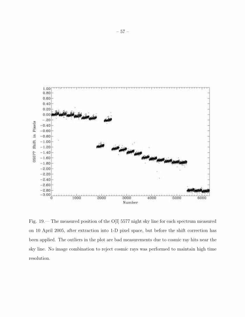
Figure 19 shows the pixel shifts for each spectrum on the night of 10 April 2005, which
is broadly typical. Each point represents one spectrum, and each set of 300 points represents
one CCD frame. The spectra from each frame are plotted in order, the time between
frames is not shown, but can be seen in figure 17 (the night in figure 19 is the second night
from the right). Three things are apparent in figure 19. (1) The shifts in the position
of λ5577 are large when compared with other effects. (2) The shifts change smoothly,
but with occasional discontinuities resulting from apextract’s choice of zeropoint. The
discontinuities demonstrate clearly that the shifts must be corrected before spectra may be
combined. (3) Finally, each set of 300 spectra, from a single frame, shows small, systematic
– 30 –
differences in the shift as a function of position in the frame. The amplitude of this shift,
from top to bottom, is similar to the scatter in the measurement of a single line center.
The origin of this shift is unknown, but it is not due to systematic errors in the wavelength
polynomial. We currently do not correct for this small effect.
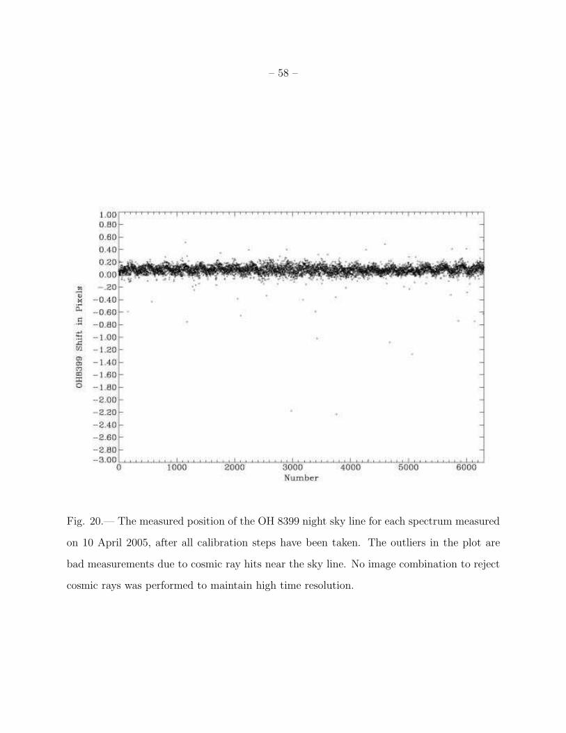
Figure 20 shows the final measured positions for the λ8399 A night sky line after the
spectra from figure 19 have been wavelength calibrated and rebinned into 1-A-wide equal
wavelength bins. The scatter about the expected value is 0.092 A, which includes the
small systematic errors seen in Figure 19. The offset of 0.075 A is approximately constant
throughout the night, and may be attributed to errors in the calibration polynomial as
there is no apparent drift.
7.3. Sky Subtraction
The removal of the night sky spectrum from observations of faint objects made with
fiber optic spectrographs has long been viewed as problematic (e.g. Wyse & Gilmore (1992),
Lissandrini et al. (1994), Watson et al. (1998)). Recently methods have been developed
which fit local variations from the mean sky due to changes in fiber transmission, focus,
etc. by means of eigenvector techniques Kurtz & Mink (2000), and B-splines Marinoni et
al. (2001). The stability of Hectospec’s bench spectrograph allows us to reach near Poisson
limited sky subtraction without having to resort to the use of eigenvectors or B-splines.
Typically 30 Hectospec fibers (10% of the total) are allocated to blank sky observations.
We reduce the data for each of the two CCD chips separately because combining sky spectra
from the two chips degrades performance. The point spread functions of the two CCDs
differ by ∼0.2 pixels FWHM, apparently due to differences in the CCD charge diffusion.
We check for objects contaminating the sky spectra in two ways. (1) We divide each
– 31 –
sky spectrum by the mean of all the sky spectra. When the RMS pixel value exceeds a
threshold the sky spectrum is considered contaminated, and is rejected. (2) We subtract
the (revised) mean sky spectrum from each remaining sky spectrum, then correlate the
residuals against our absorption and emission line galaxy templates; spectra which yield
significant redshifts (significance is determined by the Tonry & Davis (1979) r statistic) are
contaminated by galaxian or stellar light, and are rejected. For a typical sample, taken in
March and April 2005, 181 of 972 sky spectra (∼19%) were found to be contaminated by
this test.
We subtract the sky from each object spectrum by averaging the six closest (clean) sky
spectra. We rescale this average so that the flux in the OH 8399A line matches the flux in
the object spectrum, and then simply subtract the rescaled sky spectrum from the object
spectrum. For galaxies with R∼20 this procedure works very well. We test the limits of the
technique by applying it to the measurement of substantially fainter spectra.
We chose 222 objects from a deep galaxy survey (Dell’Antonio et al. 2005) that were
evenly distributed in V −R color between 0.0 < V −R < 1.3. One third were evenly divided
in bright magnitude 21 < R < 22 and two thirds were evenly divided in faint magnitude
22 < R < 22.5; figure 21 shows the distribution of objects. These objects were observed in
two different Hectospec configurations before and after transit. The first observation had
160 minutes exposure and the second 120 minutes exposure. The two data sets were reduced
separately, then summed to provide the final spectra. We obtained reliable redshifts for 137
of these objects; the remainder had insufficient signal to noise to obtain redshifts. The solid
dots in figure 21 show the galaxies with redshifts; they tend to be brighter and bluer.
Figure 22 shows the success rate as a function of the 1.5′′ diameter aperture magnitude,
which corresponds to the light down the fiber. The success rate falls rapidly for objects
fainter then R1.5
′′=23.0; essentially all of the lower central surface brightness objects with

– 32 –
reliable redshifts are emission line objects.
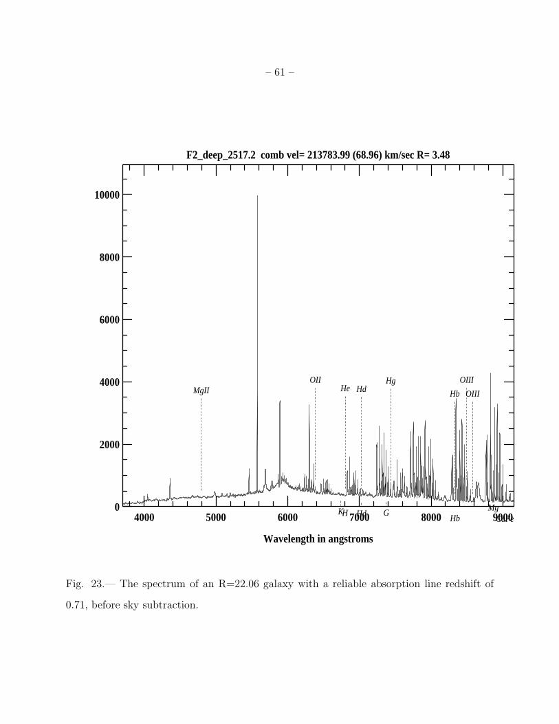
Figure 23 shows a 280 minute exposure spectrum of a galaxy at z=0.71 having with
R=22.0 and R1.5
′′=22.97 prior to sky subtraction. Figure 24 shows the spectrum after sky
subtraction and after application of an 8 A smoothing window. The CaII K line for this
galaxy is detected in absorption at ∼1.5 σ significance. There are about 450 independant
10 pixel wide regions in this spectrum, we would expect about 30 of these to have positive
fluctuations greater than the size of the K line, and 30 to have negative fluctuations. This
behavior is approximately what we see in this spectrum, taking into account that the
intensity of the sky radiation (and thus the size of the statistical fluctuations) is in some
places substantially higher than at the location of the K line.
The coincidence of several features allows a reliable redshift to be determined in this
case, but the existence of many similar sized noise spikes suggests that the spectrum of
this R∼22 galaxy is near the limit. Were this object at z=1.0 the light entering the fiber
would be reduced by half and the spectral lines would be redshifted into the OH night
sky line forest. With perfect sky subtraction the K line would be about a 0.3 σ effect;
redshift determinations are impossible at these levels. While in theory substantially longer
exposures could be made to measure higher redshift objects, in practice it makes more sense
to use higher resolution to isolate the night sky features (Davis et al. 2003). A 600 line
grating blazed in the red for the Hectospec will see first light during the second half of 2005.
8. Typical Hectospec Performance in Survey Mode
Hectospec is frequently used to observe objects with R < 21.0 with exposures of 30
to 120 minutes. Often observations are made with partial moon. Figures 25 and 26 show
representative 60 minute exposures, taken with the moon up, six days past the new moon.
– 33 –
Redshifts are determined using the methods described by Kurtz & Mink (1998), hereafter
KM98. New templates, using objects with z∼0.3 were created for the correlation analysis,
as described in KM98.
Figure 27 shows the relation between isophotal R magnitude and the Tonry & Davis
(1979) r statistic, a measure of redshift quality, for 1455 absorption line galaxies observed
with one hour exposures (some with moon) in March and April 2005 as part of the
gravitational lensing survey (Geller et al. 2005). All these spectra yielded reliable redshifts.
There is little correlation between the magnitude and the quality of the redshift.
Figure 28 shows the same 1455 absorption line galaxies, but with the 1.5′′
aperture
magnitude, which represents the light down the fiber, vs. the r statistic. As expected there
is now a strong correlation. The Mt. Hopkins R band dark sky brightness is typically 20.0
in a 1.5′′
aperture (Massey & Foltz 2000; Patat 2003). The Hectospec routinely obtains
absorption line redshifts for objects at 20% of the sky in one hour exposures.
Following KM98 we use 332 objects with duplicate spectra to estimate the error in a
redshift measurement as a function of the r statistic. We find that the median velocity error
for absorption line redshifts can described by ∆vabs = 130/(1 + r) + 5 km s−1 while the
emission line redshift errors can be described by ∆vem = 100/(1 + r) + 5 km s−1. The mean
errors are about twice these, and are well represented by the normal xcsao error estimator
(KM98).
9. Discussion and Conclusions
Hectospec is a powerful, wide-field spectrograph that makes excellent use of the
converted MMT’s 1◦ diameter and 6.5 meter aperture. It reaches to R=21.5 with ease, and
the sky subtraction with standard data reduction allows quality spectroscopy to R=22 with
– 34 –
sufficient exposure. Fiber spectrographs have an unjustified reputation in some quarters
for compromised throughput that is probably due to design shortcomings in the fiber run
between the focal plane and the spectrograph and in the design of bench spectrographs.
Hectospec’s peak system throughput of 10% including aperture losses, and 17% correcting
for aperture losses, is quite competitive with slit spectrographs when its huge multiplex
advantage is taken into account. A high-throughput long-slit spectrograph like the FAST
spectrograph on the Whipple Observatory’s 1.5m Tillinghast Reflector (Fabricant et al.
1998a) has a peak system throughput (correcting for aperture losses by using a wide slit)
that reaches 30% with fresh mirror and corrector coatings, but is more typically ∼25% in
average conditions.
Hectospec is a popular instrument at the MMT. Users respond favorably to the
flexibility and efficiency of the queue observing mode. We designed Hectospec to rapidly
survey normal intermediate redshift galaxies and high redshift active galaxies identified
through by space X-ray and infrared observatories, and these are active areas of research
with Hectospec. A wide variety of other programs are underway, including several stellar
programs. Because Hectospec can offer effective sky subtraction to R∼22, essentially
limited by Poisson noise, it is a surprisingly versatile general-purpose spectrograph.
We are in the process of building a complementary optical imaging spectrograph for
the MMT (Binospec, Fabricant et al. (2003)). A wide-field imaging spectrograph will allow
us to efficiently survey galaxy dynamics at intermediate redshifts and will offer very high
throughput (potentially twice Hectospec’s) and even more precise sky subtraction for very
faint objects. However, Binospec’s advantages come at a price: its field of view is only 8%
of Hectospec’s, and with likely slitlet lengths of 10′′ to 12′′, Binospec will offer ∼50% of
Hectospec’s multiplex advantage. The Hectospec will remain the instrument of choice for
large surveys to depths of R∼22.

– 35 –
We are grateful for the contributions of the entire MMT instrument team, students, and
of the MMT and Whipple Observatory staff. We thank Steve Amato, David Becker, Kevin
Bennett, David Bosworth, David Boyd, Daniel Blanco, William Brymer, David Caldwell,
Richard Cho, Shawn Callahan, Florine Collette, Dylan Curley, Emilio Falco, Craig Foltz,
Art Gentile, Everett Johnston, Sheila Kannappan, Frank Licata, Steve Nichols, Dale Noll,
Ricardo Ortiz, Tim Pickering, Frank Rivera, Phil Ritz, Rachel Roll, Cory Sassaman, Gary
Schmidt, Dennis Smith, Ken Van Horn, David Weaver, Grant Williams and J.T. Williams.
We thank the Hectospec robot operators: Perry Berlind and Mike Calkins, and the MMT
operators: Mike Alegria, Alejandra Milone, and John McAfee. We are grateful to the efforts
of the Harvard College Observatory Model Shop led by Larry Knowles. We thank Robert
Dew and Diane Nutter of Cleveland Crystals and Terry Facey, formerly of Goodrich Optical
Systems.
Facilities: MMT.
– 36 –
REFERENCES
Barden et al. 1993, ASP Conf. Ser. 37: Fiber Optics in Astronomy II, 152, 185
Blanco et al. 2004, Proc. SPIE, 5489, 300
Callahan, S., Cuerdan, B., Fabricant, D., & Martin, H. 2004, Proc. SPIE, 5495, 228
Davis, M., et al. 2003, Proc. SPIE, 4834, 161
Dell’Antonio, I. 2005, private communication
Epps, H. & Vogt, S., Appl. Opt., 32, 6272
Fabricant, D. et al. 1998, PASP, 110, 79
Fabricant, D. et al. 1998, Proc. SPIE, 3355, 285
Fabricant, D. et al. 2003, Proc. SPIE, 4841, 134
Fabricant, D. et al. 2004, Proc. SPIE, 5492, 767
Fabricant, D., Hertz, E., & Szentgyorgyi, A. 1994, Proc. SPIE, 2198, 251
Fata, R., Kradinov, V., & Fabricant, D. et al. 2004, Proc. SPIE, 5492, 553
Fata, R & Fabricant, D. 1998, Proc. SPIE, 3355, 275
Fata, R & Fabricant, D. 1994, Proc. SPIE, 2199, 580
Fata, R & Fabricant, D. 1993, Proc. SPIE, 1998, 32
Geary, J. 2000, in Further Developments in Scientific Optical Imaging, ed. Denton, M. B.,
(Cambridge, U.K.: Roy. Soc. Chem.)
Geller, M. J. 2005, to be submitted to ApJ
– 37 –
Kurtz, M. J., & Mink, D. J. 1998, PASP, 110, 934
Kurtz, M. J., & Mink, D. J. 2000, ApJ, 533, L183
Lissandrini, C., Cristiani, S., & La Franca, F. 1994, PASP, 106, 1157
Marinoni, C., Davis, M., Coil, A. L., & Finkbeiner, D. 2001, in Where’s the Matter?,
Proceeding of the 3rd Marseille Cosmology Conference, eds. L. Tresse and M. Treyer,
p. 118, also astro-ph/0109164
Massey, P., & Foltz, C. B. 2000, PASP, 112, 566
Mink, D. M., Wyatt, W. F., Roll, J. B., Tokarz, S. B., Conroy, M. A., Caldwell, N., Kurtz,
M. J., and Geller, M. J., Astronomical Data Analysis Software and Systems XIV,
ASP Conference Series, in press.
Parry, I & Gray, P. 1986, Proc. SPIE, 627, 118
Patat, F. 2003, A&A, 400, 1183
Pickering, T., West, S., & Fabricant, D. 2004, Proc. SPIE, 5489, 1041
Roll, J.B. Jr., Fabricant, D., & McLeod, B. 1998, Proc. SPIE, 3355, 324
Roll, J. 1996, ASP Conf. Ser. 101: Astronomical Data Analysis Software and Systems V,
101, 536
Szentgyorgyi, A. et al. 1998, Proc. SPIE, 3355, 242
Tokarz, S. P., & Roll, J. 1997, ASP Conf. Ser. 125: Astronomical Data Analysis Software
and Systems VI, 125, 140
Tonry, J., & Davis, M. 1979, AJ, 84, 1511
– 38 –
Valdes, F. 1995, “Guide to the Multifiber Reduction Task DOFIBERS,” IRAF On-line
document; http://iraf.noao.edu.
Valdes, F. 1992, ASP Conf. Ser. 25: Astronomical Data Analysis Software and Systems I,
25, 417
Valdes, F. 1995, “Guide to the Multifiber Reduction Task DOFIBERS,” IRAF On-line
document; http://iraf.noao.edu.
Vogt, S. et al. 1994, Proc. SPIE, 2198, 362
Watson, F., Offer, A. R., Lewis, I. J., Bailey, J. A., & Glazebrook, K. 1998, ASP
Conf. Ser. 152: Fiber Optics in Astronomy III, 152, 50
Wyse, R. F. G., & Gilmore, G. 1992, MNRAS, 257, 1
This manuscript was prepared with the AAS LATEX macros v5.2.
– 39 –
Fig. 1.— Three views of the fiber button assembly. Light from the backlit fiber is visible
in the upper panel. The pivot point that allows the button assembly to accommodate the
curved focal surface is visible in the middle panel. The rectangular NeFeB magnet bonded
into the button assembly is visible in the lower panel.
– 40 –
Fig. 2.— Disassembled fiber pivots. Pins register and screws hold the upper and lower halves
of the fiber pivots together when the pivots are assembled. The pivot points are defined by
the intersection of two cones. The pivots are arranged in two vertical levels so that the fiber
syringes are fed into two vertical levels of separator trays.
– 41 –
Fig. 3.— Upper unit of the fiber positioner. The X-axis stages and ball screws run vertically
and the Y-axis stages and ballscrews run horizontally in this picture. The Z-axes run into
the paper. The Θ gimbal axis tilts along the X direction, while the Φ axis tilts along the Y
direction. The two grippers are the two circular assemblies near the center of the picture.
The pair of X-axis collision bumpers are visible above and to the side of the two Z-axis
assemblies.
– 42 –
Fig. 4.— Lower unit of the fiber positioner. This section of the fiber positioner can be
unbolted from the upper unit that contains the robots (as shown). The lower unit contains
the 300 fiber optic probes, the curved focal plate that holds the fiber optic probes, guide
trays for the fiber probes, as well as the three guider probes (not visible).
– 43 –
Fig. 5.— Top view of the assembled fiber positioner. This photograph was taken with
upper cover assembly removed to allow a clearer view of the two six-axis robots. The X-axis
collision bumpers are visible at the left and right. The two rectangular assemblies marked
“EOSI” are the intensified TV cameras that travel with the robots. These TV cameras are
used for calibration, alignment tests, and the initial acquistion of guide stars.
– 44 –
Fig. 6.— Z axis assembly of the fiber positioner. The Z axis motor, encoder and brake are
visible at the center left. The cover for the metal drive band is mounted to the top of the Z
axis motor assembly. The gripper jaws are visible at the lower right. The Θ axis actuator
is located at the center right. The bearing assemblies for the Θ and Φ axes are located just
above the gripper jaws at the lower right. The corner cube and fold mirrors for the robot
TV cameras are located above the bearing assemblies.
– 45 –
Fig. 7.— Gripper assembly used to pick and place fiber buttons. The three gripper jaws are
actuated by a rotation of the outer ring to which the gripper fingers are attached, much like
an iris mechanism.
– 46 –
Fig. 8.— The Hectospec dewar assembly. The field flattener lens is obscured by a protective
cover to the center left. The evacuated tube surrounding the cold finger runs horizontally.
The LN2 tank is prominent at the upper right.
– 47 –
Fig. 9.— The rotary shutter assembly mounted on the fiber shoe. The small stepper motor
used to drive the shutter is visible at the top center. This motor is coupled to the rotary
shutter mechanism with a long shaft. The shutter itself is located at the lower left.
– 48 –
Fig. 10.— Coiled 26 m fiber run. The four thermal break assemblies are located at one, four,
and eight o’clock. The fiber probe assemblies, protected by plastic tubes, are laid across the
center running from the lower left to the upper right.

– 49 –
Fig. 11.— One of four fiber thermal breaks in the fiber run. A shipping clamp restraining
the separation of the teflon tubes from the stainless thermal break tubes is in place at the
right.
– 50 –
Fig. 12.— Fiber throughput at 6000 A as measured in the laboratory.
– 51 –
Fig. 13.— The main screen of the Hobserve GUI. Hobserve is a tcl/tk script that provides
a step by step procedural interface that guides the robot operator through the procedure of
calculating the appropriate fiber configuration for the chosen observing time, calculating the
sequence of fiber moves required to attain that configuration, issuing the move commands
to the robots, and setting up the guiding on the field with the preselected guide stars.
– 52 –
Fig. 14.— The guidegui display showing the guide star images from the guider probes and
the reference positions. The robots are stowed during normal observations, so no guide stars
are visible in the leftmost windows.
– 53 –
Fig. 15.— The SPICE program provides a GUI interface to the spectrograph and camera
controls and sequences the operations for various types of exposures. The GUI consists of
two fixed displays at the top of the window along with several tab selectable displays that
appear at the bottom of the window.
– 54 –
4000 5000 6000 7000 8000λ
0.02
0.04
0.06
0.08
0.1
Eff
icie
ncy
Fig. 16.— The measured system throughput as a function of wavelength in 1′′ seeing.
Aperture losses and losses in the telescope optics are included.
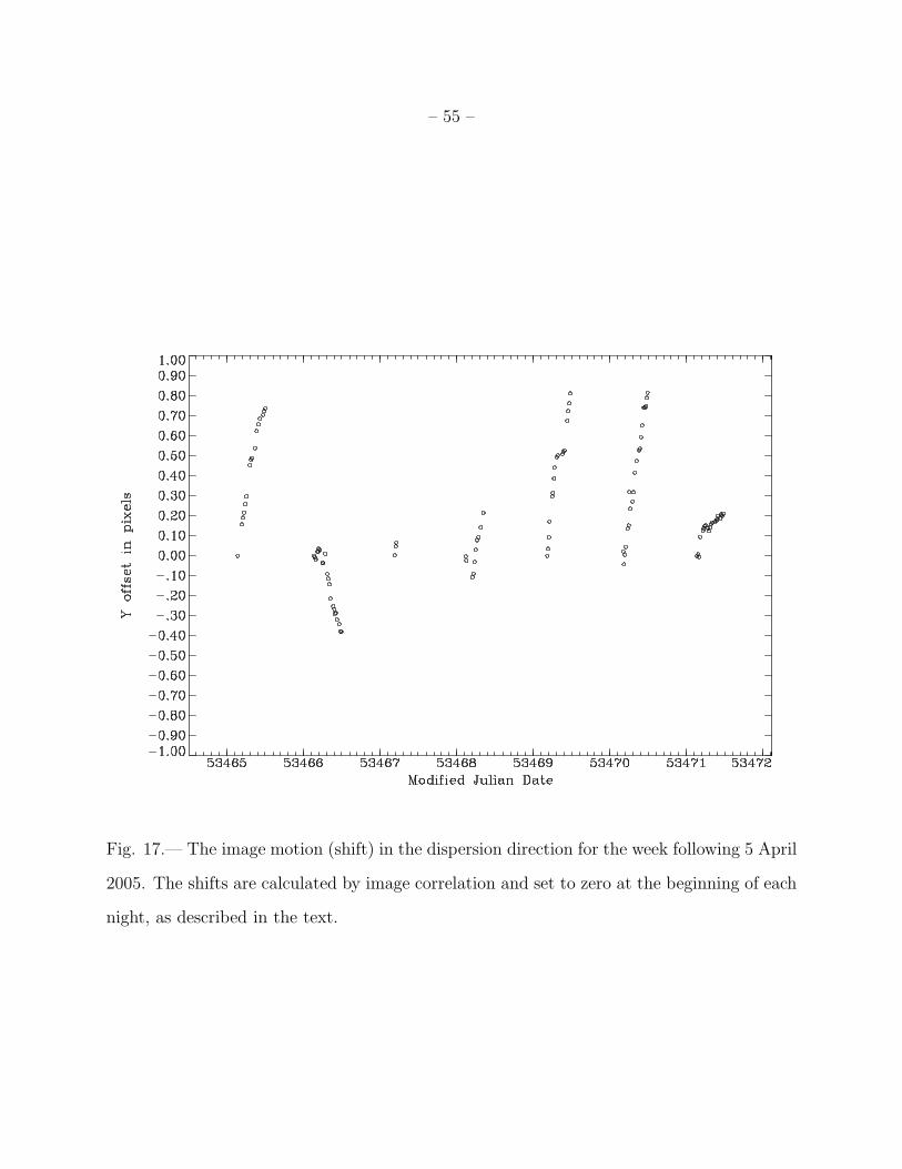
– 55 –
Fig. 17.— The image motion (shift) in the dispersion direction for the week following 5 April
2005. The shifts are calculated by image correlation and set to zero at the beginning of each
night, as described in the text.
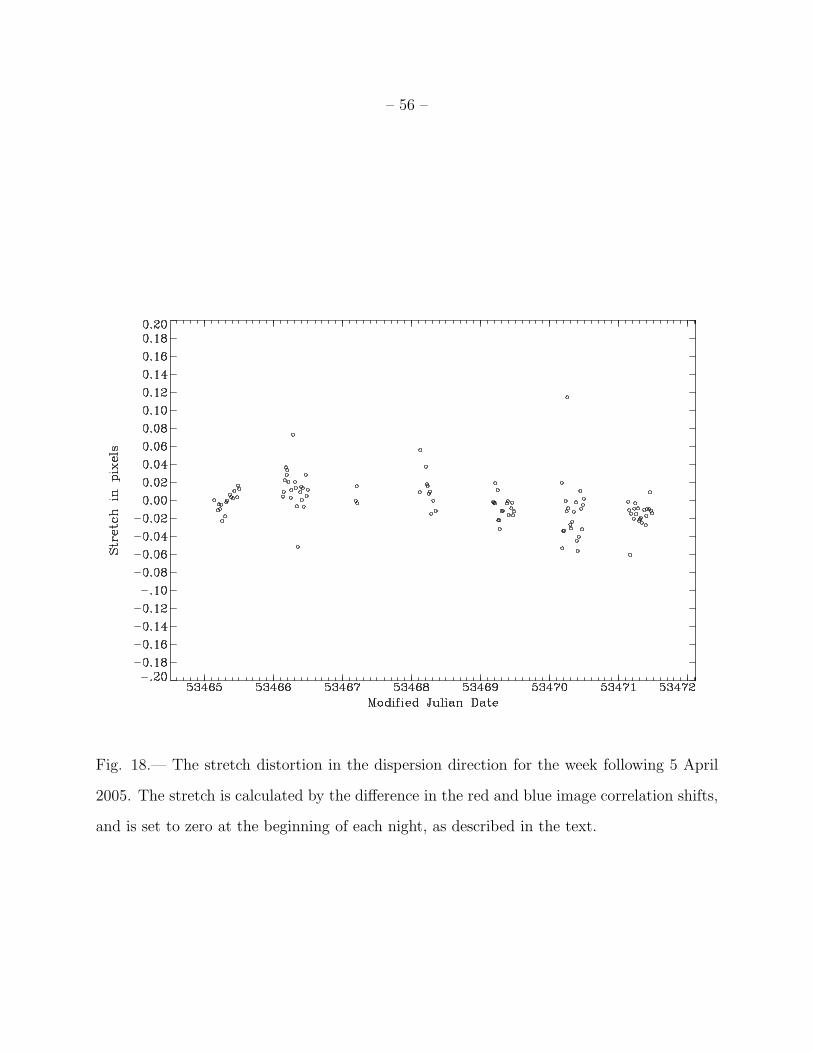
– 56 –
Fig. 18.— The stretch distortion in the dispersion direction for the week following 5 April
2005. The stretch is calculated by the difference in the red and blue image correlation shifts,
and is set to zero at the beginning of each night, as described in the text.
– 57 –
Fig. 19.— The measured position of the O[I] 5577 night sky line for each spectrum measured
on 10 April 2005, after extraction into 1-D pixel space, but before the shift correction has
been applied. The outliers in the plot are bad measurements due to cosmic ray hits near the
sky line. No image combination to reject cosmic rays was performed to maintain high time
resolution.
– 58 –
Fig. 20.— The measured position of the OH 8399 night sky line for each spectrum measured
on 10 April 2005, after all calibration steps have been taken. The outliers in the plot are
bad measurements due to cosmic ray hits near the sky line. No image combination to reject
cosmic rays was performed to maintain high time resolution.

– 59 –
Fig. 21.— The distribution in V − R color and isophotal R magnitude of the objects used
to test the sky subtraction techniques; filled circles represent objects with reliable redshifts
after 280 minutes exposure.

– 60 –
Fig. 22.— The fraction of objects which have successful redshift measurements as a function
of the light down the fiber, a 1.5′′ aperture. All of the lowest central surface brightness
objects with successful redshifts have strong emission lines.
– 61 –
4000 5000 6000 7000 8000 90000
2000
4000
6000
8000
10000
Wavelength in angstroms
F2_deep_2517.2 comb vel= 213783.99 (68.96) km/sec R= 3.48
MgIIOII
He HdHg
Hb OIII
OIII
KH GMg
CaFeHd Hb
Fig. 23.— The spectrum of an R=22.06 galaxy with a reliable absorption line redshift of
0.71, before sky subtraction.

– 62 –
4000 5000 6000 7000 8000 9000
0
25
50
75
100
Wavelength in angstroms
F2_deep_2517 comb vel= 213783.99 (68.96) km/sec R= 3.48
MgII
OII
He
Hd Hg
HbOIII
OIII
KH
G
Mg
CaFe
Hd
Hb
Fig. 24.— The spectrum of an R=22.06 galaxy with a reliable absorption line redshift of 0.71,
after sky subtraction. The 1.5′′ diameter aperture magnitude is 22.97. The sky subtraction
(see text) is effectively limited by Poisson noise.

– 63 –
4000 5000 6000 7000 8000 9000
0
25
50
75
100
Wavelength in angstroms
043.F2new_6_12075.ms corr vel= 136064.74 (45.65) km/sec R= 6.90
MgII
OII
He
Hd
Hg
Hb OIIIOIII
KH
GMg
CaFe
Na
Hd
Hb
Fig. 25.— The spectrum of a typical absorption line galaxy, from a one hour exposure with
the moon up. The object has an isophotal R magnitude of 19.00, a 1.5′′
magnitude of 21.23,
and a redshift of 0.45.

– 64 –
4000 5000 6000 7000 8000 90000
250
500
750
1000
1250
1500
Wavelength in angstroms
110.F2new_6_9447.ms corr vel= 87668.62 (26.50) km/sec R= 8.39
OII
He Hd
Hg
Hb
OIII
OIII
OI
HaN2
N1S1S2
K
HG
MgCaFeNaHd Hb
Fig. 26.— The spectrum of a typical emission line galaxy, from a one hour exposure with
the moon up. The object has an isophotal R magnitude of 19.12, a 1.5′′
magnitude of 20.31,
and a redshift of 0.29.

– 65 –
Fig. 27.— The isophotal R magnitude vs. the quality of the redshift as measured by the
Tonry & Davis (1979) r statistic for 1455 one hour exposures of absorption line galaxies.
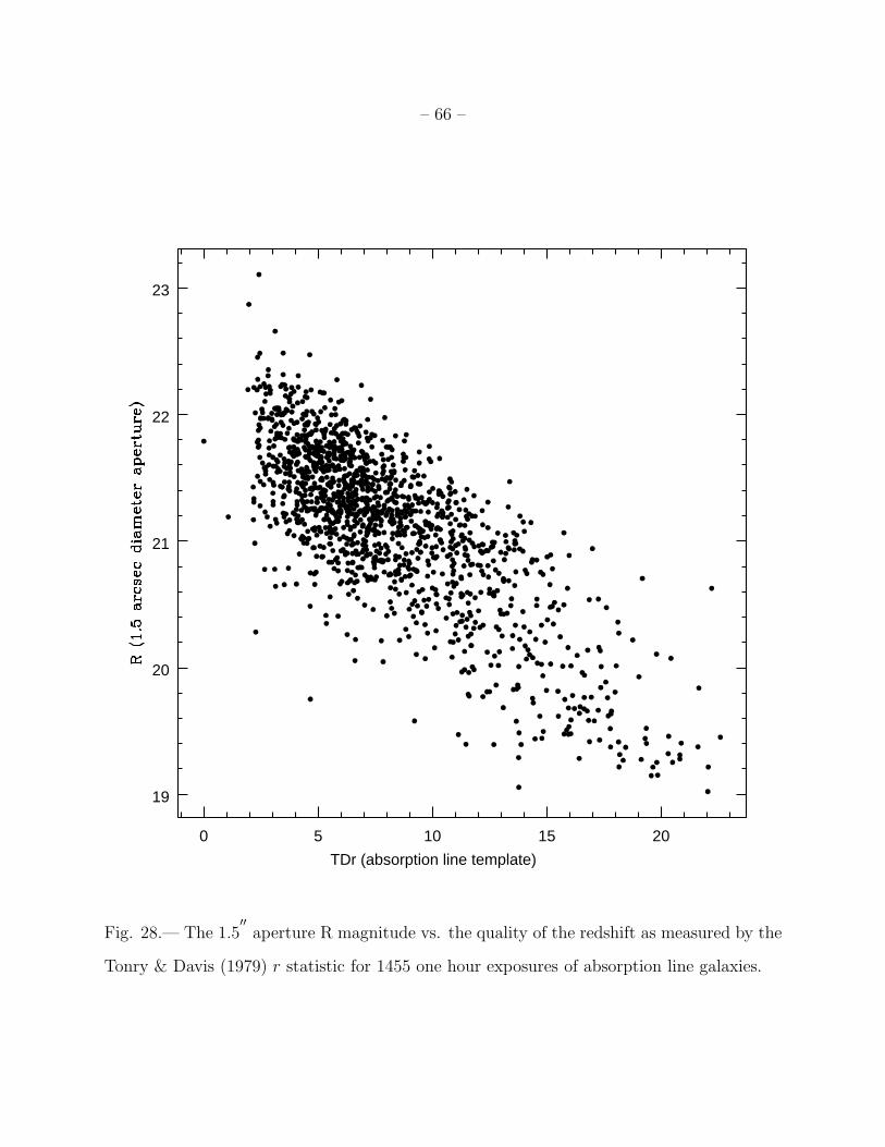
– 66 –
0 5 10 15 20
19
20
21
22
23
TDr (absorption line template)
Fig. 28.— The 1.5′′
aperture R magnitude vs. the quality of the redshift as measured by the
Tonry & Davis (1979) r statistic for 1455 one hour exposures of absorption line galaxies.
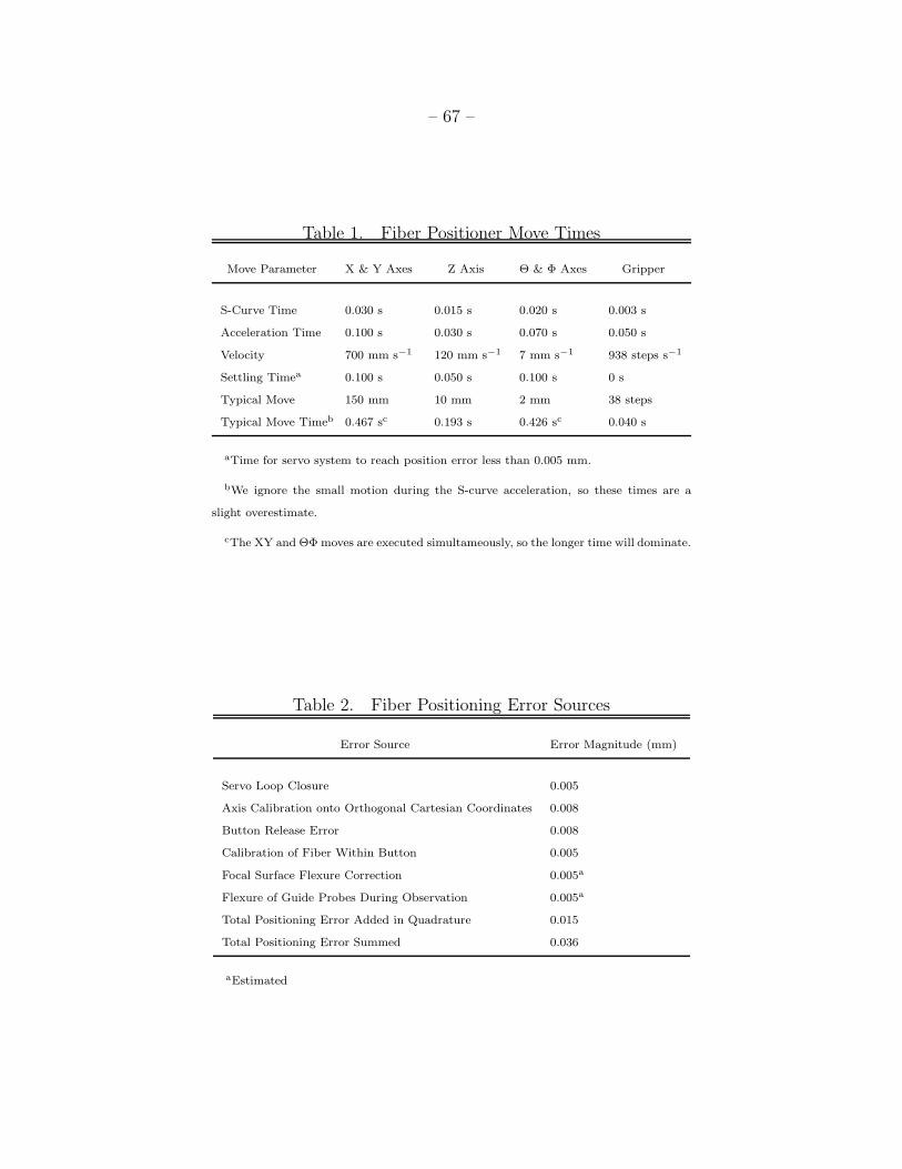
– 67 –
Table 1. Fiber Positioner Move Times
Move Parameter X & Y Axes Z Axis Θ & Φ Axes Gripper
S-Curve Time 0.030 s 0.015 s 0.020 s 0.003 s
Acceleration Time 0.100 s 0.030 s 0.070 s 0.050 s
Velocity 700 mm s−1 120 mm s−1 7 mm s−1 938 steps s−1
Settling Timea 0.100 s 0.050 s 0.100 s 0 s
Typical Move 150 mm 10 mm 2 mm 38 steps
Typical Move Timeb 0.467 sc 0.193 s 0.426 sc 0.040 s
aTime for servo system to reach position error less than 0.005 mm.
bWe ignore the small motion during the S-curve acceleration, so these times are a
slight overestimate.
cThe XY and ΘΦ moves are executed simultameously, so the longer time will dominate.
Table 2. Fiber Positioning Error Sources
Error Source Error Magnitude (mm)
Servo Loop Closure 0.005
Axis Calibration onto Orthogonal Cartesian Coordinates 0.008
Button Release Error 0.008
Calibration of Fiber Within Button 0.005
Focal Surface Flexure Correction 0.005a
Flexure of Guide Probes During Observation 0.005a
Total Positioning Error Added in Quadrature 0.015
Total Positioning Error Summed 0.036
aEstimated

– 68 –
Table 3. Fiber Positioning Reconfiguration Overhead
Activity Elapsed Time (s)
Readout CCD and Request Slew 60 s
Slew Telescope to Zenith 60 s
Reconfigure Fibers 320 s
Move Guider Probes 30 s
Slew to WFS Star 60 s
Acquire WFS and Correct 300 s
Slew to Field and Track 30 s
Setup on Guide Stars 180 s
Total 1040 s
aEstimated