This is a repository copy of Modelling the potential for multi-location in-sewer heat recovery at a city scale under different seasonal scenarios.

White Rose Research Online URL for this paper:http://eprints.whiterose.ac.uk/136415/

Version: Accepted Version

Article:

Abdel-Aal, M. orcid.org/0000-0002-6726-5826, Schellart, A., Kroll, S. et al. (2 more authors) (2018) Modelling the potential for multi-location in-sewer heat recovery at a city scale under different seasonal scenarios. Water Research, 145. pp. 618-630. ISSN 0043-1354

https://doi.org/10.1016/j.watres.2018.08.073

Article available under the terms of the CC-BY-NC-ND licence (https://creativecommons.org/licenses/by-nc-nd/4.0/).

eprints@whiterose.ac.ukhttps://eprints.whiterose.ac.uk/

Reuse

This article is distributed under the terms of the Creative Commons Attribution-NonCommercial-NoDerivs (CC BY-NC-ND) licence. This licence only allows you to download this work and share it with others as long as you credit the authors, but you can’t change the article in any way or use it commercially. More information and the full terms of the licence here: https://creativecommons.org/licenses/

Takedown

If you consider content in White Rose Research Online to be in breach of UK law, please notify us by emailing eprints@whiterose.ac.uk including the URL of the record and the reason for the withdrawal request.

Accepted Manuscript

Modelling the potential for multi-location in-sewer heat recovery at a city scale underdifferent seasonal scenarios

Mohamad Abdel-Aal, Alma Schellart, Stefan Kroll, Mostafa Mohamed, Simon Tait

PII: S0043-1354(18)30703-6

DOI: 10.1016/j.watres.2018.08.073

Reference: WR 14049

To appear in: Water Research

Received Date: 2 March 2018

Revised Date: 27 August 2018

Accepted Date: 31 August 2018

Please cite this article as: Abdel-Aal, M., Schellart, A., Kroll, S., Mohamed, M., Tait, S., Modelling thepotential for multi-location in-sewer heat recovery at a city scale under different seasonal scenarios,Water Research (2018), doi: 10.1016/j.watres.2018.08.073.

This is a PDF file of an unedited manuscript that has been accepted for publication. As a service toour customers we are providing this early version of the manuscript. The manuscript will undergocopyediting, typesetting, and review of the resulting proof before it is published in its final form. Pleasenote that during the production process errors may be discovered which could affect the content, and alllegal disclaimers that apply to the journal pertain.

MA

NU

SC

RIP

T

AC

CE

PTE

D

ACCEPTED MANUSCRIPT

Hea

t

Exchan

ger

Heat

Recovery

Heat TransferMass & Heat

Balance00:00 23:00

Hea

t R

eco

ver

y

(MW

h)

0 7

15

Wastewater

Treatment

Plant

Spatial Heat Recovery Computational Modelling Outputs

Temperature Simulation

Hydrodynamic

& heat transfer

models

1 n

Wa

stew

ate

r

Tem

per

atu

re (

ºC)

5 10 15

With heat

recovery

No heat

recovery

Pipe No.

Summer Winter

Time

MA

NU

SC

RIP

T

AC

CE

PTE

D

ACCEPTED MANUSCRIPT

1

Modelling the potential for multi-location in-sewer heat recovery at a city scale under different seasonal scenarios 1 2 Mohamad Abdel-Aal1*, Alma Schellart 1, Stefan Kroll2, Mostafa Mohamed3, and Simon Tait1. 3 4 1 Pennine Water Group, Department of Civil and Structural Engineering, University of Sheffield, Mappin 5 Street, Sheffield, S1 3JD, UK. 6 2 Aquafin NV, Dijkstraat 8, 2630 Aartselaar, Belgium 7 3 School of Engineering, University of Bradford, Bradford, BD7 1PD UK 8 9 *Corresponding author’s email: m.abdel-aal@sheffield.ac.uk 10

Abstract 11

A computational network heat transfer model was utilised to model the potential of heat energy recovery at 12

multiple locations from a city scale combined sewer network. The uniqueness of this network model lies in 13

its whole system validation and implementation for seasonal scenarios in a large sewer network. The 14

network model was developed, on the basis of a previous single pipe heat transfer model, to make it suitable 15

for application in large sewer networks and its performance was validated in this study by predicting the 16

wastewater temperature variation in a sewer network. Since heat energy recovery in sewers may impact 17

negatively on wastewater treatment processes, the viability of large scale heat recovery across a network 18

was assessed by examining the distribution of the wastewater temperatures throughout the network and the 19

wastewater temperature at the wastewater treatment plant inlet. The network heat transfer model was applied 20

to a sewer network with around 3000 pipes and a population equivalent of 79500. Three scenarios; winter, 21

spring and summer were modelled to reflect seasonal variations. The model was run on an hourly basis 22

during dry weather. The modelling results indicated that potential heat energy recovery of around 116, 160 23

& 207 MWh/day may be obtained in January, March and May respectively, without causing wastewater 24

temperature either in the network or at the inlet of the wastewater treatment plant to reach a level that was 25

unacceptable to the water utility. 26

27

Key words: Heat recovery, heat transfer modelling, wastewater temperature prediction, clean thermal energy 28

1 Introduction 29

The potential heat available for recovery from sewers in the UK is thought to be significant, when estimated 30

theoretically, due to the high volumes of collected wastewater and the relatively high wastewater 31

MA

NU

SC

RIP

T

AC

CE

PTE

D

ACCEPTED MANUSCRIPT

2

temperatures found throughout the UK’s combined and foul sewer networks. The UK’s 347,000km of 32

sewers (Defra, 2002) are generally located in urban catchments where the domestic heat demand is 33

estimated to be around 300 TWh/year (ECUK, 2017). Considering heat recovery will result in a 2°C 34

wastewater temperature reduction (Buri & Kobel, 2005), the 11 billion litres of wastewater produced per day 35

(Defra, 2002), would potentially result in up to 390 TWh of heat recovery per year. This estimate is based 36

on the first law of thermodynamics, where the potential rate of heat recovery is the product of wastewater 37

mass flow rate, its specific thermal capacity and the consequent temperature reduction, and assumes a 100% 38

efficient heat recovery systems installed across all the UK’s sewer networks. 39

40

The key technical challenge for efficient in-sewer heat recovery is to enable heat recovery sufficiently close 41

to points of local demand. To meet this challenge it is essential to quantify the impact of simultaneous heat 42

recovery at multiple locations within a sewer network. This “locality” constraint can reduce the overall 43

system potential. For example, in Austria, Kretschmer et al. (2015) estimated that 10% of Austrian houses 44

can benefit from heat recovered from wastewater. Another barrier for recovering heat from sewers is that 45

any reduction in wastewater temperature may cause difficulties with treatment processes and incur extra 46

costs at the end of system wastewater treatment plant (WwTP). It is therefore important to ensure that even 47

with multiple locations of heat recovery, the wastewater temperature reduction is limited at the inlet to the 48

WwTP. The nitrification process at the WwTP may be compromised by low wastewater temperatures, as 49

demonstrated by Shammas (1986), who tested the impact of varying the wastewater temperatures, from 4 to 50

35°C, on the nitrification quality and concluded that nitrification is much more effective at temperatures in 51

the upper part of this range, i.e. between 25 and 35°C. This finding is in line with a number of other studies 52

summarised in Metcalf & Eddy (2004), who reported that the optimum wastewater temperature for 53

nitrification was estimated to be between 25 and 35°C. Previous authors such as Wanner et al. (2005) 54

examined the impact of the reduction in temperature on wastewater nitrification and concluded that 1°C 55

reduction in wastewater temperature may reduce the nitrifier growth by 10%. Such a reduction would 56

require a 10% increase in the sludge retention time, to maintain the same nitrification quality achieved at the 57

unadjusted wastewater temperatures. 58

MA

NU

SC

RIP

T

AC

CE

PTE

D

ACCEPTED MANUSCRIPT

3

59

Previous studies have examined the variation in wastewater temperature in order to estimate the potential of 60

heat energy recovery and its impact on the treatment processes in WwTPs. Early work by Bischofsberger et 61

al. (1984) measured wastewater temperatures in Hamburg, Germany, for a year at five locations in a 62

combined sewer network, and observed that the wastewater temperatures varied between 7°C and 28°C 63

during the year. This temperature range was close to that observed in other in-sewer wastewater temperature 64

measurements reported in Dürrenmatt and Wanner (2008), Schilperoort and Clemens (2009), Cipolla and 65

Maglionico (2014), Abdel-Aal (2015) and Simperler (2015) in a number of combined sewer networks across 66

Europe. 67

68

Some studies have used simple relationships to estimate the impact of recovering heat energy on in-sewer 69

wastewater temperature, Kretschmer et al. (2016) estimated the potential heat energy recovery to be a linear 70

function of wastewater temperature, flow rate, temperature reduction and the heat capacity of water. No 71

estimate was made, by these authors, of the heat flux between the flowing wastewater and the in-sewer air 72

and the surrounding soil. Assessing the impact of heat energy recovery from a sewer pipe has led some 73

authors to develop more complex computational models to predict the wastewater temperature variation 74

along a sewer pipe taking into account heat flux into the surrounding soil and into the in-sewer air above the 75

wastewater flow. These models were developed for single pipes but by linking pipe sections they could be 76

used to estimate the cumulative effect along extended sewer pipes (Dürrenmatt, 2006; Dürrenmatt and 77

Wanner, 2008; Dürrenmatt and Wanner, 2014; Abdel-Aal et al., 2014; Abdel-Aal, 2015). The model 78

developed by Dürrenmatt and Wanner (2008), named TEMPEST, was the first capable of predicting 79

wastewater temperature in successive sewer pipes. Published studies have shown that TEMPEST was 80

implemented in a single string of sewer pipes; 1.85km long (Dürrenmatt and Wanner, 2014) and 3km long 81

(Sitzenfrei et al., 2017). The TEMPEST model was calibrated using a dataset collected over a 5 week period 82

from 14th February to 22nd March 2008. Elías-Maxil et al. (2017) developed a parsimonious model based on 83

TEMPEST yet excluded computation of the heat transfer between wastewater and in-sewer air. They 84

claimed that the heat flux between the wastewater and in-sewer air was not significant and could be ignored. 85

MA

NU

SC

RIP

T

AC

CE

PTE

D

ACCEPTED MANUSCRIPT

4

Elías-Maxil et al. (2017) used flow and temperature data collected in a 300 m long pipe to calibrate and 86

validate their model by adding hot water at a temperature of 50°C for six hours instead of simulating the 87

temperature variation of the wastewater. Abdel-Aal (2015) utilised measured flow and wastewater data 88

collected over a four month period in a small number of pipes within a combined sewer network to analyse 89

the sensitivity of the calibration parameters in the empirical equations describing the heat flux between the 90

in-sewer air and the wastewater and between the wastewater and surrounding soil. The calibration 91

parameters were varied from 10% to 400% of their default values, found in literature, and the impact of 92

these variations on the predicted downstream wastewater temperature was quantified. Increasing the heat 93

transfer coefficient between wastewater and in-sewer air by four times resulted in a 0.4°C variation, which 94

was the largest change among all other empirical heat transfer parameters taken into account, i.e. soil 95

thermal conductivity, soil penetration depth and pipe wall thermal conductivity. Hence, the sensitivity 96

analysis indicated that the heat flux between the wastewater and the in-sewer air should not be ignored if an 97

accurate estimate of the reduction in wastewater temperature along a sewer pipe is to be obtained. 98

99

The simulations reported in this paper utilised a network computational heat transfer model developed by 100

Abdel-Aal (2015), and validated in this work, which is able to predict in-pipe wastewater temperatures 101

throughout a large sewer network. The network heat flux model links an in-pipe heat transfer model, 102

accounting for air-wastewater, wastewater-pipe and wall-soil heat fluxes with a hydrodynamic sewer 103

network model. The model of Elías-Maxil (2015) was implemented on a single sub-catchment in a sewer 104

network and was used to predict in-pipe wastewater temperatures. It was not utilised to investigate the 105

impact of several locations of heat recovery on in-sewer wastewater temperatures. The uniqueness of this 106

work is the simultaneous modelling of heat recovery from multiple locations within a single network over 107

long durations. This has allowed the assessment of the in-sewer heat recovery reliability from a real large 108

sewer network over different periods within a year. Predicting the rate of heat recovery and assessing its 109

reliability are keys to making a believable economic assessment. 110

MA

NU

SC

RIP

T

AC

CE

PTE

D

ACCEPTED MANUSCRIPT

5

2 Methodology 111

A heat transfer model was initially developed for a single sewer pipe and then modified and implemented in 112

a large sewer network, hence ‘single pipe’ and ‘network’ heat transfer models are used in this paper to 113

describe both model types respectively. This section briefly explains the method followed in the 114

development of the single pipe heat transfer model and how it was initially calibrated and validated. The 115

build-up, calibration and validation of the sewer network hydrodynamic model for the case study catchment 116

is then described. Following these descriptions an explanation is given as to how the single pipe heat 117

transfer model was further developed and then linked with the hydrodynamic sewer network model in order 118

to deliver a network heat transfer model. The predictive performance of the network heat transfer model was 119

then validated using collected field data from the case study catchment. 120

121

Calibration is defined in this paper as adjusting model parameters to minimise the differences between 122

predictions and observations . The validation process quantified model accuracy by implementing the 123

obtained calibrated parameters in model simulations and comparing predicted values with measured data 124

that were independent of those used for calibration. In the case of validating the hydrodynamic model, after 125

comparing measured and modelled flow rates and depths during dry weather flow days, head loss 126

parameters were adjusted to take into account the local energy losses and hence, improve the model 127

accuracy at specific locations. This section ends by explaining how the predicted wastewater temperatures, 128

in the network and at the WwTP inlet, were employed to model the potential heat energy recovery at 129

multiple locations on hourly basis, for different months. 130

2.1 The single pipe heat transfer model 131

This section briefly explains how a previously created single pipe heat transfer model was developed, 132

calibrated and validated so that it was then suitable for use in this study. 133

2.1.1 Development of the single pipe heat transfer model 134

The aim of this single pipe model was to produce an efficient sub-model that can be ultimately used in a 135

more complex model to obtain network temperature simulations while accounting for all the major heat 136

transfer processes observed within a single sewer pipe. Implementing the first law of thermodynamics and 137

MA

NU

SC

RIP

T

AC

CE

PTE

D

ACCEPTED MANUSCRIPT

6

accounting for the thermal convection between wastewater and in-sewer air and conduction between 138

wastewater, at the invert level, and the surrounding soil through the pipe wall, the wastewater temperature 139

variation along a single sewer pipe can be expressed by Equation 1, (Abdel-Aal, 2015). 140

���� = �� − ��

� ��������� �� ����������×�×�� ∆�� (1) 141

When heat was recovered upstream of a sewer pipe in the network, it was assumed that wastewater 142

temperature at the point downstream of any heat energy recovery location is reduced as a result of the heat 143

recovery process, which can be estimated using Equation 2. 144

���� = �� − � !�∀��# (2) 145

T is temperature (K), m is an expression of the wastewater temperature location within a longitudinal 146 computational mesh along the pipe length, R is thermal resistivity (m.K/W) between wastewater and in-147 sewer air (wa) and between wastewater and soil (ws), ∆� is the computational increment length stream-wise 148 (m) based on dividing each pipe into 10 increments, ∃% is the wastewater density (kg/m3), Q is the 149 wastewater volumetric flow rate (m3/s) and cp is the specific heat capacity for wastewater (J/kg.K), HR is the 150 rate of heat recovered in Watts. 151 152

Equation 1 interprets the energy balance by expressing the thermal convection and conduction in terms of 153

thermal resistivity which is a function of the wastewater velocity, its surface width and the pipe wetted 154

perimeter which were ultimately computed using hydraulic data and pipe shapes retrieved from the sewer 155

network hydrodynamic model. 156

157

The wastewater temperature was modelled with the assumption that the in-sewer pipe flow has a free 158

surface. This is because typical DWF, in a sewer pipe, has a larger proportion of in-sewer air volume to that 159

of wastewater. For example, the average measured wastewater depth to pipe diameter ratio was 8% in urban 160

residential sewers and 42% in large sewer collectors (Abdel-Aal, 2015). 161

162

Edwini-Bonsu and Steffler (2006) installed a scrubber in a sewer pipe within a small network with 15 163

manholes to measure the influence of forced ventilation on the in-sewer air velocity by switching the 164

scrubber on and off. Measured field data in the latter study showed that there was around a 10% variation in 165

the in-sewer air velocity between trapped in-sewer air and forced ventilation conditions. Therefore, the 166

MA

NU

SC

RIP

T

AC

CE

PTE

D

ACCEPTED MANUSCRIPT

7

effect of active air ventilation in the sewer pipes was neglected in the in-sewer air/wastewater convection 167

based heat transfer model. The use of a conduction based heat transfer relationship between wastewater and 168

the surrounding soil is based on the assumption that there is no slip conditions between wastewater and inner 169

surface of the pipe wall, as detailed in Abdel-Aal (2015). 170

171

2.1.2 Calibration of the single pipe heat transfer model 172

The calibration of the single pipe heat transfer model was performed using data collected in four pipes of the 173

case study catchment. Hydraulic data was logged every 2 minutes, and soil temperature was measured every 174

20 minutes, while the upstream and downstream wastewater and in-sewer air temperatures were recorded 175

every 15 minutes in two larger collector sewers, and every 20 minutes in two smaller urban sewers. Such 176

data monitoring frequencies were found reasonable and adequate to calibrate and validate the single pipe 177

heat transfer model. The measured hydraulic and temperature data was logged continuously in February, 178

March and May 2012 for sewer pipes located in the case study catchment. Wastewater temperatures were 179

observed, by Tinytag (PBRF-5006-5m) sensors with ± 0.06°C accuracy and better than 0.05°C resolution. 180

181

The importance of simulating the heat transfer between wastewater and in-sewer air for the prediction of 182

wastewater temperature variation, as mentioned above, led the authors to study and analyse the heat transfer 183

process between wastewater and in-sewer air. This relation was represented in Equation 1 by the thermal 184

resistivity between wastewater and in-sewer air (Rwa) and can be described by Equation 3. 185

&%∋ = �(�×) (3) 186

hwa is the convective heat transfer coefficient between wastewater and in-sewer air (W/m2.K), b is the 187 surface width of wastewater running in a sewer pipe (m). 188 189

The traditional approach in estimating the heat transfer coefficient between water and air is through the use 190

of an empirical relationship. Flinspach (1973) proposed a relation, which is a function of the relative 191

wastewater velocity to that of in-sewer air, to estimate the heat transfer coefficient between wastewater and 192

in-sewer air (hwa). However, the origin and underlying assumptions of Flinspach’s relation is not well 193

recorded and it performed inconsistently. Hence, and in an attempt to improve the modelling accuracy, a 194

new more physically based parameterisation was developed to incorporate the influence of the wastewater 195

MA

NU

SC

RIP

T

AC

CE

PTE

D

ACCEPTED MANUSCRIPT

8

surface velocity, as it is associated with in-sewer air velocity (Edwini-Bonsu and Steffler, 2006) and depth, 196

to estimate hwa, using the dimensionless Froude number. 197

198

The soil penetration depth and soil thermal conductivity were also calibrated to estimate the thermal 199

resistivity between wastewater and the surrounding soil (Rws), which is given by Equation 4. This is 200

because, in addition to the heat transfer between wastewater and in-sewer air, the single pipe heat transfer 201

model was sensitive to the soil penetration depth and its thermal conductivity (Abdel-Aal, 2015). Moreover, 202

measuring the soil thermophysical properties in the field was impractical and the relevant parameters had 203

wide ranges in literature. 204

&%∗ = +�,�×%−+./ + 1�

,�×%−+./ (4) 205

tp is the pipe wall thickness (m), ds is the soil penetration depth (m), kp and ks are the thermal conductivities 206 for pipe wall material and soil respectively (W/m.K) and wet.p is the pipe wetted perimeter (m). 207 208

Dürrenmatt (2006) and Dürrenmatt and Wanner (2014) incorporated more parameters such as, Chemical 209

Oxygen Demand (COD) and its degradation rate, in their TEMPEST model. However, variation of these 210

parameters showed insignificant impacts (less than 0.2%) on the predicted wastewater temperature 211

(Dürrenmatt, 2006). In order to develop a computationally efficient simulation for use in a large sewer 212

network, the single pipe heat transfer model was developed using only relationships which were significant 213

in terms of the predicted wastewater temperature. Calibration of the single pipe heat transfer model was 214

achieved using optimisation tools in Matlab to minimise the root mean squared error (RMSE) for each 215

month’s dataset, using Equation 5. A time step of 2 minutes, at which hydraulic data was measured, was 216

utilised for calibrating the single pipe heat transfer model. 217

&234 = 5∑ �78��98�:;8<�= (5) 218

T is the wastewater temperature (°C), M and P stand for measured and predicted respectively, N is the total 219 number of time steps and j is data point number. 220 221 The model error was also computed to assess the single pipe heat transfer model accuracy in terms of over 222

and under prediction, which was the average predicted minus measured wastewater temperatures for a full 223

month dataset. 224

MA

NU

SC

RIP

T

AC

CE

PTE

D

ACCEPTED MANUSCRIPT

9

2.1.3 Validation of the single pipe heat transfer model 225

Validation was carried out using independent datasets from that utilised for calibrating the single pipe heat 226

transfer model. The validation data was measured in sewer sites with similar characteristics to those used for 227

calibration, i.e. large collector and urban sewers, and in the same period, using identical sensor types 228

described in section 2.1.2. The model validation was assessed by the RMSE and modelling errors in a 229

similar manner described in section 2.1.2. 230

2.2 The hydrodynamic sewer network model 231

Hydraulic data, such as the wastewater flow rate, velocity and depth is necessary for simulating the in-sewer 232

wastewater temperatures. Therefore, a hydrodynamic model built in Infoworks CS, was used to provide the 233

hydraulic data for the case study sewer network. The Infoworks CS model used a numerical scheme to solve 234

the Saint-Venant and the Colebrook-White equations in order to calculate wastewater velocity and depth in 235

all pipes throughout the network at all time steps. 236

237

The sewer network used in this study, consisted of 3093 links, 3048 of which were sewer pipes (conduits) 238

while the rest of the links were valves, pumps and other connections. There were 2296 sub-catchments 239

which can contribute two types of flow. Most catchments contributed ‘foul’ (domestic wastewater inflow), 240

as well as ‘trade’ flows, which referred to industrial inflows and occurred in a limited number of the 241

catchments. Some of the pipes carrying trade flows did not contain flow at all timesteps, and occasionally 242

there were flow reversals in this network. Hence, both zero and negative values of flow were possible in the 243

hydraulic output from this Infoworks CS model. Therefore, the hydraulic output data was filtered by 244

replacing zero and negative values of wastewater depth, velocity and flow with a very small positive default 245

values (0.0001 m, m/s or m3/s) to ensure the stability of the heat transfer modelling. This filtration process 246

had an insignificant effect on the predicted total daily wastewater volume, the difference did not exceed 247

0.5% in January, March and May, while the adjustment of negative and zero wastewater level values 248

accounted for less than 0.7% of the total values in the three months. 249

250

MA

NU

SC

RIP

T

AC

CE

PTE

D

ACCEPTED MANUSCRIPT

10

In this study only dry weather flow (DWF) conditions on working days was considered. The DWF days 251

were selected by observing the flow variation plots in the measurement period for each site. The rainfall 252

events were obvious, hence periods without rainfall that showed consistent flow patterns for a continuous 253

period of three or more days were considered to be DWF days. 254

2.2.2 Building and calibration of the hydrodynamic model 255

Aquafin (2014) standards was utilised to construct the Infoworks CS model. The hydrodynamic model was 256

built using historical datasets of the pipe geometries, characteristics and connectivity. This data was 257

compared to records of the current state of the network and field observations and the model geometry was 258

corrected when needed. The DWF at each model input node was estimated based on the local population 259

equivalent (PE), the average wastewater production rate per person and an empirical diurnal wastewater 260

profile. Trade flow was predicted from records of the maximum permitted industrial inputs. The diurnal 261

variation in flow was calibrated using measured flow rates at seven locations across the network during two 262

dry weather days. 263

2.2.3 Validation of the hydrodynamic model 264

A flow monitoring campaign was carried out specifically for this study that included the installation of 265

flowmeters in seven locations across the sewer network. The modelled wastewater flow was visually 266

compared with measured data based on time-series datasets and the total flow was checked against the 267

measured downstream flow of the entire network. In cases where the observation showed large 268

discrepancies (e.g. bias in wastewater depth greater than 2 cm), the model was updated by adjusting 269

relevant parameters, such as the local and pipe head loss coefficients and the height of the fixed sediment 270

layer, so that the modelled results better matched the observed data. An acceptable level of performance 271

level was determined by an experienced hydrodynamic modeller through visual comparisons between 272

modelled and monitored values of flow rates at the seven locations throughout the network. 273

2.3 The network heat transfer model 274

This model was created by developing and using the single pipe heat transfer model and linking this to the 275

hydrodynamic model. The simulation of wastewater temperatures at all locations within a large sewer 276

MA

NU

SC

RIP

T

AC

CE

PTE

D

ACCEPTED MANUSCRIPT

11

network was achieved by implementing the network heat transfer model. This section explains how the 277

model was developed, used for identifying heat recovery locations and validated. 278

279 2.3.1 Development of the network heat transfer model 280

Three main datatypes were generated from the Infoworks CS model, these are: the details of the network 281

links, hydraulic data and soil types. The details of the network links provided information on the way the 282

links were connected, link type, geometry, dimension and the material of each link in the network. The link 283

types mainly included conduits (pipes), valves and pumps, and each link had a unique identifier number 284

which can be utilised to identify its streamwise location of the network. The hydraulic data consisted of the 285

Infoworks CS modelled wastewater flow rate, velocity and depth in each link for a full year at two minute 286

timesteps. Table 1 shows a summary of the data and pipe details retrieved from the hydrodynamic model 287

and literature, in order to create the network heat transfer network model. 288

289

290

291

292

293

294

295

296

297

298

299

300

301

302

303

304

MA

NU

SC

RIP

T

AC

CE

PTE

D

ACCEPTED MANUSCRIPT

12

305

Table 1: Summary of the data used to create the network heat transfer model. 306

Category Model input Value / Range Unit Notes

Sewer temperatures

In-sewer air temperature 8.6 to 15.5 °C Measured in the case study sewers during January, March and May 2012.

Hydraulic data for each pipe

Wastewater flow rate 0.0001 to 10.6 m3/s Full year Infoworks CS simulations, 2 minutes time step. Negative or zero values were replaced by 0.0001 m, m/s or m3/s. Assumed stream-wise flow direction.

Wastewater velocity 0.0001 to 2 m/s

Wastewater depth 0.0001 to 4.3 m

Sub-catchments connected to the sewer network

Flow of wastewater discharged from trade

0.0001 to 0.007 m3/s Full year Infoworks CS data, 2 minutes time step. Flow of wastewater discharged

from foul 0.0001 to 1.85 m3/s

Trade wastewater temperature 15 °C Assumed, based on model validation and agrees with Schilperoort & Clemens (2009) measurements.

Foul (residential) wastewater temperature

15 °C

Specifications of each sewer pipe

Sewer pipe shapes Circle, egg or rectangular

Hydrodynamic model

Sewer pipe materials

Concrete, steel, reinforced concrete, clay, brick, or polyvinyl chloride.

Sewer length 1 to 801 m increment length stream-wise (∆x), based on diving each pipe into 10 increments

0.1 to 8 m

Sewer diameter 0.08 to 5.25 m Sewer wall thickness 0.053 to 0.3 m

Soil details Soil type surrounding each pipe Sand

Provided by the regional soil database.

Soil temperature 9 & 10 °C Measured in case study catchment.

Pipe linkages Pipe identifiers

The unique pipe identifiers

Retrieved from the hydrodynamic model. The ids are used to organise the pipes in their stream-wise location and to connect incoming branches at the correct locations, and to connect the incoming foul, rainfall and trade flows in the right locations.

Sub-catchment identifiers The unique sub-catchment identifiers

307

Equation 1 was used for each pipe in the network where the upstream temperature (��) can correspond to 308

either a 1st generation or 2nd and higher generation pipes. The different pipe generations reflect the 309

streamwise locations of the pipe within the sewer network. Pipes of the 1st generation transport wastewater 310

from the most upstream area of the network, e.g. foul or trade sub-catchments, to the 2nd generation pipes 311

and consequently to the 3rd, 4th and up to the 7th generation pipes before reaching the WwTP. Figure 1 312

illustrates how the pipes were connected in the network at different generations. The wastewater temperature 313

for the 1st generation pipes was assumed to be equal to that discharged from the relevant sub-catchment, 314

MA

NU

SC

RIP

T

AC

CE

PTE

D

ACCEPTED MANUSCRIPT

13

while the upstream wastewater temperature for the 2nd and higher generations was assumed to be equal to 315

that of the downstream temperature of the preceding generation. When more than one pipe was connected to 316

one or more pipes, as shown by Figure 1, the upstream wastewater temperature was computed by Equations 317

6 and 7. 318

319

320

Figure 1: Example of two pipes connected to a third pipe in the sewer network. �� and ���? are the pipe 321 upstream and downstream wastewater temperatures respectively, n is the number of mesh points along the 322 pipe length. p and T stand for pipe and wastewater temperature respectively. The flow is assumed to be 323 heading into one direction shown by the arrows. 324

325 ≅Α = ≅� + QΧ (6) 326

��,/Α = ��ΕΦ,��×�����ΕΦ,�:×∀:�Γ (7) 327

where; T is temperature (K or °C) and p 1,2 & 3 refer to pipes 1, 2 & 3 respectively as illustrated in Figure 328 1. m is the mesh location of the predicted wastewater temperature along the pipe length, n is the number of 329 mesh points along the pipe length. 330 331

Model input temperatures, i.e. of wastewater at the 1st generation pipes, soil and in-sewer air, can be 332

retrieved from literature based on field seasonal data (see Table 1). The model output is the wastewater 333

temperature variation along the length of each sewer pipe in the network, and the WwTP influent 334

temperature. This paper’s results will focus on the minimum wastewater temperatures in the network and on 335

MA

NU

SC

RIP

T

AC

CE

PTE

D

ACCEPTED MANUSCRIPT

14

the WwTP influent to enable the assessment of the potential heat energy recovery from the sewer network. 336

Figure 2 summarises the process followed for developing the network heat transfer model, which was used 337

in this paper. 338

339

Figure 2: Flowchart of the process followed for the network heat transfer model development.340

Repeat for eachtime step

SupportinginformationProcess Output

Load hydraulic datafrom a hydrodynamic

model

Assume temperaturesof upstream

wastewater, in-sewerair and soil

Link network pipes onthe basis of their

streamwise locations

Determine thermalresistivity values for soil,

pipes and betweenwastewater and in-sewer

air

Categorisepipes into

generations

Is the pipe 1stgeneration?

Yes No

Compute wastewatertemperature variation

along the 1st generationpipes using Equation 1

Compute wastewatertemperature upstream ofthe pipe using Equation 7

Compute wastewater temperaturevariation along 2nd and higher pipe

generations using Equation 1

2 minute timestep. Data

averaged over anhour

Based on previousmeasurements by

Aquafin and reportedin literature

Heat transfercoefficient betweenwastewater and in

sewer air wascalibrated

1st generation is thevery upstream of thenetwork, followed by

2nd, 3rd etc..

Utilise informationfrom the

hydrodynamicmodel

MA

NU

SC

RIP

T

AC

CE

PTE

D

ACCEPTED MANUSCRIPT

15

2.3.2 Determination of heat recovery locations 341

The heat energy recovery locations were determined by the network heat transfer model based on selection 342

criteria for each sewer pipe determined by the model user, these are: defining a minimum wastewater 343

temperature and a minimum flow rate. Section 2.5 explains the selection criteria used in this work to create 344

the heat energy recovery scenarios. 345

2.3.3 Validation of the network heat transfer model 346

The network heat transfer model was validated using measured data in four different manhole locations 347

within the case study 3000 pipe network. The same Tinytag sensors described in section 2.1.2 were used for 348

the network model validation. Sewer pipes with different sizes and various streamwise locations were 349

selected for validation to reflect the diverse pipe characteristics in a large sewer network. Locations 1 and 2 350

were 1st and 2nd generation sewer pipes respectively, while locations 3 and 4 were 3rd generation pipes, and 351

distances between the four locations varied from 48 to 1600 meters. For effective data collection and sensor 352

maintenance, the distances between monitored locations were relatively short to support Aquafin operators 353

carry frequent site visits. Figure 3 shows the locations of the measured temperatures in the sewer pipes. 354

355 Figure 3: Locations of monitored sewer sites used to validate the network heat transfer model 356

MA

NU

SC

RIP

T

AC

CE

PTE

D

ACCEPTED MANUSCRIPT

16

Datasets used for validation were recorded on 16th January, 12th March and 5th May 2012. Hourly averages 357

of the measured data were obtained and used for validating the network heat transfer model in each of the 358

four locations. The network heat transfer model validation was based on the difference between measured 359

and predicted wastewater temperatures on an hourly basis. The RMSE for each day (N=24) was also 360

computed using Equation 5 to show the overall model daily performance. The network model error, defined 361

as the hourly average predicted minus measured wastewater temperatures, was computed to investigate the 362

model over and under prediction. A foul temperature of 15°C, which is within the range measured by 363

Schilperoort and Clemens (2009), was used for validating the network model. This is considered to be a 364

relatively low foul temperature, when compared with that measured by the aforementioned authors which 365

reached 35°C, and hence the validated model represents challenging input boundary conditions for heat 366

energy recovery applications. 367

368

2.4 Assessment of the heat energy recovery viability 369

The viability of heat energy recovery in this paper was assessed by predicting and examining the wastewater 370

temperature in the sewer network and at the WwTP influent. The influent WwTP temperature can affect the 371

nitrification quality as mentioned in Section 1, and the wastewater temperature in the sewer network needed 372

to be well above the freezing point. Water utilities may have different regulations regarding thresholds for 373

these temperatures. This paper measured the viability of heat energy recovery by referring to Aquafin’s 374

requirements regarding wastewater temperatures. Aquafin (2015) considers minimum wastewater 375

temperatures of 5°C in the sewer network to be viable as long as the WwTP influent stays 9°C or above. 376

Therefore, the aforementioned temperatures were assumed to be the thresholds criteria for a viable heat 377

energy recovery option. These temperature thresholds can be varied by the model user to simulate the 378

potential of heat recovery within the limits provided by the local regulations. 379

2.5 Heat energy recovery scenarios 380

Three scenarios were considered in this study to reflect extreme cold (January), cool (March) and moderate 381

(May) weather conditions of the winter, spring and summer seasons. The three scenarios utilised hydraulic 382

data from Infoworks CS. Apart from the variation in the hydraulic data, the main differences between the 383

MA

NU

SC

RIP

T

AC

CE

PTE

D

ACCEPTED MANUSCRIPT

17

three scenarios were the measured in-sewer air and soil temperatures, which ranged between 8.6 and 15.5°C 384

and between 9 and 10°C respectively. The calibrated heat transfer parameters were utilised for modelling 385

each scenario. Table 3 lists the values of the heat transfer parameters used in each seasonal scenario. 386

387

The minimum wastewater flow criterion for a pipe to be qualified for a heat energy recovery location was 388

set to be 25, 50, 100 & 200 L/s. Although some practitioners recommend minimum flow range of 10 to 15 389

L/s (DWA, 2009), the 25 L/s value was found to be appropriate in such a large sewer network. This is 390

because the majority of the pipes in the sewer network would have a wastewater flow rate between 10 and 391

15 L/s during a DWF day, which would result in a very large number of heat recovery locations and 392

consequently, wastewater temperature reductions would be too large. The values of 25, 50, 100 and 200 L/s 393

were decided based on a number of trials. A minimum wastewater temperature for a pipe to be qualified for 394

heat recovery was decided to be 9°C, which was equal to the minimum required for the WwTP influent. 395

Table 2 describes the three scenarios and their relevant assumptions. A rate of 200 kW heat was assumed to 396

be recovered from locations that meet the temperature and flow conditions set as minimum criteria. This 397

assumption was based on a study performed by Vlario (2015) where estimates of the total conventional 398

radiator capacity for 93 flats in Belgium were in the order of 200 kW. The DWF days were found consistent 399

in terms of the wastewater flow variation, and hence, a random working day with DWF was selected in 400

January, March and May to show the potential heat energy recovery and its implications on wastewater 401

temperatures. Each of the three seasonal scenarios shows the potential of heat energy recovery during the 402

selected day (00:00 AM to 23:59 PM) on an hourly basis. 403

404

MA

NU

SC

RIP

T

AC

CE

PTE

D

ACCEPTED MANUSCRIPT

18

405

Table 2: Scenarios of heat energy recovery in January, March and May using different measured 406 temperatures of in-sewer air. HR is the rate of heat recovery. 407

408

409

Hours between 07:00 and 08:00 AM had the highest heat energy demand in each of the scenario days, based 410

on smart meter readings for 100 residential homes across the UK (AECOM, 2014). Therefore, to investigate 411

the potential of heat recovery during DWF and relatively high heat demand conditions in more details, data 412

between 07:00 and 08:00 AM was utilised to present model outcomes using probability distribution function 413

(PDF) plots of minimum wastewater temperatures in the network. 414

3 Results 415 416 This section shows the calibrated parameters of the single pipe heat transfer model. The section then 417

presents the validation results for the single pipe and network heat transfer models. The potential of heat 418

energy recovery, on an hourly basis, in each scenario and the implications of this in terms of wastewater 419

temperature variation are described in the final part of the section. The results of modelling each scenario, 420

between 7:00 and 8:00 AM, are presented in more details through PDF plots and a summary table. 421

422

3.1 Calibration results for the single pipe heat transfer model 423

Table 3 shows the values of calibrated parameters used in the single pipe heat transfer model, in urban and 424

large collector sewers. 425

426

Scenario Date in 2012

Time of HR on hourly basis

HR from pipes with HR

Temperatures Network flow

Min. Flow

Min. Temp

Foul In-sewer air Soil

hh:mm L/s °C kW/pipe °C L/s

1 Monday 16th January

00:00 to 23:59

25, 50, 100 & 200

9

200 15

8.6 to 9.3 9

0.1 to 340 2 Monday 12th March

00:00 to 23:59

9 9.7 to 10.8 9

3 Friday 4th May

00:00 to 23:59

9 13.7 to 15.5 10

MA

NU

SC

RIP

T

AC

CE

PTE

D

ACCEPTED MANUSCRIPT

19

Table 3: Values of calibrated parameters used in the single pipe heat transfer model. ks and ds are the soil 427 thermal conductivity and its penetration depth respectively, hwa is the heat transfer coefficient between 428 wastewater and in-sewer air, Rwa and Rws stand for thermal resistivity between wastewater and in-sewer air 429 and soil respectively. 430

431

432

The calibrated parameters showed different values for different months and site characteristics, particularly 433

hwa. This is likely to be due to the seasonal differences in the thermophysical properties of the in-sewer air 434

and soil caused by the temperature variation which would influence their thermal conductivity. This effect 435

was also described in Abdel-Aal (2015). Although groundwater level may influence the soil temperature, 436

measured data showed soil temperatures in the case study catchment did only vary slightly, by 1 °C. This 437

may be due to the existence of groundwater, which its level was not measured. 438

3.2 Validation results for the single pipe heat transfer model 439

The calibrated heat transfer coefficient between wastewater and in-sewer air improved the modelling 440

accuracy, where the monthly RMSE obtained previously using the Flinspach (1973) relation was up to 441

0.83°C (Abdel-Aal, 2015) while implementing the new parameterisation on the same sewer pipe using an 442

identical validation method showed RMSE values of 0.13°C (February), 0.43°C (March) & 0.28°C (May). 443

The monthly modelling errors in the validated model, for a single pipe, ranged between -0.17 and 0.09°C in 444

winter and between -0.04 and 0.06°C in summer. The ranges of the modelling errors indicate over and under 445

prediction in each sewer pipe, which minimise the overall error in the predicted wastewater temperatures 446

across the network since the error is unlikely to accumulate. Based on the modelling errors, the resolution 447

for temperature results is reported to the nearest one decimal place. 448

449

Month ks/ds (W/m2.K) hwa (W/m2.K) Rwa (m.K/W) Rws (m.K/W)

Residential Collector Residential Collector Residential Collector Residential Collector

February No data 100 No data 66 No data 0.02 No data 0.07

March 67 100 32 58 0.07 0.02 0.32 0.08

May 63 100 7 50 0.28 0.03 0.31 0.08

MA

NU

SC

RIP

T

AC

CE

PTE

D

ACCEPTED MANUSCRIPT

20

3.3 Validation results for the network heat transfer model 450

Validation of the network heat transfer model resulted in daily RMSE values that varied from 0.44°C in 451

May, 0.45°C in January to 0.72°C in March, which can be considered reasonable for the model purpose of 452

assessing the potential of heat recovery from sewer networks. The relatively high RMSE in March is likely 453

due to the larger temperature fluctuations in the day which varied by 4°C, compared to 2°C in January and 454

May. The mechanism of heat transfer is affected by the seasonal temperature variation and hence, 455

calibrating heat transfer parameter under such large temperature variation, in March, is expected to produce 456

discrepancy in predicted results. 457

458

The hourly modelling errors varied between -0.60 to 0.87°C in January, -0.76 to 1.2°C in March and -1.2 to 459

0.90°C in May. Similar error implications to that found in the single pipe heat transfer model validation, the 460

errors in predicted wastewater temperatures, across the network, is likely to be reduced since the model 461

under and over predicts, shown by the negative and positive modelling errors respectively, in the three 462

seasons. 463

464

3.4 Scenarios 1, 2 & 3, heat energy recovery between 00:00 & 23:59 PM 465

Figure 4 shows the potential of heat energy recovery on an hourly basis over a day in January, March and 466

May, the minimum network temperatures and corresponding WwTP influent temperatures. The points 467

plotted in Figure 4 reflect the network heat transfer model outcomes for 200 kW/pipe heat recovered from 468

pipes with flow rates higher than 25, 50, 100 & 250 L/s, during 24 hour periods in January, March and May. 469

The DWF variation along the day of each scenario was found to be consistent in each month. It was also 470

noticed that DWF reached its minimum value during the hours between 03:00 AM and 04:00 AM and was 471

almost constant otherwise. 472

MA

NU

SC

RIP

T

AC

CE

PTE

D

ACCEPTED MANUSCRIPT

21

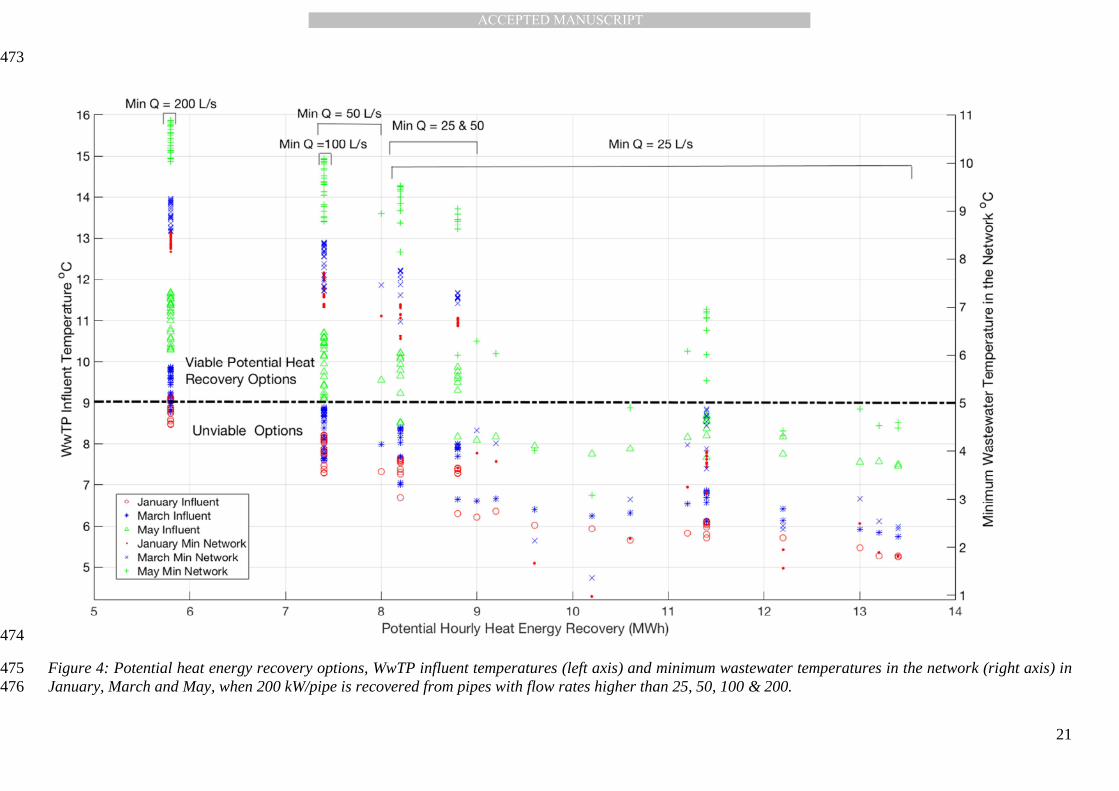
473

474

Figure 4: Potential heat energy recovery options, WwTP influent temperatures (left axis) and minimum wastewater temperatures in the network (right axis) in 475 January, March and May, when 200 kW/pipe is recovered from pipes with flow rates higher than 25, 50, 100 & 200. 476

MA

NU

SC

RIP

T

AC

CE

PTE

D

ACCEPTED MANUSCRIPT

22

The maximum potential heat energy that can be recovered from the sewer network, over an hour, was 13.4 477

MWh for January, March and May. One can notice, from Figure 4, the impact of this 13.4 MWh recovery 478

on the WwTP influent temperature, which varied from 5.3°C (January), 5.7°C (March) to 7.5°C (May). 479

Higher values for the minimum required pipe flow (e.g. 200 L/s) to recover 200 kW/pipe presented lower 480

number of locations, which estimated less potential heat energy recovery. This is expected since 97% of the 481

sewer pipes in the network had flow rates less than 27 L/s. In this work, heat energy recovery is considered 482

viable only when the WwTP influent is above or equal to 9°C and minimum wastewater temperature in the 483

sewer network is 5 °C. Such viable options were presented by the 133 points (out of 288) plotted above the 484

dash dotted line in Figure 4. The network heat transfer model predicted 116, 160 & 207 MWh/day to be 485

recovered in January, March and May respectively. The latter predictions of heat energy recovery are the 486

total of maximum hourly values that were considered viable for each day. 487

488

The time of the day had a noticeable effect on the rate of heat recovery and minimum wastewater 489

temperatures in the network and at the WwTP influent due to the variation of the DWF along the day. In 490

January, viable heat recovery was predicted to be possible during the time periods from midnight to 01:00 491

AM, and between 06:00 AM and 23:00 PM, in March it was from midnight to 02:00 AM and between 05:00 492

AM and 23:00 PM, whilst in May viable heat recovery was possible in all the 24 hours period. Figure 5 493

shows the potential heat energy recovery on an hourly basis along the 24-hour periods in January, March 494

and May. The rate of potential heat recovery, at a particular time of the day, was the same in each month, 495

hence Figure 5 only shows the results of the January scenario. The relatively low flow rate between 03:00 496

and 04:00 AM resulted in a smaller number of locations (41), which was much lower than other cases, e.g. 497

67 potential locations were identified between 10:00 and 11:00 AM in the three scenarios for heat recovery 498

from pipes with minimum flow of 25 L/s. Therefore, the maximum heat recovered between 03:00 and 04:00 499

AM was 8.2 MWh which was less than that of 13.4 MWh predicted between 10:00 and 11:00 AM. 500

Nevertheless, the minimum WwTP influent temperature in January, between 03:00 and 04:00 AM, was 501

higher (8 °C) than that between 10:00 and 11:00 AM (7 °C), and similarly, the minimum network 502

MA

NU

SC

RIP

T

AC

CE

PTE

D

ACCEPTED MANUSCRIPT

23

temperature was always above 6°C between 3:00 and 04:00 AM, which was much higher than its 1.8°C 503

equivalent obtained between 10:00 and 11:00 AM. 504

MA

NU

SC

RIP

T

AC

CE

PTE

D

ACCEPTED MANUSCRIPT

24

505

506 Figure 5: Potential heat energy recovery on hourly basis in 16th January. Other months showed the same hourly heat energy recovery.507

MA

NU

SC

RIP

T

AC

CE

PTE

D

ACCEPTED MANUSCRIPT

25

3.5 Scenarios 1, 2 & 3: heat energy recovery between 07:00 & 08:00 AM 508

This section shows the PDF of minimum network temperatures for each scenario between 07:00 & 08:00 509

AM and summarises the outcomes of the modelled scenarios during the selected hour. The area under the 510

curve between two temperature points, in a PDF plot, would indicate the probability of having pipes with 511

temperature values corresponding to these points. The PDF was also plotted for the sewer network when 512

there was no heat recovery; to enable the comparison with the heat recovery scenarios. For effective 513

utilisation of the thermal energy content in the sewer network, an ideal scenario would show a shift towards 514

the left, relative to the ‘no heat recovery’ PDF, while maintaining the network temperature thresholds. 515

516 3.5.1 Scenario 1, between 07:00 & 08:00 AM 517

Figure 6 shows the PDF of wastewater temperature at the downstream end of each pipe in Scenario 1 518

between 7:00 and 8:00 AM. Recovering heat in Scenario 1 would reduce the wastewater temperatures in the 519

network, which was evidenced by Figure 6 showing higher probabilities of wastewater temperatures being 520

between 10 and 12°C than that when no heat was recovered. 521

MA

NU

SC

RIP

T

AC

CE

PTE

D

ACCEPTED MANUSCRIPT

26

522

Figure 6: Probability distribution function (PDF) of the pipe downstream wastewater temperature, when heat is recovered in January, between 07:00 and 08:00 AM (Scenario 1). The PDF of temperatures below 9°C was equal/close to zero, and hence neglected in the plot.

MA

NU

SC

RIP

T

AC

CE

PTE

D

ACCEPTED MANUSCRIPT

27

523

3.5.2 Scenario 2, between 07:00 & 08:00 AM 524

Figure 7 shows the PDF of wastewater temperatures, at the downstream ends of each pipe in Scenario 2 525

between 07:00 and 08:00 AM. The heat energy recovery resulted in slightly larger probability of pipes with 526

temperatures between 11 and 12.3 °C. 527

MA

NU

SC

RIP

T

AC

CE

PTE

D

ACCEPTED MANUSCRIPT

28

528 Figure 7: Probability distribution function (PDF) of the pipe downstream wastewater temperature, when heat is recovered in March, between 07:00 and 08:00 AM (Scenario 2). The PDF of temperatures below 9°C was equal/close to zero, and hence neglected in the plot.

MA

NU

SC

RIP

T

AC

CE

PTE

D

ACCEPTED MANUSCRIPT

29

529

3.5.3 Scenario 3, between 07:00 & 08:00 AM 530

Figure 8 shows the PDF of pipe downstream wastewater temperatures in Scenario 3, between 07:00 and 531

08:00 AM. As expected, heat energy recovery in May results in generally higher temperatures compared to 532

Scenarios 1 and 2, and increased the probability of obtaining lower pipe temperatures (between 13.7 and 533

14.3 °C) than that of no heat recovery. 534

MA

NU

SC

RIP

T

AC

CE

PTE

D

ACCEPTED MANUSCRIPT

30

535

Figure 8: Probability distribution function (PDF) of the pipe downstream wastewater temperature, when heat is recovered in May, between 07:00 and 08:00 AM (Scenario 3). The PDF of temperatures below 13°C was equal/close to zero, and hence neglected in the plot.

MA

NU

SC

RIP

T

AC

CE

PTE

D

ACCEPTED MANUSCRIPT

31

3.5.4 Summary of Scenarios 1, 2 & 3, between 07:00 & 08:00 AM 536

Table 4 summarises the findings of Scenarios 1, 2 and 3 for the hours between 07:00 and 08:00 AM. The 537

number of locations in Table 4 refers to the number of pipes that meet the temperature (above 9°C) and the 538

flow (25, 50, 100 & 200 L/s or above) criteria for recovering heat (200 kW/pipe). The total heat energy 539

recovery for each of the three scenarios was the same for each criterion, since the number of potential 540

locations was the same. The three scenarios, presented in this section, demonstrated five potentially viable 541

heat energy recovery options where the minimum temperatures were above the thresholds. The minimum 542

influent temperature was around 3°C below the 9°C threshold while the temperatures in some pipes fell 2°C 543

below the 5°C threshold. 544

Table 4: Summary of potential heat energy recovery results from Scenarios 1, 2 and 3 between 7:00 and 545 8:00 AM. HR stands for heat recovery. 546

Scenario

Month Min Q

No. of HR locations, between

07:00 and 08:00 AM

Total HR between

07:00 and 08:00 AM

(200kW/pipe)

WwTP Influent

temperature Before HR

Minimum network

temperature Before HR

WwTP Influent

temperature After HR

Minimum network

temperature After HR

L/s MWh °C °C °C °C

1 January

25 57 11.4

12.5 8.6

5.7 3.1 50 41 8.2 7.3 6.8 100 37 7.4 7.8 7.4 200 29 5.8 9.0 8.5

2 March

25 57 11.4

13.0 9.7

6.1 3.6 50 41 8.2 7.7 7.2 100 37 7.4 8.2 7.8 200 29 5.8 9.2 8.9

3 May

25 57 11.4

14.5 13.7

7.7 5.5 50 41 8.2 9.2 8.7 100 37 7.4 9.7 9.3 200 29 5.8 10.8 10.3

547

4 Discussion 548

Linking a single pipe heat transfer model to a hydrodynamic model and validating the linked model in a 549

sewer network setting enabled the investigation of potential multi-location heat energy recovery from a 550

sewer catchment of 79500 PE. The viable potential heat energy recovery options varied depending on the 551

month, where the lowest predicted was 116 MWh/day or 42 GWh/year, assuming a 100% efficient heat 552

MA

NU

SC

RIP

T

AC

CE

PTE

D

ACCEPTED MANUSCRIPT

32

recovery system. This potential viable heat energy is adequate to cover the annual heat demands of 2500, 553

3500 or 5300 households, assuming high, medium and low UK annual gas consumption of 17, 12 and 8 554

MWh/household respectively (Ofgem, 2017 and Ali et al., 2017). March and May showed potential viable 555

heat energy recovery of 58.4 and 75.7 GWh/year, that are equivalent to annual heat demands of 4900 and 556

6300 households respectively when considering the medium demand of 12 MWh/year/household. 557

Accounting for the lowest potential heat energy recovery (January) and the range of annual household 558

demand, 7 to 15% of the 79500 PE catchment annual demand can be met, without causing wastewater 559

temperatures in the network or in the WwTP influent to be below 5 and 9°C respectively, assuming 2.3 PE 560

per household. The above percentage may rise to cover 14% and 18% of the catchment heat annual demand 561

when March and May scenarios are considered respectively, assuming medium annual UK heat demand. 562

563

The rates of predicted heat recovery were presented in more details for the hours between 07:00 and 08:00 564

AM since this is considered to be the time for high heat energy demand and showed typical representation of 565

the daily DWF. Prediction results showed that setting a low flow threshold level for pipes to recover heat 566

from (e.g. 25 L/s), larger rates of heat can potentially be recovered, which consequently resulted in lower 567

wastewater temperatures (Figure 7 & Figure 8). This was expected since the lower flow rate had less 568

thermal capacity and hence caused a larger wastewater temperature reduction in sewers (Equation 1). One 569

can notice a shift in the PDF peaks from left (low temperature) in January to the higher temperatures in 570

May. This is due to the higher in-sewer air temperature (around 14.4°C) in May which was highly 571

influenced by the ambient air temperature. Table 4 showed how recovering heat of 5.8 to 8.2 MWh, in 572

Scenarios 1, 2 and 3 can be achieved while meeting the minimum temperature criteria set by the water 573

utility. 574

575

Other studies have suggested that heat recovery from wastewater may reduce the deposition of fat, oil and 576

grease (FOG) (He, et al., 2017). This is because temperature plays a major part in influencing the FOG 577

hydrolysis rate where higher temperatures increase the rate of saponification, which increases the FOG 578

deposition (Iasmin, et al., 2016). However, the latter authors performed their study on temperatures of 22 579

MA

NU

SC

RIP

T

AC

CE

PTE

D

ACCEPTED MANUSCRIPT

33

and 45°C, hence further research is needed to investigate the impact of temperature variation, over a more 580

typical in-sewer temperature range (e.g. 5 to 25°C), on the FOG deposit formation. 581

582

This paper has not considered the practical barriers of recovering heat from a sewer network. For example, 583

there are physical limitations on the possibility of installing heat exchangers in certain pipe sizes, which is 584

dependent on the rate of heat recovery. Future work will implement a multi criteria optimisation technique 585

to maximise the potential of heat energy recovery, within a sewer network, without compromising on the 586

wastewater treatment process, and taking into account practical issues associated with the location and 587

operation of heat exchangers. 588

5 Conclusions 589

A network heat transfer model, was developed and validated in this study and was implemented to assess the 590

viability of heat energy recovery scenarios, from a large Belgian sewer network serving 79500 PE. The 591

network heat transfer model was based on single pipe heat transfer model, which utilised the first principles 592

of heat transfer including the heat exchange between wastewater and in-sewer air, and was linked to a 593

hydrodynamic model to predict wastewater temperatures throughout the network over extended periods. 594

Validation of the network heat transfer model showed a daily RMSE between measured and modelled in-595

pipe wastewater temperatures that ranged between 0.44 and 0.72 °C for the different months of the year. 596

This was based on a constant input foul temperature of 15°C, which minimised the RMSE of the measured 597

and modelled in-pipe wastewater temperatures. Three modelled seasonal scenarios showed potential heat 598

energy recovery options on an hourly basis in three days with dry weather flow during January, March and 599

May. It was found that 46% of the 288 hourly modelled heat recovery simulations predicted viable heat 600

recovery since they resulted in wastewater temperatures that were always equal or above the thresholds of 5 601

°C, in the network, and 9 °C in the WwTP influent. The predicted rate of heat energy recovery whilst 602

meeting the minimum temperature requirements varied from 116 MWh/day in January to 207 MWh/day in 603

May. This can meet 7% to 18% of the 79500 PE catchment heat demand, assuming a 100% efficient heat 604

recovery and supply system. The current network heat transfer model will be further developed to enable the 605

automated spatial optimisation of viable heat recovery locations from a large sewer network given both 606

MA

NU

SC

RIP

T

AC

CE

PTE

D

ACCEPTED MANUSCRIPT

34

practical constraints and the wish to achieve the highest heat recovery that satisfies local demand. Future 607

studies may also examine the temporal availability of heat and whether the rate of heat recovery can be 608

enhanced by better matching the temporal pattern of local heat demand and recovery. 609

6 References 610 611 Abdel-Aal, M., 2015. Modelling the Viability of Heat energy recovery from Underground Pipes- 612 Deterministic modelling of wastewater temperatures in a 3048 sewer pipes network, PhD Thesis, University 613 of Bradford. Available on http://hdl.handle.net/10454/14467. 614 615 Abdel-Aal, M., Mohamed, M., Smits, R., Abdel-Aal, R., De Gussem, K., Schellart, A. & Tait, S., 2015. 616 Predicting wastewater temperatures in sewer pipes using abductive network models. Water Science & 617 Technology 71(1), 89-96. 618 619 Abdel-Aal, M., Smits, R., Mohamed, M., De Gussem, K., Schellart, A. & Tait, S., 2014. Modelling the 620 viability of heat energy recovery from combined sewers. Water Science & Technology, 70, 297-306. 621 622 AECOM Building Engineering, 2014. Energy Demand Research Project: Early Smart Meter Trials, 2007-623 2010. [data collection]. UK Data Service. SN: 7591, http://doi.org/10.5255/UKDA-SN-7591-1 624 625 Ali A., Mohamed, M., Abdel-Aal, M., Schellart, A. & Tait, S., 2017. Analysis of ground source heat pumps 626 performance installed in residential houses in the north of England. Proceedings of the Institution of Civil 627 Engineers, 170, 103-115. 628 629 Aquafin, 2014. Hydronaut procedure 6.5 versie Juni 2014 (In Dutch, Specifications for monitoring 630 campaigns and model validation: Internal report by Aquafin). Aartselaar: Aquafin. 631 632 Aquafin, 2015. Final report on Innovative energy recovery strategies in the urban water cycle, 2015. 633 Available on http://inners.eu/wp-content/uploads/2015/07/Final-report-INNERS-project.pdf [Accessed 05 634 October 2017]. 635 636 Bischofsberger, W., Seyfried, C.F. 1984. Wärmeentnahme aus Abwasser (Heat Extraction from 637 Wastewater), Lehrstuhl und Prüfamt für Wassergütewirtschaft und Gesundheitsingenieurwesen der 638 Technischen Universität München, Garching. 639 640 Buri, B., & Kobel, R. 2005. Energie Aus Kanalabwasser Leitfaden für Ingenieure und Planer (Channel 641 Waste Energy- Guidance for engineers and planners). Available on http://www.ib-642 salzmann.de/energie_aus_abwasser/leitfaden_fuer_ingenieure_planer.pdf [Accessed 29 May 2018]. 643 644 645 Cipolla, S. & Maglionico, M., 2014. Heat energy recovery from urban wastewater: Analysis of the 646 variability of flow rate and temperature. Energy and Buildings 69, 122-130. 647 648 Defra- Department for Environment, Food and Rural Affairs, 2002. Sewage Treatment in the UK- UK 649 Implementation of the EC Urban Waste Water Treatment Directive. 650 651 Dürrenmatt, D.J., 2006. Berechnung des Verlaufs der Abwassertemperatur im Kanalisationsrohr 652 (Calculation of wastewater temperature profiles in sewers), Master’s thesis, Swiss Federal Institute of 653 Technology (ETH), Zurich, Switzerland. 654 655

MA

NU

SC

RIP

T

AC

CE

PTE

D

ACCEPTED MANUSCRIPT

35

Dürrenmatt, D.J. & Wanner, O., 2008. Simulation of the wastewater temperature in sewers with TEMPEST. 656 Water Science & Technology 57 (11), 1809-1815. 657 658 Dürrenmatt, D.J., & Wanner, O., 2014. A mathematical model to predict the effect of heat recovery on the 659 wastewater temperature in sewers. Water Research 48(1), 548-558. 660 661 DWA- Deutsche Vereinigung für Wasserwirtschaft, Abwasser und Abfall e.V. 2009. Energie aus Abwasser 662 - Wärme- und Lageenergie. (Energy from wastewater- heat and potential energy DWA-Regelwerk, 663 Merkblatt DWA-M 114, Hennef. 664 665 ECUK, Energy Consumption in the UK, 2017. Department for Business, Energy & Industrial Strategy. 666 Available on https://www.gov.uk/government/statistics/energy-consumption-in-the-uk [Accessed 25 January 667 2018]. 668 669 Edwini-Bonsu, S. & Steffler, P. M., 2006. Modeling Ventilation Phenomenon in Sanitary Sewer Systems: A 670 System Theoretic Approach, Journal of Hydraulic Engineering, 132, 778–790. 671 672 Elías-Maxil., J.A. 2015. Heat modeling of wastewater in sewer networks- Determination of thermal energy 673 content from sewage with modeling tools, PhD Thesis, TU Delft. 674 675 Elías-Maxil, J.A., Hofman, J., Wols, B., Clemens, F., van der Hoek, J.P. & Rietveld, L., 2017. Development 676 and performance of a parsimonious model to estimate temperature in sewer networks. Urban Water Journal, 677 14 (8), 829-838. 678 679 Flinspach, D., 1973. Wärmelastplan neckar plochingen bis mannheim stand. Ministerium für Ernährung, 680 Stuttgart. 681 682 He, X., Reyes, F. L. & Ducoste, J. J., 2017. A critical review of fat, oil, and grease (FOG) in sewer 683 collection systems: Challenges and control’, Critical Reviews in Environmental Science and Technology, 47 684 (13), 1191–1217. 685 686 Iasmin, M., Dean, L. O. & Ducoste, J. J., 2016. Quantifying fat, oil, and grease deposit formation kinetics, 687 Water Research, 88, 786–795. 688 689 Kretschmer, F., Weissenbacher, N., Ertl. T., 2015. Integration of Wastewater Treatment Plants into Regional 690 Energy Supply Concepts. Sustainable Sanitation Practice, 22, 4-9. 691 692 Kretschmer, F., Simperler L. & Ertl., T., 2016. Analysing wastewater temperature development in a sewer 693 system as a basis for the evaluation of wastewater heat recovery potentials. Energy and Buildings, 128, 639-694 648. 695 696 Metcalf & Eddy, 2004. Wastewater engineering treatment and reuse. 4th edition, New York: Mcgrow Hill. 697 698 Ofgem- Office of Gas and Electricity Markets, 2017. Typical Domestic Consumption Values. Available on 699 https://www.ofgem.gov.uk/gas/retail-market/monitoring-data-and-statistics/typical-domestic-consumption-700 values [Accessed 29 August 2017]. 701 702 Schilperoort, R.P. & Clemens, F.H., 2009. Fibre-optic distributed temperature sensing in combined sewer 703 systems. Water Science & Technology 60 (5), 1127-1134. 704 705 Shammas, N.K., 1986., Interactions of temperature, ph and biomass on the nitrification process. Water 706 Pollution Control Federation, 58, 52-59. 707 708

MA

NU

SC

RIP

T

AC

CE

PTE

D

ACCEPTED MANUSCRIPT

36

Simperler, L., 2015. Impact of thermal use of wastewater in a sewer on the inlet temperature of a wastewater 709 treatment plant, Master’s Thesis, University of Natural Resources and Life Sciences. 710 711 Sitzenfrei, R., Hillebrand S., & Rauch W., 2017. Investigating the interactions of decentralized and 712 centralized wastewater heat recovery systems. Water Science and Technology, 75, 1243-1250. 713 714 Vlario, 2015. Heat energy recovery from the sewer system. Available on 715 http://www.vlario.be/site/files/Appendix-6-Heat-recovery from-the-sewer-system.pdf [Accessed 19 716 October 2017]. 717 718 Wanner, O., Panagiotidis, V., Clavadetscher, P. & Siegrist, H., 2005. Effect of heat recovery from raw 719 wastewater on nitrification and nitrogen removal in activated sludge plants. Water Research, 39, 4725-4734. 720

MA

NU

SC

RIP

T

AC

CE

PTE

D

ACCEPTED MANUSCRIPT

•Potential of heat recovery form a large sewer network was modelled for the first time

•Linked network heat transfer and network hydrodynamic models were validated

•Scales of potential viable heat recovery varied seasonally from 116 to 207 MWh/day

•Viable heat recovery can meet 7% to 18% of a 79500 PE catchment demands