Universität Leipzig

Wirtschaftswissenschaftliche Fakultät

Institut für theoretische Volkswirtschaftslehre

Makroökonomik

Prof. Dr. Thomas Steger

Thema

“Happiness, Relative Income and the Specific Role

of Reference Groups”

Masterarbeit zur Erlangung des akademischen Grades

Master of Science – Volkswirtschaftslehre

vorgelegt von: Christoph Hindermann

Leipzig, den 03.03.2014

Chapter Page

Outline II

List of Figures and Tables III

Abbreviations III

1 Introduction 1

2 Measurement of Happiness in Economics 2

3 The Economics of Happiness 6

3.1 The Relation between Absolute Income and Happiness 6

3.2 Unemployment, Inflation and Inequality 12

4 The Role of Relative Income 15

4.1 Empirical Evidence 16

4.1.1 Empirical Evidence for the 'Social Comparison Effect' 16

4.1.2 Empirical Evidence for the 'Tunnel Effect' 21

4.1.3 Derived Empirical Regularities 23

4.2 Theoretical Considerations 24

4.2.1 Modeling of Utility Functions 24

4.2.2 A Contribution in Explaining the Easterlin-Paradox? 26

4.2.3 Concluding Remarks 29

5 Specifications of the Reference Group 30

5.1 The Reference Group as Exogeneous Variable 30

5.2 The Reference Group as Endogeneous Variable 33

6 Different Reference Group Specifications and Life Satisfaction 35

6.1 Data Description and Choice of Variables 36

6.2 Methodology 38

6.2.1 Data Preparation 38

6.2.2 Estimation Procedure 39

6.2.3 Further Econometric Issues 44

6.3 Relative Income and Reference Group Specifications 46

6.4 Results 49

6.4.1 Whole Sample 49

6.4.1.1 Looking for the Tunnel Effect: Young and Old respondents 54

6.4.1.2 Looking for the Tunnel Effect: Transition Countries 56

6.4.2 German Sub-Samples 57

6.4.2.1 Whole German Sample 57

6.4.2.2 Looking for the Tunnel Effect: Young and Old respondents 58

6.4.3 Summary of the Empirical Results 60

6.5 Problems and Shortcomings of the Study 61

7 Conclusion 63

Appendix A – List of Variables 65

Appendix B – Correlations 67

References 68

Statement of Authorship 74

II

List of Figures and Tables

Figures/Tables Description/Title Page

Figure 1 Happiness and GDP in the UK over time 9

Figure 2 Aspirations and Adaption 11

Figure 3 Relationship between Income, Relative Income and Happiness 28

Table 1 Selected Surveys and Questions about Happiness 3

Table 2 External Reference Group Specifications 31

Table 3 Ordered probit vs. OLS estimates 41

Table 4 Satisfaction vs. Happiness 42

Table 5 Reference Group Specifications 47

Table 6 Reference Group (Age) 49

Table 7 Reference Income 50

Table 8 Reference Groups (Whole Sample) 53

Table 9 Reference Groups (Whole Sample – Young) 54

Table 10 Reference Groups (Whole Sample – Old) 55

Table 11 Reference Groups (Whole Sample – Transition) 56

Table 12 Reference Groups (Germany) 57

Table 13 Reference Groups (Germany – Young) 59

Table 14 Reference Groups (Germany – Old) 59

Table 15 Appendix A - List of Variables 65

Table 16 Appendix B - Correlations 67

Abbreviations

BHPS British Household Panel

ESS European Social Survey

GDP Gross Domestic Product

GDR German Democratic Republic

GSOEP German Socio-Economic Panel

IMF International Monetary Fund

ISCED International Standard Classification of Education

NSFH National Survey of Families and Households

OLS Ordinary Least Squares

PUMA Public Use Microdata Area

III

1 Introduction

Many scientific disciplines such as philosophy, sociology, psychology, medicine and

neuroscience deal with happiness. Over the last decades, economists also started to pay

attention to the relation of happiness and its economic determinants. Next to personal and

demographic characteristics, a wide ranging literature has shown that also absolute income

and wealth, relative income as well as macroeconomic conditions (inflation, general

unemployment) strongly matter when explaining happiness (see MacKerron (2012) for a

review).

In particular, there are a variety of studies that show that absolute income is positively

correlated with individual well-being, but find at the same time that average income of the

reference group (comparison income) affects individual well-being most often negatively

(Clark et al., 2008). Although the results allover the literature are quite consistent, there is a

large variety how the reference group is defined. For example, some authors assume that

people compare themselves with people living in the same area (Luttmer, 2005; Graham &

Felton, 2006) or with people inside the same age range (McBride, 2001). Others define the

reference group more precisely and assume that people compare themselves with people of

same age, same education and same area of living (Ferrer-i-Carbonell, 2005). However, to the

best of my knowledge, there is no systematic empirical research on the impact of different

reference group specifications on life satisfaction in happiness regressions. Therefore, I

investigate in this master thesis to what extent different reference group specifications alter

the statistical impact of comparison income on happiness regarding sign, magnitude and

statistical significance.

To do so, I review in the first part of the thesis the literature and state empirical regularities as

well as theoretical considerations regarding absolute and relative income. In the second part

of the thesis, I use the European Social Survey (ESS) as data basis to analyze empirically how

different reference group specifications alter the effect of comparison income in happiness

equations. The results show that the specification of the reference group matters, since some

specifications produce significant and others produce insignificant coefficients.

Further, the findings suggest that also the sub-sample plays a crucial role. For example, in the

sub-sample containing old people (40 years and older), comparison income has in most

specifiactions a negative impact on satisfaction. In contrast, in the sub-sample containing only

young people (younger than 40 years), comparison income has, dependent on the reference

group specification, an insignificant or even positive effect on happiness.

1

The remainder of the thesis is structured as follows. In chapter 2, I describe shortly how

happiness can be measured and what kind of obstacles may occur. Chapter 3 serves to present

a review on the economics of happiness, in particular focusing on the relation between

absolute income and happiness. In the following chapter 4, I provide a detailed overview

about the role of relative income when explaining life satisfaction. This will be continued in

chapter 5, where I address reference groups and their specifications more extensively. Based

on this, I perform an empirical study about the impact of different reference group

specifications on life satisfaction with the help of the European Social Survey (ESS), which is

shown in chapter 6. Lastly, I conclude shortly in chapter 7.

2 Measurement of Happiness in Economics

In economics, the measurement of happiness has often been discussed. Usually, the

assumption is made that the concept of happiness1 is closely linked to the utility concept.

Hence, when economists ask for well-being or happiness, they aim at measuring the

underlying utility. Although this idea is straight forward, there has been a discussion whether

it is sufficient just to ask for happiness (subjective well-being) or if it is not more plausible to

rely on actual decisions (objective well-being).

Objective well-being is mainly based on the axiomatic concept of revealed preferences, where

the actual choice reveals all information needed to measure the individual utility (Frey &

Stutzer, 2002, p. 404). Hence, individual behavior and the individual choice between tangible

goods, services and leisure determine implicitly the best decision an individual can make to

approach the highest possible utility level (Frey, 2008, p. 15). However, there has emerged an

extensive literature about anomalies and irrationalities2 in decision making so that it has to be

questioned if utility can be derived sufficiently by actual decisions (Frey, 2008, p. 16).

Moreover, the fact that the concept of revealed preferences misses out procedural utility3

points out a further shortcoming of the positivistic view considering only actual decisions.

Subjective experiences are not objectively observable and therefore often declared as

“unscientific”, in particular since everyone has own perceptions about what happiness or the

“good life” really is (Frey, 2008, p. 15). However, vast studies apply the subjective well-being

concept, where researchers rely on the answers of the respondents when asked about their

1 The terms happiness, satisfaction and well-being are used interchangeably.2 Frey (2008, pp. 15-16) gives an overview about several anomalies (e.g. emotions, intrinsic motivation or

status) and irrationalities (e.g. preference inconsistencies). 3 Procedural utility describes that conditions and processes are also valued by people. (Frey, 2008, p. 107)

2

happiness. Generally, this concept is described to be much broader than objective well-being,

since it understands utility in hedonistic terms (experienced utility) and also accounts for

procedural utility (Frey & Stutzer, 2002, p. 405; Frey, 2008, p. 16). Consequently, the concept

allows to measure individual well-being directly, although there is some doubt if reported

well-being serves well as a proxy for decision utility4 (Frey, 2008, p. 16).

The measurement of happiness in economics is mainly based on subjective survey data

relying on the validity of the subjective well-being concept. More specifically, the

measurement of happiness offers various possibilities. Beside multiple question items, where

different questions are asked to identify an underlying dimension of happiness, overall life

happiness is most frequently inquired by one single question. Since answers are based on

individual judgments, subjective survey data tend to be biased due to the wording of

questions, the order of questions, the scales applied, the actual mood or the selection of

information processed (Frey, 2008, p. 19).

To discuss these obstacles in greater depth, table 1 shows different surveys, where people are

asked about their overall life satisfaction.

Table 1: Selected Surveys and Questions about Happiness

Survey (Single) Question

Euro-Barometer Survey“Taking all together, how happy you say you are: very happy,quite happy, not very happy, not at all happy?” (4-point scale)

World Values Surveys“All things considered, how satisfied are you with your life as awhole these days?” (11-point scale)

European Social Survey“Taking all things together, how happy would you say you are?“(11-point scale)

German Socio-EconomicPanel

“How satisfied are you with your life, all things considered?“(10-point scale)

British-Household Panel“How dissatisfied or satisfied are you with your life overall?“ (7-point scale)

US General SocialSurvey

“Taken all together, how would you say things are these days – would you say you are very happy, pretty happy, or not too happy?” (3-point scale)

Source: Codebooks of Euro-Barometer Survey (2005, p. 172), World Value Surveys (2004, p. 32), European

Social Survey (2012), German Socio-Economic Panel (2012, p. 35), British-Household Panel (2012, p. 217)

and US General Social Survey (2009, p. 277)

4 Closely related research areas show that reported variables serve well to proxy actual decisions. Examplesare that future job quits can be predicted by reported job satisfaction, that the probability of a future divorcecan be explained by the satisfaction gap between spouses, that there exists a strong correlation betweenhappiness and productivity as well as that suicides can be predicted by well-being data. (Ferrer-i-Carbonell,2012, p. 49-50)

3

As the questions show, there are differences in the order of words as well as differences in the

words used. The Euro-Barometer Survey, the European Social Survey as well as the US

General Social Survey use the word “happy”, the other surveys listed stick to “satisfied”. It

remains open if “happiness” and “satisfaction” really mean the same, i.e. have the same

connotations5 for the respondents, or if they would answer different if one word would be

replaced by an other. An argument for the conceptual difference of both words would be that

“life satisfaction refers to cognitive states of consciousness, whereas happiness is emotional

and mainly concerns intimate matters of life“ (Caporale et al., 2005, p. 43).

Another problem may arise due to the placement of the life satisfaction question in the

questionnaire. For example, Easterlin and Anglescu (2009, p. 5) report that overall life

satisfaction of respondents tend to be downward biased if there are questions about finances

inserted before. The reason is that people are in general less satisfied with their financial

situation than with their life as whole leading to a lower score in overall life happiness.

In addition, also the scales applied may matter. As table 1 shows, the scales applied vary from

3-point scales (“very happy”, “pretty happy” or “not too happy” in the US General Social

Survey) to 11-point scales (“0“– extremely unhappy to “10” – extremely happy in the

European Social Survey). Concerning 3-point scales, one could argue that happiness cannot

be captured as precise as in 11-point scales due to the missing possibility of differentiation.

Different scales may also lead to problems when merging different data-sets. For example,

Easterlin and Anglescu (2009, p. 3) solve this problem by transferring the Euro-Barometer 4-

point scale to a 10-point scale by a linear transformation in order to be able to work with a

merged data-set. Of course, it has to be questioned if rescaling does alter the validity of the

happiness data, independently on how we understand the variable measuring happiness.

There are mainly three possibilities how the variable measuring happiness can be understood

(MacKerron, 2012, p. 712; Ferrer-i-Carbonell and Frijters, 2004, p. 643):

I. Reported happiness (R) is understood as a positive monotonic transformation of an

underlying variable of interest “true happiness” or “utility” (U), where R'(U) > 0.

II. Reported happiness can be compared ordinally between people such that if Ri > Rj

then Ui > Uj , where the subscripts i and j represent different individuals.

5 Veenhoven (2012, p. 339-340) analyzes this by posing three different happiness questions (happiness-in-life,satisfaction-with-life and best/worst possible life) in eleven mono-lingual nations. The results show that therank order of happiness is nearly the same for all three questions, i.e. if Australians rank highest when askedabout their satisfaction-with-life, they are probably also highest or very high ranked when asked abouthappiness-in-life and best/worst possible life. (Germans seem to be an exception. They understand“happiness” (Glück) and “satisfaction” (Zufriedenheit) somewhat different.) Thus, there is some evidencethat the connotations of “satisfaction” and “happiness” are similar across nations.

4

III. Reported Happiness can be compared cardinally between people such that the

equation Ri – Rj = Ui – Uj holds.

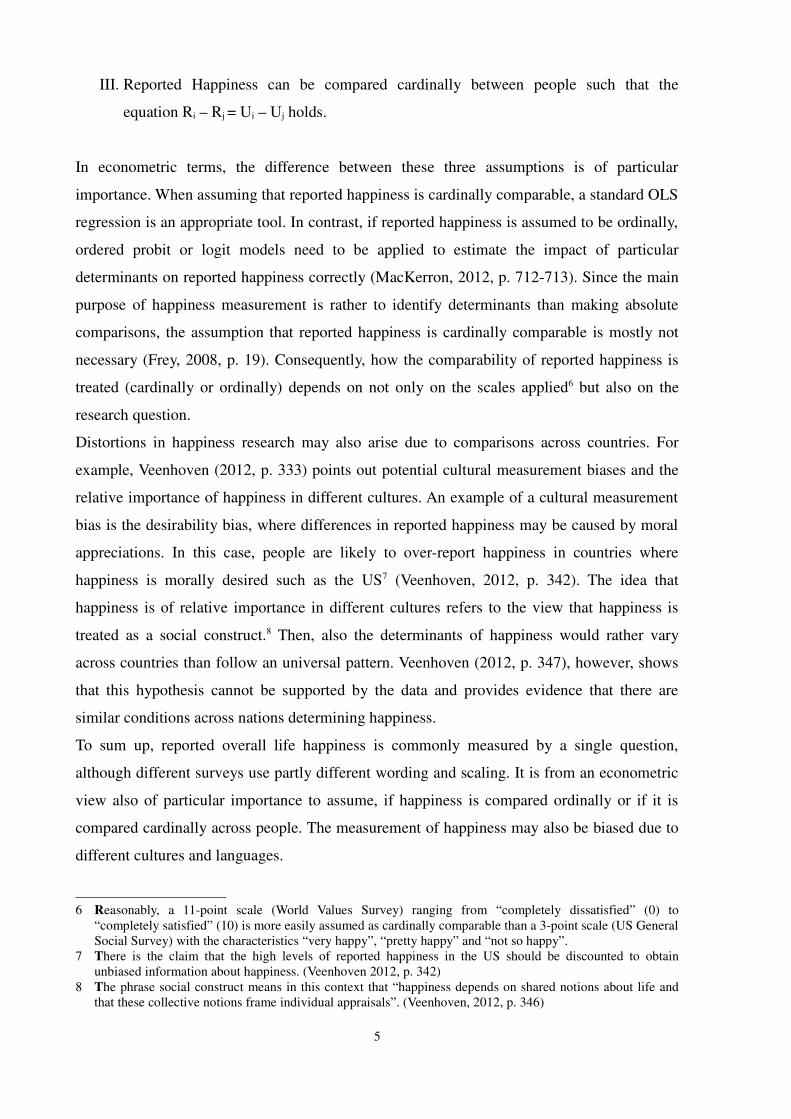
In econometric terms, the difference between these three assumptions is of particular

importance. When assuming that reported happiness is cardinally comparable, a standard OLS

regression is an appropriate tool. In contrast, if reported happiness is assumed to be ordinally,

ordered probit or logit models need to be applied to estimate the impact of particular

determinants on reported happiness correctly (MacKerron, 2012, p. 712-713). Since the main

purpose of happiness measurement is rather to identify determinants than making absolute

comparisons, the assumption that reported happiness is cardinally comparable is mostly not

necessary (Frey, 2008, p. 19). Consequently, how the comparability of reported happiness is

treated (cardinally or ordinally) depends on not only on the scales applied6 but also on the

research question.

Distortions in happiness research may also arise due to comparisons across countries. For

example, Veenhoven (2012, p. 333) points out potential cultural measurement biases and the

relative importance of happiness in different cultures. An example of a cultural measurement

bias is the desirability bias, where differences in reported happiness may be caused by moral

appreciations. In this case, people are likely to over-report happiness in countries where

happiness is morally desired such as the US7 (Veenhoven, 2012, p. 342). The idea that

happiness is of relative importance in different cultures refers to the view that happiness is

treated as a social construct.8 Then, also the determinants of happiness would rather vary

across countries than follow an universal pattern. Veenhoven (2012, p. 347), however, shows

that this hypothesis cannot be supported by the data and provides evidence that there are

similar conditions across nations determining happiness.

To sum up, reported overall life happiness is commonly measured by a single question,

although different surveys use partly different wording and scaling. It is from an econometric

view also of particular importance to assume, if happiness is compared ordinally or if it is

compared cardinally across people. The measurement of happiness may also be biased due to

different cultures and languages.

6 Reasonably, a 11-point scale (World Values Survey) ranging from “completely dissatisfied” (0) to“completely satisfied” (10) is more easily assumed as cardinally comparable than a 3-point scale (US GeneralSocial Survey) with the characteristics “very happy”, “pretty happy” and “not so happy”.

7 There is the claim that the high levels of reported happiness in the US should be discounted to obtainunbiased information about happiness. (Veenhoven 2012, p. 342)

8 The phrase social construct means in this context that “happiness depends on shared notions about life andthat these collective notions frame individual appraisals”. (Veenhoven, 2012, p. 346)

5

3 The Economics of Happiness

The economics of happiness goes back to the works by Easterlin (1974). In his seminal paper

“Does Economic Growth Improve the Human Lot?” Easterlin analyzes the relation between

income and happiness. The result, well-known as the Easterlin-Paradox, shows that within

one country there is a strong positive correlation between happiness and income at a point in

time, but no systematical correlation between these variables over time (Easterlin, 1974, p.

118). On the other hand, across countries, the correlation between income and happiness turns

out to be much weaker than within countries, whereby there is again no significant correlation

over time (Easterlin, 1974, p. 118).

The empirical evidence first provided by Easterlin (1974) is also supported by more recent

happiness studies, which find only little, if any, evidence that happiness and income are

related across countries and over time (Graham 2005, p. 45). To understand the relation

between absolute income and happiness in greater depth9, the following chapter focuses more

detailed on the empirical regularities first sketched by Easterlin (1974) and confirmed by a

variety of other studies. Of course, this chapter also points to underlying theories, which try to

explain the empirical regularities and their interactions. In addition, the chapter sketches the

relation between other macroeconomic variables (unemployment, inflation, inequality) and

happiness to give a comprehensive overview about the economics of happiness.

3.1 The Relation between Absolute Income and Happiness

The relation between income and happiness has several dimensions. The following chapter

focuses firstly on the cross-country level, where average happiness and GDP per capita are

treated in a cross-country relation. Thereafter, the link between absolute income and

happiness within countries is shortly explored. Lastly, the time-series dimension is considered

and a theoretical approach is presented to explain the empirical difference between the short-

run and the long-run relation between happiness and income.

Research on income and happiness with macro data across countries has shown that wealthier

countries seem to be happier than poor ones. However, this relation seems to hold only up to a

certain level. Beyond this level, the relation seems to vanish. (Frey & Stutzer, 2002, p. 416;

9 This chapter focuses on the relation of absolute income and happiness. The role of relative income will bediscussed in chapter 4.

6

Graham, 2005, p. 45)

Easterlin and Anglescu (2009, p. 6) report that life satisfaction increases with absolute GDP

per capita but at diminishing rates. Increases in GDP per capita have therefore a much larger

impact on poor countries than on rich countries.

As a consequence, most authors identify a concave relationship between GDP per capita and

average happiness. However, this relation has to be treated critically, since a higher GDP per

capita is often accompanied by other factors impacting positively on happiness. For example,

countries with a high GDP per capita generally have a more stable democracy, a higher health

standard and more secure basic human rights (Frey & Stutzer, 2002, pp. 416-417).

Hence, macro data provide often only a very weak relation between country GDP per capita

and happiness, in particular when national averages are used and it is controlled for education,

unemployment and other factors moderating the strength of the relationship between GDP and

income (Ferrer-i-Carbonell, 2012, p. 42; Caporale et al., 2009, p. 42). At least for developed

countries, a policy implication would be that economic growth is not of primary importance

so that politicians should also take education, unemployment and other macroeconomic

variables into account when maximizing happiness in the society (Clark et al., 2008, p. 96).

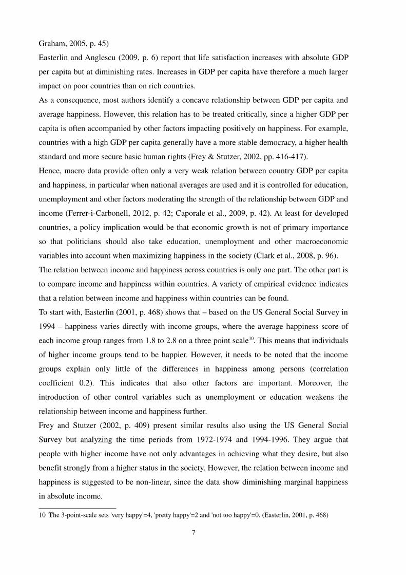
The relation between income and happiness across countries is only one part. The other part is

to compare income and happiness within countries. A variety of empirical evidence indicates

that a relation between income and happiness within countries can be found.

To start with, Easterlin (2001, p. 468) shows that – based on the US General Social Survey in

1994 – happiness varies directly with income groups, where the average happiness score of

each income group ranges from 1.8 to 2.8 on a three point scale10. This means that individuals

of higher income groups tend to be happier. However, it needs to be noted that the income

groups explain only little of the differences in happiness among persons (correlation

coefficient 0.2). This indicates that also other factors are important. Moreover, the

introduction of other control variables such as unemployment or education weakens the

relationship between income and happiness further.

Frey and Stutzer (2002, p. 409) present similar results also using the US General Social

Survey but analyzing the time periods from 1972-1974 and 1994-1996. They argue that

people with higher income have not only advantages in achieving what they desire, but also

benefit strongly from a higher status in the society. However, the relation between income and

happiness is suggested to be non-linear, since the data show diminishing marginal happiness

in absolute income.

10 The 3-point-scale sets 'very happy'=4, 'pretty happy'=2 and 'not too happy'=0. (Easterlin, 2001, p. 468)

7

There are further studies presenting similar results such as Blanchflower and Oswald (2004, p.

1381) for developed countries or Graham and Pettinato (2002, p. 100) for developing

countries. The only difference between these studies can be found regarding the slope of the

happiness-income relationship at a point in time, which is larger within developing countries

(Clark et al., 2008, p. 97).

To fully understand the relation between happiness and income, it is not sufficient to only

compare within and across countries. Rather, the relation between income and happiness

depends strongly on the time dimension being treated, namely the short-run and the long-run

dimension.

At a point in time, people with a higher income are, on average, more happy than those with

less income (Easterlin, 1974; Easterlin, 2001, p. 465). In addition, time series show that

happiness and GDP per capita are positively related in the short run.

As an example, Easterlin and Anglescu (2009, p. 10) point to transition countries such as the

former GDR, Estonia or the Russian Federation. Here, a co-movement of both variables is not

only visible but also significant in statistical terms, since the results of regressing the growth

rates of average happiness and GDP per capita on each other show a strong positive relation

(Easterlin & Anglescu, 2009, p. 22). Hence, in transition countries, a negative change in GDP

per capita is related with a negative change in average life satisfaction and vice versa

(Easterlin & Anglescu, 2009, p. 10).

In contrast, over the long run, the relation between income and happiness vanishes such that

the average happiness of a cohort remains constant (Easterlin, 2001, p. 465) or has even

declined over the same period (Frey & Stutzer, 2002, p. 413). This is in particular puzzling

since income of the most countries in the world has grown substantially (Easterlin, 2001, p.

465). For example, Easterlin and Anglescu (2009, p. 8-9) find no significant relation between

the growth rate of happiness and the growth rate in GDP per capita in the long run11,

independent of treating developed countries, developing countries, transition countries or all

countries together. Furthermore, findings show that the average happiness of a cohort remains

constant over time in the US, although income has increased considerably (Easterlin, 2001, p.

469). Lastly, observing a time period from 1973 to 2012, the following graph (figure 1) shows

the relation between average happiness and GDP per capita for the UK over time. Although

the GDP per capita has nearly doubled, average happiness remained stable.

11 Critically, the regression does not include other control-variables.

8

Despite this strong empirical evidence in the long-run, the results need to be treated critically.

On the one hand, Clark et al. (2008, p. 97) report empirical evidence that real GDP in East

Germany has grown substantially between 1991 and 200212, whereby also reported happiness

rose considerably over the same period. On the other hand, most of the results offer only

bivariate relations such that they may be sensitive to the observation period and to the

variables controlled for (Frey & Stutzer, 2002, p. 414). For example, figure 1 sketches only

average happiness and the GDP per capita in the UK and misses out other socio-demographic

and macroeconomic variables.

The relation between happiness and income has been treated differently according to the time

period. Hence, it has to be questioned why there is such a disparity between the short and the

long run. To understand this, findings about past and prospective happiness offer some

instructive information.

Interestingly, people systematically overestimate their future or prospective happiness and

underestimate their happiness in the past, independently on where people are located in the

life cycle. On average, they believe that they have been worse off in the past and they will be

12 Of course, this period could also be considered as short-run. Another problem is that Clark et al. (2008, p. 97)present only bivariate correlations.

9

Figure 1: Happiness and GDP in the UK over time

Source: World Database of Happiness (2013) and World Development Indicators (2013)

better off in the future in comparison to their current happiness level (Easterlin, 2001, p. 471).

In particular, this effect is observable by younger respondents, who envisage greater income

changes than older respondents (Easterlin, 2001, p. 471). However, when respondents are

asked again after a period of about five years, happiness is more or less on the same level as

before meaning that it stays on average unchanged.

The main argument is that people link higher future income expectations with more happiness

in the future, which also explains why younger people envisage greater changes in happiness

than older since they expect relatively higher increases in income. Hence, Frey and Stutzer

(2002, p. 403) conclude that people associate income positively with happiness, which seems

to be true in the short run but not over the long run.

Consequently, a theory needs to explain three empirical regularities. First, people are happier

at a given point in time when their income is higher. Second, people underestimate their past

happiness and overestimate their future happiness. Lastly, happiness stays more or less

unchanged over the life cycle. (Easterlin, 2001, 472)

These regularities can be explained by the process of hedonic adaption, in which people

always adapt their aspirations to new situations (Frey & Stutzer, 2002, p. 414). An increase in

income, for example, will also increase happiness in the short run. Over time, however,

aspirations rise as well such that in the end happiness converges back to the initial level. But

why do people predict their future happiness as well as their past happiness on average

incorrectly? An answer is given with the help of figure 2.

Starting with income y0, the representative individual achieves the utility level u(y0) lying on

the aspiration curve13 A0 at point 3. If the representative individual expects now a higher

future income, say y0,F, the individual also associates a higher future utility level u(y0, F)

represented at point 1. Similarly, if the representative individual has to predict its past

happiness, the individual typically report a lower utility u(y0,P) based on past income y0,P

represented at point 4. Hence, the representative individual bases its predictions in the past

and in the future on its current aspirations A0.

Now, income of the representative individual rises from y0 to y1. Then, in the short term,

utility rises as well from u(y0) to uS(y1) represented again at point 1. However, the higher

actual income (y1) alters also aspirations over time, such that the aspiration curve A0 shifts

gradually to the right until reaching the curve A1. In this new situation, the utility gained from

income level y1 is only uL(y1), which equals the initial utility level u(y0). If an individual

13 The aspiration curve states the functional relation between absolute income and utility and shifts to the right,when aspirations rise.

10

would now predict its past utility level, the individual would end up at the utility level

corresponding to point 5.

Hence, this model can easily explain the empirical regularities that have been found. The

resulting implications are that people make predictions to the past and in the future based on

their current aspiration level. They commonly neglect to anticipate changes in their aspiration

level when income changes. Furthermore, income and happiness are positively related in the

short run, but the relation vanishes over time as the aspiration level adapts to the new income

situation.

Consequently, Frey and Stutzer (2002, p. 415) conclude that rising aspirations are responsible

for the fact that people are never satisfied and want to achieve ever more. The phenomenon of

“hedonic adaption” is then also often associated with the phrase “hedonic treadmill” meaning

the effect of higher income lasting only shortly on happiness. Graham (2005, p. 47) lastly

concludes that after basic needs are met, the importance of absolute income does not matter

anymore to happiness in contrast to relative income14.

In particular in psychology, the theory of “hedonic adaption” is also called “setpoint theory”.

The “setpoint theory” states that every individual has a unique happiness setpoint, which is

14 The effect of relative income will be discussed in greater detail in chapter 4.

11

Figure 2: Aspirations and Adaption

Source: own representation based on Easterlin (2001, p. 473)

y

u(y)

y0

uL(y

1)=u(y

0)

A0

y0,Fy

0,P

uS(y

1)=u(y

0,F)

u(y0,P

)

A1

y1

1

23

4 5

formed by personality and genetic heritage. The idea is that even after major life events such

as marriage, unemployment or serious injury or diseases the individual converges over time

back to its individual setpoint. This indicates that no permanent positive or negative deviation

from the setpoint is possible. (Easterlin, 2006, p. 466; Graham, 2005, p. 47)

3.2 Unemployment, Inflation and Inequality

Beside income, unemployment has also an important role when explaining happiness. Studies

focusing on unemployment basically distinguish between personal and general

unemployment.

Personal unemployment asks to what extent unemployment affects happiness of an individual

by becoming unemployed and later reemployed. Frey and Stutzer (2002, p. 419) report that

unemployed people report systemically lower happiness than employed persons with similar

characteristics. Oswald (1997, pp. 1822/1825) reports that the unemployed are very unhappy

and have a higher probability to commit suicide, whereby the commitment of suicide is

understood as extreme unhappiness. Ferrer-i-Carbonell (2012, p. 37) reviews that personal

unemployment has a severe impact on happiness which is long lasting and remains even after

becoming reemployed. In addition, unemployment may alter the setpoint for life satisfaction

sustainably, which means that negative effects of unemployment persist over time such that

people do not adapt to unemployment as they would do to changes in income (Lucas et al.,

2004, pp. 8-13; Clark et al., 2008, p. 222; Ferrer-i-Carbonell, 2012, p. 45).

To examine the net effect of unemployment, it has also been controlled for income losses and

the benefits from the social systems. The results show that there are also severe non-pecuniary

costs of unemployment addressed as psychic and social costs. The phrase psychic costs

subsumes depression and anxiety, loss of self-esteem and personal control. In addition,

unemployed individuals suffer from worse mental health, have a higher death rate, commit

more likely suicide and consume higher quantities of alcohol. The social costs of being

unemployed are that the unemployed are often stigmatized by the society, in particular in

societies where the job position is inherently linked to the position in life. (Frey & Stutzer,

2002, p. 419-420; Oswald, 1997, p. 1825; Ferrer-i-Carbonell, 2012, p. 45)

It is, however, not clear that the causality runs only from unemployment to unhappiness or if

there is also reverse causality (Frey and Stutzer, 2002, p. 419). For example, Graham et al.

(2004, p. 319) report that happier people perform better in the labor market and, therefore, are

12

more likely to earn more income in the future. Hence, happier people are more likely to be

employed since their performance in the job is better and unhappy people are more likely to

become unemployed due to their worse performance. Then, the causality would run from

unhappy to unemployed.

Happiness is not only affected by personal unemployment but also by general unemployment.

People are negatively affected by general unemployment since the possibility of becoming

unemployed increases (Frey & Stutzer, 2002, p. 420).

How strong the effect of unemployment on happiness is depends strongly on the reference

group. Frey and Stutzer (2002, p. 421) report that individuals evaluate their own situation

relative to others such that unemployed individuals are on average less unhappy if also other

individuals are unemployed, in particular the partner or a large part of the individuals living in

the same region. Hence, increasing general unemployment lowers an individual's happiness if

that individual is employed, but it increases an individual's happiness if that individual is

already unemployed (Frey, 2008, p. 53). The argument for this phenomenon is mainly that

people are less stigmatized by unemployment such that psychic and social effects are partly

mitigated (Frey & Stutzer, 2002, p. 421).

Unemployment is not the only variable people care about. Also inflation plays a crucial role

when treating macroeconomic conditions in a country. There has been a wide ranging

discussion about the trade-off between inflation and unemployment in the short- and long-run,

mostly known in the context of the Phillips-curve (Friedman 1977, Samuelson & Solow,

1960). For the purpose of happiness research, it is most insightful to analyze which of these

variables are more relevant for the people in a country.

In a study covering twelve European countries within the period of 1975 to 1991, Di Tella,

MacCulloch and Oswald (2001, p. 335-341) find that a one percent increase in the

unemployment rate reduces happiness by 0.028 points on a four-point scale, while a one

percent increase in the inflation rate reduces happiness by only 0.012 points. Hence,

unemployment depresses happiness more than inflation. This is even the case after controlling

for country fixed effects, year fixed effects and country-specific time trends. Then, the

estimates show that a 1-percentage-point increase in the unemployment rate would be

marginally compensated by a 1.7-percent decrease in the inflation rate.

Lastly, income inequality also may have adverse effects on happiness. In general, income

inequality can be interpreted as a sign of future opportunities or as a sign of injustice. Alesina,

Di Tella and MacCulloch (2004, p. 2009) report that happiness is lowered by income

inequality even after controlling for individual characteristics, year and country dummies. The

13

effect is, however, statistically larger in Europe than in the US. Furthermore, there are huge

differences across groups. In Europe, the poor and the political left-winged are unhappier than

the rich and the politically right-winged. In the US, however, to be poor or left-winged is not

correlated with happiness. Based on the Gini coefficient, Schwarze and Härpfer (2007, p. 233)

find that Germans are inequality averse. An increase in the Gini coefficent leads to a reduction

of average life satisfaction.

To sum up, the income paradox first stated by Easterlin (1974) – a positive relation between

income and happiness at a point in time, but no systematic relation over time – can be solved

by applying the idea of rising waspirations and other control variables like unemployment,

inflation or income inequality, in particular when basic needs are met.

In addition, in particular within a country, the literature also refers to the importance of

relative income when explaining differences in happiness. Relative income is, however,

always related to a particular reference group, which is often not easy to define. Therefore, the

following chapter reviews the literature regarding relative income, states the results and

analyzes, why a particular reference group has been chosen.

14

4 The Role of Relative Income

The theoretical idea that relative status – or in particular relative income – matters for

happiness and other domains in life has a long tradition. For example, Frank (2005, p. 138)

refers to the importance of relative position (income) in a biological and evolutionary context

stating that “natural selection will favor individuals with the strongest concerns about relative

resource buildings.”

An interesting finding is also provided by Solnick and Hemenway (1998), who asked

students, staff and other individuals of the Harvard School of Public Health which of the

following scenarios A and B they would prefer:

A: Your current yearly income is $50,000; others earn $25,000.

B: Your current yearly income is $100,000; others earn $200,000.

The results show that about 50 percent of the respondents15 prefer A. Although this study is

based on a very small population in a locally and societal narrowed area, the results strongly

indicate that there are people who are more concerned about their positional status than their

absolute status, at least in a situation where their basic needs can be met.

In the context of job satisfaction, Clark and Oswald (1996, p. 359) find that workers reported

job satisfaction is negatively related to their comparison wage rates. In a health economics

context, Gravelle and Sutton (2009, p. 125) show that people report better health in Britain

when their income is higher than the regional mean income. Fischer and Torgler (2006, p. 7)

analyze the effects of the relative income position on social capital and find that social capital

rises with relative income position.

The fact that relative values matter economically was firstly proposed by Duesenberry (1949),

who made use of the 'demonstration effect' to explain in how far a family's consumption is

affected by purchases made in the direct neighborhood (Solnick & Hemenway, 1998, p. 375).

He already suggested that the individual consumption function depends on the current income

of other people (Alvarez-Cuadrado & Van Long, 2008, p. 2).

More recently, economists pay more attention to relative income concerns when explaining

happiness. Some results show that individual's happiness seems to be more affected by

relative income than by own absolute income (MacKerron, 2012, p. 720). Further, some

15 52 % of students (n=159) and 35 % of others (n=79) prefer the world in which they were relatively better off,i.e. scenario A. (Solnick & Hemenway, 1998)

15

findings suggest that relative income can affect reported happiness in two possible directions.

To underline this, the following chapter shortly reviews how relative income actually may

influence reported happiness in a positive (social comparison effect) or a negative (tunnel

effect) manner. Second, the chapter also deals with some theoretical considerations, in

particular how relative income can be incorporated in utility-functions and how it may help to

explain the Easterlin-Paradox.

4.1 Empirical Evidence

There is a bulk of empirical literature examining the relation between relative income and

reported happiness. Although most studies find that relative income matters for happiness, the

direction of the effect is not always clear. In most cases, there is evidence that relative income

– defined as the ratio y/y*, where y* is the 'reference group income' or 'comparison income' –

has a positive effect on an individual's happiness such that people are better off when earning

more income than the reference group (social comparison effect).16 Somewhat contradictory,

some studies also find that relative income has a negative effect on happiness. This means that

people are on average happier when the income of the group income y* rises. In this case,

reference income is not interpreted is terms of enviousness or social comparisons but rather as

informational value for future income prospects (tunnel effect).

4.1.1 Empirical Evidence for the 'Social Comparison Effect'

Using the data from the 1994 US General Social Survey (GSS), McBride (2001) finds that

increases in absolute income affect happiness positively, while increases in relative income

variables tend to increase happiness as well. McBride (2001, p. 264) applies two different

reference groups, namely an internal and an external reference group. Applying the idea that

people compare most of the time with people of their own age, the external reference group is

defined as the average income of everyone, who is in the range of 5 years younger to 5 years

older than the respondent. The reference group of an 35-year old is then the average income

of all the people who are 30 to 40 years old. The internal reference group captures the idea

that individuals have also an internally formed norm about income or consumption, which

may be influenced by the standard of living of their parents (McBride 2001, p. 257). To

16 That people's happiness is negatively affected by a higher income of the reference group may not necessarilydue to enviousness. It could also just mean that people use reference income to assess how good their ownincome is. (Ferrer-i-Carbonell, 2012, p. 43)

16

incorporate also this effect, “parents standard of living” is measured by the question:

“Compared to your parents when they were at the age you are now, do you think your own

standard of living is now: much better, somewhat better, about the same, somewhat worse, or

much worse?” (McBride, 2001, p. 263). The results indicate that both internal and external

reference groups have an impact on happiness. Generally, a higher income of the external

reference groups reduces individuals happiness. Similarly, if somebody states that his or her

standard of living is much worse than the standard of living of his or her parents, individual

happiness is reduced. These results, however, need to be evaluated carefully since standard

errors tend to be relative high in this study. In addition, there is also some evidence that

relative-income effects might vary with income. For example, low income groups seem to be

less affected by relative income variables rather by changes in own absolute income. In

contrast, high income groups are more sensitive to changes in relative income variables than

to absolute income variables (McBride, 2001, p. 271).

Blanchflower and Oswald (2004) analyze to what extent relative income affects happiness in

Britain and the USA with the help of the Eurobarometer Survey (1973-1998) and the US

General Social Survey (1972-1998). Having controlled for several control variables17, relative

income – spatially defined as the ratio of individual income to the state income per capita –

affects happiness significantly positive in the US (Blanchflower & Oswald, 2004, p.

1375/1376). This means that a increase in the state income per capita while keeping the

individual's income unchangd leads to a reduction in happiness. Lastly, it was also checked

for the direction of comparisons. The data offer some evidence that relative-income

comparisons are mainly upward, which was tested by the ratio of individual income to each of

the five quintiles18 of the average state income. The results show the strongest relation when

income was set into relation with the fifth quintile19 (Blanchflower & Oswald, 2004, p. 1379).

Having matched data from the National Survey of Families and Households (NSFH) with

information on local earnings, so called Public Use Microdata Areas (“PUMAs”) with around

15,000 inhabitants each, also Luttmer (2005) finds that increasing earnings of the reference

group – defined locally as average earnings in each PUMA region – lowers reported

happiness. Thus, he concludes that own income is mainly evaluated with regard to the people

living in the direct neighborhood.

17 Control variables are: Time trend, age and age squared, dummies for demographic and work characteristics,years of education, and dummies for marital status.

18 The first quintile represents the lowest income group. Hence, the fifth quintile represents the highest incomegroup.

19 The coefficients are strongly increase with the quintiles applied, i.e. the ratio of income over the first quintilestate income is lowest, the ratio of income over the fifth quintile state income is highest. (Blanchflower &Oswald, 2004, p. 1379)

17

Also Layard et al. (2009) find that relative income plays a crucial role in the US as well as in

West Germany for explaining reported happiness. For the US case, the authors use the US

General Social Survey and define comparison income20 as the average income in the same

year in the same type of household (Layard et al., 2009, p. 5). The results are similar when a

variable is included, which captures the perceived position of the respondents in the income

distribution. For the West German case, the comparison income is defined as all people being

in the same age, sex, and education group as the respondent (Layard et al., 2009, p. 7).

In the case of eighteen Latin American countries, Graham and Felton (2006) use an annual

survey provided by the “LatinoBarometro organization” to analyze the relation between social

inequality and happiness also checking for relative income effects. Since the measurement of

income in developing countries is somewhat difficult21, the “LatinoBarometro” also includes

data on ownership of 11 goods and assets22 as well as an interviewer's assessment of the

household socio-economic status, which the authors use to compile a wealth index (Graham

& Felton, 2006, p. 110-111). Based on the regression, which includes a vector of standard

demographic variables, dummies for the country and the city size23, and variables for own

wealth as well as for the average wealth of the respondents country on the right hand side, the

results show that increases in wealth of the reference group reduces an individual's reported

happiness (Graham & Felton, 2006, p. 113).

Knight et al. (2009) analyze reported happiness and its determinants in rural China using the

national household survey of 2002. Beside demographic and conventional economic variables

(per capita household income, net wealth, working hours, unemployed), the study focuses also

on spatial (e.g. household income in comparison to village average) and temporal (e.g. current

living standard in comparison to past and expected future living standard) comparison

variables. The results show that there is a strong and statistical significant comparison effect,

whereby it does not matter if people address their reference group to be within or outside the

village.24 Respondents who stated to have a household income much above village average are

happier than respondents who stated to have a household income much below village

20 The term 'comparison income' means the same as income of the reference group.21 The measurement of income in developing countries is difficult due to the fact that most respondents work in

the informal sector such that they cannot report a fixed salary. (Graham & Felton, 2006, p. 110) 22 Goods and assets range from drinking water, plumbing to computers and second homes. (Graham & Felton,

2006, p. 111) 23 The dummy for city contains the characteristics small, medium and large cities. Small cities are defined to

have less than 5000 respondents, large cities have more than 100000 respondents or are national capitals.(Graham & Felton, 2006, p. 114)

24 'Within village' contains the sub-sample of all persons who make comparisons with friends, neighbors orfellow villagers. In contrast, 'outside village' is the sub-sample of all persons who compare themselves withpeople living in the township, the county, the city or whole China. (Knight, Song, Gunatilaka, 2009, p. 641)

18

average25, whereby the poor suffer more from having an income below average than the rich

benefit from having an income above village average.26

Also Oshio et al. (2011) provide evidence for the happiness-relative income relation in Asia.

The authors use data from the General Social Survey27 conducted in China, Korea and Japan

in 2006. The relative income variable is defined as the difference between the log individual

or family income and the average income of the reference group, whereby the reference group

contains the dimensions age, gender and educational accomplishment28. For both the

individual relative income and the family relative income, the resulting coefficients are

positive and significant for China, Korea and Japan29, which confirms that the relative income

hypothesis holds at the individual and at the family level (Oshio et al. 2011, p. 362-363).

Using a data-set containing 400 Venezuelan siblings, Kuegler (2009) defines an individual's

sibling as the reference group. Siblings are considered to be the most proximate reference

group since they have similar opportunities in life and have personal characteristics which are

well-known to the survey respondents such that information asymmetries are unlikely30

(Kuegler, 2009, p. 2). The results provide evidence that relative income matters since having a

higher perceived income than one's sibling is positively linked to own reported happiness.

Interestingly, when the data-set is restricted to respondents earning less than the median

income, the relative income effect vanishes. This is supposed to be due to consumption

sharing mechanisms, which overlap negative externalities of rank concerns for people with a

very low income (Kuegler, 2009, p. 19).

Ferrer-i-Carbonell (2005) uses the German Socio-Economic Panel (GSOEP) to test not only

the importance of the own income and the relevance of the income of the reference group but

also the distance between the own income and the income of the reference group as well as

25 The results are nearly identically for the sub-group of people, who state their reference group to be outsidethe village. If the household income of the respondent is much above the 'outside village' reference grouphousehold income, the respondents are significantly better off. (Knight, Song & Guantilaka, 2009, p. 641)

26 Although not mentioned in the paper, the asymmetry between the rich and the poor regarding the comparisonincome effect indicates that comparisons are mainly upward.

27 The General Social Survey conducted in China, Korean and Japan (CGSS, KGSS and JGSS) is based on theUS General Social Survey (GSS). (Oshio, Nozaki & Koboyashi, 2011, p. 353)

28 Age was split up into five groups (20-29, 30-39, 40-49, 50-59, 60-69) and education into six categories (noformal qualification, lowest formal qualification, above lower formal qualification, higher secondaryqualification completed, above higher secondary level, university degree completed). (Oshio, Nozaki &Koboyashi, 2011, p.354/356)

29 At the individual relative income level, the coefficient is significant at the 1% level in China, but only at the10% percent level in Japan and Korea. In contrast, at the family relative income level, the coefficient is onlysignificant at the 10% percent level in China, but at the 5% percent level in Japan and Korea. The authors,therefore, conclude that Japanese and Koreans are more cautious about their family income and Chinese aremore cautious about their individual income. (Oshio, Nozaki & Koboyashi, 2011, p.360/362)

30 Hence, the author assumes that individuals compare their own income most with income of people they havesufficient information about. The reference group contains then all the people which are most likely inaccordance to proximity in characteristics and interaction. (Kuegler, 2009, p. 8)

19

the asymmetry of comparisons. Reference income is defined as the average income of the

reference group, whereby the reference group contains all individuals with a similar

education, inside the same age bracket and residence in the same region31 (Ferrer-i-Carbonell,

2005, p. 1004-1005). Estimation results show that relative income has an influence on

happiness. One the one hand, it is concluded that the larger the distance between an

individual's income in comparison to the reference group income is, the happier an individual

is. On the other hand, income comparisons are again asymmetric (mostly upward), which

means that poorer individuals are negatively affected by the reference group income and that

richer individuals are not better off by having an income above average (Ferrer-i-Carbonell,

2005, p. 1015).

Lastly, Caporale et al. (2009) focus on relative income while using the first two waves (2002

and 2004) of the European Social Survey (ESS) including 19 European countries. As

reference group, the definition of McBride (2001) was applied32 (all individuals that are in

range of 5 years younger to 5 years older than the individual concerned) (Caporale et al.,

2009, p. 46). For the full sample, the results show that the reference income has a statistically

negative effect on individuals happiness meaning that relative income contributes in

explaining happiness. Further, the introduction of relative income mitigates the strength of

absolute income. Interestingly, the social comparison effect vanishes when only Eastern

European countries are treated. In this case, reference income has a significantly positive

effect on life satisfaction showing some evidence for the 'tunnel effect'.

31 Education has been divided into five different categories (less than 10, 10, 11, 12, and 12 or more years ofschooling), age into five brackets (younger than 25, 25-34, 35-44, 45-65, and 66 or older) and regions intotwo areas (West and East Germany). All together, there are 50 different reference groups. (Ferrer-i-Carbonell,2005, p. 1005)

32 Caporale et al. (2009, p. 46) defined the reference group in an other setting according to Ferrer-i-Carbonell(2005). However, the results remained largely unaffected.

20

4.1.2 Empirical Evidence for the 'Tunnel Effect'

The 'tunnel effect' was firstly proposed by Hirschman and Rothschild (1973), who describe

the effect as follows:

“An individual's welfare depends on his present state of contentment (or, as a proxy,

income), as well as on his expected future contentment (or income). Suppose that an

individual has very little information about his future income, but at some point a few

of his relatives, neighbors, or acquaintances improve their economic or social

position. Now he has something to go on: expecting that his turn will come in due

course, he will draw gratification from the advances of others – for a while.” (pp.

545-546)

Hence, Hirschman and Rothschild (1973) argue that – in particular in the context of economic

development in combination with rapid growth and resulting inequality – a higher reference

income may indicate better own future prospects meaning that a higher reference income is

only perceived as a temporary deprivation (FitzRoy et al., 2013, p. 2). Then, the advances of

others offer a valuable information about one's potential future income, which improve

individual utility more than the social comparison effect, due to enviousness, will reduce it.

In line with this idea, Senik (2008, p. 496) argues that the tunnel effect may in particular occur

in more mobile and uncertain environments, since the informational value of reference

income is higher there. Defining the relevant reference income as the typical income of all the

people who share the same productive characteristics, Senik (2008) finds evidence for the

tunnel effect in European post-transition countries33 and in the US (a higher reference income

increases reported happiness), whereas reference income has in contrast a negative effect on

reported happiness in 'old' European countries34 showing that Europe is divided into different

attitudes towards income distribution (Senik, 2008, p. 510). The fact that Senik (2008) finds a

positive effect of comparison income in the US and in Eastern European countries needs to be

treated critically, in particular since – as shown above – Layard et al. (2009) and Luttmer

(2005) find contradictory results for the US. Although the East European results found by

Senik (2008) are in line with the results – also shown above – provided by Caporale et al.

(2009), it is also worth to mention the results of Drichoutis et al. (2010), who find no relation

33 Post-transition countries considered are Russia, Hungary, Poland and the Baltic countries.34 Old European countries considered are the UK, Germany, Denmark, Netherlands, Belgium, Luxembourg,

France, Ireland, Italy, Greece, Spain, Portugal, Austria and Finland.

21

between reported happiness and relative income in the East European transition countries

applying partly different specifications regarding data management, variables used and

econometric estimation issues than Caporale et al. (2009) (Drichoutis et al., 2010, p. 486).

Using the British Household Panel (BHPS) as well as the German Socio-Economic Panel

(GSOEP), FitzRoy et al. (2013) find some evidence for the tunnel effect for younger

respondents since the results show positive effects of comparison income on happiness for the

people who are younger than 45 years and negative effects for those who are are older than 45

years in West Germany and the UK when sub-samples are applied35. The authors argue that

the results are in line with the idea that younger people are more mobile and are more likely to

see success of one's peers as an indicator for own future prospects than older, less flexible

people do (FitzRoy et al., 2013, p. 2). However, the differences in the results may be driven

by methodological differences. Instead of controlling for the usual age and age square control,

age dummies for a 10 year period are applied. Furthermore, the reference income is also

defined slightly different since it contains not only gender and the attainment of a similar

education level but also dynamic 10-year-age intervals covering the idea that an individual

compares mostly with people, which are in range of three years younger up to six years older

than the individual (FitzRoy et al., 2013, p. 8).

When the reference group is defined as the average income of other people in the local

residential cluster, Kingdon and Knight (2007) also report that comparison income has a

positive impact on reported happiness in South Africa, which may be explained by fellow-

feeling and the sense of community of the inhabitants.36

Lastly, using data from an extensive household survey, Akay and Martinsson (2011) find no

relation between relative income and reported happiness in rural areas of northern Ethiopia.

Age, size of land holdings and geographical area define hereby the reference group basically

following Ferrer-i-Carbonell (2005). An explanation for the insignificant role of relative

income is given by the role of kinship relations, which is higher in northern rural Ethiopian

communities than in the Western world. Alternatively, one could also argue that the social

comparison effect and the tunnel effect may cancel each other out.

35 The sample is split up into the two sub-samples over and under 45 years. In contrast to the results obtained inWest Germany and the UK, there are no comparison effect in East Germany at all (independently of treatingthe full-sample or the sub-samples). In the full-sample, comparison income is also insignificant in WestGermany (FitzRoy et al., 2013, p. 21)

36 In contrast, when the reference group is defined on a broader spatial level or in accordance to race, Kingdonand Knight (2007, pp. 86-87) obtain the usual result that comparison income influences reported happinessnegatively.

22

4.1.3 Derived Empirical Regularities

To sum up, there is a wide range of literature dealing with relative income and happiness.

Most studies find that relative income matters for happiness, whereby the effect on reported

happiness is found to be mostly negative (McBride, 2001; Blanchflower & Oswald, 2004;

Luttmer, 2005; Layard et al., 2009; Graham & Felton, 2006; Knight et al., 2009; Oshio et al.,

2010; Kuegler, 2009; Ferrer-i-Carbonell, 2005; Caporale et al., 2009). However, other studies

also report a positive effect on reported happiness arguing that income of the reference group

offers information about future income or can be interpreted as the wealth of a particular

community (Senik, 2008; Caporale et al., 2009; FitzRoy et al., 2013; Kingdon & Knight,

2007; Akay & Martinsson, 2011). All these findings can be summarized to the following

empirical regularities:

• Relative income matters for explaining differences in happiness.

• Relative income (or more precise the income of the reference group) may impact

on reported happiness positively or negatively, depending on which of the two

opposing effects, social comparison effect or tunnel effect, dominate.

• If both the social comparison and the tunnel effect are equal, the net effect is zero.

(Drichoutis et al., 2010; Akay & Martinsson, 2011)

• The tunnel effect seems to be stronger in mobile and uncertain environments

(Senik, 2008; Caporale et al., 2009).

• Younger respondents are more likely to interpret reference income as an

informational value about their future income prospects (tunnel effect). (FitzRoy et

al., 2013)

• Comparisons are asymmetric (mainly upward).37 (Blanchflower & Oswald, 2004;

Knight et al., 2009; Ferrer-i-Carbonell, 2005)

Since these empirical regularities are based on the literature overview provided above, the list

is not necessarily complete and rather shows a selection. Furthermore, relative income is not

the only variable which captures negative or positive effects of comparisons on individual's

happiness. For example, Ferrer-i-Carbonell (2012, p. 44) and Clark and Senik (2010, p. 585)

refer to the finding that people who compare most are the least happy (which is however

37 In other words, the intensity of income comparisons decreases as income increases, i.e. richer peoplecompare on average less. (Ferrer-i-Carbonell, 2012, p.44)

23

correlated with relative income, since rich people compare less than poor people). In addition,

the degree of comparisons may not only depend on the income situation, but also on the

employment situation. Self-employed compare their income significantly less than employees

do38 (Clark & Senik, 2010, p. 581).

The empirical regularities of relative income also contribute to explain the Easterlin Paradox,

which states that there is no clear uptrend in happiness over time although real GDP per capita

has risen in most countries of the world (Easterlin, 1997; Easterlin, 1995). Hence, to go one

step ahead, the empirical regularities found need to be analyzed in a more formal and

theoretical context.

4.2 Theoretical Considerations

4.2.1 Modeling of Utility Functions

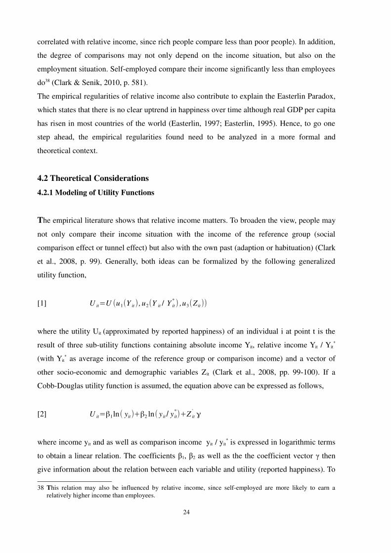
The empirical literature shows that relative income matters. To broaden the view, people may

not only compare their income situation with the income of the reference group (social

comparison effect or tunnel effect) but also with the own past (adaption or habituation) (Clark

et al., 2008, p. 99). Generally, both ideas can be formalized by the following generalized

utility function,

[1] U it=U (u1(Y it ) , u2(Y it / Y it* ) ,u3(Z it ))

where the utility Uit (approximated by reported happiness) of an individual i at point t is the

result of three sub-utility functions containing absolute income Yit, relative income Yit / Yit*

(with Yit* as average income of the reference group or comparison income) and a vector of

other socio-economic and demographic variables Zit (Clark et al., 2008, pp. 99-100). If a

Cobb-Douglas utility function is assumed, the equation above can be expressed as follows,

[2] U it=β1ln( yit )+β2 ln( y it / y it*)+Z it

` γ

where income yit and as well as comparison income yit / yit* is expressed in logarithmic terms

to obtain a linear relation. The coefficients β1, β2 as well as the the coefficient vector γ then

give information about the relation between each variable and utility (reported happiness). To

38 This relation may also be influenced by relative income, since self-employed are more likely to earn arelatively higher income than employees.

24

obtain an econometrically correct relation, the equation is extended by a constant α and an

error term η. In addition, since comparison income yit / yit* is expressed in log terms, the

equation can be rewritten as follows (Clark et al., 2008, p. 100; Clark & Senik, 2010, p. 577):

[3] U t=α+β1 ln( y it)+β2( ln y itln y it*)+Z it

` γ+η

However, the utility function shown here has some restrictions. First, it is assumed that the

variable income as well as comparison income contribute most when explaining utility

(reported happiness). However, it is questionable, if – instead of income – rather consumption

is the variable needed to explain reported happiness best. Of course, the underlying idea is

that income is a good proxy for consumption and can be applied with no or only little doubt.

For example, Clark et al. (2008, p. 100) observe that many studies assume that the sub-utility

function u(Yit / Yit*) equals u(Cit / Cit

*), with Cit* as the average consumption of the reference

group.39

Second, it is often not clear what the reference group (or the comparison income) of people

really is. In most studies, the reference group income yit* is just stated by the researcher and

constructed on basis of the data-set or an other external source (Clark & Senik, 2010, p. 578).

Further, reference income may be based on both an internal reference point, an external

reference point or a combination of both (Clark et al., 2008, p. 100).

The internal reference point is associated with own past income or expected future income

and can be, for example, modeled as a weighted average of past income streams,

[4] yit*=( yit 1)

α( y it2)β ( y it3)

γ with 0<α ,β , γ<1 ; α+β+γ=1

where the internal reference income from individual i at point t is based on the past own

income of the, for example, last three years (Clark et al., 2008, p. 104). Hence, this way of

modeling captures the idea that people do hedonically adapt to own income changes as time is

fading due to adjusting aspirations such that they converge back to some hedonic baseline

level (this process is often termed as hedonic treadmill) (Clark et al., 2008, p. 104; Easterlin &

Anglescu, 2009, p. 13).40 To give some empirical support, the studies of Brickman et al.

39 More precisely, one could also assume that income impacts on consumption, which impacts on utility suchthat u(Cit(Yit) / Cit

*(Yit*)).

40 Easterlin and Anglescu (2009, p. 13) refer to the problem that aspirations are much flexible downwards.Therefore, it has to questioned if equation [4] should be applied symmetrically for both increasing anddecreasing income over time.

25

(1978, p. 917), who find that lottery winners are not significantly happier than a control group

and achieve less pleasure from everyday events41, and Di Tella et al. (2010, p. 834), who find

that the impact of a current year increase in income loses 64 percent of its effect over the

following four years when analyzing individual panel data from about 8000 individuals over

the period 1984 to 2000 in Germany, are in line with the idea to model the internal reference

point as an weighted average of past income streams such that the income effect vanishes over

time.42

On the other hand, the external reference point may be defined – as also sketched in the

empirical literature – according to demographic groups (family, ethnicity, race), other workers

at the pace of employment or people living in the same region or country. In this case, y it* is

modeled mostly as the average income of the group people compare with,

[6] yit

*=∑ j=1

N

y jt

N

where the reference income yit* for the treated people i is the sum of the income yjt of all

people j in the reference group at point t divided by the total number of people N in the

reference group.

Thus, the difficulty is not the calculation but rather the definition of the actual reference

group, which will be discussed in greater depth in chapter 5.

4.2.2 A Contribution in Explaining the Easterlin-Paradox?

As there is evidence for relative income, it is of particular interest if relative income does

contribute to explain the Easterlin-Paradox. Repeatedly, the Easterlin Paradox states that there

is a weak relation between happiness and income in cross-country analysis, but a relation

between income and happiness within countries. In the time dimension, income and happiness

are only related in the short run.

To incorporate both the weak relation of happiness in cross-country studies and the stronger

relation within countries, Clark et al. (2008, p. 100) suggest – assuming that income is the

41 More detailed, it is analyzed if 22 lottery winners are happier than a control group of 22 people. Although thelottery winner group had a huge increase in their income, they do not feel significantly happier, rather theylost pleasure in mundane events. (Brickman et al., 1987, p. 921)

42 Clark et al. (2008, pp. 109-111) provide a more extensive overview about happiness and income adaption inthe empirical literature.

26

only variable different across countries and that reference income is the average country

income – the following utility function,

[7] U i=β1

y i

yi+A+β2 ln(

y i

yi

*)

where utility Ui (reported happiness) of an individual i in a specific country depends on the

absolute income of the individual yi and a positive constant A43 represented by the first term,

which is increasing at diminishing rates in yi since the first term's derivative with respect to yi

is positive and the second derivative is negative such that:

[8]∂U i

∂ y i

=β1

A

( y1+A)2>0 with A ,β1>0

[9]∂2

U i

∂ y i

2=β1

2 A

( y1+A)3 with A ,β1>0

According to the construction, the first term implies also that the additional effect of an

increase in absolute income on happiness approaches zero as income goes to infinity since

[10] limy i →∞

y i

y i+A=1

and yields, therefore, different results as when the effect of absolute income on utility

(reported happiness) is modeled simply as ln(yi)44 (cf. equation [2]). (Clark, Frijters & Shields,

2008, p. 100)

The second term of equation [7] represents the impact of relative income differences on utility

(reported happiness) within a country outlining that a higher reference income yi* will reduce

individuals happiness; at least as β2 is assumed to be positive, which is questionable according

to some empirical results found, for example, in Eastern Europe (Caporale et al., 2009).

The implications of the model are as follows. First, as general income rises over time, only the

first term is affected. Since marginal utility from extra absolute income approaches zero, in

43 The constant A ensures mathematically a concave relation between absolute income and happiness.

44 limy i →∞

( ln y i)=∞

27

particular rich countries benefit only little from a general rise in income (Clark et al., 2008, p.

101). Second, at a point in time, variations of utility (reported happiness) within a country are

explained by relative income differences such that individuals with an income above country

average are better off. Hence, the model predicts that the slope between income and happiness

is steeper within countries at a point in time than over time, mainly caused by status benefits

due to income differences within a country (Clark, Frijters & Shields, 2008, p. 100-101).

Figure 3 represents the relation graphically,

where the thick line shows the less steep relation between aggregate income and utility

(reported happiness) over time in a specific country and the thin line symbols relative income

differences within a country at a certain point in time, which are steeper. All together,

according to Clark et al. (2008, p. 101), the model, which incorporates relative income effects,

contributes to explain the Easterlin-Paradox. As a country becomes rich, all people earn more

income, which increases happiness on the aggregate level such that the country moves along

the thick line. On the individual level, however, also income of the reference group rises,

which reduces individuals happiness such that the net effect of a rise in overall income is

small.

28

Figure 3: Relationship between Income, Relative Income and Happiness

Source: Own representation based on Clark et al. (2008, p. 101)

Utility(Reported Happiness)

Income yi

Aggregate Level (thick line)(Relation over time of a country)

Individual Level (dotted line)(Relation within a country at a certain time)

4.2.3 Concluding Remarks

Of course, the model structure presented above is only one possibility to deal with relative

income effects. To give one further example, an other idea is that relative income matters not

only within a country but also across countries such that people gain additional utility

(reported happiness) when living in a relative successful country. To model this, again Clark

et al. (2008, p. 102) suggest to extend the utility function represented by equation [2] by an

additional term,

[11] U ijt=β1 ln( y ijt)+β2 ln( y ijt / y jt* )+β3 ln( y jt

* / y t*)+Z ijt

' γ

where Uijt is the utility (reported happiness) of an individual i in country j at point in time t, yijt

the income of individual i living in country j at point in time t, yjt* the average income in

country j and yt* the average income of the set of countries treated. The third term reflects the

idea that people, who are living in a country that is relatively richer than the average

countries, obtain a benefit in individual utility perceived by just living in such a country.

Again, if all countries grow over time with the same growth rate, the magnitude of the third

term stays unchanged in every country. Hence, the implication is then that “countries are

locked in an arms race over growth” meaning that a simultaneous economic growth does not

contribute (or only little since there still is an impact due to the first term y ijt) to aggregate

happiness (Clark et al., p. 102).

To sum up, there are various ways of modeling utility-functions that incorporate relative

income. The relevance of relative income is thereby not only empirically well-founded45, but

is also an important theoretical factor when explaining the Easterlin-Paradox. Of course,

utility-functions can contain more than one relative income variable such that utility may be

influenced by comparison income formed across and within countries. Beside the social

comparison component, there exist also internal reference points such as own past income,

which influences, at least in the short run, individual's utility (reported happiness) (Clark et

al., 2008, p. 111).

So far, the calculation of the the comparison income was based on reference groups

exogenously stated. Since the choice of the reference group is often just arbitrarily made, the

following chapter which reference group specifications have been applied in the literature.

45 Clark et al. (2008, p. 111) argue that relative income may be at least twice as important as absolute incomefor individual's happiness.

29

5 Specifications of the Reference Group

Relative income or, in absolute terms, comparison income matter when explaining happiness.

However, this leads to the question what individuals define to be their actual reference group

or, in other words, to whom they compare themselves when judging their relative position or

when searching information about potential future income prospects. In the literature, there

are mainly two ways to deal with reference groups, namely as an exogenous variable, mostly

stated by the researcher, or as an endogenous variable, defined by the respondent.

5.1 The Reference Group as Exogenous Variable

The choice of the correct reference group is of particular importance. Although there is a

consensus about the calculation method (mean income or, in some articles, median income of

the reference group) in the literature, the way of defining the individuals belonging to the

reference group is from larger variety.

There are several ways of dividing reference group specifications into sub-groups46. Basically,

the reference group can be separated into an internal and an external specification. The

internal specification captures the idea that people may compare their current situation to their

own past or to their anticipated future prospects. The external specification is based on

comparisons an individual makes with other people. (Verme, 2013, pp. 10-11)

An econometric example to incorporate internal reference groups is provided by Knight et al.

(2009, p. 645). On the one hand, they approximate an individual's own past by two dummy

variables labeled 'Current living standards better than 5 years ago' and 'Current living

standards worse than 5 years ago'. On the other hand, they approach the expectations about

the future by asking the respondents if they 'Expect a big increase in income over next 5 years'

or 'Expect a decrease in income over next 5 years'. Another example for an internal reference

group is given by McBride (2001, p. 257). He incorporates 'parents standard of living' as

explanatory variable.

However, most studies define the reference group to be external. The underlying idea is that

people compare their income mostly with people, who have similar characteristics such as

age, education, employment sector or area of living. The income of the reference group is

usually calculated as the average income of all the people having similar characteristics as the

46 Verme (2013, pp. 10-11) reviews that the literature offers several possibilities of dividing reference pointsinto sub-groups: Internal vs. external reference groups, parallel vs. longitudinal reference groups and alter vs.ego reference groups.

30

individual concerned (MacKerron, 2012, p. 720). Table 2 reviews some external reference

group specifications.

Table 2: External Reference Group Specifications

Author(s)

Chronologically orderedReference Group

Average Income of all Individuals

FitzRoy et al. (2013)

in the same education group(2 groups)

inside the same age range(-3 up to + 6 years)

with the same gender

Akay & Martinsson (2011)

inside the same age group(10 groups between 25 and 90)

size of landholdings in hectares (ha)({0}; (0;0.1]; (0.1;0.2]; (0.2;0.3]; (0.3;0.5]; (0.5;0.7]; (0.7;∞))

living in the same area(rural areas of Northern Ethiopia)

Oshio et al. (2010)

within the same age group 20-29; 30-39; 40-49, 50-59; 60-69

with the same gender

with similar educational level(no formal qualification; lowest formal qualification; above lowerformal qualification; higher secondary qualification completed; abovehigher secondary level; university degree completed)

Caporale et al. (2009)inside the same age range (± 5 years)

Layard et al. (2009)

in the same education group(3 groups)

in the same age range(± 5 years)

with the same gender

Knight et al. (2009)living inside or outside the same village(rural China)

Kuegler (2009) Venezuelan siblings

Graham & Felton (2006)living in the same country (Latin American countries)

Ferrer-i-Carbonell (2005)

with similar educational level (less than 10; 10; 11; 12; 12 and more years of schooling)

inside the same age bracket(younger than 25; 25-34; 35-44;45-65; 66 and older)

living in the same region(West and East Germany)

Luttmer (2005)living in the same region (PUMA regions)

31

Blanchflower & Oswald (2004)living in the same state (US states)

McBride (2001)inside the same age range (± 5years)

Van de Stadt et al. (1985)

with the same educational level(five different education levels)

within the same age bracket(less than 30, 30-39, 40-49, 50-65, over 65)

with the same employment status(self-employed, employee, not employed)

According to table 2, external reference groups are mostly defined according to spatial or

socio-demographic variables. Also interactions of both types are possible. An individual's

reference group becomes more individualized the more socio-demographic or spatial

variables are used to define the reference group. For example, Luttmer (2005) calculates

solely the reference group according to the average income of the state such that every

individual within the particular state faces the same comparison income. In contrast, Ferrer-i-

Carbonell (2005) computes a more individualized reference income since he differentiates

between educational level, age and region.

As the overwiew shows, there is a huge variety of literature that exogenously impose a

specific reference group as relevant for relative income or, more generally, income

comparisons (Clark & Senik, 2010, p. 573). In contrast to this general approach, there is also

the possibility to ask the respondents of a survey about their reference group in order to

endogenously obtain information on the reference group. For example, Knight et al. (2009)

not just simply state a reference group but ask the respondents to report their actucal reference

group.

Ideally, a data-set should contain a question, which directly asks the respondents about their

comparison income. For example, Clark and Senik (2010) analyze the question “Whose

income would you be most likely to compare your own with?”, which is included in the third

wave of the ESS. The respondents had to choose between the answers 'Work colleagues',

'Family members', 'Friends', 'Others' and 'Don't compare'. Most respondents answered that

they compare most to their 'Work colleagues' (36.3 %). 35.9 % answered that they 'Don't

compare' to other people and 14.9 % compare mostly with 'Friends'. Interestingly, only 5.8 %

of the respondents answered that they compare most likely with other 'Family members'.

(Clark & Senik, 2010, p. 576)

The information gathered from such a survey can be used to model the exogenous reference

32

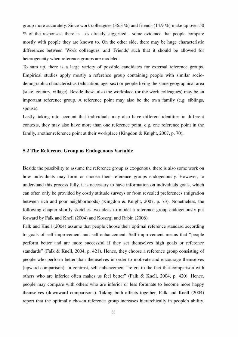
group more accurately. Since work colleagues (36.3 %) and friends (14.9 %) make up over 50

% of the responses, there is - as already suggested - some evidence that people compare

mostly with people they are known to. On the other side, there may be huge characteristic

differences between 'Work colleagues' and 'Friends' such that it should be allowed for

heterogeneity when reference groups are modeled.

To sum up, there is a large variety of possible candidates for external reference groups.

Empirical studies apply mostly a reference group containing people with similar socio-

demographic characteristics (education, age, sex) or people living the same geographical area

(state, country, village). Beside these, also the workplace (or the work colleagues) may be an

important reference group. A reference point may also be the own family (e.g. siblings,

spouse).

Lastly, taking into account that individuals may also have different identities in different

contexts, they may also have more than one reference point, e.g. one reference point in the

family, another reference point at their workplace (Kingdon & Knight, 2007, p. 70).

5.2 The Reference Group as Endogenous Variable

Beside the possibility to assume the reference group as exogenous, there is also some work on

how individuals may form or choose their reference groups endogenously. However, to

understand this process fully, it is necessary to have information on individuals goals, which

can often only be provided by costly attitude surveys or from revealed preferences (migration

between rich and poor neighborhoods) (Kingdon & Knight, 2007, p. 73). Nonetheless, the

following chapter shortly sketches two ideas to model a reference group endogenously put

forward by Falk and Knell (2004) and Koszegi and Rabin (2006).

Falk and Knell (2004) assume that people choose their optimal reference standard according

to goals of self-improvement and self-enhancement. Self-improvement means that “people

perform better and are more successful if they set themselves high goals or reference

standards” (Falk & Knell, 2004, p. 421). Hence, they choose a reference group consisting of

people who perform better than themselves in order to motivate and encourage themselves

(upward comparison). In contrast, self-enhancement “refers to the fact that comparison with

others who are inferior often makes us feel better” (Falk & Knell, 2004, p. 420). Hence,

people may compare with others who are inferior or less fortunate to become more happy

themselves (downward comparisons). Taking both effects together, Falk and Knell (2004)

report that the optimally chosen reference group increases hierarchically in people's ability.

33

People with high ability choose their reference group first in order to self-improve themselves

and, when their performance has increased, switch their reference group to self-enhance

themselves to improve their life satisfaction through downward comparison.

Another idea to model the reference group (reference point) endogenously is put forward by

Koszegi and Rabin (2006), who assume that the reference point is determined as rational

expectations about outcomes. More detailed, “a person's reference point is her probabilistic

beliefs about the relevant consumption outcome held between the time she first focused on the

decision determining the outcome and shortly before consumption occurs” (Koszegi & Rabin,

2006, p. 1141).

34

6 Different Reference Group Specifications and Life Satisfaction

As the previous chapter has shown, there are a variety of possibilities to define the reference

group. The following chapter aims at investigating different reference specifications and their

impact on life satisfaction.47 The question I want to answer is to what extent different

specifications of reference groups lead to different results. I will also give some explanations,

why different specifications may measure different effects.

To analyze this, I use the first three waves of the European Social Survey (ESS) as data basis.

The method is to analyze systematically the impact of several reference group specifications

on satisfaction. For the whole ESS sample, I use all reference specifications, which are based

in any constellation on similar 'Education', 'Age', 'Gender' and 'Country'. For the German sub-

sample, I do the same with specifications based on similar 'Education', 'Age', 'Gender' and

'Federal States' or 'East and West Germany'.

It may be important to note that the ESS data-set was already data basis of other studies

analyzing the effect of reference income on life satisfaction. In particular, I refer to the studies

performed by Caporale et al. (2009) and Drichoutis et al. (2010), on which this study is

mainly based on.

Caporale et al. (2009), who used the first two waves of the ESS and defined the reference

group according to the specification of McBride (2001), find clear evidence for the social

comparison effect in the whole sample as well as for the sub-samples only containing young

people (40 years or younger), old people (older than 40 years), well-educated, not-well-

educated, Central European Countries, Scandinavia and Southern European Countries. In

contrast, comparison income has a positive effect on life satisfaction in Eastern European

countries indicating the tunnel effect (Caporale et al., 2009, p. 49).

Drichoutis et al. (2010) recalculated the results Caporale et al. (2009) obtained by applying a

partly different methodology and modified reference group specifications. As a result,

Drichoutis et al. (2010, p. 483) report that the coefficients of comparison income are partly

different in sign, size and level of significance.

I follow in the most parts the methodology of Caporale et al. (2009) and Drichoutis et al.

(2010). Basically, my modifications are that I use the first three waves of the ESS as data

basis (instead of the first two waves), include new control variables in the regression (e.g.

47 The idea to test systematically the impact of the reference specification on life satisfaction is not new in theliterature. For example, Akay and Martinsson (2011) found that different reference group specifications alterthe impact of absolute and relative income – in particular the magnitude of the coefficients – on lifesatisfaction in rural areas of northern Ethiopia.

35

Religion and Perceived Safety) and test systematically for different reference specifications.

The remainder of this chapter is structured as follows. In sub-chapter 1, I describe shortly the

ESS data basis and the choice of the variables. Methodological and econometric issues will be

discussed in sub-chapter 2. The third sub-chapter deals in greater detail with the chosen

reference group specifications. Finally, I present, summarize and discuss the results obtained

in sub-chapter 4, where I also shortly sketch problems and shortcomings of the study.

6.1 Data Description and Choice of Variables

The first three waves (2002, 2004 and 2006) of the cross-sectional data of the European

Social Survey (ESS) is the basis for the empiricial analysis. Within these three waves, the ESS

covers 29 (mostly European) countries. Until now, there are six waves of the ESS published48,

which measure beliefs, behavioral patterns and attitudes of more than thirty nations. The

survey has been funded by the European Commisson's Framework Programmes, by the

European Science Foundation and by National funding councils in participating countries. A

key aim of the ESS is to implement high standards in its methodology regarding the sampling

of respondents, the equivalcence of translation and the questionaire.49

The ESS data provide a large variety of variables50 useful for happiness research. To measure

life satisfaction, two questions are of particular interest. The first questions asks “All things

considered, how satisfied are you with your life as a whole nowadays?“. Possible answers

range on a 11-point scale from 'extremely dissatisfied' (0) to 'extremely satisfied' (10). The

second question asks “Taking all things together, how happy would you say you are?“,

whereby the possible answers range again on a 11-point scale from 'extremely unhappy' (0) to

'extremely happy' (10).

As explanatory variables, the ESS offers several economic and socio-demographic variables.

The total household net income of the respondent is measured ordinally in twelve income

categories ranging from less than 40 Euro per week up to more than 2310 Euro per week.51 As

standard, the ESS provides information on gender and age of the respondents. Additionally,

48 I use only the first three waves of the ESS, since the measurement of the income variable was severelyaltered from the fouth wave on. Instead of concrete income intervalls, income was from the fouth wave onmeasured in ten deciles which vary across countries.

49 A more detailed description of the ESS methdology can be found at the homepage of the ESS.(http://www.europeansocialsurvey.org/methodology/)

50 The variables I used are listed in Appendix A.51 More precisely, answer categories of weekly total household net income are (in intervalls in €): [0,40); [40,

70); [70, 120); [120, 230); [230, 350); [350, 460); [460, 580); [580, 690); [690, 1150); [1150, 1730); [1730,2310); [2130, ∞).

36

information is given on the family status ('Never married', 'Married', 'Separated', 'Divorced' or

'Widowed') including Children ('Children at home'), health (ranging from 'very good' health to

'very bad' health on a 5-point scale) and religion (belonging to a religion or denomination).

Also information on the social activity (“How often socially meet with friends, relatives or

colleagues?” with answer categories 'Never', 'Less than once a month', 'Once a month',

'Several times a month', 'Once a week', 'Several times a week' and 'Every day') and the

perceived feeling of safety (“Feeling of safety of walking alone in local area after dark?” with

answers 'Very Safe', 'Safe', 'Unsafe' and 'Very unsafe') will be used in the regression analysis.

The highest level of education is separated into five categories ranging from completed

primary education or less (ISCED 0-1) to tertiary education completed (ISCED 5-6).52 To

capture also geographical effects, also the variable asking for the domicile the respondents

live will be considered (answer categories are 'Big city', 'Suburbs or outskirts of a big city',

'Town or small city', 'Village resident' and 'Countryside'). As proxy for employment status and

activity, the information is used what respondents stated having done in the last seven days

with answer possibilities 'Paid Work', 'Education', 'Unemployed', 'Permanently Disabled or

Sick', 'Retired', 'Community or Civil Service' and 'Housekeeping', whereby this question

allowed for several answers. Lastly, to capture also the long term effects of unemployment,

the variables asking for any period of unemployment and work seeking 'lasted for more than

12 months' and 'within the last 5 years' are considered. (ESS Questionnaire, 2012)

Note that I choose most of the variables in accordance of the studies made by Caporale et al.

(2009) and Drichoutis et al. (2010). Different to these studies, I expand the amount of

variables being treated by 'Religion', 'Social activity', 'Perceived Feeling of Safety' as well as

'Employment Status and Activity'. Of course, the ESS data-set provides a lot of more

variables, which I could theoretically choose as explanatory variable.

52 ISCED is the abbreveation for International Standard Classification of Education and serves to "facilitatecomparisons of education statistics and indicators across countries on the basis of uniform and internationallyagreed definitions" (UNESCO, 2014).

37

6.2 Methodology

6.2.1 Data Preparation53

In a first step, it was necessary to merge the first three waves of the ESS data-sets. The first

wave (ESS1) contained originally 565 variables and 42359 observations, the second wave

(ESS2) contained 603 variables and 47527 observations and the third wave (ESS3) contained

517 variables and 43000 observations. For the sake of clarity, I generated initially a sub-set

for each of the three waves, which contained only the variables I needed for the further

statistical analysis54. Based on the subset, I merged the three waves, whereby I needed to

recode some variables of the third wave first.55 In total, there were now 132896 observations.

In a next step, I deleted all observations, where at least one of the happiness, income or socio-

demographic variables had a missing value or had entries like “Don't know”, “Not applicable”

or “Refusal”. 82544 observations remained.

Thereafter, the remaining variables were recoded in values and labels56. Regarding the

happiness variables, I relabeled the variable asking for life satisfaction to “SAT”. The variable

asking for happiness remained the original label “HAPPY”.

Regarding the geographical variables, I generated dummy variables for each country.

Similarly, I generated five dummy variables for the variable measuring the degree of

urbanization ranging from living in “a big city” to living in a “farm or home in the

countryside”.

Treating the socio-economic variables, I had to face some difficulties. I recoded the variable

for gender to a dummy-variable (0 for “female” and 1 for “male”) and relabeled it to

“MALE”. The age of the respondent was given in a continuous form such that I could easily

calculate a variable for age squared. Then, five dummy variables were generated for the

educational level of the respondents ranging from “Less than lower secondary education” to

“Completed tertiary education”. The family status was assigned to five dummies with the

characteristics “Never married”, “Married”, “Separated”, “Divorced” and “Widowed”. The

dummy-variable “Children” was calculated stating if the respondents have at least one child at

home. Furthermore, dummy variables were calculated for “Religion” (0 if not belonging to a

particular religion, 1 if belonging to a particular religion), “Health” (1 if good or very good

53 The data preparation process can also be follwed by the provided do-file at the hard disc.54 The variables selected are presented in the Appendix A.55 The variable 'agea' was rounded to obtain whole numbers. The variable 'martiala' obtained in wave three the

first time also the status 'Civil Partnership', which were dropped. Also the variable outlining the year of theinterview was adjusted to the first and the second wave.

56 Also listed in the Appendix A.

38

health, 0 otherwise), “Social” (1 if the respondent meets colleagues, relatives or friends

several times a week or every day, 0 otherwise, i.e. less than several times a week) and

“Perceived Safety” (1 if the respondent feels safe or very safe when walking alone in the local

area after dark, 0 otherwise). In addition, I added two dummies to capture the long term

effects of unemployment. Here, the first dummy equals 1 if the respondent was unemployed

in any period in the last 12 months, the second dummy equals 1 if the respondent was

unemployed in any period in the last 5 years. Of course, I also generated dummies for the ESS

round and the year of the interview to capture variety in time.

In a next step, I treated the absolute income variable. The monthly net income of the

household was originally measured in twelve income categories ranging from “less than 40 €

net income per week” to “more than 2310 € net income per week”. Following Caporale et al.

(2009), eleven dummy variables were constructed to be able to measure the impact of

absolute household income on satisfaction, where the categories representing the two lowest

income groups were merged to one category “less than 70 € net income per week”. It is

important to notice that the income variable represents the income of an household and not of

an individual. Although the data-set offers some variables such as “Living with a partner”,

“Household size” and “Children living at home”, which offered some possibilities to

recalculate the household income to an individual income, I decided to work further with the

household income. This had two reasons. First, it was not possible to assign individual income

clearly to the respondent since individual income of other household members (partner,

children or grandparents) remained unknown. Second, both Caporale et al. (2009) and

Drichoutis et al. (2010) also worked with household income.

For the German sub-sample, I restricted the data-set to all people living in Germany. Based on

this subset, I compiled dummies for each of the 16 federal states in Germany as well as a

dummy for East and West Germany.

6.2.2 Estimation Procedure

Principally, there are different types of estimators dependent on which scale is assumed for

the dependent variable “Satisfaction” or respectively “Happiness”. If the dependent variable is

assumed to be cardinally (meaning that the difference between 1 and 2 is the same as the

difference between 5 and 6 for any individual), the OLS estimation method would be

sufficient to calculate the coefficients for the model

39

[12] Sat i= x iβ+ǫi

where Sati is either “Satisfaction” or “Happiness”, xi the vector of explanatory variables and εi

the error term, which is expected to be 0 in mean value. This method is, however, mostly

applied by psychologists and rather seldom by economists, although there are some studies by

economists that use this method such as Gardner and Oswald (2001), Luttmer (2005), Knight

et al. (2009), Clark and Senik (2010) or FitzRoy et al. (2013).

In contrast, economists usually assume that satisfaction answers are only ordinally

comparable (the difference between satisfaction is unknown, but all individuals have the same

interpretation of each possible answer) (Ferrer-i-Carbonell, 2004, p. 641). To deal with this

assumption statistically correct, an ordered probit or an ordered logit model is necessary (the

equation to estimate is principally the same as equation [12]). For example, economic studies

that apply an ordered probit model are McBride (2001), Ferrer-i-Carbonell (2005), Caporale

et al. (2009), Drichoutis et al. (2010), Akay and Martinsson (2011) and Kuegler (2009).

Ordered logit models were used by Graham and Felton (2006) and Oshio et al. (2010).

Although the assumption that happiness is measured ordinally would exactly require an

ordered logit or probit estimation, there is some evidence that OLS estimations lead to similar

results. This is mainly reasoned by the fact that Ferrer-i-Carbonell and Frijters (2004) showed

in a methodological paper that it is relatively unimportant to the results if cardinality or

ordinality is assumed. Also Luttmer (2005, p. 980-981) and Kingdon and Knight (2007, p. 76)

checked for both an ordered probit model and an OLS model and found no significant

differences regarding the sign, magnitude and significance of the coefficients. In addition,

Clark and Senik (2010) rely on the results of Ferrer-i-Carbonell and Frijters (2004) and

perform an OLS regression, since the results are also more handy to interpret.

Exemplary, table 3 compares the regression results of an ordered probit model with the results

of an OLS model including all socio-economic, geographical, educational and income

variables. Reference income is excluded.

The results show that in the most cases both estimation procedures lead to the same sign and

level of significance of the coefficients. However, there are also some exceptions. The dummy

standing for 'Divorced' is insignificant when using a ordered probit model but significant at

the 5%-level when applying OLS. Similar, the dummies for education are more likely to be

significant when applying OLS. Another difference is the dummy for doing 'Paid Work',

where OLS produces insignificant results, but the ordered probit model find a negative effect

at the 5%-level.

40

41

Table 3: Ordered probit vs. OLS estiamtes Ordered probit estimates OLS estimates

Dependent Variable: Satisfaction (1) (2)

Coeff. Coeff.

Socio-Demographic Variables

Male 182.917 0.000 -12.897 0.000

Age 326.075 0.000 -17.990 0.000

375.816 0.000 19.280 0.000

Married 375.816 0.000 17.283 0.000

Separated 45.952 0.000 -8.229 0.000

Divorced -0.013 0.599 0.439 -2.082 0.037

4.421 0.036 -2.895 0.004

Children 31.878 0.000 -5.348 0.000

Good health 2719.681 0.000 52.799 0.000

Religion 109.652 0.000 10.517 0.000

Social 558.233 0.000 23.152 0.000

Perceived Safety 275.682 0.000 19.760 0.000

Geographical Variables

Big city 47.692 0.000 -5.213 0.000

Suburbs or outskirts of big city 51.136 0.000 -5.877 0.000

Town or small city 48.938 0.000 -5.834 0.000

21.693 0.000 -3.486 0.000

Education

Low secondary -0.003 0.039 0.843 0.029 1.106 0.269

Upper secondary -0.004 0.072 0.788 2.386 0.017

Post secondary 6.871 0.009 4.256 0.000

0.014 0.953 0.329 4.493 0.000

Activity (in the last seven days)

Paid Work 4.124 0.042 -0.009 -0.388 0.698

Education 18.135 0.000 5.669 0.000

Unemployed 196.895 0.000 -16.048 0.000

Permanently Disabled or Sick 133.156 0.000 -13.784 0.000

Retired 21.479 0.000 4.372 0.000

Community or Civil Service 0.077 1.301 0.254 0.132 1.042 0.298

Housekeeping 14.621 0.000 3.379 0.001

Any Period of Unemployment and Work Seeking

Lasted for more than 12 months 87.083 0.000 -11.464 0.000

Within the last 5 years 132.869 0.000 -12.449 0.000

Income

70-120€ 84.864 0.000 12.275 0.000

120-230€ 206.772 0.000 18.766 0.000

230-350€ 321.916 0.000 22.412 0.000

350-460€ 385.856 0.000 24.120 0.000

460-580€ 427.895 0.000 24.973 0.000

580-690€ 473.961 0.000 25.980 0.000

690-1150€ 630.303 0.000 28.974 0.000

1150-1730€ 546.825 0.000 26.463 0.000

1730-2310€ 293.322 0.000 19.532 0.000

312.392 0.000 18.737 0.000

Year/ESS round/country dummies Included Included

0.240 0.259

Number of obersations 82544 82544

Wald-statistics

p-value

t-statistics

p-value

-0.107*** -0.191***

-0.026*** -0.49***

Age2 0.0003*** 0.001***

0.224*** 0.388***

-0.206*** -0.473***

-0.065**

Widoweda -0.038** -0.099***

-0.051*** -0.091***

0.459*** 0.870***

0.086*** 0.162***

0.188*** 0.346***

0.153*** 0.343***

-0.123*** -0.173***

-0.127*** -0.195***

-0.116*** -0.180***

Village residentb -0.077*** -0.108***

0.061**

0.071*** 0.217***

Tertiaryc 0.124***

-0.026**

0.073*** 0.182***

-0.279*** -0.604***

-0.256*** -0.579***

0.075*** 0.133***

0.037*** 0.061***

-0.126*** -0.293***

-0.158*** -0.321***

0.168*** 0.425***

0.252*** 0.622***

0.335*** 0.791***

0.391*** 0.907***

0.430*** 0.979***

0.466*** 1.047***

0.521*** 1.132***

0.557*** 1.183***

0.547*** 1.168***

>2310€d 0.658*** 1.299***

Pseudo R2 (Cox and Snell) / R2

Excluded categories: a Never married b Countryside c Primary or less d <70€* at 10%-level significant ** at 5%-level significant *** at 1%-level significant

42

Table 4: Satisfaction vs. Happiness Dependent: Satisfaction Dependent: Happy

Ordered probit estimates (1) (2)

Coeff. Coeff.

Socio-Demographic Variables

Male 182.917 0.000 176.355 0.000

Age 326.075 0.000 426.111 0.000

375.816 0.000 414.536 0.000

Married 375.816 0.000 783.247 0.000

Separated 45.952 0.000 56.459 0.000

Divorced -0.013 0.599 0.439 -0.002 0.010 0.920

4.421 0.036 52.267 0.000

Children 31.878 0.000 -0.014 2.526 0.112

Good health 2719.681 0.000 2704.015 0.000

Religion 109.652 0.000 75.053 0.000

Social 558.233 0.000 782.981 0.000

Perceived Safety 275.682 0.000 191.511 0.000

Geographical Variables

Big city 47.692 0.000 31.420 0.000

Suburbs or outskirts of big city 51.136 0.000 34.958 0.000

Town or small city 48.938 0.000 28.351 0.000

21.693 0.000 17.470 0.000

Education

Low secondary -0.003 0.039 0.843 -0.017 1.453 0.228

Upper secondary -0.004 0.072 0.788 -0.019 1.931 0.165

Post secondary 6.871 0.009 0.036 1.773 0.183

0.014 0.953 0.329 -0.018 1.532 0.216

Activity (in the last seven days)

Paid Work 4.124 0.042 -0.016 1.515 0.218

Education 18.135 0.000 6.795 0.009

Unemployed 196.895 0.000 93.330 0.000

Permanently Disabled or Sick 133.156 0.000 49.751 0.000

Retired 21.479 0.000 14.359 0.000

Community or Civil Service 0.077 1.301 0.254 4.668 0.031

Housekeeping 14.621 0.000 23.395 0.000

Any Period of Unemployment and Work Seeking

Lasted for more than 12 months 87.083 0.000 -11.464 0.000

Within the last 5 years 132.869 0.000 -12.449 0.000

Income

70-120€ 84.864 0.000 74.562 0.000

120-230€ 206.772 0.000 174.189 0.000

230-350€ 321.916 0.000 263.251 0.000

350-460€ 385.856 0.000 302.491 0.000

460-580€ 427.895 0.000 335.853 0.000

580-690€ 473.961 0.000 364.111 0.000

690-1150€ 630.303 0.000 405.961 0.000

1150-1730€ 546.825 0.000 387.119 0.000

1730-2310€ 293.322 0.000 176.018 0.000

312.392 0.000 185.219 0.000

Year/ESS round/country dummies Included Included

0.240 0.203

Number of obersations 82544 82544

Wald-statistics

p-value

Wald-statistics

p-value

-0.107*** -0.105***

-0.026*** -0.030***

Age2 0.0003*** 0.0003***

0.224*** 0.335***

-0.206*** -0.228***

Widoweda -0.038** -0.131***

-0.051***

0.459*** 0.458***

0.086*** 0.071***

0.188*** 0.223***

0.153*** 0.127***

-0.123*** -0.100***

-0.127*** -0.105***

-0.116*** -0.088***

Village residentb -0.077*** -0.069***

0.071***

Tertiaryc

-0.026**

0.073*** 0.045***

-0.279*** -0.193***

-0.256*** -0.157***

0.075*** 0.061***

0.147**

0.037*** 0.047***

-0.126*** -0.293***

-0.158*** -0.321***

0.168*** 0.158***

0.252*** 0.231***

0.335*** 0.303***

0.391*** 0.346***

0.430*** 0.381***

0.466*** 0.409***

0.521*** 0.418***

0.557*** 0.469***

0.547*** 0.424***

>2310€d 0.658*** 0.506***

Pseudo R2 (Cox and Snell)

Excluded categories: a Never married b Countryside c Primary or less d <70€* at 10%-level significant ** at 5%-level significant *** at 1%-level significant

As the choice of the estimation procedure leads to small differences in the results, the

following analysis sticks to ordered probit estimations and not to the more easily interpretable

OLS estimations. This decision is also in line with the idea that the dependent variable is only

ordinally and not cardinally interpretable.

Another problem to think about is the dependent variable. The ESS data-set offers two

different variables, which may be useful to measure life satisfaction. The first variable is

'Satisfaction', measured by the question “All things considered, how satisfied are you with

your life as a whole nowadays?“, the second variable is 'Happy', measured by the question

“Taking all things together, how happy would you say you are?“.

To check if both variables lead to the same results, I estimated two ordered probit models with

'Satisfaction' as dependent variable of the first model and 'Happy' as dependent of the second

model. Again excluding the reference income, both models contain the same explanatory

variables.

The results, shown in table 4, show several differences. First, the overall model fit is better

with 'Satisfaction' as the dependent variable, since the Pseudo-R2 (Cox and Snell) has value

0.240, whereas the value of the Pseudo-R2 (Cox and Snell) is 0.204 with 'Happy' as dependent

variable. Second, there are also differences in the coefficients regarding significance. A first

example is that to be 'Widowed' reduces 'Happiness' (-0.131***) statistically significiant at the

1%-level, but reduces 'Satisfaction' (-0.038**) only statistically significant at the 5%-level.

Another example is that people with 'Children' are significantly less satisfied (-0.051***) but

not significantly less happy (-0.014) than people without children at home. A last example is

that people doing 'Community or Civil Service' are not significantly more satisfied (0.077)

than people who are not doing 'Community or Civil Service', but seem to be significantly

more happy (0.147***) than people who are not doing 'Community or Civil Service'.

The other coefficients are roughly the same. Hence, it could be argued that 'Satisfaction' and

'Happiness' measure the same underlying dimension. However, there are several reason

against this argument. First, the correlation coefficient (Spearman) is 0.708. If 'Satisfaction'

and 'Happiness' would measure the same dimension, I would expect a correlation cofficient of

1 or at least very close to 1. Second, summary statistics – shown in Appendix A – show that

average satisfaction has value 7.06 and average happiness has value 7.35. To compare both

mean values, I performed a two sample t-test and found that average happiness is significantly

higher than average satisfaction at levels of significance. Hence, people systematically report

higher happiness. Lastly, the model fit (Pseudo-R2 with 'Happiness' as dependent variable is

0.203; Pseudo-R2 with 'Satisfaction' as dependent variable is 0.240) as well as some important

43

variables (Children, Widowed) show clear differences. Therefore, I assume that happiness and

satisfaction cannot be used synonymously. The argument is that “life satisfaction refers to

cognitive states of consciousness, whereas happiness is emotional and mainly concerns

intimate matters of life“ (Caporale et al., 2005, p. 43). Because of this conceptual difference

between 'Satisfaction' and 'Happiness', I decided to use 'Satisfaction' as dependent variable for

the upcoming analysis regarding the specific role of reference groups.

6.2.3 Further Econometric Issues

Before estimating the impact of the reference income on satisfaction, it is methodologically

necessary to deal with some further econometric issues such as omitted variable bias,

multicollinearity, non-linearity, concavity and convexity of the utility function as well as

possible endogeneity.

Omitted variables may have severe effects on the estimation results of a model. A first point is

that, all across the literature, happiness models can only explain little of the whole variation in

happiness shown by typically low values of R2 or pseudo-R2 (Verme, 2013, p. 17). Hence, the

introduction of omitted variables as further control variables may improve the explanatory

power of the model. Exemplary, Kuegler (2009, p. 4) provides a set of control variables,

which a happiness regression should contain such as relative and absolute income,

employment, health, education, experienced crime and social and political participation.

Beside the set of micro-level control variables, macro-economic control variables should also

be applied when treating individuals from different countries in different point in times. To

give an example, there is evidence that income inequality (Alesina et al., 2004) as well as

inflation and general unemployment (Di Tella et al., 2001) impact on the individual level of

satisfaction. In the empirical study performed here, these macro-economic effects are

considered by introducing year, ESS wave and country dummies. Another point is that

omitted variables may - as far as they are a determinant of the dependent variable and

correlated with at least one explanatory variable - alter the size, the magnitude and the level of

significance of a variable already being introduced (omitted variable bias). Since the study

here controls for most of the control variables suggested by the literature, omitted variables

bias is assumed to be of minor relevance.

Another problem in life satisfaction regressions is multicollinearity, where two or more

explanatory variables are highly correlated such that they are linear dependent or closely to. In

happiness equations, this problem mainly arises when constructed variables are introduced on

44

the right-hand-side on the happiness equation such as reference income, relative income or

income inequality (Verme, 2013, p. 16). For example, when the reference income is

constructed based on the average income of all people with the same gender, there is linear

dependence between the gender dummy and the reference income. In this case, the

introduction of the reference income in the happiness equation does not improve the

explanatory power of the model. In this case, statistical programs like SPSS exclude the

reference income automatically. Similar problems arise also when the reference income is

constructed based on several variables such as same age, gender and education. In this case,

the introduction of the reference income in happiness equations typically alter size and level

of significance of age, gender and education variables.57

Further, also non-linearity of the utility function may be an issue. For example, the relation

between absolute income and satisfaction theoretically follows a concave relationship. The

usual way to overcome this obstacle is to take the natural log of the income variable to obtain

a linear relationship between log income and satisfaction. However, since the ESS data-set

offers a categorical income variable (and not a continuous income variable), it is not

necessary to take the logarithm. Instead, the regression includes a dummy variable for each

income band, which accounts for a possible non-linear relation between income and happiness

(at least across income bands). Another typical example for a non-linearity is the relation

between satisfaction and age, where most studies find a U-shaped relation (Kuegler, 2009, p.

4). To take this into account, the right-hand-side of the equation contains not only age but also

age squared.

Lastly, also endogeneity may be an issue. For example, it is mostly assumed that a higher

level of absolute income increases peoples satisfaction. On the other hand, one could argue

that people who are more happy will be more successful in their job performance and,

therefore, will earn more money. Then, the relation would run from happiness to income.

Since this problem is difficult to address (one should have information about person specific

characteristics like genes, motivation or general life attitude) or to instrument by an

instrument variable, I will follow the literature and assume that income influences happiness.

Hence, I will not address endogeneity in greater depth.

57 This issues will be discussed in greater detail when presenting the regression results (chapter 6.4).

45

6.3 Relative Income and Reference Group Specifications

Before analyzing the impact of relative income on satisfaction, it needs to be specified, in

which way relative income should be incorporated in the happiness equation and what types

of reference groups shall be tested.

Regarding the specification of relative income, the ESS data do not allow to apply the ratio of

absolute over average income of the reference group, since income is not offered in

continuous form. That makes it also impossible to calculate the effect of the distance between

actual income and the average income of the reference income precisely. Therefore, I decided

to plug comparison income in the satisfaction equation without relating it to absolute income

relatively or absolutely. This specification leads then to the interpretation that a negative sign

of the comparison income means that a higher comparison income lowers an individual's

happiness, which would indicate a social comparison effect. In contrast, a positive sign of the

comparison income would mean that a higher comparison income increases an individual's

happiness indicating some evidence for the tunnel effect.

The next step is to define the reference group specifications. Since the literature offered a

large variety of different specifications, the question is which specification of the reference

group fits best in explaining satisfaction. To do so, I decided to define the reference group

based on the variables mostly used in the literature58: 'Age', 'Gender' and 'Education' as socio-

demographic variables and 'Country' (or 'East/West' or 'Federal States' respectively at the

German sub-sample) as spatial variable. For example, when using 'Country' and 'Gender' as

break variable59, I calculated comparison income as the average income of all individuals

living in the same country and being from same gender as the individual treated. For the

whole sample (whole ESS sample), 15 different specifications for comparison income could

theoretically be calculated based on the four break variables ('Age', 'Gender', 'Education',

'Country'). For the German Sub-Sample, the amount of different specifications for the

comparison income is little higher (23), since I check for either 'East/West' or 'Federal States'

as geographical break variable. More concrete, all theoretically possible specifications are

listed in table 5.

58 For more details see chapter 5.1.59 The break variable tells, which respondents need to be considered when aggregating income.

46

Table 5: Reference Group Specifications

Whole Sample German Sub-Sample

Age Age

Gender Gender

Education Education

Country East/West Federal States

Education, Age Education, Age

Education, Gender Education, Gender

Education, Country Education, East/West Education, Federal States

Age, Gender Age, Gender

Age, Country Age, East/West Age, Federal States

Gender, Country Gender, East/West Gender, Federal States

Education, Age, Gender Education, Age, Gender

Education, Age, Country Education, Age, East/West Education, Age, Federal States

Education, Gender, Country Education, Gender, East/West Education, Gender, Federal States

Age, Gender, Country Age, Gender, East/West Age, Gender, Federal States

Education, Age, Gender, Country Education, Age, Gender, East/West Education, Age, Gender, Federal States

Before calculating the comparison income based on the different reference group

specifications, some further obstacles had to be faced, namely how to deal with design and

population weights the ESS data-set offered and how to define age as a break variable.

Since the reference income is calculated as the average income of all respondents with the

same characteristics based on the specification of the reference group, reference income needs

to be treated as an aggregate variable. Hence, the question was if it is necessary to apply

design weights and population weights which the ESS data-set offered. Design weights are

mainly contributing in overcoming biases since not all individuals in the population older than

15 years had the same chance of selection; and population weights account for imbalances

caused by the fact that most countries taking part in the ESS have a similar sample size

independent on how large their population actually is (ESS Weight Instructions, 2013).

Precisely, it would be necessary to put both population and design weights on if neither

'Country' nor 'Age' is used as break variable. If only 'Age' is part of the comparison income

specification, only the population weights need to be applied. Similarly, if only the variable

'Country' is part of the comparison income specification, only design weights need to be

applied. If both variables 'Country' and 'Age' are part of the reference group specification, no

weights need to be applied. However, since already roughly 38% of the original observations

were deleted, it cannot be ensured that both the population and the design weights are still

47

accurate. Therefore, I decided to report both the results without weights applied when

compiling the comparison income and the results with weights applied.60

Another issue was to define 'Age' as a break variable. The literature provides a variety of

different suggestions how the 'Age' variable should be used to set a frame for the reference

group. McBride (2001) applies the idea that people compare mostly with people which are in

range of five years younger to five years older than the respondent. Ferrer-i-Carbonell (2005)

assumes that people compare to others inside the same age bracket (10-year intervals).

Similarly, Oshio et al. (2010) assume also that people compare to others inside the same age

brackets (10-year intervals) but set different borders of the brackets than Ferrer-i-Carbonell

(2005).

Based on this observation, the question was to what extent different specifications of 'Age' as

a break variable alter the results. To test for this, I used the whole sample to check for the

statistical relevance of the different specifications. In addition to the specifications presented

above, I checked also for another specification, where age brackets were defined on 5-year

intervals.61 To decide which age specification to choose, I calculated the comparison income

for every specification and tested for its statistical significance when incorporating it in the

happiness regression.

To calculate the comparison income, I used the midpoints of the reported income bands to

generate a continuous income variable62 following the approach of Clark and Senik (2010, p.

580), Caporale et al. (2009) and Drichoutis et al. (2010, p. 481), who also work with the ESS

data-set. Then, I compiled the reference income (average net household income per week)

with respect to each specification of 'Age' as a break variable. According to Drichoutis et al.

(2010), the reference income specification was finally scaled down by a factor of 100 to

obtain more handy coefficients. The results of the comparison income of each 'Age'

specification are presented in table 6.

Irrespectively of applying weights or not applying weights when calculating the reference

income, comparison income enters with a negative coefficient significant at the 1%-level.

According to the Wald-statistics, age brackets based on 5 year intervals as well as the age

range of ± 5 years seem to be most significant, although the pseudo-R2 does not improve

visibly. Since the calculation of comparison income with age brackets as break variable was

easier with SPSS and there are no differences in significance between 5 year intervals and the

60 An idea to overcome this shortcoming is to readjust or to recalculate the weights to the prepared sample.61 The brackets are [1;19], [20;24], [25;29], [30;34], [35;39], [40;44], [45;49], [50;54], [55;59], [60;64],

[65;75], [76;100].62 For the highest income category (2310 Euro and more), a value of 4000 Euro was assumed as midpoint of the

income band.

48

range of ± 5 years, I decided to work with 'Age' as a break variable defined as all individuals

being in the same age bracket (5-year intervals).

Finally, I computed comparison income for all the specifications listed in table 5. Note that

comparison income was recalculated for each sub-sample (transition countries, young and old

respondents for the whole sample and for the German sub-sample). Note also that all

reference income specifications were scaled down by a factor of 100. To obtain the results, I

performed regression runs for each reference group specification, first on the whole sample

and its sub-samples, thereafter on the sub-sample for Germany and its sub-samples. Results

are shown and discussed in the following chapter.

6.4 Results

6.4.1 Whole Sample

Table 7 shows both the regression results without comparison income (1) and the regression

results with comparison income (2) based on same 'education', 'gender' and 'country'

(unweighted calculation)63. In this specification, comparison income affects individuals

satisfaction significantly negatively with coefficient -0.055*** indicating a strong social

comparison effect as expected.

As in the literature, absolute income has a positive effect on satisfaction. Higher income

increases satisfaction, since the size of the coefficients is relatively small at the lower income

bands (e.g. 0.168*** and 0.157*** for a weekly income between 70 and 120 Euro) and relatively

high at the higher income bands (e.g. 0.658*** and 0.672*** for a weekly income being more

than 2310 Euro). The coefficients of absolute income are only little affected by the

63 All results not presented here and in the following sub-chapters can be found at the hard disk (DVD)attached.

49

Table 6: Reference Group (Age) Dependent: Satisfaction Dependent: Satisfaction

Ordered probit estimates – Whole Sample (1) –Unweighted (2) – Weighted (Population)

Coeff. Coeff.

Reference Income Specification (Age): Inside....

Age Bracket [10 year intervals] (Ferrer-i-Carbonell) 19.688 0.000 0.240 23.118 0.000 0.240

Age Bracket [10 year intervals] (Oshio et al.) 41.972 0.000 0.240 43.916 0.000 0.240

Age Bracket [5 year intervals] 58.372 0.000 0.240 59.817 0.000 0.240

Age Range (± 5 years) (McBride) 54.182 0.000 0.240 58.441 0.000 0.240

Wald-statistics

p-value

Pseudo R2 (Model)

Wald-statistics

p-value

Pseudo R2 (Model)

-0.030*** -0.040***

-0.049*** -0.061***

-0.059*** -0.070***

-0.073*** -0.085***

* at 10%-level significant ** at 5%-level significant *** at 1%-level significant Number of observations: 82544

50

Table 7: Reference Income (1) (2)

Ordered probit estimatesCoeff. Coeff.

Socio-Demographic Variables

Male 182.917 0.000 75.510 0.000

Age 326.075 0.000 327.944 0.000

375.816 0.000 376.480 0.000

Married 375.816 0.000 344.873 0.000

Separated 45.952 0.000 46.057 0.000

Divorced -0.013 0.599 0.439 -0.014 0.701 0.402

4.421 0.036 4.317 0.038

Children 31.878 0.000 31.490 0.000

Good health 2719.681 0.000 2701.099 0.000

Religion 109.652 0.000 111.333 0.000

Social 558.233 0.000 556.047 0.000

Perceived Safety 275.682 0.000 286.594 0.000

Geographical Variables

Big city 47.692 0.000 48.690 0.000

Suburbs or outskirts of big city 51.136 0.000 49.799 0.000

Town or small city 48.938 0.000 48.178 0.000

21.693 0.000 20.173 0.000

Education

Low secondary -0.003 0.039 0.843 22.398 0.000

Upper secondary -0.004 0.072 0.788 45.074 0.000

Post secondary 6.871 0.009 53.318 0.000

0.014 0.953 0.329 82.547 0.000

Activity (in the last seven days)

Paid Work 4.124 0.042 6.115 0.013

Education 18.135 0.000 17.882 0.000

Unemployed 196.895 0.000 203.048 0.000

Permanently Disabled or Sick 133.156 0.000 139.058 0.000

Retired 21.479 0.000 20.143 0.000

Community or Civil Service 0.077 1.301 0.254 0.076 1.254 0.263

Housekeeping 14.621 0.000 15.360 0.000

Any Period of Unemployment and Work Seeking

Lasted for more than 12 months 87.083 0.000 85.207 0.000

Within the last 5 years 132.869 0.000 134.081 0.000

Income

70-120€ 84.864 0.000 74.040 0.000

120-230€ 206.772 0.000 176.972 0.000

230-350€ 321.916 0.000 282.497 0.000

350-460€ 385.856 0.000 349.595 0.000

460-580€ 427.895 0.000 395.673 0.000

580-690€ 473.961 0.000 445.406 0.000

690-1150€ 630.303 0.000 611.395 0.000

1150-1730€ 546.825 0.000 554.055 0.000

1730-2310€ 293.322 0.000 305.409 0.000

312.392 0.000 325.433 0.000

Reference Income (Education, Gender, Country) - 100.375 0.000

Year/ESS round/country dummies Included Included

0.240 0.241

Number of obersations 82544 82544

Wald-statistics

p-value

Wald-statistics

p-value

-0.107*** -0.074***

-0.026*** -0.026***

Age2 0.0003*** 0.0003***

0.224*** 0.222***

-0.206*** -0.206***

Widoweda -0.038** -0.038**

-0.051*** -0.051***

0.459*** 0.457***

0.086*** 0.087***

0.188*** 0.187***

0.153*** 0.156***

-0.123*** -0.124***

-0.127*** -0.126***

-0.116*** -0.115***

Village residentb -0.077*** -0.074***

0.074***

0.120***

0.071*** 0.229***

Tertiaryc 0.257***

-0.026** -0.032**

0.073*** 0.072***

-0.279*** -0.284***

-0.256*** -0.262***

0.075*** 0.072***

0.037*** 0.038***

-0.126*** -0.125***

-0.158*** -0.158***

0.168*** 0.157***

0.252*** 0.234***

0.335*** 0.315***

0.391*** 0.373***

0.430*** 0.414***

0.466*** 0.452***

0.521*** 0.513***

0.557*** 0.561***

0.547*** 0.559***

>2310€d 0.658*** 0.672***

-0.055***

Pseudo R2 (Cox and Snell)

Excluded categories: a Never married b Countryside c Primary or less d <70€* at 10%-level significant ** at 5%-level significant *** at 1%-level significant

introduction of comparison income.

The control variables of both models are in most of the cases of same size, direction and level

of significance. The typical U-Shaped relation of individuals age and safisfaction can be

found, since 'Age' is negative (-0.026***) and 'Age squared' (0.0003***) is positive in both

models. To explain the U-shaped relation, Argyle (1999, p. 354) reviews that old people may

feel more in control of their environment or may have lower aspirations. Another reason could

be a sampling problem since unhappy people who have committed suicide or already died by

illness are not contained in the sample anymore. In both models, 'Married' people are

significantly more satisfied (0.224*** and 0.222***) with their lives than people who 'Never

married', but 'Separated' people (both -0.206***) as well as 'Widowed' (both -0.038**) are worse

off than people who have never been married. An explanation for this provides Argyle (1999,

p. 361), who mentions that marriage is “the greatest source of social support, more than

friends or kinship, including emotional and material support and companionship”. Having

'Children' at home effects life satisfaction negatively (both -0.051***). A possible explanation

is that children may increase the stress level (Argyle, 1999). To state a 'Good Health' status

has a very strong positive effect on life satisfaction (0.459*** and 0.457***). Religious people

report higher life satisfaction (0.086*** and 0.087***), which may be explained by the social

support given by a religious membership and by better health, since church members drink

and smoke less and have less promiscuous sex (Argyle, 1999, p. 366-367). Also people who

state to be 'Social' (0.188*** and 0.187***) and feel safe (0.153*** and 0.156***) report higher life

satisfaction. To live in a 'Big city' (-0.123*** and -0.124***) or in 'Outskirts of a big city' (-

0.127*** and -0.126***) has a negative effect on life satisfaction. Generally, it seems that people

feel more satisfied in rural than in urbanized areas.64 Regarding the activities, doing 'Paid

Work' reduces satisfaction little (-0.026** and -0.032**), being in 'Education' has a positive

effect on life satisfaction (0.073*** and 0.072***), being 'Unemployed' (-0.279*** and -0.284***)

and being 'Permanently disabled or sick' (-0.256*** and -0.262***) has a tremendous negative

effect on life satisfaction. Doing 'Housekeeping' (0.037*** and 0.038***) and being 'Retired'

(0.075*** and 0.072***) have a positive effect on life satisfaction. The variables capturing the

long lasting effects of unemployment show clear negative signs. If an individual had anytime

in its life, where unemployment 'lasted for more than 12 months', the individual still suffers

from this life event by reporting lower satisfaction (-0.126*** and -0.125***). Similarly, people

who state to had anytime of unemployment 'within last 5 years' also report lower satisfaction

(both -0.158***).

64 A reason for this could be that unhappy people move to cities.

51

In contrast to other control variables, the variables 'Gender' and 'Education' were altered as

reference income was introduced. Treating the variable for gender 'Male', the coefficient

becomes smaller when comparison income is introduced (-0.107*** to -0.074***). Further,

education dummies are insignificant (except 'Post secondary' 0.071***) when comparison

income is not included. When reference income is included, higher education is transmitted

into higher life satisfaction (ranging from 0.074*** for people with 'Low secondary' education

to 0.257*** for people with 'Tertiary' education65). An explanation for this is that a better

education has positive effects on life satisfaction through occupational status and social status,

but may have negative effects through rising aspirations (Argyle, 1999, p. 355). However, the

question is why the dummies for education suddenly turn significant when comparison

income is introduced.

A possible explanation is that educational dummies already capture the social comparison

effect in the model without reference income. Then, educational dummies do not show the net

effect of education on happiness but rather the gross effect of both education and social

comparisons. Introducing the reference income, educational dummies only show the net effect

of education, while reference income captures the social comparison effect. Since the

comparison income enters the equation negatively, the net effect should be still zero or close

to. A higher level of education has a higher positive net effect on satisfaction, but,

simultaneously, the reference income of more educated people is on average higher such that

they are more heavily affected by social comparisons lowering their life satisfaction.

However, when checking for other reference group specifications, it turns out that the

dummies for education only turn significant when 'Education' is used as break variable.66

Since there is a high correlation between Education and reference income when 'Education' is

used as break variable67, the result that educational dummies turn significant may simply a

consequence of linear dependency.

Since the comparison income based on 'Education', 'Gender' and 'Country' affects life

satisfaction negatively, the question was if this was the best specification to be made. Thus, I

replicated the regression shown in table 7, but replaced comparison income. Table 8

summarizes the coefficients of comparison income based on several ways of calculation. Note

that specifications solely based on 'Country', 'Education' or 'Gender' were redundant, since

they were linear dependent with the dummy variables included (Country dummies,

educational dummies or gender dummies) so that SPSS excluded these specifications

65 'Below secondary' education is set to 0.66 All regression results can be found at the DVD in the SPSS-Output-Files.67 See Appendix B.

52

automatically.68

The results show that all but two comparison income specifications are significant at the 1%-

level.69 That two specifications turn out to be insignificant may have the reason that people do

not compare themselves with other people who have the same education and have the same

gender or with people who have the same gender and live in the same country.

There are differences in the specifications significant at the 1%-level. Taking the Wald-

statistics as measure of preciseness, three specifications ('Education/Country';

'Education/Age/Country' and 'Education/Gender/Country') seem to fit best as specification for

the reference group. This can also be supported by the Pseudo-R2, which is slightly higher for

these three specifications (0.241 instead of 0.240). Following this results, people compare

themselves most with people living in same country and having the same education as the

respondent. The introduction of 'Age' or 'Gender' as break variable seems to weaken the level

of significance slightly (Wald-Statistics drops from 107.067 to 89.344 or 100.375

respectively), although having also explanatory power (e.g. only 'Age' as break variable

produces also highly significant results, but with lower Wald-statistics). Similar results were

found when the reference income was calculated with weights applied.

68 This problem is mainly caused by the fact that the ESS data-set only provides income bands and not incomein continuous form. With income in continuous form, it would have been possible to calculate the ratio or thedistance of absolute income and comparison income such that there would no linear dependency betweenreference income and the dummy variables in specification where only age, education or country would havebeen used as break variable.

69 To compare the size of the coefficient is difficult, since the tresholds of the regressions are not exactly thesame.

53

Ordered probit estimates (1) (2)

Coeff. Coeff.

Reference Income By

Age 58.372 0.000 0.240 59.817 0.000 0.240

Education, Age 29.391 0.000 0.240 27.189 0.000 0.240

Education, Gender 0.024 1.765 0.184 0.240 0.016 1.639 0.200 0.240

Education, Country 107.067 0.000 0.241 108.766 0.000 0.241

Age, Gender 48.372 0.000 0.240 50.393 0.000 0.240

Age, Country 49.825 0.000 0.240

Gender, Country -0.018 1.048 0.306 0.240 -0.023 1.151 0.283 0.240

Education, Age, Gender 21.381 0.000 0.240 15.722 0.000 0.240

Education, Age, Country 89.344 0.000 0.241

Education, Gender, Country 100.375 0.000 0.241 103.415 0.000 0.241

Age, Gender, Country 40.657 0.000 0.240

Education, Age, Gender, Country 66.223 0.000 0.240

Table 8: Reference Groups

(Whole Sample)Reference Income calculated without

weightsReference Income calculated with

weights

Wald-statistics

p-value

Pseudo R2 (Model)

Wald-statistics

p-value

Pseudo R2 (Model)

-0.059*** -0.070***

-0.031*** -0.034***

-0.062*** -0.062***

-0.049*** -0.059***

-0.030***

-0.024*** -0.021***

-0.030***

-0.055*** -0.056***

-0.025***

-0.023***

* at 10%-level significant ** at 5%-level significant *** at 1%-level significant Number of observations: 82544

6.4.1.1 Looking for the Tunnel Effect: Young and Old respondents

FitzRoy et al. (2013) report that younger people are more likely to interpret the reference

income as an informational value, which would indicate a tunnel effect. To check for the

tunnel effect, the whole sample was divided in a sub-sample covering only respondents

younger than 40 years and a sub-sample covering only respondents who are 40 years or older.

Comparison income was recalculated based on the sub-samples and several regression runs

were performed. To examine evidence for a tunnel effect, coefficients of the reference income

should be positive. Table 9 shows the results for sub-sample containing the young

respondents.

Similar to the whole sample, the specifications 'Education/Country', 'Education/Age/Country'

and 'Education/Gender/Country' turn out to fit best, since their Wald-statistics is relatively

high and they are significant at the 1%-level. The size of the coefficients is closer to zero in

all three cases than in the whole sample and in the sub-sample containing only the old (table

10), which could indicate twofold. First, if the assumption is made that the coefficients show

only the “true social comparison effect”, younger people seem to compare less than older

people. Second, if the assumption is made that the coefficients show the net effect resulting

from the difference of the social comparison effect and the tunnel effect, younger people may

actually interpret comparison income as a informational value and as value for social

comparisons. Hence, it is not clear to say, if the lower coefficients result from comparing less

54

Ordered probit estimates (1) (2)

Coeff. Coeff.

Reference Income By

Age -0.025 1.223 0.269 0.196 -0.032 1.477 0.224 0.196

Education, Age 4.642 0.031 0.196 2.913 0.088 0.196

Education, Gender 0.008 0.024 0.876 0.196 0.015 0.205 0.651 0.196

Education, Country 14.466 0.000 0.196 13.476 0.000 0.196

Age, Gender -0.020 0.947 0.331 0.196 -0.039 2.687 0.101 0.196

Age, Country -0.004 0.211 0.646 0.196

Gender, Country -0.004 0.033 0.855 0.196 -0.018 0.389 0.533 0.196

Education, Age, Gender -0.016 2.194 0.139 0.196 0.009 0.823 0.364 0.196

Education, Age, Country 10.143 0.001 0.196

Education, Gender, Country 11.527 0.001 0.196 13.554 0.000 0.196

Age, Gender, Country 0.004 0.312 0.576 0.196

Education, Age, Gender, Country 4.134 0.042 0.196

Table 9: Reference Groups

(Whole Sample – Young)Reference Income calculated without

weightsReference Income calculated with

weights

Wald-statistics

p-value

Pseudo R2 (Model)

Wald-statistics

p-value

Pseudo R2 (Model)

-0.024** -0.020*

-0.039*** -0.040***

-0.019***

-0.030*** -0.034***

-0.010**

* at 10%-level significant ** at 5%-level significant *** at 1%-level significant Number of observations: 30073

or from interpreting comparison income as informational value. A clear indication for the

tunnel effect would be a significant positive coefficient. Moreover, most coefficients in the

sub-sample for young people are insignificant. Again, this could have two reasons. First, these

specifications do not measure what they should so that the coefficients turn zero. Or second,

comparison effect and tunnel effect clearly cancel each other out so that the coefficient turns

zero. Lastly, note that the Pseudo-R2 is lower than in the model containing the whole sample

and lower than in the model containing only the old people (table 10).

Regarding the sub-sample containing the old people (table 10), the results are roughly the

same as the in whole sample. The main difference is that the Pseudo-R2 is higher when only

this sub-sample is treated. This indicates that the variables included explain better satisfaction

of old people than of young people. The specifications best fitting ('Education/Country',

'Education/Age/Country' and 'Education/Gender/Country') are in line with the specifications

of the whole sample and of the sub-sample containing only the young. Differences between

weighted and unweighted calculation of the comparison income are small.

55

Ordered probit estimates (1) (2)

Coeff. Coeff.

Reference Income By

Age 26.142 0.000 0.267 20.058 0.000 0.267

Education, Age 19.792 0.000 0.267 4.445 0.035 0.266

Education, Gender 0.009 0.292 0.589 0.266 0.011 0.683 0.409 0.266

Education, Country 85.139 0.000 0.268 81.775 0.000 0.267

Age, Gender 15.464 0.000 0.267 9.049 0.003 0.266

Age, Country 50.900 0.000 0.267

Gender, Country -0.021 1.320 0.251 0.266 -0.032 2.404 0.121 0.266

Education, Age, Gender 11.311 0.001 0.266 -0.011 2.179 0.140 0.266

Education, Age, Country 73.858 0.000 0.267

Education, Gender, Country 79.584 0.000 0.267 74.872 0.000 0.267

Age, Gender, Country 44.454 0.000 0.267

Education, Age, Gender, Country 57.634 0.000 0.267

Table 10: Reference Groups

(Whole Sample – Old)Reference Income calculated without

weightsReference Income calculated with

weights

Wald-statistics

p-value

Pseudo R2 (Model)

Wald-statistics

p-value

Pseudo R2 (Model)

-0.056*** -0.062***

-0.043*** -0.022**

-0.062*** -0.058***

-0.039*** -0.036***

-0.040***

-0.025***

-0.037**

-0.055*** -0.051***

-0.034***

-0.029***

* at 10%-level significant ** at 5%-level significant *** at 1%-level significant Number of observations: 52471

6.4.1.2 Looking for the Tunnel Effect: Transition Countries

As Senik (2008) and Caporale et al. (2009) show, there is some evidence that the tunnel effect

mainly occurs in mobile and uncertain environments. To check this hypothesis, a sub-sample

was created only containing transition countries, which can be most likely described as having

a mobile and uncertain environment. Transition countries were selected according to the IMF

specification (IMF, 2000), such that the sub-sample here contains the countries Bulgaria,

Czech Republic, Poland, Hungary, Russia, Slovenia and Slovakia. Again, comparison income

was recalculated based on the sub-sample observations. Table 11 shows the results.

The results can be interpreted as follows. First, there is a difference in the coefficients

between the reference income calculated without weights and with weights. Without weights,

the specifications based on 'Age', 'Age/Gender' and 'Age/Gender/Country' turn out to be

significant at the 10%-level. With weights applied, the specifications 'Education/Age' and

'Age/Gender/Country' are significant at the 10%-level. Since there are partly quite large

differences between both calculation methods, the results are hard to interpret due to weight

bias. Hence, only the specification 'Age/Gender/Country' seems to provide some valid

information. Second, in contrast to the whole sample and young and old sub-sample, all

specifications where 'Education' is included are insignificant (except 'Education/Age'

specification with weights applied). On the one hand, this could mean that in transition

countries people do not take educational concers into account when comparing to others. On

56

Ordered probit estimates (1) (2)

Coeff. Coeff.

Reference Income By

Age 3.484 0.062 0.208 -0.190 2.692 0.101 0.208

Education, Age 0.055 1.734 0.188 0.208 3.304 0.069 0.208

Education, Gender 0.146 1.751 0.186 0.208 0.228 1.213 0.271 0.208

Education, Country -0.034 0.939 0.333 0.208 -0.026 0.575 0.448 0.208

Age, Gender 3.376 0.066 0.208 -0.090 0.845 0.358 0.208

Age, Country -0.048 1.748 0.186 0.208

Gender, Country -0.015 0.021 0.885 0.208 0.025 0.051 0.822 0.208

Education, Age, Gender 0.031 0.883 0.348 0.208 0.049 1.725 0.189 0.208

Education, Age, Country -0.014 0.625 0.429 0.208

Education, Gender, Country -0.034 1.153 0.283 0.208 -0.030 0.993 0.319 0.208

Age, Gender, Country 2.892 0.089 0.208

Education, Age, Gender, Country -0.022 2.120 0.145 0.208

Table 11: Reference Groups

(Whole Sample – Transition)Reference Income calculated without

weightsReference Income calculated with

weights

Wald-statistics

p-value

Pseudo R2 (Model)

Wald-statistics

p-value

Pseudo R2 (Model)

-0.200*

-0.082*

-0.162*

-0.050*

* at 10%-level significant ** at 5%-level significant *** at 1%-level significant Number of observations: 15273

the other hand, this could be again a strong indication for the tunnel effect such that reference

income formed by education gives a very valuable information about future income prospects

canceling out the social comparison effect. Third, since no specification improves the Pseudo-

R2 of the model, it is questionable if the coefficients obtained have explanatory value or are

just a result of linear dependency. This suspicion is also given by the fact that the coefficients

are close to zero (insignificant) or just significant at the 10%-level.

6.4.2 German Sub-Samples

6.4.2.1 Whole German Sample

The next step was to analyze the German sub-sample. To do so, I considered only respondents

from Germany. Instead of country dummies, I introduced dummies for the federal states as

well as a East/West dummy. I recalculated comparison income based on the German sub-

sample observations. Results are shown in table 12.

57

Ordered probit estimates (1) (2)

Coeff. Coeff.

Reference Income By

Age 3.740 0.053 0.229

Education, Age 3.935 0.047 0.229

Education, Gender 3.599 0.058 0.229 3.171 0.075 0.229

Education, East/West -0.001 0.001 0.981 0.228 0.002 0.004 0.953 0.228

Education, Federal States 0.031 1.336 0.248 0.228 0.033 1.526 0.217 0.228

Age, Gender 8.195 0.004 0.229

Age, East/West -0.017 0.713 0.399 0.228

Age, Federal States -0.003 0.041 0.839 0.228

Gender, East/West -0.198 2.339 0.126 0.228 -0.196 2.339 0.126 0.228

Gender, Federal States -0.026 0.240 0.624 0.228 -0.026 0.234 0.628 0.228

Education, Age, Gender -0.023 2.516 0.113 0.228

Education, Age, East/West -0.004 0.096 0.757 0.228

Education, Age, Federal States -0.003 0.092 0.762 0.228

Education, Gender, East/West 0.260 0.537 0.464 0.228 0.031 0.827 0.363 0.228

Education, Gender, Federal States 0.030 2.470 0.116 0.228 0.031 2.615 0.106 0.228

Age, Gender, East/West 5.330 0.021 0.229

Age, Gender, Federal States -0.011 1.060 0.303 0.228

Education, Age, Gender, East/West -0.002 0.024 0.877 0.228

Education, Age, Gender, Federal States -0.002 0.059 0.809 0.228

Table 12: Reference Groups

(Germany)Reference Income calculated without

weightsReference Income calculated with

weights

Wald-statistics

p-value

Pseudo R2 (Model)

Wald-statistics

p-value

Pseudo R2 (Model)

-0.048*

-0.033**

0.129* 0.106*

-0.058***

-0.040**

* at 10%-level significant ** at 5%-level significant *** at 1%-level significant Number of observations: 6422

For the German sample, five specifications are significant at least at the 10%-level.

Interestingly, the specification 'Education/Gender' has a positive coefficient, while all other

significant specifications ('Age', 'Education/Age', 'Education/Gender',

'Age/Gender/East/West') have a negative coefficient. A possible explanation for this could be

that people try to figure out their income prospects when forming their reference group with

respect to 'Education' and 'Gender'. In contrast, when people form their reference group with

respect to 'Age', they compare themselves socially with intimate people. Taking both

observations together, using 'Age' as break variable may produce information about the

strength of the social comparison effect, using 'Education' as break variable may give hints

about the strength of the tunnel effect. Hence, since the 'Age/Education' specification is

negative (-0.033**), it could be argued that the social comparison effect dominates the tunnel

effect in the German sample. To find out if this hypothesis is true, I filtered the observations

again for young and old people. If there is a tunnel effect, positive coefficients should become

larger and negative coefficients should turn zero or positive in the sub-sample for young

Germans.

6.4.2.2 Looking for the Tunnel Effect: Young and Old respondents

The German sub-sample was split into two sub-samples, namely one containing only the

respondents who are younger than 40 years and one sub-sample containing the respondents

who are 40 years old or older. Comparison income was calculated again based on the

observations of each sub-sample. Results are presented in tables 13 and 14.

In the sub-sample containing the young respondents, there is only one specification significant

and has a positive sign (0.079***), namely 'Education/Federal States'. Hence, there is evidence

for the tunnel effect in the sample containing young Germans. Again, it is unclear if the

insignificant coefficients are a result of bad specification or a result of the two opposing

effects (social comparison effect and tunnel effect). On the one hand, there are several

specifications in the full German sample (table 12) and in the sample containing only the old

people (table 14) that indicate a social comparison effect, so that the insignificance of the

coefficients in the sub-sample of young Germans may be due to the tunnel effect being

roughly of the same size as the social comparison effect. On the other hand, the insignificance

of the coefficients could be solely due to less observations (2067 instead of 6422 in the whole

German Sub-Sample).

58

59

Ordered probit estimates (1) (2)

Coeff. Coeff.

Reference Income By

Age -0.033 0.421 0.517 0.209

Education, Age -0.036 1.218 0.270 0.209

Education, Gender 0.101 1.157 0.282 0.209 0.091 1.215 0.270 0.209

Education, East/West 0.115 1.471 0.225 0.209 0.111 1.717 0.190 0.209

Education, Federal States 6.913 0.009 0.211 7.516 0.006 0.211

Age, Gender -0.033 0.557 0.456 0.209

Age, East/West -0.024 0.316 0.574 0.209

Age, Federal States 0.023 0.830 0.362 0.209

Gender, East/West -0.341 2.537 0.111 0.209 -0.346 2.537 0.111 0.209

Gender, Federal States -0.029 0.238 0.625 0.209 -0.029 0.232 0.630 0.209

Education, Age, Gender -0.005 0.031 0.860 0.208

Education, Age, East/West -0.004 0.029 0.865 0.208

Education, Age, Federal States 0.005 0.109 0.742 0.209

Education, Gender, East/West 0.056 0.710 0.400 0.209 0.069 1.328 0.249 0.209

Education, Gender, Federal States 0.014 0.456 0.495 0.209 0.015 0.531 0.466 0.209

Age, Gender, East/West -0.040 1.323 0.250 0.209

Age, Gender, Federal States 0.020 1.169 0.280 0.209

Education, Age, Gender, East/West -0.001 0.003 0.956 0.208

Education, Age, Gender, Federal States 0.000 0.000 0.991 0.208

Table 13: Reference Groups (Germany – Young)

Reference Income calculated without weights

Reference Income calculated with weights

Wald-statistics

p-value

Pseudo R2 (Model)

Wald-statistics

p-value

Pseudo R2 (Model)

0.079*** 0.081***

* at 10%-level significant ** at 5%-level significant *** at 1%-level significant Number of observations: 2067

Ordered probit estimates (1) (2)

Coeff. Coeff.

Reference Income By

Age -0.041 1.136 0.286 0.250

Education, Age -0.037 1.690 0.194 0.250

Education, Gender 0.123 1.808 0.179 0.250 0.096 1.400 0.237 0.250

Education, East/West -0.027 0.275 0.600 0.250 -0.021 0.163 0.687 0.250

Education, Federal States 3.921 0.048 0.251 3.555 0.059 0.251

Age, Gender 3.793 0.051 0.251

Age, East/West -0.037 1.374 0.241 0.250

Age, Federal States -0.023 1.373 0.241 0.250

Gender, East/West -0.165 1.241 0.265 0.250 -0.162 1.241 0.265 0.250

Gender, Federal States 0.025 0.189 0.663 0.250 0.024 0.185 0.667 0.250

Education, Age, Gender -0.030 1.804 0.179 0.250

Education, Age, East/West -0.019 0.791 0.374 0.250

Education, Age, Federal States -0.013 1.073 0.300 0.250

Education, Gender, East/West -0.013 0.079 0.778 0.250 -0.007 0.028 0.868 0.250

Education, Gender, Federal States -0.012 0.300 0.584 0.250 -0.011 0.276 0.600 0.250

Age, Gender, East/West 5.470 0.019 0.251

Age, Gender, Federal States 4.514 0.034 0.251

Education, Age, Gender, East/West -0.011 0.416 0.519 0.250

Education, Age, Gender, Federal States 0.006 0.371 0.542 0.250

Table 14: Reference Groups

(Germany – Old)Reference Income calculated without

weightsReference Income calculated with

weights

Wald-statistics

p-value

Pseudo R2 (Model)

Wald-statistics

p-value

Pseudo R2 (Model)

-0.062** -0.059*

-0.056*

-0.059**

-0.031**

* at 10%-level significant ** at 5%-level significant *** at 1%-level significant Number of observations: 4355

For the old Germans, all significant coefficients are negative. Hence, there is evidence for the

social comparison effect. In particular the specification 'Education/Gender', which had a

positive coefficient in young sub-sample, is now significantly negative (-0.062**). This

indicates that old people take the reference income based on education not as a chance to earn

more in the future, but as a evaluation of own income position relatively to persons with the

same level of education. Furthermore, old people form their reference group mainly according

to 'Age/Gender', since specifications including both break variables are significantly negative

outlining a clear social comparison effect.

6.4.3 Summary of the Empirical Results

The empirical analysis of the specifications of the reference groups shows some interesting

insights. The following findings can be reported:

• The specification of the reference group matters. Dependent on the specification, the

coefficient may be altered in sign, size and level of significance.

• On the European level, specifications are most significant with 'Country' used as break

variable in the reference group specification. This indicates that people are more likely

compare themselves within their own country and not across borders (table 8).

• Satisfaction models seem to fit better for old people, since pseudo-R2 is higher. This

indicates that the model including income, reference income and other control

variables are better suitable to explain life satisfaction for old people than for young

people. Life satisfaction of young people may be more strongly shaped by other

unobserved factors (e.g. income of parents).

• Old people seem to interpret comparison income more seldom as informational value

but rather as a value for social status concerns, since coefficients are always

significantly negative or insignificant (table 10 and table 14).

• Coefficients for young people are generally higher (less negative or becoming

insignificant or positive) (table 9 and table 13). This can be seen as a indication for the

tunnel effect, in particular in the German sample containing only the young

respondents.

• The tunnel effect is hard to indicate in transition countries, since coefficients of

weighted and unweighted calculations of the reference income yield partly other

60

results. (table 11)

• The use of different break variables may measure different effects. In particular in the

German sample, the introduction of 'Education' as break variable produces

specifications with significantly positive coefficients ('Education/Gender' in table 12

with coefficient 0.129* and 'Education/Federal States' in table 13 with coefficient

0.079**). This may be an indication that 'Education' may be useful to measure the

tunnel effect. A reason could be that people may orientate on the average income of

people with the same educational level to form their income prospects. In contrast, the

use of 'Age' as break variable always produces – if significant – negative coefficients.

This may indicate that people evaluate their income position according to people of

similar age.

These are the main results, which can be drawn from the empirical analysis. However, the

results have to be evaluated critically, since there are a variety of problems and shortcomings

of the study.

6.5 Problems and Shortcomings of the Study

'Age' as break variable. In the study, 'Age' was used as break variable according to 5-year age

brackets. However, how 'Age' brackets are chosen is relatively arbitrary. It is worthwhile to

remember that other authors used either 10-year age brackets (Ferrer-i-Carbonell, 2005; Oshio

et al., 2009) or an area age ranges within (plus/minus 5 years) (McBride, 2001). Furthermore,

theses ways of defining 'Age' as break variable are not exhaustive. For example, it could be

assumed that people compare themselves with others, who are in range of being 10 years

younger to 10 years older than the respondent. Alternatively, the idea that people compare

mostly upwards70 may be translated into a specification, where people compare only with

people who are 5 or 10 years older. Of course, even more specifications are possible. Since

the “true” age bracket or age range is not known, it remains unclear if the specification used

here fits best. More research needs to be done on this question.

Household income. The income variable states household income of the respondents and not

individual income. Therefore, actual wealth of the respondent cannot be measured accurately,

since a specific household income has a different value for an individual living alone or a

70 Remember the finding that people compare mainly upward sketched in chapter 4.3.

61

family with children. This asymmetry is partially captured by the introduction of the control

variables for the family status (e.g. 'Married' or 'Children'), but still leaves a huge gap in the

distribution of the household income within the household.

Income bands. Since there are only income bands available in the ESS data-set, actual

household income is not accurately measurable. This leads to imprecise results when

generating reference income variables due to using midpoints of the income bands as a proxy.

Reference Income. Usually, reference income is stated as the share of individual income over

average income of the reference group or as individual income minus average income of the

reference group. Here, since income bands were used ordinally as dummies for absolute

income, the reference income was approximated solely by the average income of the

reference group. As a consequence, it was econometrically – due to linear dependency with

the control variables included - not possible to calculate the coefficients of the reference

income, where break variables were only 'Country', 'Gender' or 'Education'.

Weights. To calculate the reference income, it was necessary to aggregate the data. Correctly,

it would be necessary to apply design and population weights to address imbalances in the

sample. Since the weights are based on the original data-set, weights became incorrect after

deleting 38 % of the original observations due to missing values and answers not interested in

(e.g. 'Don't know'). Therefore, the calculation of the reference income – both with and without

weights – may be somewhat biased.

Reference group specifications. The study focused on specifications containing 'Education',

'Gender', 'Age', 'Country', 'East/West' and/or 'Federal States' as break variable. Of course,

these break variables are not exhaustive. It may be up to the researcher to use other break

variables. As an example, one could argue that – as Van de Stadt et al. (1985) assume – people

may compare most with people having the same employment status (Paid Work, Retired,

Housekeeping etc.) as the respondent.

External reference group. The study focused only on the impact of an external reference

group on satisfaction. According to theory, people may also compare to an internal reference

point such as expected own income or past income. To get more realistic results, both internal

and external reference groups/points should be included in the regression as far as there is

62

data availability (ideally panel data).

Control variables. Although most of the important control variables are included, there are

theoretically more variables, which help to explain life satisfaction. On the socio-demographic

level, Argyle (1999) reviews that ethnicity, leisure, social class, life events and activities and

competencies have explanatory power. On a macroeconomic level, general unemployment,

the crime rate, inflation and inequality have some additional explanatory power. The

macroeconomic variables are partially addressed by country dummies.

7 Conclusion

In this master thesis, I investigated the specific role of reference groups by applying different

specifications within an empirical analysis. The results show that different specifications may

lead to different results, in particular regarding the significance of the coefficients.

On the multinational level, specifications turn mostly significant with 'Country' as break

variable outlining that people mostly compare within their country. When looking for the

tunnel effect on the multinational level, no clear evidence can be found, neither in the sub-set

containing only young people nor in the sub-set containing transition countries.

On the German level, differentiation according to federal states or East- and West Germany

improved only in some cases the significance of the coefficients. In contrast to the whole

sample, evidence for the tunnel effect can be found in the sample containing only the young

people, since the specification 'Education/Federal States' turned significantly positive while

being significantly negative in the sub-sample containing the old respondents. This is also

supported by the fact that specifications containing 'Age' and 'Gender' produce negative

coefficients in the sub-sample containing the old, but becoming insignificant in the sub-

sample containing the young.

Based on these observations, it is hard to say if there is a “best” specification for the reference

group. The analysis showed that the explanatory power of the reference group specification

depends also on the sub-sample treated (on the whole German sample, the specification

'Education/Federal States' does not improve the Pseudo-R2 visibly, but does in the sub-sample

for only young German respondents). That the results depend on the sub-sample treated may

also indicate that reference groups change as individuals become older and it may indicate

that it depends on the region treated what the reference group of people really is.

Lastly, it needs to be noted that the Pseudo-R2 is generally quite low. Hence, one should take

63

care from deriving clear implications for personal life based on the results obtained, since a

large part of the variety cannot be explained by the determinants. Instead, there may be other

unobserved determinants, which may also have strong explanatory power. In addition, the

study performed here had to face several obstacles, which could not be addressed. Ideally, a

study to measure satisfaction should have panel data, continuous income bands, included

internal reference points and an expanded set of control variables.

64

Appendix A - List of Variables

65

Definition

7.06

Happy happy 7.35

Male 0.475

47.57

0.556

0.015

0.078

0.091

0.26

0.407

0.672

Religion

0.624

0.639

0.772

0.188

0.14

0.301

0.307

0.064

0.147

0.192

0.395

0.023

0.243

0.553

0.086

0.057

0.032

0.24

0.003

0.238

uemp12m

0.114

uemp5yr

0.124

Variable s (Relabe led)

Variable s

(O riginal ESS

Labe l)

Mean Value (Whole

Sample – 82544

O bservations)

Satisfact ion stflife All things considered, how sat isfied are you with your life as

a whole nowadays? Please answer using this card, where 0

means completely unsat isfied and 10 means completely

sat isfied.

T aking all things together, how happy would you say you

are? Please answer using this card, where 0 means extremely

unhappy and 10 means extremely happy.

gndr Dummy variable: 1 Male; 0 otherwise

Age agea Age in years

Married marital Dummy variable: 1 Married; 0 otherwise

Separated mart ial Dummy variable: 1 Separated; 0 otherwise

Divorced marital Dummy variable: 1 Divorced; 0 otherwise

Widowed mart ial Dummy variable: 1 Widowed; 0 otherwise

Never married mart ial Dummy variable: 1 Never married; 0 otherwise

Children chldhm Dummy variable: 1 Children at home; 0 otherwise

Good health health Dummy variable: 1 very good or good health; 0 otherwise

rlgblg

Dummy variable: 1 Belonging to part icular religion or

denomination; 0 otherwise

Social sclmeet

Dummy variable: 1 meet colleagues, relat ives or friends

several t imes a week or every day; 0 otherwise

Perceived Safety aesfdrk

Dummy variable: 1 feel safety or very safety when walking

alone in the local area after dark; 0 otherwise

Big City domicil Dummy variable: 1 Big City; 0 otherwise

Suburbs or outskirts of a

big city domicil

Dummy variable: 1 Suburbs or outskirt s of a big city; 0

otherwise

T own or small city domicil Dummy variable: 1 T own or small city; 0 otherwise

Village resident domicil Dummy variable: 1 Village resident; 0 otherwise

Countryside domicil Dummy variable: 1 Countryside; 0 otherwise

Primary or less edulvla Dummy variable: 1 Primary or less; 0 otherwise

Low secondary edulvla Dummy variable: 1 Low secondary; 0 otherwise

Upper secondary edulvla Dummy variable: 1 Upper secondary; 0 otherwise

Post secondary edulvla Dummy variable: 1 Post secondary; 0 otherwise

T ert iary edulvla Dummy variable: 1 T ert iary; 0 otherwise

Paid Work pdwrk Dummy variable: 1 Paid Work; 0 otherwise

Education edctn Dummy variable: 1 In Education; 0 otherwise

Unemployed uempla/uempli

Dummy variable: 1 Unemployed (act ively or inact ively); 0

otherwise

Permanently Disabled or

Sick dsbld

Dummy variable: 1 Permanently Disabled or Sick; 0

otherwise

Retired rtrd Dummy variable: 1 Retired; 0 otherwise

Community or Civil

Service cmsrv Dummy variable: 1 Community or Civil Service; 0 otherwise

Housekeeping hswrk Dummy variable: 1 Housekeeping; 0 otherwise

Lasted for more than 12

months

Dummy variable: 1 Unemployed for a period for more than

12 months; 0 otherwise

Within the last 5 years

Dummy variable: 1 Any t ime of unemployment within the

last 5 years; 0 otherwise

66

Variable s (Re labe le d) Defin ition

<70€ hinctnt Dummy variable: 1 <70€; 0 otherwise 0.083

70-120€ hinctnt Dummy variable: 1 70-120€; 0 otherwise 0.081

120-230€ hinctnt Dummy variable: 1 120-230€; 0 otherwise 0.138

230-350€ hinctnt Dummy variable: 1 230-350€; 0 otherwise 0.133

350-460€ hinctnt Dummy variable: 1 350-460€; 0 otherwise 0.115

460-580€ hinctnt Dummy variable: 1 460-580€; 0 otherwise 0.1

580-690€ hinctnt Dummy variable: 1 580-690€; 0 otherwise 0.094

690-1150€ hinctnt Dummy variable: 1 690-1150€; 0 otherwise 0.156

1150-1730€ hinctnt Dummy variable: 1 1150-1730€; 0 otherwise 0.066

1730-2310€ hinctnt Dummy variable: 1 1730-2310€; 0 otherwise 0.02

>2310€ hinctnt Dummy variable: 1 >2310€; 0 otherwise 0.013

Austria cntry Dummy variable: 1 Austria; 0 otherwise 0.048

Belgium cntry Dummy variable: 1 Belgium; 0 otherwise 0.049

Switzerland cntry Dummy variable: 1 Switzerland; 0 otherwise 0.056

Czech Republic cntry Dummy variable: 1 Czech Republic; 0 otherwise 0.031

Germany cntry Dummy variable: 1 Germany; 0 otherwise 0.078

Denmark cntry Dummy variable: 1 Denmark; 0 otherwise 0.046

Spain cntry Dummy variable: 1 Spain; 0 otherwise 0.036

Finland cntry Dummy variable: 1 Finland; 0 otherwise 0.042

France cntry Dummy variable: 1 France; 0 otherwise 0.02

United Kingdom cntry Dummy variable: 1 United Kingdom; 0 otherwise 0.058

Greence cntry Dummy variable: 1 Greece; 0 otherwise 0.041

Hungary cntry Dummy variable: 1 Hungary; 0 otherwise 0.015

Ireland cntry Dummy variable: 1 Ireland; 0 otherwise 0.034

Italy cntry Dummy variable: 1 Italy; 0 otherwise 0.007

Luxembourg cntry Dummy variable: 1 Luxembourg; 0 otherwise 0.021

Netherlands cntry Dummy variable: 1 Netherlands; 0 otherwise 0.061

Norway cntry Dummy variable: 1 Norway; 0 otherwise 0.063

Poland cntry Dummy variable: 1 Poland; 0 otherwise 0.053

Portugal cntry Dummy variable: 1 Portugal; 0 otherwise 0.04

Sweden cntry Dummy variable: 1 Sweden; 0 otherwise 0.064

Slovenia cntry Dummy variable: 1 Slovenia; 0 otherwise 0.033

Slovakia cntry Dummy variable: 1 Slovakia; 0 otherwise 0.019

T urkey cntry Dummy variable: 1 T urkey; 0 otherwise 0.018

Russia cntry Dummy variable: 1 Russia; 0 otherwise 0.022

Island cntry Dummy variable: 1 Island; 0 otherwise 0.005

Israel cntry Dummy variable: 1 Israel; 0 otherwise 0.02

Cyprus cntry Dummy variable: 1 Cyprus; 0 otherwise 0.008

Bulgaria cntry Dummy variable: 1 Bulgaria; 0 otherwise 0.012

ESS Round 1 essround Dummy variable: 1 ESS1; 0 otherwise 0.332

ESS Round 2 essround Dummy variable: 1 ESS2; 0 otherwise 0.339

ESS Round 3 essround Dummy variable: 1 ESS3; 0 otherwise 0.329

2002 inwyr Dummy variable: 1 2002; 0 otherwise 0.237

2003 inwyr Dummy variable: 1 2003; 0 otherwise 0.095

2004 inwyr Dummy variable: 1 2004; 0 otherwise 0.219

2005 inwyr Dummy variable: 1 2005; 0 otherwise 0.103

2006 inwyr Dummy variable: 1 2006; 0 otherwise 0.277

2007 inwyr Dummy variable: 1 2007; 0 otherwise 0.069

Variable s

(O riginal ESS

Labe l)

Mean Value (W hole

S am ple – 82544

O bse rvations)

Appendix B - Correlations (Education and Reference Group Specifications)

67

Spearman Correlation Coefficient (1) (2)

Coeff. p-value Coeff. p-value

Reference Income By

Age 0.000 0.000

Education, Age 0.000 0.000

Education, Gender 0.000 0.000

Education, Country 0.000 0.000

Age, Gender 0.000 0.000

Age, Country 0.000

Gender, Country 0.000 0.000

Education, Age, Gender 0.000 0.000

Education, Age, Country 0.000

Education, Gender, Country 0.000 0.000

Age, Gender, Country 0.000

Education, Age, Gender, Country 0.000

Correlation (Whole Sample)

Education vs. Reference Income

Reference Income calculated without

weights

Reference Income calculated with

weights

0.234*** 0.238***

0.857*** 0.764***

0.966*** 0.902***

0.511*** 0.500***

0.239*** 0.242***

0.223***

0.145*** 0.137***

0.833*** 0.751***

0.481***

0.513*** 0.494***

0.231***

0.470***

* at 10%-level significant ** at 5%-level significant *** at 1%-level significant

References

Akay, Alpaslan & Martinsson, Peter (2011). Does relative income matter for the very poor?

Evidence from rural Ethopia, Economic Letters 110, 213-215.

Alesina, Roberto; Di Tella, Rafael & MacCulloch, Robert (2004). Inequality and happiness:

are Euorpeans and Americans different?, Journal of Public Economics 88, 2009-2042.

Alvarez-Cuadrado, Francisco & Van Long, Ngo (2008). A permanent income version of the

relative income hypothesis, CESifo working paper 2361.

Argyle, Michael (1999). Causes and Correlates of Happiness, In Kahneman, D.; Diener, E. &

Schwarrz, N.: Well-being: the foundations of hedonic psychology, New York.

Blanchflower, David G. and Oswald, Andrew J. (2004). Well-being over time in Britain and

the USA, Journal of Public Economics 88, 1359-1386.

Brickman, Philip; Coates, Dan & Janoff-Bulman, Ronnie (1978). Lottery winners and

accident victims: Is happiness relative?, Journal of Personality & Social Psychology 36, 917-

927.

British Household Panel (2012). Codebook: Living in Britain/Scotland/Wales – Wave 18.

Caporale, Gugliemo Maria; Georgellis, Yannis; Tsitsianis, Nicholas & Yin, Ya Ping (2009).

Income and happiness across Europe: Do reference values matter?, Journal of Economic

Psychology 30, 42-51.

Clark, Andrew E.; Frijters, Paul and Shields, Michael A. (2008). Relative Income, Happiness,

and Utility: An Explanation for the Easterlin Paradox and Other Puzzles, Journal of

Economic Literature 46, 95-144.

Clark, Andrew E. & Oswald, Andrew J. (1996). Satisfaction and comparison income, Journal

of Public Economics 61, 359-381.

68

Clark, Andrew E. & Senik, Claudia (2010). Who compares to whom? The anatomy of income

comparisons in Europe, The Economic Journal 120, 573-595.

Di Tella, Rafael; Haisken-De New, John & MacCulloch, Robert (2010). Happiness adaption

to income and to status in an individual panel, Journal of Economic Behavior & Organization

76, 834-852.

Di Tella, Rafael; MacCulloch, Robert J & Oswald, Andrew J. (2001). Preferences over

Inflation and Unemployment: Evidence from Surveys of Happiness, The American Economic

Review 91, 335-341.

Drichoutis, Andreas C.; Nayga Jr., Rodolfo M. & Lazaridis, Panagiotis (2010). Do reference

values matter? Some notes and extensions on „income and happiness across Euorpe“, Journal

of Economic Psychology 31, 479-486.

Duesenberry, James S. (1949). Income, Savings, and the Theory of Consumer Behavior,

Cambrigde, Mass.: Harvard University Press.

Easterlin, Richard A. (1974). Does Economic Growth Improve the Human Lot? Some

Empirical Evidence, Nations and Households in Economic Growth: Essays in Honor of

Moses Abramowitz, 89-125.

Easterlin, Richard A. (2001). Income and Happiness: Towards a Unified Theory, The

Economic Journal 111, 465-484.

Easterlin, Richard A. (2006). Life cycle happiness and its sources – Intersections of

psychology, economics, and demography, Journal of Economic Psychology 27, 463-482.

Easterlin, Richard A. and Angelescu, Laura (2009). Happiness and growth the world over:

time series evidence on the happiness-income paradox, IZA discussion papers 4060.

ESS Weight Instructions (2013). Weighting European Social Suvey Data. (viewed on 2013-

12-07 at http://www.europeansocialsurvey.org/docs/methodology/ESS_weighting_data.pdf)

69

European Social Survey (2012). Questionaire. Core module.

(http://www.europeansocialsurvey.org/methodology/questionnaire/)

Euro-Baromenter Survey (2005). The Mannheim Eurobarometer Trend File 1970 – 2002:

Codebook and Unweighted Frequency Distributions.

Falk, Armin & Knell, Markus (2004). Choosing the Joneses: Endogeneous Goals and

Reference Standards, Scandinavian Journal of Economics 106, 417-435.

Ferrer-i-Carbonell, Ada and Frijters, Paul (2004). How Important is Methodology for the

Estimates of the Determinants of Happiness?, The Economic Journal 114, 641-659.

Ferrer-i-Carbonell, Ada (2005). Income and well-being: an empricial analysis of the

comparison income effect, Journal of Public Economics 89, 997-1019.

Ferrer-i-Carbonell, Ada (2012). Happiness economics, SERIEs (Journal of the Spanish

Economic Association) 4, 35-60.

Fischer, Justina A.V. & Torgler, Benno (2006). The Effect of Relative Income on Position on

Social Capital, Economics Bulletin 26, 1-20.

FitzRoy, Felix R., Nolan, Michael A., Steinhardt, Max F., & Ulph, David (2013). Testing the

Tunnel Effect: Comparison, Age and Happiness in UK and German Panels, IZA Discussion

Paper 7452.

Frank, Robert H. (2005). Positional Externalities Cause Large and Preventable Welfare

Losses, The American Economic Review 95, 137-141.

Frey, Bruno S. and Stutzer, Alois (2002). What can Economists Learn from Happiness

Research?, Journal of Economic Literature 40, 402-435.

Frey, Bruno S. (2008). Happiness – A Revolution in Economics, Cambridge, MA: MIT Press.

70

Friedman, M. (1977). Inflation and Unemployment: Nobel lecture, Journal of Political

Economy 85, 451-472.

German Socio-Economic Panel (2012). Living in Germany – Survey 2012 on the social

situations of households, TNS Infratest Sozialforschung.

Graham, Carol & Felton, Andrew (2006). Inequality and happiness: Insights from Latin

America, Journal of Economic Inequality 4, 107-122.

Graham, Carol & Pettinato, Stefano (2002). Frustrated Achievers: Winners, Losers and

Subjective Well-Being in New Market Economies, The Journal of Development Studies 38,

100-140.

Graham, Carol; Eggers, Andrew & Sukhtankar, Sandip (2004). Does happiness pay? An

exploration based on panel data from Russia, Journal of Economic Behavior & Organization

55, 319-342.

Graham, Carol (2005). The Economics of Happiness, World Economics 6, 41-55.

Gravelle, Hugh & Sutton, Matt (2009). Income, Relative Income, and Self-Reported Health in

Britain 1979-2000, Health Economics 18, 125-145.

Hirschman, Albert O. & Rothschild, Michael (1973). The Changing Tolerance for Income

Inequality in the Course of Economic Development, The Quarterly Journal of Economics 87,

544-566.

IMF (2000). Transition Economies: An IMF Perspective on Progress and Prospects. (viewed

on 2014-03-01 at https://www.imf.org/external/np/exr/ib/2000/110300.htm#I)

Kingdon, Geeta Ghandi & Knight, John (2007). Community, comparisons and subjective

well-being in a divided society, Journal of Economic Behavior & Organization 64, 69-90.

Knight, John; Song, Lisa & Gunatilaka, Ramani (2009). Subjective well-being and its

determinants in rural China, China Economic Review 20, 635-649.

71

Koszegi, Botond & Rabin, Matthew (2006). A model of reference-dependent preferences, The

Quarterly Journal of Economics 121, 1133-1166.

Kuegler, Alice (2009). A Curse of Comparison? Evidence on Reference Groups for Relative

Income Concers, World Bank.

Layard, Richard; Mayraz, Guy & Nickell, Stephen (2009). Does Relative Income Matter? Are

the Critics Right?, Centre for Economic Performance.

Lucas, Richard E.; Clark, Andrew E.; Georgellis, Yannis & Diener, Ed (2004). Unemployment

Alters the Set Point for Life Satisfaction, Psychological Science 15, 8-13.

Luttmer, Erzo F. P. (2005). Neighbors as negatives: Relative Earnings and Well-Being, The

Quarterly Journal of Economics.

MacKerron, George (2012). Happiness Economics From 35000 Feet, Journal of Economic

Surveys 26, 705-735.

McBride, Michael (2001). Relative-income effects on subjective well-being in the cross

section, Journal of Economic Behavior & Organization 45, 251-278.

Oshio, Takashi; Nozaki, Kayo & Koboyashi, Miki (2011). Relative Income and Happiness in

Asia: Evidence from Nationwide Surveys in China, Japan, and Korea, Social Indicators

Research 103, 351-367.

Oswald, Andrew J. (1997). Happiness and Economic Performance, The Economic Journal

107, 1815-1831.

Samuelson, Paul A. & Solow, Robert (1960). Analytical Aspects of Anti-Inflation Policy,

American Economic Review 50, 177-184.

Senik, Claudia (2008). Ambition and Jealousy: Income Interactions in the 'Old' Europe versus

the 'New' Europe and the United States, Economica 75, 495-513.

72

Schwarze, Johannes & Härpfer, Marco (2007). Are people inequality avers, and do they prefer

redistribution by the state? Evidence from German longitudinal data on life satisfaction, The

Journal of Socio-Economics 36, 233-249.

Solnick, Sara J. & Hemenway, David (1998). Is more always better? A survey on positional

concers, The Journal of Economic Behavior & Organization 37, 373-383.

UNESCO (2014). ISCED: International Standard Classification of Education. (viewed on

2014-02-14 at http://www.uis.unesco.org/Education/Pages/international-standard-

classification-of-education.aspx)

US General Social Survey (2009). General Social Surveys 1972-2008: Cumulative Codebook.

Van de Stadt, Huib; Kapteyn, Arie & Van de Geer, Sara (1985). The relativity of utility:

Evidence from panel data, The Review of Economics and Statistics, 179-187.

Veenhoven, Ruut (2012). Cross-national differences in happiness: Cultural measurement bias

or effect of culture?, International Journal of Well Being 2, 333-353.

Verme, Paolo (2013). The relative income hypothesis and relative deprivation hypotheses: a

review of the empirical literature.

World Database of Happiness (2013). Happiness in United Kingdom (GB), World Database

of Happiness. (viewed on 2013-10-07 at http://worlddatabaseofhappiness.eur.nl)

World Development Indicators (2013). GDP per capita (constant 2005 $) in the UK. World

Bank Database. (viewed on 2013-10-07 at http://databank.worldbank.org/data/)

World Values Surveys (2004). User Guide and Codebook.

73

Statement of Authorship

I declare that this document and the accompanying code has been composed by myself, and

describes my own work, unless otherwise acknowledged in the text. It has not been accepted

in any previous application for a degree. All verbatim extracts have been distinguished by

quotation marks, and all sources of information have been specifically acknowledged.

--------------------------------- -----------------------------------

Place, Date Author

74