Bulletin of Mathematical Biology (2009)DOI 10.1007/s11538-009-9460-4

O R I G I NA L A RT I C L E

Hantavirus Transmission in Sylvan and PeridomesticEnvironments

Tomáš Gedeona,∗, Clara Bodelónb, Amy Kuenzic

aDepartment of Mathematical Sciences, Montana State University, Bozeman MT 59715, USAbDepartment of Epidemiology, University of Washington, Seattle, WA 98195, USAcDepartment of Biology, Montana Tech of the University of Montana, Butte, MT 59701, USA

Received: 16 October 2008 / Accepted: 14 September 2009© Society for Mathematical Biology 2009

Abstract We developed a compartmental model for hantavirus infection in deer mice(Peromyscus maniculatus) with the goal of comparing relative importance of direct andindirect transmission in sylvan and peridomestic environments. A direct transmission oc-curs when the infection is mediated by the contact of an infected and an uninfected mouse,while an indirect transmission occurs when the infection is mediated by the contact of anuninfected mouse with, for instance, infected soil. Based on population dynamics dataand estimates of hantavirus decay in the two types of environments, our model predictsthat direct transmission dominates in the sylvan environment, while both pathways areimportant in peridomestic environments. The model allows us to compute a basic repro-duction number R0, which indicates whether the virus will be endemic or eradicated fromthe mouse population, in both an autonomous and a time-periodic model. Our analysiscan be used to evaluate various eradication strategies.

Keywords Sin Nombre hantavirus · Deer mice · Compartmental model

1. Introduction

Hantaviruses (family Bunyaviridae, genus Hantavirus) are rodent-borne negative-strandedRNA viruses that may produce chronic infections in their reservoir hosts (species in thefamily Muridae). In humans, hantaviruses are responsible for hemorrhagic fever with re-nal syndrome (HFRS) throughout Asia and Europe and hantavirus pulmonary syndrome(HPS) in the Americas (Calisher et al., 2003). Prior to 1993, only two hantavirus species,Prospect Hill and Seoul viruses, had been described in North America (Lee et al., 1985;Glass et al., 1993) with no significant human diseases associated with either virus inthe United States. In 1993, an outbreak of a respiratory illness of unknown etiologyin the Four Corners region of the southwestern United States led to the isolation and

∗Corresponding author.E-mail address: gedeon@math.montana.edu (Tomáš Gedeon).

Gedeon et al.

identification of Sin Nombre virus (SNV) and to the description of Hantavirus Pul-monary Syndrome (HPS) (Nichol et al., 1993). The fatality/case ratio of HPS is ap-proximately 35% (Centers for Disease Control and Prevention, 2007). At least threeother etiologic agents of HPS are now known for North America including Bayouvirus, New York virus, and Black Creek Canal virus, but SNV is believed to be re-sponsible for the majority of HPS cases. The primary reservoir of SNV is the deermouse, Peromyscus maniculatus (Childs et al., 1994). Epidemiological studies indi-cate that hantaviruses including SNV are transmitted to humans through inhalation ofaerosols generated from urine, feces, and/or saliva shed by infected rodents (Tsai, 1987;Khan et al., 1996). Most human cases of HPS are likely acquired in peridomestic set-tings including human dwellings, out-buildings, corrals, and ranch yards (Armstronget al., 1995) through the inhalation of aerosolized saliva and/or excreta of infected ro-dents (CDC MMWR, 2002). However, deer mice populations occur in both sylvan (nat-ural) and peridomestic settings (Kuenzi et al., 2001b, 2005).

There is evidence for different forms of virus transmission. One of them is the di-rect transmission route. Infected mice are more likely to have scars compared to unin-fected mice (Abbott et al., 1999; Calisher et al., 1999). This may be evidence of in-creased fighting between males for dominance and the transmission of the virus dur-ing fighting. It may be the cause of higher seroprevalence in males compared to fe-males. However, recent experimental evidence from a study of Andes Hantavirus (Padulaet al., 2004) suggests that, at least in one South American species (Oligoryzomys lon-gicaudatus), the primary mode of transmission appears to be direct mucus membranecontact with saliva or respiratory droplets rather than biting. In addition to the aboveform of transmission, the infected mice shed the virus in their saliva, urine, and feces,contaminating the ground. Apart from this being the main transmission route for hu-man infection, susceptible mice could also be indirectly infected (Kuenzi et al., 2001a).Peridomestic settings in Montana contain numerous out-buildings (barns, storage sheds,grain bins, etc.), which are notoriously dusty. Because these buildings prevent exposureto direct solar ultraviolet (UV) light, which can kill many types of viruses (Shechmeis-ter, 1991), SNV may persist on dust particles in buildings longer than on particles ex-posed to sunlight. While direct measurements of SNV persistence in sylvan and perido-mestic environments are not available, persistence will depend on environmental con-ditions. Taking into account smaller home ranges and greater densities of peridomes-tic population (Douglass et al., 2006) as well as the sheltering effect of the buildings,the virus may survive up to about 2 weeks in indoor environments and much shorterperiods (perhaps hours) when exposed to sunlight outdoors (Schmaljohn et al., 1999;Kalio et al., 2006).

In this paper, we develop a compartmental deterministic model of hantavirus transmis-sion in deer mice. Our principal goal is to compare the importance of direct and indirecttransmission pathways in peridomestic and sylvan environments. In previous modelingworks, various aspects of hantavirus contamination of a rodent population have been ex-plored. Abramson and Kenkre (2002), Abramson et al. (2003) modeled SNV epidemics indeer mice. Their model consisted of coupled reaction–diffusion equations and they stud-ied spatial aspects of the epidemics in one-dimensional environments. The population wasdivided into susceptible and infected classes and growth was driven by the carrying ca-pacity of the environment. The model of Kenkre et al. (2007) examined the idea that the

Hantavirus Transmission in Sylvan and Peridomestic Environments

spread of SNV was mainly caused by highly mobile juvenile mice, while adult mice werelargely confined to their home ranges.

Sauvage et al. (2003) applied their model to Puumala virus contamination in bankvoles (Clethrionomys glareolus). The population was subdivided into susceptible and in-fected individuals and stratified further to juveniles and adults. Population dynamics weredriven by a periodic birth function and a 3-year periodic carrying capacity. Their goal wasto assess the role of indirect transmission in virus persistence in a fluctuating populationin changing habitats. A further refinement of their model (Wolf et al., 2006) included mul-tiple environmental patches. A general theoretical extension of these models was studiedby Wolf (2004). He showed the existence and uniqueness of solutions for a structuredpopulation model where the population was stratified by birth, chronological age, and agesince contamination.

Allen et al. (2003) studied the dynamics of infection by two viruses, hantavirus andarenavirus, in cotton rats (Sigmodontine hispidus). They found that when the transmissionof one virus occurred by vertical transmission (transmission occurred during the prenatalperiod or at birth ) and the other by horizontal transmission (transmission not occurringduring pregnancy and birth), the two viruses could coexist in the same population. Allen etal. (2006) also developed a SEIR (Susceptible-Exposed-Infected-Recovered) model withthe population divided into males and females. The ordinary differential equation versionof the model captured higher seroprevalence in males, while the stochastic version of themodel captured variability in seroprevalence levels.

In this paper, we examine the role of direct and indirect transmission of SNV infec-tion in deer mice, similar to Sauvage et al. (2003). However, since SNV transmission tohumans occur almost exclusively in peridomestic situations, where most control methodsare likely to be applied, we explore this question in the context of peridomestic and sylvanenvironments. Because of the widely varying time scales of virus persistence in the twoenvironments, we hypothesize that the relative strength of direct and indirect transmissionroutes are different in the two environments. To test this hypothesis, we estimated thedecay time of the virus in both sylvan (mostly natural settings like open grassland) andperidomestic environments and developed a compartmental epidemiological model forhantavirus infection of deer mice. Population parameters were estimated from field datacollected at a study site located near Anaconda, Montana, which provides over 4 1/2 yearsof data. A detailed description of the study site and trapping methodology can be foundin Kuenzi et al. (2005). We used both an autonomous model, where the birth and deathrate are (estimated) constants, and a more realistic time periodic model where these ratesare periodic functions of time (with a period of one year). The autonomous model has theadvantage that the basic reproduction number, R0, which indicates whether the virus willbe endemic or eradicated from the mice population, can be computed analytically.

Using the autonomous model, values of direct and indirect transmission rates were es-timated by matching the output of the model to the average prevalence of the data. Weused these constant transmission rates in the periodic model and compared the result-ing periodic prevalence to the data-derived periodic prevalence. Although R0 cannot becomputed analytically in the periodic model, we computed the value of R0 numerically.

The principal qualitative conclusion from both models is that the indirect transmissionroute is secondary to the direct transmission route in the sylvan environment, but it isclearly important in peridomestic situations. While both models agree in this qualitativeconclusion, the quantitative conclusions differ between the two models. While there is

Gedeon et al.

a very good match between the output of the autonomous and periodic models in thesylvan environment for both R0 and the prevalence, we found that in the peridomesticenvironment, R0 and the average prevalence were higher in the output of the periodicmodel than observed in the data.

In both environments, we computed the values of the transmission rates which wouldyield R0 < 1, and hence the eradication of the virus in the population. For the choice ofparameters that replicate the data derived prevalence, the autonomous model predictedthat in the sylvan environment lowering the direct transmission rate to 40% of the orig-inal value would lead to the eradication of the virus, while the prediction from the peri-odic model was significantly higher (79%). In the peridomestic situation, the autonomousmodel predicted that lowering the indirect transmission rate to 30% would lead to viruseradication, while the corresponding number was 39% for the periodic model.

Our results can be used to evaluate various intervention strategies designed to eitherlower the prevalence or to completely eradicate hantavirus from deer mice populations.Trapping to remove populations from outbuildings may reduce direct transmission of thevirus but not eradicate it. On the other hand, frequent disinfection methods may be moreeffective in achieving eradication of the virus.

2. Model development

We consider a compartmental model with three compartments: a susceptible populationof mice S(t), an infected population of mice I (t), and the number of contaminated sitesin the environment G(t). Since there is evidence that mice become infected during adult-hood (Mills et al., 1999), we identify S as the susceptible adult population and I as theinfected adult population. To model the environment, we assume that there is a discretenumber of sites (burrows in the sylvan population and corners and walls for the perido-mestic populations) that are visited by mice. Each site is small enough to be infected bya single mouse. We assume that the collection of sites under consideration is statisticallyrepresentative of all sites. This representation of the environment can also facilitate futurefitting of the experimental data, since in many experiments mice are caught and examinedat discrete sites. As is the case with discrete populations of infected and susceptible mice,we assume that the total number of sites M is large and we represent it by a continuousvariable.

We let N(t) be the total population of mice, N := S + I . The time will be in unitsof months. We denote by c the number of direct contacts between mice that can leadto transmission of the infection per susceptible mouse per month. These contacts mayinvolve biting and scratching and are thought to occur predominantly between sexuallyactive males (Abbott et al., 1999; Calisher et al., 1999). We call these active contacts. Thenumber of active contacts per month is then cS. Given a contact between two mice, one ofwhich is susceptible, the probability that the other mouse is infected is the fraction of theinfected mice in the population, I/N . Finally, let β be the probability that given an activecontact between susceptible and infected mouse, an infection of the susceptible mousetakes place. We call β a direct transmission rate. Combining these numbers, the changein number of susceptible mice due to direct transmission per month is −βcSI/N .

For the indirect transmission route, we let c be the number of contacts between amouse and all the potentially contaminated sites per susceptible mouse per month. Using

Hantavirus Transmission in Sylvan and Peridomestic Environments

similar reasoning as above, we model the change in susceptible mice due to the indirecttransmission per month as −αcSG/M , where G/M is the proportion of contaminatedsites and α, an indirect transmission rate, is the probability that given a contact betweensusceptible mouse and contaminated site, an infection of the susceptible mouse takesplace.

Finally, we model the process of site contamination by infected mice. This is analogousto the model of infection of susceptible mice, where the role of susceptible mice is playedby the uncontaminated site. Therefore, in analogy to the above, we let d be the numberof contacts between the mice and the site that can lead to transmission of the infectionper uncontaminated site per month. Then the number of contacts between uncontami-nated site and mice per month is d(M − G) and the proportion of such contacts with theinfected mice is d I

N(M − G). The site contamination rate, γ , is the probability of site

contamination, given a contact between an uncontaminated site and an infected mouse.Therefore, the change in the number of contaminated sites per month is γ d I

N(M − G).

Our model of the transmission process assumes that c, c, and d are independent ofthe population size. This is a reasonable assumption because the population, even at itshighest density, is relatively dispersed and the time unit is relatively long. The basic modelis as follows:

S = B − μS − αcSG

M− βc

SI

N,

I = −μI + αcSG

M+ βc

SI

N, (1)

G = γ dI

N(M − G) − δG.

The constant B is a supply rate of the susceptible population. Our data have three ageclasses of mice: juvenile, subadult, and adult. Since S is the susceptible adult population,B is the rate of transfer from the subadult to the adult age class. Subadult mice are verymobile (King, 1983, 1968) and are likely to move from areas where they were born tonew areas. Since the new supply of adult susceptible mice may arise as a promotion ofsubadults from the local population, or by an influx of subadults from neighboring com-munities, we model this influx by a constant (or a periodic) rate. If the new susceptibleswere strictly the progeny of the local population, then a growth term proportional to thetotal local population or a logistic growth term would be appropriate. Our model is consis-tent with other epidemiological models where the susceptibles come from sources otherthan local population growth. In order to simplify our terminology, we will refer to B inthe rest of the paper as the susceptible birth rate or simply as the birth rate.

The constant μ is the death rate, which we assume is the same for the infected and thesusceptible class, since hantavirus is not lethal to mice (Mills et al., 1999). The mice areinfected for the rest of their lives (Mills et al., 1999; Kuenzi et al., 1999) so there is noreentry into the susceptible population.

The constant δ is the disinfection rate, which measures how quickly the sites be-come uncontaminated after being contaminated. This parameter is different in sylvan andperidomestic situations, since in the former, sunlight disinfects the virus present in urinewithin hours, while in a sheltered place, like a barn, the virus may be active for a coupleof weeks (Kalio et al., 2006).

Gedeon et al.

Notice that the constants α,β, and γ , being conditional probabilities, satisfy 0 ≤α,β, γ ≤ 1. We estimate the parameters B and μ from experimental data.

2.1. Parameter estimation

Parameter estimation was based on the data collected at the Anaconda site in Montana,from May 2002 to December 2006 (Kuenzi et al., 2005). There was at least one data col-lection session every month during this period, although the exact dates of data collectionvaried slightly by month. The data consist of the Minimum Number Alive (MNA) per ses-sion, the Minimal Number of Infected mice (MNI) per session (determined from bloodsamples extracted from each mouse), the number of adult mice (divided into males andfemales) per session, and the numbers of juvenile and subadults animals (again dividedin males and females) per session. The MNA index was calculated by taking the totalnumber of individual deer mice captured during each 3-day trapping session and addingto that sum the number that were captured on at least 1 previous and also on 1 subse-quent session (Krebs, 1966), but not during the month of interest. Even though they werenot caught, these mice must have been alive during the month of interest. The minimumnumber of infected (hantavirus antibody-positive) mice (MNI) was calculated in the sameway.

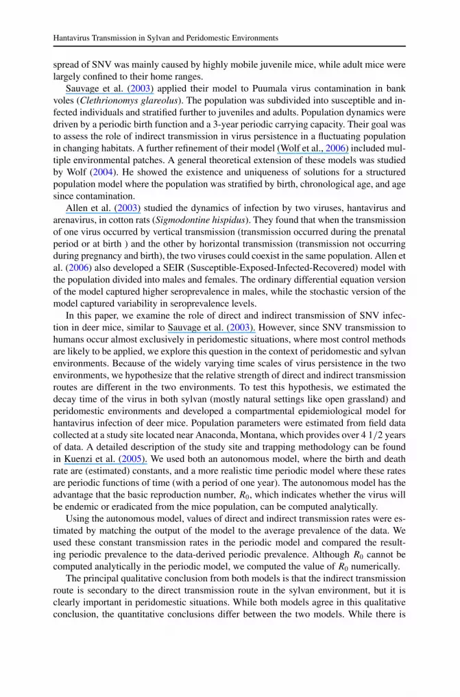
Figure 1 shows the MNA and the MNI for the 54 months that the data were collected,t is in months. For comparison with our simulations, the MNA was taken as the totalpopulation of deer mice(N(t)) and the MNI as the number of infected mice (I (t)) ata given month. In months when there were multiple measurements, we averaged thesemeasurements to get the data point for that month. The number of susceptible mice wasdetermined as S(t) = MNA(t) − MNI(t) and the prevalence of infection was estimatedas MNI/MNA for a given month.

Fig. 1 Raw data collected at the Anaconda site in Montana. The upper curve is the Minimum NumberAlive (MNA) mice per month during the 54 months that the data was collected. (A) The lower curve is thesum of juveniles in month t and subadults in month t + 1; (B) The lower curve is the infected number ofmice (I ). Vertical lines at every 12 months of data collection.

Hantavirus Transmission in Sylvan and Peridomestic Environments

2.1.1. Birth rateThe number of juvenile mice caught in traps is very likely to be an underestimate ofthe actual juvenile population, because juvenile mice stay in burrows and do not ventureout as much as older mice. To estimate the number of mice born in month t we added thenumber of juvenile mice caught in month t to the number of subadults caught in the montht + 1. Since mice become adults in approximately 6–8 week this is a better estimate ofthe true susceptible influx rate. Furthermore, since a very small number of juvenile miceare caught again a month later as subadults (we do not have any recorded evidence ofthis), it is unlikely that the summation would count any mice twice. With this data weestimated the constant birth rate as an average over the 54 months of data collection andgot B = 5.85.

2.1.2. Death rateTo estimate the number of mice e(t) that died in month t we subtract the number of liveadult mice MNA(t) in month t from the available supply of adult mice that could be alivein month t . The second number is the sum of the adult and subadult mice in month t − 1,that is MNA(t − 1) + sub(t − 1). Therefore,

e(t) := MNA(t − 1) + sub(t − 1) − MNA(t).

The death rate in month t was then computed by dividing the number e(t) of dead adultmice in month t by the number of adult live mice in month t −1. If this number is negative,we set the death rate to zero

μ(t) = max{0, e(t)/MNA(t − 1)

}.

The average value μ of μ(t) over 54 months was μ = 0.246.

2.1.3. Disinfection rate δ

The constant δ represents the disinfection rate of the contaminated sites. Since exposure toUV light kills the virus (Shechmeister, 1991), these rates will be substantially different forsylvan populations and peridomestic populations. We have estimated that sunlight likelykills all but a negligible amount of the virus in about 4 hours (Schmaljohn et al., 1999). Weuse this estimate when modeling sylvan environments. Recent experimental data (Kalioet al., 2006) have shown that even without exposure to direct sunlight, Puumala virus wasdeactivated in 24 hours at 37◦C. In the peridomestic situation, the virus is shed in placeswith no direct sunlight, which usually have lower temperatures. The same study (Kalio etal., 2006) found that virus can remain infectious for 2 weeks in contaminated beddings ofvoles. Therefore, we use this estimate, 2 weeks, for our peridomestic settings.

To turn these estimates into an estimate of δ, we observe that δ satisfies G = −δG, andthus is the exponential decay coefficient of the solution G(t) = G0e

−δt . We will consider1% of the initially contaminated sites as “negligible” contamination. Then the time td thatit takes for a site to cease to be infectious satisfies the equation 0.01G0 = G0e

−δtd , whereG0 is the initial number of infected sites. Hence,

δ = − ln 0.01/td .

Because the data is in units of months, we express td in months. For the peridomestic envi-ronment, we have td = 0.5 months, corresponding to 2 weeks, and for sylvan environment

Gedeon et al.

td = 0.005 months which corresponds to approximately 4 hours. Using these values andsolving for δ, one gets a peridomestic value of δ = 9.21 and a sylvan value of δ = 921.

2.1.4. Site contamination rate γ

We cannot estimate the site contamination rate γ . In order to concentrate on the qualitativecomparison between the direct and indirect transmission rates, we will keep γ constantat γ = 0.5. Since γ represents contamination rate of a site given, the contact betweenan infected mice and an uncontaminated site, the constant γ will be much larger thanthe rates α and β . We have seen only modest qualitative changes in our results when theparameter γ varied in its range γ ∈ [0.1,1] (figure not shown). In general, larger γ makesthe indirect route more important relative to the direct infection route, as expected. Thiseffect is, however, dominated by the effect of δ.

2.1.5. Number of contacts c, c and d

The number of contacts is very difficult to estimate. For simplicity, we will keep thesenumbers constant at c = c = d = 60 for our simulations, but in a general form in theanalysis in Appendix A. We have found that doubling this common value has no qualita-tive effect on our results. Since c, c, and d always multiply one of the parameters α,β, γ ,their effect is to effectively shift the values of α,β, and γ . We choose to model c, c, andd separately from α,β, and γ because the latter constants have an interpretation of con-ditional probability, and hence have values between zero and one. For further discussionon the effect of c, c, and d on our results, see Section 3.5.

2.1.6. Mean prevalenceWe can compute the mean prevalence from the data as the mean of the ratio of MNI/MNAover 54 months. This gives a prevalence value of 0.1535 with a standard error of 0.002.The mean prevalence of 15% is in general agreement with the 13% mean prevalence atsylvan sites throughout Montana reported by Douglass et al. (2001) and the mean preva-lence of 16% at sylvan sites reported by Kuenzi et al. (2001b). Since our data were col-lected on a trapping grid that is adjacent to both peridomestic habitat and sylvan habitat,we can associate the computed prevalence to both environments. Therefore, we will testthe model assuming that the 15% represents the prevalence in both sylvan and perido-mestic environments, even though there is some evidence (Kuenzi et al., 2001b) that theprevalence may be higher in the peridomestic setting.

3. Results

The results are divided into four parts. We will first examine the autonomous model wherewe assume that the population parameters (birth rate and death rate) are constant through-out the year. Although biologically unrealistic, this assumption allows us to completelyanalyze the model and derive closed form expression for the basic reproductive ratio R0

as a function of the parameters. If R0 > 1 then the hantavirus infection is endemic, whileif R0 < 1 hantavirus disappears from the population. Further, we numerically simulatethe autonomous model and find combinations of direct and indirect infection rate valuesthat produce the observed average prevalence of 15%. We find that the prevalence in the

Hantavirus Transmission in Sylvan and Peridomestic Environments

model is largely independent of the indirect infection rate in sylvan populations, while itdepends on both rates in the peridomestic environment.

With the values of α and β fixed by the autonomous model to match the averageprevalence from the data, we fit periodic birth and death rates to the data and computedR0 for the periodic model in both sylvan and peridomestic case. We found that for thesylvan environment, both autonomous and periodic model produce nearly identical R0

(Raut0 = 1.28 vs. R

per0 = 1.26) and they are independent on the indirect infection rate α.

Furthermore, the prevalence computed by the time-periodic model matches well the data-derived periodic prevalence (Fig. 6(B)).

In contrast, for the peridomestic environment, the value Raut0 = 1.45 predicted by the

autonomous model differs significantly from that predicted by the periodic model Rper0 =

1.60. Since we matched the autonomous model to the average prevalence to computedirect and indirect transmission rates and these were used in the periodic model, it is notsurprising that the higher R

per0 causes the prevalence given by the time-periodic model to

be higher than the data-derived periodic prevalence (Fig. 6(A)).We show in Appendix A that in the autonomous model Raut

0 > 1 implies that an en-demic equilibrium is globally asymptotically stable and hantavirus infection is endemicin the population, while Raut

0 < 1 indicates that the population is virus-free. For the peri-odic model R

per0 > 1 indicates instability, while R

per0 < 1 local stability of the virus-free

periodic solution. Using Raut0 and R

per0 , we can evaluate effectiveness of putative interven-

tion strategies for virus eradication. If the intervention lowers the indirect transmissionrate α, then we can compute the value α∗ at which either Raut

0 or Rper0 is equal to one. An

explicit expression for Raut0 (defined below in (2)) allows testing intervention strategies

that change multiple parameters at the same time.Comparing the predictions of the autonomous and periodic models we find that in

both cases the periodic model suggests easier eradication than the autonomous model.Interestingly, this is true even in the peridomestic situation where the R

per0 > Raut

0 and theperiodic model produces higher prevalence. Therefore, the periodic model predicts higher,yet more fragile virus population.

3.1. The autonomous model

We show in Appendix A that for an arbitrary initial condition and arbitrary set of parame-ters, the corresponding solution of (1) converges to an equilibrium. We show in Proposi-tion A.1 that the basic reproductive ratio is

Raut0 = δβc + √

(δβc)2 + 4δμαcγ d

2δμ. (2)

Further, we show that if Raut0 > 1 then all positive solutions converge to an endemic

equilibrium E = (S∗, I ∗,G∗) with the persistent population of infected mice I ∗ > 0. Inthis case the prevalence can be computed as I∗

S∗+I∗ . On the other hand, if Raut0 < 1 then

all non-negative solutions converge to a disease-free equilibrium F where (S, I,G) =(B/μ,0,0).

To investigate the impact of the direct and indirect transmission rates on prevalencelevels, we simulate the system (1) for different values of the parameters α and β in twoenvironmental conditions: sylvan (δ = 921) and peridomestic (δ = 9.21). The parameters

Gedeon et al.

Fig. 2 Gray scale-coded values of the prevalence I∗/(I∗ + S∗) at the equilibrium of the system (1) fordifferent values of α and β in (A) sylvan (δ = 921) and (B) peridomestic (δ = 9.21). Dark indicates lowprevalence and light high prevalence. Signs for each combination of α and β indicates the sign of R0 − 1.The “minus” signs (mostly obscured by dark) indicate R0 < 1, and hence a globally stable disease-freeequilibrium and “plus” indicates R0 > 1 and a stable endemic equilibrium.

γ, c, c, d,B, and μ are fixed at values described in the previous section. We check forconvergence to the equilibrium by requiring that the relative error is below 10−7.

In Fig. 2, we graph the prevalence I ∗/(S∗ + I ∗) at the equilibrium as a function ofthe parameters α and β . We take 25 values for both α and β in sylvan (Fig. 2(A)) andperidomestic (Fig. 2(B)) environments. The gray scale codes for value of the prevalencewhere lighter color denote higher prevalence.

We conclude that in the sylvan environment (Fig. 2(A)) the steady state prevalence islargely independent of the indirect transmission rate α, and depends only on the value ofthe direct transmission rate β . In other words, the fast disinfection rate outdoors makes theinfection level of the population independent of the indirect infection rate. The direct in-fection rate β largely determines the prevalence in the population. Therefore, all measuresdesigned to eradicate hantavirus from sylvan deer mice populations should concentrate onlowering the direct transmission rate β . In the peridomestic environment (Fig. 2(B)), bothtransmission modes are important.

We can find the values (α,β) at which the prevalence in the model matches the averagemeasured prevalence of 15%. These values form a one-dimensional curve in the α,β

parameter space. For each value of δ, we have one such curve. In Fig. 3, we present theselines for values of δ that represent sylvan and peridomestic environments.

3.2. The time-periodic model

In the previous section, we considered all the parameters in the system (1) to be constantand we took averages over all data points to estimate the birth and death rates. It is clearfrom seasonal changes in mice life cycles that the birth and death rates are periodic. Inthis section, we look at (1) when the birth rate B = B(t) and the death rate μ = μ(t) are

Hantavirus Transmission in Sylvan and Peridomestic Environments

Fig. 3 Values of the parameters α and β that match the observed average prevalence of 15% in thepopulation. The axis are the same as in Fig. 2. Dashed line represents values of α,β for peridomesticsituation (δ = 9.21) and the solid line for sylvan environment δ = 921.

periodic functions of time. The model becomes

S = B(t) − μ(t)S − αcSG

M− βc

SI

N,

I = −μI + αcSG

M+ βc

SI

N, (3)

G = γ dI

N(M − G) − δG.

We fit a periodic function to the birth data described in Section 2.1.1. We first average theavailable data for each month of the year. Since we have data for 4 and 1/2 years (54 datapoints), there are 5 data points for May through October time period and 4 data pointsfor the other months. We used two different ways to fit the data. First, we used the leastsquare best fit to find the best 3rd degree polynomial. Second, we fitted a periodic functionto the data by performing a discrete Fourier transform of the data. After finding the threecoefficients with largest modulus and setting other coefficients to zero, we computed theinverse FFT to get the periodic estimate of the birth rate. These two approaches yieldedvery similar results; see Fig. 4(A). The resulting birth function B(t) is periodic with a12-month period.

The same approach was used to fit the periodic death rate. Comparison between thirdorder polynomial fit and periodic fit are shown in Fig. 4(B). The prevalence (MNI/MNA)also varies in time, see Fig. 1. As with the birth and death rates, we fitted a 3rd orderpolynomial to the prevalence on a period of 12 consecutive months. The results are shownin Fig. 4(C). We simulated the system (3) with the time-periodic birth rate and death rate

Gedeon et al.

Fig. 4 Solid lines represent (A) Average number of newborn mice per month; (B) Average number of deadmice per month; and (C) mean prevalence over a period of 12 consecutive months. Error bars represent thestandard error and in all cases dash-dot line is the least square fit by the third order polynomial. In (A) and(B), the dashed curve is the result of Fourier 3-term truncation.

described in Fig. 4. We used the Fourier fit for the birth rate and the polynomial fit for thedeath rate, but the results are very similar for other combinations of these two choices. Weused γ = 0.5, M = 50 and initial conditions S = 22, I = 3,G = 10. For each value δ =9.21 and δ = 921, we used the values of α and β that were determined from the prevalencefit of the autonomous equation. Since for each δ there is a set of (α,β) that producethe same average prevalence 15% (see Fig. 3), we chose one set for each δ: for δ =9.21 we set (α,β) = (0.0016,0.0024) and for δ = 921 we set (α,β) = (0.0016,0.0052).Recent experiments (Padula et al., 2004) attempted to measure direct infection rate β inOligoryzomys longicaudatus who carry the Andes hantavirus. Susceptible mice were putin close proximity to infected mice for 24 hours and then tested for virus. The resultssuggested that the infection rate was between 12–17%. If β = 0.0052 and we assume 60active contacts per month, which is 2 contacts per 24 hour, our model predicts an infectionrate of about 1% per 24 hour period. This implies that, under the assumption that miceconfined in close proximity have 10–20 times more active contacts than free mice, theestimate for β lies in [0.0025,0.0050]. We tested multiple choices from this interval forboth environments and found no qualitative differences in our results.

The solutions of the two systems averaged over a 5 year period are shown in Fig. 5.As expected, when δ is small (Fig. 5(A)), the amount of contaminated soil (solid curve)becomes more significant.

3.3. Comparison of autonomous and periodic models

The prevalence resulting from our simulations should resemble the prevalence observed inthe data. We compared the periodic prevalence computed as an average over 5 years fromthe simulation shown in Fig. 5 to the periodic prevalence from the data; see Fig. 4(C).The results are shown in Fig. 6. Notice that the prevalence from the periodic model forperidomestic environment is well above the prevalence from the data, while the model forsylvan environment matches data very well. We note that the parameters α and β wereselected by matching the autonomous system prevalence to the average data prevalence,and the periodic birth and death rate average to the constant birth and death rate used in theautonomous system. To address the source of the discrepancy in the prevalence betweenthe autonomous and periodic models, we computed the basic reproduction number R0 forboth cases.

Hantavirus Transmission in Sylvan and Peridomestic Environments

Fig. 5 Solutions of the system (3) for γ = 0.5 and (A) δ = 9.21, α = 0.0016, β = 0.0024 (peridomesticenvironment); (B) δ = 921, α = 0.0016, β = 0.0052 (sylvan environment) averaged over a time period of5 years. All parameters lie on the respective curves in Fig. 3. The dash-dotted line indicates the number ofthe susceptible mice, the dashed line the number of infected mice and the solid line the number of infectedplaces in the environment.

3.3.1. Peridomestic environmentFor the peridomestic environment, we set γ = 0.5, c = c = d = 60,μ = 0.246, δ = 9.21,which were used to produce Fig. 2(B) and then selected α = 0.0016 and β = 0.0024which produced the prevalence of 15% (see Fig. 3) in the autonomous model. Then from(2) we computed the value Raut

0 = 1.45. There is no closed form expression analogousto (2) for R

per0 in the periodic model. We computed R

per0 for the periodic model by a

method introduced by Bacaer (2007) that uses Floquet theory. We obtained Rper0 = 1.60

(the details of the computation can be found in Appendix A). This higher basic repro-duction number is reflected in the higher average prevalence of 21% in the periodic case(see Fig. 6(A)) compared to 15% in the autonomous case. Therefore, in the peridomesticsetting seasonal periodicity leads to higher R0 and higher prevalence. This result shouldbe contrasted with the result of Bacaer (2007) for vector-borne diseases which showsthat if the seasonal change is sinusoidal and small, then the first correction term to theautonomous Raut

0 due to a periodic forcing is negative and so Rper0 < Raut

0 . Our periodicforcing function S(t), depicted in Fig. 7, is not a small perturbation of the identity.

3.3.2. Sylvan environmentFor the sylvan environment, we set γ = 0.5, c = c = 60,μ = 0.246, δ = 921 that wereused to produce Fig. 2(A) and then selected α = 0.0016 and β = 0.0052 which produceda prevalence of 15% (see Fig. 3) in the autonomous model. Then from (2) we computedthe value Raut

0 = 1.28.R

per0 is defined as a spectral radius of a next generator integral operator K. Since one

of the off-diagonal elements of this operator is proportional to the indirect transmissionrate α, and since α does not affect the epidemic in the sylvan environment, the opera-tor K is dominated by its diagonal terms. This has two consequences. On one hand the

Gedeon et al.

Fig. 6 Model prevalence (dashed line) over the last cycle for the simulations shown in Fig. 5 comparedto fitted prevalence (solid line) shown in Fig. 3.

Fig. 7 Function S(t) is not a small perturbation of the unity.

Floquet theory method of computation of Rper0 does not work; on the other we can ap-

proximate the next generation operator K by its diagonal terms and compute Rper0 directly

from this approximation. This yields Rper0 = 1.26 (the details of the computation are in

Appendix A). We observe that in the sylvan environment Raut0 ≈ R

per0 and the periodic

prevalence matches the prevalence in the data; see Fig. 6(B).

3.4. Eradication of the infection

The basic reproduction number R0 gives us the ability to predict change in transmissionparameters α and β that would lead to eradication of SNV infection in deer mice. Re-call that to eradicate SNV we have to make R0 < 1. We analyzed how R0 changed as afunction of α and β for both autonomous and periodic models. Since we have a closedform expression for Raut

0 in the autonomous model (2), we can make a few analyticalobservations:

Hantavirus Transmission in Sylvan and Peridomestic Environments

1. If we lower the direct transmission rate β to its lowest possible value of 0 then Raut0 =√

αcγ d

δμ. Therefore, the eradication by lowering β is only possible if

δμ ≥ cdαγ. (4)

The left side expresses a decay of infection either by direct disinfection of the ground(δ) or by a removal of the infected mice (μ). The right-hand side represents the in-fection rate in the indirect pathway and includes both the number of contacts betweeninfected mice and uncontaminated sites d and the number of contacts between con-taminated sites and susceptible mice c. We conclude that the strong indirect pathwaymay prevent eradication of the virus in the population by attempts to lower the directtransmission rate β .

2. When we set α = 0 in (2), we recover the standard expression Raut0 = βc

μ. Thus, the

eradication by lowering α is only possible if the death rate dominates the direct trans-mission rate

βc ≤ μ. (5)

3. Raut0 does not depend on the birth rate B , or the maximal number of contaminated

sites M .

We apply these observations to our models with parameters described in Sections 3.3.1and 3.3.2.

3.4.1. Peridomestic environmentWe set the parameters as in Section 3.3.1 which produced Raut

0 = 1.45. We note that thecondition (4) reads 2.27 ≥ 2.88 while the condition (5) reads 0.144 ≤ 0.246. Therefore,the disease can be eradicated by lowering α (moving left in Fig. 2(B)), but not by loweringβ (moving down in Fig. 2(B)). We computed the critical value of α at which the virusis eradicated by setting Raut

0 = 1 in (2) and solving for αaut = 0.0005219. To eradicatehantavirus under these conditions, the indirect infection rate has to drop from α = 0.0016to α = 0.0005, that is to 30% of the original value.

Recall that Rper0 = 1.60. Using the Floquet method (see Appendix A) we computed

numerically the critical value αper at which Rper0 = 1. This value is αper = 0.00063, which

is 39% of the original value and it is higher than αaut. This leads to an interesting obser-vation. In spite of higher levels of virus predicted by the periodic model, this model alsopredicts higher sensitivity to change in the rate of indirect transmission and easier erad-ication. However, since we have not proved that in the periodic model the disease-freesolution is globally stable if, and only if R

per0 < 1, it is possible that the endemic solution

persists even for Rper0 < 1.

3.4.2. Sylvan populationWe set the parameters as in Section 3.3.1 that produced Raut

0 = 1.28. With these para-meters, the condition (4) reads 226.6 ≥ 2.88 and the condition (5) reads 0.246 ≥ 55.260.Therefore, we can eradicate SNV by lowering β , but not by lowering α. To find the criticalβ we solved (2) with Raut

0 = 1 for βaut = 0.0021. Therefore, according to the autonomousmodel, to eradicate hantavirus in sylvan population the direct transmission rate has to dropfrom β = 0.0052 to 0.0021, that is to about 40% of the original value.

Gedeon et al.

Recall that Rper0 = 1.26. We computed the critical value βper at which R

per0 = 1 and find

βper = 0.0041, which is about 79% of the original value (see Appendix A). Note that as inthe peridomestic case, the critical value of the parameter in the periodic model is higherthan in the autonomous model, βper > βaut.

Therefore, in both peridomestic and sylvan cases, the periodic model predicts thatthe virus population is more fragile when compared to the prediction of the autonomousmodel.

3.5. Effect of the other parameters

So far, we have concentrated on the effect of direct and indirect transmission rate on thevirus prevalence (Fig. 2). We briefly discuss the effect of the other parameters. Since c

multiplies β , c multiplies α, and d multiplies γ the change in value of c = c = d does notchange the qualitative character of Fig. 2. The larger this common value, the smaller thearea in (α,β) space which admits infection free equilibrium. If we keep c fixed and lowerc = d then Fig. 2(B) may start to resemble Fig. 2(A), but only after the value of c = d

drops to single digits. Finally, γ has a limited effect on Fig. 2 when kept in the rangeγ ∈ [0.1,1]. If γ is allowed to become smaller than α and β , then Fig. 2(B) will start toresemble Fig. 2(A). However, the site contamination rate should be higher than either thedirect or the indirect infection rate.

4. Conclusions

We have developed a compartmental model for hantavirus infection in deer mice withthe goal of comparing the relative importance of direct and indirect transmission in syl-van and peridomestic environments. Based on population dynamics data and estimates ofSin Nombre virus persistence in sylvan and peridomestic environments, our autonomousmodel predicts that direct transmission dominates in the sylvan environment, while bothpathways are important in the peridomestic environment. This conclusion has been con-firmed by the time-periodic model where we used data-fitted time-periodic birth and deathrates.

We computed the basic reproduction number R0 in both environments and in bothtypes of models. While we found a very good fit between the autonomous and periodicmodels in sylvan environment in both R0 and the prevalence, we found that in the perido-mestic environment both the R0 and the average prevalence are higher in the periodicmodel.

We analyzed R0 in both models and environments to compute the critical values of thetransmission rates which would lead to virus eradication. For one choice of parameters,that replicate the data derived prevalence, our results predicted that completely abolish-ing indirect transmission would not eradicate virus in the sylvan population. On the otherhand, the analysis of the autonomous model shows that lowering the direct transmissionto 40% of the original value would lead to eradication of the virus. The correspondingprediction from the periodic model is qualitatively the same but quantitatively different:abolishing the indirect rate would not eradicate the virus, while lowering the direct trans-mission rate to 79% of the original value would lead to eradication of the virus.

Hantavirus Transmission in Sylvan and Peridomestic Environments

In the peridomestic situation abolishing direct transmission would not lead to erad-ication, but lowering the indirect transmission rate would. The predictions again varybetween the autonomous and periodic models: lowering the indirect transmission rate to30% (autonomous) or 39% (periodic) would lead to virus eradication.

These results can perhaps be used to guide eradication strategies in peridomestic envi-ronments. Trapping to remove the population from outbuildings may reduce direct trans-mission of the virus but not eradicate it. On the other hand, frequent disinfection methodsmay be more effective to achieve eradication. We hasten to add that since the choice ofparameters that reproduce the observed prevalence is not unique, these results are onlyqualitative. Furthermore, while the predictions from the autonomous and periodic modelsare qualitatively the same, the qualitative predictions differ considerably, with the peri-odic model suggesting that the virus population is more fragile and can be eradicatedmore easily.

Our work provides a basic framework for the analysis of hantavirus transmission in adeer mice populations. We hope that as further data collection fills in the values of miss-ing parameters, we will be able to make our model even more quantitative by includingseasonal and spatial variation.

Acknowledgements

We would like to thank the anonymous reviewers whose comments greatly improved thescope and the presentation of the paper. The research of the first and the third author waspartially supported by NIH-NCRR grant PR16445.

Appendix A

A.1 The equilibria and local stability for the autonomous model

We first observe that by adding the first and second equations in (1) we get

d

dt(S + I ) = B − μ(S + I ) (A.1)

which implies that S + I converges exponentially to the value Bμ

. Therefore, any equilib-

rium (S∗, I ∗,G∗) of the system lies on the plane given S∗ +I ∗ = N = Bμ

. The disease-freeequilibrium F := (x, y, z) = (N,0,0) always exists, independently of the value of the pa-rameters. In many epidemiological models, the local asymptotic stability of the diseasefree equilibrium F depends on a threshold parameter R0 known as a basic reproductionnumber. Diekmann et al. (1990) defined R0 as a spectral radius of the next generationmatrix and this calculation has been made explicit for a large class of epidemiologicalmodels by van den Driessche and Watmough (2002).

Proposition A.1 (Existence and local stability of equilibria). The basic reproductionnumber for (1) is

Raut0 = δβc + √

(δβc)2 + 4δμαcγ d

2δμ.

Gedeon et al.

The disease-free equilibrium F is asymptotically stable if, and only if, Raut0 < 1. Further-

more, if Raut0 > 1, then there exists unique endemic equilibrium E := (S∗, I ∗,G∗) with

0 < S∗ < N , 0 < I ∗ < N , and 0 < G∗ < M .

Proof: The first part is standard and follows from a general argument in van den Driess-che and Watmough (2002). Indeed, in our model there are two infected compartments I

and G and the function F characterizing the appearance of new infections in these twocompartments is F = (αc SG

M+ βc SI

S+I, γ d I

S+I(M − G)). The rate of transfer out of these

compartments is V = (μ, δ). Then R0 is the spectral radius of FV −1 where F := [ ∂F∂I,G

]and V := [ ∂V

∂I,G] are 2 × 2 restrictions of the Jacobians of F and V to variables I and G,

evaluated at the disease free equilibrium. A straightforward calculation gives

FV −1 =[

βc 1μ

αc SMδ

γ d MSμ

0

]

and its characteristic equation λ2δμ − βcδλ − αcγ d = 0 from which the value of Raut0

follows.To prove the second part, we compute other equilibria. We first solve for I from the

last equation in

0 = B − μS − αcSG

M− βc

SI

N,

0 = −μI + αcSG

M+ βc

SI

N, (A.2)

0 = γ dI

N(M − G) − δG

and plug it to the first equation (where we use B − μS = μI ) to get

0 = Gc

d

(μδN

γ c(M − G)− αdc

cMS − S

βδ

γ (M − G)

)

from which

S =μδN

cγ

βδ

γ+ α cd

cM(M − G)

. (A.3)

Using S + I = N we compute a quadratic function whose roots determine values of G atequilibria

h(G) = αc

cM(γ d + δ)G2 −

(δ2β

γ d+ αδc

c− μδ

c+ βδ + 2

αcdγ

c

)G

+ M

(βδ + αdγ

c

c− μδ

c

)= 0.

Observe that the leading coefficient of the quadratic polynomial h(G) is positive and

that h(M) = − δ2β

γ d< 0. Thus, h(G) has one zero at some G > M .

Hantavirus Transmission in Sylvan and Peridomestic Environments

Note that h(0) = Mc(βδc + αdγ c − μδ) and a short computation shows that h(0) < 0

if, and only if, R0 < 1. If h(0) < 0, then h(G) cannot have a zero in (0,M), and so F

is the only equilibrium of (1). If h(0) > 0 (and hence R0 > 1), then h(G) has a uniquezero G∗ in (0,M). To finish, we need to prove that corresponding values S∗ and I ∗ at theequilibrium lie in (0,N). By (A.3) and the last equation in (A.2), if G∗ ∈ (0,M), thenS∗ > 0 and I ∗ > 0. Since S∗ + I ∗ = N , the result follows. �

Proposition A.2 (Stability of the endemic equilibrium). If the endemic equilibrium E

exists, then it is always locally asymptotically stable.

Proof: By (A.1), the linearization at both equilibria E and F have one negative eigen-value −μ which represents a convergence to the carrying capacity B

μfor the total popu-

lation S + I . The other two eigenvalues govern local dynamics within the invariant planeS + I = B

μ. To find out the signs of these eigenvalues, we consider linearization of the last

two equations in (1), where we replace S by Bμ

− I to reflect the constraint S + I = Bμ

I = −μI + αc(B

μ− I )G

M+ βc

(Bμ

− I )I

N,

G = γ dI

N(M − G) − δG.

We rescale the variables y = IcN

and z = GcM

and get

y = −μy + α(c − y)z + βy(c − y), (A.4)

z = γd

cy(c − z) − δz.

We linearize to get

Df(y, z) =[−μ − αz + β(c − 2y) α(c − y)

γ dc(c − z) −γ d

cy − δ

]. (A.5)

We evaluate the linearization (A.5) at the endemic equilibrium E = (x∗, y∗, z∗) andshow that Df(E) has a negative trace and a positive determinant. The trace of Df(E) is

Tr(Df(E)) = −μ − αz∗ + β(c − 2y∗) − γd

cy∗ − δ.

Since E is an equilibrium of (1), then it is also an equilibrium of (A.4) and so −μy∗ +α(c − y∗)z∗ + βy∗(c − y∗) = 0. This is equivalent to

−μ + β(c − y∗) = −α(c − y∗)z∗

y∗ . (A.6)

Since 0 < y∗, z∗ < c plugging this into the expression for the trace, we get

Tr(Df(E)) = −α(c − y∗)z∗

y∗ − βy∗ − αz∗ − γd

cy∗ − δ < 0.

Gedeon et al.

Now we compute the determinant of (A.5) at the endemic equilibrium

det(Df(E)) = (−μ − αz∗ + β(c − 2y∗))(

−γd

cy∗ − δ

)− αγ

d

c(c − z∗)(c − y∗)

=(

−α(c − y∗)z∗

y∗ − αz∗ − βy∗)

×(

−γd

cy∗ − δ

)− αγ

d

c(c − z∗)(c − y∗)

where we used (A.6). Since from the second equation in (A.4), we have y∗ = δcγ d

z∗c−z∗ , we

get γ dc(c − z∗) = δz∗

y∗ . Using this in the last expression above, we get

det(Df(E)) =(

α(c − y∗)z∗

y∗ + αz∗ + βy∗)(

γd

cy∗ + δ

)− α

δz∗

y∗ (c − y∗)

= (αz∗ + βy∗)(

γd

cy∗ + δ

)

+ α(c − y∗)z∗

y∗

(γ

d

cy∗ + δ

)− α

(c − y∗)z∗

y∗ δ

= (αz∗ + βy∗)(

γd

cy∗ + δ

)+ αγ

d

c(c − y∗)z∗ > 0. �

A.2 Global convergence to the equilibria

Proposition A.3. If Raut0 < 1 all solutions starting in the nonnegative orthant of R3 con-

verge to the disease-free equilibrium F , and if Raut0 > 1 then almost all solutions starting

in the nonnegative orthant converge to the endemic equilibrium E.

Proof: All solutions in the nonnegative orthant approach exponentially the plane S +I = N . Therefore, the invariant set lies in the intersection of this plane and the nonnegativeorthant, which we denote Σ . The rescaled equations describing dynamics on Σ are (A.4).

When Raut0 < 1 then by Proposition A.1 Σ contains unique equilibrium F on its bound-

ary. Since every closed orbit in the plane has to contain an equilibrium in its interior, thereare no periodic orbits in Σ . A local stability of F rules out existence of homoclinic orbits.Therefore, by the Poincaré–Bendixson theorem all solutions in Σ converge to F .

When Raut0 > 1, by Proposition A.1 Σ contains two equilibria: F on its boundary and

an internal equilibrium E. The equilibrium E is stable by Proposition A.2. The divergenceof the vector field (A.4) is

−δ − (μ − cβ) − 2βy − γd

cy.

A short calculation shows that Raut0 > 1 implies cβ − 2μ > 0, which in turn shows that

the second term above is negative. Since the entire expression is negative, we conclude byDulac’s criterion (Hale and Kocak, 1991) that there are no periodic orbits in Σ . A local

Hantavirus Transmission in Sylvan and Peridomestic Environments

stability of E (Proposition A.2) rules out the existence of orbits homoclinic to E and bythe Poincaré–Bendixson theorem all solutions in Σ , except those on the stable manifoldof F , converge to E. �

A.3 R0 for the periodic model

The basic reproduction number for the periodic model is a spectral radius of a linearintegral operator (Diekmann et al., 1990; Bacaer, 2007)

(Kv)(t) =∫ ∞

0K(t, x)v(t − x)dx (A.7)

where the matrix K(t, x) describes the expected number of newly infected individuals.More specifically, given n infected compartments I1, I2, . . . , In, the (i, j) entry Ki,j (t, x)

represents the expected number of individuals in compartment Ii that one individual incompartment Ij generates at the beginning of the epidemic per unit time at time t ifit has been in the compartment Ij for x units of time. The basic reproduction numberdetermines if the epidemics can invade a disease-free population. In the periodic case,this corresponds to a T -periodic solution F(t) := (S(t),0,0) where S(t) is the steadystate periodic solution of S = B(t) − μ(t)S and B(t) and μ(t) are the T -periodic birthand death functions. There are two infected compartments I and G and linearizing aboutF(t) (taking into account that N(t) = S(t) + I (t)) we get a linear system

I = (−μ(t) + cβ)I + cα

MS(t)G,

(A.8)

G = γ dM1

S(t)I − δG.

Solving the first equation, we get

I (t) =∫ ∞

0

cα

MS(t − x1) exp

(−

∫ t

t−x1

(μ(u) − cβ

)du

)G(t − x1) dx1 (A.9)

and, therefore, K1,2 = cαM

S(t − x1) exp(− ∫ t

t−x1(μ(u) − cβ)du). Similarly, we solve the

second equation

G(t) =∫ ∞

0γ dM

1

S(t − x2)exp(−δx2)I (t − x2) dx2 (A.10)

and arrive at K2,1 = γ dM 1S(t−x2)

exp(−δx2). Then the kernel of the next generation oper-ator (A.7) is

K(t, x) :=[

0 K1,2

K2,1 0

]

which is T -periodic for every fixed value of x = x1 = x2 with x ≥ 0. The eigenvalueproblem

∫ ∞

0K(t, x)

(I (t − x),G(t − x)

)Tdx = R0

(I (t),G(t)

)T(A.11)

Gedeon et al.

on the space T -periodic functions with values in R2 determines the basic reproductionconstant R0. Bacaer (2007) proposed several ways to compute R0. Since both K1,2 andK2,1 are time dependent, only one of these methods is applicable to our problem. Wecompute R0 using Floquet theory for the parameters corresponding to the peridomesticcase.

We first note that we can turn the 2 × 2 integral eigenvalue problem (A.11) to a scalarproblem by substituting for G(t) in (A.9) from (A.10) to get

(R

per0

)2I (t) =

∫ ∞

0

∫ ∞

0cαγ d

S(t − x1)

S(t − x1 − x2)

× exp

(−

∫ t

t−x1

(μ(u) − cβ

)du

)

× exp(−δx2)I (t − x1 − x2) dx1 dx2. (A.12)

By Floquet theory, the equilibrium solution (I,G) = (0,0) loses stability when the largestcharacteristic multiplier λ0 of the periodic system (A.8) is equal to 1. We introduce aparameter ξ and solve a linear variational equation dX

dt= AX for X(T , ξ) with X(0) an

identity matrix and

A =[−μ(t) + cβ cαS(t)

Mξ

γ dM 1S(t)

δ

]

.

By changing the parameter ξ, we find a critical value ξ ∗ such that X(T , ξ ∗) has spectralradius λ0(ξ

∗) = 1. We note that if (I ∗,G∗) is the corresponding eigenvector, then I ∗ isan initial condition of a T -periodic solution I (t) which is an eigenvector of the integralequation

I (t) =∫ ∞

0

∫ ∞

0

cαγ d

ξ ∗S(t − x1)

S(t − x1 − x2)

× exp

(−

∫ t

t−x1

(μ(u) − cβ

)du

)exp(−δx2)I (t − x1 − x2) dx1 dx2. (A.13)

Direct comparison with (A.12) shows (Rper0 )2 = ξ ∗. By combining a bisection method

with the numerical integration of dXdt

= AX, we computed in the peridomestic case ξ ∗ =2.55 and

Rper0 = √

ξ ∗ = 1.60.

We also note that (A.13) shows that if we replace the value of α by the value α/ξ ∗ thenR

per0 = 1. Therefore, αper = 0.0016/2.55 = 0.000627.

Unfortunately, we cannot use this approach for the computation of Rper0 in the sylvan

case. Since δ = 921, the diagonal terms in A dominate the off-diagonal terms and thereis no ξ > 0 that would produce λ0 = 1. In fact, ξ = 1 yields λ0 = 1.79 while droppingboth off-diagonal terms (this corresponds to ξ = ∞) yields λ0 = 1.74. Because of thedominance of the diagonal entries in (A.8), we approximate (A.8) by a diagonal system

I = (−μ(t) + cβ)I, G = −δG.

Hantavirus Transmission in Sylvan and Peridomestic Environments

Then the matrix operator K is diagonal and the disease-free solution (I,G) = (0,0) isunstable if, and only if, the integral over one period

∫ T

0

(−μ(t) + cβ)dt > 0.

This condition is equivalent to Rper0 > 1 where R

per0 := cβ

μand μ :=

∫ T0 μ(t)

Tis the average

death rate. In our case, μ = μ = 0.246 and Rper0 = 1.26. Using this formula for R

per0 , we

compute the critical value of βper in the sylvan case βper = 0.0041.

References

Abbott, K.D., Ksiazek, T.G., Mills, J.N., 1999. Long-term hantavirus persistency in rodent populations incentral Arizona. Emerg. Infect. Dis. 5, 102–112.

Abramson, G., Kenkre, V.M., 2002. Spatiotemporal patterns in the hantavirus infection. Phys. Rev. E 66,011912.

Abramson, G., Kenkre, V.M., Yates, T.L., Parmenter, R.R., 2003. Travelling waves of infection in thehantavirus epidemics. Bull. Math. Biol. 65, 271–281.

Allen, L.J.S., Langlais, M., Phillips, C., 2003. The dynamics of two viral infections in a single host popu-lation with application to hantavirus. Math. Biosci. 186, 191–217.

Allen, L.J.S., McCormack, R.K., Jonsson, C.B., 2006. Mathematical models for hantavirus infection inrodents. Bull. Math. Biol. 68, 511–524.

Armstrong, L.R., Zaki, S.R., Goldoft, M.J., Todd, R.L., Khan, A.S., Khabbaz, R.F., Ksiazek, T.G., Peters,C.J., 1995. Hantavirus pulmonary syndrome associated with entering or cleaning rarely used, rodent-infested structures. J. Infect. Dis. 172, 1166.

Bacaer, N., 2007. Approximation of the basic reproduction number R0 for vector borne diseases with aperiodic vector population. Bull. Math. Biol. 69, 1067–1091.

Calisher, C.H., Root, J.J., Mills, J.N., Beaty, B.J., 2003. Hantaviruses: etiologic agents of rare, but poten-tially life-threatening zoonotic diseases. J. Am. Vet. Med. Assoc. 222, 163–166.

Calisher, C.H., Sweeney, W., Mills, J.N., Beaty, B.J., 1999. Natural history of Sin Nombre virus in westernColorado. Emerg. Infect. Dis. 5, 126–134.

CDC MMWR, 2002. Hantavirus pulmonary syndrome—United States: updated recommendations for riskreduction. Center Dis. Control Morb. Mort. Weekly Rep. 51, 1–12.

Centers for Disease Control and Prevention, 2007. Case information: hantavirus pulmonary syndrome casecount and descriptive statistics as of March 2007. National Center for Infectious Diseases, SpecialPathogens Branch

Childs, J.E., Ksiazek, T.G., Spiropoulou, C.F., Krebs, J.W., Morzunov, S., Maupin, G.O., Rollin, P.E.,Sarisky, J., Enscore, R.E., 1994. Serologic and genetic identification of Peromyscus maniculatus asthe primary rodent reservoir for a new hantavirus in southwestern United States. J. Infect. Dis., 1271–1280.

Diekmann, O., Heesterbeek, J.A.P., Metz, J.A.J., 1990. On the definition and the computation of the basicreproduction ratio R0 in models for infectious diseases in heterogeneous populations. J. Math. Biol.28, 365.

Douglass, R.J., Semmens, W.J., Matlock-Cooley, S.J., Kuenzi, A.J., 2006. Deer mouse movements inperidomestic and sylvan settings in relation to Sin Nombre virus antibody prevalence. J. Wildlife Dis.42(4), 813–818.

Douglass, R.J., Wilson, T., Semmens, W.J., Zanto, S.N., Bond, C.W., Van Horn, R.C., Mills, J.N., 2001.Longitudinal studies of Sin Nombre virus in deer mouse dominated ecosystems in Montana. Am. J.Trop. Med. Hyg. 65(1), 33–41.

Glass, G.E., Watson, A.J., LeDuc, J.W., Kelen, G.D., Quinn, T.C., Childs, J.E., 1993. Infection with a rat-borne hantavirus in United States residents is consistently associated with hypertensive renal disease.J. Infect. Dis. 167, 614–619.

Hale, J., Kocak, H., 1991. Dynamics and Bifurcations. Springer, Berlin.

Gedeon et al.

Kalio, E., Klingstrom, J., Gustafsson, E., Manni, T., Vaheri, A., Henttonen, H., Vapalahti, O., Lund-kvist, A., 2006. Prolonged survival of Puumala hantavirus outside the host: evidence for indirecttransmission via the environment. J. Gen. Virol. 87, 2127–2134.

Kenkre, V.M., Giuggioli, L., Abramson, G., Camelo-Neto, G., 2007. Theory of hantavirus infection spreadincorporating localized adult and itinerant juvenile mice. Eur. Phys. J. 55, 461–470.

Khan, A.S., et al., 1996. Hantavirus pulmonary syndrome: the first 100 US cases. J. Infect. Dis. 173,1297–1303.

King, J.A., 1968. Biology of Peromyscus (Rodentia), 1st edn. The American Society of Mammalogists,Stillwater.

King, J.A., 1983. Seasonal dispersal in a semi-natural population of Peromyscus maniculatus. Can. J. Zool.61(12), 11.

Krebs, C.J., 1966. Demographic changes in fluctuating populations of Microtus californicus. Ecol.Monogr. 36, 239–273.

Kuenzi, A.J., Douglass, R.J., White, D. Jr., Bond, C.W., Mills, J.N., 2001a. Antibody to Sin Nombre virusin rodents associated with peridomestic habitats in west central Montana. Am. J. Trop. Med. Hyg. 64,137–146.

Kuenzi, A.J., Douglass, R.J. Jr., White, D., Bond, C.W., Mills, J.N., 2001b. Antibody to Sin Nombre virusin rodents associated with peridomestic habitats in west central Montana. Am. J. Trop. Med. Hyg. 64,137–146.

Kuenzi, A.J., Douglass, R.J., Bond, C.W., Calisher, C.H., Mills, J.N., 2005. Long-term dynamics of SinNombre viral RNA and antibody in deer mice in Montana. J. Wildlife Dis. 41, 473–481.

Kuenzi, A.J., Morrison, M.L., Swann, D.E., Hardy, P.C., Downard, G.T., 1999. A longitudinal study of SinNombre virus prevalence in rodents in southwestern Arizona. Emerg. Infect. Dis. 5, 113–117.

Kuenzi, A.J., Zumbrun, M.M., Hughes, K., 2005. Ear tags versus passive integrated transponder (pit) tagsfor effectively marking deer mice. Int. J. Sci. 11, 66–70.

Lee, P.W., Amyx, H.L., Yanagihara, R., Gajdusek, D.C., Goldgaber, D., Gibbs, C.J. Jr., 1985. Partial char-acterization of Prospect Hill virus isolated from meadow voles in the United States. J. Infect. Dis. 152,826–829.

Mills, J.N., Ksiazek, T.G., Peters, C.J., Childs, J.E., 1999. Long-term studies of hantavirus reservoir pop-ulations in the southwestern United States: a synthesis. Emerg. Infect. Dis. 5, 135–142.

Nichol, S.T., Spiropoulou, C.F., Morzunov, S., Rollin, P.E., Ksiazek, T.G., Feldmann, H., Sanchez, A.,Childs, J., Zaki, S., Peters, C.J., 1993. Genetic identification of a hantavirus associated with an out-break of acute respiratory illness. Science 262, 914–917.

Padula, P., Figueroa, R., Navarrete, M., Pizarro, E., Cadiz, R., Bellomo, C., Jofre, C., Zaror, L., Rodriguez,E., Murua, R., 2004. Transmission study of Andes hantavirus infection in wild sigmodontine rodents.J. Virol., 11972–11979.

Sauvage, F., Langlais, M., Yoccoz, N.G., Pontier, D., 2003. Modeling hantavirus in fluctuating populationsof bank voles: the role of indirect transmission on virus persistence. J. Anim. Ecol. 72, 1–13.

Schmaljohn, C., Huggins, J., Calisher, C.H., 1999. Laboratory and field safety. In Lee, H.W., Calisher,C.H., Schmaljohn, C. (Eds.), Manual of Hemorrhagic Fever with Renal Syndrome and HantavirusPulmonary Syndrome, pp. 192–198. WHO Collaborating Center for Virus Reference and Research(Hantaviruses), Asian Institute for Life Sciences, Seoul, Korea.

Shechmeister, I.L., 1991. Sterilization by ultraviolet irradiation. In: Block, S.S. (Ed.), Disinfection, Steril-ization, and Preservation, p. 553. Lea and Febiger, Philadelphia

Tsai, T.F., 1987. Hemorrhagic fever with renal syndrome: mode of transmission to humans. Lab. Anim.Sci. 37, 430.

van den Driessche, P., Watmough, J., 2002. Reproduction numbers and sub-threshold endemic equilibriafor compartmental models of disease transmission. Math. Biosci. 10, 29–48.

Wolf, C., 2004. A mathematical model for the propagation of a hantavirus in structured populations. Dis-crete Contin. Dyn. Syst. B 4(4), 1065–1089.

Wolf, C., Langlais, M., Sauvage, F., Pontier, D., 2006. A multi-patch epidemic model with periodic de-mography, direct and indirect transmission and variable maturation rate. Math. Popul. Stud. 13(3),153–177.