Habitat associations of woodland birds II

Jane Carpenter, Elisabeth Charman,

Jennifer Smart, Arjun Amar, Derek

Gruar, & Phil Grice

Habitat associations of

woodland birds II

RSPB Research Report No. 36

ii

Habitat associations of woodland birds II

RSPB Research Report Number 36

Jane Carpenter, Elisabeth Charman, Jennifer Smart, Arjun

Amar, Derek Gruar, & Phil Grice

Recommend citation: Jane Carpenter, Elisabeth Charman, Jennifer Smart, Arjun Amar,

Derek Gruar, & Phil Grice. 2009. Habitat associations of woodland birds II. RSPB

Research Report No. 36. ISBN 978-1-905601-20-2.

Carpenter, Charman et al. 2009.

1

Contents

Contents 1

1

Introduction

4 1.1 Background 4

1.2 The repeat woodland bird survey 5

1.3 Habitat associations of woodland birds 1st report 6

1.4 Habitat associations of woodland birds II: Scope and aims 7

1.4.1 Securing the future 7

1.4.2 The woodland bird sustainability indicator 7

1.4.3 Aim of this report 8

1.5 Layout of the report 8

1.6 Acknowledgements 10

2

Methods

11 2.1 Study sites 11

2.2 Bird population data 12

2.3 Habitat data 13

2.4 Landscape data 16

2.5 Climate data 17

2.6 Deer and predator data 20

2.6.1 Deer data 20

2.6.2 Squirrel data 21

2.6.3 Avian predator data 21

2.7 Statistical analyses 22

2.7.1 Model selection process 22

2.7.2 Analyses 23

3

Results

26 3.1 Blackbird 26

3.1.1 Introduction 26

3.1.2 Results 27

3.1.3 Discussion 31

3.2 Bullfinch 35


3.2.2 Results 37

3.2.3 Discussion 41

3.3 Chaffinch 43


3.3.2 Results 45

3.3.3 Discussion 49

3.4 Coal tit 51


3.4.2 Results 53

3.4.3 Discussion 56

2

3.5

Dunnock

60


3.5.2 Results 61

3.5.3 Discussion 67

3.6 Goldcrest 69


3.6.2 Results 71

3.6.3 Discussion 76

3.7 Green woodpecker 78


3.7.2 Results 80

3.7.3 Discussion 85

3.8 Jay 87


3.8.2 Results 89

3.8.3 Discussion 93

3.9 Long-tailed tit 95


3.9.2 Results 97

3.9.3 Discussion 101

3.10 Nuthatch 103


3.10.2 Results 105


3.11 Robin 113


3.11.2 Results 115


3.12 Siskin 121


3.12.2 Results 122


3.13 Song thrush 132


3.13.2 Results 134


3.14 Treecreeper 141


3.14.2 Results 143


3.15 Willow tit 150


3.15.2 Results 151


3.16 Wren 156


3.16.2 Results 158


3

4 General discussion 166 4.1 Overview of woodland bird associations 166

4.1.1 Large-scale variables 166

4.1.2 Field-layer variables 169

4.1.3 Understorey variables 170

4.1.4 Tree size variables 172

4.1.5 Deadwood variables 173

4.1.6 Landscape variables 174

4.1.7 Deer variables 174

4.1.8 Predator variables 175

4.1.9 Other variables 176

4.2 Conclusion 177

References 179

4

1 INTRODUCTION

1.1 Background

There has been concern for some time about the state of some British woodland bird

populations (e.g. Fuller et al., 2005; Amar et al., 2006; Smart et al., 2007). However,

although certain woodland birds have undergone serious long-term population declines

(e.g. willow tit Poecile montana; lesser spotted woodpecker Dendrocopos minor), others

(e.g. great tit Paris major; great spotted woodpecker Dendrocopos major) have increased

over the same time-period (Eaton et al., 2006). The situation is further complicated due to

the declining species being a mixture of resident species, and long distance migrants,

making easy identification of a single overriding factor for the declines difficult (Fuller et

al., 2005; Amar et al., 2006). A lack of detailed research on many British woodland birds,

both increasing and declining species, also adds to this problem (Amar et al., 2006), as

little is known of the behaviour and ecology, even of common species.

Fuller et al. (2005) reviewed the potential causes of the decline. They identified the

following seven key areas where further research was required:

1. Pressures on long-distance migrants

2. Climate change

3. Reduction of invertebrate food supplies

4. Changes in the quality and quantity of woodland edge habitat

5. Reduction in woodland management

6. Increased grazing and browsing pressure, particularly from deer

7. Increased nest predation from avian and mammalian predators

https://www.researchgate.net/publication/230853566_Habitat_associations_of_woodland_birds_implications_for_woodland_management_for_declining_species?el=1_x_8&enrichId=rgreq-770261ad-7197-4a14-bbf4-812097cc1e1c&enrichSource=Y292ZXJQYWdlOzI2NTI3NzAyMjtBUzoxODI5MTM0Mjk2ODAxMjlAMTQyMDYyMTM2ODUxNw==

5

Since the publication of this review, two reports detailing large-scale analyses aiming to

gather further information on woodland bird populations (Amar et al., 2006) and their

habitat requirements (Smart et al., 2007) have been produced. Details of these reports are

outlined below.

1.2 The repeat woodland bird survey (Amar et al., 2006)

The aim of the original repeat woodland bird survey (RWBS) (Amar et al., 2006) was to

provide new information on population changes in British woodland birds, and on how

these relate to a wide range of woodland and other environmental characteristics. The

analyses were designed to address, where possible, the key hypotheses for decline

identified by Fuller et al. (2005) above. The RWBS was also the first confirmation of

many of the declines operating within woodlands which had been identified by national

monitoring schemes in the wider landscape.

The RWBS identified the regional and national population trends for woodland bird

species, examined environmental correlates of population change (habitat, climate

change, deer, landscape and grey squirrel), and for a reduced set of habitat variables the

link between habitat change and population change. As is to be expected with a project

on the scale of the RWBS, many relationships between bird population change and

environmental variables were detected. Nonetheless, there was some consistent evidence

across a number of the declining species that population decline was correlated with

factors relating to a reduction in woodland management. Weaker evidence was provided


6

for several of the other hypotheses, such as climate change. Amar et al. (2006) conclude

that they did not identify a single over-arching hypothesis to explain the declines of

woodland birds, although woodland management cessation was the strongest contender

for the most species, and pointed to a number of areas where further research was needed.

1.3 Habitat associations of woodland birds 1st report (Smart et al., 2007)

The first report on habitat associations of woodland birds (Smart et al., 2007) followed on

from the RWBS. The aim was to discover the important habitat associations of several

declining species, and some closely related species whose populations were increasing.

This was considered an important next step in understanding our woodland bird

populations, given the possible importance of habitat, and changes in woodland

management, identified by the RWBS (Smart et al., 2007). The project used data from the

RWBS to relate presence and abundance of 16 woodland bird species (11 of which were

declining) to various habitat variables. This allowed some insight into the likely habitat

requirements of these birds; of which little was understood previously for many species.

This was a valuable first step in further understanding the needs of our woodland birds.

Furthermore, based on these results, information was provided for woodland managers on

how to best manage woodlands for each species.




7

1.4 Habitat associations of woodland birds II: Scope and aims

1.4.1 Securing the future

‘Securing the future’ is the UK Governments Sustainable Development Strategy,

launched in 2005 and building on the original 1999 strategy (Hall et al., 2007). This

strategy names 68 indicators through which to review progress towards ‘enabling all

people throughout the world to satisfy their basic needs and enjoy a better quality of life,

without compromising the quality of life of future generations’ (Hall et al., 2006). These

indicators vary widely to encompass the four priority areas: sustainable consumption and

production, climate change and energy, natural resource protection and enhancing the

environment, creating sustainable communities and a fairer world. Bird populations make

up one of these indicators, and this indicator is further split into three sections; farmland

birds, coastal birds and woodland birds.

1.4.2 The woodland bird sustainability indicator

The woodland bird sustainability indicator comprises 38 species (Defra, 2006), 12 of

which are considered as generalists, and 26 as specialists (Defra, 2006; see Table 1.1). Of

these indicator species, 18 are declining and 20 are stable or increasing (Table1.1).

Several of these species were included in the 1st habitat associations report (Table 1.1),

and hence there is now further understanding of the requirements of these species. As

declining species (or comparable increasing species), gaining information on the ecology

8

of these species was of high priority. However, it is also essential that we further

understand the habitat requirements of a wide range of woodland bird species, specialists

and generalists, those increasing and those in decline, to ensure information is available

to allow sensible management decisions to be made. Understanding the habitat

requirements of all the sustainability indicator species is therefore the next natural step,

and this led to the implementation of the current study.

1.4.3 Aim of this report

This report follows on from the 1st habitat associations report, and provides data on the

likely habitat requirements for a further 16 woodland bird species. With the completion

of this report, the analysis will have been completed for all woodland bird sustainability

indicator species where data are available (32 of the 38 species). Along with the first

habitat associations report, the aim is to provide woodland managers and policy makers

with much needed information to further understand the needs of our woodland birds,

although the results we present can only be seen as a first step, due to the correlative

nature of the study. We recommend that further, experimental, work is completed to test

our results before major management decisions are made.

1.5 Layout of this report

Chapter 2 outlines the methods used in the study. Chapter 3, the results section, is

compiled differently to traditional scientific reports, due to the multi species nature of this

report. Each species is taken in turn. First, the species is introduced in terms of its

9

population status, and any available literature on possible habitat requirements presented.

Secondly, the formal results are presented, and thirdly, these results are discussed in light

of the habitat requirements presented in the species introduction. A general discussion,

summarising the habitat requirements of all species, follows in Chapter 4.

Table 1.1. Species included on the woodland bird sustainability indicator list. Species in bold are

considered to be woodland specialists (Defra, 2006). Declining = Y: bird included as one of 18

declining species in the woodland bird indicator. Report: which report the analysis of habitat

associations is included in, either this report (Current), or the first habitat associations report

(Smart et al., 2007). If no author is given, the species has not been included in the analysis, due to

a lack of data. Species Scientific name Declining Report

Blackbird Turdus merula Y Current

Blackcap Sylvia atricapilla Smart et al. 2006

Blue tit Cyanistes caeruleus Smart et al. 2006

Bullfinch Pyrrhula pyrrhula Y Current

Chaffinch Fringilla coelebs Current

Chiffchaff Pylloscopus collybita Smart et al. 2006

Coal tit Periparus ater Current

Dunnock Prunella modularis Y Current

Garden warbler Sylvia borin Smart et al. 2006

Goldcrest Regulus regulus Y Current

Great spotted woodpecker Dendrocopos major Smart et al. 2006

Great tit Parus major Smart et al. 2006

Green woodpecker Picus viridis Current

Hawfinch Coccothraustes coccothraustes Y Smart et al. 2006

Jay Garrulus glandarius Y Current

Lesser redpoll Carduelis cabaret Y Smart et al. 2006

Lesser spotted woodpecker Dendrocopos minor Y Smart et al. 2006

Lesser whitethroat Sylvia curruca

Long-tailed tit Aegithalos caudatus Current

Marsh tit Poecile palustris Y Smart et al. 2006

Nightingale Luscinia megarhynchos Y

Nuthatch Sitta europaea Current

Redstart Phoenicurus phoenicurus Smart et al. 2006

Robin Erithacus rubecula Current

Siskin Carduelis spinus Current

Song thrush Turdus philomelos Y Current

Sparrowhawk Accipiter nisus

Spotted flycatcher Muscicapa striata Y Smart et al. 2006

Tawny owl Strix aluco Y

Tree pipit Anthus trivialis Y Smart et al. 2006

Treecreeper Certhia familiaris Y Current

Willow tit Poecile montana Y Current

Willow warbler Phylloscopus trochilus Y Smart et al. 2006

Wood warbler Phylloscopus sibilatrix Y Smart et al. 2006

Wren Troglodytes troglodytes Current

10

1.6 Acknowledgements

The production of this report was funded by the Royal Society for the Protection of Birds

and Natural England. The Repeat Woodland Bird Survey, the source of the data used in

this report, also received funding from the British Trust for Ornithology, Defra, Forestry

Commission England, Forestry Commission Scotland and Forestry Commission Wales,

and the Woodland Trust.

We are grateful to the Met Office for provision of the UK CIP climate data with which

we calculated our climate gradients. Paul Britten and Lucy Arnold, from the Data Unit at

the RSPB, produced maps and extracted GIS data for the RWBS, data which was used

again in this study.

We are indebted to all the fieldworkers who collected the data used in this analysis. We

are equally indebted to all the woodland owners, managers and their agents for

permission to work on their sites. Without the help of both groups, the RWBS, and

therefore this report, would not have been possible.

11

2 METHODS

2.1 Study sites

The RWBS dataset includes data collected by RSPB and BTO for different projects in the

past. However, the methods for gathering the bird data differed and it was deemed

inappropriate to merge these two datasets with respect to the current study. Therefore, we

used the data collected by the RSPB because i) this dataset was the larger of the two

(RSPB, n = 253; BTO, n = 153) and ii) it included sites in Scotland and therefore had a

better geographical coverage. The RSPB study sites were originally selected for a project

in the 1980’s, which aimed to establish the relative importance of different UK

woodlands for woodland birds. Figure 2.1 shows the distribution of study sites and the

clustering of sites within specific localities (n = 16). However, some localities only have

a small number of sites and/or are geographically distant from all other localities. For

these reasons, for the current analyses Haweswater was excluded (site n = 1), Cree (site n

= 1) was joined with Argyll, and Tudeley (site n = 2) and Hertfordshire (site n = 4) were

joined with Buckinghamshire. Furthermore, other localities were excluded from some

analyses because of restricted species distribution. This was determined by overlaying the

locality map on the dot-distribution maps of the breeding atlas (Gibbons et al. 1993).

When the area covered by the locality had < 40% of the total area with the species

present then that locality was excluded for that species (Table 2.1).

12

Welsh Marches

Highland

Argyll

New Forest

Devon & Somerset

Forest of Dean

Gloucestershire

Suffolk

Hertfordshire

Northamptonshire

Buckinghamshire

Tudeley

Gwynedd

Powys

Cree

Haweswater

Welsh Marches

Highland

Argyll

New Forest

Devon & Somerset

Forest of Dean

Gloucestershire

Suffolk

Hertfordshire

Northamptonshire

Buckinghamshire

Tudeley

Gwynedd

Powys

Cree

Haweswater

Highland

Argyll

New Forest

Devon & Somerset

Forest of Dean

Gloucestershire

Suffolk

Hertfordshire

Northamptonshire

Buckinghamshire

Tudeley

Gwynedd

Powys

Cree

Haweswater

Figure 2.1. The location of all study woodlands across the UK showing the localities

within which woodlands are clustered. Solid lines show the localities used in analyses

and dotted lines show localities that were joined with other localities (Cree, Tudeley

& Hertfordshire) or excluded completely (Haweswater only).

2.2 Bird population data

Birds were surveyed in 2003-2004 and abundance estimates were obtained through point

counts. Most sites had 10 points within each wood, although this varied between sites

(mean ± SE no. points = 9.76 ± 0.11, range = 2 - 27). Point count locations were chosen

using a random number table. Points were not permitted to be closer than 50 m from the

edge of the wood, nor were any two points within 100 m of each other. Points were

marked on a map, located in the field and then marked with flagging tape to allow easy

13

relocation. Each point count lasted 5 minutes and was carried out during two visits to

each site. First visits were in April or the first week of May, and the second visits were in

the last three weeks of May or first half of June. Around 20% of sites (n = 56) were

surveyed in both 2003 and 2004, and the remainder were surveyed in only one year,

either 2003 or 2004.

For each species, we were therefore able to calculate presence and abundance at two

spatial scales. At the woodland-scale, species abundance was the sum of the maximum

count from visit 1 and 2 and at the point-scale, species abundance was the absolute

number of each species counted at each point. Where sites were surveyed in two years,

the maximum count across all visits from both years was used.

2.3 Habitat data

Habitat data were recorded between the middle of May and the middle of July. Habitat

recording was undertaken at each point count location at survey sites. Importantly, point-

level bird and habitat data were therefore collected from identical locations. Each point

count formed the centre of a 25m-radius circle in which habitat recording took place (Fig.

2.2). Some measurements were recorded from the centre of the 25m-radius plot whilst

others were recorded in four 5m radius subplots centred 12.5m in each of the four

cardinal directions from the centre of the plot. For variables recorded at the sub-plot

level, we calculated a mean from the four sub-plots for each point, these values and those

made at the 25m-radius plot level were used in point-level analyses. For

14

Table 2.1 (continued on next page). For each region (Reg), the locality (Loc) codes used and for each species and analysis (wood-scale

presence, P; wood-scale abundance, A; small-scale abundance, S) details of localities that have been included (grey cells) and excluded (white

cells). Those localities included alone with no merging have a unique number; those merged due to zero-marginals or a small number of sites

share a number with another locality. Localities were excluded because of species distribution (D), some species were not counted or not present

in some localities (N). Blackbird Bullfinch Chaffinch Coal tit Dunncok Goldcrest Green woodpecker Jay

Reg Loc P A S P A S P A S P A S P A S P A S P A S P A S

SE NF na 1 1 1 1 1 1 1 1 1 1 1 1 1 1 1 1 1 1 1 1 1 1 1

BU na 2 2 2 2 2 2 2 2 1 2 2 2 2 2 2 2 2 2 2 2 2 2 2

EE SU na 3 3 3 3 3 3 3 3 1 3 3 3 3 3 2 2 2 3 3 3 2 2 2

NO na 4 4 3 3 3 4 4 4 1 4 4 4 4 4 3 3 3 N N N 3 3 3

SW DS na 5 5 4 4 4 5 5 5 1 5 5 5 1 1 1 4 4 N N N 4 4 4

FD na 6 6 5 5 5 6 6 6 1 6 6 6 5 5 4 5 5 N N N 5 5 5

GB na 7 7 5 5 5 6 6 6 1 7 7 6 5 5 4 6 6 N N N 5 5 5

WM WM na 8 8 6 6 6 7 7 7 1 8 8 7 6 6 4 7 7 N N N 6 6 6

WA PO na 9 9 7 7 7 8 8 8 2 9 9 8 7 7 5 8 8 N N N 7 7 7

GW na 10 10 8 8 7 9 9 9 2 10 10 9 8 8 5 9 9 4 4 4 8 8 8

SC HI 1 11 11 9 9 8 10 10 10 3 11 11 10 9 9 6 10 10 D D D 9 9 9

AR 2 12 12 D D D 11 11 11 3 12 12 11 10 10 7 11 11 D D D 10 10 10

2 12 12 9 9 8 11 11 11 3 12 12 11 10 10 7 11 11 4 4 4 10 10 10

15

Table 2.1 (continued)

Long-tailed tit Nuthatch Robin Siskin Song thrush Treecreeper Willow tit Wren

Reg Loc P A S P A S P A S P A S P A S P A S P A S P A S

SE NF 1 1 1 1 1 1 1 1 1 1 1 1 1 1 1 1 1 1 1 1 1 1 1 1

BU 2 2 2 2 2 2 2 2 2 D D D 2 2 2 1 2 2 N N N 2 2 2

EE SU 3 2 2 3 3 3 3 3 3 D D D 3 3 3 1 3 3 N N N 3 3 3

NO 4 3 3 4 4 4 4 4 4 D D D 4 4 4 1 4 4 2 2 2 4 4 4

SW DS 5 4 4 5 5 5 5 5 5 D D D 5 5 5 1 5 5 1 1 1 5 5 5

FD 6 5 5 6 6 6 6 6 6 D D D 6 6 6 1 6 6 N N N 6 6 6

GB 6 5 5 7 7 7 7 7 7 D D D 7 7 7 1 7 7 3 3 3 7 7 7

WM WM 7 6 6 8 8 8 8 8 8 D D D 8 8 8 1 8 8 3 3 3 8 8 8

WA PO 8 7 7 9 9 9 9 9 9 D D D 9 9 9 2 9 9 N N N 9 9 9

GW 9 8 8 10 10 10 10 10 10 D D D 10 10 10 2 10 10 D D D 10 10 10

SC HI 10 9 9 D D D 11 11 11 2 2 2 11 11 11 3 11 11 D D D 11 11 11

AR 11 10 10 D D D 12 12 12 3 3 3 12 12 12 3 12 12 D D D 12 12 12

11 10 10 10 10 10 12 12 12 3 3 3 12 12 12 3 12 12 3 3 3 12 12 12

Regions: SE, South East England; EE, East England; SW, South West England; WM, West Midlands; WA, Wales; SC, Scotland.

Localities: NF, New Forest; BU, Buckinghamshire; SU, Suffolk; NO, Northamptonshire; DS, Devon & Somerset; FD, Forest of Dean; GB,

Gloucestershire; WM, Welsh Marches; PO, Powys; GW, Gwynedd; HI, Highland; AR, Argyll.

16

wood-level analyses, we calculated a mean for the site from the plot means and for

variables recorded at the 25m-radius plot, we used the mean score calculated from all

plots within a site. Table 2.2 outlines each habitat variable, the level and unit of

measurement and a description of how each habitat variable was collected.

Figure 2.2 The study design: a) woodland showing the random location of 10 points

where point-bird counts and habitat recording took place and b) for each point, the

dimensions and location of the plot and sub-plots used for measuring the different

habitat variables outlined in Table 2.2.

2.4 Landscape composition

We calculated the composition of surrounding habitat within 3-km radius buffer

circles centred on the central location of each site using CEH’s Land Cover Map 2000

(LCM 2000) within Arc GIS version 9. We calculated the percentage composition of

all habitat classes at LCM level 2 within these circles. The 15 habitat variables with

the highest percentage around sites contributed to 98% of the total area and these

variables were then grouped into eight broad habitat categories (broadleaved

woodland, improved grass, arable/horticultural, coniferous woodland, other grass,

urban/suburban, dwarf shrub heath & inland water). In further analyses, we ignored

25m

5m

Point count location Sub-plotPlotWood

a) b)

25m

5m

Point count location Sub-plotPlotWood

25m

5m

25m

5m

Point count locationPoint count location Sub-plotSub-plotPlotPlotWoodWood

a) b)

17

the remaining 2% of other habitat types. We then used Principle Components

Analyses (PCA) to reduce the number of landscape variables entering our analysis.

Components 1 and 2 explained 28% and 17% of the variance in landscape

composition respectively, and the results of this PCA are summarised in Table 2.3.

Component 1 describes a gradient from an agricultural landscape to a non-agricultural

landscape whereas component 2 is a wooded landscape to a non-wooded, grassier

landscape.

2.5 Climate data

We used data on spring weather conditions from the UKCIP data (Met Office) to

obtain measures of climate for each site. The UKCIP provides interpolated data at the

5km x 5km square level. We calculated the five-year average (1996-2000) for three

weather variables for both April and May: temperature, rainfall and number of days

where rainfall > = 1mm. These spring months were chosen since these were

considered likely to have the greatest direct effect, as they were the months over

which most woodland birds would be nesting. We then used a PCA to reduce the

number of climate variables entering our analysis. Components 1 and 2 explained

76% and 17% of the variance in climate respectively (Table 2.3). Component 1

describes a gradient from the relatively dry climate of the east to the wet climate of

the west whereas component 2 was principally temperature driven by temperature and

was a gradient from a warm climate of the south to the cooler climate of the north

(Fig. 2.3.).

18

Table 2.2. The location of different aspects of woodland habitat structure, the variable

name, level and unit of measurement and description of how each variable was

measured during habitat surveys of 253 UK woodlands in 2003 and 2004. Variable

names in bold are those variables where we tested for a quadratic effect. Location Variable Level/Unit Description

Field layer Bracken

Bramble

Herb

Grass

Moss

Bare ground

Leaf litter

Sub-plot/ % cover The % cover of each variable below 0.5m was estimated

across the sub-plot.

Understorey Cover 0.5 - 2 m

Cover 2 - 4 m

Cover 4 - 10 m

Sub-plot/ % cover The total % cover of vegetation of the 5m sub-plot as if

viewed from above taking only the vegetation in each

height band in turn.

Horizontal

visibility

Sub-plot/ no. Horizontal visibility – a 2.4m pole with alternate orange

and black 10cm sections was placed in the centre of the

plot and viewed from the centre of each sub-plot. The

number of orange sections (max 12) at least 50% visible

were recorded.

Tree structure Canopy cover Sub-plot/ no. The number of 2cm squares (max 16) in a 4x4 wire grid

in which at least 50% of the square was covered in

canopy level vegetation (min 10m high) when viewed

directly from below. The grid was held horizontally

60cm above the observer using a marked stick with a

plumb line.

Basal area Plot centre/

no. of tree stems

Basal area – using a standardised relascope to count the

number of stems of each tree species that scored

accordingly (Hamilton 1975).

Max dbh Plot centre/ m Tree with the maximum diameter at breast height

Max height Plot centre/ m Tree with the maximum height.

Deadwood Dead trees Plot centre/ no. Number of dead trees.

Dead limbs Sub-plot/ no. Number of dead limbs attached to trees at any height in

the sub-plot.

Ground wood Sub-plot/ no. Number of pieces of dead wood on the ground >10cm

diameter and 1m in length.

Other habitat Dominant tree Plot centre /

category: ash, beech,

birch or oak

Dominant tree species – proportion of oak, ash, beech

and birch from the total number counted by the relascope.

Species with the highest proportion equals the dominant

species.

Lichen Sub-plot/ category Abundance scored as 0 = absent, 1 = present, 2 =

frequent.

Ivy Sub-plot/ category Abundance scored as 0 = absent, 1 = present, 2 =

frequent.

Shrub diversity Plot centre/ index Total number of shrub species divided by 36 (total

number of shrub species recorded across all RWBS

sites).

Water features Plot centre/ presence Presence/absence wet features (bog, stream, flush or

pond).

Altitude Plot centre/ m Recorded from a GPS.

Slope Plot centre/ degrees The slope of the plot was estimated.

Size Wood-level only/ ha Using the National Inventory of Woodland and Trees the

area of all polygons of contiguous (no gaps >25m) non-

coniferous woodland was calculated.

Tracks Plot centre/ category Presence of tracks: 0 = none, 1 = single foot track, 2 =

vehicle width track.

19

Table 2.3. Results of principal components analysis of two large-scale variables

(landscape composition and climate) for 253 woods in the UK surveyed in 2003 and

2004. The loading of each variable on each component is shown and all loadings >

0.4 for wood-level analyses are shown in bold, but where a variable scores highly for

both axis only the highest score is highlighted. For each analysis, an explanation of

what each axis describes is also given. PCA Variables included Axis 1 score Axis 2 score

Landscape Broadleaved woodland -0.00 -0.72 Improved grass +0.33 +0.17

Arable/horticultural +0.46 +0.08

Coniferous woodland -0.42 -0.42 Other grass -0.32 +0.46 Urban/suburban +0.25 -0.10

Dwarf shrub heath -0.51 +0.07

Inland water -0.29 +0.24

Variation explained 28% 17%

Axis 1 explanation Woods set in an agriculture landscape to those set in a more natural landscape.

Axis 2 explanation Woods set in a wooded landscape to those in a less wooded, grassier landscape.

Climate April temperature +0.39 +0.53 May temperature +0.38 +0.55 April rainfall -0.38 +0.48 May rainfall -0.41 +0.39

April rain days -0.44 +0.19

May rain days -0.45 -0.02

Variation explained 76% 17%

Axis 1 explanation Gradient from a warm, dry climate to a cooler wetter climate, east to west.

Axis 2 explanation Gradient from woods with a warm to a cooler climate, north to south

-4

-3

-2

-1

0

1

2

3

4

-10 -8 -6 -4 -2 0 2 4

Climate PCA 1

Cli

ma

te P

CA

2

Figure 2.3. Plotted scores for each site from the climate PCA axis 1 and 2, classified

according to region (Scotland: open squares, Wales: crosses, West Midlands: open

circles, South west: closed squares, South east: open triangle, East: closed diamond)

20

2.6 Deer and predator data

2.6.1 Deer data

The relationship between deer activity and the occurrence and abundance of bird

species was examined. Data on several signs of deer activity were collected during

habitat recording, and these were used to construct a PCA of deer activity and damage

signs. For each measure a score per point was derived, and then a score per wood. A

PCA was then constructed using seven variables (Table 2.4). Component 1 explained

53% of the variation, and for this axis a high score indicated high abundance of deer

signs. Component 2 explained 20% of the variation, and this axis separated sites with

high levels of browsed bramble from those with a high browse line. Therefore, this

measure reflects a sites field layer to some degree; only those sites with plenty of

bramble could score highly for browsed bramble.

Table 2.4. Results of principal components analysis of deer activity and damage for

253 woods in the UK surveyed in 2003 and 2004. The loading of each variable on

each component is shown and all loadings >0.4 for wood-level analyses are shown in

bold, but where a variable scores highly for both axis only the highest score is

highlighted.

Deer variable Axis 1 score Axis 2 score

Slots 0.41 -0.01

Pellets 0.48 -0.21

Browsed line presence 0.59 -0.27

Brrowse line height 0.58 -0.31

Browsed bramble 0.35 0.92

Browsed stem 0.97 -0.08

Frayed stem 0.36 0.1

Variation explained 53 (%) 20 (%)

21

2.6.2 Squirrel data

The relationship between grey squirrel density and the occurrence and abundance of

bird species was examined. Estimates of squirrel abundance were obtained from the

number of dreys counted on transect lines of approximately 1000m length within each

site. Each site was surveyed up to three times. Where multiple surveys were

completed, the maximum score was used in analyses. The distance from the transect

line of each drey recorded was measured with a laser range finder. These data were

analysed using DISTANCE software to generate estimates of drey density per wood

(see Amar et al., 2006 for further details of analysis).

2.6.3. Avian predator data

Data on two potential avian predators, great spotted woodpecker and jay, were

included. The abundance of each avian predator at each woodland (taken from the

RWBS dataset) was included in each species wood-occupancy and wood-abundance

analysis (see section 2.7, below).

22

2.7 Statistical analyses

2.7.1 Model selection process

In all our models of habitat association, irrespective of the response variable, species

and spatial scale used, we used a three stage filtering process with the aim of reducing

the number of covariates entering our final model stage. The three stages were as

follows:

1. We examined the significance of each variable on its own and any variables

that were not significant at the 10% level at this univariate stage were

discarded from any further analysis. Furthermore, for the nine variables

associated with tree and understorey structure and altitude (Table 2.2) we felt

that there was a possibility for non-linear habitat associations therefore we also

tested for any quadratic association by including the single term and the

squared term together.

2. Many of the variables related to similar measures and were often correlated

with one another. We categorised these terms into six groups: large-scale

variables, field-layer, understorey structure, tree structure, deadwood and

landscape. Where more than one term from these groups was significant at the

univariate stage, we ran a multivariate backward stepwise model to identify

terms to be entered into the final model. Terms were entered together and

removed in a stepwise fashion until only those that were significant at the 10%

level remained.

3. At this final stage, all variables remaining after stage 2 and those from stage 1

which did not fall within any of the groups were then entered into a final

23

model. We ran the full model, again removing the least significant term in a

stepwise fashion until only those that were significant at the 5% level

remained. Those terms formed the basis of the final models for each species.

At the woodland scale (see below), deer and predator variables were included in the

analyses for each species. However, to look at the effect that including these variables

had on the results, and to allow direct comparison between this report and Smart et al.

(2007), wherever deer or predator variables were entered into the final model, we also

re-ran the final model again without these variables. If this changed the results of the

final models, both models are included in the results section.

2.7.2 Analyses

We aimed to answer three questions for each species, as follows:

1. At the woodland scale, what are the correlates of species presence?

2. In occupied woods, what are the correlates of species abundance?

3. In occupied woods, what are the correlates of species abundance and/or presence at

small-scale locations within woods?

To answer these questions we undertook separate analyses for each species in turn and

in each analysis, we used the model selection criteria outlined above:

24

Analysis 1. Wood-occupancy

The probability of species presence was modelled using binary logistic regression

using the LOGISTIC procedure in SAS v9.1 (SAS Institute 2001). When categorical

variables are used within a binary logistic model, zero-marginals (levels of categorical

variable with all 0’s or 1’s) will cause models to fail to converge. We looked for the

presence of zero-marginals in our categorical variables, locality and dominant tree.

This was found to be a problem for locality so when present, localities were either

excluded or merged, importantly, localities were only merged when it was

geographically sensible to do so (Table 2.1). We examined a range of model

performance statistics for the final models including the area under the ROC curve

(AUC), a measure of the trade-off between true positives and false positives in a

binomial trial, and percent concordant and these statistics are shown. In addition, we

also tested for a lack-of-fit using the Hosmer-and-Lemeshow test. In the other two

further analyses, woods that were unoccupied for each species are excluded.

Analysis 2. Wood-abundance (occupied woods only)

We modelled woodland-scale species abundance using a generalised linear model

with the GENMOD procedure in SAS. We specified a poisson error structure, a

logarithmic link and the natural logarithm of the number of points surveyed in each

wood as an offset to account for the likelihood of higher species counts in woods

where more points were surveyed. We examined the proportion of deviance (R2

statistic) explained by our large-scale variables (either locality or climate PC1), by our

25

habitat covariates and finally the model with both large-scale and habitat covariates

included.

Analysis 3. Small-scale abundance (occupied woods only)

We modelled species abundance using generalised linear mixed models (GLMM)

using the GLIMMIX procedure in SAS v9.1 (SAS Institute 2001). We specified a

poisson error structure, a logarithmic link and fitted a residual term to correct the

analysis for any overdispersion in the data. We fitted wood as a random effect to

account for the lack of independence between points in the same wood. For some

species data for small-scale abundance were sparse. In these cases, a binomial

analysis was run in addition to, or instead of, the abundance analysis.

26

3 RESULTS

3.1 Blackbird

3.1.1 Introduction

Repeat woodland bird survey summary

The RSPB dataset reported a large increase in the blackbird Turdus merula

population, whereas the national monitoring schemes and the BTO dataset suggested

the population was relatively stable (Table 3.1.1). However, this increase in the RSPB

data occurred largely outside the south and east of England, and the BTO data also

showed increases in NW and NE England. The blackbird fared better at sites with

lower canopy cover and basal area, lower tree height and lower diameter at breast

height.

Table 3.1.1: National population change (%) for blackbird from the RWBS and

national monitoring schemes. No changes were significant. RWBS data are taken

from the national Repeat Woodland Bird Survey (Amar et al. 2006); woodland CBC

is taken from the woodland only CBC index.

RWBS Woodland

RSPB BTO CBC CBC/BBS

Blackbird 64.3 15.8 5 1.3

27

Qualitative habitat descriptions

Qualitative descriptions of blackbird ecology and habitat have been given using the

available literature. Using this information, the likely habitat associations of the

blackbird have been determined, and predictions of the direction of the effect made

(Table 3.1.2). Blackbirds are commonly found in almost all woodland types except

dense conifer plantations. A dense understorey for nesting and foraging, access to

bare ground for foraging, and shade are the main requirements (Cramp 1988). We

would therefore expect positive relationships with cover variables, bramble, and bare

ground and a negative association with horizontal visibility.

3.1.2 Results

Blackbirds are widely distributed across Britain, and hence these results are generally

applicable throughout the country. However, blackbirds were in fact present in all

study woodlands across England and Wales. Therefore, wood occupancy analysis

results only include, and are only applicable to, woodlands in Scotland.

In the wood-occupancy analysis, 59 Scottish woods were included (occupied = 29,

unoccupied = 30). Nine covariates, plus locality, were associated univariately with

wood-occupancy (Table 3.1.1). Altitude and weather PCA1 were retained within the

final model (AUC = 0.83, % concordant = 83.1, R2 = 0.40, Hosmer and Lemeshow

goodness-of-fit = 0.28; Table 3.1.1). In Scotland, wood-occupancy was highest at

lower altitudes, and in wetter areas (mean ± SE: altitude, occupied = 94.9 ± 8.3,

28

Table 3.1.2: Descriptions of the ecology and habitat selection of the blackbird, with

the source of the information. Based on these descriptions, the habitat variables

expected to be important and the expected direction of the effect for habitat and other

variables measured in this study are included. + = positive response, - = negative

response, ∩ and U = lowest and highest response respectively at intermediate levels. Habitat and Ecological Features Prediction Source

Nest Open cup, in tree or shrub or in

roots of fallen trees, less than 3m

above ground. Usually well

concealed

+ 0.5 - 2 m cover

+ 2 - 4 m cover

+ bramble

Cramp 1988

Foraging On ground for insects and worms.

In trees on berries

+ bare ground

+ leaf litter

+ 2 - 4 m cover

Cramp 1988

Field layer Sifts through leaf litter + leaf litter

Cramp 1988

Understorey Dense structure required for

nesting

+ 0.5 - 2 m cover

+ 2 - 4 m cover

+ bramble

Cramp 1988

Structure Dense woodland with shaded

glades and access to bare ground

+ 0.5 - 2 m cover

+ 2 - 4 m cover

- horizontal visibility

+ bare ground

Cramp 1988

Deadwood Can use fallen tree roots as nesting

sites

+ ground wood Cramp 1988

Landscape No information Cramp 1988

Preferred

trees/shrubs

None preferred over others Cramp 1988

Wet features Indifferent to presence of water

bodies

Cramp 1988

Tracks No information

unoccupied = 162.0 ± 17.7; weather PCA1, occupied = -1.6 ± 0.2, unoccupied = -3.2

± 0.4; Fig 3.1.1).

Wood-abundance across Great Britain was associated univariately with locality and

27 of the 34 other covariates. Locality and two of the habitat covariates were retained

within the final model, which explained 56% of the variation in blackbird abundance

(Locality only R2 = 0.44, other covariates only R

2 = 0.23; Table 3.1.1). Blackbird

abundance was lower in Scotland and Wales, higher in the south-east of England, and

29

was strongly related to the dominant tree species (less abundant in woods dominated

by birch; Fig 3.1.2) and maximum tree height (most abundant at intermediate tree

height; Fig. 3.1.2). Removing deer and predators from the final model stage did not

change the final model output.

In the small-scale abundance analysis, 252 woods were included (locations within

woods, n = 2285, occupied = 83%). Small-scale abundance was associated

univariately with locality and 17 of the 27 other covariates. Locality and three other

covariates were retained in the final model, which explained 48% of the variation in

abundance (locality only R2 = 0.47, other covariates only R

2 = 0.04; Table 3.1.1). At

this scale, abundance increased strongly with increasing shrub diversity, and was

quadratically associated with basal area (highest abundance at low and high basal

a) b)

0

0.5

1

30 80 130 180 230 280

Altitude

Pro

bab

ility

of

wo

od o

ccu

pan

cy

0

5

10

5

0

0

0.5

1

30 80 130 180 230 280

Altitude

Pro

bab

ility

of

wo

od o

ccu

pan

cy

0

0.5

1

30 80 130 180 230 280

0

0.5

1

30 80 130 180 230 280

Altitude

Pro

bab

ility

of

wo

od o

ccu

pan

cy

0

5

0

5

10

5

0

10

5

0

0

0.5

1

-8 -6 -4 -2 0

Weather PCA1

Pro

babili

ty o

f w

ood

occu

pancy

0

5

10

15

10

5

0

0

0.5

1

-8 -6 -4 -2 0

Weather PCA1

Pro

babili

ty o

f w

ood

occu

pancy

0

0.5

1

-8 -6 -4 -2 0

0

0.5

1

-8 -6 -4 -2 0

Weather PCA1

Pro

babili

ty o

f w

ood

occu

pancy

0

5

10

0

5

10

15

10

5

0

15

10

5

0

Figure 3.1.1. The influence of a) altitude (m) and b) weather PCA1 on the probability of

blackbird occupying woods (Final model: total R2 = 0.28; Altitude, Wald X

21 = 6.55, P =

0.01; Weather PCA1, Wald X2

1 = 5.10, P = 0.02). Lines were fitted from the final model

output; a dotted line is used as locality was not retained in the final model. Each line was

fitted after accounting for the parameter estimate of the other continuous explanatory

variable in the model, assuming a mean value for it.

30

Table 3.1.1. A comparison of the results of the modelling of the habitat correlates of

blackbird presence and abundance at the scale of the wood and locations within

woods. Variable names in bold are those variables where the effect of the quadratic

term was tested. Dark grey cells are those variables retained in the final model stage,

grey shaded symbols are those variables retained after the within group analysis

(large-scale, field layer, understorey, tree size & landscape) and un-highlighted

symbols are those variables significant at a univariate stage. The number of symbols

denotes the level of significance (e.g. + P < 0.1, ++ P < 0.05, +++ P < 0.01, ++++ P <

0.001). nc = model failed to converge, na = variable not appropriate for the species or

that spatial scale. Pr* = occupancy analysis carried out on Scottish woodlands only.

Species Blackbird

Scale Wood Wood Point

Response Pr* Ab Pr

Model Logistic GLM GLMM

Large-scale Wood na na random

Locality °°° °°°° °°°°

Weather PCA ++ + na

Field layer Bracken - - -

Bramble ++++ ++++

Herb ++++

Grass - - - - - -

Moss - - - - - - -

Bare ground +++

Leaf litter +++ ++++

Understorey Cover 05-2m ns,UUU +++

Cover 2-4m UU,UUUU ++

Cover 4-10m + ∩∩,∩∩

Horizontal viz

Tree size Canopy cover ∩∩∩,∩∩∩ ∩∩∩∩,∩∩∩∩

Basal area UU,UUU

Max dbh ++ ++ ∩∩,∩∩

Max height ++ ∩∩,∩∩∩ ∩∩∩,∩

Deadwood Dead trees -

Dead limbs

Ground wood ++++

Landscape GIS P1 3km ++ ++++ na

P2 3km - - - - na

Deer Deer PCA1 +++ na

Deer PCA2 ++++ na

Other habitat Dominant tree °°°° °°°°

Lichen - - - - °°°

Ivy ++

Shrub diversity +++ ++++ ++++

Water features - - - -

Altitude - - - ++

Size na

Slope na na - - -

Tracks ++++

Drey density ++++ na

GRSWO ++++ na

Jay +++ +++ na

31

area; Fig. 3.1.3), and with maximum diameter at breast height and understorey cover

at 4 – 10 m (highest abundance at intermediate level; Fig. 3.1.3).

3.1.3 Discussion

In the wood occupancy analysis, for Scottish woods only (as blackbirds were present

throughout the English and Welsh woods), only altitude was retained in the final

model. Blackbirds were less likely to inhabit woods at higher altitude. There were also

positive associations with tree size (height and diameter at breast height) and with

landscape PCA1 (axis from agricultural to non-agricultural landscape).

a) b)

0

0.5

1

1.5

Ash Beech Birch Oak

Dominant tree species

Ab

un

da

nce

+/-

SE

0

1

2

3

4

5

5 10 15 20 25 30

Maximum tree height

Ab

un

da

nce

Figure 3.1.2. Relationship between a) dominant tree species and b) maximum tree height

(m) and the abundance of blackbirds within occupied woods (Final model: total R2 = 0.56;

Locality, F11,215 = 14.42, P < 0.0001; Dominant tree, F3,215 = 15.94, P < 0.0001; Height, F1,215

= 5.73, P = 0.02; Height2, F1,215 = 6.96; P = 0.008). Lines were fitted from the final model

output (solid line) and from the final model minus the locality effect, as the habitat

covariate was still significant (dashed line, P < 0.05), for the explanatory variable.

32

a) b)

0

2

4

6

8

10

12

0 0.1 0.2 0.3

Shrub diversity

Ab

un

da

nce

0

2

4

6

8

10

12

0 10 20 30 40

Basal area

Ab

un

da

nce

c) d)

0

2

4

6

8

10

12

0 50 100 150 200

Maximum diameter at beast height

Ab

un

da

nce

0

2

4

6

8

10

12

0 20 40 60 80 100

Understorey cover at 4 - 10 m

Ab

un

da

nce

Figure 3.1.3. Relationship between a) shrub diversity (no. spp.), b) basal area (m2ha-1), c)

maximum diameter at breast height (cm) and d) understorey cover at 4 – 10 m (%) and

blackbird abundance at locations within occupied woods (Final model: total R2 = 0.48;

Locality, F11,209 = 19.64, P < 0.0001; Shrub diversity, F1,1295 = 10.99, P = 0.0009; Basal area,

F1,2216 = 4.91, P = 0.03; Basal area2, F1,2207 = 6.87, P = 0.009; Max DBH, F1,2220 = 5.32, P =

0.02; Max DBH2, F1,2201 = 5.43, P = 0.02; Cover at 4 – 10 m, F1,2237 = 4.94, P = 0.03; Cover

at 4 – 10 m2, F1,2239 = 4.96, P = 0.03). Lines were fitted from the final model output (solid

line) and from the final model minus the locality effect when the habitat covariate was still

significant (dashed line, P < 0.05). Each line was fitted after accounting for the parameter

estimates of the other continuous explanatory variables in the model, assuming a mean

value of each.

33

In the abundance analyses, the expected relationships with field-layer variables, such

as positive associations with bramble, bare ground and leaf litter, were found.

However, none of these were retained in either final model, even though they were

thought to be important for the species. Blackbird wood-abundance was quadratically

associated with the cover variables (0.5 – 2 m and 2 – 4 m), with abundance being

highest at low and high cover. This could reflect the trade off between having access

to bare ground and leaf litter for foraging and heavy cover for nesting. Again, these

variables were not retained in the final model, despite expectation. The two variables,

along with locality, which were retained were the maximum tree height (quadratic,

highest abundance at intermediate height), and the dominant tree species. Neither

relationship was predicted. Blackbirds are less likely to be present in birch dominated

woods than oak, ash or beech dominated woods. Birch woods are likely to be

younger, and less likely to have heavy cover for nesting, which could explain this

relationship.

At locations within woods, there was a positive relationship with cover at 0.5 – 2 m

and 2 – 4 m, as was predicted. The relationship with cover at 4 – 10 m, which was not

predicted, was quadratic (highest abundance at intermediate cover), and this

relationship was retained in the final model at locations within woods. All tree size

categories were quadratically associated with blackbird abundance at locations within

woods, and two of these were retained in the final model. Shrub diversity was also

retained.

To summarise, access to foraging areas and cover for nesting were clearly important

to the blackbird, as was predicted. However, we found that tree size was also

34

important to the species, which was not predicted. Blackbirds appear to prefer trees of

intermediate size (height, diameter at breast height and canopy cover). This may, in

fact, reflect their need for low cover and understorey, as mature woodlands with high

canopy cover may not allow enough light through to the lower woodland areas, and

young woods may not have yet developed such cover.

35

3.2 Bullfinch

3.2.1 Introduction


The national monitoring schemes detected a moderate significant population decline

in the bullfinch Pyrrhula pyrrhula, but this finding was not supported by either

RWBS dataset (Table 3.2.1). However, these overall national trends recorded in the

RWBS mask large between-site variation in population change; for example in RSPB

sites the bullfinch increased by 268.4% in Wales, but decreased by -91.4% in eastern

England. Bullfinch decline was more likely at sites with higher canopy cover, lower

basal area, fewer dead limbs, and at sites where understorey cover at 0.5 – 2 m had

declined.

Table 3.2.1: National population change (%) for bullfinch from the RWBS and

national monitoring schemes. Changes in bold were significant at P < 0.05. RWBS

data are taken from the national Repeat Woodland Bird Survey (Amar et al. 2006);

woodland CBC is taken from the woodland only CBC index.

RWBS Woodland


Bullfinch -1.9 10.7 -20.5 -20.3

36


Qualitative descriptions of habitat requirements for the bullfinch, obtained from the

literature, are given below. Using this information, the likely habitat associations of

the bullfinch have been determined, and predictions of the direction of the effect made

(Table 3.2.2).

The bullfinch is thought to inhabit broad-leaved woodlands, and to require areas of

dense cover for nesting and foraging (Cramp and Perrins, 1994). Dense scrub is

preferred over young small trees, although this latter category is selected over tall

mature trees (Bannerman, 1953a; Yapp, 1962; Sharrock, 1976; in Cramp and Perrins,

1994).

The bullfinch readily utilises agricultural habitats; indeed, Hinsley et al. (1995) found

a strong positive correlation between woodland occupancy and the length of

hedgerow in the adjacent habitat. Furthermore, Siriwardena et al. (2000) showed that

bullfinch breeding performance increased in territories containing mixed farmland,

and Proffitt et al. (2004) found no difference in breeding success or timing of breeding

between farmland and woodland nesting bullfinches.

When predicting habitat requirements of bullfinches, a strong positive association

with understorey cover across all three of the height categories (0.5 – 2, 2 – 4 and 4 –

10 m), and hence a negative association with horizontal visibility, would be expected.

Furthermore, a positive association with farmland in the surrounding habitat (negative

association with landscape PCA1) would also be expected.

37

Table 3.2.2: Descriptions of the ecology and habitat selection of the bullfinch, with





Nest In dense cover, bushes and

hedgerows, usually lower than 3m

above ground

+ 0.5 - 2 m cover

+ 2 - 4 m cover


Cramp and

Perrins, 1994

Foraging Seeds of fleshy fruit taken in situ,

close to dense cover

+ 0.5 - 2 m cover

+ 2 - 4 m cover


+ shrub diversity

Cramp and

Perrins, 1994

Field layer Occasionally forages on seeds of

herbs

+ herb Cramp and

Perrins, 1994

Understorey Dense cover + 0.5 - 2 m cover

+ 2 - 4 m cover

+ 4 - 10 m cover


Cramp and

Perrins, 1994

Structure Dense scrub and areas with small

trees favoured over tall mature

trees

- basal area, dbh, height

- deer PCA1

Cramp and

Perrins, 1994

Deadwood No information

Landscape Prefers woodlands surrounded by

mixed farmland and hedgerows.

- landscape PCA1

Cramp and

Perrins, 1994

Hinsley et al. 1995

Siriwardena et al.

2000

Preferred

trees/shrubs

Broad-leaved woodland preferred.

Ash, Birch

Dom tree - birch

Dom tree - ash

Cramp and

Perrins, 1994

Wet features No evidence of attraction Cramp and

Perrins, 1994

Tracks Shy nature - tracks Cramp and

Perrins, 1994

3.2.2 Results

The bullfinch is widely distributed across Britain, and hence these results are

generally applicable throughout the country.

In the wood-occupancy analysis, 145 woods were included (occupied = 61,

unoccupied = 84). Locality and five other covariates were associated univariately with

wood-occupancy (Table 3.2.3). Dominant tree species and horizontal visibility were

38

retained in the final model (AUC = 0.72, % concordant = 72.0, R2 = 0.19, Hosmer and

Lemeshow goodness-of-fit = 0.95; Table 3.2.3). The probability of wood-occupancy

increased in woods dominated by birch, decreased in woods dominated by oak, and

decreased with increasing horizontal visibility (mean ± SE: horizontal visibility,

occupied = 7.7 ± 0.2, unoccupied = 8.5 ± 0.2; Fig 3.2.3).

Wood-abundance was associated univariately with locality and seven of the 34 other

covariates. Locality and one habitat covariate were retained in the final model, which

explained 38% of the variation in bullfinch abundance (Locality only R2 = 0.19, other

covariate only R2 = 0.13; Table 3.2.3). Bullfinch abundance was higher in Scotland

and the south-east of England, and was strongly positively correlated with understorey

cover at 2 – 4 m (Fig 3.2.2). Removing predators from the final model stage did not

change the final model output.

a) b)

0

0.1

0.2

0.3

0.4

0.5

0.6

0.7

0.8

Ash Beech Birch Oak


Pro

babili

ty o

f w

ood o

ccupancy

0

0.5

1

3.5 5 6.5 8 9.5 11Horizontal visibility

Pro

bab

ilit

y o

f w

oo

d-o

ccu

pa

nc

y

0

10

20

20

10

0

0

0.5

1


Pro

bab

ilit

y o

f w

oo

d-o

ccu

pa

nc

y

0

0.5

1

3.5 5 6.5 8 9.5 11

0

0.5

1


Pro

bab

ilit

y o

f w

oo

d-o

ccu

pa

nc

y

0

10

20

0

10

20

20

10

0

20

10

0

Figure 3.2.1. The influence of a) dominant tree species and b) horizontal visibility (%) on

the probability of bullfinch occupying woods (Final model: total R2 = 0.19; Dominant

tree species, Wald X2

3 = 13.85, P = 0.003; Horizontal visibility, Wald X2

1 = 4.48, P =

0.03). The line for the continuous variable was fitted from the final model output

39


bullfinch presence at the scale of the wood and locations within woods, and

abundance at the scale of the wood. Variable names in bold are those variables where

the effect of the quadratic term was tested. Dark grey cells are those variables

retained in the final model stage, grey shaded symbols are those variables retained

after the within group analysis (large-scale, field layer, understorey, tree size &

landscape) and un-highlighted symbols are those variables significant at a univariate

stage. The number of symbols denotes the level of significance (e.g. + P < 0.1, ++ P <

0.05, +++ P < 0.01, ++++ P < 0.001). nc = model failed to converge, na = variable not

appropriate for the species or that spatial scale.

Bullfinch


Response Pr Ab Pr



Locality °°° °°° Weather PCA na

Field layer Bracken ++

Bramble

Herb

Grass +++

Moss

Bare ground

Leaf litter

Understorey Cover 05-2m UUU,UUU

Cover 2-4m ++++

Cover 4-10m +++ ∩,∩

Horizontal viz - - - - -

Tree size Canopy cover - - - - -

Basal area

Max dbh UU,UU

Max height - - -


Dead limbs - -

Ground wood

Landscape GIS P1 3km - - - na

P2 3km na

Deer Deer PCA1 na

Deer PCA2 na

Other habitat Dominant tree °°° °

Lichen Ivy nc

Shrub diversity

Water features

Altitude

Size na

Slope na na

Tracks

Drey density - - na

GRSWO na

Jay na

40

0

0.2

0.4

0.6

0.8

1

0 20 40 60


Ab

un

da

nce

Figure 3.2.2. Relationship between understorey cover at 2 – 4 m (%) and the abundance

of bullfinch within occupied woods (Final model: total R2 = 0.38; Locality, F5,53 = 4.27,

P = 0.003; Understorey cover at 2 – 4 m, F1,53 = 16.03. P = 0.0002). Lines were fitted

from the final model output (solid line) and from the final model minus the locality

effect, as the habitat covariate was still significant (dashed line, P < 0.05).


woods, n = 799, occupied = 19%). Due to little variation in numbers of bullfinch at

locations within woodlands, abundance analysis could not be carried out, and hence a

binomial analysis was performed. Eight of the habitat covariates had a univariate

association with presence at locations within woods (Table 3.2.3). Two of these were

retained in the final model, which explained 1% of the variation in occupancy (Table

3.2.3). The probability of presence at small-scale locations decreased with increasing

dead limbs on trees, and was related quadratically to maximum diameter at breast

height, with presence less likely at intermediate diameter (Figure 3.2.3).

41

a) b)

0.5

0

1

0 2 4 6 8 10 12

Dead limbs

Pro

bab

ility

of

po

int

occu

pa

ncy

0

100

200

300

400

200

0

0.5

0

1

0 2 4 6 8 10 12

Dead limbs

Pro

bab

ility

of

po

int

occu

pa

ncy

0.5

0

1

0 2 4 6 8 10 12

Dead limbs

Pro

bab

ility

of

po

int

occu

pa

ncy

0

100

200

300

400

200

0

400

200

0

0

0.5

1

0 20 40 60 80 100 120 140 160 180Maximum diameter at breast height (cm)

Pro

babili

ty o

f poin

t occupancy

0

100

200

100

0

0

0.5

1

0 20 40 60 80 100 120 140 160 180

0

0.5

1

0 20 40 60 80 100 120 140 160 180Maximum diameter at breast height (cm)

Pro

babili

ty o

f poin

t occupancy

0

100

200

0

100

200

100

0

100

0

Figure 3.2.3. The influence of a) dead limbs (no. ha-1) and b) maximum diameter at breast

height (cm) on the probability of bullfinch being present at locations within woodlands

(Final model: total R2 = 1%; Dead limbs, F1,696 = 6.13, P = 0.01; Max dbh, F1,696 = 4.82, P =

0.03; Max dbh2 F1,696 = 5.86, P = 0.02). Lines were fitted from the final model output and, as

locality was not retained, are shown as a dotted line. Each line was fitted after accounting

for the parameter estimates of the other continuous explanatory variable in the model,

assuming a mean value of it.

3.2.3 Discussion

Our prediction of a positive association between the bullfinch and the understorey

layer was borne out in our analysis. We also predicted an association with birch trees,

which was also found in our analysis. Bullfinches were less likely to occupy woods

with high horizontal visibility (and hence little understorey cover), and were more

likely to occupy birch-dominated woods. They were more likely to be abundant in

woods with high cover at 2 – 4 m. We also expected to see a negative association with

tree size variables, which was found, although these relationships were not retained in

any final models. A quadratic relationship with tree diameter at breast height was

found and retained in the point presence analysis, with fewer bullfinches found at

intermediate diameter at breast height.

42

Bullfinches have been shown to prefer woodlands surrounded by mixed farmland and

hedgerows (Cramp and Perrins, 1994; Hinsley et al., 1995; Siriwardena et al., 2000).

The observed negative relationship between bullfinch abundance in woods and

landscape PCA1 supports this, although the relationship was not retained in the final

model.

A negative relationship between bullfinch abundance and squirrel drey density was

found. Although this was not retained in the final model it does suggest a possible

negative impact of too many squirrels on bullfinch numbers in woods.

The data we present here are consistent with many of the previously published data on

bullfinch habitat requirements. They require plenty of understorey, prefer birch

dominated woods, and therefore younger woods, surrounded by farms and hedgerows.

Furthermore, our data suggests high squirrel density may affect their ability to become

abundant in woodlands.

43

3.3 Chaffinch

3.3.1 Introduction


The national monitoring schemes, and the RSPB RWBS data, found no change in the

chaffinch Fringilla coelebs population trend. Conversely, the BTO RWBS data found

a moderate significant increase (Table 3.3.1). This increase was primarily restricted to

the West Midlands and North West. No changes in habitat were found to be

significant in contributing to population change for this species; however, trends for

this species seemed to be strongly linked to climate variables, particularly spring

temperature.

Table 3.3.1: National population change (%) for chaffinch from the RWBS and




RWBS Woodland


Chaffinch -5.5 25.9 -6.3 9.2


Qualitative descriptions of the ecology and habitat of this species are given using

available literature (Table 3.3.2). These descriptions provide clues to which habitat

features may be important for the chaffinch and allow for predictions of the expected

44

direction of effect (Table 3.3.2). The chaffinch is a widespread species in almost all

woodland types (Cramp and Perrins, 1994). Nests are located in the fork of trees or

bushes (Cramp and Perrins, 1994), therefore we may expect a positive association

with cover at 2 – 4 m and at 4 – 10 m, and a positive association with canopy

Table 3.3.2: Descriptions of the ecology and habitat selection of the chaffinch, with




response, ∩ and U = lowest and highest response respectively at intermediate levels Habitat and Ecological Features Prediction Source

Nest Open cup in fork of tree or bush,

needs strong substrate, usually less

than 5m above ground.

+ canopy cover

+ 2 - 4 m cover

+ 4 - 10 m cover

Cramp and

Perrins, 1994

Foraging Seeds in autumn and winter taken

from ground.

Fly-catches and leaf gleans

invertebrates in summer.

+ bare ground

+ leaf litter

- 0.5 - 2 m cover

+ 4 - 10 m cover

+ canopy cover

Whittingham et

al., 2001

Field layer Open ground to enable access to

fallen seeds

- 0.5 - 2m cover

+ bare ground

Cramp and

Perrins, 1994

Whittingham et

al., 2001

Understorey Oak woods with hazel understorey

occupied

Beech woods with no understorey

occupied

+ /- 2 - 4 m cover

+/- 4 - 10 m cover

+ DBH

+ canopy cover

Cramp and

Perrins, 1994

Structure Associated with woodland edges + cover at 0.5 – 2 m,

2 – 4 m, 4 – 10 m

+ shrub diversity

+ tracks

Mason 2001


Landscape Some evidence numbers

proportionally higher in small

woods

Habitat fragmentation positive

- wood size

- landscape PCA1

+ landscape PCA2

Nour et al., 1999

Bellamy et al.,

2000

Preferred

trees/shrubs

Oak and willow for foraging,

beechmast in winter. Year round

resident in beech and hornbeam

woodland.

Dom tree - oak

Dom tree - beech

Chamberlain et

al., 2007

Wet features No Information

Tracks No Information

cover. In the summer, the species feeds on invertebrates from the middle canopy; in

the winter, it feeds on seeds from the ground, such as beechmast (Whittingham et al.,

2001). Hence, a positive association with canopy cover and cover at 4 – 10 m might

45

be expected, as well as an association with beech trees, leaf litter and bare ground. As

oak and willow are the preferred species from which to glean insects (Whittingham et

al., 2001), a positive association may also be expected with these species.

3.3.2 Results

The chaffinch is widely distributed across Britain, and hence these results are

generally applicable throughout the country. Indeed, the chaffinch was present in all

study woodlands, and hence no occupancy analysis could be performed.

In 252 study woodlands, chaffinch abundance in woods was associated univariately

with locality and 20 of the 34 other covariates. Locality and two habitat covariates

were retained in the final model, which explained 32% of the variation in chaffinch

abundance (Locality only R2 = 0.28, other covariates only R

2 = 0.15; Table 3.3.3).

Chaffinch abundance was higher in Scotland and the south-east of England, was

higher in birch dominated woodlands, and was positively correlated with field layer

grass cover (Fig 3.3.1).

Removing predators from the final model stage changed the final model output.

Although the three initial final model variables remained (locality, dominant tree

species and field-layer grass cover) two more variables were retained (Table 3.3.3).

This model explained 35% of the variation in chaffinch abundance (Locality only R2

= 0.28, other covariates only R2 = 0.17). In this final model, chaffinch abundance was

further positively correlated with field-layer moss cover, and was lowest at

intermediate levels of understorey cover at 2 – 4 m (Fig 3.3.2).

46

a) b)

0

1

2

3

Ash Beech Birch Oak


Me

an S

E a

bu

nda

nce

0

1

2

3

4

5

6

0 50 100

Field layer - grass cover

Abundance

Figure 3.3.1. Relationship between a) dominant tree species and b) field layer-grass

cover (%) and the abundance of chaffinch within occupied woods (Final model: total

R2 = 0.32; Locality, F10,235 = 6.26, P < 0.0001; Dominant tree, F3,235 = 3.66, P = 0.01;

Grass, F1,235 = 5.38, P = 0.02.). Lines were fitted from the final model output (solid

line) and from the final model minus the locality effect, as the habitat covariate was

still significant (dashed line, P < 0.05), for the explanatory variable.


woods, n = 2454, occupied = 93%). Locality and seven of the habitat covariates had a

univariate association with abundance at locations within woods (Table 3.3.3). Two of

these were retained in the final model, which explained 22% of the variation in

abundance (Locality only R2 = 0.19, other covariates only R

2 = 0.05; Table 3.3.3).

Chaffinch abundance at locations within woods was lowest at intermediate

understorey cover at 0.5 – 2 m, and highest at intermediate maximum tree height

(Figure 3.3.3).

47


chaffinch presence and abundance at the scale of the wood and locations within








that spatial scale. Ab* = final model re-run excluding predators and deer.

Species Chaffinch


Response Ab Ab* Pr

Model GLM GLM GLMM


Locality °°°° °°°° °°°°

Weather PCA - - - - - - - - na

Field layer Bracken ++ ++

Bramble - - - - - -

Herb

Grass ++ ++ ++

Moss ++ ++

Bare ground - - - - - -

Leaf litter - - - - - - - - - - -

Understorey Cover 05-2m UU,U U,UU UUUU,UUU

Cover 2-4m - - -

Cover 4-10m

Horizontal viz

Tree size Canopy cover - - - - - - - - -

Basal area

Max dbh - - - -

Max height - - - - - - - - ∩∩∩,∩∩∩

Deadwood Dead trees

Dead limbs

Ground wood

Landscape GIS P1 3km - - - - - - - - na

P2 3km na

Deer Deer PCA1 + na na

Deer PCA2 - - - - na na

Other habitat Dominant tree °°° °°°

Lichen ++++ ++++

Ivy - - - - - - - -

Shrub diversity - - - - - - -

Water features

Altitude

Size na

Slope na na

Tracks - - - - - - - -

Drey density - - - na na

GRSWO na na

Jay na na

48

a) b)

0

1

2

3

4

5

6

0 20 40 60 80 100

Field-layer grass cover

Ab

und

ance

0

1

2

3

Ash Beech Birch Oak


Me

an S

E a

bu

nda

nce

c) d)

0

1

2

3

4

5

6

0 20 40 60

Field-layer moss cover

Abu

nda

nce

0

1

2

3

4

5

6

0 20 40 60

Understorey cover 0.5 - 2 m

Abu

ndance

Figure 3.3.2. Relationship between a) field-layer grass cover (%), b) dominant tree

species, c) field-layer moss cover (%) and d) understorey cover at 0.5 – 2 m (%) and the

abundance of chaffinch within occupied woods (Final model: total R2 = 0.35; Locality,

F10,232 = 6.47, P = 0.0001; Field-layer grass cover, F1,232 = 5.58, P = 0.02; Dominant tree

species, F3,232 = 2.76, P = 0.04; Field-layer moss cover F1,232 = 4.13, P = 0.04; Cover at

0.5 – 2 m, F1,232 = 3.72, P = 0.06; Cover at 0.5 – 2 m2, F1,232 = 4.37, P = 0.04). Lines were

fitted from the final model output (solid line). Each line was fitted after accounting for

the parameter estimates of the other continuous explanatory variables in the model,

assuming a mean value of each.

49

a) b)

0

1

2

3

4

5

6

7

8

9

10

0 20 40 60 80 100

Understorey cover at 0.5 - 2 m

Abu

nd

an

ce

0

1

2

3

4

5

6

7

8

9

10

0 10 20 30 40 50

Maximum tree height (m)

Ab

un

da

nce

Figure 3.3.3. Relationship between a) understorey cover at 0.5 – 2 m (%) and b) maximum

tree height (m) and chaffinch abundance at locations within occupied woods (Final model:

total R2 = 0.22; Locality, F10,233 = 7.67, P < 0.0001; Cover at 0.5 – 2 m, F1,2337 = 17.15, P =

0.0001; Cover at 0.5 - 2m2, F1,2337 = 9.75, P = 0.002; Height, F1,2396 = 7.18, P = 0.007;

Height2, F1,2396 = 7.97, P = 0.005). Lines were fitted from the final model output (solid line)

and from the final model minus the locality effect when the habitat covariate was still


estimates of the other continuous explanatory variable in the model, assuming a mean

value of it.

3.3.3 Discussion

The chaffinch was present in all our study woodlands, and therefore only abundance

analyses were carried out. Based on the published literature, we expected the

chaffinch to be positively associated with cover between two and 10 m, canopy

cover,, and oak and beech dominated woodlands. We also expected a negative

association with landscape PCA1 (agricultural landscape to a non-agricultural

landscape) and a positive association with landscape PCA2 (wooded to a non-wooded

grassier landscape).

50

The results we obtained were therefore somewhat unexpected. Although dominant

tree species was retained in the wood-abundance final model, it was actually birch-

dominated woods that were preferred by the chaffinch. The other variable retained

was grass cover, a field layer variable which was not expected from any of our

predictions. Removing predators from the final model stage led to the addition of

moss (positive association) and cover at 0.5 – 2 m (quadratic association), further

unexpected relationships. The association with canopy cover was in the opposite

direction to that predicted. The expected negative relationship with landscape PCA1

was found, but this was not retained in the final model, either with or without

predators.

Relationships found at locations within woods were also contrary to those expected.

Again, cover at 0.5 – 2 m was retained, with lowest chaffinch abundance at

intermediate cover, and maximum tree height was also retained, with highest

abundance at intermediate height. At this scale, the relationship with cover at 2 – 4 m

was in the opposite direction to that expected.

Our results, therefore, do not really tally with information contained in the published

literature, and it is unclear why this may be so. Several of the sources referred to are

recent studies (e.g. Mason. 2001; Whittingham et al., 2001; Chamberlain et al., 2007)

so our differing results cannot be simply due to a change in requirements over time.

However, the chaffinch can survive in all woodland types and habitats, as shown by

its presence in all study woodlands. It is possible therefore that the differences

observed arise as the generalist nature of the species makes it difficult to predict

concrete requirements across time and space.

51

3.4 Coal tit

3.4.1 Introduction


Both the RSPB and BTO RWBS datasets showed a large increase in the coal tit

Periparus ater population, which contrasted with the small increase or little change

reported by the national monitoring schemes (Table 3.4.1).

Coal tit populations increased in woods in which birch was the dominant tree species

rather than oak, ash or beech. Sites with increased bramble browsing by deer were

most likely to have suffered declines. Decreased amounts of coniferous woodland in a

surrounding1km radius caused populations in broadleaved woods to increase.

Table 3.4.1: National population change (%) for coal tit from the RWBS and national

monitoring schemes. Changes in bold were significant at P < 0.05. RWBS data are

taken from the national Repeat Woodland Bird Survey (Amar et al. 2006); woodland

CBC is taken from the woodland only CBC index.

RWBS Woodland


Coal tit 48.7 74.0 4.4 11.7


Although our study focused on deciduous woodlands, coal tits are adapted to forage in

coniferous woods. Most of the available literature was therefore focused on

52

coniferous woodlands; meaning information was sparse on likely requirements in

deciduous woods. However, available literature on relevant woodland types was

searched, and information on the ecology and habitat of the coal tit is given in Table

3.4.2. Cramp and Perrins (1993) state that the species tends to forage in large trees,

mainly on leaves and tiny twigs on the outermost sections. A positive correlation with

tree size categories, such as canopy cover and diameter at breast height would

therefore be expected.

Table 3.4.2: Descriptions of the ecology and habitat selection of the coal tit, with the

source of the information. Based on these descriptions, the habitat variables expected

to be important and the expected direction of the effect for habitat and other variables

measured in this study are included. + = positive response, - = negative response, ∩

and U = lowest and highest response respectively at intermediate levels. Habitat and Ecological Features Prediction Source

Nest Hole in tree or tree trunk, can be at

ground level amongst tree roots.

+ dead trees

+ dead limbs

Cramp and Perrins, 1993

Foraging High in large trees on outermost

leaves. Ground feeding, especially

in winter

+ canopy cover

+ tree height

+ dbh

+ bare ground

- 0.5 -2 m cover


Field layer Forages on ground - 0.5 - 2 m cover

+ bare ground

+ grass cover


Understorey Appears unimportant

Structure Tall mature trees. + dbh

+ canopy cover

+ tree height



Landscape No information

Preferred

trees/shrubs

Occurs in western oak woodland

and northern birch woods.

Honeysuckle important.

Dom tree – oak

Dom tree – birch


Sehhatisabet et al., 2008

Wet features No information


Foraging can sometimes also be on the ground, though particularly in winter (Cramp

and Perrins, 1993), but we may therefore expect a negative correlation with cover at

0.5 – 2 m, and a positive correlation with some field-layer variables such as bare

ground and grass cover. Honeysuckle has also been recorded as an important diet

53

component (Sehhatisabet et al., 2008), and this could lead to a positive correlation

with some understorey variables such as cover at 4 – 10 m. The species uses natural

cavities in trees for nesting, which can be at ground level (Cramp and Perrins, 1993),

so we would expect a positive association with all three dead wood categories.

3.4.2 Results

The coal tit is distributed across Britain, and hence these results are generally

applicable throughout the country. The coal tit was, in fact, present in all but 13 of the

study woodlands, and so to enable occupancy analysis, while controlling for locality

to some degree, woods were classed by country; England, Scotland or Wales.

In the wood-occupancy analysis, all 252 woods were included (occupied = 239,

unoccupied = 13). Ten covariates were associated univariately with wood-occupancy

(Table 3.4.3). Field-layer herb cover, landscape PCA2 and altitude were retained in

the final model (AUC = 0.83, % concordant = 82.9, R2 = 0.25, Hosmer and


decreased with increasing herb layer, decreased with increasing non-wooded, grassy

landscape surrounding the woodlands, and increased with increasing altitude (mean ±

SE: field-layer herb, occupied = 14.7 ± 0.9, unoccupied = 28.1 ± 4.9; landscape PCA,

occupied = -0.1 ± 0.1, unoccupied = 0.6 ± 0.3; altitude, occupied = 148.1 ± 5.1,

unoccupied = 106.8 ± 18.0; Fig 3.4.1).

54

a) b)

0

0.5

1

0 10 20 30 40 50 60 70

Field-layer herb cover

Pro

ba

bili

ty o

f w

oo

d o

ccu

pa

ncy

0

20

60

40

20

0

0

0.5

1

0 10 20 30 40 50 60 70


Pro

ba

bili

ty o

f w

oo

d o

ccu

pa

ncy

0

0.5

1

0 10 20 30 40 50 60 70

0

0.5

1

0 10 20 30 40 50 60 70


Pro

ba

bili

ty o

f w

oo

d o

ccu

pa

ncy

0

20

0

20

60

40

20

0

60

40

20

0

0

0.5

1

-3.5 -2 -0.5 1 2.5

Landscape PCA 2

Pro

bab

ility

of

wo

od o

ccupan

cy

0

20

40

20

0

0

0.5

1

-3.5 -2 -0.5 1 2.5

Landscape PCA 2

Pro

bab

ility

of

wo

od o

ccupan

cy

0

0.5

1

-3.5 -2 -0.5 1 2.5

0

0.5

1

-3.5 -2 -0.5 1 2.5

Landscape PCA 2

Pro

bab

ility

of

wo

od o

ccupan

cy

0

20

0

20

40

20

0

40

20

0

c)

0

0.5

1

20 120 220 320

Altitude

Pro

bab

ility

of

woo

d o

ccup

ancy

0

20

40

20

0

0

0.5

1

20 120 220 320

Altitude

Pro

bab

ility

of

woo

d o

ccup

ancy

0

0.5

1

20 120 220 320

0

0.5

1

20 120 220 320

Altitude

Pro

bab

ility

of

woo

d o

ccup

ancy

0

20

0

20

40

20

0

40

20

0

Figure 3.4.1. The influence of a) field-layer herb cover (%), b) landscape PCA2 and c)

altitude (m) on the probability of coal tit occupying woods (Final Model: total R2 = 0.09;

Field-layer herb cover, Wald X2

1 = 10.03, P = 0.002; Landscape PCA2, Wald X2

1 = 6.57, P

= 0.01; Altitude, Wald X2

1 = 5.99, P = 0.01). Lines were fitted from the final model output;

a dotted line is used as locality was not retained in the final model. Each line was fitted

after accounting for the parameter estimate of the other continuous explanatory variables in

the model, assuming a mean value for each.

55


coal tit presence and abundance at the scale of the wood and locations within woods.

Variable names in bold are those variables where the effect of the quadratic term was

tested. Dark grey cells are those variables retained in the final model stage, grey

shaded symbols are those variables retained after the within group analysis (large-

scale, field layer, understorey, tree size & landscape) and un-highlighted symbols are

those variables significant at a univariate stage. The number of symbols denotes the

level of significance (e.g. + P < 0.1, ++ P < 0.05, +++ P < 0.01, ++++ P < 0.001). nc =

model failed to converge, na = variable not appropriate for the species or that spatial

scale.

Species Coal tit


Response Pr Ab Pr



Locality °°°° °°°°

Weather PCA na

Field layer Bracken ++

Bramble -

Herb - - -

Grass

Moss ++

Bare ground

Leaf litter ++ +++

Understorey Cover 05-2m

Cover 2-4m

Cover 4-10m ∩∩,∩∩

Horizontal viz + +++

Tree size Canopy cover

Basal area ∩∩,∩∩

Max dbh ∩,∩∩

Max height

Deadwood Dead trees + ++ +

Dead limbs

Ground wood

Landscape GIS P1 3km - - na

P2 3km - - - - - na

Deer Deer PCA1 ++ na

Deer PCA2 na

Other habitat Dominant tree °°°°

Lichen nc

Ivy

Shrub diversity +

Water features

Altitude +++ UUU,UUU

Size na

Slope na na

Tracks

Drey density + na

GRSWO + +++ na

Jay ++ na

56

Coal tit abundance in woods was associated univariately with locality and 11 of the 34

other covariates. Locality and four other covariates were retained in the final model,

which explained 30% of the variation in coal tit abundance (Locality only R2 = 0.20,

other covariates only R2 = 0.12; Table 3.4.3). Coal tit abundance was higher in

Scotland and the south-east of England, and was positively correlated with field-layer

leaf litter, great spotted woodpecker abundance, dead trees and increasing deer

activity (Fig 3.4.2). Removing deer and predators from the final model stage did not

change the final model output, except for their exclusion.


woods, n = 2332, occupied = 53%). Locality and six of the habitat covariates had a

univariate association with point-abundance (Table 3.4.3). Four of these were retained

in the final model, which explained 16% of the variation in abundance (Locality only

R2 = 0.14, habitat covariates only R

2 = 0.00; Table 3.4.3). Coal tit abundance at

locations within woods was lowest at intermediate altitude, increased with increasing

horizontal visibility and moss cover, and was highest at intermediate basal area

(Figure 3.4.3).

3.4.3 Discussion

A review of the literature suggested there should be strong positive relationships

between coal tit occupancy or abundance and tree size categories, a negative

relationship with cover at 0.5 – 2 m, and positive relationships with dead wood. The

only one of these predictions to be borne out in our analysis was a positive association

with dead trees, and this was retained in the final model in the abundance analysis.

57

a) b)

0

0.5

1

1.5

2

0 20 40 60 80 100

Field-layer leaf litter

Ab

un

da

nce

0

0.5

1

1.5

2

0 0.5 1 1.5 2

Great spotted woodpecker abundance

Ab

un

da

nce

c) d)

0

0.5

1

1.5

2

0 2 4 6 8 10

Dead trees

Ab

un

da

nce

0

0.5

1

1.5

2

-1.5 0 1.5 3

Deer PCA1

Ab

un

da

nce

Figure 3.4.2. Relationship between a) field-layer leaf litter (%), b) great spotted

woodpecker abundance (no.), c) dead trees (no. ha-1) and d) deer PCA1 and the abundance

of coal tit within occupied woods (Final model: total R2 = 0.30; Locality, F11,222 = 5.26, P <

0.0001; Leaf litter, F1,222 = 9.11, P = 0.003; Great spotted woodpecker abundance, F1,222 =

8.42, P = 0.004; Dead trees, F1,222 = 5.64, P = 0.02; Deer PCA1, F1,222 = 5.33, P = 0.02).

Lines were fitted from the final model output (solid line) and from the final model minus

the locality effect, if the habitat covariate was still significant (dashed line, P < 0.05). Each

line was fitted after accounting for the parameter estimates of the other continuous

explanatory variables in the model, assuming a mean value of each.

58

a) b)

0

1

2

3

4

5

6

7

0 100 200 300 400

Altitude

Ab

un

da

nce

0

1

2

3

4

5

6

7

0 2 4 6 8 10 12

Horizontal visibility

Ab

un

da

nce

c) d)

0

1

2

3

4

5

6

7

0 20 40 60 80 100

Field-layer moss cover

Ab

un

da

nce

0

1

2

3

4

5

6

7

0 5 10 15 20 25 30 35 40 45

Basal area

Ab

un

da

nce

Figure 3.4.3. Relationship between a) altitude (m), b) horizontal visibility (%), c) field-

layer moss cover (%) and d) basal area (m2ha-1) and coal tit abundance at locations within

occupied woods (Final model: total R2 = 0.16; Locality, F1,237 = 5.05, P < 0.0001;

Altitude, F1,520 = 7.83, P = 0.005; Altitude2, F1,636 = 6.09, P = 0.01; Horizontal visibility,

F1,2155 = 6.64, P = 0.01; Moss, F1,2067 = 5.89, P = 0.02; Basal area, F1,2195 = 4.99, P = 0.03;

Basal area2, F1,2185 = 4.38, P = 0.04). Lines were fitted from the final model output (solid

line) and from the final model minus the locality effect when the habitat covariate was

still significant (dashed line, P < 0.05). Each line was fitted after accounting for the

parameter estimates of the other continuous explanatory variables in the model, assuming

a mean value of each.

This suggests that dead wood, which they use for nesting, is an important resource for

coal tits.

59

That many of the other predictions were not realised may well be due to the paucity of

literature relating to coal tits in deciduous woodlands. Although they may be

specialised for coniferous woodlands, deciduous woodland is an important habitat for

them in Britain, and this study highlights a significant gap in knowledge, and provides

some initial data to further understand habitat associations of coal tits in deciduous

woods.

Contrary to our expectation, there were just two relationships detected with tree size,

and these were quadratic, suggesting that trees of intermediate height are preferable.

Understorey variables also showed few relationships, suggesting this section of the

woodland may not be important for coal tits. There were several positive associations

with field-layer variables, and a negative association with herb cover, suggesting the

field-layer could be of importance to the species. In particular, a positive association

with leaf litter was seen in both the presence and abundance analysis. Presumably, this

is a foraging resource for the species. Coal tits were more likely to occupy, and more

likely to be abundant in, woods set in a wooded landscape compared to those set in a

grassier landscape.

60

3.5 Dunnock

3.5.1 Introduction


There has been no change, or possibly a small increase, in the dunnock Prunella

modularis population according to the RWBS datasets (Table 3.5.1). This finding

supports that of the national monitoring schemes; that since the decline between the

1960s and 1980s, the species has stabilised, or possibly increased in certain areas.

Dunnock populations were more likely to increase at sites with low basal area, low

levels of bare ground and increasing maximum tree height.

Table 3.5.1: National population change (%) for dunnock from the RWBS and

national monitoring schemes. No significant changes were recorded. RWBS data are



RWBS Woodland


Dunnock 13 -5.8 -22.1 8


Qualitative descriptions of the habitat and ecology of the dunnock are given using the

available literature, providing insight as to the important habitat associations for the

species, and the expected direction of the effect (Table 3.5.2).

61

The dunnock shows preference for scrub and shrub dominated habitats, including

coppice woodland, both for nesting (Cramp 1988; Tuomenpuro, 1991) and foraging

(Cramp 1988). Additionally, the species forages in the canopy during the breeding

season (Cramp 1988). We would therefore expect to find a strong positive association

between canopy cover and understorey cover across all three categories (0.5 – 2, 2 –

4, 4 – 10 m), and a negative association with horizontal visibility.

3.5.2 Results

The dunnock is widely distributed across Britain, and hence these results are generally

applicable throughout the country. In the wood-occupancy analysis, 252 woods were

included (occupied = 88, unoccupied = 164). Locality and 20 other covariates were

associated univariately with wood-occupancy (Table 3.5.3). Lichen, bramble and

woodland size were retained in the final model (AUC = 0.74, % concordant = 74.2, R2

= 0.21, Hosmer and Lemeshow goodness-of-fit = 0.96; Table 3.5.3). The probability

of wood-occupancy decreased with increasing lichen and woodland size, and

increased with increasing bramble cover (mean ± SE: lichen, occupied = 0.44 ± 0.06,

unoccupied = 0.77 ± 0.4; bramble, occupied = 13.9 ± 1.9, unoccupied = 5.5 ± 0.9;

woodland size, occupied = 182.5 ± 35.0, unoccupied = 352.6 ± 49.7; Fig 3.5.1).

When the final model was rerun excluding deer and predators, the final model output

changed. In this case, locality and basal area were retained in the final model (AUC =

0.57, % concordant = 56.0, R2 = 0.28, Hosmer and Lemeshow goodness-of-fit = 0.73;

62

Table 3.5.3). Probability of wood-occupancy decreased with increasing basal area

(Fig 3.5.2).

Table 3.5.2: Descriptions of the ecology and habitat selection of the dunnock, with the





Nest Bush or hedge, 0.5 to 3.5m above

ground. Well concealed,

particularly from above and the

sides. Also brash piles.

+ 0.5 - 2 m cover

+ 2 - 4 m cover


Cramp 1988

Tuomenpuro, 1991

Foraging Feeds on ground under cover.

Gleans foliage in breeding season

in lower canopy

+ bare ground

+ 0.5 - 2 m cover

+ 2 - 4 m cover

+ canopy cover

Cramp 1988

Field layer Leaf litter

Bramble, Nettle, Dog Rose

+ leaf litter

+ bramble

+ herb

Cramp 1988

Bishton, 2001

Understorey Dense vigorous growth + 0.5 - 2 m cover

+ 2 - 4 m cover

+ 4 - 10 m


Cramp 1988

Structure Scrub and coppice, widely spaced

standard trees

+ 2 - 4 m cover

+ 4 - 10 m

+ basal area

+ dbh

Cramp 1988

Fuller and

Henderson, 1992


Landscape Small woods preferred - wood size

Bellamy et al., 2000

Preferred

trees/shrubs

No information



63


dunnock presence and abundance at the scale of the wood and locations within








that spatial scale. Pr* = final model rerun without predators or deer.

Dunnock

Scale Wood Wood Wood Point

Response Pr Pr* Ab Pr

Model Logistic Logistic GLM GLMM

Large-scale Wood na na na random

Locality °°° °°°° °°° °

Weather PCA +++ ++ ++ na

Field layer Bracken - - - - - - ++

Bramble +++ +++ + +++

Herb +++

Grass - - - - - -

Moss - - - - - -

Bare ground

Leaf litter ++

Understorey Cover 05-2m ++ ++ +++ ∩∩,∩∩∩

Cover 2-4m +++ -

Cover 4-10m - - - -

Horizontal viz - - - - - - - - - - -

Tree size Canopy cover ∩∩,∩∩

Basal area - - - - - - - - - - -

Max dbh

Max height +++ +++

Deadwood Dead trees - - - - - -

Dead limbs

Ground wood ++

Landscape GIS P1 3km ++++ ++++ + na

P2 3km na

Deer Deer PCA1 na

Deer PCA2 ++++ na ++ na

Other habitat Dominant tree nc

Lichen - - - - - - - - - - - - nc

Ivy - nc

Shrub diversity ++ ++ ++

Water features - - - - - -

Altitude

Size - - - - - - na

Slope

Tracks ++ ++

Drey density ++++ na na

GRSWO ++ na na

Jay ++ na na

64

a) b)

0

0.5

1

0 10 20 30 40 50 60 70

Bramble cover

Pro

ba

bili

ty o

f w

oo

d-o

ccu

pa

ncy

0

20

40

60

0

20

40

60

0

0.5

1

0 10 20 30 40 50 60 70

Bramble cover

Pro

ba

bili

ty o

f w

oo

d-o

ccu

pa

ncy

0

0.5

1

0 10 20 30 40 50 60 70

0

0.5

1

0 10 20 30 40 50 60 70

Bramble cover

Pro

ba

bili

ty o

f w

oo

d-o

ccu

pa

ncy

0

20

40

60

0

20

40

60

0

20

40

60

0

20

40

60

40

20

0

0

20

40

0

0.5

1

0 0.5 1 1.5 2

LichenP

robabili

ty o

f w

oo

d-o

ccup

ancy

40

20

0

40

20

0

0

20

40

0

20

40

0

0.5

1

0 0.5 1 1.5 2

LichenP

robabili

ty o

f w

oo

d-o

ccup

ancy

0

0.5

1

0 0.5 1 1.5 2

0

0.5

1

0 0.5 1 1.5 2

LichenP

robabili

ty o

f w

oo

d-o

ccup

ancy

c)

0

0.5

1

0 2000 4000 6000

Size

Pro

ba

bili

ty o

f w

oo

d o

ccu

pa

ncy

0

50

100

100

50

0

0

0.5

1

0 2000 4000 6000

Size

Pro

ba

bili

ty o

f w

oo

d o

ccu

pa

ncy

0

0.5

1

0 2000 4000 6000

Size

Pro

ba

bili

ty o

f w

oo

d o

ccu

pa

ncy

0

0.5

1

0 2000 4000 6000

0

0.5

1

0 2000 4000 6000

Size

Pro

ba

bili

ty o

f w

oo

d o

ccu

pa

ncy

0

50

100

0

50

100

100

50

0

100

50

0

Figure 3.5.1. The influence of a lichen, b) bramble cover (%) and c) woodland size (m)

on the probability of dunnock occupying woods (Final model: total R2 = 0.21; Lichen,

Wald X2

1 = 12.52, P = 0.0004; Bramble, Wald X2

1 = 7.91, P = 0.005; Woodland size,

Wald X2

1 = 5.27, P = 0.02). Lines were fitted from the final model output; a dotted line is

used as locality was not retained in the final model. Each line was fitted after accounting

for the parameter estimate of the other continuous explanatory variables in the model,

assuming a mean value for each.

65

0.5

0

1

2 4 6 8 10 12 14 16 18

Basal area

Pro

ba

bili

ty o

f w

ood o

ccupancy

40

20

0

0

20

40

0.5

0

1

2 4 6 8 10 12 14 16 18

Basal area

Pro

ba

bili

ty o

f w

ood o

ccupancy

0.5

0

1

2 4 6 8 10 12 14 16 18

0

1

2 4 6 8 10 12 14 16 18

Basal area

Pro

ba

bili

ty o

f w

ood o

ccupancy

40

20

0

40

20

0

0

20

40

0

20

40

Figure 3.5.2. The influence of basal area (m2ha

-1) on the probability of dunnock

occupying woods (Final Model: R2 = 0.28; Locality, Wald X

29 = 41.10, P < 0.0001;

Basal, Wald X2

1 = 5.78, P = 0.02). The line was fitted from the final model output

(solid line).

Dunnock abundance in woods was associated univariately with locality and 16 of the

34 other covariates. Locality and basal area were retained in the final model, which

explained 21% of the variation in dunnock abundance (Locality only R2 = 0.17, other

covariates only R2 = 0.06; Table 3.5.3). Dunnock abundance was lower in Scotland

and Wales, and was negatively correlated with basal area (Fig 3.5.3).

Due to little variation in dunnock numbers at locations within woods, a binomial

analysis was carried out instead of an abundance analysis. Eighty-five woods were

included (locations within woods, n = 844, occupied = 19%) in the analysis. Locality

and eight of the habitat covariates had a univariate association with presence at

locations within woods (Table 3.5.3). Two habitat covariates were retained in the final

model, which explained 21% of the variation in presence (Table 3.5.3). Dunnock

presence at locations within woods decreased with increasing understorey cover at 4 –

10 m and was highest at intermediate understorey cover at 0.5 – 2 m (Figure 3.5.4).

66

0

0.1

0.2

0.3

0.4

0.5

0.6

0.7

3 8 13

Basal

Ab

un

da

nce

Figure 3.5.3. Relationship between basal area (m

2ha

-1) and the abundance of dunnock

within occupied woods (Final Model: total R2 = 21%, Locality, F8,120 = 2.94, P =

0.005; Basal, F1,120= 6.89, P = 0.009). Lines were fitted from the final model output

(solid line) and from the final model minus the locality effect, if the habitat covariate

was still significant (dashed line, P < 0.05).

a) b)

0

0.2

0.4

0.6

0.8

1

1.2

0 20 40 60 80 100


Pro

babili

ty o

f w

ood o

ccu

pancy

0

50

100

100

50

0

0

0.2

0.4

0.6

0.8

1

1.2

0 20 40 60 80 100


Pro

babili

ty o

f w

ood o

ccu

pancy

0

0.2

0.4

0.6

0.8

1

1.2

0 20 40 60 80 100


Pro

babili

ty o

f w

ood o

ccu

pancy

0

0.2

0.4

0.6

0.8

1

1.2

0 20 40 60 80 100

0

0.2

0.4

0.6

0.8

1

1.2

0 20 40 60 80 100


Pro

babili

ty o

f w

ood o

ccu

pancy

0

50

100

0

50

100

100

50

0

100

50

0

0

0.5

1

0 20 40 60 80 100


Pro

ba

bili

ty o

f p

oin

t-o

ccu

pa

ncy

0

100

200

300

100

0

0

0.5

1

0 20 40 60 80 100


Pro

ba

bili

ty o

f p

oin

t-o

ccu

pa

ncy

0

0.5

1

0 20 40 60 80 100

0

0.5

1

0 20 40 60 80 100


Pro

ba

bili

ty o

f p

oin

t-o

ccu

pa

ncy

0

100

200

300

0

100

200

300

100

0

100

0

Figure 3.5.4. The influence of a) understorey cover at 4 – 10 m (%) and b) understorey

cover at 0.5 – 2 m (%) on the probability of dunnock being present at locations within

occupied woods (Final model: total R2 = 21%; cover at 4 – 10 m, F1,747 = 17.28, P <

0.0001; cover at 0.5 – 2 m, F1,747 = 5.63, P = 0.02; cover at 0.5 – 2 m2, F1,747 = 4.10, P =

0.04). Lines were fitted from the final model output. A dashed line is shown as locality

was not retained in the final model. Each line was fitted after accounting for the

parameter estimate of the other continuous explanatory variable in the model, assuming

a mean value of each.

67

3.5.3 Discussion

A review of the published literature suggested that the understorey was an important

resource for dunnocks, both for nesting and foraging. We therefore expected to find

strong positive relationships with understorey cover variables, and a negative

association with horizontal visibility. We also expected positive associations with tree

size variables such as canopy cover, and a negative association with woodland size.

For dunnock presence within woodlands, the predicted negative relationship with

woodland size was found and retained in the final model. However, although the

expected relationships were found with some understorey variables, these were not

retained in the final model, whereas a negative association with lichen, not predicted,

was retained. However, a positive association with bramble was retained in the final

model. When predators were removed from the final model stage basal area was

instead retained, but as a negative relationship. The expected relationship with canopy

cover was not found, although positive association with tree height was found.

A negative association with basal area was again retained in the wood-abundance

final model. Again, understorey relationships were found but were not retained in the

final model, and the relationship with canopy cover was quadratic, with dunnocks

being most abundant in woods with intermediate canopy cover. This perhaps makes

sense given the importance of understorey cover and bramble cover, as well as canopy

cover; too much canopy cover could shade out the lower woodland layers.

68

Interestingly, at locations within woods, the relationship with cover at 2 – 4 m and 4 –

10 m was negative, and this latter relationship was retained in the final model, along

with a quadratic association with cover at 0.5 – 2 m. Therefore although at the

woodland scale understorey cover is important, at locations within woods it is less so.

This could be due to the positive relationships seen at this scale with field layer

variables such as bracken and bramble cover.

Some strong positive associations were recorded between dunnock presence and

abundance and predators, although none were retained in the final models.

Overall, the importance of understorey cover to dunnocks was borne out in our

analyses, although apparently this relationship was not as important, and hence was

not retained, as we expected. Bramble may be more important to the species than

previously recognised, presumably as a nesting resource. Woodland size was also an

important factor in dunnock occupation of woodlands; they were less likely to be

found in larger woodlands. However, the expected relationships with tree size

variables were not borne out in the current study.

69

3.6 Goldcrest

3.6.1 Introduction


The large population increase in the goldcrest Regulus regulus detected by both

RWBS datasets contrasts markedly with the no change or small decline detected by

the national monitoring schemes (Table 3.6.1). This inconsistency possibly reflects

the fluctuating goldcrest population, or differences in the time-periods used to

calculate changes.

Population change in the goldcrest was unrelated to any of the habitat change

measures. However, the species fared better at sites showing lower changes in May

temperature and in April rainfall.

Table 3.6.1: National population change (%) for goldcrest from the RWBS and




RWBS Woodland


Goldcrest 87.5 138.3 -11.7 2.4

70


Qualitative descriptions of goldcrest habitat requirements, obtained from the


the goldcrest have been determined, and predictions of the effect direction made

(Table 3.6.2).

Table 3.2.2: Descriptions of the ecology and habitat selection of the goldcrest, with





Nest Suspended in twigs of the end branches

of tall, mature trees

+ canopy cover

+ max tree height

+ dbh

Cramp and Brooks,

1992

Foraging Insects in crown of canopy, lower in

broadleaved trees than coniferous

woodlands

+ canopy cover

Cramp and Brooks,

1992

Field layer Used for foraging, more so over winter + herb

+ grass

+ bramble

Cramp and Brooks,

1992

Understorey Used for foraging, more so over winter + 0.5 - 2 m cover

+ 2 - 4 m cover

+ 4 - 10 m cover

Cramp and Brooks,

1992

Structure Dominant bird species in tall mature

conifer plantations

+ dbh

+ max tree height

Cramp and Brooks,

1992


Landscape Woodland preferred over farmland

hedgerows

+ woodland size

- landscape PCA2

Fuller et al., 2001

Preferred

trees/shrubs

Spruce, Silver Fir, Pine, Yew Cramp and Brooks,

1992

Wet features No information Cramp and Brooks,

1992

Tracks Woodland edge species, though

reluctant to cross wide tracks

+/- tracks Creegan and

Osborne, 2005

The goldcrest is primarily associated with conifer woodland and is the dominant

species in mature conifer plantations. However, the RWBS was focused in

broadleaved or mixed woodlands only, hence conifer species did not appear as a

dominant tree species, and no relationship will be expected. Woods containing tall

71

mature trees are important for the goldcrest, both for nesting and foraging (Cramp and

Brooks, 1992). A positive association with variables associated with tree size

(maximum diameter at breast height, basal area and tree height), and canopy cover

may therefore be expected.

3.6.2 Results

The goldcrest is widely distributed across Britain, and hence these results are

generally applicable throughout the country. In the wood-occupancy analysis, all 252

woods were included (occupied = 221, unoccupied = 31). Locality and 13 other

covariates were associated univariately with wood-occupancy (Table 3.6.3). Locality

and landscape PCA2 were retained in the final model (AUC = 0.79, % concordant =

78.7, R2 = 0.24, Hosmer and Lemeshow goodness-of-fit = 0.23; Table 3.6.3). The

probability of wood-occupancy decreased with increasing grassier, non-wooded

landscape surrounding the woodland (mean ± SE: landscape PCA2, occupied = -0.2 ±

0.01, unoccupied = 0.4 ± 0.04; Fig 3.6.1).

Goldcrest abundance in woods was associated univariately with locality and 21 of the

34 other covariates. Locality and three other covariates were retained in the final

model, which explained 37% of the variation in goldcrest abundance (Locality only

R2 = 0.25, other covariates only R

2 = 0.14; Table 3.6.3). Goldcrest abundance was

lower in Scotland, was highest at intermediate altitude, increased with increasing deer

activity, and decreased with increasing lichen (Fig 3.6.2). Removing deer from the

final model stage did not change the final model output, except for the exclusion of

deer PCA1.

72


goldcrest presence and abundance at the scale of the wood and locations within








that spatial scale.

Species Goldcrest


Response Pr Ab Pr



Locality °°°° °°°° °°°°

Weather PCA ++ na

Field layer Bracken

Bramble + +

Herb

Grass - - - - - -

Moss - - -

Bare ground

Leaf litter +++ +++ +++

Understorey Cover 05-2m +

Cover 2-4m U,UU

Cover 4-10m

Horizontal viz

Tree size Canopy cover +++ ∩∩,∩∩ ∩∩∩,∩∩

Basal area ∩∩∩∩,∩∩∩ ∩∩,∩∩

Max dbh ++ +++

Max height ∩∩∩,∩∩ ++ ∩∩∩,∩∩

Deadwood Dead trees

Dead limbs

Ground wood

Landscape GIS P1 3km ++ na

P2 3km - - - - - - - na

Deer Deer PCA1 ++ na

Deer PCA2 na

Other habitat Dominant tree ° °°° °°

Lichen - - °°

Ivy +++ ++++ °°°

Shrub diversity ++ ++

Water features - - - -

Altitude ∩∩,∩∩ ∩,∩∩ ∩,∩∩

Size + +++ na

Slope na na

Tracks ++++

Drey density na

GRSWO +++ na

Jay na

73

0

0.5

1

-3.6 -1.6 0.4 2.4

Landscape PCA 2

Pro

ba

bili

ty o

f w

ood o

ccupan

cy

0

20

60

40

20

0

0

0.5

1

-3.6 -1.6 0.4 2.4

Landscape PCA 2

Pro

ba

bili

ty o

f w

ood o

ccupan

cy

0

0.5

1

-3.6 -1.6 0.4 2.4

0

0.5

1

-3.6 -1.6 0.4 2.4

Landscape PCA 2

Pro

ba

bili

ty o

f w

ood o

ccupan

cy

0

20

0

20

60

40

20

0

60

40

20

0

Figure 3.6.1. The influence of landscape PCA2 on the probability of goldcrest

occupying woods (Final model: total R2 = 0.24, Locality, Wald X

26 = 23.32, P =

0.0007; Landscape PCA 2, Wald X2

1 = 6.58, P = 0.01). Lines were fitted from the

final model output (solid line) and from the final model minus the locality effect, if

the habitat covariate was still significant (dashed line, P < 0.05).


woods, n = 2147, occupied = 45%). Locality and ten of the habitat covariates had a

univariate association with abundance at locations within woods (Table 3.6.3). Four

of these were retained in the final model, which explained 36% of the variation in

abundance (Locality only R2 = 0.33, habitat covariates only R

2 = 0.22; Table 3.6.3).

Goldcrest abundance at locations within woods was highest at intermediate tree height

and intermediate altitude, increased with increasing field-layer leaf litter and differed

across lichen categories (Figure 3.6.3).

74

a) b)

0

0.5

1

1.5

2

2.5

0 100 200 300 400Altitude

Ab

un

da

nce

0

0.5

1

1.5

2

2.5

-1.5 -0.5 0.5 1.5 2.5 3.5

Deer PCA 1A

bu

nd

an

ce

c)

0

0.5

1

1.5

2

2.5

0 0.5 1 1.5 2

Lichen

Ab

un

da

nce

Figure 3.6.2. Relationship between a) altitude (m), b) deer PCA1 and c) lichen and the

abundance of goldcrest within occupied woods (Final model: total R2 = 0.37; Locality,

F10,195 = 7.38, P < 0.0001; Altitude, F1,195 = 3.77, P = 0.05; Altitude2, F1,195 = 5.72, P =

0.02; Deer PCA1, F1,195 = 4.79, P = 0.03; Lichen, F1,195 = 3.99, P = 0.04). Lines were

fitted from the final model output (solid line) and from the final model minus the

locality effect, if the habitat covariate was still significant (dashed line, P < 0.05). Each

line was fitted after accounting for the parameter estimates of the other continuous

explanatory variables in the model, assuming a mean value of each.

75

a) b)

0

1

2

3

4

5

6

0 10 20 30 40

Maximum tree height

Ab

un

da

nce

0

1

2

3

4

5

6

0 20 40 60 80 100


Ab

un

da

nce

c) d)

0

1

2

3

4

5

0 100 200 300 400

Altitude

Ab

un

da

nce

0

0.2

0.4

0.6

0.8

1

1.2

0 0.25 0.5 0.75 1 1.25 1.5 1.75 2 3.25

Lichen

Me

an

ab

un

da

nce

+/-

SE

Figure 3.6.3. Relationship between a) maximum tree height (m) b) field-layer leaf litter

(%), c) altitude (m) and d) lichen and goldcrest abundance at locations within occupied

woods (Final model: R2 = 0.36; Locality, F10,220 = 4.89, P < 0.0001; Tree height, F1,1890 =

7.43, P = 0.006; Tree height2, F1,1880 = 5.31, P = 0.02; Leaf litter, F1,1448 = 7.01, P = 0.008;

Altitude, F1,435 = 3.54, P = 0.06; Altitude2, F1,517 = 6.23, P = 0.01; Lichen, F9,1926 = 1.90, P =

0.04). Lines were fitted from the final model output (solid line) and from the final model

minus the locality effect when the habitat covariate was still significant (dashed line, P <

0.05). Each line was fitted after accounting for the parameter estimates of the other

continuous explanatory variables in the model, assuming a mean value of each.

76

3.6.3 Discussion

A review of the literature suggested that goldcrests should be positively associated

with tree size variables, but also that the understorey and field layer could be used for

foraging. A positive relationship with woodland size was expected, and a negative

trend with landscape PCA2 (wooded landscape to a non-wooded, grassier landscape).

Goldcrests were more likely to occupy woodlands set in a less wooded, grassier

landscape, as predicted. A positive relationship was found with canopy cover, as

predicted. However, this was not retained in the final model, and relationships with

basal area and tree height were quadratic, rather than positive, with goldcrests more

likely to occupy woods of intermediate size. Few positive relationships were found

with understorey or field layer variables, although such relationships were predicted.

None of the final model variables (deer PCA1, lichen and altitude) in the wood

abundance analysis were predicted, and the association with high levels of deer

activity goes against the expected positive relationships with understorey and field

layer variables. The expected negative relationship with landscape PCA2 was found,

but not retained, and positive relationships were found with tree diameter at breast

height and tree height, as predicted. At locations within woods, relationships with tree

size were quadratic rather than positive, and leaf litter, lichen and altitude were

retained, but not expected.

The importance of intermediate altitude to goldcrests was not discovered from our

literature review, and yet was clearly an important factor in goldcrest presence and

77

abundance in woodlands. Also of high importance, and predicted to be so, was the

importance of non-wooded, grassier landscapes surrounding the woods. Although a

positive association with tree size variables was predicted, it appears that intermediate

size and cover may be of highest importance to goldcrests. Few of the expected

positive relationships with field and understorey variables were found, suggesting

these layers may not be as important as previously reported.

78

3.7 Green woodpecker

3.7.1 Introduction


The significant national population increase of the green woodpecker Picus viridis as

detected by national monitoring schemes was supported by both RWBS datasets,

although the increase seen in the RSPB data was much higher than that recorded by

others (Table 3.7.1). The species fared better at sites with the largest spring

temperature increases, and lower spring rainfall increases. The species also fared

better in woodlands surrounded by more open, less wooded habitats, and in

woodlands with higher bramble cover. Population increases were associated with sites

which had become drier, had a reduction in dead trees, and an increase in canopy

cover.

Table 3.7.1: National population change (%) for green woodpecker from the RWBS

and national monitoring schemes. Changes in bold were significant at P < 0.05.

RWBS data are taken from the national Repeat Woodland Bird Survey (Amar et al.

2006); woodland CBC is taken from the woodland only CBC index.

RWBS Woodland


Green woodpecker 269.3 80.7 44.1 125.4

79


Qualitative descriptions of the ecology and habitat of this species are given using

available literature (Table 3.7.2). These descriptions provide clues to which habitat

features may be important for the green woodpecker, and allow predictions of the

expected direction of effect to be made. Green woodpeckers forage on ants from the

woodland floor (Cramp, 1985). We might therefore expect negative correlations with

some field-layer variables, such as bramble cover, and also with understorey cover at

0.5 – 2 m. The green woodpecker nests in cavities within the trunks

Table 3.7.2: Descriptions of the ecology and habitat selection of the green

woodpecker, with the source of the information. Based on these descriptions, the

habitat variables expected to be important and the expected direction of the effect for

habitat and other variables measured in this study are included. + = positive response,

- = negative response, ∩ and U = lowest and highest response respectively at

intermediate levels. Habitat and Ecological Features Prediction Source

Nest Cavity in tree up to 8m from

ground

+ dbh

+ basal area

Cramp, 1985

Glue and Boswell,

1994

Foraging Feeds primarily on the ground + bare ground

- bramble

- grass

- 0.5 - 2 m cover

Cramp, 1985

Field layer Low sward height, high grazing

pressure

- bramble

- 0.5 - 2 m cover

Cramp, 1985

Understorey In open pine woods Cramp, 1985

Structure Mature trees with closed canopy + canopy cover Cramp, 1985

Deadwood No selection for deadwood like

other woodpeckers

Smith 2007

Landscape Woods surrounded by meadows

and pasture

+ landscape PCA2 Rolstad 2000

Preferred

trees/shrubs

Oak, avoids close stands of conifers Dom tree - oak

Cramp, 1985



of large trees; more live trees are used than by Dendrocopos woodpeckers (Glue and

Boswell 1994, Smith 2007). Therefore, we would expect a positive correlation with

tree diameter at breast height. Green woodpeckers prefer woods which are surrounded

80

by meadows and pastures, to allow access to their primary food source of ants

(Rolstad 2000). We would therefore expect a positive association with landscape

PCA2.

3.7.2 Results

The green woodpecker is distributed across most of Britain, except for the north-west

of Scotland and Ireland; these results are therefore applicable throughout most of the

country. In the wood-occupancy analysis, 73 woods were included (occupied = 47,

unoccupied = 26). Locality and 13 other covariates were associated univariately with

wood-occupancy (Table 3.7.3). Weather PCA1 and jay abundance were retained in



increased with increasing wet weather, and with increasing jay abundance (mean ±

SE: weather PCA, occupied = 1.3 ± 0.1, unoccupied = -0.9 ± 0.1; jay abundance,

occupied = 0.20 ± 0.01, unoccupied = 0.13 ± 0.01; Fig 3.7.1).

Removing predators from the final model changed the final model output. In this case,

the final model was weather PCA1 and understorey cover at 4 – 10 m (AUC = 0.83,

% concordant = 83.3, R2 = 0.28, Hosmer and Lemeshow goodness-of-fit = 0.28; Table

3.7.3). The probability of wood-occupancy decreased with increasing cover at 4 – 10

m (Fig 3.7.2).

81

Green woodpecker abundance in woods was associated univariately with locality and

16 of the 34 other covariates. Just one covariate, drey density, was retained in the final

model, which explained 78% of the variation in green woodpecker abundance (Table

3.7.3). Green woodpecker abundance was positively correlated with drey density (Fig

3.7.3).

When deer and predators were removed from the final model, a different covariate

was retained, field-layer grass cover (Table 3.7.3). Green woodpecker abundance was

positively correlated with field-layer grass cover (Figure 3.7.4).

a) b)

0

0.5

1

-8.2 -5.2 -2.2 0.8 3.8

Weather PCA1

Pro

bab

ility

of

wo

od o

ccu

pa

ncy

0

5

10

15

10

5

0

0

0.5

1

-8.2 -5.2 -2.2 0.8 3.8

Weather PCA1

Pro

bab

ility

of

wo

od o

ccu

pa

ncy

0

0.5

1

-8.2 -5.2 -2.2 0.8 3.8

Weather PCA1

Pro

bab

ility

of

wo

od o

ccu

pa

ncy

0

0.5

1

-8.2 -5.2 -2.2 0.8 3.8

0

0.5

1

-8.2 -5.2 -2.2 0.8 3.8

Weather PCA1

Pro

bab

ility

of

wo

od o

ccu

pa

ncy

0

5

10

0

5

10

15

10

5

0

15

10

5

0

0

0.5

1

0 0.2 0.4 0.6 0.8

Jay abundance

Pro

ba

bili

ty o

f w

oo

d o

ccu

pa

ncy

0

10

20

20

10

0

0

0.5

1

0 0.2 0.4 0.6 0.8

Jay abundance

Pro

ba

bili

ty o

f w

oo

d o

ccu

pa

ncy

0

0.5

1

0 0.2 0.4 0.6 0.8

0

0.5

1

0 0.2 0.4 0.6 0.8

Jay abundance

Pro

ba

bili

ty o

f w

oo

d o

ccu

pa

ncy

0

10

20

0

10

20

20

10

0

20

10

0

Figure 3.7.1. The influence of a) weather PCA1 and b) jay abundance on the probability

of green woodpecker occupying woods (Final model: total R2 = 0.36; Weather PCA1,

Wald X2

1 = 9.91, P = 0.002; Jay, Wald2

1 = 5.06, P = 0.02). Lines were fitted from the

final model output; a dotted line is used as locality was not retained in the final model.

Each line was fitted after accounting for the parameter estimate of the other continuous

explanatory variable in the model, assuming a mean value for it.

82


green woodpecker presence and abundance at the scale of the wood and locations

within woods. Variable names in bold are those variables where the effect of the

quadratic term was tested. Dark grey cells are those variables retained in the final

model stage, grey shaded symbols are those variables retained after the within group

analysis (large-scale, field layer, understorey, tree size & landscape) and un-

highlighted symbols are those variables significant at a univariate stage. The number

of symbols denotes the level of significance (e.g. + P < 0.1, ++ P < 0.05, +++ P <

0.01, ++++ P < 0.001). nc = model failed to converge, na = variable not appropriate

for the species or that spatial scale. Pr* and Ab* = final models re-run excluding deer

and predators.

Green woodpecker

Scale Wood Wood Wood Wood Point

Response Pr Pr* Ab Ab* Pr

Model Logistic Logistic GLM GLM GLMM

Large-scale Wood na na na na random

Locality °°° °°° °°°° °°°° °°°

Weather PCA ++++ ++++ na

Field layer Bracken

Bramble +++ +++

Herb

Grass - - - - - - - - - - - - - - - - -

Moss - - -

Bare ground +++ +++

Leaf litter ++++ ++++ +++

Understorey Cover 05-2m ns,UU ns,UU

Cover 2-4m ns,UUU ns,UUU ++

Cover 4-10m - - - - ++ ++

Horizontal viz - - - -

Tree size Canopy cover UU,U

Basal area - -

Max dbh

Max height

Deadwood Dead trees - -

Dead limbs - - -

Ground wood

Landscape GIS P1 3km ++ ++ na

P2 3km ++ ++ na

Deer Deer PCA1 na na na

Deer PCA2 na +++ na na

Other habitat Dominant tree °

Lichen - - - - - - - - - - °°

Ivy - - - -

Shrub diversity +++ +++

Water features - - - - - - - - - -

Altitude - - - - - -

Size na

Slope na na na na - -

Tracks +++ +++

Drey density na ++++ na na

GRSWO na + na na

Jay ++ na na na

83

a) b)

0

0.5

1

-8.2 -5.2 -2.2 0.8 3.8

Weather PCA1

Pro

bab

ility

of

wood o

ccupancy

0

5

10

15

10

5

0

0

0.5

1

-8.2 -5.2 -2.2 0.8 3.8

Weather PCA1

Pro

bab

ility

of

wood o

ccupancy

0

0.5

1

-8.2 -5.2 -2.2 0.8 3.8

0

0.5

1

-8.2 -5.2 -2.2 0.8 3.8

Weather PCA1

Pro

bab

ility

of

wood o

ccupancy

0

5

10

0

5

10

15

10

5

0

15

10

5

0

0

0.5

1

5 25 45 65 85


Pro

bab

ility

of

woo

d o

ccup

an

cy

0

5

10

5

0

0

0.5

1

5 25 45 65 85


Pro

bab

ility

of

woo

d o

ccup

an

cy

0

0.5

1

5 25 45 65 85

0

0.5

1

5 25 45 65 85


Pro

bab

ility

of

woo

d o

ccup

an

cy

0

5

0

5

10

5

0

10

5

0

Figure 3.7.2. The influence of a) weather PCA1 and b) understorey cover at 4 10 m on the

probability of green woodpecker occupying woods (Final model: total R2 = 0.28; Weather

PCA1, Wald X2

1 = 11.16, P = 0.0008; Understorey cover at 4 – 10 m, Wald X2

1 = 5.95, P =

0.02). Lines were fitted from the final model output; a dotted line is used as locality was

not retained in the final model. Each line was fitted after accounting for the parameter

estimate of the other continuous explanatory variable in the model, assuming a mean value

for it.

0

0.2

0.4

0.6

0.8

1

0 2 4 6

Drey density

Ab

un

da

nce

Figure 3.7.3. Relationship between drey density and the abundance of green woodpecker

within occupied woods (Final model: total R2 = 0.78; Drey density, F1,38 = 12.19, P =

0.001). The line was fitted from the final model output, and a dotted line is shown as

locality was not retained in the model.

84

0

0.2

0.4

0.6

0.8

1

1.2

0 10 20 30 40 50


Ab

un

da

nce

Figure 3.7.4. Relationship between field-layer grass cover (%) and the abundance of

green woodpecker within occupied woods (Final model: total R2 = 0.36; Grass, F1,44 =

24.69, P < 0.0001). The line was fitted from the final model output, and a dotted line is

shown as locality was not retained in the model. No predators or deer


woods, n = 1693, occupied = 22%). There was little variation in numbers of green

woodpecker at locations within woods, hence a binomial analysis was carried out.

Locality and ten of the habitat covariates had a univariate association with presence at

locations within woods (Table 3.7.3). Locality and two habitat covariates were

retained in the final model, which explained 28% of the variation in abundance

(Locality only R2 = 0.28, habitat covariates only R

2 = 0.16 Table 3.7.3). The

probability of presence was higher in England, and decreased with increasing field-

layer grass cover and increasing slope (Figure 3.7.5).

85

a) b)

0

0.5

1

0 20 40 60 80 100Field-layer grass cover

Pro

babili

ty o

f poin

t occu

pancy

0

100

200

200

100

0

0

0.5

1


Pro

babili

ty o

f poin

t occu

pancy

0

0.5

1

0 20 40 60 80 100

0

0.5

1


Pro

babili

ty o

f poin

t occu

pancy

0

100

200

0

100

200

200

100

0

200

100

0

0

0.5

1

0 20 40 60

Slope

Pro

babili

ty o

f poin

t occupancy

0

100

200

300

100

0

0

0.5

1

0 20 40 60

Slope

Pro

babili

ty o

f poin

t occupancy

0

0.5

1

0 20 40 60

0

0.5

1

0 20 40 60

Slope

Pro

babili

ty o

f poin

t occupancy

0

100

200

300

0

100

200

300

100

0

100

0

Figure 3.7.5. The influence of a) field-layer grass cover (%) and b) slope (º) on the

probability of green woodpecker occupying woods (Final model: total R2 = 0.28;

Locality, F9,957 = 2.55, P = 0.007; Grass, F1,957 = 6.05, P = 0.01; Slope, F1,957 = 4.36; P =

0.04). Lines were fitted from the final model output (solid line) and from the final model

minus the locality effect when the habitat covariate was still significant (dashed line, P <

0.05). Each line was fitted after accounting for the parameter estimate of the other

continuous explanatory variable in the model, assuming a mean value for it.

3.7.3 Discussion

The main predictions obtained from a review of the literature were a positive

association with tree size categories and bare ground, and negative associations with

other field-layer and low cover variables such as bramble, grass and cover at 0.5 – 2

m. We also predicated a positive association with landscape PCA2, as the species has

been shown to prefer woods surrounded by meadows and pasture to give access to

their food source (Rolstad, 2000).

The results we obtained were consistent with several of the predictions made. Leaf

litter was positively associated with green woodpecker abundance, and bare ground

was positively associated with abundance. This supports the theory that the species

needs access to the ground for foraging. This is further supported by the negative

86

association with grass cover across all three analyses, and this was retained in the final

model for green woodpecker abundance at the woodland scale (excluding predators)

and at locations within woods. The predicted positive association with landscape

PCA2 was borne out in our analysis, as well as a positive association with landscape

PCA1, showing that the species also prefers woods which are surrounded by a more

natural landscape. However, the predicted associations with tree size were almost

entirely lacking in our analyses.

It appears, however, that ready access to its primary food source of ants is of high

importance to this species, and that most habitat associations we detected were

consistent with this relationship.

87

3.8 Jay

3.8.1 Introduction


The moderate declines in the jay Garrulus glandarius population detected by the

national monitoring schemes were supported by both RWBS datasets (Table 3.8.1).

However, these recent declines followed peaks in the 1980s (Amar et al., 2006) and so

there has been little change in the population over longer time-periods. The jay was

more likely to have declined at sites with few signs of deer activity, and was

associated with sites where canopy cover had decreased.

Table 3.2.1: National population change (%) for jay from the RWBS and national




RWBS Woodland


Jay -19.9 -26.8 -17.0 -22.9


Qualitative descriptions of the jay ecology and habitat have been given using the

available literature. Using this information, the likely habitat associations of the jay

have been determined, and predictions of the direction of the effect made (Table

3.8.2).

88

The jay is an arboreal species, particularly associated with oak woodlands (acorns

make up a high proportion of the birds winter diet) and areas of dense cover of trees

and scrub (Cramp and Perrins, 1994). A positive association with oak dominated

woodlands may be expected, and with measures of tree size such as maximum

diameter at breast height and maximum tree height. Additionally we might expect

positive associations with cover across all three categories (0.5 – 2 m, 2 – 4 m and 4 –

10 m), and an associated negative association with horizontal visibility. Jays bury and

cache acorns for the winter (Cramp and Perrins, 1994); therefore, a positive

association with leaf litter may be expected, and hence associated negative

associations with herb and grass cover.

Table 3.8.2: Descriptions of the ecology and habitat selection of the jay, with the





Nest Fork of tree or bush. Middle to

lower crown. Often in creepers

+ ivy

+ canopy cover

Cramp and Perrins,

1994

Foraging On ground, near cover. Leaf gleans - 0.5 - 2 m cover

+ 2 - 4 m cover

Cramp and Perrins,

1994

Field layer Buries acorns in leaf litter + leaf litter

- grass, herb

Cramp and Perrins,

1994

Understorey Dense cover + 0.5 - 2 m

+ 2 - 4 m cover

+ 4 - 10 m


Cramp and Perrins,

1994

Structure Dense cover from trees, scrub and

undergrowth

+ canopy cover

+ 0.5 - 2 m

+ 2 - 4 m cover

+ 4 - 10 m


Cramp and Perrins,

1994


Landscape Strongly associated with

woodlands

+ woodland size

+ landscape PCA1

- landscape PCA2

Cramp and Perrins,

1994

Preferred

trees/shrubs

Oak Dom tree - oak Cramp and Perrins,

1994


Tracks Not attracted to glades or clearings - tracks Cramp and Perrins,

1994

89

3.8.2 Results

The jay is widely distributed across much of Britain, except for the northern half of

Scotland; and hence these results are generally applicable except to the north of

Scotland. In the wood-occupancy analysis, 223 woods were included (occupied = 155,

unoccupied = 68). Locality and 13 other covariates were associated univariately with

wood-occupancy (Table 3.8.3). Dominant tree species, landscape PCA1 and shrub

diversity were retained in the final model (AUC = 0.75, % concordant = 74.5, R2 =

0.20, Hosmer and Lemeshow goodness-of-fit = 0.49; Table 3.8.3). There was a higher

probability of beech or oak dominated woods being occupied, and the probability of

wood-occupancy increased with increasing landscape PCA1 and shrub diversity

(mean ± SE: landscape PCA1, occupied = -0.13 ± 0.10, unoccupied = -0.84 ± 0.20;

shrub diversity, occupied = 0.26 ± 0.01, unoccupied = 0.21 ± 0.01; Fig 3.8.1).

Jay abundance in woods was associated univariately with locality and 12 of the 34

other covariates. Locality and one other covariate, great spotted woodpecker

abundance, were retained in the final model, which explained 38% of the variation in

jay abundance (Locality only R2 = 0.27, other covariate only R

2 = 0.23; Table 3.8.3).

Jay abundance was higher in the south-east of England, lower in Scotland, and was

positively correlated with great spotted woodpecker abundance (Fig 3.8.2). When

predators and deer were removed from the final model only locality was retained.

90


jay presence and abundance at the scale of the wood and locations within woods.








scale.

Species Jay


Response Pr Ab Ab



Locality °° °°°° °°°°

Weather PCA ++++ na

Field layer Bracken

Bramble ++ ++

Herb - -

Grass - -

Moss - - -

Bare ground

Leaf litter ++ +++ ++

Understorey Cover 05-2m UUUU,UUU

Cover 2-4m -

Cover 4-10m

Horizontal viz +

Tree size Canopy cover +

Basal area

Max dbh ++

Max height ∩∩,∩∩ +++

Deadwood Dead trees

Dead limbs

Ground wood ++ ++

Landscape GIS P1 3km ++ +++ na

P2 3km na

Deer Deer PCA1 na

Deer PCA2 ++++ +++ na

Other habitat Dominant tree °°°

Lichen - - - - - -

Ivy - - nc

Shrub diversity ++ +++

Water features - -

Altitude

Size

Slope na na

Tracks

Drey density + ++++ na

GRSWO + ++++ na

Jay na na na

91

a) b)

0

10

20

30

40

50

60

70

80

90

Ash Birch Beech Oak


% o

f w

oods jay p

resent

0

0.5

1

-4 -2 0 2

Landscape PCA1

Pro

babili

ty o

f w

ood o

ccupancy

0

10

30

20

10

0

0

0.5

1

-4 -2 0 2

Landscape PCA1

Pro

babili

ty o

f w

ood o

ccupancy

0

0.5

1

-4 -2 0 2

0

0.5

1

-4 -2 0 2

Landscape PCA1

Pro

babili

ty o

f w

ood o

ccupancy

0

10

0

10

30

20

10

0

30

20

10

0

c)

0

0.5

1

0 0.2 0.4 0.6

Shrub diversity

Pro

babili

ty o

f w

ood o

ccu

pancy

0

10

20

30

20

10

0

0

0.5

1

0 0.2 0.4 0.6

Shrub diversity

Pro

babili

ty o

f w

ood o

ccu

pancy

0

0.5

1

0 0.2 0.4 0.6

0

0.5

1

0 0.2 0.4 0.6

Shrub diversity

Pro

babili

ty o

f w

ood o

ccu

pancy

0

10

20

0

10

20

30

20

10

0

30

20

10

0

Figure 3.8.1. The influence of a) dominant tree species, b) landscape PCA1 and c)

shrub diversity (no. spp.) on the probability of jay occupying woods (Final Model:

total R2 = 0.20; Dominant tree, Wald X

23 = 15.19, P = 0.001; Landscape PCA 1, Wald

X2

1 = 5.91, P = 0.02; Shrub diversity, Wald X2

1 = 4.46, P = 0.03). Lines were fitted

from the final model output; a dotted line is used as locality was not retained in the

final model. Each line was fitted after accounting for the parameter estimate of the

other continuous explanatory variable in the model, assuming a mean value for it.

92

0

0.2

0.4

0.6

0.8

1

0 0.5 1 1.5 2


Ab

un

da

nce

Figure 3.8.2. Relationship between great spotted woodpecker abundance and the

abundance of jay within occupied woods (Final model: total R2 = 0.38; Locality, R

2 =

0.27, F8,144 = 4.62, P = 0.0004; Great spotted woodpecker abundance, F1,144 = 26.71, P

< 0.0001;). Lines were fitted from the final model output (solid line) and from the

final model minus the locality effect, as the habitat covariate was still significant

(dashed line, P < 0.05).


woods, n = 2468, occupied = 14%). Locality and eight of the habitat covariates had a

univariate association with abundance at locations within woods (Table 3.8.1).

Locality and two habitat covariates were retained in the final model, which explained

24% of the variation in abundance (Locality only R2 = 0.26, habitat covariates only R

2

= -0.05; Table 3.8.3). Jay abundance at locations within woods was lowest at

intermediate understorey cover at 0.5-2 m, and increased with increasing tree diameter

at breast height (Figure 3.8.3).

93

a) b)

0

1

2

3

4

5

6

0 20 40 60 80 100


Ab

un

da

nce

0

1

2

3

4

5

6

0 50 100 150 200

Maximum diameter at breast height

Ab

un

da

nce

Figure 3.8.3. Relationship between a) understorey cover at 0.5 – 2 m (%) and b) maximum

diameter at breast height (cm) and jay abundance at locations within occupied woods

(Final model: total R2 = 0.24; Locality, F10,268 = 4.28, P < 0.0001; Understorey cover at 0.5

– 2 m, F1,1260 = 13.12, 0.0003; Understorey cover at 0.5 – 2 m2, F1,1260 = 8.32, P = 0.004;

Maximum diameter at breast height, F1,1133 = 5.02. P = 0.03). Lines were fitted from the

final model output (solid line) and from the final model minus the locality effect when the

habitat covariate was still significant (dashed line, P < 0.05). Each line was fitted after

accounting for the parameter estimate of the other continuous explanatory variable in the

model, assuming a mean value of it.

3.8.3 Discussion

As predicted from the review of the literature, oak dominated woodlands were

strongly associated with jay occupancy of woods. However, beech dominated woods

were equally as important as oak dominated, which was not predicted, and suggests

that beech mast, as well as acorns, may be an important food resource to the species.

The predicted positive relationship with landscape PCA1 was also found, and retained

in the final model, as was shrub diversity, which was not predicted. The predicted

positive relationship with leaf litter was found, although not retained. The positive

relationship with understorey cover variables, which was predicted from the literature,

was not found.

94

A strong positive relationship between jay wood abundance and great spotted

woodpecker abundance was found, and was the only variable retained. When

predators and deer were removed from the final model stage, only locality was

retained. The importance of locality overrides any habitat variables in determining the

abundance of jays in woods. The abundance of jays at locations in woods was best

predicted by increasing tree diameter at breast height and cover at 0.5 – 2 m, although

this relationship was quadratic, with highest abundance of jays at high and low levels

of cover. It is important to note, however, that for this latter analysis the R2 value for

habitat variables was negative. This negative value is due to inaccuracies when

calculating the R2, and in effect the true R

2 value would be zero, or very slightly

positive. The habitat variables, therefore, make little or no improvement to the amount

of variation explained by the model.

Overall, our data suggest that jays require oak or beech dominated woodlands, set in a

non-agricultural, wooded landscape. Shrub diversity and leaf litter also appear to be

important habitat requirements for the species. Although we expected dense cover at

the canopy and understorey level to be important, our analysis suggests this is not the

case.

95

3.9 Long-tailed tit

3.9.1 Introduction


The large increase in the long-tailed tit Aegithalos caudatus population recorded by

the RWBS BTO data was in line with that recorded by the CBC/BBS over the same

time-period (Table 3.9.1). These results contrast with the RWBS RSPB data, and the

woodland CBC trend to 1999, which record only a slight increase (Table 3.9.1).

Reasons for the differences in results are unclear. Furthermore, no analyses could be

carried out to investigate correlates of habitat change, as the models did not converge.

Table 3.9.1: National population change (%) for long-tailed tit from the RWBS and




RWBS Woodland


Long-tailed tit 12.7 130.8 16.2 61.5


Qualitative descriptions of long-tailed tit habitat requirements, from the literature, are

given below. Using this information, the likely habitat associations of the long-tailed

tit have been determined, and predictions of the direction of the effect made (Table

3.9.2). Long-tailed tits use low thorny shrubs and bushes below 3 m for nesting,

though they will also nest in trees at a height of 6 – 20 m (Cramp and Perrins, 1993).

Therefore, a positive association with bramble cover, and understorey cover at 0.5 – 2

96

m and 2 – 4 m, may be expected. A positive association has been demonstrated

between long-tailed tit presence and woodland size (Bellamy et al., 2000); hence, we

would expect to find a positive association with woodland size. Hinsley et al. (1995)

demonstrated that long-tailed tit presence in woodlands was strongly correlated to the

length of hedgerow in the adjacent habitat; hence, a negative association with

landscape PCA1 could be expected.

Table 3.9.2: Descriptions of the ecology and habitat selection of the long-tailed tit,

with the source of the information. Based on these descriptions, the habitat variables




Nest Low thorny bushes up to 3 m high

above ground, or fork of tree

between 6 - 20 m high

+ bramble

+ 0.5 - 2 m

+ 2 - 4 m cover

Cramp and Perrins,

1993

Foraging Upper shrub layer and canopy,

usually less than 8m height

∩ tree height

+ canopy cover

+ 4 - 10 m cover

Cramp and Perrins,

1993

Field Layer Occasionally used for foraging + herb

+ grass

+ bramble

Cramp and Perrins,

1993

Understorey Thick undergrowth + 0.5 - 2 m

+ 2 - 4 m cover

+ 4 - 10 m cover


Cramp and Perrins,

1993

Structure Deciduous and mixed woodland with

dense undergrowth

+ 0.5 - 2 m

+ 2 - 4 m cover

+ 4 - 10 m cover


Cramp and Perrins,

1993


Landscape Prefer larger woods

Prefer woods surrounded by

hedgerows

+ woodland size

- landscape PCA1

Cramp and Perrins,

1993

Bellamy et al.,

2000

Hinsley et al., 1995

Jansson 1999

Preferred

trees/shrubs

Oak, Ash, Sycamore Dom tree - oak

Dom tree - sycamore

Cramp and Perrins,

1993

Wet features Not particularly attracted to wet

features

Cramp and Perrins,

1993


97

3.9.2 Results

The long-tailed tit is distributed across all of Britain, but for the very northern tip of

Scotland, and hence these results are generally applicable throughout the country. In

the wood-occupancy analysis, all 252 woods were included (occupied = 159,

unoccupied = 93). Locality and ten other covariates were associated univariately with

wood-occupancy (Table 3.9.1). Shrub diversity and woodland size were retained in



increased with increasing shrub diversity and increasing woodland size (mean ± SE:

shrub diversity, occupied = 0.24 ± 0.01, unoccupied = 0.20 ± 0.01; size, occupied =

358.3 ± 51.7, unoccupied = 191.7 ± 37.0; Fig 3.9.1). Excluding deer and predators

from the final model stage did not change the final model output.

Long-tailed tit abundance in woods was associated univariately with locality and 12

of the 34 other covariates. Locality and two other covariates were retained in the final

model, which explained 33% of the variation in long-tailed tit abundance (Locality

only R2 = 0.16, other covariates only R

2 = 0.20; Table 3.9.1). Long-tailed tit

abundance was higher in Scotland, and was positively correlated with understorey

cover at 2 – 4 m and field-layer bracken cover (Fig 3.9.2). Removing deer and

predators from the final model stage did not change the final model output, except for

their exclusion.

98


long-tailed tit presence and abundance at the scale of the wood and locations within








that spatial scale.

Long-tailed tit


Response Pr Ab Ab



Locality °° °°°° °°°

Weather PCA - na

Field layer Bracken ++++ ++

Bramble

Herb

Grass

Moss

Bare ground

Leaf litter

Understorey Cover 05-2m ++

Cover 2-4m + ++++ ∩∩∩,∩∩

Cover 4-10m ++

Horizontal viz

Tree size Canopy cover - - - -

Basal area - -

Max dbh U,U -

Max height - - -

Deadwood Dead trees

Dead limbs

Ground wood

Landscape GIS P1 3km - na

P2 3km - - na

Deer Deer PCA1 +++ - - na

Deer PCA2 na

Other habitat Dominant tree °°

Lichen nc

Ivy nc

Shrub diversity +++

Water features nc

Altitude - -

Size ++ na

Slope na na -

Tracks

Drey density na

GRSWO na

Jay ++ na

99

a) b)

0

0.5

1

0 0.1 0.2 0.3 0.4 0.5

Shrub diversity

Pro

ba

bili

ty o

f w

oo

d-o

ccup

ancy

0

20

40

40

20

0

0

0.5

1

0 0.1 0.2 0.3 0.4 0.5

0

0.5

1

0 0.1 0.2 0.3 0.4 0.5

Shrub diversity

Pro

ba

bili

ty o

f w

oo

d-o

ccup

ancy

0

20

40

40

20

0

0

20

40

0

20

40

40

20

0

40

20

0

0

0.5

1

0 1000 2000 3000 4000 5000 6000

Size

Pro

ba

bili

ty o

f w

ood

-occup

ancy

0

50

100

100

50

0

0

0.5

1

0 1000 2000 3000 4000 5000 6000

0

0.5

1

0 1000 2000 3000 4000 5000 6000

Size

Pro

ba

bili

ty o

f w

ood

-occup

ancy

0

50

100

0

50

100

100

50

0

100

50

0

Figure 3.9.1. The influence of a) shrub diversity (no.spp) and b) woodland size (ha)

on the probability of long-tailed tit occupying woods (Final Model: total R2 = 0.07;

Shrub diversity, Wald X2

1 = 7.03, P = 0.008; Size, Wald X2

1 = 4.86, P = 0.03). Lines

were fitted from the final model output; a dotted line is used as locality was not

retained in the final model. Each line was fitted after accounting for the parameter

estimate of the other continuous explanatory variable in the model, assuming a mean

value for it.

a) b)

0

0.5

1

1.5

2

2.5

3

3.5

0 20 40 60


Ab

un

da

nce

0

0.5

1

1.5

2

2.5

3

3.5

0 20 40 60 80

Field-layer bracken cover

Ab

un

da

nce

Figure 3.9.2. Relationship between a) understorey cover at 2- -4 m (%) and b) field-

layer bracken cover (%) and the abundance of long-tailed tit within occupied woods

(Final model: total R2 = 0.33; Locality, F9,146 = 3.73, P = 0.0003; Cover at 2 – 4 m,

F1,146 = 19.78 P < 0.0001; Bracken cover, F1,146 = 14.20, P = 0.0002). Lines were fitted


effect, if the habitat covariate was still significant (dashed line, P < 0.05). Each line

was fitted after accounting for the parameter estimate of the other continuous

explanatory variable in the model, assuming a mean value of it.

100


woods, n = 1693, occupied = 20%). Locality and five of the habitat covariates had a

univariate association with abundance at locations within woods (Table 3.9.1). Two of



2 = 0.17; Table 3.9.1).

Long-tailed tit abundance at locations within woods was highest at intermediate

understorey cover at 2 – 4 m, and increased with increasing field-layer bracken cover

(Figure 3.9.3).

a) b)

0

2

4

6

8

10

12

0 20 40 60 80 100


Ab

un

da

nce

0

2

4

6

8

10

12

0 20 40 60 80 100

Field-layer bracken cover

Ab

un

da

nce

Figure 3.9.3. Relationship between a) understorey cover at 2 – 4 m (%) and b) field-layer

bracken cover (%) and long-tailed tit abundance at locations within occupied woods (Final

Model: total R2 = 0.34; Locality, F9,186 = 2.52, P = 0.01; Understorey cover at 2 – 4 m, F1,896

= 7.89, P = 0.005; Understorey cover at 2 – 4 m2, F1,1162 = 4.35, P = 0.04; Bracken, F1,575 =

4.96, P = 0.03). Lines were fitted from the final model output (solid line) and from the final

model minus the locality effect when the habitat covariate was still significant (dashed line,

P < 0.05). Each line was fitted after accounting for the parameter estimate of the other

continuous explanatory variable in the model, assuming a mean value of it.

101

3.9.3 Discussion

Long-tailed tit wood presence was positively associated with the final model variables

woodland size and shrub diversity. The former variable was predicted from our

literature review. The latter, shrub diversity, was not predicted, but we did predict a

strong association with understorey cover up to 4 m, and so this relationship could

stem from this. However, we only in fact detected a weak positive relationship

between occupancy and cover at 2 – 4 m.

Abundance of long-tailed tits in woods was strongly related to cover at 2 – 4 m, as we

expected from our literature review. It was further strongly related to bracken cover,

which was not predicted. Abundance was also positively related to cover at 0.5 – 2 m

and at 4 – 10 m, although these variables were not retained in the final model.

Abundance was negatively related to three of the four tree size variables, and

quadratically related to the fourth. This was not as we predicted. At locations within

woods, abundance was again positively related to bracken cover, and quadratically

related to cover at 2 – 4 m, with highest abundance at intermediate cover. The only

other relationships found at this scale were weak.

The findings of our analysis for long-tailed tit generally support the data found in the

literature, that the long-tailed tit requires understorey cover, particularly at 2 – 4 m,

and is more likely to be present in larger woods. The positive associations with shrub

diversity and bracken were not predicted, but were retained in the final model.

Presumably, both variables are required for successful foraging by the species. We

found no evidence of a relationship with bramble, although we expected this to be

102

used for nesting. This suggests that long-tailed tits may, in fact, rely more on

understorey species as a nesting resource.

103

3.10 Nuthatch

3.10.1 Introduction


The BTO and national monitoring schemes both detected large increases in the

nuthatch Sitta europaea population. This large increase was not detected in the RSPB

data; this may be due a lack of RSPB survey woods in the east midlands or the north,

where the nuthatch population is expanding.

The nuthatch fared better at sites with high lichen and canopy cover, and with low

understorey cover at 4 – 10 m. No differences in habitat change and population trends

were noted.

Table 3.10.1: National population change (%) for nuthatch from the RWBS and




RWBS Woodland


Nuthatch 9.8 78.7 39.1 58.3

104

Qualitative habitat requirements

Qualitative descriptions of the habitat and ecology of the nuthatch are given using the


species, and the expected direction of the effect (Table 3.10.2).

The nuthatch is well documented as occupying woodlands with mature trees (Cramp

and Perrins, 1993; Enoksson and Nilsson, 1983). As well as foraging on tree trunks,

the woodland floor is also used, particularly in winter (Enoksson and Nilsson, 1983).

The species nests in natural cavities or old woodpecker holes, high above the ground,

and often in dead branches (Cramp and Perrins, 1993).

Positive associations with trees size categories such as diameter at breast height,

maximum tree height, and canopy cover would therefore be expected. We would also

expect positive associations with dead trees and limbs of trees. A positive association

with bare ground, and negative associations with bramble cover and cover at 0.5 – 2

m, are also predicted.

Due to their sedentary nature, the species is more likely to occur in woodlands set in a

wooded landscape. We would therefore expect a negative correlation with landscape

PCA2.

105

Table 3.10.2: Descriptions of the ecology and habitat selection of the nuthatch, with





Nest Hole in tree. Either natural cavity or

old woodpecker hole, often 10m

above the ground.

+ height

+ dead trees

+ dead limbs

Cramp and Perrins,

1993

Foraging Tree trunk, branches > 5 cm

diameter.

+ dbh

Cramp and Perrins,

1993

Field layer Access to ground for winter foraging - bramble

- 0.5-2m cover

+ bare ground

+ leaf litter

Cramp and Perrins,

1993

Enoksson and

Nilsson, 1983

Understorey Unimportant, but does feed on hazel

nuts when present

Cramp and Perrins,

1993

Structure Mature trees, large trunks, well-

spread crown

+ dbh

+ canopy cover

+ height

Cramp and Perrins,

1993

Deadwood Used as nest sites and foraging. + dead trees

+ dead limbs

Cramp and Perrins,

1993

Landscape Most likely to occur with woodland

in neighbouring habitat.

- landscape PCA2 Cramp and Perrins,

1993

Preferred

trees/shrubs

All large deciduous trees Cramp and Perrins,

1993


Tracks Confiding species, tolerant of man + tracks Cramp and Perrins,

1993

3.10.2 Results

The nuthatch is widely distributed across England and Wales, but is absent from

Scottish study woods. Therefore, these results do not apply here. In the wood-

occupancy analysis, 194 woods were included (occupied = 173, unoccupied = 21).

Locality and 16 other covariates were associated univariately with wood-occupancy

(Table 3.10.3). Altitude, woodland size, ivy and field-layer leaf litter were retained in



increased with increasing altitude,

106


nuthatch presence and abundance at the scale of the wood and locations within








that spatial scale. Ab* = final model re-run excluding predators and deer.

Nuthatch

Scale Wood Wood Wood Point

Response Pr Ab Ab* Pr

Model Logistic GLM GLM GLMM

Large-scale Wood na na na random

Locality °°° °°°° °°°° °°°°

Weather PCA na

Field layer Bracken +++

Bramble + +

Herb

Grass - - - - - -

Moss - - - -

Bare ground +++ ++

Leaf litter ++ ++ ++

Understorey Cover 05-2m - - U,UU U,UU

Cover 2-4m

Cover 4-10m - - - - -

Horizontal viz ++

Tree size Canopy cover - - - -

Basal area +++ U,UU U,UU

Max dbh ++ +++

Max height + +++ +++ +

Deadwood Dead trees

Dead limbs

Ground wood ++

Landscape GIS P1 3km - - na

P2 3km na

Deer Deer PCA1 na na

Deer PCA2 na na

Other habitat Dominant tree ° °°° °°°° °°

Lichen ++

Ivy ++

Shrub diversity ++ ++

Water features

Altitude ++++ + +

Size ++ na

Slope na na

Tracks

Drey density ++++ na na

GRSWO ++++ na na

Jay +++ na na

107

woodland size, ivy and field-layer leaf litter (mean ± SE: altitude, occupied = 162.6 ±

6.21, unoccupied = 110.0 ± 11.8; woodland size, occupied = 301.7 ± 38.1, unoccupied

= 87.1 ± 19.5; ivy, occupied = 0.21 ± 0.02, unoccupied = 0.07 ± 0.03; field-layer leaf

litter, occupied = 47.4 ± 2.1, unoccupied = 32.2 ± 4.9; Fig 3.10.1).

a) b)

0

20

0

0.5

1

0 100 200 300 400

Altitude

Pro

babili

ty o

f w

ood o

ccupancy

40

20

0

0

20

0

20

0

0.5

1

0 100 200 300 400

Altitude

Pro

babili

ty o

f w

ood o

ccupancy

0

0.5

1

0 100 200 300 400

Altitude

Pro

babili

ty o

f w

ood o

ccupancy

40

20

0

40

20

0

0

0.5

1

0 500 1000 1500 2000 2500Woodland size

Pro

babili

ty o

f w

ood o

ccupancy

0

50

100

50

0

0

0.5

1

0 500 1000 1500 2000 2500Woodland size

Pro

babili

ty o

f w

ood o

ccupancy

0

50

0

50

100

50

0

100

50

0

c) d)

0

0.5

1

0 0.5 1

Ivy

Pro

babili

ty o

f w

ood o

ccupancy

0

20

40

20

0

0

0.5

1

0 0.5 1

Ivy

Pro

babili

ty o

f w

ood o

ccupancy

0

0.5

1

0 0.5 1

0

0.5

1

0 0.5 1

Ivy

Pro

babili

ty o

f w

ood o

ccupancy

0

20

0

20

40

20

0

40

20

0

0

0.5

1

0 20 40 60 80 100


Pro

ba

bili

ty o

f w

oo

d o

ccu

pan

cy

0

10

20

10

0

0

0.5

1

0 20 40 60 80 100


Pro

ba

bili

ty o

f w

oo

d o

ccu

pan

cy

0

0.5

1

0 20 40 60 80 100

0

0.5

1

0 20 40 60 80 100


Pro

ba

bili

ty o

f w

oo

d o

ccu

pan

cy

0

10

0

10

20

10

0

20

10

0

Figure 3.10.1. The influence of a) altitude (m), b) woodland size (ha), c) ivy and d) field-

layer leaf litter (%) on the probability of nuthatch occupying woods (Final Model: total

R2 = 0.37; Altitude, Wald X

21 = 13.20, P = 0.0003; Size, Wald X

21 = 4.99, P = 0.03; Ivy,

Wald X2

1 = 4.71, P = 0.03; Leaf litter, Wald X2

1 = 4.41, P = 0.04). Lines were fitted from

the final model output; a dotted line is used as locality was not retained in the final

model. Each line was fitted after accounting for the parameter estimate of the other

continuous explanatory variables in the model, assuming a mean value for each.

108

Nuthatch abundance in woods was associated univariately with locality and 15 of the

34 other covariates. Locality and three other covariates were retained in the final

model, which explained 49% of the variation in nuthatch abundance (Locality only R2

= 0.24, other covariates only R2 = 0.33; Table 3.10.3). Nuthatch abundance was

higher in the south-east of England, lower in north Wales, and was positively

correlated with great spotted woodpecker abundance, drey density and bare ground

(Fig 3.10.2).

Removing predators and deer from the final model changed the final model variables.

Locality, dominant tree species and bare ground were retained in the final model,

which explained 36% of the variation in nuthatch abundance (Locality only R2 = 0.24,

other covariates only R2 = 0.10; Table 3.10.3). Nuthatch abundance was higher in

birch and oak dominated woodlands, and was positively associated with bare ground

(Fig. 3.10.3).


woods, n = 1704, occupied = 50%). Locality and five of the habitat covariates had a


Locality and two habitat covariates were retained in the final model, which explained


2

= 0.04; Table 3.10.3). Nuthatch abundance was negatively associated with

understorey cover at 4 – 10 m, and positively associated with tree diameter at breast

height (Figure 3.10.4).

109

a) b)

0

0.5

1

1.5

2

2.5

0 0.5 1 1.5 2


Ab

un

da

nce

0

0.5

1

1.5

2

2.5

0 2 4 6 8

Drey densityA

bu

nd

an

ce

c)

0

0.5

1

1.5

2

2.5

0 5 10 15 20 25 30 35

Field layer - bare ground

Ab

un

da

nce

Figure 3.10.2. Relationship between a) great spotted woodpecker abundance (no.), b)

drey density and c) field –layer bare ground (%) and the abundance of nuthatch within

occupied woods (Final model: total R2 = 0.49; Locality, F9,155 = 5.49, P < 0.0001; Great

spotted woodpecker abundance, F1,155 = 29.25, P < 0.0001; Drey density, F1,155 = 13.59, P

= 0.0003; Bare ground, F1,155 = 9.44, P = 0.003). Lines were fitted from the final model

output (solid line) and from the final model minus the locality effect, if the habitat

covariate was still significant (dashed line, P < 0.05). Each line was fitted after

accounting for the parameter estimates of the other continuous explanatory variables in

the model, assuming a mean value of each.

110

a) b)

0

0.2

0.4

0.6

0.8

1

Ash Beech Birch Oak


Me

an

+/-

SE

0

0.5

1

1.5

2

2.5

0 5 10 15 20 25 30 35

Field layer - bare ground

Ab

un

da

nce

Figure 3.10.3. Relationship between a) dominant tree species and b) field-layer leaf litter

(%) and the abundance of nuthatch within occupied woods (Final model: total R2 = 0.36;

Locality, F9,158 = 7.05, P < 0.0001; Dominant tree species, F3,158 = 7.22, P < 0.0001; Bare

ground, F1,158 = 4.91, P = 0.03). The line for the continuous variables was fitted from the

final model output (solid line) and from the final model minus the locality effect, if the

habitat covariate was still significant (dashed line, P < 0.05).

a) b)

0

1

2

3

4

5

6

0 20 40 60 80 100


Ab

un

da

nce

0

1

2

3

4

5

6

0 50 100 150 200

Tree diameter at breast height

Ab

un

da

nce

Figure 3.10.4. Relationship between a) understorey cover at 4 – 10 m (%) and b) diameter

at breast height (cm) and nuthatch abundance at locations within occupied woods (Final

model: total R2 = 0.24; Locality, F9,176 = 5.08, P < 0.0001; Understorey cover at 4 – 10 m,

F1,1591 = 8.85, P = 0.003; Maximum diameter at breast height, F1,1663 = 7.83, P = 0.005).

Lines were fitted from the final model output (solid line) and from the final model minus

the locality effect when the habitat covariate was still significant (dashed line, P < 0.05).

Each line was fitted after accounting for the parameter estimate of the other continuous

explanatory variable in the model, assuming a mean value of it.

111

3.10.3 Discussion

A review of the literature led to predictions that the nuthatch would be positively

associated with tree size categories, such as diameter at breast height and maximum

height, and dead wood, bare ground and leaf litter. Linked to the requirement for bare

ground and leaf litter, we expected negative correlations with understorey cover,

particularly at 0.5 – 2 m.

The positive association with tree size was generally borne out in our analysis. The

nuthatch was positively correlated with tree height in all analyses, and with diameter

at breast height in the occupancy analysis and the abundance at locations within

woods analysis. This variable was retained in the final model of the latter analysis.

The relationship with basal area was less clear; a positive association was seen with

nuthatch wood occupancy, but a quadratic relationship (highest abundance at low and

high basal area) was seen in the wood abundance analysis. Furthermore, a negative

relationship existed between nuthatch wood abundance and canopy cover. Overall,

however, it appears that the nuthatch prefers woodlands which have trees of a large

size.

Dead wood was not related to nuthatch wood occupancy or abundance, except for a

weak relationship with ground wood. It was thought that this would be an important

nesting resource. It is possible that dead wood is not, in fact limiting in most British

woodlands, and hence no relationship can be detected. Indeed deadwood has

increased over time (Amar et al., 2006), perhaps supporting this theory.

112

Nuthatches were more likely to occupy woods with high levels of leaf litter, as

predicted, and this was retained in the final model. Bare ground and leaf litter were

both positively associated with nuthatch wood abundance, and bare ground was

retained in the final model both with and without predators included. Furthermore, the

expected negative relationships with understorey cover (and hence positive with

horizontal visibility) were also found. This suggests that access to bare ground, and

preferably also with leaf litter, is of high importance to nuthatches as a foraging

resource.

Although our predictions were largely borne out in the analysis, there were also

several relationships retained in the final occupancy models which were not predicted.

Nuthatch wood occupancy was positively associated with ivy, altitude and woodland

size. The association with wood size could be linked to the sedentary nature of the

species, leading to low dispersal distances.

113

3.11 Robin

3.11.1 Introduction


Large increases in the robin Erithacus rubecula population were detected by both

RWBS datasets and the national monitoring schemes (Table 3.11.1). These increases

were seen across all regions.

The robin fared better at sites with less grass cover and fewer tracks, and where

understorey cover at 2 – 4 m had increased. It also did better at sites with the highest

increase in rainy days in May.

Table 3.11.1: National population change (%) for robin from the RWBS and national




RWBS Woodland


Robin 71.3 63.5 25.6 51.4


Qualitative descriptions of habitat requirements for the robin, obtained from the


114

the robin have been determined, and predictions of the direction of the effect made

(Table 3.11.2).

Table 3.11.2: Descriptions of the ecology and habitat selection of the robin, with the





Nest Natural hollow in tree stump, bank,

tree roots, rock crevice, hollow tree,

from ground level up to 5 m

+ dead trees

+ dead limbs

Cramp, 1988

Foraging Predominately on the ground or

from perch to ground.

Relies on disturbance of leaf litter

by other animals for foraging on

woodland floor

Avoids hard dry surfaces

+ bare ground

+ leaf litter

+ bracken

Cramp, 1988

Field layer Requires access to areas free from

dense vegetation

- 0.5 - 2 m cover

+ horizontal visibility

Cramp, 1988

Understorey Medium density

Requires song and foraging perches

with visibility

∩ horizontal visibility ∩ 0.5 - 2 m ∩ 2 - 4 m cover

Cramp, 1988

Structure Woodland with moderate density,

canopy cover providing shade

+ canopy cover

+ basal area

∩ horizontal visibility ∩ 0.5 - 2 m ∩ 2 - 4 m cover

Cramp, 1988

Deadwood Tree stumps and roots used for

nesting sites

+ dead trees

+ dead limbs

Cramp, 1988


Preferred

trees/shrubs

No apparent preference Cramp, 1988

Wet features Avoidance of large wetlands

without dense undergrowth

Some small wet features recorded

as being positive

+/- water features Cramp, 1988

Tracks Confiding species and tolerant of

man in Britain

+ tracks Cramp, 1988

The robin inhabits almost all woodland habitat types that lack wide-open spaces

(Cramp, 1988). The species nests either on the ground, or in tree stumps and roots, or

anywhere else containing a natural hollow (Cramp, 1988). Access to the ground for

foraging is essential, and the robin relies on disturbance of leaf litter, to forage

115

amongst it, by other woodland inhabitants (Cramp, 1988). This suggests that there

will be strong positive associations with dead wood, bare ground and leaf litter.

Preferences for medium understorey cover, and high levels of canopy cover are also

detailed (Cramp, 1988); hence, a quadratic association with understorey variables, and

positive association with canopy cover might be expected.

3.11.2 Results

The robin is distributed widely across Britain, and hence these results are generally

applicable throughout the country. The robin was, in fact, present in all study

woodlands, and so only abundance analyses could be carried out.

Robin abundance in woods was associated univariately with locality and 28 of the 34

other covariates. Locality and three other covariates were retained in the final model,

which explained 46% of the variation in robin abundance (Locality only R2 = 0.33,

other covariates only R2 = 0.24; Table 3.11.3). Robin abundance was lower in

Scotland, Wales and the west of England, and higher in the south east of England.

Robin abundance was further positively correlated with understorey cover at 0.5 – 2

m and ground deadwood, and negatively correlated with tracks (Fig 3.11.1).

Removing deer and predators from the final model stage did not change the final

model output.

116


robin abundance at the scale of the wood and locations within woods. Variable names

in bold are those variables where the effect of the quadratic term was tested. Dark

grey cells are those variables retained in the final model stage, grey shaded symbols

are those variables retained after the within group analysis (large-scale, field layer,

understorey, tree size & landscape) and un-highlighted symbols are those variables

significant at a univariate stage. The number of symbols denotes the level of

significance (e.g. + P < 0.1, ++ P < 0.05, +++ P < 0.01, ++++ P < 0.001). na =

variable not appropriate for the species or that spatial scale.

Species Robin Scale Wood Point

Response Ab Pr

Model GLM GLMM

Large-scale Wood na random

Locality °°°° °°°°

Weather PCA ++ na

Field layer Bracken - - -

Bramble ++ ++

Herb -

Grass - - - - - - -

Moss - - -

Bare ground

Leaf litter ++++ ++++

Understorey Cover 05-2m ++++ ∩∩∩,∩∩∩

Cover 2-4m ns,UU

Cover 4-10m ++++ ∩∩∩,∩∩∩

Horizontal viz - - - -

Tree size Canopy cover ∩∩∩,∩∩ +

Basal area

Max dbh ∩∩,∩∩ UUU,UUU

Max height +++ ∩∩,∩∩

Deadwood Dead trees

Dead limbs +

Ground wood +++

Landscape GIS P1 3km ++++ na

P2 3km na

Deer Deer PCA1 +++ na

Deer PCA2 ++++ na

Other habitat Dominant tree °°°°

Lichen - - - -

Ivy +

Shrub diversity ++++ ++++

Water features - - -

Altitude ∩∩∩∩,∩∩∩ ∩∩∩,∩∩∩

Size na

Slope na

Tracks +++

Drey density +++ na

GRSWO ++++ na

Jay +++ na

117


woods, n = 2453, occupied = 91%). Locality and 11 of the habitat covariates had a


Locality and five habitat covariates were retained in the final model, which explained


2

= 0.09; Table 3.11.3). Robin abundance at locations within woods was lowest at

intermediate diameter at breast height, and was highest at intermediate levels of

understorey cover at 4 - 10 m, altitude and tree height (Figure 3.11.2).

3.11.3 Discussion

The robin was associated with 29 of the 35 covariates included in the analysis. The

final model variables were locality, and positive associations with cover at 0.5 – 2 m,

dead wood on the ground and tracks. Almost half (46%) of the variation was

explained by these four variables alone. Our review of the literature allowed us to

predict the relationships found with dead wood and tracks, but conflicting information

about understorey cover in general made it difficult to predict relationships for this

layer. Our data suggest a strong association between robin abundance and cover at 0.5

– 2 m.

Locality and four other variables were retained in the final model predicting robin

abundance at locations within woods. These other variables all showed quadratic

relationships with robin abundance. Robin abundance peaked at intermediate levels

118

a) b)

0

0.5

1

1.5

2

2.5

3

3.5

4

4.5

0 20 40 60


Ab

un

da

nce

0

1

2

3

4

5

0 0.5 1 1.5 2

Tracks

Ab

un

da

nce

c)

0

1

2

3

4

5

0 2 4 6 8 10

Dead wood - ground

Ab

un

da

nce

Figure 3.11.1. Relationship between a) understorey cover 0.5 – 2 m (%), b) tracks (scale)

and c) deadwood - ground (no. ha-1) and the abundance of robin within occupied woods

(Final model: total R2 = 0.46, Locality, F10,236 = 9.00, P < 0.0001; Cover at 0.5 – 2 m, F1,236

= 39.58, P < 0.0001; Tracks, F1,236 = 8.27, P = 0.004; Dead wood - ground, F1,236 = 10.07, P

= 0.002). Lines were fitted from the final model output (solid line) and from the final

model minus the locality effect, if the habitat covariate was still significant (dashed line,

P < 0.05). Each line was fitted after accounting for the parameter estimates of the other


119

a) b)

0

1

2

3

4

5

6

7

8

9

10

0 50 100 150 200


Abu

ndance

0

1

2

3

4

5

6

7

8

9

10

0 20 40 60 80 100


Abu

nda

nce

c) d)

0

1

2

3

4

5

6

7

8

9

10

0 100 200 300 400

Altitude

Ab

un

da

nce

0

1

2

3

4

5

6

7

8

9

10

0 10 20 30 40 50

Maximum tree height (m)

Abu

nda

nce

Figure 3.11.2. Relationship between a) maximum diameter at breast height (cm), b)

understorey cover at 4 – 10 m (%), c) altitude (m) and d) maximum tree height (m) and

robin abundance at locations within occupied woods (Final model: total R2 = 0.23;

Locality, F11,220 = 5.60, P < 0.0001; Max DBH, F1,2288 = 8.63, P = 0.003; Max DBH2, F1,2268 =

7.68, P = 0.006; Cover at 4 – 10 m, F1,2322 = 6.87, P = 0.009; Cover at 4 – 10 m2, F1,2315 =

8.31, P = 0.004; Altitude, F1,798 = 7.63, P = 0.006; Altitude2, F1,993 = 5.96, P = 0.01; Max tree

height, F1,2322 = 4.97, P = 0.03; Max tree height2, F1,2323 = 4.63, P = 0.03). Lines were fitted

from the final model output (solid line) and from the final model minus the locality effect

when the habitat covariate was still significant (dashed line, P < 0.05). Each line was fitted

after accounting for the parameter estimates of the other continuous explanatory variables

in the model, assuming a mean value of each.

120

for three (cover at 4 – 10 m, maximum tree height and altitude) variables, and was

lowest at intermediate levels for the fourth (tree diameter at breast height). None of

these relationships were predicted, but these five variables were responsible for

almost a quarter (23%) of the variation in robin abundance at locations within woods,

suggesting some importance for these habitat covariates to this species.

121

3.12 Siskin

3.12.1 Introduction


Both RWBS datasets recorded a substantial increase in the siskin Carduelis spinus

population. Unfortunately, no data were available from the national monitoring

schemes, as trends were not generated from the CBC. BBS results showed a decline

since the 1990s, after a period of increase.

Table 3.12.1: National population change (%) for siskin from the RWBS. Data were

not available from the national monitoring schemes. No significant changes were

recorded. RWBS data are taken from the national Repeat Woodland Bird Survey

(Amar et al. 2006); woodland CBC is taken from the woodland only CBC index.

RWBS Woodland


Siskin 28.4 107.6 n/a n/a


Qualitative descriptions of the habitat and ecology of the siskin are given using the


species, and the expected direction of the effect (Table 3.12.2). However, due to its

preference for coniferous woods, data is sparse on requirements in deciduous or

mixed woodland. However, siskins apparently prefer tall trees, obviously coniferous,

but also alder and birch (Cramp and Perrins, 1994). Positive correlations with tree

122

height, diameter at breast height and canopy cover are therefore predicted, along with

a preference for woodlands dominated by birch. As well as foraging from these trees,

siskins also forage amongst the herb layer and on the ground (Cramp and Perrins,

1994), meaning positive correlations with these field-layer variables are to be

expected. Streamside locations are preferred (Cramp and Perrins, 1994) and so a

positive association with water features can also be expected.

Table 3.12.2: Descriptions of the ecology and habitat selection of the siskin, with the





Nest High up in outer branches, usually of

conifer

+ canopy cover

+ height

Cramp and Perrins,

1994

Foraging Seeds and some invertebrates from

outer edges of conifer, alder, birch,

herbs and ground

+ canopy cover

+ herb

+ grass

+ bare ground

Cramp and Perrins,

1994

Field layer Forages on tall herbs and bare

ground

+ herb

+ grass

+ bare ground

Cramp and Perrins,

1994

Understorey No information

Structure Coniferous or mixed woods, with

well-grown and well-spaced trees

+ max height

+ dbh

Cramp and Perrins,

1994



Preferred

trees/shrubs

Spruce, pine, alder, birch Dom tree - birch Cramp and Perrins,

1994

Wet features Streamside locations preferred + water Cramp and Perrins,

1994


123

3.12.2 Results

In our analyses Siskin was only present in three localities; the New Forest and the two

Scottish localities. Our results are only applicable in these three areas. In the wood-

occupancy analysis, 79 woods were included (occupied = 53, unoccupied = 26).

Locality and 22 other covariates were associated univariately with wood-occupancy

(Table 3.12.3). Lichen, understorey cover at 0.5 – 2 m and horizontal visibility were

retained in the final model (AUC = 0.86, % concordant = 85.6, R2 = 0.45, Hosmer and


increased with increasing lichen, and decreased with increasing understorey cover at

0.5 – 2 m and horizontal visibility (mean ± SE: lichen, occupied = 1.10 ± 0.06,

unoccupied = 0.58 ± 0.09; understorey cover at 0.5 – 2 m, occupied = 10.5 ± 1.1,

unoccupied = 17.3 ± 2.5; horizontal visibility, occupied = 7.58 ± 0.26, unoccupied =

8.79 ± 0.33; Fig 3.12.1).

Siskin abundance in woods was associated univariately with locality and 16 of the 34

other covariates. Locality and two other covariates were retained in the final model,

which explained 37% of the variation in siskin abundance (Locality only R2 = 0.19,

other covariates only R2 = 0.26; Table 3.12.3). Siskin abundance was higher in

Scotland, and was positively correlated with water features, and negatively associated

with ground dead wood (Fig 3.12.2).

124


siskin presence and abundance at the scale of the wood and locations within woods.








scale. Ab* = final model rerun excluding predators and deer.

Siskin

Scale Wood Wood Wood Point Point

Response Pr Ab Ab* Pr Ab

Model Logistic GLM GLM GLMM GLMM

Large-scale Wood na na na random random

Locality °°°° °° °°° °°°° °°°°

Weather PCA - - - na na

Field layer Bracken

Bramble -

Herb +

Grass ++++ ++

Moss ++

Bare ground +

Leaf litter - - - - - - - - - - - - -

Understorey Cover 05-2m - -

Cover 2-4m UUU,UU UUU,UU

Cover 4-10m - - - - - - - - - - -

Horizontal viz - - - - - -

Tree size Canopy cover - - - - - - - - - - - - - -

Basal area - - -

Max dbh - - - - - ++++

Max height - - - -


Dead limbs -

Ground wood - - - - - - - -

Landscape GIS P1 3km - - - - - - - na na

P2 3km ++++ na na

Deer Deer PCA1 na na

Deer PCA2 + + na na

Other habitat Dominant tree °° ° ° °

Lichen +++ °°

Ivy - - nc nc

Shrub diversity - - - - - - - -

Water features +++ ++

Altitude ∩∩∩,∩∩ ∩∩,∩∩ ∩∩,∩

Size na na

Slope na na

Tracks - - - - - - ° °°

Drey density - - - - - - - na na

GRSWO - - - - na na

Jay na na

125

a)

b)

0

0.5

1

0 0.5 1 1.5 2Lichen

Pro

babili

ty o

f w

ood o

ccupancy

0

5

10

5

0

0

0.5

1

0 0.5 1 1.5 2Lichen

Pro

babili

ty o

f w

ood o

ccupancy

0

0.5

1

0 0.5 1 1.5 2

0

0.5

1

0 0.5 1 1.5 2Lichen

Pro

babili

ty o

f w

ood o

ccupancy

0

5

0

5

10

5

0

10

5

0

0

0.5

1

0 10 20 30 40 50


Pro

babili

ty o

f w

ood o

ccup

ancy

0

5

10

10

5

0

0

0.5

1

0 10 20 30 40 50


Pro

babili

ty o

f w

ood o

ccup

ancy

0

0.5

1

0 10 20 30 40 50

0

0.5

1

0 10 20 30 40 50


Pro

babili

ty o

f w

ood o

ccup

ancy

0

5

10

0

5

10

10

5

0

10

5

0

c)

0

0.5

1

3.5 5 6.5 8 9.5 11


Pro

bab

ility

of

woo

d o

ccupancy

0

5

10

5

0

0

0.5

1

3.5 5 6.5 8 9.5 11


Pro

bab

ility

of

woo

d o

ccupancy

0

5

0

5

10

5

0

10

5

0

Figure 3.12.1. The influence of a) lichen, b) understorey cover at 0.5 – 2 m (%) and c)

horizontal visibility (%) on the probability of siskin occupying woods (Final model: total

R2 = 0.45; Lichen, Wald X

21 = 7.47, P = 0.006; Cover at 0.5 – 2 m, Wald X

21 = 5.81, P =

0.02; Horizontal visibility, Wald X2

1 = 5.43, P = 0.02). Lines were fitted from the final

model output; a dotted line is used as locality was not retained in the final model. Each

line was fitted after accounting for the parameter estimate of the other continuous

explanatory variables in the model, assuming a mean value for each.

126

a) b)

0

0.2

0.4

0.6

0.8

1

1.2

1.4

0 0.2 0.4 0.6 0.8

Water

Ab

un

da

nce

0

0.2

0.4

0.6

0.8

1

1.2

1.4

0 1 2 3

Dead wood - ground

Ab

un

da

nce

Figure 3.12.2. Relationship between a) water features and b) dead ground wood (no. ha-

1) and the abundance of siskin within occupied woods (Final model: total R2 = 0.37;

Locality, F2,47 = 4.17, P = 0.02; Water, F1,47 = 7.85, P = 0.007; Dead wood – ground, F1,47

= 6.41, P = 0.01). Lines were fitted from the final model output (solid line) and from

the final model minus the locality effect, if the habitat covariate was still significant

(dashed line, P < 0.05). Each line was fitted after accounting for the parameter

estimates of the other continuous explanatory variable in the model, assuming a mean

value of it.

Removing predators and deer from the final model changed the final model variables.

In this instance, locality and three other covariates were retained, explaining 46% of

the variation in siskin abundance (Locality only R2 = 0.19, other covariates only R

2 =

0.34; Table 3.12.3). Siskin abundance was positively associated with water features,

negatively associated with horizontal visibility, and was highest at intermediate

altitude (Fig 3.12.3).

Due to little variation in siskin numbers at locations within woods, both presence and

abundance analyses were conducted. In both analyses, 52 woods were included

(locations within woods, n = 520, occupied = 32%).

127

a) b)

0

0.2

0.4

0.6

0.8

1

1.2

1.4

0 0.2 0.4 0.6 0.8Water

Ab

un

da

nce

0

0.2

0.4

0.6

0.8

1

1.2

1.4

3.5 5 6.5 8 9.5 11


Ab

un

da

nce

c)

0

0.2

0.4

0.6

0.8

1

1.2

1.4

1.6

0 100 200 300Altitude

Ab

un

da

nce

Figure 3.12.3. Relationship between a) water features (P/A), b) horizontal visibility

(%) and c) altitude (m) and the abundance of siskin within occupied woods (Final

model: total R2 = 0.46; Locality, F2,43 = 5.06, P = 0.01; Water, F1,43 = 4.90, P = 0.03;

Horizontal visibility, F1,43 = 3.94, P = 0.05; Altitude, F1,43 = 3.92, P = 0.05; Altitude2,

F1,43 = 4.50, P = 0.04). Lines were fitted from the final model output (solid line) and

from the final model minus the locality effect, if the habitat covariate was still

significant (dashed line, P < 0.05). Each line was fitted after accounting for the

parameter estimates of the other continuous explanatory variables in the model,


In the small-scale presence analysis, locality and 10 of the habitat covariates had a

univariate association with presence at locations within woods (Table 3.12.3). Three

habitat covariates were retained in the final model, which explained 29% of the

128

variation in presence (Table 3.12.3). The probability of siskin being present at

locations within woods decreased with increasing leaf litter and shrub diversity, and

was more likely at lower lichen categories (Figure 3.12.4).

a) b)

0

0.5

1

0 20 40 60 80 100Field-layer leaf litter

Pro

babili

ty o

f poin

t occupancy

0

50

100

150

100

50

0

0

0.5

1


Pro

babili

ty o

f poin

t occupancy

0

0.5

1

0 20 40 60 80 100

0

0.5

1


Pro

babili

ty o

f poin

t occupancy

0

50

100

150

0

50

100

150

100

50

0

100

50

0

0

0.5

1

0 0.05 0.1 0.15 0.2 0.25 0.3

Shrub diversity

Pro

bab

ility

of

po

int o

ccu

pa

ncy

0

25

50

75

50

25

0

0

0.5

1

0 0.05 0.1 0.15 0.2 0.25 0.3

Shrub diversity

Pro

bab

ility

of

po

int o

ccu

pa

ncy

0

0.5

1

0 0.05 0.1 0.15 0.2 0.25 0.3

0

0.5

1

0 0.05 0.1 0.15 0.2 0.25 0.3

Shrub diversity

Pro

bab

ility

of

po

int o

ccu

pa

ncy

0

25

50

75

0

25

50

75

50

25

0

50

25

0

c)

0.2

0.3

0.4

0.5

0 0.25 0.5 0.75 1 1.25 1.5 1.75 2

Lichen category

Pro

ba

bili

ty o

f p

oin

t o

ccu

pa

ncy

Figure 3.12.4. The influence of a) field-layer leaf litter (%), b) shrub diversity (no.spp.)

and c) lichen on the probability of siskin being present at locations within woods (Final

model: total R2 = 0.29; Leaf litter, F1,455 = 7.78, P = 0.006; Shrub diversity, F1,455 = 6.08,

P = 0.01; Lichen, F8,455 = 2.20, P = 0.02). Lines were fitted from the final model output;

a dotted line is used as locality was not retained in the final model. Each line was fitted

after accounting for the parameter estimate of the other continuous explanatory

variables in the model, assuming a mean value for each.

129

In the small-scale abundance analysis, locality and eight of the habitat covariates had

a univariate association with abundance at locations within woods (Table 3.12.3). One

of these was retained in the final model, which explained 19% of the variation in

abundance (Table 3.12.3). Siskin abundance at locations within woods increased with

increasing tree diameter at breast height (Figure 3.12.5).

0

0.5

1

1.5

2

2.5

3

3.5

4

0 50 100 150 200


Ab

un

da

nce

Figure 3.12.5. Relationship between maximum diameter at breast height and siskin

abundance at locations within occupied woods (Final Model: total R2 = 0.19;

Locality, F2,91 = 10.89, P < 0.0001; Maximum diameter at breast height, F1,459 = 19.63;

P < 0.0001). The line was fitted from the final model output (solid line) and from the

final model minus the locality effect as the habitat covariate was still significant

(dashed line, P < 0.05).

3.12.3 Discussion

Making predictions for the siskin was more difficult than for many of the other

species, as it is largely found in coniferous woodland, whereas our analysis

concentrated on deciduous woodland. We predicted that the species should be

130

positively correlated with tree height, canopy cover, herb and grass cover, bare ground

and water features.

Although there were many relationships with tree size categories across all the

analyses, contrary to expectation these were all negative, except for one. Siskins were

positively associated with diameter at breast height at locations within woods, and this

was the only habitat variable to be retained in the final model. However, the numerous

negative associations suggest that tree size is not as important as predicted, at least in

deciduous woodland.

There were univariate positive associations with herb and grass cover, as predicted,

but these were not retained in any further models. No relationships were found with

bare ground, and strong negative associations were found with leaf litter. However,

the predicted positive association with water features was found in our analysis, and

this was retained in the final wood abundance model, both with and without predators.

No information was available on likely associations with the understorey variables. In

our analyses, the evidence was a little conflicting. Siskins were more likely to occupy

woods with low cover at 0.5 – 2 m and at 4 – 10 m, but were also negatively

associated with horizontal visibility. The former and latter relationships were retained

in the final model. This is slightly counter-intuitive however, as horizontal visibility

should increase as cover decreases. The negative relationship with cover at 4 – 10 m

and horizontal visibility are also seen in the wood abundance analysis, and horizontal

visibility is again retained in the final model (when predators are excluded). It is

difficult to understand how both relationships can be negative, but as horizontal

131

visibility is the variable retained, we might assume that this is the more important

relationship.

In conclusion, further research on siskin populations in mixed and deciduous woods,

as well as in coniferous woods, is highly desirable; to further understand the needs of

the species in this, its secondary habitat.

132

3.13 Song thrush

3.13.1 Introduction


The RSPB dataset recorded a substantial increase for the song thrush Turdus

philomelos population, and the BTO a less substantial increase (Table 3.13.1). In

contrast, the national monitoring schemes recorded little change in the population

(Table 3.13.1). However, the CBC may have emphasised the less positive trends in

the south and east.

The song thrush increases were associated with decreases in basal area, in the number

of dead trees and herbs.

Table 3.13.1: National population change (%) for song thrush from the RWBS and

national monitoring schemes. No significant changes were recorded. RWBS data are



RWBS Woodland


Song thrush 52.2 15.7 -0.6 -0.8

133

Qualitative habitat requirements

Qualitative descriptions of the habitat and ecology of the song thrush are given using

the available literature, providing insight as to the important habitat associations for

the species, and the expected direction of the effect (Table 3.13.2).

Table 3.13.2: Descriptions of the ecology and habitat selection of the song thrush,

with the source of the information. Based on these descriptions, the habitat variables



response, ∩ and U = lowest and highest response respectively at intermediate levels. Habitat and Ecological

Features

Prediction Source

Nest Open cup, usually in shrub up to

3 m from ground. Sometimes in

creepers tree trunk.

+ 0.5 - 2 m cover

+ 2 - 4 m cover


+ ivy

Cramp, 1988

Kelleher and

O’Halloran, 2007

Foraging In spring summer, sifts leaf litter

for invertebrates. Late

summer/winter feeds on fruit

either in situ or that which has

fallen to the ground. Forages

amongst grass

+ bare ground

+ leaf litter

+ grass

Cramp, 1988

Peach et al., 2004

Field layer Forages for earthworms in short

grass or bare ground

+ grass

+ bare ground

Cramp, 1988

Peach et al., 2004

Understorey Dense and woody, required for

nesting substrate

+ 0.5 - 2 m cover

+ 2 - 4 m cover

+ 4 - 10 m cover


Cramp, 1988

Structure Canopy cover + canopy cover Cramp, 1988

Deadwood Some deadwood required for

production of nest lining

+ ground dead wood Cramp, 1988

Landscape Access to open or grassy areas.

Avoid cereals for foraging

+ landscape PCA1

+ landscape PCA2

Cramp, 1988

Peach et al 2004

Preferred

trees/shrubs

Beech, birch and oak Dom tree - beech

Dom tree - birch

Dom tree - oak

Cramp, 1988

Wet features Moist soil essential to forage on

earthworms and snails

+ water Cramp, 1988


134

The song thrush is a widespread species found in all types of woodland habitat where

bushes and trees are accompanied by access to open areas with moist bare ground

(Cramp, 1988). A dense shrub layer, up to 3 m, is required for nesting (Cramp, 1988;

Kelleher and O’Halloran, 2007), and therefore we predict a positive association with

cover at 0.5 – 2 m and 2 – 4 m, and a negative association with horizontal visibility.

The species forages on the ground, and amongst leaf litter and grass (Cramp, 1988;

Peach et al, 2004) and so positive associations with these variables are predicted. The

species was shown to make substantial use of grassland, but avoid cereals when

foraging (Peach et al, 2004), and we would therefore predict a positive relationship

with both landscape PCA1 and landscape PCA2.

3.13.2 Results

The song thrush is widely distributed across Britain, and hence these results are

generally applicable throughout the country. The song thrush was, in fact, present in

all but seven of the study woodlands. With so few absences it was not possible to

carry out occupancy analysis.

Song thrush abundance in woods was associated univariately with locality and 22 of

the 34 other covariates. Locality and three other covariates were retained in the final

model, which explained 45% of the variation in song thrush abundance (Locality only


2 = 0.34; Table 3.13.3). Song thrush abundance was

lower in Scotland and Suffolk, and was positively correlated with understorey cover at

0.5 – 2 m, dead ground wood and jay abundance (Fig 3.13.1).

135

a) b)

0

0.5

1

1.5

2

2.5

3

3.5

0 20 40 60


Ab

un

da

nce

0

0.5

1

1.5

2

2.5

3

3.5

0 2 4 6 8 10

Dead wood - groundA

bu

nd

an

ce

c)

0

0.5

1

1.5

2

2.5

3

3.5

0 0.2 0.4 0.6 0.8 1

Jay abundance

Ab

un

da

nce

Figure 3.13.1. Relationship between a) understorey cover at 0.5 – 2 m (%), b) dead wood –

ground (no. ha-1) and c) jay abundance (no.) and the abundance of song thrush within

occupied woods (Final model: total R2 = 0.45; Locality, F10,178 = 3.68, P = 0.0002; Cover at

0.5 – 2 m, F1,178 = 21.10, P < 0.0001; Dead wood – ground, F1,178 = 6.42, P = 0.01; Jay

abundance, F1,178 = 4.04, P = 0.04). Lines were fitted from the final model output (solid line)

and from the final model minus the locality effect, if the habitat covariate was still



value of each.

136


song thrush presence and abundance at the scale of the wood and locations within








that spatial scale. Ab* = final model rerun excluding predators and deer.

Song thrush

Scale Wood Wood Point Point

Response Ab Ab* Pr Ab

Model GLM GLM GLMM GLMM

Large-scale Wood na na random random

Locality °°°° °°°° °°°° °°°°

Weather PCA + + na na

Field layer Bracken - - - - - -

Bramble ++++ ++++

Herb

Grass - - - - - -

Moss - - - - - -

Bare ground + +

Leaf litter

Understorey Cover 05-2m ++++ ++++

Cover 2-4m ++ ++

Cover 4-10m

Horizontal viz ns,∩

Tree size Canopy cover ∩∩,∩ ∩∩,∩ ns,∩

Basal area

Max dbh UUUU,UUU

Max height +++ +++

Deadwood Dead trees - - - - - -

Dead limbs +++ +++

Ground wood +++ ++

Landscape GIS P1 3km ++++ +++ na na

P2 3km na na

Deer Deer PCA1 na na na

Deer PCA2 ++++ na na na

Other habitat Dominant tree °°° °°° °°° °

Lichen - - - - - - - -

Ivy


Water features - - - - - - - -

Altitude

Size na na

Slope na na

Tracks +++ +++

Drey density na na na

GRSWO ++++ na na na

Jay ++ na na na

137

Removing predators and deer from the final model stage changed the final model

variables. In this instance locality and two other variables were retained in the final

model, explaining 38% of the variation in song thrush abundance (Locality only R2 =

0.22, other covariates only R2 = 0.25; Table 3.13.3). Song thrush abundance was

positively correlated with dead ground wood and increased with increasing non-

agricultural landscape in the surrounding habitat (Fig 3.13.2).

a) b)

0

0.5

1

1.5

2

2.5

3

3.5

0 2 4 6 8 10

Dead wood - ground

Ab

un

da

nce

0

0.5

1

1.5

2

2.5

3

3.5

-5 -4 -3 -2 -1 0 1 2

Landscape PCA1

Ab

un

da

nce

Figure 3.13.2. Relationship between a) dead wood - ground (no. ha-1) and b) landscape

PCA1 and the abundance of song thrush within occupied woods (Final model: total R2 =

0.38; Locality, F11,227 = 4.66, P < 0.0001; Dead wood – ground, F1,227 = 4.69, P = 0.03;

Landscape PCA1, F1,227 = 6.48, P = 0.01). Lines were fitted from the final model output

(solid line) and from the final model minus the locality effect, if the habitat covariate was

still significant (dashed line, P < 0.05). Each line was fitted after accounting for the

parameter estimate of the other continuous explanatory variable in the model, assuming a

mean value of it.

138


woods, n = 2394, occupied = 82%). Locality and four of the habitat covariates had a

univariate association with point-abundance (Table 3.13.3). However, only locality

was retained in the final model (Table 3.13.3) Therefore, a point presence analysis

was also carried out. In this case, locality and two habitat variables had a univariate

association with song thrush presence at locations within woodlands, and all three of



2 = -0.01; Table 3.13.3).

Song thrush presence at locations within woods was lowest at intermediate tree

diameter at breast height, and was higher in woods dominated by birch or oak (Figure

3.13.3).

a) b)

0

0.5

1

0 50 100 150 200


Pro

ba

bili

ty o

f po

int

occup

ancy

0

250

500

250

0

0

0.5

1

0 50 100 150 200


Pro

ba

bili

ty o

f po

int

occup

ancy

0

250

0

250

500

250

0

500

250

0

0.7

0.75

0.8

0.85

0.9

Ash Beech Birch Oak


Pro

ba

bili

ty o

f p

oin

t o

ccu

pa

ncy

Figure 3.13.3. Relationship between a) maximum diameter at breast height (cm) and b)

dominant tree species and song thrush presence at locations within occupied woods (Final

model: total R2 = 0.09; Locality, F11,2133 = 3.20, P = 0.0003; Max dbh, F1,2133 = 14.33, P =

0.0002; Max dbh2, F1,2133 = 8.25, P = 0.004; Dominant tree species, F3,2133 = 4.29, P = 0.005).

The line for the continuous explanatory variable was fitted from the final model output

(solid line) and from the final model minus the locality effect when the habitat covariate

was still significant (dashed line, P < 0.05).

139

3.13.3 Discussion

The strong relationship expected with understorey cover variables up to 4 m was

found in our analysis. Song thrush wood abundance was highly positively correlated

with cover at 0.5 – 2 m, and to a lesser extent with cover at 2 – 4 m. The predicted

relationship with ground dead wood was also found, and was retained in the final

model of song thrush wood abundance. It was expected that the song thrush would

prefer woods dominated by beech, oak or birch. In fact, the species was shown to

prefer woods dominated by beech or oak, and this was retained in the final model for

predicting song thrush presence at locations within woods. However, it should be

noted that the R2 value for the habitat variables in the small-scale analysis was very

slightly negative. This is due to inaccuracies in the calculation process, but the true R2

value would be zero, or close to it, suggesting that the habitat variables add little or

nothing to the variation explained by the model.

The predicted positive relationships with bare ground, leaf litter and grass cover were

not realised, however, save for a weak relationship with bare ground. The relationship

with grass cover was, in fact, strongly negative at the univariate level. Indeed, there

was a strong positive relationship with bramble, which is not necessarily to be

expected if other field-layer variables are important. This suggests that these variables

are unimportant to the song thrush. However, as they were predicted to be important

to allow foraging, this raises the question of how the species forages. Positive

relationships were predicted for both landscape variables, as foraging in the

surrounding landscape was thought to be important. A strong, positive association

with landscape PCA1 (agricultural to non-agricultural landscape) was found,

140

suggesting that this hypothesis could, indeed, be true. This could explain why the

predicted relationships with grass cover and bare ground were not realised.

To summarise, in our analysis the song thrush preferred woods which were dominated

by beech or oak, were set in a non-agricultural landscape, which had high levels of

understorey cover up to 4 m high, and plenty of dead wood on the ground.

141

3.14 Treecreeper

3.14.1 Introduction


Both RWBS datasets reported a large increase in the treecreeper Certhia familiaris

population across all regions surveyed (Table 3.14.1). This differed markedly from

the small decline reported by the national monitoring schemes over the same time-

period (Table 3.14.1). There was no obvious explanation for the difference in results.

The treecreeper fared better at sites with more grass, moss and bracken cover, and less

bramble and leaf litter. The species did better at sites with increased woodland in the

surrounding landscape. Treecreeper population increases were associated with sites

where the number of wet features had declined, and where canopy cover had

increased.

Table 3.14.1: National population change (%) for treecreeper from the RWBS and




RWBS Woodland


Treecreeper 95.1 51.5 -9.6 -15.3

142


Qualitative descriptions of the habitat and ecology of the treecreeper are given using



Table 3.14.2: Descriptions of the ecology and habitat selection of the treecreeper, with





Nest On tree trunk, behind flap of loose

bark or in natural crevice. Mostly

below 2m in deciduous trees

+ dbh

+ dead trees

Cramp and Perrins,

1993

Foraging Mainly on large tree trunks,

extracting food from crevices,

also large branches

+ dbh

+ tree height

Cramp and Perrins,

1993

Jantti et al., 2007

Field layer Appears unimportant Cramp and Perrins,

1993

Understorey Appears unimportant Cramp and Perrins,

1993

Structure Any deciduous or mixed

woodland with closely spaced

perpendicular trunks.

+ basal area Suorsa et al., 2005

Deadwood Nests in natural crevice or

amongst bark

+ dead trees

+ dead limbs

Cramp and Perrins,

1993

Landscape Only occasionally forages outside

mature forests

Increased nest predation near

agricultural land

+ wood size

+ landscape PCA1

- landscape PCA2

Jantti et al., 2007

Huhta et al., 2004

Preferred

trees/shrubs

Oak, birch Dom tree -oak

Dom tree - birch

Cramp and Perrins,

1993



There was relatively little available literature on habitat requirements of treecreepers.

The species requires access to large tree trunks for foraging (Cramp and Perrins,

1993: Jantti et al., 2007) and nesting (Cramp and Perrins, 1993), giving rise to an

expected positive correlation with tree diameter at breast height and tree height.

143

Huhta et al. (2004) found that an increase in agricultural land near to nesting sites

increased the likelihood of nest predation, therefore a positive association with

landscape PCA1 is predicted. The species is also expected to prefer oak or birch

dominated woodlands (Cramp and Perrins, 1993).

3.14.2 Results

The treecreeper is widely distributed across Britain, and hence these results are

generally applicable throughout the country. In the wood-occupancy analysis, all 252

woods were included (occupied = 241, unoccupied = 11). Locality and 12 covariates

were associated univariately with wood-occupancy (Table 3.14.3). Canopy cover and

dead trees were retained in the final model (AUC = 0.87, % concordant = 86.5, R2 =

0.32, Hosmer and Lemeshow goodness-of-fit = 0.75; Table 3.14.3). The probability of

wood-occupancy was highest at intermediate canopy cover, and increased with

increasing dead trees (mean ± SE: dead trees, occupied = 1.6 ± 0.1, unoccupied = 0.5

± 0.1; Fig 3.14.1).

Treecreeper abundance in woods was associated univariately with locality and 21 of

the 34 other covariates. Locality and four other covariates were retained in the final

model, which explained 33% of the variation in treecreeper abundance (Locality only


2 = 0.21; Table 3.14.3). Treecreeper abundance was

higher in southern England, and was highest at intermediate canopy cover, and

positively correlated with dead trees, shrub diversity and great spotted woodpecker

abundance (Fig 3.14.2). Removing deer and predators from the final model stage did

not change the final model output, except for their exclusion.

144


treecreeper presence and abundance at the scale of the wood and locations within








that spatial scale.

Species Treecreeper


Response Pr Ab Ab



Locality °° °°°° °°°°

Weather PCA ++ na

Field layer Bracken

Bramble +

Herb

Grass -

Moss

Bare ground

Leaf litter +

Understorey Cover 05-2m ++ +++

Cover 2-4m ++ ns,U ns,∩

Cover 4-10m ++ ++

Horizontal viz ++++ ∩∩∩,∩∩

Tree size Canopy cover ∩∩∩∩,∩∩∩ ∩∩∩∩,∩∩∩∩ ∩∩,∩∩

Basal area ++ ∩∩,∩

Max dbh ∩∩,∩∩ ∩∩∩∩,∩∩∩

Max height +++ ∩∩∩∩,∩∩∩∩ ∩∩∩,∩∩

Deadwood Dead trees ++ ++++ ++++

Dead limbs ++ ++

Ground wood ++

Landscape GIS P1 3km + na

P2 3km + - - na

Deer Deer PCA1 + na

Deer PCA2 na

Other habitat Dominant tree °° °°°° °°°°

Lichen

Ivy +++

Shrub diversity ++

Water features

Altitude UUU,UU

Size ++ na

Slope na na

Tracks +

Drey density na

GRSWO +++ ++ na

Jay na

145

a) b)

0

0.5

1

0 2 4 6 8 10 12 14 16

Canopy cover

Pro

bab

ility

of

woo

d o

ccup

an

cy

0

25

50

25

0

0

0.5

1

0 2 4 6 8 10 12 14 16

Canopy cover

Pro

bab

ility

of

woo

d o

ccup

an

cy

0

25

0

25

50

25

0

50

25

0

0

0.5

1

0 2 4 6 8

Dead trees

Pro

ba

bili

ty o

f w

ood

occup

ancy

0

50

100

50

0

0

0.5

1

0 2 4 6 8

Dead trees

Pro

ba

bili

ty o

f w

ood

occup

ancy

0

0.5

1

0 2 4 6 8

0

0.5

1

0 2 4 6 8

Dead trees

Pro

ba

bili

ty o

f w

ood

occup

ancy

0

50

0

50

100

50

0

100

50

0

Figure 3.14.1. The influence of a) canopy cover (%) and b) dead trees (no.ha-1) on the

probability of treecreeper occupying woods (Final model: total R2 = 0.32; Canopy

cover, Wald X2

1 = 10.44, P = 0.001; Canopy cover2, Wald X

21 = 8.71, P = 0.003;

Dead trees, Wald X2

1 = 3.66, P = 0.05). Lines were fitted from the final model output;

a dotted line is used as locality was not retained in the final model. Each line was

fitted after accounting for the parameter estimate of the other continuous explanatory

variable in the model, assuming a mean value for it.


woods, n = 2336, occupied = 49%). Locality and ten of the habitat covariates had a


Locality and five of these were retained in the final model, which explained 31% of

the variation in abundance (Locality only R2 = 0.19, habitat covariates only R

2 = 0.16;

Table 3.14.3). Treecreeper abundance at locations within woods was positively

associated with dead trees and dead limbs, was highest at intermediate levels of tree

height and horizontal visibility, and was lowest at intermediate altitude (Figure

3.14.3).

146

a) b)

0

0.2

0.4

0.6

0.8

1

1.2

1.4

1.6

0 2 4 6 8 10 12 14 16

Canopy cover

Ab

un

da

nce

0

0.2

0.4

0.6

0.8

1

1.2

1.4

1.6

0 2 4 6 8 10Dead trees

Ab

un

da

nce

c) d)

0

0.2

0.4

0.6

0.8

1

1.2

1.4

1.6

0 0.2 0.4 0.6

Shrub diversity

Ab

un

da

nce

0

0.2

0.4

0.6

0.8

1

1.2

1.4

1.6

0 0.5 1 1.5 2


Ab

un

da

nce

Figure 3.14.2. Relationship between a) canopy cover (%), b) dead trees (no.ha-1), c) shrub

diversity (no.spp.) and d) great spotted woodpecker abundance (no.) and the abundance of

treecreeper within occupied woods (Final model: total R2 = 0.33; Locality, F11,221 = 3.38, P

= 0.0002; Canopy cover, F1,221 = 14.54, P = 0.0002; Canopy cover2, F1,221 = 14.00, P =

0.0002; Dead trees, F1,221 = 11.14, P = 0.001; Shrub diversity, F1,221 = 5.09, P = 0.03; Great

spotted woodpecker abundance, F1,221 = 4.75, P = 0.03). Lines were fitted from the final

model output (solid line) and from the final model minus the locality effect, if the habitat

covariate was still significant (dashed line, P < 0.05). Each line was fitted after accounting

for the parameter estimates of the other continuous explanatory variables in the model,


147

a) b)

0

0.5

1

1.5

2

2.5

3

3.5

4

0 10 20 30 40 50

Dead trees

Ab

un

da

nce

0

0.5

1

1.5

2

2.5

3

3.5

4

0 10 20 30 40 50

Maximum tree heightA

bu

nd

an

ce

c) d)

0

0.5

1

1.5

2

2.5

3

3.5

4

0 2 4 6 8 10 12


Ab

un

da

nce

0

0.5

1

1.5

2

2.5

3

3.5

4

0 100 200 300 400

Altitude

Ab

un

da

nce

e)

0

0.5

1

1.5

2

2.5

3

3.5

4

0 2 4 6 8 10 12

Dead limbs

Ab

un

da

nce

148

Figure 3.14.3 (previous page). Relationship between a) dead trees b) maximum tree

height, c) horizontal visibility (%), d) altitude and e) dead limbs (no.ha-1) and

treecreeper abundance at locations within occupied woods (Final model: total R2 =

0.31; Locality, F11,227 = 4.49, P < 0.0001; Dead trees, F1,2184 = 10.36, P = 0.001; Tree

height, F1,1965 = 8.24, P = 0.004; Tree height2, F1,1942 = 5.10, P = 0.02; Horizontal

visibility, F1,2188 = 8.33, P = 0.003; Horizontal visibility2, F1,2198 = 5.10, P = 0.02;

Altitude, F1,414 = 6.46, P = 0.01; Altitude2, F1,487 = 5.38, P = 0.02; Dead limbs, F1,1771 =

4.00, P = 0.05). Lines were fitted from the final model output (solid line) and from the

final model minus the locality effect when the habitat covariate was still significant

(dashed line, P < 0.05). Each line was fitted after accounting for the parameter


value of each.

3.14.3 Discussion

Although existing information on treecreeper habitat requirements was somewhat

scarce, we were able to predict that the species should be positively correlated with

tree size categories, dead trees and limbs, and landscape PCA1. There was no

information on relationships with field layer or understorey variables.

The predicted positive relationships with dead wood were found across all three

analyses, and dead trees were retained in all final models; dead wood is clearly an

important resource for the treecreeper. Although positive relationships with diameter

at breast height and tree height were predicted, quadratic relationships were actually

found, for all four tree size variables, in the analysis. In all cases, treecreeper presence

or abundance was highest at intermediate tree size. Canopy cover was retained in the

final model in the wood-scale analyses, and tree height in the small-scale analysis.

No information was available for field-layer variables, and very few relationships

were identified through our analyses, suggesting that this section of woodlands is not

149

of particular importance for treecreepers. There was also no information found the for

understorey layer, but in our analyses we found several positive associations across all

three size categories (0.5 – 2, 2 – 4, 4 – 10 m). However, a positive relationship was

also found for horizontal visibility in the wood abundance analysis, which somewhat

contradicts the positive relationships with cover variables. If there is high cover, then

low visibility is to be expected. In the small-scale abundance analysis, the relationship

with horizontal visibility is quadratic (highest abundance at intermediate visibility),

and is retained in the final model. It seems that, overall, intermediate levels of

understorey cover may be preferable for the species, but further study is required to

confirm this.

To summarise, dead wood was of high importance to the species, as was intermediate

tree size, and either positive or intermediate understorey cover. Field-layer variables

were not important to the species.

150

3.15 Willow tit

3.15.1 Introduction

Repeat woodland bird summary

The RWBS datasets and the national monitoring schemes all showed a large

population decline in the willow tit Poecile montana (Table 3.15.1). Indeed three of

the four trends were significant (P < 0.05) (Table 3.15.1).

The species was more likely to decline at sites with higher basal area, cover at 4 – 10

m and moss, and lower diameter at breast height.

Table 3.15.1: National population change (%) for willow tit from the RWBS and

national monitoring schemes. Significant changes (P < 0.05) are shown in bold.

RWBS data are taken from the national Repeat Woodland Bird Survey (Amar et al.

2006); woodland CBC is taken from the woodland only CBC index.

RWBS Woodland


Willow tit -68.8 -77.5 -65.5 -76.2

Qualitative habitat associations

Qualitative descriptions of the habitat and ecology of the willow tit are given using



151

The willow tit requires dead trees for nesting, and good cover in the understorey layer

for foraging (Cramp and Perrins, 1993). Therefore, positive association are predicted

with dead trees and limbs, and all understorey cover variables, and a negative

association with horizontal visibility. Cramp and Perrins (1993) also note that the

species peals lichen when foraging, so a further positive association with lichen would

be expected.

Birch trees are particularly important as they provide a good substrate for the species

to excavate its nest cavity (Cramp and Perrins, 1993), therefore woods dominated by

birch trees should be preferred.

Lewis et al. (2007) stated that the drying out of woodland habitats could be a major

factor in the decline of willow tits. However, the species is attracted to damp

woodland, rather than actual features such as ponds or streams (Cramp and Perrins,

1993; Lewis et al., 2007), so in fact no relationship with water features is predicted.

3.15.2 Results

The willow tit is distributed across most of Britain, but not the north of Scotland.

However, as only English sites were included this analysis, these results are only

applicable to England. Furthermore, only seven woods, out of 92 included, had

willow tits present making occupancy analysis difficult, and abundance analyses

impossible. Therefore, only woodland occupancy analyses are presented.

152

Table 3.15.2: Descriptions of the ecology and habitat selection of the willow tit, with





Nest Self excavated cavity in dead or

rotting stumps.

+ dead trees

+ dead limbs

Cramp and Perrins,

1993

Foraging Forages in shrubs, on small

branches, and on trunks where it

peels lichen, all usually below 10

m. Also forages in herb layer

+ 2 - 4 m cover

+ 4 - 10 m cover


+ herb

Cramp and Perrins,

1993

Field layer Herb layer used as a foraging site,

rarely on the ground.

+ herb layer

- bare ground

Cramp and Perrins,

1993

Understorey Forges in shrubs in deciduous

woodland

+ 0.5 - 2 m cover

+ 2 - 4 m cover

+ 4 - 10 m cover


Cramp and Perrins,

1993

Structure Woodland with low trees, standing

dead wood, defined understorey

- tree height

+ dead trees

+ 0.5 - 2 m cover

+ 2 - 4 m cover

+ 4 - 10 m cover

Cramp and Perrins,

1993

Deadwood Nests in dead or rotting stumps + dead trees

+ dead limbs

Cramp and Perrins,

1993


Preferred

trees/shrubs

Willow, alder, birch and elder Dom tree - birch Cramp and Perrins,

1993

Wet features Attracted to damp woodland rather

than actual wet features such as

ponds or streams

Cramp and Perrins,

1993

Lewis et al., 2007

Tracks No Information

Three covariates were associated univariately with wood-occupancy (Table 3.15.3).

Only jay abundance was retained in the final model (AUC = 0.75, % concordant =


probability of wood-occupancy increased with increasing jay abundance (mean ± SE:

jay abundance, occupied = 0.33 ± 0.1, unoccupied = 0.15 ± 0.01; Fig 3.15.1).

Removing predators from the final model stage changed the final model variables, in

this case understorey cover at 2 – 4 m was retained (AUC = 0.76, % concordant =


153

probability of wood-occupancy decreased with increasing understorey cover at 2 – 4

m (Fig. 3.15.2).


willow tit presence at the scale of the wood. Variable names in bold are those

variables where the effect of the quadratic term was tested. Dark grey cells are those

variables retained in the final model stage, grey shaded symbols are those variables

retained after the within group analysis (large-scale, field layer, understorey, tree size

& landscape) and un-highlighted symbols are those variables significant at a

univariate stage. The number of symbols denotes the level of significance (e.g. +

P<0.1, ++ P<0.05, +++ P<0.01, ++++ P<0.001). nc = model failed to converge, na =

variable not appropriate for the species or that spatial scale. Pr* = model rerun

excluding predators.

Willow Tit

Scale Wood Wood

Response Pr Pr*

Model Logistic Logistic

Large-scale Wood na na

Locality

Weather PCA

Field layer Bracken

Bramble

Herb

Grass

Moss

Bare ground

Leaf litter

Understorey Cover 05-2m - -

Cover 2-4m - - - -

Cover 4-10m

Horizontal viz

Tree size Canopy cover

Basal area

Max dbh

Max height

Deadwood Dead trees

Dead limbs

Ground wood

Landscape GIS P1 3km

P2 3km

Deer Deer PCA1 na

Deer PCA2 na

Other habitat Dominant tree

Lichen

Ivy

Shrub diversity

Water features

Altitude

Size

Slope na

Tracks

Drey density na

GRSWO na

Jay +++ na

154

0

0.5

1

0 0.1 0.2 0.3 0.4 0.5 0.6 0.7 0.8

Jay abundance

Pro

babili

ty o

f w

ood o

ccupancy

0

10

20

10

0

0

0.5

1

0 0.1 0.2 0.3 0.4 0.5 0.6 0.7 0.8

0

0.5

1

0 0.1 0.2 0.3 0.4 0.5 0.6 0.7 0.8

Jay abundance

Pro

babili

ty o

f w

ood o

ccupancy

0

10

20

10

0

Figure 3.15.1. The influence of jay abundance on the probability of willow tit

occupying woods (Final model: total R2 = 0.06; Jay, Wald X

21 = 5.61, P = 0.02). The

line was fitted from the final model output; a dotted line is used, as locality was not

retained in the final model.

0

0.5

1

0 10 20 30 40 50 60Understorey cover at 2 - 4 m

Pro

babili

ty o

f w

oo

d o

ccu

pancy

0

5

10

5

0

0

0.5

1


Pro

babili

ty o

f w

oo

d o

ccu

pancy

0

0.5

1

0 10 20 30 40 50 60

0

0.5

1


Pro

babili

ty o

f w

oo

d o

ccu

pancy

0

5

10

0

5

10

5

0

5

0

Figure 3.15.1. The influence of understorey cover at 2 – 4 m on the probability of

willow tit occupying woods (Final model: total R2 = 0.06; Cover at 2 – 4 m, Wald X

21

= 3.74, P = 0.05). The line was fitted from the final model output; a dotted line is

used, as locality was not retained in the final model.

155

3.15.3 Discussion

Due to the low number of woods with willow tits present (7 occupied, out of 92

included), these results should perhaps be interpreted with caution, and further

research on the behaviour and ecology of this severely declining species should be

seen as high priority.

We predicted positive associations with dead wood variables and understorey

variables. No relationships were found with dead wood, an unexpected result. As the

willow tit is highly reliant on dead wood, particularly birch stumps, a positive

association would be expected. However, if dead wood was not limiting then a

relationship may not be detected. Negative associations, rather than the expected

positive associations, were found with cover at 0.5 – 2 m and 2 – 4 m, with no

relationships detected for cover at 4 – 10 m or horizontal visibility. With so few

presences, it is possible that relationships that should be there cannot be detected.

To summarise, few relationships were detected, although this is to be expected with so

few data points. Detected relationships were in the opposite direction from the

predicted one, but it is difficult to know if this is because of the poor dataset, or real

relationships. Further research on the willow tit must be seen as of the highest

priority.

156

3.16 Wren

3.16.1 Introduction


All population trend data showed an increase in the wren Troglodytes troglodytes

population (Table 3.16.1). However, the increase seen in both RWBS datasets were

higher than those reported by the national monitoring schemes (Table 3.16.1). Wrens

fared better at sites with lower cover at 4 – 10 m, and increases were seen in such

areas. They also fared better at sites with more dead trees, and increased at sites

showing a decrease in basal area and in herb cover.

Table 3.16.1: National population change (%) for wren from the RWBS and national




RWBS Woodland


Wren 91.0 56.5 15.2 47.0


Qualitative descriptions of habitat requirements for the wren, obtained from the


the wren have been determined, and predictions of the direction of the effect made

(Table 3.16.2).

157

The wren is highly reliant on dense cover in the field layer and lower understorey

layers, both for nesting (De Santo et al., 2003) and foraging (Cramp and Perrins,

1993). Dead wood can also be important as a nesting location (De Santo et al., 2003).

There is also some evidence that damp deciduous woodland is their preferred

woodland type (Cramp and Perrins, 1993). Positive associations with bramble, other

field layer variables, understorey cover variables and dead wood variables would

therefore be expected.

Table 3.2.2: Descriptions of the ecology and habitat selection of the wren, with the





Nest Low, well hidden in bushes, crevices,

log stumps, fallen trees etc.

+ 0.5 - 2 m cover

+ 2 - 4 m cover


+ dead wood - ground

De Santo et al.,

2003

Foraging Insectivorous, feeds close to the

ground. Using herb and shrub layer

+ bramble

+ 0.5 - 2 m cover

+ 2 -4 m cover

+ herb cover

Cramp and

Perrins, 1993

Field layer Dense field layer used for foraging + 0.5-2m cover

+ grass

+ herb

+ bramble

+ bracken

Cramp and

Perrins, 1993

Understorey Dense cover for nesting and foraging + grass

+ herb

+ bramble

+ bracken

+ 0.5-2m cover

+ 2-4m cover

Cramp and

Perrins, 1993

Structure Low dense cover.

Understorey more important than

canopy

+ 0.5 - 2 m cover

+ 2 - 4 m cover

Cramp and

Perrins, 1993

Deadwood May nest in roots of fallen trees + ground deadwood

+ dead trees

Cramp and

Perrins, 1993

Landscape Proportionally higher numbers in

smaller woods

- wood size Bellamy et al.,

2000

Preferred

trees/shrubs

Bramble for nesting Hawthorn for

foraging

+ bramble Cramp and

Perrins, 1993

Wet features Streams and brooks + water features Cramp and

Perrins, 1993


158

3.16.2 Results

The wren is widely distributed across Britain, and hence these results are generally

applicable throughout the country. Indeed the wren was present in all study

woodlands; therefore, only abundance analyses could be carried out.

Wren abundance in woods was associated univariately with locality and 14 of the 34

other covariates. Locality and five other covariates were retained in the final model,

which explained 40% of the variation in wren abundance (Locality only R2 = 0.20,

other covariates only R2 = 0.18; Table 3.16.3). Wren abundance was higher in the

south-east of England, and lower in Scotland. Wren abundance was higher in woods

dominated by ash or oak, was positively correlated with dead ground wood and deer

PCA2, and negatively correlated with water features and great spotted woodpecker

abundance (Fig 3.16.1).

When predators and deer were removed from the final model stage, the result was

different. Locality and four habitat covariates were retained, explaining 45% of the

variation in wren abundance (Locality only R2 = 0.20, other covariates only R

2 = 0.26;

Table 3.16.3). Dominant tree species and dead ground wood were retained as before,

but additionally wren abundance was positively correlated with understorey cover at

0.5 – 2 m, and negatively correlated with grass cover (Fig 3.16.2).

159


wren presence and abundance at the scale of the wood and locations within woods.






level of significance (e.g. + P<0.1, ++ P<0.05, +++ P<0.01, ++++ P<0.001). nc =


scale. Ab* = final model re-run excluding predators and deer. (°°°) = Outlier driving

relationship, when removed, variable dropped out of final model, but the rest of the

model did not change.

Species Wren


Response Ab Ab* Pr

Model GLM GLM GLMM

Large-scale Wood na na

Locality °°°° °°°° °°°°

Weather PCA na

Field layer Bracken ++++ ++++

Bramble ++

Herb +

Grass - - - -

Moss

Bare ground - - - -

Leaf litter - - - -

Understorey Cover 05-2m ns,UUU ns,UU ∩,∩∩∩∩

Cover 2-4m ns,UUU ns,UUU - - - -

Cover 4-10m - - -

Horizontal viz

Tree size Canopy cover ∩∩∩,∩∩∩ ∩∩∩,∩∩∩ ∩∩∩,∩∩

Basal area ns,UU

Max dbh

Max height

Deadwood Dead trees

Dead limbs +++ +++

Ground wood ++++ ++++

Landscape GIS P1 3km na

P2 3km na

Deer DeerPCA1 na na

DeerPCA2 +++ na na

Other habitat Dominant tree °°°° °°°°

Lichen - - - - - - - - (°°°)

Ivy


Water features - - +

Altitude

Size na

Slope na na

Tracks -

Drey density na na

GRSWO +++ na na

Jay ++ na na

160

a) b)

0

1

2

3

Ash Beech Birch Oak


Me

an a

bu

nd

an

ce +

/-

sta

nd

ard

err

or

0

1

2

3

4

5

0 2 4 6 8 10

Dead wood - ground

Ab

un

da

nce

c) d)

0

1

2

3

4

5

-3 -1 1 3

Deer PCA2

Ab

un

da

nce

0

1

2

3

4

5

0 0.5 1 1.5 2


Ab

un

da

nce

e)

0

1

2

3

4

5

0 0.2 0.4 0.6 0.8 1

Water features

Ab

un

da

nce

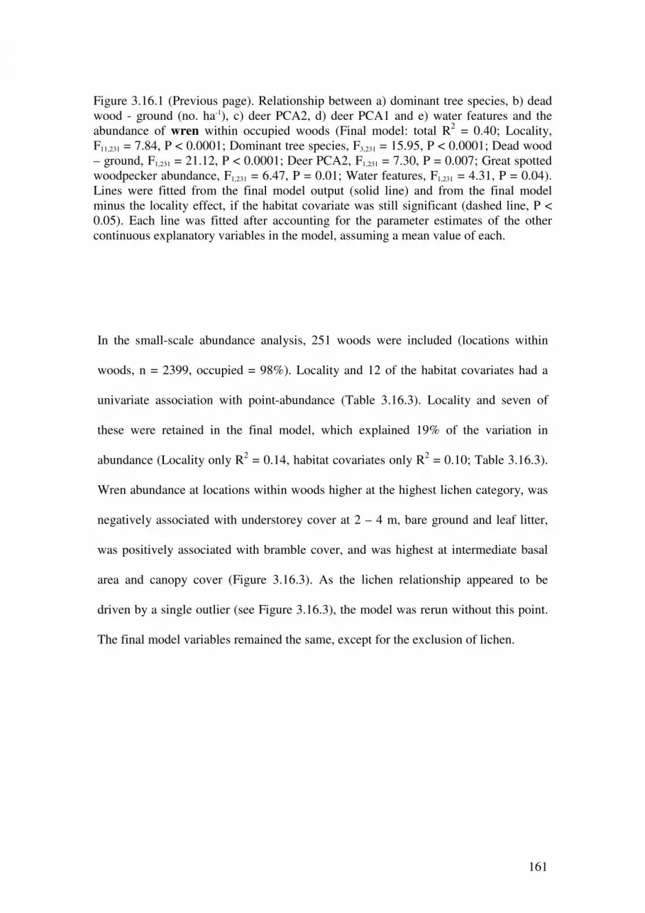
161

Figure 3.16.1 (Previous page). Relationship between a) dominant tree species, b) dead

wood - ground (no. ha-1), c) deer PCA2, d) deer PCA1 and e) water features and the

abundance of wren within occupied woods (Final model: total R2 = 0.40; Locality,

F11,231 = 7.84, P < 0.0001; Dominant tree species, F3,231 = 15.95, P < 0.0001; Dead wood

– ground, F1,231 = 21.12, P < 0.0001; Deer PCA2, F1,231 = 7.30, P = 0.007; Great spotted

woodpecker abundance, F1,231 = 6.47, P = 0.01; Water features, F1,231 = 4.31, P = 0.04).

Lines were fitted from the final model output (solid line) and from the final model

minus the locality effect, if the habitat covariate was still significant (dashed line, P <

0.05). Each line was fitted after accounting for the parameter estimates of the other



woods, n = 2399, occupied = 98%). Locality and 12 of the habitat covariates had a

univariate association with point-abundance (Table 3.16.3). Locality and seven of



2 = 0.10; Table 3.16.3).

Wren abundance at locations within woods higher at the highest lichen category, was

negatively associated with understorey cover at 2 – 4 m, bare ground and leaf litter,

was positively associated with bramble cover, and was highest at intermediate basal

area and canopy cover (Figure 3.16.3). As the lichen relationship appeared to be

driven by a single outlier (see Figure 3.16.3), the model was rerun without this point.

The final model variables remained the same, except for the exclusion of lichen.

162

a) b)

0

1

2

3

Ash Beech Birch Oak


Me

an a

bu

nd

an

ce +

/-

sta

nd

ard

err

or

0

1

2

3

4

5

0 2 4 6 8 10Dead wood - ground

Ab

un

da

nce

c) d)

0

1

2

3

4

5

0 20 40 60


Ab

un

da

nce

0

1

2

3

4

5

0 20 40 60 80 100


Ab

un

da

nce

Figure 3.16.2. Relationship between a) dominant tree species, b) dead wood - ground

(no. ha-1), c) understorey cover at 0.5 – 2 m (%) and d) field-layer grass cover (%) and

the abundance of wren within occupied woods (Final model: total R2 = 0.45; Locality,

F11,231 = 7.17, P < 0.0001; Dominant tree species, F3,231 = 10.60, P < 0.0001; Dead wood –

ground, F1,231 = 18.96, P < 0.0001; Cover at 0.5 – 2 m, F1,231 = 0.10, P = 0.75; Cover at

0.5 – 2 m2, F1,231 = 4.89, P = 0.03; Grass cover, F1,231 = 4.39, P = 0.04). Lines were fitted


effect, if the habitat covariate was still significant (dashed line, P < 0.05). Each line was

fitted after accounting for the parameter estimates of the other continuous explanatory

variables in the model, assuming a mean value of each.

163

a) b)

0

1

2

3

4

5

6

7

8

0 20 40 60 80 100

Bare ground

Ab

un

da

nce

0

1

2

3

4

5

6

7

8

0 20 40 60 80 100

Understorey cover at 2 -4 m

Ab

un

da

nce

c) d)

0

1

2

3

4

5

6

7

8

0 20 40 60 80 100


Ab

un

da

nce

0

1

2

3

4

5

6

7

0 0.25 0.5 0.75 1 1.25 1.5 1.75 2 3.25

Lichen

Me

an

ab

un

da

nce

+/-

SE

e) f)

0

1

2

3

4

5

6

7

8

0 5 10 15

Canopy cover

Abu

nd

an

ce

0

1

2

3

4

5

6

7

8

0 10 20 30 40

Basal area

Ab

un

da

nce

Figure 3.16.3 - Continues over

164

g)

0

1

2

3

4

5

6

7

8

0 20 40 60 80 100

Field-layer bramble cover

Ab

un

da

nce

Figure 3.16.3. Relationship between a) bare ground (%), b) understorey cover at 2 – 4 m

(%), c) field-layer leaf litter (%), d) lichen, e) canopy cover (%), f) basal area (m2ha-1)

and g) bramble cover (%) and wren abundance at locations within occupied woods

(Final model: total R2 = 0.19; Locality, F11,259 = 4.20, P < 0.0001; Bare ground, F1,2384 =

17.61, P < 0.0001; Cover at 2 – 4 m, F1,2344 = 11.96, P = 0.0006; Leaf litter, F1,2275 =

11.16, P = 0.0009; Lichen, F9,2342 = 2.55, P = 0.007; Canopy cover, F1,2386 = 6.96, P =

0.008; Canopy cover2, F1,2385 = 5.87, P = 0.02; Basal, F1,2325 = 1.61, P = 0.20; Basal

2,

F1,2280 = 4.77, P = 0.0291; Bramble cover, F1,2361 = 3.87, P = 0.05). Lines were fitted from

the final model output (solid line) and from the final model minus the locality effect

when the habitat covariate was still significant (dashed line, P < 0.05). Each line was

fitted after accounting for the parameter estimates of the other continuous explanatory

variables in the model, assuming a mean value of each.

3.16.3 Discussion

General predictions made, for the important habitat associations of the wren, were of a

positive association with bramble and other field layer variables, understorey cover

variables and dead wood variables.

As predicted, both dead limbs and dead ground wood were associated with wren

abundance in woodlands; the latter category was highly significant and retained in the

final model. None of the other four associations in the final model (deer PCA2,

dominant tree, water features and great spotted woodpecker abundance) were

165

predicted, and indeed the opposite relationship was predicted for water features. When

deer and predators were removed from the model, the output changed, and although

dead wood and dominant tree species remained, a negative association with grass was

included (opposite to that predicted) and a quadratic association with cover at 0.5 – 2

m was included. Only the positive section of this quadratic relationship was

significant however, and this agreed with the prediction made from the literature.

Eight variables were retained in the final model for wren abundance at locations

within woods. One of these, lichen, appeared to be being driven by one outlier. When

this outlier was removed and the model rerun, lichen dropped out. Therefore, this

variable is not discussed further. Three field layer variables were retained, although

only one of these, bramble, was a positive association as predicted, the other two, bare

ground and leaf litter, being strongly negative. One understorey variable, cover at 2 –

4 m, was retained, but this association was strongly negative, the opposite to that

predicted. Although not predicted to be important, two tree size variables were

retained; the wren was most abundant at intermediate canopy cover, and least

abundant at intermediate basal area.

Therefore, although the predicted strong association with dead wood was borne out in

our analysis, many of the other expected relationships were not found, or were the

opposite to that predicted. In our study therefore, wren habitat requirements were very

different to information gained in the literature. However, the wood abundance model

explained 40% of variation in wren abundance, and when deer and predators were

removed this rose to 45%. This suggests that the relationships we found for wren

wood abundance are important in explaining the variation in the model.

166

4 GENERAL DISCUSSION

4.1 Overview of woodland bird associations

Table 4.1 summarises the results of the analyses carried out in this report, and table

4.2 the analyses carried out in Smart et al. (2007). Final model variables are

highlighted for each species, and the direction of the effect shown. If more than one

direction was found across the different analyses, then the direction thought to be the

most important is shown. These tables are intended to show commonality across

habitat variables and groups of species.

Tables 4.3 and 4.4 summarise our findings in terms of declining and non-declining

species, to further understand which habitat relationships, if any, are particularly

important for declining species.

Each group of similar variables is discussed in turn, below, to bring together

understanding of relationships between woodland birds and environmental variables.

4.1.1 Large-scale variables

Locality was an important factor in determining the presence and abundance of

woodland birds for all species except the willow tit (Table 4.1 and 4.2). However, the

low number of woods containing this species may have masked any effect of locality.

167

Table 4.1: Summarising the results of associations of woodland birds. Species analysed in the

current report are included. Cells of variables retained in any final model (wood presence or

abundance, or small scale abundance) are highlighted grey for each species, and the overall

direction of the effect shown. See individual species results for further details. Declining

species are highlighted in bold. Species codes: BB = blackbird, BF = bullfinch, CH =

chaffinch, CT = coal tit, DU = dunnock, GC = Goldcrest, GR = green woodpecker, JY = jay,

LT = long-tailed tit, NU = nuthatch, RO = robin, SI = siskin, ST = song thrush, TR =

treecreeper, WT = willow tit, WR = Wren. Habitat variables highlighted bold: tested for a

quadratic relationship.

Species BB BF CH CT DU GC GR JY LT NU RO SI ST TR WT WR

Large-scale Locality

Weather PCA +

Field layer Bracken +

Bramble + +

Herb -

Grass + - -

Moss + +

Bare ground + -

Leaf litter + + + - -

Understorey Cover 05-2m U ∩ U + - + U

Cover 2-4m + + - -

Cover 4-10m ∩ - - - ∩

Horiz. viz - + - ∩

Tree size Can. cover ∩ ∩

Basal area U ∩ - U

Max dbh ∩ U + + U + U

Max height ∩ ∩ ∩ ∩ ∩

Deadwood Dead trees + +

Dead limbs - +

Ground wood + - + +

Landscape GIS P1 3km + +

P2 3km - -

Deer Deer PCA1 + +

Deer PCA2 +

Other habitat Dominant tree -BI BI, -O BI BE, O BI, O BE, O A, O

Lichen - - +

Ivy +

Shrub div + + + - +

Water feat + -

Altitude - U ∩ + ∩ ∩ U

Size - + +

Slope -

Tracks +

Drey density + +

GRSWO + + + + +

Jay + + +

168

Table 4.2: Summarising the results of associations of woodland birds. Species analysed in Smart

et al. (2007) are included. Cells of variables retained in any final model (wood presence or

abundance, or small scale abundance) are highlighted grey, and the overall direction of the

effect shown. See Smart et al. (2007) for further details. Declining species are highlighted in

bold. Species codes: BC = blackcap, BT = blue tit, CC = chiffchaff, GS = great spotted

woodpecker, GT = great tit, GW = garden warbler, HF = hawfinch, LR = lesser redpoll, LS =

lesser spotted woodpecker, MT = marsh tit, PF = pied flycatcher, RD = redstart, SF = spotted

flycatcher, TP = tree pipit, WI = willow warbler, WO = wood warbler. Habitat variables

highlighted bold: tested for a quadratic relationship.

Species BC BT CC GS GT GW HF LR LS MT PF RD SF TP WI WO

Large-scale Locality

Weather PCA

Field layer Bracken + + +

Bramble + + + - - -

Herb + + - - - -

Grass + +

Moss - + + + +

Bare ground + -

Leaf litter - - - -

Understorey Cover 05-2m ∩ ∩ - ∩

Cover 2-4m + + ∩ -

Cover 4-10m - ∩ - ∩

Horiz. viz - - + + U - + + ∩ - +

Tree size Can. cover U ∩ + ∩ - ∩

Basal area - - ∩ - + + +

Max dbh + + ∩ +

Max height + + ∩ U - ∩ -

Deadwood Dead trees + + + + + -

Dead limbs + + - - +

Ground wood +

Landscape GIS P1 3km + + - -

P2 3km + - - -

Deer Deer PCA1 na na na + na na na na na na na na na na

Deer PCA2 na na na na na na na na na na na na na Other habitat Dominant tree A,O O A O BI O O,BI -BE O

Lichen - + + + +

Ivy -

Shrub div + + + - +

Water feat -

Altitude - - ∩ - ∩ - - ∩

Size +

Slope - - - +

Tracks -

169

Geographical location appears to be an important consideration when managing

woodlands for bird species, and this was also noted by Amar et al. (2006). Different

species will be better suited to different geographical locations. Conversely, the

weather PCA was not retained in any final models, except for the green woodpecker

(Table 4.1 and 4.2).

4.1.2 Field-layer variables

Across all 32 bird species studied, there were 25 positive associations with field-layer

variables, and 19 negative associations retained in final models (Table 4.3). Most field

layer associations were seen in non-declining species (29 compared to 15; Table 4.3),

but whereas for the non-declining species more associations were positive,

associations were equally positive or negative for the declining species (Table 4.3).

Table 4.3: The number of associations, across all woodland bird species classed by

population status, with habitat, deer and predator variables. Those variables retained

in any final model (wood presence and abundance and small-scale abundance) for

each species are included. Quadratic effects were only tested for in understorey and

tree size categories. Several other variables, which could not be classed into a group,

have been omitted from this table, but are included elsewhere. * = Variables only

included in the current report, not in Smart et al. (2007). ** = Variables only included

in the current report, and for the tit species in Smart et al. (2007).

Declining species Stable or increasing species

+ - ∩ U + - ∩ U

Field-layer 7 8 18 11

Understorey 5 7 7 2 7 9 4 2

Tree size 5 3 8 4 7 4 8 3

Deadwood 6 4 9 1

Landscape 3 4 4 1

Deer** 1 0 3 0

Predators* 3 0 7 0

170

Looking in more detail, the most common variables to be associated with bird species

were leaf litter, bramble and moss (Table 4.4). Most bird species which had a retained

association with leaf litter, whether declining or not, showed a negative relationship

(Table 4.4). Only one third of associations were positive. The associations with

bramble were more complex. Four out of five associations with non-decliners were

positive, whereas one out of three associations with decliners was positive (Table 4.4).

It seems that when associations exist, they can be either positive or negative, and

hence any woodland management would depend on the species being targeted. Six out

of the seven associations with moss were positive, and no declining species showed a

negative association with moss (Table 4.4). This suggests that moss cover is an

important resource for a number of woodland bird species. Of the other habitat

variables, no positive associations were detected with herb cover for the declining

species, while three negative associations were detected, and no associations were

detected in either direction for grass cover (Table 4.4).

4.1.3 Understorey variables

Across all bird species, 43 associations with understorey variables were retained in

final models (Table 4.3). Twenty-one of these were with declining species, and 22

with non-decliners (Table 4.3). There was a mixture of relationship directions, but

only four of these were quadratic with lowest presence/abundance at intermediate

levels (Table 4.3).

171

Table 4.4: The number of associations, across all woodland bird species classed by

population status, with individual habitat, deer and predator variables. Those variables

retained in any final model (wood presence and abundance and small-scale

abundance) for each species are included. Quadratic effects were only tested for in

understorey and tree size categories, and altitude (highlighted bold). * = Variables

only included in the current report, not in Smart et al. (2007). ** = Variables only

included in the current report, and for the tit species in Smart et al. (2007).

Declining species Stable or increasing species

+ - ∩ U + - ∩ U

Field-layer Bracken 2 0 2 0

Bramble 1 2 4 1

Herb 0 3 2 2

Grass 0 0 3 2

Moss 3 0 3 1

Bare ground 0 1 2 1

Leaf litter 1 2 2 4

Understorey Cover 0.5-2m 1 1 2 1 1 1 2 2

Cover 2-4m 2 2 1 0 2 1 0 0

Cover 4-10m 0 1 2 0 0 4 2 0

Horizontal viz 2 3 2 1 4 3 0 0

Tree size Canopy cover 1 1 3 1 0 0 2 0

Basal area 2 1 0 1 1 3 2 1

Max dbh 2 0 1 2 4 0 1 1

Max height 0 1 4 0 2 1 3 1

Deadwood Dead trees 2 1 5 0

Dead limbs 2 3 2 0

Ground wood 2 0 2 1

Landscape P1 3km 2 1 2 1

P2 3km 0 4 1 1

Deer Deer PCA1** 1 0 2 0

Deer PCA2** 0 0 1 0

Other Lichen 1 2 4 1

Ivy 0 1 1 0

Shrub diversity 5 1 3 1

Water features 0 1 1 1

Altitude 0 3 2 1 1 3 4 1

Size 0 1 3 0

Slope 1 1 0 3

Tracks 0 1 1 0

Predators Drey density* 0 0 2 0

G S woodpecker* 1 0 4 0

Jay* 2 0 1 0

172

Looking in more detail, the picture is equally as unclear. There was no clear

consensus across declining or non-declining species as to which direction of effect is

more or less important than another. This suggests that, as might be expected, across

the spectrum of woodland bird species some are understorey specialists while others

are not, and in fact are negatively associated with understorey. However, the fact that

there were non-declining, as well as declining, species positively associated with

understorey cover variables makes loss of woodland understorey as a possible

contributing factor to some species’ decline, as has been suggested (e.g. Fuller et al.,

2005), more difficult to understand. It could be that the declining species are affected

by another factor not measured, such as competition, and this along with understorey

decline has made these species tip into decline.

4.1.4 Tree size variables

Forty-two associations with tree size variables were retained in final models (Table

4.3). Twenty of these were with declining species, and 22 were with non-decliners

(Table 4.3). There appear to be more positive and quadratic (highest

presence/abundance at intermediate levels) associations than negative or the opposite

quadratic associations (28 compared to 14; Table 4.3), and this split could be seen in

both the declining and non-declining species (Table 4.3).

Intermediate levels of canopy cover was important both for declining and non-

declining species. Five out of the eight associations retained in final models were in

this direction (Table 4.4). There was no clear pattern for basal area (Table 4.4). For

maximum diameter at breast height, however, most associations were positive, and no

173

negative associations were retained across declining and non-declining species (Table

4.4). Diameter at breast height is a measure of tree age, and hence this suggests that

several woodland bird species prefer mature woodlands. Most retained associations

with maximum tree height were quadratic (highest presence/abundance at

intermediate levels), and this was particularly so for declining species, with four out

of five associations in this direction (Table 4.4). Overall, therefore, there is a general

trend for woodland birds to prefer woodlands containing mature trees, of intermediate

height and canopy cover.

4.1.5 Deadwood

Twenty associations with deadwood were retained in final models, ten of which were

with declining, and ten with non-declining, species (Table 4.3). Fifteen out of the 20

associations were positive, with only five negative (Table 4.3), suggesting that for

many woodland bird species deadwood is an important resource.

Although most retained associations were positive, for declining species the situation

was less clear. Only six out of the ten retained associations were positive, and for dead

limbs, more relationships were negative than positive (Table 4.4). Therefore, although

overall, woodland birds appear to be positively correlated with deadwood, certain

declining species may, in fact, need early successional, scrub habitat where deadwood

is absent due to the nature of the woodland. This would not be a reason to remove

deadwood, but rather to create a heterogeneous structure encompassing areas of old

growth and early successional habitats.

174

4.1.6 Landscape

Most retained associations with landscape PCA1 were positive, both for declining and

non-declining species (Table 4.4). However, relationships were retained for only six

species. Landscape PCA1 is a gradient from woods set in an agricultural landscape to

those set in a non-agricultural landscape. Therefore, although most woodland birds

did not have this variable retained, of those that did, most preferred woodlands set in a

non-agricultural landscape.

Four of the six retained associations with landscape PCA2 were for declining species

(Table 4.4). All of these were negative associations, and so there appears to be a

preference, by some declining species, for woods to be set in a wooded landscape.

However, the situation is less clear for non-decliners. Only two species had

associations with the variables, and of these, one was positive and one was negative

(Table 4.4).

4.1.7 Deer

It is important to note that the deer PCAs were a measure of the impact of the deer on

the vegetation, which has then been correlated with bird presence and abundance.

Therefore, we have not directly measured the association between deer numbers and

birds, but rather the impact of deer on vegetation.

Only four associations with deer PCAs were retained, but all of these were positive

(Table 4.3). However, only bird species included in the current study, plus the tit

species from Smart et al. (2007) had deer variables included in the analysis. Only one

175

declining species, the goldcrest, retained a positive association with deer. This species

showed few associations with understorey cover, and several negative associations

with field-layer variables, and hence the positive association with deer is consistent

with this species not being associated with field or understorey variables.

Deer variables were included in the analysis, as deer have been implicated in the

decline of woodland birds (Perrins and Overall, 2001; Perrins, 2003). However, very

few negative relationships with deer were recorded in this study, and none were

retained; whereas several species showed positive associations with deer signs.

However, Amar et al. (2006) state that the measures used may not give a good

reflection of deer activity and impact. Therefore, these results, and the lack of

negative associations, should perhaps be viewed with caution.

4.1.8 Predators

Predators have only been included in the current report, and not Smart et al. (2007).

Ten associations were retained, all of which were positive (Table 4.3 and 4.4). Two

avian predators, plus the grey squirrel, were included in the analysis, as predation has

been suggested as a possible cause of woodland bird decline (Fuller et al., 2005). It

might have been expected that negative associations would exist between some bird

species and predators, but in fact, virtually all associations recorded were positive.

Negative associations were obtained for the chaffinch and bullfinch and drey density,

although these were not retained in final models. However, these species, and

particularly the chaffinch, are perhaps among the most likely to be affected by

predation by grey squirrels, due to their nest locations.

176

However, a more meaningful analysis would be to look at population change with

respect to predator numbers; simply looking at associations across sites may not

detect a relationship, or indeed may detect a positive association, as their habitat needs

may covary.

4.1.9 Other variables

Some variables included in the analysis could not be formed into groups of similar

variables, and hence were kept separate. Dominant tree species, altitude, shrub

diversity and lichen were retained in final models for several species (Table 4.1, 4.2

and 4.4), and these results are discussed further below.

Dominant tree species was retained in the final model for half (16) of the species

studied (Table 4.1 and 4.2). Overall, the commonest relationship appeared to be a

preference for oak dominated woodlands, although birch dominated woodlands were

also often associated.

Altitude was retained in 15 final models. Twelve of these associations were either

negative or quadratic (highest presence/abundance at intermediate altitude), and this

preference was seen by declining and non-declining species. Relationships with

altitude were rarely predicted from the species-specific literature review, yet almost

half of the species studied showed a strong preference for a particular altitude. This is

perhaps an overlooked factor when considering the needs of woodland birds.

177

Shrub diversity was retained in final models for 10 species; six of these species were

declining, and four were not (Table 4.4). In all but two cases (one declining, one non-

decliner), the association was positive. This suggests that shrub diversity in woodland

is important for a range of bird species, and would be an important consideration for

woodland management.

Lichen was retained in final models for eight species. For four out the five non-

declining species associated with lichen, the relationship was positive. However, for

two out of the three declining species, the relationship was positive. Overall, there

was no clear pattern.

4.2 Conclusion

As was to be expected with a study of this magnitude, including 252 woodlands and

numerous habitat variables, many relationships have been detected. Also perhaps as

expected, most of these associations were to be found with tree size and understorey

variables. However, whereas there appears to be a general preference for woods with

mature trees of intermediate height and canopy cover, it was difficult to detect any

overall trend for understorey variables. Our results suggest that individual species

vary with respect to their need, or lack of it, for understorey. This suggests that to

manage woodlands for the maximum number of species, woodlands need to be

heterogeneous in their understorey. Eight out of ten species showed a preference for

high shrub diversity, suggesting that where understorey is present, it needs to be of

high species diversity.

178

The work can be developed and improved in several ways:

• Habitat associations of woodland birds using data from the 1980s will provide

a complete picture of habitat associations then, and habitat associations now.

Although understanding current associations was of highest priority,

understanding the situation in the 1980s is an important next step.

• Associations with deer and predators were only completed in the current work,

and not in Smart et al (2007). Completion of these tests for all species is a

natural next step.

• A limitation of including predators in the habitat associations work is that

habitat requirements for predators and prey may covary, giving rise to positive

associations. Therefore, using data on population change with predator

presence may provide a better test, and is recommended.

Correlations with habitat associations and other environmental variables have been

obtained for 32 species of woodland bird, and for all but four of the woodland bird

indicator species. Although the RWBS woods are a biased sample of woodlands, and

tend to be old, mature, large woodlands, the importance of the analysis should not be

underestimated. Some caution is also required so as not to over interpret the results

obtained; as was stated at the outset of this report, this study is intended only as a first

step in understanding habitat requirements of woodland birds. Due to its correlative

nature, and the possibility of bias in the study woodlands, we recommend that the

results of both habitat associations’ reports be used as a foundation on which to begin

manipulative work. Nonetheless, this work was an important first step in further

understanding the needs of our woodland birds.

179

References

Amar, A., Hewson, C.M., Thewlis, R.M., Smith, K.W., Fuller, R.J., Lindsell, J.,

Conway, G., Butler, S. and MacDonald, M.A. 2006. What’s happening to our

woodland birds? Long-term changes in the population of woodland birds.

RSPB research report no. 19; BTO research report no. 169.

Bellamy, P.E., Rothery, P., Hinsley, S.A. and Newton, I. 2000. Variation in the

relationship between numbers of breeding pairs and woodland area for

passerines in fragmented habitat. Ecography, 23, 130-138.

Bishton, G. 2001. Social structure, habitat use and breeding biology of hedgerow

Dunnocks Prunella modularis. Bird Study, 48, 188-193.

Chamberlain, D.E., Gosler, A.G. and Glue, D.E. 2007. Effects of winter beechmast

crop on bird occurrence in British gardens. Bird Study, 54, 120-126.

Cramp, S. 1985. Handbook of the birds of Europe, the Middle East and North Africa:

The birds of the Western Palaearctic Vol. 4. Oxford University Press, Oxford.

Cramp, S. 1988. Handbook of the birds of Europe, the Middle East and North Africa:

The birds of the Western Palaearctic Vol. 5. Oxford University Press, Oxford.

Cramp, S. and Brooks, D.C. 1992. Handbook of the birds of Europe, the Middle East

and North Africa: The birds of the Western Palaearctic Vol. 6. Oxford

University Press, Oxford.

Cramp, S. and Perrins, C.M. 1993. Handbook of the birds of Europe, the Middle East



Cramp, S. and Perrins, C.M. 1994. Handbook of the birds of Europe, the Middle East



Creegan, H.P. and Osborne, P.E. 2005. Gap-crossing decisions of woodland songbirds

in Scotland: an experimental approach. Journal of Applied Ecology, 42, 678-

687.

DEFRA. 2006. Wild Bird Populations 2006: Sustainable Development Strategy and

Public Service Agreement Indicators. DEFRA, UK.

Eaton, M.A., Ausden, M., Burton, N., Grice, P.V., Hearn, R.D., Hewson, C.M.,

Hilton, G.M., Noble, D.G., Ratcliffe, N. and Rehfisch, M.M. 2006. The state

of the UK’s birds 2005. RSPB, BTO, WWT, CCW, EN, EHS and SNH.

Sandy, Bedfordshire.

180

Enoksson, B. and Nilsson, S. G. 1983. Territory size and population density in

relation to food supply in the nuthatch Sitta europaea (Aves). Journal of

Animal Ecology, 52, 927-935.

Fuller, R.J. and Henderson, A.C.B. 1992. Distribution of breeding songbirds in

Bradfield Woods, Suffolk, in relation to vegetation and coppice management.

Bird Study, 39, 73-88.

Fuller, R.J., Chamberlain, D.E., Burton, N.H.K. and Gough, S.J. 2001. Distributions

of birds in lowland agricultural landscapes of England and Wales: How

distinctive are bird communities of hedgerows and woodland? Agriculture,

Ecosystems and Environment, 84, 79-92.

Fuller, R.J., Noble, D.G., Smith, K.W. and Vanhinsbergh, D. 2005. Recent declines in

populations of woodland birds in Britain: a review of possible causes. British

Birds, 98, 116-143.

Gibbons, D.W., Reid, J.B. and Chapman, R.A. 1993. The New Atlas of Breeding Birds

in Britain and Ireland: 1998-1991. T & A D Poyser.

Glue, D. E. and Boswell, T. 1994. Comparative nesting of the three British breeding

woodpeckers. British Birds, 87, 253-269.

Gregory, R.D., Wilkinson, N.I., Noble, D.G., Robinson, J.A., Brown A.F.,

Hughes, J., Procter, DA., Gibbons, D.W. and Galbraith, C.A. 2002. The

population status of birds in the United Kingdom, Channel Islands and Isle of

Man: an analysis of conservation concern 2002-2007. British Birds, 95, 410-

450.

Hall, S., Inglese, S. and Tinsley, J. 2007. Sustainable Development Indicators in your

pocket 2007; An update of the UK Government Strategy Indicators. DEFRA,

UK.

Hinsley, S.A., Bellamy, P.E., Newton, I. and Sparks, T.H. 1995. Habitat and

landscape factors influencing the presence of individual breeding bird species

in woodland fragments. Journal of Avian Biology, 26, 94-104.

Jantti, A., Hakkarainen, H., Kuitunen, M. and Suhonen, J. 2007. The importance of

landscape structure for nest defence in the Eurasian Treecreeper Certhia

familiaris. Ornis fennica, 84, 145-154.

Jansson, G., Saari, L. 1999. Suitable habitat distribution for the Long-tailed Tit

(Aegithalos caudatus) as indicated by the frequency of occurrence - a long-

term study. Ornis Fennica, 76, 115-122.

Kelleher, K. M. and O'Halloran, J. 2007. Influence of nesting habitat on breeding

Song Thrushes Turdus philomelos. Bird Study, 54, 221-229.

181

Lewis, A. J. G., Amar, A., Cordi-Piec, D. and Thewlis, R. M. 2007. Factors

influencing Willow Tit Poecile montanus site occupancy: a comparison of

abandoned and occupied woods. Ibis, 149, 205-213.

Mason, C.F. 2001. Woodland area, species turnover and the conservation of bird

assemblages in lowland England. Biodiversity and Conservation, 10, 495-510.

Nour N, van Damme R, Matthysen E, Dhondt AA. 1999. Forest birds in forest

fragments: are fragmentation effects independent of season? Bird Study, 46,

279-288.

Peach, W.J., Robinson, R.A. and Murray K.A. 2004. Demographic and environmental

causes of the decline of rural Song Thrushes Turdus philomelos in lowland

Britain. Ibis, 146, 50-59.

Perrins, C.M. 2003. The status of Marsh and Willow Tits in the UK. British Birds, 96,

418-426.

Perrins, C.M. and Overall, R. 2001. Effect of increasing numbers of deer on bird

populations in Wytham Woods, central England. Forestry, 74, 299-309.

Proffitt, F.M., Newton, I., Wilson, J.D., Siriwardena, G.M. 2004. Bullfinch Pyrrhula

pyrrhula breeding ecology in lowland farmland and woodland: comparisons

across time and habitat. Ibis 146, 78-86.

Rolstad, J., Loken, B. and Rolstad, E. 2000. Habitat selection as a hierarchical spatial

process: the green woodpecker at the northern edge of its distribution range.

Oecologia, 124, 116-129.

Sehhatisabet, M. E., Kiabi, B., Pazuki, A., Alipanah, H., Khaleghizadeh, A., Barari,

H., Basiri, R. and Aghabeigi, F. 2008. Food diversity and niche-overlap of

sympatric tits (Great Tit, Parus major, Blue Tit, Cyanistes caeruleus and Coal

Tit Periparus ater) in the Hyrcanian Plain Forests. Zoology in the Middle East,

44, 17-30.

Siriwardena, G.M., Crick, H.Q.P, Baillie, S.R. and Wilson, J.D. 2000. Agricultural

habitat-type and the breeding performance of granivorous farmland birds in

Britain. Bird Study, 47, 66-81.

Smart, J., Taylor, E., Amar, A., Smith, K., Bierman, S., Carpenter, J., Grice, P.,

Currie, F. and Hewson, C. 2007. Habitat associations of woodland birds:

Implications for woodland management for declining species. RSPB Research

Report No. 26.

Smith, K.W. 2007. The utilization of dead wood resources by woodpeckers in Britain.

Ibis, 149, 183-192.

Suorsa, P., Huhta, E., Jantti, A., Nikula, A., Helle, H., Kuitunen, M., Koivunen, V.

and Hakkarainen, H. 2005. Thresholds in selection of breeding habitat by the

182

Eurasian treecreeper (Certhia familiaris). Biological Conservation, 121, 443-

452.

Tuomenpuro, J. 1991. Effect of nest site on nest site survival in the dunnock Prunella

modularis. Ornis Fennica, 68, 49-56.

Whittingham, M.J., Bradbury, R.B., Wilson, J.D., Morris, A.J., Perkins, A.J. and

Siriwardena G.M. 2001. Chaffinch Fringilla coelebs foraging patterns, nestling

survival and territory distribution on lowland farmland. Bird Study, 48, 257-

270

Habitat associations of woodland birds II

Documents

Transcript of Habitat associations of woodland birds II