A Generic Approach toQuantitative Verification

Habilitation à diriger des recherches de l'Université Paris-Saclay

présentée et soutenue à Saclay,le 10 mai 2022, par

Uli FAHRENBERG

Composition du jury

Christel BAIERProfesseur, Technische Universität Dresden, Allemagne

Rapportrice

Paul-André MELLIÈSDirecteur de recherche, CNRS & Université Paris Denis Diderot

Rapporteur

Rob VAN GLABBEEKConjoint Professor, The University of New South Wales, Australia

Rapporteur

Nathalie BERTRANDDirectrice de recherche, Inria Rennes - Bretagne Atlantique

Examinatrice

Patricia BOUYER-DECITREDirectrice de recherche, CNRS & ENS Paris-Saclay

Examinatrice

Georg STRUTHProfesseur, The University of Sheffield, UK

Examinateur

Hab

ilit

ati

on

à d

irig

er

des

rech

erc

hes

arX

iv:2

204.

1130

2v1

[cs

.LO

] 2

4 A

pr 2

022

Titre : Une approche générique à la vérification quantitative

Mots clés : vérification quantitative, compositionnalité, incrémentalité, robustesse

Résumé : Ce mémoire porte sur la vérifica-tion quantitative, c’est-à-dire la vérification despropriétés quantitatives des systèmes quantitatifs.Ces systèmes se retrouvent dans de nombreusesapplications, et leur vérification quantitative estimportante, mais aussi assez complexe. En par-ticulier, étant donné que la plupart des systèmestrouvés dans les applications sont plutôt larges, ilest alors essentiel que les méthodes soient compo-sitionnelles et incrémentielles.Afin d’assurer la robustesse de la vérification,nous remplaçons les réponses booléennes de lavérification standard par des distances. Selon lecontexte de l’application, de nombreux types dedistances différentes sont utilisées dans la vérifi-cation quantitative. Par conséquent, il est néces-saire d’avoir une théorie générale des distances desystèmes qui puisse s’abstraire des distances con-crètes, et de développer une vérification quanti-tative qui est indépendante de la distance. Noussommes de l’avis que dans une théorie de la véri-fication quantitative, les aspects quantitatifs de-vraient être traités, tout autant que les aspects

qualitatifs, comme des éléments d’entrée d’unproblème de vérification.Dans ce travail, nous développons de la sorte unethéorie générale de la vérification quantitative.Nous supposons comme entrée une distance en-tre traces, ou exécutions, puis utilisons la théoriedes jeux à objectifs quantitatifs pour définir desdistances entre systèmes quantitatifs. Différentesversions du jeu de bisimulation ( quantitatif ) don-nent lieu à différents types de distances : distancede bisimulation, distance de simulation, distanced’équivalence de trace, etc., permettant de con-struire une généralisation quantitative du spec-tre temps linéaire–temps de branchement de vanGlabbeek.Nous étendons notre théorie générale de la véri-fication quantitative à une théorie des spécifica-tions quantitatives. Pour cela nous utilisons dessystèmes de transitions modaux, et nous dévelop-pons les propriétés quantitatives des opérateursusuels pour les théories de spécifications. Toutcela est indépendant de la distance concrète entreles traces utilisée.

Title: A Generic Approach to Quantitative Verification

Keywords: quantitative verification, compositionality, incrementality, robustness

Abstract: This thesis is concerned with quan-titative verification, that is, the verification ofquantitative properties of quantitative systems.These systems are found in numerous applica-tions, and their quantitative verification is impor-tant, but also rather challenging. In particular,given that most systems found in applications arerather big, compositionality and incrementality ofverification methods are essential.In order to ensure robustness of verification, wereplace the Boolean yes-no answers of standardverification with distances. Depending on theapplication context, many different types of dis-tances are being employed in quantitative verifi-cation. Consequently, there is a need for a generaltheory of system distances which abstracts awayfrom the concrete distances and develops quan-titative verification at a level independent of thedistance. It is our view that in a theory of quanti-tative verification, the quantitative aspects shouldbe treated just as much as input to a verification

problem as the qualitative aspects are.In this work we develop such a general theoryof quantitative verification. We assume as in-put a distance between traces, or executions, andthen employ the theory of games with quantita-tive objectives to define distances between quan-titative systems. Different versions of the quan-titative bisimulation game give rise to differenttypes of distances, viz. bisimulation distance, sim-ulation distance, trace equivalence distance, etc.,enabling us to construct a quantitative general-ization of van Glabbeek’s linear-time–branching-time spectrum.We also extend our general theory of quantitativeverification to a theory of quantitative specifica-tions. For this we use modal transition systems,and we develop the quantitative properties of theusual operators for behavioral specification theo-ries. All this is independent of the concrete dis-tance between traces which is utilized.

Contents

1 Introduction 11.1 Motivation . . . . . . . . . . . . . . . . . . . . . . . . . . . . . 11.2 Contributions . . . . . . . . . . . . . . . . . . . . . . . . . . . . 81.3 Applications . . . . . . . . . . . . . . . . . . . . . . . . . . . . . 251.4 Conclusion and Perspectives . . . . . . . . . . . . . . . . . . . . 281.5 About the Author . . . . . . . . . . . . . . . . . . . . . . . . . 311.6 Acknowledgments . . . . . . . . . . . . . . . . . . . . . . . . . . 41

2 Quantitative Analysis of Weighted Transition Systems 432.1 Weighted transition systems . . . . . . . . . . . . . . . . . . . . 432.2 Quantitative Analysis . . . . . . . . . . . . . . . . . . . . . . . 442.3 Properties of distances . . . . . . . . . . . . . . . . . . . . . . . 512.4 Conclusion . . . . . . . . . . . . . . . . . . . . . . . . . . . . . 53

3 A Quantitative Characterization of Weighted KripkeStructures in Temporal Logic 553.1 Preliminaries . . . . . . . . . . . . . . . . . . . . . . . . . . . . 553.2 Weighted CTL . . . . . . . . . . . . . . . . . . . . . . . . . . . 563.3 Bisimulation . . . . . . . . . . . . . . . . . . . . . . . . . . . . . 593.4 Characterization . . . . . . . . . . . . . . . . . . . . . . . . . . 613.5 Conclusion . . . . . . . . . . . . . . . . . . . . . . . . . . . . . 64

4 Metrics for Weighted Transition Systems: Axiomatization 654.1 Simulation distances . . . . . . . . . . . . . . . . . . . . . . . . 654.2 Axiomatizations for Finite Weighted Processes . . . . . . . . . 684.3 Axiomatizations for Regular Weighted Processes . . . . . . . . 72

5 The Quantitative Linear-Time–Branching-Time Spectrum 775.1 Traces, Trace Distances, and Transition Systems . . . . . . . . 775.2 Examples of Trace Distances . . . . . . . . . . . . . . . . . . . 785.3 Quantitative Ehrenfeucht-Fraïssé Games . . . . . . . . . . . . . 795.4 General Properties . . . . . . . . . . . . . . . . . . . . . . . . . 825.5 The Distance Spectrum . . . . . . . . . . . . . . . . . . . . . . 855.6 Recursive Characterizations . . . . . . . . . . . . . . . . . . . . 90

i

Contents

5.7 Recursive Characterizations for Example Distances . . . . . . . 97

6 Weighted Modal Transition Systems 1016.1 Weighted Modal Transition Systems . . . . . . . . . . . . . . . 1016.2 Thorough and Modal Refinement Distances . . . . . . . . . . . 1036.3 Relaxation . . . . . . . . . . . . . . . . . . . . . . . . . . . . . . 1116.4 Limitations of the Quantitative Approach . . . . . . . . . . . . 1136.5 Structural Composition and Quotient . . . . . . . . . . . . . . 1166.6 Conclusion . . . . . . . . . . . . . . . . . . . . . . . . . . . . . 121

7 General Quantitative Specification Theories with ModalTransition Systems 1237.1 Structured Modal Transition Systems . . . . . . . . . . . . . . 1237.2 Refinement Distances . . . . . . . . . . . . . . . . . . . . . . . 1297.3 Structural Composition and Quotient . . . . . . . . . . . . . . 1357.4 Conjunction . . . . . . . . . . . . . . . . . . . . . . . . . . . . . 1437.5 Logical Characterizations . . . . . . . . . . . . . . . . . . . . . 148

8 Logical vs. Behavioral Specifications 1518.1 Specification Formalisms . . . . . . . . . . . . . . . . . . . . . . 1518.2 Structural Equivalence . . . . . . . . . . . . . . . . . . . . . . . 1578.3 Specification Theory . . . . . . . . . . . . . . . . . . . . . . . . 1678.4 Related Work . . . . . . . . . . . . . . . . . . . . . . . . . . . . 1838.5 Conclusion . . . . . . . . . . . . . . . . . . . . . . . . . . . . . 184

9 Compositionality for Quantitative Specifications 1879.1 Structured Labels . . . . . . . . . . . . . . . . . . . . . . . . . . 1879.2 Specification Formalisms . . . . . . . . . . . . . . . . . . . . . . 1899.3 Specification theory . . . . . . . . . . . . . . . . . . . . . . . . 1949.4 Robust Specification Theories . . . . . . . . . . . . . . . . . . . 2009.5 Conclusion . . . . . . . . . . . . . . . . . . . . . . . . . . . . . 216

10 References 219

ii

1 Introduction

This thesis is concerned with quantitative verification, that is, the verificationof quantitative properties of quantitative systems. These systems are foundin numerous applications, and their quantitative verification is important, butalso rather challenging. In particular, given that most systems found in appli-cations are rather big, compositionality and incrementality are essential. Thatis, quantitative verification should be applied as much as possible to subsys-tems and at as high a level as possible, and then verified partial specificationsshould be composed and refined into an implementation.

Much work has been done in the area of compositional and incrementaldesign, but robust quantitative frameworks are lacking. This thesis presentswork published between 2009 and 2020 by the author and various co-authorswhich attempts to introduce such a framework. Much remains to be done,in particular in applications to real-time and hybrid systems, but we believethat the foundations laid out here will be useful in this endeavor.

1.1 Motivation

1.1.1 Quantitative Verification

Motivated by applications in real-time systems, hybrid systems, embeddedsystems, and other areas, formal verification has seen a trend towards modelingand analyzing systems which contain quantitative information. Quantitativeinformation can thus be a variety of things: probabilities, time, tank pressure,energy intake, etc.

A number of quantitative models have been developed: probabilistic au-tomata [SL94]; stochastic process algebras [Hil96]; timed automata [AD94];hybrid automata [ACH+95]; timed variants of Petri nets [MF76,Han93]; con-tinuous-time Markov chains [Ste94]; etc. Similarly, there is a number of spec-ification formalisms for expressing quantitative properties: timed computa-tion tree logic [HNSY94]; probabilistic computation tree logic [HJ94]; metrictemporal logic [Koy90]; stochastic continuous logic [ASSB00]; etc. Quanti-tative model checking, the verification of quantitative properties for quanti-tative systems, has also seen rapid development: for probabilistic systems inPRISM [KNP02] and PEPA [GH94]; for real-time systems in Uppaal [LPY97],

1

1. Introduction

x := 0 close

x ≥ 60 train

A

x := 0 close

x ≥ 58 train

B

x := 0 close

x ≥ 1 train

C

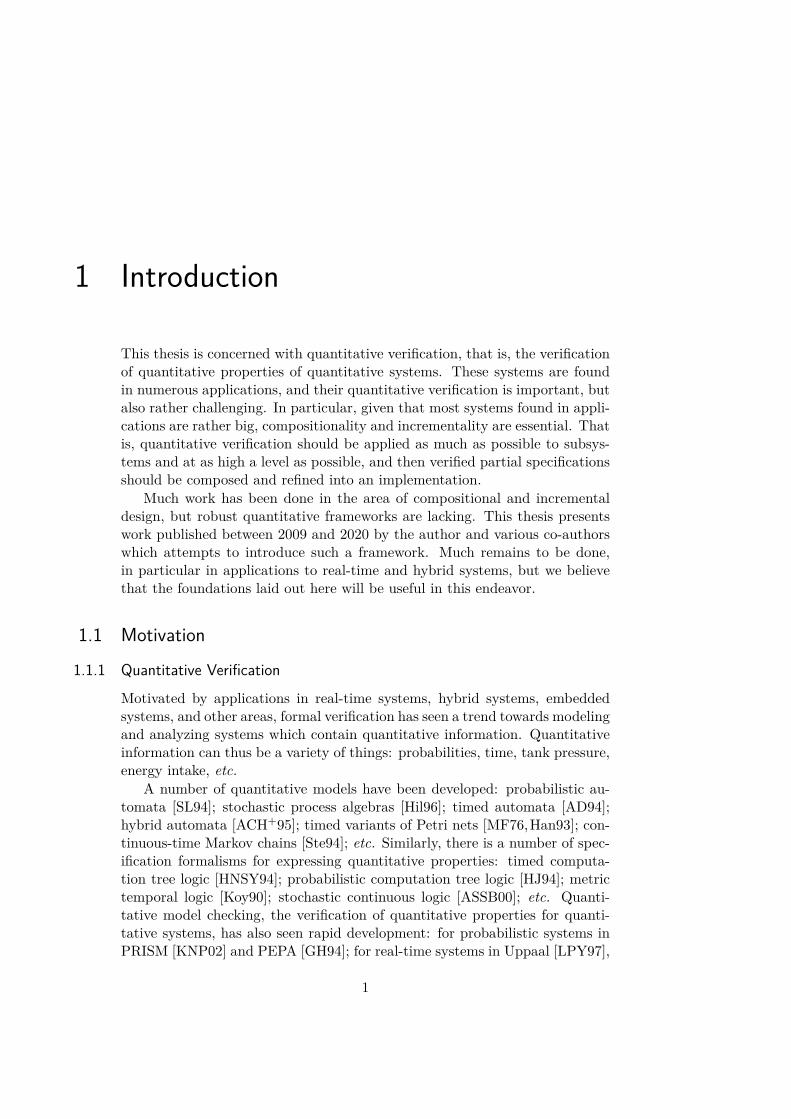
Figure 1.1: Three timed automata modeling a train crossing.

RED [WME93], TAPAAL [BJS09] and Romeo [GLMR05]; and for hybrid sys-tems in HyTech [HHWT97], SpaceEx [FGD+11] and HySAT [FH07], to namebut a few.

Quantitative model checking has, however, a problem of robustness. Whenthe answers to model checking problems are Boolean—either a system meetsits specification or it does not—then small perturbations in the system’s pa-rameters may invalidate the result. This means that, from a model checkingpoint of view, small, perhaps unimportant, deviations in quantities are indis-tinguishable from larger ones which may be critical.

As an example, Figure 1.1 shows three simple timed-automaton models ofa train crossing, each modeling that once the gates are closed, some time willpass before the train arrives. Now assume that the specification of the systemis

The gates have to be closed 60 seconds before the train arrives.

Model A does guarantee this property, hence satisfies the specification. ModelB only guarantees that the gates are closed 58 seconds before the train arrives,and in model C, only one second may pass between the gates closing and thetrain.

Neither model B or C satisfy the specification, so this is the result whicha model checker like for example Uppaal would output. What this does nottell us, however, is that model C is dangerously far away from the specifica-tion, whereas model B only violates it slightly and may be acceptable givenother engineering constraints, or may be more easily amenable to satisfy thespecification than model C.

In order to address the robustness problem, our approach is to replacethe Boolean yes-no answers of standard verification with distances. That is,the Boolean co-domain of model checking is replaced by the non-negative realnumbers. In this setting, the Boolean true corresponds to a distance of zero,and false corresponds to any non-zero number, so that quantitative model

2

1.1. Motivation

checking can now tell us not only that a specification is violated, but alsohow much it is violated, or how far the system is from corresponding to itsspecification.

In the example of Figure 1.1 and for a simple definition of system distances,the distance from A to our specification would be 0, whereas the distancesfrom B and C to the specification would be 2 and 59, respectively. Theprecise interpretation of distance values will be application-dependent; but inany case, it is clear that C is much farther away from the specification thanB is.

1.1.2 Specification Theories

One of the major current challenges to rigorous design of software systemsis that these systems are becoming increasingly complex and difficult to rea-son about [Sif11]. As an example, an integrated communication system ina modern airplane can have more than 10900 distinct states [BBB+10], andstate-of-the-art tools offer no possibility to reason about, and model check,the system as a whole. One promising approach to overcome such problems isthe one of compositional and incremental design. Here the reasoning is doneas much as possible at higher specification levels rather than with implementa-tions; partial specifications are proven correct and then composed and refineduntil one arrives at an implementation model. Practical experience indicatesthat this is a viable approach [Str,SPE].

Specifications of system requirements are high-level finite abstractions ofpossibly infinite sets of implementations. A model of a system is consideredan implementation of a given specification if the behavior defined by the im-plementation is implied by the description provided by the specification.

Any practical specification formalism comes equipped with a number ofoperations which permit compositional and incremental reasoning. The firstof these is a refinement relation which allows to successively distill specifi-cations into more detailed ones and eventually into implementations. In animplementation, all optional behavior defined in the specification has beendecided upon in compliance with the specification. Also needed is an opera-tion of logical conjunction which allows to combine specifications so that thesystems which refine the conjunction of two specifications are precisely theones which satisfy both of them. Refinement and conjunction together permitincremental reasoning as specifications are successively refined and conjoined.

For compositional reasoning, one needs another operation of structuralcomposition which allows to infer specifications from sub-specifications of in-dependent requirements, mimicking at the implementation level for examplethe interaction of components in a distributed system. A partial inverse ofthis operation is given by a quotient operation which allows to synthesize aspecification of missing components from an overall specification and an im-plementation which realizes a part of that specification.

3

1. Introduction

receivedeliver

check

deliver

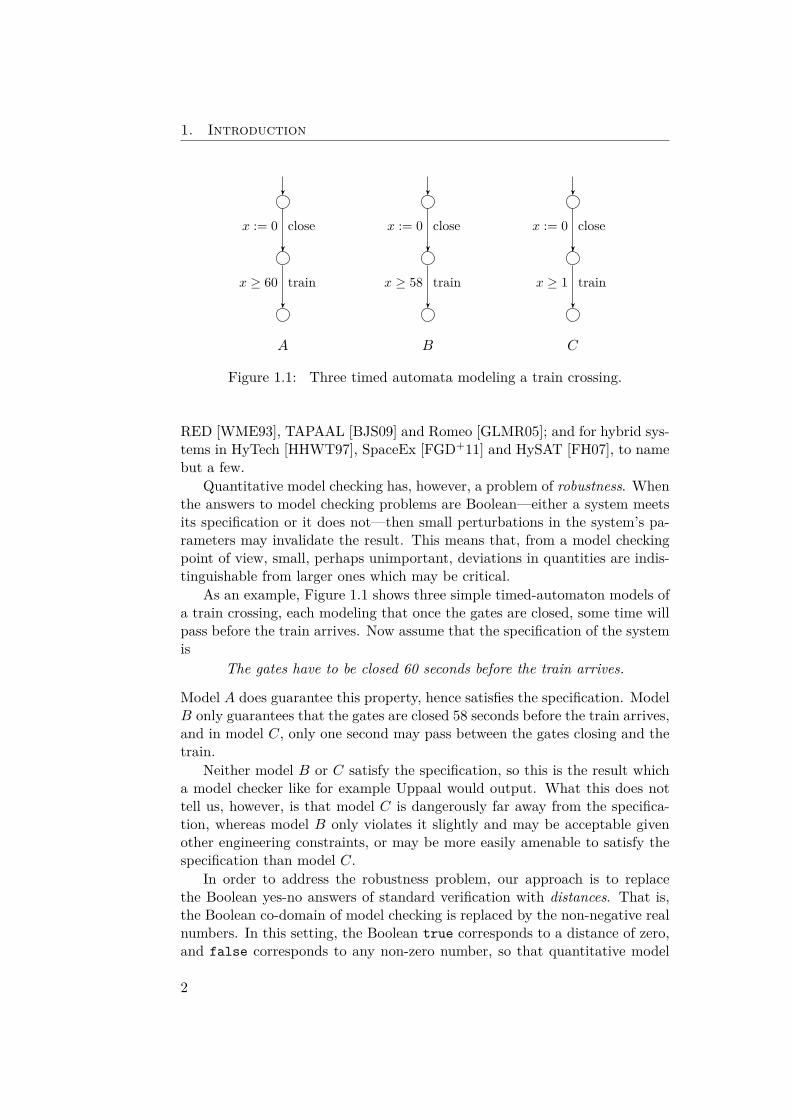
Figure 1.2: Modal transition system modeling a simple email system, withan optional behavior: Once an email is received it may e.g., be scanned forcontaining viruses, or automatically decrypted, before it is delivered to thereceiver.

Over the years, there have been a series of advances on specification the-ories [dAH05,CdAHM02,DLL+10,Del10,LT89,Nym08,Thr11]. The predom-inant approaches are based on modal logics and process algebras but havethe drawback that they cannot naturally embed both logical and structuralcomposition within the same formalism [Lar89]. Hence such formalisms donot permit to reason incrementally through refinement.

In order to leverage these problems, the concept of modal transition sys-tems was introduced [Lar89]. In short, modal transition systems are labeledtransition systems equipped with two types of transitions: must transitionswhich are mandatory for any implementation, and may transitions which areoptional for implementations. It is well established that modal transitionsystems match all the requirements of a reasonable specification theory, andmuch progress has been made in this area, see for example [Nym08,GLS08,GHJ01, GLLS05] or [AHL+08] for an overview. Also, practical experienceshows that the formalism is expressive enough to handle complex industrialproblems [Str,SPE].

As an example, consider the modal transition system shown in Figure 1.2which models the requirements of a simple email system in which emails arefirst received and then delivered. Before delivering the email, the systemmay check or process the email, for example for en- or decryption, filtering ofspam emails, or generating automatic answers using an auto-reply feature (seealso [Hal00]). Must transitions, representing obligatory behavior, are drawn assolid arrows, whereas may transitions, modeling optional behavior, are shownas dashed arrows: hence any implementation of this email system specificationmust be able to receive and deliver email, and it may also be able to checkarriving email before delivering it. No other behavior is allowed.

Implementations can also be represented within the modal transition sys-tem formalism, simply as specifications without may transitions. Here, anyimplementation choice has been resolved, so that implementations are (isomor-phic to) plain labeled transition systems. Formally, for a labeled transitionsystem to be an implementation of a given specification, we require that thestates of the two objects are related by a refinement relation with the prop-erty that all behavior required by the specification has been implemented, and

4

1.1. Motivation

receivedeliver

check

check

deliver

deliver

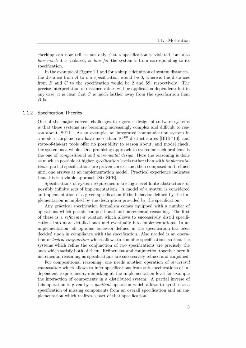
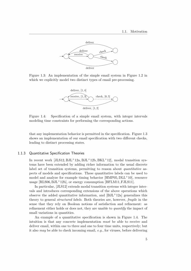
Figure 1.3: An implementation of the simple email system in Figure 1.2 inwhich we explicitly model two distinct types of email pre-processing.

receive, [1, 3]

deliver, [1, 4]

check, [0, 5]

deliver, [1, 2]

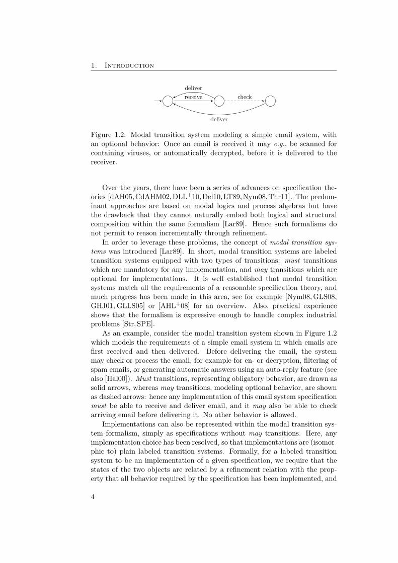
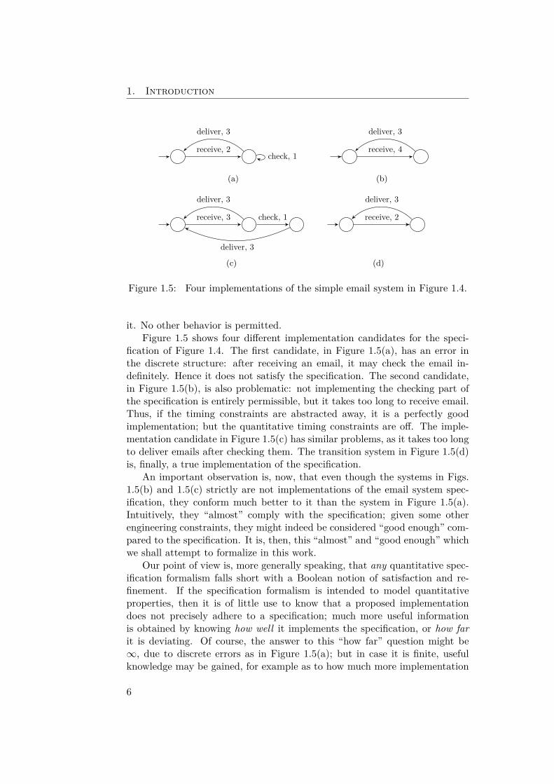
Figure 1.4: Specification of a simple email system, with integer intervalsmodeling time constraints for performing the corresponding actions.

that any implementation behavior is permitted in the specification. Figure 1.3shows an implementation of our email specification with two different checks,leading to distinct processing states.

1.1.3 Quantitative Specification Theories

In recent work [JLS12, BJL+12a, BJL+12b, BKL+12], modal transition sys-tems have been extended by adding richer information to the usual discretelabel set of transition systems, permitting to reason about quantitative as-pects of models and specifications. These quantitative labels can be used tomodel and analyze for example timing behavior [HMP05,DLL+10], resourceusage [RLS06,BJL+12b], or energy consumption [BFLM11,FJLS11].

In particular, [JLS12] extends modal transition systems with integer inter-vals and introduces corresponding extensions of the above operations whichobserve the added quantitative information, and [BJL+12a] generalizes thistheory to general structured labels. Both theories are, however, fragile in thesense that they rely on Boolean notions of satisfaction and refinement: asrefinement either holds or does not, they are unable to quantify the impact ofsmall variations in quantities.

An example of a quantitative specification is shown in Figure 1.4. Theintuition is that any concrete implementation must be able to receive anddeliver email, within one to three and one to four time units, respectively; butit also may be able to check incoming email, e.g., for viruses, before delivering

5

1. Introduction

receive, 2

deliver, 3

check, 1

(a)

receive, 4

deliver, 3

(b)

receive, 3

deliver, 3

check, 1

deliver, 3

(c)

receive, 2

deliver, 3

(d)

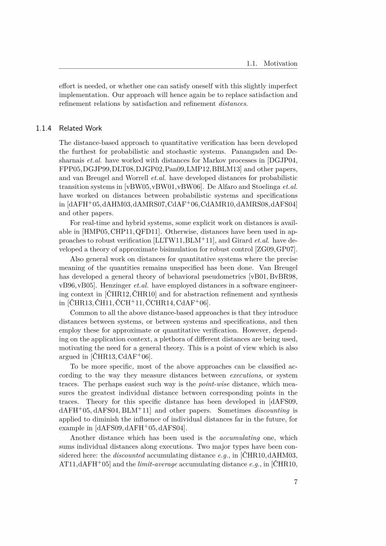
Figure 1.5: Four implementations of the simple email system in Figure 1.4.

it. No other behavior is permitted.Figure 1.5 shows four different implementation candidates for the speci-

fication of Figure 1.4. The first candidate, in Figure 1.5(a), has an error inthe discrete structure: after receiving an email, it may check the email in-definitely. Hence it does not satisfy the specification. The second candidate,in Figure 1.5(b), is also problematic: not implementing the checking part ofthe specification is entirely permissible, but it takes too long to receive email.Thus, if the timing constraints are abstracted away, it is a perfectly goodimplementation; but the quantitative timing constraints are off. The imple-mentation candidate in Figure 1.5(c) has similar problems, as it takes too longto deliver emails after checking them. The transition system in Figure 1.5(d)is, finally, a true implementation of the specification.

An important observation is, now, that even though the systems in Figs.1.5(b) and 1.5(c) strictly are not implementations of the email system spec-ification, they conform much better to it than the system in Figure 1.5(a).Intuitively, they “almost” comply with the specification; given some otherengineering constraints, they might indeed be considered “good enough” com-pared to the specification. It is, then, this “almost” and “good enough” whichwe shall attempt to formalize in this work.

Our point of view is, more generally speaking, that any quantitative spec-ification formalism falls short with a Boolean notion of satisfaction and re-finement. If the specification formalism is intended to model quantitativeproperties, then it is of little use to know that a proposed implementationdoes not precisely adhere to a specification; much more useful informationis obtained by knowing how well it implements the specification, or how farit is deviating. Of course, the answer to this “how far” question might be∞, due to discrete errors as in Figure 1.5(a); but in case it is finite, usefulknowledge may be gained, for example as to how much more implementation

6

1.1. Motivation

effort is needed, or whether one can satisfy oneself with this slightly imperfectimplementation. Our approach will hence again be to replace satisfaction andrefinement relations by satisfaction and refinement distances.

1.1.4 Related Work

The distance-based approach to quantitative verification has been developedthe furthest for probabilistic and stochastic systems. Panangaden and De-sharnais et.al. have worked with distances for Markov processes in [DGJP04,FPP05,DGJP99,DLT08,DJGP02,Pan09,LMP12,BBLM13] and other papers,and van Breugel and Worrell et.al. have developed distances for probabilistictransition systems in [vBW05,vBW01,vBW06]. De Alfaro and Stoelinga et.al.have worked on distances between probabilistic systems and specificationsin [dAFH+05,dAHM03,dAMRS07,CdAF+06,CdAMR10,dAMRS08,dAFS04]and other papers.

For real-time and hybrid systems, some explicit work on distances is avail-able in [HMP05,CHP11,QFD11]. Otherwise, distances have been used in ap-proaches to robust verification [LLTW11,BLM+11], and Girard et.al. have de-veloped a theory of approximate bisimulation for robust control [ZG09,GP07].

Also general work on distances for quantitative systems where the precisemeaning of the quantities remains unspecified has been done. Van Breugelhas developed a general theory of behavioral pseudometrics [vB01,BvBR98,vB96,vB05]. Henzinger et.al. have employed distances in a software engineer-ing context in [ČHR12,ČHR10] and for abstraction refinement and synthesisin [ČHR13,ČH11,ČCH+11,ČCHR14,CdAF+06].

Common to all the above distance-based approaches is that they introducedistances between systems, or between systems and specifications, and thenemploy these for approximate or quantitative verification. However, depend-ing on the application context, a plethora of different distances are being used,motivating the need for a general theory. This is a point of view which is alsoargued in [ČHR13,CdAF+06].

To be more specific, most of the above approaches can be classified ac-cording to the way they measure distances between executions, or systemtraces. The perhaps easiest such way is the point-wise distance, which mea-sures the greatest individual distance between corresponding points in thetraces. Theory for this specific distance has been developed in [dAFS09,dAFH+05, dAFS04, BLM+11] and other papers. Sometimes discounting isapplied to diminish the influence of individual distances far in the future, forexample in [dAFS09,dAFH+05,dAFS04].

Another distance which has been used is the accumulating one, whichsums individual distances along executions. Two major types have been con-sidered here: the discounted accumulating distance e.g., in [ČHR10,dAHM03,AT11,dAFH+05] and the limit-average accumulating distance e.g., in [ČHR10,

7

1. Introduction

AT11]. Both are well-known from the theory of discounted and mean-payoffgames [EM79,ZP96].

For real-time systems, a useful distance is the maximum-lead distanceof [HMP05] which measures the maximum difference between accumulatedtime delays along traces. For hybrid systems, things are more complicated,as distances between hybrid traces have to take into account both spatial andtiming differences, see for example [QFD11,Gir10,ZG09,GP07].

1.1.5 A General Theory of Quantitative VerificationDepending on the application context, many different types of distances arebeing employed in quantitative verification. Consequently, there is a need fora general theory of system distances which abstracts away from the concretedistances and develops quantitative verification at a level independent of thedistance. It is our view that in a theory of quantitative verification, thequantitative aspects should be treated just as much as input to a verificationproblem as the qualitative aspects are.

In this work we develop such a general theory of quantitative verifica-tion. We assume as input a distance between traces, or executions, and thenemploy the theory of games with quantitative objectives to define distancesbetween quantitative systems. Different versions of the (quantitative) bisimu-lation game give rise to different types of distances, viz. bisimulation distance,simulation distance, trace equivalence distance, etc., enabling us to constructa quantitative generalization of the linear-time–branching-time spectrum.

We also extend our general theory of quantitative verification to a theoryof quantitative specifications. For this we use modal transition systems, andwe develop the quantitative properties of the usual operators for behavioralspecification theories. All this is independent of the concrete distance betweentraces which is utilized.

1.2 ContributionsIn the following chapters we present work based on eight papers, publishedbetween 2009 and 2020 by the author of this thesis with different co-authors,on quantitative verification and quantitative specification theories. The firstthree, Chapters 2 to 4, are each concerned with properties of three specific sys-tem distances: the point-wise distance, the discounted accumulating distance,and the maximum-lead distance. The next Chapter 5 develops our generaltheory of quantitative verification and shows basic properties. Chapters 6and 7 then extend this theory to specification theories, first for the discountedaccumulating distance in Chapter 6 and then for the general setting in Chap-ter 7. In Chapter 8 we take a break from the quantitative setting in orderto introduce an extension of modal transition systems and show that the so-obtained specification theory is closely related to other popular specification

8

1.2. Contributions

formalisms. The final Chapter 9 extends these results to general quantitativeand develops their properties.

Compared to their sources, all chapters have been heavily redacted inorder to correct errors, unify notation, and smoothen the presentation. Anyremaining errors are the sole responsibility of the author of this thesis.

1.2.1 Geometric Preliminaries

Before we can give an overview of our contributions, we recall a few standardnotions from geometry and topology which we will use throughout. Let R≥0∪{∞} denote the extended non-negative reals.

A hemimetric on a set X is a function d : X × X → R≥0 ∪ {∞} whichsatisfies d(x, x) = 0 and d(x, y) + d(y, z) ≥ d(x, z) (the triangle inequality) forall x, y, z ∈ X. The hemimetric is said to be symmetric if also d(x, y) = d(y, x)for all x, y ∈ X; it is said to be separating if d(x, y) = 0 implies x = y.

A symmetric hemimetric is generally called a pseudometric, and a hemi-metric which is both symmetric and separating is simply a metric. The tuple(X, d) is called a (hemi/pseudo)metric space.

Note that our hemimetrics are extended in that they can take the value∞. This is convenient for several reasons, cf. [Law73], one of them being thatit allows for a disjoint union, or coproduct, of hemimetric spaces: the disjointunion of (X1, d1) and (X2, d2) is the hemimetric space (X1, d1)∪+ (X1, d2) =(X1∪+X2, d) where points from different components are infinitely far awayfrom each other, i.e., with d defined by

d(x, y) =

d1(x, y) if x, y ∈ X1,

d2(x, y) if x, y ∈ X2,

∞ otherwise.

The product of two hemimetric spaces (X1, d1) and (X2, d2) is the hemimetricspace (X1, d1)× (X2, d2) = (X1×X2, d) with d given by d((x1, x2), (y1, y2)) =max(d1(x1, y1), d2(x2, y2)).

The symmetrization of a hemimetric d on X is the symmetric hemimetricd : X × X → R≥0 ∪ {∞} defined by d(x, y) = max(d(x, y), d(y, x)); this isthe smallest among all pseudometrics d′ on X for which d ≤ d′. The topologygenerated by a hemimetric d on X is defined to be the same as the onegenerated by its symmetrization d; it has as open sets all unions of open ballsB(x; r) = {y ∈ X | d(x, y) < r}, for x ∈ X and r > 0.

A continuous function f : X → X on a pseudometric space (X, d) is calleda contraction if there exists 0 ≤ α < 1 (its Lipschitz constant) such thatd(f(x), f(y)) ≤ αd(x, y) for all x, y ∈ X.

Two pseudometrics d1, d2 on X are said to be

9

1. Introduction

• topologically equivalent provided that for all x ∈ X and all ε ∈ R+,there exists δ ∈ R+ such that d1(x, y) < δ implies d2(x, y) < ε andd2(x, y) < δ implies d1(x, y) < ε for all y ∈ X,

• Lipschitz equivalent if there exist m,M ∈ R+ such that md1(x, y) ≤d2(x, y) ≤Md1(x, y) for all x, y ∈ X.

Hemimetrics are topologically or Lipschitz equivalent if their symmetrizationsare.

Topological equivalence is the same as asking the identity function id :(X, d1)→ (X, d2) to be a homeomorphism, and Lipschitz equivalence impliestopological equivalence.

Topological equivalence of d1 and d2 is also the same as requiring thetopologies generated by d1 and d2 to coincide. Topological equivalence hencepreserves topological notions such as convergence of sequences: If a sequence(xj) of points in X converges in one pseudometric, then it also converges inthe other. As a consequence, topological equivalence of hemimetrics d1 andd2 implies that for all x, y ∈ X, d1(x, y) = 0 if, and only if, d2(x, y) = 0.

Topological equivalence is the weakest of the common notions of equiva-lence for metrics; it does not preserve geometric properties such as distances orangles. We are hence mainly interested in topological equivalence as a tool forshowing negative properties; we will later prove a number of results on topo-logical inequivalence of hemimetrics which imply that any other reasonablemetric equivalence, such as Lipschitz equivalence, also fails for these cases.

The Hausdorff hemimetric associated with a hemimetric d : X × X →R≥0 ∪ {∞} is the function dH : 2X × 2X → R≥0 ∪ {∞} given for subsetsA,B ⊆ X by

dH(A,B) = supx∈A

infy∈B

d(x, y).

This is a well-known construction for metric spaces, cf. [Mun00,AB07]; thereit is usually symmetrized and defined only for closed subsets, in which caseit is a metric. The following alternative formulation follows straight from thedefinition:

1.1 Proposition. For a hemimetric d on X, A,B ⊆ X, and ε ∈ R+, we haved(A,B) ≤ ε if and only if for any x ∈ A there exists y ∈ B for whichd(x, y) ≤ ε.

A sequence (xj) in a metric space X is a Cauchy sequence if it holds thatfor all ε > 0 there exist N ∈ N such that d(xm, xn) < ε for all n,m ≥ N . Xis said to be complete if every Cauchy sequence in X converges in X.

Finally, we recall the Banach fixed-point theorem: Any contraction on acomplete metric space has precisely one fixed point.

10

1.2. Contributions

1.2.2 Chapter 2, “Quantitative Analysis of Weighted Transition Systems”

In Chapter 2 we introduce the point-wise, accumulating and maximum-leadtrace distances, all in a discounted version which allows to diminish the in-fluence of future differences. In a notation which is simpler than the oneused in Chapter 2 and follows the one of later chapters, these are givenas follows. Let K be a set of symbols together with an extended metricdK : K×K→ R≥0 ∪ {∞}. A trace σ = (σ0, σ1, . . . ) is an infinite sequence ofsymbols in K. Let λ ∈ R≥0 with λ ≤ 1 be a discounting factor and σ and τtraces.

• The point-wise trace distance between σ and τ is

dT• (σ, τ) = sup

i≥0λidK(σi, τi) .

• The accumulating trace distance between σ and τ is

dT+(σ, τ) =

∑i≥0

λidK(σi, τi) .

• The maximum-lead trace distance between σ and τ is

dT±(σ, τ) = sup

i≥0λi∣∣∣ ∑0≤j≤i

(σi − τi)∣∣∣ .

Note that the definition of the last distance requires extra structure of additionand subtraction on K; generally this is only used for K = Z or K = R.

We then use these trace distances to define point-wise, accumulating andmaximum-lead linear distances between states in weighted transition systems.If dT is any of the above trace distances, then the linear distance between twostates s and t of a transition system is defined to be

dL(s, t) = supσ∈Tr(s)

infτ∈Tr(t)

dT(σ, τ) ,

where Tr(s) denotes the set of traces emanating from s, similarly for Tr(t).This is thus the Hausdorff distance from Tr(s) to Tr(t); note that the definitionis independent of which particular trace distance is used.

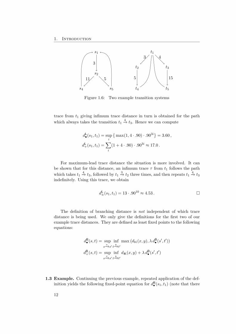
1.2 Example. We show a computation of the different distances between thestates s1 and t1 in the transition system in Figure 1.6. Edges without specifiedweight have weight 0, and the discounting factor is λ = .90.

It is easy to see that supremum trace distance is obtained for the pathfrom s1 which always turns left at s2, i.e., takes the transition s2

11−→ s4, andthen for the point-wise and accumulating trace distances, that the matching

11

1. Introduction

s1

s2

s5s4

3

511

t1

t2 t3

t4 t5

3 4

5 15

Figure 1.6: Two example transition systems

trace from t1 giving infimum trace distance in turn is obtained for the pathwhich always takes the transition t1 4−→ t3. Hence we can compute

dL•(s1, t1) = sup

i

{max(1, 4 · .90) · .903i} = 3.60 ,

dL+(s1, t1) =

∑i

(1 + 4 · .90) · .903i ≈ 17.0 .

For maximum-lead trace distance the situation is more involved. It canbe shown that for this distance, an infimum trace τ from t1 follows the pathwhich takes t1 4−→ t3, followed by t1 3−→ t2 three times, and then repeats t1 4−→ t3indefinitely. Using this trace, we obtain

dL±(s1, t1) = 13 · .9010 ≈ 4.53 . �

The definition of branching distance is not independent of which tracedistance is being used. We only give the definitions for the first two of ourexample trace distances. They are defined as least fixed points to the followingequations:

dB• (s, t) = sup

sx−→s′

infty−→t′

max(dK(x, y), λ dB

• (s′, t′))

dB+(s, t) = sup

sx−→s′

infty−→t′

dK(x, y) + λ dB• (s′, t′)

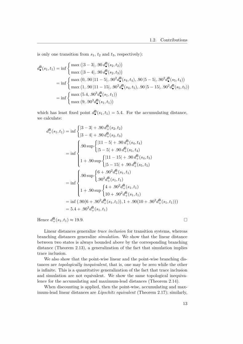
1.3 Example. Continuing the previous example, repeated application of the def-inition yields the following fixed-point equation for dB

• (s1, t1) (note that there

12

1.2. Contributions

is only one transition from s1, t2 and t3, respectively):

dB• (s1, t1) = inf

{max

(|3− 3|, .90 dB

• (s2, t2))

max(|3− 4|, .90 dB

• (s2, t3))

= inf{

max(0, .90 |11− 5|, .902dB

• (s4, t4), .90 |5− 5|, .902dB• (s5, t4)

)max

(1, .90 |11− 15|, .902dB

• (s4, t5), .90 |5− 15|, .902dB• (s5, t5)

)= inf

{max

(5.4, .903dB

• (s1, t1))

max(9, .903dB

• (s1, t1))

which has least fixed point dB• (s1, t1) = 5.4. For the accumulating distance,

we calculate:

dB+(s1, t1) = inf

{|3− 3|+ .90 dB

+(s2, t2)|3− 4|+ .90 dB

+(s2, t3)

= inf

.90 sup

{|11− 5|+ .90 dB

+(s4, t4)|5− 5|+ .90 dB

+(s5, t4)

1 + .90 sup{|11− 15|+ .90 dB

+(s4, t5)|5− 15|+ .90 dB

+(s5, t5)

= inf

.90 sup

{6 + .902dB

+(s1, t1).902dB

+(s1, t1)

1 + .90 sup{

4 + .902dB+(s1, t1)

10 + .902dB+(s1, t1)

= inf(.90(6 + .902dB

+(s1, t1)), 1 + .90

(10 + .902dB

+(s1, t1)))

= 5.4 + .903dB+(s1, t1)

Hence dB+(s1, t1) ≈ 19.9. �

Linear distances generalize trace inclusion for transition systems, whereasbranching distances generalize simulation. We show that the linear distancebetween two states is always bounded above by the corresponding branchingdistance (Theorem 2.13), a generalization of the fact that simulation impliestrace inclusion.

We also show that the point-wise linear and the point-wise branching dis-tances are topologically inequivalent, that is, one may be zero while the otheris infinite. This is a quantitative generalization of the fact that trace inclusionand simulation are not equivalent. We show the same topological inequiva-lence for the accumulating and maximum-lead distances (Theorem 2.14).

When discounting is applied, then the point-wise, accumulating and max-imum-lead linear distances are Lipschitz equivalent (Theorem 2.17); similarly,

13

1. Introduction

the three branching distances are Lipschitz equivalent (Theorem 2.18). With-out discounting, the distances are topologically inequivalent. Lipschitz equiva-lence means that one distance is bounded by the other, multiplied by a scalingfactor; hence properties of one distance may be transferred to the other.

Chapter 2 is based on work by the author’s PhD student Claus Thrane,Kim G. Larsen, and the author, which has been presented at the 20th NordicWorkshop on Programming Theory (NWPT) [TFL08] and subsequently pub-lished in the Journal of Logic and Algebraic Programming (now the Journalof Logical and Algebraic Methods in Programming) in 2010 [TFL10].

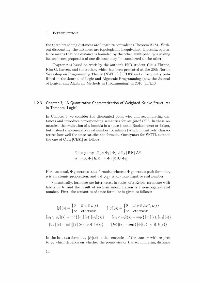
1.2.3 Chapter 3, “A Quantitative Characterization of Weighted Kripke Structuresin Temporal Logic”

In Chapter 3 we consider the discounted point-wise and accumulating dis-tances and introduce corresponding semantics for weighted CTL. In these se-mantics, the evaluation of a formula in a state is not a Boolean true or false,but instead a non-negative real number (or infinity) which, intuitively, charac-terizes how well the state satisfies the formula. Our syntax for WCTL extendsthe one of CTL [CE81] as follows:

Φ ::= p | ¬p | Φ1 ∧ Φ2 | Φ1 ∨ Φ2 | EΨ | AΨΨ ::= XcΦ | GcΦ | FcΦ | [Φ1UcΦ2]

Here, as usual, Φ generates state formulae whereas Ψ generates path formulae,p is an atomic proposition, and c ∈ R≥0 is any non-negative real number.

Semantically, formulae are interpreted in states of a Kripke structure withlabels in K, and the result of such an interpretation is a non-negative realnumber. First, the semantics of state formulae is given as follows:

JpK(s) ={

0 if p ∈ L(s)∞ otherwise

J¬pK(s) ={

0 if p ∈ AP \ L(s)∞ otherwise

Jϕ1 ∨ ϕ2K(s) = inf{Jϕ1K(s), Jϕ2K(s)

}Jϕ1 ∧ ϕ2K(s) = sup

{Jϕ1K(s), Jϕ2K(s)

}JEψK(s) = inf

{JψK(σ) | σ ∈ Tr(s)

}JAψK(s) = sup

{JψK(σ) | σ ∈ Tr(s)

}

In the last two formulae, JψK(σ) is the semantics of the trace σ with respectto ψ, which depends on whether the point-wise or the accumulating distance

14

1.2. Contributions

is used. For example, the point-wise path semantics is given as follows:

JϕK(σ) = JϕK(σ0)

JXcϕK(σ) = max(dK(σ0, c), λJϕK(σ1)

}JFcϕK(σ) = inf

k≥0

(max

(max

0≤j<k

(λjdK(σj , c)

), λkJϕK(σk)

))JGcϕK(σ) = sup

k≥0

(max

(max

0≤j<k

(λjdK(σj , c)

), λkJϕK(σk)

))Jϕ1Ucϕ2K(σ) = inf

k≥0

(max

(max

0≤j<k

(λjdK(Jϕ1K(σj), c)

), λkJϕ2K(σk)

))Here σk = (σk, σk+1, . . . ) denotes the k-shift of the trace σ = (σ0, σ1, . . . ).

We then show in Theorems 3.11 and 3.13 that with these semantics, WCTLis adequate for the corresponding bisimulation distances. That is, the bisimu-lation distance between two states is precisely the supremum, over all WCTLformulae, of the absolute value of the difference of the formula’s evaluation inthese two states.

We also show, in Theorems 3.17 and 3.18, that with the correspondingsemantics, WCTL is expressive for the discounted point-wise and accumulatingdistances. This means that given a state in a Kripke structure, there exists aWCTL formula which characterizes the state in the sense that the bisimulationdistance to any other state is precisely the evaluation of the formula in thatstate.

Our notions of adequacy and expressiveness are standard quantitative gen-eralizations of Hennessy and Milner’s definitions from [HM85].

Chapter 3 is based on work by the author’s PhD student Claus Thrane,Kim G. Larsen, and the author, which has been presented at the 5th Confer-ence on Mathematical and Engineering Methods in Computer Science(MEMICS; best paper award) [FLT09] and subsequently published in theJournal of Computing and Informatics [FLT10].

1.2.4 Chapter 4, “Metrics for Weighted Transition Systems: Axiomatization”In Chapter 4 we develop sound and complete axiomatizations of the point-wiseand the discounted accumulating distances for finite and for regular weightedprocesses. In this context, a finite weighted process is given using the grammar

E ::= 0 | n.E | E + E | n ∈ K ,

where K is a finite set of weights, with a metric dK, and 0 denotes the emptyprocess. A regular weighted process is given using the grammar

E ::= U | X | n.E | E + E | µX.E n ∈ K, X ∈ V ,

where V is a set of variables, U is the universal process, and µX.E denotes aminimal fixed point.

15

1. Introduction

(A1) 0 ./ r` [0, E] ./ r(A2) ∞ ./ r

` [n.E,0] ./ r

` [E,F ] ./ r1(R1•) max(dK(n,m), λr1) ./ r` [n.E,m.F ] ./ r

` [E,F ] ./ r1(R1+) dK(n,m) + λr1 ./ r` [n.E,m.F ] ./ r

` [E1, F ] ./ r1 ` [E2, F ] ./ r2(R2) max(r1, r2) ./ r` [E1 + E2, F ] ./ r

` [n.E, F1] ./ r1 ` [n.E, F2] ./ r2(R3) min(r1, r2) ./ r` [n.E, F1 + F2] ./ r

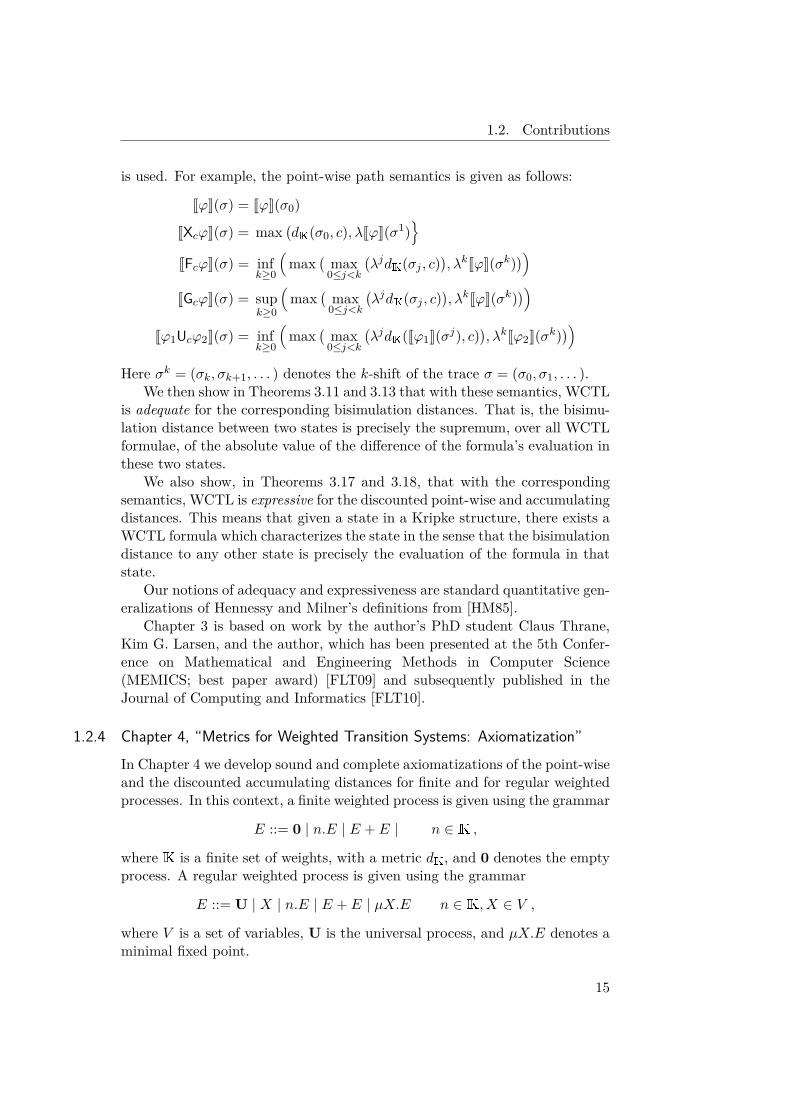
Figure 1.7: Axiomatization of point-wise and discounted accumulating dis-tance for finite weighted processes

We then give axiomatizations of the point-wise and the discounted ac-cumulating distances for finite weighted processes, as shown in Figure 1.7.These differ only in one proof rule: for the point-wise distance, rule (R1•)applies, for the discounted accumulating distance, rule (R1+). We show theaxiomatizations to be sound and complete in Theorems 4.8, 4.9 and 4.10.

For regular weighted processes, we develop similar axiomatizations, whichwe then show to be sound and ε-complete in Theorems 4.12, 4.16 and 4.17.Here, ε-completeness means that a distance of d can be proven within aninterval [d− ε, d+ ε], for any positive real ε.

Chapter 4 is based on work by the author’s PhD student Claus Thrane,Kim G. Larsen, and the author, which has been published in TheoreticalComputer Science [LFT11].

1.2.5 Chapter 5, “The Quantitative Linear-Time–Branching-Time Spectrum”

Chapter 5 presents a generalization of the work in Chapter 2 along several di-rections. Instead of developing theory separately for different trace distances,we treat the trace distance as an input and develop a general theory of linearand branching distances pertaining to a given, but unspecified, trace distance.

Let again K be a set of symbols, and denote by K∞ = K∗ ∪ Kω the

set of finite and infinite traces in K. A trace distance is, then, a functiond : K∞×K∞ → R≥0∪{∞} which satisfies d(σ, σ) = 0 and d(σ, τ) +d(τ, χ) ≥d(σ, χ) for all σ, τ, χ ∈ K∞, and additionally, d(σ, τ) = ∞ if σ and τ havedifferent length.

16

1.2. Contributions

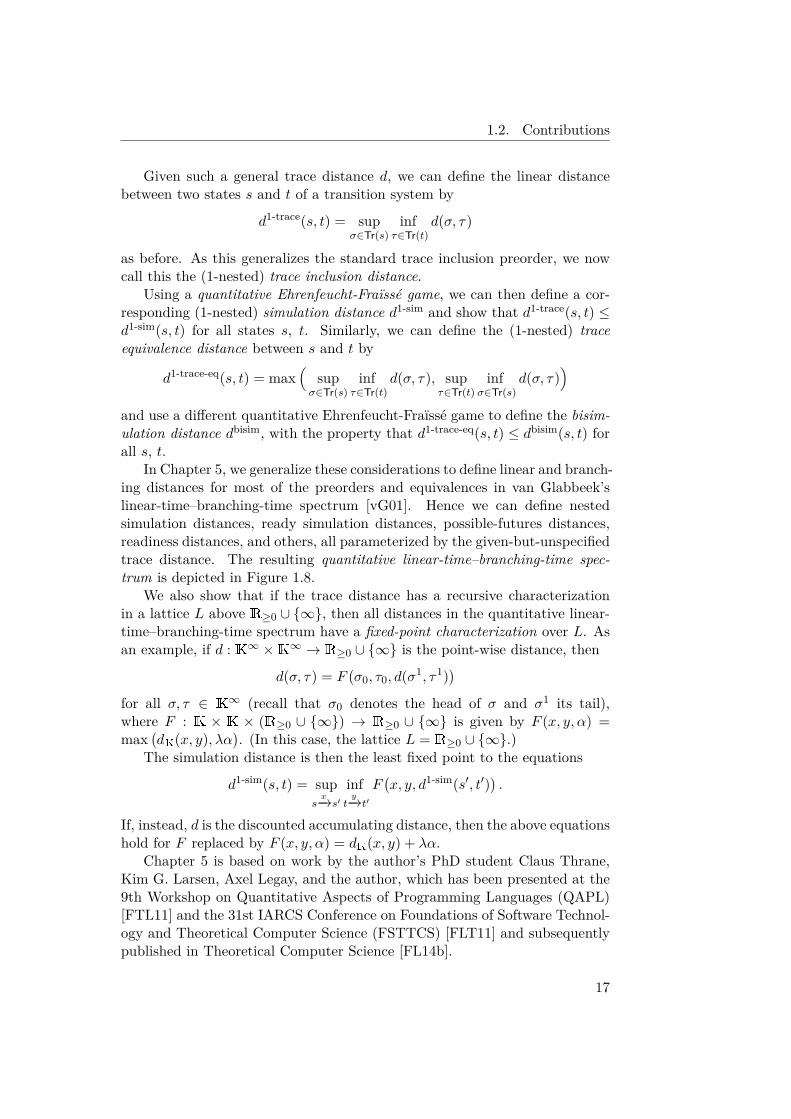
Given such a general trace distance d, we can define the linear distancebetween two states s and t of a transition system by

d1-trace(s, t) = supσ∈Tr(s)

infτ∈Tr(t)

d(σ, τ)

as before. As this generalizes the standard trace inclusion preorder, we nowcall this the (1-nested) trace inclusion distance.

Using a quantitative Ehrenfeucht-Fraïssé game, we can then define a cor-responding (1-nested) simulation distance d1-sim and show that d1-trace(s, t) ≤d1-sim(s, t) for all states s, t. Similarly, we can define the (1-nested) traceequivalence distance between s and t by

d1-trace-eq(s, t) = max(

supσ∈Tr(s)

infτ∈Tr(t)

d(σ, τ), supτ∈Tr(t)

infσ∈Tr(s)

d(σ, τ))

and use a different quantitative Ehrenfeucht-Fraïssé game to define the bisim-ulation distance dbisim, with the property that d1-trace-eq(s, t) ≤ dbisim(s, t) forall s, t.

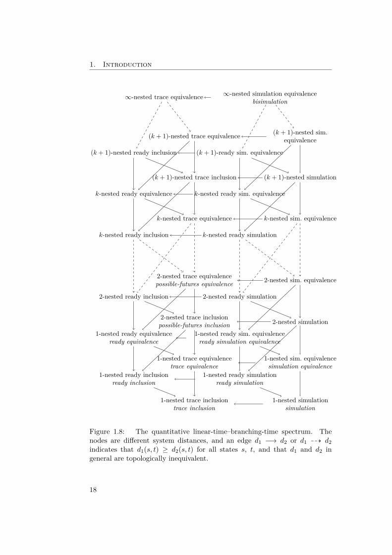
In Chapter 5, we generalize these considerations to define linear and branch-ing distances for most of the preorders and equivalences in van Glabbeek’slinear-time–branching-time spectrum [vG01]. Hence we can define nestedsimulation distances, ready simulation distances, possible-futures distances,readiness distances, and others, all parameterized by the given-but-unspecifiedtrace distance. The resulting quantitative linear-time–branching-time spec-trum is depicted in Figure 1.8.

We also show that if the trace distance has a recursive characterizationin a lattice L above R≥0 ∪ {∞}, then all distances in the quantitative linear-time–branching-time spectrum have a fixed-point characterization over L. Asan example, if d : K∞ ×K∞ → R≥0 ∪ {∞} is the point-wise distance, then

d(σ, τ) = F(σ0, τ0, d(σ1, τ1)

)for all σ, τ ∈ K

∞ (recall that σ0 denotes the head of σ and σ1 its tail),where F : K × K × (R≥0 ∪ {∞}) → R≥0 ∪ {∞} is given by F (x, y, α) =max

(dK(x, y), λα

). (In this case, the lattice L = R≥0 ∪ {∞}.)

The simulation distance is then the least fixed point to the equations

d1-sim(s, t) = supsx−→s′

infty−→t′

F(x, y, d1-sim(s′, t′)

).

If, instead, d is the discounted accumulating distance, then the above equationshold for F replaced by F (x, y, α) = dK(x, y) + λα.

Chapter 5 is based on work by the author’s PhD student Claus Thrane,Kim G. Larsen, Axel Legay, and the author, which has been presented at the9th Workshop on Quantitative Aspects of Programming Languages (QAPL)[FTL11] and the 31st IARCS Conference on Foundations of Software Technol-ogy and Theoretical Computer Science (FSTTCS) [FLT11] and subsequentlypublished in Theoretical Computer Science [FL14b].

17

1. Introduction

∞-nested trace equivalence

(k + 1)-nested ready inclusion

(k + 1)-nested trace equivalence

k-nested ready equivalence

(k + 1)-nested trace inclusion

k-nested ready inclusion

k-nested trace equivalence

2-nested ready inclusion

2-nested trace equivalencepossible-futures equivalence

1-nested ready equivalenceready equivalence

2-nested trace inclusionpossible-futures inclusion

1-nested ready inclusionready inclusion

1-nested trace equivalencetrace equivalence

1-nested trace inclusiontrace inclusion

∞-nested simulation equivalencebisimulation

(k + 1)-ready sim. equivalence

(k + 1)-nested sim.equivalence

k-nested ready sim. equivalence

(k + 1)-nested simulation

k-nested ready simulation

k-nested sim. equivalence

2-nested ready simulation

2-nested sim. equivalence

1-nested ready sim. equivalenceready simulation equivalence

2-nested simulation

1-nested ready simulationready simulation

1-nested sim. equivalencesimulation equivalence

1-nested simulationsimulation

Figure 1.8: The quantitative linear-time–branching-time spectrum. Thenodes are different system distances, and an edge d1 −→ d2 or d1 99K d2indicates that d1(s, t) ≥ d2(s, t) for all states s, t, and that d1 and d2 ingeneral are topologically inequivalent.

18

1.2. Contributions

1.2.6 Chapter 6, “Weighted Modal Transition Systems”

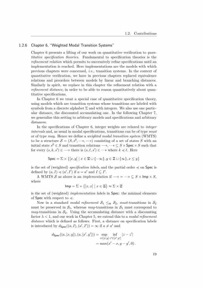
Chapter 6 presents a lifting of our work on quantitative verification to quan-titative specification theories. Fundamental to specification theories is therefinement relation which permits to successively refine specifications until animplementation is reached. Here implementations are the models with whichprevious chapters were concerned, i.e., transition systems. In the context ofquantitative verification, we have in previous chapters replaced equivalencerelations and preorders between models by linear and branching distances.Similarly in spirit, we replace in this chapter the refinement relation with arefinement distance, in order to be able to reason quantitatively about quan-titative specifications.

In Chapter 6 we treat a special case of quantitative specification theory,using models which are transition systems whose transitions are labeled withsymbols from a discrete alphabet Σ and with integers. We also use one partic-ular distance, the discounted accumulating one. In the following Chapter 7,we generalize this setting to arbitrary models and specifications and arbitrarydistances.

In the specifications of Chapter 6, integer weights are relaxed to integerintervals and, as usual in modal specifications, transitions can be of type mustor of type may. Hence we define a weighted modal transition system (WMTS)to be a structure S = (S, s0, 99K,−→) consisting of a set of states S with aninitial state s0 ∈ S and transition relations −→, 99K ⊆ S× Spec×S such thatfor every (s, k, s′) ∈ −→ there is (s, `, s′) ∈ 99K where k 4 `. Here

Spec = Σ×{[x, y]

∣∣ x ∈ Z ∪ {−∞}, y ∈ Z ∪ {∞}, x ≤ y}is the set of (weighted) specification labels, and the partial order 4 on Spec isdefined by (a, I) 4 (a′, I ′) if a = a′ and I ⊆ I ′.

A WMTS S as above is an implementation if −→ = 99K ⊆ S × Imp × S,where

Imp = Σ×{[x, x]

∣∣ x ∈ Z} ≈ Σ× Z

is the set of (weighted) implementation labels in Spec: the minimal elementsof Spec with respect to 4.

Now in a standard modal refinement S1 ≤m S2, must-transitions in S2must be preserved in S1, whereas may-transitions in S1 must correspond tomay-transitions in S2. Using the accumulating distance with a discountingfactor λ < 1, and our work in Chapter 5, we extend this to a modal refinementdistance which is defined as follows. First, a distance on specification labelsis introduced by dSpec((a, I), (a′, I ′)) =∞ if a 6= a′ and

dSpec((a, [x, y]), (a, [x′, y′])

)= sup

z∈[x,y]inf

z′∈[x′,y′]|z − z′|

= max(x′ − x, y − y′, 0) .

19

1. Introduction

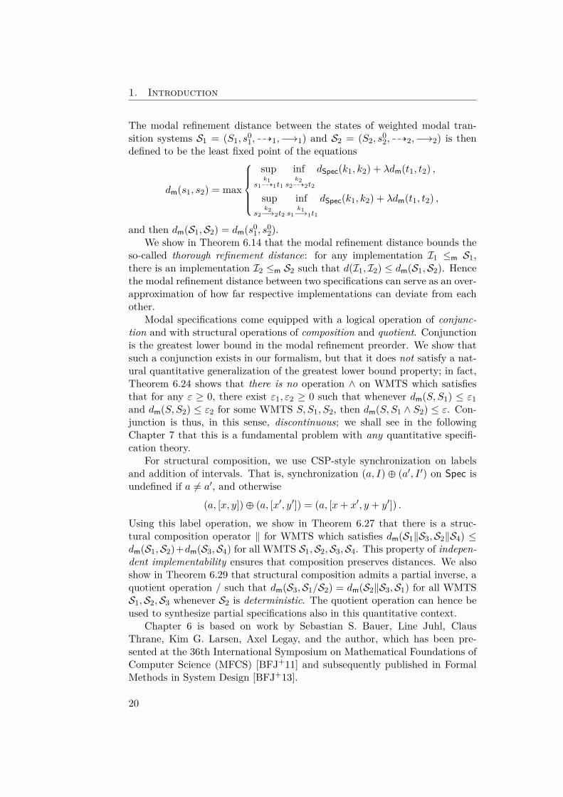
The modal refinement distance between the states of weighted modal tran-sition systems S1 = (S1, s

01, 99K1,−→1) and S2 = (S2, s

02, 99K2,−→2) is then

defined to be the least fixed point of the equations

dm(s1, s2) = max

sup

s1k199K1t1

infs2

k299K2t2

dSpec(k1, k2) + λdm(t1, t2) ,

sups2

k2−→2t2

infs1

k1−→1t1

dSpec(k1, k2) + λdm(t1, t2) ,

and then dm(S1,S2) = dm(s01, s

02).

We show in Theorem 6.14 that the modal refinement distance bounds theso-called thorough refinement distance: for any implementation I1 ≤m S1,there is an implementation I2 ≤m S2 such that d(I1, I2) ≤ dm(S1,S2). Hencethe modal refinement distance between two specifications can serve as an over-approximation of how far respective implementations can deviate from eachother.

Modal specifications come equipped with a logical operation of conjunc-tion and with structural operations of composition and quotient. Conjunctionis the greatest lower bound in the modal refinement preorder. We show thatsuch a conjunction exists in our formalism, but that it does not satisfy a nat-ural quantitative generalization of the greatest lower bound property; in fact,Theorem 6.24 shows that there is no operation ∧ on WMTS which satisfiesthat for any ε ≥ 0, there exist ε1, ε2 ≥ 0 such that whenever dm(S, S1) ≤ ε1and dm(S, S2) ≤ ε2 for some WMTS S, S1, S2, then dm(S, S1 ∧ S2) ≤ ε. Con-junction is thus, in this sense, discontinuous; we shall see in the followingChapter 7 that this is a fundamental problem with any quantitative specifi-cation theory.

For structural composition, we use CSP-style synchronization on labelsand addition of intervals. That is, synchronization (a, I) � (a′, I ′) on Spec isundefined if a 6= a′, and otherwise

(a, [x, y])� (a, [x′, y′]) = (a, [x+ x′, y + y′]) .

Using this label operation, we show in Theorem 6.27 that there is a struc-tural composition operator ‖ for WMTS which satisfies dm(S1‖S3,S2‖S4) ≤dm(S1,S2)+dm(S3,S4) for all WMTS S1,S2,S3,S4. This property of indepen-dent implementability ensures that composition preserves distances. We alsoshow in Theorem 6.29 that structural composition admits a partial inverse, aquotient operation / such that dm(S3,S1/S2) = dm(S2‖S3,S1) for all WMTSS1,S2,S3 whenever S2 is deterministic. The quotient operation can hence beused to synthesize partial specifications also in this quantitative context.

Chapter 6 is based on work by Sebastian S. Bauer, Line Juhl, ClausThrane, Kim G. Larsen, Axel Legay, and the author, which has been pre-sented at the 36th International Symposium on Mathematical Foundations ofComputer Science (MFCS) [BFJ+11] and subsequently published in FormalMethods in System Design [BFJ+13].

20

1.2. Contributions

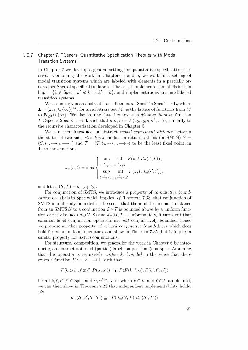
1.2.7 Chapter 7, “General Quantitative Specification Theories with ModalTransition Systems”In Chapter 7 we develop a general setting for quantitative specification the-ories. Combining the work in Chapters 5 and 6, we work in a setting ofmodal transition systems which are labeled with elements in a partially or-dered set Spec of specification labels. The set of implementation labels is thenImp = {k ∈ Spec | k′ 4 k ⇒ k′ = k}, and implementations are Imp-labeledtransition systems.

We assume given an abstract trace distance d : Spec∞×Spec∞ → L, whereL = (R≥0∪{∞})M , for an arbitrary set M , is the lattice of functions fromMto R≥0 ∪ {∞}. We also assume that there exists a distance iterator functionF : Spec× Spec× L→ L such that d(σ, τ) = F (σ0, τ0, d(σ1, τ1)), similarly tothe recursive characterization developed in Chapter 5.

We can then introduce an abstract modal refinement distance betweenthe states of two such structured modal transition systems (or SMTS) S =(S, s0, 99KS ,−→S) and T = (T, t0, 99KT ,−→T ) to be the least fixed point, inL, to the equations

dm(s, t) = max

sup

sk99KS s′

inft`99KT t′

F (k, `, dm(s′, t′)) ,

supt`−→T t′

infs

k−→S s′

F (k, `, dm(s′, t′)) ,

and let dm(S, T ) = dm(s0, t0).For conjunction of SMTS, we introduce a property of conjunctive bound-

edness on labels in Spec which implies, cf. Theorem 7.33, that conjunction ofSMTS is uniformly bounded in the sense that the modal refinement distancefrom an SMTS U to a conjunction S ∧T is bounded above by a uniform func-tion of the distances dm(U ,S) and dm(U , T ). Unfortunately, it turns out thatcommon label conjunction operators are not conjunctively bounded, hencewe propose another property of relaxed conjunctive boundedness which doeshold for common label operators, and show in Theorem 7.35 that it implies asimilar property for SMTS conjunctions.

For structural composition, we generalize the work in Chapter 6 by intro-ducing an abstract notion of (partial) label composition � on Spec. Assumingthat this operator is recursively uniformly bounded in the sense that thereexists a function P : L× L→ L such that

F (k � k′, `� `′, P (α, α′)) vL P (F (k, `, α), F (k′, `′, α′))

for all k, `, k′, `′ ∈ Spec and α, α′ ∈ L for which k � k′ and `� `′ are defined,we can then show in Theorem 7.23 that independent implementability holds,viz.

dm(S‖S ′, T ‖T ′) vL P (dm(S, T ), dm(S ′, T ′))

21

1. Introduction

for all SMTS S, T , S ′, T ′. In examples, we expose several different labelcomposition operators and show that they are uniformly bounded. We showthat the quotient operator / from Chapter 6 has a similar generalization toSMTS.

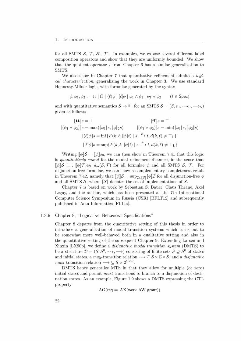
We also show in Chapter 7 that quantitative refinement admits a logi-cal characterization, generalizing the work in Chapter 3. We use standardHennessy-Milner logic, with formulae generated by the syntax

φ, φ1, φ2 := tt | ff | 〈`〉φ | [`]φ | φ1 ∧ φ2 | φ1 ∨ φ2 (` ∈ Spec)

and with quantitative semantics S → L, for an SMTS S = (S, s0, 99KS ,−→S)given as follows:

JttKs = ⊥ JffKs = >J(φ1 ∧ φ2)Ks = max(Jφ1Ks, JφK2s) J(φ1 ∨ φ2)Ks = min(Jφ1Ks, Jφ2Ks)

J〈`〉φKs = inf{F (k, `, JφKt) | s k−→ t, d(k, `) 6= >L}

J[`]φKs = sup{F (k, `, JφKt) | s k99K t, d(k, `) 6= >L}

Writing JφKS = JφKs0, we can then show in Theorem 7.41 that this logicis quantitatively sound for the modal refinement distance, in the sense thatJφKS vL JφKT �L dm(S, T ) for all formulae φ and all SMTS S, T . Fordisjunction-free formulae, we can show a complementary completeness resultin Theorem 7.42, namely that JφKS = supI∈JSKJφKI for all disjunction-free φand all SMTS S, where JSK denotes the set of implementations of S.

Chapter 7 is based on work by Sebastian S. Bauer, Claus Thrane, AxelLegay, and the author, which has been presented at the 7th InternationalComputer Science Symposium in Russia (CSR) [BFLT12] and subsequentlypublished in Acta Informatica [FL14a].

1.2.8 Chapter 8, “Logical vs. Behavioral Specifications”Chapter 8 departs from the quantitative setting of this thesis in order tointroduce a generalization of modal transition systems which turns out tobe somewhat more well-behaved both in a qualitative setting and also inthe quantitative setting of the subsequent Chapter 9. Extending Larsen andXinxin [LX90b], we define a disjunctive modal transition system (DMTS) tobe a structure D = (S, S0, 99K,−→) consisting of finite sets S ⊇ S0 of statesand initial states, a may-transition relation 99K ⊆ S×Σ×S, and a disjunctivemust-transition relation −→ ⊆ S × 2Σ×S .

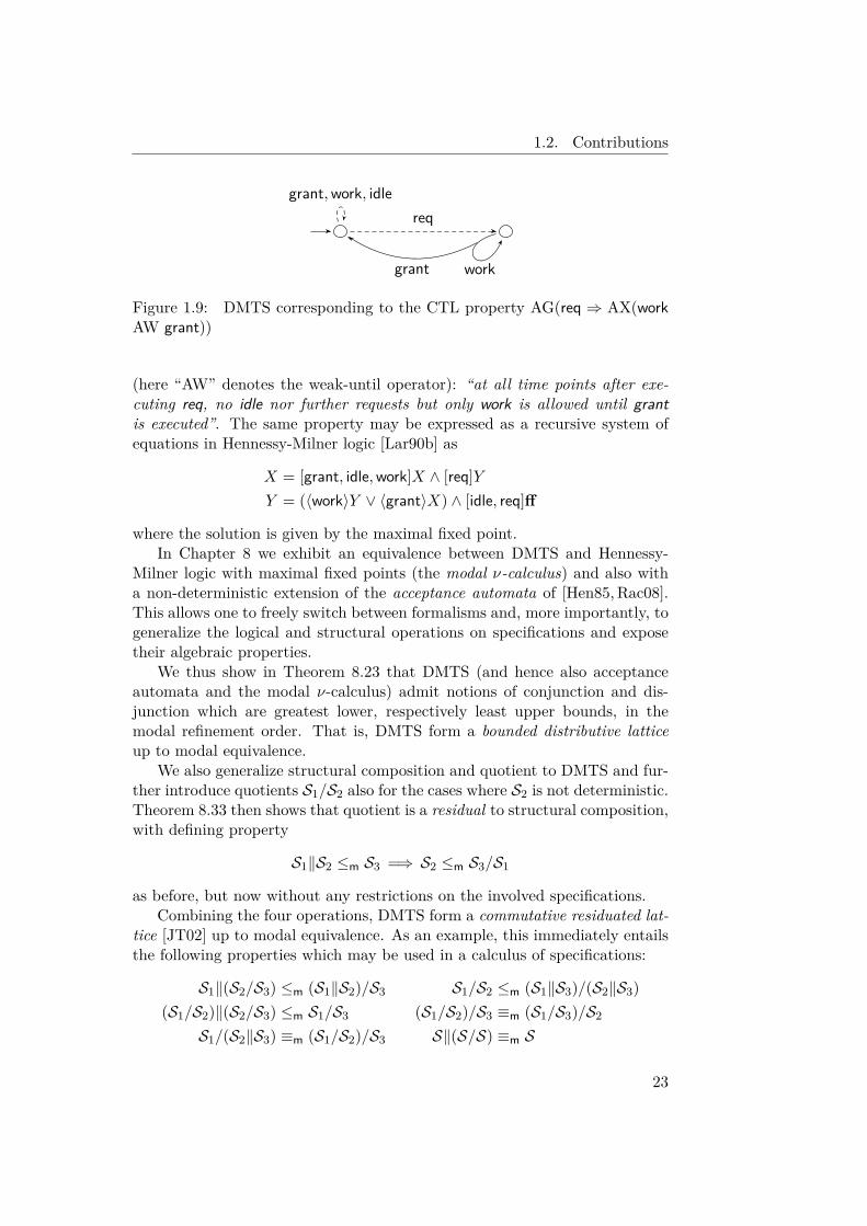
DMTS hence generalize MTS in that they allow for multiple (or zero)initial states and permit must transitions to branch to a disjunction of desti-nation states. As an example, Figure 1.9 shows a DMTS expressing the CTLproperty

AG(req⇒ AX(work AW grant))

22

1.2. Contributions

reqgrant,work, idle

workgrant

Figure 1.9: DMTS corresponding to the CTL property AG(req ⇒ AX(workAW grant))

(here “AW” denotes the weak-until operator): “at all time points after exe-cuting req, no idle nor further requests but only work is allowed until grantis executed”. The same property may be expressed as a recursive system ofequations in Hennessy-Milner logic [Lar90b] as

X = [grant, idle,work]X ∧ [req]YY = (〈work〉Y ∨ 〈grant〉X) ∧ [idle, req]ff

where the solution is given by the maximal fixed point.In Chapter 8 we exhibit an equivalence between DMTS and Hennessy-

Milner logic with maximal fixed points (the modal ν-calculus) and also witha non-deterministic extension of the acceptance automata of [Hen85,Rac08].This allows one to freely switch between formalisms and, more importantly, togeneralize the logical and structural operations on specifications and exposetheir algebraic properties.

We thus show in Theorem 8.23 that DMTS (and hence also acceptanceautomata and the modal ν-calculus) admit notions of conjunction and dis-junction which are greatest lower, respectively least upper bounds, in themodal refinement order. That is, DMTS form a bounded distributive latticeup to modal equivalence.

We also generalize structural composition and quotient to DMTS and fur-ther introduce quotients S1/S2 also for the cases where S2 is not deterministic.Theorem 8.33 then shows that quotient is a residual to structural composition,with defining property

S1‖S2 ≤m S3 =⇒ S2 ≤m S3/S1

as before, but now without any restrictions on the involved specifications.Combining the four operations, DMTS form a commutative residuated lat-

tice [JT02] up to modal equivalence. As an example, this immediately entailsthe following properties which may be used in a calculus of specifications:

S1‖(S2/S3) ≤m (S1‖S2)/S3 S1/S2 ≤m (S1‖S3)/(S2‖S3)(S1/S2)‖(S2/S3) ≤m S1/S3 (S1/S2)/S3 ≡m (S1/S3)/S2

S1/(S2‖S3) ≡m (S1/S2)/S3 S‖(S/S) ≡m S

23

1. Introduction

Chapter 8 is based on work by Nikola Beneš, Jan Křetínský, Axel Legay,Louis-Marie Traonouez, and the author, which has been presented at the 24thInternational Conference on Concurrency Theory (CONCUR) [BDF+13] andat the 11th International Colloquium on Theoretical Aspects of Computing(ICTAC) [FLT14b] and subsequently published in Information and Computa-tion [BFK+20].

1.2.9 Chapter 9, “Compositionality for Quantitative Specifications”The final Chapter 9 combines the work of Chapters 7 and 8. It introduces gen-eral quantitative specification theories based on disjunctive modal transitionsystems [LX90b] and (non-deterministic) acceptance automata [Hen85,Rac08]on the one hand and abstract trace distances on the other hand.

As in Chapter 7, specification labels are partially ordered by a label re-finement relation �, and implementation labels are those specification labelswhich cannot be further refined. We also assume partial conjunction andsynchronization operators on labels and work with specification-labeled dis-junctive modal transition systems and acceptance automata.

Also as in Chapter 7, we assume given a recursively specified distance onspecification traces, which takes values in a commutative quantale: a com-plete lattice L together with a commutative operation �L which distributesover arbitrary suprema. We then generalize the translations between DMTS,acceptance automata, and the modal ν-calculus from Chapter 8 to our gen-eral setting and show in Theorem 9.20 that they respect modal refinementdistances: denoting the translations by da, dn etc.,

dm(D1,D2) = dm(da(D1), da(D2)),dm(A1,A2) = dm(ad(A1), ad(A2)),dm(D1,D2) = dm(dn(D1), dn(D2)),dm(N1,N2) = dm(nd(N1),nd(N2)).

We then turn to the quantitative properties of the operations and showin Theorem 9.26 that disjunction is quantitatively sound and complete inthe sense that dm(S1 ∨ S2,S3) = max(dm(S1,S3), dm(S2,S3)) for all specifi-cations S1, S2 and S3. Conjunction on the other hand is only quantitativelysound, for the same reasons as exposed in Chapter 6. Assuming a uniformbound on label synchronization, we again derive a quantitative version of in-dependent implementability in Theorem 9.28. We also show in Theorem 9.29that with our new generalized definition of DMTS quotient, it holds thatdm(S1‖S2,S3) = dm(S2,S3/S1) for all specifications S1, S2 and S3.

Chapter 9 is based on work by Jan Křetínský, Axel Legay, Louis-MarieTraonouez, and the author, which has been presented at the 11th InternationalSymposium on Formal Aspects of Component Software (FACS) [FKLT14] andsubsequently published in Soft Computing [FKLT18].

24

1.3. Applications

1.3 Applications

Our theory of quantitative specification and verification has found applicationsin robustness of real-time systems, feature interactions in software productlines, compatibility of service interfaces, text separation, and other areas. Wepresent four such applications here.

1.3.1 A Robust Specification Theory for Modal Event-Clock Automata

The paper [FL12], written by Axel Legay and the author and presented atthe Fourth Workshop on Foundations of Interface Technologies, contains anapplication of the general quantitative framework of this thesis in the areaof real-time specifications. We define a notion of robustness for the modalevent-clock specifications (MECS) of [BLPR09,BLPR12].

We propose a new version of refinement for MECS which is adequate toreason on MECS in a robust manner. We then proceed to exhibit the prop-erties of the standard operations of specification theories: conjunction, struc-tural composition and quotient, with respect to this quantitative refinement.We show that structural composition and quotient have properties which areuseful generalizations of their standard Boolean properties, hence they canbe employed for robust reasoning on MECS. Conjunction, on the other hand,is generally not robust, but together with the new operator of quantitativewidening can be used in a robust manner.

MECS are modal transition systems in which may- and must-transitionsare labeled with symbols from a set Σ and annotated with constraints whichare used to enable or disable transitions depending on the values of real vari-ables. In the language of Section 1.2.7, their semantics is given as SMTS overthe set

Spec = (Σ× {[0, 0]}) ∪ ({δ} × I) ⊆ (Σ ∪ {δ})× I

of specification labels. Here I = {[x, y] | x ∈ R≥0, y ∈ R≥0 ∪ {∞}, x ≤ y}is the set of closed extended non-negative real intervals, and δ /∈ Σ denotes aspecial symbol which signifies passage of time.

The partial order on Spec is given by (a, [l, r]) 4 (a′, [l′, r′]) iff a = a′,l ≥ l′, and r ≤ r′ (hence [l, r] ⊆ [l′, r′]). Thus the implementation labels areImp = Σ×{0}∪{δ}×R≥0, so that implementations are usual timed transitionsystems with discrete transitions s a,0−→ s′ and delay transitions s δ,d−→ s′.

We use the maximum-lead distance to measure differences between timedtraces. For structural composition, we employ CSP-style label synchronizationand intersection of timing intervals; hence in a composition, the timing con-straints are conjunctions of the components’ constraints. We then show thatstructural composition is bounded and that conjunction is relaxed bounded;the quotient operator is similarly well-behaved.

25

1. Introduction

1.3.2 Measuring Global Similarity between TextsThe paper [FBC+14], written by Fabrizio Biondi, Kevin Corre, Cyrille Jé-gourel, Simon Kongshøj, Axel Legay, and the author and presented at theSecond International Conference on Statistical Language and Speech Process-ing, contains an application of some of the theory presented here to a problemin statistical natural-language processing. We introduce a new type of dis-tance between texts and show that it can be used to separate different classesin corpuses of scientific papers.

We measure the similarity of two texts using a discounted accumulatingdistance. Given two texts A = (a1, a2, . . . , aNA) and B = (b1, b2, . . . , bNB ),seen as finite sequences of words (and hence stripped of punctuation), we firstdefine an indicator function δi,j , for i, j ≥ 0, by

δi,j ={

0 if i ≤ NA, j ≤ NB and ai = bj ,

1 otherwise ,

and thend(i, j, λ) =

∞∑k=0

λkδi+k,j+k ,

for a discounting factor λ ∈ R≥0 with λ < 1. This measures how much thetexts A and B “look alike” when starting with the tokens ai in A and bj in B.This position match distance is then summarized and symmetrized as follows:

d′(A,B, λ) = 1NA

NA∑i=1

minj=1,...,NB

d(i, j, λ)

d(A,B, λ) = max(d′(A,B, λ), d′(B,A, λ))

We have implemented this computation and then used this implementa-tion to statistically separate different types of scientific papers. In a firstexperiment, we successfully separate 42 scientific papers from 8 automaticallygenerated “fake” scientific papers (using the tool SCIgen1). With very highdiscounting, we also achieve a classification where papers which share au-thors or are otherwise similar are classified as such. In a second experiment,we compare 97 scientific papers with 100 “fake” ones generated by differentmethods. Also here we achieve a complete classification. For high discountingfactors, our classifications are better than those achieved by other work usingbag-of-words distances.

1.3.3 Measuring Behavior Interactions between Product-Line FeaturesThe paper [AFL15], written by Joanne M. Atlee, Axel Legay and the authorand presented at the 3rd IEEE/ACM FME Workshop on Formal Methods

1http://pdos.csail.mit.edu/scigen/

26

1.3. Applications

in Software Engineering, suggests a new method for measuring the degree towhich features interact in software product lines.

The paper first introduces a distance between labeled transition systemswhich is similar to the (undiscounted) accumulating simulation distance, ex-cept that every pair of states is only treated once. That is, the functioncomputing d(s, s′) tries to match every transition s a−→ t in the first system Swith a transition s′ a−→ t′ in the second system S ′. If no such exists, a missingbehavior is detected and 1 is added to the score; if there are transitions s′ a−→ t′,then distance is recursively computed for the pair t, t′ with the best match.Once a pair of states has been checked for behavior mismatches in this way,it is added to a Passed list of states which need not be checked again.

We model software product lines using featured transition systems, whichare transition systems in which transitions are conditioned on the presence orabsence of distinct features. A product is then simply a set of features, anda product p has a behavior interaction with a feature f in a given featuredtransition system S if the projection onto p of S and the projection onto p ofthe projection onto p ∪ {f} of S are not bisimilar.

We then generalize this notion to a behavior interaction distance, usingthe above distance between transition systems. We give evidence that this isa useful notion to assess the degree of feature interactions and show that itcan be efficiently computed on the given featured transition system, withoutresorting to the projections.

1.3.4 Compatibility Flooding: Measuring Interaction of Behavioral Models

The paper [OFLS17], written by Meriem Ouederni, Axel Legay, Gwen Salaün,and the author and presented at the 32nd ACM SIGAPP Symposium onApplied Computing, deals with compatibility verification of service interfaces,focusing on the interaction protocol level.

Checking the compatibility of interaction protocols is a tedious and hardtask, even though it is of utmost importance to avoid run-time errors, e.g., dead-lock situations or unmatched messages. Most of the existing approaches re-turn a “True” or “False” result to detect whether services are compatible ornot, but for many issues such a Boolean answer is not very helpful. In realworld situations, there will seldom be a perfect match, and when service pro-tocols are not compatible, it is useful to differentiate between services that areslightly incompatible and those that are totally incompatible. Our paper aimsat quantifying the compatibility degree of service interfaces, taking a semanticpoint of view.

Incompatibilities are measured between transition systems modeling ser-vice interfaces, using a version of discounted accumulating bisimulation dis-tance where differences are propagated both forward and backwards. Thedistance takes into account the compatibility of parameters and labels and isdefined for two different scenarios, one in which all sent and received messages

27

1. Introduction

must be matched, and an asymmetric one where one of the components maysend and receive other messages which are irrelevant for the composition.

1.4 Conclusion and PerspectivesWe have developed a general theory of quantitative verification and quan-titative specification theories. The theory is independent of how preciselyquantitative differences are measured and applicable to a large class of dis-tances used in practice. The quantative spefication formalism introduced inthe last Chapter 9 is also rather robust, admitting translations between sev-eral different specification formalisms, and has good algebraic and geometricproperties.

On a theoretical level, the above is motivation to concern oneself withthe question what precisely is a specification theory. While there is someagreement to this at the qualitative / Boolean level, it is not clear how toextend this to the quantitative world. This question is important not onlytheoretically, but also in applications, given that the algebraic properties of aformalism determine how precisely it can be used in practice.

Somewhat related to the question above is the problem of how to treatsilent or spontaneous transitions. In applications it is common to modeluncertainty or ambiguity with silent transitions, and these are rather well-understood in the qualitative setting; but again it is unclear how to lift themto the quantitative world.

Further, and taking a more applied view, it is somewhat problematic thatall the formalisms treated here are based on discrete transition systems. Whenconsidering applications in real-time or hybrid systems, discreteness is notsufficient and some treatment of continuous time is required. There is somework on specification theories for real-time systems, but for hybrid systemsthese are lacking, and in any case it is unclear how to relate them to thequantitative specification theories we have exposed here.

Below we treat the questions and problems above in some more detail andtry to show some avenues for further work on these subjects.

1.4.1 Specification TheoriesThe work presented here has led to more fundamental questions as to whatprecisely is, or should be, a specification theory. This is what we set out toanswer, together with Axel Legay, in [FL17], presented at the 43rd Interna-tional Conference on Current Trends in Theory and Practice of ComputerScience (SOFSEM) and subsequently published in the Journal of Logical andAlgebraic Methods in Programming [FL20b], and in [FL20a], to be presentedat the 2021 ISoLA Symposium.

We propose here that a specification theory for a set of models M consistsof the following ingredients:

28

1.4. Conclusion and Perspectives

• a set S of specifications;

• a mapping χ : M→ S; and

• a refinement preorder ≤ on S which is an equivalence relation on theimage of χ in S.

It then follows that for allM ∈M, χ(M) is the characteristic formula [Pnu85]for M .

Logical operations on specifications are then obtained by asserting that Sforms a bounded distributive lattice up to ≡, the equivalence on S defined byS1 ≡ S2 iff S1 ≤ S2 and S2 ≤ S1. Structural composition and quotient are de-fined by an extra operation ‖ on specifications which turns S into a (boundeddistributed) commutative residuated lattice. This puts specification theoriesinto a well-understood algebraic context, see for example [JT02], which alsoappears in linear logic [Gir87] and other areas.

It is an open question how to transfer this algebraic point of view to thequantitative setting. It is clear that the refinement order above should bereplaced by a hemimetric d on S, and also that d should be symmetric on theimage of χ in S; but we do not know how to correctly introduce characteristicformulae into this setting.

1.4.2 Silent Transitions

Another open question is how to deal with silent transitions in the quantita-tive setting. Van Glabbeek defines a linear-time–branching-time spectrum for“processes with silent moves” in [vG93], but it is unclear how to translate thisinto a game framework in order to replicate the work contained in Chapter 5.

Silent transitions are obtained whenever two processes synchronize on in-ternal actions, so they are important from an application point of view. Re-cent advances on coalgebraic approaches to silent transitions [Bre15] and oncodensity games [KKH+19] appear to provide a way forward.

1.4.3 Applications

Much work is to be done in order to apply our work to real-time, hybrid,or embedded systems. Specification theories for real-time and probabilisticsystems do exist, see below, but they all have problems with robustness. Forhybrid systems, no work on compositional specification theories seems to beavailable. Generally speaking, the problem with real-time and hybrid sys-tems is that time itself provides an implicit synchronization mechanism, socompositionality is difficult to achieve for real-time and hybrid systems.

29

1. Introduction

Modal event-clock specifications

We have already mentioned modal event-clock specifications (MECS) in Sec-tion 1.3.1. Introduced in [BLPR09,BLPR12], these form a specification the-ory for event-clock automata [AFH99], a determinizable subclass of timedautomata [AD94], under timed bisimilarity. Models and specifications areassume to be deterministic, thus S1 ≤ S2 iff ModS1 ⊆ ModS2 in this case.

In [BLPR12] it is shown that MECS admit a conjunction, thus forminga meet-semilattice up to ≡. The authors also introduce composition andquotient; but computation of quotient incurs an exponential blow-up. Usingthe maximum-lead distance to measure differences between timed traces, wehave shown in [FL12] how to develop a framework for robust quantitativereasoning.

Timed input/output automata

[DLL+15,DLL+12a] introduce a specification theory based on a variant of thetimed input/output automata (TIOA) of [KLSV10, KLSV03]. Both modelsand specifications are TIOA which are action-deterministic and input-enabled;but models are further restricted using conditions of output urgency and inde-pendent progress. The equivalence on models being specified is timed bisimi-larity.

In [DLL+15] it is shown that TIOA admit a conjunction. The paper alsointroduces a composition operation and a quotient, but the quotient is onlyshown to satisfy the property that

S1‖M ≤ S3 ⇔M≤ S3/S1

for all specifications S1,S3 and all models M. No robust quantitative specifi-cation theories for TIOA are available.

Abstract probabilistic automata

Abstract probabilistic automata (APA), introduced in [DKL+13, DFLL14],form a specification theory for probabilistic automata [SL95] under proba-bilistic bisimilarity. They build on earlier models of interval Markov chains(IMC) [DLL+12b], see also [BDF+18,DLP16] for a related line of work.

In [DKL+13] it is shown that APA admit a conjunction, but that IMCdo not. Also a composition is introduced in [DKL+13], and it is shown thatcomposing two APA with interval constraints (hence, IMCs) may yield anAPA with polynomial constraints (not an IMC); but APA with polynomialconstraints are closed under composition. No robust quantitative specificationtheories for APA are available.

30

1.5. About the Author

1.5 About the Author

Ulrich (Uli) Fahrenberg holds a PhD in mathematics from Aalborg University,Denmark. For his thesis, which he defended in 2005, he worked in algebraictopology and its applications in concurrency theory. His work was supervisedby Lisbeth Fajstrup and Martin Raussen, and his thesis bore the title “Higher-Dimensional Automata from a Topological Viewpoint”.

After his PhD, Fahrenberg started a career in computer science as an as-sistant professor at Aalborg University. During this time, he worked withKim G. Larsen and others on weighted timed automata and quantitative ver-ification. The work reported in this thesis was started together with KimG. Larsen and Fahrenberg’s PhD student Claus Thrane while Fahrenberg wasat this position. In 2010, Fahrenberg passed his University Teacher Educationfor Assistant Professors, the prerequisite for holding a permanent post at aDanish university.

From 2010 to 2016, Fahrenberg has worked as a postdoc at Inria Rennes,France, in the group of Axel Legay. During this time, he deepened his workin quantitative analysis and verification and started his work in quantitativespecification theories. Between 2016 and 2021 Fahrenberg was a researcherat the computer science lab at École polytechnique in Palaiseau, France, andsince 2021 he is associate professor at EPITA Rennes. His current researchcenters on the theory of concurrent, distributed, and hybrid systems.

Since 2001, Fahrenberg has published 96 scientific contributions, amongwhich 24 papers in peer-reviewed international journals and 47 papers in peer-reviewed international conference or workshop proceedings. He has been amember of numerous program committees, and since 2016 he is a reviewer forAMS Mathematical Reviews. He is a member of the Steering Committee ofthe RAMiCS international conferences and has been PC co-chair of RAMiCS-2020 and RAMiCS-2021.

Fahrenberg has been co-supervisor for one PhD student and three Mastersstudents. He has supervised two PhD students’ internships and two Mastersstudents’ internships and also taught a number of courses both in mathematicsand computer science.

Bibliography

Refereed Journal Papers

[1] Uli Fahrenberg, Christian Johansen, Christopher Trotter, and KrzysztofZiemiański. Domain semirings united. Acta Cybernetica, 2022.

[2] Giovanni Bacci, Patricia Bouyer, Uli Fahrenberg, Kim G. Larsen, NicolasMarkey, and Pierre-Alain Reynier. Optimal and robust controller syn-

31

1. Introduction

thesis using energy timed automata with uncertainty. Formal Aspects ofComputing, 33(1):3–25, 2021.

[3] Uli Fahrenberg, Christian Johansen, Georg Struth, and Krzysztof Ziemi-ański. Languages of higher-dimensional automata. Mathematical Struc-tures in Computer Science, 31(5):575–613, 2021.

[4] Uli Fahrenberg, Christian Johansen, Christopher Trotter, and KrzysztofZiemiański. Sculptures in concurrency. Logical Methods in ComputerScience, 17(2), 2021.

[5] Nikola Beneš, Uli Fahrenberg, Jan Křetínský, Axel Legay, and Louis-Marie Traonouez. Logical vs. behavioural specifications. Informationand Computation, 271:104487, 2020.

[6] Uli Fahrenberg and Axel Legay. A linear-time-branching-time spectrumfor behavioral specification theories. Journal of Logic and Algebraic Meth-ods in Programming, 110, 2020.

[7] Uli Fahrenberg, Axel Legay, and Karin Quaas. Computing branching dis-tances with quantitative games. Theoretical Computer Science, 847:134–146, 2020.

[8] David Cachera, Uli Fahrenberg, and Axel Legay. An ω-algebra for real-time energy problems. Logical Methods in Computer Science, 15(2), 2019.

[9] Uli Fahrenberg and Axel Legay. Quantitative properties of featured au-tomata. International Journal on Software Tools for Technology Transfer,21(6):667–677, 2019.

[10] Uli Fahrenberg, Jan Křetínský, Axel Legay, and Louis-Marie Traonouez.Compositionality for quantitative specifications. Soft Computing,22(4):1139–1158, 2018.

[11] Zoltán Ésik, Uli Fahrenberg, Axel Legay, and Karin Quaas. An algebraicapproach to energy problems I: ∗-Continuous Kleene ω-algebras. ActaCybernetica, 23(1):203–228, 2017.

[12] Zoltán Ésik, Uli Fahrenberg, Axel Legay, and Karin Quaas. An algebraicapproach to energy problems II: The algebra of energy functions. ActaCybernetica, 23(1):229–268, 2017.

[13] Thi Thieu Hoa Le, Roberto Passerone, Uli Fahrenberg, and Axel Legay.Contract-based requirement modularization via synthesis of correct de-compositions. ACM Transactions on Embedded Computing Systems,15(2):33, 2016.

32

1.5. About the Author

[14] Thi Thieu Hoa Le, Roberto Passerone, Uli Fahrenberg, and Axel Legay.A tag contract framework for modeling heterogeneous systems. Scienceof Computer Programming, 115-116:225–246, 2016.

[15] Xavier Allamigeon, Uli Fahrenberg, Stéphane Gaubert, Ricardo D. Katz,and Axel Legay. Tropical Fourier-Motzkin elimination, with an appli-cation to real-time verification. International Journal of Algebra andComputation, 24(5):569–608, 2014.

[16] Benoît Delahaye, Uli Fahrenberg, Kim G. Larsen, and Axel Legay. Re-finement and difference for probabilistic automata. Logical Methods inComputer Science, 10(3), 2014.

[17] Uli Fahrenberg and Axel Legay. General quantitative specification the-ories with modal transition systems. Acta Informatica, 51(5):261–295,2014.

[18] Uli Fahrenberg and Axel Legay. The quantitative linear-time–branching-time spectrum. Theoretical Computer Science, 538:54–69, 2014.

[19] Sebastian S. Bauer, Uli Fahrenberg, Line Juhl, Kim G. Larsen, AxelLegay, and Claus Thrane. Weighted modal transition systems. FormalMethods in System Design, 42(2):193–220, 2013.

[20] Qi Lu, Michael Madsen, Martin Milata, Søren Ravn, Uli Fahrenberg, andKim G. Larsen. Reachability analysis for timed automata using max-plusalgebra. Journal of Logic and Algebraic Programming, 81(3):298–313,2012.

[21] Patricia Bouyer, Uli Fahrenberg, Kim G. Larsen, and Nicolas Markey.Quantitative analysis of real-time systems using priced timed automata.Communications of the ACM, 54(9):78–87, 2011.

[22] Kim G. Larsen, Uli Fahrenberg, and Claus Thrane. Metrics for weightedtransition systems: Axiomatization and complexity. Theoretical Com-puter Science, 412(28):3358–3369, 2011.

[23] Uli Fahrenberg, Kim G. Larsen, and Claus Thrane. A quantitative char-acterization of weighted Kripke structures in temporal logic. Computingand Informatics, 29(6+):1311–1324, 2010.

[24] Claus Thrane, Uli Fahrenberg, and Kim G. Larsen. Quantitative analysisof weighted transition systems. Journal of Logic and Algebraic Program-ming, 79(7):689–703, 2010.

[25] Uli Fahrenberg and Martin Raussen. Reparametrizations of continuouspaths. Journal of Homotopy and Related Structures, 2(2):93–117, 2007.

33

1. Introduction

Refereed Conference and Workshop Publications[26] Cameron Calk, Uli Fahrenberg, Christian Johansen, Georg Struth, and

Krzysztof Ziemiański. `r-multisemigroups, modal quantales and the ori-gin of locality. In Uli Fahrenberg, Mai Gehrke, Luigi Santocanale, andMichael Winter, editors, RAMiCS, volume 13027 of Lecture Notes inComputer Science, pages 90–107. Springer-Verlag, 2021.

[27] Uli Fahrenberg and Axel Legay. Featured games. In TASE, pages 167–174. IEEE Computer Society, 2021.

[28] Uli Fahrenberg, Christian Johansen, Georg Struth, and Ratan BahadurThapa. Generating posets beyond N. In Uli Fahrenberg, Peter Jipsen,and Michael Winter, editors, RAMiCS, volume 12062 of Lecture Notes inComputer Science, pages 82–99. Springer-Verlag, 2020.

[29] Uli Fahrenberg and Axel Legay. Behavioral specification theories: Analgebraic taxonomy. In Tiziana Margaria and Bernhard Steffen, editors,ISoLA, volume 12476 of Lecture Notes in Computer Science, pages 262–274. Springer-Verlag, 2020.

[30] Uli Fahrenberg, Axel Legay, and Karin Quaas. Computing branchingdistances using quantitative games. In Robert M. Hierons and MohamedMosbah, editors, Theoretical Aspects of Computing - ICTAC 2019, vol-ume 11884 of Lecture Notes in Computer Science, pages 59–75. Springer-Verlag, 2019.

[31] Giovanni Bacci, Patricia Bouyer, Uli Fahrenberg, Kim G. Larsen, NicolasMarkey, and Pierre-Alain Reynier. Optimal and robust controller synthe-sis - using energy timed automata with uncertainty. In Klaus Havelund,Jan Peleska, Bill Roscoe, and Erik P. de Vink, editors, FM, volume 10951of Lecture Notes in Computer Science, pages 203–221. Springer-Verlag,2018.

[32] Uli Fahrenberg. Higher-dimensional timed automata. In AlessandroAbate, Antoine Girard, and Maurice Heemels, editors, ADHS, volume 51of IFAC-PapersOnLine, pages 109–114. Elsevier, 2018.

[33] Uli Fahrenberg and Kim G. Larsen. Energiautomater, energifunktionerog Kleene-algebra. In Ingrid Chieh Yu, Birgit Rognebakke Krogstie, andEinar Broch Johnsen, editors, Norsk Informatikkonferanse, 2018.

[34] Rafael Olaechea, Joanne M. Atlee, Axel Legay, and Uli Fahrenberg. Tracechecking for dynamic software product lines. In Jesper Andersson andDanny Weyns, editors, SEAMS@ICSE, pages 69–75. ACM, 2018.

[35] Uli Fahrenberg and Axel Legay. Featured weighted automata. In For-maliSE@ICSE, pages 51–57. IEEE, 2017.

34

1.5. About the Author

[36] Uli Fahrenberg and Axel Legay. A linear-time-branching-time spectrumof behavioral specification theories. In Bernhard Steffen, Christel Baier,Mark van den Brand, Johann Eder, Mike Hinchey, and Tiziana Margaria,editors, SOFSEM, volume 10139 of Lecture Notes in Computer Science,pages 49–61. Springer-Verlag, 2017.

[37] Meriem Ouederni, Uli Fahrenberg, Axel Legay, and Gwen Salaün. Com-patibility flooding: measuring interaction of services interfaces. In AhmedSeffah, Birgit Penzenstadler, Carina Alves, and Xin Peng, editors, SAC,pages 1334–1340. ACM, 2017.

[38] Rafael Olaechea, Uli Fahrenberg, Joanne M. Atlee, and Axel Legay. Long-term average cost in featured transition systems. In Hong Mei, editor,SPLC, pages 109–118. ACM, 2016.

[39] Joanne M. Atlee, Sandy Beidu, Uli Fahrenberg, and Axel Legay. Mergingfeatures in featured transition systems. In Michalis Famelis, Daniel Ratiu,Martina Seidl, and Gehan M. K. Selim, editors, MoDeVVa@MoDELS,volume 1514 of CEUR Workshop Proceedings, pages 38–43. CEUR-WS.org, 2015.

[40] Joanne M. Atlee, Uli Fahrenberg, and Axel Legay. Measuring behaviourinteractions between product-line features. In FormaliSE, pages 20–25.IEEE, 2015.

[41] David Cachera, Uli Fahrenberg, and Axel Legay. An ω-algebra for real-time energy problems. In Prahladh Harsha and G. Ramalingam, editors,FSTTCS, volume 45 of LIPIcs, pages 394–407. Schloss Dagstuhl - Leibniz-Zentrum für Informatik, 2015.

[42] Zoltán Ésik, Uli Fahrenberg, and Axel Legay. ∗-continuous Kleene ω-algebras for energy problems. In Ralph Matthes and Matteo Mio, editors,FICS, volume 191 of Electr. Proc. Theor. Comput. Sci., pages 48–59,2015.

[43] Zoltán Ésik, Uli Fahrenberg, and Axel Legay. ∗-continuous Kleene ω-algebras. In Igor Potapov, editor, DLT, volume 9168 of Lecture Notes inComputer Science, pages 240–251. Springer-Verlag, 2015.

[44] Uli Fahrenberg and Axel Legay. Partial higher-dimensional automata.In Lawrence S. Moss and Pawel Sobocinski, editors, CALCO, volume 35of LIPIcs, pages 101–115. Schloss Dagstuhl - Leibniz-Zentrum für Infor-matik, 2015.

[45] Uli Fahrenberg, Mathieu Acher, Axel Legay, and Andrzej Wąsowski.Sound merging and differencing for class diagrams. In Stefania Gnesi andArend Rensink, editors, FASE, volume 8411 of Lecture Notes in ComputerScience, pages 63–78. Springer-Verlag, 2014.

35

1. Introduction

[46] Uli Fahrenberg, Fabrizio Biondi, Kevin Corre, Cyrille Jégourel, SimonKongshøj, and Axel Legay. Measuring global similarity between texts. InLaurent Besacier, Adrian Horia Dediu, and Carlos Martín-Vide, editors,SLSP, volume 8791 of Lecture Notes in Computer Science, pages 220–232.Springer-Verlag, 2014.

[47] Uli Fahrenberg and Axel Legay. Configurable formal methods for extrememodeling. In Davide Di Ruscio, Juan de Lara, and Alfonso Pierantonio,editors, XM@MoDELS, volume 1239 of CEUR Workshop Proceedings,pages 52–57. CEUR-WS.org, 2014.

[48] Uli Fahrenberg, Axel Legay, and Louis-Marie Traonouez. Structural re-finement for the modal nu-calculus. In Gabriel Ciobanu and DominiqueMéry, editors, ICTAC, volume 8687 of Lecture Notes in Computer Sci-ence, pages 169–187. Springer-Verlag, 2014.

[49] Ulrich Fahrenberg, Jan Křetínský, Axel Legay, and Louis-MarieTraonouez. Compositionality for quantitative specifications. In IvanLanese and Eric Madelaine, editors, FACS, volume 8997 of Lecture Notesin Computer Science, pages 306–324. Springer-Verlag, 2014.

[50] Nikola Beneš, Benoît Delahaye, Uli Fahrenberg, Jan Křetínský, and AxelLegay. Hennessy-Milner logic with greatest fixed points as a completebehavioural specification theory. In Pedro R. D’Argenio and Hernán C.Melgratti, editors, CONCUR, volume 8052 of Lecture Notes in ComputerScience, pages 76–90. Springer-Verlag, 2013.

[51] Benoît Delahaye, Uli Fahrenberg, Kim G. Larsen, and Axel Legay. Re-finement and difference for probabilistic automata. In Kaustubh R.Joshi, Markus Siegle, Mariëlle Stoelinga, and Pedro R. D’Argenio, ed-itors, QEST, volume 8054 of Lecture Notes in Computer Science, pages22–38. Springer-Verlag, 2013.

[52] Zoltán Ésik, Uli Fahrenberg, Axel Legay, and Karin Quaas. Kleene al-gebras and semimodules for energy problems. In Dang Van Hung andMizuhito Ogawa, editors, ATVA, volume 8172 of Lecture Notes in Com-puter Science, pages 102–117. Springer-Verlag, 2013.

[53] Uli Fahrenberg and Axel Legay. Generalized quantitative analysis ofmetric transition systems. In Chung-chieh Shan, editor, APLAS, volume8301 of Lecture Notes in Computer Science, pages 192–208. Springer-Verlag, 2013.

[54] Uli Fahrenberg and Axel Legay. History-preserving bisimilarity forhigher-dimensional automata via open maps. In MFPS, volume 298 ofElectronic Notes in Theoretical Computer Science, pages 165–178. Else-vier, 2013.

36

1.5. About the Author

[55] Thi Thieu Hoa Le, Roberto Passerone, Uli Fahrenberg, and Axel Legay.A tag contract framework for heterogeneous systems. In FOCLASA,volume 393 of Communications in Computer and Information Science,pages 204–217. Springer-Verlag, 2013.

[56] Thi Thieu Hoa Le, Roberto Passerone, Uli Fahrenberg, and Axel Legay.Tag machines for modeling heterogeneous systems. In ACSD, pages 186–195. IEEE, 2013.

[57] Sebastian S. Bauer, Uli Fahrenberg, Axel Legay, and Claus Thrane. Gen-eral quantitative specification theories with modalities. In Edward A.Hirsch, Juhani Karhumäki, Arto Lepistö, and Michail Prilutskii, editors,CSR, volume 7353 of Lecture Notes in Computer Science, pages 18–30.Springer-Verlag, 2012.

[58] Benoît Delahaye, Uli Fahrenberg, Thomas A. Henzinger, Axel Legay,and Dejan Ničković. Synchronous interface theories and time trig-gered scheduling. In Holger Giese and Grigore Rosu, editors,FMOODS/FORTE, volume 7273 of Lecture Notes in Computer Science,pages 203–218. Springer-Verlag, 2012.

[59] Uli Fahrenberg and Axel Legay. A robust specification theory for modalevent-clock automata. In Sebastian S. Bauer and Jean-Baptiste Raclet,editors, FIT, volume 87 of Electr. Proc. Theor. Comput. Sci., pages 5–16,2012.

[60] Sebastian S. Bauer, Uli Fahrenberg, Line Juhl, Kim G. Larsen, AxelLegay, and Claus Thrane. Quantitative refinement for weighted modaltransition systems. In Filip Murlak and Piotr Sankowski, editors,MFCS, volume 6907 of Lecture Notes in Computer Science, pages 60–71. Springer-Verlag, 2011.

[61] Uli Fahrenberg, Line Juhl, Kim G. Larsen, and Jiří Srba. Energy gamesin multiweighted automata. In Antonio Cerone and Pekka Pihlajasaari,editors, ICTAC, volume 6916 of Lecture Notes in Computer Science, pages95–115. Springer-Verlag, 2011.

[62] Uli Fahrenberg, Axel Legay, and Claus Thrane. The quantitative linear-time–branching-time spectrum. In Supratik Chakraborty and Amit Ku-mar, editors, FSTTCS, volume 13 of LIPIcs, pages 103–114. SchlossDagstuhl - Leibniz-Zentrum für Informatik, 2011.

[63] Uli Fahrenberg, Axel Legay, and Andrzej Wąsowski. Make a difference!(Semantically). In Jon Whittle, Tony Clark, and Thomas Kühne, editors,MoDELS, volume 6981 of Lecture Notes in Computer Science, pages 490–500. Springer-Verlag, 2011.

37

1. Introduction

[64] Uli Fahrenberg, Claus Thrane, and Kim G. Larsen. Distances for weightedtransition systems: Games and properties. In Mieke Massink and GethinNorman, editors, QAPL, volume 57 of Electr. Proc. Theor. Comput. Sci.,pages 134–147, 2011.

[65] Patricia Bouyer, Uli Fahrenberg, Kim G. Larsen, and Nicolas Markey.Timed automata with observers under energy constraints. In Karl HenrikJohansson and Wang Yi, editors, HSCC, pages 61–70. ACM, 2010.

[66] Uli Fahrenberg and Kim G. Larsen. Discounting in time. In QAPL,volume 253 of Electronic Notes in Theoretical Computer Science, pages25–31. Elsevier, 2009.

[67] Uli Fahrenberg, Kim G. Larsen, and Claus Thrane. A quantitative char-acterization of weighted Kripke structures in temporal logic. InMEMICS,2009. Best paper award.

[68] Uli Fahrenberg, Kim G. Larsen, and Claus Thrane. Verification, perfor-mance analysis and controller synthesis for real-time systems. In FarhadArbab and Marjan Sirjani, editors, FSEN, volume 5961 of Lecture Notesin Computer Science, pages 34–61. Springer-Verlag, 2009.

[69] Patricia Bouyer, Uli Fahrenberg, Kim G. Larsen, Nicolas Markey, and JiříSrba. Infinite runs in weighted timed automata with energy constraints.In Franck Cassez and Claude Jard, editors, FORMATS, volume 5215 ofLecture Notes in Computer Science, pages 33–47. Springer-Verlag, 2008.

[70] Uli Fahrenberg and Kim G. Larsen. Discount-optimal infinite runs inpriced timed automata. In INFINITY, volume 239 of Electronic Notesin Theoretical Computer Science, pages 179–191. Elsevier, 2008.

[71] Ulrich Fahrenberg. A category of higher-dimensional automata. InVladimiro Sassone, editor, FOSSACS, volume 3441 of Lecture Notes inComputer Science, pages 187–201. Springer-Verlag, 2005.

[72] Uli Fahrenberg. A dihomotopy double category of a po-space. In GETCO,volume NS-04-2 of BRICS Notes Series, pages 75–80. BRICS, Aarhus,2004.

[73] Uli Fahrenberg. Directed homology. In GETCO&CMCIM, volume 100of Electronic Notes in Theoretical Computer Science, pages 111–125. El-sevier, 2004.

[74] Uli Fahrenberg. The geometry of timed PV programs. In GETCO, vol-ume 81 of Electronic Notes in Theoretical Computer Science, pages 1–14.Elsevier, 2003.

38

1.5. About the Author

Conference Abstracts

[75] Uli Fahrenberg, Christian Johansen, Georg Struth, and Ratan BahadurThapa. Posets with interfaces. In WATA, 2020.

[76] Uli Fahrenberg. Higher-dimensional timed automata. In NWPT, 2018.

[77] Uli Fahrenberg. Pomset languages of higher-dimensional automata. InNWPT, 2016.

[78] Uli Fahrenberg. Star-continuous Kleene omega-algebras: Theory andapplications. In WATA, 2016.

[79] Uli Fahrenberg, Axel Legay, and Karin Quaas. Weighted reachabilitygames. In WATA, 2016.

[80] Uli Fahrenberg, Axel Legay, and Karin Quaas. Values and metrics forweighted automata – towards some unification. In WATA, 2014.

[81] Uli Fahrenberg, Axel Legay, and Karin Quaas. Büchi conditions for gen-eralized energy automata. In WATA, 2012.

[82] Jesper Dyhrberg, Qi Lu, Michael Madsen, Søren Ravn, and Uli Fahren-berg. Computations on zones using max-plus algebra. In NWPT, 2010.

[83] Uli Fahrenberg. How to pull back open maps along semantics functors.In ACCAT, 2008.

[84] Claus Thrane, Uli Fahrenberg, and Kim G. Larsen. Quantitative simula-tions of weighted transition systems. In NWPT, 2008.

[85] Uli Fahrenberg. Simulation of timed game automata. In NWPT, 2001.

Books

[86] Uli Fahrenberg, Mai Gehrke, Luigi Santocanale, and Michael Winter,editors. Relational and Algebraic Methods in Computer Science - 19thInternational Conference, RAMiCS 2021, volume 13027 of Lecture Notesin Computer Science. Springer-Verlag, 2021.

[87] Uli Fahrenberg, Peter Jipsen, and Michael Winter, editors. Relationaland Algebraic Methods in Computer Science - 18th International Confer-ence, RAMiCS 2020, volume 12062 of Lecture Notes in Computer Science.Springer-Verlag, 2020.

[88] Uli Fahrenberg, Axel Legay, and Claus R. Thrane, editors. ProceedingsQuantities in Formal Methods, volume 103 of Electr. Proc. Theor. Comput.Sci., 2012.

39

1. Introduction

[89] Uli Fahrenberg and Stavros Tripakis, editors. Formal Modeling and Ana-lysis of Timed Systems - 9th International Conference, volume 6919 ofLecture Notes in Computer Science. Springer-Verlag, 2011.

[90] Uli Fahrenberg, Eric Goubault, Thomas T. Hildebrandt, and AlexanderKurz, editors. GETCO&CMCIM, volume 100 of Electronic Notes in The-oretical Computer Science. Elsevier, 2004.

Book Chapters[91] Patricia Bouyer, Uli Fahrenberg, Kim G. Larsen, Nicolas Markey, Joël

Ouaknine, and James Worrell. Model checking real-time systems. InEdmund M. Clarke, Thomas A. Henzinger, Helmut Veith, and RoderickBloem, editors, Handbook of Model Checking., pages 1001–1046. Springer-Verlag, 2018.

[92] Kim G. Larsen, Uli Fahrenberg, and Axel Legay. From timed automata tostochastic hybrid games model checking, synthesis, performance analysisand machine learning. In Dependable Software Systems Engineering, pages60–103. IOS Press, 2017.

[93] Uli Fahrenberg, Kim G. Larsen, Axel Legay, and Louis-Marie Traonouez.Parametric and quantitative extensions of modal transition systems. InSaddek Bensalem and Axel Legay, editors, From Programs to Systems,volume 8415 of Lecture Notes in Computer Science. Springer-Verlag, 2014.

[94] Uli Fahrenberg, Axel Legay, and Louis-Marie Traonouez. Specificationtheories for probabilistic and real-time systems. In Saddek Bensalem andAxel Legay, editors, From Programs to Systems, volume 8415 of LectureNotes in Computer Science. Springer-Verlag, 2014.

[95] Uli Fahrenberg, Kim G. Larsen, and Axel Legay. Model-based verifi-cation, optimization, synthesis and performance evaluation of real-timesystems. In Zhiming Liu, Jim Woodcock, and Huibiao Zhu, editors, Uni-fying Theories of Programming and Formal Engineering Methods, volume8050 of Lecture Notes in Computer Science, pages 67–108. Springer-Verlag,2013.

[96] Uli Fahrenberg, Kim G. Larsen, Axel Legay, and Claus Thrane. Model-based verification, optimization, synthesis and performance evaluation ofreal-time systems. In Manfred Broy, Doron Peled, and Georg Kalus, edi-tors, Engineering Dependable Software Systems, volume 34 of NATO Sci-ence for Peace and Security Series – D: Information and CommunicationSecurity, pages 235–273. IOS Press, 2013.

[97] Uli Fahrenberg, Kim G. Larsen, and Claus Thrane. Model-based ver-ification and analysis for real-time systems. In Manfred Broy, Christian

40

1.6. Acknowledgments

Leuxner, and Tony Hoare, editors, Software and Systems Safety - Specifica-tion and Verification, volume 30 of NATO Science for Peace and SecuritySeries - D: Information and Communication Security, pages 231–259. IOSPress, 2011.

[98] Uli Fahrenberg, Kim G. Larsen, and Claus Thrane. Verification, perfor-mance analysis and controller synthesis for real-time systems. In ManfredBroy, Wassiou Sitou, and Tony Hoare, editors, Engineering Methods andTools for Software Safety and Security, volume 22 of NATO Science forPeace and Security Series – D: Information and Communication Security.IOS Press, 2009.

Theses[99] Uli Fahrenberg. Higher-Dimensional Automata from a Topological View-

point. PhD thesis, Aalborg University, 2005.

[100] Uli Fahrenberg. Towards an efficient algorithm for detecting unsafestates in timed concurrent systems. Master’s thesis, Aalborg University,2002.

1.6 AcknowledgmentsThe author would like to thank all coauthors involved in the papers which formthe basis for this thesis. In alphabetical order, these are Sebastian S. Bauer,Munich, Germany; Nikola Beneš, Brno, Czechia; Line Juhl, Aalborg, Den-mark; Jan Křetínský, Munich, Germany; Kim G. Larsen, Aalborg, Denmark;Axel Legay, Louvain-la-Neuve, Belgium; Claus Thrane, Copenhagen, Den-mark; Louis-Marie Traonouez, Rennes, France.

41

2 Quantitative Analysis of WeightedTransition Systems1

This chapter introduces a notion of weighted transition system (WTS), es-sentially an extension of the standard concept of (labeled) transition sys-tem [Plo81] which has been used to introduce operational semantics for awide range of systems. It then proceeds to define what is meant by linearand branching distances between such WTS, and introduces three examplesof such distances: the point-wise, accumulated, and maximum-lead distances.Finally, it is shown that linear distances are bounded by branching distances,and some results on topological inequivalence are provided.

2.1 Weighted transition systemsThe intention of WTS is to describe a system’s behavior as well as quantitativeproperties in terms of transition weights. Recall that a transition system is aquadruple (S, s0,Σ, R) consisting of a set S of states with initial state s0 ∈ S,a finite set Σ of labels, and a set of transitions R ⊆ S × Σ× S.

2.1 Definition. A weighted transition system is a tuple (S, s0,Σ, R,w), where

• (S, s0,Σ, R) is a transition system, and

• w : R→ R≥0 assigns weights to transitions.

We write s α,w−−→ s′ whenever (s, α, s′) ∈ R and w(s, α, s′) = w, and s 6→ ifthere is no transition (s, α, s′) in R for any α and s′.

We lift the standard notions of path and trace to WTS:

2.2 Definition. Let S = (S, s0,Σ, R,w) be a WTS and s ∈ S. A path froms in S is a (possibly infinite) sequence ((s0, α0, s1), (s1α1, s2), . . . ) of transi-tions (si, αi, si+1) ∈ R with s0 = s. A (weighted) trace from s is a sequence((α0, w0), (α1, w1), . . . ) of pairs (αi, wi) ∈ Σ × R≥0 for which there exists apath ((s0, α0, s1), (s1α1, s2), . . . ) from s for which wi = w(si, αi, si+1).

1This chapter is based on the journal paper [TFL10] published in the Journal of Logicand Algebraic Programming.

43

2. Quantitative Analysis of Weighted Transition Systems

The set of traces from a state s is denoted Tr(s). Given a trace σ, we denoteby U(σ) ∈ Σω its label sequence (i.e., the associated unweighted trace), andby σi its i’th label-weight pair.

2.2 Quantitative AnalysisIn this section we introduce our quantitative analysis of WTS, both in a linearand in a branching setting. For ease of exposition we concentrate on traceinclusion and simulation here and defer treatment of both trace equivalenceand bisimulation to other work. We shall introduce three different quantitativenotions of trace inclusion and of simulation, all filling in the gap between theunweighted and the weighted relations, which we recall below:

2.3 Definition. Let (S, s0,Σ, R,w) be a WTS. A relation R ⊆ S × S is

• an unweighted simulation provided that for all (s, t) ∈ R and s α,c−−→ s′,also t α,d−−→ t′ for some d ∈ R≥0 and (s′, t′) ∈ R,

• a (weighted) simulation provided that for all (s, t) ∈ R and sα,c−−→ s′,

also t α,c−−→ t′ for some (s′, t′) ∈ R.

We write

• s 4u t if (s, t) ∈ R for some unweighted simulation R,

• s 4 t if (s, t) ∈ R for some weighted simulation R.

Also, we write

• s ≤u t if U(Tr(s)) ⊆ U(Tr(t)),

• s ≤ t if Tr(s) ⊆ Tr(t).

We shall fill in the gap between unweighted and weighted relations using(asymmetric) distance functions d : S×S → R≥0∪{∞}. Any of the distancesdefined below will obey the properties given in the following definition.

2.4 Definition. A hemimetric d : S × S → R≥0 ∪ {∞} defined on the states of aWTS (S, s0,Σ, R,w) is called

• a linear distance if s ≤ t implies d(s, t) = 0 and s 6≤u t implies d(s, t) =∞,

• a branching distance if s 4 t implies d(s, t) = 0 and s 64u t impliesd(s, t) =∞.

44

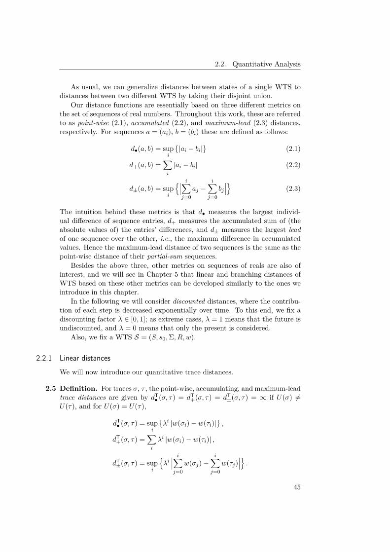
2.2. Quantitative Analysis

As usual, we can generalize distances between states of a single WTS todistances between two different WTS by taking their disjoint union.

Our distance functions are essentially based on three different metrics onthe set of sequences of real numbers. Throughout this work, these are referredto as point-wise (2.1), accumulated (2.2), and maximum-lead (2.3) distances,respectively. For sequences a = (ai), b = (bi) these are defined as follows:

d•(a, b) = supi

{|ai − bi|

}(2.1)

d+(a, b) =∑i

|ai − bi| (2.2)

d±(a, b) = supi

{∣∣∣ i∑j=0

aj −i∑

j=0bj∣∣∣} (2.3)

The intuition behind these metrics is that d• measures the largest individ-ual difference of sequence entries, d+ measures the accumulated sum of (theabsolute values of) the entries’ differences, and d± measures the largest leadof one sequence over the other, i.e., the maximum difference in accumulatedvalues. Hence the maximum-lead distance of two sequences is the same as thepoint-wise distance of their partial-sum sequences.

Besides the above three, other metrics on sequences of reals are also ofinterest, and we will see in Chapter 5 that linear and branching distances ofWTS based on these other metrics can be developed similarly to the ones weintroduce in this chapter.

In the following we will consider discounted distances, where the contribu-tion of each step is decreased exponentially over time. To this end, we fix adiscounting factor λ ∈ [0, 1]; as extreme cases, λ = 1 means that the future isundiscounted, and λ = 0 means that only the present is considered.

Also, we fix a WTS S = (S, s0,Σ, R,w).

2.2.1 Linear distances

We will now introduce our quantitative trace distances.

2.5 Definition. For traces σ, τ , the point-wise, accumulating, and maximum-leadtrace distances are given by dT

• (σ, τ) = dT+(σ, τ) = dT

±(σ, τ) = ∞ if U(σ) 6=U(τ), and for U(σ) = U(τ),

dT• (σ, τ) = sup

i

{λi |w(σi)− w(τi)|

},

dT+(σ, τ) =

∑i

λi |w(σi)− w(τi)| ,

dT±(σ, τ) = sup

i

{λi∣∣∣ i∑j=0

w(σj)−i∑

j=0w(τj)

∣∣∣} .45

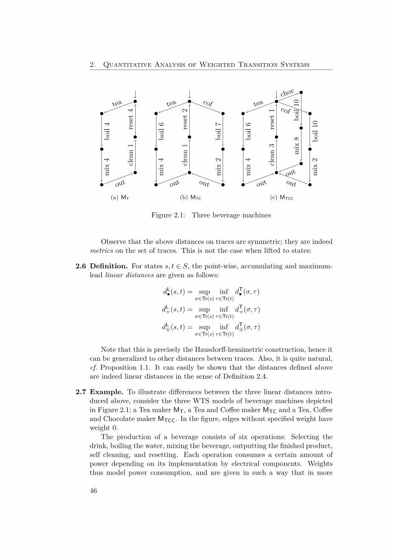
2. Quantitative Analysis of Weighted Transition Systems

tea

out

boil4

mix

4 clean1

reset4

(a) MT

tea

out

cof

out

boil6

mix

4 clean1

reset2

boil7

mix

2

(b) MTC

tea

out

choc

out

cof

out

boil6

mix

4 clean3

reset1

boil10

mix

2

boil10

mix

8

(c) MTCC

Figure 2.1: Three beverage machines

Observe that the above distances on traces are symmetric; they are indeedmetrics on the set of traces. This is not the case when lifted to states:

2.6 Definition. For states s, t ∈ S, the point-wise, accumulating and maximum-lead linear distances are given as follows:

dL•(s, t) = sup

σ∈Tr(s)inf

τ∈Tr(t)dT• (σ, τ)

dL+(s, t) = sup

σ∈Tr(s)inf

τ∈Tr(t)dT

+(σ, τ)

dL±(s, t) = sup

σ∈Tr(s)inf

τ∈Tr(t)dT±(σ, τ)

Note that this is precisely the Hausdorff-hemimetric construction, hence itcan be generalized to other distances between traces. Also, it is quite natural,cf. Proposition 1.1. It can easily be shown that the distances defined aboveare indeed linear distances in the sense of Definition 2.4.

2.7 Example. To illustrate differences between the three linear distances intro-duced above, consider the three WTS models of beverage machines depictedin Figure 2.1; a Tea maker MT, a Tea and Coffee maker MTC and a Tea, Coffeeand Chocolate maker MTCC. In the figure, edges without specified weight haveweight 0.

The production of a beverage consists of six operations: Selecting thedrink, boiling the water, mixing the beverage, outputting the finished product,self cleaning, and resetting. Each operation consumes a certain amount ofpower depending on its implementation by electrical components. Weightsthus model power consumption, and are given in such a way that in more

46

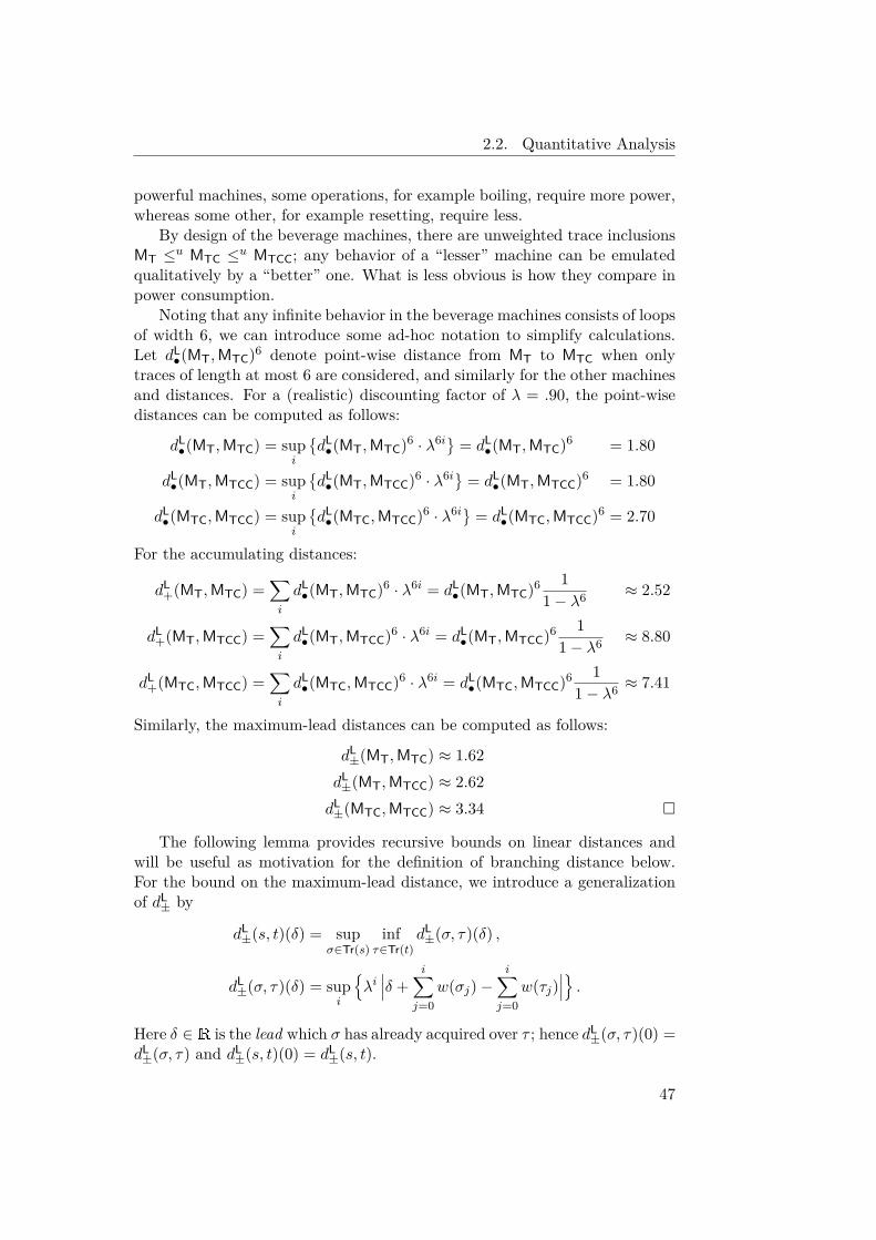
2.2. Quantitative Analysis

powerful machines, some operations, for example boiling, require more power,whereas some other, for example resetting, require less.

By design of the beverage machines, there are unweighted trace inclusionsMT ≤u MTC ≤u MTCC; any behavior of a “lesser” machine can be emulatedqualitatively by a “better” one. What is less obvious is how they compare inpower consumption.

Noting that any infinite behavior in the beverage machines consists of loopsof width 6, we can introduce some ad-hoc notation to simplify calculations.Let dL

•(MT,MTC)6 denote point-wise distance from MT to MTC when onlytraces of length at most 6 are considered, and similarly for the other machinesand distances. For a (realistic) discounting factor of λ = .90, the point-wisedistances can be computed as follows:

dL•(MT,MTC) = sup

i

{dL•(MT,MTC)6 · λ6i} = dL

•(MT,MTC)6 = 1.80

dL•(MT,MTCC) = sup

i

{dL•(MT,MTCC)6 · λ6i} = dL

•(MT,MTCC)6 = 1.80

dL•(MTC,MTCC) = sup

i

{dL•(MTC,MTCC)6 · λ6i} = dL

•(MTC,MTCC)6 = 2.70

For the accumulating distances:

dL+(MT,MTC) =

∑i

dL•(MT,MTC)6 · λ6i = dL

•(MT,MTC)6 11− λ6 ≈ 2.52

dL+(MT,MTCC) =

∑i

dL•(MT,MTCC)6 · λ6i = dL

•(MT,MTCC)6 11− λ6 ≈ 8.80

dL+(MTC,MTCC) =

∑i

dL•(MTC,MTCC)6 · λ6i = dL

•(MTC,MTCC)6 11− λ6 ≈ 7.41

Similarly, the maximum-lead distances can be computed as follows:

dL±(MT,MTC) ≈ 1.62

dL±(MT,MTCC) ≈ 2.62

dL±(MTC,MTCC) ≈ 3.34 �

The following lemma provides recursive bounds on linear distances andwill be useful as motivation for the definition of branching distance below.For the bound on the maximum-lead distance, we introduce a generalizationof dL

± by

dL±(s, t)(δ) = sup

σ∈Tr(s)inf

τ∈Tr(t)dL±(σ, τ)(δ) ,

dL±(σ, τ)(δ) = sup

i

{λi∣∣∣δ +

i∑j=0

w(σj)−i∑

j=0w(τj)

∣∣∣} .Here δ ∈ R is the lead which σ has already acquired over τ ; hence dL

±(σ, τ)(0) =dL±(σ, τ) and dL

±(s, t)(0) = dL±(s, t).

47

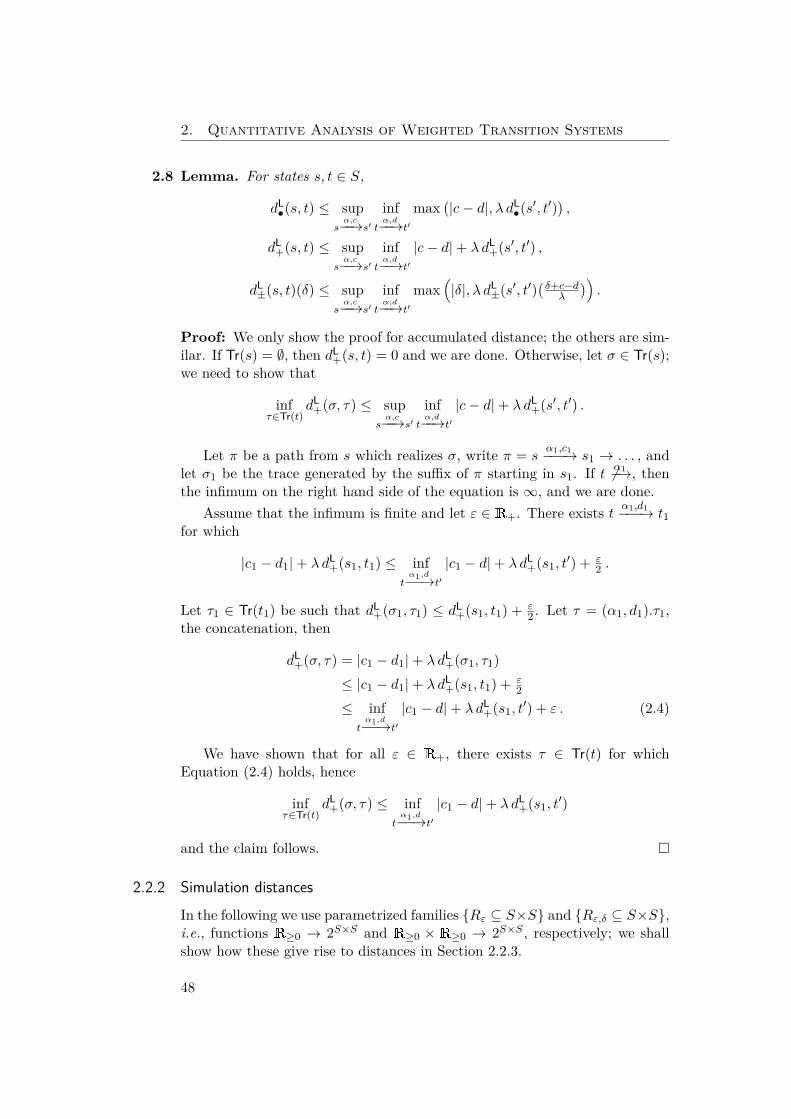
2. Quantitative Analysis of Weighted Transition Systems

2.8 Lemma. For states s, t ∈ S,

dL•(s, t) ≤ sup

sα,c−−→s′

inftα,d−−→t′

max(|c− d|, λ dL

•(s′, t′)),

dL+(s, t) ≤ sup

sα,c−−→s′

inftα,d−−→t′

|c− d|+ λ dL+(s′, t′) ,

dL±(s, t)(δ) ≤ sup

sα,c−−→s′

inftα,d−−→t′

max(|δ|, λ dL

±(s′, t′)(δ+c−dλ

)).

Proof: We only show the proof for accumulated distance; the others are sim-ilar. If Tr(s) = ∅, then dL

+(s, t) = 0 and we are done. Otherwise, let σ ∈ Tr(s);we need to show that

infτ∈Tr(t)

dL+(σ, τ) ≤ sup

sα,c−−→s′

inftα,d−−→t′

|c− d|+ λ dL+(s′, t′) .

Let π be a path from s which realizes σ, write π = sα1,c1−−−→ s1 → . . . , and

let σ1 be the trace generated by the suffix of π starting in s1. If t 6 α1−→, thenthe infimum on the right hand side of the equation is ∞, and we are done.

Assume that the infimum is finite and let ε ∈ R+. There exists t α1,d1−−−→ t1for which

|c1 − d1|+ λ dL+(s1, t1) ≤ inf

tα1,d−−→t′

|c1 − d|+ λ dL+(s1, t

′) + ε2 .

Let τ1 ∈ Tr(t1) be such that dL+(σ1, τ1) ≤ dL

+(s1, t1) + ε2 . Let τ = (α1, d1).τ1,

the concatenation, then

dL+(σ, τ) = |c1 − d1|+ λ dL

+(σ1, τ1)≤ |c1 − d1|+ λ dL

+(s1, t1) + ε2

≤ inftα1,d−−→t′

|c1 − d|+ λ dL+(s1, t

′) + ε . (2.4)

We have shown that for all ε ∈ R+, there exists τ ∈ Tr(t) for whichEquation (2.4) holds, hence

infτ∈Tr(t)

dL+(σ, τ) ≤ inf

tα1,d−−→t′

|c1 − d|+ λ dL+(s1, t

′)

and the claim follows. �

2.2.2 Simulation distancesIn the following we use parametrized families {Rε ⊆ S×S} and {Rε,δ ⊆ S×S},i.e., functions R≥0 → 2S×S and R≥0 × R≥0 → 2S×S , respectively; we shallshow how these give rise to distances in Section 2.2.3.

48

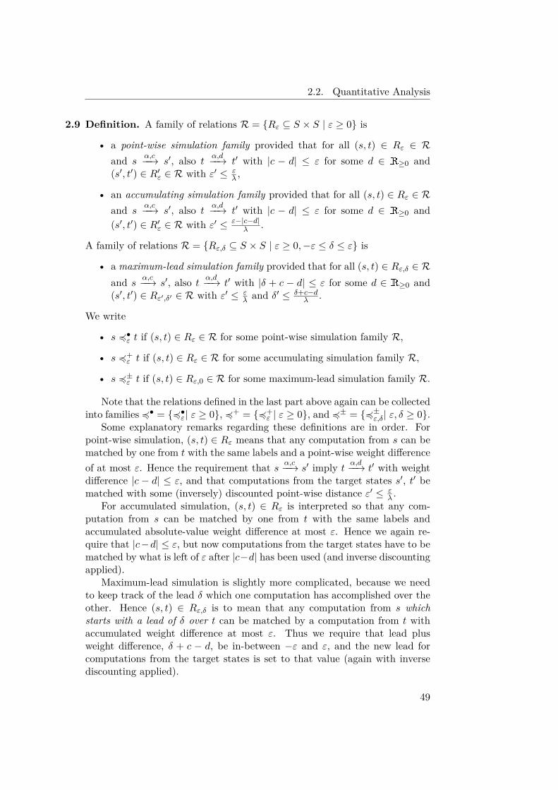
2.2. Quantitative Analysis

2.9 Definition. A family of relations R = {Rε ⊆ S × S | ε ≥ 0} is

• a point-wise simulation family provided that for all (s, t) ∈ Rε ∈ Rand s

α,c−−→ s′, also tα,d−−→ t′ with |c − d| ≤ ε for some d ∈ R≥0 and

(s′, t′) ∈ R′ε ∈ R with ε′ ≤ ελ ,

• an accumulating simulation family provided that for all (s, t) ∈ Rε ∈ Rand s

α,c−−→ s′, also tα,d−−→ t′ with |c − d| ≤ ε for some d ∈ R≥0 and

(s′, t′) ∈ R′ε ∈ R with ε′ ≤ ε−|c−d|λ .

A family of relations R = {Rε,δ ⊆ S × S | ε ≥ 0,−ε ≤ δ ≤ ε} is

• a maximum-lead simulation family provided that for all (s, t) ∈ Rε,δ ∈ Rand s α,c−−→ s′, also t α,d−−→ t′ with |δ + c − d| ≤ ε for some d ∈ R≥0 and(s′, t′) ∈ Rε′,δ′ ∈ R with ε′ ≤ ε

λ and δ′ ≤ δ+c−dλ .

We write

• s 4•ε t if (s, t) ∈ Rε ∈ R for some point-wise simulation family R,

• s 4+ε t if (s, t) ∈ Rε ∈ R for some accumulating simulation family R,

• s 4±ε t if (s, t) ∈ Rε,0 ∈ R for some maximum-lead simulation family R.

Note that the relations defined in the last part above again can be collectedinto families 4• = {4•ε| ε ≥ 0}, 4+ = {4+

ε | ε ≥ 0}, and 4± = {4±ε,δ| ε, δ ≥ 0}.Some explanatory remarks regarding these definitions are in order. For

point-wise simulation, (s, t) ∈ Rε means that any computation from s can bematched by one from t with the same labels and a point-wise weight differenceof at most ε. Hence the requirement that s α,c−−→ s′ imply t α,d−−→ t′ with weightdifference |c − d| ≤ ε, and that computations from the target states s′, t′ bematched with some (inversely) discounted point-wise distance ε′ ≤ ε

λ .For accumulated simulation, (s, t) ∈ Rε is interpreted so that any com-

putation from s can be matched by one from t with the same labels andaccumulated absolute-value weight difference at most ε. Hence we again re-quire that |c−d| ≤ ε, but now computations from the target states have to bematched by what is left of ε after |c−d| has been used (and inverse discountingapplied).

Maximum-lead simulation is slightly more complicated, because we needto keep track of the lead δ which one computation has accomplished over theother. Hence (s, t) ∈ Rε,δ is to mean that any computation from s whichstarts with a lead of δ over t can be matched by a computation from t withaccumulated weight difference at most ε. Thus we require that lead plusweight difference, δ + c − d, be in-between −ε and ε, and the new lead forcomputations from the target states is set to that value (again with inversediscounting applied).

49

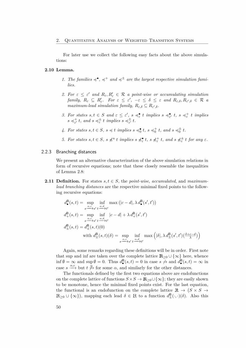
2. Quantitative Analysis of Weighted Transition Systems

For later use we collect the following easy facts about the above simula-tions:

2.10 Lemma.

1. The families 4•, 4+ and 4± are the largest respective simulation fami-lies.

2. For ε ≤ ε′ and Rε, R′ε ∈ R a point-wise or accumulating simulation

family, Rε ⊆ R′ε. For ε ≤ ε′, −ε ≤ δ ≤ ε and Rε,δ, Rε′,δ ∈ R amaximum-lead simulation family, Rε,δ ⊆ Rε′,δ.

3. For states s, t ∈ S and ε ≤ ε′, s 4•ε t implies s 4•ε′ t, s 4+ε t implies

s 4+ε′ t, and s 4±ε t implies s 4±ε′ t.

4. For states s, t ∈ S, s 4 t implies s 4•0 t, s 4+0 t, and s 4±0 t.

5. For states s, t ∈ S, s 64u t implies s 64•ε t, s 64+ε t, and s 64±ε t for any ε.

2.2.3 Branching distancesWe present an alternative characterization of the above simulation relations inform of recursive equations; note that these closely resemble the inequalitiesof Lemma 2.8:

2.11 Definition. For states s, t ∈ S, the point-wise, accumulated, and maximum-lead branching distances are the respective minimal fixed points to the follow-ing recursive equations:

dB• (s, t) = sup

sα,c−−→s′

inftα,d−−→t′

max(|c− d|, λ dB

• (s′, t′))

dB+(s, t) = sup

sα,c−−→s′

inftα,d−−→t′

|c− d|+ λ dB+(s′, t′)

dB±(s, t) = dB

±(s, t)(0)

with dB±(s, t)(δ) = sup

sα,c−−→s′

inftα,d−−→t′

max(|δ|, λ dB

±(s′, t′)(δ+c−dλ

))

Again, some remarks regarding these definitions will be in order. First notethat sup and inf are taken over the complete lattice R≥0 ∪ {∞} here, whenceinf ∅ = ∞ and sup ∅ = 0. Thus dB

• (s, t) = 0 in case s 6→ and dB• (s, t) = ∞ in

case s α,c−−→ but t 6 α−→ for some α, and similarly for the other distances.The functionals defined by the first two equations above are endofunctions

on the complete lattice of functions S×S → R≥0∪{∞}; they are easily shownto be monotone, hence the minimal fixed points exist. For the last equation,the functional is an endofunction on the complete lattice R →

(S × S →

R≥0 ∪ {∞}), mapping each lead δ ∈ R to a function dB

±(·, ·)(δ). Also this

50

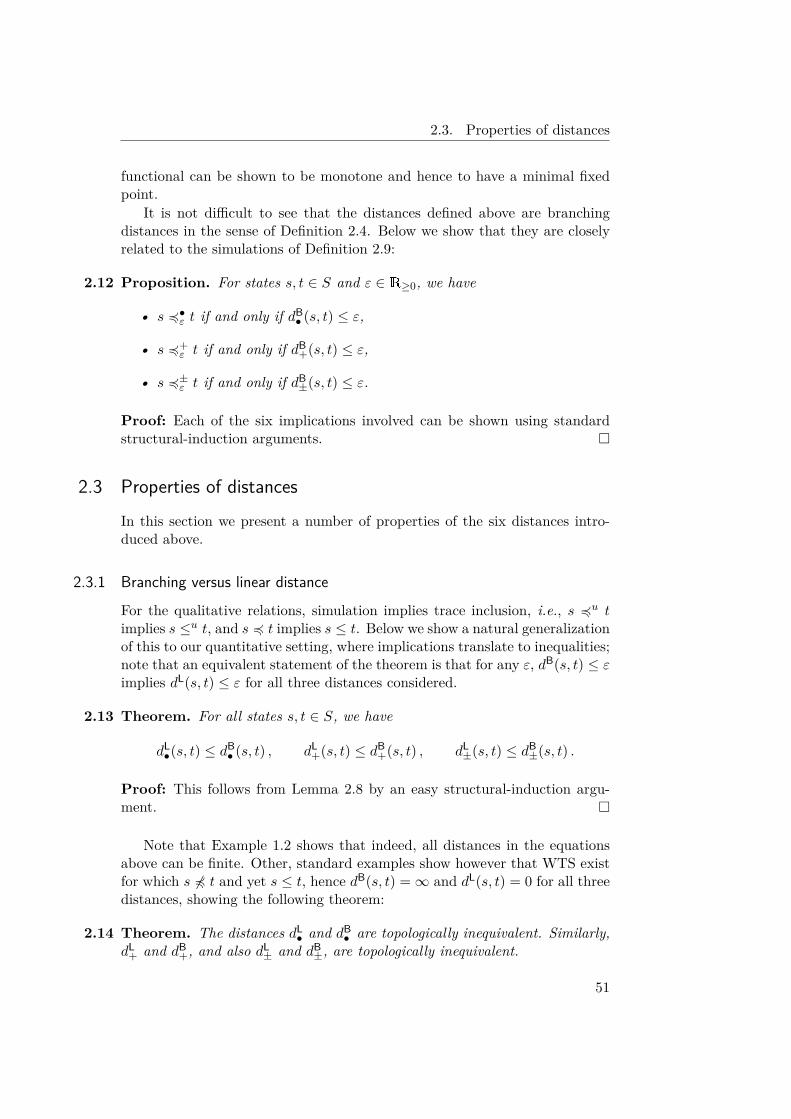
2.3. Properties of distances

functional can be shown to be monotone and hence to have a minimal fixedpoint.

It is not difficult to see that the distances defined above are branchingdistances in the sense of Definition 2.4. Below we show that they are closelyrelated to the simulations of Definition 2.9:

2.12 Proposition. For states s, t ∈ S and ε ∈ R≥0, we have

• s 4•ε t if and only if dB• (s, t) ≤ ε,

• s 4+ε t if and only if dB

+(s, t) ≤ ε,

• s 4±ε t if and only if dB±(s, t) ≤ ε.

Proof: Each of the six implications involved can be shown using standardstructural-induction arguments. �

2.3 Properties of distancesIn this section we present a number of properties of the six distances intro-duced above.

2.3.1 Branching versus linear distance

For the qualitative relations, simulation implies trace inclusion, i.e., s 4u timplies s ≤u t, and s 4 t implies s ≤ t. Below we show a natural generalizationof this to our quantitative setting, where implications translate to inequalities;note that an equivalent statement of the theorem is that for any ε, dB(s, t) ≤ εimplies dL(s, t) ≤ ε for all three distances considered.

2.13 Theorem. For all states s, t ∈ S, we have

dL•(s, t) ≤ dB

• (s, t) , dL+(s, t) ≤ dB

+(s, t) , dL±(s, t) ≤ dB

±(s, t) .

Proof: This follows from Lemma 2.8 by an easy structural-induction argu-ment. �

Note that Example 1.2 shows that indeed, all distances in the equationsabove can be finite. Other, standard examples show however that WTS existfor which s 64 t and yet s ≤ t, hence dB(s, t) =∞ and dL(s, t) = 0 for all threedistances, showing the following theorem:

2.14 Theorem. The distances dL• and dB

• are topologically inequivalent. Similarly,dL

+ and dB+, and also dL

± and dB±, are topologically inequivalent.

51

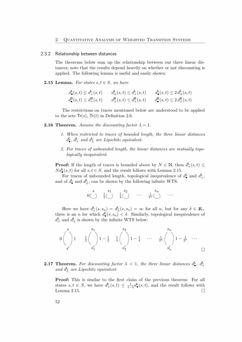
2. Quantitative Analysis of Weighted Transition Systems

2.3.2 Relationship between distancesThe theorems below sum up the relationship between our three linear dis-tances; note that the results depend heavily on whether or not discounting isapplied. The following lemma is useful and easily shown:

2.15 Lemma. For states s, t ∈ S, we have

dL•(s, t) ≤ dL

+(s, t) dL±(s, t) ≤ dL

+(s, t) dL•(s, t) ≤ 2 dL

±(s, t)dB• (s, t) ≤ dB

+(s, t) dB±(s, t) ≤ dB

+(s, t) dB• (s, t) ≤ 2 dB

±(s, t)

The restrictions on traces mentioned below are understood to be appliedto the sets Tr(s), Tr(t) in Definition 2.6.

2.16 Theorem. Assume the discounting factor λ = 1.

1. When restricted to traces of bounded length, the three linear distancesdL•, dL

+ and dL± are Lipschitz equivalent.

2. For traces of unbounded length, the linear distances are mutually topo-logically inequivalent.

Proof: If the length of traces is bounded above by N ∈ N, then dL+(s, t) ≤

NdL•(s, t) for all s, t ∈ S, and the result follows with Lemma 2.15.For traces of unbounded length, topological inequivalence of dL

• and dL+,

and of dL• and dL

±, can be shown by the following infinite WTS:

s s1 s2· · ·

sn· · ·0 1

214

12n

Here we have dL+(s, sn) = dL

±(s, sn) = ∞ for all n, but for any δ ∈ R+there is an n for which dL

•(s, sn) < δ. Similarly, topological inequivalence ofdL

+ and dL± is shown by the infinite WTS below:

s s1 s2 sn

s′ s′1 s′2

· · ·

s′n

· · ·0 12

14

12n1 1− 1

2 1− 14 1− 1

2n

�

2.17 Theorem. For discounting factor λ < 1, the three linear distances dL•, dL

+and dL

± are Lipschitz equivalent.

Proof: This is similar to the first claim of the previous theorem: For allstates s, t ∈ S, we have dL

+(s, t) ≤ 11−λd

L•(s, t), and the result follows with

Lemma 2.15. �

52

2.4. Conclusion

2.18 Theorem. For discounting factor λ = 1, the three branching distances dB• , dB

+and dB

± are mutually topologically inequivalent. For λ < 1, they are Lipschitzequivalent.

Proof: The first claim can be shown using the same example WTS as for thesecond part of the proof of Theorem 2.16, and for the second claim we havedB

+(s, t) ≤ 11−λd

B• (s, t) and can apply Lemma 2.15. �

2.4 ConclusionWe have argued above that our proposed extension of the qualitative notionof trace inclusion and simulation to a quantitative setting is reasonable.

For the three types of distances considered in this chapter, we have seenthat linear distances can easily be introduced, whereas definition of branchingdistances requires more work and involves fixed-point computations. OurLemma 2.8 remedies some of these difficulties, and we expect this remedyto also be applicable for other interesting trace distances. We will show inChapter 5 that a general procedure for obtaining branching distances fromlinear distances is available.

We have shown that all our three linear distances are topologically inequiv-alent to their corresponding branching distance, thus measure inherently dif-ferent properties. Still, and analogously to the qualitative setting, the branch-ing distance can be used as an over-approximation of the linear distance. Also,and perhaps more surprisingly, whether different linear or branching distancesare mutually equivalent depends on the usage of discounting. We expect mostof these results to also hold for other kinds of trace distances, see again Chap-ter 5.

We have mentioned earlier that in this work we concentrate on trace inclu-sion and simulation (asymmetric) distances, and of course similar treatmentshould be given to trace equivalence and bisimulation distances. Symmetriclinear distances are easily defined as symmetrizations of the linear distancesintroduced here, but for the branching distances there are subtle differencesbetween symmetrized simulation distances on the one hand and bisimulationdistances on the other hand. The next chapter will be concerned with bisim-ulation distances.

53

3 A Quantitative Characterization ofWeighted Kripke Structures inTemporal Logic1

This chapter is concerned with weighted Kripke structures (WKS), which rep-resent a straight-forward extension of Kripke structures with a weighted tran-sition relation labeling each transition. It then proceeds to define a weightedversion of Computation Tree Logic (WCTL) together with two different se-mantics which mirror the point-wise and accumulating distances of the previ-ous chapter. It is then shown that WCTL is adequate and expressive for thecorresponding bisimulation distances.

3.1 PreliminariesAs in Chapter 2, the results presented in this chapter are based on metrics onsequences of real numbers. Let a = (ai) and b = (bi) be such sequences, wethen define for λ ∈ ]0, 1[ the following basic distances:

d+(a, b) =∑i

λi|ai − bi| (3.1)

d•(a, b) = supi{λi|ai − bi|} (3.2)

Throughout the chapter we will refer to (3.1) and (3.2), as well other distancesbased on these, as an accumulating distance and as a point-wise distance,respectively. For the remainder of this chapter we fix a discounting factor λ ∈]0, 1[; note that contrary to the previous chapter, we here assume 0 < λ < 1.

We proceed to introduce WKS. A natural interpretation is to view thelabellings as the cost of taking transitions in the structure. This extension issimilar to the one presented in Chapter 2 for labeled transition systems, thusthe results presented in the previous chapter are transferable to the currentsetting.

1This chapter is based on the journal paper [FLT10] published in Computing and Infor-matics.

55

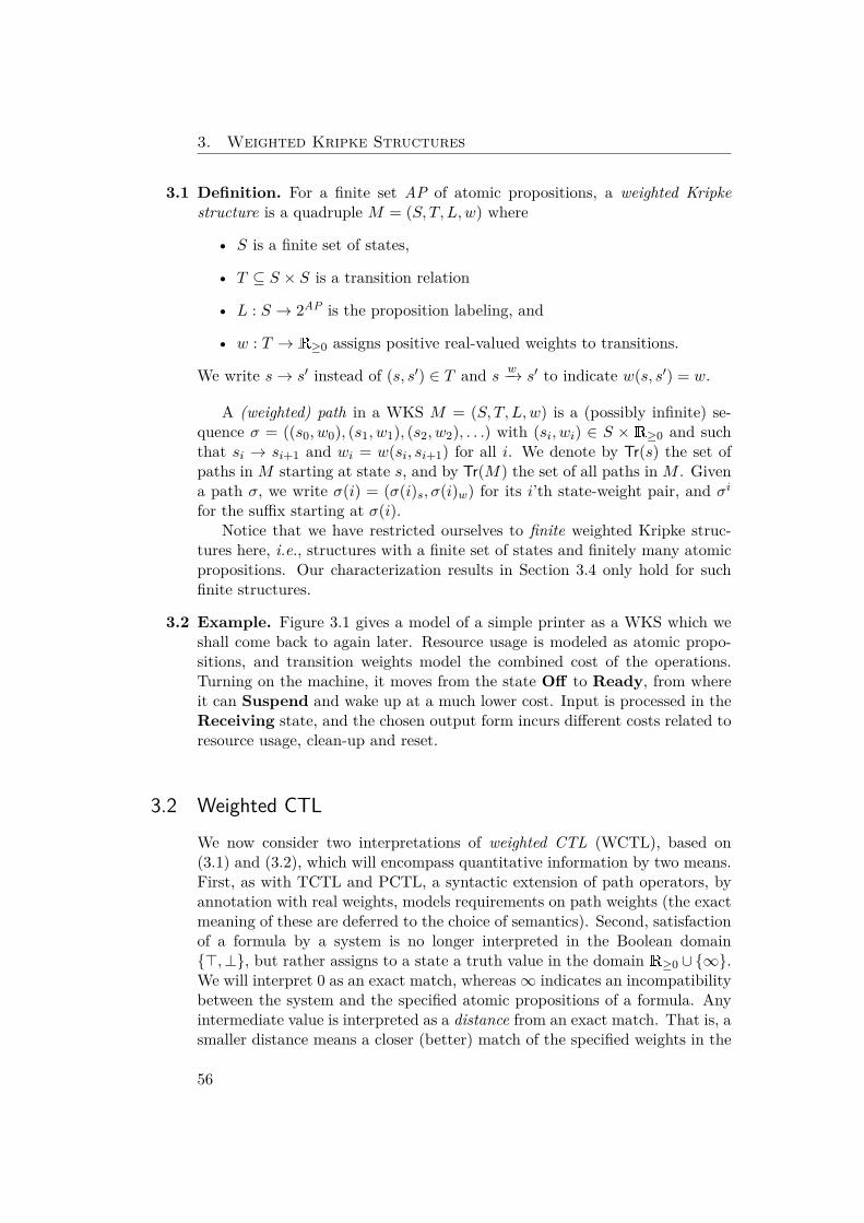
3. Weighted Kripke Structures

3.1 Definition. For a finite set AP of atomic propositions, a weighted Kripkestructure is a quadruple M = (S, T, L,w) where

• S is a finite set of states,

• T ⊆ S × S is a transition relation

• L : S → 2AP is the proposition labeling, and

• w : T → R≥0 assigns positive real-valued weights to transitions.

We write s→ s′ instead of (s, s′) ∈ T and s w−→ s′ to indicate w(s, s′) = w.

A (weighted) path in a WKS M = (S, T, L,w) is a (possibly infinite) se-quence σ = ((s0, w0), (s1, w1), (s2, w2), . . .) with (si, wi) ∈ S ×R≥0 and suchthat si → si+1 and wi = w(si, si+1) for all i. We denote by Tr(s) the set ofpaths in M starting at state s, and by Tr(M) the set of all paths in M . Givena path σ, we write σ(i) = (σ(i)s, σ(i)w) for its i’th state-weight pair, and σifor the suffix starting at σ(i).

Notice that we have restricted ourselves to finite weighted Kripke struc-tures here, i.e., structures with a finite set of states and finitely many atomicpropositions. Our characterization results in Section 3.4 only hold for suchfinite structures.

3.2 Example. Figure 3.1 gives a model of a simple printer as a WKS which weshall come back to again later. Resource usage is modeled as atomic propo-sitions, and transition weights model the combined cost of the operations.Turning on the machine, it moves from the state Off to Ready, from whereit can Suspend and wake up at a much lower cost. Input is processed in theReceiving state, and the chosen output form incurs different costs related toresource usage, clean-up and reset.

3.2 Weighted CTLWe now consider two interpretations of weighted CTL (WCTL), based on(3.1) and (3.2), which will encompass quantitative information by two means.First, as with TCTL and PCTL, a syntactic extension of path operators, byannotation with real weights, models requirements on path weights (the exactmeaning of these are deferred to the choice of semantics). Second, satisfactionof a formula by a system is no longer interpreted in the Boolean domain{>,⊥}, but rather assigns to a state a truth value in the domain R≥0 ∪ {∞}.We will interpret 0 as an exact match, whereas∞ indicates an incompatibilitybetween the system and the specified atomic propositions of a formula. Anyintermediate value is interpreted as a distance from an exact match. That is, asmaller distance means a closer (better) match of the specified weights in the

56

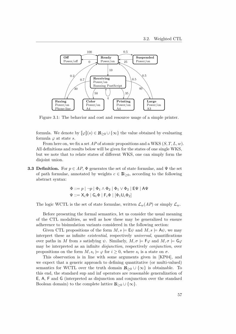
3.2. Weighted CTL

OffPower/off

ReadyPower/on

SuspendedPower/on

ReceivingPower/onRunning PostScript

PrintingPower/onA4

ColorPower/onA4

FaxingPower/onPhone-line

LargePower/onA3

100 0.5

0 25

10

3050

435

40

0.50.50.7

0.2

Figure 3.1: The behavior and cost and resource usage of a simple printer.

formula. We denote by JϕK(s) ∈ R≥0 ∪ {∞} the value obtained by evaluatingformula ϕ at state s.

From here on, we fix a setAP of atomic propositions and aWKS (S, T, L,w).All definitions and results below will be given for the states of one single WKS,but we note that to relate states of different WKS, one can simply form thedisjoint union.

3.3 Definition. For p ∈ AP, Φ generates the set of state formulae, and Ψ the setof path formulae, annotated by weights c ∈ R≥0, according to the followingabstract syntax:

Φ ::= p | ¬p | Φ1 ∧ Φ2 | Φ1 ∨ Φ2 | EΨ | AΨΨ ::= XcΦ | GcΦ | FcΦ | [Φ1UcΦ2]

The logic WCTL is the set of state formulae, written Lw(AP) or simply Lw.

Before presenting the formal semantics, let us consider the usual meaningof the CTL modalities, as well as how these may be generalized to ensureadherence to bisimulation variants considered in the following section:

Given CTL propositions of the form M, s |= Eψ and M, s |= Aψ, we mayinterpret these as infinite existential, respectively universal, quantificationsover paths in M from s satisfying ψ. Similarly, M,σ |= Fϕ and M,σ |= Gϕmay be interpreted as an infinite disjunction, respectively conjunction, overpropositions on the form M, si |= ϕ for i ≥ 0, where si is a state on σ.

This observation is in line with some arguments given in [KP04], andwe expect that a generic approach to defining quantitative (or multi-valued)semantics for WCTL over the truth domain R≥0 ∪ {∞} is obtainable. Tothis end, the standard sup and inf operators are reasonable generalization ofE, A, F and G (interpreted as disjunction and conjunction over the standardBoolean domain) to the complete lattice R≥0 ∪ {∞}.

57

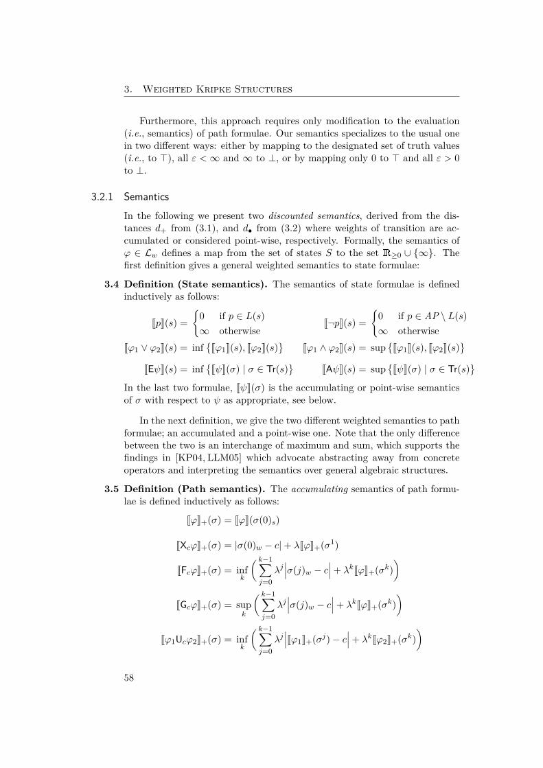
3. Weighted Kripke Structures

Furthermore, this approach requires only modification to the evaluation(i.e., semantics) of path formulae. Our semantics specializes to the usual onein two different ways: either by mapping to the designated set of truth values(i.e., to >), all ε <∞ and ∞ to ⊥, or by mapping only 0 to > and all ε > 0to ⊥.

3.2.1 SemanticsIn the following we present two discounted semantics, derived from the dis-tances d+ from (3.1), and d• from (3.2) where weights of transition are ac-cumulated or considered point-wise, respectively. Formally, the semantics ofϕ ∈ Lw defines a map from the set of states S to the set R≥0 ∪ {∞}. Thefirst definition gives a general weighted semantics to state formulae:

3.4 Definition (State semantics). The semantics of state formulae is definedinductively as follows:

JpK(s) ={

0 if p ∈ L(s)∞ otherwise

J¬pK(s) ={

0 if p ∈ AP \ L(s)∞ otherwise

Jϕ1 ∨ ϕ2K(s) = inf{Jϕ1K(s), Jϕ2K(s)

}Jϕ1 ∧ ϕ2K(s) = sup

{Jϕ1K(s), Jϕ2K(s)

}JEψK(s) = inf

{JψK(σ) | σ ∈ Tr(s)

}JAψK(s) = sup

{JψK(σ) | σ ∈ Tr(s)

}In the last two formulae, JψK(σ) is the accumulating or point-wise semanticsof σ with respect to ψ as appropriate, see below.

In the next definition, we give the two different weighted semantics to pathformulae; an accumulated and a point-wise one. Note that the only differencebetween the two is an interchange of maximum and sum, which supports thefindings in [KP04, LLM05] which advocate abstracting away from concreteoperators and interpreting the semantics over general algebraic structures.

3.5 Definition (Path semantics). The accumulating semantics of path formu-lae is defined inductively as follows:

JϕK+(σ) = JϕK(σ(0)s)

JXcϕK+(σ) = |σ(0)w − c|+ λJϕK+(σ1)

JFcϕK+(σ) = infk

( k−1∑j=0

λj∣∣∣σ(j)w − c

∣∣∣+ λkJϕK+(σk))

JGcϕK+(σ) = supk

( k−1∑j=0

λj∣∣∣σ(j)w − c

∣∣∣+ λkJϕK+(σk))

Jϕ1Ucϕ2K+(σ) = infk

( k−1∑j=0

λj∣∣∣Jϕ1K+(σj)− c

∣∣∣+ λkJϕ2K+(σk))

58

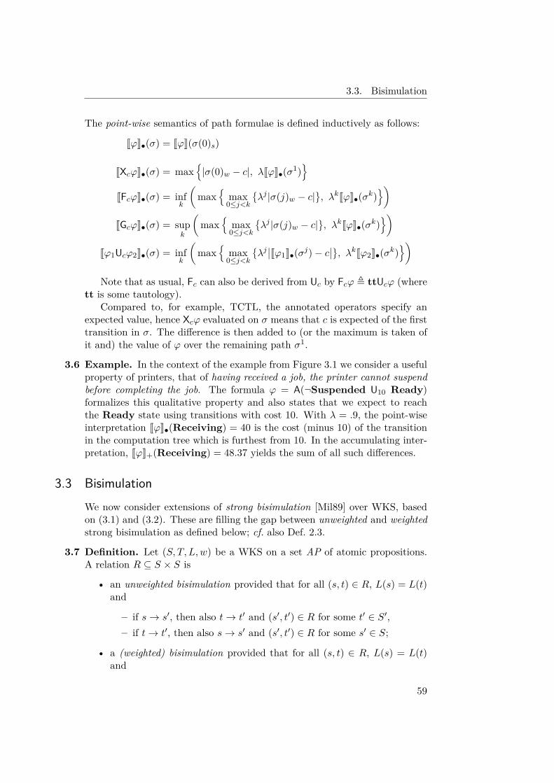
3.3. Bisimulation

The point-wise semantics of path formulae is defined inductively as follows:

JϕK•(σ) = JϕK(σ(0)s)

JXcϕK•(σ) = max{|σ(0)w − c|, λJϕK•(σ1)

}JFcϕK•(σ) = inf

k

(max

{max

0≤j<k

{λj |σ(j)w − c|

}, λkJϕK•(σk)

})JGcϕK•(σ) = sup

k

(max

{max

0≤j<k

{λj |σ(j)w − c|

}, λkJϕK•(σk)

})Jϕ1Ucϕ2K•(σ) = inf

k

(max

{max

0≤j<k

{λj∣∣Jϕ1K•(σj)− c

∣∣}, λkJϕ2K•(σk)})

Note that as usual, Fc can also be derived from Uc by Fcϕ , ttUcϕ (wherett is some tautology).

Compared to, for example, TCTL, the annotated operators specify anexpected value, hence Xcϕ evaluated on σ means that c is expected of the firsttransition in σ. The difference is then added to (or the maximum is taken ofit and) the value of ϕ over the remaining path σ1.

3.6 Example. In the context of the example from Figure 3.1 we consider a usefulproperty of printers, that of having received a job, the printer cannot suspendbefore completing the job. The formula ϕ = A(¬Suspended U10 Ready)formalizes this qualitative property and also states that we expect to reachthe Ready state using transitions with cost 10. With λ = .9, the point-wiseinterpretation JϕK•(Receiving) = 40 is the cost (minus 10) of the transitionin the computation tree which is furthest from 10. In the accumulating inter-pretation, JϕK+(Receiving) = 48.37 yields the sum of all such differences.

3.3 BisimulationWe now consider extensions of strong bisimulation [Mil89] over WKS, basedon (3.1) and (3.2). These are filling the gap between unweighted and weightedstrong bisimulation as defined below; cf. also Def. 2.3.

3.7 Definition. Let (S, T, L,w) be a WKS on a set AP of atomic propositions.A relation R ⊆ S × S is

• an unweighted bisimulation provided that for all (s, t) ∈ R, L(s) = L(t)and

– if s→ s′, then also t→ t′ and (s′, t′) ∈ R for some t′ ∈ S′,– if t→ t′, then also s→ s′ and (s′, t′) ∈ R for some s′ ∈ S;

• a (weighted) bisimulation provided that for all (s, t) ∈ R, L(s) = L(t)and

59

3. Weighted Kripke Structures

– if s c−→ s′, then also t c−→ t′ and (s′, t′) ∈ R for some t′ ∈ S′,– if t c−→ t′, then also s c−→ s′ and (s′, t′) ∈ R for some s′ ∈ S.

We write s ∼u t if (s, t) ∈ R for some unweighted bisimulation R, and s ∼ t if(s, t) ∈ R for some weighted bisimulation R.

The motivation for the variants defined below is that, in order to relatestructures, we do not always need perfect matching of transition weights;rather we would like to know how accurately weights are matched. As withthe simulation distances of Chapter 2, we call a bisimulation distance anypseudometric on the states of a WKS which mediates between unweightedand weighted bisimilarity:

3.8 Definition. A bisimulation distance on a WKS (S, T, L,w) is a function d :S × S → R≥0 ∪ {∞} which satisfies the following for all s1, s2, s3 ∈ S:

• d(s1, s1) = 0,

• d(s1, s2) + d(s2, s3) ≥ d(s1, s3),

• d(s1, s2) = d(s2, s1),

• s1 ∼ s2 implies d(s1, s2) = 0 and

• d(s1, s2) 6=∞ implies s1 ∼u s2

Our distances are based on distances of (infinite) sequences of realnumbers, which is appropriate, as for (s, t) in ∼u (or in ∼), any path(s, a, s1, a1, s2, . . . ) ∈ Tr(s) must be matched by an equal-length path(t, b, t1, b1, t2, . . . ) ∈ Tr(t) with (si, ti) in ∼u (respectively ∼).

By extending bisimulation with the d+ and d• distances, we collect a familyof relations {Rε ⊆ S×S} (i.e., a map R≥0 → 2S×S) since, due to discounting,for each step the distance between each successor pair may grow:

3.9 Definition. A family of relations R = {Rε ⊆ S × S | ε > 0} is

• an accumulating bisimulation family provided that for all (s, t) ∈ Rε ∈R, L(s) = L(t) and

– if s c−→ s′, then also t d−→ t′ with |c − d| ≤ ε for some d ∈ R≥0 and(s′, t′) ∈ Rε′ ∈ R with ε′λ ≤ ε− |c− d|, and

– if t c−→ t′, then also s d−→ s′ with |c − d| ≤ ε for some d ∈ R≥0 and(s′, t′) ∈ Rε′ ∈ R with ε′λ ≤ ε− |c− d|.

• a point-wise bisimulation family provided that for all (s, t) ∈ Rε ∈ R,L(s) = L(t) and

60

3.4. Characterization

– if s c−→ s′, then also t d−→ t′ with |c − d| ≤ ε for some d ∈ R≥0 and(s′, t′) ∈ Rε′ ∈ R with ε′λ ≤ ε, and

– if t c−→ t′, then also s d−→ s′ with |c − d| ≤ ε for some d ∈ R≥0 and(s′, t′) ∈ Rε′ ∈ R with ε′λ ≤ ε .

We write s ∼+ε t and s ∼•ε t, if (s, t) ∈ Rε ∈ R for an accumulating, respec-

tively point-wise, bisimulation family R.

Both variants of bisimulation families give raise to a bisimulation distancein the sense of Definition 3.8 by d+(s, t) = inf{ε | s ∼+

ε t} and d•(s, t) =inf{ε | s ∼•ε t}. Observe the following easy facts:

3.10 Lemma.

1. For ε ≤ ε′ and members Rε, Rε′ ∈ R of an accumulating or point-wisebisimulation family, Rε ⊆ Rε′.

2. Given s ∼+ε t, then every path σ = (s0, w0, s1, w1s2, . . . ) ∈ Tr(s) has a

corresponding path σ′ = (t0, w′0, t1, w′1t2, . . . ) ∈ Tr(t) such that ε = ε0and si ∼+

εi ti for all i, where εi+1λ = εi − |wi − w′i|.

3. Given s ∼•ε t, then every path σ = (s0, w0, s1, w1s2, . . . ) ∈ Tr(s) has acorresponding path σ′ = (t0, w′0, t1, w′1t2, . . . ) ∈ Tr(t) such that ε = ε0and si ∼•εi ti for all i, where εi+1λ = εi.

Note that as we only consider finite WKS, all Rε relations are finite. Also,we shall speak of corresponding paths when referring to the second and thirdproperties of the above lemma.

3.4 CharacterizationIn this section we show that the presented WCTL interpretations are adequateand expressive with respect to the appropriate bisimilarity variant.

3.4.1 AdequacyThe link between accumulating bisimilarity and our accumulating semanticsfor WCTL is as follows:

3.11 Theorem. For s, t ∈ S, s ∼+ε t iff ∀ϕ ∈ Lw :

∣∣JϕK+(s)− JϕK+(t)∣∣ ≤ ε.

The proof follows from Lemmas 3.15 and 3.16 below. Observe that thisprovides us with the following corollary which is precisely the standard notionof adequacy, see [HM85]:

3.12 Corollary. For s, t ∈ S, s ∼+0 t iff JϕK+(s) = JϕK+(t) for all ϕ ∈ Lw.

61

3. Weighted Kripke Structures

We obtain an equivalent result for the point-wise semantics:

3.13 Theorem. For s, t ∈ S, s ∼•ε t iff ∀ϕ ∈ Lw :∣∣JϕK•(s)− JϕK•(t)∣∣ ≤ ε.

3.14 Example. We consider again the printer from Figure 3.1. When ignoringColor and Printing as atomic propositions, we have Color ∼+

.2 Printing,as the two initial transition are the only difference. As a formula which realizesthis bisimulation distance one can take ϕ = power/on∧A4∧AX0.5Ready; thenJϕK+(Printing) = 0 and JϕK+(Color) = .2.

The proofs of adequacy, and also of expressivity below, for the accumulat-ing and point-wise cases are similar, hence we concentrate on the accumulat-ing case. In the proof we will repeatedly make use of the lesser-known littlebrother of the triangle inequality∣∣|x− y| − |x− z|∣∣ ≤ ∣∣y − z∣∣ .

3.15 Lemma. Let s, t ∈ S with s ∼+ε t, and let σ = (s, u, s1, u1, . . .) ∈ Tr(s), τ =

(t, v, t1, v1, . . .) ∈ Tr(t) be corresponding paths. Then∣∣JϕK+(s) − JϕK+(t)

∣∣ ≤ εfor all state formulae ϕ, and

∣∣JϕK+(σ)− JϕK+(τ)∣∣ ≤ ε for all path formulae ϕ.

Proof: We prove the lemma by structural induction in ϕ. The inductionbase is clear, as s ∼+

ε t implies that p ∈ L(s) if and only if p ∈ L(t), henceJϕK+(s) = JϕK+(t) for ϕ = p or ϕ = ¬p. For the inductive step, we examineeach syntactic construction in turn:

1. ϕ = ϕ1 ∨ ϕ2

There are four cases to consider, corresponding to whether Jϕ1K+(s) ≤Jϕ2K+(s) or Jϕ1K+(s) > Jϕ2K+(s) and similarly for Jϕ1K+(t) and Jϕ2K+(t).We show the proof for one of the “mixed” cases; the other three aresimilar or easier:Assume Jϕ1K+(s) ≤ Jϕ2K+(s) and Jϕ1K+(t) > Jϕ2K+(t). Then Jϕ1 ∨ϕ2K+(s)−Jϕ1∨ϕ2K+(t) = Jϕ1K+(s)−Jϕ2K+(t), and Jϕ1K+(s)−Jϕ1K+(t) ≤Jϕ1K+(s)−Jϕ2K+(t) ≤ Jϕ2K+(s)−Jϕ2K+(t), and by induction hypothesis,−ε ≤ Jϕ1K+(s)− Jϕ1K+(t) and Jϕ2K+(s)− Jϕ2K+(t) ≤ ε.

2. ϕ = ϕ1 ∧ ϕ2. This is similar to the previous case.

3. ϕ = Eϕ1

By definition of JEϕ1K+ there is a path σ ∈ Tr(s) for which Jϕ1K+(σ) =JϕK+(s). By Lemma 3.10 there is a corresponding path τ ∈ Tr(t), andfrom the induction hypothesis we know that |Jϕ1K+(σ)− Jϕ1K+(τ)| ≤ ε.Thus |JϕK+(s)− JϕK+(t)| ≤ ε.

4. ϕ = Aϕ1. This is similar to the previous case.

62

3.4. Characterization

5. ϕ = Xcϕ1

By definition, JϕK+(σ) = λJϕ1K+(σ1)+|c−u| and JϕK+(τ) = λJϕ1K+(τ1)+|c−v|, where σ = s

u−→ σ1 and τ = tv−→ τ1. Since s ∼+

ε t and σ and τ cor-respond, we have σ(1) ∼+

ε′ τ(1) with ε′λ ≤ ε− |u− v|, and by inductionhypothesis |Jϕ1K+(σ1) − Jϕ1K+(τ1)| ≤ ε′. Hence

∣∣JϕK+(σ) − JϕK+(τ)∣∣ ≤∣∣|c− u| − |c− v|∣∣+ λ

∣∣Jϕ1K+(σ1)− Jϕ2K+(τ1)∣∣ ≤ |u− v|+ ε− |u− v| = ε.

6. ϕ = Fcϕ1

Pick any δ > 0, then there is k ∈ N for which Sk = ∑k−1j=0 λ

j |σ(j)w −c| + λkJφK+(σk) ≤ JφK+(σ) + δ. As the paths σ and τ correspond, wealso have Tk = ∑k−1

j=0 λj |τ(j)w − c| + λkJφK+(τk) ≤ JφK+(τ) + δ. Re-

peated use of the definition of ∼+ε yields σ(k) ∼+

ε′ τ(k) with ε′λk ≤ε−

∑k−1j=0 λ

j∣∣σ(j)w− τ(j)w

∣∣, hence by induction hypothesis,∣∣JφK+(σk)−

JφK+(τk)∣∣ ≤ ε′. Thus ∣∣JφK+(σ)−JφK+(τ)

∣∣ ≤ ∣∣Sk−Tk∣∣+δ ≤∑k−1j=0 λ

j∣∣|σ(j)w−

c| − |τ(j)w − c|∣∣+ λk

∣∣JφK+(σk)− JφK+(τk)∣∣+ δ ≤ ε+ δ. As these consid-

erations hold for any δ > 0, we must have∣∣JφK+(σ)− JφK+(τ)

∣∣ ≤ ε.7. ϕ = Gcϕ1; ϕ = ϕ1Ucϕ2. These are similar to the previous case. �

3.16 Lemma. Let s, t ∈ S and assume that∣∣JϕK+(s) − JϕK+(t)

∣∣ ≤ ε for all stateformulae ϕ ∈ Lw. Then s ∼+

ε t.

Proof: This follows directly from Theorem 3.17 below, but one can also ob-serve that the accumulating family R = {Rε} defined by

Rε ={(s, t) | s, t ∈ S, ∀ϕ ∈ Lw :

∣∣JϕK+(s)− JϕK+(t)∣∣ ≤ ε}

is indeed an accumulating bisimulation in terms of Definition 3.9. �

3.4.2 ExpressivityWe show that WCTL with accumulating semantics is expressive with respectto accumulating bisimulation in the following sense:

3.17 Theorem. For each s ∈ S and every γ ∈ R+, there exists a state formulaϕsγ ∈ Lw, interpreted over the accumulating semantics, which characterizes sup to accumulating bisimulation and up to γ, i.e., such that for all s′ ∈ S,s ∼+

ε s′ if and only if JϕsγK+(s′) ∈ [ε− γ, ε+ γ] for all γ.

Proof: We define characteristic formulae of unfoldings, as follows: For eachs ∈ S and n ∈ N, denote L(s) = {p1, . . . , pk} and AP \ L(s) = {q1, . . . , q`}and let ϕ(s, n) be the WCTL formula defined inductively as follows:

ϕ(s, 0) = (p1 ∧ · · · ∧ pk) ∧ (¬q1 ∧ · · · ∧ ¬q`)

ϕ(s, n+ 1) =∧

sw−→s′

EXwϕ(s′, n) ∧∧

w:sw−→s′

AXw( ∨sw−→s′

ϕ(s′, n))∧ ϕ(s, 0)

63

3. Weighted Kripke Structures

It is easy to see that Jϕ(s, n)K+(s) = 0 for all n.To complete the proof, one observes that for each γ > 0, there is n(γ) ∈ N

such that ϕ(s, n(γ)) can play the role of φsγ in the theorem. Intuitively thisis due to discounting: The further the unfolding in ϕ(s, n), the higher are theweights discounted, hence from some n(γ) on, maximum weight difference isbelow γ. �

3.18 Theorem. For each s ∈ S and every γ ∈ R+, there exists a state formulaϕsγ ∈ Lw, interpreted over the point-wise semantics, which characterizes s upto point-wise bisimulation and up to γ, i.e., such that for all s′ ∈ S, s ∼•ε s′ ifand only if JϕsγK•(s′) ∈ [ε− γ, ε+ γ] for all γ.

3.5 ConclusionWe have shown in this chapter that weighted CTL with an accumulating se-mantics is adequate and expressive for accumulating bisimulation for weightedKripke structures. We have also seen that the same holds for the point-wisesemantics for WCTL with respect to point-wise bisimulation.

We will see in Chapter 5 that these results can be lifted to a common ab-stract framework which also encompasses other weighted bisimulations suchas the maximum-lead bisimulation of [HMP05] presented in the previous chap-ter.

64

4 Metrics for Weighted TransitionSystems: Axiomatization1

In this chapter we turn to axiomatizations of the point-wise and accumulatingsimulation distances. We first present axiomatizations for finite processes andthen for regular processes. We then show that the axiomatizations for finiteprocesses are sound and complete, whereas the ones for regular processes aresound and ε-complete.

4.1 Simulation distancesThroughout this chapter we fix a finite metric spaceK of weights with a metricdK : K ×K → R. We also fix a discounting factor λ with 0 ≤ λ < 1, whichwill be used in the definition of accumulating distance below.

4.1 Definition. A weighted transition system is a tuple (S, T ), where S is a finiteset of states and T ⊆ S ×K× S is a set of (weighted) transitions.

Note that all transition systems in this chapter are indeed assumed finite,hence requiring finiteness of the metric spaceK does not add extra restrictions.

We fix a weighted transition system (S, T ) and introduce simulation dis-tance between states in (S, T ). We concentrate on two types here, accumulat-ing and point-wise distance, but other kinds may indeed be defined.

4.1.1 Accumulating distance4.2 Definition. For states s, t ∈ S, the accumulating simulation distance from s

to t is defined to be the least fixed point to the set of equations

d+(s, t) = maxsn−→s′

mintm−→t′

(dK(n,m) + λd+(s′, t′)

). (4.1)

To justify this definition, we need to show that the equations (4.1) indeedhave a least solution. To this end, write S = {s1, . . . , sp} and assume for

1This chapter is based on the journal paper [LFT11] published in Theoretical ComputerScience.

65

4. Axiomatization

the moment that the transition system (S, T ) is non-blocking such that everysi ∈ S has an outgoing transition si n−→ sk for some sk ∈ S. Define a functionF : Rp×p

≥0 → Rp×p≥0 by

F (x)i,j = maxsi

n−→sk

minsj

m−→s`

(dK(n,m) + λxk,`

).

Here we are using the standard linear-algebra notation Rp×p≥0 for p×p-matrices

with entries in R≥0 and xk,` for the entry in their k’th row and `’th column.

4.3 Lemma. With metric on Rp×p≥0 defined by d(x, y) = maxpi,j=1 |xi,j −yi,j |, F is

a contraction with Lipschitz constant λ.

Proof: (Cf. also the proof of [ZP96, Thm. 5.1].) We can partition Rp×p≥0 into

finitely many (indeed at most 2p2q2 with q = |K|) closed polyhedral regionsRi,j (some of which may be unbounded) such that for x, y ∈ Ri,j in a commonregion, the p2 max-min equations get resolved to the same transitions. Inmore precise terms, there are mappings n,m, k, ` : {1, . . . , p} × {1, . . . , p} →{1, . . . , p} such that F (x)i,j = dK(n(i, j),m(i, j))+λxk(i,j),`(i,j) for all x ∈ Ri,j .

Now if x, y ∈ Ri,j are in a common region, then

d(F (x), F (y)) ≤ λmaxi,j|xk(i,j),`(i,j) − yk(i,j),`(i,j)|

≤ λmaxi,j|xi,j − yi,j | = λd(x, y) .

If x ∈ Ri1,j1 , y ∈ Ri2,j2 are in different regions, a bit more work is needed.The straight line segment between x and y admits finitely many intersectionpoints with the regions Ri,j ; denote these x = z0, . . . , zq = y. We have

d(F (x), F (y)) ≤ d(F (z0), F (z1)) + · · ·+ d(F (zq−1, zq))≤ λ

(d(z0, z1) + · · ·+ d(zq−1, zq)

)= λd(x, y) .

Note that the last equality only holds because all zi are on a straight line. �

Using the Banach fixed-point theorem and completeness of Rp×p≥0 we can

hence conclude that F has a unique fixed point. In the general case, where(S, T ) may not be non-blocking, F is a function [0,∞] → [0,∞] with (extra)fixed point [∞, . . . ,∞]. Hence as a function [0,∞] → [0,∞], F has at most

66

4.1. Simulation distances

two fixed points. Now we can write the equation set from the definition as

d+(s1, s1) d+(s1, s2) · · · d+(s1, sp)d+(s2, s1) d+(s2, s2) · · · d+(s2, sp)

...... . . . ...

d+(sp, s1) d+(sp, s2) · · · d+(sp, sp)

= F

d+(s1, s1) d+(s1, s2) · · · d+(s1, sp)d+(s2, s1) d+(s2, s2) · · · d+(s2, sp)

...... . . . ...

d+(sp, s1) d+(sp, s2) · · · d+(sp, sp)

,

hence (4.1) has indeed a unique least fixed point.

4.1.2 Point-wise distance

For point-wise simulation distance we follow a lattice-theoretic rather than acontraction approach.

4.4 Definition. For states s, t ∈ S, the point-wise simulation distance from s tot is defined to be the least fixed point to the set of equations

d•(s, t) = maxsn−→s′

mintm−→t′

max(dK(n,m), d•(s′, t′)

).

Note that in this chapter, the point-wise distance is undiscounted.Let G : [0,∞]p×p → [0,∞]p×p be the function defined by

G(x)i,j = maxsi

n−→sk

minsj

m−→s`

max(dK(n,m), xk,`

).

4.5 Lemma. With partial order on [0,∞]p×p defined by x ≤ y iff xi,j ≤ yi,j forall i, j, G is (weakly) increasing.

Proof: Trivial. �

Now the Tarski fixed-point theorem allows us to conclude that G has aunique least fixed point, hence the above definition is justified.

4.1.3 Properties

4.6 Proposition. The functions d+ and d• are hemimetrics on S.

67

4. Axiomatization

Proof: To show that d+(s, s) = d•(s, s) = 0 is trivial. The triangle inequal-ities can be shown inductively; we prove the one for d+: For s, t, u ∈ S, wehave

d+(s, t) + d+(t, u) = maxsn−→s′

mintm−→t′

(dK(n,m) + λd+(s′, t′)

)+ maxtm−→t′

minuz−→u′

(dK(m, z) + λd+(t′, u′)

)≥ max

sn−→s′

mintm−→t′

minuz−→u′

(dK(n,m) + dK(m, z)

+ λ(d+(s′, t′) + d+(t′, u′)

))≥ max

sn−→s′

minuz−→u′

(dK(n, z) + λd+(s′, u′)

)= d+(s, u)

assuming the triangle inequality has been proven for the triple (s′, t′, u′). �

In the next proposition we take the standard liberty of comparing different(weighted) transition systems by considering their disjoint union.

4.7 Proposition. The weighted transition systems 0 and U given as 0 = ({s1}, ∅)and U = ({s1}, {(s1, n, s1) | n ∈ K}) are respectively minimal and maximalelements with respect to both d+(·, ·) and d•(·, ·), that is, d+(0, A) = d•(0, A) =d+(A,U) = d•(A,U) = 0 for any WTS A.

Proof: For d+(0, A) and d•(0, A), the maximum maxs1 n−→s′1is taken over the

empty set and hence is 0. For d+(A,U) and d•(A,U), any transition s n−→ s′

in A can be matched by s1n−→ s1 in U, hence the distance is again 0. �

4.2 Axiomatizations for Finite Weighted Processes

We now turn to a setting where our weighted transition systems are generatedby finite or regular (weighted) process expressions. We construct a sound andcomplete axiomatization of simulation distance in a setting without recursionfirst and show afterwards how this may be extended to a setting with recursion.

Let P be the set of process expressions generated by the following gram-mar:

E ::= 0 | n.E | E + E | n ∈ K

Here 0 is used to denote the empty process, cf. Proposition 4.7.The semantics of finite process expressions is a weighted transition system

generated by the following standard SOS rules:

n.En−→ E

E1n−→ E′1

E1 + E2n−→ E′1

E2n−→ E′2

E1 + E2n−→ E′2

68

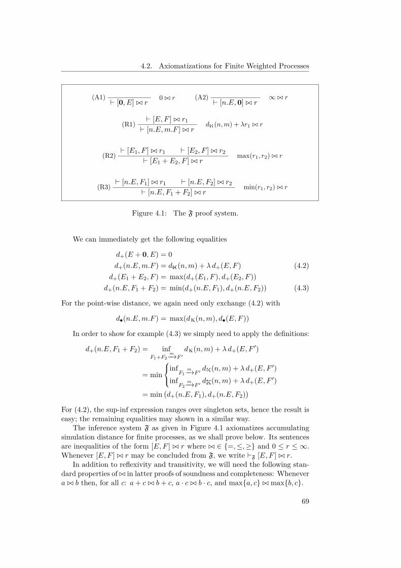
4.2. Axiomatizations for Finite Weighted Processes

(A1) 0 ./ r` [0, E] ./ r(A2) ∞ ./ r

` [n.E,0] ./ r

` [E,F ] ./ r1(R1) dK(n,m) + λr1 ./ r` [n.E,m.F ] ./ r

` [E1, F ] ./ r1 ` [E2, F ] ./ r2(R2) max(r1, r2) ./ r` [E1 + E2, F ] ./ r

` [n.E, F1] ./ r1 ` [n.E, F2] ./ r2(R3) min(r1, r2) ./ r` [n.E, F1 + F2] ./ r

Figure 4.1: The F proof system.

We can immediately get the following equalities

d+(E + 0, E) = 0d+(n.E,m.F ) = dK(n,m) + λ d+(E,F ) (4.2)

d+(E1 + E2, F ) = max(d+(E1, F ), d+(E2, F ))d+(n.E, F1 + F2) = min(d+(n.E, F1), d+(n.E, F2)) (4.3)

For the point-wise distance, we again need only exchange (4.2) with

d•(n.E,m.F ) = max(dK(n,m), d•(E,F ))

In order to show for example (4.3) we simply need to apply the definitions:

d+(n.E, F1 + F2) = infF1+F2

m−→F ′dK(n,m) + λ d+(E,F ′)

= min

infF1

m−→F ′dK(n,m) + λ d+(E,F ′)

infF2

m−→F ′dK(n,m) + λ d+(E,F ′)

= min(d+(n.E, F1), d+(n.E, F2)

)For (4.2), the sup-inf expression ranges over singleton sets, hence the result iseasy; the remaining equalities may shown in a similar way.

The inference system F as given in Figure 4.1 axiomatizes accumulatingsimulation distance for finite processes, as we shall prove below. Its sentencesare inequalities of the form [E,F ] ./ r where ./ ∈ {=,≤,≥} and 0 ≤ r ≤ ∞.Whenever [E,F ] ./ r may be concluded from F, we write `F [E,F ] ./ r.

In addition to reflexivity and transitivity, we will need the following stan-dard properties of ./ in latter proofs of soundness and completeness: Whenevera ./ b then, for all c: a+ c ./ b+ c, a · c ./ b · c, and max{a, c} ./ max{b, c}.

69

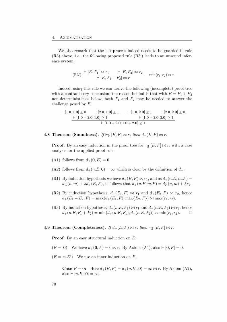
4. Axiomatization

We also remark that the left process indeed needs to be guarded in rule(R3) above, i.e., the following proposed rule (R3′) leads to an unsound infer-ence system:

` [E,F1] ./ r1 ` [E,F2] ./ r2(R3′) min(r1, r2) ./ r` [E,F1 + F2] ./ r

Indeed, using this rule we can derive the following (incomplete) proof treewith a contradictory conclusion; the reason behind is that with E = E1 + E2non-deterministic as below, both F1 and F2 may be needed to answer thechallenge posed by E:

` [1.0, 1.0] ≥ 0 ` [2.0, 1.0] ≥ 1` [1.0 + 2.0, 1.0] ≥ 1

` [1.0, 2.0] ≥ 1 ` [2.0, 2.0] ≥ 0` [1.0 + 2.0, 2.0] ≥ 1

` [1.0 + 2.0, 1.0 + 2.0] ≥ 1

4.8 Theorem (Soundness). If `F [E,F ] ./ r, then d+(E,F ) ./ r.

Proof: By an easy induction in the proof tree for `F [E,F ] ./ r, with a caseanalysis for the applied proof rule:

(A1) follows from d+(0, E) = 0.

(A2) follows from d+(n.E,0) =∞ which is clear by the definition of d+.

(R1) By induction hypothesis we have d+(E,F ) ./ r1, and as d+(n.E,m.F ) =dK(n,m) + λd+(E,F ), it follows that d+(n.E,m.F ) = dK(n,m) + λr1.

(R2) By induction hypothesis, d+(E1, F ) ./ r1 and d+(E2, F ) ./ r2, henced+(E1 + E2, F ) = max(d+(E1, F ),max{E2, F}) ./ max(r1, r2).

(R3) By induction hypothesis, d+(n.E, F1) ./ r1 and d+(n.E, F2) ./ r2, henced+(n.E, F1 + F2) = min(d+(n.E, F1), d+(n.E, F2)) ./ min(r1, r2). �

4.9 Theorem (Completeness). If d+(E,F ) ./ r, then `F [E,F ] ./ r.

Proof: By an easy structural induction on E:

(E = 0) We have d+(0, F ) = 0 ./ r. By Axiom (A1), also ` [0, F ] = 0.

(E = n.E′) We use an inner induction on F :

Case F = 0: Here d+(E,F ) = d+(n.E′,0) =∞ ./ r. By Axiom (A2),also ` [n.E′,0] =∞.

70

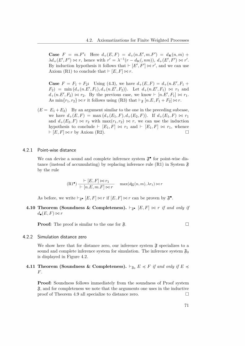
4.2. Axiomatizations for Finite Weighted Processes

Case F = m.F ′: Here d+(E,F ) = d+(n.E′,m.F ′) = dK(n,m) +λd+(E′, F ′) ./ r, hence with r′ = λ−1(r − dK(, nm)), d+(E′, F ′) ./ r′.By induction hypothesis it follows that ` [E′, F ′] ./ r′, and we can useAxiom (R1) to conclude that ` [E,F ] ./ r.

Case F = F1 + F2: Using (4.3), we have d+(E,F ) = d+(n.E′, F1 +F2) = min

(d+(n.E′, F1), d+(n.E′, F2)

). Let d+(n.E′, F1) ./ r1 and

d+(n.E′, F2) ./ r2. By the previous case, we know ` [n.E′, F1] ./ r1.As min{r1, r2} ./ r it follows using (R3) that `F [n.E, F1 + F2] ./ r.

(E = E1 +E2) By an argument similar to the one in the preceding subcase,we have d+(E,F ) = max

(d+(E1, F ), d+(E2, F )

). If d+(E1, F ) ./ r1

and d+(E2, F ) ./ r2 with max(r1, r2) ./ r, we can use the inductionhypothesis to conclude ` [E1, F ] ./ r1 and ` [E1, F ] ./ r1, whence` [E,F ] ./ r by Axiom (R2). �

4.2.1 Point-wise distance

We can devise a sound and complete inference system F• for point-wise dis-tance (instead of accumulating) by replacing inference rule (R1) in System Fby the rule

` [E,F ] ./ r1(R1•) max(dK(n,m), λr1) ./ r` [n.E,m.F ] ./ r

As before, we write `F• [E,F ] ./ r if [E,F ] ./ r can be proven by F•.

4.10 Theorem (Soundness & Completeness). `F• [E,F ] ./ r if and only ifd•(E,F ) ./ r

Proof: The proof is similar to the one for F. �

4.2.2 Simulation distance zero

We show here that for distance zero, our inference system F specializes to asound and complete inference system for simulation. The inference system F0is displayed in Figure 4.2.

4.11 Theorem (Soundness & Completeness). `F0 E 4 F if and only if E 4F .

Proof: Soundness follows immediately from the soundness of Proof systemF, and for completeness we note that the arguments one uses in the inductiveproof of Theorem 4.9 all specialize to distance zero. �

71

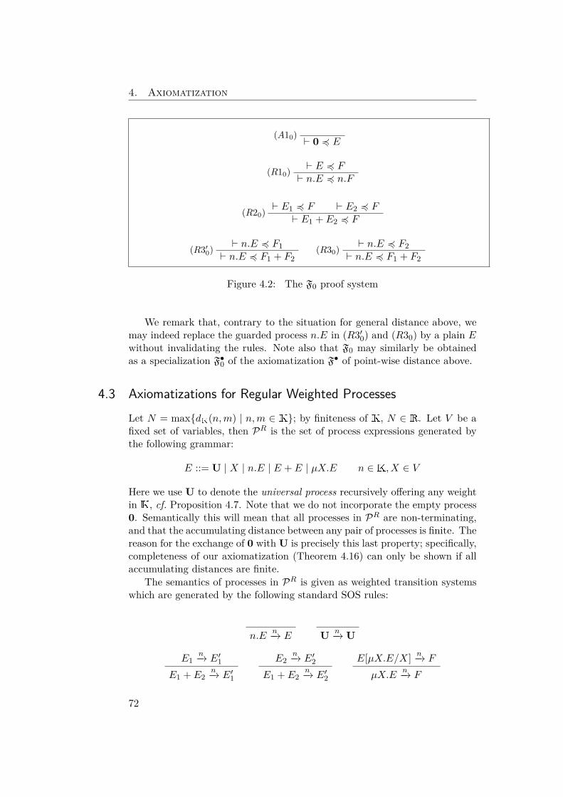
4. Axiomatization

(A10) ` 0 4 E

` E 4 F(R10) ` n.E 4 n.F

` E1 4 F ` E2 4 F(R20) ` E1 + E2 4 F

` n.E 4 F1(R3′0) ` n.E 4 F1 + F2

` n.E 4 F2(R30) ` n.E 4 F1 + F2

Figure 4.2: The F0 proof system

We remark that, contrary to the situation for general distance above, wemay indeed replace the guarded process n.E in (R3′0) and (R30) by a plain Ewithout invalidating the rules. Note also that F0 may similarly be obtainedas a specialization F•0 of the axiomatization F• of point-wise distance above.

4.3 Axiomatizations for Regular Weighted ProcessesLet N = max{dK(n,m) | n,m ∈ K}; by finiteness of K, N ∈ R. Let V be afixed set of variables, then PR is the set of process expressions generated bythe following grammar:

E ::= U | X | n.E | E + E | µX.E n ∈ K, X ∈ V

Here we use U to denote the universal process recursively offering any weightin K, cf. Proposition 4.7. Note that we do not incorporate the empty process0. Semantically this will mean that all processes in PR are non-terminating,and that the accumulating distance between any pair of processes is finite. Thereason for the exchange of 0 with U is precisely this last property; specifically,completeness of our axiomatization (Theorem 4.16) can only be shown if allaccumulating distances are finite.

The semantics of processes in PR is given as weighted transition systemswhich are generated by the following standard SOS rules:

n.En−→ E U n−→ U

E1n−→ E′1

E1 + E2n−→ E′1

E2n−→ E′2

E1 + E2n−→ E′2

E[µX.E/X] n−→ F

µX.En−→ F

72

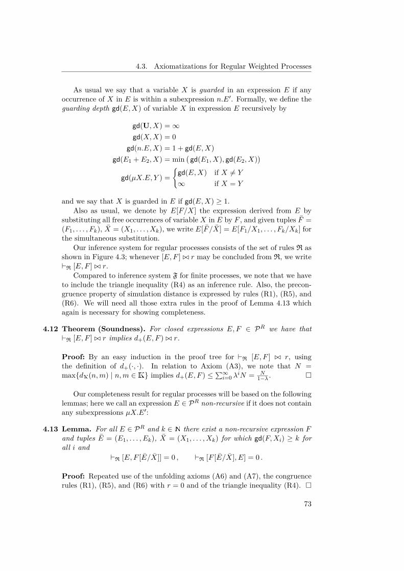
4.3. Axiomatizations for Regular Weighted Processes

As usual we say that a variable X is guarded in an expression E if anyoccurrence of X in E is within a subexpression n.E′. Formally, we define theguarding depth gd(E,X) of variable X in expression E recursively by

gd(U, X) =∞gd(X,X) = 0

gd(n.E,X) = 1 + gd(E,X)gd(E1 + E2, X) = min

(gd(E1, X), gd(E2, X)

)gd(µX.E, Y ) =

{gd(E,X) if X 6= Y

∞ if X = Y

and we say that X is guarded in E if gd(E,X) ≥ 1.Also as usual, we denote by E[F/X] the expression derived from E by

substituting all free occurrences of variable X in E by F , and given tuples F =(F1, . . . , Fk), X = (X1, . . . , Xk), we write E[F /X] = E[F1/X1, . . . , Fk/Xk] forthe simultaneous substitution.

Our inference system for regular processes consists of the set of rules R asshown in Figure 4.3; whenever [E,F ] ./ r may be concluded from R, we write`R [E,F ] ./ r.

Compared to inference system F for finite processes, we note that we haveto include the triangle inequality (R4) as an inference rule. Also, the precon-gruence property of simulation distance is expressed by rules (R1), (R5), and(R6). We will need all those extra rules in the proof of Lemma 4.13 whichagain is necessary for showing completeness.

4.12 Theorem (Soundness). For closed expressions E,F ∈ PR we have that`R [E,F ] ./ r implies d+(E,F ) ./ r.

Proof: By an easy induction in the proof tree for `R [E,F ] ./ r, usingthe definition of d+(·, ·). In relation to Axiom (A3), we note that N =max{dK(n,m) | n,m ∈ K} implies d+(E,F ) ≤∑∞i=0 λ

iN = N1−λ . �

Our completeness result for regular processes will be based on the followinglemmas; here we call an expression E ∈ PR non-recursive if it does not containany subexpressions µX.E′:

4.13 Lemma. For all E ∈ PR and k ∈ N there exist a non-recursive expression Fand tuples E = (E1, . . . , Ek), X = (X1, . . . , Xk) for which gd(F,Xi) ≥ k forall i and

`R [E,F [E/X]] = 0 , `R [F [E/X], E] = 0 .

Proof: Repeated use of the unfolding axioms (A6) and (A7), the congruencerules (R1), (R5), and (R6) with r = 0 and of the triangle inequality (R4). �

73

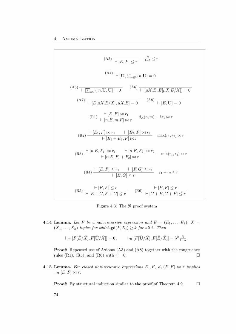
4. Axiomatization

(A3) N1−λ ≤ r` [E,F ] ≤ r

(A4)` [U,

∑n∈K n.U] = 0

(A5)` [∑n∈K n.U,U] = 0

(A6)` [µX.E,E[µX.E/X]] = 0

(A7)` [E[µX.E/X], µX.E] = 0

(A8)` [E,U] = 0

` [E,F ] ./ r1(R1) dK(n,m) + λr1 ./ r` [n.E,m.F ] ./ r

` [E1, F ] ./ r1 ` [E2, F ] ./ r2(R2) max(r1, r2) ./ r` [E1 + E2, F ] ./ r

` [n.E, F1] ./ r1 ` [n.E, F2] ./ r2(R3) min(r1, r2) ./ r` [n.E, F1 + F2] ./ r

` [E,F ] ≤ r1 ` [F,G] ≤ r2(R4) r1 + r2 ≤ r` [E,G] ≤ r

` [E,F ] ≤ r(R5)

` [E +G,F +G] ≤ r` [E,F ] ≤ r

(R6)` [G+ E,G+ F ] ≤ r

Figure 4.3: The R proof system

4.14 Lemma. Let F be a non-recursive expression and E = (E1, . . . , Ek), X =(X1, . . . , Xk) tuples for which gd(F,Xi) ≥ k for all i. Then

`R [F [E/X], F [U/X]] = 0 , `R [F [U/X], F [E/X]] = λk N1−λ .

Proof: Repeated use of Axioms (A3) and (A8) together with the congruencerules (R1), (R5), and (R6) with r = 0. �

4.15 Lemma. For closed non-recursive expressions E, F , d+(E,F ) ./ r implies`R [E,F ] ./ r.

Proof: By structural induction similar to the proof of Theorem 4.9. �

74

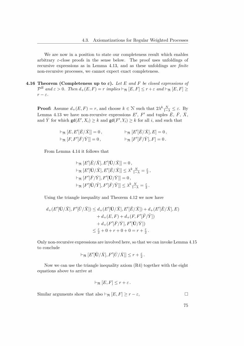
4.3. Axiomatizations for Regular Weighted Processes

We are now in a position to state our completeness result which enablesarbitrary ε-close proofs in the sense below. The proof uses unfoldings ofrecursive expressions as in Lemma 4.13, and as these unfoldings are finitenon-recursive processes, we cannot expect exact completeness.

4.16 Theorem (Completeness up to ε). Let E and F be closed expressions ofPR and ε > 0. Then d+(E,F ) = r implies `R [E,F ] ≤ r+ ε and `R [E,F ] ≥r − ε.

Proof: Assume d+(E,F ) = r, and choose k ∈ N such that 2λk N1−λ ≤ ε. By

Lemma 4.13 we have non-recursive expressions E′, F ′ and tuples E, F , X,and Y for which gd(E′, Xi) ≥ k and gd(F ′, Yi) ≥ k for all i, and such that

`R [E,E′[E/X]] = 0 , `R [E′[E/X], E] = 0 ,`R [F, F ′[F /Y ]] = 0 , `R [F ′[F /Y ], F ] = 0 .

From Lemma 4.14 it follows that

`R [E′[E/X], E′[U/X]] = 0 ,`R [E′[U/X], E′[E/X]] ≤ λk N

1−λ = ε2 ,

`R [F ′[F /Y ], F ′[U/Y ]] = 0 ,`R [F ′[U/Y ], F ′[F /Y ]] ≤ λk N

1−λ = ε2 .

Using the triangle inequality and Theorem 4.12 we now have

d+(E′[U/X], F ′[U/X]) ≤ d+(E′[U/X], E′[E/X]) + d+(E′[E/X], E)+ d+(E,F ) + d+(F, F ′[F /Y ])+ d+(F ′[F /Y ], F ′[U/Y ])≤ ε

2 + 0 + r + 0 + 0 = r + ε2 .

Only non-recursive expressions are involved here, so that we can invoke Lemma 4.15to conclude

`R [E′[U/X], F ′[U/X]] ≤ r + ε2 .

Now we can use the triangle inequality axiom (R4) together with the eightequations above to arrive at

`R [E,F ] ≤ r + ε .

Similar arguments show that also `R [E,F ] ≥ r − ε, �

75

4. Axiomatization

4.3.1 Point-wise distanceAgain we can easily convert our proof systemR into one for point-wise (insteadof accumulating) distance. In this case, we obtain R• by replacing inferencerule (R1) by (R1•) as we did for Proof system F, and (A3) needs to be replacedby

(A3•)` [E,F ] ≤ N

With these replacements we have a sound and ε-complete axiomatization ofpoint-wise simulation distance for recursive weighted processes:

4.17 Theorem (Soundness & Completeness up to ε). Let E and F be closedexpressions of PR, then `R• [E,F ] ./ r implies d•(E,F ) ./ r, and d•(E,F ) =r implies `R• [E,F ] ≤ r + ε and `R• [E,F ] ≥ r − ε for any ε > 0.

Proof: The proof is similar to that for accumulated distance. �

76

5 The QuantitativeLinear-Time–Branching-TimeSpectrum1

This chapter generalizes the work presented so far in several ways and devel-ops a general theory of linear and branching distances depending on a given,but unspecified, trace distance. It introduces quantitative Ehrenfeucht-Fraïsségames as a central tool for this generalization and then proceeds to define aspectrum of linear and branching distances which generalizes the one of vanGlabbeek [vG01].

5.1 Traces, Trace Distances, and Transition Systems

For a finite non-empty sequence a = (a0, . . . , an), we write last(a) = an andlen(a) = n+1 for the length of a; for an infinite sequence a we let len(a) =∞.Concatenation of finite sequences a and b is denoted a · b. We denote byak = (ak, ak+1, . . . ) the k-shift and by ai the (i + 1)st element of a (finite orinfinite) sequence, and by ε the empty sequence.

Throughout this chapter we fix a setK of labels, and we letK∞ = K∗∪Kω

denote the set of finite and infinite traces (i.e., sequences) in K. A hemimetricdT : K∞×K∞ → R≥0∪{∞} is called a trace distance if len(σ) 6= len(τ) impliesdT(σ, τ) =∞.

A labeled transition system (LTS) is a pair (S, T ) consisting of states Sand transitions T ⊆ S×K×S. We often write s x−→ t to signify that (s, x, t) ∈T . Given e = (s, x, t) ∈ T , we write src(e) = s and tgt(e) = t for thesource and target of e. A path in (S, T ) is a finite or infinite sequence π =((s0, x0, t0), (s1, x1, t1), . . . ) of transitions (sj , xj , tj) ∈ T which satisfy tj =sj+1 for all j. We denote by tr(π) = (x0, x1, . . . ) the trace induced by such apath π. For s ∈ S we denote by Pa(s) the set of (finite or infinite) paths froms and by Tr(s) = {tr(π) | π ∈ Pa(s)} the set of traces from s.

1This chapter is based on the journal paper [FL14b] published in Theoretical ComputerScience.

77

5. The Quantitative Linear-Time–Branching-Time Spectrum

5.2 Examples of Trace DistancesWe give a systematic treatment of trace distances with which our quantitativeframework can be instantiated. Some of them have appeared in previouschapters; some others are new, but have been used elsewhere in the literature.

Most of the trace distances one finds in the literature are defined by givinga hemimetric d on K and a method to combine the so-defined distances onindividual symbols to a distance on traces. Three general methods are usedfor this combination:

• The point-wise trace distance: PWλ(d)(σ, τ) = supj λjd(σj , τj);

• the accumulating trace distance: ACλ(d)(σ, τ) = ∑j λ

jd(σj , τj);

• The limit-average trace distance: AV(d)(σ, τ) = lim infj 1j+1

∑ji=0d(σi, τi).

Note that the trace distances are parametrized by the label distance d : K×K → R≥0 ∪ {∞}. Also, λ is a discounting factor with 0 < λ ≤ 1, andwe assume that the involved traces have equal length; otherwise any tracedistance has value∞. The point-wise distance thus measures the (discounted)greatest individual symbol distance in the traces, whereas accumulating andlimit-average distance accumulate these individual distances along the traces.

If the distance on K is the discrete distance given by ddisc(x, x) = 0 andddisc(x, y) =∞ for x 6= y, then all trace distances above agree, for any λ. Thisdefines the discrete trace distance dT

disc = PWλ(ddisc) = ACλ(ddisc) = AV(ddisc)given by dT

disc(σ, τ) = 0 if σ = τ and ∞ otherwise. We will show below thatfor the discrete trace distance, our quantitative linear-time–branching-timespectrum specializes to the qualitative one of [vG01].

If one lets d(x, x) = 0 and d(x, y) = 1 for x 6= y instead, then AC1(d) isHamming distance [Ham50] for finite traces, and ACλ(d) with λ < 1 andAV(d) are two sensible ways to define Hamming distance also for infinitetraces. PW1(d) is topologically equivalent to the discrete distance; indeed,PW1(d)(σ, τ) = 1 iff dT

disc(σ, τ) =∞.A generalization of the above distances may be obtained by equipping K

with a preorder � ⊆ K×K indicating that a label x ∈ K may be replaced byany y ∈ K with x � y, as for example in [Tho87]. If we define d(x, y) = 0 ifx � y and d(x, y) =∞ otherwise (note that this is a hemimetric which is notnecessarily symmetric), then again PWλ(d) = ACλ(d) = AV(d) for any λ.

Point-wise and accumulating distances have been studied in a number ofpapers [dAFS09,ČHR12,CDH10, vB05] and in previous chapters. PW1(d) isthe point-wise distance from [dAFS09,DLT08], and PWλ(d) for λ < 1 is thediscounted distance from [dAFS09,dAHM03]. Accumulating distance ACλ(d)has been studied in [dAFS09], and AV(d) in [CDH10,ČHR12]. Both ACλ(d)and AV(d) are well-known from the theory of discounted and mean-payoffgames [EM79,ZP96].

78

5.3. Quantitative Ehrenfeucht-Fraïssé Games

All distances above were obtained from distances on individual symbolsin K. A trace distance for which this is not the case is the maximum-leaddistance from [HMP05] defined for K ⊆ Σ × R, where Σ is an alphabet.Writing x ∈ K as x = (x`, xw), it is given by

dT±(σ, τ) =

{supj

∣∣∑ji=0 σ

wi −

∑ji=0 τ

wi

∣∣ if σ`j = τ `j for all j,∞ otherwise.

As this measures differences of accumulated labels along runs, it is especiallyuseful for real-time systems, cf. [HMP05,FL12].

As a last example of a trace distance we mention the Cantor distance givenby dT

C(σ, τ) = (1 + inf{j | σj 6= τj})−1. Cantor distance hence measures the(inverse of the) length of the common prefix of the sequences and has beenused for verification e.g., in [DHLN10]. Both Hamming and Cantor distancehave applications in information theory and pattern matching.

We will return to our example trace distances in Section 5.7 to show howour framework may be applied to yield concrete formulations of distances inthe linear-time–branching-time spectrum relative to these.

5.3 Quantitative Ehrenfeucht-Fraïssé GamesTo lift the linear-time–branching-time spectrum to the quantitative setting,we define below a quantitative Ehrenfeucht-Fraïssé game [Ehr61,Fra54] whichis similar to the well-known bisimulation game of [Sti95].

Let (S, T ) be a LTS and dT : K∞ ×K∞ → R≥0 ∪ {∞} a trace distance.The intuition of the game is as follows: The two players, with Player 1

starting the game, alternate to choose transitions, or moves, in T , startingwith transitions from given start states s and t and continuing their choicesfrom the targets of the transitions chosen in the previous step. At each ofhis turns, Player 1 also makes a choice whether to choose a transition fromthe target of his own previous choice, or from the target of his opponent’sprevious choice (to “switch paths”). We use a switch counter to keep track ofhow often Player 1 has chosen to switch paths. Player 2 has then to respondwith a transition from the remaining target. This game is played for an infinitenumber of rounds, or until one player runs out of choices, thus building twofinite or infinite paths. The value of the game is then the trace distance of thetraces of these two paths.

We proceed to formalize the above intuition. A Player-1 configurationof the game is a tuple (π, ρ,m) ∈ Tn × Tn × N, for n ∈ N, such that forall i ∈ {0, . . . , n − 2}, either src(πi+1) = tgt(πi) and src(ρi+1) = tgt(ρi), orsrc(πi+1) = tgt(ρi) and src(ρi+1) = tgt(πi). Similarly, a Player-2 configurationis a tuple (π, ρ,m) ∈ Tn+1 × Tn × N such that for all i ∈ {0, . . . , n − 2},either src(πi+1) = tgt(πi) and src(ρi+1) = tgt(ρi), or src(πi+1) = tgt(ρi) and

79

5. The Quantitative Linear-Time–Branching-Time Spectrum

src(ρi+1) = tgt(πi); and src(πn) = tgt(πn−1) or src(πn) = tgt(ρn−1). The setof all Player-i configurations is denoted Confi.

Intuitively, the configuration (π, ρ,m) keeps track of the history of thegame; π stores the choices of Player 1, ρ the choices of Player 2, and m is theswitch counter. Hence π and ρ are sequences of transitions in T which canbe arranged by suitable swapping to form two paths (π,ρ). How exactly thesesequences are constructed is determined by a pair of strategies which specifyfor each player which edge to play from any configuration.

A Player-1 strategy is hence a partial mapping θ1 : Conf1 ⇀ T ×N suchthat for all (π, ρ,m) ∈ Conf1 for which θ1(π, ρ,m) = (e′,m′) is defined,

• src(e′) = tgt(last(π)) and m′ = m or m′ = m+ 1, or

• src(e′) = tgt(last(ρ)) and m′ = m+ 1.

A Player-2 strategy is a partial mapping θ2 : Conf2 ⇀ T ×N such that for all(π · e, ρ,m) ∈ Conf2 for which θ2(π · e, ρ,m) = (e′,m′) is defined, m′ = m, andsrc(e′) = tgt(last(ρ)) if src(e) = tgt(last(π)), src(e′) = tgt(last(π)) if src(e) =tgt(last(ρ)). The sets of Player-1 and Player-2 strategies are denoted Θ1 andΘ2.

Note that if Player 1 chooses a transition from the end of the previouschoice of Player 2 (case src(e′) = tgt(last(ρ)) above), then the switch counteris increased; but Player 1 may also choose to increase the switch counterwithout switching paths. Player 2 does not touch the switch counter.

We can now define what it means to update a configuration accordingto a strategy: For θ1 ∈ Θ1 and (π, ρ,m) ∈ Conf1, updθ1(π, ρ,m) is definedif θ1(π, ρ,m) = (e′,m′) is defined, and then updθ1(π, ρ,m) = (π · e′, ρ,m′).Similarly, for θ2 ∈ Θ2 and (π · e, ρ,m) ∈ Conf2, updθ2(π · e, ρ,m) is defined ifθ2(π ·e, ρ,m) = (e′,m′) is defined, and then updθ2(π ·e, ρ,m) = (π ·e, ρ ·e′,m′).

For any pair of states (s, t) ∈ S ×S, a pair of strategies (θ1, θ2) ∈ Θ1×Θ2inductively determines a sequence (πj , ρj ,mj) of configurations, by

(π0, ρ0,m0) = (s, t, 0);

(π2j+1, ρ2j+1,m2j+1) ={undef. if updθ1(π2j , ρ2j ,m2j) is undefined,updθ1(π2j , ρ2j ,m2j) otherwise;

(π2j , ρ2j ,m2j) =

undef. if updθ2(π2j−1, ρ2j−1,m2j−1)

is undefined,updθ2(π2j−1, ρ2j−1,m2j−1) otherwise.

Note that indeed, we are updating configurations by alternating between thetwo strategies θ1, θ2.

The configurations in this sequence satisfy πj ≤p πj+1 and ρj ≤p ρj+1 forall j, where ≤p denotes prefix ordering, hence the direct limits π = lim−→πj , ρ =

80

5.3. Quantitative Ehrenfeucht-Fraïssé Games

lim−→ ρj exist (as finite or infinite paths). By our conditions on configurations,the pair (π, ρ) in turn determines a pair (π, ρ) of paths in S, as follows:

(π1, ρ1) ={

(π1, ρ1) if src(π1) = s

(ρ1, π1) if src(π1) = t

(πj , ρj) ={

(πj , ρj) if src(πj) = tgt(πj−1)(ρj , πj) if src(πj) = tgt(ρj−1)

The outcome of the game when played from (s, t) according to a strategypair (θ1, θ2) is defined to be out(θ1, θ2)(s, t) = (π, ρ), and its utility is definedby util(θ1, θ2)(s, t) = dT(tr(out(θ1, θ2)(s, t))) = dT(tr(π), tr(ρ)).

Recall that dT is given as a parameter to the game; if we want to makeexplicit the parametrization on the trace distance dT on which utility depends,we write utildT(θ1, θ2)(s, t).

Note that util(θ1, θ2)(s, t) is defined both in case the paths π and ρ arefinite and in case they are infinite (the case where one is finite and the other isinfinite cannot occur). Also, if the paths are finite because θ1(πj , ρj ,mj) wasundefined for some configuration (πj , ρj ,mj) in the sequence, then len(π) =len(ρ); if on the other hand the reason is that θ2(πj , ρj ,mj) was undefined,then len(π) = len(ρ)± 1, and util(θ1, θ2)(s, t) =∞. Hence if the game reachesa configuration in which Player 2 has no moves available, the utility is ∞.

The objective of Player 1 in the game is to maximize utility, whereasPlayer 2 wants to minimize it. Hence we define the value of the game from(s, t) to be

v(s, t) = supθ1∈Θ1

infθ2∈Θ2

util(θ1, θ2)(s, t) .

For a given subset Θ′1 ⊆ Θ1 we will write

v(Θ′1)(s, t) = supθ1∈Θ′1

infθ2∈Θ2

util(θ1, θ2)(s, t) ,

and if we need to emphasize dependency of the value on the given trace dis-tance, we write v(dT,Θ′1). The following lemma states the immediate factthat if Player 1 has fewer strategies available, the game value decreases.

5.1 Lemma. For all Θ′1 ⊆ Θ′′1 ⊆ Θ1 and all s, t ∈ S, v(Θ′1)(s, t) ≤ v(Θ′′1)(s, t).

The above definition of strategies is slightly too general in that whetheror not a strategy is defined in a given configuration should only depend onthe actual part of the configuration on which the strategy has an effect. Wehence define a notion of uniformity which we will assume from now:

5.2 Definition. A strategy θ1 ∈ Θ1 is uniform if it holds for all configurations(π, ρ,m), (π, ρ,m), (π, ρ,m) ∈ Conf1 that whenever θ1(π, ρ,m) = (e′,m′) isdefined,

81

5. The Quantitative Linear-Time–Branching-Time Spectrum

• if src(e′) = tgt(last(π)), then also θ1(π, ρ,m) is defined, and

• if src(e′) = tgt(last(ρ)), then also θ1(π, ρ,m) is defined.

A strategy θ2 ∈ Θ2 is uniform if it holds for all configurations (π · e, ρ,m), (π ·e, ρ,m), (π · e, ρ,m) ∈ Conf2 that whenever θ2(π · e, ρ,m) = (e′,m′) is defined,

• if src(e′) = tgt(last(ρ)), then also θ2(π · e, ρ,m) is defined, and

• if src(e′) = tgt(last(π)), then also θ2(π · e, ρ,m) is defined.

A subset Θ′1 ⊆ Θ1 is uniform if all strategies in Θ′1 are uniform. Uniformityof strategies is used to combine paths built from different starting states in theproof of Proposition 5.5 below, and it allows us to show a minimax theoremfor our setting.

The concrete strategy subsets we will consider in later sections will all beuniform, so from now on we only consider the subsets of Θ1 and Θ2 consistingof uniform strategies. Abusing notation, we will also denote these by Θ1and Θ2.

5.3 Lemma. For any uniform Θ′1 ⊆ Θ1 and all s, t ∈ S,

supθ1∈Θ′1

infθ2∈Θ2

util(θ1, θ2)(s, t) = infθ2∈Θ2

supθ1∈Θ′1

util(θ1, θ2)(s, t) .

Proof: By uniformity, neither of the two players has any possibility to in-fluence the configurations reachable by the other’s strategies. Hence it isimmaterial which player gets to choose strategy first. �

5.4 General PropertiesWe show here that under the uniformity condition, the game value is indeed adistance, and that results concerning inequalities in the qualitative dimensioncan be transfered to topological inequivalences in the quantitative setting. Saythat a Player-1 strategy θ1 ∈ Θ1 is non-switching if it holds for all (π, ρ,m)for which θ1(π, ρ,m) = (e′,m′) is defined that m = m′, and let Θ0

1 be the setof non-switching Player-1 strategies. We first show a lemma which shows thatany pair of traces can be generated by a non-switching strategy:

5.4 Lemma. For all s, t ∈ S and all σ ∈ Tr(s), τ ∈ Tr(t) there exist θ1 ∈ Θ01 and

θ2 ∈ Θ2 for which util(θ1, θ2)(s, t) = dT(σ, τ).

Proof: Let (π, ρ, 0) ∈ Conf1 for finite paths π, ρ with len(π) = len(ρ) = k ≥ 0and tr(π) = σ0 . . . σk−1, tr(ρ) = τ0 . . . τk−1. If len(σ) ≥ k, then there ise = (last(π), σk, s′) ∈ T , and we define θ1(π, ρ, 0) = (e, 0). If also len(τ) ≥ k,then there is e′ = (last(ρ), τk, t′) ∈ T , and we let θ2(π · e, ρ, 0) = (e′, 0).

82

5.4. General Properties

Let (π, ρ) = out(θ1, θ2)(s, t). If both σ and τ are infinite traces, thentr(π) = σ and tr(ρ) = τ ; otherwise, tr(π) and tr(ρ) will be finite prefixes of σand τ for which dT(tr(π), tr(ρ)) = dT(σ, τ). �

The following proposition shows that the distance defined by our quanti-tative game is a hemimetric. Note that the proof of the triangle inequalityuses uniformity.

5.5 Proposition. For all Θ′1 ⊆ Θ1 with Θ01 ⊆ Θ′1, v(Θ′1) is a hemimetric on S.

Proof: We write v = v(Θ′1) during this proof. It is clear that v(s, s) = 0 forall s ∈ S: if the players are making their choices from the same state, Player 2can always answer by choosing exactly the same transition as Player 1. Forproving the triangle inequality v(s, u) ≤ v(s, t) + v(t, u), let ε > 0 and useLemma 5.3 to choose Player-2 strategies θs,t2 , θt,u2 ∈ Θ2 for which

supθ1∈Θ′1

util(θ1, θs,t2 )(s, t) < v(s, t) + ε

2 ,

supθ1∈Θ′1

util(θ1, θt,u2 )(t, u) < v(t, u) + ε

2 .(5.1)

We define a strategy θs,u2 ∈ Θ2 which uses three paths and two configurationsin S as extra memory. This is only for convenience, as these can be recon-structed by Player 2 at any time; hence we do not extend the capabilities ofPlayer 2:

θs,u2 (π · e, χ,m; π, ρ′, χ, π′, ρ′1, ρ′2, χ′) =

(θt,u2

(ρ′2 · θ

s,t2,1(π′ · e, ρ′1,m), χ′,m

);

π · e,ρ′ · θs,t2,1(π′ · e, ρ′1,m),χ · θt,u2,1

(ρ′2 · θ

s,t2,1(π′ · e, ρ′1,m)

),

π′ · e,ρ′1 · θ

s,t2,1(π′ · e, ρ′1,m),

ρ′2 · θs,t2,1(π′ · e, ρ′1,m),

χ′ · θt,u2,1(ρ′2 · θ

s,t2,1(π′ · e, ρ′1,m)

))if src(e) = tgt(last(π)),(

θs,t2(π′ · θt,u2,1(ρ′2 · e, χ′,m), ρ′1,m

);

π · θs,t2,1(π′ · θt,u2,1(ρ′2 · e, χ′,m)

),

ρ′ · θt,u2,1(ρ′2 · e, χ′,m),χ · e,π′ · θt,u2,1(ρ′2 · e, χ′,m),ρ′1 · θ

s,t2,1(π′ · θt,u2,1(ρ′2 · e, χ′,m)

)ρ′2 · e,χ′ · θt,u2,1(ρ′2 · e, χ′,m)

)if src(e) = tgt(last(χ)).

83

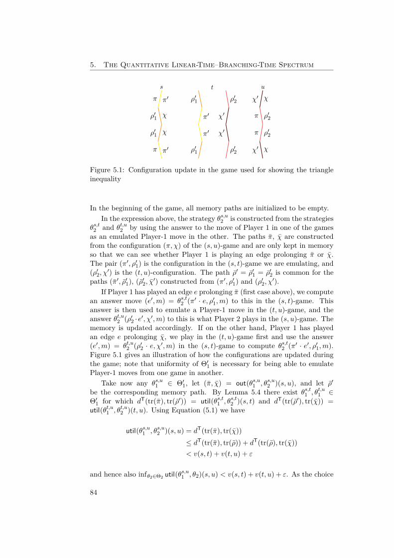
5. The Quantitative Linear-Time–Branching-Time Spectrum

s t u

π

π

π

π

χ

χ

χ

χ

π′

π′

π′

π′

ρ′1

ρ′1

ρ′1

ρ′1

ρ′2

ρ′2

ρ′2

ρ′2

χ′

χ′

χ′

χ′

Figure 5.1: Configuration update in the game used for showing the triangleinequality

In the beginning of the game, all memory paths are initialized to be empty.In the expression above, the strategy θs,u2 is constructed from the strategies

θs,t2 and θt,u2 by using the answer to the move of Player 1 in one of the gamesas an emulated Player-1 move in the other. The paths π, χ are constructedfrom the configuration (π, χ) of the (s, u)-game and are only kept in memoryso that we can see whether Player 1 is playing an edge prolonging π or χ.The pair (π′, ρ′1) is the configuration in the (s, t)-game we are emulating, and(ρ′2, χ′) is the (t, u)-configuration. The path ρ′ = ρ′1 = ρ′2 is common for thepaths (π′, ρ′1), (ρ′2, χ′) constructed from (π′, ρ′1) and (ρ′2, χ′).

If Player 1 has played an edge e prolonging π (first case above), we computean answer move (e′,m) = θs,t2 (π′ · e, ρ′1,m) to this in the (s, t)-game. Thisanswer is then used to emulate a Player-1 move in the (t, u)-game, and theanswer θt,u2 (ρ′2 ·e′, χ′,m) to this is what Player 2 plays in the (s, u)-game. Thememory is updated accordingly. If on the other hand, Player 1 has playedan edge e prolonging χ, we play in the (t, u)-game first and use the answer(e′,m) = θt,u2 (ρ′2 · e, χ′,m) in the (s, t)-game to compute θs,t2 (π′ · e′, ρ′1,m).Figure 5.1 gives an illustration of how the configurations are updated duringthe game; note that uniformity of Θ′1 is necessary for being able to emulatePlayer-1 moves from one game in another.

Take now any θs,u1 ∈ Θ′1, let (π, χ) = out(θs,u1 , θs,u2 )(s, u), and let ρ′be the corresponding memory path. By Lemma 5.4 there exist θs,t1 , θt,u1 ∈Θ′1 for which dT(tr(π), tr(ρ′)) = util(θs,t1 , θs,t2 )(s, t) and dT(tr(ρ′), tr(χ)) =util(θt,u1 , θt,u2 )(t, u). Using Equation (5.1) we have

util(θs,u1 , θs,u2 )(s, u) = dT(tr(π), tr(χ))≤ dT(tr(π), tr(ρ)) + dT(tr(ρ), tr(χ))< v(s, t) + v(t, u) + ε

and hence also infθ2∈Θ2 util(θs,u1 , θ2)(s, u) < v(s, t) + v(t, u) + ε. As the choice

84

5.5. The Distance Spectrum

of θs,u1 was arbitrary, this implies

supθ1∈Θ′1

infθ2∈Θ2

util(θ1, θ2)(s, u) ≤ v(s, t) + v(t, u) + ε ,

and as also ε was chosen arbitrarily, we have v(s, u) ≤ v(s, t) + v(t, u). �

Next we show a transfer principle which allows us to generalize counterex-amples regarding the equivalences in the qualitative linear-time–branching-time spectrum [vG01] to the qualitative setting. We will make use of thisprinciple later to show that all distances we introduce are topologically in-equivalent.

5.6 Lemma. Let Θ′1,Θ′′1 ⊆ Θ1, and assume dT to be separating. If there existstates s, t ∈ S for which v(dT

disc,Θ′1)(s, t) = 0 and v(dTdisc,Θ′′1)(s, t) =∞, then

v(dT,Θ′1) and v(dT,Θ′′1) are topologically inequivalent.

Proof: By v(dTdisc,Θ′1)(s, t) = 0, we know that for any θ1 ∈ Θ′1 there exists

θ2 ∈ Θ2 for which (π, ρ) = out(θ1, θ2)(s, t) satisfy tr(π) = tr(ρ), hence alsov(dT,Θ′1)(s, t) = 0. Conversely, as dT is separating, v(dT,Θ′′1)(s, t) = 0 wouldimply that also v(dT

disc,Θ′′1)(s, t) = 0, hence we must have v(dT,Θ′′1)(s, t) 6= 0,entailing topological inequivalence. �

5.5 The Distance SpectrumIn this section we introduce the distances depicted in Figure 5.2 and showtheir relationship. Note again that the results obtained here are independentof the particular trace distance considered. Throughout this section, we fix aLTS (S, T ) and a trace distance dT : K∞ ×K∞ → R≥0 ∪ {∞}.

5.5.1 Branching DistancesIf the switching counter in the game introduced in Section 5.3 is unbounded,Player 1 can choose at any move whether to prolong the previous choice or toswitch paths, hence this resembles the bisimulation game [Sti95].

5.7 Definition. The bisimulation distance between s and t is dbisim(s, t) = v(s, t).

5.8 Theorem. For dT = dTdisc the discrete trace distance, dbisimdisc (s, t) = 0 iff s and

t are bisimilar.

Proof: By discreteness of dTdisc, we have dbisimdisc (s, t) = 0 iff it holds that for

all θ1 ∈ Θ1 there exists θ2 ∈ Θ2 for which util(θ1, θ2)(s, t) = 0. Hence for eachreachable Player-1 configuration (π, ρ,m) with θ1(π, ρ,m) = (e′,m′), we haveθ2(π ·e′, ρ,m′) = (e′′,m′) with tr(e′) = tr(e′′), i.e., Player 2 matches the labelschosen by Player 1 precisely, implying that s and t are bisimilar. The proofof the other direction is trivial. �

85

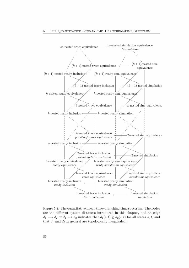
5. The Quantitative Linear-Time–Branching-Time Spectrum

∞-nested trace equivalence

(k + 1)-nested ready inclusion

(k + 1)-nested trace equivalence

k-nested ready equivalence

(k + 1)-nested trace inclusion

k-nested ready inclusion

k-nested trace equivalence

2-nested ready inclusion

2-nested trace equivalencepossible-futures equivalence

1-nested ready equivalenceready equivalence

2-nested trace inclusionpossible-futures inclusion

1-nested ready inclusionready inclusion

1-nested trace equivalencetrace equivalence

1-nested trace inclusiontrace inclusion

∞-nested simulation equivalencebisimulation

(k + 1)-ready sim. equivalence

(k + 1)-nested sim.equivalence

k-nested ready sim. equivalence

(k + 1)-nested simulation

k-nested ready simulation

k-nested sim. equivalence

2-nested ready simulation

2-nested sim. equivalence

1-nested ready sim. equivalenceready simulation equivalence

2-nested simulation

1-nested ready simulationready simulation

1-nested sim. equivalencesimulation equivalence

1-nested simulationsimulation

Figure 5.2: The quantitative linear-time–branching-time spectrum. The nodesare the different system distances introduced in this chapter, and an edged1 −→ d2 or d1 99K d2 indicates that d1(s, t) ≥ d2(s, t) for all states s, t, andthat d1 and d2 in general are topologically inequivalent.

86

5.5. The Distance Spectrum

We can restrict the strategies available to Player 1 by allowing only apre-defined finite number of switches:

Θk-sim1 = {θ1 ∈ Θ1 | if θ1(π, ρ,m) = (e′,m′) is defined, then m′ ≤ k − 1}

In the so-defined k-nested simulation game, Player 1 is only allowed to switchpaths k − 1 times during the game. Note that Θ1-sim

1 = Θ01 is the set of

non-switching strategies.

5.9 Definition. The k-nested simulation distance from s to t, for k ∈ N+, isdk-sim(s, t) = v(Θk-sim

1 )(s, t). The k-nested simulation equivalence distancebetween s and t is dk-sim-eq(s, t) = max(v(Θk-sim

1 )(s, t), v(Θk-sim1 )(t, s)).

5.10 Theorem. For dT = dTdisc the discrete trace distance,

• dk-simdisc (s, t) = 0 iff there is a k-nested simulation from s to t,

• dk-sim-eqdisc (s, t) = 0 iff there is a k-nested simulation equivalence betweens and t.

Especially, d1-simdisc corresponds to the usual simulation preorder, and d2-sim

discto two-nested simulation. Similarly, d1-sim-eq

disc is similarity, and d2-sim-eqdisc is two-

nested simulation equivalence. We refer to [GV92,HM85] for definitions anddiscussion of two-nested and k-nested simulation.

Proof: This is similar to the proof of Theorem 5.8: If dk-simdisc (s, t) = 0, thenany θ1 ∈ Θk-sim

1 has a counter-strategy θ2 ∈ Θ2 which matches the labelschosen by Player 1 precisely, implying k-nested simulation from s to t. Theother direction is again trivial. �

5.11 Theorem. For all k, ` ∈ N+ with k < ` and all s, t ∈ S,

dk-sim-eq(s, t) ≤ d`-sim(s, t) ≤ d`-sim-eq(s, t) ≤ dbisim(s, t).

If the trace distance dT is separating, then all distances above are topologicallyinequivalent.

Proof: The first part of the theorem follows from the inclusions Θk-sim-eq1 ⊆

Θ`-sim1 ⊆ Θ`-sim-eq

1 ⊆ Θ1 and Lemma 5.1. Topological inequivalence followsfrom Lemma 5.6 and the fact that for the discrete relations correspondingto the distances above (obtained by letting dT = dT

disc), the inequalities arestrict [vG01]. �

As a variation of k-nested simulation, we can consider strategies whichallow Player 1 to switch paths k times during the game, but at the last switch,

87

5. The Quantitative Linear-Time–Branching-Time Spectrum

he may only pose one transition as a challenge, to which Player 2 must answer,and then the game finishes:

Θk-rsim1 = {θ1 ∈ Θ1 | if θ1(π, ρ,m) is defined, then m ≤ k − 1}

Hence after his k’th switch, Player 1 has no more moves available, and thegame finishes after the answer move of Player 2. Again, we allow Player 1 toincrease the switch counter without actually switching paths.

5.12 Definition. The k-nested ready simulation distance from s to t, for k ∈ N+, isdk-rsim(s, t) = v(Θk-rsim

1 )(s, t). The k-nested ready simulation equivalence dis-tance between s and t is dk-rsim-eq(s, t) = max(v(Θk-rsim

1 )(s, t), v(Θk-rsim1 )(t, s)).

For the discrete case, it seems only k = 1 has been considered; the proofis similar to the one of Theorem 5.8.

5.13 Theorem. For dT = dTdisc the discrete trace distance,

• d1-rsimdisc (s, t) = 0 iff there is a ready simulation from s to t,

• d1-rsim-eqdisc (s, t) = 0 iff s and t are ready simulation equivalent.

The next theorem finishes our work on the right half of Figure 5.2.

5.14 Theorem. For all k, ` ∈ N+ with k < ` and all s, t ∈ S,

dk-sim(s, t) ≤ dk-rsim(s, t) ≤ d`-sim(s, t) ,dk-sim-eq(s, t) ≤ dk-rsim-eq(s, t) ≤ d`-sim-eq(s, t) .

Additionally, dk-rsim and dk-sim-eq are incomparable, and also dk-rsim-eq andd(k+1)-sim are incomparable. If the trace distance dT is separating, then alldistances above are topologically inequivalent.

Proof: Like in the proof of Theorem 5.11, the inequalities follow from strategyset inclusions and topological inequivalence from Lemma 5.6. The incompara-bility results follow from the corresponding results for dT

disc and Lemma 5.6.�

5.5.2 Linear DistancesAbove we have introduced the distances in the right half of the quantitativelinear-time–branching-time spectrum in Figure 5.2 and shown the relationsclaimed in the diagram. To develop the left half, we need the notion of blindstrategies. For any subset Θ′1 ⊆ Θ1 we define the set of blind Θ′1-strategies by

Θ′1 = {θ1 ∈ Θ′1 | ∀π, ρ, ρ′,m : θ1(π, ρ,m) = θ1(π, ρ′,m),or θ1(π, ρ,m) = (e,m+ 1) and tgt(last(ρ)) 6= tgt(last(ρ′))}.

88

5.5. The Distance Spectrum

Hence in such a blind strategy, either the edge chosen by Player 1 does notdepend on the choices of Player 2, or the switch counter is increased, in whichcase the Player-1 choice only depends on the target of the last choice of Player 2(note that this dependency is necessary if Player 1 wants to switch paths).

Now we can define, for s, t ∈ S and k ∈ N+,

• the ∞-nested trace equivalence distance: d∞-trace-eq(s, t) = v(Θ1)(s, t),

• the k-nested trace distance: dk-trace(s, t) = v(Θk-sim1 )(s, t),

• the k-nested trace equivalence distance:dk-trace-eq(s, t) = max(v(Θk-sim

1 )(s, t), v(Θk-sim1 )(t, s)),

• the k-nested ready distance: dk-ready(s, t) = v(Θk-rsim1 )(s, t), and

• the k-nested ready equivalence distance:dk-ready-eq(s, t) = max(v(Θk-rsim

1 )(s, t), v(Θk-rsim1 )(t, s)).

Our approach is justified by the following lemma which shows that the (1-nested) trace distance from s to t is precisely the Hausdorff distance betweenthe sets of traces available from s and t, respectively.

5.15 Lemma. For s, t ∈ S, d1-trace(s, t) = supσ∈Tr(s) infτ∈Tr(t) dT(σ, τ).

Proof: We have d1-trace(s, t) = v(Θ01)(s, t), with Θ0

1 = {θ1 ∈ Θ01 | ∀π, ρ, ρ′,m :

θ1(π, ρ,m) = θ1(π, ρ′,m)}. Hence, and as strategies in Θ01 are non-switching,

every strategy θ1 ∈ Θ01 gives rise to precisely one trace σ = σ(θ1) ∈ Tr(s) inde-

pendently of Player-2 strategy θ2 ∈ Θ2. Conversely, by Lemma 5.4 (noticingthat indeed, we have constructed a blind Player-1 strategy in the proof ofthat lemma), every trace σ ∈ Tr(s) is generated by a strategy θ1 ∈ Θ0

1 withσ = σ(θ1).

We can finish the proof by showing that for all θ1 ∈ Θ01,

infθ2∈Θ2

dT(σ(θ1), tr(ρ(θ1, θ2))) = infτ∈Tr(t)

dT(σ(θ1), τ) .

But again using Lemma 5.4, we see that any τ ∈ Tr(t) is generated by astrategy θ2 ∈ Θ2, hence this is clear. �

Using the discrete trace distance, we recover the following standard rela-tions [vG01]. The theorem follows by Lemma 5.15 and arguments similar tothe ones used in the proofs of the corresponding theorems in the precedingsection. We refer to [RB81,HM85] for definitions and discussion of possible-futures inclusion and equivalence.

5.16 Theorem. For dT = dTdisc the discrete trace distance and s, t ∈ S we have

• d1-tracedisc (s, t) = 0 iff there is a trace inclusion from s to t,

89

5. The Quantitative Linear-Time–Branching-Time Spectrum

• d1-trace-eqdisc (s, t) = 0 iff s and t are trace equivalent,

• d2-tracedisc (s, t) = 0 iff there is a possible-futures inclusion from s to t,

• d2-trace-eqdisc (s, t) = 0 iff s and t are possible-futures equivalent,

• d1-readydisc (s, t) = 0 iff there is a readiness inclusion from s to t,

• d1-ready-eqdisc (s, t) = 0 iff s and t are ready equivalent.

The following theorem entails all relations in the left side of Figure 5.2;the right-to-left arrows follow from the strategy set inclusions Θ′1 ⊆ Θ′1 forany Θ′1 ⊆ Θ1 and Lemma 5.1. As with Theorems 5.11 and 5.14, the theoremfollows by strategy set inclusion, Lemma 5.6, and corresponding results forthe discrete relations.

5.17 Theorem. For all k, ` ∈ N+ with k < ` and s, t ∈ S,

dk-trace-eq(s, t) ≤ d`-trace(s, t) ≤ d`-trace-eq(s, t) ≤ d∞-trace-eq(s, t),dk-trace(s, t) ≤ dk-ready(s, t) ≤ d`-trace(s, t),dk-trace-eq(s, t) ≤ dk-ready-eq(s, t) ≤ d`-trace-eq(s, t).

Additionally, dk-ready and dk-trace-eq are incomparable, and also dk-ready-eq andd(k+1)-trace are incomparable. If the trace distance dT is separating, then alldistances above are topologically inequivalent.

5.6 Recursive Characterizations

We now turn our attention to an important special case in which the giventrace distance has a specific recursive characterization; we show that in thiscase, all distances in the spectrum can be characterized as least fixed points.We will see in Section 5.7 that this can be applied to all examples of tracedistances mentioned in Section 5.2.

Note that all theorems require the LTS in question to be finitely branching;this is a standard assumption which goes back to [Sti95]. In most cases it maybe relaxed to compact branching in the sense of [vB96], but to keep thingssimple, we do not do this here.

5.6.1 Fixed-Point Characterizations

Let L be a complete lattice with order v and bottom and top elements ⊥, >.Let f : K∞×K∞ → L, g : L→ R≥0∪{∞} and F : K×K×L→ L such that

90

5.6. Recursive Characterizations

dT = g ◦ f , g is monotone, F (x, y, ·) : L→ L is monotone for all x, y ∈ K, and

f(σ, τ) =

F (σ0, τ0, f(σ1, τ1)) if σ, τ 6= ε,

> if σ = ε, τ 6= ε or σ 6= ε, τ = ε,

⊥ if σ = τ = ε

(5.2)

for all σ, τ ∈ K∞.We hence assume that dT has a recursive characterization (using F ) on top

of a complete (but otherwise arbitrary) lattice L which we introduce betweenK∞ and R≥0 ∪ {∞} to serve as a memory. Below we will work with different

endofunctions I on the set of mappings (N+ ∪ {∞}) × {1, 2} → LS×S whichare parametrized by the number m of switches in N+ ∪ {∞} which Player 1has left, and a value p ∈ {1, 2} which keeps track of whether Player 1 currentlyis building the left or the right path.

5.18 Theorem. The endofunction I on (N+ ∪ {∞})× {1, 2} → LS×S defined by

I(hm,p)(s, t) =

max

supsx−→s′

infty−→t′

F (x, y, hm,1(s′, t′))

supty−→t′

infsx−→s′

F (x, y, hm−1,2(s′, t′))if m ≥ 2, p = 1

supsx−→s′

infty−→t′

F (x, y, hm,1(s′, t′)) if m = 1, p = 1

max

supty−→t′

infsx−→s′

F (x, y, hm,2(s′, t′))

supsx−→s′

infty−→t′

F (x, y, hm−1,1(s′, t′))if m ≥ 2, p = 2

supty−→t′

infst

x−→s′

F (x, y, hm,2(s′, t′)) if m = 1, p = 2

has a least fixed point h∗ : (N+∪{∞})×{1, 2} → LS×S, and if the LTS (S, T )is finitely branching, then dk-sim = g ◦ h∗k,1, dk-sim-eq = g ◦max(h∗k,1, h∗k,2) forall k ∈ N+ ∪ {∞}.

Hence I iterates the function h over the branching structure of (S, T ),computing all nested branching distances at the same time. Note the spe-cialization of this to simulation and bisimulation distance, where we have thefollowing fixed-point equations, using h∗1,1 = h1-sim and h∗∞,1 = hbisim:

h1-sim(s, t) = supsx−→s′

infty−→t′

F (x, y, h1-sim(s′, t′))

hbisim(s, t) = max

supsx−→s′

infty−→t′

F (x, y, hbisim(s′, t′))

supty−→t′

infsx−→s′

F (x, y, hbisim(s′, t′))

91

5. The Quantitative Linear-Time–Branching-Time Spectrum

Proof: The lattice of mappings (N+∪{∞})×{1, 2} → LS×S with the point-wise partial order is complete, and I is monotone because F is, so by Tarski’sfixed-point theorem, I has indeed a least fixed point h∗. To show that dk-sim =g◦h∗k,1 for all k, we pull back dk-sim along g: Define w : (N+∪{∞})×{1, 2} →LS×S by

wk,1(s, t) = supθ1∈Θk-sim

1

infθ2∈Θ2

f(tr(out(θ1, θ2)(s, t)))

wk,2(s, t) = supθ1∈Θk-sim

1

infθ2∈Θ2

f(tr(out(θ1, θ2)(t, s)))

then dk-sim = g ◦ f(k, 1) for all k by monotonicity of g. We will be done oncewe can show that w = h∗.

We first show that w is a fixed point for I. Let s, t ∈ S, then (assumingk ≥ 2)

I(wk,1)(s, t)

= max

supsx−→s′

infty−→t′

F (x, y, wk,1(s′, t′))

supty−→t′

infsx−→s′

F (x, y, wk−1,2(s′, t′))

= max

supsx−→s′

infty−→t′

F (x, y, supθ1∈Θk-sim

1

infθ2∈Θ2

f(tr(out(θ1, θ2)(s′, t′))))

supty−→t′

infsx−→s′

F (x, y, supθ1∈Θ(k−1)-sim

1

infθ2∈Θ2

f(tr(out(θ1, θ2)(t′, s′))))

= max

supsx−→s′

infty−→t′

supθ1∈Θk-sim

1

infθ2∈Θ2

F (x, y, f(tr(out(θ1, θ2)(s′, t′))))

supty−→t′

infsx−→s′

supθ1∈Θ(k−1)-sim

1

infθ2∈Θ2

F (x, y, f(tr(out(θ1, θ2)(t′, s′))))

= max

supsx−→s′

infty−→t′

supθ1∈Θk-sim

1

infθ2∈Θ2

f(x · tr(out1(θ1, θ2)(s′, t′)), y · tr(out2(θ1, θ2)(s′, t′)))supty−→t′

infsx−→s′

supθ1∈Θ(k−1)-sim

1

infθ2∈Θ2

f(x · tr(out1(θ1, θ2)(t′, s′)), y · tr(out2(θ1, θ2)(t′, s′))) ,

the next-to-last step by monotonicity of F . By uniformity, the choices ofty−→ t′ and θ1 ∈ Θk-sim

1 do not depend on each other, so the corresponding inf

92

5.6. Recursive Characterizations

and sup can be exchanged, whence

I(wk,1)(s, t) = max

supsx−→s′

supθ1∈Θk-sim

1

infty−→t′

infθ2∈Θ2

f(x · tr(out1(θ1, θ2)(s′, t′)), y · tr(out2(θ1, θ2)(s′, t′)))supty−→t′

supθ1∈Θ(k−1)-sim

1

infsx−→s′

infθ2∈Θ2

f(x · tr(out1(θ1, θ2)(t′, s′)), y · tr(out2(θ1, θ2)(t′, s′)))

= max

sup

θ1∈Θk-sim1,ns

infθ2∈Θ2

f(tr(out(θ1, θ2)(s, t)))

supθ1∈Θk-sim

1,s

infθ2∈Θ2

f(tr(out(θ1, θ2)(s, t)))

= wk,1(s, t).

In the last max expression, Θk-sim1,ns ⊆ Θk-sim

1 is the subset of Player-1 strate-gies θ1 which do not switch from the configuration (s, t, 0), i.e., for whichsrc(θ1,1(s, t, 0)) = s, and Θk-sim

1,s = Θk-sim1 \ Θk-sim

1,ns consists of the strategieswhich do switch from (s, t, 0). The other cases in the definition of I—I(w1,1),I(w1,2), and I(wk,2) for k ≥ 2—can be shown similarly, and we can concludethat I(wk,p) = wk,p for all k ∈ N+ ∪ {∞}, p ∈ {1, 2}.

To show that w is the least fixed point for I, let h : (N+∪{∞})×{1, 2} →LS×S be such that I(h) = h. We prove that w ≤ h, and again we show onlythe case wk,1 ≤ hk,1 for k ≥ 2. Note first that as the LTS (S, T ) is finitelybranching, we can use the equation for I(hk,1)(s, t) to conclude that for alls, t ∈ S,

for any s x−→ s′ there is t y−→ t′ such that F (x, y, hk,1(s′, t′)) ≤ I(hk,1)(s, t),(5.3)

for any t y−→ t′ there is s x−→ s′ such that F (x, y, hk−1,2(s′, t′)) ≤ I(hk,1)(s, t).(5.4)

Now let θ1 ∈ Θk-sim1 ; the proof will be finished once we can find θ2 ∈ Θ2

for which f(tr(out(θ1, θ2)(s, t))) ≤ hk,1(s, t). Let (π · e, ρ,m) ∈ Conf2 andwrite s = tgt(last(π)), t = tgt(last(ρ)). Assume first that e = (s, x, s′), let t =tgt(last(ρ)) and e = (t, y, t′) an edge which satisfies the inequality of (5.3), anddefine θ2(π · e, ρ,m) = (e′,m). For the so-defined Player-2 strategy θ2 we havef(tr(out(θ1, θ2)(s, t))) ≤ sup

sx−→s′

infty−→t′

F (x, y, hk,1(s′, t′)) ≤ I(hk,1)(s, t) =hk,1(s, t) for all s, t ∈ S. The case e = (t, y, t′) is shown similarly, using (5.4)instead. �

The fixed-point characterization for the ready simulation distances is sim-ilar (and so is its proof, which we hence omit):

93

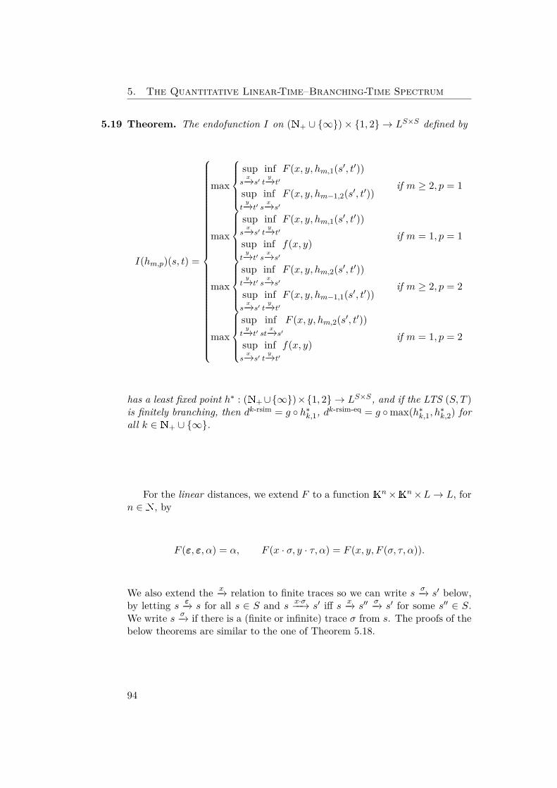
5. The Quantitative Linear-Time–Branching-Time Spectrum

5.19 Theorem. The endofunction I on (N+ ∪ {∞})× {1, 2} → LS×S defined by

I(hm,p)(s, t) =

max

supsx−→s′

infty−→t′

F (x, y, hm,1(s′, t′))

supty−→t′

infsx−→s′

F (x, y, hm−1,2(s′, t′))if m ≥ 2, p = 1

max

supsx−→s′

infty−→t′

F (x, y, hm,1(s′, t′))

supty−→t′

infsx−→s′

f(x, y)if m = 1, p = 1

max

supty−→t′

infsx−→s′

F (x, y, hm,2(s′, t′))

supsx−→s′

infty−→t′

F (x, y, hm−1,1(s′, t′))if m ≥ 2, p = 2

max

supty−→t′

infst

x−→s′

F (x, y, hm,2(s′, t′))

supsx−→s′

infty−→t′

f(x, y)if m = 1, p = 2

has a least fixed point h∗ : (N+∪{∞})×{1, 2} → LS×S, and if the LTS (S, T )is finitely branching, then dk-rsim = g ◦ h∗k,1, dk-rsim-eq = g ◦max(h∗k,1, h∗k,2) forall k ∈ N+ ∪ {∞}.

For the linear distances, we extend F to a function Kn×Kn×L→ L, forn ∈ N, by

F (ε, ε, α) = α, F (x · σ, y · τ, α) = F (x, y, F (σ, τ, α)).

We also extend the x−→ relation to finite traces so we can write s σ−→ s′ below,by letting s ε−→ s for all s ∈ S and s x·σ−−→ s′ iff s

x−→ s′′σ−→ s′ for some s′′ ∈ S.

We write s σ−→ if there is a (finite or infinite) trace σ from s. The proofs of thebelow theorems are similar to the one of Theorem 5.18.

94

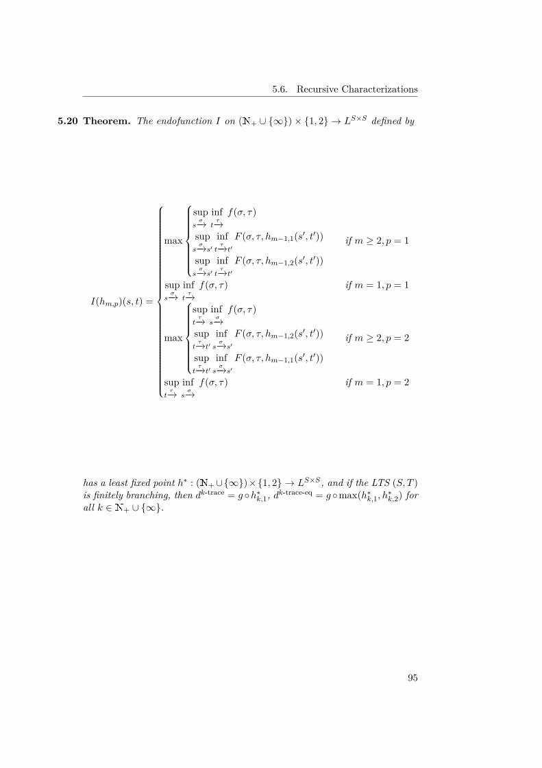
5.6. Recursive Characterizations

5.20 Theorem. The endofunction I on (N+ ∪ {∞})× {1, 2} → LS×S defined by

I(hm,p)(s, t) =

max

supsσ−→

inftτ−→f(σ, τ)

supsσ−→s′

inftτ−→t′

F (σ, τ, hm−1,1(s′, t′))

supsσ−→s′

inftτ−→t′

F (σ, τ, hm−1,2(s′, t′))

if m ≥ 2, p = 1

supsσ−→

inftτ−→f(σ, τ) if m = 1, p = 1

max

suptτ−→

infsσ−→f(σ, τ)

suptτ−→t′

infsσ−→s′

F (σ, τ, hm−1,2(s′, t′))

suptτ−→t′

infsσ−→s′

F (σ, τ, hm−1,1(s′, t′))

if m ≥ 2, p = 2

suptτ−→

infsσ−→f(σ, τ) if m = 1, p = 2

has a least fixed point h∗ : (N+∪{∞})×{1, 2} → LS×S, and if the LTS (S, T )is finitely branching, then dk-trace = g ◦h∗k,1, dk-trace-eq = g ◦max(h∗k,1, h∗k,2) forall k ∈ N+ ∪ {∞}.

95

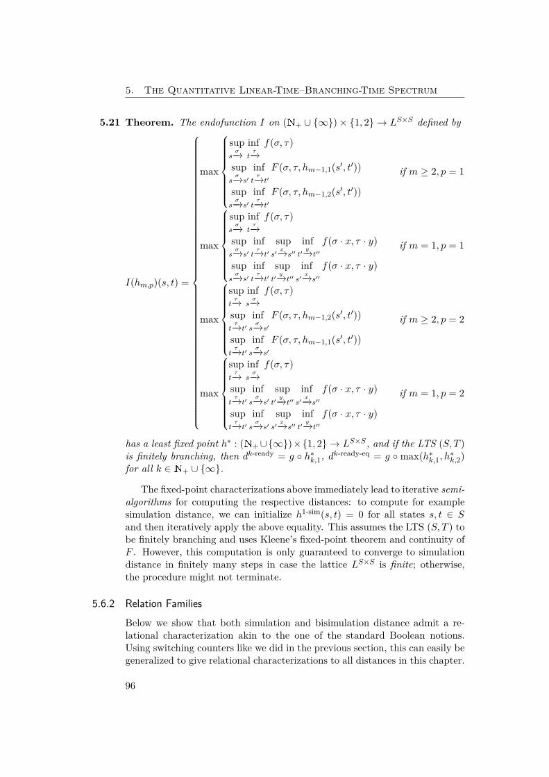
5. The Quantitative Linear-Time–Branching-Time Spectrum

5.21 Theorem. The endofunction I on (N+ ∪ {∞})× {1, 2} → LS×S defined by

I(hm,p)(s, t) =

max

supsσ−→

inftτ−→f(σ, τ)

supsσ−→s′

inftτ−→t′

F (σ, τ, hm−1,1(s′, t′))

supsσ−→s′

inftτ−→t′

F (σ, τ, hm−1,2(s′, t′))

if m ≥ 2, p = 1

max

supsσ−→

inftτ−→f(σ, τ)

supsσ−→s′

inftτ−→t′

sups′x−→s′′

inft′y−→t′′

f(σ · x, τ · y)

supsσ−→s′

inftτ−→t′

supt′y−→t′′

infs′x−→s′′

f(σ · x, τ · y)

if m = 1, p = 1

max

suptτ−→

infsσ−→f(σ, τ)

suptτ−→t′

infsσ−→s′

F (σ, τ, hm−1,2(s′, t′))

suptτ−→t′

infsσ−→s′

F (σ, τ, hm−1,1(s′, t′))

if m ≥ 2, p = 2

max

suptτ−→

infsσ−→f(σ, τ)

suptτ−→t′

infsσ−→s′

supt′y−→t′′

infs′x−→s′′

f(σ · x, τ · y)

suptτ−→t′

infsσ−→s′

sups′x−→s′′

inft′y−→t′′

f(σ · x, τ · y)

if m = 1, p = 2

has a least fixed point h∗ : (N+∪{∞})×{1, 2} → LS×S, and if the LTS (S, T )is finitely branching, then dk-ready = g ◦ h∗k,1, dk-ready-eq = g ◦ max(h∗k,1, h∗k,2)for all k ∈ N+ ∪ {∞}.

The fixed-point characterizations above immediately lead to iterative semi-algorithms for computing the respective distances: to compute for examplesimulation distance, we can initialize h1-sim(s, t) = 0 for all states s, t ∈ Sand then iteratively apply the above equality. This assumes the LTS (S, T ) tobe finitely branching and uses Kleene’s fixed-point theorem and continuity ofF . However, this computation is only guaranteed to converge to simulationdistance in finitely many steps in case the lattice LS×S is finite; otherwise,the procedure might not terminate.

5.6.2 Relation FamiliesBelow we show that both simulation and bisimulation distance admit a re-lational characterization akin to the one of the standard Boolean notions.Using switching counters like we did in the previous section, this can easily begeneralized to give relational characterizations to all distances in this chapter.

96

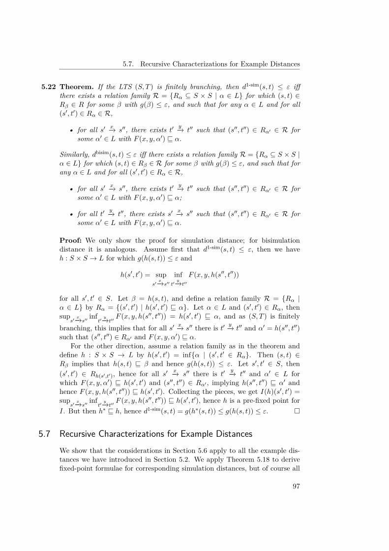
5.7. Recursive Characterizations for Example Distances

5.22 Theorem. If the LTS (S, T ) is finitely branching, then d1-sim(s, t) ≤ ε iffthere exists a relation family R = {Rα ⊆ S × S | α ∈ L} for which (s, t) ∈Rβ ∈ R for some β with g(β) ≤ ε, and such that for any α ∈ L and for all(s′, t′) ∈ Rα ∈ R,

• for all s′ x−→ s′′, there exists t′ y−→ t′′ such that (s′′, t′′) ∈ Rα′ ∈ R forsome α′ ∈ L with F (x, y, α′) v α.

Similarly, dbisim(s, t) ≤ ε iff there exists a relation family R = {Rα ⊆ S × S |α ∈ L} for which (s, t) ∈ Rβ ∈ R for some β with g(β) ≤ ε, and such that forany α ∈ L and for all (s′, t′) ∈ Rα ∈ R,

• for all s′ x−→ s′′, there exists t′ y−→ t′′ such that (s′′, t′′) ∈ Rα′ ∈ R forsome α′ ∈ L with F (x, y, α′) v α;

• for all t′ y−→ t′′, there exists s′ x−→ s′′ such that (s′′, t′′) ∈ Rα′ ∈ R forsome α′ ∈ L with F (x, y, α′) v α.

Proof: We only show the proof for simulation distance; for bisimulationdistance it is analogous. Assume first that d1-sim(s, t) ≤ ε, then we haveh : S × S → L for which g(h(s, t)) ≤ ε and

h(s′, t′) = sups′x−→s′′

inft′y−→t′′

F (x, y, h(s′′, t′′))

for all s′, t′ ∈ S. Let β = h(s, t), and define a relation family R = {Rα |α ∈ L} by Rα = {(s′, t′) | h(s′, t′) v α}. Let α ∈ L and (s′, t′) ∈ Rα, thensup

s′x−→s′′

inft′y−→t′′

F (x, y, h(s′′, t′′)) = h(s′, t′) v α, and as (S, T ) is finitelybranching, this implies that for all s′ x−→ s′′ there is t′ y−→ t′′ and α′ = h(s′′, t′′)such that (s′′, t′′) ∈ Rα′ and F (x, y, α′) v α.

For the other direction, assume a relation family as in the theorem anddefine h : S × S → L by h(s′, t′) = inf{α | (s′, t′ ∈ Rα}. Then (s, t) ∈Rβ implies that h(s, t) v β and hence g(h(s, t)) ≤ ε. Let s′, t′ ∈ S, then(s′, t′) ∈ Rh(s′,t′), hence for all s′ x−→ s′′ there is t′ y−→ t′′ and α′ ∈ L forwhich F (x, y, α′) v h(s′, t′) and (s′′, t′′) ∈ Rα′ , implying h(s′′, t′′) v α′ andhence F (x, y, h(s′′, t′′)) v h(s′, t′). Collecting the pieces, we get I(h)(s′, t′) =sup

s′x−→s′′

inft′y−→t′′

F (x, y, h(s′′, t′′)) v h(s′, t′), hence h is a pre-fixed point forI. But then h∗ v h, hence d1-sim(s, t) = g(h∗(s, t)) ≤ g(h(s, t)) ≤ ε. �

5.7 Recursive Characterizations for Example DistancesWe show that the considerations in Section 5.6 apply to all the example dis-tances we have introduced in Section 5.2. We apply Theorem 5.18 to derivefixed-point formulae for corresponding simulation distances, but of course all

97

5. The Quantitative Linear-Time–Branching-Time Spectrum

other distances in the quantitative linear-time–branching-time spectrum havesimilar characterizations.

Let d be a hemimetric on K, then for all σ, τ ∈ K∞ and 0 < λ ≤ 1,

PWλ(d)(σ, τ) =

max(d(σ0, τ0), λPWλ(d)(σ1, τ1)) if σ, τ 6= ε,

∞ if σ = ε, τ 6= ε or σ 6= ε, τ = ε,

0 if σ = τ = ε,

ACλ(d)(σ, τ) =

d(σ0, τ0) + λACλ(d)(σ1, τ1) if σ, τ 6= ε,

∞ if σ = ε, τ 6= ε or σ 6= ε, τ = ε,

0 if σ = τ = ε,

hence we can apply the iteration theorems with lattice L = R≥0∪{∞}, g = idthe identity function, and the recursion function F given like the formulaeabove. Using Theorem 5.18 we can derive the following fixed-point expressionsfor simulation distance:

PWλ(d)1-sim(s, t) = supsx−→s′

infty−→t′

max(d(x, y), λPWλ(d)1-sim(s′, t′))

ACλ(d)1-sim(s, t) = supsx−→s′

infty−→t′

(d(x, y) + λACλ(d)1-sim(s′, t′))

Incidentally, these are exactly the expressions introduced in [dAFS09] and inprevious chapters.

Also note that if S is finite with |S| = n, then undiscounted point-wise distance PW1(d) can only take on the finitely many values {d(x, y) |(s, x, s′), (t, y, t′) ∈ T}, hence the fixed-point algorithm given by Kleene’s the-orem converges in at most n2 steps. This algorithm is used in [dAFS09,DLT08, LFT11]. For undiscounted accumulating distance AC1(d), it can beshown [LFT11] that with D = max{d(x, y) | (s, x, s′), (t, y, t′) ∈ T}, distanceis either infinite or bounded above by 2n2D, hence the AC1(d) algorithm eitherconverges in at most 2n2D steps or diverges.

For the limit-average distance AV(d), we let L = (R≥0 ∪ {∞})N, g(h) =lim infj h(j), and f(σ, τ)(j) = 1

j+1∑ji=0 d(σi, τi) the j’th average. The intu-

ition is that L is used for “remembering” how long in the traces we have pro-gressed with the computation. With F given by F (x, y, h)(n) = 1

n+1d(x, y) +nn+1h(n − 1) it can be shown that (5.2) holds, giving the following fixed-point expression for limit-average simulation distance (which to the best ofour knowledge is new):

h1-simn (s, t) = sup

sx−→s′

infty−→t′

( 1n+1d(x, y) + n

n+1h1-simn−1 (s′, t′)

)For the maximum-lead distance, we let L = (R≥0 ∪ {∞})R, the lattice of

mappings from leads to maximum leads. Using the notation from Section 5.2,

98

5.7. Recursive Characterizations for Example Distances

we let g(h) = h(0) and f(σ, τ)(δ) = max(|δ|, supj |δ + ∑ji=0 σ

wi −

∑ji=0 τ

wj |)

the maximum-lead distance between σ and τ assuming that σ already hasa lead of δ over τ . With F (x, y, h)(δ) = max(|δ|, h(δ + x − y)) it can beshown that (5.2) holds, and then the fixed-point expression for maximum-lead simulation distance becomes the one given in Chapter 2:

h1-sim(δ)(s, t) = supsx−→s′

infty−→t′

max(|δ|, h1-sim(s′, t′)(δ + x− y))

Again it can be shown [HMP05] that for S finite with |S| = n and D =max{d(x, y) | (s, x, s′), (t, y, t′) ∈ T}, the iterative algorithm for computingmaximum-lead distance either converges in at most 2n2D steps or diverges.

Regarding Cantor distance, a useful recursive formulation is

f(σ, τ)(n) ={f(σ1, τ1)(n+ 1) if σ0 = τ0,

n otherwise,

which iteratively counts the number of matching symbols in σ and τ . Herewe use L = (R≥0 ∪ {∞})N and g(h) = 1

h(0) ; note that the order on L hasto be reversed for g to be monotone. The fixed-point expression for Cantorsimulation distance becomes

h1-simn (s, t) = max(n, sup

sx−→s′

inftx−→t′

h1-simn+1 (s′, t′))

but as the order on L is reversed, the sup now means that Player 1 is tryingto minimize this expression, and Player 2 tries to maximize it. Hence Player 2tries to find maximal matching subtrees; the corresponding Cantor simulationequivalence distance between s and t hence is the inverse of the maximumdepth of matching subtrees under s and t. The Cantor bisimulation distancein turn is the same as the inverse of bisimulation depth [HM85].

99

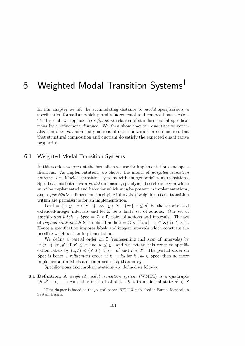
6 Weighted Modal Transition Systems1

In this chapter we lift the accumulating distance to modal specifications, aspecification formalism which permits incremental and compositional design.To this end, we replace the refinement relation of standard modal specifica-tions by a refinement distance. We then show that our quantitative gener-alization does not admit any notions of determinization or conjunction, butthat structural composition and quotient do satisfy the expected quantitativeproperties.

6.1 Weighted Modal Transition SystemsIn this section we present the formalism we use for implementations and spec-ifications. As implementations we choose the model of weighted transitionsystems, i.e., labeled transition systems with integer weights at transitions.Specifications both have amodal dimension, specifying discrete behavior whichmust be implemented and behavior which may be present in implementations,and a quantitative dimension, specifying intervals of weights on each transitionwithin are permissible for an implementation.

Let I ={[x, y]

∣∣ x ∈ Z ∪ {−∞}, y ∈ Z ∪ {∞}, x ≤ y}be the set of closed

extended-integer intervals and let Σ be a finite set of actions. Our set ofspecification labels is Spec = Σ × I, pairs of actions and intervals. The setof implementation labels is defined as Imp = Σ ×

{[x, x]

∣∣ x ∈ Z} ≈ Σ × Z.Hence a specification imposes labels and integer intervals which constrain thepossible weights of an implementation.

We define a partial order on I (representing inclusion of intervals) by[x, y] 4 [x′, y′] if x′ ≤ x and y ≤ y′, and we extend this order to specifi-cation labels by (a, I) 4 (a′, I ′) if a = a′ and I 4 I ′. The partial order onSpec is hence a refinement order; if k1 4 k2 for k1, k2 ∈ Spec, then no moreimplementation labels are contained in k1 than in k2.

Specifications and implementations are defined as follows:

6.1 Definition. A weighted modal transition system (WMTS) is a quadruple(S, s0, 99K,−→) consisting of a set of states S with an initial state s0 ∈ S

1This chapter is based on the journal paper [BFJ+13] published in Formal Methods inSystem Design.

101

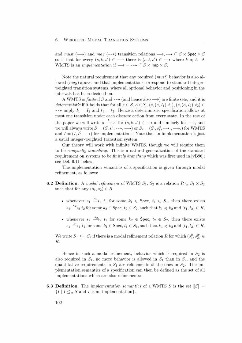
6. Weighted Modal Transition Systems

and must (−→) and may (99K) transition relations −→, 99K ⊆ S × Spec × Ssuch that for every (s, k, s′) ∈ −→ there is (s, `, s′) ∈ 99K where k 4 `. AWMTS is an implementation if −→ = 99K ⊆ S × Imp× S.

Note the natural requirement that any required (must) behavior is also al-lowed (may) above, and that implementations correspond to standard integer-weighted transition systems, where all optional behavior and positioning in theintervals has been decided on.

A WMTS is finite if S and 99K (and hence also −→) are finite sets, and it isdeterministic if it holds that for all s ∈ S, a ∈ Σ,

(s, (a, I1), t1

),(s, (a, I2), t2

)∈

99K imply I1 = I2 and t1 = t2. Hence a deterministic specification allows atmost one transition under each discrete action from every state. In the rest ofthe paper we will write s k

99K s′ for (s, k, s′) ∈ 99K and similarly for −→, andwe will always write S = (S, s0, 99K,−→) or Si = (Si, s0

i , 99Ki,−→i) for WMTSand I = (I, i0,−→) for implementations. Note that an implementation is justa usual integer-weighted transition system.

Our theory will work with infinite WMTS, though we will require themto be compactly branching. This is a natural generalization of the standardrequirement on systems to be finitely branching which was first used in [vB96];see Def. 6.11 below.

The implementation semantics of a specification is given through modalrefinement, as follows:

6.2 Definition. A modal refinement of WMTS S1, S2 is a relation R ⊆ S1 × S2such that for any (s1, s2) ∈ R

• whenever s1k199K1 t1 for some k1 ∈ Spec, t1 ∈ S1, then there exists

s2k299K2 t2 for some k2 ∈ Spec, t2 ∈ S2, such that k1 4 k2 and (t1, t2) ∈ R,

• whenever s2k2−→2 t2 for some k2 ∈ Spec, t2 ∈ S2, then there exists

s1k1−→1 t1 for some k1 ∈ Spec, t1 ∈ S1, such that k1 4 k2 and (t1, t2) ∈ R.

We write S1 ≤m S2 if there is a modal refinement relationR for which (s01, s

02) ∈

R.

Hence in such a modal refinement, behavior which is required in S2 isalso required in S1, no more behavior is allowed in S1 than in S2, and thequantitative requirements in S1 are refinements of the ones in S2. The im-plementation semantics of a specification can then be defined as the set of allimplementations which are also refinements:

6.3 Definition. The implementation semantics of a WMTS S is the set JSK ={I | I ≤m S and I is an implementation}.

102

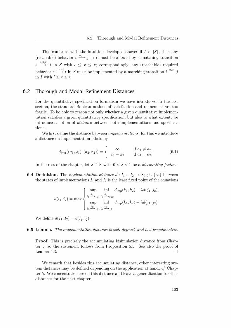
6.2. Thorough and Modal Refinement Distances

This conforms with the intuition developed above: if I ∈ JSK, then any(reachable) behavior i a,x−→ j in I must be allowed by a matching transitionsa,[l,r]99K t in S with l ≤ x ≤ r; correspondingly, any (reachable) required

behavior s a,[l,r]−→ t in S must be implemented by a matching transition i a,x−→ jin I with l ≤ x ≤ r.

6.2 Thorough and Modal Refinement DistancesFor the quantitative specification formalism we have introduced in the lastsection, the standard Boolean notions of satisfaction and refinement are toofragile. To be able to reason not only whether a given quantitative implemen-tation satisfies a given quantitative specification, but also to what extent, weintroduce a notion of distance between both implementations and specifica-tions.

We first define the distance between implementations; for this we introducea distance on implementation labels by

dImp((a1, x1), (a2, x2)

)={

∞ if a1 6= a2,|x1 − x2| if a1 = a2.

(6.1)

In the rest of the chapter, let λ ∈ R with 0 < λ < 1 be a discounting factor.

6.4 Definition. The implementation distance d : I1 × I2 → R≥0 ∪ {∞} betweenthe states of implementations I1 and I2 is the least fixed point of the equations

d(i1, i2) = max

sup

i1k1−→1j1

infi2

k2−→2j2

dImp(k1, k2) + λd(j1, j2),

supi2

k2−→2j2

infi1

k1−→1j1

dImp(k1, k2) + λd(j1, j2).

We define d(I1, I2) = d(i01, i02).

6.5 Lemma. The implementation distance is well-defined, and is a pseudometric.

Proof: This is precisely the accumulating bisimulation distance from Chap-ter 5, so the statement follows from Proposition 5.5. See also the proof ofLemma 4.3. �

We remark that besides this accumulating distance, other interesting sys-tem distances may be defined depending on the application at hand, cf. Chap-ter 5. We concentrate here on this distance and leave a generalization to otherdistances for the next chapter.

103

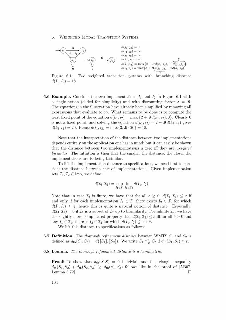
6. Weighted Modal Transition Systems

i1 j1

k1

37 6

9

i2 j26

7

d(j1, j2) = 0d(i1, j2) =∞d(j1, i2) =∞d(k1, j2) =∞d(k1, i2) = max{2 + .9 d(k1, i2), .9

0︷ ︸︸ ︷d(j1, j2)}

d(i1, i2) = max{3 + .9 d(j1, j2)︸ ︷︷ ︸0

, .9 d(k1, i2)}

Figure 6.1: Two weighted transition systems with branching distanced(I1, I2) = 18.

6.6 Example. Consider the two implementations I1 and I2 in Figure 6.1 witha single action (elided for simplicity) and with discounting factor λ = .9.The equations in the illustration have already been simplified by removing allexpressions that evaluate to ∞. What remains to be done is to compute theleast fixed point of the equation d(k1, i2) = max

{2 + .9 d(k1, i2), 0

}. Clearly 0

is not a fixed point, and solving the equation d(k1, i2) = 2 + .9 d(k1, i2) givesd(k1, i2) = 20. Hence d(i1, i2) = max{3, .9 · 20} = 18.

Note that the interpretation of the distance between two implementationsdepends entirely on the application one has in mind; but it can easily be shownthat the distance between two implementations is zero iff they are weightedbisimilar. The intuition is then that the smaller the distance, the closer theimplementations are to being bisimilar.

To lift the implementation distance to specifications, we need first to con-sider the distance between sets of implementations. Given implementationsets I1, I2 ⊆ Imp, we define

d(I1, I2) = supI1∈I1

infI2∈I2

d(I1, I2)

Note that in case I2 is finite, we have that for all ε ≥ 0, d(I1, I2) ≤ ε ifand only if for each implementation I1 ∈ I1 there exists I2 ∈ I2 for whichd(I1, I2) ≤ ε, hence this is quite a natural notion of distance. Especially,d(I1, I2) = 0 if I1 is a subset of I2 up to bisimilarity. For infinite I2, we havethe slightly more complicated property that d(I1, I2) ≤ ε iff for all δ > 0 andany I1 ∈ I1, there is I2 ∈ I2 for which d(I1, I2) ≤ ε+ δ.

We lift this distance to specifications as follows:

6.7 Definition. The thorough refinement distance between WMTS S1 and S2 isdefined as dth(S1, S2) = d

(JS1K, JS2K

). We write S1 ≤εth S2 if dth(S1, S2) ≤ ε.

6.8 Lemma. The thorough refinement distance is a hemimetric.

Proof: To show that dth(S, S) = 0 is trivial, and the triangle inequalitydth(S1, S2) + dth(S2, S3) ≥ dth(S1, S3) follows like in the proof of [AB07,Lemma 3.72]. �

104

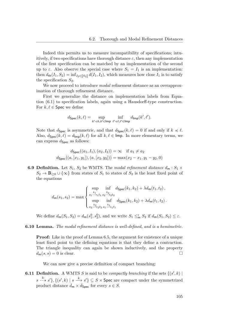
6.2. Thorough and Modal Refinement Distances

Indeed this permits us to measure incompatibility of specifications; intu-itively, if two specifications have thorough distance ε, then any implementationof the first specification can be matched by an implementation of the secondup to ε. Also observe the special case where S1 = I1 is an implementation:then dth(I1, S2) = infI2∈JS2K d(I1, I2), which measures how close I1 is to satisfythe specification S2.

We now proceed to introduce modal refinement distance as an overapprox-imation of thorough refinement distance.

First we generalize the distance on implementation labels from Equa-tion (6.1) to specification labels, again using a Hausdorff-type construction.For k, ` ∈ Spec we define

dSpec(k, `) = supk′4k,k′∈Imp

inf`′4`,`′∈Imp

dImp(k′, `′).

Note that dSpec is asymmetric, and that dSpec(k, `) = 0 if and only if k 4 `.Also, dSpec(k, `) = dImp(k, `) for all k, ` ∈ Imp. In more elementary terms, wecan express dSpec as follows:

dSpec((a1, I1), (a2, I2)

)=∞ if a1 6= a2

dSpec((a, [x1, y1]), (a, [x2, y2])

)= max(x2 − x1, y1 − y2, 0)

6.9 Definition. Let S1, S2 be WMTS. The modal refinement distance dm : S1 ×S2 → R≥0 ∪ {∞} from states of S1 to states of S2 is the least fixed point ofthe equations

dm(s1, s2) = max

sup

s1k199K1t1

infs2

k299K2t2

dSpec(k1, k2) + λdm(t1, t2) ,

sups2

k2−→2t2

infs1

k1−→1t1

dSpec(k1, k2) + λdm(t1, t2) .

We define dm(S1, S2) = dm(s01, s

02), and we write S1 ≤εm S2 if dm(S1, S2) ≤ ε.

6.10 Lemma. The modal refinement distance is well-defined, and is a hemimetric.

Proof: Like in the proof of Lemma 6.5, the argument for existence of a uniqueleast fixed point to the defining equations is that they define a contraction.The triangle inequality can again be shown inductively, and the propertydm(s, s) = 0 is clear. �

We can now give a precise definition of compact branching:

6.11 Definition. A WMTS S is said to be compactly branching if the sets {(s′, k) |s

k99K s′}, {(s′, k) | s k−→ s′} ⊆ S × Spec are compact under the symmetrized

product distance dm × dSpec for every s ∈ S.

105

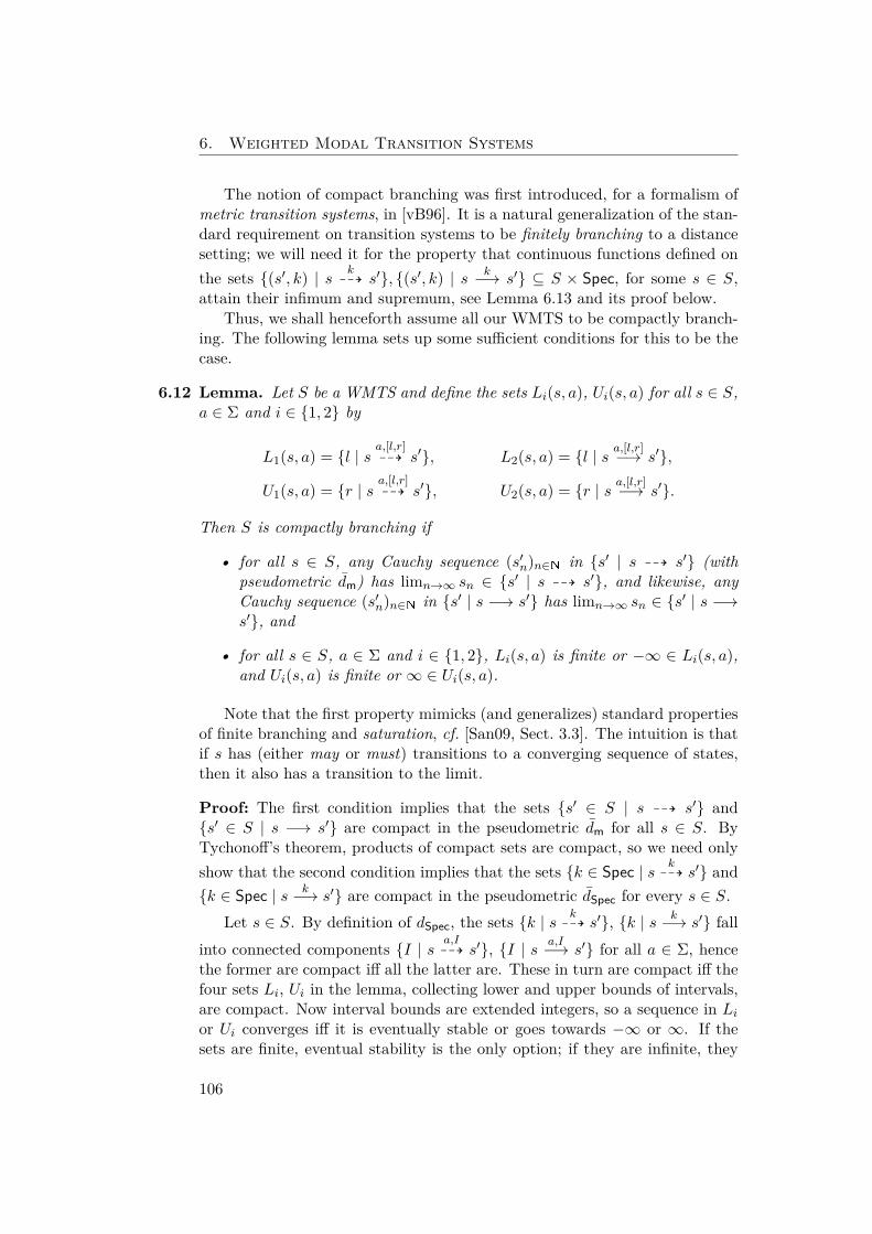
6. Weighted Modal Transition Systems

The notion of compact branching was first introduced, for a formalism ofmetric transition systems, in [vB96]. It is a natural generalization of the stan-dard requirement on transition systems to be finitely branching to a distancesetting; we will need it for the property that continuous functions defined onthe sets {(s′, k) | s k

99K s′}, {(s′, k) | s k−→ s′} ⊆ S × Spec, for some s ∈ S,attain their infimum and supremum, see Lemma 6.13 and its proof below.

Thus, we shall henceforth assume all our WMTS to be compactly branch-ing. The following lemma sets up some sufficient conditions for this to be thecase.

6.12 Lemma. Let S be a WMTS and define the sets Li(s, a), Ui(s, a) for all s ∈ S,a ∈ Σ and i ∈ {1, 2} by

L1(s, a) = {l | sa,[l,r]99K s′}, L2(s, a) = {l | s a,[l,r]−→ s′},

U1(s, a) = {r | sa,[l,r]99K s′}, U2(s, a) = {r | s a,[l,r]−→ s′}.

Then S is compactly branching if

• for all s ∈ S, any Cauchy sequence (s′n)n∈N in {s′ | s 99K s′} (withpseudometric dm) has limn→∞ sn ∈ {s′ | s 99K s′}, and likewise, anyCauchy sequence (s′n)n∈N in {s′ | s −→ s′} has limn→∞ sn ∈ {s′ | s −→s′}, and

• for all s ∈ S, a ∈ Σ and i ∈ {1, 2}, Li(s, a) is finite or −∞ ∈ Li(s, a),and Ui(s, a) is finite or ∞ ∈ Ui(s, a).

Note that the first property mimicks (and generalizes) standard propertiesof finite branching and saturation, cf. [San09, Sect. 3.3]. The intuition is thatif s has (either may or must) transitions to a converging sequence of states,then it also has a transition to the limit.

Proof: The first condition implies that the sets {s′ ∈ S | s 99K s′} and{s′ ∈ S | s −→ s′} are compact in the pseudometric dm for all s ∈ S. ByTychonoff’s theorem, products of compact sets are compact, so we need onlyshow that the second condition implies that the sets {k ∈ Spec | s k

99K s′} and{k ∈ Spec | s k−→ s′} are compact in the pseudometric dSpec for every s ∈ S.

Let s ∈ S. By definition of dSpec, the sets {k | s k99K s′}, {k | s k−→ s′} fall

into connected components {I | s a,I99K s′}, {I | s a,I−→ s′} for all a ∈ Σ, hence

the former are compact iff all the latter are. These in turn are compact iff thefour sets Li, Ui in the lemma, collecting lower and upper bounds of intervals,are compact. Now interval bounds are extended integers, so a sequence in Lior Ui converges iff it is eventually stable or goes towards −∞ or ∞. If thesets are finite, eventual stability is the only option; if they are infinite, they

106

6.2. Thorough and Modal Refinement Distances

need to include the limit points −∞ (for the lower interval bounds in Li) or∞ (for the upper interval bounds in Ui). �

We extend the notion of relation families from revious chapters to modalrefinement distance. We define a modal refinement family as an R≥0-indexedfamily of relations R = {Rε ⊆ S1 × S2 | ε ≥ 0} such that for any ε and any(s1, s2) ∈ Rε ∈ R,

• whenever s1k199K t1 for some k1 ∈ Spec, t1 ∈ S1, then there exists

s2k299K t2 for some k2 ∈ Spec, t2 ∈ S2, such that dSpec(k1, k2) ≤ ε and

(t1, t2) ∈ Rε′ ∈ R for some ε′ ≤ λ−1(ε− dSpec(k1, k2)),

• whenever s2k2−→ t2 for some k2 ∈ Spec, t2 ∈ S2, then there exists

s1k1−→ t1 for some k1 ∈ Spec, t1 ∈ S1, such that dSpec(k1, k2) ≤ ε and

(t1, t2) ∈ Rε′ ∈ R for some ε′ ≤ λ−1(ε− dSpec(k1, k2)).

Note that modal refinement families are

• upward closed in the sense that (s1, s2) ∈ Rε implies that (s1, s2) ∈ Rε′for all ε′ ≥ ε, and

• downward compact in the sense that for any set E ⊆ R≥0, if (s1, s2) ∈ Rεfor all ε ∈ E, then also (s1, s2) ∈ Rinf E . This property follows from theassumption that our WMTS are compactly branching.

Following the proof strategy developed in previous chapters for imple-mentations, we can show the following characterization of modal refinementdistance by modal refinement families:

6.13 Lemma. S1 ≤εm S2 iff there is a modal refinement family R with (s01, s

02) ∈

Rε ∈ R.

Proof: First, assume that S1 ≤εm S2, i.e., dm(s01, s

02) ≤ ε, and define a relation

family R = {Rδ | δ ≥ 0} by Rδ = {(s1, s2) ∈ S1 × S2 | dm(s1, s2) ≤ δ} for allδ ≥ 0, then (s0

1, s02) ∈ Rε holds by assumption. We show that R is a modal

refinement family. Let (s1, s2) ∈ Rδ for some δ ≥ 0, then by definition weknow that dm(s1, s2) ≤ δ. Assume s1

k199K1 t1. From dm(s1, s2) ≤ δ we can

infer thatinf

s2k299K2t2

dSpec(k1, k2) + λdm(t1, t2) ≤ δ .

Hence, because S2 is compactly branching, there exists a may-transition s2k299K

t2 such that dSpec(k1, k2) ≤ δ and dm(t1, t2) ≤ λ−1(δ − dSpec(k1, k2)). Thelatter implies that (t1, t2) ∈ Rδ′ for some δ′ ≤ λ−1(δ − dSpec(k1, k2)) whichwas to be shown. The argument for the other assertion for must-transitions is

107

6. Weighted Modal Transition Systems

symmetric. This proves that there is a modal refinement family R such that(s0

1, s02) ∈ Rε ∈ R.

For the reverse direction, assume that (s01, s

02) ∈ Rε ∈ R for some modal

refinement family R = {Rε | ε ≥ 0}. We prove that (s1, s2) ∈ Rδ, for someδ ≥ 0, implies dm(s1, s2) ≤ δ. The claim S1 ≤εm S2 then follows from theassumption (s0

1, s02) ∈ Rε.

To this end, observe that the space of functions ∆ = [S1×S2 → R≥0∪{∞}]forms a complete lattice, when the partial order ≤∆ is defined such that forf, f ′ ∈ ∆, f ≤∆ f ′ iff f(s1, s2) ≤ f ′(s1, s2) for all s1 ∈ S1, s2 ∈ S2. Moreover,since max, sup, inf and + are monotone, the function D defined for all f ∈ ∆by

D(f) = max

sup

s1k199K1t1

infs2

k299K2t2

dSpec(k1, k2) + λf(t1, t2) ,

sups2

k2−→2t2

infs1

k1−→1t1

dSpec(k1, k2) + λf(t1, t2)

is a monotone endofunction on ∆, hence by Tarski’s fixed point theorem, Dhas a least fixed point. Now define h(s1, s2) = inf{δ | (s1, s2) ∈ Rδ ∈ R};since Rδ is downward compact, we have (s1, s2) ∈ Rh(s1,s2). By showing thath is a pre-fixed point of D, i.e., that D(h) ≤∆ h, we get that (s1, s2) ∈ Rδimplies that dm(s1, s2) ≤ δ, since h(s1, s2) ≤ δ and dm(s1, s2) ≤ h(s1, s2).

Since (s1, s2) ∈ Rh(s1,s2), every s1k199K s′1 can be matched by some s2

k299K s′2

such that dSpec(k1, k2) + λδ′ ≤ h(s1, s2) for some δ′ where (s′1, s′2) ∈ Rδ′ ,implying h(s′1, s′2) ≤ δ′, but then also dSpec(k1, k2) + λh(s′1, s′2) ≤ h(s1, s2).Similarly, every s2

k2−→ s′2 has a match s1k1−→ s′1 such that dSpec(k1, k2) +

λh(s′1, s′2) ≤ h(s1, s2). Hence we have D(h) ≤∆ h which was to be shown. �

The next theorems show that modal refinement distance indeed overap-proximates thorough refinement distance, and that it is exact for determinis-tic WMTS. Note that nothing general can be said about the precision of theoverapproximation in the nondeterministic case; the standard counterexam-ple given for the Boolean case in [BKLS09] shows that there exist WMTS forwhich dth(S1, S2) = 0 but dm(S1, S2) =∞.

6.14 Theorem. For WMTS S1, S2 we have dth(S1, S2) ≤ dm(S1, S2).

Proof: If dm(S1, S2) = ∞, we have nothing to prove. Otherwise, let R ={Rε ⊆ S1 × S2 | ε ≥ 0} be a modal refinement family which witnessesdm(S1, S2), i.e., such that (s0

1, s02) ∈ Rdm(S1,S2), and let I1 ∈ JS1K. We have to

expose I2 ∈ JS2K for which d(I1, I2) ≤ dm(S1, S2).Let R ⊆ I1 × S1 be a witness for I1 ≤m S1, define R′ε = R ◦ Rε ⊆ I1 × S2

for all ε ≥ 0, and let R′ = {R′ε | ε ≥ 0}. The states of I2 = (I2, i02, Imp,−→I2)

are I2 = S2 with i02 = s02, and the transitions we define as follows:

108

6.2. Thorough and Modal Refinement Distances

For any i1k′1−→I1 j1 and any s2 ∈ S2 for which (i1, s2) ∈ R′ε ∈ R′ for some

ε, we have s2k299K2 t2 in S2 with dSpec(k′1, k2) ≤ ε and (j1, t2) ∈ R′ε′ ∈ R′ for

some ε′ ≤ λ−1(ε − dSpec(k′1, k2)). Write k′1 = (a′1, x′1) and k2 =

(a2, [x2, y2]

),

then we must have a′1 = a2. Let

x′2 =

x2 if x′1 < x2,

x′1 if x2 ≤ x′1 ≤ y2,

y2 if x′1 > y2

(6.2)

and k′2 = (a2, x′2), and put s2

k′2−→I2 t2 in I2. Note that

dSpec(k′1, k′2) = dSpec(k′1, k2). (6.3)

Similarly, for any s2k2−→2 t2 in S2 and any i1 ∈ I1 with (i1, s2) ∈ R′ε ∈ R′

for some ε, we have i1k′1−→I1 j1 with dSpec(k′1, k2) ≤ ε and (j1, t2) ∈ R′ε′ ∈ R′

for some ε′ ≤ λ−1(ε−dSpec(k′1, k2)). Write k′1 = (a′1, x′1) and k2 = (a2, [x2, y2]),

define x′2 as in (6.2) and k′2 = (a2, x′2), and put s2

k′2−→I2 t2 in I2.We show that the identity relation idS2 = {(s2, s2) | s2 ∈ S2} ⊆ S2 × S2

witnesses I2 ≤m S2. Let first s2k′2−→I2 t2; we must have used one of the two

constructions above for creating this transition. In the first case, we haves2

k299K2 t2 with k′2 4 k2, and in the second case, we have s2

k2−→2 t2, hence alsos2

k299K2 t2, with the same property. For a transition s2

k2−→2 t2 on the otherhand, we have introduced s2

k′2−→I2 t2 in the second construction above, withk′2 4 k2.

We also want to show that the family R′ is a witness for d(I1, I2) ≤dm(S1, S2). We have (i01, s0

2) ∈ R′dm(S1,S2) = R◦Rdm(S1,S2), so let (i1, s2) ∈ R′ε ∈

R′ for some ε ≥ 0. For any i1k′1−→I1 j1 we have s2

k299K2 t2 and s2

k′2−→I2 t2 by thefirst part of our construction above, with dSpec(k′1, k′2) = dSpec(k′1, k2) ≤ ε be-cause of (6.3), and also (j1, t2) ∈ R′ε′ ∈ R′ for some ε′ ≤ λ−1(ε−dSpec(k′1, k2)

).

For any s2k′2−→I2 t2, we must have used one of the constructions above to in-

troduce this transition, and both give us i1k′1−→I1 j1 with dSpec(k′1, k′2) ≤ ε and

(j1, t2) ∈ R′ε′ ∈ R′ for some ε′ ≤ λ−1(ε− dSpec(k′1, k2)). �

The fact that modal refinement only equals thorough refinement for de-terministic specifications is well-known from the theory of modal transitionsystems [Lar89], and the special case of S2 deterministic is important, as itcan be argued [Lar89] that deterministic specifications are sufficient for appli-cations.

6.15 Theorem. If S2 is deterministic, then dth(S1, S2) = dm(S1, S2).

109

6. Weighted Modal Transition Systems

Proof: If dth(S1, S2) = ∞, we are done by Theorem 6.14. Otherwise, letR = {Rε | ε ≥ 0} be the smallest relation family for which

• (s01, s

02) ∈ Rdth(S1,S2) and

• whenever we have (s1, s2) ∈ Rε ∈ R, s1a,I199K1 t1, and s2

a,I299K2 t2, then

(t1, t2) ∈ Rλ−1(ε−dSpec((a,I1),(a,I2))) ∈ R.

We show below that R is well-defined (also that ε−dSpec((a, I1), (a, I2)

)≥ 0 in

all cases) and a modal refinement family. We will use the convenient notation(s1, S1) for the WMTS S1 with initial state s0

1 replaced by s1, similarly for(s2, S2).

We first show inductively that for any pair of states (s1, s2) ∈ Rε ∈ R wehave dth

((s1, S1), (s2, S2)

)≤ ε. This is obviously the case for s1 = s0

1 and s1 =s0

2, so assume now that (s1, s2) ∈ Rε ∈ R is such that dth((s1, S1), (s2, S2)

)≤ ε

and let s1a,I199K1 t1, s2

a,I299K2 t2. Let (q′1, P ′1) ∈ J(t1, S1)K and x1 ∈ I1.

There is an implementation (p1, P1) ∈ J(s1, S1)K for which p1a,x1−−→ q1 and

such that (q1, P1) ≤m (q′1, P ′1). Now

dth((p1, P1), (s2, S2)

)≤ dth

((p1, P1), (s1, S1)

)+ dth

((s1, S1), (s2, S2)

)≤ ε,

hence we must have s2a′2,I

′2

99K2 t′2 with dSpec((a, x1), (a′2, I ′2)

)≤ ε. But then

a′2 = a, hence by determinism of S2, I2 = I ′2 and t2 = t′2.The above considerations hold for any x1 ∈ I1, hence dSpec

((a, I1), (a, I2)

)≤

ε. Thus ε−dSpec((a, I1), (a, I2)

)≥ 0, and the definition of R above is justified.

Now let x2 ∈ I2 such that dSpec((a, x1), (a, x2)

)= dSpec

((a, x1), (a, I2)

), then

there is an implementation (p2, P2) ∈ J(s2, S2)K for which p2a,x2−−→ q2, and

d((q′1, P ′1), (q2, P2)

)≤ λ−1(ε− dSpec((a, x1), (a, x2))

)= λ−1(ε− dSpec((a, I1), (a, I2))

),

which, as (q′1, P ′1) ∈ J(t1, S1)K was chosen arbitrarily, entails

dth((s1, S1), (s2, S2)

)≤ λ−1(ε− dSpec((a, I1), (a, I2))

).

We are ready to show that R is a modal refinement family. Let (s1, s2) ∈Rε ∈ R for some ε, and assume s1

a,I199K1 t1. Let x ∈ I1, then there is (p, P x) ∈

J(s1, S1)K with a transition pm−→ q. Now dth

((p, P x), (s2, S2)

)≤ ε, hence

we have a transition s2a,Ix299K2 tx2 with dSpec

((a, x), (a, Ix2 )

)≤ ε. Also for any

other x′ ∈ I1 we have a transition s2a,Ix

′299K2 t

x′2 with dSpec

((a, x′), (a, Ix′2 )

)≤ ε,

hence by determinism of S2, Ix2 = Ix′

2 and tx2 = tx′

2 . It follows that there is aunique transition s2

a,I299K t2, and as dSpec

((a, x), (a, I2)

)≤ ε for all x ∈ I1, we

110

6.3. Relaxation

have dSpec((a, I1), (a, I2)

)≤ ε, and (t1, t2) ∈ Rλ−1(ε−dSpec((a,I1),(a,I2))) ∈ R by

definition.Now assume s2

a,I2−→2 t2. Let (p1, P1) ∈ J(s1, S1)K, then we have (p2, P2) ∈J(s2, S2)K with d

((p1, P1), (p2, P2)

)≤ ε. Now any (p2, P2) ∈ J(s2, S2)K has

p2a,x2−−→ q2 with x2 ∈ I2, thus there is also p1

a,x1−−→ q1 with dSpec((a, x1), (a, x2)

)≤

ε and d((q1, P1), (q2, P2)

)≤ λ−1(ε − dSpec((a, x1), (a, x2))

). This in turn

implies that s1a,I1−→1 t1 for some x1 ∈ I1. We will be done once we can

show dSpec((a, I1), (a, I2)

)≤ ε, so assume to the contrary that there is x′1 ∈

I1 with dSpec((a, x′1), (a, I2)

)> ε. Then there must be an implementation

(p′1, P ′1) ∈ J(s1, S1)K with p′1a,x′1−−→ q′1, hence a transition s2

a,I′299K2 t′2 with

dSpec((a, x′1), (a, I ′2)

)≤ ε. But I ′2 = I2 by determinism of S2, a contradic-

tion. �

6.3 RelaxationWe introduce here a notion of relaxation which is specific to the quantitativesetting. Intuitively, relaxing a specification means to weaken the quantitativeconstraints, while the discrete demands on which transitions may or must bepresent in implementations are kept. A similar notion of strengthening maybe defined, but we do not use this here.

6.16 Definition. For WMTS S, S′ and ε ≥ 0, S′ is an ε-relaxation of S if S ≤m S′

and S′ ≤εm S.

Hence the quantitative constraints in S′ may be more permissive than theones in S, but no new discrete behavior may be introduced. Also note that anyimplementation of S is also an implementation of S′, and no implementationof S′ is further than ε away from an implementation of S. The followingproposition relates specifications to relaxed specifications:

6.17 Proposition. If S′1 and S′2 are ε-relaxations of S1 and S2, respectively, thendm(S1, S2) − ε ≤ dm(S1, S

′2) ≤ dm(S1, S2) and dm(S1, S2) ≤ dm(S′1, S2) ≤

dm(S1, S2) + ε.

Proof: By the triangle inequality we have

dm(S1, S′2) ≤ dm(S1, S2) + dm(S2, S

′2),

dm(S1, S2) ≤ dm(S1, S′2) + dm(S′2, S2),

dm(S1, S2) ≤ dm(S1, S′1) + dm(S′1, S2),

dm(S′1, S2) ≤ dm(S′1, S1) + dm(S1, S2). �

On the syntactic level, we can introduce the following widening operatorwhich relaxes all quantitative constraints in a systematic manner. We writeI ± δ = [x− δ, y + δ] for an interval I = [x, y] and δ ∈ N.

111

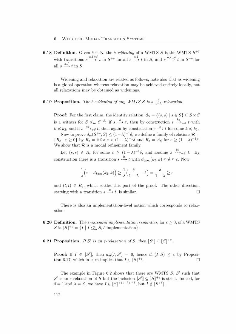
6. Weighted Modal Transition Systems

6.18 Definition. Given δ ∈ N, the δ-widening of a WMTS S is the WMTS S+δ

with transitions s a,I±δ99K t in S+δ for all s a,I

99K t in S, and s a,I±δ−→ t in S+δ forall s a,I−→ t in S.

Widening and relaxation are related as follows; note also that as wideningis a global operation whereas relaxation may be achieved entirely locally, notall relaxations may be obtained as widenings.

6.19 Proposition. The δ-widening of any WMTS S is a δ1−λ -relaxation.

Proof: For the first claim, the identity relation idS = {(s, s) | s ∈ S} ⊆ S×Sis a witness for S ≤m S+δ: if s k

99K t, then by construction sk299K+δ t with

k 4 k2, and if s k2−→+δ t, then again by construction s k−→ t for some k 4 k2.Now to prove dm(S+δ, S) ≤ (1−λ)−1δ, we define a family of relations R =

{Rε | ε ≥ 0} by Rε = ∅ for ε < (1 − λ)−1δ and Rε = idS for ε ≥ (1− λ)−1δ.We show that R is a modal refinement family.

Let (s, s) ∈ Rε for some ε ≥ (1− λ)−1δ, and assume s k299K+δ t. By

construction there is a transition s k99K t with dSpec(k2, k) ≤ δ ≤ ε. Now

1λ

(ε− dSpec(k2, k)

)≥ 1λ

( δ

1− λ − δ)

= δ

1− λ ≥ ε

and (t, t) ∈ Rε, which settles this part of the proof. The other direction,starting with a transition s k−→ t, is similar. �

There is also an implementation-level notion which corresponds to relax-ation:

6.20 Definition. The ε-extended implementation semantics, for ε ≥ 0, of a WMTSS is JSK+ε =

{I∣∣ I ≤εm S, I implementation

}.

6.21 Proposition. If S′ is an ε-relaxation of S, then JS′K ⊆ JSK+ε.

Proof: If I ∈ JS′K, then dm(I, S′) = 0, hence dm(I, S) ≤ ε by Proposi-tion 6.17, which in turn implies that I ∈ JSK+ε. �

The example in Figure 6.2 shows that there are WMTS S, S′ such thatS′ is an ε-relaxation of S but the inclusion JS′K ⊆ JSK+ε is strict. Indeed, forδ = 1 and λ = .9, we have I ∈ JSK+(1−λ)−1δ, but I /∈ JS+δK.

112

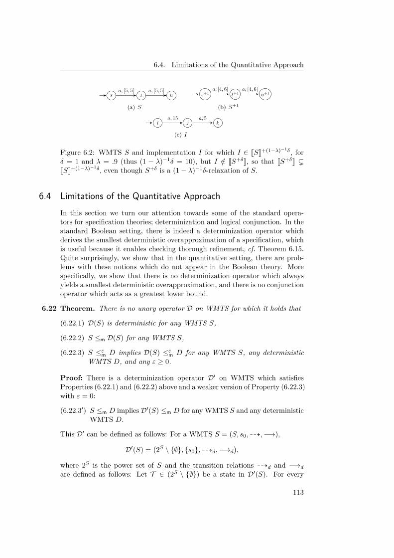
6.4. Limitations of the Quantitative Approach

s t ua, [5, 5] a, [5, 5]

(a) S

s+1 t+1 u+1a, [4, 6] a, [4, 6]

(b) S+1

i j ka, 15 a, 5

(c) I

Figure 6.2: WMTS S and implementation I for which I ∈ JSK+(1−λ)−1δ, forδ = 1 and λ = .9 (thus (1 − λ)−1δ = 10), but I /∈ JS+δK, so that JS+δK (JSK+(1−λ)−1δ, even though S+δ is a (1− λ)−1δ-relaxation of S.

6.4 Limitations of the Quantitative ApproachIn this section we turn our attention towards some of the standard opera-tors for specification theories; determinization and logical conjunction. In thestandard Boolean setting, there is indeed a determinization operator whichderives the smallest deterministic overapproximation of a specification, whichis useful because it enables checking thorough refinement, cf. Theorem 6.15.Quite surprisingly, we show that in the quantitative setting, there are prob-lems with these notions which do not appear in the Boolean theory. Morespecifically, we show that there is no determinization operator which alwaysyields a smallest deterministic overapproximation, and there is no conjunctionoperator which acts as a greatest lower bound.

6.22 Theorem. There is no unary operator D on WMTS for which it holds that

(6.22.1) D(S) is deterministic for any WMTS S,

(6.22.2) S ≤m D(S) for any WMTS S,

(6.22.3) S ≤εm D implies D(S) ≤εm D for any WMTS S, any deterministicWMTS D, and any ε ≥ 0.

Proof: There is a determinization operator D′ on WMTS which satisfiesProperties (6.22.1) and (6.22.2) above and a weaker version of Property (6.22.3)with ε = 0:

(6.22.3′) S ≤m D implies D′(S) ≤m D for any WMTS S and any deterministicWMTS D.

This D′ can be defined as follows: For a WMTS S = (S, s0, 99K,−→),

D′(S) =(2S \ {∅}, {s0}, 99Kd,−→d

),

where 2S is the power set of S and the transition relations 99Kd and −→d

are defined as follows: Let T ∈ (2S \ {∅}) be a state in D′(S). For every

113

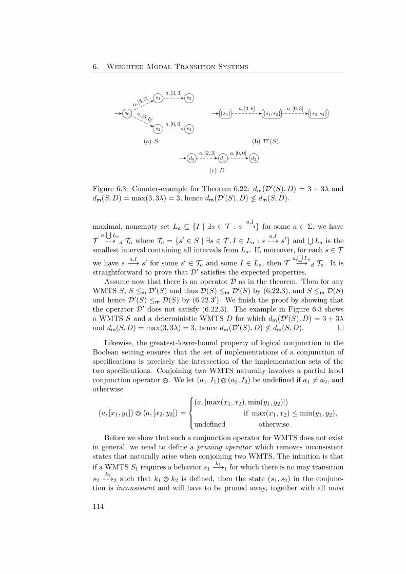
6. Weighted Modal Transition Systems

s0

s1

s2

s3

s4

a, [3, 3]

a, [5, 6]a, [0, 0]

a, [3, 3]

(a) S

{s0} {s1, s2} {s3, s4}a, [3, 6] a, [0, 3]

(b) D′(S)

d0 d1 d2a, [2, 3] a, [0, 0]

(c) D

Figure 6.3: Counter-example for Theorem 6.22: dm(D′(S), D

)= 3 + 3λ and

dm(S,D) = max(3, 3λ) = 3, hence dm(D′(S), D

)6≤ dm(S,D).

maximal, nonempty set La ⊆ {I | ∃s ∈ T : s a,I99K} for some a ∈ Σ, we have

Ta,⋃La

99K d Ta where Ta = {s′ ∈ S | ∃s ∈ T , I ∈ La : s a,I99K s′} and ⋃La is the

smallest interval containing all intervals from La. If, moreover, for each s ∈ Twe have s a,I−→ s′ for some s′ ∈ Ta and some I ∈ La, then T

a,⋃La−→ d Ta. It is

straightforward to prove that D′ satisfies the expected properties.Assume now that there is an operator D as in the theorem. Then for any

WMTS S, S ≤m D′(S) and thus D(S) ≤m D′(S) by (6.22.3), and S ≤m D(S)and hence D′(S) ≤m D(S) by (6.22.3′). We finish the proof by showing thatthe operator D′ does not satisfy (6.22.3). The example in Figure 6.3 showsa WMTS S and a deterministic WMTS D for which dm

(D′(S), D

)= 3 + 3λ

and dm(S,D) = max(3, 3λ) = 3, hence dm(D′(S), D

)6≤ dm(S,D). �

Likewise, the greatest-lower-bound property of logical conjunction in theBoolean setting ensures that the set of implementations of a conjunction ofspecifications is precisely the intersection of the implementation sets of thetwo specifications. Conjoining two WMTS naturally involves a partial labelconjunction operator 7. We let (a1, I1)7 (a2, I2) be undefined if a1 6= a2, andotherwise

(a, [x1, y1]

)7(a, [x2, y2]

)=

(a, [max(x1, x2),min(y1, y2)]

)if max(x1, x2) ≤ min(y1, y2),

undefined otherwise.

Before we show that such a conjunction operator for WMTS does not existin general, we need to define a pruning operator which removes inconsistentstates that naturally arise when conjoining two WMTS. The intuition is thatif a WMTS S1 requires a behavior s1

k1−→1 for which there is no may transitions2

k299K2 such that k1 7 k2 is defined, then the state (s1, s2) in the conjunc-

tion is inconsistent and will have to be pruned away, together with all must

114

6.4. Limitations of the Quantitative Approach

s ta, [1, 2]

(a) S

s1 t1a, [0, 1]

(b) S1

s2 t2a, [2, 3]

(c) S2

(s1, s2)

(d) S1 ∧ S2

Figure 6.4: Counter-example for Theorem 6.24: dm(S, S1) = dm(S, S2) = 1,but dm(S, S1 ∧ S2) =∞.

transitions leading to it. In the definition below, pre∗ denotes the reflexive,transitive closure of pre.

6.23 Definition. For a WMTS S, let pre : 2S → 2S be given by pre(B) = {s ∈S | s k−→ t ∈ B for some k}. Let B ⊆ S be a set of inconsistent states.If s0 /∈ pre∗(B), then the pruning of S w.r.t. B is defined by ρB(S) =(Sρ, s0, 99Kρ,−→ρ) where Sρ = S \pre∗(B), 99Kρ = 99K∩

(Sρ×Spec×Sρ

)and

−→ρ = −→∩(Sρ × Spec× Sρ

).

6.24 Theorem. There is no partial binary operator ∧ on WMTS for which it holdsthat, for all WMTS S, S1, S2 such that S1 and S2 are deterministic,

(6.24.1) whenever S1 ∧ S2 is defined, then S1 ∧ S2 ≤m S1 and S1 ∧ S2 ≤m S2,

(6.24.2) whenever S ≤m S1 and S ≤m S2, then S1 ∧ S2 is defined and S ≤mS1 ∧ S2,

(6.24.3) for any ε ≥ 0, there exist ε1 ≥ 0 and ε2 ≥ 0 such that if S1 ∧ S2 isdefined, S ≤ε1m S1 and S ≤ε2m S2, then S ≤εm S1 ∧ S2.

Proof: We follow the same strategy as in the proof of Theorem 6.22. Onecan define a partial conjunction operator ∧′ defined for WMTS which satisfiesProperties (6.24.1) and (6.24.2) as follows: For deterministic WMTS S1 andS2, S1∧′ S2 = ρB(S1×S2, (s0

1, s02), 99K,−→) where the transition relations 99K

and −→ and the set B ⊆ S1 × S2 of inconsistent states are defined by the

115

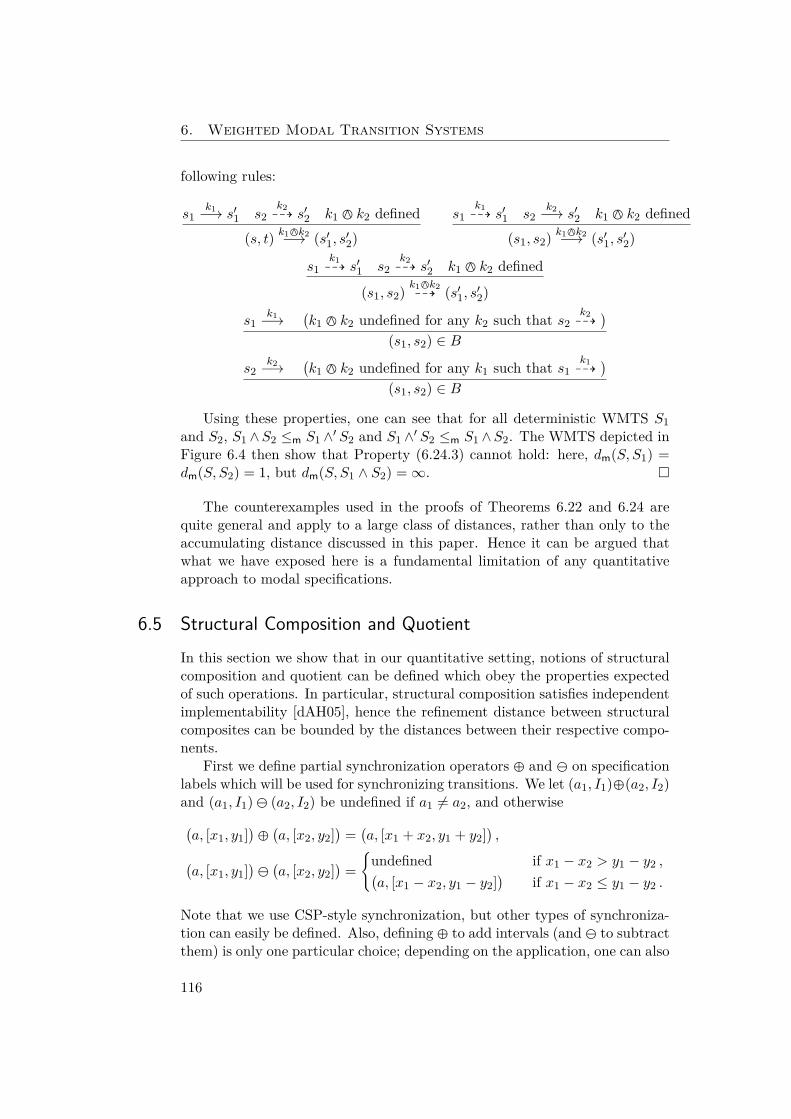
6. Weighted Modal Transition Systems

following rules:

s1k1−→ s′1 s2

k299K s′2 k1 7 k2 defined

(s, t) k17k2−→ (s′1, s′2)s1

k199K s′1 s2

k2−→ s′2 k1 7 k2 defined(s1, s2) k17k2−→ (s′1, s′2)

s1k199K s′1 s2

k299K s′2 k1 7 k2 defined

(s1, s2) k17k299K (s′1, s′2)

s1k1−→

(k1 7 k2 undefined for any k2 such that s2

k299K

)(s1, s2) ∈ B

s2k2−→

(k1 7 k2 undefined for any k1 such that s1

k199K

)(s1, s2) ∈ B

Using these properties, one can see that for all deterministic WMTS S1and S2, S1 ∧S2 ≤m S1 ∧′ S2 and S1 ∧′ S2 ≤m S1 ∧S2. The WMTS depicted inFigure 6.4 then show that Property (6.24.3) cannot hold: here, dm(S, S1) =dm(S, S2) = 1, but dm(S, S1 ∧ S2) =∞. �

The counterexamples used in the proofs of Theorems 6.22 and 6.24 arequite general and apply to a large class of distances, rather than only to theaccumulating distance discussed in this paper. Hence it can be argued thatwhat we have exposed here is a fundamental limitation of any quantitativeapproach to modal specifications.

6.5 Structural Composition and QuotientIn this section we show that in our quantitative setting, notions of structuralcomposition and quotient can be defined which obey the properties expectedof such operations. In particular, structural composition satisfies independentimplementability [dAH05], hence the refinement distance between structuralcomposites can be bounded by the distances between their respective compo-nents.

First we define partial synchronization operators � and � on specificationlabels which will be used for synchronizing transitions. We let (a1, I1)�(a2, I2)and (a1, I1) � (a2, I2) be undefined if a1 6= a2, and otherwise(a, [x1, y1]

)�(a, [x2, y2]

)=(a, [x1 + x2, y1 + y2]

),

(a, [x1, y1]

)�(a, [x2, y2]

)={undefined if x1 − x2 > y1 − y2 ,(a, [x1 − x2, y1 − y2]

)if x1 − x2 ≤ y1 − y2 .

Note that we use CSP-style synchronization, but other types of synchroniza-tion can easily be defined. Also, defining � to add intervals (and � to subtractthem) is only one particular choice; depending on the application, one can also

116

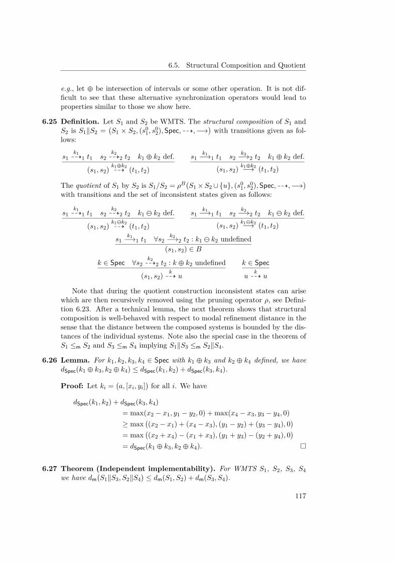
6.5. Structural Composition and Quotient

e.g., let � be intersection of intervals or some other operation. It is not dif-ficult to see that these alternative synchronization operators would lead toproperties similar to those we show here.

6.25 Definition. Let S1 and S2 be WMTS. The structural composition of S1 andS2 is S1‖S2 =

(S1 × S2, (s0

1, s02), Spec, 99K,−→

)with transitions given as fol-

lows:

s1k199K1 t1 s2

k299K2 t2 k1 � k2 def.

(s1, s2) k1�k299K (t1, t2)

s1k1−→1 t1 s2

k2−→2 t2 k1 � k2 def.(s1, s2) k1�k2−→ (t1, t2)

The quotient of S1 by S2 is S1/S2 = ρB(S1×S2 ∪{u}, (s0

1, s02), Spec, 99K,−→

)with transitions and the set of inconsistent states given as follows:

s1k199K1 t1 s2

k299K2 t2 k1 � k2 def.

(s1, s2) k1�k299K (t1, t2)

s1k1−→1 t1 s2

k2−→2 t2 k1 � k2 def.(s1, s2) k1�k2−→ (t1, t2)

s1k1−→1 t1 ∀s2

k2−→2 t2 : k1 � k2 undefined(s1, s2) ∈ B

k ∈ Spec ∀s2k299K2 t2 : k � k2 undefined

(s1, s2) k99K u

k ∈ Spec

uk99K u

Note that during the quotient construction inconsistent states can arisewhich are then recursively removed using the pruning operator ρ, see Defini-tion 6.23. After a technical lemma, the next theorem shows that structuralcomposition is well-behaved with respect to modal refinement distance in thesense that the distance between the composed systems is bounded by the dis-tances of the individual systems. Note also the special case in the theorem ofS1 ≤m S2 and S3 ≤m S4 implying S1‖S3 ≤m S2‖S4.

6.26 Lemma. For k1, k2, k3, k4 ∈ Spec with k1 � k3 and k2 � k4 defined, we havedSpec(k1 � k3, k2 � k4) ≤ dSpec(k1, k2) + dSpec(k3, k4).

Proof: Let ki =(a, [xi, yi]

)for all i. We have

dSpec(k1, k2) + dSpec(k3, k4)= max(x2 − x1, y1 − y2, 0) + max(x4 − x3, y3 − y4, 0)≥ max

((x2 − x1) + (x4 − x3), (y1 − y2) + (y3 − y4), 0

)= max

((x2 + x4)− (x1 + x3), (y1 + y3)− (y2 + y4), 0

)= dSpec(k1 � k3, k2 � k4). �

6.27 Theorem (Independent implementability). For WMTS S1, S2, S3, S4we have dm

(S1‖S3, S2‖S4

)≤ dm(S1, S2) + dm(S3, S4).

117

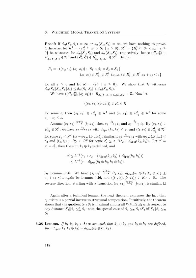
6. Weighted Modal Transition Systems

Proof: If dm(S1, S2) = ∞ or dm(S3, S4) = ∞, we have nothing to prove.Otherwise, let R1 = {R1

ε ⊆ S1 × S2 | ε ≥ 0}, R2 = {R2ε ⊆ S3 × S4 | ε ≥

0} be witnesses for dm(S1, S2) and dm(S3, S4), respectively; hence (s01, s

02) ∈

R1dm(S1,S2) ∈ R

1 and (s03, s

04) ∈ R2

dm(S3,S4) ∈ R2. Define

Rε ={(

(s1, s3), (s2, s4))∈ S1 × S3 × S2 × S4

∣∣(s1, s2) ∈ R1

ε1 ∈ R1, (s3, s4) ∈ R2

ε2 ∈ R2, ε1 + ε2 ≤ ε

}for all ε ≥ 0 and let R = {Rε | ε ≥ 0}. We show that R witnessesdm(S1‖S3, S2‖S4

)≤ dm(S1, S2) + dm(S3, S4).

We have((s0

1, s03), (s0

2, s04))∈ Rdm(S1,S2)+dm(S3,S4) ∈ R. Now let

((s1, s3), (s2, s4)

)∈ Rε ∈ R

for some ε, then (s1, s2) ∈ R1ε1 ∈ R

1 and (s3, s4) ∈ R2ε2 ∈ R

2 for someε1 + ε2 ≤ ε.

Assume (s1, s3) k1�k399K (t1, t3), then s1

k199K1 t1 and s3

k399K3 t3. By (s1, s2) ∈

R1ε1 ∈ R

1, we have s2k299K2 t2 with dSpec(k1, k2) ≤ ε1 and (t1, t2) ∈ R1

ε′1∈ R1

for some ε′1 ≤ λ−1(ε1−dSpec(k1, k2)); similarly, s4

k499K4 t4 with dSpec(k3, k4) ≤

ε2 and (t3, t4) ∈ R2ε′2∈ R2 for some ε′2 ≤ λ−1(ε2 − dSpec(k3, k4)

). Let ε′ =

ε′1 + ε′2, then the sum k2 � k4 is defined, and

ε′ ≤ λ−1(ε1 + ε2 − (dSpec(k1, k2) + dSpec(k3, k4)))

≤ λ−1(ε− dSpec(k1 � k3, k2 � k4))

by Lemma 6.26. We have (s2, s4) k2�k499K (t2, t4), dSpec(k1 � k3, k2 � k4) ≤

ε1 + ε2 ≤ ε again by Lemma 6.26, and((t1, t3), (t2, t4)

)∈ Rε′ ∈ R. The

reverse direction, starting with a transition (s2, s4) k2�k4−→ (t2, t4), is similar. �

Again after a technical lemma, the next theorem expresses the fact thatquotient is a partial inverse to structural composition. Intuitively, the theoremshows that the quotient S1/S2 is maximal among all WMTS S3 with respect toany distance S2‖S3 ≤εm S1; note the special case of S3 ≤m S1/S2 iff S2‖S3 ≤mS1.

6.28 Lemma. If k1, k2, k3 ∈ Spec are such that k1 � k2 and k2 � k3 are defined,then dSpec(k3, k1 � k2) = dSpec(k2 � k3, k1).

118

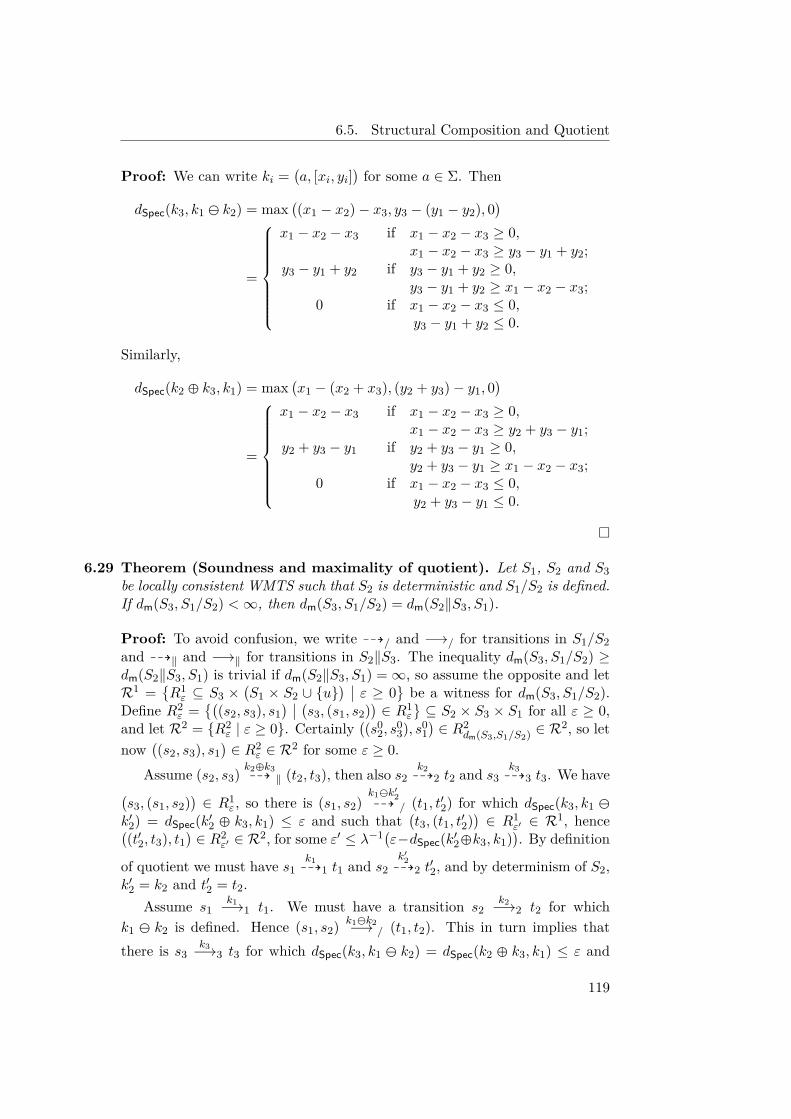
6.5. Structural Composition and Quotient

Proof: We can write ki =(a, [xi, yi]

)for some a ∈ Σ. Then

dSpec(k3, k1 � k2) = max((x1 − x2)− x3, y3 − (y1 − y2), 0

)

=

x1 − x2 − x3 if x1 − x2 − x3 ≥ 0,x1 − x2 − x3 ≥ y3 − y1 + y2;

y3 − y1 + y2 if y3 − y1 + y2 ≥ 0,y3 − y1 + y2 ≥ x1 − x2 − x3;

0 if x1 − x2 − x3 ≤ 0,y3 − y1 + y2 ≤ 0.

Similarly,

dSpec(k2 � k3, k1) = max(x1 − (x2 + x3), (y2 + y3)− y1, 0

)

=

x1 − x2 − x3 if x1 − x2 − x3 ≥ 0,x1 − x2 − x3 ≥ y2 + y3 − y1;

y2 + y3 − y1 if y2 + y3 − y1 ≥ 0,y2 + y3 − y1 ≥ x1 − x2 − x3;

0 if x1 − x2 − x3 ≤ 0,y2 + y3 − y1 ≤ 0.

�

6.29 Theorem (Soundness and maximality of quotient). Let S1, S2 and S3be locally consistent WMTS such that S2 is deterministic and S1/S2 is defined.If dm(S3, S1/S2) <∞, then dm(S3, S1/S2) = dm(S2‖S3, S1).

Proof: To avoid confusion, we write 99K/ and −→/ for transitions in S1/S2and 99K‖ and −→‖ for transitions in S2‖S3. The inequality dm(S3, S1/S2) ≥dm(S2‖S3, S1) is trivial if dm(S2‖S3, S1) =∞, so assume the opposite and letR1 =

{R1ε ⊆ S3 ×

(S1 × S2 ∪ {u}

) ∣∣ ε ≥ 0}be a witness for dm(S3, S1/S2).

Define R2ε =

{((s2, s3), s1

) ∣∣ (s3, (s1, s2))∈ R1

ε

}⊆ S2 × S3 × S1 for all ε ≥ 0,

and let R2 = {R2ε | ε ≥ 0}. Certainly

((s0

2, s03), s0

1)∈ R2

dm(S3,S1/S2) ∈ R2, so let

now((s2, s3), s1

)∈ R2

ε ∈ R2 for some ε ≥ 0.Assume (s2, s3) k2�k3

99K ‖ (t2, t3), then also s2k299K2 t2 and s3

k399K3 t3. We have(

s3, (s1, s2))∈ R1

ε, so there is (s1, s2)k1�k′299K / (t1, t′2) for which dSpec(k3, k1 �

k′2) = dSpec(k′2 � k3, k1) ≤ ε and such that(t3, (t1, t′2)

)∈ R1

ε′ ∈ R1, hence((t′2, t3), t1

)∈ R2

ε′ ∈ R2, for some ε′ ≤ λ−1(ε−dSpec(k′2�k3, k1)). By definition

of quotient we must have s1k199K1 t1 and s2

k′299K2 t′2, and by determinism of S2,

k′2 = k2 and t′2 = t2.Assume s1

k1−→1 t1. We must have a transition s2k2−→2 t2 for which

k1 � k2 is defined. Hence (s1, s2) k1�k2−→ / (t1, t2). This in turn implies thatthere is s3

k3−→3 t3 for which dSpec(k3, k1 � k2) = dSpec(k2 � k3, k1) ≤ ε and

119

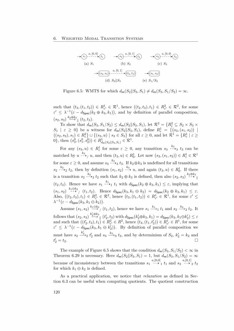
6. Weighted Modal Transition Systems

s1 t1a, [0, 0]

(a) S1

s2 t2a, [0, 1]

(b) S2

s3 t3a, [0, 0]

(c) S3

(s2, s3) (t2, t3)a, [0, 1]

(d) S2‖S3

(s1, s2)

(e) S1/S2

Figure 6.5: WMTS for which dm(S2‖S3, S1) 6= dm(S3, S1/S2) =∞.

such that(t3, (t1, t2)

)∈ R1

ε′ ∈ R1, hence((t2, t3), t1

)∈ R2

ε′ ∈ R2, for someε′ ≤ λ−1(ε − dSpec(k2 � k3, k1)

), and by definition of parallel composition,

(s2, s3) k2�k3−→ ‖ (t2, t3).To show that dm(S3, S1/S2) ≤ dm(S2‖S3, S1), let R2 = {R2

ε ⊆ S2 × S3 ×S1 | ε ≥ 0} be a witness for dm(S2‖S3, S1), define R1

ε ={(s3, (s1, s2)

) ∣∣((s2, s3), s1

)∈ R2

ε

}∪{(s3, u)

∣∣ s3 ∈ S3}for all ε ≥ 0, and let R1 = {R1

ε | ε ≥0}, then

(s0

3, (s01, s

02))∈ R1

dm(S2‖S3,S1) ∈ R1.

For any (s3, u) ∈ R1ε for some ε ≥ 0, any transition s3

k399K3 t3 can be

matched by u k399K/ u, and then (t3, u) ∈ R1

0. Let now(s3, (s1, s2)

)∈ R1

ε ∈ R1

for some ε ≥ 0, and assume s3k399K3 t3. If k2�k3 is undefined for all transitions

s2k299K2 t2, then by definition (s1, s2) k3

99K u, and again (t3, u) ∈ R10. If there

is a transition s2k299K2 t2 such that k2 � k3 is defined, then also (s2, s3) k2�k3

99K ‖

(t2, t3). Hence we have s1k199K1 t1 with dSpec(k2 � k3, k1) ≤ ε, implying that

(s1, s2) k1�k299K / (t1, t2). Hence dSpec(k3, k1 � k2) = dSpec(k2 � k3, k1) ≤ ε.

Also,((t2, t3), t1

)∈ R2

ε′ ∈ R2, hence(t3, (t1, t2)

)∈ R1

ε′ ∈ R1, for some ε′ ≤λ−1(ε− dSpec(k3, k1 � k2)

).

Assume (s1, s2) k1�k2−→ / (t1, t2), hence we have s1k1−→1 t1 and s2

k2−→2 t2. It

follows that (s2, s3)k′2�k3−→ ‖ (t′2, t3) with dSpec(k′2�k3, k1) = dSpec(k3, k1�k′2) ≤ ε

and such that((t′2, t3), t1

)∈ R2

ε′ ∈ R2, hence(t3, (t1, t′2)

)∈ R1

ε′ ∈ R1, for someε′ ≤ λ−1(ε − dSpec(k3, k1 � k′2)

). By definition of parallel composition we

must have s2k′2−→2 t

′2 and s3

k3−→3 t3, and by determinism of S2, k′2 = k2 andt′2 = t2. �

The example of Figure 6.5 shows that the condition dm(S3, S1/S2) <∞ inTheorem 6.29 is necessary. Here dm(S2‖S3, S1) = 1, but dm(S3, S1/S2) = ∞because of inconsistency between the transitions s1

a,[0,0]99K 1 t1 and s2

a,[0,1]99K 2 t2

for which k1 � k2 is defined.

As a practical application, we notice that relaxation as defined in Sec-tion 6.3 can be useful when computing quotients. The quotient construction

120

6.6. Conclusion

in Definition 6.25 introduces inconsistent states (which afterwards are pruned)whenever there is a must transition s1

k1−→1 s′1 such that k1 � k2 is undefined

for all transitions s2k2−→2 s

′2. Looking at the definition of �, we see that this

is the case if k1 = (a1, [x1, y1]) and k2 = (a2, [x2, y2]) are such that a1 6= a2or x1 − x2 > y1 − y2. In the first case, the inconsistency is of a structuralnature and cannot be dealt with; but in the second case, it may be avoidedby enlarging k1: decreasing x1 or increasing y1 so that now, x1−x2 ≤ y1−y2.

Enlarging quantitative constraints is exactly the intuition of relaxation,thus in practical cases where we get a quotient S1/S2 which is “too incon-sistent”, we may be able to solve this problem by constructing a suitableε-relaxation S′1 of S1. Theorems 6.27 and 6.29 can then be used to ensurethat also S′1/S2 is a relaxation of S1/S2.

6.6 ConclusionWe have shown in this chapter that within the quantitative specification frame-work of weighted modal transition systems, refinement and implementationdistances provide a useful tool for robust compositional reasoning. Note thatthese distances permit us not only to reason about differences between imple-mentations and from implementations to specifications, but they also providea means by which we can compare specifications directly at the abstract level.

We have shown that for some of the ingredients of our specification theory,namely structural composition and quotient, our formalism is a conservativeextension of the standard Boolean notions. We have also noted however, thatfor determinization and logical conjunction, the properties of the Booleannotions are not preserved, and that this seems to be a fundamental limitationof any reasonable quantitative specification theory. We will have more to sayabout this in the next chapter.

121

7 General Quantitative SpecificationTheories with Modal TransitionSystems1

This chapter combines the work of the two previous chapters. It uses thegeneral theory of linear and branching distances developed in Chapter 5 tointroduce general refinement distances between structured modal transitionsystems. It then proceeds to consider quantitative properties of structuralcomposition, quotient, and conjunction, and finishes with a logical character-ization of quantitative refinement using Hennessy-Milner logic.

7.1 Structured Modal Transition Systems

We work with a poset Spec of specification labels with a partial order 4 anddenote by Spec∞ = Spec∗ ∪ Specω the set of finite and infinite traces overSpec. In applications, Spec may be used to model data about the behaviorof a system; for specifications this may be considered as legal parametersof operation, whereas for implementations it may be thought of as observedinformation.

The partial order 4 is meant to model refinement of data; if k 4 `, then kis more refined (leaves fewer choices) than `. The set Imp = {k ∈ Spec | k′ 4k =⇒ k′ = k} is called the set of implementation labels; these are the datawhich cannot be refined further. We let JkK = {k′ ∈ Imp | k′ 4 k} and assumethat JkK 6= ∅ for all k ∈ Spec.

When k 64 `, we want to be able to quantify the impact of this differencein data on the systems in question, thus circumventing the fragility of thetheory. To this end, we introduce a general notion of distance on sequences ofdata following the approach laid out in Chapter 5.

1This chapter is based on the journal paper [FL14a] published in Acta Informatica.

123

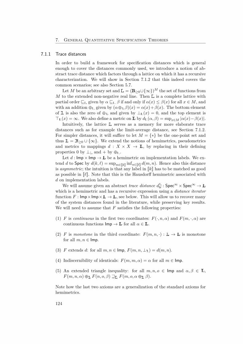
7. General Quantitative Specification Theories

7.1.1 Trace distances

In order to build a framework for specification distances which is generalenough to cover the distances commonly used, we introduce a notion of ab-stract trace distance which factors through a lattice on which it has a recursivecharacterization. We will show in Section 7.1.2 that this indeed covers thecommon scenarios; see also Section 5.7.

LetM be an arbitrary set and L = (R≥0∪{∞})M the set of functions fromM to the extended non-negative real line. Then L is a complete lattice withpartial order vL given by α vL β if and only if α(x) ≤ β(x) for all x ∈M , andwith an addition �L given by (α�Lβ)(x) = α(x)+β(x). The bottom elementof L is also the zero of �L and given by ⊥L(x) = 0, and the top element is>L(x) =∞. We also define a metric on L by dL(α, β) = supx∈M |α(x)−β(x)|.

Intuitively, the lattice L serves as a memory for more elaborate tracedistances such as for example the limit-average distance, see Section 7.1.2.For simpler distances, it will suffice to let M = {∗} be the one-point set andthus L = R≥0 ∪ {∞}. We extend the notions of hemimetrics, pseudometricsand metrics to mappings d : X × X → L, by replacing in their definingproperties 0 by ⊥L and + by �L.

Let d : Imp× Imp→ L be a hemimetric on implementation labels. We ex-tend d to Spec by d(k, `) = supm∈JkK infn∈J`K d(m,n). Hence also this distanceis asymmetric; the intuition is that any label in JkK has to be matched as goodas possible in J`K. Note that this is the Hausdorff hemimetric associated withd on implementation labels.

We will assume given an abstract trace distance dLtr : Spec∞× Spec∞ → L

which is a hemimetric and has a recursive expression using a distance iteratorfunction F : Imp× Imp×L→ L, see below. This will allow us to recover manyof the system distances found in the literature, while preserving key results.We will need to assume that F satisfies the following properties:

(1) F is continuous in the first two coordinates: F (·, n, α) and F (m, ·, α) arecontinuous functions Imp→ L for all α ∈ L.

(2) F is monotone in the third coordinate: F (m,n, ·) : L → L is monotonefor all m,n ∈ Imp.

(3) F extends d: for all m,n ∈ Imp, F (m,n,⊥L) = d(m,n).

(4) Indiscernibility of identicals: F (m,m,α) = α for all m ∈ Imp.

(5) An extended triangle inequality: for all m,n, o ∈ Imp and α, β ∈ L,F (m,n, α) �L F (n, o, β) wL F (m, o, α�L β).

Note how the last two axioms are a generalization of the standard axioms forhemimetrics.

124

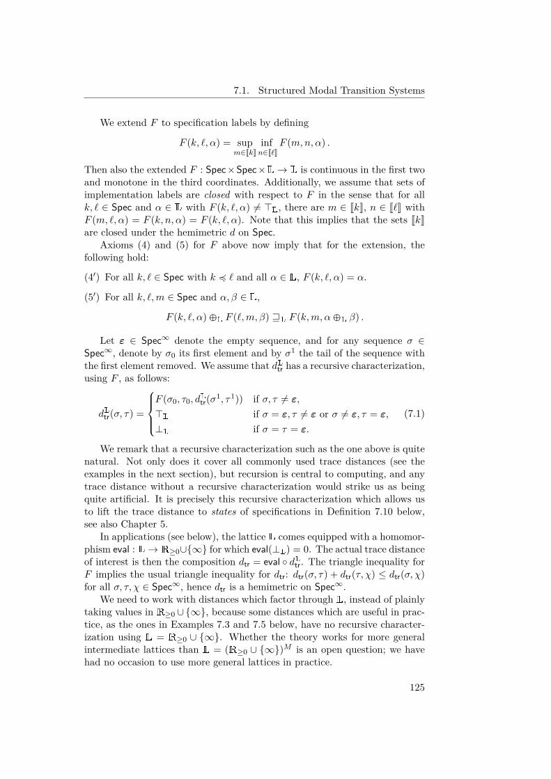
7.1. Structured Modal Transition Systems

We extend F to specification labels by defining

F (k, `, α) = supm∈JkK

infn∈J`K

F (m,n, α) .

Then also the extended F : Spec×Spec×L→ L is continuous in the first twoand monotone in the third coordinates. Additionally, we assume that sets ofimplementation labels are closed with respect to F in the sense that for allk, ` ∈ Spec and α ∈ L with F (k, `, α) 6= >L, there are m ∈ JkK, n ∈ J`K withF (m, `, α) = F (k, n, α) = F (k, `, α). Note that this implies that the sets JkKare closed under the hemimetric d on Spec.

Axioms (4) and (5) for F above now imply that for the extension, thefollowing hold:

(4′) For all k, ` ∈ Spec with k 4 ` and all α ∈ L, F (k, `, α) = α.

(5′) For all k, `,m ∈ Spec and α, β ∈ L,

F (k, `, α) �L F (`,m, β) wL F (k,m, α�L β) .

Let ε ∈ Spec∞ denote the empty sequence, and for any sequence σ ∈Spec∞, denote by σ0 its first element and by σ1 the tail of the sequence withthe first element removed. We assume that dLtr has a recursive characterization,using F , as follows:

dLtr(σ, τ) =

F (σ0, τ0, d

Ltr(σ1, τ1)) if σ, τ 6= ε,

>L if σ = ε, τ 6= ε or σ 6= ε, τ = ε,

⊥L if σ = τ = ε.

(7.1)

We remark that a recursive characterization such as the one above is quitenatural. Not only does it cover all commonly used trace distances (see theexamples in the next section), but recursion is central to computing, and anytrace distance without a recursive characterization would strike us as beingquite artificial. It is precisely this recursive characterization which allows usto lift the trace distance to states of specifications in Definition 7.10 below,see also Chapter 5.

In applications (see below), the lattice L comes equipped with a homomor-phism eval : L→ R≥0∪{∞} for which eval(⊥L) = 0. The actual trace distanceof interest is then the composition dtr = eval ◦ dLtr. The triangle inequality forF implies the usual triangle inequality for dtr: dtr(σ, τ) + dtr(τ, χ) ≤ dtr(σ, χ)for all σ, τ, χ ∈ Spec∞, hence dtr is a hemimetric on Spec∞.

We need to work with distances which factor through L, instead of plainlytaking values in R≥0 ∪{∞}, because some distances which are useful in prac-tice, as the ones in Examples 7.3 and 7.5 below, have no recursive character-ization using L = R≥0 ∪ {∞}. Whether the theory works for more generalintermediate lattices than L = (R≥0 ∪ {∞})M is an open question; we havehad no occasion to use more general lattices in practice.

125

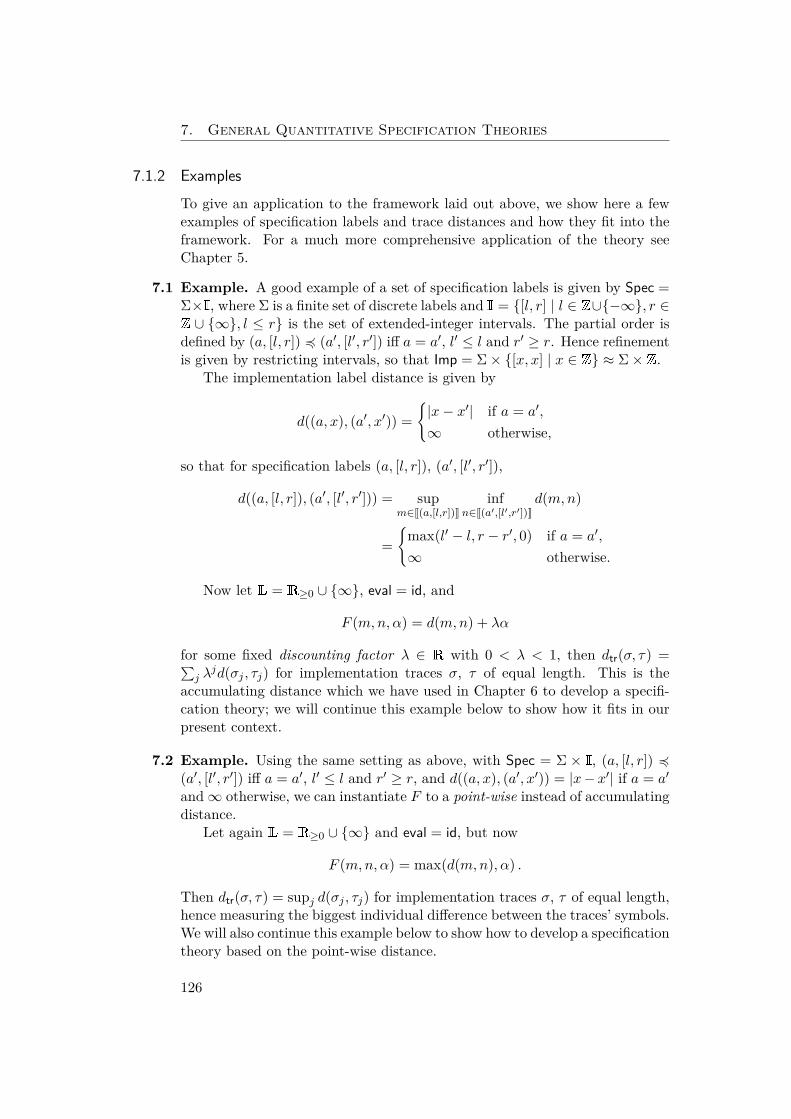
7. General Quantitative Specification Theories

7.1.2 ExamplesTo give an application to the framework laid out above, we show here a fewexamples of specification labels and trace distances and how they fit into theframework. For a much more comprehensive application of the theory seeChapter 5.

7.1 Example. A good example of a set of specification labels is given by Spec =Σ×I, where Σ is a finite set of discrete labels and I = {[l, r] | l ∈ Z∪{−∞}, r ∈Z ∪ {∞}, l ≤ r} is the set of extended-integer intervals. The partial order isdefined by (a, [l, r]) 4 (a′, [l′, r′]) iff a = a′, l′ ≤ l and r′ ≥ r. Hence refinementis given by restricting intervals, so that Imp = Σ× {[x, x] | x ∈ Z} ≈ Σ× Z.

The implementation label distance is given by

d((a, x), (a′, x′)) ={|x− x′| if a = a′,

∞ otherwise,

so that for specification labels (a, [l, r]), (a′, [l′, r′]),

d((a, [l, r]), (a′, [l′, r′])) = supm∈J(a,[l,r])K

infn∈J(a′,[l′,r′])K

d(m,n)

={

max(l′ − l, r − r′, 0) if a = a′,

∞ otherwise.

Now let L = R≥0 ∪ {∞}, eval = id, and

F (m,n, α) = d(m,n) + λα

for some fixed discounting factor λ ∈ R with 0 < λ < 1, then dtr(σ, τ) =∑j λ

jd(σj , τj) for implementation traces σ, τ of equal length. This is theaccumulating distance which we have used in Chapter 6 to develop a specifi-cation theory; we will continue this example below to show how it fits in ourpresent context.

7.2 Example. Using the same setting as above, with Spec = Σ × I, (a, [l, r]) 4(a′, [l′, r′]) iff a = a′, l′ ≤ l and r′ ≥ r, and d((a, x), (a′, x′)) = |x−x′| if a = a′

and∞ otherwise, we can instantiate F to a point-wise instead of accumulatingdistance.

Let again L = R≥0 ∪ {∞} and eval = id, but now

F (m,n, α) = max(d(m,n), α) .

Then dtr(σ, τ) = supj d(σj , τj) for implementation traces σ, τ of equal length,hence measuring the biggest individual difference between the traces’ symbols.We will also continue this example below to show how to develop a specificationtheory based on the point-wise distance.

126

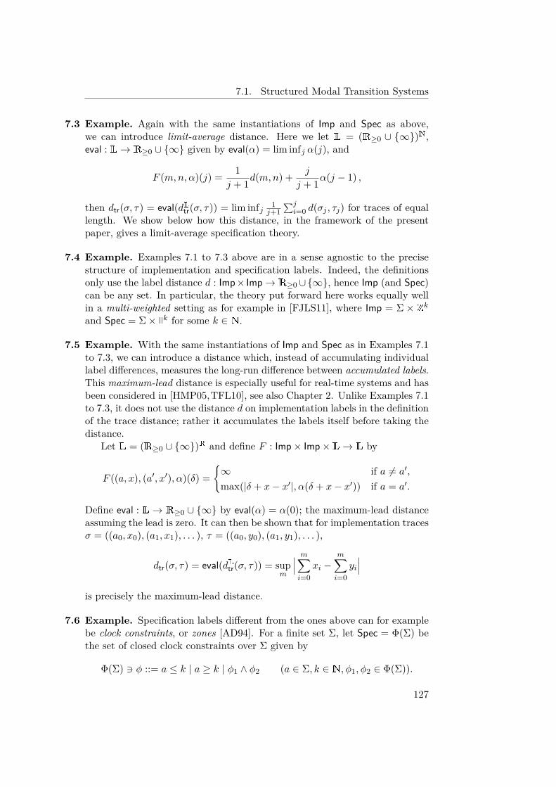
7.1. Structured Modal Transition Systems

7.3 Example. Again with the same instantiations of Imp and Spec as above,we can introduce limit-average distance. Here we let L = (R≥0 ∪ {∞})N,eval : L→ R≥0 ∪ {∞} given by eval(α) = lim infj α(j), and

F (m,n, α)(j) = 1j + 1d(m,n) + j

j + 1α(j − 1) ,

then dtr(σ, τ) = eval(dLtr(σ, τ)) = lim infj 1j+1

∑ji=0 d(σj , τj) for traces of equal

length. We show below how this distance, in the framework of the presentpaper, gives a limit-average specification theory.

7.4 Example. Examples 7.1 to 7.3 above are in a sense agnostic to the precisestructure of implementation and specification labels. Indeed, the definitionsonly use the label distance d : Imp× Imp→ R≥0∪{∞}, hence Imp (and Spec)can be any set. In particular, the theory put forward here works equally wellin a multi-weighted setting as for example in [FJLS11], where Imp = Σ × Zkand Spec = Σ× Ik for some k ∈ N.

7.5 Example. With the same instantiations of Imp and Spec as in Examples 7.1to 7.3, we can introduce a distance which, instead of accumulating individuallabel differences, measures the long-run difference between accumulated labels.This maximum-lead distance is especially useful for real-time systems and hasbeen considered in [HMP05,TFL10], see also Chapter 2. Unlike Examples 7.1to 7.3, it does not use the distance d on implementation labels in the definitionof the trace distance; rather it accumulates the labels itself before taking thedistance.

Let L = (R≥0 ∪ {∞})R and define F : Imp× Imp× L→ L by

F ((a, x), (a′, x′), α)(δ) ={∞ if a 6= a′,

max(|δ + x− x′|, α(δ + x− x′)) if a = a′.

Define eval : L→ R≥0 ∪ {∞} by eval(α) = α(0); the maximum-lead distanceassuming the lead is zero. It can then be shown that for implementation tracesσ = ((a0, x0), (a1, x1), . . . ), τ = ((a0, y0), (a1, y1), . . . ),

dtr(σ, τ) = eval(dLtr(σ, τ)) = supm

∣∣∣ m∑i=0

xi −m∑i=0

yi∣∣∣

is precisely the maximum-lead distance.

7.6 Example. Specification labels different from the ones above can for examplebe clock constraints, or zones [AD94]. For a finite set Σ, let Spec = Φ(Σ) bethe set of closed clock constraints over Σ given by

Φ(Σ) 3 φ ::= a ≤ k | a ≥ k | φ1 ∧ φ2 (a ∈ Σ, k ∈ N, φ1, φ2 ∈ Φ(Σ)).

127

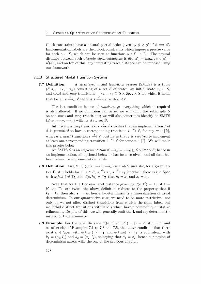
7. General Quantitative Specification Theories

Clock constraints have a natural partial order given by φ 4 φ′ iff φ =⇒ φ′.Implementation labels are then clock constraints which impose a precise valuefor each a ∈ Σ, which can be seen as functions u : Σ → N. The naturaldistance between such discrete clock valuations is d(u, u′) = maxa∈Σ |u(a) −u′(a)|, and on top of this, any interesting trace distance can be imposed usingour framework.

7.1.3 Structured Modal Transition Systems7.7 Definition. A structured modal transition system (SMTS) is a tuple

(S, s0, 99KS ,−→S) consisting of a set S of states, an initial state s0 ∈ S,and must and may transitions −→S , 99KS ⊆ S × Spec × S for which it holdsthat for all s k−→S s

′ there is s `99KS s′ with k 4 `.

The last condition is one of consistency: everything which is requiredis also allowed. If no confusion can arise, we will omit the subscripts Son the must and may transitions; we will also sometimes identify an SMTS(S, s0, 99KS ,−→S) with its state set S.

Intuitively, a may transition s k99K s′ specifies that an implementation I of

S is permitted to have a corresponding transition im−→ i′, for any m ∈ JkK,

whereas a must transition s `−→ s′ postulates that I is required to implementat least one corresponding transition i n−→ i′ for some n ∈ J`K. We will makethis precise below.

An SMTS S is an implementation if −→S = 99KS ⊆ S× Imp×S; hence inan implementation, all optional behavior has been resolved, and all data hasbeen refined to implementation labels.

7.8 Definition. An SMTS (S, s0, 99KS ,−→S) is L-deterministic, for a given lat-tice L, if it holds for all s ∈ S, s k1

99K s1, sk299K s2 for which there is k ∈ Spec

with d(k, k1) 6= >L and d(k, k2) 6= >L that k1 = k2 and s1 = s2.

Note that for the Boolean label distance given by d(k, k′) = ⊥L if k =k′ and >L otherwise, the above definition reduces to the property that ifk1 = k2, then also s1 = s2, hence L-determinism is a generalization of usualdeterminism. In our quantitative case, we need to be more restrictive: notonly do we not allow distinct transitions from s with the same label, butwe forbid distinct transitions with labels which have a common quantitativerefinement. Despite of this, we will generally omit the L and say deterministicinstead of L-deterministic.

7.9 Example. For the label distance d((a, x), (a′, x′)) = |x − x′| if a = a′ and∞ otherwise of Examples 7.1 to 7.3 and 7.5, the above condition that thereexist k ∈ Spec with d(k, k1) 6= >L and d(k, k2) 6= >L is equivalent, withk1 = (a1, I1) and k2 = (a2, I2), to saying that a1 = a2, hence our notion ofdeterminism agrees with the one of the previous chapter.

128

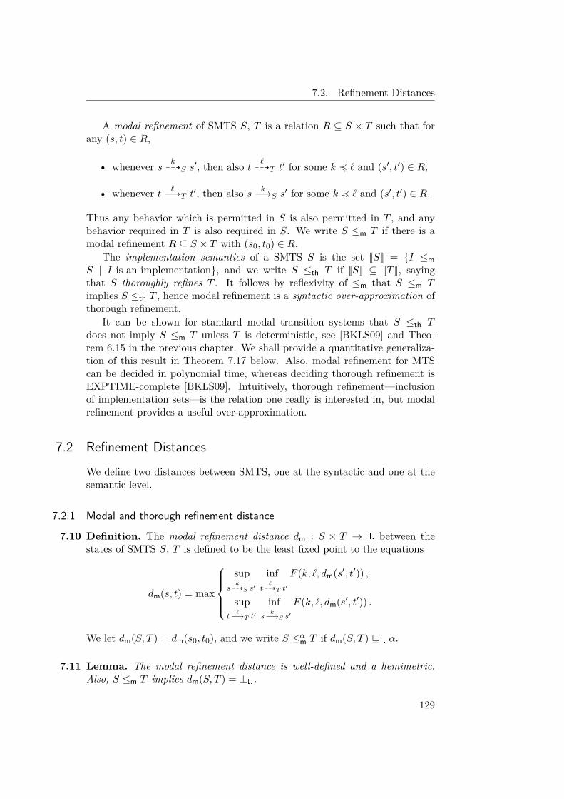
7.2. Refinement Distances

A modal refinement of SMTS S, T is a relation R ⊆ S × T such that forany (s, t) ∈ R,

• whenever s k99KS s′, then also t `

99KT t′ for some k 4 ` and (s′, t′) ∈ R,

• whenever t `−→T t′, then also s k−→S s

′ for some k 4 ` and (s′, t′) ∈ R.

Thus any behavior which is permitted in S is also permitted in T , and anybehavior required in T is also required in S. We write S ≤m T if there is amodal refinement R ⊆ S × T with (s0, t0) ∈ R.

The implementation semantics of a SMTS S is the set JSK = {I ≤mS | I is an implementation}, and we write S ≤th T if JSK ⊆ JT K, sayingthat S thoroughly refines T . It follows by reflexivity of ≤m that S ≤m Timplies S ≤th T , hence modal refinement is a syntactic over-approximation ofthorough refinement.

It can be shown for standard modal transition systems that S ≤th Tdoes not imply S ≤m T unless T is deterministic, see [BKLS09] and Theo-rem 6.15 in the previous chapter. We shall provide a quantitative generaliza-tion of this result in Theorem 7.17 below. Also, modal refinement for MTScan be decided in polynomial time, whereas deciding thorough refinement isEXPTIME-complete [BKLS09]. Intuitively, thorough refinement—inclusionof implementation sets—is the relation one really is interested in, but modalrefinement provides a useful over-approximation.

7.2 Refinement Distances

We define two distances between SMTS, one at the syntactic and one at thesemantic level.

7.2.1 Modal and thorough refinement distance

7.10 Definition. The modal refinement distance dm : S × T → L between thestates of SMTS S, T is defined to be the least fixed point to the equations

dm(s, t) = max

sup

sk99KS s′

inft`99KT t′

F (k, `, dm(s′, t′)) ,

supt`−→T t′

infs

k−→S s′

F (k, `, dm(s′, t′)) .

We let dm(S, T ) = dm(s0, t0), and we write S ≤αm T if dm(S, T ) vL α.

7.11 Lemma. The modal refinement distance is well-defined and a hemimetric.Also, S ≤m T implies dm(S, T ) = ⊥L.

129

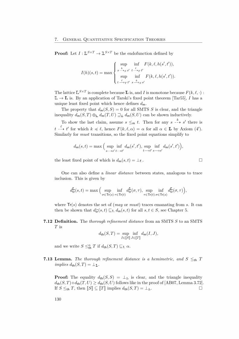
7. General Quantitative Specification Theories

Proof: Let I : LS×T → LS×T be the endofunction defined by

I(h)(s, t) = max

sup

sk99KS s′

inft`99KT t′

F (k, `, h(s′, t′)),

supt`−→T t′

infs

k−→S s′

F (k, `, h(s′, t′)).

The lattice LS×T is complete because L is, and I is monotone because F (k, `, ·) :L→ L is. By an application of Tarski’s fixed point theorem [Tar55], I has aunique least fixed point which hence defines dm.

The property that dm(S, S) = 0 for all SMTS S is clear, and the triangleinequality dm(S, T )�L dm(T,U) wL dm(S,U) can be shown inductively.

To show the last claim, assume s ≤m t. Then for any sk99K s′ there is

t`99K t′ for which k 4 `, hence F (k, `, α) = α for all α ∈ L by Axiom (4′).

Similarly for must transitions, so the fixed point equations simplify to

dm(s, t) = max(

sups99Ks′

inft99Kt′

dm(s′, t′), supt−→t′

infs−→s′

dm(s′, t′)),

the least fixed point of which is dm(s, t) = ⊥L. �

One can also define a linear distance between states, analogous to traceinclusion. This is given by

dLtr(s, t) = max(

supσ∈Tr(s)

infτ∈Tr(t)

dLtr(σ, τ), supτ∈Tr(t)

infσ∈Tr(s)

dLtr(σ, τ)),

where Tr(s) denotes the set of (may or must) traces emanating from s. It canthen be shown that dLtr(s, t) vL dm(s, t) for all s, t ∈ S, see Chapter 5.

7.12 Definition. The thorough refinement distance from an SMTS S to an SMTST is

dth(S, T ) = supI∈JSK

infJ∈JT K

dm(I, J),

and we write S ≤αth T if dth(S, T ) vL α.

7.13 Lemma. The thorough refinement distance is a hemimetric, and S ≤th Timplies dth(S, T ) = ⊥L.

Proof: The equality dth(S, S) = ⊥L is clear, and the triangle inequalitydth(S, T )+dth(T,U) ≥ dth(S,U) follows like in the proof of [AB07, Lemma 3.72].If S ≤th T , then JSK ⊆ JT K implies dth(S, T ) = ⊥L. �

130

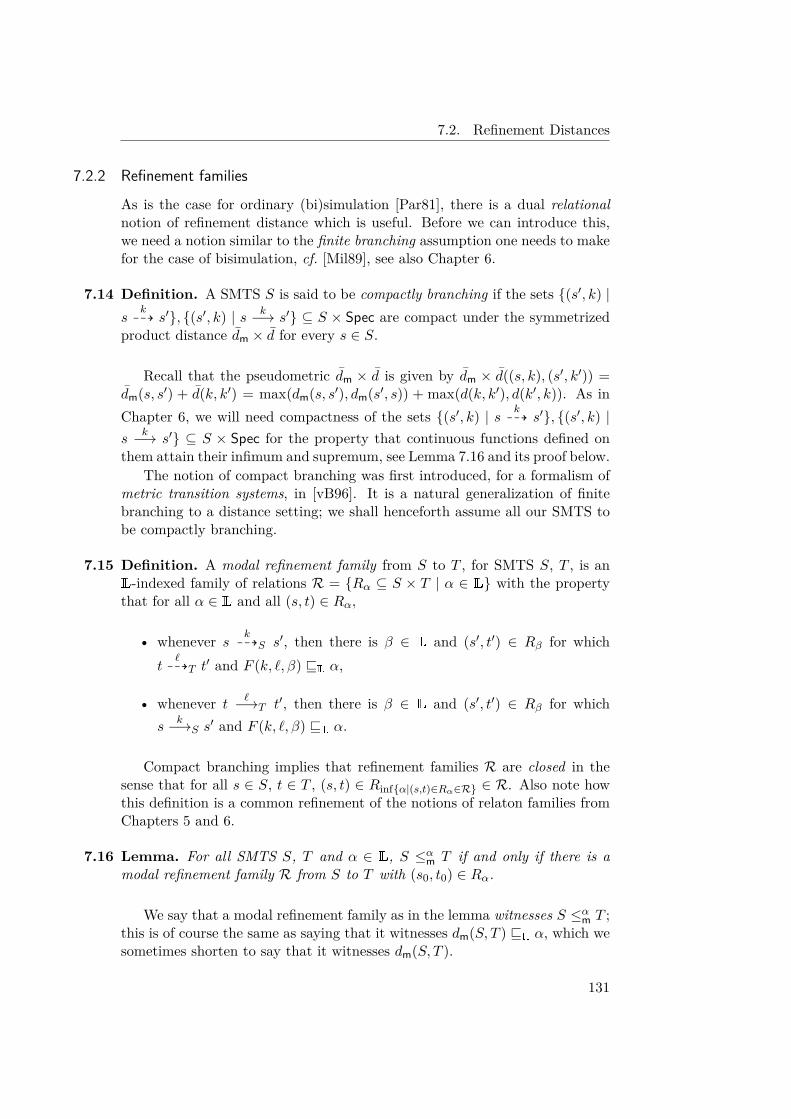
7.2. Refinement Distances

7.2.2 Refinement families

As is the case for ordinary (bi)simulation [Par81], there is a dual relationalnotion of refinement distance which is useful. Before we can introduce this,we need a notion similar to the finite branching assumption one needs to makefor the case of bisimulation, cf. [Mil89], see also Chapter 6.

7.14 Definition. A SMTS S is said to be compactly branching if the sets {(s′, k) |s

k99K s′}, {(s′, k) | s k−→ s′} ⊆ S × Spec are compact under the symmetrized

product distance dm × d for every s ∈ S.

Recall that the pseudometric dm × d is given by dm × d((s, k), (s′, k′)) =dm(s, s′) + d(k, k′) = max(dm(s, s′), dm(s′, s)) + max(d(k, k′), d(k′, k)). As inChapter 6, we will need compactness of the sets {(s′, k) | s k

99K s′}, {(s′, k) |s

k−→ s′} ⊆ S × Spec for the property that continuous functions defined onthem attain their infimum and supremum, see Lemma 7.16 and its proof below.

The notion of compact branching was first introduced, for a formalism ofmetric transition systems, in [vB96]. It is a natural generalization of finitebranching to a distance setting; we shall henceforth assume all our SMTS tobe compactly branching.

7.15 Definition. A modal refinement family from S to T , for SMTS S, T , is anL-indexed family of relations R = {Rα ⊆ S × T | α ∈ L} with the propertythat for all α ∈ L and all (s, t) ∈ Rα,

• whenever s k99KS s′, then there is β ∈ L and (s′, t′) ∈ Rβ for which

t`99KT t′ and F (k, `, β) vL α,

• whenever t `−→T t′, then there is β ∈ L and (s′, t′) ∈ Rβ for whichs

k−→S s′ and F (k, `, β) vL α.

Compact branching implies that refinement families R are closed in thesense that for all s ∈ S, t ∈ T , (s, t) ∈ Rinf{α|(s,t)∈Rα∈R} ∈ R. Also note howthis definition is a common refinement of the notions of relaton families fromChapters 5 and 6.

7.16 Lemma. For all SMTS S, T and α ∈ L, S ≤αm T if and only if there is amodal refinement family R from S to T with (s0, t0) ∈ Rα.

We say that a modal refinement family as in the lemma witnesses S ≤αm T ;this is of course the same as saying that it witnesses dm(S, T ) vL α, which wesometimes shorten to say that it witnesses dm(S, T ).

131

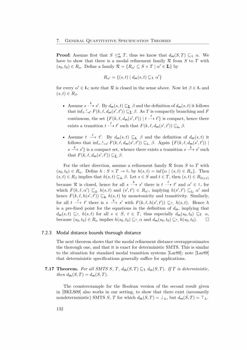
7. General Quantitative Specification Theories

Proof: Assume first that S ≤αm T , thus we know that dm(S, T ) vL α. Wehave to show that there is a modal refinement family R from S to T with(s0, t0) ∈ Rα. Define a family R = {Rα′ ⊆ S × T | α′ ∈ L} by

Rα′ = {(s, t) | dm(s, t) vL α′}

for every α′ ∈ L; note that R is closed in the sense above. Now let β ∈ L and(s, t) ∈ Rβ.

• Assume s k99K s′. By dm(s, t) vL β and the definition of dm(s, t) it follows

that inft `99Kt′ F (k, `, dm(s′, t′)) vL β. As T is compactly branching and Fcontinuous, the set {F (k, `, dm(s′, t′)) | t `

99K t′} is compact, hence thereexists a transition t `

99K t′ such that F (k, `, dm(s′, t′)) vL β.

• Assume t `−→ t′. By dm(s, t) vL β and the definition of dm(s, t) itfollows that infs k−→s′ F (k, `, dm(s′, t′)) vL β. Again {F (k, `, dm(s′, t′)) |s

k−→ s′} is a compact set, whence there exists a transition s k−→ s′ suchthat F (k, `, dm(s′, t′)) vL β.

For the other direction, assume a refinement family R from S to T with(s0, t0) ∈ Rα. Define h : S × T → L by h(s, t) = inf{α | (s, t) ∈ Rα}. Then(s, t) ∈ Rβ implies that h(s, t) vL β. Let s ∈ S and t ∈ T , then (s, t) ∈ Rh(s,t)

because R is closed, hence for all s k99K s′ there is t `

99K t′ and α′ ∈ L forwhich F (k, `, α′) vL h(s, t) and (s′, t′) ∈ Rα′ , implying h(s′, t′) vL α′ andhence F (k, `, h(s′, t′)) vL h(s, t) by monotonicity and transitivity. Similarly,for all t `−→ t′ there is s k−→ s′ with F (k, `, h(s′, t′)) vL h(s, t). Hence his a pre-fixed point for the equations in the definition of dm, implying thatdm(s, t) vL h(s, t) for all s ∈ S, t ∈ T , thus especially dm(s0, t0) vL α,because (s0, t0) ∈ Rα implies h(s0, t0) vL α and dm(s0, t0) vL h(s0, t0). �

7.2.3 Modal distance bounds thorough distance

The next theorem shows that the modal refinement distance overapproximatesthe thorough one, and that it is exact for deterministic SMTS. This is similarto the situation for standard modal transition systems [Lar89]; note [Lar89]that deterministic specifications generally suffice for applications.

7.17 Theorem. For all SMTS S, T , dth(S, T ) vL dm(S, T ). If T is deterministic,then dth(S, T ) = dm(S, T ).

The counterexample for the Boolean version of the second result givenin [BKLS09] also works in our setting, to show that there exist (necessarilynondeterministic) SMTS S, T for which dth(S, T ) = ⊥L, but dm(S, T ) = >L.

132

7.2. Refinement Distances

Proof: For the first claim, if dm(S, T ) = >L, we have nothing to prove.Otherwise, let R = {Rα ⊆ S × T | α ∈ L} be a modal refinement familywhich witnesses dm(S, T ), then (s0, t0) ∈ Rdm(S,T ). Let I ∈ JSK; we willexpose J ∈ JT K for which dm(I, J) vL dm(S, T ).

Let R ⊆ I × S be a witness for I ≤m S, define R′α = R ◦ Rα ⊆ I × T forall α ∈ L, and let R′ = {R′α | α ∈ L}. We let the states of J be J = T , withj0 = t0, and define 99KJ = −→J as follows:

For any im−→I i

′ and any t ∈ T for which (i, t) ∈ R′α ∈ R′ for someα ∈ L, α 6= >L, we have t `

99KT t′ with (i′, t′) ∈ R′β ∈ R′ for some β ∈ Lwith F (m, `, β) vL α. As J`K is closed under F , there is n ∈ J`K for whichF (m,n, β) = F (m, `, β), and we add a transition t n−→J t

′ to J .Similarly, for any t `−→T t′ and any i ∈ I for which (i, t) ∈ R′α ∈ R′ for

some α ∈ L, α 6= >L, we have i m−→I i′ with (i′, t′) ∈ R′β for some β ∈ L

with F (m, `, β) vL α. Using again closedness of J`K, we find n ∈ J`K for whichF (m,n, β) = F (m, `, β) and add a transition t n−→J t

′ to J .We show that the identity relation {(t, t) | t ∈ T} ⊆ J × T witnesses

J ≤m T . Let first t n−→J t′; we must have used one of the two constructions

above for creating this transition. In the first case, there is t `99KT t′ with

n ∈ J`K, and in the second case, there is t `−→T t′, hence also t `′99KT t′ with

` 4 `′, thus n ∈ J`K ⊆ J`′K. Now let t `−→T t′, then the second constructionabove has introduced t n−→J t

′ with n ∈ J`K.To finish the proof, we show that the family R′ is a witness for dm(I, J) vL

dm(S, T ). First, (i0, s0) ∈ R and (s0, t0) ∈ Rdm(S,T ) imply (i0, t0) ∈ R′dm(S,T ).Let (i, t) ∈ R′α ∈ R′ for some α ∈ L, α 6= >L, and assume first i m−→I i

′.Then t

`99KT t′ and t

n−→J t′ by the first part of our above construction,and (i′, t′) ∈ R′β with F (m,n, β) vL F (m, `, β) vL α. For the converse, atransition t

n−→J t′ must have been introduced above, and in both cases,i

m−→I i′ with (i′, t′) ∈ R′β and F (m,n, β) vL F (m, `, β) vL α.

Now to the proof of the second assertion of the theorem. If dth(S, T ) = >L,we are done. Otherwise we inductively construct a relation family R = {Rα ⊆S × T | α ∈ L} which satisfies dth((s, S), (t, T )) v α for any (s, t) ∈ Rα, asfollows: Begin by letting Rα = {(s0, t0)} for all α wL dth(S, T ), and let now(s, t) ∈ Rα with dth((s, S), (t, T )) v α 6= >L.

Let s k99KS s′ and t

`99KT t′ such that d(k, `) 6= >L. Let (i′, I ′) ∈

J(s′, S)K and m ∈ JkK, then there is (i, I) ∈ J(s, S)K for which im−→I i′′

and (i′′, I) ≤m (i′, I ′). By the triangle inequality we have dth((i, I), (t, T )) vLdth((i, I), (s, S)) �L dth((s, S), (t, T )) vL α, hence there is t `′

99K t′′ for whichd(m, `′) vL α. But we also have d(m, `) vL d(m, k)�L d(k, `) = d(k, `) 6= >L,so by determinism of T it follows that ` = `′ and t′ = t′′.

As m ∈ JkK was chosen arbitrarily above, we have d(m, `) vL α for allm ∈ JkK, hence d(k, `) = F (k, `,⊥L) v α. Let B = {β′ ∈ L | F (k, `, β′) vL α}

133

7. General Quantitative Specification Theories

and β = supB, then F (k, `, β) vL α as ⊥L ∈ S. Add (s′, t′) to Rγ for allγ wL β.

We miss to show that dth((s′, S), (t′, T )) vL β. By dth((s, S), (t, T )) vL αwe must have (j, J) ∈ J(t, T )K, j n−→J j

′, and an element β′ ∈ L for whichdm((i′, I ′), (j′, J)) vL β′ and F (m,n, β′) vL α. Then

F (k, `, β′) = F (m, `, β′) vL F (m,n, β′) vL α ,

hence β′ ∈ B, implying that dth((s′, S), (t′, T )) vL β′ vL β.We show that R is a refinement family which witnesses dm(S, T ). Let

(s, t) ∈ Rα ∈ R for some α ∈ L and assume s k99KS s′. Let m ∈ JkK, then

there is (i, I) ∈ J(s, S)K with i m−→I i′. As dth((i, I), (t, T )) vL α, this implies

that there is t `99KT t′ with d(m, `) vL α. Also for any other m′ ∈ JkK we

have t `′99KT t′′ with d(m, `′) vL α, hence ` = `′ and t′ = t′′ by determinism.

As m was chosen arbitrarily, we have d(m, `) v α for all m ∈ JkK, henced(k, `) = F (k, `,⊥L) v α. By construction of R, (s′, t′) ∈ Rβ for β = sup{β′ ∈L | F (k, `, β′) vL α}.

Now assume t `−→T t′. Let (i, I) ∈ J(s, S)K, then we have (j, J) ∈ J(t, T )K

with dm((i, I), (j, J)) vL α. We must have j n−→J j′ with n ∈ J`K, hence there

are i m−→I i′ and β′ ∈ L with dm((i′, I), (j′, J)) vL β′ and F (m,n, β′) vL α.

The above considerations hold for all (i, I) ∈ J(s, S)K, hence there is k ∈ Lwith m ∈ JkK, s k−→S s

′, and F (k, `, β′) = F (m, `, β′). But then F (k, `, β′) vLF (m,n, β′) vL α, hence by construction of R, (s′, t′) ∈ Rβ for β = sup{β′ ∈L | F (k, `, β′) vL α}. �

7.2.4 Quantitative relaxation

In a quantitative framework, it can be useful to be able to relax and strengthenspecifications during the development process. Which precise relaxations andstrengthenings one wishes to apply will depend on the actual application, butwe can here show three general relaxations which differ from each other in thelevel of the theory at which they are applied. For α ∈ L and SMTS S, T ,

• T is an α-widening of S if there is a relation R ⊆ S × T for which(s0, t0) ∈ R and such that for all (s, t) ∈ R, s k

99KS s′ if and only ift

`99KT t′, and s k−→S s

′ if and only if t `−→T t′, for k 4 `, d(`, k) vL α,

and (s′, t′) ∈ R;

• T is an α-relaxation of S if S ≤m T and T ≤αm S;

• the α-extended implementation semantics of S is

JSK+α = {I ≤αm S | I implementation}.

134

7.3. Structural Composition and Quotient

All three notions have also been introduced for the special case of integerweights in Section 6.3; but note that the notion of widening presented here ismore synthetic than the one of the previous chapter.

The notion of α-widening is entirely syntactic: up to unweighted bisimu-lation, T is the same as S, but transition labels in T can be α “wider” than inS (hence also S ≤m T ). The second notion, α-relaxation, works at the level ofsemantics of specifications, whereas the last notion is at implementation level.A priori, there is no relation between the syntactic and semantic notions, eventhough one can be established in some special cases.

7.18 Example. For the accumulated distance with discounting factor λ, any α-widening is also an α

1−λ -relaxation, see Proposition 6.19. This is due tothe fact that for traces σ, τ ∈ Spec∞ with d(σj , τj) ≤ α for all j, we have∑j λ

jd(σj , τj) ≤∑j λ

jα ≤ (1−λ)−1α by convergence of the geometric series.For the point-wise distance, it is easy to see that any α-widening is also

an α-relaxation, and the same holds for the limit-average distance:

lim infj

1j+1

j∑i=0

d(σi, τi) ≤ lim infj

1j+1 jα = α

7.19 Example. For the maximum-lead distance on the other hand, it is easy toexpose cases of α-widenings which are not β-relaxations for any β. One exam-ple consists of two one-state SMTS S, T with loops s0

a,1−→ s0 and t0a,[0,2]−→ t0;

then T is an α-widening of S for α(δ) = |δ + 1|, but dm(T, S) = >L.

7.20 Proposition. If T is an α-relaxation of S, then JT K ⊆ JSK+α. �

It can be shown for special cases that the inclusion in the proposition isstrict, see Section 6.3; for its proof one only needs the fact that dm(I, S) vLdm(I, T )�L dm(T, S) vL α for all I ∈ JT K.

Also of interest is the relation between relaxations of different specifica-tions. An easy application of the triangle inequality for dm shows that thedistance between relaxations is bounded by the sum of the relaxation con-stants and the unrelaxed systems’ distances:

7.21 Proposition. Let T be an α-relaxation of S and T ′ an α′-relaxation of S′.Then dm(T, T ′) vL α�L dm(S, S′) and dm(T ′, T ) vL α′ �L dm(S′, S). �

7.3 Structural Composition and QuotientWe now introduce the different operations on SMTS which make up a specifi-cation theory. Firstly, we are interested in composing specifications S, S′ intoa specification S‖S′ by synchronizing on shared actions. Secondly, we need aquotient operator which solves equations of the form S‖X ≡ T , that is, thequotient synthesizes the most general specification T � S which describes allSMTS X satisfying the above equation.

135

7. General Quantitative Specification Theories

7.3.1 Structural composition

To structurally compose SMTS, we assume given a generic partial label com-position operator � : Spec × Spec ⇀ Spec which specifies which labels cansynchronize, cf. [WN95]. We will need to assume the following property:

• for all `, `′ ∈ Spec, (∃k ∈ Spec : d(k, `) 6= >L, d(k, `′) 6= >L) ⇔ (∃m ∈Spec : `�m, `′ �m are defined).

This operator permits to compose labels at transitions which are executedin parallel; the property required relates composability to distances in such away that two labels have a common quantitative refinement if and only if theyhave a common synchronization. This is quite natural and holds for all ourexamples, and is needed to relate determinism to composition in the proof ofTheorem 7.29 below.

Additionally, we must assume that there exists a function P : L× L→ L

which allows us to infer bounds on distances on synchronized labels. We as-sume that P is monotone in both coordinates, has P (⊥L,⊥L) = ⊥L, P (α,>L) =P (>L, α) = >L for all α ∈ L, and that

F (k � k′, `� `′, P (α, α′)) vL P (F (k, `, α), F (k′, `′, α′))

for all k, `, k′, `′ ∈ Spec and α, α′ ∈ L for which k � k′ and `� `′ are defined.Hence d(k�k′, `�`′) vL P (d(k, `), d(k′, `′)) for all such k, `, k′, `′ ∈ Spec, thusP indeed bounds distances of synchronized labels.

Intuitively, P gives us a uniform bound on label composition: distancesbetween composed labels can be bounded above using P and the individuallabels’ distances.

7.22 Definition. The structural composition of two SMTS S and T is the SMTSS‖T = (S × T, (s0, t0), 99KS‖T ,−→S‖T ) with transitions defined as follows:

sk99KS s′ t

`99KT t′ k � ` defined

(s, t) k�`99KS‖T (s′, t′)

sk−→S s

′ t`−→T t

′ k � ` defined(s, t) k�`−→S‖T (s′, t′)

The next theorem shows that structural composition supports quantitativeindependent implementability: the distance between structural compositionscan bounded above using P and the distances between the individual compo-nents.

7.23 Theorem. For all SMTS S, T , S′ and T ′ with dm(S‖S′, T‖T ′) 6= >L,dm(S‖S′, T‖T ′) vL P (dm(S, T ), dm(S′, T ′)).

136

7.3. Structural Composition and Quotient

Proof: Let R = {Rα ⊆ S × T | α ∈ L}, R′ = {R′α ⊆ S′ × T ′ | α ∈ L} bewitnesses for dm(S, T ) and dm(S′, T ′), respectively, and define

R‖β = {((s, s′), (t, t′)) ∈ S × S′ × T × T ′ |

∃α, α′ ∈ L : (s, t) ∈ Rα ∈ R, (s′, t′) ∈ R′α′ ∈ R′, P (α, α′) vL β}

for all β ∈ L. We show that R‖ = {R‖β | β ∈ L} witnesses dm(S‖S′, T‖T ′) vLP (dm(S, T ), dm(S′, T ′)).

First, ((s0, s′0), (t0, t′0)) ∈ R‖P (dm(S,T ),dm(S′,T ′)). Let now β ∈ L \ {>L} and

((s, s′), (t, t′)) ∈ R‖β ∈ R‖, then we have α, α′ ∈ L\{>L} with (s, t) ∈ Rα ∈ R,(s′, t′) ∈ R′α′ ∈ R′, and P (α, α′) vL β.

Let (s, s′) k�k′

99KS‖S′ (s, s′), then s k99KS s and s′

k′99KS′ s′. As (s, t) ∈ Rα ∈ R,

we have t `99KT t and α ∈ L with (s, t) ∈ Rα ∈ R and F (k, `, α) vL α.

Similarly, (s′, t′) ∈ R′α′ ∈ R′ implies that there is t′ `′99KT ′ t′ and α′ ∈ L with

(s′, t′) ∈ R′α′ ∈ R′ and F (k′, `′, α′) vL α′.Now if the composition `� `′ is undefined, then dm(S‖S′, T‖T ′) = >L. If

it is defined, then we have (t, t′) `�`′99KT‖T ′ (t, t′) by definition of S‖S′. Also,

(t, t′) ∈ R‖P (α,α′) ∈ R‖ and

F (k � k′, `� `′, P (α, α′)) vL P (F (k, `, α), F (k′, `′, α′)) vL P (α, α′) .

The reverse direction, assuming a transition (t, t′) `�`′−→T‖T ′ (t, t′), is similar.�

7.24 Example. One popular label synchronization operator for the set Spec =Σ× I from our examples, also used in Chapter 6, is given by adding intervalboundaries, viz.

(a, [l, r])� (a′, [l′, r′]) ={

(a, [l + l′, r + r′]) if a = a′,

undefined otherwise.

It can then be shown that

d(k � k′, `� `′) ≤ d(k, `) + d(k′, `′) (7.2)

for all k, `, k′, `′ ∈ Spec for which k � k′ and `� `′ are defined.For the accumulating distance, (7.2) implies that � is bounded above by

P (α, α′) = α+ α′:

F (k � k′, `� `′, α+ α′) = d(k � k′, `� `′) + λ(α+ α′)≤ d(k, `) + λα+ d(k′, `′) + λα′

= F (k, `, α) + F (k′, `′, α′)

Theorem 7.23 thus specializes to Theorem 6.27: dm(S‖S′, T‖T ′) ≤ dm(S, T )+dm(S′, T ′) for all SMTS S, T, S′, T ′.

137

7. General Quantitative Specification Theories

7.25 Example. Also for the point-wise distance, a bound is given by P (α, α′) =α+ α′:

F (k � k′, `� `′, α+ α′) = max(d(k � k′, `� `′), α+ α′)≤ max(d(k, `) + d(k′, `′), α+ α′)≤ max(d(k, `), α) + max(d(k′, `′), α′)= F (k, `, α) + F (k′, `′, α′) ,

the last inequality because of distributivity of addition over maximum. Thusalso here, dm(S‖S′, T‖T ′) ≤ dm(S, T ) + dm(S′, T ′) for all SMTS S, T, S′, T ′.

7.26 Example. For the limit-average distance, a similar bound P (α, α′) = α�Lα′

works: For all j ∈ N,

F (k � k′, `� `′, α�L α′)(j)= 1

j+1d(k � k′, `� `′) + jj+1(α(j − 1) + α′(j − 1))

≤ 1j+1d(k, `) + j

j+1α(j − 1) + 1j+1d(k′, `′) + j

j+1α′(j − 1)

= F (k, `, α)(j) + F (k′, `′, α′)(j) .

Hence also for the limit-average distance, we have dm(S‖S′, T‖T ′) ≤ dm(S, T )+dm(S′, T ′) for all SMTS S, T, S′, T ′.

7.27 Example. In a real-time setting, a label synchronization operator which usesintersection of intervals instead of addition has been used [FL12, BLPR09].That is,

(a, [l, r])� (a′, [l′, r′]) =

(a, [max(l, l′),min(r, r′)])

if a = a′,max(l, l′) ≤ min(r, r′),undefined otherwise.

We show that for the maximum-lead distance, � is bounded above by P (α, α′) =max(α, α′), that is,

F (k � k′, `� `′,max(α, α′))(d) ≤ max(F (k, `, α)(d), F (k′, `′, α′)(d)) .

Applying the definition of F , we see that this is equivalent to

supp∈Jk�k′K

infq∈J`�`′K

max(|d+ p− q|,max(α(d+ p− q), α′(d+ p− q)))

≤ max

supm∈JkK

infn∈J`K

max(|d+m− n|, α(d+m− n))

supm′∈Jk′K

infn′∈J`′K

max(|d+m′ − n′|, α′(d+m′ − n′)) ;

138

7.3. Structural Composition and Quotient

note that we are abusing notation by identifying p = (a, x) with x etc. Thisinequality in turn is equivalent to

max

supp∈Jk�k′K

infq∈J`�`′K

|d+ p− q|

supp∈Jk�k′K

infq∈J`�`′K

α(d+ p− q)

supp∈Jk�k′K

infq∈J`�`′K

α′(d+ p− q)

≤ max

supm∈JkK

infn∈J`K

|d+m− n|

supm∈JkK

infn∈J`K

α(d+m− n)

supm′∈Jk′K

infn′∈J`′K

|d+m′ − n′|

supm′∈Jk′K

infn′∈J`′K

α′(d+m′ − n′) .

In this expression, the first line on the left-hand side is bounded by the right-hand side’s first line, the second line on the left by the second line on theright, and the left-hand side’s last line by the last line of the right-hand side,so that altogether, it holds. Theorem 7.23 then translates to dm(S‖S′, T‖T ′) ≤max

(dm(S, T ), dm(S′, T ′)

).

7.3.2 Quotient

For quotients of SMTS, we need a partial label operator� : Spec×Spec⇀ Specfor which it holds that

• for all k, `,m ∈ Spec, `� k is defined and m 4 `� k if and only if k�mis defined and k �m 4 `;

• for all `, `′ ∈ Spec, (∃k ∈ Spec : d(k, `) 6= >L, d(k, `′) 6= >L) ⇔ (∃m ∈Spec : m� `,m� `′ are defined).

The first condition ensures that � is adjoint to �, and the second relates itto distances just as we did for � above. Extending the first condition, we saythat

• � is quantitatively well-behaved if it holds for all k, `,m ∈ Spec that`� k is defined and d(m, `� k) 6= >L if and only if k�m is defined andd(k�m, `) 6= >L, and in that case, F (m, `� k, α) wL F (k�m, `, α) forall α ∈ L, and that

• � is quantitatively exact if the inequality can be sharpened to F (m, `�k, α) = F (k �m, `, α).

Both of these are useful quantitative generalization of the adjunction between� and �; we will see examples below of quantitatively exact and quantitativelywell-behaved label quotients.

In the definition of quotient below, we denote by ρB(S) the pruning of aSMTS S with respect to the states in B ⊆ S, see Section 6.4.

139

7. General Quantitative Specification Theories

7.28 Definition. For SMTS S, T , the quotient of T by S is the SMTS T/S =ρB(T × S ∪ {u}, (t0, s0), 99KT/S ,−→T/S) given as follows (if it exists):

t`99KT t′ s

k99KS s′ `� k defined

(t, s) `�k99KT/S (t′, s′)

t`−→T t

′ sk−→S s

′ `� k defined(t, s) `�k−→T/S (t′, s′)

t`−→T t

′ ∀s k−→S s′ : `� k undefined

(t, s) ∈ B

m ∈ Spec ∀s k99KS s′ : k �m undefined

(t, s) m99KT/S u

m ∈ Specu

m99KT/S u

In the above definition, u is a new universal state from which everything isallowed and nothing required (last SOS rule). This state is reached from a quo-tient state (t, s) under labelm whenever there is no may transition from s withwhose label m can synchronize (next-to-last SOS rule), because in that case,any transition in the quotient will be canceled in the structural composition(cf. Theorem 7.29 below), and we need the quotient to be maximal. Similarly,if t specifies a must transition under a label ` which cannot be matched byany transition from s, then the quotient state (t, s) is inconsistent; hence weadd it to B and remove it when pruning.

The next theorem shows that under certain standard conditions, quotientis sound and maximal with respect to structural composition.

7.29 Theorem. Let S, T , X be SMTS such that S is deterministic and T/S exists.Then X ≤m T/S if and only if S‖X ≤m T . Also,

• if � is quantitatively well-behaved, then dm(X,T/S) wL dm(S‖X,T );

• if � is quantitatively exact and dm(X,T/S) 6= >L, then dm(X,T/S) =dm(S‖X,T ).

The (Boolean) property that X ≤m T/S iff S‖X ≤m T implies unique-ness of quotient [FLW11]. For the quantitative generalizations, the propertyinduced by a well-behaved � means that distances to the quotient bounddistances of structural compositions, which can be useful in further calcula-tions; similarly for exact �. Note that uniqueness implies that if a certaininstantiation of our framework admits a quotient which is not quantitativelywell-behaved, there is no hope that one can find another one which is.

Proof: The proof that X ≤m T/S if and only if S‖X ≤m T is in [BJL+12a].For the other properties, assume first � to be quantitatively well-behaved; weshow that dm(S‖X,T ) vL dm(X,T/S). If dm(X,T/S) = >L, there is nothingto prove, so assume dm(X,T/S) 6= >L and let R = {Rα ⊆ X× (T ×S∪{u})}be a witness for dm(X,T/S). Define R′α = {((s, x), t) | (x, (t, s)) ∈ Rα} ⊆

140

7.3. Structural Composition and Quotient

S ×X × T for all α ∈ L and collect these to a family R′ = {R′α | α ∈ L}. Weshow that R′ is a witness for dm(S‖X,T ) vL dm(X,T/S).

We have ((s0, x0), t0) ∈ R′dm(X,T/S) ∈ R′, so let α ∈ L and ((s, x), t) ∈

R′α ∈ R′, and assume first that (s, x) k�m99KS‖X (s′, x′). Then s

k99KS s′ and

xm99KX x′ by definition of S‖X. Now (x, (t, s)) ∈ Rα ∈ R implies that

there is (t, s) `�k′99KT/S (t′, s′′) and α′ ∈ L for which F (m, ` � k′, α′) vL α and

(x′, (t′, s′′)) ∈ Rα′ ∈ R. But then also ((s′′, x′), t′) ∈ R′α ∈ R′, hence k′ �m isdefined and F (k′ �m, `, α′) vL F (m, `� k′, α′) vL α.

Now k � m and k′ � m being defined implies that there is k′′ for whichd(k′′, k) 6= >L and d(k′′, k′) 6= >L, and by definition of T/S, s k′

99KS s′′. As Sis deterministic, this implies k = k′ and s′ = s′′. Hence ((s′, x′), t′) ∈ R′α′ ∈ R′and F (k �m, `, α′) vL α.

Assume now that t `−→T t′. We must have s k−→S s′ for which ` � kis defined, for otherwise (t, s) ∈ B and hence (t, s) would have been prunedin T/S. Thus (t, s) `�k−→T/S (t′, s′), which by (x, (t, s)) ∈ Rα ∈ R impliesthat there is x m−→X x′ and α′ ∈ L for which F (m, ` � k, α′) vL α and(x′, (t′, s′)) ∈ Rα′ ∈ R, hence ((s′, x′), t′) ∈ R′α′ ∈ R′. But then k � m isdefined and F (k�m, `, α′) vL F (m, `�k, α′) vL α, and (s, x) k�m−→S‖X (s′, x′).

In order to prove the theorem’s last claim, let � be quantitatively exact.To show that dm(X,T/S) vL dm(S‖X,T ), assume that dm(S‖X,T ) 6= >L(otherwise there is nothing to prove), let R = {Rα ⊆ S × X × T | α ∈L} be a witness for dm(S‖X,T ), and define R′α = {(x, (t, s)) | ((s, x), t) ∈Rα} ∪ {(x, u) | x ∈ X} ⊆ X × (T × S ∪ {u}) for all α ∈ L. We show thatR′ = {R′α | α ∈ L} is a witness for dm(X,T/S) vL dm(S‖X,T ).

We have (x0, (t0, s0)) ∈ R′dm(S‖X,T ) ∈ R′. Let α ∈ L, (x, u) ∈ R′α ∈ R′ and

xm99KX x′, then also u m

99KT/S u, F (m,m,⊥L) v α, and (x′, u) ∈ R′⊥L ∈ R′.

Now let (x, (t, s)) ∈ R′α ∈ R′ and xm99KX x′. If k � m is undefined for all

sk99KS s′, then by definition of T/S, (t, s) m

99KT/S u, F (m,m,⊥L) v α, and(x′, u) ∈ R′⊥L ∈ R

′.

If there is a transition s k99KS s′ for which k�m is defined (by determinism

there can be at most one), then also (s, x) k�m99KS‖X (s′, x′). As ((s, x), t) ∈

Rα ∈ R, we must have t `99K t′ and α′ ∈ L with F (k � m, `, α′) vL α and

((s′, x′), t′) ∈ Rα′ ∈ R, hence (x′, (t′, s′)) ∈ R′α′ ∈ R′. Then ` � k is definedand F (m, `� k, α′) vL α, and by definition of T/S, (t, s) `�k

99KT/S (t′, s′).Now assume that (t, s) `�k−→T/S (t′, s′), then t

`−→T t′ and sk−→S s′ by

definition of T/S. By ((s, x), t) ∈ Rα ∈ R, we have (s, x) k′�m−→ S‖X (s′′, x′) and

α′ ∈ L with F (k′ �m, `, α′) vL α and ((s′′, x′), t′) ∈ Rα′ ∈ R. This in turnimplies that s k′−→S s

′′ and x m−→X s′ by definition of S‖X. We also see that

141

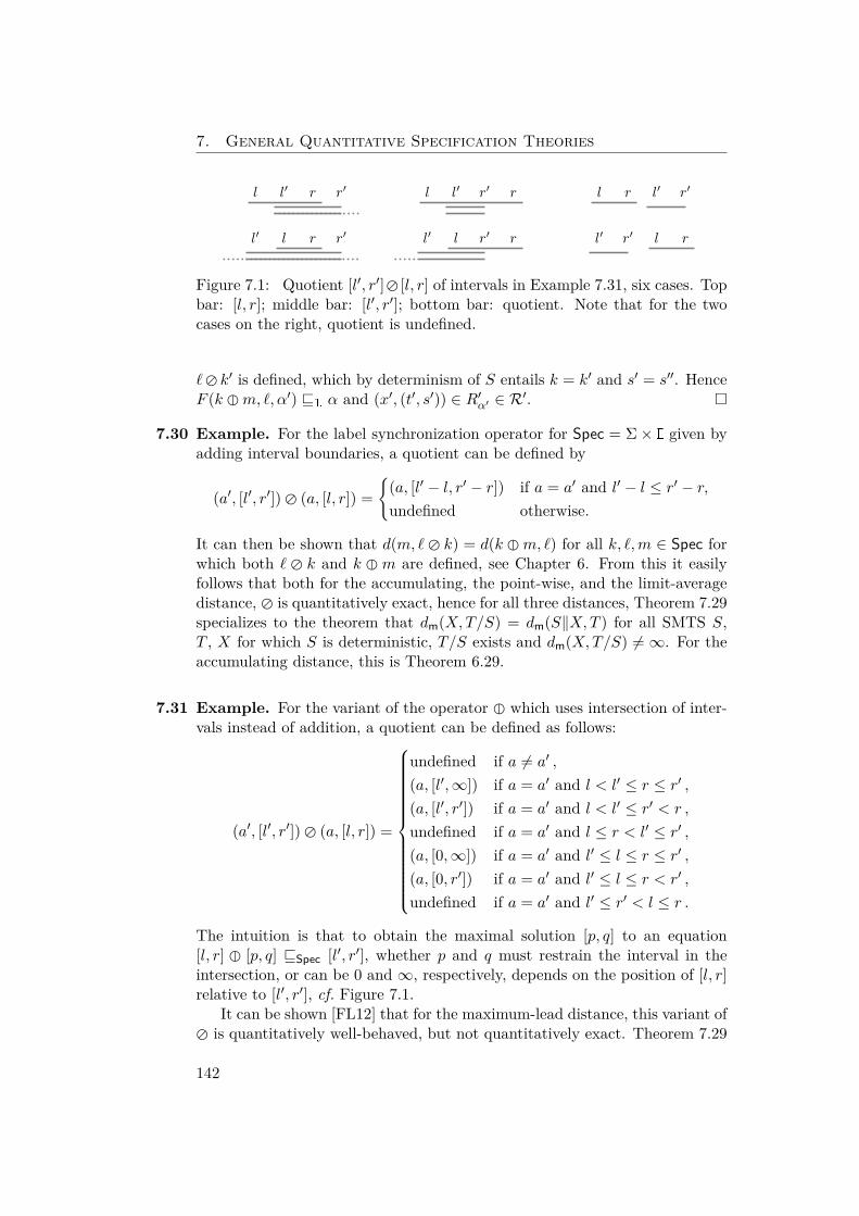
7. General Quantitative Specification Theories

l l′ r r′ l l′ r′ r l r l′ r′

l′ l r r′ l′ l r′ r l′ r′ l r

Figure 7.1: Quotient [l′, r′]� [l, r] of intervals in Example 7.31, six cases. Topbar: [l, r]; middle bar: [l′, r′]; bottom bar: quotient. Note that for the twocases on the right, quotient is undefined.

`� k′ is defined, which by determinism of S entails k = k′ and s′ = s′′. HenceF (k �m, `, α′) vL α and (x′, (t′, s′)) ∈ R′α′ ∈ R′. �

7.30 Example. For the label synchronization operator for Spec = Σ× I given byadding interval boundaries, a quotient can be defined by

(a′, [l′, r′])� (a, [l, r]) ={

(a, [l′ − l, r′ − r]) if a = a′ and l′ − l ≤ r′ − r,undefined otherwise.

It can then be shown that d(m, `� k) = d(k �m, `) for all k, `,m ∈ Spec forwhich both ` � k and k �m are defined, see Chapter 6. From this it easilyfollows that both for the accumulating, the point-wise, and the limit-averagedistance, � is quantitatively exact, hence for all three distances, Theorem 7.29specializes to the theorem that dm(X,T/S) = dm(S‖X,T ) for all SMTS S,T , X for which S is deterministic, T/S exists and dm(X,T/S) 6=∞. For theaccumulating distance, this is Theorem 6.29.

7.31 Example. For the variant of the operator � which uses intersection of inter-vals instead of addition, a quotient can be defined as follows:

(a′, [l′, r′])� (a, [l, r]) =

undefined if a 6= a′ ,

(a, [l′,∞]) if a = a′ and l < l′ ≤ r ≤ r′ ,(a, [l′, r′]) if a = a′ and l < l′ ≤ r′ < r ,

undefined if a = a′ and l ≤ r < l′ ≤ r′ ,(a, [0,∞]) if a = a′ and l′ ≤ l ≤ r ≤ r′ ,(a, [0, r′]) if a = a′ and l′ ≤ l ≤ r < r′ ,

undefined if a = a′ and l′ ≤ r′ < l ≤ r .

The intuition is that to obtain the maximal solution [p, q] to an equation[l, r] � [p, q] vSpec [l′, r′], whether p and q must restrain the interval in theintersection, or can be 0 and ∞, respectively, depends on the position of [l, r]relative to [l′, r′], cf. Figure 7.1.

It can be shown [FL12] that for the maximum-lead distance, this variant of� is quantitatively well-behaved, but not quantitatively exact. Theorem 7.29

142

7.4. Conjunction

hence translates to the fact that for all SMTA S, T , X for which S is deter-ministic and T/S exists, dm(X,T/S) ≥ dm(S‖X,T ).

7.4 ConjunctionConjunction of SMTS can be used to merge two specifications into one. Let7 : Spec× Spec⇀ Spec be a partial label operator for which it holds that

• for all k, ` ∈ Spec, if k 7 ` is defined, then k 7 ` 4 k, k 7 ` 4 `, and

• for all `, `′ ∈ Spec, (∃k ∈ Spec : d(k, `) 6= >L, d(k, `′) 6= >L) ⇔ (∃m ∈Spec : `7m, `′ 7m are defined).

The first requirement above ensures that conjunction acts as a lower bound,and the second one relates it to distances such that two labels have a commonquantitative refinement if and only if they have a common conjunction. Onealso usually wants conjunction to be a greatest lower bound; we say that 7 isconjunctively compositional if it holds for all k, `,m ∈ Spec for which m 4 kand m 4 ` that also k 7 ` is defined and m 4 k 7 `.

As a quantitative generalization, and analogously to what we did forstructural composition, we say that 7 is conjunctively bounded by a functionC : L × L → L if C is monotone in both coordinates, has C(⊥L,⊥L) = ⊥L,C(α,>L) = C(>L, α) = >L for all α ∈ L, and if it holds for all k, `,m ∈ Specfor which d(m, k) 6= >L and d(m, `) 6= >L that k 7 ` is defined and

F (m, k 7 `, C(α, α′)) vL C(F (m, k, α), F (m, `, α′))

for all α, α′ ∈ L. Note that this implies that d(m, k7`) vL C(d(m, k), d(m, `)),hence conjunctive boundedness implies conjunctive compositionality. Like Pfor structural composition, C gives a uniform bound on label conjunction.

7.32 Definition. The conjunction of two SMTS S and T is the SMTS S ∧ T =ρB(S × T, (s0, t0), 99KS∧T ,−→S∧T ) given as follows:

sk−→S s

′ t`99KT t′ k 7 ` defined

(s, t) k7`−→S∧T (s′, t′)s

k99KS s′ t

`−→T t′ k 7 ` defined

(s, t) k7`−→S∧T (s′, t′)

sk99KS s′ t

`99KT t′ k 7 ` defined

(s, t) k7`99KS∧T (s′, t′)

sk−→S s

′ ∀t `99KT t′ : k 7 ` undef.

(s, t) ∈ Bt

`−→T t′ ∀s k

99KS s′ : k 7 ` undef.(s, t) ∈ B

Note that like for quotient, conjunction of SMTS may give inconsistentstates which need to be pruned after. As seen in the last two SOS rulesabove, this is the case when one SMTS specifies a must transition with which

143

7. General Quantitative Specification Theories

the other SMTS cannot synchronize; then, the demand on implementationswould be that they simultaneously must and cannot have a transition, whichof course is unsatisfiable.

The next theorem shows the precise conditions under which conjunction isa greatest lower bound. Note that the greatest-lower-bound condition U ≤m S,U ≤m T ⇒ U ≤m S ∧ T entails uniqueness.

7.33 Theorem. Let S, T , U be SMTS. If S ∧ T is defined, then S ∧ T ≤m S andS ∧ T ≤m T . If, additionally, S or T are deterministic, then:

• If 7 is conjunctively compositional, U ≤m S, and U ≤m T , then S ∧ Tis defined and U ≤m S ∧ T .

• If 7 is conjunctively bounded by C, dm(U, S) 6= >L, and dm(U, T ) 6= >L,then S ∧ T is defined and dm(U, S ∧ T ) vL C(dm(U, S), dm(U, T )).

Proof: The proof of the two first claims is in [BJL+12a]. For the third claim,let R = {Rα ⊆ U × S | α ∈ L} and R′ = {R′α ⊆ U × T | α ∈ L} berelation families witnessing dm(U, S) and dm(U, T ), respectively, define R∧β ={(u, (s, t)) | ∃α, α′ ∈ L : (u, s) ∈ Rα, (u, t) ∈ R′α′ , C(α, α′) vL β} ⊆ U × S × Tfor all β ∈ L, and let R∧ = {R∧β | β ∈ L}. We show that R∧ is a witness fordm(U, S ∧ T ) vL C(dm(U, S), dm(U, T )).

We have (u0, (s0, t0)) ∈ R∧C(dm(U,S),dm(U,T )) ∈ R∧. Let β ∈ L \ {⊥L} and

(u, (s, t)) ∈ R∧β ∈ R∧, then we have α, α′ ∈ L \ {⊥L} with (u, s) ∈ Rα ∈ R,(u, t) ∈ R′α′ ∈ R′, and C(α, α′) vL β.

Assume u m99KU u′, then there exist s k

99KS s′ and α ∈ L for which (u′, s′) ∈Rα ∈ R and F (m, k, α) vL α, and similarly t `

99KT t′ and α′ with (u′, t′) ∈R′α′ ∈ R′ and F (m, `, α′) v α′. Then d(m, k) 6= >L and d(m, `) 6= >L, so byconjunctive boundedness k7` is defined, and (s, t) k7`

99KS∧T (s′, t′) by definitionof S ∧ T . Also, (u′, (s′, t′)) ∈ R∧C(α,α′) ∈ R

∧ and F (m, k 7 `, C(α, α′)) vLC(F (m, k, α), F (m, `, α′)) vL C(α, α′).

Assume (s, t) k7`−→S∧T (s′, t′), then s k−→S s′ and t `−→T t

′ by definition ofS ∧ T . We can without loss of generality postulate that T is deterministic.The fact that (u, s) ∈ Rα ∈ R implies that there are u m−→U u

′ and α ∈ L forwhich (u′, s′) ∈ Rα ∈ R and F (m, k, α) vL α. We must also have u m′

99KU u′

for some m′ wSpec m, and then (u, t) ∈ R′α ∈ R′ implies that there existt

`′99KT t′′ and α′ ∈ L with (u′, t′′) ∈ R′α′ ∈ R′ and F (m′, `′, α′) vL α′.The triangle inequality for F gives

F (m, `′, α′) vL F (m,m′,⊥L)�L F (m′, `′, α′) vL α′ ,

hence d(m, `′) 6= >L. Together with d(m, k) 6= >L, conjunctive boundednessallows us to conclude that k7 `′ is defined, but then both k7 ` and k7 `′ aredefined, hence by determinism of T , ` = `′ and t′ = t′′. �

144

7.4. Conjunction

7.34 Example. For the set Spec = Σ× I from our examples, the unique composi-tional conjunction operator on is given, on labels, by intersection of intervals:

(a, [l, r])7 (a′, [l′, r′]) =

(a, [max(l, l′),min(r, r′)])

if a = a′,max(l, l′) ≤ min(r, r′),undefined otherwise.

We can easily show that 7 is not conjunctively bounded: with m = (a, [2, 2]),k = (a, [0, 1]) and ` = (a, [3, 4]), we have d(m, k) = d(m, `) = 1, but k7` is notdefined. Noting that this statement does not involve the distance iterator F ,we conclude that neither accumulating, point-wise nor limit-average distanceadmit a bounded conjunction operator. For the accumulating distance, thisstatement is Theorem 6.24.

To deal with the problem that, as in the above example, conjunction maynot be conjunctively bounded, we introduce another, weaker, property whichensures some compatibility of conjunction with distances. We say that 7 isrelaxed conjunctively bounded by a function C : L× L→ L if C is monotonein both coordinates, has C(⊥L,⊥L) = ⊥L, C(α,>L) = C(>L, α) = >L forall α ∈ L, and such that for all k, ` ∈ Spec for which there is m ∈ Spec withd(m, k) 6= >L and d(m, `) 6= >L, there exist k′, `′ ∈ Spec with k′ 7 `′ defined,k 4 k′, ` 4 `′, d(k′, k) 6= >L, and d(`′, `) 6= >L, such that for all m′ ∈ Spec,α, α′ ∈ L,

F (m′, k′ 7 `′, C(α, α′)) vL C(F (m′, k, α), F (m′, `, α′)). (7.3)

The following theorem shows that relaxed boundedness of 7 entails a sim-ilar property for SMTS conjunction.

7.35 Theorem. Let S, T be SMTS with S or T deterministic and 7 relaxed con-junctively bounded by C. If there is an SMTS U for which dm(U, S) 6= >L anddm(U, T ) 6= >L, then there exist β- and γ-widenings S′ of S and T ′ of T suchthat S′ ∧ T ′ is defined, and dm(U ′, S′ ∧ T ′) vL C(dm(U ′, S), dm(U ′, T )) for allSMTS U ′.

Proof: We start by constructing S′ and T ′, almost as in the proof of the thirdclaim of Theorem 7.33. The states of S′ and T ′ will be the same as for S andT , and we start by letting β = ⊥L, γ = ⊥L.

Let U fulfill dm(U, S) 6= >L and dm(U, T ) 6= >L, let R = {Rα ⊆ U × S |α ∈ L} and R′ = {R′α ⊆ U × T | α ∈ L} be relation families witnessingdm(U, S) and dm(U, T ), respectively, define R∧η = {(u, (s, t)) | ∃α, α′ ∈ L :(u, s) ∈ Rα, (u, t) ∈ R′α′ , C(α, α′) vL η} ⊆ U × S × T for all η ∈ L, and letR∧ = {R∧η | η ∈ L}.

Now let η ∈ L \ {>L} and (u, (s, t)) ∈ R∧η ∈ R∧, then we have α, α′ ∈L \ {⊥L} with (u, s) ∈ Rα ∈ R, (u, t) ∈ R′α′ ∈ R′, and C(α, α′) vL η.

145

7. General Quantitative Specification Theories

Let u m99KU u′, then also s k

99KS s′ and t`99KT t′, and there are α, α′ ∈ L \

{>L} with F (m, k, α) vL α and F (m, `, α′) vL α′. Hence d(m, k) 6= >L andd(m, `) 6= >L, and by relaxed conjunctive boundedness we have k′, `′ ∈ Specwith k 4 k′, ` 4 `′, d(k′, k) 6= >L, d(`′, `) 6= >L, and k′7`′ defined. We add thetransitions s k′

99KS′ s′, t`′99KT ′ t′ to S′ and T ′ and update β := max(β, d(k′, k)),

γ := max(γ, d(`′, `)).As the sets {k ∈ Spec | s k

99KS s′}, {` ∈ Spec | t `99KT t′} are compact,

the above process converges to some β, γ 6= >L. The must transitions we justcopy from S to S′ and from T to T ′, and then S′ is a β-widening of S and T ′is a γ-widening of T .

We must show that S′ and T ′ satisfy the properties claimed. By con-struction S′ ∧ T ′ is defined, so let U ′ be an SMTS with dm(U ′, S) 6= >L anddm(U ′, T ) 6= >L (otherwise we have nothing to prove). We must show thatdm(U ′, S′ ∧ T ′) vL C(dm(U ′, S), dm(U ′, T )). Let R = {Rα ⊆ U ′ × S | α ∈ L}and R′ = {R′α ⊆ U ′ × T | α ∈ L} be relation families witnessing dm(U ′, S)and dm(U ′, T ), respectively, define R∧′η = {(u′, (s, t)) | ∃α, α′ ∈ L : (u′, s) ∈Rα, (u′, t) ∈ R′α′ , C(α, α′) vL η} ⊆ U ′ × S × T for all η ∈ L, and letR∧′ = {R∧′η | η ∈ L}.

We have (u′0, (s0, t0)) ∈ R∧′

C(dm(U ′,S),dm(U ′,T )) ∈ R∧′ . Let η ∈ L \ {⊥L}

and (u′, (s, t)) ∈ R∧′η , then we have α, α′ ∈ L \ {⊥L} with (u′, s) ∈ Rα ∈ R,(u′, t) ∈ R′α′ ∈ R′, and C(α, α′) vL η. Let u′ m

99KU ′ u′′, then also s k99KS s′

and t `99KT t′, and there are α, α′ ∈ L\{>L} with (u′′, s′) ∈ Rα, (u′′, t′) ∈ R′α′ ,

F (m, k, α) vL α, and F (m, `, α′) vL α′.By construction of S′ and T ′, we have s k′

99KS′ s′ and t`′99KT ′ t′ with k 4 k′,

` 4 `′, d(k′, k) vL β, and d(`′, `) vL γ, and such that k′ 7 `′ is defined. Also,(u′′, (s′, t′)) ∈ R∧′C(α,α′) and

F (m, k′ 7 `′, C(α, α′)) vL C(F (m, k, α), F (m, `, α′)) vL C(α, α′).

The other direction of the proof, starting with a transition (s, t) k7`−→S′∧T ′

(s′, t′), is an exact copy of the corresponding part of the proof of Theo-rem 7.33. �

7.36 Example. For the set Spec = Σ× I from our examples, the following lemmashows a one-step version of relaxed conjunctive boundedness.

7.37 Lemma. For all k, ` ∈ Spec for which there is m ∈ Spec with d(m, k) 6= ∞and d(m, `) 6= ∞, there exist k′, `′ ∈ Spec with k 4 k′, ` 4 `′, d(k′, k) 6= ∞,d(`′, `) 6=∞, and k′7`′ defined, and then d(m′, k′7`′) ≤ max(d(m′, k), d(m′, `))for all m′ ∈ Spec.

Proof: Let k, ` ∈ Spec such that there is m ∈ Spec with d(m, k) 6= ∞ andd(m, `) 6= ∞. This implies that k = (a, [l, r]) and ` = (a, [l′, r′]) for some

146

7.4. Conjunction

a ∈ Σ, k, l, k′, l′ ∈ Z ∪ {−∞,∞}. Without loss of generality we can assumethat l ≤ l′.

If r ≥ l′, then k7 ` = (a, [l′, r]) is defined, and we take k′ = k, `′ = `. Nowlet m′ = (a′, [l′′, r′′]) ∈ Spec. If a′ 6= a, the property to prove is trivially true.If a′ = a, then we have

d(m′, k′ 7 `′) = max(0, l′ − l′′, r′′ − r) ,d(m′, k) = max(0, l − l′′, r′′ − r) ,d(m′, `) = max(0, l′ − l′′, r′′ − r′) .

Thus we need to show that

max(0, l′ − l′′, r′′ − r) ≤ max(0, l − l′′, r′′ − r, l′ − l′′, r′′ − r′) ,

which is clear as all left-hand terms also appear on the right-hand side.In case r < l′, we let k′ = (a, [l, l′]) and `′ = (a, [r, r′]). Then k 4 k′, ` 4 `′,

and k′ 7 `′ = (a, [r, l′]) is defined. Also, d(k′, k) = d(`′, `) = l′ − r 6=∞.Let m′ = (a′, [l′′, r′′]) as before, then the case a′ 6= a is again trivial. We

haved(m′, k′ 7 `′) = max(0, r − l′′, r′′ − l′) ,

so we need to show that

max(0, r − l′′, r′′ − l′) ≤ max(0, l − l′′, r′′ − r, l′ − l′′, r′′ − r′)= max(0, r′′ − r, l′ − l′′) ,

where the equality follows from l ≤ l′, hence l− l′′ ≤ l′− l′′, and r ≤ r′, hencer′′ − r′ ≤ r′′ − r. But 0 ≤ l′ − r, r − l′′ < l′ = l′′, and r′′ − l′ < r′′ − r becauseof r < l′, so the inequality follows. �

For the accumulating distance, it then follows that 7 is relaxed conjunc-tively bounded by C(α, α′) = α+α′: Using the notation from Lemma 7.37, weneed to show (7.3), i.e., that d(m′, l′7`′)+λ(α+α′) ≤ d(m′, k)+λα+d(m′, `)+λα′, which however is clear by d(m′, k′ 7 `′) ≤ max(d(m′, k), d(m′, `)) ≤d(m′, k) + d(m′, `).

7.38 Example. For the pointwise distance, 7 is relaxed conjunctively bounded byC(α, α′) = max(α, α′): (7.3) is then equivalent to max(d(m′, k′ 7 `′), α, α′) ≤max(d(m′, k), d(m′, `), α, α′), which follows from Lemma 7.37.

7.39 Example. For the limit-average distance, 7 is relaxed conjunctively boundedby C(α, α′) = α �L α′: Again using the notation from Lemma 7.37, we needto show (7.3), so we need to see that for all j ∈ N+,

1j+1d(m′, k′ 7 `′) + j

j+1α(j − 1) + jj+1α

′(j − 1)

≤ 1j+1d(m′, k) + j

j+1α(j − 1) + 1j+1d(m′, `) + j

j+1α′(j − 1) .

147

7. General Quantitative Specification Theories

This follows again from d(m′, k′ 7 `′) ≤ max(d(m′, k), d(m′, `)) ≤ d(m′, k) +d(m′, `).

7.40 Example. Also for the maximum-lead distance, 7 is relaxed conjunctivelybounded by C(α, α′) = α �L α′. To see this, we again use the notation fromLemma 7.37. We need to show that for all α, α′ ∈ L and all d ∈ R,

supl′′≤z≤r′′

infr≤w≤l′

max(|d+ z − w|, α(d+ z − w) + α′(d+ z − w))≤ sup

l′′≤z≤r′′infl≤x≤r

max(|d+ z − x|, α(d+ z − x))

+ supl′′≤z≤r′′

infl′≤y≤r′

max(|d+ z − y|, α′(d+ z − y))

(7.4)

Now for all z ∈ [l′′, r′′], we have

infr≤w≤l′

|d+ z − w| ≤ infl≤x≤r

|d+ z − x|+ infl′≤y≤r′

|d+ z − y|

and

infr≤w≤l′

(α(d+ z − w) + α′(d+ z − w))≤ inf

l≤x≤rα(d+ z − x) + inf

l′≤y≤r′α′(d+ z − y) ;

both can be shown by simply considering all cases of the placement of theinfima. But then also

max( infr≤w≤l′

|d+ z − w|, infr≤w≤l′

(α(d+ z − w) + α′(d+ z − w)))

≤ max

inf

l≤x≤r|d+ z − x|+ inf

l′≤y≤r′|d+ z − y|

infl≤x≤r

α(d+ z − x) + infl′≤y≤r′

α′(d+ z − y))

≤ max( infl≤x≤r

|d+ z − x|, infl≤x≤r

α(d+ z − x))

+ max( infl′≤y≤r′

|d+ z − y|, infl′≤y≤r′

α′(d+ z − y)) ,

the last inequality by distributivity of + over max. As this holds for all z, wehave proven (7.4).

7.5 Logical CharacterizationsWe show that quantitative refinement admits a logical characterization. Ourresults extend the logical characterization of modal transition systems in [Lar89].Our logic L is the smallest set of expressions generated by the following ab-stract syntax:

φ, φ1, φ2 := tt | ff | 〈`〉φ | [`]φ | φ1 ∧ φ2 | φ1 ∨ φ2 (` ∈ Spec)

148

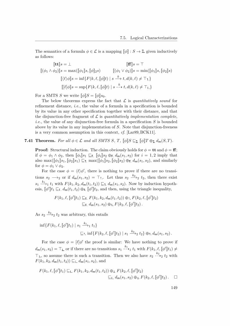
7.5. Logical Characterizations

The semantics of a formula φ ∈ L is a mapping JφK : S → L given inductivelyas follows:

JttKs = ⊥ JffKs = >J(φ1 ∧ φ2)Ks = max(Jφ1Ks, JφK2s) J(φ1 ∨ φ2)Ks = min(Jφ1Ks, Jφ2Ks)

J〈`〉φKs = inf{F (k, `, JφKt) | s k−→ t, d(k, `) 6= >L}

J[`]φKs = sup{F (k, `, JφKt) | s k99K t, d(k, `) 6= >L}

For a SMTS S we write JφKS = JφKs0.The below theorems express the fact that L is quantitatively sound for

refinement distance, i.e., the value of a formula in a specification is boundedby its value in any other specification together with their distance, and thatthe disjunction-free fragment of L is quantitatively implementation complete,i.e., the value of any disjunction-free formula in a specification S is boundedabove by its value in any implementation of S. Note that disjunction-freenessis a very common assumption in this context, cf. [Lar89,BCK11].

7.41 Theorem. For all φ ∈ L and all SMTS S, T , JφKS vL JφKT �L dm(S, T ).

Proof: Structural induction. The claim obviously holds for φ = tt and φ = ff ;if φ = φ1 ∧ φ2, then JφiKs1 vL JφiKs2 �L dm(s1, s2) for i = 1, 2 imply thatalso max(Jφ1Ks1, Jφ2Ks1) vL max(Jφ1Ks2, Jφ2Ks2) �L dm(s1, s2), and similarlyfor φ = φ1 ∨ φ2.

For the case φ = 〈`〉φ′, there is nothing to prove if there are no transi-tions s2 −→2 or if dm(s1, s2) = >L. Let thus s2

k2−→2 t2, then there exists1

k1−→1 t1 with F (k1, k2, dm(t1, t2)) vL dm(s1, s2). Now by induction hypoth-esis, Jφ′Kt1 vL dm(t1, t2) �L Jφ′Kt2, and then, using the triangle inequality,

F (k1, `, Jφ′Kt1) vL F (k1, k2, dm(t1, t2)) �L F (k2, `, Jφ′Kt2)vL dm(s1, s2) �L F (k2, `, Jφ′Kt2) .

As s2k2−→2 t2 was arbitrary, this entails

inf{F (k1, `, Jφ′Kt1) | s1k1−→1 t1}

vL inf{F (k2, `, Jφ′Kt2) | s1k2−→2 t2}�L dm(s1, s2) .

For the case φ = [`]φ′ the proof is similar: We have nothing to prove ifdm(s1, s2) = >L or if there are no transitions s1

k199K1 t1 with F (k1, `, Jφ′Kt1) 6=

>L, so assume there is such a transition. Then we also have s2k299K2 t2 with

F (k1, k2, dm(t1, t2)) vL dm(s1, s2), and

F (k1, `, Jφ′Kt1) vL F (k1, k2, dm(t1, t2))�L F (k2, `, Jφ′Kt2)vL dm(s1, s2)�L F (k2, `, Jφ′Kt2) . �

149

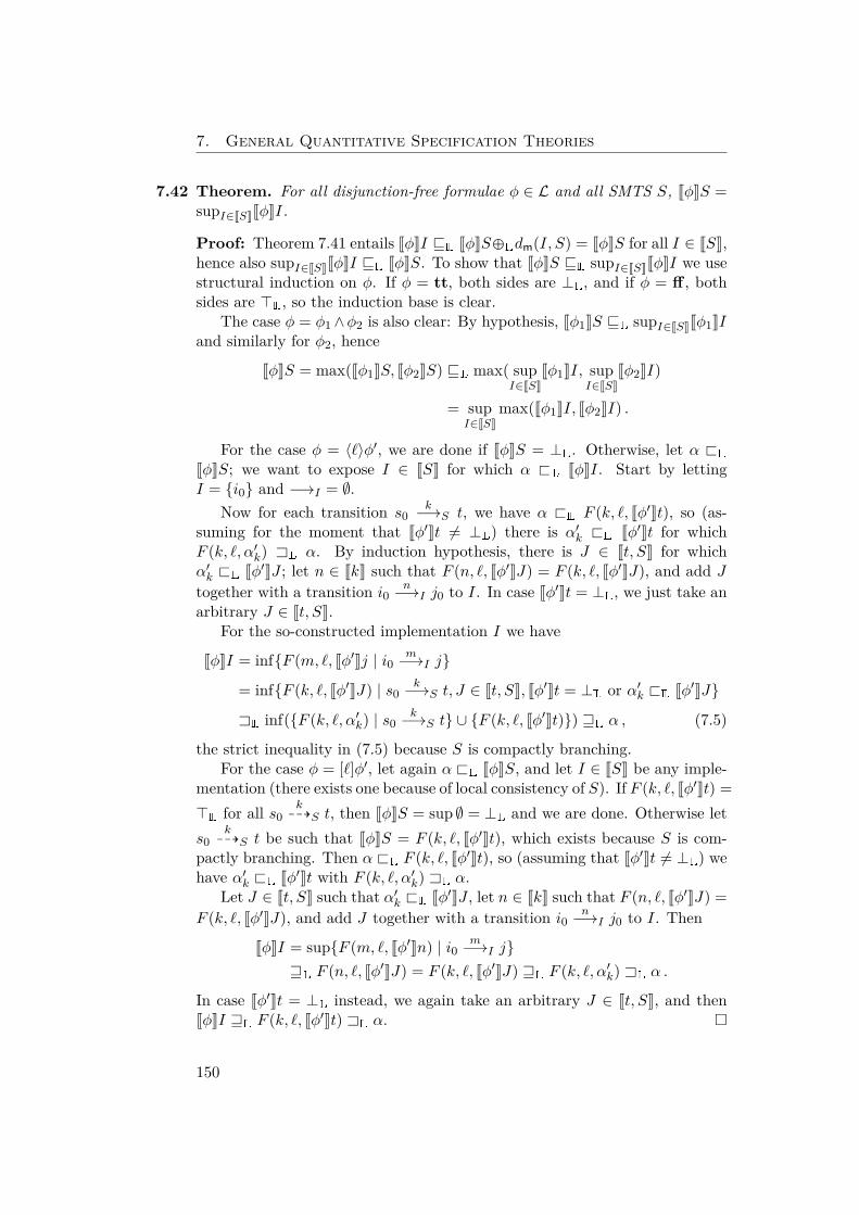
7. General Quantitative Specification Theories

7.42 Theorem. For all disjunction-free formulae φ ∈ L and all SMTS S, JφKS =supI∈JSKJφKI.

Proof: Theorem 7.41 entails JφKI vL JφKS�Ldm(I, S) = JφKS for all I ∈ JSK,hence also supI∈JSKJφKI vL JφKS. To show that JφKS vL supI∈JSKJφKI we usestructural induction on φ. If φ = tt, both sides are ⊥L, and if φ = ff , bothsides are >L, so the induction base is clear.

The case φ = φ1∧φ2 is also clear: By hypothesis, Jφ1KS vL supI∈JSKJφ1KIand similarly for φ2, hence

JφKS = max(Jφ1KS, Jφ2KS) vL max( supI∈JSK

Jφ1KI, supI∈JSK

Jφ2KI)

= supI∈JSK

max(Jφ1KI, Jφ2KI) .

For the case φ = 〈`〉φ′, we are done if JφKS = ⊥L. Otherwise, let α @LJφKS; we want to expose I ∈ JSK for which α @L JφKI. Start by lettingI = {i0} and −→I = ∅.

Now for each transition s0k−→S t, we have α @L F (k, `, Jφ′Kt), so (as-

suming for the moment that Jφ′Kt 6= ⊥L) there is α′k @L Jφ′Kt for whichF (k, `, α′k) AL α. By induction hypothesis, there is J ∈ Jt, SK for whichα′k @L Jφ

′KJ ; let n ∈ JkK such that F (n, `, Jφ′KJ) = F (k, `, Jφ′KJ), and add Jtogether with a transition i0 n−→I j0 to I. In case Jφ′Kt = ⊥L, we just take anarbitrary J ∈ Jt, SK.

For the so-constructed implementation I we have

JφKI = inf{F (m, `, Jφ′Kj | i0 m−→I j}

= inf{F (k, `, Jφ′KJ) | s0k−→S t, J ∈ Jt, SK, Jφ′Kt = ⊥L or α′k @L Jφ′KJ}

AL inf({F (k, `, α′k) | s0k−→S t} ∪ {F (k, `, Jφ′Kt)}) wL α , (7.5)

the strict inequality in (7.5) because S is compactly branching.For the case φ = [`]φ′, let again α @L JφKS, and let I ∈ JSK be any imple-

mentation (there exists one because of local consistency of S). If F (k, `, Jφ′Kt) =>L for all s0

k99KS t, then JφKS = sup ∅ = ⊥L and we are done. Otherwise let

s0k99KS t be such that JφKS = F (k, `, Jφ′Kt), which exists because S is com-

pactly branching. Then α @L F (k, `, Jφ′Kt), so (assuming that Jφ′Kt 6= ⊥L) wehave α′k @L Jφ′Kt with F (k, `, α′k) AL α.

Let J ∈ Jt, SK such that α′k @L Jφ′KJ , let n ∈ JkK such that F (n, `, Jφ′KJ) =F (k, `, Jφ′KJ), and add J together with a transition i0 n−→I j0 to I. Then

JφKI = sup{F (m, `, Jφ′Kn) | i0 m−→I j}wL F (n, `, Jφ′KJ) = F (k, `, Jφ′KJ) wL F (k, `, α′k) AL α .

In case Jφ′Kt = ⊥L instead, we again take an arbitrary J ∈ Jt, SK, and thenJφKI wL F (k, `, Jφ′Kt) AL α. �

150

8 Logical vs. Behavioral Specifications1

In this chapter we depart from the quantitative setting of this thesis and intro-duce disjunctive modal transition systems. We show that this generalizationof MTS is closely related to other specification formalisms, viz. acceptanceautomata and the modal ν-calculus and that it admits both disjunction andconjunction as well as a general notion of quotient which was unavailable forMTS.

8.1 Specification FormalismsIn this section we introduce the four specification formalisms with which thischapter is concerned. For the rest of the chapter, we fix a finite alphabetΣ. In each of the formalisms, the semantics of a specification is a set ofimplementations, in our case always a set of (finite) labeled transition systems(LTS) over Σ, i.e., structures I = (S, s0,−→) consisting of a finite set S ofstates, an initial state s0 ∈ S, and a transition relation −→ ⊆ S × Σ× S.

8.1.1 Disjunctive Modal Transition Systems

8.1 Definition. A disjunctive modal transition system (DMTS) is a structureD = (S, S0, 99K,−→) consisting of finite sets S ⊇ S0 of states and initialstates, a may-transition relation 99K ⊆ S × Σ × S, and a disjunctive must-transition relation −→ ⊆ S × 2Σ×S . It is assumed that for all (s,N) ∈ −→and all (a, t) ∈ N , (s, a, t) ∈ 99K; furthermore, if (s, ∅) ∈ −→ then there areno a and t such that (s, a, t) ∈ 99K.

As customary, we write s a99K t instead of (s, a, t) ∈ 99K, s −→ N instead

of (s,N) ∈ −→, s a99K if there exists t for which s

a99K t, and s

aX99K if there

does not.The intuition is that may-transitions s a

99K t specify which transitions arepermitted in an implementation, whereas a must-transition s −→ N stipulatesa disjunctive requirement: at least one of the choices (a, t) ∈ N has to be

1This chapter is based on the journal paper [BFK+20] published in Information andComputation.

151

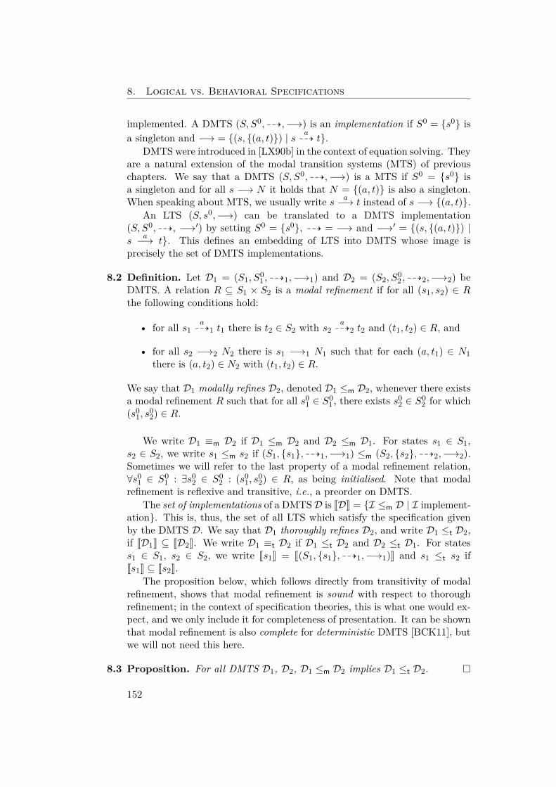
8. Logical vs. Behavioral Specifications

implemented. A DMTS (S, S0, 99K,−→) is an implementation if S0 = {s0} isa singleton and −→ = {(s, {(a, t)}) | s a

99K t}.DMTS were introduced in [LX90b] in the context of equation solving. They

are a natural extension of the modal transition systems (MTS) of previouschapters. We say that a DMTS (S, S0, 99K,−→) is a MTS if S0 = {s0} isa singleton and for all s −→ N it holds that N = {(a, t)} is also a singleton.When speaking about MTS, we usually write s a−→ t instead of s −→ {(a, t)}.

An LTS (S, s0,−→) can be translated to a DMTS implementation(S, S0, 99K, −→′) by setting S0 = {s0}, 99K = −→ and −→′ = {(s, {(a, t)}) |s

a−→ t}. This defines an embedding of LTS into DMTS whose image isprecisely the set of DMTS implementations.

8.2 Definition. Let D1 = (S1, S01 , 99K1,−→1) and D2 = (S2, S

02 , 99K2,−→2) be

DMTS. A relation R ⊆ S1 × S2 is a modal refinement if for all (s1, s2) ∈ Rthe following conditions hold:

• for all s1a99K1 t1 there is t2 ∈ S2 with s2

a99K2 t2 and (t1, t2) ∈ R, and

• for all s2 −→2 N2 there is s1 −→1 N1 such that for each (a, t1) ∈ N1there is (a, t2) ∈ N2 with (t1, t2) ∈ R.

We say that D1 modally refines D2, denoted D1 ≤m D2, whenever there existsa modal refinement R such that for all s0

1 ∈ S01 , there exists s0

2 ∈ S02 for which

(s01, s

02) ∈ R.

We write D1 ≡m D2 if D1 ≤m D2 and D2 ≤m D1. For states s1 ∈ S1,s2 ∈ S2, we write s1 ≤m s2 if (S1, {s1}, 99K1,−→1) ≤m (S2, {s2}, 99K2,−→2).Sometimes we will refer to the last property of a modal refinement relation,∀s0

1 ∈ S01 : ∃s0

2 ∈ S02 : (s0

1, s02) ∈ R, as being initialised. Note that modal

refinement is reflexive and transitive, i.e., a preorder on DMTS.The set of implementations of a DMTSD is JDK = {I ≤m D | I implement-

ation}. This is, thus, the set of all LTS which satisfy the specification givenby the DMTS D. We say that D1 thoroughly refines D2, and write D1 ≤t D2,if JD1K ⊆ JD2K. We write D1 ≡t D2 if D1 ≤t D2 and D2 ≤t D1. For statess1 ∈ S1, s2 ∈ S2, we write Js1K = J(S1, {s1}, 99K1,−→1)K and s1 ≤t s2 ifJs1K ⊆ Js2K.

The proposition below, which follows directly from transitivity of modalrefinement, shows that modal refinement is sound with respect to thoroughrefinement; in the context of specification theories, this is what one would ex-pect, and we only include it for completeness of presentation. It can be shownthat modal refinement is also complete for deterministic DMTS [BCK11], butwe will not need this here.

8.3 Proposition. For all DMTS D1, D2, D1 ≤m D2 implies D1 ≤t D2. �

152

8.1. Specification Formalisms

8.1.2 The Modal ν-CalculusWe recall the syntax and semantics of the modal ν-calculus, the fragment ofthe modal µ-calculus [SdB69,Koz83] with only greatest fixed points. Instead ofan explicit greatest fixed point operator, we use the representation by equationsystems in Hennessy-Milner logic developed in [Lar90b].

For a finite set X of variables, let H(X) be the set of Hennessy-Milnerformulae, generated by the abstract syntax

H(X) 3 φ ::= tt | ff | x | 〈a〉φ | [a]φ | φ ∧ φ | φ ∨ φ ,

for a ∈ Σ and x ∈ X.A declaration is a mapping ∆ : X → H(X); we recall the greatest fixed

point semantics of declarations from [Lar90b]. For an LTS (S, s0,−→), an as-signment is a mapping σ : X → 2S . The set of assignments forms a completelattice with order σ1 v σ2 iff σ1(x) ⊆ σ2(x) for all x ∈ X and least upperbound

(⊔i∈I σi

)(x) = ⋃

i∈I σi(x).The semantics of a formula is a subset of S, given relative to an assign-

ment σ, defined as follows: JttKσ = S, JffKσ = ∅, JxKσ = σ(x), Jφ ∧ ψKσ =JφKσ ∩ JψKσ, Jφ ∨ ψKσ = JφKσ ∪ JψKσ, and

J〈a〉φKσ = {s ∈ S | ∃s a−→ s′ : s′ ∈ JφKσ},J[a]φKσ = {s ∈ S | ∀s a−→ s′ : s′ ∈ JφKσ}.

The semantics of a declaration ∆ is then the assignment defined by

J∆K =⊔{σ : X → 2S | ∀x ∈ X : σ(x) ⊆ J∆(x)Kσ};

the greatest (post)fixed point of ∆.A ν-calculus expression is a structure N = (X,X0,∆), with X0 ⊆ X

sets of variables and ∆ : X → H(X) a declaration. We say that an LTSI = (S, s0,−→) implements (or models) the expression, and write I |= N ,if there is x0 ∈ X0 such that s0 ∈ J∆K(x0). We write JN K for the set ofimplementations (models) of a ν-calculus expression N . As for DMTS, wewrite JxK = J(X, {x},∆)K for x ∈ X, and thorough refinement of expressionsand variables is defined accordingly.2

We are now going to introduce a normal form for ν-calculus expressions.The purpose of this normal form is twofold. One is to allow us to define modalrefinement for ν-calculus, an analogue to the DMTS modal refinement thatcan be seen as a sound approximation of the logical implication, cf. Propo-sition 8.3. The second purpose is to facilitate a simple translation betweenDMTS and ν-calculus expressions, see Section 8.2.1 below.

2Any ν-calculus expression is thoroughly equivalent to one with precisely one initialstate, i.e., X0 a singleton, however this is not true for ν-calculus expressions in normal formas defined below. See also Section 8.2.5.

153

8. Logical vs. Behavioral Specifications

8.4 Lemma. For any ν-calculus expression N1 = (X1, X01 ,∆1), there exists an-

other expression N2 = (X2, X02 ,∆2) with JN1K = JN2K and such that for any

x ∈ X, ∆2(x) is of the form

∆2(x) =∧i∈I

( ∨j∈Ji〈aij〉xij

)∧∧a∈Σ

[a]( ∨j∈Ja

ya,j)

(8.1)

for finite (possibly empty) index sets I, Ji, Ja, for i ∈ I and a ∈ Σ, and allxij , ya,j ∈ X2. Additionally, for all i ∈ I and j ∈ Ji, there exists j′ ∈ Jaij forwhich xij ≤t yaij ,j′. Also if at least one of the Ji = ∅ then Ja = ∅ for all a.

Remark that this normal form includes a semantic check (xij ≤t yaij ,j′),so it is not entirely syntactic.

Proof: It is shown in [BL92] that any Hennessy-Milner formula is equivalentto one in so-called strong normal form, i.e., of the form ∨

i∈I(∧j∈Ji〈aij〉φij ∧∧

a∈Σ[a]ψi,a) for HML formulas φij , ψi,a which are also in strong normal form,and such that for all i, j, φij ≤t ψi,aij .

We can replace the φij , ψi,a by (new) variables xij , yi,a and add declara-tions ∆2(xij) = φij , ∆2(yi,a) = ψi,a to arrive at an expression in which allformulae are of the form ∆2(x) = ∨

i∈I(∧j∈Ji〈aij〉xij ∧

∧a∈Σ[a]yi,a) and such

that for all i, j, xij ≤t yi,aij .Now for each such formula, replace (recursively) x by new variables {xi |

i ∈ I}, similarly for y, and set ∆2(xi) = ∧j∈Ji〈aij〉

(∨k x

kij

)∧∧a∈Σ[a]

(∨k y

ki,a

).

Using initial variables X02 = {xi | x ∈ X0

1}, the so-constructed ν-calculusexpression is equivalent to the original one. We know that for all i, j, ∨k xkij ≤t∨k y

ki,aij

, hence for all i, j, k there exists k′ such that xkij ≤t yk′i,aij

. We can thusrename variables and apply the distributivity of 〈·〉 over ∨.

Finally, if at least one of the Ji = ∅ then ∆2 is false and we can simply setJa = ∅ for all a without changing the semantics of ∆2. �

As this is a type of conjunctive normal form, it is clear that translatinga ν-calculus expression into normal form may incur an exponential blow-up.

We introduce some notation for ν-calculus expressions in normal formwhich will make our life easier later. LetN = (X,X0,∆) be such an expressionand x ∈ X, with ∆(x) = ∧

i∈I(∨

j∈Ji〈aij〉xij)∧∧a∈Σ[a]

(∨j∈Ja ya,j

)as in the

lemma. Define ♦(x) = {{(aij , xij) | j ∈ Ji} | i ∈ I} and, for each a ∈ Σ,�a(x) = {ya,j | j ∈ Ja}. Note that now,

∆(x) =∧

N∈♦(x)

( ∨(a,y)∈N

〈a〉y)∧∧a∈Σ

[a]( ∨y∈�a(x)

y).

8.5 Definition. Let N1 = (X1, X01 ,∆1), N2 = (X2, X

02 ,∆2) be ν-calculus expres-

sions in normal form and R ⊆ X1×X2. The relation R is a modal refinementif it holds for all (x1, x2) ∈ R that

154

8.1. Specification Formalisms

• for all a ∈ Σ and every y1 ∈ �a1(x1), there is y2 ∈ �a2(x2) for which(y1, y2) ∈ R, and

• for all N2 ∈ ♦2(x2) there is N1 ∈ ♦1(x1) such that for each (a, y1) ∈ N1,there exists (a, y2) ∈ N2 with (y1, y2) ∈ R.

We say that N1 modally refines N2, denoted N1 ≤m N2, whenever there existsa modal refinement R such that for every x0

1 ∈ X01 there exists x0

2 ∈ X02 for

which (x01, x

02) ∈ R.

We say that a ν-calculus expression (X,X0,∆) in normal form is an im-plementation if X0 = {x0} is a singleton, ♦(x) = {{(a, y)} | y ∈ �a(x), a ∈ Σ}and �a(x) = ∅ for all a /∈ Σ, for all x ∈ X.

We can translate an LTS (S, s0,−→) to a ν-calculus expression (S, S0,∆)in normal form by setting S0 = {s0} and ♦(s) = {{(a, t)} | s a−→ t} and�a(s) = {t | s a−→ t} for all s ∈ S, a ∈ Σ. Like for DMTS, this defines anembedding of LTS into the modal ν-calculus whose image are precisely theν-calculus implementations.

We will show below in Theorem 8.12 that for any LTS I and any ν-calculusexpression N in normal form, I |= N iff I ≤m N , hence the fixed-pointsemantics of [Lar90b] and our refinement semantics agree. As a corollaryof this result, we get that modal refinement is a sound approximation tological implication, i.e., that N1 ≤m N2 implies that for all implementationsI, (I |= N1)⇒ (I |= N2).

8.1.3 Nondeterministic Acceptance Automata8.6 Definition. A nondeterministic acceptance automaton (AA) is a structureA = (S, S0,Tran), with S ⊇ S0 finite sets of states and initial states andTran : S → 22Σ×S an assignment of transition constraints.

Acceptance automata were first introduced in [Rac07] (see also [Rac08],where a slightly different language-based approach is taken), based on thenotion of acceptance trees in [Hen85]; however, these are deterministic. Weextend the formalism to a nondeterministic setting here. The following notionof modal refinement was introduced in [BKL+11].

8.7 Definition. Let A1 = (S1, S01 ,Tran1) and A2 = (S2, S

02 ,Tran2) be AA. A

relation R ⊆ S1 × S2 is a modal refinement if it holds for all (s1, s2) ∈ R andall M1 ∈ Tran1(s1) that there exists M2 ∈ Tran2(s2) such that

∀(a, t1) ∈M1 : ∃(a, t2) ∈M2 : (t1, t2) ∈ R ,∀(a, t2) ∈M2 : ∃(a, t1) ∈M1 : (t1, t2) ∈ R .

(8.2)

We say that A1 modally refines A2, and write A1 ≤m A2, whenever thereexists a modal refinement R such that for all s0

1 ∈ S01 , there exists s0

2 ∈ S02 for

which (s01, s

02) ∈ R.

155

8. Logical vs. Behavioral Specifications

An AA is an implementation if S0 = {s0} is a singleton and, for all s ∈ S,Tran(s) = {M} is a singleton. An LTS (S, s0,−→) can be translated to anAA by setting S0 = {s0} and Tran(s) = {{(a, t) | s a−→ t}}. This defines anembedding of LTS into AA whose image are precisely the AA implementations.As for DMTS, we write JAK for the set of implementations of an AA A, andthrough refinement and equivalence are defined accordingly.

8.1.4 Hybrid Modal Logic

As our fourth specification formalism, we introduce a hybrid modal logic,closely related to the Boolean modal transition systems of [BKL+11] andhybrid in the sense of [Pri68,Bla00]: it contains nominals, and the semanticsof a nominal is given as all sets which contain the nominal.

For a finite set X of nominals, let L(X) be the set of formulae generatedby the abstract syntax L(X) 3 φ := tt | ff | 〈a〉x | ¬φ | φ ∧ φ, for a ∈ Σ andx ∈ X. The semantics of a formula is a set of subsets of Σ×X, given as follows:JttK = 2Σ×X , JffK = ∅, J¬φK = 2Σ×X\JφK, J〈a〉xK = {M ⊆ Σ×X | (a, x) ∈M},and Jφ ∧ ψK = JφK ∩ JψK. We also define disjunction φ1 ∨ φ2 = ¬(¬φ1 ∧ ¬φ2).

An L-expression is a structure E = (X,X0,Φ) consisting of finite setsX0 ⊆ X of variables and a mapping Φ : X → L(X). Such an expression is animplementation if JΦ(x)K = {M} is a singleton for each x ∈ X.

8.8 Definition. Let E1 = (X1, X01 ,Φ1) and E2 = (X2, X

02 ,Φ2) be L-expressions.

A relation R ⊆ X1 ×X2 is a modal refinement if it holds for all (x1, x2) ∈ Rand all M1 ∈ JΦ1(x1)K that there exists M2 ∈ JΦ2(x2)K such that

• ∀(a, y1) ∈M1 : ∃(a, y2) ∈M2 : (y1, y2) ∈ R,

• ∀(a, y2) ∈M2 : ∃(a, y1) ∈M1 : (y1, y2) ∈ R.

We say that E1 modally refines E2, denoted E1 ≤m E2, whenever there existsa modal refinement R such that for all x0

1 ∈ X01 , there exists x0

2 ∈ X02 for

which (x01, x

02) ∈ R.

We can translate an LTS (S, s0,−→) to an L-expression (S, S0,Φ) by set-ting S0 = {s0} and Φ(s) = ∧

sa−→t〈a〉t ∧

∧s 6 b−→u

¬〈b〉u. This defines an embed-ding of LTS into L-expressions whose image are precisely the L-implementations.As for DMTS, we write JEK for the set of implementations of an L-expressionE , and through refinement and equivalence are defined accordingly.

8.9 Remark. As all our four specification formalisms have the same type of im-plementations, labeled transition systems, we can use thorough refinementand equivalence cross-formalism. As an example example, for a given DMTSD and an AA A, the expression D ≤t A is valid. We will use these types ofthorough refinement and equivalence in many places throughout the paper.

156

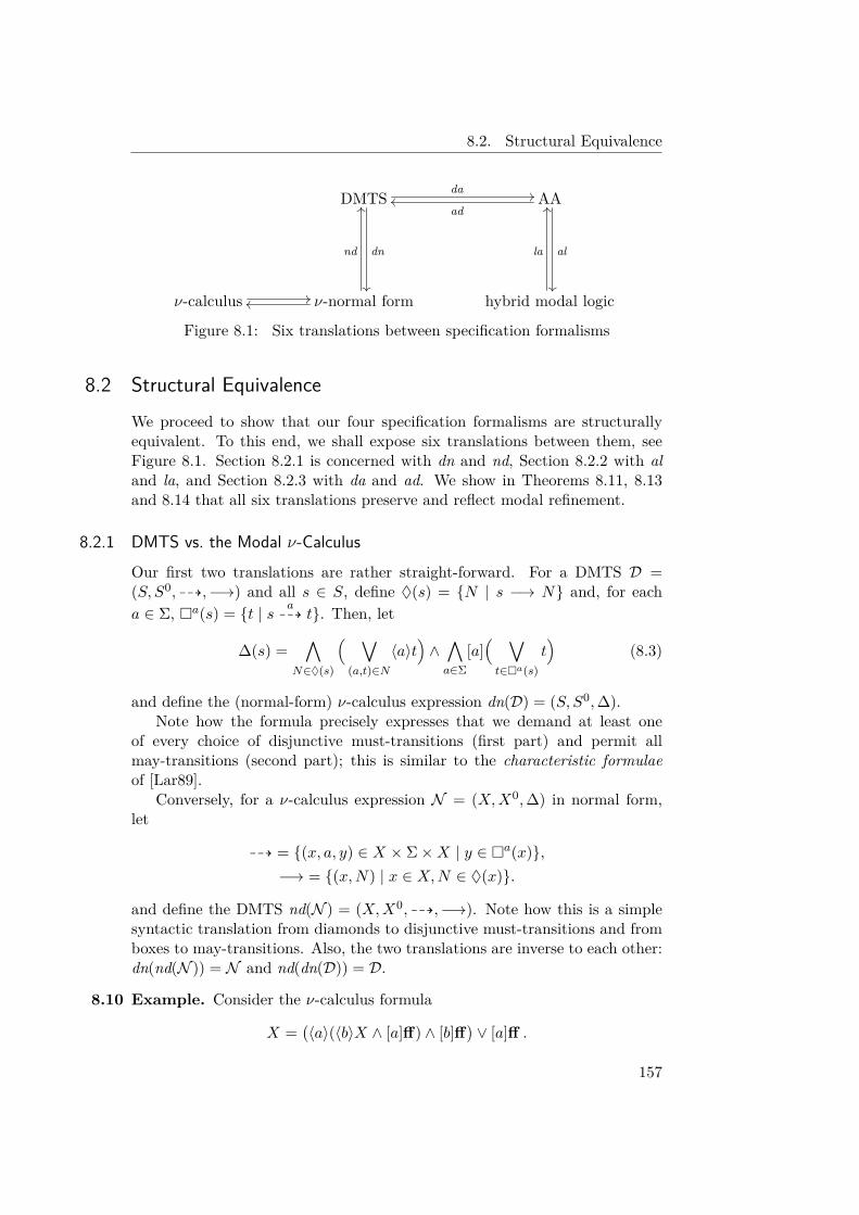
8.2. Structural Equivalence

DMTS da //

dn

��

AAad

oo

al

��

ν-calculus // ν-normal formoo

nd

OO

hybrid modal logic

la

OO

Figure 8.1: Six translations between specification formalisms

8.2 Structural EquivalenceWe proceed to show that our four specification formalisms are structurallyequivalent. To this end, we shall expose six translations between them, seeFigure 8.1. Section 8.2.1 is concerned with dn and nd, Section 8.2.2 with aland la, and Section 8.2.3 with da and ad. We show in Theorems 8.11, 8.13and 8.14 that all six translations preserve and reflect modal refinement.

8.2.1 DMTS vs. the Modal ν-CalculusOur first two translations are rather straight-forward. For a DMTS D =(S, S0, 99K,−→) and all s ∈ S, define ♦(s) = {N | s −→ N} and, for eacha ∈ Σ, �a(s) = {t | s a

99K t}. Then, let

∆(s) =∧

N∈♦(s)

( ∨(a,t)∈N

〈a〉t)∧∧a∈Σ

[a]( ∨t∈�a(s)

t)

(8.3)

and define the (normal-form) ν-calculus expression dn(D) = (S, S0,∆).Note how the formula precisely expresses that we demand at least one

of every choice of disjunctive must-transitions (first part) and permit allmay-transitions (second part); this is similar to the characteristic formulaeof [Lar89].

Conversely, for a ν-calculus expression N = (X,X0,∆) in normal form,let

99K = {(x, a, y) ∈ X × Σ×X | y ∈ �a(x)},−→ = {(x,N) | x ∈ X,N ∈ ♦(x)}.

and define the DMTS nd(N ) = (X,X0, 99K,−→). Note how this is a simplesyntactic translation from diamonds to disjunctive must-transitions and fromboxes to may-transitions. Also, the two translations are inverse to each other:dn(nd(N )) = N and nd(dn(D)) = D.

8.10 Example. Consider the ν-calculus formula

X =(〈a〉(〈b〉X ∧ [a]ff) ∧ [b]ff

)∨ [a]ff .

157

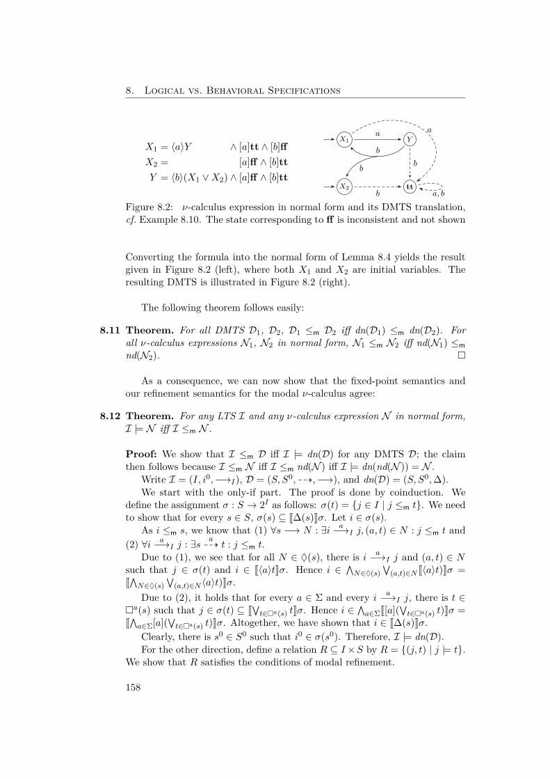
8. Logical vs. Behavioral Specifications

X1 = 〈a〉Y ∧ [a]tt ∧ [b]ffX2 = [a]ff ∧ [b]ttY = 〈b〉(X1 ∨X2) ∧ [a]ff ∧ [b]tt

X1

ttX2

Y

aa

b

b

b

b

a, b

Figure 8.2: ν-calculus expression in normal form and its DMTS translation,cf. Example 8.10. The state corresponding to ff is inconsistent and not shown

Converting the formula into the normal form of Lemma 8.4 yields the resultgiven in Figure 8.2 (left), where both X1 and X2 are initial variables. Theresulting DMTS is illustrated in Figure 8.2 (right).

The following theorem follows easily:

8.11 Theorem. For all DMTS D1, D2, D1 ≤m D2 iff dn(D1) ≤m dn(D2). Forall ν-calculus expressions N1, N2 in normal form, N1 ≤m N2 iff nd(N1) ≤mnd(N2). �

As a consequence, we can now show that the fixed-point semantics andour refinement semantics for the modal ν-calculus agree:

8.12 Theorem. For any LTS I and any ν-calculus expression N in normal form,I |= N iff I ≤m N .

Proof: We show that I ≤m D iff I |= dn(D) for any DMTS D; the claimthen follows because I ≤m N iff I ≤m nd(N ) iff I |= dn(nd(N )) = N .

Write I = (I, i0,−→I), D = (S, S0, 99K,−→), and dn(D) = (S, S0,∆).We start with the only-if part. The proof is done by coinduction. We

define the assignment σ : S → 2I as follows: σ(t) = {j ∈ I | j ≤m t}. We needto show that for every s ∈ S, σ(s) ⊆ J∆(s)Kσ. Let i ∈ σ(s).

As i ≤m s, we know that (1) ∀s −→ N : ∃i a−→I j, (a, t) ∈ N : j ≤m t and(2) ∀i a−→I j : ∃s a

99K t : j ≤m t.Due to (1), we see that for all N ∈ ♦(s), there is i a−→I j and (a, t) ∈ N

such that j ∈ σ(t) and i ∈ J〈a〉tKσ. Hence i ∈ ∧N∈♦(s)∨

(a,t)∈N J〈a〉t)Kσ =J∧N∈♦(s)

∨(a,t)∈N 〈a〉t)Kσ.

Due to (2), it holds that for every a ∈ Σ and every i a−→I j, there is t ∈�a(s) such that j ∈ σ(t) ⊆ J

∨t∈�a(s) tKσ. Hence i ∈ ∧a∈ΣJ[a](∨t∈�a(s) t)Kσ =

J∧a∈Σ[a](∨t∈�a(s) t)Kσ. Altogether, we have shown that i ∈ J∆(s)Kσ.Clearly, there is s0 ∈ S0 such that i0 ∈ σ(s0). Therefore, I |= dn(D).For the other direction, define a relation R ⊆ I×S by R = {(j, t) | j |= t}.

We show that R satisfies the conditions of modal refinement.

158

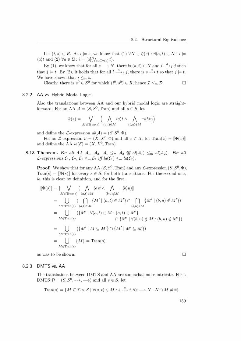
8.2. Structural Equivalence

Let (i, s) ∈ R. As i |= s, we know that (1) ∀N ∈ ♦(s) : ∃(a, t) ∈ N : i |=〈a〉t and (2) ∀a ∈ Σ : i |= [a](∨t∈�a(s) t).

By (1), we know that for all s −→ N , there is (a, t) ∈ N and i a−→I j suchthat j |= t. By (2), it holds that for all i a−→I j, there is s a

99K t so that j |= t.We have shown that i ≤m s.

Clearly, there is s0 ∈ S0 for which (i0, s0) ∈ R, hence I ≤m D. �

8.2.2 AA vs. Hybrid Modal LogicAlso the translations between AA and our hybrid modal logic are straight-forward. For an AA A = (S, S0,Tran) and all s ∈ S, let

Φ(s) =∨

M∈Tran(s)

( ∧(a,t)∈M

〈a〉t ∧∧

(b,u)/∈M¬〈b〉u

)and define the L-expression al(A) = (S, S0,Φ).

For an L-expression E = (X,X0,Φ) and all x ∈ X, let Tran(x) = JΦ(x)Kand define the AA la(E) = (X,X0,Tran).

8.13 Theorem. For all AA A1, A2, A1 ≤m A2 iff al(A1) ≤m al(A2). For allL-expressions E1, E2, E1 ≤m E2 iff la(E1) ≤m la(E2).

Proof: We show that for any AA (S, S0,Tran) and any L-expression (S, S0,Φ),Tran(s) = JΦ(s)K for every s ∈ S, for both translations. For the second one,la, this is clear by definition, and for the first,

JΦ(s)K = J∨

M∈Tran(s)

( ∧(a,t)∈M

〈a〉t ∧∧

(b,u)/∈M¬〈b〉u

)K

=⋃

M∈Tran(s)

( ⋂(a,t)∈M

{M ′ | (a, t) ∈M ′} ∩⋂

(b,u)/∈M{M ′ | (b, u) /∈M ′}

)=

⋃M∈Tran(s)

({M ′ | ∀(a, t) ∈M : (a, t) ∈M ′}

∩ {M ′ | ∀(b, u) /∈M : (b, u) /∈M ′})

=⋃

M∈Tran(s)

({M ′ |M ⊆M ′} ∩ {M ′ |M ′ ⊆M}

)=

⋃M∈Tran(s)

{M} = Tran(s)

as was to be shown. �

8.2.3 DMTS vs. AAThe translations between DMTS and AA are somewhat more intricate. For aDMTS D = (S, S0, 99K,−→) and all s ∈ S, let

Tran(s) = {M ⊆ Σ× S | ∀(a, t) ∈M : s a99K t,∀s −→ N : N ∩M 6= ∅}

159

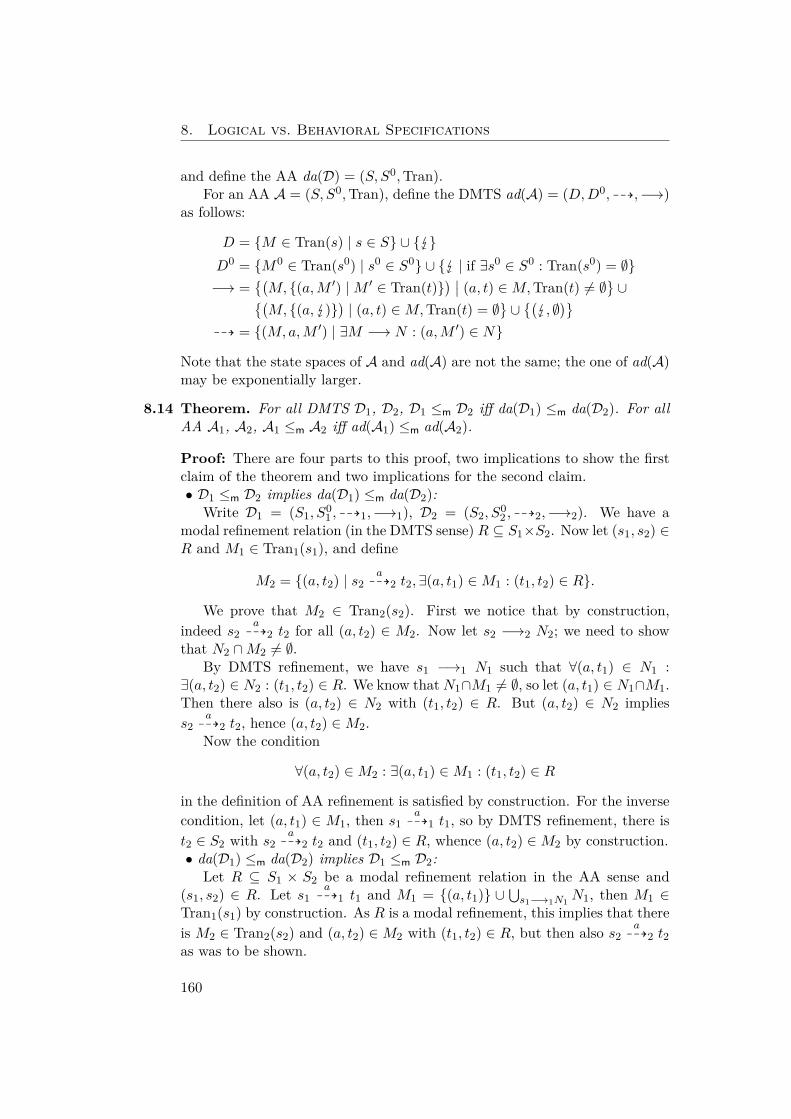
8. Logical vs. Behavioral Specifications

and define the AA da(D) = (S, S0,Tran).For an AA A = (S, S0,Tran), define the DMTS ad(A) = (D,D0, 99K,−→)

as follows:

D = {M ∈ Tran(s) | s ∈ S} ∪ { }D0 = {M0 ∈ Tran(s0) | s0 ∈ S0} ∪ { | if ∃s0 ∈ S0 : Tran(s0) = ∅}−→ =

{(M, {(a,M ′) |M ′ ∈ Tran(t)}

) ∣∣ (a, t) ∈M,Tran(t) 6= ∅}∪{(

M, {(a, )})| (a, t) ∈M,Tran(t) = ∅

}∪{( , ∅

)}99K = {(M,a,M ′) | ∃M −→ N : (a,M ′) ∈ N}

Note that the state spaces of A and ad(A) are not the same; the one of ad(A)may be exponentially larger.

8.14 Theorem. For all DMTS D1, D2, D1 ≤m D2 iff da(D1) ≤m da(D2). For allAA A1, A2, A1 ≤m A2 iff ad(A1) ≤m ad(A2).

Proof: There are four parts to this proof, two implications to show the firstclaim of the theorem and two implications for the second claim.• D1 ≤m D2 implies da(D1) ≤m da(D2):

Write D1 = (S1, S01 , 99K1,−→1), D2 = (S2, S

02 , 99K2,−→2). We have a

modal refinement relation (in the DMTS sense) R ⊆ S1×S2. Now let (s1, s2) ∈R and M1 ∈ Tran1(s1), and define

M2 = {(a, t2) | s2a99K2 t2,∃(a, t1) ∈M1 : (t1, t2) ∈ R}.

We prove that M2 ∈ Tran2(s2). First we notice that by construction,indeed s2

a99K2 t2 for all (a, t2) ∈ M2. Now let s2 −→2 N2; we need to show

that N2 ∩M2 6= ∅.By DMTS refinement, we have s1 −→1 N1 such that ∀(a, t1) ∈ N1 :

∃(a, t2) ∈ N2 : (t1, t2) ∈ R. We know thatN1∩M1 6= ∅, so let (a, t1) ∈ N1∩M1.Then there also is (a, t2) ∈ N2 with (t1, t2) ∈ R. But (a, t2) ∈ N2 impliess2

a99K2 t2, hence (a, t2) ∈M2.Now the condition

∀(a, t2) ∈M2 : ∃(a, t1) ∈M1 : (t1, t2) ∈ R

in the definition of AA refinement is satisfied by construction. For the inversecondition, let (a, t1) ∈ M1, then s1

a99K1 t1, so by DMTS refinement, there is

t2 ∈ S2 with s2a99K2 t2 and (t1, t2) ∈ R, whence (a, t2) ∈M2 by construction.

• da(D1) ≤m da(D2) implies D1 ≤m D2:Let R ⊆ S1 × S2 be a modal refinement relation in the AA sense and

(s1, s2) ∈ R. Let s1a99K1 t1 and M1 = {(a, t1)} ∪ ⋃s1−→1N1 N1, then M1 ∈

Tran1(s1) by construction. As R is a modal refinement, this implies that thereis M2 ∈ Tran2(s2) and (a, t2) ∈M2 with (t1, t2) ∈ R, but then also s2

a99K2 t2

as was to be shown.

160

8.2. Structural Equivalence

Let s2 −→2 N2 and assume, for the sake of contradiction, that there is nos1 −→1 N1 for which ∀(a, t1) ∈ N1 : ∃(a, t2) ∈ N2 : (t1, t2) ∈ R holds. Thenfor each s1 −→1 N1, there is an element (aN1 , tN1) ∈ N1 for which there is no(aN1 , t2) ∈ N2 with (tN1 , t2) ∈ R.

LetM1 = {(aN1 , tN1) | s1 −→1 N1}, thenM1 ∈ Tran1(s1) by construction.Hence we have M2 ∈ Tran2(s2) satisfying the conditions in the definition ofAA refinement. By construction of Tran2(s2), s2 −→2 N2 and N2 ∩M2 6= ∅,so let (a, t2) ∈ N2 ∩M2. Then there exists (a, t1) ∈M1 for which (t1, t2) ∈ R,in contradiction to the definition of M1.• A1 ≤m A2 implies ad(A1) ≤m ad(A2):

Write A1 = (S1, S01 ,Tran1), A2 = (S2, S

02 ,Tran2), with DMTS transla-

tions (D1, D01,−→1, 99K1), (D2, D

02,−→2, 99K2). We have a modal refinement

relation (in the AA sense) R ⊆ S1 × S2. Define R′ ⊆ D1 ×D2 by

R′ = {( ,M2) |M2 ∈ D2}∪ {(M1,M2) | ∃(s1, s2) ∈ R : M1 ∈ Tran1(s1),M2 ∈ Tran(s2),

∀(a, t1) ∈M1 : ∃(a, t2) ∈M2 : (t1, t2) ∈ R,∀(a, t2) ∈M2 : ∃(a, t1) ∈M1 : (t1, t2) ∈ R}.

We show that R′ is a modal refinement in the DMTS sense. Let (M1,M2) ∈ R′.If M1 = then R′ trivially satisfies the modal refinement conditions as

there is no a99K transition and every M2 −→ N2 is matched by −→ ∅. Let

us henceforth assume that M1 6= .Let M2 −→2 {(a, )}. By construction of −→2, there is (a, t2) ∈ M2 with

Tran2(t2) = ∅. Then (M1,M2) ∈ R′ implies that there must be (a, t1) ∈ M1for which (t1, t2) ∈ R. As R is a AA refinement, this means that Tran1(t1) = ∅and thusM1 −→1 {(a, )}. Clearly, (a, ) is matched by (a, ) and ( , ) ∈ R′.

Let M2 −→2 N2 6= {(a, )}. By construction of −→2, there is (a, t2) ∈M2such that N2 = {(a,M ′2) |M ′2 ∈ Tran2(t2)} 6= ∅. Then (M1,M2) ∈ R′ impliesthat there must be (a, t1) ∈M1 for which (t1, t2) ∈ R.

If Tran1(t1) = ∅, we know that M1 −→1 {(a, )}. We can then match(a, ) with arbitrary (a,M ′2) ∈ N2 as ( ,M ′2) ∈ R′.

If Tran1(t1) 6= ∅, we can define N1 = {(a,M ′1) | M ′1 ∈ Tran1(t1)}, whenceM1 −→1 N1. We show that ∀(a,M ′1) ∈ N1 : ∃(a,M ′2) ∈ N2 : (M ′1,M ′2) ∈ R′.Let (a,M ′1) ∈ N1, then M ′1 ∈ Tran1(t1). From (t1, t2) ∈ R we hence get M ′2 ∈Tran2(t2), and then (a,M ′2) ∈ N2 by construction of N2 and (M ′1,M ′2) ∈ R′due to the conditions of AA refinement (applied to (t1, t2) ∈ R).

Let M1a99K1 . We then have M1 −→ {(a, )} which means that there is

(a, t1) ∈M1 with Tran1(t1) = ∅. By (M1,M2) ∈ R′ we get (a, t2) ∈M2, henceM2 −→2 N2 with some (a,M ′2) ∈ N2 and M2

a99K M ′2. By definition of R′,

( ,M ′2) ∈ R′.Let M1

a99K1 M ′1 6= , then we have M1 −→1 N1 for which (a,M ′1) ∈ N1

and by construction of 99K1. This in turn implies that there must be (a, t1) ∈

161

8. Logical vs. Behavioral Specifications

M1 such that N1 = {(a,M ′′1 ) |M ′′1 ∈ Tran1(t1)} 6= ∅, and then by (M1,M2) ∈R′, we get (a, t2) ∈ M2 for which (t1, t2) ∈ R. Due to the conditions ofAA refinement, Tran2(t2) 6= ∅. Let N2 = {(a,M ′2) | M ′2 ∈ Tran2(t2)}, thenM2 −→2 N2 and hence M2

a99K2 M ′2 for all (a,M ′2) ∈ N2. Furthermore, the

argument above shows that there is (a,M ′2) ∈ N2 for which (M ′1,M ′2) ∈ R′.We miss to show that R′ is initialised. If ∈ D0

1, then ( ,M02 ) ∈ R′ for

any M02 ∈ D0

2. If 6= M01 ∈ D0

1, then we have s01 ∈ S0

1 with M01 ∈ Tran1(s0

1).As R is initialised, this entails that there is s0

2 ∈ S02 with (s0

1, s02) ∈ R, which

gives usM02 ∈ Tran2(s0

2) which satisfies the AA refinement conditions, whence(M0

1 ,M02 ) ∈ R′.

• ad(A1) ≤m ad(A2) implies A1 ≤m A2:Let R ⊆ D1 ×D2 be a modal refinement relation in the DMTS sense and

define R′ ⊆ S1 × S2 by

R′ = {(s1, s2) | ∀M1 ∈ Tran1(s1) : ∃M2 ∈ Tran2(s2) : (M1,M2) ∈ R} ;

we will show that R′ is an AA modal refinement.Observe first that (M1, ) ∈ R implies M1 = as is the only state in

D1 that has a must transition −→1 ∅. We shall occasionally refer to thisobservation in the following.

Let (s1, s2) ∈ R′ and M1 ∈ Tran1(s1), then by construction of R′, we haveM2 ∈ Tran2(s2) with (M1,M2) ∈ R.

Let (a, t2) ∈M2; we need to find (a, t1) ∈M1 such that (t1, t2) ∈ R′.If Tran2(t2) = ∅, then M2 −→2 {(a, )}. From (M1,M2) ∈ R we get

M1 −→1 N1 such that all (a,M ′1) ∈ N1 are matched by (a, ) with (M ′1, ) ∈R. By the observation above, this means that M ′1 = and thus N1 = {(a, )}due to the construction. This means that there exists (a, t1) ∈ M1 withTran1(t1) = ∅. Hence (t1, t2) ∈ R′.

If Tran2(t2) 6= ∅, define N2 = {(a,M ′2) | M ′2 ∈ Tran2(t2)}, then M2 −→2N2. Now (M1,M2) ∈ R implies that there must be M1 −→1 N1 satisfying∀(a,M ′1) ∈ N1 : ∃(a,M ′2) ∈ N2 : (M ′1,M ′2) ∈ R. If N1 = {(a, )}, we have(a, t1) ∈M1 with Tran1(t1) = ∅ and thus trivially (t1, t2) ∈ R′. Otherwise, wehave (a, t1) ∈M1 such that N1 = {(a,M ′1) |M ′1 ∈ Tran1(t1)}; we only miss toshow that (t1, t2) ∈ R′.

Let M ′1 ∈ Tran1(t1), then (a,M ′1) ∈ N1, hence there is (a,M ′2) ∈ N2with (M ′1,M ′2) ∈ R, but (a,M ′2) ∈ N2 also entails M ′2 ∈ Tran2(t2); thus(t1, t2) ∈ R′.

Let now (a, t1) ∈M1; we need to find (a, t2) ∈M2 such that (t1, t2) ∈ R′.If Tran1(t1) = ∅, then M1 −→1 {(a, )} and M1

a99K . By modal refine-

ment, we have M2a99KM ′2 with ( ,M ′2) ∈ R. In any case (whether M ′2 = or

not), this means that there exists some (a, t2) ∈M2 and trivially (t1, t2) ∈ R′.In case Tran1(t1) 6= ∅, define N1 = {(a,M ′1) | M ′1 ∈ Tran1(t1)}, then

N1 6= ∅ and M1 −→1 N1. Now let (a,M ′1) ∈ N1, then M1a99K1 M ′1, hence

we have M2a99K2 M ′2 for some (M ′1,M ′2) ∈ R by modal refinement. Note that

162

8.2. Structural Equivalence

M ′1 6= implies M ′2 6= due to the observation above. By construction of99K2, this implies that there is M2 −→2 N2 with (a,M ′2) ∈ N2, and we have(a, t2) ∈ M2 for which N2 = {(a,M ′′2 ) | M ′′2 ∈ Tran2(t2)}. We show that(t1, t2) ∈ R′.

Let M ′′1 ∈ Tran1(t1), then (a,M ′′1 ) ∈ N1, thus M1a99K1 M ′′1 , so that

there is M2a99K2 M ′′2 with (M ′′1 ,M ′′2 ) ∈ R. By construction of 99K2, there is

M2 −→2 N′2 with (a,M ′′2 ) ∈ N ′2, hence also M ′′2 ∈ Tran2(t2).

We miss to show that R′ is initialised. Let s01 ∈ S0

1 ; if Tran1(s01) = ∅,

then trivially (s01, s

02) ∈ R′ for any s0

2 ∈ S02 . If Tran1(s0

1) 6= ∅, then there isM0

1 ∈ Tran1(s01). As R is initialised, this gets usM0

2 ∈ D2 with (M01 ,M

02 ) ∈ R,

but M02 ∈ Tran2(s0

2) for some s02 ∈ S0

2 , and then (s01, s

02) ∈ R′. �

8.15 Corollary. For all DMTS D, ν-calculus expressions N , AA A, and L-ex-pressions E, dn(D) ≡t da(D) ≡t D, nd(N ) ≡t N , ad(A) ≡t al(A) ≡t A, andla(E) ≡t E. �

8.2.4 Translation ComplexityWe have shown that our four specification formalisms are structurally equiv-alent, which will be useful for us from a theoretical point of view. From apractical point of view however, some of the translations may incur expo-nential blow-ups, hence care has to be taken. On the other hand, all ourtranslations can be implemented in an on-the-fly manner, only creating stateswhen necessary.

We already noticed that the translation of ν-calculus expressions into nor-mal form may incur an exponential blow-up, so this also affects our translationfrom the modal ν-calculus to DMTS. When considering only normal-form ex-pressions, the translations to and from DMTS incur no blow-ups.

When translating from AA to our hybrid modal logic, we see that, dueto the complementation (b, u) /∈M , the length of a formula Φ(s) is quadraticin the representation of Tran(s). For the reverse translation, the number ofTran constraints can be exponential in the number of states. The worst caseis Φ(s) = tt, which gets translated to Tran(s) = 22Σ×S .

8.16 Remark. There is a direct translation from DMTS to hybrid modal logic:for a DMTS D = (S, S0, 99K,−→), define dl(D) = (S, S0,Φ) with

Φ(s) =∧

s−→N

∨(a,t)∈N

〈a〉t ∧∧s 6a99Ku

¬〈a〉u

for all s ∈ S. This translation is again quadratic, and da(D) = la(dl(D)).

The translations between DMTS and AA may involve exponential blow-ups both ways. For the first translation, we can see this by considering the one-state DMTS ({s}, {s}, 99K,−→) with 99K = {(s, a, s) | a ∈ Σ} and −→ = ∅.Then Tran(s) = 22Σ×S .

163

8. Logical vs. Behavioral Specifications

The fact that also the translation from AA to DMTS may be exponential inspace is evident from the definition. To see that this blow-up is unavoidable,we expose a special property of the Tran-sets arising in the DMTS-to-AAtranslation.

8.17 Lemma. Let D = (S, S0, 99K,−→) be a DMTS and s ∈ S. For all M1,M2 ∈Tran(s) and all M ⊆ Σ× S with M1 ⊆M ⊆M1 ∪M2, also M ∈ Tran(s).

Proof: For i = 1, 2, since Mi ∈ Tran(s), we know that

• for all (a, t) ∈Mi, sa99K t, and

• for all s −→ N , there is (a, t) ∈Mi ∩N .

Now as M ⊆ M1 ∪M2, it directly follows that for all (a, t) ∈ M , we haves

a99K t. Moreover, since M1 ⊆ M , we also have that for all s −→ N , there

exists (a, t) ∈M ∩N . As a consequence, M ∈ Tran(s). �

Using this, we can show the following.

8.18 Proposition. There exists a one-state AA A for which any DMTS D ≡t Ahas at least 2n−1 states, where n is the size of the alphabet Σ.

Proof: Let Σ = {a1, . . . , an} andA = ({s0}, {s0},Tran) the AA with Tran(s0) ={M ⊆ Σ × {s0} | ∃k : |M | = 2k} the transition constraint containing all dis-junctive choices of even cardinality. Let D = (T, T 0, 99K,−→) be a DMTSwith D ≡t A; we claim that D must have at least 2n−1 initial states.

Assume, for the purpose of contradiction, that T 0 = {t01, . . . , t0m} withm <2n−1. AsD ≡t A, we must have⋃mi=1 Tran(t0i ) = {M ⊆ Σ×T | ∃k : |M | = 2k},so that there is an index j ∈ {1, . . . ,m} for which Tran(t0j ) = {M1,M2}contains two different disjunctive choices from Tran(s0). By Lemma 8.17,also M ∈ Tran(t0j ) for any M with M1 ⊆ M ⊆ M1 ∪M2. But M1 ∪M2 hasgreater cardinality than M1, so that there will be an M ∈ Tran(t0j ) with oddcardinality. �

Figure 8.3 sums up the translation complexities.

8.2.5 Initial StatesWe finish this section with a justification for why we allow our specificationsto have several (or possibly zero) initial states. The first lemma shows thatfor AA, and up to thorough refinement, this is inessential; due to their closerelationship, this also holds for L-expressions.

8.19 Lemma. For any AA A1, there is an AA A2 = (S2, S02 ,Tran2) with S0

2 = {s02}

a singleton and A1 ≡t A2.

164

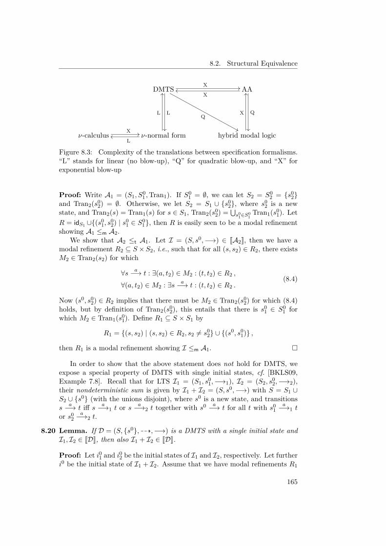
8.2. Structural Equivalence

DMTS X //

L

��

Q

&&

AAX

oo

Q

��

ν-calculus X // ν-normal formL

oo

L

OO

hybrid modal logic

X

OO

Figure 8.3: Complexity of the translations between specification formalisms.“L” stands for linear (no blow-up), “Q” for quadratic blow-up, and “X” forexponential blow-up

Proof: Write A1 = (S1, S01 ,Tran1). If S0

1 = ∅, we can let S2 = S02 = {s0

2}and Tran2(s0

2) = ∅. Otherwise, we let S2 = S1 ∪ {s02}, where s0

2 is a newstate, and Tran2(s) = Tran1(s) for s ∈ S1, Tran2(s0

2) = ⋃s01∈S

01Tran1(s0

1). LetR = idS1 ∪{(s0

1, s02) | s0

1 ∈ S01}, then R is easily seen to be a modal refinement

showing A1 ≤m A2.We show that A2 ≤t A1. Let I = (S, s0,−→) ∈ JA2K, then we have a

modal refinement R2 ⊆ S ×S2, i.e., such that for all (s, s2) ∈ R2, there existsM2 ∈ Tran2(s2) for which

∀s a−→ t : ∃(a, t2) ∈M2 : (t, t2) ∈ R2 ,

∀(a, t2) ∈M2 : ∃s a−→ t : (t, t2) ∈ R2 .(8.4)

Now (s0, s02) ∈ R2 implies that there must be M2 ∈ Tran2(s0

2) for which (8.4)holds, but by definition of Tran2(s0

2), this entails that there is s01 ∈ S0

1 forwhich M2 ∈ Tran1(s0

1). Define R1 ⊆ S × S1 by

R1 = {(s, s2) | (s, s2) ∈ R2, s2 6= s02} ∪ {(s0, s0

1)} ,

then R1 is a modal refinement showing I ≤m A1. �

In order to show that the above statement does not hold for DMTS, weexpose a special property of DMTS with single initial states, cf. [BKLS09,Example 7.8]. Recall that for LTS I1 = (S1, s

01,−→1), I2 = (S2, s

02,−→2),

their nondeterministic sum is given by I1 + I2 = (S, s0,−→) with S = S1 ∪S2 ∪ {s0} (with the unions disjoint), where s0 is a new state, and transitionss

a−→ t iff sa−→1 t or s a−→2 t together with s0 a−→ t for all t with s0

1a−→1 t

or s02

a−→2 t.

8.20 Lemma. If D = (S, {s0}, 99K,−→) is a DMTS with a single initial state andI1, I2 ∈ JDK, then also I1 + I2 ∈ JDK.

Proof: Let i01 and i02 be the initial states of I1 and I2, respectively. Let furtheri0 be the initial state of I1 + I2. Assume that we have modal refinements R1

165

8. Logical vs. Behavioral Specifications

D

a

b

I1

a

I2

b

Figure 8.4: DMTS D with two initial states and its two implementations I1,I2

and R2 such that (i01, s0) ∈ R1 and (i02, s0) ∈ R2. Let R = R1 ∪R2 ∪{(i0, s0)}.Clearly, R is a modal refinement witnessing I1 + I2 ≤m D.

Now let D be the DMTS, with two initial states, depicted in Figure 8.4,then JDK = {I1, I2} as also seen in Figure 8.4, but I1 + I2 /∈ JDK. Hence D isnot thoroughly equivalent to any DMTS with a single initial state.

Applying the construction from the proof of Lemma 8.19 to the AA gen-erated by the DMTS in Figure 8.4 gives an AA A2 = (S2, {s0

2},Tran2) withTran2(s0

2) = {{(a, s1)}, {(b, t1)}} (where s1 and t1 are the target states of thea and b transitions in D, respectively). This specifies an exclusive disjunction:one of a and b has to be implemented, but not both. This also serves to showthat Lemma 8.20 does not hold for AA.

8.21 Corollary. There is a DMTS D1 for which there is no DMTS D2 = (S2, S02 ,

99K,−→) with S02 = {s0

2} a singleton and D1 ≡t D2. �

Due to their close relationship with DMTS, this property also holds for ν-calculus expressions in normal form: there exist ν-calculus expressions whichare not equivalent to any normal-form ν-calculus expression with a single ini-tial variable. (Of course, omitting “normal form” would make this statementinvalid; as disjunction is part of the syntax, any ν-calculus expression is thor-oughly equivalent to one with only one initial variable.)

We also remark that the above argument can easily be extended to showthat for any k ∈ N, there exists a DMTS with k+ 1 initial states which is notthoroughly equivalent to any DMTS with at most k initial states.

Using again the example in Figure 8.4, we can also show that the statementin Lemma 8.19 does not hold when thorough equivalence is replaced by modalequivalence. Let A1 = da(D), with initial states s0 and t0, be the AA transla-tion of the DMTS in Figure 8.4 and assume that there exists an AA A2 withsingle initial state s0

2 for which A2 ≤m A1. Then there is a modal refinementR with (s0

2, s0), (s0

2, t0) ∈ R. Let M2 ∈ Tran2(s0

2), then by (s02, s

0) ∈ R, theremust be some (a, t2) ∈M2 with (t2, s1) ∈ R. By (s0

2, t0) ∈ R, this implies that

there must be (a, t1) ∈ Tran1(t0), a contradiction.

166

8.3. Specification Theory

8.3 Specification TheoryBehavioral specifications typically come equipped with operations which al-low for compositional reasoning, viz. conjunction, composition and quotient,cf. [BDH+12]. On deterministic MTS, these operations can be given easilyusing simple structural operational rules. For non-deterministic systems thisis significantly harder.

We remark that composition and quotient operators are well-known fromsome logics, such as, e.g., linear [Gir87] or spatial logic [CC03], and were ex-tended to quite general contexts [CLM11]. However, whereas these operatorsare part of the formal syntax in those logics, for us they are simply opera-tions on logical expressions (or DMTS, or AA). Consequently, composition isgenerally only a sound over-approximation of the semantic composition.

Given the structural equivalence of DMTS, the modal ν-calculus, AA, andour hybrid modal logic exposed in the previous section, it suffices to introducethe operations for one of the four types of specifications. On the other hand,we will often state properties for all four types of specifications at the sametime, letting S stand for a specification of any type.

8.3.1 Disjunction and ConjunctionDisjunction of specifications is easily defined as we allow multiple initial states.For DMTS D1 = (S1, S

01 , 99K1,−→1), D2 = (S2, S

02 , 99K2,−→2), we can hence

define D1 ∨D2 = (S1 ∪ S2, S01 ∪ S0

2 , 99K1 ∪ 99K2,−→1 ∪−→2) (with all unionsdisjoint). Similar definitions are available for the other types of specifications,and disjunction commutes with the translations.

Conjunction for DMTS is an extension of the construction from [BCK11]for multiple initial states. Given two DMTS D1 = (S1, S

01 , 99K1,−→1), D2 =

(S2, S02 , 99K2,−→2), we define D1 ∧ D2 = (S, S0, 99K,−→) with S = S1 × S2,

S0 = S01 × S0

2 , and

• (s1, s2) a99K (t1, t2) iff s1

a99K1 t1 and s2

a99K2 t2,

• for all s1 −→1 N1, (s1, s2) −→ {(a, (t1, t2)) | (a, t1) ∈ N1, s2a99K2 t2},

• for all s2 −→2 N2, (s1, s2) −→ {(a, (t1, t2)) | (a, t2) ∈ N2, s1a99K1 t1}.

For AA, conjunction can be defined using auxiliary projection functionsπi : 2Σ×S1×S2 → 2Σ×Si given by

π1(M) ={(a, s1) | ∃s2 ∈ S2 : (a, s1, s2) ∈M} ,π2(M) ={(a, s2) | ∃s1 ∈ S1 : (a, s1, s2) ∈M} .

Then for AA A1 = (S1, S01 ,Tran1), A2 = (S2, S

02 ,Tran2), we let A1 ∧ A2 =

(S, S0,Tran), with S = S1 × S2, S0 = S01 × S0

2 and Tran((s1, s2)) = {M ⊆Σ× S | π1(M) ∈ Tran1(s1), π2(M) ∈ Tran2(s2)}.

167

8. Logical vs. Behavioral Specifications

We can also define conjunction for L-expressions, using similar auxiliarymappings on formulae. For sets X1, X2 and i ∈ {1, 2}, we define ρi : L(Xi)→L(X1 ×X2) inductively, by

• ρi(tt) = tt, ρi(ff) = ff , ρi(¬φ) = ¬ρi(φ), ρi(φi ∧ φ2) = ρi(φi) ∧ ρi(φ2),

• ρ1(〈a〉x1) = ∨x2∈X2〈a〉(x1, x2),

• ρ2(〈a〉x2) = ∨x1∈X1〈a〉(x1, x2).

Then, for L-expressions E1 = (X1, X01 ,Φ1), E2 = (X2, X

02 ,Φ2), we let E1∧E2 =

(X1 ×X2, X01 ×X0

2 ,Φ) with Φ((x1, x2)) = ρ1(Φ1(x1)) ∧ ρ2(Φ2(x2)).

8.22 Lemma. For all DMTS D1, D2, AA A1, A2, and L-expressions E1, E2,da(D1∧D2) = da(D1)∧da(D2), al(A1∧A2) = al(A1)∧al(A2), and la(E1∧E2) =la(E1) ∧ la(E2).

Note that above makes no statement about the ad translation; due to thechange of state space during the translation, equality does not hold here.

Proof: The last two claims follow easily once one notices that for i ∈ {1, 2}and all M , M |= ρi(φ) iff πi(M) |= φ. To show the first claim, let D1 =(S1, S

01 , 99K1,−→1) and D2 = (S2, S

02 , 99K2,−→2) be DMTS, with AA trans-

lations da(D1) = (S1, S01 ,Tran1) and da(D2) = (S2, S

02 ,Tran2). Write A∧ =

da(D1 ∧ D2) and A∧ = da(D1) ∧ da(D2); we show that A∧ = A∧.First, remark that A∧ and A∧ have precisely the same state space S1×S2

and initial states S01 × S0

2 . We now show that they have the same transitionconstraints. Let Tran∧ (resp. Tran∧) be the transition constraints mapping ofA∧ (resp. A∧). Let (s1, s2) ∈ S1 × S2 and M ∈ Tran∧(s1, s2).

By construction of Tran∧, there must be M1 ∈ Tran1(s1) and M2 ∈Tran2(s2) such that π1(M) = M1 and π2(M) = M2. We show that M ∈Tran∧(s1, s2). Let (a, (t1, t2)) ∈M . Since π1(M) = M1 and π2(M) = M2, wehave (a, t1) ∈ M1 and (a, t2) ∈ M2. As a consequence, there are transitionss1

a99K t1 and s2

a99K t2 in D1 and D2, respectively. Thus, by construction,

there is a transition (s1, s2) a99K (t1, t2) in D1 ∧ D2.

Let (s1, s2) −→ N in D1 ∧ D2. By construction, N is such that either (1)there exists N1 such that s1 −→ N1 in D1 and N = {(a, (t1, t2)) | (a, t1) ∈N1, (s1, s2) a

99K (t1, t2)}, or (2) there exists N2 such that s2 −→ N2 in D2 andN = {(a, (t1, t2)) | (a, t2) ∈ N2, (s1, s2) a

99K (t1, t2)}. Assume that (1) holds(case (2) being symmetric). Since M1 ∈ Tran1(s1), there must be (a, t1) ∈N1 ∩M1. As π1(M) = M1, there must be t2 ∈ S2 such that (a, (t1, t2)) ∈M .As a consequence, there is (a, (t1, t2)) ∈M ∩N .

We have shown that M ∈ Tran∧(s1, s2). Similarly, we can show that forall M ∈ Tran∧(s1, s2), we also have M ∈ Tran∧(s1, s2). We can thus concludethat Tran∧ = Tran∧, hence A∧ = A∧. �

168

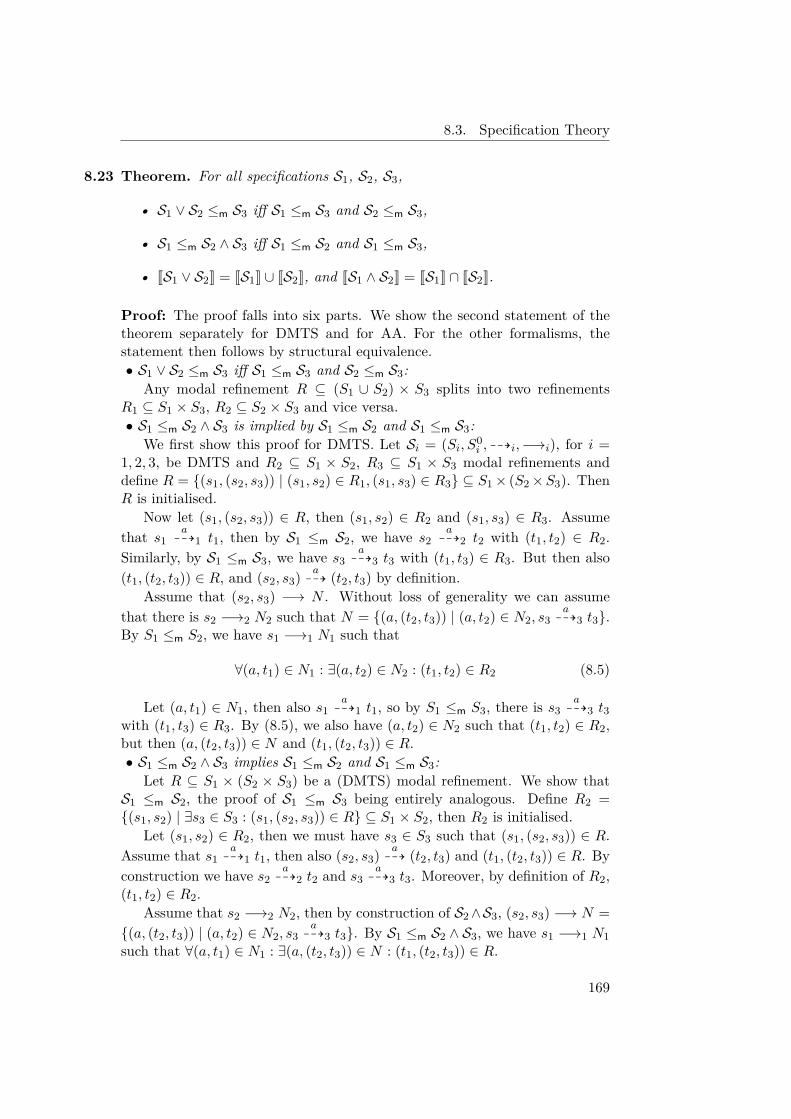
8.3. Specification Theory

8.23 Theorem. For all specifications S1, S2, S3,

• S1 ∨ S2 ≤m S3 iff S1 ≤m S3 and S2 ≤m S3,

• S1 ≤m S2 ∧ S3 iff S1 ≤m S2 and S1 ≤m S3,

• JS1 ∨ S2K = JS1K ∪ JS2K, and JS1 ∧ S2K = JS1K ∩ JS2K.

Proof: The proof falls into six parts. We show the second statement of thetheorem separately for DMTS and for AA. For the other formalisms, thestatement then follows by structural equivalence.• S1 ∨ S2 ≤m S3 iff S1 ≤m S3 and S2 ≤m S3:

Any modal refinement R ⊆ (S1 ∪ S2) × S3 splits into two refinementsR1 ⊆ S1 × S3, R2 ⊆ S2 × S3 and vice versa.• S1 ≤m S2 ∧ S3 is implied by S1 ≤m S2 and S1 ≤m S3:

We first show this proof for DMTS. Let Si = (Si, S0i , 99Ki,−→i), for i =

1, 2, 3, be DMTS and R2 ⊆ S1 × S2, R3 ⊆ S1 × S3 modal refinements anddefine R = {(s1, (s2, s3)) | (s1, s2) ∈ R1, (s1, s3) ∈ R3} ⊆ S1× (S2×S3). ThenR is initialised.

Now let (s1, (s2, s3)) ∈ R, then (s1, s2) ∈ R2 and (s1, s3) ∈ R3. Assumethat s1

a99K1 t1, then by S1 ≤m S2, we have s2

a99K2 t2 with (t1, t2) ∈ R2.

Similarly, by S1 ≤m S3, we have s3a99K3 t3 with (t1, t3) ∈ R3. But then also

(t1, (t2, t3)) ∈ R, and (s2, s3) a99K (t2, t3) by definition.

Assume that (s2, s3) −→ N . Without loss of generality we can assumethat there is s2 −→2 N2 such that N = {(a, (t2, t3)) | (a, t2) ∈ N2, s3

a99K3 t3}.

By S1 ≤m S2, we have s1 −→1 N1 such that

∀(a, t1) ∈ N1 : ∃(a, t2) ∈ N2 : (t1, t2) ∈ R2 (8.5)

Let (a, t1) ∈ N1, then also s1a99K1 t1, so by S1 ≤m S3, there is s3

a99K3 t3

with (t1, t3) ∈ R3. By (8.5), we also have (a, t2) ∈ N2 such that (t1, t2) ∈ R2,but then (a, (t2, t3)) ∈ N and (t1, (t2, t3)) ∈ R.• S1 ≤m S2 ∧ S3 implies S1 ≤m S2 and S1 ≤m S3:

Let R ⊆ S1 × (S2 × S3) be a (DMTS) modal refinement. We show thatS1 ≤m S2, the proof of S1 ≤m S3 being entirely analogous. Define R2 ={(s1, s2) | ∃s3 ∈ S3 : (s1, (s2, s3)) ∈ R} ⊆ S1 × S2, then R2 is initialised.

Let (s1, s2) ∈ R2, then we must have s3 ∈ S3 such that (s1, (s2, s3)) ∈ R.Assume that s1

a99K1 t1, then also (s2, s3) a

99K (t2, t3) and (t1, (t2, t3)) ∈ R. Byconstruction we have s2

a99K2 t2 and s3

a99K3 t3. Moreover, by definition of R2,

(t1, t2) ∈ R2.Assume that s2 −→2 N2, then by construction of S2∧S3, (s2, s3) −→ N =

{(a, (t2, t3)) | (a, t2) ∈ N2, s3a99K3 t3}. By S1 ≤m S2 ∧ S3, we have s1 −→1 N1

such that ∀(a, t1) ∈ N1 : ∃(a, (t2, t3)) ∈ N : (t1, (t2, t3)) ∈ R.

169

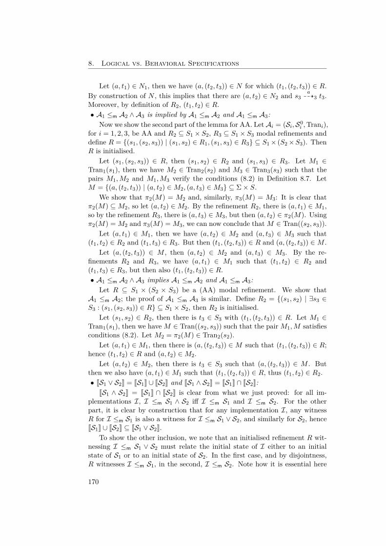
8. Logical vs. Behavioral Specifications

Let (a, t1) ∈ N1, then we have (a, (t2, t3)) ∈ N for which (t1, (t2, t3)) ∈ R.By construction of N , this implies that there are (a, t2) ∈ N2 and s3

a99K3 t3.

Moreover, by definition of R2, (t1, t2) ∈ R.• A1 ≤m A2 ∧ A3 is implied by A1 ≤m A2 and A1 ≤m A3:

Now we show the second part of the lemma for AA. LetAi = (Si,S0i ,Trani),

for i = 1, 2, 3, be AA and R2 ⊆ S1 × S2, R3 ⊆ S1 × S3 modal refinements anddefine R = {(s1, (s2, s3)) | (s1, s2) ∈ R1, (s1, s3) ∈ R3} ⊆ S1× (S2×S3). ThenR is initialised.

Let (s1, (s2, s3)) ∈ R, then (s1, s2) ∈ R2 and (s1, s3) ∈ R3. Let M1 ∈Tran1(s1), then we have M2 ∈ Tran2(s2) and M3 ∈ Tran3(s3) such that thepairs M1,M2 and M1,M3 verify the conditions (8.2) in Definition 8.7. LetM = {(a, (t2, t3)) | (a, t2) ∈M2, (a, t3) ∈M3} ⊆ Σ× S.

We show that π2(M) = M2 and, similarly, π3(M) = M3: It is clear thatπ2(M) ⊆M2, so let (a, t2) ∈M2. By the refinement R2, there is (a, t1) ∈M1,so by the refinement R3, there is (a, t3) ∈M3, but then (a, t2) ∈ π2(M). Usingπ2(M) = M2 and π3(M) = M3, we can now conclude thatM ∈ Tran((s2, s3)).

Let (a, t1) ∈ M1, then we have (a, t2) ∈ M2 and (a, t3) ∈ M3 such that(t1, t2) ∈ R2 and (t1, t3) ∈ R3. But then (t1, (t2, t3)) ∈ R and (a, (t2, t3)) ∈M .

Let (a, (t2, t3)) ∈ M , then (a, t2) ∈ M2 and (a, t3) ∈ M3. By the re-finements R2 and R3, we have (a, t1) ∈ M1 such that (t1, t2) ∈ R2 and(t1, t3) ∈ R3, but then also (t1, (t2, t3)) ∈ R.• A1 ≤m A2 ∧ A3 implies A1 ≤m A2 and A1 ≤m A3:

Let R ⊆ S1 × (S2 × S3) be a (AA) modal refinement. We show thatA1 ≤m A2; the proof of A1 ≤m A3 is similar. Define R2 = {(s1, s2) | ∃s3 ∈S3 : (s1, (s2, s3)) ∈ R} ⊆ S1 × S2, then R2 is initialised.

Let (s1, s2) ∈ R2, then there is t3 ∈ S3 with (t1, (t2, t3)) ∈ R. Let M1 ∈Tran1(s1), then we haveM ∈ Tran((s2, s3)) such that the pairM1,M satisfiesconditions (8.2). Let M2 = π2(M) ∈ Tran2(s2).

Let (a, t1) ∈M1, then there is (a, (t2, t3)) ∈M such that (t1, (t2, t3)) ∈ R;hence (t1, t2) ∈ R and (a, t2) ∈M2.

Let (a, t2) ∈ M2, then there is t3 ∈ S3 such that (a, (t2, t3)) ∈ M . Butthen we also have (a, t1) ∈M1 such that (t1, (t2, t3)) ∈ R, thus (t1, t2) ∈ R2.• JS1 ∨ S2K = JS1K ∪ JS2K and JS1 ∧ S2K = JS1K ∩ JS2K:JS1 ∧ S2K = JS1K ∩ JS2K is clear from what we just proved: for all im-

plementations I, I ≤m S1 ∧ S2 iff I ≤m S1 and I ≤m S2. For the otherpart, it is clear by construction that for any implementation I, any witnessR for I ≤m S1 is also a witness for I ≤m S1 ∨ S2, and similarly for S2, henceJS1K ∪ JS2K ⊆ JS1 ∨ S2K.

To show the other inclusion, we note that an initialised refinement R wit-nessing I ≤m S1 ∨ S2 must relate the initial state of I either to an initialstate of S1 or to an initial state of S2. In the first case, and by disjointness,R witnesses I ≤m S1, in the second, I ≤m S2. Note how it is essential here

170

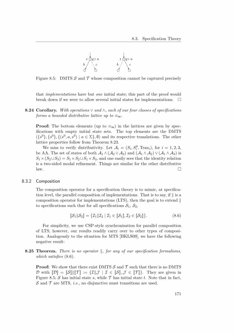
8.3. Specification Theory

s ta a

b c b c

Figure 8.5: DMTS S and T whose composition cannot be captured precisely

that implementations have but one initial state; this part of the proof wouldbreak down if we were to allow several initial states for implementations. �

8.24 Corollary. With operations ∨ and ∧, each of our four classes of specificationsforms a bounded distributive lattice up to ≡m.

Proof: The bottom elements (up to ≡m) in the lattices are given by spec-ifications with empty initial state sets. The top elements are the DMTS({s0}, {s0}, {(s0, a, s0) | a ∈ Σ}, ∅) and its respective translations. The otherlattice properties follow from Theorem 8.23.

We miss to verify distributivity. Let Ai = (Si, S0i ,Trani), for i = 1, 2, 3,

be AA. The set of states of both A1 ∧ (A2 ∨A3) and (A1 ∧A2)∨ (A1 ∧A3) isS1×(S2∪S3) = S1×S2∪S1×S3, and one easily sees that the identity relationis a two-sided modal refinement. Things are similar for the other distributivelaw. �

8.3.2 Composition

The composition operator for a specification theory is to mimic, at specifica-tion level, the parallel composition of implementations. That is to say, if ‖ is acomposition operator for implementations (LTS), then the goal is to extend ‖to specifications such that for all specifications S1, S2,

JS1‖S2K ={I1‖I2 | I1 ∈ JS1K, I2 ∈ JS2K

}. (8.6)

For simplicity, we use CSP-style synchronisation for parallel compositionof LTS, however, our results readily carry over to other types of composi-tion. Analogously to the situation for MTS [BKLS09], we have the followingnegative result:

8.25 Theorem. There is no operator ‖, for any of our specification formalisms,which satisfies (8.6).

Proof: We show that there exist DMTS S and T such that there is no DMTSD with JDK = JSK‖JT K := {I‖J | I ∈ JSK,J ∈ JT K}. They are given inFigure 8.5; S has initial state s, while T has initial state t. Note that in fact,S and T are MTS, i.e., no disjunctive must transitions are used.

171

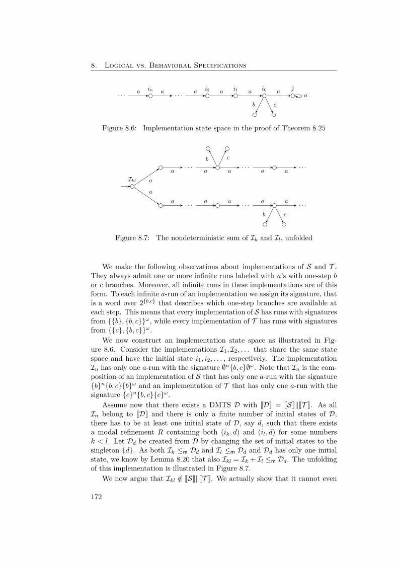
8. Logical vs. Behavioral Specifications

ji0i1i2· · ·

in· · · a

b c

aaaaaa

Figure 8.6: Implementation state space in the proof of Theorem 8.25

Ikl

· · ·

· · ·

· · ·

· · ·

· · ·

· · ·

a

a

a

a

a

a

a

a

a

a

a

a

b c

b c

Figure 8.7: The nondeterministic sum of Ik and Il, unfolded

We make the following observations about implementations of S and T .They always admit one or more infinite runs labeled with a’s with one-step bor c branches. Moreover, all infinite runs in these implementations are of thisform. To each infinite a-run of an implementation we assign its signature, thatis a word over 2{b,c} that describes which one-step branches are available ateach step. This means that every implementation of S has runs with signaturesfrom {{b}, {b, c}}ω, while every implementation of T has runs with signaturesfrom {{c}, {b, c}}ω.

We now construct an implementation state space as illustrated in Fig-ure 8.6. Consider the implementations I1, I2, . . . that share the same statespace and have the initial state i1, i2, . . . , respectively. The implementationIn has only one a-run with the signature ∅n{b, c}∅ω. Note that In is the com-position of an implementation of S that has only one a-run with the signature{b}n{b, c}{b}ω and an implementation of T that has only one a-run with thesignature {c}n{b, c}{c}ω.

Assume now that there exists a DMTS D with JDK = JSK‖JT K. As allIn belong to JDK and there is only a finite number of initial states of D,there has to be at least one initial state of D, say d, such that there existsa modal refinement R containing both (ik, d) and (il, d) for some numbersk < l. Let Dd be created from D by changing the set of initial states to thesingleton {d}. As both Ik ≤m Dd and Il ≤m Dd and Dd has only one initialstate, we know by Lemma 8.20 that also Ikl = Ik + Il ≤m Dd. The unfoldingof this implementation is illustrated in Figure 8.7.

We now argue that Ikl /∈ JSK‖JT K. We actually show that it cannot even

172

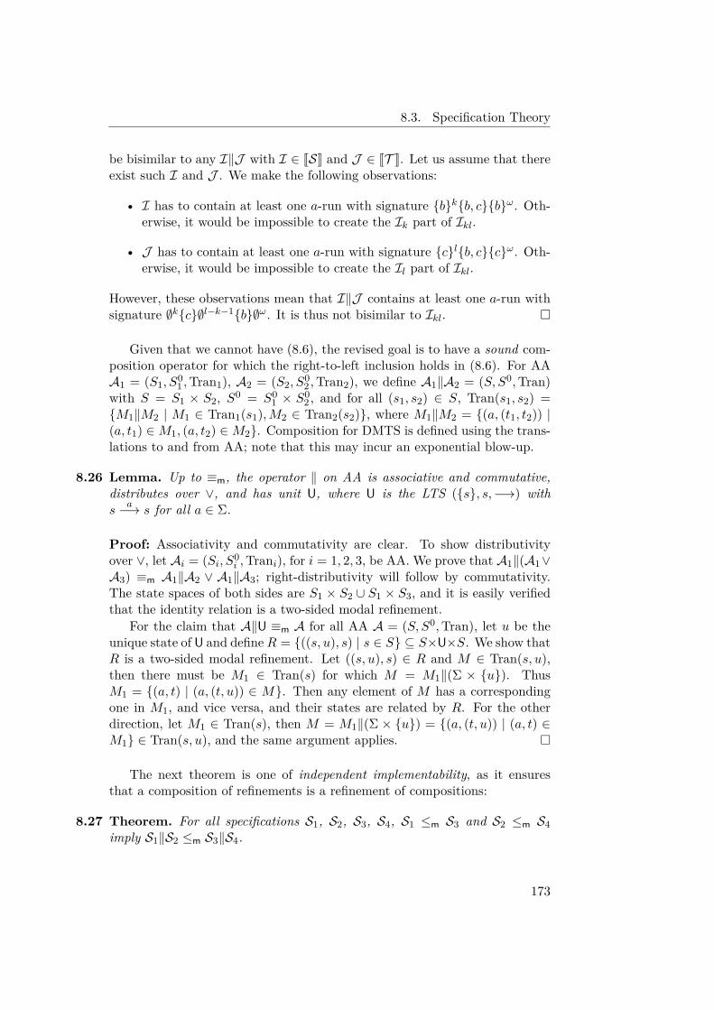
8.3. Specification Theory

be bisimilar to any I‖J with I ∈ JSK and J ∈ JT K. Let us assume that thereexist such I and J . We make the following observations:

• I has to contain at least one a-run with signature {b}k{b, c}{b}ω. Oth-erwise, it would be impossible to create the Ik part of Ikl.

• J has to contain at least one a-run with signature {c}l{b, c}{c}ω. Oth-erwise, it would be impossible to create the Il part of Ikl.

However, these observations mean that I‖J contains at least one a-run withsignature ∅k{c}∅l−k−1{b}∅ω. It is thus not bisimilar to Ikl. �

Given that we cannot have (8.6), the revised goal is to have a sound com-position operator for which the right-to-left inclusion holds in (8.6). For AAA1 = (S1, S

01 ,Tran1), A2 = (S2, S

02 ,Tran2), we define A1‖A2 = (S, S0,Tran)

with S = S1 × S2, S0 = S01 × S0

2 , and for all (s1, s2) ∈ S, Tran(s1, s2) ={M1‖M2 | M1 ∈ Tran1(s1),M2 ∈ Tran2(s2)}, where M1‖M2 = {(a, (t1, t2)) |(a, t1) ∈M1, (a, t2) ∈M2}. Composition for DMTS is defined using the trans-lations to and from AA; note that this may incur an exponential blow-up.

8.26 Lemma. Up to ≡m, the operator ‖ on AA is associative and commutative,distributes over ∨, and has unit U, where U is the LTS ({s}, s,−→) withs

a−→ s for all a ∈ Σ.

Proof: Associativity and commutativity are clear. To show distributivityover ∨, let Ai = (Si, S0

i ,Trani), for i = 1, 2, 3, be AA. We prove that A1‖(A1∨A3) ≡m A1‖A2 ∨ A1‖A3; right-distributivity will follow by commutativity.The state spaces of both sides are S1 × S2 ∪ S1 × S3, and it is easily verifiedthat the identity relation is a two-sided modal refinement.

For the claim that A‖U ≡m A for all AA A = (S, S0,Tran), let u be theunique state of U and defineR = {((s, u), s) | s ∈ S} ⊆ S×U×S. We show thatR is a two-sided modal refinement. Let ((s, u), s) ∈ R and M ∈ Tran(s, u),then there must be M1 ∈ Tran(s) for which M = M1‖(Σ × {u}). ThusM1 = {(a, t) | (a, (t, u)) ∈ M}. Then any element of M has a correspondingone in M1, and vice versa, and their states are related by R. For the otherdirection, let M1 ∈ Tran(s), then M = M1‖(Σ × {u}) = {(a, (t, u)) | (a, t) ∈M1} ∈ Tran(s, u), and the same argument applies. �

The next theorem is one of independent implementability, as it ensuresthat a composition of refinements is a refinement of compositions:

8.27 Theorem. For all specifications S1, S2, S3, S4, S1 ≤m S3 and S2 ≤m S4imply S1‖S2 ≤m S3‖S4.

173

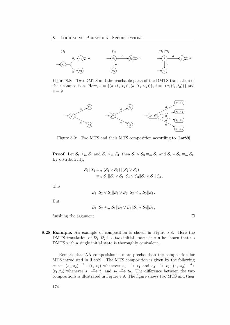
8. Logical vs. Behavioral Specifications

D1

s1

t1

u1

a

b

a

D2

s2 t2

u2

a

a

a

D1‖D2

s t

u

a

a

a

Figure 8.8: Two DMTS and the reachable parts of the DMTS translation oftheir composition. Here, s = {(a, (t1, t2)), (a, (t1, u2))}, t = {(a, (t1, t2))} andu = ∅

s0

s1

s2

a

a

t0

t1

t2

a

a

s0, t0

s1, t1

s1, t2

s2, t1

s2, t2

a

a

a

a

Figure 8.9: Two MTS and their MTS composition according to [Lar89]

Proof: Let S1 ≤m S3 and S2 ≤m S4, then S1 ∨ S3 ≡m S3 and S2 ∨ S4 ≡m S4.By distributivity,

S3‖S4 ≡m (S1 ∨ S3)‖(S2 ∨ S4)≡m S1‖S2 ∨ S1‖S4 ∨ S3‖S2 ∨ S3‖S4 ,

thusS1‖S2 ∨ S1‖S4 ∨ S3‖S2 ≤m S3‖S4 .

ButS1‖S2 ≤m S1‖S2 ∨ S1‖S4 ∨ S3‖S2 ,

finishing the argument. �

8.28 Example. An example of composition is shown in Figure 8.8. Here theDMTS translation of D1‖D2 has two initial states; it can be shown that noDMTS with a single initial state is thoroughly equivalent.

Remark that AA composition is more precise than the composition forMTS introduced in [Lar89]. The MTS composition is given by the followingrules: (s1, s2) a

99K (t1, t2) whenever s1a99K t1 and s2

a99K t2, (s1, s2) a−→

(t1, t2) whenever s1a−→ t1 and s2

a−→ t2. The difference between the twocompositions is illustrated in Figure 8.9. The figure shows two MTS and their

174

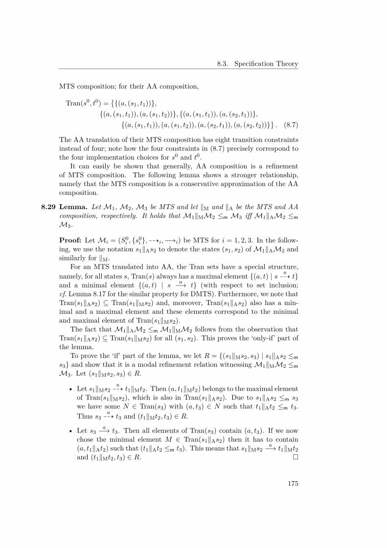
8.3. Specification Theory

MTS composition; for their AA composition,

Tran(s0, t0) ={{(a, (s1, t1))},

{(a, (s1, t1)), (a, (s1, t2))}, {(a, (s1, t1)), (a, (s2, t1))},{(a, (s1, t1)), (a, (s1, t2)), (a, (s2, t1)), (a, (s2, t2))}

}. (8.7)

The AA translation of their MTS composition has eight transition constraintsinstead of four; note how the four constraints in (8.7) precisely correspond tothe four implementation choices for s0 and t0.

It can easily be shown that generally, AA composition is a refinementof MTS composition. The following lemma shows a stronger relationship,namely that the MTS composition is a conservative approximation of the AAcomposition.

8.29 Lemma. LetM1,M2,M3 be MTS and let ‖M and ‖A be the MTS and AAcomposition, respectively. It holds that M1‖MM2 ≤m M3 iff M1‖AM2 ≤mM3.

Proof: LetMi = (S0i , {s0

i }, 99Ki,−→i) be MTS for i = 1, 2, 3. In the follow-ing, we use the notation s1‖As2 to denote the states (s1, s2) ofM1‖AM2 andsimilarly for ‖M.

For an MTS translated into AA, the Tran sets have a special structure,namely, for all states s, Tran(s) always has a maximal element {(a, t) | s a

99K t}and a minimal element {(a, t) | s a−→ t} (with respect to set inclusion;cf. Lemma 8.17 for the similar property for DMTS). Furthermore, we note thatTran(s1‖As2) ⊆ Tran(s1‖Ms2) and, moreover, Tran(s1‖As2) also has a min-imal and a maximal element and these elements correspond to the minimaland maximal element of Tran(s1‖Ms2).

The fact thatM1‖AM2 ≤m M1‖MM2 follows from the observation thatTran(s1‖As2) ⊆ Tran(s1‖Ms2) for all (s1, s2). This proves the ‘only-if’ part ofthe lemma.

To prove the ‘if’ part of the lemma, we let R = {(s1‖Ms2, s3) | s1‖As2 ≤ms3} and show that it is a modal refinement relation witnessingM1‖MM2 ≤mM3. Let (s1‖Ms2, s3) ∈ R.

• Let s1‖Ms2a99K t1‖Mt2. Then (a, t1‖Mt2) belongs to the maximal element

of Tran(s1‖Ms2), which is also in Tran(s1‖As2). Due to s1‖As2 ≤m s3we have some N ∈ Tran(s3) with (a, t3) ∈ N such that t1‖At2 ≤m t3.Thus s3

a99K t3 and (t1‖Mt2, t3) ∈ R.

• Let s3a−→ t3. Then all elements of Tran(s3) contain (a, t3). If we now

chose the minimal element M ∈ Tran(s1‖As2) then it has to contain(a, t1‖At2) such that (t1‖At2 ≤m t3). This means that s1‖Ms2

a−→ t1‖Mt2and (t1‖Mt2, t3) ∈ R. �

175

8. Logical vs. Behavioral Specifications

8.3.3 QuotientThe quotient operator for a specification theory is used to synthesise specifi-cations for components of a composition. Hence it is to have the property, forall specifications S, S1 and all implementations I1, I2, that

I1 ∈ JS1K and I2 ∈ JS/S1K imply I1‖I2 ∈ JSK. (8.8)

Furthermore, S/S1 is to be as permissive as possible.

Quotient for MTS

Before we describe the general construction of the quotient, we start witha simpler construction that works for the important special case of MTS.However, MTS are not closed under quotient, cf. [Lar90a, Thm. 5.5]; we showthat the quotient of two MTS will generally be a DMTS.

Recall that MTS have only one initial state and all their must transitionsare singletons. LetM1 = (S1, s

01, 99K1,−→1) andM2 = (S2, s

02, 99K2,−→2) be

MTS. We defineM1/M2 = (S, s0, 99K,−→) with S = 2S1×S2 , s0 = {(s01, s

02)},

and the transition relations given as follows.For s = {(s1

1, s12), . . . , (sn1 , sn2 )} ∈ S we say that a ∈ Σ is permissible from

s if for all i = 1, . . . , n either si1a99K or si2

aX99K.

For a permissible from s and i ∈ {1, . . . , n}, let {ti,12 , . . . , ti,mi2 } = {t2 ∈ S2 |si2

a99K t2} be an enumeration of the possible states in S2 after an a-transition

from si2. We then define the set of possible transitions from s under a aspta(s) =

{{(ti,j1 , ti,j2 ) | i = 1, . . . , n, j = 1, . . . ,mi}

∣∣ ∀i, j : si1a99K ti,j1

}.

The transitions of s are now given as follows: for every a permissible froms and every t ∈ pta(s), let s a

99K t. Furthermore, for every si1a−→ t1 let

s −→ {(a,M) ∈ {a} × pta(s) | ∃t2 : (t1, t2) ∈M, si2a−→ t2}.

Note that as a special case we obtain ∅ a99K ∅ for all a ∈ Σ and there are

no must transitions from ∅.

8.30 Example. We illustrate the construction on an example. Let S and T be theMTS on the top of Figure 8.10. We construct S/T , displayed below; this canbe further simplified into the system on the bottom.

First we construct the may-successors of s0/t0. Both b and c are admissibledue to t0 b

X99K and t0cX99K and thus with pt()b(s0/t0) = pt()c(s0/t0) = {∅}.

Consequently, the only successor here is ∅. Further, a is also admissible dueto s0 a

99K. For may-transitions under a, we have to consider all mappingsof successors of t0 to successors of s0, namely {s1/t1, s1/t2}, {s1/t1, s2/t2},{s2/t1, s1/t2}, and {s2/t1, s2/t2}. Besides, since there is a must-transitionfrom s0 (to s1), we create a disjunctive must-transition to all successors thatcan be used to yield this must-transition s0 a−→ s1 when composed with themust-transition t0 a−→ t1. These are all successors where t1 is mapped to s1,hence the first two.

176

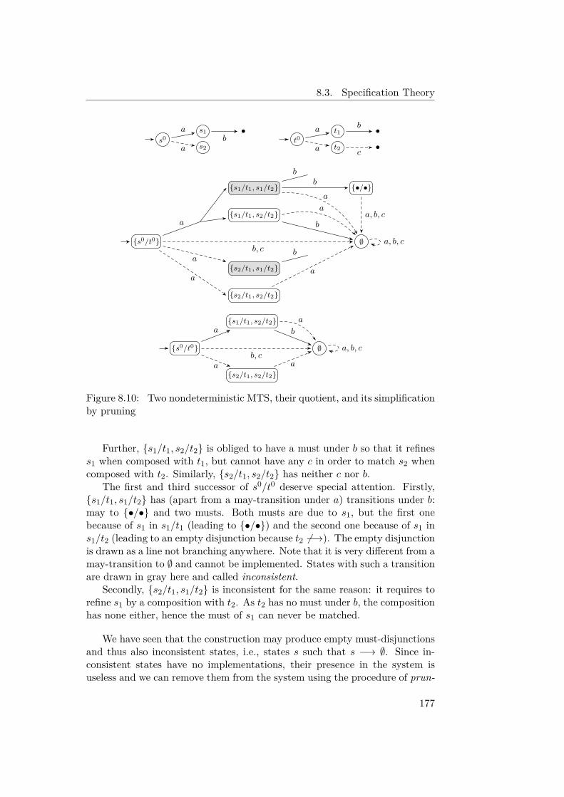
8.3. Specification Theory

t0t1a

t2a

•b

•c

s0s1a

s2a

•b

{s0/t0}

{s1/t1, s1/t2}

{s1/t1, s2/t2}a

{•/•}b

b

{s2/t1, s1/t2}a

b

{s2/t1, s2/t2}

a

∅

a

b

a

a

b, ca, b, c

a, b, c

{s0/t0}

{s1/t1, s2/t2}a

{s2/t1, s2/t2}a

∅

b

a

ab, c

a, b, c

Figure 8.10: Two nondeterministic MTS, their quotient, and its simplificationby pruning

Further, {s1/t1, s2/t2} is obliged to have a must under b so that it refiness1 when composed with t1, but cannot have any c in order to match s2 whencomposed with t2. Similarly, {s2/t1, s2/t2} has neither c nor b.

The first and third successor of s0/t0 deserve special attention. Firstly,{s1/t1, s1/t2} has (apart from a may-transition under a) transitions under b:may to {•/•} and two musts. Both musts are due to s1, but the first onebecause of s1 in s1/t1 (leading to {•/•}) and the second one because of s1 ins1/t2 (leading to an empty disjunction because t2 6−→). The empty disjunctionis drawn as a line not branching anywhere. Note that it is very different from amay-transition to ∅ and cannot be implemented. States with such a transitionare drawn in gray here and called inconsistent.

Secondly, {s2/t1, s1/t2} is inconsistent for the same reason: it requires torefine s1 by a composition with t2. As t2 has no must under b, the compositionhas none either, hence the must of s1 can never be matched.

We have seen that the construction may produce empty must-disjunctionsand thus also inconsistent states, i.e., states s such that s −→ ∅. Since in-consistent states have no implementations, their presence in the system isuseless and we can remove them from the system using the procedure of prun-

177

8. Logical vs. Behavioral Specifications

ing. This procedure produces a more readable system that has the sameset of implementations and, moreover, is modally refining the original sys-tem. The procedure is standard for MTS, see e.g. [BJL+12a]; here we de-scribe its straightforward adaptation for DMTS. The procedure exhaustivelyrepeats the following: if there is an inconsistent state s, then remove it to-gether with all its outgoing transitions (both may and must) and incomingmay-transitions, and each remaining must-transition t −→ D is modified intot −→ D \ (Σ× {s}); intuitively, we are removing the incoming must-branches(not the whole transitions). This may of course turn other states inconsistentand thus the procedure is repeated until there are no more inconsistent states.

8.31 Example. When we apply pruning to the quotient in the previous example,we obtain the system on the bottom of Figure 8.10. Here the gray inconsis-tent states are removed and the disjunctive must from {s0/t0} leads only to{s1/t1, s2/t2}.

Now it is easy to see that T‖(S/T ) ≡m S in this case.

Recall from Lemma 8.29 that the MTS composition is a conservative ap-proximation to the AA composition. This means that the following theoremholds regardless of which of the two compositions is used.

8.32 Theorem. For all MTS specifications M1, M2 and M3, M1‖M2 ≤m M3iffM2 ≤m M3/M1.

Proof: In this proof only, let ‖ denote MTS composition.Write Mi = (Si, s0

i , 99Ki,−→i) for i = 1, 2, 3. We use the following nota-tion to help distinguish states ofM1‖M2 andM3/M1. The states ofM1‖M2are denoted by s1‖s2 instead of (s1, s2) while the states of M3/M1 are de-noted by {s3/s1, . . .} instead of {(s3, s1), . . .}. We also note that for states ofM3/M1, s ⊇ t implies s ≤m t due to the construction.

Now assume that M2 ≤m M3/M1 and let R = {(s1‖s2, s3) | s2 ≤m{s3/s1}}. We show that R is a witness for M1‖M2 ≤m M3, i.e., that itsatisfies the conditions of Definition 8.2. Let (s1‖s2, s3) ∈ R.

• Let s1‖s2a99K t1‖t2. As s2 ≤m {s3/s1} this means that {s3/s1}

a99K

{t13/t11, . . . , tk3/tk1} = t and t2 ≤m t. Due to the construction of {s3/s1},we know that there is an index j for which tj1 = t1 and s3

a99K tj3. Let

t3 = tj3. As t ⊇ {t3/t1}, t ≤m {t3/t1}. Therefore, since t2 ≤m t, we havet2 ≤m {t3/t1} and thus (t1 ‖ t2, t3) ∈ R.

• Let s3a−→ t3. This means that {s3/s1} −→ U = {(a, u) ∈ {a} ×

pta({s3/s1}) | ∃t1 : t3/t1 ∈ u, s1a−→ t1}. As s2 ≤m {s3/s1}, we know

that s2a−→ t2 and t2 ≤m u for some (a, u) ∈ U . Due to the construction

of U we know that there exists t1 such that t3/t1 ∈ u with s1a−→ t1.

Thus s1‖s2a−→ t1‖t2. Again, as u ⊇ {t3/t1}, t2 ≤m {t3/t1}. Therefore,

(t1 ‖ t2, t3) ∈ R.

178

8.3. Specification Theory

Assume, for the other direction of the proof, that M1 ‖ M2 ≤m M3.Define

R = {(s2, {s13/s

11, . . . , s

n3/s

n1}) | ∀i = 1, . . . , n : si1 ‖ s2 ≤m si3} ;

note that (s2, ∅) ∈ R for all s2 ∈ S2. We show that R is a witness forM2 ≤m M3/M1. Let (s2, s) ∈ R with s = {s1

3/s11, . . . , s

n3/s

n1}.

• Let s2a99K t2. If there is no i such that si1

a99K then s a

99K ∅ and (t2, ∅) ∈R. Otherwise, for each i ∈ {1, . . . , n} and each j ∈ {1, . . . ,mi} such thatsi1

a99K ti,j1 consider that we have si1‖s2

a99K ti,j1 ‖t2 and as si1‖s2 ≤m si3 we

also have a corresponding si3a99K ti,j3 with ti,j1 ‖t2 ≤m ti,j3 . We fix these

ti,j3 for each i and j. Let t = {ti,j3 /ti,j1 | i ∈ {1, . . . , n}, j ∈ {1, . . . ,mi}}.Clearly, s a

99K t and (t2, t) ∈ R.

• Let s −→ U (note that this means that s 6= ∅) and let si3a−→ ti3 be the

corresponding must transition in the construction. As si1‖s2 ≤m si3, thismeans that s2

a−→ t2 and si1a−→ ti1 such that ti1‖t2 ≤m ti3. This also

means that s2a99K t2. We thus build t as we did in the previous case

where for i, j such that ti,j1 = ti1 we choose the corresponding ti,j3 to beti3. Clearly (t2, t) ∈ R. �

Quotient for AA

We now introduce the general quotient operator for AA. The constructionis similar to the previous one, with the notions of permissibility and pta(s)adapted to the more general setting.

Let A1 = (S1, S01 ,Tran1), A2 = (S2, S

02 ,Tran2) be AA and define A1/A2 =

(S, S0,Tran), with S = 2S1×S2 . To define the set of initial states, let us firstenumerate the initial states of A2 as follows: S0

2 = {s0,12 , . . . , s0,p

2 }. The set ofinitial states is given by all possible assignments of states from S0

1 to statesof S0

2 , formally: S0 ={{(s0,q

1 , s0,q2 ) | q ∈ {1, . . . , p}}

∣∣ ∀q : s0,q1 ∈ S0

1}.

The assignment of transition constraints Tran is given as follows. LetTran(∅) = 2Σ×{∅}. For s = {(s1

1, s12), . . . , (sn1 , sn2 )} ∈ S, say that a ∈ Σ is

permissible from s if it holds for all i = 1, . . . , n that there is M1 ∈ Tran1(si1)and t1 ∈ S1 for which (a, t1) ∈ M1, or else there is no M2 ∈ Tran2(si2) andt2 ∈ S2 with (a, t2) ∈M2.

Let us now fix a nonempty s = {(s11, s

12), . . . , (sn1 , sn2 )} ∈ S. We intro-

duce some notation that we are going to use throughout this construction andthe following proof to denote the successor states of si2 for all i. For eachsi2 let Tran2(si2) = {M i,1

2 , . . . ,M i,mi2 } be a fixed enumeration of Tran2(si2).

For each a permissible from s and for each M i,j2 we further fix an enumera-

tion of all states in M i,j2 after an a-transition: {t2 ∈ S2 | (a, t2) ∈ M i,j

2 } ={ti,j,a,1, . . . , ti,j,a,ri,j,a}. This means that ti,j,a,k is the kth state (out of ri,j,a)

179

8. Logical vs. Behavioral Specifications

with an a-transition in M i,j2 , which is the jth member of Tran2(si2), where si2

is the state in the ith pair in s.For a permissible from s, we define

pta(s) ={{(ti,j,a,k1 , i, j, ti,j,a,k2 ) | i = 1, . . . , n, j = 1, . . . ,mi, k = 1, . . . , ri,j,a}∣∣ ∀i, j, k : ∃M1 ∈ Tran1(si1) : (a, ti,j,a,k1 ) ∈M1

},

the set of all sets of possible assignments of next-a states from si1 to next-astates from si2. Note that unlike the case of MTS quotient, we also keepthe indices i, j in the assignments. We further define pt(s) = {(a, x) |a permissible from s, x ∈ pta(s)}.

To deal with the elements of pta(s) we define the following auxiliary opera-tions. The first operation ` allows us to “forget” the indices i, j and is definedas follows: `(x) = {(t1, t2) | ∃i, j : (t1, i, j, t2) ∈ x}. The operation can benaturally lifted to subsets of pt(s) as follows: `(N) = {(a, `(x)) | (a, x) ∈ N}where N ⊆ pt(s).

The second operation is a type of projection that given the two indicesi, j and the state ti,j,a,k2 produces the next-a state of s1 assigned in thegiven element x of pta(s). Note that the projection is defined uniquely:x � (i, j, ti,j,a,k2 ) = ti,j,a,k1 where x = {. . . , (ti,j,a,k1 , i, j, ti,j,a,k2 ), . . .}. The projec-tion operation can also be lifted to subsets N of pt(s) and setsM2 ∈ Tran2(s2

i )as follows: N � (i, j,M2) = {(a, x � (i, j, t2)) | (a, t2) ∈ M2}. Note that theresult of this operation is then a set of elements of the form (a, t3) where t3 isan a-successor of s3.

Having the two auxiliary operations, we can then finally define

Tran(s) = {`(N) | N ⊆ pt(s),∀i ∈ {1, . . . , n}, j ∈ {1, . . . ,mj} :N � (i, j,M i,j

2 ) ∈ Tran3(si3)} . (8.9)

8.33 Theorem. For all specifications S1, S2, S3, S1‖S2 ≤m S3 iff S2 ≤m S3/S1.

Proof: We show the proof for AA. Let A1 = (S1, S01 ,Tran1) and A2 =

(S2, S02 ,Tran2), A3 = (S3, S

03 ,Tran3); we show that A1‖A2 ≤m A3 iff A2 ≤m

A3/A1.We use the notation introduced in the proof of Theorem 8.32, i.e., s1‖s2

instead of (s1, s2) when speaking about states of A1‖A2 and {s3/s1, . . .} in-stead of {(s3, s1), . . .} when speaking about states of A3/A1. We further notethat by construction, s ⊇ t implies s ≤m t for all s, t ∈ 2S3×S1 .

Now assume that A2 ≤m A3/A1 and let R = {(s1‖s2, s3) | s2 ≤m {s3/s1}};we show that R is a witness for A1‖A2 ≤m A3.

Let (s1‖s2, s3) ∈ R and M‖ ∈ Tran‖(s1‖s2). Then M‖ = M1‖M2 withM1 ∈ Tran1(s1) and M2 ∈ Tran2(s2). As s2 ≤m {s3/s1}, we can pair M2 withan M/ ∈ Tran/({s3/s1}), such that the conditions in (8.2) are satisfied (seeDefinition 8.7).

180

8.3. Specification Theory

Note that, as M1 ∈ Tran1(s1), there exists some j such that M1 = M1,j1 ,

i.e., M1 is the jth element of Tran(s1) in the enumeration as described inthe construction of the quotient. Further note that M‖ = `(N) for someN ⊆ pt({s3/s1}) satisfying the conditions in (8.9).

We now define M3 = N � (1, j,M1) and show that (8.2) holds for the pairM‖,M3:

• Let (a, t1‖t2) ∈ M‖, then there are (a, t1) ∈ M1 and (a, t2) ∈ M2.By (8.2) applied to the pair M2, M/, there is (a, t) ∈ M/ such thatt2 ≤m t. This means that there is (a, x) ∈ N such that t = `(x).Due to the construction of pt({s3/s1}) there has to be some t3 suchthat (t3, 1, j, t1) ∈ x. Due to the definition of M3, this means that(a, t3) ∈ M3. We also know that t ⊇ {t3/t1}, hence t ≤m {t3/t1}, andtogether with t2 ≤m t we get t2 ≤m {t3/t1}. Thus (t1‖t2, t3) ∈ R.

• Let (a, t3) ∈ M3. This means that there is some (a, x) ∈ N with(t3, 1, j, t1) ∈ x and (a, t1) ∈ M1. Therefore, `(x) = t ∈ M/ witht3/t1 ∈ t. Due to (8.2) applied to M2, M/, there has to be a corre-sponding (a, t2) ∈ M2 such that t2 ≤m t. Thus (a, t1‖t2) ∈ M‖ andagain by t ⊇ {t3/t1} we have t2 ≤m {t3/t1} and hence (t1‖t2, t3) ∈ R.

It remains to show that R is initialised. Let s01‖s0

2 be an initial state ofA1‖A2. By A2 ≤m A3/A1 we know that s0

2 ≤m s0 for some s0 ∈ S0. We thentake s0

3 ∈ S03 such that s0

3/s01 ∈ s0 (there has to be exactly one due to the

definition of s0). We then have s0 ⊇ {s03/s

01} and thus s0 ≤m {s0

3/s01}. This

means that s02 ≤m {s0

3/s01} and hence (s0

1‖s02, s

03) ∈ R.

Assume, for the other direction of the proof, that A1‖A2 ≤m A3. DefineR ⊆ S2 × 2S3×S1 by

R = {(s2, {s13/s

11, . . . , s

n3/s

n1}) | ∀i = 1, . . . , n : si1‖s2 ≤m si3} ;

we show that R is a witness for A2 ≤m A3/A1. We first note that (s2, ∅) ∈ Rfor all s2. Let now (s2, s) ∈ R, with nonempty s = {s1

3/s11, . . . , s

n3/s

n1}, and

M2 ∈ Tran2(s2).Note that for every M i,j

1 ∈ Tran(si1) we can build M i,j‖ = M i,j

1 ‖M2, andas si1‖s2 ≤m si3, there has to be a corresponding M3 ∈ Tran(si3) satisfying theconditions of (8.2). We fix such M3 for every i, j and denote it by M i,j

3 .We are going to build a subset N of pt(s). To that end, we first define an

auxiliary notion of an adequate element of pt(s) with respect to (a, t2) ∈ M2as follows. Let (a, x) ∈ pt(s). We say that (a, x) is adequate w.r.t. (a, t2) iffor every i ∈ {1, . . . , n}, j ∈ {1, . . . ,mi}, and k ∈ {1, . . . , ri,j,a}, the projectiont3 = x � (i, j, ti,j,k1 ) satisfies (a, t3) ∈M i,j

3 and ti,j,k1 ‖t2 ≤m t3.Clearly, if we have (a, x) adequate w.r.t. (a, t2), then (t2, `(x)) ∈ R.We can now define

N = {(a, x) ∈ pt(s) | ∃(a, t2) ∈M2 : (a, x) is adequate w.r.t. (a, t2)} .

181

8. Logical vs. Behavioral Specifications

We first need to show that `(N) ∈ Tran/(s). Let i ∈ {1, . . . , n} andj ∈ {1, . . . ,mj}. We want to show that N � (i, j,M i,j

1 ) = M i,j3 . Let first

(a, t3) ∈ N � (i, j,M i,j1 ). This means that there is some (a, x) ∈ N with

x = (t3, i, j, ti,j,k1 ). Due to the definition of N , (a, t3) ∈M i,j3 . Let now (a, t3) ∈

M i,j3 . Recall that the pair M i,j

1 ‖M2, M i,j3 satisfies (8.2). This means that

for (a, t3) ∈ M i,j3 there exists (a, ti,j,k1 ‖t2) ∈ M i,j

1 ‖M2 such that ti,j,k1 ‖t2 ≤mt3. Hence (a, (t3, i, j, ti,j,k1 )) is adequate w.r.t. (a, t2) and thus (a, t3) ∈ N �(i, j,M i,j

1 ).We now show that the pairM2,M = `(N) satisfies the conditions of (8.2).

• Let (a, t2) ∈M2. We need to show that there exists (a, x) ∈ N adequatew.r.t. (a, t2). Recall that the pair M i,j

1 ‖M2, M i,j3 satisfies (8.2) for every

i, j. For every (a, ti,j,k1 ‖t2) there thus has to be (a, t3) ∈ M i,j3 with

ti,j,k1 ‖t2 ≤m t3. We fix such t3 for every i, j, k and denote it by ti,j,k3 .We then set x = {(ti,j,k3 , i, j, ti,j,k1 | i ∈ {1, . . . , n}, j ∈ {1, . . . ,mi}, k ∈{1, . . . , ri,j,a}. Clearly (a, x) ∈ N and (a, x) is adequate w.r.t. (a, t2). Asnoted above, we have (t2, `(x)) ∈ R.

• Let (a, t) ∈ M . This means that there is some (a, x) ∈ N such thatt = `(x). Due to the definition of N , there exists (a, t2) ∈ M2 suchthat (a, x) is adequate w.r.t. (a, t2). Again, as noted above, we have(t2, t) = (t2, `(x)) ∈ R.

It remains to show that R is initialised. Let s02 be an initial state of A2.

By A1‖A2 ≤m A3 we know that for every s0,q1 ∈ S0

1 (recall the enumerationof initial states in the construction of the quotient) there exists s0

3 ∈ S03 such

that s0,q1 ‖s0

2 ≤m s03. Let us fix for every q such s0

3 and denote it by s0,q3 . Let

then s0 = {s0,q3 /s0,q

1 | q ∈ {1, . . . , p}}. Clearly, s0 is an initial state of A3/A1and (s0

2, s0) ∈ R. �

As a corollary, we get (8.8): If I2 ∈ JS/S1K, i.e., I2 ≤m S/S1, thenS1‖I2 ≤m S, which using I1 ≤m S1 and Theorem 8.27 implies I1‖I2 ≤mS1‖I2 ≤m S. The reverse implication in Theorem 8.33 implies that S/S1 is aspermissive as possible.

8.34 Corollary. With operations ∧, ∨, ‖ and /, each of our four classes of speci-fications forms a commutative residuated lattice up to ≡m.

Proof: We have already seen in Corollary 8.24 that the class of AA formsa lattice, up to ≡m, under ∧ and ∨, and by Theorem 8.33, / is the residual,up to ≡m, of ‖. All other properties (such as distributivity of ‖ over ∨ orN‖⊥ ≡m ⊥) follow. �

182

8.4. Related Work

8.4 Related Work

The modal ν-calculus is equivalent to the Hennessy-Milner logic with great-est fixed points, which arises from Hennessy-Milner logic (HML) [HM85] byintroducing variables and greatest fixed points. If also least fixed points areallowed, one arrives at the full modal µ-calculus [SdB69,Pra81,Koz83]. Janinand Walukiewicz have in [JW95] introduced an automata-like representationfor the modal µ-calculus which seems related to our AA.

DMTS have been proposed as solutions to algebraic process equations inLarsen and Xinxin’s [LX90b] and further investigated also as a specificationformalism [Lar90a,BCK11]. The DMTS formalism is a member of the modaltransition systems (MTS) family and as such has also received attention re-cently. The MTS formalisms have proven to be useful in practice. Industrialapplications started with Bruns’ [Bru97] where MTS have been used for anair-traffic system at Heathrow airport. Besides, MTS classes are advocated asan appropriate base for interface theories by Raclet et.al. in [RBB+09] andfor product line theories in Nyman’s [Nym08]. Further, an MTS based soft-ware engineering methodology for design via merging partial descriptions ofbehavior has been established by Uchitel and Chechik in [UC04] and methodsfor supervisory control of MTS shown by Darondeau et.al. in [DDM10]. Toolsupport is quite extensive, e.g., [BLS95,DFFU07,BML11,KS13b].

Over the years, many extensions of MTS have been proposed, surveyedin more detail in [Kře17, FLLT14, FLT14a]. While MTS can only specifywhether or not a particular transition is required, some extensions equip MTSwith more general abilities to describe what combinations of transitions arepossible. These include DMTS [LX90b], Fecher and Schmidt’s 1-MTS [FS08]allowing to express exclusive disjunction, OTS [BK10] capable of express-ing positive Boolean combinations, and Boolean MTS [BKL+11] covering allBoolean combinations. The last one is closely related to our AA as well ashybrid modal logic [Pri68,Bla00]. Our results show that all these formalismsare at most as expressive as DMTS.

Larsen has shown in [Lar89] that any finite acyclic MTS is equivalentto a HML formula (without recursion or fixed points), the characteristicformula of the given MTS, cf. (8.3). Conversely, Boudol and Larsen showin [BL92] that any consistent and prime HML formula is equivalent to a MTS.3Here we extend these results to ν-calculus formulae, and show that any suchformula is equivalent to a DMTS, solving a problem left open in [LX90b].Hence the modal ν-calculus supports full compositionality and decompositionin the sense of [Lar90a]. This finishes some of the work started in [Lar89,BL92, Lar90a]. Recently, the graphical representability of a variant of alter-nating simulation called covariant-contravariant simulation has been studied

3A HML formula is prime if implying a disjunction means implying one of the alterna-tives.

183

8. Logical vs. Behavioral Specifications

in [AFdFE+13].Quotients are related to decomposition of processes and properties, an is-

sue which has received considerable attention through the years. In [LX90b],a solution to bisimulation C(X) ∼ P for a given process P and context C isprovided (as a DMTS). This solves the quotienting problem P/C for the spe-cial case where both P and C are processes. This is extended in [LX90a] to thesetting where the context C can have several holes and C(X1, . . . , Xn) mustsatisfy a ν-calculus property Q. However, C remains to be a process context,not a specification context. Our specification context allows for arbitrary spec-ifications, representing infinite sets of processes and process equations. Otherextensions use infinite conjunctions [FvGdW06], probabilistic processes [GF12]or processes with continuous time and space [CLM11].

Quotient operators, or guarantee or multiplicative implication as they arecalled there, are also well-known from various logical formalisms. Indeed,the algebraic properties of our parallel composition ‖ and quotient / resem-ble closely those of multiplicative conjunction & and implication ( in linearlogic [Gir87], and of spatial conjunction and implication in spatial logic [CC03]and separation logic [Rey02,ORY01]. For these and other logics, proof systemshave been developed which allow one to reason about expressions containingthese operators. In these logics, & and ( are first-class operators on parwith the other logical operators, and their semantics are defined as certainsets of processes. In contrast, for AA and hence, via the translations, alsofor ν-calculus, ‖ and / are derived operators, and we provide constructions toreduce any expression which contains them, to one which does not. This is im-portant from the perspective of reuse of components and useful in industrialapplications. To the best of our knowledge, there are no other such reduc-tions of quotient for the synchronisation type of composition in the context ofspecifications.

8.5 Conclusion

In this chapter we have introduced a general specification framework whose ba-sis consists of four different but equally expressive formalisms: one of a graph-ical behavioral kind (DMTS), one logic-based (ν-calculus) and two intermedi-ate languages between the former two (AA and hybrid modal logic). We haveshown their structural equivalence.

The established connection implies several consequences. On the one hand,it allows for a graphical representation of ν-calculus. Further, composition onDMTS can be transferred to the modal ν-calculus, hence turning it into amodal process algebra. On the other hand, such a correspondence identifiesa class of modal transition systems with a natural expressive power and pro-vides another justification of this formalism. Further, this class is closed underboth conjunction and disjunction, a requirement raised by component-based

184

8.5. Conclusion

design methods. However, it is not closed under complement and difference.4Nevertheless, since DMTS are closed under conjunction, disjunction and com-position, we still have a positive Boolean process algebra.

Altogether, we have shown that the framework possesses a rich algebraicstructure that includes logical (conjunction, disjunction) and behavioral oper-ations (parallel composition and quotient) and forms a complete specificationtheory in the sense of [Lar90a,BDH+12].

Moreover, the construction of the quotient solves an open problem in thearea of MTS. All attempts to find the quotient for variants of MTS so farhave been limited to the much simpler deterministic case [Rac08]. Here wehave given the first solution to the quotient on nondeterministic specifications:first, a quotient construction for MTS, and then a quotient for general DMTS.Due to the established correspondence, the quotient can be applied also to ν-calculus formulae. We remark that all our translations and constructions arebased on a new normal form for ν-calculus expressions, and that turninga ν-calculus expression into normal form may incur an exponential blow-up.However, the translations and constructions preserve the normal form, so thatthis translation only need be applied once in the beginning.

4Previous results on difference [SCU11] are incorrect due to a mistake in [FU08] onconjunction of MTS, see [Kře14, p. 36].

185

9 Compositionality for QuantitativeSpecifications1

This chapter continues and finishes the work of Chapter 7. It extends thequantitative theory of that chapter to the disjunctive modal transition systems(DMTS) of Chapter 8 and shows that also in the quantitative setting, DMTSare closely related to acceptance automata and the modal ν-calculus. Thequantitative theory of DMTS is shown to be rather pleasant, with betterproperties than for pure MTS.

9.1 Structured LabelsLet Σ be a poset with partial order 4. We think of 4 as label refinement, sothat if a 4 b, then a is less permissive (more restricted) than b.

9.1 Definition. A label a ∈ Σ is an implementation label if b 4 a implies b = afor all b ∈ Σ. The set of implementation labels is denoted Γ, and for a ∈ Σ,we let JaK = {b ∈ Γ | b 4 a} denote the set of its implementations.

Hence a is an implementation label iff a cannot be further refined. Notethat a 4 b implies JaK ⊆ JbK for all a, b ∈ Σ.

9.2 Example. A trivial but important example of our label structure is the dis-crete one in which label refinement 4 is equality (and Γ = Σ). This is equiv-alent to the “standard” case of unstructured labels.

A typical label set in quantitative applications consists of a discrete com-ponent and real-valued weights. For specifications, weights are replaced by(closed) weight intervals, so that Σ = U × {[l, r] | l ∈ R ∪ {−∞}, r ∈R ∪ {∞}, l ≤ r} for a finite set U , cf. [BFJ+13, BJL+12a]. Label refine-ment is given by (u1, [l1, r1]) 4 (u2, [l2, r2]) iff u1 = u2 and [l1, r1] ⊆ [l2, r2],so that labels are more refined if they specify smaller intervals; thus, Γ =U × {[x, x] | x ∈ R} ≈ U ×R.

For a quite general setting, we can instead start with an arbitrary set Γof implementation labels, let Σ = 2Γ, the powerset, and 4 = ⊆ be subset

1This chapter is based on the journal paper [FKLT18] published in Soft Computing.

187

9. Compositionality for Quantitative Specifications

inclusion. Then JaK = a for all a ∈ Σ. (Hence we identify implementationlabels with one-element subsets of Σ.)

9.1.1 Label operationsSpecification theories come equipped with several standard operations thatmake compositional software design possible [BDH+12]: conjunction for merg-ing viewpoints covering different system’s aspects [UC04,BDCU13], structuralcomposition for running components in parallel, and quotient to synthesizemissing parts of systems [LX90b]. In order to provide them for DMTS, wefirst need the respective atomic operations on their action labels.

We hence assume that Σ comes equipped with a partial conjunction,i.e., an operator 7 : Σ× Σ ⇀ Σ for which it holds that

(1) if a1 7 a2 is defined, then a1 7 a2 4 a1 and a1 7 a2 4 a2, and

(2) if a3 4 a1 and a3 4 a2, then a1 7 a2 is defined and a3 4 a1 7 a2.

Note that by these properties, any two partial conjunctions on Σ have to agreeon elements for which they are both defined.

9.3 Example. For discrete labels, the unique conjunction operator is given by

a1 7 a2 ={a1 if a1 = a2 ,

undef. otherwise .

Indeed, by property (2), a1 7 a2 must be defined for a1 = a2, and by (1), ifa1 7 a2 = a3 is defined, then a3 = a1 and a3 = a2.

For labels in U × {[l, r] | l, r ∈ R, l ≤ r}, the unique conjunction is

(u1, [l1, r1])7 (u2, [l2, r2]) ={undef. if u1 6= u2 or [l1, r1] ∩ [l2, r2] = ∅ ,(u1, [l1, r1] ∩ [l2, r2]) otherwise .

To see uniqueness, let ai = (ui, [li, ri]) for i = 1, 2, 3. Using property (2), we seethat a17a2 must be defined when u1 = u2 and [l1, r1]∩ [l2, r2] 6= ∅, and by (2),if a1 7 a2 = a3 is defined, then u3 = u1 and u3 = u2, and [l3, r3] ⊆ [l1, r1],[l3, r3] ⊆ [l2, r2] imply [l1, r1] ∩ [l2, r2] 6= ∅.

Finally, for the case of specification labels as sets of implementation labels,the unique conjunction is a1 7 a2 = a1 ∩ a2.

For structural composition and quotient of specifications, we assume apartial label synchronization operator � : Σ × Σ ⇀ Σ which specifies how tocompose labels. We assume � to be associative and commutative, with thefollowing technical property which we shall need later: For all a1, a2, b1, b2 ∈ Σwith a1 4 a2 and b1 4 b2, a1�b1 is defined iff a2�b2 is, and if both are defined,then a1 � b1 4 a2 � b2.

188

9.2. Specification Formalisms

9.4 Example. For discrete labels, the conjunction of Example 9.3 is the same asCSP-style composition, i.e., a � b = a if a = b and undefined otherwise, butother compositions can easily be defined.

For labels in U×{[l, r] | l, r ∈ R, l ≤ r}, several useful label synchronizationoperators may be defined for different applications. One is given by additionof intervals, i.e.,

(u1, [l1, r1]) +� (u2, [l2, r2]) =

{undef. if u1 6= u2 ,

(u1, [l1 + l2, r1 + r2]) otherwise ,

for example modeling computation time of actions on a single processor. An-other operator, useful in scheduling, uses maximum instead of addition:

(u1, [l1, r1]) ∨� (u2, [l2, r2]) ={undef. if u1 6= u2 ,

(u1, [max(l1, l2),max(r1, r2)]) otherwise .

For set-valued specification labels, we may take any synchronization oper-ator � given on implementation labels Γ and lift it to one on Σ by a1 � a2 ={b1 � b2 | b1 ∈ Ja1K, b2 ∈ Ja2K}.

9.2 Specification FormalismsIn this section we introduce the specification formalisms which we use in therest of the paper. The universe of models for our specifications is the one ofstandard labeled transition systems. For simplicity of exposition, we work onlywith finite specifications and implementations, but most of our results extendto the infinite (but finitely branching) case.

A labeled transition system (LTS) is a structure I = (S, s0,−→) consistingof a finite set S of states, an initial state s0 ∈ S, and a transition relation−→ ⊆ S × Γ × S. We usually write s a−→ t instead of (s, a, t) ∈ −→. Notethat transitions are labeled with implementation labels.

9.2.1 Disjunctive Modal Transition SystemsA disjunctive modal transition system (DMTS) is a structure D = (S, S0,99K,−→) consisting of finite sets S ⊇ S0 of states and initial states, respec-tively, may-transitions 99K ⊆ S × Σ × S, and disjunctive must-transitions−→ ⊆ S × 2Σ×S . It is assumed that for all (s,N) ∈ −→ and (a, t) ∈ N thereis (s, b, t) ∈ 99K with a 4 b.

Note that we allow multiple (or zero) initial states. We write s a99K t in-

stead of (s, a, t) ∈ 99K and s −→ N instead of (s,N) ∈ −→.A DMTS (S, S0, 99K,−→) is an implementation if 99K ⊆ S×Γ×S, −→ =

{(s, {(a, t)}) | s a99K t}, and S0 = {s0} is a singleton; DMTS implementations

are hence isomorphic to LTS.

189

9. Compositionality for Quantitative Specifications

DMTS were introduced in [LX90b] in the context of equation solving,or quotient of specifications by processes and are used e.g., in [BCK11] forLTL model checking. They are a natural extension of modal transition sys-tems [LT88], which are DMTS in which all disjunctive must-transitions s −→N lead to singletons N = {(a, t)}; in fact, DMTS are the closure of MTSunder quotient [LX90b].

We introduce a notion of modal refinement of DMTS with structured la-bels. For discrete labels, it coincides with the classical definition [LX90b].

9.5 Definition. Let D1 = (S1, S01 , 99K1,−→1) and D2 = (S2, S

02 , 99K2,−→2) be

DMTS. A relation R ⊆ S1 × S2 is a modal refinement if it holds for all(s1, s2) ∈ R that

• for all s1a199K1 t1 there is s2

a299K2 t2 such that a1 4 a2 and (t1, t2) ∈ R,

and

• for all s2 −→2 N2 there is s1 −→1 N1 such that for all (a1, t1) ∈ N1there is (a2, t2) ∈ N2 with a1 4 a2 and (t1, t2) ∈ R.

D1 refines D2, denoted D1 ≤m D2, if there exists an initialized modal refine-ment R, i.e., one for which it holds that for every s0

1 ∈ S01 there is s0

2 ∈ S02 for

which (s01, s

02) ∈ R.

Note that this definition reduces to the one of [LX90b,BCK11] for discretelabels (cf. Example 9.2).

We write D1 ≡m D2 if D1 ≤m D2 and D2 ≤m D1. The implementationsemantics of a DMTS D is JDK = {I ≤m D | I implementation}. This is,thus, the set of all LTS which satisfy the specification given by the DMTS D.We say that D1 thoroughly refines D2, and write D1 ≤t D2, if JD1K ⊆ JD2K.

The below proposition, which follows directly from transitivity of modalrefinement, shows that modal refinement is sound with respect to thoroughrefinement; in the context of specification theories, this is what one would ex-pect. It can be shown that modal refinement is also complete for deterministicDMTS [BKLS09], but we will not need this here.

9.6 Proposition. For all DMTS D1, D2, D1 ≤m D2 implies D1 ≤t D2. �

9.2.2 Acceptance automataAn acceptance automaton (AA) is a structure A = (S, S0,Tran), with S ⊇ S0

finite sets of states and initial states and Tran : S → 22Σ×S an assignment oftransition constraints. The intuition is that a transition constraint Tran(s) ={M1, . . . ,Mn} specifies a disjunction of n choices M1, . . . ,Mn as to whichtransitions from s have to be implemented.

An AA is an implementation if S0 = {s0} is a singleton and it holds for alls ∈ S that Tran(s) = {M} ⊆ 2Γ×S is a singleton; hence AA implementations

190

9.2. Specification Formalisms

are isomorphic to LTS. Acceptance automata were first introduced in [Rac07],based on the notion of acceptance trees in [Hen85]; however, there they arerestricted to be deterministic. We employ no such restriction here.

Let A1 = (S1, S01 ,Tran1) and A2 = (S2, S

02 ,Tran2) be AA. A relation

R ⊆ S1 × S2 is a modal refinement if it holds for all (s1, s2) ∈ R and allM1 ∈ Tran1(s1) that there exists M2 ∈ Tran2(s2) such that

∀(a1, t1) ∈M1 : ∃(a2, t2) ∈M2 : a1 4 a2, (t1, t2) ∈ R ,∀(a2, t2) ∈M2 : ∃(a1, t1) ∈M1 : a1 4 a2, (t1, t2) ∈ R .

(9.1)

The definition reduces to the one of [Rac07] in case labels are discrete. Wewill write M1 4R M2 if M1, M2, R satisfy (9.1).

In Chapter 8 we have introduced translations between DMTS and AA. Fora DMTS D = (S, S0, 99K,−→) and s ∈ S, let Tran(s) = {M ⊆ Σ×S | ∀(a, t) ∈M : s a

99K t,∀s −→ N : N ∩M 6= ∅} and define the AA da(D) = (S, S0,Tran).For an AA A = (S, S0,Tran), define the DMTS ad(A) = (D,D0, 99K,−→) by

D = {M ∈ Tran(s) | s ∈ S} ,D0 = {M0 ∈ Tran(s0) | s0 ∈ S0} ,−→ =

{(M, {(a,M ′) |M ′ ∈ Tran(t)}

) ∣∣ (a, t) ∈M},

99K = {(M,a,M ′) | ∃M −→ N : (a,M ′) ∈ N} .

Theorem 8.14 is easily extended to our case of structured labels:

9.7 Theorem. For all DMTS D1, D2 and AA A1, A2, D1 ≤m D2 iff da(D1) ≤mda(D2) and A1 ≤m A2 iff ad(A1) ≤m ad(A2). �

This structural equivalence will allow us to freely translate forth and backbetween DMTS and AA in the rest of the paper. Note, however, that thestate spaces of A and ad(A) are not the same; the one of ad(A) may beexponentially larger. Proposition 8.18 shows that this blow-up is unavoidable.

From a practical point of view, DMTS are a somewhat more useful spec-ification formalism than AA. This is because they are usually more compactand easily drawn and due to their close relation to the modal ν-calculus, seebelow.

9.2.3 The Modal ν-Calculus

The modal ν-calculus [FP07] is the maximal-fixed point fragment of the modalµ-calculus [Koz83], i.e., the modal µ-calculus without negation and withoutthe minimal fixed point operator. This is also sometimes called Hennessy-Milner logic with maximal fixed points and represented using equation sys-tems in Hennessy-Milner logic with variables, see [Lar90b,AILS07]. We willuse this representation below. In Chapter 8 we have introduced translations

191

9. Compositionality for Quantitative Specifications

between DMTS and the modal ν-calculus, showing that for discrete labels,these formalisms are structurally equivalent.

For a finite set X of variables, let H(X) be the set of Hennessy-Milnerformulae, generated by the abstract syntax H(X) 3 φ ::= tt | ff | x | 〈a〉φ |[a]φ | φ ∧ φ | φ ∨ φ, for a ∈ Σ and x ∈ X. A ν-calculus expression is astructure N = (X,X0,∆), with X0 ⊆ X sets of variables and ∆ : X → H(X)a declaration.

We recall the greatest fixed point semantics of ν-calculus expressions from[Lar90b], but extend it to structured labels. Let (S, S0,−→) be an LTS, thenan assignment is a mapping σ : X → 2S . The set of assignments forms acomplete lattice with order σ1 v σ2 iff σ1(x) ⊆ σ2(x) for all x ∈ X and lowestupper bound

(⊔i∈I σi

)(x) = ⋃

i∈I σi(x).The semantics of a formula in H(X) is a function from assignments to

subsets of S defined as follows: JttKσ = S, JffKσ = ∅, JxKσ = σ(x), Jφ∧ψKσ =JφKσ ∩ JψKσ, Jφ ∨ ψKσ = JφKσ ∪ JψKσ, and

J〈a〉φKσ = {s ∈ S | ∃s b−→ t : b ∈ JaK, t ∈ JφKσ},

J[a]φKσ = {s ∈ S | ∀s b−→ t : b ∈ JaK⇒ t ∈ JφKσ}.

The semantics of a declaration ∆ is then the assignment defined by

J∆K =⊔{σ : X → 2S | ∀x ∈ X : σ(x) ⊆ J∆(x)Kσ};

the greatest (pre)fixed point of ∆.An LTS I = (S, s0,−→) implements (or models) the expressionN , denoted

I |= N , if there is x0 ∈ X0 such that s0 ∈ J∆K(x0).In Chapter 8 we have introduced another semantics for ν-calculus expres-

sions, which is given by a notion of refinement, like for DMTS and AA. Forthis we recall the normal form for ν-calculus expressions:

9.8 Lemma. For any ν-calculus expression N1 = (X1, X01 ,∆1), there exists an-

other N2 = (X2, X02 ,∆2) with JN1K = JN2K and such that for any x ∈ X,

∆2(x) is of the form

∆2(x) =∧i∈I

( ∨j∈Ji〈aij〉xij

)∧∧a∈Σ

[a]( ∨j∈Ja

ya,j)

for finite (possibly empty) index sets I, Ji, Ja and all xij , ya,j ∈ X2. �

As this is a type of conjunctive normal form, it is clear that translating aν-calculus expression into normal form may incur an exponential blow-up.

We introduce some notation for ν-calculus expressions in normal form. LetN = (X,X0,∆) be such an expression and x ∈ X, with

∆(x) =∧i∈I

( ∨j∈Ji〈aij〉xij

)∧∧a∈Σ

[a]( ∨j∈Ja

ya,j)

192

9.2. Specification Formalisms

as in the lemma. Define ♦(x) = {{(aij , xij) | j ∈ Ji} | i ∈ I} and, for eacha ∈ Σ, �a(x) = {ya,j | j ∈ Ja}. Intuitively, ♦(x) collects all 〈a〉-requirementsfrom x, whereas �a(x) specifies the disjunction of [a]-properties which musthold from x. Note that now,

∆(x) =∧

N∈♦(x)

( ∨(a,y)∈N

〈a〉y)∧∧a∈Σ

[a]( ∨y∈�a(x)

y). (9.2)

Let N1 = (X1, X01 ,∆1), N2 = (X2, X

02 ,∆2) be ν-calculus expressions in

normal form and R ⊆ X1 × X2. The relation R is a modal refinement if itholds for all (x1, x2) ∈ R that

• for all a1 ∈ Σ and y1 ∈ �a11 (x1) there is a2 ∈ Σ and y2 ∈ �a2

2 (x2) witha1 4 a2 and (y1, y2) ∈ R, and

• for all N2 ∈ ♦2(x2) there is N1 ∈ ♦1(x1) such that for all (a1, y1) ∈ N1there exists (a2, y2) ∈ N2 with a1 4 a2 and (y1, y2) ∈ R.

We say that a ν-calculus expression (X,X0,∆) in normal form is an im-plementation if X0 = {x0} is a singleton, ♦(x) = {{(a, y)} | y ∈ �a(x), a ∈ Σ}and �a(x) = ∅ for all a /∈ Γ, for all x ∈ X.

We can translate a LTS (S, S0,−→) to a ν-calculus expression (S, S0,∆)in normal form by setting ♦(s) = {{(a, t)} | s a−→ t} and �a(s) = {t | s a−→ t}for all s ∈ S, a ∈ Σ. This defines a bijection between LTS and ν-calculusimplementations, hence, like for DMTS and AA, an embedding of LTS intothe modal ν-calculus.

We have shown in Chapter 8 that for discrete labels, the refinement se-mantics and the fixed point semantics of the modal ν-calculus agree; the proofcan easily be extended to our case of structured labels:

9.9 Theorem. For any LTS I and any ν-calculus expression N in normal form,I |= N iff I ≤m N . �

For a DMTS D = (S, S0, 99K,−→) and all s ∈ S, let ♦(s) = {N | s −→ N}and, for each a ∈ Σ, �a(s) = {t | s a

99K t}. Define the (normal-form) ν-calculus expression dn(D) = (S, S0,∆), with ∆ given as in (9.2). For a ν-calculus expression N = (X,X0,∆) in normal form, let 99K = {(x, a, y) ∈X × Σ × X | y ∈ �a(x)}, −→ = {(x,N) | x ∈ X,N ∈ ♦(x)} and define theDMTS nd(N ) = (X,X0, 99K,−→). Given that these translations are entirelysyntactic, the following theorem is not a surprise:

9.10 Theorem. For DMTS D1, D2 and ν-calculus expressions N1, N2, D1 ≤m D2iff dn(D1) ≤m dn(D2) and N1 ≤m N2 iff nd(N1) ≤m nd(N2). �

193

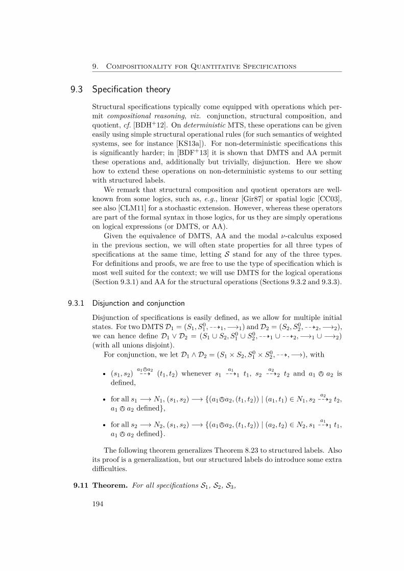
9. Compositionality for Quantitative Specifications

9.3 Specification theoryStructural specifications typically come equipped with operations which per-mit compositional reasoning, viz. conjunction, structural composition, andquotient, cf. [BDH+12]. On deterministic MTS, these operations can be giveneasily using simple structural operational rules (for such semantics of weightedsystems, see for instance [KS13a]). For non-deterministic specifications thisis significantly harder; in [BDF+13] it is shown that DMTS and AA permitthese operations and, additionally but trivially, disjunction. Here we showhow to extend these operations on non-deterministic systems to our settingwith structured labels.

We remark that structural composition and quotient operators are well-known from some logics, such as, e.g., linear [Gir87] or spatial logic [CC03],see also [CLM11] for a stochastic extension. However, whereas these operatorsare part of the formal syntax in those logics, for us they are simply operationson logical expressions (or DMTS, or AA).

Given the equivalence of DMTS, AA and the modal ν-calculus exposedin the previous section, we will often state properties for all three types ofspecifications at the same time, letting S stand for any of the three types.For definitions and proofs, we are free to use the type of specification which ismost well suited for the context; we will use DMTS for the logical operations(Section 9.3.1) and AA for the structural operations (Sections 9.3.2 and 9.3.3).

9.3.1 Disjunction and conjunction

Disjunction of specifications is easily defined, as we allow for multiple initialstates. For two DMTSD1 = (S1, S

01 , 99K1,−→1) andD2 = (S2, S

02 , 99K2,−→2),

we can hence define D1 ∨ D2 = (S1 ∪ S2, S01 ∪ S0

2 , 99K1 ∪ 99K2,−→1 ∪ −→2)(with all unions disjoint).

For conjunction, we let D1 ∧ D2 = (S1 × S2, S01 × S0

2 , 99K,−→), with

• (s1, s2) a17a299K (t1, t2) whenever s1

a199K1 t1, s2

a299K2 t2 and a1 7 a2 is

defined,

• for all s1 −→ N1, (s1, s2) −→ {(a17a2, (t1, t2)) | (a1, t1) ∈ N1, s2a299K2 t2,

a1 7 a2 defined},

• for all s2 −→ N2, (s1, s2) −→ {(a17a2, (t1, t2)) | (a2, t2) ∈ N2, s1a199K1 t1,

a1 7 a2 defined}.

The following theorem generalizes Theorem 8.23 to structured labels. Alsoits proof is a generalization, but our structured labels do introduce some extradifficulties.

9.11 Theorem. For all specifications S1, S2, S3,

194

9.3. Specification theory

• S1 ∨ S2 ≤m S3 iff S1 ≤m S3 and S2 ≤m S3,

• S1 ≤m S2 ∧ S3 iff S1 ≤m S2 and S1 ≤m S3,

• JS1 ∨ S2K = JS1K ∪ JS2K, and JS1 ∧ S2K = JS1K ∩ JS2K.

Proof: The proof that S1∨S2 ≤m S3 iff S1 ≤m S3 and S2 ≤m S3 is trivial: anymodal refinement R ⊆ (S1∪S2)×S3 splits into two refinements R1 ⊆ S1×S3,R2 ⊆ S2 × S3 and vice versa.

For the proof of the second claim, which we show for DMTS, we prove theback direction first. Let R2 ⊆ S1 × S2, R3 ⊆ S1 × S3 be initialized (DMTS)modal refinements which witness S1 ≤m S2 and S1 ≤m S3, respectively. DefineR = {(s1, (s2, s3)) | (s1, s2) ∈ R2, (s1, s3) ∈ R3} ⊆ S1 × (S2 × S3), then R isinitialized.

Now let (s1, (s2, s3)) ∈ R, then (s1, s2) ∈ R2 and (s1, s3) ∈ R3. Assumethat s1

a199K1 t1, then by S1 ≤m S2, we have s2

a299K2 t2 with a1 4 a2 and

(t1, t2) ∈ R2. Similarly, by S1 ≤m S3, we have s3a399K3 t3 with a1 4 a3

and (t1, t3) ∈ R3. But then also a1 4 a2 7 a3 and (t1, (t2, t3)) ∈ R, and(s2, s3) a27a3

99K (t2, t3) by definition.Assume that (s2, s3) −→ N . Without loss of generality we can assume that

there is s2 −→2 N2 such thatN = {(a27a3, (t2, t3)) | (a2, t2) ∈ N2, s3a399K3 t3}.

By S1 ≤m S2, we have s1 −→1 N1 such that ∀(a1, t1) ∈ N1 : ∃(a2, t2) ∈ N2 :a1 4 a2, (t1, t2) ∈ R2.

Let (a1, t1) ∈ N1, then also s1a199K1 t1, so by S1 ≤m S3, there is s3

a399K3 t3

with a1 4 a3 and (t1, t3) ∈ R3. By the above, we also have (a2, t2) ∈ N2 suchthat a1 4 a2 and (t1, t2) ∈ R2, but then (a2 7 a3, (t2, t3)) ∈ N , a1 4 a2 ∧ a3,and (t1, (t2, t3)) ∈ R.

For the other direction of the second claim, let R ⊆ S1 × (S2 × S3) bean initialized (DMTS) modal refinement which witnesses S1 ≤m S2 ∧ S3. Weshow that S1 ≤m S2, the proof of S1 ≤m S3 being entirely analogous. DefineR2 = {(s1, s2) | ∃s3 ∈ S3 : (s1, (s2, s3)) ∈ R} ⊆ S1 × S2, then R2 is initialized.

Let (s1, s2) ∈ R2, then we must have s3 ∈ S3 such that (s1, (s2, s3)) ∈ R.Assume that s1

a199K1 t1, then also (s2, s3) a

99K (t2, t3) for some a with a1 4 a

and (t1, (t2, t3)) ∈ R. By construction we have s2a299K2 t2 and s3

a399K3 t3 such

that a = a2 7 a3, but then a1 4 a2 7 a3 4 a2 and (t1, t2) ∈ R2.Assume that s2 −→2 N2, then by construction we have (s2, s3) −→ N =

{(a2 7 a3, (t2, t3)) | (a2, t2) ∈ N2, s3a399K3 t3}. By S1 ≤m S2 ∧ S3, there is

s1 −→1 N1 such that ∀(a1, t1) ∈ N1 : ∃(a, (t2, t3)) ∈ N : a1 4 a, (t1, (t2, t3)) ∈R.

Let (a1, t1) ∈ N1, then we have (a, (t2, t3)) ∈ N for which a1 4 a and(t1, (t2, t3)) ∈ R. By construction ofN , this implies that there are (a2, t2) ∈ N2

and s3a399K3 t3 such that a = a2 7 a3, but then a1 4 a2 7 a3 4 a2 and

(t1, t2) ∈ R.

195

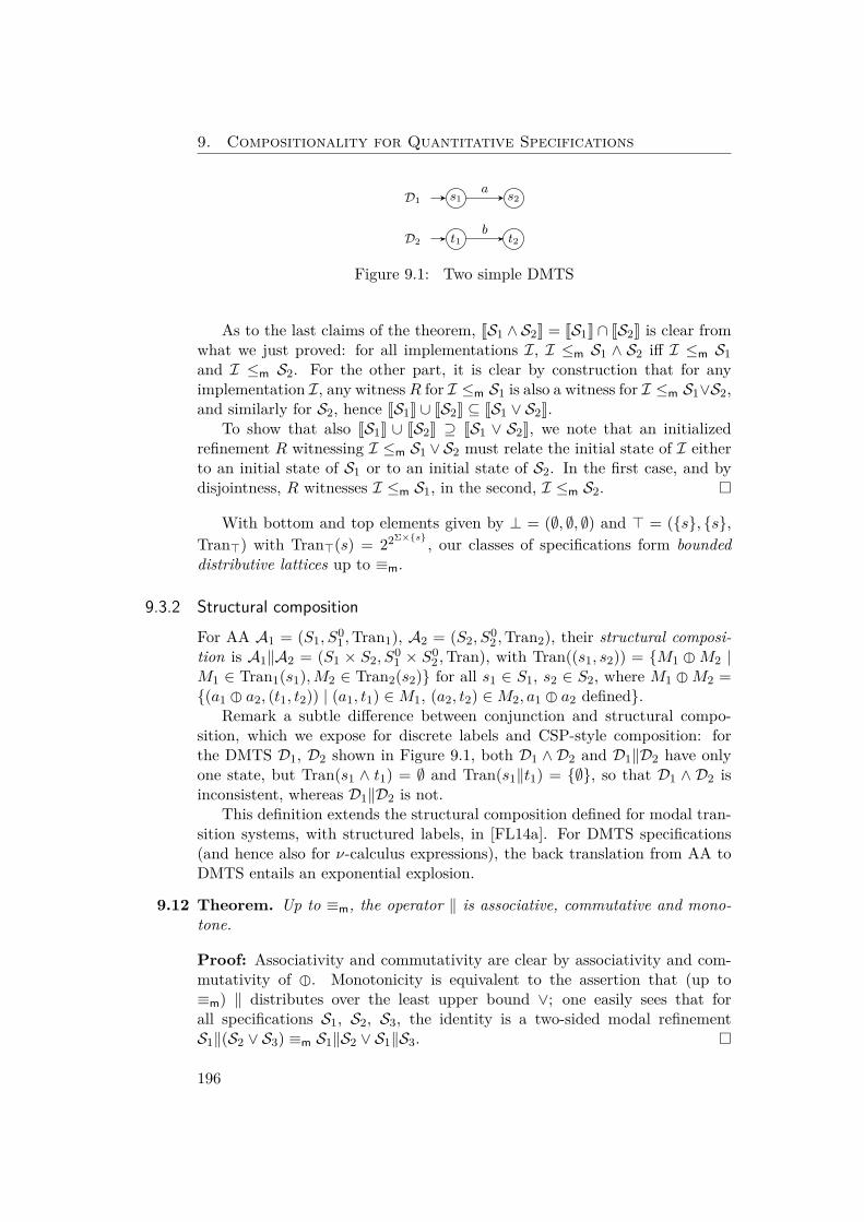
9. Compositionality for Quantitative Specifications

D1

D2

s1 s2

t1 t2

a

b

Figure 9.1: Two simple DMTS

As to the last claims of the theorem, JS1 ∧ S2K = JS1K ∩ JS2K is clear fromwhat we just proved: for all implementations I, I ≤m S1 ∧ S2 iff I ≤m S1and I ≤m S2. For the other part, it is clear by construction that for anyimplementation I, any witness R for I ≤m S1 is also a witness for I ≤m S1∨S2,and similarly for S2, hence JS1K ∪ JS2K ⊆ JS1 ∨ S2K.

To show that also JS1K ∪ JS2K ⊇ JS1 ∨ S2K, we note that an initializedrefinement R witnessing I ≤m S1 ∨ S2 must relate the initial state of I eitherto an initial state of S1 or to an initial state of S2. In the first case, and bydisjointness, R witnesses I ≤m S1, in the second, I ≤m S2. �

With bottom and top elements given by ⊥ = (∅, ∅, ∅) and > = ({s}, {s},Tran>) with Tran>(s) = 22Σ×{s} , our classes of specifications form boundeddistributive lattices up to ≡m.

9.3.2 Structural compositionFor AA A1 = (S1, S

01 ,Tran1), A2 = (S2, S

02 ,Tran2), their structural composi-

tion is A1‖A2 = (S1 × S2, S01 × S0

2 ,Tran), with Tran((s1, s2)) = {M1 �M2 |M1 ∈ Tran1(s1),M2 ∈ Tran2(s2)} for all s1 ∈ S1, s2 ∈ S2, where M1 �M2 ={(a1 � a2, (t1, t2)) | (a1, t1) ∈M1, (a2, t2) ∈M2, a1 � a2 defined}.

Remark a subtle difference between conjunction and structural compo-sition, which we expose for discrete labels and CSP-style composition: forthe DMTS D1, D2 shown in Figure 9.1, both D1 ∧ D2 and D1‖D2 have onlyone state, but Tran(s1 ∧ t1) = ∅ and Tran(s1‖t1) = {∅}, so that D1 ∧ D2 isinconsistent, whereas D1‖D2 is not.

This definition extends the structural composition defined for modal tran-sition systems, with structured labels, in [FL14a]. For DMTS specifications(and hence also for ν-calculus expressions), the back translation from AA toDMTS entails an exponential explosion.

9.12 Theorem. Up to ≡m, the operator ‖ is associative, commutative and mono-tone.

Proof: Associativity and commutativity are clear by associativity and com-mutativity of �. Monotonicity is equivalent to the assertion that (up to≡m) ‖ distributes over the least upper bound ∨; one easily sees that forall specifications S1, S2, S3, the identity is a two-sided modal refinementS1‖(S2 ∨ S3) ≡m S1‖S2 ∨ S1‖S3. �

196

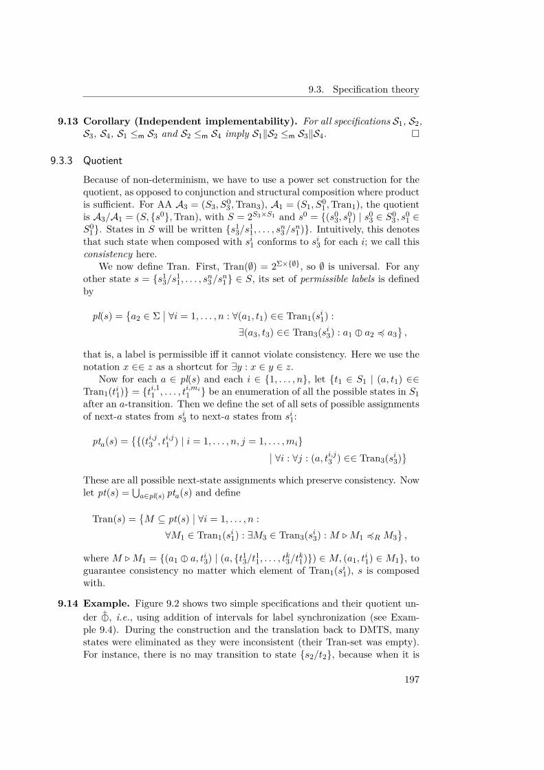
9.3. Specification theory

9.13 Corollary (Independent implementability). For all specifications S1, S2,S3, S4, S1 ≤m S3 and S2 ≤m S4 imply S1‖S2 ≤m S3‖S4. �

9.3.3 QuotientBecause of non-determinism, we have to use a power set construction for thequotient, as opposed to conjunction and structural composition where productis sufficient. For AA A3 = (S3, S

03 ,Tran3), A1 = (S1, S

01 ,Tran1), the quotient

is A3/A1 = (S, {s0},Tran), with S = 2S3×S1 and s0 = {(s03, s

01) | s0

3 ∈ S03 , s

01 ∈

S01}. States in S will be written {s1

3/s11, . . . , s

n3/s

n1 )}. Intuitively, this denotes

that such state when composed with si1 conforms to si3 for each i; we call thisconsistency here.

We now define Tran. First, Tran(∅) = 2Σ×{∅}, so ∅ is universal. For anyother state s = {s1

3/s11, . . . , s

n3/s

n1} ∈ S, its set of permissible labels is defined

by

pl(s) ={a2 ∈ Σ

∣∣ ∀i = 1, . . . , n : ∀(a1, t1) ∈∈ Tran1(si1) :∃(a3, t3) ∈∈ Tran3(si3) : a1 � a2 4 a3

},

that is, a label is permissible iff it cannot violate consistency. Here we use thenotation x ∈∈ z as a shortcut for ∃y : x ∈ y ∈ z.

Now for each a ∈ pl(s) and each i ∈ {1, . . . , n}, let {t1 ∈ S1 | (a, t1) ∈∈Tran1(ti1)} = {ti,11 , . . . , ti,mi1 } be an enumeration of all the possible states in S1after an a-transition. Then we define the set of all sets of possible assignmentsof next-a states from si3 to next-a states from si1:

pta(s) ={{(ti,j3 , ti,j1 ) | i = 1, . . . , n, j = 1, . . . ,mi}∣∣ ∀i : ∀j : (a, ti,j3 ) ∈∈ Tran3(si3)

}These are all possible next-state assignments which preserve consistency. Nowlet pt(s) = ⋃

a∈pl(s) pta(s) and define

Tran(s) ={M ⊆ pt(s)

∣∣ ∀i = 1, . . . , n :∀M1 ∈ Tran1(si1) : ∃M3 ∈ Tran3(si3) : M .M1 4R M3

},

where M .M1 = {(a1 � a, ti3) | (a, {t13/t11, . . . , tk3/tk1)}) ∈M, (a1, ti1) ∈M1}, to

guarantee consistency no matter which element of Tran1(si1), s is composedwith.

9.14 Example. Figure 9.2 shows two simple specifications and their quotient un-der +

�, i.e., using addition of intervals for label synchronization (see Exam-ple 9.4). During the construction and the translation back to DMTS, manystates were eliminated as they were inconsistent (their Tran-set was empty).For instance, there is no may transition to state {s2/t2}, because when it is

197

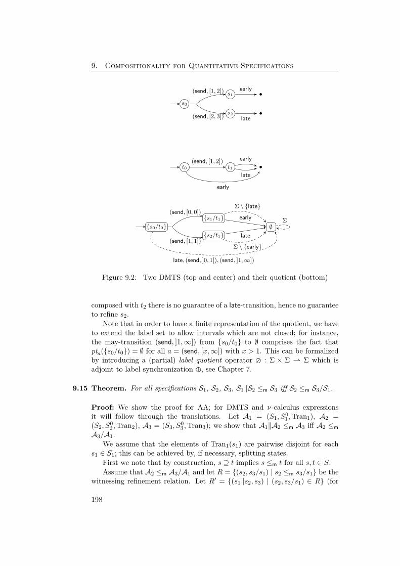
9. Compositionality for Quantitative Specifications

s0

s1(send, [1, 2])

s2(send, [2, 3])

•early

•late

t0 t1(send, [1, 2])

•early

late

early

{s0/t0}{s1/t1}

{s2/t1}∅

Σ(send, [0, 0])

(send, [1, 1])

late, (send, ]0, 1[), (send, ]1,∞])

Σ \ {late}

early

Σ \ {early}

late

Figure 9.2: Two DMTS (top and center) and their quotient (bottom)

composed with t2 there is no guarantee of a late-transition, hence no guaranteeto refine s2.

Note that in order to have a finite representation of the quotient, we haveto extend the label set to allow intervals which are not closed; for instance,the may-transition (send, ]1,∞]) from {s0/t0} to ∅ comprises the fact thatpta({s0/t0}) = ∅ for all a = (send, [x,∞]) with x > 1. This can be formalizedby introducing a (partial) label quotient operator � : Σ × Σ ⇀ Σ which isadjoint to label synchronization �, see Chapter 7.

9.15 Theorem. For all specifications S1, S2, S3, S1‖S2 ≤m S3 iff S2 ≤m S3/S1.

Proof: We show the proof for AA; for DMTS and ν-calculus expressionsit will follow through the translations. Let A1 = (S1, S

01 ,Tran1), A2 =

(S2, S02 ,Tran2), A3 = (S3, S

03 ,Tran3); we show that A1‖A2 ≤m A3 iff A2 ≤m

A3/A1.We assume that the elements of Tran1(s1) are pairwise disjoint for each

s1 ∈ S1; this can be achieved by, if necessary, splitting states.First we note that by construction, s ⊇ t implies s ≤m t for all s, t ∈ S.Assume that A2 ≤m A3/A1 and let R = {(s2, s3/s1) | s2 ≤m s3/s1} be the

witnessing refinement relation. Let R′ = {(s1‖s2, s3) | (s2, s3/s1) ∈ R} (for

198

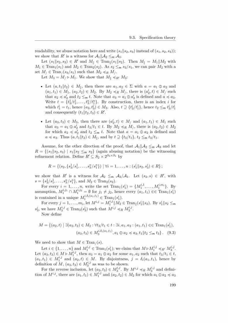
9.3. Specification theory

readability, we abuse notation here and write (s1‖s2, s3) instead of (s1, s2, s3));we show that R′ is a witness for A1‖A2 ≤m A3.

Let (s1‖s2, s3) ∈ R′ and M‖ ∈ Tran‖(s1‖s2). Then M‖ = M1‖M2 withM1 ∈ Tran1(s1) and M2 ∈ Tran2(s2). As s2 ≤m s3/s1, we can pair M2 with aset M/ ∈ Tran/(s3/s1) such that M2 4R M/.

Let M3 = M/ . M1. We show that M‖ 4R′ M3:

• Let (a, t1‖t2) ∈ M‖, then there are a1, a2 ∈ Σ with a = a1 � a2 and(a1, t1) ∈ M1, (a2, t2) ∈ M2. By M2 4R M/, there is (a′2, t) ∈ M/ suchthat a2 4 a′2 and t2 ≤m t. Note that a3 = a1 � a′2 is defined and a 4 a3.Write t = {t13/t11, . . . , tn3/tn1}. By construction, there is an index i forwhich ti1 = t1, hence (a3, t

i3) ∈M3. Also, t ⊇ {ti3/ti1}, hence t2 ≤m ti3/t

i1

and consequently (t1‖t2, t3) ∈ R′.

• Let (a3, t3) ∈ M3, then there are (a′2, t) ∈ M/ and (a1, t1) ∈ M1 suchthat a3 = a1 � a′2 and t3/t1 ∈ t. By M2 4R M/, there is (a2, t2) ∈ M2for which a2 4 a′2 and t2 ≤m t. Note that a = a1 � a2 is defined anda 4 a3. Thus (a, t1‖t2) ∈M‖, and by t ⊇ {t3/t1}, t2 ≤m t3/t1.

Assume, for the other direction of the proof, that A1‖A2 ≤m A3 and letR = {(s1‖s2, s3) | s1‖s2 ≤m s2} (again abusing notation) be the witnessingrefinement relation. Define R′ ⊆ S2 × 2S3×S1 by

R ={(s2, {s1

3/s11, . . . , s

n3/s

n1})

∣∣ ∀i = 1, . . . , n : (si1‖s2, si3) ∈ R} ;

we show that R′ is a witness for A2 ≤m A3/A1. Let (s2, s) ∈ R′, withs = {s1

3/s11, . . . , s

n3/s

n1}, and M2 ∈ Tran2(s2).

For every i = 1, . . . , n, write the set Tran1(si1) = {M i,11 , . . . ,M i,mi

1 }. Byassumption, M i,j1

1 ∩M i,j21 = ∅ for j1 6= j2, hence every (a1, t1) ∈∈ Tran1(si1)

is contained in a unique M i,δi(a1,t1)1 ∈ Tran1(si1).

For every j = 1, . . . ,mi, letM i,j = M i,j1 ‖M2 ∈ Tran‖(si1‖s2). By si1‖s2 ≤m

si3, we have M i,j3 ∈ Tran3(si3) such that M i,j 4R M

i,j3 .

Now define

M ={(a2, t)

∣∣ ∃(a2, t2) ∈M2 : ∀t3/t1 ∈ t : ∃i, a1, a3 : (a1, t1) ∈∈ Tran1(si1),

(a3, t3) ∈M i,δi(a1,t1)3 , a1 � a2 4 a3, t1‖t2 ≤m t3} . (9.3)

We need to show that M ∈ Tran/(s).Let i ∈ {1, . . . , n} andM i,j

1 ∈ Tran1(si1); we claim thatM .M i,j1 4R′ M

i,j3 .

Let (a3, t3) ∈M .M i,j1 , then a3 = a1 � a2 for some a1, a2 such that t3/t1 ∈ t,

(a1, t1) ∈ M i,j1 and (a2, t) ∈ M . By disjointness, j = δi(a1, t1), hence by

definition of M , (a3, t3) ∈M i,j3 as was to be shown.

For the reverse inclusion, let (a3, t3) ∈M i,j3 . By M i,j 4R M

i,j3 and defini-

tion of M i,j , there are (a1, t1) ∈M i,j1 and (a2, t2) ∈M2 for which a1�a2 4 a3

199

9. Compositionality for Quantitative Specifications

and t1‖t2 ≤m t3. Thus j = δi(a1, t1), so that there must be (a2, t) ∈ M forwhich t3/t1 ∈ t, but then also (a1 � a2, t3) ∈M .M i,j

1 .We show that M2 4R′ M .

• Let (a2, t2) ∈M2. For every i = 1, . . . , n and every (a1, t1) ∈∈ Tran1(ti1),we can use M i,j 4R M

i,j3 and choose an element (ηi(a1, t1), τi(a1, t1)) ∈

Mi,δi(a1,t1)3 for which t1‖t2 ≤m τi(a1, t1) and a1 � a2 4 ηi(a1, t1). Let

t = {τi(a1, t1)/t1 | i = 1, . . . , n, (a1, t1) ∈∈ Tran1(ti1)}, then (a2, t) ∈ Mand (t2, t) ∈ R′.

• Let (a2, t) ∈ M , then we have (a2, t2) ∈ M2 satisfying the conditionsin (9.3). Hence t1‖t2 ≤m t3 for all t3/t1 ∈ t, so that (t2, t) ∈ R′. �

9.4 Robust Specification TheoriesWe proceed to lift the results of the previous sections to a quantitative setting,where the Boolean notions of modal and thorough refinement are replacedby refinement distances. We have shown in previous chapters that a goodsetting for quantitative analysis is given by the one of recursively specifiedtrace distances on an abstract complete lattice L. In order to extend thisto specification theories, we enrich L with an addition like in Chapter 7 andrequire it to be a (commutative) quantale, see below.

Denote by Σ∞ = Σ∗ ∪ Σω the set of finite and infinite traces over Σ.

9.4.1 Recursively specified trace distances

Recall that a (commutative) quantale consists of a complete lattice (L,vL)and a commutative, associative addition operation �L which distributes overarbitrary suprema; we denote by ⊥L, >L the bottom and top elements ofL. We call a function d : X × X → L, for a set X and a quantale L,an L-hemimetric if it satisfies d(x, x) = ⊥L for all x ∈ X and d(x, z) vLd(x, y) �L d(y, z) for all x, y, z ∈ X.

L-hemimetrics are generalizations of distances: for L = R≥0 ∪ {∞} theextended real line, an (R≥0∪{∞})-hemimetric is simply an extended hemimet-ric, i.e., a function d : X ×X → R≥0 ∪ {∞} which satisfies d(x, x) = 0 for allx ∈ X and the triangle inequality d(x, z) ≤ d(x, y) +d(y, z) for all x, y, z ∈ X.If d also is symmetric, i.e., satisfies d(x, y) = d(y, x) for all x, y ∈ X, then d isusually called a pseudometric. If d also satisfies the principle of separability,or indiscernibility of identicals, i.e., such that d(x, y) = 0 implies x = y, it iscalled a metric.

A recursive trace distance specification (L, eval, dLtr, F ) consists of a quan-tale L, a quantale morphism eval : L → R≥0 ∪ {∞}, an L-hemimetricdLtr : Σ∞ × Σ∞ → L (called lifted trace distance), and a distance iterator

200

9.4. Robust Specification Theories

function F : Σ × Σ × L → L. For our purposes, F must be monotone inthe third and anti-monotone in the second coordinate and satisfy an extendedtriangle inequality: for all a, b, c ∈ Σ and α, β ∈ L, F (a, b, α)�L F (b, c, β) wLF (a, c, α�L β).

F is to specify dLtr recursively in the sense that for all a, b ∈ Σ and allσ, τ ∈ Σ∞ (and with “.” denoting concatenation),

dLtr(a.σ, b.τ) = F (a, b, dLtr(σ, τ)) . (9.4)

The trace distance associated with such a distance specification is dtr : Σ∞ ×Σ∞ → R≥0 given by dtr = eval ◦ dLtr.

Note that dLtr specializes to a distance on labels (because Σ ⊆ Σ∞);we require that this is compatible with label refinement in the sense thata 4 b implies dLtr(a, b) = ⊥L. Then (9.4) implies that whenever a 4 b, thenF (a, b,⊥L) = dLtr(a, b) = ⊥L. As an inverse property, we say that F is recur-sively separating if F (a, b, α) = ⊥L implies that a 4 b and α = ⊥L.

9.16 Example. We have shown in previous chapters that all commonly used tracedistances obey recursive characterizations as above. We give a few examples,all of which are recursively separating:

The point-wise distance from [dAFH+05] has L = R≥0 ∪ {∞}, eval = idand

dLtr(a.σ, b.τ) = max(d(a, b), dLtr(σ, τ)) ,where d : Σ × Σ → R≥0 ∪ {∞} is a hemimetric on labels. For the label setΣ = U×{[l, r] | l ∈ R∪{−∞}, r ∈ R∪{∞}, l ≤ r} from Example 9.2, one use-ful example of such a hemimetric is d((u1, [l1, r1]), (u2, [l2, r2])) = supx1∈[l1,r1]infx2∈[l2,r2] |x1 − x2| = max(l2 − l1, r1 − r2, 0) if u1 = u2 and ∞ otherwise.

The discounting distance, also used in [dAFH+05], again uses L = R≥0 ∪{∞} and eval = id, but

dLtr(a.σ, b.τ) = d(a, b) + λdLtr(σ, τ)

for a constant λ ∈ [0, 1[.For the limit-average distance used in [ČHR12] and other papers, L =

(R≥0 ∪ {∞})N, eval(α) = lim infj∈N α(j), and

dLtr(a.σ, b.τ)(j) = 1j+1d(a, b) + j

j+1dL

tr(σ, τ)(j − 1) .

It is clear that limit-average distance has no recursive specification which usesL = R≥0 ∪ {∞} as for the other distances above. Intuitively, the quantale(R≥0∪{∞})N has to be used to memorize how many symbols one has seen inthe sequences σ, τ . This and other examples show that using general quantalesin recursive trace distance specifications instead of simply L = R≥0 ∪ {∞} isnecessary.

The discrete trace distance is given by dtr(σ, τ) = 0 if σ 4 τ and ∞otherwise (here we have extended 4 to traces in the obvious way). It has a

201

9. Compositionality for Quantitative Specifications

recursive characterization with L = R≥0 ∪ {∞}, eval = id, and dtr(a.σ, b.τ) =dtr(σ, τ) if a 4 b and ∞ otherwise.

For the rest of this paper, we fix a recursively specified trace distance.

9.4.2 Refinement distancesWe lift the notions of modal refinement, for all our formalisms, to distances.Conceptually, this is done by replacing “∀” quantifiers by “sup” and “∃” by“inf” in the definitions, and then using the distance iterator to introduce arecursive functional whose least fixed point is the distance.

9.17 Definition. The lifted refinement distance on the states of DMTS D1 =(S1, S

01 , 99K1,−→1) and D2 = (S2, S

02 , 99K2,−→2) is the least fixed point to

the equations

dLm(s1, s2) = max

sups1

a199Kt1

infs2

a299Kt2

F (a1, a2, dLm(t1, t2)) ,

sups2−→N2

infs1−→N1

sup(a1,t1)∈N1

inf(a2,t2)∈N2

F (a1, a2, dLm(t1, t2)) ,

for s1 ∈ S1, s2 ∈ S2. For AA A1 = (S1, S01 ,Tran1), A2 = (S2, S

02 ,Tran2), the

right-hand side is replaced by

supM1∈Tran1(s1)

infM2∈Tran2(s2)

max

sup

(a1,t1)∈M1

inf(a2,t2)∈M2

F (a1, a2, dLm(t1, t2)) ,

sup(a2,t2)∈M2

inf(a1,t1)∈M1

F (a1, a2, dLm(t1, t2)) ,

and for ν-calculus expressions N1 = (X1, X01 ,∆1), N2 = (X2, X

02 ,∆2) in nor-

mal form, it is

max

sup

a1∈Σ,y1∈�a11 (x1)

infa2∈Σ,y2∈�

a22 (x2)

F (a1, a2, dLm(y1, y2)) ,

supN2∈♦2(x2)

infN1∈♦1(x1)

sup(a1,y1)∈N1

inf(a2,y2)∈N2

F (a1, a2, dLm(y1, y2)) .

Using Tarski’s fixed point theorem, one easily sees that the lifted refine-ment distances are indeed well-defined. (Here one needs monotonicity of F inthe third coordinate, together with the fact that sup and inf are monotonic.)

Note that we define the distances using least fixed points, as opposed tothe greatest fixed point definition of standard refinement. Informally, this isbecause our order is reversed: we are not interested in maximizing refinementrelations, but in minimizing refinement distance.

The lifted refinement distance between specifications is defined by

dLm(S1,S2) = sups01∈S

01

infs02∈S

02

dLm(s01, s

02) .

202

9.4. Robust Specification Theories

Analogously to thorough refinement, there is also a lifted thorough refinementdistance, given by dLth(S1,S2) = supI1∈JS1K infI2∈JS2K d

Lm(I1, I2).

Using the eval function, one gets distances dm = eval ◦ dLm and dth =eval ◦ dLth, with values in R≥0 ∪ {∞}, which will be the ones one is interestedin for concrete applications.

We recall the notion of refinement family from Chapter 7 and extend it tospecifications. We give the definition for AA only; for DMTS and the modalν-calculus it is similar.

9.18 Definition. A refinement family from A1 to A2, for AA A1 = (S1, S01 ,Tran1),

A2 = (S2, S02 ,Tran2), is an L-indexed family of relations R = {Rα ⊆ S1×S2 |

α ∈ L} with the property that for all α ∈ L with α 6= >L, all (s1, s2) ∈ Rα,and all M1 ∈ Tran1(s1), there is M2 ∈ Tran2(s2) such that

• ∀(a1, t1) ∈M1 : ∃(a2, t2) ∈M2, β ∈ L : (t1, t2) ∈ Rβ, F (a1, a2, β) v α,

• ∀(a2, t2) ∈M2 : ∃(a1, t1) ∈M1, β ∈ L : (t1, t2) ∈ Rβ, F (a1, a2, β) v α.

9.19 Lemma. For all AA A1 = (S1, S01 ,Tran1), A2 = (S2, S

02 ,Tran2), there exists

a refinement family R from A1 to A2 such that for all s01 ∈ S0

1 , there is s02 ∈ S0

2for which (s0

1, s02) ∈ RdLm(A1,A2).

We say that a refinement family as in the lemma witnesses dLm(A1,A2).

Proof: Define R by Rα = {(s1, s2) | dLm(s1, s2) vL α}. First, as (s01, s

02) ∈

RdLm(s01,s02) for all s01 ∈ S0

1 , s02 ∈ S0

2 , it is indeed the case that for all s01 ∈ S0

1 ,there is s0

2 ∈ S02 for which

(s01, s

02) ∈ RdLm(A1,A2) = Rmax

s01∈S01

mins02∈S

02dLm(s01,s02) .

Now let α ∈ L with α 6= >L and (s1, s2) ∈ Rα. Let M1 ∈ Tran1(s1). Wehave dLm(s1, s2) vL α, hence there is M2 ∈ Tran2(s2) such that

α wL max

sup

(a1,t1)∈M1

inf(a2,t2)∈M2

F (a1, a2, dLm(t1, t2)) ,

sup(a2,t2)∈M2

inf(a1,t1)∈M1

F (a1, a2, dLm(t1, t2)) .

But this entails that for all (a1, t1) ∈ M1, there is (a2, t2) ∈ M2 and β =dLm(t1, t2) with F (a1, a2, β) vL α, and that for all (a2, t2) ∈ M2, there is(a1, t1) ∈M1 and β = dLm(t1, t2) such that F (a1, a2, β) vL α. �

The following quantitative extension of Theorems 9.7 and 9.10 shows thatour translations preserve and reflect refinement distances.

203

9. Compositionality for Quantitative Specifications

9.20 Theorem. For all DMTS D1,D2, all AA A1, A2 and all ν-calculus expres-sions N1, N2:

dLm(D1,D2) = dLm(da(D1), da(D2))dLm(A1,A2) = dLm(ad(A1), ad(A2))dLm(D1,D2) = dLm(dn(D1), dn(D2))dLm(N1,N2) = dLm(nd(N1),nd(N2))

Proof:dLm(da(D1), da(D2)) vL dLm(D1,D2):

Let D1 = (S1, S01 , 99K1,−→1) and D2 = (S2, S

02 , 99K2,−→2) be DMTS.

There exists a DMTS refinement family R = {Rα ⊆ S1 × S2 | α ∈ L} suchthat for all s0

1 ∈ S01 , there is s0

2 ∈ S02 with (s0

1, s02) ∈ RdLm(D1,D2). We show that

R is an AA refinement family.Let α ∈ L and (s1, s2) ∈ Rα. Let M1 ∈ Tran1(s1) and define

M2 ={(a2, t2) | s2

a299K2 t2,∃(a1, t1) ∈M1 : ∃β ∈ L :

(t1, t2) ∈ Rβ, F (a1, a2, β) vL α}.

The condition

∀(a2, t2) ∈M2 : ∃(a1, t1) ∈M1, β ∈ L : (t1, t2) ∈ Rβ, F (a1, a2, β) v α

is satisfied by construction. For the inverse condition, let (a1, t1) ∈ M1, thens1

a199K1 t1, and as R is a DMTS refinement family, this implies that there is

s2a299K2 t2 and β ∈ L for which (t1, t2) ∈ Rβ and F (a1, a2, β) vL α, so that

(a2, t2) ∈M2 by construction.We are left with showing that M2 ∈ Tran2(s2). First we notice that by

construction, indeed s2a299K2 t2 for all (a2, t2) ∈ M2. Now let s2 −→ N2; we

need to show that N2 ∩M2 6= ∅.We have s1 −→ N1 such that ∀(a1, t1) ∈ N1 : ∃(a2, t2) ∈ N2, β ∈ L :

(t1, t2) ∈ Rβ, F (a1, a2, β) vL α. We know that N1 ∩M1 6= ∅, so let (a1, t1) ∈N1 ∩M1. Then there is (a2, t2) ∈ N2 and β ∈ L such that (t1, t2) ∈ Rβ andF (a1, a2, β) vL α. But (a2, t2) ∈ N2 implies s2

a299K2 t2, hence (a2, t2) ∈M2.

dLm(D1,D2) vL dLm(da(D1), da(D2)):Let D1 = (S1, S

01 , 99K1,−→1) and D2 = (S2, S

02 , 99K2,−→2) be DMTS.

There exists an AA refinement family R = {Rα ⊆ S1 × S2 | α ∈ L} such thatfor all s0

1 ∈ S01 , there is s0

2 ∈ S02 for which (s0

1, s02) ∈ RdLm(da(D1),da(D2)). We

show that R is a DMTS refinement family. Let α ∈ L and (s1, s2) ∈ Rα.Let s1

a199K1 t1, then we cannot have s1 −→ ∅. LetM1 = {(a1, t1)}∪⋃{N1 |

s1 −→ N1}, then M1 ∈ Tran1(s1) by construction. This implies that thereis M2 ∈ Tran2(s2), (a2, t2) ∈ M2 and β ∈ L such that (t1, t2) ∈ Rβ andF (a1, a2, β) vL α, but then also s2

a299K t2 as was to be shown.

204

9.4. Robust Specification Theories

Let s2 −→ N2 and assume, for the sake of contradiction, that there isno s1 −→ N1 for which ∀(a1, t1) ∈ N1 : ∃(a2, t2) ∈ N2, β ∈ L : (t1, t2) ∈Rβ, F (a1, a2, β) vL α holds. Then for each s1 −→ N1, there is an element(aN1 , tN1) ∈ N1 such that ∃(a2, t2) ∈ N2, β ∈ L : (tN1 , t2) ∈ Rβ, F (aN1 , a2,β) vL α does not hold.

Let M1 = {(aN1 , tN1) | s1 −→ N1}, then M1 ∈ Tran1(s1) by construction.Hence we have M2 ∈ Tran2(s2) such that ∀(a2, t2) ∈ M2 : ∃(a1, t2) ∈ M1, β ∈L : (t1, t2) ∈ Rβ, F (a1, a2, β) v α. Now N2 ∩ M2 6= ∅, so let (a2, t2) ∈N2 ∩M2, then there is (a1, t1) ∈ M1 and β ∈ L such that (t1, t2) ∈ Rβ andF (a1, a2, β) vL α, in contradiction to how M1 was constructed.dLm(ad(A1), ad(A2)) vL dLm(A1,A2):

Let A1 = (S1, S01 ,Tran1), A2 = (S2, S

02 ,Tran2) be AA, with DMTS trans-

lations ad(A1) = (D1, D01,−→1, 99K1), ad(A2) = (D2, D

02,−→2, 99K2). There

is an AA refinement family R = {Rα ⊆ S1 × S2 | α ∈ L} such that for alls0

1 ∈ S01 , there is s0

2 ∈ S02 with (s0

1, s02) ∈ RdLm(A1,A2).

Define a relation family R′ = {R′α ⊆ D1 ×D2 | α ∈ L} by

R′α ={(M1,M2)

∣∣ ∃(s1, s2) ∈ Rα : M1 ∈ Tran1(s1),M2 ∈ Tran(s2),∀(a1, t1) ∈M1 : ∃(a2, t2) ∈M2, β ∈ L :

(t1, t2) ∈ Rβ, F (a1, a2, β) vL α ,∀(a2, t2) ∈M2 : ∃(a1, t1) ∈M1, β ∈ L :

(t1, t2) ∈ Rβ, F (a1, a2, β) vL α}.

We show that R′ is a witness for dLm(ad(A1), ad(A2)) vL dLm(A1,A2). Letα ∈ L and (M1,M2) ∈ R′α.

Let M2 −→2 N2. By construction of −→, there is (a2, t2) ∈M2 such thatN2 = {(a2,M

′2) | M ′2 ∈ Tran2(t2)}. Then (M1,M2) ∈ R′α implies that there

must be (a1, t1) ∈M1 and β ∈ L such that (t1, t2) ∈ Rβ and F (a1, a2, β) vL α.Let N1 = {(a1,M

′1) |M ′1 ∈ Tran1(t1)}, then M1 −→1 N1.

We show that ∀(a1,M′1) ∈ N1 : ∃(a2,M

′2) ∈ N2 : (M ′1,M ′2) ∈ R′β: Let

(a1,M′1) ∈ N1, then M ′1 ∈ Tran1(t1). From (t1, t2) ∈ Rβ we get M ′2 ∈

Tran2(t2) such that

∀(b1, u1) ∈M ′1 : ∃(b2, u2) ∈M ′2, γ ∈ L : (u1, u2) ∈ Rγ , F (b1, b2, γ) vL β ,∀(b2, u2) ∈M ′2 : ∃(b1, u1) ∈M ′1, γ ∈ L : (u1, u2) ∈ Rγ , F (b1, b2, γ) vL β ,

hence (M ′1,M ′2) ∈ R′β; also, (a2,M′2) ∈ N2 by construction of N2.

Let M1a199K1 M ′1, then we have M1 −→1 N1 for which (a1,M

′1) ∈ N1 by

construction of 99K1. This in turn implies that there must be (a1, t1) ∈ M1such that N1 = {(a1,M

′′1 ) | M ′′1 ∈ Tran1(t1)}. By (M1,M2) ∈ R′α, we get

(a2, t2) ∈ M2 and β ∈ L such that (t1, t2) ∈ Rβ and F (a1, a2, β) vL α. LetN2 = {(a2,M

′2) | M ′2 ∈ Tran2(t2)}, then M2 −→2 N2 and hence M2

a299K2 M ′2

205

9. Compositionality for Quantitative Specifications

for all (a2,M′2) ∈ N2. By the same arguments as above, there is (a2,M

′2) ∈ N2

for which (M ′1,M ′2) ∈ R′β.We miss to show that R′ is initialized. LetM0

1 ∈ D01, then we have s0

1 ∈ S01

with M01 ∈ Tran1(s0

1). As R is initialized, this entails that there is s02 ∈ S0

2with (s0

1, s02) ∈ RdLm(A1,A2), which gives us M0

2 ∈ Tran2(s02) which satisfies the

conditions in the definition of R′dLm(A1,A2), whence (M01 ,M

02 ) ∈ R′dLm(A1,A2).

dLm(A1,A2) vL dLm(ad(A1), ad(A2)):Let A1 = (S1, S

01 ,Tran1), A2 = (S2, S

02 ,Tran2) be AA, with DMTS trans-

lations ad(A1) = (D1, D01,−→1, 99K1), ad(A2) = (D2, D

02,−→2, 99K2). There

is a DMTS refinement family R = {Rα ⊆ D1 ×D2 | α ∈ L} such that for allM0

1 ∈ D01, there exists M0

2 ∈ D02 with (M0

1 ,M02 ) ∈ RdLm(ad(A1),ad(A2)).

Define a relation family R′ = {R′α ⊆ S1 × S2 | α ∈ L} by

R′α ={(s1, s2)

∣∣ ∀M1 ∈ Tran1(s1) : ∃M2 ∈ Tran2(s2) : (M1,M2) ∈ Rα}

;

we will show that R′ is a witness for dLm(A1,A2) vL dLm(ad(A1), ad(A2)).Let α ∈ L, (s1, s2) ∈ R′α and M1 ∈ Tran1(s1), then by construction of R′,

we have M2 ∈ Tran2(s2) with (M1,M2) ∈ Rα.Let (a2, t2) ∈ M2 and define N2 = {(a2,M

′2) | M ′2 ∈ Tran2(t2)}, then

M2 −→2 N2. Now (M1,M2) ∈ Rα implies that there must be M1 −→1N1 satisfying ∀(a1,M

′1) ∈ N1 : ∃(a2,M

′2) ∈ N2, β ∈ L : (M ′1,M ′2) ∈ Rβ,

F (a1, a2, β) vL α. We have (a1, t1) ∈ M1 such that N1 = {(a1,M′1) | M ′1 ∈

Tran1(t1)}; we only miss to show that (t1, t2) ∈ R′β for some β ∈ L for whichF (a1, a2, β) vL α. Let M ′1 ∈ Tran1(t1), then (a1,M

′1) ∈ N1, hence there is

(a2,M′2) ∈ N2 and β ∈ L such that (M ′1,M ′2) ∈ Rβ and F (a1, a2, β) v α, but

(a2,M′2) ∈ N2 also entails M ′2 ∈ Tran2(t2).

Let (a1, t1) ∈ M1 and define N1 = {(a1,M′1) | M ′1 ∈ Tran1(t1)}, then

M1 −→1 N1. Now let (a1,M′1) ∈ N1, then M1

a199K1 M ′1, hence we have

M2a299K2 M ′2 and β ∈ L such that (M ′1,M ′2) ∈ Rβ and F (a1, a2, β) vL α. By

construction of 99K2, this implies that there isM2 −→2 N2 with (a2,M′2) ∈ N2,

and we have (a2, t2) ∈M2 for which N2 = {(a2,M′′2 ) |M ′′2 ∈ Tran2(t2)}. Now

if M ′′1 ∈ Tran1(t1), then (a1,M′′1 ) ∈ N1, hence there is (a2,M

′′2 ) ∈ N2 with

(M ′′1 ,M ′′2 ) ∈ Rβ, but (a,M ′′2 ) ∈ N2 also gives M ′′2 ∈ Tran2(t2).We miss to show that R′ is initialized. Let s0

1 ∈ S01 and M0

1 ∈ Tran1(s01).

As R is initialized, this gets us M02 ∈ D2 with (M0

1 ,M02 ) ∈ RdLm(ad(A1),ad(A2)),

but M02 ∈ Tran2(s0

2) for some s02 ∈ S0

2 , and then (s01, s

02) ∈ R′dLm(ad(A1),ad(A2)).

dLm(dn(D1), dn(D2)) vL dLm(D1,D2):Let D1 = (S1, S

01 , 99K1,−→1) and D2 = (S2, S

02 , 99K2,−→2) be DMTS,

with ν-calculus translations dn(D1) = (S1, S01 ,∆1) and dn(D2) = (S2, S

02 ,∆2).

There is a DMTS refinement family R = {Rα ⊆ S1 × S2 | α ∈ L} such thatfor all s0

1 ∈ S01 , there exists s0

2 ∈ S02 for which (s0

1, s02) ∈ RdLm(D1,D2).

206

9.4. Robust Specification Theories

Let α ∈ L, (s1, s2) ∈ Rα, a1 ∈ Σ, and t1 ∈ �a11 (s1). Then s1

a199K1 t1, hence

we have s2a299K2 t2 and β ∈ L with (t1, t2) ∈ Rβ and F (a1, a2, β) vL α, but

then also t2 ∈ �a22 (s2).

Let N2 ∈ ♦2(s2), then also s2 −→2 N2, so that there must be s1 −→1 N1such that ∀(a1, t1) ∈ N1 : ∃(a2, t2) ∈ N2, β ∈ L : (t1, t2) ∈ Rβ, F (a1, a2, β) vLα, but then also N1 ∈ ♦1(s1).dLm(D1,D2) vL dLm(dn(D1), dn(D2)):

Let D1 = (S1, S01 , 99K1,−→1) and D2 = (S2, S

02 , 99K2,−→2) be DMTS,

with ν-calculus translations dn(D1) = (S1, S01 ,∆1) and dn(D2) = (S2, S

02 ,∆2).

There is a ν-calculus refinement family R = {Rα ⊆ S1×S2 | α ∈ L} such thatfor all s0

1 ∈ S01 , there exists s0

2 ∈ S02 for which (s0

1, s02) ∈ RdLm(D1,D2).

Let α ∈ L and (s1, s2) ∈ Rα, and assume that s1a199K1 t1. Then t1 ∈

�a11 (s1), so that there is a2 ∈ Σ, t2 ∈ �a2

2 (s2) and β ∈ L for which (t1, t2) ∈ Rβand F (a1, a2, β) vL α, but then also s2

a299K2 t2.

Assume that s2 −→2 N2, then N2 ∈ ♦2(s2). Hence there is N1 ∈ ♦1(s1)so that ∀(a1, t1) ∈ N1 : ∃(a2, t2) ∈ N2, β ∈ L : (t1, t2) ∈ Rβ, F (a1, a2, β) vL α,but then also s1 −→1 N1.dLm(nd(N1),nd(N2)) vL dLm(N1,N2):

Let N1 = (X1, X01 ,∆1), N2 = (X2, X

02 ,∆2) be ν-calculus expressions in

normal form, with DMTS translations nd(N1) = (X1, X01 , 99K1,−→1) and

nd(N2) = (X2, X02 , 99K2,−→2). There is a ν-calculus refinement family R =

{Rα ⊆ X1×X2 | α ∈ L} such that for all x01 ∈ X0

1 , there is x02 ∈ X0

2 for which(x0

1, x02) ∈ RdLm(N1,N2).

Let α ∈ L and (x1, x2) ∈ Rα, and assume that x1a199K1 y1. Then y1 ∈

�a11 (x1), hence there are a2 ∈ Σ, y2 ∈ �a2

2 and β ∈ L such that (y1, y2) ∈ Rβand F (a1, a2, β) vL α, but then also x2

a299K2 y2.

Assume that x2 −→2 N2, then N2 ∈ ♦2(x2). Hence there must beN1 ∈ ♦1(x1) such that ∀(a1, y1) ∈ N1 : ∃(a2, y2) ∈ N2, β ∈ L : (y1, y2) ∈Rβ, F (a1, a2, β) vL α, but then also x1 −→1 N1.dLm(N1,N2) vL dLm(nd(N1),nd(N2)):

Let N1 = (X1, X01 ,∆1), N2 = (X2, X

02 ,∆2) be ν-calculus expressions in

normal form, with DMTS translations nd(N1) = (X1, X01 , 99K1,−→1) and

nd(N2) = (X2, X02 , 99K2,−→2). There is a DMTS refinement family R =

{Rα ⊆ X1×X2 | α ∈ L} such that for all x01 ∈ X0

1 , there is x02 ∈ X0

2 for which(x0

1, x02) ∈ RdLm(N1,N2).

Let α ∈ L, (x1, x2) ∈ Rα, a1 ∈ Σ, and y1 ∈ �a11 (x1). Then x1

a199K1 y1,

hence we have x2a299K2 y2 and β ∈ L so that (y1, y2) ∈ Rβ and F (a1, a2, β) vL

α, but then also y1 ∈ �a22 (x2).

Let N2 ∈ ♦2(x2), then also x2 −→2 N2. Hence we must have x1 −→1 N1with ∀(a1, y1) ∈ N1 : ∃(a2, y2) ∈ N2, β ∈ L : (y1, y2) ∈ Rβ, F (a1, a2, β) vL α,but then also N1 ∈ ♦1(x1). �

207

9. Compositionality for Quantitative Specifications

9.4.3 PropertiesWe sum up some important properties of our distances.

9.21 Proposition. For all specifications S1, S2, S1 ≤m S2 implies dLm(S1,S2) =⊥L, and S1 ≤t S2 implies dLth(S1,S2) = ⊥L. If F is recursively separating,then dLm(S1,S2) = ⊥L implies S1 ≤m S2.

Proof: We show the proposition for AA. First, if A1 ≤m A2, with A1 =(S1, S

01 ,Tran1), A2 = (S2, S

02 ,Tran2), then there is an initialized refinement

relation R ⊆ S1×S2, i.e., such that for all (s1, s2) ∈ R and allM1 ∈ Tran1(s1),there is M2 ∈ Tran2(s2) for which

• ∀(a1, t1) ∈M1 : ∃(a2, t2) ∈M2 : a1 4 a2, (t1, t2) ∈ R and

• ∀(a2, t2) ∈M2 : ∃(a1, t1) ∈M1 : a1 4 a2, (t1, t2) ∈ R.

Defining R′ = {R′α | α ∈ L} by R′α = R for all α ∈ L, we see that R′ is aninitialized refinement family which witnesses dLm(A1,A2) = ⊥L.

We have shown thatA1 ≤m A2 implies dLm(A1,A2) = ⊥L. Now ifA1 ≤t A2instead, then for all I ∈ JA1K, also I ∈ JA2K, hence dLth(A1,A2) = ⊥L.

To show the last property, assume F to be recursively separating. DefineR ⊆ S1 × S2 by R = {(s1, s2) | dLm(s1, s2) = ⊥L}; we show that R is a witnessfor A1 ≤m A2. By dLm(A1,A2) = ⊥L, R is initialized.

Let (s1, s2) ∈ R and M1 ∈ Tran1(s1), then there is M2 ∈ Tran2(s2) suchthat

∀(a1, t1) ∈M1 : ∃(a2, t2) ∈M2, β1 ∈ L :dLm(t1, t2) vL β1, F (a1, a2, β1) = ⊥L ,

∀(a2, t2) ∈M2 : ∃(a1, t1) ∈M1, β1 ∈ L :dLm(t1, t2) vL β1, F (a1, a2, β1) = ⊥L .

As F is recursively separating, we must have a1 4 a2 in both these equationsand β1 = β2 = ⊥L. But then (t1, t2) ∈ R, hence R is indeed a witness forA1 ≤m A2. �

9.22 Proposition. The functions dLm and dLth are L-hemimetrics, and dm, dth arehemimetrics.

Proof: We show the proof for AA. The properties that dLm(A,A) = ⊥L anddLth(A,A) = ⊥L follow from Proposition 9.21.

We show the triangle inequality for dLm. The triangle inequality for dLthwill then follow from standard arguments used to show that the Hausdorffmetric satisfies the triangle inequality, see for example [AB07, Lemma 3.72].Let A1 = (S1, S

01 ,Tran1), A2 = (S2, S

02 ,Tran2), A3 = (S3, S

03 ,Tran3) be AA

and R1 = {R1α ⊆ S1 × S2 | α ∈ L}, R2 = {R2

α ⊆ S2 × S3 | α ∈ L} refinement

208

9.4. Robust Specification Theories

families such that ∀s01 ∈ S0

1 : ∃s02 ∈ S0

2 : (s01, s

02) ∈ R1

dLm(A1,A2) and ∀s02 ∈ S0

2 :∃s0

3 ∈ S03 : (s0

2, s03) ∈ R2

dLm(A2,A3).Define R = {Rα ⊆ S1 × S3 | α ∈ L} by

Rα ={(s1, s3)

∣∣ ∃α1, α2 ∈ L, s2 ∈ S2 :(s1, s2) ∈ R1

α1 , (s2, s3) ∈ R2α2 , α1 �L α2 = α

}.

Then for all s01 ∈ S0

1 there is s03 ∈ S0

3 such that (s01, s

03) ∈ RdLm(A1,A2)�LdLm(A2,A3);

we show that R is a refinement family from A1 to A2.Let α ∈ L and (s1, s3) ∈ Rα, then we have α1, α2 ∈ L and s2 ∈ S2 such

that α1 �L α2 = α, (s1, s2) ∈ R1α1 and (s2, s3) ∈ R2

α2 . Let M1 ∈ Tran1(s1),then we have M2 ∈ Tran2(s2) such that

∀(a1, t1) ∈M1 : ∃(a2, t2) ∈M2, β1 ∈ L :(t1, t2) ∈ R1

β1 , F (a1, a2, β1) vL α1 , (9.5)∀(a2, t2) ∈M2 : ∃(a1, t1) ∈M1, β1 ∈ L :

(t1, t2) ∈ R1β1 , F (a1, a2, β1) vL α1 . (9.6)

This in turn implies that there is M3 ∈ Tran3(s3) with

∀(a2, t2) ∈M2 : ∃(a3, t3) ∈M3, β2 ∈ L :(t2, t3) ∈ R2

β2 , F (a2, a3, β2) vL α2 , (9.7)∀(a3, t3) ∈M3 : ∃(a2, t2) ∈M2, β2 ∈ L :

(t2, t3) ∈ R2β2 , F (a2, a3, β2) vL α2 . (9.8)

Now let (a1, t1) ∈ M1, then we get (a2, t2) ∈ M2, (a3, t3) ∈ M3 andβ1, β2 ∈ L as in (9.5) and (9.7). Let β = β1 �L β2, then (t1, t3) ∈ Rβ, andby the extended triangle inequality for F , F (a1, a3, β) vL F (a1, a2, β1) �LF (a2, a3, β2) vL α1 �L α2 = α.

Similarly, given (a3, t3) ∈M3, we can apply (9.8) and (9.6) to get (a1, t1) ∈M1 and β ∈ L such that (t1, t3) ∈ Rβ and F (a1, a3, β) vL α.

We have shown that dLm and dLtr are L-hemimetrics. Using monotonicity ofthe eval function, it follows that dm and dtr are hemimetrics. �

9.23 Proposition. For the discrete distances, ddiscm (S1,S2) = 0 if S1 ≤m S2 and∞ otherwise. Similarly, ddiscth (S1,S2) = 0 if S1 ≤t S2 and ∞ otherwise.

Proof: We show the proposition for AA. We already know that, also for thediscrete distances, A1 ≤m A2 implies dm(A1,A2) = 0 and that A1 ≤t A2implies dth(A1,A2) = 0. We show that dm(A1,A2) = 0 implies A1 ≤m A2.Let R = {Rα ⊆ S1 × S2 | α ∈ L} be a refinement family such that ∀s0

1 ∈ S01 :

∃s02 ∈ S0

2 : (s01, s

02) ∈ R0. We show that R0 is a witness for A1 ≤m A2; it is

clearly initialized.

209

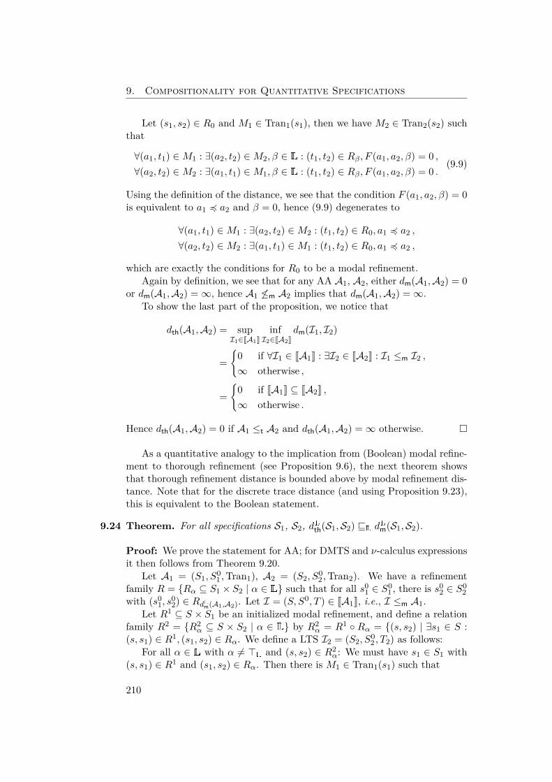
9. Compositionality for Quantitative Specifications

Let (s1, s2) ∈ R0 and M1 ∈ Tran1(s1), then we have M2 ∈ Tran2(s2) suchthat

∀(a1, t1) ∈M1 : ∃(a2, t2) ∈M2, β ∈ L : (t1, t2) ∈ Rβ, F (a1, a2, β) = 0 ,∀(a2, t2) ∈M2 : ∃(a1, t1) ∈M1, β ∈ L : (t1, t2) ∈ Rβ, F (a1, a2, β) = 0 .

(9.9)

Using the definition of the distance, we see that the condition F (a1, a2, β) = 0is equivalent to a1 4 a2 and β = 0, hence (9.9) degenerates to

∀(a1, t1) ∈M1 : ∃(a2, t2) ∈M2 : (t1, t2) ∈ R0, a1 4 a2 ,

∀(a2, t2) ∈M2 : ∃(a1, t1) ∈M1 : (t1, t2) ∈ R0, a1 4 a2 ,

which are exactly the conditions for R0 to be a modal refinement.Again by definition, we see that for any AA A1, A2, either dm(A1,A2) = 0

or dm(A1,A2) =∞, hence A1 6≤m A2 implies that dm(A1,A2) =∞.To show the last part of the proposition, we notice that

dth(A1,A2) = supI1∈JA1K

infI2∈JA2K

dm(I1, I2)

={

0 if ∀I1 ∈ JA1K : ∃I2 ∈ JA2K : I1 ≤m I2 ,

∞ otherwise ,

={

0 if JA1K ⊆ JA2K ,∞ otherwise .

Hence dth(A1,A2) = 0 if A1 ≤t A2 and dth(A1,A2) =∞ otherwise. �

As a quantitative analogy to the implication from (Boolean) modal refine-ment to thorough refinement (see Proposition 9.6), the next theorem showsthat thorough refinement distance is bounded above by modal refinement dis-tance. Note that for the discrete trace distance (and using Proposition 9.23),this is equivalent to the Boolean statement.

9.24 Theorem. For all specifications S1, S2, dLth(S1,S2) vL dLm(S1,S2).

Proof: We prove the statement for AA; for DMTS and ν-calculus expressionsit then follows from Theorem 9.20.

Let A1 = (S1, S01 ,Tran1), A2 = (S2, S

02 ,Tran2). We have a refinement

family R = {Rα ⊆ S1 × S2 | α ∈ L} such that for all s01 ∈ S0

1 , there is s02 ∈ S0

2with (s0

1, s02) ∈ RdLm(A1,A2). Let I = (S, S0, T ) ∈ JA1K, i.e., I ≤m A1.

Let R1 ⊆ S × S1 be an initialized modal refinement, and define a relationfamily R2 = {R2

α ⊆ S × S2 | α ∈ L} by R2α = R1 ◦ Rα = {(s, s2) | ∃s1 ∈ S :

(s, s1) ∈ R1, (s1, s2) ∈ Rα. We define a LTS I2 = (S2, S02 , T2) as follows:

For all α ∈ L with α 6= >L and (s, s2) ∈ R2α: We must have s1 ∈ S1 with

(s, s1) ∈ R1 and (s1, s2) ∈ Rα. Then there is M1 ∈ Tran1(s1) such that

210

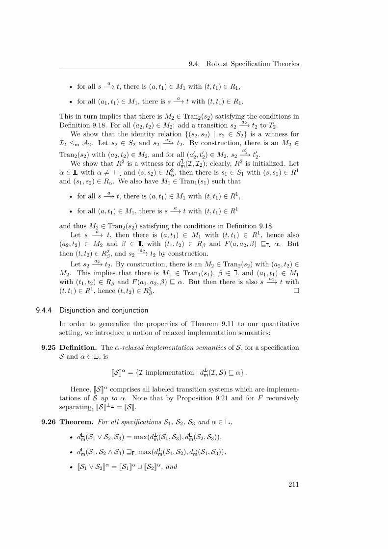
9.4. Robust Specification Theories

• for all s a−→ t, there is (a, t1) ∈M1 with (t, t1) ∈ R1,

• for all (a1, t1) ∈M1, there is s a−→ t with (t, t1) ∈ R1.

This in turn implies that there is M2 ∈ Tran2(s2) satisfying the conditions inDefinition 9.18. For all (a2, t2) ∈M2: add a transition s2

a2−→ t2 to T2.We show that the identity relation {(s2, s2) | s2 ∈ S2} is a witness for

I2 ≤m A2. Let s2 ∈ S2 and s2a2−→ t2. By construction, there is an M2 ∈

Tran2(s2) with (a2, t2) ∈M2, and for all (a′2, t′2) ∈M2, s2a′2−→ t′2.

We show that R2 is a witness for dLm(I, I2); clearly, R2 is initialized. Letα ∈ L with α 6= >L and (s, s2) ∈ R2

α, then there is s1 ∈ S1 with (s, s1) ∈ R1

and (s1, s2) ∈ Rα. We also have M1 ∈ Tran1(s1) such that

• for all s a−→ t, there is (a, t1) ∈M1 with (t, t1) ∈ R1,

• for all (a, t1) ∈M1, there is s a−→ t with (t, t1) ∈ R1

and thus M2 ∈ Tran2(s2) satisfying the conditions in Definition 9.18.Let s a−→ t, then there is (a, t1) ∈ M1 with (t, t1) ∈ R1, hence also

(a2, t2) ∈ M2 and β ∈ L with (t1, t2) ∈ Rβ and F (a, a2, β) vL α. Butthen (t, t2) ∈ R2

β, and s2a2−→ t2 by construction.

Let s2a2−→ t2. By construction, there is an M2 ∈ Tran2(s2) with (a2, t2) ∈

M2. This implies that there is M1 ∈ Tran1(s1), β ∈ L and (a1, t1) ∈ M1with (t1, t2) ∈ Rβ and F (a1, a2, β) v α. But then there is also s a1−→ t with(t, t1) ∈ R1, hence (t, t2) ∈ R2

β. �

9.4.4 Disjunction and conjunctionIn order to generalize the properties of Theorem 9.11 to our quantitativesetting, we introduce a notion of relaxed implementation semantics:

9.25 Definition. The α-relaxed implementation semantics of S, for a specificationS and α ∈ L, is

JSKα = {I implementation | dLm(I,S) v α} .

Hence, JSKα comprises all labeled transition systems which are implemen-tations of S up to α. Note that by Proposition 9.21 and for F recursivelyseparating, JSK⊥L = JSK.

9.26 Theorem. For all specifications S1, S2, S3 and α ∈ L,

• dLm(S1 ∨ S2,S3) = max(dLm(S1,S3), dLm(S2,S3)),

• dLm(S1,S2 ∧ S3) wL max(dLm(S1,S2), dLm(S1,S3)),

• JS1 ∨ S2Kα = JS1Kα ∪ JS2Kα, and

211

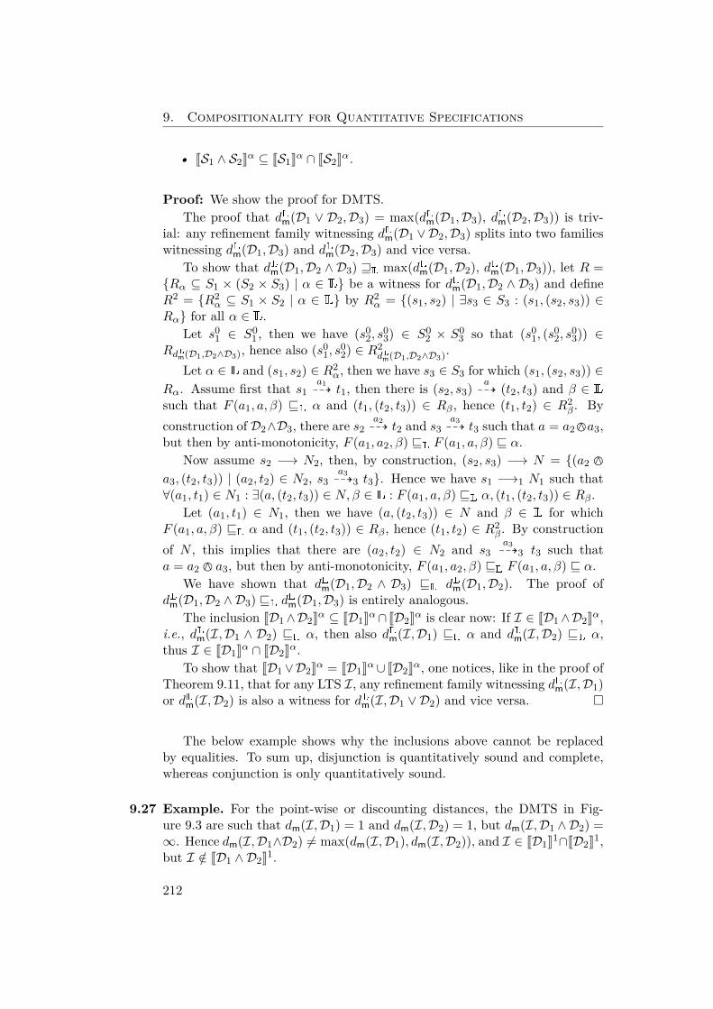
9. Compositionality for Quantitative Specifications

• JS1 ∧ S2Kα ⊆ JS1Kα ∩ JS2Kα.

Proof: We show the proof for DMTS.The proof that dLm(D1 ∨ D2,D3) = max(dLm(D1,D3), dLm(D2,D3)) is triv-

ial: any refinement family witnessing dLm(D1 ∨D2,D3) splits into two familieswitnessing dLm(D1,D3) and dLm(D2,D3) and vice versa.

To show that dLm(D1,D2 ∧ D3) wL max(dLm(D1,D2), dLm(D1,D3)), let R ={Rα ⊆ S1 × (S2 × S3) | α ∈ L} be a witness for dLm(D1,D2 ∧ D3) and defineR2 = {R2

α ⊆ S1 × S2 | α ∈ L} by R2α = {(s1, s2) | ∃s3 ∈ S3 : (s1, (s2, s3)) ∈

Rα} for all α ∈ L.Let s0

1 ∈ S01 , then we have (s0

2, s03) ∈ S0

2 × S03 so that (s0

1, (s02, s

03)) ∈

RdLm(D1,D2∧D3), hence also (s01, s

02) ∈ R2

dLm(D1,D2∧D3).Let α ∈ L and (s1, s2) ∈ R2

α, then we have s3 ∈ S3 for which (s1, (s2, s3)) ∈Rα. Assume first that s1

a199K t1, then there is (s2, s3) a

99K (t2, t3) and β ∈ Lsuch that F (a1, a, β) vL α and (t1, (t2, t3)) ∈ Rβ, hence (t1, t2) ∈ R2

β. Byconstruction of D2∧D3, there are s2

a299K t2 and s3

a399K t3 such that a = a27a3,

but then by anti-monotonicity, F (a1, a2, β) vL F (a1, a, β) v α.Now assume s2 −→ N2, then, by construction, (s2, s3) −→ N = {(a2 7

a3, (t2, t3)) | (a2, t2) ∈ N2, s3a399K3 t3}. Hence we have s1 −→1 N1 such that

∀(a1, t1) ∈ N1 : ∃(a, (t2, t3)) ∈ N, β ∈ L : F (a1, a, β) vL α, (t1, (t2, t3)) ∈ Rβ.Let (a1, t1) ∈ N1, then we have (a, (t2, t3)) ∈ N and β ∈ L for which

F (a1, a, β) vL α and (t1, (t2, t3)) ∈ Rβ, hence (t1, t2) ∈ R2β. By construction

of N , this implies that there are (a2, t2) ∈ N2 and s3a399K3 t3 such that

a = a2 7 a3, but then by anti-monotonicity, F (a1, a2, β) vL F (a1, a, β) v α.We have shown that dLm(D1,D2 ∧ D3) vL dLm(D1,D2). The proof of

dLm(D1,D2 ∧ D3) vL dLm(D1,D3) is entirely analogous.The inclusion JD1∧D2Kα ⊆ JD1Kα∩ JD2Kα is clear now: If I ∈ JD1∧D2Kα,

i.e., dLm(I,D1 ∧ D2) vL α, then also dLm(I,D1) vL α and dLm(I,D2) vL α,thus I ∈ JD1Kα ∩ JD2Kα.

To show that JD1∨D2Kα = JD1Kα∪ JD2Kα, one notices, like in the proof ofTheorem 9.11, that for any LTS I, any refinement family witnessing dLm(I,D1)or dLm(I,D2) is also a witness for dLm(I,D1 ∨ D2) and vice versa. �

The below example shows why the inclusions above cannot be replacedby equalities. To sum up, disjunction is quantitatively sound and complete,whereas conjunction is only quantitatively sound.

9.27 Example. For the point-wise or discounting distances, the DMTS in Fig-ure 9.3 are such that dm(I,D1) = 1 and dm(I,D2) = 1, but dm(I,D1 ∧D2) =∞. Hence dm(I,D1∧D2) 6= max(dm(I,D1), dm(I,D2)), and I ∈ JD1K1∩JD2K1,but I /∈ JD1 ∧ D2K1.

212

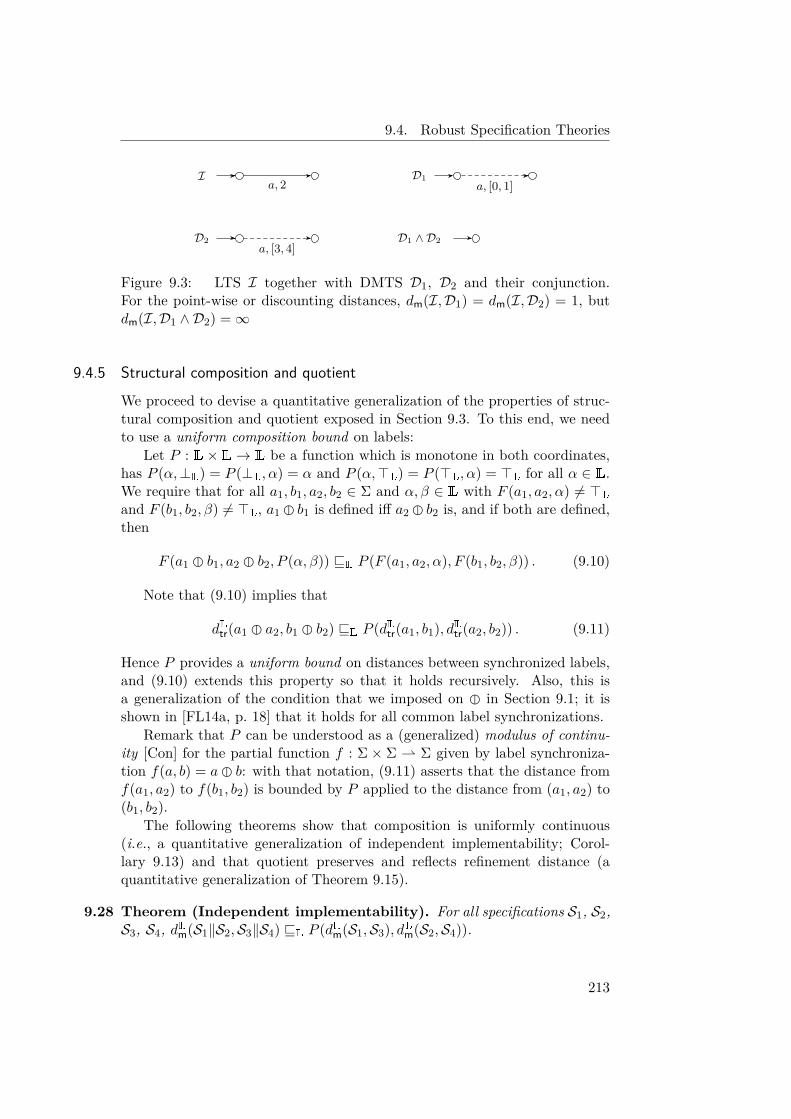
9.4. Robust Specification Theories

Ia, 2

D1a, [0, 1]

D2a, [3, 4]

D1 ∧ D2

Figure 9.3: LTS I together with DMTS D1, D2 and their conjunction.For the point-wise or discounting distances, dm(I,D1) = dm(I,D2) = 1, butdm(I,D1 ∧ D2) =∞

9.4.5 Structural composition and quotient

We proceed to devise a quantitative generalization of the properties of struc-tural composition and quotient exposed in Section 9.3. To this end, we needto use a uniform composition bound on labels:

Let P : L× L→ L be a function which is monotone in both coordinates,has P (α,⊥L) = P (⊥L, α) = α and P (α,>L) = P (>L, α) = >L for all α ∈ L.We require that for all a1, b1, a2, b2 ∈ Σ and α, β ∈ L with F (a1, a2, α) 6= >Land F (b1, b2, β) 6= >L, a1 � b1 is defined iff a2 � b2 is, and if both are defined,then

F (a1 � b1, a2 � b2, P (α, β)) vL P (F (a1, a2, α), F (b1, b2, β)) . (9.10)

Note that (9.10) implies that

dLtr(a1 � a2, b1 � b2) vL P (dLtr(a1, b1), dLtr(a2, b2)) . (9.11)

Hence P provides a uniform bound on distances between synchronized labels,and (9.10) extends this property so that it holds recursively. Also, this isa generalization of the condition that we imposed on � in Section 9.1; it isshown in [FL14a, p. 18] that it holds for all common label synchronizations.

Remark that P can be understood as a (generalized) modulus of continu-ity [Con] for the partial function f : Σ × Σ ⇀ Σ given by label synchroniza-tion f(a, b) = a� b: with that notation, (9.11) asserts that the distance fromf(a1, a2) to f(b1, b2) is bounded by P applied to the distance from (a1, a2) to(b1, b2).

The following theorems show that composition is uniformly continuous(i.e., a quantitative generalization of independent implementability; Corol-lary 9.13) and that quotient preserves and reflects refinement distance (aquantitative generalization of Theorem 9.15).

9.28 Theorem (Independent implementability). For all specifications S1, S2,S3, S4, dLm(S1‖S2,S3‖S4) vL P (dLm(S1,S3), dLm(S2,S4)).

213

9. Compositionality for Quantitative Specifications

Proof: We show the proof for AA. For i = 1, 2, 3, 4, let Ai = (Si, S0i ,Trani).

Let R1 = {R1α ⊆ S1 × S3 | α ∈ L}, R2 = {R2

α ⊆ S2 × S4 | α ∈ L} berefinement families such that ∀s0

1 ∈ S01 : ∃s0

3 ∈ S03 : (s0

1, s03) ∈ R1

dLm(A1,A3) and∀s0

2 ∈ S02 : ∃s0

4 ∈ S04 : (s0

2, s04) ∈ R2

dLm(A2,A4). Define R = {Rα ⊆ (S1 × S2) ×(S3 × S4) | α ∈ L} by

Rα ={((s1, s2), (s3, s4))

∣∣ ∃α1, α2 ∈ L :(s1, s3) ∈ R1

α1 , (s2, s4) ∈ R2α2 , P (α1, α2) vL α

},

then it is clear that ∀(s01, s

02) ∈ S0

1×S02 : ∃(s0

3, s04) ∈ S0

3×S04 : ((s0

1, s02), (s0

3, s04)) ∈

RP (dLm(A1,A3),dLm(A2,A4)). We show that R is a refinement family from A1‖A2to A3‖A4.

Let α ∈ L and ((s1, s2), (s3, s4)) ∈ Rα, then we have α1, α2 ∈ L with(s1, s3) ∈ R1

α1 , (s2, s4) ∈ R2α2 and P (α1, α2) vL α. Let M12 ∈ Tran((s1, s2)),

then there must be M1 ∈ Tran1(s1), M2 ∈ Tran2(s2) for which M12 = M1 �M2. Thus we also have M3 ∈ Tran3(s3) and M4 ∈ Tran4(s4) such that

∀(a1, t1) ∈M1 : ∃(a3, t3) ∈M3, β1 ∈ L :(t1, t3) ∈ R1

β1 , F (a1, a3, β1) vL α1 , (9.12)∀(a3, t3) ∈M3 : ∃(a1, t1) ∈M1, β1 ∈ L :

(t1, t3) ∈ R1β1 , F (a1, a3, β1) vL α1 , (9.13)

∀(a2, t2) ∈M2 : ∃(a4, t4) ∈M4, β2 ∈ L :(t2, t4) ∈ R2

β2 , F (a2, a4, β2) vL α2 , (9.14)∀(a4, t4) ∈M4 : ∃(a2, t2) ∈M2, β2 ∈ L :

(t2, t4) ∈ R2β2 , F (a2, a4, β2) vL α2 . (9.15)

Let M34 = M3 �M4, then M34 ∈ Tran((s3, s4)). Let (a12, (t1, t2)) ∈ M12,then there are (a1, t1) ∈ M1 and (a2, t2) ∈ M2 for which a12 = a1 � a2.Using (9.12) and (9.14), we get (a3, t3) ∈M3, (a4, t4) ∈M4 and β1, β2 ∈ L suchthat (t1, t3) ∈ R1

β1, (t2, t4) ∈ R2

β2, F (a1, a3, β1) vL α1, and F (a2, a4, β2) vL

α2.Let a34 = a3 � a4 and β = P (β1, β2), then we have (a34, (t3, t4)) ∈ M34.

Also, (t1, t3) ∈ R1β1

and (t2, t4) ∈ R2β2

imply that ((t1, t2), (t3, t4)) ∈ Rβ, and

F (a12, a34, β) = F (a1 � a2, a3 � a4, P (β1, β2))v P (F (a1, a3, β1), F (a2, a4, β2))vL P (α1, α2) vL α .

We have shown that for all (a12, (t1, t2)) ∈ M12, there exists (a34, (t3, t4)) ∈M34 and β ∈ L such that ((t1, t2), (t3, t4)) ∈ Rβ and F (a12, a34, β) vL α. Toshow the reverse property, starting from an element (a34, (t3, t4)) ∈ M34, wecan proceed entirely analogous, using (9.13) and (9.15). �

214

9.4. Robust Specification Theories

9.29 Theorem. For all specifications S1, S2, S3, dLm(S1‖S2,S3) = dLm(S2,S3/S1).

Proof: We show the proof for AA. Let Ai = (Si, S0i , Trani) for i = 1, . . . , 3;

we prove that dLm(A1‖A2,A3) = dLm(A2,A3/A1).We assume that the elements of Tran1(s1) are pairwise disjoint for each

s1 ∈ S1; this can be achieved by, if necessary, splitting states.Define R = {Rα ⊆ S1 × S2 × S3 | α ∈ L} by Rα = {(s1‖s2, s3) |

dLm(s2, s3/s1) vL α}. (We again abuse notation and write (s1‖s2, s3) insteadof (s1, s2, s3).) We show that R is a witness for dLm(A1‖A2,A3).

Let s01‖s0

2 ∈ S01 × S0

2 , then there is s03/s

01 ∈ s0 for which it holds that

dLm(s02, s

03/s

01) vL dLm(A2,A3/A1), hence (s0

1‖s01, s

03) ∈ RdLm(A2,A3/A1).

Let α ∈ L \ {>L}, (s1‖s2, s3) ∈ Rα and M‖ ∈ Tran‖(s1‖s2). Then M‖ =M1‖M2 with M1 ∈ Tran1(s1) and M2 ∈ Tran2(s2). As dLm(s2, s3/s1) vL α,we can pair M2 with an M/ ∈ Tran/(s3/s1), i.e., such that the conditions inDefinition 9.18 are satisfied.

Let M3 = M/ . M1. We show that the conditions in Definition 9.18 aresatisfied for the pair M‖,M3:

• Let (a, t1‖t2) ∈ M‖, then there are a1, a2 ∈ Σ with a = a1 � a2 and(a1, t1) ∈M1, (a2, t2) ∈M2. Hence there is (a′2, t) ∈M/ and β ∈ L suchthat F (a2, a

′2, β) vL α and dLm(t2, t) vL β.

Note that a3 = a1 � a′2 is defined and F (a, a3, β) v α. Write t ={t13/t11, . . . , tn3/tn1}. By construction, there is an index i for which ti1 = t1,hence (a3, t

i3) ∈ M3. Also, t ⊇ {ti3/ti1}, hence dLm(t2, ti3/ti1) v β and

consequently (t1‖t2, t3) ∈ Rβ.

• Let (a3, t3) ∈ M3, then there are (a′2, t) ∈ M/ and (a1, t1) ∈ M1 suchthat a3 = a1�a′2 and t3/t1 ∈ t. Hence there are (a2, t2) ∈M2 and β ∈ Lfor which F (a2, a

′2, β) vL α and dLm(t2, t) vL β. Note that a = a1�a2 is

defined and F (a, a3, β) vL α. Thus (a, t1‖t2) ∈ M , and by t ⊇ {t3/t1},dLm(t2, t3/t1) v β.

Assume, for the other direction of the proof, that A1‖A2 ≤m A3. DefineR = {Rα ⊆ S2 × 2S3×S1 | α ∈ L} by

Rα ={(s2, {s1

3/s11, . . . , s

n3/s

n1})

∣∣ ∀i = 1, . . . , n : dLm(si1‖s2, si3) vL α

};

we show that R is a witness for dLm(A2,A3/A1).Let s0

2 ∈ S02 . We know that for every s0

1 ∈ S01 , there exists σ(s0

1) ∈ S03 such

that dLm(s01‖s0

2, s03) vL dLm(A1‖A2,A3). By s0 ⊇ {σ(s0

1)/s01 | s0

1 ∈ S01}, we see

that (s02, s

0) ∈ RdLm(A1‖A2,A3).Let α ∈ L \ {>L} and (s2, s) ∈ Rα, with s = {s1

3/s11, . . . , s

n3/s

n1}, and

M2 ∈ Tran2(s2).For every i = 1, . . . , n, let us write Tran1(si1) = {M i,1

1 , . . . ,M i,mi1 }. By

assumption, M i,j11 ∩M i,j2

1 = ∅ for j1 6= j2, hence every (a1, t1) ∈∈ Tran1(si1)is contained in a unique M i,δi(a1,t1)

1 ∈ Tran1(si1).

215

9. Compositionality for Quantitative Specifications

For every j = 1, . . . ,mi, let M i,j = M i,j1 ‖M2 ∈ Tran‖(si1‖s2). From

dLm(si1‖s2, si3) vL α we have M i,j

3 ∈ Tran3(si3) such that the conditions inDefinition 9.18 hold for the pair M i,j ,M i,j

3 .Now define

M ={(a2, t)

∣∣ ∃(a2, t2) ∈M2 : ∀t3/t1 ∈ t : ∃i, a1, a3, β :

(a1, t1) ∈∈ Tran1(si1), (a3, t3) ∈M i,δi(a1,t1)3 ,

F (a1 � a2, a3, β) vL α, dLm(t1‖t2, t3) vL β}. (9.16)

We need to show that M ∈ Tran/(s).Let i ∈ {1, . . . , n} and M i,j

1 ∈ Tran1(si1); we claim that M .M i,j1 4R M

i,j3 .

Let (a3, t3) ∈M .M i,j1 , then a3 = a1 � a2 for some a1, a2 such that t3/t1 ∈ t,

(a1, t1) ∈ M i,j1 and (a2, t) ∈ M . By disjointness, j = δi(a1, t1), hence by

definition of M , (a3, t3) ∈M i,j3 as was to be shown.

For the reverse inclusion, let (a3, t3) ∈ M i,j3 . By definition of M i,j , there

are (a1, t1) ∈ M i,j1 , (a2, t2) ∈ M2 and β ∈ L for which F (a1 � a2, a3, β) vL α

and dLm(t1‖t2, t3) vL β. Thus j = δi(a1, t1), so that there must be (a2, t) ∈Mfor which t3/t1 ∈ t, but then also (a1 � a2, t3) ∈M .M i,j

1 .We show that the pair M2,M satisfies the conditions of Definition 9.18.

• Let (a2, t2) ∈M2. For every i = 1, . . . , n and every (a1, t1) ∈∈ Tran1(ti1),we can use Definition 9.18 applied to the pairM i,δi(a1,t1)

1 ‖M2,Mi,δi(a1,t1)3

to choose an element (ηi(a1, t1), τi(a1, t1)) ∈ M i,δi(a1,t1)3 and βi(a1, t1) ∈

L for which dLm(t1‖t2, τi(a1, t1)) vL βi(a1, t1) and F (a1 � a2, ηi(a1, t1),βi(a1, t1)) vL α. Let t = {τi(a1, t1)/t1 | i = 1, . . . , n, (a1, t1) ∈∈Tran1(ti1)}, then (a2, t) ∈M and (t2, t) ∈ Rβ.

• Let (a2, t) ∈ M , then we have (a2, t2) ∈ M2 satisfying the conditionsin (9.16). Hence for all t3/t1 ∈ t, there are i, a1, a3, and β(t3/t1)such that (a3, t3) ∈ M

i,δi(a1,t1)3 , F (a1 � a2, a3, β(t3/t1)) vL α, and

dLm(t1‖t2, t3) vL β(t3/t1). Let β = sup{β(t3/t1) | t3/t1 ∈ t}, thendLm(t1‖t2, t3) vL β for all t3/t1 ∈ t, hence (t2, t) ∈ Rβ. �

9.5 ConclusionWe have presented a framework for compositional and iterative design andverification of systems which supports quantities and system and action refine-ment. Moreover, it is robust, in that it uses distances to measure quantitativerefinement and the operations preserve distances.

The framework is very general. It can be applied to a large variety ofquantities (energy, time, resource consumption etc.) and implement the ro-bustness notions associated with them. It is also agnostic with respect to the

216

9.5. Conclusion

type of specifications used, as it applies equally to behavioral and logical spec-ifications. This means that logical and behavioral quantitative specificationscan be freely combined in quantitative system development.

217

10 References

[AB07] Charalambos D. Aliprantis and Kim C. Border. Infinite Dimen-sional Analysis: A Hitchhiker’s Guide. Springer-Verlag, 2007.

[ACH+95] Rajeev Alur, Costas Courcoubetis, Nicolas Halbwachs,Thomas A. Henzinger, Pei-Hsin Ho, Xavier Nicollin, AlfredoOlivero, Joseph Sifakis, and Sergio Yovine. The algorithmic ana-lysis of hybrid systems. Theoretical Computer Science, 138(1):3–34, 1995.

[AD94] Rajeev Alur and David L. Dill. A theory of timed automata.Theoretical Computer Science, 126(2):183–235, 1994.

[AFdFE+13] Luca Aceto, Ignacio Fábregas, David de Frutos-Escrig, Anna In-gólfsdóttir, and Miguel Palomino. On the specification of modalsystems: A comparison of three frameworks. Science of Com-puter Programming, 78(12):2468–2487, 2013.

[AFH99] Rajeev Alur, Limor Fix, and Thomas A. Henzinger. Event-clockautomata: A determinizable class of timed automata. Theoreti-cal Computer Science, 211(1-2):253–273, 1999.

[AFL15] Joanne M. Atlee, Uli Fahrenberg, and Axel Legay. Measuringbehaviour interactions between product-line features. In For-maliSE, pages 20–25. IEEE, 2015.

[AHL+08] Adam Antonik, Michael Huth, Kim G. Larsen, Ulrik Nyman,and Andrzej Wąsowski. 20 years of modal and mixed specifica-tions. Bulletin of the EATCS, 95:94–129, 2008.

[AILS07] Luca Aceto, Anna Ingólfsdóttir, Kim G. Larsen, and Jiří Srba.Reactive Systems. Cambridge University Press, 2007.

[ASSB00] Adnan Aziz, Kumud Sanwal, Vigyan Singhal, and Robert K.Brayton. Model-checking continous-time Markov chains. ACMTransactions on Computational Logics, 1(1):162–170, 2000.

219

10. References

[AT11] Rajeev Alur and Ashutosh Trivedi. Relating average and dis-counted costs for quantitative analysis of timed systems. InChakraborty et al. [CJBF11], pages 165–174.

[BBB+10] Ananda Basu, Saddek Bensalem, Marius Bozga, Benoît Cail-laud, Benoît Delahaye, and Axel Legay. Statistical abstrac-tion and model-checking of large heterogeneous systems. InJohn Hatcliff and Elena Zucca, editors, FMOODS/FORTE, vol-ume 6117 of Lecture Notes in Computer Science, pages 32–46.Springer-Verlag, 2010.

[BBLM13] Giorgio Bacci, Giovanni Bacci, Kim G. Larsen, and Radu Mar-dare. On-the-fly exact computation of bisimilarity distances.In Nir Piterman and Scott A. Smolka, editors, TACAS, vol-ume 7795 of Lecture Notes in Computer Science, pages 1–15.Springer-Verlag, 2013.

[BCK11] Nikola Beneš, Ivana Cerná, and Jan Křetínský. Modal transitionsystems: Composition and LTL model checking. In Bultan andHsiung [BH11], pages 228–242.

[BDCU13] Shoham Ben-David, Marsha Chechik, and Sebastián Uchitel.Merging partial behaviour models with different vocabularies.In D’Argenio and Melgratti [DM13], pages 91–105.

[BDF+13] Nikola Beneš, Benoît Delahaye, Uli Fahrenberg, Jan Křetínský,and Axel Legay. Hennessy-Milner logic with greatest fixed pointsas a complete behavioural specification theory. In D’Argenio andMelgratti [DM13], pages 76–90.

[BDF+18] Anicet Bart, Benoît Delahaye, Paulin Fournier, Didier Lime,Eric Monfroy, and Charlotte Truchet. Reachability in parametricinterval Markov chains using constraints. Theoretical ComputerScience, 747:48–74, 2018.

[BDH+12] Sebastian S. Bauer, Alexandre David, Rolf Hennicker, Kim G.Larsen, Axel Legay, Ulrik Nyman, and Andrzej Wąsowski. Mov-ing from specifications to contracts in component-based design.In Juan de Lara and Andrea Zisman, editors, FASE, volume 7212of Lecture Notes in Computer Science, pages 43–58. Springer-Verlag, 2012.

[BFJ+11] Sebastian S. Bauer, Uli Fahrenberg, Line Juhl, Kim G. Larsen,Axel Legay, and Claus Thrane. Quantitative refinement forweighted modal transition systems. In Filip Murlak and Pi-otr Sankowski, editors, MFCS, volume 6907 of Lecture Notes inComputer Science, pages 60–71. Springer-Verlag, 2011.

220

[BFJ+13] Sebastian S. Bauer, Uli Fahrenberg, Line Juhl, Kim G. Larsen,Axel Legay, and Claus Thrane. Weighted modal transition sys-tems. Formal Methods in System Design, 42(2):193–220, 2013.

[BFK+20] Nikola Beneš, Uli Fahrenberg, Jan Křetínský, Axel Legay, andLouis-Marie Traonouez. Logical vs. behavioural specifications.Information and Computation, 271:104487, 2020.

[BFLM11] Patricia Bouyer, Uli Fahrenberg, Kim G. Larsen, and NicolasMarkey. Quantitative analysis of real-time systems using pricedtimed automata. Communications of the ACM, 54(9):78–87,2011.

[BFLT12] Sebastian S. Bauer, Uli Fahrenberg, Axel Legay, and ClausThrane. General quantitative specification theories with modali-ties. In Edward A. Hirsch, Juhani Karhumäki, Arto Lepistö, andMichail Prilutskii, editors, CSR, volume 7353 of Lecture Notesin Computer Science, pages 18–30. Springer-Verlag, 2012.

[BH11] Tevfik Bultan and Pao-Ann Hsiung, editors. Automated Technol-ogy for Verification and Analysis, 9th International Symposium,ATVA 2011, Taipei, Taiwan, October 11-14, 2011. Proceedings,volume 6996 of Lecture Notes in Computer Science. Springer-Verlag, 2011.

[BJL+12a] Sebastian S. Bauer, Line Juhl, Kim G. Larsen, Axel Legay,and Jiří Srba. Extending modal transition systems with struc-tured labels. Mathematical Structures in Computer Science,22(4):581–617, 2012.

[BJL+12b] Sebastian S. Bauer, Line Juhl, Kim G. Larsen, Jiří Srba, andAxel Legay. A logic for accumulated-weight reasoning on multi-weighted modal automata. In Tiziana Margaria, Zongyan Qiu,and Hongli Yang, editors, TASE, pages 77–84. IEEE, 2012.

[BJS09] Joakim Byg, Kenneth Yrke Jørgensen, and Jiří Srba. TAPAAL:editor, simulator and verifier of timed-arc Petri nets. In ZhimingLiu and Anders P. Ravn, editors, ATVA, volume 5799 of LectureNotes in Computer Science, pages 84–89. Springer-Verlag, 2009.

[BK10] Nikola Beneš and Jan Křetínský. Process algebra for modal tran-sition systemses. In Ludek Matyska, Michal Kozubek, TomásVojnar, Pavel Zemcík, and David Antos, editors, MEMICS, vol-ume 16 of OASICS, pages 9–18. Schloss Dagstuhl - Leibniz-Zentrum für Informatik, Germany, 2010.

221

10. References

[BKL+11] Nikola Beneš, Jan Křetínský, Kim G. Larsen, Mikael H. Møller,and Jiří Srba. Parametric modal transition systems. In Bultanand Hsiung [BH11], pages 275–289.

[BKL+12] Nikola Beneš, Jan Křetínský, Kim G. Larsen, Mikael H. Møller,and Jiří Srba. Dual-priced modal transition systems with timedurations. In Nikolaj Bjørner and Andrei Voronkov, editors,LPAR, volume 7180 of Lecture Notes in Computer Science, pages122–137. Springer-Verlag, 2012.

[BKLS09] Nikola Beneš, Jan Křetínský, Kim G. Larsen, and Jiří Srba. Ondeterminism in modal transition systems. Theoretical ComputerScience, 410(41):4026–4043, 2009.

[BL92] Gérard Boudol and Kim G. Larsen. Graphical versus logicalspecifications. Theoretical Computer Science, 106(1):3–20, 1992.

[BL14] Saddek Bensalem and Axel Legay, editors. From Programs toSystems – The Systems Perspective in Computing, 2014, Pro-ceedings, volume 8415 of Lecture Notes in Computer Science.Springer-Verlag, 2014.

[Bla00] Patrick Blackburn. Representation, reasoning, and relationalstructures: a hybrid logic manifesto. Log. J. IGPL, 8(3):339–365, 2000.

[BLM+11] Patricia Bouyer, Kim G. Larsen, Nicolas Markey, Ocan Sankur,and Claus Thrane. Timed automata can always be made imple-mentable. In Joost-Pieter Katoen and Barbara König, editors,CONCUR, volume 6901 of Lecture Notes in Computer Science,pages 76–91. Springer-Verlag, 2011.

[BLPR09] Nathalie Bertrand, Axel Legay, Sophie Pinchinat, and Jean-Baptiste Raclet. A compositional approach on modal specifica-tions for timed systems. In Karin Breitman and Ana Cavalcanti,editors, ICFEM, volume 5885 of Lecture Notes in Computer Sci-ence, pages 679–697. Springer-Verlag, 2009.

[BLPR12] Nathalie Bertrand, Axel Legay, Sophie Pinchinat, and Jean-Baptiste Raclet. Modal event-clock specifications for timedcomponent-based design. Science of Computer Programming,77(12):1212–1234, 2012.

[BLS95] Anders Børjesson, Kim G. Larsen, and Arne Skou. General-ity in design and compositional verification using TAV. FormalMethods in System Design, 6(3):239–258, 1995.

222

[BML11] Sebastian S. Bauer, Philip Mayer, and Axel Legay. MIO work-bench: A tool for compositional design with modal input/outputinterfaces. In Bultan and Hsiung [BH11], pages 418–421.

[BR12] Sebastian S. Bauer and Jean-Baptiste Raclet, editors. Proceed-ings of the Fourth Workshop on Foundations of Interface Tech-nologies (FIT), volume 87 of Electronic Proceedings in Theoret-ical Computer Science, 2012.

[Bre15] Tomasz Brengos. Weak bisimulation for coalgebras over orderenriched monads. Logical Methods in Computer Science, 11(2),2015.

[Bru97] Glenn Bruns. An industrial application of modal process logic.Science of Computer Programming, 29(1-2):3–22, 1997.

[BvBR98] Marcello M. Bonsangue, Franck van Breugel, and Jan J. M. M.Rutten. Generalized metric spaces: Completion, topology, andpowerdomains via the Yoneda embedding. Theoretical ComputerScience, 193(1-2):1–51, 1998.

[CC03] Luís Caires and Luca Cardelli. A spatial logic for concurrency(part I). Information and Computation, 186(2):194–235, 2003.

[ČCH+11] Pavol Černý, Krishnendu Chatterjee, Thomas A. Henzinger, Ar-jun Radhakrishna, and Rohit Singh. Quantitative synthesis forconcurrent programs. In Gopalakrishnan and Qadeer [GQ11],pages 243–259.

[ČCHR14] Pavol Černý, Martin Chmelik, Thomas A. Henzinger, and Ar-jun Radhakrishna. Interface simulation distances. TheoreticalComputer Science, 560:348–363, 2014.

[CdAF+06] Krishnendu Chatterjee, Luca de Alfaro, Marco Faella,Thomas A. Henzinger, Rupak Majumdar, and MariëlleStoelinga. Compositional quantitative reasoning. In QEST,pages 179–188. IEEE Computer Society, 2006.

[CdAHM02] Arindam Chakrabarti, Luca de Alfaro, Thomas A. Henzinger,and Freddy Y. C. Mang. Synchronous and bidirectional com-ponent interfaces. In CAV, volume 2404 of Lecture Notes inComputer Science, pages 414–427, 2002.

[CdAMR10] Krishnendu Chatterjee, Luca de Alfaro, Rupak Majumdar, andVishwanath Raman. Algorithms for game metrics. Logical Meth-ods in Computer Science, 6(3), 2010.

223

10. References

[CDH10] Krishnendu Chatterjee, Laurent Doyen, and Thomas A. Hen-zinger. Quantitative languages. ACM Transactions on Compu-tational Logics, 11(4), 2010.

[CE81] Edmund M. Clarke and E. Allen Emerson. Design and synthe-sis of synchronization skeletons using branching-time temporallogic. In Dexter Kozen, editor, Logic of Programs, volume 131of Lecture Notes in Computer Science, pages 52–71. Springer-Verlag, 1981.

[ČH11] Pavol Černý and Thomas A. Henzinger. From Boolean to quanti-tative synthesis. In Chakraborty et al. [CJBF11], pages 149–154.

[CHP11] Krishnendu Chatterjee, Thomas A. Henzinger, and Vinayak S.Prabhu. Timed parity games: Complexity and robustness. Log-ical Methods in Computer Science, 7(4), 2011.

[ČHR10] Pavol Černý, Thomas A. Henzinger, and Arjun Radhakrishna.Simulation distances. In Paul Gastin and François Laroussinie,editors, CONCUR, volume 6269 of Lecture Notes in ComputerScience, pages 253–268. Springer-Verlag, 2010.

[ČHR12] Pavol Černý, Thomas A. Henzinger, and Arjun Radhakrishna.Simulation distances. Theoretical Computer Science, 413(1):21–35, 2012.

[ČHR13] Pavol Černý, Thomas A. Henzinger, and Arjun Radhakrishna.Quantitative abstraction refinement. In Roberto Giacobazzi andRadhia Cousot, editors, POPL, pages 115–128. ACM, 2013.

[CJBF11] Samarjit Chakraborty, Ahmed Jerraya, Sanjoy K. Baruah, andSebastian Fischmeister, editors. Proceedings of the 11th Interna-tional Conference on Embedded Software, EMSOFT 2011, partof the Seventh Embedded Systems Week, ESWeek 2011, Taipei,Taiwan, October 9-14, 2011. ACM, 2011.

[CLM11] Luca Cardelli, Kim G. Larsen, and Radu Mardare. ModularMarkovian logic. In Luca Aceto, Monika Henzinger, and JiříSgall, editors, ICALP (2), volume 6756 of Lecture Notes in Com-puter Science, pages 380–391. Springer-Verlag, 2011.

[Con] Continuity, modulus of. Encyclopedia of Mathematics.http://www.encyclopediaofmath.org/index.php?title=Continuity,_modulus_of&oldid=30705.

[dAFH+05] Luca de Alfaro, Marco Faella, Thomas A. Henzinger, RupakMajumdar, and Mariëlle Stoelinga. Model checking discounted

224

temporal properties. Theoretical Computer Science, 345(1):139–170, 2005.

[dAFS04] Luca de Alfaro, Marco Faella, and Mariëlle Stoelinga. Linear andbranching metrics for quantitative transition systems. In JosepDíaz, Juhani Karhumäki, Arto Lepistö, and Donald Sannella,editors, ICALP, volume 3142 of Lecture Notes in Computer Sci-ence, pages 97–109. Springer-Verlag, 2004.

[dAFS09] Luca de Alfaro, Marco Faella, and Mariëlle Stoelinga. Linearand branching system metrics. IEEE Transactions on SoftwareEngineering, 35(2):258–273, 2009.

[dAH05] Luca de Alfaro and Thomas A. Henzinger. Interface-based de-sign. In Manfred Broy, Johannes Grünbauer, David Harel, andTony Hoare, editors, Engineering Theories of Software IntensiveSystems, volume 195 of NATO Science Series II: Mathematics,Physics and Chemistry, pages 83–104. Springer-Verlag, 2005.

[dAHM03] Luca de Alfaro, Thomas A. Henzinger, and Rupak Majumdar.Discounting the future in systems theory. In Jos C. M. Baeten,Jan Karel Lenstra, Joachim Parrow, and Gerhard J. Woegin-ger, editors, ICALP, volume 2719 of Lecture Notes in ComputerScience, pages 1022–1037. Springer-Verlag, 2003.

[dAMRS07] Luca de Alfaro, Rupak Majumdar, Vishwanath Raman, andMariëlle Stoelinga. Game relations and metrics. In LICS, pages99–108. IEEE Computer Society, 2007.

[dAMRS08] Luca de Alfaro, Rupak Majumdar, Vishwanath Raman, andMariëlle Stoelinga. Game refinement relations and metrics. Log-ical Methods in Computer Science, 4(3), 2008.

[DDM10] Philippe Darondeau, Jérémy Dubreil, and Hervé Marchand.Supervisory control for modal specifications of services. InWODES, pages 428–435, 2010.

[Del10] Benoît Delahaye. Modular Specification and Compositional Ana-lysis of Stochastic Systems. PhD thesis, Université de Rennes 1,2010.

[DFFU07] Nicolás D’Ippolito, Dario Fischbein, Howard Foster, and Se-bastián Uchitel. MTSA: Eclipse support for modal transitionsystems construction, analysis and elaboration. In L. Cheng,A. Orso, and M. P. Robillard, editors, ETX, pages 6–10. ACM,2007.

225

10. References

[DFLL14] Benoît Delahaye, Uli Fahrenberg, Kim G. Larsen, and AxelLegay. Refinement and difference for probabilistic automata.Logical Methods in Computer Science, 10(3), 2014.

[DGJP99] Josée Desharnais, Vineet Gupta, Radha Jagadeesan, andPrakash Panangaden. Metrics for labeled Markov systems. InJos C. M. Baeten and Sjouke Mauw, editors, CONCUR, vol-ume 1664 of Lecture Notes in Computer Science, pages 258–273.Springer-Verlag, 1999.

[DGJP04] Josee Desharnais, Vineet Gupta, Radha Jagadeesan, andPrakash Panangaden. Metrics for labelled Markov processes.Theoretical Computer Science, 318(3):323–354, 2004.

[DHLN10] Laurent Doyen, Thomas A. Henzinger, Axel Legay, and DejanNičković. Robustness of sequential circuits. In Luís Gomes,Victor Khomenko, and João M. Fernandes, editors, ACSD, pages77–84. IEEE Computer Society, 2010.

[DJGP02] Josee Desharnais, Radha Jagadeesan, Vineet Gupta, andPrakash Panangaden. The metric analogue of weak bisimulationfor probabilistic processes. In LICS [LIC02], pages 413–422.

[DKL+13] Benoît Delahaye, Joost-Pieter Katoen, Kim G. Larsen, AxelLegay, Mikkel L. Pedersen, Falak Sher, and Andrzej Wasowski.Abstract probabilistic automata. Information and Computation,232:66–116, 2013.

[DLL+10] Alexandre David, Kim G. Larsen, Axel Legay, Ulrik Nyman, andAndrzej Wąsowski. Timed I/O automata: a complete specifica-tion theory for real-time systems. In Karl Henrik Johansson andWang Yi, editors, HSCC, pages 91–100. ACM, 2010.

[DLL+12a] Alexandre David, Kim G. Larsen, Axel Legay, Mikael H. Møller,Ulrik Nyman, Anders P. Ravn, Arne Skou, and Andrzej Wą-sowski. Compositional verification of real-time systems usingEcdar. International Journal on Software Tools for TechnologyTransfer, 14(6):703–720, 2012.

[DLL+12b] Benoît Delahaye, Kim G. Larsen, Axel Legay, Mikkel L. Ped-ersen, and Andrzej Wąsowski. Consistency and refinement forinterval Markov chains. Journal of Logic and Algebraic Program-ming, 81(3):209–226, 2012.

[DLL+15] Alexandre David, Kim G. Larsen, Axel Legay, Ulrik Nyman,Louis-Marie Traonouez, and Andrzej Wąsowski. Real-time spec-ifications. International Journal on Software Tools for Technol-ogy Transfer, 17(1):17–45, 2015.

226

[DLP16] Benoît Delahaye, Didier Lime, and Laure Petrucci. Parametersynthesis for parametric interval Markov chains. In Barbara Job-stmann and K. Rustan M. Leino, editors, VMCAI, volume 9583of Lecture Notes in Computer Science, pages 372–390. Springer-Verlag, 2016.

[DLT08] Josée Desharnais, François Laviolette, and Mathieu Tracol. Ap-proximate analysis of probabilistic processes. In QEST, pages264–273. IEEE Computer Society, 2008.

[DM13] Pedro R. D’Argenio and Hernán C. Melgratti, editors. CON-CUR 2013 - Concurrency Theory - 24th International Confer-ence, CONCUR 2013, Buenos Aires, Argentina, August 27-30,2013. Proceedings, volume 8052 of Lecture Notes in ComputerScience. Springer-Verlag, 2013.

[Ehr61] Andrzej Ehrenfeucht. An application of games to the complete-ness problem for formalized theories. Fundamenta Mathemati-cae, 49:129–141, 1961.

[EM79] Andrzej Ehrenfeucht and Jan Mycielski. Positional strategiesfor mean payoff games. International Journal of Game Theory,8:109–113, 1979.

[FBC+14] Uli Fahrenberg, Fabrizio Biondi, Kevin Corre, Cyrille Jégourel,Simon Kongshøj, and Axel Legay. Measuring global similaritybetween texts. In Laurent Besacier, Adrian Horia Dediu, andCarlos Martín-Vide, editors, SLSP, volume 8791 of Lecture Notesin Computer Science, pages 220–232. Springer-Verlag, 2014.

[FGD+11] Goran Frehse, Colas Le Guernic, Alexandre Donzé, Scott Cot-ton, Rajarshi Ray, Olivier Lebeltel, Rodolfo Ripado, AntoineGirard, Thao Dang, and Oded Maler. SpaceEx: Scalable verifi-cation of hybrid systems. In Gopalakrishnan and Qadeer [GQ11],pages 379–395.

[FH07] Martin Fränzle and Christian Herde. HySAT: An efficient proofengine for bounded model checking of hybrid systems. FormalMethods in System Design, 30(3):179–198, 2007.

[FJLS11] Uli Fahrenberg, Line Juhl, Kim G. Larsen, and Jiří Srba. Energygames in multiweighted automata. In Antonio Cerone and PekkaPihlajasaari, editors, ICTAC, volume 6916 of Lecture Notes inComputer Science, pages 95–115. Springer-Verlag, 2011.

[FKLT14] Ulrich Fahrenberg, Jan Křetínský, Axel Legay, and Louis-MarieTraonouez. Compositionality for quantitative specifications. InLanese and Madelaine [LM15], pages 306–324.

227

10. References

[FKLT18] Uli Fahrenberg, Jan Křetínský, Axel Legay, and Louis-MarieTraonouez. Compositionality for quantitative specifications. SoftComputing, 22(4):1139–1158, 2018.

[FL12] Uli Fahrenberg and Axel Legay. A robust specification theoryfor modal event-clock automata. In Bauer and Raclet [BR12],pages 5–16.

[FL14a] Uli Fahrenberg and Axel Legay. General quantitative specifica-tion theories with modal transition systems. Acta Informatica,51(5):261–295, 2014.

[FL14b] Uli Fahrenberg and Axel Legay. The quantitative linear-time–branching-time spectrum. Theoretical Computer Science,538:54–69, 2014.

[FL17] Uli Fahrenberg and Axel Legay. A linear-time-branching-timespectrum of behavioral specification theories. In Bernhard Stef-fen, Christel Baier, Mark van den Brand, Johann Eder, MikeHinchey, and Tiziana Margaria, editors, SOFSEM, volume 10139of Lecture Notes in Computer Science, pages 49–61. Springer-Verlag, 2017.

[FL20a] Uli Fahrenberg and Axel Legay. Behavioral specification theo-ries: An algebraic taxonomy. In Tiziana Margaria and BernhardSteffen, editors, ISoLA, volume 12476 of Lecture Notes in Com-puter Science, pages 262–274. Springer-Verlag, 2020.

[FL20b] Uli Fahrenberg and Axel Legay. A linear-time-branching-timespectrum for behavioral specification theories. Journal of Logicand Algebraic Methods in Programming, 110, 2020.

[FLLT14] Uli Fahrenberg, Kim G. Larsen, Axel Legay, and Louis-MarieTraonouez. Parametric and quantitative extensions of modaltransition systems. In Bensalem and Legay [BL14].

[FLT09] Uli Fahrenberg, Kim G. Larsen, and Claus Thrane. A quantita-tive characterization of weighted Kripke structures in temporallogic. In MEMICS, 2009. Best paper award.

[FLT10] Uli Fahrenberg, Kim G. Larsen, and Claus Thrane. A quantita-tive characterization of weighted Kripke structures in temporallogic. Computing and Informatics, 29(6+):1311–1324, 2010.

[FLT11] Uli Fahrenberg, Axel Legay, and Claus Thrane. The quantitativelinear-time–branching-time spectrum. In Supratik Chakrabortyand Amit Kumar, editors, FSTTCS, volume 13 of LIPIcs, pages

228

103–114. Schloss Dagstuhl - Leibniz-Zentrum für Informatik,2011.

[FLT14a] Uli Fahrenberg, Axel Legay, and Louis-Marie Traonouez. Speci-fication theories for probabilistic and real-time systems. In Ben-salem and Legay [BL14].

[FLT14b] Uli Fahrenberg, Axel Legay, and Louis-Marie Traonouez. Struc-tural refinement for the modal nu-calculus. In Gabriel Ciobanuand Dominique Méry, editors, ICTAC, volume 8687 of LectureNotes in Computer Science, pages 169–187. Springer-Verlag,2014.

[FLW11] Uli Fahrenberg, Axel Legay, and Andrzej Wąsowski. Make adifference! (Semantically). In Jon Whittle, Tony Clark, andThomas Kühne, editors, MoDELS, volume 6981 of Lecture Notesin Computer Science, pages 490–500. Springer-Verlag, 2011.

[FOC81] 22nd Annual Symposium on Foundations of Computer Science,Nashville, Tennessee, USA, 28-30 October 1981. IEEE Com-puter Society, 1981.

[FP07] Guillaume Feuillade and Sophie Pinchinat. Modal specificationsfor the control theory of discrete event systems. Discrete EventDynamic Systems, 17(2):211–232, 2007.

[FPP05] Norm Ferns, Prakash Panangaden, and Doina Precup. Metricsfor Markov decision processes with infinite state spaces. In UAI,pages 201–208. AUAI Press, 2005.

[Fra54] Roland Fraïssé. Sur quelques classifications des systèmes de re-lations. Publications Scientifiques de l’Université d’Alger, SérieA, 1:35–182, 1954.

[FS08] Harald Fecher and Heiko Schmidt. Comparing disjunctive modaltransition systems with an one-selecting variant. J. Logic Algebr.Program., 77(1-2):20–39, 2008.

[FT11] Uli Fahrenberg and Stavros Tripakis, editors. Formal Modelingand Analysis of Timed Systems - 9th International Conference,volume 6919 of Lecture Notes in Computer Science. Springer-Verlag, 2011.

[FTL11] Uli Fahrenberg, Claus Thrane, and Kim G. Larsen. Distances forweighted transition systems: Games and properties. In MiekeMassink and Gethin Norman, editors, QAPL, volume 57 of Elec-tronic Proceedings in Theoretical Computer Science, pages 134–147, 2011.

229

10. References

[FU08] Dario Fischbein and Sebastián Uchitel. On correct and com-plete strong merging of partial behaviour models. In Mary JeanHarrold and Gail C. Murphy, editors, SIGSOFT FSE, pages297–307. ACM, 2008.

[FvGdW06] Wan Fokkink, Rob J. van Glabbeek, and Paulien de Wind. Com-positionality of Hennessy-Milner logic by structural operationalsemantics. Theoretical Computer Science, 354(3):421–440, 2006.

[GF12] Daniel Gebler and Wan Fokkink. Compositionality of probabilis-tic Hennessy-Milner logic through structural operational seman-tics. In Maciej Koutny and Irek Ulidowski, editors, CONCUR,volume 7454 of Lecture Notes in Computer Science, pages 395–409. Springer-Verlag, 2012.

[GH94] Stephen Gilmore and Jane Hillston. The PEPA workbench: Atool to support a process algebra-based approach to performancemodelling. In Günter Haring and Gabriele Kotsis, editors, CPE,volume 794 of Lecture Notes in Computer Science, pages 353–368. Springer-Verlag, 1994.

[GHJ01] Patrice Godefroid, Michael Huth, and Radha Jagadeesan.Abstraction-based model checking using modal transition sys-tems. In Larsen and Nielsen [LN01], pages 426–440.

[Gir87] Jean-Yves Girard. Linear logic. Theoretical Computer Science,50:1–102, 1987.

[Gir10] Antoine Girard. Synthesis using approximately bisimilar ab-stractions: Time-optimal control problems. In CDC, pages 5893–5898. IEEE, 2010.

[GLLS05] Orna Grumberg, Martin Lange, Martin Leucker, and SharonShoham. Don’t know in the µ-calculus. In VMCAI, volume 3385of Lecture Notes in Computer Science, pages 233–249. Springer-Verlag, 2005.

[GLMR05] Guillaume Gardey, Didier Lime, Morgan Magnin, and Olivier H.Roux. Romeo: A tool for analyzing time Petri nets. In KoushaEtessami and Sriram K. Rajamani, editors, CAV, volume 3576of Lecture Notes in Computer Science, pages 418–423. Springer-Verlag, 2005.

[GLS08] Alexander Gruler, Martin Leucker, and Kathrin D. Scheide-mann. Modeling and model checking software product lines.In Gilles Barthe and Frank S. de Boer, editors, FMOODS, vol-ume 5051 of Lecture Notes in Computer Science, pages 113–131.Springer-Verlag, 2008.

230

[GP07] Antoint Girard and George J. Pappas. Approximation metricsfor discrete and continuous systems. IEEE Transactions on Au-tomatic Control, 52(5):782–798, 2007.

[GQ11] Ganesh Gopalakrishnan and Shaz Qadeer, editors. ComputerAided Verification - 23rd International Conference, CAV 2011,Snowbird, UT, USA, July 14-20, 2011. Proceedings, volume 6806of Lecture Notes in Computer Science. Springer-Verlag, 2011.

[GV92] Jan Friso Groote and Frits W. Vaandrager. Structured opera-tional semantics and bisimulation as a congruence. Informationand Computation, 100(2):202–260, 1992.

[Hal00] Robert J. Hall. Feature interactions in electronic mail. In MuffyCalder and Evan H. Magill, editors, FIW, pages 67–82. IOSPress, 2000.

[Ham50] Richard W. Hamming. Error detecting and error correctingcodes. Bell System Technical Journal, 29:147–160, 1950.

[Han93] Hans-Michael Hanisch. Analysis of place/transition nets withtimed arcs and its application to batch process control. InMarco Ajmone Marsan, editor, ATPN, volume 691 of LectureNotes in Computer Science, pages 282–299. Springer-Verlag,1993.

[Hen85] Matthew Hennessy. Acceptance trees. Journal of the ACM,32(4):896–928, 1985.

[HHWT97] Thomas A. Henzinger, Pei-Hsin Ho, and Howard Wong-Toi.HYTECH: A model checker for hybrid systems. InternationalJournal on Software Tools for Technology Transfer, 1(1-2):110–122, 1997.

[Hil96] Jane Hillston. A Compositional Approach to Performance Mod-elling. Cambridge University Press, 1996.

[HJ94] Hans Hansson and Bengt Jonsson. A logic for reasoning abouttime and reliability. Formal Aspects of Computing, 6(5):512–535,1994.

[HM85] Matthew Hennessy and Robin Milner. Algebraic laws for nonde-terminism and concurrency. Journal of the ACM, 32(1):137–161,1985.

[HMP05] Thomas A. Henzinger, Rupak Majumdar, and Vinayak S.Prabhu. Quantifying similarities between timed systems. InPaul Pettersson and Wang Yi, editors, FORMATS, volume 3829

231

10. References

of Lecture Notes in Computer Science, pages 226–241. Springer-Verlag, 2005.

[HNSY94] Thomas A. Henzinger, Xavier Nicollin, Joseph Sifakis, and Ser-gio Yovine. Symbolic model checking for real-time systems. In-formation and Computation, 111(2):193–244, 1994.

[JLS12] Line Juhl, Kim G. Larsen, and Jirí Srba. Modal transition sys-tems with weight intervals. Journal of Logic and Algebraic Pro-gramming, 81(4):408–421, 2012.

[JT02] Peter Jipsen and Constantine Tsinakis. A survey of residuatedlattices. In Ordered algebraic structures, volume 7, pages 19–56.Kluwer Acad. Publ., 2002.

[JW95] David Janin and Igor Walukiewicz. Automata for the modalmu-calculus and related results. In Jirí Wiedermann and PetrHájek, editors, MFCS, volume 969 of Lecture Notes in ComputerScience, pages 552–562. Springer-Verlag, 1995.

[KKH+19] Yuichi Komorida, Shin-ya Katsumata, Nick Hu, Bartek Klin,and Ichiro Hasuo. Codensity games for bisimilarity. In LICS,pages 1–13. IEEE, 2019.

[KLSV03] Dilsun Kirli Kaynar, Nancy A. Lynch, Roberto Segala, andFrits W. Vaandrager. Timed I/O automata: A mathematicalframework for modeling and analyzing real-time systems. InRTSS, pages 166–177. IEEE Computer Society, 2003.

[KLSV10] Dilsun Kirli Kaynar, Nancy A. Lynch, Roberto Segala, andFrits W. Vaandrager. The Theory of Timed I/O Automata. Syn-thesis Lectures on Distributed Computing Theory. Morgan &Claypool Publishers, second edition, 2010.

[KNP02] Marta Z. Kwiatkowska, Gethin Norman, and David Parker.Probabilistic symbolic model checking with prism: A hybrid ap-proach. In Joost-Pieter Katoen and Perdita Stevens, editors,TACAS, volume 2280 of Lecture Notes in Computer Science,pages 52–66. Springer-Verlag, 2002.

[Koy90] Ron Koymans. Specifying real-time properties with metric tem-poral logic. Real-Time Systems, 2(4):255–299, 1990.

[Koz83] Dexter Kozen. Results on the propositional µ-calculus. Theoret-ical Computer Science, 27:333–354, 1983.

232

[KP04] Beata Konikowska and Wojciech Penczek. On designated valuesin multi-valued CTL∗ model checking. Fundamenta Informati-cae, 60(1-4):211–224, 2004.

[Kře14] Jan Křetínský. Modal Transition Systems: Extensions and Ana-lysis. PhD thesis, Masaryk University, Brno, Dept. of ComputerScience, 2014.

[Kře17] Jan Křetínský. 30 years of modal transition systems: Survey ofextensions and analysis. In Luca Aceto, Giorgio Bacci, GiovanniBacci, Anna Ingólfsdóttir, Axel Legay, and Radu Mardare, ed-itors, Models, Algorithms, Logics and Tools - Essays Dedicatedto Kim Guldstrand Larsen on the Occasion of His 60th Birth-day, volume 10460 of Lecture Notes in Computer Science, pages36–74. Springer, 2017.

[KS13a] Bartek Klin and Vladimiro Sassone. Structural operational se-mantics for stochastic and weighted transition systems. Infor-mation and Computation, 227:58–83, 2013.

[KS13b] Jan Křetínský and Salomon Sickert. MoTraS: A tool for modaltransition systems and their extensions. In Dang Van Hung andMizuhito Ogawa, editors, ATVA, volume 8172 of Lecture Notesin Computer Science, pages 487–491. Springer-Verlag, 2013.

[Lar89] Kim G. Larsen. Modal specifications. In Automatic VerificationMethods for Finite State Systems, volume 407 of Lecture Notesin Computer Science, pages 232–246. Springer-Verlag, 1989.

[Lar90a] Kim G. Larsen. Ideal specification formalism = expressivity +compositionality + decidability + testability + ... In Jos C. M.Baeten and Jan Willem Klop, editors, CONCUR, volume 458of Lecture Notes in Computer Science, pages 33–56. Springer-Verlag, 1990.

[Lar90b] Kim G. Larsen. Proof systems for satisfiability in Hennessy-Milner logic with recursion. Theoretical Computer Science,72(2&3):265–288, 1990.

[Law73] F. William Lawvere. Metric spaces, generalized logic, and closedcategories. Rendiconti del seminario matématico e fisico di Mi-lano, XLIII:135–166, 1973.

[LFT11] Kim G. Larsen, Uli Fahrenberg, and Claus Thrane. Metricsfor weighted transition systems: Axiomatization and complexity.Theoretical Computer Science, 412(28):3358–3369, 2011.

233

10. References

[LIC02] 17th IEEE Symposium on Logic in Computer Science (LICS2002), 22-25 July 2002, Copenhagen, Denmark, Proceedings.IEEE Computer Society, 2002.

[LLM05] Alberto Lluch-Lafuente and Ugo Montanari. Quantitative mu-calculus and CTL defined over constraint semirings. TheoreticalComputer Science, 346(1):135–160, 2005.

[LLTW11] Kim G. Larsen, Axel Legay, Louis-Marie Traonouez, and An-drzej Wąsowski. Robust specification of real time components.In Fahrenberg and Tripakis [FT11], pages 129–144.

[LM15] Ivan Lanese and Eric Madelaine, editors. Formal Aspects ofComponent Software - 11th International Symposium, FACS2014, Bertinoro, Italy, September 10-12, 2014, Revised SelectedPapers, volume 8997 of Lecture Notes in Computer Science.Springer-Verlag, 2015.

[LMP12] Kim G. Larsen, Radu Mardare, and Prakash Panangaden. Tak-ing it to the limit: Approximate reasoning for Markov processes.In Branislav Rovan, Vladimiro Sassone, and Peter Widmayer,editors, MFCS, volume 7464 of Lecture Notes in Computer Sci-ence, pages 681–692. Springer-Verlag, 2012.

[LN01] Kim G. Larsen and Mogens Nielsen, editors. CONCUR 2001- Concurrency Theory, 12th International Conference, Aalborg,Denmark, August 20-25, 2001, Proceedings, volume 2154 of Lec-ture Notes in Computer Science. Springer-Verlag, 2001.

[LPY97] Kim G. Larsen, Paul Pettersson, and Wang Yi. Uppaal in anutshell. International Journal on Software Tools for TechnologyTransfer, 1(1-2):134–152, 1997.

[LT88] Kim G. Larsen and Bent Thomsen. A modal process logic. InLICS, pages 203–210. IEEE Computer Society, 1988.

[LT89] Nancy Lynch and Mark R. Tuttle. An introduction to in-put/output automata. CWI-Quarterly, 2(3), 1989.

[LX90a] Kim G. Larsen and Liu Xinxin. Compositionality through anoperational semantics of contexts. In Mike Paterson, editor,ICALP, volume 443 of Lecture Notes in Computer Science, pages526–539. Springer-Verlag, 1990.

[LX90b] Kim G. Larsen and Liu Xinxin. Equation solving using modaltransition systems. In LICS, pages 108–117. IEEE ComputerSociety, 1990.

234

[MF76] Philip M. Merlin and David J. Farber. Recoverability of com-munication protocols–implications of a theoretical study. IEEETransactions on Communications, 24(9):1036 – 1043, 1976.

[Mil89] Robin Milner. Communication and Concurrency. Prentice Hall,1989.

[Mun00] James R. Munkres. Topology. Prentice-Hall, 2000.

[Nym08] Ulrik Nyman. Modal Transition Systems as the Basis for Inter-face Theories and Product Lines. PhD thesis, Aalborg Univer-sity, 2008.

[OFLS17] Meriem Ouederni, Uli Fahrenberg, Axel Legay, and GwenSalaün. Compatibility flooding: measuring interaction of ser-vices interfaces. In Ahmed Seffah, Birgit Penzenstadler, Ca-rina Alves, and Xin Peng, editors, SAC, pages 1334–1340. ACM,2017.

[ORY01] Peter W. O’Hearn, John C. Reynolds, and Hongseok Yang. Localreasoning about programs that alter data structures. In LaurentFribourg, editor, CSL, volume 2142 of Lecture Notes in Com-puter Science, pages 1–19. Springer-Verlag, 2001.

[Pan09] Prakash Panangaden. Labelled Markov Processes. Imperial Col-lege Press, 2009.

[Par81] David Michael Ritchie Park. Concurrency and automata on in-finite sequences. In Peter Deussen, editor, Theoretical ComputerScience, volume 104 of Lecture Notes in Computer Science, pages167–183. Springer-Verlag, 1981.

[Plo81] Gordon D. Plotkin. A structural approach to operational se-mantics. Technical Report DAIMI FN-19, University of Aarhus,1981.

[Pnu85] Amir Pnueli. Linear and branching structures in the seman-tics and logics of reactive systems. In Wilfried Brauer, editor,ICALP, volume 194 of Lecture Notes in Computer Science, pages15–32. Springer-Verlag, 1985.

[Pra81] Vaughan R. Pratt. A decidable mu-calculus: Preliminary report.In FOCS [FOC81], pages 421–427.

[Pri68] Arthur N. Prior. Papers on Time and Tense. Oxford: ClarendonPress, 1968.

235

10. References

[QFD11] Jan-David Quesel, Martin Fränzle, and Werner Damm. Crossingthe bridge between similar games. In Fahrenberg and Tripakis[FT11], pages 160–176.

[Rac07] Jean-Baptiste Raclet. Residual for component specifications.Publication interne 1843, IRISA, Rennes, 2007.

[Rac08] Jean-Baptiste Raclet. Residual for component specifications.Electronic Notes in Theoretical Computer Science, 215:93–110,2008.

[RB81] William C. Rounds and Stephen D. Brookes. Possible futures,acceptances, refusals, and communicating processes. In FOCS[FOC81], pages 140–149.

[RBB+09] Jean-Baptiste Raclet, Eric Badouel, Albert Benveniste, BenoîtCaillaud, and Roberto Passerone. Why are modalities good forinterface theories? In ACSD, pages 119–127. IEEE ComputerSociety, 2009.

[Rey02] John C. Reynolds. Separation logic: A logic for shared mutabledata structures. In LICS [LIC02], pages 55–74.

[RLS06] Jacob Illum Rasmussen, Kim G. Larsen, and K. Subramani. Onusing priced timed automata to achieve optimal scheduling. For-mal Methods in System Design, 29(1):97–114, 2006.

[San09] Davide Sangiorgi. On the origins of bisimulation and coinduc-tion. ACM Transactions on Programming Languages and Sys-tems, 31(4), 2009.

[SCU11] Mathieu Sassolas, Marsha Chechik, and Sebastián Uchitel. Ex-ploring inconsistencies between modal transition systems. Soft-ware and System Modeling, 10(1):117–142, 2011.

[SdB69] Dana Scott and Jaco W. de Bakker. A theory of programs.Unpublished manuscript, IBM, Vienna, 1969.

[Sif11] Joseph Sifakis. A vision for computer science – the systemperspective. Central European Journal of Computer Science,1(1):108–116, 2011.

[SL94] Roberto Segala and Nancy A. Lynch. Probabilistic simulationsfor probabilistic processes. In Bengt Jonsson and Joachim Par-row, editors, CONCUR, volume 836 of Lecture Notes in Com-puter Science, pages 481–496. Springer-Verlag, 1994.

236

[SL95] Roberto Segala and Nancy A. Lynch. Probabilistic simulationsfor probabilistic processes. Nord. J. Comput., 2(2):250–273,1995.

[SPE] SPEEDS: Speculative and Exploratory Design in Systems Engi-neering. http://www.speeds.eu.com/.

[Ste94] William J. Stewart. Introduction to the Numerical Solution ofMarkov Chains. Princeton University Press, 1994.

[Sti95] Colin Stirling. Modal and temporal logics for processes. In FaronMoller and Graham M. Birtwistle, editors, Banff Higher OrderWorkshop, volume 1043 of Lecture Notes in Computer Science,pages 149–237. Springer-Verlag, 1995.

[Str] STREP COMBEST: Component-based embedded systems de-sign techniques. http://www.combest.eu/home/.

[Tar55] Alfred Tarski. A lattice-theoretical fixpoint theorem and its ap-plications. Pacific Journal of Mathematics, 5:285–309, 1955.

[TFL08] Claus Thrane, Uli Fahrenberg, and Kim G. Larsen. Quantitativesimulations of weighted transition systems. In NWPT, 2008.

[TFL10] Claus Thrane, Uli Fahrenberg, and Kim G. Larsen. Quantitativeanalysis of weighted transition systems. Journal of Logic andAlgebraic Programming, 79(7):689–703, 2010.

[Tho87] Bent Thomsen. An extended bisimulation induced by a preorderon actions. Master’s thesis, Aalborg University Centre, 1987.

[Thr11] Claus Thrane. Quantitative Models and Analysis For ReactiveSystems. PhD thesis, Aalborg University, 2011.

[UC04] Sebastián Uchitel and Marsha Chechik. Merging partial be-havioural models. In Richard N. Taylor and Matthew B. Dwyer,editors, SIGSOFT FSE, pages 43–52. ACM, 2004.

[vB96] Franck van Breugel. A theory of metric labelled transition sys-tems. Annals of the New York Academy of Sciences, pages 69–87,1996.

[vB01] Franck van Breugel. An introduction to metric semantics: Op-erational and denotational models for programming and specifi-cation languages. Theoretical Computer Science, 258(1-2):1–98,2001.

237

10. References

[vB05] Franck van Breugel. A behavioural pseudometric for metric la-belled transition systems. In Martín Abadi and Luca de Alfaro,editors, CONCUR, volume 3653 of Lecture Notes in ComputerScience, pages 141–155. Springer-Verlag, 2005.

[vBW01] Franck van Breugel and James Worrell. An algorithm for quan-titative verification of probabilistic transition systems. In Larsenand Nielsen [LN01], pages 336–350.

[vBW05] Franck van Breugel and James Worrell. A behavioural pseudo-metric for probabilistic transition systems. Theoretical ComputerScience, 331(1):115–142, 2005.

[vBW06] Franck van Breugel and James Worrell. Approximating and com-puting behavioural distances in probabilistic transition systems.Theoretical Computer Science, 360(1-3):373–385, 2006.

[vG93] Rob J. van Glabbeek. The linear time - branching time spectrumII. In Eike Best, editor, CONCUR, volume 715 of Lecture Notesin Computer Science, pages 66–81. Springer-Verlag, 1993.

[vG01] Rob J. van Glabbeek. The linear time - branching time spectrumI. In Jan A. Bergstra, Alban Ponse, and Scott A. Smolka, editors,Handbook of Process Algebra, Chapter 1, pages 3–99. Elsevier,2001.

[WME93] Farn Wang, Aloysius K. Mok, and E. Allen Emerson. Sym-bolic model checking for distributed real-time systems. In JimWoodcock and Peter Gorm Larsen, editors, FME, volume 670of Lecture Notes in Computer Science, pages 632–651. Springer-Verlag, 1993.

[WN95] Glynn Winskel and Mogens Nielsen. Models for concurrency. InSamson Abramsky, Dov M. Gabbay, and Thomas S.E. Maibaum,editors, Handbook of Logic in Computer Science, volume 4, pages1–148. Clarendon Press, Oxford, 1995.

[ZG09] Gang Zheng and Antoine Girard. Bounded and unboundedsafety verification using bisimulation metrics. In Rupak Ma-jumdar and Paulo Tabuada, editors, HSCC, volume 5469 of Lec-ture Notes in Computer Science, pages 426–440. Springer-Verlag,2009.

[ZP96] Uri Zwick and Mike Paterson. The complexity of mean payoffgames on graphs. Theoretical Computer Science, 158(1&2):343–359, 1996.

238