Journal of Hydrology (2007) 333, 275–287

ava i lab le a t www.sc iencedi rec t . com

journal homepage: www.elsevier .com/ locate / jhydrol

Grasping the unavoidable subjectivity incalibration of flood inundation models:A vulnerability weighted approach

Florian Pappenberger a,d,*, Keith Beven a, Kevin Frodsham b,Renata Romanowicz a, Patrick Matgen c

a Environmental Science/Lancaster Environment Centre, Lancaster University, Lancaster LA1 4YQ, UKb JBA Consulting, The Brew House, Wilderspool Park, Greenall’s Avenue, Warrington WA4 6HL, UKc Cellule de Recherche en Environnement et Biotechnologies, Centre de Recherche Public-Gabriel Lippmann, Luxembourgd European Centre for Medium-Range Weather Forecasts, Shinfield Park, Reading RG2 9AX, UK

Received 10 March 2006; received in revised form 14 August 2006; accepted 30 August 2006

Summary Quantitative modeling of risk and hazard from flooding involves decisions regardingthe choice of model and goal of the modeling exercise, expressed by some measure of perfor-mance. This paper shows how the subjectivity in the choices of performance measures andobservation sets used for model calibration inevitably results in variability in the estimationof flood hazard. We compare the predictions of a 2D flood inundation model obtained using dif-ferent global and local evaluation criteria. It is shown that traditional area averaging perfor-mance measures are inadequate in the face of model imperfection, especially when suchmodels are calibrated for flood hazard studies. In this study we include flood risk weighting intothe performance measure of the model. This allows us to calibrate the model to places that areimportant, e.g. location of houses. The quantification of the importance of places requires thenecessity of engaging stakeholders into the model calibration process.ª 2006 Elsevier B.V. All rights reserved.

KEYWORDSFlood inundation model;LISFLOOD-FP;GLUE;Raster map comparison;Utility function;Flood risk;Flood hazard

0d

b

Introduction

Accurate quantification of flood risk is important for fore-casting, planning and in many decision making processes.The term ‘risk’ is interpreted in many different ways in

022-1694/$ - see front matter ª 2006 Elsevier B.V. All rights reservedoi:10.1016/j.jhydrol.2006.08.017

* Corresponding author.E-mail address: florian.pappenberger@ecmwf.int (F. Pappen-

erger).

the context of natural hazards (for a comprehensive sum-mary, see Kelman, 2002). Hazard in this study will be de-fined by a characteristic of or phenomenon from thenatural environment which has the potential for causingdamage to society, and will here be restricted to flood haz-ards such as water depth and velocity (Kelman, 2002). Vul-nerability refers to a characteristic of society whichindicates the potential for damage to occur as a result ofhazards (Kelman, 2002). This paper will concentrate on

.

276 F. Pappenberger et al.

making estimates of flood hazard as the probability of inun-dation in the face of inadequate observational data andmodels that do not perform well everywhere.

The estimate of flood hazard involves estimating twotypes of probability: the probability of exceedence of anevent of a given magnitude, and the probability of inunda-tion (and consequent damage) during any particular event.The first is subject to considerable uncertainty (see, forexample, Blazkova and Beven, 2004; Cameron et al.,2000) but in this paper, we focus on estimating the uncer-tainties associated with the hazard for any particular event.Historical records of flood events are scarce and thus usuallyflood inundation models are used to determine the hazardparameters such as water depth and flow velocity. ‘Confi-dence’ in the model outputs is in many cases establishedthrough calibration of the model on past flood events. How-ever, in many situations models have to be used where nohistorical data are available or where there is a need toextrapolate to higher discharges.

In these cases, it is commonly assumed that all the approx-imations made are correct, or errors are negligible, and thatthemethodology andmodel are a valid and reasonable repre-sentation of the real physical system. This may not necessar-ily be the case in the face of different sources of uncertainty(see, for example Romanowicz and Beven, 2003). Currentmodels are imperfect as they cannot reproduce satisfactorilymeasured data in every local location in time and space (forexample Pappenberger et al., 2006b). Admittedly, many ofthosemodels have been designed for large scale applications,however, their results are also used on a local scale to deter-mine flood hazard/risk. It then follows thatmodel calibrationwith global performance measures will not necessarily pro-vide accurate estimates of inundation probability every-where. In what follows, the possibility of using localperformance measures based on vulnerability is explored asone possible response to model inadequacy.

Past studies have shown that the choice of performancemeasure used for a flood inundation model can significantlyinfluence flood hazard map predictions (Hunter, 2006).Here, we make use of that dependency to propose the useof performance measures related directly to the vulnerabil-ity of locations on the flood plain. The aim is to attach themost importance in assessing model predictions to thoseplaces that are of most interest. This then might give riseto an issue of model overfitting in order to get better resultsat locations of interest, with the danger that extrapolationto other conditions, even for those locations, may be lessrobust. This is, in part, mitigated by carrying out the cali-bration within the framework of the generalised likelihooduncertainty estimation (GLUE) methodology (Beven, 2006;Beven and Binley, 1992). The approach will be illustratedwith examples from the 2003 flood on the river Alzette(Grand Duchy of Luxembourg) and the LISFLOOD-FP model.

Introducing the challenges

If a flood model could reproduce flood outlines without er-ror, then the challenges in this paper would not exist. How-ever, for large scale modelling exercises to estimate floodhazard or risk, this still seems to be a long way off. Currently,both models and the observational data available to evalu-ate model predictions are subject to significant error. This

then gives rise to an interesting problem: a model that givesa good overall fit to the available data may not give locallygood results in locations that are of particular interest toflood planners and risk assessors. For such purposes, modelpredictions may well be looked at very closely at the local le-vel, particularly in areas where the hazard may be high. Wefocus this paper on two questions: is global performance anadequate measure for the evaluation of local hazard andhow can risk be included into the calibration process. Bothpoints will be explained in detail in what follows.

Question 1: Is global performance the rightmeasure to assess local hazard?

To date 2D inundation models have always been evaluatedagainst inundation extent using global (average) perfor-mance measures that are obtained by averaging spatial per-formance over the entire flood domain (for example Aronicaet al., 1998; Bates and De Roo, 2000). In the case of floodinundation models the calibration domain is usually con-strained by data availability for both input data (topogra-phy, flood plain infrastructure, upstream discharges,effective roughness estimates) and calibration data suchas recorded inundation extent for past events. Reliableinundation data can be exceptionally scarce for some ofthese problems, in terms of both events and spatial andtemporal coverage during an event. The availability of bothtypes of data, therefore, may give rise to bias and uncer-tainty in the predictions for high risk areas of interest.

The computation of global performance ignores the factthat flood inundation is a local as well as global phenome-non. Past experience in calibrating inundation models sug-gests that parameter sets which result in an acceptablemodel performance derived for global models may be en-tirely different for models calibrated on local performance.Ideally this would not be the case, a model based on a goodrepresentation of the physics, with good input data and ade-quate calibration data should, it would be hoped, give goodresults everywhere (Pappenberger et al., 2006b). This is notthe case in many, if not all, applications of the current gen-eration of 1D and 2D inundation models. Hunter (2006) hasargued that local failure of globally calibrated modelsshould be considered as part of the model precision and thatcalibration should aim to achieve a balance of bias and var-iance of the performance measure.

Such an approach, however, might still result in local er-ror. The results of flood inundation models are usually usedat a local scale (e.g. to determine the risk/hazard for a newdevelopment) and thus from the arguments given above, aglobal calibration alone will be inadequate. We will demon-strate this by using three different ways to compute modelperformance: a global performance measure over the entiredomain; sub-domain performance measures (LS), which willconcentrate on sub-domains; and point performance mea-sures which express model performance only in respect tothe correctness to a certain cell (LP).

Question 2: How can ‘risk’ be included in theevaluation process?

In most studies of predicting flood inundation it has been as-sumed that average global performance is the best way to

Grasping the unavoidable subjectivity in calibration of flood inundation models: A vulnerability weighted approach 277

calibrate models. But if this might lead to error in predictinginundation in high risk areas, it leads to the question ofwhether local estimation of hazard might be improved bythe use of local performance measures, with the danger,as in any calibration exercise, of overfitting the model toparticular circumstances which might then lead to predic-tion error in other circumstances. The danger is alwaysgreatest when calibration data are scarce and model struc-ture error or input data errors are significant. Some compro-mise between matching local detail and the danger ofoverfitting will always be needed in model calibration.Here, we show that global calibration can lead to error inpredicting inundation in high risk areas and look at waysof incorporating risk into the calibration process.

Many ways to compute risk have been postulated (Alex-ander, 1991; European Environment Agency, 2006; Grangeret al., 1999; Kelman, 2002; Smith, 2001). It has to bepointed out that a full risk assessment should include envi-ronmental and social impacts of floods (Bouma et al., 2005),pricing methods (Jonkman et al., 2003; Turner et al., 2001),preparedness (Thieken et al., 2005) and many other factors(for a summary see Thieken et al., 2005). In the same waythat model performance functions influence the estimationof flood hazard, so different methods of quantifying vulner-ability have similar impact on flood risk maps (an extensivecomparison is given in Jonkman et al., 2003). In particular,the uncertainty in quantifying risk components such as cost,can be influential (Merz et al., 2004; Soetanto and Proverbs,2004). In this paper, we will neglect the uncertainty in quan-tifying risk, or social vulnerability (Wu et al., 2002) and useonly a simple assessment of relative risk for different loca-tions on the flood plain. However, the methodology which ispresented in this paper is general and the neglected factorscould be easily included.

Methodologies

Inundation model and study region

Data from the River Alzette in Luxembourg for a mediumscale flood event in January 2003 will be used. Discharge

Table 1 Parameters included in the uncertainty analysis and ran

Parameter Sampling range Distr

Floodplain roughness 0.05–0.3 Log-Channel roughness 0.01–0.2 Log-

Effective river width ±10% Log-Outflow roughness 0.01–0.4 Log-Inflow magnitude 1–20 Unif

Initial error on first cross-section ±15 cm Unif

Standard deviation for cross-section error 0.01–0.1 Unif

potentially peaked at around 63 m3s�1 (see below) and theextent of inundation were recorded by the Synthetic Aper-ture Radar (SAR) sensors on board ENVISAT and ERS-2 satel-lites at a time close to this estimated peak discharge, whichwill be used for model calibration. The event has been mod-elled with the 2D raster based LISFLOOD-FP model (Batesand De Roo, 2000; Hunter et al., 2005). A detailed descrip-tion of model set-up and implementation is given in Pappen-berger et al. (2006b).

Calibration strategy

The model has been evaluated within the Monte Carlobased Generalized Likelihood Uncertainty Estimation(GLUE) framework. This methodology recognises that manydifferent combinations of effective model parameters canlead to results which are acceptable representations ofthe available observations. In GLUE the model is run withmultiple parameter sets and the performance for eachevaluation computed (concept of equifinality Beven,2006; Beven and Binley, 1992). All effective parameter setswhich have an acceptable model performance are retainedfor further analysis (for an implementation with flood mod-els see Pappenberger et al., 2005; Romanowicz and Beven,2003; Romanowicz et al., 1996). For this analysis prior dis-tributions from which the effective parameters are sam-pled have to be allocated (for a summary see Table 1and for more details see Pappenberger et al., 2006b).Channel and floodplain friction have been assumed as con-stant over the reach. The downstream boundary conditionwas approximated by uniform flow and therefore requiredthe additional specification of a roughness value. Channelwidths along the reach were allowed to vary by ±10% fromthe values obtained from the channel surveys. In order toreplicate the uncertainty that is believed to be inherentin using stream hydrographs as model inputs (Pappenbergeret al., 2006b), a set of 20 different input hydrographs wereprepared that were consistent with the available stagedata via rating curves. The depth and slope of the channelbed have been derived from 73 surveyed cross-sections,which have been included in the LISFLOOD model. To allow

ges sampled

ibution Additional description

normalnormal Channel friction always lower than Floodplain

frictionnormalnormalorm A set of 20 contrasting hydrographs, that were

consistent with the available stage data via ratingcurves have been prepared and used (afterPappenberger et al., 2006b)

orm For each model simulation an error has beenassigned to the first cross-section

orm The error of the next cross-section has beenderived from a normal distribution with the errorof the previous cross-section as mean. A negativeslope has been enforced by re-sampling until thecondition has been met

278 F. Pappenberger et al.

for error in these cross-sectional data in representing theeffective form of the channel in each reach, for each mod-el simulation an error of the lowest elevation has been as-signed to the first cross-section. The error of the nextcross-section has been derived from a normal distributionwith the error of the previous cross-section as mean. A po-sitive slope has been enforced by re-sampling until the con-dition has been met. Thus only two parameters needed tobe specified: the initial error and a variance. A series of�28,000 simulations was performed using parameter valueschosen at random from the designated ranges and resultswere presented as water depth maps at the time of satel-lite overpass.

2

3

4

5

6

7

1

1,000Meters

Legend

Alzette

Buidlings

Point 1

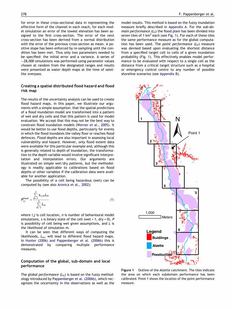
Creating a spatial distributed flood hazard and floodrisk map

The results of the uncertainty analysis can be used to createflood hazard maps. In this paper, we illustrate our argu-ments with a simple assumption: that the spatial predictionsof a flood inundation model are transformed into a patternof wet and dry cells and that this pattern is used for modelevaluation. We accept that this may not be the best way toconstrain flood inundation models (Werner et al., 2005). Itwould be better to use flood depths, particularly for eventsin which the flood inundates the valley floor or reaches flooddefences. Flood depths are also important in assessing localvulnerability and hazard. However, only flood extent datawere available for this particular example and, although thisis generally related to depth of inundation, the transforma-tion to the depth variable would involve significant interpre-tation and interpolation errors. Our arguments areillustrated on simple wet/dry patterns, but the methodol-ogy is readily applicable to calibrations based on flooddepths or other variables if the calibration data were avail-able for another application.

The possibility of a cell being hazardous (wet) can becomputed by (see also Aronica et al., 2002):

Pfloodi;j ¼

Pn

m¼1si;j;mLm

Pn

m¼1Lm

ð1Þ

where i,j is cell location, n is number of behavioural modelsimulations, s is binary state of the cell (wet = 1, dry = 0), Pis possibility of cell being wet given assumptions, and L isthe likelihood of simulation m.

It can be seen that different ways of computing thelikelihoods, Lm, will lead to different flood hazard maps.In Hunter (2006) and Pappenberger et al. (2006b) this isdemonstrated by comparing multiple performancemeasures.

Floodoutline

Figure 1 Outline of the Alzette catchment. The tiles indicatethe area on which each subdomain performance has beencalibrated. Point 1 shows the location of the point performancemeasure.

Computation of the global, sub-domain and localperformance

The global performance (LG) is based on the fuzzy method-ology introduced by Pappenberger et al. (2006b), which rec-ognizes the uncertainty in the observations as well as the

model results. This method is based on the fuzzy inundationmeasure briefly described in Appendix A. For the sub-do-main performance (LS) the flood plain has been divided intoseven tiles of 1 km2 each (see Fig. 1). For each of these tilesthe same performance measure as for the global computa-tion has been used. The point performance (LP) measurewas devised based upon evaluating the shortest distancefrom a specified target cell to cells of a given inundationprobability (Fig. 1). This effectively enables model perfor-mance to be evaluated with respect to a single cell as thedistance from a critical target structure such as a hospitalor emergency control centre to any number of possibleshoreline scenarios (see Appendix B).

Grasping the unavoidable subjectivity in calibration of flood inundation models: A vulnerability weighted approach 279

Results

Global, sub-domain and local performance

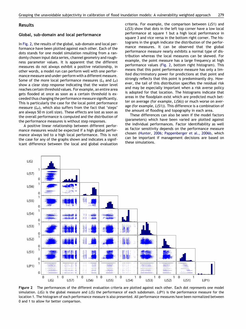
In Fig. 2, the results of the global, sub-domain and local per-formance have been plotted against each other. Each of thedots stands for one model simulation resulting from a ran-domly chosen input data series, channel geometry and rough-ness parameter values. It is apparent that the differentmeasures do not always exhibit a positive relationship, inother words, a model run can perform well with one perfor-mancemeasure and under-performwith a differentmeasure.Some of the more local performance measures (LS and LP)show a clear step response indicating that the water levelreaches certain threshold values. For example, an entire areagets flooded at once as soon as a certain threshold is ex-ceeded thus changing the performancemeasure significantly.This is particularly the case for the local point performancemeasure (LP), which also suffers from the fact that ‘steps’are always 50 m (cell size). These effects are lost as soon asthe overall performance is computed and the distribution ofthe performance measures is without step responses.

A positive linear relationship between different perfor-mance measures would be expected if a high global perfor-mance always led to a high local performance. This is notthe case for any of the graphs shown and indicates a signif-icant difference between the local and global evaluation

Figure 2 The performances of the different evaluation criteria asimulation. L(G) is the global measure and L(S) the performancelocation 1. The histogram of each performance measure is also prese0 and 1 to allow for better comparison.

criteria. For example, the comparison between L(S1) andL(S3) show that dots in the left top corner have a low localperformance at square 1 but a high local performance insquare 3 and vice versa in the bottom right corner. The his-tograms in the graph indicate the distribution of the perfor-mance measures. It can be observed that the globalperformance measure nearly exhibits a normal type of dis-tribution whereas the local measures can be skewed. Forexample, the point measure has a large frequency at highperformance values (Fig. 2, bottom right histogram). Thismeans that this point performance measure has only a lim-ited discriminatory power for predictions at that point andstrongly reflects that this point is predominantly dry. How-ever, the tail of this distribution specifies the residual riskand may be especially important when a risk averse policyis adopted for that location. The histograms indicate thatareas in the floodplain exist which are predicted much bet-ter on average (for example, L(S6)) or much worse on aver-age (for example, L(S1)). This difference is a combination ofthe amount of flooding and topography in each area.

These differences can also be seen if the model factors(parameters) which have been varied are plotted againstthe individual performances. Factor identifiability as wellas factor sensitivity depends on the performance measurechosen (Hunter, 2006; Pappenberger et al., 2006b, whichcan be important if management decisions are based onthese simulations.

re plotted against each other. Each dot represents one modelof each subdomain. L(P1) is the performance measure for thented. All performance measures have been normalized between

280 F. Pappenberger et al.

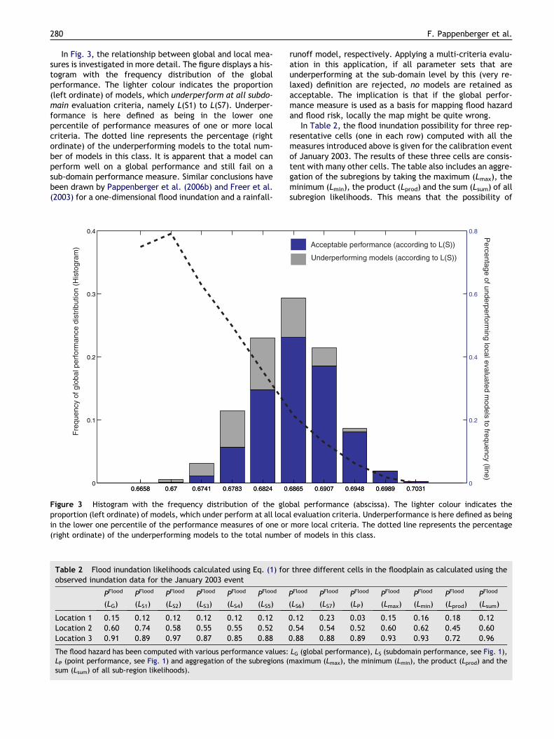
In Fig. 3, the relationship between global and local mea-sures is investigated in more detail. The figure displays a his-togram with the frequency distribution of the globalperformance. The lighter colour indicates the proportion(left ordinate) of models, which underperform at all subdo-main evaluation criteria, namely L(S1) to L(S7). Underper-formance is here defined as being in the lower onepercentile of performance measures of one or more localcriteria. The dotted line represents the percentage (rightordinate) of the underperforming models to the total num-ber of models in this class. It is apparent that a model canperform well on a global performance and still fail on asub-domain performance measure. Similar conclusions havebeen drawn by Pappenberger et al. (2006b) and Freer et al.(2003) for a one-dimensional flood inundation and a rainfall-

0.6658 0.67 0.6741 0.6783 0.6824 00

0.1

0.2

0.3

0.4

0.6658 0.67 0.6741 0.6783 0.6824 0

Fre

quen

cy o

f glo

bal p

erfo

rman

ce d

istr

ibut

ion

(His

togr

am)

Figure 3 Histogram with the frequency distribution of the gloproportion (left ordinate) of models, which under perform at all locain the lower one percentile of the performance measures of one or(right ordinate) of the underperforming models to the total numbe

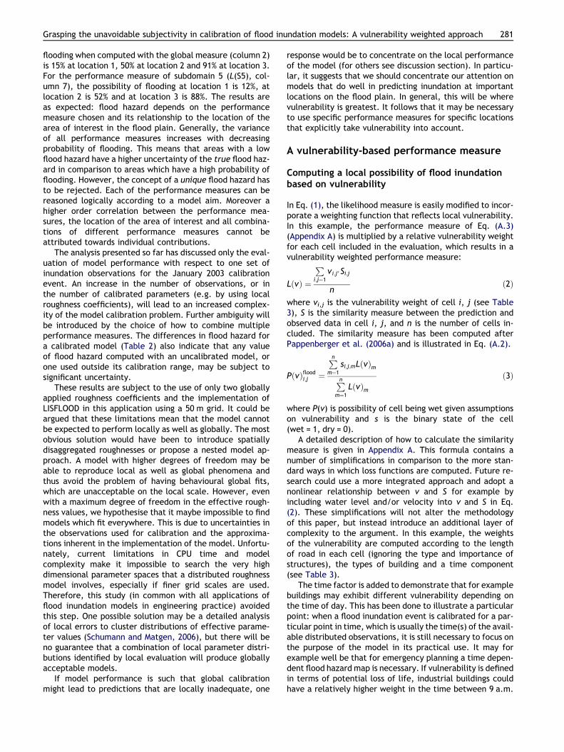
Table 2 Flood inundation likelihoods calculated using Eq. (1) forobserved inundation data for the January 2003 event

PFlood

(LG)PFlood

(LS1)PFlood

(LS2)PFlood

(LS3)PFlood

(LS4)PFlood

(LS5)

Location 1 0.15 0.12 0.12 0.12 0.12 0.12Location 2 0.60 0.74 0.58 0.55 0.55 0.52Location 3 0.91 0.89 0.97 0.87 0.85 0.88

The flood hazard has been computed with various performance values:LP (point performance, see Fig. 1) and aggregation of the subregions (sum (Lsum) of all sub-region likelihoods).

runoff model, respectively. Applying a multi-criteria evalu-ation in this application, if all parameter sets that areunderperforming at the sub-domain level by this (very re-laxed) definition are rejected, no models are retained asacceptable. The implication is that if the global perfor-mance measure is used as a basis for mapping flood hazardand flood risk, locally the map might be quite wrong.

In Table 2, the flood inundation possibility for three rep-resentative cells (one in each row) computed with all themeasures introduced above is given for the calibration eventof January 2003. The results of these three cells are consis-tent with many other cells. The table also includes an aggre-gation of the subregions by taking the maximum (Lmax), theminimum (Lmin), the product (Lprod) and the sum (Lsum) of allsubregion likelihoods. This means that the possibility of

.6865 0.6907 0.6948 0.6989 0.7031.6865 0.6907 0.6948 0.6989 0.70310

0.2

0.4

0.6

0.8

Underperforming models (according to L(S))

Acceptable performance (according to L(S))

Percentage of underperform

ing local evaluated models to frequency (line)

bal performance (abscissa). The lighter colour indicates thel evaluation criteria. Underperformance is here defined as beingmore local criteria. The dotted line represents the percentager of models in this class.

three different cells in the floodplain as calculated using the

PFlood

(LS6)PFlood

(LS7)PFlood

(LP)PFlood

(Lmax)PFlood

(Lmin)PFlood

(Lprod)PFlood

(Lsum)

0.12 0.23 0.03 0.15 0.16 0.18 0.120.54 0.54 0.52 0.60 0.62 0.45 0.600.88 0.88 0.89 0.93 0.93 0.72 0.96

LG (global performance), LS (subdomain performance, see Fig. 1),maximum (Lmax), the minimum (Lmin), the product (Lprod) and the

Grasping the unavoidable subjectivity in calibration of flood inundation models: A vulnerability weighted approach 281

flooding when computed with the global measure (column 2)is 15% at location 1, 50% at location 2 and 91% at location 3.For the performance measure of subdomain 5 (L(S5), col-umn 7), the possibility of flooding at location 1 is 12%, atlocation 2 is 52% and at location 3 is 88%. The results areas expected: flood hazard depends on the performancemeasure chosen and its relationship to the location of thearea of interest in the flood plain. Generally, the varianceof all performance measures increases with decreasingprobability of flooding. This means that areas with a lowflood hazard have a higher uncertainty of the true flood haz-ard in comparison to areas which have a high probability offlooding. However, the concept of a unique flood hazard hasto be rejected. Each of the performance measures can bereasoned logically according to a model aim. Moreover ahigher order correlation between the performance mea-sures, the location of the area of interest and all combina-tions of different performance measures cannot beattributed towards individual contributions.

The analysis presented so far has discussed only the eval-uation of model performance with respect to one set ofinundation observations for the January 2003 calibrationevent. An increase in the number of observations, or inthe number of calibrated parameters (e.g. by using localroughness coefficients), will lead to an increased complex-ity of the model calibration problem. Further ambiguity willbe introduced by the choice of how to combine multipleperformance measures. The differences in flood hazard fora calibrated model (Table 2) also indicate that any valueof flood hazard computed with an uncalibrated model, orone used outside its calibration range, may be subject tosignificant uncertainty.

These results are subject to the use of only two globallyapplied roughness coefficients and the implementation ofLISFLOOD in this application using a 50 m grid. It could beargued that these limitations mean that the model cannotbe expected to perform locally as well as globally. The mostobvious solution would have been to introduce spatiallydisaggregated roughnesses or propose a nested model ap-proach. A model with higher degrees of freedom may beable to reproduce local as well as global phenomena andthus avoid the problem of having behavioural global fits,which are unacceptable on the local scale. However, evenwith a maximum degree of freedom in the effective rough-ness values, we hypothesise that it maybe impossible to findmodels which fit everywhere. This is due to uncertainties inthe observations used for calibration and the approxima-tions inherent in the implementation of the model. Unfortu-nately, current limitations in CPU time and modelcomplexity make it impossible to search the very highdimensional parameter spaces that a distributed roughnessmodel involves, especially if finer grid scales are used.Therefore, this study (in common with all applications offlood inundation models in engineering practice) avoidedthis step. One possible solution may be a detailed analysisof local errors to cluster distributions of effective parame-ter values (Schumann and Matgen, 2006), but there will beno guarantee that a combination of local parameter distri-butions identified by local evaluation will produce globallyacceptable models.

If model performance is such that global calibrationmight lead to predictions that are locally inadequate, one

response would be to concentrate on the local performanceof the model (for others see discussion section). In particu-lar, it suggests that we should concentrate our attention onmodels that do well in predicting inundation at importantlocations on the flood plain. In general, this will be wherevulnerability is greatest. It follows that it may be necessaryto use specific performance measures for specific locationsthat explicitly take vulnerability into account.

A vulnerability-based performance measure

Computing a local possibility of flood inundationbased on vulnerability

In Eq. (1), the likelihood measure is easily modified to incor-porate a weighting function that reflects local vulnerability.In this example, the performance measure of Eq. (A.3)(Appendix A) is multiplied by a relative vulnerability weightfor each cell included in the evaluation, which results in avulnerability weighted performance measure:

LðvÞ ¼

P

i;j¼1vi;j�Si;j

nð2Þ

where vi,j is the vulnerability weight of cell i, j (see Table3), S is the similarity measure between the prediction andobserved data in cell i, j, and n is the number of cells in-cluded. The similarity measure has been computed afterPappenberger et al. (2006a) and is illustrated in Eq. (A.2).

PðvÞfloodi;j ¼

Pn

m¼1si;j;mLðvÞmPn

m¼1LðvÞm

ð3Þ

where P(v) is possibility of cell being wet given assumptionson vulnerability and s is the binary state of the cell(wet = 1, dry = 0).

A detailed description of how to calculate the similaritymeasure is given in Appendix A. This formula contains anumber of simplifications in comparison to the more stan-dard ways in which loss functions are computed. Future re-search could use a more integrated approach and adopt anonlinear relationship between v and S for example byincluding water level and/or velocity into v and S in Eq.(2). These simplifications will not alter the methodologyof this paper, but instead introduce an additional layer ofcomplexity to the argument. In this example, the weightsof the vulnerability are computed according to the lengthof road in each cell (ignoring the type and importance ofstructures), the types of building and a time component(see Table 3).

The time factor is added to demonstrate that for examplebuildings may exhibit different vulnerability depending onthe time of day. This has been done to illustrate a particularpoint: when a flood inundation event is calibrated for a par-ticular point in time, which is usually the time(s) of the avail-able distributed observations, it is still necessary to focus onthe purpose of the model in its practical use. It may forexample well be that for emergency planning a time depen-dent flood hazard map is necessary. If vulnerability is definedin terms of potential loss of life, industrial buildings couldhave a relatively higher weight in the time between 9 a.m.

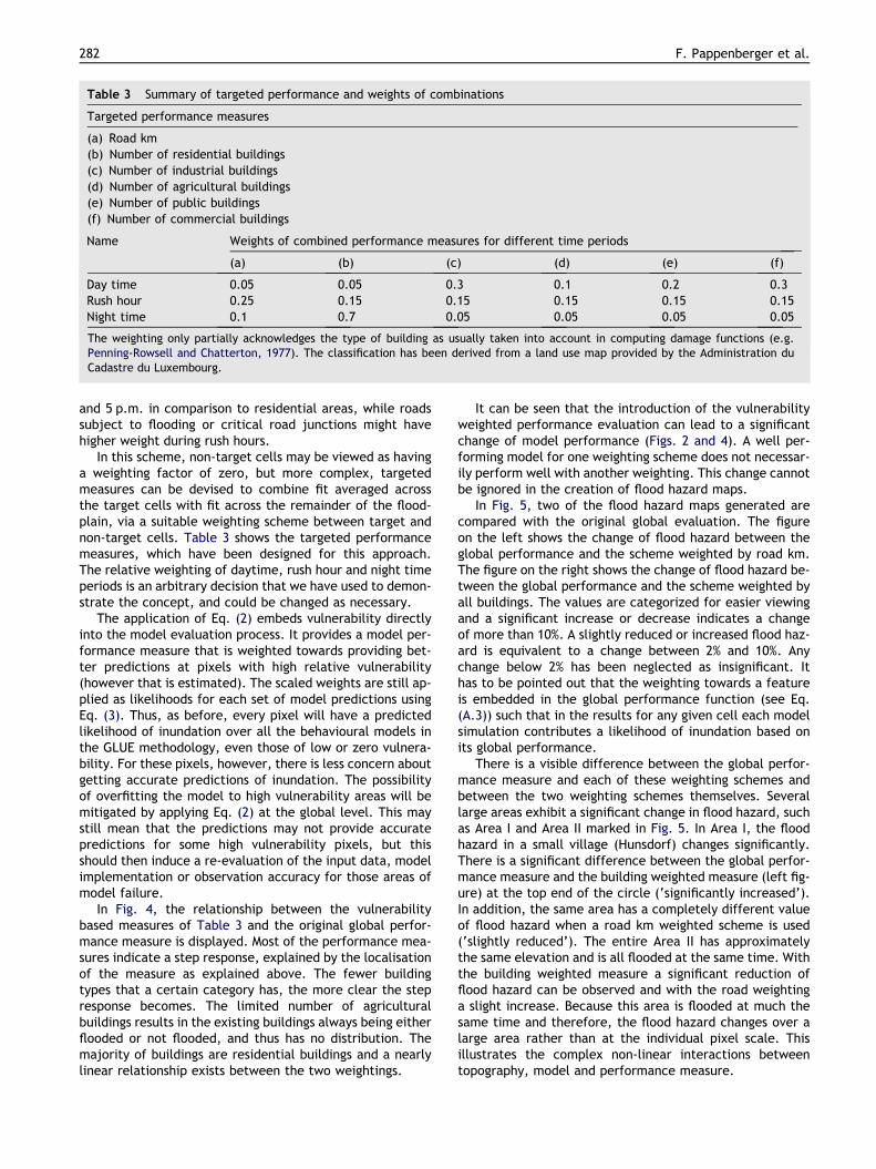
Table 3 Summary of targeted performance and weights of combinations

Targeted performance measures

(a) Road km(b) Number of residential buildings(c) Number of industrial buildings(d) Number of agricultural buildings(e) Number of public buildings(f) Number of commercial buildings

Name Weights of combined performance measures for different time periods

(a) (b) (c) (d) (e) (f)

Day time 0.05 0.05 0.3 0.1 0.2 0.3Rush hour 0.25 0.15 0.15 0.15 0.15 0.15Night time 0.1 0.7 0.05 0.05 0.05 0.05

The weighting only partially acknowledges the type of building as usually taken into account in computing damage functions (e.g.Penning-Rowsell and Chatterton, 1977). The classification has been derived from a land use map provided by the Administration duCadastre du Luxembourg.

282 F. Pappenberger et al.

and 5 p.m. in comparison to residential areas, while roadssubject to flooding or critical road junctions might havehigher weight during rush hours.

In this scheme, non-target cells may be viewed as havinga weighting factor of zero, but more complex, targetedmeasures can be devised to combine fit averaged acrossthe target cells with fit across the remainder of the flood-plain, via a suitable weighting scheme between target andnon-target cells. Table 3 shows the targeted performancemeasures, which have been designed for this approach.The relative weighting of daytime, rush hour and night timeperiods is an arbitrary decision that we have used to demon-strate the concept, and could be changed as necessary.

The application of Eq. (2) embeds vulnerability directlyinto the model evaluation process. It provides a model per-formance measure that is weighted towards providing bet-ter predictions at pixels with high relative vulnerability(however that is estimated). The scaled weights are still ap-plied as likelihoods for each set of model predictions usingEq. (3). Thus, as before, every pixel will have a predictedlikelihood of inundation over all the behavioural models inthe GLUE methodology, even those of low or zero vulnera-bility. For these pixels, however, there is less concern aboutgetting accurate predictions of inundation. The possibilityof overfitting the model to high vulnerability areas will bemitigated by applying Eq. (2) at the global level. This maystill mean that the predictions may not provide accuratepredictions for some high vulnerability pixels, but thisshould then induce a re-evaluation of the input data, modelimplementation or observation accuracy for those areas ofmodel failure.

In Fig. 4, the relationship between the vulnerabilitybased measures of Table 3 and the original global perfor-mance measure is displayed. Most of the performance mea-sures indicate a step response, explained by the localisationof the measure as explained above. The fewer buildingtypes that a certain category has, the more clear the stepresponse becomes. The limited number of agriculturalbuildings results in the existing buildings always being eitherflooded or not flooded, and thus has no distribution. Themajority of buildings are residential buildings and a nearlylinear relationship exists between the two weightings.

It can be seen that the introduction of the vulnerabilityweighted performance evaluation can lead to a significantchange of model performance (Figs. 2 and 4). A well per-forming model for one weighting scheme does not necessar-ily perform well with another weighting. This change cannotbe ignored in the creation of flood hazard maps.

In Fig. 5, two of the flood hazard maps generated arecompared with the original global evaluation. The figureon the left shows the change of flood hazard between theglobal performance and the scheme weighted by road km.The figure on the right shows the change of flood hazard be-tween the global performance and the scheme weighted byall buildings. The values are categorized for easier viewingand a significant increase or decrease indicates a changeof more than 10%. A slightly reduced or increased flood haz-ard is equivalent to a change between 2% and 10%. Anychange below 2% has been neglected as insignificant. Ithas to be pointed out that the weighting towards a featureis embedded in the global performance function (see Eq.(A.3)) such that in the results for any given cell each modelsimulation contributes a likelihood of inundation based onits global performance.

There is a visible difference between the global perfor-mance measure and each of these weighting schemes andbetween the two weighting schemes themselves. Severallarge areas exhibit a significant change in flood hazard, suchas Area I and Area II marked in Fig. 5. In Area I, the floodhazard in a small village (Hunsdorf) changes significantly.There is a significant difference between the global perfor-mance measure and the building weighted measure (left fig-ure) at the top end of the circle (‘significantly increased’).In addition, the same area has a completely different valueof flood hazard when a road km weighted scheme is used(‘slightly reduced’). The entire Area II has approximatelythe same elevation and is all flooded at the same time. Withthe building weighted measure a significant reduction offlood hazard can be observed and with the road weightinga slight increase. Because this area is flooded at much thesame time and therefore, the flood hazard changes over alarge area rather than at the individual pixel scale. Thisillustrates the complex non-linear interactions betweentopography, model and performance measure.

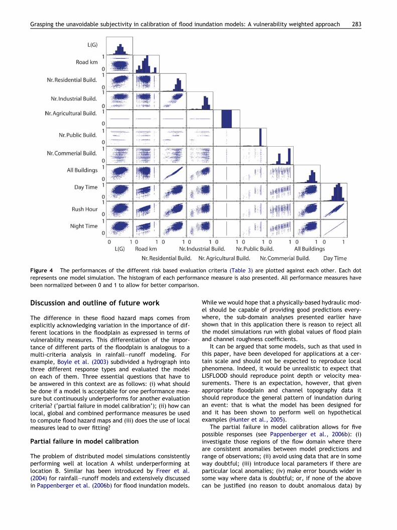
Figure 4 The performances of the different risk based evaluation criteria (Table 3) are plotted against each other. Each dotrepresents one model simulation. The histogram of each performance measure is also presented. All performance measures havebeen normalized between 0 and 1 to allow for better comparison.

Grasping the unavoidable subjectivity in calibration of flood inundation models: A vulnerability weighted approach 283

Discussion and outline of future work

The difference in these flood hazard maps comes fromexplicitly acknowledging variation in the importance of dif-ferent locations in the floodplain as expressed in terms ofvulnerability measures. This differentiation of the impor-tance of different parts of the floodplain is analogous to amulti-criteria analysis in rainfall–runoff modeling. Forexample, Boyle et al. (2003) subdivided a hydrograph intothree different response types and evaluated the modelon each of them. Three essential questions that have tobe answered in this context are as follows: (i) what shouldbe done if a model is acceptable for one performance mea-sure but continuously underperforms for another evaluationcriteria? (‘partial failure in model calibration’); (ii) how canlocal, global and combined performance measures be usedto compute flood hazard maps and (iii) does the use of localmeasures lead to over fitting?

Partial failure in model calibration

The problem of distributed model simulations consistentlyperforming well at location A whilst underperforming atlocation B. Similar has been introduced by Freer et al.(2004) for rainfall–runoff models and extensively discussedin Pappenberger et al. (2006b) for flood inundation models.

While we would hope that a physically-based hydraulic mod-el should be capable of providing good predictions every-where, the sub-domain analyses presented earlier haveshown that in this application there is reason to reject allthe model simulations run with global values of flood plainand channel roughness coefficients.

It can be argued that some models, such as that used inthis paper, have been developed for applications at a cer-tain scale and should not be expected to reproduce localphenomena. Indeed, it would be unrealistic to expect thatLISFLOOD should reproduce point depth or velocity mea-surements. There is an expectation, however, that givenappropriate floodplain and channel topography data itshould reproduce the general pattern of inundation duringan event: that is what the model has been designed forand it has been shown to perform well on hypotheticalexamples (Hunter et al., 2005).

The partial failure in model calibration allows for fivepossible responses (see Pappenberger et al., 2006b): (i)investigate those regions of the flow domain where thereare consistent anomalies between model predictions andrange of observations; (ii) avoid using data that are in someway doubtful; (iii) introduce local parameters if there areparticular local anomalies; (iv) make error bounds wider insome way where data is doubtful; or, if none of the abovecan be justified (no reason to doubt anomalous data) by

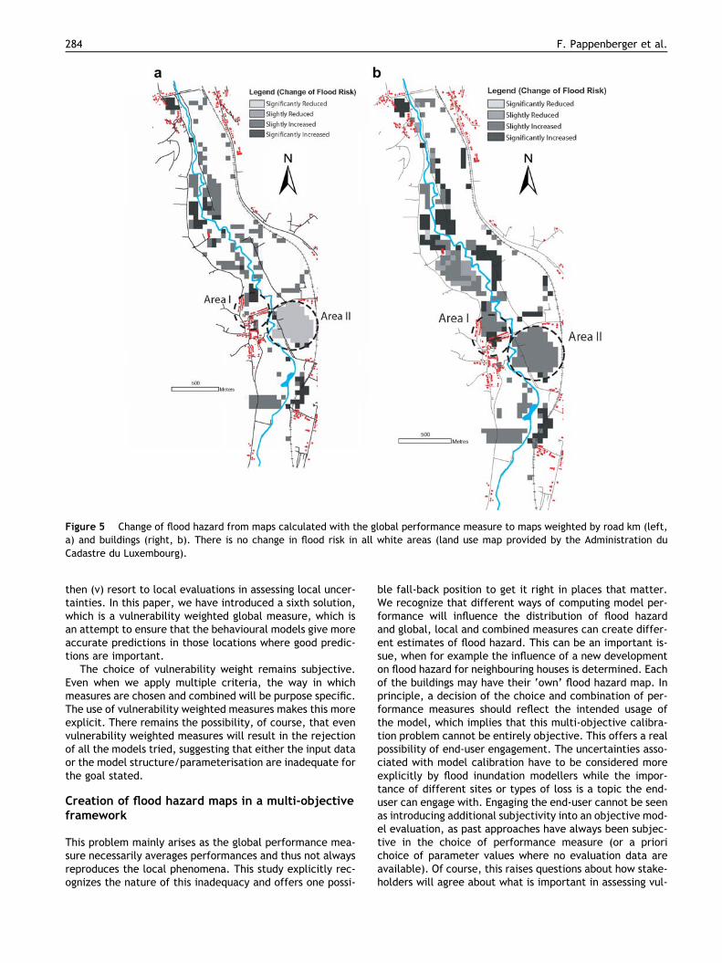
Figure 5 Change of flood hazard from maps calculated with the global performance measure to maps weighted by road km (left,a) and buildings (right, b). There is no change in flood risk in all white areas (land use map provided by the Administration duCadastre du Luxembourg).

284 F. Pappenberger et al.

then (v) resort to local evaluations in assessing local uncer-tainties. In this paper, we have introduced a sixth solution,which is a vulnerability weighted global measure, which isan attempt to ensure that the behavioural models give moreaccurate predictions in those locations where good predic-tions are important.

The choice of vulnerability weight remains subjective.Even when we apply multiple criteria, the way in whichmeasures are chosen and combined will be purpose specific.The use of vulnerability weighted measures makes this moreexplicit. There remains the possibility, of course, that evenvulnerability weighted measures will result in the rejectionof all the models tried, suggesting that either the input dataor the model structure/parameterisation are inadequate forthe goal stated.

Creation of flood hazard maps in a multi-objectiveframework

This problem mainly arises as the global performance mea-sure necessarily averages performances and thus not alwaysreproduces the local phenomena. This study explicitly rec-ognizes the nature of this inadequacy and offers one possi-

ble fall-back position to get it right in places that matter.We recognize that different ways of computing model per-formance will influence the distribution of flood hazardand global, local and combined measures can create differ-ent estimates of flood hazard. This can be an important is-sue, when for example the influence of a new developmenton flood hazard for neighbouring houses is determined. Eachof the buildings may have their ‘own’ flood hazard map. Inprinciple, a decision of the choice and combination of per-formance measures should reflect the intended usage ofthe model, which implies that this multi-objective calibra-tion problem cannot be entirely objective. This offers a realpossibility of end-user engagement. The uncertainties asso-ciated with model calibration have to be considered moreexplicitly by flood inundation modellers while the impor-tance of different sites or types of loss is a topic the end-user can engage with. Engaging the end-user cannot be seenas introducing additional subjectivity into an objective mod-el evaluation, as past approaches have always been subjec-tive in the choice of performance measure (or a priorichoice of parameter values where no evaluation data areavailable). Of course, this raises questions about how stake-holders will agree about what is important in assessing vul-

Grasping the unavoidable subjectivity in calibration of flood inundation models: A vulnerability weighted approach 285

nerability, or how to deal with multiple measures of‘‘importance’’. The result may not be one single flood haz-ard map, but rather purpose specific hazard maps. Weacknowledge that this will pose additional problems in thecommunication of flood hazard, but such a discussion is be-yond the scope of this paper.

Over-fitting and predictability

The starting point for the use of vulnerability weighted like-lihood weighting as used in the paper, was the potential forrejecting all the inundation models considered behaviouralin terms of the normal global evaluation, when their localinundation predictions were evaluated. The use of local per-formance measures, or vulnerability weighted measures,however, will introduce the potential for overfitting themodel to the errors in the modelling process for particularareas, which could lead to biased or wrong predictions fora different event of different magnitude. Romanowicz andBeven (2003), for example, show how distributions of effec-tive channel and floodplain roughness values could be quitedifferent when evaluated for events of different magnitudebut the number of studies in which the predictions for dif-ferent events could be assessed remains very small. To as-sess predictability, or the potential for overfitting, weneed much more experience in assessing model extrapola-tions to either different events or different rivers.

Robustness in such extrapolations implies avoiding overfit-ting by a form of averaging of errors. There is a seamless tran-sition between a local and global orientated performanceevaluation as the more points one uses for fitting, the moreglobal will be the properties of the evaluation. How ‘local’an evaluation should be depends on the objectives of themodelling exercise. A balance between fitting the model toindividual pixels and averaging the overall performance hasto be found. Hence, the approach adopted here to give great-er weight to those areas considered to be more vulnerabilitybut to average the resulting measure globally over the fullreach. In this way, the effects of very specific errors at spe-cific locations might, to some extent, also be averaged out.The evaluation process should be based on a conscious deci-sion about relative vulnerability, rather than a decisionpurely based on the size of the available image.

In this paper, we have not considered the possibility ofallowing channel and flood plain roughness to vary spatially.In principle, we would expect local values of roughness togive more accurate local predictions (though we are notsure how great this effect might be). While recognising thatvarying only global values of roughness must inherently re-sult in error for particular locations, however, allowingroughness to vary downstream will introduce its own overfit-ting problem. The more values of roughness that are in-cluded in the analysis, the more potential there is offitting to local error, reducing predictability in extrapola-tion. The curse of dimensionality also arises: the greaterthe number of parameter dimensions to be considered,the greater the computational problem in making enoughruns to evaluate the range of responses. Again, there is littleexperience available in the literature to enable the value ofintroducing varied roughness to be assessed in different cir-cumstances. The study of Werner (2004) is interesting in thisrespect. He showed that introducing spatially variable flood

plain roughness made the distribution of the channel rough-ness (but not the floodplain roughness) for the behaviouralmodels more identifiable. This result has yet to be con-firmed elsewhere, and the resulting parameter estimateswere not, in his study, subjected to an evaluation of predic-tions at another event magnitude.

Conclusion

Flood events causing major damage generally occur veryrarely and thus historical records of areas liable to floodingare always scarce. Therefore, most flood hazard maps arebased on numerical modelling and, in some cases, thesemodels can be calibrated and evaluated on data from pastevents. A flood hazard map can be conditioned on the modelperformance in the calibration exercise. It has been docu-mented that the different ways of computing the perfor-mance have a significant impact on the assessment offlood hazard for particular locations. This can be mainlyattributed to the fact that the predictions of current floodmodels are subject to error in input data, model structureand the observations used in model evaluation. Therefore,the problem of deriving a correct flood hazard map is morefundamental: to date, 2D inundation models have alwaysbeen evaluated against inundation extent using global per-formance measures that are obtained by averaging spatialperformance across a suitable domain. In the case of floodinundation models this is normally an estimate of the floodprone area. Conditioning models on global performance hasthe disadvantage that the performance at a local scale isonly considered indirectly. Here, it has been shown thatall the models considered acceptable in terms of global per-formance can be rejected on the basis of equivalent sub-do-main performance measures.

Should the affected cells contain buildings, transporta-tion links or similar, then the potential economic and socialconsequences of the inadequate prediction of local hazardwill be more severe than if the cells contain only undevel-oped agricultural land. In order to support flood hazardmanagement decisions with imperfect models, the calibra-tion or conditioning of flood inundation models can beweighted in favour of the vulnerability of target structuressuch as buildings and roads rather than just relying on globalperformance in predicting inundation. Additionally, when aflood inundation event is calibrated for a particular point intime, which is usually the time of observation, it is still nec-essary to focus on the usage of the model. For example, foremergency planning a time dependent flood hazard mapcould be derived. Indeed, the potential consequences offalse flood warnings to key buildings such as hospitals aresufficiently severe that it might even be considered prudentto condition a model solely in relation to the fit associatedwith a single structure, while remaining aware of the poten-tial danger of less robust predictions in other conditions as aresult of overfitting the calibration data. Consequently, in asetting in which the model is used to produce flood hazardmaps, for e.g. a particular town, the vulnerability cannotbe used as a simple add-on to the modelling process, butshould be incorporated into the calibration procedure. Thisapproach allows stakeholders to uniquely engage in themodeling process and offers the potential for new ways ofcalibrating flood inundation models in the future.

286 F. Pappenberger et al.

Acknowledgements

We thank Georges Muller of the Service de la Gestion del’Eau for providing some of the data used in this study.The land use map has been provided by the Administrationdu Cadastre du Luxembourg for which we are grateful. Thisstudy would have been impossible without the help of PaulBates (Professor of Hydrology, Bristol University) and NeilHunter (Bristol University). The paper is based on the MasterThesis by Kevin Frodsham for his Master degree in Environ-mental Science (distinction). Florian Pappenberger and Re-nata Romanowicz have been funded by the Flood RiskManagement Research Consortium (http://www.flood-risk.org.uk). Development of extensions to the GLUE meth-odology has been supported by NERC Grant NER/L/S/2001/00658 awarded to Prof. Keith Beven.

Appendix A. Fuzzy performance measure

Traditionally inundation model have been evaluated on byseparating observations in each cell into binary categoriesof wet or dry (Aronica et al., 2002; Bates and De Roo,2000; Horritt and Bates, 2001; Hunter, 2006). However,the true inundation extent can be estimated in many casesonly with large uncertainties. Therefore, in Pappenbergeret al. (2006b) a fuzzy mapping technique has been appliedwhich takes account of this uncertainty. Fuzzy categories(high, medium, low, no flooding) have been created fromthe observed and modelled data for this computation, whichreflect the certainty in the flooding of a particular cell.These maps have then been compared and a fuzzy perfor-mance value computed.

Four Fuzzy categories have been assigned to each cell ofthe observed and modeled maps a detailed description onderiving these categories has been presented by Pappenber-ger et al. (2006a). The categories of the observed map havebeen derived from the uncertainty in classifying the back-scatter of a SAR image. The modeled categories are basedon the uncertainty in the topography of surrounding cells.

VCAT ¼ fVCAThigh ;VCATmedium;VCATlow ;VCATnog ðA:1Þ

whereVCAThigh ¼ ð1; 0:6; 0:3; 0Þ, VCATmedium¼ ð0:6; 1; 0:6; 0:3Þ,

VCATlow ¼ ð0:3; 0:6; 1; 0:6Þ, VCATno ¼ ð0; 0:3; 0:6; 1Þ. The similar-ity measure has then be computed by comparing the fuzzycategories of the observed (A) and modelled maps (B):

SðVA;VBÞ ¼ kACAThigh ;BCAThigh jmin; jACATmedium;BCATmedium

jmin;

jACATlow ;BCATlow jmin; jACATno ;BCATno jminjmax ðA:2Þ

L ¼

P

i;j¼1Si;jðVA;VBÞ

nðA:3Þ

where n representing the number of inundation prone cellsfor all simulations and the observed data set. i and j give thecell location.

Appendix B. Point performance method

For this study, the boundary between the zero possibilityinundation category and the nearest cell of any other fuzzycategory (see Appendix A) was selected to divide the maps

into wet and dry sectors. A detailed description of thismethod is given in Pappenberger et al. (2006a). This choiceof boundary represents a conservative choice for the shore-line and was chosen to reflect a close to maximum hazard tothe target cell as would have to be considered in a risk anal-ysis. Other choices of boundary can be chosen from fuzzycategory maps to represent different hazard levels; forexample, analyzing performance with respect to the dis-tance from target to nearest cell of a high inundation prob-ability would be a suitable choice to condition the model onthe hazard of severe flooding to the target cell. The perfor-mance measure LPA was evaluated as the absolute differ-ence between the observed (distA,OBS) and modelled(distA,MOD) distances from the target cell, A, to the nearestcell across the hypothetical shoreline. h is the angular com-ponent as an approaching flood may be important dependingon the direction of approach from all directions. For exam-ple, evacuation roads may be situated in only one direction.Such a measure could be sophisticated by mapping the en-tire access roads and include them into the analysis of Eq.(A.4). w(t) is a weight for the time component as the evac-uation during peak time of surgeries conducted may bemore significant than otherwise. The angle as well as thetime weight are included in Eq. (A.4) for completenessand are not used in this paper

LP ¼ h�wðtÞ�jdistA;OBS � distA;MODj: ðA:4Þ

An optimum fit for LP, as defined in Eq. (A.4), of zero willoccur when the target cells are both wet and the chosenshoreline is equidistant from the target cell on both ob-served and model predicted maps irrespective of the direc-tion of nearest approach.

References

Alexander, D., 1991. Natural disasters: a framework for researchand teaching. Disasters 15 (3), 209–226.

Aronica, G., Bates, P.D., Horritt, M.S., 2002. Assessing theuncertainty in distributed model predictions using observedbinary pattern information within GLUE. Hydrological Processes16 (10), 2001–2016.

Aronica, G., Hankin, B., Beven, K.J., 1998. Uncertainty andequifinality in calibrating distributed roughness coefficients ina flood propagation model with limited data. Advances in WaterResources 22 (4), 349–365.

Bates, P.D., De Roo, A.P.J., 2000. A simple raster-based model forflood inundation simulation. Journal of Hydrology 236 (1-2), 54–77.

Beven, K.J., 2006. A manifesto for the equifinality thesis. Journal ofHydrology 320 (1–2), 18–36.

Beven, K.J., Binley, A., 1992. The future of distributed models –model calibration and uncertainty prediction. HydrologicalProcesses 6 (3), 279–298.

Blazkova, S., Beven, K., 2004. Flood frequency estimation bycontinuous simulation of subcatchment rainfalls and dischargeswith the aim of improving dam safety assessment in a large basinin the Czech Republic. Journal of Hydrology 292 (1-4), 153–172.

Bouma, J.J., Francois, D., Troch, P., 2005. Risk assessment andwater management. Environmental Modelling & Software 20 (2),141–151.

Boyle, D.P., Gupta, H., Sorooshian, S., 2003. Multicriteria calibra-tion of hydrologic models. In: Duan, Q., Gupta, H., Sorooshian,S., Rousseau, A.N., Turcotte, R. (Eds.), Advances in Calibrationof Watershed Models. American Geophysical Union, Washington.

Grasping the unavoidable subjectivity in calibration of flood inundation models: A vulnerability weighted approach 287

Cameron, D., Beven, K., Tawn, J., Naden, P., 2000. Floodfrequency estimation by continuous simulation (with likelihoodbased uncertainty estimation). Hydrology and Earth SystemSciences 4 (1), 23–34.

European Environment Agency, 2006. EEA multilingual environmen-tal glossary, http://glossary.eea.eu.int/EEAGlossary/. EuropeanEnvironment Agency.

Freer, J., Beven, K.J., Peters, N., 2003. Multivariate seasonalperiod model rejection within the generalised likelihood uncer-tainty estimation procedure. In: Duan, Q.Y., Gupta, H., Soro-oshian, S., Rousseau, A., Turcotte, R. (Eds.), Calibration ofWatershed Models. American Geophysical Union, Washington,pp. 69–88.

Freer, J.E., McMillan, H., McDonnell, J.J., Beven, K.J., 2004.Constraining dynamic TOPMODEL responses for imprecise watertable information using fuzzy rule based performance measures.Journal of Hydrology 291 (3–4), 254–277.

Granger, K., Jones, T., Leiba, M., Scott, G., 1999. Community Riskin Cairns: A Multihazard Risk Assessment. AGSO (AustralianGeological Survey Organisation) Cities Project, Department ofIndustry, Science and Resources, Australia.

Horritt, M.S., Bates, P.D., 2001. Predicting floodplain inundation:raster-based modelling versus the finite-element approach.Hydrological Processes 15 (5), 825–842.

Hunter, N.M., 2006. Flood Inundation Modelling – PhD Thesis,School of Geography, Bristol University, Bristol.

Hunter, N.M., Horritt, M.S., Bates, P.D., Wilson, M.D., Werner,M.G.F., 2005. An adaptive time step solution for raster-basedstorage cell modelling of floodplain inundation. Advances inWater Resources 28 (9), 975–991.

Jonkman, S.N., van Gelder, P.H.A.J.M., Vrijling, J.K., 2003. Anoverview of quantitative risk measures for loss of life andeconomic damage. Journal of Hazardous Materials 99 (1), 1–30.

Kelman, I., 2002. Physical Flood Vulnerability of ResidentialProperties in Coastal, Eastern England, PhD Thesis, Universityof Cambridge, UK. Available from: <http://www.ilankel-man.org/phd.html>.

Merz, B., Kreibich, H., Thieken, A., Schmidtke, R., 2004. Estimationuncertainty of direct monetary flood damage to buildings.Natural Hazards and Earth System Sciences 4 (1), 153–163.

Pappenberger, F., Beven, K.J., Frodsham, K., Romanowicz, R.,Matgen, P., 2006a. Fuzzy set approach to calibrating distributedflood inundation models using remote sensing observations.Hydrology and Earth System Sciences (Discussions). Available

from: <http://www.copernicus.org/EGU/hess/hessd/3/2243/hessd-3-2243.htm>.

Pappenberger, F., Beven, K.J., Horritt, M.S., Blazkova, S., 2005.Uncertainty in the calibration of effective roughness parametersin HEC-RAS using inundation and downstream level observations.Journal of Hydrology 302, 46–69.

Pappenberger, F., Matgen, P., Beven, K.J., Henry, J.-B., Pfister, L.,de Fraipont, P., 2006b. Influence of uncertain boundary condi-tions and model structure on flood inundation predictions.Advances in Water Resources 29 (10), 1430–1449.

Penning-Rowsell, E.C., Chatterton, J.B., 1977. The Benefits of FloodAlleviation: Manual of Assessment Techniques. Gower, Aldershot.

Romanowicz, R., Beven, K.J., 2003. Estimation of flood inundationprobabilities as conditioned on event inundation maps. WaterResources Research 39 (3), W01073. doi:10.1029/2001WR001056.

Romanowicz, R., Beven, K.J., Tawn, J., 1996. Bayesian calibrationof flood inundation models. In: Anderson, M.G., Walling, D.E.,Bates, P.D. (Eds.), Floodplain Processes. John Wiley & Sons, NewYork, pp. 333–360.

Schumann, G., Matgen, P., 2006. Personal communication.Smith, K., 2001. Environmental Hazards: Assessing Risk and Reduc-

ing Disaster. Routledge, London, 392 pp.Soetanto, R., Proverbs, D.G., 2004. Impact of flood characteristics

on damage caused to UK domestic properties: the perceptions ofbuilding surveyors. Structural Survey 22 (2), 95–104 (specialissue, Flooding: Implications for the Construction Industry).

Thieken, A.H., Muller, M., Kreibich, H., Merz, B., 2005. Flooddamage and influencing factors: New insights from the August2002 flood in Germany. Water Resources Research 41 (12).

Turner, R.K., Bateman, I., Adger, N., 2001. Economics of coastaland water resources: valuing environmental functionsStudies inEcological Economics, vol. 3. Kluwer Academic, Dordrecht,London, vii, 342 pp.

Werner, M., 2004. Spatial flood extent modeling: A performance-based comparison, PhD Thesis, Delft University of Technology/DUP Science/Delft Hydraulics Select Series 4 (ISBN 90-407-2559-4). Available from: <http://www.wldelft.nl/rnd/publ/docs/We_2004a.pdf>.

Werner, M., Blazkova, S., Petr, J., 2005. Spatially distributedobservations in constraining inundation modelling uncertainties.Hydrological Processes 19 (16), 3081–3096.

Wu, S.Y., Yarnal, B., A., F., 2002. Vulnerability of coastalcommunities to sea-level rise: a case study of Cape May County,New Jersey, USA. Climate Research 22(3), 255–270.